performance and spectral efficiency.pdf
TRANSCRIPT

ESCOLA DE ENXEÑARÍA DE TELECOMUNICACIÓN DEPARTAMENTO DE TEORÍA DO SINAL E COMUNICACIÓNS
Performance and Spectral
Efficiency
of OFDM systems
on urban radio channels
Author: José Acuña González Advisor: Iñigo Cuiñas Gómez
Ph.D. programme in Signal Theory and Communications
2012/2013

Dedicated to my parents Ana María and José and my wife Patricia.

iii
Acknowledgements
Part of the research work of this Thesis has been financially supported by the Autonomic
Government of Galicia (Xunta de Galicia), Spain, through project InCiTe 08MRU045322PR.
This project has been partially financed with EU funds (FEDER program). The author and the
advisor would like to thank Xunta de Galicia for this support, which has been essential to
perform the experimental research and the dissemination of the results.
This work was partially funded by Spanish State Secretary for Research under project
TEC2011-28789-C02-02, that was co-funded using European Regional Development Funds
(ERDF).
I want to thank the people who made this possible: Fernando Obelleiro (Obi), José Luis
Rodriguez (Banner) for the generous host, and the professors Gregory Randall, Luis
Casamayou, María Simon who believed in me for this task.
I cannot forget Prof. Juan Martony who helped me in preparing myself for this endeavor. I
cannot forget Laura Landin who did a lot of paper work needed to formalize the necessary to
make the course.
How can I thank Jose María Nuñez (Tyson) and Ines GT for their friendship? I really enjoy
all days we share together.
A special gratitude I wish to give to Paula Gomez who shares some experimental outcomes
of her work with me.
Also, I want to thank the people of Grupo de Sistemas Radio to let me work with them from
Uruguay.
And the last person I want to thank is a very important one, who spend many hours to help
me, directed, corrected the work many times, recommended a lot of things and gave me a lot
of fundamental advices, a great professional and better human being, my “tutor” INHIGO.

Abstract
The increasing in the demand of mobile data, generally Internet access, at rates near 45% per
year, but not exclusively, and the decreasing of the gigabyte price are pushing the
telecommunication industry to improve the spectral efficiency of the networks. The work on
this PhD Thesis is involved in this path.
Many simulations were done to know the details of the performance and the spectral
efficiency of fourth generation (4G) systems. These simulations have been done using both
4G standards, Worldwide Interoperability for Microwave Access (WIMAX) and Long Term
Evolution (LTE), with some modifications exploring the alternatives that should increase the
spectral efficiency at reasonable distances and with an acceptable bit error rate (BER).
Multiple input multiple output (MIMO) and Code Division Multiple Access (CDMA)
schemes, added to the basic standard system, have been tested as possible solutions with its
advantages and disadvantages.
Two techniques of channel estimation and pre-equalization are proposed to use, along this
PhD Thesis, to reduce the BER reaching a reasonable value at low signal to noise ratio (SNR),
chosen after evaluation of some candidates. Also many urban channels models were used in
the simulations because they are present where the high demand is required: Modified
Stanford University Interim channels as SUI4 or SUI6 and actual radio channels indoor. The
additive white Gaussian noise (AWGN) channel is also used for standard comparisons.
Another topic to be improved is related to radio wave propagation model. A high density
building urban environment is modeled based in COST 231 WI model, upgrading in the
following items: the loss dependence on the angle between the propagation direction and the
street axis; takes into account the street crossings when predicting the signal attenuation along
the block; and the dependence of propagation loss with the terrain height at the mobile and at
the base station locations. This model gives the loss as a function of the distance, so it is
useful for radio network planning purposes but not for system technology performance as SUI
channels models.
As the presence of trees also affects the radio wave propagation, many vegetal species are
modeled with a measurements-derived attenuation factor, which depends on their geometrical
arrangement. Thus, the use of vegetal barriers to diminish interference in Wi-Fi networks
inside buildings or to isolate networks from outdoors is investigated, as a way to take
advantage of the attenuation induced by such obstacles.
Due to the scarcity of radio spectrum, the frequency reuse within a network deployment has
been analyzed with and without inter-cell interference coordination (ICIC), using the channel

ABSTRACT
v
sizes proposed by service providers and the minimum SNR needed for QPSK, 16 and 64
QAM modulations.
A relation between the distances of two mobiles to their serving base stations when the
frequency is reused is presented. The total capacity of a sector with multi-modulation scheme
is derived.
The efforts were put mainly at the 64 QAM, due to its high throughput capacity. As a
collateral product, a simulation platform was developed in Simulink-Matlab© to make more
tests of this type of systems, making easy the implementation of new ideas for the physical
layer of orthogonal frequency division multiplexing (OFDM) systems. It brings the possibility
to compare performances, basically BER vs. SNR, between these systems, over these or other
channels.
Resumen
Introducción
El aumento en la demanda de datos móviles principalmente por el acceso a Internet a tasas de
cerca de 45% por año, y la disminución del precio del gigabyte están empujando a la industria
de las telecomunicaciones a mejorar la eficiencia espectral de las redes de comunicaciones
inalámbricas. El trabajo desarrollado en esta Tesis Doctoral se encamina en esta dirección.
Muchas simulaciones se han realizado en este trabajo para conocer los detalles del
funcionamiento y de la eficiencia espectral de los sistemas de cuarta generación (4G). Estas
simulaciones se han realizado utilizando los estándares 3.9/4G, WiMAX y LTE, con algunas
modificaciones para explorar las alternativas que deberían aumentar la eficiencia espectral a
distancias razonables a una tasa de error de bits aceptable (BER).
También se han estudiado los sistemas MIMO y CDMA-OFDM, añadidos al sistema
estándar básico, para verificar si son posibles soluciones a los problemas que se plantean en
el despliegue de la cuarta generación, con sus ventajas y desventajas.
A lo largo de esta tesis doctoral se proponen utilizar dos técnicas de estimación de canal y
pre-ecualización, para reducir la BER a un valor razonable de SNR, elegidas después de la
evaluación de algunas candidatas. También fueron utilizados muchos modelos de canales
radio urbanos en las simulaciones, ya que están presentes en lugares donde se requiere alta
demanda: como los SUI4 o SUI6 y canales de interior reales. El canal con ruido aditivo
blanco gaussiano (AWGN) también se utiliza para comparaciones con el estándar.
Otro de los temas que aporta este trabajo está relacionado con el modelo de propagación de
ondas de radio. El canal radio de un entorno urbano con alta densidad de construcción se
modela basado en COST 231 modelo WI, al cual este trabajo le añade algunas mejoras: la
dependencia de la pérdida de potencia o atenuación con el ángulo entre la dirección de
propagación y el eje de la calle; se toma en cuenta los cruces de calle estimando más
exactamente la atenuación de la señal a lo largo de la cuadra, y la dependencia de la
atenuación según la diferencia de la altura del terreno en el móvil y de la estación base. Este
modelo ofrece la pérdida como una función de la distancia de manera que es útil para los
propósitos de planificación radio, pero no para el rendimiento del sistema.
Como la presencia de árboles también afecta a la propagación de ondas de radio, muchas
especies vegetales se modelan a partir de un factor de atenuación, derivado de mediciones,
que depende de su disposición geométrica. También se investigó el uso de barreras vegetales
para disminuir la interferencia en redes WiFi, como una manera de tomar ventaja de la
atenuación inducida por dichos obstáculos.
RESUMEN
vii
En otro orden de cosas y debido a la escasez de espectro de radio, la reutilización de
frecuencias dentro de un despliegue de red ha sido analizada con y sin coordinación de la
interferencia entre células (ICIC), utilizando los tamaños de canal propuestos por los
proveedores de servicios y la SNR mínima necesaria para las modulaciones QPSK, 16QAM y
64QAM.
Se propone una relación entre las distancias de dos móviles a sus estaciones base cuando se
reutiliza la frecuencia.
Asimismo se presenta la capacidad total de un sector con múltiples esquemas de modulación
en este trabajo.
Los esfuerzos se han puesto principalmente en la modulación 64QAM, debido a su alto
rendimiento. Como producto colateral, una plataforma de simulación fue desarrollada en
Simulink, Matlab © para hacer más pruebas de este tipo de sistemas, facilitando la puesta en
práctica de nuevas ideas para la capa física OFDM. Se brinda la posibilidad de comparar los
resultados, básicamente BER vs SNR, entre estos sistemas, a través de estos canales u otros
que se deseen.
En las secciones siguientes se resume, en castellano, el contenido de los distintos capítulos de
la Tesis, redactada en inglés. Por coherencia con el texto completo, las ecuaciones, tablas y
figuras siguen la numeración propia de los capítulos en las que se se desarrollan.

RESUMEN
viii
Modelo de canal radio MOPEM
Introducción
En este capítulo se presenta el modelo de propagación MOPEM para áreas urbanas densas en
la banda de frecuencias 850 a 900 MHz. Este trabajo está basado en el modelo COST231WI,
pero la hipótesis de pantallas infinitas se sustituye por pantallas finitas, teniendo en cuenta los
cruces de las calles, logrando así la predicción de la atenuación de la señal a lo largo de la
cuadra. La dependencia de la pérdida de propagación con la altura del terreno se revisa y
optimiza considerando una referencia absoluta, mientras que la dependencia del ángulo entre
la calle y la propagación de la onda se modifica para obtener una función de pérdida
continuamente diferenciable. La desviación estándar obtenida con este modelo es de 5,1 dB y
el error medio es de 0 dB frente a 6,6 dB y 6,2 respectivamente para la COST231WI, con
mediciones de validación de las dos áreas en la ciudad de Montevideo.
Desarrollo
A continuación se presenta la ecuación 3.6, que muestra la atenuación de este modelo, cuyos
términos son descritos por las ecuaciones 3.2 y 3.7 a 3.10 del capítulo 3.
Los términos subrayados son las modifciones propuestas en este trabajo.
MOPEM o rts MOPEM msd MOPEM esqL L L L L (3.6)
Los términos , y rts MOPEM msd MOPEM esqL L L son las contribuciones de este trabajo.
El término Lrts-MOPEM mostrado en 3.7 agrega dos nuevas mejoras al término Lrts de 3.3:
incluye la altura del terreno hAm y hAroof, y la función Lori-MOPEM .
10 10 101.87 10log ( ) 10log ( ) 10.4log ( )rts MOPEM Aroof Am ori MOPEML w f h h L
(3.7)
4 3 2
2.8 13.2 29.5 30.3 3.545 45 45 45
ori MOPEML
(3.8)
10 10 10 1054 18log (1 ) log ( ) 27.7log ( ) 9log ( )msd MOPEM Abase Aroof fL h h k f d b (3.9)
con 4 0.7 / 925 1fk f de (E. Damoso, 1999).
La altura hAroof y la hAbase son medidas desde un nivel común de referencia que puede ser el
nivel del mar.
El término Lesq modela la variación de la señal a lo largo de la cuadra.
La expresión fue ajustada empíricamente.
10 1 10 211.32 3.3 log logesq esq esqL d d
(3.10)
RESUMEN
ix
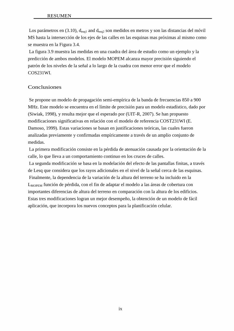
Los parámetros en (3.10), desq1 and desq2 son medidos en metros y son las distancias del móvil
MS hasta la intersección de los ejes de las calles en las esquinas mas próximas al mismo como
se muestra en la Figura 3.4.
La figura 3.9 muestra las medidas en una cuadra del área de estudio como un ejemplo y la
predicción de ambos modelos. El modelo MOPEM alcanza mayor precisión siguiendo el
patrón de los niveles de la señal a lo largo de la cuadra con menor error que el modelo
COS231WI.
Conclusiones
Se propone un modelo de propagación semi-empírica de la banda de frecuencias 850 a 900
MHz. Este modelo se encuentra en el límite de precisión para un modelo estadístico, dado por
(Siwiak, 1998), y resulta mejor que el esperado por (UIT-R, 2007). Se han propuesto
modificaciones significativas en relación con el modelo de referencia COST231WI (E.
Damoso, 1999). Estas variaciones se basan en justificaciones teóricas, las cuales fueron
analizadas previamente y confirmadas empíricamente a través de un amplio conjunto de
medidas.
La primera modificación consiste en la pérdida de atenuación causada por la orientación de la
calle, lo que lleva a un comportamiento continuo en los cruces de calles.
La segunda modificación se basa en la modelación del efecto de las pantallas finitas, a través
de Lesq que considera que los rayos adicionales en el nivel de la señal cerca de las esquinas.
Finalmente, la dependencia de la variación de la altura del terreno se ha incluido en la
LMOPEM función de pérdida, con el fin de adaptar el modelo a las áreas de cobertura con
importantes diferencias de altura del terreno en comparación con la altura de los edificios.
Estas tres modificaciones logran un mejor desempeño, la obtención de un modelo de fácil
aplicación, que incorpora los nuevos conceptos para la planificación celular.
RESUMEN
x
Diferencias en la planificación de redes celulares en
calles arboladas y parques
Introducción
A pesar de que la propagación de ondas de radio en entornos de vegetación ha sido
ampliamente estudiada, la situación real es que la cobertura de los sistemas de comunicación
en áreas vegetadas es inferior que en lugares abiertos dentro de nuestras ciudades. Esto indica
una carencia en las herramientas de simulación que se utilizan actualmente para la
planificación de la red de radio. En este capítulo se presentan amplias campañas de medida,
proporcionando los datos numéricos que pueden ser útiles para corregir la planificación de la
red de radio cuando los parques o bosques están alrededor de las estaciones base. Se
proporciona una estimación de la reducción de la cobertura de radio, sobre la base de estas
mediciones, así como variaciones estadísticas cuyos comportamientos parecen depender de la
presencia de vegetación en el entorno. Por último se enuncia una propuesta para mejorar las
predicciones mediante el uso de un método combinado determinístico y probabilístico.
Desarrollo Se realizaron medidas de cobertura (intensidad de campo eléctrico) en distintas zonas de tres
ciudades con tipologías suficientemente diferenciadas: Montevideo, Oviedo y Vigo. La tabla
4.1 resume los estadísticos estudiados.
Los sistemas en los que se basaron las medidas son los de comunicaciones móviles celulares
ya instalados, de modo que se disponen de datos de cobertura reales. A la hora de analizar las
coberturas, el objetivo han sido los sistemas 2.5G o 3G, instalados en frecuencias en el
entorno de los 2 GHz (1,8, 1,9 o 2,1 GHz) y por tanto mayores a las de 2G o GSM, lo cual
hace que se observe mayor atenuación por los árboles.
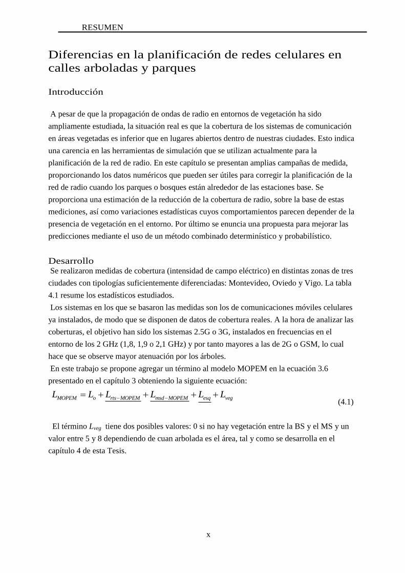
En este trabajo se propone agregar un término al modelo MOPEM en la ecuación 3.6
presentado en el capítulo 3 obteniendo la siguiente ecuación:
MOPEM o rts MOPEM msd MOPEM esq vegL L L L L L (4.1)
El término Lveg tiene dos posibles valores: 0 si no hay vegetación entre la BS y el MS y un
valor entre 5 y 8 dependiendo de cuan arbolada es el área, tal y como se desarrolla en el
capítulo 4 de esta Tesis.
RESUMEN
xi
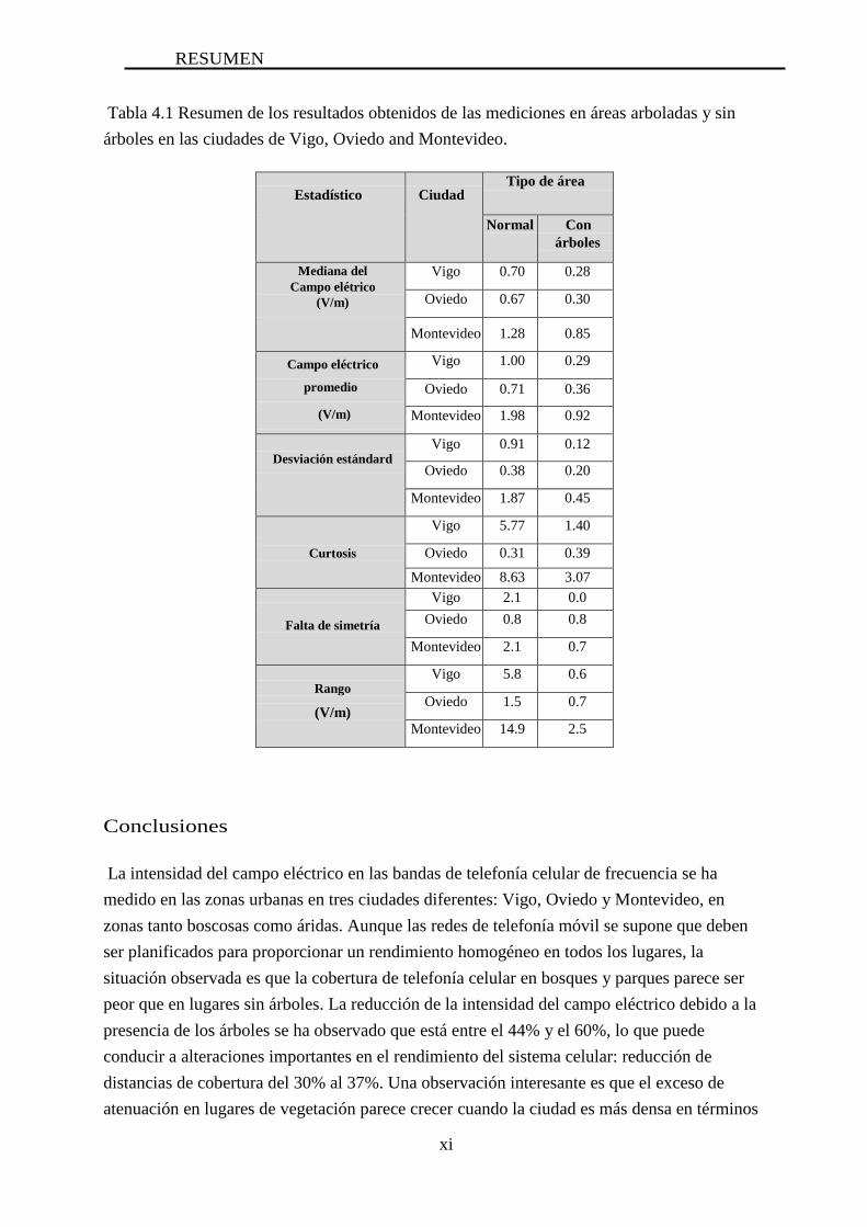
Tabla 4.1 Resumen de los resultados obtenidos de las mediciones en áreas arboladas y sin
árboles en las ciudades de Vigo, Oviedo and Montevideo.
Estadístico
Ciudad Tipo de área
Normal Con
árboles
Mediana del
Campo elétrico
(V/m)
Vigo 0.70 0.28
Oviedo 0.67 0.30
Montevideo 1.28 0.85
Campo eléctrico
promedio
(V/m)
Vigo 1.00 0.29
Oviedo 0.71 0.36
Montevideo 1.98 0.92
Desviación estándard
Vigo 0.91 0.12
Oviedo 0.38 0.20
Montevideo 1.87 0.45
Curtosis
Vigo 5.77 1.40
Oviedo 0.31 0.39
Montevideo 8.63 3.07
Falta de simetría
Vigo 2.1 0.0
Oviedo 0.8 0.8
Montevideo 2.1 0.7
Rango
(V/m)
Vigo 5.8 0.6
Oviedo 1.5 0.7
Montevideo 14.9 2.5
Conclusiones
La intensidad del campo eléctrico en las bandas de telefonía celular de frecuencia se ha
medido en las zonas urbanas en tres ciudades diferentes: Vigo, Oviedo y Montevideo, en
zonas tanto boscosas como áridas. Aunque las redes de telefonía móvil se supone que deben
ser planificados para proporcionar un rendimiento homogéneo en todos los lugares, la
situación observada es que la cobertura de telefonía celular en bosques y parques parece ser
peor que en lugares sin árboles. La reducción de la intensidad del campo eléctrico debido a la
presencia de los árboles se ha observado que está entre el 44% y el 60%, lo que puede
conducir a alteraciones importantes en el rendimiento del sistema celular: reducción de
distancias de cobertura del 30% al 37%. Una observación interesante es que el exceso de
atenuación en lugares de vegetación parece crecer cuando la ciudad es más densa en términos
RESUMEN
xii
de construcciones: avenidas amplias de Montevideo presentan atenuaciones alrededor de 5
dB, mientras que en Oviedo y Vigo, que son ciudades más densas, los valores medidos son 7
y 8 dB, respectivamente. Aún más, Oviedo presenta más parques y áreas abiertas que Vigo, lo
que confirma la tendencia.
Esa tendencia claramente diferente entre los dos tipos de zonas se confirma por la media de la
intensidad de campo medida, que es la mitad o incluso menos en arbolado en comparación
con las zonas abiertas. Además, la desviación estándar es visiblemente más grande en áreas
abiertas, como consecuencia de una gama más amplia de valores y su distribución más
dispersa, que en bosques y parques. Los rangos que contienen los puntos de medición de
campo eléctrico en lugares parecen ser más grandes (de dos a diez veces más) que en las
zonas con vegetación, en todas las ciudades consideradas.
Todas las estadísticas confirman una tendencia claramente diferente en la intensidad de
campo eléctrico en los dos tipos de ambientes.
Esta conclusión anterior parece ser más problemática, ya que muchos de los sistemas
modernos de planificación de redes no consideran la presencia de vegetación en los lugares a
ser cubiertos. Si la cobertura se ha calculado teniendo en cuenta la vegetación, se podría
pensar que los árboles no están correctamente modelados en estas herramientas de
planificación. Y si los diseñadores no han considerado la presencia de vegetación, esta
simplificación parece ser muy importante que se adopten en tal desarrollo de la red.
El problema en las redes 3G y 4G sería más fuerte que en 2G, debido a sus frecuencias más
altas, la cercanía a la frecuencia de resonancia del agua, el fenómeno de la respiración celular
y la inexactitud de los modelos de árboles utilizados para la planificación de 2G.
La propuesta para tratar de superar esos errores reside en la combinación de modelos
determinísticos de propagación, para obtener la cobertura general teniendo en cuenta sólo las
estructuras estáticas en el entorno (como se hace hoy en día), añadiendo una corrección
probabilística basada en los resultados proporcionados en este trabajo. Así, en las zonas de
vegetación, los resultados proporcionados por las herramientas de simulación estándar deben
ser corregidos añadiendo atenuaciones entre 5 y 8 dB, en función de la densidad de
construcción de la ciudad considerada: cuanto más denso sea el lugar, mayor será el exceso de
atenuación en las áreas de vegetación.

RESUMEN
xiii
Protección e interferencia de redes inalámbricas por
medio de barreras de vegetación
Introducción
La atenuación de las ondas de radio que se propagan a través de la vegetación es un efecto
bien conocido, pero sus consecuencias, los mecanismos y las posibles aplicaciones de este
fenómeno no se han explorado completamente. En este capítulo se presenta una posible
aplicación de ese efecto de atenuación. La vegetación, al obstruir el canal de radio, podría
proporcionar una atenuación suficiente para: a) reducir la distancia a la que los elementos de
diferentes redes se pueden instalar sin generar y recibir interferencia, y b) reducir la distancia
a la que un usuario externo (no autorizado ni deseado) podría acceder a los equipos
confidenciales de la red. Por lo tanto, una decisión correcta en la ubicación de las plantas tanto
en el interior como exterior podría beneficiar al rendimiento de la red inalámbrica mejorando
la protección contra la interferencia y / o los ataques externos.
Se ha realizado una amplia campaña de medición que incluye siete especies diferentes para
apoyar la propuesta, y sus resultados se presentan a lo largo de este capítulo.
Desarrollo
El efecto de las barreras de vegetación debe ser trasladado como atenuación adicional a los
resultados de los modelos. Esta atenuación adicional se corresponde con los valores
presentados en las tablas 5.2 a 5.5, en el capítulo 5 de la memoria. Por lo tanto, los modelos
con vegetación se usaron para analizar los radios de cobertura con y sin barreras de
vegetación, siendo las pérdidas de propagación con barreras la indicada por la ecuación 5.6,
que modifica la ecuación 5.2. Lbarrier representa la contribución de la barrera a la atenuación
total.
max( ) tx tx rx barrierL d P G G S L (5.6)
Algunos parámetros se eligieron para calcular numéricamente los radios de cobertura:
Ptx = 20 dBm, S = −78 dBm, Gtx = 6 dBi, Grx = 2 dBi.
Los resultados presentados en el trabajo se calcularon usando dos atenuaciones posibles de
las barreras, 5 y 10 dB a los efectos de tener una idea representativa y debido a que la mayor
parte de las atenuaciones medidas se encontraban entre estos parámetros.
La siguiente tabla muestra los resultados para estos dos valores y en 3 modelos de
propagación, observándose la reducción de las distancias de cobertura generada por la barrera
vegetal.

RESUMEN
xiv
Tabla 5.6. Distancias de cobertura (m) para diferentes valores de atenuación debido a barreras
de vegetación.
Barrera de
vegetación
Atenuación
adicional
(dB)
Distancia de cobertura (m) Modelo interior-
exterior
interior ITU-R Estadístico
Sin barrera 0 37 81 87 Barrera 1 5 26 55 62 Barrera 2 10 18 37 44
Otro escenario podría ser definido cuando varios puntos de acceso deben ser instalados en
áreas adyacentes, lo más cerca posible si hay mucha densidad de tráfico medida en Mbps por
m2.
La relación entre la distancia entre nodos y el radio de cobertura mide que tan cerca se
pueden instalar dos puntos de acceso y esta relación es dada por la ecuación 5.7
(
)
(5.7)
En esta ecuación, Ninterf es el número de puntos de acceso adyacentes, atbarr es la atenuación
de la barrera, c es la potencia de la portadora e i es la potencia transmitida por los puntos de
acceso adyacentes que interfieren. Considerando c/i aproximadamente igual a 100 y n = 3.4
para los cálculos de la tabla 5.7., en dicha tabla se muestran valores de D/R sin barrera, y con
barreras de 5 y 10 dB de atenuación adicional.
Tabla 5.7. Relación de distancia entre los nodos y el radio de cobertura.
Barrera Atenuación adicional
(dB)
D/R
Sin barrera 0 4.9
Barrera 1 5 3.8
Barrera 2 10 3.0
Conclusiones
Una amplia campaña de medición ha sido desarrollada con el fin de analizar la atenuación
inducida por barreras de vegetación, con configuraciones diferentes. Las mediciones se
realizaron tomando una referencia con línea de vista exactamente en el mismo ambiente
donde se obtienen los datos con obstrucción. Así, el exponente de pérdida de propagación con
la distancia se supone que es el mismo en ambos escenarios y la única diferencia entre ellos
sería la atenuación de la barrera de vegetación inducida entre el transmisor y el receptor. Por
lo tanto, las pérdidas debidas a los obstáculos se obtienen comparando las pérdidas en
condiciones NLoS de cada serie de mediciones con la referencia LoS. Se han detectado

RESUMEN
xv
atenuaciones de hasta 21 dB a 5,8 GHz o superior a 10 dB a 2,4 GHz. Estas capacidades de
atenuación de las barreras de vegetación luego se traduce en la reducción de la distancia de
cobertura, que se propone para ser utilizado en el ámbito de las redes inalámbricas, en dos
direcciones: la ampliación de la distancia libre de interferencias entre nodos de redes
adyacentes, y la protección contra ataques de intrusos informáticos que se conectan de forma
inalámbrica a la red WiFi.
Los resultados son alentadores debido a que las barreras parecen producir atenuación
suficiente para alcanzar reducciones interesantes en la distancia a los nodos adyacentes
(permiten instalar nodos de dos redes a distancias cercanas evitando la interferencia), y
también en la distancia a la que un hacker debe estar instalado para acceder a una red (lo que
obligaría a los intrusos a situarse muy cerca del edificio corporativo donde se ubica la red).
Las distancias de cobertura se calculan utilizando tres modelos diferentes, tanto en interiores
como interior-exterior, y estos resultados indican que esta reducción es más importante cuanto
mayor es la atenuación. Como ejemplo, para atenuaciones de 5 dB y 10 dB adicionales
debidas a las barreras de vegetación, las reducciones de la distancia son de 30 a 50%
respectivamente que se podría conseguir, en comparación con los escenarios sin barreras.
La relación entre la distancia entre los nodos y el radio de cobertura también se ha deducido
como una medida de que tan cercanos los nodos de dos redes adyacentes podrían ser
instalados cuando una línea de arbustos se utiliza para separar las zonas de cobertura. Se
calculó la eficiencia de la red en presencia de barreras de vegetación, en términos de la
reducción en la distancia de reuso de frecuencia.
En la medida que estos obstáculos no son caros, generan un ambiente agradable y son bien
aceptados por la gente, se espera que la propuesta tenga éxito.

RESUMEN
xvi
El rendimiento de los sistemas de OFDM 64 QAM
en canales radio de múltiples trayectos
Introducción
En este trabajo han sido analizados algunos sistemas OFDM basados en el estándar IEEE
802.16e con modulación 64 QAM, tasa de codificación ¾ y dúplex por división de tiempo
(TDD) por un canal de ancho de banda de 3,5 MHz. Dos clases de estos sistemas fueron
utilizados: MIMO y MC-CDMA o Coded-OFDM.
Varias simulaciones se realizaron con diferente cantidad de antenas en el transmisor y
receptor de hasta 2x2 sobre el canal AWGN y los canales Rayleigh multitrayecto como el
SUI4, SUI-6 y canales reales interiores. Se ha analizado el rendimiento de dos detectores
basados en el esquema de Alamouti, que se distingue por asumir o no el mismo CIR para
todas las antenas que reciben desde cada antena de transmisor. El equilibrio entre el uso de los
pilotos para la estimación de canal y de la diversidad de transmisión ha sido analizado con el
transmisor estándar, para lograr una ganancia de 6 dB en la SNR para una BER 10-2
. La
influencia del tiempo de guarda en la BER ha sido también crítica, lo que confirma que la
BER aumenta 104 veces con una SNR de 20 dB cuando el retraso de los rayos con amplitudes
importantes es mayor que el tiempo de guarda. Se propone un sistema MIMO 64 QAM que
logra una BER de sólo 2% sobre canales de Rayleigh.
También se presenta el rendimiento de dos sistemas MC-CDMA. La BER de los dos sistemas
MC-CDMA y MC-CDMA de secuencia directa (MC-DS-CDMA) el que se calculó mediante
Simulink® en entornos basados en canales AWGN, SUI-4, el SUI-6 y cuatro canales
interiores reales medidos, y luego se compararon con el rendimiento del estándar. Se logró
una reducción de 100 en la BER para el mismo rendimiento, con 26 dB de Eb / No. La
estimación de canal y predicción, así como los métodos de pre-ecualización también fueron
evaluadas para dichos sistemas y canales. La dependencia de BER con la desviación de
frecuencia Doppler se analiza entonces para el canal AWGN.
Desarrollo
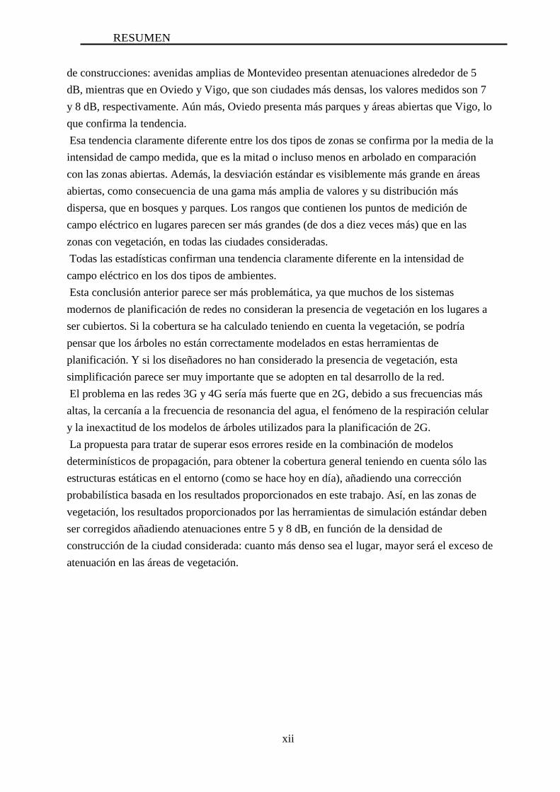
Los tipos de esquemas con varias antenas en transmisión y recepción se describen en la figura
6.6 Estos son: SISO cuando M=N=1, SIMO cuando N=1 y M>1, MISO con N>1 y M=1 y
MIMO con N>1 y M>1.
RESUMEN
xvii
Figura 6.6: Diferentes esquemas con diferente cantidad de antenas de Tx y Rx.
El esquema CDMA que se propone agregar al estándar tiene la siguiente estructura:
Se inserta el bloque CDMA entre el interleaver y el modulador.
Figura 6.9: Sistema CDMA mas OFDM del transmisor y del receptor.
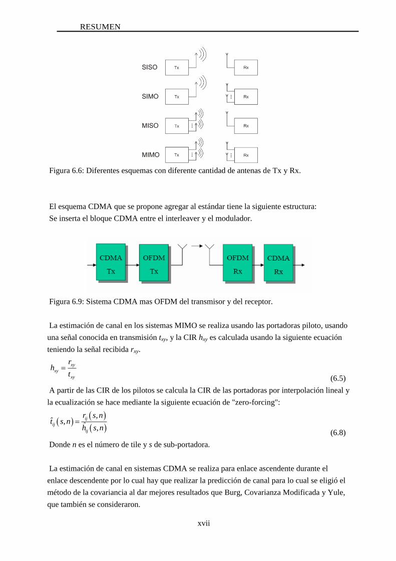
La estimación de canal en los sistemas MIMO se realiza usando las portadoras piloto, usando
una señal conocida en transmisión txy, y la CIR hxy es calculada usando la siguiente ecuación
teniendo la señal recibida rxy.
xy
xy
xy
rh
t
(6.5)
A partir de las CIR de los pilotos se calcula la CIR de las portadoras por interpolación lineal y
la ecualización se hace mediante la siguiente ecuación de "zero-forcing":
,,
,
ij
ij
ij
r s nt s n
h s n
(6.8)
Donde n es el número de tile y s de sub-portadora.
La estimación de canal en sistemas CDMA se realiza para enlace ascendente durante el
enlace descendente por lo cual hay que realizar la predicción de canal para lo cual se eligió el
método de la covariancia al dar mejores resultados que Burg, Covarianza Modificada y Yule,
que también se consideraron.
RESUMEN
xviii
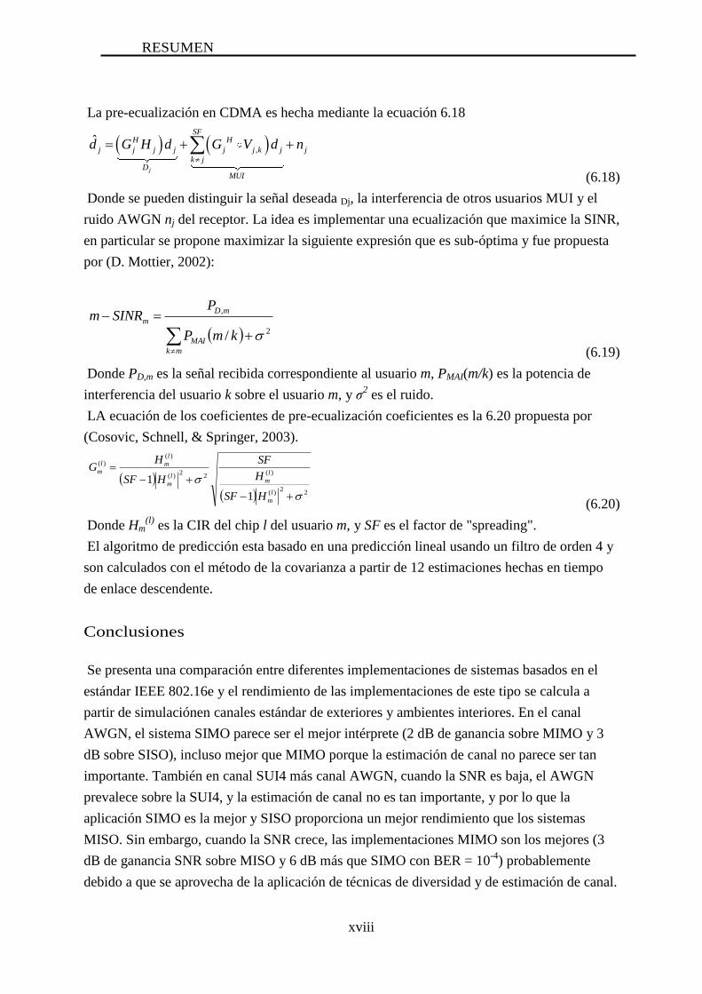
La pre-ecualización en CDMA es hecha mediante la ecuación 6.18
,ˆ
j
SFH H
j j j j j j k j j
k jD
MUI
d G H d G V d n
(6.18)
Donde se pueden distinguir la señal deseada Dj, la interferencia de otros usuarios MUI y el
ruido AWGN nj del receptor. La idea es implementar una ecualización que maximice la SINR,
en particular se propone maximizar la siguiente expresión que es sub-óptima y fue propuesta
por (D. Mottier, 2002):
2
,
/
mk
MAI
mD
m
kmP
PSINRm
(6.19)
Donde PD,m es la señal recibida correspondiente al usuario m, PMAI(m/k) es la potencia de
interferencia del usuario k sobre el usuario m, y σ2 es el ruido.
LA ecuación de los coeficientes de pre-ecualización coeficientes es la 6.20 propuesta por
(Cosovic, Schnell, & Springer, 2003).
2
2)(
)(2
2)(
)()(
1
1
l
m
l
ml
m
l
ml
m
HSF
H
SF
HSF
HG
(6.20)
Donde Hm(l)
es la CIR del chip l del usuario m, y SF es el factor de "spreading".
El algoritmo de predicción esta basado en una predicción lineal usando un filtro de orden 4 y
son calculados con el método de la covarianza a partir de 12 estimaciones hechas en tiempo
de enlace descendente.
Conclusiones
Se presenta una comparación entre diferentes implementaciones de sistemas basados en el
estándar IEEE 802.16e y el rendimiento de las implementaciones de este tipo se calcula a
partir de simulaciónen canales estándar de exteriores y ambientes interiores. En el canal
AWGN, el sistema SIMO parece ser el mejor intérprete (2 dB de ganancia sobre MIMO y 3
dB sobre SISO), incluso mejor que MIMO porque la estimación de canal no parece ser tan
importante. También en canal SUI4 más canal AWGN, cuando la SNR es baja, el AWGN
prevalece sobre la SUI4, y la estimación de canal no es tan importante, y por lo que la
aplicación SIMO es la mejor y SISO proporciona un mejor rendimiento que los sistemas
MISO. Sin embargo, cuando la SNR crece, las implementaciones MIMO son los mejores (3
dB de ganancia SNR sobre MISO y 6 dB más que SIMO con BER = 10-4
) probablemente
debido a que se aprovecha de la aplicación de técnicas de diversidad y de estimación de canal.

RESUMEN
xix
Con este esquema, se alcanzó una BER baja en la modulación 64QAM comparando con la
literatura actual.
Se puede observar el incremento de la BER cuando el número de pilotos se reduce de cuatro
a dos, entre SISO con 4 pilotos y SISO-2P (dos pilotos), y SIMO y SIMO-2P con el canal
AWGN destacando la relevancia de la pilotos para estimar el canal y reducir la BER.
Otra conclusión es que la interpolación de la CIR por las subportadoras, implementado en el
esquema algebraico, proporciona mejores resultados que asumir el mismo CIR que los pilotos
adyacentes, tal como se aplica en Alamouti para todos los canales probados.
Una verificación adicional es que la diversidad en el receptor, mejora significativamente la
BER en sistemas SISO y MISO para todos los canales. La diversidad de transmisión mejora el
rendimiento canales Rayleigh (SUI4 y SUI6), pero la aplicación del transmisor y el receptor
crece en complejidad.
Analizando canales interiores medidos, con datos reales, los sistemas MIMO se desempeñan
significativamente mejor que los demás. En los entornos de laboratorio, sistemas MIMO
necesita una SNR de 16 dB aproximadamente para llegar a una BER de 10-4
, y en los canales
de oficina una SNR de 11 dB. Los otros sistemas necesitan una mayor SNR de 22 dB o 17 dB,
respectivamente, para lograr un BER de 10-4
. Así sistemas MIMO producen una ganancia de
alrededor de 6 dB en la relación señal ruido.
El sistema MIMO reduce significativamente la BER en comparación con el SIMO o MISO, a
veces logrando una disminución de más de diez veces. Sin embargo, en esta norma, el ciclo de
prefijo debe ser más grande que el retardo de los rayos con una considerable amplitud en la
propagación por trayectos múltiples. De lo contrario, la eficacia del sistema MIMO se reduce
como en el SUI6 canal. Esto es válido también para CDMA. Las pruebas en el canal AWGN
muestra un comportamiento similar para todas las implementaciones de OFDM-CDMA,
porque este canal es aleatorio, por lo que los mecanismos de predicción de canal, pre-
igualación y de control de potencia no tienen ningún efecto en la reducción de la BER. (Figura
6.35).
En los sistemas de CDMA cuando más usuarios están en él, la longitud del código aumenta y
así aumenta la diversidad y la BER se reduce a SNR constante, pero la tasa de transferencia
por usuario se reduce.
La predicción de canal y pre-ecualización se pusieron a prueba en los canales SUI con buenos
resultados que alientan su aplicación.
Las mejores implementaciones son MC-CDMA y la peor es MC-DS-CDMA Classic. La
razón es que hay mayor dispersión de la información en el dominio del tiempo en los primeros
y eso los hacen mas inmune al efecto Doppler. Sin embargo, estos sistemas han demostrado
ser canales de trayectos múltiples muy sensibles.
Entre todos los métodos predicciones el mejor rendimiento se logra por el método de
covarianza.

RESUMEN
xx
Cuando el número de usuarios varía desde 2 hasta 8 usuarios lo que puede observarse es que
la diversidad producida por la difusión no tiene un efecto importante sobre la BER frente la
Eb/No. El sistema logra una BER de 10-6
con Eb/No entre 10 y 15 dB, superando el estándar
que presenta una BER mayor a 10-4
para Eb/No similar.

RESUMEN
xxi
Eficiencia espectral promedio de sistemas celulares
con múltiple modulaciones
Introducción
Los sistemas de cuarta generación proponen la creación de redes inalámbricas ampliadas
mediante la aplicación de técnicas de reutilización de frecuencia basado en un esquema
celular. El ancho de banda necesario para instalar un despliegue FDMA metropolitana
depende del ancho de banda de canal y en la relación de protección de señal a interferencia.
La eficiencia espectral de la red es inversamente proporcional al ancho de banda requerido por
el racimo (clúster) que es mayor para las modulaciones más eficientes porque tienen grandes
relaciones de protección.
Este compromiso se analiza en el séptimo capítulo para sistemas con varios esquemas de
modulación (QPSK, 16 y 64QAM), obteniendo el porcentaje de la superficie celular que
podría ser gestionado con cada modulación, teniendo en cuenta los sectores con carga
completa. Se calcula el área de una celda con los móviles que utilizan cierta modulación en el
caso de reutilización 1. Un ejemplo, calculado para 3,5 GHz, muestra una reducción del 35%
de la máxima eficiencia espectral, que cae a 1.6 bps / Hz. El ancho de banda total requerido
para tres celdas sectorizadas con canales de 10 MHz da 360 MHz. Este es un gran problema
ya que el tamaño de las bandas es generalmente de 200 MHz. Para resolver este problema, los
autores de la norma están buscando métodos de ICIC y FFR o reinstalación en estaciones
repetidoras.
Se presentan las condiciones en distancias entre dos usuarios que comparten las mismas
subportadoras en dos estaciones de base manteniendo las SNRs necesarios para ambos
usuarios.
Y se proponen dos algoritmos para la asignación de potencia y programación de usuario para
ser evaluados en futuros trabajos.
Desarrollo
Primero se verifican las condiciones que deben cumplir las distancias de los móviles a la
estaciones base servidora e interferente
Si hay m interferentes y d21 es la mínima distancia entre las BS interferentes y M1, el peor
caso para la SNIR esta dado por la ecuación:
111 21 21
21 211 11
. 1
. .
nn
pn
total
P d dS c Pr
N I i mP m d P m d
(7.2)
Si se consideran la misma potencia de transmisión.

RESUMEN
xxii
Por otro lado se calcula el ancho de banda mínimo para un despliegue con la siguiente
ecuación:
2
1
sec sec
11
3n
total tor p torBW J s BW m r s BW
(7.4)
Donde J es la cantidad de celdas mínima correspondientes a la de un clúster, s la cantidad de
sectores de la celda y BWsector es el ancho de banda del canal del sector.
En otro orden de cosas para alcanzar la SNIR para dos móviles en BS adyacentes con la
misma frecuencia uno a distancia d11 de BS1 con potencia P1 y otro a distancia d22 asociado a
BS2 con potencia P2, se deben cumplir las condiciones de las ecuaciones7.7 a 7.10.
Las cuales culminan en la ecuación 7.11
12 2122 2/
11
.
.n
p
d dd
r d
(7.11)
En la siguiente figura se muestra gráficamente los resultados de la ecuación 7.11.
Figure 7.3: Distancias relativas de dos usuarios en BS adyacentes reusando la frecuencia,
d22/R vs. d11/R para las modulaciones QPSK, 16 y 64 QAM..
Para calcular la capacidad de un sector con múltiples modulaciones se deben calcular las
áreas de cada una de ellas relativas al área total de la celda.
Las ecuaciones que proponemos son las siguientes:
21/
16
1/
16
1 ( . )
1 ( . )
n
QAM pQPSK
n
QPSK p QAM
A m r
A m r
(7.14)
1E-8
1E-7
1E-6
1E-5
1E-4
1E-3
1E-2
1E-1
1E+0
1E+1
1E+20,1 0,2 0,3 0,4 0,5 0,6 0,7 0,8 0,9 1
d22/R
d11/R
64 QAM
16 QAM
QPSK
RESUMEN
xxiii
21/
64
1/
64
1 ( . )
1 ( . )
n
QAM pQPSK
n
QPSK p QAM
A m r
A m r
(7.15)
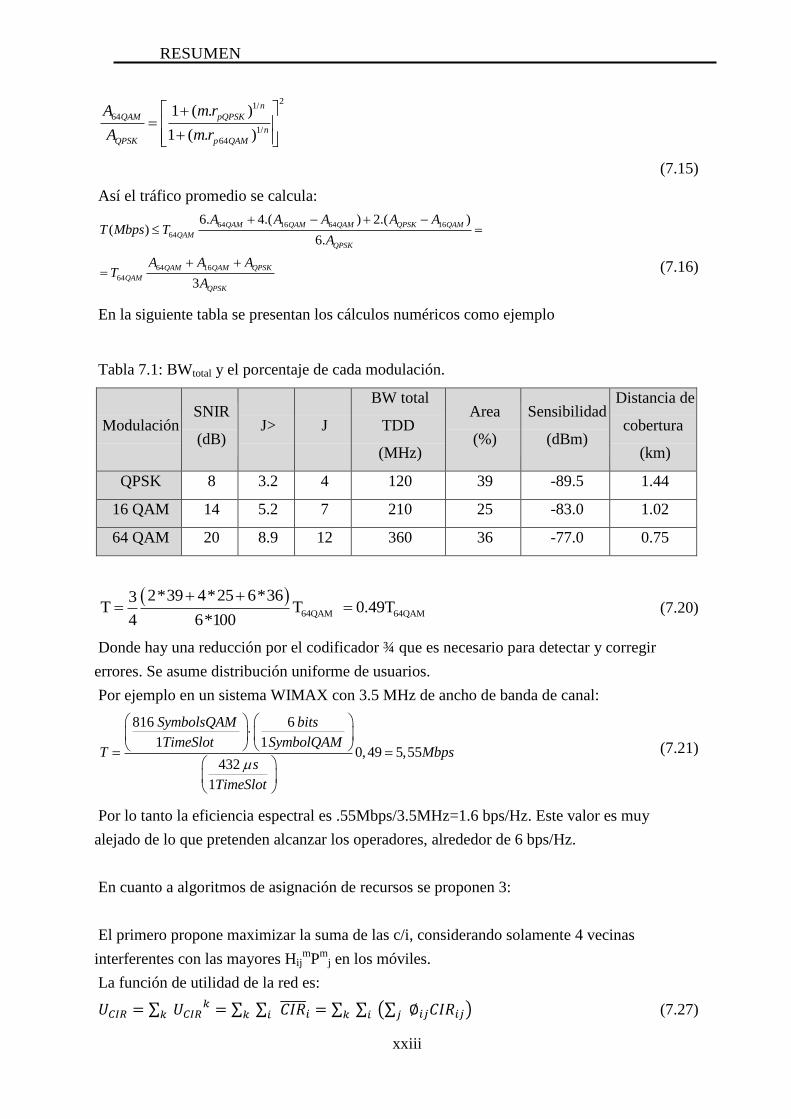
Así el tráfico promedio se calcula:
64 16 64 16
64
64 16
64
6. 4.( ) 2.( )( )
6.
3
QAM QAM QAM QPSK QAM
QAM
QPSK
QAM QAM QPSK
QAM
QPSK
A A A A AT Mbps T
A
A A AT
A
(7.16)
En la siguiente tabla se presentan los cálculos numéricos como ejemplo
Tabla 7.1: BWtotal y el porcentaje de cada modulación.
Modulación SNIR
(dB) J> J
BW total
TDD
(MHz)
Area
(%)
Sensibilidad
(dBm)
Distancia de
cobertura
(km)
QPSK 8 3.2 4 120 39 -89.5 1.44
16 QAM 14 5.2 7 210 25 -83.0 1.02
64 QAM 20 8.9 12 360 36 -77.0 0.75
64QAM 64QAM
2*39 4*25 6*363T T 0.49T
4 6*100
(7.20)
Donde hay una reducción por el codificador ¾ que es necesario para detectar y corregir
errores. Se asume distribución uniforme de usuarios.
Por ejemplo en un sistema WIMAX con 3.5 MHz de ancho de banda de canal:
816 6
1 10,49 5,55
432
1
SymbolsQAM bits
TimeSlot SymbolQAMT Mbps
s
TimeSlot
(7.21)
Por lo tanto la eficiencia espectral es .55Mbps/3.5MHz=1.6 bps/Hz. Este valor es muy
alejado de lo que pretenden alcanzar los operadores, alrededor de 6 bps/Hz.
En cuanto a algoritmos de asignación de recursos se proponen 3:
El primero propone maximizar la suma de las c/i, considerando solamente 4 vecinas
interferentes con las mayores Hijm
Pm
j en los móviles.
La función de utilidad de la red es:
∑
∑ ∑ ̅̅ ̅̅ ̅ ∑ ∑ (∑ ) (7.27)

RESUMEN
xxiv
con
∑
(7.28)
El primer algoritmo surge de resolverel problema anterior por el método del gradiente y el
segundo es usando las condiciones KKT descripto en las ecuaciones 7.30 a 7.39.
Y se propone un tercer algoritmo descrito en 7.4.1 donde se usa la relación de distancias
entre usuarios que reúsan frecuencias 7.11.
Conclusiones
Los anchos de banda necesarios para modulaciones más densas, incluso en los sistemas TDD,
son difíciles de obtener, 630 MHz para 16 QAM, y 1080 MHz para 64 QAM. Esto podría ser
una barrera para el despliegue de estos sistemas a un coste razonable. El espectro está
disponible principalmente en las altas frecuencias, lo que implica radio de celda muy corto del
orden de cientos de metros.
Estas consideraciones deben ser tenidas en cuenta por los reguladores que gestionan el
espectro y por los operadores, para conocer las características esperadas de la red, a fin de
evitar alguna información comercial lejos de los funcionamientos reales.
El procedimiento para calcular el rendimiento de tales sistemas celulares limitados en
interferencia se introduce en este trabajo, y algunos resultados de simulación se presentan para
resaltar los problemas en el despliegue de estas redes. El hecho de que la modulación QPSK
sea dominante en el análisis de la interferencia hace que el tráfico medio de un sector sea
cerca del 50% de la capacidad máxima de 64 QAM. QPSK podría ser el esquema de
modulación que domina el plan de frecuencias y la distribución de clúster. Pero esta selección
disminuye la eficiencia espectral en comparación con una 64QAM, reduce la capacidad de
tráfico del sector y, por lo tanto, afecta al negocio. También limita el rendimiento máximo por
cliente limitando los precios y debilitando esta tecnología frente a la competencia frente otras
tecnologías como ADSL. Por lo tanto, las constelaciones más densas no implican
necesariamente un aumento lineal de la capacidad de la red o el móvil. El aumento de la
eficiencia espectral se logrará al reducir la rp.
Se deduce la restricción a la reutilización de la frecuencia entre dos estaciones base
adyacentes y se presenta la relación entre las potencias y la restricción de distancia entre dos
usuarios y sus BS dada la rp.
En este trabajo se proponen tres algoritmos para la asignación de recursos, potencia y agenda
de usuarios pero uno esta basado en esta relación.
A medida que la reutilización de las frecuencias es posible hasta el 70% del radio o 49% de la
superficie de la célula en el mejor de los casos (QPSK), la reutilización de la frecuencia
asignada a los móviles en el medio externo de la célula es inviable. Con la reutilización 1, sólo
el 36% de la superficie celular podría ser utilizado con 16 QAM y el 20% con 64 QAM. Esto
RESUMEN
xxv
es independiente del método utilizado para elegir los usuarios y la potencia o la zona asignada
a cada conjunto de frecuencias, pero todos estos métodos deben considerar esta restricción
para evitar la interferencia que provoca un valor de BER inaceptable.
El estándar LTE considera el reuso de frecuencia fraccional, que divide el canal con la
ventaja de que a veces el canal completo se podría utilizar, pero si no es utilizada por sectores
adyacentes. Esto se está debatiendo en el grupo 3GPP (3GPP, 2010).
Otro camino para explorar es la reducción de la capacidad de los usuarios cerca del borde de
la célula, generando dos clases de clientes. Por lo tanto, el acceso a un producto de alta
velocidad, sería imposible para todos los clientes de forma simultánea. Una de las estrategias
para resolver este problema es utilizando estaciones repetidoras, pero aumenta los costos.
Un equilibrio entre la optimización, la precisión y el tráfico de señalización y procesamiento
es evidente cuando el rendimiento total de la red se maximiza.
Muchos métodos para resolver la asignación de potencia y programación de usuarios fueron
revisados; básicamente los que utilizan la ICIC, pero también la reutilización de portadoras en
forma estática, la semi-estática y la flexible.
Se analizaron algunos métodos basados en funciones de utilidad con las que se propone
aprovechar al máximo, por ejemplo, el rendimiento total con restricciones en potencia y
planificación equitativa de los usuarios. Una propuesta presenta un método de programación
del gradiente y otros usan la condiciones KKT para convertir el problema en uno sin
restricciones obligado a incrementar el número de variables basadas en los operadores de
Lagrange.
Por lo tanto, se propone una nueva función de utilidad usando la suma de la CIR de los
usuarios, y con las condiciones KKT. Pero también pueden ser resueltos por cualquier otro
método de maximización. Y se propone un algoritmo para la asignación de recursos utilizando
esta nueva función de utilidad.
xxvi
Index
Acknowledgements…………………………………………………………………………..ii
Abstract……………………………………………………………………………………….iii
Resumen……………………………………………………………………………………….v
Introducción ........................................................................................................................... vi
Modelo de canal radio MOPEM .......................................................................................... viii
Diferencias en la planificación de redes celulares en calles arboladas y parques .................. x
Protección e interferencia de redes inalámbricas por medio de barreras de vegetación ...... xiii
El rendimiento de los sist. de OFDM 64 QAM en canales radio de múltiples trayectos ... xvi
Eficiencia espectral promedio de sistemas celulares con múltiple modulaciones ............... xxi
Chapter 1
Introduction……………………………………………………………………….... .............. 1
1.1 Motivation of the Thesis .......................................................................................... 1
1.2 Organization of the Thesis ....................................................................................... 3
Chapter 2 Review of the Literature…….. ............................................................................. .7
2.1. Urban channel model ............................................................................................... 7
2.2. Effects of vegetation in the radio channel ................................................................ 9
2.3. Use of vegetation for interference and security protection .................................... 12
2.4. Implementation of OFDM 64 QAM systems ........................................................ 12
2.5. Spectral efficiency of multimodulation cellular systems ....................................... 15
Chapter 3 Propagation Model for Small Urban Macro Cell………………………...…… . .17
3.1 Introduction ....................................................................................................... 17
3.2 Theoretical Analysis .............................................................................................. 18
3.2.1. Influence of the terrain height variation ................................................................. 19
xxvii
3.2.2. Dependence on the angle between the prop. direction and the street center line .. 21
3.3 Mopem Model ........................................................................................................ 23
3.4 Environment and measurements ............................................................................ 24
3.4.1. Area Description .................................................................................................... 24
3.4.2. Attenuation measurement ...................................................................................... 25
3.5 Results .................................................................................................................... 26
3.5.1. Model adjustment ................................................................................................... 26
3.5.2. Model validation .................................................................................................... 26
3.5.3. Comparison with the COST231-WI model ........................................................... 27
3.5.4. Distance dependence adjustment ........................................................................... 28
3.5.5. The influence of the terrain height variation .......................................................... 29
3.5.6. The finite multi-screens effect ............................................................................... 29
3.5.7. Street orientation dependence ................................................................................ 30
3.6 Applications ........................................................................................................... 32
3.6.1. Coverage area depending on the transmitter orientation ....................................... 32
3.6.2. Prediction improvements along the block .............................................................. 32
3.7 Conclusions ............................................................................................................ 33
Chapter 4 Cellular network planning imbalances at wooded streets and parks............... ... ..35
4.1. Introduction ............................................................................................................ 35
4.2. Measurements Campaigns ..................................................................................... 37
4.2.1. Vigo ........................................................................................................................ 38
4.2.2. Oviedo .................................................................................................................... 38
4.2.3. Montevideo ............................................................................................................ 39
4.3. Results .................................................................................................................... 39
4.3.1. Graphic results ....................................................................................................... 40
4.3.2. Numerical results ................................................................................................... 43
4.3.3. Extension of prediction models ............................................................................. 45
4.4. Conclusions ............................................................................................................ 46

xxviii
Chapter 5 Wireless Networks interference and security protection by means of vegetation
barriers………………………………………………………………………………… ....... 47
5.1. Introduction ............................................................................................................ 47
5.2. Measurements Campaigns ..................................................................................... 49
5.3. Measurements Results ........................................................................................... 60
5.4. Coverage Analysis ................................................................................................. 62
5.4.1. Empirical Indoor-to-outdoor Model ...................................................................... 63
5.4.2. ITU-R Model (Indoor) ........................................................................................... 63
5.4.3. Statistical Path Loss Model (Indoor) ..................................................................... 64
5.5. Coverage Results ................................................................................................... 64
5.6. Conclusions ............................................................................................................ 67
Chapter 6 Performance of OFDM 64 QAM systems over multipath channels………… .... 69
6.1. Introduction ............................................................................................................ 70
6.2. OFDM .................................................................................................................... 71
6.2.1. Mathematical description of OFDM signals .......................................................... 72
6.3. MIMO system ........................................................................................................ 73
6.4. CDMA System ....................................................................................................... 76
6.5. Channel description ............................................................................................... 77
6.5.1. Channel AWGN ..................................................................................................... 78
6.5.2. Channel SUI 4 and SUI 6 ....................................................................................... 78
6.5.3. Measured indoor channels ..................................................................................... 79
6.6. Channel Estimation ................................................................................................ 80
6.6.1. Channel Estimation in MIMO systems .................................................................. 80
6.6.2. Channel Estimation on CDMA .............................................................................. 80
6.6.2.1. Burg ........................................................................................................................ 82
6.6.2.2. Covariance ............................................................................................................. 83
6.6.2.3. Modified Covariance ............................................................................................. 83
6.6.2.4. Yule ........................................................................................................................ 83
6.7. Pre-equalization for CDMA ................................................................................... 83
6.8. Alamouti coding for MIMO ................................................................................... 85

xxix
6.8.1. Classical Alamouti detection ................................................................................. 86
6.8.2. Algebraic detection ................................................................................................ 86
6.9. Implementation ...................................................................................................... 86
6.9.1. Common parameters .............................................................................................. 87
6.9.2. Transceiver ............................................................................................................. 88
6.9.2.1. MIMO Transmitter - Receiver ............................................................................... 88
6.9.2.2. CDMA Transmitter-Receiver ................................................................................ 89
6.9.2.3. MC-DS-CDMA SYSTEMS................................................................................... 91
6.10. Simulink Implementation ....................................................................................... 93
6.10.1. Block scheme of one transmitter and one receiver ................................................ 93
6.10.2. Block scheme of MC-CDMA system .................................................................... 94
6.10.3. Block scheme of MIMO-OFDM simulator ........................................................... 96
6.11. Results .................................................................................................................... 98
6.11.1. MIMO Results ....................................................................................................... 98
6.11.1. CDMA Results ..................................................................................................... 103
6.12. Conclusions .......................................................................................................... 108
Chapter 7 Average spectral efficiency of multi modulation cellular systems…………. ... 111
7.1. Introduction .......................................................................................................... 112
7.2. Foundations .......................................................................................................... 113
7.2.1. Previous works ..................................................................................................... 113
7.2.2. Total bandwidth of a network deployment .......................................................... 114
7.2.3. Distance relation of mobiles reusing the frequency in adjacent cells .................. 117
7.2.4. Average Sector Traffic ......................................................................................... 119
7.3. Results .................................................................................................................. 122
7.4. Inter-Cell Interference Mitigation Approaches .................................................... 123
7.4.1. Static Inter-Cell Interference Coordination ......................................................... 123
7.4.2. Semi-Static ICI coordination ............................................................................... 124
7.4.3. Softer Frequency Reuse ....................................................................................... 124
7.4.4. Resource allocation algorithm proposed #1 ......................................................... 126
7.4.5. Resource allocation algorithm proposed #2 ......................................................... 127
xxx
7.5. Conclusions .......................................................................................................... 129
Chapter 8 Conclusions…………………………………………………………… ………131
8.1. Radio propagation channels ................................................................................. 131
8.2. MIMO-OFDM and MC-CDMA systems ............................................................ 133
8.3. Frequency reuse in 4G systems ............................................................................ 135
8.4. General conclusion ............................................................................................... 136
8.5. Published results .................................................................................................. 137
8.5.1. Journal papers ...................................................................................................... 137
8.5.2. Conference contributions ..................................................................................... 137
References…………………………………………………………………………………..139
1
Chapter 1 Introduction
1.1 Motivation of the Thesis
The aim of this Thesis is to investigate the performance of the Fourth Generation (4G) data
networks based on OFDM technology over many urban channels, from various focuses: radio
propagation, system implementation, and spectral efficiency.
But as strictly 4G is when you have more than 100 Mbps throughput technologies, we will be
analyzing 3.5 G networks as they are the base of 4G networks.
The Thesis is focused on denser modulations as 64 QAM over the most actual urban
channels, where there are more users, to learn the behavior at maximum capacity with the
more common so more interesting environment. One of the most important issues in the
cellular planning is the confidence in the radio propagation model used to do it. A large
measurement campaign was done in the most populated neighborhoods of Montevideo City,
Pocitos and Punta Carretas, to confirm the validity of the used models. As a result, a new
propagation model has been proposed, which improves the performance of previous
simulation tools, as COST 231-WI (COST 231).
Other particular channels were also investigated in deep: vegetal barriers, indoor and indoor-
outdoor channels, actual indoor channels, and WIMAX proposed channels, the SUI channels
(Erceg, Hari, & Smith, 2001)
The influence of trees in the streets is analyzed to improve the electromagnetic power density
estimation that determines the service provided. Some applications were proposed to use the
attenuation property of vegetables, for example to limit the coverage of a wireless network to
a certain area. The vegetal barriers have been also considered and modeled to quantify the
reduction they induce in the radio coverage, looking for a novel application: the reduction of
interference amongst neighbor wireless networks, as well as the improvement of protection
against external unauthorized intrusion.
CHAPTER 1. Motivation of the Thesis
2
For testing 4G system implementation, the modulation chosen was 64 QAM because it
provides the biggest capacity, so it is of great interest to operators, and it was proposed in both
main 4G standards, WIMAX (IEEE Comp., MW T.&T. Soc., 2004) (IEEE Comp.,MW T.&
T.Soc., 2006) and LTE (3GPP RAN TSG, 2009), as the densest modulation. The analysis of
other modulations has been mainly done for comparison purposes.
Two transmission schemes have been considered to achieve the better performance: MIMO
and Coded OFDM or CDMA-OFDM. The idea was to investigate how these strategies could
help to reduce the BER over fading channels and to evaluate advantages and disadvantages of
both implementation strategies.
Some software, based in Simulink-Matlab©, has been developed to simulate the systems
founded in IEEE802.16e and the channels used in this work, calculating their performances.
The performance was measured through the BER vs. the SNR of the systems under test over
the earlier mentioned channels.
The reuse of the frequency was also analyzed because it determines the spectrum bandwidth
needed for the network and the number of base stations, and both represent a big percentage
of the cost of the network. As many providers promote the frequency reuse 1 (Wimax Forum,
2006) (Ohm, 2008), where all users in each cell have access to the entire bandwidth, but as
these systems has a FDMA scheme, a deeper look was done to understand how it could works
and what is the spectral efficiency than can be expected. Some providers propose a reuse 1 for
cell interior users and reuse 1/3 for cell edge users, which is called Fractional Frequency
Reuse (FFR) strategy (Boudreau, Panicker, Guo, Chang, Wang, & Vrzic, 2009). Besides, the
spectrum necessary to implement an actual network was derived considering the protection
ratio without intelligent reuse or any kind of ICIC.
The detail on how the power is distributed over a carrier in different base stations to serve
many mobiles to achieve a general maximum of the throughput was also analyzed.
Finally the theoretical average throughput that can be expected for 4G Networks Standards is
discussed to understand the difference with the announcements of hundreds of Mbps that can
be offered to the users (Ericsson, 2009), taking in mind that 100 Mbps at mobile applications
represents the low boundary for a system to be considered 4G.
CHAPTER 1. Organization of the Thesis
3
1.2 Organization of the Thesis
The thesis is structured in eight chapters: this introduction, a bibliography review, five
research chapters, and the conclusions. The second chapter contains the state of the art. From
chapter 3 to chapter 5 the radio propagation channels are analyzed, Chapter 6 is dedicated to
simulation of different coding strategies, MIMOs and CDMA-OFDM systems, channel
estimation and equalization. In Chapter 7 the reuse of the frequency is studied in detail for
network deployment of OFDM systems. And finally, we conclude in chapter 8.
The second chapter contains a review of related literature previously published on the topic,
analyzing the state of the art, and highlighting the newness of this Thesis contents.
The third chapter, called “Propagation Model for Small Urban Macro Cells”, presents the
MOPEM1 propagation model for dense urban areas in the frequency band from 850 to 900
MHz. This work is based on the COST231-WI model, but the hypothesis of infinite screen
blocks is replaced by finite screens taking into account the street crossings, predicting the
signal attenuation along the block. The dependence of propagation loss with terrain height is
reviewed and optimized by considering an absolute reference, while the dependence on the
angle between the street and the wave propagation is modified to obtain a continuously
differentiable loss function.
The fourth chapter, “Cellular network planning imbalances at wooded streets and parks”,
presents large measurement campaigns results providing numerical data that could be useful
to correct the radio network planning when parks or groves are around the base stations. An
estimation of coverage radius reduction is provided, based on such measurements, as well as
various statistics which behaviors seem to depend on the presence of vegetation in the
environment. Finally, a proposal for improving the predictions done by radio network
planning tools by using a combined deterministic and probabilistic method is enunciated. The
cities involved in the study were Vigo and Oviedo, in Spain, and Montevideo, in Uruguay.
The chapter five, “Wireless Networks interference and security protection by means of
vegetation barriers”, proposes the use of vegetation barriers to create shadowing areas with
excess attenuations in the edge of the service area, in order to reduce and limit the coverage
distance of each wireless node, reducing the possible interference to and from other networks
as well as improving security aspects by minimizing the signal strength outside the service
area. Based on measurement results, the coverage distances were computed by using three
different models, two indoors and one indoor-to-outdoor. Then, these distances have been
used to analyze both new proposals, which try to take advantage of a phenomenon that has
been previously considered a problem: the attenuation induced by vegetation in the radio
wave propagation.
1 Spanish acronym for Propagation Model for Small Urban Macro Cells
CHAPTER 1. Organization of the Thesis
4
The sixth chapter, “Performance of OFDM 64 QAM systems over multipath channels”, is
focused in MIMO and CDMA-OFDM schemes. Some OFDM systems based on IEEE
802.16e with 64 QAM modulation have been compared by simulation with different quantity
of antennas in transmitter and receiver over the AWGN, and the multipath Rayleigh SUI-4
and SUI-6 channels, as well as actual indoor channels. The performance of two detectors has
been analyzed based on the Alamouti scheme, both considering and not considering the same
channel in the receiving antennas. The tradeoff between the use of pilots for channel
estimation and transmission diversity has been analyzed for the standard transmitter. The
influence of the guard time on the BER has been also reviewed, confirming that the BER
increases for the same SNR when the delay of rays with important amplitudes is greater than
the guard time.
Besides, the performance of two multi carrier code-division multiple access (MC-CDMA)
systems are presented based on the IEEE 802.16e standard, using 64 QAM modulation
scheme. The BER of the two systems was computed in a Simulink-MATLAB based
environment over AWGN, SUI-4, SUI-6 and four indoor measured channels, and then
compared with the standard’s performance. Also the channel estimation and prediction, and
pre-equalization methods are evaluated for those systems and channels. The BER dependence
with the Doppler frequency deviation is analyzed for SUI-6 channel.
Chapter 7, “Average spectral efficiency of multi modulation cellular systems”, analyzes
fourth generation systems focused on creating extend wireless networks by applying
frequency reuse techniques based on a cellular scheme with only one carrier. The bandwidth
required to install a metropolitan deployment will depend on the channel bandwidth and on
the signal to interference protection ratio. Each modulation scheme has its own protection
ratio and its spectral efficiency: so that, there is a trade-off between the total bandwidth
needed by a cluster of cells and the spectral efficiency of the network. This compromise is
analyzed in this work for systems with various modulation schemes (QPSK, 16 QAM and 64
QAM), deriving the percentage of the cell area corresponding to each modulation when
considering full load sectors. Then, an estimation of the spectral efficiency of such frequency
reuse application is analyzed.
The relation between the distances of two users reusing the same frequency in next to base
stations is derived and also the relation between the transmission power from BS.
Finally, the chapter 8 summarizes the conclusions extracted at each part of the research work,
as well as the general conclusion of the PhD Thesis.
5
Chapter 2 Review of the Literature
The present doctoral research is focused on 4G wireless communication systems. These
systems are mainly defined in two standards, WIMAX (IEEE Comp.,MW T.& T.Soc., 2006)
and LTE (3GPP RAN TSG, 2009), as well as their possible implementations. These 4G
standards appear to drive the convergence of cellular phone networks and computer networks,
as a consequence of the evolution of wireless communications. Typically, voice
communications were managed by cellular phone networks, whereas data was cursed by
computer networks and now by smart phones and tablets. First and second generations (1G
and 2G) of mobile phone systems (Young, 1979)were focused on voice and short message
service (sms) communications supported by cellular phone networks. The GPRS mobile
network was designed to transmit IP packets to external networks such as the Internet. The
GPRS system is an integrated part of the GSM network switching system. The radio and
network resources are accessed on-demand basis, when data actually needs to be transmitted
between the mobile user and the network. The data is divided into packets and is then
transferred via the radio and core network.
GPRS facilitates instant connections whereby information can be sent or received
immediately as the need arises, subject to radio coverage, in the way that the GPRS users are
always connected (always on).The downlink data capacity per user in 2.5 G networks in
average is 150 kbps approximately (3gpp, 2012).Third generation (3G) (itu:Cellular Standards
for the Third Generation, 2011) was also a cellular phone network defined in the release 99 of
the 3GPP, but it has larger capabilities (video, video calls, data, and obviously voice and sms)
achieving near 500 kbps of throughput. The 3.5G is defined by the Release 5 of the 3GPP and
achieves 2 Mbps of average downlink throughput per user, the 3.9G (HSPA+) networks
achieves 8 Mbps described in version 7 of the 3GPP (3GPP, 2012). However, a parallel
exists in wireless computer networks, the weel-known as Wi-Fi (IEEE, 1999). 4G looks for a
convergence between both apparently antagonist worlds: voice cellular networks and

CHAPTER 2. Review of the Literature
6
computer networks. This is driven by the convergence in the user equipment as the mobile
terminals are each day more smart, so they behavior is as the sum of a phone and a computer
in the traffic point of view. Also the low prices of mobile computers increased its presence in
the market pushing the need of more mobile bandwidth what it is planned to satisfy through
4G networks soon. The real average traffic per user that could be expected in my opinion will
vary between 5 and 10 Mbps, because a typical sector will have a channel bandwidth of 10
MHz, a spectral efficiency of 2, a reuse factor of 10 and 20 to 40 users. Table 2.1 shows the
cellular technologies classified by generation. The WIMAX standard IEEE802.16e appears in
2004 with a corrigendum in 2005. It has laid the foundation for interoperability in the market
for broadband wireless access. This technology is gestated in parallel to the evolution of the
family of Wi-Fi standards (IEEE, 1999), but far surpasses all his predecessors in bandwidth,
performance and coverage. While Wi-Fi has been designed to provide coverage over
relatively small areas such as offices or hotspots, WIMAX offers around 30 Mbps in downlink
and 23 Mbps in Uplink per sector (Wimax Forum, 2006) over 10 MHz channels with one
transmitter antenna and one receiving antenna (single input- single output: SISO) at distances
up to 48 kilometers, to thousands of users from a single base station according to its
proponents.
The main goal was to provide the interoperability that at that moment the providers lacked,
because all the systems were proprietaries. Also the increase in spectral efficiency was an
issue this standard must improve respect to that systems.
The LTE standard (3GPP RAN TSG, 2009) is a technology that was initially conceived as an
evolution of UMTS/HSPA, a 3G standard, on its way to the fourth generation, but a series of
decisions have catapulted it as the de facto standard for the evolution of all existing mobile
technologies. The standard was ready in 2008 and the first service appears in December 2009
in Oslo and Stockholm by the TeliaSonera provider. The goal of this standard was unify the
circuit switched and packet switched networks of the 3G Network in an all IP network. Its
proponents claim that it can bring 100 Mbps in downlink and 50 Mbps in uplink over a 20
MHz channel (Motorola, 2011).
The work presented along this Thesis is centered in the improvement of such 4G standard
systems, trying to identify errors or mismatches done during the implementation of previous
generation technologies and looking for solutions that solve, or at least overpass, such
inaccuracies. Thus, work has been done at radio propagation models, effects of vegetation and
obstacles on the radio channel, possible implementations of 4G systems, and improvement of
frequency reuse in such networks. The following subsections analyze the state of the art at
those different aspects regarding this Thesis research.
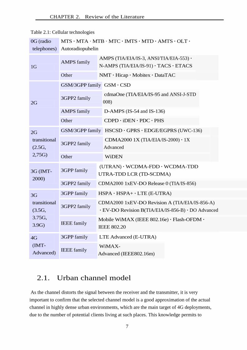
CHAPTER 2. Review of the Literature
7
Table 2.1: Cellular technologies
0G (radio
telephones)
MTS · MTA · MTB · MTC · IMTS · MTD · AMTS · OLT ·
Autoradiopuhelin
1G AMPS family
AMPS (TIA/EIA/IS-3, ANSI/TIA/EIA-553) ·
N-AMPS (TIA/EIA/IS-91) · TACS · ETACS
Other NMT · Hicap · Mobitex · DataTAC
2G
GSM/3GPP family GSM · CSD
3GPP2 family
cdmaOne (TIA/EIA/IS-95 and ANSI-J-STD
008)
AMPS family D-AMPS (IS-54 and IS-136)
Other CDPD · iDEN · PDC · PHS
2G
transitional
(2.5G,
2,75G)
GSM/3GPP family HSCSD · GPRS · EDGE/EGPRS (UWC-136)
3GPP2 family
CDMA2000 1X (TIA/EIA/IS-2000) · 1X
Advanced
Other WiDEN
3G (IMT-
2000)
3GPP family (UTRAN) · WCDMA-FDD · WCDMA-TDD
UTRA-TDD LCR (TD-SCDMA)
3GPP2 family CDMA2000 1xEV-DO Release 0 (TIA/IS-856)
3G
transitional
(3.5G,
3.75G,
3.9G)
3GPP family HSPA · HSPA+ · LTE (E-UTRA)
3GPP2 family
CDMA2000 1xEV-DO Revision A (TIA/EIA/IS-856-A)
· EV-DO Revision B(TIA/EIA/IS-856-B) · DO Advanced
IEEE family
Mobile WiMAX (IEEE 802.16e) · Flash-OFDM ·
IEEE 802.20
4G
(IMT-
Advanced)
3GPP family LTE Advanced (E-UTRA)
IEEE family
WiMAX-
Advanced (IEEE802.16m)
2.1. Urban channel model
As the channel distorts the signal between the receiver and the transmitter, it is very
important to confirm that the selected channel model is a good approximation of the actual
channel in highly dense urban environments, which are the main target of 4G deployments,
due to the number of potential clients living at such places. This knowledge permits to

CHAPTER 2. Urban channel model
8
compensate the channel effect and to accurately predict the coverage of wireless systems.
During the bibliography review some issues were detected as candidates to be improved after
measurements.
There are several previously published urban propagation models, some empirical as
Okumura-Hata and other based on ray-tracing techniques. Okumura carried out extensive
drive test measurements with range of clutter type, frequency, transmitter height, and
transmitter power. It states that the signal strength decreases at much greater rate with distance
than that predicted by free space loss (Okumura, 1968). Hata model was based on Okumura’s
field test results and predicted various equations for path loss with different types of clutter.
The limitations on Hata Model due to range of test results from carrier frequency 150Mhz to
1500Mhz, the distance from the base station ranges from 1Km to 20Km, the height of base
station antenna ranges from 30m to 200m and the height of mobile antenna ranges from 1m to
10m. Hata created a number of representative path loss mathematical models for each of the
urban, suburban and open country environments (Hata, 1980).
Another approach is the Saunders–Bonar (S.R.Saunders & Bonar, 1994) semi-empirical
model of urban propagation in environments with different heights and spacing. It is based in
Vogler’s integral that apply for uniform building height and spacing.
The Walfish – Bertoni model (J.Walfisch & Bertoni, 1988) assumes that the street grid in a
typical city organizes buildings into rows that are nearly parallel, where the precise heights
and spacing of the buildings have been ignored and the profile is characterized by just two
parameters: the mean building spacing, and the mean building height. The transmitting
antenna is positioned at certain height above rooftop level and the receiver antenna is
positioned at certain distance below the rooftop height.
The loss dependence on the angle φ, between the propagation direction and the street axis, is
a phenomenon that has already been studied by (E. Damoso, 1999) and (F. Ikegami, 1980).
The model proposed in (F. Ikegami, 1980) considers the angle φ, and then it calculates the
electric field E at the mobile station (MS). The computation is based in the Fresnel Equation
of diffraction that depends on the distance between the MS and the diffracting point on the
last diffracting building edge. This distance is */ sinw where w* is the horizontal distance
between the MS and the building. This calculation leads to Equation 2.1, which shows the
relation between the diffracted electrical field E, and the incident electrical field E0 at the
diffracting point in terms of φ. K in Equation 2.1 is a constant independent of φ and E0.
0. . * / sinE K E w (2.1)
This approach does not address two important issues. On the one hand, for small angles the
equation results in an incorrectly infinity prediction when the street is parallel to the direction
of propagation, but in this case there is no diffraction. On the other hand, it is calculated using
the hypothesis of infinite screens and therefore underestimates the E level at the corners.
CHAPTER 2. Urban channel model
9
An improvement appears at (J.Walfisch & Bertoni, 1988), which eliminates the line of sight
(LOS) hypothesis to the last diffracting building, studying the multiple screen diffraction and
proposing a simple solution to the electromagnetic problem under the additional hypothesis of
uniformity of building height, modeled as absorbent screens. It considers the base station
height greater than building height. This model takes into account the street width (w) and
buildings separation (b), but it does not consider the angle φ.
The COST-231 European action had, among several objectives, the aim of defining a very
precise and wide range applicable model. The model known as COST231-WI represents an
evolution of Walfish and Ikegami models (COST Action 231, 1999).
The model considers the buildings in the vertical plane between the transmitter and the
receiver. Street widths, buildings heights as well as transmitter and receiver heights are
considered.
The accuracy of this empirical model is quite high because in urban environments the
propagation in the vertical plane and over the rooftops (multiple diffractions) is dominating,
especially if the transmitters are mounted above roof top levels.
If the wave guiding effects due to multiple reflections in streets are dominating, the accuracy
of the COST Walfisch-Ikegami model is limited because it is focused on the multiple
diffractions in the vertical plane.
The ranges of the parameters of this model are:
Frequency, f (800-2000 MHz)
Height of the base station, hTX (4-50 m)
Height of the user equipment, hRX (1-3 m)
Distance, d, between transmitter and receiver (20-5000 m)
2.2. Effects of vegetation in the radio channel
Probably, the mismatches between the predictions of many tools in environments with
important presence of trees come from the methods used to model the vegetation effects.
The propagation in vegetation media through isolated trees has been treated in several
studies. The general objective of such studies was the accurate determination of the
propagation mechanisms generated by the vegetation element, so that the individual
contribution of the tree constituents could be assessed, i.e. trunk, branches, and leaves. These
models have been developed on a basis of experimental results, coupled to electromagnetic
wave theory, obtained both under controlled environments, e.g. anechoic chambers
environments, and in outdoor, open rural areas. These studies identified up to three main
propagation phenomena usually present in vegetation media: attenuation due to absorption;
scattering and depolarization.

CHAPTER 2. Use of vegetation for interference and security
protection
10
Results reporting the attenuation due to absorption could be found in several papers. The
attenuation measurements were generally performed by using a bi-static configuration system.
Attenuation rates between 8.6 and 11.4 dB/m at 20 GHz, and between 11.4 and 18.6 dB/m at
62.4 GHz, for a ficus specimen, are reported in (Caldeirinha & Al-Nuaimi, 2002). Also, in
good agreement, is the attenuation rate of 20.9 dB/m at 62.4 GHz, reported in (Scammell,
Hammoudeh, & Sánchez, 2001), also for ficus. The effect of the presence or absence of leaves
(as it is the case of deciduous trees) has been studied at 11.2 GHz (Al-Nuaimi & Hammoudeh,
1994), reporting attenuations of up to 2.1 dB/m and 1.74 dB/m, for apple trees with and
without leaves, respectively. However, different attenuation rates were reported for coniferous
trees, in particular pines, from 2 to 2.7 dB/m, and deciduous trees, i.e. maples, from 2 to 2.6
dB/m. These attenuation rates are reported at 5.85 GHz for outdoor mature vegetation
(Durgin, Rappaport, & Xu, 1998). The attenuation rate yielded by a mature and large oak tree
at 2.88 GHz was reported to be up to 0.6 dB/m (LaGrone & Chapman, 1961). A large
variability in the attenuation at 2.44 GHz, being from 2 to 18 dB, is presented in (Y.I.
Nechayev, 2001). These models can be assessed with measurement results at 2.1 GHz
presented in (Gómez, Cuiñas, Alejos, García, & Caldeirinha, 2010), despite the scarcity of
information on the attenuation rates reported for both isolated and groups of trees.
An alternative technique for measuring the attenuation rate induced by trees in open
environments could be the millimeter wave radar backscattering configuration, proposed in
(Nashashibi, Ulaby, Frantzis, & Roo, 2002). Attenuations below 6.4 dB/m are reported at 95
GHz for individual Arbor Vitae trees.
Most of the results obtained within anechoic chambers or other controlled environments are
focused on scattering phenomena. An appropriate knowledge of the scattering mechanism,
which is generated within the tree canopy due to the random distribution of the tree
constituents and their relative sizes compared to the transmitted signal wavelength, is essential
in communication system planning. This is because it could lead to either a reduction in the
received power at a desired location or to an increase in the multipath components of the
received signal. But the scattering is also interesting in terms of radar systems, as it could be
employed to detect vegetation by remote sensing techniques, or even to identify the target
trees. The backscattering of trees seems to present a rather isotropic angular distribution (Al-
Nuaimi & Hammoudeh, 1994). The scattering seems to be stronger when the foliage is denser
and the leaves are large (Al-Nuaimi & Hammoudeh, 1994) (Narayan, Nelson, & Dalton,
1993). However, other studies indicate that the main signal contribution is due to the trunk
and branches (Lang, Landry, Franchois, Nesti, & Sieber, 1998).
Furthermore, several other studies related to modeling of scattering due to the presence of
trees were also found in the literature. A classical and widely used model is the Radioactive
Energy Transfer theory (RET) (Johnson & Schwering, 1885) and its derivatives, such as the
Dynamic Vegetative Model presented in (R.F.S. Caldeirinha, 2006), or those related in
variants (R.A. Johnson, 1985; Gay-Fernandez, 2010), which are difficult to implement in

CHAPTER 2. Use of vegetation for interference and security
protection
11
common planning tools, as their complexity would extremely extend the computation time.
There also exist different paths to simulate the problem, as the Coherent Scattering model (Lin
& Sarabandi, 1996), based on Monte Carlo simulations of fractal trees generated by
Lindenmayer systems.
Markedly, the attenuation and scattering phenomena in vegetation media have been widely
studied hitherto. And even the time and spatial variability of the propagation characteristics
due to the vegetation under windy conditions has been previously addressed. Several papers
have dealt with variability effects, both in open environment, and in the anechoic chamber;
using either artificially generated constant air movement or natural wind.
In (Crosby, Abhayawardhana, Wassell, Brown, & Sellars, 2005), it was concluded that the
dominant fading mechanism, for a fixed wireless access channel at 3.5 GHz, was observed to
be caused by natural wind blowing on the canopy, and the long term fading was best modeled
by a Rician distribution (Crosby, Abhayawardhana, Wassell, Brown, & Sellars, 2005). Also,
the Rician K factor in winter seems to be 3.2 higher than in the summer season. Additionally,
the Rician distribution is also suggested to be used at 1.8 GHz to model radio wave
propagation, as a result of measurement obtained in open environments (Hashim & Stavrou,
2005). Data recorded inside an anechoic chamber at 900 MHz and 2, 12 and 17 GHz,
confirms that the use of Rician distribution is appropriate to model the fast fading when the
wind is smooth, although the distribution tends to become Rayleigh when the wind speed is
increased (Hashim & Stavrou, 2003). Such results are difficult to reproduce as the original
paper does not report any information on the distances between antennas and obstacles, sizes
of vegetation, and even the species considered.
The behavior of radio wave propagation in vegetation media appears to be strongly wind
speed dependent, especially when the environment is starting to change from calm to windy
conditions. However, once in the windy state, any further increment in wind speed seems to
have less effect (Hashim & Stavrou, 2006). Attenuations of 3.5 dB (or 2.2 dB/m) have also
been reported at 5 GHz, as a result of measuring the propagation, in windy conditions,
through canopies configured by the bundled branches of mature trees (Kajiwara, 2000;
Kajiwara, 2000). These experiments were performed within an anechoic chamber, but some
doubts appear regarding the validity of measuring the attenuation due to dry branches, as the
water contents of the tree seems to be a determinant factor. Again, Rician distributions are
proposed to model the fast fading due to the swaying branches. Attenuations between 9 and
22 dB, with no data on the size of the canopies, are reported at 38 GHz. This large variability
seems to be explained by the random nature of the position of branches and leaves (Seville,
1997). The measured attenuation is also larger than in the predictions (COST235, 1996) as the
young plants used for the anechoic chamber measurements were generally of denser foliage
when compared to the ones normally found outdoors, i.e. mature trees (Seville, 1997).
It is worthwhile to mention that the published studies previously outlined were mainly
focused on the millimeter wave frequencies.
CHAPTER 2. Use of vegetation for interference and security
protection
12
Among the various previously published, there is the ITU‐R Recommendation P.833 (ITU‐R,
2003), which provides a simple method to compute the attenuation excess due to isolated trees
and also masses of trees. The low mathematical complexity of the model allows its usage
within a coverage planning tool, but its own simplicity leads to not very exact results.
The exactness could be improved by applying methods that takes into account the variety or
kind of tree in the environment (Gómez, Cuiñas, Alejos, García, & Caldeirinha, 2010), which
are less used due to their novelty as well as the added complexity of identifying the vegetation
varieties at each analyzed environment.
Most of the commented papers conclude that the effect of the vegetation is not easy to be
modeled by means of a closed equation, as it is not an absolutely predictable action. So, a less
computation resource consumption method could be the combination of deterministic models
(as those commented in section 2.1) to define the fixed and structural elements of the
environment, and probabilistic corrections that may be obtained from actual measurements to
take into account the vegetation and other non-structural elements in the radio channel.
2.3. Use of vegetation for interference and
security protection
There is several propagation research done in the area of wireless networks, from general
works to more specific ones. Typically, deterministic methods have been proposed to model
static elements, both constructive and natural obstacles (Bertoni, 2000). However, there are
other kinds of obstacles in the radio links that must be modeled by stochastic procedures
(Chizcik, 2008). Such obstacles may be persons (Kara, 2009), furniture (I. Cuiñas, 2004),
vegetation (Gay-Fernandez, 2010), or in general non-polygonal structures (A. Kara, 2008).
All these obstructions can mitigate the received power in a radio link, or even they could
break the connection.
The usage of this induced attenuation to provide the own network with protection against
interference from other networks, or to improve the security against external attacks is a topic
not too explored and only suggested in (I.Cuiñas, P.Gómez, M.G.Sánchez, & Alejos, 2008),
and which are analyzed in this Thesis. The results could be compared to those provided at
(Cuiñas, Gómez, Alejos, Sánche, & Gay‐Fernández, 2011) obtained at lower frequencies
(900, 1800 and 2100 MHz), when also lower attenuations were detected. That paper proposed
the use of vegetation barriers to reduce the Electromagnetic pollution in populated areas,
whereas in this Thesis the objective of measuring and analyzing the vegetation barriers is to
reduce the interference and improve the security.
2.4. Implementation of OFDM 64 QAM systems
CHAPTER 3. Implementation of OFDM 64 QAM systems
Implementation of OFDM 64 QAM systems
13
The fundamental systems considered along this research are based in OFDM: WIMAX (IEEE
Comp., MW T.&T. Soc., 2004) (IEEE Comp.,MW T.& T.Soc., 2006) and LTE (3GPP RAN
TSG, 2009). Both are based on the OFDM scheme proposed in (Chang, 1970), which consists
on transmitting orthogonal carriers with spectrum overlapping.
MIMO system performance has been the subject of intense research in the past decade
(Gesbert, Shafi, Shiu, Smith, & Naguib, 2003) (Foschini & Gans) (Telatar, 1995). Foschini
and Telatar have shown that for independent and identically distributed channels, MIMO
system capacity increases linearly with the minimum of the number transmit antennas and
receive antennas. This is a must to increase the capacity of the systems, because the SISO
channel is limited by Shannon law (Shannon, 1948.). But MIMO could be used to increase the
availability of the system using for redundancy purposes, i.e. Alamouti scheme (Alamouti,
1998). The standards allow the use of MIMO that creates MxN (where M is the quantity of
transmitting antennas and N the receiving antennas) channels between the transmitter and the
receiver that can be used for diversity and/or capacity, with a tradeoff analyzed in (L. Zheng,
2003).
Another strategy to increase the system capacity is using the CDMA-OFDM or MC-CDMA
non-standard implementation, consisting on a CDMA transmitter in series with an OFDM
transmitter as presented in (Yee, Linnartz, & Fettweis, 1993), and the same occurs in the
receiver but with the inverse order. The idea is to increase the symbol time of CDMA to solve
the multipath distortion using multiple carriers, but OFDM has the problem of sensitivity to
frequency offset and non-linear amplification. They propose that each bit is transmitted in
parallel on multiple independently fading subcarriers. The CDMA coding is applied across the
carriers, with each carrier modulated by a single code chip. There is another method, MC-DS-
CDMA (Kondo & Milstein, 1994), where the modulated code chips are spread over time and
therefore each subcarrier is used as a narrow channel for transmitting DS-CDMA signals. To
achieve frequency diversity, the same DS-CDMA spread data bit is usually transmitted over
each subcarrier in parallel and the received signals are combined to give more robust data
estimation.
As this Thesis is focused in the uplink (UL) channel, where all the signals mix at the base
station, there is no possibility to estimate the channel directly, so estimation during downlink
time in TDD systems is proposed. This results in the need of channel prediction, and in this
Thesis the linear prediction was chosen to do this task. The Linear Prediction is a
mathematical operation where the future values are estimated as a linear combination of the
past values (Makhoul, 1975). It states that when the vectors of coefficients of the linear
combination must be estimated, there are two approaches to solve the problem. The first one
is the optimum coefficients derivation by analytical methods, in the sense of minimizing the
expected energy of the prediction error, when has a perfect knowledge of the statistical
characteristics of the channel. On the other hand, it proposes the derivation of robust
CHAPTER 3. Implementation of OFDM 64 QAM systems
Implementation of OFDM 64 QAM systems
14
coefficients that always allow the predictions of near future values even if the surveys, carried
out previously, lead to imperfect channel estimation.
The first method suffers from the defect of being an inapplicable method because there is
always error in the estimation of the channel. Therefore it is only useful when there are good
channel estimates.
Four methods are analyzed to predict the channel in UL time: Burg (Hanzo, M.Munster,
B.J.Choi, & T.Keller, 2003), Covariance noise (J. R. Deller Jr., 1993) (Leroux & C.Gueguen,
1979), Modified Covariance (Semmelrodt & Kattenbach, 2003) and Yule-Walker (Yule,
1927) (Walker, 1931). Their general objective is to minimize the energy of the error.
The equation optimal coefficients are proposed to be reached (Hanzo, M.Munster, B.J.Choi,
& T.Keller, 2003) from two methods (gradient cancellation and principle of orthogonality of
the error), which reduces the problem to a linear optimization; although in this case it also
takes real values (but easily convertible to complex case).
Applying it to our system, as the signal is distorted by the channel, its influence could be
canceled if it could be estimated in advance. But each MS has its own channel with the BS,
and it is difficult to separate the signals of the MS in the uplink, so the estimation must be
done during downlink time. However, this introduces the need of a predictor. Some prediction
methods were considered, but finally a linear predictor called Covariance presented in
(Makhoul, 1975) is used to extrapolate the behavior of the process beyond the available
channel samples.
The idea is to implement a method that minimizes the multi user interference (MUI) and the
noise terms, to maximize the signal to interference plus noise ratio (SINR). But the optimum
solution needs that each MS knows the channel impulse response (CIR) of all other MS of the
same sector. A sub-optimal but efficient solution is maximizing another quantity called m-
SINR quotient instead of the SNIR proposed in (D. Mottier, 2002).
The channel correction in these systems is needed to minimize the MUI, but frequency
equalization is not enough. Using the downlink channel estimation, and based in the
reciprocity with the uplink channel, a pre-equalization process compensates the effects that
the transmitted signal from de MS will suffer during its channel crossing.
Different schemes of pre-equalization were reviewed. The contribution (Hara & Prasad,
1997) proposes to cancel the Multiple Access Interference (MAI) with an algorithm called
zero forcing or Orthogonality Restoring Combining (ORC). However, as indicated in the
work, this method is sensible to pronounced fading, amplifying the noise and increasing the
transmitted power as indicated in (D. Mottier, 2002) that also proposes an expression for the
modified SNIR to maximize and to find the optimum coefficients. As a solution, (Hara &
Prasad, 1997) proposes a scheme, derived from the zero forcing, called controlled
equalization. This method minimizes the excessive noise amplification using a limit in the
gain based in maximum ratio combining (MRC).
The expression for the pre-equalization coefficients is given in (I. Cosovic, 2003).

CHAPTER 3. Implementation of OFDM 64 QAM systems
Implementation of OFDM 64 QAM systems
15
The proposal of this Thesis is to obtain better results than the found in the following
bibliography. The (Li, Winters, & Sollenberger, 2002) reference presents a spectral efficiency
of 3.2 b/s/Hz with a 4x4 antenna system at SNR of 12 dB to achieve a
BER=10-3
. Again, a SNR of 12 dB is needed for QPSK modulation in (H. Miao, 2005) to
reach the best performance at BER=10-3
, with 2x4 antennas and space-time block code
(STBC). In (K.W. Park, 2005), a 16 QAM system is presented where a SNR=12 dB is needed
for a BER=10-3
over an I-METRA channel of 2 GHz. Another work (F.A. Jubair, 2009)
presents a 2x2 antenna system, with BPSK modulation which needs a SNR=10 to achieve a
BER=10-3
over channel A of (ETSI, 1998) with 50 ns of delay spread.
In (Kong, 1999) the block error rate is simulated for a SUI-3 channel against SNR, achieving
a BLER = 0.1 at SNR greater than 30 dB for a 64 QAM 2/3 coding.
2.5. Spectral efficiency of multimodulation
cellular systems
The frequency reuse has been proposed to improve the spectral efficiency of radio systems
that need to have reasonable cost and throughput services in networks growing very fast. The
reuse 1, mentioned for the WIMAX and LTE standards, jointly with high dense modulation as
64 QAM, propose a challenge in the systems that must be proved in the theory and in the
field. Some providers relax the reuse 1 and propose reuse 1 for internal users and reuse 3 for
edge users. But this introduces the question about what percentage of the cell area is
considered internal and how much area is for edge users. The Inter-Cell Interference will be
reviewed in chapter 7. The document (3GPP TSG RAN, 2005) describes some proposals of
randomization, cancellation and coordination. As the coordination is proved as the best
method, three types are analyzed: static, semi-static (Siemens, 2005) and dynamic frequency
reuse (Zhang, Hee, Jiang, & Xu, 2008) (Stolyar & Viswanathan, 2008). Depending on the
reuse, there are different methods. In Fractional Frequency Reuse (FFR), a fraction of the
spectrum has reuse factor 1 and rest 3. The Soft Frequency Reuse is an evolution of FFR
because if some sub-bands are not used in one cell they could be used in a neighbor cell
(Khan, 2009). As the traffic load varies with the time, an adaptive frequency reuse scheme
appears to outperform any static frequency assignment. In (Fan, Chen, & Zhang, 2007) and
improvement respect to the above scheme is implemented, because it also considers the traffic
of the neighbors cells.
The relation between the distances of two mobiles in next to cells reusing the same carrier is
frequency is presented. Also the relation between the power of the BS to these mobiles to
meet the level of receiving power above the S and the level of SNIR specified. Three
algorithms for resource allocation is proposed, one based in this issue.
CHAPTER 3. Spectral efficiency of multimodulation cellular systems
Implementation of OFDM 64 QAM systems
16
Previously published work (Suh, 2006) shows that for NLOS scenarios, a seventh order
cluster is needed to achieve a SNIR of 6.46 dB with cell of one sector and 190 m of radius; or
a SNIR of 15 dB but with 2 sectors and 190m radius cells. When FDMA systems, as OFDM,
apply frequency reuse techniques, the network planning must consider a SNIR according to
the modulation used for a given BER (3GPP, 2010). This determines the order of the cluster
ergo the number of cells of a cluster, J, within which frequencies should not be repeated so the
spectrum bandwidth needed for a metropolitan deployment. Some works propose the relay in
repeaters stations to solve the problem for outer mobiles.
Some references proposes algorithm for resource allocation based in the maximization of one
Utility function. In this thesis another algorithm is also proposed based in a utility function
calculated as the sum of the SNIR of all users.

Chapter 3 Propagation Model for Small Urban Macro Cells
This chapter presents the MOPEM1
propagation model for dense urban areas in the frequency
band from 850 to 900 MHz. This work is based on the COST231WI model, but the hypothesis of
infinite screen blocks is replaced by finite screens taking into account the street crossings,
predicting the signal attenuation along the block. The dependence of propagation loss with
terrain height is reviewed and optimized by considering an absolute reference, while the
dependence on the angle between the street and the wave propagation is modified to obtain a
continuously differentiable loss function. The standard deviation obtained with this model is 5.1
dB and the mean error is 0 dB vs. 6.6 dB and 6.2 dB respectively for the COST 231 WI, with
validation measurements from two areas in Montevideo city.
3.1 Introduction
The new services being launched in mobile networks, such as multimedia transmissions,
produce a traffic increase that together with constant service price reduction demands a more
accurate cell planning from the operator and his suppliers. The progressive cell size reduction
requires a greater accuracy of system coverage estimations. This requires an accurate coverage
prediction methodology with an easy implementation. Current models do not consider the height
difference between the floor levels at the MS location and the base station (BS), nor the signal
strength variation along the block, and do not have a differentiable orientation angle dependent
loss function.
The aim of this work is to find a model for the radio channel loss, in the frequency range from
850 to 900 MHz. This model has been developed for urban areas with small macro cells2 in
1 Spanish acronym for Propagation Model for Small Urban Macro Cells 2 According to [1], a small macro cell is an outdoor cell which is placed higher than the average building height, but some buildings could
be higher than the antennas. Its typical coverage radius is less than 3 km.

CHAPTER 3. Introduction
18
Montevideo, Uruguay, with non-line of sight (NLoS) between transmitter and receiver. The
model gives a propagation loss function (LMOPEM) with the following parameters: frequency (f),
base station height (hbase), mobile station height (hm), distance between MS and BS (d), street
width (w), angle between the street and the propagation direction (φ), building height (hroof),
building separation (b), and terrain height. The MOPEM model outperforms the COST231 WI in
this area, due to the fitting of the loss function, the adding of the terrain height, for considering
the buildings as finite screens and modifying the orientation loss function.
3.2 Theoretical Analysis
The MOPEM model bases its initial analysis on the semi-empirical propagation models
proposed by COST231-WI (E. Damoso, 1999), Ikegami and Yoshida (F. Ikegami, 1980) and
Walfisch and Bertoni (J.Walfisch & Bertoni, 1988). All of them consider multiple rays between
the BS and the MS. The model presented in (F. Ikegami, 1980) considers two rays as illustrated
in Figure 3.1, the ray A has experienced one diffraction while ray B one diffraction and one
reflection.
Figure 3.1. Two rays at the MS considered by models in (COST Action 231, 1999) and (F.
Ikegami, 1980)
The most restrictive hypothesis of model (F. Ikegami, 1980) is to consider line of sight (LoS),
hence free space propagation between the BS and the diffracting building.
Figure 3.2. Definition of b, w and φ as the angle between the axis of the street and the direction
of the propagation.
It also shows lower dependence on the distance than what is verified with measurements, but it
takes into account parameters of the mobile environment such as hroof and w. It also introduces a
factor that accounts for the dependence with the angle φ shown in Figure 3.2, which is the most
innovative contribution.
B
A 2 1
BS
MS
w b

CHAPTER 3. Theoretical Analysis
19
Reference (J.Walfisch & Bertoni, 1988) eliminates the LoS hypothesis to the last diffracting
building, studying the multiple screen diffraction and proposing a simple solution to the
electromagnetic problem under the additional hypothesis of uniformity of hroof, modeled as
absorbent screens. It considers hbase greater than hroof. This model takes into account the street
width (w) and buildings separation (b), but it does not consider the angle φ.
The COST231 WI model proposed in (E. Damoso, 1999) considers the loss composed by the
free space loss (Lo), multi-diffraction loss (Lmsd) and the roof to street diffraction loss (Lrts), as
can be observed in (3.1) to (3.4):
231COST WI o rts msdL L L L (3.1)
0 32.4 20log 20logL d f (3.2)
16.9 10log 10log 20log( )rts roof m oriL w f h h L (3.3)
log log 9logmsd bsh a d fL L k k d k f b (3.4)
Where [d]=km, [f]=MHz, [w]=m, [hroof]=m, [hm]=m, [φ]=º, [b]=m
kd=18, kf= -4,06, ka= 54, Lbsh= -18.log(1+hbase-hroof)
The COST231 WI model includes the contributions from (F. Ikegami, 1980) and (J.Walfisch &
Bertoni, 1988), with the terms Lrts and Lmsd. The estimated mean error (ē) is from –3 to 3 dB and
the standard deviation () is between 4 and 8 dB.
The reason to choose the COST231 WI as the base model for the present work is that it was
fitted using measurements in European cities, and Montevideo is very similar to these cities. The
MOPEM model is obtained from Equations 3.1 to 3.4 modifying the underlined terms and adding
a new term called Lesq.
3.2.1. Influence of the terrain height variation
The loss dependence on the hm has been extensively analyzed in previous works, but its
influence is different in each model. The empirical models are fitted with measurements like the
Ibrahim and Parsons Method (Parsons, 1992), which obtained an 8.log10(hm) law. In the semi-
empirical models, like COST 231, the attenuation produced between the diffracting edge and the
MS depends on the distance between the MS (hm) and buildings roofs (hroof), with the term:
1020log ( )roof mh h.
The Parameters hroof and hm are measured with respect to the floor level at the site.
The MOPEM model considers the dependence with the height using a fitted khm instead of 20
with the term: 10log ( )hm Aroof Amk h h
The heights hAroof and hAm are measured with respect to a common reference level, for example

CHAPTER 3. Theoretical Analysis
20
the sea level to account for terrain height variations (see Figure 3.3).
It is necessary to define a criterion to estimate hroof and hm. Usually, the hm is taken as 1.5 m
above ground, because it is the mean value between the head and the waist of a person. The
MOPEM model adds the terrain height to this value when measuring from a common reference
level.
Two methods to estimate the parameter hroof has been reported in the literature. The first one is
to take hroof as the last building height (building # 2 in Figure 3.1). Nevertheless, it is inaccurate
in environments with great different building heights, because in several cases a higher building
located between the BS and the last building produces the last diffraction. Another method is to
use a local height average but the choice of the area size is arbitrary and not well justified. The
MOPEM model proposes the evaluation of hAroof as an average height as proposed in (S.
Sakagami, 1991) considering the highest buildings of each block in the studied area but measured
from a common reference level. This criterion was based on urban considerations, since the most
significant screens between the BS and the MS are the prominent buildings.
In order to understand the influence of variable terrain heights when using an averaged building
height, see Figure 3.3.
Figure 3.3. Model considering heights from a common reference level instead the local floor
level.
Mobiles in low areas (m1) have lower signal than mobiles in higher areas (m2) because they are
far from the average building height, and also have larger diffraction angle (1) which reduces
the received signal.
The MOPEM model considers the variation of the terrain height by using a common reference
level for the heights hAroof and hAm. The dependence is adjusted through finite multi-screen effect.
The effect of the multi-screen diffraction is based on the analysis presented in (J.Walfisch &
Bertoni, 1988), when the BS antenna is placed above the hroof (requirement that is fulfilled in this
work). The buildings are considered as absorbent half screens of the same height, infinite width
Average Building height
Terrain height
Common reference level
2 1
m
1
m
2
hAm1 hAroof hAm2
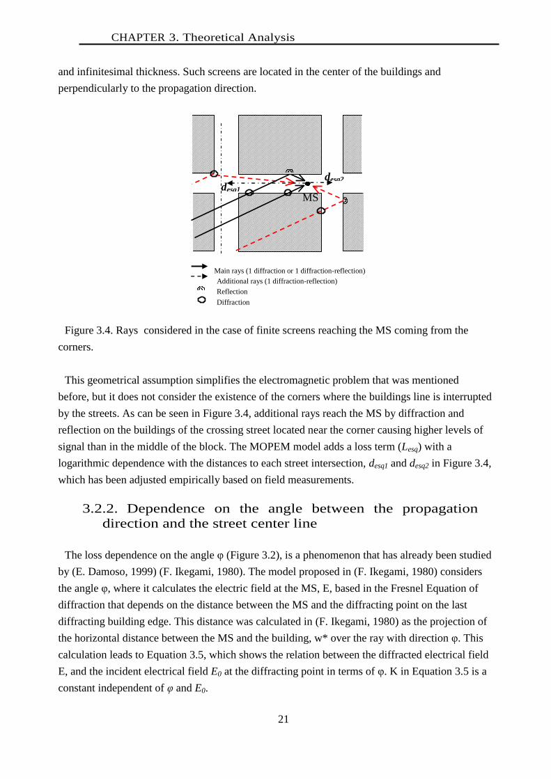
CHAPTER 3. Theoretical Analysis
21
and infinitesimal thickness. Such screens are located in the center of the buildings and
perpendicularly to the propagation direction.
Figure 3.4. Rays considered in the case of finite screens reaching the MS coming from the
corners.
This geometrical assumption simplifies the electromagnetic problem that was mentioned
before, but it does not consider the existence of the corners where the buildings line is interrupted
by the streets. As can be seen in Figure 3.4, additional rays reach the MS by diffraction and
reflection on the buildings of the crossing street located near the corner causing higher levels of
signal than in the middle of the block. The MOPEM model adds a loss term (Lesq) with a
logarithmic dependence with the distances to each street intersection, desq1 and desq2 in Figure 3.4,
which has been adjusted empirically based on field measurements.
3.2.2. Dependence on the angle between the propagation
direction and the street center line
The loss dependence on the angle φ (Figure 3.2), is a phenomenon that has already been studied
by (E. Damoso, 1999) (F. Ikegami, 1980). The model proposed in (F. Ikegami, 1980) considers
the angle φ, where it calculates the electric field at the MS, E, based in the Fresnel Equation of
diffraction that depends on the distance between the MS and the diffracting point on the last
diffracting building edge. This distance was calculated in (F. Ikegami, 1980) as the projection of
the horizontal distance between the MS and the building, w* over the ray with direction φ. This
calculation leads to Equation 3.5, which shows the relation between the diffracted electrical field
E, and the incident electrical field E0 at the diffracting point in terms of φ. K in Equation 3.5 is a
constant independent of φ and E0.
desq1
desq2
MS
Main rays (1 diffraction or 1 diffraction-reflection)
Additional rays (1 diffraction-reflection)
Reflection
Diffraction
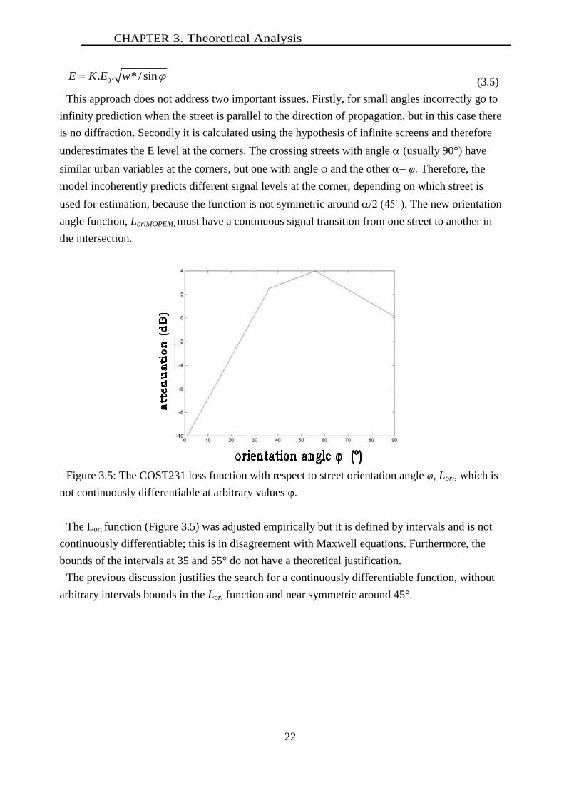
CHAPTER 3. Theoretical Analysis
22
0. . * / sinE K E w (3.5)
This approach does not address two important issues. Firstly, for small angles incorrectly go to
infinity prediction when the street is parallel to the direction of propagation, but in this case there
is no diffraction. Secondly it is calculated using the hypothesis of infinite screens and therefore
underestimates the E level at the corners. The crossing streets with angle (usually 90°) have
similar urban variables at the corners, but one with angle φ and the other φ. Therefore, the
model incoherently predicts different signal levels at the corner, depending on which street is
used for estimation, because the function is not symmetric around . The new orientation
angle function, LoriMOPEM, must have a continuous signal transition from one street to another in
the intersection.
Figure 3.5: The COST231 loss function with respect to street orientation angle φ, Lori, which is
not continuously differentiable at arbitrary values φ.
The Lori function (Figure 3.5) was adjusted empirically but it is defined by intervals and is not
continuously differentiable; this is in disagreement with Maxwell equations. Furthermore, the
bounds of the intervals at 35 and 55° do not have a theoretical justification.
The previous discussion justifies the search for a continuously differentiable function, without
arbitrary intervals bounds in the Lori function and near symmetric around 45°.

CHAPTER 3. Mopem Model
3.3 Mopem Model
The MOPEM model describes the loss as the sum of four independent terms: Lo in (2) is the loss
due to the free space propagation, Lrts-MOPEM is the loss of the diffraction from the last building to the
MS, Lmsd-MOPEM is the loss caused by the multi-screen diffraction andLesq accounts for the finite
multi-screen assumption. Equation 3.6 shows the base attenuation model, which terms are described
by Equations 3.2 and 3.7 to 3.10.
MOPEM o rts MOPEM msd MOPEM esqL L L L L (3.6)
The terms ,rts MOPEM msd MOPEML L and esqL are new contributions.
The following parameters that describe the urban environment are defined in Figure 3.2 and 3.6:
Buildings height hAroof: average heights of the highest buildings of each block [m].
Street width w: the average width of all streets [m].
Buildings separation b: estimated as half of the block average [m].
Orientation angle φ: bounded by the street center line and the propagation direction as seen in
Figure 3.2 [º].
The average of the parameters is estimated in the coverage area.
Figure 3.6. Definition of the urban parameters of the MOPEM model.
The Lrts-MOPEM term 3.7 adds two new improvements to the Lrts term 3.3: the terrain height included
in hAm and hAroof, and the Lori-MOPEM function.
10 10 101.87 10log ( ) 10log ( ) 10.4log ( )rts MOPEM Aroof Am ori MOPEML w f h h L (3.7)
4 3 2
2.8 13.2 29.5 30.3 3.545 45 45 45
ori MOPEML
(3.8)
The Lmsd-MOPEM term models the loss due to the multi-screen diffraction as proposed in (E.
Damoso, 1999) and (J.Walfisch & Bertoni, 1988). This term is based on Equation 3.4 and has been
empirically fitted in this work, with d, to achieve more accuracy:
hroo
f
hbas
e
d
hAm
hAroof w
b
MS
hbase
BS
w
block

CHAPTER 3. Mopem model
24
10 10 10 1054 18log (1 ) log ( ) 27.7log ( ) 9log ( )msd MOPEM Abase Aroof fL h h k f d b (3.9)
With 4 0.7 / 925 1fk f from (E. Damoso, 1999).
The hAroof and hAbase are measured from a common reference level.
The Lesq term models the signal variation along the block. The expression was fitted empirically.
(3.10)
The parameters in (3.10), desq1 and desq2 are measured in meters, are the distances from the MS to
each center of the streets intersection as defined in Figure 3.4.
The signal values taken to derive this dependence were obtained by averaging measurements in
40in this case, 14 m intervals according to ITU-R P.1406 recommendation (ITU-R, 2007) to
eliminate the fast fading.
Figure 3.7. Circle where Lesq is equal to the value on the boundary
Thus the expression is strictly valid outside a 7m circle from the center of the street intersection as
can be seen in Figure 3.7. Inside the 7m circle we recommend to maintain the boundary value.
3.4 Environment and measurements
A brief description of the environment and an explanation of the parameters used in the
proposed model are presented below. A complete area description and the survey methods used
can be found in (Casaravilla J., 2002).
3.4.1. Area Description
The Figure 3.8 shows the studied area, located in two neighborhoods of Montevideo city called
Pocitos and Punta Carretas. Pocitos has a hroof of approximately 24 m and a b of 50 m. In the
center of the blocks there is an area free of buildings. Pocitos includes two different areas:
Pocitos Viejo, with one-family houses of hroof aprox. 9 m, and the area near the coast line, with
high-rise buildings (hroof aprox. 30 m ).
mr 7

CHAPTER 3. Environment and Measurements
25
Figure 3.8. Map ofthe studied area showing the Pocitos and Punta Carretas neighborhoods of
Montevideo city.
Punta Carretas has a hroof of 5 floors. It has a high occupation of the land, but with some parks.
Further reference on these areas can be found in (Casaravilla J., 2002).
3.4.2. Attenuation measurement
The measured cellular system was the AMPS and D-AMPS system in the 850 MHz frequency
band. Three different macro cell sectors of two BS were chosen, two of them covering the same
area of Pocitos from different angles and another covering Punta Carretas area. The sites are
located at 34º54’51.27’’ S 56º09’05’’ W and 34º54º27.76’’ S 56º09’11,7’’ W as can be seen in
Figure 3.8.
The analog and digital control channels of each sector were used in order to measure the
attenuation, and it is calculated as follows.
L EIRP RSSI (3.11)
Where L is the signal loss between the BS and the MS, expressed in dB. The EIRP (Effective
Isotropic Radiated Power) is the power radiated from the BS antenna, measured in dBm, and the
RSSI (Received Signal Strength Indication) indicates the power received in dBm measured with
a TEMS Agilent E7474A TDMA Drive Test System. A total of 90,000 significant measurements
of RSSI were taken in two different campaigns to overcome temporal effects that could produce
distortion in the measurements. According to (ITU-R, 2007), it is convenient to divide spatial
variability into fast fading and slow fading. When analyzing measurements, fast fading can be
eliminated by taking a median signal level from 36 measurements in a distance of about
40(14m), obtaining an accuracy within 1 dB with 90% probability. Experience has shown that
the distribution of these median values will be log-normal, and therefore their distribution can be
characterized by their mean or median, and their standard deviation. This leads to an averaging of
the measurements in 14 m intervals thus obtaining a set of 2,500 representative values of RSSI.
Pocitos
Punta Carretas

CHAPTER 3. Environment and Measurements
26
This set was subdivided in two sets, one used for model tuning (T set) and the other for model
validation (V set).
3.5 Results
In this section the result are presented classified by the modification proposed. First, the
adjustment and validation of the model are described in detail.
3.5.1. Model adjustment
Two indicators were used to quantify the model performance: the mean error ē and the standard
deviation . The model tuning was made by minimizing the mean square error using the T set of
measurements. The model uncertainty was estimated considering of the prediction error (4.4
dB) and the uncertainties in the measured values (RSSI and urban parameters, 2.6 dB).
3.5.2. Model validation
In order to validate the model, hypothesis testing of model ē and based on the V set of
measurements was carried out, which definitions and values are.
1
/ 0.003n
i ip
i
e y y n dB
(3.12)
n
2
1
( ) / n-1 4.4i ip
i
y y dB
(3.13)
For the model mean error, the null hypothesis Ho is defined as:
:o oH (3.14)
and the confidence interval according to [8] :
( / 2,n-1) n, ( / 2,n-1) n 0.269 , 0.269o oI t t (3.15)
where I is the mean error of the model and is the proposed mean error of the model, which
is 0 in this test. The significance level is taken as 95% in this test for a confidence level of
95%. Parameter
t(/2,n-1) is the inverse Student distribution function with (n-1) degrees of freedom for /2.
Parameter n is the number of samples (measurements), yi is the ith
sample of the V set of
measurements and yip is the model predicted value for yi. As e is inside the 95% confidence
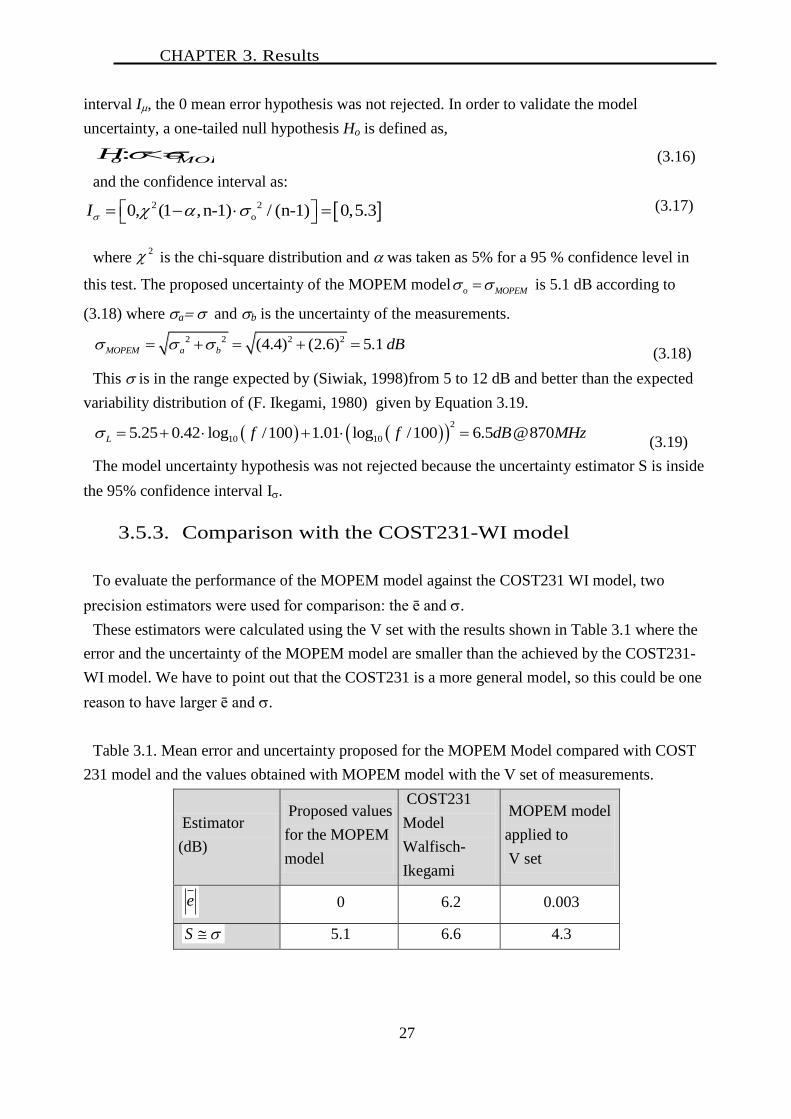
CHAPTER 3. Results
27
interval I, the 0 mean error hypothesis was not rejected. In order to validate the model
uncertainty, a one-tailed null hypothesis Ho is defined as,
MOPEMoH : (3.16)
and the confidence interval as:
(3.17)
where is the chi-square distribution and was taken as 5% for a 95 % confidence level in
this test. The proposed uncertainty of the MOPEM model o MOPEM is 5.1 dB according to
(3.18) where a andb is the uncertainty of the measurements.
2 2 2 2(4.4) (2.6) 5.1 MOPEM a b dB (3.18)
This is in the range expected by (Siwiak, 1998)from 5 to 12 dB and better than the expected
variability distribution of (F. Ikegami, 1980) given by Equation 3.19.
2
10 105.25 0.42 log /100 1.01 log /100 6.5 @870L f f dB MHz (3.19)
The model uncertainty hypothesis was not rejected because the uncertainty estimator S is inside
the 95% confidence interval I.
3.5.3. Comparison with the COST231-WI model
To evaluate the performance of the MOPEM model against the COST231 WI model, two
precision estimators were used for comparison: the ē and .
These estimators were calculated using the V set with the results shown in Table 3.1 where the
error and the uncertainty of the MOPEM model are smaller than the achieved by the COST231-
WI model. We have to point out that the COST231 is a more general model, so this could be one
reason to have larger ē and .
Table 3.1. Mean error and uncertainty proposed for the MOPEM Model compared with COST
231 model and the values obtained with MOPEM model with the V set of measurements.
Estimator
(dB)
Proposed values
for the MOPEM
model
COST231
Model
Walfisch-
Ikegami
MOPEM model
applied to
V set
e
0 6.2 0.003
S 5.1 6.6 4.3
2
2 2
o0, (1 ,n-1) / (n-1) 0,5.3I
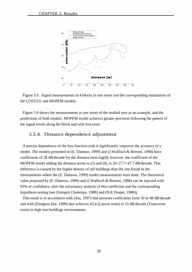
CHAPTER 3. Results
28
Figure 3.9. Signal measurements in 4 blocks in one street and the corresponding estimations of
the COST231 and MOPEM models.
Figure 3.9 shows the measurements in one street of the studied area as an example, and the
predictions of both models. MOPEM model achieves greater precision following the pattern of
the signal levels along the block and with less error.
3.5.4. Distance dependence adjustment
A precise dependence of the loss function with d significantly improves the accuracy of a
model. The models presented in (E. Damoso, 1999) and (J.Walfisch & Bertoni, 1988) have
coefficients of 38 dB/decade for the distance term log(d); however, the coefficient of the
MOPEM model adding the distance terms in (2) and (9), is 20+27.7=47.7 dB/decade. This
difference is caused by the higher density of tall buildings than the one found in the
environments where the (E. Damoso, 1999) model measurements were done. The theoretical
value proposed by (E. Damoso, 1999) and (J.Walfisch & Bertoni, 1988) can be rejected with
95% of confidence, after the uncertainty analysis of this coefficient and the corresponding
hypothesis testing (see (Samprit Chatterjee, 1988) and (N.R Draper, 1980)).
This result is in accordance with (Xia, 1997) that presents coefficients from 30 to 48 dB/decade
and with (Dongsoo Har, 1999) that achieves 43,4 (Lateral route) to 55 dB/decade (Transverse
route) in high rise buildings environments.

CHAPTER 3. Results
29
3.5.5. The influence of the terrain height variation
If the terrain variation is not considered in the model, a correlation between it and the error can
be observed. This can be verified in Table 3.2 where the measurements were fitted without taking
heights from a common reference.
Table 3.2. Mean error for different ranges of terrain height measured from a common reference
level.
Range of heights in
relation to sea level
(m)
4-9 9-14 14-19 19-24
Mean error in the
range (dB)
1.02 0.22 -0.30 -1.4
It can be seen that for ranges of terrain heights below 14m over the sea level the attenuation is
underestimated, while it is overestimated in ranges over 14m.
Previous models average this effect, appearing as a model uncertainty. Taking into account the
terrain height variation, modeled by (3.7) and (3.9), reduces the uncertainty in 1.1 dB.
3.5.6. The finite multi-screens effect
The traditional model prediction uses an approach for the signal behavior, which predicts
globally along several blocks averaging the signal behavior within the block. In contrast, the
MOPEM model considers the variations within a block, through a variable attenuation Lesq that
depends on the distance to the center of the streets intersection.
On the other hand, MOPEM model predicts the signal increase behavior in the corners.T. This
assumption is confirmed by measurements. A comparison between the COST231 WI and the
MOPEM model predictions along a block can be observed in Figure 3.9, while the term
calculated as a gain in the signal (-Lesq), can be seen in Figure 3.10.

CHAPTER 3. Results
30
Figure 3.10: Gain produced by finite screens (-Lesq) in a 100m block proposed in the MOPEM
model.
Rays diffracted in the corner edges increase the signal near them.
The term was tested to be statistically significant, in the adjustment of the constants in the term
with a confidence level of 95%. The uncertainty is reduced by 0.1 dB with this contribution, and
is important in the signal description along the block, showing lower values than the average
along it and revealing possible coverage holes.
3.5.7. Street orientation dependence
The measurements are consistent with the theoretical analysis of the attenuation signal
dependence on the orientation angle φ (Figure 3.11) and shows that the minimum attenuation is
observed on angles near 0º and 90º. A graphical criterion, suggested by (Samprit Chatterjee,
1988) and (N.R Draper, 1980), is to plot in the y-axis the prediction error without against in
the x-axis.
Figure 3.11. Example of the error distribution between the predictions without and the
measurements.
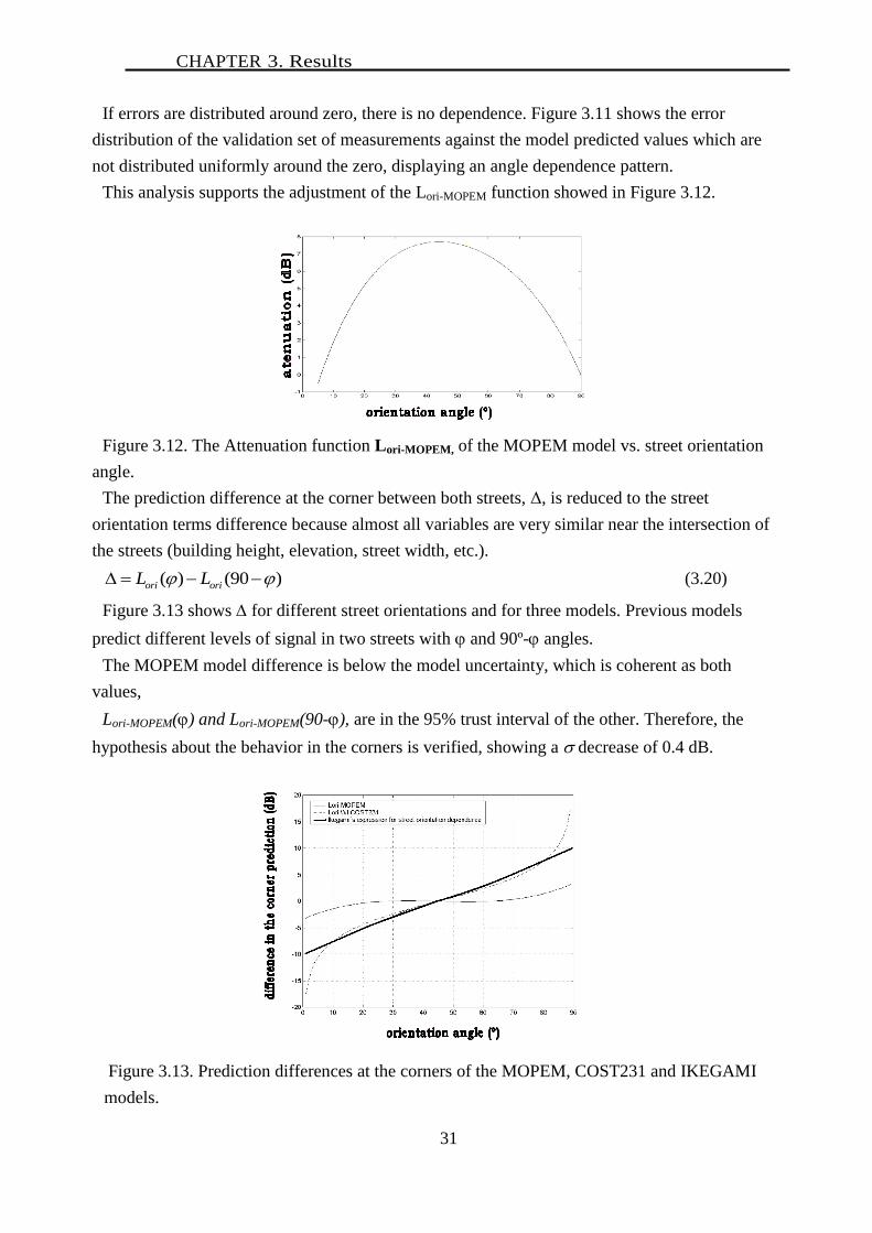
CHAPTER 3. Results
31
If errors are distributed around zero, there is no dependence. Figure 3.11 shows the error
distribution of the validation set of measurements against the model predicted values which are
not distributed uniformly around the zero, displaying an angle dependence pattern.
This analysis supports the adjustment of the Lori-MOPEM function showed in Figure 3.12.
Figure 3.12. The Attenuation function Lori-MOPEM, of the MOPEM model vs. street orientation
angle.
The prediction difference at the corner between both streets, Δ, is reduced to the street
orientation terms difference because almost all variables are very similar near the intersection of
the streets (building height, elevation, street width, etc.).
( ) (90 )ori oriL L (3.20)
Figure 3.13 shows for different street orientations and for three models. Previous models
predict different levels of signal in two streets with and 90º- angles.
The MOPEM model difference is below the model uncertainty, which is coherent as both
values,
Lori-MOPEM() and Lori-MOPEM(90-), are in the 95% trust interval of the other. Therefore, the
hypothesis about the behavior in the corners is verified, showing a decrease of 0.4 dB.
Figure 3.13. Prediction differences at the corners of the MOPEM, COST231 and IKEGAMI
models.

CHAPTER 3. Applications
3.6 Applications
The most remarkable applications of the proposed model are described below.
3.6.1. Coverage area depending on the transmitter orientation
The L oriMOPEM function has its minimums at φ=0º and φ=90º and a maximum at φ=45º.
Therefore, in a cell with the direction of maximum propagation parallel to the streets, the
MOPEM model estimates a longer and narrow coverage area, as shown in Figure 3.14 for Tx1.
On the other hand, a transmitter with an antenna with its maximum propagation direction at 45º
with respect to the street axis, has a broader and shorter coverage area, as shown in Figure 3.14
for Tx2.
Figure 3.14. Influence of the street grid in the coverage area produced by the orientation angle
dependence.
3.6.2. Prediction improvements along the block
The Lesq term accounts for the variation of the signal along the block, for example it has 2 dB in
100m blocks. The improved prediction obtained allows plans based on the worst case, using
central points of each block for coverage area analysis, and values close to the corners for
interference analysis.
Tx2 Tx1
Coverage area calculated without considering
the street grid
Coverage area when considering the street grid,
according to the MOPEM model

CHAPTER 3. Conclusions
33
3.7 Conclusions
A semi-empirical propagation model for the frequency band from 850 to 900 MHz was
proposed. This model is in the accuracy limit for a statistical model, as given by (Siwiak, 1998)
and better than the expected by (ITU-R, 2007). Significant modifications have been proposed
with regard to the reference model COST 231-WI (E. Damoso, 1999). These variations are based
on theoretical justifications, which were previously analyzed and empirically confirmed through
a wide set of measurements.
The first modification involves the attenuation loss caused by the street orientation, leading to a
continuous behavior at the streets crossings.
The second modification is based on the modeling of the finite screens effect, through Lesq that
considers additional rays in the signal level near the corners.
Finally, the dependence on the terrain height variation has been included in the loss function
LMOPEM, in order to adapt the model to coverage areas with important terrain height differences
compared with the buildings height.
Estimation of the coverage area depens on the terrain height. In the MOPEM model prediction,
the coverage footprint becomes considerably misshapen, when the terrain height varies around
20 m, with lower signal in low areas and increased signal in high areas. Therefore, the MOPEM
model allows to calculate the signal with more accuracy, and to reveal coverage holes in low
areas and interfered points in high areas.
These three modifications achieve a better performance, obtaining a model of easy application,
which incorporates new concepts for the cell planning.
CHAPTER 3. Conclusions
34

Chapter 4 Cellular network planning imbalances at
wooded streets and parks
Although the propagation of radio waves in vegetation environments has been widely studied, the
actual situation is that wireless communication systems coverage in vegetation areas appears to be
still clearly poorer than in open places within our cities. This indicates a lack in the simulation tools
currently used for radio network planning. Large measurement campaigns results are presented in
this chapter, affording numerical data that could be useful to correct the radio network planning
when parks or groves are around the base stations. An estimation of coverage radius reduction is
provided, based on such measurements, as well as various statistics which behaviors seem to
depend on the presence of vegetation in the environment. Finally, a proposal for improving the
predictions by using a combined deterministic and probabilistic method is enunciated.
4.1. Introduction
When planning a wireless communication network (i.e. cellular phone), the objective used to
be to provide the more homogeneous coverage as possible, at any place where a subscriber could
need to establish a link with the network. However, our experience as consumers tells something
different: the quality of service of cellular phone systems at groves and parks seems to be
commonly worse than at areas without trees. The same happens when focusing in computer
wireless networks. And this occurs even though the environment is tried to be concerned about
when planning the radio network (F. Ikegami, 1980) (M. G. Sánchez, 1996) (H.L. Bertoni, 1994)
(G. Liang, 1998) (T. Kürner, 2002). This fact has been confirmed by means of experimental work.
The most used channel models and also the model derived during this Thesis and presented in chapter 3,
do not consider the variations due to the presence of trees. For this reason, a large measurement
campaigns were developed in three different cities in Spain and the Oriental Republic of Uruguay:
Vigo, Oviedo and Montevideo, in order to obtain electric field strength values at both vegetation
and open urban areas. The places where the data were collected are different enough to be
CHAPTER 4. Introduction
36
convinced on the validity of the study in most zones of the World: we consider cities with different
sizes, design and topography.
We followed two different strategies during the measurement campaigns, due to different
equipment access at both National research groups. Those developed in European cities were
conducted by applying the procedures designed to measure the electromagnetic pollution and to
compare it to the healthy limits (i.e. reference levels) established by the Spanish and European
legislations (Ministerio de la Presidencia, 2001) (Ministerio de Ciencia y Tecnología, 2002)
(Council Recommendation, 1999) . The South American data was caught by means of a Test
Mobile System (TEMS), as used to check the coverage of radio systems (in our case, a cellular
phone radio system). The power levels provided by the TEMS were converted to electric field
strength in order to allow the comparison to European data. These measurement campaigns offered
the information required to comparing the coverage at both vegetation and open areas within
different cities. The outcomes of this experimental work are electric field strengths at both wooded
places and areas without trees, and they are used to compare the coverage between both kinds of
zones.
The analysis of the results shows that median measured electric field strength at wooded areas
seems to be clearly lower than that measured at open areas. This fact confirms what any user could
assume from his experience. That difference could represent a reduction in the communication
system performance. Another interesting observation is the distribution of the measured values
around the median: whereas most of the measurements are closely near their median in presence of
vegetation, in zones with no trees the range of data is wider, as it extends to larger values.
The experimental results appear to suggest that cellular phone coverage is significantly worse in
wooded areas although it is expected that modern planning tools take into account the presence of
trees. This could indicate that these planning tools are not working as well as expected, or perhaps
the electromagnetic behavior of the tree is not precisely defined in that kind of software (S .A.
Tor r i co , 1998) . Probably, the mismatches come from the methods used to model the
vegetation effects. Among the various previously published, there is the ITU‐R Recommendation
P.833 (ITU‐R, 2003), which provides a simple method to compute the attenuation excess due to
isolated trees and also masses of trees. The low mathematical complexity of the model allows its
usage within a coverage planning tool, but its own simplicity leads to not very exact results. The
exactness could be improved by applying methods that takes into account the variety or kind of tree
in the environment (Paula Gómez, 2010), which are less used due to their novelty as well as the
added complexity of identifying the vegetation varieties at each analyzed environment. There exist
different paths to simulate the problem, as the coherent scattering model (Y.C.Lin, 1996), based on
Monte Carlo simulations of fractal trees generated by Lindenmayer systems. There are also very
complex models, as radioactive energy transfer (RET) theory and its variants (R.A. Johnson, 1985)
(R.F.S. Caldeirinha, 2006) (Fernandes, 2007), which are difficult to implement in common
planning tools, as their complexity would extremely extend the computation time. So, a less
computation resource consumption method could be the combination of deterministic models to

CHAPTER 4. Introduction
37
define the fixed and structural elements of the environment, and probabilistic corrections that may
be obtained from actual measurements. That means that a combination of MOPEM method with a
probabilistic addition explained in this chapter would result in a good approach for the detected
problem.
The introduced problem, which has been mainly detected in GSM networks, would be enlarged
when deploying UMTS or any other 3G networks due to several reasons. The frequency allocation
of the 3G is higher than 2G systems, which means that attenuation induced by trees would be larger.
Even more, the new frequencies are nearer the water resonance, which forces deeper attenuation.
This has capital importance when talking about shrubs and trees, as they could store large volumes
of water (D.M. Le Vine, 1996). Besides, the use of similar prediction tools for planning both radio
networks (2G and 3G) would lead to similar imbalances in the wooded areas. And, finally but not
less important, the cellular breathing phenomena in UMTS systems could overcharge the base
stations in the vicinity of groves to compensate the coverage reduction due to the presence of
trees: the area of coverage of each base station in UMTS systems is continuously adapted to the
traffic needing. The problem could be even more evident for 4G systems if higher frequency bands
are used. Thus, a bad network planning in wooded areas would lead to mismatches in all the
surrounding base stations coverage.
4.2. Measurements Campaigns
It is well known that vegetation induces additional attenuation to propagation waves, and that this
attenuation depends on several factors: frequency, vegetation density, humidity, wind, etc.
(ITU‐R, 2003) (Hashim & Stavrou, Wind influence on radio waves propagating through
vegetation at 1.8 GHz, 2005). However, this knowledge appears to have slight practical
application in wireless network deployment, as the installed network does not provide the expected
homogeneous coverage: this seems to be different at open and vegetation areas. Checking this non
homogeneity of the radio coverage is the objective of the measurement campaigns in Spanish and
Uruguayan cities that are going to be described in the following subsections.
In Spain, the measurements were performed in a wide band (100 KHz to 3 GHz) but in Uruguay
the measurements were performed at 850 MHz. At the Spanish measurement points the distance to
the target radio station was always less or around 100 m, being other stations far away, which
indicates that most of the variation in the measured electric field strength would come from the
station under study.
4.2.1. Vigo
The city of Vigo is located in the Atlantic coast of Spain. The port of Vigo, one of the finest
natural ports in the World, was the origin of this city fringed by mountains. Its maritime qualities,
already exploited in Roman times, have given rise to the present‐day marinas and the transatlantic
CHAPTER 4. Measurements Campaigns
38
harbor, as well as to the fishing and canning industries. All of this has contributed to the urban
development of Vigo, which includes the traditional port area and boasts major historic buildings
and wide tree‐lined avenues. The population of Vigo is almost 300,000 although the number of
people who actually work, study and live in the city may reach half a million. Vigo is a relatively
modern city.
The measurements in the streets and parks of Vigo were taken during the Spanish National
campaign to check the radio electric pollution levels in places where people stay (Ministerio de la
Presidencia, 2001) (Ministerio de Ciencia y Tecnología, 2002), at 2002. The applied procedure was
defined by the National legislation, and included a two-step method: the first step was an
exploration measurement and the second one the exposition measurement. The equipment used
was an electric field strength meter, with a broad band isotropic probe. Concretely, the Narda
EMR‐300 with the probe type 18 (Narda, 2005) provides the electric field strength in a band from
100 kHz to 3 GHz. The exploration measurement step consisted on a walk along streets and parks
around each mobile phone base station, looking for the places with higher field strength levels.
Once five or six of such places were selected around each base station, the second step was applied
at each location.
The exposition measurement step takes six minutes, averaging field strength data sampled at a rate
of 1 second or less, at a fixed and static location. The averaged value was then compared to the
limits defined by ICNIRP (International Commission for Non Ionizing Radiation Protection)
(ICNIRP, 1998), assumed by the European Union (Council Recommendation, 1999) . As
the National legislation defines “sensitive areas”, as gardens or parks in which children and elderly
stay (Ministerio de la Presidencia, 2001), a lot of measurements at urban vegetation environments
were taken during the campaign. Almost two hundred locations (i.e. measurement points) were
used for the present research, being 25 % of the measurements gotten at vegetation environments,
and the rest in arid or almost arid places.
4.2.2. Oviedo
The Municipality of Oviedo is in the North of Spain, situated in the central area of Asturias,
between the river Nalón and the river Nora. Its maximum height is Mount Picayu (709 m). The city
central area is 227 m height above sea‐level, being the city center almost flat. Its current
population is about 210,000 people. Oviedo enjoys more than one million square meters of parks
and open spaces, the vast majority of which correspond to the large Oviedo parks. This makes
the city an interesting environment for the purposes of this experimental work.
The measurement procedure applied during Oviedo campaign was similar to that used in Vigo,
with a little difference. The data were taken during the annual campaign to check the
electromagnetic pollution in “sensitive areas”: the National legislation, once every base station
environment was certified at 2002, obligated to measure yearly in those areas. This means that the
surroundings of any park, children garden, hospital or geriatric institution had to be checked yearly.
The exploration step of the measurement procedure was then reduced to a short walk constrained to
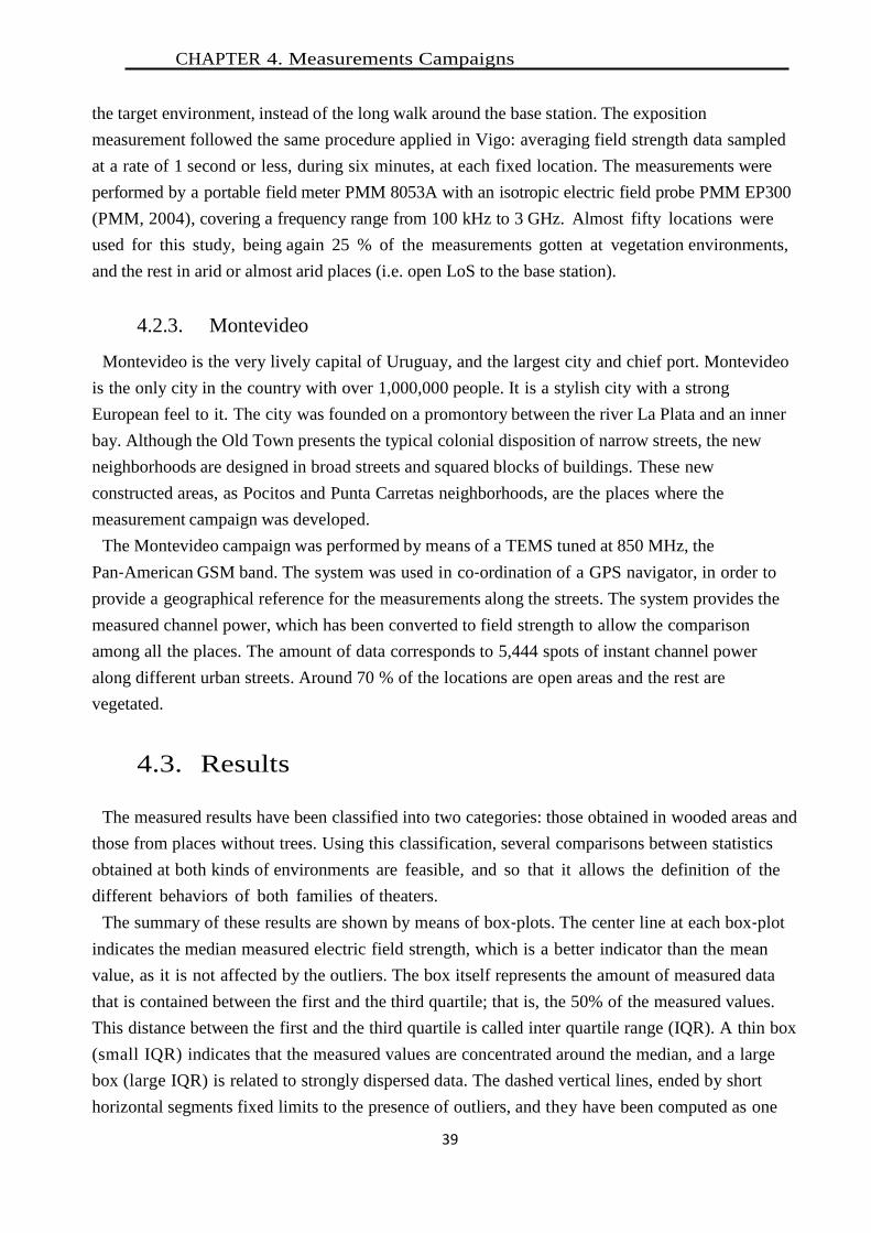
CHAPTER 4. Measurements Campaigns
39
the target environment, instead of the long walk around the base station. The exposition
measurement followed the same procedure applied in Vigo: averaging field strength data sampled
at a rate of 1 second or less, during six minutes, at each fixed location. The measurements were
performed by a portable field meter PMM 8053A with an isotropic electric field probe PMM EP300
(PMM, 2004), covering a frequency range from 100 kHz to 3 GHz. Almost fifty locations were
used for this study, being again 25 % of the measurements gotten at vegetation environments,
and the rest in arid or almost arid places (i.e. open LoS to the base station).
4.2.3. Montevideo
Montevideo is the very lively capital of Uruguay, and the largest city and chief port. Montevideo
is the only city in the country with over 1,000,000 people. It is a stylish city with a strong
European feel to it. The city was founded on a promontory between the river La Plata and an inner
bay. Although the Old Town presents the typical colonial disposition of narrow streets, the new
neighborhoods are designed in broad streets and squared blocks of buildings. These new
constructed areas, as Pocitos and Punta Carretas neighborhoods, are the places where the
measurement campaign was developed.
The Montevideo campaign was performed by means of a TEMS tuned at 850 MHz, the
Pan‐American GSM band. The system was used in co‐ordination of a GPS navigator, in order to
provide a geographical reference for the measurements along the streets. The system provides the
measured channel power, which has been converted to field strength to allow the comparison
among all the places. The amount of data corresponds to 5,444 spots of instant channel power
along different urban streets. Around 70 % of the locations are open areas and the rest are
vegetated.
4.3. Results
The measured results have been classified into two categories: those obtained in wooded areas and
those from places without trees. Using this classification, several comparisons between statistics
obtained at both kinds of environments are feasible, and so that it allows the definition of the
different behaviors of both families of theaters.
The summary of these results are shown by means of box‐plots. The center line at each box‐plot
indicates the median measured electric field strength, which is a better indicator than the mean
value, as it is not affected by the outliers. The box itself represents the amount of measured data
that is contained between the first and the third quartile; that is, the 50% of the measured values.
This distance between the first and the third quartile is called inter quartile range (IQR). A thin box
(small IQR) indicates that the measured values are concentrated around the median, and a large
box (large IQR) is related to strongly dispersed data. The dashed vertical lines, ended by short
horizontal segments fixed limits to the presence of outliers, and they have been computed as one
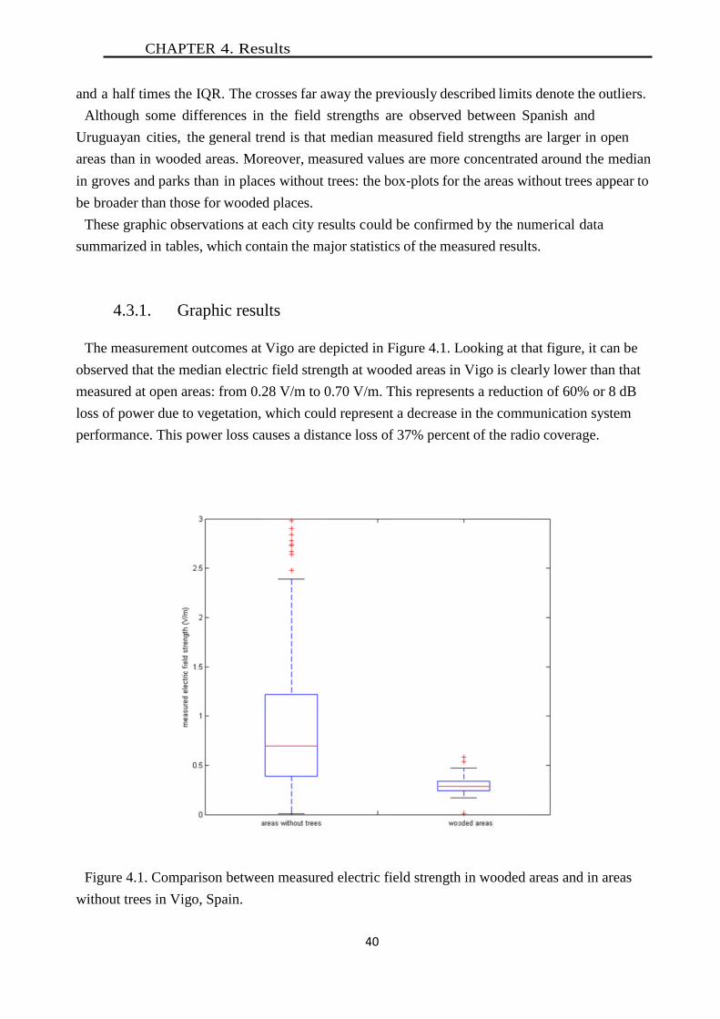
CHAPTER 4. Results
40
and a half times the IQR. The crosses far away the previously described limits denote the outliers.
Although some differences in the field strengths are observed between Spanish and
Uruguayan cities, the general trend is that median measured field strengths are larger in open
areas than in wooded areas. Moreover, measured values are more concentrated around the median
in groves and parks than in places without trees: the box‐plots for the areas without trees appear to
be broader than those for wooded places.
These graphic observations at each city results could be confirmed by the numerical data
summarized in tables, which contain the major statistics of the measured results.
4.3.1. Graphic results
The measurement outcomes at Vigo are depicted in Figure 4.1. Looking at that figure, it can be
observed that the median electric field strength at wooded areas in Vigo is clearly lower than that
measured at open areas: from 0.28 V/m to 0.70 V/m. This represents a reduction of 60% or 8 dB
loss of power due to vegetation, which could represent a decrease in the communication system
performance. This power loss causes a distance loss of 37% percent of the radio coverage.
Figure 4.1. Comparison between measured electric field strength in wooded areas and in areas
without trees in Vigo, Spain.
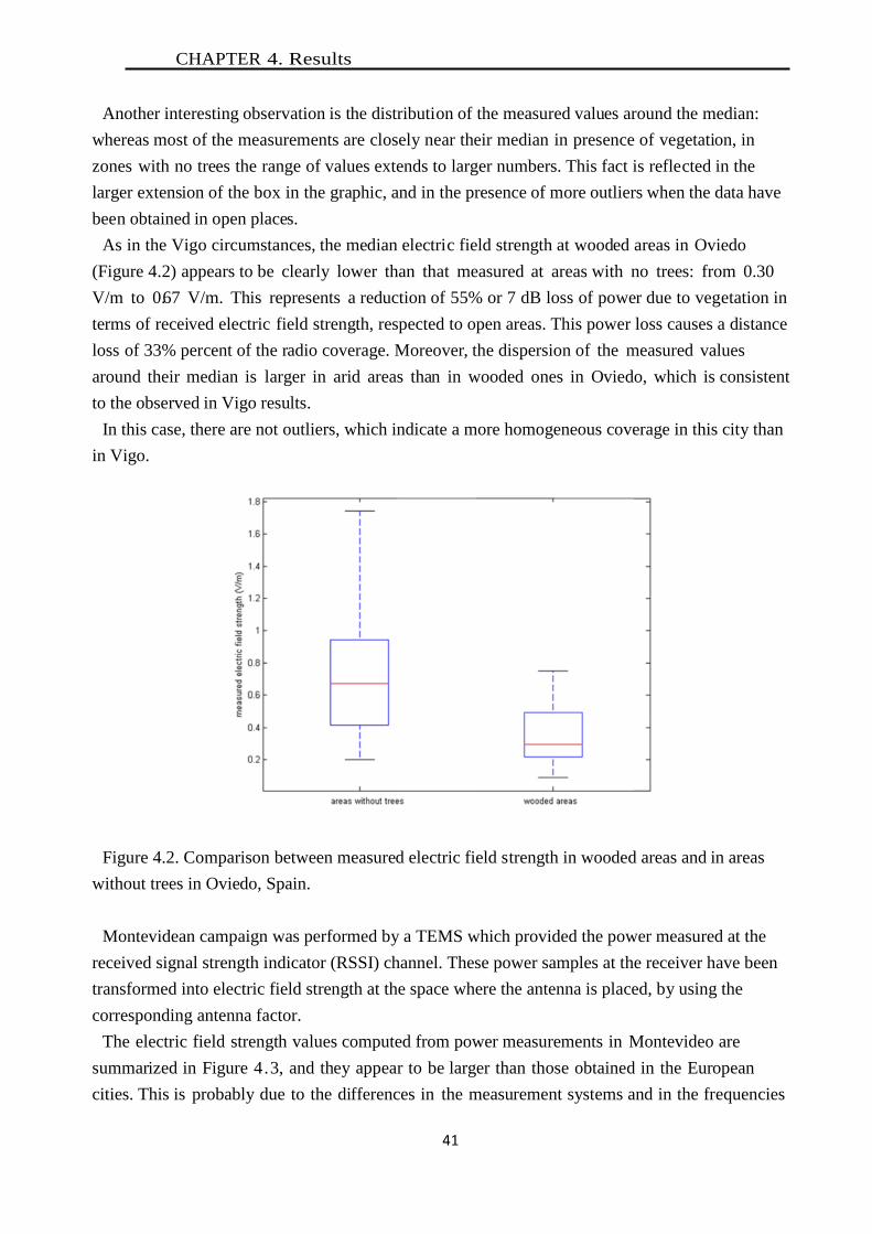
CHAPTER 4. Results
41
Another interesting observation is the distribution of the measured values around the median:
whereas most of the measurements are closely near their median in presence of vegetation, in
zones with no trees the range of values extends to larger numbers. This fact is reflected in the
larger extension of the box in the graphic, and in the presence of more outliers when the data have
been obtained in open places.
As in the Vigo circumstances, the median electric field strength at wooded areas in Oviedo
(Figure 4.2) appears to be clearly lower than that measured at areas with no trees: from 0.30
V/m to 0.67 V/m. This represents a reduction of 55% or 7 dB loss of power due to vegetation in
terms of received electric field strength, respected to open areas. This power loss causes a distance
loss of 33% percent of the radio coverage. Moreover, the dispersion of the measured values
around their median is larger in arid areas than in wooded ones in Oviedo, which is consistent
to the observed in Vigo results.
In this case, there are not outliers, which indicate a more homogeneous coverage in this city than
in Vigo.
Figure 4.2. Comparison between measured electric field strength in wooded areas and in areas
without trees in Oviedo, Spain.
Montevidean campaign was performed by a TEMS which provided the power measured at the
received signal strength indicator (RSSI) channel. These power samples at the receiver have been
transformed into electric field strength at the space where the antenna is placed, by using the
corresponding antenna factor.
The electric field strength values computed from power measurements in Montevideo are
summarized in Figure 4.3, and they appear to be larger than those obtained in the European
cities. This is probably due to the differences in the measurement systems and in the frequencies

CHAPTER 4. Results
42
used by the mobile standards. However, the general trends seem to be similar than those detected
in European cities, which could help in the extraction of conclusions.
Again, the median electric field strength at wooded areas is clearly lower than that measured at
open areas: from 0.85 V/m to 1.28 V/m. This represents a reduction of 44% or 5 dB loss of power
due to vegetation in terms of received electric field strength, respected to arid places.
Figure 4.3. Comparison between measured electric field strength in wooded areas and in areas
without trees in Montevideo, Uruguay.
This power loss causes a distance loss of 30% percent of the radio coverage. The dispersion of
the measured values around their median is larger when no vegetation is in the propagation
channel, which is consistent to the observed in results from other places. Moreover, the open areas
present a larger number of outlier values than the wooded, as occurred in Vigo.
4.3.2. Numerical results
Table 4.1 contains the major statistics of the measured results, and it allows the numerical
analysis. It can be observed that median field strength in wooded areas appears to be 44% less
than in non‐vegetation areas, in the better balanced case, and 60% lower in the most imbalanced.
This clearly different trend between both kinds of areas is confirmed by the mean, which is at least
half in groves compared to open zones. The standard deviation is visibly larger in arid areas, as a
consequence of a wider range of values and their more disperse distribution. Furthermore, the
range of values is wider in the measurements at open areas than those obtained in wooded places.
The degree of asymmetry of the electric field strength distribution around its mean has been
characterized by the skewness coefficients. The values at table 4.1 indicate that the distribution is
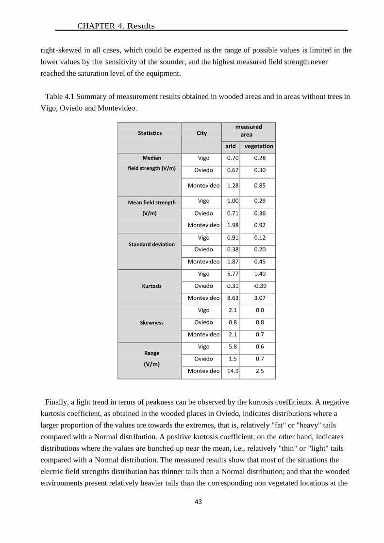
CHAPTER 4. Results
43
right ‐skewed in all cases, which could be expected as the range of possible values is limited in the
lower values by the sensitivity of the sounder, and the highest measured field strength never
reached the saturation level of the equipment.
Table 4.1 Summary of measurement results obtained in wooded areas and in areas without trees in
Vigo, Oviedo and Montevideo.
Statistics
City measured
area
arid vegetation
Median
field strength (V/m)
Vigo 0.70 0.28
Oviedo 0.67 0.30
Montevideo 1.28 0.85
Mean field strength
(V/m)
Vigo 1.00 0.29
Oviedo 0.71 0.36
Montevideo 1.98 0.92
Standard deviation
Vigo 0.91 0.12
Oviedo 0.38 0.20
Montevideo 1.87 0.45
Kurtosis
Vigo 5.77 1.40
Oviedo 0.31 ‐0.39
Montevideo 8.63 3.07
Skewness
Vigo 2.1 0.0
Oviedo 0.8 0.8
Montevideo 2.1 0.7
Range
(V/m)
Vigo 5.8 0.6
Oviedo 1.5 0.7
Montevideo 14.9 2.5
Finally, a light trend in terms of peakness can be observed by the kurtosis coefficients. A negative
kurtosis coefficient, as obtained in the wooded places in Oviedo, indicates distributions where a
larger proportion of the values are towards the extremes, that is, relatively "fat" or "heavy" tails
compared with a Normal distribution. A positive kurtosis coefficient, on the other hand, indicates
distributions where the values are bunched up near the mean, i.e., relatively "thin" or "light" tails
compared with a Normal distribution. The measured results show that most of the situations the
electric field strengths distribution has thinner tails than a Normal distribution; and that the wooded
environments present relatively heavier tails than the corresponding non vegetated locations at the
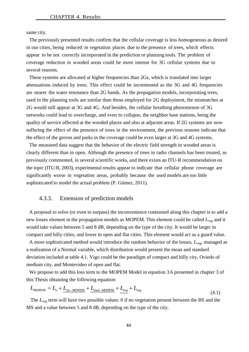
CHAPTER 4. Results
44
same city.
The previously presented results confirm that the cellular coverage is less homogeneous as desired
in our cities, being reduced in vegetation places due to the presence of trees, which effects
appear to be not correctly incorporated in the prediction or planning tools. The problem of
coverage reduction in wooded areas could be more intense for 3G cellular systems due to
several reasons.
These systems are allocated at higher frequencies than 2Gs, which is translated into larger
attenuations induced by trees. This effect could be incremented as the 3G and 4G frequencies
are nearer the water resonance than 2G bands. As the propagation models, incorporating trees,
used in the planning tools are similar than those employed for 2G deployment, the mismatches at
2G would still appear at 3G and 4G. And besides, the cellular breathing phenomenon of 3G
networks could lead to overcharge, and even to collapse, the neighbor base stations, being the
quality of service affected at the wooded places and also at adjacent areas. If 2G systems are now
suffering the effect of the presence of trees in the environment, the previous reasons indicate that
the effect of the groves and parks in the coverage could be even larger at 3G and 4G systems.
The measured data suggest that the behavior of the electric field strength in wooded areas is
clearly different than in open. Although the presence of trees in radio channels has been treated, as
previously commented, in several scientific works, and there exists an ITU‐R recommendation on
the topic (ITU‐R, 2003), experimental results appear to indicate that cellular phone coverage are
significantly worse in vegetation areas, probably because the used models are too little
sophisticated to model the actual problem (P. Gómez, 2011).
4.3.3. Extension of prediction models
A proposal to solve (or even to surpass) the inconvenience contrasted along this chapter is to add a
new losses element in the propagation models as MOPEM. This element could be called Lveg and it
would take values between 5 and 8 dB, depending on the type of the city. It would be larger in
compact and hilly cities, and lower in open and flat cities. This element would act as a guard value.
A more sophisticated method would introduce the random behavior of the losses, Lveg, managed as
a realization of a Normal variable, which distribution would present the mean and standard
deviation included at table 4.1. Vigo could be the paradigm of compact and hilly city, Oviedo of
medium city, and Montevideo of open and flat.
We propose to add this loss term to the MOPEM Model in equation 3.6 presented in chapter 3 of
this Thesis obtaining the following equation:
MOPEM o rts MOPEM msd MOPEM esq vegL L L L L L (4.1)
The Lveg term will have two possible values: 0 if no vegetation present between the BS and the
MS and a value between 5 and 8 dB, depending on the type of the city.

CHAPTER 4. Conclusions
45
4.4. Conclusions
The electric field strength at cellular phone frequency bands has been measured in urban locations
at three different cities: Vigo, Oviedo and Montevideo, in both wooded and arid zones.
Although the mobile phone networks are supposed to be planned to provide a homogeneous
performance at any places, the observed situation is that the cellular phone coverage in groves
and parks appears to be worse than in places without trees. The electric field strength reduction due
to the presence of trees has been observed to be between 44% and 60%, which may lead to
important alterations in the cellular system performance: reduction of coverage distances from 30 %
to 37%. An interesting observation is that the excess attenuation at vegetation places seems to
grow as the city is denser in terms of buildings: Montevideo large avenues presented attenuations
around 5 dB, whereas at Oviedo and Vigo, which are denser cities, the measured values are 7 and
8 dB, respectively. Even more, Oviedo presents more parks and open areas than Vigo, which
confirms the tendency.
That clearly different trend between both kinds of areas is confirmed by the mean of the
measured field strength, which is half or even less in wooded compared to arid zones. Moreover,
the standard deviation is visibly larger in open areas, as a consequence of a wider range of values
and their more disperse distribution, than in groves and parks. The ranges that contain the
measured electric field strengths in open places seem to be larger (from double to ten times) than in
vegetated areas, at all the considered cities.
The distribution of the measured electric field strengths appears to be right‐skewed in all cases,
whereas there is a light trend in terms of peakness, as the wooded environments present relatively
heavier tails than the corresponding non vegetated locations at the same city. All these statistics
confirm a clearly different trend between electric field strengths at both classes of environments.
This previous conclusion appears to be more problematic as the modern network planning systems
consider the presence of vegetation in the places to be served. If the coverage has been computed
taking into account the vegetation, it could be thought that trees are not correctly modeled in these
planning tools. And if designers have not considered the presence of vegetation, this simplification
seems to be too significant to be adopted in such a network development.
The problem at 3G and 4G networks would be stronger than at 2G due to their higher
frequencies, the neighborhood to water resonance, the cellular breathing phenomenon, and the
inaccuracy of the tree models used for 2G planning.
A proposal to go beyond such mistakes would reside on combining deterministic propagation
models, to obtain the general coverage taking into account just the structures in the environment (as
it is done nowadays), and a probabilistic correction founded on the results provided by this paper.
Thus, in vegetation areas, the results provided by the standard simulation tools must be corrected
adding excess attenuations of 5 to 8 dB, depending on the building density of the considered city:
the denser the place, the larger the excess attenuation in vegetation areas.

CHAPTER 4. Conclusions
46

Chapter 5 Wireless Networks interference and security protection by means of vegetation barriers
The success of wireless technologies could paradoxically leads to a collapse in their performance:
the interference between adjacent networks and the attacks done by users from outside the expected
coverage limits are two important enemies to the well function of the networks. In chapter 4, the
attenuation induced by vegetation has been accounted. This attenuation is commonly identified as a
problem, as the radio coverage is reduced as a consequence, but it also could be an advantage. The
proposal of this chapter is simple but efficient: the use of vegetation barriers to create shadowing
areas with excess attenuations in the edge of the service area, in order to reduce the coverage
distance of each wireless node, reducing the possible interference to other networks as well as
improving security aspects by minimizing the signal strength outside the service area.
5.1. Introduction
The wireless paradigm has become one of the technological successes of last years. The
different standards (IEEE Part 11, 2007) (IEEE Computer Society ; IEEE Microwave
Theory Techniques Society, 2006) allow high speed connectivity, which in the past was the
main disadvantage of wireless networks compared to wired ones. At this point, the corporative
and domestic computing networks, which were traditionally projected following a wired scheme,
are rapidly migrating to wireless. This fact full fits the people requirements in terms of mobility
and connectivity, but it also suffers some important problems as interference between adjacent
or neighbor networks and undesired access to the network facilities by unknown users from outside
the service area.
These problems could appear in domestic networks, but it is in trade buildings where the
situation becomes worse: various neighbor networks (corresponding to different companies or
departments within the same company) could interfere one among the others, overloading the

CHAPTER 5. Introduction
48
network facilities with retransmission events, and then degrading its performance. Besides, the
number of unauthorized accesses could grow: both for using services (people surfing the
Internet “for free”, occupying resources paid by the company) and for damaging purposes (done
by hackers).
There is several propagation research done in the area of wireless network planning, from
general works to more specific ones. Typically, deterministic methods have been proposed to
model static elements, both constructive and natural obstacles (Bertoni, 2000). However, there
are other kinds of obstacles in the radio links that must be modeled by stochastic procedures
(Chizcik, 2008). Such obstacles may be persons (Kara A. , 2009), furniture (I. Cuiñas, 2004),
vegetation (Gay-Fernandez , 2010) , or in general non-polygonal structures (Kara &
Yazgan, 2008). All these obstructions can mitigate the received power in a radio link, or
even they could break the connection.
The aim of this chapter is to propose the use of vegetation barriers to mitigate such problems.
The induction of attenuation in the radio waves propagating across vegetation media is a well-
known effect, but its consequences, mechanics and applications have not been completely
explored. This chapter presents a possible application of that attenuation effect. The vegetation
obstructing the radio channel could provide attenuation enough in the edge of the service area
to: a) reduce the distance at which elements of different networks can be installed without
generating and receiving interference; and b) shorten the distance at which an external user
could access the network servers or facilities. Thus, a correct decision in the location of indoor or
outdoor plants could benefit the performance of the wireless network to be protected against
interference and/or external attacks.
A large measurement campaign involving seven different species have been performed to
support the proposal, and its results are presented along this chapter.

CHAPTER 5. Measurements Campaigns
49
5.2. Measurements Campaigns
The measurement campaign was performed in an open area, with separate transmitter and
receiver. The transmitter was based on a Rohde & Schwarz radio signal generator SMR-40 (Rohde
& Schwarz)whereas the receiver was constructed around a Rohde & Schwarz spectrum analyzer
FSP-40 (Rohde & Schwarz, 2009). The narrow-band measurements were performed at 2.4 and 5.8
GHz, which are frequencies in bands used by wireless standards. Although the actual wireless world
is dominated by omnidirectional antennas, which pick up all scattering energy around the receiver,
the measurements were performed with directional antennas. This decision was adopted as the
objective was to isolate the effect of the vegetation barrier from the environment scatterers. The use
of omnidirectional antennas would probably lead to deeper attenuations but the measurement results
would also include many environment effects which would be difficult to extract to define the
attenuation strictly induced by the vegetation. Then, both ends of the measurement setup were
installed with log-periodic antennas Electrometrics EM6952, which gain is 4.72 dBi at 2.4 GHz and
4.62 dBi at 5.8 GHz, placed at 1.25 meters height.
The measurement setup was completed by a linear positioner that supports the receiving antenna
and allows its movement parallel to a vegetation barrier. The positioning platform is driven by a
stepper motor, connected to an indexer. The scheme can be observed at Figure 5.1, and an image of
the setup without vegetation barrier is presented at Figure 5.2. This photograph allows the
observation of the antennas and the linear positioner.
Figure 5.1. Scheme of the basic geometry of the measurement system (zenithal
view).
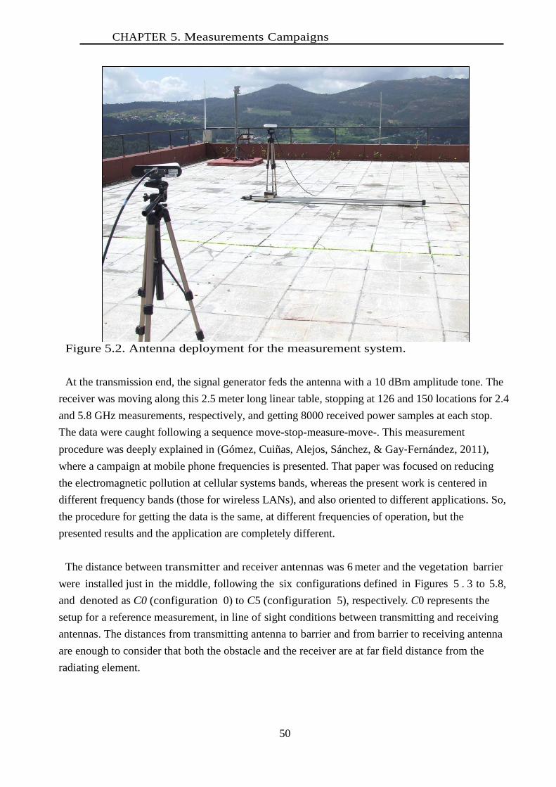
CHAPTER 5. Measurements Campaigns
50
Figure 5.2. Antenna deployment for the measurement system.
At the transmission end, the signal generator feds the antenna with a 10 dBm amplitude tone. The
receiver was moving along this 2.5 meter long linear table, stopping at 126 and 150 locations for 2.4
and 5.8 GHz measurements, respectively, and getting 8000 received power samples at each stop.
The data were caught following a sequence move-stop-measure-move-. This measurement
procedure was deeply explained in (Gómez, Cuiñas, Alejos, Sánchez, & Gay‐Fernández, 2011),
where a campaign at mobile phone frequencies is presented. That paper was focused on reducing
the electromagnetic pollution at cellular systems bands, whereas the present work is centered in
different frequency bands (those for wireless LANs), and also oriented to different applications. So,
the procedure for getting the data is the same, at different frequencies of operation, but the
presented results and the application are completely different.
The distance between transmitter and receiver antennas was 6 meter and the vegetation barrier
were installed just in the middle, following the six configurations defined in Figures 5 . 3 to 5.8,
and denoted as C0 (configuration 0) to C5 (configuration 5), respectively. C0 represents the
setup for a reference measurement, in line of sight conditions between transmitting and receiving
antennas. The distances from transmitting antenna to barrier and from barrier to receiving antenna
are enough to consider that both the obstacle and the receiver are at far field distance from the
radiating element.

CHAPTER 5. Measurements Campaigns
51
Figure 5.3. Vegetation barrier configuration C0
Figure 5.4. Vegetation barrier configuration C 1

CHAPTER 5. Measurements Campaigns
52
Figure 5.5. Vegetation barrier configuration C2.
Figure 5.6. Vegetation barrier configuration C3

CHAPTER 5. Measurements Campaigns
53
Figure 5.7. Vegetation barrier configuration C4.
Figure 5.8. Vegetation barrier configuration C5
Seven different species were considered separately to build the vegetation barrier, which was
constructed with up to ten individuals of the same species. Both indoor and outdoor shrub
species have been considered in this study. Among the indoor shrub species, the Dypsis lutescens
(Areca palm), the Heptapleurum arboricola gold capella (Schefflera) and the Ficus elastica (Ficus)
were used. All of them are common indoor species used frequently as decorative elements in
buildings and indoor yards. The outdoor species have been chosen either for being typically used to

CHAPTER 5. Measurements Campaigns
54
construct quick growth private fences, or because of their large but dense foliage that favors the
electromagnetic shielding. In order to analyze both characteristics, the species considered were as
follows: the Callistemon laevis (Callistemon or Bottlebrush), the Camellia japonica (Camellia), the
Juniperus communis hibernica (Irish juniper) and the Thuja atrovirens (White cedar).
The Dypsis lutescens (Figure 5.9) is one of the most common indoor specie. It can be seen as a
trunk ended in palms, whose height may vary from 1.5 to 3 m when used as a bush or until 9 m
when grows as a palm. It can be seen frequently as a decorative element at indoor yards.
Figure 5.9. The Dypsis lutescens specimen measured in anechoic chamber
The ficus (Figure 5.10) is an evergreen genus including around 800 species of trees, bushes and
climbing plants, although most commonly used is Ficus elastica that has been the one chosen for
this campaign. The size may vary depending on the variety, and it is usually found as a bush at
indoor gardens, or even as a decorative element at home. They can reach 12 m when developed as a
tree, but the mean height at indoor conditions is between 1 and 1.5 meter.
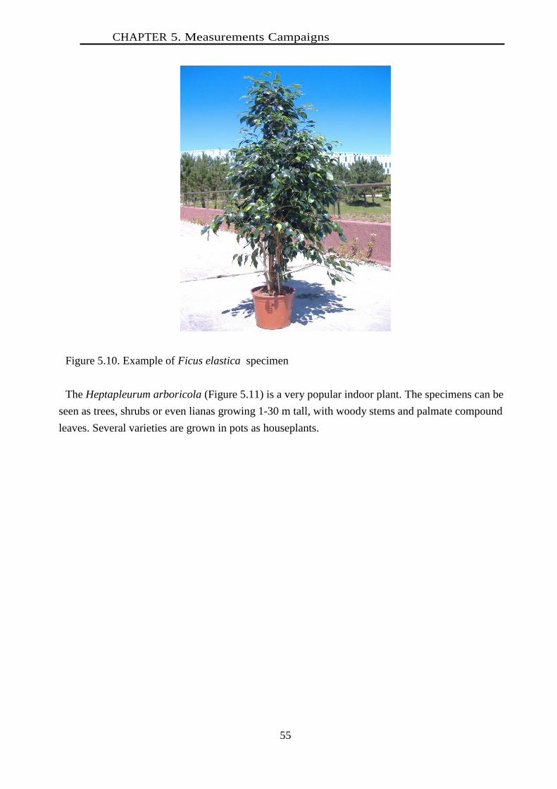
CHAPTER 5. Measurements Campaigns
55
Figure 5.10. Example of Ficus elastica specimen
The Heptapleurum arboricola (Figure 5.11) is a very popular indoor plant. The specimens can be
seen as trees, shrubs or even lianas growing 1-30 m tall, with woody stems and palmate compound
leaves. Several varieties are grown in pots as houseplants.
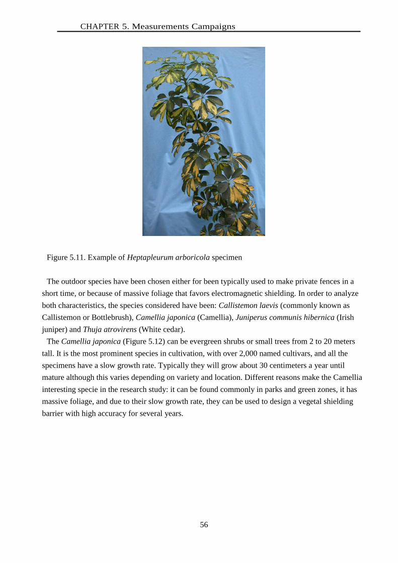
CHAPTER 5. Measurements Campaigns
56
Figure 5.11. Example of Heptapleurum arboricola specimen
The outdoor species have been chosen either for been typically used to make private fences in a
short time, or because of massive foliage that favors electromagnetic shielding. In order to analyze
both characteristics, the species considered have been: Callistemon laevis (commonly known as
Callistemon or Bottlebrush), Camellia japonica (Camellia), Juniperus communis hibernica (Irish
juniper) and Thuja atrovirens (White cedar).
The Camellia japonica (Figure 5.12) can be evergreen shrubs or small trees from 2 to 20 meters
tall. It is the most prominent species in cultivation, with over 2,000 named cultivars, and all the
specimens have a slow growth rate. Typically they will grow about 30 centimeters a year until
mature although this varies depending on variety and location. Different reasons make the Camellia
interesting specie in the research study: it can be found commonly in parks and green zones, it has
massive foliage, and due to their slow growth rate, they can be used to design a vegetal shielding
barrier with high accuracy for several years.

CHAPTER 5. Measurements Campaigns
57
Figure 5.12. The Camellia japonica specimen measured in anechoic chamber
The Juniperus communis hibernica (Figure 5.13) are coniferous plants in the genus Juniperus of
the cypress family Cupressaceae. Junipers vary in size and shape from tall trees, 20-40 m tall, to
columnar or low spreading shrubs with long trailing branches. They are evergreen with either
needle-like and/or scale-like leaves. Junipers are usually used to make vegetal fences between
properties, and so, they are very interesting specimens for our campaign. On the same family of
brushes, white cedar (Figure 5.14) has similar characteristics, being their foliage a less dense than
juniper foliage.
Figure 5.13. The Juniperus communis hibernica specimen
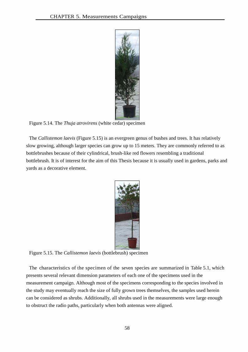
CHAPTER 5. Measurements Campaigns
58
Figure 5.14. The Thuja atrovirens (white cedar) specimen
The Callistemon laevis (Figure 5.15) is an evergreen genus of bushes and trees. It has relatively
slow growing, although larger species can grow up to 15 meters. They are commonly referred to as
bottlebrushes because of their cylindrical, brush-like red flowers resembling a traditional
bottlebrush. It is of interest for the aim of this Thesis because it is usually used in gardens, parks and
yards as a decorative element.
Figure 5.15. The Callistemon laevis (bottlebrush) specimen
The characteristics of the specimen of the seven species are summarized in Table 5.1, which
presents several relevant dimension parameters of each one of the specimens used in the
measurement campaign. Although most of the specimens corresponding to the species involved in
the study may eventually reach the size of fully grown trees themselves, the samples used herein
can be considered as shrubs. Additionally, all shrubs used in the measurements were large enough
to obstruct the radio paths, particularly when both antennas were aligned.

CHAPTER 5. Measurements Campaigns
59
Table 5.1. Dimensions of the shrubs, in cm.
Specie shrub leaf
height diameter length width
areca 150 70 25 1
schefflera 160 60 10 4.5
ficus 170 55 7 3
callistemon 150 80 7 4
camellia 165 90 8 6
Irish juniper 205 55 2 0.5
thuja 165 45 0.5 0.2
Table 5.2 classifies the species into three different groups or types, as a function of flexibility of
their stems, shape of their leaves, kind of leaf movement induced by the wind (twisting and/or
swaying), and the density of their canopies. This classification could be interesting in order to
organize the conclusions by typology instead of specie. Thus, the results analysis would be
applicable to other families of shrubs by observing their characteristics and by associating them
with any of these types.
Table 5.2 Description of shrub specimens: Typology.
Trunk Leaves Movement of
leaves
Canopy
Type I Ficus
flexible long twist and sway light Schefflera
Type II
Callistemon
wooden elliptic sway very dense Camellia
Irish juniper
Type III Areca palm flexible long/large mainly sway,
and few twist
medium
density Thuja wooden long/small
The geographical region in which measurements took place is particularly wet all year round.
Additionally, the specimens were watered on a daily basis, so they were considered reasonably wet
during the measurement campaign.
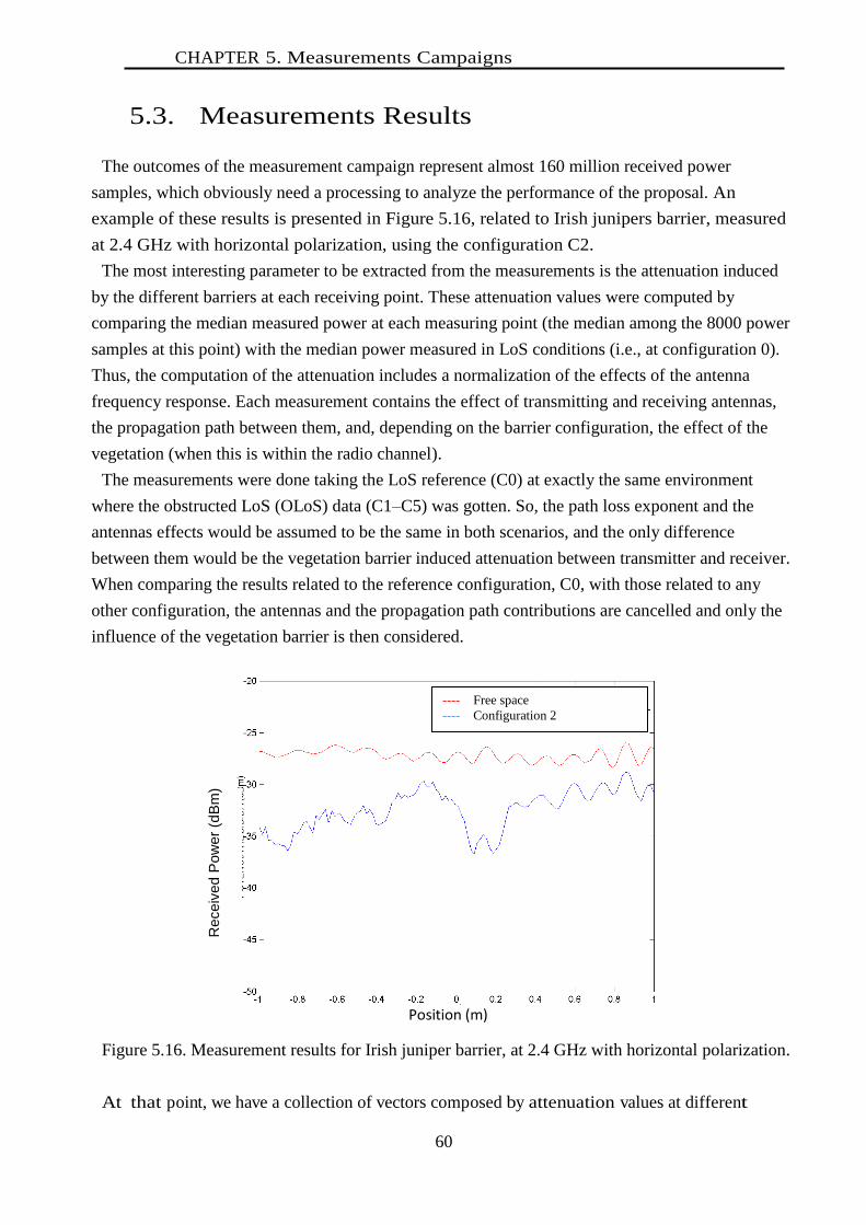
CHAPTER 5. Measurements Campaigns
60
5.3. Measurements Results
The outcomes of the measurement campaign represent almost 160 million received power
samples, which obviously need a processing to analyze the performance of the proposal. An
example of these results is presented in Figure 5.16, related to Irish junipers barrier, measured
at 2.4 GHz with horizontal polarization, using the configuration C2.
The most interesting parameter to be extracted from the measurements is the attenuation induced
by the different barriers at each receiving point. These attenuation values were computed by
comparing the median measured power at each measuring point (the median among the 8000 power
samples at this point) with the median power measured in LoS conditions (i.e., at configuration 0).
Thus, the computation of the attenuation includes a normalization of the effects of the antenna
frequency response. Each measurement contains the effect of transmitting and receiving antennas,
the propagation path between them, and, depending on the barrier configuration, the effect of the
vegetation (when this is within the radio channel).
The measurements were done taking the LoS reference (C0) at exactly the same environment
where the obstructed LoS (OLoS) data (C1–C5) was gotten. So, the path loss exponent and the
antennas effects would be assumed to be the same in both scenarios, and the only difference
between them would be the vegetation barrier induced attenuation between transmitter and receiver.
When comparing the results related to the reference configuration, C0, with those related to any
other configuration, the antennas and the propagation path contributions are cancelled and only the
influence of the vegetation barrier is then considered.
Figure 5.16. Measurement results for Irish juniper barrier, at 2.4 GHz with horizontal polarization.
At that point, we have a collection of vectors composed by attenuation values at different
---- Free space
---- Configuration 2
Receiv
ed
Pow
er
(dB
m)
Position (m)

CHAPTER 5. Measurements Campaigns
61
locations within the shadow area behind the barrier. The median of each of these vectors is a good
representation of the median attenuation provided by each barrier in its shadow area.
The results obtained at 2.4 GHz are presented in Tables 5.3 and 5.4, for horizontal and vertical
polarization respectively, whereas Tables 5.5 and 5.6 are related to 5.8 GHz experiences. It must
be observed that the attenuation appears to be larger for vertical polarization than for horizontal,
as it occurs in most of the measurement results related in the literature. The explanation must
be the own geometry of the vegetation, which is vertically organized: the trunks are clearly
vertical; the disposition of leaves is also dominantly vertical, whereas the orientation of branches
appears to be more random.
Table 5.3. Median attenuation (dB) at 2.4 GHz, with horizontal polarization.
Specie barrier configuration
C 1 C 2 C 3 C 4 C 5
areca 0.1 0.2 0.4 2.9 0.1
schefflera 0.4 0.8 1.6 1.9 0.7
ficus 2.2 2.8 4.3 4.7 2.7
callistemon 2.1 2.5 3.5 3.3 1.5
camellia 3.1 3.2 3.9 5.9 2.9
Irish juniper 5.2 5.2 8.9 6.2 4.5
thuja 1.6 1.5 1.8 2.1 1.4
Table 5.4. Median attenuation (dB) at 2.4 GHz, with vertical polarization.
Specie barrier configuration
C 1 C 2 C 3 C 4 C 5
areca 3.2 3.5 2.5 2.1 3.2
schefflera 0.1 0.9 1.5 1.0 0.4
ficus 2.1 4.1 5.1 5.9 2.0
callistemon 3.3 3.0 6.9 5.4 3.0
camellia 5.4 5.5 6.9 8.2 5.2
Irish juniper 9.6 9.8 10.7 10.1 8.0
thuja 3.5 3.8 5.6 6.2 3.5
Table 5.5. The median attenuation (dB) at 5.8 GHz, with horizontal polarization.
Specie barrier configuration
C 1 C 2 C 3 C 4 C 5
areca 0.1 0.1 0.9 4.1 0.1
schefflera 0.1 0.2 5.6 6.7 1.0
ficus 6.2 5.4 9.3 11.3 5.3
callistemon 1.1 4.0 6.5 7.7 2.4
camellia 10.1 12.4 12.1 13.2 10.7
Irish juniper 6.8 5.9 13.2 10.6 8.1
thuja 3.9 5.1 6.3 6.8 4.7
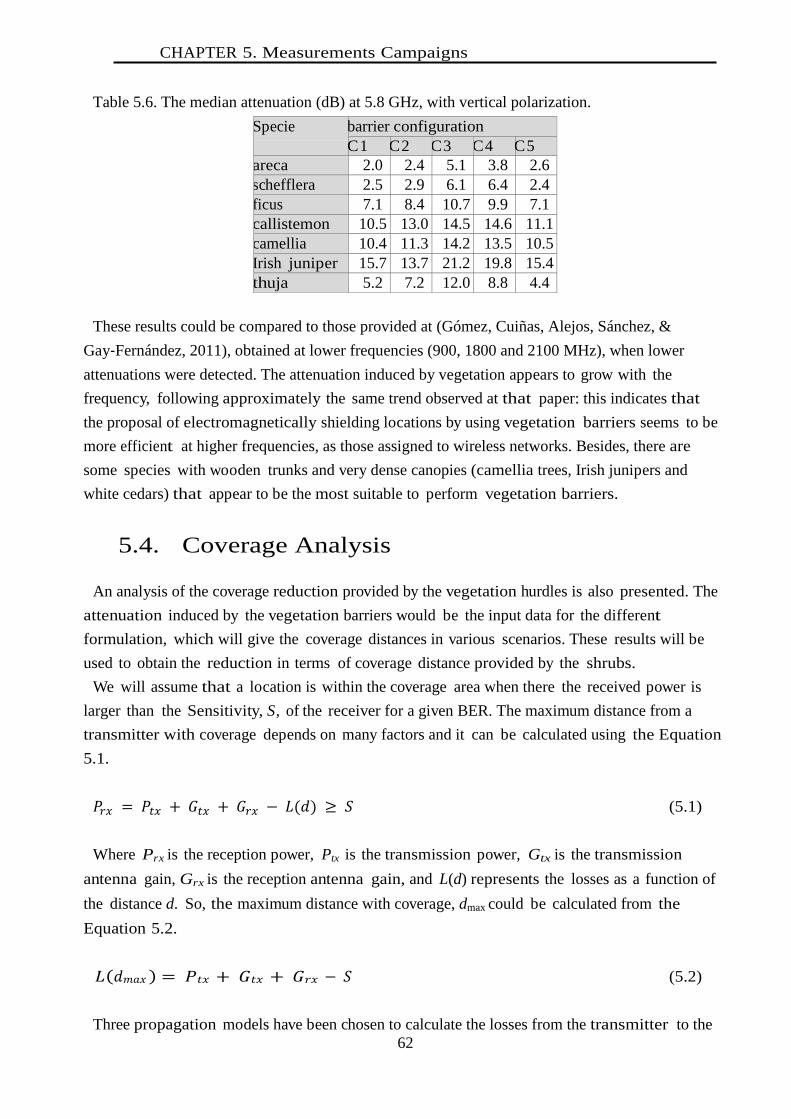
CHAPTER 5. Measurements Campaigns
62
Table 5.6. The median attenuation (dB) at 5.8 GHz, with vertical polarization.
Specie barrier configuration
C 1 C 2 C 3 C 4 C 5
areca 2.0 2.4 5.1 3.8 2.6
schefflera 2.5 2.9 6.1 6.4 2.4
ficus 7.1 8.4 10.7 9.9 7.1
callistemon 10.5 13.0 14.5 14.6 11.1
camellia 10.4 11.3 14.2 13.5 10.5
Irish juniper 15.7 13.7 21.2 19.8 15.4
thuja 5.2 7.2 12.0 8.8 4.4
These results could be compared to those provided at (Gómez, Cuiñas, Alejos, Sánchez, &
Gay‐Fernández, 2011), obtained at lower frequencies (900, 1800 and 2100 MHz), when lower
attenuations were detected. The attenuation induced by vegetation appears to grow with the
frequency, following approximately the same trend observed at that paper: this indicates that
the proposal of electromagnetically shielding locations by using vegetation barriers seems to be
more efficient at higher frequencies, as those assigned to wireless networks. Besides, there are
some species with wooden trunks and very dense canopies (camellia trees, Irish junipers and
white cedars) that appear to be the most suitable to perform vegetation barriers.
5.4. Coverage Analysis
An analysis of the coverage reduction provided by the vegetation hurdles is also presented. The
attenuation induced by the vegetation barriers would be the input data for the different
formulation, which will give the coverage distances in various scenarios. These results will be
used to obtain the reduction in terms of coverage distance provided by the shrubs.
We will assume that a location is within the coverage area when there the received power is
larger than the Sensitivity, S, of the receiver for a given BER. The maximum distance from a
transmitter with coverage depends on many factors and it can be calculated using the Equation
5.1.
(5.1)
Where Prx is the reception power, Ptx is the transmission power, Gtx is the transmission
antenna gain, Grx is the reception antenna gain, and L(d) represents the losses as a function of
the distance d. So, the maximum distance with coverage, dmax could be calculated from the
Equation 5.2.
(5.2)
Three propagation models have been chosen to calculate the losses from the transmitter to the

CHAPTER 5. Coverage Analysis
63
receiver, and the distance that limits the coverage, dmax .
Two of them are full indoor models and the other has part of the path indoor and part of the path
outdoor. The considered propagation models are going to be identified as the empirical indoor-
to-outdoor (Valcarce, 2010), International Telecommunications Union (ITU) indoor ( I T U -
R , 2 0 0 1 ) , and the statistical indoor ( P e r e z - V e g a , 1 9 9 7 ) . This selection of models
covers the different situations mentioned in the introduction section: the possible interference
between adjacent wireless networks within the same building (the full indoor models), and the
hacker attack from the surroundings of the building hosting the network (the indoor to outdoor
model). The following paragraphs describe the three considered propagation models: empirical
indoor-to-outdoor, ITU-R, and statistical path loss.
5.4.1. Empirical Indoor-to-outdoor Model
The empirical indoor-to-outdoor model (Valcarce, 2010) is formulated as in Equation 5.3. It is
an outdoor-indoor model, so it considers a wall between the transmitter and the receiver.
(5.3)
At the equation, L is the total path loss, in dB; f i s the frequency of transmission, in GHz; d
is the distance between transmitter and receiver, in m; and Nw is the number of walls between
the transmitter and the outdoor receiver.
5.4.2. ITU-R Model (Indoor)
The ITU model (ITU-R, 2001) is defined by Equation 5.4. The model has been proposed for a
frequency range from 900 MHz to 5.2 GHz, and it considers 1 to 3 floors.
(5.4)
Where the different parameters are: f , the frequency in MHz; N , the distance power loss
coefficient (N = 30.5 at 2.4 GHz); n, number of floors between the transmitter and receiver; and
Pf (n), the floor loss penetration factor (one floor: 15 dB).
The distance power loss coefficient, N, is the quantity that expresses the loss of signal power
with distance. This coefficient is empirical. The floor penetration loss factor is another
empirical constant which depends on the number of floors the waves need to penetrate. Some
values for both parameters are proposed in

CHAPTER 5. Coverage Analysis
64
(ITU-R, 2001).
5.4.3. Statistical Path Loss Model (Indoor)
The statistical path loss model ( E r c e g , y o t r o s , 1 9 9 9 ) is described by the Equation 5.5.
(
)
(5.5)
Where n is the mean path loss exponent, and its proposed values depends on the environment:
Classroom LoS n = 1.8, corridors LoS n = 1, one wall OLoS n = 3.4 and multiple walls OLoS n =
3.46.
5.5. Coverage Results
The effect of the vegetation barriers must be translated into excess attenuations to the models
results: the attenuation induced by the barriers has to be added to that attenuation computed by the
proposed models. These excess attenuations correspond to the values presented in Tables 5.2 to 5.5.
So, the three models have been used to analyze the coverage distances with and without vegetation
barriers, being the propagation path losses in presence of vegetation barriers as indicated by
Equation 5.6, which modifies Equation 5.2. Lbarrier represents the contribution of the vegetation
barrier to the total attenuation.
max( ) tx tx rx barrierL d P G G S L (5.6)
Some parameters were chosen to do this calculus, which are common to the three models:
Ptx = 20 dBm, S = −78 dBm, Gtx = 6 dBi, Grx = 2 dBi.
The results presented in this section has been computed by using two standard excess attenuation
(Lbarrier) of 5 and 10 dB, representing two of the possible attenuations due to the vegetation barrier.
This has been done in order to reduce the number of considered scenarios, which in other case
would be as many as 140: four times (two frequencies, two polarizations) the 35 measured barriers
(five configurations with seven vegetation species). In fact, the use of measured results led to more
exact computations in terms of distances. However, we decided to present results corresponding to
5 and 10 dB attenuation to illustrate the performance of the proposal, because of the large amount of
data available. The results related to both attenuation levels appear to be significant to demonstrate
the validity of the proposal; whereas provided attenuation values are useful to compute the exact
coverage distances at each situation. Thus, these results can show an illustration of the performance
of the proposal by using a reduced amount of data. So, we computed dmax in line of sight conditions,
and also when Lbarrier equals 5 and 10 dB, by means of the three proposed propagation models.

CHAPTER 5. Coverage Results
65
Table 5.6. Coverage distances (m), with different barrier attenuations and propagation models.
Vegetation barrier
Excess attenuation
(dB)
Coverage distance (m) Empirical
indoor-to-
outdoor
indoor ITU-R Statistical
No barrier 0 37 81 87 Standard 1 5 26 55 62 Standard 2 10 18 37 44
Table 5.6 contains the computed values of coverage distance, provided at 2.4 GHz, a common
frequency band for wireless networks (Wi-Fi).
The first row at Table 5.6 (no barrier) gives the maximum distances calculated using the three
models previously mentioned without vegetation barrier. This represents a reference for the
other results. The second and third rows show the new distances with 5 and 10 dB of excess
attenuation due to the standard vegetation barriers, defined as a good representative of the
actual performance.
The difference between these rows and the first one in indoor models (ITU-R (ITU-R, 2001) and
statistical (Perez-Vega, 1997)) columns indicates how close nodes from two adjacent
networks could be installed, avoiding interference events, when vegetation barriers providing
attenuations of 5 or 10 dB are installed. The selection of the indoor model could lead to
different results, but both provide values in similar magnitude order: maximum coverage
distances of 81 and 87 meter in open LoS conditions, for ITU-R and statistical respectively; and
coverage from 55 to 62 meter when the barriers induce attenuation of 5 dB and from 37 to 44
meter when the induced attenuation is 10 dB. So, in general terms, in such indoor
environments the distance appears to be reduced to the 70% with the 5 dB standard barrier and to
the 50% with that inducing attenuation of 10 dB. This indicates that the prevention of
interference between wireless networks is possible by installing vegetation barriers.
The analysis made by the empirical indoor-to-outdoor model ( V a l ca r c e , 2 0 1 0 ) is related
to the hacker capability to illegally connect to the network from a place out of the company
domains. It can be seen that with a 5 dB barrier this distance is reduced to 70% percent and with
10 dB to the 50% approximately. In many cases these reduction made impossible to be
connected from the street or from a car, as the network coverage could be limited to the
company building and gardens: thus, the task of the possible hacker would be more difficult than
in non-vegetation surrounded networks.
Another scenario could be defined when many access points have to be deployed in adjacent
areas. In such situations, it is very important to install all access points as close as possible. The
relation between the distance among nodes, D and the coverage radius R, represents a
measurement on how close they can be installed. This relation is enunciated in Equation 5.7.
(
)
(5.7)
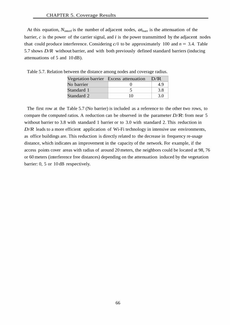
CHAPTER 5. Coverage Results
66
At this equation, Ninterf is the number of adjacent nodes, atbarr is the attenuation of the
barrier, c is the power of the carrier signal, and i is the power transmitted by the adjacent nodes
that could produce interference. Considering c/i to be approximately 100 and n = 3.4. Table
5.7 shows D/R without barrier, and with both previously defined standard barriers (inducing
attenuations of 5 and 10 dB).
Table 5.7. Relation between the distance among nodes and coverage radius.
Vegetation barrier Excess attenuation
(dB)
D/R
No barrier 0 4.9
Standard 1 5 3.8
Standard 2 10 3.0
The first row at the Table 5.7 (No barrier) is included as a reference to the other two rows, to
compare the computed ratios. A reduction can be observed in the parameter D/R: from near 5
without barrier to 3.8 with standard 1 barrier or to 3.0 with standard 2. This reduction in
D/R leads to a more efficient application of Wi-Fi technology in intensive use environments,
as office buildings are. This reduction is directly related to the decrease in frequency re-usage
distance, which indicates an improvement in the capacity of the network. For example, if the
access points cover areas with radius of around 20 meters, the neighbors could be located at 98, 76
or 60 meters (interference free distances) depending on the attenuation induced by the vegetation
barrier: 0, 5 or 10 dB respectively.

CHAPTER 5. Conclusions
67
5.6. Conclusions
A large measurement campaign has been developed in order to analyze the attenuation
induced by vegetation barriers, with different configurations. The measurements were done
taking a LoS reference at exactly the same environment where we get the OLoS data. So, the
path loss exponent would be assumed to be the same in both scenarios and the only difference
between them would be the vegetation barrier induced attenuation between transmitter and
receiver. Thus, the LoS path loss would be cancelled by comparing the LoS reference and each
measurement series, and only attenuation due to the barrier is the result of the comparison.
Attenuations up to 21 dB at 5.8 GHz and up to 10 dB at 2.4 GHz have been detected. These
shadowing capabilities of the vegetation lines are then translating into coverage distance
reduction, which is proposed to be used in the ambit of wireless networks, in two directions: the
reduction of the free interference distance between nodes from adjacent networks, and the
protection against hacker attacks that wirelessly connects to the network from streets or parking
areas.
The results are encouraging because the barriers seem to produce attenuation enough to
reach interesting reductions in the distance to the adjacent nodes, avoiding interference, and
also in the distance at which a hacker must be installed to access a network.
The coverage distances were computed by using three different models, both indoor and
indoor-to-outdoor, and these results indicate that this reduction is more important the larger
the attenuation is. As an example, for 5 dB and 10 dB excess attenuations due to the vegetation
barriers, reductions of distance from 30 to 50% could be achieved, compared to scenarios with
no barriers.
The relation between the distance among nodes D and the coverage radius R has been also
analyzed as a measure on how close nodes from two adjacent networks could be installed when
a line of shrubs is used to separate the coverage areas. The improvement of network efficiency in
presence of vegetation barriers, in terms of the reduction in frequency re-usage distance has
been then computed.
As these barriers are not expensive, environment friendly and well accepted by the people, the
success of the proposal is expected.

CHAPTER 5. Conclusions
68

Chapter 6 Performance of OFDM 64 QAM systems over multipath channels
Some OFDM systems based on IEEE 802.16e with 64 QAM modulation, with ¾ coding rate and
time division duplex (TDD) mode over a 3.5 MHz bandwidth channel have been analyzed. Two
classes of these systems were used: MIMO and multi carrier CDMA (MC-CDMA).
A simulation with different quantity of antennas in transmitter and receiver up to 2x2 over the
AWGN, and the multipath Rayleigh SUI-4, SUI-6 channels and actual indoor channels were done.
The performance of two detectors has been analyzed based on the Alamouti scheme,
distinguished by assuming the same CIR for all receiving antennas from each transmitter antenna or
not. The trade-off between the use of pilots for channel estimation and transmission diversity has
been analyzed for the standard transmitter, achieving a 6 dB gain in SNR for a 10-2
BER. The
influence of the guard time on the BER has been also reviewed, confirming that the BER increases
104 times for a SNR equal to 20 dB when the delay of rays with important amplitudes is larger than
the guard time. A MIMO 64 QAM system is proposed that achieves a BER of only 2% under
Rayleigh channels.
Also the performance of two multi carrier code-division multiple access (MC-CDMA) systems are
also presented. The BER of two systems, MC-CDMA and MC direct sequence CDMA (MC-DS-
CDMA) was computed in a Simulink-based environment over AWGN, SUI-4, SUI-6 and four
actual indoor measured channels, and then compared with the standard performance. A reduction of
100 in BER was found for the same throughput, with 26 dB of Eb/No. The channel estimation and
prediction, as well as the pre-equalization methods are also evaluated for those systems and
channels. The BER dependence with the Doppler frequency deviation is then analyzed for AWGN
channel.

CHAPTER 6. Introduction
70
6.1. Introduction
The extension of high capacity networks are stopped, in most cases, due to the congestion of the
last mile connections. The initial wireless solutions provide mobility to the users, but they do not fit
the high speed requirements of modern communications.
The OFDM is one of the technologies that are trying to satisfy the demand of high capacity
wireless last mile connectivity. The most important systems that use OFDM are WIMAX (IEEE
Comp. and MW T.& T. Soc., 2004) (IEEE Comp. Soc. ; IEEE MW Theory Tech. Soc., 2006) and
LTE (3GPP RAN Technical Specification Group, 2009), both considered the paradigms of 4G
systems.
They are based on the OFDM scheme proposed in (Chang, 1970), which consists on orthogonal
carriers with spectrum overlapping. The aim is to achieve a technology that can bring a high data
throughput with high spectral efficiency at distances of some kilometers and in almost all the cell
area.
The WIMAX standard specifies the transmitted signal and some quality requirements, but the
receiver is free of specification. So, the quality achieved by systems from different providers
depends on the design of this open receiver. There are many improvements that manufacturers can
carry out in the receiver, and some optional features they can implement in the transmitter and
receiver according to WIMAX standard.
In this work, the performance of some implementations of OFDM systems is studied, analyzing
the BER of the uplink (UL, mobile to base station) considering only one user with two schemes:
MIMO and CDMA, independently. Among all the options included in WIMAX, the system
described in item 8.4.9 was chosen. The practical implementation is described in section 6.9. The
simulations were conducted over seven different radio channels: single path AWGN, multiple paths
with Rayleigh probability density function SUI-4, SUI-6 (Erceg, Hari, & Smith, 2001), and four
measured actual indoor channels (I. Cuiñas, 2001).
All the possible combinations were simulated to analyze MIMO: single input-single output
(SISO), single input-multiple output (SIMO), multiple input-single output (MISO) and MIMO
implementations with Simulink-Matlab® software. The BER of two MIMO receivers are
compared: the Alamouti receiver, which assumes the same CIR between one transmitter antenna
and the receiving antennas, and the algebraic receiver that supposes the different CIRs between
each transmit antenna and all receiving antennas.
Some strategies to reduce the BER for the same SNR with a CDMA layer are also analyzed and
simulated. The usage of CDMA technology for medium access leads to an increase of the system
diversity spreading the information bits in time and or frequency. This usage introduces advantages
and disadvantages, so in this work this system is simulated to know if it really outperforms or not
compared with the standard. One of the advantages is the reduction of the interference between
cells, so the frequency reuse could be widely implemented. The disadvantages of the CDMA are
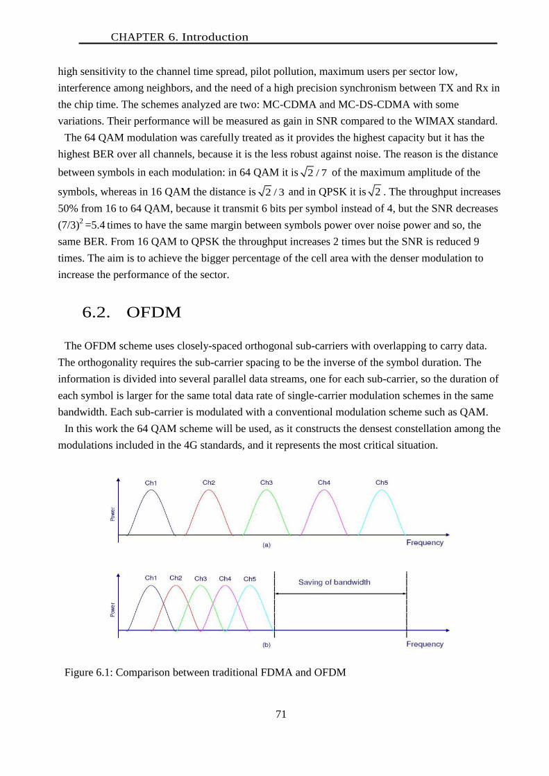
CHAPTER 6. Introduction
71
high sensitivity to the channel time spread, pilot pollution, maximum users per sector low,
interference among neighbors, and the need of a high precision synchronism between TX and Rx in
the chip time. The schemes analyzed are two: MC-CDMA and MC-DS-CDMA with some
variations. Their performance will be measured as gain in SNR compared to the WIMAX standard.
The 64 QAM modulation was carefully treated as it provides the highest capacity but it has the
highest BER over all channels, because it is the less robust against noise. The reason is the distance
between symbols in each modulation: in 64 QAM it is 2 / 7 of the maximum amplitude of the
symbols, whereas in 16 QAM the distance is 2 / 3 and in QPSK it is 2 . The throughput increases
50% from 16 to 64 QAM, because it transmit 6 bits per symbol instead of 4, but the SNR decreases
(7/3)2
=5.4 times to have the same margin between symbols power over noise power and so, the
same BER. From 16 QAM to QPSK the throughput increases 2 times but the SNR is reduced 9
times. The aim is to achieve the bigger percentage of the cell area with the denser modulation to
increase the performance of the sector.
6.2. OFDM
The OFDM scheme uses closely-spaced orthogonal sub-carriers with overlapping to carry data.
The orthogonality requires the sub-carrier spacing to be the inverse of the symbol duration. The
information is divided into several parallel data streams, one for each sub-carrier, so the duration of
each symbol is larger for the same total data rate of single-carrier modulation schemes in the same
bandwidth. Each sub-carrier is modulated with a conventional modulation scheme such as QAM.
In this work the 64 QAM scheme will be used, as it constructs the densest constellation among the
modulations included in the 4G standards, and it represents the most critical situation.
Figure 6.1: Comparison between traditional FDMA and OFDM
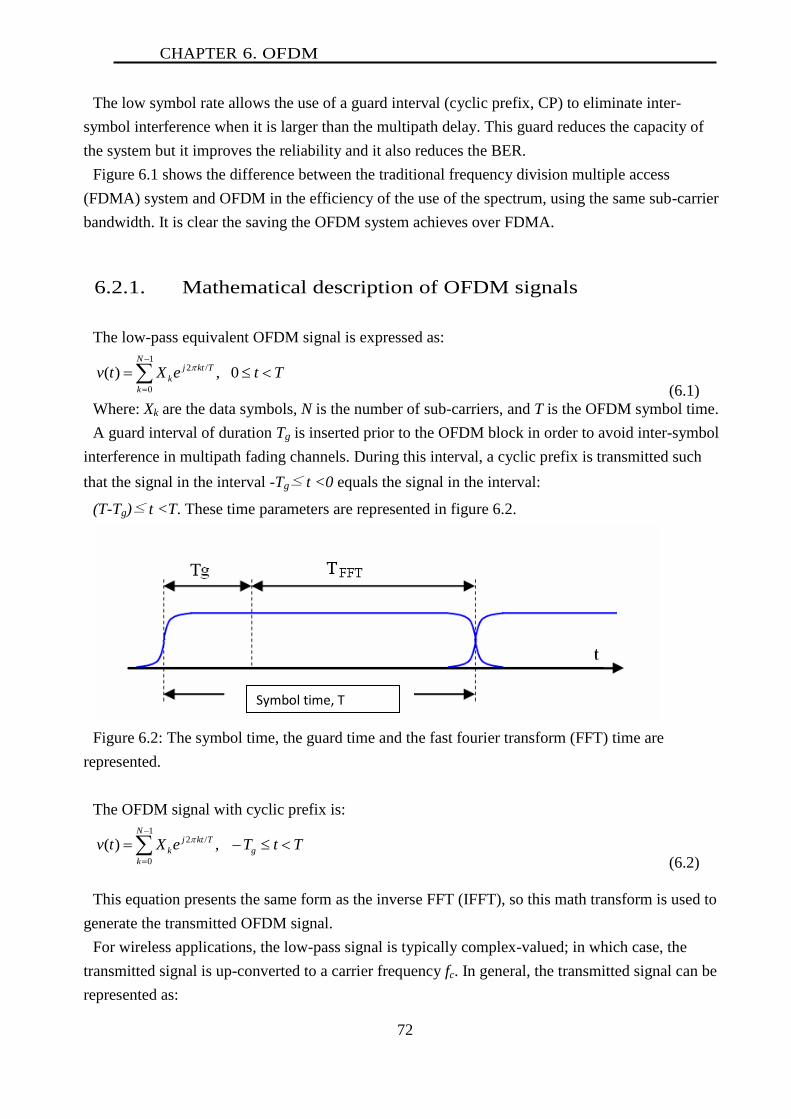
CHAPTER 6. OFDM
72
The low symbol rate allows the use of a guard interval (cyclic prefix, CP) to eliminate inter-
symbol interference when it is larger than the multipath delay. This guard reduces the capacity of
the system but it improves the reliability and it also reduces the BER.
Figure 6.1 shows the difference between the traditional frequency division multiple access
(FDMA) system and OFDM in the efficiency of the use of the spectrum, using the same sub-carrier
bandwidth. It is clear the saving the OFDM system achieves over FDMA.
6.2.1. Mathematical description of OFDM signals
The low-pass equivalent OFDM signal is expressed as:
12 /
0
( ) , 0N
j kt T
k
k
v t X e t T
(6.1)
Where: Xk are the data symbols, N is the number of sub-carriers, and T is the OFDM symbol time.
A guard interval of duration Tg is inserted prior to the OFDM block in order to avoid inter-symbol
interference in multipath fading channels. During this interval, a cyclic prefix is transmitted such
that the signal in the interval -Tg≤ t <0 equals the signal in the interval:
(T-Tg)≤ t <T. These time parameters are represented in figure 6.2.
Figure 6.2: The symbol time, the guard time and the fast fourier transform (FFT) time are
represented.
The OFDM signal with cyclic prefix is:
12 /
0
( ) , N
j kt T
k g
k
v t X e T t T
(6.2)
This equation presents the same form as the inverse FFT (IFFT), so this math transform is used to
generate the transmitted OFDM signal.
For wireless applications, the low-pass signal is typically complex-valued; in which case, the
transmitted signal is up-converted to a carrier frequency fc. In general, the transmitted signal can be
represented as:
Symbol time, T

CHAPTER 6. OFDM
73
1
2
0
1( ) ( ) cos 2 / arg
2c
Nj f t
k c k
k
s t v t e X f k T t X
(6.3)
Figure 6.3: A 3D representation of the OFDM symbols with the sub-carriers and time-slots.
Figure 6.3 represents in time and frequency the OFDM signal of equation 6.3. In this figure can be
seen the sub-carriers in the frequency domain and the symbols with it guard time in the time
domain.
The flow of bits is divided according the modulation scheme, for example 64 QAM 3/4 uses
groups of 9 bits per 2 symbols, and each sub-carrier transports 1 symbol, so an OFDM symbol of
512 data sub carriers, needs 512x4.5=2304 bits. There is a series to parallel conversion to do that.
This set of sub-carriers are modulated each time slot having some guard times between them.
6.3. MIMO system
MIMO schemes use N antennas in the transmitter (Tx) and M in the receiver (Rx) as shown in
figure 6.4. This creates NxM channels between the transmitter and the receiver that can be used for
diversity and/or capacity, with a tradeoff analyzed in (Zheng & Tse, 2003). In this work it will be
used for diversity looking for improving the behavior in the 64 QAM modulation scheme in order to
obtain the minimum BER.
The diversity gain is showed in the figure 6.5, for the best signal selection, where the detected
signal has not the deep fading found in one receiving antenna solution. This is not the only solution
to obtain a signal between multiple receiving antennas, but this is an example how this array
improves the received signal avoiding deep fading.

CHAPTER 6. MIMO System
74
Figure 6.4: MIMO scheme with N Transmitter antennas and M Receiving antennas
If the noise is constant, the SNR increases because of the increase in the signal. Using the Shannon
formula, the capacity of the channel is also increased C=B.log(1+SNR).
If M is greater than one, there is reception diversity. In this case a decoding is needed to achieve
the best result selecting or combining the received signals.
Figure 6.5: The result of diversity by selection of the best signal between two signals affected by
fading.
The diversity implementation applied to all MIMO systems in this thesis is Maximum Ratio
Combining (MRC), because the SNR of the selection combining (SC) is (
) and the SNR of the MRC is higher being (Kong, 1999). Nr is the
number of channels.
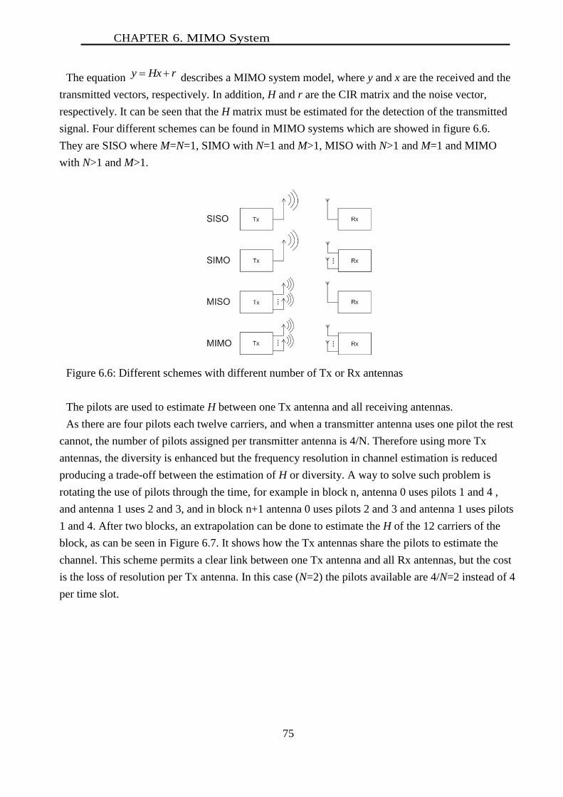
CHAPTER 6. MIMO System
75
The equation y Hx r describes a MIMO system model, where y and x are the received and the
transmitted vectors, respectively. In addition, H and r are the CIR matrix and the noise vector,
respectively. It can be seen that the H matrix must be estimated for the detection of the transmitted
signal. Four different schemes can be found in MIMO systems which are showed in figure 6.6.
They are SISO where M=N=1, SIMO with N=1 and M>1, MISO with N>1 and M=1 and MIMO
with N>1 and M>1.
Figure 6.6: Different schemes with different number of Tx or Rx antennas
The pilots are used to estimate H between one Tx antenna and all receiving antennas.
As there are four pilots each twelve carriers, and when a transmitter antenna uses one pilot the rest
cannot, the number of pilots assigned per transmitter antenna is 4/N. Therefore using more Tx
antennas, the diversity is enhanced but the frequency resolution in channel estimation is reduced
producing a trade-off between the estimation of H or diversity. A way to solve such problem is
rotating the use of pilots through the time, for example in block n, antenna 0 uses pilots 1 and 4 ,
and antenna 1 uses 2 and 3, and in block n+1 antenna 0 uses pilots 2 and 3 and antenna 1 uses pilots
1 and 4. After two blocks, an extrapolation can be done to estimate the H of the 12 carriers of the
block, as can be seen in Figure 6.7. It shows how the Tx antennas share the pilots to estimate the
channel. This scheme permits a clear link between one Tx antenna and all Rx antennas, but the cost
is the loss of resolution per Tx antenna. In this case (N=2) the pilots available are 4/N=2 instead of 4
per time slot.

CHAPTER 6. MIMO System
76
Figure 6.7: Scheme of pilots and carriers in a tile with two Tx antennas in one time slot.
6.4. CDMA System
The system analyzed in this item consists on a CDMA Transmitter in series with an OFDM
transmitter, presented in (N. Yee, 1993), and the same occurs in the receiver but with the inverse
order. There are many options to implement a MC-CDMA over the IEEE 802.16e system,
depending on how the chips are distributed over the standard sub-carriers structure. The Walsh
orthogonal codes will be used for coding in the CDMA systems, avoiding the Pseudo Random
Binary Sequence (PRBS) because the randomization destroys the orthogonality as seen in figure
6.8. With these conditions, a frequency spreading is implemented. This spreading occurs when each
chip of a bit is mapped in a different sub-carrier.
Figure 6.8: Coding with CDMA code
The throughput of each sub-carrier is the same to the input flow before the coding, because it
transports the traffic of SF users with SF chips of the code. Each bit is expanded in SF bits by the
code, but as SF users can be transmitted in the same carrier without problem, the total traffic of the
Antenna 0 Antenna 1
Used pilot Non used
time
frequency
ts1
ts2
ts3
fn fn+1 fn+2 fn+3 fn fn+1 fn+2 fn+3
h11 h11
h34 h34 h31
h14 h14
h31
h14 h14
h14 h14 h14 h14
h14 h14
h14 h14
h14 h14 h14 h14
h14 h14
carrier
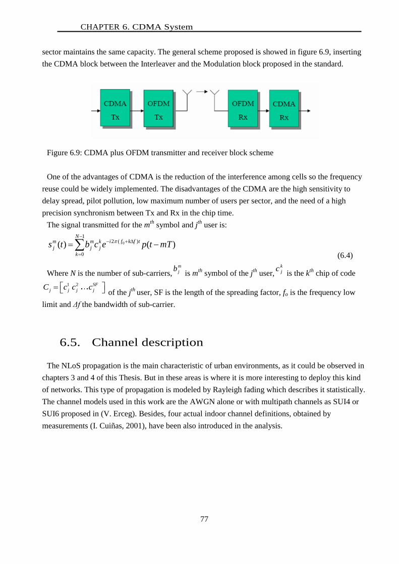
CHAPTER 6. CDMA System
77
sector maintains the same capacity. The general scheme proposed is showed in figure 6.9, inserting
the CDMA block between the Interleaver and the Modulation block proposed in the standard.
Figure 6.9: CDMA plus OFDM transmitter and receiver block scheme
One of the advantages of CDMA is the reduction of the interference among cells so the frequency
reuse could be widely implemented. The disadvantages of the CDMA are the high sensitivity to
delay spread, pilot pollution, low maximum number of users per sector, and the need of a high
precision synchronism between Tx and Rx in the chip time.
The signal transmitted for the mth
symbol and jth
user is:
1
0
)(2)()( 0
N
k
tfkfik
j
m
j
m
j mTtpecbts
(6.4)
Where N is the number of sub-carriers,m
jb is m
th symbol of the j
th user,
k
jc is the k
th chip of code
1 2 SF
j j j jC c c c of the jth
user, SF is the length of the spreading factor, fo is the frequency low
limit and Δf the bandwidth of sub-carrier.
6.5. Channel description
The NLoS propagation is the main characteristic of urban environments, as it could be observed in
chapters 3 and 4 of this Thesis. But in these areas is where it is more interesting to deploy this kind
of networks. This type of propagation is modeled by Rayleigh fading which describes it statistically.
The channel models used in this work are the AWGN alone or with multipath channels as SUI4 or
SUI6 proposed in (V. Erceg). Besides, four actual indoor channel definitions, obtained by
measurements (I. Cuiñas, 2001), have been also introduced in the analysis.
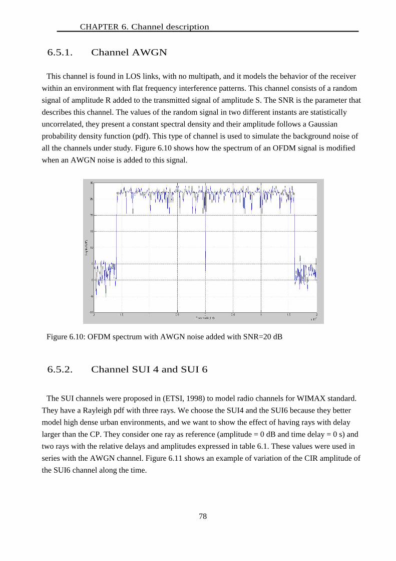
CHAPTER 6. Channel description
78
6.5.1. Channel AWGN
This channel is found in LOS links, with no multipath, and it models the behavior of the receiver
within an environment with flat frequency interference patterns. This channel consists of a random
signal of amplitude R added to the transmitted signal of amplitude S. The SNR is the parameter that
describes this channel. The values of the random signal in two different instants are statistically
uncorrelated, they present a constant spectral density and their amplitude follows a Gaussian
probability density function (pdf). This type of channel is used to simulate the background noise of
all the channels under study. Figure 6.10 shows how the spectrum of an OFDM signal is modified
when an AWGN noise is added to this signal.
Figure 6.10: OFDM spectrum with AWGN noise added with SNR=20 dB
6.5.2. Channel SUI 4 and SUI 6
The SUI channels were proposed in (ETSI, 1998) to model radio channels for WIMAX standard.
They have a Rayleigh pdf with three rays. We choose the SUI4 and the SUI6 because they better
model high dense urban environments, and we want to show the effect of having rays with delay
larger than the CP. They consider one ray as reference (amplitude = 0 dB and time delay = 0 s) and
two rays with the relative delays and amplitudes expressed in table 6.1. These values were used in
series with the AWGN channel. Figure 6.11 shows an example of variation of the CIR amplitude of
the SUI6 channel along the time.
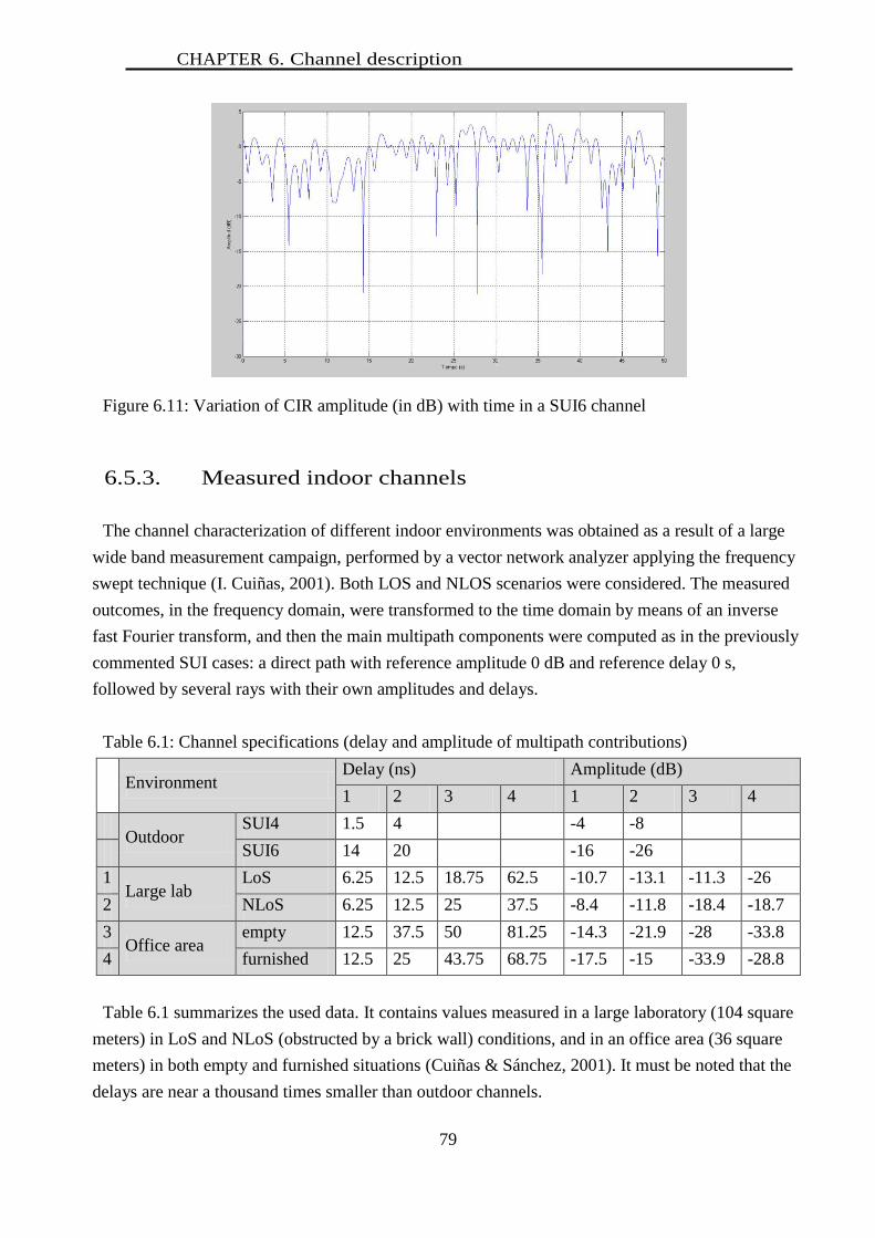
CHAPTER 6. Channel description
79
Figure 6.11: Variation of CIR amplitude (in dB) with time in a SUI6 channel
6.5.3. Measured indoor channels
The channel characterization of different indoor environments was obtained as a result of a large
wide band measurement campaign, performed by a vector network analyzer applying the frequency
swept technique (I. Cuiñas, 2001). Both LOS and NLOS scenarios were considered. The measured
outcomes, in the frequency domain, were transformed to the time domain by means of an inverse
fast Fourier transform, and then the main multipath components were computed as in the previously
commented SUI cases: a direct path with reference amplitude 0 dB and reference delay 0 s,
followed by several rays with their own amplitudes and delays.
Table 6.1: Channel specifications (delay and amplitude of multipath contributions)
Environment Delay (ns) Amplitude (dB)
1 2 3 4 1 2 3 4
Outdoor
SUI4 1.5 4 -4 -8
SUI6 14 20 -16 -26
1 Large lab
LoS 6.25 12.5 18.75 62.5 -10.7 -13.1 -11.3 -26
2 NLoS 6.25 12.5 25 37.5 -8.4 -11.8 -18.4 -18.7
3 Office area
empty 12.5 37.5 50 81.25 -14.3 -21.9 -28 -33.8
4 furnished 12.5 25 43.75 68.75 -17.5 -15 -33.9 -28.8
Table 6.1 summarizes the used data. It contains values measured in a large laboratory (104 square
meters) in LoS and NLoS (obstructed by a brick wall) conditions, and in an office area (36 square
meters) in both empty and furnished situations (Cuiñas & Sánchez, 2001). It must be noted that the
delays are near a thousand times smaller than outdoor channels.
CHAPTER 6. Channel estimation
80
6.6. Channel Estimation
The channel estimation is done to recover as closely the transmitted signal. Two different
strategies will be implemented depending if the system is MIMO or CDMA.
6.6.1. Channel Estimation in MIMO systems
In MIMO systems the channel estimation is needed to estimate the transmitted signal and for the
Alamouti detection. This estimation is done using the pilots (xy = (1,1), (3,1), (1,4) and (3,4)) of the
tile as shown in Figure 6.7. To estimate the channel response hxy for the data carriers a time and a
frequency interpolation will be done. The channel estimation is done per pilot, using a known signal
transmitted txy, and the CIR hxy is calculated by the following equation having the received signal
rxy.
xy
xy
xy
rh
t
(6.5)
Where rxy is the received pilot and txy is the transmitted pilot.
The CIR of the sub-carriers is estimated using the CIR of the pilots. In this work the CIR for the
data sub-carriers (1,2), (1,3), (3,2) and (3,3) are derived by extrapolating linearly in frequency at the
same time, from the CIR of the pilots using equation 6.6.
4 1 1
1
3xy x x x
yh h h h
(6.6)
The equation 6.7 is used to extrapolate the CIR for sub-carriers h2y (y=1..4).
2 1 3
1
2y y yh h h
(6.7)
Once the channel estimations were done, the zero-forcing equalization is made to cancel the
channel distortion with:
,,
,
ij
ij
ij
r s nt s n
h s n
(6.8)
Where n is the number of the tile and s the sub-channel.
6.6.2. Channel Estimation on CDMA
The channel estimation would be useful to define the equalization needed to compensate the
distortion produced by the channel. This technique could reduce the BER at low values of SNR in
multipath environments. So, it is investigated integrated with these systems. An estimation of the
CIR during uplink (UL) transmission, HUL, can be obtained using equation 6.9.
CHAPTER 6. Channel estimation
81
knnknHknsknx UL
m
mULmULUL ,,,, ,,
(6.9)
Where xUL[n,k] is the signal coming from all the MS and received by the BS during the nth
OFDM
symbol time over the kth
sub-carrier, sUL,m[n,k]=dUL,m cUL,m(j), being dUL,m the original transmitted
signal by mth
MS, cUL,m(j) the jth
chip of the spreading code assigned to the mth
user, HUL,m[n,k] the
channel response in UL, and nUL[n,k] the AWGN noise term.
The transmission made by the MS number µ, may be extracted in the receiver as shown in
equation 6.10.
SF
j
ULUL
m
m
SF
j
mULmULULmUL
SF
j
UL
ULUL jcjnjHjcjcdSF
jHdd
1
*
,
1
,,
*
,,
1
,
,,ˆ
(6.10)
The code is represented by cUL,µ[j]. Once the received signal is multiplied by the code to isolate
the original data using a matched filter, dUL,µ is the estimated data. The first term corresponds to the
desired signal attenuated by a channel defined factor. The second one shows the interference due to
other users or multi user interference (MUI) under non ideal channels, and it is one of the major
problems in any actual CDMA system. It should be 0, but for imperfections it is near 0. The third
one corresponds to the filtered noise.
The channel estimation is not feasible at the receiver in the BS because the signals from the MSs
are already mixed up in CDMA schemes because more than one MS will share the same sub-
carrier, making the pilot sub-carriers unsuited for its objective (at least partially as we will see) and
the received data will be scrambled. The CIR during downlink (DL) transmission, HDL, could be
estimated at several times in order to obtain the HUL estimation by MS’s. Then, we could made use
of the reciprocity principle because it is a TDD system, which uses the same frequency for UL and
DL, to approximate HUL by HDL (HUL ≈ HDL). The predicted HUL may be used for pre-equalizing the
signals in an attempt to maintain the orthogonality of the codes at the receiver, and gets a signal as
close to the transmitted reducing the MUI that it is the second term of equation 6.10.
As this work is focused in the uplink, a straight and nonstandard method is used for HDL
estimation and it is assumed that a more compliant one should be implemented in future works. It
consists of transmitting successive training sequences of a single isolated impulse to the MS for
estimation.
During downlink time, the system obtains 12 consecutive HDL estimations corresponding to the
last 12 symbol periods before the uplink time, each having 512 samples (taken in frequency
dimension) as NFFT=512 was used, one per sub-carrier. This data is arranged, for mathematical
analysis, in a 512 x12 matrix, with its rows synchronized with receiver sample time and its columns
to the standard symbol time. As the channel delay spread should be shorter than the OFDM symbol
time, the first samples should only contain AWGN noise.
The data collected in DL time is a time series, so a linear prediction of the channel in UL time will
be used. With twelve samples in DL 6 estimations are derived for UL.
This work will present the results of four prediction techniques (Makhoul, 1975) in figure 6.39,

CHAPTER 6. Channel estimation
82
assuming a wide-sense stationary uncorrelated scattering (WSSUS) model, indicating that the CIR
for a delay l is independent of other delays. The problem of prediction can be expressed as:
0, 1
ˆ1, ,m M
h n l f h n m l
(6.11)
Where n is the number of the last sample, l the number of the tap, and M the number of samples
considered. The error of the prediction is:
1, 1, 1,e n l h n l h n l (6.12)
The linear prediction (Makhoul, 1975)is represented by the following expression:
1
0
ˆ1, 1 . ,Q
l
q
h n l c q h n q l
(6.13)
Where Q is the order of the filter, with Q<M. Each tap that represents a path in the channel is
treated independently and is the parameter l that represents them.
(Hanzo, M.Munster, B.J.Choi, & T.Keller, 2003) found that the autoregressive (AR) model
outperforms the robust coefficients for linear estimation. Therefore, in this Thesis some AR
methods will be compared and the best implemented in the simulator. The coefficients cl are
calculated by least squares and there are different ways to calculate them originating different
methods.
1
0
ˆ1, 1, 1 . ,Q
l
q
e n l h n l c q h n q l
(6.14)
These methods are simple and have good computational efficiency.
Four methods are analyzed to predict the channel in UL time: Burg, Covariance, Modified
Covariance and Yule. Their general objective is to minimize the energy of the error. The
characteristics of each four methods are commented in the following paragraphs.
6.6.2.1. Burg
This is an autoregressive (AR) all-pole model with parameters estimated using Burg method
(Hanzo, M.Munster, B.J.Choi, & T.Keller, 2003). In an AR model of order Q, the current output is
a linear combination of the past Q outputs plus a white noise input. The mean-square prediction
error of the auto regression is minimized by the weights of the Q past outputs.
The reflection coefficients are the partial autocorrelation coefficients scaled by (–1). The reflection
coefficients indicate the time dependence between h[n] and h[n-k] after subtracting the prediction
based on the intervening k-1 time steps. The Burg method estimates the reflection coefficients and
uses these coefficients to estimate the AR coefficients recursively. The recursion and lattice filter
relations describing the update of the forward and backward prediction errors could be found in the
reference.
CHAPTER 6. Channel estimation
83
6.6.2.2. Covariance
The covariance method fits a Qth
order AR model to the input signal, h, which is assumed to be the
output of an AR system driven by white noise (J. R. Deller Jr., 1993) (Leroux & C.Gueguen, 1979).
It chooses the short term filter coefficients cl called linear prediction (LP coefficients) in such a way
that the residual energy (the energy in the error signal) is minimized. The classical least square
technique is used for that purpose only in windows of Q elements.
The covariance method windows the error signal instead of the original speech signal.
The resulting matrix equation is not Toeplitz, but it is symmetric and positive defined. The
decomposition method is generally used for solving the covariance equations.
6.6.2.3. Modified Covariance
A linear predictor presented in (Semmelrodt & Kattenbach, 2003) is used to extrapolate the
behavior of the process beyond the available channel samples. The time-variant wireless channel is
modeled as an AR process of order Q with time-variant coefficients. The Modified Covariance
(Mod. Cov.) prediction algorithm uses the least squares method to solve the linear equations system
for computing the model coefficients. This linear predictor allows only a single signal sample to be
predicted at a time.
6.6.2.4. Yule
This is an AR model of order Q, so the current output is a linear combination of the past Q outputs
plus a white noise input. The mean-square prediction error of the auto regression is minimized by
the weights on the Q past outputs. At first, the signal is multiplied by a window to get a windowed
signal segment, because the signal is considered 0 outside the window for the autocorrelation. As
the autocorrelation matrix is Toeplitz, where all elements along a given diagonal are equal, the
recursive method of Levinson-Durbin can be used to find the coefficients (Golub & Loan, 1989) or
even the Schur algorithm (Leroux & C.Gueguen, 1979). The synthesis filter is stable due to the
Toeplitz structure.
6.7. Pre-equalization for CDMA
As mentioned before, the channel-correction strategy proposed in this work is based mainly in an
equalization mechanism. It would be capable of mitigate each user and each sub-carrier channel
distortions by restoring the signal orthogonality and also to achieve a relatively flat spectrum signal
at the reception, by redistribution of the signal strength. We propose to implement a pre-
equalization scheme in the MSs aiming to correct the distortion produced by the Rayleigh fading
channel. Additionally, we introduce an amplitude attenuation correction scheme based in an

CHAPTER 6.Pre-equalization for CDMA
84
alternative use of the pilots already defined in the standard. Therefore, modifying the relative
weight of each sub-carrier will produce a redistribution of the transmitted energy, without an
increase of the transmitted power. We could express the transmitted signal, before the IFFT
operation and the cyclic prefix (CP) addition, by:
*
j j j js G C d (6.15)
where sj is the data of the j user, dj the data transmitted, Gj the pre-equalization vector and Cj is the
spreading code. The operator ‘º’ denotes element-wise product, and ‘*’ the complex conjugate
operation. Similarly, we can represent the received signal r, after the FFT operation and CP
removal, by the following expression:
1 *
1
,..,SF
TSF
j j j j
j
r r r H G C d n
(6.16)
where now Hj represents the channel coefficients in frequency domain for jth
user .
Finally, given a user j, the detected signal ˆ
jd at the receiver will be the received signal r
multiplied by the code corresponding to the user j, CjH:
*
1
ˆSF
H H H
j j j j j j j j
j
d C r C H G C d C n
(6.17)
Defining nj=CjH.n and Vj,k=Cj*◦Hj◦Cj, we can reorganize the equation 6.17 obtaining three well
differentiated terms in the detected signal:
,ˆ
j
SFH H
j j j j j j k j j
k jD
MUI
d G H d G V d n
(6.18)
We can clearly identify a wanted-signal term Dj, the MUI term that is generated by the remaining
users sharing the channel, and the AWGN nj contribution due to limitations at the receiver. The idea
is to implement a method that minimizes the MUI and the nj terms, in order to maximize the SINR.
But the optimum solution needs that each MS knows the CIRs Hj corresponding to all other MS
within the same sector. A sub-optimal, but efficient, solution is proposed in (D. Mottier, 2002)
which proposes maximize the m-SINR quotients presented in equation 6.19.
2
,
/
mk
MAI
mD
m
kmP
PSINRm
(6.19)
Where PD,m is the detected signal corresponding to the m user, PMAI(m/k) is the interference power
of the k user over m user, and σ2 is the noise.
The expression for the pre-equalization coefficients is given by equation 6.20 (Cosovic, Schnell,
& Springer, 2003).

CHAPTER 6.Pre-equalization for CDMA
85
2
2)(
)(2
2)(
)()(
1
1
l
m
l
ml
m
l
ml
m
HSF
H
SF
HSF
HG
(6.20)
Where Hm(l)
is the CIR of the l chip of the user m, and SF is the spreading factor.
The prediction algorithm, implemented in the proposed systems built on CDMA, is based in an
adaptive linear prediction using a fourth order filter, whose coefficients are calculated by covariance
method, from 12 estimates made at the downlink stage.
6.8. Alamouti coding for MIMO
A scheme implemented as a Space Frequency block coding based in Alamouti must be used to
obtain the benefits of MIMO idea: the diversity gain. This strategy was initially proposed in
(Alamouti, 1998) with a space–time (ST) block code of rate 1 symbol per channel. The transmitted
block code is represented as follows:
1 2
2 * *
2 1
s sC
s s
(6.21)
where the rows are along the spatial dimension (different Tx antennas) and the columns are along
the frequency dimension (different sub-carriers). In this example the four symbols are transmitted
during the first time slot of the tile.
In this case it is assumed h0
12= h013= h
014 = 0
1h and h1
12= h113= h
111= h
11. This results in spatial and
frequency diversity. Each Rx antenna receives the following signals:
0 1 *
1 1 1 1 1 2( )r r f h s h s (6.22)
0 1 *
2 2 1 2 1 1( )r r f h s h s (6.23)
Where h1x is the CIR between Tx antenna x (for all sub carriers) and one receiver on the time slot
1, estimated through the pilots.
The received tile, three time slots and four sub-carriers, is the represented by the table 6.2.
Table 6.2 Received tile by MIMO system with 2 Tx antennas .
Sub-carrier 1 Sub-carrier 2 Sub-carrier 3 Sub-carrier 4
Time slot 1 P1h
111 s1h
012 -s2
∗h1
12 s1h013 +s2
∗h1
13 P0h
014
Time slot 2 s3h021 -s4
∗h1
21 s4 h022 +s3
∗ h122 s5 h
023 -s6
∗ h1
23 s6 h024 +s5
∗ h124
Time slot 3 P0h
031 s7h
032 -s8
∗h1
32 s8h033 +s7
∗h1
33 P1h
134
The Px is the pilot transmit power at antenna x. For the symbols s3 to s8 analogs equations of 6.22
and 6.23 are used for it calculus.
CHAPTER 6.Alamouti coding for MIMO
86
6.8.1. Classical Alamouti detection
The CIR estimation is needed to decode the Alamouti coding, because the decoding is based in
equations 6.24 and 6.25, where the hx is supposed to be known.
*0 1 *
1 1 2s h r h r (6.24)
*0 1 *
2 2 1s h r h r (6.25)
where ŝi is the estimation of the transmitted symbol si. It should be pointed out that the channel
coefficients of the two sub-carriers for each Tx-Rx antenna pair are assumed to be equal at
equations 6.22 to 6.25. In this case the MIMO is used for frequency and space diversity, not for
multiplexing or throughput gain.
6.8.2. Algebraic detection
This scheme considers that each carrier of the tile has its own CIR. As the conjugate symbols are
sent over different frequencies, they are affected by different channels. The nomenclature is: hxyz,
corresponds to the CIR of the x Tx antenna, at y time slot and over the z sub-carrier.
The received symbol by each receiving antenna is described by:
0 1 *
1 1 12 1 12 2( )r r f h s h s (6.26)
0 1 *
2 2 13 2 13 1( )r r f h s h s (6.27)
The difference between the receivers antennas are the hxyz calculated with equations 6.26 and 6.27.
In this work, the following equations are proposed for the estimation of transmitted symbols:
0* 1 *
13 1 12 21 0 0* 1 *1
12 13 12 13
h r h rs
h h h h
(6.28)
0* 1 *
12 2 13 12 0 0* 1 0*
13 12 13 12
h r h rs
h h h h
(6.29)
The other symbols are calculated similarly. After the detection, the demodulation of the symbols
of the OFDMA is identical to a SISO system.
6.9. Implementation
The implementation is based in the IEEE802.16e or WIMAX standard which has four physical
layer options proposed in the standard. In this work, the system called WirelessMAN-OFDMA
PHY layer, specified in section 8.4.9 (IEEE Comp. and MW T.& T. Soc., 2004) (IEEE Comp. Soc.
; IEEE MW Theory Tech. Soc., 2006), has been simulated. As mentioned in the standard, this
physical layer is designed for NLOS operation in the frequency bands below 11 GHz. Channel
coding procedures include randomization (8.4.9.1), FEC encoding (8.4.9.2) bit interleaving (8.4.9.3)
and modulation (8.4.9.4). The basic block shall pass the regular coding chain where the first sub-

CHAPTER 6. Implementation
87
channel shall set the randomization seed used in 8.4.9.1, and the data shall follow the coding chain
up to the mapping. The data outputted from the modulation (8.4.9.4) shall be mapped onto the block
of sub-channels allocated for the basic block and then it will be also mapped on the following
consecutive allocated sub-channels. Figure 6.12 shows the blocks of the transmitter and the receiver
channel coding.
Figure 6.12: The transmitter and the receiver common block diagram of IEEE 802.16e system
with two antennas
6.9.1. Common parameters
There are many options inside section 8.4.9 but we choose the 512-FFT OFDMA uplink sub-
carrier allocations for PUSC defined by table 313-b (IEEE Comp. Soc. ; IEEE MW Theory Tech.
Soc., 2006), with the followings parameters:
Number of sub-channels, 17
Carrier frequency (fc), 3.5 GHz
Data duration (T), 128µs
Sampling factor (n)=8/7
Guard time (Tg)= 1/8Tb = 16 µs (from table 213 of (IEEE Comp. and MW T.& T. Soc., 2004))
Total symbol time (T+Tg), 144 µs
Sampling frequency (fs)=4 MHz
Sub carrier bandwidth (Δf)= 7.8125 kHz (from 8.3.2.2 of (IEEE Comp. and MW T.& T. Soc.,
2004))
Data to
transmit
to PHY
Randomizer
8.4.9.1
FEC
8.4.9.2
Antenna
1
Bit-
interleaver
8.4.9.3
Modulation
8.4.9.4
Add cyclic
prefix
Antenna
0
demodulation
FFT
Remove
cyclic
prefix Antenna
1
MRC
Antenna
0 Carrier selection
and
de- randomization
Channel
equalization
QAM64 to
Bit
conversion
Data to transmit
to layer 2
Transmitter
Receiver

CHAPTER 6. Implementation
88
Number of sub-carriers, 512
Channel bandwidth, 3.5 MHz.
The block diagram of the PHY layer is showed in Figure 6.12.
The blocks are specified in section 8.4.9 (IEEE Comp. Soc. ; IEEE MW Theory Tech. Soc., 2006)
from item 1 to item 4. The profile used is the defined in table 415 which recommends a receiver
power of -72 dBm for a BER=10-6
with a SNR=20 dB (table 338). The modulation scheme is
64QAM ¾ as 8.4.9.4 of the standard. The frame structure is presented in section 8.4.4.2, figure 218
of the reference. The forward error correction (FEC) block is encoded by a binary convolutional
encoder defined in 8.4.9.2.1 (IEEE Comp. and MW T.& T. Soc., 2004) for a ¾ code rate where
also the frame duration chosen was 5 ms as defined in table 274. When there is transmission
diversity (MIMO), the Alamouti coding is used.
The data mapping on the sub-carriers is done by the equation 114 of the standard which is the
6.3030 equation here.
( ) ( ) (6.30)
Where n is the index of the data from 0 to 47, s is the number of the sub-channel, Sub-carrier (n,s)
is the sub-carrier assigned to transport the data n on the sub-channel s. Nsub-carriers is the number of
sub-carriers per slot.
6.9.2. Transceiver
Two different transceivers were implemented, one for MIMO and other for CDMA simulation.
Both are described in the following sections.
6.9.2.1. MIMO Transmitter - Receiver
The detection is done before the maximum ratio combining (MRC) in MIMO systems with
Alamouti coding. This diversity technique is used to maximize the signal strength inside the
receiver with more than one antenna. Such a technique would allow the receiver to take advantage
of the multi-antenna installation. After the detection, the signal powers are measured separately; and
then, a weighted sum is done, with more weight for the stronger root mean square (RMS) signal.
The resulted signal presents more amplitude than any of the original ones. Then, this signal is
processed as in a SISO receiver. The MRC was implemented in all SIMO and MIMO systems.
After this process, the cyclic prefix is removed and the FFT is calculated to demodulate the signal.
Immediately the next block proceeds to remove the carriers that bring no information. Next, the
carrier de-randomizer block arranges the carriers in the order of the bits stream. The channel
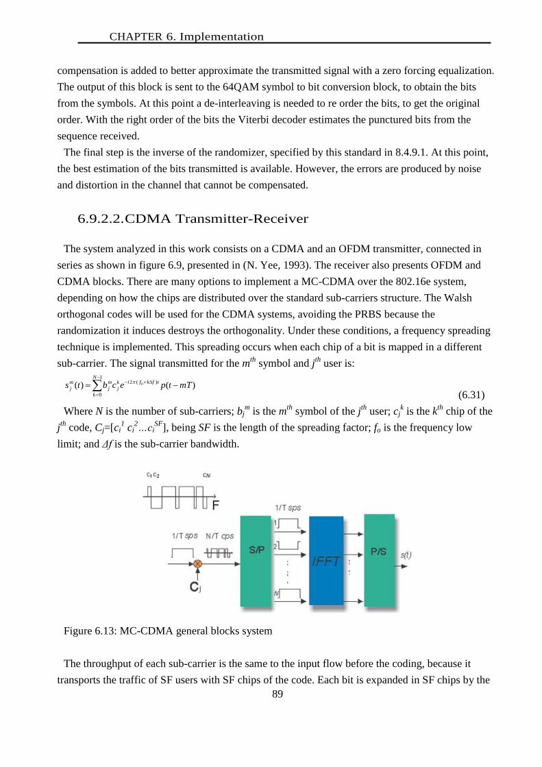
CHAPTER 6. Implementation
89
compensation is added to better approximate the transmitted signal with a zero forcing equalization.
The output of this block is sent to the 64QAM symbol to bit conversion block, to obtain the bits
from the symbols. At this point a de-interleaving is needed to re order the bits, to get the original
order. With the right order of the bits the Viterbi decoder estimates the punctured bits from the
sequence received.
The final step is the inverse of the randomizer, specified by this standard in 8.4.9.1. At this point,
the best estimation of the bits transmitted is available. However, the errors are produced by noise
and distortion in the channel that cannot be compensated.
6.9.2.2. CDMA Transmitter-Receiver
The system analyzed in this work consists on a CDMA and an OFDM transmitter, connected in
series as shown in figure 6.9, presented in (N. Yee, 1993). The receiver also presents OFDM and
CDMA blocks. There are many options to implement a MC-CDMA over the 802.16e system,
depending on how the chips are distributed over the standard sub-carriers structure. The Walsh
orthogonal codes will be used for the CDMA systems, avoiding the PRBS because the
randomization it induces destroys the orthogonality. Under these conditions, a frequency spreading
technique is implemented. This spreading occurs when each chip of a bit is mapped in a different
sub-carrier. The signal transmitted for the mth
symbol and jth
user is:
1
0
)(2)()( 0
N
k
tfkfik
j
m
j
m
j mTtpecbts
(6.31)
Where N is the number of sub-carriers; bjm is the m
th symbol of the j
th user; cj
k is the k
th chip of the
jth
code, Cj=[ci1 ci
2…ci
SF], being SF is the length of the spreading factor; fo is the frequency low
limit; and Δf is the sub-carrier bandwidth.
Figure 6.13: MC-CDMA general blocks system
The throughput of each sub-carrier is the same to the input flow before the coding, because it
transports the traffic of SF users with SF chips of the code. Each bit is expanded in SF chips by the

CHAPTER 6. Implementation
90
code, but as SF users can be transmitting in the same carrier without problem, the total traffic of the
sector maintains the same capacity.
Figure 6.13 shows the blocks and signals in this type of system. The source bits, c1-cn, are
multiplied by the code cj, and then it passes through a serial to parallel system. At its output, the
signals of each chip have the period Tsps equal to the source period. After that, the IFFT plus the
parallel to serial block produce the OFDM signal to feed the up converter.
Some set of SF sub-carriers are defined inside the slot, called partition Pk(f), where a QAM
symbol of a user is transmitted. If there is one partition per user, the transmitted signal for user j
could be expressed by:
1
SFk k
j j j
k
x f b c P f
(6.32)
where bj is the data to be transmitted in the user partition.
In the shared channel, the signals of the N users of the same sector are mixed and could be
represented by
1 1
N SFk k
j j
j k
y f b c P f
(6.33)
To isolate the pth
user data it must be multiplied by the corresponding code Cp(f), obtaining
p py f y f C f
1 1 1 1 1
SF N SF N SFh h k k k k k
p p j j j p j
h j k j k
y f c P f b c P f b c c P f
(6.34)
At QAM symbol level the last expression can be transformed in:
1 1
N SFk k
p j p j
j k
x b c c
2
1 1 1
SF N SFk k k
p p p j p j
k j kj p
x b c b c c
(6.35)
being the second factor of the first term being the detection gain and the second term the MUI
factor.
6.9.2.2.1. MC-CDMA: “Classic”
The QAM symbol is multiplied by the code of the own user. After that, the chips are allocated in
adjacent sub-carriers of the same OFDMA symbol, so the equation 6.30 is not applied, but the rest
of the standard allocation is executed. It is called classic MC-CDMA, and figure 6.14 shows how
the chips are allocated.
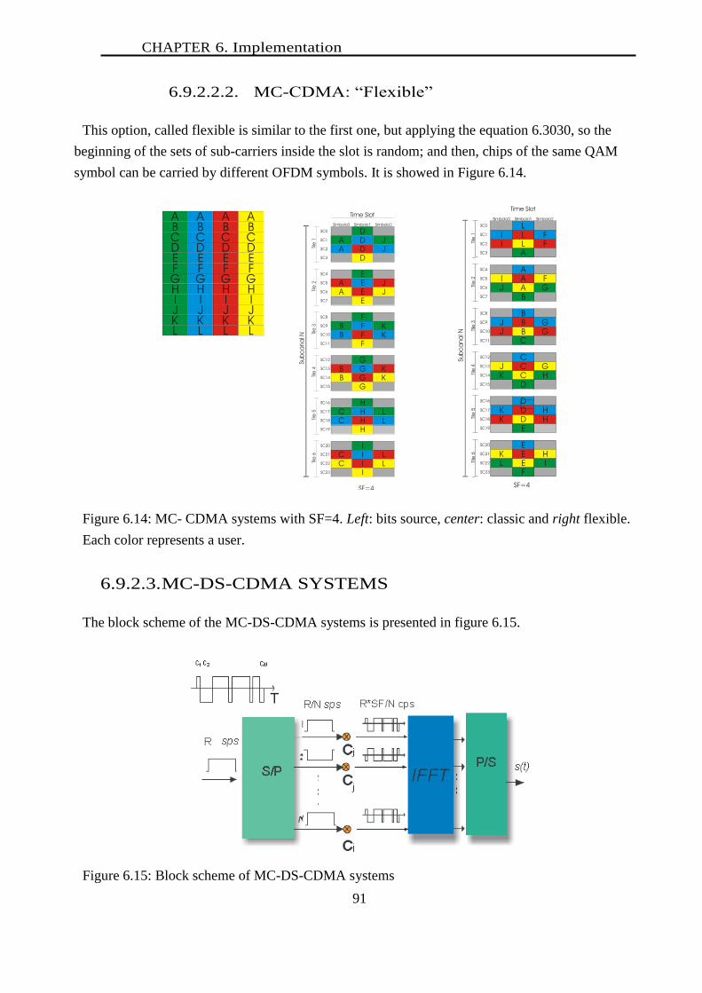
CHAPTER 6. Implementation
91
6.9.2.2.2. MC-CDMA: “Flexible”
This option, called flexible is similar to the first one, but applying the equation 6.3030, so the
beginning of the sets of sub-carriers inside the slot is random; and then, chips of the same QAM
symbol can be carried by different OFDM symbols. It is showed in Figure 6.14.
Figure 6.14: MC- CDMA systems with SF=4. Left: bits source, center: classic and right flexible.
Each color represents a user.
6.9.2.3. MC-DS-CDMA SYSTEMS
The block scheme of the MC-DS-CDMA systems is presented in figure 6.15.
Figure 6.15: Block scheme of MC-DS-CDMA systems

CHAPTER 6. Implementation
92
This system transmits all the chips of a bit in the same sub-carrier in SF OFDMA symbols
(Prasad, 2004). So the system implements time diversity but not frequency diversity as shown in
Figure 6.15. The mth
QAM symbol of the jth
user is:
1
0
1
0
)(2, 0).()(N
g
SF
k
tfgfi
c
k
j
gm
j
m
j ekTmTtpcbts
(6.36)
Being: bjm,g
: the mth
symbol of the jth
user carried by the gth
sub-carrier, T the symbol period and Tc
the chip period (Tc=T/SF).
6.9.2.3.1. MC- DS-CDMA: “Masked”
This system consists on a SF set of sub-carriers, in order to send one chip of a bit per set. SF slots
are needed to transport all the data of a sub-channel. As a sub-channel has 48 places for chips, the
48 bits of a sub-channel are transformed into 48xSF chips, being SF the length of the CDMA code.
During the first time slot, the first 48/SF bits are sent. The equation 6.3030 is applied. Each chip of
a bit will be sent in a different set of sub-carriers achieving frequency and time diversity. Figure
6.16 shows how the chips are allocated.
Figure 6.16: Bit distribution over sub carriers in MC-DS-CDMA “Masked” system
6.9.2.3.2. MC-DS-CDMA: “DS Classic”
In this system, one chip of a bit is transmitted per slot. It is similar to the first option, but with a set
of all 48 sub-carriers. The chips are sent to the OFDM transmitter, SF times for SF time slots to
complete the bit transmission. The equation 6.30 is not applied, but the rest of the allocation scheme
of the standard is implemented as is shown in figure 6.17.
Copier Reshape
Allocation
Mask

CHAPTER 6. Implementation
93
Figure 6.17: Bit distribution over sub carriers in MC-DS-CDMA “DS Classic” system
6.9.2.3.3. MC-DS-CDMA: Third option
It is a variant of the first option where the Equation 6.3030 is applied after the CDMA coder
block. It implies that the number of the first sub-carrier is pseudo-random.
6.10. Simulink Implementation
Simulink® is an environment for multi-domain simulation and Model-Based Design for dynamic
and embedded systems. It provides an interactive graphical environment and a customizable set of
block libraries that allow to design, simulate, implement, and test a variety of time-varying systems,
including communications, controls, signal processing, video processing, and image processing.
Two simulators were developed, based on the WIMAX standard to simulate MIMO and CDMA
systems.
6.10.1. Block scheme of one transmitter and one receiver
Figure 6.18 shows the blocks that simulate the PHY layer of a WIMAX system option 8.4.9.
Basically, the transmitter has the source of bits, after that is the channel encoding, following it the
modulation system and at the end the antenna system. The data outputted by the Transmitter pass
through the channel, which has an AWGN and a Rayleigh block to simulate the multipath. The
receiver starts with the antennas, after that the demodulator and the decoder. To calculate the
performance of the system through the BER a block comparator is introduced, between the data
Simbolo0 Simbolo1 Simbolo2
SC0
SC1
SC2
SC3
Tile
1
Time Slot
SC4
SC5
SC6
SC7
Tile
2
SC8
SC9
SC10
SC11
Tile
3
SC12
SC14
SC15
Tile
4
SC16
SC17
SC18
SC19
Tile
5
SC20
SC21
SC22
SC23
Tile
6
Su
bc
an
alN
Slot 1
Simbolo0 Simbolo1 Simbolo2
SC0
SC1
SC2
SC3
Tile
1
Time Slot
SC4
SC5
SC6
SC7
Tile
2
SC8
SC9
SC10
SC11
Tile
3
SC12
SC14
SC15
Tile
4
SC16
SC17
SC18
SC19
Tile
5
SC20
SC21
SC22
SC23
Tile
6
Su
bc
an
alN
Slot 2
Simbolo0 Simbolo1 Simbolo2
SC0
SC1
SC2
SC3
Tile
1
Time Slot
SC4
SC5
SC6
SC7
Tile
2
SC8
SC9
SC10
SC11
Tile
3
SC12
SC14
SC15
Tile
4
SC16
SC17
SC18
SC19
Tile
5
SC20
SC21
SC22
SC23
Tile
6
Su
bc
an
alN
Slot 3
Simbolo0 Simbolo1 Simbolo2
SC0
SC1
SC2
SC3
Tile
1
Time Slot
SC4
SC5
SC6
SC7
Tile
2
SC8
SC9
SC10
SC11
Tile
3
SC12
SC14
SC15
Tile
4
SC16
SC17
SC18
SC19
Tile
5
SC20
SC21
SC22
SC23
Tile
6
Su
bc
an
alN
Slot 4
J= 4

CHAPTER 6. Simulink Implementation
94
source in the transmitter and the data received in the output of the receiver.
6.10.2. Block scheme of MC-CDMA system
Figure 6.18: CDMA-OFDM scheme block in Simulink
The CDMA-OFDM transmitter showed in figure 6.19 consists on the FEC detailed in the
standard WIMAX and in figure 6.12, a modulator block, the CDMA block detailed in figure 6.13
for MC-CDMA and figure 6.15 for MC-DS-CDMA. This block spread the bit into chips coding as a
CDMA signal. After that, a Data Allocation Block distributes the bits between the sub-carriers.
Then the Tx channel interface modulates the signal through the IFFT and inserts the CP.
Figure 6.19: MC-CDMA transmitter

CHAPTER 6. Simulink Implementation
95
The CDMA-OFDM receiver makes the inverse functions of the TX and in inverse order.
First the channel interface demodulates the signal received by the antenna through the FFT and
removes de CP.
The Rx data allocation subsystem arranges the chips to collect the corresponding chips of the
same bit according its distribution over the sub-carriers. This data is passes to the MC-CDMA to
obtain the bit from the chips multiplying with the corresponding code. This system produces a
QAM symbol that it passes to the demodulator, which retrieves the bits. Then the bits pass through
the blocks in the inverse process of the FEC of the Tx.
Figure 6.20: CDMA-OFDM receiver scheme block.
The Channels block has the Rayleigh process of the Tx signals, the channel estimation, channel
prediction and the pre-equalization process. It transforms time data in frequency response
information.
The main part is showed in figure 6.21.
Figure 6.21 Channel block of MC-CDMA transmitter.

CHAPTER 6. Simulink Implementation
96
6.10.3. Block scheme of MIMO-OFDM simulator
The MIMO–OFDM simulator also implements the blocks of channel coding proposed by the
WIMAX standard. These blocks were implemented with the standard blocks included in Simulink
library.
Figure 6.22: SIMO model in Simulink
As there are 17 sub-channels with 48 QAM symbols each, a total of 816 complex values must be
sent to the transmitter. The frequency response of each sub-carrier is done with the equations 6.6
and 6.7.
When there is reception diversity a MRC block is used to combine the received signals as showed
in figure 6.23.
Figure 6.23: MRC scheme blocks with two receiving antennas.

CHAPTER 6. Simulink Implementation
97
Figure 6.24: Simulink block scheme of MISO system
The transmission diversity is implemented using Alamouti coding and it is implemented with the
blocks showed in figure 6.24. The transmit power per antenna is the half when there is only one
antenna. Another change is that only two pilots is used to transmit per antenna to keep a clear signal
between each transmit antenna and all receiving antennas as showed in figure 6.7.
The MIMO system is implemented with the scheme showed in figure 6.25. The channel is a
matrix of NxM elements, each representing one channel between one Tx antenna with one Rx
antenna. The transmitter implements the Alamouti coding and the receiver includes the MRC block
after the Alamouti detection.

CHAPTER 6. Simulink Implementation
98
Figure 6.25: MIMO system Simulink scheme block
6.11. Results
This section has been organized into two subsections, one focused on MIMO and the other on
CDMA implementations.
6.11.1. MIMO Results
The effect of reducing the number of pilots from 4 to 2 was analyzed through the variation of the
BER as a function of the SNR in figure 6.26. It shows a trade-off between the increase of diversity
and the reduction in estimation capacity, because the standard shares the pilots between the
transmitter antennas. At the figure, we can observe the increment of the BER when the number of
pilots is reduced from four to two, between SISO with 4 pilots and SISO-2P (two pilots), and SIMO
and SIMO-2P with the AWGN channel.
The second comparison of the systems is done over the AWGN channel. The diversity in
transmission (MISO) presents the worst performance due to the reduction of pilots per transmitter
antenna, followed by SISO schemes; whereas, the best result was obtained with reception diversity
(SIMO) which has diversity in the receiver and all pilots for the antenna transmitter, according to
figure 6.27.
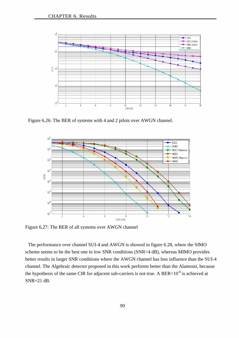
CHAPTER 6. Results
99
Figure 6.26: The BER of systems with 4 and 2 pilots over AWGN channel.
Figure 6.27: The BER of all systems over AWGN channel
The performance over channel SUI-4 and AWGN is showed in figure 6.28, where the SIMO
scheme seems to be the best one in low SNR conditions (SNR<4 dB), whereas MIMO provides
better results in larger SNR conditions where the AWGN channel has less influence than the SUI-4
channel. The Algebraic detector proposed in this work performs better than the Alamouti, because
the hypothesis of the same CIR for adjacent sub-carriers is not true. A BER=10-6
is achieved at
SNR=21 dB.
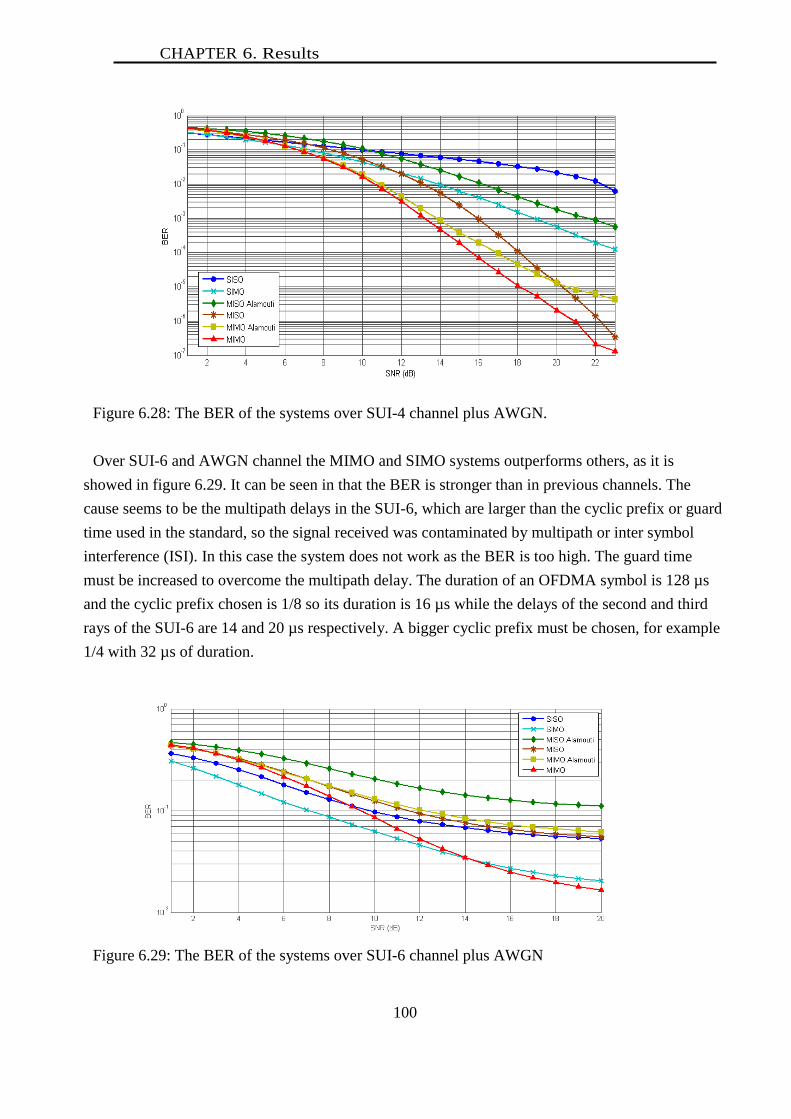
CHAPTER 6. Results
100
Figure 6.28: The BER of the systems over SUI-4 channel plus AWGN.
Over SUI-6 and AWGN channel the MIMO and SIMO systems outperforms others, as it is
showed in figure 6.29. It can be seen in that the BER is stronger than in previous channels. The
cause seems to be the multipath delays in the SUI-6, which are larger than the cyclic prefix or guard
time used in the standard, so the signal received was contaminated by multipath or inter symbol
interference (ISI). In this case the system does not work as the BER is too high. The guard time
must be increased to overcome the multipath delay. The duration of an OFDMA symbol is 128 µs
and the cyclic prefix chosen is 1/8 so its duration is 16 µs while the delays of the second and third
rays of the SUI-6 are 14 and 20 µs respectively. A bigger cyclic prefix must be chosen, for example
1/4 with 32 µs of duration.
Figure 6.29: The BER of the systems over SUI-6 channel plus AWGN
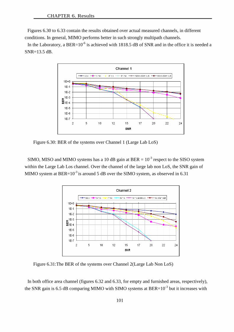
CHAPTER 6. Results
101
Figures 6.30 to 6.33 contain the results obtained over actual measured channels, in different
conditions. In general, MIMO performs better in such strongly multipath channels.
In the Laboratory, a BER=10-6
is achieved with 1818.5 dB of SNR and in the office it is needed a
SNR=13.5 dB.
Figure 6.30: BER of the systems over Channel 1 (Large Lab LoS)
SIMO, MISO and MIMO systems has a 10 dB gain at BER = 10-3
respect to the SISO system
within the Large Lab Los channel. Over the channel of the large lab non LoS, the SNR gain of
MIMO system at BER=10-3
is around 5 dB over the SIMO system, as observed in 6.31
Figure 6.31:The BER of the systems over Channel 2(Large Lab Non LoS)
In both office area channel (figures 6.32 and 6.33, for empty and furnished areas, respectively),
the SNR gain is 6.5 dB comparing MIMO with SIMO systems at BER=10-3
but it increases with

CHAPTER 6. Results
102
SNR. It can be seen a similar performance of both MIMO schemes, and only in channel 1, MISO
systems have similar BER performance.
Figure 6.32: The BER of the systems over Channel 3(empty office area)
Figure 6.33: The BER of the systems over Channel 4 (furnished office area)
If we compare this results with the related literature, we can see that a 3.2 b/s/Hz , 4x4 antenna
system is presented in (Li, Winters, & Sollenberger, 2002), where a SNR of 12 dB is needed at least
to achieve a BER=10-3
. Again, a SNR of 12 dB is needed for QPSK (Miao & Juntti, 2005) to reach
the best performance at BER=10-3
, with 2x4 antennas and space-time block code (STBC). In (Park
& Y.S.Cho, 2005), a 16 QAM system is presented where a SNR=12 dB is needed for a BER=10-3
1E-7
1E-6
1E-5
1E-4
1E-3
1E-2
1E-1
1E+0
2 5 10 12 15 17 20 22 24
BE
R
SNR
Channel 4
siso simo miso
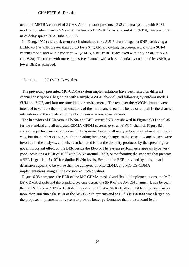
CHAPTER 6. Results
103
over an I-METRA channel of 2 GHz. Another work presents a 2x2 antenna system, with BPSK
modulation which need a SNR=10 to achieve a BER=10-3
over channel A of (ETSI, 1998) with 50
ns of delay spread (F.A. Jubair, 2009).
In (Kong, 1999) the block error rate is simulated for a SUI-3 channel against SNR, achieving a
BLER =0.1 at SNR greater than 30 dB for a 64 QAM 2/3 coding. In present work with a SUI-4
channel model and with a coder of 64 QAM ¾, a BER=10-7
is achieved with only 23 dB of SNR
(fig. 6.20). Therefore with more aggressive channel, with a less redundancy coder and less SNR, a
lower BER is achieved.
6.11.1. CDMA Results
The previously presented MC-CDMA system implementations have been tested on different
channel descriptions, beginning with a simple AWGN channel, and following by outdoor models
SUI4 and SUI6, and four measured indoor environments. The test over the AWGN channel were
intended to validate the implementations of the model and check the behavior of mainly the channel
estimation and the equalization blocks in non-selective environments.
The behaviors of BER versus Eb/No, and BER versus SNR, are showed in Figures 6.34 and 6.35
for the standard and all analyzed CDMA-OFDM systems over an AWGN channel. Figure 6.34
shows the performance of only one of the systems, because all analyzed systems behaved in similar
way, but the number of users, so the spreading factor SF, change. In this case, 2, 4 and 8 users were
involved in the analysis, and what can be noted is that the diversity produced by the spreading has
not an important effect on the BER versus the Eb/No. The system performance appears to be very
good, achieving a BER of 10-55
with Eb/No around 10 dB, outperforming the standard that presents
a BER larger than 5x10⁻⁴
for similar Eb/No levels. Besides, the BER provided by the standard
definition appears to be worse than the achieved by MC-CDMA and MC-DS-CDMA
implementations along all the considered Eb/No values.
Figure 6.35 compares the BER of the MC-CDMA masked and flexible implementations, the MC-
DS-CDMA classic and the standard systems versus the SNR of the AWGN channel. It can be seen
that at SNR below 7 dB the BER difference is small but at SNR=10 dB the BER of the standard is
more than 100 times the BER of the MC-CDMA systems and at 15 dB is 100.000 times larger. So,
the proposed implementations seem to provide better performance than the standard itself.
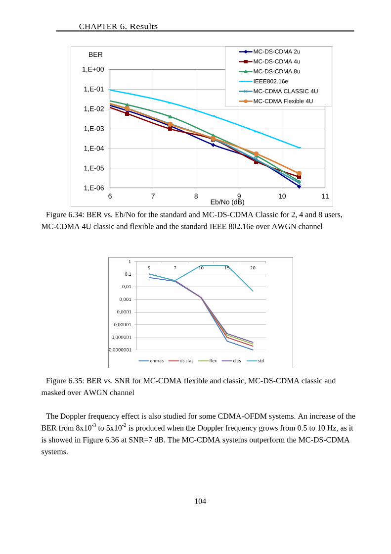
CHAPTER 6. Results
104
Figure 6.34: BER vs. Eb/No for the standard and MC-DS-CDMA Classic for 2, 4 and 8 users,
MC-CDMA 4U classic and flexible and the standard IEEE 802.16e over AWGN channel
Figure 6.35: BER vs. SNR for MC-CDMA flexible and classic, MC-DS-CDMA classic and
masked over AWGN channel
The Doppler frequency effect is also studied for some CDMA-OFDM systems. An increase of the
BER from 8x10⁻³
to 5x10⁻²
is produced when the Doppler frequency grows from 0.5 to 10 Hz, as it
is showed in Figure 6.36 at SNR=7 dB. The MC-CDMA systems outperform the MC-DS-CDMA
systems.
1,E-06
1,E-05
1,E-04
1,E-03
1,E-02
1,E-01
1,E+00
6 7 8 9 10 11
BER
Eb/No (dB)
MC-DS-CDMA 2u
MC-DS-CDMA 4u
MC-DS-CDMA 8u
IEEE802.16e
MC-CDMA CLASSIC 4U
MC-CDMA Flexible 4U

CHAPTER 6. Results
105
Figure 6.36: BER vs. Doppler frequency of four systems over AWGN channel
In all SUI4 channel simulations, the MC-CDMA first option, called `masked´ scheme,
outperforms all other systems comparing the BER against SNR at the AWGN channel added to the
Rayleigh channel.
The BER level is larger than 10-2
, indicating that these systems with 64QAM are very sensitive to
the Rayleigh channels, principally the SUI 6 (Figure 6.37) because the cyclic prefix is smaller than
the delay spread of the channel. It can be seen that the SNR of the AWGN has not influence in the
BER and the mechanisms to predict and equalize the channel neither.
Figure 6.37: BER vs. SNR of four MC-CDMA and the Standard system over SUI 6 channel
masked DS classic classic

CHAPTER 6. Results
106
Figure 6.38 shows a comparison of the BER vs. the SNR of four systems over the indoor actual
channel within a furnished office area, where we can appreciate that the `masked´ MC-CDMA
performs better than the others. However, it still presents high BER values with large SNR due to
the multipath phenomenon.
Figure 6.38. BER vs. SNR over indoor channel 4, the furnished office area
The huge BER is caused because this channel, as other actual indoor channels, presents multipath
components with delays larger than the 16 ms cyclic prefix and also with considerable amplitudes
as can be seen in table 6.1.
The channel prediction schemes were also compared along the time in Figure 6.39. The firsts 12
time slots were caught during downlink time, when the system follows the channel. The next time
slots are the estimations during uplink period. It can be seen that the covariance method provides
the nearest results to the actual channel. Therefore, it was chosen to be implemented in all systems
of this work. The used Doppler frequency was 250Hz and the noise power was 2x10⁻⁵
W.
masked DS classic classic
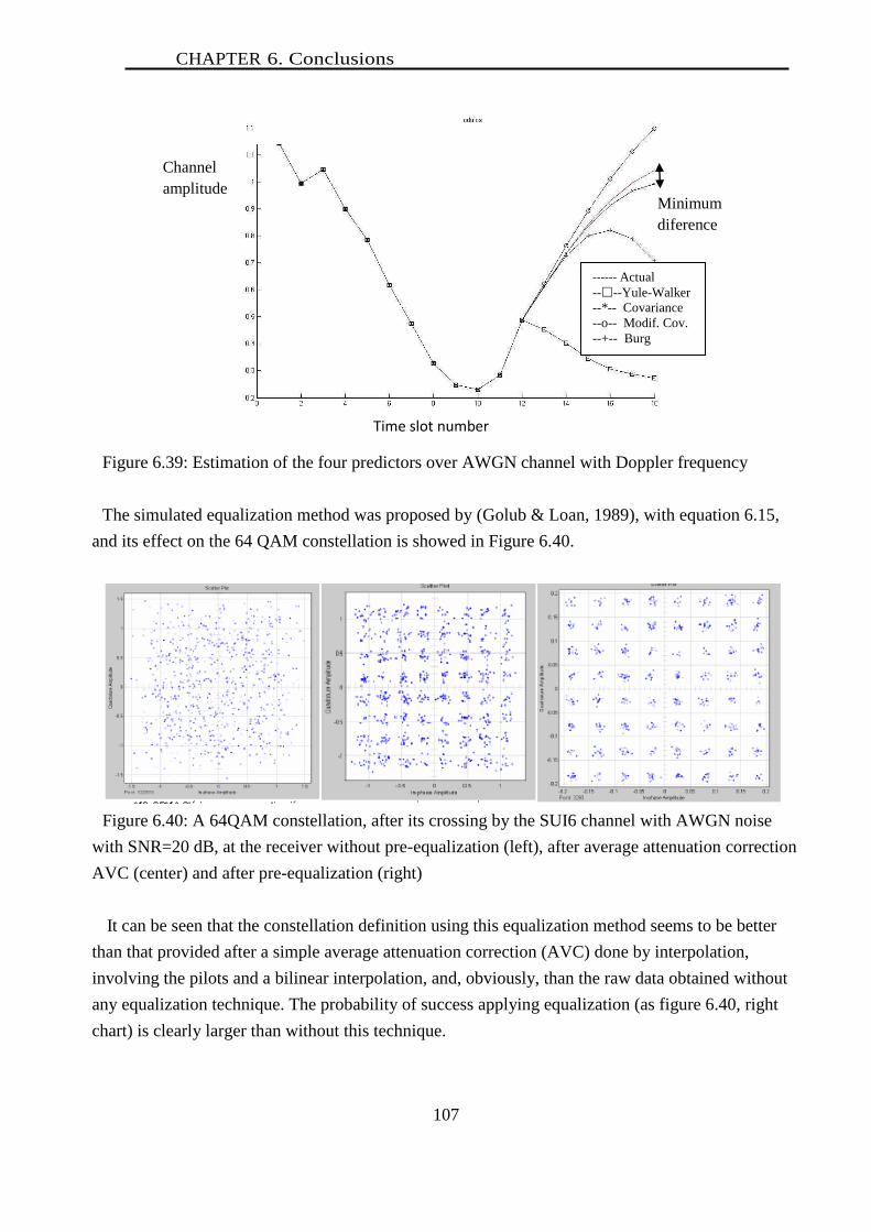
CHAPTER 6. Conclusions
107
Figure 6.39: Estimation of the four predictors over AWGN channel with Doppler frequency
The simulated equalization method was proposed by (Golub & Loan, 1989), with equation 6.15,
and its effect on the 64 QAM constellation is showed in Figure 6.40.
Figure 6.40: A 64QAM constellation, after its crossing by the SUI6 channel with AWGN noise
with SNR=20 dB, at the receiver without pre-equalization (left), after average attenuation correction
AVC (center) and after pre-equalization (right)
It can be seen that the constellation definition using this equalization method seems to be better
than that provided after a simple average attenuation correction (AVC) done by interpolation,
involving the pilots and a bilinear interpolation, and, obviously, than the raw data obtained without
any equalization technique. The probability of success applying equalization (as figure 6.40, right
chart) is clearly larger than without this technique.
Time slot number
Channel
amplitude
------ Actual
----Yule-Walker
--*-- Covariance
--o-- Modif. Cov.
--+-- Burg
Minimum
diference
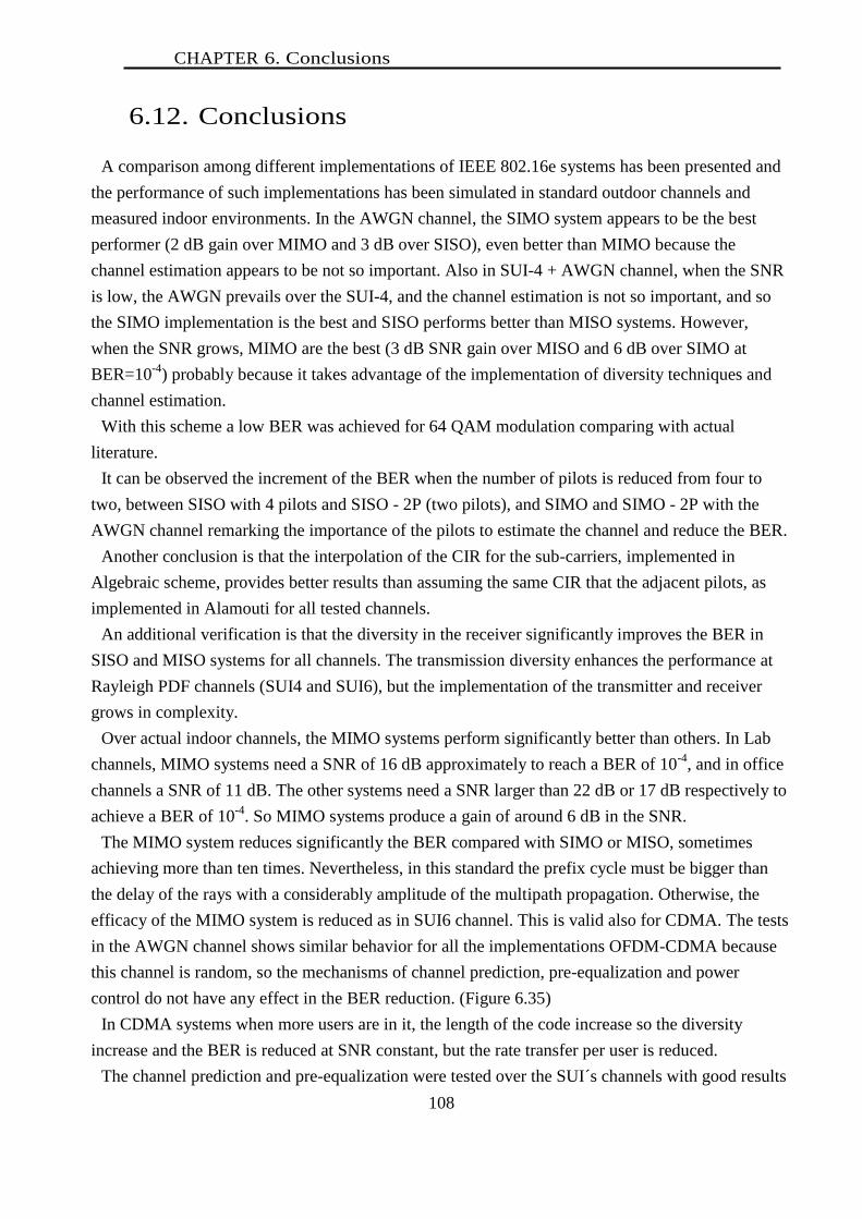
CHAPTER 6. Conclusions
108
6.12. Conclusions
A comparison among different implementations of IEEE 802.16e systems has been presented and
the performance of such implementations has been simulated in standard outdoor channels and
measured indoor environments. In the AWGN channel, the SIMO system appears to be the best
performer (2 dB gain over MIMO and 3 dB over SISO), even better than MIMO because the
channel estimation appears to be not so important. Also in SUI-4 + AWGN channel, when the SNR
is low, the AWGN prevails over the SUI-4, and the channel estimation is not so important, and so
the SIMO implementation is the best and SISO performs better than MISO systems. However,
when the SNR grows, MIMO are the best (3 dB SNR gain over MISO and 6 dB over SIMO at
BER=10-4
) probably because it takes advantage of the implementation of diversity techniques and
channel estimation.
With this scheme a low BER was achieved for 64 QAM modulation comparing with actual
literature.
It can be observed the increment of the BER when the number of pilots is reduced from four to
two, between SISO with 4 pilots and SISO - 2P (two pilots), and SIMO and SIMO - 2P with the
AWGN channel remarking the importance of the pilots to estimate the channel and reduce the BER.
Another conclusion is that the interpolation of the CIR for the sub-carriers, implemented in
Algebraic scheme, provides better results than assuming the same CIR that the adjacent pilots, as
implemented in Alamouti for all tested channels.
An additional verification is that the diversity in the receiver significantly improves the BER in
SISO and MISO systems for all channels. The transmission diversity enhances the performance at
Rayleigh PDF channels (SUI4 and SUI6), but the implementation of the transmitter and receiver
grows in complexity.
Over actual indoor channels, the MIMO systems perform significantly better than others. In Lab
channels, MIMO systems need a SNR of 16 dB approximately to reach a BER of 10-4
, and in office
channels a SNR of 11 dB. The other systems need a SNR larger than 22 dB or 17 dB respectively to
achieve a BER of 10-4
. So MIMO systems produce a gain of around 6 dB in the SNR.
The MIMO system reduces significantly the BER compared with SIMO or MISO, sometimes
achieving more than ten times. Nevertheless, in this standard the prefix cycle must be bigger than
the delay of the rays with a considerably amplitude of the multipath propagation. Otherwise, the
efficacy of the MIMO system is reduced as in SUI6 channel. This is valid also for CDMA. The tests
in the AWGN channel shows similar behavior for all the implementations OFDM-CDMA because
this channel is random, so the mechanisms of channel prediction, pre-equalization and power
control do not have any effect in the BER reduction. (Figure 6.35)
In CDMA systems when more users are in it, the length of the code increase so the diversity
increase and the BER is reduced at SNR constant, but the rate transfer per user is reduced.
The channel prediction and pre-equalization were tested over the SUI´s channels with good results
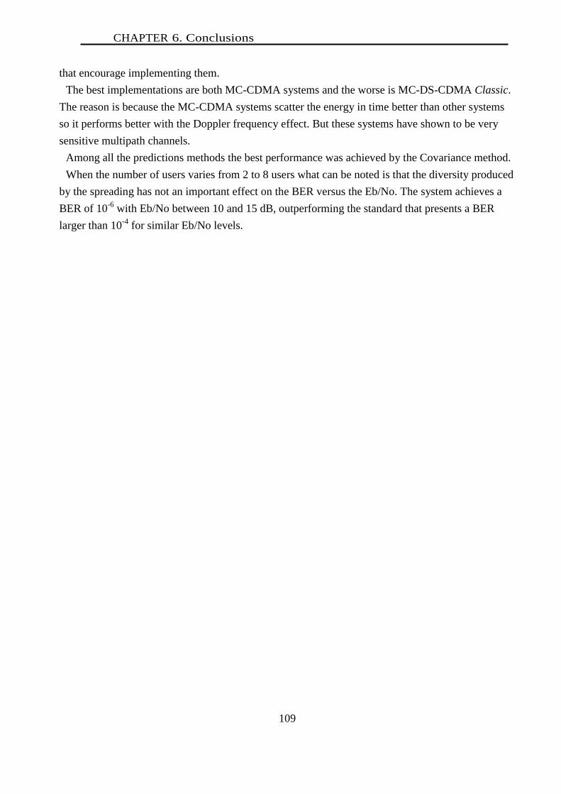
CHAPTER 6. Conclusions
109
that encourage implementing them.
The best implementations are both MC-CDMA systems and the worse is MC-DS-CDMA Classic.
The reason is because the MC-CDMA systems scatter the energy in time better than other systems
so it performs better with the Doppler frequency effect. But these systems have shown to be very
sensitive multipath channels.
Among all the predictions methods the best performance was achieved by the Covariance method.
When the number of users varies from 2 to 8 users what can be noted is that the diversity produced
by the spreading has not an important effect on the BER versus the Eb/No. The system achieves a
BER of 10-6
with Eb/No between 10 and 15 dB, outperforming the standard that presents a BER
larger than 10-4
for similar Eb/No levels.

CHAPTER 6. Conclusions
110

Chapter 7 Average spectral efficiency of multi modulation cellular systems
Fourth generation systems are proposed to create extended wireless networks by applying
frequency reuse techniques based on a cellular scheme. The bandwidth needed to install a FDMA metropolitan deployment depends on the channel bandwidth and on the signal to interference protection ratio. The spectral efficiency of the network is inversely proportional to the bandwidth required by the cluster which is larger for the more efficient modulations because they have bigger protection ratios.
This trade-off is analyzed in this chapter for systems with various modulation schemes (QPSK, 16 QAM and 64 QAM), founding the percentage of the cell area that could be managed with each modulation, considering full load sectors. The area of a cell with mobiles using certain modulation in case of reuse 1 is calculated. An example, computed at 3.5 GHz band, shows a reduction of 35% of the peak spectral efficiency, which falls to1.6 bps/Hz. The total bandwidth required for three sectored cells with 10 MHz channel results to be 360 MHz. This is a big issue since the size of the bands is generally 200 MHz. To solve this issue, the proponents of the standard are looking for methods of ICIC and FFR or relaying in repeaters stations.
The conditions to share the same subcarriers between two users in next to BSs are presented maintaining the SNRs required for both users.
Two algorithms for power allocation and user scheduling are proposed to be evaluated in future works.
CHAPTER 7. Introduction
112
7.1. Introduction
The new technologies proposed for the 3.9 and 4G systems, WiMAX (IEEE Computer Society ; IEEE Microwave Theory Techniques Society, 2006) and LTE (3GPP RAN Technical Specification Group, 2009), are promising huge sector traffic capacity at realistic distances to achieve a metropolitan coverage with a reasonable number of base stations. The way they expect to achieve the increase in capacity is by using larger channel bandwidth and denser modulation constellations, for example 16 and 64 QAM, instead of QPSK.
The problem caused by the increment of the channel bandwidth is the need to transmit more power for the same signal to noise and interference ratio (SNIR) at a constant noise density and interference levels. But what it really matters is the increase in the spectral efficiency (SE), that it is proposed to achieve with denser constellations. . The difficulty of this strategy is the requisite of larger SNIR for maintaining the same BER. The minimum SNIR required for a given BER is called the protection ratio (rp). This demands wider bandwidth for network deployments because the number of cells per cluster, known as the order of the cluster, increases. This fact appears despite the orthogonal frequency division multiplexing (OFDM) system is optimal in terms of spectrum reuse, as it allows the carrier overlapping while FDMA requires a certain frequency separation between adjacent carriers. Thus, OFDM provides an advantage in the closer the sub-carriers can be located. The idea is to deploy all the sub-carriers in all sectors. In this chapter, the procedure to compute the total bandwidth as a function of the channel bandwidth and the rp, is proposed. Moreover, the actual traffic capacity can be computed at each base station sector, taking into account the implemented modulations and the percentage of the cell area corresponding to each one to calculate the achievable sector traffic.
There are some important differences between the performance reported by other works (Hoymann & Goebbels, 2007) and the promised data throughputs of the considered technologies (B. Upase, 2007) .This differences support the interest of the computations presented at this paper, which analyses the ability of such standards to meet the promising future they announced.
The chapter is organized in four sections. After this section introducing the topic, a second section is focused on the foundations of the work, divided into four subsections: the previously published work followed by the theoretical derivation of the total bandwidth of a network deployment, the distance relation of mobiles reusing the frequency in adjacent cells, and the average Sector Traffic calculations. The third section is devoted to simulation results, applied to three different modulation schemes: QPSK, 16QAM and 64QAM; and the fourth section summarizes the conclusions.

CHAPTER 7. Foundations
113
7.2. Foundations
This section enunciates the fundamentals of the proposed calculus. At the 7.2.1 subsection, some previous works are reviewed. The needed bandwidth for a network deployment is derived in the section 7.2.2, which is the same to the bandwidth of a cluster. The 7.2.3 subsection derives the distance relation of mobiles reusing the frequency in adjacent cells and the 7.2.4 subsection is focused on the estimation of sector average traffic with multi-modulation scheme.
7.2.1. Previous works
Previously published work (Hoymann & Goebbels, 2007) shows that for non-light of sight (NLOS) scenarios, a seventh order cluster is needed to achieve a SNIR of 6.46 dB with cell of one sector and 190 m of radius; or a SNIR of 15 dB but with 2 sectors and 190m radius cells. Those results contrast with the promised 70 Mbps data throughputs and coverage distances of around 50 km (B. Upase, 2007), considering that a reasonable radius to reach efficient metropolitan coverage would be 1000 m. These results open the debate on the ability of such standards to meet the great promising future they seem to bring.
Different implementations of frequency reuse have been proposed in previously published works:
1. Predefined Reuse Scheme (PRS) where the entire bandwidth is divided into several bands called as sub-bands. Each cell uses a predefined sub-band to avoid other cell interference (OCI) from neighboring cells (LGE Electronics, R1-050833). It avoids the interference but has low frequency reuse factor (FRF) so low SE.
2. Reuse partitioning scheme (RPS) was proposed to focus on SE more than OCI mitigation compared to PRS (LG Electronics , R1-051051), (Oh, Cho, Han, Woo, & Hong, 2006). The FRF of RPS is n with cluster of order n.
3. The soft frequency reuse partitioning scheme (SFRPS) was proposed in (Kwon, Song, Lee, Kim, Lee, & Hong, 2008) to increase the SE compared to RPS (Huawei, R1-050629), (Huawei, R1-050841). The FRF of RPS is (n + 1)/2 with n-cell patterns.
4. The power division reuse partitioning scheme (PDRPS) achieves the FRF of 1/2 irrespective of n-cell patterns. The main idea for increasing capacity is to assign more bandwidth to MSs at low SINR (e.g. MSs located in inner region) and give more power to MSs at high SINR (e.g. MSs located in the outer region).
Simulation results in (Jia, Zhang, Yu, Cheng, & Li, 2007) show that the frequency reuse of 1 is unacceptable which will be confirmed in this work. Fractional frequency reuse strategies with the values of area fraction η less than about 0.2 are feasible in practical system deployments and mention that the maximum SE of 10 bps/Hz is achieved.

CHAPTER 7. Foundations
114
In reference (Boustani, Khorsandi, Danesfahani, & MirMotahhary, 2009) the users within 80% of the cell radius are considered as members of the inner-cell region but the SE achieved is 1.7/5=0.34 bps/Hz that is very low SE for the today state of the art.
Reference (Najjar, Hamdi, & Bouallegue, 2009) proposes an optimal dimension (a=inner radius/cell radius) of the central region based on the average to variance ratio of the received SINR at a given user. This optimal distance between user and it's serving base station is equal to 360m for a 1000m radius and the optimal size of two partitions of subcarriers is achieved with aopt = 0.36.
This review shows some values that are consistent with our results. The overlapping coverage and reuse partitioning are used in (Chu & Rappaport, 1997) to reduce the
blocking and hand-offs. The scheme helps mobile users who are distant from base stations, but the spectrum is divided in channels sub-sets to be used by different areas.
Cellular relay networks are used to improve the radio link of edge users and (Liang, Yin, Chen, Li, & Liu, 2011) presents a dynamic full frequency reuse scheme is proposed to improve the spectral efficiency. They use full frequency reuse scheme and the adaptive subcarrier scheduling sharing the carriers between the relay stations (RS) and mobiles users. The problem of relay schemes is the cost of the added stations, in this case 6 RSs per BS.
Another paper that considers a relay scheme is (Chen, Tseng, Wang, Wang, & Wu, 2009) where they study how to exploit spectral reuse in an IEEE 802.16 mesh network through timeslot allocation, bandwidth adaptation, hierarchical scheduling, and routing. They mention that improves throughput 2 to 3 times the normal pattern, but no absolute values are presented for comparison with other schemes.
The throughput per user is estimated in (Oh, Cho, Han, Woo, & Hong, Performance Analysis of Reuse-Partitioning-Based Subchannelized OFDMA Uplink Systems in Multicell Environments, 2008) for some reuse schemes, with reuse 1 for inner users and reuse 3 for outer users. It only takes account the interference from the first-tier neighboring cells. But none of the above works show restrictions of the frequency reuse between mobiles in different BSs.
7.2.2. Total bandwidth of a network deployment
When frequency division multiple access (FDMA) systems, as OFDM, apply frequency reuse techniques, the network planning must consider a SNIR larger than rp for a given BER (Z. Wang, 2002). This determines the order of the cluster ergo the number of cells of a cluster, J, within which frequencies should not be repeated. Thus, the clusters can be located next to each other maintaining the same interference among all cells. Therefore the total bandwidth needed by a network is the same needed for a cluster.
Notation: the power on mobile Mi, received from base station BSj is: Pij, and the power emitted from BSj is Pj. Figure 7.1 shows all the magnitudes used in the equations.

CHAPTER 7. Foundations
115
Figure 7.1: Geometry and magnitudes of equations. We will analyze the case of reuse one where all sectors has the same frequency, particularly two
faced sectors with one MS each one. The SNIR will be represented by the carrier to interference ratio (C/I) at M1, in this case (P11/P21)
since the noise N is negligible compared with the interference. P11 is the received power by M1 transmitted by BS1 and P21 is the received power at M1 received from the BS2 in the subcarrier 1. The relation between the distance of two co-channel cells, denoted as D, and the cell radius, R, is related to the carrier to interference ratio, and therefore to the rp, by the equation 7.1. The worst case is a mobile at distance R from its serving cell and at D-R from the interfering cells. Figure 7.1 helps in the description of the geometrical arrangement.
111 21 21
21 211 11
..
nn
pn
total
P d dS c Pr
N I i P d P d
(7.1)
Being n the propagation index, P1=P2 ,
111
11n
PP k
d
and
221
21n
PP k
d
. If there are m interferers and d21 is taken as the minimum distance between the BS interferers and
M1, the worst case in SNIR is given by:
111 21 21
21 211 11
. 1. .
nn
pn
total
P d dS c Pr
N I i mP m d P m d
(7.2) The number of the cells in a cluster J is given by the following expression (Lee, 1989).
211 1 .
3n
pJ m r
(7.3)
J must be rombic (to allow the installation of adjacent cluster maintaining the interference constant
d11
M1
BS1 BS2
M2
d21 d12 d22
P1 P2
D
R R
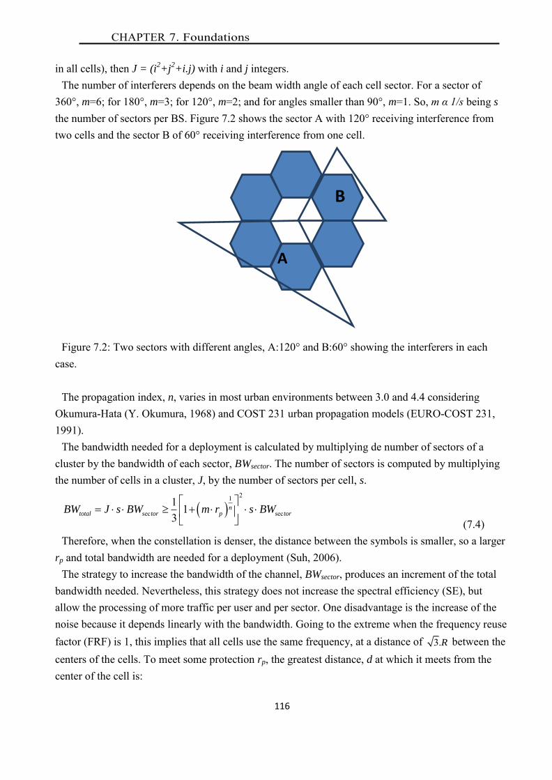
CHAPTER 7. Foundations
116
in all cells), then J = (i2+j
2+i.j) with i and j integers.
The number of interferers depends on the beam width angle of each cell sector. For a sector of 360°, m=6; for 180°, m=3; for 120°, m=2; and for angles smaller than 90°, m=1. So, m α 1/s being s the number of sectors per BS. Figure 7.2 shows the sector A with 120° receiving interference from two cells and the sector B of 60° receiving interference from one cell.
Figure 7.2: Two sectors with different angles, A:120° and B:60° showing the interferers in each case.
The propagation index, n, varies in most urban environments between 3.0 and 4.4 considering
Okumura-Hata (Y. Okumura, 1968) and COST 231 urban propagation models (EURO-COST 231, 1991).
The bandwidth needed for a deployment is calculated by multiplying de number of sectors of a cluster by the bandwidth of each sector, BWsector. The number of sectors is computed by multiplying the number of cells in a cluster, J, by the number of sectors per cell, s.
21
sec sec1 13
ntotal tor p torBW J s BW m r s BW
(7.4) Therefore, when the constellation is denser, the distance between the symbols is smaller, so a larger
rp and total bandwidth are needed for a deployment (Suh, 2006). The strategy to increase the bandwidth of the channel, BWsector, produces an increment of the total
bandwidth needed. Nevertheless, this strategy does not increase the spectral efficiency (SE), but allow the processing of more traffic per user and per sector. One disadvantage is the increase of the noise because it depends linearly with the bandwidth. Going to the extreme when the frequency reuse factor (FRF) is 1, this implies that all cells use the same frequency, at a distance of 3.R between the centers of the cells. To meet some protection rp, the greatest distance, d at which it meets from the center of the cell is:
A
B
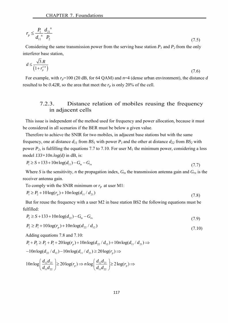
CHAPTER 7. Foundations
117
1 21
11 2
n
p n
P dr
d P
(7.5) Considering the same transmission power from the serving base station P1 and P2 from the only
interferer base station,
1/
3.1 n
p
Rd
r
(7.6) For example, with rp=100 (20 dB, for 64 QAM) and n=4 (dense urban environment), the distance d
resulted to be 0.42R, so the area that meet the rp is only 20% of the cell.
7.2.3. Distance relation of mobiles reusing the frequency in adjacent cells
This issue is independent of the method used for frequency and power allocation, because it must be considered in all scenarios if the BER must be below a given value.
Therefore to achieve the SNIR for two mobiles, in adjacent base stations but with the same frequency, one at distance d11 from BS1 with power P1 and the other at distance d22 from BS2 with power P2, is fulfilling the equations 7.7 to 7.10. For user M1 the minimum power, considering a loss model 133+10n.log(d) in dB, is:
1 11133 10 log( ) tx rxP S n d G G (7.7) Where S is the sensitivity, n the propagation index, Gtx the transmission antenna gain and Grx is the
receiver antenna gain. To comply with the SNIR minimum or rp at user M1:
1 2 11 2110log( ) 10 log( / )pP P r n d d (7.8) But for reuse the frequency with a user M2 in base station BS2 the following equations must be
fulfilled:
2 22133 10 log( ) tx rxP S n d G G (7.9)
2 1 22 1210log( ) 10 log( / )pP P r n d d (7.10) Adding equations 7.8 and 7.10:
1 2 2 1 22 12 11 2120log( ) 10 log( / ) 10 log( / )pP P P P r n d d n d d 22 12 11 2110 log( / ) 10 log( / ) 20log( )pn d d n d d r
12 21 12 21
11 22 11 22
10 log 20log( ) log 2log( )p p
d d d dn r n r
d d d d
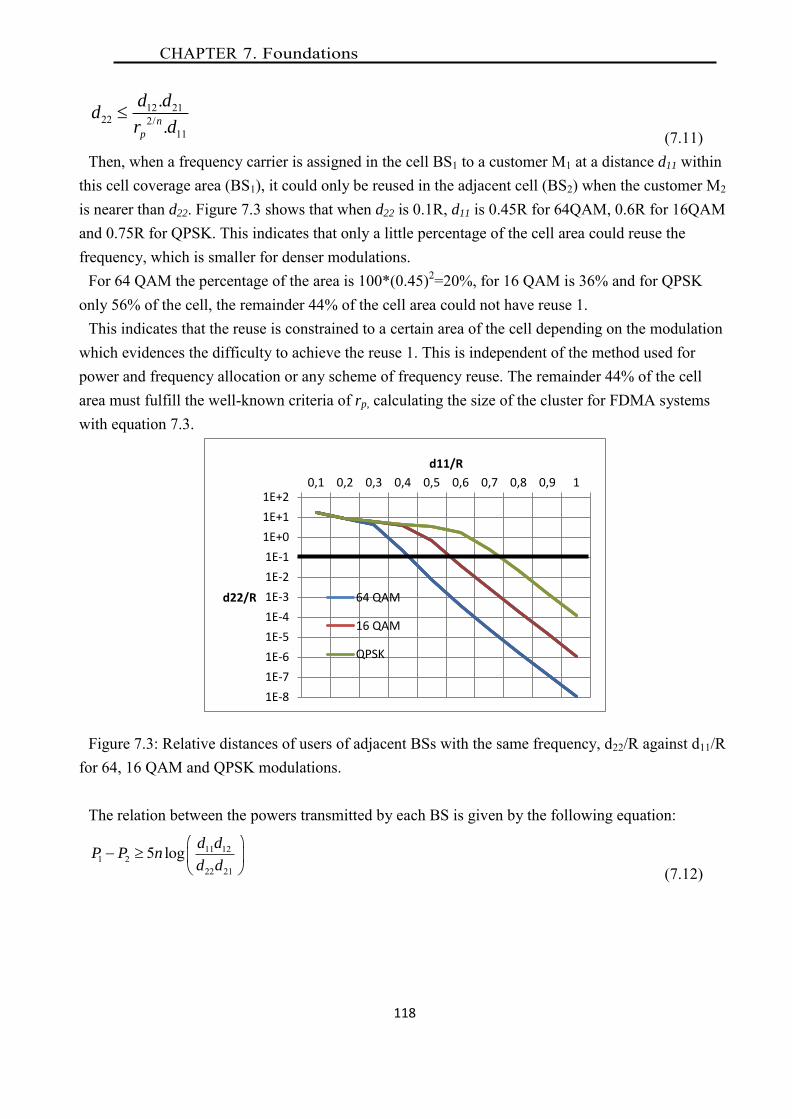
CHAPTER 7. Foundations
118
12 2122 2/
11
..n
p
d dd
r d
(7.11) Then, when a frequency carrier is assigned in the cell BS1 to a customer M1 at a distance d11 within
this cell coverage area (BS1), it could only be reused in the adjacent cell (BS2) when the customer M2 is nearer than d22. Figure 7.3 shows that when d22 is 0.1R, d11 is 0.45R for 64QAM, 0.6R for 16QAM and 0.75R for QPSK. This indicates that only a little percentage of the cell area could reuse the frequency, which is smaller for denser modulations.
For 64 QAM the percentage of the area is 100*(0.45)2=20%, for 16 QAM is 36% and for QPSK only 56% of the cell, the remainder 44% of the cell area could not have reuse 1.
This indicates that the reuse is constrained to a certain area of the cell depending on the modulation which evidences the difficulty to achieve the reuse 1. This is independent of the method used for power and frequency allocation or any scheme of frequency reuse. The remainder 44% of the cell area must fulfill the well-known criteria of rp, calculating the size of the cluster for FDMA systems with equation 7.3.
Figure 7.3: Relative distances of users of adjacent BSs with the same frequency, d22/R against d11/R for 64, 16 QAM and QPSK modulations.
The relation between the powers transmitted by each BS is given by the following equation:
11 121 2
22 21
5 log d dP P n
d d
(7.12)
1E-8
1E-7
1E-6
1E-5
1E-4
1E-3
1E-2
1E-1
1E+0
1E+1
1E+20,1 0,2 0,3 0,4 0,5 0,6 0,7 0,8 0,9 1
d22/R
d11/R
64 QAM
16 QAM
QPSK

CHAPTER 7. Foundations
119
7.2.4. Average Sector Traffic
Another strategy to increase the sector traffic is by means of the transport of more bits per symbol. An important aspect to be considered in multi-modulation technologies (QPSK, 16 and 64 QAM for example, as typical for IEEE 802.16e and LTE standards) is the existence of different rp for each modulation. Because of this, each modulation will have a different coverage radius, R, as showed by equation 7.13. The modulation with larger rp will present the smaller radius.
1/1 ( . ) n
p
DR
m r
(7.13)
Where D is the distance between cells. The capacity of each sector depends on the implemented modulation, because each modulation carries different number of bits per symbol: 64 QAM carries 6 bits; 16 QAM, 4 bits; and QPSK, 2 bits (E.A. Lee, 1988). But the performance of the sector depends on the area covered by each modulation so it will be calculated by weighting the coverage area of the implemented modulation by the number of bits that it carries. There is a trade-off between the bits and the percentage of the cell covered by the modulation. When the modulation has more bits per symbol there is less distance between symbols, so less tolerance to noise, then the SNIR required or the rp is larger, as showed in table1.
Taking 1 as the maximum amplitude of symbols, while QPSK has a distance between symbols of
2 , 16 QAM has a distance of 2 / 3and for 64 QAM it is 2 / 7 , as showed in figures 7.4 and 7.5. For his reason there are three different rp values, presenting the following theoretical relations: rp
16QAM rp QPSK*9 (or 9.5 dB more), and rp 64QAM rp QPSK*49 (or 17 dB more). Some codification can reduce the quantity of bits per symbol, for example a ¾ codec reduce from 4 to 3 because one bit is used for redundancy.
Figure 7.4. QPSK modulator, signals and constellation and distance between symbols.
√

CHAPTER 7. Foundations
120
Figure 7.5: The 16 and 64 QAM constellations As there are three possible values of rp (rp QPSK, rp 16QAM and rp 64QAM), there are three possible results
of equation 7.13 (three cell radii), and then, three coverage areas: AQPSK, A16QAM and A64QAM depicted in figure 7.6. As QPSK is the modulation with lower rp, it determines the maximum cell radius, R=RQPSK, and the maximum cell area A=AQPSK. The area ratios between the higher order modulations respect to the cell area are calculated with equations 7.14 and 7.15:
21/16
1/16
1 ( . )1 ( . )
n
QAM pQPSK
n
QPSK p QAM
A m r
A m r
(7.14)
21/64
1/64
1 ( . )1 ( . )
n
QAM pQPSK
n
QPSK p QAM
A m r
A m r
(7.15)
Figure 7.6: Areas with different modulations in a cell. Green: 64 QAM, red: 16 QAM and blue:
QPSK areas.
The data at each base station is always tried to be cursed using the most efficient modulation as
AQPSK
-A16QAM
Rp=8 A
16QAM-A
64QAM
Rp=14 dB
A64QAM
Rp=20 dB
√ √ √ /7
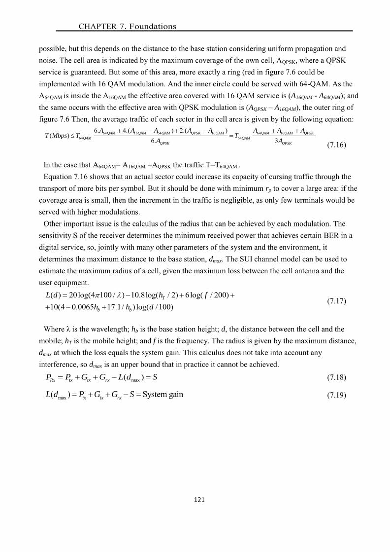
CHAPTER 7. Foundations
121
possible, but this depends on the distance to the base station considering uniform propagation and noise. The cell area is indicated by the maximum coverage of the own cell, AQPSK, where a QPSK service is guaranteed. But some of this area, more exactly a ring (red in figure 7.6 could be implemented with 16 QAM modulation. And the inner circle could be served with 64-QAM. As the A64QAM is inside the A16QAM the effective area covered with 16 QAM service is (A16QAM - A64QAM); and the same occurs with the effective area with QPSK modulation is (AQPSK – A16QAM), the outer ring of figure 7.6 Then, the average traffic of each sector in the cell area is given by the following equation:
64 16 64 16 64 1664 64
6. 4.( ) 2.( )( )
6. 3QAM QAM QAM QPSK QAM QAM QAM QPSK
QAM QAM
QPSK QPSK
A A A A A A A AT Mbps T T
A A
(7.16)
In the case that A64QAM= A16QAM =AQPSK the traffic T=T64QAM . Equation 7.16 shows that an actual sector could increase its capacity of cursing traffic through the
transport of more bits per symbol. But it should be done with minimum rp to cover a large area: if the coverage area is small, then the increment in the traffic is negligible, as only few terminals would be served with higher modulations.
Other important issue is the calculus of the radius that can be achieved by each modulation. The sensitivity S of the receiver determines the minimum received power that achieves certain BER in a digital service, so, jointly with many other parameters of the system and the environment, it determines the maximum distance to the base station, dmax. The SUI channel model can be used to estimate the maximum radius of a cell, given the maximum loss between the cell antenna and the user equipment.
( ) 20log(4 100 / ) 10.8log( / 2) 6log( / 200)10(4 0.0065 17.1/ ) log( /100)
T
b b
L d h f
h h d
(7.17)
Where λ is the wavelength; hb is the base station height; d, the distance between the cell and the mobile; hT is the mobile height; and f is the frequency. The radius is given by the maximum distance, dmax at which the loss equals the system gain. This calculus does not take into account any interference, so dmax is an upper bound that in practice it cannot be achieved.
max( )Rx tx tx rxP P G G L d S (7.18)
max( ) System gaintx tx rxL d P G G S (7.19)

CHAPTER 7. Results
122
7.3. Results
The procedure is applied to a system based on three different modulation schemes: QPSK, 16QAM and 64QAM. As an example, a 3/4 codification is used with the following parameters: channel bandwidth=10MHz; frequency=3.5GHz; hm=1.5m; hb=30 m; Ptx=30dBm; Gtx=15 dBi; Grx=1 dBi; s= 3 sectors/cell. The sensitivity for a QPSK 3/4 is fixed in -89.5dBm (IEEE Computer Society ; IEEE Microwave Theory Techniques Society, 2006).
Table 7.1 shows the values of the cluster order, J, the total bandwidth of a cluster, BWtotal, and the percentage of the cell area served by each considered modulation. This definition enables to plan adjacent clusters where all cells have the same interference. This formula also explains the values at the fourth column of table 1, labeled as “J”, where J is computed considering the condition of the third column, labeled “J>”, derived from equation 7.3.
Table 7.1: BWtotal and percentage of the cell area served by each modulation.
Modulation SNIR
(dB) J> J
BW total
TDD
(MHz)
Area
percentage
(%)
Sensitivity
(dBm)
Maximum
coverage
distance
(km)
QPSK 8 3.2 4 120 39 -89.5 1.44
16 QAM 14 5.2 7 210 25 -83.0 1.02
64 QAM 20 8.9 12 360 36 -77.0 0.75
From equation 7.16, the average sector traffic T as a function of the peak traffic (considering 64QAM) is:
64QAM 64QAM
2*39 4*25 6*363T T 0.49T4 6*100
(7.20)
Where there is a reduction for the 3/4 coder, plus the reduction of the implementation of multiple modulation schemes depending on the location of the user. This 3/4 code is needed to detect and correct errors. A uniform distribution of users in all the coverage area is assumed for the calculations.
For example, in a WiMAX system, the achievable traffic with a 3.5 MHz channel would be:
816 61 1
0,49 5,55432
1
SymbolsQAM bits
TimeSlot SymbolQAMT Mbps
s
TimeSlot
(7.21)

CHAPTER 7. Results
123
Therefore the spectral efficiency is 5.55Mbps/3.5MHz=1.6 bps/Hz. This value appears to be far from the announced 6 bps/Hz.
Now, an example is presented to see all the details of the consequences of the calculus described above. When a 64 QAM modulation is used instead of QPSK, the distance between the symbols is reduced from 1 to 1/7, so the rp increased 49 times or 17 dB. Increasing the channel bandwidth from 5 to 20 MHz to increase the traffic, the noise also increases 4 times or 6 dB. Therefore passing from a QPSK 5 MHz system to a 64 QAM 20 MHz system, the received power must be 23 dB greater to maintain the SNIR constant, so the coverage radio is reduced to the 30%, therefore the coverage area is reduced to the 10% of the area, so the number of cell increases 10 times if all the area must be covered with 64 QAM. The total bandwidth required by the cluster or network, increases BW20/BW5
x J64QAM/JQPSK= 4x3=12 times. All these costs are to obtain an increase of 12 times in the sector capacity in Mbps.
So the disadvantages must be compared with the advantages to take the right decisions.
7.4. Inter-Cell Interference Mitigation Approaches There are many approaches to Inter-Cell Interference (ICI) mitigation, but the most relevant are:
cancellation, randomization and coordination (3GPP TSG RAN, 2005). The cancellation approach only reduces the interference with processing gain. Randomization helps statistically but in high load situations is not very effective. Therefore the coordination strategy is the best solution for interference mitigation at the cost of more intelligence or processing and signaling traffic (Xiangning, Si, & Xiaodong, 2007). Three types of coordination could be considered: static, semi-static and dynamic.
7.4.1. Static Inter-Cell Interference Coordination
(Fan, Chen, & Zhang, 2007) analyzes different proposals on static ICIC, as Ericsson’s, and Alcatel’s proposals.
Ericsson proposes reuse one in the cell center and reuse 3 in the cell edge, this means that the size of the cluster is 3 for the edge, what implies a rp of 7 dB what only allows a QPSK modulation with the corresponding loss on spectral efficiency because only can transmit 2 bits per symbol instead of 6 bits as 64 QAM does.
Alcatel splits the spectrum in 7 or 9 sub-bands, leaving few MHz per sector so, only can achieves few Mbps per sector. For example if the operator has 20 MHz, divided by 7 is near 3 MHz, considering a SE of 2, only 6 Mbps can be achieved what is less than HSPA+ technology over 5 MHz.
CHAPTER 7. Inter-cell interference
124
7.4.2. Semi-Static ICI coordination
Siemens´s solution also proposes reuse 3 in the border and reuse 1 in the center but the sub-bands used in the edge are adjustable depending upon the traffic load (Fan, Chen, & Zhang, 2007). A cell with high load can use sub-carriers with frequency assigned to its neighbors if they are not being used
7.4.3. Softer Frequency Reuse
The spectrum is divided into three bands in Soft Frequency Reuse (SFR) (Zhang, Hee, Jiang, & Xu, 2008). Cell center users can exploit the entire spectrum with reuse 1, but the cell edge users could only utilize 1/3 and they have reuse factor of 3. The other 2/3 of the spectrum can be used by neighboring cell edge users. When the edge has low load, the sub-bands can be used by the center users in low power, so they not produce interference in the neighbor’s cells. The problem is when the cell edge area represents an important percentage of the cell as we see in table 7.1, where the cell could be the QPSK at minimum that is a 39% and it is served with only 1/3 of the spectrum with a modulation with 1/3 of throughput. So the 39% percent of the cell has only 11% of the capacity of the sector, so the users can achieve a 28% of the throughput of the cell center users.
Another proposal was done by (Stolyar & Viswanathan, 2008), where the authors presented two algorithms to schedule users and power allocation on sub-bands of each sector. For power allocation they propose to maximize the total throughput of the network or a big number of cells, i.e. 19 with three sectors each. They showed that gradient scheduling algorithm at each time slot asymptotically converges to the optimal allocation. Furthermore, gradient scheduling boils down to a weighted sum-rate maximization problem with power constraint and scheduling constraint.
The model is as follows. The utility of the system or network is:
∑ ∑ ∑ ( ) ∑ ∑ (∑ ) (7.22) With
(
) (7.23)
Where
∑
(7.24)
Being: the utility of the sector k or the total throughput, the average throughput of the user i, is the fraction of time an algorithm chooses user i for transmission in sub-band j, is the rate available to user i (in its sector) in sub-band j, if this user is chosen for transmission in a time slot. W is the channel bandwidth, is the CIR of the user i respect the sector k at sub-band j, is the
power of the sub-band j at sector k. is the noise density and I the total interference at user i in the

CHAPTER 7. Inter-cell interference
125
sub-band j. With the following restrictions:
∈ [0, 1] and ∑ (7.25)
[ ] ∑
(7.26)
The problem is that it is done sector by sector considering the others sectors with certain power allocation, so only the last sector will be really optimized and the others assumed a power allocation that changes after the algorithm has run in this sector. They show that the system converges to a very good solution compared with a Universal method as showed in figure 7.7 extracted from the reference.
Figure 7.7: Geometric average of user throughputs Vs. 5-% edge throughput Uniform user distribution; fast fading.
The geometric average throughput [
∑
], is used to compare how the low 5
percentile of users with less throughput is enhanced compared with other schemes as seen in figure 7.7. Where Ntotal is the total number of users in the system and Xi is the average throughput of the user i. The second procedure analyzed was proposed in (Vaidhiyan, Subramanian, & Sundaresan, 2011 ) involves a multi-round algorithm which goes back and forth between power allocation and scheduling until convergence of the weighted sum rate is attained. They proposed a centralized
CHAPTER 7. Inter-cell interference
126
procedure which requires high signaling traffic, so they propose some simplification, for example they studied the top-two interferers algorithm, where for each user they consider only the top two interfering base stations and scheduling from only a subset of users instead of considering the entire set of users within a BS during the scheduling and power allocation interval.
7.4.4. Resource allocation algorithm proposed #1 and #2 We propose to maximize the sum of the c/i, considering only the 4 neighbors sectors that the
mobile see with more power and a centralized scheme where the 4 largest received interfering powers Hij
mPmj by the mobiles are reported to calculate simultaneously the optimum point of
scheduling and power. The utility of the system or network is:
∑
∑ ∑ ̅̅ ̅̅ ̅ ∑ ∑ (∑ ) (7.27) With
∑
(7.28)
The idea is to consider only the 4 interferers per user with the largest HijmPm
j. Therefore:
{
∑
∑
(∑
)
(7.29)
With the same conditions proposed in 7.25 and 7.26 equations. By this way calculating the logarithms is no longer necessary saving calculus power and time. The algorithm #1 is using this utility function and the gradient method to solve the problem. The algorithm #2 uses the utility function proposed here but solving the problem for all sectors
simultaneously instead of doing one by one as in (Stolyar & Viswanathan, 2008), where the first optimized sectors are far from the optimum because the assumed powers of the rest of the sectors change after it optimization. The procedure to solve this could be the Lagrangian with the Karush-Khun-Tucker (KKT) conditions.
The references which present some similar cases of the KKT procedure are (Tao, Liang, & Zhang, 2008) and (Huang, Subramanian, Agrawal, & Berry, 2009) but their proposal consider only one BS.
Other published works, as (Huang, Subramanian, Agrawal, & Berry, 2009), considers scheduling and resource allocation for the downlink of an OFDM-based wireless network. During each time-slot the scheduling and resource allocation problem involves selecting a subset of users for transmission, determining the assignment of available subcarriers to selected users, and for each subcarrier determining the transmission power and the coding and modulation scheme used. They address this
CHAPTER 7. Inter-cell interference
127
in the context of a utility-based scheduling and resource allocation scheme. They give optimal and sub-optimal algorithms for its solution.
Methods to solve the problem could be the Interior-Point Optimization presented in (Byrd, Gilbert, & Nocedal, 2000) or the trust-region-reflective algorithm is a subspace trust-region method and is based on the interior-reflective Newton method described in (Coleman & Li, 1996) and (Coleman & Li, 1994).
The equations 7.24 to 7.28 explain the Karush-Khun-Tucker (KKT) conditions for the (Stolyar & Viswanathan, 2008) utility function. The Lagrangian function is:
(
) ∑ ∑ ∑
(∑
)
∑
( ∑
)
∑ ( ∑
) (7.30)
And the KKT conditions are described in equations 7.30 to 7.35:
(7.31)
and (7.32)
(7.33)
( ∑
)
( ∑
) (7.34)
∑
and ∑
(7.35)
[
]
=0 (7.36)
With:
{
∑
( ( )) ( )
∑
( ( )) ( )
(7.37)
( )
(7.38)
(7.39)
This algorithm improves the calculus compared to (Stolyar & Viswanathan, 2008) because it considers all sectors at the same time.
7.4.5. Resource allocation algorithm proposed #3
Knowing the relationship between the distances of a user at sector BS1 and a user in an interfering
and an interfered sector (I&IS) BS2, an algorithm to resource allocation is proposed: If the sector angle is greater than 60 °, it should be taken into account all its I&ISs choose what
users can reuse the frequency and a what power.

CHAPTER 7. Inter-cell interference
128
The algorithm is: 1. – The N sub-carriers available at sector BS1 is distributed among the M1
i users, some getting int(M/N) and l=remainder(M/N) will have one more sub-carrier.
2. – For each mobile M1i search for M2
i mobiles in one of the I&IS satisfying the conditions of equation 7.11 assuming 64 QAM, if no one is found try with 16QAM, and is failed with QPSK, and finally in case there is no one that satisfy, these sub-carriers cannot be reused in this sector.
If there are many mobiles that satisfy the condition, that mobile which is closest to the equality of equation 7.11 is chosen.
After the M2I is chosen, the power P1 from BS1 in these sub-carriers, must satisfy the equality of
equation 7.7 and P2 from BS2 must satisfy the equality of equation 7.10. 3.-Continue looking for mobiles in the (SI&I) of sectors BS2 to BSt, that meets the equation 7.11
for each mobile M2i …Mt
i in all I&IS. 4.-Then in the next TS the algorithm begins with BS2 and BS1 is the consider at the end, so in TS j
The process begins in sector BSJ and ends in sector BS(J-1). If the sector angle is not greater than 60 °, there is one sector Bk’ interfering and interfered by the
sector Bk, so the algorithm could be applied per couple of sectors. 1. – The N sub-carriers available at sector BS1 is distributed among the Mk
i users, some getting int(M/N) and l=remainder(M/N) will have one more sub-carrier.
2. – For each mobile Mki at sector Bk search for any Mk’
i mobile in the corresponding sector (SI & I) Bk’satisfying the conditions of equation 7.11 assuming 64 QAM, if no one is found try with 16QAM, and if it fails try with QPSK, and finally in case there is no one that satisfy, these sub-carriers are exclusively for MS1 and that cannot be reused.
If there are many mobiles that satisfy the condition, that mobile which is closest to the equality of equation 7.11 is chosen.
After the Mk’I is chosen, the power of BSk and BSk’ in these sub-carriers, Pk as P1 must satisfy the
equality of equation 7.7 and Pk’ as P2 must satisfy equality of equation 7.10. 4.-Then in the next TS the algorithm begins with BSk’. So in even TS the algorithm stars with the
Bk’ and in odd TS starts with Bk sectors in all couples. The advantage of this algorithm is that it no has intensive calculus and it complies with the
restrictions. Also it may be near an optimum because it chooses the user closest to verify the condition. But it has to be tested and compared to others to know its actual advantages and disadvantages.

CHAPTER 7. Conclusions
129
7.5. Conclusions
The minimum total bandwidth required for QPSK WiMAX with a channel of 10 MHz is 360 MHz for three operators. Thus, the needed bandwidths for denser modulations, even in TDD systems, are hard to obtain, 630 MHz for 16 QAM, and 1080 MHz for 64 QAM. This could be a barrier for the deployment of these systems at reasonable costs. The spectrum is mainly available at high frequencies, which implies very short cell radius on the order of hundred meters.
These considerations should be taken into account by regulators which manage the spectrum and by operators, to know the expected characteristics of the network, in order to avoid some commercial information far from actual performances.
The procedure to compute the performance of such interference limited cellular systems is introduced in this chapter, and some simulation results are presented to highlight the problems in deploying these networks. Choosing the QPSK modulation as the dominant in the interference analysis, the average traffic of a sector appears to be near the 50% of the maximum capacity at 64 QAM. QPSK could be the modulation scheme that dominates the frequency plan and the cluster distribution. But this selection diminishes the spectral efficiency compared to a 64 QAM, reducing the sector traffic capacity and, therefore, affecting the business rates. It also limits the maximum throughput per customer limiting the prices and weakening the competition against other technologies like ADSL. Therefore, denser constellations do not necessarily imply a linear increase of the capacity of the network or the mobile. The increase of spectral efficiency will be achieved reducing the rp.
The restriction to reuse the frequency between two adjacent base stations is derived. The power relation and the distance restriction of the second user in a next to BS given the rp and the distance of one user are presented. An algorithm to resource allocation is proposed based in this relation.
As the frequency reuse is possible up to 70% of the radius or 49% of the area of the cell in the best case (QPSK), the reuse of the frequency assigned to the mobiles in the external half of the cell is unfeasible. With reuse 1, only 36% of the cell area could be used with 16 QAM and 20% with 64 QAM. This is independent of the method used to choose the users, the carrier and the power or the area assigned to each set of frequencies, but all these methods must consider this restriction to avoid interference which causes an unacceptable BER value.
The standard LTE consider fractional frequency re-usage, but it divides the channel with the advantage that sometimes the full channel could be used, but if it is not used by adjacent sectors. This is being discussed in the 3GPP group (3GPP, 2010).
Another path to explore is the reduction of the capacity of users near the edge of the cell, generating two classes of customers. Thus, the access to a high speed product would be impossible to all customers simultaneously. One strategy to solve this issue is using relay stations but it increases the

CHAPTER 7. Conclusions
130
costs. A trade-off between optimization, precision and signaling traffic and processing is evident when the
total throughput of the network is maximized. Many methods to solve the power allocation and user scheduling were reviewed; basically those
which use Inter Cell Coordination, but also static, semi-static and softer frequency reuse of sub-bands.
Some methods based on utility functions were analyzed which propose to maximize for example the total throughput constrained by power and fair scheduling of users. One proposal presents a gradient scheduling method and other uses KKT conditions to convert the constrained problem to unconstrained increasing the number of variables based in the Lagrange operators.
Thus, a new utility function is proposed, using the sum of the CIR of the users, and the KKT conditions presented. Added to that, another maximization method is recommended to do the maximization process with all sectors (four neighbors) together. An algorithm for resource allocation is proposed using this new utility function.
Chapter 8 Conclusions
In this chapter, all the conclusions derived from this research work and contributions of this thesis
are presented. The conclusions are grouped into the same three parts that this Thesis was organized,
as discussed in the introduction.
The first group of conclusions refers to the radio propagation channels, the second group relates to
the simulation of MIMO- OFDM and MC_CDMA systems and finally the conclusions about the
frequency reuse in 4G systems.
8.1. Radio propagation channels
A semi-empirical propagation model for the frequency band from 850 to 900 MHz was proposed.
This model is in the accuracy limit for a statistical model, as given by (Siwiak, 1998) and better
than the expected by (ITU-R, 2007). Significant modifications have been proposed with regard to
the reference model COST 231-WI (E. Damoso, 1999). These variations are based on theoretical
justifications, which were previously analyzed and empirically confirmed through a wide set of
measurements.
The first modification involves the attenuation loss caused by the street orientation, leading to a
continuous behavior at the streets crossings.
The second modification is based on the modeling of the finite screens effect, through Lesq that
considers additional rays in the signal level near the corners.
Finally, the dependence on the terrain height variation has been included in the loss function
LMOPEM, in order to adapt the model to coverage areas with important terrain height differences
compared with the buildings height. These three modifications achieve a better performance,
obtaining a model of easy application, which incorporates new concepts for the cell planning.

132
The electric field strength at cellular phone frequency bands has been measured in urban locations
at three different cities: Vigo, Oviedo and Montevideo, in both wooded and arid zones. The electric
field strength reduction due to the presence of trees has been observed to be between 44% and 60%,
which may lead to important alterations in the cellular system performance: reduction of coverage
distances from 30 % to 37%. An interesting observation is that the excess attenuation at vegetation
places seems to grow as the city is denser in terms of buildings: Montevideo large avenues
presented attenuations around 5dB, whereas at Oviedo and Vigo, which are denser cities, the
measured values are 7 and 8dB. Even more, Oviedo presents more parks and open areas than Vigo,
which confirms the tendency.
That clearly different trend between both kinds of areas is confirmed by the mean of the measured
field strength, which is half or even less in wooded compared to arid zones. Moreover, the standard
deviation is visibly larger in open areas, as a consequence of a wider range of values and their more
disperse distribution, than in groves and parks. The ranges that contain the measured electric field
strengths in open places seem to be larger (from double to ten times) than in vegetated areas, at all
the considered cities.
The distribution of the measured electric field strengths appears to be right‐skewed in all cases,
whereas there is a light trend in terms of the peaks as the wooded environments present relatively
heavier tails than the corresponding non vegetated locations at the same city. All these statistics
confirm a clearly different trend between electric field strengths at both classes of environments.
The problem at 3G and 4G networks would be stronger than at 2G due to their higher frequencies,
the neighborhood to water resonance, the cellular breathing phenomenon, and the inaccuracy of the
tree models used for 2G planning.
A proposal to go beyond such mistakes would reside on combining deterministic propagation
models, to obtain the general coverage taking into account just the structures in the environment (as
it is done nowadays), and a probabilistic correction based on the results provided by this Thesis.
Thus, in vegetation areas, the results provided by the standard simulation tools must be corrected
adding excess attenuations of 5 to 8 dB, depending on the building density of the considered city:
the denser the place, the larger the excess attenuation in vegetation areas.
A large measurement campaign has been also developed in order to analyze the attenuation
induced by vegetation barriers, with different configurations. Attenuations up to 21 dB at 5.8 GHz
and up to 10 dB at 2.4 GHz have been detected. These shadowing capabilities of the vegetation
lines are then translating into coverage distance reduction, which is proposed to be used in the
ambit of wireless networks, in two directions: the reduction of the free interference distance
between nodes from adjacent networks, and the protection against hacker attacks that wirelessly

133
connects to the network from streets or parking areas.
The coverage distances were computed by using three different models, both indoor and indoor-
to-outdoor, and these results indicate that this reduction is more important the larger the attenuation
is. As an example, for 5 dB and 10 dB excess attenuations due to the vegetation barriers, reductions
of distance from 30 to 50% could be achieved, compared to scenarios with no barriers.
The relation between the distance among nodes D and the coverage radius R has been also
analyzed as a measure on how close nodes from two adjacent networks could be installed when a
line of shrubs is used to separate the coverage areas. The improvement of network efficiency in
presence of vegetation barriers, in terms of the reduction in frequency re-usage distance has been
then computed.
8.2. MIMO-OFDM and MC-CDMA systems
A comparison among different implementations of IEEE 802.16e systems has been presented and
the performance of such implementations has been simulated in standard outdoor channels and
measured indoor environments. In the AWGN channel, the SIMO system appears to be the best
performer (2 dB gain over MIMO and 3 dB over SISO), even better than MIMO because the
channel estimation appears to be not so important. Also in SUI4 + AWGN channel, when the SNR
is low, the AWGN prevails over the SUI4, and the channel estimation is not so important, and so
the SIMO implementation is the best and SISO performs better than MISO systems. However,
when the SNR grows, MIMO are the best (3 dB SNR gain over MISO and 6 dB over SIMO at
BER=10-4
), probably because it takes advantage of the implementation of diversity techniques and
channel estimation.
With this scheme, a lower BER was achieved for 64 QAM modulation comparing with actual
literature.
It can be observed the increment of the BER when the number of pilots is reduced from four to
two, between SISO with 4 pilots and SISO - 2P (two pilots), and SIMO and SIMO - 2P with the
AWGN channel remarking the importance of the pilots to estimate the channel and reduce the BER.
Another conclusion is that the interpolation of the CIR for the sub-carriers, implemented in
Algebraic scheme, provides better results than assuming the same CIR that the adjacent pilots, as
implemented in Alamouti for all tested channels.
An additional verification is that the diversity in the receiver significantly improves the BER in
SISO and MISO systems for all channels. The transmission diversity technique enhances the
performance at Rayleigh PDF channels (SUI4 and SUI6), but the implementation of the transmitter
and receiver grows in complexity.
Over actual indoor channels, the MIMO systems perform significantly better than others. In Lab
channels, MIMO systems need a SNR of 16 dB approximately to reach a BER of 10-4
, and in office
channels a SNR of 11 dB. The other systems need a SNR larger than 22 dB or 17 dB respectively to
achieve a BER of 10-4
. So MIMO systems produce a gain of around 6 dB in the SNR.
134
The MIMO system reduces significantly the BER compared with SIMO or MISO, sometimes
achieving more than ten times. Nevertheless, in this standard the prefix cycle must be bigger than
the delay of the rays with a considerably amplitude of the multipath propagation. Otherwise, the
efficacy of the MIMO system is reduced as in SUI6 channel. This is valid also for CDMA. In
CDMA systems when more users are in it, the length of the code increase so the diversity increase
and the BER is reduced at SNR constant, but the rate transfer per user is reduced.
The channel prediction and pre-equalization schemes tested over the SUI´s channels produce good
results that encourage implementing them. Among all the tested prediction methods, the best
performance was achieved by the Covariance method.
The best implementations are both MC-CDMA systems and the worse is MC-DS-CDMA Classic.
The reason is because the MC-CDMA systems scatter the energy in time better than other systems
so it performs better with the Doppler frequency effect.
When the number of users varies from 2 to 8 users what can be noted is that the diversity
produced by the spreading has not an important effect on the BER versus the Eb/No. The system
achieves a BER of 10-6
with Eb/No between 10 and 15 dB, outperforming the standard that presents
a BER larger than 10-4
for similar Eb/No levels.
Finally the CDMA implementation over OFDM systems appears to be interesting because it
reduces the BER in all scenarios despite of the increases in the complexity and the costs. The
reduction of the throughput can be compensated using more carriers for each user.

135
8.3. Frequency reuse in 4G systems
The reuse of the frequency using fixed power requires a minimum of 360 MHz bandwidth for
QPSK WiMAX when three operators share the spectrum with their own networks. This is when a
channel bandwidth of 10 MHz and QPSK modulation was chosen. Thus, the needed bandwidths for
denser modulations, even in TDD systems, are hard to obtain. And the situation is worse as most
markets have three operators: the requirements would be a minimum of 360 MHz for QPSK, 630
MHz for 16 QAM, and 1080 MHz for 64 QAM.
The procedure to compute the performance of such interference limited cellular systems has been
introduced, and some simulation results are presented to highlight the problems in deploying these
networks. Choosing the QPSK modulation as the dominant in the interference analysis, the average
traffic of a sector appears to be near the 50% of the maximum capacity at 64 QAM. QPSK could be
the modulation scheme that dominates the frequency plan and the cluster distribution. But this
selection diminishes the spectral efficiency compared to a 64 QAM, reducing the sector traffic
capacity and, therefore, affecting the business rates. It also limits the maximum throughput per
customer limiting the prices and weakening the competition against other technologies like ADSL.
Therefore, denser constellations do not necessarily imply a linear increase of the capacity of the
network or the mobile. The increase of spectral efficiency will be achieved reducing the rp.
The restriction to reuse the frequency between two adjacent base stations is derived. The power
relation and the distance restriction of the second user in a next to BS given the rp and the distance
of one user are presented.
As the frequency reuse is possible up to 70% of the radius, therefore up to the 49% of the area of
the cell in the best case QPSK, the reuse of the frequency assigned to the terminals in the external
half of the cell is unfeasible. With reuse 1, only 36% of the cell area could be used with 16 QAM
and for 64 QAM the percentage of the area is reduced to only 20%.
The standard LTE considers fractional frequency re-usage, but it is a way of dividing the channel
into small ones, with the advantage that sometimes the full channel could be used, but only if it is
not used by adjacent sectors. This is being discussed in the 3GPP group (3GPP, 2010).
Another path to explore is the reduction of the capacity of users near the edge of the cell,
generating two classes of customers. Thus, the access to a high speed product would be impossible
to all customers simultaneously.
A trade-off between optimization precision and signaling traffic and processing is evident when
the total throughput of the network is maximized.
Many methods to solve the power allocation and user scheduling were reviewed; basically those
which use Inter Cell Coordination, but also static, semi-static and softer frequency reuse of sub-
bands.
Some methods base in utility functions were analyzed which propose to maximize for example the
total throughput constrained by power and fair scheduling of users. One proposal presents a
gradient scheduling method and other uses KKT conditions to convert the constrained problem to

136
unconstrained increasing the number of variables based in the Lagrange operators.
Thus, a new utility function is proposed, using the sum of the SNIR of the users, and the KKT
conditions presented. But it also can be solved for any other maximization method.
8.4. General conclusion
Some issues regard to the last mile performance of OFDM systems were analyzed and some
improvements were introduced in the radio channel, in the frequency reuse, in the bandwidth of
multi-modulation systems and in the resource allocations algorithms.
Summarizing an improvement to the Walfish Ikegami model was presented, jointly with the
increasing in the accuracy of predictions of electric field in urban environments with trees. Over
that deterministic proposal, statistics of electric field strength variation due to the presence of
vegetation have been extracted from measurements. Those data would be useful to adjust the
deterministic models by adding a probabilistic factor that takes into account an intrinsically random
effect: the attenuation due to vegetation.
Besides, the use of vegetation barriers to reduce the interference between networks and to improve
their security has been proposed and its performance has been numerically evaluated.
MIMO systems over WiMAX 802.16e systems were simulated showing what is important to
achieve low BER in different channels.
Many CDMA systems were tested over OFDM to check what can be expected from this mix of
technologies.
Channel estimation, prediction and reception signal combining were tested jointly with the
schemes mentioned before to know the impact in the performance.
Also the necessary spectrum to develop 4G technologies was calculated concluding that it is more
demanding than one can expect at first glance because the reuse 1 is not possible in 100% of the
area, neither the denser modulation can be used in most of the area preventing to achieve the high
throughput that it is generally mentioned.
Finally, the strategies to optimize the throughput were reviewed mainly based on ICIC and a new
utility function is proposed to maximize, the sum of the SNIR of all the mobiles. Three algorithms
for resource allocation were proposed.
137
8.5. Published results
As a result of the work done along the research conducting to this PhD Thesis, some papers and
conference contributions have been written and published. This section is devoted of this research
outcome.
8.5.1. Journal papers
Juan Casaravilla, Gabriel Dutra, Natalia Pignataro, José Acuña, “Propagation Model for small
Urban Macro Cells”, IEEE Transactions on Vehicular Technology, vol. 58, issue 7, pp. 3094-3101,
September 2009
José E. Acuña, Iñigo Cuiñas, Paula Gómez, Manuel G. Sánchez, “Urban cellular network planning
imbalances at wooded streets and parks”, IEEE Antennas and Propagation Magazine, vol.53, no.5,
pp. 197-204, October 2011
José Acuña, Iñigo Cuiñas, Paula Gómez, “Wireless Networks Interference and Security Protection
by means of Vegetation Barriers”, Progress In Electromagnetics Research M (PIER M), vol, 21, pp.
223-236, November 2011
José Acuña , Iñigo Cuiñas, “Average spectral efficiency of multi modulation cellular systems”,
IET Communications. Accepted with minor changes, September 2012
José Acuña, Iñigo Cuiñas, Claudio Avallone, Juan Vaneiro, Marcelo Lavagna, “Performance
analysis of MC-CDMA systems based on IEEE 802.16e”, Submitted to ETRI Journal, May 2012
José Acuña, Santiago Belcredi, Viken Boyadjian, Eduardo Hernández, Iñigo Cuiñas,
“Performance of MIMO OFDM 64 QAM receiving systems over multipath channels”, Submitted to
Electronics and Electrical Engineering, August 2012

138
8.5.2. Conference contributions
Iñigo Cuiñas, Paula Gómez, Ana Vázquez Alejos, Manuel García Sánchez, José E. Acuña,
“Reduction of interferences to adjacent networks by combined lattice structures and shrub barriers”,
WINSYS 2009, Internacional Conference on Wíreless Information Networks and Systems, Milán
(Italia), 2009
Iñigo Cuiñas, Paula Gómez, José E. Acuña, Manuel García Sánchez,” Cellular phone coverage in
urban vegetation areas”, EuCAP2009, European Conference on Antennas and Propagation, Berlín
(Alemania), 2009

139
References
3GPP. (march 19, 2010). Enhanced Inter-Cell Interference Control (ICIC) for non-Carrier
Aggregation (CA) based deployments of heterogeneous networks for LTE. Retrieved on
2011, http://www.3gpp.org/ftp/Specs/html-info/FeatureOrStudyItemFile-470007.htm
3GPP. (January 2010). TR 36.814 V1.6.0, Further advancements for EUTRA Physical Layer
aspects, Release 9. Technical Specification Group Radio Access Network (TSG RAN).
3GPP. (2012). http://www.3gpp.org/. Retrieved on May 27, 2012,
http://www.3gpp.org/article/gprs-edge
3GPP. (2012). http://www.3gpp.org/Releases. Retrieved on May 27, 2012,
http://www.3gpp.org/Releases
3GPP RAN TSG. (June 2009). E-UTRA/ E-UTRAN Overall description, stage 2. Technical Report
TR 36.300, ver. 9.0.0. Retrieved from 3gpp.org: http://www.3gpp.org/ftp/Specs/html-
info/36-series.htm
3GPP TSG RAN. (June 10, 2005). TR 25.814, “Physical Layer Aspects for Evolved UTRA”,. V1.0.1.
Aguiar, A., & Wolisz, A. (2007). Comparative Evaluation of Prediction Heuristics for Wireless
Channels. (I. Press, Ed.) Proc. 2007 IEEE 65th Vehicular Technology Conf. (VTC 2007-
Spring), 1091-1095.
Alamouti, S. (October 1998). A simple transmit diversity technique for wireless
communications. IEEE Journal on Selected Areas in Communications, 1451–1458.
Al-Nuaimi, M., & Hammoudeh, A. (April 1994). Measurements and Predictions of Attenuation
and Scatter of Microwave Signals by Trees. IEE Proceedings Microwaves, Antenas and
Propagation, 141(2), 70-76.
Bertoni, H. L. (2000). Radio Propagation for Modern Wireless Systems. Prentice Hall.
Boudreau, G., Panicker, J., Guo, N., Chang, R., Wang, N., & Vrzic, S. (April 2009). Interference
coordination and cancellation for 4G networks. IEEE Communications Magazine, 47(4),
74–81.
Caldeirinha, R., & Al-Nuaimi, M. (2002). Propagation Modelling of Bistatic Scattering of Isolated
Trees for Micro- and Millimeter Wave urban Microcells. The 13th IEEE International
Symposium on Personal, Indoor and Mobile Radio Communications, 135-139.
Caldeirinha, R., Morgadinho, S., Frazao, L., Cuiñas, I., Sánchez, M., & l-Nuaimi, M. (2006). Wind
incidence effects on channel dynamics in vegetation media at 40 GHz. IEEE
Internacional Geoscience and Remote Sensing Symposium, IGARSS 2006.
Carlson, A., Crilly, P., & Rutledge, J. (s.f.). Communication Systems (Fourth Edition ed.). Mc.
Graw Hill.
140
Casaravilla J., D. G. (2002). Modelo de propagación para entornos urbanos de pequeñas
macroceldas (Propagation Model for Urban Areas of Small Macrocells in Urban Areas).
Academic studies final project, Universidad de la República.
Chang, R. (January 6, 1970). Patente nº US3488445. UR.
Chizcik, D. ,. (2008). Propagation over clutter: Physical stochastic model. IEEE Trans. on
Antennas and Prop., 56(4), 1071–1077.
Cosovic, I., Schnell, M., & Springer, A. (October 2003). Pre-Compensation of Fading Channels
for Uplink Time Division Duplex MC-CDMA Systems. Proc. of ECWT, 51-54.
COST 231. (s.f.). Urban transmission loss models for mobile radio in the 900- and 1800- MHz
bands (Revision 2). COST 231 TD (90), 119.
COST Action 231. (1999). Digital Mobile Radio Towards Future Generations systems. European
Communities.
COST235. (1996). Radio wave propagation effects on next-generation terrestrial
telecommunications services. Final Report.
Crosby, D., Abhayawardhana, V., Wassell, I., Brown, M., & Sellars, M. (2005). Time Variability of
the Foliated Fixed Wireless Access Channel at 3.5 GHz. IEEE 61st Vehicular Technology
Conference, VTC 2005-Spring, 1, 106-110.
Cuiñas, I., & Sánchez, M. G. (July 2004). Wideband measurements of non-deterministic effects
on the BRAN indoor radio channel. IEEE Trans. on Vehicular Technology, 53(4), 1167–
1175.
Cuiñas, I., Gómez, P., Alejos, A., Sánchez, M.& Gay‐Fernández, J. (April 2011). Analysis of the
performance of vegetation barriers to reduce electromagnetic pollution. IET
Microwaves, Antennas & Propagation, 5(6), 651‐663.
Cuiñas, I., Gómez, P., Sánchez, M. G., & Alejos, A. (2008). Improvement of wireless network
isolation and security by shrub barriers”, WINSYS 2008, International Conference on
Wireless Information Networks and Systems. Oporto (Portugal).
Damoso, E., & Correia, L. (1999). Digital Mobile Radio Towards Future Generations systems.
European Commission, COST Office. Brussels.
Deller, J. R., Proakis, J. G., & Hansen, J. H. (1993). Discrete-Time Processing of Speech Signals.
Macmillan.
Draper, N., & H.Smith. (1980). Applied Regression Analysis. Toronto: John Wiley & Sons.
Durgin, G., Rappaport, T., & Xu, H. (1998). Measurements and Models for Radio Path Loss and
Penetration Loss in and around Homes and Trees at 5.85 GHz. IEEE Transactions on
Communications, 1484-1496.
Erceg, V., Hari, K., & Smith, M. (2001). Channel models for fixed wireless applications. IEEE.
Ericsson. (2009). LTE- an introduction.
ETSI. (March 1998). ETSI EP BRAN 3ERI085B: Channel models for HIPERLAN/2 in different
indoor scenarios.

141
Fan, X., Chen, S., & Zhang, X. (September 2007). An inter-cell interference coordination
technique based on users' ratio and multi-level frequency allocations,”. Proceedings of
the International Conference on Wireless Communications, Networking and Mobile
Computing (WiCOM '07), 799–802.
Foschini, G. J., & Gans, M. J. (s.f.). On limits of wireless communications in a fading
environment when using multiple antennas. Wireless Pers. Comm., 6(3).
Gay-Fernandez, J. A.-S. (2010). Propagation analysis and deployment of a wireless sensor
network in a forest. Progress In Electromagnetics Research, 106, 121–145.
Gesbert, D., Shafi, M., Shiu, D. s., Smith, P. J., & Naguib, A. (April 2003). From theory to
practice: an overview of MIMO space-time coded wireless systems. IEEE J. Select.
Areas Commun., 21(3), 281–302.
Gómez, P., Cuiñas, I., Alejos, A., García, M., & Caldeirinha, R. (2010). Shrub‐Blown Time
Variability in Attenuation and Scattering at Cellular Frequencies. IET Microwaves,
Antennas and Propagation, 4(4), 526‐542.
Hanzo, L., M.Munster, B.J.Choi, & T.Keller. (2003). OFDM and MC-CDMA for broadband Multi
user Communications, WLANs and Broadcasting. John Wiley & Sons.
Har, D., Xia, & H., H. (SEPTEMBER 1999). Path-Loss Prediction Model for Microcells. IEEE
TRANSACTIONS ON VEHICULAR TECHNOLOGY, 48(5), 1453-1462.
Hara, S., & Prasad, R. (1997). Overview of Multicarrier CDMA. Communications Magazine, IEEE,
35(12), 126-133.
Hashim, M., & Stavrou, S. (2003). Dynamic impact characterization of vegetation movements
on radiowave propagation in controlled environment. IEEE Antennas and Wireless
Propagation Letters, 316-318.
Hashim, M., & Stavrou, S. (2005). Wind influence on radio waves propagating through
vegetation at 1.8 GHz. IEEE Antennas and Wireless Propagation Letters, 143-146.
Hashim, M., & Stavrou, S. (2006). Measurements and modeling of wind influence on radiowave
propagation through vegetation. IEEE Trans. Wirel. Commun., 3(5), 1055–1064.
Hata, M. (1980). Empirical Formula for Propagation Loss in Land Mobile Radio Services. IEEE
Trans. Vehicular Technology(VT-29), 317-325.
IEEE. (1999). 802.11b-1999 Higher Speed Physical Layer Extension in the 2.4 GHz band.
Retrieved on March 23, 2012, http://standards.ieee.org/about/get/802/802.11.html
IEEE Comp., MW T.&T. Soc. (October 2004). IEEE Standard for Local and Metropolitan Area
Networks Part 16, Air Interface for Fixed Broadband Wireless Access Systems.
IEEE Comp.,MW T.& T.Soc. (February 2006). IEEE Std 802.16eTM-2005 and IEEE Std 802.16TM-
2004/Cor1-2005 (Amendment and Corrigendum to IEEE Std 802.16TM-2004).
Ikegami, F., & S.Yoshida. (July 1980). “Analysis of multipath propagation structure in urban
mobile radio environments”. IEEE Trans. Antenna propagation, 28, 531-537.
Islam, T. (2000). Interpolation of Linear Prediction Coefficients for Speech Coding. Montreal,
Canada.

142
ITU. (April 4, 2011). Cellular Standards for the Third Generation. Retrieved on march23, 2012,
http://www.itu.int/osg/spu/imt-2000/technology.html#Cellular Standards for the
Third Generation
ITU‐R. (2003). Attenuation in vegetation, P.833‐4.
ITU-R. (2007). Propagation effects relating to terrestrial land mobile service in the VHF and UHF
bands. P.1406 Recommendation.
Johnson, R., & Schwering, F. (1985). A transport theory of millimetre wave propagation in
woods and forest. Forth Monmouth, NJ.
Jubair, F., & Hasan, M. (2009). Performance evaluation of IEEE 802-16e (Mobile WiMAX) in
OFDM Physical Layer. Master Thesis, Blekinge Institute of Technology.
Kajiwara, A. (2000). Foliage attenuation characteristics for LMDS radio channel. IEICE
Transactions on Communications, E-83-B(9), 2130-2134.
Kajiwara, A. (2000). LMDS radio channel obstructed by foliage. IEEE International Conference
on Communications, ICC 2000, 3, 1583-1587.
Kara, A. (2009). Human body shadowing variability in short range indoor radio links at 3-11
GHz. Int. Journal of Electronics(96), 205–211.
Kara, A., & Yazgan, E. (2008). Modelling of shadowing loss due to huge non-polygonal
structures in urban radio propagation. Progress In Electromagnetic Research B, 6, 123–
134.
Khan, F. (2009). LTE for 4G Mobile Broadband: Air Interface Technologies and Performance.
Cambridge, UK: Cambridge University Press.
Kondo, S., & Milstein, L. (June 1994). Multicarrier CDMA system with co-channel interference
cancellation. Proc. IEEE Vehicular Technology Conference VTC, 1640-1644.
Kong, & Ning. (March 1999). Average SNR of a Generalized Diversity. Selection Combining
Scheme IEEE COMMUNICATIONS LETTERS, 3(3), 57-59.
Labovitz, C. (April 6, 2011). Retrieved on 12 2 2012,
http://www.monkey.org/~labovit/papers/gpf_2011.pdf
LaGrone, A., & Chapman, C. (September 1961). Some Propagation Characteristics of High UHF
Signals in the Immediate Vicinity of Trees. IEEE Transactions on Antennas and
Propagation, 487-491.
Lang, R., Landry, R., Franchois, A., Nesti, G., & Sieber, A. (1998). Microwave Tree Scattering
Experiment: Comparison of Theory and Experiment. IEEE International Geoscience and
Remote Sensing Symposium, 5, 2384-2386.
Lee, E., & Messerschmitt, D. (1988). Digital Communication. Boston: Kluwer Academic
Publishers.
Leroux, J., & C.Gueguen. (1979). A fixed point computation of partial correlation coefficients.
IEEE Trans. Acoustics, Speech, Signal Processing, 25, 257–259.
143
Li, N., Winters, Y., & Sollenberger, J. (September 2002). MIMO-OFDM for Wireless
Communications: Signal Detection With Enhanced Channel Estimation. IEEE Trans. on
Comm., 50(9), 8-17.
Lin, Y.-C., & Sarabandi, K. (May 1996). A Coherent Scattering Model for Forest Canopies Based
on Monte Carlo Simulation of Fractal Generated Trees. IGARSS '96 Remote Sensing for
a Sustainable Future, 1334-1336.
Makhoul, J. (April 1975). Linear prediction: A tutorial review. Proceedings IEEE, 63, 561–580.
Miao, H., & Juntti, M. (November 2005). Space-Time Channel Estimation and Performance
Analysis for Wireless MIMO-OFDM Systems With Spatial Correlation. IEEE Trans on
Vehic Tech., 55(6), 526-535.
Motorola. (2011). Long Term Evolution (LTE): A technical overview.
Mottier, D., & Castelain, D. (September 2002). SINR-Based Channel Pre-Equalization for Uplink
Multicarrier CDMA Systems. Proc. of PIMRC, 4, 1488-1492.
Narayan, R., Nelson, S., & Dalton, J. (April 1993). Azimuthal Scattering Pattern of Trees at X-
Band. IEEE Transactions on Aerospace and Electronic Systems, 29(2), 588-593.
Nashashibi, A., Ulaby, F., Frantzis, P., & Roo, R. d. (April 2002). Measurements of the
Propagation Parameters of Tree Canopies at MMW Frequencies. IEEE Transactions on
Geoscience and Remote Sensing, 40(2), 298-304.
Nechayev, Y., Constantinou, C., & Mughal, M. (April 2001). Scattering by Trees in Microcellular
Environments. 11th IEE International Conference on Antennas and Propagation, 511-
515.
Ohm, M. (2008). Technologies for LTE-Advanced.
Okumura, Y. (1968). Field Strength and its Variability in VHF and UHF Land-Mobile. Radio
Service. Rev. Elec. Comm. Lab.(9-10), 825 - 873.
Park, K., & Y.S.Cho. (July 2005). An MIMO-OFDM Technique for High-Speed Mobile Channels.
IEEE Comm Lett., 9(7), 604-606.
Parsons, J. (1992). The Mobile Radio Propagation Channel. New York: John Wiley & Sons.
Sakagami, S., & Kuboi, K. (1991). Mobile propagation loss prediction for arbitrary urban
environments. Trans. Inst. Electron. Inform. Comm. Engrs (Japan), J74-B-111, 17-25.
Samprit Chatterjee, A. S. (1988). Sensitivity Analysis in Linear Regression. New York: John Wiley
& Sons.
Saunders, S., & Bonar, F. (February 1994). Prediction of Mobile Radio Wave Propagation Over
Buildings of Irregular Heights and Spacings. IEEE Transactions on Antennas and
Propagation, 42(2), 137-144.
Scammell, D., Hammoudeh, A., & Sánchez, M. (2001). Characterisation of 62.4 GHz Radiowave
Propagation Through a Single Tree Using Wideband Measurements. 11th IEE
International Conference on Antennas and Propagation, 184-187.
Semmelrodt, S., & Kattenbach, R. (January 2003). Performance analysis and comparison of
different fading forecast schemes for flat radio channels. COST Technical Report.

144
Seville, A. (1997). Vegetation attenuation: modeling and measurements at millimetric
frequencies. 10th IEE International Conference on Antennas and Propagation, 2, 5 – 8.
Shannon, C. E. ( October 1948). A Mathematical Theory of Communication. Bell Syst. Techn. J.,
27, 379-423, 623-656.
Siemens. ( August-September 2005). Interference mitigation—considerations and results on
frequency reuse. Tech. Rep. TSGRAN WG1 R1-050738, 3rd Generation Partnership
Project (3GPP).
Siwiak, K. (1998). Radiowave propagation and Antennas for Personal Communications, 2nd ed.
Boston: Artech House Publishers.
Stolyar, A., & Viswanathan, H. (2008). Self-organizing Dynamic Fractional Frequency Reuse for
Best-Effort Traffic Through Distributed Inter-cell Coordination. Bell Labs Technical
Memo.
Suh, & Kyoung-Whoan. (2006). Derivation of the protection ratio for a fixed wireless system
with diversity applicable to basic guidance for frequency coordination. Pacific Science
Review, 8, 77-82.
Telatar, I. E. (1995). Capacity of multi-antenna gaussian channels. AT&T Bell Labs. : Office for
Official Publications of the European Communities.
Walfisch, J., & Bertoni, H. (1988). A Theoretical Model of UHF Propagation in Urban
Environments. IEEE Transactions on Antennas and Propagation, 36(12), 1788-1796.
Walker, G. (1931). On Periodicity in Series of Related Terms. Proceedings of the Royal Society
of London, 131, 518–532.
Wimax Forum. (August 2006). Mobile WiMAX – Part I: A Technical Overview and Performance
Evaluation.
Xia, & H., H. (NOVEMBER 1997). A Simplified Analytical Model for Predicting Path Loss in
Urban and Suburban Environments. IEEE TRANSACTIONS ON VEHICULAR
TECHNOLOGY, 46(4), 1040 - 1046.
Yee, N., Linnartz, J., & Fettweis, G. (1993). Multi-Carrier CDMA in indoor wireless Radio
Networks. IEEE Personal Indoor and Mobile Radio Communications (PIMRC) Int.
Conference, (págs. 109-113). Yokohama.
Young, W. R. (January 1979). AMPS: Introduction, Background, and Objectives. Bell System
Technical Journal, 58, 1-14.
Yule, G. U. (1927). On a Method of Investigating Periodicities in Disturbed Series, with Special
Reference to Wolfer's Sunspot Numbers. Philosophical Transactions of the Royal
Society of London, 226, 267–298.
Zhang, X., Hee, C., Jiang, L., & Xu, J. (2008). Inter-cell Interference Coordination Based on Softer
Frequency Reuse in OFDMA Cellular Systems . IEEE Int. Conference Neural Networks.
Zheng, L., & Tse. (May 2003). Diversity and multiplexing: a fundamental tradeoff in multiple-
antenna channels. IEEE Trans on Info Theory, 49(5), 1073-1096.

145