performance comparison of electromagnetism-like …file.scirp.org/pdf/am20123000007_64009232.pdf ·...

Applied Mathematics, 2012, 3, 1265-1275 http://dx.doi.org/10.4236/am.2012.330183 Published Online October 2012 (http://www.SciRP.org/journal/am)

Performance Comparison of Electromagnetism-Like Algorithms for Global Optimization

Jun-Lin Lin1, Chien-Hao Wu1, Hsin-Yi Chung2 1Department of Information Management, Yuan Ze University, Chung-Li, Chinese Taipei

2Green Energy & Environment Research Laboratories, Industrial Technology Research Institute, Hsinchu, Chinese Taipei Email: [email protected], [email protected], [email protected]

Received June 8, 2012; revised September 6, 2012; accepted September 13, 2012

ABSTRACT

Electromagnetism-like (EML) algorithm is a new evolutionary algorithm that bases on the electromagnetic attraction and repulsion among particles. It was originally proposed to solve optimization problems with bounded variables. Since its inception, many variants of the EML algorithm have been proposed in the literature. However, it remains unclear how to simulate the electromagnetic heuristics in an EML algorithm effectively to achieve the best performance. This study surveys and compares the EML algorithms in the literature. Furthermore, local search and perturbed point are two techniques commonly used in an EML algorithm to fine tune the solution and to help escaping from local optimums, respectively. Performance study is conducted to understand their impact on an EML algorithm. Keywords: Electromagnetism-Like Algorithm; Meta-Heuristics; Evolutionary Algorithm; Optimization

1. Introduction

This paper studied the performance of a new class of evolutionary algorithms called electromagnetism-like (EML) algorithm, recently proposed by Birbil and Fang [1], for optimization problems with bounded variables in the form of:

min , s.t.f x x L U (1)

where f(x) is the objective function to be minimized,

1 2,( , , ) nnx x x x R is the variable vector, and L = (l1,

l2, ···, ln) and U = (u1, u2, ···, un) are the lower bound and upper bound of x, respectively. That is, li ≤ xi ≤ ui for i = 1 to n.

EML algorithm simulates the interaction caused by electromagnetic force between electrically charged particles. Due to its effectiveness, EML algorithm has been applied to various optimization problems, such as scheduling [2-4], vehicle routing problems [5], feature selection [6], fuzzy neural system [7], and engineering design problems [8] since its inception.

The general scheme of an ELM algorithm [1] is shown in Figure 1. It consists of four phases: initialize a population of particles (step 1 in Figure 1), local search to exploit local optimums (step 3 in Figure 1), calculate the force exerted on each particle (step 4 in Figure 1), and move each particle along the direction of the force (step 5 in Figure 1).

Because of the simplicity of the EML scheme, many EML or EML-hybrid algorithms have been proposed in

the literature. These algorithms mainly differ in the last three phases of the above general EML scheme. That is, different local search method can be used, and the force exerted on each particle and the new position of each particle can be calculated differently in different EML algorithms. Many of these EML algorithms have persua- sive experimental results showing their superior performance over the original EML algorithm of Birbil and Fang [1]. However, due to the lack of comparison among these algorithms, the best way to design an EML algorithm remains unclear. Further, most of the experimental results are for optimization problems in a lower dimensional space, and it is unclear whether these EML algorithms scale well with high dimensionality. Birbil et al. [9] pointed out the premature convergence problem of the original EML algorithm, however, it also remains unclear whether these new EML algorithms can escape from local optimums effectively and efficiently.

The objectives of this study are threefold. Firstly, it surveys the literature for the alternatives for force calculation in the EML algorithms. Secondly, it uses an artifi-

1. InitializeParticles( );

2. while the termination criteria are not satisfied do

3. LocalSearch( );

4. CalcForce( );

5. MoveParticles( );

6. end while

Figure 1. The general EML scheme.

Copyright © 2012 SciRes. AM

J.-L. LIN ET AL. 1266

cial problem instance together with non-uniformly distributed particles to provide a sanity check of these EML algorithms on their ability to escape from local optimums. Thirdly, it compares the performance of these EML algorithms using a set of well-known benchmark functions, ranging from low to high dimensionality. The results not only provide better understanding of these EML algorithms, but also guide the development of new EML algorithms.

2. Survey of EML Algorithms

This section reviews various local search methods (step 3 in Figure 1), force calculation methods (step 4 in Figure 1) and particle moving methods (step 5 in Figure 1) that have been adopted in the EML algorithms in the literature.

2.1. Local Search Methods

The purpose of local search is to move a particle to its nearby local optimums. Birbil and Fang [1] indicated that local search can be either omitted or applied to all particles or only the current best particle in the population. Omitting local search, an EML algorithm relies solely on the EML heuristics to find the optimal solution. However, applying local search to all particles is time consuming and offers slight improvement over applying local search only to the current best particle [1]. Therefore, in this study, local search is either omitted or applied only to the current best particle.

Various local search methods have been used in EML algorithms. Theoretically, any local search method can be adopted in ELM algorithms. Complex local search methods (e.g. chaos optimization [10] and pattern search [11]) help converge to and escape from local optimums. The original EML algorithm [1] uses a simple local search, called random line search, so that the benefit of the electromagnetism heuristics can be better appreciated. Therefore, random line search is also adopted in this study to allow fair comparison among various imple- mentations of the electromagnetic heuristics in ELM algorithms.

Random line search requires two parameters: δ and LsIter. First, the maximum feasible step length rk at each dimension k is calculated as the product of δ and the range of dimension k (i.e. uk − lk). Then, for each particle i, this method searches along each dimension k for improvement of particle i for no more than LsIter times, as shown in Figure 2. Notably, this local search method is simple but has weak capability of escaping from local optimums.

2.2. Calculate Force and Move Particles

Various EML algorithms employ the electromagnetic

1. For each dimension k do

2. k k kr u l

3. counter 1 4. While counter ≤ LsIter do 5. Do

6. iy x

7. 1,1U

8. k k ky y r

9. while ( ork k k ky u y l )

10. If if y f x then

11. ix y

12. counter LsIter 13. End if 14. counter counter+1 15. End while 16. End for

Figure 2. Random line search (for particle i at xi). heuristics somewhat differently. For example, to move a particle, some algorithms consider the force exerting from all other particles to this particle, while some algorithms only consider the force exerting from an another particle. Furthermore, in some EML algorithms, the magnitude of the force between two particles is not inversely proportional to the square of their distance. The rest of this section surveys how the electromagnetism heuristics are interpreted in various EML algorithms.

2.2.1. Original Method The original EML algorithm of Birbil and Fang [1] uses an electromagnetism-like attraction-repulsion mechanism to move particles as follows.

First, calculate the charge qi of each particle i using Equation (2):

best

best1

exp ,i

i

m kk

f x f xq n

f x f x

i

(2)

where xbest denotes the particle with the best objective value in current population (i.e. xbest = argmin{f(x), i}), m is the number of particles, and n is the number of dimensions. All particles have charge between 0 and 1, and particles with better objective values have higher charges.

Then, the force ijF exerted on particle i from another

particle j is calculated using Equation (3):

if

, ,

if

j i i jj i

j i j i

ij i j i j

j i

j i j i

x x q qf x f x

x x x xF i j

x x q qf x f x

x x x x

(3)



where j ix x denote the distance between ix and jx . Notably, j i j ix x x x and i j ix x x xj in Equation (3) are unit vectors, and thus the force i

jF is inversely proportional to j ix x , which contradicts the electromagnetic heuristics that the force between two particles should be inversely proportional to the square of their distance. The total force iF exerted on particle i from all other particles in the population is calculated using Equation (4):

mi ijj i

F F

(4)

Finally, all particles except xbest are moved using Equa- tion (5):

if 0

, be

if 0

ii i ikk k k ki

ik i

i i ikk k k ki

Fx u x F

Fx

Fx x l F

F

sti

(5)

where k = 1, ···, n, and λ is a random value uniformly distributed between 0 and 1. One advantage of Equation (5) is that it does not move particles outside the feasible space. However, Equation (5) does not move each particle exactly in the direction of the force exerted on them, and thus does not closely follow the electromagnetic heuristics. Also notably, the best particle is not moved.

2.2.2. Original Method with a Perturbed Point Birbil et al. [9] indicated that the original EML method could converge prematurely, and thus they modified the original method by introducing the idea of a perturbed point. The perturbed point, xp is the farthest particle from the current best particle xbest in the current population, i.e.

bestarg max , 1,2, ,p ix x x i m (6)

Their new method works exactly the same as the original EML method [1] does except that the calculation of the force exerted on xp is modified as follows. First, the force p

jF exerted on xp from particle xj is perturbed by multiplying a random value λ ~ U (0, 1), as shown in Equation (7).

if

,

if

j p p jj p

j p j p

pj p j p j

j p

j p j p

x x q qf x f x

x x x xF j

x x q qf x f x

x x x x

(7)

Then, the force pjF reverses its direction if λ < ν

where ν is a parameter between 0 and 1. Finally, the total force exerted on particle p is calculated using Equation (4).

2.2.3. Debels’s Method In the original EML method, either with or without using

rticle xi, another pa

a perturbed point, all particles in a population exert a force on all other particles. Debels et al. [2] proposed a simplified EML method by considering only the force from a randomly chosen particle. This method is adopted as the mutation operation in the hybrid algorithms by Kaelo and Ali [12] and Chang et al. [3].

To calculate the force exerted on a particle xj is selected randomly from the current popula-

tion. Then, the force exerted on xi from xj is calculated using Equation (8):

worst best

i j

i j ij

f x f xF x x

f x f x

best

(8)

where xworst and x are the worst particle and the best particle in current population, respectively.

Next, particle xi is moved to i ijx F . Notably, if f(xi)

< f(xj), then it is possible to mo ut of the feasible space of problem (1). An extra step is taken here to re- strict xi inside the feasible space using Equation (9).

ve xi o

max min , , , 1, ,i ik k k kx x u l k n (9)

Strictly speaking, this method is not electromlik

agnetism- e because the magnitude of the force i

jF is linear proportional to the distance between xi and j, not inversely proportional to the square of their distance.

x

2.2.4. Rocha’s Method of Shrinking Population eedup

e of

Rocha and Fernandes proposed a method to spEML algorithms by shrinking the size of a population whenever the spread of the objective values reduces by a predefined percentage [11]. Essentially, this idea can be applied to any population-based evolutionary methods.

The spread of the objective values w.r.t. the best valu a population is defined as follows.

1

2 2best1

m ii

f x f xSPR

m

(10)

Initially, SPRref is set as the SPR of the initial popula- tio

2.2.5. Rocha’s Method of Modified Force ML method

The total force F exerted on particle i in the current it-

n. Then, every time after local search in an EML algorithm, if the remaining population size is greater than twice the number of dimensions, then the SPR of the current population is calculated. If the current SPR is less than εSPRref, then half of the population is discarded and SPRref is set to current SPR. Here, ε is a used-defined threshold.

Rocha and Fernandes proposed another Ewhich only differs from the original EML method on the calculation of the total force exerted on each particle [13]. This method takes the change of the force into account.

i



eration is calculated as follows. First, Fi is calculated using Equations (2)-(4), as did in the original EML method. Then, the change Δi of the force is set to 0 for the first iteration, and is set to ,i i prevF F for the rest iterations of the algorithm, where ,i prevF denotes the total force exerted on particle i in ous iteration. Finally, Fi is adjusted as Fi + βΔi, whe is a parameter in the interval [0, 1). Notably, if β = 0, this method is the same as the original EML method. The suggested value for β is 0.1.

2.2.6. Rocha

the previre β

’s Method of Modified Charge Rocha and Fernandes proposed two methods that intend

cy of EML to improve the efficiency and solution accuraalgorithms [14]. Both methods differ from the original EML method on how the charge of a particle is calculated. Their first and second methods replace Equation (2) of the original EML with Equations (11) and (12), respectively.

best

expi

if x f x

q n worst best

, if x f x

(11)

1best

worst best1 ,

i

if x f x

q nf x f x

i (12)

Both Equations (11) and (12) still yield qi band 1. Furthermore, both methods replace Equation (3) of

etween 0

the original EML with Equation (13) such that the magnitude of the force i

jF exerted on particle xi from particle xj is inversely proportional to the square of the distance between xi and x o be consistent with the electromagnetism heuristics.

j t

2

2

if

, ,

if

ij i jx x q j i

j i j i

ij

i j i jj i

j i j i

qf x f x

x x x xF i j

x x q qf x f x

x x x x

(13)

2.2.7. Yurtkuran’s Method of Reducing MovemenYurtkuran and Emel [5] propose an EML method that

t

differs from Debels’s method [2] only on how the elec-tromagnetic force moves a particle. Their method reduces the effect of the force as the number of iterations increases. Let iter denote the current number of iterations. After calculating the force i

jF exerted on particle xi from particle xj using equation (8) as did in Debels’s method, xi is moved to i i

jx F iter instead of xi + ijF .

Consequently, this method has the effect of reducing the range of movement as th f iterations increases. As in Debels’s method, this method could move particles

out of the feasible space, and thus Equation (9) should be applied to confine particles inside the feasible space.

2.2.8. Shang’s Method of High Charged Particles

e number o

Shang et al. proposed an EML method that ignores the s to force exerted from those particles with small charge

improve efficiency [15]. First, the charge of each particle is calculated using Equation (2), as did in the original EML method. Those particles with charges lower than half of the average charge of all particles cannot exert force on other particle. This can be done by introducing a modified charge i

q of particle xi as follows.

1if m k

i i kq

q

1

2 , ,

0 if 2

i

m ki k

qmq i j

qq

m

(14)

Then, Equation (15) is used to calculate the force ijF

exerted on particle xi from particle xj.

1

1

if

exp

if

exp

j i jij i

j i

m k i

kij i j ji

j i

j i

j i j i

m k i

k

x x q qf x f x

x x x x

x xF

x x q qf x f x

x x x x

x x

(15)

Equation (15) does not closely follow the electromnetic heuristics. The rest of this method is the same aori

e

ag- s the

ginal EML method. The composite force Fi exerted on particle xi is calculated using Equation (4), and the new position of particle xi is calculated using Equation (5).

3. A Sanity Test for Premature Convergenc

Birbil and et al. [9] used a simple example to show the premature convergence problem of the original EML algorithm of Birbil and Fang [1], described in Section 2.2.1. In this section, we adopt the same example and show that all the EML variants described in Sections 2.2.3 - 2.2.8 suffer from the same problem.

Consider the objective function f(x), shown in Figure 3,

x

f(x)

Figure 3. Premature convergence of EML alogorthms.



for a one dimensional minimization problem. Supposed that all of the particles (shown as solid circles) in the current population are located on the right of the position marked with a star. Let xi and xj be two particles in the population. No matter xj is on the left or on the right of xi, the direction of the force exerted on xi from xj is toward the right, according to Equation (3), (8), (13) or (15 Co s

erturbed particle is the leftmost pa

on the right of th

est pa

).nsequently, the electromagnetic force will alway

move all particles, excluding the best particle, in the current population to the right, and miss the global optimum on the left at the origin.

Birbil and et al. [9] proved that their perturbed EML method, described in Section 2.2.2, terminates with an “ε-optimal” solution when the number of iterations is large enough. This is achieved by stochastically revers- ing the direction of the electromagnetic force exerted on the particle (called the perturbed particle) that is farthest from the current best particle. For the example in Figure 3, it is obvious that the p

rticle in the population, and it could be moved to the left of the star sign, and consequently converges to the origin, using the perturbed EML method.

Consider another example in Figure 4, where the perturbed particle is the rightmost particle in the population, and the current best particle is the second leftmost particle. In this case, the reversed electromagnetic force does not help because if the perturbed particle is moved by its reversed electromagnetic force, it will be moved to the right, and consequently further away from the origin.

If the perturbed particle (or any particlee current best particle) in Figure 4 is moved by its

electromagnetic force, it will be moved to the left. How- ever, this movement is beneficial only if the particle can be moved pass the star sign. In other words, the electromagnetic force provides the direction of movement, but the distance of the movement should not be restricted to the distance between the particle and the current b

rticle. For example, Equation (5) provides the greatest freedom by allowing the movement up to the boundary of the feasible space. However, such freedom also reduces the convergence speed to the global optimum, and makes the direction of the movement somewhat different from the direction of the electromagnetic force. On the other hand, Debel’s method, described in Section 2.2.3, provides less freedom by restricting the distance of

x

f(x)

Figure 4. Example of a useless perturbed particle.

the movement up to the distance between the two particles under consideration. Therefore, it is more likely to trap in a local optimum.

4. Performance Study

4.1. Experimental Setting

Sinc the

. The shrinking population method is not included because its idea is applicable to

onary algorithm. For ease of ethods are listed in

without local search; method 2L refers to D

e our interest is on the various interpretations ofelectromagnetic heuristics, all methods, described in Sec- tion 2, except the shrinking population method are implemented for this study

any population-based evolutiexposition, the seven implemented mTable 1.

Furthermore, the idea of the perturbed point method [9], described in Section 2.2.2, is extended to and implemented as an option for all seven methods in Table 1. Local search for the current best particle is also implemented as an option. Therefore, method 2 refers to De- bel’s method without perturbed point and local search; method 2P refers to Debel’s method with perturbed point but

ebel’s method with local search but without perturbed point.

A set of six well-known benchmark functions, listed in Table 2, was used in this experiment. The number n of dimensions ranges from 10 to 50. The first benchmark function is unimodal, while the remaining five are multimodal. The number of particles and the maximum number of iteration are set to 2n and 25n, respectively.

For each setting, 30 runs were conducted, and their average performance was obtained. Each run stops until the maximum number of iterations is reached. For the same run, the same set of initial particles was generated for all methods. This performance study is divided into three parts, which are described in the subsequent three sections.

4.2. Heuristic Test

This section focuses on the effectiveness of various

Table 1. ELM methods.

Method No. Description

1 Original EML algorithm [1]

2 Debel’s metho

3 Rocha’s method of

d [2]

modified force [13]

5 Rocha’ ] using Equation (12)

ethod [5]

7 Shang’s method [15]

4 Rocha’s method of modified charge [14] using Equation (11)

s method of modified charge [14

6 Yurtkuran’s m


J.-L. LIN ET AL.


1270

simu ions heuristics, and ignores the i act rbed point and local search. Specifically, we compare the EML methods with both pertu ed ctivated, i.e. meth s 1

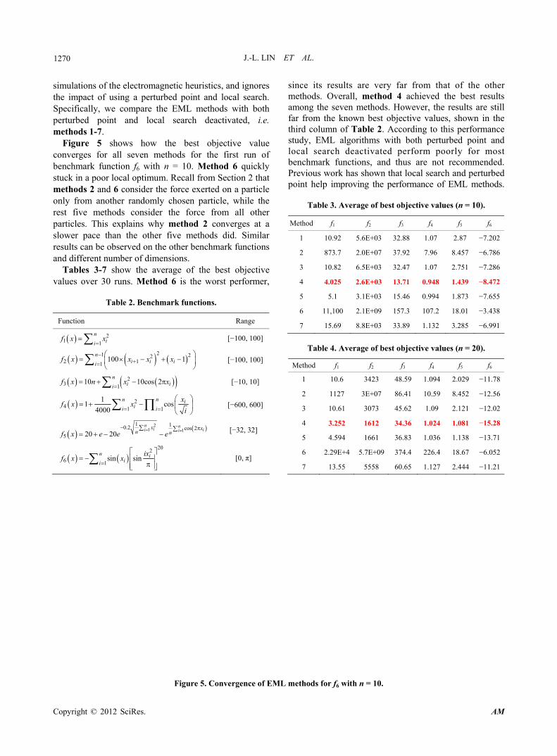
Fi re conv es ods for the first run of benchmark f = 10. Method 6 quickly stuck a p . Recall from Section 2 that

an the other five methods did. Similar re

since its results are very far from that of t methods. Overall, method 4 achieved the b lts among the seven methods. However, the results are still far from the known best objective values, show e third column of Table 2. According to this performance

he otherest resu

n in th

lat of the electromagnetic mp of using a pertu

rb point and local search deaod -7.

gu 5 shows how the best objective value erg for all seven meth

unction f with n6

oor local optimum inmethods 2 and 6 consider the force exerted on a particle only from another randomly chosen particle, while the rest five methods consider the force from all other particles. This explains why method 2 converges at a slower pace th

sults can be observed on the other benchmark functions and different number of dimensions.

Tables 3-7 show the average of the best objective values over 30 runs. Method 6 is the worst performer,

Table 2. Benchmark functions.

Function Range

21 1

nii

f x x

[−100, 100]

21 22

2 11100 1

ni i ii

f x x x x

study, EML algorithms with both perturbed point and local search deactivated perform poorly for most benchmark functions, and thus are not recommended. Previous work has shown that local search and perturbed point help improving the performance of EML methods.

Table 3. Average of best objective values (n = 10).

Method f1 f2 f3 f4 f5 f6

1 10.92 5.6E+03 32.88 1.07 2.87 −7.202

2 873.7 2.0E+07 37.92 7.96 8.457 −6.786

3 86

4. 2.6E+03 1 0. 1. −8. 2

10.82 6.5E+03 32.47 1.07 2.751 −7.2

4 025 3.71 948 439 47

5 5.1 3.1E+03 15.46 0.994 1.873 −7.655

6 11,100 2.1E+09 157.3 107.2 18.01 −3.438

7 15.69 8.8E+03 33.89 1.132 3.285 −6.991

Table ver es ti e 2

M od

4. A age of b t objec ve valu s (n = 0).

eth f1 f2 f3 f4 f5 f6

1 10.6 3423 48.59 1.094 2.029 −11.78

23 1

10 10cos 2n

i ii

[−100, 100]

f x n x x

[−10, 10]

2 1127 3E+07 86.41 10.59 8.452 −12.56

3 .02

3. 1 3 1. 1. −1

2

21 1

os0

nn iii i4

11 c

400

xf x [−600, 600]x

i

10.61 3073 45.62 1.09 2.121 −12

4 252 612 4.36 024 081 5.28

5 4.594 1661 36.83 1.036 1.138 −13.71

6 .29E+4 5.7E+09 374.4 226.4 18.67 −6.052

7 13.55 5558 60.65 1.127 2.444 −11.21

2

1 11 10.2 cos 2

5 20 20n n

i ii ix xn nf x e e e

[− 32, 32]

202

6 1sin sin

n iii

ixf x x

[0, π]

Figure 5. Convergence of EML methods for f6 with n = 10.




Subsequent two sections study their impact on the performance.

4.3. Local Search Test

Birbil and Fang [1] suggested that applying local search on the current best particle improves the performance of their EML method without incurring much overhead. This section evaluates the performance of the seven EML methods with local search on the best particle. We adopted the same local search method as Birbil and Fang [1] did, i.e. random line search, described in Figure 2.

The two parameters for random line search are set as follows: δ = 1E−3 or 1E−4 and LsIter = 150. No attempt is made to fine tune these two parameters to fit different benchmark functions. Notably, for an EML method without local search, the objective function needs to be calculated m − 1 times in each iteration, where m is the

a population. With local search umber becomes m − 1 + n ×

LsI , wh is t f i hLsIter > s n se u that on the electrom etic h istics.

F ure ho ow o e converges for all seven methods for the first run of benchmark function f6 with n = 10 and δ = 1E−3. methods 6L, 7L and 2L converged slower than the other methods did. Table 8. Average of best objective values (n = 10, δ = 1E−3).


1 8.322 2046 30.11 1.079 1.505 −15.93

2 1332 3.1E+07 138.4 14.16 8.317 −16.07

3 8.604 2357 31.03 1.077 1.509 −15.99

4 2.800 1047 64.42 1.013 0.7174 −20.39

5 3.138 1260 57.95 1.021 0.7779 −19.27

6 38,510 1.073E+10 600.1 343.3 18.91 −8.269

7 10.85 3814 45.24 1.093 1.656 −15



1 7.066 1752 25.03 1.062 1.134 −19.72

2 .44

7 1622 24. 1.060 1.157 −19.97

8 1 0. 0

8 0 0

1. 8

2830 3

1693 3.4E+07 200.4 16.45 8.444 −17

3 .085 94

4 2.270 64.1 09.9 9788 .5137 −25.73

5 2.455 863 3.08 .9942 .5263 −24.98

6 51,850 6E+10 51.4 462.5 19 −10.21

7 8.521 8.55 1.08 1.22 −18.49

l era est i e 0

Me 1 2 3 4 5 6

Tab e 7. Av ge of b object ve valu s (n = 5 ).

thod f f f f f f

1 5.261 1400 2 0 −1.54 1.047 .8917 23.34

2

3 5.720 1347 20.80 1.051 0.8957 −22.88

1. 6 140 0. 8 0. −2

1903 5.6E+07 263.1 18.4 8.054 −20

4 879 83.5 886 3154 9.46

5 2.074 764 97.81 0.9206 0.4278 −28.58

6 66,470 2.1E+10 1113 607.1 19.05 −12.24

7 7.382 2337 38.57 1.071 0.8624 −21.89

number of p rticles in the on the best particle, this n

ter ere n he number o dimens ons. W en n × m − 1, the time pent o local arch s rpasses

agnws h

eur theig 6 s best bjectiv value

1L 5.691E−3 32.32 11.89 0.5938 2.215 −8.427

2L 0.7051 2.5E+5 31.77 4.113 8.618 −8.186

3L 5.870E−3 32.32 12.53 0.6692 2.409 −8.370

4L 6.170E−3 124 9.229 0.5563 1.312 −9.045

5L 3.645E−3 106.2 15.77 0.5882 2.163 −8.384

6L 2866 1.8E+8 137.7 64.62 17.58 −6.187

7L 6.825E−3 70.91 12.62 0.6323 2.255 −8.625

Figure 6. C e thods with local search for f6 with n = 10. onverg nce of EML me



Table 9. Average of best objective values (n = 20, δ = 1E−3).


1L 4.337E−2 57.13 20.65 0.419 2.033 –16.45

2L 1.287E−2 513.3 73.04 1.738 9.102 −14.62

3L 4.376E−2 57.13 20.65 0.4191 2.052 −16.44

4L 3.710E−2 45.12 13.47 0.2677 1.315 −18.27

5L 4.239E−2 62.6 23.45 0.2709 1.354 −16.61

6L 818.1 3.1E+7 343.4 33.34 18.49 −13.15

7L 3.629E−2 78.86 19.29 0.4496 2.285 −15.49



1L 0.142 123.2 23.59 0.466 0.996 −23.37

2L 0.027 277.1 125.5 1.480 8.527 −22.46

3L 0.144 123.2 23.59 0.466 0.891 −23.25

4L 0.103 81.27 18.33 0.383 1.227 −25.9

5L 0.119 122.9 28.58 0.385 0.252 −24.04

6L 70.03 3.7E+5 500 26.54 18.72 −18.48

7L 0.127 131 28.56 0.486 1.468 −23.21



1L 0.2384 165.4 27.73 0.4911 0.214 −28.9

2L 3.724E−2 446.9 176.8 1.302 9.058 −26.43

3L 0.2373 165

135.9 39.49 0.4665 0.1159 −29.82

0 756.1 715.9 21.92 18.75 −25.05

0

.4 27.73 0.4911 0.2619 −28.99

4L 0.2521 151.9 30.13 0.4737 1.233 −32.38

5L 0.1979

6L .249

7L 0.2447 151.8 35.36 .5769 0.6629 −28.36

Table 12. Average of best objectiv s 1E−

m

e value (n = 50, δ =3).

ethod f1 f2 f3 f4 f5 f6

1L 0.3521 215.7 3 0. 06.56 5982 .2164 −33.37

2L 6.768E−02 362.5 2 0

3L 0.3525 215.7 36.6 0.5982 0.185 −33.83

5L 0.3499 197.4 55.4 0.503 7.15E−2 −33.54

0.3464 979.5 914.5 16.37 18.83 −28.59

35.37 0.6467 0.3426

19.2 .5261 8.599 −30.97

4L 0.331 213.5 32.35 0.4423 1.226 −39.09

6L

7L 0.3261 228.1 −33.06

Tables 8-12 show the average of the best objective values over 30 runs when δ = 1E−3. Similar to the pre- vi

nt in Tables 8-12. We reduced the

−4, almost all methods with local search yield Table 13. Average of best objectiv s 1E−

M

ous test, method 6L is the worst performer. Compar- ing the results in Tables 8-12 to their counterparts in Tables 3-7, local search on the best particles improves the results in most cases but with some exceptions shown in italicized foparameter δ from 1E−3 to1E−4, and repeated the same experiment. The results are shown in Tables 13-17. With δ = 1E

e value (n = 10, δ =4).


1L 0.8366 375.6 10.16 0.312 1.812 −7.784

2L 482.8 1.9E+7 24.8 8 9.237 −7.233

3L 0.728 305.3 10.15 0.312 1.812 −7.895

4L 3.073E−2 350.9 6.411 0.2346 0.7673 −8.855

5L 9.776E−2 161.1 9.904 0.2009 1.251 −8.205

6L 1.056E+4 1.7E+9 140 92.67 17.43 −4.592

7L 1.525 604.6 9.253 0.3928 2.018 −7.676



1L 4.08E−4 23.55 10.85 0.1026 1.352 −15.71

2L 291 9.6E+6 46.74 3.191 9.181 −14.87

3L 4.21E−4 23.6 10.82 0.1026 −15.81

578E−2 0.4712 −17.59

4 1 2

1 4

3. 1 0.1236

1.352

4L 4.14E−4 14.89 9.699 5.

5L .43E−4 25.2 5.03 5. 44E−2 0.6467 −15.60

6L .92E+4 .6E+9 305 175.3 18.11 −10.87

7L 34E−4 41.4 1.28 1.587 −15.39

Table 15. Average of best objectiv e 1E


e valu s (n = 30, δ =−4).

M

1L 1.14E−3 23.65 3.452 6.907E−2 0.6621 −23.87

2L 87.21 9.5E 74.92 1.933 8.354 −22.57

1 2 3 6

1 3.

1 2 2 4

6 5

8. 7 7

+6

3L .15E−3 3.74 .485 .907E−2 0.7306 −23.94

4L 1.16E−3 28.1 3.12 329E−2 0.1476 −26.11

5L .07E−3 8.91 1.56 .811E−2 0.1288 −23.93

6L 2.7E+4 .3E+9 34.2 215.1 18.56 −17.45

7L 78E−4 27.9 .862 .322E−2 1.309 −23.75



Table 16. Average of best objectiv es 1E−


e valu (n = 40, δ =4).

M

1L 1.95E−3 44.19 1.629 5.55E−2 2.18E−2 −32.01

2L 35.87 5.2E+6 114.3 1.561 8.508 −30.02

1.92 44. 1.6 5.55 2 9.6 2 −31.85

1. 3 2 3. 8

3 8.

3 7. 7

2 4 4

3L E−3 13 29 E− 3E−

4L 87E−3 4.92 2.48 26E−2 .84E−2 −34.93

5L 2.29E−3 39.14 28.3 .83E−2 35E−3 −31.78

6L .1E+4 4E+9 05.6 288.4 18.76 −24.3

7L .1E−3 0.52 3.22 .97E−2 0.4307 −31.80

Ta 17. e t ti ue 5 1E−

ble 4).

Averag of bes objec ve val s (n = 0, δ =

method f1 f2 f3 f4 f5 f6

1L 3.22E−3 47.1 0.139 4.76E−2 1.1E−2 −40.31

2L 16.27 4.4E+6 157.6 0.671 8.056 −36.14

3L 3.28E−3 47.08 0.139 4.75E−2 6.91E−2 −40.56

4L 4.33E−3 49.4 26 3.58E−2 4.48E−2 −43.13

5L 3.52E−3 58.88 37.14 3.43E−2 1.08E−2 −39.75

6L 3.66E+4 7.7E+9 825.3 324.4 18.89 −30.24

7L 3.62E−3 47.39 0.67 4.42E−2 0.3323 −39.23

better results than their counterparts without local search, with few exceptions of method 2L on f5 for n = 10 to 50 a for = 10.

According to Tables 8-17, method 6L remains the wo an od e s y astances. Al h n e od p form all instances, a ap r tw erfo m 1 o w n ins es

4.4. Perturbed Point Test

As described in Section 2.2.2, Birbil et al. [9] proposed a ne ML od m e o al EML

ethod using a perturbed point. Since the original EML

is denoted as method 1P herein. Both methods d ly how e fo exer on th rtu ed p lated.

ed a a ho a d us e per d , the tin h denoted as methods 2P-7P. Notably, these perturbed me ds te tiv ti e nu r o s n r r

The param ν ned Sect 2. or t pe s t i s show the performance results of these perturbed methods.

Ta 18 e ob ve (n

M d

nd on f4 n

rst, d meth 2L p rform poorl on m ny in- thoug o singl meth er s the best on

methodsrmers.

4Lethod

nd 5LL als

pea does

to be tell o

he top someo p

tanc .

w E meth that odifi s the riginmmethod is denoted as method 1 in Table 1, the new method

iffer onarticle is calcu

on th

rce ted e pe rb

Bas on the s me ide , met ds 2-7 re mo ified toe th turbe particle and resul g met ods are

tho calcula s the objec e func on th samembe f times a their on-pe turbed counterpa ts do.

eter method

, defiis set

ino 0.5

ion n this test

2.2, f. Table

hese 18-22rturbed

ble . Averag of best jecti values = 10, perturb).

etho f1 f2 f3 f4 f5 f6

1P 10.89 4.9E+3 34.59 1.11 2.922 −7.014

2P 712.8 1.9E+7 47.841 6.568 8.855 −6.643

3P 11.14 6602 31.497 1.098 2.885 −7.075

2.2E

1.0E

4P 4.185 2534 12.431 0.961 1.199 −8.604

5P 5.53 3279 18.105 1.017 1.703 −7.765

6P 1.1E+4 +9 157.73 108.449 18.052 −3.377

7P 15.18 +4 34.93 1.101 3.251 −6.778

Ta 19 e o o e

M d

ble . Averag f best bjective values (n = 20, p rturb).


1P 11.33 3 2843 47.11 1.097 .127 −11.87

2P 1611 9.34E+7 142.22 16.274 9.210 −11.63

3P 10.75 3961 45.624 1.098 2.147 −11.931

−

6

4P 3.149 1487 33.88 1.024 0.898 14.947

5P 4.444 1989 35.002 1.034 1.205 −14.621

6P 23,442 .1E+9 373.42 230.95 18.675 −6.161

7P 13.77 5388 56.742 1.120 2.434 −11.321

Table 20. Avera objective va

M d

ge of best lues (n = 30, perturb).


1P 8.634 2477 29.79 1.078 1.509 −15.77

2P 3015.6 1.4E+8 249.925 30.663 8.547 −14.46

3P 8.645 2316.8 30.842 1.073 1.516 −15.93

1043. 67.331

3.151 1099.9 62.754 1.022

1 6

4 45

4P 2.633 1 1.003 0.858 −20.61

5P 0.783 −19.64

6P 38,769 E+10 01.736 349.424 18.904 −8.29

7P 10.49 038 .664 1.105 1.697 −15.23

Ta 21 o o e

M d

ble . Average f best bjective values (n = 40, p rturb).


1P 6.861 1657 26.45 1.064 1.113 −19.67

2P 0.00195 44.188 1.6287 0.056 0.022 −32.01

3P 0.00223 42.143 2.3595 0.072 0.212 −32.154

4P 35.8705 5,234,622 114.29 1.561 8.508 −30.017

5P 0.00192 44.128 1.6288 0.056 0.096 −31.847

6P 0.00187 34.920 22.4778 0.033 0.088 −34.934

7P 0.00229 39.141 28.2972 0.038 0.008 −31.782



Table 22. Average of best objective values (n = 50, perturb).

f4 f5 f6 Method f1 f2 f3

1P 5.72 1355 22.64 1.047 0.8617 −23.47

2P 0.0032 47.099 0.139 0.048 0.0110 −40.305

3P 0.0031 52.434 0.338 0.037 0.0109 −39.668

4P 16.27 4,366,733 157.607 0.671 8.0557 −36.135

5P 0.0033 47.078 0.139 0.048 0.0691 −40.565

6P 0.0043 49.402 26.001 0.036 0.0448 −43.134

7P 0.0035 58.879 37.136 0.034 0.0108 −39.753

Among them, method 4P appears to perform the best

for n ≤ 30, while methods 5P-7P perform the best for n > 30.

However, when comparing to their non-perturbed counterparts in Tables 3-7, these perturbed methods often yield no improvement (shown in italicized font in Tables 18-22), especially for n ≤ 30. Although these p d m ds b er ch o escape f local optimums, they often require much more iterations to reach t ba u nce ma n of iteratio re t m dim ons, t ese pe ur et t expe ence nefi of a be ino ge e

5. Conclusions

This paper studies various interpretations of the electro netic heur al m r

ow that EML methods without local search and

methods 2 and 6. Notably, methods 2 and iffer om o ethods in two aspects. Firstly, they con er the elect ne rc ra chosen pa h ti e , they move er th h r me ds eci y, e , p ex to p e d e movement ri to han the dista be es j. t o is n e . ri s ne to th pr o o .

e, e n her be nt ca ,

n ran bett perfo ance. Actually si le interpretation of the electromagnetic heuristics con- sis ly ms er oth not e e h p o best ethod th rt po , its u v d b s quite unstable. Overall, these perturbed methods often yield

po re th ir tu o a . Therefore, i pr ur e que a int tin io L od fu research top

6. kn dg n

under Grant NSC 99-2221-E-155-048-MY3, and by the B of E rgy, M stry o conom s, Ta an, un the ect he of As ti - coupling Algorithms.

R E[1] . I. a ti

ec fo O t o o l , Vol. 25 03, pp .

oi: A: 26

erturbe etho have a ett ance t rom

he glo l optim m. Si the ximal umberns is set to 25n, whe n is he nu ber of

ensiri

h the be

rtt

bed mpertur

hods md part

ight ncle whe

ot yen n is

t lar nough.

mag istics in EML gorith s. Ou resultsshperturbed point often yield poor results, especially for

6 d frsidther EML m

romag tic fo e from only one ndomlyrticle particles in

instead o a less free m

f all ot er parann

cles. San t

condlye othe

tho do. Sp ficall with m thod 2 when article ierts a force move articl j, the istanc of this

is restparticl

ctedi and

no greater tThe dis

ncevementtween ance of this m

eve smaller with m thod 6 Further expe ment ieded

abl findven usi

e culg eit

it for th pertur

eir pod poi

r perfor lo

rmancel searchNot

methods 2P, 2L, 6P and 6L still yield unstable results. Strictly following the electromagnetic heuristics does

ot gua tee er rm , no ng

tent perfor bett than er interpretations. Onabl xample is met od 4, which ap ears t be the m

pert wi

rbed no localersion,

and pemetho

urbed4P,

int. Hoecome

wever

orer sults an the un-per rbed c unterp rts dom

g varoving tus EM

he pert meth

bed ts are

chniture

ndegraics.

Ac owle eme ts

This research is supported by National Science Council

ureau ne ini f E ic Affair iwder proj of T Study socia ve De

REFE ENC S S Birbil and S. C. F ng, “An Electromagne sm-Like

MOptimization

hanism r Global, No

ptimiza. 3, 20

ion,” J. 263-282

urnal f Globa

d 10.1023/ 102245 26305

[2] . D . D k, , b

l. 1 . 638-653:10 16/j.ejor.2004.08 0

D ebels, B e Reyc R. Leus et al., “A Hy rid Scat-ter Search/Electromagnetism Meta-Heuristic for Project Scheduling,” European Journal of Operational Research, Vo 69, No. 2,

.102006, pp .

doi .02

[3] . C. g, S hen . , br - om m Al

Problem,” Exp , ol . 2 pp 12oi:1 6/

P Chan . H. C and C Y. Fan “A Hy id Electr agnetis -Like gorithm for Single Machine SchedulingV

ert Systems with Applications. 1259-. 36, No , 2009, 67.

d 0.101 j.eswa.2007.11.050

[4] . ko h . , le gne ike ani nd Si a

eal o or o ein th W T a

Knowledge-Based Systems, Vol. 23, No. 2, 2010, pp.

B Naderi, R. Tavak li-Mog addam and M Khalili“En

ctromaing Alg

tism-Lrithms f

Mech Flowsh

sm ap Sch

mulduling Problems

ted An-

M imizing e Total eighted ardiness and M kespan,”

77-85. doi:10.1016/j.knosys.2009.06.002

[5] A. Yurtkuran and E. Emel, “A New Hybrid Electromag- netism-Like Algorithm for Capacitated Vehicle Routing Problems,” Expert Systems with Applications, Vol. 37, No. 4, 2010, pp. 3427-3433. doi:10.1016/j.eswa.2009.10.005

[6] C. T. Su and H. C. Lin, “Applying Electromagnetism-Like Mechanism for Feature Selection,” Information Sciences, Vol. 181, No. 5, 2011, pp. 972-986. doi:10.1016/j.ins.2010.11.008

[7] C. H. Lee and Y. C. Lee, “Nonlinear Systems Design by a Novel Fuzzy Neural System via Hybridization of Elec- tromagnetism-Like Mechanism and Particle Swarm Optimisation Algorithms,” Information Sciences, Vol. 186, No. 1, 2012, pp. 59-72. doi:10.1016/j.ins.2011.09.036

[8] A. M. A. C. Rocha and E. M. G. P. Fernandes, “Hybrid- agnetism-like Algorithm with Descent

lving Engineering Design Problems,” izing the ElectromSearch for SoInternational Journal of Computer Mathematics, Vol. 86, No. 10-11, 2009, pp. 1932-1946. doi:10.1080/00207160902971533

[9] S. I. Birbil, S. C. Fang and R. L. Sheu, “On the Conver- gence of a Population-Based Global Optimization Algo- rithm,” Journal of Global Optimization, Vol. 30, No. 2-3,


J.-L. LIN ET AL.


1275

2004, pp. 301-318. doi:10.1007/s10898-004-8270-3

[10] Q. Wang, J. Zeng and W. Song, “A New Electromagnet- ism-Like Algorithm with Chaos Optimization,” Proceed- ings of 2010 International Conference on Computational Aspects of Social Networks, Taiyuan, 26-28 September 2010, pp. 535-538.

[11] A. M. A. C. Rocha and E. M. G. P. Fernandes, “Numeri- cal Experiments with a Population Shrinking Strategy within an Electromagnetism-Like Algorithm,” Interna- tional Journal of Mathematics and Computers in Simula- tion, Vol. 1, No. 3, 2007, pp. 238-243.

[12] P. Kaelo and M. M. Ali, “Differential Evolution Algo- rithms Using Hybrid Mutation,” Computational Optimi- zation and Applications, Vol. 37, No. 2, 2007, pp. 231-246. doi:10.1007/s10589-007-9014-3

[13] A. M. A. C. Rocha and E. M. G. P. Fernandes, “Perfor-

mance Profile Assessment of Electromagnetism-like Al- gorithms for Global Optimization,” International Elec- tronic Conference on Computer Science, AIP Conference Proceedings, Vol. 1060, 2008, pp. 15-18 doi:10.1063/1.3037042

[14] A. M. A. C. Rocha and E. Fernandes, “On Charge Effects to the Electromagnetism-Like Algorithm,” Proceedings of Euro Mini Conference “Continuous Optimization and Knowledge-Based Technologies”, Ne2008, pp. 198-203.

ringa, 20-23 May

, pp. 165-169.

[15] Y. Shang, J. Chen and Q. Wang, “Improved Electromag- netism-like Mechanism Algorithm for Constrained Opti- mization Problem,” Proceedings of 2010 International Conference on Computational Intelligence and Security, Nanning, 11-14 December 2010

http://dx.doi.org/10.1016%2Fj.eswa.2009.10.005

performance comparison of electromagnetism-like …file.scirp.org/pdf/am20123000007_64009232.pdf ·...

Documents