1

Performance Evaluation of an Improved Fully Stressed Design

Evolution Strategy on Simultaneous Topology, Shape and Size

Optimization of Large-Scale Truss Structures

Ali Ahraria* and Kalyanmoy Deb

COIN Report Number 2016023

Notice

This is the pre-print version of the paper entitled “An improved fully stressed design evolution

strategy for layout optimization of truss structures” published in “Computers & Structures”.

Some revisions were performed in the subsequent stages. Please use the published version [1] for

citation. If you are interested in this work but do not have access to the published version, please

contact the corresponding author.

[1] Ahrari, A., & Deb, K. (2016). An improved fully stressed design evolution strategy for layout

optimization of truss structures. Computers & Structures, 164, 127-144.

doi:10.1016/j.compstruc.2015.11.009

The source code in MATLAB, with some minor revisions, is also available at the Research

Gate page of the first author:

https://www.researchgate.net/publication/296694688_Source_code_for_the_improved_fully_stre

ssed_design_evolution_strategy_FSD-ES_II

2

Performance Evaluation of an Improved Fully Stressed Design

Evolution Strategy on Simultaneous Topology, Shape and Size

Optimization of Large-Scale Truss Structures

Ali Ahraria and Kalyanmoy Debb

a Graduate Student. Department of Mechanical Engineering, Michigan State University, East Lansing,

MI, USA, email: aliahrari1983@gmail.com

b Koenig Endowed Chair Professor, Department of Electrical and Computer Engineering, Michigan State

University, East Lansing, MI, USA, email: kdeb@egr.msu.edu, http://www.egr.msu.edu/~kdeb

Abstract During the recent decade, truss optimization by metaheuristics has gradually replaced

deterministic and optimality criteria-based methods. While they may provide some advantages

regarding their robustness and ability to avoid local minima, the required evaluation budget grows

fast when the number of design variables is increased. This practically limits the size of the

problems to which they can be applied. Furthermore, most recent stochastic optimization methods

handle the size optimization only, the potential saving from which is highly limited, when

compared to the most sophisticated, and obviously the most challenging scenario, simultaneous

topology, shape and size (TSS) optimization. In a recent study by the authors, a method based on

combination of optimality criteria and evolution strategies, called fully stressed design based on

evolution strategies (FSD-ES), was proposed for TSS optimization of truss structures. FSD-ES

outperformed available truss optimizers in the literature, both in efficiency and robustness. The

contribution of this study is two-fold. First, an improved version of FSD-ES method, called FSD-

ES-II, is proposed. In comparison with the earlier version, it takes the displacement constraints in

the resizing step into account and can handle constraints governed by practically used

specifications. Update of strategy parameters is also revised following contemporary and new

developments in evolution strategies. Second, a test suite consisting of large scale TSS

optimization problems is developed to overcome some shortcomings in available benchmark

problems. For each problem, performance of FSD-ES-II is compared with the best results

available in the literature, often showing a significant superiority.

Keywords: Covariance matrix self-adaptation, Mixed-variable problem, Structural optimization,

Stochastic rounding, Adaptive penalty function

3

1 Introduction

Truss design optimization can be considered from three distinct perspectives. Topology

optimization determines the optimum connection plot of members. Shape optimization optimize

coordinates of the nodes for a known topology and size optimization finds the optimum cross

sections of the members. The optimized structure should satisfy some constraints on member

stress, node displacement, slenderness ratio or even natural frequency.

The methods commonly used for truss optimization are based on optimality criteria or

mathematical programing [1, 2]. The former assumes that the optimal design should satisfy a priori

conditions [3]. The concept of fully stressed design (FSD) is the most common approach in this

group, which assumes in the optimally sized structure, all members reach the stress limit at least

in one of the load cases [3]. Accordingly, all members are iteratively resized to reach this goal,

assuming that the force distribution does not change when members are resized. This assumption

is perfectly valid for determinate structures, in which FSD can potentially reach the global

minimum in one iteration. This is not the case for indeterminate structures, however, when the

number of redundant members is small, the error prompted by this assumption is usually small,

and iterative resizing, at least when the resizing step is controlled [3], can reach a high quality

design. The required number of design evaluations is almost independent of the number of

members [3], and the method usually reaches a good solution after a few iterations [3]. Later, the

concept of FSD was extended to handle problems with multiple load cases, displacement

constraints, or when more sophisticated failure criteria are governed by design specifications [1].

For these reasons, FSD used to be preferred over mathematical programming, when the

computation resources were limited [3], except for highly indeterminate structures, where FSD

risks divergence [3]. However, it does not take the objective function into account and thus, use of

more sophisticated objective functions that consider other factors in the overall cost, is not directly

applicable. When there are multiple displacement constraints, FSD leads to a resizing problem

which is not easy to solve analytically.

Unlike optimality criteria, mathematical programming are robust tools to solve general

optimization problems [3]. With recent development in computation tools and parallel computing,

the challenge of costly evaluations has been moderated to great extent. At the same time, stochastic

optimization techniques such as evolutionary algorithms (EAs) and swarm-based methods were

developed and demonstrated some advantages over deterministic approaches, especially in

4

multimodal problems. There has been a large number of studies on truss optimization with

stochastic methods in the recent decade. Most of them, however, consider the simplest scenario,

size optimization. The number of recent publications on size optimization with stochastic methods

is relatively huge, too many to cite. Some examples can be found in [4, 5].

More sophisticated schemes consider shape or topology optimization as well. Topology

optimization is particularly a challenging task, since even a small variation in topology can result

in significant change in member forces and besides, many kinematically unstable structures might

be produced during the search. The most sophisticated scheme, and potentially the most effective

one [2], performs topology, shape and size (TSS) optimization at the same time. Nevertheless,

studies on TSS optimization are comparatively scarce, possibly because of the complexity of the

problem nature which demands sophisticated specialization of metaheuristics. Several strategies

to circumvent this complexity, in the case of TSS optimization, were proposed in the literature,

however, they usually reduces potential for better solutions [6]. Moreover, the size of the test

problems employed to validate the algorithms is usually small or moderate at best [7, 8, 9, 10, 11].

A few studies tried fairly large problems as well [12, 13, 6], but comparison with other methods

were not provided.

In a recent method, called fully stressed design based evolution strategy (FSD-ES) [14, 6], the

concept of FSD was employed to resize the designs produced by an evolution strategy. In

comparison with earlier stochastic optimization methods, FSD-ES could reach lighter structures

in smaller number of function evaluations. The resizing step helps the method find near optimally

sized structure for a given shape or topology defined by the evolution strategy.

This study aims at overcoming some general drawbacks in stochastic TSS truss optimization

by improving the earlier version of FSD-ES. The contributions of this study to truss optimization

field are as follows:

- An improved version of the resizing technique is proposed, which can take displacement

constraints into account. We also propose an optimality criteria-based heuristic to solve the

resizing problem.

- The employed evolution strategy is revised and the traditional mutative self-adaptation

concept is replaced by a strategy based on contemporary evolution strategies.

5

- A revision to the fitness function is provided to compare kinematically unstable structures

as well.

- Emphasis is put on large-scale TSS problems, with up to 308 design parameters. Some of

the test problems are proposed in this study, by converting a simpler problem to a

complicated TSS problem.

In the next section, previous work on two main components of FSD-ES are briefly reviewed.

The improved method, called FSD-ES-II, is explained in section 3. A test suite consisting of large

scale TSS truss optimization problems is formed in section 4 and results from FSD-ES-II are

compared to the best available results in the literature in section 5.

2 Main parts

FSD-ES utilized two underlying concepts: The ES part performs the stochastic global search in

the whole search space while the FSD part optimize the size variables of the solution provided by

the ES. By using FSD, problem specific knowledge is incorporated to the algorithm. These two

parts are briefly discussed in this section.

2.1 Fully Stressed Design (FSD)

In general, the truss optimization problem can be formulated as follows:

Minimize 𝑤𝑒𝑖𝑔ℎ𝑡(𝛉) = 𝜌 ∑ 𝐴𝑖𝑙𝑖𝑁𝑚𝑖=1

subject to

𝑢𝑘𝑙 ≤ 𝑢𝑘all , 𝑘 = 1, 2, … , 𝐷𝑁𝑛, 𝑙 = 1, 2, … , 𝑁𝑙,

|𝜎𝑖𝑙| ≤ 𝜎𝑖all , 𝑖 = 1, 2, … , 𝑁𝑚, 𝑙 = 1, 2, … , 𝑁𝑙,

𝐴𝑖 ∈ 𝔸, 𝑖 = 1, 2, … , 𝑁𝑚, (1)

where θ determines a design. Nm, Nn and Nl are the number of members, nodes and load cases

respectively. D=2 for planar and D=3 for spatial trusses. σ and u represent the member stress and

the node displacement respectively and superscript ‘all’ stands for the allowable limit, which is

known or can be computed. ρi, Ai and li are the density, cross-section area and length of the i-th

member respectively and 𝔸 is the given set of available sections.

FSD is based on iterative resizing of the member cross section areas to minimize the truss

weight such that all constraints are satisfied. No change on the topology or shape is made and thus,

6

the only design parameters are member sections, A. The force distribution is assumed to be

independent of the member cross section areas. For this case, the effect of each member on

displacement can be computed using the unit load method:

𝑢𝑘𝑙(𝑨) = |∑𝑐𝑖𝑘𝑙

𝐴𝑖

𝑚

𝑖=1

| , (2)

where cikl’s are known from the truss analysis. Since each displacement constraint depends on

many or even all sections, solving the resizing problem, in general, is not easy. In a study [3], a

two-step approach was employed such that in the first step, member sections are increased or

decreased so that all stress constraints are satisfied and activated. In the second step, satisfaction

of displacement constraints is pursued, while, no reduction in the cross section areas is allowed.

For the case with only one displacement constraint, using optimality criteria leads to [15]:

𝐶𝐸 =𝜕𝑤

𝜕𝐴𝑖

𝜕𝑢

𝜕𝐴𝑖⁄ , 𝑖 = 1,2, … , 𝑁𝑚, (3)

which can be interpreted as cost effectiveness (CE) of the i-th member in reduction of the constraint

[15]. According to the equation 3, in the optimally sized structure, cost effectiveness of all

members are the same. When sections are discrete, average cost effectiveness should be defined:

𝐶𝐸 ≅∆𝑤

∆𝐴𝑖

∆𝑔

∆𝐴𝑖⁄ , 𝑖 = 1,2, … , 𝑁𝑚, (4)

where ΔAi is the difference between the current section area and the next/previous area in 𝔸. For

the more general case, when there are multiple displacement constraints, the common approach is

to merge all displacement constraints into one constraint [15]. Schevenels et al. [15] proposed

computation of average cost effectiveness of each member for all possible solutions around the

current design, and selecting the one with the least average cost effectiveness. This process is

repeated until a convergence condition is met. Although it was demonstrated that this strategy is

able to reach a stable point, the computation of average cost effectiveness for all possible designs

around the current design is exponentially expensive, which limits the number of independent

sections in the problem.

2.2 Evolution strategies

Evolution strategies (ESs) are one the main streams of EAs which follow the principles of

evolutionary biology including recombination, mutation and selection. In the general form, λ

descendants are produced from μ parents. Selection is performed over the offspring only (comma

7

scheme) or the union of offspring and parents (plus scheme) to select parental population for the

next generation. Mutation is rendered by variation of all variables simultaneously, using

multivariate normal distribution. Parameters of the mutation distribution, called endogenous

strategy parameters [16], are adjusted during the optimization. In traditional ESs, these parameters,

are updated according to the concept of mutative self-adaptation [16] [17], according to which

strategy parameters are mutated first, and the new solution is generated using the mutated

parameters. Fitness of the individual is correlated to the aptness of the mutation and thus, strategy

parameters are updated similar to the way the design (object) variables are.

In covariance matrix adaptation evolution strategy (CMA-ES) [18], known as the state of the

art ES [19, 17], adaptation of the global step size is rendered using cumulation, and the covariance

matrix is adapted in a de-randomized manner, in order to overcome some shortcomings of self-

adaptation. For the same reasons, most contemporary evolution strategies employ the de-

randomized approach [17].

CMA-ES, and its variants [17], provide spectacular results in unconstrained continuous

parameter optimization, especially in ill-conditioned problems. Nevertheless, the complexity of

the adaptation process reduces its flexibility, when applied to constrained mixed-variable

problems. In another study [20], a simpler variant of this method, called CMSA-ES, was proposed

which may compete with the original CMA-ES, at least when highly ill-conditioned problems are

excluded. Because of its simplicity, it shows more flexibility for specialization for highly

constrained mixed-variable TSS problems. The pseudo code of one iteration of CMSA-ES can be

summarized as follows:

For j=1 to λ

𝜎𝑗 = 𝜎mean exp(𝜏𝒩(0,1)), 𝒛𝑗 = √𝐂 𝓝(𝟎, 𝟏), 𝒙𝑗 = 𝒙mean + 𝜎𝑗𝒛𝑗

Compute f(xj)

End

Sort individuals (xj’s) based on their function value.

Let 𝜎mean ⟵ ∏ ((𝜎𝑗)𝑤𝑗

)𝜇𝑗=1 , 𝒙mean ⟵ ∑ 𝑤𝑗𝒙𝑗

𝜇𝑗=1 , 𝐂 ⟵ (1 −

1

𝜏𝑐) 𝐂 +

1

𝜏𝑐∑ 𝑤𝑗𝒛𝑗𝒛𝑗

𝑇𝜇𝑗=1

In the pseudo code, λ is the population size, μ is the number of parents, σj is the individual step

size generated from the global step size σmean, C is the covariance matrix and σjzj is the perturbation

applied to the recombinant design, xmean, to generate the new solution, xj. τ and τc are fixed numbers

8

specifying the learning rate for the global step size and the adaption interval for the covariance

matrix respectively. wj’s specify the weights of parents in the updating process. In CMSA-ES,

these weights are equal (wj=1/μ), while in the original CMA-ES, logarithmically decreasing

weights [18] (𝑤𝑗 = (ln(𝜇 + 1) − ln(𝑗))/ ∑ (ln(𝜇 + 1) − ln(𝑗)))𝜇𝑗=1 were preferred.

Several ES-based methods for structural optimization have been developed in the last decades

[21, 22, 23]. However, most of them demonstrate significant deviation from the state-of-the-art

ESs [14]. Although this might be necessary to handle mixed-variable highly constrained truss

optimization problems, such modifications may result in a significant decline in capabilities of the

method. Direct implementation of the standard CMA-ES for truss optimization, as performed in a

few studies [24, 25], may have its own disadvantages. Size parameters should be assumed to be

continuous, a condition which can hardly be met in practice. The CMA-ES method needs a

separate handling of constraints, which remains a constant challenge to its users.

3. FSD-ES-II

The main steps of the FSD-ES-II are explained in details. Some steps are quite similar to the older

version, FSD-ES [6].

3.1 Problem representation

In FSD-ES-II, each candidate design, θ, is represented by 3 vectors:

- M is a vector of size Nm, whose elements are Boolean variables that determine whether a

member is active (Mi=1) or passive (Mi=0) in the design.

- X is a vector of size DNn, whose elements are continuous variables that determine nodal

coordinates, where D=2 for planar and D=3 for spatial trusses.

- A is a vector of size Nm, whose elements are discrete variables that determine member

cross sections areas.

Accordingly, θ={M, X, A} is a vector of size 2Nm+DNn, with upper and lower limits of θu and θl

respectively.

3.2 ES-based sampling of new designs

Because of its simplicity, and thus flexibility for tailoring for highly constrained mixed-variable

TSS problems, CMSA-ES is preferred over CMA-ES in this study. In FSD-ES-II, only diagonal

9

elements of the covariance matrix are considered. This reduces the covariance matrix to vector d,

which is of the size of θ. all solutions are sampled by applying a perturbation to the recombinant

design, θmean={Mmean, Xmean, Amean}. In the first iteration, Xmean and Amean are the center of the range

defined by the search space limits. Mmean=1 so that most sampled solutions in the early iterations

have sufficient number of members. To generate a new solution, the global step size is mutated

first:

𝜎𝑗 = 𝜎mean exp(𝜏𝒩(0,1)). (5)

σj is then used to generate θj:

𝚯up = 𝑭(𝜽U, 𝜽mean, 𝜎𝑗𝒅), 𝚯low = 𝑭(𝜽L, 𝜽mean, 𝜎𝑗𝒅), (6)

𝜽𝑗 = 𝑭−1(𝒓⨂(𝚯up − 𝚯low) + 𝚯low, 𝜽mean, 𝜎𝑗𝒅), (7)

where F(θU, θmean, σjd) computes the cumulative function of normal distribution at θU with mean

of θmean and standard deviation of σjd in an element-wise manner. The sign ⨂ denotes element-

wise multiplication and r is a vector of uniform random numbers in [0, 1]. Equation 6 demonstrates

that θj is sampled from the truncated normal distribution such that it falls within the limits defined

by θL and θU. θj consists of continuous numbers and thus cannot be evaluated. The stochastic

rounding technique utilized in FSD-ES [6] is applied to size and topology variables to create the

actual design, which stochastically rounds the size and the topology variables to the upper or lower

permissive value. The flowing necessary conditions are then checked for kinematic stability and

acceptability of the generated design [26]:

All necessary nodes must be active.

Truss must have at least the minimum number of members required for kinematic stability:

The number of active members plus the number of reactions from the supports must be

equal or greater than the number of active nodes multiplied by D.

The number of members connected to an active node plus the number of reactions on that

node must be equal or greater than D.

Checking these necessary, but not sufficient, conditions for kinematic stability is

computationally inexpensive, since it does not require performing a finite element analysis. If the

generated design does not satisfy any of these conditions, it is discarded and a new topology is

sampled. This process continues until a design that satisfies all these conditions is generated and

accepted. For each accepted design, vector 𝝕𝑗𝑋 of size DNn and vector 𝝕𝑗

𝐴 of size Nm store the data

10

pertaining to activeness or passiveness of shape and size variables in θj respectively. These vectors

consists of Boolean variables, in which ‘1’ refers to an active and ‘0’ refers to a passive size or

shape variable. These vectors are utilized to exclude the effect of passive shape and size variables

on the updating process, which is explained in section 3.5.

3.3 Design evaluation

Analytically, a truss is kinematically stable if an only if the determinant of the stiffness matrix is

not zero; however, since software computes the determinant numerically and the precision is

limited, this cannot be employed as a reliable metric. In this study, the command ‘rcond’ of

MATLAB© software is used to calculate an estimate for the condition number of the stiffness

matrix. It is assumed that truss is kinematically stable if and only if rcond(Kj)>10-12, where Kj is

the stiffness matrix of the structure. If the truss is found to be kinematically unstable, the cost of

the truss is assigned as follows:

𝑓(𝜽𝑗) = 10100 × (1 +𝑛𝑢𝑙(𝐊𝑗) + 𝑁𝑗

red

𝑁𝑗req ) , if 𝑟𝑐𝑜𝑛𝑑(𝐊𝑗) ≤ 10−12, (8)

where nul(Kj) is nullity of Kj, Njreq is the minimum number of members required for kinematic

stability of the truss and Njred is the number of redundant members. Applying the coefficient of

10100 ensures all kinematically unstable structures are inferior to all stable ones. nul(Kj) is an

integer number which shows how much the structure is far from kinematic stability, or

equivalently, how kinematically unstable the structure is. This provides a unique tool for

comparing even kinematically unstable designs so that by preferring less kinematically unstable

designs, the population size is directed towards regions with kinematically stable designs. Using

equation (8) is and should be considered as a function evaluation, even though the full analysis of

the structure is not performed, since it requires formation of the stiffness matrix and computation

of the nullity, the required time for which is in the same order of a full analysis.

If the design is kinematically stable, the system response, including the member forces and

node displacements to the external load(s), as well as the unit loads (required to compute cikl’s in

Equation 2), are computed. FSD-ES [6] utilizes a specialized penalty function based on the

estimated required increase in the cross section areas such that all constraints are satisfied. This

required increase, when multiplied by the penalty coefficients, form the penalty term. The penalty

term in FSD-ES-II follows the same strategy, with slight modification in formulation. First, for

11

each member, the smallest section area Âji ≥ Aji is sought such that it satisfies all member-based

constraints (slenderness, buckling and stress), assuming that the axial force does not change. If the

largest section in 𝔸 cannot satisfy these constraints, a virtual Âji that satisfies these constraint is

determined whose radius of gyration is equal to the radius of gyration of the largest section area in

𝔸. Âji − Aji is the estimated required increase in the current value of Aji so that the i-th member

satisfies all member-based constraints. To compute the required increase for satisfaction of

displacement constraints, section areas of all members are increased proportionally:

�̌�𝑗𝑖 = 𝐴𝑗𝑖 max𝑘,𝑙

{|𝑢𝑗𝑘𝑙

𝑢𝑘all

|} , 𝑘 = 1, 2, … , 𝐷𝑁𝑛, 𝑙 = 1, 2, … , 𝑁𝑙, (9)

According to equation 9, if Ăji’s replace Aji’s, all displacement constraints will be satisfied. The

penalized objective function is calculated considering the estimated required increase in the

structure weight as follows:

𝑓(𝜽𝑗) = ∑ 𝜌𝑖𝐴𝑗𝑖𝑙𝑗𝑖

𝑁𝑚

𝑖=1

+ ∑ 𝜌𝑖𝑙𝑗𝑖 max{𝑃𝑖(�̂�𝑗𝑖 − 𝐴𝑗𝑖), (�̌�𝑗𝑖 − 𝐴𝑗𝑖)},

𝑁𝑚

𝑖=1

(10)

where Pi ≥1 is the penalty coefficient for the i-th member, applied to member-based constraint

violations only, since the required increase of Âji−Aji is computed assuming the member force does

not change when the section is modified. If a displacement constraint is violated, all cross sections

are proportionally increased, which does not affect member forces even in indeterminate

structures, and thus, the penalty coefficients are not applied to the Ăji−Aji term. Pi’s are iteratively

adapted at the end of each iteration, as it will be explained in section 3.5. For the first iteration,

Pi=1, i=1, 2, …, Nm.

3.4 Resizing

In the resizing step of FSD-ES, a new design (θj+λ ) is generated by resizing the members of θj,

without any change to the shape or topology variables. θj+λ can be interpreted as a near optimally

sized structure whose shape and topology is prescribed by θj. Member forces and coefficients cijl’s

in Equation 2 are known from evaluation of θj, which are assumed to be independent of member

cross section areas. Resizing is performed only if θj is kinematically stable, otherwise we simply

set θj+λ = θj. In FSD-ES-II, resizing is performed in two steps. In the first step, members are resized

12

for stress constraints and in the second step, the resized members are resized again so that all

displacement constraints are satisfied.

3.4.1 Stress-based resizing

For each member, a new cross section is assigned such that the member satisfies all member-based

constraints. Search for the acceptable section performs in a limited range around the current value:

�́�𝑗𝑖d = 𝑅𝑜𝑢𝑛𝑑𝑈𝑝𝐴 (

𝐴𝑗𝑖

1 + (𝑐𝐴 − 1)exp(1 − 𝑃𝑖)) , �́�𝑗𝑖

u = 𝑅𝑜𝑢𝑛𝑑𝑈𝑝𝐴(𝑐𝐴𝐴𝑗𝑖),

�́�𝑗𝑖 = 𝐹𝑖𝑛𝑑𝐴𝑐𝑐𝑆𝑒𝑐([𝐹𝑖1, 𝐹𝑖2, … , 𝐹𝑖𝑁𝑙]; �́�𝑗𝑖

d ; �́�𝑗𝑖u ), (11)

where function RoundUpA rounds the argument to the nearest available section area in 𝔸 and

function FindAccSec finds the smallest acceptable section area (�́�𝑗𝑖 , �́�𝑗𝑖d ≤ �́�𝑗𝑖 ≤ �́�𝑗𝑖

u ) such that it

satisfies all member-based constraints in all load cases. Fil’s are member forces in different load

cases. If such a section cannot be found in the provided range, the function simply selects �́�𝑗𝑖 =

𝐴𝑗𝑖u . cA controls the maximum possible change in Áji. As it will be explained in section 3.5, an

increase in Pi implies in most recently generated solutions, Áji has violated a constraint. If this

happens, reduction of Áji becomes more limited to prevent algorithm divergence. cA is adapted

iteratively based on the success of resizing in reduction of the cost, which will be explained in

section 3.5. However, 𝑐𝐴d≤cA≤𝑐𝐴

u, where 𝑐𝐴d is the maximum of the ratio of areas of two successive

sections in 𝔸 and 𝑐𝐴u is the ratio of the largest to the smallest areas in 𝔸. For the first iteration,

cA=𝑐𝐴u.

3.4.2 Displacement-based resizing

Áji’s determined from the stress-based resizing presumably satisfies all member constraints.

However, the areas of some members should be increased to satisfy all displacement constraints

as well. The complicated problem of finding out which member areas and how much to increase

is handled by iteratively solving a very simple problem: At each iteration, the most critical

displacement constraint (uc) is selected and cost effectiveness of all members, when reduction of

uc is pursued, is computed. Combining Equations 2 and 3 leads to:

𝐶𝐸𝑗𝑖 = (𝜕𝑤

𝜕�́�𝑗𝑖

𝜕𝑢𝑐

𝜕�́�𝑗𝑖

⁄ ) = −𝜌𝐿�́�𝑗𝑖

2

𝑐𝑗𝑖𝑙× sgn (∑

𝑐𝑖𝑘𝑙

�́�𝑗𝑖

𝑚

𝑖=1

) , 𝑖 = 1,2, … , 𝑁𝑚, (12)

The most efficient way to reduce u0 is to increase the area of the section with minimum CEji.

However, the value of CEji increases when the corresponding cross section area is increased, and

13

hence, the computed value of CEji should be updated whenever a small change is applied to Áji.

Instead of finding the section with minimum CEji over and over, which is computationally

expensive, a target cost effectiveness (𝐶𝐸T ∈ [𝐶𝐸0L, 𝐶𝐸0

U]) is found such that if all sections with

CEji <CET are increased to have CEji = CET , then uc decreases by the desired amount:

�́�𝑐 = max {𝑢call,

𝑢c

𝑟uc}, (13)

where úc is the goal value of uc and ruc>1 specifics the desired reduction in uc. Greater values of

this parameter reduce the required computation by applying more change to member sections,

however, the quality of the resized structure may reduce. By default, ruc=1.05. The search for

CET is performed in the range

[𝐶𝐸0L, 𝐶𝐸0

U] = [min𝑖

{𝐶𝐸𝑗𝑖} , min {100, 210 ×𝑢c

�́�𝑐} × min

𝑖{𝐶𝐸𝑗𝑖}], (14)

using standard bisection method for 10 iterations, which computes CET with accuracy of 𝑟uc

2 . After

finding CET, the new value of the sections to be changed are computed form Equation 12 as

follows:

�́�𝑗𝑖 ⟵ {|𝑐𝑗𝑖𝑙 × 𝐶𝐸𝑇

𝜌𝑖𝑙𝑖|

0.5

, if 𝐶𝐸𝑗𝑖 < 𝐶𝐸𝑇 ,

�́�𝑗𝑖 , otherwise.

(15)

The structure with the new value of Áji computed from Equation 15 reduces uc to úc, however, Áji’s

are continuous values. The closest upper (�́�𝑗𝑖+) and lower (�́�𝑗𝑖

−) section areas in 𝔸 are found. Some

Áji’s should be rounded to �́�𝑗𝑖+’s to satisfy the desired change in uc, while the rest should be rounded

to �́�𝑗𝑖− to avoid unnecessary weight increase. The proper number (N0) of sections to round to the

upper values are sought so that in the resized design, uc is reduced by the desired amount. These

N0 sections are selected based on their priority, which is the relative closeness to �́�𝑗𝑖+:

Priority(�́�𝑗𝑖) =�́�𝑗𝑖 − �́�𝑗𝑖

−

�́�𝑗𝑖+ − �́�𝑗𝑖

−. (16)

After rounding, �́�𝑗𝑖 ∈ 𝔸 and presumably uc≤úc. All ukl’s are updated using Equation 2 when

member sections are Áji. The most critical displacement constraint is detected again and reduced.

This process continues until all displacement constraints are satisfied or the most critical

displacement cannot be reduced anymore. The final Áji specifies the sections of the new design:

𝐴𝑗+𝜆,𝑖 = �́�𝑗𝑖 , 𝑖 = 1,2, … , 𝑁𝑚. (17)

14

The new design is analyzed and evaluated using Equation 10.

3.5 Updating parameters

In addition to the strategy and design parameters of the evolution strategy, the penalty coefficients

and the learning rates of d and σmean are updated at the end of each iteration.

3.5.1 Updating mutation parameters

The mutation parameters are the global step size, σmean and coordinate-wise scaling factors, d=[dM,

dX , dA]. All 2λ designs are sorted based on their objective function values. The best μ designs are

selected to update σmean and d. σmean is updated as follows:

𝜎mean = ∏((𝜎𝑗)𝑤𝑗

)

𝜇

𝑗=1

, (18)

which is very similar to the corresponding step in the original CMSA-ES [20], except that

logarithmically decreasing weight (wj’s) [18] are used. d is updated as follows:

𝒁𝑗M ← 𝑴R − 𝑴𝑗; 𝒁𝑗

X ← 𝑿R − 𝑿𝑗; 𝒁𝑗A ← 𝑨R − 𝑨𝑗 , 𝑗 = 1,2, … ,2𝜆,

𝒅𝑋 ← ((1 −1

𝜏𝑐∑ 𝑤𝑗𝝕𝑗

𝑋

𝜇

𝑗=1

) ⊗ (𝒅𝑋 ⊗ 𝒅𝑋) +1

𝜏𝑐∑ 𝑤𝑗(𝝕𝑗

𝑋 ⊗ 𝒁𝑗X ⊗ 𝒁𝑗

X)

𝜇

𝑗=1

)

0.5

, (19)

𝒅A ← ((1 −1

𝜏𝑐∑ 𝑤𝑗𝝕𝑗

𝐴

𝜇

𝑗=1

) ⊗ (𝒅𝐴 ⊗ 𝒅𝐴) +1

𝜏𝑐∑ 𝑤𝑗(𝝕𝑗

𝐴 ⊗ 𝒁𝑗A ⊗ 𝒁𝑗

A)

𝜇

𝑗=1

)

0.5

. (20)

In the sampling section, some topologies were discarded because of violation of a necessary

condition. This rejection makes distribution of topology variables in the population anisotropic.

To compensate this effect, in FSD-ES, adaptation of the topology variables and their corresponding

scaling factors is based on comparison of values of topology variables in the offspring and parental

populations:

𝒅M ← (𝒅M ⊗ 𝒅M +1

𝜏𝑐(∑ 𝑤𝑗(𝒁𝑗

M ⊗ 𝒁𝑗M)

𝜇

𝑗=1

−1

2𝜆∑(𝒁𝑗

M ⊗ 𝒁𝑗M)

2𝜆

𝑗=1

))

0.5

. (21)

15

3.5.1 Updating the recombinant design

Shape and size variables of the recombinant design are updated by computing the weighted average

of the parental population, however, the effects of passive members and nodes are excluded:

𝑿mean ← ∑ 𝑤𝑗 ((𝟏 − 𝝕𝑗𝑋) ⊗ 𝑿mean + 𝝕𝑗

𝑋 ⊗ 𝑿𝑗) ,

𝜇

𝑗=1

(22)

𝑨mean ← ∑ 𝑤𝑗 ((𝟏 − 𝝕𝑗𝐴) ⊗ 𝑨mean + 𝝕𝑗

𝐴 ⊗ 𝑨𝑗) .

𝜇

𝑗=1

(23)

Because of anisotropy in distribution of topology variables, they are updated based on difference

between their distribution in the offspring and parental populations. The proposed relation in FSD-

ES-II is as follows:

𝑴mean ← 𝑴mean + (∑ 𝑤𝑗𝑴𝑗

𝜇

𝑗=1

−1

2𝜆∑ 𝑴𝑗

2𝜆

𝑗=1

), (24)

which is very similar to that of the FSD-ES. The new recombinant design is θmean={Mmean, Xmean,

Amean}.

3.5.3 Updating penalty coefficients

Adaptation of Pi’s is performed based on the fraction of designs in the parental population in which

the i-th member is responsible for a constraint violation. If this fraction is greater than 0.5, the

corresponding penalty coefficient is increased. If a displacement constraint is violated, all

members are assumed to be responsible for that. Accordingly, pij measures responsibility of the i-

th member in possible constraint violation of the j-th design as follows:

pij=0, if θj is kinematically stable, the i-th member is active in the design, the design

satisfies all displacement constraints and the i-th member does not violate a stress,

slenderness or buckling constraint.

pij=1, if θj is kinematically stable, the i-th member is active in the design, but the design

violates a displacement constraints or the i-th member violates a stress, slenderness or

buckling constraint.

pij=0.5, if θj is kinematically unstable or the i-th member is passive in the design.

16

The value of 0.5 is a neutral value which neither increases nor decreases a penalty term. The

weighted average of pij’s shows whether a penalty term should be increased or decreased:

𝜓𝑖old ← 𝜓𝑖

new , 𝜓𝑖new ← ∑ 𝑤𝑗

𝜇

𝑗=1

𝑝𝑗𝑖,

𝑃𝑖 ← {𝑃𝑖,

𝑃𝑖 exp(𝜏𝑃(𝜓𝑖new − 0.5)),

if 0.5 < 𝜓𝑖new < 𝜓𝑖

old

otherwise. , 𝑖 = 1,2, … , 𝑁𝑚. (25)

where τP specifies the learning rate for the penalty coefficients. By default, τP=τ0.5. 𝜓𝑖new>0.5 refers

that most of the times the i-th member has violated a constraint, and thus the corresponding penalty

term should be intensified. It may take the algorithm several iterations to reach regions where

𝜓𝑖new < 0.5. To give the algorithm the sufficient time, the corresponding penalty term is not

intensified if 𝜓𝑖new < 𝜓𝑖

old, which demonstrates some progress in moving towards the feasible

regions was made.

3.5.4 Updating cA

FSD assumes that the axial force remains constant when a cross section is changed. The error

caused by this assumption increases when the amount of change increases, therefore, the resized

solution might be even worse than the original one. The alternative is to reduce the possible amount

of change in the section area, which is controlled by cA, so that the error caused by the

aforementioned assumption is reduced. The adaption of cA is based on the resizing efficiency,

which is proportional to the fraction of times in which the resized solution (θj+λ) is better than the

original one (θj):

𝑅eff =1

𝜆∑ sgn (1 −

𝑓(𝜽𝑗+𝜆)

𝑓(𝜽𝑗))

𝜆

𝑗=1

, 𝑐𝐴 ← max{𝑐𝐴d , min{cA

u , 𝑐𝐴 × exp(𝑅eff × √𝜏)}}, (26)

where −1≤Reff≤1 measures the resizing efficiency. Equation 26 indicates that cA should increase

if the resizing efficiency is high and vice versa.

3.6 Stopping criteria and parameter tuning

All parameters of the FSD part are set to their default values. In evolution strategies, τ, τc, μ and λ

are selected based on the number of design parameters and population size for continuous

unconstrained optimization. Our preliminary parameter study, in accordance with previous version

17

of FSD-ES [6], revealed that for highly constrained mixed-variable TSS optimization problems,

the types of variables and the number of constraints should also be taken into account in computing

the effective number design parameters. The proposed relation to compute the effective number of

variables (Neff) is as follows:

𝑁VAR = (√𝑁top + √𝑁shape + √𝑁size)2, 𝑁CON = √𝑁𝑙 × (√𝑁𝑢 + √𝑁𝑚)

2,

𝑁eff = (𝑁VAR) (1 +𝑁CON

𝑁VAR)

0.5

, (27)

where Nu is the number of displacement constraints per load case and Ntop, Nshape and Nsize are the

independent number of topology, shape and size variables. NVAR is the effective number of design

parameters and NCON integrate the effect of the number of constraints. The parameters of the

evolution strategy part are then set a follows:

𝜏 =1

√2𝑁eff

, 𝜏𝑐 =𝜇 + 𝑁eff × (𝑁eff + 1)

𝜇,

𝜆 = 2√𝑁eff , 𝜇 = ⌊0.3𝜆⌋ , 𝑀𝑎𝑥𝐼𝑡𝑒𝑟 = 75√𝑁eff. (28)

The maximum number of iterations is set to a conservatively large value. However, based on the

employed performance measure (section 5), the performance is measured by the consumed

evaluation budget to reach the desired target weight instead of the allocated budget.

4 Test problems

To analyze and compare FSD-ES-II with the best TSS optimization methods, a test suite consisting

of large-scale truss problems is formed. Simple test problems that are commonly employed in most

available studies are overlooked. Some of the test problems are introduced in this study, mainly

by converting an available shape and size optimization problem to a TSS optimization problem.

Two goals are pursued by this modification: First, to measure the potential extra saving when a

more flexible and intricate ground structure is used and second, whether employing an

optimization method can detect such a potential gain, if any.

It is notable that some of the structures in the employed test problems are modular. For TSS

optimization of modular trusses, the specialized formulation proposed in [27] can lead to better

results than the conventional concept of the ground structure, nevertheless, in this study, the

concept of the ground structure is employed for all problems in order to have a unified formulation

18

method. For clarity, only nodes are numbered in the ground structure, and members are determined

by their end nodes. For example, A1-2 denotes the cross section area of the member connecting

node 1 to node 2.

4.1 47-bar transmission tower

The first problem is the 47-bar transmission tower truss problem, commonly employed as a shape

and size optimization in many previous studies [27, 28, 29] but rarely as TSS optimization problem

[28]. For shape and size optimization, FED-ES [14, 6] could reach a relatively lighter structure

compared to available results in the literate. The TSS version of this problem is solved in this study

by FSD-ES-II. Symmetry about x=0 is imposed which reduces the number of shape and size

variables to 17 and 27 respectively. The search range for shape variables were not explicitly

reported in [28], and thus a quite large range, with respect to the original configuration of the nodes

in the depicted ground structure (Figure 1a) is considered in this study (Table 1). The ground

structure has limited flexibility for topology optimization, since only 7 members (A3-4, A5-6, A7-8,

A9-10, A11-12, A13-14, A21-22) might be eliminated without kinematic instability of the structure,

however, this information was not given to the method in [28]. For fair comparison, the same

procedure is followed in this study and thus 27 topology variables are considered for this problem.

Nodes 15, 16, 17 and 18 cannot move, and nodes 1 and 2 can move horizontally only.

Table 1. Simulation Data for the 47-bar truss problem

Design

Variables

Shape (17) x1, x3, x5, x7, x9, x11, x13, x19, x21, y3, y5, y7, y9, y11, y13, y19, y21

Size (27) 27 size variables for 27 independent members, cross section of other members is dependent

and determined using symmetry about x=0.

Topology (27) One topology variable per size variable

Constraints Stress (σc)i ≤ 103.42 MPa (15 ksi); (σc)i ≤ 3.96EAi/li

2 ; (σt)i ≤137.90 MPa (20 ksi), i=1, 2, …, 47

Displacement None

Search

Range

Shape

Variables

−180″ ≤ x1, x3, x5, x7 ≤ −10″ ; −90″ ≤ x9, x11, x13, x21 ≤ −10″ ; −150″ ≤ x19 ≤ −10″; 120×(i−1)″ ≤ y2i+1 ≤ 120×(i+1)″, i=1, 2, 3;

60×(i+1)″≤ y2i+1 ≤ 60×(i+3)″, i=4, 5, 6;

560″ ≤ y19, y21 ≤ 660″;

Size Variables A∈𝔸 , 𝔸 ={0.1, 0.2, 0.3, …, 4.9, 5} (in²)

Loading

Nodes Fx Fy

Case I 17,18 26.689 KN (6 kips) -62.275 KN (-14 kips)

Case II 17 26.689 KN (6 kips) -62.275 KN (-14 kips)

Case III 18 26.689 KN (6 kips) -62.275 KN (-14 kips)

Mechanical Properties Modulus of elasticity: E=206.84 GPa (3.0×104 ksi)

Density of the material: ρ=8304.0 Kg/m³ (0.3 lb/in.3);

1 in=2.54 cm, 1 in²= 6.452 cm²,

19

4.2 68-bar truss problem

The second test problem is TSS optimization of a 68-bar truss (Figure 1b) subjected to two load

cases at the end, which is directly derived from [5]. Data required for simulation of this problem

is presented in Table 2. Horizontal and vertical coordinates of the nodes may vary within 120″

and 40″ of the initial position in ground structure respectively. Nodes 1, 3, and 17 cannot be

removed.

Table 2. Simulation data doe the 68-bar truss problem

Design Variables Shape (31) y17, xi, yi, i=2,4,5,6,…, 14,15,16,18

Size (68) ai , i=1,2,…,68

Constraints

Stress (σc)i ≤137.9 MPa (20 ksi); (σt)i ≤137.9 MPa (20 ksi), |(σc)i|≤αEai/li2 , i=1,2,…,68, α=3.96 i=1, 2, …, 68

Displacement uj≤2.5 in., j=1, 2, 3, …, 68

Buckling

Search Range

Shape Variables

Horizontal coordinates may vary within ±120 in of their initial value.

Vertical coordinates may vary within ±40 in of their initial value.

Size Variables

Ai∈S , i = 1, . . . , 68

S={0.111, 0.141, 0.174, 0.22, 0.27, 0.287, 0.347, 0.44, 0.539, 0.954, 1.081, 1.174, 1.333, 1.488, 1.764,

2.142, 2.697, 2.8, 3.131, 3.565, 3.813, 4.805, 5.952, 6.572, 7.192, 8.525, 9.3, 10.85} (in.2)

S={0.716, 0.910, …, 70.0} (cm2)

Loading

Nodes Fx Fy KN (kips)

Case I

Case II

17

17

222.41 KN (-50 Kip)

222.41 KN (-50 Kip)

0

-66.72 KN (-15 Kip)

Mechanical Properties

Modulus of elasticity: E=206.84 GPa (3.0×104 ksi)

Density of the material: ρ=0.081434 N/cm3 (0.3 lb/in.3);

4.3 77 bar bridge truss

This problem was adapted from [22], in which a bridge consisting of 20 panels with span of

20×300=6,000″ should carry a static uniform load applied to the lower cord (Figure 1c). The lower

cord is pre-defined and cannot be modified. Such trusses are more realistic than those used in usual

studies. In [22] several models were tried for the topology of the bridge, including Parker, K-truss

and Pettit model, however, for each case, only the shape and the size were optimized while the

topology remained fixed. Among them, the Parke model, when optimized, resulted in the lightest

structure, and thus is selected to test FSD-ES-II on. Symmetry about x=3,000″ (center of the

bridge) is exploited. Size variables are section area of the members on the left side of the symmetry

plane and shape variables are vertical coordinates of the nodes on the upper cord. Data required

for simulation of this problem are provided in Table 3.

20

Table 3. Simulation data for simulation of the 77-bar problem

Design

Variables

Shape (10) y2i+1, i=1 2, …, 10

Size (39) Cross sections of 39 members on the left side of the symmetry plane of the bridge, including those on the

symmetry plane.

Topology (0) No topology variable

Constraints Stress AISC-ASD design specification, with Fy=248.21 MPa (36.0 ksi)

Displacement uk ≤ 25.4 cm (10″), k=1, 2,…, DNn

Search

Range

Shape Variables 50″ ≤ y2i+1≤ 1000″, i=1, 2, …, 10

Size Variables A∈𝔸, where 𝔸 is the set of 83 sections in W-shape profile list of AISC-ASD between W10×12 and W14×730.

Loading Node Fx (kip) Fy (kip)

2, 4, 6, …, 38 0.0 −60.0

Mechanical Properties Modulus of elasticity: E=200 GPa (29000 ksi)s

Density of the material: ρ=7850 Kg/m3 (0.2836 lb/in.3);

4.4 110-bar transmission tower

The 47-bar transmission tower problem is revisited by proposing a more intricate ground structure

to have more flexibility in the topology optimization phase. The alternative ground structure with

110-bar (Figure 2a) allows for elimination of redundant nodes as well. Nodes 21, 22, 23 and 24

cannot move and symmetry about x=0 is imposed. Presence of no member seems necessary for

kinematic stability of the structure, and thus a topology variable per independent section is allotted,

resulting in 60, 24 and 60 topology, shape and size variables respectively. Data required for

simulation of this problem are provided in Table 4.

Table 4. Simulation Data for the 110-bar truss problem

Design

Variables

Shape (24) x1, x3, x5, x7, x9, x11, x13, x15, x17, x19, x25, x27

y3, y5, y7, y9, y11, y13, y15, y17, y19, y25, y27, y29

Size (60) 60 size variables for 60 independent members, cross section of other members is

dependent and determined using symmetry about x=0.

Topology (60) One topology variable per size variable.

Constraints

(Variant I)

Stress (σc)i ≤103.42 MPa (15 ksi); (σt)i ≤137.90 MPa (20 ksi), (σc)i ≤ 3.96EA/li2

Displacement No displacement constraint

Search

Range

Shape Variables

−180″ ≤ x1, x3, x5, x7, x9 ≤ 0″; −90″ ≤ x11, x13, x15, x17 ,x19, x27 ≤ 0″; −150″ ≤ x25 ≤ 0″;

75×(i−1)″ ≤ y2i+1 ≤ 75×(i+1)″, i=1, 2, 3, 4;

50×(i+1)″ ≤ y2i+1 ≤ 50×(i+3)″, i=5, 6, 7, 8, 9; 550″ ≤ y25, y27, y29 ≤ 650″;

Size Variables A∈𝔸 , 𝔸 ={0.1, 0.2, 0.3, …, 4.9, 5} (in²)

Loading

Nodes Fx Fy

Case I 23, 24 26.689 KN (6 kips) -62.275 KN (-14 kips)

Case II 23 26.689 KN (6 kips) -62.275 KN (-14 kips)

Case III 24 26.689 KN (6 kips) -62.275 KN (-14 kips)

Mechanical Properties Modulus of elasticity: E=206.84 GPa (3.0×104 ksi);

Density of the material: ρ=8304.0 Kg/m³ (0.3 lb/in³);

1 in=2.54 cm, 1 in²= 6.4516 cm²

21

Table 5. Simulation data for the 224-bar pyramid

sign

Variables

Shape (18) x2, x3, y3, y4, x18, x19, y19, y20, x34, x35, y35, y36, x50, x51, y51, z2, z18, z34

Size (32) A1-2, A1-3, A1-4, A2-3 A3-4, A2-18, A2-19, A3-18, A3-19, A3-20, A4-19, A4-20, A18-19, A19-20, A19-34, A18-35, A19-34,

A19-35, A19-36, A20-35, A20-36, A34-35, A35-36, A34-50, A34-51, A35-50, A35-51, A35-52, A36-51, A36-52, A50-51, A51-52

Topology (32) One topology variable per size variable.

Constraints Stress AISC-ASD design specification with Fy=248.21 MPa (36.0 ksi)

Displacement uk ≤ 1 cm (0.39370″), k=1, 2,…, DNn

Search

Range

Shape Variables

x2, x3, y3, y4 may vary within ±1.25 m of the default value in the ground structure. x18, x19, y19, y20 may vary within ±2.5 m of the default value in the ground structure.

x34, x35, y35, y36 may vary within ±3.75 m of the default value in the ground structure.

x50, x51, y51 may vary within ±5.0 m of the default value in the ground structure. z2, z18, z34 may vary within ±2.5 m of the default value in the ground structure.

Size Variables A∈𝔸, where 𝔸 is the set of circular hollow section in AISC-ASD

Loading Nodes Fx (KN) Fy (KN) Fz (KN)

1 500 500 −1000

Mechanical Properties Modulus of elasticity: E=200 GPa (29000 ksi)

Density of the material: ρ=7850 Kg/m³ (0.2836 lb/in³);

3x120=360"3x60=180"

5x6

0=

30

0"

210"

240"

1357

2468

91113

15

17

19

21

22

20

18

101214

16

xy

(a)

1512963 18

1310741 16

2141185

17

5x120=600"

2x40=

80"

y

x

(b)

1

2 4 6 8 10 12 14 16 18 20

21191715131197

53

10x300=3000"

x

y

Sym. Plane

(c)

Figure 1. Ground structure for the a) 47-bar, b) 68-bar and c) 77-bar test problems.

22

23

2x60=120''

25 27 29 28 26 24

21 2219 20

17 18

15 16

13 14

11 12

9

7

5

3

1

8

6

4

10

2

4x75=

300"

5x50=

250"

27

0"

xy

30

0"

3x120

=360"

3x60=

180"

5x60=300"

7

5

3

1

8

6

4

2

9 10

11 12

13 14

15 16

17 1819 21 22 20

21

0"

24

0" 4x2.5

=10 m

60

1

789

1113

2

17

14

1516

3 4 5 6

1012

30 29 28 27 26

18 19 20 21 22

25

24

23

31

32

33

42

58

43444546

3837363534

596162

52 54535150

41

40

39

47

48

49

63

64

65

57

56

55

x

z

4x5=20 m

150"

xy

y

23

2x60=120''

25 27 29 28 26 24

21 2219 20

17 18

15 16

13 14

11 12

9

7

5

3

1

8

6

4

10

2

4x7

5=

30

0"

5x5

0=

25

0"

27

0"

xy

30

0"

3x1

20

=3

60

"3

x6

0=

18

0"

5x60=300"

7

5

3

1

8

6

4

2

9 10

11 12

13 14

15 16

17 1819 21 22 20

21

0"

24

0" 4x2

.5=

10

m

60

1

789

1113

2

17

14

1516

3 4 5 6

1012

30 29 28 27 26

18 19 20 21 22

25

24

23

31

32

33

42

58

43444546

3837363534

596162

52 54535150

41

40

39

47

48

49

63

64

65

57

56

55

x

z

4x5=20 m

150"

xy

y

(a) (b)

Figure 2. Ground structure for the a) 110-bar and b) 224-bar test problems

4.5 224-bar pyramid

The ground structure for the 224-bar pyramid test problem is depicted in Figure 2b, which is

directly adopted from [12, 28]. There are 4 planes of symmetry (xy=0, y±x=0) and besides, for

structural aesthetics, all nodes that have similar z in the ground structure must always have similar

z. Nodes 1, 52, 56, 60 and 64 are critical nodes and cannot move in any direction. Other nodes,

including the supports, can be eliminated if necessary. Despite the large number of members, the

number of design variables is moderate. This problem has scarcely been used as a TSS

optimization problem, despite the fact that it is more challenging and realistic than most

conventional yet simple TSS problems. Design specifications are governed by AISC-ASD code.

The search range of the shape variables and the material density were not explicitly mentioned in

23

the referenced studies, therefore, a relatively large range is selected in this study considering

relative distance of nodes in the ground structure. The material density is set to 7,850 Kg/m³, a

commonly used value for structural steel which also matches the results provided in [28].

Simulation data for this problem are provided in Table 5.

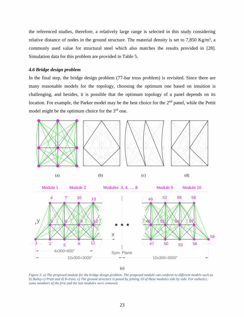
4.6 Bridge design problem

In the final step, the bridge design problem (77-bar truss problem) is revisited. Since there are

many reasonable models for the topology, choosing the optimum one based on intuition is

challenging, and besides, it is possible that the optimum topology of a panel depends on its

location. For example, the Parker model may be the best choice for the 2nd panel, while the Pettit

model might be the optimum choice for the 3rd one.

(a) (b) (c) (d)

1 2 5

3 6

8 11

9 12

59

5653

5754

5047

5148

4 7 10 13 58695249

Module 1 Modules 3, 4, ..., 8

10x300=3000"

4x300=600" Sym. Plane

10x300=3000"

y

x

Module 2 Module 9 Module 10

(e)

Figure 3. a) The proposed module for the bridge design problem. The proposed module can conform to different models such as

b) Bailey c) Pratt and d) K-truss. e) The ground structure is posed by joining 10 of these modules side by side. For esthetics,

some members of the first and the last modules were removed.

24

To reduce the burden on the designer for deciding on these important factors, this problem is

revisited by proposing an intricate ground structure, consisting of 10 modules. Each module

consists of 3×3=9 nodes and 33 members. The lower cord is pre-designed [22] and cannot be

changed. Adjacent modules share 3 nodes and 3 members, thus the grounds structure has 59 nodes

and 277 members. The selected module can conform to most models conventionally used for

bridge design, including Parker, Bailey and K-truss, and many non-standard models. Three

variants of this problem are solved in this study, with distinct amount of flexibility in the design.

Variant I: The 1st and the 2nd modules are independent while modules 2, 3, 4 and 5 are

topologically similar to the 2nd model. This reduces the number of topology parameters to

43. There is only one shape variable, vertical position of the upper cord. The height of

nodes on the middle cord is half of the adjacent node on the upper cord. No node may move

horizontally. There is one size variable per member on the left part of the bridge.

Variant II: similar to variant I, but vertical position of the nodes on the upper cord are

independent of each other, however, the height of nodes on the middle cord is half of the

adjacent node on the upper cord, which increases the number of shape variable to 10.

Variant III: Topologies of modules are independent of each other. There is one topology

variable per member on the left part of the bridge except for the members on the lower

cord, which must be active. Nodes on the middle and upper cord can move in any direction

independent of each other, except the nodes on x=3,000″, which can move vertically only.

The overall number of design variables is 308 for this case.

In all variants, symmetry about x=3,000″ is imposed, location of nodes on the lower cord is

fixed and members on the lower cord (20 members) must remain active. Each variant provides

more flexibility in design optimization than the previous one. This increases the potential material

saving when optimization is performed, however, since the complexity of the problem exacerbates,

the achieved solution might become even heavier than the previous variant, especially if the extra

potential saving is small in comparison with the added complexity. Furthermore, modularity of the

structure disrupts in later variants. For example, in variant I, shape and topology of modules are

similar, which facilitates construction and improve esthetics. In variant II, modules are

topologically similar, but differ in shape and cross sections. Finally, in variant III, the structure is

not modular anymore. Whether the extra saving, if achieved, compensates for deterioration of

structural esthetics and increase in construction costs depends on the amount of the saving, and is

25

a decision which should be made by the decision maker. Later variants are however more

interesting for benchmarking, since they provide more challenging situations with larger number

of design parameters, which can reliably illuminate the gap among different optimization methods.

The problem of possible overlapping members in the final design, which is assumed to be

practically undesirable, is handled by imposing an overlap prevention rule: For a set of three nodes

that must remain vertically aligned and are connected to one another (two short members and one

long member), the long member may be active only if the two short members are passive. For

example, this rule is applied to the set {2, 3, 4}. This means the long member can be active (M2-

4=1) only if the two short members are passive (M2-3=M3-4=0). A revision is performed to handle

sampled designs that violate this rule. If a set of three members violates this rule, first a random

number is generated (r0∈[0, 1]) and then, the following correction is applied:

{Remove all 3 members, Remove the long member, Remove the short members,

ififif

𝑟0 ≤ 0.2, 0.2 ≤ 𝑟0 ≤ 0.8,0.8 ≤ 𝑟0.

The probabilities are computed based on the fact that in 8 possible combinations for

absence/absence of 3 members, 5 combinations do not violate the overlapping rule. In 1 out of 5,

no member is present, in 1 out of 5, only the long member is present and in 3 out of 5, at least one

short member is present. This rule is applied to the 19 sets of vertically aligned nodes ({2, 3, 4},

{5, 6, 7}, …., {56, 57, 58}) in variants I and II. It is notable that this undesirable feature is unlikely

to happen in variant III, since nodes may move horizontally as well. Data required for simulation

of this problem are summarized in Table 6.

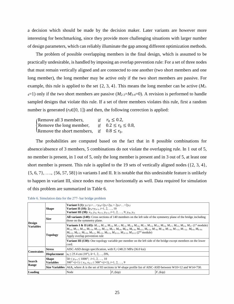
Table 6. Simulation data for the 277- bar bridge problem

Design

Variables

Shape

Variant I (1): y4=y7=…=y58=2y3=2y6 = 2y9=…=2y57

Variant II (10): 2y3i=y3i+1, i=1, 2, …, 10

Variant III (38): x3i, y3i, x3i+1, y3i+1, i=1, 2, …, 9; y30, y31

Size All variants (140): Cross sections of 140 members on the left side of the symmetry plane of the bridge, including those on the symmetry plane.

Topology

Variants I & II (43): M1-3, M1-4, M1-6, M1-7, M2-3, M2-4, M2-6, M2-7, M3-4, M3-5, M3-6, M3-7, M4-5, M4-6, M4-7 (1st module)

M5-6, M5-7, M5-9, M5-10, M5-12, M5-13, M6-7, M6-8, M6-9, M6-10, M6-11, M6-13, M7-8, M7-9, M7-10, M7-11, M7-12, M8-9, M8-10,

M8-12, M8-13, M9-10, M9-11, M9-12, M9-13, M10-11, M10-12, M10-13 (2nd module)

Apply overlap prevention rule

Variant III (130): One topology variable per member on the left side of the bridge except members on the lower

cord.

Constraints Stress AISC-ASD design specification, with Fy=248.21 MPa (36.0 ksi)

Displacement uk ≤ 25.4 cm (10″), k=1, 2,…, DNn

Search

Range

Shape

Variables

50 ≤ y3i+1 ≤ 1000″; i=1, 2, …, 10

300″×(i-1) ≤ x3i, x3i+1 ≤ 300″×(i+1), i=1, 2, …, 9

Size Variables A∈𝔸, where 𝔸 is the set of 83 sections in W-shape profile list of AISC-ASD between W10×12 and W14×730.

Loading Node Fx (kip) Fy (kip)

26

2, 5, 8, …, 56 0.0 −60.0

Mechanical Properties Modulus of elasticity: E=200 GPa (29000 ksi)

Density of the material: ρ=7850 Kg/m3 (0.2836 lb/in.3);

5 Results and discussions

FSD-ES-II is employed to solve the employed optimization problems. All parameters are set to

their default values, and thus the required tuning effort is zero. Each problem is solved 100 times

independently and the best solution found is reported. However, comparing different methods

solely based on the best solution found, as followed in most previous studies, is not a reliable

method, due to stochastic nature of the experiment and possibility of obtaining better solutions if

the evaluation budget or the number of independent runs is increased. The recommended

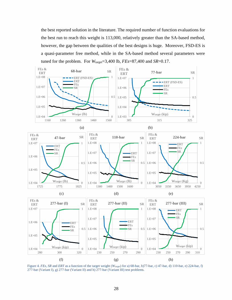
performance measure is comparison of the expected running time (ERT) [30] to reach an arbitrary

target weight (Wtarget).

𝐸𝑅𝑇(𝑊target) =𝐹𝐸𝑠(𝑊target)

𝑆𝑅(𝑊target), (29)

where FEs(Wtarget) is the average number of the require function evaluations to reach the desired

target weight of Wtarget, provided that the run could reach Wtarget. SR is the fraction of runs in which

the algorithm could reach Wtarget. FEs, SR and consequently ERT depends on Wtarget, and thus for

each problem, these measures are plotted for a range of Wtarget. Unless only a few runs could reach

Wtarget, these measures are robust with respect to stochastic nature the experiment. ERT is of

particular interest, since it facilitates comparison of optimization methods by combining the effects

of efficiency, measured by FEs, and reliability, measured by SR.

To increase reliability of statistical measures, each problem is solved 500 times independently.

Because of the large number of independent runs, measured values of SR, FEs and ERT are

assumed to be reliable if SR≥0.05. Figures 3 illustrate FEs, SR and ERT curves as a function of

Wtarget for each problem. The best solution found for each problem is illustrated in Figures 4 and

the corresponding design parameters are provided in Appendix. The obtained results demonstrate

that:

- For the 47-bar truss problem, the best solution found by FSD-ES-II weighs 1,728 lb,

reached after about 61,000 evaluations, although ERT is much greater. For Wtarget=1,750

lb, FEs=38,800 and SR=0.24, sufficiently high to draw reliable conclusions. In comparison

with a previous GA-based method [28], which reached the best solution of 1,885 lb, at the

27

end of 100,000 evaluations, FSD-ES-II could reach an 8.3% lighter structure relatively

faster. For the case in which only shape and size optimization are performed, this problem

has been solved with different methods in previous studies, among which the results

provided by the earlier version of FSD-ES [6] outperformed the others. In comparison with

the best design for shape and size optimization which weighs 1,847 lb [6], performing TSS

optimization resulted in an extra 6.4% reduction in the overall weight, which is quite

significant considering the limited flexibility of the topology of the ground structure.

- For the 68-bar problem, the best solution of FSD-ES-II weighs 1,166 lb, about 3.1% lighter

than that found by FSD-ES [6]. More important, FSD-ES-II is several times faster when

ERT of both methods are compared. Considering that some displacement constraints are

active in the optimized solution, this advantage probably originates from the performed

improvement in the resizing step so that the resizing scheme explicitly takes the

displacement constraints into account.

- For the 77-bar bridge design problem, the best solution of FSD-ES-II weighs 306.0 kip,

almost the same as the best solution of the earlier version [14]. The FEs of the older version

is slightly smaller initially, however, for Wtarget ≤ 312 kip, performance of both methods is

similar. For this problem, best solution of Hasançebi [22] weighs Wtarget=317.1 kip, reached

after about 150,000 evaluations. For the same target weight, FSD-ES-II is almost 8.5 times

faster. The ground structure of this problem is determinate, where the assumption of FSD

part are totally valid, which maximizes benefits of FSD concept. This could be one of the

reasons for spectacular advantage of FSD-ES and FSD-ES-II over the ES-based method

proposed in [22].

- For the 110-bar problem, the best solution of FSD-ES weighs 1,314 lb, which demonstrates

by providing more flexibility in topology optimization, it is possible to save an extra 24%

in weight, when compared to the best solution of the 47-bar problem. The topology of the

optimized solution could hardly be concluded by engineering intuition, even though it is

only a little more complicated than the optimized solution of 47-bar problem. 28.6% of

runs could reach Wtarget=1,450 lb, on average after 66,200 evaluations.

- For the 224 bar pyramid problem, the best solutions in the literature weighs 4,587 Kg [12],

reached by an SA-based algorithm after 300 cooling cycles (presumably 24,600 function

evaluations). The best solution of FSD-ES weighs 3,079 Kg, which is 32.8% lighter than

28

the best reported solution in the literature. The required number of function evaluations for

the best run to reach this weight is 113,000, relatively greater than the SA-based method,

however, the gap between the qualities of the best designs is huge. Moreover, FSD-ES is

a quasi-parameter free method, while in the SA-based method several parameters were

tuned for the problem. For Wtarget=3,400 lb, FEs=87,400 and SR=0.17.

(a) (b)

(c) (d) (e)

(f) (g) (h)

Figure 4. FEs, SR and ERT as a function of the target weight (Wtarget) for a) 68-bar, b)77-bar, c) 47-bar, d) 110-bar, e) 224-bar, f)

277-bar (Variant I), g) 277-bar (Variant II) and h) 277-bar (Variant III) test problems.

0

0.5

1

1.E+04

1.E+05

1.E+06

1.E+07

1.E+08

1160 1260 1360 1460 1560

SRFEs &

ERT

Wtarget (lb)

68-bar

ERT (FSD-ES)ERTFEsSR

0

0.5

1

1.E+03

1.E+04

1.E+05

1.E+06

1.E+07

305 315 325

SRFEs &

ERT

Wtarget (kip)

77-bar

ERT (FSD-ES)

ERT

FEs

SR

0

0.5

1

1.E+04

1.E+05

1.E+06

1.E+07

1725 1775 1825

SRFEs &

ERT

Wtarget (lb)

47-bar

ERT

FEs

SR

0

0.5

1

1.E+04

1.E+05

1.E+06

1.E+07

1.E+08

1300 1400 1500 1600

SRFEs &

ERT

Wtarget (lb)

110-bar

ERT

FEs

SR

0

0.5

1

1.E+04

1.E+05

1.E+06

1.E+07

1.E+08

3050 3350 3650 3950 4250

SRFEs &

ERT

Wtarget (Kg)

224-bar

ERT

FEs

SR

0

0.5

1

1.E+04

1.E+05

1.E+06

1.E+07

280 300 320

SRFEs &

ERT

Wtarget (kip)

277-bar (I)

ERT

FEs

SR

0

0.5

1

1.E+04

1.E+05

1.E+06

1.E+07

1.E+08

230 250 270 290

SRFEs &

ERT

Wtarget (kip)

277-bar (II)

ERT

FEs

SR

0

0.5

1

1.E+04

1.E+05

1.E+06

1.E+07

1.E+08

230 250 270 290 310

SRFEs &

ERT

Wtarget (kip)

277-bar (III)

ERT

FEs

SR

29

Sym.

plane

(a) (b) (c)

(d)

Sym. plane Sym. plane

Sym. plane Sym. plane

(e) (f)

Sym. plane Sym. plane

Sym. plane Sym. plane

(g) (h)

Figure 5. The best feasible solution found for diffeent test problems. a) 47-bar (W=1727.6 lb), b) 110-bar (W=1314.0

lb), c) 224-bar (W=3079.4 Kg), d) 68-bar (W=1166.1 lb), e) 77-bar (W=305.96 kip), f) 277-bar in case I (W=282.03

kip), g) 277-bar in case II (W=236.54 kip), h) 277-bar in case III (W=231.94 kip)

30

- In the variant I of bridge design problem, FSD-ES-II could reach the weight of 282.0 kip,

which is surprisingly lighter than the best solution found in [22], even those that have

higher flexibility for shape variation (317 kip [22], 307 kip [14] and 306 kip in the 77-bar

test problem of this study). This demonstrates the optimized design of variant I is not only

lighter, but also has less fabrication and assembly cost, due to similarity of modules

(identical shape and topology versus identical topology only). It also excels in esthetics.

The topology of the best solution found resembles the Bailey model to some extent. 12.6%

of runs could each Wtarget=282.5 kip after 125,700 evaluations. The best solution of variant

II of this problem weighs 236.5 kip, 16.1% lighter than best solution of variant I and 22.7%

lighter than the case when the Parker model is optimized for shape and size. The arch-

shape of the upper cord in the best found solution of variant II matches engineering

intuition. In variant III, there is only 1.9% achieved extra saving, in comparison with the

best solution of variant II, which also comes at the cost of excessive function evaluations.

For example, for Wtarget=240 kip, ERT in case III is about 12 times greater than the ERT in

case II. The structural esthetics and ease of assembly has degraded as well.

6. Summary and conclusions

In this study, an improved version of the fully stressed design based on evolution strategy (FSD-

ES) has been developed for simultaneous topology, shape and size (TSS) optimization of large-

scale truss structures. In comparison with the earlier version, the new method, called FSD-ES-II,

is able to explicitly handle displacement constraints in the resizing step. Some specialization on

the evolution strategy part has also been performed to handle mixed variable nature of the TSS

optimization problems while principles of the contemporary evolution strategies have been

followed.

Efficiency and efficacy of the proposed FSD-ES-II have been tested on some complicated and

large-scale TSS test problems to evaluate the algorithm for more practical and challenging

scenarios. Three of the test problems, the 47-bar transmission tower, the 77-bar bridge and the

224-bar pyramid, have been directly adapted from the literature, for which FSD-ES-II could

surpass the best available results by a clear margin. A few other test problems have been posed by

converting available size and shape optimization problems to suitable TSS problems by providing

more intricacy and flexibility in the ground structure. The results from FSD-ES-II on the newly

31

developed TSS problems have revealed that a huge saving (as high as 32%) in the structural weight

can be achieved by more reliance on a potent optimization tool than human intuition. This

highlights advantages of the computer methods in truss optimization field, where more reliance on

optimization methods can result in superior results. Engineering intuition can be very helpful by

defining a reasonable ground structure or problem formulation, to avoid unnecessary complexities.

Overall, the proposed FSD-ES-II has been demonstrated to handle a large number of design

parameters, much larger than those usually considered in existing truss optimization studies, within

a relatively small evaluation budget. More importantly, no ad-hoc parameter tuning is required

with the proposed approach, thereby making FSD-ES-II a pragmatic tool for structural engineers.

The amount of saving in computation and the significant difference in performance compared

to other contemporary methods in these problems have demonstrated a need for further research

along the lines of our proposed algorithm. Realistic and complex TSS problems, including those

developed in this study, may provide a reliable tool to compare different truss optimization

methods in more realistic situations. It is believed that the introduction of these large-scale truss-

structure optimization problems and their optimized solutions reported in this paper should remain

as benchmark problems for future researchers in the area. After many decades of research, it is

now time to demonstrate the power of current optimization methodologies to solve realistic

problems so that the use of optimization can finally become a regular event in everyday design

activities.

7. Acknowledgement

Computational work in support of this research was performed at Michigan State University’s

High Performance Computing Facility.

References

[1] M. P. Saka, "Optimum design of pin-jointed steel structures with practical applications," Journal of Structural Engineering, vol. 116,

no. 10, pp. 2599-2620, 1990.

[2] B. H. V. Topping, "Shape optimization of skeletal structures: a review," Journal of Structural Engineering, vol. 109, no. 8, pp. 1933-

1951, 1983. [3] C. Feury and M. Geradin, "Optimality criteria and mathematical programming in structural weight optimization," Computers &

Structures, vol. 8, no. 1, pp. 7-17, 1978.

[4] O. Hasançebi, S. D. E. Çarbaş, F. Erdal and M. P. Saka, "Performance evaluation of metaheuristic search techniques in the optimum design of real size pin jointed structures," Computers & Structures, vol. 87, no. 5, pp. 284-302, 2009.

[5] A. Kaveh and Z. A, "Comparison of nine meta-heuristic algorithms for optimal design of truss structures with frequency constraints,"

Advances in Engineering Software, vol. 76, pp. 9-30, 2014. [6] A. Ahrari, A. A. Atai and K. Deb, "Simultaneous topology, shape and size optimization of truss structures by fully stressed design

based on evolution strategy," Engineering Optimization, p. in press, 2014.

32

[7] K. Deb and S. Gulati, "Design of truss-structures for minimum weight using genetic algorithms," Finite elements in analysis and

design, vol. 37, no. 5, pp. 447-465, 2001. [8] H. Rahami, A. Kaveh and Y. Gholipour, "Sizing, geometry and topology optimization of trusses via force method and genetic

algorithm," 2008, vol. 30, no. 9, pp. 2360-2369, Engineering Structures.

[9] G. C. Luh and C. Y. Lin, "Optimal design of truss-structures using particle swarm optimization," Computers & Structures, vol. 89, no. 23, pp. 2221-2232, 2011.

[10] L. F. F. Miguel, R. H. Lopez and L. F. F. Miguel, "Multimodal size, shape, and topology optimisation of truss structures using the

Firefly algorithm. ,," Advances in Engineering Software, vol. 56, pp. 23-37, 2013. [11] S. Gholizadeh, "Layout optimization of truss structures by hybridizing cellular automata and particle swarm optimization," Computers

& Structures, vol. 125, pp. 86-99, 2013.

[12] O. Hasançebi and F. Erbatur, "Layout optimisation of trusses using simulated annealing," Advances in Engineering Software, vol. 33, no. 7, pp. 681-696, 2002.

[13] N. Noilublao and S. Bureerat, "Simultaneous topology, shape and sizing optimisation of a three-dimensional slender truss tower using

multiobjective evolutionary algorithms," Computers & Structures,, vol. 89, no. 23, pp. 2531-2538, 2001. [14] A. Ahrari and A. A. Atai, "Fully Stressed Design Evolution Strategy for Shape and Size Optimization of Truss Structures," Computers

& Structures, vol. 123, pp. 58-67, 2013.

[15] M. Schevenels, S. McGinn, A. Rolvink and J. Coenders, "An optimality criteria based method for discrete design optimization taking into account buildability constraints," Structural and Multidisciplinary Optimization, p. in press, 2014.

[16] H. G. Beyer and H. P. Schwefel, "Evolution strategies–A comprehensive introduction," Natural computing, vol. 1, no. 1, pp. 3-52,

2002.

[17] T. Bäck, C. Foussette and P. Krause, Contemporary Evolution Strategies, Springer, 2013.

[18] N. Hansen and A. Ostermeier, "Completely derandomized self-adaptation in evolution strategies," Evolutionary computation, vol. 9,

no. 2, pp. 159-195, 2001. [19] O. Kramer, "Evolutionary self-adaptation: a survey of operators and strategy parameters," Evolutionary Intelligence, vol. 3, no. 2, pp.

51-65, 2010.

[20] H. G. Beyer and B. Sendhoff, "Covariance matrix adaptation revisited–the CMSA evolution strategy," in Parallel Problem Solving from Nature–PPSN X , Berlin Heidelberg, Springer, 2008, pp. 123-132.

[21] S. D. Rajan, "Sizing, shape, and topology design optimization of trusses using genetic algorithm," Journal of Structural Engineering, vol. 121, no. 10, pp. 1480-1487, 1995.

[22] O. Hasançebi, "Adaptive evolution strategies in structural optimization: Enhancing their computational performance with applications

to large-scale structures," Computers & structures, vol. 86, no. 1, pp. 119-132, 2008. [23] C. Ebenau, J. Rottschäfer and G. Thierauf, "An advanced evolutionary strategy with an adaptive penalty function for mixed-discrete

structural optimisation," Advances in Engineering Software, vol. 36, no. 1, pp. 29-38, 2005.

[24] A. Kaveh, M. Kalateh-Ahani and M. S. Masoudi, "The CMA evolution strategy based size optimization of truss structures," International journal of optimization in civil engineering, vol. 2, pp. 233-256, 2011.

[25] W. Hare, J. Nutini and S. Tesfamariam, "A survey of non-gradient optimization methods in structural engineering," Advances in

Engineering Software, vol. 59, pp. 19-28, 2013. [26] D. Li, S. Chen and H. Huang, "Improved genetic algorithm with two-level approximation for truss topology optimization," Structural

and Multidisciplinary Optimization, vol. 49, no. 5, pp. 795-814, 2014.

[27] A. Ahrari and A. Atai, "Efficient simulation for optimization of topology, shape and size of modular truss structures," International Journal of Optimization in Civil Engineering, vol. 3, no. 2, pp. 209-223, 2013.

[28] O. Hasançebi and F. Erbatur, "Layout optimization of trusses using improved GA methodologies," Acta mechanica, vol. 146, no. 1-2,

pp. 87-107, 2001. [29] E. Salajegheh and G. N. Vanderplaats, "Optimum design of trusses with discrete sizing and shape variables," Structural Optimization,

vol. 6, no. 2, pp. 79-85, 1993.

[30] N. Hansen, A. Auger, S. Finck and R. Ros, "Real-Parameter Black-Box Optimization Benchmarking 2010: Experimental Setup," INRIA, 2010.

[31] C. Fleury, "An efficient optimality criteria approach to the minimum weight design of elastic structures," Computers & Structures, vol.

11, no. 3, pp. 163-173, 1980. [32] S. R. Hansen and G. N. Vanderplaats, "Approximation method for configuration optimization of trusses," AIAA journal, vol. 28, no.

1, pp. 161-168, 1990.

[33] American Institute of Steel Construction (AISC). Manual of Steel Construction: Allowable Stress Design, 1989. [34] O. Hasançebi, "Optimization of truss bridges within a specified design domain using evolution strategies," Engineering Optimization,

vol. 39, no. 6, pp. 737-756, 2007.

[35] P. Hajela and E. Lee, "Genetic algorithms in truss topological optimization," International journal of solids and structures, vol. 32, no. 22, pp. 3341-3357, 1995.

[36] S. M. Shrestha and J. Ghaboussi, "Evolution of optimum structural shapes using genetic algorithm," Journal of Structural Engineering,

vol. 124, no. 11, pp. 1331-1338, 1998.

33

Appendix: Parameters of the best solution found for each problem

47-bar y15 412.900 x12 331.501 x36 -478.008 A14-16 55.8 A24-29 14.4 A20-23 39.9 A1-2 19.1

(1727.6241 lb) x17 -10.813 y12 58.396 y51 -17.302 A15-16 15.8 A25-28 75.6 A21-23 9.71 A1-3 50

in & in2 y17 453.908 x13 430.570 x51 -657.798 A15-17 75.6 A26-29 55.8 A21-24 6.49 A2-3 6.49

x1 -127.426 x19 -78.574 y13 -15.651 A36-51 35.9999 A16-17 14.4 A28-30 9.71 A22-24 9.71 A2-5 20

x3 -98.277 y19 500.112 x14 512.163 A36-52 6.9032 A16-18 55.8 A28-31 75.6 A22-25 56.8 A3-4 55.8

y3 151.332 x25 -122.764 y14 23.357 A19-36 27.7419 A17-18 21.8 A29-30 6.49 A23-24 9.71 A3-5 9.71

x5 -76.494 y25 552.032 x15 445.326 A20-36 17.2903 A17-19 75.6 A30-31 6.49 A23-26 39.9 A3-7 8.79

y5 260.438 x27 -85.107 y15 48.998 A2-19 4.3161 A18-19 14.4 277-bar (II) A24-25 9.71 A4-6 62

x7 -64.180 y27 599.788 x16 518.860 A3-19 23.7419 A18-20 56.8 (236543.28 lb) A24-26 9.71 A4-7 6.49

y7 370.620 y29 582.204 y16 -0.055 A4-19 3.1871 A19-20 21.8 in & in2 A24-27 6.49 A5-7 6.49

x9 -53.706 A1-3 0.5 y17 37.942 A3-20 3.1871 A19-21 75.6 y4 314.233 A25-27 9.71 A5-8 20

y9 435.519 A1-5 2.6 x18 522.801 A4-20 17.2903 A20-21 15.8 y7 485.359 A25-28 56.8 A5-9 4.99

x11 -44.619 A3-5 0.1 y18 60.286 A19-20 2.7935 277-bar (I) y10 617.425 A26-29 42.7 A6-10 7.61

y11 513.943 A3-7 0.1 A1-2 3.131 A1-2 6.9032 (282032.88 lb) y13 739.897 A27-29 9.71 A6-13 61.8

x13 -53.559 A3-8 0.5 A2-3 1.333 A1-3 27.7419 in & in2 y16 830.438 A27-30 6.49 A7-8 6.49

y13 536.863 A5-7 0.1 A1-4 3.131 A2-3 1.6129 y31 748.714 y19 899.228 A28-30 9.71 A7-9 5.57

x19 -102.846 A5-9 2.6 A2-4 0.539 A1-4 17.2903 A1-2 21.8 y22 950.765 A28-31 56.8 A8-11 24.1

y19 628.453 A7-9 0.5 A2-5 1.333 A3-4 4.1226 A1-3 68.5 y25 985.011 A29-30 9.71 A9-11 9.71

x21 -10.378 A9-11 1.6 A2-6 1.081 77-bar A2-3 6.49 y28 993.227 A30-31 9.71 A10-11 7.65

y21 618.162 A9-13 1.2 A3-6 2.142 (305963.97 lb) A2-5 21.8 y31 997.973 277-bar (III) A10-12 7.65

A1-3 3.0 A11-13 0.1 A4-5 0.347 in & in2 A3-5 9.71 A1-2 25.6 (231943.31 lb) A10-13 9.71

A2-3 0.3 A11-15 1.6 A5-6 0.347 y3 224.347 A3-6 11.5 A1-4 67.7 in & in2 A11-12 6.49

A3-5 2.6 A13-15 0.2 A4-7 3.131 y5 321.370 A3-7 61.8 A2-4 6.49 x3 208.021 A11-14 32.9

A4-5 1.5 A13-18 1.1 A5-7 0.44 y7 431.315 A5-6 6.49 A2-5 25.6 y3 289.400 A12-14 3.54

A5-7 2.8 A15-17 0.6 A5-9 1.081 y9 521.002 A5-8 21.8 A4-5 7.65 x4 514.544 A12-15 3.54

A6-7 0.6 A15-19 1.4 A6-9 1.488 y11 592.148 A6-7 23.2 A4-6 6.49 y4 463.214 A12-19 7.61

A7-9 2.3 A17-19 1.0 A7-8 0.27 y13 650.329 A6-8 9.71 A4-7 55.8 x6 879.829 A13-15 7.65

A7-10 1.1 A17-20 0.8 A8-9 0.44 y15 703.318 A6-10 42.7 A5-6 6.49 y6 646.499 A13-16 75.6

A9-11 2.5 A19-21 0.4 A7-10 2.8 y17 741.956 A6-11 14.4 A5-8 29.1 x7 623.346 A14-17 28.2

A10-11 0.6 A19-25 1.1 A8-10 0.44 y19 761.865 A7-10 26.5 A6-7 4.41 y7 186.673 A14-19 6.49

A11-13 2.3 A19-29 1.1 A8-11 0.111 y21 765.677 A8-11 24.1 A6-8 6.49 x9 819.550 A15-16 6.49

A12-13 1.4 A21-25 0.2 A8-12 0.27 A1-2 35.3 A10-12 19.1 A6-9 6.49 y9 62.113 A15-19 6.49

A13-21 0.7 A21-27 0.2 A9-12 2.142 A1-3 68.5 A10-13 56.8 A7-9 6.49 x10 1107.381 A16-18 83.3

A13-15 1.6 A21-29 0.2 A11-12 0.111 A2-3 3.54 A11-12 9.71 A7-10 56.8 y10 433.965 A17-19 3.54

A19-21 0.9 A23-25 1.1 A10-13 2.697 A2-4 35.3 A11-14 31.2 A8-11 32.9 x12 1480.945 A17-20 28.2

A15-19 0.8 A23-27 0.7 A11-13 0.111 A3-4 14.4 A12-13 6.49 A9-11 7.65 y12 233.424 A18-21 14.4

A15-21 0.2 A27-29 0.7 A12-15 2.142 A3-5 68.5 A12-14 9.71 A9-12 6.49 x13 1227.996 A18-25 83.3

A17-19 0.9 68-bar A13-14 1.333 A4-5 14.4 A12-16 21.8 A10-12 6.49 y13 749.968 A19-20 6.49

A15-17 1.2 (1166.0624 lb) A14-15 0.954 A4-6 46.7 A12-17 15.6 A10-13 56.8 x15 1544.228 A19-21 10

A14-21 1.1 in & in2 A13-16 1.333 A5-6 7.65 A13-16 56.8 A11-12 6.49 y15 455.410 A20-21 3.54

A21-22 1.2 x2 77.158 A14-16 0.347 A5-7 75.6 A14-17 32.9 A11-14 35.3 x16 1633.329 A20-23 32.9

110-bar y2 2.241 A14-17 1.333 A6-7 7.65 A16-18 9.71 A12-13 6.49 y16 836.159 A21-23 4.41

(1314.0468 lb) x4 102.478 A14-18 0.539 A6-8 50 A16-19 67.7 A12-14 9.71 x18 2085.647 A21-24 11.2

in & in2 y4 -63.299 A15-18 1.174 A7-8 9.71 A17-18 17 A12-15 6.49 y18 921.111 A23-24 3.54

x1 -147.839 x5 149.668 A16-17 1.333 A7-9 75.6 A17-20 46.7 A13-15 7.65 x19 1790.757 A23-26 32

x3 -61.793 y5 39.504 A17-18 1.081 A8-9 9.71 A18-19 6.49 A13-16 55.8 y19 146.595 A24-26 4.41

y3 92.508 x6 112.369 A9-10 0.111 A8-10 51.8 A18-20 9.71 A14-17 38.8 x21 2243.269 A24-28 6.49

x5 -127.842 y6 69.877 224-bar A9-10 13.3 A18-22 21.8 A15-17 9.71 y21 179.840 A24-29 8.79

y5 139.089 x7 206.289 (3079.4455 Kg) A9-11 75.6 A18-23 14.4 A15-18 6.49 x24 2571.264 A25-28 9.71

x7 -24.589 y7 -62.871 cm & cm2 A10-11 11.5 A19-22 67.7 A16-18 9.71 y24 58.838 A25-30 83.3

y7 183.323 x8 284.375 y2 -150.800 A10-12 55.8 A20-23 50 A16-19 56.8 x25 2549.469 A26-27 3.54

x9 -108.653 y8 -20.567 z2 718.123 A11-12 14.4 A22-24 9.71 A17-18 7.65 y25 935.135 A26-28 6.49

y9 270.627 x9 219.291 y3 -46.344 A11-13 75.6 A22-25 75.6 A17-20 38.8 x27 2848.702 A26-29 35.3

x11 -88.025 y9 54.045 x3 -191.008 A12-13 14.4 A23-24 9.71 A18-19 7.65 y27 162.706 A27-29 3.54

y11 381.346 x10 308.332 x4 -172.365 A12-14 55.8 A23-26 51.8 A18-20 9.71 x28 2615.871 A27-31 6.49

x13 -39.385 y10 -50.950 y19 -44.058 A13-14 14.4 A24-25 6.49 A18-21 6.49 y28 378.151 A30-31 7.65

y13 362.847 x11 372.474 x19 -280.169 A13-15 75.6 A24-26 9.71 A19-21 9.71 y30 944.284

x15 -81.704 y11 21.145 x20 -322.412 A14-15 14.4 A24-28 14.4 A19-22 55.8 y31 499.294