performance evaluation of tracking for public transport

LEUNG ET AL: EVALUATION OF NETWORK TRACKING 1Annals of the BMVA Vol. 2010, No. 6, pp 1–12 (2010)

Performance Evaluation of Trackingfor Public Transport SurveillanceV. Leung, J.Orwell and S.A. Velastin

Digital Imaging Research Centre,Faculty of Computing, Information Systems and Mathematics,Kingston University,Kingston upon Thames, KT1 2EE〈[email protected];j.orwell,[email protected]〉

Abstract

Starting with the end-user requirements, it is argued that the most appropriate perfor-mance metric with which to evaluate video-based tracking methods, in the public trans-port domain, is to measure the information gained through their use. This is equiva-lent to the reduction in uncertainty about a passenger’s whereabouts, after tracking andappearance-based measurements have been taken into account. In this paper, we presenta framework for the performance evaluation of such a system. Error propagation anal-ysis is performed to investigate the impact of each system component on the final un-certainty, and allows an end-user requirement to be propagated through the system todetermine the minimum performance requirement for each component. This proposedanalysis framework is demonstrated on a simulated system.

1 Introduction

In public transport networks, the quality and quantity of available video surveillance datahas increased significantly in recent years. Digital cameras, wireless transmission systemsand effective digital compression standards have simultaneously reduced cost and increasedthe potential for higher quality signals. There is clearly the potential for automatic analysisof the data for various purposes.

This paper considers one particular objective for automatic analysis: the tracking of anindividual (or ‘target’) as they use a small urban ‘metro’ network of stations and trains, fromtheir point of entrance into the network, to the point when they leave. In this scenario, anoperator manually ‘tags’ them in one camera, and the system subsequently displays the bestavailable camera view of them, hence the application is called ‘Tag and Track’.

In this analysis, a model is introduced for the transport network, the passengers’ move-ment, and the processing of surveillance data. We propose that the appropriate performance

c© 2010. The copyright of this document resides with its authors.It may be distributed unchanged freely in print or electronic forms.

http://www.bmva.org/annals/2010/2010/2010-0006.pdf

http://www.bmva.org/w/doku.php?id=annals_of_the_bmva

2 LEUNG ET AL: EVALUATION OF NETWORK TRACKINGAnnals of the BMVA Vol. 2010, No. 6, pp 1–12 (2010)

evaluation metric for such a system is the expected number of manual interventions neces-sary to maintain the correct view of the person. This has a direct relationship to the uncer-tainty associated with their position, and this uncertainty is reduced by the application ofcomputer vision methods such as tracking and appearance-based recognition.

This model is applied to the Torino Metro network, and an analysis based on simulateddata is carried out. The first result is the predicted overall efficacy for given levels of perfor-mance from specific computer vision components. The second result is the derivation of theerror contribution from each component to allow the calculation of the performance levelsneeded for a given overall end-user requirement. A study of the marginal impact of changesin performance is also presented.

There are numerous applications of this analysis. Thus, in addition to the public trans-port (metro) scenario, it may be applied to any multi-sensor tracking problem, e.g. vehiclesin a road system, or people in a shopping centre. The analysis can be applied to real-timesystems, or to systems that track forward through archives (‘where did this person go?’),or backwards through archives (‘where did this person come from?’) In each of these sce-narios, the analysis may be used in several ways. First, it can be used to estimate the ex-pected amount of manual intervention necessary to maintain correct tracks. Second, it allowscomparisons of different scenarios e.g. levels of crowding or camera resolution. Finally, itprovides a mechanism for understanding how improvements to specific components of thetracking and recognition solution will affect the overall performance.

1.1 Previous work

Tracking pedestrians between multiple cameras for both overlapping and non-overlappingcases have been studied extensively recently [Kim and Davis, 2006, Javed et al., 2005, Fleuretet al., 2008, Makris et al., 2004, Rahimi et al., 2004, Khan and Shah, 2006]. For overlappingcameras, the geometric relations between the cameras are used to integrate the observations[Fleuret et al., 2008, Khan and Shah, 2006]. For non-overlapping cameras, the relationshipbetween cameras are provided by observing the location and velocity of the objects travers-ing the scene [Makris et al., 2004, Rahimi et al., 2004], and trajectories of the pedestrians canbe estimated by techniques such as Kalman filter and particle filter [Kim and Davis, 2006,Fleuret et al., 2008]. In both settings, the appearance of the target is modelled, typicallyusing colour distributions, providing an independent term to the probabilistic expression.The ‘Tag and Track’ application can be viewed as a subset of the multi-object multi-cameraproblem.

The assessment of the performance of many tracking approaches is usually carried outon an algorithmic level, e.g. the spatial accuracy and continuity of the tracks, the abilityto resolve occlusions etc., and many methods have been proposed for this purpose. [Blacket al., 2003] proposed a method where ground truth is automatically generated, eliminatingthe laborious task of manual ground truth generation. Their tracking metrics include posi-tional error and tracking success rate. [Brown et al., 2005] investigated a two-pass methodto address track merging and fragmentation errors. The approach in [Needham and Boyle,2003] focussed on trajectory comparison, taking into account temporal lag and spatial shift.In order to allow the different algorithms to be compared, efforts such as the PETS work-shops[PETS] provide standard datasets for testing and evaluation; the tracking metrics in-clude the number of track false positives and average positional error.

From a systems evaluation point of view, the iLIDS dataset [HOSDB] provided by the




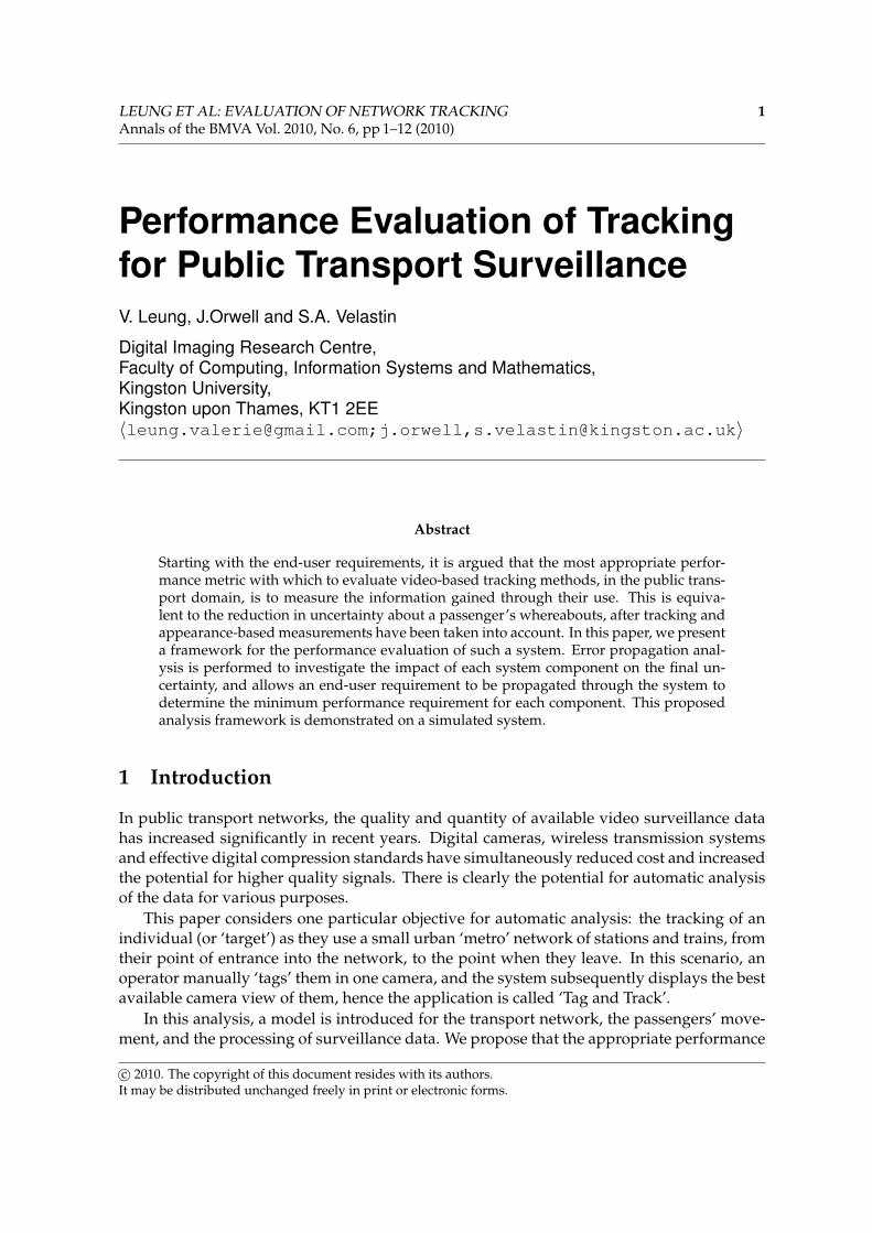
(a) Single station; the numbers 1 to4 represent the hall, the mezzanine,and the two platforms respectively

(b) Interconnections among stations;note that the platforms are connectedwith unidirectional arrows.

Figure 1: Layout of a camera network.

HOSDB (Home Office Scientific Development Branch) has recently been extended to multi-camera ‘Tag and Track’ scenarios. Their proposed evaluation metric is the F-measure [Van Ri-jsbergen, 1979], examining the number of instances that a track is successful. [Ning and Tan,2006] proposed a framework for tracking a moving target in an environment with a hetero-geneous camera setup. The evaluation metrics used are coverage and accuracy, and multiplecandidate targets are returned for operator inspection to determine the correct match.

While these current evaluation methodologies can be applied to the ’Tag and Track’ ap-plication here, many tend to focus on the algorithmic performance, which is insufficient inconveying the system performance to the operators. [Ning and Tan, 2006] provide the end-users with multiple candidate targets which is useful, but they have not provided a directlink between algorithmic performance and an operator-relevant metric.

In this paper, we argue that an information-theoretic evaluation approach is appropriatefor two reasons. First, it can accommodate many algorithmic components in its formulation,and combine their contribution in a consistent manner. Second, it can summarise the con-stituent algorithmic performance into one metric that is relevant to the operators. The metricis appropriate because it provides an estimate of the potential for the time that can be savedby deploying the tracking system in a given environment. This is achieved by examining theexpected rate of interactions required to correct the track produced by the system, comparedwith the expected rate of interactions required if no system was present. This expectationis based on prior distributions of activity, which are assumed to be valid for the prediction.If estimates are required for different sub-groups, then multiple metrics would need to bedefined and calculated. Finally, the end-user may have different requirements, e.g. unbiasedestimates of pedestrian density or route selection, which do not make use of the proposedmetric, and would require an additional metric.




2 System representation

A metro train network can be represented as a directed graph of nodes and edges. Usuallythese represent stations and routes, however the graph can include further detail such as theareas within each station that passengers traverse in order to complete their journey. Thisresults in a network such as that shown in Fig. 1, which includes the ticket hall, mezzanineand platforms for each station. Each edge in the graph can be assigned several attributes,such as the characteristic journey time between nodes and the expected density of passengerjourneys between the respective nodes.

The model from which these attributes are generated can be simple or complex. Forexample one approach is to use Gaussian models for the distributions of journey times, pas-senger densities that vary according to the time of day but not the day of the week, and afixed, empirically derived distribution between the possible journeys available to a passen-ger. More complex system behaviour can also be modelled, such as time-dependent distri-butions of choice of route and passenger speed (people walk quicker in the ‘rush-hour’), andalso mixtures of passenger behaviour (some passengers are ‘loitering’ and have no intentionof travelling to another station).

Two categories of computer vision components are included in this system model: track-ing, and appearance-based recognition. The former is intended to be used when consecutivecameras along a passenger’s journey have overlapping or adjacent fields of view. The latteris used when there is a significant gap between the fields of view covered by these cameras.An illustration of the ‘Tag and Track’ system model is shown in Fig. 2(a), and an example ofthe entrance distribution constructed from statistics from the end-user is shown in Fig. 2(b).

(a) System diagram (b) Entry distribution

Figure 2: (a) System diagram. (b) An illustration of the entry distribution at the Torino metro network, showingthe probability of entry at each station and time (discretised).

3 Evaluation of Automatic Tracking

The proposed method of performance evaluation is to measure the expected informationgain that results from the application of any method to track or recognise the passengers.This is equivalent to the reduction in uncertainty (entropy) of the random variable used todescribe the whereabouts of the person to be tracked. This section presents the notation forthis framework; further details can be found in [Leung et al., 2008].




3.1 Uncertainty of localisation in a public transport network

In this framework, the following assumptions have been made. It is assumed that a closedworld of N people use the network exactly one time each; that each observation refers toexactly one ‘passenger’; and that the waypoints used to calculate the prior uncertainty H(Y)are the entrance and exit of each passenger.

The set of entrance observations are represented as the set of events {x1, . . . , xi, . . . , xN}and the set of exit observations are represented as {y1, . . . , yi, . . . , yN}. Each event has anassociated time t and waypoint index u, defining when and where it took place: xi =xi(ti, ui), yj = yj(tj, uj). The times ti and tj are between 0 and τ (e.g. over 24 hours) andthe waypoints ui and uj take values between 1 and U. These entrance and exit events aresamples from the underlying probability density functions (p.d.f.s), px(t, u) and py(t, u), re-spectively. Both these p.d.f.s represent a single entrance (or exit) event, happening at one ofthe waypoints. The entrance density function is specified externally (an illustration is shownin Fig. 2(b)), while the exit density function can be calculated from the convolution of theentrance p.d.f. with a dispersion p.d.f. θ, which specifies the relative likelihood of each ofthe routes and journey times that are available to the passenger.

The operator I(·) is used to denote the identity of the passenger associated with theevent. The situation in which a passenger’s entrance and exit were correctly recorded as xiand yj respectively is written as I(xi) = I(yj). More generally, a random variable Yi can bedefined over the sample space of exit events {yj} to represent the probability P(Iij) that yj isthe correct association with the entrance event xi:

P(Iij) = P(I(xi(ti, ui))=I(yj(tj, uj))). (1)

3.2 Prior uncertainty

The ‘tagging’ performed by the operator corresponds to the localisation xi at time ti and way-point ui. The uncertainty associated with the exit events yj(tj, uj) depends on two factors.The first is the relation between the times (ti, tj) and the waypoints referenced by (ui, uj).Some combinations of these values are impossible because of causality and physical con-straints (e.g. south-bound trains can only reach stations south of the station from which aperson boards), while some journeys are more likely than others. This relationship is ex-pressed in the dispersion p.d.f. θ:

θ(αij, µij, σij, tj − ti) =

{Cθ

αij

σij√

2πexp

{−(tj−ti−µij)2

2σ2ij

}if(tj − ti) > 0

0 otherwise

where µij is the mean travel time between the waypoints corresponding to the entry andexit events, with standard deviation σij, and Cθ is a normalising constant. αij is the relativefrequency with which passengers make the journey from waypoint ui to waypoint uj.

The dispersion model chosen here is one possibility; models of higher complexity can beused, and different dispersion models can be applied to represent different passenger states.For example, the ‘commuter’ would follow a different prior distribution from the ‘loiterer’.The state can be set by the operator, or determined automatically by assessing the fit betweenthe models and the observed data.




The second factor on which the uncertainty associated with the exit event yj(tj, uj) de-pend is the number of other passengers present at this point and time in the network. For ex-ample, if the passenger in question was the only one present on the network, then P(Iij) = 1.On the other hand, if there were many other passengers exiting from waypoint uj at aroundthe time tj, then the probability mass would be divided between (at least) these correspond-ing exit events. The probability P(Iij), using only the prior information, is therefore:

P(Iij) =P(yj(tj, uj)|xi(ti, ui))

P(yj(tj, uj)|xi(ti, ui)) + (N − 1)P(yj(tj, uj))(2)

=θ(αij, µij, σij, tj − ti)

θ(αij, µij, σij, tj − ti) + (N − 1)P(yj(tj, uj)). (3)

The first and second terms in the denominator correspond to the ‘correct answer’ and the‘clutter’ (or the presence of other people) respectively. The entropy of Yi is therefore:

H(Yi) = −N

∑j=1

P(Iij) log P(Iij) (4)

Finally, to obtain an expression for the overall uncertainty, we must generalize over the ex-pected distribution of entrance events xi (occurring at the various stations ui and times ti):

H(Y) = EX[H(Yi)] =U

∑u′=1

∫ τ

0δ(u′ = ui)P(xi(ti, ui))H(Yi)dt. (5)

3.3 Reducing the uncertainty through measurements

The surveillance information is gained through measurements Z, resulting in a reduced un-certainty H(Y|Z). These measurements can encompass appearance-based cues ZA, trackingbased on spatial continuity ZT, and any other approach that is thought to deliver additionalinformation about the whereabouts of a passenger, and provide a conditional probability ofthe correct re-acquisition, P(Iij|Z):

P(Iij|Z) =P(yj|xi)P(yj|ZA)P(yj|ZT)2

P(yj|xi)P(yj|ZA)P(yj|ZT)2 + ¬P(yj|xi)¬P(yj|ZA)¬P(yj|ZT)2 (6)

where ¬P(yj|ZT) = 1− P(yj|ZT), i.e. the symbol ¬ represents the cases where the exit locali-sation is from the other N− 1 people in the network. The tracking terms are squared becauseof the two tracking components in the system (assumed to have the same parameters). Fur-ther measurements can be directly included in the formulation if they are independent ofthe other measurements; similarly, if only one type of measurement is considered, the otherterms can be removed. The uncertainty of the localisation given the measurements is:

H(Yi|Z) = −N

∑j=1

P(Iij|Z) log P(Iij|Z). (7)

H(Y|Z) uses the expected value of Eq.(7), as in Eq.(5).




Tracking measurementsThe term P(yj|ZT) is defined as the probability that a track is maintained successfully overone camera view (or a series of overlapping camera views) for the entire duration that theperson is in view. This is equivalent to the probability that a measurement is correctly asso-ciated with the track over that time period. The following is summarised from [Mori et al.,1992]. Mathematically, the probability P(yj|ZT) is defined as:

P(yj|ZT) = P fc , Pc = exp{−Cmβσ̄m}, Cm = 2m−1π(m−1)/2 Γ(m+1

2 )Γ(m/2 + 1)

(8)

where Pc is the probability of correct data association. f is the number of frames and m is thedimension of the measurement space. Γ(·) is the Gamma function. The average innovationsstandard deviation, σ̄, summarises the performance of the tracker:

σ̄ = det (Q + R)1

2m (9)

where Q and R are the covariance matrices of the process and measurement noises respec-tively. The term β is the object density in the measurement space, defined as:

β =ν

Bmrm , Bm =πm/2

Γ(m2 + 1)

. (10)

r is the radius of the m-ball in the measurement space, and ν is the mean number of people,modeled by a Poisson distribution 1.

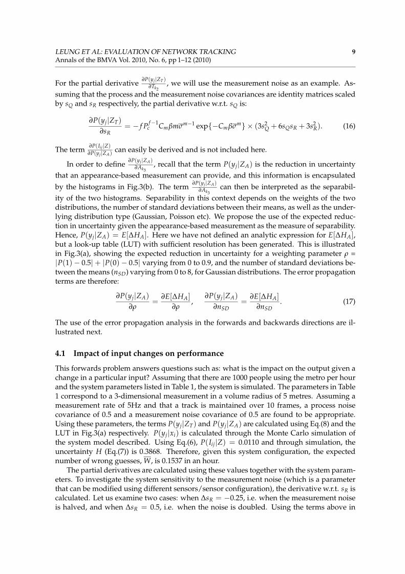
Appearance-based measurementsThe probability P(yj|ZA) is the reduction in uncertainty that an appearance-based measure-ment alone can provide 2. ZA can be a scalar (from a single feature), or a vector of measure-ments of multiple features. Measurements of a single feature from a sample population willproduce histograms similar to those in Fig. 3(b). The solid histograms represent the distancebetween the measurements given the correct and incorrect identity respectively, while thefitted models are shown respectively as a dotted line and crosses. Thus the more separa-ble the two distributions are, the higher the probability of a correct match. The histogramsshown have been generated using a population of 47 [Annesley et al., 2006]; more sampleswill result in smoother histograms. Extension to multi-dimensional features is achieved byfitting Gaussian Mixture Models to the multi-dimensional histograms.

4 Error propagation analysis

This section presents the error propagation analysis of the system, examining the relation-ship between the final performance and the constituent components. This result can be usedto examine both the expected change in the output given a change in the input, and howgood a particular system component has to be given a required level of output performance.

1The number of people in a given space is discrete, and the presence of each person is assumed independent.2This reduction in uncertainty is a property of the appearance-based measurement, and is different from the

overall reduction in uncertainty, given by the difference between H(Y) and H(Y|Z).




The final performance figure is the expected number of times an operator’s attention isrequired, or the expected number of ‘wrong guesses’ that is made before the correct answeris given. We denote this figure of merit as W, defined as:

W =2H − 1

2. (11)

The derivation of this expression is straightforward by considering the case with a uniformprior, and the cumulative probabilities along the branches of a decision tree for a given pop-ulation size. This result can be extended to the cases with non-uniform priors.

To examine the relationship between the input parameters and W, error propagation canbe applied to relate the change in W, ∆W, with the change in each input parameter. Here,the input parameters can be divided into three parts : those related to the dispersion p.d.f.θ, the tracking measurements ZT, and the appearance measurements ZA. The respectiveparameters are enumerated by k1, k2 and k3. The change in ∆W introduced by the change ineach parameter can then be computed by taking the partial derivative of W with respect tothe particular parameter, multiplied by the change. The overall change ∆W is therefore:

∆W = ∑k1

∣∣∣∣∣∂W∂H· ∂H

∂P(Iij|Z)·

∂P(Iij|Z)∂P(yj|xi)

·∂P(yj|xi)

∂θk1

∣∣∣∣∣ · ∆θk1 +

+ ∑k2

∣∣∣∣∣∂W∂H· ∂H

∂P(Iij|Z)·

∂P(Iij|Z)∂P(yj|ZT)

·∂P(yj|ZT)

∂Tk2

∣∣∣∣∣ · ∆Tk2 +

+ ∑k3

∣∣∣∣∣∂W∂H· ∂H

∂P(Iij|Z)·

∂P(Iij|Z)∂P(yj|ZA)

·∂P(yj|ZA)

∂Ak3

∣∣∣∣∣ · ∆Ak3 . (12)

For this subsequent analysis, the partial derivatives w.r.t. Tk2 and Ak3 are examined to inves-tigate how changes to the performance of these components affect the overall performance.(We do not examine partial derivatives of the parameters of θ, because these parameters de-scribe the dynamics of the system under observation, and are therefore considered constantfor this exercise.)

The calculation of the partial derivatives of Eq.(12) are now explained. The first twopartial derivatives common to each additive term are:

∂W∂H

= 2H−1 ln 2 (13)

∂H∂P(Iij|Z)

= −N

∑j=1

1 + log P(Iij|Z). (14)

In order to calculate the partial derivative ∂P(Iij|Z)∂P(yj|ZT) , we refer to Eq.(6) and denote the denom-

inator and the numerator as F and G respectively. The partial derivative is therefore:


=2P(yj|xi)P(yj|ZA)P(yj|ZT)

F−

−2G(P(yj|xi)P(yj|ZA)P(yj|ZT)−¬P(yj|xi)¬P(yj|ZA)¬P(yj|ZT))

F2 .(15)




For the partial derivative ∂P(yj|ZT)∂Tk2

, we will use the measurement noise as an example. As-suming that the process and the measurement noise covariances are identity matrices scaledby sQ and sR respectively, the partial derivative w.r.t. sQ is:

∂P(yj|ZT)∂sR

= − f P f−1c Cmβmσm−1 exp{−Cmβσm} × (3s2

Q + 6sQsR + 3s2R). (16)

The term ∂P(Iij|Z)∂P(yj|ZA) can easily be derived and is not included here.

In order to define ∂P(yj|ZA)∂Ak3

, recall that the term P(yj|ZA) is the reduction in uncertaintythat an appearance-based measurement can provide, and this information is encapsulated

by the histograms in Fig.3(b). The term ∂P(yj|ZA)∂Ak3

can then be interpreted as the separabil-ity of the two histograms. Separability in this context depends on the weights of the twodistributions, the number of standard deviations between their means, as well as the under-lying distribution type (Gaussian, Poisson etc). We propose the use of the expected reduc-tion in uncertainty given the appearance-based measurement as the measure of separability.Hence, P(yj|ZA) = E[∆HA]. Here we have not defined an analytic expression for E[∆HA],but a look-up table (LUT) with sufficient resolution has been generated. This is illustratedin Fig.3(a), showing the expected reduction in uncertainty for a weighting parameter ρ =|P(1)− 0.5|+ |P(0)− 0.5| varying from 0 to 0.9, and the number of standard deviations be-tween the means (nSD) varying from 0 to 8, for Gaussian distributions. The error propagationterms are therefore:

∂P(yj|ZA)∂ρ

=∂E[∆HA]

∂ρ,

∂P(yj|ZA)∂nSD

=∂E[∆HA]

∂nSD. (17)

The use of the error propagation analysis in the forwards and backwards directions are il-lustrated next.

4.1 Impact of input changes on performance

This forwards problem answers questions such as: what is the impact on the output given achange in a particular input? Assuming that there are 1000 people using the metro per hourand the system parameters listed in Table 1, the system is simulated. The parameters in Table1 correspond to a 3-dimensional measurement in a volume radius of 5 metres. Assuming ameasurement rate of 5Hz and that a track is maintained over 10 frames, a process noisecovariance of 0.5 and a measurement noise covariance of 0.5 are found to be appropriate.Using these parameters, the terms P(yj|ZT) and P(yj|ZA) are calculated using Eq.(8) and theLUT in Fig.3(a) respectively. P(yj|xi) is calculated through the Monte Carlo simulation ofthe system model described. Using Eq.(6), P(Iij|Z) = 0.0110 and through simulation, theuncertainty H (Eq.(7)) is 0.3868. Therefore, given this system configuration, the expectednumber of wrong guesses, W, is 0.1537 in an hour.

The partial derivatives are calculated using these values together with the system param-eters. To investigate the system sensitivity to the measurement noise (which is a parameterthat can be modified using different sensors/sensor configuration), the derivative w.r.t. sR iscalculated. Let us examine two cases: when ∆sR = −0.25, i.e. when the measurement noiseis halved, and when ∆sR = 0.5, i.e. when the noise is doubled. Using the terms above in




0.04 0.2 0.36 0.52 0.68 0.84 1−0.1

0

0.1

0.2

0.3

0.4

0.5

0.6

0.7

0.8

0.9

Weighting parameter ρ

Exp

ecte

d re

duct

ion

in u

ncer

tain

ty

8 s.d.s apart

0 s.d.s apart

(a) Look-up table

0

0.005

0.01

0.015

0.02

0.025

0.03

0.035

0.04

0.045

0.05

Scalable Color 256 Match Measure

2.84

5.54

0.14

1.49

x10e−4

4.19

6.89

8.24

9.59

10.94

12.30

Incorrectmatches

Correctmatches

(b) Histograms

6 8 10 12 14 16

Distribution 1with s.d. 1

Distribution 2with s.d. 1

(c) Distributions 3 s.d.s apart

Figure 3: (a) The expected reduction in uncertainty for a weighting parameter varying from 0 to 0.9, andthe number of standard deviations between the means varying from 0 to 8, for Gaussian distributions. (b)Normalised histogram for correct and incorrect matches, as a function of the distance measure for the MPEG-7color descriptor Scalable Color. Solid lines: from experiments. Dotted line/crosses: fitted curves. The priorbetween correct and incorrect matches is reflected in the respective vertical scales are on the left and right of thegraph. They have been displayed together for clarity. These histograms correspond to the dot in (a). (c) Twoequal-prior distributions with 3 standard deviations between the means. These histograms correspond to thesquare in (a).

Eq.(12) gives:

∆W =

∣∣∣∣∣∂W∂H· ∂H

∂P(Iij|Z)·


·∂P(yj|ZT)

∂sR

∣∣∣∣∣ · ∆sR

=∣∣0.6537 · 5.5064 · 0.1578 · −0.4452

∣∣ · ∆sR (18)

Therefore, halving the measurement noise variance reduces W by 0.0632, while doubling themeasurement noise variance increases W by 0.1265.

Table 1: Metro system parameters.Parameter Symbol Value

Dimension of measurement space m 3Volume radius for data association r 5

Variance of process noise sQ 0.5Variance of measurement noise sR 0.5

Numframes to track over f 10

4.2 Required component performance level for overall end-user requirement

This backwards problem starts with the end-user requirement, and examines how good eachor a particular constituent component has to be to meet this requirement. This analysis isuseful for two reasons. First, it relates the system performance to component performance,




and provides a ‘target’ level of performance for algorithmic development. If a componentis ‘good enough’, then effort should be focussed on other parts of the system. Second, insystem design, if a system is not performing to a desired level, it can be difficult to attributethis under-performance to a component without an analysis tool.

Here we consider the case where only appearance-based measurements are used, illus-trating that a subset of the model can be used. Starting from the value of the expectednumber of wrong guesses W = 10, which from requirements elicitation from our projectend-users is within the range of acceptable performance, the uncertainty H is 4.3923 andP(Iij|Z) is required to be 0.4640 for a throughput of 1000 people per hour. From the simu-lations, P(yj|xi) = 0.2015, therefore P(yj|ZA) is 0.7743. This means that the expected reduc-tion in uncertainty, E[∆HA], is also 0.7743. Referring to Fig. 3(a), at equal prior, 3 standarddeviations between the means of the distributions are required to achieve the desired per-formance. Fig. 3(c) shows an example of these distributions. This can be used as a criterionin the selection and assessment of feature(s) and sets a minimum performance level for al-gorithm evaluation.

5 Conclusions

We have presented a framework for evaluating video-based tracking methods in the publictransport domain, using the information gained through their use as an evaluation metric.This metric has two distinct advantages: it summarises and abstracts from the implemen-tation details of the video-based tracking methods, and it links the technical performanceof the system directly with the end-users’ requirements, which is the frequency with whichoperator attention is required, i.e. the expected number of wrong guesses. A comprehensivemathematical framework of the system has been presented, and error propagation analysishas been carried out to allow the investigation of system sensitivity and end-user drivenanalysis; examples have been given illustrating their use. This framework is directly appli-cable to existing ‘Tag and Track’ methods in transport networks, by modelling the topologyof the network of interest, as well as each technical component analytically. While the fi-nal performance of each method will undoubtedly depend on the system parameters, theirresults can be compared directly by using the proposed approach.

Acknowledgements

The work is funded under the CARETAKER project (European Union IST 4-027231). Ourthanks to Gruppo Torinese Trasporti for giving permission for images of their stations to beused in this publication.

References

J. Annesley, V. Leung, A. Colombo, J. Orwell, and S.A. Velastin. Fusion of multiple featuresfor identity estimation. pages 534–539. The Institution of Engineering and TechnologyConference on Crime and Security, June 2006.

J. Black, T. Ellis, and P. Rosin. A novel method for video tracking performance evaluation.




pages 125–132. Joint IEEE Int. Workshop on Visual Surveillance and Performance Evalua-tion of Tracking and Surveillance (VS-PETS), October 2003.

L.M. Brown, A.W. Senior, Y-L. Tian, J. Connell, and A. Hampapur. Performance evaluationof surveillance systems under varying conditions. IEEE Int. Workshop on PerformanceEvaluation of Tracking and Surveillance (PETS), October 2005.

F. Fleuret, J. Berclaz, R. Lengagne, and P. Fua. Multi-camera people tracking with a prob-abilistic occupancy map. IEEE. Trans. Pattern Analysis and Machine Intelligence, 30(2):267–282, 2008.

HOSDB. http://scienceandresearch.homeoffice.gov.uk/hosdb/cctv-imaging-technology/video-based-detection-systems/i-lids.

O. Javed, K. Shafique, and M. Shah. Appearance modeling for tracking in multiple non-overlapping cameras. volume 2, pages 26–33. CVPR, 2005.

S.M. Khan and M. Shah. A multiview approach to tracking people in crowded scenes usinga planar homography constraint. pages 133–146. ECCV, May 2006.

K. Kim and L.S. Davis. Multi-camera tracking and segmentation of occluded people onground plane using search-guided particle filtering. pages 98–109. ECCV, May 2006.

V. Leung, J. Orwell, and S.A. Velastin. Performance evaluation of re-acquisition methodsfor public transport surveillance. pages 705–712. IEEE Tenth Int. Conference on Control,Automation, Robotics and Vision, December 2008.

D. Makris, T.J. Ellis, and J.K. Black. Bridging the gaps between cameras. pages 205–210.CVPR, 2004.

S. Mori, K.-C. Chang, and C.-Y. Chong. Performance Analysis of Optimal Data Associationwith Applications to Multiple Target Tracking. In Multitarget-Multisensor Tracking: Appli-cations and Advances, volume II, chapter 7, pages 183–234. Artech House, 1992.

C.J. Needham and R.D. Boyle. Performance evaluation metrics and statistics for positionaltracker evaluation. pages 278–289. Int. Conference on Computer Vision Systems (ICVS),April 2003.

N. Ning and T. Tan. A framework for tracking moving target in a heterogeneous camerasuite. pages 1–5. IEEE Ninth Int. Conference on Control, Automation, Robotics and Vision,December 2006.

PETS. http://www.cvg.cs.rdg.ac.uk/slides/pets.html.

A. Rahimi, B. Dunagan, and T. Darrell. Simultaneous calibration and tracking with a net-work of non-overlapping sensors. pages 187–194. CVPR, 2004.

C.J. Van Rijsbergen. Information Retrieval. Butterworth-Heinemann Ltd., 2nd edition, 1979.



performance evaluation of tracking for public transport

Documents