performance improvements for lidar-based visual...
TRANSCRIPT

Performance Improvements for Lidar-Based
Visual Odometry
by
Hang Dong
A thesis submitted in conformity with the requirementsfor the degree of Master of Applied Science
Graduate Department of Aerospace Science and EngineeringUniversity of Toronto
Copyright c© 2013 by Hang Dong

Abstract
Performance Improvements for Lidar-Based Visual Odometry
Hang Dong
Master of Applied Science
Graduate Department of Aerospace Science and Engineering
University of Toronto
2013
Recent studies have demonstrated that images constructed from lidar reflectance informa-
tion exhibit superior robustness to lighting changes. However, due to the scanning nature
of the lidar and assumptions made in previous implementations, data acquired during
continuous vehicle motion suffer from geometric motion distortion and can subsequently
result in poor metric visual odometry (VO) estimates, even over short distances (e.g.,
5-10 m). The first part of this thesis revisits the measurement timing assumption made
in previous systems, and proposes a frame-to-frame VO estimation framework based on a
pose-interpolation scheme that explicitly accounts for the exact acquisition time of each
intrinsic, geometric feature measurement. The second part of this thesis investigates a
novel method of lidar calibration that can be applied without consideration of the internal
structure of the sensor. Both methods are validated using experimental data collected
from a planetary analogue environment with a real scanning laser rangefinder.
ii

Acknowledgements
First and foremost, I would like to acknowledge my parents for their decision to
immigrate to Canada, and the sacrifice they made, and continue making everyday, to
provide my sister and me the opportunities that they never had growing up. Given the
initial language barrier, the first couple of years at school were very tough for me. I
would like to thank my middle school science teacher, Mr. Glenn Miller, for giving me
the confidence to excel when I needed it the most.
At University of Waterloo, the Mechatronics Engineering program provided me an
opportunity to explore academic and engineering concurrently. Specifically, I would like
thank to Professor Kaan Erkorkmaz for giving me the opportunity to conduct academic
research without prior experience, and Professor Steven Waslander for introducing me
to the world of autonomous robotics. Without either of these experience, I would likely
have decided against pursuing graduate study.
At University of Toronto, amazing things happened. Academically, I was exposed to
the latest in state estimation research, and was able to innovate and contribute a number
of small, but concrete improvements. Entirely unexpected to me, I also experienced much
personal development here. From holding up everything I do to the highest standard, to
surviving the wilderness of Northern Labrador, I experienced amazing transformation in
the past three years. Without my supervisor, Professor Tim Barfoot, none of this would
have been possible.
Since space limitations prevent me from personalizing all of my messages, to my
colleagues in the Autonomous Space Robotics Lab, Paul, Braden, Colin, Keith, Chi,
Goran, Andrew, Rehman, Jon, Sean, Chris, Erik, and Peter, thank you.
I would like to thank Sagar Kakade for proofreading this thesis, and Professor Jonathan
Kelly for reviewing it. Lastly, I want to thank the National Science and Engineering Re-
search Council of Canada for their financial support through the CGS-M award.
iii

Contents
1 Introduction 1
2 Background Literature Review 4
2.1 Dark Navigation Technology Overview . . . . . . . . . . . . . . . . . . . 4
2.2 Lidar Intensity Imaging . . . . . . . . . . . . . . . . . . . . . . . . . . . . 5
2.3 2D Keypoint Matching . . . . . . . . . . . . . . . . . . . . . . . . . . . . 7
2.4 Visual SLAM Using Passive Cameras . . . . . . . . . . . . . . . . . . . . 8
2.5 Lidar-based Implementation . . . . . . . . . . . . . . . . . . . . . . . . . 9
3 Lidar Simulation 12
3.1 3D Lidar Simulator . . . . . . . . . . . . . . . . . . . . . . . . . . . . . . 12
3.2 Analysis of Simulated Datasets . . . . . . . . . . . . . . . . . . . . . . . 15
3.2.1 Dataset 1 - Translational Motion . . . . . . . . . . . . . . . . . . 15
3.2.2 Dataset 2 - Translational and Rotational Motion . . . . . . . . . . 17
4 Motion Compensated Lidar VO 19
4.1 Related Works . . . . . . . . . . . . . . . . . . . . . . . . . . . . . . . . . 20
4.2 Methodology . . . . . . . . . . . . . . . . . . . . . . . . . . . . . . . . . 22
4.2.1 VO Problem Setup . . . . . . . . . . . . . . . . . . . . . . . . . . 23
4.2.2 Rotation Interpolation . . . . . . . . . . . . . . . . . . . . . . . . 24
4.2.3 General Form of Rotation Perturbation . . . . . . . . . . . . . . . 29
iv

4.2.4 Perturbing Interpolated Poses . . . . . . . . . . . . . . . . . . . . 32
4.2.5 Linearized Error Terms . . . . . . . . . . . . . . . . . . . . . . . . 33
4.3 VO Algorithm Test . . . . . . . . . . . . . . . . . . . . . . . . . . . . . . 34
4.3.1 System Testing using Lidar Simulator . . . . . . . . . . . . . . . . 35
4.3.2 Hardware Description . . . . . . . . . . . . . . . . . . . . . . . . . 36
4.3.3 Field Testing Results . . . . . . . . . . . . . . . . . . . . . . . . . 38
4.4 Conclusion . . . . . . . . . . . . . . . . . . . . . . . . . . . . . . . . . . . 40
5 Lidar Calibration 42
5.1 Related Works . . . . . . . . . . . . . . . . . . . . . . . . . . . . . . . . . 44
5.2 Methodology . . . . . . . . . . . . . . . . . . . . . . . . . . . . . . . . . 45
5.2.1 Sensor Model . . . . . . . . . . . . . . . . . . . . . . . . . . . . . 47
5.2.2 Bundle Adjustment Formulation . . . . . . . . . . . . . . . . . . . 52
5.2.3 Measurement Correction . . . . . . . . . . . . . . . . . . . . . . . 55
5.3 Experiment . . . . . . . . . . . . . . . . . . . . . . . . . . . . . . . . . . 56
5.3.1 Calibration Dataset . . . . . . . . . . . . . . . . . . . . . . . . . . 56
5.3.2 Calibration Results . . . . . . . . . . . . . . . . . . . . . . . . . . 57
5.4 Conclusion . . . . . . . . . . . . . . . . . . . . . . . . . . . . . . . . . . . 60
6 Extended Experimental Results 61
7 Summary 66
Bibliography 67
v

Notation
a : Symbols in this font are real scalars.
a : Symbols in this font are real column vectors.
A : Symbols in this font are real matrices.
E[·] : The expectation operator.
∼ N (a,B): Normally distributed with mean a and covariance B.
F−→a : A reference frame in three dimensions.
(·) : Symbols with an overbar are nominal values of a quantity.
(·)× : The cross-product operator that produces a skew-symmetric matrix
from a 3× 1 column.
1 : The identity matrix.
0 : The zero matrix.
pc,ba : A vector from point b to point c (denoted by the superscript) and
expressed in F−→a (denoted by the subscript).
pc,ba : The vector pc,ba expressed in homogeneous coordinates.
Cab : The 3 × 3 rotation matrix that transforms vectors from F−→b to F−→a:
pc,ba = Cabp
c,bb .
Tab : The 4× 4 transformation matrix that transforms homogeneous points
from F−→b to F−→a: pc,aa = Tabp
c,bb .
vi

Chapter 1
Introduction
Due to their compact size, solid construction, and relatively low barrier to entry, stereo
cameras have become a popular sensor of choice for applications ranging from underwater
vehicles to micro aerial vehicles and everything in between. The Mars Exploration Rover
(MER) is the first space rover to implement such a system for low-level driving autonomy,
with limited computing power, that can run either obstacle detection or visual odometry
(VO) but not both at the same time. The onboard vision system was deemed instrumental
in enabling over 6 kilometres of travel for each of the rovers (Matthies et al., 2007).
Since cameras are passive sensors, nearly all existing vision-based techniques rely on
the assumption of consistent ambient lighting conditions. This, however, is not the case
for the majority of unstructured, three-dimensional environments, such as most outdoor
applications, where images taken even a few hours apart can appear drastically different
as lighting conditions change. A specific instance of visual odometry failure onboard
MER, noted in Matthies et al. (2007), occurred when the rover’s shadow dominated the
stereo camera’s view.
With greater onboard capability, such as with the new radioisotope thermoelectric
generators (RTGs) on Mars Science Laboratory (MSL) providing constant power during
all seasons and through the day and night, it is desirable to have robust autonomous
1

Chapter 1. Introduction 2
capabilities that allow a rover to drive in the dark, thereby doubling its daily travel
range to maximize scientific return. In the case of lunar missions, with permanently
shadowed craters, having such a capability is a prerequisite before a mission can even
enter the planning stage.
Unlike stereo cameras, light detection and ranging (lidar) sensors are active sensors
that use one-axis or two-axis scanning lasers to generate 2D or 3D information about
the surrounding environment. Earlier work on appearance-based lidar navigation by
McManus et al. (2011) demonstrated that images constructed from lidar reflectance in-
formation exhibit superior robustness to lighting changes in outdoor environments in
comparison to traditional passive camera imagery. Moreover, for visual navigation meth-
ods originally developed using stereo vision, such as visual odometry (VO) and visual
teach and repeat (VT&R), scanning lidar can serve as a direct replacement for the passive
sensor. This results in systems that retain the efficiency of the sparse, appearance-based
techniques while overcoming the dependence on adequate/consistent lighting conditions
required by traditional cameras.
However, due to the scanning nature of the lidar and assumptions made in previous
implementations, data acquired during continuous vehicle motion suffer from geometric
motion distortion and can subsequently result in poor metric VO estimates, even over
short distances (e.g., 5-10 m).
A high-level literature review is presented in Chapter 2 to serve as background in-
formation for the entire thesis, followed by a detailed “Related Works” section in each
technical component in Chapter 4 and Chapter 5. In order to systematically study the
effect of the motion distortion, a 3D lidar simulator is created to replicate the scanning
pattern of an existing lidar sensor. This simulator enables generation of datasets both
with and without motion distortion in a controlled environment, as well as manipulation
of traverse trajectory to amplify this effect. This work is documented in Chapter 3.
Chapter 4 of this thesis revisits the measurement timing assumption made in previous
Chapter 1. Introduction 3
systems, and proposes a frame-to-frame VO estimation framework based on a novel pose
interpolation scheme that explicitly accounts for the exact acquisition time of each feature
measurement. The proposed technique is demonstrated using data generated from the
aforementioned lidar simulator as well as 500 m of experimental traverse data.
In addition to accounting for exact measurement timing in the estimation framework,
accurate pose estimation also relies on high-quality sensor measurements. Due to man-
ufacturing tolerance, every sensor (camera or lidar) needs to be individually calibrated.
Feature-based techniques using simple calibration targets (e.g., a checkerboard pattern)
have become the dominant approach to camera sensor calibration. Existing lidar cali-
bration methods require a controlled environment (e.g., a space of known dimension) or
specific configurations of supporting hardware (e.g., coupled with GPS/IMU). Chapter 5
of this thesis presents a calibration procedure for a two-axis scanning lidar using only an
inexpensive checkerboard calibration target. In addition, the proposed method general-
izes a two-axis scanning lidar as an idealized spherical camera with additive measurement
distortions. Conceptually, this is not unlike normal camera calibration in which an arbi-
trary camera is modelled as an idealized projective (pinhole) camera with tangential and
radial distortions.
In Chapter 6, both motion compensation and sensor calibration are tested individu-
ally and then together using over 10 km of experimental traverse data collected from a
planetary analogue environment to demonstrate the performance improvement each of
these components contribute toward VO estimates. Finally, the results and contributions
of this thesis are summarized in Chapter 7.

Chapter 2
Background Literature Review
This chapter presents a high-level review of the related technology and literature to serve
as background information for the rest of the thesis. Detailed literature reviews are
carried out in Chapter 4 and Chapter 5 as part of the technical components.
2.1 Dark Navigation Technology Overview
Stereo vision with LED strobe lighting was first considered by NASA Ames (Husmann
and Pedersen, 2008). They found that due to the inverse-square illumination drop off
with distance, in a single frame, the parts of the image of nearby terrain had a tendency
to oversaturate, while the ones of objects far away are under exposed. They concluded
that realistic continuous locomotion would require specialized camera hardware with a
logarithmic response to get high-dynamic-range (HDR) in a single image, along with high
peak power (1 kW) lighting, to obtain 10 m look-ahead with 90◦ field of view (FOV).
Flash lidar technology delivers instantaneous range and intensity images. The com-
mercially available SwissRanger SR3000 and a prototype from Ball Aerospace were tested
by Pedersen et al. (2008). The SR3000 is deemed usable for detecting rocks only 5.5 m
away and is subject to motion blur. The Ball sensor is a time-of-flight system that can
measure targets several kilometres away, but suffers from a limited 8◦ FOV.
4

Chapter 2. Background Literature Review 5
Advanced Scientific Concepts’ flash lidar has been flight tested during the final Space
Shuttle missions (STS-127, STS-133), and subsequently used on-board the SpaceX Dragon
spacecraft for state estimation during automated docking with the International Space
Station. The sensor is currently capable of 128x128 pixels resolution at 5 Hz and a max-
imum range of 60 metres (45◦ FOV) to 1.1 km (3◦ FOV). Stettner (2010) noted that
imaging arrays up to 512x512 pixels are also under development.
Rankin et al. (2007) detected negative obstacles (e.g., ditches, holes, and other de-
pressions) using intensity images from a thermal video camera. This study was carried
out based on the assumption that at night the interiors of negative obstacles generally
remain warmer than the surrounding terrain throughout the night. While this study ob-
tained good experimental results, the thermal signature assumption does not necessarily
hold up in extraterrestrial environments.
2.2 Lidar Intensity Imaging
Lidar technology has been widely adopted for surveying, both as airborne instruments
for capturing topographic information of the Earth surfaces (Brock et al., 2002), and for
ground surveying stations digitizing detailed 3D scenes locally (Nagihara et al., 2004). In
recent years, emphasis has shifted to incorporating both range and intensity information
for the above applications. Examples of lidar generated images can be seen in Figures 2.1
and 2.2.
Hofle and Pfeifer (2007) described how the intensity readings theoretically depend
on surface reflectance, ρ (which, in turn, depends on whether the object is wet or dry),
atmospheric attenuation, a [dB/km], the local incidence angle, α, and the range to the
target, R [m] according to the following relationship:
I ∝ ρ
R210−2R·a/10000 cosα · C

Chapter 2. Background Literature Review 6
Figure 2.1: Airborne lidar configuration (Wan and Zhang, 2006) and resulting lidarintensity image (Hofle and Pfeifer, 2007).
Note that C represents other sensor parameters (e.g., aperture diameter, system losses),
which are assumed to be constant.
Actual lidar data, however, show relatively low dependence on the local incidence
angle (Kaasalainen et al., 2005). For a non-Lambertian surface (e.g., smooth or glossy
man-made surfaces, or wet surfaces), weaker return reflections are expected as the local
angle of incidence increases. Natural surfaces, such as volcanic units, behave as Lam-
bertian reflectors within the range of adopted incidence angles (Mazzarini et al., 2006).
By definition, a Lambertian surface will return the same signal strength irrespective of
the incidence angle. The returned light is then filtered to reject light with frequencies
different from the original emitted beam, thus giving the intensity measurement an ex-
cellent ability to handle environmental ambient light change, as seen in Figure 2.2, where
the intensity image is unaffected by the large amount of shadows observed in the normal
passive image.
Lidar intensity images are inherently noisier than their passive counterparts due to
the nature of the imaging mechanism. According to Fowler (2000), the noise appears
discretely in the intensity image, and does not appear as clustered groups. Wan and
Zhang (2006) proposed a noise removal technique based on the orientation gradient of

Chapter 2. Background Literature Review 7
Figure 2.2: Outdoor image comparison. The post-processed lidar intensity informationresulted in a shadow-free image (left). The passive image (right) was heavily influencedby environmental lighting condition, seen here with large amount of shadow (Burton andWood, 2010).
the distance information, and qualitatively demonstrated improvements in the signal to
noise ratio (SNR).
2.3 2D Keypoint Matching
Algorithms for viewpoint-invariant keypoint detection and matching were originally de-
veloped for object recognition by machine vision researchers. The algorithms’ powerful
abilities to find the correspondence between two images of a generic scene or object have
propelled their adoption in other computer vision applications, such as camera calibra-
tion, 3D reconstruction, and image registration. Many existing visual-based navigational
techniques rely on image feature detection and tracking to calculate egomotion as well
as to detect loop closure (i.e., when returning to a place viewed before).
Lowe (1999)’s scale-invariant feature transform (SIFT) detector and descriptor, com-
puted from local gradient histograms, has been shown to work well in robotic applica-
tions, both in structured indoor environments (Se et al., 2002, 2005) and unstructured
outdoor terrain (Barfoot, 2005). To minimize computation slow down, Barfoot (2005)

Chapter 2. Background Literature Review 8
delegated SIFT feature extraction to a custom FPGA hardware while parallelizing fea-
ture matching onboard the host PC. A GPU implementation of SIFT by Sinha et al.
(2006) achieved a ten-fold speed-up in feature extraction in comparison to the original
CPU implementation.
The speeded up robust features (SURF) algorithm was developed by Bay et al. (2006)
to address the computational requirements of SIFT. This algorithm takes advantage of a
fast approximation of second-order Gaussian derivatives evaluated using integral images.
Versions of GPU-accelerated SURF are also available as closed-source binaries (Terriberry
et al., 2008) and open-source code (Furgale et al., 2009).
Calonder et al. (2010) developed an even more efficient feature point description using
compact signature, which exploits the sparsity of the signature produced by a randomized
tree structure known as Generic Trees (Lepetit and Fua, 2006). Konolige et al. (2010)
demonstrated the application of this algorithm as a method for re-localization and online
place recognition (PR) inside a visual simultaneous localization and mapping (VSLAM)
engine.
2.4 Visual SLAM Using Passive Cameras
Most appearance-based navigation techniques can trace their roots to the visual odometry
(VO) work by Matthies and Shafer (1987). VO estimates vehicle pose changes using
sequential camera images. Generally, the ego motion estimates from VO pipeline are
used to form the initial conditions for more complex navigation techniques, such as visual
teach and repeat (VT&R) by Furgale and Barfoot (2010) and VSLAM by Konolige et al.
(2010).
Current state-of-the-art VSLAM systems consist of a core SLAM engine running in
an incremental mode and a place recognition (PR) system to detect large-scale loop
closures. The VSLAM system by Konolige et al. (2010) employs a VO engine using
Chapter 2. Background Literature Review 9
FAST features, which continuously matches the current frame against the last keyframe,
until a given distance has been traversed or the match becomes too weak. This algorithm
produces a stream of keyframes at a spaced distance, and forms the backbone of their
constraint graph. The PR engine opportunistically finds other views that match the
current keyframe and previous views, and creates additional constraints when matches
are found. Similar in architecture, Sibley et al. (2009) uses sliding window relative bundle
adjustment technique to estimate the relative pose changes between keyframes.
While some are more robust than others, most existing VSLAM methods suffer from
the same failure mode, with VO and/or PR no longer capable of performing reliably
under significant changes in ambient lighting. A notable exception is Milford and Wyeth
(2012)’s SeqSLAM. Instead of calculating the single location most likely given a current
image, their approach calculates the best candidate matching location within every local
navigation sequence. Under the assumption that the perspective and the speed of the
camera is similar on repeated journeys through each part of a route, SeqSLAM’s PR
engine was able to successfully match footages taken at different time of the day, as well
in different seasons.
2.5 Lidar-based Implementation
In the robotic literature, the intensity information from lidar sensors are generally dis-
carded, with most algorithms working only with range data. While such approaches
have achieved some success with 2D planar lidar scanners in structured indoor environ-
ments, the greatly increased data produced by 3D lidar scanners requires significantly
more efficient methods of processing and matching.
An intuitive and common approach to lidar-based motion estimation is through the
alignment of lidar scans using the iterative closest point (ICP) algorithm (Chen and
Medioni, 1991; Besl and McKay, 1992). It requires an immense amount of computation

Chapter 2. Background Literature Review 10
power and becomes infeasible in large environments.
Magnusson et al. (2009) developed a compact representation of 3D point clouds that
is discriminative enough to detect loop closures. Their approach uses surface shape
histograms to create a condensed representation of 3D point cloud that is invariant to
rotation. During exploration, histograms from current scans are compared against all
previous histogram signatures to detect loop closure. Their field test covers 1.24 km of
rover traverse.
Neira et al. (1999) combined both range and intensity data from a one-axis scan-
ner using an extended Kalman filter (EKF) to localize against a known indoor planar
map. Guivant et al. (2000) noted the distinctiveness of reflective marks in the intensity
information, and used it to simplify outdoor data association of their SLAM algorithm.
May et al. (2009) recently developed an indoor 3D SLAM system using keypoint
features extracted from flash lidar intensity images. The study demonstrated their key-
point descriptor-based system is far more efficient than ICP-based SLAM using the same
dataset. Unfortunately, this particular implementation can not be directly adapted to a
large, unstructured outdoor environment, due to the sensor’s short maximum range (7m)
and high sensitivity to environmental noise.
To date, the most relevant work to this thesis in appearance-based lidar navigation
was carried out by McManus et al. (2011). Using a survey-grade 3D lidar sensor, they
acquired lidar intensity images outdoors over a 24 hour period, and determined the
stability of SURF keypoints extracted from intensity images to be vastly superior than
their counterparts from passive cameras. McManus et al. (2011) further validated their
approach by implementing a visual odometry algorithm on a sequence of lidar intensity
images. Note that since the ILRIS lidar sensor used was not designed for high framerate
acquisition, the VO experiment was restricted to stop-scan-go at each frame. In follow-
up studies (McManus et al., 2012, 2013), a high framerate lidar was used to carry out
continuous navigation based on VO. While the relative frame-to-frame VO estimates was

Chapter 2. Background Literature Review 11
sufficiently accurate for lidar-based VT&R, the cumulative metric estimate in a global
frame drifted quickly beyond 5-10 m of travel (McManus et al., 2012). In comparison,
state-of-art stereo-vision-based VO systems largely retain global metric accuracy over
multi-kilometre traverses (Lambert et al., 2012); there is clearly room for improvement
in lidar-based VO. This thesis will attempt to improve the metric accuracy of lidar-based
VO by compensating for motion distortion and also improve lidar intrinsic geometric
calibration.

Chapter 3
Lidar Simulation
3.1 3D Lidar Simulator
Earlier work on appearance-based lidar navigation by McManus et al. (2011) revealed
promising results: As shown in Figure 3.1(a), VO estimation performance comparable to
that of established stereo-vision based methods was obtained using stop-scan-go acquisi-
tion method, and the lidar-based approach was shown to be significantly more robust to
ambient light changes.
0 20 40 60 80 100
0
10
20
30
x [m]
y [
m]
Ilris VO
Stereo VO
GPS (Fixed RTK)
GPS (Float RTK/SPS)
Start End
(a) VO estimation results, showing comparable lidar-based andcamera-based VO estimates (McManus et al., 2011)
ILIRS Lidar
DGPS
Stereo Camera
(b) Rover configuration
Figure 3.1: ILRIS lidar-based stop-scan-go VO system
It is, however, more desirable for a rover to traverse continuously, and this is the case
for existing passive camera-based navigation techniques. Unlike charge-coupled device
12
Chapter 3. Lidar Simulation 13
(CCD) camera sensor, which captures a complete image frame at a single instant of
time, scanning lidar acquires one pixel at a time, which leads to motion distortion when
an entire image of scan data are incorrectly assumed to have been acquired at a single
instant in time during VO processing.
0 10 20 30 40 50 60 70 80 90
−30
−25
−20
−15
−10
−5
0
5
10
x [m]
y [m
]
Autonosys VO
Stereo VO
GPS (Post processed)
Start
End
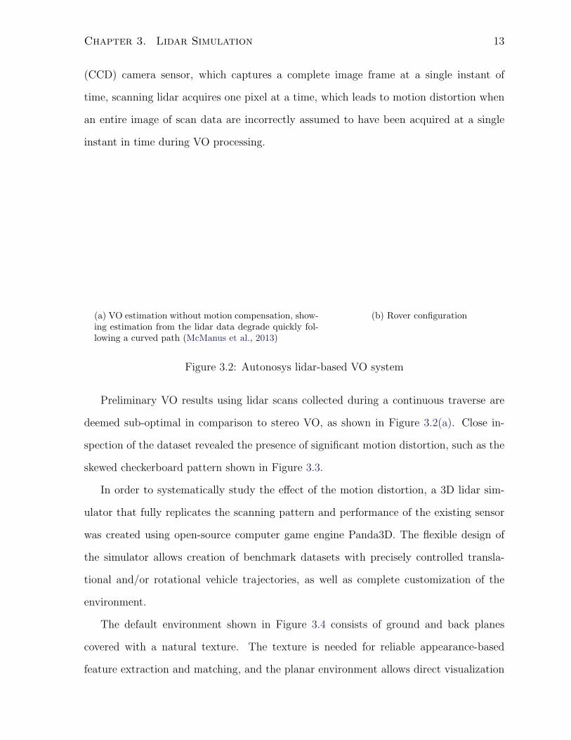
(a) VO estimation without motion compensation, show-ing estimation from the lidar data degrade quickly fol-lowing a curved path (McManus et al., 2013)
Autonosys Lidar
DGPS
Stereo Camera
(b) Rover configuration
Figure 3.2: Autonosys lidar-based VO system
Preliminary VO results using lidar scans collected during a continuous traverse are
deemed sub-optimal in comparison to stereo VO, as shown in Figure 3.2(a). Close in-
spection of the dataset revealed the presence of significant motion distortion, such as the
skewed checkerboard pattern shown in Figure 3.3.
In order to systematically study the effect of the motion distortion, a 3D lidar sim-
ulator that fully replicates the scanning pattern and performance of the existing sensor
was created using open-source computer game engine Panda3D. The flexible design of
the simulator allows creation of benchmark datasets with precisely controlled transla-
tional and/or rotational vehicle trajectories, as well as complete customization of the
environment.
The default environment shown in Figure 3.4 consists of ground and back planes
covered with a natural texture. The texture is needed for reliable appearance-based
feature extraction and matching, and the planar environment allows direct visualization

Chapter 3. Lidar Simulation 14
Nodding
Mirror
Polygonal
Mirror(8000 RPM)
Laser
Range�nder
Vertical
Scan Dir.
Landmark
r1,2
r0,1
r
F→p
F→k
F→l
Image k
Image K
Scan Direction
Image K+1
Scan Direction
Figure 3.3: Simplified illustration of the Autonosys lidar’s two-axis scanning mechanism(O’Neill et al., 2007) (left) and geometric motion distortion effect as seen in intensityimages (right). Note that in the intensity images, the rover was turning left duringboth scans. Different skewing effects of the rectangular checkerboard were caused by thenodding behaviour of this lidar. The raw intensity information provided by the lidar is afunction of the emitted beam energy, range, target reflectance, and its surface orientationwith respect to the lidar. See McManus et al. (2011) for details on how our intensityimages are assembled.
Figure 3.4: Default lidar simulator environment.
of the motion distortion effect due to its simple geometry.
Using a curved trajectory, we recreated similar skewing distortion that was previously
observed in the Autonosys intensity images. A checkerboard, displayed in Figure 3.5, is
added to the scene to improve visual clarity of the motion distortion.

Chapter 3. Lidar Simulation 15
Figure 3.5: Example of simulated intensity data with distortion.
3.2 Analysis of Simulated Datasets
Using the lidar simulator, a total of 7 datasets were generated with a variety of linear
and rotational trajectories. The analysis of two representative datasets using the frame-
to-frame VO state estimator developed by McManus et al. (2013) are highlighted in this
section.
3.2.1 Dataset 1 - Translational Motion
Dataset 1 consists of pure translational motion. In it, the rover followed a linear trajectory
with a constant velocity of 1 m/s along the x-axis, essentially driving straight into the
scene. The VO estimation result from this dataset is shown in Figure 3.6, along with the
the results from the control case where the image data contains no motion distortion.
x [m]
z[m
]
-35 -34.5 -34 -33.5 -33 -32.5 -32 -31.5 -31 -30.5-0.2
00.20.40.60.8
Figure 3.6: First 5 seconds of linear traverse. The ground truth is shown in blue, theestimate from the dataset with motion distortion in green, and the estimate from thedataset without motion distortion in red.

Chapter 3. Lidar Simulation 16
A predominant saw-tooth shaped estimation error is observed in z-axis direction,
as shown in Figure 3.6. This behaviour is a direct result of the nodding vertical scan,
and can be explained by inspecting the scans of a planar wall, as shown in Figure 3.7.
As the vehicle moves forward towards the wall, the physical distance changes inversely
proportional with time. Hence, during a downward scan, the bottom of image is warped
closer toward rover than the top of the image. This effect reverses in the next frame as
the lidar changes its vertical scanning direction.
Figure 3.7: 3D reprojected lidar scans - downward (left) and upward (right) scans. Notethat the amount of motion distortion has been been exaggerated here for visual clarity.These two scans are generated using 5 m/s as vehicle velocity as oppose to the 1 m/s inDataset 1.
This motion distortion effect, however, is not accounted for in the VO algorithm, as
the entire frame is assumed to be taken at the same instant of time. Therefore, to the
estimator, a slanted wall would imply a translation and rotation of the camera position.
It can be visualized by superimposing the frames, shown in Figure 3.8 in a simplified side
view (xz- plane).
The root cause of the saw-tooth error is that the scanning lidar measurement collected
during continuous motion violates the measurement timing assumption that each image is
a static capture of a single instant of time. The simulated control dataset based on stop-
scan-go method does not suffer from this problem, as a time-lapse (scanning capture) of a
static scene is same as a single snapshot of the environment when the observer (camera)

Chapter 3. Lidar Simulation 17
Actual Rover Path VO Estimate
Figure 3.8: Simplified side view of superimposed lidar scans, demonstrating the cause ofsaw-tooth estimation result
is also static.
3.2.2 Dataset 2 - Translational and Rotational Motion
The rover is given a planar sinusoidal trajectory, along with an analytical heading pointed
in the direction of motion. This trajectory introduces additional rotational motion dis-
tortion due to the heading changes.
As shown in Figure 3.9(a), the previously observed saw-tooth error pattern returned
here in the height (z-axis) and camera tilt (axis angle about y-axis) estimates. Also note
the cyclic error in the heading estimate is caused essentially by a phase delay between
actual trajectory and estimation result. These comparisons demonstrate that vehicle
motion distortion in lidar image stacks is indeed a major challenge to existing estimation
framework used by vision-based method as it violates the assumption that all pixels in
each image arrive simultaneously. As such, we need to rethink our estimation strategy.

Chapter 3. Lidar Simulation 18
x [m]y[m
]
-35 -34.5 -34 -33.5 -33 -32.5 -32 -31.5 -31 -30.5
-0.4-0.20
0.2
x [m]
z[m
]
-35 -34.5 -34 -33.5 -33 -32.5 -32 -31.5 -31 -30.5
-0.20
0.20.4
(a) Position estimate from the first 5 seconds of traverse
Orientation Error (expressed in axis angle) (SG-red, Motion-green)
Abtx-axis
[deg]
Abty-axis
[deg]
Abtz-ax
is[deg]
time [s]
0 5 10 15 20 25 30
0 5 10 15 20 25 30
0 5 10 15 20 25 30
-5
0
5
-5
0
5
-1
0
1
(b) Heading error
Figure 3.9: VO estimates from simulated lidar dataset 2 with translational and rotationalmotion. The ground truth is shown in blue, the estimate from dataset with motiondistortion in green, and the estimate from dataset without motion distortion in red.

Chapter 4
Motion Compensated Lidar VO
The extent of motion distortion is related to the vehicle’s velocity and scan rate. Off-
the-shelf, one-axis lidar scanners typically take milliseconds to produce a scan line (e.g.,
as little as 2 ms on SICK LMS 111), and at a speed of 1 m/s, the vehicle would only
have moved few millimeters during a scan. Relatively trivial in magnitude, the motion
distortion effect is generally not accounted for when working with a one-axis scanner. In
comparison, a two-axis scanner takes significantly longer to produce a full scan; depending
on the lidar, it can take anywhere from 100 ms to minutes. Hence, the effect of motion
distortion is no longer inconsequential. For our experiment, we have selected Autonoys’
LVC0702 two-axis scanning lidar over the well-known Velodyne HDL-64E for its higher
(and adjustable) vertical scan resolution. At its 2 Hz scan setting, the lidar produced
intensity images that still allow for reliable SURF feature extraction and matching with
a nominal rover speed of 0.5 m/s as demonstrated by McManus et al. (2012).
To achieve accurate VO estimates despite lidar motion distortion, this chapter pro-
poses an algorithm that explicitly compensates for motion distortion by accounting for the
exact measurement time of each lidar return, and still remains computationally tractable
using a novel pose-interpolation scheme. While many other pose-interpolation schemes
have been proposed in the past, to our knowledge this is the first one that cleanly han-
dles rotations, and at the same time allows for derivation of analytical Jacobians that
19

Chapter 4. Motion Compensated Lidar VO 20
are used during a bundle adjustment nonlinear optimization, resulting in a more efficient
algorithm than comparable systems using numerical Jacobians (Forssen and Ringaby,
2010).
4.1 Related Works
The intensity information is often available on laser rangefinders, though its quality differs
greatly depending on the model. Neira et al. (1999) combined both range and intensity
data from a one-axis scanner using an EKF to localize against a known indoor planar
map. Guivant et al. (2000) noted the distinctiveness of reflective marks in the intensity
information, and used it to simplify outdoor data association. A notable use of inten-
sity information came out of the DARPA Urban Grand Challenge; the Stanford racing
team successfully used the intensity information from a Velodyne lidar to localize against
an intensity-based occupancy grid map (Levinson, 2011), providing the vehicle higher
localization accuracy than what was obtainable from GPS. Similar technology enabled
Google’s self-driving car to complete over 300,000 km of autonomous traverse (Thrun
and Urmson, 2011). It is worth noting that the Google system tightly couples intensity-
data-based localization with an inertially-aided GPS, and requires a preprocessed map
of the environment, neither of which are available for space rovers.
As for lidar motion distortion, thus far there have been three primary approaches to
mitigate its impact on estimation accuracy:
1. Reducing acquisition time per scan: given the same platform velocity, spending less
time on each scan results in less motion distortion. Most lidars have a fixed data
acquisition rate, so this approach typically involves a trade-off between scan rate
and scan resolution.
2. Dewarping the point cloud directly using an external motion estimate such as from
an inertial measurement unit (IMU).

Chapter 4. Motion Compensated Lidar VO 21
3. Dewarping the point cloud iteratively by calculating a motion estimate using the it-
erative closest point (ICP) method and motion-distorted scan, then updating/dewarping
the scan using the motion estimate. The process repeats until the motion estimate
converges. To speed up the algorithm, Bosse and Zlot (2009) preprocessed the
dense point cloud into more sparse voxelized version, while Moosmann and Stiller
(2011) used sub-sampled surface normals for scan matching.
We approach this problem a bit differently. Instead of viewing the entire scan as
a unit of acquisition and attempting to correct for motion distortion by dewarping the
scan, we view each lidar time-of-flight measurement as our base unit of acquisition. This
change of perspective effectively turns a motion-distorted scan (say containing 100,000
points) as viewed from a single pose into 100,000 accurate lidar measurements taken from
100,000 slightly different poses. The large number of poses is non-ideal; each pose in 3D
space has six degrees of freedom (DOF). As the number of poses increases, the solution
quickly becomes computationally intractable.
Assuming that the platform travels with reasonably constant linear/angular velocity
between two consecutive lidar scans, which is approximately true for mobile ground
robots if the time between scans is short (in our case 0.5 seconds), it is then possible to
represent the large number of poses by interpolating between only two poses.
SLERP (Shoemake, 1985) is a quaternion interpolation scheme commonly used in
computer graphic animation. Faced with similar motion distortion effects in complemen-
tary metal-oxide-semiconductor (CMOS) camera sensors and the need to represent large
numbers of poses, Forssen and Ringaby (2010) applied SLERP to interpolate poses in
their work. Since there exists no simple way to incorporate SLERP analytically into the
optimization process, Forssen and Ringaby (2010) resorted to using numerical Jacobians
for nonlinear optimization.
Another alternative is to parameterize rotations using Euler angles, which are subject
to singularities. Moreover, interpolating Euler angles can lead to strange results (Grassia,

Chapter 4. Motion Compensated Lidar VO 22
1998). As such we set out to find a simple ‘linear’ interpolation scheme that not only
handles rotations cleanly, but also allows for derivation of analytical Jacobians that can
be used during the optimization process. Our scheme will be presented in detail in
Section 4.2.2.
4.2 Methodology
Raw lidar data
(UDP Packets)
ROS driver
Image stack
creation
SURF scale
invariant features
Feature
detection
Frame-to-frame
feature tracking
Data
association
RANSAC using
three-point model
generation
Outlier
detection
Frame-to-frame
maximum-likelihood
solution
Nonlinear
optimization
Rover pose
estimate
Figure 4.1: Major processing blocks of our VO algorithm.
The data flow in our VO algorithm is similar to its stereo-vision counterpart, and is
nearly identical to the system presented in McManus et al. (2011). We no longer use stereo
geometry to extract 3D information as this is directly available in the lidar data. In brief,
we extract and match sparse SURF features in consecutive pairs of lidar intensity images,
introduce the associated range images to obtain 3D feature locations, run RANdom
SAmple Consensus (RANSAC) to reject outliers, and then perform a bundle adjustment
nonlinear optimization to determine pose change from frame to frame. We record exact
timestamps for every laser return, which enables pose interpolation inside the frame-
to-frame maximum-likelihood solution. Moreover, with motion distortion, we find it
necessary to relax the RANSAC matching threshold to avoid throwing away valid feature
matches that are temporally far apart. At the same time, this change does allow more
outliers to pass RANSAC. We handle these remaining outliers using a Geman-McClure
M-estimator during iterative nonlinear optimization. A typical set of post-RANSAC
feature tracks is shown in Figure 4.2. Although it is not applied in this thesis, it is worth
nothing that Anderson and Barfoot (2013) further improved the matching quality more
recently by introducing an iterative outer-loop around the RANSAC matching process,

Chapter 4. Motion Compensated Lidar VO 23
(a) A downward scanmatched to an upward scan.
(b) An upward scan matchedto a downward scan.
(c) Repeating pattern in (a).
Figure 4.2: Sample post-RANSAC feature tracks from four consecutive frames (threepairs). The outliers that made it past RANSAC but exceeded M-estimator threshold areshown in yellow. Note the feature tracks’ lengths change between consecutive frame-to-frame matching pairs, as a result of the nodding behaviour of the scanning mechanism.
and dewarping feature locations using motion estimate from the previous iteration. For
this thesis, the most significant change in VO pipeline occurs inside the formulation of
the maximum-likelihood solution, to which we will devote the remainder of this section.
4.2.1 VO Problem Setup
Our VO algorithm is essentially a frame-to-frame bundle adjustment technique that solves
for the following incremental variables:
rk+1,kk : translation of camera pose k + 1 relative to pose k, expressed in frame k,
Ck+1,k : rotation matrix of camera pose k + 1 (from pose k to pose k + 1),
pj,kk : position of landmark j relative to pose k, expressed in frame k,
where j = 1 . . . J . After calculating the incremental transforms, we can compose them
to obtain metric pose estimates with respect to the initial coordinate frame. Thus from
here, we will focus on solving for the incremental variables.
Let a bearing, tilt, and range measurement be defined as y := [α β r]T , then the
measurement error term is given by

Chapter 4. Motion Compensated Lidar VO 24
ejl(rl,kk ,Cl,k,p
j,kk ) := yjl − f
(
Cl,k(pj,kk − r
l,kk )
)
, ∀(j, l)
where yjl is the measurement taken at time tl ∈ [tk, tk+1], l = 1 . . . L), and f(·) is a
nonlinear camera model (5.1). We seek to find the values of Ck+1,k, rk+1,kk , and p
j,kk to
minimize the following objective function:
J(x) :=1
2
∑
j,l
ejl(rl,kk ,Cl,k,p
j,kk )TR−1
jl ejl(rl,kk ,Cl,k,p
j,kk ), (4.1)
where x is the full state that we wish to estimate (pose and landmarks) and Rjl is the
symmetric, positive-definite covariance matrix associated with the (j, l)-th measurement.
The usual approach to this problem is to apply the Gauss-Newton method (Gauss, 1809).
The added challenge here lies in the fact that our state variables are at times tk while our
measurements are at times tl, which do not line up. Our approach will be to ‘linearly’
interpolate poses between the tk times.
4.2.2 Rotation Interpolation
Background on Rotations
We recall Euler’s theorem, which says that every rotation may be expressed using a single
axis-angle pair. It turns out, we can write a rotation matrix using the exponential map,
C(φ) = e−φa×
= e−φ×
,
where φ is the angle, a is the unit-length axis, φ := φ a, and
v× :=
0 −v3 v2
v3 0 −v1−v2 v1 0
,
is the skew-symmetric operator used to form the cross product of some vector, v.
Chapter 4. Motion Compensated Lidar VO 25
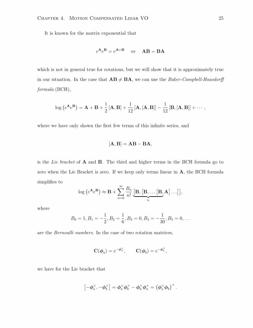
It is known for the matrix exponential that
eAeB = eA+B ⇔ AB = BA
which is not in general true for rotations, but we will show that it is approximately true
in our situation. In the case that AB 6= BA, we can use the Baker-Campbell-Hausdorff
formula (BCH),
log(eAeB
)= A+B+
1
2[A,B] +
1
12[A, [A,B]]− 1
12[B, [A,B]] + · · · ,
where we have only shown the first few terms of this infinite series, and
[A,B] = AB−BA,
is the Lie bracket of A and B. The third and higher terms in the BCH formula go to
zero when the Lie Bracket is zero. If we keep only terms linear in A, the BCH formula
simplifies to
log(eAeB
)≈ B+
∞∑
n=0
Bn
n!
[B,
[B, . . .
[B,
︸ ︷︷ ︸
n
A]. . .
]],
where
B0 = 1, B1 = −1
2, B2 =
1
6, B3 = 0, B4 = −
1
30, B5 = 0, . . .
are the Bernoulli numbers. In the case of two rotation matrices,
C(φa) = e−φ×
a , C(φb) = e−φ×
b ,
we have for the Lie bracket that
[−φ×
a ,−φ×
b
]= φ×
a φ×
b − φ×
b φ×
a =(φ×
a φb
)×
.

Chapter 4. Motion Compensated Lidar VO 26
To make the Lie bracket zero, we need to have φ×
a φb = 0. In other words, the two
rotations must share an axis of rotation. Now, suppose we have a rotation matrix, C(φ),
given by
C(φ) := e−φ× ≡ cosφ1+ (1− cosφ)aaT − sinφa× ≡
∞∑
n=0
(−1)n 1
n!
(φ×
)n,
and then define
S(φ) :=sinφ
φ1+
(
1− sinφ
φ
)
aaT − 1− cosφ
φa× ≡
∞∑
n=0
(−1)n 1
(n+ 1)!
(φ×
)n.
This matrix shows up in a variety of places related to rotations. It can be shown that
S(φ)−1 ≡ φ
2cot
φ
21+
(
1− φ
2cot
φ
2
)
aaT +φ
2a× ≡
∞∑
n=0
(−1)nBn
n!
(φ×
)n. (4.2)
If we define the perturbation,
C(φ) = C(δφ)C(φ),
then it turns out that
φ ≈ φ+ S(φ)−1 δφ, (4.3)
correct to first order in δφ. We can see this by noting
C(φ) = e−φ×
= e−δφ×
e−φ×
= C(δφ)C(φ),
and then applying the BCH formula (keeping only terms linear in δφ). Thus
e−φ× ≈ e−φ
×+∑
∞
n=0Bnn! ((−φ
×)n(−δφ))
×
= e−(φ+S(φ)−1 δφ)×
,
which is the desired result.

Chapter 4. Motion Compensated Lidar VO 27
Scheme Definition
Without loss of generality, suppose that tk ≤ tl ≤ tk+1 for a particular l. Our job in this
section is to define exact expressions for the pose at time tl, given the poses at times tk
and tk+1. The main challenge here is dealing with the rotations, so we begin with that.
We seek an interpolation scheme, I,
I : SO(3)× R 7→ SO(3)
so that
Cl,k = I(Ck+1,k, tl).
We define the interpolation variable, αl ∈ [0, 1], as
αl :=tl − tk
tk+1 − tk. (4.4)
We then define our interpolation of rotation variables to be
Cl,k := Ck+1,k
αl
= e−αlφ×
k+1,k . (4.5)
It is easy to see that
αl = 0 ⇒ Cl,k = 1, αl = 1 ⇒ Cl,k = Ck+1,k,
as desired. We are effectively just scaling the angle of rotation by αl and leaving the
axis untouched. This is not the only way we could define the interpolation, but it is a
notationally simple one that avoids singularities1. Also, this expression produces a valid
1Still, it will probably fail to produce a sensible answer when Ck+1,k is too large. Also, this expressioncould encounter numerical instability if either exponent gets too small; in this case, we use limα→0 C
α =1.

Chapter 4. Motion Compensated Lidar VO 28
rotation matrix for all αl. We can see this by forming
Cl,kCl,kT
= Ck+1,k
αl
Ck+1,k
αTl
=(
e−αlφ×
k+1,k
)(
e−αlφ×
k+1,k
)T
= e−αlφ×
k+1,keαlφ×
k+1,k = e−αlφ×
k+1,k+αlφ
×
k+1,k = 1,
which does not require any approximation.
Trivially, we interpolate the translation variable according to
rl,kk := αl r
k+1,kk , (4.6)
so that αl = 0 implies rl,kk = 0 and αl = 1 implies rl,kk = rk+1,kk .
Interpretation
Another way to justify this interpolation scheme is to think of both Ck+1,0 and Ck,0 as
being rotations compounded with Cl,0 according to
Ck+1,0 = e−φ×
k+1,lCl,0, Ck,0 = e−φ×
k,lCl,0
and subject to an interpolation constraint,
αlφk+1,l + (1− αl)φk,l = 0.
Here we are directly carrying out the interpolation on the 3× 1 parameterization of the
rotations. Note, however, that this means that φk+1,l and φk,l must be parallel and hence
[φk+1,l,φk,l
]= 0.
We then note that
Ck+1,k = Ck+1,0CTk,0 = e−φ
×
k+1,l Cl,0CTl,0
︸ ︷︷ ︸
1
eφ×
k,l = e−φ×
k+1,leφ×
k,l =: e−φ×
k+1,k .

Chapter 4. Motion Compensated Lidar VO 29
Using the BCH formula, we have that
φk+1,k = φk+1,l − φk,l,
with no approximation since[φk+1,l,φk,l
]= 0. We thus have two equations in two
unknowns, which together imply that
φk+1,l = (1− αl)φk+1,k, φk,l = −αlφk+1,k.
Rearranging for Cl,k we see that
Cl,k = Cl,0CTk,0 = eφ
×
k,l = e−αlφ×
k+1,k =(
e−φ×
k+1,k
)αl
= Ck+1,k
αl
,
which is identical to the scheme we defined above. This section was provided merely
for interpretation. The next section will explore what happens to our interpolation
expressions when we perturb the pose variables.
4.2.3 General Form of Rotation Perturbation
To perturb a rotation variable, let it be a combination of a large nominal rotation, C,
and a small perturbation, δC = e−δφ×
:
C = δCC.
Then we have that
C = δCC = e−δφ×
C ≈(1− δφ×
)C,
where we have used that δφ is small to make the usual infinitesimal rotation approxima-
tion. The question we ask in this section is how to perturb Cα, where α ∈ [0, 1] is some
interpolation variable.

Chapter 4. Motion Compensated Lidar VO 30
Suppose for the moment that α is actually an integer rather than a floating point
number. Then
Cα = CC · · ·C︸ ︷︷ ︸
α
= e−δφ×
Ce−δφ×
C · · · e−δφ×
C︸ ︷︷ ︸
α
.
Repeatedly using the identity that
e−(Cδφ)×
≡ Ce−δφ×
CT,
we have
Cα = e−δφ×
e−(C δφ)×
· · · e−(Cα−1
δφ)×
Cα
≈(1− δφ×
) (
1−(C δφ
)×
)
· · ·(
1−(
Cα−1
δφ)×
)
Cα
≈(1− α (Φ δφ)×
)C
α, (4.7)
where
αΦ :=α−1∑
m=0
Cm.
We now expand C using the matrix exponential so that
Cm=
(
e−φ×)m
=∞∑
n=0
1
n!
(
−φ×
)n
mn.
Under this assumption we have that
αΦ =α−1∑
m=0
Cm=
α−1∑
m=0
∞∑
n=0
1
n!
(
−φ×
)n
mn =∞∑
n=0
1
n!
(
−φ×
)nα−1∑
m=0
mn
=∞∑
n=0
1
n!
(
−φ×
)n Bn+1(α)− Bn+1(0)
n+ 1︸ ︷︷ ︸
Faulhaber’s formula
,

Chapter 4. Motion Compensated Lidar VO 31
where the Bn(·) are the Bernouilli polynomials. The first few terms of Φ are
Φ = 1− α− 1
2φ
×
+(α− 1)(2α− 1)
12φ
×
φ× − α(α− 1)2
24φ
×
φ×
φ×
+ · · · ,
and higher-order terms will become progressively smaller if φ is small. A good question
is whether this formula applies when α is not an integer but rather lies in [0, 1].
To look at this another way, we write out Cα in two different forms (see section 4.2.2
for some background math):
Cα =(
e−δφ×
C)α
=(
e−δφ×
e−φ×)α
≈(
e−(φ+S(φ)−1 δφ)×)α
= e−(αφ+αS(φ)−1 δφ)×
,
Cα = e−δψ×
Cα
= e−δψ×
e−αφ× ≈ e−(αφ+S(αφ)−1 δψ)
×
.
We equate the two exponents to have
δψ ≈ αS(αφ)S(φ)−1 δφ.
Substituting the expression for S(·) and its inverse (see section 4.2.2) we have
δψ = α
(
1− α1
2φ
×
+ α21
6φ
×
φ× − α3 1
24φ
×
φ×
φ×
+ · · ·)
(
1+1
2φ
×
+1
12φ
×
φ×
+ 0 φ×
φ×
φ×
+ · · ·)
δφ
= α
(
1− α− 1
2φ
×
+(α− 1)(2α− 1)
12φ
×
φ× − α(α− 1)2
24φ
×
φ×
φ×
+ · · ·)
δφ
= αΦ δφ.
Thus we are justified in using Φ even when α ∈ [0, 1]. We can also plug in the full

Chapter 4. Motion Compensated Lidar VO 32
expressions for S(αφ) and S(φ)−1 to show that:
Φ ≡ β1+ (1− β) aaT − γa×
β :=1
2α
(
(1− cos(αφ)) + sin(αφ) cotφ
2
)
γ :=1
2α
(
(1− cos(αφ)) cotφ
2− sin(αφ)
)
where φ = |φ| and a = φ/φ. To summarize, we will use (4.7) to perturb interpolated
rotation matrices; we also now have that Φ ≡ S(αφ)S(φ)−1, which can be expressed in
closed form.
4.2.4 Perturbing Interpolated Poses
Based on the previous section, the perturbations that we will use are
Ck+1,k = eδφ×
k+1,kCk+1,k, (4.8)
rk+1,kk = r
k+1,kk + δrk+1,k
k , (4.9)
and Cl,k ≈(
1− αl
(Φl δφk+1,k
)×
)
Cl,k, (4.10)
rl,kk = r
l,kk + αlδr
k+1,kk , (4.11)
pj,kk = p
j,kk + δpj,k
k , (4.12)
Cl,k := Ck+1,kαl , (4.13)
rl,kk := αlr
k+1,kk , (4.14)
Φl := S(αlφk+1,k
)S(φk+1,k
)−1, (4.15)
S (φ) :=sinφ
φ1+
(
1− sinφ
φ
)
aaT − 1− cosφ
φa×, (4.16)
φk+1,k can be determined from Ck+1,k exactly and should not be near a singularity so
long as the rotation is not large. In the next section we will use these perturbations to
linearize our error terms. After solving for the incremental quantities at each iteration

Chapter 4. Motion Compensated Lidar VO 33
of Gauss-Newton, we will update the mean quantities according to the following update
rules:
Ck+1,k ← e−δφ×
k+1,kCk+1,k,
rk+1,kk ← r
k+1,kk + δrk+1,k
k ,
pj,kk ← p
j,kk + δpj,k
k .
4.2.5 Linearized Error Terms
The last step is to use our perturbed pose expressions to come up with the linearized
error terms. Consider just the first nonlinearity before the camera model:
pj,ll := Cl,k
(
pj,kk − r
l,kk
)
.
Inserting (5.18), (4.11), and (4.12) and dropping products of small terms we have
pj,ll ≈
(
1− αl
(Φl δφk+1,k
)×
)
Cl,k
(
pj,kk + δpj,k
k − rl,kk − αlδr
k+1,kk
)
≈ Cl,k
(
pj,kk − r
l,kk
)
︸ ︷︷ ︸
pj,l
l
+
[
−αlCl,k αlpj,l×
l Φl Cl,k
]
︸ ︷︷ ︸
=:Djl
δrk+1,kk
δφk+1,k
δpj,kk
︸ ︷︷ ︸
=:δxjl
= pj,ll +Djl δxjl.
Inserting this into the full error expression we have
ejl(xjl + δxjl) ≈ yjl − f(
pj,ll +Djl δxjl
)
≈ yjl − f(
pj,ll
)
︸ ︷︷ ︸
=:ejl
−FjlDjl︸ ︷︷ ︸
=:−Ejl
δxj,l
= ejl + Ejl δxjl,

Chapter 4. Motion Compensated Lidar VO 34
where
Fjk :=∂f
∂p
∣∣∣∣pj,l
l
.
We can then insert this approximation into the objective function in (4.1), causing it to
become quadratic in x, and proceed in the usual Gauss-Newton fashion, being sure to
update our rotation variables properly at each iteration. The advantage of our technique
is that we have been able to compute the Jacobian of our interpolated variables in closed
form.
4.3 VO Algorithm Test
Testing of the algorithm was conducted in two stages:
1. Using data produced by the lidar simulator, described in Chapter 3, which forms
a controlled environment and provides 6 DOF groundtruth information.
2. Using real lidar data collected from a planetary analogue site in complete darkness,
demonstrating the lighting-invariant aspect of the system, as well as its actual
performance in an outdoor unstructured 3D environment. Groundtruth is provided
by DGPS.
At each stage we will compare the VO estimates with and without motion compensation
against the groundtruth.

Chapter 4. Motion Compensated Lidar VO 35
4.3.1 System Testing using Lidar Simulator
The purpose of testing with simulated data was to validate the algorithm as much as
possible in a controlled environment. We configured the lidar simulator using parameters
from a real scanning laser rangefinder (see details in Section 4.3.2). This included giving
it the identical scan resolution of 480 × 360 pixels and the scanning frequency of 2 Hz,
as well as the exact same scanning pattern caused by the nodding mirror inside the real
sensor (see Figure 3.3).
During the simulation, the rover was given a sinusoidal trajectory with amplitude 0.25
meters in the xy-plane. Yaw heading angle was tangential to the xy planar trajectory.
−34.5 −34 −33.5 −33 −32.5 −32 −31.5 −31 −30.5 −30−1
−0.5
0
0.5
1
x [m]
y [
m]
−34.5 −34 −33.5 −33 −32.5 −32 −31.5 −31 −30.5 −30−1.5−1
−0.50
0.51
1.5
x [m]
z [
m]
No Motion Comp.With Motion Comp.Groundtruth
(a) Groundtruth vs. estimates from first 5seconds of traverse.
0 5 10 15 20 25 300
0.5
1
1.5
2
2.5
Traversed distance [m]
Euclid
ean e
rror
[m]
No Motion Comp.
With Motion Comp
(b) Euclidean error over traversed distance.
Figure 4.3: VO estimates using simulated lidar data. The estimated rover track withmotion compensation is smoother and accumulates error at a much lower rate.
As shown in Figure 4.3, the VO estimate without motion compensation struggled to
match with the groundtruth; a distinctive sawtooth-shaped estimate is clearly visible in
the xz-plane as a result of motion distortion. On the other hand, the VO algorithm with
motion compensation produced a smooth estimate that closely follows the groundtruth.
Figure 4.4 provides 6 DOF error plots to further demonstrate the contrast in quality
between the two estimators. Note the small sinusoidal error in yaw angle even with

Chapter 4. Motion Compensated Lidar VO 36
−0.5
0
0.5x [
m]
−1
−0.5
0
0.5
y [
m]
0 5 10 15 20 25 30−4
−2
0
2
z [
m]
Time [s]
No Motion Comp.With Motion Comp.
(a) Position estimation error.
−2
0
2
4
Roll
[deg]
−5
0
5
Pitch [
deg]
0 5 10 15 20 25 30−5
0
5
Yaw
[deg]
Time [s]
No Motion Comp.
With Motion Comp.
(b) Orientation estimation error.
Figure 4.4: Simulated lidar VO estimation errors in all 6 DOF. Note that during esti-mation, attitude was represented using a rotation matrix, which is decomposed into roll,pitch, and yaw here for comparison against groundtruth.
motion compensation, indicating that the interpolation-based motion compensation is
not sufficient to completely capture a nonlinear sinusoidal motion, which is expected.
4.3.2 Hardware Description
Our field experiment was carried out using a ROC6 skid-steered rover, an Autonosys
LVC0702 lidar sensor, and a differential GPS for groundtruth positioning. The configu-
ration is shown in Figure 4.5(a).
The Autonosys lidar employs a unique two-axis scanning system (see Figure 3.3).
While the horizontal scanning direction is consistent, a nodding-mirror-based vertical
scanning mechanism switches scanning direction after each scan to avoid the need for
quick return. As a result, the motion distortion in adjacent scans has completely opposite
distortion effects, as shown in Figure 3.3. With a field of view (FOV) similar to traditional
stereo cameras, this lidar is also referred to as a lidar video camera by the manufacturer,
capable of producing 480×360 pixel lidar scans at 2 Hz. The lidar sensor has a horizontal
FOV of 90 degrees, and vertical FOV of 30 degrees. In order to maximize valid lidar

Chapter 4. Motion Compensated Lidar VO 37
GPS Antenna
AC Generator
ROC6 Rover
Autonosys Lidar
(a) Hardware configuration.
25 meters
North
Seg. 1 Start
23:35:05
Seg. 1 End
23:45:30
Seg. 2 Start
23:46:09
Seg. 2 End
00:00:12
Courtesy of Google Earth - 46°25’22”N 80°50’58” W
(b) GPS tracks of two traverse segments used forVO testing and their associated collection times.
Figure 4.5: Appearance-based lidar VO experiment setup (left) and traverse pathgroundtruth (right).
returns, the sensor was aimed 15 degrees down, giving it an effective vertical FOV from
−30 to 0 degrees.
Since it was dangerous and nearly impossible for a human operator to pilot the robot in
complete darkness, all the data used in this section were collected autonomously; during
the daytime, the path was driven once manually, and repeated at night autonomously at
a nominal speed of 0.5 m/s using VT&R (McManus et al., 2012). The data used in this
thesis were logged as a byproduct of this unrelated test. The traversed path is shown in
Figure 4.5(b). Note that while the raw sensor data logged during the VT&R experiment
were uncalibrated, we performed sensor calibration at a later time, as documented in
Chapter 5, and applied the calibrated sensor model during this experiment.
Segment 1 is 225 meters in length, and contains mostly a long smooth traverse and
gradual turns. There is one direction switch in the latter half of the traverse. Segment
2 is 300 meters in length, and contains many sharp turns and more elevation changes.
There is also a three-point turn in the middle of this traverse.

Chapter 4. Motion Compensated Lidar VO 38
4.3.3 Field Testing Results
As shown in Figure 4.6, the VO estimator with motion compensation performed better
qualitatively in both traverse segments than the estimator that does not address motion
distortion. Closer inspection of the Euclidean error plots (see Figure 5.3) reveals that
the motion-compensated case has much lower error in segment 2 than in segment 1. The
Euclidean-error-to-distance-travelled ratio remains under 5% on segment 2 as compared
to 7% on segment 1, despite the fact that segment 2 was anecdotally a more challenging
traverse. From the VO estimate result of segment 1, we can see that while the incremental
heading estimate appears to be accurate, there was a gradual accumulation of heading
error. As the attitude estimate drifted, the error grew superlinearly, similarly to stereo-
camera-based VO results reported by Lambert et al. (2012). The direction switches
and heading changes in segment 2 incidentally had a net effect of partially cancelling
estimation error in different parts of the traverse, therefore resulting in a better VO
estimate.
−40 −20 0 20 40 60−100
−90
−80
−70
−60
−50
−40
−30
−20
−10
0
x [m]
y [
m]
No Motion Comp..
With Motion Comp.
GPS
Start
End
(a) Segment 1.
−80 −70 −60 −50 −40 −30 −20 −10 0
−10
0
10
20
30
40
x [m]
y [
m]
No Motion Comp..
With Motion Comp.
GPS
Start
End
(b) Segment 2.
Figure 4.6: VO estimates of the two traverse segments in Figure 4.5(b). The estimatorwithout motion compensation severely underestimates both rotational and translationalchanges.

Chapter 4. Motion Compensated Lidar VO 39
0 50 100 150 200 2500
5
10
15
20
25
30
35
40
Traversed distance [m]
Eu
clid
ea
n e
rro
r [m
]
No Motion Comp.
With Motion Comp.
(a) Segment 1.
0 50 100 150 200 250 300 3500
5
10
15
20
25
30
35
40
45
Traversed distance [m]
Eu
clid
ea
n e
rro
r [m
]
No Motion Comp.
With Motion Comp.
(b) Segment 2.
Figure 4.7: Euclidean estimation error vs. traverse distance plots, showing the cumulativepose error grows significantly slower with motion compensation.
−7 −6 −5 −4 −3 −2 −1 0
−3
−2
−1
0
1
2
x [m]
y [
m]
No Motion Comp..
With Motion Comp.
GPS
Start
End
(a) Sharp turn located at (−30 m, 25 m) insegment 2.
−15 −10 −5 0 5 10
−20
−15
−10
−5
0
x [m]
y [
m]
No Motion Comp..
With Motion Comp.
GPS
Start
End
(b) Three-point turn located at (−75 m, −5m) in segment 2.
Figure 4.8: Close-ups of segment 2. In the estimates without motion compensation, thesawtooth-shaped error previously observed during simulation is clearly visible at thisscale.
As for the reason behind why VO without motion compensation performed much
worse in segment 2, we can explain it by zooming in on short stretches of traverse, shown
in Figure 4.8. The estimate exhibited a choppy sawtooth shape due to motion distortion,
and as a whole underestimated both rotational and translational motion. In contrast, the

Chapter 4. Motion Compensated Lidar VO 40
estimate with motion compensation was smooth and closely followed the groundtruth.
This agrees with our earlier observation made using simulated lidar data.
Another source of error is the assumption of constant velocity between poses previ-
ously introduced by our pose-interpolation scheme. Since our formulation only estimates
one pose placed at the center of each scan, it is insufficient at times to fully capture the
motion of the rover in a rough terrain (e.g., when driving over a rock). This error can be
mitigated by reducing the temporal spacing between poses (similar to higher sampling
rate in analogue to digital conversion).
Currently, the system is not able to correct orientation error accumulated over time as
the estimates produced by VO are incremental in nature. Lambert et al. (2012) demon-
strated with stereo-based VO that by continuously incorporating absolute orientation
measurements from an inclinometer and a sun sensor, highly accurate metric VO can
be expected over multi-kilometer traverses during the daytime. Given the lidar-based
VO’s ability to operate in complete darkness, a natural extension of this work is to fuse
absolute orientation measurements available at night using a star tracker (Enright et al.,
2012). More recently, Gammell et al. (2013) tested this specific sensor fusion combination
using a slower SICK scanning lidar.
4.4 Conclusion
In this chapter, we have presented an improved appearance-based lidar navigation system
that exhibits the computational efficiency of sparse visual techniques, typically associated
with stereo cameras, while overcoming the lighting dependence of traditional cameras.
The contributions of this work include:
1. A novel pose-interpolation strategy based on the exponential map that allows for
derivation of analytical Jacobians used during a bundle adjustment nonlinear op-
timization.

Chapter 4. Motion Compensated Lidar VO 41
2. A VO algorithm based on #1 that compensates for motion distortion in lidar scans
acquired during continuous vehicle motion.
3. Testing of #2 using a simulated lidar dataset and over 500 meters of experimental
data collected from a planetary analogue environment with a real scanning laser
rangefinder in complete darkness.
Our results demonstrate clear improvement in the VO estimate by compensating for
the motion distortion effect. We obtained 5-7% linear error growth in hundred-meter-
scale traverses during our field experiment using only lidar data and no other sensor
information. This work can be further improved by carrying out global minimization
over a small set of scans and/or introducing additional attitude sensors, such as an incli-
nometer or star tracker into the system. Furthermore, it maybe feasible to move beyond
linear interpolation, as a spline-based interpolation approach may better approximate
the nonlinear motion of the robot (Furgale et al., 2012; Tong et al., 2012).
Finally, any estimation problem in which there is a large collection of sensor data with
distinct measurement times can be solved using far fewer poses/variables by interpolating
poses. With new sensors producing measurements at higher and higher rates, and the fact
that it may not always be possible to trigger/synchronize different sensors, the proposed
interpolation scheme and its associated derivation could be useful for a general set of
problems.

Chapter 5
Lidar Calibration
Camera and lidar sensors are fundamental components for today’s advanced robotic
systems. For example, numerous cameras are used in NASA’s Mars Exploration Rover
(Maki et al., 2003) and Mars Science Laboratory (Maki et al., 2012) missions to enable
safe rover descent, autonomous driving, and science data collection. Similarly on Earth-
bound systems, such as Google’s self-driving car, lidar sensors are used for mapping,
localization, and detecting other nearby hazards/vehicles (Thrun and Urmson, 2011).
Whether the output of these sensors is the final data product or is used for closed-loop
control, data accuracy is important. Since each sensor is different due to manufacturing
tolerance, and can change over time (e.g., at different operating temperatures), a flexible
calibration procedure that is also accessible to the end user can be critical to the success
of the overall system.
The introduction of Bouguet’s camera calibration toolbox for Matlab (Bouguet, 2004),
and its subsequent C implementation in OpenCV (Bradski, 2009) drastically reduced the
learning curve associated with camera calibration. Based on a flexible calibration tech-
nique pioneered by Zhang (2000), these packages allow anyone to quickly obtain the
intrinsic (sensor internal parameters) and extrinsic (relative pose between sensors) cali-
bration for most passive camera sensor configurations using only a checkerboard pattern
42

Chapter 5. Lidar Calibration 43
as the calibration target.
The same level of maturity does not currently exist in lidar calibration. While a num-
ber of packages for computing six-degree-of-freedom extrinsic calibration between camera
and lidar sensors have been made available (Geiger et al., 2012; Unnikrishnan and Hebert,
2005), they assume the intrinsic calibration has been done through other means. Finding
a mathematical model that accurately describes the physical behaviour of the sensor is
still non-trivial. The dominant approach to lidar calibration requires knowledge of the
internal structure of a particular sensor in order to produce equations with parameters
that describe the internal beam path. A least-squares problem is then formulated to
find optimal values of these parameters using a calibration dataset. For passive cameras,
the dominant system identification paradigm is more flexible and generic. An arbitrary
camera/lens configuration is modelled as a pinhole camera with tangential and radial dis-
tortion. The intrinsic calibration process then characterizes the extent of lens distortion
using only a few parameters.
Given the success of the black-box approach to camera calibration, we are interested
in seeing whether a similar approach can be applied to lidar calibration. To test this idea,
we modelled a real two-axis scanning lidar using a spherical camera model with additive
distortion, and developed the necessary equations to solve for the distortion map using
least-squares optimization. An experimental calibration dataset was gathered using a
standard checkerboard pattern printed on a planar surface. The preliminary result of the
intrinsic calibration is very promising; the nominal landmark re-projection error on the
calibration dataset is reduced from over 25 mm without calibration to less than 5.5 mm
with calibration. All this was accomplished without explicit consideration of the internal
structure of the sensor. We believe the generality of our approach will allow it to be used
by a variety of two-axis scanning lidars.

Chapter 5. Lidar Calibration 44
5.1 Related Works
Due to its success in the DARPA Urban Challenge, the Velodyne HDL-64 is perhaps the
most popular commercial two-axis scanning lidar in use today. While the manufacturer
provides intrinsic calibration with each sensor, many teams still found it beneficial to
re-do calibration in-house to improve measurement accuracy. The Stanford racing team,
for example, was able to solve for both the intrinsic and extrinsic parameters of the lidar
using driving data acquired in an outdoor environment. This particular formulation also
depended on local pose data from an integrated GPS/IMU system on-board their vehicle
(Levinson, 2011). Atanacio-Jimenez et al. (2011) find the intrinsic parameters of the
sensor through the use of a known geometric target (e.g., a squash court). While both
methods produced good lidar calibration results, the use of additional hardware or a
very specific environment made them less flexible than traditional pattern-based camera
calibration methods.
Working with a tilting Hokuyo UTM-30LX sensor, the calibration technique devel-
oped by Pradeep et al. (2010) for Willow Garage’s PR2 robot modelled the two-axis
scanner as a kinematic chain with a one-axis scanner at the end, which is mathemati-
cally identical to writing out the lidar model based on the sensor’s physical construction.
Similar to this work, the proposed calibration approach also uses a checkerboard pat-
tern in conjunction with lidar intensity imagery to solve the pose-related aspects of the
problem using bundle adjustment.
Inter-lidar geometric and temporal calibration has recently been investigated by Shee-
han et al. (2011). Their two-axis scanning lidar is created from three SICK LMS-151
planar lidars and a spinning plate. When spun on top of the plate, the SICK lidars shared
a common field-of-view (FOV). This allowed them to form a cost function that captured
the quality of an aggregated point cloud using data from all three sensors. Although this
approach does not require external localization or a specific calibration environment, it
is not applicable to two-axis scanners with a single laser beam.

Chapter 5. Lidar Calibration 45
Nodding
Mirror
Polygonal
Mirror(8000 RPM)
Laser
Range�nder
Vertical
Scan Dir.
Landmark
r1,2
r0,1
r
F→p
F→k
F→l
Figure 5.1: Simplified illustration of the Autonosys LV0702 lidar’s two-axis scanningmechanism O’Neill et al. (2007). The raw range measurement reported by the laserrangefinder, r′, consists of two internal lengths, r0,1 and r1,2, and the actual range to thetarget, r.
In terms of the scanning mechanism, a tilting-mirror-based scanning lidar developed
by Ryde and Hu (2008) perhaps has the most in common with our sensor. The sensor is
calibrated by scanning a flat ceiling, visualizing the point cloud and manually adjusting
the intrinsic parameters to make the scan planar.
To the best of our knowledge, all existing lidar geometric calibration methods, whether
modelling the sensor as a kinematic chain or ray-casting for a mirror-based scanner,
assume knowledge of the internal sensor structure. Our method does not make this
assumption, making it more feasible for end users who have no access to such information.
5.2 Methodology
The lidar sensor that we want to calibrate is an Autonosys LVC0702 scanning lidar;
it employs a unique two-axis scanning system (see Figure 5.1). While the horizontal
scanning direction is consistent, a nodding mirror is used to alternate the vertical scan
direction, avoiding the need for a quick return. The sensor is capable of producing 500,000

Chapter 5. Lidar Calibration 46
points per second, with a maximum frame rate of 10 Hz, a horizontal FOV of 90 degrees,
and a vertical FOV of up to 45 degrees. For our work, we acquire scans with a resolution
of 480× 360 pixels at 2 Hz.
Our method does not require this particular mirror assembly, or even knowledge of the
scanning mechanism. As a result, we believe the method can be directly applied to a num-
ber of two-axis scanning lidars, such as the mirror-based Optech ILRIS-3D scanner, Nip-
pon Signal’s FX8 MEMS-mirror scanner, or the popular ‘do-it-yourself’ SICK/Hokuyo
planar lidar on a pan-and-tilt unit.
To fully demonstrate the generality of our method, let us first consider the problem
with using the dominant parametric approach. To write out the inverse sensor model
(a.k.a, the ray casting model), we need to know the pose of the laser rangefinder, F−→l (as
defined in Figure 5.1), the polygonal mirror position and rotational axis as represented by
F−→p, the size of the polygonal mirror, the nodding mirror position and rotational axis as
represented by F−→k, and the offset, if any, between the nodding mirror’s reflective surface
and its rotational axis. Additionally, we need to consider the offsets in the angular
encoders’ outputs due to mounting tolerances. To perform a complete calibration, all
of these parameters would need to be estimated. In practice, to keep the number of
variables to a manageable amount, some carefully chosen assumptions are generally made
(Pradeep et al., 2010). For example, assuming an orthogonal relationship between the
laser rangefinder and the polygonal mirror’s rotational axis would drastically reduce the
complexity of the resulting mathematical model. This formulation requires intimate
knowledge of the hardware, which is not always available to the end user. Moreover, the
resulting model is sensor-specific.
An alternative to solving for the sensor’s full parametric model is to map the difference
between its actual and ideal behaviour. We will refer to this difference as a distortion,
borrowing the term from the computer vision approach to passive camera calibration.
The non-ideal behaviour of a real lens is said to have radial and tangential distortions in

Chapter 5. Lidar Calibration 47
comparison to the simplified pinhole camera model.
A similar method of distortion mapping, known as volumetric error correction, is
used in the precision machining community. During the calibration process, data from
an unbiased instrument, such as an external laser interferometer is compared against
data from encoders mounted on the CNC machine. The difference is then used as a
feed-forward correction during the actual machining operation (Donmez et al., 1986),
resulting in significant improvement in tool position accuracy.
5.2.1 Sensor Model
We will start our formulation by defining the ideal sensor model and a grid-based model
for distortion mapping.
Ideal sensor model
Drawing from the similarity of the bearing and tilt encoder angles to azimuth and eleva-
tion in the spherical coordinate frame, we can write out the ideal inverse sensor model
using the spherical-to-Euclidean coordinate conversion formula. In this case, the fixed
sensor frame orientation is defined as follows: x-axis parallel to the rotational axis of
the hexagonal mirror (toward the front of the sensor), y-axis to the port side (left side
when viewed from behind) of the sensor, which constrains the z-axis to point to the top
of the sensor. Note the position of this frame is not strictly defined at this point. Let a
bearing, tilt, and range measurement be defined as y := [α β r]T and the Euclidean point
be defined as x := [x y z]T . The mapping from measurement to Euclidean coordinates
is given by
x = f−1(y) =
r cosα cos β
r sinα
r cosα sin β
. (5.1)

Chapter 5. Lidar Calibration 48
From the above inverse model, we can write the ideal sensor model:
y = f(x) =
arctan(y,√x2 + z2
)
arctan (z, x)√
x2 + y2 + z2
. (5.2)
The physical construction of our sensor is different from the ideal model, and we will
use an additive distortion model to handle this difference, where variables with (·)′ rep-
resent real measurements, and variables without (·)′ represent ideal measurements. Our
distortion model is
α′ := α + δα(α′, β′, r′) + nα, (5.3)
β′ := β + δβ(α′, β′, r′) + nβ, (5.4)
r′ := r + δr(α′, β′, r′) + nr, (5.5)
where δi(·, ·, ·) is a distortion function, and ni is a zero-mean Gaussian measurement
noise. These are combined to give us the following stacked distortion equation:
y′ := y+D(y′) + n n ∼ N (0,R) , (5.6)
where R is the covariance of the measurement noise.
Distortion model
The distortion model, D(·), captures the difference between the actual sensor behaviour
and the ideal sensor model. In other words, for every raw sensor measurement, y′, we
want the ability to reconstruct its corresponding measurement, y, in the idealized sensor
space, and vice versa. Since y′ is three-dimensional, we naturally may be led to the
use of a grid-based mapping using trilinear interpolation. However, if we strategically

Chapter 5. Lidar Calibration 49
place the origin of the ideal sensor frame where the laser beam nominally intersects
with the nodding mirror, located at F−→k in Figure 5.1, at a zero-degree bearing and a
zero-degree tilt, then the range component, r′, will have trivial impact on ideal bearing
and tilt readings. As such, it may be feasible to capture the distortion using only the
values of the two encoders as inputs, and hence only bilinear interpolation is required.
Avoiding the need to deal with distortion as a function of raw range, r′, is also a necessary
compromise dictated by the size of the checkerboard pattern and the pixel resolution of
the lidar; given the fixed angular resolutions in each scan, it is not possible to reliably
extract checkerboard corner features beyond a certain range.
Accordingly, we rewrite the distortion function as
D(α′, β′) = Φ(α′, β′)c , (5.7)
where Φ(·, ·) is a predetermined set of basis functions, and c are coefficients. In this
work, we choose to use a grid-based bilinear interpolation for our basis functions.
Bilinear interpolation
We begin using a familiar example: terrain mapping. One way to capture a continuous
landscape is by sampling it at regular intervals. This effectively carries out a grid-
based (along the x- and y-axes) discretization with elevation sampling, v, at each vertex.
From the discretized samples, we can then look up the interpolated elevation, vx,y, at
an arbitrary location using its neighbouring samples, (v0,0, v1,0, v0,1, v1,1), as shown in
Figure 5.2. Procedurally, we first compute interpolation constants based on the location
of the point relative to its neighbours:
λx =x− x0
x1 − x0
, λy =y − y0y1 − y0
. (5.8)
By definition, interpolation requires x0 ≤ x ≤ x1 and y0 ≤ y ≤ y1, which implies that

Chapter 5. Lidar Calibration 50
x0 x1
x
y
y0
y1
v0,0 v1,0
v0,1 v1,1
vx,y
vx,0
vx,1
Figure 5.2: Bilinear interpolation: conceptually, to compute the interpolated value at(x,y), we first interpolate along x-axis to obtain vx,0 and vx,1, and then interpolate asecond time along y-axis to obtain vx,y.
0 ≤ λx ≤ 1 and 0 ≤ λy ≤ 1. We interpolate along the x- and then y-axis to obtain vx,y:
vx,y =
[
1− λy λy
]
1− λx λx 0 0
0 0 1− λx λx
v0,0
v1,0
v0,1
v1,1
. (5.9)
The matrix-notation in (5.9) is for a 1 × 1 grid with four samples. To generalize the
interpolation math for higher-resolution grids, let us consider a sizeM×N grid containing
(M +1)(N +1) samples. We assume the samples are arranged as a column vector in the
following order:
v =
[
v0,0 v1,0 · · · vM−1,0 vM,0 · · · v0,N · · · vM,N
]T
. (5.10)
An arbitrary location would then have four neighbour samples, denoted by vh,i, vh+1,i,
vh,i+1, vh+1,i+1. Indices h = 0 . . .M and i = 0 . . . N , where xh ≤ x ≤ xh+1 and yi ≤ y ≤

Chapter 5. Lidar Calibration 51
yi+1. Using these generalized parameters, we update (5.8) as
λx =x− xh
xh+1 − xh
, λy =y − yi
yi+1 − yi. (5.11)
We recognize that a given interpolation process actively involves only 4 samples in v,
v =
[
· · · vh,i vh+1,i · · · vh,i+1 vh+1,i+1 · · ·]T
. (5.12)
A projection matrix, P, is then used to pick out the four necessary rows of v, resulting
in a generalized bilinear interpolation equation for arbitrary grid size:
vx,y =
[
1− λy λy
]
1− λx λx 0 0
0 0 1− λx λx
P
︸ ︷︷ ︸
Λ(x,y)
v. (5.13)
To store additional information (say temperature and humidity maps), we simply
repeat the above step three times:
v1x,y
v2x,y
v3x,y
=
Λ(x, y) 0 0
0 Λ(x, y) 0
0 0 Λ(x, y)
︸ ︷︷ ︸
Φ(x,y)
v1
v2
v3
︸ ︷︷ ︸
c
. (5.14)
Instead of storing elevations, temperatures, and humidities along an xy-grid, we use
this technique to capture the measurement distortions in bearing, tilt, and range as
a function of raw bearing, α′, and raw tilt, β′, measurements. Note that while this
generalized math makes no assumption of uniform grid spacing, we choose to work with
square grid and uniform spacing in our application.

Chapter 5. Lidar Calibration 52
5.2.2 Bundle Adjustment Formulation
Problem setup
Our calibration algorithm is a batch bundle adjustment technique that solves for the
following variables:
Tkm : 4×4 transformation matrix that represents the relative pose change from checker-
board pose m to camera pose k,
c : distortion mapping coefficients,
where k = 1 . . . K is the time (frame) index. The position of the j-th checkerboard corner
relative to checkerboard pose m, expressed in frame m, pj,mm , is a known quantity that
we measure directly from the physical checkerboard, where j = 1 . . . J is the landmark
(checkerboard corner) index.
These variables are combined with (5.2), (5.6), and (5.14) to produce the following
measurement error term:
ejk (Tkm, c) := y′
jk − f(Tkmp
j,mm
)−Φ(α′
jk, β′
jk)c, ∀(j, k). (5.15)
where y′
jk is the measured quantity and f(·) is the nonlinear ideal sensor model defined
in (5.2).
Note the potential interaction between the camera pose, Tkm, and the distortion
coefficients, c. For instance, all camera poses may be overestimated by a few degrees
in pitch, only to be compensated by the same amount of tilt distortion in the reverse
direction. Left as is, the system has no unique solution. To address this problem,
we introduce a weak prior on the distortion parameters, which results in the following
additional error term:
ep (c) := c. (5.16)

Chapter 5. Lidar Calibration 53
We seek to find the values of Tkm and c to minimize the following objective function:
J(x) :=1
2
∑
j,k
ejk (Tkm, c)TR−1
jk ejk (Tkm, c) +1
2ep (c)
TQ−1ep (c) , (5.17)
where x is the full state that we wish to estimate (poses and calibration), Rjk is the
symmetric, positive-definite covariance matrix associated with the (j, k)-th measurement,
and Q is a diagonal matrix controlling the strength of the prior term. In practice, only
weak priors on the bearing and tilt vertex coefficients are necessary. We then solve this
optimization problem by applying the Gauss-Newton method (Gauss, 1809).
Linearization strategy
In this section, we will present a linearization strategy taken directly from existing state
estimation machinery. The complete derivation can be found in Furgale (2011). In order
to linearize our error terms, we perturb the pose variables according to
Tkm = e−δψ⊞kmTkm, (5.18)
where we use the definition,
u
v
⊞
:=
v× −u
0T 0
, (5.19)
and (·)× is the skew-symmetric operator given by
u1
u2
u3
×
:=
0 −u3 u2
u3 0 −u1
−u2 u1 0
. (5.20)
It can be shown that for a small pose perturbation, δψ, the linearization can be further
simplified to
Tkm ≈(1− δψ⊞
km
)Tkm, (5.21)
where 1 is a 4× 4 identity matrix.

Chapter 5. Lidar Calibration 54
After solving for the incremental quantities at each iteration of Gauss-Newton, we
will update the mean quantities according to the following update rules:
Tkm ← e−δψ⊞kmTkm (5.22)
c ← c+ δc. (5.23)
Linearized error terms
The last step is to use our perturbed pose expressions to come up with the linearized
error terms. Consider just the first nonlinearity before the ideal sensor model:
pj,kk := Tkmp
j,mm .
Substituting (5.21), we obtain
pj,kk ≈
(1− δψ⊞
km
)Tkmp
j,mm
= Tkmpj,mm − δψ⊞
kmTkmpj,mm
= Tkmpj,mm +
(Tkmp
j,mm
)⊟δψkm
= pj,kk +[(Tkmp
j,mm
)⊟0]
︸ ︷︷ ︸
=:Hjk
δψkm
δc
︸ ︷︷ ︸
=:δxjk
, (5.24)
where we define the operator,
s
t
⊟
:=
t1 s×
0T 0T
, (5.25)
which exhibits the useful relationship,
δψ⊞Tp = −(Tp)⊟δψ. (5.26)
Chapter 5. Lidar Calibration 55
Inserting (5.24) into the full measurement error expression in (5.15), we have
ejk (xjk + δxjk) ≈ y′
jk − f(
pj,kk +Hjkδxjk
)
−Φ(α′
jk, β′
jk
)(c+ δc)
≈ y′
jk − f(
pj,kk
)
−Φ(α′
jk, β′
jk
)c
︸ ︷︷ ︸
ejk(xjk)
−FjkHjkδxjk −[0 Φ
(α′
jk, β′
jk
)]
︸ ︷︷ ︸
=:Ejk
δxjk
= ejk (xjk)− [FjkHjk +Ejk]︸ ︷︷ ︸
=:−Gjk
δxjk
= ejk (xjk) +Gjkδxjk (5.27)
where
Fjk :=∂f
∂p
∣∣∣∣pj,k
k
.
The prior error term is linear, and has a trivial linearized form when perturbed:
ep (c+ δc) := ep (c) + δc. (5.28)
We can then insert the linearized approximation (5.27) and (5.28) into the objective
function in (5.17), causing it to become quadratic in δx, and proceed in the usual Gauss-
Newton fashion, being sure to update our transformation matrix variables using the
procedure in (5.22) at each iteration.
5.2.3 Measurement Correction
Once the values of the distortion mapping coefficients, c, are determined, we simply
manipulate (5.6) and (5.7) to obtain the corrected measurement according to
y = y′ −Φ(α′, β′)c. (5.29)

Chapter 5. Lidar Calibration 56
5.3 Experiment
5.3.1 Calibration Dataset
Our calibration data were collected using a single checkerboard target measuring 0.8
m in width and 0.6 m in height. The complete dataset contains scans taken at 55
unique target poses, shown in Figure 5.4, with 15-20 scans at each pose to account for
noise in the lidar data. Sample intensity images are provided in Figure 5.3(a). Next,
we extracted grid corners from the images using the Harris corner detector supplied
by the camera calibration toolbox for Matlab (Bouguet, 2004), shown in Figure 5.3(b).
Figure 5.3(c) demonstrates our verification process, in which we overlap the extracted
corners’ Euclidean positions on top of the original lidar point cloud.
(a) Sample lidar intensityimages
1
2
3
4
5
6
7
8
9
10
11
12
13
14
15
16
17
18
19
20
21
22
23
24
25
26
27
28
29
30
31
32
33
34
35
36
37
38
39
40
41
42
43
44
45
46
47
48
Xc (in camera frame)
Yc (
in c
am
era
fra
me
)
130 140 150 160 170 180 190 200 210 220
80
90
100
110
120
130
140
150
160
(b) Extracted corners
0
0.0996
0.199
0.299
0.398
0.498
0.598
0.697
0.797
0.896
0.996
(c) 3D re-projection
Figure 5.3: Stages of calibration dataset post-processing: (a) Lidar intensity images withenhanced contrast through linear range correction (McManus et al., 2012). (b) Cornersextracted from a intensity image using Harris corner detector. Note the labelled indexnumber next to each corner. This sequence of corner extraction was consistent over allimages, thus providing the necessary data association for bundle adjustment. (c) Basedon the sub-pixel coordinates of corners extracted in (b), we interpolated the lidar mea-surements from nearby pixels to obtain the full bearing, tilt, and range measurementsof the extracted corners. Here we re-projected the corner measurements into Euclideanspace using (5.1), and plotted them over the original lidar point cloud for visual verifi-cation.
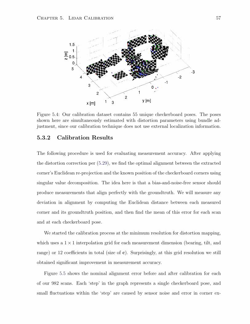
Chapter 5. Lidar Calibration 57
Figure 5.4: Our calibration dataset contains 55 unique checkerboard poses. The posesshown here are simultaneously estimated with distortion parameters using bundle ad-justment, since our calibration technique does not use external localization information.
5.3.2 Calibration Results
The following procedure is used for evaluating measurement accuracy. After applying
the distortion correction per (5.29), we find the optimal alignment between the extracted
corner’s Euclidean re-projection and the known position of the checkerboard corners using
singular value decomposition. The idea here is that a bias-and-noise-free sensor should
produce measurements that align perfectly with the groundtruth. We will measure any
deviation in alignment by computing the Euclidean distance between each measured
corner and its groundtruth position, and then find the mean of this error for each scan
and at each checkerboard pose.
We started the calibration process at the minimum resolution for distortion mapping,
which uses a 1× 1 interpolation grid for each measurement dimension (bearing, tilt, and
range) or 12 coefficients in total (size of c). Surprisingly, at this grid resolution we still
obtained significant improvement in measurement accuracy.
Figure 5.5 shows the nominal alignment error before and after calibration for each
of our 982 scans. Each ‘step’ in the graph represents a single checkerboard pose, and
small fluctuations within the ‘step’ are caused by sensor noise and error in corner ex-

Chapter 5. Lidar Calibration 58
100 200 300 400 500 600 700 800 9000
10
20
30
40
50
60
Avg
. F
ea
ture
Eu
clid
ea
n E
rro
r [m
m]
Frame Index
No Calibration
With Cal. (1 × 1 Grid Res.)
Figure 5.5: There was a large improvement in accuracy after calibration, even with thelowest possible resolution of distortion map.
1 2 3 4 5 65.42
5.44
5.46
5.48
5.5
5.52
5.54
5.56
5.58
5.6
Avg
. F
ea
ture
Eu
clid
ea
n E
rro
r [m
m]
Distortion Mapping Resolution [grid segments per axis]1 2 3 4 5 6
2
2.05
2.1
2.15
2.2
2.25
2.3
2.35
2.4
2.45
Sta
nd
ard
De
via
tio
n [
mm
]
Figure 5.6: We incrementally increased grid resolution from 1 × 1 to 6 × 6. While themeasurement error continues to decrease, there is a clear trend that higher resolutionmodels offer diminishing returns in accuracy improvement.
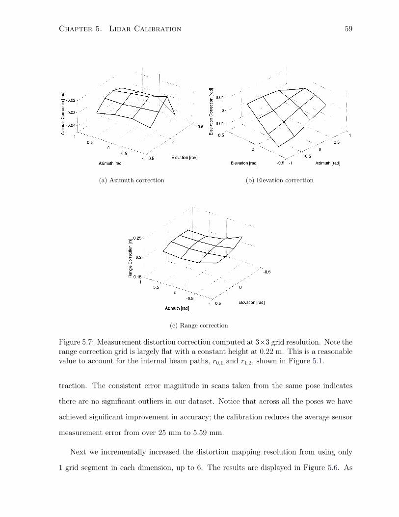
Chapter 5. Lidar Calibration 59
(a) Azimuth correction (b) Elevation correction
(c) Range correction
Figure 5.7: Measurement distortion correction computed at 3×3 grid resolution. Note therange correction grid is largely flat with a constant height at 0.22 m. This is a reasonablevalue to account for the internal beam paths, r0,1 and r1,2, shown in Figure 5.1.
traction. The consistent error magnitude in scans taken from the same pose indicates
there are no significant outliers in our dataset. Notice that across all the poses we have
achieved significant improvement in accuracy; the calibration reduces the average sensor
measurement error from over 25 mm to 5.59 mm.
Next we incrementally increased the distortion mapping resolution from using only
1 grid segment in each dimension, up to 6. The results are displayed in Figure 5.6. As

Chapter 5. Lidar Calibration 60
the number of distortion parameters is increased, we note a diminishing return in the
reduction of measurement error. At grid resolution N , we need three N × N grids or
3(N +1)2 coefficients in our state vector, c. In addition to the fact that higher resolution
is more prone to over-fitting, the (N + 1)2 increase in state size coupled with the cubic
complexity of solving bundle adjustment made it unappealing for us to use a very high
resolution. We found the 3× 3 grid resolution to be a reasonable compromise, and have
been using it as the standard calibration model for our lidar-based navigation work.
Computationally, the Matlab implementation we executed on a 2010 Macbook Pro with
Intel i7 CPU at 2.66 Ghz and 4 GB of memory converged in 14.5 seconds at the 3 × 3
grid distortion. The resulting distortion correction grids are shown in Figure 5.7.
5.4 Conclusion
In this chapter, we have presented a geometric lidar calibration method that closely
resembles traditional camera calibration. It offers the following advantages:
1. Leveraging lidar intensity images allowed for the use a planar calibration target,
which is more flexible than existing lidar calibration methods that require either
external localization or a more specialized calibration environment.
2. By not formulating the sensor model around a specific scanning mechanism, we
have arrived at a generalized calibration method that is directly applicable to a
number of two-axis scanning lidars.
We have demonstrated the calibration method experimentally on a complex two-axis
scanning lidar, reducing the sensor measurement error from over 25 mm to less than 5.5
mm. In the next chapter, we will compare state estimation results with and without
applying the calibration to quantify its impact in a long range VO system.
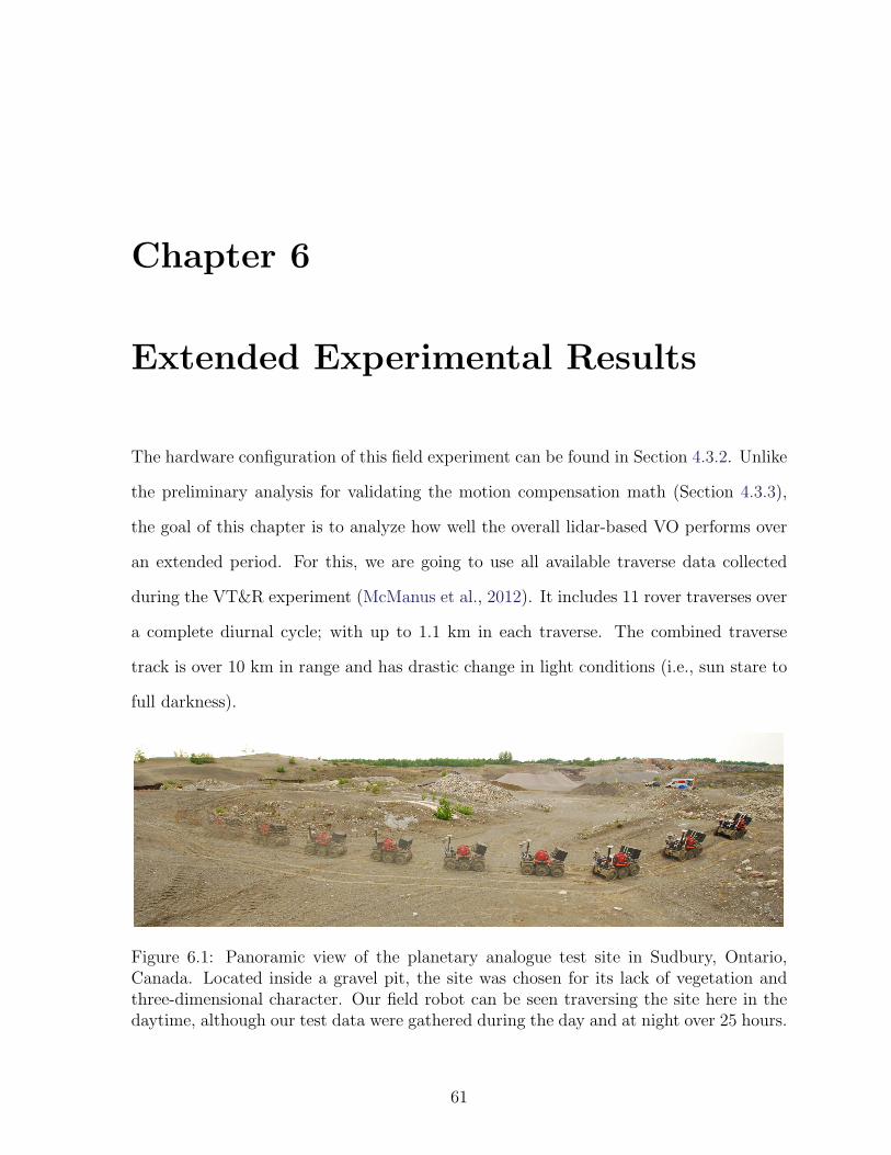
Chapter 6
Extended Experimental Results
The hardware configuration of this field experiment can be found in Section 4.3.2. Unlike
the preliminary analysis for validating the motion compensation math (Section 4.3.3),
the goal of this chapter is to analyze how well the overall lidar-based VO performs over
an extended period. For this, we are going to use all available traverse data collected
during the VT&R experiment (McManus et al., 2012). It includes 11 rover traverses over
a complete diurnal cycle; with up to 1.1 km in each traverse. The combined traverse
track is over 10 km in range and has drastic change in light conditions (i.e., sun stare to
full darkness).
Figure 6.1: Panoramic view of the planetary analogue test site in Sudbury, Ontario,Canada. Located inside a gravel pit, the site was chosen for its lack of vegetation andthree-dimensional character. Our field robot can be seen traversing the site here in thedaytime, although our test data were gathered during the day and at night over 25 hours.
61

Chapter 6. Extended Experimental Results 62
20 m
North
Start/End
Courtesy of Google Earth - 46°25’22”N 80°50’58” W
Figure 6.2: GPS track of a typical 1.1-km traverse performed during VT&R experiment(McManus et al., 2012).
To evaluate the impact of motion compensation and calibration on overall estimation
quality, we systematically applied one of them at a time and then together. The VO
estimates from of a typical traverse is shown in Figure 6.3, followed by the error plot in
Figure 6.4. There are two things worth noting in these figures, and they are especially
apparent in the error plot:
1. Applying the calibrated sensor model resulted in better VO estimate if motion
compensation is also used, but calibration without motion compensation actually
resulted in slightly worse estimate. Without going into detailed analysis on this
phenomenon, we suspect this occurred due to the pitch estimate bias introduced by
sensor measurement error (due to higher density of measurements near the bottom
of the scan) and the estimate bias introduced by motion distortion have a partial
cancelling effect on each other.
2. In terms of absolute Euclidean error, at the end of the 1.1-km traverse, the esti-
mators without motion compensation actually did better than ones with motion
compensation. Though this is purely coincidental and is not a reflection of better
estimation quality. It does beg the question that perhaps comparing absolute error
over very long range is not the best metric for our incremental VO system.
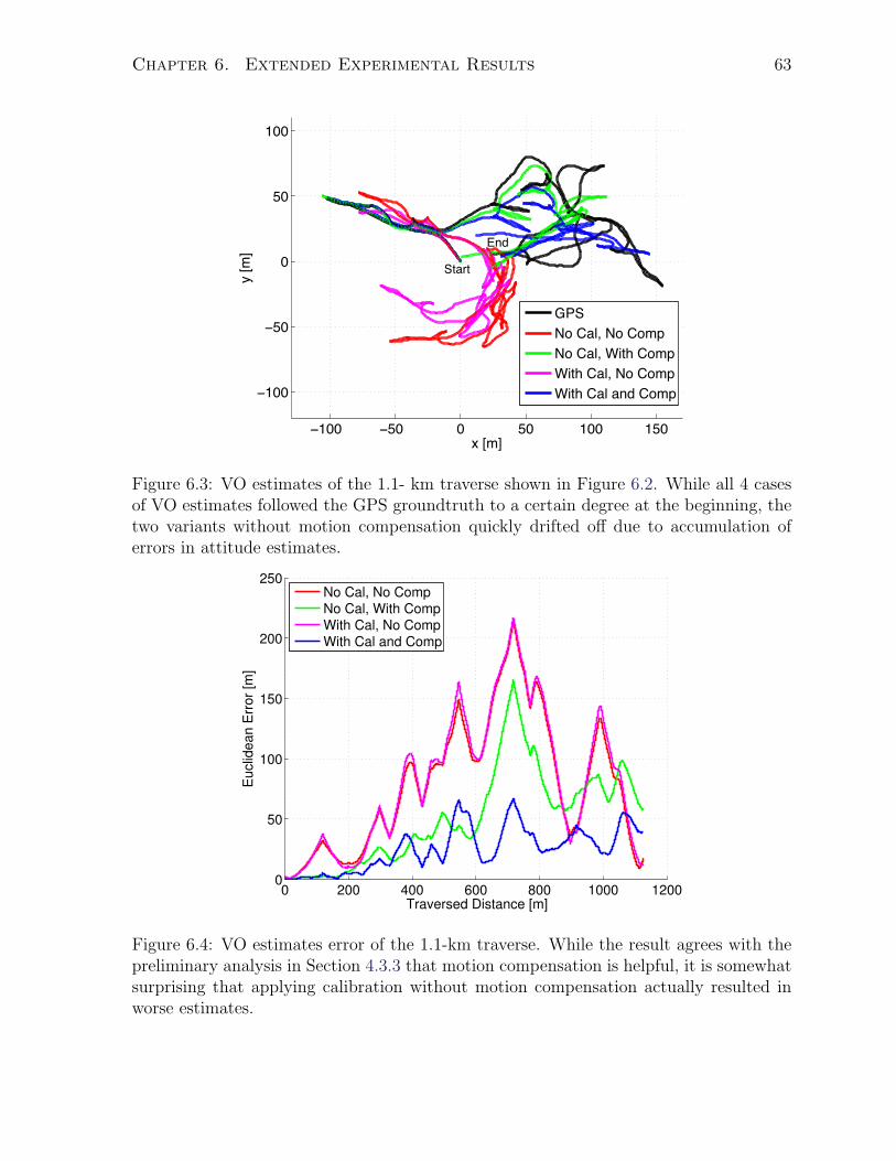
Chapter 6. Extended Experimental Results 63
−100 −50 0 50 100 150
−100
−50
0
50
100
x [m]
y [
m]
GPS
No Cal, No Comp
No Cal, With Comp
With Cal, No Comp
With Cal and Comp
Start
End
Figure 6.3: VO estimates of the 1.1- km traverse shown in Figure 6.2. While all 4 casesof VO estimates followed the GPS groundtruth to a certain degree at the beginning, thetwo variants without motion compensation quickly drifted off due to accumulation oferrors in attitude estimates.
0 200 400 600 800 1000 12000
50
100
150
200
250
Traversed Distance [m]
Eu
clid
ea
n E
rro
r [m
]
No Cal, No Comp
No Cal, With Comp
With Cal, No Comp
With Cal and Comp
Figure 6.4: VO estimates error of the 1.1-km traverse. While the result agrees with thepreliminary analysis in Section 4.3.3 that motion compensation is helpful, it is somewhatsurprising that applying calibration without motion compensation actually resulted inworse estimates.
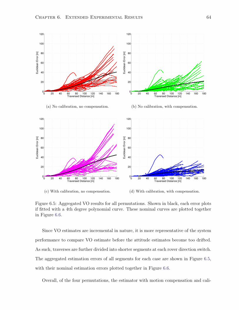
Chapter 6. Extended Experimental Results 64
0 20 40 60 80 100 120 140 160 1800
20
40
60
80
100
120
Traversed Distance [m]
Euclid
ean E
rror
[m]
(a) No calibration, no compensation.
0 20 40 60 80 100 120 140 160 1800
20
40
60
80
100
120
Traversed Distance [m]
Euclid
ean E
rror
[m]
(b) No calibration, with compensation.
0 20 40 60 80 100 120 140 160 1800
20
40
60
80
100
120
Traversed Distance [m]
Euclid
ean E
rror
[m]
(c) With calibration, no compensation.
0 20 40 60 80 100 120 140 160 1800
20
40
60
80
100
120
Traversed Distance [m]
Euclid
ean E
rror
[m]
(d) With calibration, with compensation.
Figure 6.5: Aggregated VO results for all permutations. Shown in black, each error plotsif fitted with a 4th degree polynomial curve. These nominal curves are plotted togetherin Figure 6.6.
Since VO estimates are incremental in nature, it is more representative of the system
performance to compare VO estimate before the attitude estimates become too drifted.
As such, traverses are further divided into shorter segments at each rover direction switch.
The aggregated estimation errors of all segments for each case are shown in Figure 6.5,
with their nominal estimation errors plotted together in Figure 6.6.
Overall, of the four permutations, the estimator with motion compensation and cali-

Chapter 6. Extended Experimental Results 65
bration performed the best; it accumulates estimation error at less than half of the rate
in comparison to the original estimator that does not account for motion distortion and
sensor calibration. While the approximate 10 percent error-growth is less than what
state-of-art stereo-camera-based VO is capable of, it clearly demonstrates that computa-
tionally efficient lidar-based VO can indeed be improved using the motion compensation
and calibration methods proposed in this thesis, and sets a upper bound that can be im-
proved upon using techniques such as multi-frames bundle-adjustment, and sensor fusion
with IMU and/or star tracker.
0 20 40 60 80 100 120 140 160 1800
10
20
30
40
50
60
Traversed Distance [m]
Eu
clid
ea
n E
rro
r [m
]
No Cal, No Comp
No Cal, With Comp
With Cal, No Comp
With Cal and Comp
Figure 6.6: Nominal VO estimation errors. Once again, the estimator with calibrationbut no motion compensation performed the worst, and the one with both calibration andcompensation performed the best.

Chapter 7
Summary
Due to the scanning nature of the lidar and assumptions made in previous implemen-
tations, data acquired during continuous vehicle motion suffer from geometric motion
distortion and can subsequently result in poor metric VO estimates, even over short
distances (e.g., 5-10 m).
To fully understand the impact of motion distortion in lidar-based VO, a 3D lidar
simulator was created to replicate the scanning pattern of an existing lidar sensor. This
simulator enabled generation of datasets both with and without motion distortion. Sub-
sequent analysis of VO estimates computed using simulated lidar data demonstrated a
clear need to address the motion distortion problem, and identified the root cause of
the systematic estimation error to be, in previous systems, true acquisition time of each
measurement was not exactly accounted for when working with scanning lidars.
The measurement timing assumption made in previous systems was revised, followed
by the development of a frame-to-frame VO estimation framework based on a pose in-
terpolation scheme that explicitly accounts for the exact acquisition time of each feature
measurement. This proposed method was preliminarily validated using simulated lidar
data and 500 m of experimental traverse data collected from a planetary analogue envi-
ronment. This work has been peer reviewed and published in Dong and Barfoot (2012).
66
Chapter 7. Summary 67
A second problem that was addressed is the need to calibrate the sensor to obtain
accurate lidar measurements. The proposed method generalizes a two-axis scanning lidar
as an idealized spherical camera with additive measurement distortions. It also leverages
lidar intensity imagery to enable calibration using only an inexpensive checkerboard
calibration target. The resulting calibration method can be readily applied to a variety
of two-axis scanning lidars. This improved lidar calibration method and its associated
experimental results has been peer reviewed and published in Dong et al. (2013).
Finally, an extended lidar-based VO performance analysis was carried out using 4
variants of state estimators covering all permutations involving with/without calibra-
tion and with/without motion compensation. The results clearly demonstrated the VO
estimator with motion compensation and sensor calibration performed the best, and
achieved an error-growth-rate of less than half of that original state estimator without
motion compensation and proper sensor calibration.
In is worth noting that while the improved estimation framework and sensor calibra-
tion resulted in large improvement in lidar-based VO performance, the nearly 10 percent
error-growth rate is far worse than the state of the art camera-based VO systems, where
2-3 percent error-growth rate has been achieved. A number of approaches should be
considered to further improve lidar-based VO performance, specifically:
1. Moving beyond frame-to-frame VO to multi-frame bundle-adjustment. This should
lead to more robust RANSAC and better pose estimates.
2. Incorporating additional sensor data, such as the absolute orientation measure-
ments provided by an inclinometer and/or a star tracker. The added measurements
will constrain the heading estimate drift and result in better absolute pose estimate
over long distance.
3. Adding loop closure information using place recognition, and solving the pose esti-
mation problem using a full SLAM solution.

Bibliography
Anderson, S. and Barfoot, T. D. (2013.). Ransac for motion-distorted 3d visual sensors.
In IEEE/RSJ International Conference on Intelligent Robots and Systems (IROS), to
appear., Tokyo, Japan. (ref. page 22)
Atanacio-Jimenez, G., Gonzalez-Barbosa, J., Hurtado-Ramos, J., Ornelas-Rodrıguez, F.,
Jimenez-Hernandez, H., Garcıa-Ramirez, T., and Gonzalez-Barbosa, R. (2011). Lidar
velodyne hdl-64e calibration using pattern planes. Int J Adv Robotic Sy, 8(5):70–82.
(ref. page 44)
Barfoot, T. (2005). Online visual motion estimation using FastSLAM with SIFT features.
In Intelligent Robots and Systems, 2005.(IROS 2005). 2005 IEEE/RSJ International
Conference on, pages 579–585. IEEE. (ref. page 7)
Bay, H., Tuytelaars, T., and Van Gool, L. (2006). Surf: Speeded up robust features.
Computer Vision–ECCV 2006, pages 404–417. (ref. page 8)
Besl, P. and McKay, N. (1992). A method for registration of 3-D shapes. IEEE Trans-
actions on pattern analysis and machine intelligence, pages 239–256. (ref. page 9)
Bosse, M. and Zlot, R. (2009). Continuous 3d scan-matching with a spinning 2d laser.
In Robotics and Automation (ICRA), 2009 IEEE International Conference on, pages
4312–4319. IEEE. (ref. page 21)
Bouguet, J.-Y. (2004). Camera calibration toolbox for matlab. (ref. pages 42 and 56)
68

BIBLIOGRAPHY 69
Bradski, G. (2009). The OpenCV Library. Dr. Dobb’s Journal of Software Tools. (ref.
page 42)
Brock, J., Wright, C., Sallenger, A., Krabill, W., and Swift, R. (2002). Basis and methods
of NASA airborne topographic mapper lidar surveys for coastal studies. Journal of
Coastal Research, 18(1):1–13. (ref. page 5)
Burton, D. and Wood, L. J. (2010). Lidar intensity as a remote sensor of rock properties.
Powerpoint Presentation. (ref. page 7)
Calonder, M., Lepetit, V., Fua, P., Konolige, K., Bowman, J., and Mihelich, P. (2010).
Compact signatures for high-speed interest point description and matching. In Com-
puter Vision, 2009 IEEE 12th International Conference on, pages 357–364. IEEE. (ref.
page 8)
Chen, Y. and Medioni, G. (1991). Object modelling by registration of multiple range
images. Image Vision Comput., 10(3):145–155. (ref. page 9)
Dong, H., Anderson, S., and Barfoot, T. D. (2013). Two-axis scanning lidar geometric
calibration using intensity imagery and distortion mapping. In Proceedings of the
IEEE International Conference on Robotics and Automation (ICRA), pages 3657–
3663, Karlsruhe, Germany. (ref. page 67)
Dong, H. J. and Barfoot, T. D. (2012). Lighting-invariant visual odometry using lidar in-
tensity imagery and pose interpolation. In Proceedings of the International Conference
on Field and Service Robotics (FSR), Matsushima, Japan. (ref. page 66)
Donmez, M., Blomquist, D., Hocken, R., Liu, C., and Barash, M. (1986). A general
methodology for machine tool accuracy enhancement by error compensation. Precision
Engineering, 8(4):187–196. (ref. page 47)

BIBLIOGRAPHY 70
Enright, J., Barfoot, T. D., and Soto, M. (2012). Star tracking for planetary rovers. In
Proceedings of the IEEE Aerospace Conference, pages 1–13, Big Sky, MT. (ref. page
40)
Forssen, P.-E. and Ringaby, E. (2010). Rectifying rolling shutter video from hand-held
devices. In IEEE Conference on Computer Vision and Pattern Recognition, San Fran-
cisco, USA. IEEE Computer Society, IEEE. (ref. pages 20 and 21)
Fowler, R. (2000). The low down on LIDAR. Earth Observation Magazine, 9(3). (ref.
page 6)
Furgale, P. and Barfoot, T. (2010). Visual teach and repeat for long-range rover au-
tonomy. Journal of Field Robotics, special issue on “Visual mapping and navigation
outdoors”, 27(5):534–560. (ref. page 8)
Furgale, P., Tong, C., and Kenway, G. (2009). ECE1724 Project Speeded-Up Speeded-Up
Robust Features. (ref. page 8)
Furgale, P. T. (2011). Extensions to the Visual Odometry Pipeline for the Exploration of
Planetary Surfaces. PhD thesis, University of Toronto. (ref. page 53)
Furgale, P. T., Barfoot, T. D., and Sibley, G. (2012). Continuous-time batch estimation
using temporal basis functions. In Proceedings of the IEEE International Conference
on Robotics and Automation (ICRA), pages 2088–2095, St. Paul, USA. (ref. page 41)
Gammell, J. D., Tong, C. H., Berczi, P., Anderson, S., Barfoot, T. D., and Enright, J.
(2013). Rover odometry aided by a star tracker. In Proceedings of the IEEE Aerospace
Conference, pages 1–10, Big Sky, MT. (ref. page 40)
Gauss, K. (1809). Theory of the motion of the heavenly bodies moving about the sun in
conic sections: Reprint 2004. (ref. pages 24 and 53)

BIBLIOGRAPHY 71
Geiger, A., Moosmann, F., Car, O., and Schuster, B. (2012). A toolbox for automatic
calibration of range and camera sensors using a single shot. In International Conference
on Robotics and Automation (ICRA), St. Paul, USA. (ref. page 43)
Grassia, F. (1998). Practical parameterization of rotations using the exponential map.
Journal of graphics tools, 3:29–48. (ref. page 21)
Guivant, J., Nebot, E., and Baiker, S. (2000). Localization and map building using laser
range sensors in outdoor applications. Journal of Robotic Systems, 17(10):565–583.
(ref. pages 10 and 20)
Hofle, B. and Pfeifer, N. (2007). Correction of laser scanning intensity data: Data and
model-driven approaches. ISPRS Journal of Photogrammetry and Remote Sensing,
62(6):415–433. (ref. pages 5 and 6)
Husmann, K. and Pedersen, L. (2008). Strobe lit high dynamic range stereo imagery for
dark navigation. In International Symposium on Artificial Intelligence, Robotics and
Automation in Space (iSAIRAS). (ref. page 4)
Kaasalainen, S., Ahokas, E., Hyyppa, J., and Suomalainen, J. (2005). Study of surface
brightness from backscattered laser intensity: calibration of laser data. Geoscience and
Remote Sensing Letters, IEEE, 2(3):255–259. (ref. page 6)
Konolige, K., Bowman, J., Chen, J., Mihelich, P., Calonder, M., Lepetit, V., and Fua, P.
(2010). View-based maps. The International Journal of Robotics Research, 29(8):941–
957. (ref. page 8)
Lambert, A., Furgale, P. T., Barfoot, T. D., and Enright, J. (2012). Field testing of
visual odometry aided by a sun sensor and inclinometer. Journal of Field Robotics,
special issue on “Space Robotics”, 29(3):426–444. (ref. pages 11, 38, and 40)

BIBLIOGRAPHY 72
Lepetit, V. and Fua, P. (2006). Keypoint recognition using randomized trees. IEEE
Transactions on Pattern Analysis and Machine Intelligence, pages 1465–1479. (ref.
page 8)
Levinson, J. (2011). Automatic laser calibration, mapping, and localization for au-
tonomous vehicles. PhD thesis, Stanford University. (ref. pages 20 and 44)
Lowe, D. G. (1999). Object recognition from local scale-invariant features. In Com-
puter vision, 1999. The proceedings of the seventh IEEE international conference on,
volume 2, pages 1150–1157. Ieee. (ref. page 7)
Magnusson, M., Andreasson, H., Nuchter, A., and Lilienthal, A. (2009). Automatic
appearance-based loop detection from three-dimensional laser data using the normal
distributions transform. Journal of Field Robotics, 26(11-12):892–914. (ref. page 10)
Maki, J., Bell, J., Herkenhoff, K., Squyres, S., Kiely, A., Klimesh, M., Schwochert, M.,
Litwin, T., Willson, R., Johnson, A., et al. (2003). Mars exploration rover engineering
cameras. J. Geophys. Res, 108:8071. (ref. page 42)
Maki, J., Thiessen, D., Pourangi, A., Kobzeff, P., Litwin, T., Scherr, L., Elliott, S.,
Dingizian, A., and Maimone, M. (2012). The mars science laboratory engineering
cameras. Space Science Reviews, pages 1–17. (ref. page 42)
Matthies, L., Maimone, M., Johnson, A., Cheng, Y., Willson, R., Villalpando, C., Gold-
berg, S., Huertas, A., Stein, A., and Angelova, A. (2007). Computer vision on Mars.
International Journal of Computer Vision, 75(1):67–92. (ref. page 1)
Matthies, L. and Shafer, S. (1987). Error modeling in stereo navigation. Robotics and
Automation, IEEE Journal of, 3(3):239–248. (ref. page 8)
May, S., Fuchs, S., Malis, E., Nuchter, A., and Hertzberg, J. (2009). Three-dimensional

BIBLIOGRAPHY 73
mapping with time-of-flight cameras. Journal of Field Robotics, 26(11-12):934–965.
(ref. page 10)
Mazzarini, F., Pareschi, M., Favalli, M., Isola, I., Tarquini, S., Boschi, E., et al. (2006).
Lava flow identification and ageing by means of LiDAR intensity: the Mt. Etna case.
J. Geophys. Res. (ref. page 6)
McManus, C., Furgale, P. T., and Barfoot, T. D. (2011). Towards appearance-based
methods for lidar sensors. In Robotics and Automation (ICRA), 2011 IEEE Interna-
tional Conference on, pages 1930–1935, Shanghai, China. (ref. pages 2, 10, 12, 14,
and 22)
McManus, C., Furgale, P. T., and Barfoot, T. D. (2013). Towards lighting-invariant
visual navigation: An appearance-based approach using scanning laser-rangefinders.
Robotics and Autonomous Systems, 61:836–852. (ref. pages 10, 13, and 15)
McManus, C., Furgale, P. T., Stenning, B. E., and Barfoot, T. D. (2012). Visual teach
and repeat using appearance-based lidar. In Proceedings of the IEEE International
Conference on Robotics and Automation (ICRA), pages 389–396, St. Paul, USA. (ref.
pages 10, 11, 19, 37, 56, 61, and 62)
Milford, M. J. and Wyeth, G. F. (2012). Seqslam: Visual route-based navigation for
sunny summer days and stormy winter nights. In Robotics and Automation (ICRA),
2012 IEEE International Conference on, pages 1643–1649. IEEE. (ref. page 9)
Moosmann, F. and Stiller, C. (2011). Velodyne SLAM. In Intelligent Vehicles Symposium
(IV), 2011 IEEE, pages 393–398. IEEE. (ref. page 21)
Nagihara, S., Mulligan, K., and Xiong, W. (2004). Use of a three-dimensional laser
scanner to digitally capture the topography of sand dunes in high spatial resolution.
Earth Surface Processes and Landforms, 29(3):391–398. (ref. page 5)

BIBLIOGRAPHY 74
Neira, J., Tardos, J., Horn, J., and Schmidt, G. (1999). Fusing range and intensity
images for mobile robot localization. Robotics and Automation, IEEE Transactions
on, 15(1):76–84. (ref. pages 10 and 20)
O’Neill, J., Moore, W., Williams, K., and Bruce, R. (2007). Scanning system for lidar.
US Patent App. 12/447,937. (ref. pages 14 and 45)
Pedersen, L., Han, S., and Vitus, M. (2008). Dark navigation: sensing and rover nav-
igation in permanently shadowed lunar craters. In 9th International Symposium on
Artificial Intelligence. Robotics, Automation in Space, Los Angeles. (ref. page 4)
Pradeep, V., Konolige, K., and Berger, E. (2010). Calibrating a multi-arm multi-sensor
robot: A bundle adjustment approach. In International Symposium on Experimental
Robotics (ISER), New Delhi, India. (ref. pages 44 and 46)
Rankin, A., Huertas, A., and Matthies, L. (2007). Nighttime negative obstacle detec-
tion for off-road autonomous navigation. In Society of Photo-Optical Instrumentation
Engineers (SPIE) Conference Series, volume 6561, page 2. Citeseer. (ref. page 5)
Ryde, J. and Hu, H. (2008). 3d laser range scanner with hemispherical field of view for
robot navigation. In Advanced Intelligent Mechatronics, 2008. AIM 2008. IEEE/ASME
International Conference on, pages 891–896. IEEE. (ref. page 45)
Se, S., Lowe, D., and Little, J. (2002). Mobile robot localization and mapping with un-
certainty using scale-invariant visual landmarks. The international Journal of robotics
Research, 21(8):735–758. (ref. page 7)
Se, S., Lowe, D., and Little, J. (2005). Vision-based global localization and mapping for
mobile robots. Robotics, IEEE Transactions on, 21(3):364–375. (ref. page 7)
Sheehan, M., Harrison, A., and Newman, P. (2011). Self-calibration for a 3d laser. The
International Journal of Robotics Research. (ref. page 44)
BIBLIOGRAPHY 75
Shoemake, K. (1985). Animating rotation with quaternion curves. ACM SIGGRAPH
computer graphics, 19(3):245–254. (ref. page 21)
Sibley, G., Mei, C., Reid, I., and Newman, P. (2009). Adaptive relative bundle adjust-
ment. In Robotics Science and Systems Conference. (ref. page 9)
Sinha, S., Frahm, J., Pollefeys, M., and Genc, Y. (2006). GPU-based video feature track-
ing and matching. In EDGE, Workshop on Edge Computing Using New Commodity
Architectures, volume 278. Citeseer. (ref. page 8)
Stettner, R. (2010). Compact 3D flash LIDAR video cameras and applications. In
Proceedings of SPIE, volume 7684, page 768405. (ref. page 5)
Terriberry, T., French, L., and Helmsen, J. (2008). GPU accelerating speeded-up robust
features. In Proc. Int. Symp. on 3D Data Processing, Visualization and Transmission
(3DPVT), pages 355–362. Citeseer. (ref. page 8)
Thrun, S. and Urmson, C. (2011). How Google’s self-driving car works. Intelligent Robots
and Systems (IROS). (ref. pages 20 and 42)
Tong, C. H., Furgale, P. T., and Barfoot, T. D. (2012). Gaussian process gauss-newton:
Non-parametric state estimation. In 9th Canadian Conference on Computer and Robot
Vision (CRV), to appear, Toronto, Canada. (ref. page 41)
Unnikrishnan, R. and Hebert, M. (2005). Fast extrinsic calibration of a laser rangender
to a camera. Technical Report CMU-RI-TR-05-09, Robotics Institute, CMU. (ref.
page 43)
Wan, Y. and Zhang, S. (2006). Filtering LIDAR intensity image based on orientation
gradient of distance image. In Proceedings of SPIE, volume 6419, page 64191D. (ref.
page 6)

BIBLIOGRAPHY 76
Zhang, Z. (2000). A flexible new technique for camera calibration. Pattern Analysis and
Machine Intelligence, IEEE Transactions on, 22(11):1330–1334. (ref. page 42)