performance of a parabolic trough solar
TRANSCRIPT

PERFORMANCE OF A
PARABOLIC TROUGH SOLAR COLLECTOR
by
Michael John Brooks
Thesis presented in partial fulfillment of the requirements for the degree of
Master of Science in Engineering at the University of Stellenbosch
Thesis supervisor:
Associate Professor T.M. Harms
February 2005

ii
DECLARATION
I, Michael John Brooks, submit this thesis in partial fulfillment of the requirements of the
degree MScEng at the University of Stellenbosch and hereby declare that the work contained
in this thesis is my own original work and that I have not previously, in its entirety or in part,
submitted it at any university for a degree.
Signed: _________________________ Date: _______________
(M. J. Brooks)

iii
ABSTRACT
Parabolic trough solar collectors (PTSCs) constitute a proven source of thermal energy for
industrial process heat and power generation, although their implementation has been strongly
influenced by economics. In recent years, environmental concerns and other geopolitical
factors have focused attention on renewable energy resources, improving the prospects for
PTSC deployment. Further work is needed to improve system efficiencies and active areas of
research include development of advanced heat collecting elements and working fluids,
optimisation of collector structures, thermal storage and direct steam generation (DSG).
A parabolic trough collector, similar in size to smaller-scale commercial modules, has been
developed locally for use in an ongoing PTSC research programme. The aim of this study
was to test and fully characterise the performance of the collector.
Specialised logging software was developed to record test data and monitor PTSC
performance in real-time. Two heat collecting elements were tested with the collector, one
unshielded and the other with an evacuated glass cover. Testing was carried out according to
the ASHRAE 93-1986 (RA 91) standard, yielding results for the thermal efficiency, collector
acceptance angle, incidence angle modifier and collector time constant. Peak thermal
efficiency was 55.2 % with the unshielded receiver and 53.8 % with the glass-shielded unit.
The evacuated glass shield offered superior performance overall, reducing the receiver heat
loss coefficient by 50.2 % at maximum test temperature. The collector time constant was less
than 30 s for both receivers, indicating low thermal inertia. Thermal loss tests were conducted
and performance of the trough’s tracking system was evaluated. The measured acceptance
angles of 0.43° (unshielded) and 0.52° (shielded) both exceeded the tracking accuracy of the
PTSC, ensuring that the collector operated within 2 % of its optimal efficiency at all times.
Additionally, experimental results were compared with a finite-volume thermal model, which
showed potential for predicting trough performance under forced convection conditions.

iv
OPSOMMING
Paraboliese trog sonkollekteerders is een van die belowende tegnologiese ontwikkelings wat
sonenergie op industriële vlak kan gebruik vir die vervaardiging van hitte en elektriese krag.
Alhoewel die grootskaalse implementasie van sonergie as ’n alternatiewe energiebron deur
ekonomiese oorwegings beïnvloed word het die verhoogde omgewingsbewustheid en
geopolitieke faktore, gedurende die afgelope jare, die klem verskuif na hernubare
energiebronne. Die vooruitsig om sonkollekteerders op groot skaal te ontplooi het drasties
verbeter. Die aandag is nou gevestig op die verbetering van sisteem effektiwiteit en aktiewe
navorsing fokus op gevorderde hitte elemente, werkbare vloeistowwe, optimisering van
hitteversameling strukture, storing van hitte energie en direkte stoom vervaardiging.
‘n Paraboliese trog sonkollekteerder, vergelykbaar met die grootte van kleiner kommersieële
eenhede, is plaaslik ontwikkel vir gebruik in die paraboliese trog sonkollekteerder
navorsingsprojek. Die doel van die studie was die toets en karakterisering van die
effektiwiteit van die paraboliese trog sonkollekteerder.
Gespesialiseerde data vasleggings programme is ontwikkel ten einde ‘n ware-tyd
werkverrigtings analise van die paraboliese trog sonkollekteerder te doen. Twee potensiële
elemente vir hitteversameling is vervaardig en vergelyk. Die eerste element is onbeskud
terwyl die tweede element deur ‘n glasbuis onder vakuum beskerm word. Vergelyking van
die elemente is volgens die ASHRAE 93-1986 (RA91) standaard gedoen, wat resultate van
die prestasie van hitte effektiwiteit, aanvaardingshoeke van die kollekteerder, hoek van inval
modifiseerder, en tydkonstante waardes insluit. Die best termiese effektiwiteit van die
sonkollekteerder is bereken as 55.2 % met die onbeskutte ontvanger en 53.8 % met die
glasomhulsel. Resultate wys dat die glasomhulsel in die algemeen beter werkverrigting lewer
aangesien die hitteverlies koëfisient onder vakuum en maksimum toets temperatuur met 50.2
% verminder het. Die tydkonstante waardes was minder as 30s vir beide ontvangers wat op
lae termiese inersie dui. Hitteverlies is bepaal en die werkverrigting van die
sonopsporingsisteem van die trog is geëvalueer. In beide gevalle is die akuraatheid van die
aanvaardingshoeke, 0.43° (onbeskut) en 0.52° (glasomhulde ontvanger), beter as die
sonopsporing van die paraboliese trog kollekteerder. Dit verseker dat die sonkollekteerder te
alle tye binne 2 % van optimale effektiwiteit kan werk.

v
Eksperimentele resultate is ook vergelyk met resultate van ‘n eindige volume termiese model.
Die gevolgtrekking van hierdie vergelyking bevestig dat die model potensiaal toon vir die
skatting van termiese werkverrigting gedurende geforseerde konveksie toestande.

vi
To my parents, for their love, patience and sense of humour...
…et in honorem Mariae, sedis sapientiae, quae nos ducit ad Christum.
Ora pro nobis, Sancta Mater Dei!

vii
ACKNOWLEDGEMENTS
Many people have supported and contributed to this project – their efforts are acknowledged
and sincerely appreciated. Special thanks to the following:
Mangosuthu Technikon:
• Mrs. Ewa Zawilska, Head of Mechanical Engineering, whose professionalism and untiring
support of this project and those involved, enabled it to take place
• Dr. Anette van der Mescht, Research Director, for enabling the development of the test
facility, steering the research project through numerous challenges and providing
invaluable support and advice
• Mr. Ian Mills, Senior Laboratory Technician, for his hard work and technical expertise
• Prof. E. C. Zingu and senior management of Mangosuthu Technikon
• Messrs. Andrew Nunn, Teddy Singh and all staff in the Department of Mechanical
Engineering
• Messrs. Mike Maree and Julian Thompson and their staff in the departments of
Maintenance and Information Technology
• Messrs. Ralph Naidoo, Magan Moodley, John van Rensburg, Cannon Maxongo and Chris
Presmeg and the staff and students in the Department of Civil Engineering and Surveying
University of Stellenbosch:
• A/Prof. Thomas Harms, for support, advice and supervision of this project
• Mrs. Ilse du Toit, Mr. Cobus Zietsman and the academic and administrative staff in the
Department of Mechanical Engineering
• Messrs. Meiring Beyers, Johan Potgieter, Rhydar Harris and Paul Wipplinger of M303
The support of the following is acknowledged and greatly appreciated:
• Mr. Ryan Botha, AfricaBlue and Autodesk, for graphical renditions of the collector
• The United States Agency for International Development (USAID)
• Mrs. Meena Dhavraj-Lysko, Prof. Jørgen Lovseth (Norwegian University for Science and
Technology) and Mr. Robert van den Heetkamp (University of KwaZulu-Natal)
Finally, thanks to friends and family for their encouragement and support.

TABLE OF CONTENTS
Page
TITLE PAGE..............................................................................................................................i
DECLARATION.......................................................................................................................ii
ABSTRACT ............................................................................................................................ iii
OPSOMMING..........................................................................................................................iv
DEDICATION..........................................................................................................................vi
ACKNOWLEDGEMENTS.....................................................................................................vii
TABLE OF CONTENTS ...................................................................................................... viii
LIST OF TABLES.....................................................................................................................x
LIST OF FIGURES.................................................................................................................xii
LIST OF SYMBOLS...............................................................................................................xv
1. INTRODUCTION...............................................................................................................1
2. MOTIVATION....................................................................................................................3
3. DESCRIPTION OF TEST APPARATUS ..........................................................................7
3.1 Parabolic Trough Collector Structure.........................................................................7
3.2 Heat Collecting Elements ...........................................................................................7
3.3 Fluid Circulation System............................................................................................8
3.4 Drive, Tracking and Control System (DTCS) ............................................................9
4. TEST METHODOLOGY..................................................................................................11
4.1 Introduction ..............................................................................................................11
4.2 The ASHRAE 93-1986 (RA 91) Testing Standard ..................................................11
4.2.1 Thermal efficiency test procedure ...................................................................13
4.2.2 Collector time constant test procedure ............................................................17
4.2.3 Incidence angle modifier test procedure..........................................................18
4.2.4 Collector acceptance angle test procedure.......................................................19
4.3 PTSC Test Schedule .................................................................................................20
4.3.1 Planned schedule .............................................................................................20
4.3.2 Completed test schedule ..................................................................................22
4.4 Development of Data Logging Software Applications ............................................25
4.4.1 SolarStation .....................................................................................................25
4.4.2 SCATTAscan and SCATTAlog ......................................................................27
4.5 Summary...................................................................................................................29 viii

ix
5. EXPERIMENTAL RESULTS ..........................................................................................30
5.1 Introduction ..............................................................................................................30
5.2 Tracking Performance ..............................................................................................30
5.2.1 Fixed rate tracking ...........................................................................................30
5.2.2 PSA Algorithm-based tracking........................................................................33
5.3 PTSC Performance Results ......................................................................................34
5.3.1 Collector time constant....................................................................................35
5.3.2 Collector acceptance angle ..............................................................................41
5.3.3 Thermal efficiency...........................................................................................44
5.3.4 Incidence angle modifier .................................................................................48
5.4 Receiver Thermal Loss Tests ...................................................................................52
5.5 Summary...................................................................................................................56
6. THERMAL MODELLING OF PTSC PERFORMANCE................................................58
6.1 Introduction ..............................................................................................................58
6.2 Thermal Model of Collector Performance................................................................59
6.3 Results ......................................................................................................................62
6.4 Summary...................................................................................................................69
7. DISCUSSION....................................................................................................................71
7.1 Experimental Results................................................................................................71
7.2 Thermal Modelling of PTSC Performance...............................................................79
8. SUMMARY.......................................................................................................................83
9. RECOMMENDATIONS...................................................................................................85
REFERENCES ........................................................................................................................88
APPENDIX A DESIGN AND CONSTRUCTION OF PTSC .........................................A1
APPENDIX B MATLAB CODE FOR PTSC INTERCEPT FACTOR........................... B1
APPENDIX C THE PSA ALGORITHM: CALCULATIONS AND DATA................... C1
APPENDIX D LABVIEW SOFTWARE: SCATTALOG DATA SAMPLE ..................D1
APPENDIX E SUMMARY OF EXPERIMENTAL TEST DATA ................................. E1
APPENDIX F THERMAL MODEL DATA.....................................................................F1

x
LIST OF TABLES
Page
2.1 Comparison of performance and other key parameters for theree solar thermal
technologies (* Schlaich, 1996; ** SolarPACES, 1999)...............................................3
3.1 PTSC key features and material properties ...................................................................8
4.1 Planned PTSC test schedule ........................................................................................22
4.2 Schedule of completed PTSC tests..............................................................................23
5.1 Key data from time constant tests................................................................................40
5.2 Key data from thermal efficiency tests........................................................................47
5.3 Key data from incidence angle modifier tests .............................................................51
5.4 PTSC performance summary.......................................................................................57
A.1 Comparison of reflective surface options...................................................................A8
A.2 Error sets used to determine absorber diameter in figure A.5 ..................................A12
A.3 Error sets used in PTSC analysis of Güven et al. (1986) .........................................A16
A.4 Intercept factor for PTSC with rim angle of 82° and aperture width of 1.5 m.........A17
A.5 Operating modes for the DTCS................................................................................A31
A.6 Summary of key features of PTSC...........................................................................A35
C.1 Solar zenith and azimuth data for a range of days covering one year, generated
using the PSA Algorithm (MATLAB programme “psa_16days.m”) and
compared with output from the Multi-Year Interactive Computer Almanac
(MICA) of the U.S. Naval Observatory ..................................................................... C8
D.1 Extract from Excel spreadsheet showing processed output from LabVIEW
application SCATTAlog for collector acceptance angle test .....................................D2
D.2 List of columns from table E1 and description of data types .....................................D4
E.1 Summary of data for collector time constant tests ..................................................... E2
E.2 Thermal efficiency test data for glass-shielded receiver (19 February 2004) ............ E3
E.3 Summary of data for thermal efficiency tests with unshielded receiver .................... E6
E.4 Summary of data for thermal efficiency tests with glass-shielded receiver ............... E6
E.5 Summary of data for collector acceptance angle tests with unshielded
and glass-shielded receiver......................................................................................... E7
E.6 Summary of data for incidence angle modifier tests with unshielded receiver.......... E7
E.7 Summary of data for incidence angle modifier tests with glass-shielded
receiver ....................................................................................................................... E7

xi
F.1 Output from MATLAB thermal modelling programme for unshielded
receiver (wind speed of 4.8 m/s, inlet temperature of 27.12 °C and beam
irradiance of 928.23 W/m2) .........................................................................................F2
F.2 Loss output from MATLAB thermal modelling programme for unshielded
receiver (wind speed of 1.34 m/s, inlet temperature of 29.77 °C, ambient
temperature of 21.2 °C and zero beam irradiance)......................................................F3
F.3 Output from MATLAB thermal modelling programme for glass-shielded
receiver (wind speed of 4.6 m/s, inlet temperature of 27.27 °C and beam
irradiance of 841.73 W/m2) .........................................................................................F4
LIST OF FIGURES
Page
2.1 Solar Electric Generating Systems (SEGS) collector field
(www.kjcsolar.com, 2004) ............................................................................................4
2.2 Parabolic trough test loop, Plataforma Solar de Almeria (www.psa.es, 2004) .............5
3.1 Parabolic trough collector module.................................................................................7
3.2 Schematic layout of fluid circulation system with PTSC structure removed
and (inset) three-dimensional sketch .............................................................................9
3.3 PTSC with glass-shielded receiver during operation and vacuum pump visible
in foreground ...............................................................................................................10
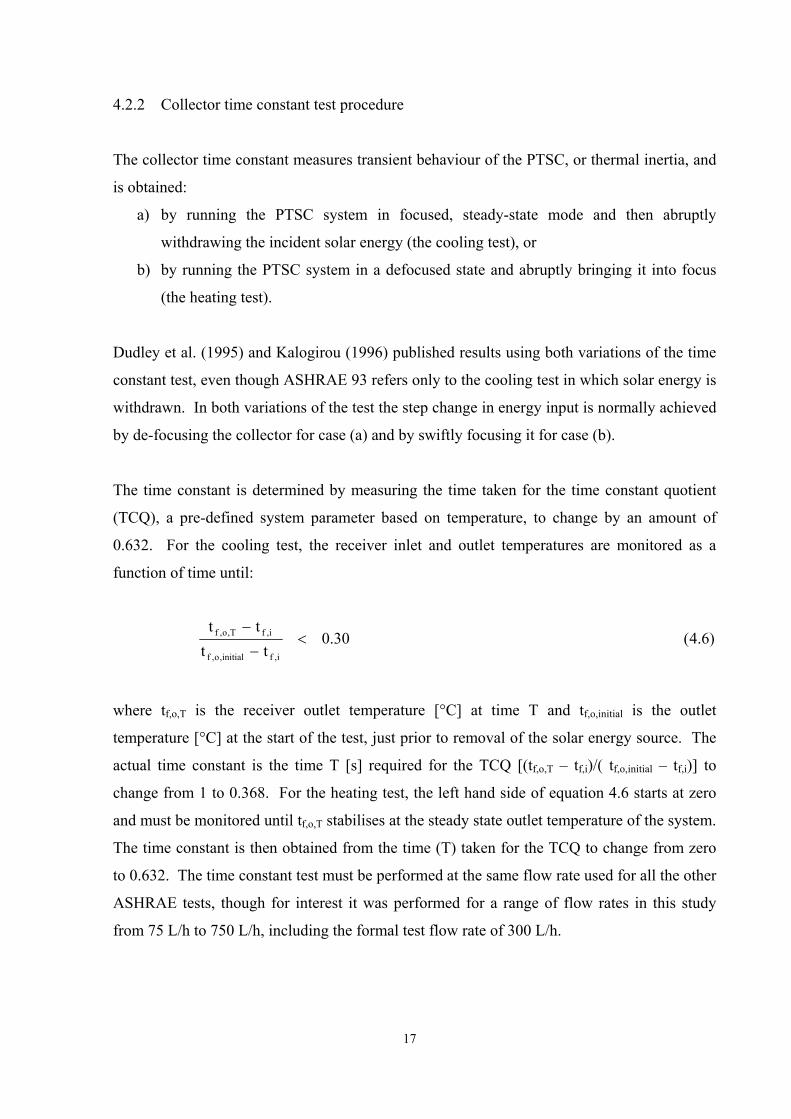
4.1 Solar map for Mangosuthu Technikon Solar Energy Test Facility with
morning and afternoon threshold irradiance times ......................................................21
4.2 Solar map indicating completed ASHRAE 93 tests ....................................................24
4.3 Front panel GUI of LabVIEW application SolarStation .............................................25
4.4 Schematic diagrams of (a) main block diagram and (b) structural hierarchy
of LabVIEW application SolarStation.........................................................................26
4.5 Front panel GUI of LabVIEW application SCATTAlog ............................................28
5.1 PTSC performance for fixed rate tracking (mode 2) based on VSD on-time .............31
5.2 PTSC performance for combination of fixed rate tracking (mode 2) and
manual adjustment.......................................................................................................32
5.3 PTSC performance for fixed pulse tracking (mode 2) ................................................33
5.4 PTSC performance for PSA Algorithm-based tracking (mode 3)...............................34
5.5 Time constant quotient for unshielded receiver (cooling test) ....................................35
5.6 Time constant quotient for unshielded receiver (heating test) ....................................36
5.7 Time constant for unshielded receiver (cooling and heating tests) .............................36
5.8 Time constant quotient for glass-shielded receiver (cooling test) ...............................37
5.9 Time constant quotient for glass-shielded receiver (heating test) ...............................38
5.10 Time constant for glass-shielded receiver (cooling and heating tests) ........................38
5.11 Comparison of time constants for glass-shielded and unshielded receivers ...............39
5.12 Collector acceptance angle results for unshielded receiver.........................................41
5.13 Collector acceptance angle results for glass-shielded receiver ...................................42
5.14 Collector acceptance angle results for unshielded and glass-shielded receivers.........43
5.15 Thermal efficiency with unshielded receiver ..............................................................44
5.16 Thermal efficiency with glass-shielded receiver .........................................................45 xii
5.17 Comparison of thermal efficiencies.............................................................................46
5.18 Incidence angle modifier for unshielded receiver .......................................................49
5.19 Incidence angle modifier for glass-shielded receiver ..................................................49
5.20 Incidence angle modifier for unshielded and glass-shielded receivers .......................50
5.21 Temperature data from thermal loss test for unshielded receiver ...............................53
5.22 Thermal loss and wind data for unshielded receiver ...................................................54
5.23 Temperature data for glass-shielded receiver..............................................................55
5.24 Thermal loss and wind data for glass-shielded receiver..............................................55
5.25 Thermal loss for glass-shielded and unshielded receivers...........................................56
6.1 Heat transfer model for unshielded receiver (Lamprecht, 2000).................................60
6.2 Heat transfer model for glass-shielded receiver (Lamprecht, 2000) ...........................60
6.3 Segment control volume for absorber with liquid flow (Lamprecht, 2000)................60
6.4 Unshielded model results for a range of receiver inlet temperatures ..........................63
6.5 Free and forced convection models with experimental data (unshielded) ..................63
6.6 Output from forced convection model for varying wind speed (unshielded)..............64
6.7 Off-sun thermal loss from forced convection model (unshielded)..............................65
6.8 Fluid and glass temperatures for two wind speeds ......................................................66
6.9 Free and forced convection models with experimental data (glass-shielded) .............67
6.10 Output from forced convection model for varying wind speed (glass-shielded) ........68
6.11 Off-sun thermal loss from forced convection model (glass-shielded receiver)...........69
7.1 PTSC system on rooftop of test facility with prevailing wind directions ...................81
A.1 PTSC macro- and micro-level design stages proposed by Güven et al. (1986) .........A3
A.2 PTSC torque-tube collector structure with parabolic ribs ..........................................A4
A.3 Polypropylene parabolic rib........................................................................................A5
A.4 Parabolic rib attachment method ................................................................................A6
A.5 PTSC collector structure.............................................................................................A7
A.6 (a) stainless steel substrate prior to installation (b) assuming parabolic shape .........A9
A.7 Solar intercept angle due to sun width and image spread due to optical errors .......A10
A.8 Absorber diameter for γ = 0.95 using error analysis of Stine and Harrigan (1985) .A13
A.9 Intercept factor γ as a function of β* and d* for σ* = 0.0 ........................................A18
A.10 Intercept factor γ as a function of β* and d* for σ* = 0.1798
(error set B3 indicated) .............................................................................................A19
A.11 Intercept factor as a function of β* for fixed d* and six values of σ*......................A20
A.12 Intercept factor as a function of d* for fixed β* and six values of σ*......................A20 xiii

xiv
A.13 Intercept factor as a function of d* for fixed β* and σ* and six rim angles.............A21
A.14 Intercept factor as a function of receiver diameter D for fixed σ* and β*
and six values of (dr)y ...............................................................................................A22
A.15 (a) general dimensions of receiver (b) receiver drive end (c) non-drive end
with instrumentation sections (d) three-dimensional view of drive end
instrumentation section.............................................................................................A25
A.16 (a) detailed view of ring holder and positioning bolts (b) attachment of
receiver to the collector structure .............................................................................A26
A.17 (a) glass shield, absorber, vacuum vent and o-ring seal arrangement at drive end
(b) and (c) o-ring seal (d) vacuum seal arrangement at drive end of PTSC ............A27
A.18 (a) Samples of tube with Cu2S coating obtained after exposure to NH4S for
(left to right) 20 s, 40 s, 60 s, 120 s and 5 min (b) CuO surface coating
showing blue-black finish.........................................................................................A28
A.19 Schematic diagram of incidence angle θi at solar noon on solstices and
equinoxes for a PTSC located in Durban, South Africa, and aligned in the N-S
direction (adapted from Stine and Harrigan, 1985)..................................................A30
A.20 Development of tracking error as sun moves through PTSC focus .........................A32
A.21 Schematic diagram of the solar vector (θz and A) and tracking angle (ρ) for
an N-S aligned PTSC rotated through ρT degrees to the east ...................................A34

LIST OF SYMBOLS
Nomenclature
A Area, [m2] or solar azimuth angle, [rad]
C Geometric concentration ratio
cp Specific heat at constant pressure, [J/kgK]
D Absorber tube diameter, [m]
d Aperture width of parabola, [m] or day number of the month
(dr) y Receiver mislocation along the optical axis of the reflector, [cm]
d* Universal nonrandom error parameter due to receiver mislocation
ep Obliquity of the ecliptic, [rad]
FR Heat removal factor
f Focal length of parabola, [m] or friction factor
G Irradiance, [W/m2]
g Mean anomaly of the sun, [rad]
gmst Greenwich mean sidereal time, [h]
h Height of parabola, [m] or convective heat transfer coefficient, [W/m2K]
hour Hour of the day in Universal Time and decimal format, [h]
jd Julian Day, [days]
Kατ Incidence angle modifier
k Thermal conductivity, [W/mK]
L Mean longitude of the sun, [rad] or litres
l Ecliptic longitude of the sun, [rad]
lmst Local mean sidereal time, [h]
long Geographical longitude, [deg]
m Month of the year or mass flow rate, [kg/s]
n Number of standard deviations or difference between the current Julian Day
and Julian Day corresponding to 1 January 2000
Q Volumetric flow rate, [L/h] or heat flow [W]
QO Off-sun thermal loss per unit area of receiver, [W/m2]
Q+ On-sun thermal loss per unit area of receiver, [W/m2]
R2 Coefficient of determination
r Distance from reflector surface to focal point of parabola, [m]
ra Right ascension, [rad] xv

s Arc length, [m]
T Torque, [Nm] or time, decimal [h] or [s]
ta Ambient air temperature, [°C]
tf,i Fluid temperature at inlet to receiver, [°C]
tf,o Fluid temperature at outlet from receiver, [°C]
U Overall heat transfer coefficient, [W/m2K]
V Air velocity, [m/s]
v Fluid velocity, [m/s]
y Gregorian year
Greek symbols
α Absorptance
β Reflector misalignment and tracking error angle, [rad]
β* Universal nonrandom error parameter due to angular errors, [rad]
γ Intercept factor
δ Dispersion angle, [rad], declination angle, [rad] or beam deflection, [m]
ΔT Time difference or sampling interval, [s]
Δt Difference between receiver inlet temperature and ambient, [°C]
Δtave Difference between average receiver fluid temperature and ambient, [°C]
Δtr Difference between receiver outlet and inlet temperatures, [°C]
ε Thermal emittance
ηg Thermal efficiency
ηo Optical efficiency
θi Angle of incidence of central solar ray with collector aperture, [deg]
θz Solar zenith angle, [rad]
μ Dynamic viscosity, [kg/ms]
ρ Density, [kg/m3] or reflectance
ρT Collector tracking angle, [deg]
σ Random optical error, [rad]
σ* Universal random error parameter, [rad]
σcontour Rms transverse deviation of contour from design direction, [mrad]
σcontour Rms longitudinal deviation of contour from design direction, [mrad]
σdisplacement Equivalent rms angular spread from receiver misplacement, [mrad]
σdrive Standard deviation of tracker drive errors, [mrad] xvi

σoptical Rms angular spread caused by all optical errors, [mrad]
σrec Standard deviation of receiver location errors, [mrad]
σrefl Standard deviation of mirror specularity errors, [mrad]
σsensor Standard deviation of tracking sensor errors, [mrad]
σslope Standard deviation of mirror slope errors, [mrad]
σspecular Rms transverse deviation of contour from design direction, [mrad]
σspecular Rms longitudinal deviation of contour from design direction, [mrad]
σsun Standard deviation equivalent to sun’s width, [mrad]
σtot Weighted standard deviation of collector errors or total rms beam spread,
[mrad]
σtracking Rms tracking error, [mrad]
σ1D Standard deviation of one-dimensional collector errors, [mrad]
σ2D Standard deviation of two-dimensional collector errors, [mrad]
τ Transmittance
Φ Geographical latitude, [deg]
ψ Angle between parabolic axis and point on mirror surface, [deg]
ψrim Rim angle, [deg]
ω Hour angle, [rad]
Subscripts
a aperture or ambient
ave average
bp beam in plane
ce convective external
DN direct normal
e effective
f fluid
G glass
g gross
i inlet or internal
inst instantaneous
initial initial
L loss
MAX maximum xvii

n index value or normal
o outlet or optical
r receiver
T time
t total
U unshielded
z zenith
Dimensionless groups
Nu Nusselt number, hD/k
Pr Prandtl number, μcp/k
Re Reynolds number, ρVD/μ
Abbreviations
AC Alternating current
ASHRAE American Society of Heating, Refrigerating and Air-Conditioning Engineers
AWJ Abrasive water-jet
CAD Computer-aided design
CAM Computer-aided manufacturing
CD Compact disc
DOE Department of energy
DTCS Drive, tracking and control system
E East
EDEP Energy deposition
GUI Graphical user interface
HCE Heat collecting element
HT High temperature
IST Industrial Solar Technology
KJC Kramer Junction Company
LT Low temperature
MICA Multi-year interactive computer almanac
N North
NIP Normal incidence pyrheliometer
NREL National Renewable Energy Laboratory xviii

xix
NSTTF National Solar Thermal Test Facility
PLC Programmable logic controller
PSA Plataforma Solar de Almeria
PSP Precision spectral pyranometer
PTSC Parabolic trough solar collector
S South
Sandia Sandia National Laboratories
SEGS Solar Electric Generating System
SAST South African Standard Time
ST Solar time
TC Thermocouple
U.S. United States of America
USNO United States Naval Observatory
VSD Variable speed drive
W West

1
1. INTRODUCTION
Solar thermal systems play an important role in providing non-polluting energy for domestic
and industrial applications. Concentrating solar technologies, such as the parabolic dish,
compound parabolic collector and parabolic trough can operate at high temperatures and are
used to supply industrial process heat, off-grid electricity and bulk electrical power. In a
parabolic trough solar collector, or PTSC, the reflective profile focuses sunlight on a linear
heat collecting element (HCE) through which a heat transfer fluid is pumped. The fluid
captures solar energy in the form of heat that can then be used in a variety of applications.
Key components of a PTSC include the collector structure, the receiver or HCE, the drive
system and the fluid circulation system, which delivers thermal energy to its point of use.
The use of concentrating solar energy collectors dates back to the late 19th century. The
technology was originally used for pumping water although more unusual applications
included a steam-powered printing press exhibited at the 1902 Paris Exposition (Duffie and
Beckman, 1991). It was not until the mid-1970s that large-scale development of PTSCs
began in the United States under the Energy Research and Development Administration
(ERDA), later the Department of Energy (DOE) (U.S. Department of Energy, 2004). This
development was strongly influenced by geopolitical factors, such as the oil crisis, and
focused on the provision of industrial process heat rather than electrical power. Typical
applications of trough technology included laundry processing, oil refining and steam
production for sterilisation of medical instruments (Stine and Harrigan, 1985).
The first trough-based Solar Electric Generating Systems (SEGS I) power plant was
constructed in 1984 in the U.S. state of California. Eight further plants followed, the last
being completed in 1991. Together, SEGS I to IX represent a total of 354 MW of installed
electrical capacity and all the plants are still operational. A tenth plant was planned but
abandoned when the development company failed to secure financing for construction and
went bankrupt (U.S. Department of Energy, 2004). Cheap and stable oil supplies through the
1980s meant no new parabolic trough power plants have been constructed since.
In recent years, a new momentum in PTSC research has developed, fuelled by climate
concerns, dwindling oil reserves and political instability in some oil-producing countries. An

2
attractive feature of the technology is that PTSCs are already in use in great numbers and
research output is likely to find immediate application. Parabolic trough technology has made
the crucial leap from pure concept to working solution, offering a real alternative to fossil fuel
energy sources. This demonstrated capability gives credibility to trough research, which is
now focused on ways to advance PTSC technology and lower the costs of constructing and
operating trough-based power plants.
For researchers interested in contributing to the development of PTSCs it is important to be
able to test new collector components. To this end, the construction of a parabolic trough
collector is vital and a number of such PTSCs have been constructed for research institutions,
ranging in size from 1 m2 to 100 m2. Smaller-scale PTSCs can be used to test advances in
receiver design, reflective materials, control methods, structural design, thermal storage,
testing and tracking methods (Thomas, 1994; Bakos et al., 1999; Almanza et al., 1997). One
such PTSC of aperture area 7.5 m2 has been developed at Mangosuthu Technikon.
The aim of this study is to test the newly developed PTSC and characterise its performance.
This is to be done using a suitable solar collector test standard and the results compared with a
thermal model of the PTSC.
The results of this study will allow the performance of new parabolic trough components such
as heat collecting elements, surface materials and tracking systems to be measured when the
collector becomes a test-rig in an ongoing solar thermal research programme.

3
2. MOTIVATION
Faced with shrinking fossil fuel resources, growing global energy demands and increasing
CO2 levels in the Earth’s atmosphere (Sayigh, 1999), the “global village” urgently needs to
reassess how it generates and consumes power. Renewable energy technologies such as
geothermal, hydro-power, biomass conversion and wind energy all offer potential for
replacing conventional coal-, gas- and oil-fired power-plants, though not yet on the same scale
or for the same cost.
Solar thermal energy systems are among the most promising of the renewable technologies.
Three such concepts for bulk electricity production are the central receiver, the solar chimney
and parabolic trough solar collector. Table 2.1 presents a comparison of key parameters for
the three technologies. The parabolic trough data are based on actual commercial plant
performance.
Table 2.1 Comparison of performance and other key parameters for three solar thermal technologies
(* Schlaich, 1996; ** SolarPACES, 1999)
While each of the technologies shown in Table 2.1 has its advantages, only the parabolic
trough system has been commercialised. The central receiver concept has a potentially higher
Solar Chimney * Central Receiver ** Parabolic Trough **
Capacity (MW) < 200 30 - 200 30 - 80
Levelized energy cost (c/kWh) 50 - 105 70 - 100 85
Installed capacity (MW) - 10 354
Efficiency (%) 2 23 (peak), 14-19 (annual)
21 (peak), 14–18 (annual)
Next hurdle?First commercial
station. 1000m high stack.
Volumetric receiver. Molten salts. Heliostats.
Storage
Advanced collector. Direct Steam
Generation (DSG). Storage.

4
operating efficiency and the solar chimney has built-in thermal storage but neither concept has
a commercial track record. In contrast, the first SEGS plant has been operating successfully
for over 20 years.
Figure 2.1 Solar Electric Generating Systems (SEGS) collector field (www.kjcsolar.com, 2004)
With the performance of SEGS I to IX and the experience gained in operating and
maintaining them, research into the next generation of PTSC systems has commenced. The
two most prominent large-scale PTSC test facilities are Sandia National Laboratories (Sandia)
in the U.S. state of New Mexico and the Plataforma Solar de Almeria (PSA) in Spain.
The National Solar Thermal Test Facility (NSTTF) at Sandia was established in 1976 and is
operated by the U.S. DOE through its business unit SunLab. The NSTTF covers 45 hectares
of land and includes a central receiver test facility with a central tower and 222 heliostats, a
16 kW solar furnace, a rotating azimuth-tracking platform for parabolic trough research
(Dudley et al., 1995) and a Distributed Receiver Test Facility with two 75 kW parabolic
dishes. The technology that made it possible to commercialise parabolic troughs was
originally developed at Sandia’s NSTTF (SunLab, 2000).
5
At the commercial level, trough research in the U.S. is now focused on thermal storage and
the development of “next generation” collectors and components (Energy Efficiency and
Renewable Energy Network, 2003). Key areas identified in the Parabolic-Trough Technology
Roadmap, compiled by Price and Kearney (1999), include development of an advanced
collector structure, heat collecting element (HCE), mirrors and thermal storage. The
document acknowledges the need for international collaboration in research as well as the
possibility of U.S. industry losing its competitive edge in trough production in the face of
greater funding of research efforts in Europe.
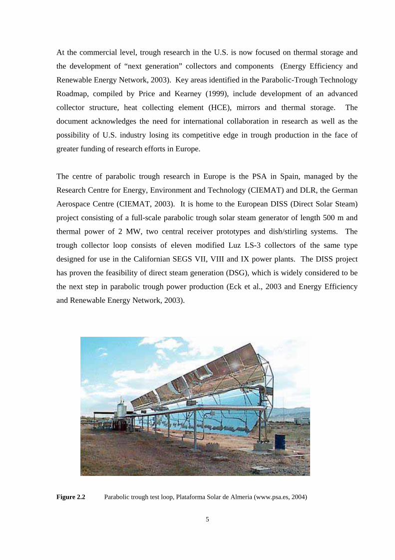
The centre of parabolic trough research in Europe is the PSA in Spain, managed by the
Research Centre for Energy, Environment and Technology (CIEMAT) and DLR, the German
Aerospace Centre (CIEMAT, 2003). It is home to the European DISS (Direct Solar Steam)
project consisting of a full-scale parabolic trough solar steam generator of length 500 m and
thermal power of 2 MW, two central receiver prototypes and dish/stirling systems. The
trough collector loop consists of eleven modified Luz LS-3 collectors of the same type
designed for use in the Californian SEGS VII, VIII and IX power plants. The DISS project
has proven the feasibility of direct steam generation (DSG), which is widely considered to be
the next step in parabolic trough power production (Eck et al., 2003 and Energy Efficiency
and Renewable Energy Network, 2003).
Figure 2.2 Parabolic trough test loop, Plataforma Solar de Almeria (www.psa.es, 2004)

6
Research into advanced collector structures (the so-called “torque-box” design) is also under
way at the PSA through the EuroTrough initiative. This is a collaborative venture aimed at
developing a high-performance European collector. Initial tests carried out at the PSA have
shown a performance improvement over existing designs of 3 %. A 50 MW power plant with
549 000 m2 of these collectors is planned for southern Spain – the first commercial plant to be
constructed since 1991 (Geyer et al., 2002).
With abundant levels of solar irradiance and an inevitable move away from fossil-fuel based
power stations, South Africa is well positioned to take advantage of solar thermal energy.
Power producer Eskom is considering the construction of a 100 MW power plant in the
Northern Cape, based on the central receiver concept. They anticipate a high degree of local
content in the plant’s manufacture (up to 90 %). A fully imported plant would have a capital
cost of approximately R 24 000 per kilowatt compared with R 10 000 per kilowatt for a coal-
fired power station, leading to an estimated electricity cost of 60 c/kWh. Notwithstanding the
higher cost, Eskom is giving serious consideration to the project (Engineering News Online,
2003).
The age of the “fossil-fuel economy” is coming to an end and the development of new sources
of power is becoming a priority. Against a backdrop of renewed global interest in solar
thermal power generation, this study is motivated by the desire to further develop South
Africa’s research capacity in alternative energy systems, with particular emphasis on
parabolic trough solar collectors.

7
3. DESCRIPTION OF TEST APPARATUS
Parabolic Trough Collector Structure
The equipment tested in this study consisted of a locally developed parabolic trough solar
collector. The PTSC has a torque-tube structure with a length of 5 m, aperture width of 1.5 m
and a rim angle of 82° (see figure 3.1). The reflective surface consists of stainless steel sheets
covered with SA-85 aluminised acrylic reflective film and clamped into the profile formed by
parabolic ribs. Aspects of the design and construction of the collector are given in Appendix
A.
Figure 3.1 Parabolic trough collector module
3.2 Heat Collecting Elements
Two HCEs, or receivers, were tested - one an unshielded copper tube and the other a similar
tube enclosed in an evacuated glass shield. Both absorber tubes are coated with a commercial
selective coating (Solkote) to reduce thermal emittance and increase absorptance. Table 3.1
summarises the key parameters of the PTSC for both receivers. The optical efficiencies (ηo)
were obtained from an error analysis conducted to determine the intercept factor (γ), details of
which are given in Appendix A, together with diagrams of the receivers.
5 m 1.5 m

8
Table 3. 1 PTSC key parameters and material properties
Feature / Parameter Value
Collector dimensions 5.0 m x 1.5 m
Rim angle, ψrim 82.2°
Absorber diameter, D 28.6 mm
Concentration ratio, C 16.7
Intercept factor, γ 0.823
Surface reflectance, ρ 0.83
Receiver absorptance, α 0.88
Receiver emittance, ε 0.49
Glass-shield transmittance, τ 0.92
ηo (unshielded receiver) 0.601
ηo (glass-shielded receiver) 0.553
3.3 Fluid Circulation System
The fluid driver is a 960 rev/min Howden GF positive displacement (helical element) pump
with flange-mounted 0.75 kW motor and a high-temperature Viton stator. Maximum output
ranges from 700 L/hr at 100 kPa to 400 L/hr at 500 kPa. Pump speed is controlled by a
Siemens 6SE6440 variable speed drive (VSD) to provide variable flow rate via a manual dial
in the control room of the solar energy test facility (Brooks, 2005). High-temperature (HT)
and low-temperature (LT) tanks enable water to be supplied for testing purposes up to a
maximum of 85 °C. A Tecfluid SC-250 variable area flow meter (100 L/hr to 1000 L/hr)
provides flow data. Ten type-K thermocouple (TC) probes enable temperatures to be
recorded during testing of the PTSC.
A test flow rate of 300 L/h was used to ensure turbulent conditions in the receiver throughout
the expected temperature range. Fluid density fluctuations were accommodated during data
processing using the water temperature to calculate mass flow rate for each datum point.
During testing, flow meter readings were checked by physical measurement. Small variations
in mass flow rate were allowed between low and high temperature tests, but properly
accounted for in the processing of test data. Figure 3.2 shows the layout of the fluid
circulation system.

9
Primary distribution manifold
Secondary distribution manifold
HT tank
Return manifold
LT tank
Pump
Receiver inlet
Receiver outlet
Return line
Flexible hose
PTSC receiver
Direction of flow
Main supply
Flexible hose
Figure 3.2 Schematic layout of fluid circulation system with PTSC structure removed and (inset) three-
dimensional sketch
3.4 Drive, Tracking and Control System (DTCS)
The PTSC is aligned along a true-north line and employs single-axis tracking. The tracking
hardware consists of a Siemens 0.25 kW, 685 rev/min, 8-pole AC motor with
electromechanical brake and a 463:1 high-reduction helical gearbox. A Siemens VSD enables
the system to operate at trough rotational speeds of between 1.5 rev/min and zero rev/min.

10
The control hardware consists of a 2500-pulse rotary encoder mounted on the shaft of the
PTSC to provide angular feedback information, and a Siemens S7 programmable logic
controller (PLC). Tracking of the collector is exercised via PLC-control of the VSD. Three
tracking modes were available during this study: manual jogging of the collector, fixed-rate
angular corrections based on the sun’s apparent motion (0.25 °/min) and virtual tracking using
solar angle information from the implementation of the PSA Algorithm (Blanco-Muriel et al.,
2001). Appendix A includes further information on the DTCS, while a sample calculation
using the PSA Algorithm is given in appendix C. The tracking system is described in detail
by Naidoo (2005). A photograph of the parabolic trough in operation is shown in figure 3.3.
Figure 3.3 PTSC with glass-shielded receiver during operation and vacuum pump visible in foreground
11
4. TEST METHODOLOGY
4.1 Introduction
To ensure the quality of results and to allow for comparison of performance with other
collectors, the PTSC was tested according to a recognised solar collector standard. This
chapter describes the chosen standard, the planned and completed test schedules and the
software applications developed to log test data.
The formalisation of collector test procedures is a recent development. Duffie and Beckmann
(1991) note that this became necessary in the mid-1970s when many new designs appeared on
the commercial market. Standard tests were required to provide operating data, especially
with respect to energy absorption, heat loss, effects of incidence angle and heat capacity. In
the U.S. the National Bureau of Standards devised a test procedure that was modified by the
American Society of Heating, Refrigerating and Air-conditioning Engineers (ASHRAE).
This eventually became the ASHRAE Standard 93-1986, which is used in this study and
described in 4.2.
Of those making use of ASHRAE 93, Kalogirou (1996) has published full results of a
parabolic trough collector test using the standard. Although Dudley et al. (1995) do not refer
to the standard in their description of the Industrial Solar Technology (IST) parabolic trough
tests at Sandia, they follow the same principles as ASHRAE 93 in their procedures. A
significant difference is their definition of collector efficiency using a second order
polynomial in Δt (fluid inlet temperature above ambient or (tf,i – ta)), and not a linear function.
The extensive international use of ASHRAE 93 for commercial purposes, its accessibility and
the comprehensive manner in which it describes the various test procedures, supported its use
in this study.
4.2 The ASHRAE 93-1986 (RA 91) Testing Standard
ASHRAE Standard 93-1986 (RA 91), first published in 1977 and updated in 1991, applies to
those concentrating and nonconcentrating collectors in which a fluid enters through a single

12
inlet and leaves through a single outlet. A separate standard (ASHRAE 96-1990) is used for
collectors in which the heat transfer fluid changes phase, such as DSG trough systems
(ASHRAE, 1991).
The four tests included under the ASHRAE 93 standard are:
• Thermal efficiency, ηg
• Collector time constant
• Incidence angle modifier, Kτα(θi)
• Collector acceptance angle
The standard defines the allowed variation in system operating parameters to ensure steady
state conditions during testing. These prescribed limits may be categorised as either fluid-
related, climatological or radiometric and are listed below.
Fluid constraints
• The working fluid temperature and flow rate of the collector at receiver inlet
should remain constant to within ± 1 °C and 0.000315 L/s respectively for 15 min
prior to the start of data logging (that is, the system should be properly stabilised)
• The receiver inlet temperature of the fluid should be controlled to within ± 0.05 °C
of the desired test value throughout the test period
• For the collector acceptance angle test (only), the receiver inlet temperature should
preferably be controlled to within ± 1 °C of the ambient air temperature
Climatological constraints
• The maximum ambient air temperature during testing should not exceed 30 °C
• Ambient temperature should not vary by more than ± 1.5 °C during a 15-minute
interval prior to the start of data logging
• For thermal efficiency and incident angle modifier tests, the average wind velocity
should be between 2.2 m/s and 4.5 m/s (4.3 knots and 8.7 knots) during the test
period and for 10 min prior to the start of data logging

13
Radiometric constraints
• Average normal beam irradiance should exceed 790 W/m2 and should not vary by
more than ± 32 W/m2 during the data logging period and for 10 min prior to it
• During testing the collector should be maintained within 2.5° of the angle of
incidence for which the test is conducted
• During collector acceptance angle tests, normal beam irradiance should exceed
800 W/m2 and remain as constant as possible
In addition to the above, the collector reflective surface should be checked prior to testing for
pollution or dust deposits and cleaned.
4.2.1 Thermal efficiency test procedure
Thermal efficiency (ηg) is obtained by measuring Δtr, the temperature increase of the working
fluid through the receiver (Δtr = (tf,o – tf,i)). Together with the fluid properties and mass flow
rate, this gives the rate of thermal energy input. Dividing this by the solar radiation falling on
the collector gives a measure of the collector’s efficiency. By repeating the test for increasing
Δt, a linear model of the collector efficiency can be obtained. From ASHRAE 93, the
efficiency equation has the form
In equation 4.1, Ar, Ag and Aa are the receiver area, the collector gross area (“footprint” of the
whole collector including support structure) and the collector aperture area respectively, UL is
an overall heat loss coefficient, FR is a heat removal factor and Gbp represents the component
of the normal beam irradiance in the plane of the collector aperture. Equation 4.2 may be
used to determine Gbp from calculated angles of incidence (θi) and values of GDN obtained by
measurement, using a pyrheliometer.
)AAfor(FG
tA
FUA
)1.4(FAA
Gt
AFUA
gaoRbpa
RLr
oRg
a
bpg
RLrg
=η+⎟⎟⎠
⎞⎜⎜⎝
⎛ Δ⎟⎟⎠
⎞⎜⎜⎝
⎛−=
η⎟⎟⎠
⎞⎜⎜⎝
⎛+⎟
⎟⎠
⎞⎜⎜⎝
⎛ Δ⎟⎟⎠
⎞⎜⎜⎝
⎛−=η
)2.4(]m/W[cosGG 2iDNbp θ=

14
In this study, the collector gross area was taken to equal the aperture area, since the module
under test was a research prototype, not a commercial unit, and the “footprint” area occupied
by the support frame was almost the same as the aperture area. The minor difference caused
by the frame’s two end bearing-supports was negligible.
The straight line represented by equation 4.1 has a gradient of –(ArULFR/Aa) [W/m2K] and y-
intercept of (FRηo). The optical efficiency can be obtained from equation A.1, enabling the
calculation of the heat removal factor, FR. Alternatively, with accurate knowledge of the
conditions under which heat transfer takes place from the receiver to the surrounding
atmosphere, a value for UL can be calculated from heat transfer theory and FR can be obtained
from the gradient of equation 4.1
ASHRAE 93 requires that all thermal efficiency tests be conducted at normal or near-normal
angles of incidence, which contributes to the difficulty of running such tests using a single-
axis tracking system, since θi cannot be held constant over the course of a day or even
throughout a season. In this project it was planned to schedule efficiency tests for the time of
year when incidence angle was at its minimum so as to restrict θi to a maximum value of 10°
(see 4.3). For the glass-shielded receiver, which was installed after the unshielded unit, it was
not possible to complete all efficiency tests before θi had risen to 15°. This was unavoidable
because of poor weather over the summer rainfall season.
In practice, the efficiency of the PTSC is determined by dividing the energy absorbed by the
working fluid as it passes through the receiver, by the solar energy falling on the collector
aperture. This can be expressed as follows:
Equation 4.3 is used to process the experimental data gathered during tests. The linear model
of ηg given by equation 4.1 is imposed on the graph obtained from the experimental data after
processing.
( )
bpa
rp
bpa
i,fo,fpg
GAtcm
)3.4(GA
ttcm
Δ=
−=η

15
Equation 4.1 requires that the difference between the working fluid inlet temperature and the
ambient air temperature (Δt) be varied to determine PTSC performance. Inlet temperatures
should span the normal operating range of the collector. In this project, the receiver inlet
temperature was limited by the fluid circulation system, which could supply water at a
maximum temperature of approximately 85 °C, thus the inlet range was from 20 °C to 85 °C.
During efficiency tests, the standard requires that at least four data points be obtained for each
value of Δt, with two each obtained symmetrically before and after solar noon. This is to
ensure that transient effects do not bias the results. The efficiency curve described by
equation 4.1 must be established using at least 16 points, or four sets of four data points. To
compute the thermal efficiency for each data point, ASHRAE 93 gives the following
equation:
where T1 and T2 represent the start and finish times for the test period and G is the beam
irradiance in the plane of the collector aperture. In the original form of the equation Ag
replaces Aa, although here the aperture area is used for the reasons described above. In
practice, each integral in equation 4.4 is converted to a summation of discrete values since
data samples of temperatures and irradiance are logged at fixed time intervals. The time
interval chosen for this study was 6 s, giving 10 readings per minute. The integrals were thus
determined using numerical integration with an element “width” of 6 s.
According to the test standard, the duration of each thermal efficiency trial must equal one
collector time constant, or five minutes, whichever is larger. For example, where the trial
lasts five minutes (300 s) consisting of 50 intervals of 6 s each, equation 4.4 becomes:
)4.4(dTGA
dT)tt(cm
2
1
2
1
T
Ta
T
Ti,fo,fp
g
∫
∫ −
=η

16
In this study, the receiver inlet and outlet temperatures in equation 4.5 were measured using
the TC probes described in appendix A.3.2 and shown in figure A.15. The mass flow rate was
determined by multiplying the volumetric flow rate of the working fluid (300 L/h) by its
density. Both density and specific heat were calculated for each time step using the average
measured receiver temperature. The aperture area was constant at 7.5 m2. Although the value
of the time step disappears from equation 4.5, it is not irrelevant in the calculation. By setting
the time step too large, stabilising the system becomes difficult and compromises the accuracy
of the results. Too small a time step does not meaningfully improve the quality of the
efficiency results beyond a certain point and complicates data processing by generating too
much unnecessary information.
Dudley et al. (1995) used a time step of 20 s for the IST tests conducted at Sandia. The fluid
residence time in the receiver was approximately 15 s giving a rate of 0.75 samples per
receiver pass. In this study, the fluid residence time was 33 s giving a rate of 5.5 samples per
receiver pass. This higher rate was considered necessary to accurately monitor the tracking
performance of the PTSC and to ensure steady state operation. All sub-calculations in
equation 4.5 were done in real-time during testing by the data acquisition software written for
this project and checked for accuracy during processing of the data in Microsoft Excel. A
sample calculation of efficiency is given in appendix E.
)5.4(GA
)t()c(m
)s6T(]GGG([A6
])t()c(m)t()c(m)t()c(m[6]TGTGTG([A
T)t()c(mT)t()c(mT)t()c(m
TGA
T)tt()c(m
50
1nna
50
1nnrnpn
n5021a
50r50p502r2p21r1p1
50502211a
5050r50p5022r2p211r1p1
50
1nnna
50
1nnni,fo,fnpn
g
∑
∑
∑
∑
=
=
=
=
Δ=
=Δ+++/
Δ++Δ+Δ/=
Δ++Δ+Δ
ΔΔ++ΔΔ+ΔΔ=
Δ
Δ−=η
K
K
K
K
17
4.2.2 Collector time constant test procedure
The collector time constant measures transient behaviour of the PTSC, or thermal inertia, and
is obtained:
a) by running the PTSC system in focused, steady-state mode and then abruptly
withdrawing the incident solar energy (the cooling test), or
b) by running the PTSC system in a defocused state and abruptly bringing it into focus
(the heating test).
Dudley et al. (1995) and Kalogirou (1996) published results using both variations of the time
constant test, even though ASHRAE 93 refers only to the cooling test in which solar energy is
withdrawn. In both variations of the test the step change in energy input is normally achieved
by de-focusing the collector for case (a) and by swiftly focusing it for case (b).
The time constant is determined by measuring the time taken for the time constant quotient
(TCQ), a pre-defined system parameter based on temperature, to change by an amount of
0.632. For the cooling test, the receiver inlet and outlet temperatures are monitored as a
function of time until:
where tf,o,T is the receiver outlet temperature [°C] at time T and tf,o,initial is the outlet
temperature [°C] at the start of the test, just prior to removal of the solar energy source. The
actual time constant is the time T [s] required for the TCQ [(tf,o,T – tf,i)/( tf,o,initial – tf,i)] to
change from 1 to 0.368. For the heating test, the left hand side of equation 4.6 starts at zero
and must be monitored until tf,o,T stabilises at the steady state outlet temperature of the system.
The time constant is then obtained from the time (T) taken for the TCQ to change from zero
to 0.632. The time constant test must be performed at the same flow rate used for all the other
ASHRAE tests, though for interest it was performed for a range of flow rates in this study
from 75 L/h to 750 L/h, including the formal test flow rate of 300 L/h.
)6.4(30.0tt
tt
i,finitial,o,f
i,fT,o,f <−
−

18
4.2.3 Incidence angle modifier test procedure
The incidence angle modifier, Kατ, enables the performance of the collector to be predicted for
solar angles of incidence other than 0°. This is important in commercial systems that operate
throughout the year and experience a reduction in performance during winter when the sun is
lower in the sky.
Incidence angle modifier tests are run essentially the same way as normal thermal efficiency
tests, with PTSC performance measured for a receiver inlet temperature near the ambient air
temperature. Data are processed as before using equation 4.5, however each test is conducted
at a set value of θi and Kατ is then calculated using equation 4.7.
ASHRAE 93 recommends that the value of θi be increased from zero to a maximum of 60°
for the incidence angle modifier tests and that a total of four data points be generated with one
each at 0°, 30°, 45° and 60°. A curve-fitting exercise can be applied to the resulting graph to
yield an equation for Kατ in terms of θi. Kalogirou (1996) presents Kατ as a polynomial in (θi)3
while Dudley et al. (1995) use a mixed equation in (cos(θi)) and (θi)2.
The denominator in equation 4.7 is a constant and is equal to the y-intercept of the thermal
efficiency curve obtained from equation 4.1 for the PTSC at normal or near-normal angles of
incidence. The incidence angle modifier is thus a dimensionless measure of the performance
of a solar collector at a set value of θi compared with its optimum performance at normal or
near-normal incidence. The determination of Kατ takes place after thermal efficiency tests
have been completed.
( ) ( )[ ]
( )[ ]
oR
g
ganeR
g
neRga
g
F
)AAfor(F
)7.4(FA/A
K
η
η=
=ργατ
η=
ργατ
η=ατ
19
Because of the need to fix θi during testing, determining Kατ normally requires that the
collector be capable of two-axis tracking. In two-axis tracking systems the PTSC is mounted
on a movable test rack (altazimuth collector mount) so that its horizontal axis can be rotated
for azimuth control and the collector can track the sun about two axes, thereby maintaining
any desired θi accurately and continuously. Alternatively the tilt of the collector should be
adjustable. Being able to set and maintain a desired value of θi enables the PTSC operator to
complete the ASHRAE incidence angle modifier tests within one or two days.
Owing to the size of the PTSC, costs, the scope of the project and weight restrictions on the
roof of the test facility, a two-axis tracking capability could not be provided in this study.
Instead, the PTSC test programme was extended and the natural seasonal change in θi was
used to generate a curve of Kατ. The disadvantage was having to wait for the seasonal change
in θi to take effect. Careful scheduling was required to avoid excessive handling of the fragile
glass-shielded receiver. Instead of repeatedly swapping receivers, tests with the glass-
shielded HCE were completed first and the unshielded unit was then reinstalled to complete
all outstanding tests by the end of July 2004. This prolonged testing but reduced the risk of
destroying the glass shield midway through the test programme.
4.2.4 Collector acceptance angle test procedure
The collector acceptance angle defines the sensitivity of the collector to tracking
misalignment. The collector is positioned ahead of the sun and its performance continuously
measured as the sun moves into and out of focus. By monitoring thermal efficiency as a
function of tracking angle (ρT), the maximum allowable focal misalignment of the collector
can be obtained. This is useful for determining the accuracy required of the tracking system.
To start the test, the PTSC is rotated to a position between 7.5° and 10° west of the sun and
the tracking system is disengaged. Fluid flow rate is set at the normal test value, receiver inlet
temperature is maintained as close as possible to ambient temperature and the thermal
efficiency is recorded normally, though the standard suggests measurements be taken once per
minute during the time when the sun is within 5 min of the plane of focus of the collector. In
this study, measurements were taken at 6-second intervals and each efficiency point was
based on 10 such intervals, giving a continuous series of 1-minute rolling average efficiency

20
values. This was to damp out minor spikes in the instantaneous efficiency values, caused by
small variations in temperature and irradiance point-measurements.
After the sun has traversed through the PTSC’s focal position, thermal efficiency values are
divided by the peak efficiency recorded at zero angle of incidence, as measured in a plane
perpendicular to the receiver (the plane in which tracking angle is measured). This yields a
form of incidence angle modifier or efficiency factor between zero and 1, which is a function
of ρT, not θi. ASHRAE 93 defines the collector acceptance angle as the range of incident
angles in which the modifier varies by no more than ± 2 % from the normal incident value.
4.3 PTSC Test Schedule
4.3.1 Planned schedule
The test programme was scheduled to run from the end of December 2003 to the end of
February 2004, with only the incidence angle modifier tests continuing beyond February to
June. Without the capacity to set and maintain a zero angle of incidence, the timetable for
thermal efficiency tests had to be planned to accommodate daily and seasonal changes in
incidence angle. The main objective was to schedule all tests in an appropriate order to fulfill
the ASHRAE 93 requirements regarding minimum threshold beam irradiance (790 W/m2) and
incidence angle. It was also necessary to meet the requirements regarding wind and ambient
temperature. From the monitoring exercise done at the solar energy test facility since
February 2003, some idea of the expected rainfall, temperature and wind patterns had been
obtained (Brooks, 2005). Nevertheless general weather conditions were less predictable than
threshold irradiance levels and disruptions to testing caused by cloudy and windy conditions
were plentiful and had to be tolerated.
To assist with scheduling, the PSA Algorithm was used to generate a graph of the daily
change in θi for a range of dates from 22 December 2003 to the winter solstice on 21 June
2004 (the expected PTSC test period). This was transformed into a 6-month solar map of the
test facility using a solar irradiance profile developed by Brooks (2005) to describe the
morning time at which normal beam irradiance first exceeds 790 W/m2. This map, shown in
figure 4.1, gave each day’s expected “test window” during which the angle of incidence was
21
determined and the normal beam irradiance conformed to the ASHRAE minimum threshold
value.
Figure 4.1 Solar map for Mangosuthu Technikon Solar Energy Test Facility with morning and afternoon
threshold irradiance times
To finish the test programme by the end of July, the final test point for the incidence angle
modifier for the unshielded receiver had to be obtained at an incidence angle of 37°
(according to figure 4.1), not the recommended 30°. This was not problematic since the
resulting curve for Kατ (a fitted regression polynomial) would be negligibly affected by
-25.00
-20.00
-15.00
-10.00
-5.00
0.00
5.00
10.00
15.00
20.00
25.00
30.00
35.00
40.00
45.00
50.00
55.00
60.00
06:00 07:00 08:00 09:00 10:00 11:00 12:00 13:00 14:00 15:00 16:00 17:00 18:00
Solar Time
Ang
le o
f Inc
iden
ce θ
i (d
eg)
21 Jun
21 Jan6 Jan
21 Feb
6 Feb
20 May
6 May
20 Apr
6 Apr
20 Mar
6 Mar
6 Jun
22 Dec
790 W/m2 Afternoon Threshold
Sunrise Sunset
790 W/m2 Morning Threshold

22
shifting one data point by 7°. The planned test schedule for both receivers is shown in table
4.1.
Table 4.1 Planned PTSC test schedule
Date Unshielded receiver Glass-shielded receiver
Thermal efficiency Time const. Accept.
angle Inc. angle
mod. Thermal efficiency Time const. Accept.
angle Inc. angle
mod. 22 Dec 2003
to 15 Jan 2004
X X X θi ≈ 0°
16 Jan 2004 Change from unshielded receiver to glass-shielded receiver. 17 Jan 2004
to 31 Jan 2004
X X X θi ≈ 0°
20 Mar 2004 θi ≈ 30°
6 May 2004 θi ≈ 45°
6 June 2004 θi ≈ 50°
7 June 2004 Change from glass-shielded receiver to unshielded receiver.
8 June 2004 θi ≈ 50° and 45°)
31 July 2004 θi ≈ 38°
4.3.2 Completed test schedule
Deviations from the schedule shown in table 4.1 were caused by periods of poor weather
during January and February 2004. This led to numerous delays in completing the thermal
efficiency tests for the unshielded receiver. It was particularly difficult to obtain results
symmetrically before and after noon because of deteriorating afternoon weather conditions
typical of the summer weather pattern in Kwazulu-Natal. Although a full set of 20 tests was
completed for the shielded receiver, the morning/afternoon requirement was dropped for the
shielded receiver so that the test programme could be completed before θi became too large.
As a result, only 10 tests were conducted for the unshielded HCE, though these spanned the
full receiver inlet temperature range. In addition, weather delays meant some of the tests for
the shielded HCE had to be conducted at θi values as high as 15°. On average, the angle of
incidence for the unshielded receiver efficiency tests was 7.09° while for the glass-shielded

23
efficiency tests it rose to 11.42° (see chapter 5). Table 4.2 gives the actual completed test
schedule, while figure 4.2 shows all eight series of ASHRAE 93 tests, as they occurred,
superimposed on the solar map from figure 4.1.
Table 4.2 Schedule of completed PTSC tests
Date Unshielded receiver Glass-shielded receiver
Thermal efficiency Time const. Accept.
angle Inc. angle
mod. Thermal efficiency Time const. Accept.
angle Inc. angle
mod.
Marker symbol for figure 5.2
x
+
22 Dec 2003 to
2 Feb 2004 X X X θi ≈ 0°
10 Feb 2004 Change from unshielded receiver to glass-shielded receiver.
11 Feb 2004 to
19 Feb 2004 X X X θi ≈ 0°
28 Mar to 21 Apr 2004 θi ≈ 30°
19 Apr to 1 May 2004 θi ≈ 45°
22 May to 9 Jun 2004 θi ≈ 50°
11 Jun 2004 Change from glass-shielded receiver to unshielded receiver.
11 Jun to 12 Jul 2004 θi ≈ 50°
and 45°
29 July 2004 θi ≈ 37°

24
-25.00
-20.00
-15.00
-10.00
-5.00
0.00
5.00
10.00
15.00
20.00
25.00
30.00
35.00
40.00
45.00
50.00
55.00
60.00
06:00 07:00 08:00 09:00 10:00 11:00 12:00 13:00 14:00 15:00 16:00 17:00 18:00
Solar Time
Ang
le o
f Inc
iden
ce θ
i (d
eg)
21 Jun
21 Jan
6 Jan
21 Feb
6 Feb
20 May
6 May
20 Apr
6 Apr
20 Mar
6 Mar
6 Jun
22 Dec
790 W/m2 Afternoon Threshold
Sunrise Sunset
790 W/m2 Morning Threshold
Figure 4.2 Solar map indicating completed ASHRAE 93 tests
Set up tests were also conducted to ensure the PTSC system functioned as expected. These
included:
• Tests of fluid system flow rates versus pressure to verify pump performance
• Tank heating and cooling tests to determine the time taken to raise water in the HT
tank to its maximum temperature, as well as the rate at which heat was lost (this
was to help plan the high-temperature tests)
• Thermal loss tests to determine the heat transfer characteristics of the glass-
shielded and unshielded receivers
• DTCS tests to determine tracking performance

25
4.4 Development of Data Logging Software Applications
Three software applications were developed for data monitoring and acquisition. These were
created using National Instruments LabVIEW 7.0 Express and made it possible to:
• Plan daily PTSC tests by verifying the sun’s position and monitoring the change in
crucial solar angles (in real-time) using SolarStation,
• Operate the PTSC system, monitor its behaviour and stabilise it properly before
starting a formal test (using SCATTAscan), and
• Acquire and log PTSC test data during formal ASHRAE 93 tests using SCATTAlog.
4.4.1 SolarStation
SolarStation provided the PTSC operator located in the test facility control room with a real-
time stream of values for the solar azimuth angle A, the zenith angle θz and the PTSC angle of
incidence θi. This allowed quick decisions to be made as to whether PTSC tests should be run
or not. The application provided date and time information (both SAST and solar time), the
sun’s declination angle and the PTSC’s required tracking angle ρT (the tracking angle was for
information only – the data acquisition PC was not connected to the trough’s DTCS). The
application was intended to float on top of other Microsoft Windows applications running on
the control room PCs and the graphical user interface (GUI), or front panel, was sized to make
it unobtrusive. A screen-captured image of the front panel is shown in figure 4.3.
Figure 4.3 Front panel GUI of LabVIEW application SolarStation
At the core of SolarStation is a sub-VI (virtual instrument) implementing the PSA Algorithm.
This accesses the PC clock-time at 1-second intervals to generate updates of the variables.

26
During execution, the PSA sub-VI calls a further seven sub-VIs, each implementing stages of
the algorithm. Figure 4.4 (a) shows the main block diagram of SolarStation. The PSA sub-VI
is visible at the top left of the block with its output consisting of time and date information
(top centre) and a cluster containing the internal variables from the PSA Algorithm (for
example mean longitude, mean anomaly and ecliptic longitude). The variable cluster is wired
to display only those variables from the PSA Algorithm that appear on the front panel shown
in figure 4.3. Figure 4.4 (b) shows the sub-VI building blocks in the structural hierarchy of
the application.
(a) (b)
Figure 4.4 Schematic diagrams of (a) main block diagram and (b) structural hierarchy of LabVIEW
application SolarStation
Each of the sub-VIs shown below the PSA sub-VI in figure 4.4 (b) consists of a block
diagram similar to that in figure 4.4 (a). These are not shown, although the SolarStation
application is included on the computer disc submitted with this study.

27
4.4.2 SCATTAscan and SCATTAlog
The LabVIEW scanning and logging applications used to monitor PTSC performance were
almost identical, except for additions in SCATTAlog to write the data to file. A description
of the logging application is given here.
The main purpose of SCATTAlog was to sample and log temperature and irradiance data
during PTSC testing. The programme’s functionality was extended to include processing of
data and to generate real-time thermal efficiency values. This was to help the operator
stabilise the system during testing. A range of information and trough performance variables
was provided for, including:
• PSA solar position data, updated once per second
• ASHRAE 93 thermal efficiency (as given by equation 4.4)
• Instantaneous thermal efficiency
• Collector time constant quotient (as given by equation 4.5)
• Temperature output from TC probes
• Irradiance values from the pyranometer and pyrheliometer
• Receiver fluid temperature, density, viscosity, specific heat and thermal conductivity
• Theoretical Reynolds, Prandtl and Nusselt numbers, fluid mass flow rate, friction
factor and convective heat transfer coefficient
In SCATTAlog the above information is presented numerically. Three sets of axes are also
positioned on the front panel to provide a real-time graphing function of the behaviour of the
ASHRAE 93 thermal efficiency (equation 4.5), the instantaneous thermal efficiency and the
collector time constant (equation 4.6). The programme requires the user to enter the fluid
volumetric flow rate and the sampling interval in seconds. The thermophysical properties of
the working fluid (water) are based on its average temperature through the receiver and
calculated from equations given by Kröger (1998).
On start-up the application requests a filename under which to save the logged data. This
allows data to be catalogued and facilitates processing. The programme opens a tab-delimited
file and writes data to it each time values are sampled at the user-defined interval (6 s for most

28
of the tests conducted). On completion of the test the files can be opened in Microsoft Excel
for data processing. Each batch of values written to file during the PTSC test is date- and
time-stamped with the local clock time and solar time. Figure 4.5 shows the front panel of
SCATTAlog. An extract from a logged data file is given in appendix D.
Figure 4.5 Front panel GUI of LabVIEW application SCATTAlog
The development of SCATTAlog was an ongoing project and was successful in facilitating
the logging and processing of test data. Two faults were discovered in the application during
Fluid flow and heat transfer parameters
Fluid temperature and thermophysical data
User settings for sampling interval, flow rate, ambient temperature and
system pressure
Efficiency and TCQ graphs
Solar position data from PSA algorithm
Schematic of PTSC system showing
temperature data from TC probes
Radiometric data

29
the course of the project – the first was a minor error in the calculation of the difference
between the receiver fluid inlet temperature and ambient temperature (Δt). This was manually
corrected during processing of the data in Microsoft Excel. The second fault occurred in a
later update of the software and was caused by an error in the processing sequence of certain
internal variables. In all cases the errors were manually corrected. The unprocessed
temperature and radiometric data were unaffected by the problem, as were the PSA solar
position data. The extract from a SCATTAlog data file shown in appendix D is from an early
version of the software and contains no errors. Copies of SCATTAlog and SCATTAscan are
included on the computer disc submitted as part of this study.
4.5 Summary
Conducting the PTSC test programme was difficult at times because of the weather conditions
that forced the postponement of numerous tests and caused several violations of ASHRAE 93
test conditions (see chapter 5). This was unavoidable and compromises had to be made to
finish testing. Despite delays, the programme proceeded well and generated a significant
amount of performance data. Approximately 120 individual tests were run from December
2003 to July 2004 representing 130 hours of testing time and generating 25 megabytes of
unprocessed information. This produced over 30 000 lines of processed spreadsheet data.
Coordinating and executing the test programme was helped by the following:
• Access to a well-equipped, dedicated and secure solar energy test facility
• Results from the radiometric and meteorological monitoring programmes conducted
during 2003
• The implementation of the ASHRAE 93 testing standard
• Comprehensive instrumenting of the PTSC system
• The development of flexible data acquisition software for conducting tests and logging
data

30
5. EXPERIMENTAL RESULTS
5.1 Introduction
Performance results are presented from the PTSC test programme described in chapter 4 and
cover both receivers. These were generated from two types of tests:
• Tracking tests to verify performance of the DTCS
• PTSC performance tests as described by the ASHRAE 93-1986 (RA 91) standard
(including receiver heat loss)
5.2 Tracking Performance
Results of the DTCS performance are discussed in detail by Naidoo (2005) and are restricted
here to a brief summary.
5.2.1 Fixed rate tracking
Early tests to measure PTSC efficiency under fixed rate tracking conditions, showed the
DTCS could not maintain focus without fine, manual adjustments being made. With the PLC
programmed to jog the VSD at 5.6 rev/min for exactly 4 s every 69.2 s (see appendix A), the
PTSC would lag behind the sun, as shown in figure 5.1, which gives tracking performance in
terms of an instantaneous efficiency factor:
ηinst,T is the instantaneous thermal efficiency of the collector at time T and ηinst,MAX is the
maximum measured instantaneous efficiency from the test. Equation 5.1 is helpful in
comparing tracking performance from different tests as it eliminates variations that arise from
tests being performed at different receiver inlet temperatures. Instantaneous efficiency is the
point efficiency of the collector, determined using equation 4.3, not equation 4.5. See
appendix E for a sample calculation. To obtain the results shown in figure 5.1, the collector
)1.5(factorEfficiencyMAX,inst
T,inst
ηη
=

31
was positioned slightly ahead of the sun and Mode 2 tracking was engaged using the above
VSD on-time settings.
Figure 5.1 PTSC performance for fixed rate tracking (Mode 2) based on VSD on-time
The increase and subsequent decrease in performance was due to the collector entering and
leaving focus, as the frequency and duration of jog pulses were incapable of keeping pace
with the sun. The lag was the result of a time delay in the VSD caused by the ramping up of
the speed from zero to the set value of 5.6 rev/min as well as shorter timing delays in the
switchgear. To improve tracking performance, the VSD on-time was manipulated until a
value was found that enabled the PTSC to maintain the sun in focus. To prevent the
maximum tracking error of 0.2° being exceeded, the time interval between jog periods was
reduced to 32 s and a VSD on-time of 2.4 s employed. Combined with fine, manual
adjustment of the collector based on a visual assessment of the receiver light pattern and close
monitoring of the receiver outlet temperature, it was possible to maintain the trough in focus.
This method of control was facilitated by the LabVIEW data acquisition system which
provided real-time temperature data and the positioning of the PTSC control panel, which
enabled the operator to observe the light focus pattern on the receiver, monitor the collector
0.0
0.1
0.2
0.3
0.4
0.5
0.6
0.7
0.8
0.9
1.0
1.1
1.2
0 5 10 15 20 25
Elapsed time (min)
Effic
ienc
y fa
ctor

32
performance on SCATTAscan and make fine adjustments to the fixed rate tracking system.
Figure 5.2 illustrates the improvement in tracking performance with this method.
Figure 5.2 PTSC performance for combination of fixed rate tracking (Mode 2) and manual adjustment
The method of counting VSD on-time was changed to counting individual pulses from the
rotary encoder instead. Tests showed that the PLC/VSD combination was able to start, turn
and stop the collector accurately through a single pulse, or 0.144°, as indicated on the PLC
(Naidoo, 2005). This enabled the fixed rate tracking method to be changed from counting
VSD on-time to counting 1 pulse on the encoder at a fixed time interval of 34.56 s, giving the
required angular velocity of 0.25 °/min.
Figure 5.3 shows the performance of the collector for fixed pulse tracking. The successful
operation of the tracking system is visible in the consistent performance of the collector, as
measured by the efficiency factor.
0.0
0.1
0.2
0.3
0.4
0.5
0.6
0.7
0.8
0.9
1.0
1.1
1.2
0 1 2 3 4 5 6 7 8 9 10
Elapsed time (min)
Effic
ienc
y fa
ctor

33
Figure 5.3 PTSC performance for fixed pulse tracking (Mode 2)
5.2.2 PSA Algorithm-based tracking
PSA Algorithm-based tracking (Mode 3) became operational by mid-February 2004, seven
weeks into the PTSC test programme. Under Mode 3 control, the DTCS was able to rotate
the trough to locate the position of the sun and keep it focused using continuous positioning
updates via the PLC, VSD and drive system. These updates were triggered when the
difference between the calculated angular position of the collector (output from the PSA
Algorithm) and the actual position (read from the rotary encoder) exceeded 1 pulse on the
encoder (0.144°). Thus Mode 3 tracking had a similar level of accuracy to Mode 2, but could
also locate the sun and accurately follow it independently of weather conditions (cloud) and
the PTSC operator.
Figure 5.4 shows Mode 3 tracking in operation, with the collector initially defocused and then
brought into focus by the DTCS. During commissioning it was necessary to introduce a
constant offset value of 1° to the PLC code to enable the collector to focus optimally. This
was most likely due to the presence of inaccuracies in the physical orientation of the collector
as well as receiver mislocation and reflector misalignment.
0
0.1
0.2
0.3
0.4
0.5
0.6
0.7
0.8
0.9
1
1.1
1.2
0 1 2 3 4 5 6 7 8 9 10
Elapsed time (min)
Effic
ienc
y fa
ctor

34
Figure 5.4 PTSC performance for PSA Algorithm-based tracking (Mode 3)
The system worked correctly once the offset factor had been introduced. The offset had to be
modified several months later once the unshielded receiver had been replaced by the glass-
shielded unit. It is believed that the change of receivers, together with the increase in winter
solar angles of incidence, led to a change in the way beam irradiance interacted with errors in
the collector’s construction and set up, as compared with summertime conditions. Seasonal
variability in tracking performance thus remained an area requiring further study.
Although some problems were experienced with the DTCS, the system worked progressively
better as the test programme continued and initial problems were gradually eliminated.
Showing excellent potential for expansion into a comprehensive tracking and control system,
the DTCS remained under development on completion of this project.
5.3 PTSC Performance Results
Results are presented for the four ASHRAE 93 tests conducted to determine the performance
characteristics of the PTSC.
0
0.1
0.2
0.3
0.4
0.5
0.6
0.7
0.8
0.9
1
1.1
1.2
0 1 2 3 4 5 6 7 8 9 10
Elapsed Time (min)
Effic
ienc
y fa
ctor

35
0.00
0.10
0.20
0.30
0.40
0.50
0.60
0.70
0.80
0.90
1.00
1.10
0 25 50 75 100 125 150 175 200 225 250 275 300
Elapsed tme (s)
Tim
e co
nsta
nt q
uotie
nt
75 L/h150 L/h300 L/h450 L/h600 L/h750 L/h0.368Time Constant
5.3.1 Collector time constant
Unshielded receiver
Results from the collector time constant tests are shown graphically in figures 5.5 and 5.6.
Table E.1 (appendix E) gives a full summary of the results, including meteorological,
radiometric and fluid system data from the each test.
For the set of flow rates used, the time constant for the unshielded receiver ranged from 12.1 s
to 97.1 s for the cooling tests and from 15.6 s to 98.0 s for the heating tests. At the formal test
flow rate of 300 L/h the time constant was 30.5 s for the cooling test and 27.7 s for the heating
test, giving an overall average of 29.1 s. In both cases (cooling and heating) the time constant
was less than 300 s, which meant that all thermal efficiency tests had to be conducted over a
5-minute period (see 4.2.1). Figure 5.7 compares the heating and cooling results for the
unshielded receiver. At higher flow rates the heating time constant was marginally greater
although overall the values were similar.
Figure 5.5 Time constant quotient for unshielded receiver (cooling test)

36
0
10
20
30
40
50
60
70
80
90
100
110
120
0 100 200 300 400 500 600 700 800
Flow rate (L/h)
Col
lect
or ti
me
cons
tant
(s)
Cooling
Heating
0.00
0.10
0.20
0.30
0.40
0.50
0.60
0.70
0.80
0.90
1.00
1.10
0 25 50 75 100 125 150 175 200 225 250 275 300
Elapsed time (s)
Tim
e co
nsta
nt q
uotie
nt
75 L/h150 L/h300 L/h450 L/h600 L/h750 L/h0.632Time Constant
Figure 5.6 Time constant quotient for unshielded receiver (heating test)
Figure 5.7 Time constant for unshielded receiver (cooling and heating tests)

37
Glass-shielded receiver
Results from time constant tests for the glass-shielded receiver are shown in figures 5.8 and
5.9. The time constant varied from 10.8 s to 108.7 s for the cooling tests and from 12.3 s to
103.2 s for the heating tests across the range of test flow rates (75 L/h to
750 L/h). At the chosen the test flow rate of 300 L/h the time constant was 28.6 s for the
cooling test and 26.4 s for the heating test giving an average for both tests of 27.5 s. As with
the unshielded receiver, the time constants at 300 L/h were both below 300 s, confirming the
duration of thermal efficiency tests at 5 min.
Figure 5.10 provides a comparison between cooling and heating results. At the higher flow
rates there was no significant difference between results, but at 75 L/h and 150 L/h the
cooling time constants were 5.3 % and 10.8 % higher respectively than the heating values.
Figure 5.8 Time constant quotient for glass-shielded receiver (cooling test)
0.00
0.10
0.20
0.30
0.40
0.50
0.60
0.70
0.80
0.90
1.00
1.10
0 25 50 75 100 125 150 175 200 225 250 275 300
Elapsed time (s)
Tim
e co
nsta
nt q
uotie
nt
75 L/h150 L/h300 L/h450 L/h600 L/h750 L/h0.368Time constant
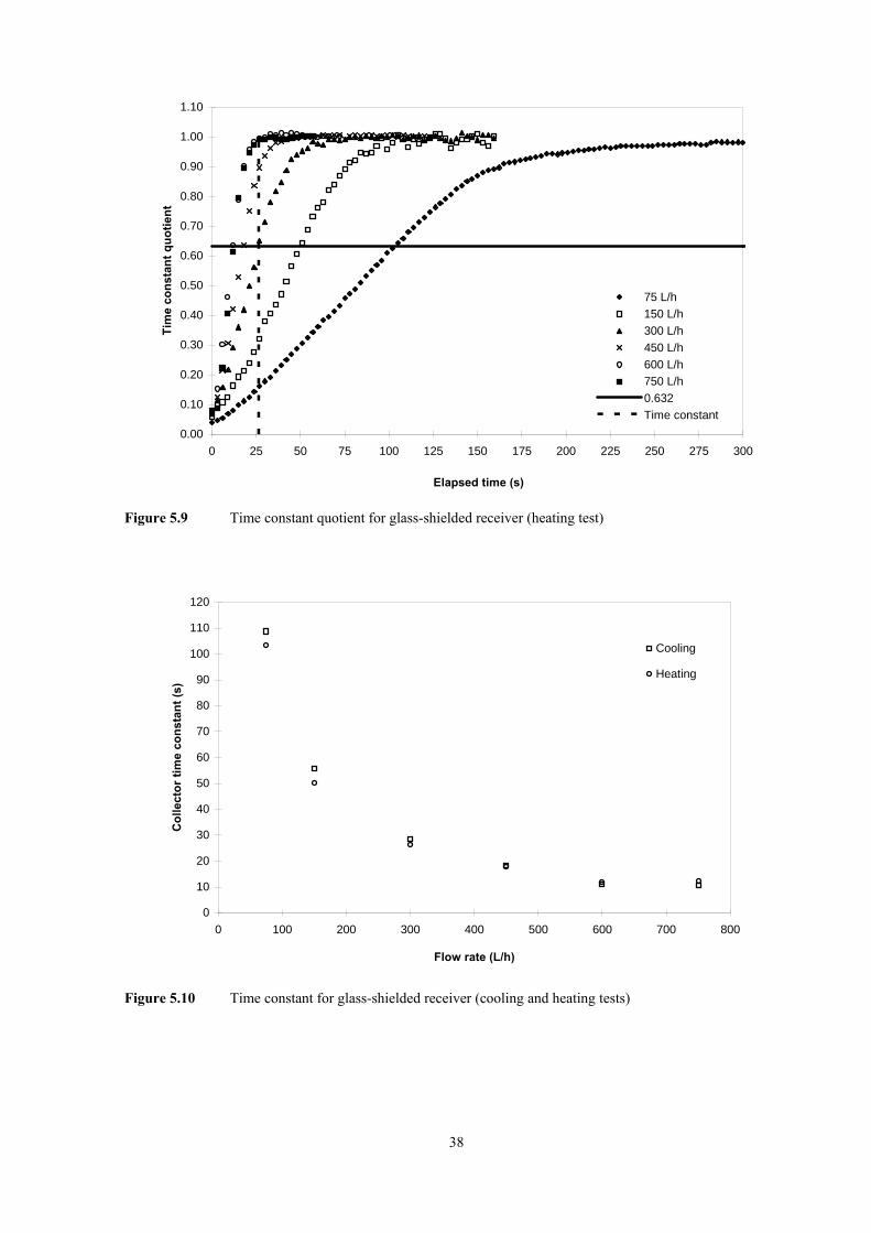
38
0
10
20
30
40
50
60
70
80
90
100
110
120
0 100 200 300 400 500 600 700 800
Flow rate (L/h)
Col
lect
or ti
me
cons
tant
(s)
Cooling
Heating
Figure 5.9 Time constant quotient for glass-shielded receiver (heating test)
Figure 5.10 Time constant for glass-shielded receiver (cooling and heating tests)
0.00
0.10
0.20
0.30
0.40
0.50
0.60
0.70
0.80
0.90
1.00
1.10
0 25 50 75 100 125 150 175 200 225 250 275 300
Elapsed time (s)
Tim
e co
nsta
nt q
uotie
nt
75 L/h150 L/h300 L/h450 L/h600 L/h750 L/h0.632Time constant

39
Comparison of results
Figure 5.11 compares the heating and cooling results for both HCE types. Results were
similar with the only significant difference occurring at the lower flow rates of 75 L/h and
150 L/h, where the time constants for the glass-shielded receiver were noticeably higher.
At the lowest flow rate, the time constants for the shielded receiver were 108.7 s and 103.2 s
respectively. During cooling at this flow rate, the time constant was 11.4 % higher than the
average of the results for the unshielded receiver (97.6 s), while the time constant for the glass
receiver under heating was 5.8 % higher. At maximum flow rate the highest time constant
was measured for the unshielded receiver during heating.
Figure 5.11 Comparison of time constants for glass-shielded and unshielded receivers
ASHRAE 93 compliance
Meteorological, radiometric and fluid system variables were monitored to assess compliance
with the ASHRAE 93 test conditions described in chapter 4. A summary of key variables is
given in table 5.1. The data are given in detail in appendix E.
0
20
40
60
80
100
120
0 100 200 300 400 500 600 700 800
Flow rate (L/h)
Col
lect
or ti
me
cons
tant
(s)
Glass cooling
Glass heating
Unshielded heating
Unshielded cooling

40
Table 5.1 Key data from time constant tests
(tf,i - ta) (°C)
Max. Δ(tf,i)(°C)
Ave. GDN (W/m2)
Ave. θi (deg)
ta (°C)
Ave. wind vel. (m/s)
Unshielded (cooling) 3.08 0.05 869.08 3.75 24.72 5.1
Unshielded (heating) 2.36 0.09 907.79 7.67 26.03 4.7
Glass-shielded (cooling) 4.33 0.09 891.10 13.96 26.82 5.4
Glass-shielded (heating) 4.28 0.07 887.76 13.88 26.83 5.4
AVERAGE 3.51 0.08 888.93 9.82 26.1 5.2
On average, it was not possible to maintain the fluid receiver inlet temperature (tf,i) to within
± 1 °C of the ambient air temperature, which was an average of 3.5 °C lower than that of the
fluid. For consistency, the ambient temperature was measured throughout the test programme
using the test facility’s weather station and entered manually in the SCATTAlog application
during testing. Although no formal tests were conducted to compare the weather station
temperature readings with those of a stand-alone thermometer, measurements taken near the
trough suggested that the weather station tended to under-read temperature. This was
probably due to its position on the edge of the rooftop test facility, where winds appeared
stronger than at the trough collector position, providing a cooling effect to the instruments
contained within the station’s sensor suite. To avoid introducing variations in the test
procedure, no adjustments were made to the ambient temperature readings, nor was any
adjustment made to account for the violation of ASHRAE requirements regarding Δt.
The variation in receiver fluid inlet temperature (tf,i) was well controlled, with the maximum
variation restricted to an average of 0.08 °C, within the ASHRAE 93 limit of 0.1 °C (± 0.05
°C of the chosen set-point). Although less important during time constant tests, the average
normal beam irradiance was also monitored and remained above the minimum required value
of 790 W/m2 during the focused period of the tests. Ambient temperature remained below the
ASHRAE 93 limit of 30 °C.
On average, wind velocity exceeded the prescribed limit of 4.5 m/s (8.7 knots). Care was
taken to avoid running tests on excessively windy days and a test was abandoned if the
velocity exceeded 6.7 m/s (13 knots).

41
As with ambient temperature, qualitative observations suggested that wind speeds were higher
where the anemometer was located than near the PTSC receiver, though no portable
equipment was available to confirm this at the time and, for consistency, no attempt was made
to adjust the wind velocity during data logging to account for differences.
5.3.2 Collector acceptance angle
Unshielded receiver
Results from the collector acceptance angle test for the unshielded receiver are shown
graphically in figure 5.12.
Figure 5.12 Collector acceptance angle results for unshielded receiver
The efficiency factor is calculated in the same way as tracking efficiency factor, except that a
10-point average is used (see 4.2.4 and appendix E for a sample calculation). The values are
plotted against angle of incidence, which is measured in a plane perpendicular to the receiver
and represents the angle through which the collector must be turned to focus properly at any
moment. For the unshielded receiver, the collector acceptance angle was 0.43°, this being the
0.0
0.2
0.4
0.6
0.8
1.0
1.2
-4 -3 -2 -1 0 1 2 3 4
Angle of incidence (deg)
Inci
denc
e an
gle
eff.
fact
or

42
angular interval in which thermal performance of the PTSC remained within 2 % of peak
performance.
Glass-shielded receiver
The collector acceptance angle results for the glass-shielded receiver are shown in figure 5.13.
For this configuration, the acceptance angle was measured at 0.52°.
Figure 5.13 Collector acceptance angle results for glass-shielded receiver
Comparison of results
In figure 5.14, data from both the collector acceptance angle tests (unshielded and glass-
shielded) are shown on the same set of axes, which have been scaled to illustrate the 2 % band
in which collector performance is permitted to fluctuate. Overall, the glass-shielded receiver
was slightly more tolerant of being in an out-of-focus position than the unshielded receiver,
though the results were similar.
0.0
0.2
0.4
0.6
0.8
1.0
1.2
-4 -3 -2 -1 0 1 2 3 4Angle of incidence (deg)
Inci
denc
e an
gle
eff.
fact
or

43
Figure 5.14 Collector acceptance angle results for unshielded and glass-shielded receivers
ASHRAE 93 compliance
Table E.4 (appendix E) contains data used to determine compliance with ASHRAE 93 limits.
The test for the unshielded receiver took place on 28 December 2003 shortly after solar noon.
Average wind velocity was within ASHRAE 93 limits at 4.1 m/s (8.0 knots), as were the
normal beam irradiance average and variation as well as the variation in receiver fluid inlet
temperature. The average angle of incidence was 6.62°. The only violation of the ASHRAE
93 limit occurred with regard to the difference between receiver inlet temperature and ambient
air temperature, Δt. This was measured at an average of 2.62 °C for the test. The test
standard prescribes an inlet temperature of ta ± 1 °C.
For the glass-shielded receiver, violations of the ASHRAE 93 limit occurred with regard to
average wind velocity (5.7 m/s or 11 knots), Δt (3.38 °C) and variation in receiver fluid inlet
temperature (0.18 °C). These violations were not excessive. The average angle of incidence
was 17.52°, which was somewhat higher than ideal. The need to conduct the collector
acceptance angle test at solar noon precluded reducing the value of θi since the test was
performed during February, by which time θi had increased appreciably from its mid-summer
low.
0.90
0.92
0.94
0.96
0.98
1.00
1.02
-0.5 -0.4 -0.3 -0.2 -0.1 0 0.1 0.2 0.3 0.4 0.5
Angle of incidence (deg)
Inci
denc
e an
gle
eff.
fact
or
Glass-shielded
Unshielded

44
5.3.3 Thermal efficiency
Unshielded receiver
Twenty tests were conducted to generate the thermal efficiency curve of the PTSC, which is
shown in figure 5.15.
Figure 5.15 Thermal efficiency with unshielded receiver
The best fit curve in figure 5.15 was obtained from a regression analysis using the method of
least squares. This yielded equation 5.2, the thermal performance equation for the collector
with the unshielded receiver.
The coefficient of determination (R2) for equation 5.2 was 0.934, indicating a good fit with
the data. From equation 5.2, (ArULFR/Aa) = 2.0099 W/m2K and FRηo = 0.5523.
)2.5(5523.0G
t0099.2bp
g +⎟⎟⎠
⎞⎜⎜⎝
⎛ Δ−=η
0.0
0.1
0.2
0.3
0.4
0.5
0.6
0.7
0.8
0.9
1.0
0.00 0.01 0.02 0.03 0.04 0.05 0.06
(tf,i - ta)/Gbp (m2K/W)
Ther
mal
effi
cien
cy η
g
Efficiency dataLinear best fit

45
For a geometric concentration ratio (Aa/Ar) of 16.70 the gradient of equation 5.2 gives
ULFR = 33.57 W/m2K. The optical efficiency can be calculated from equation A.1, for which
ηo = 0.601 at near-normal angles of incidence. This results in a heat removal factor (FR) of
0.919. The heat removal factor represents the ratio of actual useful energy gain of the
collector to the useful gain if the whole receiver were at the fluid inlet temperature. This in
turn yields an overall heat loss coefficient (UL) of 36.53 W/m2K.
Glass-shielded receiver
Due to weather delays, the test programme for the glass-shielded HCE was shortened and 10
tests were conducted to determine the thermal efficiency curve, which is shown in figure 5.16.
Figure 5.16 Thermal efficiency with glass-shielded receiver
A regression analysis yielded the following performance equation for the collector with the
glass-shielded receiver:
0.0
0.1
0.2
0.3
0.4
0.5
0.6
0.7
0.8
0.9
1.0
0 0.01 0.02 0.03 0.04 0.05 0.06
(tf,i - ta)/Gbp (m2K/W)
Ther
mal
effi
cien
cy η
g
Efficiency data
Linear best fit
)3.5(5381.0G
t0595.1bp
g +⎟⎟⎠
⎞⎜⎜⎝
⎛ Δ−=η

46
For equation 5.3, R2 was 0.922. From equation 5.3, (ArULFR/Aa) = 1.0595 W/m2K and
FRηo = 0.5381. For a concentration ratio of 16.70, the gradient of equation 5.3 gives
ULFR = 17.69 W/m2K. As with the unshielded receiver, the optical efficiency can be
calculated from equation A.1. The presence of the glass shield reduces ηo from 0.601 to 0.553
at near-normal angles of incidence. This results in a heat removal factor (FR) for the shielded
receiver of 0.973 and an overall heat loss coefficient (UL) of 18.18 W/m2K.
Comparison of results
Data from both sets of thermal efficiency tests are consolidated in figure 5.17. The point at
which the performance curves cross corresponds to a thermal efficiency of 52.23 %, with
(Δt/Gbp) = 0.0149 m2K/W. For a normal beam irradiance value of 900 W/m2 this equates to a
fluid inlet temperature 13.45 °C above ambient. For fluid temperatures greater than this, the
glass-shielded receiver performs better than the unshielded unit.
Figure 5.17 Comparison of thermal efficiencies
0.30
0.35
0.40
0.45
0.50
0.55
0.60
0.65
0 0.01 0.02 0.03 0.04 0.05 0.06(tf,i - ta)/Gbp (m2K/W)
Ther
mal
effi
cien
cy η
g
Unshielded dataGlass dataUnshielded best fitGlass best fit

47
ASHRAE 93 compliance
Tables E.2 and E.3 give key data from all 20 thermal efficiency tests conducted for the PTSC
with the unshielded receiver and the 10 tests conducted with the glass-shielded receiver. A
summary of the data is given in table 5.2.
Table 5.2 Key data from thermal efficiency tests
ta
(°C)
Ave. GDN
(W/m2)
Max. Δ(GDN) (W/m2)
Max. Δ(tf,i) (°C)
Ave. θi
(deg)
Max. Δ(θi) (deg)
Ave. wind
vel. (m/s) Unshielded AVERAGE 27.12 937.17 11.51 0.52 7.08 0.20 4.8
Glass-shielded AVERAGE 27.27 861.58 10.11 0.52 10.11 0.26 4.6
At no time during the tests with the unshielded receiver did the ambient air temperature
exceed the ASHRAE 93 limit of 30 °C, and the average test temperature was 27.12 °C.
Likewise, the standard’s requirement of normal beam irradiance greater than 790 W/m2 was
met in all tests, with an average for the batch of 937.17 W/m2. The average maximum
variation in beam irradiance across all 20 tests was 11.51 W/m2, well within the prescribed
limit of ± 32 W/m2, and no violations of this limit occurred in any of the tests. The calculated
average angle of incidence was 7.08°, with a minimum value of 0.10° and a maximum of
11.53°. The maximum variation during any one test was 0.38°, with an average variation of
0.20°.
Violations of the ASHRAE 93 test limits occurred with respect to variation of tf,i and
measured wind speed. The average maximum variation in tf,i was 0.52 °C, considerably
higher than the limit of 0.1 °C (± 0.05 °C). The ASHRAE 93 limit was exceeded in 15 of 20
tests and was more pronounced at higher fluid inlet temperatures, where accurate temperature
control was more difficult.
Average wind velocity exceeded the ASHRAE 93 maximum limit of 4.5 m/s. Violations
occurred in just over half the tests, although they were minor in magnitude and wind speed
never exceeded 6.7 m/s (13.0 knots).

48
For the glass-shielded receiver, the average air temperature was 27.27 °C with no violations
of the ASHRAE 93 upper limit. Average normal beam irradiance was lower than the
unshielded tests at 861.58 W/m2, reflecting the expected seasonal reduction with the passing
of summer. Variations in GDN were minimal and within limits.
As with the unshielded receiver tests, controlling tf,i proved difficult and the variation of this
parameter was 0.52 °C, identical to the unshielded tests. With the tests having been
conducted later in the year, the average angle of incidence was 10.11°, with a minimum value
of 2.71° and a maximum of 15.80°. The maximum, minimum and average wind speeds were
5.2 m/s (10.0 knots), 3.6 m/s (7.0 knots) and 4.6 m/s (8.9 knots) respectively.
5.3.4 Incidence angle modifier
Unshielded receiver
Data for the unshielded receiver are presented graphically in figure 5.18 with a fitted curve
obtained from regression analysis.
The data were obtained using equation 4.7 and the y-intercept of the linear curve fitted to the
data in figure 5.15. This gave a value for FRηo of 0.5523, representing the peak performance
of the PTSC at near-normal angles of incidence. Values of Kατ at increased angles of
incidence were obtained by dividing efficiency values into the peak value. A regression
analysis provided the following equation for Kατ as a function of θi:
Kατ = -2.032 x 10⁻⁶ (θi)3 + 1.199 x 10⁻⁴ (θi)2 – 3.940 x 10⁻³ (θi) + 1.005 (5.4)
For this regression analysis, R2 = 0.966, indicating a very good fit with the data.

49
0.0
0.1
0.2
0.3
0.4
0.5
0.6
0.7
0.8
0.9
1.0
1.1
0 5 10 15 20 25 30 35 40 45 50 55 60
Angle of incidence (deg)
Inci
dent
ang
le m
odifi
er K
ατ
Unshielded data
Unshielded best fit
Figure 5.18 Incidence angle modifier for unshielded receiver
Glass-shielded receiver
Figure 5.19 illustrates the performance of the PTSC with the glass-shielded HCE installed.
Figure 5.19 Incidence angle modifier for glass-shielded receiver
0.0
0.1
0.2
0.3
0.4
0.5
0.6
0.7
0.8
0.9
1.0
1.1
0 5 10 15 20 25 30 35 40 45 50 55 60
Angle of incidence (deg)
Inci
dent
ang
le m
odifi
er K
ατ
Glass data
Glass best fit

50
Equation 5.5 was obtained for Kατ by linear regression.
Kατ = 9.360 x 10⁻⁷ (θi)3 – 1.616 x 10⁻⁴ (θi)2 + 1.061 x 10⁻³ (θi) + 1.009 (5.5)
As for the unshielded receiver, the coefficient of determination confirmed a very good fit with
the data (R2 = 0.967).
Comparison of results
Figure 5.20 shows equations 5.4 and 5.5 plotted on the same axes. For interest, a cosine plot
is included to illustrate the difference between the experimental equations and a much simpler
model for the incidence angle modifier, Kατ.
Figure 5.20 Incidence angle modifier for unshielded and glass-shielded receivers
Up to an incidence angle of approximately 25° the glass-shielded receiver performed slightly
better, but beyond that its performance declined more rapidly and was inferior to that of the
unshielded receiver. From figure 5.20, the calculated value of Kατ was 0.75 for the glass-
shielded receiver at the maximum tested incidence angle of 53°. This was 9.6 % lower than
0.0
0.1
0.2
0.3
0.4
0.5
0.6
0.7
0.8
0.9
1.0
1.1
0 5 10 15 20 25 30 35 40 45 50 55 60
Angle of incidence (deg)
Inci
dent
ang
le m
odifi
er K
ατ
Unshielded best fitGlass best fitCosine

51
for the unshielded receiver, which had an incidence angle modifier of 0.83, as calculated from
equation 5.4. At the same maximum angle of incidence, the simplified cosine model under-
predicted Kατ by 27.5 % for the unshielded receiver and by 19.8 % for the glass-shielded unit.
ASHRAE 93 compliance
Table 5.3 contains summarised data from both sets of incidence angle modifier tests. The
source data are given in appendix E.
Ten thermal efficiency tests were used to determine the incidence angle modifier for the
unshielded receiver. Violations of ASHRAE 93 prescribed limits occurred with respect to
receiver fluid inlet temperature, both in absolute value above ambient air temperature and in
variation. On average Δt was 3.02 °C. This was greater than the allowable variation of ± 1
°C above or below ta. The average variation in tf,i of 0.32 °C was also over the prescribed
limit, which was exceeded in 7 out of 10 tests. Apart from this, normal beam irradiance levels
were acceptable, as was their variation. Average wind speed was also within limits, though in
three tests it exceeded the maximum limit of 4.5 m/s slightly and in four tests it was either
borderline or lower than the minimum of 2.2 m/s. In two of the tests there were no wind data
available due to a weather station failure.
Eleven tests were used to determine Kατ for the glass-shielded receiver. As can be seen from
table 5.3 and tables E.5 and E.6, the extent of ASHRAE 93 compliance and transgression was
similar. Average recorded wind speed was within limits, although in two tests it was
measured at 6.2 m/s (12 knots) and in three tests it fell below the minimum level of 2.2 m/s.
As with all testing, there was nothing that could be done to alter wind conditions other than
abandon a test if the wind speed became unreasonably high. With little time to reschedule
tests, minor violations of ASHRAE 93 with were disregarded.
Table 5.3 Key data from incidence angle modifier tests
ta (tf,i - ta) Ave. GDN Max. Δ(tf,i) Max. Δ(GDN) Max. Δ(θi) Ave. wind (°C) (°C) (W/m2) (°C) (W/m2) (deg) vel. (m/s)
Unshielded AVERAGE 23.32 3.02 826.67 0.32 14.38 0.30 3.2
Glass-shielded AVERAGE 26.34 2.90 859.37 0.30 13.18 0.20 3.8

52
5.4 Receiver Thermal Loss Tests
The aim of these tests was to determine steady state heat loss as a function of operating
temperature (Dudley et. al, 1995). Two tests were conducted, one each for the unshielded and
glass-shielded receivers. Before each test the HT tank was filled and heated to its maximum
temperature of approximately 85 °C. At sunset, the PTSC fluid circulation pump was started
and the flow rate set at 300 L/h. Temperature data were then logged at regular intervals,
specifically the temperature drop as the hot water passed through the receiver. The system
was left to run overnight, during which the fluid was constantly recirculated through the
PTSC, gradually cooling as heat was lost. By monitoring (tf,i – tf,o) versus (tf,i – ta), a measure
of the thermal loss in Watts per square metre of receiver area was obtained, this being the
“off-sun” loss Q0. Off-sun loss differs from the “on-sun” loss experienced during daytime
focusing of the PTSC. On-sun loss per unit receiver area, Q+, is determined from the heat
gain difference between the operating efficiency and the optical efficiency, and is equal to the
product ULFR, as determined from the thermal efficiency curve, and the receiver fluid inlet
temperature above ambient. Off-sun loss, which contributes to the total thermal loss under
normal operating conditions, is lower than on-sun loss because during normal operation of the
collector the sun’s energy causes the external surface of the receiver to heat up, increasing
heat loss via the normal mechanisms of conduction, convection and radiation (Dudley et. al,
1995). Losses can be calculated from equations 5.6 and 5.7.
In equation 5.7, Δtave represents the average receiver fluid temperature above ambient and
ULFR is 33.57 W/m2K for the unshielded receiver and 17.69 W/m2K for the glass-shielded
receiver. The on-sun loss is an approximation, since ULFR is obtained from the thermal
efficiency curve which is determined using (tf,i – ta), not Δtave. Since the actual temperature
drop through the receiver for the loss tests ranged from zero at receiver temperatures close to
ambient to less than 3 °C at maximum inlet temperature, the difference between (tf,i – ta) and
Δtave was negligible.
( )
)7.5(]m/W[tFUQlosssunOn
)6.5(]m/W[A
ttcmQlosssunOff
2aveRL
2
r
o,fi,fp0
Δ==−
−==−
+

53
0
10
20
30
40
50
60
70
80
0 1 2 3 4 5 6 7 8 9 10 11 12 13Elapsed time (h)
Tem
pera
ture
(°C
)
-0.5
0.0
0.5
1.0
1.5
2.0
2.5
3.0
Rec
eive
r tem
pera
ture
dro
p (°
C)
Receiver fluid (ave.)
Ambient
Receiver temp. drop
By conducting thermal loss tests at night, all energy input to the collector was eliminated
enabling true measurement of the off-sun loss (running thermal loss tests during the day with
the PTSC defocused does not completely eliminate heat input to the receiver).
Unshielded receiver
In figure 5.21, the average receiver fluid temperature ((tf,i + tf,o)/2), the ambient air
temperature (ta) and the fluid temperature drop across the receiver (tf,i – tf,o) are shown over
the duration of the nighttime loss test for the unshielded receiver. Since heat loss can be
severely affected by wind conditions during testing, wind data for the night of the test were
logged and are presented in figure 5.22.
Figure 5.21 Temperature data from thermal loss test for unshielded receiver
Figure 5.22 compares the measured off-sun thermal loss, Q0U, and on-sun loss, Q+U, for the
unshielded receiver, as determined from figure 5.21 and equations 5.6 and 5.7. Following the
approach of Dudley et. al (1995) and Stine and Harrigan (1985), the calculated data points for
off-sun loss for the unshielded HCE were used to generate a third order polynomial curve
describing thermal loss as a function of average receiver fluid temperature above ambient:

54
Q0U = 0.0033 (Δtave)3 – 0.1935 (Δtave)2 + 23.2746 (Δtave) [W/m2] (5.8)
For this equation, R2 = 0.936. The average value of Gbp for the 20 thermal efficiency tests
from which the on-sun curve was obtained, was 928.23 W/m2.
Figure 5.22 Thermal loss and wind data for unshielded receiver
Glass-shielded receiver
Results from the thermal loss test for the glass-shielded receiver are shown graphically in
figures 5.23 and 5.24. The curve describing heat loss as a function of average receiver fluid
temperature above ambient is given as:
Q0G = – 0.0036 (Δtave)3 + 0.3511 (Δtave)2 + 0.3392 (Δtave) [W/m2] (5.9)
For this equation, R2 = 0.995. The average value of beam irradiance (Gbp) for the 10 tests,
from which the on-sun curve in figure 5.24 was obtained, was 841.73 W/m2.
0
200
400
600
800
1000
1200
1400
1600
0 10 20 30 40 50 60
Average receiver fluid temperature above ambient (°C)
Ther
mal
loss
(W
/m2 )
0
2
4
6
8
10
12
Win
d sp
eed
(m/s
)On-sun loss(eqn. 5.7)
Off-sun loss(eqns. 5.6 and 5.8)
Wind (off-sun, best fit)

55
0
200
400
600
800
1000
0 10 20 30 40 50 60
Average receiver fluid temperature above ambient (°C)
Ther
mal
loss
(W
/m2 )
0
2
4
6
8
10
Win
d sp
eed
(m/s
)Off-sun loss(eqns 5.6 and 5.9)
On-sun loss(eqn. 5.7)
Wind (Off-sun)
Figure 5.23 Temperature data for glass-shielded receiver
Figure 5.24 Thermal loss and wind data for glass-shielded receiver
0
10
20
30
40
50
60
70
80
0 1 2 3 4 5 6 7 8 9 10 11 12 13 14
Elapsed time (h)
Tem
pera
ture
(°C
)
0
0.1
0.2
0.3
0.4
0.5
0.6
0.7
0.8
Rec
eive
r tem
pera
ture
dro
p (°
C)
Receiver fluid (ave.)
Ambient
Receiver temp. drop

56
Comparison of results
Figure 5.25 compares thermal loss results for both receivers, including the wind conditions
under which tests were conducted.
Figure 5.25 Thermal loss for glass-shielded and unshielded receivers
Compared to figure 5.22, the off-sun loss data in figure 5.24 showed considerably less scatter.
This is discussed further in chapter 7.
5.5 Summary
A summary of the thermal performance of the PTSC is presented in table 5.4 for both receiver
types, as determined from the ASHRAE 93 tests and thermal loss tests conducted on the
collector.
0
200
400
600
800
1000
1200
0 10 20 30 40 50 60
Average receiver fluid temperature above ambient (°C)
Ther
mal
loss
(W
/m2 )
0
2
4
6
8
10
12
Win
d sp
eed
(m/s
)
Off-sun loss (glass)
Off-sun loss (unshielded)
Wind (unshielded)
Wind (glass)
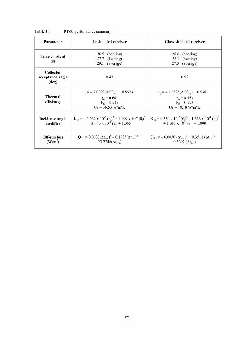
57
Table 5.4 PTSC performance summary
Parameter Unshielded receiver Glass-shielded receiver
Time constant (s)
30.5 (cooling) 27.7 (heating) 29.1 (average)
28.6 (cooling) 26.4 (heating) 27.5 (average)
Collector acceptance angle
(deg) 0.43 0.52
Thermal efficiency
ηg = – 2.0099(Δt/Gbp) + 0.5523 ηo = 0.601 FR = 0.919
UL = 36.53 W/m2K
ηg = – 1.0595(Δt/Gbp) + 0.5381 ηo = 0.553 FR = 0.973
UL = 18.18 W/m2K
Incidence angle modifier
Kατ = – 2.032 x 10⁻⁶ (θi)3 + 1.199 x 10⁻⁴ (θi)2 – 3.940 x 10⁻³ (θi) + 1.005
Kατ = 9.360 x 10⁻⁷ (θi)3 – 1.616 x 10⁻⁴ (θi)2 + 1.061 x 10⁻³ (θi) + 1.009
Off-sun loss (W/m2)
Q0U = 0.0033(Δtave)3 – 0.1935(Δtave)2 + 23.2746(Δtave)
Q0G = – 0.0036 (Δtave)3 + 0.3511 (Δtave)2 + 0.3392 (Δtave)

58
6. THERMAL MODELLING OF PTSC PERFORMANCE
6.1 Introduction
Conventional PTSC models treat the receiver as a single unit into and out of which energy is
transferred (Stine and Harrigan, 1985; Incropera and DeWitt, 1990; Duffie and Beckman,
1991; Bakos et al., 1999). The principle source of energy is solar irradiance reflected from
the mirror surface of the collector to the absorber, through which a heat transfer fluid is
pumped. Several heat loss mechanisms are active as a result of the absorber’s raised
temperature, mainly radiation and residual gas conduction from the absorber to the glass
shield (if present), convection from the outer surface of the receiver to atmosphere,
conduction through end connections and radiation loss to the sky (Odeh et al., 1998). Heat
“loss” to the working fluid is the intended aim of the PTSC.
The magnitudes of thermal losses change depending on operating conditions. Convective
losses are strongly dependent on ambient wind conditions and whether or not the absorber is
shielded, conductive losses are usually small and radiation heat loss is a strong function of the
receiver temperature. Under steady state conditions, the energy flows into and out of the
receiver are balanced enabling the calculation of parameters such as the absorber wall
temperature and rise in fluid temperature. The temperature rise causes a positive gradient in
the receiver wall temperature from inlet to outlet. In the conventional modelling approach,
this lengthwise gradient is either ignored by using averaged temperature values for the wall of
the receiver and the working fluid (Stine and Harrigan, 1985), or it is circumvented by
introducing a heat removal factor (FR) to account for the reduction in effectiveness of the
absorber (Duffie and Beckman, 1991).
As an alternative to the conventional modelling approach, the receiver is divided into short
lengths or segments and an energy balance is performed on each segment, leading to a
solution for the temperature of the fluid and that of the absorber wall within each segment,
from inlet to outlet of the receiver. This finite volume approach is followed by Odeh et al.
(1998) and Lamprecht (2000), and is used in this study to model the thermal efficiency of the
PTSC. In this chapter, a brief description of the model presented by Lamprecht (2000) is

59
given. Results from the implementation of the model are presented and a comparison is made
between the model’s results and those obtained by experiment.
6.2 Thermal Model of Collector Performance
In implementing the PTSC performance model of Lamprecht (2000), the following
assumptions and constraints were adopted:
• Steady state operation was assumed
• Only single phase (liquid) flow was considered in the absorber
• Circumferential temperature gradients in the absorber wall were ignored
• Fluid pressure was assumed constant through the absorber
• Heat transfer between absorber and glass-shield was by radiation only
• Heat conduction along the length of the absorber was ignored
• Turbulent flow in the absorber was assumed
• Forced convection was assumed from the receiver to atmosphere
• For calculation purposes, the length of the receiver was set at 5 m
• During simulation of the performance of the unshielded and glass-shielded receivers,
average ambient conditions (wind speed, irradiance, fluid and air temperatures) from
the completed PTSC test programme were used as inputs to the model so as to enable
meaningful comparison between model and experiment
To accommodate the unshielded and glass-shielded receivers used in this project, the model
configurations shown in figures 6.1 and 6.2 were used. In figure 6.1 the energy flows and
temperatures for the unshielded receiver are shown, while those applicable to the glass-
shielded receiver are illustrated in figure 6.2. Heat flows in [W] to the control volume in
figure 6.1 include beam radiation from the sun (Qq-a) and radiation from the sky (Qsky-a), while
losses from the absorber include radiation to the sky (Qrad(a-s)) and convection to the
atmosphere (Qconv(a-s)), which is at ambient temperature ta. The absorber wall temperature is
twa, fluid enters the segment at temperature ti and leaves at ti+1, with an average bulk value of
tb. Heat flow from the wall to the working fluid is Qwall.

60
Figure 6.1 Heat transfer model for unshielded receiver (Lamprecht, 2000)
Figure 6.2 Heat transfer model for glass-shielded receiver (Lamprecht, 2000)
Figure 6.3 Segment control volume for absorber with liquid flow (Lamprecht, 2000)
Qq-a Qsky-a
Qwall
tb
ti+1 ti
Twa Qconv(a-s) Qrad(a-s)
ta tsky
Qq-aQsky-a
Qsky-g Qq-g
Qwall
Qrad(a-g)
tb
ti+1 ti
twa
Qconv(g-s)Qrad(g-s) twg
tatsky
Twe
tb
hi+1 mi+1 vi+1
hi mi vi
Qw = mCp(ti+1 – ti)
ti+1 ti

61
In figure 6.2, additional energy flows include absorption of beam and sky radiation by the
glass shield (Qq-g and Qsky-g), net radiation exchange between the absorber and the glass shield
(Qrad(a-g)), radiation loss from the glass to the sky (Qrad(g-s)) and convective loss from the glass
to atmosphere (Qconv(g-s)).
In the sketch of the control volume (figure 6.3), the working fluid enters the segment with
specific enthalpy hi [J/kg], velocity vi [m/s] and at a mass flow rate of mi [kg/s]. The rate at
which energy is absorbed by the fluid (Qw = mcp(ti+1 – ti)) is equal to the heat transfer-rate
through the absorber wall (Qwall), changing the fluid properties at outlet to ti+1 and hi+1 (vi+1
and mi+1 are assumed to remain constant from the inlet).
In Lamprecht’s model, only free convection is assumed in the calculation of the external
convective heat transfer coefficient, hce. The model was therefore modified to reflect more
accurately the conditions experienced during testing in this study when the average recorded
wind speed was 4.8 m/s for the unshielded receiver tests and 4.6 m/s for the glass-shielded
receiver. Under these conditions, the free convection model would have under-predicted heat
loss. Duffie and Beckman (1991) recommend the following equations for determining the
Nusselt number for flow across a single tube exposed to wind in an outdoor environment:
Nu = 0.40 + 0.54 Re0.52 for 0.1 < Re < 1000 (6.1)
Nu = 0.30 Re0.6 for 1000 < Re < 50 000 (6.2)
where Re is the Reynolds number based on the outer diameter of the absorber or, if
applicable, the glass-shield. Once the Nusselt number is known, the convective heat transfer
coefficient can be obtained from equation 6.3.
Here, ka is the thermal conductivity of the air [W/mK] at a mean film temperature determined
for each control volume of the model and D is the outer diameter of the tube [m] from which
heat is lost. This heat transfer coefficient is then used in the calculation of the convective heat
)3.6(]Km/W[DkNuh 2a
ce =

62
loss terms Qconv(a-s) and Qconv(g-s), which form part of the energy balance equations that emerge
from the thermal model of the receiver.
To produce a solution, the model proceeds from the receiver inlet, where fluid conditions are
known, and the energy balance equations that are graphically illustrated in figures 6.1 and 6.2
are solved for each successive control volume. Two MATLAB programmes based on a
Visual Basic application by Lamprecht (2000) were used to implement the solution scheme
for both receiver types. Inputs include fluid inlet temperature, ambient air temperature, wind
velocity, beam irradiance, PTSC dimensions and material properties. Outputs include inlet,
outlet and bulk fluid temperature for each segment and the absorber wall temperature and
glass shield temperature (if applicable) for each segment.
The model configurations were used to predict the total rise in temperature through the
unshielded and glass-shielded receivers (Δtr) for the same conditions under which the
experimental PTSC efficiency tests were conducted. Equation 4.3 was then used to calculate
efficiency in the same way as during physical testing. To produce thermal performance
graphs such as those in figures 5.15 and 5.16, a range of receiver inlet temperatures was used
to simulate actual conditions.
Results
Unshielded receiver
Output from the finite volume model is shown in figure 6.4. This gives receiver fluid
temperatures for each of the model segments for a range of inlet values. Inlet temperatures
were chosen to give an even spread comparable to the values used in testing. Values of wind
speed and beam irradiance equal to actual test averages (4.8 m/s and 928.23 W/m2) were used.
Table F.1 contains raw data from a single run of the MATLAB programme written to
implement the thermal model for the unshielded receiver. Using the temperature gains shown
in figure 6.4, thermal efficiency data were derived for the receiver and these appear in figure
6.5. This graph includes results from the free convection model of Lamprecht (2000), the
modified forced convection model and experimental test data from figure 5.15.

63
Figure 6.4 Unshielded model results for a range of receiver inlet temperatures
Figure 6.5 Free and forced convection models with experimental data (unshielded)
0.0
0.1
0.2
0.3
0.4
0.5
0.6
0.7
0.8
0.9
1.0
0 0.01 0.02 0.03 0.04 0.05 0.06
(tf,i - ta)/Gbp (m2K/W)
Ther
mal
effi
cien
cy η
g
Free convectionExperimental dataForced convection (wind at 4.8 m/s)
0
20
40
60
80
100
120
0.0 0.5 1.0 1.5 2.0 2.5 3.0 3.5 4.0 4.5 5.0
Distance along absorber (m)
Flui
d te
mpe
ratu
re (°
C)
82.8 °C 73.5 °C64.3 °C 55.0 °C45.7 °C 36.4 °C27.1 °C (ambient)

64
From figure 6.5, the performance data of the free and forced convection models intercept the
efficiency axis at 0.588 and 0.520 respectively, with the experimental value at 0.552 obtained
from the best fit curve (equation 5.2). FRηo is 6.5 % higher than the test result for the free
convection model and 5.8 % lower for the forced convection model. At the maximum inlet
temperature tested, the free and forced convection models give efficiency results that are
22.6 % higher and 27.2 % lower respectively. Since the gradient of the efficiency curve is
dependent on the system’s overall heat loss coefficient (UL), it can be concluded that the free
convection model under-predicts heat loss and the forced convection model, with an input
wind speed of 4.8 m/s, over-predicts it.
To investigate the effect of wind speed on the predicted performance of the unshielded
receiver, the forced convection model was tested for a range of wind speeds, from near-zero
to 4.8 m/s. A velocity of 0.001 m/s was entered for the near-zero condition to ensure Re > 0.1
(see equation 6.1). The results are shown in figure 6.6.
Figure 6.6 Output from forced convection model for varying wind speed (unshielded)
0.25
0.30
0.35
0.40
0.45
0.50
0.55
0.60
0.65
0.00 0.01 0.02 0.03 0.04 0.05 0.06 0.07
(tf,i - ta)/Gbp (m2K/W)
Ther
mal
effi
cien
cy η
g
0.0 m/s
1.0 m/s
2.0 m/s
3.0 m/s
4.8 m/s
1.5 m/s
Experimental best fit curve(eqn. 5.2)
+ Experimental data
Modelwind speed

65
Although the average recorded wind speed during testing was 4.8 m/s, the forced convection
model shows excellent agreement with the experimental data at a wind speed of 1.5 m/s.
Lamprecht’s model was not intended to be used to determine thermal loss under zero
irradiance conditions but for interest the MATLAB programme developed for this project was
run with a beam irradiance value (Gbp) of 0 W/m2 to simulate conditions during the off-sun
loss tests described in 5.4. The output from one such run is given in table F.2. The results of
implementing the forced convection model at zero beam irradiance over a range of wind
speeds are shown in figure 6.7. A wind speed of 1.34 m/s and ambient temperature of 21.2 °C
were used to simulate actual test conditions. Experimental data are also shown with predicted
values for near-zero wind speed. As in figures 6.5 and 6.6, the experimental values fall
between the free convection data and those at the average recorded wind speed.
Figure 6.7 Off-sun thermal loss from forced convection model (unshielded)
In figure 6.6, the thermal performance model showed excellent agreement with experimental
data for a wind speed of 1.5 m/s, or 31.3 % of the recorded average from the test facility’s
anemometer. For interest, the same scaling factor (0.313) was applied to the average wind
speed measured during off-sun loss tests (1.34 m/s), to yield an adjusted wind speed of
0
200
400
600
800
1000
1200
1400
1600
0 10 20 30 40 50
Average receiver fluid temperature above ambient (°C)
Ther
mal
loss
(W
/m2 )
Model at 1.34 m/sModel at 0.42 m/sModel at 0.0 m/sExperiment

66
0.42 m/s. This speed was used in the performance model to produce the third set of data
shown in figure 6.7. Under these conditions, agreement between the model and the
experimental data is close.
Glass-shielded receiver
Results from two runs of the programme written to implement the forced convection model
for the glass-shielded receiver are given in figure 6.8. Fluid and glass shield temperatures are
presented for wind speeds of 4.6 m/s and 1.0 m/s. In both cases, the fluid temperature rise
from an inlet value of 27.3 °C is similar, but at the higher wind speed, the glass temperature is
lower reflecting the increased heat loss to atmosphere due to convection. A sample of data
from the implementation of the model is given in appendix F.
Figure 6.8 Fluid and glass temperatures for two wind speeds
Efficiency results are shown in figure 6.9. The graph includes output from the free
convection model, the modified forced convection model at a wind speed of 4.6 m/s (the
average recorded wind speed during testing) and experimental test data from figure 5.16. A
beam irradiance value of 841.73 W/m2 was used to simulate actual test conditions.
15
20
25
30
35
40
45
50
55
60
0.0 0.5 1.0 1.5 2.0 2.5 3.0 3.5 4.0 4.5 5.0
Distance along absorber (m)
Flui
d te
mpe
ratu
re (°
C)
Fluid temperature (4.6 m/s)Glass temperature (4.6 m/s)Fluid temperature (1.0 m/s)Glass temperature (1.0 m/s)
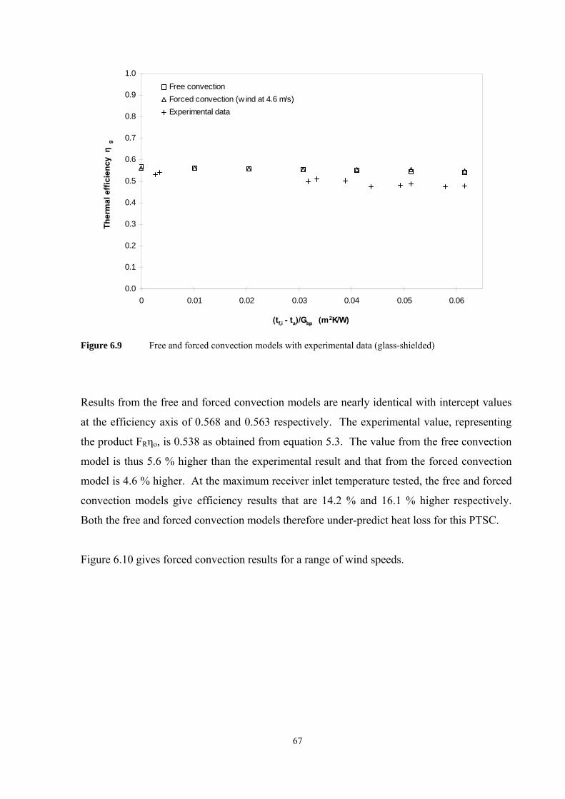
67
Figure 6.9 Free and forced convection models with experimental data (glass-shielded)
Results from the free and forced convection models are nearly identical with intercept values
at the efficiency axis of 0.568 and 0.563 respectively. The experimental value, representing
the product FRηo, is 0.538 as obtained from equation 5.3. The value from the free convection
model is thus 5.6 % higher than the experimental result and that from the forced convection
model is 4.6 % higher. At the maximum receiver inlet temperature tested, the free and forced
convection models give efficiency results that are 14.2 % and 16.1 % higher respectively.
Both the free and forced convection models therefore under-predict heat loss for this PTSC.
Figure 6.10 gives forced convection results for a range of wind speeds.
0.0
0.1
0.2
0.3
0.4
0.5
0.6
0.7
0.8
0.9
1.0
0 0.01 0.02 0.03 0.04 0.05 0.06
(tf,i - ta)/Gbp (m2K/W)
Ther
mal
effi
cien
cy η
g
Free convectionForced convection (w ind at 4.6 m/s)Experimental data

68
Figure 6.10 Output from forced convection model for varying wind speed (glass-shielded)
Increasing wind speed has little effect on the predicted efficiency, yet figure 6.8 shows an
increase in glass temperature at lower wind speeds. As the receiver fluid temperature is
increased, the growing difference between the predicted and measured performance of the
PTSC in figure 6.9 suggests that the modelled loss from the absorber to the glass shield is
lower than that measured experimentally. The negligible effect of wind speed on thermal
efficiency suggests that heat build-up in the glass shield is more a function of absorbed solar
energy than of transfer from the absorber. Based on the data in figures 6.9 and 6.10, not all
heat loss mechanisms are adequately accounted for in the model of the glass-shielded
receiver.
Attempts to use Lamprecht’s model to simulate off-sun loss for the glass-shielded receiver
(see figure 5.24) were not successful, as shown in figure 6.11. For this investigation, the
model was implemented with a Gbp value of 0 W/m2. Although it correctly shows a trend of
increasing thermal loss with fluid inlet temperature, the model wrongly predicts a small
temperature rise through the receiver for inlet temperatures below 55 °C. Clearly this is
incorrect for a zero beam irradiance input. Since the glass-shielded model is considerably
0.45
0.47
0.49
0.51
0.53
0.55
0.57
0.59
0.61
0.63
0.65
0.00 0.01 0.02 0.03 0.04 0.05 0.06 0.07
(tf,i - ta)/Gbp (m2K/W)
Ther
mal
effi
cien
cy η
g
Model at 0.0 m/sModel at 1.0 m/sModel at 3.0 m/sModel at 4.6 m/sExperimental dataExperimental best fit (eqn. 6.6)

69
more complex than the unshielded version, employs a different method of solution and is
untested for a zero irradiance input, further study of the modelling scheme would be required
to explain the anomalous results shown in figure 6.11.
Figure 6.11 Off-sun thermal loss from forced convection model (glass-shielded)
6.4 Summary
Two thermal models developed in the Department of Mechanical Engineering at the
University of Stellenbosch (Lamprecht, 2000) were tested against experimental results from
the PTSC test programme. The models, which were adapted to account for forced convection
from the receiver, used a finite volume approach in which the receiver was divided into
multiple control volumes or segments. The energy balance equations for each segment were
then solved yielding temperature data from which thermal efficiency values could be obtained
and compared with experimental results. The results for the forced convection, unshielded
model showed the following:
-200
-100
0
100
200
300
400
500
600
0 10 20 30 40 50 60
Average receiver fluid temperature above ambient (°C)
Ther
mal
loss
(W
/m2 )
Model at 2.34 m/sExperiment

70
• The model was highly sensitive to wind speed
• At the test-average wind speed of 4.8 m/s the predicted thermal efficiency of the PTSC
was lower than that determined experimentally
• Excellent agreement was obtained between the model and experimental results for the
forced convection model at a wind speed of 1.5 m/s, reinforcing doubts about the
accuracy of the measured test wind speed (4.8 m/s)
• After adjusting the wind speed according to results from the thermal efficiency tests,
output from the model showed close agreement with data from experimental off-sun
thermal loss tests
For the glass-shielded model with forced convection:
• In predicting thermal efficiency, the model showed agreement to within 5 % of
experiment at ambient fluid inlet temperature, but results were less accurate at higher
inlet temperatures
• The model was insensitive to wind speed with almost no change in thermal efficiency
as wind speed increased
• The model under-predicted heat loss and could not accurately predict off-sun thermal
loss

71
7. DISCUSSION
7.1 Experimental Results
Tracking performance
The combined use of fixed rate tracking (Mode 2) and manual adjustment (Modes 1a and 1c)
to track the sun early in the test programme was a necessary measure. While not ideal, it
proved quite successful as seen in the performance curve of figure 5.2, and enabled the test
programme to proceed while work continued on the algorithm-based system. The
introduction of fixed pulse tracking was an improvement over the fixed rate method, yielding
a tracking accuracy of 0.144°.
As a new method of determining the solar vector, use of the PSA Algorithm is not widely
reported in the literature. Development of Mode 3 tracking was therefore a significant
milestone in this project. The need for an offset factor indicates that further study is required
regarding the accuracy of the PTSC’s construction and alignment. Nevertheless the
algorithm-based tracking mode worked well and the use of powerful and programmable
components such as the Siemens PLC and VSD provided great flexibility in configuring
tracking modes.
The use of a high-reduction gearbox and AC motor with electro-mechanical brake was
effective. Although other hardware options were possible, such as a highly geared DC motor
or linear actuators (mechanical, hydraulic or electric) of the types used on satellite tracking
dishes, the chosen equipment was well suited to the needs of the project, considering cost,
complexity and time limitations.
Initial plans to include optical feedback in the tracking system were not pursued due to a lack
of time and resources. Such a system would have measured the difference in light falling on
two accurately positioned light dependent resistors (LDRs) to verify actual focusing and to
make fine adjustments to the collector’s position. Optical feedback would have improved the
accuracy of Mode 2 tracking early in the test programme when effective VSD settings were
being developed. Setting up a feedback system would have introduced additional problems,
however, such as accurately locating the LDRs and calibrating their response to differential

72
shading. This would have required time to correct and would have delayed PSA Algorithm-
based tracking, which was the more important goal. Optical feedback remains a worthwhile
addition to the DTCS and should be pursued as part of the system’s ongoing development.
In general, the DTCS functioned sufficiently well to enable trough testing to proceed,
although much work remains to transform it into a comprehensive drive, tracking and control
system.
PTSC performance results
i) Collector time constant
Figures 5.5, 5.6, 5.8 and 5.10 show that at higher flow rates the collector time constant was
reduced, regardless of heating or cooling. This is because heat transfer is more effective at
higher flow rates and the receiver does not heat up as much, so reaching thermal equilibrium
whether by adding or removing heat takes less time. The shapes of the curves in figures 5.7
and 5.10 confirm the exponential nature of the time constant with regard to flow rate, as
described in ASHRAE 93 (ASHRAE, 1991).
The measured time constants for both receivers (at the test flow rate of 300 L/h) were low at
an average of 29.1 s for the unshielded and 27.5 s for the glass-shielded receiver. By
comparison, Kalogirou (1996) published results for a PTSC with aperture width of 1.46 m and
area of 3.5 m2 for which the average time constant was 50 s. Comparison with the IST results
of Dudley et al. (1995) is not possible because they report the total time taken for the system
to stabilise and not a time constant value. This inability to compare results from different
programmes makes a good argument for standardising PTSC test methods.
The comparison of results given in figure 5.11 suggests a trend of slightly higher time
constants for the glass-shielded receiver during cooling and at low flow rates. A likely
explanation is that low flow rates produce higher temperatures in the fluid and the absorber
wall. In shedding this heat during the cooling stage of the test, heat loss by convection from
the absorber to the surrounding air is retarded by the glass shield, increasing the time constant.
At higher flow rates the data are close together and no clear trends are obvious.
73
ASHRAE 93 compliance was generally good throughout the tests, although it appeared that
wind speeds were higher at the weather station’s position than at the receiver, an effect that
was noticed several times during the programme. For the time constant tests, absolute wind
speed was less important than change in speed, which could have introduced variations in the
results. The recorded wind speeds shown in table 5.1 were close (all within 10 % of the
average), ensuring consistency in the test data.
ii) Collector acceptance angle
The acceptance angles for the unshielded and glass-shielded receivers (0.43° and 0.52°
respectively) were similar. By comparison, Kalogirou (1996) reports a value of 1° for the
same collector referred to in the time constant discussion.
A notable feature of figure 5.14 is the slight asymmetry of the unshielded data, compared with
the glass-shielded results. This probably indicates mislocation of the receiver or the
asymmetrical effects of other optical errors, such as reflector misalignment. The larger
acceptance angle and symmetrical data for the glass-shielded receiver possibly suggest that
refraction of incoming light rays by the glass helps to “damp out” optical image spread. It is
also possible that the insulating effect of the glass acts to smooth the thermal efficiency results
that make up the data.
Both ASHRAE 93 (1991) and Kalogirou (1996) link acceptance angle to tracking accuracy.
For this PTSC the tracking accuracy is equal to the angular magnitude of 1 pulse on the rotary
encoder, since this is the minimum angle through which the DTCS can turn the collector.
Therefore the trough has a tracking accuracy of 0.144°. Provided the DTCS maintains its
degree of accuracy, the collector will always operate within 2 % of its optimal efficiency
since the acceptance angle for both receivers is greater than the angular accuracy of the
tracking system.
ASHRAE 93 compliance was generally good during acceptance angle tests, although the
angle of incidence recorded for the glass-shielded test (θi = 17.52°) was higher than ideal.
This was a concern since the amount of reflection from a glass shield increases with θi (Duffie
and Beckman, 1991).

74
iii) Thermal efficiency
Thermal efficiency is an important measure of performance. It relates PTSC behaviour to the
working fluid temperature and assists in predicting overall performance of large-scale
systems. Commercial software packages used to predict the technical and economic
performance of planned installations, such as TRNSYS, SOLTES, DELSOL and WATSUN,
rely on performance models of the collector field, which are developed from the results of
thermal efficiency tests conducted on individual modules (Stine and Harrigan, 1985; Duffie
and Beckman, 1991).
For this PTSC, the peak efficiencies were 55.2 % and 53.8 % for the unshielded and glass-
shielded receivers respectively. These results are lower than those of commercial trough
collectors. For example, the IST collector tested by Dudley et al. (1995) showed a maximum
efficiency of between 70.8% and 76.3 %, depending on the type of receiver used. Peak
efficiency of the newest Eurotrough collector is approximately 75 % (Geyer et al., 2002).
Superior performance in commercial PTSCs is due to several factors, including higher
intercept factors (enabling an increase in concentration ratio), highly reflective mirror surfaces
and receivers incorporating ceramic-metal coatings with very high solar absorptance.
Efficiency results from this test programme are closer to those of other research troughs, for
which peak efficiency values of 63.8 % (Kalogirou, 1996), 62 % (Ibrahim, 1996) and
approximately 45 % (Bakos et al., 1999) are reported in the literature.
The gradient of the thermal efficiency equation gives a measure of the overall heat loss
coefficient (UL), which was found to be 36.53 W/m2K for the unshielded receiver and
18.18 W/m2K for the glass-shielded unit. The presence of the evacuated glass-shield
therefore reduced UL by 50.23 % producing a 9.2 % improvement in performance at
maximum test temperature. The results clearly show the benefit of installing a glass-shield.
Few authors provide a performance equation in their results, making it difficult to compare
heat loss from different PTSCs. An exception is Kalogirou (1996) who reported a loss
coefficient of 8.2 W/m2K. Details of the receiver’s construction were not given.

75
For high-temperature PTSCs a linear efficiency model is inadequate because radiation loss is
a nonlinear function of temperature-difference and the model becomes progressively less
accurate with increasing temperature. Inspection of IST performance graphs (Dudley et al.,
1995) suggests nonlinearity of the efficiency curve does not become pronounced until the
average receiver fluid temperature exceeds ambient temperature by approximately 100 °C.
While this is not necessarily true of other collectors, it gives some indication of the fluid
temperature range over which a linear model might be used. Each collector should be
evaluated independently to determine the most appropriate model, but the results from this
study confirmed the suitability of the linear model.
In figure 5.17 it can be seen that the glass-shielded receiver performs better for fluid
temperatures greater than 13.45 °C above ambient. Below this temperature heat loss is low
and the glass adversely affects performance by reducing optical efficiency. At higher
temperatures performance is dominated by heat loss, which is prevented more effectively by
the shielded receiver. In fact, a direct comparison of the thermal efficiency curves is not
strictly correct since they were generated using data obtained at different values of Gbp
(varying Gbp can result in temperature and heat loss changes). However, the efficiency results
of Dudley et al. (1995) show a very weak dependence on irradiance at low receiver
temperatures and a comparison was considered acceptable. The results of Lamprecht (2000)
also show a crossover point in the performance of a trough with two receivers (shielded and
unshielded) built at the University of Stellenbosch.
The temperature range over which a PTSC’s efficiency is tested should correspond to the
temperatures expected in service, which for commercial units can range from less than 100 °C
to over 400 °C. For a research collector such as this, the testing range is dictated by the aims
of the programme. In this case, the collector was built to establish a testing capacity for
components such as reflective surfaces, tracking systems and receivers, not all of which
require high-temperature testing. Thus, although a higher temperature range would have been
preferred it was not essential. It should be added that three of the four ASHRAE 93 tests are
performed with fluid at ambient temperatures. Also, not all commercial PTSC systems
operate at high temperature. At the Campbell Soup Company in California PTSCs provide
hot water at 91 °C for can washing (Stine and Harrigan, 1985) and the Phoenix Federal
Correctional Institution installed a PTSC system in 1998 to supply hot water for the washing,

76
kitchen and laundry needs of inmates (National Renewable Energy Laboratory, 2004).
Parabolic trough component testing at lower temperatures is therefore necessary and relevant.
In time, the scope of testing will be expanded and a possible solution to the limitations of the
fluid system may be found in the approach of Dudley et al. (1995), who used water for low-
temperature tests on the IST collector at Sandia, and oil for tests conducted up to 400 °C.
ASHRAE 93 compliance was acceptable during efficiency testing except for high wind speed
and variations in the receiver inlet temperature, which was difficult to hold constant at higher
temperatures. ASHRAE 93 recommends controlling fluid temperatures with an inline heater
and heat exchanger (ASHRAE, 1991). With time and cost constraints it was not possible to
implement such a system and this remains to be resolved on completion of the project. A
more accurate method of recording wind speed nearer to the collector is also needed.
Overall, the thermal efficiency performance of this PTSC was pleasing, given the larger size
of this trough relative to most research units.
iv) Incidence angle modifier
The behaviour of the incidence angle modifier curves in figures 5.18 and 5.19 is consistent
with that described in the literature, with a smooth reduction in collector performance as θi
increases (ASHRAE, 1991). The polynomial equations 5.4 and 5.5 each match the
experimental data very well, as shown by the statistical parameter R2 (coefficient of multiple
determination), which indicates the proportion of the data explained by the model (Walpole
and Myers, 1990).
Two primary factors are responsible for the decline in performance of a PTSC with increasing
θi: the geometric reduction in irradiance falling on the aperture as θi increases, called the
“cosine effect” (Stine and Harrigan, 1985), and the change in optical efficiency as light
interacts differently with the reflective surface of the collector, the glass shield (if present) and
the absorber. Nothing can be done to counter the first effect apart from tilting or rotating the
PTSC constantly so as to keep it oriented perpendicular to the sun’s rays. In commercial
systems this is not possible and the cosine effect must be accounted for when calculating
expected energy output from a field of collectors over the course of a year (Stine and
Harrigan, 1985). To calculate the thermal efficiency of a solar collector, only that component

77
of the sun’s irradiance normal to the aperture plane should be considered, hence the use of Gbp
in equation 4.3 and not GDN (ASHRAE, 1991). Since the cosine effect is accounted for in the
calculation of thermal efficiency, it might be expected that a collector’s performance would
remain unchanged as θi increased, yet this does not occur due to the second of the two
primary factors mentioned above.
Apart from the cosine effect, the result of increasing θi is a reduction in the intercept factor γ
and changes to the mirror surface reflectance ρ, glass transmittance τ and receiver surface
absorptance α. Practically, γ declines because light rays must travel further from the
reflective surface of the trough to the receiver as θi increases, magnifying the effect of any
optical errors present. The material properties change because of the way light interacts with
surfaces at different incidence angles. The introduction of the incidence angle modifier Kατ
allows for the overall effect of changes to γ, ρ, τ and α to be measured. Kατ does not account
for the cosine effect, which has already been negated in the calculation of Gbp. Interestingly,
in publishing results from the IST collector tests at Sandia, Dudley et al. (1995) use GDN in
the calculation of efficiency, not Gbp. This reduces thermal efficiency at high angles of
incidence since the larger value of GDN appears in the denominator of equation 4.3. To
accommodate this, their equation for Kατ is not a simple polynomial in θi but includes a cos(θi)
term as described in 4.2.3.
In this project the PTSC collector structure and reflective surface were identical for both
receivers. Assuming the receivers were set up similarly within the ring holders of the PTSC,
any change in θi would produce similar changes in γ for both, and any difference in Kατ could
then be ascribed to the only major difference between the two receivers, namely the glass
shield. Since high angles of incidence increase reflection from the surface of a glass cover
(Duffie and Beckman, 1991), the crossover point in figure 5.20 and subsequent decrease in
performance of the glass-shielded receiver, is most likely due to reduced transmittance of the
glass.
v) Thermal loss
The method used to obtain the data shown in figures 5.21 to 5.24 was to conduct continuous,
overnight tests. An alternative method would have been to run short tests at specific fluid
temperatures, though this would have required repeated adjustment of the water temperature

78
in the HT tank by introducing cold water, and it was more convenient to leave the system to
run and adjust naturally.
Key results to emerge from the thermal loss tests were:
• Performance equations for both receivers for off-sun loss (Q0) as a function of Δtave
• Heat loss sensitivity of the unshielded receiver to variation in wind speed
• Corresponding insensitivity of the glass-shielded receiver
Care must be exercised in interpreting the results from the loss tests. In particular the
following must be considered:
• Heat loss is affected by wind speed and since the tests were conducted on different
nights, ambient conditions must be considered before drawing general conclusions
about the loss performance of the receivers. This is further complicated by the change
in ambient conditions over the course of the night-time test period.
• The heat loss equations obtained from both tests (equations 5.8 and 5.9) are not
intended to represent an exact model of receiver heat loss, but are an empirical fit of
recorded data expressing loss in terms of receiver area.
• The on-sun loss curves in figures 5.22 and 5.24 are only valid for the range of receiver
temperatures tested and the average recorded beam irradiance values (Gbp) from which
the thermal efficiency curves (equations 5.2 and 5.3) were generated. Receiver wall
temperature is a function of irradiance and increasing Gbp would increase heat loss,
changing the curves.
• Equations 5.8 and 5.9 should not be extrapolated to predict PTSC loss performance
outside the range of tested temperatures, since heat loss mechanisms change (the
equations do not account for increased radiation loss and other effects).
The degree of scatter in the data of figure 5.22 confirms that wind severely affected heat loss
performance of the unshielded receiver while the glass-shielded results showed almost no
scatter at all. This is shown in the excellent fit with the regression equation, for which
R2 = 0.995. Clearly, the use of a glass-shield is preferable in reducing heat loss, particularly
in high-wind locations.
79
Figure 5.25 illustrates the considerable difference in loss performance between the two
receivers. Wind speed was included because of the sensitivity of the unshielded data to this
parameter. With this in mind, it would be better to run repeated thermal loss tests to increase
the reliability of the data. Results from night tests with similar ambient conditions could then
be isolated for comparison. This is suggested for future tests.
7.2 Thermal Modelling of PTSC Performance
Implementing the performance model of Lamprecht (2000) produced encouraging results.
These suggested the need for certain refinements, the first of which was carried out early in
the modelling process: a forced convection heat transfer coefficient was introduced to
sensitise the model to the effects of wind across the receiver.
Although figure 6.5 shows the unshielded model over-predicts heat loss, figure 6.6 suggests
that the wind speed used in the simulation was too high. Good agreement is seen between the
model and experimental data for a wind speed of 1.5 m/s. While this reinforces suspicions
that wind intensity was greater at the edge of the rooftop site than at its centre, it does not
necessarily prove the model accurate. As a further complication the heat transfer model
assumes a constant wind speed, yet the rooftop location experiences considerable turbulence
that the model cannot accommodate. Still, results suggest that the forced convection
modification improves the accuracy of the model. In this regard the model confirms what was
found experimentally, that heat loss from the unshielded receiver is strongly dependent on
wind speed.
The thermal loss results shown in figure 6.7 were produced by applying a scaling factor to the
simulated wind speed (0.313), which gave better results. Although this does not confirm the
accuracy of the heat transfer model, it again suggests a consistent difference between wind
intensity at the receiver and that measured at the edge of the test facility. When tests are done
to confirm this, the scaling factor will provide a means of crosschecking the results.
Compared with experimental data, output from the glass-shielded model shows good
agreement at ambient inlet temperature (figure 6.9). Of interest is the gradient of the

80
simulated efficiency curve, which contains the effect of the heat loss coefficient UL. For the
simulated results this gradient is small (approximately – 0.2 W/m2K), while that of the
experimental curve is considerably greater (– 1.06 W/m2K from equation 5.3). These results
should be assessed together with figure 6.8, which shows an increased glass temperature at
lower wind speeds. By way of explanation, the glass shield receives heat energy both from
radiation exchange between the absorber and the glass and from absorption of the sun’s
energy as it passes from the reflective surface of the PTSC to the absorber. Although the
glass temperature clearly increases as the wind speed drops (see figure 6.8), the model shows
almost no change in thermal efficiency as wind speed is increased (figure 6.10). This
suggests the following:
• The rise in glass temperature at low wind speeds is more the result of retention of
absorbed heat from incoming solar radiation, than from absorber-glass heat transfer
• The model under-predicts heat loss from the absorber tube to the glass-shield
With limited heat transfer from absorber to glass, the amount of heat lost via convection from
the glass to atmosphere is reduced, neutralising the influence of increased wind speed on
thermal efficiency. To improve its accuracy, the model should be adapted to include
conduction loss through the ends of the receiver, loss through the annular spacing rings placed
along the length of the receiver and loss through the end o-ring seal arrangements shown in
figure A.14. Odeh et al. (1998) provide an expression for the heat transfer coefficient in low-
density residual gas. Inclusion of an air-conduction loss term would be especially worthwhile
given the likelihood that the new generation receivers will have low-conducting gas pumped
into the annulus, instead of an evacuated space (Sargent & Lundy LLC Consulting Group,
2003). Ignoring these losses leaves radiation as the only mode heat transfer between absorber
and glass. Because radiation loss is low at low receiver temperatures, the model under-
predicts absorber-loss, producing a near-flat efficiency curve for the glass-shielded receiver.
Rectifying this would improve the forced convection model.
In spite of some shortcomings, the modified heat transfer models tested in this study showed
promising results for both receiver types. Results suggest that with some refinement the
models should accurately simulate the thermal performance of parabolic trough collectors.
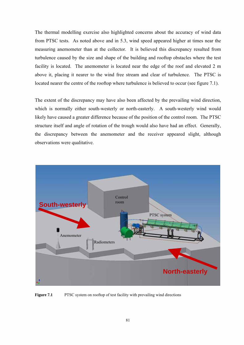
81
Anemometer
The thermal modelling exercise also highlighted concerns about the accuracy of wind data
from PTSC tests. As noted above and in 5.3, wind speed appeared higher at times near the
measuring anemometer than at the collector. It is believed this discrepancy resulted from
turbulence caused by the size and shape of the building and rooftop obstacles where the test
facility is located. The anemometer is located near the edge of the roof and elevated 2 m
above it, placing it nearer to the wind free stream and clear of turbulence. The PTSC is
located nearer the centre of the rooftop where turbulence is believed to occur (see figure 7.1).
The extent of the discrepancy may have also been affected by the prevailing wind direction,
which is normally either south-westerly or north-easterly. A south-westerly wind would
likely have caused a greater difference because of the position of the control room. The PTSC
structure itself and angle of rotation of the trough would also have had an effect. Generally,
the discrepancy between the anemometer and the receiver appeared slight, although
observations were qualitative.
Figure 7.1 PTSC system on rooftop of test facility with prevailing wind directions
Control room
Radiometers
PTSC system
South-westerly
North-easterly

82
The implications of the wind difference for ASHRAE test results were not considered severe,
since wind speed is not a direct factor in any of the calculations, although it is used to
determine whether a test should proceed or not (see 4.2). Since the ASHRAE wind speed
violations were mostly high, any measurement error would have helped bring test conditions
into line with ASHRAE criteria.
Implications for the modelling exercise were more serious since the unshielded receiver is
sensitive to forced convection effects and wind speed is an input to the convective heat
transfer coefficient through the Nusselt number (equations 6.1 to 6.3). The model also
assumes a constant wind velocity although the PTSC may at times have experienced turbulent
gusts. This made it difficult to draw conclusions about the models’ accuracy, although the
scaling factor obtained from figure 6.6 and checked using the data in figure 6.7 suggests heat
loss is properly modelled for the unshielded receiver. Little can be said about the effects of
the wind measurement discrepancy on the glass-shielded model, which is insensitive to wind
and does not appear to account for all heat transfer modes.
Clearly the qualitative analysis above is only a start and further tests are needed to quantify
the differences between the measured wind speed and that experienced by the collector.
These will be undertaken on completion of the project.

83
8. SUMMARY
A parabolic trough solar collector, developed locally for use in a solar thermal research
programme, was tested to characterise its performance. The torque-tube based PTSC was 5 m
long with an aperture width of 1.5 m, a rim angle of 82° and a concentration ratio of 16.7.
The surface consisted of 3M SA-85 aluminised acrylic film on a stainless steel substrate. The
intercept factor of 0.8231 was determined by conducting an optical error analysis. The
collector’s tracking capability consisted of manual adjustment as well as automatic tracking
using the PSA Algorithm to determine the solar vector. Tracking accuracy was 0.144°.
The ASHRAE 93-1986 (RA 91) standard was selected to evaluate performance of the
collector. A comprehensive LabVIEW software application was developed to display and log
real-time radiometric data, PTSC temperatures and solar angles.
Two receivers were tested, one unshielded and the other with an evacuated glass shield to
limit convective heat loss. The absorber tubes were covered with a high-absorptance solar-
selective coating, giving optical efficiencies of 0.601 (unshielded) and 0.553 (glass-shielded)
The peak thermal efficiencies obtained during testing were 55.2 % for the unshielded receiver
and 53.8 % for the glass-shielded unit. Although the unshielded receiver performed better at
ambient fluid temperature, overall heat loss was greater with a measured test slope of
– 2.01 W/m2K versus – 1.06 W/m2K for the glass-shielded receiver. The presence of the
evacuated glass shield reduced the overall heat loss coefficient by 50.2 % producing a 9.2 %
improvement in performance at maximum test temperature. The average collector time
constants were 29.1 s and 27.5 s for the unshielded and glass-shielded receivers respectively.
Acceptance angles were measured at 0.43° (unshielded) and 0.52° (glass-shielded), both of
which were greater than the tracking accuracy (0.144°) indicating that the PTSC operated
within 2 % of its optimum efficiency at all times. The incidence angle modifiers for both
receivers were determined empirically and characterised using polynomial equations. Tests
conducted to determine off-sun heat loss showed the unshielded receiver to be highly
sensitive to wind intensity.

84
As part of the study, performance of the PTSC was simulated using a finite volume heat
transfer model adapted to include forced convection effects. Heat loss was over-predicted at
the measured wind speed of 4.8 m/s, although wind speeds are thought to have been higher at
the weather station than at the collector. The model showed excellent correlation with
experimental data at an adjusted wind speed of 1.5 m/s and confirmed wind-sensitivity in the
absence of the glass shield. The heat transfer model under-predicted heat loss from the glass-
shielded receiver due to the assumption that absorber-glass heat transfer was by radiation
only. Although the results of the simulation exercise suggested a need for some refinement of
the model, it showed potential as a tool for predicting the performance of parabolic trough
solar collectors.

85
9. RECOMMENDATIONS
The following recommendations are made for expanding on the work done in this project.
1. The PTSC fluid circulation system should be improved to enable high-temperature
testing of the collector up to 400 °C. This could be done by installing either a high-
pressure/high-temperature water system or an oil heater. The water option is
preferable because it would also enable the collector to be used for direct steam
generation.
2. Differences between the wind intensity at the edge of the test facility and at other
points on the rooftop need to be quantified. A trial is proposed using a second
anemometer for comparing wind speed under different conditions – to this end a
portable anemometer has already been obtained. This study will help determine the
accuracy of the heat transfer model implemented in chapter 6.
3. Based on the discussion in chapter 7, the heat transfer model of Lamprecht (2000)
should be refined to accurately account for all heat loss mechanisms. Results from
the suggested wind study would be needed before evaluating changes to the model. It
would be interesting to investigate the effects of rooftop turbulence on heat loss from
the receiver.
4. The trough collector offers an excellent opportunity to test new methods of improving
PTSC performance. One possible method is the use of a twisted tape element inside
the absorber tube to promote fluid turbulence and enhance heat transfer from the wall
to the fluid. Kumar and Prasad (2000) report heat transfer improvements of between
18 % and 70 % for twisted tape inserts in a flat-plate solar water heater, albeit at the
cost of a higher pressure drop. Little work has been done relating to similar
experiments on concentrating collectors. The analysis of the effects of a twisted tape
insert in a PTSC is proposed as the subject of future study.
5. The work done in this project to develop a LabVIEW application for monitoring
collector performance presents considerable opportunities. It is recommended that

86
the SCATTAlog programme be expanded into a comprehensive solar collector test
application, enabling the user to run performance tests on different types of collectors,
including domestic solar hot water units, PTSCs (at different orientations) and solar
cookers. Incorporating modified versions of the Parasim software developed by
Lamprecht (2000) would add a further dimension to the programme and enable real-
time comparison between actual and simulated performance.
6. An analysis of the PTSC structure would be of interest. This would take place with
regard to material strength and deformation of the collector and would be useful in
quantifying the magnitudes of optical errors that degrade performance. A finite
element approach would seem appropriate. The strength and deformation
characteristics of the polypropylene ribs would be of particular interest. In this
regard, two unused ribs are available for conducting physical tests.
7. The reflective surface of the PTSC should be replaced, given the weathering that is
starting to occur. After replacement (preferably with a superior reflective material), it
would be advisable to run a series of tests to quantify changes in collector
performance.
8. Though it would present a challenge, it would be greatly beneficial to install a
rotating platform on the rooftop test site for conducting constant angle of incidence
tests. This would considerably expand the capabilities of the solar energy test facility
and shorten the duration of future PTSC test programmes.
9. The radiometric equipment available at the test facility presents an excellent
opportunity to expand the monitoring programme begun in this project. As a starting
point, it is recommended that methods of data collection be improved to conform to
accepted international standards. Collaboration with other researchers in this field
should also be pursued. A step in this direction has already been taken involving
NTNU, but enormous scope exists for data-exchange with other universities and
laboratories.

87
10. It is recommended that a thermal storage component be added to the PTSC project.
With the short-term performance of the collector well defined, the next step would be
to investigate its performance over extended periods. The integration of an energy-
storage system would fit in well and increase the relevance of the research
programme. Research into types of storage media and methods of controlling flow
rate and fluid outlet temperature should be included.
11. It is recommended that special attention be paid to the emergence of advanced
materials that might improve the performance of PTSC components. One such
material is the 3M product Vikuiti, which is a non-metallic composite with
reflectance greater than 97 %. Although it was not designed for outdoor exposure it
shows excellent potential for use on solar collectors, provided it can be protected.
Another such material is Aerogel, an extremely lightweight ceramic with very low
thermal conductivity. Recent research has shown that aerogels can be produced in a
transparent form, leading to their possible use as glass shields in parabolic trough
collectors. Depending on the transmittance, this could eliminate the need for complex
evacuated tubes and seal arrangements.
12. Other areas of potential study linked to this project include:
• Use of the PTSC to initiate a research project in concentrating photovoltaic
collector technology
• The use of shape memory alloys as thermal actuators in solar energy systems
• Alternative methods of solar tracking, including development of an optical
feedback component to the DTCS

88
REFERENCES
Agnihotri O. P. and Gupta B. K. (1981) Solar selective surfaces, John Wiley & Sons, Inc.,
United States
Almanza R., Lentz A. and Jiménez G. (1997) Receiver behavior in direct steam generation
with parabolic troughs, Solar Energy, vol. 61, no. 4, pp. 275-278
ASHRAE (1991) Standard 93-1986 (RA 91) Methods of testing to determine the thermal
performance of solar collectors, American Society of Heating, Refrigerating and Air-
conditioning Engineers, Inc.
Bakos G. C., Adamopoulos D., Soursos M. and Tsagas N. F. (1999) Design and construction
of a line-focus parabolic trough solar concentrator for electricity generation, Proceedings of
ISES Solar World Congress, Jerusalem, p. 16
Blanco-Muriel M., Alarcón-Padilla D. C., López-Moratalla T. and Lara-Coira M. (2001)
Computing the solar vector, Solar Energy, vol. 70, no. 5, pp. 431-441
Brooks M. J. (2005) Development of an outdoor test facility for solar thermal energy research,
In preparation
CIEMAT (2003)
Site: www.ciemat.es/eng/infogral/psolar
Dudley V. E., Evans L. R. and Matthews C. W. (1995) Test results. Industrial Solar
Technology. Parabolic trough solar collector, SAND94-1117, Sandia National Laboratories
Duffie J. A. and Beckman W. A. (1991) Solar engineering of thermal processes, 2nd ed., John
Wiley & Sons, Inc., United States

89
Eck M., Zarza E., Eickhoff M., Rheinländer J., Valenzuela L. (2003) Applied research
concerning the direct steam generation in parabolic troughs, Solar Energy, Article in press,
pp. 1-11
Energy Efficiency and Renewable Energy Network (2003)
Site: www.eere.energy.gov/troughnet
Engineering News Online (2003)
Site: www.engineeringnews.co.za
Geyer M., Lüpfert E., Osuna R., Esteban A., Schiel W., Schweitzer A., Zarza E., Nava P.,
Langenkamp J. and Mandelberg E. (2002) EuroTrough – Parabolic trough collector developed
for cost efficient solar power generation, Paper presented at the 11th Int. Symposium on
Concentrating Solar Power and Chemical Energy Technologies, Zurich
Güven H. M., Mistree F. and Bannerot R. B. (1986) A conceptual basis for the design of
parabolic troughs for different design environments, Journal of Solar Energy Engineering,
vol. 108, pp. 60-66
Güven H. M. and Bannerot R. B. (1986a) Determination of error tolerances for the optical
design of parabolic troughs for developing countries, Solar Energy, vol. 36, no. 6, pp. 535-550
Güven H. M. and Bannerot R. B. (1986b) Derivation of universal error parameters for
comprehensive optical analysis of parabolic troughs, Journal of Solar Energy Engineering,
vol. 108, pp. 275-281
Güven H. M. (1994) Optimization of parabolic trough collector design for varying
manufacturing tolerances using a closed-form expression for intercept factor, Journal of Solar
Energy Engineering, vol. 116, pp. 164-166
Ibrahim S. M. A. (1996) The forced circulation performance of a sun tracking parabolic
concentrator collector, Proceedings of the World Renewable Energy Congress, pp. 568-571

90
Incropera F. P. and DeWitt D. P. (1990) Fundamentals of heat and mass transfer, 3rd Ed.,
John Wiley & Sons, Singapore
Kalogirou S. (1996) Parabolic trough collector system for low temperature steam generation:
design and performance characteristics, Applied Energy, vol. 55, pp. 1-19
Kalogirou S. (1996a) Design and construction of a one-axis sun-tracking system, Solar
Energy, vol. 57, no. 6, pp. 465-469
Kalogirou S., Lloyd S. and Ward J. (1996) A simplified method for estimating intercept factor
of parabolic trough collectors, Proceedings of the fourth World Renewable energy Congress,
Denver, vol. 3, pp. 1782-1786
Kröger D. G. (1998) Air-cooled heat exchangers and cooling towers. Thermal flow
performance evaluation and design, Department of Mechanical Engineering, University of
Stellenbosch, South Africa
Kumar A. and Prasad B. N. (2000) Investigation of twisted tape inserted solar water heaters –
heat transfer, friction factor and thermal performance results, Renewable Energy, vol. 19, pp.
370-398
Lamprecht A. J. (2000) Efficiency improvement of parabolic trough solar collector,
Mechanical Project 478, University of Stellenbosch
Naidoo P. (2005) Intelligent control and tracking of a solar parabolic trough, PhD dissertation,
Nelson Mandela Metropolitan University, In preparation
National Renewable Energy Laboratory (2004)
Site: www.nrel.gov/docs/fy04osti/33211.pdf
Neethling A. (2002) Computer simulation for parabolic trough solar collector, Mechanical
Project 478, University of Stellenbosch

91
Odeh S. D., Morrison G. L. and Behnia M. (1998) Modelling of parabolic trough direct steam
generation solar collectors, Solar Energy, vol. 62, no. 6, pp. 395-406
Price H., Kearney D. (1999) Parabolic-trough technology roadmap: a pathway for sustained
commercial development and deployment of parabolic-trough technology, Technology
workshop of the U.S. Department of Energy and SunLab
Sargent & Lundy LLC Consulting Group (2003) Assessment of parabolic trough and power
tower solar technology cost and performance forecasts, NREL/SR-550-34440, National
Renewable Energy Laboratory
Sayigh A. (1999) Renewable energy – the way forward, Applied Energy, vol. 64, pp. 15-30
Schlaich, J. (1995) The solar chimney: electricity from the sun, Edition Axel Menges,
Stuttgart, Germany
Schott-Rohrglass GmbH (2004)
Site: www.schott.com
SolarPACES (1999)
Site: www.solarpaces.org/publications/sp99_tec
SunLab (2000)
Site: www.energylan.sandia.gov/sunlab/Snapshot/FACILITY.HTM
Stine W. B. and Harrigan R. W. (1985) Solar energy fundamentals and design: with computer
applications, John Wiley & Sons, Inc., United States
Thomas A. (1994) Simple structure for parabolic trough concentrator, Energy Conversion
Management, vol. 35, no. 7, pp. 569-573
U.S. Department of Energy (2004)
Site: www.eere.energy.gov/troughnet/

92
U.S. Naval Observatory (2003)
Site: aa.usno.navy.mil
Walpole R. E. and Myers R. H. (1990) Probability and statistics for engineers and scientists,
4th Ed., Macmillan Publishing Company, Singapore

A1
APPENDIX A
DESIGN AND CONSTRUCTION OF PTSC

A2
A.1 Introduction
The development of PTSCs by universities and institutes for research purposes is well
documented in the literature. For example, Kalogirou (1996) describes the design of a trough
collector with aperture area of 3.5 m2, rim angle of 90° and concentration ratio of 21.2. The
performance of the collector is reported in terms of the recommended ASHRAE 93 procedure
(ASHRAE, 1991). Ibrahim (1996) reports the performance of a multiple-trough collector,
consisting of six connected parabolic troughs, each 1.14 m in length and 0.12 m wide giving a
total aperture area of 0.82 m2. Almanza et al. (1997) successfully produced steam in the
absorber tubes of an existing 29 m long parabolic trough collector of aperture width 2.5 m and
absorber diameter of 25.4 mm. Bakos et al. (1999) describe the construction of a trough with
approximately 12 m2 of aperture area and the capacity to track the sun about two axes. This is
achieved by connecting one end of the parabolic trough to a vertical sliding mechanism and
hinged “turret” or pylon.
Key aspects of the design and construction of the structure, heat collecting elements and
tracking system of this PTSC are briefly described here.
A.2 Collector Structure
The primary objective in the design and construction of this collector was to ensure that the
reflective surface exhibited a stable, accurate parabolic profile. The basics of parabolic
geometry (for example, focal length, rim angle, width and height) are readily available in the
literature and are omitted here. Factors considered in the construction of this PTSC included
optical error tolerance, material cost and availability and manufacturing constraints.
Güven et al. (1986) studied the overall process of parabolic trough design with specific
reference to accommodating multiple objectives and working in different design
environments. They highlighted the need for a design approach that takes into account the
differences between a developed country, like the U.S., and developing nations, where design
objectives are not limited to maximising thermal efficiency, but must also favour cheaper,
labour-intensive design and production techniques. A schematic diagram of this process of is

A3
shown in figure A.1. The macro-level design stage entails specifying the characteristics of the
reflector surface, reflector support structure, receiver and tracking system. In the micro-level
stage these subsystem components are integrated.
Figure A.1 PTSC macro- and micro-level design stages proposed by Güven et al. (1986)
TRACKING SYSTEM DESIGN
• Type of tracker • Tracking mode
MACRO-LEVEL DESIGN: Subsystem design
REFLECTOR DESIGN
Reflective material • Reflectivity • Diffusivity
Supporting Structure • Type of supporting structure • Fabrication method
RECEIVER DESIGN
Type • Evacuated • Non-evacuated
Glazing • Properties
(τ, α, ρ, ε)
Selective Coating • Properties
(α, ε)
MICRO-LEVEL DESIGN: Subsystem Integration
Aperture width
l
ψrim
D

A4
The sequence shown in figure A.1 was followed in the design and construction of this PTSC,
particularly with regard to the use of universal error parameters in the design of the receiver.
Deviations from the process included pre-selecting the rim angle of the collector based on
parabolic-rib material constraints and selection of the receiver glass envelope diameter based
on availability of Schott tubing, not on the optimum calculated gap width between absorber
and glass envelope. These compromises were dictated by material availability and cost and
were unavoidable.
Design alternatives for the PTSC structure-type included truss, torque-tube, torque-box,
stamped profile and moulded fibre-glass structures. The torque-tube structure (see figure A.2)
was selected for simplicity and ease of manufacture.
Figure A.2 PTSC torque-tube collector structure with parabolic ribs
The parabolic ribs were cut from a sheet of polypropylene, to provide the shape of the surface,
in a CAD/CAM process using abrasive water jet machining (AWJ). Figures A.3 to A.5 show
schematics of the rib, the rib attachment method and the collector structure.
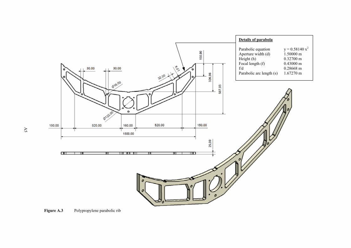
A5
Details of parabola Parabolic equation y = 0.58140 x2 Aperture width (d) 1.50000 m Height (h) 0.32700 m Focal length (f) 0.43000 m f/d 0.28668 m Parabolic arc length (s) 1.67270 m
Figure A.3 Polypropylene parabolic rib
A5

A6
Figure A.4 Parabolic rib attachment method
A6

A7
Figure A.5 PTSC collector structure
A7

A8
Possible alternatives for the reflective surface of the trough included back-silvered thin glass,
bare aluminium, polished stainless steel, aluminised acrylic plastic and advanced composite
coatings. Table A.1 provides a comparison of these alternatives.
Table A.1 Comparison of reflective surface options
Reflective surface Advantages Disadvantages
Back-silvered glass • High reflectance • Load carrying capacity • Surface accuracy independent of
PTSC structure • Good weathering protection
• Very expensive • Specialised equipment needed for
manufacture
Bare aluminium (eg. Alanod MIRO)
• Reflectances up to 95 % possible • Inexpensive • Various gauges available • Lightweight
• No weathering protection • Highly susceptible to abrasion • Requires stable, accurate parabolic
structure
Polished stainless steel • Inexpensive • Various gauges available
• Low reflectance (< 70 %) • Susceptible to abrasion • Requires stable, accurate parabolic
structure
Aluminised acrylic perspex • Reflectance up to 80 % possible • Inexpensive • Lightweight
• Limited weathering protection • Susceptible to abrasion • Requires stable, accurate parabolic
structure and substrate • Deforms easily
Aluminised acrylic film (eg. 3M SA-85)
• Reflectance up to 85 % possible • Relatively inexpensive • Some weathering protection
• Susceptible to abrasion • Requires stable, accurate parabolic
structure and substrate • Out of production
Advanced composite film (eg. 3M Vikuiti)
• Very high reflectance (> 97 %) • Non-metallic composite
• Susceptible to abrasion • Requires stable, accurate parabolic
structure and substrate • No weathering protection • Very expensive
Early tests with aluminised acrylic Perspex showed high levels of surface distortion.
Although it is now out of production, a quantity of SA-85 film was obtained. This was
applied to a stainless steel substrate, which was clamped into the profile formed by the
parabolic ribs, producing a stable and sufficiently rigid surface (see figure A.6). The
clamping system was designed to allow easy swapping of surface sheets for comparative
testing of different materials.

A9
(a) (b)
Figure A.6 (a) stainless steel substrate prior to installation (b) assuming parabolic shape
A.3 Heat Collecting Element
The receiver of a PTSC is that element of the system where solar radiation is absorbed and
converted primarily into heat. It includes the absorber tube through which the heat transfer
fluid flows, the tube transparent cover or envelope, if applicable, and any insulation. In the
case of a parabolic trough, which is defined as a linear imaging concentrator, the receiver is
located so as to coincide with the focal line of the trough (Duffie and Beckman, 1991).
An optical error analysis was used to determine the size of the absorber for this project. The
design and construction of two receivers are briefly described – one unshielded and one with
an evacuated glass envelope.
A.3.1 Optical error analysis
The design of a receiver must include both optical and thermal considerations. If the optical
characteristics of the receiver materials are assumed to be temperature independent, the
optical and thermal analyses can be de-coupled and most of the optical design work carried
out independently (Güven and Bannerot, 1986a). A good starting point is the definition of
collector optical efficiency, which is the ratio of solar energy falling on the surface of the
absorber tube (the inner conduit of the receiver) to that which falls on the reflective surface of
the collector. It can also be expressed as the product of glass cover transmittance, absorber
surface absorptance, collector surface reflectance and the intercept factor.
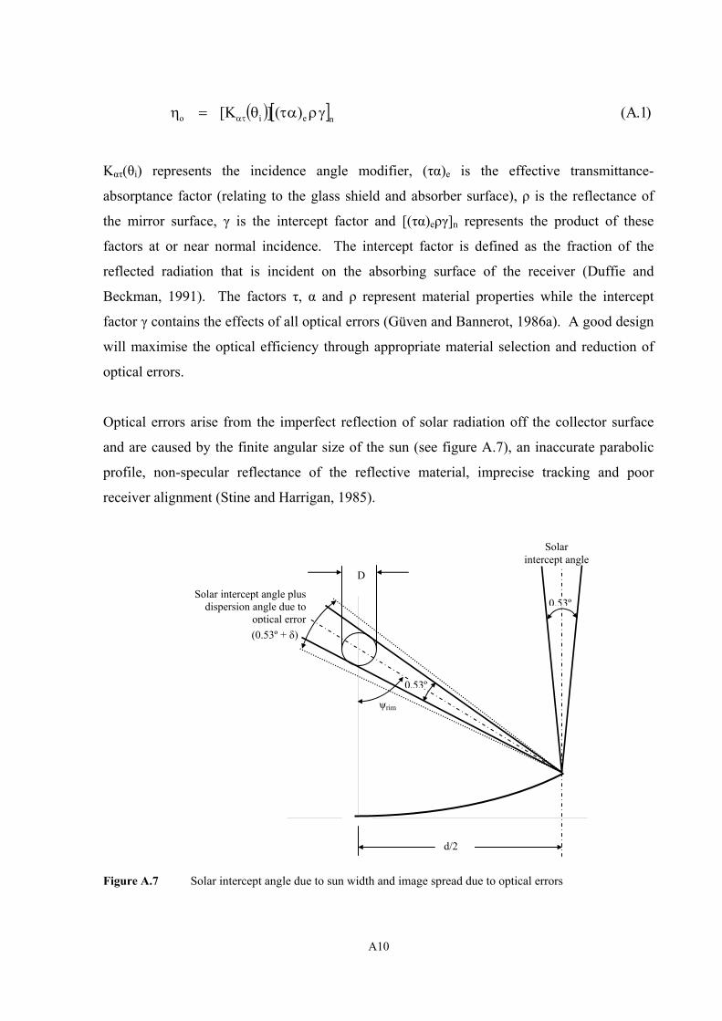
A10
Kατ(θi) represents the incidence angle modifier, (τα)e is the effective transmittance-
absorptance factor (relating to the glass shield and absorber surface), ρ is the reflectance of
the mirror surface, γ is the intercept factor and [(τα)eργ]n represents the product of these
factors at or near normal incidence. The intercept factor is defined as the fraction of the
reflected radiation that is incident on the absorbing surface of the receiver (Duffie and
Beckman, 1991). The factors τ, α and ρ represent material properties while the intercept
factor γ contains the effects of all optical errors (Güven and Bannerot, 1986a). A good design
will maximise the optical efficiency through appropriate material selection and reduction of
optical errors.
Optical errors arise from the imperfect reflection of solar radiation off the collector surface
and are caused by the finite angular size of the sun (see figure A.7), an inaccurate parabolic
profile, non-specular reflectance of the reflective material, imprecise tracking and poor
receiver alignment (Stine and Harrigan, 1985).
Figure A.7 Solar intercept angle due to sun width and image spread due to optical errors
( ) [ ] )1.A()(]K[ neio γρατθ=η ατ
d/2
ψrim
(0.53º + δ)
Solar intercept angle plus
dispersion angle due to optical error
D
Solar
intercept angle
0.53º
0.53º

A11
The absorber tube should be made large enough to capture as much of the reflected solar
energy from the collector surface as possible. Opposing this is the need to minimise absorber
diameter to increase the concentration ratio of the collector and cut thermal losses. Sizing the
absorber thus becomes a compromise between conflicting requirements. The design process
requires knowledge of the intercept factor γ, which in turn requires knowledge of the errors
likely to be encountered with the chosen design, construction method, operating loads and the
tracking system employed.
Two methods are described in the literature for analysing the nature and effect of optical
errors. One treats all optical errors as random and provides a relatively simple method of
determining absorber tube diameter D (‘Method A’). A second separates errors into random
and nonrandom and allows for the calculation of the PTSC intercept factor (‘Method B’). In
this study, both were investigated as part of the HCE design process.
Method A
In the approach followed by Stine and Harrigan (1985), among others, all errors are treated as
independent, random processes with the combined effect determined statistically. Sources of
error, quoted in [mrad], are given as: structural (slope imperfections) σslope, tracking (sensor
and drive non-uniformity) σtracking, receiver misalignment σrec, mirror specular reflectance σrefl,
and sun width or solar intercept angle σsun.
These are either one-dimensional (in the plane of curvature of the parabola) or two-
dimensional (out of the plane of curvature) and combined to give a total optical error σtot as
follows:
( ) ( ) ( ) ( )[ ]
( )
( ) )4.A(]mrad[
)3.A(]mrad[cos
)2.A(]mrad[2
21
2D2
2D1tot
i
21
refl2
sun2
D2
21
2rec
2drive
2sensor
2slopeD1
σ+σ=σ
θσ+σ
=σ
σ+σ+σ+σ=σ

A12
The slope error is doubled to account for the implications of Snell’s Law. The diameter of the
absorber tube D can be determined from a geometrical analysis of image-spread at the focal
point. Thus,
where r is the distance from the reflector surface to the focal point and n is the number of
standard deviations into which the given errors fall (in this approach, the probability
associated with the total sum of optical errors falling within n standard deviations for a
standard normal distribution, is effectively the same thing as the intercept factor). By
increasing n the designer can ensure that a higher percentage of the spread image is
intercepted (n = 1 guarantees interception of 68.27 % of the image, n = 2 guarantees 95.45 %
and n = 3 guarantees 99.73 %). By assuming values for the random errors and selecting a
desired intercept factor (probability), the required absorber tube diameter can be calculated.
The weakness in this approach is the assumption that all errors are random.
The dimensions of the parabolic trough in this project were used to obtain an approximate
absorber diameter from the error analysis of Stine and Harrigan (1985). Based on equation
A.5, figure A.8 shows how the required absorber diameter for this PTSC changes with
variation in the types and magnitudes of optical errors. Four error sets are considered, as
shown in table A.2, ranging from the “best case” scenario (set A1) where the collector
contains no errors other than the sun width, to set A5 representing severe imperfections.
Table A.2 Error sets used to determine absorber diameter in figure A.5
Error Set Description of Errors
A1 (Best case) Sun width only – no other errors
A2 Typical PTSC errors as given by Stine and Harrigan (1985)
A3 Errors as reported by Kalogirou for hand-built fiberglass PTSC (1996)
A4 1° tracking error, other errors typical as per set 2
A5 (Worst case) 1° tracking error, twice the structural errors of Set 2, other errors as per set 2
[ ] )5.A(m2
ntanr2D tot ⎟⎠⎞
⎜⎝⎛ σ
=

A13
0
10
20
30
40
50
60
70
0 5 10 15 20 25 30 35 40 45 50 55 60 65 70 75 80 85 90
ψ (deg)
Abs
orbe
r dia
met
er D
(mm
)
A2
A3
A4
A5
A1
0<ψ<ψrim
ψrim = 82.18°y = 0.5814x2
f = 0.430 mγ = 0.95
Figure A.8 Absorber diameter for γ = 0.95 using error analysis of Stine and Harrigan (1985)
Figure A.8 is plotted for a statistical capture rate (intercept factor) of 95 % of the total solar
radiation falling on the reflector surface. In practice, the absorber diameter must be
determined by considering error effects at the extreme value of ψ, namely the rim angle ψrim
(82.18°), where image spread is greatest.
Assuming errors for the trough in this project similar to those reported by Kalogirou (1996)
for a hand-produced fibreglass trough (set A3), figure A.8 gives a required absorber diameter
of 30 mm, resulting in a geometric concentration ratio of 15.9. For error sets A4 and A5, D
becomes 56 mm and 62 mm respectively. In the best case scenario (set A1) the absorber
diameter for this PTSC would be 7.25 mm and the maximum geometric concentration ratio
65.9.
Method B
In the approach proposed by Güven and Bannerot, (1986b) some optical errors are treated as
random (for example light scattering and reflector waviness) and some as nonrandom (for
example receiver misalignment and an inaccurate parabolic profile). Whereas in Method A
the error values are combined with a chosen intercept factor to generate an absorber diameter,

A14
Method B combines error values (both random and nonrandom) with a chosen absorber
diameter to determine the resulting intercept factor. Because optical errors are dealt with
more realistically in Method B, it is the more accurate approach, although it is more difficult
to implement.
Güven and Bannerot (1986a) argue that not all optical errors are random and although the
assumption of normal distributions throughout simplifies the analysis, it is not valid for all
practical applications. They propose that scattering effects caused by random slope errors and
reflector surface imperfections, as well as transient tracking errors, are random and
consequently have normal distributions that can be grouped together in the random error
parameter σ (Güven and Bannerot, 1986b).
Nonrandom errors include reflector surface profile errors due to distortion, consistent tracking
errors, systematic misalignment of the reflector with respect to the PTSC’s intended
geographic axis and mislocation of the receiver with respect to the reflector. These are treated
as geometric effects. Two independent nonrandom variables are proposed: β in [deg] for the
tracking error and reflector misalignment and (dr)y in [cm] for both the receiver mislocation
and reflector profile imperfections. It is argued that this method provides a much more
realistic approach for:
• one-off projects where errors are not averaged over an entire collector field
• low-technology environments, such as developing countries
The error parameters σ, β and (dr)y are combined with C (concentration ratio) and D (absorber
tube diameter) to yield parameters universal to all collector geometries, as given by equations
A.6 to A.8. σ*, β* and d* are the universal random error parameter in [rad], the universal
nonrandom error parameter due to angular errors in [rad] and the universal nonrandom error
parameter due to receiver mislocation and reflector profile errors (dimensionless)
respectively.

A15
The intercept factor γ is determined numerically using a modified version of the EDEP
(Energy DEPosition) code developed at Sandia. This code is not given in the literature
although Güven and Bannerot (1986b) provide a closed form expression for γ:
Güven (1994) suggests solving equation A.9 by numerical integration (trapezoidal method).
Kalogirou et al. (1996) developed a BASIC computer programme to solve equation A.9 using
the Simpson integration method. They present results from their code and compare these with
results obtained using a trapezoidal integration method, as well as results from the original
EDEP programme. The BASIC programme is found to approximate the EDEP results
closely. The approach adopted for this study was as follows:
1. Establish reasonable estimates for the optical errors likely to be encountered during
construction of the PTSC, as was done in Method A.
2. Use the absorber diameter and concentration ratio from Method A as a starting point
to universalise the random and nonrandom error parameters.
3. Solve equation A.9 for the intercept factor γ using MATLAB code.
4. Investigate the effect of varying error parameters on the intercept factor.
5. Finalise the absorber dimensions, taking into account the results of the analysis,
material cost, availability, strength and concentration ratio effects.
( )( ) ( )( )∫
Ψ
⎢⎢⎣
⎡
⎭⎬⎫
⎩⎨⎧
Ψ+σπΨ+βπ−Ψ−Ψ+Ψ
⋅ΨΨ+
=γ rim
0rim
*rim
**rim
rim
rim
cos12cos1sind21cos1sinerf
sin2cos1
( )( ) ( )( ) ( ) )9.A(
cos1d
cos12cos1sind21cos1sinerf
rim*
rim**
rim
Ψ+Ψ
⎥⎥⎦
⎤
⎭⎬⎫
⎩⎨⎧
Ψ+σπΨ+βπ+Ψ+Ψ+Ψ
−
)8.A(D
)d(d
)7.A(]rad[C
)6.A(]rad[C
yr*
*
*
=
β=β
σ=σ

A16
Since the error parameters in Method B are defined differently to those in Method A, the
literature was consulted to determine reasonable error values for a PTSC constructed under
the type of conditions experienced in this project. Güven et al. (1986) give a table of values
for three PTSC types: a PTSC typical of the high-technology U.S. trough systems and two
lower-technology PTSC types representative of developing country conditions. The
developing country values are not measured but estimated by inflating the U.S. high-
technology data. (As the authors point out, there were no realistic data available regarding
actual hardware for developed countries when the work was published.) These values are
shown in table A.3 along with a further 3 error sets, which were modified error values used as
estimates for this PTSC project.
Table A.3 Error sets used in PTSC analysis of Güven et al. (1986)
Errors given by Güven et al. (1986) Error sets for this PTSC
Parameter U.S. high-
tech PTSC
Developing
country #1
Developing
country #2 Set B1 Set B2 Set B3
σ [rad] 0.0064 0.0087 0.0113 0.0087 0.0113 0.0113
β [deg] 0.25 0.50 1.00 0.50 1.00 0.375
(dr)y [mm] 3.10 6.20 6.20 6.20 6.20 7.75
D [mm] 24.80 24.80 24.80 30.00 30.00 30.00
C 28.00 21.00 16.00 15.92 15.92 15.92
σ* [rad] 0.1792 0.1827 0.1808 0.1385 0.1798 0.1798
β* [rad] 0.1222 0.1833 0.2793 0.1389 0.2778 0.1111
d* 0.125 0.250 0.250 0.2067 0.2067 0.2583
Error set B1 was obtained by using the values from Developing Country #1, together with a
starting absorber diameter of 30.00 mm. Set B2 used the values from Developing Country #2
while set B3 used the same random error value σ as set B2, a reduced tracking and reflector
misalignment error β and a receiver mislocation error (dr)y inflated by 25 % over the
Developing Country #2 case proposed by Güven et al. (1986). The reasons for using these
values were as follows:

A17
• It was anticipated that the tracking system for this PTSC would be more accurate than
Developing Country #1 owing to the use of sophisticated hardware. Thus the value of
β was set midway between the high-technology U.S. case and Developing Country #1
• The set-up of the receiver was undertaken using basic measuring tools, and it was
reasoned that (dr)y would likely be greater given the larger size of the collector
(increasing the chance of surface distortion) compared to research units described in
the literature
• Errors incorporated in σ were likely to be much the same as those proposed by Güven
et al. (1986) since the construction of the PTSC was carried out using a mix of basic
and advanced fabrication methods and materials (for example, water cutting of the
parabolic ribs)
Equation A.9 was solved using a MATLAB programme. The two error function terms in the
integral were solved using MATLAB’s erf function with 0.5° increments. The result was
integrated over the total rim angle value using MATLAB’s trapz trapezoidal numerical
integration function. The MATLAB programme was tested prior to use and all variations of
the basic “paracept.m” code showed good agreement with values calculated by Güven (also
using trapezoidal numerical integration) and reported by Kalogirou et al. (1996). Two of the
computer programmes written for the project are included in appendix B. Table A.4 shows
the results for γ based on error sets B1, B2 and B3 and determined using the “paracept_pt.m”
code. A starting absorber diameter of 30 mm was used from the Method A analysis.
Table A.4 Intercept factor for PTSC with rim angle of 82° and aperture width of 1.5 m
Method B error eets for this PTSC
Parameter Set B1 Set B2 Set B3
D [mm] 30.00 30.00 30.00
C 15.92 15.92 15.92
σ* [rad] 0.1385 0.1798 0.1798
β* [rad] 0.1389 0.2778 0.1111
d* 0.2067 0.2067 0.2583
γ 0.8728 0.6148 0.8231

A18
Results for errors sets 1 and 2 showed a sharp reduction in γ from 0.873 to 0.615 as the
random, tracking and misalignment errors were increased. Error set B3, which was the best
estimate of error parameters for this project, gave an intercept factor of 0.823. This was lower
than the 0.95 assumed in Method A but more realistic given the manner in which the error
parameters were determined.
Figures A.9 and A.10 illustrate how the error parameters σ*, β* and d* combine to degrade γ
as they are increased. The graphs are drawn for a rim angle of 82°, representing the PTSC of
this project.
Figure A.9 Intercept factor γ as a function of β* and d* for σ* = 0.0
The plateau area in figure A.9 shows the PTSC design is fully tolerant of β* and d* values up
to 0.30 and 0.45 respectively with no associated reduction in γ. Below σ* = 0.10 the design
remains tolerant of β* and d* values up to 0.30 and 0.45, with a reduction in γ of only 10 %
from 1.00 to 0.90. The benefit of restricting σ* (through reduction of random slope errors

A19
during construction) was thus a greater tolerance of systematic profile distortion and
misalignment well beyond the levels expected in this project.
Figure A.10 Intercept factor γ as a function of β* and d* for σ* = 0.1798 (error set B3 indicated)
Figure A.10 represents the case for the expected value of σ* = 0.1798. The marker lines for
β* = 0.1111 and d* = 0.2583 indicate the calculated intercept factor of 0.8231. The linearity
and gradient of the contour lines ( 64.0/ ** ≈∂∂ dβ for γ = 0.82) suggested the PTSC design
would be more tolerant of receiver mislocation and reflector profile errors than of tracking
and misalignment errors. Figure A.11 allows the effect of varying σ* to be seen on a single
graph for constant d* = 0.2583. The plateau of figure A.9 where γ remains unaffected by β*
and d* is visible for σ* = 0.00. Also visible is the convergence of the curves for β* ≈ 0.30,
indicating that γ becomes independent of σ* around that value. Figure A.12 shows similar
features for β* = 0.1111, as per error set 3.

A20
0 0.1 0.2 0.3 0.4 0.5 0.6 0.7 0.8 0.9 10
0.1
0.2
0.3
0.4
0.5
0.6
0.7
0.8
0.9
1
Error parameter β*
Inte
rcep
t fac
tor γ
0.0 0.1 0.17980.2 0.3 0.4
d* = 0.2583
σ*
Figure A.11 Intercept factor as a function of β* for fixed d* and six values of σ*
Figure A.12 Intercept factor as a function of d* for fixed β* and six values of σ*
0 0.1 0.2 0.3 0.4 0.5 0.6 0.7 0.8 0.9 10
0.1
0.2
0.3
0.4
0.5
0.6
0.7
0.8
0.9
1
Error Parameter d*
Inte
rcep
t fac
tor γ
0.0 0.1 0.17980.2 0.3 0.4
β* = 0.1111
σ*

A21
To evaluate the choice of collector rim angle equation A.9 was solved for a range of rim
angles from 50° to 130°. The results are shown in figure A.13. Although concentration ratio
is maximised for a rim angle of 90°, the intercept factor increases with increasing rim angle.
For a low rim angle of 50°, the maximum possible intercept factor for this PTSC would have
been approximately 80 % (assuming zero mislocation error). A rim angle of 130° would have
given the best result for γ, but the closeness of the curves for rim angles from 80° to 130°
indicates that for the error set used here, the range of optimum rim angles is wide and the
chosen value of 82° falls within that range. A higher rim angle would therefore have had little
positive effect on the intercept factor.
Figure A.13 Intercept factor as a function of d* for fixed β* and σ* and six rim angles
Figure A.14 illustrates the relationship between intercept factor and absorber diameter D for
β* = 0.1111, σ* = 0.1798 and a range of receiver mislocation values (dr)y. The concentration
ratio (C) is also shown. Maximising both C and γ results in opposing requirements, since
reducing the diameter to increase C necessarily implies intercepting less reflected energy from
0 0.1 0.2 0.3 0.4 0.5 0.6 0.7 0.8 0.9 10
0.1
0.2
0.3
0.4
0.5
0.6
0.7
0.8
0.9
1
d* = (dr)y/D
Inte
rcep
t fac
tor γ
50o 70o 82o 90o 110o
130o
σ* = 0.1798β* = 0.1111
ψrim
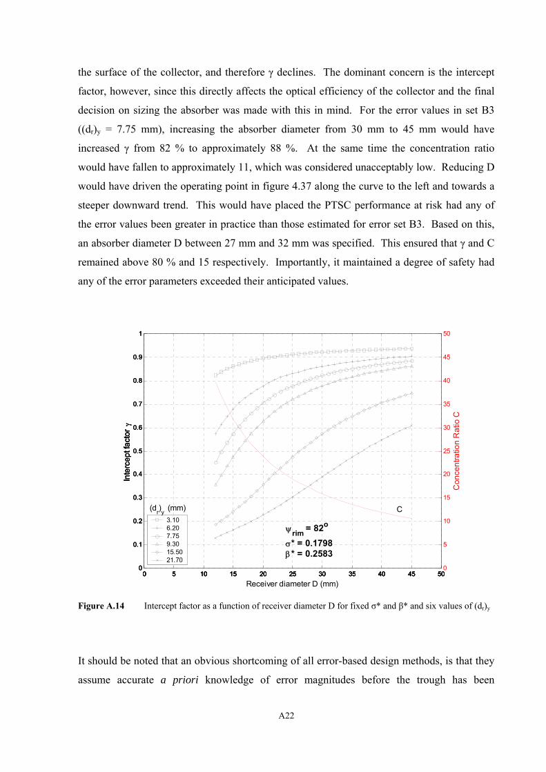
A22
the surface of the collector, and therefore γ declines. The dominant concern is the intercept
factor, however, since this directly affects the optical efficiency of the collector and the final
decision on sizing the absorber was made with this in mind. For the error values in set B3
((dr)y = 7.75 mm), increasing the absorber diameter from 30 mm to 45 mm would have
increased γ from 82 % to approximately 88 %. At the same time the concentration ratio
would have fallen to approximately 11, which was considered unacceptably low. Reducing D
would have driven the operating point in figure 4.37 along the curve to the left and towards a
steeper downward trend. This would have placed the PTSC performance at risk had any of
the error values been greater in practice than those estimated for error set B3. Based on this,
an absorber diameter D between 27 mm and 32 mm was specified. This ensured that γ and C
remained above 80 % and 15 respectively. Importantly, it maintained a degree of safety had
any of the error parameters exceeded their anticipated values.
0 5 10 15 20 25 30 35 40 45 500
0.1
0.2
0.3
0.4
0.5
0.6
0.7
0.8
0.9
1
Receiver diameter D (mm)
Inte
rcep
t fac
tor γ
3.10 6.20 7.75 9.30 15.5021.70
0 5 10 15 20 25 30 35 40 45 500
0.1
0.2
0.3
0.4
0.5
0.6
0.7
0.8
0.9
1
Inte
rcep
t fac
tor γ
3.10 6.20 7.75 9.30 15.5021.70
0 5 10 15 20 25 30 35 40 45 500
0.1
0.2
0.3
0.4
0.5
0.6
0.7
0.8
0.9
1
Inte
rcep
t fac
tor γ
3.10 6.20 7.75 9.30 15.5021.70
0 5 10 15 20 25 30 35 40 45 500
5
10
15
20
25
30
35
40
45
50
Con
cent
ratio
n R
atio
C
ψrim = 82o
σ* = 0.1798 β* = 0.2583
(dr)y (mm) C
Figure A.14 Intercept factor as a function of receiver diameter D for fixed σ* and β* and six values of (dr)y
It should be noted that an obvious shortcoming of all error-based design methods, is that they
assume accurate a priori knowledge of error magnitudes before the trough has been

A23
constructed. Since very limited data are available for PTSCs built in developing countries,
the results obtained for γ, while useful, remain only an approximation. In summary:
• For the error values expected in this project (random and nonrandom) the intercept
factor γ was 82.3 %, a reduction from 95 % as determined using the less rigorous
method based on random errors only
• By solving equation A.9 for variations in σ*, β* and d*, it was possible to identify
trends in the behaviour of γ using 3-dimensional and 2-dimensional visualisation
• The region in which the PTSC was expected to operate, showed no serious sensitivity
of γ with regards σ*, β* and d*
• The proposed PTSC design was more tolerant of receiver mislocation and reflector
profile errors than of tracking and misalignment errors
• The intercept factor showed a relatively weak dependence on random errors
• The closeness of the γ-curves for rim angles from 80° to 130° indicated that the range
of optimum rim angles was wide and included the value of 82° chosen for this PTSC
• An absorber diameter of between 27 mm and 32 mm ensured the intercept factor γ
remained above 80 % and the concentration ratio above 15
A.3.2 Receiver design
Almanza et al. (1997) showed that steel receivers can bend during operation due to poor
thermal conduction and the creation circumferential thermal gradients. They changed their
design material to copper. For similar reasons copper was used in this project. The only
grade of SABS tubing that fell within the range of diameters determined from the optical error
analysis had an outer diameter of 28.58 mm and wall thickness of 1.02 mm. The resulting
concentration ratio of the PTSC was 16.70.
To measure the performance of the PTSC, two lengths of piping were designed to
accommodate TC probes and pressure gauges, one for each end of the receiver. These were
coupled to the absorber tubes via flanges so that they could be disconnected and left in place
should the receivers need to be switched. These instrumentation sections were held in
position by additional ring holders. They formed the connection between the receiver and the
flexible hydraulic hosing at each end of the PTSC.

A24
The glass tube of the shielded receiver was manufactured by a chemical glass blower using 4
lengths of Schott Duran borosilicate glass tubing with transmittance of 0.92 and refractive
index of 1.473 (Schott, 2004). Each tube had an outer diameter of 44.0 mm, wall thickness of
2.3 mm and length of 1500 mm. This left an annular gap between the absorber and the glass
envelope of 5.4 mm, which was the best possible geometry given the diameter of the absorber
and the available glass dimensions. The shield was produced in a glass-working lathe with a
total length of 5380 mm and a single vent located 50 mm from one end for drawing a vacuum
(vent dimensions: length = 15 mm, internal diameter = 7 mm).
A double o-ring arrangement was fabricated to seal the annular gap between the inner
absorber tube and the outer glass cylinder of the shielded receiver. A narrow sleeve
containing two machined grooves, forming a double-seat, was soldered on to the absorber at
each end. Two high-temperature Viton o-rings were slid over the edge of the sleeve and into
the recesses formed by the grooves. The o-rings were selected to make contact with the inner
surface of the glass envelope when it was slid into position over the absorber, closing the
annular gap between the glass and the copper absorber. The arrangement formed a flexible,
airtight seal that allowed for expansion of the copper absorber tube within the glass cylinder.
Sketches showing the dimensions of the PTSC receiver and the instrumentation sections are
shown in figure A.15. Figure A.16 shows the receiver in place on the trough collector, with
the surface of the collector removed. A sketch of one of the ring holders is also shown with
its positioning bolts cradling the shielded receiver. Figure A.17 shows the vacuum seal
arrangement for the shielded receiver.

A25
(a)
(b)
(c)
Pressure gauge TC probe
Receiver
(d)
Flange
Figure A.15 (a) general dimensions of receiver (b) receiver drive end (c) non-drive end with instrumentation sections (d) three-dimensional view of drive end
instrumentation section
A25
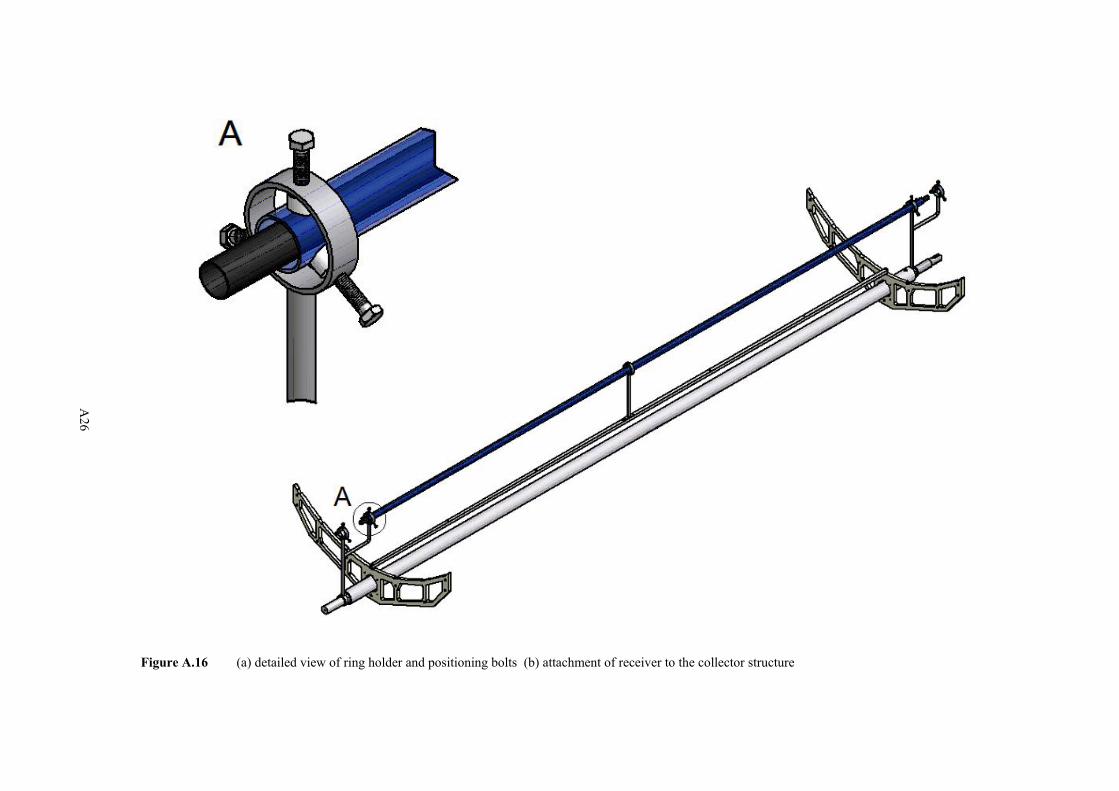
A26
Figure A.16 (a) detailed view of ring holder and positioning bolts (b) attachment of receiver to the collector structure
A26
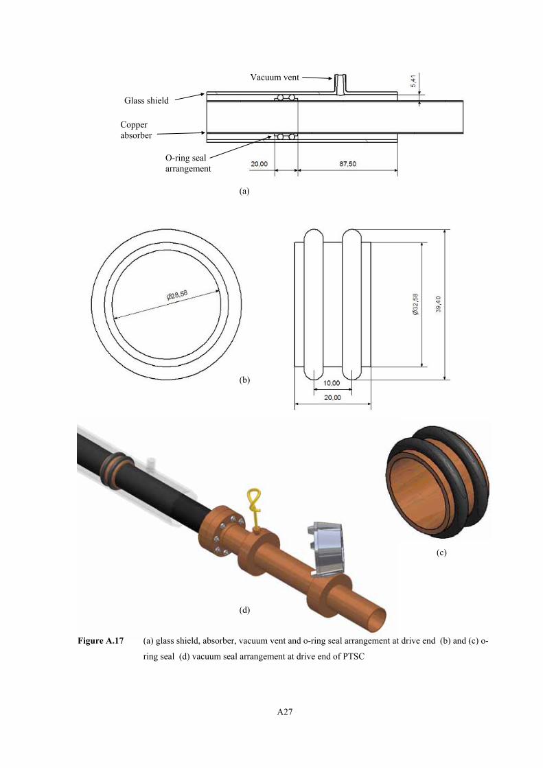
A27
(d)
(a)
(b)
Glass shield
Copper absorber
Vacuum vent
O-ring seal arrangement
(c)
Figure A.17 (a) glass shield, absorber, vacuum vent and o-ring seal arrangement at drive end (b) and (c) o-
ring seal (d) vacuum seal arrangement at drive end of PTSC

A28
Most PTSC absorbers are coated with a low-emittance/high-absorptance selective coating to
improve performance. Such a coating was sought, first by experimenting with chemical
conversion of the outer surface of the copper tubing, and secondly by application of a
commercial spray. Attempts to produce a lasting, absorber-reflector tandem on copper tube
samples under laboratory conditions, were not successful. In the first attempt, samples of
copper tube were cleaned with acetone and immersed in a commercial solution of ammonium
sulphide (NH4S) to produce a black copper sulphide (Cu2S) coating. The samples were
exposed to the sulphide solution for increasing periods of time to test the surface quality.
Figure A.18 (a) shows five of the test pieces. Severe peeling of the coating is visible on three
of the tubes. Best results were obtained for a tube exposed to the chemical solution for a
period of 40 s. This coating appeared reasonably stable though the initial dark, velvet finish
was easily rubbed off. The long-term durability of the coating remained questionable.
Thermal emittance results were disappointing with none of the samples giving a value below
0.72 up to temperatures of 100 °C. The value of emittance (0.20) reported by Agnihotri and
Gupta (1981) could not be reproduced and no South African laboratory could be found to test
solar absorptance (α), which the above authors give as 0.79.
(a) (b)
Figure A.18 (a) Samples of tube with Cu2S coating obtained after exposure to NH4S for (left to right) 20 s,
40 s, 60 s, 120 s and 5 min (b) CuO surface coating showing blue-black finish
Attempts were made to produce a copper oxide (CuO) film on sample tubes by immersing
them in a bath of sodium hydroxide (NaOH) and sodium chloride (NaCl) at approximately

A29
140 °C for between 3 min and 13 min. These were only partially successful. Whereas the
Cu2S film had appeared matt-black, the CuO treatment produced only a blue-black surface
that was still mostly reflective. The samples were tested for emittance and showed a value of
0.29 at 90 °C, though this was probably due to the weak surface coating. Figure A.18 (b)
shows a length of copper tube with the CuO coating applied.
A solution to the coating problem was found with a commercial product called Solkote
Hi/Sorb II (Solkote). This is a spray-on liquid specially formulated for solar thermal
applications, giving a tested emittance of 0.28 to 0.49 and absorptance of 0.88 to 0.94.
Advantages included easy application to the copper absorbers using a standard spray gun,
good long-term stability and excellent optical properties (including published values for
emittance and absorptance).
A.4 Drive, Tracking and Control System (DTCS)
A brief description is given of the design and implementation of a drive, tracking and control
system for the PTSC. This was a collaborative work between the author and Naidoo (2005).
The author’s responsibilities included specifying DTCS requirements selecting the tracking
methodology, selecting and analysing a suitable tracking algorithm and specifying the drive
hardware.
The requirements of the tracking system were:
• To control the PTSC so as to track the sun accurately about a single axis
• To offer sufficient flexibility to the operator of the system so as to enable the full array
of PTSC performance tests to be completed
• To ensure safe operation of the PTSC
• To be upgradeable in time from a pure tracking system to a fully functional control
system
Linear imaging concentrators can be tracked about one axis (single-axis tracking) or two axes
(double-axis tracking) though in practice, two-axis tracking is not feasible for commercial
systems of great length. They are normally aligned along a true north-south (N-S) line or a
true east-west (E-W) line, though any alignment is technically possible. In deciding on the

A30
alignment, primary concerns are the amount of energy captured over the course of a year and
the demands of the market. For example, in the SEGS plants, the collectors are aligned N-S,
which results in slightly less energy captured over a year, but which favours summertime
operation when peak power is needed and its sale brings the greatest revenue (Duffie and
Beckman, 1991).
The amount of energy captured is largely a function of seasonal changes in sun strength and
its angle of incidence (θi), which is the angle between the sun’s rays and a normal to the
collector aperture, when the collector is in focus. Figure A.19 illustrates how θi changes
seasonally for a PTSC aligned N-S and located at the solar energy test facility at Mangosuthu
Technikon.
Figure A.19 Schematic diagram of incidence angle θi at solar noon on solstices and equinoxes for a PTSC
located in Durban, South Africa, and aligned in the N-S direction (adapted from Stine and
Harrigan, 1985)
E
W
N S Tracking axis
ρ (Tracking angle)
Normal
θi
22 Dec θi = 6.52°
20 Mar/23 Sept θi = 29.97°
21 Jun θi = 53.42°

A31
Values of θi less than zero are possible for Durban during the summer months due to the sun’s
apparent motion around the outside of an angled disc whose centre shifts along an axis
inclined to the horizon by the latitude angle, pointing toward Polaris. Thus in mid-summer
the sun will rise behind a Durban-based observer who faces north, only to appear slightly
north of the observer at solar noon.
Consideration of the effects of θi is important because PTSC performance is negatively
affected as θi increases. (This effect is quantified in equations A.1 and 4.1.) It was decided to
align this PTSC along an N-S line for the following reasons:
• More stable daily test conditions are possible with respect to θi with an N-S orientation
• Although θi changes throughout the day for N-S aligned collectors, this change is less
in magnitude than for E-W alignment and the change is relatively slow so that test
results are negligibly affected
• The rate of change in angle of incidence for E-W aligned collectors throughout the day
is much greater and obtaining test results for a specific angle of incidence is difficult
The operating modes specified in the design of the DTCS are summarised in table A.5.
Table A.5 Operating modes for the DTCS
1 a Jog left slow Manual positioning using on/off switch
1 b Jog left fast Manual positioning using on/off switch
1 c Jog right slow Manual positioning using on/off switch
1 d Jog right fast Manual positioning using on/off switch
2 Fixed rate tracking PLC instructs motor to switch on and off to maintain fixed angular velocity of 0.25 °/min
3 PSA tracking
PLC instructs motor to turn through a calculated number of pulses on the encoder to locate the sun using the PSA algorithm. Motor switches on and off to maintain focus according to PSA algorithm
4 Stop/park Stop all operations and hold as is
Mode Trough Response Description

A32
To ensure a level of tracking accuracy consistent with the value of the error parameter β
adopted in A.3.1, a maximum tracking error of 0.2° was assumed. This was in line with the
tracking system described by Kalogirou (1996a) for a smaller research trough. (In table A.3
the value of β was set at 0.375° which includes an allowance for misalignment as well as
tracking error.)
For Mode 2, or fixed rate tracking, a control scheme was developed by considering the motion
of the sun relative to the PTSC. Figure A.20 shows the sun’s movement from A through B to
C and the development of the tracking error as the collector stands still between corrective
steps.
Figure A.20 Development of tracking error as sun moves through PTSC focus
The collector is correctly focused in position B. For a tracking error of 0.2° either side of B,
the trough can be positioned ahead (west) of the sun at A and left standing until the sun moves
through a total of 0.4° which would take 96 s. Once the sun reaches C, the DTCS must rotate
the trough west through 0.4° to reposition for A. The process is therefore a series of discrete,
corrective movements through a fixed angle.
For the rotary encoder used, a rotational movement of 0.4° equated to 2.79 pulses (0.144
°/pulse). Trough corrections were therefore made with 2 pulses to ensure that the maximum
A
A
B
B
C
C
0.2°
Sun moves at 0.25°/min
PTSC rotation
0.2°

A33
misalignment error was not exceeded. This required a trough angular speed of 0.288/4 =
0.072 °/s for a VSD/motor “on-time” of 4 s. Working back through the drive train, the
gearbox input speed (equal to the VSD output speed) would be 33.34 °/s or 5.56 rev/min. The
time interval between corrective steps was therefore (0.288/0.25)60 = 69.12 s, minus the 4 s
required for the trough to rotate into its new position, that is, 65.12 s.
The following is noted:
• Provided the angular error limit of 0.2° was not exceeded, many other combinations of
VSD switching-rate and “on-time” would have given the same overall result
• The analysis provided target values for drive speed and motor on-time during the
design of the system. Because of added factors such as the VSD ramp time and other
drive settings, the values were modified during testing. Counting pulses (instead of
time) during each corrective tracking step was found to offer better accuracy (see
5.2.1)
Virtual tracking of the PTSC was accomplished using the PSA Algorithm. This was
developed by workers at the Plataforma Solar de Almeria (Blanco-Muriel et al., 2001). The
only inputs to the calculation are geographic latitude and longitude (entered in degrees) and
Universal Time in year, month, day, hours, minutes and seconds. The algorithm proceeds
through the following steps:
• Calculate the Julian Day
• Determine the ecliptic coordinates of the sun
• Convert ecliptic coordinates to celestial coordinates
• Convert celestial coordinates to horizontal Earth-based coordinates and
output the solar vector consisting of azimuth and zenith angles (A and θz)
Figure A.21 illustrates the relationship between a PTSC aligned in the N-S direction and the
angles A, θz and ρT. Sixteen computations are performed to determine the solar vector,
consisting of the solar azimuth and zenith angles.

A34
Figure A.21 Schematic diagram of the solar vector (θz and A) and tracking angle (ρ) for an N-S aligned
PTSC rotated through ρT degrees to the east
To ensure correct implementation of the PSA Algorithm, a number of MATLAB programmes
were written and the output compared with an online software product of the United States
Naval Observatory (USNO) called the Multi-Year Interactive Computer Almanac (MICA),
which gives solar data accurate to within half a second of arc (U.S. Naval Observatory, 2003).
Results showed that the MATLAB code ran without error (see appendix C). The code was
implemented on the system PLC by Naidoo (2005) to enable Mode 3 tracking.
A.5 Summary
The key features of the PTSC system designed and constructed for this project are presented
in table A.6, together with a brief summary of motivating factors.
Normal to PTSC
Vertical
Sun
Tracking axis
ρT
θz
A
E
W
N
S
Solar vector
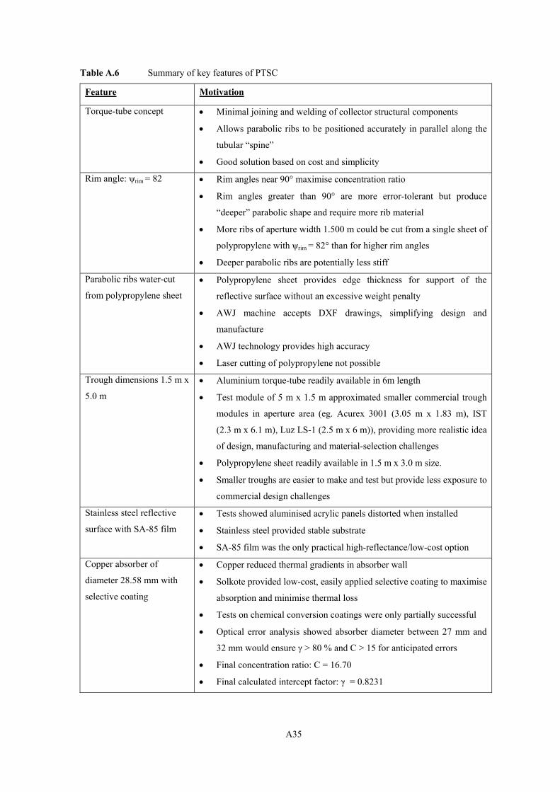
A35
Table A.6 Summary of key features of PTSC
Feature Motivation
Torque-tube concept • Minimal joining and welding of collector structural components
• Allows parabolic ribs to be positioned accurately in parallel along the
tubular “spine”
• Good solution based on cost and simplicity
Rim angle: ψrim = 82 • Rim angles near 90° maximise concentration ratio
• Rim angles greater than 90° are more error-tolerant but produce
“deeper” parabolic shape and require more rib material
• More ribs of aperture width 1.500 m could be cut from a single sheet of
polypropylene with ψrim = 82° than for higher rim angles
• Deeper parabolic ribs are potentially less stiff
Parabolic ribs water-cut
from polypropylene sheet
• Polypropylene sheet provides edge thickness for support of the
reflective surface without an excessive weight penalty
• AWJ machine accepts DXF drawings, simplifying design and
manufacture
• AWJ technology provides high accuracy
• Laser cutting of polypropylene not possible
Trough dimensions 1.5 m x
5.0 m
• Aluminium torque-tube readily available in 6m length
• Test module of 5 m x 1.5 m approximated smaller commercial trough
modules in aperture area (eg. Acurex 3001 (3.05 m x 1.83 m), IST
(2.3 m x 6.1 m), Luz LS-1 (2.5 m x 6 m)), providing more realistic idea
of design, manufacturing and material-selection challenges
• Polypropylene sheet readily available in 1.5 m x 3.0 m size.
• Smaller troughs are easier to make and test but provide less exposure to
commercial design challenges
Stainless steel reflective
surface with SA-85 film
• Tests showed aluminised acrylic panels distorted when installed
• Stainless steel provided stable substrate
• SA-85 film was the only practical high-reflectance/low-cost option
Copper absorber of
diameter 28.58 mm with
selective coating
• Copper reduced thermal gradients in absorber wall
• Solkote provided low-cost, easily applied selective coating to maximise
absorption and minimise thermal loss
• Tests on chemical conversion coatings were only partially successful
• Optical error analysis showed absorber diameter between 27 mm and
32 mm would ensure γ > 80 % and C > 15 for anticipated errors
• Final concentration ratio: C = 16.70
• Final calculated intercept factor: γ = 0.8231

A36
Table A.6 (Continued) Summary of key features of PTSC
Feature Motivation
Glass-shielded and
unshielded receivers
• Creating shielded and unshielded receivers allowed for comparison
between their performance
Optical properties • SA-85 surface reflectance ρ = 0.83
• Schott glass shield transmittance τ = 0.92
• Solkote surface absorptance α = 0.88 and thermal emittance ε = 0.49
• Optical efficiencies: 0.601 (unshielded) and 0.553 (glass-shielded)
Water circulation system
with test flow rate 300 L/hr
• Required flexible system to test PTSC according to principles of
ASHRAE 93 standard (1991)
• Two-tank system enabled high temperature water supply to PTSC
• Flow rate of 300 L/hr ensured turbulent flow and reasonable residence
time in receiver
Positive displacement
pump with VSD on motor
• Helical element pump ensured good performance with regard to flow
rate versus pressure in the required operating range
• VSD permitted accurate, uncomplicated control of flow rate for testing
at reasonable cost
Tracking system with
multiple modes of
operation
• Manual control of PTSC as well as automatic tracking necessary for
completion of collector tests
• PSA algorithm highly accurate, relatively simple to implement and
superior to existing numerical algorithms
Drive system with AC
motor, VSD and PLC
• AC motor provided greater flexibility when coupled to VSD than
alternative systems using stepper motors or DC drives
• VSD and PLC combination expanded capabilities of system to enable
future development of DTCS based on intelligent control principles

B1
APPENDIX B
MATLAB CODE FOR PTSC INTERCEPT FACTOR
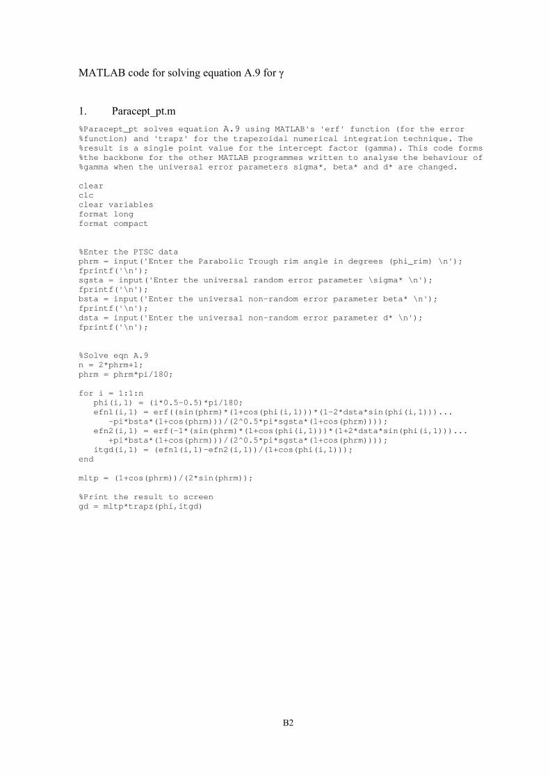
B2
MATLAB code for solving equation A.9 for γ
1. Paracept_pt.m %Paracept_pt solves equation A.9 using MATLAB's 'erf' function (for the error %function) and 'trapz' for the trapezoidal numerical integration technique. The %result is a single point value for the intercept factor (gamma). This code forms %the backbone for the other MATLAB programmes written to analyse the behaviour of %gamma when the universal error parameters sigma*, beta* and d* are changed. clear clc clear variables format long format compact %Enter the PTSC data phrm = input('Enter the Parabolic Trough rim angle in degrees (phi_rim) \n'); fprintf('\n'); sgsta = input('Enter the universal random error parameter \sigma* \n'); fprintf('\n'); bsta = input('Enter the universal non-random error parameter beta* \n'); fprintf('\n'); dsta = input('Enter the universal non-random error parameter d* \n'); fprintf('\n'); %Solve eqn A.9 n = 2*phrm+1; phrm = phrm*pi/180; for i = 1:1:n phi(i,1) = (i*0.5-0.5)*pi/180; efn1(i,1) = erf((sin(phrm)*(1+cos(phi(i,1)))*(1-2*dsta*sin(phi(i,1)))... -pi*bsta*(1+cos(phrm)))/(2^0.5*pi*sgsta*(1+cos(phrm)))); efn2(i,1) = erf(-1*(sin(phrm)*(1+cos(phi(i,1)))*(1+2*dsta*sin(phi(i,1)))... +pi*bsta*(1+cos(phrm)))/(2^0.5*pi*sgsta*(1+cos(phrm)))); itgd(i,1) = (efn1(i,1)-efn2(i,1))/(1+cos(phi(i,1))); end mltp = (1+cos(phrm))/(2*sin(phrm)); %Print the result to screen gd = mltp*trapz(phi,itgd)

B3
2. Paracept3d3D.m %Paracept3d2D and Paracept3d3D generate solutions to the closed-form expression %for gamma as given by Guven et al. (1986) and shown in equation A.9. The user %enters a value for sigma* and the programme produces a solution for gamma in %terms of d* and beta*. The graph is a 3-dimensional contour plot (the 2-D plot %is obtained using paracept3d2D). Vector V must be defined so as to enable manual %annotation of the countour lines shown. clear clc clg clear variables format long format compact %Enter the magnitude of the random error, sigma*. sgsta = 0.0; phrm = 82; n = 2*phrm+1; phrm = phrm*pi/180; [X,Y] = meshgrid(0:0.05:1,0:0.05:1); %Solve equation A.9 for a range of beta* and d* values, using the trapezoidal %numerical integration method. (The 'trapz' and 'erf' MATLAB functions are used.) for j = 1:1:21 bsta = 0.05*j-0.05; for k = 1:1:21 dsta = 0.05*k-0.05; for i = 1:1:n phi(i,1) = (i*0.5-0.5)*pi/180; efn1(i,1) = erf((sin(phrm)*(1+cos(phi(i,1)))*(1-2*dsta*... sin(phi(i,1)))-pi*bsta*(1+cos(phrm)))/(2^0.5*pi*sgsta*(1+cos(phrm)))); efn2(i,1) = erf(-1*(sin(phrm)*(1+cos(phi(i,1)))*(1+2*dsta*... sin(phi(i,1)))+pi*bsta*(1+cos(phrm)))/(2^0.5*pi*sgsta*(1+cos(phrm)))); itgd(i,1) = (efn1(i,1)-efn2(i,1))/(1+cos(phi(i,1))); end mltp = (1+cos(phrm))/(2*sin(phrm)); gd(j,k,2) = mltp*trapz(phi,itgd); end end Z = gd(:,:,2); %Enter the range of values for manually annotating the contour lines v = [0.1 0.2 0.3 0.4 0.5 0.6 0.7 0.8 0.9 1.0]; %Plot the contour lines of the surface solution [C,h] = contour3(X,Y,Z,v) set(gca,'FontSize',10); clabel(C,h,'manual') axis([0 1 0 1 0 1]) surface(X,Y,Z,'EdgeColor',[.8 .8 .8],'FaceColor','none') xlabel('d*','FontSize',13) ylabel('\beta*','FontSize',13) zlabel('Intercept factor \gamma*','FontSize',13) title('Intercept factor \gamma as a function of d* and \beta*','FontSize',14) colormap winter %Set the 3-dimensional viewing position az = 120; el = 45; view(az, el);

C1
APPENDIX C
THE PSA ALGORITHM: CALCULATIONS AND DATA
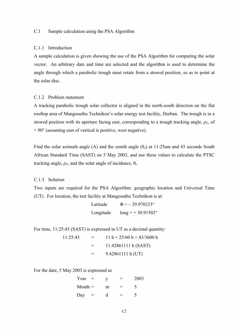
C2
C.1 Sample calculation using the PSA Algorithm
C.1.1 Introduction
A sample calculation is given showing the use of the PSA Algorithm for computing the solar
vector. An arbitrary date and time are selected and the algorithm is used to determine the
angle through which a parabolic trough must rotate from a stowed position, so as to point at
the solar disc.
C.1.2 Problem statement
A tracking parabolic trough solar collector is aligned in the north-south direction on the flat
rooftop area of Mangosuthu Technikon’s solar energy test facility, Durban. The trough is in a
stowed position with its aperture facing east, corresponding to a trough tracking angle, ρT, of
+ 90° (assuming east of vertical is positive, west negative).
Find the solar azimuth angle (A) and the zenith angle (θz) at 11:25am and 43 seconds South
African Standard Time (SAST) on 5 May 2003, and use these values to calculate the PTSC
tracking angle, ρT, and the solar angle of incidence, θi.
C.1.3 Solution
Two inputs are required for the PSA Algorithm: geographic location and Universal Time
(UT). For location, the test facility at Mangosuthu Technikon is at:
Latitude Φ = – 29.970233°
Longitude long = + 30.91502°
For time, 11:25:43 (SAST) is expressed in UT as a decimal quantity:
11:25:43 = 11 h + 25/60 h + 43/3600 h
= 11.42861111 h (SAST)
= 9.42861111 h (UT)
For the date, 5 May 2003 is expressed as
Year = y = 2003
Month = m = 5
Day = d = 5

C3
With the input values established in the correct format, the PSA Algorithm is implemented:
1. Calculate the Julian Day:
jd = (1461(y + 4800 + (m – 14)/12))/4
+ (367(m – 2 – 12((m – 14)))/12
– (3((y + 4900 + (m – 14)/12)/100))/4
+ d – 32075 – 0.5 + hour/24.0 (C1)
= 2 452 764.893 days
Note: Every division in the above equation, except the last, is an integer division.
This means that decimal fractions left over from any of the internal division terms,
except the last, are dropped. For example, in the first line (m – 14)/12 = (5 – 14)/12 =
– 0.75 = 0. Extreme care must be exercised in applying equation C1.
2. Compute the ecliptic coordinates of the sun, noting that all angles are in radians:
n = jd – 2451545.0 (C2)
= 1219.89286
Ω = 2.1429 – 0.0010394594(n) (C3)
= 0.87487139 rad
L (mean longitude) = 4.8950630 + 0.017202791698(n) (C4)
= 25.880624491 rad
g (mean anomaly) = 6.2400600 + 0.0172019699(n) (C5)
= 27.22461916 rad
l (ecliptic longitude) = L + 0.03341607sin(g)
+ 0.00034894sin(2g) – 0.0001134
– 0.0000203sin(Ω) (C6)
= 25.90917575 rad
ep (obliquity of the ecliptic) = 0.4090928 – 6.2140 x 10⁻⁹(n)

C4
+ 0.0000396cos(Ω) (C7)
= 0.4091106 rad
3. Convert ecliptic to celestial coordinates:
ra (right ascension) = atan[cos(ep)sin(l)/cos(l)] (C8)
= 0.73346270 rad
δ (declination) = asin[(sin(ep))(sin(l))] (C9)
= 0.28249216 rad
4. Convert celestial to horizontal coordinates:
gmst (Greenwich mean sidereal time) = 6.6974243242
+ 0.0657098283(n) + hour (C10)
= 96.28498544 h
lmst (local mean sideral time) = (gmst(15) + long)(π/180) (C11)
= 25.74691913 h
Note: “long” is entered in degrees, not radians.
ω (hour angle) = lmst – ra (C12)
= 25.01345643 rad
θz (zenith angle) = acos[cos(Φ)cos(ω)cos(δ) + sin(δ)sin(Φ)] (C13)
= 0.81373639 rad
Note: For the geometric arguments in eqn. C13, Φ is entered in degrees, the others are
entered in radians.
A (solar azimuth) = atan[(-sin(ω))/(tan(δ)cos(Φ) – sin(Φ)cos(ω))] (C14)
= 0.15788706 rad
Parallax = (Earth Mean Radius)/(Astronomical Unit)sin(θz) (C15)
= (6371.01 km)/(149597890 km)sin(0.813736392)
= 0.00003096 rad

C5
θz = θz + Parallax (C16)
= 0.81376735 rad
The calculation of a corrected zenith angle concludes the PSA Algorithm. For a tracking
PTSC, the results from the algorithm can be combined to obtain the angle of incidence or a
tracking angle through which the trough must be turned to intercept the sun.
C.1.4 Calculation of the collector tracking angle, ρT
For a horizontal collector orientated in the north-south direction, Stine and Harrigan (1985)
give the following equation for determining the tracking angle ρT:
tan ρT = sin(A)/tan(90 – θz) (C17)
Thus for this example, ρT = atan[sin(A)/tan(π/2 – θz)]
= atan[(sin(0.157887058)/tan(π/2 – 0.813767347)]
= + 0.16490476 rad
= + 9.448347°
Since the trough is currently pointing east with ρT = + 90°, the angle through which the trough
must be rotated in order to intercept the sun, ρcorrection is:
ρcorrection = 90° – 9.448347°
= 80.551653°
C.1.5 Calculation of the angle of incidence, θi
For an N-S aligned trough collector, Stine and Harrigan (1985) provide a method for
determining angle of incidence, using azimuth and zenith angles:
θi = acos[1 – cos2Acos2((π/2) – θz)]1/2 (C18)
= acos[1+
– cos2(0.15788706) cos2((π/2) – 0.81376735)]1/2
= 0.80069262 rad
= 45.87630769°
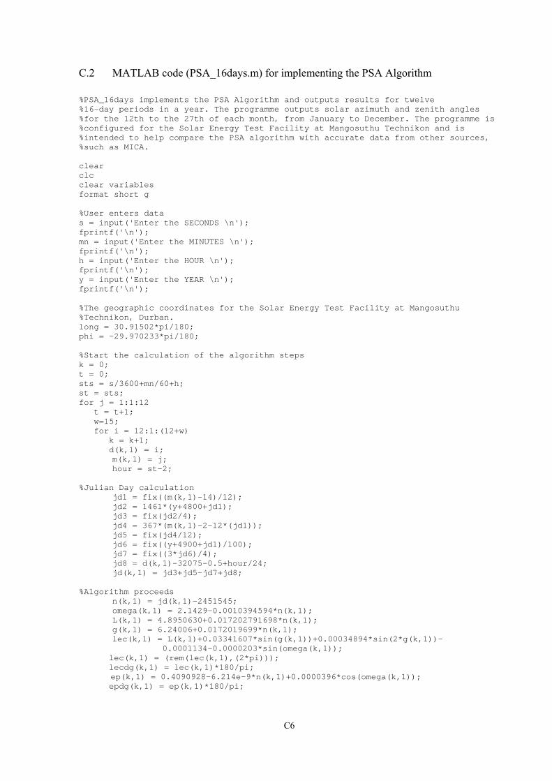
C6
C.2 MATLAB code (PSA_16days.m) for implementing the PSA Algorithm %PSA_16days implements the PSA Algorithm and outputs results for twelve %16-day periods in a year. The programme outputs solar azimuth and zenith angles %for the 12th to the 27th of each month, from January to December. The programme is %configured for the Solar Energy Test Facility at Mangosuthu Technikon and is %intended to help compare the PSA algorithm with accurate data from other sources, %such as MICA. clear clc clear variables format short g %User enters data s = input('Enter the SECONDS \n'); fprintf('\n'); mn = input('Enter the MINUTES \n'); fprintf('\n'); h = input('Enter the HOUR \n'); fprintf('\n'); y = input('Enter the YEAR \n'); fprintf('\n'); %The geographic coordinates for the Solar Energy Test Facility at Mangosuthu %Technikon, Durban. long = 30.91502*pi/180; phi = -29.970233*pi/180; %Start the calculation of the algorithm steps k = 0; t = 0; sts = s/3600+mn/60+h; st = sts; for j = 1:1:12 t = t+1; w=15; for i = 12:1:(12+w) k = k+1; d(k,1) = i; m(k,1) = j; hour = st-2; %Julian Day calculation jd1 = fix((m(k,1)-14)/12); jd2 = 1461*(y+4800+jd1); jd3 = fix(jd2/4); jd4 = 367*(m(k,1)-2-12*(jd1)); jd5 = fix(jd4/12); jd6 = fix((y+4900+jd1)/100); jd7 = fix((3*jd6)/4); jd8 = d(k,1)-32075-0.5+hour/24; jd(k,1) = jd3+jd5-jd7+jd8; %Algorithm proceeds n(k,1) = jd(k,1)-2451545; omega(k,1) = 2.1429-0.0010394594*n(k,1); L(k,1) = 4.8950630+0.017202791698*n(k,1); g(k,1) = 6.24006+0.0172019699*n(k,1); lec(k,1) = L(k,1)+0.03341607*sin(g(k,1))+0.00034894*sin(2*g(k,1))- 0.0001134-0.0000203*sin(omega(k,1)); lec(k,1) = (rem(lec(k,1),(2*pi))); lecdg(k,1) = lec(k,1)*180/pi; ep(k,1) = 0.4090928-6.214e-9*n(k,1)+0.0000396*cos(omega(k,1)); epdg(k,1) = ep(k,1)*180/pi;

C7
%A series of checks is performed to ensure that the angles obtained %are located in the correct trigonometric quadrants if (cos(ep(k,1))*sin(lec(k,1)))>0 & (cos(lec(k,1))>0) ra(k,1) = atan((cos(ep(k,1))*sin(lec(k,1)))/cos(lec(k,1))); elseif (cos(ep(k,1))*sin(lec(k,1)))>0 & (cos(lec(k,1))<0) prodra(k,1) = -1*(cos(ep(k,1))*sin(lec(k,1)))/cos(lec(k,1)); raint(k,1) = atan(prodra(k,1)); ra(k,1) = pi-raint(k,1); elseif (cos(ep(k,1))*sin(lec(k,1)))<0 & (cos(lec(k,1))<0) prodra(k,1) = (cos(ep(k,1))*sin(lec(k,1)))/cos(lec(k,1)); raint(k,1) = atan(prodra(k,1)); ra(k,1) = pi+raint(k,1); elseif (cos(ep(k,1))*sin(lec(k,1)))<0 & (cos(lec(k,1))>0) prodra(k,1) = -1*(cos(ep(k,1))*sin(lec(k,1)))/cos(lec(k,1)); raint(k,1) = atan(prodra(k,1)); ra(k,1) = 2*pi-raint(k,1); end if ra(k,1)<0 ra(k,1) = ra(k,1)+2*pi; end radg(k,1) = ra(k,1)*180/pi; decl(k,1) = asin((sin(ep(k,1))*sin(lec(k,1)))); decldg(k,1) = decl(k,1)*180/pi; gmst(k,1) = 6.6974243242+0.0657098283*n(k,1)+hour; lmst(k,1) = gmst(k,1)*15*pi/180+long; hang(k,1) = lmst(k,1)-ra(k,1); hang(k,1) = (rem(hang(k,1),(2*pi))); hangdg(k,1) =hang(k,1)*180/pi; zen(k,1) = acos(cos(phi)*cos(hang(k,1))*cos(decl(k,1))+ sin(decl(k,1))*sin(phi)); %Further checks are performed to ensure the correct trigonometric results if (-1*(sin(hang(k,1))))>0 & (tan(decl(k,1))*cos(phi)- sin(phi)*cos(hang(k,1)))>0 az(k,1) = atan((-1*(sin(hang(k,1))))/(tan(decl(k,1))*cos(phi)- sin(phi)*cos(hang(k,1)))); elseif (-1*(sin(hang(k,1))))>0 & (tan(decl(k,1))*cos(phi)- sin(phi)*cos(hang(k,1)))<0 prodaz(k,1) = -1*(-1*(sin(hang(k,1))))/(tan(decl(k,1))*cos(phi)- sin(phi)*cos(hang(k,1))); azint(k,1) = atan(prodaz(k,1)); az(k,1) = pi-azint(k,1); elseif (-1*(sin(hang(k,1))))<0 & (tan(decl(k,1))*cos(phi)- sin(phi)*cos(hang(k,1)))<0 prodaz(k,1) = (-1*(sin(hang(k,1))))/(tan(decl(k,1))*cos(phi)- sin(phi)*cos(hang(k,1))); azint(k,1) = atan(prodaz(k,1)); az(k,1) = pi+azint(k,1); elseif (-1*(sin(hang(k,1))))<0 & (tan(decl(k,1))*cos(phi)- sin(phi)*cos(hang(k,1)))>0 prodaz(k,1) = -1*(-1*(sin(hang(k,1))))/(tan(decl(k,1))*cos(phi)- sin(phi)*cos(hang(k,1))); azint(k,1) = atan(prodaz(k,1)); az(k,1) = 2*pi-azint(k,1); end para = (6371.01/149597890)*sin(zen(k,1)); zen(k,1) = zen(k,1)+para; zend(k,1) = zen(k,1)*180/pi; azd(k,1) = az(k,1)*180/pi; end end %Output the results in column form for the day, month, azimuth and zenith [d m azd zend]

C8
C.3 Comparison of output from PSA_16days.m with Multi-Year Interactive Computer
Almanac (MICA)
Table C.1 Solar zenith and azimuth data for a range of days covering one year, generated using the PSA
Algorithm (MATLAB programme “psa_16days.m”) and compared with output from the
Multi-Year Interactive Computer Almanac (MICA) of the U.S. Naval Observatory
Year Month Day Hour 10h00 (SAST) 14h00 (SAST) MICA PSA_16days.m MICA PSA_16days.m Zenith Azimuth Zenith Azimuth Zenith Azimuth Zenith Azimuth (deg) (deg) (deg) (deg) (deg) (deg) (deg) (deg)
2003 Jun 18 60.349 31.152 60.349 31.151 60.959 327.635 60.960 327.630 19 60.391 31.190 60.392 31.190 60.951 327.695 60.951 327.690 20 60.427 31.233 60.428 31.232 60.936 327.751 60.937 327.750 21 60.458 31.279 60.458 31.279 60.916 327.804 60.916 327.800 22 60.482 31.329 60.482 31.329 60.890 327.852 60.890 327.850 23 60.500 31.383 60.501 31.383 60.858 327.897 60.858 327.900 Sept 18 41.457 44.499 41.456 44.500 44.386 310.132 44.385 310.130 19 41.096 44.749 41.094 44.751 44.156 309.668 44.155 309.670 20 40.735 45.004 40.733 45.005 43.927 309.199 43.926 309.200 21 40.374 45.263 40.372 45.265 43.700 308.726 43.698 308.720 22 40.013 45.527 40.011 45.528 43.474 308.250 43.473 308.250 23 39.653 45.796 39.651 45.797 43.249 307.769 43.248 307.770 Dec 18 25.943 82.051 25.946 82.055 29.082 275.409 29.079 275.410 19 26.039 82.201 26.042 82.204 28.967 275.438 28.964 275.440 20 26.139 82.333 26.141 82.336 28.853 275.484 28.851 275.480 21 26.242 82.449 26.243 82.451 28.743 275.545 28.741 275.550 22 26.347 82.547 26.349 82.549 28.634 275.622 28.633 275.620 23 26.456 82.629 26.457 82.630 28.529 275.715 28.527 275.720
2004 Mar 18 41.538 51.132 41.539 51.131 40.156 311.410 40.157 311.410 19 41.782 50.651 41.783 50.649 40.505 311.720 40.506 311.720 20 42.027 50.174 42.028 50.172 40.854 312.025 40.856 312.030 21 42.274 49.701 42.274 49.698 41.205 312.325 41.207 312.320 22 42.522 49.232 42.522 49.229 41.556 312.620 41.558 312.620 23 42.772 48.768 42.771 48.765 41.908 312.910 41.910 312.910

D1
APPENDIX D
LABVIEW SOFTWARE: SCATTALOG DATA SAMPLE
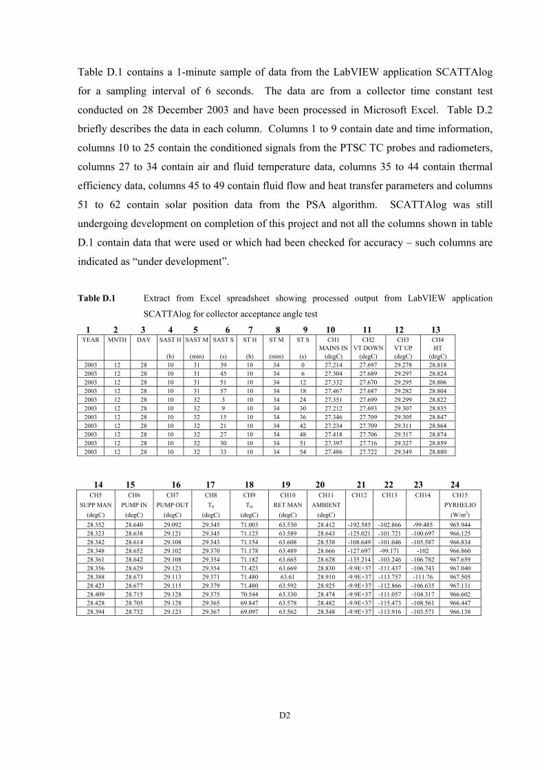
D2
Table D.1 contains a 1-minute sample of data from the LabVIEW application SCATTAlog
for a sampling interval of 6 seconds. The data are from a collector time constant test
conducted on 28 December 2003 and have been processed in Microsoft Excel. Table D.2
briefly describes the data in each column. Columns 1 to 9 contain date and time information,
columns 10 to 25 contain the conditioned signals from the PTSC TC probes and radiometers,
columns 27 to 34 contain air and fluid temperature data, columns 35 to 44 contain thermal
efficiency data, columns 45 to 49 contain fluid flow and heat transfer parameters and columns
51 to 62 contain solar position data from the PSA algorithm. SCATTAlog was still
undergoing development on completion of this project and not all the columns shown in table
D.1 contain data that were used or which had been checked for accuracy – such columns are
indicated as “under development”.
Table D.1 Extract from Excel spreadsheet showing processed output from LabVIEW application
SCATTAlog for collector acceptance angle test
1 2 3 4 5 6 7 8 9 10 11 12 13 YEAR MNTH DAY SAST H SAST M SAST S ST H ST M ST S CH1 CH2 CH3 CH4
MAINS IN VT DOWN VT UP HT (h) (min) (s) (h) (min) (s) (degC) (degC) (degC) (degC)
2003 12 28 10 31 39 10 34 0 27.214 27.697 29.278 28.818 2003 12 28 10 31 45 10 34 6 27.304 27.689 29.297 28.824 2003 12 28 10 31 51 10 34 12 27.332 27.670 29.295 28.806 2003 12 28 10 31 57 10 34 18 27.467 27.687 29.282 28.804 2003 12 28 10 32 3 10 34 24 27.351 27.699 29.299 28.822 2003 12 28 10 32 9 10 34 30 27.212 27.693 29.307 28.835 2003 12 28 10 32 15 10 34 36 27.346 27.709 29.305 28.847 2003 12 28 10 32 21 10 34 42 27.234 27.709 29.311 28.864 2003 12 28 10 32 27 10 34 48 27.418 27.706 29.317 28.874 2003 12 28 10 32 30 10 34 51 27.397 27.716 29.327 28.859 2003 12 28 10 32 33 10 34 54 27.486 27.722 29.349 28.880
14 15 16 17 18 19 20 21 22 23 24
CH5 CH6 CH7 CH8 CH9 CH10 CH11 CH12 CH13 CH14 CH15 SUPP MAN PUMP IN PUMP OUT Tfi Tfo RET MAN AMBIENT PYRHELIO
(degC) (degC) (degC) (degC) (degC) (degC) (degC) (W/m2) 28.352 28.640 29.092 29.345 71.003 63.530 28.412 -192.585 -102.866 -99.485 965.944 28.323 28.638 29.121 29.345 71.123 63.589 28.643 -125.021 -101.721 -100.697 966.125 28.342 28.614 29.108 29.343 71.154 63.608 28.538 -108.649 -101.046 -105.587 966.834 28.348 28.652 29.102 29.370 71.178 63.489 28.666 -127.697 -99.171 -102 966.860 28.361 28.642 29.108 29.354 71.182 63.665 28.628 -135.214 -103.246 -106.782 967.659 28.356 28.629 29.123 29.354 71.423 63.669 28.830 -9.9E+37 -111.437 -106.743 967.040 28.388 28.673 29.113 29.371 71.480 63.61 28.910 -9.9E+37 -113.757 -111.76 967.505 28.423 28.677 29.115 29.379 71.480 63.592 28.925 -9.9E+37 -112.866 -106.635 967.131 28.409 28.715 29.128 29.375 70.544 63.330 28.474 -9.9E+37 -111.057 -104.317 966.602 28.428 28.705 29.128 29.365 69.847 63.578 28.482 -9.9E+37 -115.473 -108.561 966.447 28.394 28.732 29.123 29.367 69.097 63.562 28.548 -9.9E+37 -113.916 -103.571 966.138

D3
Table D.1 (Continued) Extract from Excel spreadsheet showing output from LabVIEW application
SCATTAlog for collector acceptance angle test 25 26 27 28 29 30 31 32 33 34 35 36 37
CH16 Iterns. Flow Mass t f,e,init TCQ t a t f,i - t a Av. Delta Th. Eff t fi 50mean t fi50SD PYRANO Flow CORRECTED Fl Temp Temp
(W/m2) (l/h) kg/s) (degC) (degC) (degC) (degC) (degC) (%) (%) 1023.771 60 100 0.027 70.7 1.007 24.1 4.718 50.174 41.658 66.731 29.31 0.029 1023.576 61 100 0.027 70.7 1.01 24.1 4.724 50.234 41.778 66.706 29.312 0.027 1023.797 62 100 0.027 70.7 1.011 24.1 4.706 50.249 41.811 66.683 29.314 0.026 1024.344 63 100 0.027 70.7 1.012 24.1 4.704 50.274 41.808 66.659 29.316 0.024 1024.799 64 100 0.027 70.7 1.012 24.1 4.722 50.268 41.828 66.635 29.318 0.024 1024.552 65 100 0.027 70.7 1.017 24.1 4.735 50.389 42.069 66.604 29.320 0.023 1024.851 66 100 0.027 70.7 1.019 24.1 4.747 50.425 42.109 66.589 29.322 0.022 1024.435 67 100 0.027 70.7 1.019 24.1 4.764 50.430 42.101 66.575 29.324 0.021 1023.901 68 100 0.027 70.7 0.996 24.1 4.774 49.959 41.169 66.577 29.326 0.022 1023.576 69 100 0.027 70.7 0.979 24.1 4.759 49.606 40.482 66.541 29.328 0.022 1023.510 70 100 0.027 70.7 0.961 24.1 4.780 49.232 39.730 66.491 29.329 0.022
38 39 40 41 42 43 44 45 46 47 48 49
t fi50Var n 50mean n 50 SD n 50 Var n 10 mean n 10 SD n 10 Var Re Pr fD Nu h
(%) (%) (W/m2K) 0.001 66.858 0.084 0.007 66.808 0.028 0.001 2477.29 1.457 0.049 10.472 626.373 0.001 66.861 0.076 0.006 66.797 0.035 0.001 2479.74 1.456 0.049 10.483 626.965 0.001 66.863 0.072 0.005 66.784 0.042 0.002 2480.34 1.456 0.049 10.486 627.108 0.001 66.863 0.071 0.005 66.769 0.049 0.002 2481.38 1.455 0.049 10.491 627.360 0.001 66.862 0.074 0.005 66.752 0.055 0.003 2481.14 1.455 0.049 10.490 627.301 0.001 66.859 0.079 0.006 66.735 0.062 0.004 2486.07 1.453 0.049 10.512 628.488
0 66.855 0.087 0.008 66.715 0.069 0.005 2487.58 1.452 0.049 10.518 628.852 0 66.85 0.095 0.009 66.694 0.072 0.005 2487.75 1.452 0.049 10.519 628.891 0 66.845 0.102 0.01 66.671 0.070 0.005 2468.52 1.462 0.049 10.433 624.250 0 66.839 0.109 0.012 66.651 0.065 0.004 2454.09 1.470 0.049 10.368 620.733
0.001 66.832 0.117 0.014 66.63 0.063 0.004 2438.84 1.479 0.049 10.299 616.990
50 51 52 53 54 55 56 57 58 59 60 61 62
Pressure DECL HANG ZENITH AZIMUTH TRACK AOI UT JD n l ep ra
(kPa) (deg) (deg) (deg) (deg) (deg) (deg) (h) (days) (days) (rad) (rad) (rad) 4 -23.296 -21.497 20.303 75.938 19.742 4.836 8.528 2453002 1456.9 29.953 0.409 4.83 4 -23.296 -21.472 20.282 75.912 19.720 4.840 8.529 2453002 1456.9 29.953 0.409 4.83 4 -23.296 -21.447 20.261 75.885 19.697 4.845 8.531 2453002 1456.9 29.953 0.409 4.83 4 -23.296 -21.422 20.24 75.858 19.674 4.849 8.533 2453002 1456.9 29.953 0.409 4.83 4 -23.296 -21.397 20.219 75.831 19.652 4.853 8.534 2453002 1456.9 29.953 0.409 4.83 4 -23.296 -21.372 20.198 75.804 19.629 4.857 8.536 2453002 1456.9 29.953 0.409 4.83 4 -23.296 -21.347 20.177 75.777 19.606 4.861 8.538 2453002 1456.9 29.953 0.409 4.83 4 -23.296 -21.322 20.156 75.750 19.584 4.866 8.539 2453002 1456.9 29.953 0.409 4.83 4 -23.296 -21.297 20.135 75.723 19.561 4.870 8.541 2453002 1456.9 29.953 0.409 4.83 4 -23.296 -21.284 20.125 75.710 19.550 4.872 8.542 2453002 1456.9 29.953 0.409 4.83 4 -23.296 -21.272 20.114 75.696 19.539 4.874 8.542 2453002 1456.9 29.953 0.409 4.83

D4
Table D.2 List of columns from table D1 and description of data types
Column Data description 1 Year 2 Month 3 Day number of the month 4 Clock time - hours (South African Standard Time) 5 Clock time - minutes (South African Standard Time) 6 Clock time - seconds (South African Standard Time) 7 Solar time - hours 8 Solar time - minutes 9 Solar time - seconds
10 Instrument channel 1 – Main water supply manifold temperature 11 Instrument channel 2 – High temperature (HT) tank temperature (lower TC) 12 Instrument channel 3 – High temperature (HT) tank temperature (upper TC) 13 Instrument channel 4 – Low temperature (LT) tank temperature 14 Instrument channel 5 – Main distribution manifold fluid temperature 15 Instrument channel 6 – Pump inlet temperature 16 Instrument channel 7 – Pump outlet temperature 17 Instrument channel 8 – Receiver fluid inlet temperature, tf,i 18 Instrument channel 9 – Receiver fluid outlet temperature, tf,o 19 Instrument channel 10 – Return manifold fluid temperature
20 Instrument channel 11 – Ambient air temperature (Not used - more accurate value was obtained from the weather station and manually entered)
21 Instrument channel 12 – Unused data logging channel 22 Instrument channel 13 – Unused data logging channel 23 Instrument channel 14 – Unused data logging channel 24 Instrument channel 15 – Normal beam irradiance from NIP 25 Instrument channel 16 – Total global irradiance from PSP 26 Number of programme loop iterations 27 Volumetric flow rate (manually entered) 28 Fluid mass flow rate 29 Initial receiver fluid outlet temperature tf,e,initial (for time constant tests; see equation 5.5) 30 Time constant quotient 31 Ambient air temperature, ta (manually entered from weather station readout)
32 Temperature difference between receiver fluid at inlet and ambient air temperature, Δt (manually corrected to account for software error)
33 Average receiver fluid temperature 34 Fluid temperature difference across receiver, Δtr 35 ASHRAE 93 thermal efficiency (see equation 5.4) 36 Under development – 50-point rolling average of receiver fluid inlet temperature, tf,i 37 Under development – standard deviation of 50-point rolling average of tf,i 38 Under development – variance of 50-point rolling average of tf,i 39 Under development – 50-point rolling average of ASHRAE 93 thermal efficiency 40 Under development – standard deviation of 50-point rolling average thermal efficiency 41 Under development – variance of 50-point rolling average thermal efficiency 42 Under development – 10-point rolling average of ASHRAE 93 thermal efficiency 43 Under development – standard deviation of 10-point rolling average thermal efficiency 44 Under development – variance of 10-point rolling average thermal efficiency
45 Reynolds number for receiver flow based on average receiver fluid temperature (Kröger, 1998): (Re = ρvD/μ, where D is the inner diameter of the absorber)
46 Prandtl number for receiver flow based on average receiver fluid temperature (Kröger, 1998): (Pr = μcp/k)

D5
Table D.2 (Contnued) List of columns from table D1 and description of data types
Column Data description
47 Friction factor for receiver flow based on average receiver fluid temperature (Kröger, 1998): (f = (1.82log10Re-1.64)-2)
48
Nusselt number for receiver flow based on average receiver fluid temperature (Kröger, 1998): ( ( )( ) ( )[ ]
( ) ( )1Pr8/f7,121
L/d1Pr1000Re8/fNu
67.05.0
67.0
−++
+−= )
49 Heat transfer coefficient based on average receiver fluid temperature (Kröger, 1998): (h = (Nu)k/D, where D is the inner diameter of the absorber)
50 PTSC fluid system pressure 51 Solar declination angle, δ 52 Hour angle 53 Zenith angle, θz 54 Azimuth angle, A 55 PTSC tracking angle, ρT 56 Angle of incidence, θi 57 Universal time 58 Julian Day 59 Difference between current Julian Day and Julian Day corresponding to 1 January 2000 60 Ecliptic longitude of the sun 61 Obliquity of the ecliptic 62 Right ascension

E1
APPENDIX E
SUMMARY OF EXPERIMENTAL TEST DATA

E2
Table E.1 Summary of data for collector time constant tests
GLASS-SHIELDED RECEIVER Cooling tests Date Test time Flow rate Time const. (tf,i - ta) Max. Δ(tf,i) Ave. GDN Ave. θi ta Ave. wind (solar) (L/h) (s) (°C) (°C) (W/m2) (deg) (°C) vel. (knots)15-Feb-04 12:56 75 108.71 4.21 0.11 892.60 16.35 27.00 10.0 15-Feb-04 13:15 150 55.63 3.92 0.05 905.44 15.67 27.00 10.0 15-Feb-04 13:29 300 28.55 4.14 0.05 905.42 15.03 26.70 12.0 15-Feb-04 13:50 450 18.36 3.94 0.08 891.30 14.04 26.92 10.0 15-Feb-04 14:20 600 11.13 7.77 0.25 881.45 12.01 26.60 11.0 15-Feb-04 14:38 750 10.82 1.99 0.03 870.36 10.66 26.70 10.0 AVERAGE 4.33 0.09 891.10 13.96 26.82 10.5 Heating tests Date Test time Flow rate Time const. (tf,i - ta) Max. Δ(tf,i) Ave. GDN Ave. θi ta Ave. wind (solar) (L/h) (s) (°C) (°C) (W/m2) (deg) (°C) vel. (knots)15-Feb-04 13:04 75 103.21 4.33 0.11 894.67 16.11 27.00 10.0 15-Feb-04 13:19 150 50.21 3.92 0.05 896.70 15.51 27.00 10.0 15-Feb-04 13:33 300 26.40 4.18 0.05 901.29 14.84 26.70 12.0 15-Feb-04 13:52 450 17.85 3.89 0.04 896.08 13.81 27.00 10.0 15-Feb-04 14:14 600 11.95 7.35 0.11 871.37 12.45 26.60 11.0 15-Feb-04 14:39 750 12.29 2.02 0.07 866.46 10.57 26.70 10.0 AVERAGE 4.28 0.07 887.76 13.88 26.83 10.5 UNSHIELDED RECEIVER Cooling tests Date Test time Flow rate Time const. (tf,i - ta) Max. Δ(tf,i) Ave. GDN Ave. θi ta Ave. wind (solar) (L/h) (s) (°C) (°C) (W/m2) (deg) (°C) vel. (knots)28-Dec-03 10:43 75 97.14 5.29 0.06 965.76 4.90 24.10 9.0 28-Dec-03 11:04 150 52.11 4.17 0.06 972.08 5.78 24.20 9.0 28-Dec-03 09:52 300 30.45 3.12 0.05 948.50 2.69 23.70 9.0 28-Dec-03 11:24 450 21.65 2.70 0.04 978.84 6.33 24.60 9.0 29-Dec-03 09:15 600 14.29 1.02 0.04 854.86 0.19 25.80 10.0 29-Dec-03 09:50 750 12.09 2.15 0.05 494.44* 2.61 25.90 13.0 AVERAGE 3.08 0.05 869.08 3.75 24.72 9.8 * Cloud obstructed pyrheliometer only after PTSC defocused - test unaffected. Heating tests Date Test time Flow rate Time const. (tf,i - ta) Max. Δ(tf,i) Ave. GDN Ave. θi ta Ave. wind (solar) (L/h) (s) (°C) (°C) (W/m2) (deg) (°C) vel. (knots)09-Jan-04 11:24 75 98.00 5.24 0.09 925.78 7.44 25.60 9.0 11-Jan-04 11:57 150 51.27 2.89 0.24 910.70 8.09 26.20 9.0 09-Jan-04 10:45 300 27.72 1.81 0.06 885.14 6.43 25.90 9.0 11-Jan-04 12:07 450 19.31 1.51 0.05 913.61 8.09 26.20 9.0 11-Jan-04 12:17 600 16.65 1.38 0.05 900.61 8.03 26.10 9.0 11-Jan-04 12:24 750 15.56 1.31 0.06 910.90 7.95 26.20 9.0 AVERAGE 2.36 0.09 907.79 7.67 26.03 9.0

E3
Table E.2 Thermal efficiency test data for glass-shielded receiver (19 February 2004)
COLUMN A B C D E F G H I J
Elapsed
time tf,i tf,o GDN θi Gbp m cp mcpΔt AaGbp
ROW (s) (°C) (°C) (W/m2) (deg) (W/m2) (kg/s) (J/kgK) (W) (W) 1 6 57.855 66.734 838.094 15.034 809.408 0.082 4185.63 3047.47 6070.56 2 12 57.894 66.736 838.210 15.028 809.543 0.082 4185.65 3034.78 6071.57 3 18 57.894 66.720 838.275 15.022 809.628 0.082 4185.64 3029.28 6072.21 4 24 57.902 66.734 837.320 15.016 808.728 0.082 4185.65 3031.35 6065.46 5 30 57.889 66.714 836.766 15.010 808.216 0.082 4185.64 3028.94 6061.62 6 36 57.904 66.754 835.760 15.004 807.267 0.082 4185.66 3037.53 6054.50 7 42 57.889 66.773 836.224 14.998 807.738 0.082 4185.66 3049.20 6058.03 8 48 57.887 66.759 837.449 14.992 808.944 0.082 4185.65 3045.08 6067.08 9 54 57.914 66.757 836.714 14.986 808.257 0.082 4185.66 3035.13 6061.92
10 60 57.920 66.793 836.779 14.980 808.342 0.082 4185.68 3045.44 6062.56 11 66 57.924 66.785 836.662 14.974 808.252 0.082 4185.67 3041.32 6061.89 12 72 57.930 66.816 837.823 14.968 809.396 0.082 4185.69 3049.91 6070.47 13 78 57.955 66.791 838.404 14.962 809.980 0.082 4185.69 3032.75 6074.85 14 84 57.951 66.816 838.287 14.956 809.889 0.082 4185.69 3042.71 6074.17 15 90 57.949 66.834 838.158 14.949 809.791 0.082 4185.70 3049.58 6073.43 16 96 57.935 66.820 838.171 14.943 809.826 0.082 4185.69 3049.57 6073.70 17 102 57.947 66.859 838.442 14.937 810.111 0.082 4185.71 3058.85 6075.83 18 108 57.961 66.879 838.068 14.931 809.772 0.082 4185.72 3060.92 6073.29 19 114 57.969 66.887 837.488 14.925 809.234 0.082 4185.73 3060.92 6069.26 20 120 57.978 66.892 837.307 14.919 809.082 0.082 4185.73 3059.55 6068.12 21 126 57.998 66.916 836.972 14.913 808.781 0.082 4185.75 3060.94 6065.86 22 132 57.992 66.873 837.204 14.907 809.028 0.082 4185.73 3048.22 6067.71 23 138 57.988 66.916 836.611 14.901 808.477 0.082 4185.74 3064.36 6063.58 24 144 57.986 66.912 835.566 14.895 807.490 0.082 4185.74 3063.68 6056.17 25 150 57.992 66.906 834.883 14.889 806.852 0.082 4185.74 3059.56 6051.39 26 156 57.994 66.937 834.315 14.882 806.329 0.082 4185.75 3069.52 6047.47 27 162 58.000 66.935 833.555 14.876 805.617 0.082 4185.75 3066.78 6042.13 28 168 58.006 66.896 834.225 14.870 806.287 0.082 4185.74 3051.32 6047.15 29 174 57.986 66.877 834.586 14.864 806.659 0.082 4185.73 3051.66 6049.94 30 180 57.980 66.908 835.399 14.858 807.467 0.082 4185.74 3064.36 6056.00 31 186 57.986 66.855 836.224 14.852 808.287 0.082 4185.72 3044.10 6062.15 32 192 57.984 66.857 834.186 14.846 806.339 0.082 4185.72 3045.47 6047.54 33 198 57.982 66.840 833.065 14.839 805.282 0.082 4185.71 3040.32 6039.61 34 204 57.996 66.885 831.685 14.833 803.970 0.082 4185.73 3050.97 6029.78 35 210 57.976 66.873 830.859 14.827 803.194 0.082 4185.72 3053.71 6023.95 36 216 57.986 66.869 830.975 14.821 803.328 0.082 4185.72 3048.91 6024.96 37 222 58.002 66.857 830.189 14.815 802.591 0.082 4185.73 3039.30 6019.43 38 228 57.990 66.812 831.079 14.809 803.473 0.082 4185.71 3027.96 6026.05 39 234 57.994 66.822 830.485 14.802 802.925 0.082 4185.71 3030.02 6021.94 40 240 57.994 66.814 830.485 14.796 802.947 0.082 4185.71 3027.27 6022.10 41 246 58.000 66.799 830.640 14.790 803.119 0.082 4185.71 3020.06 6023.39 42 252 58.004 66.838 830.421 14.784 802.930 0.082 4185.72 3032.09 6021.97 43 258 57.986 66.892 830.279 14.778 802.815 0.082 4185.73 3056.81 6021.11 44 264 58.015 66.826 829.428 14.771 802.018 0.082 4185.72 3024.19 6015.13 45 270 58.000 66.826 828.461 14.765 801.105 0.082 4185.71 3029.34 6008.28 46 276 58.017 66.855 828.267 14.759 800.939 0.082 4185.73 3033.47 6007.04 47 282 58.023 66.847 827.700 14.753 800.413 0.082 4185.73 3028.66 6003.10 48 288 57.996 66.883 826.965 14.747 799.724 0.082 4185.73 3050.29 5997.93 49 294 57.982 66.916 826.036 14.740 798.851 0.082 4185.74 3066.42 5991.39 50 300 57.980 66.865 825.598 14.734 798.450 0.082 4185.72 3049.59 5988.37
SUM TOTAL 152289.58 302303.17

E4
Sample calculation of thermal efficiency (ηg): The following illustrates the application of equation 4.5 to determine a single PTSC thermal
efficiency point, using the data in table E.2. The data were obtained from a test conducted on
19 February 2004 for the PTSC with glass-shielded receiver.
The temperature and irradiance data in columns B, C and D are measured values. Column E
is based on the PSA Algorithm (see appendix C for sample calculation). Values for Gbp, cp,
mcpΔt and AaGbp are obtained as follows, using row 1 as an example:
Cell F1: Gbp = (Gbp) cos(θi) (Eqn. 4.2)
= (838.094) cos(15.034)
= 809.41 W/m2
Cell H1: cp = 8.15599 x 10³ – 2.80627 x 10 (tave) + 5.11283 x 10⁻² (tave)2
– 2.17582 x 10⁻¹³ (tave)6 (Kröger, 1998)
where tave = (57.855 + 66.734)/2 + 273.15 = 335.445 K
=> cp = 8.15599 x 10³ – 2.80627 x 10 (335.445)
+ 5.11283 x 10⁻² (335.445)2
– 2.17582 x 10⁻¹³ (335.445)6
= 4185.63 J/kgK
Cell I1: Rate of thermal energy input to the working fluid:
mcpΔt = (0.082)(4185.63)(66.734 – 57.855) (Numerator of eqn. 4.3)
= 3047.47 W
Cell J1: Rate of solar energy input to PTSC system:
AaGbp = (7.5)(809.408) (Denominator of eqn. 4.3)
= 6070.56 W

E5
For the calculation of thermal efficiency over the required 5-minute period, equation 4.5 is
used:
From table E.2, column I represents the numerator in equation 4.5 and column J the
denominator. The totals of these columns are 152 289.58 W and 302303.17 W respectively,
giving a single thermal efficiency point for the PTSC with glass-shielded receiver (see table
E.4):
ηg = (152 289.58/302303.17)
= 50.38 %
Instantaneous efficiency, ηinst,T
The instantaneous efficiency of the collector, as defined in equation E.3 and used in the
calculation of the tracking efficiency factor (equation 5.1), is determined by dividing the
thermal power absorbed by the working fluid, by the rate of energy input to the PTSC system.
Using the values from the above sample calculation for row 1:
ηinst,T = (mcpΔt)/( AaGbp) (5.3)
= (3047.47)/(6070.56)
= 50.20 %
To determine the tracking efficiency factor (equation 5.1), the same calculation is repeated for
each time interval to find the maximum instantaneous efficiency. This becomes the
denominator in equation 5.1, from which the remaining data are obtained. In a similar way,
for the collector acceptance angle results given in 5.4.2, 10 instantaneous efficiency points are
used to give a 1-minute average. Each of these values is then divided by the maximum
efficiency to yield a single datum point.
)5.4(GA
)t()c(m
50
1nna
50
1nnrnpn
g
∑
∑
=
=
Δ=η

E6
Table E.3 Summary of data for thermal efficiency tests with unshielded receiver
Date Test time ta (tf,i - ta) Ave. GDN (tf,i - ta)/Gbp
Max. Δ(tf,i)
Max. Δ(GDN) Efficiency Ave. θi
Max. Δ(θi)
(solar) (°C) (°C) (W/m2) (m2°C/W) (°C) (W/m2) (%) (deg) (deg)
Ave. wind vel.
(knots)02-Jan-04 10:10 27.50 2.66 901.60 0.0030 0.07 10.20 54.75 4.03 0.26 * 02-Jan-04 10:30 28.40 0.63 905.58 0.0007 0.06 11.86 53.92 5.04 0.21 * 02-Jan-04 13:51 26.20 2.86 899.68 0.0032 0.09 10.69 54.49 3.91 0.27 * 02-Jan-04 13:19 26.00 3.30 900.85 0.0037 0.09 7.63 54.52 5.42 0.19 * 26-Jan-04 14:28 26.80 22.40 918.33 0.0245 0.65 29.27 50.63 5.47 0.36 13.0 12-Jan-04 09:34 29.40 16.71 925.05 0.0181 0.07 7.69 50.82 3.05 0.34 12.0 13-Jan-04 11:56 28.30 21.64 930.87 0.0235 0.28 5.21 51.26 8.41 0.01 8.0 13-Jan-04 12:04 28.40 21.80 925.66 0.0238 0.21 16.40 52.62 8.41 0.01 8.0 25-Jan-04 09:42 26.70 29.31 951.93 0.0310 1.24 3.10 49.24 6.19 0.33 7.0 02-Jan-04 14:50 26.00 33.70 871.89 0.0387 0.30 12.47 47.87 0.10 0.38 * 25-Jan-04 09:50 26.89 30.81 954.92 0.0325 1.14 5.44 47.93 6.71 0.31 7.0 11-Jan-04 14:44 27.60 30.59 876.66 0.0349 0.45 16.35 47.66 1.49 0.37 9.0 25-Jan-04 10:59 26.70 44.76 979.37 0.0464 1.52 2.70 45.71 9.96 0.25 10.0 25-Jan-04 11:08 27.20 45.52 984.95 0.0470 1.22 5.47 45.58 10.17 0.13 8.0 25-Jan-04 13:09 27.00 45.49 974.61 0.0473 0.28 10.55 44.31 9.62 0.18 10.0 25-Jan-04 12:59 27.20 45.52 981.06 0.0471 0.55 12.26 47.55 9.95 0.15 9.0 25-Jan-04 12:29 26.50 55.97 985.29 0.0578 0.48 9.63 43.51 10.67 0.08 10.0 25-Jan-04 12:39 26.80 56.43 981.20 0.0585 0.69 7.75 44.77 10.53 0.10 10.0 27-Jan-04 11:24 26.30 49.61 912.06 0.0554 0.71 32.25 44.60 11.04 0.09 8.0 28-Jan-04 11:37 26.50 56.56 981.79 0.0588 0.40 13.36 41.05 11.52 0.06 11.0
AVERAGE 27.12 937.17 0.52 11.51 7.08 0.20 9.3
* No wind data available due to weather station failure
Table E.4 Summary of data for thermal efficiency tests with glass-shielded receiver
Date Test time ta (tf,i - ta) Ave. GDN (tf,i - ta)/Gbp
Max. Δ(tf,i)
Max. Δ(GDN) Efficiency Ave. θi
Max. Δ(θi)
Ave. wind
(solar) (°C) (°C) (W/m2) (m2°C/W) (°C) (W/m2) (%) (deg) (deg) vel.
(knots)13-Feb-04 15:09 26.00 2.20 809.05 0.0027 0.22 15.20 52.97 7.26 0.44 10.0 11-Feb-04 15:51 27.60 2.81 792.44 0.0036 0.05 21.07 54.21 2.71 0.50 10.0 11-Feb-04 10:17 27.30 38.09 889.88 0.0439 1.15 6.80 47.42 12.59 0.28 7.0 19-Feb-04 13:55 26.60 31.37 834.14 0.0389 0.17 12.84 50.38 14.89 0.30 10.0 11-Feb-04 09:01 25.80 26.00 825.11 0.0318 0.49 10.66 49.93 7.53 0.42 7.0 11-Feb-04 09:21 26.40 27.94 847.77 0.0334 0.54 6.60 50.88 9.26 0.19 7.0 11-Feb-04 10:37 27.80 43.11 899.31 0.0494 1.04 7.21 48.22 13.96 0.22 9.0 11-Feb-04 10:50 27.80 44.75 898.75 0.0514 0.55 7.47 48.81 14.54 0.18 9.0 11-Feb-04 12:04 28.80 50.70 909.18 0.0580 0.70 5.89 47.54 15.80 0.01 10.0 11-Feb-04 12:19 28.60 53.99 910.19 0.0616 0.33 7.39 48.01 15.68 0.06 10.0
AVERAGE 27.27 861.58 0.52 10.11 11.42 0.26 8.9
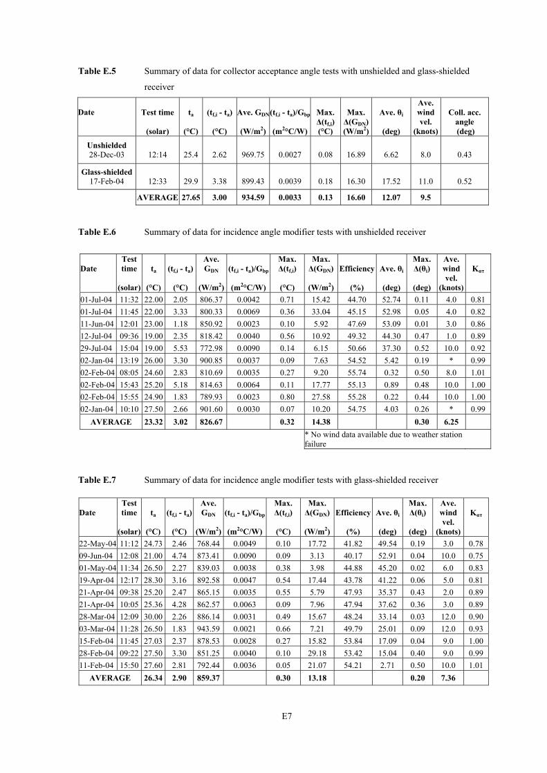
E7
Table E.5 Summary of data for collector acceptance angle tests with unshielded and glass-shielded
receiver
Date
Test time
(solar)
ta
(°C)
(tf,i - ta)
(°C)
Ave. GDN
(W/m2)
(tf,i - ta)/Gbp
(m2°C/W)
Max. Δ(tf,i) (°C)
Max. Δ(GDN)(W/m2)
Ave. θi
(deg)
Ave. wind vel.
(knots)
Coll. acc. angle (deg)
Unshielded 28-Dec-03
12:14
25.4
2.62
969.75
0.0027
0.08
16.89
6.62
8.0
0.43
Glass-shielded 17-Feb-04
12:33
29.9
3.38
899.43
0.0039
0.18
16.30
17.52
11.0
0.52
AVERAGE 27.65 3.00 934.59 0.0033 0.13 16.60 12.07 9.5
Table E.6 Summary of data for incidence angle modifier tests with unshielded receiver
Table E.7 Summary of data for incidence angle modifier tests with glass-shielded receiver
Date Test time ta (tf,i - ta)
Ave. GDN (tf,i - ta)/Gbp
Max. Δ(tf,i)
Max. Δ(GDN) Efficiency Ave. θi
Max. Δ(θi)
Ave. wind Kατ
(solar) (°C) (°C) (W/m2) (m2°C/W) (°C) (W/m2) (%) (deg) (deg) vel.
(knots) 22-May-04 11:12 24.73 2.46 768.44 0.0049 0.10 17.72 41.82 49.54 0.19 3.0 0.78 09-Jun-04 12:08 21.00 4.74 873.41 0.0090 0.09 3.13 40.17 52.91 0.04 10.0 0.75 01-May-04 11:34 26.50 2.27 839.03 0.0038 0.38 3.98 44.88 45.20 0.02 6.0 0.83 19-Apr-04 12:17 28.30 3.16 892.58 0.0047 0.54 17.44 43.78 41.22 0.06 5.0 0.81 21-Apr-04 09:38 25.20 2.47 865.15 0.0035 0.55 5.79 47.93 35.37 0.43 2.0 0.89 21-Apr-04 10:05 25.36 4.28 862.57 0.0063 0.09 7.96 47.94 37.62 0.36 3.0 0.89 28-Mar-04 12:09 30.00 2.26 886.14 0.0031 0.49 15.67 48.24 33.14 0.03 12.0 0.90 03-Mar-04 11:28 26.50 1.83 943.59 0.0021 0.66 7.21 49.79 25.01 0.09 12.0 0.93 15-Feb-04 11:45 27.03 2.37 878.53 0.0028 0.27 15.82 53.84 17.09 0.04 9.0 1.00 28-Feb-04 09:22 27.50 3.30 851.25 0.0040 0.10 29.18 53.42 15.04 0.40 9.0 0.99 11-Feb-04 15:50 27.60 2.81 792.44 0.0036 0.05 21.07 54.21 2.71 0.50 10.0 1.01
AVERAGE 26.34 2.90 859.37 0.30 13.18 0.20 7.36
Date Test time ta (tf,i - ta)
Ave. GDN (tf,i - ta)/Gbp
Max. Δ(tf,i)
Max. Δ(GDN) Efficiency Ave. θi
Max. Δ(θi)
Ave. wind Kατ
(solar) (°C) (°C) (W/m2) (m2°C/W) (°C) (W/m2) (%) (deg) (deg) vel.
(knots) 01-Jul-04 11:32 22.00 2.05 806.37 0.0042 0.71 15.42 44.70 52.74 0.11 4.0 0.81 01-Jul-04 11:45 22.00 3.33 800.33 0.0069 0.36 33.04 45.15 52.98 0.05 4.0 0.82 11-Jun-04 12:01 23.00 1.18 850.92 0.0023 0.10 5.92 47.69 53.09 0.01 3.0 0.86 12-Jul-04 09:36 19.00 2.35 818.42 0.0040 0.56 10.92 49.32 44.30 0.47 1.0 0.89 29-Jul-04 15:04 19.00 5.53 772.98 0.0090 0.14 6.15 50.66 37.30 0.52 10.0 0.92 02-Jan-04 13:19 26.00 3.30 900.85 0.0037 0.09 7.63 54.52 5.42 0.19 * 0.99 02-Feb-04 08:05 24.60 2.83 810.69 0.0035 0.27 9.20 55.74 0.32 0.50 8.0 1.01 02-Feb-04 15:43 25.20 5.18 814.63 0.0064 0.11 17.77 55.13 0.89 0.48 10.0 1.00 02-Feb-04 15:55 24.90 1.83 789.93 0.0023 0.80 27.58 55.28 0.22 0.44 10.0 1.00 02-Jan-04 10:10 27.50 2.66 901.60 0.0030 0.07 10.20 54.75 4.03 0.26 * 0.99
AVERAGE 23.32 3.02 826.67 0.32 14.38 0.30 6.25
* No wind data available due to weather station failure

F1
APPENDIX F
THERMAL MODEL DATA
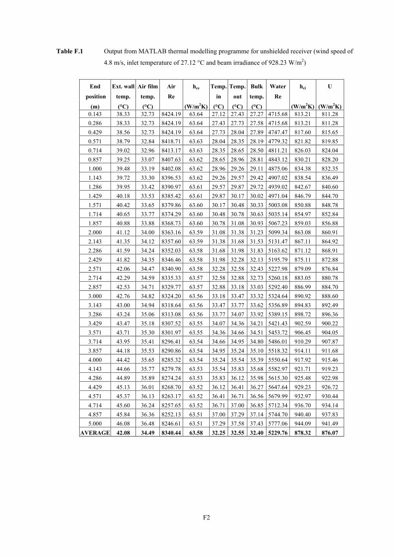
F2
Table F.1 Output from MATLAB thermal modelling programme for unshielded receiver (wind speed of
4.8 m/s, inlet temperature of 27.12 °C and beam irradiance of 928.23 W/m2)
End Ext. wall Air film Air hce Temp. Temp. Bulk Water hci U
position temp. temp. Re in out temp. Re
(m) (°C) (°C) (W/m2K) (°C) (°C) (°C) (W/m2K) (W/m2K)0.143 38.33 32.73 8424.19 63.64 27.12 27.43 27.27 4715.68 813.21 811.28 0.286 38.33 32.73 8424.19 63.64 27.43 27.73 27.58 4715.68 813.21 811.28 0.429 38.56 32.73 8424.19 63.64 27.73 28.04 27.89 4747.47 817.60 815.65 0.571 38.79 32.84 8418.71 63.63 28.04 28.35 28.19 4779.32 821.82 819.85 0.714 39.02 32.96 8413.17 63.63 28.35 28.65 28.50 4811.21 826.03 824.04 0.857 39.25 33.07 8407.63 63.62 28.65 28.96 28.81 4843.12 830.21 828.20 1.000 39.48 33.19 8402.08 63.62 28.96 29.26 29.11 4875.06 834.38 832.35 1.143 39.72 33.30 8396.53 63.62 29.26 29.57 29.42 4907.02 838.54 836.49 1.286 39.95 33.42 8390.97 63.61 29.57 29.87 29.72 4939.02 842.67 840.60 1.429 40.18 33.53 8385.42 63.61 29.87 30.17 30.02 4971.04 846.79 844.70 1.571 40.42 33.65 8379.86 63.60 30.17 30.48 30.33 5003.08 850.88 848.78 1.714 40.65 33.77 8374.29 63.60 30.48 30.78 30.63 5035.14 854.97 852.84 1.857 40.88 33.88 8368.73 63.60 30.78 31.08 30.93 5067.23 859.03 856.88 2.000 41.12 34.00 8363.16 63.59 31.08 31.38 31.23 5099.34 863.08 860.91 2.143 41.35 34.12 8357.60 63.59 31.38 31.68 31.53 5131.47 867.11 864.92 2.286 41.59 34.24 8352.03 63.58 31.68 31.98 31.83 5163.62 871.12 868.91 2.429 41.82 34.35 8346.46 63.58 31.98 32.28 32.13 5195.79 875.11 872.88 2.571 42.06 34.47 8340.90 63.58 32.28 32.58 32.43 5227.98 879.09 876.84 2.714 42.29 34.59 8335.33 63.57 32.58 32.88 32.73 5260.18 883.05 880.78 2.857 42.53 34.71 8329.77 63.57 32.88 33.18 33.03 5292.40 886.99 884.70 3.000 42.76 34.82 8324.20 63.56 33.18 33.47 33.32 5324.64 890.92 888.60 3.143 43.00 34.94 8318.64 63.56 33.47 33.77 33.62 5356.89 894.83 892.49 3.286 43.24 35.06 8313.08 63.56 33.77 34.07 33.92 5389.15 898.72 896.36 3.429 43.47 35.18 8307.52 63.55 34.07 34.36 34.21 5421.43 902.59 900.22 3.571 43.71 35.30 8301.97 63.55 34.36 34.66 34.51 5453.72 906.45 904.05 3.714 43.95 35.41 8296.41 63.54 34.66 34.95 34.80 5486.01 910.29 907.87 3.857 44.18 35.53 8290.86 63.54 34.95 35.24 35.10 5518.32 914.11 911.68 4.000 44.42 35.65 8285.32 63.54 35.24 35.54 35.39 5550.64 917.92 915.46 4.143 44.66 35.77 8279.78 63.53 35.54 35.83 35.68 5582.97 921.71 919.23 4.286 44.89 35.89 8274.24 63.53 35.83 36.12 35.98 5615.30 925.48 922.98 4.429 45.13 36.01 8268.70 63.52 36.12 36.41 36.27 5647.64 929.23 926.72 4.571 45.37 36.13 8263.17 63.52 36.41 36.71 36.56 5679.99 932.97 930.44 4.714 45.60 36.24 8257.65 63.52 36.71 37.00 36.85 5712.34 936.70 934.14 4.857 45.84 36.36 8252.13 63.51 37.00 37.29 37.14 5744.70 940.40 937.83 5.000 46.08 36.48 8246.61 63.51 37.29 37.58 37.43 5777.06 944.09 941.49
AVERAGE 42.08 34.49 8340.44 63.58 32.25 32.55 32.40 5229.76 878.32 876.07

F3
Table F.2 Loss output from MATLAB thermal modelling programme for unshielded receiver (wind
speed of 1.34 m/s, inlet temperature of 29.77 °C, ambient temperature of 21.2 °C and zero
beam irradiance)
Position Ext. wall Air film Air hce Temp. Temp. Bulk Water hci U
temp. temp. Re in out temp. Re (m) (°C) (°C) (W/m2K) (°C) (°C) (°C) (W/m2K) (W/m2K)
0.143 29.17 25.17 2456.80 29.72 29.77 29.75 29.76 4975.41 854.82 852.69 0.286 29.17 25.17 2456.80 29.72 29.75 29.74 29.74 4975.41 854.82 852.69 0.429 29.15 25.17 2456.80 29.72 29.74 29.72 29.73 4973.58 854.58 852.45 0.571 29.14 25.16 2456.92 29.72 29.72 29.70 29.71 4971.76 854.35 852.22 0.714 29.12 25.15 2457.04 29.72 29.70 29.68 29.69 4969.93 854.11 851.99 0.857 29.10 25.14 2457.16 29.72 29.68 29.67 29.67 4968.11 853.88 851.75 1.000 29.09 25.14 2457.29 29.72 29.67 29.65 29.66 4966.29 853.65 851.52 1.143 29.07 25.13 2457.41 29.72 29.65 29.63 29.64 4964.47 853.41 851.29 1.286 29.05 25.12 2457.53 29.72 29.63 29.61 29.62 4962.66 853.18 851.06 1.429 29.03 25.11 2457.65 29.72 29.61 29.60 29.61 4960.85 852.95 850.83 1.571 29.02 25.10 2457.77 29.72 29.60 29.58 29.59 4959.04 852.72 850.60 1.714 29.00 25.09 2457.89 29.72 29.58 29.56 29.57 4957.23 852.49 850.37 1.857 28.99 25.09 2458.01 29.72 29.56 29.55 29.55 4955.42 852.25 850.14 2.000 28.97 25.08 2458.13 29.72 29.55 29.53 29.54 4953.62 852.02 849.91 2.143 28.95 25.07 2458.24 29.72 29.53 29.51 29.52 4951.82 851.79 849.68 2.286 28.94 25.06 2458.36 29.72 29.51 29.49 29.50 4950.02 851.56 849.45 2.429 28.92 25.05 2458.48 29.72 29.49 29.48 29.49 4948.22 851.33 849.22 2.571 28.90 25.04 2458.60 29.72 29.48 29.46 29.47 4946.43 851.10 848.99 2.714 28.89 25.04 2458.72 29.72 29.46 29.44 29.45 4944.64 850.87 848.76 2.857 28.87 25.03 2458.84 29.72 29.44 29.43 29.44 4942.85 850.64 848.53 3.000 28.85 25.02 2458.96 29.72 29.43 29.41 29.42 4941.06 850.41 848.30 3.143 28.84 25.01 2459.08 29.72 29.41 29.39 29.40 4939.28 850.18 848.08 3.286 28.82 25.00 2459.20 29.72 29.39 29.38 29.38 4937.50 849.95 847.85 3.429 28.80 25.00 2459.31 29.72 29.38 29.36 29.37 4935.72 849.73 847.62 3.571 28.79 24.99 2459.43 29.72 29.36 29.34 29.35 4933.94 849.50 847.39 3.714 28.77 24.98 2459.55 29.72 29.34 29.33 29.33 4932.17 849.27 847.17 3.857 28.75 24.97 2459.67 29.72 29.33 29.31 29.32 4930.40 849.04 846.94 4.000 28.74 24.96 2459.79 29.72 29.31 29.29 29.30 4928.63 848.81 846.71 4.143 28.72 24.95 2459.90 29.72 29.29 29.28 29.28 4926.86 848.59 846.49 4.286 28.71 24.95 2460.02 29.72 29.28 29.26 29.27 4925.09 848.36 846.26 4.429 28.69 24.94 2460.14 29.72 29.26 29.24 29.25 4923.33 848.13 846.03 4.571 28.67 24.93 2460.26 29.72 29.24 29.22 29.23 4921.57 847.90 845.81 4.714 28.66 24.92 2460.37 29.72 29.22 29.21 29.22 4919.81 847.68 845.58 4.857 28.64 24.91 2460.49 29.72 29.21 29.19 29.20 4918.05 847.45 845.36 5.000 28.62 24.91 2460.61 29.72 29.19 29.17 29.18 4916.30 847.23 845.13
AVERAGE 28.90 25.04 2458.61 29.72 29.48 29.46 29.47 4946.50 851.11 849.00
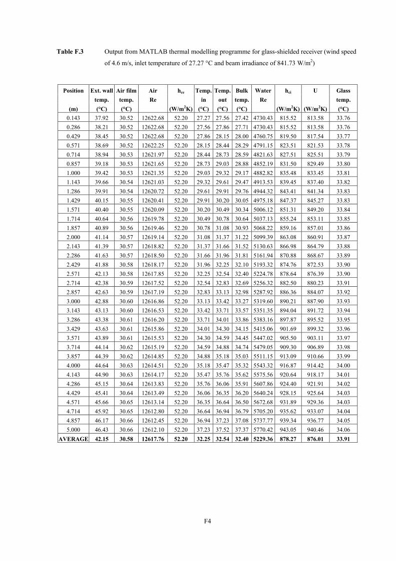
F4
Table F.3 Output from MATLAB thermal modelling programme for glass-shielded receiver (wind speed
of 4.6 m/s, inlet temperature of 27.27 °C and beam irradiance of 841.73 W/m2)
Position Ext. wall Air film Air hce Temp. Temp. Bulk Water hci U Glass temp. temp. Re in out temp. Re temp.
(m) (°C) (°C) (W/m2K) (°C) (°C) (°C) (W/m2K) (W/m2K) (°C) 0.143 37.92 30.52 12622.68 52.20 27.27 27.56 27.42 4730.43 815.52 813.58 33.76 0.286 38.21 30.52 12622.68 52.20 27.56 27.86 27.71 4730.43 815.52 813.58 33.76 0.429 38.45 30.52 12622.68 52.20 27.86 28.15 28.00 4760.75 819.50 817.54 33.77 0.571 38.69 30.52 12622.25 52.20 28.15 28.44 28.29 4791.15 823.51 821.53 33.78 0.714 38.94 30.53 12621.97 52.20 28.44 28.73 28.59 4821.63 827.51 825.51 33.79 0.857 39.18 30.53 12621.65 52.20 28.73 29.03 28.88 4852.19 831.50 829.49 33.80 1.000 39.42 30.53 12621.35 52.20 29.03 29.32 29.17 4882.82 835.48 833.45 33.81 1.143 39.66 30.54 12621.03 52.20 29.32 29.61 29.47 4913.53 839.45 837.40 33.82 1.286 39.91 30.54 12620.72 52.20 29.61 29.91 29.76 4944.32 843.41 841.34 33.83 1.429 40.15 30.55 12620.41 52.20 29.91 30.20 30.05 4975.18 847.37 845.27 33.83 1.571 40.40 30.55 12620.09 52.20 30.20 30.49 30.34 5006.12 851.31 849.20 33.84 1.714 40.64 30.56 12619.78 52.20 30.49 30.78 30.64 5037.13 855.24 853.11 33.85 1.857 40.89 30.56 12619.46 52.20 30.78 31.08 30.93 5068.22 859.16 857.01 33.86 2.000 41.14 30.57 12619.14 52.20 31.08 31.37 31.22 5099.39 863.08 860.91 33.87 2.143 41.39 30.57 12618.82 52.20 31.37 31.66 31.52 5130.63 866.98 864.79 33.88 2.286 41.63 30.57 12618.50 52.20 31.66 31.96 31.81 5161.94 870.88 868.67 33.89 2.429 41.88 30.58 12618.17 52.20 31.96 32.25 32.10 5193.32 874.76 872.53 33.90 2.571 42.13 30.58 12617.85 52.20 32.25 32.54 32.40 5224.78 878.64 876.39 33.90 2.714 42.38 30.59 12617.52 52.20 32.54 32.83 32.69 5256.32 882.50 880.23 33.91 2.857 42.63 30.59 12617.19 52.20 32.83 33.13 32.98 5287.92 886.36 884.07 33.92 3.000 42.88 30.60 12616.86 52.20 33.13 33.42 33.27 5319.60 890.21 887.90 33.93 3.143 43.13 30.60 12616.53 52.20 33.42 33.71 33.57 5351.35 894.04 891.72 33.94 3.286 43.38 30.61 12616.20 52.20 33.71 34.01 33.86 5383.16 897.87 895.52 33.95 3.429 43.63 30.61 12615.86 52.20 34.01 34.30 34.15 5415.06 901.69 899.32 33.96 3.571 43.89 30.61 12615.53 52.20 34.30 34.59 34.45 5447.02 905.50 903.11 33.97 3.714 44.14 30.62 12615.19 52.20 34.59 34.88 34.74 5479.05 909.30 906.89 33.98 3.857 44.39 30.62 12614.85 52.20 34.88 35.18 35.03 5511.15 913.09 910.66 33.99 4.000 44.64 30.63 12614.51 52.20 35.18 35.47 35.32 5543.32 916.87 914.42 34.00 4.143 44.90 30.63 12614.17 52.20 35.47 35.76 35.62 5575.56 920.64 918.17 34.01 4.286 45.15 30.64 12613.83 52.20 35.76 36.06 35.91 5607.86 924.40 921.91 34.02 4.429 45.41 30.64 12613.49 52.20 36.06 36.35 36.20 5640.24 928.15 925.64 34.03 4.571 45.66 30.65 12613.14 52.20 36.35 36.64 36.50 5672.68 931.89 929.36 34.03 4.714 45.92 30.65 12612.80 52.20 36.64 36.94 36.79 5705.20 935.62 933.07 34.04 4.857 46.17 30.66 12612.45 52.20 36.94 37.23 37.08 5737.77 939.34 936.77 34.05 5.000 46.43 30.66 12612.10 52.20 37.23 37.52 37.37 5770.42 943.05 940.46 34.06
AVERAGE 42.15 30.58 12617.76 52.20 32.25 32.54 32.40 5229.36 878.27 876.01 33.91