performance of danish banks during the financial crisis...
TRANSCRIPT

_____________________________________________________________________
_____________________________________________________________________
Performance of Danish Banks during the Financial Crisis - From a DEA Perspective
Author Charlotte Moeslund Madsen
CM87217
Supervisor Christian Schmaltz
Number of characters:
129.367
M.Sc. Finance and International Business Aarhus University
March 2015

Abstract The purpose of this study is to determine whether it possible to discriminate between failed and non-failed Danish banks before and during the financial crisis, and if it is possible to predict, which banks were to fail. The focus is solely on Danish banks in the years 2007 and 2010. The analysis was performed using a Slack-Based Measure of efficiency (SBM), which is a variant of the Data Envelopment Analysis (DEA). The model was composed of seven variables. Six of those were from the bank evaluation model CAMELS, which is an acronym for Capital adequacy, Asset quality, Management efficiency, Earnings, Liquidity, and Sensitivity to market risk. The last variable was the banks exposure to commercial real estate. The analysis follows and extends to the work of Avkiran and Cai (2014), who used the CAMELS variables to predict bankruptcy in US banks by performing a super-SBM model. The SMB model had an input-orientation, as the input variables were more discretionary than the output variables. For scaling method Variables Return to Scale (VRS) was chosen, to incorporate economies of scale into the model. This followed the preferred orientation and scaling of the existing DEA literature, despite the fact that the choice of variables in this study is untraditional compared to the existing literature. The SBM model yields efficiency scores for all the banks from 0 to 1, with 1 being the best. The analysis contained four methods for testing whether there was a significant difference between the efficiency score of the failed and of the non-failed banks and to learn if it was possible to predict, which banks would fail during the crisis. In the 2007 analysis the Mann-Whitney U-test found a significant difference between the failed and the non-failed, implying that the model was able to discriminate between the two groups. The Gini-coefficient was not as high as expected but at a fair level, implying that inequality was present in the sample, giving the model discriminative powers. The layer analysis showed predictive powers, as the non-failed banks were mainly in the upper layers of the analysis and the failed banks were in the lower levels. Lastly, the robustness test showed that the mean values did not differ much, when the sample was changed. Hence, the results were robust. In the 2010 analysis the Mann-Whitney U-test was only significant at a 10 percent significance level. Again the Gini-coefficient was at a fair level, implying that the model should be able to distinguish between the failed and the non-failed. Furthermore, the layer analysis showed no clear signs of predictive powers. However, it was better at identifying the critical failures in the lower layers of the Layer analysis. The robustness test further revealed lacking robustness in the analysis. These tests indicate that the model is capable of discriminating between failing and non-failing banks and predict, which banks will fail. However, during the crisis the model looses both discriminative and predictive powers. The decrease in powers might be

explained by the introduction of the Danish FSA’s Supervisory Diamond, which was a tool to prevent bank failure in Denmark. Furthermore, both analyses seemed to be affected greatly by the largest banks, which seemed to force the mean values up for the efficient banks, possibly due to their large sizes. Keywords: Data Envelopment Analysis, DEA, Danish Banks, Banking, Financial Crisis, Performance, Bank Failure

Content ______________________________________________________________________________________________________________________________________________________________________
i
Table of Contents
PART I 1. RESEARCH DESIGN ................................................................................................. 2
1.1. INTRODUCTION .......................................................................................................................... 2 1.2. PROBLEM STATEMENT ............................................................................................................... 3 1.3. DELIMITATION ........................................................................................................................... 3 1.4. METHOD AND STRUCTURE OF PAPER .................................................................................... 5
PART II 2. DATA ENVELOPMENT ANALYSIS ........................................................................ 8
2.1. TRADITIONAL DEA ................................................................................................................... 8 2.1.1. Notation .................................................................................................................................. 9 2.1.2. Assumptions ............................................................................................................................ 9 2.1.3. Choice of Scaling .................................................................................................................... 10 2.1.4. Inputs and outputs ................................................................................................................. 11 2.1.5. Graphical Explanation ......................................................................................................... 12 2.1.6. Calculating Efficiency Scores .................................................................................................. 14
3. SLACK-BASED MEASURE OF EFFICIENCY ....................................................... 17 3.1. ADVANTAGES OF SBM ............................................................................................................ 17 3.2. SBM EFFICIENCY ..................................................................................................................... 18 3.3. SBM NOTATION ....................................................................................................................... 18 3.4. CHOICE OF SCALING ................................................................................................................ 20
PART III 4. LITERATURE REVIEW ........................................................................................... 22
4.1. PERFORMANCE AND PREDICTING BANKRUPTCY .............................................................. 22 4.2. DEA AND BANKS ..................................................................................................................... 23
4.2.1. Development in DEA models ................................................................................................ 24 4.2.2. Return to scale ....................................................................................................................... 24 4.2.3. Selection of inputs and outputs ................................................................................................ 25 4.2.4. Orientation ............................................................................................................................ 26
4.3. CAMELS AND BANKS ............................................................................................................. 26
PART IV 5. VARIABLES ............................................................................................................... 29
5.1. THE CAMELS VARIABLES ...................................................................................................... 29 5.1.1. Capital Adequacy .................................................................................................................. 30 5.1.2. Asset Quality ........................................................................................................................ 30 5.1.3. Management Efficiency .......................................................................................................... 31 5.1.4. Earnings ............................................................................................................................... 31 5.1.5. Liquidity ............................................................................................................................... 32 5.1.6. Sensitivity to Market Risk ..................................................................................................... 33
5.2. EXPOSURE TO REAL ESTATE .................................................................................................. 33
6. CHOOSING INPUTS AND OUTPUTS .................................................................. 35 6.1. FULFILLING THE ASSUMPTIONS ............................................................................................. 36

Content ______________________________________________________________________________________________________________________________________________________________________
ii
7. DATA COLLECTION ............................................................................................... 38 7.1. BANKSCOPE ............................................................................................................................... 39
8. METHODS ................................................................................................................ 41 8.1. MANN-WHITNEY U-TEST ....................................................................................................... 41 8.2. GINI-COEFFICIENT .................................................................................................................. 42 8.3. LAYER ANALYSIS ...................................................................................................................... 43 8.4. ROBUSTNESS TEST ................................................................................................................... 44
9. DESCRIPTIVE STATISTIC ..................................................................................... 46 9.1. DESCRIPTIVE STATISTICS 2007 .............................................................................................. 46 9.2. DESCRIPTIVE STATISTICS 2010 .............................................................................................. 47
PART V 10. ANALYSIS ................................................................................................................ 50
10.1. DEA ANALYSIS ....................................................................................................................... 50 10.1.1. Software .............................................................................................................................. 50 10.1.2. Complications for the Analysis ............................................................................................ 51
10.2. EMPIRICAL RESULTS .............................................................................................................. 52 10.2.1. Empirical Findings 2007 .................................................................................................... 53 10.2.2. Empirical Findings 2010 .................................................................................................... 56
PART VI 11. DISCUSSION .......................................................................................................... 61
11.1. FURTHER RESEARCH ............................................................................................................. 62
12. CONCLUSION ........................................................................................................ 63
13. REFERENCES ........................................................................................................ 65
APPENDIX ........................................................................................................................ 69

iii
List of figures Figure 1 - Structure of the paper .................................................................................................. 6 Figure 2 - Production Possibility Set ......................................................................................... 10 Figure 3 - Graphical Explanation .............................................................................................. 13 Figure 4 - DEA Solver Interface ................................................................................................ 50
List of tables Table 1 - 1 input and 2 outputs .................................................................................................. 11 Table 2 - CAMELS & Proxies ................................................................................................... 29 Table 3 - Inputs 2007 ................................................................................................................... 46 Table 4 - Outputs 2007 ............................................................................................................... 47 Table 5 - Inputs 2010 ................................................................................................................... 47 Table 6 - Outputs 2010 ............................................................................................................... 48 Table 7 - Empirical Findings 2007 ............................................................................................ 53 Table 8 - Layer Analysis 2007 ..................................................................................................... 54 Table 9 - Robustness Test 2007 ................................................................................................. 56 Table 10 - Empirical Findings 2010 .......................................................................................... 57 Table 11 - Layer Analysis 2010 .................................................................................................. 58 Table 12 - Robustness Test 2010 ............................................................................................... 59

iv
List of abbreviations and acronyms Abbreviation Explanation CRS Constant Return to Scale VRS Variable Return to Scale DMU Decision-Making Unit DEA Data Envelopment Analysis SBM Slack-Based Measure of efficiency CAMELS Bank rating model CCR Same as CRS BBC Same as VRS LP Linear Programming TE Technical Efficiency SE Scale Efficiency PTE Pure Technical Efficiency

______________________________________________________________________________________________________________________________________________________________________
1
Part I
Introduction

______________________________________________________________________________________________________________________________________________________________________
2
1. Research Design
1.1. Introduction Basically, a bank is a financial intermediary between a borrower and a saver. They simply establish the contact between the two, so it should be possible to manage without them. However, already as the financial crisis started the banks were blamed for causing the crisis from multiple sides, implying that the role of the banks is not as simple as just a financial intermediary (Udvalget om Finanskrisens Årsager, Erhvervs- og Vækstministeriet 2013). Banks are relevant for the public as they bring down transaction costs and risk for the borrower and the saver. Instead of searching for a counterpart the borrower and the saver can simply contact the bank and eliminate the time and challenges of finding a fitting counterpart (Baldvinsson 2011). Today banks are deeply involved in the society and their actions can imply severe consequences such as stagnating development, if they are reluctant to provide capital for businesses. Furthermore, they are connected to almost all parts of the society through loans, deposits, and bank accounts. Hence, when a bank fails it can have tremendous impact on the customers but also on all other stakeholders, such as the society and other banks. Because of this influence, the literature has attempted several routes to foresee the failure of banks to avoid crisis like the recent one, where a few bank failures started an avalanche of distressed banks (Iversen 2013). In this paper the multidimensional Data Envelopment Analysis (DEA) model will be used to measure the performance of the Danish banks before and during the financial crisis from 20081 to 20132, by using data from 2007 and 2010. The model will make a so-called efficient frontier consisting of a number of banks, which are best practice banks. This frontier will help divide the banks into groups, dependent on their performance, as it is assumed that the higher the efficiency score a bank achieves, the better it performs. Hence, it is expected that the failing banks will encounter low efficiency scores. This paper ceases to fill a gap in the literature. Not since the early 1990’s where Bukh used DEA models to examine Nordic and Danish banks, have any DEA research focused solely on Denmark (Bukh, Førsund & Berg 1995, Bukh 1994) . This is despite the fact that the Danish financial sector is quite interesting from a research perspective. Since the crisis the profitability of Danish banks has been half the
1 The sub-prime crisis in US started during 2007. However, it was not until 2008 that the first Danish bank, BankTrelleborg, were taken over by another bank, Sydbank, making this the starting point for this study. 2 In 2013 Denmark received the highest credit rating from the three largest credit rating agencies and were recognized for their stabile bank market (Iversen, 2013). Hence, 2013 will be the ending year in this study.

______________________________________________________________________________________________________________________________________________________________________
3
level of their peers3 mainly attributable to the five largest banks. The remaining banks have had poor profitability. Additionally, the asset quality in Danish banks is lower than for their peers. To compensate for the low quality the Danish banks had very large reserve coverage (IMF 2013). Furthermore, as the crisis hit Denmark the Government established Finansiel Stabilitet, an organization with the purpose of taking over distressed banks. A highly unique initiative (Udvalget om Finanskrisens Årsager, Erhvervs- og Vækstministeriet 2013). Despite these issues, Denmark and the Danish banks were among the first countries to receive the highest rating from the credit rating agencies and return to a stabile bank market. Hence, Denmark is a truly interesting country when considering banks. This study seeks to identify and distinguish between the failed and the non-failed Danish banks by performing the DEA analysis variant, the Slack-Based Measure of efficiency (SBM), with a set of untraditional variables.
1.2. Problem statement Using the Data Envelopment Analysis model with the variables from the CAMELS bank evaluation model and a commercial real estate loan variable, this paper seeks to discover which banks had the best and worst performance during the recent financial crisis. The main purpose of this thesis is to examine whether it is possible to predict which banks would fail during the financial crisis, by using the efficiency scores from a DEA analysis. It is also considered whether it is possible to identify the failing banks both before and during the financial crisis by using the DEA efficiency scores. Lastly, it is investigated if the discriminating and the predictive powers of the DEA model are significant. In other words, if the model will be able to distinguish between the two groups of banks and be able to predict, which banks are failing.
1.3. Delimitation The analysis will incorporate factors from the CAMELS model together with a real estate variable, as these have proven to be relevant in foreseeing bank failure (Cole, White 2012, Avkiran, Cai 2014). Besides these seven variables, other factors could have been relevant to incorporate. However, every time an extra variable is included, the model will be less discriminating. So it is important to choose the variables carefully to maintain discriminatory power while still choosing enough variables to explain the issue.
3 IMF uses Austria, Finland, France, Germany, the Netherlands, Norway, Sweden, Switzerland, and the United Kingdom as peers.
______________________________________________________________________________________________________________________________________________________________________
4
The model has some restrictions, which means that the variables included have to have the same format such as volume, index, and percentage. Of these, volume variables are mostly preferred in the literature (Thanassoulis 2003). This issue implies that some factors, which would have been relevant to this study, cannot be included due to their format. An example is the lending growth. A high lending growth has proved to be correlated with the risk of failure, so this could have been an insightful variable. However, as this factor is measured in percentage, it is not possible to include it in the model. The same goes for the sum of large exposures and the funding-ratio, which are both variables from the Supervisory Diamond4 that could have been relevant to incorporate (The Danish FSA 2010). Another issue is the format of the analysis, which implies that the banks will be evaluated solely on one year’s performance. This might seem narrow if considering a bank, which is otherwise healthy but have had a weak year that particular year. However, the model consists of seven different variables, so a single bad year might make some of the numbers seem poor but ceteris paribus not all of them, unless the bank is distressed and therefore potentially a failing bank. Another material delimitation is caused by the use of accounting data. The balance is a snapshot of the current situation in the bank and not an average of the past year. Hence, it is possible to make the bank look better at the end of the year, than what would have been the case if the balance had been an average view. On the other hand, a bank may also encounter a loss just before formulating the balance, which will make it look like it is in a worse position than what is actually the case (Baldvinsson 2011). However, as the annual report is generally used to valuate banks, and other companies, the author believes it to be a suitable tool for this analysis too. One large challenge for the analysis is the classification of the banks. When identifying the distressed banks all banks, which either went bankrupt, ceased activity or got acquired by another bank, is classified as failed banks in the analysis. This has two consequences. First of all, it is impossible to know whether any of the banks that got overtaken during the crisis could have survived on its own and therefore should not have been classified as a failed bank. Second, as the financial crisis started rolling it got very clear that Danske Bank was in great danger of failing but got saved by the government, as it was ‘too big to fail’. Under normal circumstances the bank would probably have failed, but as the consequences of letting it fail were too big with regards to the financial market, the investors, and the customers, the bank was rescued. This implies that Danske Bank, might look like a bank, which is about to fail. As it did not fail, their figures and the figures of other banks, which where rescued or got helped by a bank package, might skew the result (Iversen 2013).
4 The variables of the Supervisory Diamond are based on learnings and experiences from the recent financial crisis regarding the distressed and failed banks. By 2012 all Danish banks had to fulfill the limits of the diamond as an attempt to limit the number of bank failures in the future (The Danish FSA 2010).

______________________________________________________________________________________________________________________________________________________________________
5
As the bank market has a great influence on other markets and the society in general, many accords and compliances are imposed on the banks. Even though these are relevant for the market and have great influences, most of these accords and compliances will not be dealt with due to the scope and focus of this paper.
1.4. Method and Structure of paper This study is based on Avkiran & Cai’s article Identifying distress among banks prior to a major crisis using non-oriented super-SBM. Especially, Avkiran is well-known within the field of DEA and their article has been published in the Annals of Operations Research, which is a journal published by Springer that engages in key aspects in operations research, including DEA. The author of this paper therefore believes the article to be reliable and trustworthy. The remainder of the empirical material is mainly consisting of articles, which have been published in other well-established and professional journals and books written by contributors to the DEA theory. The author feels, that this paper builds on a strong empirical background. Furthermore, it is assumed that as the paper only focuses on the banking sector, articles and research from other parts of the world than Denmark still have a high transferability to this study. The data used in the analysis is solely stemming from the annual reports of the banks and the database Bankscope. The annual reports have been approved by an auditor and must be considered trustworthy, even though some of the banks may wish to conceal and postpone issues such as large amount of impaired loans. This will be elaborated later in the paper (Finanstilsynet 2012). However, as the annual reports are the most direct way of getting large amounts of information about the banks, these are used in the analysis without further adjustments. Furthermore, the data from Bankscope have been reviewed to ensure that it is consistent with the data in the annual reports. Below Figure 1 displays the structure of the paper.

______________________________________________________________________________________________________________________________________________________________________
6
Figure 1 - Structure of the paper
Source: Own contribution
Each part of the paper covers different relevant areas of the study. Part I – The research design of the study and introduction is presented. Part II – The DEA approach used in this paper will be presented to ensure that the reader has an understanding of the concept and the terminology. Part III – The Literature Review sets out the conceptual framework of the paper and goes through relevant literature, hereunder performance and bankruptcy, the rating model CAMELS, and DEA and banks. Part IV – The methodology and data used in this paper will be examined. Chapter 5 gives a comprehensive explanation to the variables included in the model. Chapter 6 will go through the selection of inputs and outputs from a DEA perspective and Chapter 7 will describe the process of collecting the data for the paper. Chapter 8 presents the four methods used for examining the results of the DEA analyses and Chapter 9 provides the descriptive statistics. Part V – The results of the DEA analysis will be processed and tested using the four methods introduced in Chapter 8. Part VI – Chapter 11 is a discussion on how to use the results and if the current interventions towards banks are enough. Further research areas are also suggested. Finally, chapter 12 is a conclusion on the study.
Chapter 1 Research Design
Chapter 2 Data Envelopment Analysis
Chapter 3 Slack-based Measure of Efficiency
Chapter 4 Literature Review
Chapter 5 Variables
Chapter 6 Choosing Inputs and Outputs
Chapter 7 Data Collection
Chapter 8 Methods
Chapter 9 Descriptive Statistics
Chapter 10 Analysis
Chapter 11 Discussion
Chapter 12 ConclusionPart
VI
Part
IV
Part
IPa
rt I
IPa
rt I
IIPa
rt V

______________________________________________________________________________________________________________________________________________________________________
7
Part II
Data Envelopment Analysis

Part II – Data Envelopment Analysis ______________________________________________________________________________________________________________________________________________________________________
8
2. Data Envelopment Analysis
In 1978 Charnes, Cooper and Rhodes proposed a model for Measuring the efficiency of decision making units, where they used linear programming to measure efficiency while considering multiple inputs and outputs simultaneously (Charnes et al, 1978, p. 1). Today this model is known as Data Envelopment Analysis (DEA) with constant return to scale (CSR). The model is also known as the CCR model after the authors. In 1984 Banker, Charnes and Cooper extended the DEA model with variable return to scale (VRS), which also got known as the BCC model. The model is basically the same as the original model besides the different scaling choice (Banker, Charnes & Cooper 1984) . Since 1978 the DEA model has been extended with many different variations but all with basis in one of the two original models (Cooper, Seiford & Tone 2000) .
2.1. Traditional DEA Traditionally DEA is a method of performance measurement used to assess the comparative efficiency of homogenous units or observations. In the DEA terminology these units are called Decision Making Units or DMUs. As DEA is a multidimensional model it can consider multiple inputs and outputs at the same time, and hereby identify the most efficient DMUs. Performance measurement in a DEA context is the efficiency of resource utilization. In other words, how well a certain DMU transforms the inputs it gets into outputs. Naturally, the idea is to identify those DMUs, which use the fewest inputs to produce the most outputs. Hence, in most cases the method will be used in an operational setting, like a production, where there is a clear connection between the inputs used and the outputs produced. Over the years, the model has been expanded to areas where the connection is a little less profound but where the general idea of identifying best performance is still relevant (Thanassoulis 2003). As the DEA model is non-parametric, it does not require a functional form to be determined before the analysis. This implies that it is not possible to specify a ‘wrong’ functional form. Compared to other analysis methods this is a great advantage, as most real data does not fit a certain functional form and therefore often will skew the results. However, the model is also deterministic. This means that everything lower than the efficient frontier is considered inefficient. This makes the model sensitive to outliers, as an outlier risk forcing up the efficient frontier, making efficient DMUs seem inefficient. This will be elaborated later in Part II.

Part II – Data Envelopment Analysis ______________________________________________________________________________________________________________________________________________________________________
9
2.1.1. Notation As DEA is capable of handling multiple inputs and outputs and several DMUs, vector notation is used to keep it simple and clear. Consider
-‐ n observed DMUs (j = 1,…, n) -‐ all using m different inputs (i = 1, … , m) -‐ to produce s different outputs (r = 1, …, s)
This means that DMU j is defined by -‐ the input vector 𝑥! ∈ ℜ!
! and -‐ the output vector 𝑦! ∈ ℜ!
! The production possibility set (PPS) is defined as:
-‐ 𝑃𝑃𝑆 = (𝑥,𝑦) 𝑥 ∈ ℜ!! 𝑐𝑎𝑛 𝑝𝑟𝑜𝑑𝑢𝑐𝑒 𝑦 ∈ ℜ!
! This means that in a DEA model every DMU has the same m input variables and s output variables. When the analysis is performed the most efficient ones, meaning the ones that use the lowest level of inputs to produce the highest level of outputs, will compose the so-called efficient frontier. The area below this efficient frontier is called the Production Possibility Set (PPS) and all the inefficient DMUs are enveloped in this area. This notation is adopted from Thanassoulis (2003) and will be used throughout the paper. Unfortunately, as this is not unique DEA notation different sources may use other notations.
2.1.2. Assumptions When performing a DEA analysis a number of conditions must be assumed to construct the PPS. These conditions are:
1. Inefficient production is possible. This has two consequences a. Strong free disposability of input: It is always possible to use more input
without increasing the output level. This also implies that it is possible to use less input without decreasing the outputs as long as the DMU is inefficient.
b. Strong free disposability of output: It is always possible to produce less output without decreasing the level of inputs and vice versa as long as the DMU is inefficient.
2. No output can be produced without some input: This is also known as the ‘no free lunch’ assumption. This means that no positive output can be produced without a positive input. Hence, 𝑥!, 0 ∈ 𝑃𝑃𝑆 but if y’ > 0 then (0,𝑦!) ∉ 𝑃𝑃𝑆. This is very logical when considering an operational model, where physical inputs are used to produce physical outputs. However, in a situation where the

Part II – Data Envelopment Analysis ______________________________________________________________________________________________________________________________________________________________________
10
production is more theoretical it can cause some problems if the model includes variables like net income or other variables, which easily can have value of zero or even a negative value. As this is an issue for some of the variables in this study, this assumption will be dealt with later.
3. Minimum extrapolation: This means that all DMUs are part of the PPS and that the PPS is the smallest set that fulfills the above conditions.
4. Constant return to scale: If x’, y’ ∈ 𝑃𝑃𝑆 then for all 𝜆 > 0 we have 𝜆𝑥!, 𝜆𝑦! ∈ 𝑃𝑃𝑆 - This means that the model will identify the most efficient
DMU(s) and create the efficient frontier as a straight tangent on this or these DMU(s). This last assumption can be omitted and in that case the model will have variable return to scale (VRS). This is also the difference between the two original models, the CRS and the VRS model.
2.1.3. Choice of Scaling When creating a DEA model the choice of scaling is an important subject. There are two options; Constant return to scale (CRS) and Variable return to scale (VRS). Figure 2 shows an example of the two scaling methods. The green line is CRS and the blue line is VRS. Figure 2 - Production Possibility Set
Source: Own contribution
When using CRS the model will identify the most efficient DMU5 in the sample. In the simplest model with a single input and a single output the model will make a straight line from the origin and through the efficient DMU. This straight line is the efficient frontier and the positive area below it, is the PPS. All the remaining DMUs will be enveloped by
5 Or DMUs if two or more DMUs are equally efficient.
VRS
CRS
PPS
0
5
10
15
20
25
30
0 1 2 3 4 5 6
Output
Input

Part II – Data Envelopment Analysis ______________________________________________________________________________________________________________________________________________________________________
11
the efficient frontier in this area. Their efficiency is dependent on their distance from the frontier. The more efficient they are, the closer they will be to the frontier. When using the CRS model the fourth condition is effective, which implies that it is possible to multiply the input/output-combination of an efficient DMU with a factor and receive another larger or smaller efficient DMU, which will be placed further up or down the frontier. In reality, a production facility will often experience economies of scale, when they increase their production and if they get too large, they will experience diminishing economies of scale. This implies that it is often difficult for small and large-sized DMUs to be deemed efficient under CRS (Thanassoulis 2003). The VRS has a slightly different approach. In Figure 2, it is easy to see that the model incorporates economies of scale and encounters both increasing and decreasing economies of scale on the efficient frontier. Instead of just creating a straight line, the model finds the best performing DMUs at different sizes and creates the frontier along those DMUs. Both scaling choices have some pros and cons. When applying VRS the efficiency measures are more robust compared to those calculated with CRS. However, some DMUs might seem efficient without being it, solely because there is no better alternative at that size. Hence, when using VRS any DMUs with either very large outputs or very small inputs compared to the other DMUs, will most likely become efficient due to their extreme values. On the other hand, using CRS requires that the DMUs are able replicate combinations from efficient banks, which in reality often is impossible due to advantages such as economies of scale (Bukh 1995).
2.1.4. Inputs and outputs When choosing inputs and outputs for a DEA model several things should be considered. One thing to keep in mind is the format of the inputs and outputs. In general, the values are preferred to be volume measures, however it is possible to use e.g. indices, as long as two or more formats are not combined. If volume measures and indices are combined, it can result in some DMUs becoming inefficient even though they are efficient. See the Table 1 below for an example.
Table 1 - 1 input and 2 outputs
Input 1 Output 1 Output 2 DMU 1 5 20 2,5 DMU2 10 40 2,5
Source: Own contribution

Part II – Data Envelopment Analysis ______________________________________________________________________________________________________________________________________________________________________
12
Imagine DMU 1 and 2 as two factories that produce furniture; chairs and tables. The input is wood, output 1 is total number of chairs and output 2 is number of tables per machine. When looking at input 1 and output 1 for DMU 1 and 2 it is clear, that the two DMUs are equally efficient, but that DMU 2 has a larger production than DMU 1. Now, imagine that DMU 1 produces five tables on two machines and DMU 2 produces ten tables on four machines. Hence, the production is still twice as big for DMU 2 but output 2, the tables per machine, is now 2,5 for both. DMU 1 will now seem more efficient than DMU 2 even though that is not the case. For the model to make the two DMUs equally efficient output 2 should have been five for DMU 2, implying that DMU 2 should have produced twenty tables on the four machines. However, as the index is standardized and therefore independent of size, the two DMUs will have the same output. As this example clearly illustrates the inputs and outputs of a DEA model should be kept in volume measures or alternatively, all in indices. However, using only indices also implies that only CSR can be applied to the model, as the sizes of the DMUs, which the VRS is based on, will be standardized.
2.1.5. Graphical Explanation Figure 3 is an example of the simplest version of a DEA model with a single-input and a single-output. In practice, this model will never be used, as the advantage of DEA is its ability to handle multiple inputs and outputs simultaneously. However, it is a good graphical explanation of how DEA works. Under the VRS method DMU F, A, D, and E define the so-called efficient frontier, which is shown as the blue dotted line in Figure 3. These four DMUs are considered best practice. Below the efficient frontier is the production possibility set (PPS), where the remaining DMUs are located. The PPS contains all feasible combinations of inputs and outputs. The green dotted line is the efficient frontier under CRS. It is clear that under CRS only DMU A is deemed efficient, as it has the highest slope of the DMUs and hence the highest efficiency, as it only needs two inputs to produce 12 outputs. From Figure 3 it is clear to see, that the DMUs with the lowest levels of inputs and the highest levels of outputs easily are deemed efficient under VRS but not necessarily under CRS.

Part II – Data Envelopment Analysis ______________________________________________________________________________________________________________________________________________________________________
13
Figure 3 - Graphical Explanation
Source: Own contribution
Looking at the DMUs in Figure 3 it is clear how an outlier easily could skew the results. Imagine if DMU A, by mistake, had been entered into the model with 21 outputs instead of the current 12 outputs. This would shift the CRS frontier to a much steeper slope, which none of the other DMUs would be able to conform with. Further, all of the other DMUs would get very low efficiency scores compared to DMU A. As an example, DMU D, which is almost
efficient under CRS, would suddenly have an efficiency score of !"!",!
= 0,54.
The outlier would also cause problems under VRS. DMU F would due to its lower levels of input compared to DMU A, still be deemed efficient as the only one. However, none of the other DMUs would now be efficient, as their outputs were smaller than DMU A’s outputs. The difference would not be as severe as under CRS, but DMU D would now,
instead of being efficient, have an efficiency score of !"!"
= 0,81 with an output-
orientation. Usually not is possible to draw the model due to the multidimensional form, so the outliers must be identified using other methods. This could be through simple calculation, where the different variables are standardized and compared, to see if any of them stands out. The software used in this paper provides another option. The results calculated by the software contain a reference set for reach DMU, which can give an indication of potential outliers. A reference set shows for each the inefficient DMUs, which efficient DMUs it should try to replicate. If one of the efficient DMUs is referred to constantly in the reference sets, it could be an indication of an outlier. A thorough explanation of the reference set and an example of how the solution to a DEA model with more than three variables is calculated, are found in the appendix.
A B
C D E
F
G
0
5
10
15
20
25
30
0 1 2 3 4 5 6
Output
Input

Part II – Data Envelopment Analysis ______________________________________________________________________________________________________________________________________________________________________
14
2.1.6. Calculating Efficiency Scores When calculating the efficiency scores the formulation of the calculation is dependent on the orientation of the model. In an input-oriented model the inputs are examined for possible reductions while the outputs are held constant. In an output-orientation the inputs are constant, while the model looks to increase the outputs. Under VRS the choice of orientation is important, as the efficiency scores can change if the orientation is changed. Imagine in Figure 3 on page 13 a new DMU with 1 input and 2 outputs. It would be situated just below DMU F. If an input-orientation were used, the new DMU would be deemed efficient, as it were not possible to find a lower level of inputs, while keeping the outputs constant. However, if an output-orientation were used, the DMU would be deemed inefficient, as the DMU should be able to maintain the input level, but produce the same outputs as DMU F. This is also known as mix-efficiency (Thanassoulis 2003). Under CRS the efficiency scores will be the same independent of the orientation of the model. When calculating the efficiency, each of the DMUs will by turns be the unit of assessment. In the model the DMU of assessment is called DMU0. The formulation for the input-oriented model is: 𝑀𝑖𝑛 𝜃 Subject to
𝜆!𝑥!" ≤ 𝜃𝑥!!, 𝑖 = 1,… ,𝑚!
!!!
𝜆!𝑦!" ≥ 𝑦!!, 𝑟 = 1, . . , 𝑠!
!!!
𝜆! = 1 𝑉𝑅𝑆!
!!!
𝜆! ≥ 0, 𝑗 = 1, . . ,𝑁 Where theta, 𝜃, is the objective function and the efficiency score, which for the input-oriented model should be minimized. The right-hand side of the first two constraints attempts to minimize the input level of DMU0, while keeping the output level constant. The purpose is to find the lambdas, which will fulfill both sides of the constraints while minimizing theta. The third constraint is only relevant for VRS models. This constraint forces the efficient frontier to follow the most efficient DMUs at different sizes making the line piecewise. If this constraint is removed, the model will identify the most efficient DMU(s) and scale the combination of inputs and outputs to form the efficient frontier (Thanassoulis 2003).
Part II – Data Envelopment Analysis ______________________________________________________________________________________________________________________________________________________________________
15
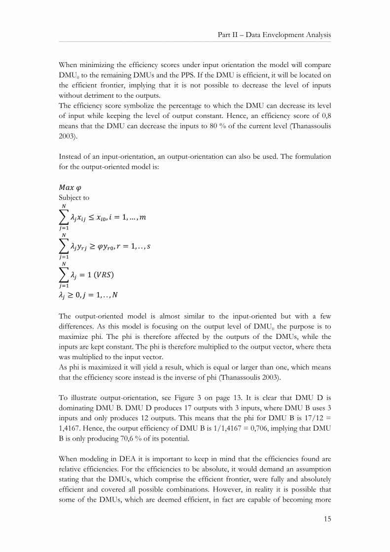
When minimizing the efficiency scores under input orientation the model will compare DMU0 to the remaining DMUs and the PPS. If the DMU is efficient, it will be located on the efficient frontier, implying that it is not possible to decrease the level of inputs without detriment to the outputs. The efficiency score symbolize the percentage to which the DMU can decrease its level of input while keeping the level of output constant. Hence, an efficiency score of 0,8 means that the DMU can decrease the inputs to 80 % of the current level (Thanassoulis 2003). Instead of an input-orientation, an output-orientation can also be used. The formulation for the output-oriented model is: 𝑀𝑎𝑥 𝜑 Subject to
𝜆!𝑥!" ≤ 𝑥!!, 𝑖 = 1,… ,𝑚!
!!!
𝜆!𝑦!" ≥ 𝜑𝑦!!, 𝑟 = 1, . . , 𝑠!
!!!
𝜆! = 1 𝑉𝑅𝑆!
!!!
𝜆! ≥ 0, 𝑗 = 1, . . ,𝑁 The output-oriented model is almost similar to the input-oriented but with a few differences. As this model is focusing on the output level of DMU0 the purpose is to maximize phi. The phi is therefore affected by the outputs of the DMUs, while the inputs are kept constant. The phi is therefore multiplied to the output vector, where theta was multiplied to the input vector. As phi is maximized it will yield a result, which is equal or larger than one, which means that the efficiency score instead is the inverse of phi (Thanassoulis 2003). To illustrate output-orientation, see Figure 3 on page 13. It is clear that DMU D is dominating DMU B. DMU D produces 17 outputs with 3 inputs, where DMU B uses 3 inputs and only produces 12 outputs. This means that the phi for DMU B is 17/12 = 1,4167. Hence, the output efficiency of DMU B is 1/1,4167 = 0,706, implying that DMU B is only producing 70,6 % of its potential. When modeling in DEA it is important to keep in mind that the efficiencies found are relative efficiencies. For the efficiencies to be absolute, it would demand an assumption stating that the DMUs, which comprise the efficient frontier, were fully and absolutely efficient and covered all possible combinations. However, in reality it is possible that some of the DMUs, which are deemed efficient, in fact are capable of becoming more

Part II – Data Envelopment Analysis ______________________________________________________________________________________________________________________________________________________________________
16
efficient. Hence, the efficiencies in DEA cannot be more than relative efficiencies based on the included DMUs. The efficiency score is more complex than what is seen at first sight. Hence, a DMU can be deemed efficient in different ways. Technical efficiency (TE) is full efficiency in a CRS model, while efficiency in a VRS model is called pure technical efficiency (PTE). The difference between the two efficiencies is called scale efficiency (Cooper, Seiford & Tone 2000) . Scale efficiency (SE) shows how much the choice of scale impacts the efficiency score. Imagine a DMU with the following efficiency scores, 𝜃!"#! and 𝜃!"#! , under CRS and VRS, respectively. Using these scores the SE is measured as:
SE = !!"#!
!!"#!
The SE can never be larger than one, as the VRS efficiency score always will be larger or equal to the CRS efficiency score, due to the nature of the scaling methods. In order to find the TE for a DMU in a VRS-model the relationship between the different efficiencies can be used. Hence, TE = PTE * SE Using this decomposition makes it possible to depict the source of inefficiency for a DMU, whether it is caused by inefficient operations, represented by PTE, or disadvantageous conditions, represented by the SE, or both (Cooper, Seiford & Tone 2000) . In the appendix a more thorough graphical example is included. As mentioned earlier, the literature has undergone a great development since the introduction of the two original models. Many variations and improvements have been presented and the next section will examine one of these extensions to the original models.
Part II – Data Envelopment Analysis ______________________________________________________________________________________________________________________________________________________________________
17
3. Slack-based Measure of Efficiency
For this study the original DEA model, hereafter known as DEA, is not sufficient. As mentioned above the DEA model cannot handle negative values and values of 0. As the model in this study will contain variables, which can obtain negative values, another model must be considered. What DEA lacks is translation invariance, the ability to handle negative values. One translation invariant model is the Additive model. However, as this model has serious imperfections regarding the efficiency scores and the calculation hereof, this model is hardly ever used. Instead it is often replaced by the Slack-based Measure of efficiency (SBM). The SBM provides almost the same advantages as the Additive model, but offers a more useful result.
3.1. Advantages of SBM The SBM model has several favorable characteristics. Even though it is not fully translation invariant like the Additive model, it allows for input values to be semi-positive, which means it can handle values of 0. Additionally, the output values are ‘free’ meaning it permits all values (Cooper, Seiford & Tone 2000) . The efficiency score is also unit invariant. This means that the results will be the same independent of the scale of the variables. As an example, the efficiency scores would be the same if the net income variable were changed from one currency to another. This is not the case with the DEA model (Cooper, Seiford & Tone 2000) . This is a great advantage when using data from an annual report, which consist of both accumulated and static data. By using the SBM model, the difference in the format of the figures is irrelevant and will not skew the results (Cooper, Seiford & Tone 2000) . Another important quality for the SBM model is that the DMUs are monotone decreasing in each of the slacks. This means that if just one of the input or output values is changed, it will affect the efficiency score. In DEA the efficiency scores are found with radial projection, where the model put weights on the different inputs and outputs when comparing them. This implies that it is possible to change an input or output value in the model and still get the same result. However, as the SBM accumulates all the slacks, any changes will be detected and affect the efficiency score (Cooper, Seiford & Tone 2000) .

Part II – Data Envelopment Analysis ______________________________________________________________________________________________________________________________________________________________________
18
3.2. SBM Efficiency One of the biggest differences between the DEA and the SBM model is the introduction of 𝑠!!and 𝑠!!, which is input excess and output shortfall, respectively, or in other words; slack. By inserting the two slack variables, the model becomes capable of detecting any slack present in all the inputs and outputs for each DMU.
3.3. SBM Notation In this section the efficiency score and the constraints of an SBM model will be examined and compared to DEA.
𝜌 = 1− 1𝑚
𝑠!!𝑥!!
!!!!
1+ 1𝑠𝑠!!𝑦!!
!!!!
Subject to:
𝜆!𝑥!" + 𝑠! = 𝑥!!, 𝑖 = 1,… ,𝑚!
!!!
𝜆!𝑦!" − 𝑠! = 𝑦!!, 𝑟 = 1, . . , 𝑠!
!!!
𝜆! , 𝑠!, 𝑠! ≥ 0, 𝑗 = 1, . . ,𝑁 At first sight, the formulation is seemingly similar to DEA. However, the objective function is more comprehensive, as the slack variables have been incorporated (Cooper, Seiford & Tone 2000) . The last part of the numerator of the efficiency score calculation is the slack for each input (𝑠!!) divided by the value of the input (𝑥!!) it refers to. By dividing with the input value the slacks get standardized. Hence, the size of the DMU will not influence the size of the slack, as slacks from large banks are divided with large input values and vice versa for small banks. The sum of the all the standardized input slacks is then divided by the number of inputs (m) to get the average slack per input. If there is no input slack, meaning the DMU is efficient, this part of the numerator will be 0 and the total numerator will be 1. If the DMU does experience input slack the numerator will yield a value below 1. The same is valid for the denominator of the efficiency score but with opposite sign. If the DMU does not experience output slack the denominator will be 1, but if there is slack in just one of the outputs, the value of the denominator will be above 1. Hence, in the SBM model a DMU can only become efficient if both the inputs and the outputs are efficient.

Part II – Data Envelopment Analysis ______________________________________________________________________________________________________________________________________________________________________
19
The first two constraints seem similar to DEA asides the inclusion of the slack variables, and that the ‘less than’- and ‘greater than’-signs are replaced by equal signs. The equal signs are due to the slack variables, as they catch any difference between the right-hand side and the left-hand side, resulting in the two sides becoming equal. Finally, the lambdas and the slack variables all have to be positive or 0. As the software used in this paper does not allow for a standard SBM but only for an input- or output-oriented SBM, the objective has to be revised to reflect one of the two orientations. If the standard SBM were to be used, the software should yield results for both input and output variables simultaneously, but this is not an option in the software used in this study. Additionally, it is important to consider whether all the variables are discretionary. If this is not the case, it might be more accurate to focus on either the input or output-orientation, to ensure that the result is found from variables, which are under managerial control (Thanassoulis 2003). Hence, the SBM formulation is revisited. For an input-oriented SBM-model the following notation is used.
𝜌!" = 1− 1𝑚
𝑠!!
𝑥!!
!
!!!
Subject to:
𝜆!𝑥!" + 𝑠! = 𝑥!!, 𝑖 = 1,… ,𝑚!
!!!
𝜆!𝑦!" − 𝑠! = 𝑦!!, 𝑟 = 1, . . , 𝑠!
!!!
𝜆! , 𝑠!, 𝑠! ≥ 0, 𝑗 = 1, . . ,𝑁 For an output-oriented SBM-model the following notation is used.
𝜌!"# = 1+ 1𝑠
𝑠!!
𝑦!!
!
!!!
Subject to:
𝜆!𝑥!" + 𝑠! = 𝑥!!, 𝑖 = 1,… ,𝑚!
!!!
𝜆!𝑦!" − 𝑠! = 𝑦!!, 𝑟 = 1, . . , 𝑠!
!!!
𝜆! , 𝑠!, 𝑠! ≥ 0, 𝑗 = 1, . . ,𝑁

Part II – Data Envelopment Analysis ______________________________________________________________________________________________________________________________________________________________________
20
The new objective functions are now a modified version of the original SBM objective function, focusing on either input slacks or output slacks. The models have many of the same advantages as the original SBM model but give the analyst an opportunity to choose an orientation for the model.
3.4. Choice of scaling As with the orientation, the software also requires a choice of scaling. The different pros and cons mentioned in the section 2.1.3 Choice of Scaling are also present when using a SBM model. Hence, using the CRS method implies that all banks have to achieve the same level of efficiency, but at different activity levels. Economies of scale is not present in this model, meaning that small banks should be able to obtain the same efficiency as larger banks, that operate under economies of scale. Hence, a bank, which operates fully efficiently, might not be efficient in the model, because another bank has better conditions for efficiency. In return, economies of scale is present with the VRS method. However, if the VRS method is used, the risk of deeming an inefficient DMU efficient increases. Especially, DMUs with extremely low or high values are likely to be deemed efficient, solely based on the extreme values. Hence, it is important to clarify what scaling method is used and to be fully aware of the consequences the chosen method can have.

______________________________________________________________________________________________________________________________________________________________________
21
Part III
Literature Review

Part III – Literature Review ______________________________________________________________________________________________________________________________________________________________________
22
4. Literature Review
The Literature Review will go through performance and bankruptcy both regarding regular companies and banks. Next, an overview of how DEA has been used in predicting bank failure is presented. Finally, the CAMELS model and how it has been used in the banking literature is examined. The appendix holds an overview of the Danish bank and the financial crisis with a focus on the Danish bank packages.
4.1. Performance and Predicting Bankruptcy When discussing corporate performance in finance theory, one concept is predominating. Good performance is equal to maximization of shareholder’s wealth, hence the market value of the company (Berk, DeMarzo 2011). Normally, the job of predicting good performance and bankruptcy is reserved to credit rating agencies such as Moody’s Investors Service (Moody’s) and Standard and Poor’s (S&P). The rating agencies assess and rate the risk and quality of companies, debt securities and countries, and assign them with a rating from AAA to CCC dependent on, the risk and quality. If a company receives a CCC rating it is in severe danger of going bankrupt (Casu, Girardone & Molyneux 2006) . When analyzing banks, it is easy to just consider them as any other company. However, it is important to be aware of the differences between a bank and an ordinary company, as this has a great influence on how to view concepts such as stakeholders, risk, and not least performance. Normally, a company will supply a service or a product to its customers. However, a bank is instead a financial intermediary between borrowers and savers. Basically, a bank deposits money for savers and lend them to borrowers. This intermediary role requires a well-performing institution as deposits will often have a short-term horizon and should be available instantly or within a short period to the saver. However, the deposits are simultaneously used to supply loans for the borrowers. These loans will often have a medium to long-term horizon, which creates a mismatch between the incoming and the outgoing funds. If this mismatch is not handled carefully, it will increase the liquidity risk, which means that the bank might not be able to fulfill its liabilities (Casu, Girardone & Molyneux 2006) . The idea of foreseeing bankruptcy is a common goal both for the corporate world and the banking world. In 1968, Altman published his work on the Z-score formula for predicting bankruptcy. This Z-score consisted of five ratios; working capital to total assets, retained earnings to total assets, EBIT to total assets, market value of equity to total book value of liabilities, and sales to total assets. Each of the ratios are positively

Part III – Literature Review ______________________________________________________________________________________________________________________________________________________________________
23
correlated to the Z-score and the higher the score the lower the risk of bankruptcy (Altman 1968). Ever since Altman published his Z-score the academic world has been trying to come up with an even better prediction method, using various kinds analysis techniques (Demyanyk, Hasan 2010, Altman 1968). Canbas, Cabuk, and Kilic (2005) used a principal component analysis to built an integrated early warning system, which can identify banks with serious problems. Fiordelisi, Marques-Ibanez and Molyneux (2011) used Granger-causality techniques to measure the relationship between risk, capital and bank efficiency in European banks. Cox and Wang (2014) used discriminant analysis to identify the main predictors of bank failure to use these indicators in an early warning system. Kolari, Glennon, Shin, and Caputo (2002) used a parametric logit analysis and a non-parametric trait recognition approach in the attempt of predicting failures in large US commercial banks. Generally, there are many approaches to predicting bank failures both in terms of model choices and variables to be included.
4.2. DEA and banks Since the late 1980’s, DEA analyst have been absorbed with finding the best way to measure performance and efficiency in banks using DEA models. Consequently, banking is one of the most used keywords in DEA articles (Emrouznejad, Thanassoulis 1996). A survey, which covered the last 30 years of DEA practice, found that ‘bank or banking’, were the 12th most used keyword in DEA articles and more used than keywords such as production, optimization, and benchmarking (Emrouznejad, Parker & Tavares 2008) . In 1992, Siems presented what is thought to be the first article, which used a DEA model to distinguish between failed and non-failed US banks, focusing on management quality (Siems 1992, Avkiran, Cai 2014). Since then, many have tried to improve and extend the DEA analysis for bank failure prediction. Despite the high interest and the many published DEA articles on the subject, there is no clear-cut way on how to predict failures or measure performance in banks. Therefore, the literature opens up for a large degree of freedom when analyzing banks. However, this freedom implies that it can be very difficult to compare analyses and get an overview of the literature and the methods used. The following sections will go through some of the issues in the literature and how the many methods differ.

Part III – Literature Review ______________________________________________________________________________________________________________________________________________________________________
24
4.2.1. Development in DEA models When Charnes, Cooper and Rhodes (1978) introduced the CCR model in 1978, the purpose was to measure efficiency in public ‘programs’ such as schools and other non-profit entities. The focus on the public sector was due to a lack of prices and profits in the model, which implies that the inputs and outputs are independent of cost and price. This cause that the model is not suitable for private sector, as the competition would force prices to be involved in the analysis (Charnes, Cooper & Rhodes 1978) . In 1984 Banker, Charnes, and Cooper (1984) extended the work from the CCR models by including a convexity constraint. The extension builds on the economic theory of production, as the concept of constant return to scale might be too theoretical. In reality a production will often experience both increasing return to scale, constant return to scale and decreasing return to scale, as the production increases in size. Hence, the BCC model incorporated these scaling differences with the convexity constraint (Banker, Charnes & Cooper 1984, Cook, Seiford 2009) . Both the CCR model and the BCC model builds on radial projection, which means that it requires an orientation. As it in some cases might be an issue that only the inputs or the outputs are in question, Charnes et al (1985) introduced the Additive model. The Additive model combines both orientations, as it incorporates slacks in the constraints. The objective function in this model is to maximize the sum of the input and the output slacks. This has some consequences; the efficiency scores can now obtain any value instead of a value in the interval 0: 1 , making the efficiency scores difficult to interpret and compare. Another issue is that the inputs and outputs might be measured in non-commensurate units, making the sum of the slacks an unsuitable measure. In other words, the Additive model is not unit invariant, which in a worst-case scenario can make the efficiency score useless (Cook, Seiford 2009). Since 1985, many different attempts to fix the issues with the Additive model have been published and one solution is Tone’s (2001) Slack-Based Measure of efficiency (SBM). The SBM model has many of the same advantages as the Additive model. Additionally, it has one advantage compared to the Additive model, as it provides comparable efficiency scores in the interval 0: 1 , just like DEA (Cooper, Seiford & Tone 2000) . Many other model variances, both radial and non-radial, have been published through the years, but this paper only focuses on some of the more popular and relevant models for this study.
4.2.2. Return to scale The choice between CRS and VRS can have a great effect on the results of the DEA analysis and it is therefore important to consider both pros and cons of both scaling methods. The VRS method seems to be preferred by most authors in recent time, to

Part III – Literature Review ______________________________________________________________________________________________________________________________________________________________________
25
avoid the strict scaling of the CRS method, even if it might imply an advantage for some of the DMUs (Pasiouras, Fethi 2010). In their study on efficiency in European banks, Altunbas et al (2001) found, that in most countries, including Denmark, small banks experienced constant return to scale. This implies that for some countries it might be more appropriate to use a mix of VRS and CRS such as the non-increasing return to scale. This is easily done by changing the constraint for VRS from 𝜆! = 1 !
!!! to 𝜆! ≤ 1 !!!! (Thanassoulis 2003).
However, as most software packages only allow the user to choose between CRS and VRS, this is often not an option. Due to the complexity in the choice of the return of scale, many authors choose to use both scaling methods in their publications and therefore report two results; one result for CRS and one for VRS. Using both scaling methods allow the author to identify scale efficiency as well and hence get a better understanding of the efficiency score (Zuzana 2014, Seiford, Zhu 1999).
4.2.3. Selection of inputs and outputs There have been almost as many assumptions of inputs and outputs as there have been applications of DEA (Bergendahl 1998, p. 235). Bergendahl’s quote on the choice of inputs and outputs in a DEA bank analysis is still, 17 years later, valid. Each bank analysis seems to have its own set of inputs and outputs. An explanation to this variance is most likely that the literature still lacks to identify a set of inputs and outputs, which catch the entire complexity of a bank (Berger, Humphrey 1997, Pasiouras, Fethi 2010). The selection of inputs and outputs can often cause trouble due to the literature’s inconsistent concerning the variables to be included. Obviously, the variables will be dependent on the purpose of the analysis but even analyses with the same purpose can have very differing inputs and outputs (Pasiouras, Fethi 2010). An example is the classification of deposits. Some see deposit as an input, others as an output. Some even divided the deposits into subsections and use some as inputs and others as outputs. Hence, dependent on the approach and the purpose of the analysis, the deposits can be used very different (Pasiouras, Fethi 2010). Historically, the bank analyses have, despite the variety, been very true to the idea of the input and output linkage; the inputs are used to produce the output and an increase in input should increase the outputs as well. Hence, the input variables were often factors like labor, number of branches, capital and other factors, which the bank needed to ‘produce’ the output variables, such as loans, interest income, and total income (Bergendahl 1998, Pasiouras, Fethi 2010). Compared to other methods of predicting bank failure, this approach often makes DEA stand out. Whereas other methods usually

Part III – Literature Review ______________________________________________________________________________________________________________________________________________________________________
26
focus on more financial figures such as financial ratios, risky assets, and market value of the bank, DEA analysis has held on to the production idea (Altman 1968, Canbas, Cabuk & Kilic 2005, Demyanyk, Hasan 2010) . In recent years, some DEA papers have challenged the traditional approach to bank studies, perhaps inspired by some of the other research fields in banking. Avkiran is one of the leading advocates for a more financially based DEA model. He finds that traditional DEA, despite the idea of linkage, often has an ill-explained selection of inputs and outputs, with an unclear link to theory. Moreover, he concluded that the, in a financial setting, untraditional choice of variables in the DEA literature, makes it difficult to compare the results to other methods (Avkiran 2006). Instead he introduced traditional finance and banking theory to his DEA models (Avkiran 2009, 2006, Avkiran, Cai 2014).
4.2.4. Orientation As touched upon earlier, the choice of orientation can have a great influence on the efficiency scores and on how the results are interpreted. In the literature, most authors choose the input-orientation, as the inputs are often discretionary factors, which are easier to change for the management, compared to the outputs. This could be inputs such as labor, expenses, and capital and outputs such as loans, number of transactions, and income. Hence, it is ceteris paribus easier for the management to hire more labor than to double the number of transactions. Even though most studies use input-orientation, some analysts use the output-orientation while others use models without orientation6 (Pasiouras, Fethi 2010).
4.3. CAMELS and banks In November 1979, the Uniform Financial Institutions Rating System was introduced by the Federal Financial Institutions Examination Council (FFIEC) in the USA. The purpose of the rating system was to evaluate financial institutions and identify those that was in distress and needed more attention. Originally, the system was known as CAMEL, which was an acronym for the five variables; Capital adequacy, Asset quality, Management efficiency, Earnings, and Liquidity. However, as the banking industry incurred some changes, the original model was no longer sufficient. So in 1997 the sixth variable, Sensitivity to market risk, was added to the model and the name was extended to CAMELS. Despite the American origin, various bank sectors around the world are now evaluated with the CAMELS model (Federal Deposit Insurance Corporation 1997, Barr et al. 2002, Sayed, Sayed 2013).
6 An example of a model without orientation is the SBM model. However, it can be used with orientations as well, as is seen in this paper.

Part III – Literature Review ______________________________________________________________________________________________________________________________________________________________________
27
When the FFIEC evaluates financial institutions with the CAMELS model, they assign a number between 1 and 5 to the financial institution based on how well they perform on the six variables. The best rating is 1 and this group includes sound financial institutions with no need for supervisory concern. The worst rating is 5 and the institutions in this group have unsafe and unsound practices or conditions, which require ongoing supervisory attention, as failure is highly likely (Federal Deposit Insurance Corporation 1997). The CAMELS model has always been shrouded in a little mystery, as the public does not know exactly what the six different factors cover. Despite that obvious challenge, numerous analyses have been published using the CAMEL or the CAMELS model to evaluate banks. Cole and White (2012) use proxies for the six CAMELS variables in combination with other variables in their multivariate logistic regression, where the dependent variable is a binary variable with the two outcomes; fail or survive. They find that the CAMELS variables are capable of explaining bank failures both in the recent crisis and in the American bank crisis in 1985-1992. Barr el al (2002) has another approach to the CAMELS model than most studies. Instead of finding proxies for the six CAMELS variables, they use the actual CAMELS scores that each bank has received, in a DEA model to evaluate the productive efficiency in US banks. Based on their results they recommend using CAMELS as a monitoring tool. Hence, the CAMELS variables have been used in different approaches and seem to be a good predictor of bank failure.

______________________________________________________________________________________________________________________________________________________________________
28
Part IV
Methodology and Data
Part IV – Methodology and Data ______________________________________________________________________________________________________________________________________________________________________
29
5. Variables
As the literature review revealed, the DEA theory is filled with many different attempts to find the most appropriate and accurate set of inputs and outputs for measuring bank performance and foreseeing bankruptcy. This paper follows the idea of Avkiran and Cai (2014) to use more financially grounded inputs and outputs and relax the production idea. The factors in the financial DEA model might be more accurate in explaining failure compared to factors like labor and deposits. However, this implies that the efficiency score in itself has a different meaning than in most DEA bank models (Avkiran, Cai 2014, Pasiouras, Fethi 2010). Avkiran and Cai make two models using the factors from the CAMELS model and a market model, respectively, and use a Super-SBM7 to examine if it is possible to identify the banks, which failed. This paper will only focus on the CAMELS model and extend those but only use a regular SBM model instead of a super-SBM. In this paper, the CAMELS model will be applied by substituting the six variables with accounting-based proxies. The use of proxies composed of accounting figures ensures transparency and makes it easy to replicate. Furthermore, it is not possible to use the actual factors, as it is not known in the public how the authorities measure the CAMELS ratings (Kerstein, Kozberg 2013).
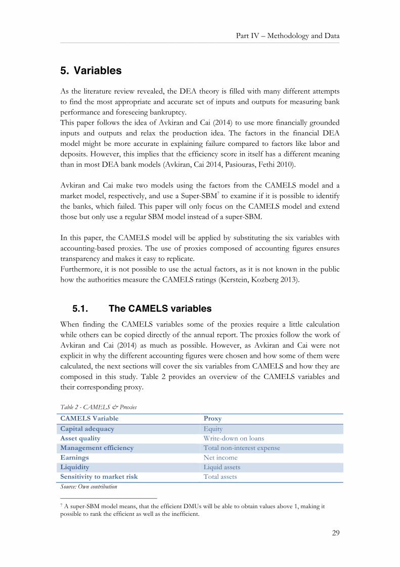
5.1. The CAMELS variables When finding the CAMELS variables some of the proxies require a little calculation while others can be copied directly of the annual report. The proxies follow the work of Avkiran and Cai (2014) as much as possible. However, as Avkiran and Cai were not explicit in why the different accounting figures were chosen and how some of them were calculated, the next sections will cover the six variables from CAMELS and how they are composed in this study. Table 2 provides an overview of the CAMELS variables and their corresponding proxy. Table 2 - CAMELS & Proxies
CAMELS Variable Proxy Capital adequacy Equity Asset quality Write-down on loans Management efficiency Total non-interest expense Earnings Net income Liquidity Liquid assets Sensitivity to market risk Total assets Source: Own contribution
7 A super-SBM model means, that the efficient DMUs will be able to obtain values above 1, making it possible to rank the efficient as well as the inefficient.

Part IV – Methodology and Data ______________________________________________________________________________________________________________________________________________________________________
30
5.1.1. Capital Adequacy Capital adequacy is a term introduced with the Basel Accords, and states how much capital a bank should hold in relation to the riskiness of the business activities, meaning both assets and off-balance activities. Hence, the more risky a bank is, the more capital it needs to hold (Casu, Molyneux 2003). This is obviously not possible to calculate with accounting numbers, as it also concerns off-balance sheet risks. Instead Equity is used as a substitute, as this posting is an indication on how solid the bank is. The Equity can be seen as a capital cushion, which the bank can be forced to use if the loans they have provided, are not paid back. Hence, Equity is not an immaterial figure. Compared to a normal company, a bank will often have a higher leverage. A manufacturing firm will often have debt-to-equity ratio just above 1, whereas a bank can have a debt-to-equity ratio as high as 11,5. Despite this high leverage Equity is crucial for the bank, as it risks becoming technically insolvent, if the Equity is not large enough to cover the loss from loans that are not paid (Casu, Girardone & Molyneux 2006) . As the Equity consists of prior years profit, and also is a measure of the banks’ risk appetite, it is expected that distressed banks will have a lower level of Equity and vice versa for the well-performing banks. Hence, Capital Adequacy, represented by Equity, is an output variable in the model.
5.1.2. Asset Quality This proxy is a part of the Write-down on loans etc. from the income statement. It is an impairment allowance, which is set aside if a loan is impaired. The write-downs often receive great focus from the general public, as it indicates how risky the loans of the bank are (Baldvinsson 2011). The posting in the income statement is a combination of the write-downs the bank had encountered this year for both individual and group level8, but it also includes refunds from previous years. If a loan, which had been written down, for some reason is paid back, the bank can reverse the amount. This means that the variable can contain refunds from previous years and obtain a negative value if the refunds are larger than the write-downs. In order to ensure consistency and comparability between the banks, the proxy will only be comprised by Individuals write-downs and Group write-downs from the current year.
8 The bank has to make an assessment on individual level to identify any loss-making events and hereafter on group level. The group level is used if a loss-making event hits a group of loan takers, for example farmers. It might be impossible for the bank to identify the farmers, which should be written down due to the hit, so instead the write-down is done for the entire group of farmers (Baldvinsson 2011).

Part IV – Methodology and Data ______________________________________________________________________________________________________________________________________________________________________
31
From a DEA perspective the proxy Write-down on loans is not an appropriate input variable, as it lacks the linkage between inputs and outputs. In a normal setting an increase in inputs would increase the outputs as a result hereof but if the Write-down on loans increase, there is no connection to ensure that any of the outputs in this study will increase too. However, as it is expected that the write-downs are larger for banks with riskier loans and lower for well-performing banks with less risky loans, the proxy is assumed to be useful for this study. Following the same logic, the Asset Quality variable will be an input-variable.
5.1.3. Management Efficiency The variable ‘Management efficiency’ (M) is one of the more difficult factors to translate into accounting data. In many empirical studies where the CAMELS factors are used, the M is left out of the analysis (Pasiouras, Fethi 2010). The Total non-interest expense consists of Staff costs and administrative expenses, Depreciation, amortization and impairment of property, plant and equipment as well as intangible assets, and Other operating expenses, which are all present in the banks’ income statements. These entries are all necessary to maintain the bank and the staff, and in a well-run bank it is expected that these expenses will be at a fair level. Hence, the assumption is that the better the management is, the less expenses will be needed. It is important to keep in mind that the inputs are to be minimized for each DMU but not to be spared. Just as in the original model, the amount of input should be as low as possible, but there is no free lunch, which means that it is not possible to produce outputs without any inputs. Further, the technical efficiency score is often viewed as managerial efficiency, so in that sense the efficiency score in itself will contain an indication of the management efficiency (Thanassoulis 2003) . As this variable is expected to be low for well-performing banks, it will be an input variable in the model.
5.1.4. Earnings Net income is an easy way of assessing a bank’s condition, but it is also important to keep in mind, that it is a broad overview. The notes and the rest of the annual report can contain troubled figures, pointing towards distress, which are not directly visible but still very important. For instance, just before the financial crisis the economy had been going very well and optimism was everywhere. This was very evident in the lending growth of many banks, which skyrocketed. At first glance the income statement would look good, as the banks would receive a lot of interests from the many loans. However, as the crisis

Part IV – Methodology and Data ______________________________________________________________________________________________________________________________________________________________________
32
started many banks encountered impaired loans and lacking liquidity, which eventually led to the failure of some of the banks. Hence, Net income cannot stand alone when measuring the performance of a bank. As with all other performance analyses, it is obvious that the Net income should be as high as possible and therefore it will be an output variable in the model.
5.1.5. Liquidity Liquidity is crucial for a bank, as it needs to be able to meet its engagements. This was visible leading up to the financial crisis where many banks had higher loans than deposits and had to lend money on the expensive interbank market in order to have liquidity enough (Baldvinsson 2011). When dealing with Liquid assets it is difficult to state exactly what should be included, as there are different degrees of liquidity. In the asset side of the balance sheet the different postings are listed with descending degrees of liquidity but it is difficult to draw a line between liquid and highly liquid assets. However, to construct the variable for the analysis it is necessary (Baldvinsson 2011). The first posting in the balance sheet is Cash balance and demand deposits with central banks. This posting is clearly highly liquid as this is the capital the bank has in its possession. Most of it is the money the banks physically hold to be able to serve the customers (Baldvinsson 2011). The next posting is Receivables from credit institutions and central banks. This consists of the claims between banks, which are settled on a daily basis but it also contains the deals the banks make on the interbank market, which have maturities from 1 day to a year. Hence, some of the capital in this posting is highly liquid, while some of it is less liquid. Despite the variance in liquidity, the entire posting is included in the variable. The third posting is Loans. This is not included as it contains all loans and receivables with very different degrees of liquidity. The fourth and the fifth posting are for most banks bonds and shares, respectively. The bonds are divided into Bonds at fair value and Bonds at amortized value. The first is held for trading and is therefore liquid. The latter are the bonds, which the bank expects to hold to maturity, which implies low liquidity. Hence, bonds at fair value are included in the variable. The next positing is shares, which are disclosed different from bank to bank, so to ensure high liquidity, no further postings are included (Baldvinsson 2011). This means that the variable Liquid assets is composed by Cash balance and demand deposits with central banks, Receivables from credit institutions and central banks, and Bonds at fair value. As this is obviously crucial for a bank’s survival to have sufficient liquidity, this proxy will be an output variable in the model.

Part IV – Methodology and Data ______________________________________________________________________________________________________________________________________________________________________
33
5.1.6. Sensitivity to Market Risk Sensitivity to market risk is especially difficult to replace by an accounting-based proxy, as it is not possible to fully capture it in one or a few accounting figures. Evidence from the crisis and the literature in general, are agreeing on one thing regarding sensitivity. Smaller banks were in general more likely to fail during the crisis, implying that size and Sensitivity to market risk are correlated (Cole, White 2012). Hence, in order to find a proxy for the sensitivity a size measure must be found. There are many suggestions for size proxies in the literature. Some examples are Interest expenses to deposits, Market size estimators, Total risk weighted assets, Number of FTE, and the Natural logarithm of Total assets (Claro 2013, Thanassoulis 1999, Avkiran 2006, Sufian 2009). However, Total assets as a size proxy seems to be preferred (Casu, Molyneux 2003, Avkiran, Cai 2014, Bauer et al. 1998). Using Total assets as a proxy causes some trouble, as it is highly correlated with some of the other variables, especially Liquid assets. Both variables are output variables, so any banks with large amounts of Liquid assets will ceteris paribus have a high amount of Total assets. Consequently, the DMU will be rewarded twice for the large amount of Liquid assets. However, Total assets will be used as a proxy despite the challenges, to follow the study of Avkiran and Cai (2014). As size and failure are negatively correlated, the size proxy will be an output variable.
5.2. Exposure to real estate Even though the CAMELS model has proved to be a good predictor of bank failure, it is best at a short-term horizon. At a more long-term horizon the exposure to commercial real estate loans is more correlated with distress (Cole, White 2012). The use of the real estate loans for identifying distressed banks is not a new idea. Cole and Fenn (1995) found evidence that real estate loans played a big role in the American bank crisis in 1985-93, and the Danish FSA included the exposure to real estate loans in the Supervisory Diamond, which is a tool instituted to prevent bank failures in Denmark. The relative distribution of loans and warranties for a bank is found in the notes of the annual report. This list is divided into business sectors and private customer loans. The business sectors are further segmented and contain the postings Property administration and business, business services or Property business. This share reveals how large a percentage of the total loans and warranties the bank has placed in commercial real estate. Despite the inclusion of warranties, this figure will be used to find the share commercial real estate each bank has. As the figures used in the analysis have to be

Part IV – Methodology and Data ______________________________________________________________________________________________________________________________________________________________________
34
volume measures, the Total loans is multiplied to the share of real estate, to find the share of real estate loans in DKK. As the literature has shown a positive correlation between real estate loans and bank failure, this variable will be an input in the model, as it is expected to be high for banks, which are likely to get distressed and vice versa. The seven variables in the model are all found in the annual report and four of them are posted in the balance sheet. This means that some of the variables are highly correlated, especially Total assets and Liquid assets, and might skew the result for some banks. As Total assets is included in the model as size factor, it might be worth considering using another variable to represent size instead of the assets, to avoid the high correlation. This could be number of employees or branches. However, as these variables are not always available in the annual report, and as Avkiran and Cai use Total assets in their model, the size factor will be represented by Total assets in this study (Avkiran, Cai 2014).
Part IV – Methodology and Data ______________________________________________________________________________________________________________________________________________________________________
35
6. Choosing Inputs and Outputs The variables and the proxies used in this study are listed below. Inputs
• Asset Quality - Write-down on Loans • Management Efficiency - Total Non-interest Expenses • Concentration of Commercial Real Estate Loans (Real Estate)
Outputs
• Capital Adequacy - Equity • Earnings - Net Income • Liquidity - Liquid Assets • Sensitivity to Market Risk - Total Assets
When choosing inputs and outputs for a DEA model, Dyson et al. (2001) suggest four key assumptions to ensure the model is comprehensive:
• It covers the full source of resources used • Captures all activity levels and performance measures • The set of factors are common to all units • Environmental variation has been assessed and captured if necessary
(Dyson et al. 2001, p. 248) It is clear that the assumptions are made with a focus on capturing operational efficiency with the model. However, the general ideas of the assumptions are still valid and useful when assessing the inputs and outputs for other types of DEA models. The first two assumptions ensure that the model is covering all relevant aspects of the issue to be measured regarding both to the inputs and the outputs. These two assumptions are important, because if a model fails to include a relevant factor, it might deem the wrong DMUs efficient, due to the lacking information. This will obviously have a great impact on the quality of the results. Hence, it is important to identify all relevant factors and aspects of what is being measured, in order to ensure that the model covers everything. However, it is also important to emphasize that not all factors can be included. First, the model would quickly get huge and confusing, which will make it difficult for the inefficient DMUs to identify their true improvement potential in the results. Second, if too many inputs and outputs are included, the model will lack discrimination, which will cause artificially high efficiency scores. With many variables to choose from, the model can make most DMUs efficient, as it is weighing the different variables to each DMU’s advantage. Hence, the more variables included in the model, the easier it is for the DMUs to become efficient (Thanassoulis 2003).

Part IV – Methodology and Data ______________________________________________________________________________________________________________________________________________________________________
36
To ensure the model’s discriminative powers, when many inputs and outputs are added to the model, the number of DMUs is crucial. The rule of thumb is that the number of DMUs should be 2(m ∙ s) where m ∙ s is the product of the number of inputs and outputs (Dyson et al. 2001). Hence, for a model like the one in this study with three inputs and four outputs there should be at least (2 ∙ 3 ∙ 4) = 24 DMUs. The third assumption implies that all the DMUs must be homogenous. Hence, to compare the DMUs it is important that all the variables are applicable to all the DMUs. The DMUs should differ in levels of activity and resources, but should be homogenous with regards to inputs and outputs. Otherwise it will be like comparing apples to pears (Thanassoulis 2003). The fourth assumption regarding environmental variation can be very important. Imagine two post offices, where one is more efficient than the other. If the main difference between the two offices is that the efficient office is located in a big city, where letters can be dropped of within a few meters distance and the other office is located in the countryside, where the distance between the houses are measures in kilometers, it is clear that the latter will never be able to obtain the same efficiency, due to the environmental factor. In that case, it would be a good idea to adjust for the environmental variance, so the countryside post office is not deemed inefficient solely because of the city office’s advantage.
6.1. Fulfilling the assumptions In this study, most of the variables originate from a model, which is used to rate the performance of a bank. It is therefore assumed that all relevant factors for evaluating banks are included in the study. Since the CAMELS model seems to be best at predicting bank failures on a short-term horizon, a variable concerning the real estate loans has been included. This variable has proved to be a good proxy for predicting bank failures on a long-term horizon (Cole, White 2012). Hence, all relevant factors are assumed to be included in the model, fulfilling the first two assumptions. The third assumption, the homogeneity assumption, might be problematic. All the banks in the model are Danish and the model only contains banks and not bank-like institutions such as investment banks and mortgage banks. However, as some of the banks may choose not to lend out money to commercial real estate or has no write-downs, it could be discussed if the variables are applicable to them, but as the option is available to all the banks, it is assumed fulfilled. The environmental factor is likely the biggest issue, when it comes to fulfilling the assumptions. The banks differ remarkably in size and where some cover the entire

Part IV – Methodology and Data ______________________________________________________________________________________________________________________________________________________________________
37
country, others are only present in one small part of the country, so the diverse environment could affect the banks in different ways. However, as all banks are operating in Denmark under the same conditions and with the same options, the assumption is considered fulfilled, despite the differences. Further, as the purpose of this paper is not to find improvement material for the individual DMUs but to identify good and bad performances, this assumption is not believed to be crucial.

Part IV – Methodology and Data ______________________________________________________________________________________________________________________________________________________________________
38
7. Data collection The first task when collecting data is to decide, which years to include in the analysis. In this analysis, year 2007 and year 2010 are used. Year 2007 is used, as it was the year leading up to the financial crisis. Hence, it is assumed that any indications of distress in the banks would be visible in the annual reports, making the difference between the failing and the non-failing banks significant. Year 2010 was chosen, as it was amidst the financial crisis and it would be interesting to see if the model could foresee failures both before and during the crisis, as this would give institutions such as the Danish FSA, an opportunity to track the distressed banks during a crisis. Next, the relevant data must be collected. The data collection was done using different data sources and is explained step by step below. Every year the Danish FSA (Finanstilsynet) makes a statement comprising the Danish banks grouped after the size of their working capital. As this statement only contains banks and not any other bank-like institutions, this was chosen to be the list of banks for the analyses (Finanstilsynet 2014). For the 2007 analysis, the list from primo January 2008 was used to identify the relevant banks for the analysis. This was used to exclude all banks, which have failed before and during 2007. For the 2010 analysis the list from January 2011 was used, following the same logic as above. The statement also contained foreign banks with a branch in Denmark and Faroese banks, but both of these categories were left out of the analysis to ensure consistency and homogenous banks. In 2007 the list included 147 Danish banks and in 2010 the list included 123 Danish banks. In the years 2007-2010, 25 Danish banks failed and a single bank was set up. The data for the analysis was mainly generated in the database Bankscope. Data, which were not available on Bankscope, were retrieved from the annual reports of the banks. The annual reports were found either on the webpage of the bank or at cvr.dk9. As the data from Bankscope and the annual reports of all the banks were found, a few banks were excluded from the analysis. This was done either because the annual report could not be found or because the format of the annual report was different from the other banks’ reports. In the 2007 analysis eight banks were excluded; four of them did not have an available annual report and the remaining four had not disclosed all the needed information. Hence, in the 2007 analysis there will be 139 banks. For the 2010 analysis the list contained 123 banks. Out of those eleven banks were excluded; five of them did not have an available annual report, 4 of them had been
9 cvr.dk is a Government-owned webpage, where it is possible to retrieve old annual reports for both active and inactive Danish companies.

Part IV – Methodology and Data ______________________________________________________________________________________________________________________________________________________________________
39
overtaken by Finansiel Stabilitet (Financial Stability) or another bank prior to the 2010 analysis, and the last remaining two had not disclosed all the needed information. This means that there will be 112 banks in the 2010 analysis. The excluded banks and the reason for excluding them can be found in the appendix. Some of the annual reports included data from both the bank and a group. In those cases, the data from the group were used. This was done both because Bankscope used the data from the group but also because this gave a more accurate picture of the means available to the bank.
7.1. Bankscope A number of the variables were generated from the database Bankscope. These variables were:
-‐ Previous Bank name -‐ Total Non-interest Expense, Org. Currency, Last avail. year - 3/Last avail. year -
6 -‐ Total Assets, Org. Currency, Last avail. year - 3/Last avail. year - 6 -‐ Equity, Org. Currency, Last avail. year - 3/Last avail. year - 6 -‐ Net Income, Org. Currency, Last avail. year - 3/Last avail. year - 6 -‐ Loans, Org. Currency, Last avail. year - 3/Last avail. year - 6
Variables labeled ‘Last avail. year – 3’ is equivalent with year 2010 and the variables labeled ‘Last avail. year – 6’ is equivalent with year 2007, as the last available year is 2013. The first step in the process was to match the banks in the statement from the Danish FSA with the banks from Bankscope, as the list from Bankscope included 176 active and inactive Danish banks and bank-like institutions. As some of the banks had changed their name one or more times since 2007 and 2010, and Bankscope had the banks listed with the newest name, the variable Previous Bank Name was included in the data set to help match the banks in the FSA statement with the banks from Bankscope. The next four variables, Total non-interest expenses, Total assets, Equity, and Net income, were all variables to be used in the analysis with no further adjustments. During the analysis it was discovered that Bankscope was not consistent in its data work. This meant that some of the data was from another year than the requested, other variables were not consistent with the data from annual reports and some variables were simply lacking values. Hence, all values in the data set were examined and compared to the annual reports to ensure that the analysis was as accurate as possible and containing the correct data. Additionally, a few of the smallest banks in the FSA statement were not present in Bankscope, so all their data was entered manually to the analysis using the annual reports.

Part IV – Methodology and Data ______________________________________________________________________________________________________________________________________________________________________
40
The last variable generated from Bankscope, Total loans, is not a variable but part of the calculation for another variable. To find the banks commercial real estate variable, the Total loans were multiplied with the share of real estate loans, as explained in section 5.2. The share of commercial real estate was found manually in the notes for all banks. For some of the variables Bankscope did not provide the correct format for analysis. So even though the two variables Write-down on loans and Liquid assets both were available in Bankscope, they had to be found in the annual reports. The first variable, Write-down on loans, seems similar to the variable Loan loss provision10 from Bankscope. However, as explained in section 5.1.2, this variable was not suitable for the analysis. Instead the write-downs on Individual loans and Group loans for the current year were found manually in the notes and aggregated in the analysis. This meant that the smallest value the variable could take was 0, if a bank had encountered no write-downs that year. The variable Liquid asset was also available in Bankscope, but as the variable was not transparent and seemed to differ from bank to bank, this variable was found manually in the balance sheet to ensure consistency and transparency in the analysis. The variable consists of the postings Cash balance and demand deposits with central banks, Receivables from credit institutions and central banks, and Bonds at fair value as explained in section 5.1.5. As all the data are gathered, the banks are given an abbreviation. For the banks that failed, the abbreviation start with a capital F for failed. Next, was the year in which they failed and lastly a random number to make it unique. Hence, the first bank on the list, which failed in 2012, would get the abbreviation F121. In order to determine and assign the correct year to the banks, a list of the failed banks from the Danish Ministry of Business and Growth from their publication regarding the financial crisis in Denmark, was used (Udvalget om Finanskrisens Årsager, Erhvervs- og Vækstministeriet 2013). As the paper was published in 2013, the last banks to fail in 2013 were obviously not included. Instead, this information was obtained from Bankscope. The remaining banks were assigned a random, unique letter-combination ranging from A to CCC. The material described in this section can be found in the appendix.
10 Similar to the Write-down on loans, etc.-posting in the income statement
Part IV – Methodology and Data ______________________________________________________________________________________________________________________________________________________________________
41
8. Methods This section will review the four methods used to analyze the efficiency scores provided by the SBM analysis.
8.1. Mann-Whitney U-Test The first test performed on the efficiency scores, is a test on the mean values of the failed and the non-failed banks, to see if there is any significant difference between the two groups or in other words, to test the discriminatory powers of the SBM model. As the SBM model is non-parametric, a normal two-sample t-test is not suitable, as it is a parametric test and therefore requires the difference between the two data sets to be normally distributed. Instead the Mann-Whitney U-test is used. The test is hereafter called the U-test. This test is consistent with the work of Pille and Paradi (2002). The 0-hypothesis for the test states that the mean values of the two groups of banks are equal to each other. Hence, the prospect is to reject the 0-hypothesis, which will imply significant discriminatory powers for the SBM model (Israel 2008, Keller 2009). In the U-test all the efficiency scores are ranked in descending order. In a case with ten observations, the observations will be assigned ranks from one to ten, with one being the best. In case of a tie between two or more DMUs, they will receive the average of their combined score. Hence, if observation four and five had the same value, they would both be assigned the ranking 4,5. When all the observations have been assigned ranks, they are divided into the two groups; failed and non-failed. For each group the sum of ranks are calculated. The sums are called R1 and R2, respectively. Next, the parameter U1 is calculated for the first group of banks using the following formula
𝑈! = 𝑛!𝑛! + 𝑛!(𝑛! + 1)
2 − 𝑅!
Where n1 is the number of DMUs in the first group and n2 is the number of DMUs in the second group. The parameter U is also found for the other group of banks using the formula
𝑈! = 𝑛!𝑛! + 𝑛!(𝑛! + 1)
2 − 𝑅! 𝑜𝑟 𝑈! = 𝑛!𝑛! − 𝑈!
If the number of DMUs is larger than 20 for both groups, the sample is approximately normally distributed and the critical value can be found using, a Z-test with the following parameters:

Part IV – Methodology and Data ______________________________________________________________________________________________________________________________________________________________________
42
𝜇! = 𝑛!𝑛!2
𝜎! = 𝑛!𝑛!(𝑛! + 𝑛! + 1)
12
The z-statistic is
𝑍 = 𝑈 − 𝜇!𝜎!
As the sum of the two U-values equals the product of the two sample sizes (𝑛! ∙ 𝑛!) both U-values will yield the same Z-value, but with opposite operational sign (Israel 2008, Keller 2009) . To determine whether it is possible to reject the 0-hypothesis, two options are available. One option is to find the critical value of Z and the other is to find the corresponding p-value to the observed Z-value. If the observed Z-value is larger than the critical Z-value, it is possible to reject the 0-hypothesis. The critical value at a 5 percent significance level is ± 1,96 for a two-tailed test and ± 1,645 for a one-tailed test. This study uses a one-tailed test. If the p-value is smaller than 0,05 it is possible to reject the 0-hypothesis at a probability of 95 % (Keller 2009).
8.2. Gini-coefficient In bank failure prediction studies, the discriminative powers are occasionally assessed using the Gini-coefficient. The Gini-coefficient is mostly known as a statistics to calculate the inequality in countries, but it is also used in prediction models to test the inequality and the discriminative powers of the sample (Dixon et al. 1987, Damgaard, Weiner 2000). Compared to other measures of discriminative powers, such as the U-test, which compares two mean values, the Gini-coefficient measures the inequality in the entire sample and compares all the DMUs to each other. The coefficient is between 0 and 1, where a coefficient of 0 means that all the observations in the sample are identical and a coefficient of 1 means that the sample experiences complete inequality. The Gini-coefficient will function as a support to the U-test in this study, as the format of the test is not completely suitable for a DEA analysis. The formulation below will show why. The observations, or in this study DMUs, in the sample are ranked in ascending order and assigned a number corresponding to the rank. The Gini-coefficient is than calculated using the formula below
𝐺 = (2𝑖 − 𝑛 − 1)𝑥!!!
!!!
𝑛!𝜇
Part IV – Methodology and Data ______________________________________________________________________________________________________________________________________________________________________
43
Where i is the rank of the DMU, n is the sample size, x’i is the efficiency score and μ is the mean value of the sample (Dixon et al. 1987, Damgaard, Weiner 2000). All the efficient DMUs will have the same x’i-value of 1, which implies that the Gini-coefficient is expected to be lower than in other studies. This is both due to the lacking inequality in the efficient DMUs and to the fact, that some of the efficient DMUs are more efficient than others and therefore should be assigned a higher x’I-value. As this is not an option in the SBM-model, the Gini-coefficient will be lower than in comparable studies. Hence, when comparing the coefficient to other studies, it must be treated with great caution.
8.3. Layer Analysis The third analysis is a Layer analysis. This analysis is used to examine whether the model assesses any predictive powers. The method is consistent with the work of Paradi, Asmild, and Simak (2004) and Avkiran and Cai (2014). As the name suggests, the analysis consists of multiple layers. In the first layer, the SBM analysis is performed on all the banks. As the SBM analysis has been performed, all the efficient DMUs are removed from the data set and the inefficient DMUs from the first layer are then used as the sample in the second layer. This procedure is repeated until all DMUs are deemed efficient. The idea is to divide the DMUs into layers, to learn how many of the efficient banks in each layer failed and non-failed banks, respectively (Avkiran, Cai 2014). It is expected that the non-failed banks will be the majority in the first layers but that the two groups will converge, as more layers are included. To use this model as a predictive tool, a cut-off layer must be identified when all the layers have been identified. The cut-off layer will divide the analysis in two groups. The upper layers are the expected non-failing banks and the lower layers are the expected failing banks. The choice of a cut-off layer must be made with respect to the type I and type II errors, and which of the two error types that are most acceptable to the analyst. Type I error is the misclassification of failing banks as non-failing banks and type II error is the misclassification of non-failing banks as failing banks. Hence, the analyst must choose whether it is better to misclassify failing or non-failing banks, as there is a trade-off between the two. If all the failing banks have to be labeled as failing, which is equal to minimizing the type I errors, this will inevitably increase the type II errors, that non-failing banks are classified as failing. To make the results of the analysis more useful, the failed banks have further been divided into four groups based on how they ceased activity. The first group is the banks, which received capital from Finansiel Stabilitet but still had to be taken over by Finansiel Stabilitet. These are named FS Takeover in the table. The second group is the banks,

Part IV – Methodology and Data ______________________________________________________________________________________________________________________________________________________________________
44
which received capital from Finansiel Stabilitet but were taken over by another bank. These banks are called FS Aid in the table. The third group is other banks, which ceased activity but did not received capital from Finansiel Stabilitet. These banks were mostly taken over by another bank and will be named Other ceased in the table. The last group is the banks where it is unknown how they ceased activity. It is assumed that most of these belong to the third group. These banks are named Unknown (Udvalget om Finanskrisens Årsager, Erhvervs- og Vækstministeriet 2013). The subgroups will make it easier to identify the most appropriate cut-off layer, as it from an economic point of view is more essential to identify the banks from the first two groups, instead of the two latter groups. It is expected that the takeovers in the first two groups were solely default-driven, whereas the banks in the last two groups might have merged for other reasons such as a larger market share. In their study Paradi, Asmild, and Simak (2004) tries to predict bankruptcy in general, but their methods are relevant for this study too. Besides the layer analysis, they have another method for classifying banks and predicting bankruptcy. They incorporate a cut-off value in their analysis. The cut-off value is an easy way of classifying the DMUs as either failing or non-failing. If the efficiency score of a DMU is below the cut-off value, the DMU is classified as failing and if the efficiency score is above the cut-off value the DMU is classified as non-failing. However, this method has a great challenge in determining the cut-off value. In their study, they rely on the cost of the type I error and of the type II error, found by Altman and Hull. These costs are multiplied to the number of type I and type II errors, which occur in their study and summed together. However, these values are approximately 20 years old and the conditions on the financial market have changed significantly since then, making it unlikely that the values are suitable for the current market (Paradi, Asmild & Simak 2004) . Hence, this study will only perform the layer analysis, as it does not rely on static values and can be changed dependent on the purpose of study and the preferences of the analyst.
8.4. Robustness Test To determine how strong the results from the previous tests are, a robustness test is performed. The test will examine if changing the sample will affect the results. The Danish FSA divide the Danish banks in four groups dependent on the size of their working capital (Finanstilsynet 2014). The largest banks are classified as group 1. Five banks were classified as group 1 in 2007 and six banks were classified as group 1 in 2010. The largest of the four groups in 2007 and in 2010 was group 3 with 89 and 80 banks, respectively. These groups will be used in the robustness test to learn whether the results change if the SBM analysis is performed while excluding some of the groups.

Part IV – Methodology and Data ______________________________________________________________________________________________________________________________________________________________________
45
If the mean values are the same for the failed and non-failed banks independent on which groups are included in the sample, the test is robust in the sense that the conclusion will not be affected by changing the banks included in sample.

Part IV – Methodology and Data ______________________________________________________________________________________________________________________________________________________________________
46
9. Descriptive statistic Before initiating the SBM analysis it could be interesting to examine if there are any initial differences between the failed and the non-failed banks. As it is found that most of the failed banks are small banks, it brings no value just to compare the mean values of the seven variables. As Total assets is included in the model as a size factor, it will be used to standardize the values of the remaining variables. Hence, all six variables will be divided with Total assets to achieve a comparable value, which will make it possible to identify any significant differences in the values of the failed and the non-failed banks. As the input values are expected to be lower for well-performing banks, it is expected that the non-failed banks will have a lower mean value in the inputs than the failed bank. Hence, it is also expected that the non-failed banks will have a higher mean value in the output values.
9.1. Descriptive Statistics 2007 Table 3 shows the mean values of the inputs for the failed banks (F) and the non-failed banks (NF). As expected the mean values are lower for the non-failed banks compared to the failed banks. The question remains if the difference is significant. At the bottom of the table the p-value11 for the t-test is displayed. The p-value shows that only the Real Estate variable has significantly different mean values and it is significant at a 5% significance level. The two other variables encounter p-values at 0,16 and 0,89, implying that it is not possible to reject the 0-hypothesis that the two mean values are equal to each other for those variables (Keller 2009). Table 3 - Inputs 2007
Source: Own contribution
Table 4 shows the mean values for the outputs in 2007. As expected the non-failed banks have higher mean values for all the variables, but at a 5 % significance level none of the mean values are significantly different. However, at a 10 % significance level both the Net income variable and the Liquid assets variable show a significant difference. 11 A two-sample equal variance test was performed using the formula T.TEST in Excel to see if there is a significant difference between the mean values of the failed and non-failed banks.
F NF F NF F NFMean 0,75% 0,56% 3,11% 3,08% 9,56% 6,83%T-test p-value
Write-downs / Total Assets
Total Non-interest Expense / Total Assets
Real Estate / Total Assets
0,16 0,89 0,03
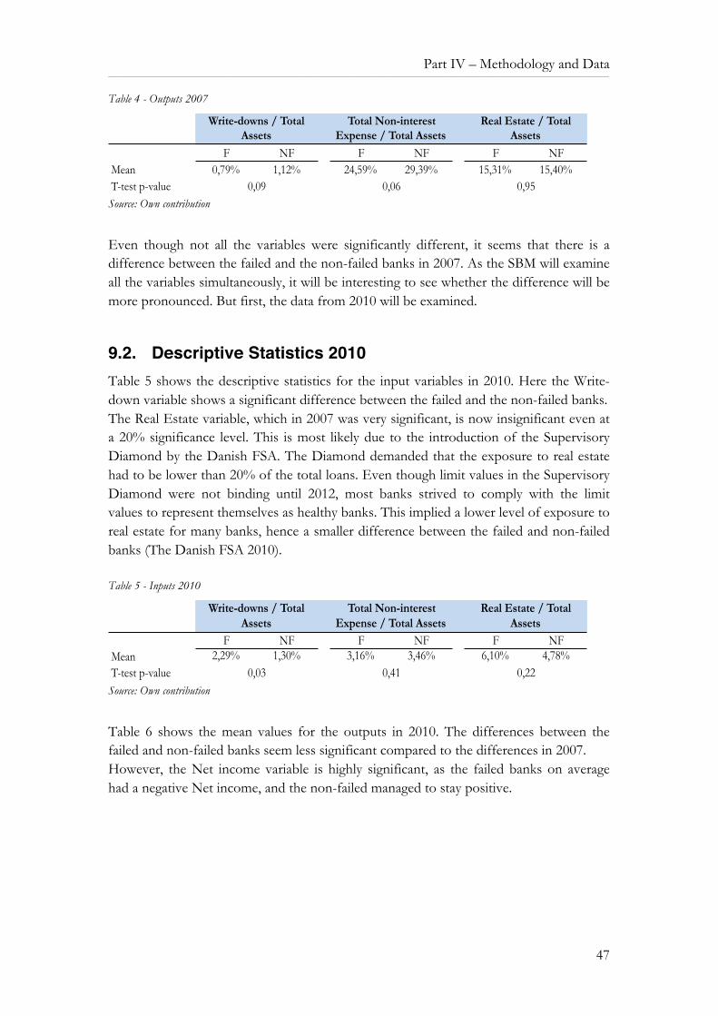
Part IV – Methodology and Data ______________________________________________________________________________________________________________________________________________________________________
47
Table 4 - Outputs 2007
Source: Own contribution
Even though not all the variables were significantly different, it seems that there is a difference between the failed and the non-failed banks in 2007. As the SBM will examine all the variables simultaneously, it will be interesting to see whether the difference will be more pronounced. But first, the data from 2010 will be examined.
9.2. Descriptive Statistics 2010 Table 5 shows the descriptive statistics for the input variables in 2010. Here the Write-down variable shows a significant difference between the failed and the non-failed banks. The Real Estate variable, which in 2007 was very significant, is now insignificant even at a 20% significance level. This is most likely due to the introduction of the Supervisory Diamond by the Danish FSA. The Diamond demanded that the exposure to real estate had to be lower than 20% of the total loans. Even though limit values in the Supervisory Diamond were not binding until 2012, most banks strived to comply with the limit values to represent themselves as healthy banks. This implied a lower level of exposure to real estate for many banks, hence a smaller difference between the failed and non-failed banks (The Danish FSA 2010). Table 5 - Inputs 2010
Source: Own contribution
Table 6 shows the mean values for the outputs in 2010. The differences between the failed and non-failed banks seem less significant compared to the differences in 2007. However, the Net income variable is highly significant, as the failed banks on average had a negative Net income, and the non-failed managed to stay positive.
F NF F NF F NFMean 0,79% 1,12% 24,59% 29,39% 15,31% 15,40%T-test p-value 0,09 0,06 0,95
Write-downs / Total Assets
Total Non-interest Expense / Total Assets
Real Estate / Total Assets
F NF F NF F NFMean 2,29% 1,30% 3,16% 3,46% 6,10% 4,78%T-test p-value
Real Estate / Total Assets
0,41
Write-downs / Total Assets
0,03 0,22
Total Non-interest Expense / Total Assets
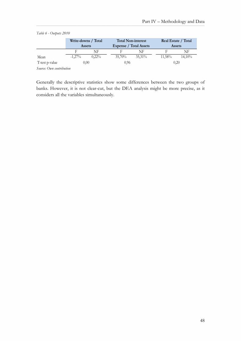
Part IV – Methodology and Data ______________________________________________________________________________________________________________________________________________________________________
48
Table 6 - Outputs 2010
Source: Own contribution
Generally the descriptive statistics show some differences between the two groups of banks. However, it is not clear-cut, but the DEA analysis might be more precise, as it considers all the variables simultaneously.
F NF F NF F NFMean -1,27% 0,22% 35,70% 35,31% 11,58% 14,10%T-test p-value 0,96
Total Non-interest Expense / Total Assets
Real Estate / Total Assets
0,200,00
Write-downs / Total Assets

______________________________________________________________________________________________________________________________________________________________________
49
Part V
Empirical Findings

Part V – Analysis ______________________________________________________________________________________________________________________________________________________________________
50
10. Analysis
10.1. DEA analysis This section will go through the results obtained in the DEA analysis. But first, the used software will be introduced and any problems with the analysis will be highlighted. Next, the choices of scaling and orientation for this study will be explained.
10.1.1. Software As DEA is still a niche method compared to for example regressions, only a few software programs exists. Most of these programs require extensive coding skills and a deep understanding of the program, especially when using other models than the original DEA model. However, a few programs with a more user-friendly interface and process have been published, though many of them still have complications. As this paper uses the SBM model, the choice of software has been limited even more, as it is not a standard model in all software packages. For the analysis the DEA-solver Software from Cooper, Seiford, and Tone (2000) will be used. The software is made as a macro in Excel, which makes the software seem familiar and easy to use. As the Excel-file opens, a message box appears and introduces the software. The first step is to choose a model. This software contains a variety of different models, most of them in four versions with a choice of input- or output-orientation and a choice of VRS or CRS. These choices mean that the program offers 46 different models (Cooper, Seiford & Tone 2000) . The interface of the DEA solver, when choosing the model, is shown below in Figure 4. Figure 4 - DEA Solver Interface
Source: DEA Solver Software
Part V – Analysis ______________________________________________________________________________________________________________________________________________________________________
51
When the correct model has been chosen, an Excel-file with the data to be used in the analysis must be imported to the software. It is important that the names of the DMUs are located in the first row, followed by the inputs and outputs in the following rows. The input rows should be marked (I) and the name variable in the first cell of the row, and the output rows should be marked (O) and the name variable, so the software knows, which rows contain inputs and outputs, respectively. Hence, the first cell in the row containing the output Net income should be named ‘(O) Net income’ (Cooper, Seiford & Tone 2000) . The appendix holds the data files, which were used in the analysis. Hereafter, the analysis is named and saved, and the software starts running the analysis. The software generates a result file with multiple sheets. The most important sheet for this analysis is the sheet ‘Score’. This sheet contains the efficiency score of each of the DMUs and their reference set. In this analysis only the scores are relevant. The next important sheet is the ‘Summary’-sheet. This sheet contains an overview of the inputs and outputs used, so it is a good idea to check that all variables are included in this overview. Further, it shows the correlation between the different variables and general statistic for all the variables. At the bottom are the most important features. First, a list of DMUs, which the model found had abnormal solutions, and therefore have been excluded from the analysis and second, a list of how many times each DMU has been included in a reference set. As mentioned earlier, this list could reveal potential outliers, because if a DMU is used almost constantly as a reference, this could imply that it had too high or low values. Hence, the analyst should run through the list to ensure that an outlier has not altered the efficient frontier.
10.1.2. Complications for the Analysis One of the disadvantages of using this software, is that the macro codes embedded in the model is secured with a password, which means that it is not possible to see which codes the programmers have used. The analysis has some complications as well. According to the theory, the model should be capable of handling semi-positive values in the input values, and both positive and negative values in the output values. However, when running the model, the results will be disrupted if more than one of the input variables contains a value of 0. Hence, in the analysis all DMUs with a value of 0 in the Real Estate variable and for some in the Write-down on loans variable, will be assigned a value of 1 instead. The change is so small that it will not damage or influence the result, so this correction is made to ensure that the analysis can be performed, even though it is not optimal. In the 2007 analysis 8 values were changed from 0 to 1. In the 2010 analysis 16 values were changed from 0 to 1.

Part V – Analysis ______________________________________________________________________________________________________________________________________________________________________
52
Another issue is with the software’s precautions. As it runs the model, it will search for outliers and remove any DMUs with an abnormal solution from the model. In the 2007 analysis a single DMU were removed from the analysis before it was deemed efficient, due to the model finding its solution abnormal12. In the 2010 analysis two DMUs were removed as the model found their solution abnormal, leaving 121 banks.
10.2. Empirical results As with all other DEA analyses it is necessary to decide on a scaling method and an orientation. The exposition in the beginning of the paper showed that the choice of scaling method can influence the results and that each of the two methods has pros and cons. For this analysis the VRS is chosen for different reasons. In recent years, this has been the preferred scaling method in literature concerning DEA and banking, hence, to follow the literature the VRS is used in the study too. Furthermore, the analysis is performed on all sizes of banks from one-branch banks to Nordic-reaching, enormous banks. Using the CRS model would mean rejecting any economies of scale and suggesting that small banks should be able to achieve the same efficiency as the large banks. For this study, the CRS condition, that the inputs and outputs of an efficient DMU could be multiplied with a factor to achieve another efficient DMU, is even less suitable. Due to the choice of the untraditional variables, the linkage between the inputs and outputs are weak. Hence, if the level of the inputs were doubled, there is no guarantee that the output levels would be doubled too, making the CRS unsuitable for this study. Even though the choice of VRS might favor the extremes, and perhaps deem some of the banks efficient even though they are not, it is believed to be a better solution than the strict CRS. As for the orientation, the model can either be input-oriented or output-oriented. Either one of orientations is in favor of the other, as it depends on the data and the variables chosen. However, in the literature the input-orientation has been preferred, as input variables in a normal DEA bank analysis often are more discretionary than the output variables. As an example, it is easier to change the number of employees than the Net income. Despite the fact that this paper has another approach to the selection of variables than most other DEA banking analyses, the input variables are still more discretionary than the output variables. This means that the input-orientation also will be used in this study. The analysis will consist of four parts. First, a U-test to see if the non-failed banks have significantly higher efficiency scores compared to the failed banks, which would indicate that the model has discriminative powers. Second, as a supporting test, the Gini-coefficient will be assessed to clarify the inequality in the sample, which again will 12 The DMU was not removed until second round of the layer analysis, so it will appear in first round of the analysis.

Part V – Analysis ______________________________________________________________________________________________________________________________________________________________________
53
determine the discriminative powers. The third part is a so-called layer analysis. This will determine whether the SBM analysis holds any predictive powers and lastly, a robustness test will be performed to support the results from the first three tests.
10.2.1. Empirical Findings 2007 In the 2007 analysis 139 banks are included in the analysis. Of the 139 banks, 60 of them failed in the period from 2008 to 2013, leaving 79 non-failing banks. Table 7 shows the average efficiency scores and the median for both the failed and the non-failed banks. It shows that the non-failed banks on average had an efficiency score of 57,7%, whereas the failed banks only had an average efficiency score of 40,6%. Furthermore, the median for the non-failed banks was 0,435 and only 0,359 for the failed banks. It seems that the non-failed banks generally have higher efficiency scores than the failed banks in this model. Table 7 - Empirical Findings 2007
Source: Own contribution
The mean values of the two groups of banks are tested to see if they are significantly different from each other, or in other words, to test the discriminatory power of the SBM model. As the SBM model is non-parametric a U-test will be used. Since the sample contains 139 DMUs, they will be ranked based on their efficiency score from 1 to 139, where 1 is the best. 27 DMUs were efficient and had an efficiency score of 1, so they will receive the average of the 27 rankings, which is 14. Next the U-values for the two groups are calculated.
U1 = 𝑛!𝑛! + !!(!!!!)
!− 𝑅! = 79 ∙ 60+ !"∙ !"!!
!− 4856 = 3044
U2 = 𝑛!𝑛! − 𝑈! = 79 ∙ 60− 3044 = 1696 As the Z-statistic yields the same result independent of the U-value used, the following calculations will only be performed with U1, the non-failed banks.
𝜇! = 𝑛!𝑛!2 =
79 ∙ 602 = 2370
𝜎! = 𝑛!𝑛!(𝑛! + 𝑛! + 1)
12 =79 ∙ 60 ∙ (79+ 60+ 1)
12 = 235,2
Failed bank Non-failed bankMean 0,406 0,577Median 0,359 0,435

Part V – Analysis ______________________________________________________________________________________________________________________________________________________________________
54
The observed Z-value for the sample is
𝑍 = 𝑈 − 𝜇!𝜎!
= 3044− 2370
235,2 = 2,866
A Z-value of 2,87 is equal to a p-value of 0,0021. Hence, the 0-hypothesis, that the two mean values are equal to each other, can be rejected (Keller 2009). Hence, the U-test shows that the non-failed banks had significantly higher efficiency scores than the failed banks. Another method for testing the discriminative power of the DEA model is by calculating the Gini-coefficient. This measure has, to the author’s knowledge, not been used in any DEA bank prediction model before but is occasionally used in other prediction studies. The 2007 sample yields a Gini-coefficient of 0,296. It is not possible to state how large the inequality is simply from this figure, but in a study on comparing failure prediction models Oogen and Barcaen (2007) Gini-coefficients between -5 % and 65 %, however with most values around 40 %. This indicates that the Gini-coefficient for this study is not high but considering the drawbacks it is assumed to be at a fair value, implying that the model does hold discriminative values. The calculation of the Gini-coefficient is contained in the appendix. Where the first tests focused on the discriminating powers of the DEA model, the next test will assess the predictive powers of the model. This is done using a layer analysis. The analysis is consistent with the work of Avkiran and Cai (2014) and Paradi, Asmild, and Simak (2004). Table 8 - Layer Analysis 200713
Source: Own contribution
13 The Layer analysis only contains 138 banks, as one of the banks was removed by the software in round 2, due to a abnormal solution. So this bank was removed from the analysis.
1. layer 2. layer 3. layer 4. layer 5. layerEfficient 4 22 21 11 2
FS Takeover 6 3FS Aid 3 4Other ceased 3 11 13 7 1Non-known 1 5 2 1
Amount 60 56 34 13 2Share 0,067 0,367 0,350 0,183 0,033Acc. Share 0,067 0,433 0,783 0,967 1,000Efficient 23 24 18 10 3Amount 78 55 31 13 3Share 0,295 0,308 0,231 0,128 0,038Acc. Share 0,295 0,603 0,833 0,962 1,000N
on-f
aile
dFa
iled

Part V – Analysis ______________________________________________________________________________________________________________________________________________________________________
55
Table 8 shows the layer analysis for 2007. The first row in each section shows how many of the DMUs that are deemed efficient in each layer. Below the first row the subgroups of the failed banks are presented, making it possible to see in which layer the different banks are deemed efficient. Next, the total number of failed and non-failed banks in each layer is displayed. The third row shows how large a share of the DMUs is deemed efficient in each layer. The last row shows the accumulated share of efficient DMUs in the current layer. The different scores and the complete Layer analysis are presented in the appendix. In Table 8, it is clear that the majority of the non-failed banks are deemed efficient in the first two layers. After layer 2 more than 60 % of the non-failed banks are deemed efficient. The failed banks are mainly deemed efficient in the middle layers and not the last layers as preferred. This complicates the process of finding a cut-off layer. Especially, as the failing banks in the first group, FS Takeover, all are deemed efficient in layer 2 and 3. Prior to the analysis it would be assumed that these banks would be deemed efficient in the last layers. However, what the table is not capable of showing is that, these banks were quite large banks such as Roskilde Bank, Fionia Bank, and Amagerbanken, so they most likely become efficient in the first layers due to their size. Despite the challenges, a cut-off layer most be decided. The choice of cut-off layer is dependent on the purpose of the analysis. If layer 2 is choosing more than 93 % of the failing banks are classified correct. However, the type II errors are high. By choosing layer 2 as cut-off layer, 70 % of the non-failed banks are misclassified. By choosing layer 3 as cut-off layer the total number of DMUs that are classified correct is high, but the amount of type I errors, misclassification of failed banks, increase. The analyst must decide whether it is more important to identify the failing banks and minimize type I errors or to classify most banks in the correct group. The remaining layers of the analysis are not suitable as cut-off layer due to even higher type I and type II errors. In this study, layer 2 is chosen as cut-off layer as the prediction of which banks are failing is the purpose. This choice will result in high type II errors but it will catch all the large, failing banks. To investigate the results from the three tests above, a robustness test of the data is performed. Table 9 shows the mean value of the failed and the non-failed banks, when the banks included in the sample are changed. Generally, the test shows similar mean values for the failed banks independent on the sample. However, it is noteworthy that the mean value decreases from 0,43 to 0,40 when the banks in group 2 are combined with the banks in group 3. This indicates that the banks in group 2 has an effect on the efficient frontier and that the worst performing, failed banks are found in this group. As the sample size of group 2 is too small, it is thus not possible to test this presumption, as it would result in artificially high efficiency scores.

Part V – Analysis ______________________________________________________________________________________________________________________________________________________________________
56
The non-failed banks differ more in the mean value when the sample is changed. The mean value ranges from 0,50 when only considering group 3 banks, to 0,58 when considering all banks. The numbers indicate that the group 1 banks are forcing the mean value up. This is interesting for two reasons. First, Danske Bank, which was suspected of skewing the results, is deemed efficient. Second, all the banks in group 1 is deemed efficient, most likely because their variables are considerably larger than the remaining banks. Hence, these banks may skew the mean value of the non-failed banks gratuitous upwards. To test this a U-test is performed on all the banks except from the banks in group 1. The Z-test yield a value of 2,41, which is still above the critical value. Hence, there is still a significant difference between the failed and the non-failed banks, but it is not as strong as when the five banks in group 1 are included in the sample. Hence, they seem to have a great influence on the efficiency scores. Table 9 - Robustness Test 2007
Source: Own contribution
At first sight, the 2007 analysis seems to possess both discriminative and predictive powers. However, as the numbers are investigated, the discriminative powers seem to dependent largely on the group 1 banks. If these are removed from the analysis, the powers of the model decrease but the difference is still significant. The model does possess some predictive powers, but it comes at the expense of exceptionally high type II errors.
10.2.2. Empirical Findings 2010 As the 2007 showed both discriminatory and predictive powers, it is interesting to see if the 2010 analysis can follow the example. Table 10 shows the mean value and median for the 2010 analysis. Compared to the 2007 analysis, the difference between the two mean values is not as clear. In the 2007 analysis there was a difference between the two mean values at 0,17 but in the 2010 analysis the difference is only 0,06.
Failed Non-failed Sample sizeAll banks 0,41 0,58 139Without group 1 0,41 0,55 134Without group 4 0,41 0,56 101Group 3 0,43 0,50 84Group 2 & 3 0,40 0,53 97
Mean values

Part V – Analysis ______________________________________________________________________________________________________________________________________________________________________
57
Table 10 - Empirical Findings 2010
Source: Own contribution
Hence, to test if the difference is still significant the U-test is performed. The U-test yields the following values:
U1 =80 ∙ 30+!"∙(!"!!)
!− 4856 = 1398
σU = !"∙!"∙(!"!!"!!)!"
= 149
μU = !"∙!"!
Z = !! !!!!
= !"#$!!"##!"#
= 1,329
The observed Z-value is 1,33, which is equivalent to a p-value of 0,0918. This means that with a significance level of 5 % it is not possible to reject the 0-hypothesis, that the two mean values are equal to each other. In other words, there is no significant difference between mean values of the failed and the non-failed banks. However, if the significance level is raised to 10 %, it is possible to reject the 0-hypothesis and conclude a significant difference between the two groups. However, it is far from as strong as the 2007 analysis. The Gini-coefficient for the 2010 sample is a little higher than for the 2007 with a value of 0,319. Hence, again the Gini-coefficient seems to be at a fair value, implying that the model does are able to distinguish between failed and non-failed banks (Ooghe, Balcaen 2007). The discriminatory powers of the model in the 2010 analysis are ambiguous compared to the 2007 analysis, as the U-test was lower and insignificant but the Gini-coefficient was higher. Hence, it will be interesting to see if the predictive powers are more convincing. Table 11 shows the layer analysis for 2010. The lacking differences between the failing and the non-failing banks from the previous analyses recur in the layer analysis. This is clear when looking at the share of efficient DMUs for the two groups. With the five efficient failing banks in layer 1, almost 17 % of the failing banks are deemed efficient in the first layer of the test. The corresponding figure for the non-failing banks is 20 %. It seems like the 2010 analysis does not hold the same predictive powers as the 2007 analysis. However, the 2010 analysis does have a noteworthy quality. The failed banks, which were aided or taken over by Finansiel Stabilitet, are almost solely placed in the lower layers of the model.
Failed bank Non-failed bankMean 0,429 0,490Median 0,292 0,351

Part V – Analysis ______________________________________________________________________________________________________________________________________________________________________
58
This could indicate that the model still holds predictive powers but that the majority of mergers, which was made outside of Finansiel Stabilitet, were not default-driven but instead driven by other factors such as gaining a larger market share. This however, is only speculation. Table 11 - Layer Analysis 2010
Source: Own contribution
If layer 2 also is chosen as cut-off layer in the 2010 analysis, both error types will be larger compared to the 2007 analysis. Only 83,3 % of the failing banks, would be classified correct and 80 % of the non-failing banks would be misclassified. However, if layer 3 is chosen as cut-off layer, 57 % of the failed banks and 51 % of the non-failed banks are classified correct, which implies lower type II errors but a drastic increase in type I errors. This indicates that both type I and type II errors are higher for 2010 independent in the cut-off layer and that the predictive powers are lacking for the model during the crisis. However, the model seems to be better at classifying the worst performing, failing banks. Finally, the powers of the three tests above are assessed in a robustness test. Table 12 shows how the mean values of the failed and the non-failed banks change, when the banks included in the sample are changed. Similar to the test from the 2007 analysis, the group 1 banks seem to have a great effect on the efficient frontier. As these banks are removed from the sample, the mean values increase for both the failing and the non-failing banks. Compared to the 2007 robustness analysis, the 2010 analysis is generally more dispersed in the mean values. This indicates that the results are lacking robustness, and in consequence make the results from the previous tests weaker.
1. layer 2. layer 3. layer 4. layer 5. layerEfficient 5 8 5 10 2
FS Takeover 1 1 1FS Aid 3 1Other ceased 4 4 5 5Non-known 1 3 1
Amount 30 25 17 12 2Share 0,167 0,267 0,167 0,333 0,067Acc. Share 0,167 0,433 0,600 0,933 1,000Efficient 16 25 26 11 2Amount 80 64 39 13 2Share 0,200 0,313 0,325 0,138 0,025Acc. Share 0,200 0,513 0,838 0,975 1,000
Faile
dN
on-f
aile
d

Part V – Analysis ______________________________________________________________________________________________________________________________________________________________________
59
Table 12 - Robustness Test 2010
Source: Own contribution
The results of the SBM analysis are ambiguous. In the 2007 analysis the model had significant discriminatory and predictive powers. This meant that the model was able to distinguish between the failed and the non-failed banks and to some extend predict, which banks would fail. However, in the 2010 analysis the model had both low discriminatory and predictive powers, as none of the two tests showed strong, significant differences between the two groups. However, the layer analysis did a better job than the 2007 analysis, in placing the most critical, failing banks in the lower layers of the analysis. This implies that the DEA model with the CAMELS and the real estate variables seems to be better at predicting failures in the bank industry prior to the crisis and that it has little predictive powers during the crisis. An explanation might be that the incentive for merging changed during the crisis, meaning that some of the banks, which merged after 2010 might have survived the crisis without the merger. Another explanation could be that the Danish FSA started to monitor the banks closely during to crisis and with the introduction of the Supervisory Diamond the banks were forced to comply with a number of limit values, such as the amount of real estate loans, which would influence the variables in the SBM model (The Danish FSA 2010).
Failed Non-failed Sample sizeAll banks 0,43 0,49 110Without group 1 0,48 0,53 106Without group 4 0,43 0,52 79Group 3 0,51 0,57 67Group 2 & 3 0,47 0,56 74
Mean values

______________________________________________________________________________________________________________________________________________________________________
60
Part VI
Concluding Remarks

Part VI – Concluding Remarks ______________________________________________________________________________________________________________________________________________________________________
61
11. Discussion
Many articles and research papers focus on the object of predicting bank failures, mainly with the purpose of avoiding them. However, the next step after predicting the failures might not be as straightforward for different reasons. Hence, a question may arise – even if we succeeded in foreseeing all bank failures, would it change anything? As the post-crisis examinations of the failed banks showed that some banks made decisions, which were highly risky and irresponsible, regulation might not be able to stand alone. It seemed that during the crisis some banks were willing to do what ever it took to survive, even though it damaged their customers. In a documentary in 4 episodes, Danish television, DR, highlighted some of the actions of the Danish banks, such as parking loans with previous bankrupt creditors and providing highly risky loans to real estate investors (Danmarks Radio (DR) 2015). With that in mind the regulations imposed on the banks before and during the crisis, seem to be lacking impact in some areas. However, the question remains if more regulation is the way to go. Instead focus might be on promoting behavioral changes in the banks and enhancing the morality. This is not as simple as imposing regulations and compliances on the banks but it might be more effective and useful in the long run. Thus, while regulation of the banking industry is necessary to avoid large losses, which will have to be covered by the taxpayers and the remaining banks, too much regulation can also imply higher interest rates, lower growth and reduced profitability. Hence, finding the balance between under-regulating and over-regulating is crucial (Kerstein, Kozberg 2013). Further, as regulation is often equal to reducing risk, it is important to remember that risk is a part of banking. Each bank has its own risk appetite and can act according to it. The customers have a free choice, so they can ceteris paribus select a bank with a risk appetite that matches their appetite. When running a bank, risk is necessary, as there often is a mismatch between the duration of loans and deposits. To eliminate the risks connected to banking, the banks should at all time have enough capital to pay the deposits back. This would imply sky-high interest rates and make it almost impossible to take out a loan with longer expiration or to withdraw large amounts with short notice. Hence, it is necessary to accept that banking and risk belong together and regulating it too much can have just as comprehensive consequences as under-regulation (Kerstein, Kozberg 2013). In 2007, the concentration of the five largest banks in Denmark based on assets was 85 %. This meant that approximately 165 banks shared the last 15 % of the market (Udvalget om Finanskrisens Årsager, Erhvervs- og Vækstministeriet 2013). During the financial crisis more than 40 % of the Danish banks ceased activity, despite numerous attempts to help the banks and the bank market in general. These figures pose the

Part VI – Concluding Remarks ______________________________________________________________________________________________________________________________________________________________________
62
undesirable questions if the bank failures were inevitable due to the concentration and size of the market. That the market was sate, and it was only a matter of time before the banks would fail, as there were not customers enough to keep them all going. Instead the crisis became a survival of the fittest where the weakest banks failed. Furthermore, the large number of small banks might have made the competition between the banks very hard, forcing some of them to take more risk, making the many failures a positive consequence for the bank market and the customers, as it would help lower the banks’ risk appetite. However, this is only speculation but worth considering next time the economy is hit by a crisis. Perhaps the many failed banks are not only a negative event that should be corrected and regulated against, but just an inevitable consequence of the market. Instead focus could be on protecting the creditors and ensuring that no bank gets ‘too big to fail’.
11.1. Further Research The financial industry has always received great attention from the academic world and this will probably continue for years to come. Hence, it is important to identify areas, which have not been examined and reviewed yet, that could reveal further knowledge. As the analysis showed great discriminatory and predictive powers before the crisis started but not during, it would be interesting to see, if the model has the same powers prior to other financial crises, such as the bank crisis in the 1980’s. If this is the case, the DEA model could prove a strong and helpful tool for institutions such as the Danish FSA prior to crises. Furthermore, the data for the model was from just before the crisis. Hence, another possibility would be to expand the number of years before the crisis to see how far back the model possesses discriminatory and predictive powers. This would reveal both what the time horizon for the model is, meaning how far back it could foresee failures, but also if the discriminatory and predictive powers improve or worsen when the time horizon is changed. This study only contains Danish banks and contains all banks independent on size. Hence, the difference between the smallest and the largest banks might be too big, also with respect to the choice of VRS as scaling method. For future research, it might be an idea to include more countries and instead focus on banks with the same size and product line, to avoid the rather unreasonable comparisons between the large and the small banks. This would also give a larger sample size, which would make it possible to divide the failed banks into subgroups, to see if this could reveal further information about the failing banks. However, when extending a study it is crucial to remember, that the efficiency scores cannot be compared to other studies, not even if the DMUs are the same and the years are different. The efficiency score is a product of the efficient frontier and the efficient DMUs, so a comparison could result in a wrong conclusion (Dyson et al. 2001)

Part VI – Concluding Remarks ______________________________________________________________________________________________________________________________________________________________________
63
12. Conclusion
After performing the SBM analysis on the 2007 and 2010 data set, the results were examined with a Mann-Whitney U-test, the Gini-coefficient, and a Layer analysis, to identify any differences between the failed and the non-failed banks. Lastly, these results were checked by a robustness test, by changing the sample. In the 2007 analysis, the U-test yielded a p-value below 0,05, implying that the non-failed banks had a higher efficiency score, and thus a better performance, than the failed banks. Additionally, the Gini-coefficient was 0,29, which seemed fair compared to other failure prediction studies. In the 2010 analysis, the U-test was only efficient at a 10 percent significance level, implying that the difference between the failed and the non-failed banks were less pronounced compared to the 2007 analysis. However, the Gini-coefficient was with a value of 0,31 higher than in the 2007 analysis. The Layer analysis made it possible to divide the data into two groups; failed and non-failed banks. In the 2007 analysis the cut-off layer was layer 2, to ensure that all the most critical failed banks are classified correct. Hence, 93 % of the failed and 30 % of the non-failed banks were classified correct. The type I errors were low, but at the expense of severe type II errors. As with the U-test, the Layer analysis for 2010 was less clear. If layer 3 was chosen as the cut-off layer only 57 % of the failed banks and 51 % of the non-failed banks were classified correct, which means it encountered both large type I and type II errors. However, the most critical failed banks were almost solely found in the last layers of the analysis. The robustness test utilized the four subgroups, which the Danish banks are divided into based on the size of their working capital, to change the sample. The robustness test was strong for the 2007 analysis, which showed little diversion as the sample was changed. On the contrary, the 2010 analysis showed weak robustness when the sample was changed. For both tests the large banks in group 1 seemed to have severe impact on the results. The results from the analyses indicate that it is possible to discriminate between the failed and non-failed banks and that it is possible to identify most of the banks, which will fail though at the expense of high type II errors. The results are strongest in the 2007 analysis, prior to the crisis. In the data from 2010 the model encounters both decreasing discriminative and predictive powers, compared to the results from 2007. However, the 2010 analysis seemed to be better at predicting the most crucial bank failures, as the majority of these banks were found in the last layers of the analysis. This is a great advantage compared to the 2007 analysis where most of the banks, which received aid from Finansiel Stabilitet, were deemed efficient in the second and third layer of the analysis. Conclusively, the model had higher discriminating and predicting powers in the 2007 analysis but was better at predicting the more crucial bank failures in the 2010 analysis.

Part VI – Concluding Remarks ______________________________________________________________________________________________________________________________________________________________________
64
The model and the analyses are extensions of the work of Avkiran and Cai (2014) and Paradi, Asmild, and Simak (2004). Avkiran and Cai use a Super-SBM model and the six variables from the CAMELS model to predict failure amongst US banks. This study uses the same six variables but extend the data set with the inclusion of a real estate variable, which Cole and White (2012) find is a good predictor of distress on a long-term horizon. As oppose to the study of Avkiran and Cai (2014), this analysis is performed with an input-oriented SBM model under VRS and solely on Danish banks. The model faces certain issues with correlation among the variables, which might give some of the banks an advantage. Paradi, Asmild, and Simak (2004) used a Layer analysis and a cut-off value in their study. However, this study only utilizes the Layer analysis. As the data only contains Danish banks, the results are mainly valid for the Danish bank market. However, as Avkiran and Cai (2014) found similar results in their analysis of US banks, this could indicate that the model is suitable for a broader market than only Danish banks. To extend this study it could be interesting to include more years of data from the Danish banks to see if the model could maintain the same discriminative powers prior to the crisis, and how fast the worst bank failures got isolated in the last layers of the analysis. Furthermore, as the largest banks seemed to have a great impact on the results and as the banks in group 2 seemed to have the lowest efficiency scores for failed banks, it could be interesting to include more countries and divide the banks in sizes corresponding to the groups from the Danish FSA’s statement. This could clarify if the largest Danish banks are truly efficient or only deemed efficient in this study, due to their unique values, and if the banks in group 2 do have the lowest efficiency. However, when extending a study it is important to keep in mind that the individual efficiency scores cannot be compared between studies, as the score is a product of the frontier, which it is measured on.

Appendix ______________________________________________________________________________________________________________________________________________________________________
65
13. References
Books
Baldvinsson, C. 2011, Dansk Bankvæsen, 6.th edn, Karnov Group, Kbh.
Berk, J. & DeMarzo, P. 2011, Corporate finance, 2. global edition edn, Pearson, Boston, MA.
Bukh, P.N.D. 1995, Produktivitet og efficiens i pengeinstitutsektoren - Overvejelser ved valg af input og output i forbindelse med DEA-analyser, Ledelse & Erhvervsøkonomi.
Bukh, P.N.D., Førsund, F.R. & Berg, S.A. 1995, Banking efficiency in the Nordic countries : a four-country Malmquist index analysis, Norges Bank, Oslo.
Casu, B., Girardone, C. & Molyneux, P. 2006, Introduction to banking, Prentice Hall, Harlow.
Cooper, W.W., Seiford, L.M. & Tone, K. 2000, Data Envelopment Analysis - A Comprehensive Text with Models, Applications, References and DEA-Solver Software, Kluwer Academic Publishers.
Israel, D. 2008, Data analysis in business research : a step-by-step nonparametric approach, Response Books, Sage Publications.
Iversen, M.J. 2013, Sidste udvej : Finansiel Stabilitet og Danmarks Bankkrise, 1.th edn, Lindhardt og Ringhof, Kbh.
Keller, G. 2009, Managerial statistics, 8. ed. edn, South-Western, Mason, Ohio.
Thanassoulis, E. 2003, Introduction to the theory and application of Data Envelopment Analysis, 2nd edn, Springer Science & Business, New York.
Udvalget om Finanskrisens Årsager & Erhvervs- og Vækstministeriet 2013, Den finansielle krise i Danmark: Årsager, konsekvenser og læring, Erhvervs- og Vækstministeriet, Kbh.
Generic Material
Cole, R.A. & Fenn, G.W. 1995, The role of commercial real estate investments in the banking crisis of 1985–92, Presented at the Annual Meeting of American Real Estate and Urban Economics Association.
Emrouznejad, A. & Thanassoulis, E. 1996, An Extensive Bibliography of Data Envelopment Analysis (DEA) - Volume II: Journal Papers.
Finanstilsynet 2012, Redegørelse on inspektion i Sparekassen Lolland A/S, finanstilsynet.dk.

Appendix ______________________________________________________________________________________________________________________________________________________________________
66
IMF 2013, Financial Stability in an Evolving Regulatory and Supervisory Landscape, Working paper no. 13/47, European Department.
The Danish FSA 2010, The Danish FSA introduces the 'Supervisory Diamond' for banks.
Journal Articles
Altman, E.I. 1968, "Financial Ratios, Discriminant Analysis and the Prediction of Corporate Bankruptcy", The Journal of Finance, vol. 23, no. 4, pp. 589.
Altunbas, Y., Gardener, E.P.M., Molyneux, P. & Moore, B. 2001, "Efficiency in European banking", European Economic Review, vol. 45, no. 10, pp. 1931.
Avkiran, N.K. 2009, "Opening the black box of efficiency analysis : an illustration with UAE banks", Omega, vol. 37, no. 4, pp. 930.
Avkiran, N.K. 2006, "Developing foreign bank efficiency models for DEA grounded in finance theory", Socio-economic planning sciences, vol. 40, no. 4, pp. 275.
Avkiran, N.K. & Cai, L. 2014, "Identifying distress among banks prior to a major crisis using non-oriented super-SBM", Annals of Operations Research, vol. 217, no. 1, pp. 31.
Banker, R.D., Charnes, A. & Cooper, W.W. 1984, "Some Models for Estimating Technical and Scale Inefficiencies in Data Envelopment Analysis", Management Science, vol. 30, no. 9, pp. 1078.
Barr, R.S., Killgo, K.A., Siems, T.F. & Zimmel, S. 2002, "Evaluating the productive efficiency and performance of US commercial banks", Managerial Finance, vol. 28, no. 8, pp. 3.
Bauer, P.W., Berger, A.N., Ferrier, G.D. & Humphrey, D.B. 1998, "Consistency Conditions for Regulatory Analysis of Financial Institutions: A Comparison of Frontier Efficiency Methods", Journal of economics and business, vol. 50, no. 2, pp. 85.
Bergendahl, G. 1998, "DEA and benchmarks – an application to Nordic banks", Annals of Operations Research, vol. 82, pp. 233.
Berger, A.N. & Humphrey, D.B. 1997, "Efficiency of financial institutions: International survey and directions for future research", European Journal of Operational Research, vol. 98, no. 2, pp. 175-212.
Bukh, P.N.D. 1994, "Data envelopment analysis: en analyse af inefficiens og stordrift i den danske pengeinstitutsektor", Symposium i Anvendt Statistik, vol. 1994, pp. 52-69.
Canbas, S., Cabuk, A. & Kilic, S.B. 2005, "Prediction of commercial bank failure via multivariate statistical analysis of financial structures: The Turkish case", European Journal of Operational Research, vol. 166, no. 2, pp. 528.
Casu, B. & Molyneux, P. 2003, "A comparative study of efficiency in European banking", Applied Economics, vol. 35, no. 17, pp. 1865.

Appendix ______________________________________________________________________________________________________________________________________________________________________
67
Charnes, A., Cooper, W.W., Golany, B., Seiford, L. & Stutz, J. 1985, "Foundations of data envelopment analysis for Pareto-Koopmans efficient empirical production functions", Journal of Econometrics, vol. 30, no. 1, pp. 91.
Charnes, A., Cooper, W.W. & Rhodes, E. 1978, "Measuring the efficiency of decision making units", European Journal of Operational Research, vol. 2, no. 6, pp. 429.
Claro, L.L.d. 2013, "Determining the effectiveness of the CAMELS approach towards timely prediction of bank failures", Journal of global business and economics, vol. 6, no. 1.
Cole, R.A. & White, L.J. 2012, "Déjà Vu All Over Again: The Causes of U.S. Commercial Bank Failures This Time Around", Journal of Financial Services Research, vol. 42, no. 1, pp. 5.
Cook, W.D. & Seiford, L.M. 2009, "Data envelopment analysis (DEA) – Thirty years on", European Journal of Operational Research, vol. 192, no. 1, pp. 1.
Cox, R.A.K. & Wang, G.W.Y. 2014, "Predicting the US bank failure: A discriminant analysis", Economic Analysis and Policy, vol. 44, no. 2, pp. 202.
Damgaard, C. & Weiner, J. 2000, "Describing Inequality in Plant Size or Fecundity", Ecology, vol. 81, no. 4, pp. 1139-1142.
Demyanyk, Y. & Hasan, I. 2010, "Financial crises and bank failures: a review of prediction methods", Omega, vol. 38, no. 5, pp. 315.
Dixon, P.M., Weiner, J., Mitchell-Olds, T. & Woodley, R. 1987, "Bootstrapping the Gini Coefficient of Inequality", Ecology, vol. 68, no. 5, pp. 1548-1551.
Dyson, R.G., Allen, R., Camanho, A.S., Podinovski, V.V., Sarrico, C.S. & Shale, E.A. 2001, "Pitfalls and protocols in DEA", European Journal of Operational Research, vol. 132, no. 2, pp. 245.
Emrouznejad, A., Parker, B.R. & Tavares, G. 2008, "Evaluation of research in efficiency and productivity: A survey and analysis of the first 30 years of scholarly literature in DEA", Socio-economic planning sciences, vol. 42, no. 3, pp. 151.
Fiordelisi, F. & Marques-Ibanez, D. 2011, "Efficiency and risk in European banking", Journal of banking & finance, vol. 35, no. 5, pp. 1315.
Kerstein, J. & Kozberg, A. 2013, "Using accounting proxies of proprietary FDIC ratings to predict bank failures and enforcement actions during the recent financial crisis", Journal of accounting, auditing & finance, vol. 28, no. 2, pp. 128.
Kolari, J., Glennon, D., Shin, h. & Caputo, M. 2002, "Predicting large US Commercial Bank Failures", Journal of Economics and Business, vol. 54, no. 4, pp. 361-387.
Ooghe, H. & Balcaen, S. 2007, "Are failure prediction models widely usable? : an empirical study using a Belgian dataset", Multinational finance journal, vol. 11, no. 1/2, pp. 33-76.
Paradi, J.C., Asmild, M. & Simak, P.C. 2004, "Using DEA and Worst Practice DEA in Credit Risk Evaluation", Journal of Productivity Analysis, vol. 21, no. 2, pp. 153.

Appendix ______________________________________________________________________________________________________________________________________________________________________
68
Pasiouras, F. & Fethi, M.D. 2010, "Assessing bank efficiency and performance with operational research and artificial intelligence techniques: a survey", European Journal of Operational Research, vol. 204, no. 2, pp. 189.
Pille, P. & Paradi, J.C. 2002, "Financial performance analysis of Ontario (Canada) Credit Unions: An application of DEA in the regulatory environment", European Journal of Operational Research, vol. 139, no. 2, pp. 339.
Sayed, G.J. & Sayed, N.S. 2013, "Comparative Analysis of Four Private Sector Banks as per CAMELS rating", Business Perspectives and Research, vol. January-June.
Seiford, L.M. & Zhu, J. 1999, "Profitability and Marketability of the Top 55 U.S. Commercial Banks", Management Science, vol. 45, no. 9, pp. 1270.
Siems, T. 1992, "Quantifying management’s role in bank survival", Economic Review, vol. 1, pp. 29-41.
Sufian, F. 2009, "Determinants of bank efficiency during unstable macroeconomic environment: empirical evidence from Malaysia", Research in international business and finance, vol. 23, no. 1, pp. 54.
Thanassoulis, E. 1999, "Data Envelopment Analysis and Its Use in Banking", Interfaces, vol. 29, no. 3, pp. 1.
Tone, K. 2001, "A slacks-based measure of efficiency in data envelopment analysis", European Journal of Operational Research, vol. 130, no. 3, pp. 498.
Zuzana, S. 2014, "Comparison and Evaluation of Bank Efficiency in Austria and the Czech Republic", Journal of Competitiveness, vol. 6, no. 2, pp. 15.
Motion Picture
Danmarks Radio (DR) 2015, Finanskrisen Forfra, DR, dr.dk.
Webpages
Federal Deposit Insurance Corporation 1997, Uniform Financial Institutions Rating System. Available: https://www.fdic.gov/regulations/laws/rules/5000-900.html [2014, 12/15].
Finansiel Stabilitet 2014, Bankpakker og Erhvervspolitiske Initiativer. Available: https://www.finansielstabilitet.dk/Default.aspx?ID=106 [2014, 12].
Finanstilsynet 2014, Pengeinstitutternes størrelsesgruppering. Available: https://www.finanstilsynet.dk/da/tal-og-fakta/statistik-noegletal-analyser/statistik-om-sektoren/pengeinstitutternes-stoerrelsesgruppering.aspx [2014, september].
Garantifonden 2014, Om Garantifonden. Available: http://www.gii.dk/Default.aspx?ID=1370 [2015, January].