performance of large nai(tl) gamma-ray detectors over
TRANSCRIPT

PNNL-14735
Performance of Large NaI(Tl) Gamma-Ray Detectors Over Temperature -50ºC to +60ºC P. L. Reeder D. C. Stromswold June 2004 Prepared for the U.S. Department of Energy under Contract DE-AC06-76RL01830

DISCLAIMER This report was prepared as an account of work sponsored by an agency of the United States Government. Neither the United States Government nor any agency thereof, nor Battelle Memorial Institute, nor any of their employees, makes any warranty, express or implied, or assumes any legal liability or responsibility for the accuracy, completeness, or usefulness of any information, apparatus, product, or process disclosed, or represents that its use would not infringe privately owned rights. Reference herein to any specific commercial product, process, or service by trade name, trademark, manufacturer, or otherwise does not necessarily constitute or imply its endorsement, recommendation, or favoring by the United States Government or any agency thereof, or Battelle Memorial Institute. The views and opinions of authors expressed herein do not necessarily state or reflect those of the United States Government or any agency thereof. PACIFIC NORTHWEST NATIONAL LABORATORY operated by BATTELLE for the UNITED STATES DEPARTMENT OF ENERGY under Contract DE-AC06-76RL01830
This document was printed on recycled paper. (8/00)
PNNL-14735
Performance of Large NaI(Tl) Gamma-Ray Detectors Over Temperature -50oC to +60oC P. L. Reeder D. C. Stromswold June 2004 Prepared for the U.S. Department of Energy under Contract DE-AC06-76RL01830 Pacific Northwest National Laboratory Richland, Washington 99352
iii
Summary
The performance of two large NaI(Tl) scintillation detectors has been determined as a function of detector type and as a function of temperature. One detector had dimensions of 4×4×16 in.3 with a stainless steel shell while the other detector was 2×4×16 in.3 with an aluminum shell. Absolute counting efficiencies for photopeaks and total counts were measured at 0.46 m and 2.0 m for gamma sources ranging in energy from 25 keV to 2500 keV. Photopeak resolutions were measured over the same energy range. The changes in pulse height and photopeak resolution were measured as a function of temperature over the range -50°C to +60°C. As expected from prior literature data, the scintillator light output decreases at both higher and lower temperatures compared to room temperature. However, the maximum peak height in this work occurred at 0°C whereas the literature gives the maximum light output at about 40°C. This difference is attributed to the fact that in this work, the phototubes and preamplifiers were heated and cooled along with the scintillator. Both detectors continued to function successfully over the entire temperature range studied in this work. The pulse height decreased by about 33% at -50ºC and about 25% at +60°C compared to its maximum at 0°C for both detectors. The resolution of both detectors degraded from about 8% to about 10% at -50°C for the 662-keV peak in 137Cs, but it did not change significantly at elevated temperatures.

v
Acknowledgments
This work was funded by the National Nuclear Security Administration/Office of Nonproliferation Research and Engineering (NNSA/NA-22).
The assistance of Phil Smith, Mark Murphy, Michael Hamilton, Bart Gibson, Mike Mercado, and Greg Carter in using the environmental chamber in the 318 Building at Pacific Northwest National Laboratory is greatly appreciated.
vii
Contents
Summary ...................................................................................................................................................... iii
Acknowledgments......................................................................................................................................... v
1.0 Introduction....................................................................................................................................... 1.1
2.0 Experimental..................................................................................................................................... 2.1
3.0 Photopeak Resolution as a Function of Energy at Room Temperature ............................................ 3.1
3.1 Energy Calibration Curves ...................................................................................................... 3.1
3.2 Photopeak Resolution for Detector Type and Distance........................................................... 3.3
4.0 Efficiency as a Function of Energy................................................................................................... 4.1
4.1 Absolute Efficiency of Photopeak ........................................................................................... 4.1
4.2 Gross Count Rate per µCi........................................................................................................ 4.3
4.3 Added Absorber....................................................................................................................... 4.3
5.0 Performance as a Function of Temperature ...................................................................................... 5.1
5.1 Calibration Curves ................................................................................................................... 5.1 5.1.1 Reproducibility at 20 Degrees....................................................................................... 5.1 5.1.2 High Temperatures........................................................................................................ 5.3 5.1.3 Low Temperatures......................................................................................................... 5.4
5.2 Pulse Height............................................................................................................................. 5.6 5.2.1 137Cs—662 keV ............................................................................................................. 5.6 5.2.2 232Th—2614 keV........................................................................................................... 5.8
5.3 Resolution................................................................................................................................ 5.9
5.4 Shaping Time........................................................................................................................... 5.9
6.0 Summary and Conclusions ............................................................................................................... 6.1
Appendix A: Calibration and Resolution Data ........................................................................................ A.1
Appendix B: Efficiency Data....................................................................................................................B.1
Appendix C: Total Count Rates for Specific Sources...............................................................................C.1
Appendix D: Effect of Additional Absorber............................................................................................ D.1
Appendix E: Experimental Data as a Function of Temperature ...............................................................E.1
viii
Figures
2.1. Photograph of Detectors Mounted for Room Temperature Experiments .......................................... 2.1
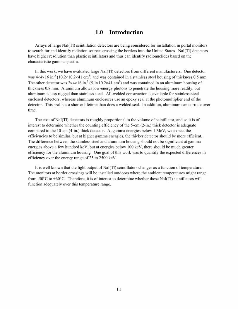
2.2. 60Co Spectrum Taken with 4×4 Detector at 0.46 m Using Low Discriminator ................................. 2.2
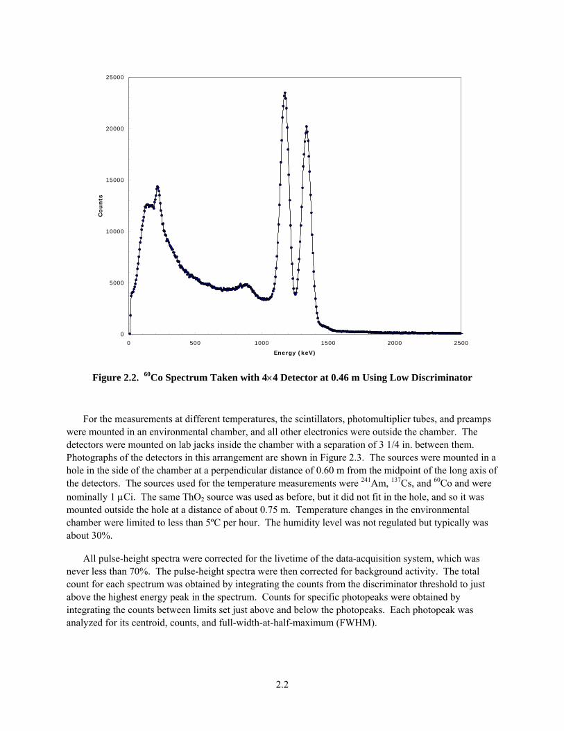
2.3. Photographs of Environmental Chamber and Detectors Mounted Inside.......................................... 2.3
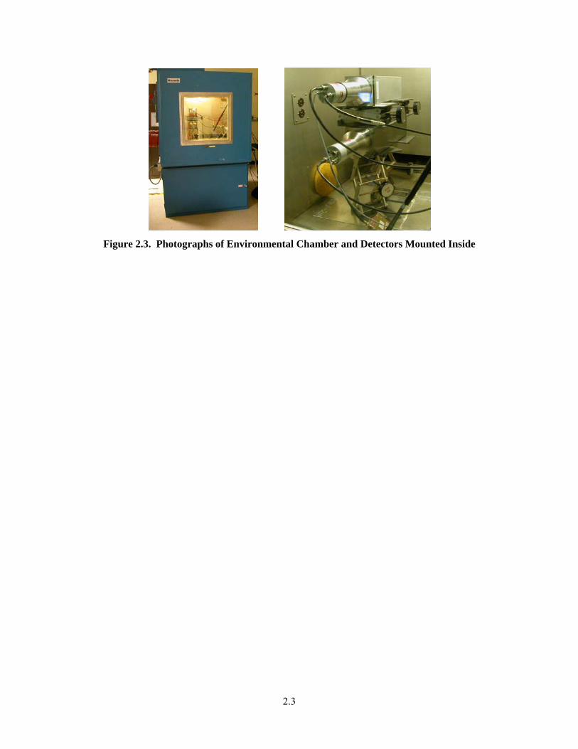
3.1. Calibration Curve for the 4×4 Detector for Sources at 0.46 m and 2.0 m for Data Obtained with the Higher Threshold Value for the Lower Level ADC Threshold ........................................... 3.1
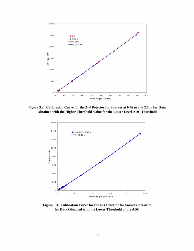
3.2. Calibration Curve for the 2×4 Detector for Sources at 0.46 m and 2.0 m for Data Obtained with the Higher Threshold Value for the Lower Level ADC Threshold ........................................... 3.2
3.3. Calibration Curve for the 4×4 Detector for Sources at 0.46 m for Data Obtained with the Lower Threshold of the ADC ............................................................................................................ 3.2
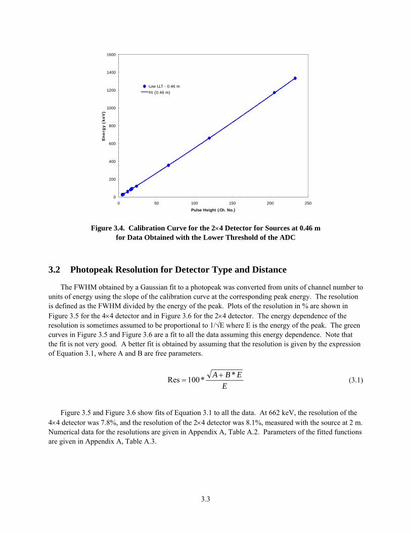
3.4. Calibration Curve for the 2×4 Detector for Sources at 0.46 m for Data Obtained with the Lower Threshold of the ADC ............................................................................................................ 3.3
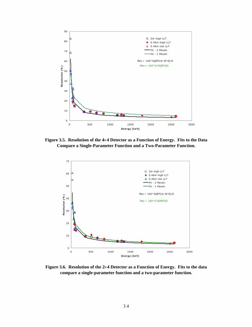
3.5. Resolution of the 4×4 Detector as a Function of Energy ................................................................... 3.4
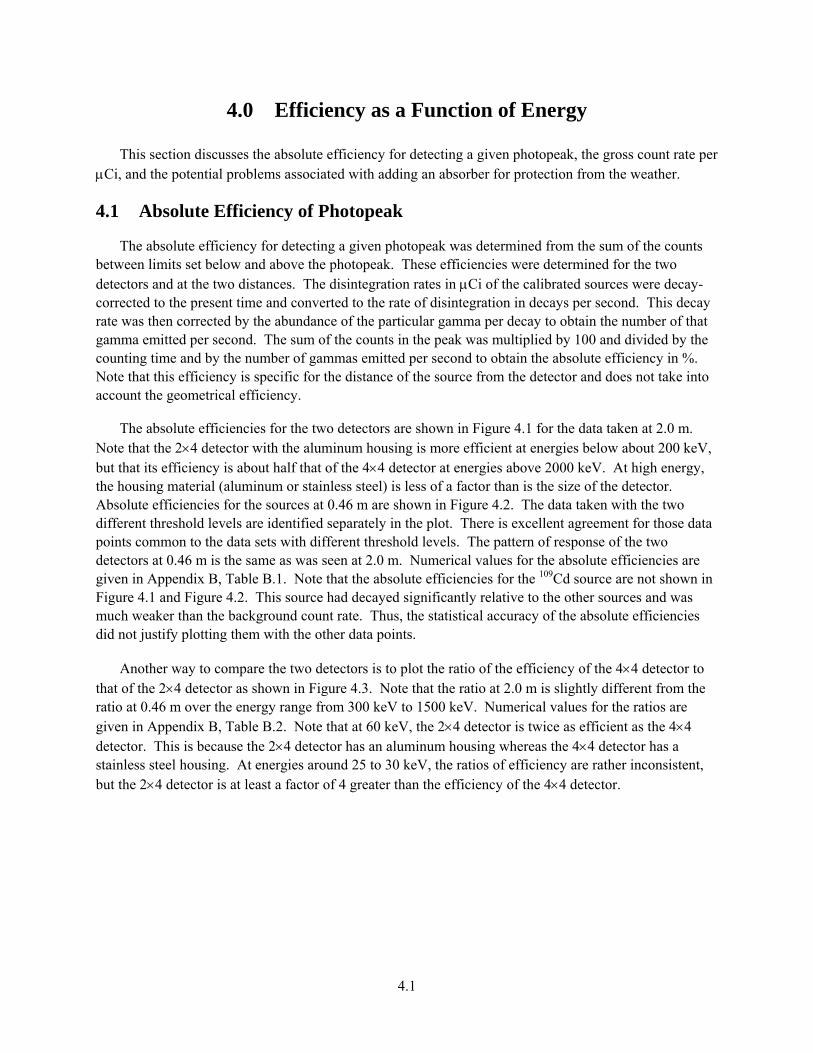
3.6. Resolution of the 2×4 Detector as a Function of Energy ................................................................... 3.4
4.1. Absolute Efficiency for Detection of Photopeaks at 2.0 m................................................................ 4.2
4.2. Absolute Efficiency for Detection of Photopeaks at 0.46 m.............................................................. 4.2
4.3. Efficiency of 4×4 Detector Relative to the Efficiency of the 2×4 Detector....................................... 4.3
5.1. Calibration Curves for the 4×4 Detector at 20ºC at the Beginning, Middle, and End of the Temperature Tests.............................................................................................................................. 5.2
5.2. Calibration Curves for the 2×4 Detector at 20ºC at the Beginning, Middle, and End of the Temperature Tests.............................................................................................................................. 5.2
5.3. Calibration Curves for the 4×4 Detector as the Temperature Was Changed from +20ºC up to +60ºC ........................................................................................................................................ 5.3
5.4. Calibration Curves for the 2×4 Detector as the Temperature Was Changed from +20ºC up to +60ºC ........................................................................................................................................ 5.4
5.5. Calibration Curves for the 4×4 Detector as the Temperature Was Changed from +20ºC down to -50ºC and back up Again ..................................................................................................... 5.5
5.6. Calibration Curves for the 2×4 Detector as the Temperature Was Changed from +20ºC down to -50ºC and back up Again ..................................................................................................... 5.5
5.7. Temperature Dependence of the 662-keV Peak in 137Cs for the 4×4 Detector .................................. 5.7
5.8. Temperature Dependence of the 662-keV Peak in 137Cs for the 2×4 Detector .................................. 5.7

ix
5.9. Temperature Dependence of the 2614-keV Peak in 232Th for the 4×4 Detector................................ 5.8
5.10. Temperature Dependence of the 2614-keV Peak in 232Th for the 2×4 Detector............................... 5.9
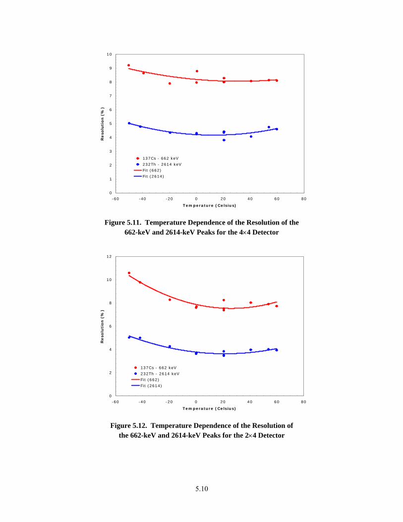
5.11. Temperature Dependence of the Resolution of the 662-keV and 2614-keV Peaks for the 4×4 Detector .................................................................................................................................... 5.10
5.12. Temperature Dependence of the Resolution of the 662-keV and 2614-keV Peaks for the 2×4 Detector .................................................................................................................................... 5.10
1.1
1.0 Introduction
Arrays of large NaI(Tl) scintillation detectors are being considered for installation in portal monitors to search for and identify radiation sources crossing the borders into the United States. NaI(Tl) detectors have higher resolution than plastic scintillators and thus can identify radionuclides based on the characteristic gamma spectra.
In this work, we have evaluated large NaI(Tl) detectors from different manufacturers. One detector was 4×4×16 in.3 (10.2×10.2×41 cm3) and was contained in a stainless steel housing of thickness 0.5 mm. The other detector was 2×4×16 in.3 (5.1×10.2×41 cm3) and was contained in an aluminum housing of thickness 0.8 mm. Aluminum allows low-energy photons to penetrate the housing more readily, but aluminum is less rugged than stainless steel. All-welded construction is available for stainless-steel enclosed detectors, whereas aluminum enclosures use an epoxy seal at the photomultiplier end of the detector. This seal has a shorter lifetime than does a welded seal. In addition, aluminum can corrode over time.
The cost of NaI(Tl) detectors is roughly proportional to the volume of scintillator, and so it is of interest to determine whether the counting efficiency of the 5-cm (2-in.) thick detector is adequate compared to the 10-cm (4-in.) thick detector. At gamma energies below 1 MeV, we expect the efficiencies to be similar, but at higher gamma energies, the thicker detector should be more efficient. The difference between the stainless steel and aluminum housing should not be significant at gamma energies above a few hundred keV, but at energies below 100 keV, there should be much greater efficiency for the aluminum housing. One goal of this work was to quantify the expected differences in efficiency over the energy range of 25 to 2500 keV.
It is well known that the light output of NaI(Tl) scintillators changes as a function of temperature. The monitors at border crossings will be installed outdoors where the ambient temperatures might range from -50°C to +60°C. Therefore, it is of interest to determine whether these NaI(Tl) scintillators will function adequately over this temperature range.

2.1
2.0 Experimental
The dynode output of the photomultiplier tube (ADIT model B89D01W; 9.0-cm diameter) attached to the 4×4×16 in.3 detector (hereafter referred to as the “4×4 detector”) was fed to the input of an Ortec 142 A preamplifier and from there to a standard shaping amplifier. The 2×4×16 in.3 detector (the “2×4 detector”) used the same photomultiplier tube and had a preamplifier built in to the photomultiplier tube base so its output went directly to a shaping amplifier. The shaping time on both amplifiers was 1 µs. The high voltage on the photomultiplier tubes and the amplifier gains were adjusted to give approximately equal gains from both detectors. The unipolar outputs of the two amplifiers were delayed and sent to channels 1 and 2 of a 4-input CAMAC(a) analog-to-digital converter (ADC). The bipolar outputs of the amplifiers were used to gate the ADC in an “OR” configuration so that either detector could create a valid gate signal to the ADC. No attempt was made to eliminate accidental coincidence events between the two detectors. A constant-rate pulser of about 30 Hz was fed to the Channel 3 input of the ADC and gated independently of the scintillator signals. The ratio of observed counts in the pulser spectrum to the expected number of counts based on the product of the known pulser rate and duration of the count determined the livetime for each measurement. Pulse-height spectra from the ADC were stored in a computer using the Kmax(b) data-acquisition software.
The measurement of the detector performance at room temperature was done with the 4×4 detector mounted on a table and the 2×4 detector mounted 4 in. above it. A photograph of the detectors mounted for these tests is shown in Figure 2.1. Calibrated radioactive sources were placed at perpendicular distances of 0.46 m and 2.0 m from the midpoint of the long dimension of the scintillators so that both detectors were simultaneously and uniformly irradiated. Most of the calibrated sources, (109Cd, 57Co, 133Ba, 137Cs, 54Mn, 22Na, and 60Co) had an activity of about 10 µCi. In addition, a 1-µCi 241Am source was used as well as an 83.32 g ThO2 source. It was assumed that the daughter activities were in equilibrium with the 232Th. An example of the 60Co pulse height spectrum is shown in Figure 2.2.
Figure 2.1. Photograph of Detectors Mounted for Room Temperature Experiments
(a) CAMAC is a modular data-handling system used at almost every nuclear physics research laboratory and many
industrial sites all over the world. (b) Kmax is a general purpose software system for building data-acquisition and control applications.
2.2
0
5000
10000
15000
20000
25000
0 500 1000 1500 2000 2500
Energy (keV)
Co
un
ts
Figure 2.2. 60Co Spectrum Taken with 4×4 Detector at 0.46 m Using Low Discriminator
For the measurements at different temperatures, the scintillators, photomultiplier tubes, and preamps were mounted in an environmental chamber, and all other electronics were outside the chamber. The detectors were mounted on lab jacks inside the chamber with a separation of 3 1/4 in. between them. Photographs of the detectors in this arrangement are shown in Figure 2.3. The sources were mounted in a hole in the side of the chamber at a perpendicular distance of 0.60 m from the midpoint of the long axis of the detectors. The sources used for the temperature measurements were 241Am, 137Cs, and 60Co and were nominally 1 µCi. The same ThO2 source was used as before, but it did not fit in the hole, and so it was mounted outside the hole at a distance of about 0.75 m. Temperature changes in the environmental chamber were limited to less than 5ºC per hour. The humidity level was not regulated but typically was about 30%.
All pulse-height spectra were corrected for the livetime of the data-acquisition system, which was never less than 70%. The pulse-height spectra were then corrected for background activity. The total count for each spectrum was obtained by integrating the counts from the discriminator threshold to just above the highest energy peak in the spectrum. Counts for specific photopeaks were obtained by integrating the counts between limits set just above and below the photopeaks. Each photopeak was analyzed for its centroid, counts, and full-width-at-half-maximum (FWHM).
2.3
Figure 2.3. Photographs of Environmental Chamber and Detectors Mounted Inside
3.1
3.0 Photopeak Resolution as a Function of Energy at Room Temperature
This section describes the energy calibration curves for the 2×4 and 4×4 detectors and the photopeak resolution for the detector type and the distance.
3.1 Energy Calibration Curves
The standard gamma sources were measured at distances of 0.46 m and 2.0 m with the detectors at room temperature (22ºC). The threshold on the ADC limited these measurements to energies above 80 keV.
An additional set of measurements was done at 0.46 m using a lower threshold on the ADC so that energy spectra could be observed down to 10 keV. Plots of the peak centroids versus gamma energy gave
calibration curves used in converting the observed FWHM values in channel number to FWHM values in energy units. The calibration curves taken at 0.46 m and 2.0 m were essentially identical as shown in
Figure 3.1 for the 4×4 detector and in Figure 3.2 for the 2×4 detector. The corresponding calibration curves for the data taken with the lower value for the lower level discriminator are shown in Figure 3.3 and Figure 3.4 for the 4×4 and 2×4 detectors, respectively. NaI(Tl) scintillators are known to be non-linear at energies below 100 keV, and so quadratic equations were used to fit the data points. Parameters for the least squares fits are given in Appendix A, Table A.1.
0
500
1000
1500
2000
2500
3000
0 50 100 150 200 250 300 350 400 450 500
Pulse Height (Ch. No.)
En
erg
y (
keV
)
2 m
0.46 m
Fit (2 m)
Fit (0.46 m)
Figure 3.1. Calibration Curve for the 4×4 Detector for Sources at 0.46 m and 2.0 m for Data Obtained with the Higher Threshold Value for the Lower Level ADC Threshold
3.2
0
500
1000
1500
2000
2500
3000
0 50 100 150 200 250 300 350 400 450 500
Pulse Height (Ch. No.)
En
erg
y (
keV
)
2m
0.46 m
Fit (2m)
Fit (0.46 m)
Figure 3.2. Calibration Curve for the 2×4 Detector for Sources at 0.46 m and 2.0 m for Data Obtained with the Higher Threshold Value for the Lower Level ADC Threshold
0
200
400
600
800
1000
1200
1400
1600
0 50 100 150 200 250
Pulse Height (Ch. No.)
En
erg
y (
keV
)
Low LLT - 0.46 m
Fit (0.46 m)
Figure 3.3. Calibration Curve for the 4×4 Detector for Sources at 0.46 m for Data Obtained with the Lower Threshold of the ADC
3.3
0
200
400
600
800
1000
1200
1400
1600
0 50 100 150 200 250
Pulse Height (Ch. No.)
En
erg
y (
keV
)
Low LLT - 0.46 m
Fit (0.46 m)
Figure 3.4. Calibration Curve for the 2×4 Detector for Sources at 0.46 m for Data Obtained with the Lower Threshold of the ADC
3.2 Photopeak Resolution for Detector Type and Distance
The FWHM obtained by a Gaussian fit to a photopeak was converted from units of channel number to units of energy using the slope of the calibration curve at the corresponding peak energy. The resolution is defined as the FWHM divided by the energy of the peak. Plots of the resolution in % are shown in Figure 3.5 for the 4×4 detector and in Figure 3.6 for the 2×4 detector. The energy dependence of the resolution is sometimes assumed to be proportional to 1/√E where E is the energy of the peak. The green curves in Figure 3.5 and Figure 3.6 are a fit to all the data assuming this energy dependence. Note that the fit is not very good. A better fit is obtained by assuming that the resolution is given by the expression of Equation 3.1, where A and B are free parameters.
E
EBA **100Res += (3.1)
Figure 3.5 and Figure 3.6 show fits of Equation 3.1 to all the data. At 662 keV, the resolution of the 4×4 detector was 7.8%, and the resolution of the 2×4 detector was 8.1%, measured with the source at 2 m. Numerical data for the resolutions are given in Appendix A, Table A.2. Parameters of the fitted functions are given in Appendix A, Table A.3.
3.4
0
10
20
30
40
50
60
70
80
90
0 500 1000 1500 2000 2500 3000
Energy (keV)
Reso
luti
on
(%
)
2m-high LLT
0.46m-high LLT
0.46m-low LLT
Fit - 2 Param.
Fit - 1 Param.
Res = 100*SQRT(A+B*E)/E
Res = 100*C/SQRT(E)
Figure 3.5. Resolution of the 4×4 Detector as a Function of Energy. Fits to the Data Compare a Single-Parameter Function and a Two-Parameter Function.
0
10
20
30
40
50
60
70
0 500 1000 1500 2000 2500 3000
Energy (keV)
Reso
luti
on
(%
)
2m-high LLT
0.46m-high LLT
0.46m-low LLT
Fit - 2 Param.
Fit - 1 Param.
Res = 100*SQRT(A+B*E)/E
Res = 100*C/SQRT(E)
Figure 3.6. Resolution of the 2×4 Detector as a Function of Energy. Fits to the data compare a single-parameter function and a two-parameter function.
4.1
4.0 Efficiency as a Function of Energy
This section discusses the absolute efficiency for detecting a given photopeak, the gross count rate per µCi, and the potential problems associated with adding an absorber for protection from the weather.
4.1 Absolute Efficiency of Photopeak
The absolute efficiency for detecting a given photopeak was determined from the sum of the counts between limits set below and above the photopeak. These efficiencies were determined for the two detectors and at the two distances. The disintegration rates in µCi of the calibrated sources were decay-corrected to the present time and converted to the rate of disintegration in decays per second. This decay rate was then corrected by the abundance of the particular gamma per decay to obtain the number of that gamma emitted per second. The sum of the counts in the peak was multiplied by 100 and divided by the counting time and by the number of gammas emitted per second to obtain the absolute efficiency in %. Note that this efficiency is specific for the distance of the source from the detector and does not take into account the geometrical efficiency.
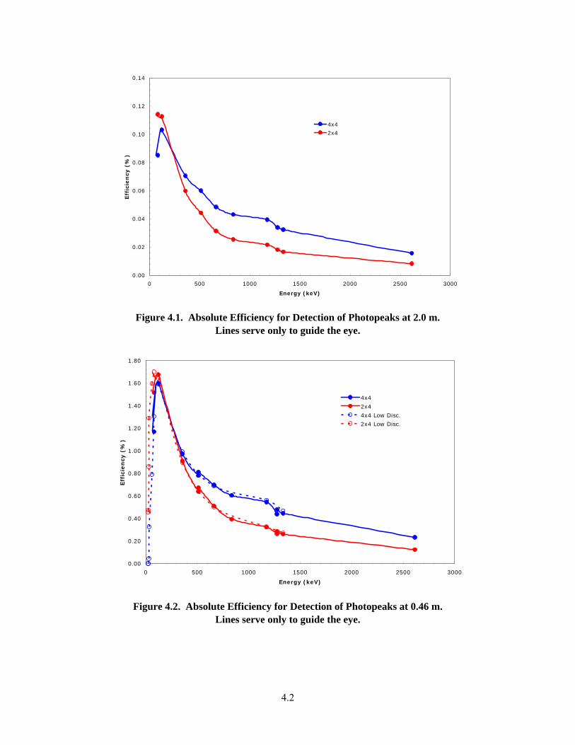
The absolute efficiencies for the two detectors are shown in Figure 4.1 for the data taken at 2.0 m. Note that the 2×4 detector with the aluminum housing is more efficient at energies below about 200 keV, but that its efficiency is about half that of the 4×4 detector at energies above 2000 keV. At high energy, the housing material (aluminum or stainless steel) is less of a factor than is the size of the detector. Absolute efficiencies for the sources at 0.46 m are shown in Figure 4.2. The data taken with the two different threshold levels are identified separately in the plot. There is excellent agreement for those data points common to the data sets with different threshold levels. The pattern of response of the two detectors at 0.46 m is the same as was seen at 2.0 m. Numerical values for the absolute efficiencies are given in Appendix B, Table B.1. Note that the absolute efficiencies for the 109Cd source are not shown in Figure 4.1 and Figure 4.2. This source had decayed significantly relative to the other sources and was much weaker than the background count rate. Thus, the statistical accuracy of the absolute efficiencies did not justify plotting them with the other data points.
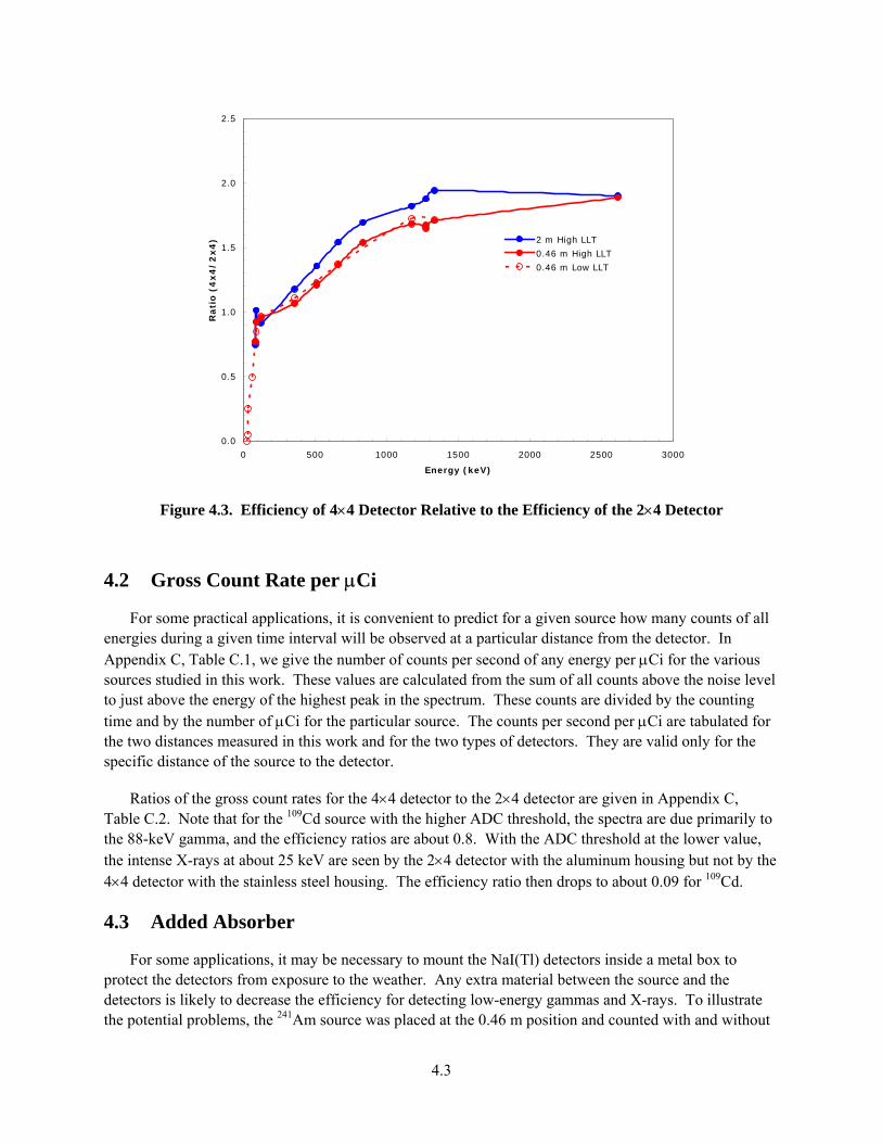
Another way to compare the two detectors is to plot the ratio of the efficiency of the 4×4 detector to that of the 2×4 detector as shown in Figure 4.3. Note that the ratio at 2.0 m is slightly different from the ratio at 0.46 m over the energy range from 300 keV to 1500 keV. Numerical values for the ratios are given in Appendix B, Table B.2. Note that at 60 keV, the 2×4 detector is twice as efficient as the 4×4 detector. This is because the 2×4 detector has an aluminum housing whereas the 4×4 detector has a stainless steel housing. At energies around 25 to 30 keV, the ratios of efficiency are rather inconsistent, but the 2×4 detector is at least a factor of 4 greater than the efficiency of the 4×4 detector.
4.2
0.00
0.02
0.04
0.06
0.08
0.10
0.12
0.14
0 500 1000 1500 2000 2500 3000
Energy (keV)
Eff
icie
ncy
(%
)4x4
2x4
Figure 4.1. Absolute Efficiency for Detection of Photopeaks at 2.0 m.
Lines serve only to guide the eye.
0.00
0.20
0.40
0.60
0.80
1.00
1.20
1.40
1.60
1.80
0 500 1000 1500 2000 2500 3000
Energy (keV)
Eff
icie
ncy
(%
)
4x4
2x4
4x4 Low Disc.
2x4 Low Disc.
Figure 4.2. Absolute Efficiency for Detection of Photopeaks at 0.46 m.
Lines serve only to guide the eye.
4.3
0.0
0.5
1.0
1.5
2.0
2.5
0 500 1000 1500 2000 2500 3000
Energy (keV)
Rati
o (
4x4
/2
x4
) 2 m High LLT
0.46 m High LLT
0.46 m Low LLT
Figure 4.3. Efficiency of 4×4 Detector Relative to the Efficiency of the 2×4 Detector
4.2 Gross Count Rate per µCi
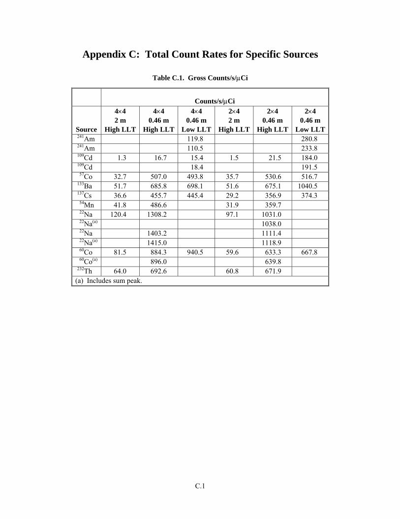
For some practical applications, it is convenient to predict for a given source how many counts of all energies during a given time interval will be observed at a particular distance from the detector. In Appendix C, Table C.1, we give the number of counts per second of any energy per µCi for the various sources studied in this work. These values are calculated from the sum of all counts above the noise level to just above the energy of the highest peak in the spectrum. These counts are divided by the counting time and by the number of µCi for the particular source. The counts per second per µCi are tabulated for the two distances measured in this work and for the two types of detectors. They are valid only for the specific distance of the source to the detector.
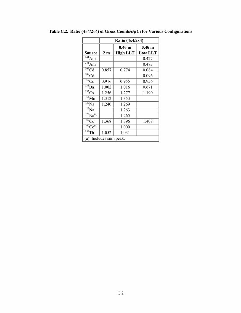
Ratios of the gross count rates for the 4×4 detector to the 2×4 detector are given in Appendix C, Table C.2. Note that for the 109Cd source with the higher ADC threshold, the spectra are due primarily to the 88-keV gamma, and the efficiency ratios are about 0.8. With the ADC threshold at the lower value, the intense X-rays at about 25 keV are seen by the 2×4 detector with the aluminum housing but not by the 4×4 detector with the stainless steel housing. The efficiency ratio then drops to about 0.09 for 109Cd.
4.3 Added Absorber
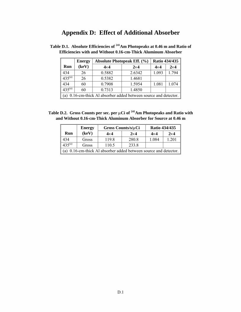
For some applications, it may be necessary to mount the NaI(Tl) detectors inside a metal box to protect the detectors from exposure to the weather. Any extra material between the source and the detectors is likely to decrease the efficiency for detecting low-energy gammas and X-rays. To illustrate the potential problems, the 241Am source was placed at the 0.46 m position and counted with and without
4.4
a 0.16-cm-thick sheet of aluminum between the source and detector. The 241Am source has a group of X-rays at about 26 keV and a gamma ray at 60 keV. Both these energies are in the region where attenuation effects should be quite noticeable.
The absolute efficiencies for the photopeaks from the 26-keV X-rays and 60-keV gammas are given in Appendix D, Table D.1. The efficiency for the gross count over the entire energy range up to 60 keV in counts per second per µCi is given in Appendix D, Table D.2. The 4×4 detector with the stainless steel housing already had low efficiencies in this energy range. These efficiencies decreased by about 10% when the aluminum absorber was added. The 2×4 detector with the aluminum housing has a much higher efficiency than the 4×4 detector in this energy range. However, its efficiency decreased by about 10% for the peak at 60 keV but decreased by more than a factor of 2 for the 26-keV peaks.
5.1
5.0 Performance as a Function of Temperature
This section discusses calibration curves derived from four standard sources at selected temperatures, the pulse heights, the resolution, and the shaping time.
5.1 Calibration Curves
The performance of the two detectors was measured as a function of temperature by counting four standard sources at each of the selected temperatures. The 241Am source gave X-rays at 26 keV and a gamma at 60 keV. The 137Cs source gave X-rays at 31 keV and a gamma at 662 keV. The 60Co source gave two gamma rays at 1173 and 1332 keV. The 232Th gives many gamma rays, but the cleanest peaks for this work were at 84.4, 238.6, 583.2, and 2614 keV. Calibration curves based on the centroids of these peaks were obtained at each temperature.
The sequence of temperatures was chosen to span the range from -50ºC to +60ºC. The first measurement was at +20ºC followed by readings at +40ºC, +53ºC, and +60ºC. The rate of temperature increase was kept to about 5ºC per hour. After the temperature was brought back to 20ºC, another measurement was made to see if the performance was reproducible after the temperature excursion. Measurements were then made at 0ºC, -20ºC, -40ºC, -50ºC, 0ºC, and +20ºC.
5.1.1 Reproducibility at 20 Degrees
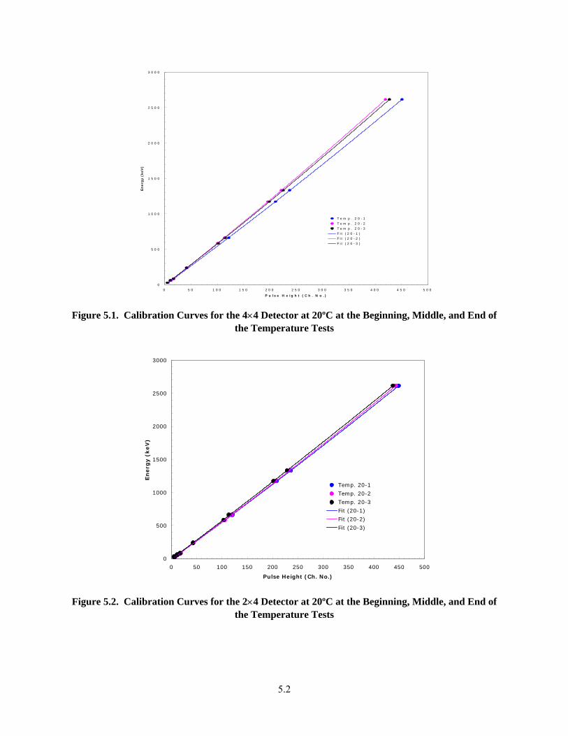
The degree of reproducibility is illustrated by plotting the three measurements at +20ºC for the 4×4 detector in Figure 5.1 and the same measurements for the 2×4 detector in Figure 5.2. The second and third measurements for the 4×4 detector agree reasonably well with each other but have a lower gain than the first measurement. One possible explanation for the change between the first and second measurements might be that the 4×4 detector suffered a permanent loss of light efficiency as the temperature was raised. However, we can not rule out the possibility that a gain shift occurred in the electronics because of a change in the preamplifier, which was inside the environmental chamber, or a change in the high voltage power supply. The three calibration curves for the 2×4 detector are in reasonable agreement with each other, which suggests that it can handle both high and low temperature extremes without changing its performance significantly. The parameters for the fits to the calibration curves at all temperatures are given in Appendix E, Table E.1.
5.2
0
5 0 0
1 0 0 0
1 5 0 0
2 0 0 0
2 5 0 0
3 0 0 0
0 5 0 1 0 0 1 5 0 2 0 0 2 5 0 3 0 0 3 5 0 4 0 0 4 5 0 5 0 0
P u ls e H e ig h t ( C h . N o . )
En
erg
y (
keV
)
T e m p . 2 0 - 1T e m p . 2 0 - 2T e m p . 2 0 - 3F i t ( 2 0 - 1 )F i t ( 2 0 - 2 )F i t ( 2 0 - 3 )
Figure 5.1. Calibration Curves for the 4×4 Detector at 20ºC at the Beginning, Middle, and End of the Temperature Tests
0
500
1000
1500
2000
2500
3000
0 50 100 150 200 250 300 350 400 450 500
Pulse Height (Ch. No.)
En
erg
y (
keV
)
Temp. 20-1
Temp. 20-2
Temp. 20-3
Fit (20-1)
Fit (20-2)
Fit (20-3)
Figure 5.2. Calibration Curves for the 2×4 Detector at 20ºC at the Beginning, Middle, and End of the Temperature Tests
5.3
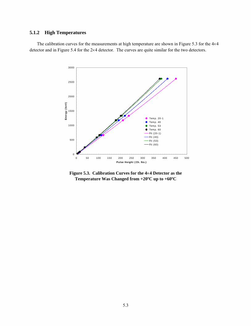
5.1.2 High Temperatures
The calibration curves for the measurements at high temperature are shown in Figure 5.3 for the 4×4 detector and in Figure 5.4 for the 2×4 detector. The curves are quite similar for the two detectors.
0
500
1000
1500
2000
2500
3000
0 50 100 150 200 250 300 350 400 450 500
Pulse Height (Ch. No.)
En
erg
y (
keV
)
Temp. 20-1
Temp. 40
Temp. 53
Temp. 60
Fit (20-1)
Fit (40)
Fit (53)
Fit (60)
Figure 5.3. Calibration Curves for the 4×4 Detector as the Temperature Was Changed from +20ºC up to +60ºC
5.4
0
500
1000
1500
2000
2500
3000
0 50 100 150 200 250 300 350 400 450 500
Pulse Height (Ch. No.)
En
erg
y (
keV
)
Temp. 20-1
Temp. 40
Temp. 53
Temp. 60
Fit (20-1)
Fit (40)
Fit (53)
Fit (60)
Figure 5.4. Calibration Curves for the 2×4 Detector as the Temperature Was Changed from +20ºC up to +60ºC
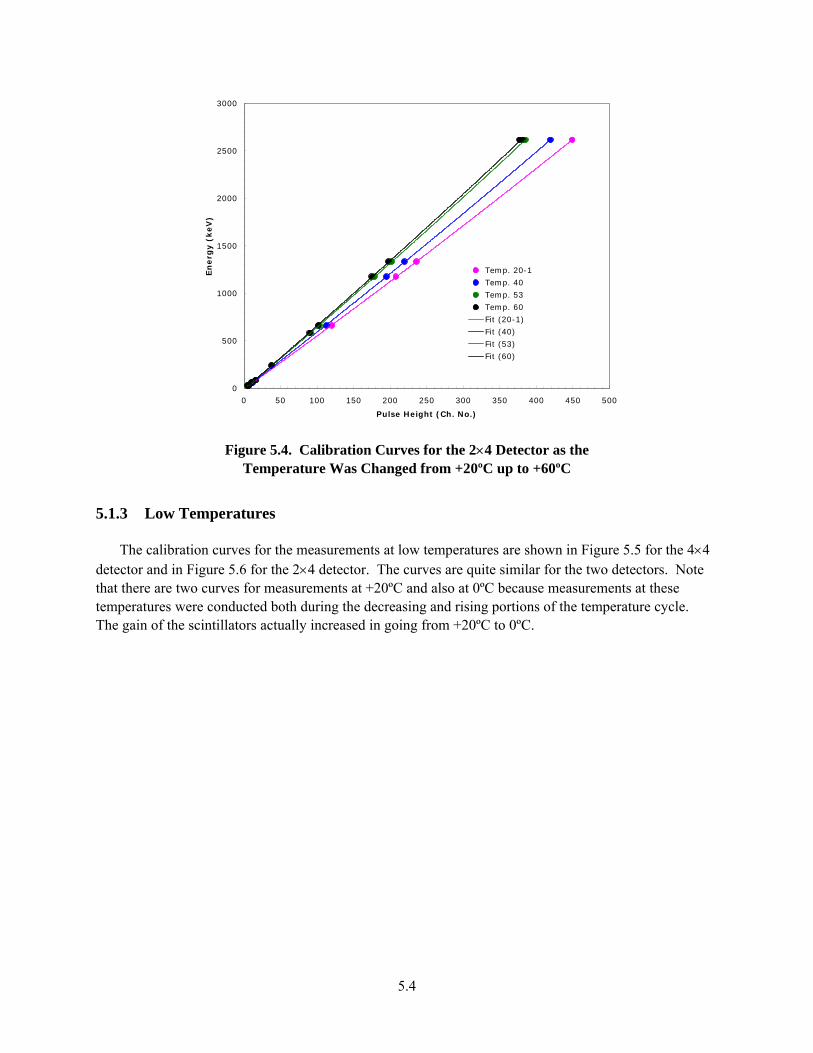
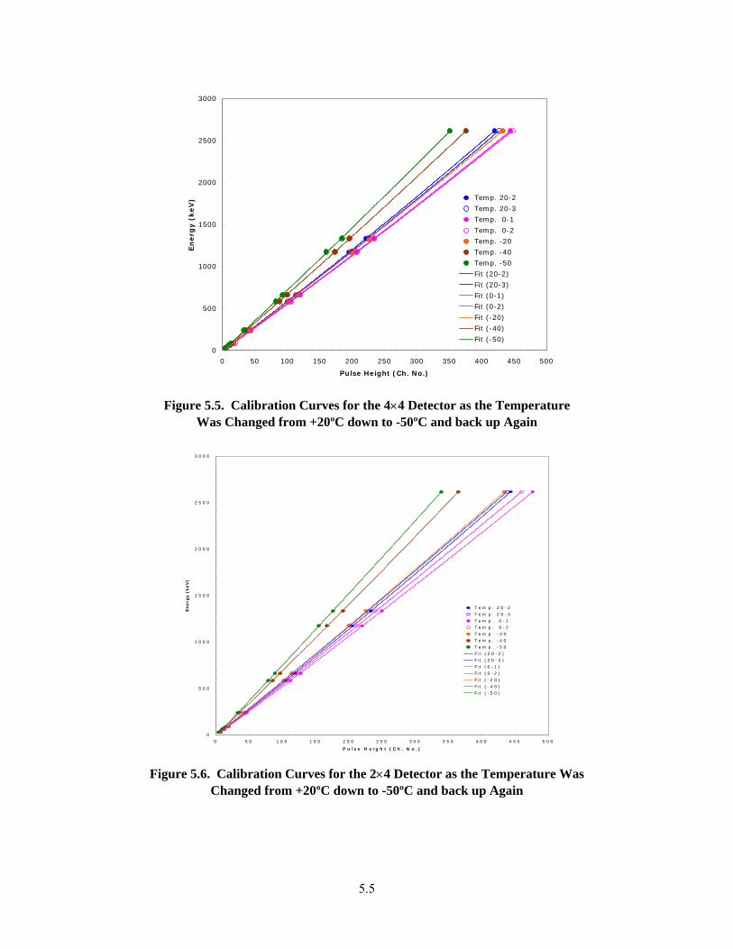
5.1.3 Low Temperatures
The calibration curves for the measurements at low temperatures are shown in Figure 5.5 for the 4×4 detector and in Figure 5.6 for the 2×4 detector. The curves are quite similar for the two detectors. Note that there are two curves for measurements at +20ºC and also at 0ºC because measurements at these temperatures were conducted both during the decreasing and rising portions of the temperature cycle. The gain of the scintillators actually increased in going from +20ºC to 0ºC.
5.5
0
500
1000
1500
2000
2500
3000
0 50 100 150 200 250 300 350 400 450 500
Pulse Height (Ch. No.)
En
erg
y (
keV
) Temp. 20-2
Temp. 20-3
Temp. 0-1
Temp. 0-2
Temp. -20
Temp. -40
Temp. -50
Fit (20-2)
Fit (20-3)
Fit (0-1)
Fit (0-2)
Fit (-20)
Fit (-40)
Fit (-50)
Figure 5.5. Calibration Curves for the 4×4 Detector as the Temperature Was Changed from +20ºC down to -50ºC and back up Again
0
5 0 0
1 0 0 0
1 5 0 0
2 0 0 0
2 5 0 0
3 0 0 0
0 5 0 1 0 0 1 5 0 2 0 0 2 5 0 3 0 0 3 5 0 4 0 0 4 5 0 5 0 0
P u ls e H e ig h t ( C h . N o . )
En
erg
y (
keV
)
T e m p . 2 0 - 2T e m p . 2 0 - 3T e m p . 0 - 1T e m p . 0 - 2
T e m p . - 2 0T e m p . - 4 0T e m p . - 5 0
F it ( 2 0 - 2 )F it ( 2 0 - 3 )F it ( 0 - 1 )F it ( 0 - 2 )
F it ( - 2 0 )F it ( - 4 0 )F it ( - 5 0 )
Figure 5.6. Calibration Curves for the 2×4 Detector as the Temperature Was Changed from +20ºC down to -50ºC and back up Again
5.6
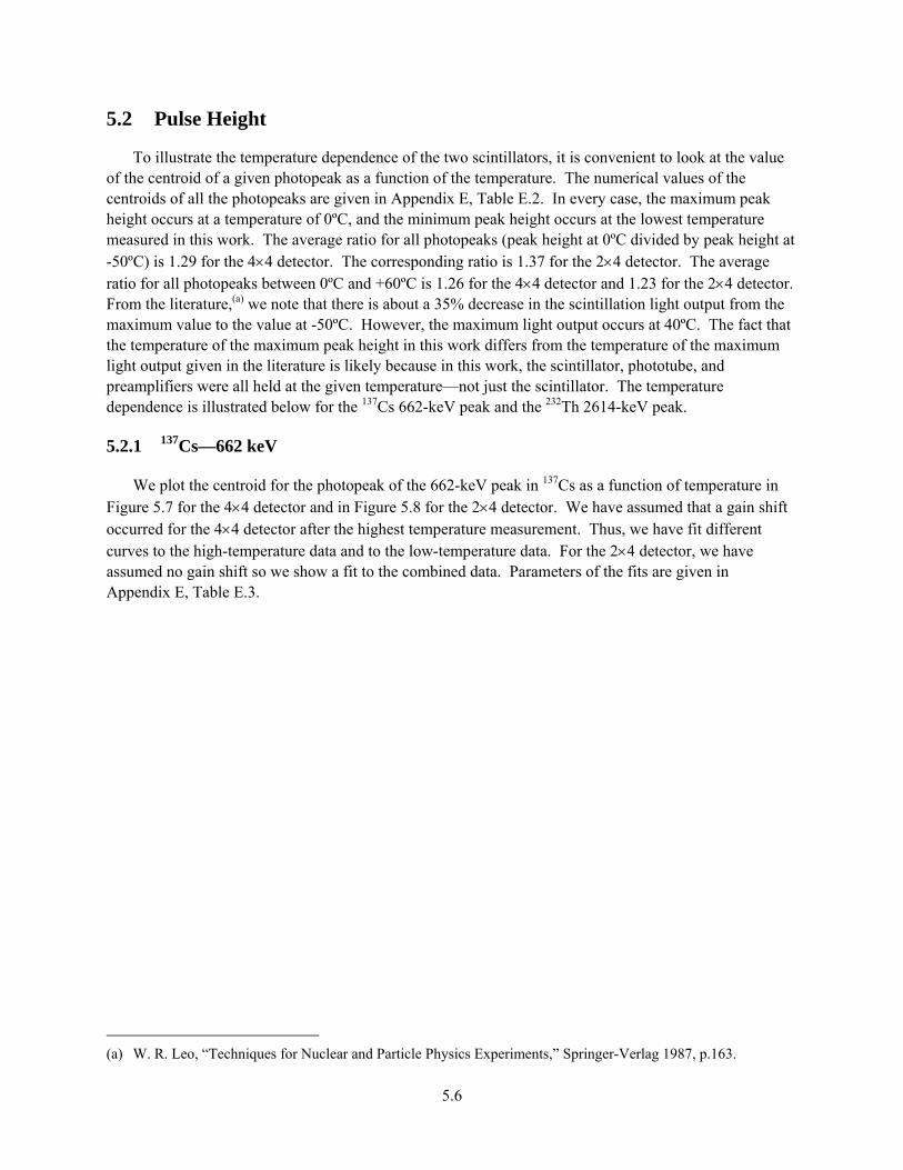
5.2 Pulse Height
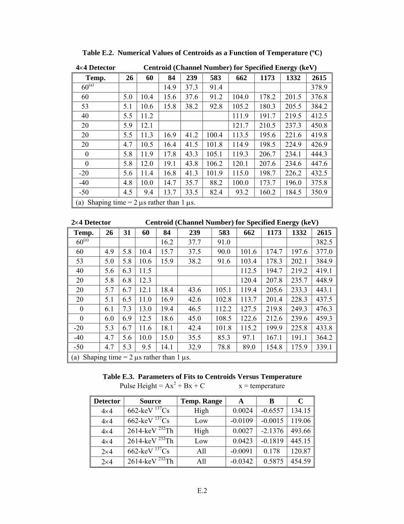
To illustrate the temperature dependence of the two scintillators, it is convenient to look at the value of the centroid of a given photopeak as a function of the temperature. The numerical values of the centroids of all the photopeaks are given in Appendix E, Table E.2. In every case, the maximum peak height occurs at a temperature of 0ºC, and the minimum peak height occurs at the lowest temperature measured in this work. The average ratio for all photopeaks (peak height at 0ºC divided by peak height at -50ºC) is 1.29 for the 4×4 detector. The corresponding ratio is 1.37 for the 2×4 detector. The average ratio for all photopeaks between 0ºC and +60ºC is 1.26 for the 4×4 detector and 1.23 for the 2×4 detector. From the literature,(a) we note that there is about a 35% decrease in the scintillation light output from the maximum value to the value at -50ºC. However, the maximum light output occurs at 40ºC. The fact that the temperature of the maximum peak height in this work differs from the temperature of the maximum light output given in the literature is likely because in this work, the scintillator, phototube, and preamplifiers were all held at the given temperature—not just the scintillator. The temperature dependence is illustrated below for the 137Cs 662-keV peak and the 232Th 2614-keV peak.
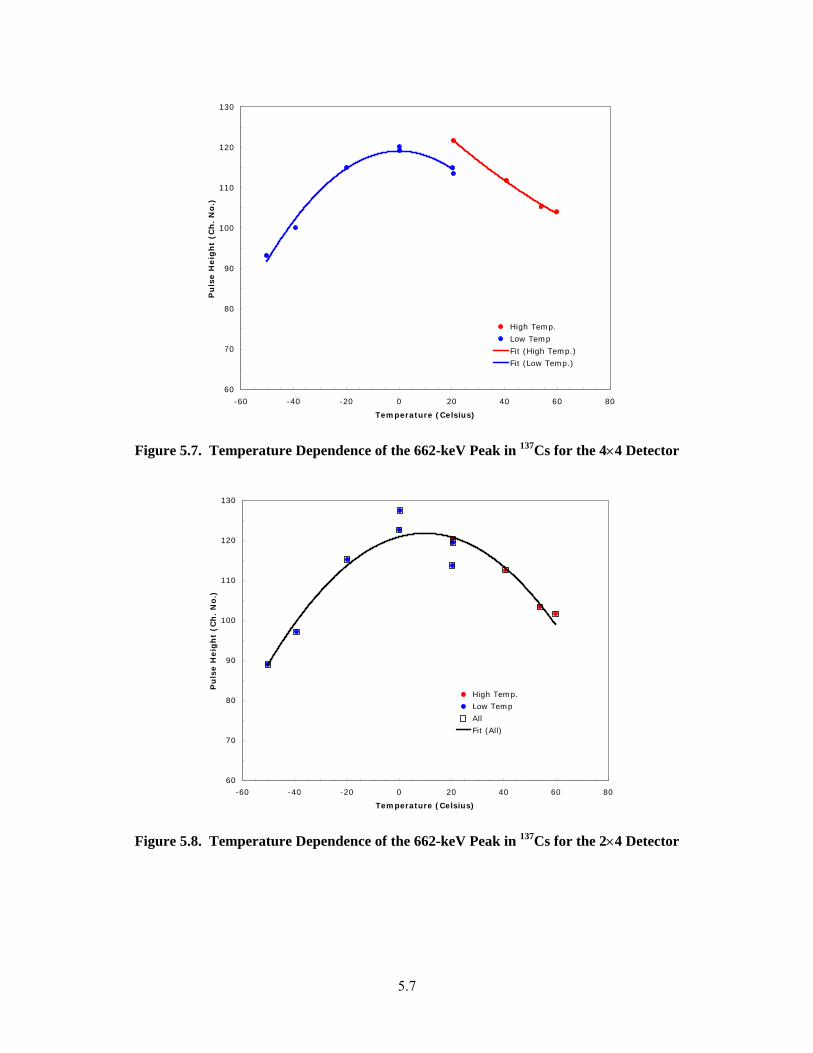
5.2.1 137Cs—662 keV
We plot the centroid for the photopeak of the 662-keV peak in 137Cs as a function of temperature in Figure 5.7 for the 4×4 detector and in Figure 5.8 for the 2×4 detector. We have assumed that a gain shift occurred for the 4×4 detector after the highest temperature measurement. Thus, we have fit different curves to the high-temperature data and to the low-temperature data. For the 2×4 detector, we have assumed no gain shift so we show a fit to the combined data. Parameters of the fits are given in Appendix E, Table E.3.
(a) W. R. Leo, “Techniques for Nuclear and Particle Physics Experiments,” Springer-Verlag 1987, p.163.
5.7
60
70
80
90
100
110
120
130
-60 -40 -20 0 20 40 60 80
Temperature (Celsius)
Pu
lse H
eig
ht
(Ch
. N
o.)
High Temp.
Low Temp
Fit (High Temp.)
Fit (Low Temp.)
Figure 5.7. Temperature Dependence of the 662-keV Peak in 137Cs for the 4×4 Detector
60
70
80
90
100
110
120
130
-60 -40 -20 0 20 40 60 80
Temperature (Celsius)
Pu
lse H
eig
ht
(Ch
. N
o.)
High Temp.
Low Temp
All
Fit (All)
Figure 5.8. Temperature Dependence of the 662-keV Peak in 137Cs for the 2×4 Detector
5.8
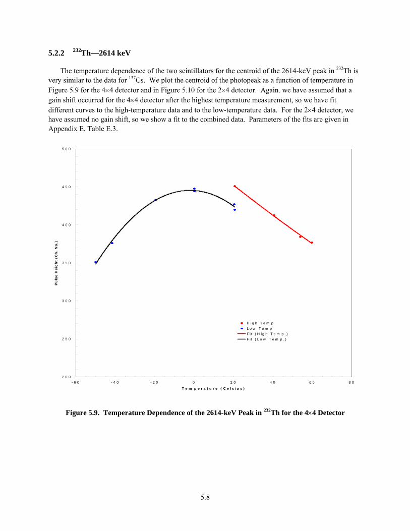
5.2.2 232Th—2614 keV
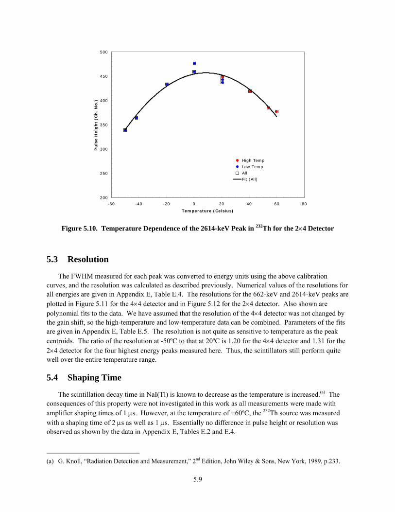
The temperature dependence of the two scintillators for the centroid of the 2614-keV peak in 232Th is very similar to the data for 137Cs. We plot the centroid of the photopeak as a function of temperature in Figure 5.9 for the 4×4 detector and in Figure 5.10 for the 2×4 detector. Again. we have assumed that a gain shift occurred for the 4×4 detector after the highest temperature measurement, so we have fit different curves to the high-temperature data and to the low-temperature data. For the 2×4 detector, we have assumed no gain shift, so we show a fit to the combined data. Parameters of the fits are given in Appendix E, Table E.3.
2 0 0
2 5 0
3 0 0
3 5 0
4 0 0
4 5 0
5 0 0
-6 0 - 4 0 - 2 0 0 2 0 4 0 6 0 8 0
T e m p e r a t u r e ( C e ls iu s )
Pu
lse H
eig
ht
(Ch
. N
o.)
H ig h T e m pL o w T e m pF it (H ig h T e m p .)F it ( L o w T e m p .)
Figure 5.9. Temperature Dependence of the 2614-keV Peak in 232Th for the 4×4 Detector
5.9
200
250
300
350
400
450
500
-60 -40 -20 0 20 40 60 80
Temperature (Celsius)
Pu
lse H
eig
ht
(Ch
. N
o.)
High Temp
Low Temp
All
Fit (All)
Figure 5.10. Temperature Dependence of the 2614-keV Peak in 232Th for the 2×4 Detector
5.3 Resolution
The FWHM measured for each peak was converted to energy units using the above calibration curves, and the resolution was calculated as described previously. Numerical values of the resolutions for all energies are given in Appendix E, Table E.4. The resolutions for the 662-keV and 2614-keV peaks are plotted in Figure 5.11 for the 4×4 detector and in Figure 5.12 for the 2×4 detector. Also shown are polynomial fits to the data. We have assumed that the resolution of the 4×4 detector was not changed by the gain shift, so the high-temperature and low-temperature data can be combined. Parameters of the fits are given in Appendix E, Table E.5. The resolution is not quite as sensitive to temperature as the peak centroids. The ratio of the resolution at -50ºC to that at 20ºC is 1.20 for the 4×4 detector and 1.31 for the 2×4 detector for the four highest energy peaks measured here. Thus, the scintillators still perform quite well over the entire temperature range.
5.4 Shaping Time
The scintillation decay time in NaI(Tl) is known to decrease as the temperature is increased.(a) The consequences of this property were not investigated in this work as all measurements were made with amplifier shaping times of 1 µs. However, at the temperature of +60ºC, the 232Th source was measured with a shaping time of 2 µs as well as 1 µs. Essentially no difference in pulse height or resolution was observed as shown by the data in Appendix E, Tables E.2 and E.4.
(a) G. Knoll, “Radiation Detection and Measurement,” 2nd Edition, John Wiley & Sons, New York, 1989, p.233.
5.10
0
1
2
3
4
5
6
7
8
9
10
-60 -40 -20 0 20 40 60 80
Temperature (Celsius)
Reso
luti
on
(%
)
137Cs - 662 keV
232Th - 2614 keV
Fit (662)
Fit (2614)
Figure 5.11. Temperature Dependence of the Resolution of the
662-keV and 2614-keV Peaks for the 4×4 Detector
0
2
4
6
8
10
12
-60 -40 -20 0 20 40 60 80
Temperature (Celsius)
Reso
luti
on
(%
)
137Cs - 662 keV
232Th - 2614 keV
Fit (662)
Fit (2614)
Figure 5.12. Temperature Dependence of the Resolution of
the 662-keV and 2614-keV Peaks for the 2×4 Detector
6.1
6.0 Summary and Conclusions
The present data demonstrate that for gamma energies greater than 1000 keV, the 10-cm (4-in.) thick detector has up to a factor of two greater photopeak efficiency than the 5-cm (2-in.) thick detector. The resolutions are not significantly different for the two types of detectors. For energies below 200 keV, the aluminum housing gives better efficiency than the stainless steel housing. If the requirement is for maximum photopeak efficiency at all energies, then a 10-cm (4-in.) thick detector in an aluminum housing would be preferred.
If one considers the total count rate at all energies for a particular source regardless of photopeak efficiency, the differences between the 10-cm-thick detector and the 5-cm-thick detector are not as noticeable. The 5-cm-thick detector partially compensates for its decrease in photopeak efficiency by an increase in the number of counts in the Compton scatter region. If the requirement is for total efficiency for detecting any gamma event from a given source, then the 5-cm-thick detector offers a possible cost-saving over the 10-cm-thick detector.
The 5-cm-thick detector in the aluminum housing was cycled smoothly from room temperature up to +60ºC, back to room temperature, down to -50ºC, and back to room temperature. The peak amplitudes changed by about 37% from the highest gain at 0ºC to the lowest gain at -50ºC and returned to their starting values. The resolutions broadened by about 31% between 20ºC and -50ºC. The situation with the 10-cm-thick detector in the stainless steel housing is more ambiguous. The peak amplitudes did not return to their starting values after the detector was heated. For the cooling cycle, however, the starting and ending values were essentially the same. It is not clear from the present data whether a permanent change in the scintillator or preamplifier was induced by the high temperature, or whether the gain shift was caused by a change in the high voltage supply or external amplifier. The resolution changed by about 20% between 20ºC and -50ºC.
The literature data for the temperature dependence of the NaI(Tl) scintillator independent of the electronics indicates that the maximum light output occurs at about +40ºC. In this work, the complete package of scintillator, photomultiplier tubes, and preamps was held at the given temperature. The fact that the maximum pulse height in this work occurred at 0ºC indicates that changes in temperature affect more than just the scintillator alone. In addition, the increase in scintillation decay time at lower temperatures suggests that longer amplifier shaping times might be required at low temperatures to fully collect all available signal. This possibility was not studied in this work.
In any case, the present data confirm that scintillator performance changes as a function of temperature. Any field use of these detectors should monitor the detector temperature and should incorporate adjustments in the data analysis to compensate for the known gain shifts. Alternatively, a constant temperature environment could be maintained for the NaI(Tl) scintillators.

Appendix A
Calibration and Resolution Data
A.1
Appendix A: Calibration and Resolution Data
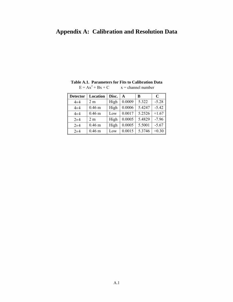
Table A.1. Parameters for Fits to Calibration Data E = Ax2 + Bx + C x = channel number
Detector Location Disc. A B C 4×4 2 m High 0.0009 5.322 -5.28 4×4 0.46 m High 0.0006 5.4247 -5.42 4×4 0.46 m Low 0.0017 5.2526 +1.67 2×4 2 m High 0.0005 5.4829 -7.96 2×4 0.46 m High 0.0005 5.5001 -5.67 2×4 0.46 m Low 0.0015 5.3746 +0.30

A.2
Table A.2. Resolution Data for both Detector Types at 2.0 m and at 0.46 m
Resolution (%)
Energy (keV)
4×4 2 m
High LLT
4×4 0.46 m
High LLT
4×4 0.46 m
Low LLT
2×4 2 m
High LLT
2×4 0.46 m
High LLT
2×4 0.46 m
Low LLT25 68.48 36.21 25 82.81 36.00 26 50.51 60.45 26 54.93 31 37.25 33.05 31 47.46 32.01 60 22.76 23.53 60 23.44 81 19.36 18.95 17.95 19.21 19.20 14.79 88 22.45 19.80 32.88 15.31 14.48 28.91 88 31.42 28.60 94 24.78 16.23
122 16.05 16.08 15.40 15.08 14.31 14.02 356 8.93 9.02 8.98 9.31 9.66 9.44 511 8.99 9.59 9.00 10.87 511 9.42 10.53 662 7.83 7.78 7.71 8.06 8.04 8.10 835 7.16 7.26 7.10 7.28
1173 5.48 5.70 5.90 5.50 5.69 5.75 1275 5.68 5.85 5.67 6.04 1275 6.15 6.02 1333 5.22 5.13 5.37 5.26 5.21 5.35 1786(a) 5.14 4.99 1786(a) 5.39 2506(b) 3.55 3.55 2614 4.36 4.36 4.17 4.32
(a) Sum Peak in 22Na (b) Sum peak in 60Co
Table A.3. Parameters of Fits to Resolution Using all Data 2 parameter Res = 100*SQRT(A+B*E)/E 1 parameter Res = 100*C/SQRT(E)
Detector A B C 4×4 182.61 2.397 2.5522×4 56.30 2.721 2.035

Appendix B
Efficiency Data
B.1
Appendix B: Efficiency Data
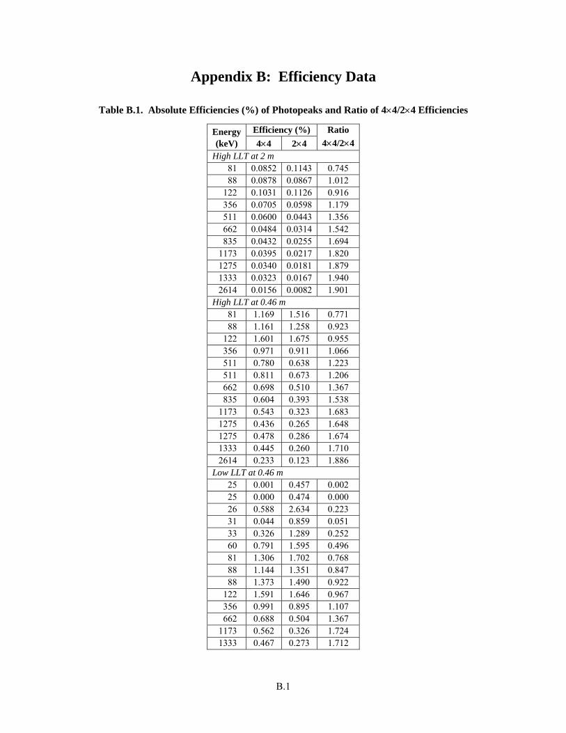
Table B.1. Absolute Efficiencies (%) of Photopeaks and Ratio of 4×4/2×4 Efficiencies
Efficiency (%) Energy(keV) 4×4 2×4
Ratio 4×4/2×4
High LLT at 2 m 81 0.0852 0.1143 0.745 88 0.0878 0.0867 1.012
122 0.1031 0.1126 0.916 356 0.0705 0.0598 1.179 511 0.0600 0.0443 1.356 662 0.0484 0.0314 1.542 835 0.0432 0.0255 1.694
1173 0.0395 0.0217 1.820 1275 0.0340 0.0181 1.879 1333 0.0323 0.0167 1.940 2614 0.0156 0.0082 1.901
High LLT at 0.46 m 81 1.169 1.516 0.771 88 1.161 1.258 0.923
122 1.601 1.675 0.955 356 0.971 0.911 1.066 511 0.780 0.638 1.223 511 0.811 0.673 1.206 662 0.698 0.510 1.367 835 0.604 0.393 1.538
1173 0.543 0.323 1.683 1275 0.436 0.265 1.648 1275 0.478 0.286 1.674 1333 0.445 0.260 1.710 2614 0.233 0.123 1.886
Low LLT at 0.46 m 25 0.001 0.457 0.002 25 0.000 0.474 0.000 26 0.588 2.634 0.223 31 0.044 0.859 0.051 33 0.326 1.289 0.252 60 0.791 1.595 0.496 81 1.306 1.702 0.768 88 1.144 1.351 0.847 88 1.373 1.490 0.922
122 1.591 1.646 0.967 356 0.991 0.895 1.107 662 0.688 0.504 1.367
1173 0.562 0.326 1.724 1333 0.467 0.273 1.712

Appendix C
Total Count Rates for Specific Sources
C.1
Appendix C: Total Count Rates for Specific Sources
Table C.1. Gross Counts/s/µCi
Counts/s/µCi
Source
4×4 2 m
High LLT
4×4 0.46 m
High LLT
4×4 0.46 m
Low LLT
2×4 2 m
High LLT
2×4 0.46 m
High LLT
2×4 0.46 m
Low LLT241Am 119.8 280.8 241Am 110.5 233.8 109Cd 1.3 16.7 15.4 1.5 21.5 184.0 109Cd 18.4 191.5 57Co 32.7 507.0 493.8 35.7 530.6 516.7
133Ba 51.7 685.8 698.1 51.6 675.1 1040.5 137Cs 36.6 455.7 445.4 29.2 356.9 374.3 54Mn 41.8 486.6 31.9 359.7 22Na 120.4 1308.2 97.1 1031.0 22Na(a) 1038.0 22Na 1403.2 1111.4 22Na(a) 1415.0 1118.9 60Co 81.5 884.3 940.5 59.6 633.3 667.8 60Co(a) 896.0 639.8
232Th 64.0 692.6 60.8 671.9 (a) Includes sum peak.
C.2
Table C.2. Ratio (4×4/2×4) of Gross Counts/s/µCi for Various Configurations
Ratio (4x4/2x4)
Source 2 m 0.46 m
High LLT0.46 m
Low LLT241Am 0.427 241Am 0.473 109Cd 0.857 0.774 0.084 109Cd 0.096 57Co 0.916 0.955 0.956
133Ba 1.002 1.016 0.671 137Cs 1.256 1.277 1.190 54Mn 1.312 1.353 22Na 1.240 1.269 22Na 1.263 22Na(a) 1.265 60Co 1.368 1.396 1.408 60Co(a) 1.000
232Th 1.052 1.031 (a) Includes sum peak.

Appendix D
Effect of Additional Absorber
D.1
Appendix D: Effect of Additional Absorber
Table D.1. Absolute Efficiencies of 241Am Photopeaks at 0.46 m and Ratio of Efficiencies with and Without 0.16-cm-Thick Aluminum Absorber
Absolute Photopeak Eff. (%) Ratio 434/435 Run
Energy (keV) 4×4 2×4 4×4 2×4
434 26 0.5882 2.6342 1.093 1.794 435(a) 26 0.5382 1.4681 434 60 0.7908 1.5954 1.081 1.074 435(a) 60 0.7313 1.4850 (a) 0.16-cm-thick Al absorber added between source and detector.
Table D.2. Gross Counts per sec. per µCi of 241Am Photopeaks and Ratio with and Without 0.16-cm-Thick Aluminum Absorber for Source at 0.46 m
Gross Counts/s/µCi Ratio 434/435 Run
Energy (keV) 4×4 2×4 4×4 2×4
434 Gross 119.8 280.8 1.084 1.201 435(a) Gross 110.5 233.8 (a) 0.16-cm-thick Al absorber added between source and detector.

Appendix E
Experimental Data as a Function of Temperature

E.1
Appendix E: Experimental Data as a Function of Temperature
Table E.1. Parameters of Fits to Calibration Curves for Various Temperatures Energy = Ax2 + Bx + C x = channel number
Detector Temp. (ºC) Meas. A B C 4×4 60 1 0.0017 6.3013 -7.31 4×4 53 1 0.0015 6.2302 -7.61 4×4 40 1 0.0011 5.8808 -6.52 4×4 20 1 0.0009 5.4215 -6.72 4×4 20 2 0.0010 5.8253 -8.41 4×4 20 3 0.0010 5.7109 -3.62 4×4 0 1 0.0008 5.5355 -7.72 4×4 0 2 0.0007 5.5456 -10.78 4×4 -20 1 0.0006 5.7845 -7.81 4×4 -40 1 0.0009 6.6439 -7.33 4×4 -50 1 0.0010 7.1374 -7.81
2×4 60 1 0.0008 6.6086 -11.40 2×4 53 1 0.0010 6.4299 -9.95 2×4 40 1 0.0008 5.9074 -7.89 2×4 20 1 0.0007 5.5097 -7.25 2×4 20 2 0.0008 5.5617 -9.07 2×4 20 3 0.0006 5.7392 -6.31 2×4 0 1 0.0006 5.2343 -9.52 2×4 0 2 0.0006 5.4306 -9.61 2×4 -20 1 0.0006 5.7961 -10.18 2×4 -40 1 0.0009 6.8785 -9.99 2×4 -50 1 0.0006 7.5424 -12.60
E.2
Table E.2. Numerical Values of Centroids as a Function of Temperature (ºC)
4×4 Detector Centroid (Channel Number) for Specified Energy (keV) Temp. 26 60 84 239 583 662 1173 1332 2615
60(a) 14.9 37.3 91.4 378.9 60 5.0 10.4 15.6 37.6 91.2 104.0 178.2 201.5 376.8 53 5.1 10.6 15.8 38.2 92.8 105.2 180.3 205.5 384.2 40 5.5 11.2 111.9 191.7 219.5 412.5 20 5.9 12.1 121.7 210.5 237.3 450.8 20 5.5 11.3 16.9 41.2 100.4 113.5 195.6 221.6 419.8 20 4.7 10.5 16.4 41.5 101.8 114.9 198.5 224.9 426.9
0 5.8 11.9 17.8 43.3 105.1 119.3 206.7 234.1 444.3 0 5.8 12.0 19.1 43.8 106.2 120.1 207.6 234.6 447.6
-20 5.6 11.4 16.8 41.3 101.9 115.0 198.7 226.2 432.5 -40 4.8 10.0 14.7 35.7 88.2 100.0 173.7 196.0 375.8 -50 4.5 9.4 13.7 33.5 82.4 93.2 160.2 184.5 350.9
(a) Shaping time = 2 µs rather than 1 µs.
2×4 Detector Centroid (Channel Number) for Specified Energy (keV) Temp. 26 31 60 84 239 583 662 1173 1332 2615 60(a) 16.2 37.7 91.0 382.5 60 4.9 5.8 10.4 15.7 37.5 90.0 101.6 174.7 197.6 377.0 53 5.0 5.8 10.6 15.9 38.2 91.6 103.4 178.3 202.1 384.9 40 5.6 6.3 11.5 112.5 194.7 219.2 419.1 20 5.8 6.8 12.3 120.4 207.8 235.7 448.9 20 5.7 6.7 12.1 18.4 43.6 105.1 119.4 205.6 233.3 443.1 20 5.1 6.5 11.0 16.9 42.6 102.8 113.7 201.4 228.3 437.5
0 6.1 7.3 13.0 19.4 46.5 112.2 127.5 219.8 249.3 476.3 0 6.0 6.9 12.5 18.6 45.0 108.5 122.6 212.6 239.6 459.3
-20 5.3 6.7 11.6 18.1 42.4 101.8 115.2 199.9 225.8 433.8 -40 4.7 5.6 10.0 15.0 35.5 85.3 97.1 167.1 191.1 364.2 -50 4.7 5.3 9.5 14.1 32.9 78.8 89.0 154.8 175.9 339.1
(a) Shaping time = 2 µs rather than 1 µs.
Table E.3. Parameters of Fits to Centroids Versus Temperature Pulse Height = Ax2 + Bx + C x = temperature
Detector Source Temp. Range A B C 4×4 662-keV 137Cs High 0.0024 -0.6557 134.15 4×4 662-keV 137Cs Low -0.0109 -0.0015 119.06 4×4 2614-keV 232Th High 0.0027 -2.1376 493.66 4×4 2614-keV 232Th Low 0.0423 -0.1819 445.15 2×4 662-keV 137Cs All -0.0091 0.178 120.87 2×4 2614-keV 232Th All -0.0342 0.5875 454.59
E.3
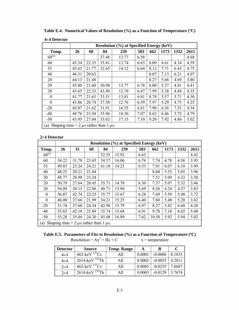
Table E.4. Numerical Values of Resolution (%) as a Function of Temperature (ºC)
4×4 Detector Resolution (%) at Specified Energy (keV)
Temp. 26 60 84 239 583 662 1173 1332 261560(a) 37.48 13.77 6.58 4.68 60 45.34 22.35 33.81 13.74 6.63 8.09 4.61 4.34 4.59 53 43.63 21.77 32.65 14.12 6.64 8.12 7.71 6.43 4.75 40 46.31 20.63 8.07 7.13 6.21 4.07 20 44.13 21.48 8.27 5.66 4.69 3.80 20 45.80 21.60 30.98 13.77 6.78 8.00 5.37 4.81 4.41 20 43.65 22.33 43.49 12.70 6.47 7.99 5.38 4.84 4.35
0 41.77 21.63 33.51 13.81 6.81 8.78 5.57 5.71 4.30 0 43.86 20.74 37.30 12.76 6.59 7.97 5.29 4.75 4.25
-20 45.07 21.62 31.91 16.55 6.81 7.90 6.36 7.53 4.34 -40 49.76 23.94 35.96 18.30 7.07 8.62 6.46 5.72 4.79 -50 43.95 27.04 33.62 17.15 7.10 9.20 7.92 4.86 5.02
(a) Shaping time = 2 µs rather than 1 µs.
2×4 Detector Resolution (%) at Specified Energy (keV)
Temp. 26 31 60 84 239 583 662 1173 1332 261560(a) 52.55 15.92 6.63 4.42 60 54.22 31.78 23.65 34.57 16.06 6.76 7.74 4.78 4.56 3.95 53 49.83 23.24 24.21 61.10 14.23 6.53 7.91 6.07 6.10 3.99 40 48.25 28.21 21.84 8.04 5.55 5.05 3.96 20 48.77 28.98 23.24 7.51 5.09 4.32 3.50 20 50.79 27.64 28.45 35.71 14.78 6.30 7.37 5.07 5.32 3.46 20 54.09 38.15 22.06 40.71 13.94 5.69 8.26 4.24 4.57 3.83
0 56.87 42.74 22.25 35.77 15.67 6.28 7.69 5.59 5.48 3.72 0 46.00 37.68 21.99 34.21 15.25 6.40 7.60 5.40 5.20 3.62
-20 51.74 37.60 24.54 42.98 15.79 6.97 8.27 5.82 6.60 4.26 -40 55.65 42.18 25.89 35.74 15.68 6.91 9.78 7.18 4.65 5.00 -50 55.28 35.04 24.20 45.08 16.89 7.62 10.58 5.92 5.94 5.02
(a) Shaping time = 2 µs rather than 1 µs.
Table E.5. Parameters of Fits to Resolution (%) as a Function of Temperature (ºC) Resolution = Ax2 + Bx + C x = temperature
Detector Source Temp. Range A B C 4×4 662-keV 137Cs All 0.0001 -0.0086 8.1833 4×4 2614-keV 232Th All 0.0002 -0.0055 4.2011 2×4 662-keV 137Cs All 0.0005 -0.0255 7.8687 2×4 2614-keV 232Th All 0.0003 -0.0129 3.7674
PNNL-14735
Distr. 1
Distribution No. of Copies OFFSITE 2 NNSA Headquarters
David Spears (2) NA-22 Forrestal Bldg. National Nuclear Security Administration 1000 Independence Washington, DC 20585-0420
1 Los Alamos National Laboratory Robbie York P.O. Box 1663 Los Alamos, NM 87545
2 Sandia National Laboratories
Dean Mitchell, MS-1207 Carolyn Pura PO Box 5800 Albuquerque, NM 87185-1201
ONSITE 22 Pacific Northwest National Laboratory
G.B. Dudder K8-29 J.H. Ely P8-20 R.R. Hansen P8-20 W.K. Hensley P8-01 R.T. Kouzes P8-20 B. D. Milbrath P8-20 P.L. Reeder P8-50 W.K. Pitts P8-01 R.C. Runkle P8-20 J.E. Schweppe P8-20 E.R. Siciliano K7-15 D.L. Stephens P8-20 D.C. Stromswold (10) P8-01