performance profiling of cache systems at scale · song jiang for access to the workloads from the...
TRANSCRIPT

PERFORMANCE PROFILING OFCACHE SYSTEMS AT SCALE
May 2014Trausti Sæmundsson
Master of Science in Computer Science


PERFORMANCE PROFILINGOF CACHE SYSTEMS AT SCALE
Trausti SæmundssonMaster of ScienceComputer ScienceMay 2014School of Computer ScienceReykjavík University
M.Sc. PROJECT REPORTISSN 1670-8539


Performance Profiling of Cache Systems at Scale
by
Trausti Sæmundsson
Project report submitted to the School of Computer Scienceat Reykjavík University in partial fulfillment of
the requirements for the degree ofMaster of Science in Computer Science
May 2014
Project Report Committee:
Ýmir Vigfússon, SupervisorAssistant Professor, Reykjavík University
Gregory ChocklerReader in Computer Science ,University of London, Royal Holloway
Björn Þór JónssonAssociate Professor, Reykjavík University

CopyrightTrausti Sæmundsson
May 2014

Date
Ýmir Vigfússon, SupervisorAssistant Professor, Reykjavík University
Gregory ChocklerReader in Computer Science ,University of London, Royal Holloway
Björn Þór JónssonAssociate Professor, Reykjavík University
The undersigned hereby certify that they recommend to the School ofComputer Science at Reykjavík University for acceptance this project reportentitled Performance Profiling of Cache Systems at Scale submitted byTrausti Sæmundsson in partial fulfillment of the requirements for the degreeof Master of Science in Computer Science.

Date
Trausti SæmundssonMaster of Science
The undersigned hereby grants permission to the Reykjavík University Li-brary to reproduce single copies of this project report entitled PerformanceProfiling of Cache Systems at Scale and to lend or sell such copies forprivate, scholarly or scientific research purposes only.
The author reserves all other publication and other rights in association withthe copyright in the project report, and except as herein before provided,neither the project report nor any substantial portion thereof may be printedor otherwise reproduced in any material form whatsoever without theauthor’s prior written permission.

Performance Profiling of Cache Systems at Scale
Trausti Sæmundsson
May 2014
Abstract
Large scale in-memory object caches such as memcached are widely used toaccelerate popular web sites and to reduce the burden on backend databases.Operation and development teams tuning a cache tier would benefit fromknowing answers to questions such as “how much total memory should beallocated to the cache tier?” and “what is the minimum cache size for a givenhit rate?”
We propose a new lightweight online profiler, MIMIR, that hooks into the re-placement policy of each cache server and periodically produces histogramsof the overall cache hit rate as a function of memory size. It predicts smallercache sizes with 99% accuracy on average at high performance. In orderto predict the hit rate for larger cache sizes than the current allocation,the metadata for some evicted keys must be available. Keeping track ofthe metadata for all evicted keys is memory expensive and under intensiveworkloads will fill up the disk space quickly. We propose a new, fast andmemory efficient method for storing a specific amount of evicted metadatawith automatic flushing using Counting Filters, an extension of Bloom Filtersto support removals. This method predicts the hit rate of a larger cache with95% accuracy on average. Experiments on the profiler within memcachedshowed that dynamic hit rate histograms are produced with relatively lowdrop in throughput. Thus our evaluation suggests that online cache profilingcan be a practical tool for improving provisioning of large caches.

Árangursvöktun á stórum flýtiminniskerfum
Trausti Sæmundsson
Maí 2014
Útdráttur
Stór flýtiminniskerfi eins og memcached eru notuð víða til þess að aukahraða á vinsælum vefsíðum og minnka álag á gagnagrunna. Kerfisstjórarmyndu njóta góðs af því að hafa svör á reiðum höndum við spurningumlíkt og “hversu mikið minni þarf fyrir flýtiminnisþjónustuna?” og “hver erlágmarksstærð á flýtiminni fyrir gefna nýtni?”
Við kynnum til sögunnar MÍMI. MÍMIR er ný vöktunarþjónustuna semtengist við sérhvern flýtiminnisþjón og framleiðir nýtnigröf í rauntíma.Gröfin sýna nýtni þjónustunnar sé stærð hennar breytt. Nákvæmnin er yfir99% að meðaltali fyrir minnkun á flýtiminniskerfinu og yfir 95% að meðaltalifyrir stækkun með litlum aukakostnaði. Til þess að spá fyrir um nýtni viðstækkun á flýtimininskerfinu þyrfti að halda utan um fingrafar af eyddumgögnum sem getur þurft mikið af minni. Við kynnum nýja aðferð til þessað halda utan um takmarkað magn af fingraförum með sjálfvirkri eyðingumeð svokölluðum teljarasíum (e. Counting Filters) sem er útgáfa af Bloomsíum (e. Bloom Filters) sem styðja einnig eyðingu. Tilraunir á MÍMI sýnaað rauntímamæling á flýtiminni sé hagnýt leið til þess að stilla af vélbúnaðfyrir stórar flýtiminnisþjónustur.

TILEINKAÐ AFA TRAUSTA
fyrir að leyfa mér að spila
Tetris í MS-DOS


vii
Acknowledgements
I want to thank the following people for supporting me throughout the research project:
Ýmir Vigfússon for allowing me to work on this project, being ready to share his visionand experience any time of day, lots of discussions and meetings on caching, and least butnot least his vast amount of patience.
Sigrún María Ammendrup and Björn Þór Jónsson for their support over the last two yearsand providing me with the great opportunity to do my Masters’s studies at ReykjavíkUniversity.
Gregory Chockler for guidance, lots of discussions, many meetings on Google Hangouts,workplace in Egham and watching Gunnar Nelson on UFC fight in the UK after the initialdraft of the ROUNDER algorithm was ready.
Hjörtur Björnsson for setting up the experiments on the cluster at Reykjavík Universityand great feedback and improvements on ROUNDER.
Páll Melsted for insightful discussions on Bloom Filters, Counting Filters and good ideasfor optimizing the ghost list.
Rajesh Nishtala for discussions on memcached at Facebook and methods for an efficientghost list implementation.
Song Jiang for access to the workloads from the LIRS and Clock-PRO papers.
The CloudPhysics team for great overall feedback on the research, on related work, onthe algorithms and pointing out to us the missing memory overhead analysis.
Bjarki Ágúst Guðmundsson for the Flask web interface skeleton, implementing the AVLtree and support with setting things up.
Freysteinn Alfreðsson for granting us high priority access to the cluster at ReykjavíkUniversity.

viii
Helgi Kristvin Sigurbjarnarson for helpful discussions on the background thread inmemcached.
For using lots of their precious time in proofreading this thesis and helping me gettingit into good shape I want to thank: Björn Þór Jónsson, Bjarki Águst Guðmundsson,Ýmir Vigfússon, Hafsteinn Baldvinsson, Arnar Jónsson and Gunnar Helgi Gunnsteins-son.
I am grateful for the all the help, inspiration and support I have received from peoplethroughout this project and for those I forgot to mention, thank you also. This researchwould have been impossible without you.
Some of the ideas and results described in this thesis appeared in the followingpublication:

ix
Publications
Hjörtur Björnsson, Gregory Chockler, Trausti Sæmundsson, and Ýmir Vigfússon. "Dy-namic performance profiling of cloud caches." In Proceedings of the 4th annual Sympo-sium on Cloud Computing, p. 59. ACM, 2013.
The publication was a short paper (and a poster) describing the ideas behind theROUNDER and STACKER algorithms (described in Section 3.3), with accuracy micro-benchmark results and first results from the experimental evaluation in memcached.My contributions to this publication was to the design of ROUNDER and STACKER. Iimplemented ROUNDER and STACKER in Python and C, and ran all microbenchmarksand accuracy evaluations.
This thesis develops the algorithms further and presents additional performance evalua-tion. Aside from subsection 3.3.3, which contains an analytic optimality result, all of theideas, algorithms and results in this thesis are my own.

x

xi
Contents
List of Figures xiii
List of Tables xvi
1 Introduction 11.1 Cache Systems at Scale . . . . . . . . . . . . . . . . . . . . . . . . . . . 11.2 Automatic Scaling . . . . . . . . . . . . . . . . . . . . . . . . . . . . . 21.3 Contributions . . . . . . . . . . . . . . . . . . . . . . . . . . . . . . . . 2
2 Background 52.1 Cache Replacement Policies . . . . . . . . . . . . . . . . . . . . . . . . 6
2.1.1 OPT: Belady’s algorithm . . . . . . . . . . . . . . . . . . . . . . 72.1.2 LRU: Least Recently Used . . . . . . . . . . . . . . . . . . . . . 72.1.3 Randomized LRU . . . . . . . . . . . . . . . . . . . . . . . . . 92.1.4 LFU: Least Frequently Used . . . . . . . . . . . . . . . . . . . . 92.1.5 CLOCK . . . . . . . . . . . . . . . . . . . . . . . . . . . . . . . 102.1.6 ARC: Adaptive Replacement Cache . . . . . . . . . . . . . . . . 112.1.7 LIRS: Low Inter-reference Recency Set . . . . . . . . . . . . . . 112.1.8 Clock-PRO . . . . . . . . . . . . . . . . . . . . . . . . . . . . . 122.1.9 Hit Rate and Throughput Comparison . . . . . . . . . . . . . . . 12
2.2 Memcached . . . . . . . . . . . . . . . . . . . . . . . . . . . . . . . . . 12
3 Methods 153.1 Introduction . . . . . . . . . . . . . . . . . . . . . . . . . . . . . . . . . 153.2 Creating an HRC for the LRU Policy . . . . . . . . . . . . . . . . . . . . 173.3 Estimating Cache Utility for n ≤ N . . . . . . . . . . . . . . . . . . . . 19
3.3.1 The Intuition behind ROUNDER and STACKER . . . . . . . . . . 193.3.2 Pseudo-Code . . . . . . . . . . . . . . . . . . . . . . . . . . . . 203.3.3 Proof of Bounded Accuracy . . . . . . . . . . . . . . . . . . . . 23

xii
3.4 Estimating Cache Utility for n > N . . . . . . . . . . . . . . . . . . . . 253.4.1 Bloom Filters and Counting Filters . . . . . . . . . . . . . . . . 253.4.2 Intuition behind COUNTINGGHOST . . . . . . . . . . . . . . . . 263.4.3 COUNTINGGHOST Algorithm Details . . . . . . . . . . . . . . . 273.4.4 Pseudo-code . . . . . . . . . . . . . . . . . . . . . . . . . . . . 28
3.5 Comparison to Related Work . . . . . . . . . . . . . . . . . . . . . . . . 303.5.1 Previous Methods . . . . . . . . . . . . . . . . . . . . . . . . . . 303.5.2 Performance Comparison . . . . . . . . . . . . . . . . . . . . . . 31
4 Implementation 334.1 MIMIR Profiling Framework . . . . . . . . . . . . . . . . . . . . . . . . 334.2 Related Work Experiment: C++ Simulator . . . . . . . . . . . . . . . . . 344.3 Implementation in Memcached . . . . . . . . . . . . . . . . . . . . . . . 35
4.3.1 Memory Overhead . . . . . . . . . . . . . . . . . . . . . . . . . 354.3.2 Joining HRCs from Different Slab Classes . . . . . . . . . . . . 36
4.4 Potential Optimizations . . . . . . . . . . . . . . . . . . . . . . . . . . . 364.5 Availability . . . . . . . . . . . . . . . . . . . . . . . . . . . . . . . . . 37
5 Experiments 395.1 Workloads . . . . . . . . . . . . . . . . . . . . . . . . . . . . . . . . . . 39
5.1.1 Extreme Workloads . . . . . . . . . . . . . . . . . . . . . . . . . 395.1.2 Smooth Workloads . . . . . . . . . . . . . . . . . . . . . . . . . 40
5.2 Accuracy . . . . . . . . . . . . . . . . . . . . . . . . . . . . . . . . . . 415.2.1 Experimental Setup . . . . . . . . . . . . . . . . . . . . . . . . . 415.2.2 ROUNDER . . . . . . . . . . . . . . . . . . . . . . . . . . . . . 415.2.3 STACKER . . . . . . . . . . . . . . . . . . . . . . . . . . . . . . 425.2.4 COUNTINGGHOST . . . . . . . . . . . . . . . . . . . . . . . . . 445.2.5 Different Cache Replacement Algorithms . . . . . . . . . . . . . 48
5.3 Overhead . . . . . . . . . . . . . . . . . . . . . . . . . . . . . . . . . . 525.3.1 Experimental Setup . . . . . . . . . . . . . . . . . . . . . . . . . 525.3.2 ROUNDER . . . . . . . . . . . . . . . . . . . . . . . . . . . . . 525.3.3 MIMIR Profiling Framework . . . . . . . . . . . . . . . . . . . . 53
5.4 Summary . . . . . . . . . . . . . . . . . . . . . . . . . . . . . . . . . . 54
6 Conclusions 57
A Appendix 67

xiii
List of Figures
2.1 Cache and database. Typical request flow from a web server to adatabase and cache. . . . . . . . . . . . . . . . . . . . . . . . . . . . . . 6
2.2 Illustrative diagram showing how the optimum cache replacement algo-rithm, OPT, handles the request stream A,B,C,D,C,A,F . The numbersabove show the time until the next request and the elements are orderedby that number. . . . . . . . . . . . . . . . . . . . . . . . . . . . . . . . 7
2.3 Illustration of how the LRU cache replacement algorithm handles therequest stream A,B,C,D,C,A,F . The numbers above show the stackdistance. . . . . . . . . . . . . . . . . . . . . . . . . . . . . . . . . . . . 8
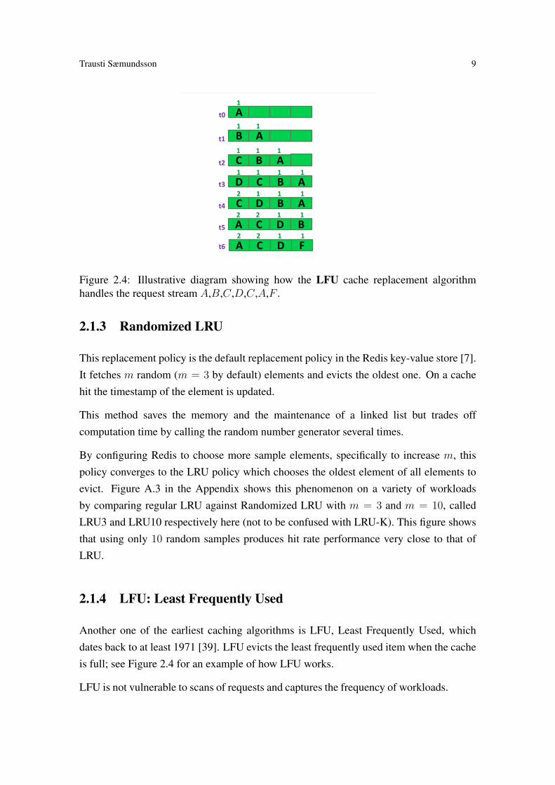
2.4 Illustrative diagram showing how the LFU cache replacement algorithmhandles the request stream A,B,C,D,C,A,F . . . . . . . . . . . . . . . . 9
2.5 Illustrative diagram showing how the CLOCK cache replacement algo-rithm handles the request stream A,B,C,D,C,A,F . The arrows indicatethe CLOCK hand. . . . . . . . . . . . . . . . . . . . . . . . . . . . . . . 10
3.1 Hit rate curve example. Diagram showing normalized hit rate achievedfor different cache sizes than currently allocated. . . . . . . . . . . . . . 16
3.2 The MIMIR profiling framework is notified of HIT, MISS, SET andEVICT events in the cache and produces a HRC when requested. . . . . . 16
3.3 Overhead comparison of regular LRU, LRU represented as an AVLtree [57, 56] and LRU with Mattson’s algorithm [38]. The AVL treeproposes 73.8% overhead on regular LRU and Mattson’s algorithmproposes 282.7% overhead. The LRU cache has capacity for 5000
elements in this experiment and the bars show the standard deviation from10 runs. . . . . . . . . . . . . . . . . . . . . . . . . . . . . . . . . . . . 18
3.4 Illustration of ROUNDER. Updates to the hit rate curve and the bucketlists of the LRU stack when element e is hit in the cache. . . . . . . . . . 19

xiv
3.5 Illustration showing elements inserted into the ghost list and how thefilters rotate. Each filter has a maximum capacity of 2 and the cachehas a maximum capacity of 4. The cache replacement policy in the maincache is LRU. . . . . . . . . . . . . . . . . . . . . . . . . . . . . . . . . 28
3.6 Overhead comparison of regular LRU, LRU with ROUNDER, LRU rep-resented as an AVL tree [57, 56] and LRU with Mattson’s algorithm [38].ROUNDERwas set to use 8 buckets and places 6.3% overhead on regularLRU, the AVL tree causes 73.8% overhead and Mattson’s algorithmyields 282.7% overhead. The LRU cache has capacity for 5000 elementsin this experiment and the bars show the standard deviation from 10 runs. 32
4.1 MIMIR’s interface: Communication between the cache and the profilingframework. . . . . . . . . . . . . . . . . . . . . . . . . . . . . . . . . . 34
4.2 Recursive formula from [57] to calculate the number of younger elementsthan a given node n. LC(n) is the left child of n and ANC(n) is eitherNULL or the nearest ancestor m of n such that m’s left child is neithern nor n’s ancestor. The intuition behind the formula is to sum up the thesizes of the left sub-trees up the path from n to the root of the tree. . . . . 34
4.3 Formula for joining HRCs from different slab classes in memcached. Cis the cache size in bytes. . . . . . . . . . . . . . . . . . . . . . . . . . . 36
5.1 HRCs for the first 6 slab class after running the YCSB b2 workload. . . . 405.2 Accuracy graphs Hit rate curves of ROUNDER on LRU (top row) and
CLOCK (bottom row) with varying bucket sizes (B) on three workloads.The true LRU and CLOCK hit rate curves are also shown. . . . . . . . . 44
5.3 Accuracy graphs Hit rate curves of STACKER on LRU (top row) andCLOCK (bottom row) with varying bucket sizes (B) on three workloads.The true LRU and CLOCK hit rate curves are also shown. . . . . . . . . 47
5.4 The accuracy of the Counting Filter ghost list predicting the hit rate fora cache of size n using only n/2 elements. This is a visual representationof the hit rate data from Table 5.5 and Table 5.6. The black dotted lineis the real LRU hit rate for a cache of each size. The red filled line is thepredicted hit rate from a cache of half the size. Under a perfect predictionthe two lines would coincide. . . . . . . . . . . . . . . . . . . . . . . . 50
5.5 HRC from MIMIR hooked into ARC, CLOCK, LFU, LRU3, LRU andRANDOM with a cache size of 1500 items on the postgres workload.The red dots show the real hit rate and the blue line is the predicted HRC. 51
5.6 Overhead of ROUNDER with different bucket sizes. . . . . . . . . . . . . 53

xv
5.7 Overhead of the full MIMIR profiling framework within memcached . . 53
A.1 The hit rate of LRU vs CLOCK in the Python simulator. Note that the hitrate of CLOCK decreases as the cache size increases from 2000 elementsto 2200 elements. This phenomeon is called Belady’s anomaly [14] . . . 68
A.2 The throughput of LRU vs CLOCK in the Python simulator. . . . . . . . 69A.3 Hit rate comparison on the default Redis cache replacement policy,
volatile-lru. This policy mixes LRU with (Time To Live) TTL expiry,but in this simulation we ignore the TTL. We simulated with 3 and 10random samples here denoted LRU3 and LRU10, respectively. The hitrate is compared to that of RANDOM and LRU. . . . . . . . . . . . . . . 70
A.4 Comparison of the hit rate of LRU, LFU, OPT, ARC, LIRS, RANDOMand LRU3 for the extreme workloads in the Python simulator. . . . . . . 71
A.5 Comparison of the throughput of LRU, LFU, OPT, ARC, LIRS, RAN-DOM and LRU3 for the extreme workloads in the Python simulator. . . . 72
A.6 The hit rate of RANDOM, LRU, OPT, ARC and LRU3 for workloadsfrom a varnish LRU cache for video chunks at the Icelandic startupcompany OZ. . . . . . . . . . . . . . . . . . . . . . . . . . . . . . . . . 73

xvi

xvii
List of Tables
2.1 Read access latency of computer hardware [22, 1]. . . . . . . . . . . . . 5
3.1 Description of MIMIR’s interface. . . . . . . . . . . . . . . . . . . . . 173.2 Overview of methods for creating an LRU histogram. N is the cache size,
time complexity is per request, for the tree compression e′ = 11+e
where eis the desired accuracy of the reuse distance, LB is the size of the largestbucket for ROUNDER and STACKER. With ROUNDER only the size oflast bucket can grow above N/B. . . . . . . . . . . . . . . . . . . . . . . 32
4.1 Number of bytes required per item in each data structure. . . . . . . . . . 35
5.1 Accuracy of ROUNDER running on LRU: Each result is given as apercentage (results generally have around 0-5% error). . . . . . . . . . . 42
5.2 Accuracy of ROUNDER running on CLOCK: Each result is given as apercentage (results generally have around 0-8% error). . . . . . . . . . . 43
5.3 Accuracy of STACKER running on LRU: Each result is given as apercentage (results generally have around 0-5% error). . . . . . . . . . . 45
5.4 Accuracy of STACKER running on CLOCK. Each result is given as apercentage (results generally have around 0-8% error). . . . . . . . . . . 46
5.5 Accuracy of COUNTINGGHOST running on LRU. Each entry in the tableshows the actual hit rate of LRU on cache size n and the predicted hit rateof LRU running at size n/2 with ghost list of capacity n/2. The averageaccuracy of all the 64 entries in the table is 95.8%. . . . . . . . . . . . . 48
5.6 Table 5.5 continued. All estimates (except 5) have over 90% accuracy andthe average accuracy is 95.8%. . . . . . . . . . . . . . . . . . . . . . . . 49
5.7 Overview of the MAE for MIMIR running on the extreme postgresworkload at cache size 1400 predicting the HRC from all cache sizesbetween 0 and 3000. The maximum discrepancy is the Kolmogorov-Smirvnov [55] distance between the HRCs which measures the largestvertical distance of the two curves. . . . . . . . . . . . . . . . . . . . . 50

xviii

1
Chapter 1
Introduction
1.1 Cache Systems at Scale
Large-scale websites serve a great number of requests, many of which are identical.Serving each request by fetching data from a database causes contention and does notsuffice under high load. Since these websites cannot scale with a database only, a newservice called memcached was created. Memcached serves all data from main memory,thus responding faster than a database which has to touch disk. The typical use case formemcached is to store newly generaed pages so they need not to be re-rendered on everyrequest. Memcached thus acts both as a memory speedup for databases and as a storagefor those queries that require many CPU cycles to generate a response. The service thussimultaneously decreases response time and reduces load on the databases.
Owing to its benefits, memcached is popular all over the world and is used soheavily at Facebook that more than one billion requests per second are served directlyfrom memcached. Caching systems, like memcached and Redis, have become a defacto standard as a layer between web servers and database back-ends. Using thosecaching systems, however, comes at a cost as they require an expensive resource: mainmemory.
Because a single computer cannot unilaterally handle significant load, many of today’scompanies invest explicitly in a special “caching” tier comprised of multiple cacheservers, each of which has a large mount of main memory. Buying more cache serversincreases the hit rate in the cache tier and can greatly reduce the load on the databasebackends preventing them from overloading. Cache servers are expensive and used inlarge numbers; Facebook, e.g., stored over 20TB of data in over 800 memcached servers

2 Performance Profiling of Cache Systems at Scale
making it the world’s heaviest memcached user already in 2008 [58]. Running at such alarge scale makes it an important question to understand how many computers are requiredto satisfy service goals.
1.2 Automatic Scaling
To shield the databases properly from load, cache operators typically add more mem-cached servers manually or increase the memory on existing servers to ensure thatthe hit rate in the cache tier is high enough. Blindly adding servers without knowingexactly how many cache servers would be needed to achieve this goal can waste valuableresources.
We therefore address this allocation problem from the automation perspective and aimto help cache operators with this manual tuning by predicting how each cache serverwould operate with different resources. This thesis describes a new profiling framework,MIMIR, designed for profiling LRU cache systems. The system generates so called hitrate curves in real-time that describe the efficacy of each cache server as a function ofcache size.
Algorithms for creating hit rate curves have been studied before, most methods focus oncreating accurate hit rate curves with considerable overhead. Our method sacrifices 5percentage points of accuracy in order to minimize the overhead.
In order to predict the hit rate for larger cache sizes than the current allocation, the meta-data for some keys that have been evicted from the cache must be available. A datastructure to store this meta-data is called a ghost list. For some workloads, such as thoseseen at Facebook [8], queries for small keys dominate: the average query is for a 31byte key and a 2 byte value. Since the keys in this case are much larger than the values,storing just the keys in a ghost list produces too much memory overhead to be applicable.To address this issue we propose a new memory efficient ghost list for storing a specificamount of evicted meta-data with Counting Filters.
1.3 Contributions
The main contributions of this work are the following:
• A new algorithm to calculate the efficacy of a cache as a function of resourcesused, especially main memory. This is done by generating so called hit rate curves,

Trausti Sæmundsson 3
defined in Chapter 3, that predict how many queries would have been responded tofrom the cache if the cache system would have those resources.
• Proof of the accuracy of the hit rate curve algorithm.
• Extensive implementation and experimental analysis of the hit rate curve generatorboth through micro-benchmarks and through implementation within the popularmemcached system. The experiments show that the approach is fast compared toalternatives, and achieves high throughput and high accuracy while giving extensiveflexibility to understand the cost benefits of the system at a granular level in termsof cache size.
• A new data structure for analyzing requests to cache keys that have been evictedfrom the cache. This data structure achieves space efficiency in exchange formodest drop in accuracy and low to sometimes significant drop in performance.
The remaining of this thesis is organized as follows. The background required forunderstanding this thesis is presented in Chapter 2. Chapter 3 provides definitions,introduces related work and the methods contributed in this thesis. Implementationdetails are discussed in Chapter 4. Experiments are evaluated in Chapter 5, and we offerconcluding thoughts in Chapter 6. Finally, the Appendix contains multiple additionalgraphs.

4

5
Chapter 2
Background
The notion of caching is to store data from a slow memory in a faster memory. Thisis done to minimize the requests to the slow memory and thus reduce memory accesslatency. Caches are used in various applications: in hard disks, web servers, databasesand CPUs to name a few. The performance improvements can be enormous. Table 2.1is indicative of the speed hierarchy of computer memories. The L1 and L2 caches onthe CPU are fastest, with a speed of 10x to 100x versus that of main memory. Reading1MB from memory is 120x faster than reading 1MB from disk and is the reason whyin-memory cache systems, introduced later in this chapter, are so fast.
L1 cache reference 0.5 nsL2 cache reference 7 nsMain memory reference 100 nsRead 1MB from memory 250,000 nsRead 1MB from a Solid State Drive 1,000,000 nsHard Disk Drive seek 10,000,000 nsRead 1MB from a Hard Disk Drive 30,000,000 ns
Table 2.1: Read access latency of computer hardware [22, 1].
Big companies, such as Facebook and Twitter, alleviate their database load by using cachesystems that store hot key value pairs in memory and serve the values via network whenkeys are requested. The most common cache systems are memcached [43] and Redis [7].Figure 2.1 shows relations between a web server, database and cache. The web serverfirst checks whether the data required is found in the cache and if not, loads the data fromthe database. The cache systems at Facebook and Twitter are composed of many cacheservers and intermediary proxies. The load is distributed between the cache servers bypartitioning the data on the keys with a method called consistent hashing. Consistent

6 Performance Profiling of Cache Systems at Scale
memcached
database
web server Fast
Slow
Figure 2.1: Cache and database. Typical request flow from a web server to a databaseand cache.
hashing enables operators to add and remove cache servers to the cache tier withoutneeding to relocate keys on existing servers.
The framework presented in this thesis is aimed to augment large cache systems andpredict accurately how the systems would behave under a different setting. One of thekey differences in the performance of those systems is the mechanism by which theyreplace old elements when the cache memory has been filled [31], the topic of the muchstudied field of cache replacement policies.
2.1 Cache Replacement Policies
Replacement policies (cache algorithms) are used to choose which element to removefrom the cache when space for a new element is needed. The element that the replacementpolicy chooses is then removed from the cache; this is called evicting the element from thecache. When we get a request to retrieve an element we first check whether the elementis stored in the cache. If the element is in the cache a cache hit occurs; otherwise a cache
miss occurs and the element must be fetched from a slow memory. Cache algorithms thatdo not depend on knowing the future are called online algorithms, while those that requireon knowledge of future accesses are called offline algorithms.

Trausti Sæmundsson 7
A 5
Requests: A B C D C A F
A 4 ∞
B
C A B
C A B D
A C B D
A C D B
A C D F
2 3 ∞
1 2 ∞ ∞
1 ∞ ∞ ∞
∞ ∞ ∞ ∞
∞ ∞ ∞ ∞
t1
t2
t3
t4
t5
t6
t0
Time until next request is shown above
Figure 2.2: Illustrative diagram showing how the optimum cache replacement algorithm,OPT, handles the request stream A,B,C,D,C,A,F . The numbers above show the timeuntil the next request and the elements are ordered by that number.
We now give an overview of cache algorithms, starting with an optimal one and workingtowards more practical ones.
2.1.1 OPT: Belady’s algorithm
L. A. Belady described an optimal cache algorithm (OPT) in 1966 [13]. When the cacheis full and a new element must be inserted, OPT replaces the element that will not get acache request for the longest period of time in the future, see Figure 2.2 for an exampleof how OPT works.
In practice, cache sequences arrive in an online fashion and future requests cannot beknown or inferred. OPT thus cannot be used in practice, but still provides an importantbaseline against which to compare other cache replacement algorithms.
2.1.2 LRU: Least Recently Used
A particularly popular cache replacement policy is the Least Recently Used (LRU)algorithm, which replaces the element that was least recently used onan eviction; seeFigure 2.3 for an example of how LRU works. The extensive literature on this algorithmdates back to at least 1965 [39].
Definition 1. The LRU stack distance of an element e in an LRU stack is thenumber of different elements between the head of the LRU stack and the elemente. If e is not in the LRU stack, the stack distance is defined to be infinite.

8 Performance Profiling of Cache Systems at Scale
A 0
head tail
B 0 1
A
C 0 1
B A
D 0 1 2 3
C B A
C 0 1 2 3
D B A
A 0 1 2 3
C D B
F 0 1 2 3
A C D
t0
t1
t2
t3
t4
t5
t6
Requests: A B C D C A F
The stack distance is shown above
Figure 2.3: Illustration of how the LRU cache replacement algorithm handles the requeststream A,B,C,D,C,A,F . The numbers above show the stack distance.
LRU handles many workloads well because in practice, recently used data tends to bereused in the near future. The algorithm is based on a similar idea to OPT, namely usingthe requests to elements to determine which elements to keep in the cache. Nevertheless,LRU is an online algorithm as opposed to the offline nature of OPT.
LRU is usually implemented with a doubly linked list. This is a drawback becausemoving elements to the most recently used position in the linked list at every requestis expensive and does not lend itself easily to parallelism. Modifying a doubly linked listwhen many threads are accessing it at the same time typically requires locks and whichfurther degrades the performance.
Another drawback of LRU is that many workloads use some elements more frequentlythan others and LRU does not make use of frequency information at all. LRU is alsovulnerable to a scan of data, i.e., a sequence of requests to elements that are not requestedagain, a scan may replace all the elements in the cache regardless of whether the elementswill be used again or not.
There are several algorithms related to LRU. Databases typically have access patternswhere LRU performs poorly and the algorithms LRU-K [47] and 2Q [35] improve onLRU for such patterns. LRU-K keeps track of the last k references of hot items in apriority queue and evicts the item with the oldest k-th access. When k = 1 this algorithmis LRU but when k > 1 this algorithm is not vulnerable to scans. 2Q uses two queuesto provide similar results as LRU-K when k = 2 but with constant time overhead versuslogarithmic time complexity of a priority queue. Another relative is S4LRU [31] which ismade of four LRU stacks and items get promoted when they are hit again.
Trausti Sæmundsson 9
A 1
B 1 1
A
C 1 1 1
B A
D 1 1 1 1
C B A
C 2 1 1 1
D B A
A 2 2 1 1
C D B
A 2 2 1 1
C D F
t0
t1
t2
t3
t4
t5
t6
Requests: A B C D C A F
The frequency is shown above
Figure 2.4: Illustrative diagram showing how the LFU cache replacement algorithmhandles the request stream A,B,C,D,C,A,F .
2.1.3 Randomized LRU
This replacement policy is the default replacement policy in the Redis key-value store [7].It fetches m random (m = 3 by default) elements and evicts the oldest one. On a cachehit the timestamp of the element is updated.
This method saves the memory and the maintenance of a linked list but trades offcomputation time by calling the random number generator several times.
By configuring Redis to choose more sample elements, specifically to increase m, thispolicy converges to the LRU policy which chooses the oldest element of all elements toevict. Figure A.3 in the Appendix shows this phenomenon on a variety of workloadsby comparing regular LRU against Randomized LRU with m = 3 and m = 10, calledLRU3 and LRU10 respectively here (not to be confused with LRU-K). This figure showsthat using only 10 random samples produces hit rate performance very close to that ofLRU.
2.1.4 LFU: Least Frequently Used
Another one of the earliest caching algorithms is LFU, Least Frequently Used, whichdates back to at least 1971 [39]. LFU evicts the least frequently used item when the cacheis full; see Figure 2.4 for an example of how LFU works.
LFU is not vulnerable to scans of requests and captures the frequency of workloads.

10 Performance Profiling of Cache Systems at Scale
A 0
0
0
0
A 1 B
0
0
1
A 1 B
C 0
1
1
t1
t0
t2 A
1 B C
D 1
1
1
A 1 B
C
D 1
1
1
A 1 B
C
D 1
1
1
F 1 B
C
D 0
0
0
t3
t4
t5
t6
Figure 2.5: Illustrative diagram showing how the CLOCK cache replacement algorithmhandles the request stream A,B,C,D,C,A,F . The arrows indicate the CLOCK hand.
However, implementing LFU requires keeping track of the request frequency of eachelement in the cache. Usually this is done with some number of bits for each element,where the number of bits limits how accurately the frequency is monitored. Regardless ofthe number of bits, finding the element with the lowest frequency is usually implementedwith a priority queue resulting in logarithmic complexity for all operations. Anotherapproach is to use two nested doubly linked lists, as described in [50], which transformsthe time complexity of all operations to O(1).
2.1.5 CLOCK
Introduced in 1968 by F. J. Corbato [20], the CLOCK algorithm arranges cache elementsin a circle and captures the recency of a workload, similar to LRU but with much lesseffort.
Every element has an associated bit called the recently used bit, which is set every timean element is accessed. The clock data structure has one hand. When an element needsto be evicted from the cache, we check whether the recently used bit is set on the elemente to which the hand points. If the recently used bit is not set on e, we replace e with thenew element. However if the recently bit is set on e, we unset the bit on e and advance thehand to the next element. We repeat this until we find an element that does not have therecently used bit set. In the worst case the hand must traverse an entire circle and removethe element to which it pointed originally. This is precisely what happens at time t6 inFigure 2.5, where A is evicted to give space for F .

Trausti Sæmundsson 11
CLOCK uses the recency of elements, similar to LRU, but without requiring locks inparallel systems. The retrieval time for each element is lower because there is no un-linking and linking required. The removal time depends, however, on how far the handhas to traverse. CLOCK also handles more requests per time unit because it does notmove elements to a new position in a list at every request. Figure A.2 shows head-to-headthroughput comparison between the algorithms.
The hit rate of CLOCK is close to that of LRU even though CLOCK uses only one bit tocapture the recency, see Figure A.1 for a hit rate comparison between the methods.
2.1.6 ARC: Adaptive Replacement Cache
The Adaptive Replacement Cache (ARC) algorithm introduced in 2003 [40] providesgood performance on workloads where the access pattern is based on recency andfrequency. To achieve this performance ARC combines LRU and LFU and is furthermoreresistant to scans. It also adapts in real-time to the recency or frequency access pattern ofthe workload.
ARC uses two lists L1 and L2. L1 stores elements that have been seen only once recentlybut L2 stores elements that have been seen at least twice, recently. It is useful to think ofL1 as the LRU list and L2 as the LFU list. ARC then adaptively changes the number ofelements stored in the cache from L1 and L2. This is done to meet the access pattern ofthe workload. The elements in L1 and L2 that are not in the cache are said to be in theghost list. Ghost lists are discussed further in Chapter 3.
Since L2 contains elements that have been seen at least twice recently it does not havelogarithmic complexity on each request like LFU. Both L1 and L2 suffer from the sameproblem as LRU, as every action requires a reordering of the elements in the list. Toaddress this issue another similar algorithm called Clock with Adaptive Replacement(CAR) [10] was proposed in 2004. It uses the clever solution from the CLOCK algorithmof using circular lists to reduce the computational complexity. Both ARC and CAR arepatented by IBM [42, 11].
2.1.7 LIRS: Low Inter-reference Recency Set
Since its introduction in 2002, the Low Inter-reference Recency Set algorithm (LIRS) [34]has seen some popularity, including being used in the popular MySQL open sourcedatabase [32]. LIRS is similar to LRU, but does not use recency as a measure to evict

12 Performance Profiling of Cache Systems at Scale
elements. Instead, it uses the more insightful reuse distance for eviction decisions, moreprecisely LIRS evicts the element with the largest reuse distance.
Definition 2. The reuse distance of a request r1 to an element e is the numberof different requests between r1 and the last request r2 to the same element e. Ifr1 is the first request to e then the reuse distance is defined to be infinite.
Let us now look at the request stream: a, b, b, c, a. The first time a is requested it hasinfinite reuse distance but the second time a is requested the reuse distance is 2 becausethere are two elements, b and c, requested in between. In the same manner, the reusedistance of b is infinite the first time it is requested and 0 the second time it is requested.The reuse distance of c is infinite.
Lemma 1. An element is contained in an LRU cache of size N if the reusedistance of the element is at most N . This is true because the reuse distance isequal to the stack distance in an infinite LRU stack.
Internally, LIRS uses a stack S and a list Q. The stack S can grow unboundedly in sizewhich could eat up a lot of memory.
2.1.8 Clock-PRO
For the same reason that CLOCK was proposed to speed up LRU, and CAR was proposedto speed up ARC, an algorithm called CLOCK-Pro was introduced in 2005 [33] tooptimize LIRS. At the foundation, CLOCK-Pro is based on LIRS but uses circular lists.The CLOCK-Pro algorithm has been used in the NetBSD operating system [32] and inthe Linux kernel [33].
2.1.9 Hit Rate and Throughput Comparison
Graphs showing hit rate and throughput comparison of the LRU, LFU, OPT, ARC, LIRS,RANDOM and LRU3 cache replacement algorithms can be seen in the Appendix, hit ratein Figure A.4 and throughput in Figure A.5.
2.2 Memcached
A wide variety of caching systems exist that rely on those algorithms. One particularlypopular implementation is the memcached (www.memcached.org), which uses the LRU

Trausti Sæmundsson 13
policy. Improvements to memcached use the CLOCK policy [26] because it is faster andworks better with multiple threads, while providing a similar hit rate to LRU. Becauseof their popularity we will focus on these two cache replacement policies (LRU andCLOCK) in the remainder of the thesis.
Memcached is an open source [44] key-value store written in approximately 10.000 linesof C code, developed initially by Brad Fitzpatrick for the website LiveJournal.comat Danga Interactive. Early versions of memcached used the default malloc from glibcfor storing items but because of internal fragmentation the servers stalled the CPU aftera week of up-time [28]. The memcached team then implemented their own memoryallocator to address this problem.
The memory allocator puts items into different slab classes, each containing its own LRUlinked list. Each slab class owns several 1MB pages split into equally sized chunks, withthe chunk size depending on the slab class. The default settings of memcached uses 42slab classes. The slab class sizes increase exponentially with factor 1.25 (can be changedwith the -f parameter). The first is responsible for 96B items (henceforth B refers tobytes), the second 120B items, and the last 1MB items. Each item is put in the slab classwith the smallest possible chunk size. Depending on the distribution of the value sizes,this factor must be configured manually to balance items evenly across the slab classes.When a slab class is full, a new 1MB page is requested. If all pages are in use, the serverevicts the least recently used item from the slab class. Expiration of elements via a Time-To-Live (TTL) flag is supported and if an item has been hit very recently, it is not movedto the LRU head.
If the workload is dynamic, some slab classes might become stale, which is referredto as “slab calcification”. This issue has been solved in the latest versions of the opensource memcached by removing pages from other slab classes. Twitter has an opensource modification of memcached, called twemcache, with a different solution withconfigurable strategies to reassign pages between slabs. At Facebook a page is movedto a slab class if the next item to be evicted was used at least 20% more recently thanthe average of the LRU tail in other slab classes [45]. The page that is moved is the onecontaining the overall least recently used element.
The memcached server uses 4 threads by default; increasing the number of threads doesnot improve the performance, due to internal locking [30]. One global lock guards theLRU cache and another lock guards the hash table. This has been improved by Fan et
al. in the MemC3 [26] system where the LRU cache replacement was replaced with theCLOCK cache replacement and the hash table was changed to concurrent cuckoo hashing,

14 Performance Profiling of Cache Systems at Scale
developed by the same team. This removes the thread scalability bottleneck and improvesthe throughput of memcached by 3x.
Facebook has been using memcached since August 2005, when Mark Zuckerberginstalled it on Facebook’s web servers. In 2013 they had around 1000 memcached servershandling billions of requests per second to serve over 28 terabytes of data to alleviate thisload from the back-end MySQL databases [49]. Since then, Facebook has customized andimproved the memcached code and contributed some of the improvements to the opensource version of memcached [45].

15
Chapter 3
Methods
3.1 Introduction
In a setup with multiple cache servers we would like to monitor the performance of eachserver and predict what would happen if resources for the servers would be changed.Resources can be changed by adding or removing a cache server. But also, the memoryof a server can be increased or decreased and this affects the performance of the cachetier. Our goal in this thesis is to profile the performance of each cache server and produceefficacy graphs showing how the hit rate would change if resources were changed. In orderto do that we must know how the cache server would perform if memory was increasedor decreased. To assess the effects of changes we generate, in real-time, so called hit ratecurves that describe the efficacy of each cache server as a function of cache size. Moreprecisely:
Definition 3. Let H(n) be the hit rate for cache size n. We call H the hit ratefunction. A hit rate curve (HRC) is a plot of the hit rate function as a functionof cache size. For a cache is running at size N , it is possible to generate the HRCfor all cache sizes n, where 0 < n ≤ kN ; in the thesis we focus on k = 2.
See Figure 3.1 for an example of a hit rate curve showing the hit rate for smaller andlarger cache sizes than the current allocation.
To solve this problem we propose the MIMIR profiling framework. This frameworkcollects data from each cache server and produces hit rate curves. Figure 3.2 showshow the cache server contacts the interface of MIMIR. The framework is notified whenan element encounters one of four possible events: HIT; MISS; SET; and EVICT. Thefunctions for those events are described in detail in Table 3.1. All functions take an

16 Performance Profiling of Cache Systems at Scale
0 1000 2000 3000Cache size (items)
0.0
0.1
0.2
0.3
0.4
0.5
0.6
Cumulative hit rate
current hit rate
Current allocation
LRU
Figure 3.1: Hit rate curve example. Diagram showing normalized hit rate achieved fordifferent cache sizes than currently allocated.
cache MIMIR
Hit(e)
Miss(key)
Set(e)
Evict(e)
Hit Rate Curve
up
dat
e
Figure 3.2: The MIMIR profiling framework is notified of HIT, MISS, SET and EVICT
events in the cache and produces a HRC when requested.
element as an argument except the MISS function which takes a key. We store a timestampon each element and need to access it on HIT; MISS and SET. On a miss, however, noelement is available and we only have the key.
How to handle those events correctly depends on the cache replacement policy; in thisthesis we describe an implementation of this interface that works with high accuracywhen running either the LRU or the CLOCK cache replacement policy.
Handling the four events happens synchronously inside MIMIR and results in an updateto an internal data structure in the framework. When the HRC is requested, it is generatedasynchronously from the internal data structure and served to the cache operator who canthen display it for each cache server in a web interface.

Trausti Sæmundsson 17
HIT(e) Accessing the requested element e causes a cache hitMISS(key) Accessing the key key causes a cache missSET(e) An element e is set in the cacheEVICT(e) A currently cached element e is being evicted from the cache
Table 3.1: Description of MIMIR’s interface.
3.2 Creating an HRC for the LRU Policy
To generate a hit rate curve for an LRU cache we use Lemma 1 from Section 2.1.7 onpage 12. The lemma states that an element is contained in an LRU cache of size N if thereuse distance is at most N . The reuse distance is equivalent to the stack distance and thisgives us an inclusion property for the LRU cache replacement policy:
Lemma 2. Contents of an LRU cache of size N are contained in an LRU cacheof size M if N ≤M .
To see why this is true, consider how an LRU stack orders elements by access time; anLRU stack of size N is the prefix of all LRU stacks of size M where M ≥ N . Thisinclusion property holds for other stack algorithms such as LFU and OPT [38] but not fora First In First Out (FIFO) algorithm [14].
Using Lemma 2 we now highlight an important concept. By tracking the stack distanceof every element we can create a hit rate curve, because the number of hits in a cache ofsize n is the number of items hit with stack distance less or equal to n.
This means that creating a hit rate curve for n ≤ N simply boils down to tracking stackdistances for elements in the cache. Creating hit rate curves for n > N requires trackingelements that have been evicted, but the principle is the same.
This is a previously studied problem dating back to at least 1970 when Mattson describedan intuitive approach, referred to in this thesis as Mattson’s algorithm [38]. Thisalgorithm assumes that the LRU cache is represented as a linked list. On a cache hitto element e, we traverse the linked list from the head and count how many elements arelocated in front of e. This is inefficient since the worst case time complexity is linear inthe cache size.
Another approach is to organize the LRU linked list in a balanced binary tree ordered bythe access time [56, 57]. This lowers the worst case time complexity to be O(logN).The stack distance is retrieved from the tree by counting the sizes of sub-trees with earlieraccess times than the requested element.

18 Performance Profiling of Cache Systems at Scale
0
500000
1000000
1500000
2000000Throughput [O
PS/s]
Statistics algorithms
lrulru+avllru+mattson
Figure 3.3: Overhead comparison of regular LRU, LRU represented as an AVL tree [57,56] and LRU with Mattson’s algorithm [38]. The AVL tree proposes 73.8% overhead onregular LRU and Mattson’s algorithm proposes 282.7% overhead. The LRU cache hascapacity for 5000 elements in this experiment and the bars show the standard deviationfrom 10 runs.
Both of those approaches are non-trivial to parallelize. Also, figure 3.3, shows that theoverhead of both approaches is non-negligible. The figure shows the throughput of aC++ simulator (described in Chapter 4) for the P10 workload (presented in Chapter 5)for LRU with no distance tracking, and with distance tracking using both an AVL treeand Mattson’s algorithm. As the Figure shows, the overhead of both algorithms is verysignificant and much too high for the methods to be usable in practice.
We propose to trade off some accuracy in order to maximize performance, by splittingthe LRU stack dynamically into a fixed number of buckets. When an element is hit inthe cache we find the bucket it belongs to and estimate its LRU stack distance range bysumming up the number of items in buckets with lower stack distances. Note that thenumber of buckets is independent of the cache size; thus the average number of elementsper bucket increases with increasing cache sizes.
In order to facilitate performance, the size of each bucket can vary. In Section 3.3, wepropose two efficient algorithms for dynamically maintaining the buckets. In Section 3.4,we then propose an efficient algorithm for approximating stack distances for items thathave been evicted from the cache. Finally, in Section 3.5, we compare our methods to therelated work.

Trausti Sæmundsson 19
g,h,u e,r,tf b,c,d,a
Bucket #0 1 2 3
HRC
(i) LRU list before
hit on item e
(iii) After request
(ii) HRC update
4 buckets (B=4)
(iv) After aging
e,g,h,u r,tf b,c,d,a
g,h,u f r,t,b,c,d,ae
Stack distance
Est
ima
ted
# o
f h
its
Figure 3.4: Illustration of ROUNDER. Updates to the hit rate curve and the bucket lists ofthe LRU stack when element e is hit in the cache.
3.3 Estimating Cache Utility for n ≤ N
We now introduce simple yet efficient methods to minimize the overhead of retrievingstack distances for elements in the cache. The methods group items together in bucketsand produce stack distance estimates. The accuracy is tunable with the number of buckets,but using fewer buckets yields higher performance. The methods are called ROUNDER
and STACKER, the former of which is designed for higher performance and the latter isdesigned for higher accuracy.
3.3.1 The Intuition behind ROUNDER and STACKER
The basic idea is to split the LRU stack into buckets. When an item is hit, we find theregion represented by the bucket and update the corresponding part of the HRC with unitvolume.
ROUNDER accumulates elements in the first bucket. When this front bucket is full, allbuckets are shifted down the list, bottom two buckets are merged and the first bucket isfreed. This aging method distributes the items across all buckets by limiting the numberof elements in the first bucket. The process is illustrated for the ROUNDER algorithm inFigure 3.4. When element e is hit, it is located in the third bucket (buckets are numberedfrom 0). The element is then removed from the third bucket and inserted into the first(head) bucket. Now the first bucket is full and aging is performed. The aging merges thelast two buckets, so that afterwards it contains items r, t and b, c, d, a from the second-

20 Performance Profiling of Cache Systems at Scale
to-last and the last bucket respectively. Now the first bucket is shifted down and a newempty bucket appears in front. Finally we insert e into the new bucket. We keep a 4byte timestamp per item to know which bucket the item belongs to. To make the aging asfast as possible, instead of aging every element, we shift the frame of reference, updatethe timestamp for the first bucket and increasing a cyclical index into a circular array ofbucket counters, all in constant time.
The last bucket can get filled up with an adversarial workload. We designed the STACKER
algorithm to prevent such cases. STACKER accumulates elements in the first bucket, likeROUNDER, but when the first bucket is full we shift some items down one bucket, i.e. weonly shift elements that correspond to the hot part of the LRU stack. The intuition here isthat when an element e is hit in a regular LRU stack, all items with lower stack distancesthan e get shifted one position down the stack but elements below e’s original position arenot moved. Now if the bottom of the stack is never being hit, those elements should notbe moved to a lower bucket, and the aging routine prevents it from happening. ROUNDER
is incapable of doing this since all items are shifted down every time the aging routine iscalled.
3.3.2 Pseudo-Code
To update the HRC in constant time we use an intermediate array, called DELTA. Weupdate the DELTA array with the updateDELTA routine, see Algorithm 1. It takes astartpoint and an endpoint and updates two locations in the DELTA array. The scale andoffset arguments are used when creating a HRC for larger cache sizes than the currentallocation using a ghost list, described and defined in Section 3.4. The scale parameteris used to scale down the estimated hit value because the ghost list is probabilistic andthe offset is used to update the ghost list part of the HRC, after the end of the maincache.
Algorithm 1 The updateDELTA routine.
UPDATEDELTA(start , end , scale, offset)
1 start = start + offset2 end = end + offset3 val = 1.0/(end − start)4 val = val · scale5 DELTA[start] = DELTA[start] + val6 // every value i ≥ start in the HRC should be incremented by val7 DELTA[end] = DELTA[end]− val8 // every value i ≥ end in the HRC should be decremented by val

Trausti Sæmundsson 21
The makeHRC routine, shown in Algorithm 2, creates the HRC directly from the DELTAarray without using a PDF array. Notice that the resulting HRC is not normalized. HRCsare often normalized by the number of requests to the cache so that the values range from0 to 1.
Algorithm 2 The makeHRC routine. Updates the HRC from the intermediate DELTAarray.
MAKEHRC()
1 HRC = [0, 0, . . . , 0]2 for i = 1 to DELTA. length − 13 HRC [i] = HRC [i− 1] + DELTA[i]
The ROUNDER algorithm is initialized according to Algorithm 3, by saving the cachesizes and the number of buckets, lines 1-2. We then initialize bucket counters to 0 inline 3 and set the head and tail bucket indices to their initial values in lines 4-5.
Algorithm 3 The Initialization routine for ROUNDER.
INITIALIZATION(cachesize, numbuckets)
1 N = cachesize2 B = numbuckets3 buckets = [0, 0, . . . , 0] // B buckets4 head = B -15 tail = 0
The HIT routine for the ROUNDER algorithm, see Algorithm 4, takes an element as anargument. It resets the activity of the value to the current tail if it has fallen behind, inlines 1-2. We next retrieve the current stack distance for the element and use it to updatethe DELTA array in line 5. Finally we get the correct bucket index for the element andremove it from the current bucket by decrementing the correct bucket counter, lines 7-8.Next we set the activity of the item to the head value and update the counter for the headbucket, lines 9-10. Notice the circular indexing into the buckets array, this trick saves usspace and time by reusing the array after every aging phase.
The SET routine for the ROUNDER algorithm, see Algorithm 5, performs aging ifrequired, in line 2. It also sets the activity of the item in line 3 and updates the bucketcounter for the head bucket.
The EVICT routine for the ROUNDER algorithm, see Algorithm 6, updates the correctbucket counter where the element is located.
The age routine in ROUNDER, see Algorithm 7, shifts the frame of reference, merges thelast two buckets and frees up one bucket.

22 Performance Profiling of Cache Systems at Scale
Algorithm 4 The HIT routine for ROUNDER.
HIT(e)
1 if e.activity < tail2 e.activity = tail3 if buckets [head ] ≥ N/B4 AGE()5 (start , end) = getStackDistance(e)6 UPDATEDELTA(start , end , 1, 0)7 i = e.activity mod B8 buckets [i] = buckets [i]− 19 e.activity = head
10 buckets [head mod B] = buckets [head mod B] + 1
Algorithm 5 The SET routine for ROUNDER.
SET(e)
1 if buckets [head mod B] ≥ N/B2 AGE()3 e.activity = head4 buckets [head ] = buckets [head ] + 1
Algorithm 6 The EVICT routine for ROUNDER.
EVICT(e)
1 if e.activity < tail2 e.activity = tail3 i = e.activity mod B4 buckets [i] = buckets [i]− 1
Algorithm 7 The internal age routine in ROUNDER.
AGE()
1 // merge the two bottom buckets and empty the top bucket2 buckets [(tail + 1) mod B] = buckets [(tail + 1) mod B] + buckets [tail mod B]3 head = head + 14 buckets [head mod B] = 05 tail = tail + 1

Trausti Sæmundsson 23
The getStackDistance routine in ROUNDER, see Algorithm 8, calculates the estimatedstack distance from the bucket counters.
The routines for STACKER are highly similar to the routines for ROUNDER except forthe age function, which loops through all the cache and ages only the items that havean activity lower than a running average of items recently hit in the cache. They are notshown in this thesis.
Algorithm 8 The internal getStackDistance routine in ROUNDER.
GETSTACKDISTANCE(e)
1 start = 02 end = 03 for i = head to tail4 end = end + buckets [i mod B]5 if e.activity == i6 break7 start = start + buckets [i mod B]8 return (start , end)
3.3.3 Proof of Bounded Accuracy
This section provides a proof of bounded accuracy for bucket algorithms. The proof usesthe Mean Average Error (MAE) to provide bounds on the bucket sizes. The MAE iscalculated by the following formula, Where M is the size of the HRC:
MAE(HRCa,HRCb) =1
M
M∑x=1
|HRCa(x)− HRCb(x)| . (3.1)
The following theorem shows that the accuracy of the HRC is limited by the size of thelargest bucket:
Theorem 3. For an LRU cache of size M during a trace of R requests,ROUNDER and STACKER with B buckets have a mean average prediction error(MAE) bounded by the largest bucket size during the trace, divided by M/2.Consequently, if no bucket grows larger than αM/B for α ≥ 1 during the trace,then the MAE for ROUNDER and STACKER is at most 2α
B.
Proof. We consider R cache requests to have true reuse distance r1, r2, . . . , rR. It sufficesto consider only requests that result in LRU hits, so ri ≤ N for all i. Define δt(x) = 1 if

24 Performance Profiling of Cache Systems at Scale
x = rt and δt(x) = 0 otherwise. Then the optimal hit rate curve HRC∗ satisfies:
HRC∗(x) =1
R
R∑t=1
x∑z=0
δt(z)
In STACKER, there are B buckets with variable boundaries over time. For request twith true reuse distance rt, we estimate the reuse distance over an interval [at, bt] thatincludes rt. Furthermore, we assign uniform probability to all possible distances withinthat interval. Define ct(x) = 1
bt−at when x ∈ [at, bt) and ct(x) = 0 otherwise. Then thehit rate curve for our algorithm satisfies:
HRC(x) =1
R
R∑t=1
x∑z=0
ct(z)
We obtain the following upper bound on the mean average error for the two HRCs.
MAE(HRC,HRC∗) =1
M
M−1∑x=0
|HRC(x)− HRC∗(x)|
=1
MR
M−1∑x=0
∣∣∣∣∣R∑t=0
x∑z=0
δt(z)− ct(z)
∣∣∣∣∣ ≤ 1
MR
R∑t=1
bt∑x=at
x∑z=0
|δt(z)− ct(z)|
≤ 1
MR
R∑t=1
bt∑x=at
x∑z=0
(|δt(z)|+ |ct(z)|) ≤1
MR
R∑t=1
bt∑x=at
(1 + 1)
=1
MR
R∑t=1
2(bt − at) ≤2
Msup
t=1,...,R(bt − at).
The result enables operators to dynamically track the MAE of the HRC estimate evenwithout computing the optimal hit rate curve. The algorithm could be extended toadaptively add or remove buckets depending on changes in the MAE so that resolution ismaintained.
Note that the supremum in the last expression measures the size of the largest bucketduring the workload. In some cases, as we have seen in our experiments, the least-significant bucket which tracks the largest reuse distances can consume a significantportion of the cache. Instead, the average bucket size for hits 2
R
∑Rt=1(bt − at) can be
tracked and used as a stronger upper bound.

Trausti Sæmundsson 25
3.4 Estimating Cache Utility for n > N
How can we predict whether the cache needs to grow in size? Typically, data-less itemscalled ghosts [25] are used as placeholders to record accesses to items whose data would
have been included in the cache if more memory had been available [48]. The ghosts arecontained in a ghost list:
Definition 4. A ghost list is a data structure for storing items that have beenevicted from a cache.
Placeholders consume a small amount of memory relative to the data normally stored byitems, so their memory overhead can be viewed as a “tax” on elements actually stored inthe LRU list. Thus when an item is evicted from the primary LRU list, it is added to aghost LRU stack. The last ghost is also popped off and discarded. This method is at theheart of recent breakthroughs in cache replacement algorithms, including the ARC, CAR,LIRS and Clock-PRO policies [41, 12, 34, 33]. But if the values are very small relativeto key size, e.g., as seen at Facebook [8], the tax can be significant. In this section wedescribe a solution to this issue. The solution is to use approximate filters to estimate thepresence of items in the cache. We propose to use Counting Filters, which are a variant ofBloom Filters. In the following, we first describe these filters before moving on to presentthe algorithm, called COUNTINGGHOST.
While hits in the ghost list are still cache misses because no data could be returned to theuser, statistics of the item itself can be gathered. Recall that H is the hit rate function andH(n) is the hit rate for cache size n. In summary, to estimate H(n) for cache memorieslarger than the current allocation, that is N ≤ n ≤ k ·N , we employ a ghost list of length(k − 1) ·N .
3.4.1 Bloom Filters and Counting Filters
A Bloom Filter [17] is a compressed hash set which trades off space for less certainty inquery answers. When a Bloom Filter is queried for a specific key it returns either “no”with full certainty or “yes” with high certainty. A false “yes” is defined as a false positive;the certainty can be increased by using more memory for the filter.
Internally the Bloom Filter uses an array A[0, ...,m − 1] of size m and l hash func-tions:
h1, h2, . . . , hl.
26 Performance Profiling of Cache Systems at Scale
To insert a key into the filter, the key is hashed with the l hash functions to produce l hashvalues:
h1(key), h2(key), . . . , hl(key)
and then the bits in the corresponding locations are set to 1, i.e.:
A[h1(key) mod m] = 1
A[h2(key) mod m] = 1
...
A[hl(key) mod m] = 1
To check whether a key is present in the filter, the same hashing is done as with an insertbut instead of setting the bits to 1 we check if they are all set to 1. If they are all set to 1,we return yes but otherwise no. It is easy to see that even though all the keys are set to 1
the key was not necessarily inserted into the filter. Perhaps some other keys were mappedto the same locations and set the bits to 1. That event is called a false positive and theprobability of a false positive is tuned with the size of the filter and the number of hashfunctions. The lowest false positive rate is achieved with the number of hash functionsequal to:
l =m
nln 2
where n is the expected number of keys in the filter.
There is no good way to remove a key from a Bloom Filter without possibly damaging thepresence of other keys. To solve this issue, Counting Filters were introduced in 1998 byFan et al. [27]. Instead of using an array of bits, it is replaced with an array of counters.On insertion, the l counters (at the hashed locations) are incremented and on removal thesame l counters are decremented. To check for a key in the filter, we simply check if thel counters are non-zero.
3.4.2 Intuition behind COUNTINGGHOST
COUNTINGGHOST is based on ROUNDER but must handle evictions on its own since itis also a ghost list. We use three filters to represent the buckets. When the first filter isfull, we empty the last filter and make it the new first filter, the old first filter becomes the

Trausti Sæmundsson 27
second filter and the old second filter becomes the last filter. The first two filters thereforehave capacity for the entire ghost list but the last filter is used as an evictable buffer tohandle the evictions.
When an element is missed in the main cache, we check if its key is found in any of thethree filters. If found, we update the corresponding region in the intermediate DELTAarray which is the base for the HRC. We then remove the element’s key from the filtersince we expect it to be inserted in the main cache after a miss. Notice that if we wereusing Bloom Filters we could not perform this removal.
There is a subtle addition here to balance the false positive rate of the Counting Filter.When we update the DELTA array, we scale the value with 1.0 − FPP_RATE becausewe want the total sum of the DELTA array to equal the number of hits and we wouldoverestimate the number of hits without scaling.
3.4.3 COUNTINGGHOST Algorithm Details
COUNTINGGHOST is a sufficient ghost list that uses three Counting Filters instead ofthree buckets. Each bucket has capacity for half the cache size. The last bucket is a bufferto flush out old keys. With a cache of size N , the ghost list keeps track of the footprint forat least (k − 1) · N extra elements (k = 2 is default). It uses three counting filters, eachwith a capacity of (k−1) ·N/2 elements. The last filter of (k−1) ·N/2 elements ensuresthat we are able to flush the last filter and make it the first filter while still keeping trackof (k − 1) ·N elements in the ghost list. We do this because we need to evict some keysfrom the ghost list but we do not know the keys themselves. When there is a miss in themain cache, the function MISS in the ghost list interface is called. Upon an eviction, thefunction EVICT is called.
We use the dablooms [16] Counting Filter library from bit.ly. They use it to efficientlycheck whether an URL is malicious or not. This library is written in C and offers Pythonbindings and we use both. We set the false positive rate to 1% in all our experiments.
Now let us walk through the illustration of COUNTINGGHOST in Figure 3.5. Thisillustration assumes that the cache has size for 4 items and runs the LRU policy. TheCOUNTINGGHOST algorithm contains 3 Counting Filters, each with capacity for 2 items.Here we assume that each get request is followed by a set request after a cache miss.
Part (a) of the illustration is the initial setup. Part (b) shows what happens after a getrequest for d, it is moved from the LRU tail to the LRU head, HIT(d) is called, andnothing happens in the ghost list. Part (c) shows what happens after a get request for m

28 Performance Profiling of Cache Systems at Scale
(a) Initial setup.
Cache: a,b,c,d filter #1: e filter #2: g,h filter #3: k,l
(b) After a get request for d.
Cache: d,a,b,c filter #1: e filter #2: g,h filter #3: k,l
(c) After a get and a set request for m.
Cache: m,d,a,b filter #1: c,e filter #2: g,h filter #3: k,l
(d) After a get and a set request for h.
Cache: h,m,d,a filter #1: b filter #2: c,e filter #3: g
Figure 3.5: Illustration showing elements inserted into the ghost list and how the filtersrotate. Each filter has a maximum capacity of 2 and the cache has a maximum capacityof 4. The cache replacement policy in the main cache is LRU.
which is neither in the cache nor in the ghost list, MISS(m.key) is called. This forcesthe cache to evict the least recently used item c, EVICT(c) is called, and insert it into theghost list. The ghost list puts c into the first filter. Part (d) shows what happens after a getrequest for h. It is not located in the cache, MISS(h.key) is called, but it is found in thesecond filter. It is removed from the second filter and inserted at the LRU head and theLRU tail, item b, is evicted, EVICT(b) is called. Now the first filter is full so we rotate thefilters and then insert b into the new and empty first filter.
3.4.4 Pseudo-code
The COUNTINGGHOST algorithm is initialized, see Algorithm 9, by allocating threeCounting Filters each with a capacity of half the cache size, lines 7-9.
The MISS routine in COUNTINGGHOST, see Algorithm 10, takes a key as an argument.The routine looks up the key in the three filters and updates the HRC accordingly.
The EVICT routine for the COUNTINGGHOST, see Algorithm 11, rotates the filter ifnecessary and inserts the key into the first filter.
The rotateFilters routine in the COUNTINGGHOST, see Algorithm 12, flushes the lastfilter and makes it the new empty filter. This method serves the same purpose as the ageroutine in ROUNDER, see Algorithm 7.

Trausti Sæmundsson 29
Algorithm 9 The Initialization routine for COUNTINGGHOST.
INITIALIZATION(capacity)
1 capacityPerFilter = capacity/2.02 counters = [0, 0, 0]3 firstFilter = 04 secondFilter = 15 thirdFilter = 26 filters = array of three Counting Filters7 filters [firstFilter ].allocateCapacity(capacityPerF ilter)8 filters [secondFilter ].allocateCapacity(capacityPerF ilter)9 filters [thirdFilter ].allocateCapacity(capacityPerF ilter)
Algorithm 10 The MISS routine for COUNTINGGHOST.
MISS(key)
1 scale = (1.0− FPP_RATE)2 if filters [firstFilter ].contains(key)3 UPDATEDELTA(0, counters [firstF ilter], scale, cachesize)4 elseif filters [secondFilter ].contains(key)5 start = counters [firstF ilter]6 end = start + counters [secondFilter]7 UPDATEDELTA(start , end , scale, cachesize)8 filters [secondFilter ].remove(key)9 filters [firstFilter ].insert(key)
10 counters [thirdFilter ] = counters [secondFilter ]− 111 counters [firstFilter ] = counters [firstFilter ] + 112 elseif filters [thirdFilter ].contains(key)13 // If the first two filters are not full, the third filter is responsible14 start = counters [firstF ilter] + counters [secondFilter]15 end = start + counters [thirdF ilter]16 UPDATEDELTA(start , end , scale, cachesize)17 filters [thirdFilter ].remove(key)18 filters [firstFilter ].insert(key)19 counters [thirdFilter ] = counters [thirdFilter ]− 120 counters [firstFilter ] = counters [firstFilter ] + 1
Algorithm 11 The EVICT routine for COUNTINGGHOST.
EVICT(key)
1 // If the first filter is full, rotate the filters2 if counters [firstFilter ] ≥ capacityPerF ilter3 ROTATEFILTERS()4 // Insert the element into the first filter5 counters [firstFilter ] = counters [firstFilter ] + 16 filters [firstFilter ].insert(key)

30 Performance Profiling of Cache Systems at Scale
Algorithm 12 The internal rotateFilters in COUNTINGGHOST.
ROTATEFILTERS()
1 filters [lastF ilter].flush()2 counters [lastFilter ] = 03 // The other counters are maintained4 firstFilter = lastFilter5 secondFilter = (firstFilter + 1) mod 36 lastFilter = (firstFilter + 2) mod 3
3.5 Comparison to Related Work
Much work has been put into creating the HRC for the entire working set. We are lookingat creating the HRC for just the cache size along with the size of the ghost list. We alsowant to do this online so we cannot do a prepass through all the data like much of therelated work does. A prepass is to go through the workload and store alongside eachrequest to an element e the last reference to e. We now give a brief overview of the highlyrelated algorithms to our approach.
3.5.1 Previous Methods
In 1970, Mattson et al. [38] studied stack algorithms in cache management and definedthe concept of stack distance. They described the first measurement algorithm for reusedistance using a stack represented as a list. The time complexity of the algorithm is linearin the cache size and traverses the stack to find the element.
Several papers [57, 46, 56] have been written on measuring reuse distances with AVLtrees. Those methods have the logarithmic time complexity in common due to the AVLtree which is ordered by access times.
Bennett and Kruskal introduced [15] a method called blocked hashing to preprocess theworkload in a single pass and then create the reuse distance histogram by splitting theworkload into segments. Using this method for our purposes is impossible due to theprepass. Olken [46] improved Bennett and Kruskal’s method by using an AVL tree forthe entire workload, which is logarithmic in the length of the workload and not applicablein our setting.
Ding and Zhong described a compression method in 2003 [24]. They store reuse distance
intervals as tree nodes and store multiple items per node. The height of the tree islogarithmic in the cache size and the compression guarantees log log time complexity.

Trausti Sæmundsson 31
The complexity of this method is much higher than our method and making it parallelwould not be trivial.
Kim et al. [36], and later systems in cache architecture such as RapidMRC [53] and PATH[9], partition the LRU list into groups to reduce cost of maintaining distances, which isconceptually similar to our approach except the group sizes are fixed as powers of two.Our variable sized buckets approach affords substantially higher accuracy in trade formodest overhead.
3.5.2 Performance Comparison
Making trees parallel has been the subject of intricate work, suggesting parallelizingan AVL tree or the methods from [46, 24]. ROUNDER is highly parallel while beingsimple, but has a weakness with the last bin getting too big. In our experiments, however,presented in Chapter 5, this was not an issue.
STACKER is similar to ROUNDER but has a better aging method and is thus more accurate,but the overhead of running STACKER over the cache replacement policy is higher thanrunning ROUNDER. The time complexity of the aging function is O(N), but is calledin worst case every N/B requests. Assuming that the total number of requests in theworkload is Q, then the number of aging operations is
Q/(N/B) =Q ·BN
and the total time spent in the aging function is then
O
(Q ·BN·N)
= O(Q ·B)
which is O(B) amortized per request over the Q requests.
It is worth taking a moment to notice that the O(B) time complexity of ROUNDER isindependent of the cache size. Table 3.2 shows a comparison of the performance ofROUNDER and STACKER to the previous work, focusing on those methods that do notrequire preprocessing. To compare the overhead head to head, we implemented thefollowing methods in C++: LRU, LRU with ROUNDER, LRU represented as an AVLtree [56, 57] and LRU with Mattson’s algorithm [38]. We did not implement STACKER inC++ since it is slower than ROUNDER and we wanted to focus on the high performanceof ROUNDER in this comparison. Figure 3.6 shows a throughput comparison of thesemethods. As the figure shows, using ROUNDER with LRU ROUNDER has the lowest

32 Performance Profiling of Cache Systems at Scale
Method Time complexity AccuracyMattson’s algorithm[38] O(N) 100%AVL-Tree [56, 57] O(log(N)) 100%Dynamic Tree Compression(e) [24] O
(log2(log1+e′(N))
)e× 100%
SC2 [18] O(1) LowROUNDER O(B) ≤ 100× 2LB/N %STACKER Amortized O(B) ≤ 100× 2LB/N %
Table 3.2: Overview of methods for creating an LRU histogram. N is the cache size,time complexity is per request, for the tree compression e′ = 1
1+ewhere e is the desired
accuracy of the reuse distance, LB is the size of the largest bucket for ROUNDER andSTACKER. With ROUNDER only the size of last bucket can grow above N/B.
0
500000
1000000
1500000
2000000
Throughput [O
PS/s]
Statistics algorithms
lrulru+rounderlru+avllru+mattson
Figure 3.6: Overhead comparison of regular LRU, LRU with ROUNDER, LRU repre-sented as an AVL tree [57, 56] and LRU with Mattson’s algorithm [38]. ROUNDERwas setto use 8 buckets and places 6.3% overhead on regular LRU, the AVL tree causes 73.8%overhead and Mattson’s algorithm yields 282.7% overhead. The LRU cache has capacityfor 5000 elements in this experiment and the bars show the standard deviation from 10runs.
overhead while, using Mattson’s algorithm reduces the throughput much more than anAVL tree. We evaluate the accuracy and overhead of ROUNDER further in Chapter 5.

33
Chapter 4
Implementation
4.1 MIMIR Profiling Framework
The MIMIR profiling framework hooks into the replacement policy with a simpleinterface consisting of four commands: HIT, MISS, SET and EVICT. MIMIR provides aghost list to contain meta-data on evicted keys if the cache service does not provide thatfunctionality already. After an eviction from the main cache, the item is added to the ghostlist MIMIR consists of two algorithms. ROUNDER is responsible for generating the HRCfor cache sizes smaller than the current allocation. COUNTINGGHOST is responsible forcache sizes larger than the current allocation.
The manner by which MIMIR hooks into the replacement policy and contacts ROUNDER
and COUNTINGGHOST is described in Figure 4.1.
Notice that the calls to the ghost list on MISS and EVICT, if the item is found in the ghostlist after a miss in the cache, the HRC is updated. All commands take an element as anargument except the MISS command which takes a key. The reason is that on a cachemiss, no element is available.
The Python implementation of MIMIR consists of three components. The first two areROUNDER and STACKER described in Chapter 3. The third component is COUNTING-GHOST also described in Chapter 3.
Our C implementation of MIMIR is focused on high performance in highly parallelsystems and therefore we omit STACKER which has higher time complexity thanROUNDER.

34 Performance Profiling of Cache Systems at Scale
cache statistics
Hit(e)
Miss(key)
Set(e)
ghostlist
Evict(e)
Miss(key)
Evict(e)
HRC
Figure 4.1: MIMIR’s interface: Communication between the cache and the profilingframework.
LD(n) =
{0 if n = NULL
LD(ANC(n)) + size(LC(n)) + 1 if n 6= NULL
Figure 4.2: Recursive formula from [57] to calculate the number of younger elementsthan a given node n. LC(n) is the left child of n and ANC(n) is either NULL or thenearest ancestor m of n such that m’s left child is neither n nor n’s ancestor. The intuitionbehind the formula is to sum up the the sizes of the left sub-trees up the path from n tothe root of the tree.
4.2 Related Work Experiment: C++ Simulator
To compare the overhead of related work we implemented a few methods. We chose C++to use an AVL tree implementation [52] based on the Introduction to Algorithms by MITon Open Courseware [23] written by an Icelandic competitive programmer. The workloadused is P10 described in Section 5.1 and the cache size is 5000 elements.
The baseline with respect to efficiency is LRU without HRC collection. To calculatethe stack distance with the AVL tree we used the recursive formula, see Equation 4.2from [57]. Each AVL node contains a timestamp used for comparing items, the LRUhead is located at the leftmost leaf and the LRU tail is located at the rightmost leaf in thetree. The baseline with respect to efficiency is LRU without collecting the HRC.
The implementation of Mattson’s algorithm is a 33 LOC (Lines of Code) add-on to LRUby walking the linked list. The AVL tree implementation extended with formula 4.2 isin total 445 LOC. The C++ ROUNDER implementation totals to 243 LOC but the multi-threaded C implementation of ROUNDER and COUNTINGGHOST together, discussed inSection 4.3, is 503 LOC.

Trausti Sæmundsson 35
Rounder Stacker Regular LRU ghost list CountingghostActivity counter 4B 4B 0B 5B
Pointers 0B 0B 8B 0B
Table 4.1: Number of bytes required per item in each data structure.
4.3 Implementation in Memcached
Since memcached is widely used as a key-value store to speed up web sites and it usesthe LRU replacement policy, it was a good fit to evaluate the overhead of the MIMIRprofiling framework which is designed for LRU. The memcached server uses 4 threadsby default and in order to handle multiple threads we made MIMIR highly parallel withCAS operations and GCC atomic builtins. Each thread updates a local copy of the HRCto prevent locks and the HRCs are joined together when requested. To serve the HRCwe added the stats hrc command to our fork of memcached and to visualize it we usethe Flask [29] web framework to poll the HRC and plot it client side in the browser withD3.js [21].
4.3.1 Memory Overhead
Table 4.1 shows the memory overhead of our methods. Memcached uses a 56 byteheader for each item; we add a 4B timestamp for STACKER and ROUNDER.
The HRC itself is compressed to contain only 100 floating point numbers per slab classper thread, totalling 16.8KB independent of the cache size. When we get a hit in thestatistics, we map the corresponding region to the correct range in the 100 element HRCin the thread local array (actually we use the intermediate PLUS array and generate theHRC when requested).
The counting filter uses approximately 5 bytes per element when the false positive rate is1%. With the Facebook workload with 31 byte keys and 2 byte values in mind this makesit an affordable memory tax. Using a regular linked list in the ghost list would require8 bytes for pointers and 31 bytes for the key, a total of 39 bytes which is not reasonablesince the values are so small.
We run one instance of ROUNDER for every slab class since each slab class has its ownLRU but one instance of COUNTINGGHOST since when a miss occurs the size of the itemis unknown and we do not know which slab class it belongs to.

36 Performance Profiling of Cache Systems at Scale
4.3.2 Joining HRCs from Different Slab Classes
Since memcached uses by default 42 slab classes to store differently sized items there areseveral ways to join the HRCs, represented as HRCi, 1 ≤ i ≤ 42, from each slab classinto a single HRC. Each slab class has its own LRU linked list so we hook one instanceof ROUNDER to each slab class. If we had one instance of COUNTINGGHOST per slabclass we would need 42 lookups on a cache miss since the value size is not known when acache miss occurs. Thus we only run one instance of COUNTINGGHOST and assume thatall items have equal sizes.
We assume that the least recently used item in each slab class has similarly “low recency”.Our formula aims to join the HRCs together into a single HRC that would have been madeif there was only one global LRU running in memcached. To join the 42 HRCs togetherwe use the following formula:
globalHRC(n) =42∑i=1
HRCi
( nC· 100
)
Figure 4.3: Formula for joining HRCs from different slab classes in memcached. C isthe cache size in bytes.
Notice that since each HRCi is a compressed 100 bucket histogram, and we have to mapthe index to the correct bucket. The intuition behind the formula is that we take the samefraction of bytes from each slab class and sum up the hits for each histogram at the correctindex.
4.4 Potential Optimizations
The 23-41% throughput degradation of MIMIR within memcached can be improvedwith several steps. We integrated MIMIR into memcached 1.4.15 but in memcached1.4.18 the default hash function has been changed to MurmurHash which is the hashfunction used by the ghost list. Reusing the hash value and reusing the key length on acache miss to skip a call to strlen would lower the performance costs. Also introducedin memcached 1.4.18 is a new background thread called lru_crawler, using this threadto alleviate some of the work from MIMIR off the critical path could also significantlyreduce the overhead.

Trausti Sæmundsson 37
4.5 Availability
Most of the code used in this this thesis is available under a BSD License on GitHubat https://www.github.com/trauzti/mimir. The Python simulator supportsseveral replacement policies and the basic functionality, of get and set from the mem-cached API (without support for flags and expiry times).
The Python simulator is not ready for a production environment at the moment but isready for experimenting with different replacement policies and the MIMIR profilingframework. It uses Twisted [37] for asynchronous network I/O. The MIMIR profilingframework is available inside the Python simulator and also hooked into memcached-1.4.15. Like memcached augmented with the MIMIR profiling framework, the Pythonsimulator also supports the stats hrc command. To visualize the HRCs from either thePython simulator or memcached the repository contains a Flask web interface that poolsHRCs via stats hrc.

38

39
Chapter 5
Experiments
In this chapter we evaluate the proposed algorithms. We first evaluate the accuracy using aPython simulator and then evaluate overhead of the framework within memcached.
5.1 Workloads
A workload is a history of cache requests saved for future use and offline analysis. Herewe present two types of workloads, extreme and smooth. The hit rate for the extremeworkloads is harder to predict than the hit rate for the smooth workloads. The reasonis that the slope of the hit rate curve for extreme workloads is increases and decreasesirregularly while the slope for smooth workloads increases or decreases regularly.
5.1.1 Extreme Workloads
We use workloads and benchmarks that are commonly used by the cache replacementalgorithm community [34, 33, 41]. The workloads 2pools, glimpse, cpp, cs, ps andsprite were collected respectively from a synthetic multi-user database, the glimpsetext information retrieval utility, the GNU C compiler pre-processor, the cs programexamination tool, join queries over four relations in the postgres relational database,and requests to file server in the Sprite network file system [34, 33]. The workloadsmulti1, multi2 and multi3 are obtained by executing multiple workloads together[34].
The P1-P10 workloads are captured from IBM SAN controllers at customer premises[41] and were collected by disk operations on different workstations over several months.
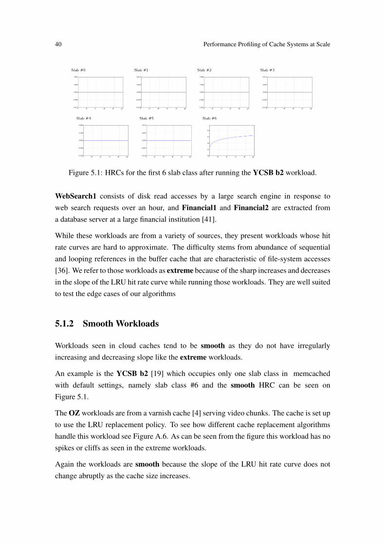
40 Performance Profiling of Cache Systems at Scale
Figure 5.1: HRCs for the first 6 slab class after running the YCSB b2 workload.
WebSearch1 consists of disk read accesses by a large search engine in response toweb search requests over an hour, and Financial1 and Financial2 are extracted froma database server at a large financial institution [41].
While these workloads are from a variety of sources, they present workloads whose hitrate curves are hard to approximate. The difficulty stems from abundance of sequentialand looping references in the buffer cache that are characteristic of file-system accesses[36]. We refer to those workloads as extreme because of the sharp increases and decreasesin the slope of the LRU hit rate curve while running those workloads. They are well suitedto test the edge cases of our algorithms
5.1.2 Smooth Workloads
Workloads seen in cloud caches tend to be smooth as they do not have irregularlyincreasing and decreasing slope like the extreme workloads.
An example is the YCSB b2 [19] which occupies only one slab class in memcachedwith default settings, namely slab class #6 and the smooth HRC can be seen onFigure 5.1.
The OZ workloads are from a varnish cache [4] serving video chunks. The cache is set upto use the LRU replacement policy. To see how different cache replacement algorithmshandle this workload see Figure A.6. As can be seen from the figure this workload has nospikes or cliffs as seen in the extreme workloads.
Again the workloads are smooth because the slope of the LRU hit rate curve does notchange abruptly as the cache size increases.

Trausti Sæmundsson 41
5.2 Accuracy
5.2.1 Experimental Setup
We measured the accuracy of ROUNDER, STACKER and COUNTINGGHOST in a Pythonsimulator. For the accuracy experiments on ROUNDER and STACKER on the first nineworkloads, we use identical cache set-up as the authors of the LIRS algorithm [34].
5.2.2 ROUNDER
This section evaluates the accuracy of ROUNDER which was introduced in Chapter 3.To get a feel for how the accuracy changes with different number of buckets we varythe bucket sizes on a variety of workloads and run the algorithm on top of LRU andCLOCK.
Tables 5.1 and 5.2 summarize the results for LRU and CLOCK respectively and handpicked lines from those tables are presented in Figure 5.2.
Running on LRU, the overall MAE is 1.93% on average for all the workloads when usingonly 8 buckets but goes down to 0.95% with 128 buckets. The worst performance is onthe cs and WebSearch1 workloads with 5.41% and 4.02% respectively using 8 bucketsbut goes down to 0.93% and 4.02% with 128 buckets for the same workloads. In fact theaccuracy of WebSearch1 does not change with more buckets.
Running on CLOCK, the overall MAE is 1.08% on average for all the workloads whenusing only 8 buckets but goes down to 0.80% with 128 buckets. The worst performanceoccurs on the postgres and glimpse workloads with 7.93% and 6.46% respectively using8 buckets but goes down to 5.98% and 4.94% with 128 buckets.
Ultimately this experiment shows that ROUNDER is very accurate in estimating the realHRC of LRU achieving a worst case MAE of 5.41% with very few buckets. WithCLOCK, on the other hand the worst case MAE is 7.93% with as little as 8 buckets.Using 128 buckets the worst cases are 4.02% and 5.98% respectively. This shows thatROUNDER works better on LRU in the worst case but better on CLOCK on average.Recalling from Section 2.1.5 that CLOCK has very similar performance to LRU weconclude that ROUNDER works well on both LRU and CLOCK, still being designed forLRU.

42 Performance Profiling of Cache Systems at Scale
Workload Requests Cache size B = 8 B = 16 B = 32 B = 64 B = 1282pools 100K 450 0.52 0.30 0.20 0.18 0.18cpp 9K 900 1.92 1.17 0.72 0.47 0.33cs 7K 1K 5.41 2.21 1.68 1.32 0.93glimpse 6K 3K 4.34 2.94 1.83 1.48 1.38multi1 16K 2K 3.56 3.83 3.48 3.16 3.00multi2 26K 3K 2.11 1.82 1.52 1.34 1.14multi3 30K 4K 1.14 0.86 0.73 0.54 0.45postgres 10K 3K 3.47 1.67 1.16 0.85 0.61sprite 134K 1K 2.09 1.82 1.65 1.57 1.53Financial1 1M 50K 2.02 0.85 0.37 0.09 0.05Financial2 3M 50K 1.82 0.98 0.77 0.74 0.78WebSearch1 1M 50K 4.02 4.02 4.02 4.02 4.02P1 3M 50K 1.64 1.30 1.19 1.14 1.12P2 666K 50K 0.93 0.84 0.80 0.80 0.77P3 239K 50K 0.76 0.42 0.28 0.24 0.21P4 967K 50K 1.01 0.78 0.58 0.53 0.45P5 1M 50K 1.08 0.81 0.68 0.57 0.51P6 520K 50K 1.31 1.18 0.98 0.86 0.80P7 751K 50K 0.93 0.69 0.58 0.50 0.44P8 2M 50K 2.24 2.21 2.20 2.17 2.15P9 682K 50K 0.97 0.80 0.68 0.63 0.60P10 1M 50K 1.16 0.85 0.74 0.62 0.58P12 547K 50K 0.94 0.67 0.60 0.58 0.56P13 1M 50K 0.82 0.66 0.56 0.50 0.46Average (%) 1.93 1.40 1.17 1.08 0.96
Table 5.1: Accuracy of ROUNDER running on LRU: Each result is given as a percentage(results generally have around 0-5% error).
5.2.3 STACKER
This section evaluates the accuracy of STACKER, which was also introduced in Chapter 3.To get a feel for how the accuracy changes with different number of buckets we varythe bucket sizes on a variety of workloads and run the algorithm on top of LRU andCLOCK.
Tables 5.3 and 5.4 summarize the results for LRU and CLOCK respectively and handpicked lines from those tables are presented in Figure 5.3.
Running on LRU, the overall MAE is 1.73% on average for all the workloads whenusing only 8 buckets but goes down to 0.20% with 128 buckets. The worst performanceis on the cs and WebSearch1 workloads with 5.30% and 4.02% respectively using 8

Trausti Sæmundsson 43
Workload Requests Cache size B = 8 B = 16 B = 32 B = 64 B = 1282pools 100K 450 1.49 1.66 1.74 1.77 1.78cpp 9K 900 1.81 1.40 1.10 0.94 0.83cs 7K 1K 3.14 1.15 0.91 0.84 0.64gli 6K 3K 6.46 5.74 5.19 5.01 4.94multi1 16K 2K 2.10 2.88 2.61 2.38 2.28multi2 26K 3K 2.31 2.43 2.29 2.19 2.07multi3 30K 4K 1.77 1.91 1.90 1.76 1.70ps 10K 3K 7.93 6.86 6.28 6.08 5.98sprite 134K 1K 1.52 1.27 1.14 1.08 1.05Financial1 1M 50K 0.02 0.01 0.01 0.01 0.01Financial2 3M 50K 0.02 0.01 0.01 0.01 0.01WebSearch1 1M 50K 0.07 0.07 0.07 0.07 0.07WebSearch2 5M 50K 0.00 0.00 0.00 0.00 0.00WebSearch3 4M 50K 0.00 0.00 0.00 0.00 0.00P1 3M 50K 0.02 0.01 0.01 0.01 0.01P2 666K 50K 0.02 0.02 0.02 0.02 0.02P3 239K 50K 0.09 0.04 0.03 0.02 0.02P4 967K 50K 0.04 0.03 0.02 0.02 0.02P5 1M 50K 0.05 0.03 0.02 0.02 0.02P6 520K 50K 0.05 0.03 0.02 0.01 0.01P7 751K 50K 0.05 0.03 0.02 0.02 0.02P8 2M 50K 0.03 0.03 0.03 0.03 0.03P9 682K 50K 0.03 0.02 0.02 0.02 0.02P10 1M 50K 0.05 0.03 0.03 0.02 0.02P12 547K 50K 0.04 0.03 0.03 0.02 0.02P13 1M 50K 0.04 0.03 0.02 0.02 0.02P14 4M 50K 0.02 0.02 0.02 0.02 0.01Average (%) 1.08 % 0.95 % 0.87 % 0.83 % 0.80 %
Table 5.2: Accuracy of ROUNDER running on CLOCK: Each result is given as apercentage (results generally have around 0-8% error).
buckets but using the same workloads this decreases down to 0.20% and 4.34% with 128
buckets.
Running on CLOCK, the overall MAE is 1.04% on average for all the workloads whenusing only 8 buckets but goes down to 0.75% with 128 buckets. The worst performanceoccurs on the postgres and glimpse workloads with 7.42% and 5.55% respectively using8 buckets and goes down to 5.65% and 4.60% with 128 buckets.
As with ROUNDER, the bucket parameter trades off overhead for accurate HRCs, andthe improvement in accuracy is evident as we increase the number of buckets B in thealgorithms. Like with ROUNDER, this experiment shows that STACKER is very accurate

44 Performance Profiling of Cache Systems at Scale
0 500 1000 1500 2000 2500Cache size (items)
0.00
0.25
0.50
Cumulative hit rate
B=8
B=16
B=32
B=64
LRU
(a) ROUNDER, glimpse, LRU
0 600 1200 1800 2400 3000Cache size (items)
0.0
0.3
0.6
Cumulative hit rate
B=8
B=16
B=32
B=64
LRU
(b) ROUNDER, postgres, LRU
0 10000 20000 30000 40000 50000Cache size (items)
0.00
0.25
0.50
Cumulative hit rate
B=8
B=16
B=32
B=64
LRU
(c) ROUNDER, Financial1, LRU
0 500 1000 1500 2000 2500Cache size (items)
0.00
0.25
0.50
Cumulative hit rate
B=8
B=16
B=32
B=64
CLOCK
(d) ROUNDER, glimpse, CLOCK
0 600 1200 1800 2400 3000Cache size (items)
0.0
0.3
0.6
Cumulative hit rate
B=8
B=16
B=32
B=64
CLOCK
(e) ROUNDER, postgres, CLOCK
0 10000 20000 30000 40000 50000Cache size (items)
0.00
0.25
0.50
Cumulative hit rate
B=8
B=16
B=32
B=64
CLOCK
(f) ROUNDER, Financial1, CLOCK
Figure 5.2: Accuracy graphs Hit rate curves of ROUNDER on LRU (top row) andCLOCK (bottom row) with varying bucket sizes (B) on three workloads. The true LRUand CLOCK hit rate curves are also shown.
in estimating the real HRC of LRU, achieving even better accuracy than ROUNDER. Theworst case MAE of 5.30% is better than the worst case MAE of 5.41 when using only8 buckets with ROUNDER. With CLOCK and 8 buckets the worst case MAE is 7.42%
compared to 7.93% with ROUNDER.
Using STACKER and 128 buckets, the worst cases are 0.82% and 4.6% respectivelycompared to 4.02% and 5.98% respectively with ROUNDER and 128 buckets. STACKER
has much higher accuracy than ROUNDER on the workload WebSearch1 and the accuracyincreases with more buckets as opposed to the fixed accuracy with ROUNDER.
5.2.4 COUNTINGGHOST
Although the use of ghost list is intuitive there are settings where maintaining the ghostlist structure imposes significant overhead on the memory cache. For instance, accordingto [8], the vast majority of values in the Facebook memory cache occupy only a fewbytes making them significantly smaller than the keys themselves. In Section 3.4.3 weintroduced the algorithm COUNTINGGHOST to attack this problem and in this section weevaluate the accuracy of this algorithm. In Section 3.4.3 we introduced a mechanism that

Trausti Sæmundsson 45
Workload Requests Cache size B = 8 B = 16 B = 32 B = 64 B = 1282pools 100K 450 0.59 0.31 0.11 0.07 0.05cpp 9K 900 1.90 1.07 0.54 0.28 0.16cs 7K 1K 5.30 1.56 0.88 0.42 0.20glimpse 6K 3K 2.56 1.62 1.03 0.42 0.21multi1 16K 2K 3.43 3.56 2.19 1.29 0.82multi2 26K 3K 2.16 1.47 0.92 0.67 0.42multi3 30K 4K 1.23 0.72 0.56 0.38 0.37postgres 10K 3K 3.77 1.78 1.00 0.50 0.23sprite 134K 1K 1.47 0.46 0.19 0.14 0.08Financial1 1M 50K 1.97 0.85 0.34 0.07 0.03Financial2 3M 50K 1.85 0.85 0.44 0.25 0.20WebSearch1 1M 50K 4.02 0.73 0.72 0.75 0.34P1 3M 50K 1.11 0.51 0.33 0.28 0.17P2 666K 50K 0.70 0.31 0.25 0.25 0.24P3 239K 50K 0.76 0.34 0.21 0.15 0.10P4 967K 50K 1.05 0.59 0.28 0.13 0.07P5 1M 50K 1.00 0.51 0.26 0.15 0.11P6 520K 50K 1.09 0.61 0.32 0.21 0.15P7 751K 50K 0.82 0.39 0.20 0.12 0.10P8 2M 50K 0.92 0.41 0.34 0.22 0.21P9 682K 50K 0.94 0.42 0.17 0.08 0.10P10 1M 50K 1.13 0.69 0.45 0.34 0.24P12 547K 50K 1.01 0.60 0.30 0.21 0.09P13 1M 50K 0.79 0.34 0.17 0.12 0.07Average (%) 1.73 0.86 0.51 0.32 0.20
Table 5.3: Accuracy of STACKER running on LRU: Each result is given as a percentage(results generally have around 0-5% error).
improves on the regular ghost list by being more space and time efficient, in exchange foraccuracy, in cases where keys are significantly longer than the values.
As opposed to ROUNDER and STACKER, which have a tunable number of buckets, thisalgorithm contains 3 hypothetical buckets represented as Counting Filters to maintain theghost list. To get a feel for the accuracy of this algorithm predicting what would happenif the cache size would be doubled, we run the algorithm on the extreme workloads ontop of LRU.
In this experiment we measured the accuracy of this method by running the ghost list withLRU on some of the extreme workloads. For reference a regular ghost list for LRU,implemented as a linked list using Mattson’s algorithm for evaluating stack distances,would have predicted the hits in the ghost list with 100% accuracy.
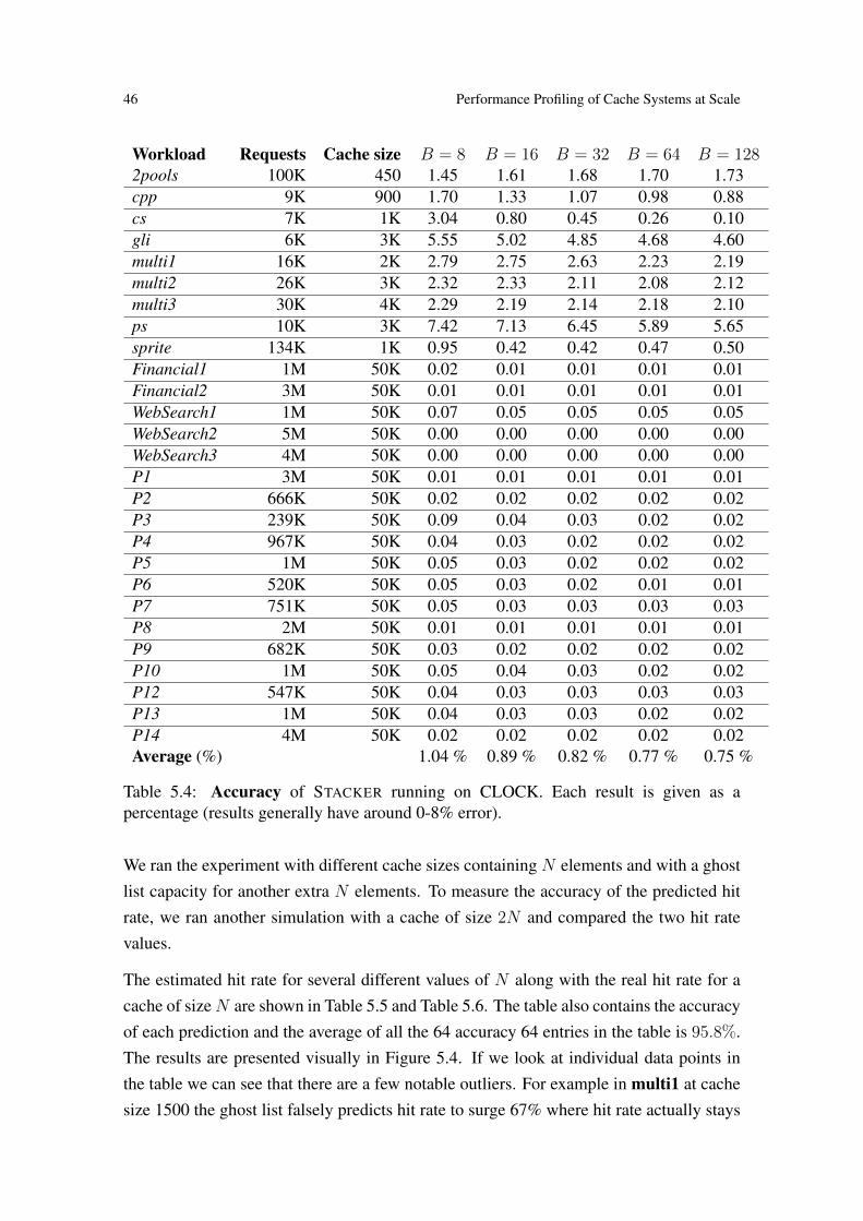
46 Performance Profiling of Cache Systems at Scale
Workload Requests Cache size B = 8 B = 16 B = 32 B = 64 B = 1282pools 100K 450 1.45 1.61 1.68 1.70 1.73cpp 9K 900 1.70 1.33 1.07 0.98 0.88cs 7K 1K 3.04 0.80 0.45 0.26 0.10gli 6K 3K 5.55 5.02 4.85 4.68 4.60multi1 16K 2K 2.79 2.75 2.63 2.23 2.19multi2 26K 3K 2.32 2.33 2.11 2.08 2.12multi3 30K 4K 2.29 2.19 2.14 2.18 2.10ps 10K 3K 7.42 7.13 6.45 5.89 5.65sprite 134K 1K 0.95 0.42 0.42 0.47 0.50Financial1 1M 50K 0.02 0.01 0.01 0.01 0.01Financial2 3M 50K 0.01 0.01 0.01 0.01 0.01WebSearch1 1M 50K 0.07 0.05 0.05 0.05 0.05WebSearch2 5M 50K 0.00 0.00 0.00 0.00 0.00WebSearch3 4M 50K 0.00 0.00 0.00 0.00 0.00P1 3M 50K 0.01 0.01 0.01 0.01 0.01P2 666K 50K 0.02 0.02 0.02 0.02 0.02P3 239K 50K 0.09 0.04 0.03 0.02 0.02P4 967K 50K 0.04 0.03 0.02 0.02 0.02P5 1M 50K 0.05 0.03 0.02 0.02 0.02P6 520K 50K 0.05 0.03 0.02 0.01 0.01P7 751K 50K 0.05 0.03 0.03 0.03 0.03P8 2M 50K 0.01 0.01 0.01 0.01 0.01P9 682K 50K 0.03 0.02 0.02 0.02 0.02P10 1M 50K 0.05 0.04 0.03 0.02 0.02P12 547K 50K 0.04 0.03 0.03 0.03 0.03P13 1M 50K 0.04 0.03 0.03 0.02 0.02P14 4M 50K 0.02 0.02 0.02 0.02 0.02Average (%) 1.04 % 0.89 % 0.82 % 0.77 % 0.75 %
Table 5.4: Accuracy of STACKER running on CLOCK. Each result is given as apercentage (results generally have around 0-8% error).
We ran the experiment with different cache sizes containing N elements and with a ghostlist capacity for another extra N elements. To measure the accuracy of the predicted hitrate, we ran another simulation with a cache of size 2N and compared the two hit ratevalues.
The estimated hit rate for several different values of N along with the real hit rate for acache of sizeN are shown in Table 5.5 and Table 5.6. The table also contains the accuracyof each prediction and the average of all the 64 accuracy 64 entries in the table is 95.8%.The results are presented visually in Figure 5.4. If we look at individual data points inthe table we can see that there are a few notable outliers. For example in multi1 at cachesize 1500 the ghost list falsely predicts hit rate to surge 67% where hit rate actually stays

Trausti Sæmundsson 47
0 500 1000 1500 2000 2500Cache size (items)
0.00
0.25
0.50
Cumulative hit rate
B=8
B=16
B=32
B=64
LRU
(a) STACKER, glimpse, LRU
0 600 1200 1800 2400 3000Cache size (items)
0.0
0.3
0.6
Cumulative hit rate
B=8
B=16
B=32
B=64
LRU
(b) STACKER, postgres, LRU
0 10000 20000 30000 40000 50000Cache size (items)
0.00
0.25
0.50
Cumulative hit rate
B=8
B=16
B=32
B=64
LRU
(c) STACKER, Financial1, LRU
0 500 1000 1500 2000 2500Cache size (items)
0.00
0.25
0.50
Cumulative hit rate
B=8
B=16
B=32
B=64
CLOCK
(d) STACKER, glimpse, CLOCK
0 600 1200 1800 2400 3000Cache size (items)
0.0
0.3
0.6
Cumulative hit rate
B=8
B=16
B=32
B=64
CLOCK
(e) STACKER, postgres, CLOCK
0 10000 20000 30000 40000 50000Cache size (items)
0.00
0.25
0.50
Cumulative hit rate
B=8
B=16
B=32
B=64
CLOCK
(f) STACKER, Financial1, CLOCK
Figure 5.3: Accuracy graphs Hit rate curves of STACKER on LRU (top row) and CLOCK(bottom row) with varying bucket sizes (B) on three workloads. The true LRU andCLOCK hit rate curves are also shown.
at 49% The sharp incline in the hit rate suggests that the underlying workload has scanswhich the ghost list is not sensitive enough to pick up and instead averages the inclineover a wider area. This experiment shows how the algorithm predicts the hit rate for acache size of size 2N when running a cache of size N . Here N = 1500. Each of thethree counting filters contains between 0 and 500 elements. They contribute to the hit ratecurve at different intervals depending on how many elements are in each filter. Thus thealgorithm is able to predict all hit rates for cache sizes between N and 2N , not only for2N like shown in this experiment.
This experiment shows that COUNTINGGHOST is fairly accurate in predicting the hit rateof LRU if the cache size would be doubled. On 5 out of 64 different settings the accuracydrops below 90% but stays above 90% for all other settings. Those outliers happen whenthere is a looping pattern in the underlying workload, creating a sudden steep increase inthe hit rate as the cache size increases. Using only three filters is not enough to capturethose events.
Overall the average accuracy is 95.8% and we conclude that the method provides highaccuracy on a variety of workloads, suggesting that Counting Filters are effective inminimizing space and time overhead of ghost lists.

48 Performance Profiling of Cache Systems at Scale
Workload Cache size Hit rate Predicted hit rate Accuracy [%]2pools 500 51.06200 51.86246 98.52pools 1000 54.41500 55.32395 98.42pools 1500 56.87700 57.96308 98.12pools 2000 59.32600 60.48172 98.12pools 2500 61.64600 62.82262 98.12pools 3000 64.00100 65.13756 98.32pools 3500 66.27000 67.33176 98.42pools 4000 68.52100 69.39331 98.7cpp 500 84.77948 85.34166 99.3cpp 1000 86.40433 86.48657 99.9cpp 1500 86.48171 86.47950 100.0cpp 2000 86.48171 86.48093 100.0cpp 2500 86.48171 86.48171 100.0cpp 3000 86.48171 86.48171 100.0cpp 3500 86.48171 86.48171 100.0cpp 4000 86.48171 86.48171 100.0cs 500 1.82864 2.69002 68.0cs 1000 1.82864 2.92361 62.5cs 1500 79.22135 78.47663 99.1cs 2000 79.22135 78.47663 99.1cs 2500 79.22135 78.44743 99.0cs 3000 79.22135 79.22135 100.0cs 3500 79.22135 79.22135 100.0cs 4000 79.22135 79.22135 100.0gli 500 0.94747 1.95096 48.6gli 1000 11.20346 18.02892 62.1gli 1500 36.55253 38.65043 94.6gli 2000 57.39694 56.17803 97.9gli 2500 57.94548 57.13414 98.6gli 3000 57.94548 57.74801 99.7gli 3500 57.94548 57.83278 99.8gli 4000 57.94548 57.93999 100.0
Table 5.5: Accuracy of COUNTINGGHOST running on LRU. Each entry in the tableshows the actual hit rate of LRU on cache size n and the predicted hit rate of LRU runningat size n/2 with ghost list of capacity n/2. The average accuracy of all the 64 entries inthe table is 95.8%.
5.2.5 Different Cache Replacement Algorithms
Now we know the profiling framework works well on LRU and that the frameworkwithout a ghostlist works relatively well on CLOCK. But how does it perform on othercache replacement policies?

Trausti Sæmundsson 49
Workload Cache size Hit rate Predicted hit rate Accuracy [%]multi1 500 46.50650 47.35654 98.2multi1 1000 48.22802 48.83510 98.8multi1 1500 48.55593 68.65450 70.7multi1 2000 83.21352 82.02087 98.6multi1 2500 83.56665 82.31082 98.5multi1 3000 83.56665 82.69214 99.0multi1 3500 83.56665 83.56596 100.0multi1 4000 83.56665 83.56312 100.0multi2 500 35.97735 37.29596 96.5multi2 1000 47.80130 48.28133 99.0multi2 1500 48.31059 48.84664 98.9multi2 2000 48.99852 52.92984 92.6multi2 2500 61.24815 68.13827 89.9multi2 3000 71.17935 71.49249 99.6multi2 3500 71.88248 72.28809 99.4multi2 4000 74.72920 73.03455 97.7ps 500 48.54518 48.74933 99.6ps 1000 48.54518 50.98038 95.2ps 1500 52.58423 52.97023 99.3ps 2000 70.48239 64.91884 92.1ps 2500 70.48239 70.36026 99.8ps 3000 70.48239 70.38869 99.9ps 3500 70.49196 70.38869 99.9ps 4000 70.49196 70.51082 100.0sprite 500 78.30234 75.18021 96.0sprite 1000 90.63853 89.44534 98.7sprite 1500 92.48410 92.22287 99.7sprite 2000 93.47667 93.44312 100.0sprite 2500 93.85579 93.92417 99.9sprite 3000 94.16102 94.19080 100.0sprite 3500 94.26028 94.32896 99.9sprite 4000 94.32147 94.35735 100.0
Table 5.6: Table 5.5 continued. All estimates (except 5) have over 90% accuracy and theaverage accuracy is 95.8%.
This experiment tests the accuracy of MIMIR on the extreme postgres workloaddescribed in Section 5.1 running on several cache replacement algorithms. In particularwe ran ARC, CLOCK, LRU, LFU, LRU3 and RANDOM within the Python simulatorwith the MIMIR profiling framework producing HRCs at the same time. We raneach simulation with a 1500 element cache and set k = 2 to produce a HRC forall cache sizes up to 3000 elements. Internally ROUNDER was set to use 64 bucketsand COUNTINGGHOST was set to use 3 filters. We then ran the cache replacement

50 Performance Profiling of Cache Systems at Scale
0
20
40
60
80
100
120
0 500 1000 1500 2000 2500 3000 3500 4000
Hit r
ate
[%
]
Cache size (items)
Workload: 2pools
LRUPredicted
(a) 2pools
0
20
40
60
80
100
120
0 500 1000 1500 2000 2500 3000 3500 4000
Hit r
ate
[%
]
Cache size (items)
Workload: cpp
LRUPredicted
(b) cpp
0
20
40
60
80
100
0 500 1000 1500 2000 2500 3000 3500 4000
Hit r
ate
[%
]
Cache size (items)
Workload: cs
LRUPredicted
(c) cs
0
10
20
30
40
50
60
70
80
90
0 500 1000 1500 2000 2500 3000 3500 4000
Hit r
ate
[%
]
Cache size (items)
Workload: gli
LRUPredicted
(d) glimpse
0
20
40
60
80
100
120
0 500 1000 1500 2000 2500 3000 3500 4000
Hit r
ate
[%
]
Cache size (items)
Workload: multi1
LRUPredicted
(e) multi1
0
20
40
60
80
100
0 500 1000 1500 2000 2500 3000 3500 4000
Hit r
ate
[%
]
Cache size (items)
Workload: multi2
LRUPredicted
(f) multi2
0
20
40
60
80
100
0 500 1000 1500 2000 2500 3000 3500 4000
Hit r
ate
[%
]
Cache size (items)
Workload: ps
LRUPredicted
(g) postgres
0
20
40
60
80
100
120
0 500 1000 1500 2000 2500 3000 3500 4000
Hit r
ate
[%
]
Cache size (items)
Workload: sprite
LRUPredicted
(h) sprite
Figure 5.4: The accuracy of the Counting Filter ghost list predicting the hit rate for acache of size n using only n/2 elements. This is a visual representation of the hit ratedata from Table 5.5 and Table 5.6. The black dotted line is the real LRU hit rate for acache of each size. The red filled line is the predicted hit rate from a cache of half thesize. Under a perfect prediction the two lines would coincide.
algorithm on cache sizes which are multiples of 100 elements ranging from 100 to 3000
elements.
Now results from the experiment can be seen in Figure 5.5 and MAE values for thecorresponding Figure are in Table 5.7. The real hit rate in the figure is marked as reddots and the predicted HRC is a blue line. Ideally the red dots would be located on thepredicted blue line.
LRU has the lowest MAE in this experiment which should be intuitive since the profilingframework was designed for LRU. If we look at the blue and red curves for LRU wesee that we curves are aligned for cache sizes smaller than 1500 items but not so well
Cache replacement algorithm Maximum discrepancy MAEARC 6.7% 2.1%
CLOCK 18.0% 5.5%LFU 13.3% 4.9%
LRU3 10.2% 1.7%LRU 8.5% 1.5%
RANDOM 13.7% 2.4%
Table 5.7: Overview of the MAE for MIMIR running on the extreme postgres workloadat cache size 1400 predicting the HRC from all cache sizes between 0 and 3000. Themaximum discrepancy is the Kolmogorov-Smirvnov [55] distance between the HRCswhich measures the largest vertical distance of the two curves.

Trausti Sæmundsson 51
0 500 1000 1500 2000 2500 3000Cache size (# items)
0.0
0.1
0.2
0.3
0.4
0.5
0.6
0.7
0.8
Cumulative hit rate
Algorithm: ARC, trace: ps and base from 1500 items
(a) ARC
0 500 1000 1500 2000 2500 3000Cache size (# items)
0.0
0.1
0.2
0.3
0.4
0.5
0.6
0.7
0.8
Cumulative hit rate
Algorithm: CLOCK, trace: ps and base from 1500 items
(b) CLOCK
0 500 1000 1500 2000 2500 3000Cache size (# items)
0.0
0.1
0.2
0.3
0.4
0.5
0.6
0.7
0.8
Cumulative hit rate
Algorithm: LFU, trace: ps and base from 1500 items
(c) LFU
0 500 1000 1500 2000 2500 3000Cache size (# items)
0.0
0.1
0.2
0.3
0.4
0.5
0.6
0.7
0.8
Cumulative hit rate
Algorithm: LRU3, trace: ps and base from 1500 items
(d) LRU3
0 500 1000 1500 2000 2500 3000Cache size (# items)
0.0
0.1
0.2
0.3
0.4
0.5
0.6
0.7
0.8
Cumulative hit rate
Algorithm: LRU, trace: ps and base from 1500 items
(e) LRU
0 500 1000 1500 2000 2500 3000Cache size (# items)
0.0
0.1
0.2
0.3
0.4
0.5
0.6
0.7
0.8
Cu
mu
lati
ve
hit
ra
te
Algorithm: RANDOM, trace: ps and base from 1500 items
(f) RANDOM
Figure 5.5: HRC from MIMIR hooked into ARC, CLOCK, LFU, LRU3, LRU andRANDOM with a cache size of 1500 items on the postgres workload. The red dotsshow the real hit rate and the blue line is the predicted HRC.
aligned for cache sizes larger than 3000 items. This is because ROUNDER was set to use64 buckets but COUNTINGGHOST only uses 3 filters. When the cache size increases to2000 items, a high increase in hit rate occurs (the red dots) and 3 filters do not capture thissteep increase but smooth it out. It is indeed the same effect as described in Section 5.2.4.This issue also appeared in our experiments with the SC2 algorithm [18] since it uses only2 recency values, either the least recently used bit is set to 0 or 1. If we would increasethe number of filters for COUNTINGGHOST we would be able to capture steep increasesbetter, just like with ROUNDER and STACKER.
Regarding the other cache replacement algorithms, MIMIR does a fairly good job topredict them all with respect to MAE but the maximum discrepancy is high (except forARC).

52 Performance Profiling of Cache Systems at Scale
5.3 Overhead
5.3.1 Experimental Setup
We ran all our experiments on memcached-1.4.15 extended with the MIMIR profilingframework. We chose to use ROUNDER instead of STACKER for higher performance andbecause ROUNDER is simpler to parallelize. We deployed libmemcached 1.0.16 on 4nodes and used the built-in workload generator. Each node requests 2 million random 16byte unique keys and 32 byte values via 10 threads and 60 connections. The proportionof GET requests to SET requests is 9:1, and we bundle 100 GETs together in a singleMULTI-GET request. Our experimental set-up follows Fan et al. [26].
We ran each experiment 10 times and present the average throughput of the 10 runs witherror bars showing the standard deviation.
5.3.2 ROUNDER
This section evaluates the overhead of ROUNDER running in memcached.
We measured the impact on performance in memcached with and without ROUNDER,running at several bucket sizes. Figure 5.6 shows the total throughput from the clients tothe central memcached server, each point measuring throughput in a 2 minute benchmarkaveraged over 10 runs.
The throughput of our augmented memcached is 2.2% lower than that of the originalmemcached implementation with B = 4 buckets, running on a 8GB cache size. Thehighest overhead is 14.6% with a 4GB cache and 4 buckets for ROUNDER.
We observe a paradoxical drop in throughput for all three services as cache size increases.This stems from memory management inefficiencies and coarse-grained lock contentionwithin memcached [54, 26] as the hit rate rises from ∼ 40% at 1GB to effectively 100%at 4GB and up.
A larger number of buckets, B = 128, to produce more granular statistics does notsignificantly impair throughput in the experiment. When using 4 buckets and a 8GB
or 16GB cache ROUNDER is extremely lightweight, only taking a < 3% throughputtax.

Trausti Sæmundsson 53
1024 2048 4096 8192 16384Memory MB
0
200000
400000
600000
800000
1000000
1200000
1400000
1600000
Throughput OP/s
5.2%
7.8%
8.0%
2.2% 2.7%
6.4%
9.6%
8.6%
3.1% 2.6%
7.8%
10.5%
9.2%2.2% 3.1%
7.5%
12.7%
14.6%4.2% 4.8%
Throughput overhead of Rounder
UnmodifiedRounder B=4Rounder B=8Rounder B=16Rounder B=32
Figure 5.6: Overhead of ROUNDER with different bucket sizes.
1024 2048 4096 8192 16384Memory MB
0
200000
400000
600000
800000
1000000
1200000
1400000
1600000
Throughput OP/s
23.0%
25.8%
29.4%
27.2%
41.0%
26.6%
27.4%
30.3%
26.2%
39.4%
27.8%
26.4%
29.4%
28.3%
41.9%
26.7%
28.7%
31.1%
29.0%
43.0%
Throughput overhead of rounder and the counting filter ghostlist
UnmodifiedRounder(B=4)+GhostlistRounder(B=8)+GhostlistRounder(B=16)+GhostlistRounder(B=32)+Ghostlist
Figure 5.7: Overhead of the full MIMIR profiling framework within memcached
5.3.3 MIMIR Profiling Framework
This section evaluates the overhead of the full MIMIR profiling framework running inmemcached.
We measured the impact on performance in memcached with and without MIMIRrunning at several bucket sizes for ROUNDER while keeping COUNTINGGHOST fixedwith 3 filters. Figure 5.7 shows the total throughput from the clients to the centralmemcached server, each point measuring throughput in a 2 minute benchmark averaged

54 Performance Profiling of Cache Systems at Scale
over 10 runs. The throughput of our augmented memcached is 23% lower than theoriginal memcached implementation with B = 4 buckets, running on a 1GB cache size.The highest overhead is 43.0% with a 16GB cache and 32 buckets for ROUNDER.
Providing a HRC for all cache sizes up to double the cache size requires in the worstcase a 41% throughput degradation within memcached. We have plans to optimize thissignificantly as described in Section 4.4. Running at 1GB it requires an overhead of23%.
5.4 Summary
We evaluated the accuracy and overhead of our three algorithms, ROUNDER, STACKER
and COUNTINGGHOST, to understand how well ROUNDER, STACKER and COUNTING-GHOST would perform in a real world setting and thus how MIMIR would perform inthis setting.
The bucket parameter trades off accuracy in ROUNDER and STACKER for performance.More buckets result in higher accuracy but worse performance.
ROUNDER is precise in estimating the real HRC of LRU, achieving over 94% accuracyon all workloads in low-profile mode, but achieving over 92% accuracy on all workloadsin low-profile mode when running on CLOCK.
STACKER is more accurate than ROUNDER. STACKER achieves over 94% accuracy on allworkloads in low-profile mode when running on LRU, but achieves over 92% accuracyon all workloads in low-profile mode when running on CLOCK. Like with ROUNDER,our experiments shows that STACKER is very accurate in estimating the real HRC ofLRU achieving over 99% accuracy on all our workloads with 128 buckets when runningon LRU. However STACKER has a higher time complexity and in practice ROUNDER
is a more suitable algorithm, still guaranteeing over 95% accuracy when running with128 buckets. To minimize overhead one would choose ROUNDER with 8 buckets or less,which results in at least 94% accuracy in the worst case.
Assuming the cache server contains its own meta-data collection on evicted keys witha ghost list, e.g., an extended LRU stack without values when running LRU, eitherROUNDER or STACKER suffices to produce hit rate curves for smaller and larger cachesizes. However if no meta-data is collected in the cache server and values are smallcompared to keys, using a regular ghost list is memory inefficient and COUNTINGGHOST
was designed to tackle this problem. Our micro-benchmark for COUNTINGGHOST show

Trausti Sæmundsson 55
that we predict the hit rate for twice the current allocation with over 90% accuracy onmost workloads (59 out of 64 different workload and cache size combinations).
Since memcached uses the LRU policy it was a good ground to evaluate the MIMIRprofiling framework. We connected the framework to memcached and evaluated theperformance before and after. Our test bed was made up of a single server and multipleclients using several connections. The result is that the framework takes only a small toll,3-8%, on the server when generating hit rate curves with ROUNDER for smaller cachesizes but a little higher, 23-41%, when evaluating hit rate curves for smaller and largercache sizes with ROUNDER and COUNTINGGHOST.
The framework was designed for LRU but we tried it on other cache replacement policies,and as could be expected this resulted in lower accuracy. To achieve higher accuracy onother cache replacement policies like ARC, RANDOM, LRU3, LFU, CLOCK, ARC ourmethod would have be customized specifically for every algorithm.

56

57
Chapter 6
Conclusions
In this thesis we asked two questions particularly relevant to many cache operatorsmanaging large distributed caches:
“how much total memory should be allocated to the cache tier?”
and
“what is the minimum cache size for a given hit rate?”.
In order not to overload databases and to maximize performance, operators often err onthe side of caution by scaling up rather than scaling out. Scaling up means adding serversor increasing memory on existing servers while scaling out means removing serversor decreasing memory on existing servers. To figure out cache performance under adifferent allocation, operators can conduct offline simulations on the current setup andadd resources progressively until performance goals are reached. However, this is notacceptable due to a number of reasons. First, it may not give up to date results. Second,it disrespects dynamicity of workloads. Third, it is manually labor intensive. And fourth,offline simulations require request logs of cache requests which use a lot of disk spacewhen the request rate in the cache tier is high.
To enable cache operators to dynamically profile cache resources in distributed caches, wepropose a new cache profiling framework called MIMIR that generates efficacy graphsfrom each cache server in the cache tier. This happens in real-time so there is nooffline simulation of the cache tier necessary to understand how it would perform undera different setting. The efficacy graphs are called hit rate curves that describe the hit rateof allocated cache servers as a function of cache size. Our framework currently supportsboth the LRU and CLOCK cache replacement policies.

58 Performance Profiling of Cache Systems at Scale
To generate the hit rate curves we track stack distance estimates for each cached element.Generating hit rate curves for the LRU cache replacement policy from stack distancesis a widely studied problem but previous methods have significant overhead and lendthemselves poorly to concurrency. Most prominent are Mattson’s algorithm that requireslinear traversal of elements in the cache on every access and commands 283% throughputoverhead on a regular cache implementation. Using balanced trees such as AVL treesimproves the throughput but still commands a 74% percent overhead in our micro-benchmarks.
To find an efficient method for dynamic profiling we trade off some accuracy in orderto minimize the overhead, on the cache server and produce the hit rate curves in highlyconcurrent systems. The overhead is 6.3% in the same setup as Mattson’s algorithm andthe AVL tree.
To estimate stack distances we introduced three algorithms: ROUNDER, STACKER andCOUNTINGGHOST. ROUNDER and STACKER estimate stack distances for all elementsin the cache with over 95% accuracy on all workloads we used in our evaluation. Inthe case where you want to estimate efficiency for cache sizes larger than the currentallocation. Implies that meta-data for evicted keys must be tracked. A list of data-lesskeys is called a ghost list. If the cache server contains its own meta-data collection onevicted keys with a ghost list, e.g., an extended LRU stack without values when runningLRU, either ROUNDER or STACKER suffices to produce hit rate curves for smaller andlarger cache sizes.
Maintaining a ghost list requires storing some amount of evicted keys in memory and canbe viewed as a tax on the currently cached elements. Some workloads, however, like seenat Facebook have smaller values than keys and in this setting the memory tax overhead istoo high for a ghost list to be an option. To address this problem we proposed the thirdalgorithm, COUNTINGGHOST, to compress the data structure for the keys and provide amemory efficient ghost list to support a workload with small values. In our evaluationson COUNTINGGHOST for predicting the hit rate if the cache size would be doubled showthat the algorithm predicts the hit rate with 95% accuracy on average.
The accuracy is thus high for our methods. On the other hand, in order to evaluatethe overhead of our methods we integrated them into the popular memcached cacheserver. When running our parallel implementation of ROUNDER within memcached wepropose a maximum of 8.0% overhead when running it in low-profile mode. Runningthe COUNTINGGHOST algorithm within memcached proposes higher overhead, at most41.0% in our evaluations.

Trausti Sæmundsson 59
There are many avenues for future work. First we aim to either optimize the COUNTING-GHOST algorithm or move it to a background thread, whichever makes the overhead moreacceptable. Also, memcached is only one of many caching services and the methodsdescribed in MIMIR can be extended to profile other services. LRU and its variants,such as CLOCK, are among the most studied and widely deployed cache replacementalgorithms. Profiling performance of other policies is an understudied area and the topicof future work. Cache profiling also opens a new window to look at cost-benefit analysisof cloud services and could be extended to provide performance analysis of CPUs, harddrives and other tunable components in today’s highly dynamic cloud environments.Cost benefit analysis of resources could expand the usability and minimize pricing inmulti-tenant [18, 51] services like Heroku [6], Amazon ElastiCache [2] or Google’s AppEngine [5]. Virtualization management is already being made easier by CloudPhysics [3]and integration with such a framework is a viable option.

60

61
Bibliography
[1] https://gist.github.com/2864150. [Online; accessed 21-November-2012].
[2] AWS | Amazon ElastiCache – in-memory cache service. https://aws.
amazon.com/elasticache/.
[3] CloudPhysics. https://www.cloudphysics.com.
[4] Front page | varnish community. http://www.varnish-cache.org/.
[5] Google App Engine. https://appengine.google.com.
[6] Heroku | Cloud Application Platform. https://www.heroku.com.
[7] Redis key-value store. http://www.redis.io.
[8] Berk Atikoglu, Yuehai Xu, Eitan Frachtenberg, Song Jiang, and Mike Paleczny.Workload analysis of a large-scale key-value store. In ACM SIGMETRICS Perfor-
mance Evaluation Review, volume 40, pages 53–64. ACM, 2012.
[9] Reza Azimi, Livio Soares, Michael Stumm, Thomas Walsh, and Angela DemkeBrown. PATH: page access tracking to improve memory management. In ISMM
’07, pages 31–42, 2007.
[10] S. Bansal and D.S. Modha. CAR: Clock with adaptive replacement. In Proceedings
of the 3rd USENIX Conference on File and Storage Technologies, pages 187–200,2004.
[11] S. Bansal and D.S. Modha. Method and system of clock with adaptive cachereplacement and temporal filtering, September 30 2004. US Patent App. 10/955,201.
[12] Sorav Bansal and Dharmendra S Modha. Car: Clock with adaptive replacement. InFAST, volume 4, pages 187–200, 2004.
[13] L. A. Belady. A study of replacement algorithms for a virtual-storage computer.IBM Systems Journal, 5(2):78–101, 1966.

62 Performance Profiling of Cache Systems at Scale
[14] Laszlo A Belady, Robert A Nelson, and Gerald S Shedler. An anomaly in space-timecharacteristics of certain programs running in a paging machine. Communications
of the ACM, 12(6):349–353, 1969.
[15] B. T. Bennett and V. J. Kruskal. LRU stack processing. IBM Journal of Research
and Development, 19(4):353–357, July 1975.
[16] bit.ly. dablooms on github. https://github.com/bitly/dablooms/.
[17] Burton H Bloom. Space/time trade-offs in hash coding with allowable errors.Communications of the ACM, 13(7):422–426, 1970.
[18] G Chockler, G Laden, and Y Vigfusson. Design and implementation of cachingservices in the cloud. IBM Journal of Research and Development, 55(6):9:1–9:11,2011.
[19] Brian F. Cooper, Adam Silberstein, Erwin Tam, Raghu Ramakrishnan, and RussellSears. Benchmarking cloud serving systems with YCSB. In SoCC ’10, pages 143–154, 2010.
[20] F. J. Corbato. A paging experiment with the multics system. MIT Project MAC
Report MAC-M-384, May 1968.
[21] D3. D3.js - Data-Driven Documents. http://d3js.org/, May 2014. [Online;accessed 06-May-2014].
[22] Jeff Dean. Software engineering advice from building large-scaledistributed systems. http://research.google.com/people/jeff/
stanford-295-talk.pdf, 2007.
[23] Eric Demaine and Srinivas Devadas. MIT Course Number 6.006, Introduction toAlgorithms (Massachusetts Institute of Technology: MIT OpenCouseWare). http://ocw.mit.edu, December 2011. [Online; accessed 15-January-2014. License:Creative Commons BY-NC-SA].
[24] Chen Ding and Yutao Zhong. Predicting whole-program locality through reusedistance analysis. In PLDI ’03, pages 245–257, 2003.
[25] M. R. Ebling, L. B. Mummert, and D. C. Steere. Overcoming the network bottleneckin mobile computing. In WMCSA ’94, pages 34–36, 1994.
[26] Bin Fan, David G Andersen, and Michael Kaminsky. Memc3: Compact andconcurrent memcache with dumber caching and smarter hashing. Proc. 10th
USENIX NSDI, 2013.

Trausti Sæmundsson 63
[27] Li Fan, Pei Cao, Jussara Almeida, and Andrei Z Broder. Summary cache: Ascalable wide-area web cache sharing protocol. In ACM SIGCOMM Computer
Communication Review, volume 28, pages 254–265. ACM, 1998.
[28] Brad Fitzpatrick. Distributed caching with memcached. Linux journal, (124):72–74,2004.
[29] Flask. Welcome | Flask (A Python Microframework). http://flask.pocoo.org/, May 2014. [Online; accessed 06-May-2014].
[30] Neil Gunther, Shanti Subramanyam, and Stefan Pravu. Hidden scalability gotchasin memcached and friends. http://assets.en.oreilly.com/1/event/44/Hidden%20Scalability%20Gotchas%20in%20Memcached%
20and%20Friends%20Presentation.pdf.
[31] Qi Huang, Ken Birman, Robbert van Renesse, Wyatt Lloyd, Sanjeev Kumar, andHarry C Li. An analysis of facebook photo caching. In Proceedings of the Twenty-
Fourth ACM Symposium on Operating Systems Principles, pages 167–181. ACM,2013.
[32] Song Jiang. http://www.ece.eng.wayne.edu/~sjiang/. [Online;accessed 18-November-2012].
[33] Song Jiang, Feng Chen, and Xiaodong Zhang. CLOCK-Pro: an effective improve-ment of the CLOCK replacement. page 35, April 2005.
[34] Song Jiang and Xiaodong Zhang. LIRS: an efficient low inter-reference recency setreplacement policy to improve buffer cache performance. In ACM SIGMETRICS
Performance Evaluation Review, volume 30, pages 31–42. ACM, 2002.
[35] Theodore Johnson and Dennis Shasha. 2q: A low overhead high performancebuffer management replacement algorithm. In Proceedings of the 20th International
Conference on Very Large Data Bases, VLDB ’94, pages 439–450, San Francisco,CA, USA, 1994. Morgan Kaufmann Publishers Inc.
[36] Jong Min Kim, Jongmoo Choi, Jesung Kim, Sam H. Noh, Sang Lyul Min, YookunCho, and Chong Sang Kim. A low-overhead high-performance unified buffermanagement scheme that exploits sequential and looping references. In OSDI ’00,pages 9–9, 2000.
[37] Twisted Matrix Labs. Twisted. http://twistedmatrix.com/trac/, May2014. [Online; accessed 05-May-2014].

64 Performance Profiling of Cache Systems at Scale
[38] R. L. Mattson, J. Gecsei, D. R. Slutz, and I. L. Traiger. Evaluation techniques forstorage hierarchies. IBM Systems Journal, 9(2):78–117, June 1970.
[39] N Megiddo and D. S. Modha. Adaptive Replacement Cache. http:
//www-vlsi.stanford.edu/smart_memories/protected/
meetings/spring2004/arc-fast.pdf, 2003. [Online; accessed 21-November-2012].
[40] N. Megiddo and D.S. Modha. ARC: A self-tuning, low overhead replacement cache.In Proceedings of the 2nd USENIX Conference on File and Storage Technologies,pages 115–130, 2003.
[41] N. Megiddo and D.S. Modha. ARC: A self-tuning, low overhead replacement cache.In FAST ’03, pages 115–130, 2003.
[42] N. Megiddo and D.S. Modha. System and method for implementing an adaptivereplacement cache policy, February 7 2006. US Patent 6,996,676.
[43] memcached. memcached - a distributed memory object caching system. http:
//www.memcached.org.
[44] memcached. memcached on github. https://github.com/memcached/
memcached.
[45] Rajesh Nishtala, Hans Fugal, Steven Grimm, Marc Kwiatkowski, Herman Lee,Harry C Li, Ryan McElroy, Mike Paleczny, Daniel Peek, Paul Saab, et al. Scalingmemcache at facebook. In Proceedings of the 10th USENIX conference on Net-
worked Systems Design and Implementation, pages 385–398. USENIX Association,2013.
[46] Frank Olken. Efficient methods for calculating the success function of fixed-spacereplacement policies. Technical report, Lawrence Berkeley Lab., CA (USA), 1981.
[47] Elizabeth J. O’Neil, Patrick E. O’Neil, and Gerhard Weikum. The lru-k pagereplacement algorithm for database disk buffering. SIGMOD Rec., 22(2):297–306,June 1993.
[48] R. H. Patterson, G. A. Gibson, E. Ginting, D. Stodolsky, and J. Zelenka. Informedprefetching and caching. In SOSP ’95, pages 79–95, 1995.
[49] Paul Saab. Scaling memcached at facebook. https://www.facebook.com/note.php?note_id=39391378919.

Trausti Sæmundsson 65
[50] Ketan Shah, Anirban Mitra, and Dhruv Matani. An O(1) algorithm for implementingthe LFU cache eviction scheme. Technical report, Technical report, 2010."http://dhruvbird. com/lfu. pdf, 2010.
[51] David Shue, Michael J Freedman, and Anees Shaikh. Performance isolation andfairness for multi-tenant cloud storage. In Proc. 10th USENIX Conference on
Operating Systems Design and Implementation, pages 349–362, 2012.
[52] SuprDewd. CompetitiveProgramming. https://github.com/
SuprDewd/CompetitiveProgramming/blob/master/code/
data-structures/avl_tree.cpp, January 2014. [Online; accessed15-January-2014].
[53] David K Tam, Reza Azimi, Livio B Soares, and Michael Stumm. Rapidmrc:approximating l2 miss rate curves on commodity systems for online optimizations.In ACM SIGARCH Computer Architecture News, volume 37, pages 121–132. ACM,2009.
[54] Alex Wiggins and Jimmy Langstone. Enhancing the scalability ofmemcached. http://software.intel.com/en-us/articles/
enhancing-the-scalability-of-memcached-0.
[55] Wikipedia. Kolmogorov–Smirnov test — Wikipedia, The Free Encyclopedia, 2014.[Online; accessed 20-June-2013].
[56] Ting Yang, Emery D. Berger, Scott F. Kaplan, and J. Eliot B. Moss. CRAMM:virtual memory support for garbage-collected applications. In OSDI ’06, pages 103–116, 2006.
[57] Weiming Zhao, Xinxin Jin, Zhenlin Wang, Xiaolin Wang, Yingwei Luo, and Xi-aoming Li. Efficient LRU-based working set size tracking. Michigan Technological
University Computer Science Technical Report, 2011.
[58] Mark Zuckerberg. Memcached tech talk (12/17/2008). https://www.
facebook.com/video/video.php?v=631826881803.

66

67
Appendix A
Appendix
This chapter contains performance and throughput graphs for several experiments to savespace from the main chapters of the thesis.

68 Performance Profiling of Cache Systems at Scale
0
20
40
60
80
100
120
0 500 1000 1500 2000 2500 3000 3500 4000
Hit r
ate
[%
]
Cache size (items)
Trace: 2pools.trc
LRUCLOCK
(a) 2pools
0
20
40
60
80
100
120
0 500 1000 1500 2000 2500 3000 3500 4000
Hit r
ate
[%
]
Cache size (items)
Trace: cpp.trc
LRUCLOCK
(b) cpp
0
20
40
60
80
100
120
0 500 1000 1500 2000 2500 3000 3500 4000
Hit r
ate
[%
]
Cache size (items)
Trace: cs.trc
LRUCLOCK
(c) cs
0
20
40
60
80
100
120
0 500 1000 1500 2000 2500 3000 3500 4000
Hit r
ate
[%
]
Cache size (items)
Trace: gli.trc
LRUCLOCK
(d) glimpse
0
20
40
60
80
100
120
0 500 1000 1500 2000 2500 3000 3500 4000
Hit r
ate
[%
]
Cache size (items)
Trace: multi1.trc
LRUCLOCK
(e) multi1
0
20
40
60
80
100
120
0 500 1000 1500 2000 2500 3000 3500 4000
Hit r
ate
[%
]
Cache size (items)
Trace: multi2.trc
LRUCLOCK
(f) multi2
0
20
40
60
80
100
120
0 500 1000 1500 2000 2500 3000 3500 4000
Hit r
ate
[%
]
Cache size (items)
Trace: multi3.trc
LRUCLOCK
(g) multi3
0
20
40
60
80
100
120
0 500 1000 1500 2000 2500 3000 3500 4000
Hit r
ate
[%
]
Cache size (items)
Trace: ps.trc
LRUCLOCK
(h) postgres
0
20
40
60
80
100
120
0 500 1000 1500 2000 2500 3000 3500 4000
Hit r
ate
[%
]
Cache size (items)
Trace: sprite.trc
LRUCLOCK
(i) sprite
Figure A.1: The hit rate of LRU vs CLOCK in the Python simulator. Note that the hit rateof CLOCK decreases as the cache size increases from 2000 elements to 2200 elements.This phenomeon is called Belady’s anomaly [14]

Trausti Sæmundsson 69
100000
150000
200000
250000
300000
350000
400000
450000
500000
0 500 1000 1500 2000 2500 3000 3500 4000
Thro
ughp
ut [r
equ
ests
/s]
Cache size (items)
Trace: 2pools.trc
LRUCLOCK
(a) 2pools
0
100000
200000
300000
400000
500000
600000
700000
0 500 1000 1500 2000 2500 3000 3500 4000
Thro
ughp
ut [r
equ
ests
/s]
Cache size (items)
Trace: cpp.trc
LRUCLOCK
(b) cpp
0
100000
200000
300000
400000
500000
600000
700000
0 500 1000 1500 2000 2500 3000 3500 4000
Thro
ughp
ut [r
equ
ests
/s]
Cache size (items)
Trace: cs.trc
LRUCLOCK
(c) cs
100000
150000
200000
250000
300000
350000
400000
450000
500000
550000
600000
0 500 1000 1500 2000 2500 3000 3500 4000
Thro
ughput [r
equests
/s]
Cache size (items)
Trace: gli.trc
LRUCLOCK
(d) glimpse
0
100000
200000
300000
400000
500000
600000
700000
0 500 1000 1500 2000 2500 3000 3500 4000
Thro
ughput [r
equests
/s]
Cache size (items)
Trace: multi1.trc
LRUCLOCK
(e) multi1
100000
150000
200000
250000
300000
350000
400000
450000
500000
550000
0 500 1000 1500 2000 2500 3000 3500 4000
Thro
ughput [r
equests
/s]
Cache size (items)
Trace: multi2.trc
LRUCLOCK
(f) multi2
100000
150000
200000
250000
300000
350000
400000
450000
500000
0 500 1000 1500 2000 2500 3000 3500 4000
Thro
ughput [r
equests
/s]
Cache size (items)
Trace: multi3.trc
LRUCLOCK
(g) multi3
0
100000
200000
300000
400000
500000
600000
700000
0 500 1000 1500 2000 2500 3000 3500 4000
Thro
ughput [r
equests
/s]
Cache size (items)
Trace: ps.trc
LRUCLOCK
(h) postgres
0
100000
200000
300000
400000
500000
600000
700000
0 500 1000 1500 2000 2500 3000 3500 4000
Thro
ughput [r
equests
/s]
Cache size (items)
Trace: sprite.trc
LRUCLOCK
(i) sprite
Figure A.2: The throughput of LRU vs CLOCK in the Python simulator.

70 Performance Profiling of Cache Systems at Scale
0
20
40
60
80
100
0 500 1000 1500 2000 2500 3000 3500 4000
Hit r
ate
[%
]
Cache size (items)
Trace: 2pools.trc
LRULRU3
LRU10RANDOM
(a) 2pools
0
20
40
60
80
100
120
0 500 1000 1500 2000 2500 3000 3500 4000
Hit r
ate
[%
]
Cache size (items)
Trace: cpp.trc
LRULRU3
LRU10RANDOM
(b) cpp
0
20
40
60
80
100
0 500 1000 1500 2000 2500 3000 3500 4000
Hit r
ate
[%
]
Cache size (items)
Trace: cs.trc
LRULRU3
LRU10RANDOM
(c) cs
0
10
20
30
40
50
60
70
80
90
0 500 1000 1500 2000 2500 3000 3500 4000
Hit r
ate
[%
]
Cache size (items)
Trace: gli.trc
LRULRU3
LRU10RANDOM
(d) gli
0
20
40
60
80
100
120
0 500 1000 1500 2000 2500 3000 3500 4000
Hit r
ate
[%
]
Cache size (items)
Trace: multi1.trc
LRULRU3
LRU10RANDOM
(e) multi1
0
20
40
60
80
100
0 500 1000 1500 2000 2500 3000 3500 4000
Hit r
ate
[%
]
Cache size (items)
Trace: multi2.trc
LRULRU3
LRU10RANDOM
(f) multi2
0
20
40
60
80
100
0 500 1000 1500 2000 2500 3000 3500 4000
Hit r
ate
[%
]
Cache size (items)
Trace: multi3.trc
LRULRU3
LRU10RANDOM
(g) multi3
0
20
40
60
80
100
0 500 1000 1500 2000 2500 3000 3500 4000
Hit r
ate
[%
]
Cache size (items)
Trace: ps.trc
LRULRU3
LRU10RANDOM
(h) ps
0
20
40
60
80
100
120
0 500 1000 1500 2000 2500 3000 3500 4000
Hit r
ate
[%
]
Cache size (items)
Trace: sprite.trc
LRULRU3
LRU10RANDOM
(i) sprite
Figure A.3: Hit rate comparison on the default Redis cache replacement policy, volatile-lru. This policy mixes LRU with (Time To Live) TTL expiry, but in this simulation weignore the TTL. We simulated with 3 and 10 random samples here denoted LRU3 andLRU10, respectively. The hit rate is compared to that of RANDOM and LRU.

Trausti Sæmundsson 71
0
20
40
60
80
100
120
0 500 1000 1500 2000 2500 3000 3500 4000
Hit r
ate
[%
]
Cache size (items)
Trace: 2pools.trc
LRULFUOPTARCLIRS
RANDOMLRU3
(a) 2pools
0
20
40
60
80
100
120
0 500 1000 1500 2000 2500 3000 3500 4000
Hit r
ate
[%
]
Cache size (items)
Trace: cpp.trc
LRULFUOPTARCLIRS
RANDOMLRU3
(b) cpp
0
20
40
60
80
100
0 500 1000 1500 2000 2500 3000 3500 4000
Hit r
ate
[%
]
Cache size (items)
Trace: cs.trc
LRULFUOPTARCLIRS
RANDOMLRU3
(c) cs
0
10
20
30
40
50
60
70
80
90
0 500 1000 1500 2000 2500 3000 3500 4000
Hit r
ate
[%
]
Cache size (items)
Trace: gli.trc
LRULFUOPTARCLIRS
RANDOMLRU3
(d) gli
0
20
40
60
80
100
120
0 500 1000 1500 2000 2500 3000 3500 4000
Hit r
ate
[%
]
Cache size (items)
Trace: multi1.trc
LRULFUOPTARCLIRS
RANDOMLRU3
(e) multi1
0
20
40
60
80
100
0 500 1000 1500 2000 2500 3000 3500 4000
Hit r
ate
[%
]
Cache size (items)
Trace: multi2.trc
LRULFUOPTARCLIRS
RANDOMLRU3
(f) multi2
0
20
40
60
80
100
0 500 1000 1500 2000 2500 3000 3500 4000
Hit r
ate
[%
]
Cache size (items)
Trace: multi3.trc
LRULFUOPTARCLIRS
RANDOMLRU3
(g) multi3
0
20
40
60
80
100
0 500 1000 1500 2000 2500 3000 3500 4000
Hit r
ate
[%
]
Cache size (items)
Trace: ps.trc
LRULFUOPTARCLIRS
RANDOMLRU3
(h) ps
0
20
40
60
80
100
120
0 500 1000 1500 2000 2500 3000 3500 4000
Hit r
ate
[%
]
Cache size (items)
Trace: sprite.trc
LRULFUOPTARCLIRS
RANDOMLRU3
(i) sprite
Figure A.4: Comparison of the hit rate of LRU, LFU, OPT, ARC, LIRS, RANDOM andLRU3 for the extreme workloads in the Python simulator.

72 Performance Profiling of Cache Systems at Scale
0
100000
200000
300000
400000
500000
600000
0 500 1000 1500 2000 2500 3000 3500 4000
Thro
ug
hput
[re
que
sts
/s]
Cache size (items)
Trace: 2pools.trc
LRULFUOPTARCLIRS
RANDOMLRU3
(a) 2pools
0
200000
400000
600000
800000
1e+06
0 500 1000 1500 2000 2500 3000 3500 4000
Thro
ug
hput
[re
que
sts
/s]
Cache size (items)
Trace: cpp.trc
LRULFUOPTARCLIRS
RANDOMLRU3
(b) cpp
0
200000
400000
600000
800000
1e+06
0 500 1000 1500 2000 2500 3000 3500 4000
Thro
ug
hput
[re
que
sts
/s]
Cache size (items)
Trace: cs.trc
LRULFUOPTARCLIRS
RANDOMLRU3
(c) cs
0
100000
200000
300000
400000
500000
600000
700000
800000
900000
0 500 1000 1500 2000 2500 3000 3500 4000
Thro
ughput [r
equests
/s]
Cache size (items)
Trace: gli.trc
LRULFUOPTARCLIRS
RANDOMLRU3
(d) gli
0
200000
400000
600000
800000
1e+06
0 500 1000 1500 2000 2500 3000 3500 4000
Thro
ughput [r
equests
/s]
Cache size (items)
Trace: multi1.trc
LRULFUOPTARCLIRS
RANDOMLRU3
(e) multi1
0
100000
200000
300000
400000
500000
600000
700000
800000
0 500 1000 1500 2000 2500 3000 3500 4000
Thro
ughput [r
equests
/s]
Cache size (items)
Trace: multi2.trc
LRULFUOPTARCLIRS
RANDOMLRU3
(f) multi2
0
100000
200000
300000
400000
500000
600000
700000
0 500 1000 1500 2000 2500 3000 3500 4000
Thro
ughput [r
equests
/s]
Cache size (items)
Trace: multi3.trc
LRULFUOPTARCLIRS
RANDOMLRU3
(g) multi3
0
100000
200000
300000
400000
500000
600000
700000
800000
900000
0 500 1000 1500 2000 2500 3000 3500 4000
Thro
ughput [r
equests
/s]
Cache size (items)
Trace: ps.trc
LRULFUOPTARCLIRS
RANDOMLRU3
(h) ps
0
200000
400000
600000
800000
1e+06
0 500 1000 1500 2000 2500 3000 3500 4000
Thro
ughput [r
equests
/s]
Cache size (items)
Trace: sprite.trc
LRULFUOPTARCLIRS
RANDOMLRU3
(i) sprite
Figure A.5: Comparison of the throughput of LRU, LFU, OPT, ARC, LIRS, RANDOMand LRU3 for the extreme workloads in the Python simulator.

Trausti Sæmundsson 73
(a) OZ cache10 (b) OZ cache1 (c) OZ cache11 (d) OZ cache12
(e) OZ cache13 (f) OZ cache14 (g) OZ cache15 (h) OZ cache3
(i) OZ cache4 (j) OZ cache5 (k) OZ cache6 (l) OZ cache7
(m) OZ cache8 (n) OZ cache9 (o) OZ frontend1 (p) OZ frontend2
Figure A.6: The hit rate of RANDOM, LRU, OPT, ARC and LRU3 for workloads froma varnish LRU cache for video chunks at the Icelandic startup company OZ.

74


School of Computer ScienceReykjavík UniversityMenntavegi 1101 Reykjavík, IcelandTel. +354 599 6200Fax +354 599 6201www.reykjavikuniversity.isISSN 1670-8539