pergamon - national chiao tung university · the unbalance distribution in flexible rotors 845...

Pergamon

PII: S0020- 7403 (96) 00078-1

Int. J. Mech. Sci. Vol. 39, No. 7, pp. 841 857, 1997 ~; 1997 Elsevier Science Ltd

Printed in Great Britain. All rights reserved 0020-7403/97 $17.00 + 0.00

I D E N T I F I C A T I O N O F T H E U N B A L A N C E D I S T R I B U T I O N

I N F L E X I B L E R O T O R S

YUAN-PIN SHIH and AN-CHEN LEE Department of Mechanical Engineering, National Chiao Tung University, Taiwan, Republic of China

(Received 10 February 1995; in revised form 12 April 1996)

Abstract--This paper presents a new method for estimating unbalance distributions of flexible shafts and constant eccentricities of rigid disks based on the transfer matrix method for analyzing the steady-state responses of rotor-bearing systems, in which the transfer matrix of a flexible shaft is derived in a continuous sense with any spatial unbalance distribution. Rotary inertia, gyroscopic and transverse-shear effects are also included. When deflections and deflection angles of one free end are measurable, the unbalance distribution of shafts and disks can be estimated under operating conditions by the proposed method. The main advantage of this identification technique is that only the state vector of the one free end of the rotating shaft need to be measured. Justification of the method is presented by numerical simulations. © 1997 Elsevier Science Ltd. All rights reserved.

Keywords: flexible rotor, unbalance identification.

A, Df, p E,G, Ks

l ,J L

M,Q P,T

e, edx , Cdy

r(Z), r~(Z), ry(Z) X , Y

Z,t ~,~

(D

11

m

q k

m l

N O T A T I O N

cross-section area, diameter and density of the shaft Young's modulus, shear modulus and shear factor transverse and polar area moment of inertia of the shaft length of the shaft segment bending moment and shear force axial force and torque acting on the shaft eccentricity of the disk and projections, respectively, in X and Y directions eccentricity of the shaft and projections, respectively, in X and Y directions deflection in X and Y directions of fixed coordinates XYZ position and time coordinates, respectively slope in the XZ and YZ planes angular position of shaft unbalance in moving coordinates rotating speed the number of the term in Fourier series the number of the shaft with unbalance distribution the number of the disk with unbalance eccentricity the number of rotating speed the number of parameters in unbalance distribution

Subscripts and superscripts b, t caused by bending moment, shear force c, s associated to cosine, sine terms

h, p homogeneous solution, particular solution r, 1 right, left

x, y components in X and Y directions ~ labeled for column vector

differentiation w.r.t. Z

I N T R O D U C T I O N

Rotor unbalance considered does not only cause vibration, it also transmits rotational forces to rotor bearings and to the supporting structure. The forces thus transmitted may damage the machine and shorten its working life. All rotors have residual unbalance during manufacturing because of machining tolerances and material inhomogeneity. Thus, it is necessary to balance these rotors, as carefully as possible, to ensure smooth running.

Over the years, two major balancing techniques have commonly been employed; the modal balancing method, and the influence coefficients method. The modal balancing technique was

841

842 Yuan-Pin Shih and An-Chen Lee

developed by Bishop [1] and further investigated by several researchers, such as Kellenberger [-2], Shimada and Miwa [-3], Shimada and Fujisawa [4] and Saito and Azuna [51. In this method, the critical speed mode shapes of the rotor must be known from either theoretical or experimental measurements. Also, mass distribution must also be determined from the geometry of the rotor. The accuracy of the method depends on the knowledge of the rotor mode shapes, which may become quite complex for modes higher than the second critical speed. The influence coefficients technique was presented by Goodman [6]. It has been improved and tested by several authors such as Lund and Tonneson [7], Tessarzik and Badgley [8], Tessarzik et al. [9, 10] and Everett [11], in the laboratory and acceptable balancing has been achieved. In general, this method requires an accurate measurement of vibration phase angle in order to produce acceptable results. Various field balancing methods have also been developed, as discussed in detail in Ehrich [12].

The subject of balancing has been of interest to users of rotating machinery and further study in the theory and practice of balancing is still going on. Intuitively, it seems clear that the best way to balance a rotor is first to find the unbalance distribution and then add weights at given radial distances from the axis of rotation to compensate for it. However, due to deficiencies in methods for finding unbalance distribution, the concept of dynamic testing has long been emphasized. Conse- quently, we may not obtain the best quality of balance.

The purpose of this paper is to present a method for estimating the unbalance distribution in flexible rotors. This article is an extension of the work of Lee [13], who first gave a complete analysis of a rotating shaft's continuous "state of unbalance". This method is based on the transfer matrix method (TMM) of analyzing the steady-state responses of rotor-beating systems. The rotor-bearing systems considered here are composed of flexible shafts with spatial unbalance distributions, multiple rigid disks with constant eccentricities and linear bearings. Each bearing can be represented by eight linearized parameters, i.e. four stiffness and four damping coefficients. Since the system considered here is driven by an unbalanced force, the steady-state of the rotor will only contain a synchronous frequency component. The rationale of the method is described as below. By transforming any continuously distributed shaft unbalance function into its Fourier series representation, we can obtain the coefficients of the sine and cosine terms. Next, the overall transfer matrix including the shaft sections, bearings and disks is derived in terms of linear combinations of the unbalance parameters and the system parameters. Then, according to the boundary conditions, we formulate the normal equation by using the relations between these unknown coefficients and the known system parameters. Finally, identification can be realized from the simulated measured response data, i.e. the state variables of both displacements and angles measured at one free end in the shaft, induced by rotor unbalance using the least-squares method. The main advantage of this method is that only the states of one free end need to be measured, along with of course system parameters such as shaft geometry of shaft, material properties, rotating speed, bearing dynamic coefficients and so on. Justification of the method is given by numerical simulation.

EQUATIONS OF DISPLACEMENT FUNCTIONS FOR THE UNBALANCED SHAFT

In this section, the primary equations needed in this paper are given. For the detail derivation of them, the readers may refer to Lee et al. [13]. The governing equations of a rotating shaft considering the rotary inertia, gyroscopic, transverse shear effects and unbalance distribution can be derived as follows

~4X (~sG P)O4X az,~ - + ~ +

p2 ~4 x pA O2X +

KsGE Ot 4 E1 &2

2po9 ( ~3y p O3y~ P (~2X Tp ~3y

E \63ZZOt KsG -~-~J E1 OZ z EIKsG OZOt 2

+ T 03Y P'A'r(Z)'o~2"cos(rnt+4)) P'r"(Z)'coZ'cos(mt+~P) E1 ~Z 3 E1 K~G

p2"r(Z)'o)4"cos(cot + qb) T .r'(Z).p.~oZ.sin(cot + (o) + - (1)

K~GE KsGEI

The unbalance distribution in flexible rotors 843

Y

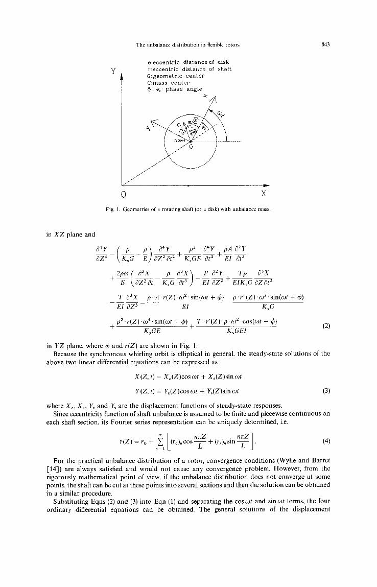
e : e c c e n t r i c d i s t a n c e of d i sk r : e c c e n t r i c d i skance of s h a f t G: geometric center C:mass center ~+%: phase angle

B -

0 X

Fig. 1. Geometries of a rotating shaft (or a disk) with unbalance mass.

in X Z plane and

~*Y ( p p ) D Y pz D Y pA a2y aZ* ~ + ~ + K,G~ at ~ + E1 at 2

2pco ( 03X p 03X~ P a2Y Tp 83X + Y k az2 at Ks G at 3 ) E1 OZ z + EIKs~ OZ at 2

T 03X p" A" r(Z)" (I) 2. sin(cot + 4)) p. r"(Z)" e) 2. sin(cot + q~)

E1 ~Z 3 E1 KsG

T. r'(Z).p" e) 2 .cos(cot + ~b) + p2. r(Z). co4. sin(cot + ~b) + (2)

KsGE KsGEI

in YZ plane, where q5 and r(Z) are shown in Fig. 1. Because the synchronous whirling orbit is elliptical in general, the steady-state solutions of the

above two linear differential equations can be expressed as

X(Z, t) = X¢(Z)coscot + Xs(Z)sincot

Y(Z, t)= Yc(Z)coscot + Y~(Z)sincot (3)

where Xo Xs, Yc and Ys are the displacement functions of steady-state responses. Since eccentricity function of shaft unbalance is assumed to be finite and piecewise continuous on

each shaft section, its Fourier series representation can be uniquely determined, i.e.

r(Z) ro + L F n~Z . ngZ~ = ,=~ k(rc),cos y + (rs), s l n y j • (4)

For the practical unbalance distribution of a rotor, convergence conditions (Wylie and Barret [14]) are always satisfied and would not cause any convergence problem. However, from the rigorously mathematical point of view, if the unbalance distribution does not converge at some points, the shaft can be cut at these points into several sections and then the solution can be obtained in a similar procedure.

Substituting Eqns (2) and (3) into Eqn (1) and separating the coscot and sincot terms, the four ordinary differential equations can be obtained. The general solutions of the displacement


function can be expressed into the sum of homogeneous and particular solutions as below.

xo(z) = x~ + x~

x ~ ( z ) = Xs ~ + x f

Y~(z) = g? + rg

5 ( z ) = r? + r? (5)

where the homogeneous solutions can be written as

4 8

X~(Z) = ~ Ai" e a'z' cos biZ + ~, Ai" e a'z" cos b~Z i = 1 i = 5

4 8

Bi" e "'z" sin biZ + ~ Bi" e a'z" sin biZ i = 1 i = 5

4-

x ~ ( z ) = E i = l

8

A~" e "'z. sin b~Z + ~ A~. e "'z" sin b~Z i = 5

+ 4 8

Bi" e "'z" cos biZ - ~ Bi" e a'z .cos biZ i = l i = 5

4 8

Y~(Z) = - ~ Ai" e "'z" sin biZ + Y~ Ai" e "'z" sin biZ i = 1 i = 5

4 8

-- ~ Bi" e "'z" cos biZ - ~ Bi" e a'z" cos biZ i = 1 i = 5

4 8

Yh(Z) = ~, A i ' e a ' Z ' c o s b i Z - ~ Ai 'e" 'Z'cosbiZ i = 1 i = 5

4 8

Bi" e "'z" sin biZ - ~ Bi" e "`z" sin biZ. (6) i = 1 i = 5

The coefficients ai and bi are, respectively, the real and imaginary part of the characteristic values (details listed in Lee et al. [ 13]).

When 4) = constant, the particular solutions can be expressed by

XP = (lo + #~.-cos --L-- + / ~ . . sin n = l

mrZ ~ . nrcZ) X~ (zo + L /~,-cos--L--- + --- .=1 ~s"' s i n - z - - )

= + v~,- sin n = l L

= ,c . s sin --L-- Y~P (4o + v~,, cos + Vs,," (7) ,=1 Z

where coefficients (,/~, v are listed in Appendix A of Lee et al. [13]. If the angular posit ion of unbalance varies along the shaft due to the mass center of shaft in three-dimensional space, we can resolve r(Z) into the components rx(z) and ry(z), respectively, in X and Y directions, with 4) = 0 ° for rx(z) and ~b = 90 ° for ry(z) for the shaft segment. Thus, we can obtain the part icular solution of q5 ¢ constant by superposing those of q5 = 0 ° for rx(Z) and ¢ = 90 ° for ry(Z) in the same manner as ~b = constant.


Differentiating Eqn (4) to yield the relationships of the real constants Ai and Bi of displacement functions and their derivatives can be written in the following form

1 Fill = X s A

{W} Y~ = IF] 1 7 x 1 7

(8)

where Xc = [X c X'c X'~' X'~']', Xs = [Xs X; X's' X~"] t, Yc = [Y~ Y~ Y~' Yc"] t, Ys = [Is Y" Ys" Ys'"'] t, A = [A1 A2 A3 A4 A5 A6 A7 As] t, B = [B1 Be B3 B4 Bs B6 B7 Bs] t.

Then introducing Z = 0 into the previous relations, it follows

-xc(o)-

{W(Z = 0)} = Yc(0) = [_M]_ . (9)

Y~(O)

1

The deflections and their derivatives at Z = L can also be obtained from Eqn (7) and written in the following form

- X c ( L ) -

{W(Z = L)} = Yc(L) = [H] . (10) Ys(L) 17×17

1

Combining two Eqns (8) and (9) results in

{W(Z = L)} = [N] . {W(Z = 0)} (11)

where [N] = [ H ] . [M]-1 . We can also derive the following relations between the derivatives of the displacement functions

and the state variables, represented in a matrix form

{W} = [A] {S} (12) 1 7 x 1 7

where {W} = (Xc, X;, X~', X~", Xs, X's, X~', X~", Yc, Y;, Y¢", Y;", Y~, Is', Is", Is"', 1) t, {S} = {Xc, Xs, Yc, Ys, ac, as, tic, fls, Mxc, Mxs, Myc, Mrs, Q~c, Qxs, Qyc, Qys, 1)' and the elements of matrix A are referred to by Lee et al. [13].

Consider the boundary conditions at Z -- 0 and Z = L, we have

{W(Z = L)} = [A]{S(Z = L)} = [ A ] { S I }

{w(z = 0)} = [A] {S(Z = 0)} = [A] {So}. (13)

The substitution of the above equations into (10) yields

{S,} = [A] - l I N ] [A] {So } = [Ts] {So }. (14)

Thus, the transfer matrix [T~], with the size of 17, x 17, is constructed by considering the effects of shaft unbalance to fit the general whirl of the elliptical orbits.

846 Yuan-Pin Shih and An-Chert Lee

,0 1 I I I , s e c t i o n ] ' 1 I

i

i

[

,2 3, ,4 m-3 I q

I t

, , Ii d i sk q I

l 't [~ d i sk 1

bear ing 1

m - 2 m - i m

1 I s e c t i o n 1 i m i

I I I I ~ _ - J

1 I ', I I

. / / / / bear ing p

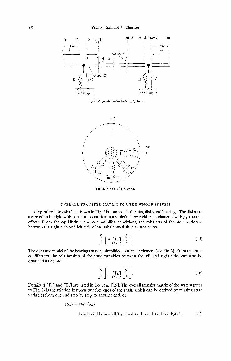
Fig. 2. A general rotor-bearing system.

/

Cy

\

c 4

Fig. 3. Model of a bearing.

Y

OVERALL TRANSFER MATRIX FOR THE WHOLE SYSTEM

A typical rota t ing shaft as shown in Fig. 2 is composed of shafts, disks and bearings. The disks are assumed to be rigid with constant eccentricities and defined by rigid mass elements with gyroscopic effects. F r o m the equi l ibr ium and compat ibi l i ty conditions, the relations of the state variables between the right side and left side of an unbalance disk is expressed as

The dynamic model of the bearings may be simplified as a linear element (see Fig. 3). F r o m the force equil ibrium, the relat ionship of the state variables between the left and right sides can also be obta ined as below

Details of [Td] and [Tb] are listed in Lee et al. [15]. The overall transfer matr ix of the system (refer to Fig. 2) is the relat ion between two free ends of the shaft, which can be derived by relating state variables f rom one end step by step to ano ther end, or

{sin} = [ w ] { s 0 }

= [ T s m l [ T b p ] E T s ( r a _ l ) ] [ T d q ] , , . . , [ T d l ] F T s 2 1 [ T b l ] [ T s l ] { S o } • (17)


Because the shear forces and bending moments are zero at both ends, Eqn (16) becomes is l [ 11 ..]Is!] = 14721 W22 ue (18)

0 0 1

where S = [Xc, Xs, Yc, Ys, ~c, ~s, tic, fl~]t 0 = [0, 0, 0, 0, 0, 0, 0, 0]'. The state variables of stages 0 can be solved by Eqn (17) and the state of other stages are obtained by multiplying transfer matrices from stage 0 of left end step by step to the specific stage by using Eqn (16).

F O R M U L A T I O N FOR UNBALANCE I D E N T I F I C A T I O N

In the matrix [F] of Eqn (7), the first 16 elements of the seventeenth column relating to the particular solutions of the displacement functions are influenced by the unbalance distribution and they can be represented as a linear relationship among the unbalance parameters of the shaft, i.e.

I-F1,17 F2,17, • . . . . . FI6 171116 1 [Ktl ',K2',t ,, t t . . . . K16] [Usl(4n+2)x 1

= [Kf ]16× l ,n+2 i [Us] (4n+2)x l (19) where the element of [Kf] are derived in Appendix A. Substituting Z = L into Eqn (18), we obtain the first 16 elements of the seventeenth column in the matrix [HI of Eqn (9), or

[H1, 17 H2,17, . . . , t (20) H16, 17116 x 1 = [-Kh] 16 x(4n+2)[Us](4n+2)x 1. Therefore, the matrix [H] can be written into the following form

[ H I = LF [H°]16 × 1601×16 [Kh]16x('t'n+2)[Us](gn+2)×l]l "

Similarly, the first 16 elements of the seventeenth column in the matrix [M] of Eqn (8), can also be expressed in the following form by substituting Z = 0 into Eqn (18),

[M1, 17 M2,17, . - . , M16,17]t16 x 1 ~--- [Km]16 x(4n+2)[Us](4n+ 2)x 1- (21)

Then the inverse matrix of [M] in Eqn (8) can be written as follows

[ M ] - I = L[ [M°] 16 ×-01x16 16 [Kmll6×(4n+2)[Us]{4n+2)×l 1]

= LI [ M I l l 6 × 1 6 Q 1 x l 6 [-Mu] 16 x (4n + ~)- [-Ss](4n+ 2) x 1] (22)

and [M.] = ( -1) [MI][Km]. The matrix IN] of Eqn (10) can be sub- where [Mt] = [Mo]- 1 sequently obtained as

[ I-No] 16 x 16 FKn]16x(4n+ 2) ['Us](4n + 2)x i] (23) I-N] = [HI F~V~]-I = m _01x16 1

where [No] = [Ho] [MI], [K.] = [Ho] [Mu] + [Kh]. Finally, the matrix [Ts] in Eqn (13), representing the relations of the state variables between the right side and left side of an unbalance shaft, can be obtained as

[Ts] = [A ] -1 [I~[] [A ]

[ [Ao] ;L 16 I 1×16

= [ [rs0116× 16 01x 16

QI~×I] [ [ )~ 0] _ [Kn][Us]] [[AO]16x16 i m Qlx16 -°16xi] 1

[Ks]16×(4n+z)[Us](4n+2)×l 1 ] (24)

where [T,o] = [ A o ] - l [ N o ] [Ao] and [ K , ] = [Ao ] - - i [Kn],


In summary, the transfer matrices of the shaft sections, bearings, and disks, respectively, can be expressed by the following form

[T~I] = [ ['Ts0i]16×16

1×16

F [-Zboj116 x 16 IT.j] / 1×16

[ [Td0k] 16 x 16 [Tdk] I_ 1x16

[-Ksi] 16 ×(4n+ 2)EUsi](4n+ 1]

_016x1]1

l-Kdk116 x 2 [Udl2 × 1] 1 (25)

where i is the ith element of the shafts, j is the j th element of the bearings, k is the kth element of the disks. Kakt13,1) = Kdgta4,1) = male -)2, Kdkt15, 1) ---- Kak(16, 17 = - - m d ~ 2 while the other elements of [Kdk] are zero and [Ud] = [ed~ eay] t. The overall transfer matrix [W] in Eqn (16), representing the relations between two free ends of the rotor, can be written as

[ w ] = [ T,.~] ITs . ] [m,(~_ 1)] ITs,] , . . . , ITs1 ] [T,~] ITs1] ITs1 ]

[ [Tsoml ['Tbopl FTso(m- l)l [Td0ql, -. - , FTdoll [-Tso21 [Tbo 11 FTsol]

L Q I-KK] I -U]] 1

= I [ -TT]16x 16 [KK]16Xll[U]m'×l ] (26) 1x16

where ml = m(4n + 2) + 2q, [ K K ] and [ U ] are listed in Appendix B. Substituting Eqn (25) above into Eqn (17), we have

[s l i ,,11 = LTT21 TT22AI6×I6 01x16

KK21 KK22~16xm, ]-U]m 1 x 1

1 (27)

Eight rows of equations can be extracted from the above equation to show as below

Q8×8 = [TTz1]s×8 So + [KK21 K22]S×m1[U]mlxl (28)

where So is the state variables of the left free end, or,

[CC]8 × m, [-U]m, x l = [ D D ] s x l (29)

where [CC] = [KK21 K K 2 2 ] , [ D D ] = - [ T T 2 1 ] s x 8 So. In the above equation, So represents the state vector of both displacements and angles measured at one free end in one shaft.The elements of [TT21 ] and [KK21 KK22] are dependent on the system's parameters, such as the geometry shape, the material properties, the rotating speed and so on and [ U ] is the parameters representing the unbalance distribution function. This is, [CC] is a 8 x ml known matrix, [ D D ] is a 8 x 1 known vector and [ U ] is a ml x 1 unknown vector. It can be shown that, for one rotating speed, there are five independent equations available in matrix Eqn (27), which may not be sufficient to solve the unbalance distribution function. In that case, the rotor system must be measured at several different rotating speeds, say k. Then, the equations can be expressed as below

-CC(o)l)- -DD(~I)--

CC(~2)

_ CC(~ok) _ 8kxm I

rUJml x 1 = DD(~o2)

_ DD(~°D_ 8kx 1

(30)

The unbalance distr ibution in flexible rotors 849

1 2 3 4 , L1, L2 ' ! - ! ~ _--q, ~--

y i t

U K I ~ C 1 , ,

i i 0 . 5

unit: cm bea r ing

L3 5 6

_ I L4~I

I I I I I i I I

J

Ke C2

/ / / / / bear ing

X

-q L2 (or L3) for case 2

T • ~ Z

L2 (or L3) for case 2

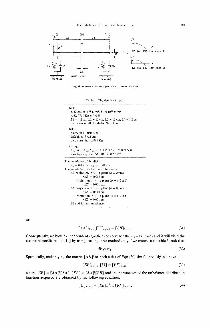
Fig. 4. A rotor-bearing system for numerical cases.

Table 1. The details of case 1

Shaft: E, G 2.07 x 1011N/'m 2, 8.1 x 101° N / m z p, Ks 7750 Kg /m 3, 0.68 L1 = 1.2 cm, L2 = 15cm, L3 = 15cm, L4 = 1.2cm diameters of all the shafts Df = 1 cm

Disk: diameter of disk 5 cm disk thick h 0.5 cm disk mass Ma 0.0761 Kg

Bearing: Kxx, Kyy, Kxy, Krx 2 .0x 106, 1.5 x 106, 0, 0 N / m Cx~, Cyy, Cxr, Cyx 200, 100, 0, 0 N . s /m

The unbalance of the disk: eax = 0.001 cm, ear = 0.001 cm.

The unbalance distribution of the shafts: L2 projection in x -- z plane (¢ = 0 rad)

r~(Z) = 0.001 cm; projection in y - z plane (4> = n/'2 rad)

r~,(Z) = 0.001 cm; L3 projection in x - z plane (¢, = 0 rad)

rx(Z) = 0.001 cm; projection in y - z plane (¢ = n/2 rad)

ry(Z) = 0.001 cm; LI and L4 no unbalance.

o r

[ A A ] ~ , [ U ] ~ , ~ , = [ B B ] ~ t. (31)

Consequently, we have 5k independent equations to solve for the ml unknowns and it will yield the estimated coefficient of [ U ] by using least squares method only if we choose a suitable k such that

5k t> ml. (32)

Specifically, multiplying the matrix [AA] t at both sides of Eqn (30) simultaneously, we have

[EEl . . . . . [U ] = [FF]m, ×a (33)

where [EEl = [AA]t[AA], [FF] = [AA] t [BB] and the parameters of the unbalance distribution function acquired are obtained by the following equation,

[U]m, ×1 = [EE]mll×,~, [FF],,1 ×1. (34)

850 Y u a n - P i n S h i h a n d A n - C h e n L e e

T a b l e 2. T h e d e t a i l s o f c a s e 2

T h e u n b a l a n c e o f t h e d i sk :

ed~ = 0.001 c m , ear = 0.001 cm.

T h e u n b a l a n c e d i s t r i b u t i o n o f t h e sha f t s :

L2 r~(Z) = O.O01"cos(r~z/L2) + O.O01-sin(zz/L2) ry(Z) = 0.001 - cos(fez~L2) + 0.001 - sin(nz/L2);

L3 rx(Z) = O.O01"cos(rcz/L3) + O.O01.sin(rcz/L3) ry(Z) = 0.001 . cos(rtz/L3) + 0.001 .sin(fez~L3);

L1 a n d L 4 n o u n b a l a n c e .

T a b l e 3. T h e d e t a i l s o f c a s e 3

T h e u n b a l a n c e o f t h e d i sk :

ed~ = 0.001 c m , edy = 0.001 c m .

T h e u n b a l a n c e d i s t r i b u t i o n o f t h e sha f t s :

L2 rx(Z) = 0 . 0 0 1 ' sin(fez~L2) ry ( Z ) = - 0 . 0 0 1 ' s in(fez/L2);

L3 r~(Z) = 0.001 .sin(nz/L3) ry(Z) = 0.001" sin(fez~L3);

L I a n d L 4 no u n b a l a n c e .

T a b l e 4. T h e n u m e r i c a l r e s u l t s o f c a s e 1

E x a c t ~1 - o)2(n = 2) o)l - ~o3(n = 3) col - ~o4(n = 4) o)1 - oJs(n = 5)

ed~ 0.001 9 .99904 x 10 - 4 9 .99908 x 10 - 4 9 .99906 x 10 _4 9 .99904 x 10 - 4 D i s k

ed~. 0.001 9 .99910 x 10 - 4 9 .99912 × 10 . 4 9 .99910 x 10 - 4 9.99911 x 10 - 4

c o n s t a n t t e r m 0.001 9 .99937 x 10 - 4 9 .99936 x 10 4 9 .99955 x 10 - 4 9 .99962 x 10 . 4

in x-z p l a n e

L 2 c o n s t a n t t e r m 0.001 9 .99969 x 10 - 4 9 .99965 x 10 - 4 9 .99971 x 10 _4 9 .99977 x 10 . 4

in y-z p l a n e

c o n s t a n t t e r m 0.001 9 .99936 x 10 - 4 9 .99937 x 10 - 4 9.99950 x 10 _4 9.99957 x 10 - 4

in x-z p l a n e L3

c o n s t a n t t e r m 0.001 9 .99968 x 10 - 4 9 .99952 x 10 - 4 9 .99967 x 10 - 4 9 .99973 x 10 '~

in y-z p l a n e

A v e r a g e e r r o r ( % ) - - 6 .2667 x 10 . 3 6.5 x 10 . 3 5.683 x 10 - 3 5 .2667 x 10 3

(uni t : c m )

T h e m e a s u r e m e n t s p e e d s o91, c,z , . . . , ~05 a r e c h o s e n as 117, 188, 292, 362, 487 ( rpm) .

T a b l e 5. T h e n u m e r i c a l r e su l t s o f c a s e 2

E x a c t (ol - m3(n = 3) (J)l - m4(n = 4) o91 - fos(n = 5) e) 1 - ~o6(n = 6)

edx 0.001 1.19157 × 10 - 3 1 .07264 × 10 3 1.01795 × 10 3 1 .00236 X 10 - 3 D i s k

edy 0.001 1.08155 X 10 - 3 9 .95921 × 10 - 4 9 .93450 X 10 - 4 9 .99738 X 10 - 4

c o n s t a n t 0 2 .2498 x 10 4 _ 8 .5479 x 1 0 - 5 _ 2.1201 x 1 0 - 5 _ 2 .8527 x 1 0 - 6

x-z cos(fez/L2) 0.001 1.14877 x 10 - 3 1.05655 x 10 . 3 1.01403 x 10 _3 1 .00189 x 10 - 3

sin(nz/L2) 0.001 1.23374 x 10 - 3 1.08878 x 10 - 3 1 .02202 x 10 3 1 .00296 x 1 0 - 3 L2

c o n s t a n t 0 -- 9 .4315 x 10 - 5 5 .04926 x 10 - 6 7 .78023 x 10 . 6 3 .05806 x 10 -~

y-z cos(~z/L2) 0.001 1.06212 x 1 0 - 3 9 .96614 x 10 4 9 .94842 x 10 - 4 9 .99798 x 10 - 4

sin(fez/L2) 0.001 1.09824 x 10 3 9 .94804 x 10 4 9 .91931 x 10 - 4 9 .99682 x 10 - 4

c o n s t a n t 0 - 1 . 9 6 2 6 x 1 0 4 _ 7 . 3 5 3 9 x 1 0 - 5 _ 1 . 7 8 6 4 x 1 0 - 5 - 2 . 1 8 8 6 x 1 0 6

x-z cos(gz/L3) 0.001 8 .37735 x 10 - 4 9 .38702 x 10 4 9 .84932 x 10 - 4 9 .98059 x 10 4

sin(Trz/L3) 0.001 1.17307 x 10 - 3 1.06437 x 10 . 3 1.01547 × 10 - 3 1 .00180 x 10 - 3 L 3

c o n s t a n t 0 - - 9 . 1 3 1 8 x 10 - 5 2 .70404 x 10 . 6 6 .19849 x 10 6 2 . 2 5 9 7 0 x 10 . 7

y-z cos(~zz/L3) 0.001 9 .28883 x 10 4 1 .00306 x 10 - 3 1.00541 x 10 - 3 1 .00020 x 1 0 - 3

sinOzz/'L3) 0.001 1.08474 x 10 - 3 9 .98411 x 10 - 4 9 .94806 x 10 4 9 .99818 × 10 - 4

A v e r a g e e r r o r ( % ) - - 1 3 . 6 7 2 % 3 . 7 9 6 7 % 1 . 1 9 9 7 % 0 . 1 2 6 4 %

(uni t : c m )

T h e m e a s u r e m e n t s p e e d s ¢~1, c,)2, . . . , e)6 a r e c h o s e n a s 9560, 9580, 9640, 9700, 11000, 12000 ( rpm) .


N U M E R I C A L E X A M P L E S

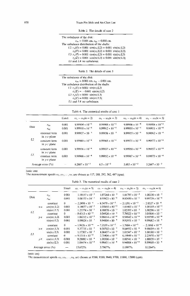
In this section, three numerical examples are presented to illustrate the feasibility and applicability of the proposed method. As shown in Fig. 4, a rotor system with separately-mounted bearings near the free ends is given. It is assumed that only the two central elements of the shafts (i.e. L2 and L3) and the disk, are unbalanced. The differences among the three cases are the unbalance distributions of the shafts, details of which are listed in Tables 1-3. In case 1, all shaft unbalances are assumed to be uniform. There are six unbalance parameters to be estimated for the disk and the shafts in this case. By Eqn (31), we at least need to measure two rotating speeds (k/> 2) to estimate the six parameters. Arbitrary simulated speeds are chosen for k = 2 - k = 5 and listed in Table 4 along with simulation results. This table shows that good results are obtained where the average error ranges from 0.00527% to 0.0065%. In case 2, the spatial unbalance distribution curve is specified, i.e. two terms of the Fourier series representation of the unbalance distribution of the shaft projected

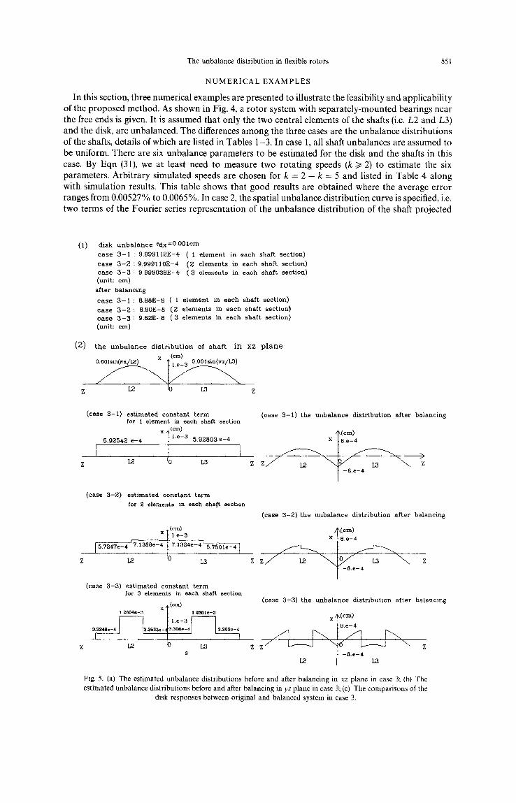
(1) disk u n b a l a n c e ectx=O.OOlcm

c a s e 3 - 1 : 9.999112E-4 ( 1 e lement in each shaf t section) ca se 3 - 2 : 9 . 9 9 9 1 1 0 E - 4 (2 e lements in each shaf t section) case 3 - 3 : 9.999038E-4 (3 e lements in each shaft section) (unit: cm) after balancing

case 3-i : g.88E-8 ( I element in each shaft section)

case 3-2: 8.90E-S (2 elements in each shaft sectioM c a s e 3 - 3 : 9 . 6 2 E - 8 ( 3 e lements in each shaf t section) (unit: cm)

(2) t h e u n b a l a n c e d i s t r i b u t i o n of s h a f t i n xz p l ane x (era)

(case 3-1 ) es t imated cons tan t t e rm for 1 element in each shaft section

x ¢(cm)

5.92542 e -4 ~ i .e-3 5.92803 e-4

Ii ' ' t I L2 '0 ' ' L 3 ' '

(case 3-2) estimated constant term

for 2 elemenLs in each shaft section

(cm) x ~ l.e-3

[ 5.7247e-4 ' 7.1386e-4 f 7,1324e-4 ' 5.7501e-4 I

. . . . i0 . . . . 12 L2

(case 3 -3 ) es t imated cons tan t t e rm for 3 elements in each shaft section

x I '(cm)

3i3348e-41 , , , 3.3~ 33e- .306T -4 3.3 2e-41

[2 L3 3

(case 3 - I ) Lhe unbalance d is t r ibut ion af ter balancing

/Ncm) x ~ 8 . e - 4

> Z

Fig. 5. (a) The estimated unbalance distributions before and after balancing in x z plane in case 3; (b) The estimated unbalance distr ibutions before and after balancing in yz plane in case 3; (c) The compar isons of the

disk responses between original and balanced system in case 3.

(case 3 -3) the unbalance d is t r ibut ion af ter balancing

x/~(cm)

(ease 3-2)the unbalance distribution afLer balancing

~(cm) x 1 8 . e - 4

,,--'7/-/-/-~, F , ~


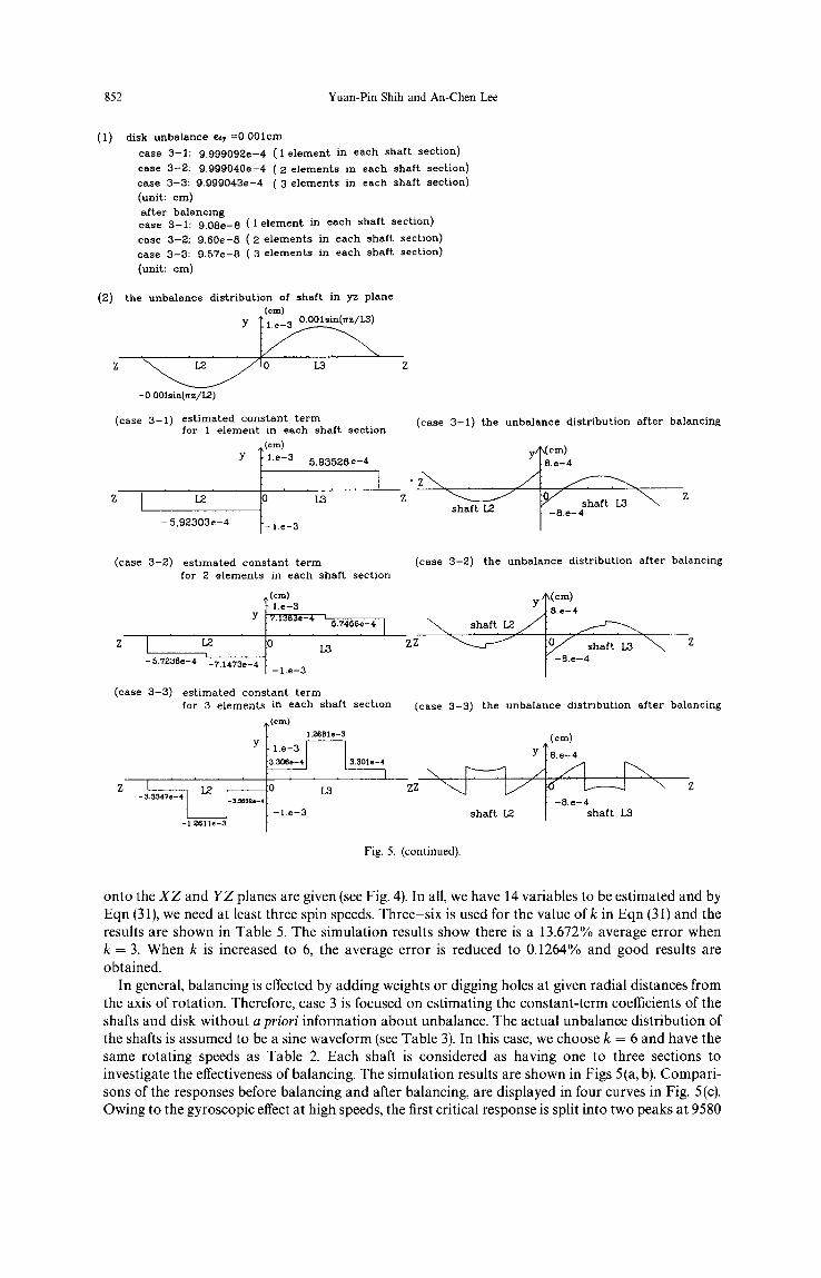
(1) disk unbalance edr =O.OOlcm case 3 - 1 : 9 . 9 9 9 0 9 2 e - 4 (1 e lement in each shaf t section) c a s e 3 - 2 : 9 . 9 9 9 0 4 0 e - 4 ( 2 e lements in each shaf t sect ion) c a s e 3 - 3 : 9 . 9 9 9 0 4 3 e - 4 ( 3 e lements in each shaf t section) (unit: cm) af ter balancing case 3 - 1 : 9 . 0 8 e - 8 (1 e l ement in each shaf t sect ion) case 3 - 2 : 9 . 6 0 e - 8 ( 2 e l ement s in each shaf t sect ion) case 3 - 3 : 9 . 5 7 e - 8 ( 3 e lements in each shalL section) (unit: cm)

(2) the unba lance d is t r ibut ion of shaf t in yz plane (era)

Z ~ L2 / / / / ~ 0 L3 Z

- O. O01sin(nz/].2)

(case 3-1) es t imated cons t an t t e rm for 1 e lement in each shaf t sect ion

. (era)

, , Y "I l'e-3, 5.93526e-4, I

Z I 1.2 L3 Z H

- 5,92303e-4 [- l .e-3

(case 3 -1 ) the unba lance d is t r ibu t ion af ter balancing

y,~(cm) /~ 8 . e - 4

shaf t L2 . e _ : h a f t !.3

(case 3 -2 ) es t imated cons t an t t e rm for 2 e lements in each shaf t sect ion

. . . . . Y 7151363e-4 L 5.7456e-4

Z ] L,2 L3 I i

- 5.7236e-4 -7.1473e-4 l .e-3

(case 3 -3 ) es t imated cons t an t t e rm for 3 e lements in each shaft sect ion

(era)

Y

[ 1.2 - 3 . S S 4 7 e - 4

-1 .2611e-3

1.2681e-3 1.e-3 - -

3.306e-4 ] 3.301e-4

- - 1 L3

- l . e - 3

(case 3 -2 ) the unba lance d is t r ibut ion af ter balancing

-.,.. shaft t z z t Z

(ease 3-31 the unba lance d is t r ibu t ion af te r balancing

(c,~) Y 18.e-4

zz \ z

shaft L2 | shaft 1.3

Fig. 5. (continued).

onto the X Z and Y Z planes are given (see Fig. 4). In all, we have 14 variables to be estimated and by Eqn (31), we need at least three spin speeds. Three six is used for the value o fk in Eqn (31) and the results are shown in Table 5. The simulation results show there is a 13.672% average error when k = 3. When k is increased to 6, the average error is reduced to 0.1264% and good results are obtained.

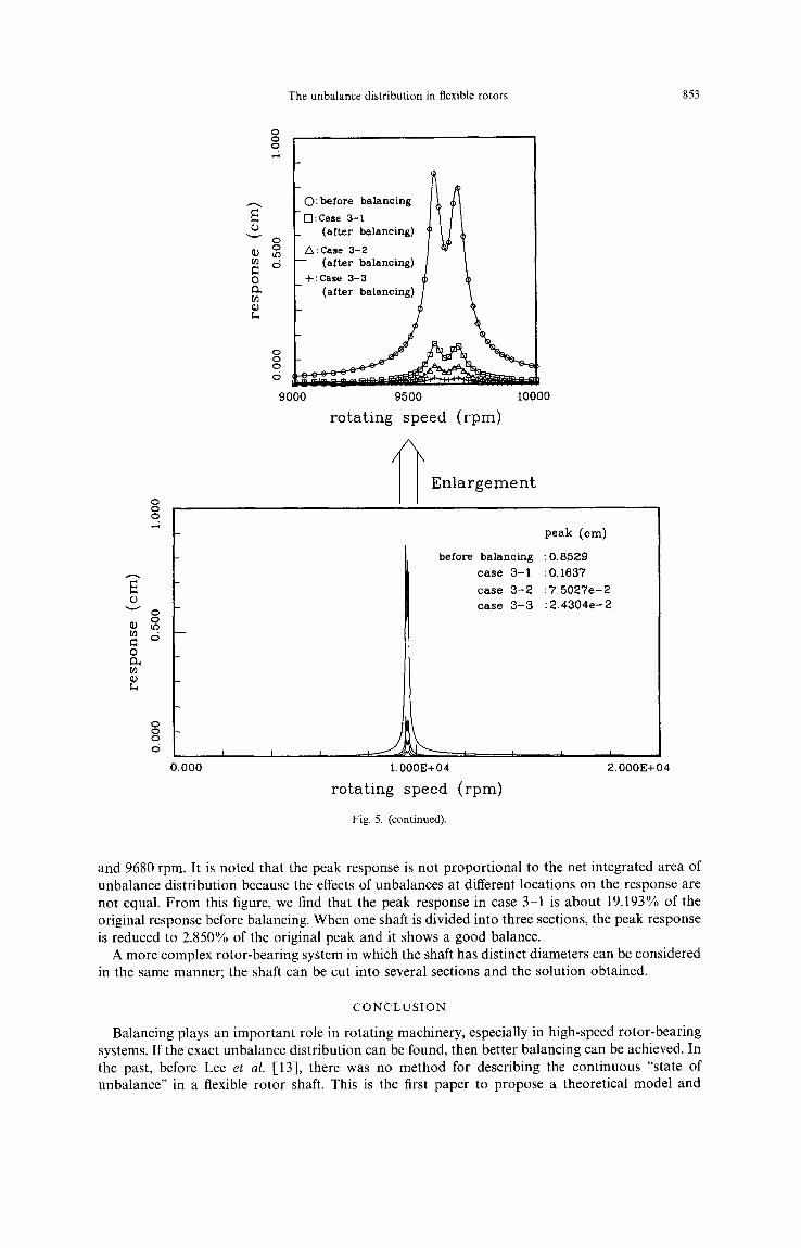
In general, balancing is effeeted by adding weights or digging holes at given radial distances from the axis of rotation. Therefore, case 3 is focused on estimating the constant-term coefficients of the shafts and disk without a priori information about unbalance. The actual unbalance distribution of the shafts is assumed to be a sine waveform (see Table 3). In this case, we choose k =- 6 and have the same rotating speeds as Table 2. Each shaft is considered as having one to three sections to investigate the effectiveness of balancing. The simulation results are shown in Figs 5(a, b). Compari- sons of the responses before balancing and after balancing, are displayed in four curves in Fig. 5(c). Owing to the gyroscopic effect at high speeds, the first critical response is split into two peaks at 9580


fi o

v

(u 09

0 C).,

(u L,

0 0 0

0

(5 -

0 0 0

(5

0.000

v

09

0

O 0 O

0

(5

0 0 0

d

9000

I I I

O: before balancing

- r-I: Case 3-1 (af ter balancing)

/x : Case 3-2 (af ter balancing)

+ : ea se 3-3

9500 10000

r o t a t i n g s p e e d ( r p m )

~ E n l a r g e r n e n t

p e a k ( e m )

before balancing :0 .8529

c a s e 3 - 1 :0.1637

case 3 - 2 : 7 . 5 0 2 7 e - 2 case 3 - 3 : 2 . 4 3 0 4 e - 2

J L_ 1.000E+04

r o t a t i n g s p e e d ( r p m )

2.000E+04

Fig. 5. (continued).

and 9680 rpm. It is noted that the peak response is not proportional to the net integrated area of unbalance distribution because the effects of unbalances at different locations on the response are not equal• From this figure, we find that the peak response in case 3-1 is about 19.193% of the original response before balancing. When one shaft is divided into three sections, the peak response is reduced to 2.850% of the original peak and it shows a good balance.

A more complex rotor-bearing system in which the shaft has distinct diameters can be considered in the same manner; the shaft can be cut into several sections and the solution obtained.

C O N C L U S I O N

Balancing plays an important role in rotating machinery, especially in high-speed rotor-bearing systems. If the exact unbalance distribution can be found, then better balancing can be achieved. In the past, before Lee et al. [13], there was no method for describing the continuous "state of unbalance" in a flexible rotor shaft. This is the first paper to propose a theoretical model and


e s t i m a t i o n t e c h n i q u e for f ind ing the u n b a l a n c e d i s t r i b u t i o n func t i on in a r o to r shaft. Th ree s imple

n u m e r i c a l cases are g iven a n d g o o d a p p r o x i m a t i o n s are ob t a ined . I t m a y be a new s tar t for ach iev ing

the be t t e r ba l an ce in ac tua l sys tems in the future.

Acknowledgements This study was supported by the National Science Council, Republic of China, under contract number NSC 81-0401-E-009-08.

R E F E R E N C E S

1. Bishop, R. E. D. and Gladwell, G. M. L., The vibration and balancing of an unbalanced rotor. Journal of Mechanical Engineering Science, 1959, 1(1) 66-77.

2. Kellenberger, W., Should a flexible rotor be balanced in n or (n + 2) planes? ASME Journal of Engineering for Industry, 1972, 94(2) 548 560.

3. Shimada, K. and Miwa, S., Balancing of a flexible rotor. Bulletin of the JSME, 1980, 23(180) 938-944. 4. Shimada, K. Fujisawa, F., Balancing method of multi-span, multi-bearings rotor system. Bulletin of the JSME, 1980,

23(185) 1894 1898. 5. Saito, S. and Azuma, T., Balancing of flexible rotors by the complex modal method. ASME Journal of Vibration,

Acoustics, Stress and Reliability in Design, 1983, 105, 94 100. 6. Goodman, T. P., A least-squares method for computing balance corrections. ASME Journal of Engineering for Industry,

Series B, 1964, 86(3) 273 279. 7. Lund, J. W. and Tonnesen, J., Analysis and experiments on multi-plane balancing of a flexible rotor. ASME Journal of

Engineering for Industry', 1972, 233 242. 8. Tessarzik, J. M. and Badgley, R. H., Experimental evaluation of the exact point-speed and least-squares procedures for

flexible rotor balancing by the influence coefficient method. ASME Journal of Engineering for Industry', Series B, 1974, 96(2) 633- 643

9. Tessarzik, J. M., Badgley, R. H. and Anderson, W. J., Flexible rotor balancing by the exact point-speed influence coefficient method. ASME Journal of Engineering for Industry, Series B, 1972, 94(1) 148-158.

10. Tessarzik, J. M., Badgley, R. H. and Fleming, D. P., Experimental evaluation of multiplane-multispeed rotor balancing through multiple critical speeds. ASME Journal of Engineering for Industry, 1976, 988 998.

11. Everett, L. J., Two-plane balancing of a rotor system without phase response measurements. ASME Journal of Vibration, Acoustics, Stress and Reliability in Design, 1987, 109, 162 167.

12. Ehrich, F. F., Handbook of Rotordynamics. McGraw-Hill, New York, 1992. 13. Lee, A. C., Shih, Y. P. and Kang Y., The analysis of linear rotor-bearing systems: a general transfer matrix method. ASME

Journal of Vibration and Acoustics, 1993, 115, 490-497. 14. Wylie, C. R. and Barrett, L. C., Advanced Engineering Mathematics. McGraw-Hill, New York, 1982, Chapter 7. 15. Lee, A. C., Kang, Y. and Liu, S. L., A modified transfer matrix method for the linear rotor-bearing system. ASME Journal

of Applied Mechanics, 1991, 58, 776-783.

A P P E N D I X A

F1 17 = X~ = (~o + / nTzZ n/~Z~

' . = L ~ " cos T + ~ " = ' sin---L-- ) [ P I ] [ V I ]

F2,17 = (FI,1Q' = [P2] [VI]

F3,17 = (F2,17)' = [P3] [Vt]

Fa. 17 = (F3.17) ' = [P , ] [VI]

Fs.l? = X~ = [P1]EV2]

F6,17 = (F5,17)' = [P2]EV2]

F7,17 = (F6,17)' = [P3][V2]

F8,13 = (/;'7,17)' = [e4] IV2]

E~,,; = Yf = [PI][V3]

Flo. 17 = (eg, 17)' = [P21 IV3]

FI,.,, = (60.,~)' = [P~] IV3]

F12,17 = (Fl,.17)' = [P4] [V3]

F~3.17 = r ~ = [ P d [ v ~ ]

FI4. I 7 = (F13.17)' = [P2] IV4]

F, 5. , 7 = (F14,17)' = [P3] IV4]

FI6.17 = {F15.17)' = [/:'4] [I/4] (A1)


where

I 2$Z nT~z . r17£.~ 1 [P1 ] = I cos ~ s in -~L . . . . . cos ~ - - sm

[ P 2 ] = 0 - -~sinnz ~_cosnZ .., ___nnsm" __nnz __nncos~_ L L L L '" L L L

g Z n / ' ~ 2 / 1 7 ~ Z sin [ P 3 ] = [ 0 - ( L ) Z C O S L - ( L ) Z s i n ~ . . . . . - ( - ~ - ) cos L ( L ) z nLz ]

[ P 4 ] = [ O ( L ) 3 s i n L - \L/(n~3c°snzL . . . . . ( L ) 3sinnn-'fz \ ~ / ~ - J

E V i l = E¢lO ]~eel ~Sl . . . . . lffcCn ,aSn] 1, IV2] = [~20 ,//sCl ~ 1 . . . . . ,/'/sen #~n] t

l-V3] = [~3o v'gl vgt . . . . . v~. v~.]', [V*] = [ff*o v~l v~l . . . . . v~. v~.] t.

The relations between the nth term of the Fourier series representing the unbalance function (see Eqn (3)) and the nth term of the particular solution in Eqn (6) can be obtained as below

_ _ m

#L ,c

~cn s

Vcn ~, c n

i v~.

= ~7 n "

m

A. 0

0 A.

0 0

0 0

0 - C .

C. 0

B. 0

0 - B.

al l )n al2)n

a21)n a22)n

a31) . a32) .

a41)n a . 2 ) .

a~l). a~2).

a61)n a62)n

a71) . a72)n

a~). as~).

0 0 0 C. - B. 0

0 0 -- C. 0 0 - B.

A. 0 B. 0 0 C.

0 A. 0 B. - C. 0

B. 0 A. 0 0 0

0 B. 0 A. 0 0

0 - C . 0 0 A. 0

C. 0 0 0 0 A.

- 1 - -

?'on COS ~b

rsn COS

- r~. sin 0

- r~. sin q5

r0. sin 0

r~. sin 4~

rcn COS ~b

Psn COS

E;::] ,A2,

where

By substituting n = 1 to

O- n 2 2 t92 4 2 4 p ' A ' t o 2 pm f n n ~ o 2p 09 T Tpo92

KZ -i' d= lK--

pro 2 po) 2 P p2(O4 p" A" co 2 2pm2 k = 2p2~°4

f l = - ' - f f - + K ~ - - E ~ ' g - K~G'--~ E1 h = E K~G~ '

( L ) 2 B . = - h +k , (7) (7/ C . = d - -c - - .

n = n into the above equation, those equations can be rearranged into the following four forms

m - - m

~1o ¢'1

~1 0

#~1 0

#~2 0

~2 0

#L 0

0 0 0 0 ... 0 0

a l l h alz)l 0 0 ..- 0 0

a21) l a22)1 0 0 . '- 0 0

0 0 a l l ) 2 a12)2 -'- 0 0

0 0 a21)2 a22)2 . . . 0 0

0 0 0 0 "'" a l l ) . a12).

0 0 0 0 "'" a21)n az2~

ro

rcl

rsl

rc2

/'s2

/'cn

rsn


p m

v g20

#h

/zg2

m

c2 0 0

0 aal}l a32)1

0 a41)l a42)1

0 0

0 0

0 0

0 0

m

0 0 --. 0 0

0 0 ... 0 0

0 0 .-. 0 0

0 a31)2 a32)2 ..- 0 0

0 a4l)2 a42)2 ' " 0 0

0 0 0 " " a31)n a32)n

0 0 0 "'" a41)n a42)n

ro

rcl

rsl

rc2

rs2

rcn

rsn

m m

v k.3o

,s Vcl ,c

¥c2

v~2

,¢ Vcn

v~.

C 3 0 0 0 0 " " 0 0

0 a51)1 a52)1 0 0 --. 0 0

0 a61)l a62)1 0 0 --. 0 0

0 0 0 a51)2 a52)2 --. 0 0

0 0 0 a61)2 a62)2 --- 0 0

0 0 0 0 0 "'" a s l j , as2),

0 0 0 0 0 " " a61)n a62)n

- - w

ro

rcl

rsl

rc2

rs2

rcn

rsn

m m

g4o ,¢

Vsl ,s

~sl ,¢

~s2

Y~2

c4 0 0 0

0 a71) l a72)1 0

0 as1)1 a82)l 0

0 0

0 0

0 0

0 0

0 -.. 0 0

0 ... 0 0

0 ... 0 0

0 a71)2 a72)2 --" 0 0

0 a81)2 a82)2 .." 0 0

0 0 0 "'" aT1) . avz)n

0 0 0 "" aSl)n asz)n

r 0

rcl

rsl

re2

rs2

rcn

r s n

where

C 1 : - - ~- 9 E1 K~GE f

1 ( -- p ' A ' o ) 2 ' s i n ( b p2 • ~04 • sin ~b)

9 \ E1 KsGE

1 ( p - A - eft. sin q5 p2. ~04 sin qS~ C 3 = - - ~- y e t X-~6-~ ;

1 (p'A'ooZ'cos(p p2 " f-O4" COS ~b.~ C4 = - 4 9 El K~GE }

For simplicity, the above four equations can be written as below

[ v , ] = [ Y I ] [ G ]

IV2] = [Y2] [U~]

[V3] = [Y~][U~]

[V4] = [Y4] [Us]

where [U,] = [ro r¢l r~l re2 rsz . . . . . re, rs,]'. Introducing (A3) into Eqn (A1), the elements of [Kf] can be acquired.

A P P E N D I X B

[Tbl] [-T~I ] m 0--1×16 1 _0J×16 1

L --01×16 1

(A3)


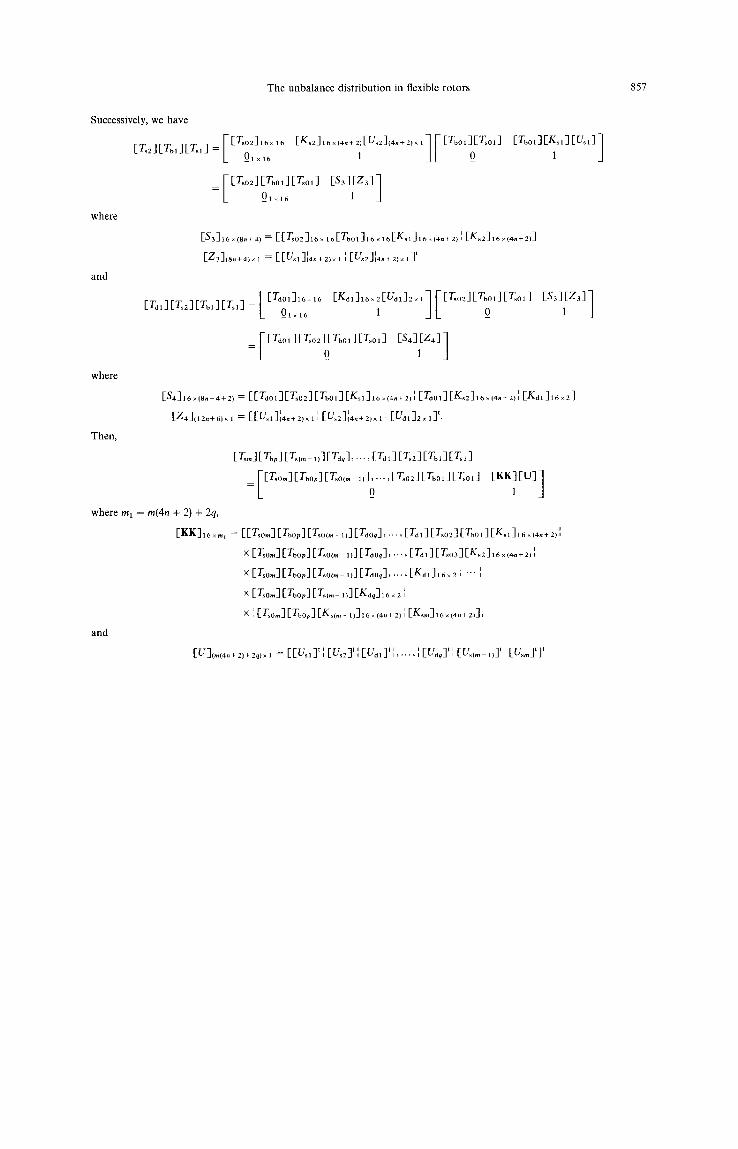
Successively, we have

I [-Ts02] 16x 16 [Ks2]16×(4n+;,[Us2](4n+2)×l][[Tbol][oTsoll [Ts2][Tbl][Tsl] = L __Olx 16

= [ [T~o2] [Tbo,] [~o l ] [S3]~Z3] ]

L o,~,6

where

and

where

Then,

[$3116×(8n+4 ) = [ITs02116 x 16[Tbolll6 × 16[Ksl]16×{4n+2) I [Ks2]16×(4n+2i]

[ Z 3 ] ( s . + , * ) × 1 ' ' = [Us2]{4n+2)× i ] t [-[Usl l(~l.n + 2)× 1 I I

[Tdl][T'2][Tbl][Tsl] =L O-L~16

=I[Tdol][Ts02][O zbO1][TsOl] [$4]~Z4] I

[-Tb011 ]-Ksl ] [Usl ] I

[$4316×18n+4-+2) = [[Ydol l[Yso2][YboL l[Ksl ll6×(4n+ 2) l [Taol][K~2]16×~a.+ 2) ll [Kdl]16×2]

I_Z4]{12n+6) x 1 = [[Usl]i4n~,2)×l l [Us2]t~4.+2)× 1 { [Ual]2× L]t.

where mL = m(4n + 2) + 2q,

[-$3 ]~ Z31 ]

and

[T~.] [TbA [T.~_ ~,] [Td.] ..... [Tal] [%2 ] [T~ ] [T.~ ]

FET, o.3 [ T.o.3 [~o,~- ,,] ..... [Tso=] [Tbol ] [T~o 1 ]

L _o [KKIeU] ]

x [T~o~] [Tbo. ] [ ~ 0 ~ . - . ] [Tdo~] . . . . . [ T d d [%03] [Ks2]~6 ×~.+ 2~ ',

x [T~om] [Tb0v] [T,o~,~- I) ] [Taoq] . . . . . [Ka l ] 16 × 2 ', " " ',

x [ T .o . ] [ Tbo~] [ T ~ . _ ~ ] [ K ~ ] ~ ~ = I

..... [u~ ] t', [u~c~ ld", [u~] ' ] '

pergamon - national chiao tung university · the unbalance distribution in flexible rotors 845...

Documents