permeability prediction and diagenesis in tight carbonates
TRANSCRIPT

This is a repository copy of Permeability Prediction and Diagenesis in Tight Carbonates Using Machine Learning Techniques.
White Rose Research Online URL for this paper:http://eprints.whiterose.ac.uk/152231/
Version: Accepted Version
Article:
Al Khalifa, H, Glover, PWJ orcid.org/0000-0003-1715-5474 and Lorinczi, P (2020) Permeability Prediction and Diagenesis in Tight Carbonates Using Machine Learning Techniques. Marine and Petroleum Geology, 112. 104096. ISSN 0264-8172
https://doi.org/10.1016/j.marpetgeo.2019.104096
© 2019 Elsevier Ltd. Licensed under the Creative Commons Attribution-NonCommercial-NoDerivatives 4.0 International License (http://creativecommons.org/licenses/by-nc-nd/4.0/).
[email protected]://eprints.whiterose.ac.uk/
Reuse
This article is distributed under the terms of the Creative Commons Attribution-NonCommercial-NoDerivs (CC BY-NC-ND) licence. This licence only allows you to download this work and share it with others as long as you credit the authors, but you can’t change the article in any way or use it commercially. More information and the full terms of the licence here: https://creativecommons.org/licenses/
Takedown
If you consider content in White Rose Research Online to be in breach of UK law, please notify us by emailing [email protected] including the URL of the record and the reason for the withdrawal request.
1
Permeability Prediction and Diagenesis in Tight 1
Carbonates Using Machine Learning Techniques 2
Al Khalifah, H.*, Glover, P.W.J.**, Lorinczi, P. 3
School of Earth and Environment, University of Leeds, UK 4
* Email: [email protected] 5
** Email: [email protected], Tel: +44 (0)113 3435213 6
7
ABSTRACT. Machine learning techniques have found their way into many problems in 8
geoscience but have not been used significantly in the analysis of tight rocks. We present a case 9
study testing the effectiveness of artificial neural networks and genetic algorithms for the 10
prediction of permeability in tight carbonate rocks. The dataset consists of 130 core plugs from 11
the Portland Formation in southern England, all of which have measurements of Klinkenberg-12
corrected permeability, helium porosity, characteristic pore throat diameter, and formation 13
resistivity. Permeability has been predicted using genetic algorithms and artificial neural 14
networks, as well as seven conventional ‘benchmark’ models with which the machine learning 15
techniques have been compared. The genetic algorithm technique has provided a new empirical 16
equation that fits the measured permeability better than any of the seven conventional 17
benchmark models. However, the artificial neural network technique provided the best overall 18
prediction method, quantified by the lowest the root-mean-square error (RMSE) and highest 19
coefficient of determination value (R2). The lowest RMSE from the conventional permeability 20
equations was from the RGPZ equation, which predicted the test dataset with an RMSE of 21
0.458, while the highest RMSE came from the Berg equation, with an RMSE of 2.368. By 22
comparison, the RMSE for the genetic algorithm and artificial neural network methods were 23
0.433 and 0.38, respectively. We attribute the better performance of machine learning 24
techniques over conventional approaches to their enhanced capability to model the connectivity 25
of pore microstructures caused by codependent and competing diagenetic processes. We also 26
provide a qualitative model for the poroperm characteristics of tight carbonate rocks modified 27
by each of eight diagenetic processes. We conclude that, for tight carbonate reservoirs, both 28
machine learning techniques predict permeability more reliably and more accurately than 29
conventional models and may be capable of distinguishing quantitatively between pore 30
microstructures caused by different diagenetic processes. 31
KEYWORDS: permeability, neural networks, genetic algorithms, machine learning, tight 32
carbonates, MICP, porosity, diagenesis.33

2
Introduction 34
The permeability of reservoir rocks needs to be measured with a high accuracy in order to 35
maximize the efficiency of hydrocarbon production from unconventional reservoirs (Ma and 36
Holditch, 2015). The pulse-decay method is an efficient method for measuring permeability in 37
very tight rocks (Rashid et al., 2017; Hussein et al., 2017). This technique measures the 38
reduction in the inlet pressure of a fixed volume of gas as it passes into a low permeability 39
sample. However, for very tight core plugs this measurement can take many hours. 40
Furthermore, multiple measurements are required at different gas pressures in order to calculate 41
the Klinkenberg-corrected permeability (Zhang et al., 2013). Since all tight rocks are extremely 42
sensitive to gas slippage, this correction is extremely important if an accurate permeability is 43
required (Akai et al., 2016). Each of these measurements is expensive, and consequently a 44
limited number of core plugs can be measured in any given reservoir. Furthermore, tight 45
carbonate reservoirs have a tendency to be heterogeneous, resulting from patchy development 46
of a range of different diagenetic properties (Al -Zainaldin et al., 2015; Glover et al., 2018), 47
leading to a variability in petrophysical properties and reservoir quality over a range of scales. 48
It is generally not possible to representatively sample and measure the permeability of 49
heterogeneous tight carbonate reservoirs because to do so would require an unfeasibly large 50
and expensive dataset. A quicker, less expensive and more reliable way to estimate the 51
permeability of very tight and heterogeneous reservoir rocks would, therefore, be a valuable 52
and welcome technical resource in the characterisation of these reservoirs. 53
In this paper, we have assessed the capability of two machine learning techniques for the 54
estimation of the permeability of tight carbonate rocks using a limited set of input parameters 55
that can be obtained easily, cheaply, and often routinely from core analysis measurements. The 56
first technique is the use of artificial neural networks (e.g., Rajasekaran and Pai, 2003), while 57
the second technique uses genetic algorithms (e.g., Cuddy and Glover, 2002; Rajasekaran and 58
Pai, 2003). The results have been compared against the predicted permeabilities from a set of 59
seven of the best currently available theoretical and empirical permeability prediction models 60
(equations) from the literature (e.g., Rashid et al., 2015a; 2015b). 61
It is not the intention of this paper to be a review of either machine learning, or of neural 62
networks or genetic algorithms, or even a review of the application of these approaches to 63
geophysical problems. There is a very rich literature for the former, the latter is served by a 64
very good reviews (e.g., Van der Baan and Jutten, 2000; Sen and Mallik, 2018). For neural 65
networks alone, there is a distinction to be made between feedforward multilayer perceptron 66

3
network (MLPN) and radial basis function (RBF) types. The former, itself has many types, 67
including probabilistic approaches (PNN), time delay neural networks (TDNN), convolutional 68
neural networks (CNN), deep stacking and tensor deep stacking neural networks (DSNN and 69
TDSNN). It is far better that we consider some of the recent applications of machine learning 70
to petrophysical applications. While there are many possible applications, recent advances have 71
included all aspects of petrophysics from logging, through facies determination and rock 72
characterisation to the determination of key parameters for calculating reservoir volumetrics 73
and permeability. 74
In logging both integrated hybrid neural network (IHNN) (Zhu et al., 2018) and Integrated 75
Deep Learning Models (IDLM) (Zhu et al., 2019a) have been implemented in order to improve 76
the estimation of total organic carbon (TOC) significantly, allowing the characterisation of 77
shale gas reservoirs to be improved, while Onalo et al. (2018; 2019) have used a non-linear 78
autoregressive neural networks with exogenous input (NARX) to estimate the shear and 79
compressional sonic travel times in well logs, finding sufficiently accurate predictions of the 80
actual sonic well logs that many of the sonic properties including sonic porosity, Poisson’s 81
ratio were capable of being predicted. 82
Machine learning has also been used to determine the optimal parameters for reservoir 83
characterisation. A good example of this is Zhu et al.’s recent study (Zhu et al., 2019b) of water 84
saturation in organic shale reservoirs, where the parameters of a shale petrophysical model are 85
calculated using genetic algorithms. The approach does not need electrical measurements as 86
input, which makes it ideally suitable for organic shale reservoirs. The characterisation of 87
fractures in reservoirs is also a multi-parameter problem which cannot be approached simply. 88
A combination of genetic algorithms and back propagation neural networks (BPNN) has been 89
found to have the ability to predict fracture zones using deep and shallow electrical logs as 90
input (Xue et al., 2014). 91
Facies determination and petrophysical characterisation is a clear beneficiary of machine 92
learning techniques. Back propagation neural networks and convolutional neural networks 93
have been used to improve the estimation of total organic carbon, as well as volatile 94
hydrocarbon and remaining hydrocarbon determinations in shale oil reservoirs (Wang et al, 95
2019), outperforming conventional methodologies for estimating these parameters. 96
In this work, we are interested in the prediction of permeability in tight carbonate rocks and 97
the effect of diagenesis. Lim and Kim (2004) proposed fuzzy logic and neural network 98
approaches to the prediction of porosity and permeability in reservoirs, indicating that the 99
approaches showed some potential for future development. Tang (2008) and Tang et al. (2011) 100

4
have used probabilistic neural networks to classify facies in carbonate reservoirs with some 101
degree of success. Zhou et al. (2019) have combined the study of diagenesis with the use of a 102
deep-autoencoder random forest algorithm to determine the link between different states of 103
diagenesis and the electrical parameters (m and n values) of tight gas sandstone reservoirs, 104
while Zhu et al. (2017a; 2017b) were able to produce a reasonable prediction of permeability 105
in tight gas sandstone reservoirs using a complex combination of machine learning techniques 106
and input from NMR data, giving results comparable to those obtained by Rashid et al. (2015b) 107
with conventional permeability prediction approaches. 108
While there are many papers now available in the literature exploring machine learning 109
methods for permeability prediction, fewer compared approaches together and also with a 110
cohort of conventional prediction methods. In addition, there are very few which concentrate 111
on the prediction of permeability in challenging tight carbonate reservoirs. Considering that 112
this type of unconventional reservoir is likely to be more important in the future, and that 113
conventional experimental determination of permeability in very low permeability rocks is 114
complex, time-consuming and expensive, the use of machine learning could be a method of 115
choice if it is found to be reliable. In this work we also consider the interplay between machine 116
learning efficacy and its derived parameters with the diagenetic processes that control 117
permeability in these rocks. 118
119
Dataset 120
The core plug dataset consisted of 130 samples derived from the Portland Formation, which 121
crops out in quarries on the Isle of Portland in southern England. The samples were all sourced 122
from either the Jordans quarry and mine, or the Fancy Beach quarry, which are all in close 123
proximity at 50o33’10”N 02o26’25”W, and which are operated by Albion Stone. The Isle of 124
Portland is composed mostly of Upper Jurassic marine strata with a small thickness of basal 125
Cretaceous Purbeck Formation on top. The lowest formation to be exposed in the area is the 126
Upper Jurassic Kimmeridge Clay, which occurs beneath Portland Harbour and Castletown and 127
is exposed under the foot of the high northern cliffs. Above it lies the Portland Sand, which is 128
composed largely of marls with some sandy horizons. The true Portland Stone lies above the 129
Portland Sand and consists of the Portland Cherty Series overlain by the Portland Freestone. 130
The Portland Freestone is a well-cemented oolitic limestone. Stone from the various beds of 131
the Portland Freestone have historically and contemporaneously been in much demand as fine 132
5
building stone (e.g., St. Paul’s Cathedral). The Purbeck sequence lies on top of the Portland 133
Freestone and marks the bottom of the Cretaceous. 134
The samples used in this work have been sourced from the Base Bed and the Whitbed, which 135
occur in the Portland Freestone, and which are dominated by sparite-cemented oolites (Barton 136
et al., 2011). The Whitbed contains common shells, usually distributed evenly but sometimes 137
concentrated in zones. These shells are commonly cemented. The Base bed is less shelly and 138
commonly contains completely cemented shell moulds. The cemented nature of this rock 139
makes it ideal building stone as well as a good, well-studied tight carbonate reservoir analogue. 140
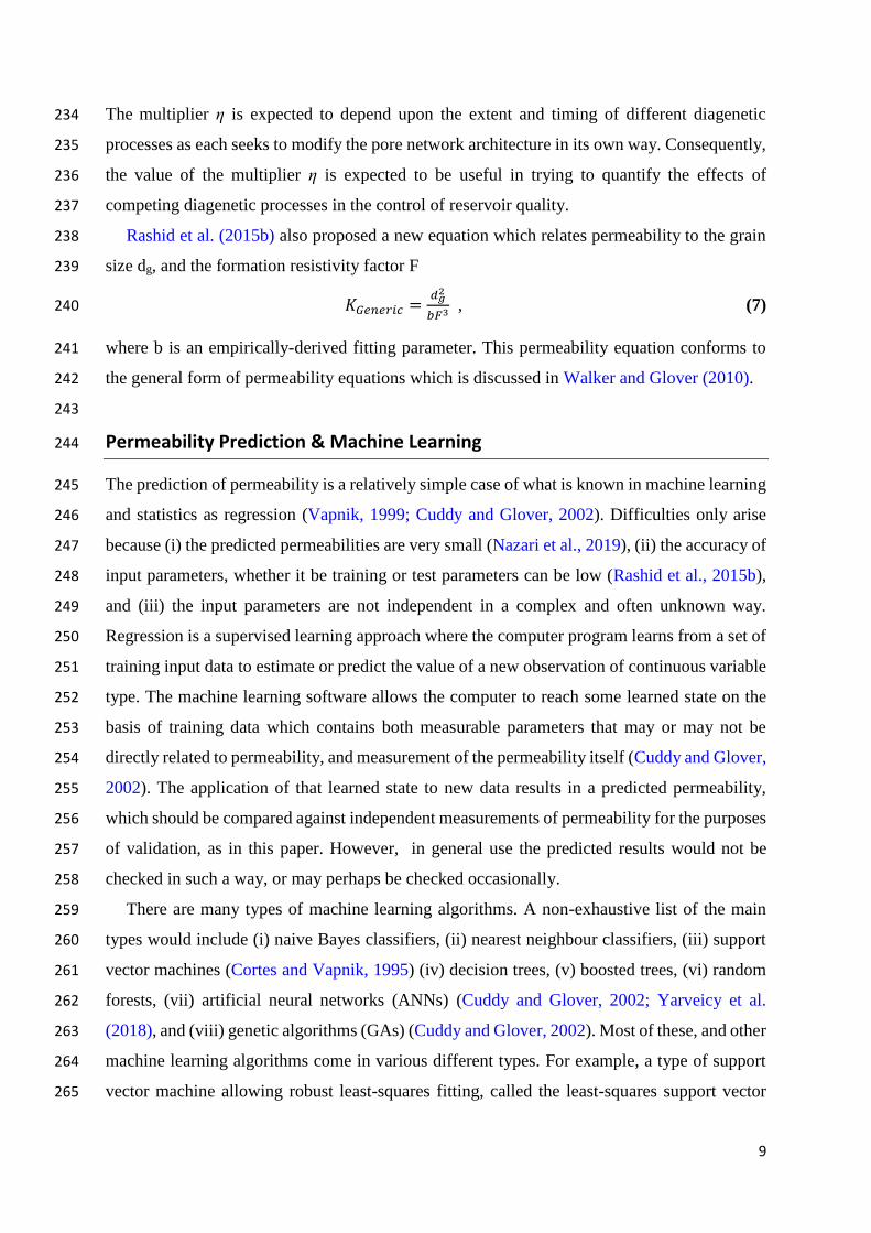
Helium porosity , characteristic pore throat size from mercury injection capillary pressure 141
measurements dPT, formation resistivity factor F, and fluid permeability k were measured on 142
each sample at the University of Aberdeen and by oil service companies in the late 1990s. 143
Table 1 gives a summary of these measurements. 144
The helium porosity was measured on dried 1.5” core plugs using a helium pycnometer that 145
had been built in the laboratory and optimised to allow measurements to be made with an error 146
of better than ±0.001, and provides measurements with approximately five times better 147
accuracy than typical standard automated commercial pycnometers. Porosity was also 148
calculated by water saturation and Archimedes bulk volume, but the difficulty in fully 149
saturating these tight carbonates resulted in discrepancies of greater than 0.05, which led us to 150
discount using the saturation porosity measurements for permeability prediction with 151
conventional methods. The mercury injection capillary measurements were made with a 152
Micromeritics Autopore V, with a maximum applied pressure of 60,000 psi. Formation factor 153
was calculated from saturated sample conductivity and saturating fluid resistivity, both 154
measured using a Quadtech LCR meter at the frequency where the quadrature component was 155
minimised (approximately 1 kHz) according to the methodologies set out in Glover (2015). 156
The observed incompleteness of saturation in some samples leads us to believe that the 157
formation factors and cementation exponents measured in this work may be in more error than 158
some of the other core measurements. However, as we will see later, such errors do not translate 159
into large errors in predicted permeability when using conventional permeability prediction 160
equations. 161
Since it is a critical parameter in the comparative analyses carried out in this work, a 162
considerable amount of effort was put into measuring the permeability of the samples 163
accurately using both steady-state measurements and pulse-decay measurements. The former 164
of these was used to measure the higher permeability samples, while the latter was used for the 165
6
tighter samples. Klinkenberg-corrected steady-state helium gas permeability was measured on 166
a bespoke gas permeability rig composing three ranges of gas pressure application and three 167
ranges of gas flow measurement. Pulse-decay measurements were made using helium as the 168
process gas according to the methodology given in Jones (1997). For both the steady-state and 169
pulse-decay measurements, Klinkenberg corrections were made based on at least 5 effective 170
pressure measurements, while measurements which did not provide the required linear plot of 171
apparent permeability against the inverse mean effective flow pressure were discarded. 172
A graphical summary of the dataset is shown in Figure 1. A portion (100) of the 130 samples 173
were used as a training data set for both of the machine learning applications, and in those 5 174
conventional models which required calibration of one or more constant values in their 175
formulae. 176
177
Conventional Permeability Models 178
A total of seven conventional permeability equations were implemented on the dataset to 179
compare with the results of the machine learning methods. The first is based on one of the 180
earliest permeability models proposed by Kozeny (1927), and modified later by Carman 181
(1937). The modified equation is commonly written (e.g., Glover et al., 2006) as 182 暫皐伺子蚕仔姿貸察珊司仕珊仔 噺 算纂賛匝 蒔惣岫層貸蒔岻匝 , (1) 183
where 轄 is porosity, dg is the mean grain size in µm, and c is a constant. Though commonly 184
used, the Kozeny-Carman relationship has been superseded by other models due to its inability 185
to take account of dead-end pores (Walker and Glover, 2010). The constant is usually found 186
empirically, though some ‘standard’ but often erroneous values have been published. 187
188
Table 1. Statistical summary of the limestone dataset used in this work. 189
Porosity (-)
Formation resistivity factor
(-)
Characteristic pore throat
diameter (m)
Permeability (mD)
Maximum 0.265 200 2.27×10⁻⁷ 0.185 Minimum 0.107 17 3.92×10⁻¹⁰ 1.917×10⁻⁶ Arithmetic
mean 0.179 62.3 2.88×10⁻⁸ 0.00525
Standard deviation
0.0371 29.6 4.06×10⁻⁸ 0.0202
Skewness 0.264 1.56 2.85 6.73 190

7
Figure 1. Graphical view of the 191
Portland dataset. Histograms of 192
parameters are shown on the 193
diagonal, while the cross-plots 194
describe the strength of 195
correlation between parameters. 196
Note the logarithmic 197
transformation applied on some 198
parameters in this figure. Phi = 199
total (He) porosity, dPT = pore 200
throat diameter (m), F = 201
Formation Factor, K = 202
Klinkenberg-corrected pulse-203
decay permeability (mD).204

8
The second equation is that of Berg (1975), which is 205 倦喋 噺 ぱ┻ね 抜 など貸態穴直態剛泰┻怠 , (2) 206
where the permeability is in m2, while the porosity 轄 is fractional, and dg is the mean grain 207
diameter in meters. This model was derived empirically from a mixed dataset including 208
carbonates, but not containing tight carbonates. Consequently, this model was not expected to 209
perform well in tight carbonates (Rashid et al., 2015b), an expectation that was borne out in 210
the results. 211
A similar equation was derived empirically by Van Baaren (Van Baaren, 1979) 212 倦蝶喋 噺 など穴鳥態剛岫戴┻滞替袋陳岻稽貸戴┻滞替 , (3) 213
where dd is the dominant modal grain size in metres, m is the cementation exponent, and B is a 214
sorting index, which is equal to 0.7 for extremely well sorted grains, and unity for extremely 215
poorly sorted grains (Glover et al., 2006). Since the sorting index is unknown here, it was 216
treated as an empirical parameter to be found from fitting the training data. 217
Unlike the previous three empirical models, the RGPZ equation is an analytically-derived 218
permeability model based on electro-kinetic theory (Glover et al., 2006). This model has both 219
an approximate and an exact form (Glover et al., 2006; Rashid et al., 2015a; 2015b) 220
倦眺弔牒跳貸銚椎椎追墜掴沈陳銚痛勅 噺 鳥虹鉄 笛典尿替銚陳鉄 , and (4) 221
倦眺弔牒跳e勅掴銚頂痛 噺 鳥虹鉄替銚陳鉄庁岫庁貸怠岻鉄 , (5) 222
where k is in m2, 轄 is porosity, dg is the grain size in meters, m is the cementation exponent, a 223
is a constant equal to 8/3 for spherical grains, and F is the formation resistivity factor. The 224
approximate form can be used only if F>>1, which for the purposes of the model practically 225
means F>20. Since all tight rocks will conform to this limitation, the approximate form of the 226
RGPZ equation should perform as well as the exact form. 227
Rashid et al. (2015b) proposed a modified form of the original RGPZ equation to 228
account for the fact that carbonate pores are less connected than pores in sandstones. The 229
resulting modified RGPZ equation for carbonates includes a multiplier さ which is carbonate 230
microstructure-dependent. The addition of this multiplier essentially converts Eqs. (4) and (5) 231
into empirical relationships with さ as a fitting parameter (Rashid et al., 2015a; 2015b) 232 倦眺弔牒跳貸頂銚追長墜津銚痛勅 噺 鳥虹鉄替銚陳鉄挺庁岫挺庁貸怠岻鉄 . (6) 233
9
The multiplier さ is expected to depend upon the extent and timing of different diagenetic 234
processes as each seeks to modify the pore network architecture in its own way. Consequently, 235
the value of the multiplier さ is expected to be useful in trying to quantify the effects of 236
competing diagenetic processes in the control of reservoir quality. 237
Rashid et al. (2015b) also proposed a new equation which relates permeability to the grain 238
size dg, and the formation resistivity factor F 239 計弔勅津勅追沈頂 噺 鳥虹鉄長庁典 , (7) 240
where b is an empirically-derived fitting parameter. This permeability equation conforms to 241
the general form of permeability equations which is discussed in Walker and Glover (2010). 242
243
Permeability Prediction & Machine Learning 244
The prediction of permeability is a relatively simple case of what is known in machine learning 245
and statistics as regression (Vapnik, 1999; Cuddy and Glover, 2002). Difficulties only arise 246
because (i) the predicted permeabilities are very small (Nazari et al., 2019), (ii) the accuracy of 247
input parameters, whether it be training or test parameters can be low (Rashid et al., 2015b), 248
and (iii) the input parameters are not independent in a complex and often unknown way. 249
Regression is a supervised learning approach where the computer program learns from a set of 250
training input data to estimate or predict the value of a new observation of continuous variable 251
type. The machine learning software allows the computer to reach some learned state on the 252
basis of training data which contains both measurable parameters that may or may not be 253
directly related to permeability, and measurement of the permeability itself (Cuddy and Glover, 254
2002). The application of that learned state to new data results in a predicted permeability, 255
which should be compared against independent measurements of permeability for the purposes 256
of validation, as in this paper. However, in general use the predicted results would not be 257
checked in such a way, or may perhaps be checked occasionally. 258
There are many types of machine learning algorithms. A non-exhaustive list of the main 259
types would include (i) naive Bayes classifiers, (ii) nearest neighbour classifiers, (iii) support 260
vector machines (Cortes and Vapnik, 1995) (iv) decision trees, (v) boosted trees, (vi) random 261
forests, (vii) artificial neural networks (ANNs) (Cuddy and Glover, 2002; Yarveicy et al. 262
(2018), and (viii) genetic algorithms (GAs) (Cuddy and Glover, 2002). Most of these, and other 263
machine learning algorithms come in various different types. For example, a type of support 264
vector machine allowing robust least-squares fitting, called the least-squares support vector 265
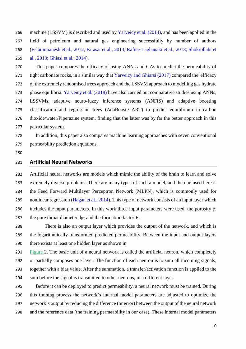
10
machine (LSSVM) is described and used by Yarveicy et al. (2014), and has been applied in the 266
field of petroleum and natural gas engineering successfully by number of authors 267
(Eslamimanesh et al., 2012; Farasat et al., 2013; Rafiee-Taghanaki et al., 2013; Shokrollahi et 268
al., 2013; Ghiasi et al., 2014). 269
This paper compares the efficacy of using ANNs and GAs to predict the permeability of 270
tight carbonate rocks, in a similar way that Yarveicy and Ghiarsi (2017) compared the efficacy 271
of the extremely randomised trees approach and the LSSVM approach to modelling gas hydrate 272
phase equilibria. Yarveicy et al. (2018) have also carried out comparative studies using ANNs, 273
LSSVMs, adaptive neuro-fuzzy inference systems (ANFIS) and adaptive boosting 274
classification and regression trees (AdaBoost-CART) to predict equilibrium in carbon 275
dioxide/water/Piperazine system, finding that the latter was by far the better approach in this 276
particular system. 277
In addition, this paper also compares machine learning approaches with seven conventional 278
permeability prediction equations. 279
280
Artificial Neural Networks 281
Artificial neural networks are models which mimic the ability of the brain to learn and solve 282
extremely diverse problems. There are many types of such a model, and the one used here is 283
the Feed Forward Multilayer Perceptron Network (MLPN), which is commonly used for 284
nonlinear regression (Hagan et al., 2014). This type of network consists of an input layer which 285
includes the input parameters. In this work three input parameters were used; the porosity , 286
the pore throat diameter dPT and the formation factor F. 287
There is also an output layer which provides the output of the network, and which is 288
the logarithmically-transformed predicted permeability. Between the input and output layers 289
there exists at least one hidden layer as shown in 290
Figure 2. The basic unit of a neural network is called the artificial neuron, which completely 291
or partially composes one layer. The function of each neuron is to sum all incoming signals, 292
together with a bias value. After the summation, a transfer/activation function is applied to the 293
sum before the signal is transmitted to other neurons, in a different layer. 294
Before it can be deployed to predict permeability, a neural network must be trained. During 295
this training process the network’s internal model parameters are adjusted to optimize the 296
network’s output by reducing the difference (or error) between the output of the neural network 297
and the reference data (the training permeability in our case). These internal model parameters 298
11
are the weighting factors connecting the neurons together and the bias values. The overall 299
process of training progressively reduces the error between the network output and the 300
reference (measured) values (Negnevitsky, 2002; Hagan et al., 2014). There are many training 301
methods such as stochastic learning and gradient descent learning (Rajasekaran and Pai, 2003). 302
The algorithm used here is Adam, one of the most efficient general purpose stochastic learning 303
algorithms which has been introduced and described in detail by Kingma and Lei Ba (2015). 304
The complexity of the neural network model is influenced by its size, i.e., the number of 305
neurons and hidden layers. Bearing in mind the principle of Occam’s razor, a network needs to 306
have enough complexity to model the patterns inherent in the data, yet not be so complex that 307
it attempts fitting any random noise that will occur to some extent in any dataset (Hagan et al., 308
2014). 309
Figure 2 shows the neural network structure adopted in this case study, and was optimised 310
by experimentation with different structures. The adopted structure is simple but also efficient 311
in capturing the inherent patterns in the data. It consists of a single neuron in each of two hidden 312
layers. 313
314
315
Figure 2. The MLPN structure which has been used in this work. There is one hidden 316
neuron in each of the hidden layers. The transfer function in the first hidden layer is a 317
sigmoidal function while the transfer function in the second hidden layer and the output layer 318
are linear functions. 319
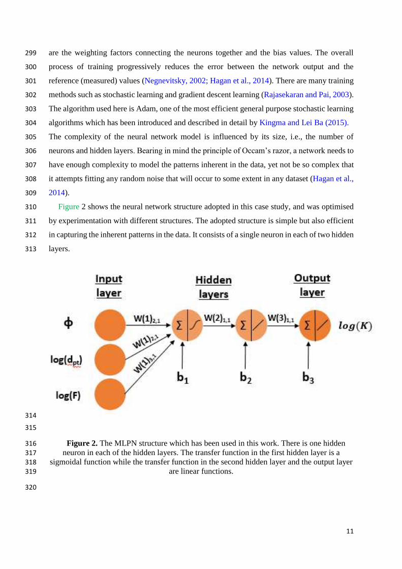
320

12
It is known that artificial neural networks perform better when their parameters are 321
distributed normally or quasi-normally (Hagan et al., 2014). Many of the used parameters are 322
naturally normal or quasi normal. However, some, such as measured permeability follow a log-323
normal distribution. These parameters were transformed so they resembled a normal 324
distribution more closely so that the modelling could take place. The results of the neural 325
network modelling can be transformed back to a lognormal distribution. 326
327
Genetic Algorithms 328
Genetic algorithms optimize fit to a pattern by simulating the process of natural selection. In 329
this process the most successful ‘organisms’ from a population survive to pass their genes on 330
to their progeny (Cuddy and Glover, 2002). The chance of survival is related to certain 331
characteristics of the organism which can be passed on to the next generation and/or mutated. 332
Consequently, some of their progeny inherit those characteristics from their parents which 333
improve their survival. 334
In the genetic algorithm method, the starting point is a population of ‘organisms’ which, in 335
this specific case represent prediction equations. These ‘organisms’ have randomly allocated 336
genes, which contain the information required to reconstruct each permeability prediction 337
equation. The most successful equations, defined as those which are best at predicting the 338
permeability of a training set of data, are allowed to partially swap their genes, in the hope that 339
their ‘progeny’ become even more successful. Random mutations are also allowed at a 340
probability which serves to enhance the diversity of the genetic information of the population 341
(Aminzadeh and De Groot, 2006). 342
The genetic algorithm technique has been used successfully in the search for suitable 343
empirical permeability prediction equations (e.g., Cuddy and Glover, 2002, Fang et al., 1992). 344
Its particular strength is that it is able to suggest the form of a prediction equation as well as its 345
various coefficients. In our application, the objective is to predict permeability from porosity, 346
pore throat diameter and formation factor. The general equation for the empirical relationship 347
that would have the ability to predict permeability from these three input parameters can be 348
written as 349 倦 噺 血岫剛┸ 穴牒脹 ┸ 繋岻 噺 岷欠 剛長峅 ぇ怠 範潔 穴牒脹鳥飯 ぇ態 岷結 繋捗峅 ぇ戴 岷訣峅 , (8) 350
where k is permeability. The coefficients and exponents are denoted as letters a, b, c, d, e, f and 351
g, all of which have continuous values, and the entities represented by ぇ怠 , ぇ態 and ぇ戴, which are 352
13
operators that can be either multiplication or addition. It should be noted that subtraction and 353
division are not required as these operations are taken account of by negative values of the 354
coefficients and exponents. These 10 parameters can be written in the form shown in Figure 3, 355
which is called a ‘chromosome’, and can be manipulated in the same way as a biological 356
chromosome. 357
358
359
Figure 3. Representation of the permeability equation using a ‘chromosome’. 360
361
Different types of encoding can be used in genetic algorithms (Rajasekaran and Pai, 2003). 362
The type used in this work is ‘value encoding’, which implies the use of actual values for the 363
numerical parameters, while binary encoding is used for the two types of operators; 364
multiplication and addition. 365
In this implementation, a genetic algorithm starts with a randomly generated population of 366
permeability prediction equations, encoded by their chromosomes. All the permeability 367
prediction equations are tested for their goodness of fit to the real data represented by the 368
training dataset. Those that perform well are allowed to survive in a mutated form, and retested 369
against the training dataset. A large number of iterations can be carried out, with the prediction 370
equations becoming more and more precise in their permeability predictions. The processes 371
stopped when a given prediction accuracy is reached. 372
The survival of permeability prediction equations is judged on the calculation of a ‘fitness 373
to survive’ parameter, which is higher for equations that provide a smaller prediction error. 374
Two successful permeability prediction equations are then chosen at random to reproduce using 375
their successful genetic information. The genetic information of all new progeny is also 376
subjected to random mutation at a certain probability (Rajasekaran and Pai, 2003). In this type 377
of genetic algorithm, the random mutation was achieved by multiplying the chromosomal 378
numerical values by a random number between 0.8 and 1.2 and flipping the binary code for the 379
operators (Cuddy and Glover, 2002). When run reiteratively, the solution improves over 380
generations until no major improvement can be achieved, and by then the solution can be 381
considered to be converged (Negnevitsky, 2002). The equation corresponding to the 382
14
chromosome having the highest fitness among the last generation is selected for being the 383
solution model because it has the highest predictive power. 384
385
Results and Discussion 386
The full dataset of 130 samples was divided at random into two subsets. The first subset, 387
comprising 100 samples, was called the training data subset. This was used to train machine 388
learning techniques and to calibrate those conventional models which required tuned empirical 389
parameters. The second subset comprised 30 samples, and was called the test data subset. This 390
was used to test the efficacy of both the machine learning techniques and the conventional 391
prediction equations. 392
393
Conventional models 394
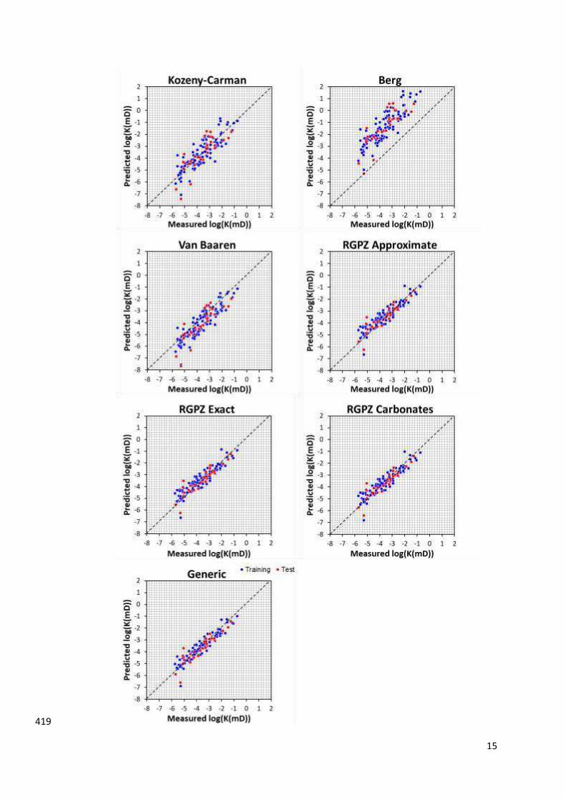
Figure 4 shows the permeability predicted using each of the benchmark conventional models 395
as a function of the measured permeability. Of the conventional models, the Berg model 396
performed the worst because this model has an empirical origin that is not calibrated for tight 397
carbonates but for the clastic dataset for which it was originally developed. Consequently, its 398
empirical coefficient of 8.4×10⁻² is fixed. If this value were allowed to vary and to be used as 399
a fitting parameter, it would provide an improved solution. 400
The other models provided very good results over almost 6 orders of magnitude, especially 401
the various forms of the RGPZ model and the Generic models, which are either purely 402
analytical (RGPZ-exact and the RGPZ-approximate models), or empirical (RGPZ-carbonate 403
and Generic models). Table 2 contains the coefficient of determination and RSME values for 404
the training and test datasets associated with each implementation, as well as the final trained 405
equation. 406
407
408
409
(Overleaf) Figure 4. Permeability prediction using the seven conventional permeability 410
prediction equations, each shown as a function of the independently measured permeability. 411
The whole dataset is split into a training subset and a test subset. Only the Berg equation and 412
the two original RGPZ equations do not require the fitting of at least one parameter to data. 413
For these three, there is no distinction between the training and test data. For the others, their 414
empirical parameters will have been fitted using the training dataset, for which the fit should 415
be optimal, and then applied to the test data, for which the fit should be slightly suboptimal. 416
In each case the uncertainties in each value are approximately the same size as that of the 417
symbols. 418
15
419

16
Overall the quality of the fits obtained from the conventional models was considered to be 420
very good. This is partly due to the choice of benchmarking conventional models we have used 421
in this paper. There are many other equations, some with a very long pedigree, that would do 422
much worse. 423
Although this paper concerns itself predominantly with machine learning, it is worthwhile 424
taking away a lesson from the conventional model test that we have done. First, permeability 425
prediction will only be good if it uses input parameters that are of high quality. In this work, 426
we strove to make the highest quality measurements we could. Second, the permeability 427
prediction equation needs to be one which is relevant to the type of rock being predicted. Hence, 428
for tight carbonate rocks, the permeability prediction equation ought to have been developed 429
with tight carbonate rocks in mind. Third, those permeability prediction equations that require 430
fitting to obtain one or more empirical coefficients need to use calibration data sets that contain 431
data for the type of rock being fitted. In our particular case this is tight carbonate rocks, the 432
observation is equally true of other types of rocks. 433
In all cases, the conventional models which have performed most successfully on tight 434
carbonate rocks are those which have either (i) been specifically designed for tight carbonate 435
rocks, or (ii) have been developed, or had their empirical coefficients determined using datasets 436
containing tight carbonate rocks. In general, good quality prediction can only be expected over 437
a large number of orders of magnitude if the calibration data also extends over a similar range 438
of orders of magnitude. In other words, if the rocks on which one wishes to predict permeability 439
varies from a few D to hundreds of mD, the calibration of the empirical coefficients needs to 440
be carried out using a dataset which covers the same range. 441
442
Neural network models 443
The optimum network structure for our implementation of the neural network approach was 444
found through experimentation, varying the number of neurons in the hidden layers and 445
observing the response of the objective function. In this work, we found predicting permeability 446
itself does not produce equally good results over the entire range. As some permeabilities are 447
order of magnitude higher than others, the error associated with these far exceeds the error from 448
lower end permeability samples, causing the algorithm to be biased toward predicting the few 449
highest permeabilities as accurately as possible, while disregarding accurate prediction of the 450
lower values. To alleviate this major issue, the root mean squared error (RMSE) of log 451
transformed permeability was implemented as the objective function. This approach has the 452

17
advantage of equalizing the contribution of the errors from the entire permeability range. The 453
objective function is given by Eq. (9), where it should be noted that the permeabilities are 454
treated in the logarithmic domain because they are distributed log normally. 455
456 頚決倹結潔建件懸結 血憲券潔建件剣券 噺 謬怠津 デ 盤lo�盤計椎追勅鳥沈頂痛勅鳥匪 伐 lo�岫計陳勅銚鎚通追勅鳥岻匪態津沈退怠 (9) 457
458
In our application, it became clear that using larger number of neurons improved the fit of 459
the predicted permeability to the training subset resulting in a lower value of the objective 460
function. However, the accuracy of the subsequent use of the neural network on unseen samples 461
diminished. This is because the neural network was ‘over-fitting’ the training samples. 462
Overfitting occurs due to the model being too powerful such that it exceeds the requirement of 463
just fitting the patterns in the data, and starts to memorize the training points. This process 464
results in the performance of the model on the training dataset increasing without limit, but 465
such an increase in performance is counter-productive because it occurs at the expense of the 466
model’s capability to fit unseen data (Negnevitsky, 2002). Since the training data points are 467
normally noise contaminated, and may not adequately represent the entire population, it is 468
critical to avoid overfitting when deciding on the size of the neural network size to be used. 469
Often simple neural networks perform just as well, and sometimes even better than very 470
complex neural networks. 471
Figure 5 shows the results of varying the number of neurons for our application with three 472
input parameters: porosity, grain size and formation factor. A network with one neuron in each 473
hidden layer was chosen, giving the smallest value of objective function for the test samples. 474
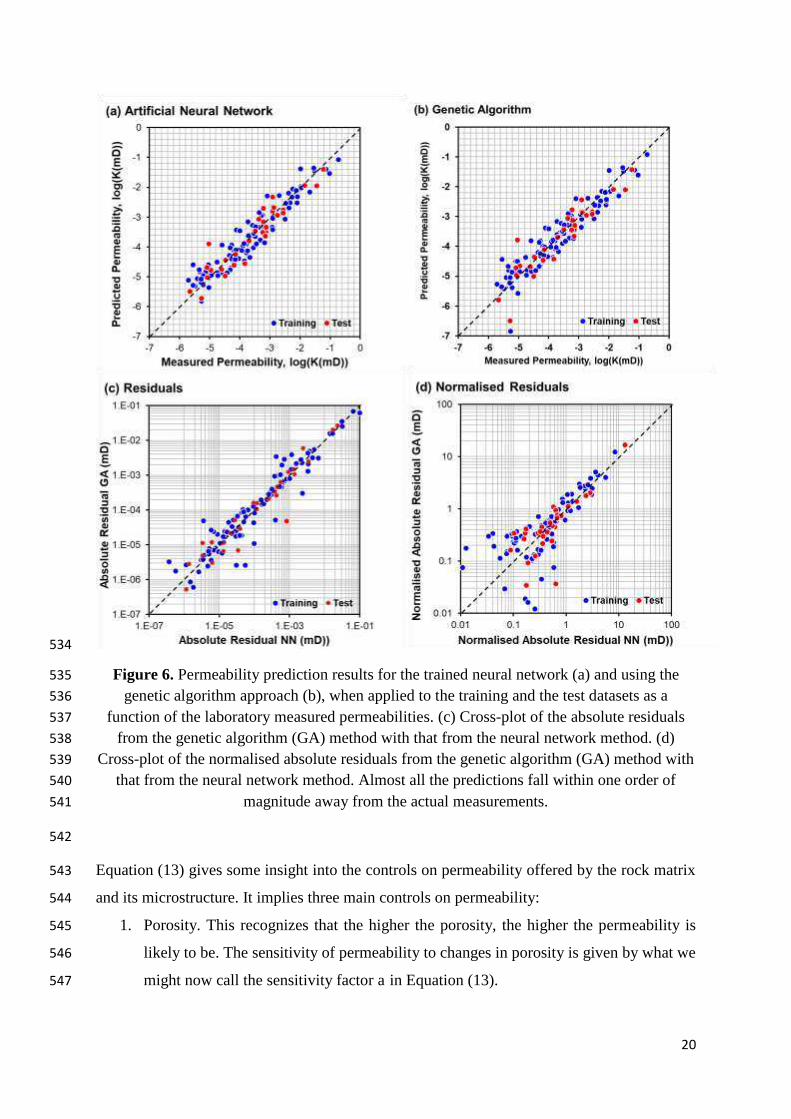
The permeability prediction results from the MLPN model are shown in Figure 6, where the 475
predicted permeability is plotted as a function of the measured permeability for both the 476
training and the test data in the dual-logarithmic domain. It is clear from this figure that the 477
neural network provides a very good fit to the measured permeability data over six orders of 478
magnitude. 479
480
481
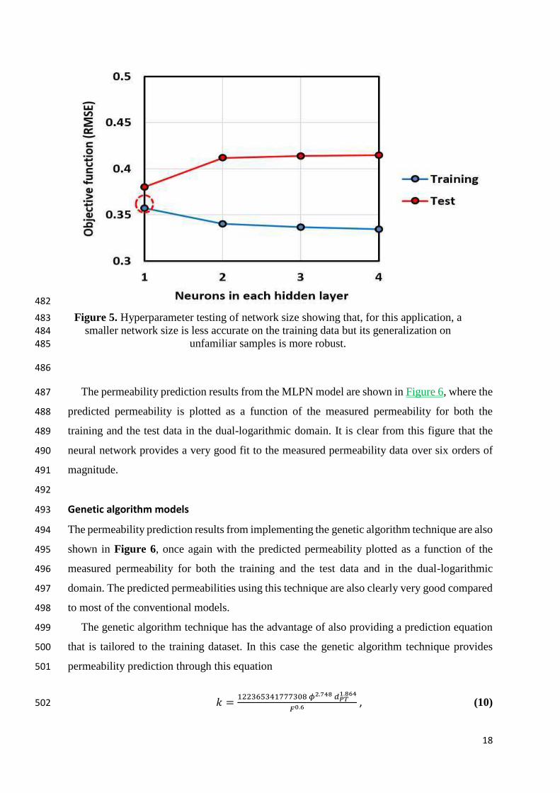
18
482
Figure 5. Hyperparameter testing of network size showing that, for this application, a 483
smaller network size is less accurate on the training data but its generalization on 484
unfamiliar samples is more robust. 485
486
The permeability prediction results from the MLPN model are shown in Figure 6, where the 487
predicted permeability is plotted as a function of the measured permeability for both the 488
training and the test data in the dual-logarithmic domain. It is clear from this figure that the 489
neural network provides a very good fit to the measured permeability data over six orders of 490
magnitude. 491
492
Genetic algorithm models 493
The permeability prediction results from implementing the genetic algorithm technique are also 494
shown in Figure 6, once again with the predicted permeability plotted as a function of the 495
measured permeability for both the training and the test data and in the dual-logarithmic 496
domain. The predicted permeabilities using this technique are also clearly very good compared 497
to most of the conventional models. 498
The genetic algorithm technique has the advantage of also providing a prediction equation 499
that is tailored to the training dataset. In this case the genetic algorithm technique provides 500
permeability prediction through this equation 501
倦 噺 怠態態戴滞泰戴替怠胎胎胎戴待腿 笛鉄┻店填添 鳥鍋畷迭┻添展填庁轍┻展 , (10) 502

19
which can be rewritten in a generalized form 503 倦 噺 暢笛尼 鳥鍋畷弐庁迩 , (11) 504
which is consistent with Eq. (10), and where M, a, b and c are fitting parameters, whose exact 505
values are sample-dependent and whose mean values are formation-dependent. 506
Equation (11) contains two parameters which are known to be partially correlated. The 507
formation factor F is known to be dependent on both porosity and cementation exponent m 508
through Archie’s first law (Archie, 1942), which can be stated as F = -m. This equation arises 509
from the fact that electrical flow through a rock with insulating grains occurs only through the 510
conducting fluid occupying the pores. The resistivity of the rock depends on the amount of 511
fluid present, which is given by the porosity and assumes that the pores are completely saturated 512
with the fluid, and also depends on how well that fluid is connected, which is described by the 513
value of the so-called cementation exponent m (Glover, 2015). Consequently, Equation (10) 514
may be rewritten as 515 倦 噺 なににぬはのぬねなばばばぬどぱ 剛岫態┻胎替腿袋待┻滞陳岻 穴牒脹怠┻腿滞替 , (12) 516
or generically as 517 倦 噺 警剛岫銚袋頂陳岻穴牒脹長 . (13) 518
The large value of M in Equation (12) arises solely from the fact that the input parameters 519
for the genetic algorithm model used permeability training data in millidarcies. When 520
converted to m2, this value becomes 0.0122, which corresponds well to the value for the 521
constant term in the RGPZ equation. This term is な ね欠兼態エ , and can be calculated for the mean 522
behaviour of the dataset from the data given in Table 1. When the cementation exponent is 523
calculated using Archie’s first law from this data, we obtain a mean cementation exponent of 524
m=2.402, which provides a value of 0.0162 for the constant term. Consequently, we conclude 525
that the M term in Equation (12) is consistent with the theoretically-derived RGPZ equation. 526
Considering the other variables in Equation (12), we find that the genetic algorithm method 527
underestimates the porosity exponent compared to the RGPZ equation, providing 2.748+0.6m, 528
which is equal to 4.189 when m=2.402, compared to a value of 3m, which is equal to 7.206 for 529
the RGPZ equation; an overestimation of just over 3. The genetic algorithm method also 530
underestimates the grain size exponent, giving 1.864 compared to the RGPZ equation’s value 531
of exactly 2. 532
533
20
534
Figure 6. Permeability prediction results for the trained neural network (a) and using the 535
genetic algorithm approach (b), when applied to the training and the test datasets as a 536
function of the laboratory measured permeabilities. (c) Cross-plot of the absolute residuals 537
from the genetic algorithm (GA) method with that from the neural network method. (d) 538
Cross-plot of the normalised absolute residuals from the genetic algorithm (GA) method with 539
that from the neural network method. Almost all the predictions fall within one order of 540
magnitude away from the actual measurements. 541
542
Equation (13) gives some insight into the controls on permeability offered by the rock matrix 543
and its microstructure. It implies three main controls on permeability: 544
1. Porosity. This recognizes that the higher the porosity, the higher the permeability is 545
likely to be. The sensitivity of permeability to changes in porosity is given by what we 546
might now call the sensitivity factor a in Equation (13). 547

21
2. Connectivity of the pores. This recognizes that high porosities, if unconnected will have 548
zero permeability and for any given porosity permeability will be greater if pore 549
connectivity is higher. The sensitivity of permeability to changes in connectivity is 550
given by what we might now call the sensitivity factor c in Equation (13). 551
3. The characteristic pore throat diameter. It is an important parameter for permeability 552
since narrower pore throats act like bottlenecks for fluid flow. The sensitivity of 553
permeability to characteristic pore throat diameter is given by what we might now call 554
the sensitivity factor b in Equation (13). 555
556
Prediction performance 557
The error metrics for all predictions are shown in Table 2 and in Figure 7. 558
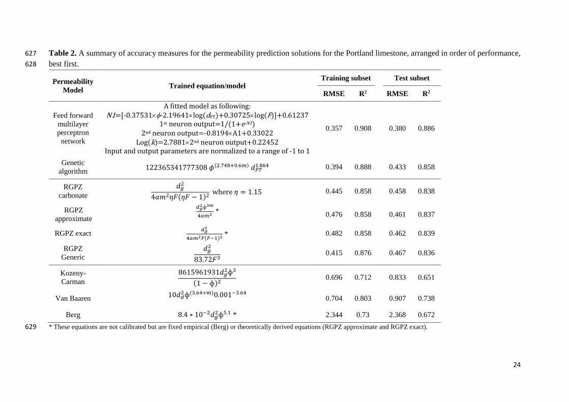
Good fits are represented by low values of root mean squared error (RSME) together with high 559
values of coefficient of determination (R2). The quality of the predictions is far from uniform. 560
Even with their historic success on conventional sandstone reservoirs, the older empirical 561
models were not successful on these tight carbonate rocks. The RGPZ-carbonate equation 562
provided the best fit from the conventional approaches, with the lowest RMSE error of 0.458. 563
The other RGPZ equations performed slightly worse as they do not include the carbonate 564
calibration parameter, but nevertheless provided acceptable predictions. The genetic 565
algorithm solution performed marginally better than the rest of the conventional equations, 566
with an RMSE of 0.433. On the other hand, the artificial neural network technique provided 567
the most accurate predictions with an RMSE of only 0.380. 568
The marginal difference between the two machine learning approaches arises from only a 569
few data points. Reference to Figure 6 shows that there are two data points, one in the training 570
dataset and another in the test dataset whose permeabilities are underestimated by one order of 571
magnitude. The reason why these particular points are not predicted well is not currently 572
known. However, we carried out a sample by sample comparison of both machine learning 573
approaches, and find that the prediction error for the genetic algorithms correlates with the 574
prediction error. Figure 6c shows a cross-plot of the absolute residuals from the genetic 575
algorithm method (GA) against that from the neural network (NN) method. It is clear that 576
samples whose permeability is badly predicted by one method is also badly predicted by the 577
other, with correlation coefficients of 0.963, 0.994 and 0.962, for the training dataset, test 578
dataset, and combined datasets, respectively. We recognise that this comparison might be 579
biased towards large permeability measurements due to the large range of permeabilities used 580

22
in the study. The large range of permeabilities covered in the prediction might lead to small 581
percentage errors in large permeabilities being given more weight than large percentage errors 582
in small permeabilities. Hence, we also show the cross-plot of the absolute residuals normalised 583
by the measured permeability, which is shown in Figure 6d. Once again, the normalised 584
absolute residuals correlate well, with coefficients of correlation of 0.945, 0.991 and 0.969, for 585
the training dataset, test dataset, and combined datasets, respectively. In Figure 6d, the abscissa 586
x=1 and ordinate y=1 represent an error in prediction of the same magnitude as the measured 587
permeability (i.e., a ±100% error) for the neural network and genetic algorithm methods, 588
respectively. Those points with coordinates (x,y) > (1,1) represent predictions by both 589
techniques that are very much in error, and for these the degree of bad prediction in one 590
machine learning method is similar to that in the other. For those points where the prediction 591
is better, i.e., (x,y) < (1,1), there is more scatter indicating that one method produces a better 592
prediction than the other. 593
From the analysis above we infer that the lack of prediction accuracy is not predominantly 594
a function of the technique being used, but due to a problem with the input parameters. There 595
are two possibilities here: (i) that non-systematic errors in one or more of the input parameters 596
leads to both machine learning techniques badly predicting some of the samples, and (ii) the 597
permeability of the tight carbonate rocks depending upon some petrophysical characteristic 598
that is not characterised sufficiently by any of the input parameters used in this study. An 599
example of the latter might be that the permeability is dependent upon the rock wettability, but 600
none of the input parameters include information about rock wettability. Further work would 601
need to be carried out in order to ascertain whether this was the case. 602
We note, however, that the few samples for which the predictions were worst have a 603
different structure from the rest of the dataset in that they have a high permeability but a low 604
porosity and a small pore throat size. From such parameters, we infer that the pore space that 605
is present must be highly connected. Samples with this type of microstructure occur when the 606
diagenetic process of cementation has occluded original pore volume, reducing the size of the 607
throats connecting the pores as well as the pores themselves, but leaving the remaining flow 608
paths highly connected. Examples of such behaviour can be found in Fontainebleau and 609
Lochaline sandstones (Walker and Glover, 2018) and in carbonates (Rashid et al., 2015a; 610
2015b, 2017). The inefficiency of the machine learning techniques stems from the relative lack 611
of samples with this type of structure in the training dataset. The permeability is predicted badly 612
precisely because the machine learning techniques have not been prepared to recognise samples 613
with this type of pore microstructure. It is a sobering thought that any machine learning 614

23
algorithm is only as good as the quality of the data with which it is trained and upon which it 615
is applied. 616
It is worth noting that the fits by empirical equations and machine learning implementations 617
are slightly better for the training dataset than the test dataset. This is due to the chance that the 618
models are calibrated on a sample that is not quite representative enough of the characteristics 619
of the formation. Besides this, there is also a chance of inclusion of two outliers in the test 620
dataset that reduces the efficacy of all the models in the test dataset. 621
622
623
624
Figure 7. Permeability prediction metrics for all conventional and machine learning 625
techniques for the training and test datasets. 626
24
Table 2. A summary of accuracy measures for the permeability prediction solutions for the Portland limestone, arranged in order of performance, 627
best first. 628
Permeability Model Trained equation/model
Training subset Test subset
RMSE R2 RMSE R2
Feed forward multilayer perceptron network
A fitted model as following:
N1=[-0.37531-2.19641log(dPT)+0.30725log(F)]+0.61237
1st neuron output=1/(1+e-N1)
2nd neuron output=-0.8194A1+0.33022
Log(k)=2.78812nd neuron output+0.22452
Input and output parameters are normalized to a range of -1 to 1
0.357 0.908 0.380 0.886
Genetic algorithm なににぬはのぬねなばばばぬどぱ 剛岫態┻胎替腿袋待┻滞陳岻 穴牒脹怠┻腿滞替 0.394 0.888 0.433 0.858
RGPZ carbonate
穴直態ね欠兼態考繋岫考繋 伐 な岻態 w�e�e 考 噺 な┻なの 0.445 0.858 0.458 0.838
RGPZ approximate
鳥虹鉄◆典悼替銚陳鉄 * 0.476 0.858 0.461 0.837
RGPZ exact 鳥虹鉄替銚陳鉄庁岫庁貸怠岻鉄 * 0.482 0.858 0.462 0.839
RGPZ Generic
穴直態ぱぬ┻ばに繋戴 0.415 0.876 0.467 0.836
Kozeny-Carman
ぱはなのひはなひぬな穴直態◆戴岫な 伐 ◆岻態 0.696 0.712 0.833 0.651
Van Baaren など穴鳥態◆岫戴┻滞替袋鱈岻ど┻どどな貸戴┻滞替 0.704 0.803 0.907 0.738
Berg ぱ┻ね 茅 など貸態穴直態◆泰┻怠 * 2.344 0.73 2.368 0.672
* These equations are not calibrated but are fixed empirical (Berg) or theoretically derived equations (RGPZ approximate and RGPZ exact). 629

25
The results presented in this paper show that the implementation of genetic algorithms and 630
artificial neural networks results in more accurate predictions in comparison to predictions 631
made by all the benchmark permeability models including the most recent ones. The genetic 632
algorithm technique helped reduce the error of the best performing conventional permeability 633
model by 5%. On the other hand, the artificial neural networks technique reduced the error by 634
17%, which is a significant improvement. On the other hand, the solution of the neural network 635
approach, which is something of a ‘black box’, is not as transparent as the trained equation 636
provided by the genetic algorithm method. The representation of the solution in a concise 637
mathematical equation provides a much clearer insight into the significance and role of each 638
input parameter into the permeability prediction. Also, the resulting equation can be applied 639
more easily to similar facies without the need for special software and/or technical skills. The 640
solution equation can also be recalibrated with a small number of samples because of the 641
smaller number of model parameters. 642
By contrast, the permeability prediction using artificial neural networks is mathematically 643
more complex. While it is simple to visualize the solution of a neural network that has a single 644
input feature on a xy graph, to visualize it when two input parameters are used requires a three-645
dimensional plot. Nonetheless, visualizing the response of networks that use multi-dimensional 646
input features is indeed challenging. 647
648
Limitations of machine learning 649
The main result of this study is that both the machine learning techniques tested performed 650
better than all of the conventional permeability equations over a range of 6 orders of magnitude. 651
There are, however, some important limitations of machine learning which need to be 652
considered before blindly applying them. 653
The first is that it can be simple to fall into the trap of creating neural networks which are 654
too complex, and which will seem to be doing a good job of permeability prediction on the 655
training data, but which lead to over-training. Such models will not perform as well on the 656
target dataset, and that partial failure will not be clear because independent permeability 657
measurements will not be available. Why, after all, predict permeability if one already knows 658
it. 659
The second is that both techniques are to some extent a black box, although that is less true 660
of genetic algorithms. Consequently, if there is a failure in the techniques, it is not always clear 661
to the operator. 662
26
Third, both techniques need training. The training dataset must be a random sample of the 663
whole population on which the technique is to be used. This is not just the trivial constraints 664
that the sampling should be truly random, of sufficient number to capture all of the complexities 665
in the target data, and covering the same range of measurements in the same proportion. By 666
definition, rare events, conditions and outliers in general will be lost from the analysis. Machine 667
learning is in a certain light, a form of conservative filtering that keeps the common and rejects 668
the rare. Consequently, machine learning will fail to predict rare but important values. 669
The fourth limitation concerns the interpretation of what is a good genetic algorithm result. 670
If there are sufficient organisms evolving, it is reasonable that one of the most successful will 671
provide the permeability prediction equation that is the most appropriate. We use the words 672
‘most appropriate’ deliberately, because it will not necessarily be the best. The set of successful 673
chromosomes, however numerous and however statistically defined are non-unique. In other 674
words, two chromosomes which are very different could provide equally good results. How is 675
one then to choose which to use on a set of target data, where the accuracy of the result cannot 676
be tested. 677
In summary, no matter how well-implemented, the use of machine learning will always be 678
associated with some anxiety that the predictions are as good as we have found. If that anxiety 679
is such that the final results always need to be validated by some independent measure of 680
permeability, the utility of the approach is weakened. 681
682
Diagenesis and machine learning 683
As we have seen, both the genetic algorithm and neural network models perform better than 684
the best of the theoretical and empirical models. It is instructive to examine the reasons for this 685
in tight, often diagenetic altered, carbonate rocks. Conventionally, the spread in a poroperm 686
diagram is attributed to the permeability depending upon factors other than porosity. However, 687
many of the theoretical and empirical models presented in this paper include a range of other 688
parameters, including, for example, grain size, formation factor and cementation exponent but 689
still result in a suboptimal prediction of permeability. This is because the permeability is some 690
additional function of a parameter that is not included in the structure of the prediction equation, 691
or that there is a lack of orthogonality between the input parameters. The defined structure of 692
the prediction equation limits the efficacy of the model to predict permeability in only those 693
rocks where the imposed structure is valid, i.e., simple functional dependencies of a limited 694
number of known input parameters. 695

27
Here, both machine learning techniques perform better than all the conventional approaches, 696
so we can infer that they have a common ability to make better use of the available data than 697
conventional predictive equations. The common characteristic of the two machine learning 698
methodologies used in this work, as well as all machine learning approaches, is that they start 699
with either no structure or relatively little structure. The neural networks have only defined 700
input and output values, while the genetic algorithm has input and output values as well as a 701
very generalised equation. In machine learning, structural complexity arises from training and 702
is theoretically only limited by the availability of a representative training dataset. 703
Consequently the result of complex interacting processes should be modellable with accuracy. 704
The permeability of tight carbonate rocks is the result of the complex, interacting process 705
of diagenesis. Hence, we hypothesize that the permeability of rocks which have undergone 706
diagenesis would be ideally suited to machine learning methods, whose greater sensitivity to 707
subtle and complex changes in the input parameters can be taken into account. 708
Of all of the conventional models, it was the carbonate version of the RGPZ model that 709
came closest to the machine learning models. This model includes the parameter, which is 710
supposed to take account of the fact that the pore network architecture in carbonate rocks is 711
more complex than that in clastic rocks (Rashid et al., 2015b). However, a single value, set to 712
=1.15 in this work, is a very crude method for taking account of the pore network which will 713
have a connectedness that may depend upon codependent and competing processes of 714
compaction, cementation, vug formation, dissolution, dolomitisation and fracturing. 715
Figure 8 shows a generic poroperm cross plot implemented for the modified carbonate 716
RGPZ model for four different grain sizes. The superimposed arrows (which are imposed at an 717
arbitrary point on an arbitrary curve, but are equally relevant to any point on any of the curves) 718
show the approximate directions each diagenetic process will produce when acting upon the 719
pore network architecture of a carbonate rock. None of the arrows follow the curves, because 720
that would indicate that the process was not altering either the rock matrix or the pore network 721
architecture. The transparent grey areas in the figure are an indication of those where gain or 722
loss in porosity leads to a loss or gain in permeability. There are however no diagenetic 723
processes which cause such tendencies. 724
725

28
726
Figure 8. Diagrammatic poroperm cross-plot based on the modified carbonate RGPZ model 727
for grain sizes. The arrows, which all originate at an arbitrary point on one of the curves, but 728
equally well apply to any point on any of the curves, represents the results of different 729
diagenetic processes altering the pore network architecture of the rock and hence its porosity 730
and permeability characteristics. High reservoir quality occurs towards the top right of the 731
figure. 732
733
Compaction (grey arrow) reduces porosity, but can result in less permeability loss than 734
expected depending on the sorting, shape and strength of the grains. Cementation (red arrow) 735
results in loss of porosity as cement fills the pore spaces, and significant loss of permeability 736
because the cement will either partially or totally occlude pore throats, hence blocking fluid 737
flow pathways. By comparison, dissolution (magenta arrow) tends to dissolve rock matrix 738
indiscriminately, increasing porosity but not preferentially in the pore throats. Consequently, 739
though mobility does increase, it does not do so significantly. Dolomitisation (orange arrow) 740
has a much greater effect because the recrystallisation concomitant upon dolomitisation 741
provides larger porosity within pores that are well connected, and hence support much greater 742

29
permeability. Vug formation (dark blue arrow), for example by preferential dissolution, 743
introduces significant porosity. However, this porosity is often distributed in an unconnected 744
manner in a background matrix of low permeability, and hence results in very little increase in 745
permeability. Stylolitisation (green arrow) has negligible impact upon the porosity of a rock, 746
but by concentrating clay minerals along the stylolite surface, the macroscopic permeability of 747
the rock perpendicular to the stylolites is greatly reduced. Since stylolite form perpendicular to 748
the direction of greatest principal stress, this direction is usually vertical. Fracturing (light blue 749
arrow), of course, introduces very little extra porosity to a rock, but that porosity is arranged 750
for the efficient transport of fluid in the direction of the fractures. Consequently, porosity 751
increases slightly upon fracturing, but permeability in the direction of the fractures can increase 752
by two or more orders of magnitude if the fractures are open. If the fractures are closed, the 753
trend would be very similar to that for the stylolites, with the closed fractures providing a 754
similar compartmentalised single role. 755
Taking all of these diagenetic factors in consideration, it is unlikely that the parameter 756
would be able to take account of all of the diagenetic controls on permeability provided by 757
these codependent and competing diagenetic processes. However, the training of either a new 758
network or genetic algorithm on a reasonable size training dataset would be likely to result in 759
a model that takes account of the main controls of diagenesis on permeability. 760
Finally, we recognize that the true novelty of this paper is not that it tests two machine 761
learning methodologies for the first time on a high-quality, well-characterised tight carbonate 762
system, but the recognition that the quasi-quantitative parameters obtained from these 763
techniques may contain information which will help us improve the quantitative analysis of the 764
type and extent of diagenesis with regards to its control on rock permeability. 765
766
Conclusions 767
In this work, both artificial neural network and genetic algorithm techniques have been 768
demonstrated to show potential for the prediction of technically challenging tight carbonate 769
reservoirs. The genetic algorithm technique is more useful if one wishes to gain more insight 770
into which parameters are controlling the predicted permeability, and has the benefit of 771
providing an equation that can be subsequently applied easily to other datasets or used as the 772
starting point of training with another dataset. However, when accuracy is the top priority, the 773
neural network technique was found to be more accurate. 774
30
We have considered the reasons for the machine learning techniques providing a better 775
predicted permeability compared to the conventional models, considering that some of the 776
conventional models are very high quality and contain the same parameters used in machine 777
learning approaches. We have concluded that the better performance of machine learning 778
techniques over conventional approaches can be attributed to their enhanced capability to 779
model the connectivity of pore microstructures using a significant training dataset. This allows 780
machine learning methods to take account of small changes in pore microstructure caused by 781
the complex, codependent and competing diagenetic processes that have conspired to create 782
the pore microstructure of any given carbonate rock. In doing so, we have created a qualitative 783
model which describes how the poroperm characteristics of tight carbonate rocks are modified 784
by each of eight diagenetic processes. 785
We conclude that, for tight carbonate reservoirs, both machine learning techniques predict 786
permeability more reliably and more accurately than conventional models and may be capable 787
of distinguishing quantitatively between pore microstructures caused by different diagenetic 788
processes. 789
790
Acknowledgements 791
The authors would like to thank two anonymous reviewers, whose incisive and constructive 792
comments have improved this paper greatly. 793
794
References 795
AKAI, T., TAKAKUWA, Y., SATO, K. & WOOD, J. M. 2016. Pressure Dependent Permeability of 796
Tight Rocks, 180262-MS SPE Conference Paper – 2016. 797
AL-ZAINALDIN, S., GLOVER, P.W.J. and LORINCZI, P., 2017. Synthetic Fractal Modelling of 798
Heterogeneous and Anisotropic Reservoirs for Use in Simulation Studies: Implications on Their 799
Hydrocarbon Recovery Prediction. Transport in Porous Media, 116(1), pp. 181-212. 800
AMINZADEH, F. & DE GROOT, P. 2006. Neural networks and other soft computing techniques with 801
applications in the oil industry, EAGE Publications. 802
ARCHIE, G. E., 1942, The electrical resistivity log as an aid in determining some reservoir 803
characteristics: Transactions of the American Institute of Mechanical Engineers, 146, 54–67. 804
BARTON, C.M.; WOODS, M.A.; BRISTOW, C.R.; NEWELL, A.J.; WESTHEAD, R.K.; EVANS, 805
D.J.; KIRBY, G.A.; WARRINGTON, G. 2011. Geology of south Dorset and south-east Devon and 806
its World Heritage Coast : Special Memoir, British Geological Survey, 161 pp. 807
BERG, R. R. 1975. Capillary pressures in stratigraphic traps. AAPG bulletin, 59, 939-956. 808
CARMAN, P. C. 1937. Fluid flow through granular beds. Transactions-Institution of Chemical 809
Engineers, 15, 150-166. 810
CORTES, C. & VAPNIK, 1995. Support-vector networks, Mach. Learn., 20, 273. 811
doi.org/10.1007/BF00994018 812

31
CUDDY, S. & GLOVER, P.W.J. 2002. The application of fuzzy logic and genetic algorithms to 813
reservoir characterization and modeling. Soft Computing for Reservoir Characterization and 814
Modeling. Springer. 815
KINGMA, D.P. and BA, J.L., 2015. Adam: A method for stochastic optimization, 3rd International 816
Conference on Learning Representations, ICLR 2015 - Conference Track Proceedings 2015. 817
FANG, J., KARR, C. L. & STANLEY, D. A. 1992. Genetic algorithm and its application to 818
petrophysics. 819
GHIASI, M.M., SHAHDI, A., BARATI, P., ARABLOO, M., 2014. Robust modeling for efficient 820
estimation of compressibility factor in retrograde gas condensate systems. Ind. Eng. Chem. Res. 821
http://dx.doi.org/10.1021/ie404269b. 822
GLOVER, P.W.J., LORINCZI, P., AL-ZAINALDIN, S., AL-RAMADAN, H., DANIEL, G. and 823
SINAN, S., 2018. Advanced fractal modelling of heterogeneous and anisotropic reservoirs, 824
SPWLA 59th Annual Logging Symposium 2018 2018. 825
GLOVER, P.W.J., 2015, Geophysical Properties of the Near Surface Earth: Electrical Properties , 826
11.03, pp. 89-137, in Treatise on Geophysics (2nd Ed.), Ed. G. Schubert 827
GLOVER, P.W.J., ZADJALI, I. & FREW, K. 2006. Permeability prediction from MICP and NMR data 828
using an electrokinetic approach. Geophysics, 71, F49-F60. 829
ESLAMIMANESH, A., GHARAGHEIZI, F., ILLBEIGI, M., MOHAMMADI, A.H., FAZLALI, A., 830
RICHON, D, 2012. Phase equilibrium modeling of clathrate hydrates of methane, carbon dioxide, 831
nitrogen, and hydrogen + water soluble organic promoters using Support Vector Machine 832
algorithm. Fluid Phase Equilibr. 316, 34-45. 833
FARASAT, A., SHOKROLLAHI, A., ARABLOO, M., GHARAGHEIZI, F., MOHAMMADI, A.H., 834
2013. Toward an intelligent approach for determination of saturation pressure of crude oil. Fuel 835
Process. Technol. 115, 201-214. 836
HAGAN, M. T., DEMUTH, H. B., BEALE, M. H. & DE JESÚS, O. 2014. Neural Network Design 837
(2nd Edition). 838
HUSSEIN, D., COLLIER, R., LAWRENCE, J.A., RASHID, F., GLOVER, P.W.J., LORINCZI, P. and 839
BABAN, D.H., 2017. Stratigraphic correlation and paleoenvironmental analysis of the hydrocarbon-840
bearing Early Miocene Euphrates and Jeribe formations in the Zagros folded-thrust belt. Arabian 841
Journal of Geosciences, 10(24). 842
KOZENY, J. 1927. Über kapillare leitung des wassers im boden:(aufstieg, versickerung und 843
anwendung auf die bewässerung), Hölder-Pichler-Tempsky. 844
LIM, J.-S. & KIM, J., 2004. Reservoir porosity and permeability estimation from well logs using fuzzy 845
logic and neural networks. SPE 88476. 846
MA, Y.Z., HOLDITCH, S., and ROYER, J.-J., 2016, Unconventional Oil and Gas Resources 847
Handbook Evaluation and Development, Elsevier, 536 pp., ISBN: 978-0-12-802238-2. 848
NAZARI, M.H., TAVAKOLI, V., RAHIMPOUR-BONAB, H. and SHARIFI-YAZDI, M., 2019. 849
Investigation of factors influencing geological heterogeneity in tight gas carbonates, Permian 850
reservoir of the Persian Gulf. Journal of Petroleum Science and Engineering, 183. 851
NEGNEVITSKY, M. 2002. Artificial Intelligence: A Guide to Intelligent Systems, Addison-Wesley. 852
ONALO, D., ADEDIGBA, S., KHAN, F., JAMES, L.A. and BUTT, S., 2018. Data driven model for 853
sonic well log prediction. Journal of Petroleum Science and Engineering, 170, pp. 1022-1037. 854
ONALO, D., OLORUNTOBI, O., ADEDIGBA, S., KHAN, F., JAMES, L. and BUTT, S., 2019. 855
Dynamic data driven sonic well log model for formation evaluation. Journal of Petroleum Science 856
and Engineering, 175, pp. 1049-1062. 857
RAFIEE-TAGHANAKI, S., ARABLOO, M., CHAMKALANI, A., AMANI, M., ZARGARI, M.H., 858
ADELZADEH, M.R., 2013. Implementation of SVM framework to estimate PVT properties of 859
reservoir oil, Fluid Phase Equilibria, 346, 25-32, doi.org/10.1016/j.fluid.2013.02.012 860
RAJASEKARAN, S. & PAI, G. V. 2003. Neural networks, fuzzy logic and genetic algorithm: synthesis 861
and applications (with cd), PHI Learning Pvt. Ltd. 862
RASHID, F., GLOVER, P.W.J., LORINCZI, P., COLLIER, R., LAWRENCE, J., Porosity and 863
permeability of tight carbonate reservoir rocks in the north of Iraq, Journal of Petroleum Science 864
and Engineering, 133, 147-161, 2015a, doi: 10.1016/j.petrol.2015.05.009 865

32
RASHID, F., GLOVER, P., LORINCZI, P., HUSSEIN, D., COLLIER, R. & LAWRENCE, J. 2015b. 866
Permeability prediction in tight carbonate rocks using capillary pressure measurements. Marine and 867
Petroleum Geology, 68, 536-550. 868
RASHID, F., GLOVER, P.W.J., LORINCZI, P., HUSSEIN, D. and LAWRENCE, J.A., 2017. 869
Microstructural controls on reservoir quality in tight oil carbonate reservoir rocks. Journal of 870
Petroleum Science and Engineering, 156, pp. 814-826. 871
SEN M.K., MALLICK S. (2018) Genetic Algorithm with Applications in Geophysics. In: Application 872
of Soft Computing and Intelligent Methods in Geophysics. Springer Geophysics. Springer, Cham 873
SHOKROLLAHI, A., ARABLOO, M., GHARAGHEIZI, F., MOHAMMADI, A.H., 2013. Intelligent 874
model for prediction of CO2 e reservoir oil minimum miscibility pressure. Fuel 112, 375e384. 875
TANG, H., 2008. Improved carbonate reservoir facies classification using artificial neural network 876
method. Proceedings of the Canadian International Petroleum Conference/SPE Gas Technology 877
Symposium 2008 Joint Conference (the Petroleum Society’s 59th Annual Technical Meeting), 878
Calgary, Alberta, Canada, 17-19 June 2008. 879
TANG, H., TOOMEY,N. and MEDDAUGH, W.S., 2011, Using an artificial – neural – network method 880
to predict carbonate well log facies successfully, SPE Reservoir Evaluation and Engineering, 881
SPE123998, 35-44. 882
VAN BAAREN, J. Quick-look permeability estimates using sidewall samples and porosity logs. 6th 883
annual European logging symposium transactions, 1979. 884
VAN DER BAAN, M. and JUTTEN, C., 2000. Neural networks in geophysical applications. 885
Geophysics, 65 (4). pp. 1032-1047. ISSN 0016-8033 886
VAPNIK, V.N., 1999. An overview of statistical learning theory. IEEE Transactions on Neural 887
Networks, 10(5), pp. 988-999. 888
WALKER, E. & GLOVER, P.W.J., Characteristic pore size, permeability and the electrokinetic 889
coupling coefficient transition frequency in porous media, Geophysics, 75(6), E235-E246, 2010. 890
WALKER, E. and GLOVER, P.W.J., 2018. Measurements of the Relationship Between Microstructure, 891
pH, and the Streaming and Zeta Potentials of Sandstones. Transport in Porous Media, 121(1), pp. 892
183-206. 893
WANG, H., WU, W., CHEN, T., DONG, X. and WANG, G., 2019. An improved neural network for 894
TOC, S1 and S2 estimation based on conventional well logs. Journal of Petroleum Science and 895
Engineering, 176, pp. 664-678. 896
XUE, Y., CHENG, L., MOU, J. and ZHAO, W., 2014. A new fracture prediction method by combining 897
genetic algorithm with neural network in low-permeability reservoirs. Journal of Petroleum Science 898
and Engineering, 121, pp. 159-166. 899
YARVEICY, H. and GHIASI, M.M., 2017. Modeling of gas hydrate phase equilibria: Extremely 900
randomized trees and LSSVM approaches. Journal of Molecular Liquids, 243, pp. 533-541. 901
YARVEICY, H., GHIASI, M.M. and MOHAMMADI, A.H., 2018. Performance evaluation of the 902
machine learning approaches in modeling of CO2 equilibrium absorption in Piperazine aqueous 903
solution. Journal of Molecular Liquids, 255, pp. 375-383. 904
YARVEICY, H., MOGHADDAM, A.K. and GHIASI, M.M., 2014. Practical use of statistical learning 905
theory for modeling freezing point depression of electrolyte solutions: LSSVM model. Journal of 906
Natural Gas Science and Engineering, 20, pp. 414-421. 907
ZHANG, X., SPIERS, C. J., PEACH, C. J., & HEBING, A. 2013. Tight rock permeability 908
measurement by pressure pulse decay and modeling. Int. Symp. Soc. Core Anal., Napa Valley, 909
California, USA, 16-19 September, 2013, 12 pp, SCA2013-10. 910
ZHOU, X., ZHANG, C., ZHANG, Z., ZHANG, R., ZHU, L., ZHANG, C., 2019. A saturation 911
evaluation method in tight gas sandstones based on diagenetic facies. Marine and Petroleum 912
Geology 107 (2019) 310–325. 913
ZHU, L., ZHANG, C., WEI, Y., ZHANG, C. 2017a. Permeability prediction of the tight sandstone 914
reservoirs using hybrid intelligent algorithm and nuclear magnetic resonance logging data. Arab J. 915
Sci. Eng. 42:1643–1654, DOI 10.1007/s13369-016-2365-2 916
ZHU, L., ZHANG, C., WEI, Y., ZHOU, X., HUANG, Y., and ZHANG, C., 2017b. Inversion of the 917
permeability of a tight gas reservoir with the combination of a deep Boltzmann kernel extreme 918
learning machine and nuclear magnetic resonance logging transverse relaxation time spectrum 919
data. Interpretation 5: T341-T350. https://doi.org/10.1190/INT-2016-0188.1 920

33
ZHU, L., ZHANG, C., ZHANG, C., WEI, Y., ZHOU, X., CHENG, Y., HUANG, Y. and ZHANG, L., 921
2018, Prediction of total organic carbon content in shale reservoir based on a new integrated 922
hybrid neural network and conventional well logging curves, J. Geophys. Eng., 15, 1050–1061, 923
https://doi.org/10.1088/1742-2140/aaa7af 924
ZHU, L., ZHANG, C., ZHANG, C., ZHANG, Z., NIE, X., ZHOU, X., LIU, W., WANG, X., 2019a. 925
Forming a new small sample deep learning model to predict total organic carbon content by 926
combining unsupervised learning with semi-supervised learning, Applied Soft Computing Journal, 927
83, 105596, 10.1016/j.asoc.2019.105596 928
ZHU, L., ZHANG, C., ZHANG, C., ZHANG, Z., ZHOU, X., ZHU, B., 2019b. An improved 929
theoretical nonelectric water saturation method for organic shale reservoirs, IEEEAccess, 7, 2169-930
3536, 10.1109/ACCESS.2019.2912214 931
932