permutation polynomials and their applications in …
TRANSCRIPT

PERMUTATION POLYNOMIALS AND
THEIR APPLICATIONS IN
CRYPTOGRAPHY
by
Rajesh Pratap Singh
DEPARTMENT OF MATHEMATICS
INDIAN INSTITUTE OF TECHNOLOGY
GUWAHATI
GUWAHATI-781039, INDIA
January, 2010

PERMUTATION POLYNOMIALS AND THEIR APPLICATIONS
IN CRYPTOGRAPHY
A Thesis Submitted
in Partial Fulfillment of the Requirements
for the Degree of
DOCTOR OF PHILOSOPHY
by
Rajesh Pratap Singh
(Roll Number: 04612304)
to the
DEPARTMENT OF MATHEMATICS
INDIAN INSTITUTE OF TECHNOLOGY GUWAHATI
January 2010
TH-830_04612304

i
DECLARATION
It is certified that the work contained in the thesis titled “Permutation Poly-
nomials and Their Applications in Cryptography” has done by me under
the Supervision of Dr. Anupam Saikia and Prof. B. K. Sarma, Department of
Mathematics, Indian Institute of Technology Guwahati, for the award of the
degree of Doctor of Philosophy and this work has not been submitted elsewhere
for a degree.
January, 2010
Rajesh Pratap Singh
(Roll no. 04612304)
Department of Mathematics
Indian Institute of Technology Guwahati
TH-830_04612304

ii
CERTIFICATE
It is certified that the work contained in the thesis titled “Permutation Poly-
nomials and their Applications in Cryptography” by Rajesh Pratap
Singh, a student in the Department of Mathematics, Indian Institute of Tech-
nology Guwahati for the award of the degree of Doctor of Philosophy has been
carried out under our supervision and this work has not been submitted else-
where for a degree.
(Prof. B. K. Sarma) (Dr. Anupam Saikia)
Department of Mathematics
Indian Institute of Technology Guwahati
TH-830_04612304

iii
Dedicated
to
My Mother
TH-830_04612304

iv
Acknowledgement
It is my pleasure to thank all who have helped me in realizing this thesis
and for making my time at IIT Guwahati enjoyable. First, I would like to
express my deep sense of gratitude to my thesis supervisors Dr. A. Saikia and
Prof. B. K. Sarma for their support and meticulous supervision in guiding me
throughout my research work. I am grateful to Dr. A. Saikia for agreeing to
be my supervisor for this thesis. His continuous encouragement and intellectual
discussions has been a driving force for me to excel in my work. I am very much
thankful to Prof B. K. Sarma for his guidance and consistent support during my
research period which has enabled me to reach this stage. His comments and
great insight into my work have helped me immensely in improving my thesis. I
am grateful to my doctoral committee members, Dr. S. Pati, Dr. K. V. Krishna
and Dr. G. Sajith for reviewing my research work giving valuable suggestions
for the improvements of my work. I would like to thank Dr. K. V. Krishna and
Dr. Kalpesh Kapoor for valuable help in understanding complexity theory. I am
thankful to Dr. K. V. Srikanth, Dr. Natesan Srinivasan, Dr. Vinay Wagh and
Dr. Sriparna Bandopadhyay for their help and support. I am thankful to Prof.
D. C. Dalal (former Head, Department of Mathematics, IIT Guwahati), Prof.
R. Alam (former Head, Department of Mathematics, IIT Guwahati) and Prof.
R. K. Sinha (Head, Department of Mathematics, IIT Guwahati) for providing
me the necessary facilities in the Department for my research work.
I would like to thank Indian Institute of Technology Guwahati (IITG) for
the facilities provided to me during my research work and to the Ministry of
Human and Resource Development, Govt. of India, for offering me financial
assistance for completion of my thesis work.
I would also like to express my gratitude to Dr. Soumen Maity, Indian In-
stitute of Science Education and Research Pune, for introducing me into cryp-
tography and motivating me to work in this area and guiding me in the initial
phase of my PhD program. I am grateful to Prof. Rana Barua of Indian Sta-
tistical Institute Kolkata, for his help, encouragement and valuable suggestions.
Discussions with Prof. Rana Barua have helped me a lot, when I was visiting
ISI Kolkata.
I am grateful to Prof. Lei Hu of Chinese Academy of Science for his con-
structive suggestions on a part of thesis work which improved the chapter 5
TH-830_04612304

v
of this thesis. I thank to Prof. Jintai Ding, University of Cincinnati USA and
Prof. Rolf Oppliger, University of Zurich, Switzerland, for answering my queries
related to cryptography.
I thank my seniors and friends Dr. Tara Kant Nayak, Dr. Safique Ahmad,
Dr. Subhash Chandra Martha, Dr. Bhupen Deka Dr. Sasmita Barik, Dr.
Madhsmita Tripati, Dr. Milan Nath, and Dr. Swapan Kumar Pandit for a lot
of help and encouragement. I offer my thanks to Mr. Shantanu Majumdar, Jr.
Technical Superintendent for technical support. Sridhar Samal, Manoj Boro of
Department of Mathematics deserve special thanks for their assistance in all
official matters.
I would also like to thank my friends I have at IIT Guwahati whose com-
pany provided academic help and a welcome distraction from academic works.
Notably Raju, Rajendra, Manas, Bibhash, Atul, Prabhanjan, Kaushik, Gau-
rav, Narsingh, Sanjay, Sukhi, Sunil, Sandeep, Ravi, Shubham, Pushpendra,
Murli, Jugal, Cosmika, Manideepa, Smruti, Suman Das, Namita, Late Achin,
Akhilesh, Rupam, Debajit, Shuvam, Raj Bhawan, Biswajit, Dinesh, Pratib-
hamoy, Kalyan, as well as sundry others who have shared many lively moments
with me. My friends at Haldwani, Rakesh, Narendra, K. B. Joshi, Veer Singh,
Laxman, Navneet, Basant, Manju deserve a special thank for being with me all
the time.
I thank to my parents and my younger brothers Kaptan and Rinku for their
love and support.
Last but not the least, to my dear Deepika, who came along with me in
every step of this journey and was always there for me whenever I needed her
most.
January 2010 (Rajesh Pratap Singh)
TH-830_04612304

vi
Abstract
A polynomial over a finite ring R is called a permutation polynomial of R if
it induces a bijection from R to R. Permutation polynomials over finite rings
have several applications in combinatorics, coding theory and cryptography.
For example, the RC6 block cipher uses the permutation polynomial x + 2x2
over the finite ring Z2n , where 2n is the word size of machine. In 2001, Rivest
found an exact characterization of permutation polynomials over finite rings Z2n .
However, using Rivest’s technique it was difficult to characterize permutation
polynomials over finite rings Zm, for m = 3n, 5n. In this thesis, we present some
methods to characterize all permutation polynomials over finite rings Zm for
m = 2n, 3n, 5n. In addition, we produce a new class of permutation binomials
over the finite fields Zp. Moreover, we show that every polynomial over finite
ring Zpn can be expressed as a triangular map over Znp . Using this representation,
we obtain sufficient conditions for a polynomial over Zpn to be a permutation
polynomial, for any prime p.
Next, we consider permutation polynomials over finite fields. Permutation
polynomials over finite fields have been the subject of study for many years.
There is a considerable interest in finding new classes of permutation polynomi-
als over finite fields. However, only a handful of specific classes of permutation
polynomials are known so far and very few of the known classes have permuta-
tion polynomials commuting with one another. We find certain new classes of
permutation polynomials over finite fields. Some of these classes are commuta-
tive.
Multivariate public key cryptography is a branch of public key cryptography
in which cryptosystems are based on the problem of solving nonlinear equations
over finite fields. This problem is proven to be NP complete. MIC*, the first
practical public key cryptosystem based on this problem, was proposed in 1988
by T. Matsumoto and H. Imai. This cryptosystem was more efficient than RSA
and ECC (Elliptic curve cryptosystems). Unfortunately, this cryptosystem was
broken by Patarin. In 1996 Patarin gave a generalization of MIC* cryptosystem
called HFE. However, in HFE the secret key computation was not as efficient
as in the original MIC* cryptosystem. The basic instance of HFE was broken
in 1999. In recent years, designing a public key cryptosystem based on the
problem of solving system of nonlinear equations has been a challenging area of
research. In this thesis, we have designed two efficient multivariate public key
cryptosystems using permutation polynomials over finite fields. We have shown
that these cryptosystems are secure against all the known attacks.
TH-830_04612304

Contents
1 Introduction 1
1.1 Permutation Polynomials over Finite Rings . . . . . . . . . . . . 1
1.2 Permutation Polynomials over Finite Fields . . . . . . . . . . . 3
1.3 Multivariate Public Key Cryptography . . . . . . . . . . . . . . 8
1.3.1 The Cryptosystem MIC* . . . . . . . . . . . . . . . . . . 11
1.3.2 The Cryptosystem HFE . . . . . . . . . . . . . . . . . . 12
1.3.3 The Cryptosystem Little Dragon . . . . . . . . . . . . . 14
1.3.4 The Cryptosystem Big Dragon . . . . . . . . . . . . . . . 15
2 Permutation Polynomials over the Finite Ring Zm 17
2.1 Introduction . . . . . . . . . . . . . . . . . . . . . . . . . . . . . 17
2.2 Congruences modulo prime powers and permutation polynomials
of finite rings Zpn . . . . . . . . . . . . . . . . . . . . . . . . . . 18
2.2.1 A new class of permutation binomials over Zp . . . . . . 23
2.3 Polynomials over the ring Zpn and Triangular mappings over Znp 25
3 Permutation Polynomials over Finite Fields 31
3.1 Introduction . . . . . . . . . . . . . . . . . . . . . . . . . . . . . 31
3.2 Some Classes of Linearized Permutation Polynomials of Fqm . . . 33
3.2.1 Characterization of the group L(m), for m = pk. . . . . . 34
3.2.2 Two more classes of linearized permutation polynomials . 39
3.3 Some Classes of Nonlinear Permutation Polynomials . . . . . . . 41
4 Public Key Cryptography Using Permutation p-Polynomials 45
4.1 Introduction . . . . . . . . . . . . . . . . . . . . . . . . . . . . . 45
vii
TH-830_04612304

viii
4.2 Public key Cryptosystem . . . . . . . . . . . . . . . . . . . . . . 46
4.2.1 Public key generation . . . . . . . . . . . . . . . . . . . . 48
4.2.2 Secret key . . . . . . . . . . . . . . . . . . . . . . . . . . 50
4.2.3 Encryption . . . . . . . . . . . . . . . . . . . . . . . . . 50
4.2.4 Decryption . . . . . . . . . . . . . . . . . . . . . . . . . 51
4.3 Security of the proposed cryptosystem . . . . . . . . . . . . . . 53
4.3.1 Linearization equation attacks. . . . . . . . . . . . . . . 54
4.3.2 Attacks with Differential Cryptanalysis . . . . . . . . . . 56
4.3.3 Attacks using the univariate polynomial representation of
multivariate public polynomials . . . . . . . . . . . . . . 56
4.3.4 Grobner basis attacks . . . . . . . . . . . . . . . . . . . . 57
4.3.5 Relinearization, XL and FXL Algorithms . . . . . . . . . 58
4.4 Complexity and number of operations for encryption and decryp-
tion . . . . . . . . . . . . . . . . . . . . . . . . . . . . . . . . . 59
4.4.1 Encryption . . . . . . . . . . . . . . . . . . . . . . . . . 59
4.4.2 Decryption . . . . . . . . . . . . . . . . . . . . . . . . . 59
4.5 Comparison with HFE . . . . . . . . . . . . . . . . . . . . . . . 60
4.6 A toy example of cryptosystem . . . . . . . . . . . . . . . . . . 60
5 Poly-Dragon:
An Efficient Multivariate
Public Key Cryptosystem 63
5.1 Intrduction . . . . . . . . . . . . . . . . . . . . . . . . . . . . . 63
5.2 The Cryptosystem Poly-Dragon . . . . . . . . . . . . . . . . . . 64
5.2.1 Public key generation. . . . . . . . . . . . . . . . . . . . 64
5.2.2 Secret Key . . . . . . . . . . . . . . . . . . . . . . . . . . 65
5.2.3 Encryption . . . . . . . . . . . . . . . . . . . . . . . . . 65
5.2.4 Decryption . . . . . . . . . . . . . . . . . . . . . . . . . 66
5.3 A Toy Example . . . . . . . . . . . . . . . . . . . . . . . . . . . 66
5.4 Security of the proposed Cryptosystem . . . . . . . . . . . . . . 68
5.4.1 Linearization Equation Attacks . . . . . . . . . . . . . . 69
5.4.2 Attacks with Differential Cryptanalysis . . . . . . . . . . 69
5.4.3 Grobner Basis Attacks . . . . . . . . . . . . . . . . . . . 69
5.4.4 Relinearization, XL and FXL Algorithms. . . . . . . . . 70
TH-830_04612304
ix
5.5 Efficiency of the proposed cryptosystem . . . . . . . . . . . . . . 70
5.5.1 Encryption . . . . . . . . . . . . . . . . . . . . . . . . . 70
5.5.2 Decryption . . . . . . . . . . . . . . . . . . . . . . . . . 70
6 Conclusion 71
References 74
TH-830_04612304

Chapter 1
Introduction
1.1 Permutation Polynomials over Finite Rings
A polynomial f(x) =∑d
i=0 aixi over a finite ring R is called a permutation
polynomial of R if it induces a bijection from R to R. Permutation polynomials
over finite rings have several applications in combinatorics, coding theory and
cryptography, see ([60], [68]). The RC6 block cipher [68] uses the permutation
polynomial x+2x2 over the finite ring Z2n , where 2n is the word size of machine.
A ring R is said to be polynomially complete if any function from R into itself
can be represented by a polynomial over R. Kempner [41] showed that the only
residue class rings Zm that are polynomially complete are the prime finite fields
(see also Bernstein [6]). Heisler [39] proved more generally that finite fields are
the only polynomially complete nonzero rings.
In 2001 [67] Rivest found an exact characterization of permutation polyno-
mials over finite rings Z2n (Theorem 2.2.3). However, the technique used to
prove this theorem was not helpful for characterizing permutation polynomials
over finite rings Zpn , p ≥ 3.
In the first part of Chapter 2, we provide a simple proof of Rivest’s theorem
using congruence. Our method enables us to obtain similar results for Zpn , p =
3, 5. Further, we find a class of permutation binomials over the prime fields Zp.
1
TH-830_04612304

CHAPTER 1 Introduction
Suppose F denotes a finite field and Fn denotes the set of all n-tuples in F.
A map φ : Fn 7→ Fn defined by
φ(x1, x2, . . . , xn) =
f1(x1)
f2(x1, x2)
f3(x1, x2, x3)...
fn(x1, x2, . . . , xn)
T
is called a triangular mapping. One well known family of invertible triangular
maps is the set of de Jonquieres maps. A map G = Fn 7→ Fn is a de Jonquieres
map if it is of the form:
φ(x1, x2, . . . , xn) =
x1
x2 + g1(x1)
x3 + g2(x1, x2)...
xn + gn−1(x1, x2, . . . , xn−1)
T
where F is any field, and gi ∈ F[x1, . . . , xn] are arbitrary polynomials.
Due to the very special structure of de Jonquieres maps, the inverse can
be easily computed. Moreover, because these maps are invertible, the closure
of this set under composition forms a group. This group is called the group of
tame transformations. Any invertible map which is not tame is called a wild
transformation [26]. It is a highly nontrivial problem to find an example of a
wild transformation, and the famous Nagata problem is such an example [62].
2
TH-830_04612304

CHAPTER 1 Introduction
A triangular map of the form
F (x1, x2, . . . , xn) =
x1
x2.l1(x1) + g1(x1)
x3.l2(x1, x2) + g2(x1, x2)...
xn.ln−1(x1, x2, . . . , xn−1) + gn−1(xn)
T
where the functions li ∈ F[x1, x2, . . . , xn] are linear (or affine) and the functions
gi ∈ F[x1, x2, . . . , xn] are quadratic, was used in cryptography by Shamir [71].
Triangular mappings were also used by Moh [58] to construct a multivariate
public key cryptosystem.
In the second part of Chapter 2, we show that every polynomial over a finite
ring Zpn can be expressed as a triangular map over Znp . Using this representation
of the polynomials, we give sufficient conditions for a polynomial over Zpn to be
a permutation polynomial for any prime p.
1.2 Permutation Polynomials over Finite Fields
Throughout this section, q = pn, where p is prime number and Fq is the finite
field of order q. Almost all results in this section are cited from Lidl and
Niederreiter’s book [50].
Before we study permutation polynomials over Fq, we observe that for every
function ϕ : Fq 7→ Fq, there is a unique polynomial function f(x) ∈ Fq[x] such
that deg f ≤ q− 1 and ϕ(a) = f(a) for all a ∈ Fq. This polynomial f(x) can be
found by the Lagrange’s Interpolation formula described in the next theorem.
Theorem 1.2.1. (Lagrange’s Interpolation Formula) Suppose F denotes an
arbitrary field. For n ≥ 0, let a0, a1, . . . , an be distinct elements of F, and
b0, b1, . . . , bn arbitrary elements of F. Then there exist exactly one polynomial
g ∈ F[x] of degree less that or equal to n such that f(ai) = bi for i = 0, 1, . . . , n.
3
TH-830_04612304

CHAPTER 1 Introduction
This polynomial is given by
g(x) =n∑
i=0
bi
n∏
k=0, k 6=i
(ai − ak)−1(x− ak).
Thus, corresponding to a given function ϕ : Fq 7→ Fq one gets a polynomial
f(x) =∑
c∈Fq
ϕ(c)(1− (x− c)q−1
)
having the property that φ(a) = f(a) for all a ∈ Fq.
We observe that a polynomial f ∈ Fq[x] is a permutation polynomial of Fq
if and only if one of the following conditions holds:
1. The function f is onto.
2. The function f is one-to-one.
3. The equation f(x) = a has a solution in Fq for each a ∈ Fq.
4. The equation f(x) = a has a unique solution in Fq for each a ∈ Fq.
In view of the above observation, we immediately have the following result.
Theorem 1.2.2. (1) Every linear polynomial that is a polynomial of the form
ax + b with a 6= 0 over Fq is a permutation polynomial of Fq.
(2) The monomial xk is a permutation polynomial of Fq if and only if gcd(k, q−1) = 1.
For permutation polynomials of Fq we have three general characterizations
which are mentioned below. The first one is almost obvious.
Theorem 1.2.3. Let f(x) ∈ Fq[x]. Write
D(f) =
{f(b)− f(a)
a− b: a 6= b ∈ Fq
}
Then f(x) is a permutation polynomial of Fq if and only if 0 /∈ D(f).
The second characterization uses characters of the field Fq. Let G be a
finite abelian group. A character χ of G is a homomorphism from G into the
4
TH-830_04612304

CHAPTER 1 Introduction
multiplicative group of complex numbers of absolute value 1. When we consider
the finite field Fq, we have two kinds of characters defined on Fq: the additive
characters defined on the additive group of Fq and the multiplicative characters
defined on the multiplicative group F∗q. The additive character χ0 of Fq satisfying
χ0(c) = 1 for all c ∈ Fq is called the trivial additive character of Fq.
Theorem 1.2.4. The polynomial f(x) ∈ Fq[x] is a permutation polynomial of
Fq if and only if∑
c∈Fqχ (f(c)) = 0 for all nontrivial additive characters χ of
Fq.
The third characterization of permutation polynomials over finite fields is
the following.
Theorem 1.2.5. (Hermite’s criterion) A polynomial f(x) ∈ Fq[x] is a permu-
tation polynomial of Fq if and only if following two conditions hold:
(1) f(x) has only one root in Fq; and
(2) for each integer t with 1 ≤ t ≤ q − 2 and t 6= 0 mod p, the reduction of
f(x)t mod (xq − x) has degree ≤ q − 2.
The reduction of f(x)t mod (xq−x) is the polynomial g(x) ∈ Fq[x] such that
deg g(x) ≤ q − 1 and f(x)t ≡ g(x) mod (xq − x). In fact, we have f(c)t = g(c)
for all c ∈ Fq, since cq = c. As a consequence of Hermite’s criterion, we get the
following result.
Corollary 1.2.6. If d ≥ 1 is a divisor of q − 1, then there is no permutation
polynomials of Fq of degree d. In particular, for any odd prime p there is no
permutation polynomial of over Zp of degree p− 1.
Theoretically, the above three characterizations are interesting. However, it
is not easy in practice to use them to check whether a given polynomial is a
permutation polynomial or not. Permutation polynomials have been a subject
of study for many years and determining new classes of permutation polynomials
is still an open research problem, see [48] and [49]. Only a handful of classes
of permutation polynomials are known so far. Some known results and known
classes of permutation polynomials over finite fields are described below.
Theorem 1.2.7. [50] Let r ∈ N with gcd(r, q − 1) = 1 and let s be a positive
divisor of q − 1. Let g ∈ Fq[x] be such that g(xs) has no nonzero root in Fq.
Then f(x) = xr (g((xs)))(q−1)/s is a permutation polynomial of Fq.
5
TH-830_04612304

CHAPTER 1 Introduction
Theorem 1.2.8. [50] For odd positive integer q, the polynomial x(q+1)/2 + ax
is a permutation polynomial of Fq if and only if η(a2 − 1) = 1, where η is the
quadratic character of Fq.
A special class of polynomial was introduced by Dickson [21] (see also Dick-
son [22]). These polynomials, known as Dickson polynomials of first kind, have
some interesting properties and they yield new examples of permutation poly-
nomials. For a ∈ Fq, the Dickson polynomial of first kind gk(x, a) is defined
as
gk(x, a) =
bk/2c∑j=0
k
k − j
(k − j
j
)(−a)jxk−j.
These polynomials are important in connection with a celebrated conjecture of
Schur which states that any f ∈ Z[x] which is a permutation polynomial of Fp,
when considered modulo p, for infinitely many primes p must be a composition of
binomials axn +b and Dickson polynomials. Schur proved the case when deg(f)
is prime and Kurbatov [46] settled the case when deg(f) is a product of at most
four distinct primes or a product of two odd prime powers. Finally, Schur’s
conjecture was proved completely by Fried [33]. Furthermore, it is shown that
if f ∈ Q[x] is a composition of binomials axn + b and Dickson polynomials and
if deg(f) is coprime to 6, then f is a permutation polynomial of Fp for infinitely
many primes p. Some more work related to this can also be found in Fried
[34, 35]. The next theorem characterizes the permutation Dickson polynomials.
Theorem 1.2.9. [50] The Dickson polynomial gk(x, a), a ∈ F∗q is a permutation
polynomial of Fq if and only if gcd(k, q2 − 1) = 1.
Corollary 1.2.10. If a ∈ F∗q and gcd(k, q2 − 1) = 1, then
∑
c∈Fq
χ (gk(c, a)) =∑
c∈Fq
χ (c) ,
for every nontrivial additive or multiplicative character χ of Fq.
For each k, the Dickson polynomial of the second kind fk(x) is defined by
fk(x) =
bk/2c∑j=0
(k − j
j
)(−a)jxk−j.
6
TH-830_04612304

CHAPTER 1 Introduction
A class of permutation polynomials amongst the Dickson polynomials of second
kind was obtained in [56]. Cohen [10] showed that in prime fields of odd order
and in their degree 2 extensions these are the only examples of such polynomials.
Some classes of permutation polynomials among the Dickson polynomials of
second kind over finite fields of characteristic ≤ 5 can be found in [40]. Coulter
and Matthews [13] expanded and simplified the known permutation behaviour
of the Dickson polynomials of the second kind in characteristic 3 case. Some
more results related to Dickson polynomials can be found in [11, 51].
Carlitz [7] found some permutation polynomials of the form xm+1 + ax over
finite fields Fq. Wan and Lidl [74] considered the polynomials of the form
xrf(x(q−1)/d) and gave a criterion for this type of polynomials to be a permuta-
tion polynomials over finite fields. Akbary and Wang [3] gave a general criterion
for permutation polynomials of the form xrf(x(q−1)/l), where r ≥ 1, l ≥ 1 and
l | (q − 1) and employed this criterion to characterize several classes of permu-
tation polynomials of this form. In 2005, Yann Laigle-Chapuy [47] gave some
classes of permutation polynomials of the form xrf(x(q−1)/d) and their applica-
tions in coding theory. Suppose p1 is a prime number such that p1 | (q − 1)
and b(x) = xu(xv + 1) ∈ Fq[x], where u and v are positive integers and the
gcd(v, q − 1) = q−1p1
. Wang [75] characterized b(x) as a permutation polynomial
for p1 = 3, 5. Later this result was generalized by Akbary and Wang [2] and
was related to Lucas sequences. In 2007, Yuan and Ding [78] investigated four
classes of permutation polynomials of the form (x2 + x + δ)s + x. In 2008,
Yuan, Ding, Wang and Piepryzyk [79] obtained several classes of permutation
polynomials of the form (xp−x+ δ)s +L(x), over the finite fields Fpm , p = 2, 3,
where δ is an element of finite field with nonzero trace and L(x) is a linearized
polynomial over finite field as defined in Chapter 3. In 2009, Ding, Xiang,
Yuan and Yuan [24] obtained six classes of linearized permutation polynomi-
als and six classes of nonlinearized permutation polynomials over finite fields
F33m . Charpin and Kyureghyan [8, 9] studied the permutation polynomials of
the form G(x) + γTr(H(x)), where γ is an element of finite field and Tr(H(x))
denotes the trace of the polynomial H(x) and gave some classes of permutation
polynomials of this form. Some more classes of permutation polynomials over
finite fields can be found in [12, 54, 1, 4].
Ribic [61] considered the problem of finding inverse of a permutation poly-
7
TH-830_04612304

CHAPTER 1 Introduction
nomial and characterized the coefficients of the inverse polynomials of a known
class of permutation polynomials. In 2009, Wang [77] gave an explicit formula
of the inverse polynomial of a permutation polynomial of the form xrf(xs) over
Fq where s | q − 1 and generalized Ribic’s result.
In 2002, Das [18] related the number of permutation polynomials in Fq[x] of
degree d ≤ q − 2 to the solutions x1, x2, . . . , xq of a system of linear equations
over Fq, with the added restriction that xi 6= 0 and xi 6= xj whenever i 6= j.
Using this he found an expression for the number of permutation polynomials of
degree p−2 in Fp[x] in terms of the permanent of a Vandermonde matrix whose
entries are the primitive pth roots of unity. This leads to nontrivial bounds for
the number of such permutation polynomials. Some more results related to to
number of permutation polynomials of Fq[x] of given degree can be found in
[45, 52, 53].
In Chapter 3 of this thesis, we generate some new classes of linearized as well
as non linearized permutation polynomials over the finite fields Fpn for p = 2, 3.
1.3 Multivariate Public Key Cryptography
The revolutionary idea of public key cryptography, which has fundamentally
changed our modern communication systems, was discovered by Diffie and Hell-
mann [23]. Before public key cryptography, the traditional symmetric key cryp-
tography used the same key for decryption and encryption. As a result, any two
users of the system who want to communicate using symmetric key cryptosystem
must have exchanged keys in a safe way. In contrast, a public key cryptosystem
uses different keys for encryption and decryption. The encryption key is to be
made public so that anyone can use this public key for encryption, while the
decryption key is kept secret so that only the intended recipient can decrypt the
secret message. Similarly, signature schemes based on public key cryptosystems
use two different keys, one is a public key for verifying signature and other is
a secret key to generate signatures. The first practical realization of public key
cryptography was the famous RSA cryptosystem by Rivest, Shamir and Adle-
mann [69]. Public key cryptography is used in e-commerce for authentication
and secure communication. The most widely used cryptosystems RSA and ECC
8
TH-830_04612304

CHAPTER 1 Introduction
(elliptic curve cryptosystems) are based on the problems of integer factorization
and discrete logarithm respectively. Improvements in factorization algorithm
and computation power demands larger bit size in RSA key. At present the
recommended key size is of 1024 bits which may still have to be increased to
4096 bits by 2015 [70]. Larger key size makes RSA less efficient for practical
applications. ECC are more efficient as compared to RSA, but its shortest sig-
nature is of 320 bits which is still long for many applications [5]. Although
RSA and ECC have these drawbacks, they are still not broken. But in 1999
Peter Shor [72] discovered the polynomial time algorithm for integer factoriza-
tion and computation of discrete logarithm on quantum computers. Thus, once
we have quantum computers the cryptosystems based on these problems can no
longer be considered secure. So, there is a strong motivation to develop public
key cryptosystems based on problems which are secure on both conventional
and quantum computers. Multivariate cryptography can be a possible option
applicable to both conventional and quantum computers [26]. In multivariate
cryptography the public key cryptosystems are based on the problem of solving
system of nonlinear equations which is proven to be NP-complete. MIC*, the
first practical public key cryptosystem based on this problem was proposed in
1988 by T. Matsumoto and H. Imai [55]. The MIC* cryptosystem was based on
the idea of hiding a monomial x2l+ 1 by two invertible affine transformations.
This cryptosystem was more efficient than RSA and ECC. Unfortunately, this
cryptosystem was broken by Patarin in 1995 [63]. In 1996, Patarin [65] gave a
generalization of MIC* cryptosystem called HFE. However, in HFE the secret
key computation was not as efficient as in the original MIC* cryptosystem. The
basic instance of HFE was broken in 1999 [42]. The attack uses the simple fact
that every homogeneous quadratic multivariate polynomial has a matrix repre-
sentation. Using this representation a highly overdefined system of equations
can be obtained and can be solved by a new technique called relinearization
[42]. Other possible attacks on the HFE scheme can be found in [15, 16, 31].
Patarin [64] investigated whether it is possible to repair MIC* with the same
kind of easy secret key computations. He designed some cryptosystems known
as Dragons with multivariate polynomials of total degree 3 or 4 in public key (in-
stead of 2) with enhanced security and with efficiency comparable to MIC*. In
Dragon cryptosystems the public key was of mixed type of total degree 3 which
9
TH-830_04612304

CHAPTER 1 Introduction
is quadratic in plaintext variables and linear in ciphertext variables. However,
Patarin found [64] that Dragon scheme with one hidden monomial is insecure.
A public key scheme based on the composition of tame transformation meth-
ods (TTM) was proposed in 1999 [58]. This scheme has been broken in 2000
[37], where the cryptanalysis is reduced to an instance of the Min-Rank prob-
lem that can be solved within a reasonable time. In 2004 Ding [25] proposed
a perturbed variant of MIC* cryptosystem called PMI. PMI cryptosystem at-
tempts to increase the complexity of the secret key computations in order to
increase security, using a system of r arbitrary quadratic equations over Fq with
the assumption that r ¿ n, where n is the bit size. PMI cryptosystem was
broken by Fouque, Granboulan and Stern [32]. The trick of the attack on PMI
is to use differential cryptanalysis to reduce the PMI system to the MIC* sys-
tem. A cryptosystem called Medium Field Equation (MFE) was proposed in
2006 [76] and was broken by Ding in 2007 [27] using high order linearization
equation attack. A multivariate public key cryptosystem based on paraunitary
matrices can be found in [20]. A detailed introduction of multivariate public
key cryptography is available in the book by Ding et. al. [26]. An interesting
introduction of hidden monomial cryptosystems can be found in reference [44].
Designing secure and efficient multivariate public key cryptosystem continues
to be a challenging area of research in recent years. In Chapter 4 and Chap-
ter 5 of this thesis, using permutation polynomials over finite fields, we present
new methods for designing efficient multivariate public key cryptosystems by
overcoming all the known attacks. We give a brief review of some multivariate
public key cryptosystems. The following constructions are used by each of these
crystosystems.
Suppose Fqn is a finite field, where q is a power of 2. Suppose B = {ϑ1, ϑ2, . . . , ϑn}is a basis of Fqn over Fq. Using the basis B, Fqn can be identified with Fn
q , the
set of all n-tuples of Fq, by the standard isomorphism φ : Fqn 7→ Fnq defined by
φ(a1ϑ1 + a2ϑ2 + . . . , anϑn) = (a1, a2, . . . , an).
Given a polynomial f ∈ Fqn [x], let f be the map on Fnq defined by
f(x1, x2, . . . , xn) = φ ◦ f ◦ φ−1(x1, x2, . . . , xn) = (f1, f2, . . . , f1), (1.1)
where f1, . . . , fn ∈ Fq[x1, x2, . . . , xn]. Suppose L1 and L2 are two invertible
10
TH-830_04612304
CHAPTER 1 Introduction
affine transformation of Fnq . Define a map on Fn
q by
F (x1, . . . , xn) = L2 ◦ f ◦ L1(x1, . . . , xn) = (f1, . . . , fn) (1.2)
where f1, . . . , fn ∈ Fq[x1, . . . , xn].
1.3.1 The Cryptosystem MIC*
Matsumoto-Imai public key cryptosystem MIC* chooses integer θ so that 0 <
θ < n and gcd(qθ + 1, qn − 1) = 1. It uses the polynomial map on Fqn given
by f(x) = xqθ+1. From Theorem 1.2.2 it is clear that f is a bijection and its
inverse map is given by xt, where t(qθ +1) ≡ 1 mod (qn−1). Moreover, we note
that, because of the monomial xqθ+1 used for obtaining them, the polynomials
f1, . . . , fn are quadratic.
The Public Key
The public key of MIC* includes the following
1.) The field Fq including its additive and multiplicative structure
2.) The n quadratic polynomials f1, . . . , fn ∈ Fq[x1, . . . , xn].
The Private Key
The private key includes the two invertible affine transformation L1 and L2.
There are only a few choices for the parameter θ and we can assume that θ is
known.
Encryption
If somebody wants to send a plaintext message x = (x1, . . . , xn), he substitutes
xi in public equations and find the yj. The y = (y1, . . . , yn) is the required
ciphertext.
Decryption
One can decrypt the ciphertext by executing the following steps
1) First compute (w1, . . . , w2) = L−12 (y1, . . . , yn);
11
TH-830_04612304

CHAPTER 1 Introduction
2) Then compute (z1, . . . , zn) = φ ◦ f−1 ◦ φ−1(w1, . . . , wn);
3) Finally compute (x1, . . . , xn) = L−11 (z1, . . . , zn).
Patarin’s Attack on MIC* Patarin [63] showed how to break the MIC*
cryptosystem. Suppose u = φ−1 ◦ L1(x1, . . . , xn) and v = φ−1 ◦ L−12 (y1, . . . , yn).
The relation between plaintext and ciphertext is v = uqθ+1. Now raising power
(qθ − 1)-st power, and multiplying both sides by uv, one can get the equation
u.vqθ
= uq2θ
. (1.3)
Note that vqθand uq2θ
are linear maps of Fqn . Now substituting u = φ−1 ◦L1(x1, . . . , xn) and v = φ−1 ◦ L−1
2 (y1, . . . , yn), where L1 and L2 are unknown
linear transformations of Fqn , and taking the n-tuple representation using the
basis B, one can get the n equations of the form
( ∑1≤i,j≤n
aijlxiyj
)+
( ∑i≤i≤n
(bilxi + cilyi)
)+ dl = 0, (1.4)
l = 1, 2, . . . , n. The coefficients aijl, bil, cil and dl are unknown. Using the
public key one can generate a large number of plaintext and ciphertext pairs.
Substituting these plaintext and ciphertext pairs in (1.4) one can get the linear
equations in the unknowns coefficients aijl, bil, cil, dl and these linear equations
can be solved to find these unknown coefficients. Once we know all the equations
(1.4) satisfied by all the ciphertext-plaintext pairs, after substituting the given
ciphertext, we get linear equations in plaintext variables xi which can be solved
efficiently by Gaussian elimination method. Detail description of this attack
can be found in [63] and [44].
1.3.2 The Cryptosystem HFE
The cryptosystem HFE (Hidden Field Equations) uses the map on Fqn given by
f(x) =
r2−1∑i=0
i∑j=0
aijxqi+qj
+
r1−1∑i=0
bixqi
+ c, (1.5)
12
TH-830_04612304

CHAPTER 1 Introduction
where the coefficients aij, bi, c ∈ Fqn are randomly chosen, and r1, r2 are chosen
so that the degree of f is less than some parameter d. Then, the polynomials
f1, . . . , fn obtained as in (1.2) are quadratic polynomials over the finite field Fq.
Public Key
The public key includes the following information:
1) The field Fq, including its additive and multiplicative structure
2) The multivariate quadratic polynomials f1, . . . , fn) ∈ Fq[x1, . . . , xn].
Private Key
The private key includes the following information:
1) The polynomial f(x)
2) The invertible affine transformations L1 and L2.
Encryption
Encryption is done by evaluating the public polynomials fi(x1, . . . , xn) at mes-
sage x = (x1, . . . , xn). If yi = fi, then corresponding ciphertext is y = (y1, . . . , yn).
Decryption
Given the ciphertext y = (y1, . . . , yn), decryption includes the following steps:
1) Compute (z1, . . . , zn) = L−12 (y1, . . . , yn).
2) Let z = φ−1(z1, . . . , zn). Compute the set
Z = {u ∈ Fqn |f(u) = z}.
To compute Z we may use Berlekamp algorithm, a root finding algorithm over
finite fields. Roots finding algorithms are polynomial in the degree of the poly-
nomials so the degree of f(x) should not be too large, otherwise the decryption
process is inefficient. Equivalently, we must not choose r1, r2 too large.
3) For each element ui ∈ Z, compute
(xi1, . . . , xin) = L−11 ◦ φ(ui)
13
TH-830_04612304

CHAPTER 1 Introduction
Although we would like that f(x) is one to one map of finite field Fqn ; that is
there is only one element in Z, it is possible that Z has multiple elements. In
this case we can use one of several techniques (hash functions, plus method,
etc.) to detect the plaintext among the solutions.
1.3.3 The Cryptosystem Little Dragon
In the Little Dragon cryptosystem, the exponent of the monomial xh has slightly
different form than in MIC*, namely, the exponent h, 0 < h < qn, such that
h + 1 is a sum of two different powers of q, that is, h = qθ + qϕ − 1. We choose
θ and ϕ from the set {1, . . . , n − 1} such that gcd(h, qn − 1) = 1. Suppose
x = (x1, . . . , xn) ∈ Fnq denotes the plaintext variable and y = (y1, . . . , yn) ∈ Fn
q
denotes the cipher text variables. For the invertible linear transformation L1
and L2 of Fnq , L1(x1, . . . , xn) and L2(y1, . . . , yn) are first computed. Suppose
u = φ−1 ◦L1(x1, . . . , xn) and v = φ−1 ◦L2(y1, . . . , yn). Now the relation between
plaintext variables and ciphertext variables is
v = uqθ+qϕ−1 (1.6)
Note that if x 6= 0 then u 6= 0 in field Fqn . From (1.6) we obtain the following
relation between the plaintext and the ciphertext:
vu = uqθ
.uqϕ
(1.7)
Note that uqθand uqϕ
are linear maps of Fqn . Now substituting u = φ−1 ◦L1(x1, . . . , xn) and v = φ−1 ◦L−1
2 (y1, . . . , yn), and taking n-tuple representation
using the basis B, one can get the n equations of the form
∑1≤i,j≤n
aijlxiyj +∑
i≤i≤n
bijlxixj = 0, (1.8)
l = 1, 2, . . . , n.
14
TH-830_04612304

CHAPTER 1 Introduction
Public Key
Public key key is the n equations described in (1.8).
Private Key
The private key is the invertible affine transformations L1 and L2.
Encryption
The encryption is done as follows: 1) First, put the plaintext (x1, . . . , xn) in
(1.8) and obtain n linear equations in the ciphertext variables yi.
2) Solve these linear equations by Gaussian elimination method to get the re-
quired ciphertext (y1, . . . , yn).
Decryption
The decryption process includes the following steps:
1) First, compute v = φ−1 ◦ L2(y1, . . . , yn).
2) Next, compute z = vt, where t(qθ + qϕ − 1) ≡ 1 mod (qn − 1).
3) Finally, compute x = L−11 (φ(z)). Then, x = (x1, . . . , xn) is the required
plaintext.
Patarin and Coopersmith [64] later found that the Little Dragon cryptosystem
is not secure. The attack on little Dragon cryptosystem can also be found in
[44].
1.3.4 The Cryptosystem Big Dragon
In Big Dragon cryptosystem the exponent of the monomial xh is an integer of
the form
h = qθ1 + qθ2 − qϕ1 − qϕ2
such that gcd(h, qn − 1) = 1. Take a linear map ψ of Fqn over Fq such thatψ(v)
vis one-to-one map on the set F∗qn of nonzero elements of Fqn . The relation
between the plaintext and the ciphertext variables is
uh =ψ(v)
v. (1.9)
15
TH-830_04612304

CHAPTER 1 Introduction
Equivalently, we have the following relation between plaintext and ciphertext
variables:
uqθ1+qθ
2v + uqϕ1 +qϕ
2 ψ(v) = 0. (1.10)
Now substituting u = φ−1 ◦ L1(x1, . . . , xn) and v = φ−1 ◦ L−12 (y1, . . . , yn), and
taking the n-tuple representation using the basis B, one can get n equations
containing terms of the form aijkxixjyk, and there might also be terms of the
forms xiyk, xixj, yk, etc. These n equations will be the public key of the cryp-
tosystem. Note that the public equations are quadratic in plaintext variables xi
and linear in ciphertext variables yj. One substitutes the plaintext in the public
key and solves the resulting system of linear equations by Gaussian elimination
method to get the ciphertext. Given a ciphertext the public equations are non-
linear in the plaintext variables. To decrypt a message one uses the private key
L1, L2, ψ and the relation (1.9).
Unfortunately, as explained in Patarin’s expanded version of the paper [64],
the Big Dragon is often vulnerable to the same type of attacks as in the case of
the Little Dragon, at least when the function ψ(v) is publicly known [64, 44].
However if ψ(v) is kept secret, there is no known attack on the Big Dragon.
In Chapter 4 and Chapter 5 of this thesis, we have designed two efficient
multivariate public key cryptosystems. Like Big Dragon Cryptosystem, the
public key is mixed type of total degree three; two in plaintext variables and
one in ciphertext variables. However it is possible to reduce the public key size
by writing it as two sets of quadratic equations.
16
TH-830_04612304

Chapter 2
Permutation Polynomials over
the Finite Ring Zm
2.1 Introduction
In this chapter, we consider the problem of characterizing permutation poly-
nomials over finite ring Zpn . For any positive integer m, Zm denotes the ring
of integers modulo m. We seek necessary and sufficient conditions on the co-
efficients of a polynomial for it to be a permutation polynomial. In Section
2 of this chapter, we characterize permutation polynomial over finite ring Zpn
for p = 2, 3, 5 and give a class of permutation binomials over finite field Zp.
In Section 3, we show that every polynomial over Zpn can be represented by
a triangular mapping over Znp and using this representation, we find sufficient
conditions for a polynomial to be a permutation polynomial over Zpn . Consider
the congruences
f(x) ≡ 0 mod pn, (2.1)
f(x) ≡ 0 mod pn−1, (2.2)
where f(x) is any integral polynomial, p is prime and n > 1. Then the following
result on solutions of the above congruences is well-known.
17
TH-830_04612304

CHAPTER 2 Permutation Polynomials Over Zm
Theorem 2.1.1. (Hardy & Wright [38]) The number of solutions of (2.1) cor-
responding to a solution ξ of (2.2) is
(a) none, if f ′(ξ) ≡ 0 mod p and ξ is not a solution of (2.1);
(b) one, if f ′(ξ) 6≡ 0 mod p;
(c) p, if f ′(ξ) ≡ 0 mod p and ξ is a solution of (2.1).
The solutions of (2.1) corresponding to ξ may be derived from ξ, in case (b)
holds, the solution is ξ(mod pn), and in case (c) holds, the solutions are by
ξ + kpn−1(mod pn), 0 ≤ k ≤ p− 1.
We will use this classical result extensively to study permutation polynomials
over the finite ring Zpn , where p is a prime.
2.2 Congruences modulo prime powers and per-
mutation polynomials of finite rings Zpn
As a consequence of the Theorem 2.1.1, we have the following result.
Proposition 2.2.1. Let p be a prime. Then f(x) is permutation polynomial
of Zpn (n > 1) if and only if it is permutation polynomial of Zp and f ′(a) 6≡0 mod p for all a ∈ Zp.
Proof. First suppose that f(x) is a permutation polynomial of Zpn . Take
any b ∈ Zp. Suppose b ∈ Zpn such that, b modulo p = b. There exist a ∈Zpn such that f(a) = b. We can take, a modulo p = a such that f(a) =
b. This proves that f(x) is a permutation polynomial of Zp. Since g(x) =
f(x) − f(a) has only one solution, therefore by the Theorem 2.1.1, we have
g′(x) = f
′(x) 6= 0 modulo p. For the converse part, take any b ∈ Zpn . Suppose
g(x) = f(x) − b. Then we have g(x) = 0 modulo p has one solution and
g′(x) = f
′(x) 6= 0 modulo p. Therefore by The Theorem 2.1.1, we have that
g(x) = 0 modulo p2 has a solution. Repeating the argument, we can say that
g(x) = 0 modulo pn has a solution, that is, f(x) is a permutation of Zpn .
18
TH-830_04612304

CHAPTER 2 Permutation Polynomials Over Zm
In this section we give necessary and sufficient conditions on the coefficients
a0, a1, . . . , ad for f(x) = a0 + a1x + a2x2 + · · ·+ adx
d to be permutation polyno-
mial modulo pn, for p = 2, 3, 5. A characterization of permutation polynomials
modulo 2n was given in [67]. Rivest [67] proved that f(x) is a permutation poly-
nomial if and only if a1 is odd, (a2+a4+a6+. . .) is even, and (a3+a5+a7+. . .) is
even. We first give a very short and simple proof of the above characterization.
We also give new characterization of permutation polynomials modulo pn for
p = 3, 5, and n > 1. A simple characterization of permutation polynomial mod-
ulo 2n, n > 1, is given in Theorem 2.2.3 of this section. The theorem requires
the following lemma.
Lemma 2.2.2. A polynomial f(x) = a0 + a1x + a2x2 + · · ·+ adx
d with integral
coefficients is a permutation polynomial modulo 2 if and only if (a1+a2+. . .+ad)
is odd.
Proof: Since 0i = 0 and 1i = 1 modulo 2 for i ≥ 1, we can write f(x) =
a0 + (a1 + a2 + · · · + ad)x mod 2. Clearly f(x) is a permutation polynomial
modulo 2 if and only if (a1 +a2 + · · ·+ad) 6≡ 0 mod 2, that is, (a1 +a2 + · · ·+ad)
is odd.
Theorem 2.2.3. (Rivest [67]) A polynomial f(x) = a0 +a1x+a2x2 + · · ·+adx
d
with integral coefficients is a permutation polynomial modulo 2n, n > 1, if and
only if a1 is odd, (a2 + a4 + a6 + . . .) is even, and (a3 + a5 + a7 + . . .) is even.
Proof: The proof given here is different from that of Rivest [67] and is relevant
to the proof of theorems to follow. The theorem is proved by making use of
Proposition 2.2.1 and Lemma 2.2.2. By Proposition 2.2.1, f(x) is a permutation
polynomial modulo 2n if and only if it is a permutation polynomial modulo 2
and f ′(x) 6≡ 0 mod 2 for every integer x ∈ Z2 . By Lemma 2.2.2, f(x) is a
permutation polynomial modulo 2 if and only if (a1 + a2 + . . . + ad) is odd.
It is easy to cheek that f ′(x) = a1 + (a3 + a5 + . . .)x mod 2. The condition
f ′(x) 6≡ 0 mod 2 with x = 0 gives a1 is odd. The condition f ′(x) 6≡ 0 mod 2
with x = 1 gives (a1 + a3 + a5 + . . .) is odd. Hence the theorem follows.
Example 2.2.4. The following are all permutation polynomials modulo 22 of
degree at most 3 and the coefficients are from Z4: x, 3x, x + 2x2, 3x + 2x2,
x + 2x3, 3x + 2x3, x + 2x + 2x3 and 3x + 2x2 + 2x3.
19
TH-830_04612304

CHAPTER 2 Permutation Polynomials Over Zm
Lemma 2.2.5. A polynomial f(x) = a0 + a1x + a2x2 + · · ·+ adx
d with integral
coefficients is a permutation polynomial modulo 3 if and only if (a1 +a3 + . . .) 6≡0 mod 3 and (a2 + a4 + . . .) ≡ 0 mod 3.
Proof: Since x2k+1 = x mod 3 and x2k = x2 mod 3 for k ≥ 1, we can write
f(x) = a0 + (a1 + a3 + . . .)x + (a2 + a4 + . . .)x2 mod 3. Letting A = (a1 + a3 +
. . .) mod 3 and B = (a2 + a4 + . . .) mod 3, we can write f(x) more compactly
as f(x) = a0 + Ax + Bx2. It follows from Corollary 1.2.6 that no permutation
polynomial over Z3 can have degree 2. Therefore, we have B ≡ 0 mod 3. Thus
f(x) is a permutation polynomial modulo 3 if and only if (a1 + a3 + . . .) 6≡0 mod 3 and (a2 + a4 + . . .) ≡ 0 mod 3.
Theorem 2.2.6. A polynomial f(x) = a0 +a1x+a2x2 + · · ·+adx
d with integral
coefficients is a permutation polynomial modulo 3n, n > 1, if and only if
(a) a1 6≡ 0 mod 3,
(b) (a1 + a3 + . . .) 6≡ 0 mod 3,
(c) (a2 + a4 + . . .) ≡ 0 mod 3,
(d) (a1 + a4 + a7 + a10 + . . .) + 2(a2 + a5 + a8 + a11 + . . .) 6≡ 0 mod 3, and
(e) (a1 + a2 + a7 + a8 + . . .) + 2(a4 + a5 + a10 + a11 + . . .) 6≡ 0 mod 3.
Proof: By Proposition 2.2.1, f(x) is a permutation polynomial modulo 3n if
and only if it is a permutation polynomial modulo 3 and f ′(x) 6≡ 0 mod 3 for
every integer x ∈ Z3. It is easy to verify that f ′(x) = a1 +(2a2 +a4 +2a8 +a10 +
2a14+a16+. . .)x+(2a5+a7+2a11+a13+2a17+a19+. . .)x2 mod 3. The condition
f ′(x) 6≡ 0 mod 3 with x = 0 gives a1 6≡ 0 mod 3. The condition f ′(x) 6≡ 0 mod 3
with x = 1 gives a1+(2a2+a4+2a8+a10+2a14+a16+. . .)+(2a5+a7+2a11+a13+
2a17 + a19 + . . .) 6≡ 0 mod 3. The condition f ′(x) 6≡ 0 mod 3 with x = 2 gives
a1+(a2+2a4+a8+2a10+a14+2a16+. . .)+(2a5+a7+2a11+a13+2a17+a19+. . .) 6≡0 mod 3. Now the theorem directly follows by combining above conditions and
Lemma 2.2.5.
Example 2.2.7. The following are some permutation polynomials modulo 9 of
degree 5 and the coefficients are from Z9: 7x+x3 +8x5, x+x2 +8x3 +8x4 +7x5,
20
TH-830_04612304

CHAPTER 2 Permutation Polynomials Over Zm
7x + 6x2 + 8x3 + 8x5 and x + 7x2 + 8x3 + 8x4 + 7x5. There are total 3888
permutation polynomials modulo 9 of degree at most 5 and the coefficients are
from Z9.
Theorem 2.2.8. (Mollin & Small [59]) Let p be a prime different from 3 such
that p ≡ 2 mod 3. Then f(x) = ax3 + bx2 + cx + d (a 6= 0) permutes Zp if and
only if b2 = 3ac.
Lemma 2.2.9. A polynomial f(x) = a0 + a1x + a2x2 + · · ·+ adx
d with integral
coefficients is a permutation polynomial modulo 5 if and only if (a4 + a8 +
a12 . . .) ≡ 0 mod 5 and
(a2 + a6 + a10 + . . .)2 ≡ 3(a1 + a5 + a9 + . . .)(a3 + a7 + a11 + . . .) mod 5.
Proof: Since x4k+1 = x mod 5, x4k+2 = x2 mod 5, x4k+3 = x3 mod 5, and
x4k = x4 mod 5 for k ≥ 1, we can write f(x) = a0 +(a1 +a5 + . . .)x+(a2 +a6 +
. . .)x2 +(a3 + a7 + . . .)x3 +(a4 + a8 + . . .)x4 mod 5. Letting A = (a1 + a5 + . . .),
B = (a2 + a6 + . . .), C = (a3 + a7 + . . .) and D = (a4 + a8 + . . .) we can write
f(x) = a0 + Ax + Bx2 + Cx3 + Dx4 mod 5. By corollary 1.2.6, no polynomial
of degree 4 can be a permutation polynomial modulo 5, so D ≡ 0 mod 5. Now
f(x) = a0 + Ax + Bx2 + Cx3 mod 5 and we are in the situation of Theorem
2.2.8. Hence, f is a permutation if and only if B2 = 3AC.
Example 2.2.10. The permutation binomials modulo 5 of degree at most 3
are: x, x3, 2x + x2 + x3, 3x + 2x2 + x3, 3x + 3x2 + x3, and 2x + 4x2 + x3.
Theorem 2.2.11. A polynomial f(x) = a0+a1x+a2x2+· · ·+adx
d with integral
coefficients is a permutation polynomial modulo 5n if and only if
(a) a1 6≡ 0 mod 5,
(b) (a4 + a8 + a12 . . .) ≡ 0 mod 5,
(c) (a2 + a6 + a10 + . . .)2 ≡ 3(a1 + a5 + a9 + . . .)(a3 + a7 + a11 + . . .) mod 5,
(d) (a1 +a6 +a11 + . . .)+2(a2 +a7 +a12 + . . .)+3(a3 +a8 +a13 + . . .)+4(a4 +
a9 + a14 + . . .) 6≡ 0 mod 5,
21
TH-830_04612304

CHAPTER 2 Permutation Polynomials Over Zm
(e) (a1 + 2a6 + 4a11 + 3a16 + a21 + . . .) + 2(2a2 + 4a7 + 3a12 + a17 + 2a22 + . . .)
+3(4a3+3a8+a13+2a18+4a23+. . .)+4(3a4+a9+2a14+4a19+3a24+. . .) 6≡0 mod 5,
(f) (a1 + 3a6 + 4a11 + 2a16 + a21 + . . .) + 2(3a2 + 4a7 + 2a12 + a17 + 3a22 + . . .)
+3(4a3+2a8+a13+3a18+4a23+. . .)+4(2a4+a9+3a14+4a19+2a24+. . .) 6≡0 mod 5, and
(g) (a1 + 4a6 + a11 + 4a16 + a21 + . . .) + 2(4a2 + a7 + 4a12 + a17 + 4a22 + . . .)
+3(a3 +4a8 +a13 +4a18 +a23 + . . .)+4(4a4 +a9 +4a14 +a19 +4a24 + . . .) 6≡0 mod 5.
Proof. By Proposition 2.2.1, f(x) is a permutation polynomial modulo 5n if
and only if it is a permutation polynomial modulo 5 and f ′(x) 6≡ 0 mod 5 for
every integer x ∈ Z5. We obtain
f ′(x) = a1 +∑
k
(4k + 2)a4k+2x +∑
k
(4k + 3)a4k+3x2 +
∑
k
(4k)a4kx3
+∑
k
(4k + 1)a4k+1x4
≡ a1 + (2a2 + a6 + 4a14 + 3a18 + 2a22 + . . .) x
+ (3a3 + 2a7 + a11 + 4a19 + 3a23 + . . .) x2
+ (4a4 + 3a8 + 2a12 + a16 + 4a24 + . . .) x3
+ (4a9 + 3a13 + 2a17 + a21 + 4a29 + . . .) x4 mod 5
Observe that f ′(0) 6≡ 0 mod 5 means a1 6≡ 0 mod 5;
f ′(1) 6≡ 0 mod 5 gives (a1 + a6 + a11 + . . .) + 2(a2 + a7 + a12 + . . .) + 3(a3 + a8 +
a13 + . . .) + 4(a4 + a9 + a14 + . . .) 6≡ 0 mod 5;
f ′(2) 6≡ 0 mod 5 gives (a1 + 2a6 + 4a11 + 3a16 + a21 + . . .) + 2(2a2 + 4a7 + 3a12 +
a17 + 2a22 + . . .) +3(4a3 + 3a8 + a13 + 2a18 + 4a23 + . . .) + 4(3a4 + a9 + 2a14 +
4a19 + 3a24 + . . .) 6≡ 0 mod 5;
f ′(3) 6≡ 0 mod 5 gives (a1 + 3a6 + 4a11 + 2a16 + a21 + . . .) + 2(3a2 + 4a7 + 2a12 +
a17 + 3a22 + . . .) +3(4a3 + 2a8 + a13 + 3a18 + 4a23 + . . .) + 4(2a4 + a9 + 3a14 +
4a19 + 2a24 + . . .) 6≡ 0 mod 5; and
f ′(4) 6≡ 0 mod 5 gives (a1 +4a6 +a11 +4a16 +a21 + . . .)+2(4a2 +a7 +4a12 +a17 +
4a22+. . .) +3(a3+4a8+a13+4a18+a23+. . .)+4(4a4+a9+4a14+a19+4a24+. . .) 6≡
22
TH-830_04612304

CHAPTER 2 Permutation Polynomials Over Zm
0 mod 5. Now the theorem directly follows by combining above conditions and
Lemma 2.2.9.
We give one example of a permutation polynomial over Z5n , n ≥ 1.
Example 2.2.12. Consider the polynomial f(x) = x + x2 + 2x3 + 2x4 + x5 +
x6 + 4x7 + 3x8 + x9 + x10. It can be easily shown that the conditions (a)-
(g) of Theorem 2.2.11 are satisfied by the coefficients of f(x). Thus f(x) is a
permutation polynomial of Z5n , n ≥ 1.
2.2.1 A new class of permutation binomials over Zp
Suppose p is an odd prime and a is an integer. a is defined to be a quadratic
residue modulo p if a 6≡ 0 (mod p) and the congruence y2 ≡ a (mod p) has a
solution y ∈ Fp. a is defined to be a quadratic non-residue modulo p if a 6≡ 0
(mod p) and a is not a quadratic residue modulo p.
Theorem 2.2.13. (Euler’s Criterion) An integer a is a quadratic residue
modulo p if and only if ap−12 ≡ 1 mod p.
Theorem 2.2.14. Let p be a prime and f(x) = xu(xp−12 + a), where u is an
integer such that (u, p − 1) = 1 and a is a non-zero element in Zp. Then f(x)
is a permutation binomial over Zp if and only if (a2 − 1)p−12 = 1 mod p.
Proof: It is known that the monomial xu is a permutation polynomial of Zp if
and only if gcd(u, p− 1) = 1. Using Euler’s criteria we can rewrite
f(x) =
0, if x = 0;
xu(a + 1), if x is quadratic residue;
xu(a− 1), if x is quadratic non-residue.
There are 12(p − 1) residues and 1
2(p− 1) non-residues of an odd prime p. The
product of two residues, or of two non-residues, is a residue, while the product
of a residue and a non-residue is a non-residue. Since u is odd, xu is residue
(resp. non-residue) if x is residue (resp. non-residue). If both a + 1 and
a−1 are residues, then f(x) maps residues to residues and non-residues to non-
residues and if both a + 1 and a− 1 are non-residues, then f(x) maps residues
23
TH-830_04612304

CHAPTER 2 Permutation Polynomials Over Zm
to non-residues and non-residues to residues. On the other hand, if a + 1 is
residue and a − 1 is non-residue then f(x) maps all the non-zero elements to
residues and if a + 1 is non-residue and a − 1 is residue then f(x) maps all
the non-zero elements to non-residues. Since xu is a permutation polynomial,
therefore f(x) is a permutation polynomial if and only if both a + 1 and a− 1
are either quadratic residues or quadratic non residues. In other words, f(x) is
a permutation polynomial over Zp if and only if (a2 − 1)p−12 = 1 mod p.
It may be noted that if the degree u+ p−12
of binomial f(x) of Theorem 2.2.14
is greater than p−1 for some values of u, then the polynomial is reduced modulo
xp − x to obtain a permutation binomial. We now generate some permutation
binomials of Zp using Theorem 2.2.14. We list these examples in the table
below.
p u a f(x)
7 1 3 x(x3 + 3)
7 1 4 x(x3 + 4)
7 5 3 x2(x3 + 5)
7 5 4 x2(x3 + 2)
11 1 2 x(x5 + 2)
11 3 4 x3(x5 + 2)
11 7 4 x2(x5 + 3)
11 9 9 x4(x5 + 5)
11 9 2 x4(x5 + 6)
11 9 4 x4(x5 + 3)
11 9 7 x4(x5 + 8)
Table 2.1: Some Permutation Binomials
24
TH-830_04612304

CHAPTER 2 Permutation Polynomials Over Zm
2.3 Polynomials over the ring Zpn and Triangu-
lar mappings over Znp
Klimov et. al. [43] showed that every polynomial over Z2n can be expressed as
a triangular mapping on Zn2 . In this section, generalizing this result we show
that every polynomial over Zpn can be represented by a triangular mapping
over Znp . An element x ∈ Zpn can be uniquely expressed as x =
∑ni=1 xip
i−1,
where xi ∈ Zp. Let θ : Zpn 7→ Znp be the isomorphism of Zpn onto Zn
p defined
by θ(x) = (x1, x2, . . . , xn). We identify x by the n-tuple (x1, x2, . . . , xn) in Znp .
For a polynomial f(x) over Zpn , we have θ(f(x)) = (f1, f2, . . . , fn), where each
fi is function of x1, x2, . . . , xn. We will denote the i-th coordinate fi(x) of f(x)
by (f(x))i.
Lemma 2.3.1. Let x, y ∈ Zpn and xi, yi, (x + y)i and (xy)i respectively denote
the i-th coordinates in the n-tuple representation of x, y, x + y and xy over Znp .
Then
(i) (x + y)1 = (x1 + y1) mod p.
(ii) for i ≥ 2, (x + y)i = (xi + yi + αi) mod p, where αi is a function of the
coordinates x1, x2, . . . , xi−1, y1, y2, . . . , yi−1.
(iii) for i ≥ 2, (xy)i = (xiy1 + x1yi + βi) mod p, where βi is a function of the
coordinates x1, x2, . . . , xi−1, y1, y2, . . . , yi−1.
(iv) for any integer m ≥ 2, (xm)1 = (x1)m mod p and (xm)i = (mxi(x1)
m−1 +
γi) mod p, if i ≥ 2, where γi is a function of the coordinates x1, x2, . . . , xi−1.
Proof. We have x =∑n
i=1 xipi−1 and y = (y1, y2, . . . , yn) =
∑ni=1 yip
i−1.
The first assertion in trivial. In (ii) αi is the carry over from the previous
coordinates in the sum, so depends only on the coordinates x1, x2, . . . , xi−1,
y1, y2, . . . , yi−1. For (iii) we note that xy = x1y1 + (x1y2 + y1x2)p + · · ·+ (xiy1 +
yix1 + xi−1y2 + · · ·+ x2yi−1)pi−1 + · · ·+ (xny1 + xn−1y2 + · · ·+ x1yn)pn−1. from
which it follows that (xy)i is the sum modulo p of the coefficient of pi−1 and
the carry over from the previous coordinates. Finally, the second part of (iv)
follows easily from (iii) by induction on m.
25
TH-830_04612304

CHAPTER 2 Permutation Polynomials Over Zm
Remark 2.3.2. The result (iv) of the above lemma shows that if f(x) is a
monomial xl, l ≥ 1, then θ(f(x)) = ((f(x))1, (f(x))2, . . . , (f(x))n) is a triangu-
lar mapping from Znp to Zn
p .
Lemma 2.3.3. Let x =∑n
i=1 xipi−1, k ≥ 1, 1 ≤ r ≤ p− 1. Then for i ≥ 2
(i)(xpk
)i= αi mod p,
(ii)(xpk+r
)i= rxi(x1)
pk+r−1 + βi mod p,
where αi, βi are functions of x1, x2, . . . , xi−1.
Proof. The results follows from (iv) of Lemma 2.3.1.
Next, we give some examples of triangular mappings obtained from mono-
mials.
Example 2.3.4. Consider the monomials x, x2, x3 over Z23 . For x = x1+x2.2+
x3.22, we have
θ(x) = (x1, x2, x3),
θ(x2) = (x1, 0, x2 + x1x2), and
θ(x3) = (x1, x1x2, x1x3).
Example 2.3.5. Consider the monomials x, x2, x3 over Z33 . For x = x1+x2.3+
x3.32, we have
θ(x) = (x1, x2, x3),
θ(x2) = (x21, 2x1x2, x
22 + 2x1x3), and
θ(x3) = (x31, 0, x
21x2).
Example 2.3.6. Consider the monomials x, x2, x4, x5 over Z54 . For x = x1 +
x2.5 + x3.52 + x4.5
3, we have
θ(x2) = (x21, 2x1x2, x
22 + 2x1x3, 2x1x4 + 2x2x3),
θ(x4) = (x41, 4x
31x2, 4x
31x3, x
21x
22, 4x
31x4 + 2x1) and
θ(x5) = (x51, 0, x
41x2, x
41x3 + 2x3
1x22).
26
TH-830_04612304

CHAPTER 2 Permutation Polynomials Over Zm
Theorem 2.3.7. Let f(x) =∑d
i=0 aixi be a polynomial of degree d over Zpn.
Suppose θ(f(x)) = (f1, f2, . . . , fn). Then θ(f(x)) is a triangular mapping from
Znp to Zn
p .
Proof. By (i) of Lemma 2.3.1, we have f1 = (f(x))1 =∑d
i=0(ai)1(x1)i mod
p. Similarly using Lemmas 2.3.1 and 2.3.3 it is easy to see that for i ≥ 1
(f(x))i = fi(x1, x2, . . . , xi) that is i-th coordinate of f(x) is function of first i
coordinates of x.
Example 2.3.8. Suppose f(x) = x + 2x2 + x3 + 4x4 + x5 is a polynomial over
Z23 , then θ(f(x)) = (x1, x2, x3 + x1x2).
In view of Theorem 2.3.7 we have the following result.
Proposition 2.3.9. Let f(x) =∑d
i=0 aixi be a polynomial over Zpn. Then f(x)
is a permutation polynomial of Zpn if and only if the corresponding triangular
mapping θ(f(x)) is permutation of Znp .
Lemma 2.3.10. Suppose ψ(x1, x2, . . . , xn) =
f1(x1)
f2(x1, x2)
f3(x1, x2, x3)...
fn(x1, x2, . . . , xn)
T
. Then ψ
is an invertible mapping from Znp to Zn
p if and only if each fi as a function of
xi is invertible over Zp for fixed xj, j < i.
Proof. First suppose that ψ is invertible over Znp , that is, given any y ∈ Zn
p
where y = (y1, y2, . . . , yn) there exists x = (x1, x2, . . . , xn) ∈ Znp such that
ψ(x) = y. Thus we can write f1(x1) = y1, f2(x1, x2) = y2, . . . , fn(x1, x2, . . . , xn) =
yn. Note that given y1 ∈ Zp there exist x1 ∈ Zp such that f1(x1) = y1 or equiv-
alently we can say that f1 is invertible over Zp. Now fixing x1 = α1,we have
f2(α1, x2) = y2. Thus given y2 ∈ Zp there is x2 ∈ Zp such that f2(α1, x2) = y2
or in other word we can say that f2(α1, x2) is invertible over Zp. In a similar
way we can prove that each fi as a function of xi is invertible over Zp for fixed
xj, j < i. It is easy to see the converse.
27
TH-830_04612304

CHAPTER 2 Permutation Polynomials Over Zm
In the following section we give sufficient conditions to be a permutation
polynomial over finite ring Zpn for all prime number p.
Now, we use the triangular mapping method to give sufficient conditions for
a polynomial over the ring Zpn , n ≥ 1, to be a permutation polynomial.
Theorem 2.3.11. Let p be a prime and f(x) = a0 + a1x + a2x2 + · · ·+ adx
d be
a polynomial with integral coefficients. Then f(x) is a permutation polynomial
over Zpn , n ≥ 1, if ∑
k=1
ak(p−1)+1 6= 0 mod p, (2.3)
∑
k=1
ak(p−1)+r = 0 mod p, for r = 0, 2, 3, . . . , p− 2, and (2.4)
p−1∑r=1
b d−rpc∑
k=0
rapk+r`pk+r−1 6= 0 mod p for ` = 0, 1, 2, . . . , p− 1. (2.5)
Proof. Consider the triangular mapping θ(f(x)) and let (f(x))i denote its
i-th coordinate function. We show that each (f(x))i, as a function of xi and for
fixed xj, j < i, is invertible. For i = 1 we note that(xk
)1
= (x1)k mod p and
(x1)k(p−1)+r = (x1)
r mod p, for 1 ≤ r ≤ p− 2. Therefore, we get
(f(x))1 =(a0 + a1x + a2x
2 + · · ·+ adxd)1
= (a0)1 + (a1)1x1 + (a2)1(x1)2 + (a3)1(x1)
3 + · · ·+ (ad)1(x1)d mod p
= (a0)1 +∑
k=1
(ak(p−1)
)1(x1)
k(p−1) +∑
k=1
(ak(p−1)+1
)1(x1)
k(p−1)+1 + · · ·
+∑
k=1
(ak(p−1)+p−2
)1(x1)
k(p−1)+p−2 mod p
= (a0)1 +
(∑
k=1
(ak(p−1)
)1
)(x1)
k(p−1) +
(∑
k=1
(ak(p−1)+1
)1
)x1 + · · ·
+
(∑
k=1
(ak(p−1)+p−2
)1
)(x1)
p−2 mod p. (2.6)
If∑
k=1
(ak(p−1)+1
)16= 0 mod p and
∑k=1
(ak(p−1)+r
)1
= 0 mod p for r =
0, 2, 3......p− 2, then the mapping in equation (2.6) will be invertible.
28
TH-830_04612304

CHAPTER 2 Permutation Polynomials Over Zm
Now for the ith coordinate i > 1, using the part (ii) of Lemma 2.3.1 recursively,
we have
(f(x))i = (a0 + a1x + a2x2 + . . . + adx
d)i
=
a0 +
b dpc∑
k=1
apkxpk +
p−1∑r=1
b d−rpc∑
k=0
apk+rxpk+r
i
=
b dpc∑
k=1
(apkx
pk)
i+
p−1∑r=1
b d−rpc∑
k=0
(apk+rx
pk+r)
i+ β1 mod p.
where β1 is a function of first i − 1 coordinates of x. Using Lemma 2.3.1 and
Lemma 2.3.3 we get
(apkx
pk)
i= (apk)i
(xpk
)1+ (apk)1
(xpk
)i+ β2 mod p
= β′,
where β′ is a function of first i− 1 coordinates of x. For the powers of x, that
are of the form r (mod p), we get
(apk+rxpk+r)i = (apk+r)i(x
pk+r)1 + (apk+r)1(xpk+r)i + β3 mod p
= (apk+r)i(xpk+r)1 + (apk+r)1
(r(x1)
pk+r−1xi + β4
)+ β3 mod p
= r(apk+r)1(x1)pk+r−1xi + γ
′mod p,
where β3, β4 and γ′ are functions of first i − 1 coordinates of x. Note that
γ′ = (apk+r)i(xpk+r)1 + (apk+r)1β4 + β3. Bringing them all together, we have
(f(x))i =
p−1∑r=1
b d−rpc∑
k=0
r(apk+r)1(x1)pk+r−1xi + β? mod p
= xi
p−1∑r=1
b d−rpc∑
k=0
r(apk+r)1(x1)pk+r−1 + β? mod p,
where β? is function of first i− 1 coordinates of x. For f(x) to be permutation
29
TH-830_04612304
CHAPTER 2 Permutation Polynomials Over Zm
polynomial this mapping should be invertible for all values of x1. Thus we get
the conditionsp−1∑r=1
b d−rpc∑
k=0
r(apk+r)1(x1)pk+r−1 6= 0 mod p
Suppose ` = x1, then we can rewrite it in the form
p−1∑r=1
b d−rpc∑
k=0
rapk+r`pk+r−1 6= 0 mod p
for ` = 0, 1, . . . , p− 1.
Example 2.3.12. We give an example of a permutation polynomial satisfy-
ing the conditions given in Theorem 2.3.11. Consider the polynomial f(x) =
x + 11x2 + 7x3 + 11x10 + 2x11 + 4x13 + 6x21. It can be seen easily that the coef-
ficients of f(x) satisfy (2.3) and (2.4). Moreover, the condition (2.5) amounts to
1 + 2.11 l + 3.7 l2 + 10.11 l9 + 2.4 l13 + 10.6 l20 6≡ 0 mod 11,
for l = 0, 1, . . . , 10. This can be easily verified to be true, noting that l10 ≡1 mod 11 for 1 ≤ l ≤ 10. Hence, f(x) is a permutation polynomial of Z11n for
all n ≥ 1.
30
TH-830_04612304

Chapter 3
Permutation Polynomials over
Finite Fields
3.1 Introduction
Let q be a prime power and let Fq denote the finite field of order q. We will
denote an extension of Fq of degree m by Fqm . An element ϑ ∈ Fqm is said to be
normal over Fq if the elements ϑ, ϑq, . . . , ϑqm−1form a basis of Fqm over Fq. In
that case the set B = {ϑ, ϑq, . . . , ϑqm−1} is called a normal basis of Fqm over Fq.
Any element x of Fqm can be expressed as x =∑m−1
i=0 xiϑqi
where xi ∈ Fq. Thus
Fqm can be identified by Fmq , the set of all m-tuples over Fq, and x ∈ Fqm can
be written as (x0, x1, . . . xm−1). If q = 2, then xi ∈ {0, 1} and in this case the
weight of x is defined to be the number of 1’s in (x0, x1, . . . , xm−1), and denote
it by w(x).
A polynomial L(x) ∈ Fqm [x] is called a linearized polynomial or p- polynomial
over Fq if
L(x) =k∑
i=0
αixqi
. (3.1)
See [50]. The linearized polynomial L(x) satisfies the following: L(β + γ) =
L(β) + L(γ) and L(aβ) = aL(β) for all β, γ ∈ Fqm and a ∈ Fq. Thus, L(x)
is a linear operator of the vector space Fqm over Fq. Consequently, L(x) is a
31
TH-830_04612304

CHAPTER 3 Permutation Polynomials over Finite Fields
permutation polynomial of Fqm if and only if the only root of L(x) in Fqm is 0.
Corresponding to an element α = (α0, α1, . . . , αm−1) of finite field Fqm , we
define a polynomial function Lα on Fqm as
Lα(x) =m−1∑i=0
αixqi
. (3.2)
Since each function on Fqm is given by a unique polynomial of degree at most
qm−1 and because the polynomial Lα(x) is of degree at most qm−1, the distinct
polynomials Lα(x) are all distinct as functions on Fqm . Note that Lα(x) are
linearized or p-polynomials in finite fields Fqm .
“Convolution” operation is well known. In the next definition we define the
convolution of finite fields elements which will be needed in the sequel.
Definition 3.1.1. Suppose α = (α0, α1, . . . , αm−1) and β = (β0, β1, . . . , βm−1),
αi, βi ∈ Fq, are two elements of finite fields Fqm . The convolution α ∗β of α and
β is defined by
α ∗ β = (γ0, γ1, . . . , γm−1), where γk =m−1∑i=0
αiβ(k−i) mod m. (3.3)
Definition 3.1.2. A polynomial f(x) ∈ Fqm [x] which is not linearized is called
a nonlinear polynomial.
In Section 2 of this chapter we characterize a group of linearized permutation
polynomials and give some classes of linearized permutation polynomials. In
Section 3 we generate two classes of permutation polynomials, which are not
linearized.
32
TH-830_04612304

CHAPTER 3 Permutation Polynomials over Finite Fields
3.2 Some Classes of Linearized Permutation Poly-
nomials of Fqm.
Let p be a prime and q is a power of p. To prove our results systematically first
we need a lemma.
Lemma 3.2.1. Suppose Lα ◦ Lβ denotes the composition of linearized polyno-
mials Lα(x) and Lβ(x). Then Lα ◦ Lβ = Lα∗β.
Proof. For α = (α0, . . . , αm−1) and β = (β0, . . . , βm−1), we have Lα(x) =∑m−1i=0 αix
qi, and Lβ(x) =
∑m−1j=0 βjx
qj. Now we have
Lα ◦ Lβ = Lα(Lβ)
=m−1∑i=0
αi
(m−1∑j=0
βjxqj
)qi
=m−1∑i=0
αi
(m−1∑j=0
βjxqi+j
)
=m−1∑i=0
m−1∑j=0
αiβjxqi+j
Suppose i+j = k, that is, j = k−i, we have Lα◦Lβ =∑m−1
k=0
(∑m−1i=0 αiβk−i
)xqk
.
Note that xqm= x = xq0
, therefore the suffix k − i will be under modulo m.
Thus in view of equation (3.3), we have Lα ◦ Lβ = Lα∗β.
In view of above lemma we conclude that the linearized polynomials Lα(x)
form a semigroup with identity. Let L(m) denote the group of all invertible lin-
earized polynomials Lα(x) over Fqm . We will identify L(m) with an appropriate
subgroup of the general linear group GL(m,Fq). Moreover we will characterize
elements of L(m) for certain values of m and thereby show that the groups
L(m) are quite large.
33
TH-830_04612304

CHAPTER 3 Permutation Polynomials over Finite Fields
3.2.1 Characterization of the group L(m), for m = pk.
A characterization of a linearized polynomial to be a permutation was given by
Dickson [21], which is as follows:
Theorem 3.2.2. [21] The linearized polynomial
L(x) =m−1∑s=0
csxqs ∈ Fqm [x]
is a permutation polynomial of Fqm if and only if
∣∣∣∣∣∣∣∣∣∣∣∣
c0 cqm−1 cq2
m−2 · · · cqm−1
1
c1 cq0 cq2
m−1 · · · cqm−1
2
......
.... . .
...
cm−1 cqm−2 cq2
m−3 · · · cqm−1
0
∣∣∣∣∣∣∣∣∣∣∣∣
6= 0. (3.4)
An m×m matrix A over a field F is said to be circulant if it has the form
A =
c0 cm−1 cm−2 · · · c1
c1 c0 cm−1 · · · c2
......
.... . .
...
cm−1 cm−2 cm−3 · · · c0
. (3.5)
Let ek denote the kth column of the identity matrix I and R be the matrix
(e2, e3, . . . , em, e1). Clearly, m is the least positive integer such that Rm = I.
Let c denote the vector (c0, c1, . . . , cm−1)T and A the circulant matrix as in
equation (3.5). Then we have
A = (c, Rc, R2c, . . . , Rm−1c) (3.6)
= c0I + c1R + c2R2+, . . . , cm−1R
m−1. (3.7)
We will denote the circulant matrix A by cir(c0, c1, . . . , cm−1). The product of
any two circulant matrices A = cir(a0, a1, a2, . . . , am−1) and B = cir(b0, b1, b2, . . . ,
34
TH-830_04612304

CHAPTER 3 Permutation Polynomials over Finite Fields
bm−1) is circulant and is given by
AB = cir(c0, c1, c2, . . . , cm−1), where ck =m−1∑i=0
aib(k−i)(mod m). (3.8)
It is known that the inverse of a nonsingular circulant matrix is circulant (see
[19]). Thus the nonsingular circulant matrices over a field F form a subgroup of
the general linear group of F. In view of equation (3.7), we note that this group
is abelian. We denote this group by C(F, m).
Lemma 3.2.3. For m ≥ 1, the groups C(Fq,m) and L(m) are isomorphic.
Proof. We define a mapping φ : L(m) → C(Fq,m) as follows: for α =
(α0, α1, . . . , αm−1)
φ(Lα(x)) = cir(α0, α1, . . . , αm−1)
Since αi ∈ Fq in Theorem 3.2.2, the determinant in (3.4) is that of the circulant
matrix cir(α0, α1, . . . , αm−1). Thus Lα is invertible if and only if the circulant
matrix cir(α0, α1, . . . , αm−1) is nonsingular. In other words, φ is a bijection. It
follows from Lemma 3.2.1 and equation (3.8) that φ is a group homomorphism.
Proposition 3.2.4. Let α = (α0, . . . , αm−1) ∈ Fqm. If the polynomial Lα(x)
is a permutation of Fqm then∑m−1
i=0 αi 6= 0 in Fq. The converse is also true if
m = pk (k ≥ 1)
Proof. Let Lα =∑m−1
i=0 αixqi. If
∑m−1i=0 αi = 0, then Lα(x) has both 0 and
1 as roots, and therefore is not a permutation. Next suppose that∑m−1
i=0 αi 6= 0
in Fq. Then
cir(α0, α1, α2, . . . , αm−1)pk
= (α0I + α1R + α2R2, . . . + αm−1R
m−1)pk
= α0I + α1Rm + α2(R
m)2 + . . . + αm−1(Rm)m−1
= α0I + α1I + α2I + . . . + αm−1I =
(m−1∑i=0
αi
)I.
35
TH-830_04612304

CHAPTER 3 Permutation Polynomials over Finite Fields
This implies that cir(α0, α1, . . . , αm−1) is invertible and therefore in view of
Lemma 3.2.3, Lα(x) is a permutation polynomial.
In view of above proposition we immediately have the following corollaries:
Corollary 3.2.5. If m = pk, then #C(Fq, m) = #L(m) = qm − qm−1, where
#L(m) denotes the cardinality of the group L(m).
Corollary 3.2.6. If m = 2k for some k ≥ 0 and α = (α0, . . . , αm−1) ∈ F2m.
Then the polynomial Lα(x) is a permutation of F2m if and only if w(α) is odd.
Corollary 3.2.7. Let Fqm is a finite field, with m = qk, k ≥ 0. Let Ljα(x)
denote the jth times composition of Lα(x) with itself. If Lα(x) is permutation
polynomial of Fqm, then the inverse polynomial of Lα(x) is Lqk−1α (x).
Proof. The result follows by noting that (cir(α0, α1, . . . , αm−1))qk
= I.
Corollary 3.2.8. Let Fqm is a finite field, with m = qk, k ≥ 0. Suppose we
are taking normal basis representation of finite field elements with respect to
normal basis B = {ϑ, ϑq, . . . , ϑqm−1}. Suppose α = (α0, . . . , αm−1) ∈ Fqm such
that∑m−1
i=0 αi 6= 0 in Fq. Then we have Lmα (x) = Lϑ(x)
Proof. First note that Lϑ = x, since ϑ = (1, 0, 0, . . . , 0). By Proposition
3.2.4, Lα(x) is permutation polynomial of Fqm and from Proposition 3.2.4 and
the Lemma 3.2.3, we have Lmα (x) = x, the identity of the group L(m). Thus
the proof follows.
Remark 3.2.9. We note that ϑ = (1, 0, 0, . . . , 0) is the identity of convolution,
that is, α ∗ ϑ = α, for all α ∈ F2m . Moreover, since L(α)m(x) = Lmα (x) = Lϑ(x),
we have (α)m = ϑ.
Lemma 3.2.3 implies, in particular, that the group L(m) is abelian. Since
there are 2m−1 different α with odd weight, L(m) has order 2m−1 when m = 2k.
For q = 2, the converse of Proposition 3.2.4 is true and can be seen in the
following Proposition.
Proposition 3.2.10. Let the integer m be such that Lα(x), α = (α0, α1, . . . , αm−1),
is a permutation polynomial over F2m whenever w(α) is odd. Then m = 2k for
some k ≥ 0.
36
TH-830_04612304
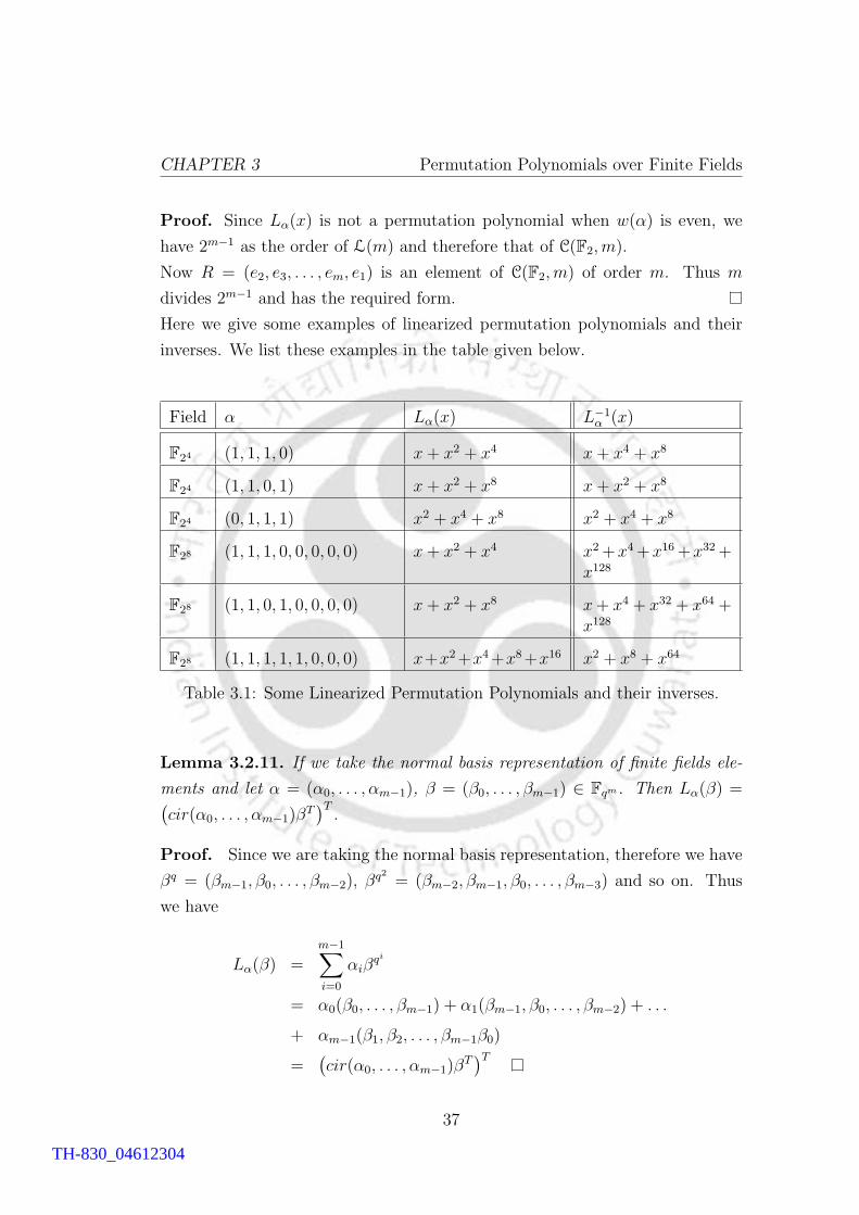
CHAPTER 3 Permutation Polynomials over Finite Fields
Proof. Since Lα(x) is not a permutation polynomial when w(α) is even, we
have 2m−1 as the order of L(m) and therefore that of C(F2,m).
Now R = (e2, e3, . . . , em, e1) is an element of C(F2,m) of order m. Thus m
divides 2m−1 and has the required form.
Here we give some examples of linearized permutation polynomials and their
inverses. We list these examples in the table given below.
Field α Lα(x) L−1α (x)
F24 (1, 1, 1, 0) x + x2 + x4 x + x4 + x8
F24 (1, 1, 0, 1) x + x2 + x8 x + x2 + x8
F24 (0, 1, 1, 1) x2 + x4 + x8 x2 + x4 + x8
F28 (1, 1, 1, 0, 0, 0, 0, 0) x + x2 + x4 x2 +x4 +x16 +x32 +x128
F28 (1, 1, 0, 1, 0, 0, 0, 0) x + x2 + x8 x + x4 + x32 + x64 +x128
F28 (1, 1, 1, 1, 1, 0, 0, 0) x+x2 +x4 +x8 +x16 x2 + x8 + x64
Table 3.1: Some Linearized Permutation Polynomials and their inverses.
Lemma 3.2.11. If we take the normal basis representation of finite fields ele-
ments and let α = (α0, . . . , αm−1), β = (β0, . . . , βm−1) ∈ Fqm. Then Lα(β) =(cir(α0, . . . , αm−1)β
T)T
.
Proof. Since we are taking the normal basis representation, therefore we have
βq = (βm−1, β0, . . . , βm−2), βq2= (βm−2, βm−1, β0, . . . , βm−3) and so on. Thus
we have
Lα(β) =m−1∑i=0
αiβqi
= α0(β0, . . . , βm−1) + α1(βm−1, β0, . . . , βm−2) + . . .
+ αm−1(β1, β2, . . . , βm−1β0)
=(cir(α0, . . . , αm−1)β
T)T
37
TH-830_04612304

CHAPTER 3 Permutation Polynomials over Finite Fields
Lemma 3.2.12. Let α, β ∈ Fqm. Then Lα(β) = Lβ(α).
Proof. Let α = (α0, . . . , αm−1), β = (β0, . . . , βm−1). Then
Lα(β) =(cir(α0, . . . , αm−1)β
T)T
=(cir(β0, . . . , βm−1)α
T)T
= Lβ(α)
Proposition 3.2.13. An element α of Fqm is a normal element of Fqm over Fq
if and only if Lα(x) is a permutation polynomial of Fqm.
Proof. Suppose α is a normal element of Fqm over Fq. Let y ∈ Fqm . Then y =∑m−1i=0 yiα
qifor some yi ∈ Fq. If z =
∑m−1i=0 yiϑ
qi, where B = {ϑ, ϑq, . . . , ϑqm−1}
is the fixed normal basis of Fqm over Fq. Then y = Lz(α) = Lα(z). Thus Lα
is surjective and therefore Lα(x) is permutation polynomial of Fqm . Conversely
suppose that Lα(x) is permutation of Fqm . Then Lα(x) = Lx(α) = y has a
unique solution for all y ∈ Fqm . This implies that α is a normal element of Fqm
over Fq.
Thus we see that there is a one-one correspondence between normal elements
of Fqm over Fq and the linear permutation polynomials of the form Lα(x). Using
the above proposition we can easily count the normal elements of Fqm over Fq.
Corollary 3.2.14. Let Fqm is a finite field, with m = pk, k ≥ 0. Then total
number of normal elements of Fqm over Fq is qm − qm−1. In particular, when
q = 2 and m = 2k, the number of normal elements is 2m−1.
Lemma 3.2.15. Suppose Lβ ∈ L(m). If α is a normal element of Fqm over Fq,
then so is Lβ(α).
Proof. The set {α, αq, . . . , αqm−1} is a basis of Fqm over Fq. Since Lβ is an in-
vertible linear operator of Fqm , therefore the set {Lβ(α), Lβ(αq), . . . , Lβ(αqm−1)}
is also a basis of Fqm over Fq. The proof is complete by noting the fact that
Lβ(αqi) = (Lβ(α))qi
.
In view of above Lemma and Proposition 3.2.13, we immediately have the
following Proposition.
38
TH-830_04612304
CHAPTER 3 Permutation Polynomials over Finite Fields
Proposition 3.2.16. Suppose for α ∈ Fqm, Lα(x) is permutation polynomial of
Fqm and f ∈ L(m) is any arbitrary element, then Lf(α)(x) is also a permutation
polynomial of Fqm.
3.2.2 Two more classes of linearized permutation poly-
nomials
In this section we will give two more classes of linearized polynomials over finite
field Fqm for q = 2, 3. Two prove our results systematically first we give a
definition from [50].
Definition 3.2.17. For α ∈ Fqm, the trace Tr(α) of α over Fq is defined as
Tr(α) = α + αq + . . . + αqm−1
.
It is easy to see that Tr(x) is a linear function from Fqm to Fq, and also note
that Tr(αqi) = Tr(α) (see chapter 3 of [50]). The following Lemma will be used
in the proof of Theorem 3.2.19.
Lemma 3.2.18. If Lα(x) ∈ L(m), then Tr(Lα(β)) = Tr(β) for all β ∈ F2m.
Proof. For β ∈ F2m , Tr(β) = β + β2 + . . . + β2m−1. Suppose α =
(α0, . . . , αm−1), where αi ∈ F2. Then Lα(β) =∑m−1
i=0 αiβ2i
. Now Tr (Lα(β)) =
Tr(∑m−1
i=0 αiβ2i). Since Tr(x) is a linear function, we have Tr (Lα(β)) =
∑m−1i=0 αiTr(β2i
). Since Tr(β2i) = Tr(β), we have Tr (Lα(β)) = w(α)Tr(β) =
Tr(β), as w(α) is odd.
Theorem 3.2.19. If Lα(x) is a permutation polynomial of F2m and a is an
element of F2m, with Tr(a) = 0 then
f(x) = Lα(x) + aTr(x)
is a permutation polynomial of F2m .
39
TH-830_04612304

CHAPTER 3 Permutation Polynomials over Finite Fields
Proof. Let β, γ be two distinct elements of F2m such that f(β) = f(γ), since
Lα(β) 6= Lα(γ), we have Tr(β) 6= Tr(γ). Without loss of generality assume
that Tr(β) = 0 and Tr(γ) = 1. Then f(β) = f(γ) implies that
Lα(β) = Lα(γ) + a
that is,
Lα(β + γ) = a
By Lemma 3.2.18, this implies that
Tr(β + γ) = Tr(Lα(β + γ)) = Tr(a) = 0
that is
Tr(β) = Tr(γ)
Which is a contradiction. Hence the result follows.
Here we generate one example for the above class of linearized permutation
polynomial.
Example 3.2.20. The polynomial x4 + x + 1 is irreducible over F2. Suppose β
is a root of x4 + x + 1 in the splitting field of F2. Then F24 = {a + bβ + cβ2 +
dβ3|a, b, c ∈ F2, β4 + β + 1 = 0} We take a = β + β2 ∈ F24 as Tr(β + β2) = 0
and Lα(x) = x + x2 + x4. Then x + x2 + x4 + (β + β2)(x + x2 + x4 + x8) =
(1 + β + β2)x + (1 + β + β2)x2 + (1 + β + β2)x4 + (β + β2)x8 is a permutation
polynomial of F24.
Theorem 3.2.21. Suppose F3m is a finite field and k is a positive integer such
that gcd(k, m) = 1 and suppose α ∈ {0, 1, 2}. Suppose k, α, and m are positive
integers such that k + αm is not multiple of 3. Then
f(x) =k−1∑i=0
x3i
+ αTr(x)
is permutation polynomial of F3m.
Proof. First note that gcd(3k − 1, 3m − 1) = 3gcd(k,m) − 1 = 2. We have
40
TH-830_04612304

CHAPTER 3 Permutation Polynomials over Finite Fields
f(x)3− f(x) = x3k −x. We note that, 0 and 1 are always roots of f(x)3− f(x).
Moreover, any root of f(x) is a root of f(x)3− f(x). If β is root of f(x)3− f(x)
other than 0 and 1, then we have β3k−1 = 1. Suppose a denotes the order of
β in F∗3m , where F∗3m denotes the group of nonzero elements of finite field F3m .
Then a divides 3k − 1 and also a divides 3m − 1, that is, a divides 2 or a = 2.
This implies that β = −1. Thus 0, 1 and −1 are the only roots of f(x)3− f(x).
But 1 and −1 are not the roots of f(x) since 3 does not divide k + αm. Thus
0 is the only root of f(x). Hence the result follows.
3.3 Some Classes of Nonlinear Permutation Poly-
nomials
Theorem 3.3.1. Let m be an odd positive integer, and β = (β0, . . . , βm−1)
be an element of F2m such that ω(β) is even and that 0 and 1 are the only
roots of Lβ(x) in F2m. Suppose k1 and k2 are non negative integers such that
gcd(2k1 + 2k2 , 2m − 1) = 1. Let ` be any positive integer with (2k1 + 2k2).` ≡1 mod 2m − 1 and γ be an element of F2m with Tr(γ) = 1. Then
f(x) = (Lβ(x) + γ)` + Tr(x)
is a permutation polynomial of F2m.
Proof. First note that Tr(Lβ(x)) = 0 and hence Tr(Lβ(x) + γ) = Tr(γ) = 1.
Thus Lβ(x) + γ 6= 0 in F2m .
Suppose, if possible, x and y are distinct elements of F2m such that f(x) =
f(y). First, suppose that Tr(x) = Tr(y). Then f(x) = f(y) gives
(Lβ(x) + γ)` = (Lβ(y) + γ)`.
Raising each of the two sides to the power 2k1 + 2k2 , we get
Lβ(x) + γ = Lβ(y) + γ
41
TH-830_04612304

CHAPTER 3 Permutation Polynomials over Finite Fields
that is Lβ(x + y) = 0. Since 0 and 1 are the only roots of Lβ(x), and because
x 6= y,we get x + y = 1. Then Tr(x + y) = Tr(1) = 1, since m is odd. That is
Tr(x) 6= Tr(y), a contradiction.
Without loss of generality assume that Tr(x) = 0 and Tr(y) = 1. Then
f(x) = f(y) implies that
(Lβ(x) + γ)` = (Lβ(y) + γ)` + 1
and therefore
Lβ(x) + γ = [(Lβ(y) + γ)` + 1]2k1+2k2
=((Lβ(y) + γ)`.2k1 + 1
)((Lβ(y) + γ)`.2k2 + 1
)
= (Lβ(y) + γ)`(2k1+2k2) + (Lβ(y) + γ)`.2k1 + (Lβ(y) + γ)`.2k2 + 1
= Lβ(y) + γ + (Lβ(y) + γ)`.2k1 + (Lβ(y) + γ)`.2k2 + 1,
since (2k1 + 2k2).` ≡ 1 mod 2m − 1. Further, Tr(Lβ(x)) = 0 and
Tr((Lβ(y) + γ)`.2k1
)= Tr
((Lβ(y) + γ)`.2k2
)= Tr
((Lβ(y) + γ)`
). Now apply-
ing the trace function to both sides of the above equation, we get
Tr(γ) = Tr(γ) + Tr(1),
which implies that Tr(1) = 0, a contradiction since m is odd.
Now we generate some examples for the above class of permutation polyno-
mial.
Example 3.3.2. The polynomial x2 + x has only roots 0 and 1 in F2m , so we
are taking Lβ(x) = x2 + x. We take γ = 1, m = 3, k2 = 0, k1 = 1, this gives
2k1 +2k2 = 3 and ` = 5. Thus (x2 +x+1)7 +Tr(x) is a permutation polynomial
of F23 .
It is easy to see that 0 and 1 are the only roots of x2k+ x in F2m if and
only if k and m are relatively prime. In the next lemma, we construct another
linearized polynomial having only roots 0 and 1 in F2m .
42
TH-830_04612304

CHAPTER 3 Permutation Polynomials over Finite Fields
Lemma 3.3.3. Let k be an even integer, with gcd(k,m) = 1. Then, 0 and 1
are the only roots of h(x) =k−1∑i=0
x2i
in F2m.
Proof. Consider h1(x) = h(x)2 + h(x) = h(x)(h(x) + 1). Clearly, each root of
h(x) is a root of h1(x). Moreover, h1(x) = x2k+ x and has 0 and 1 as its only
roots.
Example 3.3.4. We consider the field F23 and k = 4, then from above lemma
x+x2 +x4 +x8 has only roots 0, 1 in the finite field F23 . Now suppose Lβ(x) =
x+x2+x4+x8. We take k2 = 0, k1 = 2, this gives 2k1 +2k2 = 5 and ` = 3, γ = 1.
Thus by Theorem 3.3.1, (1 + x + x2 + x4 + x8)3 + Tr(x) is permutation of F23 .
Lemma 3.3.5. The polynomial f(x) = x2k2r+2r
+ x2k2r
+ x2r, where r and k
are positive integers, is a permutation polynomial of F2m if and only if 2k2r+ 2r
and 2m − 1 are co-prime.
Proof. First, note that there exist integers r and k such that 22rk+2r and 2m−1
are co-prime. It is known that composition of two polynomials is a permutation
polynomial if and only if both the polynomials are permutation polynomials
(see chapter 7 of [50]). It is easy to check that f(x + 1) = x2k2r+2r
+ 1. By
Theorem 1.2.2, f(x + 1) is a permutation polynomial if and only if 22rk + 2r
and 2m − 1 are co-prime. Since x + 1 is always a permutation of F2m , therefore
f(x) is a permutation polynomial of F2m if and only if 2k2r+ 2r and 2m − 1 are
co-prime.
As a consequence of above lemma we have the following result.
Theorem 3.3.6. The polynomial g(x) = (x2k2r
+ x2r+ α)l + x is permutation
polynomial of F2m if Tr(α) = 1 and (2k2r+ 2r).l = 1 mod 2m − 1.
Proof. Since Tr(x2k2r
+ x2r+ α) = Tr(α) = 1, x2k2r
+ x2r+ α 6= 0 for all
x ∈ F2m . Let β be an element of F2m . Then g(x) = β implies
(x2k2r
+ x2r
+ α)l = x + β.
Raising both sides to the power 2k2r+ 2r, we get
(x2k2r
+ x2r
+ α) = (x + β)2k2r+2r
,
43
TH-830_04612304

CHAPTER 3 Permutation Polynomials over Finite Fields
i.e., (x2k2r
+ x2r
+ α) + (x + β)2k2r+2r
= 0.
Suppose h(x) = (x2k2r
+ x2r+ α) + (x + β)2k2r
+2r. It is enough to show that for
any β ∈ F2m the equation h(x) = 0 has a unique solution. Note that h(x) = 0
and h(x + β) = 0 have the same number of solutions. Now h(x + β) = 0 is
equivalent to
x2k2r+2r
+ x2k2r
+ x2r
+ β2k2r
+ β2r
+ α = 0.
By Lemma 3.3.5, x2k2r+2r
+ x2k2r
+ x2ris a permutation polynomial of F2m .
Hence the equation h(x + β) = 0 has a unique solution for any β ∈ F2m .
Example 3.3.7. We consider the finite field F23 . We take r = 0, k = 2, α = 1,
this gives 2k2r+ 2r = 5 and l = 3. Then we have, (x2k2r
+ x2r+ α)l + x =
x7 + x5 + x4 + x3 + x + 1. Thus the polynomial x7 + x5 + x4 + x3 + x + 1 is a
permutation polynomial of F23 .
44
TH-830_04612304
Chapter 4
Public Key Cryptography Using
Permutation p-Polynomials
4.1 Introduction
In this chapter we propose an efficient multivariate public key cryptosystem
based on permutation p-polynomials over finite fields. We will use the group
L(m) of permutation p-polynomials which we introduced in Chapter 3. We
construct nonlinear trapdoor function based on the problem of solving nonlin-
ear equations. The complexity of encryption in our public key cryptosystem is
O(m3) multiplications which is equivalent to those of other multivariate public
key cryptosystems. But the decryption in our proposed cryptosystem is much
faster than in the other such existing cryptosystems. For decryption we need
O(m2) left cyclic shifts and O(m2) xor operations. In Section 2, we present our
public key cryptosystem and in Section 3 we give its security analysis. In Sec-
tion 4 we discuss the efficiency of our public key cryptosystem and in Section 5
we compare our public key cryptosystem with HFE. Finally, in Section 6 we
give a toy example of our cryptosystem.
45
TH-830_04612304

CHAPTER 4 Public Key Cryptography Using Permutation p-Polynomials
4.2 Public key Cryptosystem
In this section we present our multivariate public key cryptosystem using some
results from the previous chapter. Suppose B = {ϑ, ϑq, . . . , ϑqm−1} is a nor-
mal basis of Fqm over Fq. Using the representation with respect to this basis,
suppose x = (x0, x1, . . . xm−1) ∈ Fqm , where xi ∈ Fq. Then, the operation
x 7→ xq transforms x to (xm−1, x0, . . . , xm−2) which is just one left cyclic shift
of (x0, x1, . . . , xm−1). Hence the cost of exponentiating by q is negligible. From
now on we will take the normal basis representation of the elements of the finite
field Fqm over Fq with respect to the fixed normal basis B. Though the cryp-
tosystem we are proposing will work in any finite field Fqm , m = pk, for practical
point of view we consider q = 2 and m = 2k. To obtain quadratic polynomials
we use convolution of bits. We have seen in Chapter 3 that convolution of binary
bits is equivalent to the composition of corresponding p-polynomials. Moreover,
composition of two permutation p-polynomials is a permutation p-polynomial.
For x ∈ F2m let (x)t denote the t times convolution of x with itself. From now
on words we will denote the linearized polynomials Lα(x) by simply Lα. Let
the set of all odd weight element of Fm2 be denoted by OFm
2 . To describe our
cryptosystem systematically, we need a few results which are discussed below.
Lemma 4.2.1. For α = (α0, . . . , αm−1) ∈ F2m, if (α)2 = (β0, . . . , βm−1), then
β2i+1 = 0 and β2i = αi + α(m/2)+i, where 0 ≤ i ≤ (m− 2)/2.
Proof. We have, βk =∑m−1
i=0 αi.αk−i, where the suffices will be modulo m. For
0 ≤ i ≤ (m−2)/2, we have β2i+1 = α0α2i+1+α1α2i+. . .+α2i+1α0+α2i+2αm−1+
. . .+αm−1α2i+2. All the terms will be canceled out in pairs, so we have β2i+1 = 0.
In a similar manner β2i = α0α2i+α1α2i−1+ . . .+αiαi+ . . .+α2iα0+α2i+1αm−1+
. . .+αm/2+iαm/2+i + . . .+αm−1α2i+1 = α2i +α2
(m/2)+i = αi +α(m/2)+i, as x2i = xi
for xi ∈ F2.
Above lemma implies that (x)2 is a linear function on the finite field F2m .
In general, it can be proved that (x)2kis a linear function on F2m .
Lemma 4.2.2. Suppose x = (x0, x1, . . . , xm−1) is an element of Fm2 . If (x)t =
(h0, h1, . . . , hm−1), then each hi is a nonlinear function of xi of degree w(t),
where w(t) denotes the weight of t.
46
TH-830_04612304

CHAPTER 4 Public Key Cryptography Using Permutation p-Polynomials
Proof: Suppose G = (g0, g1, . . . , gm−1), where each gi is a linear polyno-
mial in variables xi and suppose (G)2l= (g
′0, g
′1, . . . , g
′m−1) and (G)2l+2k
=
(g′′0 , g
′′1 , . . . , g
′′m−1), where k > l ≥ 1. Then by lemma 4.2.1, degrees of g
′i and g
′′i
are 1 and 2, respectively. This proves the lemma.
Lemma 4.2.3. The function defined by h(x) = (x)t, where t is co-prime to m,
is a bijection from OFm2 onto OFm
2 .
Proof. Since (x)t is of odd weight whenever x is so, h(x) is a function from
OFm2 into OFm
2 . Now, since t and m are co-prime, there exist positive integers r
and k such that tk = 1+rm. Let y ∈ OFm2 . Consider x = (y)k. Then x ∈ OFm
2 .
Moreover,
L(x)t = L(y)kt = Lkt(y) = L1+rm
(y) = Ly,
Since by the Lemma 3.2.1, we have L(y)kt = Lkt(y) and from the Corollary 3.2.8,
Lmy = Lϑ. This implies that h(x) = (x)t = y. Thus, h(x) is surjective, and the
result follows.
Lemma 4.2.4. Convolution is distributive over addition in finite fields, that is,
α ∗ (β + γ) = α ∗ β + α ∗ γ, for all α, β, γ ∈ F2m.
Proof. Suppose α = (α0, . . . , αm−1), β = (β0, . . . , βm−1) and γ = (γ0, . . . , γm−1).
Then, β + γ = (β0 + γ0, . . . , βm−1 + γm−1). Now, we have
α ∗ (β + γ) =m−1∑i=0
αi
(β(k−i) mod m + γ(k−i) mod m
),
or equivalently we can write
α ∗ (β + γ) =m−1∑i=0
(αiβ(k−i) mod m + αiγ(k−i) mod m
),
that is,
α ∗ (β + γ) = α ∗ β + α ∗ γ.
47
TH-830_04612304

CHAPTER 4 Public Key Cryptography Using Permutation p-Polynomials
Lemma 4.2.5. If m = 2k, k ≥ 1 and α, β ∈ OFm2 , then α ∗ β ∈ OFm
2 , that is, if
the bit size is a power of 2 then the convolution of two odd weight binary strings
is an odd weight binary string.
Proof. By Corollary 3.2.6, the linearized polynomials Lα and Lβ are per-
mutation of F2m . Since the composition of two permutation polynomials is a
permutation polynomial, therefore Lα ◦ Lβ is a permutation of F2m . But by
Lemma 3.2.1, Lα ◦Lβ = Lα∗β, therefore Lα∗β is a permutation of F2m . Now the
result follows by Corollary 3.2.6.
4.2.1 Public key generation
Consider a message of m − 1 bit string (x0, x1, . . . , xm−2), where m is of the
form 2k. We are adjoining one more bit xm−1 to make the weight odd. After
decryption one needs to remove the last bit xm−1. So we can assume that
message X = (x0, x1, . . . , xm−1) is an m bit odd weight element of the finite field
F2m . Suppose Lα, Lβ, Lγ, Lδ, Lη are elements of the group L(m) and Lξ, Lζ are
elements of the group L(2m). Let π1,π2, π3, π4, π5 are random permutations of
{0, 1, 2, . . . , m−1} and π6, π7 are random permutations of {0, 1, 2, . . . , 2m−1}.Now compute T
′1 = Lα ◦π1, T
′2 = Lβ ◦π2, T
′3 = Lγ ◦π3, T
′4 = Lδ ◦π4, T
′5 = Lη ◦π5
and T′6 = Lξ ◦ π6, T
′7 = Lζ ◦ π7, where ◦ denotes the composition of mappings.
Now, define the affine transformation Tr(X) = T′r(X) + σr for 1 ≤ r ≤ 7, where
σr for 1 ≤ r ≤ 5 is an even weight element of F2m and σ6, σ7 are even weight
element of F22m . We note that if X is an odd weight element of F2m , then T′r(X)
and Tr(X) are odd weight element of F2m . Thus, Tr(X) is a bijection of OF2m .
Next, compute X′
= T1 (X), X′′
= T2 (X). Again, compute T3
((X
′)2 ∗X
′′)
and T4
(X
′ ∗X′′)
+ T5
((X
′)2 ∗X
′′). Suppose the quadratic polynomials fi and
fm+i denote the ith bits of T3
((X
′)2 ∗X
′′)and T4
(X
′ ∗X′′)
+ T5
((X
′)2 ∗X
′′),
respectively, in their normal basis representations. Suppose ϑ′
is the normal
element of F22m and B′ denotes the normal basis of F22m over F2 corresponding
to ϑ′. Now, consider the 2m bits (f0, f1, . . . , f2m−1) as an element of F22m
corresponding to the basis B′ . Suppose Y = (y0, y1, . . . , y2m−1, ) is the ciphertext
which is to be computed using the algorithm described in the sequel. Let Z =
T6 (Y ) and suppose λ and σ are elements of F22m of even and odd weights,
48
TH-830_04612304
CHAPTER 4 Public Key Cryptography Using Permutation p-Polynomials
respectively. Then, by Lemma 4.2.3 the function λ + σ ∗ (Z)2m−1 is a bijection
of OF22m . The relation between the plaintext and the ciphertext is:
T7 (f0, f1, . . . , f2m−1) = λ + σ ∗ (Z)2m−1 (4.1)
We note that the ciphertext Y is an odd weight element of F22m . It follows from
Remark 3.2.9 that (Z)2m = ϑ′, the identity of convolution. Taking convolution
with Z of each of the two sides of (4.1) and using Lemma 4.2.4, we have the
following relation between the plaintext and the ciphertext:
T7 (f0, f1, . . . , f2m−1) ∗ Z + λ ∗ Z + σ = 0 (4.2)
Equation (4.2) gives the 2m polynomial equations of total degree 3 in variables
x0, x1, . . . , xm−1; y0, y1, . . . , y2m−1, but of degree 1 in variables yi. Thus, we get
2m equations of the form
∑aijkxixjyk +
∑bijxiyj +
∑cijxixj +
∑dkyk +
∑ekxk + fl = 0. (4.3)
The terms aijklxixjyk, bijlxiyj and dkyk will always have nonzero coefficients
in the above equation. Each of the equations is of degree three with O(m3)
terms. Since we have 2m equations, number of terms in the system will be of
O(m4), which is large. However, it is possible to reduce the number of terms in
the polynomial equations (4.3) up to O(m3) by writing it as a two sets of pub-
lic polynomials containing only quadratic terms without changing the security,
since this can be done in polynomial time (see [64]). Thus, the public key will
be two sets of 2m quadratic equations of the form:
∑gkyk +
∑bijxiyj +
∑dkyk +
∑ekxk + fl = 0
where
gk =∑
hijkxixj.
The results in Section 3.2 are true for any arbitrary prime power q. Therefore,
the public key size can be further reduced by taking m not too large (for example
49
TH-830_04612304

CHAPTER 4 Public Key Cryptography Using Permutation p-Polynomials
m = 32) and q not too small.
4.2.2 Secret key
The linear transformations (T1, T2, T3, T4, T5, T6, T7) and finite fields elements
(λ, σ) are the required secret keys.
4.2.3 Encryption
For encrypting a plaintext M = (x0, x1, . . . , xm−1), one substitutes the plain-
text vector in the public key and solves the resulting linear equations for the
ciphertext Y = (y0, y1, . . . , y2m−1). One will get a unique ciphertext because
our encryption function is injective. Given a ciphertext Y , the public equations
are nonlinear in xi. It follows from equation (4.1) that the encryption function
is given by
E(X) = Y = T−16
(((F (X) + λ) ∗ (σ)2m−1
)2m−1)
,
where F (X) = T7(f0, f1, . . . , f2m−1).
Theorem 4.2.6. The encryption function E is well defined and bijective from
OF2m to E(OF2m), where E(OF2m) denotes the range of E in OF22m.
Proof. Suppose X1, X2 ∈ OF2m . It is easy to verify that X1 = X2 implies
E(X1) = E(X2). Now, we assume that E(X1) = E(X2), that is,
T−16
(((F (X1) + λ) ∗ (σ)2m−1
)2m−1)
= T−16
(((F (X2) + λ) ∗ (σ)2m−1
)2m−1)
.
Therefore
((F (X1) + λ) ∗ (σ)2m−1
)2m−1=
((F (X2) + λ) ∗ (σ)2m−1
)2m−1.
Since (F (X1) + λ) ∗ (σ)2m−1 and (F (X2) + λ) ∗ (σ)2m−1 are elements of OF22m ,
50
TH-830_04612304

CHAPTER 4 Public Key Cryptography Using Permutation p-Polynomials
so by Lemma 4.2.3 we have
(F (X1) + λ) ∗ (σ)2m−1 = (F (X2) + λ) ∗ (σ)2m−1.
Now, taking the convolution of both sides with σ and noting that (σ)2m = ϑ′
we have F (X1) = F (X2), which implies
T3
((X
′1)
2 ∗X′′1
)= T3
((X
′1)
2 ∗X′′1
),
and
T4
(X
′1 ∗X
′′1
)+ T5
((X
′1)
2 ∗X′′1
)= T4
(X
′2 ∗X
′′2
)+ T5
((X
′2)
2 ∗X′′2
).
From the above two relations, we have
(X′1)
2 ∗X′′1 = (X
′2)
2 ∗X′′2 and X
′1 ∗X
′′1 = X
′2 ∗X
′′2 ,
that is,
X1 ∗X′2 ∗X
′′2 = (X
′2)
2 ∗X′′2 .
This implies X1 = X2.
4.2.4 Decryption
The decryption algorithm for the cryptosystem is as follows.
Input: Ciphertext Y = (y0, . . . , ym−1) and secret parameters (T1, T2, T3, T4,
T5, T6, T7, λ, σ) and an element of α ∈ F22m such that w(α) is odd.
Output: Message X
1: Z ← T6(Y ).
2: (Z)2m−1 ← L−1α
(L2m−1
Z (α)).
3: Z′ ← λ + σ ∗ (Z)2m−1.
4: 4← T−17 (Z
′).
5: (δ0, . . . , δ2m−1) ←4.
6: 41 ← (δ0, . . . , δm−1) and 42 ← (δm, . . . , δ2m−1).
51
TH-830_04612304

CHAPTER 4 Public Key Cryptography Using Permutation p-Polynomials
7: 43 ← T−13 (41) and 44 ← T5(43).
8: 45 ←42 +44.
9: 46 ← T−14 (45).
10: 47 ← L46(α).
11: 48 ← L43(α).
12: 49 ← Lm−147
(48).
13: X ← T−11 (49).
14: Return X.
We now prove that the above algorithm gives valid plaintext X as the output
for a ciphertext Y .
Theorem 4.2.7. Given ciphertext Y , the output X given by the decryption
algorithm is a valid plaintext.
Proof. Using the Lemma 3.2.1 and 3.2.12, first note that
L−1α
(L2m−1
Z (α))
= L−1α
(L(Z)2m−1(α)
)
= L−1α
(Lα
((Z)2m−1
))
= (Z2m−1)
where Z = T6(Y ). Now suppose Z′= λ + σ ∗ (Z)2m−1. Now from relation 4.1,
we have
T7(f0, . . . , f2m−1) = λ + σ ∗ (Z)2m−1 = Z′.
that is,
(f0, . . . , f2m−1) = T−17 (Z
′) = 4 = (δ0, . . . , δ2m−1).
This implies,
(f0, . . . , fm−1) = (δ0, . . . , δm−1) and (fm, . . . , f2m−1) = (δm, . . . , δ2m−1)
that is, we have,
T3
((X
′)2 ∗X
′′)
= 41 (4.4)
and
T4
(X
′ ∗X′′)
+ T5
((X
′)2 ∗X
′′)
= 42 (4.5)
52
TH-830_04612304

CHAPTER 4 Public Key Cryptography Using Permutation p-Polynomials
From relation (4.4), we have
(X′)2 ∗X
′′= T−1
3 (41) = 43 (4.6)
and
T5
((X
′)2 ∗X
′′)
= T5(43) = 44 (4.7)
Adding relation (4.5) and (4.7), we get T4(X′ ∗ X
′′) = 42 + 44 = 45 or
equivalently, we have
X′ ∗X
′′= T−1
4 (42 +44) = 46. (4.8)
Suppose α is an odd weight element of F2m . Now from relation (4.8) and (4.6),
we have LX′∗X′′ (α) = L4(α) = 47 and L(X′ )2∗X′′ (α) = L43(α) = 48. Now
from the Lemma 3.2.1, we have L(X′)2∗X′′ (α) = LX
′ (LX′∗X′′ (α)). Thus we have
LX′ (47) = 48. Since by the Lemma 3.2.12, LX
′ (47) = L47
(X
′), therefore
we have X′= L−1
47(48). Since by Corollary 3.2.7, we know that L−1
47= Lm−1
47,
therefore we have X′= Lm−1
47(48) = 49. Thus we have X = T−1
1 (49).
4.3 Security of the proposed cryptosystem
In this section we discuss the security of the proposed cryptosystem. In general
it is very difficult to prove the security of a public key cryptosystem [57], [73].
For example if the public modulus of RSA is decomposed into its prime factors
then RSA is broken. However, it is not proved that breaking RSA is equivalent
to factoring its modulus, see [36]. In this section we will give some security ar-
guments and evidence that our cryptosystem is secure. Most of the multivariate
public key cryptosystems use the structure t(f(s(x))), where t and s are secret
invertible linear transformation and f(x) is a quadratic nonlinear function. Hid-
ing f(x) by two linear transformations does not work very effectively (see the
attack of Kipnis and Shamir on HFE [42]). We are using a different structure and
we will prove that our structure is at least as secure as the t(f(s(x))) structure.
In our cryptosystem the function f(x) is (x∗x∗x, x∗x+x∗x∗x) so t(f(s(x))) =
t (s(x) ∗ s(x) ∗ s(x), s(x) ∗ s(x) + s(x) ∗ s(x) ∗ s(x)). We take the simpler case,
53
TH-830_04612304
CHAPTER 4 Public Key Cryptography Using Permutation p-Polynomials
suppose we are not using the transformations T3, T4 and T5. Then, our structure
is T7 (T1(x) ∗ T1(x) ∗ T2(x), T1(x) ∗ T2(x) + T1(x) ∗ T1(x) ∗ T2(x)). It is clear
that if T1 = T2, then our structure is equivalent to t(f(s(x))) structure. Thus, if
it is possible to attack our structure, then it is also possible to attack t(f(s(x)))
structure. This proves that our structure is at least as secure as the com-
monly used structures t(f(s(x))) in multivariate cryptography. Moreover, our
quadratic part of the plaintext is hidden, because in this case the public poly-
nomials are the m bit representation of F (X) ∗ Z + λ ∗ Z + σ, where F (X) =
T7(f0, f1, . . . , f2m−1) and Z = T6(Y ). From F (X) ∗ Z + λ ∗ Z + σ it is not pos-
sible to compute either F (X), Z, λ or σ, because F (X) ∗Z is equivalent to the
composition of corresponding p-polynomials and in general it is very difficult
to decompose the composition of two functions. We are using affine transfor-
mations, so the bitwise representation of F (X) ∗ Z will also give the terms of
the form dkyk + ck. So it is not possible to find λ and σ from the public key.
In the rest of this section, we discuss some known attacks developed for multi-
variate cryptosystems and we will show that those attacks are not applicable to
our cryptosystem. The attacks discussed in this section are Grobner basis, uni-
variate polynomial representation, Linearization, Relinearization, XL and FXL
algorithms.
4.3.1 Linearization equation attacks.
Let F = {f0, f1, . . . , fm−1} be any set of m polynomials in Fq[x0, x1, . . . , xm−1].
A linearization equation for F is any polynomial in Fq[x0, x1, . . . , xm−1, y0, y1, . . . ,
ym−1] of the form
m−1∑i=0
m−1∑j=0
aijlxiyj +m−1∑i=0
bilxi +m−1∑j=0
cjlyj + dl (4.9)
where l = 0, 1, . . . , m− 1, where yj = fj.
Linear equation attack was first successfully applied by Patarin in [63] to break
the cryptosystem MIC* [55]. The idea of Patarin was to notice that if a
function is defined as F : x → xqi+1, then a relation between the plaintext
(x0, x1, . . . , xm−1) and the ciphertext (y0, y1, . . . , ym−1) of the form shown in
54
TH-830_04612304

CHAPTER 4 Public Key Cryptography Using Permutation p-Polynomials
equations (4.9) can be established, where aij, bi, cj and dl are unknown coeffi-
cients. By taking at least (m + 1)2 different plaintext-ciphertext pairs a linear
system of equations can be established and solved.
Ou cryptosystem does not use any function of the form xqi+1. Moreover,
here the plaintext and the ciphertext are connected by the relation (4.1), and
T6, λ and σ are secrets. So, in this case it is not possible to obtain a relation of
the form (4.9). One may try to find a relation which is linear in xi and nonlinear
in yj. However, this line of attack is not possible as the degree of the inverse
function is very high. From the relation (4.1) we have (f0, f1, . . . , f2m−1) =
T−17 (Z
′). Note that Z
′= λ + σ ∗ (Z)2m−1 and Z = T6 (Y ) so T−1
7 (Z′) will give
nonlinear polynomials of degree w(2m−1) in the ciphertext variables. Suppose
T−17 (Z
′) = (Z0, Z1, . . . , Z2m−1). Then we have the following relations between
the plaintext and the ciphertext
T3
(X
′ ∗X′ ∗X
′′)
= (Z0, Z1, . . . , Zm−1)
and
T4
(X
′ ∗X′′)
+ T5
(X
′ ∗X′ ∗X
′′)
= (Zm, Zm+1, . . . , Z2m−1) .
Using these two relations one can get the following relation between the plaintext
and the ciphertext:
X′ ∗ T−1
4 ◦ T5
(Z′)
+ T−14 (Zm, Zm+1, . . . , Z2m−1) = Z
′′, (4.10)
where X′= T1 (X), Z
′′= T−1
3 (Z0, Z − 1, . . . , Zm−1) and T1, T2, T3, T4, T5, T6 are
unknown linear transformations. Note that the relation (4.10) is of total degree
w(2m − 1) + 1; of degree w(2m − 1) degree in the ciphertext variables and of
degree one degree in the plaintext variable. Most crucially, the degree of relation
(4.10) is not constant but a function of m. Thus, to attack the cryptosystem
one will need Gaussisn reduction on O(mw(2m−1)+1) terms, which is impractical
for the bit size 64 or more, because for m = 64, w(2m− 1) + 1 = 8.
55
TH-830_04612304

CHAPTER 4 Public Key Cryptography Using Permutation p-Polynomials
4.3.2 Attacks with Differential Cryptanalysis
Differential cryptanalysis has been successfully used earlier to attack the sym-
metric cryptosystem. In recent years differential cryptanalysis has emerged as a
powerful tool to attack the multivariate public key cryptosystems too. In 2005
[32] Fouque, Granboulan and Sterm used differential cryptanalysis to attack
the multivariate cryptosystems. The key point of this attack is that in case of
quadratic polynomials the differential of public key is a linear map and its kernel
or its rank can be analyzed to get some information on the secret key. For any
multivariate quadratic function G : Fnq → Fm
q the differential operator between
any two points x, k ∈ Fnq can be expressed as LG,kG(x+k)−G(x)−G(k)+G(0)
and in fact that operator is a bilinear function. By knowing the public key of a
given multivariate quadratic scheme and by knowing the information about the
nonlinear part (xqi+1) they showed that for certain parameters it is possible to
recover the kernel of LG,k. This attack was successfully applied on Ding’s cryp-
tosystem [25] and afterwards using the same technique Dubois, Fouque, Shamir
and Sterm in 2007 [28] have completely broken all versions of the SFLASH
signature scheme proposed by Patarin, Courtois, and Goubin [66]. In our cryp-
tosystem we are not using any polynomial of the form xqi+1. Moreover the
public key in our system is not quadratic but of total degree 3, quadratic in
plaintext variables and degree one in ciphertext variables. Substituting the ci-
phertext gives quadratic plaintext variables but in that case it will be different
for different ciphertexts. So to attack our cryptosystem by the methods of [32]
and [28] is not feasible.
4.3.3 Attacks using the univariate polynomial represen-
tation of multivariate public polynomials
The fact that any function from a finite field into itself can be represented by
a univariate polynomial is sometime used to attack multivariate cryptosystem
(see [26] for example). In our case, the encryption function is from the finite field
F2m to the finite field F22m , and therefore we cannot represent the encryption
function by a polynomial directly. It is possible to have such a representation
by introducing dummy variables xm, xm+1, . . . , x2m. In our cryptosystem the
56
TH-830_04612304

CHAPTER 4 Public Key Cryptography Using Permutation p-Polynomials
relation between the plaintext and ciphertext is F (X) = λ+σ ∗ (Z)2m−1, where
F (X) = T7(f0, f1, . . . , f2m−1). Suppose G(X) = ((F (X) + λ) ∗ σ2m−1)2m−1
.
Then, we have Y = T−16 (G(X)). Note that F (X) is nonlinear of degree 2, so
that T−16 (G(X)) will give 2m multivariate polynomials of degree 2.w(2m− 1).
By Lemma 3.3 of [42], the degree of the univariate polynomial representation
is not constant but it is function of m. Thus, the degree and the number of
nonzero terms of the univariate polynomial representation of encryption func-
tion are both O(mm). The complexity of root finding algorithms, Berlekamp
algorithm for example, is polynomial in the degree of the polynomial. This re-
sults in an exponential time algorithm to find the roots of univariate polynomial.
Therefore, this approach is less efficient than the exhaustive search.
4.3.4 Grobner basis attacks
After substituting the ciphertext in the public key, one can get 2m quadratic
equations in m variables and then Grobner basis techniques can be applied to
solve the system. The classical algorithms for solving systems of multivariate
equations is Buchberger’s algorithm for constructing Grobner basis (see [17]).
Theoretically, it can solve all the multivariate quadratic equations. However,
its complexity is exponential in the number of variables, although there is no
closed-form formula for it. In the worst case the Buchberger’s algorithm is
known to run in double exponential time and on average its running time seems
to be single exponential (see [14]). There are some efficient variants F4 and F5
of Buchberger’s algorithm given by Jean-Charles Faugere (see [29] and [30]).
The complexity of computing a Grobner basis for the public polynomials of
the basic HFE scheme is not feasible using Buchberger’s algorithm. However,
it is completely feasible using the algorithm F5. The complexities of solving
the public polynomials of several instances of the HFE using the algorithm F5
are provided in [31]. Moreover, it has been expressed in [31], “A crucial point
in the cryptanalysis of HFE is the ability to distinguish a randomly algebraic
system from an algebraic system coming from HFE”. Instead of using any
polynomial of special form we are using convolution operation to construct the
public polynomials. Moreover our public key is of mixed type, this means,
for different ciphertexts we will get different system of quadratic polynomial
57
TH-830_04612304
CHAPTER 4 Public Key Cryptography Using Permutation p-Polynomials
equations, so in our public key the quadratic polynomials look random. We
have already seen that the degree of the univariate polynomial representation
of the encryption function is proportional to m. It is explained in [31] that in
this case there does not seem to exist polynomial time algorithm to compute the
Grobner basis. Hence, attack on our cryptosystem by Grobner basis method is
not feasible.
4.3.5 Relinearization, XL and FXL Algorithms
Relinearization, XL or FXL algorithm are some techniques to solve the quadratic
equations directly. The relinearization technique is developed in [42] for solving
an overdefined system of quadratic equations. However, it is shown in [14] that
the Relinearization technique is not as efficient as one may expect since many
of newly generated equations are dependent. Therefore, a technique called XL
(extended relinearization) has been proposed in [14]. It is claimed to be the
best algorithm for solving overdefined multivariate equations. However, when
the number of equations is m + r for some 1 ≤ r ≤ m, then it is proved in [14]
that XL has exponential complexity. A variant of the XL algorithm called FXL,
was introduced in [14]. In this algorithm some variables are guessed to make
the system slightly overdefined. Then the XL algorithm is applied. The main
question is how many variables must be guessed. Although more guesses make
the system more unbalanced, they add to the complexity of the algorithm. The
optimum number of guesses is provided in [14].
One will find it difficult to attack our cryptosystem by solving the quadratic
equations directly with the help of the above techniques, because our public key
is of mixed type, which means that for different ciphertexts one will have to
solve different systems of quadratic nonlinear equations.
In case of applying XL, r = m for our cryptosystem. Hence, XL algorithm
cannot be used directly to attack our cryptosystem, since it has exponential
complexity.
Even using the optimum value for the number of variables guessed in the
nonlinear equation, FXL has the exponential complexity for solving the system
of public polynomials in the proposed cryptosystem. Hence, the FXL algorithm
is not applicable to our cryptosystem.
58
TH-830_04612304

CHAPTER 4 Public Key Cryptography Using Permutation p-Polynomials
4.4 Complexity and number of operations for
encryption and decryption
In this section we discuss the complexities of the encryption and the decryption
of our cryptosystem.
4.4.1 Encryption
The public key in our cryptosystem consists of 2m equations of the form (4.3).
There are O(m2) terms of the form xixj in each of the 2m equations of the public
key. So the complexity of evaluating public key at message block x0, x1, . . . , xm−1
is O(m3). The next step of encryption is to solve the 2m linear equation in 2m
ciphertext variables y0, y1, . . . , y2m−1. This can be done efficiently by Gaussian
elimination with O(m3) complexity. Hence, the total complexity of encryption
is O(m3).
4.4.2 Decryption
In our cryptosystem decryption is very fast. For decryption we are using the
following operations: permutation of bits, xor and left cyclic shifts of bits. We
count the total number of operations to describe the exact efficiency of our
cryptosystem. To operate Ti or T−1i , 0 ≤ i ≤ 5 on a m bit string we need one
permutation on bits and at most m− 2 left cyclic shifts and m xor operations.
To operate Ti or T−1i , for i = 6, 7 on a 2m bit string we need one permutation on
2m bits and at most 2m−2 left cyclic shifts and 2m xor operations. To compute
(Z)2m−1, where Z is a 2m bit string, we need at most (2m−1)(2m−2)+2m−2
left cyclic shifts and at most (2m−1)2+2m−1 xor operations. Thus, to compute
L−1θ where θ is m bit binary string we need at most (m − 1)(m − 2) + m − 2
left cyclic shifts and at most (m − 1)2 + m − 1 xor operations. Thus, we see
that for decryption we need O(m2) xor operations and O(m2) left cyclic shifts
operations.
59
TH-830_04612304

CHAPTER 4 Public Key Cryptography Using Permutation p-Polynomials
4.5 Comparison with HFE
In our cryptosystem the complexity of encryption is O(m3), i.e., equivalent to
that of HFE. But the decryption is faster than HFE. In HFE the decryption is
slow because one needs to compute the roots of a polynomial. The decryption
complexity of HFE is O(n4d2log(d)), where d is the degree of the HFE poly-
nomial. Note that for security reasons one cannot take smaller degree. Due to
this the decryption process in HFE is slow. In our cryptosystem we are using
left cyclic shifts and xor operations resulting much faster decryption process.
In our cryptosystem we need O(m2) left cyclic shifts and O(m2) xor operations
to decrypt a message. Public key size of HFE is of O(m3) terms. In our cryp-
tosystem public key size is bigger than HFE but it is also of O(m3) terms as
it is possible to write the public key as two sets of quadratic public polynomi-
als. Secret key generation in our public key cryptosystem is faster than HFE,
because for secret keys we have to select random odd weight and even weight
binary strings and random permutations only.
4.6 A toy example of cryptosystem
Example 4.6.1. We consider finite field F24 , λ = 0 and σ = (1, 0, 0, 0, 0,
0, 0, 0). Suppose ϑ′is the normal element of F28 and we take the normal basis
representation of F28 with respect to ϑ′. Suppose T1 = π1 =
0 1 2 3
2 0 3 1
and T2 = π2 =
0 1 2 3
3 2 1 0
and T3, T4, T5 are x + x2 + x4, x2 + x4 +
x8, x + x2 + x8 respectively, T6 = π6 =
0 1 2 3 4 5 6 7
3 1 5 0 4 2 6 7
and T7 =
π7
0 1 2 3 4 5 6 7
5 3 7 2 1 0 4 6
. Message M = (x0, x1, x2, x3), T1(M) = M
′=
(x2, x0, x3, x1) and T2(M) = M′= (x3, x2, x0, x1). We compute all the bits of
M′ ∗ M
′′. Suppose [M
′ ∗ M′′]i denotes the ith bit of M
′ ∗ M′′. We obtain,
[M′ ∗ M
′′]0 = x2x3 + x0 + x3x1 + x1x2, [M
′ ∗ M′′]1 = x2 + x1, [M
′ ∗ M′′]2 =
60
TH-830_04612304

CHAPTER 4 Public Key Cryptography Using Permutation p-Polynomials
x3 +x1x0 +x2x1 +x0x2, [M′ ∗M
′′]3 = x2x0 +x0x1 +x2x3 +x1x3. Now compute
all the bits M′ ∗M
′ ∗M′′. The bits of M
′ ∗M′ ∗M
′′are [M
′ ∗M′ ∗M
′′]0 =
x2x3 + x0x1 + x3 + x1, [M′ ∗ M
′ ∗M′′]1 = x0 + x2 + x0x1 + x2x3, [M
′ ∗ M′ ∗
M′′]2 = x0x3 + x1x2, [M
′ ∗ M′ ∗ M
′′]3 = x0x3 + x1x2. (f0, f1, f2, f3) denotes
the bits of T3(M′ ∗ M
′ ∗ M′′) and (f4, f5, f6, f7) denotes the bits of T4(M
′ ∗M
′′) + T5(M
′ ∗ M′ ∗ M
′′), we have f0 = x3x2 + x0x1 + x3 + x1, f1 = 1 +
x0x3 + x1x2, f2 = 1 + x0x3 + x0x1, f3 = x0 + x2 + x3x2 + x1x2, f4 = x0 +
x0x3 + x3x2 + x1x3, f5 = 1 + x0 + x2x3 + x3x0, f6 = x3 + x2x0 + x1x2 + x0x1,
f7 = 1 + x0x1 + x0x2 + x3x1 + x2x3. Ciphertext Y = (y0, y1, y2, y3, y4, y5, y6, y7)
is an element of F22m . T6(Y ) = Z = (y3, y1, y5, y0, y4, y2, y6, y7). Note that
ϑ′= (1, 0, 0, 0, 0, 0, 0, 0). Suppose P0, P1, P2, P3, P4, P5, P6, P7 denote the bits of
T7(f0, f1, f2, f3, f4, f5, f6, f7) ∗ Z + ϑ′. We compute all the Pi, so the required
public key is :
P0 = 1 + y0(x0x1 + x1x2) + y1(x0x2) + y2(x0x3 + x2x3) + y3(x2x3 + x0x3) +
y4(x0x3 + x1x3) + y5(x2x3 + x0x3 + x1x3) + y6(x1x2 + x2x3 + x1x3) + y7(x0x1 +
x1x3)x0y3 +x1y3 +x0y7 +x2y7 +x2y6 +x0y6 +y2 +y4 +x1y0 +x3y0 +x0y5 +x1y1
P1 = y0(x2x3 + x0x3 + x1x3) + y1(x0x3 + x2x3) + y2(x0x3 + x1x3) + y3(x0x1 +
x1x2) + y4(x0x1 + x1x2) + y5(x0x2) + y6(x0x3 + x2x3) + y7(x2x3 + x1x2 + x0x2 +
x1x3)+x0y0+x0y1+x0y3+x0y7+x1y1+x1y4+x1y5+x2y3+x2y7+x3y4+y2+y6
P2 = y0(x0x2) + y1(x0x1 + x1x2) + y2(x0x1 + x1x2) + y3(x2x3 + x1x3 + x0x2 +
x1x2) + y4(x0x3 + x2x3 + x1x3) + y5(x2x3 + x0x3) + y6(x0x3 + x1x3) + y7(x0x3 +
x2x3)+x0y1+x0y3+x0y4+x0y5+x1y0+x1y2+x1y5+x2y1+x2y3+x3y2+y6+y7
P3 = y0(x0x3+x2x3)+y1(x0x2+x1x2+x2x3)+y2(x0x3+x2x3+x1x3)+y3(x2x3+
x0x3) + y4(x0x2) + y5(x0x1 + x1x2) + y6(x0x1 + x1x2) + y7(x0x3 + x1x3) + x0y0 +
x0y1 + x0y2 + x0y5 + x1y0 + x1y4 + x1y6 + x2y1 + x2y5 + x3y6 + y3 + y7
P4 = y0(x0x1 +x1x2)+ y1(x2x3 +x0x3)+ y2(x0x2)+ y3(x1x3 +x0x3)+ y4(x0x3 +
x2x3)+y5(x2x3+x0x2+x1x3+x1x2)+y6(x1x3+x2x3+x0x3)+y7(x0x3+x2x3)+
x0y0 + x0y4 + x0y5 + x0y6 + x1y4 + x1y2 + x1y7 + x2y0 + x2y5 + x3y7 + y1 + y3
P5 = y0(x0x2+x1x2+x1x3+x2x3)+y1(x0x3+x1x3)+y2(x0x3+x2x3)+y3(x0x1+
x1x2) + y4(x0x1 + x1x2) + y5(x2x3 + x0x3) + y6(x0x2) + y7(x2x3 + x0x3 + x1x3) +
x0y0 + x0y2 + x0y4 + x0y7 + x1y2 + x1y3 + x1y6 + x2y0 + x2y4 + x3y3 + y1 + y5
P6 = y0(x0x3+x2x3)+y1(x0x1+x1x2)+y2(x0x1+x1x2)+y3(x2x3+x0x3+x1x3)+
y4(x0x2 + x1x3 + x2x3 + x1x2) + y5(x0x3 + x1x3) + y6(x0x3 + x2x3) + y7(x0x2) +
x0y2 + x0y3 + x0y4 + x0y6 + x1y1 + x1y6 + x1y7 + x2y2 + x2y4 + x3y1 + y0 + y5
61
TH-830_04612304

CHAPTER 4 Public Key Cryptography Using Permutation p-Polynomials
P7 = y0(x0x3 +x1x3)+ y1(x0x3 +x1x3 +x2x3)+ y2(x0x2 +x2x3 +x1x2 +x1x3)+
y3(x0x2)+y4(x2x3 +x0x3 +x0x2)+y5(x1x2 +x0x1)+y6(x0x1 +x1x2)+y7(x2x3 +
x0x3)+x0y1+x0y2+x0y6+x0y7+x1y3+x1y5+x1y7+x2y2+x2y6+x3y5+y0+y4
The public key looks large, however it is possible to reduce the size of public
key containing only quadratic terms. The public key can be written as two sets
of public polynomials containing only quadratic terms. We have
P′0 = 1 + y0g1 + y1g0 + y2g4 + y3g4 + y4g5 + y5g3 + y6b + y7g5 + x0y3 + x1y3 +
x0y7 + x2y7 + x2y6 + x0y6 + y2 + y4 + x1y0 + x3y0 + x0y5 + x1y1
P′1 = y0g3 + y1g4 + y2g5 + y3g1 + y4g1 + y5g0 + y6g4 + y7g2 + x0y0 + x0y1 + x0y3 +
x0y7 + x1y1 + x1y4 + x1y5 + x2y3 + x2y7 + x3y4 + y2 + y6
P′2 = y0g0 + y1g1 + y2g1 + y3g2 + y4g3 + y5g4 + y6g5 + y7g4 + x0y1 + x0y3 + x0y4 +
x0y5 + x1y0 + x1y2 + x1y5 + x2y1 + x2y3 + x3y2 + y6 + y7
P′3 = y0g4 + y1g6 + y2g3 + y3g4 + y4g0 + y5g1 + y6g1 + y7g5 + x0y0 + x0y1 + x0y2 +
x0y5 + x1y0 + x1y4 + x1y6 + x2y1 + x2y5 + x3y6 + y3 + y7
P′4 = y0g1 + y1g4 + y2g0 + y3g5 + y4g4 + y5g2 + y6g3 + y7g4 + x0y0 + x0y4 + x0y5 +
x0y6 + x1y4 + x1y2 + x1y7 + x2y0 + x2y5 + x3y7 + y1 + y3
P′5 = y0g2 + y1g5 + y2g4 + y3g1 + y4g1 + y5g4 + y6g0 + y7g3 + x0y0 + x0y2 + x0y4 +
x0y7 + x1y2 + x1y3 + x1y6 + x2y0 + x2y4 + x3y3 + y1 + y5
P′6 = y0g4 + y1g1 + y2g1 + y3g3 + y4g2 + y5g5 + y6g4 + y7a0 + x0y2 + x0y3 + x0y4 +
x0y6 + x1y1 + x1y6 + x1y7 + x2y2 + x2y4 + x3y1 + y0 + y5
P′7 = y0g5 + y1g3 + y2g2 + y3g0 + y4g7 + y5g1 + y6g1 + y7g4 + x0y1 + x0y2 + x0y6 +
x0y7 + x1y3 + x1y5 + x1y7 + x2y2 + x2y6 + x3y5 + y0 + y4
Where g0 = x0x2, g1 = x0x1 + x1x2, g2 = x2x3 + x1x2 + x0x2 + x1x3, g3 =
x2x3 +x0x3 +x1x3, g4 = x2x3 +x0x3, g5 = x0x3 +x1x3, g6 = x2x3 +x1x2 +x0x2,
g7 = x2x3+x0x3+x0x2 and b = g0+g2. Suppose M = (0, 0, 0, 1) is the plaintext
message. Substituting this in above public equation we get linear equations,
y2+y4+y0 = 1, y2+y4+y6 = 0, y2+y6+y7 = 0, y3+y6+y7 = 0, y1+y3+y7 = 0,
y1 +y3 +y5 = 0, y0 +y1 +y5 = 0, y0 +y4 +y5 = 0. Solving these linear equations
by Gaussian-elimination we get (y0, y1, y2, y3, y4, y5, y6, y7) = (0, 1, 0, 0, 1, 1, 1, 1),
which is the required ciphertext.
62
TH-830_04612304
Chapter 5
Poly-Dragon:
An Efficient Multivariate
Public Key Cryptosystem
5.1 Intrduction
In this chapter we propose another multivariate public key cryptosystem. The
public key of our cryptosystem contains polynomials of total degree three in
plaintext and ciphertext variables, two in plaintext variables and one in cipher-
text variables. However, it is possible to reduce the public key size by writing
it as two sets of quadratic multivariate polynomials. The complexity of encryp-
tion in this public key cryptosystem is O(m3), where m is bit size, equivalent
to other multivariate public key cryptosystems. For decryption we need only
four exponentiations in the binary field. The public key algorithm is bijective
and can be used for encryption as well as for signatures. We will use nonlin-
ear permutation polynomials from Chapter 3. In Section 2 of this chapter we
present the cryptosystem and in Section 3, we give a toy example of the cryp-
tosystem. In Section 4, we give the security analysis and in Section 5 we discuss
the efficiency of the cryptosystem.
63
TH-830_04612304

CHAPTER 5 Poly-Dragon
5.2 The Cryptosystem Poly-Dragon
5.2.1 Public key generation.
For the public key cryptosystem we will use permutation polynomials g(x) =
(x2k2r
+x2r+α)l +x and f(x) = (Lβ(x)+γ)` +Tr(x) obtained in Theorem 3.3.1
and Theorem 3.3.6. For quadratic public key size, we cannot take all the per-
mutation polynomials of the form (x2k2r
+ x2r+ α)l + x. But the permutation
polynomials in which l is of the form 2t + 1 or 2t − 1 can be used to design
the multivariate public key cryptosystem with quadratic public key size. For l
is of the form 2t + 1 it is not clear whether g(x) is a permutation polynomial
or not. But, for r = 0, m = 2n − 1, k = n, k2 = n, k1 = 0, l = 2n − 1 and
` = 2n − 1, g(x) and f(x) are permutation polynomials because in this case
22rk + 2r = 2n + 1, 2k1 + 2k2 = 2n + 1 and (2n − 1)(2n + 1) = 1 mod 2m − 1.
So, for public key generation we will take g(x) = (x2n+ x + α)2n−1 + x and
f(x) = (Lβ(x) + γ)2n−1 + Tr(x), where α, β, γ are secret. Suppose s and t are
two invertible affine transformations. The relation between the plaintext and the
ciphertext is g(s(x)) = f(t(y)), where variable x denotes the plaintext and y the
ciphertext. Suppose s(x) = u and t(y) = v. Thus we have the following relation
between plaintext and ciphertext: (u2n+u+α)2n−1+u = (Lβ(v)+γ)2n−1+Tr(v).
Since u2n+ u + α and Lβ(v) + γ are nonzero in the field F2m , this relation gives
(u2n
+ u + α)2n
(Lβ(v) + γ) + u(u2n
+ u + α)(Lβ(v) + γ)
+(u2n
+ u + α)(Lβ(v) + γ)2n
+ Tr(v)(u2n
+ u + α)(Lβ(v) + γ) = 0.
Suppose Tr(v) = ζy ∈ {0, 1}. Using a fixed basis B = {ϑ0, . . . , ϑm−1} of F2m
over F2, we identify the field F2m by Fm2 . Substituting u = s(x) and v = t(y),
where x = (x0, . . . , xm−1) and y = (y0, . . . , ym−1), we get m nonlinear polynomial
equations of the form
∑aijkxixjyk +
∑bijxixj +
∑(cij + ζy)xiyj
+∑
(dk + ζy)yk +∑
(ek + ζy)xk + fl = 0, (5.1)
64
TH-830_04612304

CHAPTER 5 Poly-Dragon
where aij, bij, ck, dk, ek ∈ F2. These equations are of degree three and therefore
each of them contains O(m3) terms. Since we have m equations, total size will
be of O(m4), which is large. It is possible to reduce the size of polynomial equa-
tions (5.1) to O(m3) by writing it as two sets of public polynomials containing
only quadratic terms without changing the security since this can be done in
polynomial time (see [64]). Thus, the public key will be two sets of m quadratic
equations of the form:
∑gkyk +
∑(bij + ζy)xiyj +
∑(dk + ζy)yk +
∑(ek + ζy)xk + fl = 0,
where gk =∑
hijkxixj.
5.2.2 Secret Key
The invertible affine transformations (s, t) and the field elements α, β, γ are the
secret keys.
5.2.3 Encryption
If Bob wants to send a plaintext message x = (x0, . . . , xm−1) to Alice, he does
the following:
1. Bob substitutes the plaintext (x0, . . . , xm−1) and ζy = 0 in public key
and gets n linear equations in ciphertext variables y0, . . . , ym−1. Bob solve
these linear equations by Gaussian elimination and gets y′= (y0, . . . , ym−1)
2. In the second step of encryption Bob substitutes the plaintext (x0, . . . , xm−1)
and ζy = 1 in public key and gets m linear equations in ciphertext vari-
ables y0, . . . , ym−1. Now Bob solve these linear equations by Gaussian
elimination method to gets y′′
= (y0, . . . , ym−1).
3. The ordered pair (y′, y
′′) is the required ciphertext.
65
TH-830_04612304

CHAPTER 5 Poly-Dragon
5.2.4 Decryption
The decryption algorithm of the cryptosystem is as follows.
Input: Ciphertext (y′, y
′′) and secret parameters (s, t, α, β, γ).
Output: Message (x0, . . . , xm−1).
1: v1 ← t(y′) and v2 ← t(y
′′).
2: z1 ← Lβ(v1) + γ and z2 ← Lβ(v2) + γ.
3: z′3 ← (z1)
2m−1 and z′4 ← (z2)
2m−1.
4: z3 ← z′3 + Tr(v1) and z4 ← z
′4 + Tr(v2).
5: z5 ← z2m
3 + z3 + α + 1 and z6 ← z2m
4 + z4 + α + 1.
6: z7 ← z2m−15 and z8 ← z2m−1
6 .
7: X1 ← s−1(z3 + 1), X2 ← s−1(z4 + 1), X3 ← s−1(z3 + z7 + 1) and
X4 ← s−1(z4 + z8 + 1).
8: Return (X1, X2, X3, X4).
Out of X1, X2, X3, X4, one will be the correct message. There are only four
choices for the message, and it will be easy to identify the correct one.
Theorem 5.2.1. Given ciphertext, the decryption algorithm outputs a valid
plaintext.
Proof. We prove that the procedure described above outputs a valid plaintext.
The relation between the plaintext and the ciphertext is (u2n+u+α)2n−1 +u =
(Lβ(v) + γ)2n−1 + Tr(v), or equivalently, u2n+ u + α = (u + z)2n+1, where
z = (Lβ(v) + γ)2n−1 + Tr(v), and this can be converted to the form (u + z +
1)2n+1 + z + z2n+ α + 1 = 0. There are only two possibilities: either u = z + 1
or u 6= z + 1. If u = z + 1, then x = s−1(z + 1). If u 6= z + 1, then raising both
sides to power 2m − 1 in the relation (u + z + 1)2n+1 = z + z2n+ α + 1, we get
(u + z + 1) = (z + z2n+ α + 1)2n−1 or u = z + 1 + (z + z2n
+ α + 1)2n−1, which
implies x = s−1(z + 1 +
(z + z2n
+ α + 1)2n−1
).
5.3 A Toy Example
Here is a toy example for our cryptosystem. We consider the finite field F23 ,
that is, n = 2 and m = 3. The polynomial x3 + x + 1 is irreducible over
F2. Suppose ϑ is the root of this polynomial in the extension field of F2, i.e.,
66
TH-830_04612304

CHAPTER 5 Poly-Dragon
ϑ3 +ϑ+1 = 0. Using the basis {1, ϑ, ϑ2} the finite field F23 can be expressed as
F23 = {0, 1, ϑ, ϑ2, 1+ϑ, 1+ϑ2, ϑ+ϑ2, 1+ϑ+ϑ2}. We are taking α = γ = 1+ϑ+ϑ2,
as tr(1 + ϑ + ϑ2) 6= 0, and β = 1 + ϑ. Corresponding to β = 1 + ϑ = (1, 1, 0),
Lβ = x + x2. We are taking invertible transformation s(x) = A1x + c1 and
t(x) = A2x + c2, where
A1 =
1 1 0
0 1 1
0 0 1
, A2 =
1 1 1
0 1 1
0 0 1
, c1 = (1, 0, 1)T and c2 = (0, 1, 0)T .
Suppose x ∈ F23 , then x can be expressed as x = x0+x1ϑ+x2ϑ2, where xi ∈ F2.
Taking x = (x0, x1, x2)T , we have A1x + c1 = (x0 + x1 + 1, x1 + x2, x2 + 1)T
and A2x + c2 = (x0 + x1 + x2, x1 + x2 + 1, x2)T . For the plaintext variable
x = (x0, x1, x2) the corresponding ciphertext variable is y = (y0, y1, y2). We have
u = (x0+x1+1)+(x1+x2)ϑ+(x2+1)ϑ2 and v = (y0+y1+y2)+(y1+y2+1)ϑ+y2ϑ2.
The relation between the plaintext and the ciphertext is
(u2n
+ u + α)2n
(Lβ(v) + γ) + u(u2n
+ u + α)(Lβ(v) + γ)
+(u2n
+ u + α)(Lβ(v) + γ)2n
+ Tr(v)(u2n
+ u + α)(Lβ(v) + γ) = 0.
Substituting u and v and α = γ = 1+ϑ+ϑ2, and Lβ(x) = x+x2 and Tr(v) = ζy
we have the following relation between the plaintext and the ciphertext:
{1 + ζy + (1 + ζy)x2y2 + (1 + ζy)x2y1 + ζyx1y1 + x0 + y1 + x1x2 + x0x1y1+
x0x2y1 + x0x2y2} + ϑ{x1 + (ζy + 1)y1 + y2 + ζyx2 + ζyx2y1 + (ζy + 1)x2y2+
ζyx1y2 + x0x2 + x0y1 + x0x2y2 + x0x1y1 + x1y1 + x1x2y2}+
ϑ2{1 + x2 + (ζy + 1)y2 + ζyx1 + ζyy1 + (ζy + 1)x1y1 + ζyx1y2 + (ζy + 1)x2y1+
x2y2 + x0x1 + x0y1 + x0y2 + x0x1y1 + x0x1y2 + x0x2y1 + x1x2y1} = 0,
or, equivalently,
67
TH-830_04612304
CHAPTER 5 Poly-Dragon
1 + ζy + (1 + ζy)x2y2 + (1 + ζy)x2y1 + ζyx1y1+
x0 + y1 + x1x2 + x0x1y1 + x0x2y1 + x0x2y2 = 0,
x1 + (ζy + 1)y1 + y2 + ζyx2 + ζyx2y1 + (ζy + 1)x2y2 + ζyx1y2+
x0x2 + x0y1 + x0x2y2 + x0x1y1 + x1y1 + x1x2y2 = 0,
1 + x2 + (ζy + 1)y2 + ζyx1 + ζyy1 + (ζy + 1)x1y1 + ζyx1y2 + (ζy + 1)x2y1
+x2y2 + x0x1 + x0y1 + x0y2 + x0x1y1 + x0x1y2 + x0x2y1 + x1x2y1 = 0.
Above equations represent the required public key. Note that the above equa-
tions are nonlinear in the plaintext variables (x0, x1, x2) and linear in the ci-
phertext variables (y0, y1, y2).
5.4 Security of the proposed Cryptosystem
In this section, we discuss the security of the proposed cryptosystem. We give
some security arguments and evidence that our cryptosystem is secure. We are
using the polynomials (x2m+x+α)2m−1 +x, and (Lβ(x)+γ)2m−1 +Tr(x) where
α, β and γ are secret. Thus, if we write the polynomial (x2m+x+α)2m−1 +x in
the form∑d
i=0 pixi then some of coefficients will be 0 and 1 and the rest will be
some functions of α. Since α is secret, most of the coefficients of this polynomial
are also secret. Similarly, if we write the polynomial (Lβ(x)+γ)2m−1 +Tr(x) in
the form∑d
i=0 p′ix
i then all the coefficients of this polynomial are secret because
β and γ both are secret. One important point is that the degrees of these
polynomials are not constant but are functions of n, as m = (n + 1)/2. The
Coppersmith-Patarin attack on Little Dragon cryptosystem [44] is due to the use
of the monomial xn to design the Little Dragon cryptosystem, so this attack
is not applicable to our cryptosystem. Here we discuss some known attacks
developed for multivariate cryptosystems and we will show that those attacks
are not applicable to our cryptosystem. The attacks discussed in this section
are Linearization equation, Grobner basis, univariate polynomial representation,
Differential cryptanalysis, Relinearization, XL and FXL algorithms attacks.
68
TH-830_04612304

CHAPTER 5 Poly-Dragon
5.4.1 Linearization Equation Attacks
We are not using the monomial xqi+1. Moreover, in our cryptosystem the plain-
text and ciphertext are connected by the relation (u2m+ u + α)2m−1 + u =
(Lβ(v) + γ)2m−1 + Tr(v) where α, β, γ are secret. So, in this case it is not
possible to obtain a relation of the form (4.9). However, one can try to find a
relation which is linear in xi and nonlinear in yj. We will prove that this line of
attack is not possible as the degree of the inverse function is very high. Suppose
(Lβ(v)+γ)2m−1 +Tr(v) = z, then our relation between plaintext and ciphertext
is (u2m+u+α)2m−1 +u = z or equivalently we have (u2m
+u+α) = (z +u)2m+1
which is further equivalent to (z+u+1)2m+1 = z2m+z+α+1. If z+u+1 6= 0 then
raising both sides to the power 2m−1 we get (z+u+1) = (z2m+z+α+1)2m−1.
If z2m+ z + α + 1 6= 0, then we have the following relation between plaintext
and ciphertext (z + u + 1)(z2m+ z + α + 1) + (z2m
+ z + α + 1)2m= 0. This
relation gives equations which are linear in plaintext variables xi and non-linear
in ciphertext variables yi. Note that z = (Lβ(v) + γ)2m−1 + Tr(v) will give non
linear equations of degree w(2m − 1), where w(2m − 1) denotes the weight of
2m−1 so the relation (z +u+1)(z2m+z +α+1)+(z2m
+z +α+1)2m= 0 gives
equations of non linear degree 2w(2m− 1) in ciphertext variables yi. Thus, this
line of attack is completely infeasible.
5.4.2 Attacks with Differential Cryptanalysis
We are using the polynomials (x2m+ x + α)2m−1 + x and (Lβ(v) + γ)2m−1 +
Tr(v), where α, β, γ are secret. Clearly the degree of these polynomial are
not quadratic. Moreover, the public key in our cryptosystem is of mixed type.
Substituting the ciphertext gives quadratic equations in plaintext variables but
in that case, they will be different for different ciphertexts. So, attacking our
cryptosystem by the methods of [32] and [28] is not feasible.
5.4.3 Grobner Basis Attacks
Our public key is of mixed type, this mean for different ciphertexts we will
get different system of quadratic polynomial equations, so in our public key
the quadratic polynomials look random. We are using a polynomial which has
69
TH-830_04612304

CHAPTER 5 Poly-Dragon
degree proportional to n. It is explained in [31] that in this case there does not
seem to exist polynomial time algorithm to compute the Grobner basis. Hence,
Grobner basis attacks on our cryptosystem are not feasible.
5.4.4 Relinearization, XL and FXL Algorithms.
Our polynomials are not quadratic. Moreover, the degrees of our polynomials
are not constant, but are functions of m. So, the attack as given in [42] is not
feasible to our cryptosystem. Adversary can not use directly Relinearization,
XL or FXL algorithms to attack our cryptosystem, because when the num-
ber of equations is equal to the number of variables, the complexities of these
algorithms is 2m.
5.5 Efficiency of the proposed cryptosystem
In this section we discuss complexities of the encryption and decryption of our
cryptosystem.
5.5.1 Encryption
There are O(m2) terms of the form xixj in each m equations of the public key. So
the complexity of evaluating public key at message block x0, . . . , xm−1 is O(m3).
The next step of encryption is to solve the m linear equations in m ciphertext
variables y0, . . . , ym−1. This can be done efficiently by Gaussian elimination
with complexity O(m3). Hence the complexity of encryption is O(m3).
5.5.2 Decryption
For decryption in the proposed cryptosystem we need four exponentiations
namely z′3 ← (z1)
2n−1, z′4 ← (z2)
2n−1, z7 ← z2n−15 and z8 ← z2n−1
6 . So the
complexity of decryption is equivalent to Dragon cryptosystems [44], [64]. Note
that for exponentiation in finite fields F2m , there are several efficient algorithms,
so the exponentiation can be performed very efficiently. The exact complexity
of exponentiation will depend on the algorithm used for exponentiation.
70
TH-830_04612304

Chapter 6
Conclusion
In the thesis we have studied permutation polynomials over finite rings Zpn and
finite fields, and obtained some new results. We have used permutation polyno-
mials over finite fields to design two efficient multivariate public key cryptosys-
tems which we have shown to be secure against all the known attacks.
We have characterized permutation polynomials over finite ring Zpn , for
p = 2, 3, 5. Moreover, we have given sufficient conditions for a polynomial over
Zpn for any p to be a permutation polynomial. However, it is not clear at
this stage how to characterize permutation polynomials over finite rings Zpn for
primes p ≥ 7. From our results, it is clear that the main difficulty arises in the
case n = 1.
We have found some new classes of permutation polynomials over finite fields
Fpm , for p = 2, 3. In particular, we have introduced and characterized L(m),
a commutative group of linearized permutation polynomials over finite fields
F2m . Computations with the group L(m) are efficient, which makes it suitable
for cryptographic applications. We have constructed nonlinear trapdoor func-
tion using the group L(m). However, we believe that the group L(m) is of
independent interest. We have also obtained some classes of nonlinear permu-
tation polynomials and have used them to design another efficient multivariate
public key cryptosystem. Like in Big Dragon Cryptosystem, the public key in
our cryptosystems is of mixed type with total degree three; two in plaintext
variables and one in ciphertext variables. The public key size can be reduced
by writing it as two sets of quadratic equations. The efficiency of encryption in
both the cryptosystems is equivalent to those of other multivariate public key
71
TH-830_04612304
CHAPTER 6 Conclusion
cryptosystems, that is, O(m3), where m is the bit size. The decryption in both
the cryptosystem is more efficient than any other existing multivariate public
key cryptosystem. We have shown that our cryptosystems are secure against
all the known attacks.
It is not clear at this stage how to design a secure Little Dragon type cryp-
tosystems having public key of mixed type but quadratic. It will be an interest-
ing topic of future work to investigate how one can use permutation polynomials
over finite fields to devise such cryptosystems.
72
TH-830_04612304

List of Publications
1. Rajesh P. Singh, A. Saikia and B. K. Sarma, Little-Dragon Two:
An efficient Multivariate Public Key Cryptosystem, “International journal
of network security and its applications”, 2(2) 2010.
2. Rajesh P. Singh and Soumen Maity, Permutation Polynomials Mod-
ulo P n, International conference in number theory and combinatorics
(ICNTC-2006).
3. Rajesh P. Singh, B. K. Sarma and A. Saikia, Public Key Cryptog-
raphy Using Permutation P -Polynomials over Finite Fields, “Applicable
Algebra in Communications and Engineering,” Springer, Under revision
preprint http://eprint.iacr.org/2009/208.
4. Rajesh P. Singh, A. Saikia and B. K. Sarma, Poly-Dragon: An effi-
cient Multivariate Public Key Cryptosystem, communicated to the “Jour-
nal of Mathematical Cryptology,”
preprint http://eprint.iacr.org/2009/587.
5. “Permutation Polynomials and Triangular Mappings over Finite Fields”,
under preparation.
73
TH-830_04612304

Bibliography
[1] Abhyankar, S. S., Symplectic groups and permutation polynomials, partII, Finite Fields and Their Applications 8 (2002), 233–255.
[2] Akbary, A. and Wang, Q., A generalised Lucas sequence and permu-tation binomials, Proceedings of the American Mathematical Society 134(2005), no. 1, 15–22.
[3] , On Polynomials of the Form xrf(x(q−1)/l), International Journal ofMathematics and Mathematical Sciences, Hindawi Publishing Corporation(doi:10.1155/2007/23408).
[4] Akbary, A., Ghioca, D., Wang, Q., On permutation polynomials ofprescribed shape, Finite Fields and Their Applications 15 (2009), 195–206.
[5] American National Standards Institute, The elliptic curve digitalsignature algorithm (ECDSA), ANSI X9.62, 1998.
[6] Bernstein, B. A., Modular representation of finite algebras, Proc. Inter-national Math. Congress 22 (1924), no. 1, 207–216.
[7] Carlitz, L., Some theorems on permutation polynomials, Bull. Amer.Math. Soc. 68 (1962), 120–122.
[8] Charpin, P. and Kyureghyan, G. M., On a class of permutationpolynomials over F2m , SETA 2008, LNCS 5203 (2008), 368–376.
[9] , When does g(x)+γtr(h(x)) permute Fpn?, Finite Fields and TheirApplications 15 (2009), 615–632.
[10] Cohen, S. D., Dickson polynomials of the second kind that are permuta-tions, Canad. J. Math 46 (1994), 225–238.
[11] , Dickson permutations,in “number-theoretic and algebraic methodsin computer science (moscow, 1993), World Scientific Publishing, RiverEdge, NJ (1995).
[12] Coulter, R., Henderson, M. and Matthews, R., A note on con-structing permutation polynomials, Finite Fields and Their Applications 15(2009), 519–530.
74
TH-830_04612304

References 75
[13] Coulter, R. S. and Matthews, Rex W., On the permutation behaviorof dickson polynomials of second kind, Finite Fields and Their Applications8 (2002), 519–530.
[14] Courtois, N., Klimov, A., Patarin, J., and Shamir, A., Effi-cient Algorithm for Solving Overdefined System of Multivariate PolynomialEquations, EUROCRYPT ’2000, LNCS 1807 (2000), 392–407.
[15] Courtois, N. T., The security of hidden field equations (HFE), CT-RSA’01, LNCS 2020 (2001), 266–281.
[16] Courtois, N. T., Daum, M., and Felke, P., On the security of HFE,HFEv- and Quartz, PKC ’2003, LNCS 2567 (2003), 337–350.
[17] Cox, D., Little, J., and OShea, D., Ideals, varieties, and algorithms:An introduction to computational algebraic geometry and commutative al-gebra, Undergraduate Texts in Mathematics, Springer, 1997.
[18] Das, P., The number of permutation polynomials of a given degree over afinite field, Finite Fields and Their Applications 8 (2002), 478–490.
[19] Davis, P. J., Circulant matrices, American Mathematical Society, 1994.
[20] Delgosha, F., and Fekri, F., Public-Key Cryptography Using Parau-nitary Matrices, IEEE TRANSACTIONS ON SIGNAL PROCESSING 54(2006), no. 9.
[21] Dickson, L. E., The analytic representation of substitution on a powerof a prime number of letters with a discussion of the linear group, Ann. ofMath. 11 (1931), 65–120.
[22] , Linear Groups with an Exposition of the Galois Field Theory,Teubner, Leipzig, 1901; Dover New York (1958).
[23] Diffie, W., Hellman, M. E., New directions in cryptography, IEEETrans. Information Theory 22 (1976), 644–654.
[24] Ding, C. , Xiang, Q., Yuan, J., Yuan, P., Explicit classes of per-mutation polynomials of F33m , Science in China Series A: Mathematics 53(2009), 639–647.
[25] Ding, J., A New Variant of the Matsumoto-Imai Cryptosystem throughPerturbation, PKC 04, LNCS 2947 (2004), 305–318.
[26] Ding, J., Gower, J. E. and Schmidt, D. S., Multivariate public keycryptosystems, Springer, 2006.
[27] Ding, J., Hu, L., Nie, X., Li, J., and Wagner, J., High OrderLinearization Equation (HOLE) Attack on Multivariate Public Key Cryp-tosystems, PKC 2007, LNCS 4450 (2007), 223–248.
[28] Dubois, V., Fouque, P., Shamir, A., Sterm, J., Practical Cryptanal-ysis of Sflash, Advances in Cryptology-Crypto ’2007, LNCS 4622 (2007),1–12.
75
TH-830_04612304

References 76
[29] Faugere, J. C., A New efficient algorithm for computing Grobner bases(F4), Journal of Pure and Applied Algebra 139 (2002), 61–88.
[30] , A New efficient algorithm for computing Grobner bases withoutreduction to zero (F5), International Symposium on Symbolic and AlgebraicComputation - ISSAC ’2002, ACM PRESS (2002), 75–83.
[31] Faugere, J. C. and Joux, A., Algebraic Cryptanalysis of Hidden FieldEquation (HFE) Cryptosystems Using Grobner Basis, CRYPTO ’2003,LNCS 2729 (2003), 44–60.
[32] Fouque, P. A., Granboulan, L., and Sterm, J., DifferentialCryptanalysis for Multivariate Schemes, EUROCRYPT 2005, LNCS 3494(2005), 341–353.
[33] Fried, M., On a conjecture of Schur, Michigan Math. J. 17 (1970), 41–55.
[34] , On a theorem of MacCluer, Acta Arith. 25 (1974), 121–126.
[35] , Arithmatical properties of function fields (II). The generalisedschur problem, Acta Arith. 25 (1974), 225–258.
[36] Goldwasser, S. and Bellare, M., Lecture notes on cryptography[online], Available: http://www.cs.ucsd.edu/users/mihir/papers/ gb.html,2001.
[37] Goubin, L. and Courtois, N. T., Cryptanalysis of the TTM cryp-tosystem, Adv. Cryptol.-ASIACRYPT 00, LNCS 1976 (2000), 44–57.
[38] Hardy, G. H. and Wright, E. M., An introduction to the theory ofnumbers, Oxford Science Publications, 1979.
[39] Heisler, J., A characterization of finite fields, Amer. Math. Monthly 74(1967), 537–538.
[40] Henderson, M. and Matthews, R., Dickson polynomials of the secondkind which are permutation polynomials over a finite field, New Zealand J.Math 27 (1998), 227–244.
[41] Kempner, A. J., Polynomials and their residue systems, Trans. Amer.Math. Soc. 22 (1921), 240–288.
[42] Kipnis, A. and Shamir, A., Cryptanalysis of the HFE public key cryp-tosystem by relinearization, CRYPTO ’99, LNCS 1666 (1999), 19–30.
[43] Klimov, A. and Shamir, A., A New Class of Invertible Mappings, CHES2002, LNCS 2523 (2003), 470–483.
[44] Koblitz, N., Algebraic aspects of cryptography, Algorithm and Computa-tion in Mathematics, Springer., vol. 3, 1998.
[45] Konyagin, S., Pappalardi, F., Enumerating permutation polynomialsover finite fields by degree, Finite Fields and Their Applications 8 (2002),548–553.
76
TH-830_04612304
References 77
[46] Kurbatov, V.A., On the monodromy group of an algebraic function,Amer. Math. Soc. 36 (1964), no. 2, 17–62.
[47] Laigle-Chapuy, Y., Permutation polynomials and applications to codingtheory, Finite Fields and Their Applications 13 (2007), 207–213.
[48] Lidl, R. and Mullen, G.L., When does a polynomial over a finite fieldpermute the elements of the field?, Amer. Math. Monthly 95 (1988), no. 3,243–246.
[49] , When does a polynomial over a finite field permute the elementsof the field? II, The American Math. Monthly 100 (1993), no. 1, 71–74.
[50] Lidl, R. and Niederreiter, H., Finite fields, Cambridge UniversityPress, 1997.
[51] Lidl, R., Mullen, G. L., and Turnwald, G., Dickson polynomials,Pitman Monographs and Surveys in Pure and Applied Mathematics, Long-man Scientific and Technical, Essex, England 65 (1993).
[52] Malvenuto, C., Pappalardi, F., Enumerating permutation polynomi-als i:permutations with non-maximal degree, Finite Fields and Their Ap-plications 8 (2002), 531–547.
[53] , Enumerating permutation polynomials II: k cycles with minimaldegree, Finite Fields and Their Applications 10 (2004), 72–96.
[54] Marcos, J. E., Specific permutation polynomials over finite fields, FiniteFields and Their Applications in press (2009).
[55] Matsumoto, T. and Imai, H., Public quadratic polynomial-tuples forefficient signature-verification and message-encryption, Eurocrypt ’88,springer-verlag (1989), 419–453.
[56] Matthews, Rex W., Permutation polynomials in one and several vari-ables, PhD Thesis, University of Tasamania (1982).
[57] Menezes, A. J., van Oorschot, P. C., and Vanstone, S. A., Hand-book of applied cryptography, New York: CRC Press, 1997.
[58] Moh, T. T., A public key system with signature and master key functions,Commun. Algebra, 27 (1999), no. 5, 2207–2222.
[59] Mollin, R. A. and Small, C., On permutation polynomials over finitefields, Internat. J. Math. & Math. Sci. 10 (1987), no. 3, 535–544.
[60] Mullen, G. L., Permutation polynomials and nonsingular feedback shiftregisters over finite fields, IEEE Trans. Information Theory 35 (1989),no. 4, 900–902.
[61] Muratovic-Ribic, A., A note on the coefficients of inverse polynomials,Finite Fields and Their Applications 13 (2007), 977–980.
77
TH-830_04612304

References 78
[62] Nagata, M., On automorphism group of k[x,y], Lectures on Mathematics.Kyoto University, Kinokuniya, Tokyo, vol. 5, 1972.
[63] Patarin, J., Cryptanalysis of the Matsumoto and Imai public key schemeof Eurocrypt ’88,, Advances in Cryptology-Crypto ’95, springer-verlag(1996), 248–261.
[64] , Asymmetric cryptography with a hidden monomial, Advances inCryptology-Crypto ’96, Springer-verlag (1997), 45–60.
[65] , Hidden field equations (HFE) and isomorphism of polynomials(IP): two new families of asymetric algorithms, Advances in cryptology-Eurocrypt ’96, Springer-verlag (1997), 33–48.
[66] Patarin, J., Courtois, N. T., and Goubin, L., FLASH, a fast mul-tivariate signature algorithm, CT-RSA 01, LNCS 2020 (2001), 298–307.
[67] Rivest, R.L., Permutation polynomials modulo 2w, Finite Fields andTheir Applications 7 (2001), 287–292.
[68] Rivest, R.L., Robshaw, M. J. B., Sidney, R., and Yin, Y.L., The RC6 block cipher, http://theory.lcs.mit.edu/ rivest/rc6.pdf orhttp://csrc.nist.gov/encryption/aes/.
[69] Rivest, R.L., Shamir, A., Adleman, L., A method for obtaining digitalsignatures and public key cryptosystem, Communications of the ACM 21(1978).
[70] Schneier, B., Applied cryptography: Protocols, algorithms, and sourcecode in c, New York, Wiley, 1997.
[71] Shamir, A., Efficient signature schemes based on birational permutations,Adv. Cryptol.-CRYPTO 93, LNCS 773 (1994), 1–12.
[72] Shor, P., Polynomial time algorithms for prime factorization and discretelogarithms on a quantum computer, SIAM Journal on Scientific Computing26 (1997).
[73] Stinson, D. R., Cryptography: Theory and Practice, Boca Raton, FL:CRC Press, The CRC Series on Discrete Mathematics and Its Applications,1995.
[74] Wan, D. Q. and Lidl, R., Permutation polynomials of the formxrf(x(q−1)/d) and their group structure, Monatshefte fur Mathematik 112(1991), 149–163.
[75] Wang, L., On permutation polynomials, Finite Fields and their Applica-tions 8 (2002), no. 1, 311–322.
[76] Wang, L. C., Yang, B., Hu, Y. and Lai, F., A Medium- Field Multi-variate Public key Encryption Scheme, CT-RSA 2006: The CryptographersTrack at the RSA Conference 2006, LNCS 3860 (2006), 132–149.
78
TH-830_04612304

References 79
[77] Wang, Q., On inverse permutation polynomials, Finite Fields and TheirApplications 15 (2009), 58–70.
[78] Yuan, J., Ding, C., Four classes of permutation polynomials of F2m ,Finite Fields and Their Applications 13 (2007), 869–876.
[79] Yuan, J., Ding, C., Wang, H. , Pieprzyk, J., Permutation polynomi-als of the form (xp − x + δ)s + L(x), Finite Fields and Their Applications14 (2007), 482–493.
79
TH-830_04612304