persistence in inflation: long memory, aggregation, or...
TRANSCRIPT

Persistence in Inflation: Long Memory, Aggregation, or Level Shifts?
Mehmet Balcılar*
August 2002
Abstract
This paper examines persistence in inflation rates using CPI and WPI based inflation series of the Turkish economy. The inflationary process in Turkey is believed to be inertial, which should lead to strongly persistent inflation series. Persistence of 84 inflation series at different aggregation levels are examined by estimating models that allow long memory through fractional integration. The order of fractional differencing is estimates using several semiparametric and approximate maximum likelihood methods. We find that the inflation series at the highest aggregation level show strong persistence. However, the data at lower aggregation levels show no significant persistence. Thus, paper finds evidence of spurious long memory due to aggregation. The paper also examines possibility of spurious long memory due to level shifts by estimating ARFIMA models that allow stochastic permanent breaks. We find that all inflation series are antipersistent, if the effects of stochastic level shifts are taken into account.
Key words: persistence, inflation, inertia, long memory models, aggregation, level shifts.
JEL Code: C14, C22, E31
1. Introduction
A number of countries have experienced very long periods of inflation. It is argued that inflationary
processes in these countries are determined by their own inflationary experience and in the absence of
new shocks the inflation reproduces itself. This implies that time series of inflation rates are highly
persistent. Turkey is one of the very typical among these countries with a very long period of high
inflation experience since late 1970s. Chronic inflation is the main feature of the Turkish economy. In
the last 25 years the country has not faced a single year without two digit annual inflation rates.
If the inflationary process is inertial, then time series of inflation rates should have strong
persistence. Persistence refers to an important statistical property of inflation, namely the current
value of the inflation rate is strongly influenced by its past history. The major question is the
following: Do one-time inflationary shocks give rise to long-term persistence? Long memory models
are very commonly used to embody highly persistent time series data. In this paper, we examine * Kyrgyz-Turkish Manas University, Department of Economics, Tinctik Prospect 56, Bishkek, Kyrgyzstan and Çukurova University, Department of Econometrics, Adana, Turkey (on leave). Tel: +996 312 541 942, Fax: +996 312 541 935. e-mail: [email protected]. The results presented in the empirical section of this paper are part of reproducible research projects and can be duplicated using the accompanying programs available at http://rifle.manas.kg/persistence.html.

2
persistence in inflation rates using several CPI and WPI based inflation measures of the Turkish
economy. The inflationary process in Turkey is believed to be highly persistent. It is often argued that
the feedback mechanism developed between inflation and wages was so strong that current supply
shocks, such as the oil-price hikes, automatically translated into permanent increases in the rate of
inflation. Further, because the inertia in inflation rendered inflation unresponsive to demand,
monetary and fiscal policies were failed to curb inflation. Recently, Turkish government attempted to
curb inflation using a controlled exchange rate policy and later turned to more orthodox policies after
the failure of this policy. Inertial inflation was cited as the major reason for the failure of this policy.
For instance, in the Letter of Intend submitted to IMF by the Undersecretariat of Treasury in March
2000, it was stated that Inflation has remained high during December-February. This outcome
reflected ... inflation inertia ... This makes Turkey an interesting subject matter for a study on
inflationary persistence.
There have been several papers analyzing the persistence in inflation rates. These papers can be
classified into two major headings. The first group of papers test for the existence of unit roots in
inflation rates. So, the main concern in these papers is the classification of inflation rates as stationary
or nonstationary. Barsky (987), MacDonald and Murphy (1989), and Ball and Cecchetti (1990) found
evidence in support of unit roots in inflation rates. On the other hand, Rose (1988) provided evidence
against the existence of unit roots in inflation rates. Brunner and Hess (1993) claimed that the
inflation rate was stationary before the 1980s, but it became nonstationary afterward.
In response to these conflicting evidences about the stationarity of inflation rates, following the
influential paper Diebold and Rudebusch (1989), the second group papers used long memory models
to examine the strength of persistence in inflation rates. Long memory implies that shocks have a
long-lasting effect, but the underlying process is mean reversing. Furthermore, long memory is not the
property of only nonstationary processes; the stationary processes may as well have long memory.
Long memory can be captured by a fractionally integrated I(d) model, where the fractional order of
differencing d is a real number. Baillie, Chung, and Tieslau (1996) used frictionally integrated ARMA
(ARFIMA) models with GARCH errors to test for long memory in the inflation rates of the G7
countries and claim to have found significant evidence. Delgado and Robinson (1994) found
significant evidence of long memory in the Spanish inflation rate. More recently, Baum, Barkoulas,
and Caglayan (1999) found significant evidence of long memory in both CPI and WPI based inflation
rates for industrial as well as developing countries.
The purpose of this paper is twofold. The first is to show whether the aggregate CPI and WPI
based inflation series have long memory. Using several parametric and semiparametric estimators, we
show that aggregate inflation rates show moderate to high persistence and have significant long
memory parameter estimates. The estimators used include Geweke and Porter-Hudaks log
periodogram regression estimator, Robinsons Gaussian semiparametric estimator, Whittles

3
approximate maximum likelihood estimator, and a wavelet based estimator. ARMA models are also
estimated for comparison. For parametric models persistence is evaluated using the implied impulse
response functions of the estimated models. Standard errors of the impulse response functions are
obtained via bootstrap. For nine different inflation series at the highest aggregation level, all
estimators gave significant long memory estimates. The implied impulse responses of the estimated
parametric long memory models indicate strong long memory for all aggregate inflation series.
The second purpose of the paper is to investigate whether the finding of significant long memory
in inflation series is intrinsic or due to other causes. For this purpose, the paper examines possible
sources of long memory in inflation rates. Two causes of (spurious) long memory are regime
switching and aggregation. Although long memory in inflation rates may be inertial, level shifts and
aggregation can also create spurious long memory.
Aggregation over a large number of sectors each subject to white noise shocks may lead to long
memory in aggregate inflation rates. The key idea is that aggregation of independent weakly
dependent series may produce a series with strong dependence. A motivation for this can be found in
Robinson (1978) and Granger (1980). In order to examine this possibility we estimate long memory
models for 75 disaggregated inflation rates. Estimates show that disaggregated data display very weak
memory. The hypothesis of no long memory cannot be rejected for the majority of sector specific
inflation rates.
Alternatively, inflation series may show apparent long memory due to neglected occasional level
shifts. Bos, Franses, and Ooms (1999) find evidence of spurious long memory due to neglected level
shifts in inflation rates of the G7 countries. Bos, Franses, and Ooms (2001) argue that US CPI based
inflation rates may have a long memory component because of occasional breaks. In order to examine
the possibility of spurious long memory due to neglected occasional breaks the paper extends the
STOPBREAK model of Engle and Smith (1999) to ARFIMA case and shows that when an ARFIMA
model with occasional level shifts is estimated the long memory in aggregate inflation rates
completely disappear.
The organization of the rest of the paper is the following. In section 2, we briefly review the long
memory models and examine several estimation methods. How should the persistence of long
memory models be evaluated is also discussed in this section. Section 3 discusses possible causes of
long memory in economic time series. Section 4 briefly explains the dataset used in the paper. In
section 5, we present our estimation results. In section 6, we briefly discuss our findings.

4
2. The theoretical framework
2.1. Long memory models
Granger (1966) first pointed out that power spectra of many economic variables suggest
overwhelming contribution of the low frequency components. Autoregressive and moving average
models (ARMA) cannot capture this phenomenon. In the last two decades, using integrated ARMA
(ARIMA) models is the preferred approach to model this phenomenon. Overwhelming evidence of
unit roots in most economic time series encouraged researchers to use ARIMA models. However,
ARIMA models imply an extreme form of persistence since the impact of shocks on the level of time
series does not die out even in the infinite horizon. It is usually impossible to justify this type of
infinite persistence on theoretical grounds for many economic time series, such as inflation rates
examined in this paper. Based on this observation, researchers looked for alternative ways of
modeling strong persistence in economic time series data. Most recent work on persistence in
economic time series data preferred long memory models as an alternative to ARIMA models. A good
treatment of basic mathematical statistics related to long memory models can be found in Beran
(1994). The econometric literature on long memory was reviewed by Robinson (1994a) and Baillie
(1996). Here, we will only examine some salient features of long memory models relevant to our
work. There are several different ways of defining long memory of which two most common ones
will be given below. Let , 1,2, ,ty t T= … , be the time series of interest. For example, in the empirical
section of this paper, ty will represent rate of inflation. Assume that ty is weakly stationary and let
( )f λ be the spectral density of ty at frequency ( , ]λ π π∈ − satisfying
cov( , ) ( )cos( )k t t ky y f k dπ
πρ λ λ λ+ −
= = ∫ (1)
where , 0, 1, 2,k kρ = ± ± … , are the autocovariances of .ty Let spectral density of ty satisfy
2( ) ~ as 0df cλ λ λ− +→ (2)
and autocovariances follow
2 1~ as dk ck kρ − → ∞ (3)
Then, ty follows a long memory process with 0.5 0.5d− < < .
Parametric specifications of long memory models include fractional Gaussian noise (FGN) of
Hurst (1951) and Mandelbrot (1963), an extension of the Bloomfield exponential model as in 3.19 of
Robinson (1994a), and ARFIMA model of Granger and Joyeux (1980) and Hosking (1981). The FGN
model with long memory parameter d, denoted FGN(d), can be described in terms of its spectral
density as

5
2( 1)( ) 2 (1 cos ) 2 d
jf cλ λ π λ
∞− +
=−∞= − +∑ (4)
where ( ) ( )2 1(2 ) sin ( 1/ 2) 2( 1)c d dσ π π−= + Γ + . Here, 2 var( )tyσ = and ( )Γ ⋅ is the gamma function.
Neither the FGN nor the Bloomfield exponential model has shared the empirical success of the
ARFIMA model. The ARFIMA model with integration order d, autoregressive order p, and moving
average order q, is denoted as ARFIMA(p,d,q) and satisfy the difference equations
( )(1 ) ( ) ( )dt tL L y Lφ µ θ ε− − = (5)
where tε is a white noise and 1 1
( ) 1 , ( ) 1p qj jj jj j
L L L Lφ φ θ θ= =
= − = −∑ ∑ are polynomials in the lag
operator L with degrees p, q respectively. We assume that ( )zφ and ( )zθ share no common roots and
( ) 0, ( ) 0z zφ θ≠ ≠ for 1z ≤ . The order of integration d is not restricted to integer values and for any
real number 1d > − , we define the (1 )dL− by means of binomial expansion (see Granger and Joyeux
(1980), Hosking (1981), and Brockwell and Davis (1991)),
(1 )d jj
jL b L
∞
=−∞− = ∑ (6)
where
0
( ) 1 , 0,1,2,( ) ( )j
k j
j d k db jj d d k< <
Γ − − −= = =Γ + Γ − ∏ … (7)
The time series ty is denoted I(d) in reference to the degree of integration. The fundamental
properties of ty can be stated in terms of d. For 0.5 0.5d− < < ty is covariance stationary and
invertible. When 0,d = the spectral density of ty is finite and positive at 0λ = and autocorrelations
are summable. In this case, the ARFIMA model is reduced to a standard ARMA(p,q) model. The unit
root case is obtained with 1d = . For 0 0.5,d< < ty is said to have long memory with
.kkρ∞
=−∞= ∞∑ When 0.5 0d− < < , ty is called antipersistent or intermediate memory. This case is
characterized by kkρ∞
=−∞< ∞∑ with a shrinking spectral density at 0λ = and it is empirically
relevant to the extent that it describes the behavior of overdifferenced series that were mistakenly
believed to have a unit root. When 0.5,d ≤ − ty is covariance stationary but not invertible. For
.5,d ≥ ty is nonstationary and has infinite variance. For macroeconomic applications a particularly
interesting interval for d is .5 1d< < , where the time series ty has infinite variance and displays
strong persistence as measured by (8), but mean reverts in the sense that impulse response function is
slowly decaying.
6
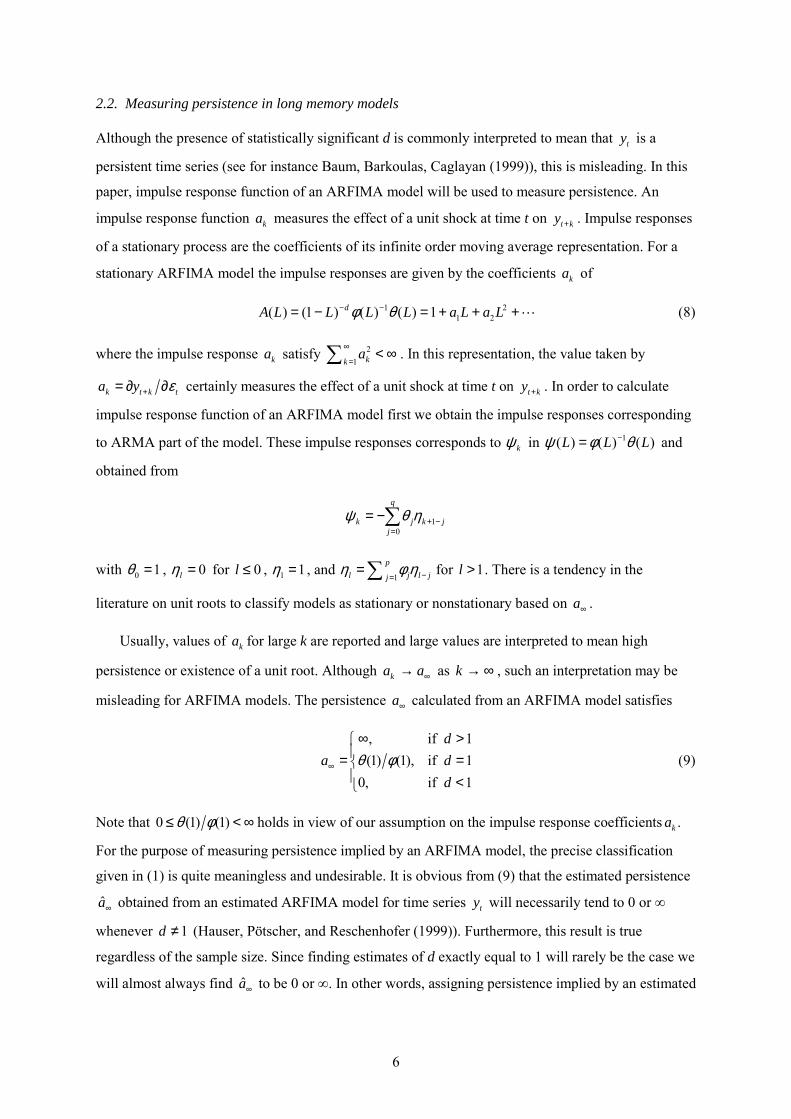
2.2. Measuring persistence in long memory models
Although the presence of statistically significant d is commonly interpreted to mean that ty is a
persistent time series (see for instance Baum, Barkoulas, Caglayan (1999)), this is misleading. In this
paper, impulse response function of an ARFIMA model will be used to measure persistence. An
impulse response function ka measures the effect of a unit shock at time t on t ky + . Impulse responses
of a stationary process are the coefficients of its infinite order moving average representation. For a
stationary ARFIMA model the impulse responses are given by the coefficients ka of
1 21 2( ) (1 ) ( ) ( ) 1dA L L L L a L a Lφ θ− −= − = + + +" (8)
where the impulse response ka satisfy 21 kka∞
=< ∞∑ . In this representation, the value taken by
k t k ta y ε+= ∂ ∂ certainly measures the effect of a unit shock at time t on t ky + . In order to calculate
impulse response function of an ARFIMA model first we obtain the impulse responses corresponding
to ARMA part of the model. These impulse responses corresponds to kψ in 1( ) ( ) ( )L L Lψ φ θ−= and
obtained from
10
q
k j k jj
ψ θ η + −=
= −∑
with 0 1θ = , 0lη = for 0l ≤ , 1 1η = , and 1
pl j l jj
η φ η −==∑ for 1l > . There is a tendency in the
literature on unit roots to classify models as stationary or nonstationary based on a∞ .
Usually, values of ka for large k are reported and large values are interpreted to mean high
persistence or existence of a unit root. Although ka a∞→ as k → ∞ , such an interpretation may be
misleading for ARFIMA models. The persistence a∞ calculated from an ARFIMA model satisfies
, if 1(1) (1), if 1
0, if 1
da d
dθ φ∞
∞ >= = <
(9)
Note that 0 (1) (1)θ φ≤ < ∞ holds in view of our assumption on the impulse response coefficients .ka
For the purpose of measuring persistence implied by an ARFIMA model, the precise classification
given in (1) is quite meaningless and undesirable. It is obvious from (9) that the estimated persistence
a∞ obtained from an estimated ARFIMA model for time series ty will necessarily tend to 0 or ∞
whenever 1d ≠ (Hauser, Pötscher, and Reschenhofer (1999)). Furthermore, this result is true
regardless of the sample size. Since finding estimates of d exactly equal to 1 will rarely be the case we
will almost always find a∞ to be 0 or ∞. In other words, assigning persistence implied by an estimated

7
ARFIMA model based on a∞ is an untenable position, since a∞ assumes a value of 0 or ∞ a priori
and a a∞ ∞→ as T → ∞ . The measure ka may also be misleading due to the fact that ka a∞→ and
ka a∞→ as k → ∞ . Therefore, estimates ka will be substantially distorted towards 0 or ∞. Another
problem with persistence measure based on ka is related to the very slow decay of ka . Consider the
following example: For an ARFIMA(0,0.4,0) processes, straightforward calculation shows that
100 0.0286a = while 1000 0.0071a = with 10
4.kka a # Indeed, for an ARFIMA(0,d,0), it is
straightforward to show that
( )( 1) ( )k
k dak dΓ +=
Γ + Γ (10)
Then, it follows that 1 1~ ( ) dka d k− −Γ as k → ∞ . For any l k> , we get 1( )d
l ka a l k −= as k → ∞ .
The above example follows with 0.4d = and 10l k= . In the special case of a unit root, we obtain the
well known result 1l ka a = . Thus, for an ARFIMA model, one gets no further information by
calculating higher order persistence measures. The ratio l ka a will always approach 1 in the limit. In
such cases, a measure of persistence that is independent of the clear-cut classification in (1) is more
appropriate. In this regard, a useful measure of persistence may be based on how fast the effects of
shocks to ty dissipate. In addition to ka we use
sup 1 , 0 1k t k tyατ ε α α+= ∂ ∂ ≤ − < < (11)
as a measure of persistence. ατ aims to capture the time required for a fraction α of the full effect of a
unit shock to complete. For 0.5,α = ατ is the period beyond which t k ty ε+∂ ∂ no longer exceed 0.5.
The measure ατ is independent of prior choice of k. k will be automatically determined once we
decide on the value of α. Therefore, it is more appropriate for ARIMA models as a measure of
persistence.
2.3. Estimation methods for long memory models
In this paper, we will evaluate the persistence in inflation rates using the impulse response functions
of the estimated ARFIMA models. In order to obtain impulse responses we first need to estimate the
parameters of the models. The most important parameter is the long memory parameter d. The
existing methods for estimating d may be grouped under four major headings: graphical, parametric,
nonparametric, and semiparametric. Among many estimators in these groups, we will briefly examine
four estimators, which are used in this paper.
Two well known parametric methods are the exact maximum likelihood estimator (Sowell
(1992a)) and the approximate Whittle estimator (Whittle (1951), Fox and Taqqu (1986)). In this
paper, only the Whittle estimator will be used. The Whittle estimator is obtained by maximizing an

8
approximation of the likelihood function in the frequency domain. In this method, the parameter
vector ( )1 1, , , , , 'p qdβ φ φ θ θ= … … is estimated by minimizing the following approximate log
likelihood function
1 1
1 1
( )log ( ) log log ( , )
( , )
m mj
jj jj
IL m m g
gλ
β λ βλ β
− −
= =
= − −∑ ∑ (12)
where ( )jI λ is the periodogram defined at the Fourier frequencies 2 / , 1,2, ,j j T j mλ π= = …
2
1
1( ) ( ) j
Tit
j tt
I T y y e λλ −
=
= −∑ (13)
[ ]( 1) 2m T= − , [ ]⋅ is the integer part, and 2( , ) 2 ( , ) /g fλ β π λ β σ= . Here, ( , )jf λ β is the spectral
density of an ARFIMA(p,d,q) model given by
22 2( )( , ) 1
2 ( )
i dii
ef ee
λλ
λσ θλ βπ φ
− −−−= − (14)
The white noise variance 2σ is estimated by
2 1
1
( ) ( , )
mj
j j
Im
gλ
σλ β
−
=
= ∑ (15)
On the assumption that the order (p,q) of the ARFIMA model is known a priori, the model parameters
β are estimated by maximizing the likelihood function in (12). The resulting estimates β are known
to be asymptotically efficient, in the sense that, under suitable regularity conditions, 1 2 ( ) (0, )dT Nβ β− → Ω as T → ∞ , where Ω is the covariance matrix of β and d→ means
convergence in distribution. Robinson (1994a) and Beran (1995) suggests a method to prove
asymptotic efficiency and normality of the Whittle estimator. The asymptotic covariance matrix of the
parameters (see Beran (1994, 1995)) is given by
1( ) (2 ) log ( , ) log ( , )'
f f dπ
πβ π λ β λ β λ
β β−
−
∂ ∂Ω =∂ ∂∫ (16)
In the empirical section of this paper, the covariance matrix of parameter estimates β is calculated
from (16) with β β= .
One difficulty with the parametric estimators is their reliance on the correct specification of the
orders (p,q). The simulation results in Taqqu and Teverovsky (1998) show that the parametric method
may not be improved upon when the orders (p,q) is correctly specified, but it performs rather poorly

9
when the order is misspecified. The semiparametric estimators of d advocated by Granger and Joyeux
(1980) and Janacek (1982), and developed by Geweke and Porter-Hudak (1983) and Robinson
(1194b, 1995a, 1995b) relies only on (2) and does not suffer from the problems of correct model
specification. The modified log periodogram regression estimator (GPH) of Geweke and
Porter-Hudak (1983) is based on the following relationship
log ( ) log (0) log 1 log ( ) / ( ) log ( ) / (0)jij u j j u j uI f d e I f f fλλ λ λ λ= − − + + (17)
where 2 / (0, )j j Tλ π π= ∈ and ( )uf ⋅ is the spectral density of (1 )dt tu L y= − given by
2 2 2( ) ( 2 )(| ( ) | | ( ) | )i iuf e eλ λλ σ π θ φ= . If jλ is near zero, say j mλ λ≤ , where mλ is small, the last term
in (17) is small relative to others and (17) can be written as a simple linear regression
, 1,2, ,j j jz c dx j mε= − + = … (18)
where log ( )j jz I λ= , log 1 jijx e λ= − , log ( ) / ( )j j jI fε λ λ= , and (0)uc f= . d can be estimated by
least squares regression of jz on , 1,2, ,jx j m= … , where m is a function of T such that 0m T → as
.T → ∞ Geweke and Porter-Hudak (1993) argue that there exists a sequence m such that 2(log ) 0n m → as T → ∞
2
1
~ , 6 ( )m
jj
d N d x xπ=
−
∑ (19)
Here 2 6π is the asymptotic variance of jε . Ooms and Hasler (1997) showed that the GPH estimator
will contain singularities when the data are deseasonalized by utilizing seasonal dummies. In order
avoid this problem, following the suggestion by Ooms and Hassler (1997), we extend the data series
to full calendar years via zero padding and then omit the periodogram ordinates corresponding to
seasonal frequencies. For consistency, this method is also followed in other frequency domain
estimators we use.
The Gaussian semiparametric estimator (GSP) suggested by Robinson (1995a) is also based on
the periodogram and it only specifies the parametric form of spectral density via (2). Like the GPH
estimator the GSP estimator involves the introduction of an additional parameter m, which can be
taken less than or equal to [ ]( 1) 2T − and should satisfy 1 0m m T+ → as T → ∞ . The GSP
estimator of d is obtained by minimizing the function
1 12
1 1
( )( ) ( , ) 1 log 2 log
m mj
jdj jj
Ir d q g d m dm
λλ
λ− −
−= =
= − = −∑ ∑ (20)
where

10
1 22
1
( ) ( , ) log
mj d
jdj j
Iq g d m g
gλ
λλ
− −−
=
= +
∑ (21)
with 1 21
( )m dj jj
g m Iλ λ−=
= ∑ . The value d which minimizes ( )r d converges in probability to the
actual value of d as T → ∞ . Robinson (1995a) also shows that 1 2 ( ) (0,1 4)dm d d N− → as T → ∞ .
The asymptotic variance of d is then equal to1 4m .
For the GPH and GSP estimators the choice of the bandwidth parameter m may be quite
important. For the GPH estimator the ad hoc 1 2T order bandwidth suggested by Geweke and
Porter-Hudak (1993) for the stationary region of d is commonly used. Hurvich, Deo, and Brodsky
(1998) prove that the mean squared error minimizing bandwidth m is of order 4 5T . This is the upper
rate for its class of estimators. However, this concerns the stationary region (0,.5)d ∈ and most
macroeconomic time series are found to be nonstationary. The larger the value of m, the faster d
converges to d. On the other hand, if the time series is not ideal, e.g. if it is an ARFIMA(p,d,q) with
not both 0p = and 0q = , then we should use small values of m, since at higher frequencies the short
run behavior of the series will affect the form of the spectral density. Sowell (1992b) argues that too
large a choice of bandwidth m leads misspecification of the short run dynamics and this results in
untrue strong mean reversion. In order to be robust against the choice of the bandwidth parameter m
we will report the GPH and GSP estimates for m Tα= for various values of [.5,1)α ∈ .
Another semiparametric estimator used in this study is the wavelet based maximum likelihood
estimator of Jensen (2000). This estimator, called wavelet MLE, is invariant to unknown, means
model specification, and contamination. In brief terms, a wavelet ( )tψ is an oscillationg function that
decreases rapidly to 0 as t → ±∞ and satisfies the admissibility condition ( ) 0,rt t dtψ =∫
0,1, , 1,r M= −… (Mallat (1989), Daubechies (1992)). The wavelet ( )tψ has M vanishing moments.
By defining the dilated and translated wavelet as 2,( ) 2 (2 )m m
m nt t nψ ψ= − , where
, 0, 1, 2, m n Z∈ = ± ± … , we obtain a function well localized in time around n. For a time series ( )y t
the wavelet ,( )m ntψ covers diverse frequencies and periods of time for different values of m and n.
The wavelet MLE is based on the wavelet transform of ( )y t defined by
, ,( ) ( )m n m nw y t t dtψ= ∫ (22)
By normalizing the time interval of ( )y t as [0,1]t ∈ , i.e., the unit interval, the support of ,m nw can be
thought of as [ 2 ,( 1)2 ]m mn n− −+ . If we observe discrete realizations ty at 0,1,2, ,2 1Jt = −… , then for

11
1m J= − , 0,1,2, ,2 1Jn = −… is needed. Therefore, for a given scale m the translation parameter
need to take values only at 0,1,2, ,2 1mn = −… .
As noted by Jensen (2000), the strength of wavelets lie in their ability to simultaneously localize a
time series in time and scale. The recent book by Gençay, Selçuk, and Whitcher (2001) contains many
practical wavelet examples from economics and finance. They also show that wavelets can
successfully be used in wide variety of challenging research problems. Wavelets can zoom in on a
time series behavior at a point in time at high frequencies (large m, 2 m n− is small). Alternatively,
wavelets can also zoom out to reveal any long and smooth (low frequency or long run) features of a
time series, such as trends and periodicity, at low frequencies (small m). The wavelet estimator of the
long memory parameter d is obtained by maximizing the approximate log likelihood function
12 1 1 1log ( ) log 2 log '2 2 2
J
L d W Wπ −−= − − Ω − Ω (23)
where 1 10,0 1,0 1,1 2,0 1,2 2 1,2 1[ , , , , , , ]J JJ JW w w w w w w− −− − − −
= … and [ ']E WWΩ = is the covariance matrix of W.
In order to estimate d by wavelet MLE we need to specify J and the functional form of the wavelet
function ,m nψ (wavelet filter). In the empirical section, we report estimates of d for several wavelets
and two different choice of J. Simulations in Jensen (2000) show that wavelet MLE estimator is
superior to the approximate frequency domain Whittle MLE when ARFIMA models are
contaminated.
3. Causes of long memory in economic time series
Although long memory in natural time series data has been established in various fields, long memory
in economic and other social time series data is at least an open question. Until now there has been a
lack of theoretical explanations for the common existence of long memory in economic time series
data (but see Haubrich and Lo (1989) for an account of long memory in the US business cycles). An
immediate explanation for evidence of long memory in economic time series is the inheritance of
climatological long memory through agricultural prices. In this way the long memory in geophysical
time series, such as rainfall, riverflow, and climatic time series, spills over into the economic time
series without any economic mechanism. Additionally, a real business cycle model with long memory
shocks can explain the presence of long memory in aggregate income and output series. Although the
inheritance of the long memory from the underlying geophysical process is not completely
impossible, there are there more appealing explanation of long memory in economic time series.
Nonstationarity of the underlying process may be a plausible explanation for long memory in the
finite sample realized time series. This explanation will not be further pursued here, since inflation
rates we examine are stationary time series.

12
One of the more appealing and one that is intrinsically rooted in the economic process is based on
an aggregation result due to Robinson (1978) and Granger (1980). Backus and Zin (1993) argue that
long memory in inflation rates are due to aggregation. More recently, Michelacci (1997) examines
this possibility in the context of output fluctuations. Granger (1980) argued that if the economy is
composed of a large number individual units each following an AR(p) process, whose coefficients are
drawn from a beta distribution on (0,1), then the additive aggregation of these AR(p) processes will
display long memory. Focusing on AR(1) for simplicity, let
1,
1, 1,2, , , 1,2, ,
n
t i ti
y n y i n t T−
=
= = =∑ … …
be the result of aggregation of n cross sectional units
, , 1 , 1,2, , , 1,2, ,i t i i t t ity y u i n t Tα ε−= + + = =… …
where tu is a common shock, ,i tε is a idiosyncratic shock, and , , ,( ) 0, ( ) 0i t j t i j tE Eε ε α ε= = for all i, j,
t. We assume that both shocks are i.i.d. white noise and iα is drawn from a beta distribution on (γ,ν).
As n → ∞ , the autocovariance of ty is
1 2 1 2 2 1
0
2 (1 )( , )
k v vk d ck
B vγρ α α α
γ+ − − −= − =∫
Therefore, ~ (1 2)ty I v− . Lippi and Zaffaroni (1999) generalize this result by replacing assumed beta
distribution with weaker semiparametric assumptions. Chambers (1998) examines temporal
aggregation as well as cross sectional aggregation in both discrete and continuous time.
A second and more recent explanation is related to structural change and based on the stochastic
permanent breaks (STOPBREAK) model of Engle and Smith (1999). The studies by Hidalgo and
Robinson (1996), Lobato and Savin (1998), Granger and Hyung (1999), Liu (2000), and Diebold and
Inoue (2001) suggested that occasional level shifts generates an illusion of apparent long memory in
economic time series. Bos, Franses, and Ooms (1999) find that evidence about the spurious long
memory due to level shifts in G7 inflation rates is weak. However, they note that long memory in
some inflation series disappear when level shifts are taken into account.
The STOPBREAK model of Engle and Smith (1999) is formulated as follows:
1 1 1
t t t
t t t t
y mm m q
εε− − −
= += +
(24)
where ( )t tq q ε= is a nondecreasing function in tε and bounded by zero and one. The innovations
tε are i.i.d. white noises. Engle and Smith (1999) use

13
2
2 , 0tt
t
q ε γγ ε
= >+
(25)
This model allows breaks (level shifts or regime switching) by allowing different innovations to have
different degrees of persistence. The specification for tq in (25) allows bigger innovations to have
more permanent effect than small ones. The parameter γ for the specification of tq in (25) controls the
likelihood of persistent innovations, with more persistent innovations more likely when γ is small. Popular tests of long memory are substantially biased when applied to time series with occasional
level shifts. This bias leads to incorrect conclusion that these time series have long memory. Diebold
and Inoue (2001) replace γ in (25) with a time varying parameter ( )T O T δγ = , for some 0δ > , and
show that the STOPBREAK process with this modification is ( )I d , where 1d δ= − . Thus, this
process will appear fractionally integrated. When 0δ = , we see that the standard STOPBRAK
process is I(1).
In odder examine possibility of long memory in inflation rates due to aggregation this paper
estimates long memory models at low aggregation levels. If the long memory in aggregate series is
due to aggregation we should find weaker memory at lower aggregation levels. In order to guard
against level shifts we modify the ARFIMA model to include a STOPBREAK component. This
model simultaneously allows long memory and level shifts (shocks) that have permanent effects.
4. Data
The long memory properties of inflation rates are examined at different aggregation levels using both
WPI and CPI based inflation rates of the Turkish economy. The literature on persistence in inflation
rates exclusively considered CPI based inflation series except Baum, Barkoulas, and Caglayan (1999).
Unlike CPI the prices of nontraded goods do not heavily influence WPI. Therefore, WPI based
inflation series are better suited in tests of the international arbitrage. Inflation rates are constructed
from the price indexes by taking 100 times the first differences of the natural logarithmic
transformation of the indexes. All seasonal inflation series show moderate to high seasonal effects.
The analyzed series are seasonally adjusted by discarding ordinates of the periodogram corresponding
to seasonal frequencies when frequency domain estimation methods are used. When the estimation is
carried out in the time domain, the data are deseasonalized by regressing the series on seasonal
dummies. However, these two methods of deseasonalization are equivalent.
At the highest aggregation level, we examine 6 WPI based inflation and 3 CPI based inflation
rates. First of these is an annual WPI based inflation series covering the period 1924-2001. The 1924-
1990 period of this series is obtained from the WPI (1968=100) given in Pakdemirli (1991). The
second part (1991-2001) is obtained from the State Institute of Statistics (SIS) All Items WPI
(1982=100) index. The second WPI based inflation series is a monthly inflation series, which is

14
obtained by augmenting the Treasury Departments (1964:1-1988:1, 1963=100) WPI index by the SIS
All Items WPI (1982=100) index and covers the period 1964:2-2002:6. The third WPI based inflation
series is based on the Treasury Departments (1964:2-1988:1, 1963=100) monthly WPI index. The
fourth aggregate WPI based inflation series we use is based on the SIS All Items WPI (1982=100)
index. This monthly inflation series covers the period 982:2-2002:6. The fifth aggregate WPI inflation
series is obtained from the Istanbul Chambers of Trade monthly WPI index and covers the period
1987:2-2002:6. The sixth WPI based inflation series is based on the SIS monthly WPI index
(1994=100) and covers the period of 1994:2-2002:6. Among the three aggregate CPI based inflation
rates, first one is an annual inflation series for 1951-2001. This series is obtained from the In IMFs
International Financial Statistics database. The second and third CPI based inflation series are both
monthly, which are obtained from the SISs 1987=100 and 1994=100 CPI indexes, and cover the
periods 1987:2-2002:6 and 1994:2-2002:6, respectively.
At lower aggregation levels we consider 3 major groups of monthly inflation series. The sector
codes together with aggregation levels are for these series are given in the Appendix. All these data
are obtained from the SIS. Several series included in the SIS database have many missing value and
excluded from the analysis. First group contain WPI (1987=100) based inflation series for the period
1982:2-2002:6. There are 26 sectoral inflation series in this group. Four of these are at 1 digit
aggregation level for agriculture, mining, manufacturing, and energy sectors. Remaining 22 series are
at 2 digit aggregation level with 7 series in agriculture, 3 series in mining, 10 series in manufacturing,
and 2 series in energy sectors. Total number of observations for each series in this group is 245. The
second group of sectoral inflation series is based on the CPI (1987=100) indexes for the period
1987:2-2002:6 (185 observations for each series) and contain 9 series. The sectors in this group are
about 1 digit aggregation level and include 7 sectors in addition to inflation series for Ankara and
Istanbul. The third group of sectoral inflation series are also CPI (1994=100) based for the period
1994:2-2002:6 and contain 40 series. 10 of the series in this group are at 1 digit aggregation level and
remaining 30 series are approximately at 3 digit aggregation level. Each series in this group has 101
observations.
5. Empirical estimates
Estimation results for the four different estimation methods are presented below. Results for the four
groups of data sets are presented separately. Examination of the sample autocorrelation functions
(available at the web site cited above) revealed that all monthly data examined in this paper show
moderate to high seasonality. The available estimation methods for the long memory models
unfortunately are not well suitable for the seasonal series. Although some progress is made in the
literature for modeling seasonal long memory time series these methods at the moment are at their
infancy and does not allow flexible modeling. Therefore, we decided to deseasonalize the data. For
the frequency domain estimation methods, which are the Whittle, GPH, and GSP estimators,
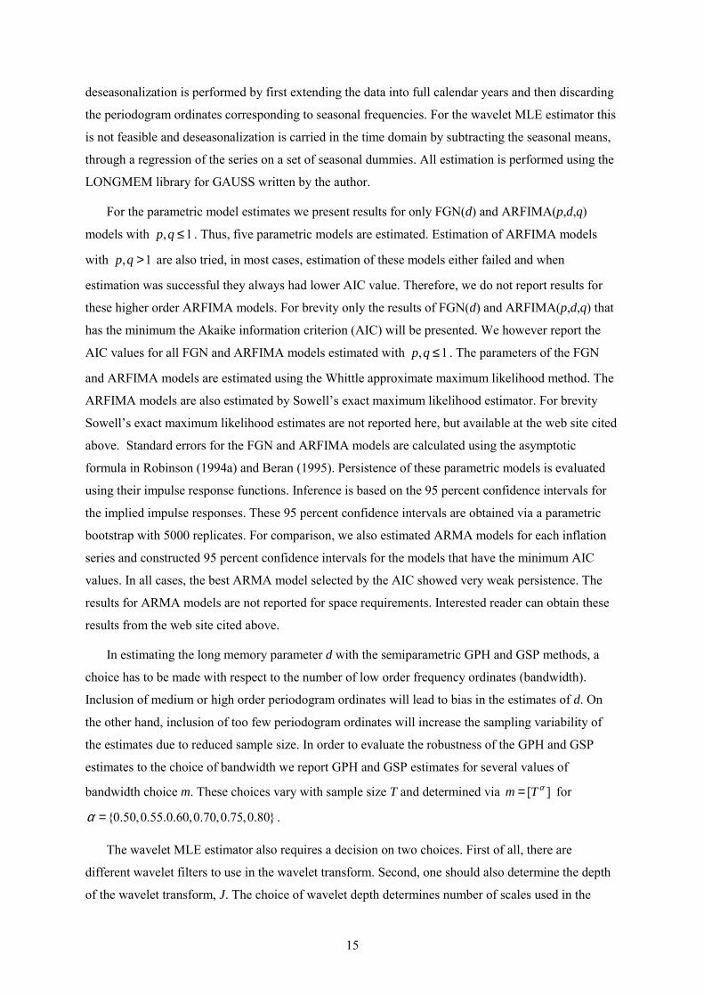
15
deseasonalization is performed by first extending the data into full calendar years and then discarding
the periodogram ordinates corresponding to seasonal frequencies. For the wavelet MLE estimator this
is not feasible and deseasonalization is carried in the time domain by subtracting the seasonal means,
through a regression of the series on a set of seasonal dummies. All estimation is performed using the
LONGMEM library for GAUSS written by the author.
For the parametric model estimates we present results for only FGN(d) and ARFIMA(p,d,q)
models with , 1p q ≤ . Thus, five parametric models are estimated. Estimation of ARFIMA models
with , 1p q > are also tried, in most cases, estimation of these models either failed and when
estimation was successful they always had lower AIC value. Therefore, we do not report results for
these higher order ARFIMA models. For brevity only the results of FGN(d) and ARFIMA(p,d,q) that
has the minimum the Akaike information criterion (AIC) will be presented. We however report the
AIC values for all FGN and ARFIMA models estimated with , 1p q ≤ . The parameters of the FGN
and ARFIMA models are estimated using the Whittle approximate maximum likelihood method. The
ARFIMA models are also estimated by Sowells exact maximum likelihood estimator. For brevity
Sowells exact maximum likelihood estimates are not reported here, but available at the web site cited
above. Standard errors for the FGN and ARFIMA models are calculated using the asymptotic
formula in Robinson (1994a) and Beran (1995). Persistence of these parametric models is evaluated
using their impulse response functions. Inference is based on the 95 percent confidence intervals for
the implied impulse responses. These 95 percent confidence intervals are obtained via a parametric
bootstrap with 5000 replicates. For comparison, we also estimated ARMA models for each inflation
series and constructed 95 percent confidence intervals for the models that have the minimum AIC
values. In all cases, the best ARMA model selected by the AIC showed very weak persistence. The
results for ARMA models are not reported for space requirements. Interested reader can obtain these
results from the web site cited above.
In estimating the long memory parameter d with the semiparametric GPH and GSP methods, a
choice has to be made with respect to the number of low order frequency ordinates (bandwidth).
Inclusion of medium or high order periodogram ordinates will lead to bias in the estimates of d. On
the other hand, inclusion of too few periodogram ordinates will increase the sampling variability of
the estimates due to reduced sample size. In order to evaluate the robustness of the GPH and GSP
estimates to the choice of bandwidth we report GPH and GSP estimates for several values of
bandwidth choice m. These choices vary with sample size T and determined via [ ]m Tα= for
0.50,0.55.0.60,0.70,0.75,0.80α = .
The wavelet MLE estimator also requires a decision on two choices. First of all, there are
different wavelet filters to use in the wavelet transform. Second, one should also determine the depth
of the wavelet transform, J. The choice of wavelet depth determines number of scales used in the

16
estimation. Thus, it is similar to bandwidth choice. To evaluate the sensitivity of estimates to the
number of scales included, we use two different choices, 2logJ T= and 4J = . In regard to the
choice of wavelet filter, we use 6 different wavelet families, compact Haar wavelet, Daubechies
wavelet of order 8 and 16 (D8, D16), minimum-bandwidth discrete-time wavelet of length 8 and 16
(MB8, MB16), and Daubechies orthonormal compactly supported wavelet of length 8 (LA8).
5.1. Empirical results for aggregate inflation series
The GPH and GSP estimates of the long memory parameter d for the 9 aggregate inflation series are
given in Table 1. For most series the results are quite robust to the choice of bandwidth. There are
only two series that show some sensitivity to the bandwidth length. Both of these series are annual
and have d greater than 0.50, .i.e., these series are nonstationary but mean reversing. Indeed, there is
some evidence that these series may even not be mean reverting, since estimates of d for some
bandwidths are close to or greater than 1. Although there is no theoretical result showing temporal
aggregation creates long memory and the result in Chambers (1998) points to this direction, the
estimates for the annual series have stronger memory than the estimates for the monthly series.
However, this may be a sample issue. The annual series we use spans the longest history of the
Turkish economy. One of the series (WPI based inflation series) spans the period of 1924-2002 and
the other series (CPI based inflation series) covers the period of 1951-2002. The longest time span the
monthly series cover is 1964-2002. We have no way of verifying whether this is a sample issue or not
since we do not have monthly data that goes back to 1950s or 1920s. Estimates from other methods
show that this maybe a sample size issue but the evidence in this direction is very weak. They also
indicate that these two annual series are indeed mean reverting and probably stationary. For the first
four and the sixth series in Table 1 estimates are all significant at the 5 percent level, except the fourth
series for which some GPH estimates are not significant. At 0.50α = (a commonly used choice) two
annual series and first four of the WPI based inflation series show significant long memory at the 5
percent level. When 0.80α = , a choice possibly leading to biased estimates due to improper inclusion
high frequency periodogram ordinates, all aggregate inflation series have significant long memory
parameter estimates.
The wavelet based MLE estimates are displayed in Table 2. The estimates are very robust to the
choices of scale and wavelet filter. Estimates closely match the estimates given in Table 1 for the
GPH and GSP estimators, except for two annual series. For two annual series, the GPH and wavelet
MLE estimates are below 0.50 across the choices of wavelet filter and scale. These two annual series
seem to be either nonstationary or near nonstationary, and the GPH and GSP estimators may
exaggerate the long memory parameter. Since wavelets strength lie in their ability to simultaneously
localize a time series in time and scale wavelet estimates may be more reliable for nonstationary or
near nonstationary time series.

17
The estimates for FGN and ARFIMA models are given in Table 3. The AIC values are always at
the minimum for ARFIMA(0,d,0) among the ARFIMA(p,d,q), , 1p q ≤ , class of models. A
comparison of the AIC values between FGN and ARFIMA models show that the AIC is at the
minimum for 6 series when the model is FGN. However, the FGN and ARFIMA models have
different spectral densities, so a comparison is not completely correct across these models. Further,
the FGN and ARFIMA(0,d,0) models are similar in terms of the behavior of the series they try to
capture. They also give very close estimates of d for all series except two annual series. All parameter
estimates for FGN and ARFIMA models are significant at the conventional 5 percent significance
level. Estimates of the long memory parameter from the FGN and ARFIMA(0,d,0) models closely
match each other for all series. These estimates are also very close to the estimates of d from the
wavelet based MLE. When 0.65α ≥ , the FGN and ARFIMA model estimates are also close to the
estimates by the semiparametric GPH and GSP methods. Thus, a value of α around 0.65 seems to be
an optimal choice for these series.
For each series, the 95 percent confidence intervals for the impulse responses of the ARFIMA
models that have the minimum AIC are given in Table 4. These confidence intervals are calculated
via a parametric bootstrap with 5000 repetitions. None of the confidence intervals brackets zero even
after 1200 periods, i.e., 100 years for monthly series and 1200 years for annual series. Long memory
properties of these aggregate inflation series are profoundly reflected in the estimated impulse
responses. As discussed in the second section, the impulse response function may not be a good mean
for measuring persistence in long memory models. A more appropriate measure, the time required for
α percent of a unit shock to dissipate, denoted ατ , is proposed in the second section. Estimates of ατ
for each aggregate inflation series are displayed in Table 5. For the monthly series the longest time
required for the 90 percent of the effect of shocks to disappear is 4 years. On the other hand, the
annual WPI inflation series needs 666 years for the 90 percent of the effects of shocks to disappear,
while the annual CPI inflation series requires even more than 1200 years. The shortest time required
for the monthly inflation series for the 99 percent of the effect of a unit shock to disappear is about 13
years, while the longest time required is about 88 years.
5.2. Empirical results for sectoral WPI based inflation series
One of the reasons, which is examined in the third section, why evidence of long memory in the
inflation series can be spurious is based on aggregation. The inflation series examined above are
based on the aggregate WPI and CPI indexes. It may well happen that the specific shocks to
inflationary process indeed do not exhibit strong persistence and the apparent long memory in the
aggregate inflation series due to aggregation as argued by Robinson (1978) and Granger (1980). To
examine this possibility, this subsection analyzes long memory properties of 26 sectoral WPI based
inflation series. The next subsection will further examine 49 sectoral CPI based inflation series.

18
The GPH and GSP estimates of long memory parameter d are given in Table 6. There are several
features of these estimates which should be noticed. First, the GPH estimates show evidence of long
memory only for two series and the GSP estimates only for three series at the 5 percent significance
level. Second, at the commonly used bandwidth choice 0.50α = , there is only 1 GPH estimate and 5
GSP estimates significant at the 5 percent level. Third, five series have negative d estimates. Fourth,
estimates are quite insensitive to the choice of bandwidth. Sixth, on average the estimates of d for
these sectoral WPI based inflation series are lower than the d estimates of aggregate inflation series.
The wavelet MLE estimates are displayed in Table 7. Estimates of d are quite robust across the
choices of wavelet filters and scales. For scale 2logJ T= , 8 series are antipersistent and, for scale
4J = , 6 series are antipersistent. On average, the wavelet MLE estimates of d are lower than the
GPH and GSP estimates. Like the GPH and GSP estimates, estimates of d for these sectoral WPI
based inflation series are significantly less than the estimates of d for the aggregate inflation series.
The estimation results for the parametric FGN and ARFIMA models are given in Table 8. From
the AIC values given in the left panel of Table 8, we see that among the family of ARFIMA(p,d,q)
models we estimated ARFIMA(0,d,0) model has the minimum AIC value for all sectoral WPI based
inflation series. For all series, the estimates of d for the FGN(d) ARFIMA(0,d,0) models are very
close to each other. For the FGN model, estimates of d for 18 series are significant at 5 percent level.
Likewise, estimates of d from the ARFIMA(0,d,0) model are significant at the five percent level for
19 series. In general, the estimates of the long memory parameter d are higher than the GPH, GSP,
and wavelet MLE estimates. However, almost all of these estimates are still lower than the estimates
for aggregate inflation series.
In order to evaluate the persistence sectoral WPI based inflation series we constructed the 95
percent confidence intervals for the impulse responses of the ARFIMA models with the minimum
AIC values. These confidence intervals are shown in Table 9. For these series, it should be noted that
estimates of d from the ARFIMA models were in general higher than the estimates obtained from
other methods, so impulse responses are evaluated at the highest estimate of the long memory
parameter and probably overstated. The confidence intervals given in Table 19 bracket zero for 22
series out of 26 at k=1200. At k=384, only confidence intervals for 6 series do not bracket zero.
Compared to the confidence intervals for the impulse responses of the aggregate series, the much
weaker persistence in the sectoral WPI based inflation series is very clearly evidenced by the
confidence intervals given in Table 9. This claim is much strongly supported by the estimates of ατ
given in Table 10. These estimates show that only for 2 series a period of more than 2 years is
required for 90 percent of the effects of shocks to dissipate. For 99 percent of the effect of a shock to
dissipate, 20 series need less than 5 years and only 6 series need more than 10 years.

19
5.3. Empirical results for sectoral CPI based inflation series
In this section we will discuss the estimation results for two groups of sectoral monthly CPI based
inflation series in the dataset we consider. The first group spans a longer time interval, 1987:2-2002:6,
but is at 1 digit aggregation level, while the second group of inflation series contains 10 series at 1
digit aggregation level and 30 series at 2 digit aggregation level, but spans a shorter time period,
1994:2-2002:6.
The semiparametric GPH and GSP estimates for the first and second group of sectoral CPI based
inflation series are given in Table 11 and Table 16, respectively. The GPH estimates of d given in the
first panel of Table 11 show that only 1 series, A07, has significant long memory at the the 5 percent
level across all choices of bandwidth. At the bandwidth choice of 0.50α = only two series have
significant long memory. The GSP estimates given in the second panel of Table 11 confirm the
significant long memory for series A07 and indicate that 3 more series have long memory when
0.50α = . Both estimators show that 3 series are indeed antipersistent. In summary, for the first group
of inflation series, there is evidence of significant long memory only for one series.
The GPH and GSP estimates of d for the second group of CPI based inflation series given in
Table 16 show that 19 out of 40 series are antipersistent when 0.50α = . Only for two series are the
GPH estimates for most of α choices significant at the 5 percent level. Likewise, the GSP estimates
indicate that only 5 series have significant long memory at the 5 percent level for all choices of α.
When 0.50α = , only two GPH estimates are significant, while for the same value of α, 11 of the GSP
estimates are significant. For this group of inflation series, the GPH and GSP estimates are somewhat
differ both in magnitude and number of significant estimates. This, however, most likely due to small
sample size, since the inflation series in this group have the smallest number of observations with a
sample size of 101.
The wavelet MLE estimates are given in Table 12 and Table 17 for the first and second groups of
inflation series, respectively. Estimates are quite insensitive to the choices of wavelet filter and scale
for both groups. For the majority of wavelet filter and scale choices, 3 series in the first group and 10
series in the second group are antipersistent. Similar to the GPH and GSP estimates the wavelet MLE
estimates of d for the majority of sectoral CPI based inflation rates are lower than the estimates of d
for the aggregate series.
The estimation results for the FGN and ARFIMA models are given in Table 13 and Table 18, for
the first and second group of sectoral CPI based inflation series, respectively. The first panels of these
tables display the AIC values for FGN and ARFIMA models. Within the class of ARFIMA models,
the AIC values are always at minimum for the ARFIMA(0,d,0) model. Like the estimates for other
inflation series the estimates of d for the FGN and ARFIMA(0,d,0) models are very close to each
other. Only half of the estimates are significant at the 5 percent significance level for both FGN and

20
ARFIMA(0,d,0) models. Magnitudes of d estimates are in most cases lower compared to the estimates
for aggregate series. Last feature of these estimates we notice is the similarity with the estimates from
wavelet MLE.
As we did for the other inflation series, we will evaluate persistence of sectoral CPI based
inflation series using the impulse responses of the ARFIMA models that has the minimum AIC values
and time required for α percent of the effect of a unit shock to dissipate. The 95 percent bootstrap
confidence intervals for the longer inflation series are given in Table 14. Confidence intervals bracket
zero for all series when impulse responses are evaluated at 1200k = (100 years). When 384k = , the
confidence intervals do not bracket zero only for 2 series. The weaker persistence in these sectoral
inflation series can be followed by narrower confidence intervals at all values of k. In Table 15, we
display estimates of ατ for the longer CPI based inflation series. Estimates for ατ point out that a
period of less than 6 months is required for 90 percent of the effects of shocks to dissipate for all
series. Moreover, only 2 series require more than 10 years an only 3 series requires more than 5 years
for 99 percent of the effects of shocks to die out.
In Table 19, we display the 95 percent confidence intervals for the shorter sectoral CPI based
inflation series. When evaluated at 1200k = , the 95 percent confidence intervals of 33 out of 40
series bracket zero. At a much shorter horizon, 384k = , the 95 percent confidence intervals do not
bracket zero only for 9 series. Although estimates of d for the ARFIMA(0,d,0) model indicate that
half the series have significant long memory, it seems that this is not fully supported by the bootstrap
estimates of impulse responses. This result suggests that there may be a small sample issue that biases
the estimates of d upward. Bootstrap is a method that reduces bias due to small sample and this is
probably why we do not observe strong persistence in the bootstrap impulse responses.
The estimates of ατ for the shorter sectoral CPI based inflation series are given in Table 20. We
observe that only 1 series require more than 3 years for 90 percent of the effect of shocks to fade
away, while only 7 series require more than 1 year. Indeed, for 28 series, time required for 90 percent
of the effects of shocks to dissipate is less than 6 months. The last column of Table 20 reveals that the
estimates of ατ are greater than 10 years for 99 percent of the effects of shocks to dissipate for 16
series, while they are less than 5 years for 21 series.
It should be noted that small sample bias will also be reflected in the estimates of ατ . A better
approach would be to consider bootstrap estimates of ατ . Even though these estimates may be upward
biased, we see that the disaggregate CPI based inflation series do not display persistence as strong as
the aggregate inflation series.

21
5.4. Long memory and regime shifts
In this subsection, we examine the possibility of spurious long memory due to neglected structural
breaks. The studies by Hidalgo and Robinson (1996), Lobato and Savin (1998), Granger and Hyung
(1999), Liu (2000), and Diebold and Inoue (2001) showed that apparent long memory may also be
caused by neglected stochastic level shifts. The stochastic permanent level shifts mimic the effect of a
persistent shock. Therefore, the long memory models fitted to the data that has occasional level shifts
may incorrectly find evidence of long memory.
Several studies examined this possibility using models that allow level shifts. Bos, Franses, and
Ooms (1999) attempt to capture the effect of level shifts by inclusion of dummy variables. This
approach is subject known critics of pretesting, since the locations of the level shifts are
predetermined. A more flexible model is the STOPBREAK model examined above (see Smith (2000)
for further details), which models the level shifts as a component with stochastic permanent shifts.
Hence, a model that can capture both long memory and occasional level shifts seems to be highly
desirable. A version of such model is studied in Hyung and Franses (2002). We consider the
following extension of an ARFIMA model
( )
( )
1 1
21
21
(1 ) ( ) ( )
t t t
t t t t td
t t
t t t st
t t t s
y m um m q
L L u L
q
εφ θ ε
ε ε εγ ε ε ε
− − −
− −
− −
= += +
− =
+ + +=
+ + + +
""
(26)
where tε is a white noise and 1 1
( ) 1 , ( ) 1p qj jj jj j
L L L Lφ φ θ θ= =
= − = −∑ ∑ are polynomials in the lag
operator L with degrees p, q respectively. We assume that ( )zφ and ( )zθ share no common roots and
( ) 0, ( ) 0z zφ θ≠ ≠ for 1z ≤ . The operator (1 )dL− is defined in (6) and (7). We will call this model
the ARFIMA-BREAK model. This model can be written as
1 1( )(1 ) ( ) ( )dt t t tL L y q Lφ ε θ ε− −− ∆ − = (27)
where 1 L∆ = − . The model examined in Hyung and Franses (2002) is a variant of this model and
given by
1 1( )(1 )dt t t tL L yφ ε θ ε− −− ∆ = −
where 1 11t tqθ − −= − .
In this susection, we will fit the ARFIMA-BREAK model given in (26) to aggregate inflation
series. Parameters of this model can be estimated using the approximate likelihood method (AML) of

22
Beran (1995). Under the regularity conditions given in Engle and Smith (1999) the AML estimator is
consistent and asymptotically normal.
We already established that disaggregated inflation series do not show significant persistence.
Therefore, we will examine the possible spurious long memory due to level shifts only for the
aggregate inflation series. In order to estimate the parameters of the ARFIMA-BREAK model one
needs to determine the orders p, q, and s. We tried to estimate models with , 0,1p q ∈ and 1,2s ∈ .
For 1q = , estimation often either failed or did not converge. Therefore, we estimated all models with
0.q =
Estimation results for the ARFIMA-BREAK model are given in Table 21. Several features of
these estimates should be noted. First, the estimates of γ for 6 series are significant at the 5 percent
significance level. Second, five inflation series have estimate of γ below 1 and all series have no γ
estimate above 6. Hence, all inflation series have high likelihood of occasional level shifts. Third,
estimates of d are all less than zero and significant at the 5 percent level except the last one. That is,
all series become antipersistent once the effects of level shifts are taken into account. All persistence
in these inflation series are then due to level shifts. Therefore, the evidence of long memory in the
aggregate inflation series we found in the previous section is spurious.
6. Discussion
Inflation has been a major problem of many economies. In order to keep inflation in check the
policymakers need to have good knowledge about the dynamic properties of the inflation. Despite
extensive research on the dynamic properties of inflation rates, there is still no agreement about the
key question of persistence in inflation. Since the early eighties the inertial inflation approach has
become very influential. The inertial inflation implies highly persistent inflation rates. Turkey is one
of the countries believed to have a highly inertial inflationary process. Thus, an examination of the
long lasting inflation in Turkey should provide a valuable contribution to the literature on the
dynamics of inflation.
The purpose of this paper has been to evaluate the persistent inflation hypothesis using an
extensive dataset on the CPI and WPI based inflation rates of the Turkish economy. The paper used
several parametric and semiparametric estimators of long memory models. All estimators gave similar
results. Thus, the findings of the paper are quite robust. The persistence in inflation series are
evaluated using the impulse responses of the estimated models. We found significant evidence of
strong persistence for the inflation series at the highest aggregation level.
The paper also examined the causes of long memory in inflation series. We considered two
reasonable explanations. The first one is due to Robinson (1978) and Granger (1980), which states
that aggregation over a large number of sectors each subject to white noise shocks may lead to long

23
memory in aggregate inflation rates. The key idea is that aggregation of independent weakly
dependent series may produce a series with strong dependence. In order to examine this possibility we
estimated long memory models for 75 disaggregated CPI and WPI based inflation rates. Estimates
show that disaggregated data display very weak memory. The hypothesis of no long memory cannot
be rejected for the majority of sector specific CPI and WPI based inflation rates.
Neglected level shifts can also cause long memory. In order to examine the possibility of spurious
long memory in inflation rates due to level shifts we extended the ARFIMA model by incorporating a
component with occasional stochastic level shifts. With this extension the effect of level shifts are
removed, and the long memory is captured by the ARFIMA component. This model is estimated for 9
inflation series at the highest aggregation level. The standard ARFIMA model estimates indicated
significant long memory for these series. After taking into account the effect of occasional level shifts,
we showed that all these series have indeed intermediate memory (antipersistent).

24
References
Backus, D.K., and S.E. Zin, (1993), Long memory inflation uncertainty: Evidence from the term structure of interest rates, Journal of Money, Credit and Banking, 25, 681-700.
Baum, C.F., J.T. Barkoulas, and M. Caglayan, (1999), Persistence in international inflation rates, Southern Economic Journal, 65, 900-913.
Baillie, R., (1996), Long memory processes and fractional integration in econometrics, Journal of Econometrics, 73, 5-59.
Baillie, R. T., C.-F. Chung, and M. A. Tieslau, (1996), Analysing inflation by the fractionally integrated ARFIMA-GARCH model, Journal of Applied Econometrics, 11, 23-40.
Barsky, R.B., (1987), The Fisher hypothesis and the forecastibility and persistence of inflation, Journal of Monetary Economics, 19, 3-24.
Beran, J., (1994) Statistics for long-memory processes, Chapman and Hall.
Beran, J., (1995), Maximum likelihood estimation of the differencing parameter for invertible short and long memory autoregressive integrated moving average models, Journal of Royal Statistical Society B, 57, 659-672.
Bos, C., P.H. Franses, and M. Ooms, (1999), Long memory and level shifts: reanalyzing inflation rates, Empirical Economics, 24, 427-449.
Bos, C., P.H. Franses, and M. Ooms, (2001), Inflation, forecast intervals and long memory regression models, International Journal of Forecasting, forthcoming.
Brunner, A.D., and G.D. Hess, (1993), Are higher levels of inflation less predictable? A state-dependent conditional heteroskedasticity approach, Journal of Business and Economic Statistics, 11, 187-197.
Chambers, M.J., (1998), Long memory and aggregation in macroeconomic time series, International Economic Review, 39, 1053-1072.
Daubechies, I., (1992), Ten Lectures on Wavelets, SIAM.
Delgado, M.A., and P.M. Robinson, (1994), New methods for the analysis of long-memory time-series: application to Spanish inflation, Journal of Forecasting, 13, 97-107.
Diebold, F.X., and G.D. Rudebusch, (1989), Long memory and persistence in aggregate output, Journal of Monetary Economics, 24, 189-209.
Diebold, F.X., and A. Inoue, (2001), Long memory and regime switching, Journal of Econometrics, 105, 131-159.
Engle, R.F., and A.D. Smith, (1999), Stochastic permanent breaks, Review of Economics and Statistics, 81, 553-574.
Fox, R., and M. S. Taqqu, (1986), Large sample properties of parameter estimates for strongly dependent stationary Gaussian time series, Annals of Statistics, 14, 517-132.
Gençay, R., F. Selçuk, and B. Whitcher, (2001), An introduction to wavelets and other filtering methods in finance and econometrics, Hartcourt Publishers.
Geweke, J., and S. Porter-Hudak, (1983), The estimation and application of long memory time series models, Journal of Time Series Analysis, 4, 15-39.
Granger, C. W. J., (1966), The typical spectral shape of an economic variable, Econometrica, 34, 150-161.
Granger, C. W. J., (1980), Long memory relationships and the aggregation of dynamic models, Journal of Econometrics, 14, 227-238.

25
Granger, C.W.J., and Z. Ding, (1996), Varieties of long memory models, Journal of Econometrics, 73, 61-78.
Granger, C.W.J. and N. Hyung, (1999), Occasional structural breaks and long memory, UCSD working paper.
Hassler, V., and J. Wolters, (1995), Long memory in inflation rates: International evidence, Journal of Business and Economic Statistics, 13, 37-45.
Haubrich, J.G. and A.W. Lo, (1989), The sources and nature of long-term memory in the business cycle, NBER Working Paper No. 2951.
Hauser, M.A., B.M. Pötscher, and E. Reschenhofer, (1999), Measuring persistence in aggregate output: ARMA models, fractionally integrated ARMA models and nonparametric procedures, Empirical Economics, 24, 243-269.
Hidalgo, J., and P.M. Robinson, (1996), Testing for structural change in long memory environment, Journal of Econometrics, 70, 159-174.
Hosking, J., (1981), Fractional differencing, Biometrika, 68, 165-176.
Hurst, H.E., (1951), Long-term storage capacity of reservoirs, Transactions of American Society of Civil Engineers, 116, 770-799.
Hurvich, C., R. Deo, and J. Brodsky, (1998), The mean squared error of Geweke and Porter-Hudaks estimator of the long memory parameter of a long memory time series, Journal of Time Series Analysis, 16, 17-41.
Hyung, N., and P.H. Franses, (2002), Inflation rates: Long-memory, level shifts, or both? manuscript, Erasmus University Rotterdam.
Janacek, G. J., (1982), Determining the degree of differencing for time series via the log spectrum, Journal of Time Series Analysis, 16, 17-41.
Jensen, M.J., (2000), An alternative maximum likelihood estimator of long memory- processes using compactly supported wavelets, Journal of Economic Dynamics and Control, 24, 361-387.
Lippi, M., and P. Zaffaroni, (1999), Contemporaneous aggregation of linear dynamic models in large economies, manuscript, Research Department, Bank of Italy.
Liu, M., (2000), Modeling long memory in stock market volatility, Journal of Econometrics, 99, 139-171.
Lobato, I.N., and N.E. Savin, (1998), Real and spurious long memory properties of stock market data, Journal of Business and Economic Statistics, 16, 261-268.
MacDonald, R, and P.D. Murphy, (1989), Testing for the long run relationship between nominal interest rates and inflation using cointegration techniques, Applied Economics, 21, 439-447.
Mallat, S. G., (1989), Multiresolution approximations and wavelet orthonormal basis of L2(R), Transactions of American Mathematical Society, 315, 6987.
Mandelbrot, B. B., (1963), The variation of certain speculative prices. Journal of Business, 36, 394-419.
Michelacci, C., (1997), Cross-sectional heterogeneity and the persistence of aggregate fluctuations, London School of Economics working paper.
Ooms, M. and U. Hassler, (1997), A note on the effect of seasonal dummies on the peridogram regression, Economic Letters, 56, 135-141.
Pakdemirli, E., (1991), Ekonomimizin 1923den 1990a sayõsal görünümü, Milliyet Yayõnlarõ.
Robinson, P.M., (1978), Statistical inference for a random coefficient autoregressive model, Scandinavian Journal of statistics, 5, 163-168.
26
Robinson, P. M., (1994a), Time series with strong dependence, in Advances in Econometrics, ed. by C. Sims, vol. 1, pp. 97-107, Cambridge University Press.
Robinson, P. M., (1994b), Semiparametric analysis of long memory time series, Annals of Statistics, 22, 515-539.
Robinson, P. M., (1995a), Gaussian semiparametric estimation of long range dependence, Annals of Statistics, 23, 1630-1661.
Robinson, P. M., (1995b), Log periodogram regression of time series with long range dependence, Annals of Statistics, 23, 1048-1072.
Smith, A.D., (2000), Forecasting inflation in the presence of structural breaks, UC Davis working paper.
Sowell, F., (1992a), Maximum likelihood estimation of stationary univariate fractionally integrated time series models, Journal of Econometrics, 53, 165-188.
Sowell, F., (1992b), Modeling long-run behaviour with the fractional ARIMA model, Journal of Monetary Economics, 29, 277-302.
Taqqu, M.S., and V. Teverovsky, (1998), Long-range dependence in finite and infinite variance time series, in A Practical Guide to Heavy Tails: Statistical Techniques and Applications, ed. by R. Adler, R. Feldman, and M. S. Taqqu, pp. 177-217, Birkhauser.
van Dijk, D.J.C., P.H. Franses, and R. Paap, (2002), A nonlinear long memory model for US unemployment, Journal of Econometrics, forthcoming.
Whittle, P., (1951), Hypothesis testing in time series analysis, Almquist and Wiksells.

Appendix: Sector Codes for Inflation Series
Code Description Aggregation
Monthly Wholesale Prices Index (1987=100)E01 Agriculture Sector Price Index 1E02 Mining Sector Price Index 1E03 Manufacturing Sector Price Index 1E04 Energy Sector Price Index 1E05 Cereals 2E06 Pulses 2E07 Other Field Products 2E08 Vegetables and Fruits 2E09 Live Animals 2E10 Animal Products 2E11 Fishery Products 2E12 Coal Mining 2E13 Crude Petroleum 2E14 Metallic Mining 2E15 Non-Metallic Mining 2E16 Food, Beverages, Tobacco 2E17 Textiles 2E18 Wood Products 2E19 Paper Products and Printing 2E20 Chemicals, Petroleum Products 2E21 Non-Metallic Minerals 2E22 Metals 2E23 Metals and Machinery 2E24 Other Industries 2E25 Water (Energy Sector) 2E26 Electricity (Energy Sector) 2
Monthly Consumer Price Index (1987=100)A01 Food-Stuffs 1A02 Clothing 1A03 House Appliances and Furniture 1A04 Medical Health and Personal Care 1A05 Transportation and Communication 1A06 Culture, Training and Entertainment 1A07 Housing 1A08 Consumer Prices Index of Ankara 1A09 Consumer Prices Index of Istanbul 1
Monthly Consumer Price Index (1994=100)T01 Food, Beverages and Tobacco 1T02 Clothing and Shoes 1T03 Housing 1T04 Houseware 1T05 Health 1T06 Transportation 1T07 Entertainment and culture 1T08 Education 1T09 Restaurant, Cafe and Hotels 1T10 Miscelaneous 1T11 Food 3
27
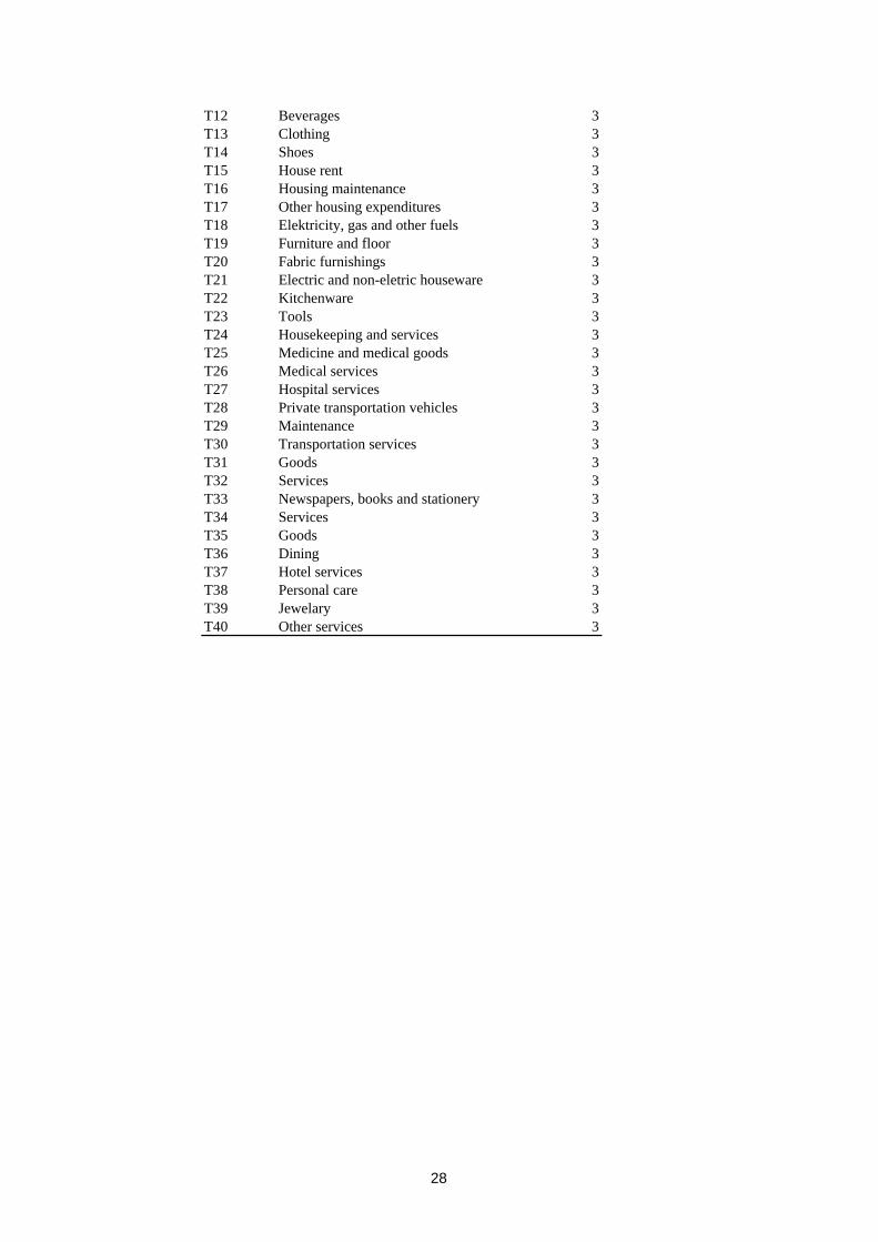
T12 Beverages 3T13 Clothing 3T14 Shoes 3T15 House rent 3T16 Housing maintenance 3T17 Other housing expenditures 3T18 Elektricity, gas and other fuels 3T19 Furniture and floor 3T20 Fabric furnishings 3T21 Electric and non-eletric houseware 3T22 Kitchenware 3T23 Tools 3T24 Housekeeping and services 3T25 Medicine and medical goods 3T26 Medical services 3T27 Hospital services 3T28 Private transportation vehicles 3T29 Maintenance 3T30 Transportation services 3T31 Goods 3T32 Services 3T33 Newspapers, books and stationery 3T34 Services 3T35 Goods 3T36 Dining 3T37 Hotel services 3T38 Personal care 3T39 Jewelary 3T40 Other services 3
28

GPH Estimates
Inflation Series α =0.50 α =0.55 α =0.60 α =0.65 α =0.70 α =0.75 α =0.80
WPI (1923-2001) d 1.151 0.936 0.636 0.663 0.656 0.701 0.673s.e. 0.347 0.295 0.246 0.215 0.182 0.162 0.147
WPI (1964:2-2002:6) d 0.373 0.568 0.558 0.420 0.384 0.342 0.308s.e. 0.176 0.143 0.120 0.100 0.084 0.071 0.061
WPI (1964:2-1988:1) d 0.477 0.633 0.507 0.306 0.282 0.274 0.205s.e. 0.210 0.171 0.146 0.121 0.103 0.088 0.076
WPI (1982:2-2002:6) d 0.320 0.419 0.283 0.215 0.202 0.282 0.346s.e. 0.220 0.182 0.150 0.129 0.109 0.094 0.082
WPI (1987:2-2002:6) d 0.505 0.529 0.307 0.206 0.277 0.353 0.446s.e. 0.243 0.202 0.171 0.145 0.124 0.107 0.094
WPI (1994:2-2002:6) d -0.059 -0.107 0.098 0.263 0.308 0.369 0.410s.e. 0.294 0.258 0.222 0.185 0.162 0.144 0.127
CPI (1951-2001) d 0.965 1.107 0.928 0.885 0.895 0.845 0.835s.e. 0.388 0.351 0.299 0.265 0.231 0.203 0.185
CPI (1987:2-2002:6) d 0.243 0.313 0.193 0.178 0.141 0.319 0.376s.e. 0.243 0.202 0.171 0.145 0.124 0.107 0.094
CPI (1994:2-2002:6) d 0.107 -0.002 0.088 0.242 0.335 0.396 0.421s.e. 0.294 0.258 0.222 0.185 0.162 0.144 0.127
GSP Estimates
WPI (1923-2001) d 0.984 0.754 0.572 0.601 0.647 0.681 0.616s.e. 0.177 0.158 0.139 0.125 0.109 0.098 0.088
WPI (1964:2-2002:6) d 0.476 0.534 0.565 0.409 0.355 0.345 0.333s.e. 0.109 0.093 0.080 0.069 0.059 0.050 0.043
WPI (1964:2-1988:1) d 0.580 0.689 0.487 0.366 0.363 0.328 0.272s.e. 0.125 0.107 0.094 0.081 0.071 0.061 0.053
WPI (1982:2-2002:6) d 0.277 0.323 0.247 0.178 0.192 0.250 0.328s.e. 0.129 0.112 0.096 0.085 0.073 0.064 0.056
WPI (1987:2-2002:6) d 0.219 0.365 0.168 0.163 0.217 0.287 0.400s.e. 0.139 0.121 0.107 0.093 0.081 0.071 0.062
WPI (1994:2-2002:6) d -0.031 -0.060 0.025 0.188 0.317 0.403 0.451s.e. 0.158 0.144 0.129 0.112 0.100 0.090 0.079
CPI (1951-2001) d 0.962 1.050 0.830 0.760 0.770 0.751 0.734s.e. 0.189 0.177 0.158 0.144 0.129 0.115 0.104
CPI (1987:2-2002:6) d 0.269 0.332 0.178 0.176 0.152 0.242 0.336s.e. 0.139 0.121 0.107 0.093 0.081 0.071 0.062
CPI (1994:2-2002:6) d 0.137 0.036 0.075 0.204 0.306 0.405 0.398s.e. 0.158 0.144 0.129 0.112 0.100 0.090 0.079
Table 1: GPH and GSP Estimates of d for Aggregate Inflation Series
Notes: GSP and GPH estimates are the Geweke and Porter-Hudak (1983) log periodogram and Robison (1995a) gaussian semiparametric estimates, respectively. s.e. is the standard error of the estimate above it. α determines the number of periodogram ordinates (sample size), m , used in the estimation by m =[T α ]. For the GSP estimates the known theoretical variance π 2/6 of innovations is imposed in the calculation of the s.e. of d . Similarly, the known innovation variance of 1/4m is imposed in the calculation of the s.e. of the GSP estimates. Data are seasonally adjusted by discarding the periodogram ordinates corresponding to seasonal frequencies.
29

Inflation Series Haar D8 D16 MB8 MB16 LA8
WPI (1923-2001) 0.459 0.460 0.429 0.448 0.451 0.480WPI (1964:2-2002:6) 0.289 0.251 0.230 0.316 0.313 0.327WPI (1964:2-1988:1) 0.277 0.275 0.246 0.205 0.283 0.299WPI (1982:2-2002:6) 0.298 0.269 0.264 0.305 0.320 0.382WPI (1987:2-2002:6) 0.311 0.313 0.317 0.380 0.389 0.393WPI (1994:2-2002:6) 0.360 0.346 0.356 0.396 0.414 0.450CPI (1951-2001) 0.484 0.456 0.485 0.476 0.487 0.483CPI (1987:2-2002:6) 0.336 0.242 0.282 0.329 0.334 0.355CPI (1994:2-2002:6) 0.373 0.299 0.330 0.377 0.390 0.438
Haar D8 D16 MB8 MB16 LA8
WPI (1923-2001) 0.433 0.413 0.423 0.418 0.423 0.431WPI (1964:2-2002:6) 0.328 0.340 0.340 0.338 0.346 0.359WPI (1964:2-1988:1) 0.289 0.294 0.307 0.287 0.297 0.307WPI (1982:2-2002:6) 0.286 0.284 0.286 0.312 0.318 0.338WPI (1987:2-2002:6) 0.283 0.297 0.282 0.318 0.330 0.344WPI (1994:2-2002:6) 0.305 0.305 0.302 0.333 0.344 0.376CPI (1951-2001) 0.444 0.449 0.453 0.452 0.455 0.446CPI (1987:2-2002:6) 0.293 0.263 0.264 0.284 0.293 0.319CPI (1994:2-2002:6) 0.326 0.298 0.301 0.334 0.341 0.373
Table 2: Wavelet Based Estimates of d for Aggregate Inflation Series
J =log2 T
J =4
Notes: The wavelet MLE estimates are obtained from the discrete wavelet transform with depth J of the inflation series. Six different wavelet filters, compact Haar wavelet, Daubechies wavelet of order 8 and 16 (D8, D16), minimum-bandwidth discrete-time wavelet of length 8 and 16 (MB8, MB16), and Daubechies orthonormal compactly supported wavelet of length 8 (LA8), are used. Data are seasonally adjusted prior to estimation using a set of seasonal dummies.
30

AIC for FGN and ARFIMA Models
Inflation Series FGN(d ) ARFIMA(0,d ,0) ARFIMA(1,d ,0) ARFIMA(0,d ,1) ARFIMA(1,d ,1)
WPI (1923-2001) 3.023 2.971 4.971 4.939 6.939WPI (1964:2-2002:6) 3.324 3.331 5.329 5.328 7.326WPI (1964:2-1988:1) 3.537 3.525 5.524 5.518 7.518WPI (1982:2-2002:6) 3.581 3.614 5.578 5.589 7.566WPI (1987:2-2002:6) 3.558 3.598 5.556 5.542 7.529WPI (1994:2-2002:6) 3.580 3.634 5.577 5.488 7.484CPI (1951-2001) 2.741 2.706 4.703 4.681 6.674CPI (1987:2-2002:6) 3.638 3.676 5.631 5.639 7.612CPI (1994:2-2002:6) 3.586 3.635 5.585 5.520 7.520
Estimates for FGN and Best ARFIMA Models Selected by AIC
FGN(d ) ARFIMA(0,d ,0)d s.e. d s.e.
WPI (1923-2001) 0.433 0.077 0.600 0.089WPI (1964:2-2002:6) 0.308 0.031 0.358 0.037WPI (1964:2-1988:1) 0.260 0.039 0.304 0.046WPI (1982:2-2002:6) 0.307 0.043 0.355 0.050WPI (1987:2-2002:6) 0.335 0.049 0.392 0.058WPI (1994:2-2002:6) 0.366 0.067 0.439 0.078CPI (1951-2001) 0.472 0.095 0.702 0.110CPI (1987:2-2002:6) 0.297 0.049 0.337 0.058CPI (1994:2-2002:6) 0.350 0.067 0.413 0.078
Table 3: Parameter Estimates and Model Selection Criteria of FGN and ARFIMA Models for Aggregate Inflation Series
Notes: First panel of the Table reports the Akaike Information Criterion (-2 ln L + 2k ) for each model, where L is the likelihood and k is the number of parameters. Both the FGN and ARFIMA models are estimated using the Whittle frequency domain approximate maximum likelihood method. The second panel shows the estimates for the FGN and ARFIMA models that have the minimum AIC. Standard errors (s.e.) are calculated using the asymptotic formula in Robinson (1994a) and Beran (1995). For an ARFIMA(0,d ,0) process the asymptotic variance is independent of d and difference in s.e. estimates in the bottom right panel of the Table is only due to sample size differences. Data are seasonally adjusted by discarding the periodogram ordinates corresponding to seasonal frequencies.
31
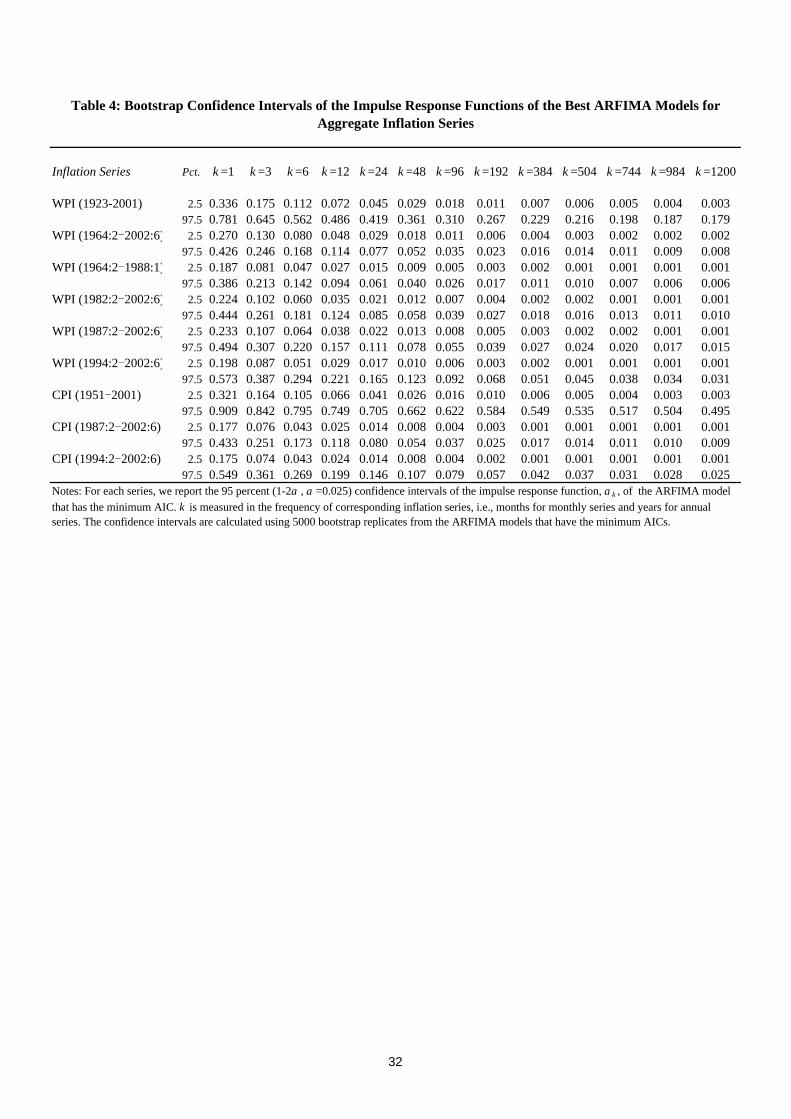
Inflation Series Pct. k =1 k =3 k =6 k =12 k =24 k =48 k =96 k =192 k =384 k =504 k =744 k =984 k =1200
WPI (1923-2001) 2.5 0.336 0.175 0.112 0.072 0.045 0.029 0.018 0.011 0.007 0.006 0.005 0.004 0.00397.5 0.781 0.645 0.562 0.486 0.419 0.361 0.310 0.267 0.229 0.216 0.198 0.187 0.179
WPI (1964:2-2002:6) 2.5 0.270 0.130 0.080 0.048 0.029 0.018 0.011 0.006 0.004 0.003 0.002 0.002 0.00297.5 0.426 0.246 0.168 0.114 0.077 0.052 0.035 0.023 0.016 0.014 0.011 0.009 0.008
WPI (1964:2-1988:1) 2.5 0.187 0.081 0.047 0.027 0.015 0.009 0.005 0.003 0.002 0.001 0.001 0.001 0.00197.5 0.386 0.213 0.142 0.094 0.061 0.040 0.026 0.017 0.011 0.010 0.007 0.006 0.006
WPI (1982:2-2002:6) 2.5 0.224 0.102 0.060 0.035 0.021 0.012 0.007 0.004 0.002 0.002 0.001 0.001 0.00197.5 0.444 0.261 0.181 0.124 0.085 0.058 0.039 0.027 0.018 0.016 0.013 0.011 0.010
WPI (1987:2-2002:6) 2.5 0.233 0.107 0.064 0.038 0.022 0.013 0.008 0.005 0.003 0.002 0.002 0.001 0.00197.5 0.494 0.307 0.220 0.157 0.111 0.078 0.055 0.039 0.027 0.024 0.020 0.017 0.015
WPI (1994:2-2002:6) 2.5 0.198 0.087 0.051 0.029 0.017 0.010 0.006 0.003 0.002 0.001 0.001 0.001 0.00197.5 0.573 0.387 0.294 0.221 0.165 0.123 0.092 0.068 0.051 0.045 0.038 0.034 0.031
CPI (1951-2001) 2.5 0.321 0.164 0.105 0.066 0.041 0.026 0.016 0.010 0.006 0.005 0.004 0.003 0.00397.5 0.909 0.842 0.795 0.749 0.705 0.662 0.622 0.584 0.549 0.535 0.517 0.504 0.495
CPI (1987:2-2002:6) 2.5 0.177 0.076 0.043 0.025 0.014 0.008 0.004 0.003 0.001 0.001 0.001 0.001 0.00197.5 0.433 0.251 0.173 0.118 0.080 0.054 0.037 0.025 0.017 0.014 0.011 0.010 0.009
CPI (1994:2-2002:6) 2.5 0.175 0.074 0.043 0.024 0.014 0.008 0.004 0.002 0.001 0.001 0.001 0.001 0.00197.5 0.549 0.361 0.269 0.199 0.146 0.107 0.079 0.057 0.042 0.037 0.031 0.028 0.025
Table 4: Bootstrap Confidence Intervals of the Impulse Response Functions of the Best ARFIMA Models for Aggregate Inflation Series
Notes: For each series, we report the 95 percent (1-2α , α =0.025) confidence intervals of the impulse response function, a k , of the ARFIMA model that has the minimum AIC. k is measured in the frequency of corresponding inflation series, i.e., months for monthly series and years for annual series. The confidence intervals are calculated using 5000 bootstrap replicates from the ARFIMA models that have the minimum AICs.
32

Inflation Series α =0.30 α =0.50 α =0.80 α =0.90 α =0.95 α =0.99
WPI (1923-2001) 1 2 21 118 666 >1200WPI (1964:2-2002:6) 1 1 3 9 26 315WPI (1964:2-1988:1) 1 1 2 6 16 159WPI (1982:2-2002:6) 1 1 3 9 25 305WPI (1987:2-2002:6) 1 1 4 12 36 508WPI (1994:2-2002:6) 1 1 5 18 60 1054CPI (1951-2001) 2 4 93 947 >1200 >1200CPI (1987:2-2002:6) 1 1 3 8 21 240CPI (1994:2-2002:6) 1 1 5 14 45 695
Table 5: Estimates of τ α for Aggregate Inflation Series
Notes: For each series, we report the time required for α percent of the effect of a unit shock to dissipate, τ α . τ α is calculated from the impulse response function of the ARFIMA model that has the minimum AIC. Time is measured in the frequency of the corresponding series, i.e., months for monthly series and years for annual series.
33

GPH Estimates GSP Estimates
Code α =0.50 α =0.55 α =0.60 α =0.65 α =0.70 α =0.75 α =0.80 α =0.50 α =0.55 α =0.60 α =0.65 α =0.70 α =0.75 α =0.80
E01 0.371 0.361 0.116 0.233 0.092 0.224 0.161 0.328 0.297 0.107 0.105 0.063 0.104 0.107E02 -0.121 -0.035 -0.051 0.024 0.037 0.140 0.193 0.161 0.168 0.113 0.114 0.130 0.167 0.219E03 0.249 0.401 0.230 0.136 0.131 0.206 0.273 0.172 0.238 0.199 0.129 0.170 0.233 0.312E04 0.162 0.270 0.338 0.239 0.205 0.112 0.094 0.120 0.250 0.263 0.158 0.041 -0.005 0.011E05 0.286 0.347 0.182 0.254 0.153 0.144 0.241 0.218 0.235 0.182 0.208 0.151 0.146 0.221E06 0.275 0.341 0.279 0.259 0.110 0.224 0.172 0.385 0.434 0.290 0.260 0.156 0.197 0.193E07 0.154 0.274 0.115 0.144 0.224 0.219 0.210 0.157 0.244 0.086 0.087 0.145 0.129 0.144E08 0.036 -0.129 -0.362 -0.190 -0.265 -0.167 -0.149 -0.022 -0.099 -0.220 -0.189 -0.197 -0.124 -0.077E09 0.061 0.070 0.131 0.079 0.038 -0.045 -0.024 0.165 0.149 0.136 0.097 0.041 -0.067 -0.056E10 0.105 0.166 0.083 -0.060 -0.048 0.019 0.029 0.084 0.087 0.103 -0.027 -0.029 0.020 0.053E11 -0.094 -0.349 -0.399 -0.424 -0.275 -0.241 -0.185 -0.190 -0.337 -0.376 -0.399 -0.342 -0.244 -0.140E12 0.472 0.266 0.133 0.111 0.115 0.115 0.109 0.296 0.233 0.146 0.121 0.114 0.123 0.122E13 0.021 0.237 -0.064 0.026 0.081 0.103 0.132 -0.069 -0.008 -0.139 -0.055 0.066 0.116 0.129E14 -0.170 -0.102 0.083 -0.035 -0.061 -0.011 -0.034 0.060 0.105 0.161 0.029 0.001 0.004 0.001E15 0.097 0.298 0.127 0.081 0.058 0.073 0.159 0.049 0.174 0.147 0.108 0.120 0.143 0.209E16 0.015 0.077 0.074 0.013 0.057 0.165 0.158 0.173 0.203 0.192 0.088 0.098 0.156 0.172E17 0.224 0.360 0.335 0.264 0.245 0.312 0.403 0.190 0.297 0.275 0.246 0.233 0.309 0.414E18 0.421 0.207 0.154 0.150 0.090 0.152 0.147 0.258 0.129 0.140 0.130 0.101 0.102 0.115E19 0.362 0.119 0.273 0.211 0.103 0.059 0.067 0.250 0.137 0.111 0.096 0.108 0.112 0.098E20 -0.045 0.028 -0.035 -0.032 0.070 0.127 0.165 0.058 0.125 0.056 0.060 0.144 0.173 0.215E21 -0.212 -0.138 -0.132 -0.193 -0.083 0.029 0.136 -0.017 -0.004 0.020 -0.053 0.001 0.076 0.179E22 0.238 0.245 0.179 0.130 0.180 0.314 0.330 0.174 0.222 0.169 0.092 0.154 0.221 0.256E23 0.396 0.492 0.392 0.310 0.285 0.317 0.464 0.298 0.421 0.321 0.260 0.254 0.291 0.384E24 0.125 -0.012 -0.015 -0.013 0.055 0.135 0.210 0.220 0.057 0.049 0.054 0.070 0.136 0.165E25 0.387 0.097 -0.005 0.147 -0.023 0.017 -0.013 0.216 -0.057 -0.066 0.016 -0.079 -0.088 -0.078E26 0.357 0.466 0.304 0.151 0.060 -0.029 -0.127 0.155 0.382 0.229 0.101 -0.023 -0.085 -0.113
s.e 0.220 0.182 0.150 0.129 0.109 0.094 0.082 0.129 0.112 0.096 0.085 0.073 0.064 0.056Notes: See notes to Table 1.
Table 6: GPH and GSP Estimates for Sectoral WPI Based Inflation Series
34

Code Haar D8 D16 MB8 MB16 LA8 Haar D8 D16 MB8 MB16 LA8
E01 0.089 0.137 0.257 0.088 0.139 0.098 0.162 0.160 0.203 0.190 0.188 0.171E02 0.249 0.285 0.248 0.269 0.246 0.250 0.234 0.244 0.226 0.259 0.241 0.247E03 0.272 0.308 0.276 0.320 0.324 0.395 0.270 0.266 0.268 0.291 0.301 0.328E04 -0.048 -0.013 -0.014 -0.063 -0.035 -0.021 -0.011 -0.009 -0.023 -0.009 -0.014 0.003E05 0.172 0.250 0.265 0.191 0.208 0.158 0.197 0.238 0.227 0.230 0.227 0.205E06 0.126 0.148 0.204 0.057 0.157 0.143 0.156 0.165 0.168 0.162 0.173 0.191E07 0.111 0.128 0.173 0.099 0.131 0.140 0.145 0.148 0.159 0.151 0.156 0.160E08 -0.131 -0.029 0.100 -0.047 -0.001 -0.045 -0.021 -0.016 0.057 0.009 0.021 -0.014E09 -0.094 -0.075 -0.036 -0.122 -0.120 -0.115 -0.063 -0.020 -0.032 -0.024 -0.047 -0.075E10 -0.003 -0.046 0.014 -0.101 -0.025 -0.122 0.021 0.016 0.027 0.019 0.028 0.039E11 -0.049 -0.065 -0.019 -0.012 -0.024 -0.059 -0.037 -0.060 -0.047 0.002 -0.020 -0.037E12 0.097 0.095 0.123 0.056 0.076 0.080 0.141 0.124 0.124 0.145 0.132 0.124E13 0.131 0.197 0.161 0.130 0.144 0.143 0.126 0.165 0.140 0.140 0.146 0.160E14 -0.026 0.071 0.016 0.027 0.009 -0.019 0.008 0.069 0.046 0.067 0.043 0.025E15 0.189 0.166 0.172 0.195 0.212 0.232 0.198 0.168 0.195 0.197 0.204 0.218E16 0.160 0.168 0.203 0.148 0.162 0.263 0.190 0.174 0.191 0.192 0.204 0.252E17 0.369 0.372 0.367 0.405 0.406 0.401 0.333 0.314 0.323 0.349 0.346 0.348E18 0.132 0.111 0.119 0.112 0.133 0.181 0.164 0.150 0.141 0.161 0.147 0.185E19 0.093 0.043 0.080 0.060 0.079 0.077 0.135 0.097 0.097 0.112 0.113 0.093E20 0.157 0.227 0.192 0.207 0.193 0.253 0.167 0.191 0.185 0.206 0.210 0.239E21 0.106 0.109 0.105 0.167 0.144 0.145 0.126 0.106 0.119 0.159 0.155 0.139E22 0.170 0.282 0.212 0.275 0.288 0.260 0.193 0.252 0.242 0.248 0.257 0.234E23 0.405 0.370 0.364 0.405 0.410 0.430 0.352 0.319 0.327 0.355 0.350 0.365E24 0.125 0.086 0.109 0.058 0.095 0.118 0.143 0.117 0.104 0.128 0.125 0.144E25 -0.050 -0.074 -0.151 -0.101 -0.119 -0.083 -0.059 -0.092 -0.093 -0.073 -0.105 -0.110E26 -0.254 -0.181 -0.167 -0.225 -0.219 -0.212 -0.202 -0.146 -0.206 -0.187 -0.193 -0.162Notes: See notes to Table 2.
J =log2 T J =4
Table 7: Wavelet Based Estimates of d for Sectoral WPI Based Inflation Series
35

AIC for FGN and ARFIMA Models Estimates for FGN and Best ARFIMA Models Selected by AICFGN(d ) ARFIMA(0,d ,0)
Code FGN(d ) ARFIMA(0,d ,0) ARFIMA(1,d ,0) ARFIMA(0,d ,1) ARFIMA(1,d ,1) d s.e. d s.e.
E01 3.837 3.872 5.762 5.853 7.762 0.210 0.042 0.209 0.050E02 3.744 3.782 5.701 5.711 7.701 0.260 0.042 0.285 0.050E03 3.647 3.679 5.643 5.646 7.626 0.291 0.043 0.338 0.050E04 4.015 3.999 5.993 5.995 6.000 -0.009 0.040 -0.017 0.050E05 3.763 3.786 5.752 5.764 6.000 0.231 0.042 0.257 0.050E06 3.899 3.897 5.897 5.897 7.869 0.148 0.042 0.172 0.050E07 3.903 3.910 5.895 5.893 7.892 0.155 0.042 0.173 0.050E08 3.993 3.997 5.845 5.860 7.835 0.088 0.041 0.038 0.050E09 4.012 3.994 5.994 5.994 7.986 -0.026 0.039 -0.043 0.050E10 4.013 4.000 6.000 6.000 7.981 0.018 0.040 0.009 0.050E11 4.006 4.000 5.836 5.818 7.796 0.057 0.041 -0.011 0.050E12 3.932 3.932 5.926 5.919 6.000 0.125 0.041 0.136 0.050E13 3.924 3.937 5.885 5.877 7.861 0.154 0.042 0.163 0.050E14 3.999 3.993 5.966 5.972 7.965 0.061 0.041 0.049 0.050E15 3.868 3.878 5.865 5.860 7.855 0.177 0.042 0.202 0.050E16 3.847 3.864 5.833 5.846 7.831 0.189 0.042 0.207 0.050E17 3.464 3.495 5.469 5.459 7.449 0.353 0.043 0.421 0.050E18 3.887 3.903 5.849 5.865 6.000 0.168 0.042 0.174 0.050E19 3.959 3.956 5.951 5.952 6.000 0.105 0.041 0.113 0.050E20 3.854 3.866 5.850 5.842 7.832 0.188 0.042 0.216 0.050E21 3.933 3.941 5.921 5.900 7.890 0.139 0.041 0.151 0.050E22 3.724 3.754 5.714 5.712 7.700 0.262 0.042 0.300 0.050E23 3.430 3.469 5.426 5.434 7.410 0.366 0.043 0.427 0.050E24 3.955 3.951 5.950 5.949 7.939 0.108 0.041 0.124 0.050E25 4.002 3.981 5.981 5.981 7.968 -0.053 0.039 -0.080 0.050E26 3.915 3.906 5.843 5.865 7.842 -0.136 0.037 -0.170 0.050Notes: See notes to Table 3.
Table 8: Parameter Estimates and Model Selection Criteria of FGN and ARFIMA Models for Sectoral WPI Based Inflation Series
36

Code Pct. k =1 k =3 k =6 k =12 k =24 k =48 k =96 k =192 k =384 k =504 k =744 k =984 k =1200
E01 2.5 0.075 0.028 0.015 0.008 0.004 0.002 0.001 0.001 0.000 0.000 0.000 0.000 0.00097.5 0.293 0.145 0.090 0.056 0.034 0.021 0.013 0.008 0.005 0.004 0.003 0.003 0.002
E02 2.5 0.156 0.065 0.037 0.020 0.011 0.006 0.004 0.002 0.001 0.001 0.001 0.000 0.00097.5 0.371 0.201 0.133 0.087 0.056 0.037 0.024 0.015 0.010 0.008 0.007 0.005 0.005
E03 2.5 0.205 0.091 0.053 0.031 0.018 0.010 0.006 0.003 0.002 0.002 0.001 0.001 0.00197.5 0.425 0.245 0.168 0.114 0.077 0.052 0.035 0.023 0.016 0.013 0.011 0.009 0.008
E04 2.5 -0.152 -0.040 -0.018 -0.008 -0.004 -0.002 -0.001 0.000 0.000 0.000 0.000 0.000 0.00097.5 0.067 0.025 0.013 0.007 0.004 0.002 0.001 0.001 0.000 0.000 0.000 0.000 0.000
E05 2.5 0.126 0.050 0.028 0.015 0.008 0.005 0.002 0.001 0.001 0.001 0.000 0.000 0.00097.5 0.340 0.177 0.114 0.073 0.046 0.029 0.019 0.012 0.007 0.006 0.005 0.004 0.004
E06 2.5 0.037 0.013 0.007 0.003 0.002 0.001 0.000 0.000 0.000 0.000 0.000 0.000 0.00097.5 0.256 0.121 0.073 0.044 0.026 0.016 0.009 0.006 0.003 0.003 0.002 0.002 0.001
E07 2.5 0.044 0.015 0.008 0.004 0.002 0.001 0.001 0.000 0.000 0.000 0.000 0.000 0.00097.5 0.258 0.122 0.074 0.045 0.027 0.016 0.010 0.006 0.003 0.003 0.002 0.002 0.001
E08 2.5 -0.095 -0.027 -0.013 -0.006 -0.003 -0.001 -0.001 0.000 0.000 0.000 0.000 0.000 0.00097.5 0.121 0.048 0.026 0.014 0.008 0.004 0.002 0.001 0.001 0.001 0.000 0.000 0.000
E09 2.5 -0.177 -0.044 -0.019 -0.008 -0.004 -0.002 -0.001 0.000 0.000 0.000 0.000 0.000 0.00097.5 0.042 0.015 0.008 0.004 0.002 0.001 0.001 0.000 0.000 0.000 0.000 0.000 0.000
E10 2.5 -0.123 -0.034 -0.015 -0.007 -0.003 -0.001 -0.001 0.000 0.000 0.000 0.000 0.000 0.00097.5 0.098 0.038 0.020 0.011 0.006 0.003 0.002 0.001 0.000 0.000 0.000 0.000 0.000
E11 2.5 -0.146 -0.039 -0.017 -0.008 -0.003 -0.002 -0.001 0.000 0.000 0.000 0.000 0.000 0.00097.5 0.074 0.027 0.014 0.008 0.004 0.002 0.001 0.001 0.000 0.000 0.000 0.000 0.000
E12 2.5 0.004 0.001 0.001 0.000 0.000 0.000 0.000 0.000 0.000 0.000 0.000 0.000 0.00097.5 0.220 0.099 0.059 0.034 0.020 0.012 0.007 0.004 0.002 0.002 0.001 0.001 0.001
E13 2.5 0.030 0.011 0.005 0.003 0.001 0.001 0.000 0.000 0.000 0.000 0.000 0.000 0.00097.5 0.250 0.117 0.071 0.042 0.025 0.015 0.009 0.005 0.003 0.003 0.002 0.002 0.001
E14 2.5 -0.086 -0.025 -0.012 -0.005 -0.003 -0.001 -0.001 0.000 0.000 0.000 0.000 0.000 0.00097.5 0.132 0.053 0.029 0.016 0.009 0.005 0.003 0.001 0.001 0.001 0.000 0.000 0.000
E15 2.5 0.069 0.026 0.013 0.007 0.004 0.002 0.001 0.001 0.000 0.000 0.000 0.000 0.00097.5 0.284 0.139 0.086 0.053 0.032 0.020 0.012 0.007 0.004 0.004 0.003 0.002 0.002
E16 2.5 0.071 0.026 0.014 0.007 0.004 0.002 0.001 0.001 0.000 0.000 0.000 0.000 0.00097.5 0.292 0.144 0.090 0.055 0.034 0.021 0.013 0.008 0.005 0.004 0.003 0.002 0.002
E17 2.5 0.287 0.141 0.088 0.054 0.033 0.020 0.012 0.008 0.005 0.004 0.003 0.002 0.00297.5 0.513 0.325 0.237 0.171 0.122 0.088 0.063 0.045 0.032 0.028 0.023 0.020 0.018
E18 2.5 0.040 0.014 0.007 0.004 0.002 0.001 0.001 0.000 0.000 0.000 0.000 0.000 0.00097.5 0.258 0.122 0.074 0.045 0.027 0.016 0.010 0.006 0.003 0.003 0.002 0.002 0.001
E19 2.5 -0.017 -0.006 -0.003 -0.001 -0.001 0.000 0.000 0.000 0.000 0.000 0.000 0.000 0.00097.5 0.195 0.085 0.050 0.029 0.016 0.009 0.005 0.003 0.002 0.001 0.001 0.001 0.001
E20 2.5 0.079 0.029 0.016 0.008 0.004 0.002 0.001 0.001 0.000 0.000 0.000 0.000 0.00097.5 0.301 0.150 0.094 0.058 0.036 0.022 0.014 0.008 0.005 0.004 0.003 0.003 0.002
E21 2.5 0.015 0.005 0.002 0.001 0.001 0.000 0.000 0.000 0.000 0.000 0.000 0.000 0.00097.5 0.237 0.109 0.065 0.039 0.023 0.014 0.008 0.005 0.003 0.002 0.002 0.001 0.001
E22 2.5 0.169 0.071 0.041 0.023 0.013 0.007 0.004 0.002 0.001 0.001 0.001 0.001 0.00197.5 0.389 0.215 0.144 0.095 0.063 0.041 0.027 0.018 0.012 0.010 0.008 0.007 0.006
E23 2.5 0.300 0.150 0.094 0.058 0.036 0.022 0.014 0.008 0.005 0.004 0.003 0.003 0.00297.5 0.518 0.330 0.241 0.175 0.126 0.090 0.065 0.046 0.033 0.029 0.024 0.021 0.019
E24 2.5 -0.009 -0.003 -0.001 -0.001 0.000 0.000 0.000 0.000 0.000 0.000 0.000 0.000 0.00097.5 0.205 0.091 0.053 0.031 0.018 0.010 0.006 0.003 0.002 0.002 0.001 0.001 0.001
E25 2.5 -0.212 -0.050 -0.021 -0.009 -0.004 -0.002 -0.001 0.000 0.000 0.000 0.000 0.000 0.00097.5 0.003 0.001 0.000 0.000 0.000 0.000 0.000 0.000 0.000 0.000 0.000 0.000 0.000
E26 2.5 -0.303 -0.060 -0.023 -0.009 -0.004 -0.002 -0.001 0.000 0.000 0.000 0.000 0.000 0.00097.5 -0.086 -0.025 -0.012 -0.006 -0.003 -0.001 -0.001 0.000 0.000 0.000 0.000 0.000 0.000
Notes: See notes to Table 4.
Table 9: Bootstrap Confidence Intervals of the Impulse Response Functions of the Best ARFIMA Models for Sectoral WPI Based Inflation Series
37

Code α =0.30 α =0.50 α =0.80 α =0.90 α =0.95 α =0.99
E01 1 1 2 3 7 53E02 1 1 2 5 14 126E03 1 1 3 8 22 241E04 1 1 1 1 1 2E05 1 1 2 4 11 91E06 1 1 1 3 5 34E07 1 1 1 3 5 35E08 1 1 1 1 1 5E09 1 1 1 1 1 4E10 1 1 1 1 1 1E11 1 1 1 1 1 2E12 1 1 1 2 4 23E13 1 1 1 2 5 31E14 1 1 1 1 1 6E15 1 1 2 3 7 48E16 1 1 2 3 7 52E17 1 1 5 15 49 783E18 1 1 1 3 5 35E19 1 1 1 2 3 17E20 1 1 2 3 8 57E21 1 1 1 2 4 27E22 1 1 2 6 15 150E23 1 1 5 16 52 867E24 1 1 1 2 3 19E25 1 1 1 1 2 7E26 1 1 1 2 3 11Notes: See notes to Table 5.
Table 10: Estimates of τ α for Sectoral WPI Based Inflation Series
38

GPH Estimates
Code α =0.50 α =0.55 α =0.60 α =0.65 α =0.70 α =0.75 α =0.80
A01 0.138 0.326 0.177 0.150 0.098 0.155 0.194A02 -0.061 -0.103 -0.026 -0.087 -0.129 -0.034 0.023A03 0.059 0.047 0.198 0.200 0.187 0.302 0.339A04 0.455 0.229 0.260 0.226 0.172 0.083 0.180A05 -0.009 0.000 -0.134 -0.101 -0.049 -0.020 0.015A06 0.045 -0.202 -0.160 -0.140 -0.048 -0.038 -0.026A07 0.486 0.426 0.392 0.296 0.290 0.243 0.246A08 0.466 0.323 0.130 0.135 0.095 0.166 0.266A09 0.398 0.427 0.254 0.246 0.168 0.176 0.094
s.e. 0.243 0.202 0.171 0.145 0.124 0.107 0.094
GSP Estimates
A01 0.160 0.218 0.043 0.033 0.034 0.113 0.181A02 0.007 -0.018 0.035 -0.044 -0.082 -0.010 0.063A03 0.160 0.158 0.186 0.205 0.199 0.257 0.288A04 0.295 0.180 0.168 0.191 0.181 0.128 0.180A05 -0.038 -0.037 -0.129 -0.108 -0.048 -0.004 0.067A06 0.228 0.050 0.037 0.068 0.087 0.088 0.059A07 0.519 0.500 0.440 0.394 0.344 0.309 0.297A08 0.317 0.282 0.121 0.144 0.113 0.164 0.212A09 0.286 0.348 0.165 0.137 0.096 0.108 0.064
s.e. 0.139 0.121 0.107 0.093 0.081 0.071 0.062Notes: See notes to Table 1.
Table 11: GPH and GSP Estimates of d for Sectoral CPI Based Inflation Series (1987-2002)
39
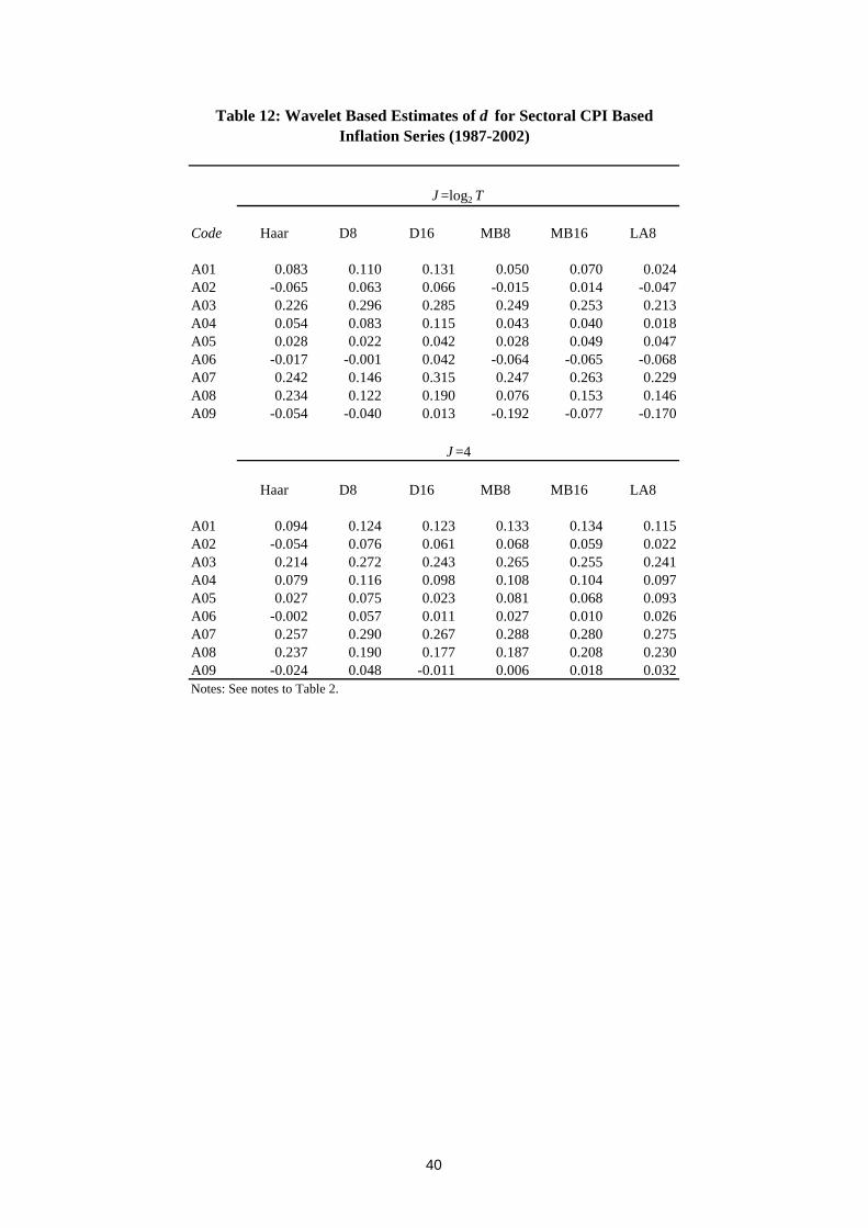
Code Haar D8 D16 MB8 MB16 LA8
A01 0.083 0.110 0.131 0.050 0.070 0.024A02 -0.065 0.063 0.066 -0.015 0.014 -0.047A03 0.226 0.296 0.285 0.249 0.253 0.213A04 0.054 0.083 0.115 0.043 0.040 0.018A05 0.028 0.022 0.042 0.028 0.049 0.047A06 -0.017 -0.001 0.042 -0.064 -0.065 -0.068A07 0.242 0.146 0.315 0.247 0.263 0.229A08 0.234 0.122 0.190 0.076 0.153 0.146A09 -0.054 -0.040 0.013 -0.192 -0.077 -0.170
Haar D8 D16 MB8 MB16 LA8
A01 0.094 0.124 0.123 0.133 0.134 0.115A02 -0.054 0.076 0.061 0.068 0.059 0.022A03 0.214 0.272 0.243 0.265 0.255 0.241A04 0.079 0.116 0.098 0.108 0.104 0.097A05 0.027 0.075 0.023 0.081 0.068 0.093A06 -0.002 0.057 0.011 0.027 0.010 0.026A07 0.257 0.290 0.267 0.288 0.280 0.275A08 0.237 0.190 0.177 0.187 0.208 0.230A09 -0.024 0.048 -0.011 0.006 0.018 0.032Notes: See notes to Table 2.
Table 12: Wavelet Based Estimates of d for Sectoral CPI Based Inflation Series (1987-2002)
J =log2 T
J =4
40

AIC for FGN and ARFIMA Models
Code FGN(d ) ARFIMA(0,d ,0) ARFIMA(1,d ,0) ARFIMA(0,d ,1) ARFIMA(1,d ,1)
A01 3.932 3.937 5.921 5.912 7.908A02 3.997 3.992 5.955 5.952 7.931A03 3.701 3.726 5.699 5.683 7.673A04 3.959 3.947 5.944 5.944 7.942A05 3.991 3.989 5.943 5.929 7.928A06 4.011 3.995 5.994 5.994 7.994A07 3.564 3.555 5.548 5.546 7.537A08 3.822 3.841 5.809 5.810 7.808A09 4.017 3.997 5.976 5.979 6.000
Estimates for FGN and Best ARFIMA Models Selected by AIC
FGN(d ) ARFIMA(0,d ,0)d s.e. d s.e.
A01 0.139 0.048 0.148 0.058A02 0.076 0.047 0.058 0.058A03 0.268 0.049 0.308 0.058A04 0.103 0.047 0.120 0.058A05 0.087 0.047 0.068 0.058A06 0.040 0.046 0.038 0.058A07 0.248 0.049 0.292 0.058A08 0.205 0.048 0.223 0.058A09 0.023 0.046 0.025 0.058Notes: See notes to Table 3.
Table 13: Parameter Estimates and Model Selection Criteria of FGN and ARFIMA Models for Sectoral CPI Inflation Series (1987-2002)
41
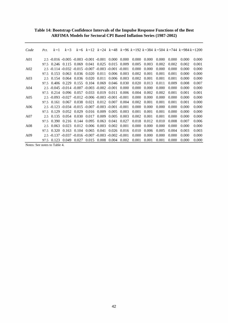
Code Pct. k =1 k =3 k =6 k =12 k =24 k =48 k =96 k =192 k =384 k =504 k =744 k =984 k =1200
A01 2.5 -0.016 -0.005 -0.003 -0.001 -0.001 0.000 0.000 0.000 0.000 0.000 0.000 0.000 0.00097.5 0.246 0.115 0.069 0.041 0.025 0.015 0.009 0.005 0.003 0.002 0.002 0.002 0.001
A02 2.5 -0.114 -0.032 -0.015 -0.007 -0.003 -0.001 -0.001 0.000 0.000 0.000 0.000 0.000 0.00097.5 0.153 0.063 0.036 0.020 0.011 0.006 0.003 0.002 0.001 0.001 0.001 0.000 0.000
A03 2.5 0.154 0.064 0.036 0.020 0.011 0.006 0.003 0.002 0.001 0.001 0.001 0.000 0.00097.5 0.406 0.229 0.155 0.104 0.069 0.046 0.030 0.020 0.013 0.011 0.009 0.008 0.007
A04 2.5 -0.045 -0.014 -0.007 -0.003 -0.002 -0.001 0.000 0.000 0.000 0.000 0.000 0.000 0.00097.5 0.214 0.096 0.057 0.033 0.019 0.011 0.006 0.004 0.002 0.002 0.001 0.001 0.001
A05 2.5 -0.093 -0.027 -0.012 -0.006 -0.003 -0.001 -0.001 0.000 0.000 0.000 0.000 0.000 0.00097.5 0.161 0.067 0.038 0.021 0.012 0.007 0.004 0.002 0.001 0.001 0.001 0.001 0.000
A06 2.5 -0.123 -0.034 -0.015 -0.007 -0.003 -0.001 -0.001 0.000 0.000 0.000 0.000 0.000 0.00097.5 0.129 0.052 0.029 0.016 0.009 0.005 0.003 0.001 0.001 0.001 0.000 0.000 0.000
A07 2.5 0.135 0.054 0.030 0.017 0.009 0.005 0.003 0.002 0.001 0.001 0.000 0.000 0.00097.5 0.390 0.216 0.144 0.095 0.063 0.041 0.027 0.018 0.012 0.010 0.008 0.007 0.006
A08 2.5 0.063 0.023 0.012 0.006 0.003 0.002 0.001 0.000 0.000 0.000 0.000 0.000 0.00097.5 0.320 0.163 0.104 0.065 0.041 0.026 0.016 0.010 0.006 0.005 0.004 0.003 0.003
A09 2.5 -0.137 -0.037 -0.016 -0.007 -0.003 -0.002 -0.001 0.000 0.000 0.000 0.000 0.000 0.00097.5 0.123 0.049 0.027 0.015 0.008 0.004 0.002 0.001 0.001 0.001 0.000 0.000 0.000
Notes: See notes to Table 4.
Table 14: Bootstrap Confidence Intervals of the Impulse Response Functions of the Best ARFIMA Models for Sectoral CPI Based Inflation Series (1987-2002)
42

Code α =0.30 α =0.50 α =0.80 α =0.90 α =0.95 α =0.99
A01 1 1 1 2 4 26A02 1 1 1 1 2 7A03 1 1 3 6 17 166A04 1 1 1 2 3 18A05 1 1 1 1 2 9A06 1 1 1 1 1 5A07 1 1 2 6 14 137A08 1 1 2 4 8 62A09 1 1 1 1 1 3Notes: See notes to Table 5.
Table 15: Estimates of τ α for Sectoral CPI Based Inflation Series (1987-2002)
43

GPH Estimates GSP Estimates
Code α =0.50 α =0.55 α =0.60 α =0.65 α =0.70 α =0.75 α =0.80 α =0.50 α =0.55 α =0.60 α =0.65 α =0.70 α =0.75 α =0.80
T01 0.265 0.054 0.059 0.195 0.342 0.493 0.503 0.184 -0.034 -0.039 0.077 0.232 0.427 0.356T02 0.637 0.461 0.373 0.356 0.588 0.504 0.450 0.449 0.378 0.349 0.337 0.357 0.381 0.396T03 0.336 0.241 0.661 0.604 0.499 0.433 0.385 0.344 0.297 0.427 0.389 0.381 0.399 0.409T04 -0.015 -0.086 0.040 0.293 0.341 0.360 0.434 -0.062 -0.092 0.016 0.246 0.376 0.397 0.493T05 0.036 0.059 0.187 0.288 0.271 0.255 0.147 0.152 0.177 0.257 0.146 0.189 0.160 0.108T06 -0.200 -0.202 -0.138 0.029 0.075 0.093 0.142 -0.103 -0.093 -0.068 0.039 0.060 0.092 0.159T07 0.252 0.360 0.245 0.304 0.196 0.174 0.289 0.163 0.179 0.218 0.215 0.193 0.211 0.318T08 -0.041 -0.011 -0.149 -0.109 -0.077 -0.206 -0.252 -0.077 -0.048 -0.119 -0.179 -0.178 -0.223 -0.216T09 0.339 0.202 0.139 0.228 0.260 0.326 0.292 0.349 0.250 0.226 0.244 0.288 0.243 0.221T10 -0.193 -0.200 -0.131 0.206 0.199 0.203 0.190 -0.213 -0.199 -0.145 0.017 0.053 0.079 0.112T11 0.176 -0.022 0.088 0.227 0.326 0.437 0.514 0.154 -0.055 -0.036 0.086 0.219 0.365 0.357T12 -0.221 -0.166 -0.133 0.029 0.068 0.040 0.030 -0.155 -0.190 -0.122 -0.033 0.069 0.070 0.073T13 0.558 0.399 0.343 0.344 0.515 0.453 0.456 0.454 0.366 0.356 0.343 0.367 0.380 0.413T14 0.424 0.412 0.306 0.328 0.427 0.461 0.384 0.411 0.406 0.310 0.266 0.284 0.314 0.264T15 1.052 0.894 0.743 0.618 0.464 0.372 0.428 0.961 0.761 0.680 0.569 0.425 0.370 0.382T16 -0.031 -0.088 0.097 0.294 0.249 0.252 0.203 0.008 0.003 0.130 0.358 0.340 0.338 0.268T17 0.023 0.062 0.026 -0.056 -0.175 -0.242 -0.096 -0.023 0.068 0.080 0.021 -0.087 -0.137 -0.053T18 -0.246 -0.273 -0.111 0.075 0.052 0.086 0.086 -0.310 -0.247 -0.066 0.091 0.086 0.116 0.147T19 0.176 0.042 0.231 0.273 0.253 0.363 0.343 0.146 0.025 0.142 0.170 0.187 0.209 0.182T20 -0.010 -0.037 0.134 0.318 0.442 0.443 0.522 -0.007 0.006 0.138 0.297 0.416 0.411 0.524T21 0.089 0.021 0.001 0.301 0.250 0.140 0.151 -0.064 -0.041 -0.020 0.222 0.230 0.141 0.153T22 -0.031 -0.136 0.123 0.271 0.355 0.408 0.488 -0.084 -0.180 -0.047 0.083 0.243 0.334 0.482T23 -0.485 -0.512 -0.342 -0.098 0.011 0.080 0.235 -0.431 -0.404 -0.235 0.010 0.197 0.291 0.445T24 -0.152 -0.242 -0.178 -0.053 0.139 0.191 0.273 -0.235 -0.276 -0.203 -0.041 0.188 0.312 0.393T25 -0.312 -0.243 -0.046 0.128 0.206 0.094 -0.009 -0.337 -0.234 -0.065 0.130 0.074 -0.031 -0.142T26 0.540 0.355 0.277 0.221 0.188 0.225 0.173 0.449 0.396 0.381 0.093 0.142 0.189 0.161T27 0.372 0.297 0.233 0.118 0.227 0.175 0.142 0.344 0.303 0.262 0.094 0.143 0.144 0.111T28 0.486 0.251 0.009 0.131 0.153 0.042 0.048 0.501 0.259 0.095 0.115 0.114 0.020 0.036T29 -0.315 -0.280 0.020 0.126 0.094 0.126 0.090 -0.329 -0.246 -0.153 -0.020 0.016 0.085 0.078T30 -0.496 -0.405 -0.384 -0.278 -0.155 -0.155 -0.033 -0.181 -0.155 -0.132 -0.102 -0.033 -0.010 0.086T31 -0.062 -0.127 -0.177 0.121 0.044 0.121 0.345 -0.108 -0.131 -0.147 0.015 -0.033 0.076 0.262T32 0.200 0.316 0.229 0.202 0.210 0.128 0.168 0.205 0.330 0.217 0.190 0.124 0.095 0.120T33 0.412 0.257 0.291 0.361 0.331 0.295 0.340 0.294 0.228 0.242 0.214 0.286 0.220 0.269T34 -0.137 -0.113 -0.242 -0.268 -0.239 -0.344 -0.382 -0.146 -0.131 -0.177 -0.251 -0.241 -0.289 -0.292T35 -0.023 0.023 -0.065 -0.044 -0.081 -0.063 -0.049 0.069 0.117 0.052 0.010 -0.030 -0.019 -0.016T36 0.342 0.190 0.153 0.208 0.216 0.262 0.274 0.325 0.226 0.228 0.232 0.259 0.212 0.207T37 0.278 0.184 0.040 0.215 0.209 0.198 0.160 0.255 0.192 0.074 0.099 0.132 0.062 0.077T38 -0.176 -0.184 -0.039 0.090 0.286 0.354 0.489 -0.140 -0.125 -0.042 0.069 0.252 0.391 0.596T39 -0.234 -0.239 -0.045 0.179 0.097 0.060 0.084 -0.288 -0.215 -0.016 0.096 0.132 0.114 0.196T40 0.554 0.291 0.128 -0.143 -0.075 -0.141 -0.235 0.395 0.138 -0.019 -0.141 -0.073 -0.104 -0.160
s.e. 0.294 0.258 0.222 0.185 0.162 0.144 0.127 0.158 0.144 0.129 0.112 0.1 0.09 0.079Notes: See notes to Table 1.
Table 16: GPH and GSP Estimates for Sectoral CPI Based Inflation Series (1994-2002)
44

Code Haar D8 D16 MB8 MB16 LA8 Haar D8 D16 MB8 MB16 LA8
T01 0.380 0.255 0.354 0.378 0.385 0.394 0.320 0.272 0.282 0.331 0.340 0.341T02 0.301 0.256 0.332 0.192 0.295 0.288 0.308 0.308 0.300 0.303 0.316 0.325T03 0.233 0.361 0.281 0.256 0.181 0.166 0.275 0.322 0.286 0.293 0.301 0.308T04 0.425 0.329 0.352 0.405 0.329 0.403 0.341 0.301 0.305 0.338 0.323 0.356T05 -0.006 -0.031 0.097 0.066 -0.157 -0.054 0.073 0.071 0.079 0.102 0.085 0.096T06 0.159 0.092 0.184 0.115 0.123 0.215 0.146 0.114 0.134 0.166 0.180 0.240T07 0.397 0.177 0.373 0.317 0.287 0.342 0.327 0.225 0.296 0.293 0.305 0.315T08 -0.370 -0.343 -0.237 -0.291 -0.392 -0.494 -0.344 -0.247 -0.263 -0.272 -0.262 -0.296T09 0.183 0.157 0.272 0.212 0.104 0.213 0.262 0.217 0.234 0.252 0.250 0.303T10 0.036 0.032 0.096 0.094 0.039 0.097 0.052 0.074 0.074 0.127 0.129 0.143T11 0.357 0.233 0.322 0.365 0.371 0.405 0.307 0.262 0.263 0.325 0.329 0.346T12 0.080 0.006 0.096 0.062 0.010 0.123 0.079 0.067 0.058 0.079 0.117 0.165T13 0.278 0.250 0.325 0.186 0.281 0.252 0.300 0.304 0.289 0.295 0.305 0.313T14 0.292 0.184 0.273 0.111 0.245 0.284 0.282 0.255 0.273 0.262 0.289 0.299T15 0.226 0.338 0.281 0.292 0.222 0.141 0.298 0.323 0.304 0.297 0.305 0.298T16 0.191 0.194 0.263 0.201 0.136 0.220 0.186 0.203 0.203 0.229 0.227 0.245T17 -0.019 -0.110 -0.065 -0.302 -0.252 -0.276 -0.021 -0.131 -0.064 -0.113 -0.118 -0.105T18 0.116 0.134 0.118 0.131 0.119 0.249 0.107 0.148 0.111 0.134 0.157 0.205T19 0.173 0.059 0.153 0.099 0.032 0.034 0.185 0.137 0.134 0.157 0.157 0.158T20 0.447 0.352 0.373 0.430 0.384 0.431 0.357 0.311 0.331 0.354 0.349 0.377T21 0.110 0.033 0.036 0.012 -0.021 0.006 0.116 0.071 0.061 0.072 0.073 0.119T22 0.428 0.349 0.404 0.447 0.436 0.463 0.330 0.298 0.331 0.356 0.353 0.386T23 0.441 0.311 0.419 0.437 0.344 0.473 0.329 0.278 0.319 0.343 0.336 0.386T24 0.454 0.275 0.354 0.418 0.362 0.456 0.355 0.258 0.301 0.333 0.332 0.371T25 -0.059 -0.197 -0.070 -0.129 -0.340 -0.181 -0.044 -0.112 -0.084 -0.058 -0.068 -0.060T26 -0.011 0.021 0.116 0.104 -0.118 -0.082 0.094 0.118 0.110 0.131 0.116 0.102T27 -0.092 -0.082 0.026 0.003 -0.155 -0.111 0.007 -0.001 0.021 0.043 0.034 0.039T28 0.089 -0.045 0.062 -0.201 -0.037 -0.009 0.098 0.061 0.065 0.049 0.055 0.069T29 0.038 -0.001 0.078 0.029 0.047 0.086 0.038 0.019 0.037 0.089 0.096 0.143T30 0.075 0.032 0.120 0.093 -0.021 0.213 0.079 0.072 0.083 0.115 0.124 0.215T31 0.411 0.133 0.259 0.313 0.281 0.356 0.308 0.163 0.232 0.258 0.280 0.300T32 -0.031 0.109 0.110 -0.021 -0.226 -0.110 0.064 0.117 0.116 0.087 0.086 0.098T33 0.221 0.198 0.335 0.215 0.218 0.265 0.235 0.239 0.258 0.233 0.246 0.263T34 -0.456 -0.496 -0.307 -0.363 -0.500 -0.500 -0.457 -0.364 -0.370 -0.386 -0.384 -0.421T35 -0.161 -0.056 -0.119 -0.165 -0.134 -0.175 -0.125 -0.018 -0.062 -0.067 -0.043 -0.051T36 0.154 0.143 0.254 0.198 0.089 0.207 0.242 0.204 0.220 0.236 0.236 0.293T37 0.044 -0.024 0.107 -0.042 -0.099 -0.148 0.112 0.070 0.078 0.072 0.090 0.109T38 0.446 0.416 0.466 0.468 0.433 0.477 0.353 0.347 0.373 0.388 0.378 0.410T39 0.031 0.205 0.113 0.071 0.060 0.112 0.028 0.186 0.094 0.099 0.129 0.122T40 -0.192 -0.213 -0.290 -0.218 -0.266 -0.231 -0.195 -0.131 -0.158 -0.139 -0.166 -0.187Notes: See notes to Table 2.
Table 17: Wavelet Based Estimates of d for Sectoral CPI Based Inflation Series (1994-2002)
J =log2 T J =4
45

AIC for FGN and ARFIMA Models Estimates for FGN and Best ARFIMA Models Selected by AICFGN(d ) ARFIMA(0,d ,0)
Code FGN(d ) ARFIMA(0,d ,0) ARFIMA(1,d ,0) ARFIMA(0,d ,1) ARFIMA(1,d ,1) d s.e. d s.e.
T01 3.612 3.678 5.580 5.519 7.512 0.362 0.067 0.419 0.078T02 3.563 3.570 5.570 5.538 7.538 0.291 0.066 0.344 0.078T03 3.641 3.641 5.641 5.594 7.586 0.274 0.066 0.334 0.078T04 3.621 3.663 5.628 5.521 7.519 0.342 0.067 0.413 0.078T05 4.019 3.989 5.978 5.973 7.966 0.055 0.063 0.056 0.078T06 3.938 3.950 5.874 5.834 7.817 0.169 0.065 0.154 0.078T07 3.693 3.744 5.652 5.644 7.604 0.308 0.066 0.332 0.078T08 3.901 3.833 5.831 5.831 7.832 -0.182 0.056 -0.262 0.078T09 3.748 3.766 5.741 5.749 6.000 0.242 0.066 0.263 0.078T10 4.002 3.988 5.956 5.880 7.879 0.096 0.064 0.073 0.078T11 3.663 3.721 5.640 5.575 7.573 0.333 0.067 0.378 0.078T12 4.005 3.990 5.957 5.892 7.890 0.092 0.064 0.067 0.078T13 3.589 3.590 5.589 5.558 7.556 0.279 0.066 0.332 0.078T14 3.683 3.693 5.690 5.661 6.000 0.255 0.066 0.290 0.078T15 3.574 3.547 5.478 5.525 7.444 0.254 0.066 0.309 0.078T16 3.855 3.858 5.855 5.760 7.755 0.204 0.065 0.237 0.078T17 4.018 3.964 5.964 5.964 7.963 -0.067 0.060 -0.117 0.078T18 3.946 3.952 5.900 5.800 7.793 0.160 0.065 0.153 0.078T19 3.967 3.953 5.952 5.897 7.895 0.121 0.064 0.127 0.078T20 3.528 3.569 5.539 5.447 7.446 0.371 0.067 0.455 0.078T21 4.022 3.994 5.994 5.916 7.904 0.055 0.063 0.046 0.078T22 3.534 3.617 5.482 5.428 7.378 0.412 0.067 0.493 0.078T23 3.593 3.678 5.510 5.463 7.379 0.402 0.067 0.472 0.078T24 3.640 3.717 5.584 5.506 7.461 0.376 0.067 0.436 0.078T25 4.001 3.944 5.942 5.865 7.845 -0.090 0.059 -0.155 0.078T26 3.975 3.952 5.947 5.947 7.927 0.100 0.064 0.108 0.078T27 4.036 4.000 5.937 5.915 7.852 0.007 0.062 0.005 0.078T28 4.009 3.989 5.945 5.975 6.000 0.079 0.064 0.058 0.078T29 4.017 3.996 5.975 5.866 7.866 0.072 0.063 0.045 0.078T30 3.972 3.981 5.833 5.840 7.792 0.146 0.065 0.101 0.078T31 3.789 3.865 5.619 5.655 7.553 0.309 0.066 0.291 0.078T32 3.994 3.974 5.973 5.973 7.972 0.092 0.064 0.090 0.078T33 3.753 3.780 5.742 5.712 7.697 0.260 0.066 0.285 0.078T34 3.776 3.711 5.694 5.700 6.000 -0.253 0.052 -0.353 0.078T35 4.028 3.981 5.980 5.980 7.920 -0.043 0.061 -0.083 0.078T36 3.779 3.798 5.758 5.776 7.736 0.233 0.066 0.247 0.078T37 4.005 3.983 5.981 5.981 7.979 0.080 0.064 0.071 0.078T38 3.336 3.429 5.218 5.222 7.123 0.470 0.068 0.683 0.078T39 3.933 3.941 5.894 5.800 7.797 0.170 0.065 0.169 0.078T40 3.983 3.924 5.923 5.886 7.883 -0.111 0.059 -0.171 0.078Notes: See notes to Table 3.
Table 18: Parameter Estimates and Model Selection Criteria of FGN and ARFIMA Models for Sectoral CPI Based Inflation Series (1994-2002)
46
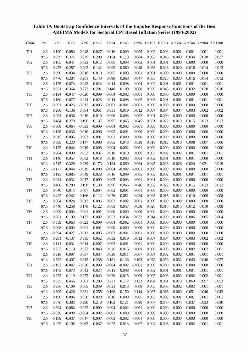
Code Pct. k =1 k =3 k =6 k =12 k =24 k =48 k =96 k =192 k =384 k =504 k =744 k =984 k =1200
T01 2.5 0.190 0.083 0.048 0.027 0.016 0.009 0.005 0.003 0.002 0.001 0.001 0.001 0.00197.5 0.559 0.371 0.279 0.208 0.154 0.113 0.084 0.062 0.045 0.040 0.034 0.030 0.027
T02 2.5 0.105 0.041 0.022 0.012 0.006 0.003 0.002 0.001 0.001 0.000 0.000 0.000 0.00097.5 0.473 0.287 0.203 0.142 0.099 0.069 0.048 0.033 0.023 0.020 0.016 0.014 0.013
T03 2.5 0.090 0.034 0.018 0.010 0.005 0.003 0.001 0.001 0.000 0.000 0.000 0.000 0.00097.5 0.470 0.284 0.201 0.140 0.098 0.068 0.047 0.033 0.023 0.020 0.016 0.014 0.012
T04 2.5 0.175 0.074 0.042 0.024 0.014 0.008 0.004 0.002 0.001 0.001 0.001 0.001 0.00197.5 0.551 0.364 0.272 0.201 0.148 0.109 0.080 0.059 0.043 0.038 0.032 0.028 0.026
T05 2.5 -0.194 -0.047 -0.020 -0.009 -0.004 -0.002 -0.001 0.000 0.000 0.000 0.000 0.000 0.00097.5 0.180 0.077 0.044 0.025 0.014 0.008 0.005 0.003 0.001 0.001 0.001 0.001 0.001
T06 2.5 -0.091 -0.026 -0.012 -0.006 -0.003 -0.001 -0.001 0.000 0.000 0.000 0.000 0.000 0.00097.5 0.280 0.136 0.084 0.051 0.031 0.019 0.012 0.007 0.004 0.004 0.003 0.002 0.002
T07 2.5 0.094 0.036 0.019 0.010 0.006 0.003 0.002 0.001 0.000 0.000 0.000 0.000 0.00097.5 0.464 0.279 0.196 0.137 0.095 0.065 0.045 0.031 0.022 0.019 0.015 0.013 0.012
T08 2.5 -0.508 -0.064 -0.023 -0.009 -0.004 -0.002 -0.001 0.000 0.000 0.000 0.000 0.000 0.00097.5 -0.129 -0.035 -0.016 -0.006 -0.002 -0.001 0.000 0.000 0.000 0.000 0.000 0.000 0.000
T09 2.5 0.015 0.005 0.003 0.001 0.001 0.000 0.000 0.000 0.000 0.000 0.000 0.000 0.00097.5 0.395 0.220 0.147 0.098 0.065 0.043 0.028 0.018 0.012 0.010 0.008 0.007 0.006
T10 2.5 -0.175 -0.044 -0.019 -0.008 -0.004 -0.002 -0.001 0.000 0.000 0.000 0.000 0.000 0.00097.5 0.204 0.090 0.053 0.031 0.018 0.010 0.006 0.003 0.002 0.002 0.001 0.001 0.001
T11 2.5 0.140 0.057 0.032 0.018 0.010 0.005 0.003 0.002 0.001 0.001 0.001 0.000 0.00097.5 0.515 0.328 0.239 0.173 0.124 0.089 0.064 0.045 0.033 0.028 0.024 0.021 0.019
T12 2.5 -0.177 -0.044 -0.019 -0.008 -0.004 -0.002 -0.001 0.000 0.000 0.000 0.000 0.000 0.00097.5 0.195 0.085 0.049 0.028 0.016 0.009 0.005 0.003 0.002 0.001 0.001 0.001 0.001
T13 2.5 0.084 0.031 0.017 0.009 0.005 0.003 0.001 0.001 0.000 0.000 0.000 0.000 0.00097.5 0.466 0.280 0.198 0.138 0.096 0.066 0.046 0.032 0.022 0.019 0.015 0.013 0.012
T14 2.5 0.040 0.014 0.007 0.004 0.002 0.001 0.001 0.000 0.000 0.000 0.000 0.000 0.00097.5 0.422 0.242 0.166 0.112 0.076 0.051 0.034 0.023 0.015 0.013 0.010 0.009 0.008
T15 2.5 0.064 0.024 0.012 0.006 0.003 0.002 0.001 0.000 0.000 0.000 0.000 0.000 0.00097.5 0.440 0.258 0.178 0.122 0.083 0.057 0.038 0.026 0.018 0.015 0.012 0.010 0.009
T16 2.5 -0.009 -0.003 -0.001 -0.001 0.000 0.000 0.000 0.000 0.000 0.000 0.000 0.000 0.00097.5 0.361 0.193 0.127 0.082 0.053 0.034 0.022 0.014 0.009 0.008 0.006 0.005 0.004
T17 2.5 -0.359 -0.063 -0.023 -0.009 -0.004 -0.002 -0.001 0.000 0.000 0.000 0.000 0.000 0.00097.5 0.008 0.003 0.001 0.001 0.000 0.000 0.000 0.000 0.000 0.000 0.000 0.000 0.000
T18 2.5 -0.094 -0.027 -0.013 -0.006 -0.003 -0.001 -0.001 0.000 0.000 0.000 0.000 0.000 0.00097.5 0.281 0.137 0.085 0.052 0.032 0.019 0.012 0.007 0.004 0.004 0.003 0.002 0.002
T19 2.5 -0.111 -0.031 -0.014 -0.007 -0.003 -0.001 -0.001 0.000 0.000 0.000 0.000 0.000 0.00097.5 0.253 0.119 0.072 0.043 0.026 0.016 0.009 0.006 0.003 0.003 0.002 0.002 0.001
T20 2.5 0.216 0.097 0.057 0.034 0.020 0.011 0.007 0.004 0.002 0.002 0.001 0.001 0.00197.5 0.592 0.407 0.313 0.238 0.181 0.136 0.103 0.078 0.059 0.052 0.045 0.040 0.037
T21 2.5 -0.192 -0.047 -0.020 -0.009 -0.004 -0.002 -0.001 0.000 0.000 0.000 0.000 0.000 0.00097.5 0.173 0.073 0.042 0.024 0.013 0.008 0.004 0.002 0.001 0.001 0.001 0.001 0.001
T22 2.5 0.252 0.119 0.072 0.043 0.026 0.015 0.009 0.005 0.003 0.003 0.002 0.002 0.00197.5 0.635 0.456 0.361 0.283 0.221 0.172 0.133 0.104 0.081 0.073 0.063 0.057 0.053
T23 2.5 0.236 0.109 0.065 0.039 0.023 0.013 0.008 0.005 0.003 0.002 0.002 0.001 0.00197.5 0.609 0.426 0.331 0.255 0.196 0.150 0.114 0.087 0.066 0.060 0.051 0.046 0.043
T24 2.5 0.196 0.086 0.050 0.029 0.016 0.009 0.005 0.003 0.002 0.001 0.001 0.001 0.00197.5 0.570 0.383 0.290 0.218 0.162 0.121 0.090 0.067 0.050 0.044 0.037 0.033 0.030
T25 2.5 -0.394 -0.064 -0.023 -0.009 -0.004 -0.002 -0.001 0.000 0.000 0.000 0.000 0.000 0.00097.5 -0.026 -0.008 -0.004 -0.002 -0.001 0.000 0.000 0.000 0.000 0.000 0.000 0.000 0.000
T26 2.5 -0.139 -0.037 -0.017 -0.007 -0.003 -0.002 -0.001 0.000 0.000 0.000 0.000 0.000 0.00097.5 0.229 0.105 0.062 0.037 0.022 0.013 0.007 0.004 0.003 0.002 0.002 0.001 0.001
Table 19: Bootstrap Confidence Intervals of the Impulse Response Functions of the Best ARFIMA Models for Sectoral CPI Based Inflation Series (1994-2002)
47

T27 2.5 -0.238 -0.053 -0.022 -0.009 -0.004 -0.002 -0.001 0.000 0.000 0.000 0.000 0.000 0.00097.5 0.133 0.054 0.030 0.016 0.009 0.005 0.003 0.001 0.001 0.001 0.000 0.000 0.000
T28 2.5 -0.184 -0.045 -0.020 -0.009 -0.004 -0.002 -0.001 0.000 0.000 0.000 0.000 0.000 0.00097.5 0.183 0.079 0.045 0.026 0.015 0.008 0.005 0.003 0.002 0.001 0.001 0.001 0.001
T29 2.5 -0.200 -0.048 -0.020 -0.009 -0.004 -0.002 -0.001 0.000 0.000 0.000 0.000 0.000 0.00097.5 0.170 0.072 0.041 0.023 0.013 0.007 0.004 0.002 0.001 0.001 0.001 0.001 0.001
T30 2.5 -0.143 -0.038 -0.017 -0.008 -0.003 -0.002 -0.001 0.000 0.000 0.000 0.000 0.000 0.00097.5 0.224 0.102 0.060 0.035 0.021 0.012 0.007 0.004 0.002 0.002 0.001 0.001 0.001
T31 2.5 0.045 0.016 0.008 0.004 0.002 0.001 0.001 0.000 0.000 0.000 0.000 0.000 0.00097.5 0.416 0.237 0.162 0.109 0.073 0.049 0.033 0.022 0.015 0.012 0.010 0.008 0.007
T32 2.5 -0.152 -0.040 -0.018 -0.008 -0.004 -0.002 -0.001 0.000 0.000 0.000 0.000 0.000 0.00097.5 0.212 0.095 0.056 0.032 0.019 0.011 0.006 0.004 0.002 0.002 0.001 0.001 0.001
T33 2.5 0.042 0.015 0.008 0.004 0.002 0.001 0.001 0.000 0.000 0.000 0.000 0.000 0.00097.5 0.418 0.239 0.163 0.110 0.074 0.050 0.033 0.022 0.015 0.013 0.010 0.009 0.008
T34 2.5 -0.596 -0.064 -0.023 -0.009 -0.004 -0.002 -0.001 0.000 0.000 0.000 0.000 0.000 0.00097.5 -0.221 -0.050 -0.017 -0.005 -0.002 -0.001 0.000 0.000 0.000 0.000 0.000 0.000 0.000
T35 2.5 -0.322 -0.061 -0.023 -0.009 -0.004 -0.002 -0.001 0.000 0.000 0.000 0.000 0.000 0.00097.5 0.043 0.015 0.008 0.004 0.002 0.001 0.001 0.000 0.000 0.000 0.000 0.000 0.000
T36 2.5 0.005 0.002 0.001 0.000 0.000 0.000 0.000 0.000 0.000 0.000 0.000 0.000 0.00097.5 0.378 0.207 0.137 0.090 0.059 0.038 0.025 0.016 0.011 0.009 0.007 0.006 0.005
T37 2.5 -0.177 -0.044 -0.019 -0.008 -0.004 -0.002 -0.001 0.000 0.000 0.000 0.000 0.000 0.00097.5 0.195 0.085 0.049 0.028 0.016 0.009 0.005 0.003 0.002 0.001 0.001 0.001 0.001
T38 2.5 0.455 0.271 0.189 0.131 0.090 0.062 0.043 0.029 0.020 0.017 0.014 0.012 0.01197.5 0.839 0.730 0.660 0.594 0.533 0.477 0.427 0.382 0.342 0.327 0.307 0.294 0.285
T39 2.5 -0.080 -0.023 -0.011 -0.005 -0.002 -0.001 -0.001 0.000 0.000 0.000 0.000 0.000 0.00097.5 0.295 0.146 0.091 0.056 0.035 0.021 0.013 0.008 0.005 0.004 0.003 0.003 0.002
T40 2.5 -0.410 -0.064 -0.023 -0.009 -0.004 -0.002 -0.001 0.000 0.000 0.000 0.000 0.000 0.00097.5 -0.042 -0.013 -0.006 -0.003 -0.002 -0.001 0.000 0.000 0.000 0.000 0.000 0.000 0.000
Notes: See notes to Table 4.
48

Code α =0.30 α =0.50 α =0.80 α =0.90 α =0.95 α =0.99
T01 1 1 5 15 48 766T02 1 1 3 8 23 262T03 1 1 3 8 21 229T04 1 1 4 14 45 691T05 1 1 1 1 2 7T06 1 1 1 2 5 28T07 1 1 3 7 20 223T08 1 1 2 2 4 12T09 1 1 2 5 11 97T10 1 1 1 1 2 9T11 1 1 4 11 32 418T12 1 1 1 1 2 8T13 1 1 3 7 20 223T14 1 1 2 6 14 133T15 1 1 3 6 17 167T16 1 1 2 4 9 72T17 1 1 1 2 3 9T18 1 1 1 2 4 28T19 1 1 1 2 4 20T20 1 1 6 20 72 >1200T21 1 1 1 1 1 6T22 1 1 8 30 116 >1200T23 1 1 7 24 89 >1200T24 1 1 5 17 58 995T25 1 1 1 2 3 10T26 1 1 1 2 3 16T27 1 1 1 1 1 1T28 1 1 1 1 2 7T29 1 1 1 1 1 5T30 1 1 1 2 3 14T31 1 1 2 6 14 135T32 1 1 1 1 2 12T33 1 1 2 5 14 126T34 1 1 2 3 4 12T35 1 1 1 1 2 7T36 1 1 2 4 10 81T37 1 1 1 1 2 9T38 1 4 66 582 >1200 >1200T39 1 1 1 2 5 33T40 1 1 1 2 3 11Notes: See notes to Table 5.
Table 20: Estimates of τ α for Sectoral CPI Based Inflation Series (1994-2002)
49

AIC for ARFIMA-BREAK Models
Inflation Series p,q,s 0,0,1 1,0,1 0,0,2 1,0,2
WPI (1923-2001) 565.163 566.050 558.293 559.321WPI (1964:2-2002:6) 1568.063 1903.738 1567.141 1756.581WPI (1964:2-1988:1) 932.742 930.237 1068.706 1059.603WPI (1982:2-2002:6) 834.759 836.639 844.394 833.697WPI (1987:2-2002:6) 602.782 602.230 665.820 684.735WPI (1994:2-2002:6) 285.473 286.603 300.401 302.376CPI (1951-2001) 337.776 336.965 330.969 328.103CPI (1987:2-2002:6) 577.562 578.538 574.401 575.137CPI (1994:2-2002:6) 226.140 246.350 224.699 224.491
Estimates for ARFIMA-BREAK Models with Minimum AIC
γ s.e. d s.e. φ1 s.e.0.150 0.113 -0.356 0.089 - -
WPI (1923-2001) 0.000 0.000 -0.476 0.037 - -WPI (1964:2-2002:6) 0.487 0.024 -0.538 0.105 0.338 0.127WPI (1964:2-1988:1) 3.071 0.125 -0.472 0.099 0.218 0.123WPI (1982:2-2002:6) 2.877 0.109 -0.624 0.134 0.353 0.160WPI (1987:2-2002:6) 0.000 0.001 -0.593 0.078 - -WPI (1994:2-2002:6) 5.458 1.700 -0.426 0.189 0.070 0.240CPI (1951-2001) 2.268 0.077 -0.407 0.058 - -CPI (1987:2-2002:6) 0.809 0.025 -0.389 0.226 0.491 0.252CPI (1994:2-2002:6)Notes: First panel of the Table reports the Akaike Information Criterion (-2 ln L + 2k ) for ecah model, where L is the likelihood and k is the number of paremters. The models are estimated using the approximate maximum likelihood function. The second panel shows the estimates for the ARFIMA-BREAK model that has the minimum AIC. Data are seasonally adjusted by subtracting the seasonal means.
Table 21: Parameter Estimates and Model Selection Criteria of ARFIMA-BREAK Models for Aggregate Inflation Series
50