persistence of vision ray-tracer (pov-ray · 2.2 what is pov-ray? . . . . . . . . . . . . . . . . ....
TRANSCRIPT
Persistence of Vision
Ray-Tracer
(POV-Ray )
User’s Documentation 3.0.10
Copyright 1996 POV-Team
Contents
1 Introduction 1
1.1 Notation . . . . . . . . . . . . . . . . . . . . . . . . . . . . . . . . . . . 1
I Installation Guide 3
2 Program Description 5
2.1 What is Ray-Tracing? . . . . . . . . . . . . . . . . . . . . . . . . . . . . 5
2.2 What is POV-Ray? . . . . . . . . . . . . . . . . . . . . . . . . . . . . . 6
2.3 Which Version of POV-Ray should you use? . . . . . . . . . . . . . . . . 7
2.3.1 IBM-PC and Compatibles . . . . . . . . . . . . . . . . . . . . . . 7
2.3.1.1 MS-Dos . . . . . . . . . . . . . . . . . . . . . . . . . . . . 7
2.3.1.2 Windows . . . . . . . . . . . . . . . . . . . . . . . . . . . 8
2.3.1.3 Linux . . . . . . . . . . . . . . . . . . . . . . . . . . . . . 9
2.3.2 Apple Macintosh . . . . . . . . . . . . . . . . . . . . . . . . . . 10
2.3.3 Commodore Amiga . . . . . . . . . . . . . . . . . . . . . . . . . 11
2.3.4 SunOS . . . . . . . . . . . . . . . . . . . . . . . . . . . . . . . . 12
2.3.5 Generic Unix . . . . . . . . . . . . . . . . . . . . . . . . . . . . 12
2.3.6 All Versions . . . . . . . . . . . . . . . . . . . . . . . . . . . . . 13
2.3.7 Compiling POV-Ray . . . . . . . . . . . . . . . . . . . . . . . . . 13
2.3.7.1 Directroy Structure . . . . . . . . . . . . . . . . . . . . . . 14
2.3.7.2 Configuring POV-Ray Source . . . . . . . . . . . . . . . . 15
2.3.7.3 Conclusion . . . . . . . . . . . . . . . . . . . . . . . . . . 16
i

ii CONTENTS
2.4 Where to Find POV-Ray Files . . . . . . . . . . . . . . . . . . . . . . . 16
2.4.1 Graphics Developer Forum on CompuServe . . . . . . . . . . . . 17
2.4.2 Internet . . . . . . . . . . . . . . . . . . . . . . . . . . . . . . . . 17
2.4.3 PC Graphics Area on America On-Line . . . . . . . . . . . . . . . 17
2.4.4 The Graphics Alternative BBS in El Cerrito, CA . . . . . . . . . . 17
2.4.5 PCGNet . . . . . . . . . . . . . . . . . . . . . . . . . . . . . . . 18
2.4.6 POV-Ray Related Books and CD-ROMs . . . . . . . . . . . . . . 20
3 Quick Start 21
3.1 Installing POV-Ray . . . . . . . . . . . . . . . . . . . . . . . . . . . . . 21
3.2 Basic Usage . . . . . . . . . . . . . . . . . . . . . . . . . . . . . . . . . 22
3.2.1 Running Files in Other Directories . . . . . . . . . . . . . . . . . 23
3.2.2 INI Files . . . . . . . . . . . . . . . . . . . . . . . . . . . . . . . 25
3.2.3 Alternatives to POVRAY.INI . . . . . . . . . . . . . . . . . . . . . 25
3.2.4 Batch Files . . . . . . . . . . . . . . . . . . . . . . . . . . . . . . 26
3.2.5 Display Types . . . . . . . . . . . . . . . . . . . . . . . . . . . . 27
II Tutorial Guide 31
4 Beginning Tutorial 33
4.1 Your First Image . . . . . . . . . . . . . . . . . . . . . . . . . . . . . . 33
4.1.1 Understanding POV-Ray’s Coordinate System . . . . . . . . . . . 33
4.1.2 Adding Standard Include Files . . . . . . . . . . . . . . . . . . . 34
4.1.3 Adding a Camera . . . . . . . . . . . . . . . . . . . . . . . . . . 35
4.1.4 Describing an Object . . . . . . . . . . . . . . . . . . . . . . . . 35
4.1.5 Adding Texture to an Object . . . . . . . . . . . . . . . . . . . . 36
4.1.6 Defining a Light Source . . . . . . . . . . . . . . . . . . . . . . . 37
4.2 Using the Camera . . . . . . . . . . . . . . . . . . . . . . . . . . . . . . 38
4.2.1 Camera Types . . . . . . . . . . . . . . . . . . . . . . . . . . . . 38
4.2.2 Using Focal Blur . . . . . . . . . . . . . . . . . . . . . . . . . . . 38
4.2.3 Using Camera Ray Perturbation . . . . . . . . . . . . . . . . . . . 38
CONTENTS iii
4.3 Simple Shapes . . . . . . . . . . . . . . . . . . . . . . . . . . . . . . . 38
4.3.1 Box Object . . . . . . . . . . . . . . . . . . . . . . . . . . . . . . 38
4.3.2 Cone Object . . . . . . . . . . . . . . . . . . . . . . . . . . . . . 39
4.3.3 Cylinder Object . . . . . . . . . . . . . . . . . . . . . . . . . . . 39
4.3.4 Plane Object . . . . . . . . . . . . . . . . . . . . . . . . . . . . . 40
4.3.5 Standard Include Objects . . . . . . . . . . . . . . . . . . . . . . 40
4.4 Advanced Shapes . . . . . . . . . . . . . . . . . . . . . . . . . . . . . . 41
4.4.1 Bicubic Patch Object . . . . . . . . . . . . . . . . . . . . . . . . 41
4.4.2 Blob Object . . . . . . . . . . . . . . . . . . . . . . . . . . . . . 48
4.4.3 Height Field Object . . . . . . . . . . . . . . . . . . . . . . . . . 48
4.4.4 Julia Fractal Object . . . . . . . . . . . . . . . . . . . . . . . . . 50
4.4.5 Lathe Object . . . . . . . . . . . . . . . . . . . . . . . . . . . . . 50
4.4.6 Mesh Object . . . . . . . . . . . . . . . . . . . . . . . . . . . . . 50
4.4.7 Polygon Object . . . . . . . . . . . . . . . . . . . . . . . . . . . 52
4.4.8 Prism Object . . . . . . . . . . . . . . . . . . . . . . . . . . . . . 54
4.4.9 Superquadric Ellipsoid Object . . . . . . . . . . . . . . . . . . . . 54
4.4.10 Surface of Revolution Object . . . . . . . . . . . . . . . . . . . . 59
4.4.11 Text Object . . . . . . . . . . . . . . . . . . . . . . . . . . . . . 60
4.4.12 Torus Object . . . . . . . . . . . . . . . . . . . . . . . . . . . . . 64
4.5 CSG Objects . . . . . . . . . . . . . . . . . . . . . . . . . . . . . . . . 70
4.5.1 What is CSG? . . . . . . . . . . . . . . . . . . . . . . . . . . . . 70
4.5.2 CSG Union . . . . . . . . . . . . . . . . . . . . . . . . . . . . . 70
4.5.3 CSG Intersection . . . . . . . . . . . . . . . . . . . . . . . . . . 72
4.5.4 CSG Difference . . . . . . . . . . . . . . . . . . . . . . . . . . . 72
4.5.5 CSG Merge . . . . . . . . . . . . . . . . . . . . . . . . . . . . . 74
4.5.6 CSG Pitfalls . . . . . . . . . . . . . . . . . . . . . . . . . . . . . 75
4.5.6.1 Coincidence Surfaces . . . . . . . . . . . . . . . . . . . . . 75
4.6 The Light Source . . . . . . . . . . . . . . . . . . . . . . . . . . . . . . 75
4.6.1 The Ambient Light Source . . . . . . . . . . . . . . . . . . . . . 76
4.6.2 The Point Light Source . . . . . . . . . . . . . . . . . . . . . . . 76

iv CONTENTS
4.6.3 The Spotlight Source . . . . . . . . . . . . . . . . . . . . . . . . 77
4.6.4 The Cylindrical Light Source . . . . . . . . . . . . . . . . . . . . 79
4.6.5 The Area Light Source . . . . . . . . . . . . . . . . . . . . . . . 79
4.6.6 Assigning an Object to a Light Source . . . . . . . . . . . . . . . 81
4.6.7 Light Source Specials . . . . . . . . . . . . . . . . . . . . . . . . 82
4.6.7.1 Using Shadowless Lights . . . . . . . . . . . . . . . . . . . 82
4.6.7.2 Using Light Fading . . . . . . . . . . . . . . . . . . . . . . 83
4.6.7.3 Light Sources and Atmosphere . . . . . . . . . . . . . . . . 84
4.7 Simple Texture Options . . . . . . . . . . . . . . . . . . . . . . . . . . . 84
4.7.1 Surface Finishes . . . . . . . . . . . . . . . . . . . . . . . . . . . 84
4.7.2 Adding Bumpiness . . . . . . . . . . . . . . . . . . . . . . . . . 85
4.7.3 Creating Color Patterns . . . . . . . . . . . . . . . . . . . . . . . 85
4.7.4 Pre-defined Textures . . . . . . . . . . . . . . . . . . . . . . . . . 86
4.8 Advanced Texture Options . . . . . . . . . . . . . . . . . . . . . . . . . 87
4.8.1 Pigment and Normal Patterns . . . . . . . . . . . . . . . . . . . . 87
4.8.2 Pigments . . . . . . . . . . . . . . . . . . . . . . . . . . . . . . . 87
4.8.2.1 Using Color List Pigments . . . . . . . . . . . . . . . . . . 88
4.8.2.2 Using Pigment and Patterns . . . . . . . . . . . . . . . . . 89
4.8.2.3 Using Pattern Modifiers . . . . . . . . . . . . . . . . . . . 89
4.8.2.4 Using Transparent Pigments and Layered Textures . . . . . 91
4.8.2.5 Using Pigment Maps . . . . . . . . . . . . . . . . . . . . . 92
4.8.3 Normals . . . . . . . . . . . . . . . . . . . . . . . . . . . . . . . 94
4.8.3.1 Using Basic Normal Modifiers . . . . . . . . . . . . . . . . 94
4.8.3.2 Blending Normals . . . . . . . . . . . . . . . . . . . . . . 95
4.8.4 Finishes . . . . . . . . . . . . . . . . . . . . . . . . . . . . . . . 97
4.8.4.1 Using Ambient . . . . . . . . . . . . . . . . . . . . . . . . 97
4.8.4.2 Using Surface Highlights . . . . . . . . . . . . . . . . . . . 99
4.8.4.3 Using Reflection and Metallic . . . . . . . . . . . . . . . . 100
4.8.4.4 Using Refraction . . . . . . . . . . . . . . . . . . . . . . . 101
4.8.4.5 Light Attenuation and Caustics . . . . . . . . . . . . . . . 102

CONTENTS v
4.8.4.6 Using Iridescence . . . . . . . . . . . . . . . . . . . . . . . 103
4.8.5 Halos . . . . . . . . . . . . . . . . . . . . . . . . . . . . . . . . . 104
4.8.5.1 What are Halos? . . . . . . . . . . . . . . . . . . . . . . . 104
4.8.5.2 The Emitting Halo . . . . . . . . . . . . . . . . . . . . . . 104
4.8.5.2.1 Starting with a Basic Halo . . . . . . . . . . . . . . 104
4.8.5.2.2 Increasing the Brightness . . . . . . . . . . . . . . . 107
4.8.5.2.3 Adding Some Turbulence . . . . . . . . . . . . . . . 107
4.8.5.2.4 Resizing the Halo . . . . . . . . . . . . . . . . . . . 108
4.8.5.2.5 Using Frequency to Improve Realism . . . . . . . . 109
4.8.5.2.6 Changing the Halo Color . . . . . . . . . . . . . . . 110
4.8.5.3 The Glowing Halo . . . . . . . . . . . . . . . . . . . . . . 111
4.8.5.4 The Attenuating Halo . . . . . . . . . . . . . . . . . . . . 112
4.8.5.4.1 Making a Cloud . . . . . . . . . . . . . . . . . . . . 112
4.8.5.4.2 Scaling the Halo Container . . . . . . . . . . . . . . 113
4.8.5.4.3 Adding Additional Halos . . . . . . . . . . . . . . . 114
4.8.5.5 The Dust Halo . . . . . . . . . . . . . . . . . . . . . . . . 115
4.8.5.5.1 Starting With an Object Lit by a Spotlight . . . . . . 115
4.8.5.5.2 Adding Some Dust . . . . . . . . . . . . . . . . . . 116
4.8.5.5.3 Decreasing the Dust Density . . . . . . . . . . . . . 116
4.8.5.5.4 Making the Shadows Look Good . . . . . . . . . . . 117
4.8.5.5.5 Adding Turbulence . . . . . . . . . . . . . . . . . . 118
4.8.5.5.6 Using a Coloured Dust . . . . . . . . . . . . . . . . 119
4.8.5.6 Halo Pitfalls . . . . . . . . . . . . . . . . . . . . . . . . . 119
4.8.5.6.1 Where Halos are Allowed . . . . . . . . . . . . . . . 119
4.8.5.6.2 Overlapping Container Objects . . . . . . . . . . . . 121
4.8.5.6.3 Multiple Attenuating Halos . . . . . . . . . . . . . . 121
4.8.5.6.4 Halos and Hollow Objects . . . . . . . . . . . . . . 121
4.8.5.6.5 Scaling a Halo Container . . . . . . . . . . . . . . . 121
4.8.5.6.6 Choosing a Sampling Rate . . . . . . . . . . . . . . 122
4.8.5.6.7 Using Turbulence . . . . . . . . . . . . . . . . . . . 122

vi CONTENTS
4.9 Using Atmospheric Effects . . . . . . . . . . . . . . . . . . . . . . . . . 122
4.9.1 The Background . . . . . . . . . . . . . . . . . . . . . . . . . . . 123
4.9.2 The Sky Sphere . . . . . . . . . . . . . . . . . . . . . . . . . . . 123
4.9.2.1 Creating a Sky with a Color Gradient . . . . . . . . . . . . 123
4.9.2.2 Adding the Sun . . . . . . . . . . . . . . . . . . . . . . . . 125
4.9.2.3 Adding Some Clouds . . . . . . . . . . . . . . . . . . . . . 126
4.9.3 The Fog . . . . . . . . . . . . . . . . . . . . . . . . . . . . . . . 127
4.9.3.1 A Constant Fog . . . . . . . . . . . . . . . . . . . . . . . . 127
4.9.3.2 Setting a Minimum Translucency . . . . . . . . . . . . . . 128
4.9.3.3 Creating a Filtering Fog . . . . . . . . . . . . . . . . . . . 129
4.9.3.4 Adding Some Turbulence to the Fog . . . . . . . . . . . . . 129
4.9.3.5 Using Ground Fog . . . . . . . . . . . . . . . . . . . . . . 130
4.9.3.6 Using Multiple Layers of Fog . . . . . . . . . . . . . . . . 130
4.9.3.7 Fog and Hollow Objects . . . . . . . . . . . . . . . . . . . 131
4.9.4 The Atmosphere . . . . . . . . . . . . . . . . . . . . . . . . . . . 131
4.9.4.1 Starting With an Empty Room . . . . . . . . . . . . . . . . 131
4.9.4.2 Adding Dust to the Room . . . . . . . . . . . . . . . . . . 133
4.9.4.3 Choosing a Good Sampling Rate . . . . . . . . . . . . . . . 133
4.9.4.4 Using a Coloured Atmosphere . . . . . . . . . . . . . . . . 135
4.9.4.5 Atmosphere Tips . . . . . . . . . . . . . . . . . . . . . . . 135
4.9.4.5.1 Choosing the Distance and Scattering Parameters . . 135
4.9.4.5.2 Atmosphere and Light Sources . . . . . . . . . . . . 136
4.9.4.5.3 Atmosphere Scattering Types . . . . . . . . . . . . . 136
4.9.4.5.4 Increasing the Image Resolution . . . . . . . . . . . 137
4.9.4.5.5 Using Hollow Objects and Atmosphere . . . . . . . 137
4.9.5 The Rainbow . . . . . . . . . . . . . . . . . . . . . . . . . . . . . 137
4.9.5.1 Starting With a Simple Rainbow . . . . . . . . . . . . . . . 137
4.9.5.2 Increasing the Rainbow’s Translucency . . . . . . . . . . . 139
4.9.5.3 Using a Rainbow Arc . . . . . . . . . . . . . . . . . . . . . 140

CONTENTS vii
III Reference Guide 143
5 POV-Ray Reference 145
6 POV-Ray Options 147
6.1 Setting POV-Ray Options . . . . . . . . . . . . . . . . . . . . . . . . . . 147
6.1.1 Command Line Switches . . . . . . . . . . . . . . . . . . . . . . 147
6.1.2 Using INI Files . . . . . . . . . . . . . . . . . . . . . . . . . . . 148
6.1.3 Using the POVINI Environment Variable . . . . . . . . . . . . . . 150
6.2 Options Reference . . . . . . . . . . . . . . . . . . . . . . . . . . . . . 151
6.2.1 Animation Options . . . . . . . . . . . . . . . . . . . . . . . . . 151
6.2.1.1 External Animation Loop . . . . . . . . . . . . . . . . . . 151
6.2.1.2 Internal Animation Loop . . . . . . . . . . . . . . . . . . . 152
6.2.1.3 Subsets of Animation Frames . . . . . . . . . . . . . . . . 153
6.2.1.4 Cyclic Animation . . . . . . . . . . . . . . . . . . . . . . . 154
6.2.1.5 Field Rendering . . . . . . . . . . . . . . . . . . . . . . . 154
6.2.2 Output Options . . . . . . . . . . . . . . . . . . . . . . . . . . . 155
6.2.2.1 General Output Options . . . . . . . . . . . . . . . . . . . 155
6.2.2.1.1 Height and Width of Output . . . . . . . . . . . . . . 155
6.2.2.1.2 Partial Output Options . . . . . . . . . . . . . . . . 155
6.2.2.1.3 Interrupting Options . . . . . . . . . . . . . . . . . . 156
6.2.2.1.4 Resuming Options . . . . . . . . . . . . . . . . . . . 157
6.2.2.2 Display Output Options . . . . . . . . . . . . . . . . . . . 158
6.2.2.2.1 Display Hardware Settings . . . . . . . . . . . . . . 158
6.2.2.2.2 Display Related Settings . . . . . . . . . . . . . . . 159
6.2.2.2.3 Mosaic Preview . . . . . . . . . . . . . . . . . . . . 160
6.2.2.3 File Output Options . . . . . . . . . . . . . . . . . . . . . 161
6.2.2.3.1 Output File Type . . . . . . . . . . . . . . . . . . . 161
6.2.2.3.2 Output File Name . . . . . . . . . . . . . . . . . . . 163
6.2.2.3.3 Output File Buffer . . . . . . . . . . . . . . . . . . . 163
6.2.2.4 CPU Utilization Histogram . . . . . . . . . . . . . . . . . . 164

viii CONTENTS
6.2.2.4.1 File Type . . . . . . . . . . . . . . . . . . . . . . . 164
6.2.2.4.2 File Name . . . . . . . . . . . . . . . . . . . . . . . 165
6.2.2.4.3 Grid Size . . . . . . . . . . . . . . . . . . . . . . . 165
6.2.3 Scene Parsing Options . . . . . . . . . . . . . . . . . . . . . . . . 166
6.2.3.1 Input File Name . . . . . . . . . . . . . . . . . . . . . . . 166
6.2.3.2 Library Paths . . . . . . . . . . . . . . . . . . . . . . . . . 166
6.2.3.3 Language Version . . . . . . . . . . . . . . . . . . . . . . 167
6.2.3.4 Removing User Bounding . . . . . . . . . . . . . . . . . . 167
6.2.4 Shell-out to Operating System . . . . . . . . . . . . . . . . . . . . 168
6.2.4.1 String Substitution in Shell Commands . . . . . . . . . . . 168
6.2.4.2 Shell Command Sequencing . . . . . . . . . . . . . . . . . 169
6.2.4.3 Shell Command Return Actions . . . . . . . . . . . . . . . 170
6.2.5 Text Output . . . . . . . . . . . . . . . . . . . . . . . . . . . . . 172
6.2.5.1 Text Streams . . . . . . . . . . . . . . . . . . . . . . . . . 173
6.2.5.2 Console Text Output . . . . . . . . . . . . . . . . . . . . . 174
6.2.5.3 Directing Text Streams to Files . . . . . . . . . . . . . . . 174
6.2.5.4 Help Screen Switches . . . . . . . . . . . . . . . . . . . . 176
6.2.6 Tracing Options . . . . . . . . . . . . . . . . . . . . . . . . . . . 176
6.2.6.1 Quality Settings . . . . . . . . . . . . . . . . . . . . . . . 176
6.2.6.2 Radiosity Setting . . . . . . . . . . . . . . . . . . . . . . . 177
6.2.6.3 Automatic Bounding Control . . . . . . . . . . . . . . . . 177
6.2.6.4 Anti-Aliasing Options . . . . . . . . . . . . . . . . . . . . 178
7 Scene Description Language 183
7.1 Language Basics . . . . . . . . . . . . . . . . . . . . . . . . . . . . . . 183
7.1.1 Identifiers and Keywords . . . . . . . . . . . . . . . . . . . . . . 183
7.1.2 Comments . . . . . . . . . . . . . . . . . . . . . . . . . . . . . . 186
7.1.3 Float Expressions . . . . . . . . . . . . . . . . . . . . . . . . . . 187
7.1.3.1 Float Literals . . . . . . . . . . . . . . . . . . . . . . . . . 188
7.1.3.2 Float Identifiers . . . . . . . . . . . . . . . . . . . . . . . . 188
7.1.3.3 Float Operators . . . . . . . . . . . . . . . . . . . . . . . . 188

CONTENTS ix
7.1.4 Vector Expressions . . . . . . . . . . . . . . . . . . . . . . . . . 190
7.1.4.1 Vector Literals . . . . . . . . . . . . . . . . . . . . . . . . 190
7.1.4.2 Vector Identifiers . . . . . . . . . . . . . . . . . . . . . . . 190
7.1.4.3 Vector Operators . . . . . . . . . . . . . . . . . . . . . . . 191
7.1.4.4 Operator Promotion . . . . . . . . . . . . . . . . . . . . . 192
7.1.5 Specifying Colors . . . . . . . . . . . . . . . . . . . . . . . . . . 192
7.1.5.1 Color Vectors . . . . . . . . . . . . . . . . . . . . . . . . . 193
7.1.5.2 Color Keywords . . . . . . . . . . . . . . . . . . . . . . . 193
7.1.5.3 Color Identifiers . . . . . . . . . . . . . . . . . . . . . . . 194
7.1.5.4 Color Operators . . . . . . . . . . . . . . . . . . . . . . . 194
7.1.5.5 Common Color Pitfalls . . . . . . . . . . . . . . . . . . . . 195
7.1.6 Strings . . . . . . . . . . . . . . . . . . . . . . . . . . . . . . . . 196
7.1.6.1 String Literals . . . . . . . . . . . . . . . . . . . . . . . . 196
7.1.6.2 String Identifiers . . . . . . . . . . . . . . . . . . . . . . . 197
7.1.7 Built-in Identifiers . . . . . . . . . . . . . . . . . . . . . . . . . . 197
7.1.7.1 Constant Built-in Identifiers . . . . . . . . . . . . . . . . . 197
7.1.7.2 Built-in Identifier clock . . . . . . . . . . . . . . . . . . 198
7.1.7.3 Built-in Identifier version . . . . . . . . . . . . . . . . . 198
7.1.8 Functions . . . . . . . . . . . . . . . . . . . . . . . . . . . . . . 199
7.1.8.1 Float Functions . . . . . . . . . . . . . . . . . . . . . . . . 199
7.1.8.2 Vector Functions . . . . . . . . . . . . . . . . . . . . . . . 201
7.1.8.3 String Functions . . . . . . . . . . . . . . . . . . . . . . . 202
7.2 Language Directives . . . . . . . . . . . . . . . . . . . . . . . . . . . . 204
7.2.1 Include Files . . . . . . . . . . . . . . . . . . . . . . . . . . . . . 204
7.2.2 Declare . . . . . . . . . . . . . . . . . . . . . . . . . . . . . . . . 205
7.2.2.1 Declaring identifiers . . . . . . . . . . . . . . . . . . . . . 205
7.2.3 Default Directive . . . . . . . . . . . . . . . . . . . . . . . . . . 206
7.2.4 Version Directive . . . . . . . . . . . . . . . . . . . . . . . . . . 208
7.2.5 Conditional Directives . . . . . . . . . . . . . . . . . . . . . . . . 209
7.2.5.1 IF ELSE Directives . . . . . . . . . . . . . . . . . . . . . . 209

x CONTENTS
7.2.5.2 IFDEF Directives . . . . . . . . . . . . . . . . . . . . . . . 209
7.2.5.3 IFNDEF Directives . . . . . . . . . . . . . . . . . . . . . . 210
7.2.5.4 SWITCH CASE and RANGE Directives . . . . . . . . . . 210
7.2.5.5 WHILE Directive . . . . . . . . . . . . . . . . . . . . . . . 211
7.2.6 User Message Directives . . . . . . . . . . . . . . . . . . . . . . 212
7.2.6.1 Text Message Streams . . . . . . . . . . . . . . . . . . . . 212
7.2.6.2 Text Formatting . . . . . . . . . . . . . . . . . . . . . . . . 213
7.3 POV-Ray Coordinate System . . . . . . . . . . . . . . . . . . . . . . . . 214
7.3.1 Transformations . . . . . . . . . . . . . . . . . . . . . . . . . . . 214
7.3.1.1 Translate . . . . . . . . . . . . . . . . . . . . . . . . . . . 214
7.3.1.2 Scale . . . . . . . . . . . . . . . . . . . . . . . . . . . . . 215
7.3.1.3 Rotate . . . . . . . . . . . . . . . . . . . . . . . . . . . . . 216
7.3.1.4 Matrix Keyword . . . . . . . . . . . . . . . . . . . . . . . 216
7.3.2 Transformation Order . . . . . . . . . . . . . . . . . . . . . . . . 217
7.3.3 Transform Identifiers . . . . . . . . . . . . . . . . . . . . . . . . 217
7.3.4 Transforming Textures and Objects . . . . . . . . . . . . . . . . . 218
7.4 Camera . . . . . . . . . . . . . . . . . . . . . . . . . . . . . . . . . . . 219
7.4.1 Type of Projection . . . . . . . . . . . . . . . . . . . . . . . . . . 220
7.4.2 Focal Blur . . . . . . . . . . . . . . . . . . . . . . . . . . . . . . 222
7.4.3 Camera Ray Perturbation . . . . . . . . . . . . . . . . . . . . . . 222
7.4.4 Placing the Camera . . . . . . . . . . . . . . . . . . . . . . . . . 222
7.4.4.1 Location and Look At . . . . . . . . . . . . . . . . . . . . 223
7.4.4.2 The Sky Vector . . . . . . . . . . . . . . . . . . . . . . . . 223
7.4.4.3 The Direction Vector . . . . . . . . . . . . . . . . . . . . . 223
7.4.4.4 Angle . . . . . . . . . . . . . . . . . . . . . . . . . . . . . 224
7.4.4.5 Up and Right Vectors . . . . . . . . . . . . . . . . . . . . . 224
7.4.4.5.1 Aspect Ratio . . . . . . . . . . . . . . . . . . . . . . 225
7.4.4.5.2 Handedness . . . . . . . . . . . . . . . . . . . . . . 226
7.4.4.6 Transforming the Camera . . . . . . . . . . . . . . . . . . 227
7.4.5 Camera Identifiers . . . . . . . . . . . . . . . . . . . . . . . . . . 228

CONTENTS xi
7.5 Objects . . . . . . . . . . . . . . . . . . . . . . . . . . . . . . . . . . . 228
7.5.1 Empty and Solid Objects . . . . . . . . . . . . . . . . . . . . . . 229
7.5.1.1 Halo Pitfall . . . . . . . . . . . . . . . . . . . . . . . . . . 229
7.5.1.2 Refraction Pitfall . . . . . . . . . . . . . . . . . . . . . . . 230
7.5.2 Finite Solid Primitives . . . . . . . . . . . . . . . . . . . . . . . . 231
7.5.2.1 Blob . . . . . . . . . . . . . . . . . . . . . . . . . . . . . . 231
7.5.2.2 Box . . . . . . . . . . . . . . . . . . . . . . . . . . . . . . 234
7.5.2.3 Cone . . . . . . . . . . . . . . . . . . . . . . . . . . . . . 235
7.5.2.4 Cylinder . . . . . . . . . . . . . . . . . . . . . . . . . . . 235
7.5.2.5 Height Field . . . . . . . . . . . . . . . . . . . . . . . . . 236
7.5.2.6 Julia Fractal . . . . . . . . . . . . . . . . . . . . . . . . . . 239
7.5.2.7 Lathe . . . . . . . . . . . . . . . . . . . . . . . . . . . . . 242
7.5.2.8 Prism . . . . . . . . . . . . . . . . . . . . . . . . . . . . . 244
7.5.2.9 Sphere . . . . . . . . . . . . . . . . . . . . . . . . . . . . 246
7.5.2.10 Superquadric Ellipsoid . . . . . . . . . . . . . . . . . . . . 246
7.5.2.11 Surface of Revolution . . . . . . . . . . . . . . . . . . . . 247
7.5.2.12 Text . . . . . . . . . . . . . . . . . . . . . . . . . . . . . . 249
7.5.2.13 Torus . . . . . . . . . . . . . . . . . . . . . . . . . . . . . 250
7.5.3 Finite Patch Primitives . . . . . . . . . . . . . . . . . . . . . . . . 251
7.5.3.1 Bicubic Patch . . . . . . . . . . . . . . . . . . . . . . . . . 252
7.5.3.2 Disc . . . . . . . . . . . . . . . . . . . . . . . . . . . . . . 253
7.5.3.3 Mesh . . . . . . . . . . . . . . . . . . . . . . . . . . . . . 254
7.5.3.4 Polygon . . . . . . . . . . . . . . . . . . . . . . . . . . . . 254
7.5.3.5 Triangle and Smooth Triangle . . . . . . . . . . . . . . . . 256
7.5.4 Infinite Solid Primitives . . . . . . . . . . . . . . . . . . . . . . . 257
7.5.4.1 Plane . . . . . . . . . . . . . . . . . . . . . . . . . . . . . 257
7.5.4.2 Poly, Cubic and Quartic . . . . . . . . . . . . . . . . . . . 258
7.5.4.3 Quadric . . . . . . . . . . . . . . . . . . . . . . . . . . . . 260
7.5.5 Constructive Solid Geometry . . . . . . . . . . . . . . . . . . . . 261
7.5.5.1 About CSG . . . . . . . . . . . . . . . . . . . . . . . . . . 261
xii CONTENTS
7.5.5.2 Inside and Outside . . . . . . . . . . . . . . . . . . . . . . 261
7.5.5.3 Inverse . . . . . . . . . . . . . . . . . . . . . . . . . . . . 262
7.5.5.4 Union . . . . . . . . . . . . . . . . . . . . . . . . . . . . . 262
7.5.5.5 Intersection . . . . . . . . . . . . . . . . . . . . . . . . . . 263
7.5.5.6 Difference . . . . . . . . . . . . . . . . . . . . . . . . . . 264
7.5.5.7 Merge . . . . . . . . . . . . . . . . . . . . . . . . . . . . . 265
7.5.6 Light Sources . . . . . . . . . . . . . . . . . . . . . . . . . . . . 265
7.5.6.1 Point Lights . . . . . . . . . . . . . . . . . . . . . . . . . . 266
7.5.6.2 Spotlights . . . . . . . . . . . . . . . . . . . . . . . . . . . 266
7.5.6.3 Cylindrical Lights . . . . . . . . . . . . . . . . . . . . . . 268
7.5.6.4 Area Lights . . . . . . . . . . . . . . . . . . . . . . . . . . 269
7.5.6.5 Shadowless Lights . . . . . . . . . . . . . . . . . . . . . . 271
7.5.6.6 Looks like . . . . . . . . . . . . . . . . . . . . . . . . . . 271
7.5.6.7 Light Fading . . . . . . . . . . . . . . . . . . . . . . . . . 272
7.5.6.8 Atmosphere Interaction . . . . . . . . . . . . . . . . . . . 272
7.5.6.9 Atmospheric Attenuation . . . . . . . . . . . . . . . . . . . 273
7.5.7 Object Modifiers . . . . . . . . . . . . . . . . . . . . . . . . . . . 273
7.5.7.1 Clipped By . . . . . . . . . . . . . . . . . . . . . . . . . . 273
7.5.7.2 Bounded By . . . . . . . . . . . . . . . . . . . . . . . . . 274
7.5.7.3 Hollow . . . . . . . . . . . . . . . . . . . . . . . . . . . . 276
7.5.7.4 No Shadow . . . . . . . . . . . . . . . . . . . . . . . . . . 276
7.5.7.5 Sturm . . . . . . . . . . . . . . . . . . . . . . . . . . . . . 277
7.6 Textures . . . . . . . . . . . . . . . . . . . . . . . . . . . . . . . . . . . 277
7.6.1 Pigment . . . . . . . . . . . . . . . . . . . . . . . . . . . . . . . 278
7.6.1.1 Solid Color Pigments . . . . . . . . . . . . . . . . . . . . . 279
7.6.1.2 Color List Pigments . . . . . . . . . . . . . . . . . . . . . 279
7.6.1.3 Color Maps . . . . . . . . . . . . . . . . . . . . . . . . . . 280
7.6.1.4 Pigment Maps . . . . . . . . . . . . . . . . . . . . . . . . 281
7.6.1.5 Image Maps . . . . . . . . . . . . . . . . . . . . . . . . . 283
7.6.1.5.1 Specifying an Image Map . . . . . . . . . . . . . . . 283

CONTENTS xiii
7.6.1.5.2 The map type Option . . . . . . . . . . . . . . . . . 284
7.6.1.5.3 The Filter and Transmit Bitmap Modifiers . . . . . . 284
7.6.1.5.4 Using the Alpha Channel . . . . . . . . . . . . . . . 285
7.6.1.6 Quick Color . . . . . . . . . . . . . . . . . . . . . . . . . 285
7.6.2 Normal . . . . . . . . . . . . . . . . . . . . . . . . . . . . . . . . 286
7.6.2.1 Slope Maps . . . . . . . . . . . . . . . . . . . . . . . . . . 288
7.6.2.2 Normal Maps . . . . . . . . . . . . . . . . . . . . . . . . . 290
7.6.2.3 Bump Maps . . . . . . . . . . . . . . . . . . . . . . . . . . 292
7.6.2.3.1 Specifying a Bump Map . . . . . . . . . . . . . . . 292
7.6.2.3.2 Bump Size . . . . . . . . . . . . . . . . . . . . . . 293
7.6.2.3.3 Use Index and Use Color . . . . . . . . . . . . . . . 293
7.6.3 Finish . . . . . . . . . . . . . . . . . . . . . . . . . . . . . . . . 294
7.6.3.1 Ambient . . . . . . . . . . . . . . . . . . . . . . . . . . . 295
7.6.3.2 Diffuse Reflection Items . . . . . . . . . . . . . . . . . . . 295
7.6.3.2.1 Diffuse . . . . . . . . . . . . . . . . . . . . . . . . . 296
7.6.3.2.2 Brilliance . . . . . . . . . . . . . . . . . . . . . . . 296
7.6.3.2.3 Crand Graininess . . . . . . . . . . . . . . . . . . . 296
7.6.3.3 Highlights . . . . . . . . . . . . . . . . . . . . . . . . . . 297
7.6.3.3.1 Phong Highlights . . . . . . . . . . . . . . . . . . . 297
7.6.3.3.2 Specular Highlight . . . . . . . . . . . . . . . . . . 298
7.6.3.3.3 Metallic Highlight Modifier . . . . . . . . . . . . . . 298
7.6.3.4 Specular Reflection . . . . . . . . . . . . . . . . . . . . . . 299
7.6.3.5 Refraction . . . . . . . . . . . . . . . . . . . . . . . . . . 299
7.6.3.5.1 Light Attenuation . . . . . . . . . . . . . . . . . . . 300
7.6.3.5.2 Faked Caustics . . . . . . . . . . . . . . . . . . . . 301
7.6.3.6 Iridescence . . . . . . . . . . . . . . . . . . . . . . . . . . 301
7.6.4 Halo . . . . . . . . . . . . . . . . . . . . . . . . . . . . . . . . . 302
7.6.4.1 Halo Mapping . . . . . . . . . . . . . . . . . . . . . . . . 303
7.6.4.2 Multiple Halos . . . . . . . . . . . . . . . . . . . . . . . . 304
7.6.4.3 Halo Type . . . . . . . . . . . . . . . . . . . . . . . . . . . 305

xiv CONTENTS
7.6.4.3.1 Attenuating . . . . . . . . . . . . . . . . . . . . . . 305
7.6.4.3.2 Dust . . . . . . . . . . . . . . . . . . . . . . . . . . 305
7.6.4.3.3 Emitting . . . . . . . . . . . . . . . . . . . . . . . . 306
7.6.4.3.4 Glowing . . . . . . . . . . . . . . . . . . . . . . . . 306
7.6.4.4 Density Mapping . . . . . . . . . . . . . . . . . . . . . . . 307
7.6.4.4.1 Box Mapping . . . . . . . . . . . . . . . . . . . . . 307
7.6.4.4.2 Cylindrical Mapping . . . . . . . . . . . . . . . . . 307
7.6.4.4.3 Planar Mapping . . . . . . . . . . . . . . . . . . . . 307
7.6.4.4.4 Spherical Mapping . . . . . . . . . . . . . . . . . . 308
7.6.4.5 Density Function . . . . . . . . . . . . . . . . . . . . . . . 308
7.6.4.5.1 Constant . . . . . . . . . . . . . . . . . . . . . . . . 308
7.6.4.5.2 Linear . . . . . . . . . . . . . . . . . . . . . . . . . 308
7.6.4.5.3 Cubic . . . . . . . . . . . . . . . . . . . . . . . . . 309
7.6.4.5.4 Poly . . . . . . . . . . . . . . . . . . . . . . . . . . 309
7.6.4.6 Halo Color Map . . . . . . . . . . . . . . . . . . . . . . . 310
7.6.4.7 Halo Sampling . . . . . . . . . . . . . . . . . . . . . . . . 310
7.6.4.7.1 Number of Samples . . . . . . . . . . . . . . . . . . 311
7.6.4.7.2 Super-Sampling . . . . . . . . . . . . . . . . . . . . 311
7.6.4.7.3 Jitter . . . . . . . . . . . . . . . . . . . . . . . . . . 311
7.6.4.8 Halo Modifiers . . . . . . . . . . . . . . . . . . . . . . . . 312
7.6.4.8.1 Turbulence Modifier . . . . . . . . . . . . . . . . . . 312
7.6.4.8.2 Octaves Modifier . . . . . . . . . . . . . . . . . . . 312
7.6.4.8.3 Omega Modifier . . . . . . . . . . . . . . . . . . . . 312
7.6.4.8.4 Lambda Modifier . . . . . . . . . . . . . . . . . . . 312
7.6.4.8.5 Frequency Modifier . . . . . . . . . . . . . . . . . . 312
7.6.4.8.6 Phase Modifier . . . . . . . . . . . . . . . . . . . . 313
7.6.4.8.7 Transformation Modifiers . . . . . . . . . . . . . . . 313
7.6.5 Special Textures . . . . . . . . . . . . . . . . . . . . . . . . . . . 313
7.6.5.1 Texture Maps . . . . . . . . . . . . . . . . . . . . . . . . . 313
7.6.5.2 Tiles . . . . . . . . . . . . . . . . . . . . . . . . . . . . . 315
CONTENTS xv
7.6.5.3 Material Maps . . . . . . . . . . . . . . . . . . . . . . . . 315
7.6.5.3.1 Specifying a Material Map . . . . . . . . . . . . . . 315
7.6.6 Layered Textures . . . . . . . . . . . . . . . . . . . . . . . . . . 317
7.6.7 Patterns . . . . . . . . . . . . . . . . . . . . . . . . . . . . . . . 318
7.6.7.1 Agate . . . . . . . . . . . . . . . . . . . . . . . . . . . . . 319
7.6.7.2 Average . . . . . . . . . . . . . . . . . . . . . . . . . . . . 319
7.6.7.3 Bozo . . . . . . . . . . . . . . . . . . . . . . . . . . . . . 320
7.6.7.4 Brick . . . . . . . . . . . . . . . . . . . . . . . . . . . . . 321
7.6.7.5 Bumps . . . . . . . . . . . . . . . . . . . . . . . . . . . . 322
7.6.7.6 Checker . . . . . . . . . . . . . . . . . . . . . . . . . . . . 322
7.6.7.7 Crackle . . . . . . . . . . . . . . . . . . . . . . . . . . . . 323
7.6.7.8 Dents . . . . . . . . . . . . . . . . . . . . . . . . . . . . . 323
7.6.7.9 Gradient . . . . . . . . . . . . . . . . . . . . . . . . . . . 324
7.6.7.10 Granite . . . . . . . . . . . . . . . . . . . . . . . . . . . . 324
7.6.7.11 Hexagon . . . . . . . . . . . . . . . . . . . . . . . . . . . 325
7.6.7.12 Leopard . . . . . . . . . . . . . . . . . . . . . . . . . . . . 326
7.6.7.13 Mandel . . . . . . . . . . . . . . . . . . . . . . . . . . . . 326
7.6.7.14 Marble . . . . . . . . . . . . . . . . . . . . . . . . . . . . 327
7.6.7.15 Onion . . . . . . . . . . . . . . . . . . . . . . . . . . . . . 328
7.6.7.16 Quilted . . . . . . . . . . . . . . . . . . . . . . . . . . . . 328
7.6.7.17 Radial . . . . . . . . . . . . . . . . . . . . . . . . . . . . . 328
7.6.7.18 Ripples . . . . . . . . . . . . . . . . . . . . . . . . . . . . 329
7.6.7.19 Spiral1 . . . . . . . . . . . . . . . . . . . . . . . . . . . . 330
7.6.7.20 Spiral2 . . . . . . . . . . . . . . . . . . . . . . . . . . . . 330
7.6.7.21 Spotted . . . . . . . . . . . . . . . . . . . . . . . . . . . . 330
7.6.7.22 Waves . . . . . . . . . . . . . . . . . . . . . . . . . . . . . 331
7.6.7.23 Wood . . . . . . . . . . . . . . . . . . . . . . . . . . . . . 331
7.6.7.24 Wrinkles . . . . . . . . . . . . . . . . . . . . . . . . . . . 331
7.6.8 Pattern Modifiers . . . . . . . . . . . . . . . . . . . . . . . . . . 332
7.6.8.1 Transforming Patterns . . . . . . . . . . . . . . . . . . . . 332
xvi CONTENTS
7.6.8.2 Frequency and Phase . . . . . . . . . . . . . . . . . . . . . 332
7.6.8.3 Waveform . . . . . . . . . . . . . . . . . . . . . . . . . . . 333
7.6.8.4 Turbulence . . . . . . . . . . . . . . . . . . . . . . . . . . 334
7.6.8.5 Octaves . . . . . . . . . . . . . . . . . . . . . . . . . . . . 335
7.6.8.6 Lambda . . . . . . . . . . . . . . . . . . . . . . . . . . . . 335
7.6.8.7 Omega . . . . . . . . . . . . . . . . . . . . . . . . . . . . 336
7.6.8.8 Warps . . . . . . . . . . . . . . . . . . . . . . . . . . . . . 336
7.6.8.8.1 Black Hole Warp . . . . . . . . . . . . . . . . . . . 336
7.6.8.8.2 Repeat Warp . . . . . . . . . . . . . . . . . . . . . . 342
7.6.8.8.3 Turbulence Warp . . . . . . . . . . . . . . . . . . . 343
7.6.8.9 Bitmap Modifiers . . . . . . . . . . . . . . . . . . . . . . . 345
7.6.8.9.1 The once Option . . . . . . . . . . . . . . . . . . . . 345
7.6.8.9.2 The ”map type” Option . . . . . . . . . . . . . . . . 345
7.6.8.9.3 The interpolate Option . . . . . . . . . . . . . . . . 346
7.7 Atmospheric Effects . . . . . . . . . . . . . . . . . . . . . . . . . . . . 347
7.7.1 Atmosphere . . . . . . . . . . . . . . . . . . . . . . . . . . . . . 347
7.7.2 Background . . . . . . . . . . . . . . . . . . . . . . . . . . . . . 350
7.7.3 Fog . . . . . . . . . . . . . . . . . . . . . . . . . . . . . . . . . . 351
7.7.4 Sky Sphere . . . . . . . . . . . . . . . . . . . . . . . . . . . . . . 352
7.7.5 Rainbow . . . . . . . . . . . . . . . . . . . . . . . . . . . . . . . 353
7.8 Global Settings . . . . . . . . . . . . . . . . . . . . . . . . . . . . . . . 355
7.8.1 ADC Bailout . . . . . . . . . . . . . . . . . . . . . . . . . . . . 356
7.8.2 Ambient Light . . . . . . . . . . . . . . . . . . . . . . . . . . . . 356
7.8.3 Assumed Gamma . . . . . . . . . . . . . . . . . . . . . . . . . . 357
7.8.3.1 Monitor Gamma . . . . . . . . . . . . . . . . . . . . . . . 357
7.8.3.2 Image File Gamma . . . . . . . . . . . . . . . . . . . . . . 358
7.8.3.3 Scene File Gamma . . . . . . . . . . . . . . . . . . . . . . 359
7.8.4 HF Gray 16 . . . . . . . . . . . . . . . . . . . . . . . . . . . . . 359
7.8.5 Irid Wavelength . . . . . . . . . . . . . . . . . . . . . . . . . . . 360
7.8.6 Max Trace Level . . . . . . . . . . . . . . . . . . . . . . . . . . 360

CONTENTS xvii
7.8.7 Max Intersections . . . . . . . . . . . . . . . . . . . . . . . . . . 361
7.8.8 Number Of Waves . . . . . . . . . . . . . . . . . . . . . . . . . 362
7.8.9 Radiosity . . . . . . . . . . . . . . . . . . . . . . . . . . . . . . . 362
7.8.9.1 How Radiosity Works . . . . . . . . . . . . . . . . . . . . 362
7.8.9.2 Adjusting Radiosity . . . . . . . . . . . . . . . . . . . . . 363
7.8.9.2.1 brightness . . . . . . . . . . . . . . . . . . . . . . . 364
7.8.9.2.2 count . . . . . . . . . . . . . . . . . . . . . . . . . . 364
7.8.9.2.3 distance maximum . . . . . . . . . . . . . . . . . . 364
7.8.9.2.4 error bound . . . . . . . . . . . . . . . . . . . . . . 365
7.8.9.2.5 gray threshold . . . . . . . . . . . . . . . . . . . . . 365
7.8.9.2.6 low error factor . . . . . . . . . . . . . . . . . . . . 366
7.8.9.2.7 minimum reuse . . . . . . . . . . . . . . . . . . . . 366
7.8.9.2.8 nearest count . . . . . . . . . . . . . . . . . . . . . 366
7.8.9.2.9 radiosity quality . . . . . . . . . . . . . . . . . . . . 367
7.8.9.2.10 recursion limit . . . . . . . . . . . . . . . . . . . . . 367
7.8.9.3 Tips on Radiosity . . . . . . . . . . . . . . . . . . . . . . . 367
IV Appendix 369
A Copyright 371
A.1 General License Agreement . . . . . . . . . . . . . . . . . . . . . . . . 371
A.2 Usage Provisions . . . . . . . . . . . . . . . . . . . . . . . . . . . . . . 372
A.3 General Rules for All Distributions . . . . . . . . . . . . . . . . . . . . . 372
A.4 Definition of Full Package . . . . . . . . . . . . . . . . . . . . . . . . . 372
A.5 Conditions for Shareware/Freeware Distribution Companies . . . . . . . 373
A.6 Conditions for On-Line Services and BBS’s Including Internet . . . . . . 374
A.7 Online or Remote Execution of POV-Ray . . . . . . . . . . . . . . . . . 374
A.8 Conditions for Distribution of Custom Versions . . . . . . . . . . . . . . 374
A.9 Conditions for Commercial Bundling . . . . . . . . . . . . . . . . . . . 376
A.10 Other Provisions . . . . . . . . . . . . . . . . . . . . . . . . . . . . . . 376
A.11 Revocation of License . . . . . . . . . . . . . . . . . . . . . . . . . . . 377
A.12 Disclaimer . . . . . . . . . . . . . . . . . . . . . . . . . . . . . . . . . 377
A.13 Technical Support . . . . . . . . . . . . . . . . . . . . . . . . . . . . . . 377
xviii CONTENTS
B Authors 379
C Contacting the Authors 385
D Postcards for POV-Ray Team Members 387
E POV-Ray Output Messages 389
E.1 Options in Use . . . . . . . . . . . . . . . . . . . . . . . . . . . . . . . 389
E.2 Warning Messages . . . . . . . . . . . . . . . . . . . . . . . . . . . . . 389
E.2.1 Warnings during the Parsing Stage . . . . . . . . . . . . . . . . . 389
E.2.2 Other Warnings . . . . . . . . . . . . . . . . . . . . . . . . . . . 389
E.3 Error Messages . . . . . . . . . . . . . . . . . . . . . . . . . . . . . . . 389
E.3.1 Scene File Errors . . . . . . . . . . . . . . . . . . . . . . . . . . 390
E.3.2 Other Errors . . . . . . . . . . . . . . . . . . . . . . . . . . . . . 390
E.4 Statistics . . . . . . . . . . . . . . . . . . . . . . . . . . . . . . . . . . 390
F Tips and Hints 391
F.1 Scene Design Tips . . . . . . . . . . . . . . . . . . . . . . . . . . . . . 391
F.2 Scene Debugging Tips . . . . . . . . . . . . . . . . . . . . . . . . . . . 391
F.3 Animation Tips . . . . . . . . . . . . . . . . . . . . . . . . . . . . . . . 392
F.4 Texture Tips . . . . . . . . . . . . . . . . . . . . . . . . . . . . . . . . . 393
F.5 Height Field Tips . . . . . . . . . . . . . . . . . . . . . . . . . . . . . . 393
F.6 Converting ”Handedness” . . . . . . . . . . . . . . . . . . . . . . . . . 394
G Frequently Asked Questions 395
G.1 General Questions . . . . . . . . . . . . . . . . . . . . . . . . . . . . . 395
G.2 POV-Ray Option Questions . . . . . . . . . . . . . . . . . . . . . . . . . 395
G.3 Atmosphere Questions . . . . . . . . . . . . . . . . . . . . . . . . . . . 396
H Suggested Reading 399

List of Figures
4.1 The lext-handed coordinate system. . . . . . . . . . . . . . . . . . . 34
4.2 The point configuration of our cup object. . . . . . . . . . . . . . . . 59
6.1 Example of how the adpative super-sampling works. . . . . . . . . . 180
7.1 The perspective camera. . . . . . . . . . . . . . . . . . . . . . . . . 220
7.2 The geometry of a box. . . . . . . . . . . . . . . . . . . . . . . . . . 234
7.3 The geometry of a cone. . . . . . . . . . . . . . . . . . . . . . . . . 235
7.4 The geometry of a cylinder. . . . . . . . . . . . . . . . . . . . . . . . 236
7.5 The size and orientation of an un-scaled height field. . . . . . . . . . 237
7.6 The geometry of a sphere. . . . . . . . . . . . . . . . . . . . . . . . 247
7.7 A segment in a surface of revolution. . . . . . . . . . . . . . . . . . . 250
7.8 Major and minor radius of a torus. . . . . . . . . . . . . . . . . . . . 251
7.9 Two overlapping objects. . . . . . . . . . . . . . . . . . . . . . . . . 262
7.10 The union of two objects. . . . . . . . . . . . . . . . . . . . . . . . . 263
7.11 The intersection between two objects. . . . . . . . . . . . . . . . . . 264
7.12 The difference between two objects. . . . . . . . . . . . . . . . . . . 264
7.13 Merge removes inner surfaces. . . . . . . . . . . . . . . . . . . . . . 265
7.14 The geometry of a spotlight. . . . . . . . . . . . . . . . . . . . . . . 267
7.15 Different light intensity multiplier curves. . . . . . . . . . . . . . . . 268
7.16 Area light adaptive sampling. . . . . . . . . . . . . . . . . . . . . . . 271
7.17 Light fading functions for different fading powers. . . . . . . . . . . . 272
7.18 An object clipped by another object. . . . . . . . . . . . . . . . . . . 274
xix
xx LIST OF FIGURES
7.19 The different halo density functions. . . . . . . . . . . . . . . . . . . 309
7.20 The hexagon pattern. . . . . . . . . . . . . . . . . . . . . . . . . . . 325
7.21 Quilted pattern functions. . . . . . . . . . . . . . . . . . . . . . . . . 329
7.22 The different atmospheric scattering functions. . . . . . . . . . . . . 348

List of Tables
2.1 Graphic-orientated BBSs in North America. . . . . . . . . . . . . . . 18
2.2 Graphic-orientated BBSs in Europe. . . . . . . . . . . . . . . . . . . 19
2.3 Graphic-orientated BBSs in the rest of the world. . . . . . . . . . . . 19
6.1 Number of samples for different super-sampling methods. . . . . . . 181
7.1 All available julia fractal functions. . . . . . . . . . . . . . . . . . . . 242
xxi

Chapter 1
Introduction
Note that this document is still in work and there may (and will) be some largerchanges. Do not waste your time, money and paper to print this document! Youshould also note that we will release a nicely formatted Postscript version of thedocs in the near future.
This document details the use of the Persistence of Vision Ray Tracer (POV-Ray ).It is broken down into four parts: the installation guide, the tutorial guide, the refer-ence guide and the appendix. The first part (see chapter 2 on page 5 chapter and 3on page 21) tells you where to get and how to install POV-Ray. It also gives a shortintroduction to ray-tracing. The tutorial explains step by step how to use the differentfeatures of POV-Ray (see chapter 4 on page 33). The reference gives a complete de-scription of all features available in POV-Ray by explaining all command line options(INI file keywords) and the scene description language (see chapter 5 on page 145,chapter 6 on page 147 and chapter 7 on page 183). The appendix includes some tipsand hints, suggested reading, contact addresses and legal information.
POV-Ray is based on DKBTrace 2.12 by David K. Buck and Aaron A. Collins.
1.1 Notation
Throughout this document the following notation is used to mark keywords of the scenedescription language, command line options, INI file keywords and file names.
name scene description keywordname command line optionname INI file keywordNAME file namename Internet address, Usenet group
1

2 CHAPTER 1. INTRODUCTION

Part I
Installation Guide
3


Chapter 2
Program Description
The Persistence of Vision Ray-Tracer creates three-dimensional, photo-realistic im-ages using a rendering technique called ray-tracing. It reads in a text file containinginformation describing the objects and lighting in a scene and generates an image ofthat scene from the view point of a camera also described in the text file. Ray-tracing isnot a fast process by any means, but it produces very high quality images with realisticreflections, shading, perspective and other effects.
2.1 What is Ray-Tracing?
Ray-tracing is a rendering technique that calculates an image of a scene by shootingrays into the scene. The scene is build from shapes, light sources, a camera, materials,special features, etc.
For every pixel in the final image a viewing ray is shot into the scene and tested forintersection with any of the objects in the scene. Viewing rays originate from theviewer, represented by the camera, and pass through the viewing window (representingthe final image).
Every time an object is hit, the color of the surface at that point is calculated. For thispurpose the amount of light coming from any light source in the scene is determinedto tell wether the surface point lies in shadow or not. If the surface is reflective ortranslucent new rays are set up and traced in order to determine the contribution of thereflected and refracted light to the final surface color.
Special features like interdiffuse reflection (radiosity), atmospheric effects and arealights make it necessary to shoot a lot of additional rays into the scene for every pixel.
5
6 CHAPTER 2. PROGRAM DESCRIPTION
2.2 What is POV-Ray?
The Persistence of Vision Ray-Tracer was developed from DKBTrace 2.12 (writtenby David K. Buck and Aaron A. Collins) by a bunch of people, called the POV-Team ,in their spare time. The headquarters of the POV-Team is in the GRAPHDEV forumon CompuServe (see 2.4.1 on page 17 for more details).
The POV-Ray package includes detailed instructions on using the ray-tracer and cre-ating scenes. Many stunning scenes are included with POV-Ray so you can start creat-ing images immediately when you get the package. These scenes can be modified soyou don’t have to start from scratch.
In addition to the pre-defined scenes is a large library of predefined shapes and mate-rials that you can use in your own scenes by just including the appropriate files andtyping the name of the shape or material.
Here are some highlights of POV-Ray’s features:
• Easy to use scene description language.• Large library of stunning example scene files.• Standard include files that pre-define many shapes, colors and textures.• Very high quality output image files (up to 48-bit color).• 15 and 24 bit color display on IBM-PC’s using appropriate hardware.• Create landscapes using smoothed height fields.• Spotlights, cylindrical lights and area lights for sophisticated lighting.• Phong and specular highlighting for more realistic-looking surfaces.• Interdiffuse reflection (radiosity) for more realistic lighting.• Atmospheric effects like atmosphere, fog and rainbow.• Halos to model effects like clouds, dust, fire and steam.• Several image file output formats including Targa, PNG and PPM.• Basic shape primitives such as . . . spheres, boxes, quadrics, cylinders,
cones, triangles and planes.• Advanced shape primitives such as . . . torii (donuts), hyperboloids,
paraboloids, bezier patches, height fields (mountains), blobs, quartics,smooth triangles, text, fractals, superquadrics, surfaces of revolution,prisms, polygons, lathes and fractals.
• Shapes can easily be combined to create new complex shapes using Con-structive Solid Geometry (CSG). POV-Ray supports unions, merges, in-tersections and differences.
• Objects are assigned materials called textures (a texture describes thecoloring and surface properties of a shape).
• Built-in color and normal patterns: Agate, Bozo, Bumps, Checker,Crackle, Dents, Granite, Gradient, Hexagon, Leopard, Mandel, Marble,Onion, Quilted, Ripples, Spotted, Sprial, Radial, Waves, Wood, Wrinklesand image file mapping.
• Users can create their own textures or use pre-defined textures such as. . . Brass, Chrome, Copper, Gold, Silver, Stone, Wood.
2.3. WHICH VERSION OF POV-RAY SHOULD YOU USE? 7
• Combine textures using layering of semi-transparent textures or tiles oftextures or material map files.
• Display preview of image while computing (not available on all plat-forms).
• Halt rendering when part way through.• Continue rendering a halted partial scene later.
2.3 Which Version of POV-Ray should you use?
POV-Ray can be used under MS-Dos, Windows 3.x, 95 and NT; Apple Macintosh 68kand Power PC; Commodore Amiga; Linux, UNIX and other platforms.
The latest versions of the necessary files are available over CompuServe, Internet,America Online and several BBS’s. See section 2.4 on page 16 for more info.
2.3.1 IBM-PC and Compatibles
Currently there are three different versions for the IBM-PC running under differentoperating systems (MS-Dos, Windows, Linux) as described below.
2.3.1.1 MS-Dos
The MS-Dos version runs under Ms-Dos or as a dos application under Windows’95,Windows NT, Windows 3.1 or 3.11. It also runs under OS/2 and Warp.
Required hardware and software:
• A 386 or better CPU and at least 4 meg of RAM.• About 6 meg disk space to install and 2-10 meg or more beyond that for
working space.• A text editor capable of editing plain ASCII text files. The EDIT program
that comes with MS-Dos will work for moderate size files.• Graphic file viewer capable of viewing GIF and perhaps TGA and PNG
formats.
Required POV-Ray files:
• POVMSDOS.EXE — a self-extracting archive containing the program,sample scenes, standard include files and documentation in a hypertexthelp format with help viewer. This file may be split into smaller files foreasier downloading. Check the directory of your download or ftp site tosee if other files are needed.
8 CHAPTER 2. PROGRAM DESCRIPTION
Recommended:
• Pentium or 486dx or math co-processor for 386 or 486sx.• 8 meg or more RAM.• SVGA display preferably with VESA interface and high color or true
color ability.
Optional: The source code is not needed to use POV-Ray. It is provided for the curiousand adventurous.
• POVMSD S.ZIP —- The C source code for POV-Ray for MS-Dos Con-tains generic parts and MS-Dos specific parts. It does not include samplescenes, standard include files and documentation so you should also getthe executable archive as well
• A C compiler that can create 32-bit protected mode applications. Wesupport Watcom 10.5a, Borland 4.52 with Dos Power Pack and DGJPP2.0 (GNU GCC) compilers.
2.3.1.2 Windows
The Windows version runs under Windows’95, Windows NT and under Windows 3.1or 3.11 if Win32s extensions are added. Also runs under OS/2 Warp.
Required hardware and software:
• A 386 or better CPU and at least 8 meg of RAM.• About 12 meg disk space to install and 2-10 meg or more beyond that for
working space.
Required POV-Ray files:
• User archive POVWIN3.EXE — a self-extracting archive containing theprogram, sample scenes, standard include files and documentation. Thisfile may be split into smaller files for easier downloading. Check thedirectory of your download or ftp site to see if other files are needed.
Recommended:
• Pentium or 486dx or math co-processor for 386 or 486sx.• 16 meg or more RAM.• SVGA display preferably with high color or true color ability and drivers
installed.
Optional: The source code is not needed to use POV-Ray. It is provided for the curiousand adventurous.

2.3. WHICH VERSION OF POV-RAY SHOULD YOU USE? 9
• POVWIN S.ZIP — The C source code for POV-Ray for Windows. Con-tains generic parts and Windows specific parts. It does not include samplescenes, standard include files and documentation so you should also getthe executable archive as well.
• POV-Ray can only be compiled using C compilers that create 32-bit Win-dows applications. We support Watcom 10.5a, Borland 4.52/5.0 compil-ers. The source code is not needed to use POV-Ray. It is provided for thecurious and adventurous.
2.3.1.3 Linux
Required hardware and software:
• A 386 or better CPU and at least 4 meg of RAM.• About 6 meg disk space to install and 2-10 meg or more beyond that for
working space.• A text editor capable of editing plain ASCII text files.• Any recent (1994 onwards) Linux kernel and support for ELF format
binaries. POV-Ray for Linux is not in a.out-format.• ELF libraries libc.so.5, libm.so.5 and one or both of libX11.so.6 or lib-
vga.so.1.
Required POV-Ray files:
• POVLINUX.TGZ or POVLINUX.TAR.GZ — archive containing an officialbinary for each SVGALib and X-Windows modes. Also contains samplescenes, standard include files and documentation.
Recommended:
• Pentium or 486dx or math co-processor for 386 or 486sx.• 8 meg or more RAM.• SVGA display preferably high color or true color ability.• If you want display, you’ll need either SVGALib or X-Windows.• Graphic file viewer capable of viewing PPM, TGA or PNG formats.
Optional: The source code is not needed to use POV-Ray. It is provided for the curiousand adventurous.
• POVUNI S.TAR.GZ or POVUNI S.TGZ — The C source code for POV-Ray for Linux. Contains generic parts and Linux specific parts. It doesnot include sample scenes, standard include files and documentation soyou should also get the executable archive as well.
• The GNU C compiler and (optionally) the X include files and librariesand knowledge of how to use it. Although we provide source code forgeneric Unix systems, we do not provide technical support on how tocompile the program.
10 CHAPTER 2. PROGRAM DESCRIPTION
2.3.2 Apple Macintosh
The Macintosh versions run under Apple’s MacOS operating system version 7.0 orbetter, on any 68020/030/040-based Macintosh (with or without a floating point copro-cessor) or any of the Power Macintosh computers.
Required hardware and software:
• A 68020 or better CPU without a floating point unit (LC or Performa orCentris series) and at least 8 meg RAM or
• A 68020 or better CPU *with* a floating point unit (Mac II or Quadraseries) and at least 8 meg RAM or
• Any Power Macintosh computer and at least 8 meg RAM.• System 7 or newer and color QuickDraw (System 6 is no longer sup-
ported).• About 6 meg free disk space to install and an additional 2-10 meg free
space for working space.• Graphic file viewer utility capable of viewing Mac PICT, GIF, and per-
haps TGA and PNG formats (the shareware GIFConverter or Graphic-Converter applications are good.)
Required POV-Ray files:
• POVMACNF.SIT or POVMACNF.SIT.HQX — a Stuffit archive containingthe non-FPU 68K Macintosh application, sample scenes, standard in-clude files and documentation (slower version for Macs without an FPU)or
• POVMAC68.SIT or POVMAC68.SIT.HQX — a Stuffit archive contain-ing the FPU 68K Macintosh application, sample scenes, standard includefiles and documentation (faster version for Macs WITH an FPU) or
• POVPMAC.SIT or POVPMAC.SIT.HQX — a Stuffit archive containing thenative Power Macintosh application, sample scenes, standard includefiles and documentation.
Recommended:
• 68030/33 or faster with FPU, or any Power Macintosh• 8 meg or more RAM for 68K Macintosh; 16 meg or more for Power
Macintosh systems.• Color monitor preferred, 256 colors OK, but thousands or millions of
colors is even better.
Optional: The source code is not needed to use POV-Ray. It is provided for the curiousand adventurous. POV-Ray can be compiled using Apple’s MPW 3.3, MetrowerksCodeWarrior 8 or Symantec 8.

2.3. WHICH VERSION OF POV-RAY SHOULD YOU USE? 11
• POVMACS.SIT or POVMACS.SIT.HQX — The full C source code forPOV-Ray for Macintosh. Contains generic parts and Macintosh specificparts. It does not include sample scenes, standard include files and docu-mentation so you should also get the executable archive as well.
2.3.3 Commodore Amiga
The Amiga version comes in several flavors: 68000/68020 without FPU (not recom-mended, very slow), 68020/68881(68882), 68030/68882 and 68040. There are alsotwo sub-versions, one with a CLI-only interface, and one with a GUI (requires MUI3.1). All versions run under OS2.1 and up. Support exists for pensharing and windowdisplay under OS3.x with 256 color palettes and CybeGFX display library support.
Required:
• at least 4 meg of RAM.• at least 2 meg of hard disk space for the necessities, 5-20 more recom-
mended for workspace.• an ASCII text editor, GUI configurable to launch the editor of your
choice.• Graphic file viewer - POV-Ray outputs to PNG, Targa (TGA) and PPM
formats, converters from the PPMBIN distribution are included to con-vert these to IFF ILBM files.
Required POV-Ray files:
• POVAMI.LHA – a LHA archive containing executible, sample scenes,standard include files and documentation.
Recommended:
• 8 meg or more of RAM.• 68030 and 68882 or higher processor.• 24bit display card (CyberGFX library supported)
As soon as a stable compiler is released for Amiga PowerPC systems, plans are to addthis to the flavor list.
Optional: The source code is not needed to use POV-Ray. It is provided for the curiousand adventurous.
• POVLHA S.ZIP — The C source code for POV-Ray for Amiga. Con-tains generic parts and Amiga specific parts, includes sample scenes,standard include files and documentation. It does not include samplescenes, standard include files and documentation so you should also getthe executable archive as well.

12 CHAPTER 2. PROGRAM DESCRIPTION
2.3.4 SunOS
Required hardware and software:
• A Sun SPARC processor and at least 4 meg of RAM.• About 6 meg disk space to install and 2-10 meg or more beyond that for
working space.• A text editor capable of editing plain ASCII text files.• SunOS 4.1.3 or other operating system capable of running such a binary
(Solaris or possibly Linux for Sparc).
Required POV-Ray files:
• POVSUNOS.TGZ or POVSUNOS.TAR.GZ — archive containing an of-ficial binary for each text-only and X-Windows modes. Also containssample scenes, standard include files and documentation.
Recommended:
• 8 meg or more RAM.• If you want display, you’ll need X-Windows or an X-Term.• preferably 24-bit TrueColor display ability, although the X display code
is known to work with ANY combination of visual and color depth.• Graphic file viewer capable of viewing PPM, TGA or PNG formats.
Optional: The source code is not needed to use POV-Ray. It is provided for the curiousand adventurous.
• POVUNI S.TGZ or POVUNI S.TAR.GZ — The C source code for POV-Ray for UNIX. Contains generic UNIX parts and Linux specific parts. Itdoes not include sample scenes, standard include files and documentationso you should also get the executable archive as well.
• A C compiler and (optionally) the X include files and libraries andknowledge of how to use it.
Although we provide source code for generic Unix systems, we do not provide techni-cal support on how to compile the program.
2.3.5 Generic Unix
Required:
• POVUNI S.TGZ or POVUNI S.TAR.GZ — The C source code for POV-Ray for Unix. Either archive contains full generic source, Unix and X-Windows specific source.

2.3. WHICH VERSION OF POV-RAY SHOULD YOU USE? 13
• POVUNI D.TGZ or POVUNI D.TAR.GZ or any archive containing the sam-ple scenes, standard include files and documentation. This could be theLinux or SunOS executable archives described above.
• A C compiler for your computer and knowledge of how to use it. Al-though we provide source code for generic Unix systems, we do not pro-vide technical support on how to compile the program.
• A text editor capable of editing plain ASCII text files.
Recommended:
• Math co-processor.• 8 meg or more RAM.• Graphic file viewer capable of viewing PPM, TGA or PNG formats.
Optional:
• X Windows if you want to be able to display as you render.• You will need the X-Windows include files as well. If you’re not familiar
with compiling programs for X-Windows you may need some help fromsomeone who is knowledgeable at your installation because the X includefiles and libraries are not always in a standard place.
2.3.6 All Versions
Each executable archive includes full documentation for POV-Ray itself as well asspecific instructions for using POV-Ray with your type of platform.
All versions of the program share the same ray-tracing features like shapes, lightingand textures. In other words, an IBM-PC can create the same pictures as a Cray super-computer as long as it has enough memory.
The user will want to get the executable that best matches their computer hardware.See the section 2.4 on page 16 for where to find these files. You can contact thosesources to find out what the best version is for you and your computer.
2.3.7 Compiling POV-Ray
The following sections will help you to compile the portable C source code into aworking executable version of POV-Ray. They are only for those people who wantto compile a custom version of POV-Ray or to port it to an unsupported platform orcompiler.
The first question you should ask yourself before proceeding is Do I really need tocompile POV-Ray at all?Official POV-Ray Team executable versions are available forMS-Dos, Windows 3.1x/95/NT, Mac 68k, Mac Power PC, Amiga, Linux for Intel x86,

14 CHAPTER 2. PROGRAM DESCRIPTION
and SunOS. Other unofficial compiles may soon be available for other platforms. Ifyou do not intend to add any custom or experimental features to the program and ifan executable already exists for your platform then you need not compile this programyourself.
If you do want to proceed you should be aware that you are very nearly on your own.The following sections and other related compiling documentation assume you knowwhat you are doing. It assumes you have an adequate C compiler installed and working.It assumes you know how to compile and link large, multi-part programs using a MAKE
utility or an IDE project file if your compiler supports them. Because makefiles andproject files often specify drive, directory or path information, we cannot promise ourmakefiles or projects will work on your system. We assume you know how to makechanges to makefiles and projects to specify where your system libraries and othernecessary files are located.
In general you should not expect any technical support from the POV-Ray Team onhow to compile the program. Everything is provided here as is. All we can say withany certainty is that we were able to compile it on our systems. If it doesn’t work foryou we probably cannot tell you why.
There is no technical documentation for the source code itself except for the commentsin the source files. We try our best to write clear, well- commented code but somesections are barely commented at all and some comments may be out dated. We donot provide any technical support to help you to add features. We do not explain how aparticular feature works. In some instances, the person who wrote a part of the programis no longer active in the Team and we don’t know exactly how it works.
When making any custom version of POV-Ray or any unofficial compile, please makesure you read and follow all provisions of our license in A on page 371. In general youcan modify and use POV-Ray on your own however you want but if you distribute yourunofficial version you must follow our rules. You may not under any circumstancesuse portions of POV-Ray source code in other programs.
2.3.7.1 Directroy Structure
POV-Ray source code is distributed in archives with files arranged in a particular hier-archy of directories or folders. When extracting the archives you should do so in a waythat keeps the directory structure intact. In general we suggest you create a directorycalled POVRAY3 and extract the files from there. The extraction will create a directorycalled SOURCE with many files and sub-directories.
In general, there are separate archives for each hardware platform and operating systembut each of these archives may support more than one compiler. For example here isthe directory structure for the MS-Dos archive.
SOURCE
SOURCE\LIBPNG

2.3. WHICH VERSION OF POV-RAY SHOULD YOU USE? 15
SOURCE\ZLIBSOURCE\MSDOS
SOURCE\MSDOS\PMODE
SOURCE\MSDOS\BORLAND
SOURCE\MSDOS\DJGPP
SOURCE\MSDOS\WATCOM
The SOURCE directory contains source files for the generic parts of POV-Ray that arethe same on all platforms. The SOURCE\LIBPNG contains files for compiling a libraryof routines used in reading and writing PNG (Portable Network Graphics) image files.The SOURCE\ZLIB contains files for compiling a library of routines used by LIBPNGto compress and uncompress data streams. All of these files are used by all platformsand compilers. They are in every version of the source archives.
The SOURCE\MSDOS directory contains all source files for the MS-Dos version com-mon to all supported MS-Dos compilers. The PMODE sub-directory contains sourcefiles for PMODE.LIB which is required by all MS-Dos versions. The BORLAND,DJGPP, and WATCOM sub-directories contain source, makefiles and project files forC compilers by Borland, DJGPP and Watcom.
The SOURCE\MSDOS directory is only in the MS-Dos archive. Similarly the Win-dows archive contains a SOURCE\WINDOWS directory. The Unix archive containsSOURCE/UNIX etc.
The SOURCE\MSDOS directory contains a file CMPL MSD.DOC which contains com-piling information specific to the MS-Dos version. Other platform specific directo-ries contain similar CMPL XXX.DOC files and the compiler specific sub-directoriesalso contain compiler specific CMPL XXX.DOC files. Be sure to read all pertinentCMPL XXX.DOC files for your platform and compiler.
2.3.7.2 Configuring POV-Ray Source
Every platform has a header file CONFIG.H that is generally in the platform specificdirectory but may be in the compiler specific directory. Some platforms have multipleversions of this file and you may need to copy or rename it as CONFIG.H. This fileis included in every module of POV-Ray. It contains any prototypes, macros or otherdefinitions that may be needed in the generic parts of POV-Ray but must be customizedfor a particular platform or compiler.
For example different operating systems use different characters as a separator betweendirectories and file names. MS-Dos uses back slash, Unix a front slash or Mac a colon.The CONFIG.H file for MS-Dos and Windows contains the following:
#define FILENAME_SEPARATOR ’\\’
which tells the generic part of POV-Ray to use a back slash.

16 CHAPTER 2. PROGRAM DESCRIPTION
Every customization that the generic part of the code needs has a default setting in thefile SOURCE\FRAME.H which is also included in every module after CONFIG.H. TheFRAME.H header contains many groups of defines such as this:
#ifndef FILENAME_SEPARATOR#define FILENAME_SEPARATOR ’/’#endif
which basically says if we didn’t define this previously inCONFIG.H then here’s adefault value. See FRAME.H to see what other values you might wish to configure.
If any definitions are used to specify platform specific functions you should also includea prototype for that function. The file SOURCE\MSDOS\CONFIG.H, for example, notonly contains the macro:
#define POV_DISPLAY_INIT(w,h) MSDOS_Display_Init ((w), (h));
to define the name of the graphics display initialization function, it contains the proto-type:
void MSDOS_Display_Init (int w, int h);
If you plan to port POV-Ray to an unsupported platform you should probably start withthe simplest, non-display generic Unix version. Then add new custom pieces via theCONFIG.H file.
2.3.7.3 Conclusion
We understand that the above sections are only the most trivial first steps but half thefun of working on POV-Ray source is digging in and figuring it out on your own. That’show the POV-Ray Team members got started. We’ve tried to make the code as clear aswe can.
Be sure to read the CMPL XXX.DOC files in your platform specific and compiler spe-cific directories for some more minor help if you are working on a supported platformor compiler.
Good luck!
2.4 Where to Find POV-Ray Files
The latest versions of the POV-Ray software are available from the following sources.

2.4. WHERE TO FIND POV-RAY FILES 17
2.4.1 Graphics Developer Forum on CompuServe
POV-Ray’s headquarters are on CompuServe, GRAPHDEV forum, ray-tracing sec-tions. We meet there to share info and graphics and discuss ray tracing, frac-tals and other kinds of computer art. Everyone is welcome to join in on the ac-tion on CIS GRAPHDEV. Hope to see you there! You can get information onjoining CompuServe by calling (800)848-8990 or visit the CompuServe home pagehttp://www.compuserve.com. Direct CompuServe access is also available inJapan, Europe and many other countries.
2.4.2 Internet
The internet home of POV-Ray is reachable on the World Wide Web via the addresshttp://www.povray.org and via ftp as ftp.povray.org. Please stop byoften for the latest files, utilities, news and images from the official POV-Ray internetsite.
The comp.graphics.rendering.raytracing newsgroup has many compe-tent POV-Ray users that are very willing to share their knowledge. They generally askthat you first browse a few files to see if someone has already answered the same ques-tion, and of course, that you follow proper ”netiquette”. If you have any doubts aboutthe qualifications of the folks that frequent the group, a few minutes spend at the RayTracing Competition pages at www.povray.org will quickly convince you!
2.4.3 PC Graphics Area on America On-Line
There’s an area now on America On-Line dedicated to POV-Ray support and infor-mation. You can find it in the PC Graphics section of AOL. Jump keyword POV (thekeyword PCGRAPHICS brings you to the top of the graphics related section). Thisarea includes the Apple Macintosh executables also. It is best if messages are left inthe Company Supportsection. Currently, Bill Pulver (BPulver) is our representativethere.
2.4.4 The Graphics Alternative BBS in El Cerrito, CA
For those on the West coast, you may want to find the POV-Ray files on The GraphicsAlternative BBS. It’s a great graphics BBS run by Adam Shiffman. TGA is high quality,active and progressive BBS system which offers both quality messaging and files to its1300+ users.
510-524-2780 (PM14400FXSA v.32bis 14.4k, Public)510-524-2165 (USR DS v.32bis/HST 14.4k, Subscribers)
18 CHAPTER 2. PROGRAM DESCRIPTION
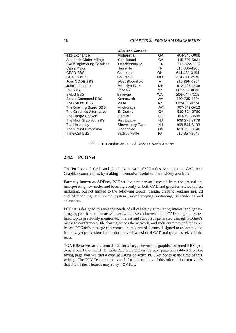
USA and Canada411-Exchange Alpharetta GA 404-345-0008Autodesk Global Village San Rafael CA 415-507-5921CAD/Engineering Services Hendersonville TN 615-822-2539Canis Major Nashville TN 615-385-4268CEAO BBS Columbus OH 614-481-3194CHAOS BBS Columbia MO 314-874-2930Joes CODE BBS West Bloomfield MI 810-855-0894John’s Graphics Brooklyn Park MN 612-425-4436PC-AUG Phoenix AZ 602-952-0638SAUG BBS Bellevue WA 206-644-7115Space Command BBS Kennewick WA 509-735-4894The CAD/fx BBS Mesa AZ 602-835-0274The Drawing Board BBS Anchorage AK 907-349-5412The Graphics Alternative El Cerrito CA 510-524-2780The Happy Canyon Denver CO 303-759-3598The New Graphics BBS Piscataway NJ 908-271-8878The University Shrewsbury Twp NJ 908-544-8193The Virtual Dimension Oceanside CA 619-722-0746Time-Out BBS Sadsburyville PA 610-857-2648
Table 2.1: Graphic-orientated BBSs in North America.
2.4.5 PCGNet
The Professional CAD and Graphics Network (PCGnet) serves both the CAD andGraphics communities by making information useful to them widely available.
Formerly known as ADEnet, PCGnet is a new network created from the ground up,incorporating new nodes and focusing evenly on both CAD and graphics related topics,including, but not limited to the following topics: design, drafting, engineering, 2dand 3d modeling, multimedia, systems, raster imaging, raytracing, 3d rendering andanimation.
PCGnet is designed to serve the needs of all callers by stimulating interest and gener-ating support forums for active users who have an interest in the CAD and graphics re-lated topics previously mentioned; interest and support is generated through PCGnet’smessage conferences, file sharing across the network, and industry news and press re-leases. PCGnet’s message conference are moderated forums designed to accommodatefriendly, yet professional and informative discussion of CAD and graphics related sub-jects.
TGA BBS serves as the central hub for a large network of graphics-oriented BBS sys-tems around the world. In table 2.1, table 2.2 on the next page and table 2.3 on thefacing page you wil find a concise listing of active PCGNet nodes at the time of thiswriting. The POV-Team can not vouch for the currency of this information, nor verifythat any of these boards may carry POV-Ray.

2.4. WHERE TO FIND POV-RAY FILES 19
AustriaAutoCAD User Group Graz 43-316-574-426
BelgiumLucas Visions BBS Boom 32-3-8447-229
DenmarkHorreby SuperBBS Nykoebing Falster 45-53-84-7074
FinlandDH-Online Jari Hiltunen 358-0-40562248Triplex BBS Helsinki 358-0-5062277
FranceCAD Connection Montesson 33-1-39529854Zyllius BBS! Saint Paul 33-93320505
GermanyRay BBS Munich Munich 49-89-984723Tower of Magic Gelsenkirchen 49-209-780670
NetherlandsBBS Bennekom: Fractal Board Bennekom 31-318-415331CAD-BBS Nieuwegein 31-30-6090287
31-30-6056353Foundation One Baarn 31-35-5422143
SloveniaMicroArt Koper 386-66-34986
SwedenAutodesk On-line Gothenburg 46-31-401718
United KingdomCADenza BBS Leicester, UK 44-116-259-6725Raytech BBS Tain, Scotland 44-1862-83-2020The Missing Link Surrey, England 44-181-641-8593
Table 2.2: Graphic-orientated BBSs in Europe.
AustraliaMULTI-CAD Magazine BBS Toowong QLD 61-7-878-2940My Computer Company Erskineville NSW 61-2-557-1489Sydney PCUG Compaq BBS Caringbah NSW 61-2-540-1842The Baud Room Melbourne VIC 61-3-481-8720
New ZealandThe Graphics Connection Wellington 64-4-566-8450The Graphics Connection II New Plymouth 64-6-757-8092The Graphics Connection III Auckland 64-9-309-2237
Table 2.3: Graphic-orientated BBSs in the rest of the world.
Country or long distance dial numbers may require additional numbers to be used.Consult your local phone company.

20 CHAPTER 2. PROGRAM DESCRIPTION
2.4.6 POV-Ray Related Books and CD-ROMs
The following items were produced by POV-Team members. Although they are onlycurrent to POV-Ray 2.2 they will still be helpful. Steps are being taken to update thePOV-Ray CDROM to version 3.0, with a new version expected around October 1996.
The books listed below have been recently listed as out-of-print but may still be foundin some bookstores or libraries (Visit http://www.dnai.com:80/waite/ for more details).
Ray Tracing Creations, 2d Ed.Chris Young and Drew WellsISBN 1-878739-69-7Waite Group Press 1994700 pages with color insert and POV-Ray 2.2 on 3.5” MS-Dos disk.
Ray Tracing Worlds with POV-RayAlexander Enzmann, Lutz Kretzschmar, Chris YoungISBN 1-878739-64-6Waite Group Press 1994Includes Moray 1.5x modeler and POV-Ray 2.2 on 3.5” MS-Dos disks.
Ray Tracing for the Macintosh CDEduard SchwanISBN 1-878739-72-7Waite Group Press, 1994Comes with a CD-ROM full of scenes, images, and QuickTime movies, andan interactive keyword reference. Also a floppy with POV-Ray for those whodon’t have a CD ROM drive.
The Official POV-Ray CDROM: The Official POV-Ray CDROM is a compilation ofimages, scene source, program source, utilities and tips on POV-Ray and 3D graphicsfrom the Internet and Compuserve. This CD is aimed not only at those who wantto create their own images or do general 3D programming work, but also at thosewho want simply to experience some high-quality renderings done by some of the bestPOV-Ray artists, and to learn from their source code. The CDROM contains over 500ray-traced images.
It’s a good resource for those learning POV-Ray as well as those who are already pro-ficient, and contains a Microsoft Windows-based interactive tutorial. The disk comeswith a fold-out poster and reference sheet. The CD is compatible with DOS/Windowsand Macintosh formats.
The CDROM is available for free retrieval and browsing on the World Wide Web athttp://www.povray.org/pov-cdrom. For more details you may also visithttp://www.povray.org/povcd.

Chapter 3
Quick Start
The next section describes how to quickly install POV-Ray and render sample scenes onyour computer. It is assumed that you are using an IBM-PC compatible computer withMS-Dos. For other platforms you must refer to the specific documentation included inPOV-Ray’s archive.
3.1 Installing POV-Ray
[*** STILL BEING WRITTEN ***]
Specific installation instructions are included with the executable program for yourcomputer. In general, there are two ways to install POV-Ray.
[ Note that the generic word ”directory” is used throughout. Your operating systemmay use another word (subdirectory, folder, etc.) ]
1) The messy way: Create a directory called POVRAY and copy all POV-Ray files intoit. Edit and run all files and programs from this directory. This method works, but isnot recommended.
Or the preferred way:
2) Create a directory called POVRAY and several subdirectories called INCLUDE,DEMO, SCENES, UTIL. The self-extracting archives used in some versions of theprogram will create subdirectories for you. If you create your own, the file tree for thisshould look something like this:
Copy the executable file and docs into the directory POVRAY. Copy the standard in-clude files into the subdirectory INCLUDE. Copy the sample scene files into the sub-directory SCENES. And copy any POV-Ray related utility programs and their relatedfiles into the subdirectory UTIL. Your own scene files will go into the SCENES subdi-rectory. Also, you’ll need to add the directories \POVRAY and \POVRAY\UTIL toyour ”search path” so the executable programs can be run from any directory.
21
22 CHAPTER 3. QUICK START
Note that some operating systems don’t have an equivalent to the multi-path searchcommand.
The second method is a bit more difficult to set-up, but is preferred. There are manyfiles associated with POV-Ray and they are far easier to deal with when separated intoseveral directories.
3.2 Basic Usage
Notice: If you did not install the program using the INSTALL.EXE system, the exam-ples and instructions given here may not work! The installation process configuresPOVRAY.INI and several important batch files. Without these files configured, the ex-amples herein may not work.
POV-Ray’s basic purpose is to read a scene description written in the POV languageand to write an image file. The scene files are plain ASCII text files that you createusing a text editor. Dozens of sample files are included with this package to illustratethe various features.
You invoke POV-Ray by typing a command at the MS-Dos prompt. The commandis POVRAY and it must be followed by one or more command line switches. Eachswitch begins with a plus or minus sign. Blanks separate the switches. The switchesmay be upper or lower case.
Note: The examples in this documentation assume you installed POV-Ray in theC:\POVRAY3 directory. The installer will let you install POV-Ray anywhere and willproperly configure it for the drive and directory you specified. You just substitute thatdrive and directory anywhere we tell you to use C:\POVRAY3. Change to that directorynow. Then type the following command line and press [ENTER]
POVRAY +ISHAPES +D1
The +I command (for input) tells the program what file to read as input. If you don’tgive an extension on the file name, .POV is assumed. Thus +ISHAPES tells it to readin SHAPES.POV to be rendered.
The +D switch (for display) tells the program to turn the graphic preview display on.A –D would turn it off. The number ”1” tells it what type of display to use. Type ”1” isthe old fashioned standard generic VGA at 320 by 200 resolution and just 256 colors.This is pretty much guaranteed to work on any VGA video system.
There are other options in effect besides those you typed on the command line. Theyare stored in a file called POVRAY.INI which was created by the install system. POV-Ray automatically looks for this file in the same directory where POVRAY.EXE resides.See 3.2.2 on page 25 and 6.1.2 on page 148 for more information on POVRAY.INI andother INI files.
3.2. BASIC USAGE 23
When you enter the command shown above, you will see brightly colored geometricshapes begin to appear as POV-Ray calculates the color of each pixel row by row. Youwill probably be disappointed with the graphic display results. That is because this isonly a preview display. The actual image is in full 24-bit color but we cannot displaythat high quality using simple VGA with a fixed set of 256 colors. If your hardwaresupports the VESA interface standard or you have a VESA TSR driver loaded, tryrunning with +DG rather than +D1. This will give you access to all of the variousmodes your video hardware can use. If you have 15-bit or 16- bit high color capabilitytry +DGH or if you have 24-bit true color capability try +DGT to see the image in allits glory. See section 3.2.5 on page 27 below for more information on graphics preview.
When the program finishes, you will hear beeps. After admiring the image, press[ENTER]. You will see a text screen of statistics. If the text is too much to fit onthe screen you may press [CURSOR UP] or [CURSOR DOWN] keys to read moretext. Notice that there are tabs at the bottom of the screen. Press [CURSOR LEFT]or [CURSOR RIGHT] keys to view other interesting text information. Press [ENTER]again to exit POV-Ray.
If you do not have high color or true color ability you will have to view the image file tosee the real colors. The image file SHAPES.TGA is written to your current directory. Bydefault POV-Ray creates files in TGA format. This is a standard format for storing 24-bit true-color images. You will need an image viewing program to view the file. Suchprograms are usually available from the same place where you obtained POV-Ray buta viewer is not included in this package.
If you cannot view TGA files you may add the switch +FN and POV-Ray will outputPNG (Portable Network Graphic) format. If PNG format viewer is not available thentype the following
T2G SHAPES
and press [ENTER]. This will run a batch file that invokes the TGA2GIF program. Theprogram will read your SHAPES.TGA file, create an optimal 256 color palette and writea GIF format file SHAPES.GIF. Most image viewing programs support GIF.
3.2.1 Running Files in Other Directories
Normally POV-Ray only looks in the current directory for the files it needs. It doesnot search your MS-Dos path for data files; it only searches for programs. In thesample scene you just ran, file SHAPES.POV was in the current directory so this wasno problem. That scene also needed other files but your POVRAY.INI file tells POV-Rayother places to search for necessary files.
If you allowed the install system to update your AUTOEXEC.BAT file, then you canchange to any drive or directory and can run POV-Ray from that directory. You willalso be able to use the batch files and utilities that came with this package in any

24 CHAPTER 3. QUICK START
directory. For future reference let’s call the ”use-C:\POVRAY3-in-your-path-plan” asplan one.
There are some circumstances where you may not want to put C:\POVRAY3 in yourpath. There is a limit of 128 characters in your path statement and you may not haveroom for it. Try rendering the SHAPES example from a different directory. If it doesn’twork, then you forgot to re-boot your system so the new path takes effect. If after re-booting it still doesn’t work, it probably means your path is too full. You will have toadopt a different plan.
Chances are, you already have several directories in your path. Most systems haveC:\DOS, C:\WINDOWS or some directory such as C:\UTILITY already in the path. Wehave provided several small batch files that you can copy to that directory. For fu-ture reference we’ll call the ”put-batch-files-in-a-directory-already-on-the-path-plan”as plan two.
At any dos prompt, type the word pathand press [ENTER]. It will show you what direc-tories are already on your path. Then copy the following files from your C:\POVRAY3directory to any of the directories already on your path. The files are:
RUNPOV.BAT RERUNPOV.BAT RUNPHELP.BAT T2G.BAT
Once you have copied these files, try the following example. In this case, do not invokethe program with the command POVRAY. Instead use RUNPOV as follows:
cd \POVRAY3\POV3DEMO\SHOWOFF
RUNPOV +ISUNSET3 +D1
This changes to the \POVRAY3\POV3DEMO\SHOWOFF directory where the file SUN-SET3.POV is found. It runs the file RUNPOV.BAT. That batch file is set up to run POV-Ray even if it is not on the dos path. It also passes the switches along to POV-Ray.These batch files have other uses, even if you are using plan oneas described above orplan threeas described below. For more on these batch files, see 3.2.4 on page 26.
All of the early examples in this document assumed you were running POV-Ray fromthe directory where it was installed such as C:\POVRAY3. This approach of alwaysusing the installation directory is in fact plan three. If you are using this method, youneed to tell POV-Ray where else to look for files. In the case of SUNSET3.POV youcould do this:
POVRAY +IC:\POVRAY3\POV3DEMO\SHOWOFF\SUNSET3 +D1
However some scenes need more than one file. For example the directory DRUMS2 thatcan be found under \POVRAY3\POVSCN\LEVEL3 contains three files: DRUMS.POV,DRUMS.INC and REDNEWT.GIF all of which are required for that one scene. In thiscase you should use the +L switch (for library) to add new library paths to those thatPOV-Ray will search. You would render the scene with this command.
POVRAY +L\POVRAY3\POVSCN\LEVEL3\DRUMS2 +IDRUMS +D1
3.2. BASIC USAGE 25
3.2.2 INI Files
There were more options used in these renderings than just the switches +I, +D, and+L that you specify. When you run the program, POV- Ray automatically looks for thefile POVRAY.INI in whatever directory that POVRAY.EXE is in. The POVRAY.INI filecontains many options that control how POV-Ray works. We have set this file up sothat it is especially easy to run your first scene with minimal problems. The file shouldbe placed in the same directory as POVRAY.EXE and it will automatically read whenPOV-Ray is run. If you ever move POVRAY.EXE to a different directory, be sure tomove POVRAY.INI too.
Complete details on all of the available switches and options that can be given on thecommand line or in POVRAY.INI are given in 6 on page 147.
You may also create INI files of your own with switches or options similar toPOVRAY.INI. If you put a file name on the command line without a plus or minussign before it, POV-Ray reads it as an INI file. Try this . . .
POVRAY RES120 +ISHAPES +D1
This causes POV-Ray to look for a file called RES120.INI which we have provided. Itsets your resolution to 120 by 90 pixels for a quick preview. The following INI fileshave been provided for you.
RES120.INI Sets resolution to 120 by 90.RES320.INI Sets resolution to 320 by 200.RES640.INI Sets resolution to 640 by 480.RES800.INI Sets resolution to 800 by 600.RES1K.INI Sets resolution to 1024 by 768.LOW.INI Sets low quality at 120 by 90.SLOW.INI Turns on radiosity and anti-aliasing; slow but beautiful.TGAFLI.INI Create an FLI animation from TGA images.PNGFLI.INI Create an FLI animation from DTA images.ZIPFLI.INI Create an FLI animation from zipped images.TGAFLC.INI Create an FLC animation from TGA images.PNGFLC.INI Create an FLC animation from DTA images.ZIPFLC.INI Create an FLC animation from zipped images.
You can create your own custom INI’s which can contain any command in the referenceguide.
3.2.3 Alternatives toPOVRAY.INI
The POVRAY.INI file is supposed to hold your favorite global default options that youwant to use all the time. You should feel free to edit it with new options that suit your

26 CHAPTER 3. QUICK START
needs. However it must be located in the same directory as POVRAY.EXE or it won’t befound. The dos path isn’t searched nor will +L commands help because POVRAY.INI isprocessed before any command line switches.
If your POVRAY.EXE resides on a CD-ROM then you can’t edit the POVRAY.INI onthe CD. There is an alternative. You may use an environment variable to specify analternative global default.
In your AUTOEXEC.BAT file add a line similar to this:
set POVINI=D:\DIRECT\FILE.INI
which sets the POVINI environment variable to whatever drive, directory and INI fileyou choose. If you specify any POVINI environment variable then POVRAY.INI is notread. This is true even if the file you named doesn’t exist. Note that you are specifyingan entire path and file name. This is not a pointer to a directory containing POVRAY.INI.It is a pointer to the actual file itself.
Note that the POVRAYOPT environment variable in previous versions of POV-Ray isno longer supported.
3.2.4 Batch Files
We’ve already described how the file RUNPOV.BAT can be used as an alternative torunning POV-Ray directly. RUNPOV.BAT also has one other use. It uses the +GI switchto create a file called RERUN.INI. This makes it very easy to run the same file overagain with the same parameters. When creating your own scene files you will probablymake dozens of test renders. This is a very valuable feature. Here is how it works . . .Suppose you render a scene as follows:
RUNPOV +IMYSCENE +D1 RES120
This renders MYSCENE.POV at 120 by 90 resolution. Note there is no such scene. Thisis hypothetical. After viewing it, you noticed a mistake which you fixed with your texteditor. To rerun the scene type:
RERUNPOV
and that’s all. It will rerun the same scene you just ran. Suppose you want more detailon the next run. You can add more switches or INI files. For example:
RERUNPOV RES320

3.2. BASIC USAGE 27
will rerun at higher resolution. Subsequent uses of RERUNPOV will be at 320 by 200until you tell it differently. As another example, the +A switch turns on anti-aliasing.Typing ”RERUNPOV +A” reruns with anti- aliasing on. All subsequent reruns will haveit on until you do a ”RERUNPOV –A” to turn it off. Note if you do another RUNPOV itstarts over from your POVRAY.INI defaults and it overwrites the old RERUN.INI.
Two other batch files are included. RUNPHELP.BAT is only used as an alternative wayto run POVHELP from another directory. If you used installation plan two then useRUNPHELP.BAT rather than POVHELP.EXE. This batch file serves no other purpose.
Finally T2G.BAT invokes the TGA2GIF.EXE program for converting TGA files to GIFfiles. You could run TGA2GIF directly but its default parameters do not generallyproduce the best results. If you use T2G instead, it adds some command line switcheswhich work better. For a full list of switches available for TGA2GIF, type TGA2GIF
with no parameters and it will display the available switches and options.
3.2.5 Display Types
You have already seen how to turn on graphics preview using +D1. Here are details onother variations of the +D switch. Use –D to turn the display off. If you use –D thenyou will probably want to add the +V switch to turn on verbose status messages so youcan monitor the progress of the rendering while in progress.
The number ”1” after the +D tells it what kind of video hardware to use. If you use +Dalone or +D0 then POV-Ray will attempt to auto detect your hardware type. Use +D?to see a message about what type of hardware POV-Ray found.
You may also explicitly tell POV-Ray what hardware to use. The following chart listsall of the supported types.
+D0 Auto detect (S)VGA type (Default)+D1 Standard VGA 320×200+D2 Standard VGA 360×480+D3 Tseng Labs 3000 SVGA 640×480+D4 Tseng Labs 4000 SVGA+D5 AT&T VDC600 SVGA 640×400+D6 Oak Technologies SVGA 640×480+D7 Video 7 SVGA 640×480+D8 Video 7 Vega (Cirrus) VGA 360×480+D9 Paradise SVGA 640×480+DA Ahead Systems Ver. A SVGA 640×480+DB Ahead Systems Ver. B SVGA 640×480+DC Chips & Technologies SVGA 640×480+DD ATI SGVA 640×480+DE Everex SVGA 640×480+DF Trident SVGA 640×480+DG VESA Standard SVGA Adapter

28 CHAPTER 3. QUICK START
+DH ATI XL display card+DI Diamond Computer Systems SpeedSTAR 24X
The most common type is a VESA standard card which uses +DG. VESA is a standardsoftware interface that works on a wide variety of cards. Those cards which do nothave VESA support directly built-in, generally have a video driver that you can load toprovide VESA support. The program UNIVBE is a high quality universal VESA driverthat may work for you. It can be found at http://www.povray.org or possiblyother POV-Ray sites.
The options listed above had been tested worked under earlier versions of POV-Ray butthere have been many changes in the program and we cannot guarantee these all stillwork. If you can use VESA then do so. It has been well tested and will give you themost flexibility.
After the +D and the type, you may specify a 3rd character that specifies the palettetype.
+D?3 Use 332 palette with dithering (default and best for VGA systems).This is a fixed palette of 256 colors with each color consisting 3-bitsof red data, 3-bits green and 2-bits blue.
+D?0 Use HSV palette option for VGA display. This is a fixed palette of256 colors where colors are matched according to hue, saturationand intensity rather than the amount of red, green and blue.
+D?G Use fixed gray scale palette option for VGA display.+D?H Use HiColor option. Displays more than 32000 colors with dither-
ing. Supported on VESA, SpeedSTAR 24X, ATI XL HiColor andTseng 4000 based cards with high color 15 or 16 bit options.
+D?T For Truecolor 24 bit cards. Use 24 bit color. Supported on the Dia-mond SpeedSTAR 24X and cards with 24bit VESA support only.
Here are some examples:
+D0H Auto detect the VGA display type and display the image to thescreen as it’s being worked on. Use the 15-bit HiColor chip anddithering to display more than 32,000 colors on screen.
+D4 Display to a TSENG 4000 chipset VGA using the 332 palette op-tion.
+D4H Display to a TSENG 4000 chipset VGA using the HiColor option.+DG0 Display to a VESA VGA adapter and use the HSV palette option.+DG3 Display to a VESA VGA adapter and use the 332 palette option.+DGH Display to a VESA VGA adapter and use the HiColor option for
over 32,000 colors.+DGT Display to a VESA VGA adapter and use the TrueColor option for
over 16 million colors.

3.2. BASIC USAGE 29
Note that your VESA BIOS must support these options in order for you to use them.Some cards may support HiColor and/or TrueColor at the hardware level but notthrough their VESA BIOS.

30 CHAPTER 3. QUICK START
Part II
Tutorial Guide
31

Chapter 4
Beginning Tutorial
The beginning tutorial explains step by step how to use POV-Ray’s scene descriptionlanguage to create your own scenes. The use of almost every feature of POV-Ray’slanguage is explained in detail. You will learn basic things like placing cameras andlight sources. You will also learn how to create a large variety of objects and how toassign different textures to them. The more sophisticated features like radiosity, halos,and atmospheric effects will also be explaind in detail.
The following sections explain the features in roughly the same order as they are de-scribed in the reference chapter.
4.1 Your First Image
Let’s create the scene file for a simple picture. Since ray-tracers thrive on spheres,that’s what we’ll render first.
4.1.1 Understanding POV-Ray’s Coordinate System
First, we have to tell POV-Ray where our camera is and where it’s looking. To do this,we use 3D coordinates. The usual coordinate system for POV-Ray has the positiveY axis pointing up, the positive X axis pointing to the right, and the positive Z axispointing into the screen as shown in figure 4.1 on the following page.
This kind of coordinate system is called a left-handed coordinate system. If you useyour left hand’s fingers you can easily see why it is called left-handed. Just point yourthumb in the direction of the positive x-axis, your index finger in the direction of thepositive y-axis and your middle finger in the positive z-axis direction. You can only dothis with your left hand. If you had used your right hand you would not have been ableto point the middle finger in the correct direction.
33

34 CHAPTER 4. BEGINNING TUTORIAL
y
x
z
Figure 4.1: The left-handed coordinate system (the z-axis is pointing away from theviewer).
The left hand can also be used to determine rotation directions. To do this you mustperform the famous Computer Graphics Aerobicsexercise. Hold up your left hand.Point your thumb in the positive direction of the axis of rotation. Your fingers will curlin the positive direction of rotation. Similarly if you point your thumb in the negativedirection of the axis your fingers will curl in the negative direction of rotation.
If you want to use a right-handed system, as some CAD systems such as AutoCAD do,the right vector in the camera specification needs to be changed. See the detaileddescription in 7.4.4.5.2 on page 226. In a right-handed system you use your right handfor the Aerobics.
Note that there is some controversy over whether POV-Ray’s method of doing a right-handed system is really proper. If you want to avoid problems we suggest you stickwith the left-handed system which is not in dispute.
4.1.2 Adding Standard Include Files
Using your personal favorite text editor, create a file called demo.pov. Now type inthe following (the input is case sensitive, so be sure to get capital and lowercase letterscorrect).
#include "colors.inc" // The include files contain#include "shapes.inc" // pre-defined scene elements#include "finish.inc"#include "glass.inc"#include "metals.inc"#include "stones.inc"#include "woods.inc"

4.1. YOUR FIRST IMAGE 35
The first include statement reads in definitions for various useful colors. The secondinclude statement reads in some useful shapes. The next read pre-defined finishes,glass, metal, stone, and wood textures. When you get a chance, have a look throughthem to see but a few of the many possible shapes and textures available.
You should only include files you really need in your scene. Some of the includefiles coming with POV-Ray are quite large and you should better save the parsing time(and memory) if you don’t need them. In the following examples we will only usethe colors.inc, finish.inc and stones.inc include files so you’ll betterremove the appropriate lines from your scene file.
You may have as many include files as needed in a scene file. Include files may them-selves contain include files, but you are limited to declaring includes nested only tenlevels ”deep”.
Filenames specified in the include statements will be searched for in the current direc-tory first and, if not found, will then be searched for in directories specified by any+L or Library Path options active. This would facilitate keeping all your ”include”(. INC) files such as SHAPES.INC, COLORS.INC, and TEXTURES.INC in an ”include”subdirectory, and giving an +L option on the command line to where your library ofinclude files are.
4.1.3 Adding a Camera
The camera declaration describes where and how the camera sees the scene. It gives x,y, z coordinates to indicate the position of the camera and what part of the scene it ispointing at. You describe x, y, zcoordinates using a three-part vector. A vector is spec-ified by putting three numeric values between a pair of angle brackets and separatingthe values with commas.
Add the following camera statement to the scene.
camera {location <0, 2, -3>look_at <0, 1, 2>
}
Briefly, location 〈0,2,−3〉 places the camera up two units and back three unitsfrom the center of the ray-tracing universe which is at 〈0,0,0〉. Remember that bydefault +z is into the screen and −z is back out of the screen.
Also look at 〈0,1,2〉 rotates the camera to point at x, y, z coordinates 〈0,1,2〉. Apoint 5 units in front of and 1 unit lower than the camera. The look at point should bethe center of attention of your image.
4.1.4 Describing an Object
Now that the camera is set up to record the scene, let’s place a yellow sphere into thescene. Add the following to your scene file:
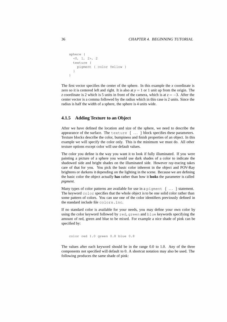
36 CHAPTER 4. BEGINNING TUTORIAL
sphere {<0, 1, 2>, 2texture {
pigment { color Yellow }}
}
The first vector specifies the center of the sphere. In this example the x coordinate iszero so it is centered left and right. It is also at y= 1 or 1 unit up from the origin. Thezcoordinate is 2 which is 5 units in front of the camera, which is at z=−3. After thecenter vector is a comma followed by the radius which in this case is 2 units. Since theradius is half the width of a sphere, the sphere is 4 units wide.
4.1.5 Adding Texture to an Object
After we have defined the location and size of the sphere, we need to describe theappearance of the surface. The texture { . . . } block specifies these parameters.Texture blocks describe the color, bumpiness and finish properties of an object. In thisexample we will specify the color only. This is the minimum we must do. All othertexture options except color will use default values.
The color you define is the way you want it to look if fully illuminated. If you werepainting a picture of a sphere you would use dark shades of a color to indicate theshadowed side and bright shades on the illuminated side. However ray-tracing takescare of that for you. You pick the basic color inherent in the object and POV-Raybrightens or darkens it depending on the lighting in the scene. Because we are definingthe basic color the object actually has rather than how it looks the parameter is calledpigment.
Many types of color patterns are available for use in a pigment { . . . } statement.The keyword color specifies that the whole object is to be one solid color rather thansome pattern of colors. You can use one of the color identifiers previously defined inthe standard include file colors.inc.
If no standard color is available for your needs, you may define your own color byusing the color keyword followed by red, green and blue keywords specifying theamount of red, green and blue to be mixed. For example a nice shade of pink can bespecified by:
color red 1.0 green 0.8 blue 0.8
The values after each keyword should be in the range 0.0 to 1.0. Any of the threecomponents not specified will default to 0. A shortcut notation may also be used. Thefollowing produces the same shade of pink:

4.1. YOUR FIRST IMAGE 37
color rgb <1.0, 0.8, 0.8>
Colors are explained in more detail in section 7.1.5 on page 192.
4.1.6 Defining a Light Source
One more detail is needed for our scene. We need a light source. Until you create one,there is no light in this virtual world. Thus add the line
light_source { <2, 4, -3> color White}
to your scene file to get your first complete POV-Ray scene file as shown below.
#include "colors.inc"
background { color Cyan }
camera {location <0, 2, -3>look_at <0, 1, 2>
}
sphere {<0, 1, 2>, 2texture {
pigment { color Yellow }}
}
light_source { <2, 4, -3> color White}
The vector in the light source statement specifies the location of the light as 2units to our right, 4 units above the origin and 3 units back from the origin. The lightsource is invisible, it only casts light, so no texture is needed.
That’s it! Close the file and render a small picture of it using the command
POVRAY +W160 +H120 +P +X +D0 –V -IDEMO.POV
If your computer does not use the command line, see your platform specific docs forthe correct command to render a scene.
You may also set any other command line options you like. The scene is written tothe image file demo.tga (or some suffix other than .TGA if your computer uses adifferent default file format).
The scene you just traced isn’t quite state of the art but we’ll have to start with thebasics before we soon get to much more fascinating features and scenes.

38 CHAPTER 4. BEGINNING TUTORIAL
4.2 Using the Camera
[ *** STILL BEING WRITTEN *** ]
4.2.1 Camera Types
[ *** STILL BEING WRITTEN *** ]
4.2.2 Using Focal Blur
[ *** STILL BEING WRITTEN *** ]
4.2.3 Using Camera Ray Perturbation
[ *** STILL BEING WRITTEN *** ]
4.3 Simple Shapes
So far we’ve just used the sphere shape. There are many other types of shapes that canbe rendered by POV-Ray. The following sections will describe how to use some of themore simple objects as a replacement for the sphere used above.
4.3.1 Box Object
The box is one of the most common objects used. Try this example in place of thesphere:
box {<-1, 0, -1>, // Near lower left corner< 1, 0.5, 3> // Far upper right corner
texture {T_Stone25 // Pre-defined from stones.incscale 4 // Scale by the same amount in all
// directions}
rotate y*20 // Equivalent to "rotate <0,20,0>"}

4.3. SIMPLE SHAPES 39
In this example you can see that a box is defined by specifying the 3D coordinates of itsopposite corners. The first vector must be the minimum x, y, zcoordinates and the 2ndvector must be the maximum x, y, zvalues. Box objects can only be defined parallel tothe axes of the world coordinate system. You can later rotate them to any angle. Notethat you can perform simple math on values and vectors. In the rotate parameter wemultiplied the vector identifier y by 20. This is the same as 〈0,1,0〉×20 or 〈0,20,0〉.
4.3.2 Cone Object
Here’s another example showing how to use a cone:
cone {<0, 1, 0>, 0.3 // Center and radius of one end<1, 2, 3>, 1.0 // Center and radius of other end
texture { T_Stone25 scale 4 }}
The cone shape is defined by the center and radius of each end. In this example one endis at location 〈0,1,0〉 and has radius of 0.3 while the other end is centered at 〈1,2,3〉with radius= 1. If you want the cone to come to a sharp point then use radius= 0.The solid end caps are parallel to each other and perpendicular to the cone axis. If youwant an open cone with no end caps then add the keyword open after the 2nd radiuslike this:
cone {<0, 1, 0>, 0.3 // Center and radius of one end<1, 2, 3>, 1.0 // Center and radius of other endopen // Removes end caps
texture { T_Stone25 scale 4 }}
4.3.3 Cylinder Object
You may also define a cylinder like this:
cylinder {<0, 1, 0>, // Center of one end<1, 2, 3>, // Center of other end0.5 // Radiusopen // Remove end caps
texture { T_Stone25 scale 4 }}

40 CHAPTER 4. BEGINNING TUTORIAL
4.3.4 Plane Object
Let’s try out a computer graphics standard — The Checkered Floor. Add the followingobject to the first version of the DEMO.POV file, the one including the sphere.
plane { <0, 1, 0>, -1pigment {
checker color Red, color Blue}
}
The object defined here is an infinite plane. The vector 〈0,1,0〉 is the surface normalof the plane (i.e. if you were standing on the surface, the normal points straight up).The number afterward is the distance that the plane is displaced along the normal fromthe origin — in this case, the floor is placed at y= −1 so that the sphere at y= 1,radius= 2, is resting on it.
Notice that there is no texture { . . . } statement. There really is an implied texturethere. You might find that continually typing statements that are nested like texture{pigment { . . . }} can get to be a tiresome so POV-Ray lets you leave out thetexture { . . . } under many circumstances. In general you only need the textureblock surrounding a texture identifier (like the T Stone25example above), or whencreating layered textures (which are covered later).
This pigment uses the checker color pattern and specifies that the two colors red andblue should be used.
Because the vectors 〈1,0,0〉, 〈0,1,0〉 and 〈0,0,1〉 are used frequently, POV-Ray hasthree built-in vector identifiers x, y, and z respectively that can be used as a shorthand.Thus the plane could be defined as:
plane { y, -1pigment { ... }
}
Note that you do not use angle brackets around vector identifiers.
Looking at the floor, you’ll notice that the ball casts a shadow on the floor. Shadowsare calculated very accurately by the ray-tracer, which creates precise, sharp shadows.In the real world, penumbral or ”soft” shadows are often seen. Later you’ll learn howto use extended light sources to soften the shadows.
4.3.5 Standard Include Objects
The standard include file SHAPES.INC contains some pre-defined shapes that are aboutthe size of a sphere with a radius of one unit. You can invoke them like this:

4.4. ADVANCED SHAPES 41
#include "shapes.inc"
object {UnitBoxtexture { T_Stone25 scale 4 }scale 0.75rotate <-20,25,0>translate y
}
4.4 Advanced Shapes
After you have gained some experience with the simpler shapes available in POV-Rayit is time to go on to the more advanced, thrilling shapes.
You should be aware that the shapes described below are not trivial to understand.Don’t worry if you do not know how to use them or how they work. Just try theexamples and play with the features described in the reference chapter. There is nothingbetter than learning by doing.
4.4.1 Bicubic Patch Object
Bicubic or Bezier patches are useful surface representations because they allow an easydefinition of surfaces using only a few control points. For ray tracing (or rendering)the patches are approximated using triangles. The control points serve to determine theshape of the patch. Instead of defining the vertices of triangles, you simply give thecoordinates of the control points. A single patch has 16 control points, four at eachcorner, and the rest positioned to divide the patch into smaller sections. Bezier patchesare almost always created using a third party modeler so for this tutorial, we will useMORAY (any other modeler that supports Bezier patches and POV can also be used).We will use MORAY only to create the patch itself, not the other elements of the scene.
Bezier patches are actually very useful and, with a little practice, some pretty amazingthings can be created with them. For our first tutorial, let’s make a sort of a teepee/tentshape using a single sheet patch.
First, start MORAY and, from the main edit screen, click on ”CREATE”. Name yourobject Teepee. The ”CREATE BEZIER PATCH” dialogue box will appear. Make surethat ”SHEET” is depressed. Click on ”OK, CREATE”. At the bottom of the main editscreen, click on ”EXTENDED EDIT”.
Hold the cursor over the ”TOP” view and right click to make the pop-up menu appear.Click on ”MAXIMIZE”. [ALT]-drag to zoom in a little. Click on ”MARK ALL”, andunder the transformation mode box, ”UFRM SCL”. Drag the mouse to scale the patch

42 CHAPTER 4. BEGINNING TUTORIAL
until it is approximately four units wide. Click on ”TRANSLATE”, and move the patchso that its center is over the origin. Right click — ”MINIMIZE”, ”UNMARK ALL”.
[SHIFT]-drag a box around the lower right control point to mark it. [ALT]-zoominto the ”FRONT” view so that you can see the patch better. In the ”FRONT” view,”TRANSLATE” that point 10 units along the negative z-axis (note that in MORAY zis up). ”UNMARK ALL”. Repeat this procedure for each of the other three cornerpoints. Make sure you remember to ”UNMARK ALL” once each point has been trans-lated. You should have a shape that looks as though it is standing on four pointed legs.”UNMARK ALL”.
Working once again in the ”TOP” view, [SHIFT]-drag a box around the four centercontrol points to mark them. Right-click over the ”TOP” view, ”MAXIMIZE”. Clickon ”UFRM SCL” and drag the mouse to scale the four points close together. [ALT]-drag to zoom closer and get them as close together as you can. [ALT]-drag to zoomout, right click, ”MINIMIZE”.
In the ”FRONT” view, ”TRANSLATE” the marked points 10 units along the positive z-axis. ”UNMARK ALL”. The resulting shape is quite interesting, was simple to model,and could not be produced using CSG primitives. Now let’s use it in a scene.
Click on ”DONE” to return to the main edit screen. Notice that U STEPS andV STEPS are both set to 3 and flatness is set to 0.01. Leave them alone for now.Click on ”FILES”, and then ”SAVE SEL” (save selection). Name your new fileTEEPEE1.MDL. Press [F3] and open TEEPEE1.MDL. There is no need to save theoriginal file. When TEEPEE1 is open, create a quick ”dummy” texture (MORAY willnot allow you to export data without a texture), say, white with default finish, name itTeePeeTex, and apply it to the object. Save the file and press [CTRL-F9]. MORAY willcreate two files: TEEPEE1.INC and TEEPEE1.POV.
Exit MORAY and copy TEEPEE1.INC and TEEPEE1.POV into your working directorywhere you are doing these tutorials. Create a new file called BEZDEMO.POV and editit as follows:
#include "colors.inc"
camera {location <0, .1, -60>look_at 0angle 36
}
background { color Gray25 }
light_source { <300, 300, -700> White }
plane { y, -12texture {
pigment {
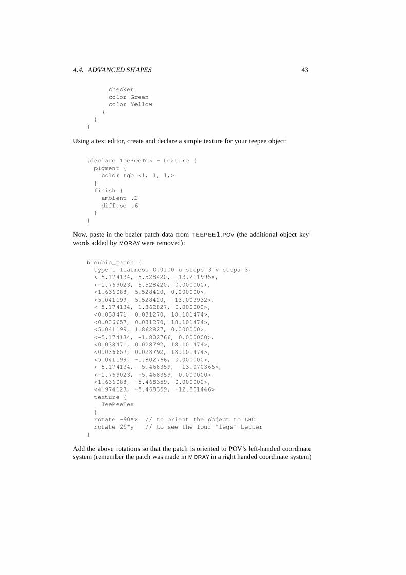
4.4. ADVANCED SHAPES 43
checkercolor Greencolor Yellow
}}
}
Using a text editor, create and declare a simple texture for your teepee object:
#declare TeePeeTex = texture {pigment {
color rgb <1, 1, 1,>}finish {
ambient .2diffuse .6
}}
Now, paste in the bezier patch data from TEEPEE1.POV (the additional object key-words added by MORAY were removed):
bicubic_patch {type 1 flatness 0.0100 u_steps 3 v_steps 3,<-5.174134, 5.528420, -13.211995>,<-1.769023, 5.528420, 0.000000>,<1.636088, 5.528420, 0.000000>,<5.041199, 5.528420, -13.003932>,<-5.174134, 1.862827, 0.000000>,<0.038471, 0.031270, 18.101474>,<0.036657, 0.031270, 18.101474>,<5.041199, 1.862827, 0.000000>,<-5.174134, -1.802766, 0.000000>,<0.038471, 0.028792, 18.101474>,<0.036657, 0.028792, 18.101474>,<5.041199, -1.802766, 0.000000>,<-5.174134, -5.468359, -13.070366>,<-1.769023, -5.468359, 0.000000>,<1.636088, -5.468359, 0.000000>,<4.974128, -5.468359, -12.801446>texture {
TeePeeTex}rotate -90*x // to orient the object to LHCrotate 25*y // to see the four "legs" better
}
Add the above rotations so that the patch is oriented to POV’s left-handed coordinatesystem (remember the patch was made in MORAY in a right handed coordinate system)
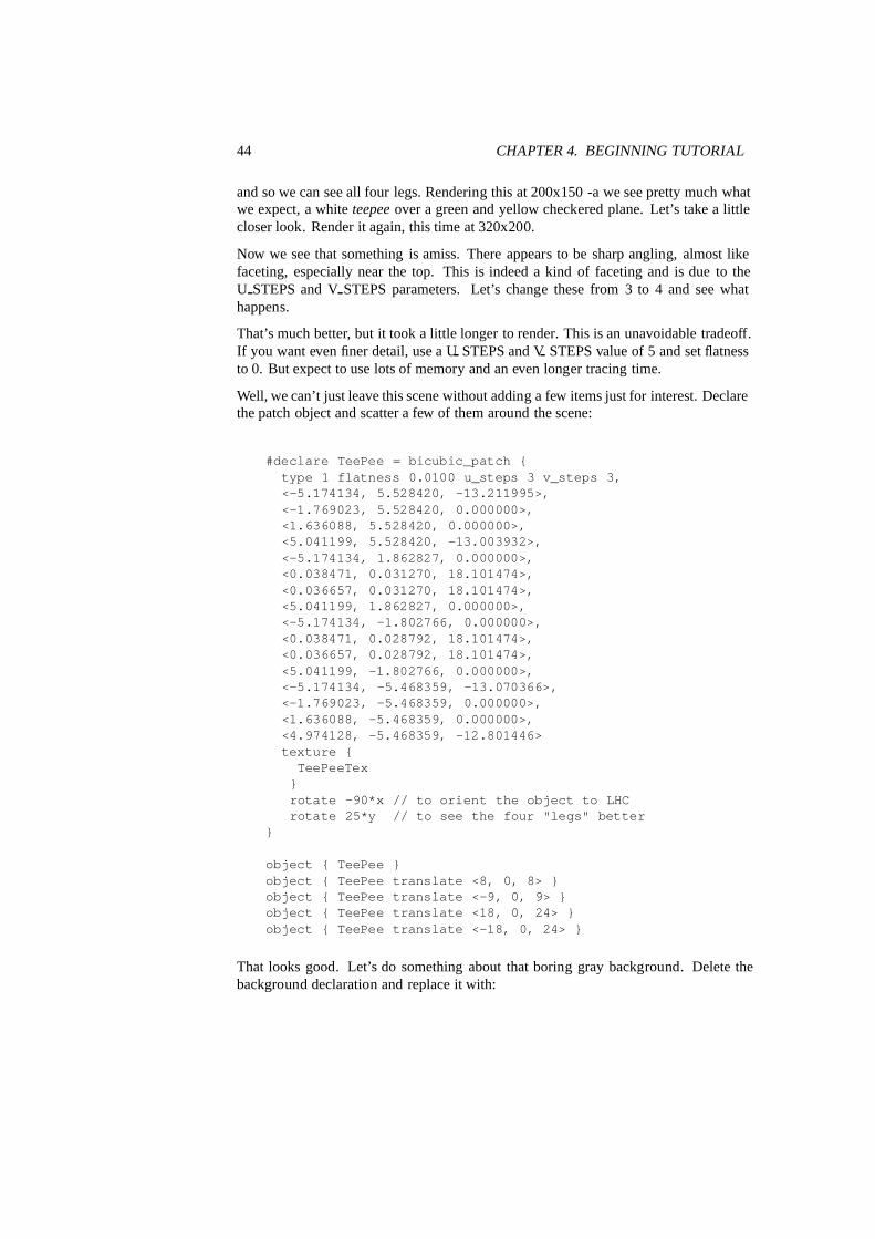
44 CHAPTER 4. BEGINNING TUTORIAL
and so we can see all four legs. Rendering this at 200x150 -a we see pretty much whatwe expect, a white teepeeover a green and yellow checkered plane. Let’s take a littlecloser look. Render it again, this time at 320x200.
Now we see that something is amiss. There appears to be sharp angling, almost likefaceting, especially near the top. This is indeed a kind of faceting and is due to theU STEPS and V STEPS parameters. Let’s change these from 3 to 4 and see whathappens.
That’s much better, but it took a little longer to render. This is an unavoidable tradeoff.If you want even finer detail, use a U STEPS and V STEPS value of 5 and set flatnessto 0. But expect to use lots of memory and an even longer tracing time.
Well, we can’t just leave this scene without adding a few items just for interest. Declarethe patch object and scatter a few of them around the scene:
#declare TeePee = bicubic_patch {type 1 flatness 0.0100 u_steps 3 v_steps 3,<-5.174134, 5.528420, -13.211995>,<-1.769023, 5.528420, 0.000000>,<1.636088, 5.528420, 0.000000>,<5.041199, 5.528420, -13.003932>,<-5.174134, 1.862827, 0.000000>,<0.038471, 0.031270, 18.101474>,<0.036657, 0.031270, 18.101474>,<5.041199, 1.862827, 0.000000>,<-5.174134, -1.802766, 0.000000>,<0.038471, 0.028792, 18.101474>,<0.036657, 0.028792, 18.101474>,<5.041199, -1.802766, 0.000000>,<-5.174134, -5.468359, -13.070366>,<-1.769023, -5.468359, 0.000000>,<1.636088, -5.468359, 0.000000>,<4.974128, -5.468359, -12.801446>texture {
TeePeeTex}rotate -90*x // to orient the object to LHCrotate 25*y // to see the four "legs" better
}
object { TeePee }object { TeePee translate <8, 0, 8> }object { TeePee translate <-9, 0, 9> }object { TeePee translate <18, 0, 24> }object { TeePee translate <-18, 0, 24> }
That looks good. Let’s do something about that boring gray background. Delete thebackground declaration and replace it with:

4.4. ADVANCED SHAPES 45
plane { y, 500texture {
pigment { SkyBlue }finish { ambient 1 diffuse 0}
}texture {
pigment {bozoturbulence .5color_map {
[0 White][1 White filter 1]
}}finish { ambient 1 diffuse 0 }scale <1000, 250, 250>rotate <5, 45, 0>
}}
This adds a pleasing cirrus-cloud filled sky. Now, let’s change the checkered plane torippled sand dunes:
plane {y,-12texture {
pigment {color <.85, .5, .15>
}finish {
ambient .25diffuse .6crand .5
}normal {
ripples .35turbulence .25frequency 5
}scale 10translate 50*x
}}
Render this at 320x240 -a. Not bad! Let’s just add one more element. Let’s place agolden egg under each of the teepees. And since this is a bezier patch tutorial, let’smake the eggs out of bezier patches.
Return to MORAY and create another bezier patch. Name it Egg1and select ”CYLIN-DRICAL 2 - PATCH” from the ”CREATE BEZIER PATCH” dialogue box. Click on

46 CHAPTER 4. BEGINNING TUTORIAL
”EXTENDED EDIT”. ”MARK ALL”, and rotate the patch so that the cylinder layson its side. ”UNMARK ALL”. In the ”FRONT” view, [SHIFT]-drag a box around thefour points on the right end to mark them. In the ”SIDE” view, right click, ”MAXI-MIZE”. [ALT]-drag to zoom in a little closer. ”UFRM SCL” the points together asclose as possible. Zoom in closer to get them nice and tight. Zoom out, right click,”MINIMIZE”.
Click on ”TRANSLATE” and drag the points to the left so that they are aligned on thez-axis with the next group of four points. This should create a blunt end to the patch.Repeat this procedure for the other end. ”UNMARK ALL”.
In the ”FRONT” view, the control grid should be a rectangle now and the patch shouldbe an ellipsoid. [SHIFT]-drag a box around the upper right corner of the control gridto mark those points. Then [SHIFT]-drag a box around the lower right corner to markthose points as well. In the ”SIDE” view, ”UFRM SCL” the points apart a little to makethat end of the egg a little wider than the other. ”UNMARK ALL”.
The egg may need a little proportional adjustment. You should be able to ”MARKALL” and ”LOCAL SCL” in the three views until you get it to look like an egg. Whenyou are satisfied that it does, ”UNMARK ALL” and click on done. Learning from ourteepee object, we now go ahead and change U STEPS and V STEPS to 4.
Create a dummy texture, white with default finish, name it EggTex, and apply it to theegg. From the FILES menu, ”SAVE SEL” to filename EGG1.MDL. Load this file andexport ([CTRL F9]). Exit MORAY and copy the files EGG1.INC and EGG1.POV intoyour working directory.
Back in BEZDEMO.POV, create a nice, shiny gold texture:
#declare EggTex = texture {pigment { BrightGold }finish {
ambient .1diffuse .4specular 1roughness 0.001reflection .5metallic
}}
And while we’re at it, let’s dandy up our TeePeeTex:
#declare TeePeeTex = texture {pigment { Silver }finish {
ambient .1diffuse .4specular 1
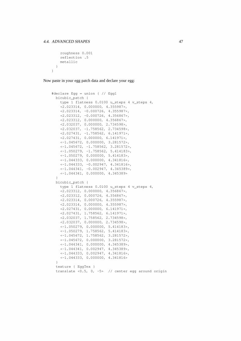
4.4. ADVANCED SHAPES 47
roughness 0.001reflection .5metallic
}}
Now paste in your egg patch data and declare your egg:
#declare Egg = union { // Egg1bicubic_patch {
type 1 flatness 0.0100 u_steps 4 v_steps 4,<2.023314, 0.000000, 4.355987>,<2.023314, -0.000726, 4.355987>,<2.023312, -0.000726, 4.356867>,<2.023312, 0.000000, 4.356867>,<2.032037, 0.000000, 2.734598>,<2.032037, -1.758562, 2.734598>,<2.027431, -1.758562, 6.141971>,<2.027431, 0.000000, 6.141971>,<-1.045672, 0.000000, 3.281572>,<-1.045672, -1.758562, 3.281572>,<-1.050279, -1.758562, 5.414183>,<-1.050279, 0.000000, 5.414183>,<-1.044333, 0.000000, 4.341816>,<-1.044333, -0.002947, 4.341816>,<-1.044341, -0.002947, 4.345389>,<-1.044341, 0.000000, 4.345389>
}bicubic_patch {
type 1 flatness 0.0100 u_steps 4 v_steps 4,<2.023312, 0.000000, 4.356867>,<2.023312, 0.000726, 4.356867>,<2.023314, 0.000726, 4.355987>,<2.023314, 0.000000, 4.355987>,<2.027431, 0.000000, 6.141971>,<2.027431, 1.758562, 6.141971>,<2.032037, 1.758562, 2.734598>,<2.032037, 0.000000, 2.734598>,<-1.050279, 0.000000, 5.414183>,<-1.050279, 1.758562, 5.414183>,<-1.045672, 1.758562, 3.281572>,<-1.045672, 0.000000, 3.281572>,<-1.044341, 0.000000, 4.345389>,<-1.044341, 0.002947, 4.345389>,<-1.044333, 0.002947, 4.341816>,<-1.044333, 0.000000, 4.341816>
}texture { EggTex }translate <0.5, 0, -5> // center egg around origin

48 CHAPTER 4. BEGINNING TUTORIAL
translate -9.8*y // place egg on the ground}
Now place a copy of the egg under each teepee. This should require only the x and zcoordinates of each teepee:
object { Egg }object { Egg translate <8, 0, 8> }object { Egg translate <-9, 0, 9> }object { Egg translate <18, 0, 24> }object { Egg translate <-18, 0, 24> }
Render this at 320x240 –A. Everything looks good so run it again at 640x480 +A. Nowwe see that there is still some faceting near the top of the teepees and on the eggs aswell. The only solution is to raise U STEPS and V STEPS from 4 to 5 and set flatnessto 0 for all our bezier objects. Make the changes and render it again at 640x480 +A.
4.4.2 Blob Object
[ *** STILL BEING WRITTEN *** Dieter Bayer ]
4.4.3 Height Field Object
A height field is an object that has a surface that is determined by the color value orpalette index number of an image designed for that purpose. With height fields, realisticmountains and other types of terrain can easily be made. First, you need an image fromwhich to create the height field. It just so happens that POV-Ray is ideal for creatingsuch an image.
Make a new file called IMAGE.POV and edit it to contain the following:
#include "colors.inc"
global_settings {assumed_gamma 2.2hf_gray_16
}
The hf gray 16 keyword causes the output to be in a special 16 bit grayscale that isperfect for generating height fields. The normal 8 bit output will lead to less smoothsurfaces.
Now create a camera positioned so that it points directly down the z-axis at the origin.

4.4. ADVANCED SHAPES 49
camera {location <0, 0, -10>look_at 0
}
Then create a plane positioned like a wall at z= 0. This plane will completely fill thescreen. It will be colored with white and gray wrinkles.
plane { z, 10pigment {
wrinklescolor_map {[0 0.3*White][1 White]}
}}
Finally, create a light source.
light_source { <0, 20, -100> color White }
Render this scene at 640x480 +A0.1 +FT. You will get an image that will produce anexcellent height field.
Now we will use this image to create a height field. Create a new file calledHFDEMO.POV and edit it as follows:
#include "colors.inc"
Add a camera that is two units above the origin and ten units back . . .
camera{location <0, 2, -10>look_at 0angle 15
}
. . . and a light source.
light_source{ <1000,1000,-1000> White }

50 CHAPTER 4. BEGINNING TUTORIAL
Now add the height field. In the following syntax, a Targa image file is specified, theheight field is smoothed, it is given a simple white pigment, it is translated to center itaround the origin, and it is scaled so that it resembles mountains and fills the screen.
height_field {tga "image.tga"smoothpigment { White }translate <-.5, -.5, -.5>scale <17, 1.75, 17>
}
Save the file and render it at 320x240 –A. Later, when you are satisfied that the heightfield is the way you want it render it at a higher resolution with antialiasing.
Wow! The Himalayas have come to your computer screen!
4.4.4 Julia Fractal Object
[ *** STILL BEING WRITTEN *** ]
4.4.5 Lathe Object
[ *** STILL BEING WRITTEN *** Dieter Bayer ]
4.4.6 Mesh Object
Mesh objects are very useful because they allow you to create objects containing hun-dreds or thousands of triangles. Compared to a simple union of triangles the meshobject stores the triangles more efficiently. Copies of mesh objects need only a littleadditional memory because the triangles are stored only once.
Almost every object can be approximated using triangles but you may need a lot oftriangles to create more complex shapes. Thus we will only create a very simple meshexample. This example will show a very useful feature of the triangles meshs though:a different texture can be assigned to each triangle in the mesh.
Now let us start. We’ll create a simple box with differently colored sides. Create anempty file called MESHDEMO.POV and add the following lines.
camera {location <20, 20, -50>look_at <0, 5, 0>
}

4.4. ADVANCED SHAPES 51
light_source { <50, 50, -50> color rgb<1, 1, 1> }
#declare Red = texture {pigment { color rgb<0.8, 0.2, 0.2> }finish { ambient 0.2 diffuse 0.5 }
}
#declare Green = texture {pigment { color rgb<0.2, 0.8, 0.2> }finish { ambient 0.2 diffuse 0.5 }
}
#declare Blue = texture {pigment { color rgb<0.2, 0.2, 0.8> }finish { ambient 0.2 diffuse 0.5 }
}
We must declare all textures we want to use inside the mesh before the mesh is created.Textures cannot be specified inside the mesh due to the worser memory performancethat would result.
Now add the mesh object. Three sides of the box will use individual textures while theother will use the ”global” mesh texture.
mesh {/* top side */triangle { <-10,10,-10>,<10,10,-10>,<10,10,10>
texture { Red }}triangle { <-10,10,-10>,<-10,10,10>,<10,10,10>
texture { Red }}/* bottom side */triangle { <-10,-10,-10>,<10,-10,-10>,<10,-10,10> }triangle { <-10,-10,-10>,<-10,-10,10>,<10,-10,10> }/* left side */triangle { <-10,-10,-10>,<-10,-10,10>,<-10,10,10> }triangle { <-10,-10,-10>,<-10,10,-10>,<-10,10,10> }/* right side */triangle { <10,-10,-10>,<10,-10,10>,<10,10,10>
texture { Green }}triangle { <10,-10,-10>,<10,10,-10>,<10,10,10>
texture { Green }}/* front side */triangle { <-10,-10,-10>,<10,-10,-10>,<-10,10,-10>
texture { Blue }
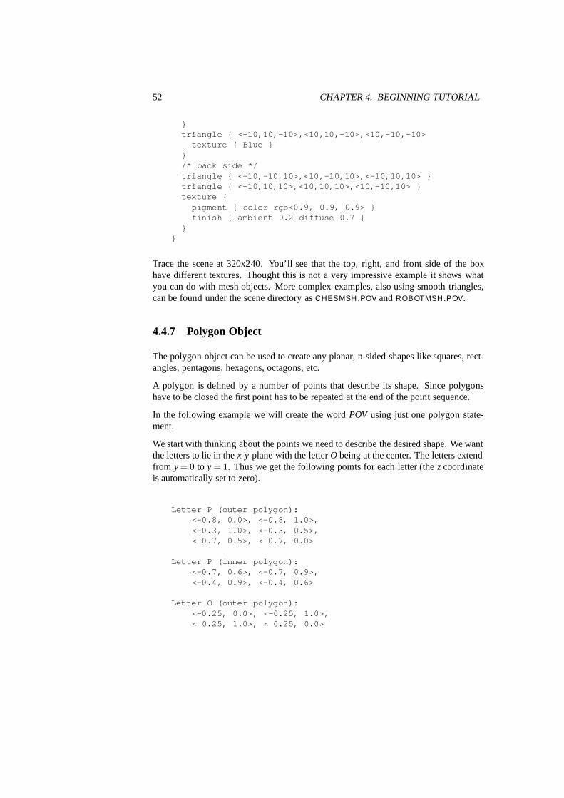
52 CHAPTER 4. BEGINNING TUTORIAL
}triangle { <-10,10,-10>,<10,10,-10>,<10,-10,-10>
texture { Blue }}/* back side */triangle { <-10,-10,10>,<10,-10,10>,<-10,10,10> }triangle { <-10,10,10>,<10,10,10>,<10,-10,10> }texture {
pigment { color rgb<0.9, 0.9, 0.9> }finish { ambient 0.2 diffuse 0.7 }
}}
Trace the scene at 320x240. You’ll see that the top, right, and front side of the boxhave different textures. Thought this is not a very impressive example it shows whatyou can do with mesh objects. More complex examples, also using smooth triangles,can be found under the scene directory as CHESMSH.POV and ROBOTMSH.POV.
4.4.7 Polygon Object
The polygon object can be used to create any planar, n-sided shapes like squares, rect-angles, pentagons, hexagons, octagons, etc.
A polygon is defined by a number of points that describe its shape. Since polygonshave to be closed the first point has to be repeated at the end of the point sequence.
In the following example we will create the word POV using just one polygon state-ment.
We start with thinking about the points we need to describe the desired shape. We wantthe letters to lie in the x-y-plane with the letter O being at the center. The letters extendfrom y= 0 to y= 1. Thus we get the following points for each letter (the zcoordinateis automatically set to zero).
Letter P (outer polygon):<-0.8, 0.0>, <-0.8, 1.0>,<-0.3, 1.0>, <-0.3, 0.5>,<-0.7, 0.5>, <-0.7, 0.0>
Letter P (inner polygon):<-0.7, 0.6>, <-0.7, 0.9>,<-0.4, 0.9>, <-0.4, 0.6>
Letter O (outer polygon):<-0.25, 0.0>, <-0.25, 1.0>,< 0.25, 1.0>, < 0.25, 0.0>
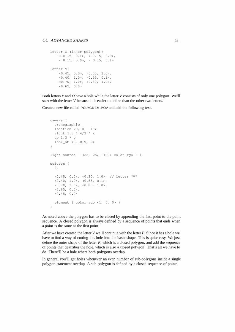
4.4. ADVANCED SHAPES 53
Letter O (inner polygon):<-0.15, 0.1>, <-0.15, 0.9>,< 0.15, 0.9>, < 0.15, 0.1>
Letter V:<0.45, 0.0>, <0.30, 1.0>,<0.40, 1.0>, <0.55, 0.1>,<0.70, 1.0>, <0.80, 1.0>,<0.65, 0.0>
Both letters P and O have a hole while the letter V consists of only one polygon. We’llstart with the letter V because it is easier to define than the other two letters.
Create a new file called POLYGDEM.POV and add the following text.
camera {orthographiclocation <0, 0, -10>right 1.3 * 4/3 * xup 1.3 * ylook_at <0, 0.5, 0>
}
light_source { <25, 25, -100> color rgb 1 }
polygon {8,
<0.45, 0.0>, <0.30, 1.0>, // Letter "V"<0.40, 1.0>, <0.55, 0.1>,<0.70, 1.0>, <0.80, 1.0>,<0.65, 0.0>,<0.45, 0.0>
pigment { color rgb <1, 0, 0> }}
As noted above the polygon has to be closed by appending the first point to the pointsequence. A closed polygon is always defined by a sequence of points that ends whena point is the same as the first point.
After we have created the letter V we’ll continue with the letter P. Since it has a hole wehave to find a way of cutting this hole into the basic shape. This is quite easy. We justdefine the outer shape of the letter P, which is a closed polygon, and add the sequenceof points that describes the hole, which is also a closed polygon. That’s all we have todo. There’ll be a hole where both polygons overlap.
In general you’ll get holes whenever an even number of sub-polygons inside a singlepolygon statement overlap. A sub-polygon is defined by a closed sequence of points.
54 CHAPTER 4. BEGINNING TUTORIAL
The letter P consists of two sub-polyons, one for the outer shape and one for the hole.Since the hole polygon overlaps the outer shape polygon we’ll get a hole.
After you’ve understood how multiple sub-polygons in a single polygon statementwork, it’s quite easy to add the missing O letter.
Finally, we get the complete word POV.
polygon {30,
<-0.8, 0.0>, <-0.8, 1.0>, // Letter "P"<-0.3, 1.0>, <-0.3, 0.5>, // outer shape<-0.7, 0.5>, <-0.7, 0.0>,<-0.8, 0.0>,
<-0.7, 0.6>, <-0.7, 0.9>, // whole<-0.4, 0.9>, <-0.4, 0.6>,<-0.7, 0.6>
<-0.25, 0.0>, <-0.25, 1.0>, // Letter "O"< 0.25, 1.0>, < 0.25, 0.0>, // outer shape<-0.25, 0.0>,
<-0.15, 0.1>, <-0.15, 0.9>, // whole< 0.15, 0.9>, < 0.15, 0.1>,<-0.15, 0.1>,
<0.45, 0.0>, <0.30, 1.0>, // Letter "V"<0.40, 1.0>, <0.55, 0.1>,<0.70, 1.0>, <0.80, 1.0>,<0.65, 0.0>,<0.45, 0.0>
pigment { color rgb <1, 0, 0> }}
4.4.8 Prism Object
[ *** STILL BEING WRITTEN *** Dieter Bayer ]
4.4.9 Superquadric Ellipsoid Object
Sometimes we want to make an object that does not have perfectly sharp edges like abox does. Then, the super quadric ellipsoid is a useful object. It is described by thesimple syntax:
superellipsoid { <r, n> }

4.4. ADVANCED SHAPES 55
Where r and n are float values greater than zero and less than or equal to one. Let’smake a superellipsoid and experiement with the values of r and n to see what kind ofshapes we can make.
Create a file called SUPELLPS.POV and edit it as follows:
#include "colors.inc"
camera {location <10, 5, -20>look_at 0angle 15
}
background { color rgb <.5, .5, .5> }
light_source { <10, 50, -100> White }
The addition of a gray background makes it a little easier to see our object. Now type:
superellipsoid { <.25, .25>pigment { Red }
}
Save the file and trace it at 200x150 –A to see the shape. It will look like a box, butthe edges will be rounded off. Now let’s experiment with different values of r and n.For the next trace, try 〈1,0.2〉. The shape now looks like a cylinder, but the top edgesare rounded. Now try 〈0.1,1〉. This shape is an odd one! We don’t know exactly whatto call it, but it is interesting. Finally, lets try 〈1,1〉. Well, this is more familiar . . . asphere!
There are a couple of facts about superellipsoids you should know. First, you shouldnot use a value of 0 for either r nor n. This will cause POV-Ray to incorrectly makea black box instead of your desired shape. Second, very small values of r and n mayyield strange results so they should be avoided. Finally, the Sturmian root solver willnot work with superellipsoids.
Superellipsoids are finite objects so they respond to auto-bounding and can be used inCSG.
Now let’s use the superellipsoid to make something that would be useful in a scene.We will make a tiled floor and place a couple of superellipsoid objects hovering overit. We can start with the file we have already made.
Rename it TILES.POV. Edit it so that it reads as follows:
#include "colors.inc"#include "textures.inc"

56 CHAPTER 4. BEGINNING TUTORIAL
camera {location <10, 5, -20>look_at 0angle 15
}background { color rgb <.5, .5, .5> }
light_source{ <10, 50, -100> White }
Note that we have added #include "textures.inc" so we can use pre-definedtextures. Now we want to define the superellipsoid which will be our tile.
#declare Tile = superellipsoid { <0.5, 0.1>scale <1, .05, 1>
}
Superellipsoids are roughly 2×2×2 units unless you scale them otherwise. If we wishto lay a bunch of our tiles side by side, they will have to be offset from each other sothey don’t overlap. We should select an offset value that is slightly more than 2 so thatwe have some space between the tiles to fill with grout. So now add this:
#declare Offset = 2.1
We now want to lay down a row of tiles. Each tile will be offset from the original byan ever-increasing amount in both the +zand −zdirections. We refer to our offset andmultiply by the tile’s rank to determine the position of each tile in the row. We alsounion these tiles into a single object called Rowlike this:
#declare Row = union {object { Tile }object { Tile translate z*Offset }object { Tile translate z*Offset*2 }object { Tile translate z*Offset*3 }object { Tile translate z*Offset*4 }object { Tile translate z*Offset*5 }object { Tile translate z*Offset*6 }object { Tile translate z*Offset*7 }object { Tile translate z*Offset*8 }object { Tile translate z*Offset*9 }object { Tile translate z*Offset*10 }object { Tile translate -z*Offset }object { Tile translate -z*Offset*2 }object { Tile translate -z*Offset*3 }object { Tile translate -z*Offset*4 }object { Tile translate -z*Offset*5 }

4.4. ADVANCED SHAPES 57
object { Tile translate -z*Offset*6 }}
This gives us a single row of 17 tiles, more than enough to fill the screen. Now wemust make copies of the Rowand translate them, again by the offset value, in both the+x and −x directions in ever increasing amounts in the same manner.
object { Row }object { Row translate x*Offset }object { Row translate x*Offset*2 }object { Row translate x*Offset*3 }object { Row translate x*Offset*4 }object { Row translate x*Offset*5 }object { Row translate x*Offset*6 }object { Row translate x*Offset*7 }object { Row translate -x*Offset }object { Row translate -x*Offset*2 }object { Row translate -x*Offset*3 }object { Row translate -x*Offset*4 }object { Row translate -x*Offset*5 }object { Row translate -x*Offset*6 }object { Row translate -x*Offset*7 }
Finally, our tiles are complete. But we need a texture for them. To do this we unionall of the Rowstogether and apply a White Marblepigment and a somewhat shinyrefelctive surface to it:
union{object { Row }object { Row translate x*Offset }object { Row translate x*Offset*2 }object { Row translate x*Offset*3 }object { Row translate x*Offset*4 }object { Row translate x*Offset*5 }object { Row translate x*Offset*6 }object { Row translate x*Offset*7 }object { Row translate -x*Offset }object { Row translate -x*Offset*2 }object { Row translate -x*Offset*3 }object { Row translate -x*Offset*4 }object { Row translate -x*Offset*5 }object { Row translate -x*Offset*6 }object { Row translate -x*Offset*7 }pigment { White_Marble }finish { phong 1 phong_size 50 reflection .35 }
}

58 CHAPTER 4. BEGINNING TUTORIAL
We now need to add the grout. This can simply be a white plane. We have stepped upthe ambient here a little so it looks whiter.
plane { y, 0 //this is the groutpigment { color White }finish { ambient .4 diffuse .7 }
}
To complete our scene, let’s add five different superellipsoids, each a different color,so that they hover over our tiles and are reflected in them.
superellipsoid {<0.1, 1>pigment { Red }translate <5, 3, 0>scale .45
}
superellipsoid {<1, 0.25>pigment { Blue }translate <-5, 3, 0>scale .45
}
superellipsoid {<0.2, 0.6>pigment { Green }translate <0, 3, 5>scale .45
}
superellipsoid {<0.25, 0.25>pigment { Yellow }translate <0, 3, -5>scale .45
}
superellipsoid {<1, 1>pigment { Pink }translate y*3scale .45
}
Trace the scene at 320x200 –A to see the result. If you are happy with that, do a finaltrace at 640x480 +A0.2.
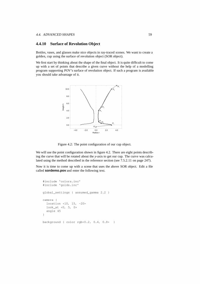
4.4. ADVANCED SHAPES 59
4.4.10 Surface of Revolution Object
Bottles, vases, and glasses make nice objects in ray-traced scenes. We want to create agolden, cup using the surface of revolution object (SOR object).
We first start by thinking about the shape of the final object. It is quite difficult to comeup with a set of points that describe a given curve without the help of a modellingprogram supporting POV’s surface of revolution object. If such a program is availableyou should take advantage of it.
−4.0 −2.0 0.0 2.0 4.0Radius r
0.0
2.0
4.0
6.0
8.0
10.0
Hei
ght h
P0
P1
P2
P3
P4
P5
P6
P7
Figure 4.2: The point configuration of our cup object.
We will use the point configuration shown in figure 4.2. There are eight points describ-ing the curve that will be rotated about the y-axis to get our cup. The curve was calcu-lated using the method described in the reference section (see 7.5.2.11 on page 247).
Now it is time to come up with a scene that uses the above SOR object. Edit a filecalled sordemo.pov and enter the following text.
#include "colors.inc"#include "golds.inc"
global_settings { assumed_gamma 2.2 }
camera {location <10, 15, -20>look_at <0, 5, 0>angle 45
}
background { color rgb<0.2, 0.4, 0.8> }
60 CHAPTER 4. BEGINNING TUTORIAL
light_source { <100, 100, -100> color rgb 1 }
plane { y, 0pigment { checker color Red, color Green scale 10 }
}
sor {8,<0.0, -0.5>,<3.0, 0.0>,<1.0, 0.2>,<0.5, 0.4>,<0.5, 4.0>,<1.0, 5.0>,<3.0, 10.0>,<4.0, 11.0>texture { T_Gold_1B }
}
The scene contains our cup object resting on a checkered plane. Trace the scene at320x240 to see the resulting image.
The surface of revolution is described by starting with the number of points followedby the points with ascending heights. Each point determines the radius the curve for agiven height. E. g. the first point tells POV-Ray that at height −0.5 the radius is 0. Youshould take care that each point has a larger height than its predecessor. If this is notthe case the program will abort with an error message.
4.4.11 Text Object
Creating text objects using POV-Ray always used to mean that the letters had to bebuilt either from CSG, a painstaking process, or by using a black and white image ofthe letters as a height field, a method that was only somewhat satisfactory. Now, forPOV-Ray 3.0, a new primitive has been introduced that can use any TrueType font tocreate text objects. These objects can be used in CSG, transformed, and textured justlike any other POV primitive.
For this tutorial, we will make two uses of the text object. First, let’s just make someblock letters sitting on a checkered plane. Any TTF font should do, but for this tutorial,we will use the ones bundled with POV-Ray 3.0.
Create a file called TEXTDEMO.POV and edit it as follows:
#include "colors.inc"
camera {location <0, 1, -10>

4.4. ADVANCED SHAPES 61
look_at 0angle 36
}
light_source { <500,500,-1000> White }
plane { y,0pigment { checker Green White }
}
Now let’s add the text object. We will use the font TIMROM.TTF and we will createthe string POV-RAY 3.0. For now, we will just make the letters red. The syntax isvery simple. The first string in quotes is the font name, the second one is the stringto be rendered. The two floats are the thickness and offset values. The thickness floatdetermines how thick the block letters will be. Values of .5 to 2 are usually best forthis. The offset value will add to the kerning distance of the letters. We will leave thisa 0 for now.
text { ttf "timrom.ttf" "POV-RAY 3.0" 1, 0pigment { Red }
}
Rendering this at 200x150 –A, we notice that the letters are off to the right of thescreen. This is because they are placed so that the lower left front corner of the firstletter is at the origin. To center the string we need to translate it−x some distance. Buthow far? In the docs we see that the letters are all 0.5 to 0.75 units high. If we assumethat each one takes about 0.5 units of space on the x-axis, this means that the string isabout 6 units long (12 characters and spaces). Let’s translate the string 3 units alongthe negative x-axis.
text { ttf "timrom.ttf" "POV-RAY 3.0" 1, 0pigment { Red }translate -3*x
}
That’s better. Now let’s play around with some of the parameters of the text object.First, let’s raise the thickness float to something outlandish . . . say 25!
text { ttf "timrom.ttf" "POV-RAY 3.0" 25, 0pigment { Red }translate -2.25*x
}
Actually, that’s kind of cool. Now let’s return the thickness value to 1 and try a differentoffset value. Change the offset float from 0 to 0.1 and render it again.
Wait a minute?! The letters go wandering off up at an angle! That is not what the docsdescribe! It almost looks as if the offset value applies in both the x- and y-axis instead

62 CHAPTER 4. BEGINNING TUTORIAL
of just the x axis like we intended. Could it be that a vector is called for here instead ofa float? Let’s try it. Replace 0.1 with 0.1*x and render it again.
That works! The letters are still in a straight line along the x axis, just a little furtherapart. Let’s verify this and try to offset just in the y axis. Replace 0.1*x with 0.1*y.Again, this works as expected with the letters going up to the right at an angle with noadditional distance added along the x axis. Now let’s try the z axis. Replace 0.1*ywith 0.1*z. Rendering this yields a disappointment. No offset occurs! The offsetvalue can only be applied in the x and y directions.
Let’s finish our scene by giving a fancier texture to the block letters, using that coollarge thickness value, and adding a slight y offset. For fun, we will throw in a skysphere, dandy up our plane a bit, and use a little more interesting camera viewpoint(render the following scene at 640x480 +A0.2):
#include "colors.inc"
camera {location <-5,.15,-2>look_at <.3,.2,1>angle 36
}
light_source { <500,500,-1000> White }
plane { y,0texture {
pigment { SeaGreen }finish { reflection .35 specular 1 }normal { ripples .35 turbulence .5 scale .25 }
}}
text { ttf "timrom.ttf" "POV-RAY 3.0" 25, 0.1*ypigment { BrightGold }finish { reflection .25 specular 1 }translate -3*x
}
#include "skies.inc"
sky_sphere { S_Cloud5 }
Now. let’s try using text in a CSG object. We will attempt to create an inlay in a stoneblock using a text object. Create a new file called TEXTCSG.POV and edit it as follows:
#include "colors.inc"#include "stones.inc"

4.4. ADVANCED SHAPES 63
background { color rgb 1 }
camera {location <-3, 5, -15>look_at 0angle 25
}
light_source { <500,500,-1000> White }
Now let’s create the block. We want it to be about eight units across because our textstring (POV-RAY 3.0) is about six units long. We also want it about four units high andabout one unit deep. But we need to avoid a potential coincident surface with the textobject so we will make the first z coordinate 0.1 instead of 0. Finally, we will give thisblock a nice stone texture.
box { <-3.5, -1, 0.1>, <3.5, 1, 1>texture { T_Stone10 }
}
Next, we want to make the text object. We can use the same object we used in the firstturorial except we will use slightly different thickness and offset values.
text { ttf "timrom.ttf" "POV-RAY 3.0" 0.15, 0pigment { BrightGold }finish { reflection .25 specular 1 }translate -3*x
}
Remember that the text object is placed by default so that its front surface lies directlyon the x-y-plane. If the front of the box begins at z= 0.1 and thickness is set at 0.15, thedepth of the ”inlay” will be 0.05 units. Go ahead and place a difference block aroundthe two objects.
difference {box { <-3.5, -1, 0.1>, <3.5, 1, 1>
texture { T_Stone10 }}text { ttf "timrom.ttf" "POV-RAY 3.0" 0.15, 0
pigment { BrightGold }finish { reflection .25 specular 1 }translate -3*x
}}

64 CHAPTER 4. BEGINNING TUTORIAL
Render this at 200x150 –A. We can see the inlay clearly and that it is indeed a brightgold color. Render this at 640x480 +A0.2 to see the results more clearly, but be fore-warned . . . this trace will take a little time.
4.4.12 Torus Object
A torus can be thought of as a donut or an innertube. It is a shape that is vastly usefulin many kinds of CSG so POV-Ray has adopted this 4th order quartic polynomial as aprimitive shape. The syntax for a torus is so simple that it makes it a very easy shapeto work with once you learn what the two float values mean. Instead of a lecture on thesubject, let’s create one and do some experiments with it.
Create a file called TORDEMO.POV. Edit it as follows:
#include "colors.inc"
camera {location <0, .1, -25>look_at 0angle 36
}
background { color Gray50 }
light_source{ <300, 300, -1000> White }
torus { 4, 1 // major and minor radiusrotate -90*x // so we can see it from the toppigment { Green }
}
Go ahead and trace this. Well, it’s a donut allright. Let’s try changing the major andminor radius values and see what happens. Change them as follows:
torus { 5, .25 // major and minor radius
That looks more like a hula-hoop! Let’s try this:
torus { 3.5, 2.5 // major and minor radius
Whoa! A donut with a serious weight problem!
With such a simple syntax, there isn’t much else you can do to a torus besides changeits texture . . . or is there? Let’s see . . .
Torus’ are very useful objects in CSG. Let’s try a little experiment. Make a differenceof a torus and a box:

4.4. ADVANCED SHAPES 65
difference {torus { 4, 1
rotate x*-90 // so we can see it from the top}box { <-5, -5, -1>, <5, 0, 1> }pigment { Green }
}
Interesting . . . a half-torus. So? So, now add another one flipped the other way. Only,let’s declare the original half-torus and the necessary transformations so we can usethem again:
#declare Half_Torus = difference {torus { 4, 1
rotate -90*x // so we can see it from the top}box { <-5, -5, -1>, <5, 0, 1> }pigment { Green }
}
#declare Flip_It_Over = 180*x
#declare Torus_Translate = 8 // 2 * major radius
Now create a union of two Half Torus objects:
union {object { Half_Torus }object { Half_Torus
rotate Flip_It_Overtranslate Torus_Translate*x
}}
This makes an S-shaped object, but we can’t see the whole thing from our presentcamera. Let’s add a few more links, three in each direction, move the object along the+z direction and rotate it about the +y axis so we can see more of it. We also noticethat there appears to be a small gap where the Half Torus’ meet. This is due to thefact that we are viewing this scene from directly on the x-z plane. We will change thecamera y coordinate from 0 to 0.1 to eliminate this.
union {object { Half_Torus }object { Half_Torus
rotate Flip_It_Overtranslate x*Torus_Translate
}

66 CHAPTER 4. BEGINNING TUTORIAL
object { Half_Torustranslate x*Torus_Translate*2
}object { Half_Torus
rotate Flip_It_Overtranslate x*Torus_Translate*3
}object { Half_Torus
rotate Flip_It_Overtranslate -x*Torus_Translate
}object { Half_Torus
translate -x*Torus_Translate*2}object { Half_Torus
rotate Flip_It_Overtranslate -x*Torus_Translate*3
}object { Half_Torus
translate -x*Torus_Translate*4}rotate y*45translate z*20
}
Rendering this we see a cool, undulating, snake-like something-or-other. Neato. Butwe want to model something useful, something that we might see in real life. Howabout a chain?
Thinking about it for a moment, we realize that a single link of a chain can be easilymodeled using two half toruses and two cylinders. Go ahead and create a new file. Youcan use the same camera, background, light source, and declared objects and transfor-mations as you used in TORDEMO.POV:
#include "colors.inc"
camera {location <0, .1, -25>look_at 0angle 36
}
background { color Gray50 }
light_source{ <300, 300, -1000> White }
#declare Half_Torus = difference {torus { 4,1
sturm
4.4. ADVANCED SHAPES 67
rotate x*-90 // so we can see it from the top}box { <-5, -5, -1>, <5, 0, 1> }pigment { Green }
}
#declare Flip_It_Over = x*180
#declare Torus_Translate = 8
Now, make a complete torus of two half toruses:
union {object { Half_Torus }object { Half_Torus rotate Flip_It_Over }
}
This may seem like a wasteful way to make a complete torus, but we are really goingto move each half apart to make room for the cylinders. First, add the declared cylinderbefore the union:
#declare Chain_Segment =cylinder { <0, 4, 0>, <0, -4, 0>, 1pigment { Green }
}
Then add two Chain Segments to the union and translate them so that they line up withthe minor radius of the torus on each side:
union {object { Half_Torus }object { Half_Torus rotate Flip_It_Over }object { Chain_Segment
translate x*Torus_Translate/2}object { Chain_Segment
translate -x*Torus_Translate/2}
}
Now translate the two half toruses +y and −y so that the clipped ends meet the ends ofthe cylinders. This distance is equal to half of the previously declared Torus Translate:
union {object { Half_Torus

68 CHAPTER 4. BEGINNING TUTORIAL
translate y*Torus_Translate/2}object { Half_Torus
rotate Flip_It_Overtranslate -y*Torus_Translate/2
}object { Chain_Segment
translate x*Torus_Translate/2}object { Chain_Segment
translate -x*Torus_Translate/2}
}
Render this and voila! A single link of a chain. But we aren’t done yet! Whoever heardof a green chain? We would rather use a nice metallic color instead. First, remove anypigment blocks in the declared toruses and cylinders. Then add the following beforethe union:
#declare Chain_Gold = texture {pigment { BrightGold }finish {
ambient .1diffuse .4reflection .25specular 1metallic
}}
Then add the texture to the union and declare the union as a single link:
#declare Link = union {object { Half_Torus
translate y*Torus_Translate/2}object { Half_Torus
rotate Flip_It_Overtranslate -y*Torus_Translate/2
}object { Chain_Segment
translate x*Torus_Translate/2}object { Chain_Segment
translate -x*Torus_Translate/2}texture { Chain_Gold }
}

4.4. ADVANCED SHAPES 69
Now make a union of two links. The second one will have to be translated +y so thatits inner wall just meets the inner wall of the other link, just like the links of a chain.This distance turns out to be double the previously declared Torus Translate minus 2(twice the minor radius). This can be described by the expression:
Torus_Translate*2-2*y
Declare this expression as follows:
#declare Link_Translate = Torus_Translate*2-2*y
In the object block, we will use this declared value so that we can multiply it to createother links. Now, rotate the second link 90*y so that it is perpendicular to the first,just like links of a chain. Finally, scale the union by 1/4 so that we can see the wholething:
union {object { Link }object { Link translate y*Link_Translate rotate y*90 }scale .25
}
Render this and you will see a very realistic pair of links. If we want to make an entirechain, we must declare the above union and then create another union of this declaredobject. Be sure to remove the scaling from the declared object:
#declare Link_Pair =union {
object { Link }object { Link translate y*Link_Translate rotate y*90 }
}
Now declare your chain:
#declare Chain = union {object { Link_Pair}object { Link_Pair translate y*Link_Translate*2 }object { Link_Pair translate y*Link_Translate*4 }object { Link_Pair translate y*Link_Translate*6 }object { Link_Pair translate -y*Link_Translate*2 }object { Link_Pair translate -y*Link_Translate*4 }object { Link_Pair translate -y*Link_Translate*6 }
}

70 CHAPTER 4. BEGINNING TUTORIAL
And, finally create your chain with a couple of transformations to make it easier to see.These include scaling it down by a factor of 1/10, and rotating it so that you can clearlysee each link:
object { Chain scale .1 rotate <0, 45, -45> }
Render this and you should see a very realistic gold chain stretched diagonally acrossthe screen.
4.5 CSG Objects
Constructive solid geomerty, CSG, is a powerful tool to combine primitve objects tocreate more complex objects as shown in the following sections.
4.5.1 What is CSG?
CSG stands for Constructive Solid Geometry. POV-Ray allows you to construct com-plex solids by combining primitive shapes in four different ways. These are union,where two or more shapes are added together, intersection where two or more shapesare combined to make a new shape that consists of the area common to both shapes, dif-ference where subsequent shapes are subtracted from the first shape, and merge whichis like a union where the surfaces inside the union are removed (useful in transparentCSG objects). We will deal with each of these in detail in the next few sections.
CSG objects can be extremely complex. They can be deeply nested. In other wordsthere can be unions of differences or intersections of merges or differences of intersec-tions or even unions of intersections of differences of merges . . . ad infinitum. CSGobjects are (almost always) finite objects and so respond to auto-bounding and can betransformed like any other POV primitive shape.
4.5.2 CSG Union
Let’s try making a simple union. Create a file called CSGDEMO.POV and edit it asfollows:
#include "colors.inc"
camera {location <0, 1, -10>look_at 0angle 36
}

4.5. CSG OBJECTS 71
light_source { <500, 500, -1000> White }
plane { y, -1.5pigment { checker Green White }
}
Now let’s add two spheres each translated 0.5 units along the x-axis in each direction.Color one blue and the other red.
sphere { <0, 0, 0>, 1pigment { Blue }translate -0.5*x
}sphere { <0, 0, 0>, 1
pigment { Red }translate 0.5*x
}
Try tracing this file now at 200x150 –A. Now place a union block around the twospheres. This will create a single CSG union out of the two objects.
union{sphere { <0, 0, 0>, 1
pigment { Blue }translate -0.5*x
}sphere { <0, 0, 0>, 1
pigment { Red }translate 0.5*x
}}
Trace the file again. The union will appear no different from what each sphere lookedlike on its own, but now we can give the entire union a single texture and transform itas a whole. Let’s do that now.
union{sphere { <0, 0, 0>, 1
translate -0.5*x*}sphere { <0, 0, 0>, 1
translate 0.5*x}pigment { Red }scale <1, .25, 1>rotate <30, 0, 45>
}

72 CHAPTER 4. BEGINNING TUTORIAL
Trace the file again. As you can see, the object has changed dramatically. Experimentwith different values of scale and rotate and try some different textures.
There are some advantages of assigning only one texture to a CSG object instead ofassigning the texture to each individual component. First, it is much easier to useone texture if your CSG object has a lot of components because changing the objectsappereance involves changing only one single texture. Second, the file parses fasterbecause the texture has to be parsed only once. This may be a great factor when do-ing large scenes or animatons. Third, using only one texture saves memory becausethe texture is only stored once and referenced by all components of the CSG object.Assigning the texture to all n components means that it is stored n times.
4.5.3 CSG Intersection
Now let’s use these same spheres to illustrate the next kind of CSG object, the in-tersection. Change the word union to intersection and delete the scale androtate statements:
intersection {sphere { <0, 0, 0>, 1
translate -0.5*x}sphere { <0, 0, 0>, 1
translate 0.5*x}pigment { Red }
}
Trace the file and you will see a lens-shaped object instead of the two spheres. Thisis because an intersection consists of the area shared by both shapes, in this case thelens-shaped area where the two spheres overlap. We like this lens-shaped object so wewill use it to demostrate differences.
4.5.4 CSG Difference
Rotate the lens-shaped intersection about the y-axis so that the broad side is facing thecamera.
intersection{sphere { <0, 0, 0>, 1
translate -0.5*x}sphere { <0, 0, 0>, 1
translate 0.5*x
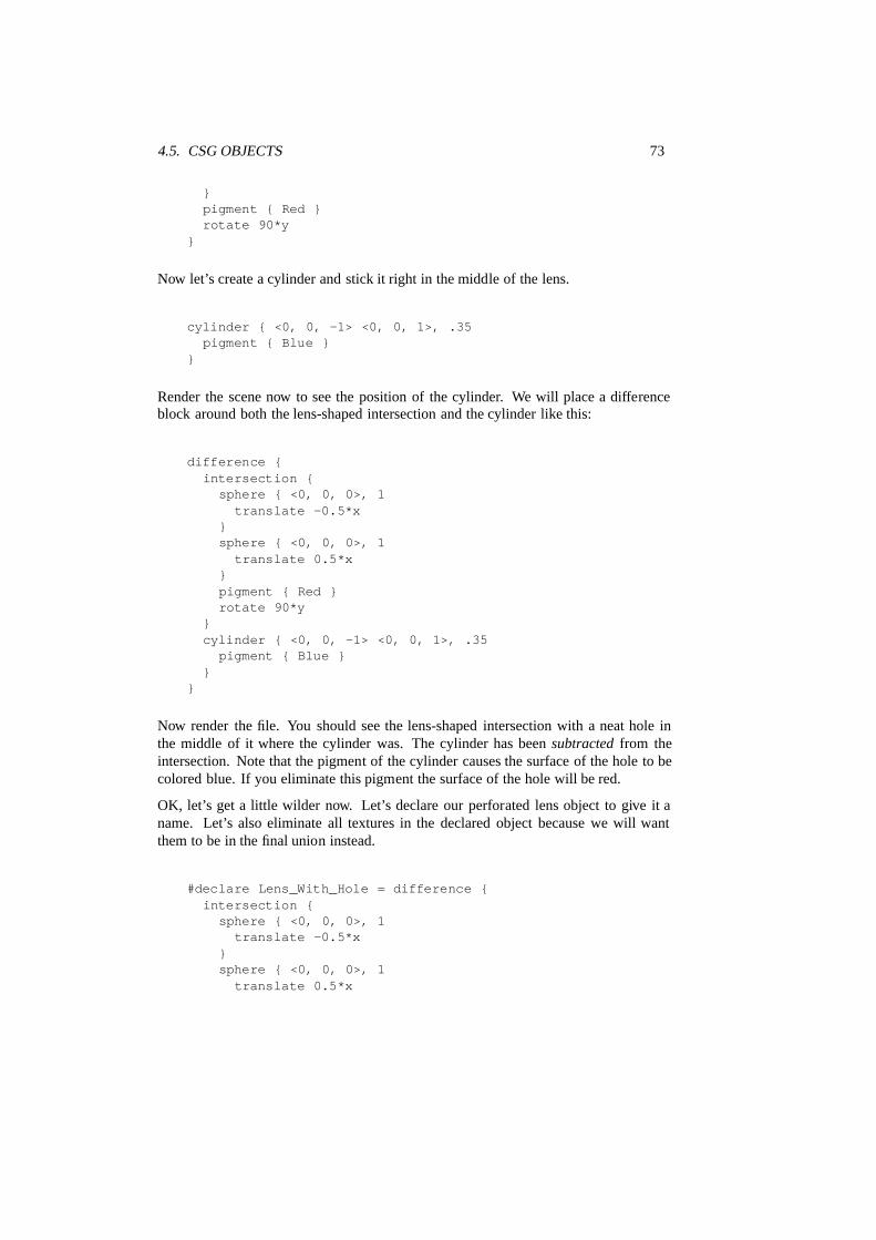
4.5. CSG OBJECTS 73
}pigment { Red }rotate 90*y
}
Now let’s create a cylinder and stick it right in the middle of the lens.
cylinder { <0, 0, -1> <0, 0, 1>, .35pigment { Blue }
}
Render the scene now to see the position of the cylinder. We will place a differenceblock around both the lens-shaped intersection and the cylinder like this:
difference {intersection {
sphere { <0, 0, 0>, 1translate -0.5*x
}sphere { <0, 0, 0>, 1
translate 0.5*x}pigment { Red }rotate 90*y
}cylinder { <0, 0, -1> <0, 0, 1>, .35
pigment { Blue }}
}
Now render the file. You should see the lens-shaped intersection with a neat hole inthe middle of it where the cylinder was. The cylinder has been subtracted from theintersection. Note that the pigment of the cylinder causes the surface of the hole to becolored blue. If you eliminate this pigment the surface of the hole will be red.
OK, let’s get a little wilder now. Let’s declare our perforated lens object to give it aname. Let’s also eliminate all textures in the declared object because we will wantthem to be in the final union instead.
#declare Lens_With_Hole = difference {intersection {
sphere { <0, 0, 0>, 1translate -0.5*x
}sphere { <0, 0, 0>, 1
translate 0.5*x

74 CHAPTER 4. BEGINNING TUTORIAL
}rotate 90*y
}cylinder { <0, 0, -1> <0, 0, 1>, .35 }
}
Now, let’s use union to build a complex shape composed of copies of this object.
union {object { Lens_With_Hole translate <-.65, .65, 0> }object { Lens_With_Hole translate <.65, .65, 0> }object { Lens_With_Hole translate <-.65, -.65, 0> }object { Lens_With_Hole translate <.65, -.65, 0> }pigment { Red }
}
Render it. An interesting object to be sure. But let’s try something more. Let’s make ita partially-transparent object by adding some filter to the pigment block.
union {object { Lens_With_Hole translate <-.65, .65, 0> }object { Lens_With_Hole translate <.65, .65, 0> }object { Lens_With_Hole translate <-.65, -.65, 0> }object { Lens_With_Hole translate <.65, -.65, 0> }pigment { Red filter .5 }
}
Now render the file again. This looks pretty good . . . only . . . you can see parts of eachof the lens objects inside the union! This is no good.
4.5.5 CSG Merge
This brings us to the fourth kind of CSG object, the merge. Merges are the same asunions, but the geometry of the objects in the CSG that is inside the merge is not traced.This should eliminate the problem with our object. Let’s try it.
merge {object { Lens_With_Hole translate <-.65, .65, 0> }object { Lens_With_Hole translate <.65, .65, 0> }object { Lens_With_Hole translate <-.65, -.65, 0> }object { Lens_With_Hole translate <.65, -.65, 0> }pigment { Red filter .5 }
}
Sure enough, it does!
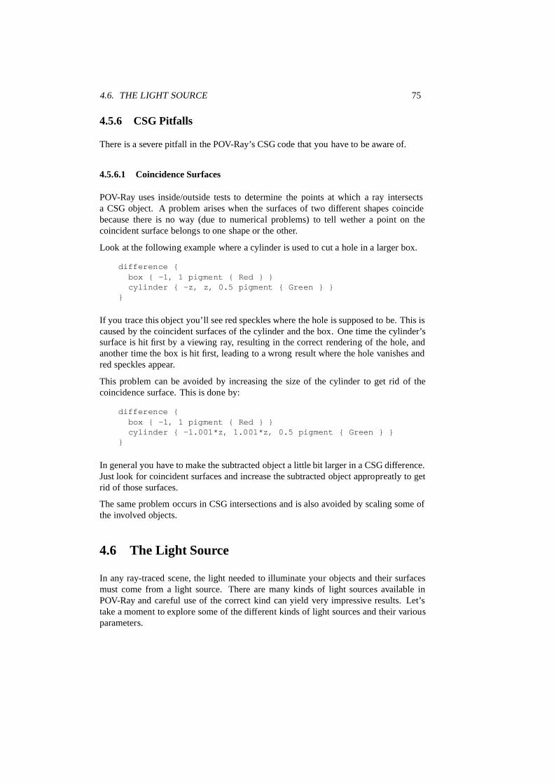
4.6. THE LIGHT SOURCE 75
4.5.6 CSG Pitfalls
There is a severe pitfall in the POV-Ray’s CSG code that you have to be aware of.
4.5.6.1 Coincidence Surfaces
POV-Ray uses inside/outside tests to determine the points at which a ray intersectsa CSG object. A problem arises when the surfaces of two different shapes coincidebecause there is no way (due to numerical problems) to tell wether a point on thecoincident surface belongs to one shape or the other.
Look at the following example where a cylinder is used to cut a hole in a larger box.
difference {box { -1, 1 pigment { Red } }cylinder { -z, z, 0.5 pigment { Green } }
}
If you trace this object you’ll see red speckles where the hole is supposed to be. This iscaused by the coincident surfaces of the cylinder and the box. One time the cylinder’ssurface is hit first by a viewing ray, resulting in the correct rendering of the hole, andanother time the box is hit first, leading to a wrong result where the hole vanishes andred speckles appear.
This problem can be avoided by increasing the size of the cylinder to get rid of thecoincidence surface. This is done by:
difference {box { -1, 1 pigment { Red } }cylinder { -1.001*z, 1.001*z, 0.5 pigment { Green } }
}
In general you have to make the subtracted object a little bit larger in a CSG difference.Just look for coincident surfaces and increase the subtracted object appropreatly to getrid of those surfaces.
The same problem occurs in CSG intersections and is also avoided by scaling some ofthe involved objects.
4.6 The Light Source
In any ray-traced scene, the light needed to illuminate your objects and their surfacesmust come from a light source. There are many kinds of light sources available inPOV-Ray and careful use of the correct kind can yield very impressive results. Let’stake a moment to explore some of the different kinds of light sources and their variousparameters.

76 CHAPTER 4. BEGINNING TUTORIAL
4.6.1 The Ambient Light Source
The ambient light source is used to simulate the effect of interdiffuse reflection. Ifthere wasn’t interdiffuse reflection all areas not directly lit by a light source would becompletely dark. POV-Ray uses the ambient keyword to determine how much lightcoming from the ambient light source is reflected by a surface.
By default the ambient light source, which emits its light everywhere and in all direc-tions, is pure white (rgb< 1,1,1>). Changing its color can be used to create interestingeffects. First of all the overall light level of the scene can be adjusted easily. Instead ofchanging all ambient values only the ambient light source is modified. By assigningdifferent colors you can create nice effects like a moody reddish ambient lighting. Formore details about the ambient light source see 7.8.2 on page 356.
Below is an example of a red ambient light source.
global_settings { ambient_light rgb<1, 0, 0> }
4.6.2 The Point Light Source
Pointlights are exactly what the name indicates. A pointlight has no size, is invisible,and illuminates everything in the scene equally no matter how far away from the lightsource it may be. This is the simplest and most basic light source. There are onlytwo important parameters, location and color. Let’s design a simple scene and place apointlight source in it.
Create a new file and name it LITEDEMO.POV. Edit it as follows:
#include "colors.inc"#include "textures.inc"
camera {location <-4, 3, -9>look_at <0, 0, 0>angle 48
}
Add the following simple objects:
plane { y, -1texture {
pigment {checkercolor rgb<0.5, 0, 0>color rgb<0, 0.5, 0.5>
}finish {

4.6. THE LIGHT SOURCE 77
diffuse 0.4ambient 0.2phong 1phong_size 100reflection 0.25
}}
}
torus { 1.5, 0.5texture { Brown_Agate }rotate <90, 160, 0>translate <-1, 1, 3>
}
box { <-1, -1, -1>, <1, 1, 1>texture { DMFLightOak }translate <2, 0, 2.3>
}
cone { <0,1,0>, 0, <0,0,0>, 1texture { PinkAlabaster }scale <1, 3, 1>translate <-2, -1, -1>
}
sphere { <0,0,0>,1texture { Sapphire_Agate }translate <1.5, 0, -2>
}
Now add a pointlight:
light_source {<2, 10, -3>color White
}
Render this at 200x150 –A. You will see that the objects are clearly visible with sharpshadows. The sides of curved objects nearest the light source are brightest in colorwith the areas that are facing away from the light source darkest. Note also that thecheckered plane is illuminated evenly all the way to the horizon. This allows us to seethe plane, but it is not very realistic.
4.6.3 The Spotlight Source
Spotlights are a very useful type of light source. They can be used to add highlightsand illuminate features much as a photographer uses spots to do the same thing. There

78 CHAPTER 4. BEGINNING TUTORIAL
are a few more parameters with spotlights than with pointlights. These are radius,falloff, tightness, and point at. The radius parameter is the angle of thefully illuminated cone. The falloff parameter is the angle of the umbra cone wherethe light falls off to darkness. The tightness is a parameter that determines the rateof the light falloff. point at is just what it says, where the spotlight is pointing to.Let’s change the light in our scene as follows:
light_source {<0, 10, -3>color Whitespotlightradius 15falloff 20tightness 10point_at <0, 0, 0>
}
Render this at 200x150 –A and you will see that only the objects are illuminated. Therest of the plane and the outer portions of the objects are now unlit. There is a broadfalloff area, but the shadows are still razor sharp. Let’s try fiddling with some of theseparameters to see what they do. Try changing the falloff value to 16 (it mustalways be larger than radius) and render again. Now the falloff is very narrow, andthe objects are either brightly lit, or in total darkness. Now, change falloff back to20 and change the tightness value to 100 (higher is tighter) and render again. Thespotlight appears to have gotten much smaller, but what has really happened is that thefalloff has become so steep that the radius actually appears smaller.
We decide that a tightness value of 10 (the default) and a falloff value of 18are best for this spotlight and we now want to put a few spots around the scene foreffect. Lets place a slightly narrower blue and a red one in addition to the white onewe already have:
light_source {<10, 10, -1>color Redspotlightradius 12falloff 14tightness 10point_at <2, 0, 0>
}
light_source {<-12, 10, -1>color Bluespotlightradius 12
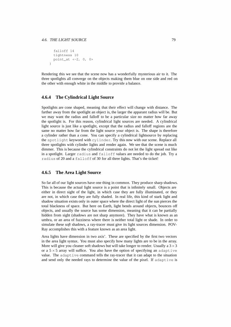
4.6. THE LIGHT SOURCE 79
falloff 14tightness 10point_at <-2, 0, 0>
}
Rendering this we see that the scene now has a wonderfully mysterious air to it. Thethree spotlights all converge on the objects making them blue on one side and red onthe other with enough white in the middle to provide a balance.
4.6.4 The Cylindrical Light Source
Spotlights are cone shaped, meaning that their effect will change with distance. Thefarther away from the spotlight an object is, the larger the apparant radius will be. Butwe may want the radius and falloff to be a particular size no matter how far awaythe spotlight is. For this reason, cylindrical light sources are needed. A cylindricallight source is just like a spotlight, except that the radius and falloff regions are thesame no matter how far from the light source your object is. The shape is thereforea cylinder rather than a cone. You can specify a cylindrical lightsource by replacingthe spotlight keyword with cylinder. Try this now with our scene. Replace allthree spotlights with cylinder lights and render again. We see that the scene is muchdimmer. This is because the cylindrical constraints do not let the light spread out likein a spotlight. Larger radius and falloff values are needed to do the job. Try aradius of 20 and a falloff of 30 for all three lights. That’s the ticket!
4.6.5 The Area Light Source
So far all of our light sources have one thing in common. They produce sharp shadows.This is because the actual light source is a point that is infinitely small. Objects areeither in direct sight of the light, in which case they are fully illuminated, or theyare not, in which case they are fully shaded. In real life, this kind of stark light andshadow situation exists only in outer space where the direct light of the sun pierces thetotal blackness of space. But here on Earth, light bends around objects, bounces offobjects, and usually the source has some dimension, meaning that it can be partiallyhidden from sight (shadows are not sharp anymore). They have what is known as anumbra, or an area of fuzziness where there is neither total light or shade. In order tosimulate these soft shadows, a ray-tracer must give its light sources dimension. POV-Ray accomplishes this with a feature known as an area light.
Area lights have dimension in two axis’. These are specified by the first two vectorsin the area light syntax. You must also specify how many lights are to be in the array.More will give you cleaner soft shadows but will take longer to render. Usually a 3×3or a 5×5 array will suffice. You also have the option of specifying an adaptivevalue. The adaptive command tells the ray-tracer that it can adapt to the situationand send only the needed rays to determine the value of the pixel. If adaptive is

80 CHAPTER 4. BEGINNING TUTORIAL
not used, a separate ray will be sent for every light in the area light. This can reallyslow things down. The higher the adaptive value the cleaner the umbra will be butthe longer the trace will take. Usually an adaptive value of 1 is sufficient. Finally, youprobably should use the jitter command. This tells the raytracer to slightly movethe position of each light in the area light so that the shadows appear truely soft insteadof giving you an umbra consisting of closely banded shadows.
OK, let’s try one. Comment out the cylinder lights and add the following:
light_source {<2, 10, -3>color Whitearea_light <5, 0, 0>, <0, 0, 5>, 5, 5adaptive 1jitter
}
This is a white area light centered at 〈2,10,−3〉. It is 5 units (along the x-axis) by5 units (along the z-axis) in size, and has 25 (5× 5) lights in it. We have specifiedadaptive 1 and jitter. Render this at 200x150 –A.
Right away we notice two things. The trace takes quite a bit longer than it did witha point or a spotlight, and the shadows are no longer sharp! They all have nice softumbras around them. Wait, it gets better.
Spotlights and cylinder lights can be area lights too! Remember those sharp shadowsfrom the spotlights in our scene? It would not make much sense to use a 5×5 array fora spotlight, but a smaller array might do a good job of giving us just the right amount ofumbra for a spotlight. Let’s try it. Comment out the area light and change the cylinderlights so that they read as follows:
light_source {<2, 10, -3>color Whitespotlightradius 15falloff 18tightness 10area_light <1, 0, 0>, <0, 0, 1>, 2, 2adaptive 1jitterpoint_at <0, 0, 0>
}
light_source {<10, 10, -1>color Redspotlightradius 12

4.6. THE LIGHT SOURCE 81
falloff 14tightness 10area_light <1, 0, 0>, <0, 0, 1>, 2, 2adaptive 1jitterpoint_at <2, 0, 0>
}
light_source {<-12, 10, -1>color Bluespotlightradius 12falloff 14tightness 10area_light <1, 0, 0>, <0, 0, 1>, 2, 2adaptive 1jitterpoint_at <-2, 0, 0>
}
You now have three area-spotlights, one unit square consisting of an array of four(2×2) lights, three different colors, all shining on your scene. Render this at 200x150–A. This appears to work perfectly. All our shadows have small, tight umbras, just thesort you would expect to find on an object under a real spotlight.
4.6.6 Assigning an Object to a Light Source
Light sources are invisible. They are just a location where the light appears to becoming from. They have no true size or shape. If you want your light source to be avisible shape, you can use the looks like keyword. You can specify that your lightsource can look like any object you choose. When you use looks like, no shadowis applied to the object automatically. This is done so that the object will not blockany illumination from the light source. If you want some blocking to occur (as in alampshade), it is better to simply use a union to do the same thing. Let’s add such anobject to our scene. Here is a light bulb I have made just for this purpose:
#declare Lightbulb = union {merge {
sphere { <0,0,0>,1 }cylinder { <0,0,1>, <0,0,0>, 1
scale <0.35, 0.35, 1.0>translate 0.5*z
}texture {
pigment {color rgb <1, 1, 1>}

82 CHAPTER 4. BEGINNING TUTORIAL
finish {ambient .8 diffuse .6}}
}cylinder { <0,0,1>, <0,0,0>, 1
scale <0.4, 0.4, 0.5>texture { Brass_Texture }translate 1.5*z
}rotate -90*xscale .5
}
Now add the light source:
light_source {<0, 2, 0>color Whitelooks_like { Lightbulb }
}
Rendering this we see that a fairly believable light bulb now illuminates the scene.However, if we do not specify a high ambient value, the light bulb is not lit by the lightsource. On the plus side, all of the shadows fall away from the light bulb, just as theywould in a real situation. The shadows are sharp, so let’s make our bulb an area light:
light_source {<0, 2, 0>color Whitearea_light <1, 0, 0>, <0, 1, 0>, 2, 2adaptive 1jitterlooks_like { Lightbulb }
}
Note that we have placed this area light in the x-y-plane instead of the x-z-plane. Notealso that the actual appearance of the light bulb is not affected in any way by the lightsource. The bulb must be illuminated by some other light source or by, as in this case,a high ambient value. More interesting results might therefore be obtained in this caseby using halos (see section 4.8.5 on page 104).
4.6.7 Light Source Specials
4.6.7.1 Using Shadowless Lights
Light sources can be assigned the shadowless keyword and no shadows will be castdue to its presence in a scene. What good is that you may ask. Sometimes, scenes
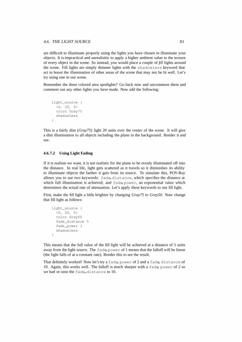
4.6. THE LIGHT SOURCE 83
are difficult to illuminate properly using the lights you have chosen to illuminate yourobjects. It is impractical and unrealisitic to apply a higher ambient value to the textureof every object in the scene. So instead, you would place a couple of fill lights aroundthe scene. Fill lights are simply dimmer lights with the shadowless keyword thatact to boost the illumination of other areas of the scene that may not be lit well. Let’stry using one in our scene.
Remember the three colored area spotlights? Go back now and uncomment them andcomment out any other lights you have made. Now add the following:
light_source {<0, 20, 0>color Gray75shadowless
}
This is a fairly dim (Gray75) light 20 units over the center of the scene. It will givea dim illumination to all objects including the plane in the background. Render it andsee.
4.6.7.2 Using Light Fading
If it is realism we want, it is not realistic for the plane to be evenly illuminated off intothe distance. In real life, light gets scattered as it travels so it diminishes its abilityto illuminate objects the farther it gets from its source. To simulate this, POV-Rayallows you to use two keywords: fade distance, which specifies the distance atwhich full illumination is achieved; and fade power, an exponential value whichdetermines the actual rate of attenuation. Let’s apply these keywords to our fill light.
First, make the fill light a little brighter by changing Gray75 to Gray50. Now changethat fill light as follows:
light_source {<0, 20, 0>color Gray50fade_distance 5fade_power 1shadowless
}
This means that the full value of the fill light will be achieved at a distance of 5 unitsaway from the light source. The fade power of 1 means that the falloff will be linear(the light falls of at a constant rate). Render this to see the result.
That definitely worked! Now let’s try a fade power of 2 and a fade distance of10. Again, this works well. The falloff is much sharper with a fade power of 2 sowe had ot raise the fade distance to 10.

84 CHAPTER 4. BEGINNING TUTORIAL
4.6.7.3 Light Sources and Atmosphere
By definition more than default, light sources are affected by atmosphere, i.e. their lightis scattered by the atmosphere. This can be turned off by adding atmosphere offto the light source block. The light emitted by a light source can also be attenuated bythe atmosphere (and also fog), that is it will be diminished as it travells through it, byadding atmospheric attenuation on. The falloff is exponential and dependeson the distance parameter of the atmosphere (or fog). You should note that thisfeatuer only affects light coming directly from the light source. Reflected and refractedlight is ignored.
Let’s experiment with these keywords. First we must add an atmosphere to our scene:
#include "atmos.inc"
atmosphere { Atmosphere2 }
Then, so the trace will not take as long and the effect will be easier to see, commentout the three lines that turn each of the three spotlights into area lights:
//area_light <1, 0, 0>, <0, 0, 1>, 2, 2//adaptive 1//jitter
Tracing the scene at 200x150 –A we see that indeed the spotlights are visible. We cansee where the blue and red spots cross each other and where the white overhead lightshines down through the center of the scene. We also notice that the spotlights appearto diminish in their intensity as the light descends from the light source to the objects.The red light is all but gone in the lower left part of the scene and the blue light all butgone in the lower right. This is due to the atmospheric attenuation and lends a furtherrealism to the scene. The atmosphere-lightsource interaction gives our scene a smoky,mysterious appearance, but the trace took a long time. Make those spotlights area lightsand it will take even longer. This is an inevitable trade-off — tracing speed for imagequality.
4.7 Simple Texture Options
The pictures rendered so far where somewhat boring regarding the appearance of theobjects. Let’s add some fancy features to the texture.
4.7.1 Surface Finishes
One of the main features of a ray-tracer is its ability to do interesting things with surfacefinishes such as highlights and reflection. Let’s add a nice little phong highlight (shiny
4.7. SIMPLE TEXTURE OPTIONS 85
spot) to the sphere. To do this you need a finish parameter. Change the definitionof the sphere to this:
sphere { <0, 1, 2>, 2texture {
pigment { color Yellow } // pre-defined in COLORS.INCfinish { phong 1 }
}}
Now render this the same way you did before. The phong keyword adds a highlightthe same color of the light shining on the object. It adds a lot of credibility to the pictureand makes the object look smooth and shiny. Lower values of phong will make thehighlight less bright (values should be between 0 and 1).
4.7.2 Adding Bumpiness
The highlight you’ve added illustrates how much of our perception depends on thereflective properties of an object. Ray-tracing can exploit this by playing tricks on ourperception to make us see complex details that aren’t really there.
Suppose you wanted a very bumpy surface on the object. It would be very difficult tomathematically model lots of bumps. We can however simulate the way bumps lookby altering the way light reflects off of the surface. Reflection calculations depend ona vector called a surface normal vector. This is a vector which points away from thesurface and is perpendicular to it. By artificially modifying (or perturbing) this normalvector you can simulate bumps. Change the scene to read as follows and render it:
sphere { <0, 1, 2>, 2texture {
pigment { color Yellow }normal { bumps 0.4 scale 0.2 }finish { phong 1 }
}}
This tells POV-Ray to use a bump pattern to modify the surface normal. The value0.4 controls the apparent depth of the bumps. Usually the bumps are about 1 unit widewhich doesn’t work very well with a sphere of radius 2. The scale makes the bumps1/5th as wide but does not affect their depth.
4.7.3 Creating Color Patterns
You can do more than assign a solid color to an object. You can create complex patternsin the pigment block. Consider this example:

86 CHAPTER 4. BEGINNING TUTORIAL
sphere { <0, 1, 2>, 2texture {
pigment {woodcolor_map {
[0.0 color DarkTan][0.9 color DarkBrown][1.0 color VeryDarkBrown]
}turbulence 0.05scale <0.2, 0.3, 1>
}finish { phong 1 }
}}
The keyword wood specifies a pigment pattern of concentric rings like rings in wood.The color map specifies that the color of the wood should blend from DarkTan toDarkBrown over the first 90% of the vein and from DarkBrown to VeryDarkBrown overthe remaining 10%. The turbulence slightly stirs up the pattern so the veins aren’tperfect circles and the scale factor adjusts the size of the pattern.
Most patterns are set up by default to give you one feature across a sphere of radius1.0. A feature is very roughly defined as a color transition. For example, a woodtexture would have one band on a sphere of radius 1.0. In this example we scalethe pattern using the scale keyword followed by a vector. In this case we scaled0.2 in the x direction, 0.3 in the y direction and the z direction is scaled by 1, whichleaves it unchanged. Scale values larger than one will stretch an element. Scale valuessmaller than one will squish an element. And a scale value of one will leave an elementunchanged.
4.7.4 Pre-defined Textures
POV-Ray has some very sophisticated textures pre-defined in the standard include filesGLASS.INC, METALS.INC, STONES.INC and WOODS.INC. Some are entire textureswith pigment, normal and/or finish parameters already defined. Some are justpigments or just finishes. Change the definition of our sphere to the following and thenre-render it:
sphere { <0, 1, 2>, 2texture {
pigment {DMFWood4 // pre-defined in textures.incscale 4 // Scale by the same amount in all
// directions

4.8. ADVANCED TEXTURE OPTIONS 87
}finish { Shiny } // pre-defined in finish.inc
}}
The pigment identifier DMFWood4 has already been scaled down quite small when itwas defined. For this example we want to scale the pattern larger. Because we want toscale it uniformly we can put a single value after the scale keyword rather than a vectorof x, y, z scale factors.
Look through the file TEXTURES.INC to see what pigments and finishes are definedand try them out. Just insert the name of the new pigment where DMFWood4 is nowor try a different finish in place of Shiny and re-render your file.
Here is an example of using a complete texture identifier rather than just the pieces.
sphere { <0, 1, 2>, 2texture { PinkAlabaster }
}
4.8 Advanced Texture Options
The extremely powerful texturing ability is one thing that really sets POV-Ray apartfrom other raytracers. So far we have not really tried anything too complex but by nowyou should be comfortable enough with the program’s syntax to try some of the moreadvanced texture options.
Obviously, we cannot try them all. It would take a tutorial a lot more pages to useevery texturing option available in POV-Ray. For this limited tutorial, we will contentourselves to just trying a few of them to give you an idea of how textures are created.With a little practice, you will soon be creating beautiful textures of your own.
4.8.1 Pigment and Normal Patterns
Previous versions of POV-Ray made a distinction between pigment and normal pat-terns, i. e. patterns that could be used inside a normal { . . . } or pigment { . . .} statement. With POV-Ray 3.0 this restriction was removed so that all patterns listedin section 7.6.7 on page 318 can be used as a pigment or normal pattern.
4.8.2 Pigments
Every surface must have a color. In POV-Ray, this color is called a pigment. It does nothave to be a single color. It can be a color pattern, a color list, or even an image map.

88 CHAPTER 4. BEGINNING TUTORIAL
Pigments can also be layered one on top of the next so long as the uppermost layers areat least partially transparent so the ones beneath can show through. Let’s play aroundwith some of these kinds of pigments.
Create a file called TEXDEMO.POV and edit it as follows:
#include "colors.inc"
camera {location <1, 1, -7>look_at 0angle 36
}
light_source { <1000, 1000, -1000> White }
plane { y, -1.5pigment { checker Green, White }
}
sphere { <0,0,0>, 1pigment { Red }
}
Giving this file a quick test render at 200x150 -A we see that it is a simple red sphereagainst a green and white checkered plane. We will be using the sphere for our textures.
4.8.2.1 Using Color List Pigments
Before we begin you should note that we have already made one kind of pigment, thecolor list pigment. In the previous example we have used a checkered pattern on ourplane. There are two other kinds of color list pigments, brick and hexagon. Let’squickly try each of these. First, change the plane’s pigment as follows:
pigment { hexagon Green, White, Yellow }
Rendering this we see a three-color hexagonal pattern. Note that this pattern requiresthree colors. Now change the pigment to$ldots
pigment { brick Gray75, Red rotate -90*x scale .25 }
Looking at the resulting image see that the plane now has a brick pattern. Note thatwe had to rotate the pattern to make it appear correctly on the flat plane. This patternnormally is meant to be used on vertical surfaces. We also had to scale the patterndown a bit so we could see it more easily. Feel free to play around with these color listpigments, change the colors, etc. until you get a floor that you like.

4.8. ADVANCED TEXTURE OPTIONS 89
4.8.2.2 Using Pigment and Patterns
Let’s begin texturing our sphere by using a pattern and a color map consisting of threecolors. Replace the pigment block with the following.
pigment {gradient xcolor_map {
[0.00 color Red][0.33 color Blue][0.66 color Yellow][1.00 color Red]
}}
Rendering this we see that it gives us an interesting pattern of vertical stripes. Trychanging the gradient direction to y. The stripes are horizontal now. Try changing thegradient direction to z. The stripes are now more like concentric rings. This is becausethe gradient direction is directly away from the camera. Change the direction back to xand add the following change to the pigment block.
pigment {gradient xcolor_map {
[0.00 color Red][0.33 color Blue][0.66 color Yellow][1.00 color Red]
}rotate -45*z // <- add this line
}
The vertical bars are now slanted at a 45 degree angle. All patterns can be rotated,scaled, and translated in this manner. Let’s now try some different types of patterns.One at a time, substitute the following keywords for gradient x and render to seethe result: bozo, marble, agate, granite, leopard, spotted, and wood (ifyou like you can test all patterns listed in section 7.6.7 on page 318).
Rendering these we see that each results in a slightly different pattern. But to get reallygood results each type of pattern requires the use of some pattern modifiers.
4.8.2.3 Using Pattern Modifiers
Let’s take a look at some pattern modifiers. First, change the pattern type to bozo. Thenadd the following change.

90 CHAPTER 4. BEGINNING TUTORIAL
pigment {bozofrequency 3 // <- add this linecolor_map {
[0.00 color Red][0.33 color Blue][0.66 color Yellow][1.00 color Red]
}rotate -45*z
}
The frequencymodifier determines the number of times the color map repeats itselfper unit of size. This change makes the bozo pattern we saw earlier have many morebands in it. Now change the pattern type to marble. When we rendered this earlier,we saw a banded pattern similar to gradient y that really did not look much likemarble at all. This is because marble really is a kind of gradient and it needs anotherpattern modifier to look like marble. This modifier is called turbulence. Changethe line frequency 3 to turbulence 1 and render again. That’s better! Nowlet’s put frequency 3 back in right after the turbulence and take another look. Evenmore interesting!
But wait, it gets better! Turbulence itself has some modifiers of its own. You can adjustthe turbulence several ways. First, the float that follows the turbulence keywordcan be any value with higher values giving you more turbulence. Second, you can usethe keywords omega, lambda, and octaves to change the turbulence parameters.Let’s try this now:
pigment {marbleturbulence 0.5lambda 1.5omega 0.8octaves 5frequency 3color_map {
[0.00 color Red][0.33 color Blue][0.66 color Yellow][1.00 color Red]
}rotate 45*z
}
Rendering this we see that the turbulence has changed and the pattern looks differ-ent. Go ahead and play around with the numerical values of turbulence, lambda,omega, and octaves to see what they do.

4.8. ADVANCED TEXTURE OPTIONS 91
4.8.2.4 Using Transparent Pigments and Layered Textures
Pigments are described by numerical values that give the rgb value of the color to beused (like color rgb〈1,0,0〉 giving you a red color). But this syntax will give youmore than just the rgb values. You can specify filtering transparency by changing itas follows: color rgbf〈1,0,0,1〉. The f stands for filter, POV-Ray’s word forfiltered transparency. A value of one means that the color is completely transparent,but still filters the light according to what the pigment is. In this case, the color will bea transparent red, like red cellophane.
There is another kind of transparency in POV-Ray. It is called transmittance or non-filtering transparency (the keyword is transmit). It is different from filter in thatit does not filter the light according to the pigment color. It instead allows all the lightto pass through unchanged. It can be specified like this: rgbt〈1,0,0,1〉.
Let’s use some transparent pigments to create another kind of texture, the layered tex-ture. Returning to our previous example, declare the following texture.
#declare LandArea = texture {pigment {
agateturbulence 1lambda 1.5omega .8octaves 8color_map {
[0.00 color rgb <.5, .25, .15>][0.33 color rgb <.1, .5, .4>][0.86 color rgb <.6, .3, .1>][1.00 color rgb <.5, .25, .15>]
}}
}}
This texture will be the land area. Now let’s make the oceans by declaring the follow-ing.
#declare OceanArea = texture {pigment {
bozoturbulence .5lambda 2color_map {
[0.00, 0.33 color rgb <0, 0, 1>color rgb <0, 0, 1>]
[0.33, 0.66 color rgbf <1, 1, 1, 1>color rgbf <1, 1, 1, 1>]

92 CHAPTER 4. BEGINNING TUTORIAL
[0.66, 1.00 color rgb <0, 0, 1>color rgb <0, 0, 1>]
}}
}}
Note how the ocean is the opaque blue area, and the land is the clear area which willallow the underlying texture to show through.
Now, let’s declare one more texture to simulate an atmosphere with swirling clouds.
#declare CloudArea = texture {pigment {
agateturbulence 1lambda 2frequency 2color_map {
[0.0 color rgbf <1, 1, 1, 1>][0.5 color rgbf <1, 1, 1, .35>][1.0 color rgbf <1, 1, 1, 1>]
}}
}
Now apply all of these to our sphere.
sphere { <0,0,0>, 1texture { LandArea }texture { OceanArea }texture { CloudArea }
}
Render this and you’ll have a pretty good rendition of a little planetoid. But it couldbe better. We don’t particularly like the appearance of the clouds. There is a way theycould be done that would be much more realistic.
4.8.2.5 Using Pigment Maps
Pigments may be blended together in the same way as the colors in a color mapusing the same pattern keywords that you can use for pigments. Rather than trying toimpress you with the possible implications of this powerful feature, let’s just give it atry.
Add the following declarations, making sure they appear before the other declarationsin the file.

4.8. ADVANCED TEXTURE OPTIONS 93
#declare Clouds1 = pigment {bozoturbulence 1color_map {
[0.0 color White filter 1][0.5 color White][1.0 color White filter 1]
}}
#declare Clouds2 = pigment {agateturbulence 1color_map {
[0.0 color White filter 1][0.5 color White][1.0 color White filter 1]}
}#declare Clouds3 = pigment {
marbleturbulence 1color_map {
[0.0 color White filter 1][0.5 color White][1.0 color White filter 1]
}}#declare Clouds4 = pigment {
graniteturbulence 1color_map {
[0.0 color White filter 1][0.5 color White][1.0 color White filter 1]
}}
Now use these declared pigments in our cloud layer on our planetoid. Replace thedeclared cloud layer with.
#declare CloudArea = texture {pigment {
gradient ypigment_map {
[0.00 Clouds1][0.25 Clouds2][0.50 Clouds3][0.75 Clouds4]

94 CHAPTER 4. BEGINNING TUTORIAL
[1.00 Clouds1]}
}}
Render this and you’ll see a remarkable pattern that looks very much like weatherpatterns on the planet earth. They are separated into bands, simulating the differentweather types found at different latitudes.
4.8.3 Normals
Objects in POV-Ray have very smooth surfaces. This is not very realistic so there areseveral ways to disturb the smoothness of an object by perturbing the surface normal.The surface normal is the vector that is perpendicular to the angle of the surface. Bychanging this normal the surface can be made to appear bumpy, wrinkled, or any of themany patterns available. Let’s try a couple of them.
4.8.3.1 Using Basic Normal Modifiers
Comment out the planetoid sphere for now and, at the bottom of the file, create a newsphere with a simple, single color texture.
sphere { <0,0,0>, 1pigment { Gray75 }normal { bumps 1 scale .2 }
}
Here we have added a normal block in addition to the pigment block (note thatthese do not have to be included in a texture block unless they need to be trans-formed together or need to be part of a layered texture). Render this to see what itlooks like. Now, one at a time, substitute for the keyword bumps the following key-owrds: dents, wrinkles, ripples, and waves (you can also use any of thepatterns listed in 7.6.7 on page 318). Render each to see what they look like. Playaround with the float value that follows the keyword. Try experimenting with the scalevalue too.
For added interest, change the plane texture to a single color with a normal as follows.
plane { y, -1.5pigment { color rgb <.65, .45, .35> }normal { dents .75 scale .25 }
}

4.8. ADVANCED TEXTURE OPTIONS 95
4.8.3.2 Blending Normals
Normals can be layered similar to pigments but the results can be unexpected. Let’s trythat now by editing the sphere as follows.
sphere { <0,0,0>, 1pigment { Gray75 }
normal { radial frequency 10 }normal { gradient y scale .2 }
}
As you can see, the resulting pattern is neither a radial nor a gradient. It is instead theresult of first calculating a radial pattern and then calculating a gradient pattern. Theresults are simply additive. This can be difficult to control so POV-Ray gives the userother ways to blend normals.
One way is to use normal maps. A normal map works the same way as the pigmentmap we used earlier. Let’s change our sphere texture as follows.
sphere { <0,0,0>, 1pigment { Gray75 }normal {
gradient yfrequency 3turbulence .5normal_map {
[0.00 granite][0.25 spotted turbulence .35][0.50 marble turbulence .5][0.75 bozo turbulence .25][1.00 granite]
}}
}
Rendering this we see that the sphere now has a very irregular bumpy surface. Thegradient pattern type separates the normals into bands but they are turbulated, givingthe surface a chaotic appearance. But this give us an idea.
Suppose we use the same pattern for a normal map that we used to create the oceanson our planetoid and applied it to the land areas. Does it follow that if we use the samepattern and modifiers on a sphere the same size that the shape of the pattern would bethe same? Wouldn’t that make the land areas bumpy while leaving the oceans smooth?Let’s try it. First, let’s render the two spheres side-by-side so we can see if the patternis indeed the same. Un-comment the planetoid sphere and make the following changes.

96 CHAPTER 4. BEGINNING TUTORIAL
sphere { <0,0,0>, 1texture { LandArea }texture { OceanArea }//texture { CloudArea } // <-comment this outtranslate -x // <- add this transformation
}
Now change the gray sphere as follows.
sphere { <0,0,0>, 1pigment { Gray75 }normal {
bozoturbulence .5lambda 2normal_map {
[0.4 dents .15 scale .01][0.6 agate turbulence 1][1.0 dents .15 scale .01]
}}translate x // <- add this transformation
}
Now render this to see if the pattern is the same. We see that indeed it is. So let’scomment out the gray sphere and add the normal block it contains to the land areatexture of our planetoid. Remove the transformations so that the planetoid is centeredin the scene again.
#declare LandArea = texture {pigment {
agateturbulence 1lambda 1.5omega .8octaves 8color_map {
[0.00 color rgb <.5, .25, .15>][0.33 color rgb <.1, .5, .4>][0.86 color rgb <.6, .3, .1>][1.00 color rgb <.5, .25, .15>]
}}normal {
bozoturbulence .5lambda 2

4.8. ADVANCED TEXTURE OPTIONS 97
normal_map {[0.4 dents .15 scale .01][0.6 agate turbulence 1][1.0 dents .15 scale .01]
}}
}
Looking at the resulting image we see that indeed our idea works! The land areas arebumpy while the oceans are smooth. Add the cloud layer back in and our planetoid iscomplete.
There is much more that we did not cover here due to space constraints. On your own,you should take the time to explore slope map, average, and bump map.
4.8.4 Finishes
The final part of a POV-Ray texture is the finish. It controls the properties of the sur-face of an object. It can make it shiny and reflective, or dull and flat. It can alsospecify what happens to light that passes through transparent pigments, what hap-pens to light that is scattered by less-than-perfectly-smooth surfaces, and what hap-pens to light that is reflected by surfaces with thin-film interference properties. Thereare twelve different properties available in POV-Ray to specify the finish of agiven object. These are ambient, diffuse, brilliance, phong, specular,metallic, reflection, refraction, caustics, attenuation, crand,and iridescence. Let’s design a couple of textures that make use of these parame-ters.
4.8.4.1 Using Ambient
Since objects in POV-Ray are illuminated by light sources, the portions of those ob-jects that are in shadow would be completely black were it not for the first two finishproperties, ambient and diffuse. Ambient is used to simulate the light that isscattered around the scene that does not come directly from a light source. Diffuse de-termines how much of the light that is seen comes directly from a light source. Thesetwo keywords work together to control the simulation of ambient light. Let’s use ourgray sphere to demonstrate this. Let’s also change our plane back to its original greenand white checkered pattern.
plane {y,-1.5pigment {checker Green, White}
}
sphere { <0,0,0>, 1pigment {Gray75}finish {

98 CHAPTER 4. BEGINNING TUTORIAL
ambient .2diffuse .6
}
In the above example, the default values for ambient and diffuse are used. Render thisto see what the effect is and then make the following change to the finish.
ambient 0diffuse 0
The sphere is black because we have specified that none of the light coming from anylight source will be reflected by the sphere. Let’s change diffuse back to the defaultof 0.6.
Now we see the gray surface color where the light from the light source falls directlyon the sphere but the shaded side is still absolutely black. Now let’s change diffuseto 0.3 and ambient to 0.3.
The sphere now looks almost flat. This is because we have specified a fairly high degreeof ambient light and only a low amount of the light coming from the light source isdiffusely reflected towards the camera. The default values of ambient and diffuseare pretty good averages and a good starting point. In most cases, an ambient value of0.1 . . .0.2 is sufficient and a diffuse value of 0.5 . . .0.7 will usually do the job. Thereare a couple of exceptions. If you have a completely transparent surface with highrefractive and/or reflective values, low values of both ambient and diffuse may be best.Here is an example.
sphere { <0,0,0>, 1pigment { White filter 1 }
finish {ambient 0diffuse 0reflection .25refraction 1ior 1.33specular 1roughness .001
}}
}
This is glass, obviously. Glass is a material that takes nearly all of its appearancefrom its surroundings. Very little of the surface is seen because it transmits or reflectspractically all of the light that shines on it. See GLASS.INC for some other examples.
If you ever need an object to be completely illuminated independently of the lightingsituation in a given scene, you can do this artificially by specifying an ambient valueof 1 and a diffuse value of 0. This will eliminate all shading and simply give the
4.8. ADVANCED TEXTURE OPTIONS 99
object its fullest and brightest color value at all points. This is good for simulatingobjects that emit light like lightbulbs, and for skies in scenes where the sky may not beadequately lit by any other means.
Let’s try this with our sphere now.
sphere { <0,0,0>, 1pigment { White }
finish {ambient 1diffuse 0
}}
}
Rendering this we get a blinding white sphere with no visible highlights or shadedparts. It would make a pretty good streetlight.
4.8.4.2 Using Surface Highlights
In the glass example above, we noticed that there were bright little hotspots on thesurface. This gave the sphere a hard, shiny appearance. POV-Ray gives you two waysto specify surface specular highlights. The first is called Phong highlighting. Usually,Phong highlights are described using two keywords: phong and phong size. Thefloat that follows phong determines the brightness of the highlight while the floatfollowing phong size determines its size. Let’s try this.
sphere { <0,0,0>, 1pigment { Gray50 }finish {
ambient .2diffuse .6phong .75phong_size 25
}}
Rendering this we see a fairly broad, soft highlight that gives the sphere a kind ofplastic appearance. Now let’s change phong size to 150. This makes a much smallerhighlight which gives the sphere the appearance of being much harder and shinier.
There is another kind of highlight that is calculated by a different means called specu-lar highlighting. It is specified using the keyword specular and operates in conjunc-tion with another keyword called roughness. These two keywords work together inmuch the same way as phong and phong size to create highlights that alter theapparent shininess of the surface. Let’s try using specular in our sphere.

100 CHAPTER 4. BEGINNING TUTORIAL
sphere { <0,0,0>, 1pigment { Gray50 }
finish {ambient .2diffuse .6specular .75roughness .1
}}
}
Looking at th result we see a broad, soft highlight similar to what we had when weused phong size of 25. Change roughness to .001 and render again. Now wesee a small, tight highlight similar to what we had when we used phong size of150. Generally speaking, specular is slightly more accurate and therefore slightly morerealistic than phong but you should try both methods when designing a texture. Thereare even times when both phong and specular may be used on a finish.
4.8.4.3 Using Reflection and Metallic
There is another surface parameter that goes hand in hand with highlights, reflection.Surfaces that are very shiny usually have a degree of reflection to them. Let’s take alook at an example.
sphere { <0,0,0>, 1pigment { Gray50 }
finish {ambient .2diffuse .6specular .75roughness .001reflection .5
}}
}
We see that our sphere now reflects the green and white checkered plane and the blackbackground but the gray color of the sphere seems out of place. This is another timewhen a lower diffuse value is needed. Generally, the higher reflection is the lowerdiffuse should be. Try lowering the diffuse value to 0.3 and the ambient value to0.1 and render again. That is much better. Let’s make our sphere as shiny as a polishedgold ball bearing.
sphere { <0,0,0>, 1pigment { BrightGold }

4.8. ADVANCED TEXTURE OPTIONS 101
finish {ambient .1diffuse .1specular 1roughness .001reflection .75
}}
}
That is very close but there is something wrong with the highlight. To make the sur-face appear more like metal the keyword metallic is used. Add it now to see thedifference.
sphere { <0,0,0>, 1pigment { BrightGold }
finish {ambient .1diffuse .1specular 1roughness .001reflection .75metallic
}}
}
We see that the highlight has taken on the color of the surface rather than the lightsource. This gives the surface a more metallic appearance.
4.8.4.4 Using Refraction
Objects that are transparent allow light to pass through them. With some substances,the light is bent as it traves from one substance into the other because of the differingoptical densities of the objects. This is called refraction. Water and glass both bendlight in this manner so to create water or glass, POV-Ray gives you a way to specifyrefraction. This is done with the keywords refraction and ior. The amount oflight that passes through an object is determined by the value of the filtering and/ortransmittance channel in the pigment. You should use the refraction value only toswitch refraction on or off using vaules of 1 or 0 respectively (or the boolean values onand off). See section 7.6.3.5 on page 299 for a detailed explanation of the reasons.
The degree of refraction, i. e. the amount of bending that occurs, is given by thekeyword ior, short for index of refraction. If you know the index of refraction of thesubstance you are trying to create, you may just use that. For instance, water is 1.33,glass is around 1.45 and diamond is 1.75. Let’s return to the example of a glass spherewe used earlier.

102 CHAPTER 4. BEGINNING TUTORIAL
sphere { <0,0,0>, 1pigment { White filter 1 }
finish {ambient 0diffuse 0reflection .25refraction 1ior 1.45specular 1roughness .001
}}
}
Render this again and notice how the plane that is visible through the sphere is distortedand turned upside-down. This is because the light passing through the sphere is beingbent or refracted to the degree specified. Try reducing ior to 1.25. Try increasing itto 1.75. Notice how the distortion changes.
4.8.4.5 Light Attenuation and Caustics
Transparent objects can be made to cause the intensity of light passing through them tobe reduced. In reality, this is due to impurities in scattering the light. Two float valuesdetermine the effect: fade distance is the distance the light has to travel to reachone-half its original intensity and fade power is the degree of falloff. Let’s try anexample of this.
sphere { <0,0,0>, 1pigment { White filter 1 }
finish {ambient .1diffuse .1reflection .15refraction 1ior 1.45specular 1roughness .001fade_distance 5fade_power 1
}}
This gives the sphere a slightly clouded look as if not all of the light was able to passthrough it. For interesting variations of this texture, try lowering ior to 1.15 andraising reflection to 0.5.

4.8. ADVANCED TEXTURE OPTIONS 103
One thing we do notice is that the shadow of the sphere is still the same old flat grayshadow we have had all along. If there is all this light refraction going on shouldn’tthere be something going on with the shadow as well? That something would be dueto an effect known as caustics. POV-Ray cannot do caustics but it can fake them tosome degree. This is an easy one. Simply add caustics 1 to the finish blockand re-render to see the effect. What we see is a highlight in the shadow that simulatesthe effect of light passing through the sphere and being focused because of the curvedsurface. Remember that this is not real caustics, so changing other finish parameterslike ior will not affect the caustic highlight. The faked caustic is limited to the areashadowed by the corresponding object.
4.8.4.6 Using Iridescence
Iridescence is what you see on the surface of an oil slick when the sun shines on it.The rainbow effect is created by something called thin-film interference (read sec-tion 7.6.3.6 on page 301 for details). For now let’s just try using it. Iridescenceis specified by the irid keyword and three values: amount, thickness andturbulence. The amount is the contribution to the overall surface color. Usually0.1 to 0.5 is sufficient here. The thickness affects the busyness of the effect. Keep thisbetween 0.25 and 1 for best results. The turbulence is a little different from pigment ornormal turbulence. You cannot set octaves, lambda or omega but you can specifyan amount which will affect the thickness in a slightly different way from the thicknessvalue. Values between 0.25 and 1 work best here too. Finally, iridescence will respondto the surface normal since it depends on the angle of incidence of the light rays strikingthe surface. With all of this in mind, let’s add some iridescence our glass sphere.
sphere { <0,0,0>, 1pigment { White filter 1 }
finish {ambient .1diffuse .1reflection .2refraction 1ior 1.5specular 1roughness .001fade_distance 5fade_power 1caustics 1irid {
0.35thickness .5turbulence .5
}}
}

104 CHAPTER 4. BEGINNING TUTORIAL
Try varying the values for amount, thickness and turbulence to see whatchanges they make. Try adding a normal block to see what happens.
4.8.5 Halos
Halos are a powerful feature that can be used to create a lot of different effects likeclouds, fogs, fire, lasers, etc. The name actually comes from the ability to render haloswith it, like the ones seen around the moon or the sun.
Due to the complexity of the halo feature and the large amount of parameters providedit is very difficult to get satisfying results. The following sections will help you tocreate a halo step by step, starting with the basic things and going to the more subtlestuff.
It is also helpful to read the halo reference sections to get a better understanding of thehalo feature. You should especially read the sections 7.5.1 on page 229 and 7.6.4.1 onpage 303 because they are essential for understanding halos.
4.8.5.1 What are Halos?
Halos are a texture feature allowing you to fill the interior of an object with particles.The distribution of these particles can be modified using several density mappings anddensity functions. The particles can emit light to give fire- or laser-like effects or theycan absorb light to create clouds or fog.
A halo is attached to an object, the so called container object, just like a pigment,normal or finish. This object is completely filled by the halo but you won’t see anythingif you do not make sure that the object is hollow and the surface is translucent. Howthis is accomplished will be shown in the next section.
When working with halos you always have to keep in mind that the container objecthas to be hollow and translucent.
4.8.5.2 The Emitting Halo
We start with one of the simpler types, the emitting halo. It uses particles that onlyemit light. There are no particles that absorb the light coming from other particles.
4.8.5.2.1 Starting with a Basic Halo
A clever approach in designing a nice halo effect is to start with a simple, unit-sizedshape that sits on the coordinate system’s origin.
In the first example (HALO01.POV) we try to create a fiery explosion, which the sphereis best suited for. We start with a simple scene consisting of a camera, a light source

4.8. ADVANCED TEXTURE OPTIONS 105
(we don’t care about shadows so we add the shadowless keyword), a checkered planeand a unit-sized sphere containing the halo.
camera {location <0, 0, -2.5>look_at <0, 0, 0>
}
light_source { <10, 10, -10> color rgb 1 shadowless }
plane { z, 2pigment { checker color rgb 0, color rgb 1 }finish { ambient 1 diffuse 0 }scale 0.5hollow
}
sphere { 0, 1pigment { color rgbt <1, 1, 1, 1> }halo {
emittingspherical_mappinglinearcolor_map {
[ 0 color rgbt <1, 0, 0, 1> ][ 1 color rgbt <1, 1, 0, 0> ]
}samples 10
}hollow
}
You’ll note that the sphere is set to be hollow and has a translucent surface (the trans-mittance channel in the pigment color is 1), just like it is required for halos. You’ll alsonote that the plane has a hollow keyword even though it has no halo. Why is thisnecessary?
The reason is quite simple. As described in section 7.5.1 on page 229 there can be nohalo inside any other non-hollow object. Since the camera is inside the plane object,i.e. it is one the side of the plane that is considered be inside, the halo will never bevisible unless the plane is made hollow (or the negative keyword is added to bringthe camera on the outside side of the plane).
What do all those halo keywords and values mean? At the beginning of the halo theemitting keyword is used to specify what type of halo we want to use. The emittinghalo emits light. That’s what’s best suited for our fiery explosion.
The spherical mapping and linear keyword need a more detailed explanationof how a halo work (this is also done in chapter 7.6.4 on page 302 in more detail).
106 CHAPTER 4. BEGINNING TUTORIAL
As noted above the halo is made up of lots of small particles. The distribution of theseparticles is described by a density function. In general, a density function tells us howmuch particles we’ll find at a given location.
Instead of using an explicitly, mathematical density function, halos rely on a given setof density mappings and density functions to model a variety of particle distributions.
The first step in this model is the density mapping function that is used to map three-dimensional points onto a one-dimensional range of values. In our example we use aspherical mapping, i.e. we take the distance of a point from the center of the coordinatesystem. This is the reason why it is clever to start with a container object sitting on thecoordinate system’s center. Since all density mappings are made relative to this centeryou won’t see anything if you start with an object sitting somewhere else. Moving thewhole object (including textures and halos) to another location is the correct way ofplacing a container object.
Now we have a single value in the range from 0 to 1. This value will be transformedusing a density function to get density values instead of distance values. Just usingthis single value won’t work because we want to have particle distributions were thedensity decreases as we move from the middle the container object to the outside.
This is done by the density function. There are several alternatives available as de-scribed in the halo reference (see section 7.6.4.5 on page 308). We use the simplelinear function that just maps values between 0 and 1 onto a 1 to 0 range. Thus we geta density value of 1 at the center of our sphere and a value of 0 at its surface.
Now that we have a density function what do we do to see something? This is wherethe colour map keyword comes into play. It is used to describe a color map thatactually tells the program what colors have to be used for what density. The relation isquite simple: colors at the beginning of the color map (with small values) will be usedfor low density values and colors at the end of the map (high values) will be used forhigh densities. In our example the halo will be yellow at the center of the sphere wherethe density is greatest and it will blend to red at the surface of the sphere where thedensity approaches zero.
The transmittance channel of the colors in the color map is used to model the translu-cency of the density field. A value of 0 represents no translucency, i. e. that areas withthe corresponding density will be (almost) opaque, while a value of 1 means (almost)total translucency.
In our example we use
color_map {[ 0 color rgbt <1, 0, 0, 1> ][ 1 color rgbt <1, 1, 0, 0> ]
}
which results in a halo with a very translucent, reddish outer area and a nearly opaque,yellowish inner areas as you can see after tracing the example image.
4.8. ADVANCED TEXTURE OPTIONS 107
There is one parameter that still needs to be explained: the samples keyword. Thiskeyword tells POV-Ray how many samples along any ray travelling through the halohave to be taken to calculate the halo. Using a low value will result in a high tracingspeed while a high value will lead to a low speed. The sample value has to be increasedif the halo looks somewhat strange, i. e. if some artifacts of the low sampling rateappear. For more details see section 7.6.4.7 on page 310.
A good starting value for the number of samples is 10.
4.8.5.2.2 Increasing the Brightness
The colors of the halo in the above image are somewhat dim. There is too much ofthe background visible through the halo. That does not look much like fire, does it?An easy way to fix this is to decrease the transparency of the particles in the areas ofhigh density. Just use the following color map instead of the old one (the negativetransmittance is correct).
color_map {[ 0 color rgbt <1, 0, 0, 1> ][ 1 color rgbt <1, 1, 0, -1> ]
}
Looking at the result of HALO02.POV we will see that the halo is indeed much brighter.
4.8.5.2.3 Adding Some Turbulence
What we now have does not look like a fiery explosion. It’s more a glowing ball thananything else. Somehow we have to make it look more chaotic, we have to add someturbulence to it.
This is done by using the turbulence keyword together with the amount of turbu-lence we want to add. Just like in the following example.
sphere { 0, 1pigment { color rgbt <1, 1, 1, 1> }halo {
emittingspherical_mappinglinearturbulence 1.5color_map {
[ 0 color rgbt <1, 0, 0, 1> ][ 1 color rgbt <1, 1, 0, -1> ]
}samples 10
}hollow
}

108 CHAPTER 4. BEGINNING TUTORIAL
Adding turbulence to the halo moves all points inside the halo container in a pseudo-random manner. This results in a particle distribution that looks like there was somekind of flow in the halo (depending on the amount of turbulence you’ll get a laminaror turbulent flow). The hight turbulence value is used because an explosion is highlyturbulent.
Looking at the example image (HALO03.POV) you’ll see that this looks more like afiery explosion than the glowing ball we got until now.
You’ll notice that the time it took to render the image increased after we added theturbulence. This is due to the fact that for every sample taken from the halo the slowturbulence function has to be evaluated.
4.8.5.2.4 Resizing the Halo
There is one strange thing about our fiery explosion though. It still looks like a sphere.Why does this happen and what can we do to avoid it?
As noted above adding turbulence moves the particles inside the halo container around.The problem is that some of the particles are actually moved out of the container object.This leads to high densities at the surface of the container object revealing the shape ofthe object (all particles outside the container are lost and will not visible resulting in alarge, highly visible density change at the surface).
An easy way of avoiding this is to make sure that the particles stay inside the containerobject even if we add some turbulence. This is done by scaling the halo to reduce itssize. We do not scale the container object, just the halo.
This is done by adding the scale keyword inside the halo statement.
sphere { 0, 1pigment { color rgbt <1, 1, 1, 1> }halo {
emittingspherical_mappinglinearturbulence 1.5color_map {
[ 0 color rgbt <1, 0, 0, 1> ][ 1 color rgbt <1, 1, 0, -1> ]
}samples 10scale 0.5
}hollowscale 1.5
}
4.8. ADVANCED TEXTURE OPTIONS 109
The scale 0.5 command tells POV-Ray to scale all points inside the halo by thisamount. This effectively scales the radius we get after the density mapping to a rangeof 0 to 0.5 instead of 0 to 1 (without turbulence). If we now add the turbulence thepoints are allowed to move half a unit in every direction without leaving the containerobject. That is excactly what we want.
To compensate for the smaller halo we would get we scale the sphere (and the haloinside) by 1.5.
Looking at the new example image (HALO04.POV) you will no longer see any signsof the container sphere. We finally have a nice fiery explosion.
The amount by which to scale the halo depends on the amount of turbulence you use.The higher the turbulence value the smaller the halo has to be scaled. That is somethingto experiment with.
Another way to avoid that points move out of the sphere is to use a larger sphere, i. e. asphere with a radius larger than one. It is important to resize the sphere before the halois added because otherwise the halo will also be scaled.
You should note that this only works for spherical and box mapping (and a non-constantdensity function). All other mapping types are (partially) infinite, i.e. the resultingparticle distribution covers an infinite space (see also 7.6.4.1 on page 303).
4.8.5.2.5 Using Frequency to Improve Realism
Another very good way of improving the realism of our explosion is to use a frequencyvalue other than one. The way frequency works is explained in section 7.6.4.8.5 onpage 312 in the reference part.
The rather mathematical explanation used there doesn’t help much in understandinghow this feature is used. It is quite simple though. The frequency value just tells theprogram how many times the color map will be repeated in the density range from 0 to1. If a frequency of one (the default) is specified the color map will be visible once inthe density field, e. g. the color at 0 will be used for density 0, color at 0.5 will be usedfor density 0.5 and the color at 1 will be used for density 1. Simple, isn’t it?
If you choose a frequency of two, the color at 0 will be used for density 0, the color at0.5 will be used for density 0.25 and the color at 1 will be used for density 0.5. Whatabout the densities above 0.5? Since there are no entries in the color map for valuesabove 1 we just start at 0 again. Thus the color at 0.1 will be used for density 0.55((2×0.55) mod 1 = 1.1 mod 1 = 0.1), the color at 0.5 will be used for density 0.75and the color at 1 will be used for density 1.
If you are good at mathematics you’ll note that the above example is not quite rightbecause (1 ∗2) mod 1 = 0 and not 1. Just think that we used a value slightly smallerthan one and everything will be fine.

110 CHAPTER 4. BEGINNING TUTORIAL
You may have noticed that in order to avoid sudden changes in the halo color for fre-quencies larger than one you’ll have to used a periodic color map, i.e. a color mapwhose entries at 0 and 1 are the same.
We’ll change our example by using a periodic color map and changing the frequencyvalue to two.
sphere { 0, 1pigment { color rgbt <1, 1, 1, 1> }halo {
emittingspherical_mappinglinearturbulence 1.5color_map {
[ 0.0 color rgbt <1, 0, 0, 1> ][ 0.5 color rgbt <1, 1, 0, -1> ][ 1.0 color rgbt <1, 0, 0, 1> ]
}frequency 2samples 20scale 0.5
}hollowscale 1.5
}
Looking at the result of (HALO05.POV) we can be quite satisfied with the explosionwe just have created, can’t we?
There’s one thing left you should be aware of when increasing the frequency value. Itis often necessary to increase the sample rate in (nearly) the same way as you changethe frequency. If you don’t do this you’ll probably get some severe aliasing artefacts(like color jumps or strange bands of colors). If this happens just change the samplesvalue according to the frequency value (twice sampling rate for a doubled frequency).
4.8.5.2.6 Changing the Halo Color
We have a nice fiery explosion but we want to try to add some science fiction touch toit by using different colors. How about a nice green, less turbulent explosion that getsred at its borders?
Nothing easier than that!
sphere { 0, 1.5pigment { color rgbt <1, 1, 1, 1> }halo {

4.8. ADVANCED TEXTURE OPTIONS 111
emittingspherical_mappinglinearturbulence 0.5color_map {
[ 0 color rgbt <0, 1, 0, 1> ][ 1 color rgbt <1, 0, 0, -1> ]
}samples 10scale 0.75
}hollowscale 1.5
}
This should do the trick. Looking at the result of HALO06.POV you may be disap-pointed. Where is the red center of the explosion? The borders are green as expectedbut there is a lot of yellow in the center and only a little bit red. What is happening?
We use an emitting halo in our example. According to the corresponding section inthe halo reference chapter (see 7.6.4.3.3 on page 306) this type of halo uses very smallparticles that do not attenuate light passing through the halo. Especially particles nearthe viewer do not attenuate the light coming from particles far away from the viewer.
During the calculation of the halo’s color near the center of the container sphere, theray steps through nearly all possible densities of the particle distribution. Thus we getred and green colors as we march on, depending on the current position in the halo.The sum of these colors is used which will gives as a yellow color (the sum of red andgreen is yellow). This is what is happening here.
How can we still get what we want? The answer is to use a glowing halo instead ofthe emitting halo. The glowing halo is very similar to the emitting one except thatit attenuates the light passing through. Thus the light of particles lying behind otherparticles will be attenuated by the particles in front.
For the results of the glowing halo see 4.8.5.3.
4.8.5.3 The Glowing Halo
We have mentioned the glowing halo in the section about the emitting halo as one wayto avoid the color mixing that is happening with emitting halos.
The gowing halo is very similar to the emitting halo except that it also absorbs light.You can view it as a combination of the emitting and the attenuating halo described insection 4.8.5.4 on the following page.
By just replacing the emitting keyword in the example in section 4.8.5.2.6 on thepreceding page with the glowing keyword we get the desired effect as shown in theexample image (HALO11.POV).

112 CHAPTER 4. BEGINNING TUTORIAL
Even though the red color of the high density areas is not very visible because the greencolored, lower density areas lying in front absorb most of the red light, you don’t getyellow color where you would have expected a red one.
Due to its similarity with the emitting halo we leave it up to you to make some exper-iments with this halo type. You just have to keep all those things you learned in theprevious sections in mind to get some satisfying results.
4.8.5.4 The Attenuating Halo
Another simple halo type is the attenuating halo that only absorbs light. It doesn’tradiate on its own.
A great difference between the attenuating halo and the other halo types is that the colorof the attenuating halo is calculated from the halo’s color map using the total particledensity along a given ray. The other types calculated a (weighted) average of the colorscalculated from the density at each sample.
4.8.5.4.1 Making a Cloud
Attenuating halos are ideal to create clouds and smoke. In the following examples wewill try to make a neat little cloud. We start again by using a unit-sized sphere that isfilled with a basic attenuating halo (HALO21.POV).
camera {location <0, 0, -2.5>look_at <0, 0, 0>
}
light_source { <10, 10, -10> color rgb 1 shadowless }
plane { z, 2pigment { checker color rgb 0, color rgb 1 }finish { ambient 1 diffuse 0 }scale 0.5hollow
}
sphere { 0, 1pigment { color rgbt <1, 1, 1, 1> }halo {
attenuatingspherical_mappinglinearcolor_map {
[ 0 color rgbt <1, 0, 0, 1> ]
4.8. ADVANCED TEXTURE OPTIONS 113
[ 1 color rgbt <1, 0, 0, 0> ]}samples 10
}hollow
}
Even though clouds normally are not red but white or gray, we use the red color tomake it more visible against the black/white checkerboard background.
The color of an attenuating halo is calculated from the total accumulated density aftera ray has marched through the complete particle field. This has to be kept in mindwhen creating the color map. We want the areas of the cloud with a low density to havea high translucency so we use a color of rgbt〈1,0,0,1〉 and we want the high densityareas to be opaque so we choose a color of rgbt〈1,0,0,0〉.
4.8.5.4.2 Scaling the Halo Container
The cloud we have created so far doesn’t look very realistic. It’s just a red, partiallytranslucent ball. In order to get a better result we use some of the methods we havealready learned in the sections about emitting halos above. We add some turbulenceto get a more realistic shape, we scale the halo to avoid the container object’s surfaceto become visible and we decrease the translucency of the areas with a high particledensity.
Another idea is to scale the container object to get an ellipsoid shape that can be usedto model a cloud pretty good. This is done by the scale 〈1.5,0.75,1〉 command atthe end of the sphere. It scales both, the sphere and the halo inside.
sphere { 0, 1pigment { color rgbt <1, 1, 1, 1> }halo {
attenuatingspherical_mappinglinearturbulence 1color_map {
[ 0 color rgbt <1, 0, 0, 1> ][ 1 color rgbt <1, 0, 0, -1> ]
}samples 10scale 0.75
}hollowscale <1.5, 0.75, 1>
}
114 CHAPTER 4. BEGINNING TUTORIAL
Looking at the results of HALO22.POV you’ll see that this looks more like a real cloud(besides the color).
4.8.5.4.3 Adding Additional Halos
Another trick to get some more realism is to use multiple halos. If you look at cumulusclouds e. g. you’ll notice that they often extend at the top while they are quite flat atthe bottom.
We want to model this appearance by adding two additional halos to our current con-tainer object (see section 7.6.4.2 on page 304 for more details). This is done in thefollowing way:
sphere { 0, 1.5pigment { color rgbt <1, 1, 1, 1> }halo {
attenuatingspherical_mappinglinearturbulence 1color_map {
[ 0 color rgbt <1, 0, 0, 1> ][ 1 color rgbt <1, 0, 0, -1> ]
}samples 10scale <0.75, 0.5, 1>translate <-0.4, 0, 0>
}halo {
attenuatingspherical_mappinglinearturbulence 1color_map {
[ 0 color rgbt <1, 0, 0, 1> ][ 1 color rgbt <1, 0, 0, -1> ]
}samples 10scale <0.75, 0.5, 1>translate <0.4, 0, 0>
}halo {
attenuatingspherical_mappinglinearturbulence 1color_map {
[ 0 color rgbt <1, 0, 0, 1> ]
4.8. ADVANCED TEXTURE OPTIONS 115
[ 1 color rgbt <1, 0, 0, -1> ]}samples 10scale 0.5translate <0, 0.2, 0>
}hollow
}
The three halos used differ only in their location, i. e. in the translation vector we haveused. The first two halos are used to form the base of the cloud while the last sits on topof the others. The sphere has a different radius than the previous ones because morespace is needed for all three halos.
The result of HALO23.POV somehwat looks like a cloud, even though it may needsome work.
4.8.5.5 The Dust Halo
The dust halo is a very complex halo type. It allows you to see the interaction of lightcoming from light sources with the particles in the halo. Those particles do absorblight like the attenuating halo. In addition they scatter light coming from light sourcespassing through them. This makes beams of light and shadows cast by objects onto thehalo become visible.
4.8.5.5.1 Starting With an Object Lit by a Spotlight
We start with a box shaped object that is lit by a spotlight. We don’t use any halo atthis moment because we want to see if the object is completely lit by the light source(HALO31.POV).
camera {location <0, 0, -2.5>look_at <0, 0, 0>
}
background { color rgb <0.2, 0.4, 0.8> }
light_source {<2.5, 2.5, -2.5>colour rgb <1, 1, 1>spotlightpoint_at <0, 0, 0>radius 12falloff 15tightness 1

116 CHAPTER 4. BEGINNING TUTORIAL
}
difference {box { -1, 1 }box { <-1.1, -0.8, -0.8>, <1.1, 0.8, 0.8> }box { <-0.8, -1.1, -0.8>, <0.8, 1.1, 0.8> }box { <-0.8, -0.8, -1.1>, <0.8, 0.8, 1.1> }pigment { color rgb <1, 0.2, 0.2> }scale 0.5rotate 45*yrotate 45*x
}
As you see the whole object is lit by the light source. Now we can start to add somedust.
4.8.5.5.2 Adding Some Dust
We use a box to contain the dust halo. Since we use a constant density function itdoesn’t matter what kind of density mapping is used. The density has the value speci-fied by the max value keyword everywhere inside the halo (the default value is one).The isotropic scattering is selected with dust type .
box { -1, 1pigment { colour rgbt <1, 1, 1, 1> }halo {
dustdust_type 1box_mappingconstantcolour_map {
[ 0 color rgbt <1, 1, 1, 1> ][ 1 color rgbt <1, 1, 1, 0> ]
}samples 10
}hollowscale 5
}
The result of HALO32.POV is too bright. The dust is too thick and we can only seesome parts of the object and no background.
4.8.5.5.3 Decreasing the Dust Density
The density inside the halo has the constant value one. This means that only the colormap entry at position one is used to determine the density and color of the dust.
4.8. ADVANCED TEXTURE OPTIONS 117
We use a transmittance value of 0.7 to get a much thinner dust.
box { -1, 1pigment { colour rgbt <1, 1, 1, 1> }halo {
dustdust_type 1box_mappingconstantcolour_map {
[ 0 color rgbt <1, 1, 1, 1.0> ][ 1 color rgbt <1, 1, 1, 0.7> ]
}samples 10
}hollowscale 5
}
Beside the ugly aliasing artefacts the image looks much better. We can see the wholeobject and even the background is slightly visible (HALO33.POV).
4.8.5.5.4 Making the Shadows Look Good
In order to reduce the aliasing artefacts we use three different techniques: jittering,super-sampling and an increased overall sampling rate.
The jittering is used to add some randomness to the sampling points making the imagelook more noisy. This helps because the regular aliasing artefacts are more annoyingthan noise. A low jitter value is a good choice.
The super-sampling tries to detect fine features by taking additional samples in ar-eas of high intensity changes. The threshold at which super-sampling is used and themaximum recursion level can be specified using the aa threshold and aa levelkeywords.
The approach that always works is to increase the overall sampling rate. Since this isalso the slowest method you should always try to use the other methods first. If theydon’t suffice you’ll have to increase the sampling rate.
We use the following halo to reduce the aliasing artefacts (HALO34.POV).
box { -1, 1pigment { colour rgbt <1, 1, 1, 1> }halo {
dustdust_type 1
118 CHAPTER 4. BEGINNING TUTORIAL
box_mappingconstantcolour_map {
[ 0 color rgbt <1, 1, 1, 1.0> ][ 1 color rgbt <1, 1, 1, 0.7> ]
}samples 50aa_level 3aa_threshold 0.2jitter 0.1
}hollowscale 5
}
The image looks much better now. There are hardly any aliasing artefacts left.
The same parameters we have used are discussed in the section about the atmospherefeature (see 4.9.4 on page 131 for further explanations).
4.8.5.5.5 Adding Turbulence
The major difference between the halo’s dust and the atmosphere described in 4.9.4 onpage 131 is the ability to choose a non-uniform particle distribution for the dust. Thisincludes the fact that the halo is limited to a container object as well as the differentdensity mappings and functions.
Another interesting way of getting an irregular disribution is to add some turbulenceto the dust. This is done with the turbulence keyword followed by the amount ofturbulence to use, like the following example shows (HALO35.POV).
box { -1, 1pigment { colour rgbt <1, 1, 1, 1> }halo {
dustdust_type 1box_mappinglinearturbulence 1colour_map {
[ 0 color rgbt <1, 1, 1, 1.0> ][ 1 color rgbt <1, 1, 1, 0.5> ]
}samples 50aa_level 3aa_threshold 0.2jitter 0.1
}

4.8. ADVANCED TEXTURE OPTIONS 119
hollowscale 5
}
The image we now get looks much more interesting due to the shifts in the particledensity.
You should note that we use a linear density function instead of the previous constantone. This is necessary because with a constant density function the density has thesame value everywhere. Adding turbulence would have no effect because wherever thepoints are moved the density will have this same value. Only a non-constant densitydistribution makes sense when turbulence is added.
The fact that the turbulence value is actually a vector can be used to create effects likewaterfalls by using a large turbulence value in on direction only (e.g. turbulence〈0.2,1,0.2〉 ).
4.8.5.5.6 Using a Coloured Dust
If you want to create a colored dust you can easily do this by using a non-white color inthe halo’s color map. In this case you’ll also have to set the filter channels in the colormap to non-zero values to specify the amount of light that will be filtered by the dust’scolor.
Use the following color map to get a partially filtering, red dust for example:
colour_map {[ 0 color rgbft <1, 0, 0, 0.5, 1.0> ][ 1 color rgbft <1, 0, 0, 0.5, 0.7> ]
}
4.8.5.6 Halo Pitfalls
Due to the complexity of the halo feature and the few experiences people have madeso far there are a lot of things still to discover.
Some of the most common problems and pitfalls are described below in order to helpyou to avoid the most common problems.
4.8.5.6.1 Where Halos are Allowed
As mentioned above a halo completly fills the interior of an object. Keeping this inmind it is reasonable that the following example does not make sense.

120 CHAPTER 4. BEGINNING TUTORIAL
sphere { 0, 1pigment {
checkertexture {
pigment { color Clear }halo { ... }
}texture {
pigment { color Red }}
}hollow
}
What’s wrong with this example? It’s simply that a halo is used to describe the interiorof an object and that you cannot describe this interior by describing how the surface ofthe object looks like. But that’s what was done in the example above. Can you imaginewhat the interior of the sphere will look like? Will it be filled completey with the halo?Will there be areas filled by the halo and some filled by air? How will those areas looklike?
You won’t be able to tell the interior’s properties from looking at the surface. It’s justnot possible. This should always be kept in mind.
If the above example was meant to create a sphere filled with a halo and covered witha checker board pattern that partially hid the halo you would have used the followingsyntax:
sphere { 0, 1pigment {
checkertexture {
pigment { color Clear }}texture {
pigment { color Red }}
}halo { ... }hollow
}
A halo is always applied to an object in the following way:
OBJECT {texture {

4.8. ADVANCED TEXTURE OPTIONS 121
pigment { ... }normal { ... }finish { ... }halo { ... }
}hollow
}
There’s no halo allowed inside any pigment statement, color map, pigment map, texturemap, material map, or whatever. You are not hindered to do this but you will not getwhat you want.
You can use a halo with a layered textures as long as you make sure that the halos areonly attached to the lowest layer (this layer has to be partially transparent to see thehalo of course).
4.8.5.6.2 Overlapping Container Objects
POV-Ray is not able to handle overlapping container objects correctly. If you createtwo overlapping spheres that contain a halo you won’t get correct results where thespheres overlap. The halo effect is calculated independently for each sphere and theresults are added.
If you want to add different halos you have to put all halos inside a single containerobject to make sure the halo is calculated correctly (see also 7.6.4.2 on page 304).
You should also note non-overlapping, stacked halo containers are handled correctly.If you put a container object in front of another container object the halos are renderedcorrectly.
4.8.5.6.3 Multiple Attenuating Halos
It is currently not possible to use mutliple attenuating halos with different color maps.The color map of the last halo will be used for all halos in the container object.
4.8.5.6.4 Halos and Hollow Objects
In order to correctly render halo effects you have to make sure that all objects thecamera is inside are hollow. This is done by adding the hollow keyword.
For a detailed explanation see 7.5.1 on page 229.
4.8.5.6.5 Scaling a Halo Container
If you scale a halo container object you should keep in mind that it makes a greatdifference where you place the scale keyword.
122 CHAPTER 4. BEGINNING TUTORIAL
Scaling the object before the halo statement will only scale the container object not thehalo. This is useful if you want to avoid that the surface of the container object becomesvisible due to the use of turbulence. As you’ve learned in the sections above particlesmay move out of the container object — where they are invisible — if turbulenceis added. This only works for spherical and box mapping because the density fieldsdescribed by the other mapping types don’t have finite dimensions.
If the scale keyword is used after the halo statement both, the halo and the containerobject, are scaled. This is useful to scale the halo to your needs.
The halo keeps its appearance regardless of the transformations applied to the containerobject (after the halo), i.e. the halo’s translucency, color and turbulence characteristicswill not change.
4.8.5.6.6 Choosing a Sampling Rate
Normally you’ll start with a low sampling rate and you’ll only increase it if any aliasingartefacts turn up (and don’t vanish by using super-sampling and jittering).
The halo’s appearance is independent from the sampling rate as long as there areenough samples to get a good estimate of what the halo really looks like. This meansthat one or two samples are hardly ever enough to determine the halo’s appearance. Asyou increase the number of samples the halo will quickly approach its real appearance.
To put it in a nutshell, the halo will not change its appearance with the sample rate aslong as you have a sufficient number of samples and no aliasing artefacts occur.
4.8.5.6.7 Using Turbulence
As noted in one of the above sections turbulence will have no effect if the constantdensity function is used (keyword constant). It doesn’t matter how much or whereyou move a point if the density is constant and thus does not depend on the pointslocation. You’ll get the same density value for all location.
Whenever you add turbulence to a halo do not use the constant density function.
4.9 Using Atmospheric Effects
POV-Ray offers a variety of atmospheric effects, i. e. features that affect the back-ground of the scene or the air by which everything is surrounded.
It is easy to assign a simple color or a complex color pattern to a virtual sky sphere.You can create anything from a cloud free, blue summer sky to a stormy, heavy cloudedsky. Even starfields can easily be created.

4.9. USING ATMOSPHERIC EFFECTS 123
You can use different kinds of fog to create foggy scenes. Multiple fog layers of differ-ent colors can add an eerie touch to your scene.
A much more realistic effect can be created by using an atmosphere, a constant fog thatinteracts with the light coming from light sources. Beams of light become visible andobjects will cast shadows into the fog.
Last but not least you can add a rainbow to your scene.
4.9.1 The Background
The background feature is used to assign a color to all rays that don’t hit any object.This is done in the following way.
camera {location <0, 0, -10>look_at <0, 0, 0>
}
background { color rgb <0.2, 0.2, 0.3> }
sphere { 0, 1pigment { color rgb <0.8, 0.5, 0.2> }
}
The background color will be visible if a sky sphere is used and if some translucencyremains after all sky sphere pigment layers are processed.
4.9.2 The Sky Sphere
The sky sphere can be used to easily create a cloud covered sky, a nightly star sky orwhatever sky you have in mind.
In the following examples we’ll start with a very simple sky sphere that will get moreand more complex as we add new features to it.
4.9.2.1 Creating a Sky with a Color Gradient
Beside the single color sky sphere that is covered with the background feature thesimplest sky sphere is a color gradient.
You may have noticed that the color of the sky varies with the angle to the earth’ssurface normal. If you look straight up the sky normally has a much deeper blue thanit has at the horizon.
We want to model this effect using the sky sphere as shown in the scene below(SKYSPH1.POV).
124 CHAPTER 4. BEGINNING TUTORIAL
#include "colors.inc"
camera {location <0, 1, -4>look_at <0, 2, 0>angle 82
}
light_source { <10, 10, -10> White }
sphere { 2*y, 1pigment { color rgb <1, 1, 1> }finish { ambient 0.2 diffuse 0 reflection 0.6 }
}
sky_sphere {pigment {
gradient ycolor_map {
[0 color Red][1 color Blue]
}scale 2translate -1
}}
The interesting part is the sky sphere statement. It contains a pigment that describethe look of the sky sphere. We want to create a color gradient along the viewing anglemeasured against the earth’s surface normal. Since the ray direction vector is used tocalculate the pigment colors we have to use the y-gradient.
The scale and translate transformation are used to map the points derived from thedirection vector to the right range. Without those transformations the pattern would berepeated twice on the sky sphere. The scale statement is used to avoid the repetitionand the translate -1 statement moves the color at index zero to the bottom of thesky sphere (that’s the point of the sky sphere you’ll see if you look straight down).
After this transformation the color entry at position 0 will be at the bottom of the skysphere, i. e. below us, and the color at position 1 will be at the top, i. e. above us.
The colors for all other positions are interpolated between those two colors as you cansee in the resulting image.
If you want to start one of the colors at a specific angle you’ll first have to convert theangle to a color map index. This is done by using the formula
color map index =1−cos(angle)
2(4.1)
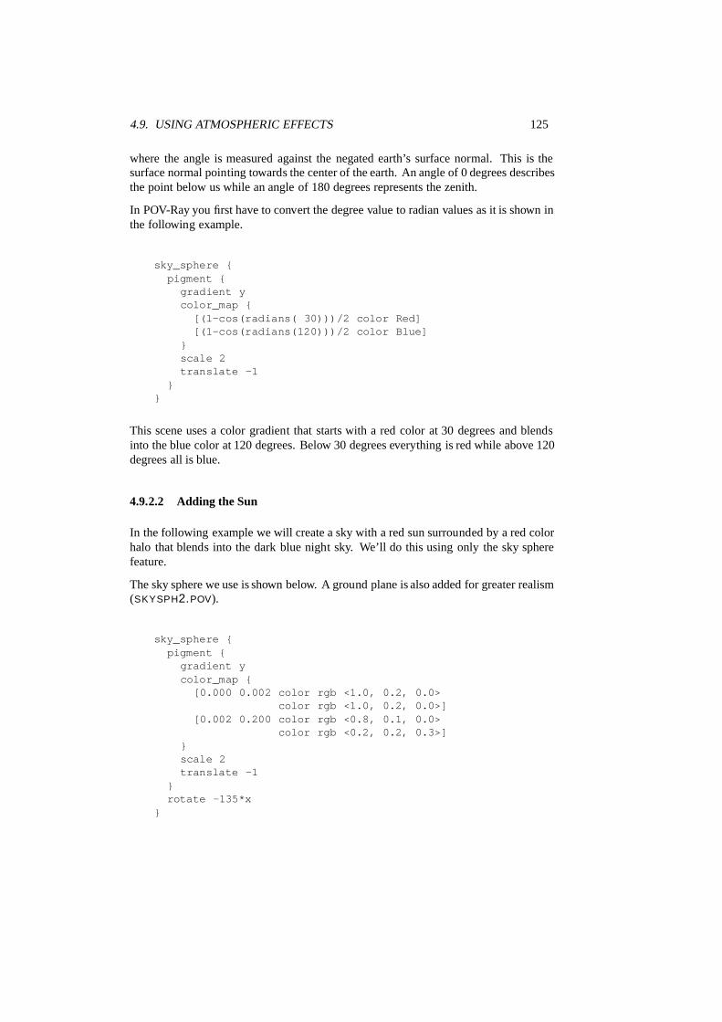
4.9. USING ATMOSPHERIC EFFECTS 125
where the angle is measured against the negated earth’s surface normal. This is thesurface normal pointing towards the center of the earth. An angle of 0 degrees describesthe point below us while an angle of 180 degrees represents the zenith.
In POV-Ray you first have to convert the degree value to radian values as it is shown inthe following example.
sky_sphere {pigment {
gradient ycolor_map {
[(1-cos(radians( 30)))/2 color Red][(1-cos(radians(120)))/2 color Blue]
}scale 2translate -1
}}
This scene uses a color gradient that starts with a red color at 30 degrees and blendsinto the blue color at 120 degrees. Below 30 degrees everything is red while above 120degrees all is blue.
4.9.2.2 Adding the Sun
In the following example we will create a sky with a red sun surrounded by a red colorhalo that blends into the dark blue night sky. We’ll do this using only the sky spherefeature.
The sky sphere we use is shown below. A ground plane is also added for greater realism(SKYSPH2.POV).
sky_sphere {pigment {
gradient ycolor_map {
[0.000 0.002 color rgb <1.0, 0.2, 0.0>color rgb <1.0, 0.2, 0.0>]
[0.002 0.200 color rgb <0.8, 0.1, 0.0>color rgb <0.2, 0.2, 0.3>]
}scale 2translate -1
}rotate -135*x
}
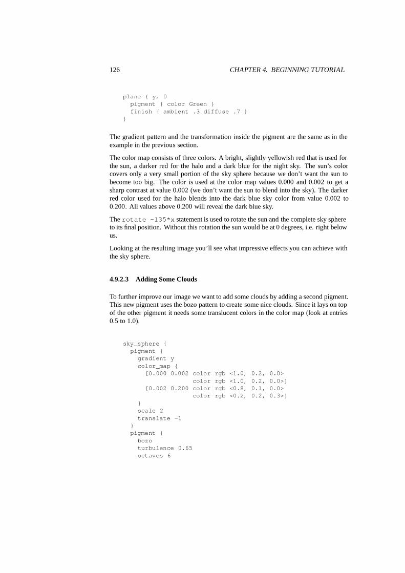
126 CHAPTER 4. BEGINNING TUTORIAL
plane { y, 0pigment { color Green }finish { ambient .3 diffuse .7 }
}
The gradient pattern and the transformation inside the pigment are the same as in theexample in the previous section.
The color map consists of three colors. A bright, slightly yellowish red that is used forthe sun, a darker red for the halo and a dark blue for the night sky. The sun’s colorcovers only a very small portion of the sky sphere because we don’t want the sun tobecome too big. The color is used at the color map values 0.000 and 0.002 to get asharp contrast at value 0.002 (we don’t want the sun to blend into the sky). The darkerred color used for the halo blends into the dark blue sky color from value 0.002 to0.200. All values above 0.200 will reveal the dark blue sky.
The rotate -135*x statement is used to rotate the sun and the complete sky sphereto its final position. Without this rotation the sun would be at 0 degrees, i.e. right belowus.
Looking at the resulting image you’ll see what impressive effects you can achieve withthe sky sphere.
4.9.2.3 Adding Some Clouds
To further improve our image we want to add some clouds by adding a second pigment.This new pigment uses the bozo pattern to create some nice clouds. Since it lays on topof the other pigment it needs some translucent colors in the color map (look at entries0.5 to 1.0).
sky_sphere {pigment {
gradient ycolor_map {
[0.000 0.002 color rgb <1.0, 0.2, 0.0>color rgb <1.0, 0.2, 0.0>]
[0.002 0.200 color rgb <0.8, 0.1, 0.0>color rgb <0.2, 0.2, 0.3>]
}scale 2translate -1
}pigment {
bozoturbulence 0.65octaves 6
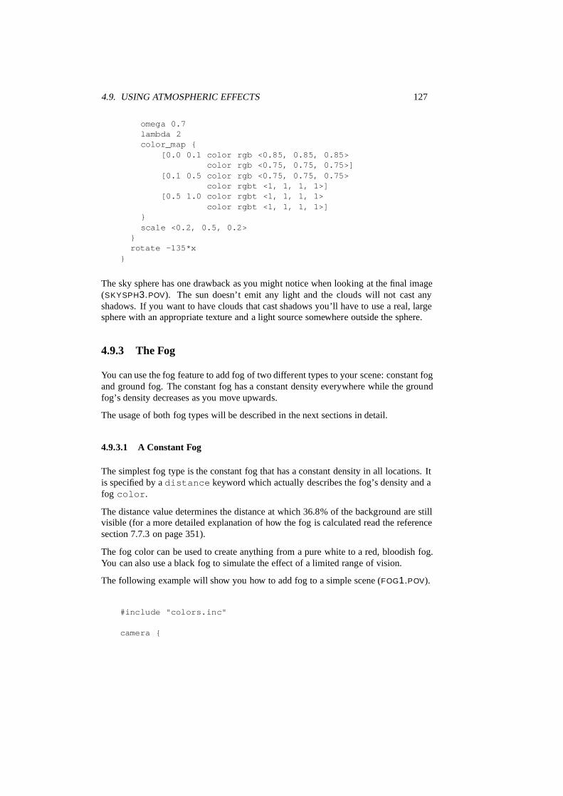
4.9. USING ATMOSPHERIC EFFECTS 127
omega 0.7lambda 2color_map {
[0.0 0.1 color rgb <0.85, 0.85, 0.85>color rgb <0.75, 0.75, 0.75>]
[0.1 0.5 color rgb <0.75, 0.75, 0.75>color rgbt <1, 1, 1, 1>]
[0.5 1.0 color rgbt <1, 1, 1, 1>color rgbt <1, 1, 1, 1>]
}scale <0.2, 0.5, 0.2>
}rotate -135*x
}
The sky sphere has one drawback as you might notice when looking at the final image(SKYSPH3.POV). The sun doesn’t emit any light and the clouds will not cast anyshadows. If you want to have clouds that cast shadows you’ll have to use a real, largesphere with an appropriate texture and a light source somewhere outside the sphere.
4.9.3 The Fog
You can use the fog feature to add fog of two different types to your scene: constant fogand ground fog. The constant fog has a constant density everywhere while the groundfog’s density decreases as you move upwards.
The usage of both fog types will be described in the next sections in detail.
4.9.3.1 A Constant Fog
The simplest fog type is the constant fog that has a constant density in all locations. Itis specified by a distance keyword which actually describes the fog’s density and afog color.
The distance value determines the distance at which 36.8% of the background are stillvisible (for a more detailed explanation of how the fog is calculated read the referencesection 7.7.3 on page 351).
The fog color can be used to create anything from a pure white to a red, bloodish fog.You can also use a black fog to simulate the effect of a limited range of vision.
The following example will show you how to add fog to a simple scene (FOG1.POV).
#include "colors.inc"
camera {

128 CHAPTER 4. BEGINNING TUTORIAL
location <0, 20, -100>}
background { colour SkyBlue }
plane { y, -10pigment {
checker colour Yellow colour Greenscale 20
}}
sphere { <0, 25, 0>, 40pigment { Red }finish { phong 1.0 phong_size 20 }
}
sphere { <-100, 150, 200>, 20pigment { Green }finish { phong 1.0 phong_size 20 }
}
sphere { <100, 25, 100>, 30pigment { Blue }finish { phong 1.0 phong_size 20 }
}
light_source { <100, 120, 40> colour White}
fog {distance 150colour rgb<0.3, 0.5, 0.2>
}
According to their distance the spheres in this scene more or less vanish in the greenishfog we used, as does the checkerboard plane.
4.9.3.2 Setting a Minimum Translucency
If you want to make sure that the background does not completely vanish in the fogyou can set the transmittance channel of the fog’s color to the amount of backgroundyou always want to be visible.
Using as transmittance value of 0.2 as in
fog {distance 150colour rgbt<0.3, 0.5, 0.2, 0.2>

4.9. USING ATMOSPHERIC EFFECTS 129
}
the fog’s translucency never drops below 20% as you can see in the resulting image(FOG2.POV).
4.9.3.3 Creating a Filtering Fog
The greenish fog we have used so far doesn’t filter the light passing through it. All itdoes is to diminish the light’s intensity. We can change this by using a non-zero filterchannel in the fog’s color (FOG3.POV).
fog {distance 150colour rgbf<0.3, 0.5, 0.2, 1.0>
}
The filter value determines the amount of light that is filtered by the fog. In our example100% of the light passing through the fog will be filtered by the fog. If we had used avalue of 0.7 only 70% of the light would have been filtered. The remaining 30% wouldhave passed unfiltered.
You’ll notice that the intensity of the objects in the fog is not only diminished due to thefog’s color but that the colors are actually influenced by the fog. The red and especiallythe blue sphere got a green hue.
4.9.3.4 Adding Some Turbulence to the Fog
In order to make our somewhat boring fog a little bit more interesting we can add someturbulence, making it look like it had a non-constant density (FOG4.POV).
fog {distance 150colour rgbf<0.3, 0.5, 0.2, 1.0>turbulence 0.2turb_depth 0.3
}
The tubulence keyword is used to specify the amount of turbulence used while theturb depth value is used to move the point at which the turbulence value is calcu-lated along the viewing ray. Values near zero move the point to the viewer while valuesnear one move it to the intersection point (the default value is 0.5). This parameter canbe used to avoid noise that may appear in the fog due to the turbulence (this normallyhappens at very far away intersecion points, especially if no intersection occurs, i. e.

130 CHAPTER 4. BEGINNING TUTORIAL
the background is hit). If this happens just lower the turb depth value until thenoise vanishes.
You should keep in mind that the actual density of the fog does not change. Only thedistance-based attenuation value of the fog is modified by the turbulence value at apoint along the viewing ray.
4.9.3.5 Using Ground Fog
The much more interesting and flexible fog type is the ground fog, which is selectedwith the fog type statement. It’s appearance is described with the fog offsetand fog alt keywords. The fog offset specifies the height, i. e. y value, belowwhich the fog has a constant density of one. The fog alt keyword determines howfast the density of the fog will approach zero as one moves along the y axis. At a heightof f og o f f set+ f og alt the fog will have a density of 25%.
The following example (FOG5.POV) uses a ground fog which has a constant densitybelow y= 25 (the center of the red sphere) and quickly falls off for increasing altitudes.
fog {distance 150colour rgbf<0.3, 0.5, 0.2, 1.0>fog_type 2fog_offset 25fog_alt 1
}
4.9.3.6 Using Multiple Layers of Fog
It is possible to use several layers of fog by using more than one fog statement in yourscene file. This is quite useful if you want to get nice effects using turbulent groundfogs. You could add up several, differently colored fogs to create an eerie scene forexample.
Just try the following example (FOG6.POV).
fog {distance 150colour rgb<0.3, 0.5, 0.2>fog_type 2fog_offset 25fog_alt 1turbulence 0.1turb_depth 0.2
}
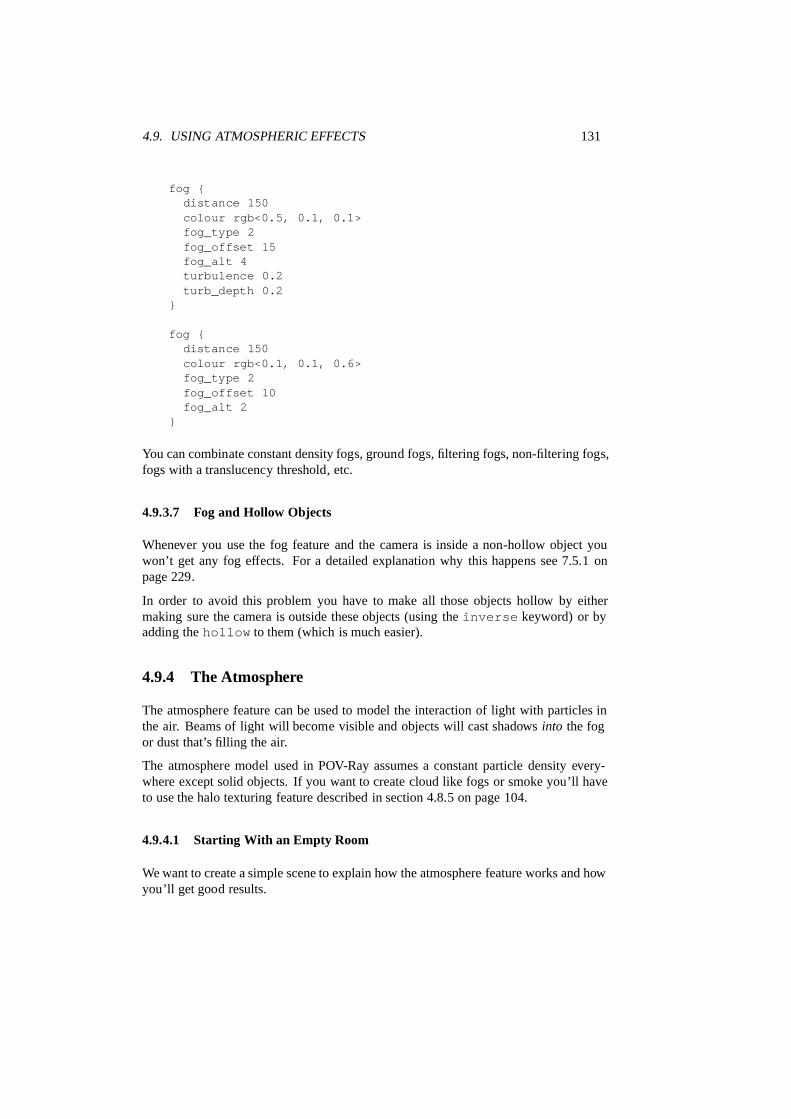
4.9. USING ATMOSPHERIC EFFECTS 131
fog {distance 150colour rgb<0.5, 0.1, 0.1>fog_type 2fog_offset 15fog_alt 4turbulence 0.2turb_depth 0.2
}
fog {distance 150colour rgb<0.1, 0.1, 0.6>fog_type 2fog_offset 10fog_alt 2
}
You can combinate constant density fogs, ground fogs, filtering fogs, non-filtering fogs,fogs with a translucency threshold, etc.
4.9.3.7 Fog and Hollow Objects
Whenever you use the fog feature and the camera is inside a non-hollow object youwon’t get any fog effects. For a detailed explanation why this happens see 7.5.1 onpage 229.
In order to avoid this problem you have to make all those objects hollow by eithermaking sure the camera is outside these objects (using the inverse keyword) or byadding the hollow to them (which is much easier).
4.9.4 The Atmosphere
The atmosphere feature can be used to model the interaction of light with particles inthe air. Beams of light will become visible and objects will cast shadows into the fogor dust that’s filling the air.
The atmosphere model used in POV-Ray assumes a constant particle density every-where except solid objects. If you want to create cloud like fogs or smoke you’ll haveto use the halo texturing feature described in section 4.8.5 on page 104.
4.9.4.1 Starting With an Empty Room
We want to create a simple scene to explain how the atmosphere feature works and howyou’ll get good results.
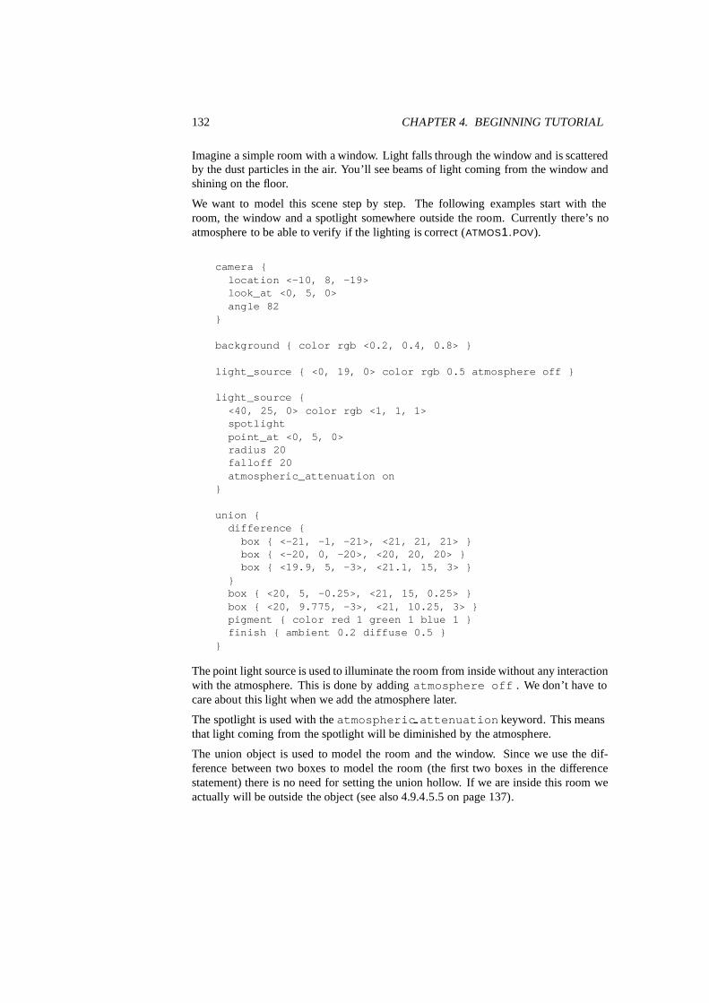
132 CHAPTER 4. BEGINNING TUTORIAL
Imagine a simple room with a window. Light falls through the window and is scatteredby the dust particles in the air. You’ll see beams of light coming from the window andshining on the floor.
We want to model this scene step by step. The following examples start with theroom, the window and a spotlight somewhere outside the room. Currently there’s noatmosphere to be able to verify if the lighting is correct (ATMOS1.POV).
camera {location <-10, 8, -19>look_at <0, 5, 0>angle 82
}
background { color rgb <0.2, 0.4, 0.8> }
light_source { <0, 19, 0> color rgb 0.5 atmosphere off }
light_source {<40, 25, 0> color rgb <1, 1, 1>spotlightpoint_at <0, 5, 0>radius 20falloff 20atmospheric_attenuation on
}
union {difference {
box { <-21, -1, -21>, <21, 21, 21> }box { <-20, 0, -20>, <20, 20, 20> }box { <19.9, 5, -3>, <21.1, 15, 3> }
}box { <20, 5, -0.25>, <21, 15, 0.25> }box { <20, 9.775, -3>, <21, 10.25, 3> }pigment { color red 1 green 1 blue 1 }finish { ambient 0.2 diffuse 0.5 }
}
The point light source is used to illuminate the room from inside without any interactionwith the atmosphere. This is done by adding atmosphere off . We don’t have tocare about this light when we add the atmosphere later.
The spotlight is used with the atmospheric attenuation keyword. This meansthat light coming from the spotlight will be diminished by the atmosphere.
The union object is used to model the room and the window. Since we use the dif-ference between two boxes to model the room (the first two boxes in the differencestatement) there is no need for setting the union hollow. If we are inside this room weactually will be outside the object (see also 4.9.4.5.5 on page 137).

4.9. USING ATMOSPHERIC EFFECTS 133
4.9.4.2 Adding Dust to the Room
The next step is to add an atmosphere to the room. This is done by the following fewlines (ATMOS2.POV).
atmosphere {type 1samples 10distance 40scattering 0.2
}
The type keyword selects the type of atmospheric scattering we want to use. In thiscase we use the isotropic scattering that equally scatters light in all directions (see 7.7.1on page 347 for more details about the different scattering types).
The samples keyword determines the number of samples used in accumulating theatmospheric effect. For every ray samples are taken along the ray to determine wethera sample is lit by a light source or not. If the sample is lit the amount of light scatteredinto the direction of the viewer is determined and added to the total intensity.
You can always start with an arbitrary number of samples. If the results do not fit yourideas you can increase the sampling rate to get better results. The problem of choosinga good sampling rate is the trade-off between a satisfying image and a fast rendering.A high sampling rate will almost always work but the rendering will also take a verylong time. That’s something to experiment with.
The distance keyword specifies the density of the atmosphere. It works in the sameway as the distance parameter of the fog feature.
Last but not least will the scattering value determine the amount of light that isscattered by the particles (the remaining light is absorbed). As you’ll later see thisparameter is very useful in adjusting the overall brightness of the atmosphere.
Looking at the image created from the above scene you’ll notice some very ugly anti-aliasing artefacts known as mach-bands. They are the result of a low sampling rate.
How this effect can be avoid is described in the following section.
4.9.4.3 Choosing a Good Sampling Rate
As you’ve seen a too low sampling rate can cause some ugly results. There are someways of reducing or even avoiding those problems.
The brute force approach is to increase the sampling rate until the artefacts vanish andyou get a satisfying image. Though this will always work it is a bad idea because itis very time consuming. A better approach is to use jittering and anti-aliasing first. Ifboth features don’t help you’ll have to increase the sampling rate.

134 CHAPTER 4. BEGINNING TUTORIAL
Jittering moves each sample point by a small, random amount along the sampling di-rection. This helps to reduce regular features resulting from aliasing. There is (hardly)nothing more annyoing to the human visual system than the regular features resultingfrom a low sampling rate. It’s much better to add some extra noise to the image byjittering the sample positions. The human eye is much more forgiving to that.
Use the jitter keyword followed by the amount of jittering you want to use. Goodjittering values are up to 0.5, higher values result in too much noise.
You should be aware that jittering can not fix the artefacts introduced by a too lowsampling rate. It can only make them less visible.
An additional and better way of reducing aliasing artefacts is to use (adaptive) super-sampling. This method casts additional samples where it is likely that they are needed.If the intensity between two adjactent samples differs too much additional samplesare taken inbetween. This step is done recursively until a specified recursion level isreached or the sample get close to each other.
The aa level and aa threshold keywords are used to control the super-sampling. The aa level keyword determines the maximum recursion level whilethe aa threshold keyword specifies the maximum allowed difference between twosample before the super-sampling is done.
After all this theory we get back to our sample scene and add the appropriate keywordsto use both jittering and supersamling (ATMOS3.POV).
atmosphere {type 1samples 50distance 40scattering 0.2aa_level 4aa_threshold 0.1jitter 0.2
}
A very low threshold value was choosen to super-sample even between adjactent pointswith a very similar intensity. The maximum recursion level of 4 will lead to a maximumof fifteen super-samples.
If you are looking at the results that you get after adding jittering and super-samplingyou won’t be satisfied. The only way of reducing the still visible artefacts is to increasethe sampling rate by choosing a higher number of samples.
Doing this you’ll get a good result showing (almost) no artefacts. Btw. the amount ofdust floating around in this room may be a little bit exaggerated but it’s just an example.And examples tend to be exaggerated.
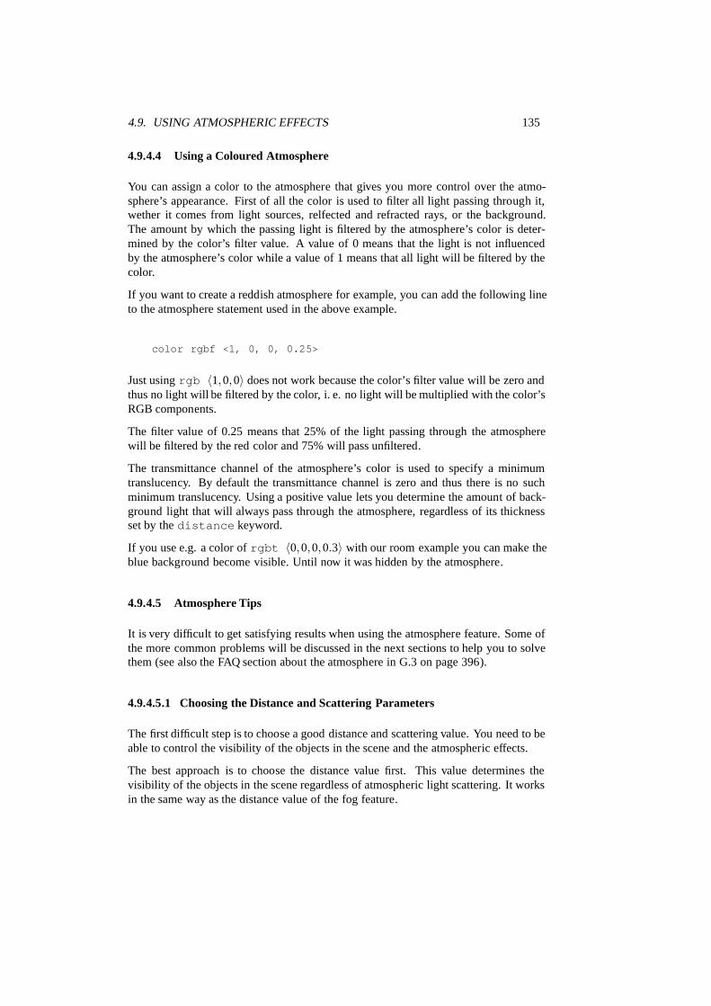
4.9. USING ATMOSPHERIC EFFECTS 135
4.9.4.4 Using a Coloured Atmosphere
You can assign a color to the atmosphere that gives you more control over the atmo-sphere’s appearance. First of all the color is used to filter all light passing through it,wether it comes from light sources, relfected and refracted rays, or the background.The amount by which the passing light is filtered by the atmosphere’s color is deter-mined by the color’s filter value. A value of 0 means that the light is not influencedby the atmosphere’s color while a value of 1 means that all light will be filtered by thecolor.
If you want to create a reddish atmosphere for example, you can add the following lineto the atmosphere statement used in the above example.
color rgbf <1, 0, 0, 0.25>
Just using rgb 〈1,0,0〉 does not work because the color’s filter value will be zero andthus no light will be filtered by the color, i. e. no light will be multiplied with the color’sRGB components.
The filter value of 0.25 means that 25% of the light passing through the atmospherewill be filtered by the red color and 75% will pass unfiltered.
The transmittance channel of the atmosphere’s color is used to specify a minimumtranslucency. By default the transmittance channel is zero and thus there is no suchminimum translucency. Using a positive value lets you determine the amount of back-ground light that will always pass through the atmosphere, regardless of its thicknessset by the distance keyword.
If you use e.g. a color of rgbt 〈0,0,0,0.3〉 with our room example you can make theblue background become visible. Until now it was hidden by the atmosphere.
4.9.4.5 Atmosphere Tips
It is very difficult to get satisfying results when using the atmosphere feature. Some ofthe more common problems will be discussed in the next sections to help you to solvethem (see also the FAQ section about the atmosphere in G.3 on page 396).
4.9.4.5.1 Choosing the Distance and Scattering Parameters
The first difficult step is to choose a good distance and scattering value. You need to beable to control the visibility of the objects in the scene and the atmospheric effects.
The best approach is to choose the distance value first. This value determines thevisibility of the objects in the scene regardless of atmospheric light scattering. It worksin the same way as the distance value of the fog feature.
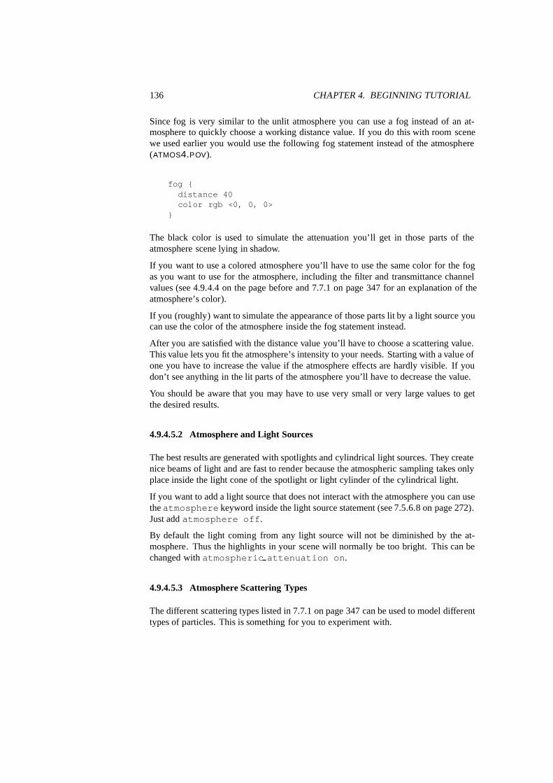
136 CHAPTER 4. BEGINNING TUTORIAL
Since fog is very similar to the unlit atmosphere you can use a fog instead of an at-mosphere to quickly choose a working distance value. If you do this with room scenewe used earlier you would use the following fog statement instead of the atmosphere(ATMOS4.POV).
fog {distance 40color rgb <0, 0, 0>
}
The black color is used to simulate the attenuation you’ll get in those parts of theatmosphere scene lying in shadow.
If you want to use a colored atmosphere you’ll have to use the same color for the fogas you want to use for the atmosphere, including the filter and transmittance channelvalues (see 4.9.4.4 on the page before and 7.7.1 on page 347 for an explanation of theatmosphere’s color).
If you (roughly) want to simulate the appearance of those parts lit by a light source youcan use the color of the atmosphere inside the fog statement instead.
After you are satisfied with the distance value you’ll have to choose a scattering value.This value lets you fit the atmosphere’s intensity to your needs. Starting with a value ofone you have to increase the value if the atmosphere effects are hardly visible. If youdon’t see anything in the lit parts of the atmosphere you’ll have to decrease the value.
You should be aware that you may have to use very small or very large values to getthe desired results.
4.9.4.5.2 Atmosphere and Light Sources
The best results are generated with spotlights and cylindrical light sources. They createnice beams of light and are fast to render because the atmospheric sampling takes onlyplace inside the light cone of the spotlight or light cylinder of the cylindrical light.
If you want to add a light source that does not interact with the atmosphere you can usethe atmosphere keyword inside the light source statement (see 7.5.6.8 on page 272).Just add atmosphere off.
By default the light coming from any light source will not be diminished by the at-mosphere. Thus the highlights in your scene will normally be too bright. This can bechanged with atmospheric attenuation on.
4.9.4.5.3 Atmosphere Scattering Types
The different scattering types listed in 7.7.1 on page 347 can be used to model differenttypes of particles. This is something for you to experiment with.

4.9. USING ATMOSPHERIC EFFECTS 137
The Rayleigh scattering is used for small particles like dust and smoke while the Miescattering is used for fog.
If you ever saw the lighthouse scene in the movie Casper you’ll know what effect thescattering type has. In this scene the beam of light coming from the lighthouse becomesvisible while it points nearly towards the viewer. As it starts to point away from theviewer it vanishes. This behaviour is typical for miniscule water droplets as modeledby the Mie scattering.
4.9.4.5.4 Increasing the Image Resolution
You have to be aware that you may have to increase the atmosphere sampling rate ifyou increase the resolution of the image. Otherwise some aliasing artefacts that wereno visible at the lower resolution may become visible.
4.9.4.5.5 Using Hollow Objects and Atmosphere
Whenever you use the atmosphere feature you have to make sure that all objects thatought to be filled with atmosphere are set to hollow using the hollow keyword.
Even though this is not obvious this holds for infinite and patch objects like quadrics,quartics, triangles, polygons, etc. Whenever you add one of those objects you shouldadd the hollow keyword as long as you are not absolutely sure you don’t need it. Youalso have to make sure that all objects the camera is inside are set to be hollow.
Whenever you get unexpected results you should check for solid objects and set themto be hollow.
4.9.5 The Rainbow
The rainbow feature can be used to create rainbows and maybe other more strangeeffects. The rainbow is a fog like effect that is restricted to a cone-like volume.
4.9.5.1 Starting With a Simple Rainbow
The rainbow is specified with a lot of parameters: the angle under which it is visible,the width of the color band, the direction of the incoming light, the fog-like distancebased particle density and last not least the color map to be used.
The size and shape of the rainbow are determined by the angle and width key-words. The direction keyword is used to set the direction of the incoming light,thus setting the rainbow’s position. The rainbow is visible when the angle betweenthe direction vector and the incident light direction is larger than angle−width/2 andsmaller than angle+width/2.
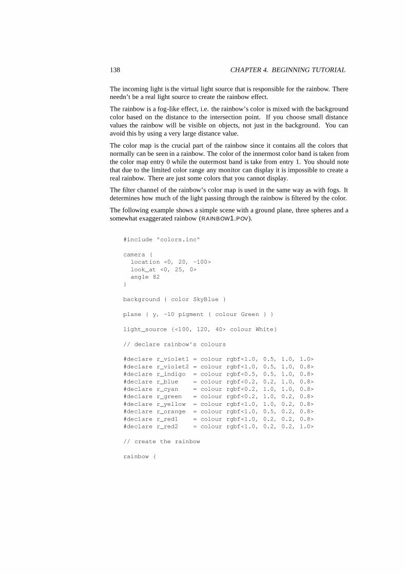
138 CHAPTER 4. BEGINNING TUTORIAL
The incoming light is the virtual light source that is responsible for the rainbow. Thereneedn’t be a real light source to create the rainbow effect.
The rainbow is a fog-like effect, i.e. the rainbow’s color is mixed with the backgroundcolor based on the distance to the intersection point. If you choose small distancevalues the rainbow will be visible on objects, not just in the background. You canavoid this by using a very large distance value.
The color map is the crucial part of the rainbow since it contains all the colors thatnormally can be seen in a rainbow. The color of the innermost color band is taken fromthe color map entry 0 while the outermost band is take from entry 1. You should notethat due to the limited color range any monitor can display it is impossible to create areal rainbow. There are just some colors that you cannot display.
The filter channel of the rainbow’s color map is used in the same way as with fogs. Itdetermines how much of the light passing through the rainbow is filtered by the color.
The following example shows a simple scene with a ground plane, three spheres and asomewhat exaggerated rainbow (RAINBOW1.POV).
#include "colors.inc"
camera {location <0, 20, -100>look_at <0, 25, 0>angle 82
}
background { color SkyBlue }
plane { y, -10 pigment { colour Green } }
light_source {<100, 120, 40> colour White}
// declare rainbow’s colours
#declare r_violet1 = colour rgbf<1.0, 0.5, 1.0, 1.0>#declare r_violet2 = colour rgbf<1.0, 0.5, 1.0, 0.8>#declare r_indigo = colour rgbf<0.5, 0.5, 1.0, 0.8>#declare r_blue = colour rgbf<0.2, 0.2, 1.0, 0.8>#declare r_cyan = colour rgbf<0.2, 1.0, 1.0, 0.8>#declare r_green = colour rgbf<0.2, 1.0, 0.2, 0.8>#declare r_yellow = colour rgbf<1.0, 1.0, 0.2, 0.8>#declare r_orange = colour rgbf<1.0, 0.5, 0.2, 0.8>#declare r_red1 = colour rgbf<1.0, 0.2, 0.2, 0.8>#declare r_red2 = colour rgbf<1.0, 0.2, 0.2, 1.0>
// create the rainbow
rainbow {

4.9. USING ATMOSPHERIC EFFECTS 139
angle 42.5width 5distance 1.0e7direction <-0.2, -0.2, 1>jitter 0.01colour_map {
[0.000 colour r_violet1][0.100 colour r_violet2][0.214 colour r_indigo][0.328 colour r_blue][0.442 colour r_cyan][0.556 colour r_green][0.670 colour r_yellow][0.784 colour r_orange][0.900 colour r_red1]
}}
Some irregularity is added to the color bands using the jitter keyword.
The rainbow in our sample is much too bright. You’ll never see a rainbow like this inreality. You can decrease the rainbow’s colors by decreasing the RGB values in thecolor map.
4.9.5.2 Increasing the Rainbow’s Translucency
The result we have so far looks much too bright. Just reducing the rainbow’s colorhelps but it’s much better to increase the translucency of the rainbow because it is morerealistic if the background is visible through the rainbow.
We can use the transmittance channel of the colors in the color map to specify aminimum translucency, just like we did with the fog. To get realistic results wehave to use very large transmittance values as you can see in the following example(RAINBOW2.POV).
rainbow {angle 42.5width 5distance 1.0e7direction <-0.2, -0.2, 1>jitter 0.01colour_map {
[0.000 colour r_violet1 transmit 0.98][0.100 colour r_violet2 transmit 0.96][0.214 colour r_indigo transmit 0.94][0.328 colour r_blue transmit 0.92][0.442 colour r_cyan transmit 0.90]

140 CHAPTER 4. BEGINNING TUTORIAL
[0.556 colour r_green transmit 0.92][0.670 colour r_yellow transmit 0.94][0.784 colour r_orange transmit 0.96][0.900 colour r_red1 transmit 0.98]
}}
The transmittance values increase at the outer bands of the rainbow to make it softlyblend into the background.
The resulting image looks much more realistic than our first rainbow.
4.9.5.3 Using a Rainbow Arc
Currently our rainbow has a circular shape, even though most of it is hidden below theground plane. You can easily create a rainbow arc by using the arc angle keywordwith an angle below 360 degrees.
If you use arc angle 120 for example you’ll get a rainbow arc that abruptly van-ishes at the arc’s ends. This does not look good. To avoid this the falloff anglekeyword can be used to specify a region where the arc smoothly blends into the back-ground.
As explained in the rainbow’s reference section (see 7.7.5 on page 353) the arc extendsfrom −arc angle/2 to arc angle/2 while the blending takes place from −arc angle/2to − f allo f f angle/2 and f allo f f angle/2 to arc angle/2. This is the reason whythe falloff angle has to be smaller or equal to the arc angle.
In the following examples we use an 120 degrees arc with a 45 degree falloff region onboth sides of the arc (RAINBOW3.POV).
rainbow {angle 42.5width 5arc_angle 120falloff_angle 30distance 1.0e7direction <-0.2, -0.2, 1>jitter 0.01colour_map {
[0.000 colour r_violet1 transmit 0.98][0.100 colour r_violet2 transmit 0.96][0.214 colour r_indigo transmit 0.94][0.328 colour r_blue transmit 0.92][0.442 colour r_cyan transmit 0.90][0.556 colour r_green transmit 0.92][0.670 colour r_yellow transmit 0.94][0.784 colour r_orange transmit 0.96]

4.9. USING ATMOSPHERIC EFFECTS 141
[0.900 colour r_red1 transmit 0.98]}
}
The arc angles are measured against the rainbows up direction which can be specifiedusing the up keyword. By default the up direction is the y-axis.
We finally have a realistic looking rainbow arc.

142 CHAPTER 4. BEGINNING TUTORIAL
Part III
Reference Guide
143

Chapter 5
POV-Ray Reference
The reference section describes all command line options and INI file switches, thescene description language and all other features that are part of POV-Ray. It is sup-posed to be used as a reference for looking up things. It does not contain detailedexplanations on how scenes are written or how POV-Ray is used. It just explains allfeatures, their syntax, applications, limits, drawbacks, etc.
145

146 CHAPTER 5. POV-RAY REFERENCE

Chapter 6
POV-Ray Options
POV-Ray was originally created as a command-line program for operating systemswithout graphical interfaces, dialog boxes and pull-down menus. Most versions ofPOV-Ray still use command-line switches to tell it what to do. This documentationassumes you are using the command-line version. If you are using Macintosh, MS-Windows or other GUI versions, there will be dialog boxes or menus which do thesame thing. There is system-specific documentation for each system describing thespecific commands.
6.1 Setting POV-Ray Options
There are two distinct ways of setting POV-Ray options: command line switches andINI file keywords. Both are explained in detail in the following sections.
6.1.1 Command Line Switches
Command line switches consist of a + (plus) or – (minus) sign, followed by one ormore alphabetic characters and possibly a numeric value. Here is a typical commandline with switches.
POVRAY +ISIMPLE.POV +V +W80 +H60
POVRAY is the name of the program and it is followed by several switches. Each switchbegins with a plus or minus sign. The +I switch with the filename tells POV-Ray whatscene file it should use as input and +V tells the program to output its status to the textscreen as it’s working. The +W and +H switches set the width and height of the imagein pixels. This image will be 80 pixels wide by 60 pixels high.
147
148 CHAPTER 6. POV-RAY OPTIONS
In switches which toggle a feature, the plus turns it on and minus turns it off. Forexample +P turns on the pause for keypress when finished option while –P turns it off.Other switches are used to specify values and do not toggle a feature. Either plus orminus may be used in that instance. For example +W320 sets the width to 320 pixels.You could also use –W320 and get the same results.
Switches may be specified in upper or lower case. They are read left to right but ingeneral may be specified in any order. If you specify a switch more than once, theprevious value is generally overwritten with the last specification. The only exceptionis the +L switch for setting library paths. Up to ten unique paths may be specified.
Almost all +/– switches have an equivalent option which can be used in an INI filewhich is described in the next section. A detailed description of each switch is given inthe option reference section.
6.1.2 Using INI Files
Because it is difficult to set more than a few options on a command line, you have theability to put multiple options in one or more text files. These initialization files or INIfiles have .INI as their default extension. Previous versions of POV-Ray called themdefault files or DEF files. You may still use existing DEF files with this version ofPOV-Ray.
The majority of options you use will be stored in INI files. The command line switchesare recommended for options which you will turn off or on frequently as you performtest renderings of a scene you are developing. The file POVRAY.INI is automaticallyread if present. You may specify additional INI files on the command-line by simplytyping the file name on the command line. For example:
POVRAY MYOPTS.INI
If no extension is given, then . INI is assumed. POV-Ray knows this is not a switchbecause it is not preceded by a plus or minus. In fact a common error among new usersis that they forget to put the +I switch before the input file name. Without the switch,POV-Ray thinks that the scene file SIMPLE.POV is an INI file. Don’t forget! If no plusor minus precedes a command line switch, it is assumed to be an INI file name.
You may have multiple INI files on the command line along with switches. For exam-ple:
POVRAY MYOPTS +V OTHER
This reads options from MYOPTS.INI, then sets the +V switch, then reads options fromOTHER.INI.
An INI file is a plain ASCII text file with options of the form . . .
6.1. SETTING POV-RAY OPTIONS 149
Option_Keyword=VALUE ; Text after semicolon is a comment
For example the INI equivalent of the switch +ISIMPLE.POV is . . .
Input_File_Name=simple.pov
Options are read top to bottom in the file but in general may be specified in any order.If you specify an option more than once, the previous values are generally overwrittenwith the last specification. The only exception is the Library Path=PATH options. Upto ten unique paths may be specified.
Almost all INI-style options have equivalent +/– switches. The option reference sectiongives a detailed description of all POV-Ray options. It includes both the INI-stylesettings and the +/– switches.
The INI keywords are not case sensitive. Only one INI option is permitted per line oftext. You may also include switches in your INI file if they are easier for you. You mayhave multiple switches per line but you should not mix switches and INI options on thesame line. You may nest INI files by simply putting the file name on a line by itselfwith no equals sign after it. Nesting may occur up to ten levels deep.
For example:
; This is a sample INI file. This entire line is a comment.; Blank lines are permitted.
Input_File_Name=simple.pov ; This sets the input file name
+W80 +H60 ; Traditional +/- switches are permitted too
MOREOPT ; Read MOREOPT.INI and continue with next line
+V ; Another switch
; That’s all folks!
INI files may have labeled sections so that more than one set of options may be storedin a single file. Each section begins with a label in [] brackets. For example:
; RES.INI; This sample INI file is used to set resolution.
+W120 +H100 ; This section has no label.; Select it with "RES"
[Low]

150 CHAPTER 6. POV-RAY OPTIONS
+W80 +H60 ; This section has a label.; Select it with "RES[Low]"
[Med]+W320 +H200 ; This section has a label.
; Select it with "RES[Med]"
[High]+W640 +H480 ; Labels are not case sensitive.
; "RES[high]" works
[Really High]+W800 +H600 ; Labels may contain blanks
When you specify the INI file you should follow it with the section label in brackets.For example . . .
POVRAY RES[Med] +IMYFILE.POV
POV-Ray reads RES.INI and skips all options until it finds the label Med. It processesoptions after that label until it finds another label and then it skips. If no label isspecified on the command line then only the unlabeled area at the top of the file is read.If a label is specified, the unlabeled area is ignored.
6.1.3 Using the POVINI Environment Variable
The environment variable POVINI is used to specify the location and name of a defaultINI file that is read every time POV-Ray is executed. If POVINI is not specified adefault INI file may be read depending on the platform used. If the specified file doesnot exist a warning message is printed.
To set the environment variable under MS-Dos you might put the following line in yourAUTOEXEC.BAT file . . .
set POVINI=C:\POVRAY3\DEFAULT.INI
On most operating systems the sequence of reading options is as follows:
1. Read options from default INI file specified by the POVINI environ-ment variable or platform specific INI file.
2. Read switches from command line (this includes reading any speci-fied INI/DEF files).
The POVRAYOPT environment variable supported by previous POV-Ray versions isno longer available.

6.2. OPTIONS REFERENCE 151
6.2 Options Reference
As explained in the previous section, options may be specified by switches or INI-styleoptions. Almost all INI-style options have equivalent +/– switches and most switcheshave equivalent INI-style option. The following sections give a detailed description ofeach POV-Ray option. It includes both the INI-style settings and the +/– switches.
The notation and terminology used is described in the tables below.
Keyword=bool turn Keyword on if bool equals true, yes, on or 1 and turnit off if it is any other value.
Keyword=true do this option if true, yes, on or 1 is specified.Keyword=false do this option if false, no, off or 0 is specified.Keyword=file any valid file name. Note: some options prohibit the use of
any of the above true or false values as a file name. Theyare noted in later sections.
n any integer such as in +W320n.n any float such as in Clock=3.450.n any float < 1.0 even if it has no leading 0s any string of textx or y any single characterpath any directory name, drive optional, no final path separator (”\” or
”/”, depending on the operating system)
Unless otherwise specifically noted, you may assume that either a plus or minus signbefore a switch will produce the same results.
6.2.1 Animation Options
POV-Ray 3.0 greatly improved its animation capability with the addition of an internalanimation loop, automatic output file name numbering and the ability to shell out tothe operating system to external utilities which can assemble individual frames intoan animation. The internal animation loop is simple yet flexible. You may still useexternal programs or batch files to create animations without the internal loop as youmay have done in POV-Ray 2.
6.2.1.1 External Animation Loop
Clock=n.n Sets clock float identifier to n.n+Kn.n Same as Clock=n.n
The Clock=n.n option or the +Kn.n switch may be used to pass a single float value tothe program for basic animation. The value is stored in the float identifier clock. If an
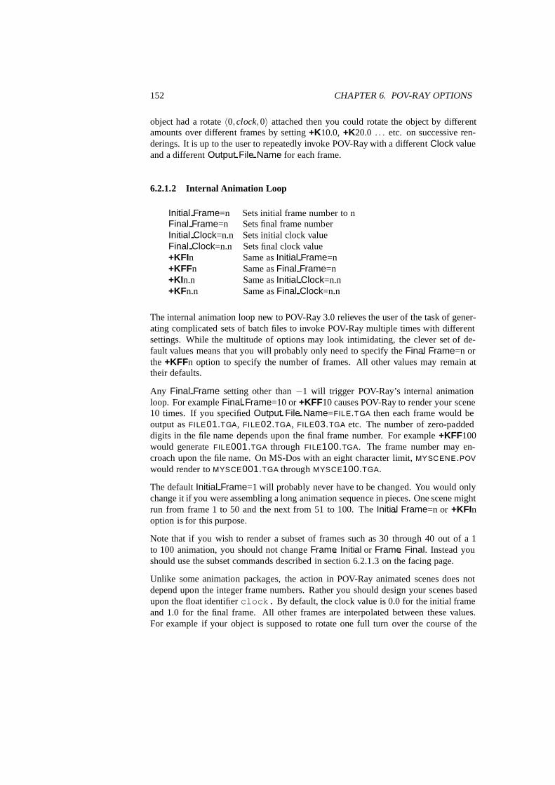
152 CHAPTER 6. POV-RAY OPTIONS
object had a rotate 〈0,clock,0〉 attached then you could rotate the object by differentamounts over different frames by setting +K10.0, +K20.0 . . . etc. on successive ren-derings. It is up to the user to repeatedly invoke POV-Ray with a different Clock valueand a different Output File Name for each frame.
6.2.1.2 Internal Animation Loop
Initial Frame=n Sets initial frame number to nFinal Frame=n Sets final frame numberInitial Clock=n.n Sets initial clock valueFinal Clock=n.n Sets final clock value+KFIn Same as Initial Frame=n+KFFn Same as Final Frame=n+KIn.n Same as Initial Clock=n.n+KFn.n Same as Final Clock=n.n
The internal animation loop new to POV-Ray 3.0 relieves the user of the task of gener-ating complicated sets of batch files to invoke POV-Ray multiple times with differentsettings. While the multitude of options may look intimidating, the clever set of de-fault values means that you will probably only need to specify the Final Frame=n orthe +KFFn option to specify the number of frames. All other values may remain attheir defaults.
Any Final Frame setting other than −1 will trigger POV-Ray’s internal animationloop. For example Final Frame=10 or +KFF10 causes POV-Ray to render your scene10 times. If you specified Output File Name=FILE.TGA then each frame would beoutput as FILE01.TGA, FILE02.TGA, FILE03.TGA etc. The number of zero-paddeddigits in the file name depends upon the final frame number. For example +KFF100would generate FILE001.TGA through FILE100.TGA. The frame number may en-croach upon the file name. On MS-Dos with an eight character limit, MYSCENE.POV
would render to MYSCE001.TGA through MYSCE100.TGA.
The default Initial Frame=1 will probably never have to be changed. You would onlychange it if you were assembling a long animation sequence in pieces. One scene mightrun from frame 1 to 50 and the next from 51 to 100. The Initial Frame=n or +KFInoption is for this purpose.
Note that if you wish to render a subset of frames such as 30 through 40 out of a 1to 100 animation, you should not change Frame Initial or Frame Final. Instead youshould use the subset commands described in section 6.2.1.3 on the facing page.
Unlike some animation packages, the action in POV-Ray animated scenes does notdepend upon the integer frame numbers. Rather you should design your scenes basedupon the float identifier clock. By default, the clock value is 0.0 for the initial frameand 1.0 for the final frame. All other frames are interpolated between these values.For example if your object is supposed to rotate one full turn over the course of the

6.2. OPTIONS REFERENCE 153
animation, you could specify rotate 360*clock*y. Then as clock runs from 0.0to 1.0, the object rotates about the y-axis from 0 to 360 degrees.
The major advantage of this system is that you can render a 10 frame animation or a100 frame or 500 frame or 329 frame animation yet you still get one full 360 degreerotation. Test renders of a few frames work exactly like final renders of many frames.
In effect you define the motion over a continuous float valued parameter (the clock)and you take discrete samples at some fixed intervals (the frames). If you take a movieor video tape of a real scene it works the same way. An object’s actual motion dependsonly on time. It does not depend on the frame rate of your camera.
Many users have already created scenes for POV-Ray 2 that expect clock values over arange other than the default 0.0 to 1.0. For this reason we provide the Initial Clock=n.nor +KIn.n and Final Clock=n.n or +KFn.n options. For example to run the clock from25.0 to 75.0 you would specify Initial Clock=25.0 and Final Clock=75.0. Then theclock would be set to 25.0 for the initial frame and 75.0 for the final frame. Inbetweenframes would have clock values interpolated from 25.0 through 75.0 proportionally.
Users who are accustomed to using frame numbers rather than clock values could spec-ify Initial Clock=1.0 and Final Clock=10.0 and Frame Final=10 for a 10 frame ani-mation.
For new scenes, we recommend you do not change the Initial Clock or Final Clockfrom their default 0.0 to 1.0 values. If you want the clock to vary over a different rangethan the default 0.0 to 1.0, we recommend you handle this inside your scene file asfollows . . .
#declare Start = 25.0#declare End = 75.0#declare My_Clock = Start+(End-Start)*clock
Then use My Clock in the scene description. This keeps the critical values 25.0 and75.0 in your .POV file.
Note that more details concerning the inner workings of the animation loop are in thesection on shell-out operating system commands in section 6.2.4 on page 168.
6.2.1.3 Subsets of Animation Frames
Subset Start Frame=n Set subset starting frame to nSubset Start Frame=0.n Set subset starting frame to n percentSubset End Frame=n Set subset ending frame to nSubset End Frame=0.n Set subset ending frame to n percent+SFn or +SF0.n Same as Subset Start Frame+EFn or +EF0.n Same as Subset End Frame

154 CHAPTER 6. POV-RAY OPTIONS
When creating a long animation, it may be handy to render only a portion of the ani-mation to see what it looks like. Suppose you have 100 frames but only want to renderframes 30 through 40. If you set Initial Frame=30 and Final Frame=40 then the clockwould vary from 0.0 to 1.0 from frames 30 through 40 rather than 0.30 through 0.40as it should. Therefore you should leave Initial Frame=1 and Final Frame=100 anduse Subset Start Frame=30 and Subset End Frame=40 to selectively render partof the scene. POV-Ray will then properly compute the clock values.
Usually you will specify the subset using the actual integer frame numbers how-ever an alternate form of the subset commands takes a float value in the range0.0 ≤ n.nnn ≤ 1.0 which is interpreted as a fraction of the whole animation. For ex-ample, Subset Start Frame=0.333 and Subset End Frame=0.667 would render themiddle 1/3rd of a sequence regardless of the number of frames.
6.2.1.4 Cyclic Animation
Cyclic Animation=bool Turn cyclic animation on/off+KC Turn cyclic animation on–KC Turn cyclic animation off
Many computer animation sequences are designed to be run in a continuous loop. Sup-pose you have an object that rotates exactly 360 degrees over the course of your ani-mation and you did rotate 360*clock*y to do so. Both the first and last frameswould be identical. Upon playback there would be a brief one frame jerkiness. To elim-inate this problem you need to adjust the clock so that the last frame does not matchthe first. For example a ten frame cyclic animation should not use clock 0.0 to 1.0. Itshould run from 0.0 to 0.9 in 0.1 increments. However if you change to 20 frames itshould run from 0.0 to 0.95 in 0.05 increments. This complicates things because youwould have to change the final clock value every time you changed Final Frame. Set-ting Cyclic Animation=on or using +KC will cause POV-Ray to automatically adjustthe final clock value for cyclic animation regardless of how many total frames. Thedefault value for this setting is off.
6.2.1.5 Field Rendering
Field Render=bool Turn field rendering on/offOdd Field=bool Set odd field flag+UF Turn field rendering on–UF Turn field rendering off+UO Set odd field flag on–UO Set odd field flag off
Field rendering is sometimes used for animations when the animation is being outputfor television. TVs only display alternate scan lines on each vertical refresh. When

6.2. OPTIONS REFERENCE 155
each frame is being displayed the fields are interlaced to give the impression of a higherresolution image. The even scan lines make up the even field, and are drawn first (i. e.scan lines 0, 2, 4, etc.), followed by the odd field, made up of the odd numbered scanlines are drawn afterwards. If objects in an animation are moving quickly, their positioncan change noticably from one field to the next. As a result, it may be desirable in thesecases to have POV-Ray render alternate fields at the actual field rate (which is twice theframe rate), rather than rendering full frames at the normal frame rate. This would savea great deal of time compared to rendering the entire animation at twice the frame rate,and then only using half of each frame.
By default, field rendering is not used. Setting Field Render=on or using +UF willcause alternate frames in an animation to be only the even or odd fields of an animation.By default, the first frame is the even field, followed by the odd field. You can havePOV-Ray render the odd field first by specifying Odd Field=on, or by using the +UOswitch.
6.2.2 Output Options
6.2.2.1 General Output Options
6.2.2.1.1 Height and Width of Output
Height=n Set screen height to nWidth=n Sets screen width to n pixels+Hn Same as Height=n (when n > 8)+Wn Same as Width=n
These switches set the height and width of the image in pixels. This specifies the imagesize for file output. The preview display, if on, will generally attempt to pick a videomode to accommodate this size but the display settings do not in any way affect theresulting file output.
6.2.2.1.2 Partial Output Options
Start Column=n Set first column to nStart Column=0.n Set first column to n percent of width+SCn or +SC0.n Same as Start Column
Start Row=n Set first row to n pixelsStart Row=0.n Set first row to n percent of height+SRn or +Sn Same as Start Row=n+SR0.n or +S0.n Same as Start Row=0.n

156 CHAPTER 6. POV-RAY OPTIONS
End Column=n Set last column to n pixelsEnd Column=0.n Set last column to n percent of width+ECn or +EC0.n Same as End Column
End Row=n Set last row to n pixelsEnd Row=0.n Set last row to n percent of height+ERn or +En Same as End Row=n+ER0.n or +E0.n Same as End Row=0.n
When doing test rendering it is often convenient to define a small, rectangular sub-section of the whole screen so you can quickly check out one area of the image. TheStart Row, End Row, Start Column and End Column options allow you to definethe subset area to be rendered. The default values are the full size of the image from(1,1) which is the upper left to (w,h) on the lower right where w and h are the Width=nand Height=n values you have set.
Note if the number specified is greater than 1 then it is interpreted as an absoluterow or column number in pixels. If it is a decimal value between 0.0 and 1.0 thenit is interpreted as a percent of the total width or height of the image. For example:Start Row=0.75 and Start Column=0.75 starts on a row 75% down from the top ata column 75% from the left. Thus it renders only the lower-right 25% of the imageregardless of the specified width and height.
The +SR, +ER, +SC and +EC switches work in the same way as the correspondingINI-style settings for both absolute settings or percentages. Early versions of POV-Rayallowed only start and end rows to be specified with +Sn and +En so they are stillsupported in addition to +SR and +ER.
6.2.2.1.3 Interrupting Options
Test Abort=bool Turn test for user abort on/off+X Turn test abort on–X Turn test abort off
Test Abort Count=n Set to test for abort every n pixels+Xn Set to test for abort every n pixels on–Xn Set to test for abort off (in future test every n pixels)
On some operating systems once you start a rendering you must let it finish. TheTest Abort=on option or +X switch causes POV-Ray to test the keyboard for keypress.If you have pressed a key, it will generate a controlled user abort. Files will be flushedand closed but only data through the last full row of pixels is saved. POV-Ray exitswith an error code 2 (normally POV-Ray returns 0 for a successful run or 1 for a fatalerror).

6.2. OPTIONS REFERENCE 157
When this option is on, the keyboard is polled on every line while parsing the scene fileand on every pixel while rendering. Because polling the keyboard can slow down a ren-dering, the Test Abort Count=n option or +Xn switch causes the test to be performedonly every n pixels rendered or scene lines parsed.
6.2.2.1.4 Resuming Options
Continue Trace=bool Sets continued trace on/off+C Sets continued trace on–C Sets continued trace off
Create Ini=FILE Generate an INI file named FILE
Create Ini=true Generate FILE.INI where file is the scene name.Create Ini=false Turn off generation of previously set FILE.INI
+GIFILE Same as Create Ini=FILE
If you abort a render while it’s in progress or if you used the End Row option to endthe render prematurely, you can use Continue Trace=on or +C option to continue therender later at the point where you left off. This option reads in the previously gener-ated output file, displays the partial image rendered so far, then proceeds with the ray-tracing. This option cannot be used if file output is disabled with Output to file=off or–F.
The Continue Trace option may not work if the Start Row option has been set toanything but the top of the file, depending on the output format being used.
POV-Ray tries to figure out where to resume an interrupted trace by reading any previ-ously generated data in the specified output file. All file formats contain the image size,so this will override any image size settings specified. Some file formats (namely TGAand PNG) also store information about where the file started (i. e. +SCn and +SRnoptions), alpha output +UA, and bit-depth +FNn, which will override these settings.It is up to the user to make sure that all other options are set the same as the originalrender.
The Create Ini option or +GI switch provides an easy way to create an INI file with allof the rendering options, so you can re-run files with the same options, or ensure youhave all the same options when resuming. This option creates an INI file with everyoption set at the value used for that rendering. This includes default values which youhave not specified. For example if you run POV-Ray with . . .
POVRAY +ISIMPLE.POV MYOPTS +GIRERUN.INI MOREOPTS
POV-Ray will create a file called RERUN.INI with all of the options used to generatethis scene. The file is not written until all options have been processed. This meansthat in the above example, the file will include options from both MYOPTS.INI andMOREOPTS.INI despite the fact that the +GI switch is specified between them. Youmay now re-run the scene with . . .
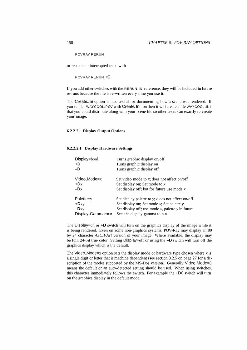
158 CHAPTER 6. POV-RAY OPTIONS
POVRAY RERUN
or resume an interrupted trace with
POVRAY RERUN +C
If you add other switches with the RERUN.INI reference, they will be included in futurere-runs because the file is re-written every time you use it.
The Create Ini option is also useful for documenting how a scene was rendered. Ifyou render WAYCOOL.POV with Create Ini=on then it will create a file WAYCOOL.INI
that you could distribute along with your scene file so other users can exactly re-createyour image.
6.2.2.2 Display Output Options
6.2.2.2.1 Display Hardware Settings
Display=bool Turns graphic display on/off+D Turns graphic display on–D Turns graphic display off
Video Mode=x Set video mode to x; does not affect on/off+Dx Set display on; Set mode to x–Dx Set display off; but for future use mode x
Palette=y Set display palette to y; d oes not affect on/off+Dxy Set display on; Set mode x; Set palette y–Dxy Set display off; use mode x, palette y in futureDisplay Gamma=n.n Sets the display gamma to n.n
The Display=on or +D switch will turn on the graphics display of the image while itis being rendered. Even on some non-graphics systems, POV-Ray may display an 80by 24 character ASCII-Art version of your image. Where available, the display maybe full, 24-bit true color. Setting Display=off or using the –D switch will turn off thegraphics display which is the default.
The Video Mode=x option sets the display mode or hardware type chosen where x isa single digit or letter that is machine dependent (see section 3.2.5 on page 27 for a de-scription of the modes supported by the MS-Dos version). Generally Video Mode=0means the default or an auto-detected setting should be used. When using switches,this character immediately follows the switch. For example the +D0 switch will turnon the graphics display in the default mode.

6.2. OPTIONS REFERENCE 159
The Palette=y option selects the palette to be used. Typically the single characterparameter y is a digit which selects one of several fixed palettes or a letter such G forgray scale, H for 15-bit or 16-bit high color or T for 24-bit true color. When usingswitches, this character is the 2nd character after the switch. For example the +D0Tswitch will turn on the graphics display in the default mode with a true color palette.
The Display Gamma=n.n setting is new with POV-Ray 3.0, and is not available as acommand-line switch. The Display Gamma setting overcomes the problem of images(whether ray-traced or not) having different brightness when being displayed on differ-ent monitors, different video cards, and under different operating systems. Note that theDisplay Gamma is a setting based on your computer’s display hardware, and shouldbe set correctly once and not changed. The Display Gamma INI setting works inconjunction with the new assumed gamma global setting to ensure that POV scenesand the images they create look the same on all systems. See section 7.8.3 on page 357which describes the assumed gamma global setting and describes gamma more thor-oughly.
While the Display Gamma can be different for each system, there are a few generalrules that can be used for setting Display Gamma if you don’t know it exactly. Ifthe Display Gamma keyword does not appear in the INI file, POV-Ray assumes thatthe display gamma is 2.2. This is because most PC monitors have a gamma valuein the range 1.6 to 2.6 (newer models seem to have a lower gamma value). MacOShas the ability to do gamma correction inside the system software (based on a usersetting in the gamma control panel). If the gamma control panel is turned off, or isnot available, the default Macintosh system gamma is 1.8. Some high-end PC graphicscards can do hardware gamma correction and should use the current Display Gammasetting, usually 1.0. A gamma test image is also available to help users to set theirDisplay Gamma accurately.
For scene files that do not have an assumed gamma global setting the Dis-play Gamma will not have any affect on the preview output of POV-Ray or for mostoutput file formats. However, the Display Gamma value is used when creating PNGformat output files, and also when rendering the POV-Ray example files (because theyhave an assumed gamma), so it should still be correctly set for your system to ensureproper results.
6.2.2.2.2 Display Related Settings
Pause When Done=bool Sets pause when done on/off+P Sets pause when done on–P Sets pause when done off
Verbose=bool Set verbose messages on/off+V Set verbose messages on–V Set verbose messages off

160 CHAPTER 6. POV-RAY OPTIONS
Draw Vistas=bool Turn draw vistas on/off+UD Turn draw vistas on–UD Turn draw vistas off
On some systems, when the image is complete, the graphics display is cleared andPOV-Ray switches back into text mode to print the final statistics and to exit. Normallywhen the graphics display is on, you want to look at the image awhile before continu-ing. Using Pause When Done=on or +P causes POV-Ray to pause in graphics modeuntil you to press a key to continue. The default is not to pause (–P).
When the graphics display is not used, it is often desirable to monitor progress ofthe rendering. Using Verbose=on or +V turns on verbose reporting of your renderingprogress. This reports the number of the line currently being rendered, the elapsed timefor the current frame and other information. On some systems, this textual informationcan conflict with the graphics display. You may need to turn this off when the displayis on. The default setting is off (–V).
The option Draw Vistas=on or +UD was originally a debugging help for POV-Ray’svista buffer feature but it was such fun we decided to keep it. Vista buffering is a spatialsub-division method that projects the 2-D extents of bounding boxes onto the viewingwindow. POV-Ray tests the 2-D x, y pixel location against these rectangular areas todetermine quickly which objects, if any, the viewing ray will hit. This option showsyou the 2-D rectangles used. The default setting is off (–UD) because the drawing ofthe rectangles can take considerable time on complex scenes and it serves no criticalpurpose. See section 6.2.6.3 on page 177 for more details.
6.2.2.2.3 Mosaic Preview
Preview Start Size=n Set mosaic preview start size to n+SPn Same as Preview Start Size=n
Preview End Size=n Set mosaic preview end size to n+EPn Same as Preview End Size=n
Typically, while you are developing a scene, you will do many low resolution testrenders to see if objects are placed properly. Often this low resolution version doesn’tgive you sufficient detail and you have to render the scene again at a higher resolution.A feature called mosaic preview solves this problem by automatically rendering yourimage in several passes.
The early passes paint a rough overview of the entire image using large blocks ofpixels that look like mosaic tiles. The image is then refined using higher resolutionson subsequent passes. This display method very quickly displays the entire image at alow resolution, letting you look for any major problems with the scene. As it refinesthe image, you can concentrate on more details, like shadows and textures. You don’thave to wait for a full resolution render to find problems, since you can interrupt the
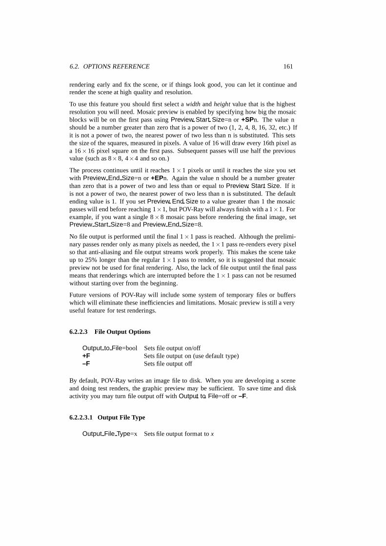
6.2. OPTIONS REFERENCE 161
rendering early and fix the scene, or if things look good, you can let it continue andrender the scene at high quality and resolution.
To use this feature you should first select a width and height value that is the highestresolution you will need. Mosaic preview is enabled by specifying how big the mosaicblocks will be on the first pass using Preview Start Size=n or +SPn. The value nshould be a number greater than zero that is a power of two (1, 2, 4, 8, 16, 32, etc.) Ifit is not a power of two, the nearest power of two less than n is substituted. This setsthe size of the squares, measured in pixels. A value of 16 will draw every 16th pixel asa 16×16 pixel square on the first pass. Subsequent passes will use half the previousvalue (such as 8×8, 4×4 and so on.)
The process continues until it reaches 1×1 pixels or until it reaches the size you setwith Preview End Size=n or +EPn. Again the value n should be a number greaterthan zero that is a power of two and less than or equal to Preview Start Size. If itis not a power of two, the nearest power of two less than n is substituted. The defaultending value is 1. If you set Preview End Size to a value greater than 1 the mosaicpasses will end before reaching 1×1, but POV-Ray will always finish with a 1×1. Forexample, if you want a single 8×8 mosaic pass before rendering the final image, setPreview Start Size=8 and Preview End Size=8.
No file output is performed until the final 1×1 pass is reached. Although the prelimi-nary passes render only as many pixels as needed, the 1×1 pass re-renders every pixelso that anti-aliasing and file output streams work properly. This makes the scene takeup to 25% longer than the regular 1×1 pass to render, so it is suggested that mosaicpreview not be used for final rendering. Also, the lack of file output until the final passmeans that renderings which are interrupted before the 1×1 pass can not be resumedwithout starting over from the beginning.
Future versions of POV-Ray will include some system of temporary files or bufferswhich will eliminate these inefficiencies and limitations. Mosaic preview is still a veryuseful feature for test renderings.
6.2.2.3 File Output Options
Output to File=bool Sets file output on/off+F Sets file output on (use default type)–F Sets file output off
By default, POV-Ray writes an image file to disk. When you are developing a sceneand doing test renders, the graphic preview may be sufficient. To save time and diskactivity you may turn file output off with Output to File=off or –F.
6.2.2.3.1 Output File Type
Output File Type=x Sets file output format to x

162 CHAPTER 6. POV-RAY OPTIONS
+Fxn Sets file output on; sets format x, depth n–Fxn Sets file output off; but in future use format x, depth
n
Output Alpha=bool Sets alpha output on/off+UA Sets alpha output on–UA Sets alpha output off
Bits Per Color=n Sets file output bits/color to n
The default type of image file depends on which platform you are using. MS-Dos andmost others default to 24-bit uncompressed Targa. See your platform-specific docu-mentation to see what your default file type is. You may select one of several differentfile types using Output File Type=x or +Fx where x is one of the following . . .
+FC Compressed Targa-24 format (RLE, run length encoded)+FN New PNG (portable network graphics) format+FP Unix PPM format+FS System-specific such as Mac Pict or Windows BMP+FT Uncompressed Targa-24 format
Note that the obsolete +FD dump format and +FR raw format have been dropped fromPOV-Ray 3.0 because they were rarely used and no longer necessary. PPM, PNG, andsystem specific formats have been added. PPM format images are uncompressed, andhave a simple text header, which makes it a widely portable image format. PNG isa new image format designed not only to replace GIF, but to improve on its short-comings. PNG offers the highest compression available without loss for high qualityapplications, such as ray-tracing. The system specific format depends on the platformused and is covered in the appropriate system specififc documentation.
Most of these formats output 24 bits per pixel with 8 bits for each of red, green and bluedata. PNG allows you to optionally specify the output bit depth from 5 to 16 bits foreach of the red, green, and blue colors, giving from 15 to 48 bits of color informationper pixel. The default output depth for all formats is 8 bits/color (16 million possiblecolors), but this may be changed for PNG format files by setting Bits Per Color=n orby specifying +FNn, where n is the desired bit depth.
Specifying a smaller color depth like 5 bits/color (32768 colors) may be enough forpeople with 8- or 16-bit (256 or 65536 color) displays, and will improve compressionof the PNG file. Higher bit depths like 10 or 12 may be useful for video or pub-lishing applications, and 16 bits/color is good for grayscale height field output (Seesection 7.5.2.5 on page 236 for details on height fields).
Targa format also allows 8 bits of alpha transparency data to be output, while PNGformat allows 5 to 16 bits of alpha transparency data, depending on the color bit depthas specified above. You may turn this option on with Output Alpha=on or +UA. The

6.2. OPTIONS REFERENCE 163
default is off or –UA. See section 7.6.1.5.4 on page 285 for further details on trans-parency.
In addition to support for variable bit-depths, alpha channel, and grayscale formats,PNG files also store the Display Gamma value so the image displays properly onall systems (see section 6.2.2.2.1 on page 158). The hf gray 16 global setting, asdescribed in section 7.8.4 on page 359 will also affect the type of data written to theoutput file.
6.2.2.3.2 Output File Name
Output File Name=FILE Sets output file to file+OFILE Same as Output File Name=FILE
The default output filename is created from the scene name and need not be speci-fied. The scene name is the input name with all drive, path, and extension informationstripped. For example if the input file name is C:\POVRAY3\MYSTUFF\MYFILE.POV
the scene name is MYFILE. The proper extension is appended to the scene name basedon the file type. For example MYFILE.TGA or MYFILE.PNG might be used.
You may override the default output name using Output File Name=FILE or +OFILE.For example:
Input File Name=MYINPUT.POV
Output File Name=MYOUTPUT.TGA
If an output file name of ”–” is specified (a single minus sign), then the image willbe written to standard output, usually the screen. The output can then be piped intoanother program or to a GUI if desired.
6.2.2.3.3 Output File Buffer
Buffer Output=bool Turn output buffering on/off+B Turn output buffering on–B Turn output buffering off
Buffer Size=n Set output buffer size to n kilobytes. If n is zero, nobuffering occurs. If n is smaller than the default, thesystem default is used.
+Bn Turn buffer on, set size n–Bn Turn buffer off, but for future set size n
The Buffer Output and Buffer Size options and the +B switch allows you to assignlarge buffers to the output file. This reduces the amount of time spent writing to the

164 CHAPTER 6. POV-RAY OPTIONS
disk. If this parameter is not specified, then as each row of pixels is finished, the line iswritten to the file and the file is flushed. On most systems, this operation ensures thatthe file is written to the disk so that in the event of a system crash or other catastrophicevent, at least a part of the picture has been stored properly and retrievable on disk. Thedefault is not to use any buffer.
6.2.2.4 CPU Utilization Histogram
The CPU utilization histogram is a way of finding out where POV-Ray is spending itsrendering time, as well as an interesting way of generating heightfields. The histogramsplits up the screen into a rectangular grid of blocks. As POV-Ray renders the image,it calculates the amount of time it spends rendering each pixel and then adds this timeto the total rendering time for each grid block. When the rendering is complete, thehistogram is a file which represents how much time was spent computing the pixels ineach grid block.
Not all versions of POV-Ray allow the creation of histograms. The histogram output isdependent on the file type and the system that POV-Ray is being run on.
6.2.2.4.1 File Type
Histogram Type=x Set histogram type to x (turn off if type is X)+HTx Same as Histogram Type=x
The histogram output file type is nearly the same as that used for the image output filetypes in 6.2.2.3.1 on page 161. The available histogram file types are as follows.
+HTC Comma separated values (CSV) often used in spreadsheets+HTN New PNG (portable network graphics) format grayscale+HTP Unix PPM format+HTS System-specific such as Mac Pict or Windows BMP+HTT Uncompressed Targa-24 format (TGA)+HTX No histogram file output is generated
Note that +HTC does not generate a compressed Targa-24 format output file but rathera text file with a comma-separated list of the time spent in each grid block, in left-to-right and top-to bottom order. The units of time output to the CSV file are systemdependent. See the system specific documentation for further details on the time unitsin CSV files.
The Targa and PPM format files are in the POV heightfield format (see 7.5.2.5 onpage 236), so the histogram information is stored in both the red and green parts ofthe image, which makes it unsuitable for viewing. When used as a height field, lowervalues indicate less time spent calculating the pixels in that block, while higher indicatemore time spent in that block.

6.2. OPTIONS REFERENCE 165
PNG format images are stored as grayscale images and are useful for both viewing thehistogram data as well as for use as a heightfield. In PNG files, the darker (lower) areasindicate less time spent in that grid block, while the brighter (higher) areas indicatemore time spent in that grid block.
6.2.2.4.2 File Name
Histogram Name=FILE Set histogram name to FILE
+HNFILE Same as Histogram Name=FILE
The histogram file name is the name of the file in which to write the histogram data. Ifthe file name is not specified it will default to HISTGRAM.EXT, where ext is based onthe file type specified previously. Note that if the histogram name is specified the filename extension should match the file type.
6.2.2.4.3 Grid Size
Histogram Grid Size=x.y Set histogram grid to x by y+HSx.y Same as Histogram Grid Size=x.y
The histogram grid size gives the number of times the image is split up in both thehorizontal and vertical directions. For example
POVRAY +ISAMPLE +W640 +H480+HTN +HS160.120 +HNHISTOGRM.PNG
will split the image into 160×120 grid blocks, each of size 4×4 pixels, and outputa PNG file, suitable for viewing or for use as a heightfield. Smaller numbers for thegrid size mean more pixels are put into the same grid block. With CSV output, thenumber of values output is the same as the number of grid blocks specified. For theother formats the image size is identical to the rendered image rather than the specifiedgrid size, to allow easy comparison between the histogram and the rendered image. Ifthe histogram grid size is not specified, it will default to the same size as the image, sothere will be one grid block per pixel.
Note that on systems that do task-switching or multi-tasking the histogram may notexactly represent the amount of time POV-Ray spent in a given grid block since thehistogram is based on real time rather than CPU time. As a result, time may be spentfor operating system overhead or on other tasks running at the same time. This willcause the histogram to have speckling, noise or large spikes. This can be reduced bydecreasing the grid size so that more pixels are averaged into a given grid block.

166 CHAPTER 6. POV-RAY OPTIONS
6.2.3 Scene Parsing Options
POV-Ray reads in your scene file and processes it to create an internal model of yourscene. The process is called parsing. As your file is parsed other files may be readalong the way. This section covers options concerning what to parse, where to find itand what version specific assumptions it should make while parsing it.
6.2.3.1 Input File Name
Input File Name=FILE Sets input file name to FILE
+IFILE Same as Input File Name=FILE
You will probably always set this option but if you do not the default input filename isOBJECT.POV. If you do not have an extension then .POV is assumed. On case-sensitiveoperating systems both .POV and .POV are tried. A full path specification may be used(on MS-Dos systems +IC:\POVRAY3\MYSTUFF\MYFILE.POV is allowed for exam-ple). In addition to specifying the input file name this also establishes the scene name.
The scene name is the input name with drive, path and extension stripped. In the aboveexample the scene name is MYFILE. This name is used to create a default output filename and it is referenced other places.
If you use ”–” as the input file name the input will be read from standard input. Thusyou can pipe a scene created by a program to POV-Ray and render it without having ascene file.
Under MS-Dos you can try this feature by typing.
type ANYSCENE.POV — POVRAY +I–
6.2.3.2 Library Paths
Library Path=PATH Add path to list of library paths+LPATH Same as Library Path=PATH
POV-Ray looks for files in the current directory. If it does not find a file it needs it looksin various other library directories which you specify. POV-Ray does not search youroperating system path. It only searches the current directory and directories which youspecify with this option. For example the standard include files are usually kept in onespecial directory. You tell POV-Ray to look there with . . .
Library_Path=c:\povray3\include
You must not specify any final path seperators (”\” or ”/”) at the end.
Multiple uses of this option switch do not override previous settings. Up to ten uniquepaths may be specified. If you specify the exact same path twice it is only counts once.The current directory will be searched first followed by the indicated library directoriesin the order in which you specified them.

6.2. OPTIONS REFERENCE 167
6.2.3.3 Language Version
Version=n.n Set initial language compatibility to version n.n+MVn.n Same as Version=n.n
While many language changes have been made for POV-Ray 3.0, all of version 2.0syntax and most of version 1.0 syntax still works. Whenever possible we try to maintainbackwards compatibility. One feature introduced in 2.0 that was incompatible with any1.0 scene files is the parsing of float expressions. Setting Version=1.0 or using +MV1.0turns off expression parsing as well as many warning messages so that nearly all 1.0files will still work. The changes between 2.0 and 3.0 are not as extensive. SettingVersion=2.0 is only necessary to eliminate some warning messages. Naturally thedefault setting for this option is Version=3.0.
The #version language directive can also be used to change modes several timeswithin scene files. The above options affect only the initial setting. See 7.2.4 onpage 208 for more details about the language version directive.
6.2.3.4 Removing User Bounding
Remove Bounds=bool Turn unnecessary bounds removal on/off+UR Turn unnecessary bounds removal on–UR Turn unnecessary bounds removal off
Split Unions=bool Turn split bounded unions on/off+SU Turn split bounded unions on–SU Turn split bounded unions off
Early versions of POV-Ray had no system of automatic bounding or spatial sub-division to speed up ray-object intersection tests. Users had to manually create bound-ing boxes to speed up the rendering. POV-Ray 3.0 has more sophisticated automaticbounding than any previous version. In many cases the manual bounding on olderscenes is slower than the new automatic systems. Therefore POV-Ray removes manualbounding when it knows it will help. In rare instances you may want to keep man-ual bounding. Some older scenes incorrectly used bounding when they should haveused clipping. If POV-Ray removes the bounds in these scenes the image will notlook right. To turn off the automatic removal of manual bounds you should specifyRemove Bounds=off or use –UR. The default is Remove Bounds=on.
One area where the jury is still out is the splitting of manually bounded unions. Un-bounded unions are always split into their component parts so that automatic boundingworks better. Most users do not bound unions because they know that doing so is usu-ally slower. If you do manually bound a union we presume you really want it bound.For safety sake we do not presume to remove such bounds. If you want to remove man-ual bounds from unions you should specify Split Unions=on or use +SU. The defaultis Split Unions=off.

168 CHAPTER 6. POV-RAY OPTIONS
6.2.4 Shell-out to Operating System
Pre Scene Command=s Set command before entire scenePre Frame Command=s Set command before each framePost Scene Command=s Set command after entire scenePost Frame Command=s Set command after each frameUser Abort Command=s Set command when user aborts POV-RayFatal Error Command=s Set command when POV-Ray has fatal error
Note that no +/– switches are available for these options. They cannot be used fromthe command line. They may only be used from INI files.
POV-Ray offers you the opportunity to shell-out to the operating system at several keypoints to execute another program or batch file. Usually this is used to manage filescreated by the internal animation loop however the shell commands are available forany scene. The CMD is a single line of text which is passed to the operating system toexecute a program. For example
Post_Scene_Command=tga2gif -d -m myfile
would use the utility TGA2GIF with the –d and –m parameters to convert MYFILE.TGA
to MYFILE.GIF after the scene had finished rendering.
6.2.4.1 String Substitution in Shell Commands
It could get cumbersome to change the Post Scene Command every time youchanged scene names. POV-Ray can substitute various values into a CMD string foryou. For example:
Post_Scene_Command=tga2gif -d -m %s
POV-Ray will substitute the %s with the scene name in the command. The scene nameis the Input File Name or +I setting with any drive, directory or extension removed.For example:
Input_File_Name=c:\povray3\scenes\waycool.pov
is stripped down to the scene name WAYCOOL which results in . . .
Post_Scene_Command=tga2gif -d -m waycool
In an animation it may be necessary to have the exact output file name with the framenumber included. The string %o will substitute the output file name. Suppose you wantto save your output files in a zip archive using PKZIP. You could do . . .
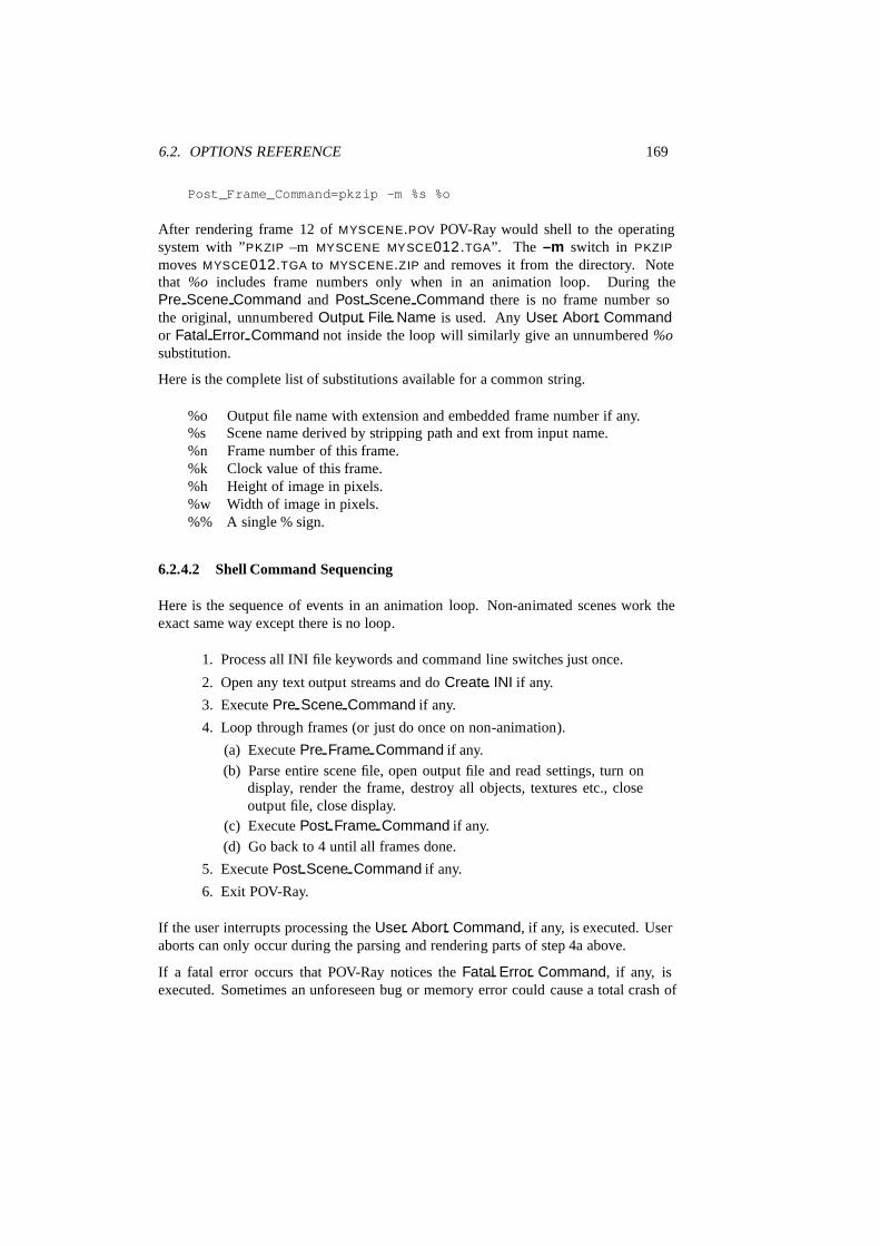
6.2. OPTIONS REFERENCE 169
Post_Frame_Command=pkzip -m %s %o
After rendering frame 12 of MYSCENE.POV POV-Ray would shell to the operatingsystem with ”PKZIP –m MYSCENE MYSCE012.TGA”. The –m switch in PKZIP
moves MYSCE012.TGA to MYSCENE.ZIP and removes it from the directory. Notethat %o includes frame numbers only when in an animation loop. During thePre Scene Command and Post Scene Command there is no frame number sothe original, unnumbered Output File Name is used. Any User Abort Commandor Fatal Error Command not inside the loop will similarly give an unnumbered %osubstitution.
Here is the complete list of substitutions available for a common string.
%o Output file name with extension and embedded frame number if any.%s Scene name derived by stripping path and ext from input name.%n Frame number of this frame.%k Clock value of this frame.%h Height of image in pixels.%w Width of image in pixels.%% A single % sign.
6.2.4.2 Shell Command Sequencing
Here is the sequence of events in an animation loop. Non-animated scenes work theexact same way except there is no loop.
1. Process all INI file keywords and command line switches just once.
2. Open any text output streams and do Create INI if any.
3. Execute Pre Scene Command if any.
4. Loop through frames (or just do once on non-animation).
(a) Execute Pre Frame Command if any.
(b) Parse entire scene file, open output file and read settings, turn ondisplay, render the frame, destroy all objects, textures etc., closeoutput file, close display.
(c) Execute Post Frame Command if any.
(d) Go back to 4 until all frames done.
5. Execute Post Scene Command if any.
6. Exit POV-Ray.
If the user interrupts processing the User Abort Command, if any, is executed. Useraborts can only occur during the parsing and rendering parts of step 4a above.
If a fatal error occurs that POV-Ray notices the Fatal Error Command, if any, isexecuted. Sometimes an unforeseen bug or memory error could cause a total crash of
170 CHAPTER 6. POV-RAY OPTIONS
the program in which case there is no chance to shell out. Fatal errors can occur justabout anywhere including during the processing of switches or INI files. If a fatal erroroccurs before POV-Ray has read the Fatal Error Command string then obviously noshell can occur.
Note that the entire scene is re-parsed for every frame. Future versions of POV-Raymay allow you to hold over parts of a scene from one frame to the next but for nowit starts from scratch every time. Note also that the Pre Frame Command occursbefore the scene is parsed. You might use this to call some custom scene generationutility before each frame. This utility could rewrite your .POV or . INC files if needed.Perhaps you will want to generate new .GIF or .TGA files for image maps or heightfields on each frame.
6.2.4.3 Shell Command Return Actions
Pre Scene Return=s Set pre scene return actionsPre Frame Return=s Set pre frame return actionsPost Scene Return=s Set post scene return actionsPost Frame Return=s Set post frame return actionsUser Abort Return=s Set user abort return actionsFatal Error Return=s Set fatal return actions
Note that no +/– switches are available for these options. They cannot be used fromthe command line. They may only be used from INI files.
Most operating systems allow application programs to return an error code if somethinggoes wrong. When POV-Ray executes a shell command it can make use of this errorcode returned from the shell process and take some appropriate action if the code iszero or non-zero. POV-Ray itself returns such codes. It returns 0 for success, 1 for fatalerror and 2 for user abort.
The actions are designated by a single letter in the different . . . Return=s options.The possible actions are:
I ignore the codeS skip one stepA all steps skippedQ quit POV-Ray immediatelyU generate a user abort in POV-RayF generate a fatal error in POV-Ray
For example if your Pre Frame Command calls a program which generates yourheight field data and that utility fails then it will return a non-zero code. We wouldprobably want POV-Ray to abort as well. The option Pre Frame Return=F will causePOV-Ray to do a fatal abort if the Pre Frame Command returns a non-zero code.

6.2. OPTIONS REFERENCE 171
Sometimes a non-zero code from the external process is a good thing. Suppose youwant to test if a frame has already been rendered. You could use the S action to skipthis frame if the file is already rendered. Most utilities report an error if the file is notfound. For example the command PKZIP –v MYSCENE MYSCE012.TGA tells pkzipyou want to view the catalog of MYSCENE.ZIP for the file MYSCE012.TGA. If the fileisn’t in the archive PKZIP returns a non-zero code.
However we want to skip if the file is found. Therefore we need to reverse the actionso it skips on zero and doesn’t skip on non-zero. To reverse the zero vs. non-zerotriggering of an action precede it with a ”-” sign (note a ”!” will also work since it isused in many programming languages as a negate operator).
Pre Frame Return=S will skip if the code shows error (non-zero) and will proceednormally on no error (zero). Pre Frame Return=–S will skip if there is no error (zero)and will proceed normally if there is an error (non-zero).
The default for all shells is I which means that the return action is ignored no matterwhat. POV-Ray simply proceeds with whatever it was doing before the shell com-mand. The other actions depend upon the context. You may want to refer back to theanimation loop sequence chart in the previous section. The action for each shell is asfollows.
On return from any User Abort Command if there is an action triggered and youhave specified . . .
F then turn this user abort into a fatal error. Do the Fa-tal Error Command if any. Exit POV-Ray with error code1.
S, A, Q, or U then proceed with the user abort. Exit POV-Ray with errorcode 2.
On return from any Fatal Error Command proceed with the fatal error no matterwhat. Exit POV-Ray with error code 1. On return from any Pre Scene Command,Pre Frame Command, Post Frame Command or Post Scene Commands ifthere is an action triggered and you have specified . . .
F then generate a fatal error. Do the Fatal Error Command if any. ExitPOV-Ray with an error code 1.
U then generate a user abort. Do the User Abort Command if any. ExitPOV-Ray with an error code 2.
Q then quit POV-Ray immediately. Acts as though POV-Ray never reallyran. Do no further shells (not even Post Scene Command and exitPOV-Ray with an error code 0.
On return from a Pre Scene Command if there is an action triggered and you havespecified . . .
172 CHAPTER 6. POV-RAY OPTIONS
S then skip rendering all frames. Acts as though the scene com-pleted all frames normally. Do not do any Pre Frame Command orPost Frame Commands. Do the Post Scene Command if any. ExitPOV-Ray with error code 0. On the earlier chart this means skip step 4on page 169.
Athen skip all scene activity. Works exactly like Q quit. On the earlierchart this means skip to step 6 on page 169.
On return from a Pre Frame Command if there is an action triggered and you havespecified . . .
S then skip only this frame. Acts as though this frame never existed. Donot do the Post Frame Command. Proceed with the next frame. Onthe earlier chart this means skip steps 4b on page 169 and 4c on page 169but loop back as needed in 4d on page 169.
A then skip rendering this frame and all remaining frames. Acts asthough the scene completed all frames normally. Do not do any fur-ther Post Frame Command. Do the Post Scene Command if any.Exit POV-Ray with error code 0. On the earlier chart this means skip therest of step 4 on page 169 and proceed at step 5 on page 169.
On return from a Post Frame Command if there is an action triggered and you havespecified . . .
S then skip rendering all remaining frames. Acts as though the scene com-pleted all frames normally. Do the Post Scene Command if any. ExitPOV-Ray with error code 0. On the earlier chart this means skip the restof step 4 on page 169 and proceed at step 5 on page 169.
A same as S for this shell command.
On return from any Post Scene Command if there is an action triggered and youhave specified . . .
S or A same as I for this shell command.
6.2.5 Text Output
Text output is an important way that POV-Ray keeps you informed about what it isgoing to do, what it is doing and what it did. New to POV-Ray 3.0, the program splitsits text messages into 7 separate streams. Some versions of POV-Ray color codes thevarious types of text. Some versions allow you to scroll back several pages of messages.All versions allow you to turn some of these text streams off/on or to direct a copy ofthe text output to one or several files. This section details the options which give youcontrol over text output.
6.2. OPTIONS REFERENCE 173
6.2.5.1 Text Streams
There are seven distinct text streams that POV-Ray uses for output. On some versionseach stream is designated by a particular color. Text from these streams are displayedwhenever it is appropriate so there is often an intermixing of the text. The distinctionis only important if you choose to turn some of the streams off or to direct some of thestreams to text files. On some systems you may be able to review the streams separatelyin their own scroll-back buffer.
Here is a description of each stream.
BANNER: This stream displays the program’s sign-on banner, copyright, contribu-tor’s list, and some help screens. It cannot be turned off or directed to a file becausemost of this text is displayed before any options or switches are read. Therefore youcannot use an option or switch to control it. There are switches which display the helpscreens. They are covered in section 6.2.5.4 on page 176.
DEBUG: This stream displays debugging messages. It was primarily designed fordevelopers but this and other streams may also be used by the user to display messagesfrom within their scene files. See 7.2.6.1 on page 212 for details on this feature. Thisstream may be turned off and/or directed to a text file.
FATAL: This stream displays fatal error messages. After displaying this text, POV-Ray will terminate. When the error is a scene parsing error, you may be shown severallines of scene text that leads up to the error. This stream may be turned off and/ordirected to a text file.
RENDER: This stream displays information about what options you have specified torender the scene. It includes feedback on all of the major options such as scene name,resolution, animation settings, anti-aliasing and others. This stream may be turned offand/or directed to a text file.
STATISTICS: This stream displays statistics after a frame is rendered. It includesinformation about the number of rays traced, the length of time of the processing andother information. This stream may be turned off and/or directed to a text file.
STATUS: This stream displays one-line status messages that explain what POV-Rayis doing at the moment. On some systems this stream is displayed on a status line at thebottom of the screen. This stream cannot be directed to a file because there is generallyno need to. The text displayed by the Verbose option or +V switch is output to thisstream so that part of the status stream may be turned off.
WARNING: This stream displays warning messages during the parsing of scene filesand other warnings. Despite the warning, POV-Ray can continue to render the scene.You will be informed if POV-Ray has made any assumptions about your scene so thatit can proceed. In general any time you see a warning, you should also assume that thismeans that future versions of POV-Ray will not allow the warned action. Thereforeyou should attempt to eliminate warning messages so your scene will be able to run infuture versions of POV-Ray. This stream may be turned off and/or directed to a textfile.

174 CHAPTER 6. POV-RAY OPTIONS
6.2.5.2 Console Text Output
Debug Console=bool Turn console display of debug info text on/off+GD Same as Debug Console=on–GD Same as Debug Console=off
Fatal Console=bool Turn console display of fatal error text on/off+GF Same as Fatal Console=on–GF Same as Fatal Console=off
Render Console=boo Turn console display of render info text on/off+GR Same as Render Console=on–GR Same as Render Console=off
Statistic Console=bool Turn console display of statistic text on/off+GS Same as Statistic Console=on–GS Same as Statistic Console=off
Warning Console=bool Turn console display of warning text on/off+GW Same as Warning Console=on–GW Same as Warning Console=off
All Console=bool Turn on/off all debug, fatal, render, statistic andwarning text to console.
+GA Same as All Console=on–GA Same as All Console=off
You may suppress the output to the console of the Debug, Fatal, Render, Statisticor Warning text streams. For example the Statistic Console=off option or the –GSswitch can turn off the Statistic stream. Using on or +GS you may turn it on again.You may also turn all five of these streams on or off at once using the All Consoleoption or +GA switch.
Note that these options take effect immediately when specified. Obviously any Erroror Warning messages that might occur before the option is read are not be affected.
6.2.5.3 Directing Text Streams to Files
Debug File=true Echo debug info text to DEBUG.OUT
Debug File=false Turn off file output of debug infoDebug File=FILE Echo debug info text to FILE
+GDFILE Both Debug Console=on, Debug File=FILE
–GDFILE Both Debug Console=off, Debug File=FILE
Fatal FILE=true Echo fatal text to FATAL.OUT

6.2. OPTIONS REFERENCE 175
Fatal File=false Turn off file output of fatalFatal File=FILE Echo fatal info text to FILE
+GFFILE Both Fatal Console=on, Fatal File=FILE
–GFFILE Both Fatal Console=off, Fatal File=FILE
Render File=true Echo render info text to RENDER.OUT
Render File=false Turn off file output of render infoRender File=FILE Echo render info text to FILE
+GRFILE Both Render Console=on, Render File=FILE
–GRFILE Both Render Console=off, Render File=FILE
Statistic File=true Echo statistic text to STATS.OUT
Statistic File=false Turn off file output of statisticsStatistic File=FILE Echo statistic text to FILE
+GSFILE Both Statistic Console=on, Statistic File=FILE
–GSFile Both Statistic Console=off, Statistic File=FILE
Warning File=true Echo warning info text to WARNING.OUT
Warning File=false Turn off file output of warning infoWarning File=FILE Echo warning info text to FILE
+GWFILE Both Warning Console=on, Warning File=FILE
–GWFILE Both Warning Console=off, Warning File=FILE
All File=true Echo all debug, fatal, render, statistic and and warningtext to ALLTEXT.OUT
All File=false Turn off file output of all debug, fatal, render, statisticand warning text
All File=FILE Echo all debug, fatal, render, statistic and warning textto file
+GAFILE Both All Console=on, All File=FILE
–GAFILE Both All Console=off, All File=FILE
You may direct a copy of the text streams to a text file for the Debug, Fatal, Render,Statistic or Warning text streams. For example the Statistic File=s option or the +GSsswitch. If the string s is true or any of the other valid true strings then that stream isredirected to a file with a default name. Valid true values are true, yes, on or 1. If thevalue is false the direction to a text file is turned off. Valid false values are false, no, offor 0. Any other string specified turns on file output and the string is interpreted as theoutput file name.
Similarly you may specify such a true, false or file name string after a switch such as+GSfile. You may also direct all five streams to the same file using the All File optionor +GA switch. You may not specify the same file for two or more streams becausePOV-Ray will fail when it tries to open or close the same file twice.
Note that these options take effect immediately when specified. Obviously any Erroror Warning messages that might occur before the option is read will not be affected.
176 CHAPTER 6. POV-RAY OPTIONS
6.2.5.4 Help Screen Switches
+H or +? Show help screen 0 if this is the only switch+H0 to +H8 Show help screen 0 to 8 if this is the only switch+?0 to +?8 Same as +H0 to +H8
Note that there are no INI style equivalents to these options.
Graphical interface versions of POV-Ray such as Mac or Windows have extensive on-line help. Other versions of POV-Ray have only a few quick-reference help screens.The +? switch, optionally followed by a single digit from 0 to 8, will display thesehelp screens to the Banner text stream. After displaying the help screens, POV-Rayterminates. Because some operating systems do not permit a question mark as a com-mand line switch you may also use the +H switch. Note however that this switch isalso used to specify the height of the image in pixels. Therefore the +H switch is onlyinterpreted as a help switch if it is the only switch on the command line and if the valueafter the switch is less than or equal to 8.
6.2.6 Tracing Options
There is more than one way to trace a ray. Sometimes there is a trade-off betweenquality and speed. Sometimes options designed to make tracing faster can slow thingsdown. This section covers options that tell POV-Ray how to trace rays with the appro-priate speed and quality settings.
6.2.6.1 Quality Settings
Quality=n Set quality value to n = 0 . . .9+Qn Same as Quality=n
The Quality=n option or +Qn switch allows you to specify the image rendering quality.You may choose to lower the quality for test rendering and raise it for final renders. Thequality adjustments are made by eliminating some of the calculations that are normallyperformed. For example settings below 4 do not render shadows. Settings below 8 donot use reflection or refraction. The values correspond to the following quality levels:
0, 1 Use ambient lighting and quick colors only. Quick colors are used onlyat 5 or below.
2, 3 Show specified diffuse and ambient lighting.4 Render shadows but no extended lights.5 Render shadows including extended lights.6, 7 Compute texture patterns.8 Compute reflected, refracted and transmitted rays.9 Compute halos.
The default is 9 if not specified.

6.2. OPTIONS REFERENCE 177
6.2.6.2 Radiosity Setting
Radiosity=bool Turns radiosity on/off+QR Turns radiosity on–QR Turns radiosity on
Radiosity is an additional calculation which computes diffuse inter-reflection. It is anextremely slow calculation that is somewhat experimental. The parameters which con-trol how radiosity calculations are performed are specified in the global settings{ radiosity { . . . } } statement. See 7.8.9 on page 362 for further details.
6.2.6.3 Automatic Bounding Control
Bounding=bool Turn bounding on/off+MB Turn bounding on; threshold 25 or previous
amount–MB Turn bounding off
Bounding Threshold=n Set bound threshold to n+MBn Turn bounding on; set future threshold to n–MBn Turn bounding off; set future threshold to n
Light Buffer=bool Turn light buffer on/off+UL Turn light buffer on–UL Turn light buffer off
Vista Buffer=bool Turn vista buffer on/off+UV Turn vista buffer on–UV Turn vista buffer off
POV-Ray uses a variety of spatial sub-division systems to speed up ray-object intersec-tion tests. The primary system uses a hierarchy of nested bounding boxes. This systemcompartmentalizes all finite objects in a scene into invisible rectangular boxes that arearranged in a tree-like hierarchy. Before testing the objects within the bounding boxesthe tree is descended and only those objects are tested whose bounds are hit by a ray.This can greatly improve rendering speed. However for scenes with only a few objectsthe overhead of using a bounding system is not worth the effort. The Bounding=offoption or –MB switch allows you to force bounding off. The default value is on.
The Bounding Threshold=n or +MBn switch allows you to set the minimum numberof objects necessary before bounding is used. The default is +MB25 which means thatif your scene has fewer than 25 objects POV-Ray will automatically turn bounding offbecause the overhead isn’t worth it. Generally it’s a good idea to use a much lowerthreshold like +MB5.

178 CHAPTER 6. POV-RAY OPTIONS
Additionally POV-Ray uses systems known as vista buffers and light buffers to furtherspeed things up. These systems only work when bounding is on and when there area sufficient number of objects to meet the bounding threshold. The vista buffer iscreated by projecting the bounding box hierarchy onto the screen and determining therectangular areas that are covered by each of the elements in the hierarchy. Only thoseobjects whose rectangles enclose a given pixel are tested by the primary viewing ray.The vista buffer can only be used with perspective and orthographic cameras becausethey rely on a fixed viewpoint and a reasonable projection (i. e. straight lines have tostay straight lines after the projection).
The light buffer is created by enclosing each light source in an imaginary box andprojecting the bounding box hierarchy onto each of its six sides. Since this relies on afixed light source, light buffers will not be used for area lights.
Reflected and transmitted rays do not take advantage of the light and vista buffer.
The default settings are Vista Buffer=on or +UV and Light Buffer=on or +UL. Theoption to turn these features off is available to demonstrate their usefulness and asprotection against unforeseen bugs which might exist in any of these bounding systems.
In general, any finite object and many types of CSG of finite objects will properly re-spond to this bounding system. In addition blobs and meshes use an additional internalbounding system. These systems are not affected by the above switch. They can beswitched off using the appropriate syntax in the scene file (see 7.5.2.1 on page 231and 7.5.3.3 on page 254 for details). Text objects are split into individual letters thatare bounded using the bounding box hierarchy. Some CSG combinations of finite andinfinite objects are also automatically bound. The end result is that you will rarely needto add manual bounding objects as was necessary in earlier versions of POV-Ray unlessyou use many infinite objects.
6.2.6.4 Anti-Aliasing Options
Antialias=bool Turns anti-aliasing on/off+A Turns anti-aliasing on with threshold 0.3 or pre-
vious amount–A Turns anti-aliasing off
Sampling Method=n Sets anti-aliasing sampling method (1 or 2)+AMn Same as Sampling Method=n
Antialias Threshold=n.n Sets anti-aliasing threshold+An.n Sets anti-aliasing on with threshold at n.n–An.n Sets anti-aliasing off (threshold n.n in future)
Jitter=bool Sets jitter on/off+J Sets jitter on with 1.0 or previous amount–J Sets jitter off

6.2. OPTIONS REFERENCE 179
Jitter Amount=n.n Sets jitter amount to n.n. If n.n ≤ 0 jitter is setoff
+Jn.n Sets jitter on; jitter amount to n.n. If n.n ≤ 0jitter is set off
–Jn.n Sets jitter off (jitter amount n.n in future)
Antialias Depth=n Sets anti-aliasing depth (n = 1 . . .9)+Rn Same as Antialias Depth=n
The ray-tracing process is in effect a discrete, digital sampling of the image with typ-ically one sample per pixel. Such sampling can introduce a variety of errors. Thisincludes a jagged, stair-step appearance in sloping or curved lines, a broken look forthin lines, moire patterns of interference and lost detail or missing objects, which areso small they reside between adjacent pixels. The effect that is responsible for thoseerrors is called aliasing.
Anti-aliasing is any technique used to help eliminate such errors or to reduce the neg-ative impact they have on the image. In general, anti-aliasing makes the ray-tracedimage look smoother. The Antialias=on option or +A switch turns on POV-Ray’s anti-aliasing system.
When anti-aliasing is turned on, POV-Ray attempts to reduce the errors by shootingmore than one viewing ray into each pixel and averaging the results to determine thepixel’s apparent color. This technique is called super-sampling and can improve theappearance of the final image but it drastically increases the time required to render ascene since many more calculations have to be done.
POV-Ray gives you the option to use one of two alternate super-sampling methods. TheSampling Method=n option or +AMn switch selects non-adaptive super-sampling(method 1) or adaptive super-sampling (method 2). Selecting one of those methodsdoes not turn anti-aliasing on. This has to be done by using the +A command lineswitch or Antialias=on option.
In the default, non-adaptive method (+AM1), POV-Ray initially traces one ray perpixel. If the color of a pixel differs from its neighbors (to the left or above) by morethan a threshold value then the pixel is super-sampled by shooting a given, fixed num-ber of additional rays. The default threshold is 0.3 but it may be changed using theAntialias Threshold=n.n option. When the switches are used, the threshold may op-tionally follow the +A. For example +A0.1 turns anti-aliasing on and sets the thresholdto 0.1.
The threshold comparison is computed as follows. If r1, g1, b1 and r2, g2, b2 are thergb components of two pixels then the difference between pixels is computed by
di f f = |r2−r1|+ |g2−g1|+ |b2−b1|. (6.1)
If this difference is greater than the threshold both pixels are super-sampled. The rgbvalues are in the range from 0.0 to 1.0 thus the most two pixels can differ is 3.0. If the

180 CHAPTER 6. POV-RAY OPTIONS
anti-aliasing threshold is 0.0 then every pixel is super-sampled. If the threshold is 3.0then no anti-aliasing is done. Lower threshold means more anti-aliasing and less speed.Use anti-aliasing for your final version of a picture, not the rough draft. The lower thecontrast, the lower the threshold should be. Higher contrast pictures can get away withhigher tolerance values. Good values seem to be around 0.2 to 0.4.
When using the non-adaptive method, the default number of super-samples is nine perpixel, located on a 3×3 grid. The Antialias Depth=n option or +Rn switch controlsthe number of rows and columns of samples taken for a super-sampled pixel. Forexample +R4 would give 4×4 = 16 samples per pixel.
The second, adaptive super-sampling method starts by tracing four rays at the cornersof each pixel. If the resulting colors differ more than the threshold amount additionalsamples will be taken. This is done recursively, i. e. the pixel is divided into foursub-pixels that are separately traced and tested for further subdivision. The advantageof this method is the reduced number of rays that have to be traced. Samples thatare common among adjacent pixels and sub-pixels are stored and reused to avoid re-tracing of rays. The recursive character of this method makes it adaptive, i. e. thesuper-sampling concentrates on those parts of the pixel that are more likely to needsuper-sampling (see figure 6.1).
level 1initial samples
level 2 level 3
new samples
one pixel
pixel corners
reused samples
Figure 6.1: Example of how the adpative super-sampling works.
The maximum number of subdivisions is specified by the Antialias Depth=n optionor +Rn switch. This is different from the non-adaptive method were the total num-ber of super-samples is specified. A maximum number of n subdivisions results in amaximum number of samples per pixel that is given by table 6.1 on the facing page.
You should note that the maximum number of samples in the adaptive case is hardlyever reached for a given pixel. If the adaptive method is used with no anti-aliasing eachpixel will be the average of the rays traced at its corners. In most cases a recursion levelof three is sufficient.
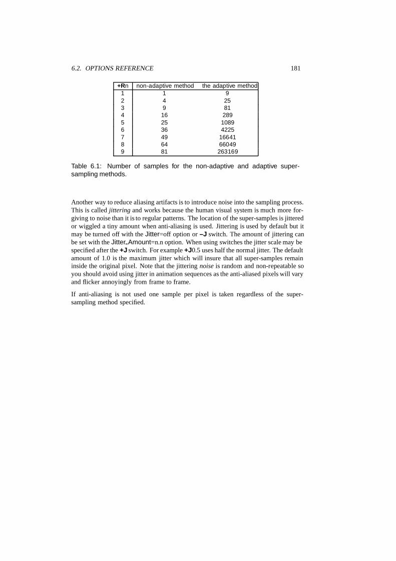
6.2. OPTIONS REFERENCE 181
+Rn non-adaptive method the adaptive method1 1 92 4 253 9 814 16 2895 25 10896 36 42257 49 166418 64 660499 81 263169
Table 6.1: Number of samples for the non-adaptive and adaptive super-sampling methods.
Another way to reduce aliasing artifacts is to introduce noise into the sampling process.This is called jittering and works because the human visual system is much more for-giving to noise than it is to regular patterns. The location of the super-samples is jitteredor wiggled a tiny amount when anti-aliasing is used. Jittering is used by default but itmay be turned off with the Jitter=off option or –J switch. The amount of jittering canbe set with the Jitter Amount=n.n option. When using switches the jitter scale may bespecified after the +J switch. For example +J0.5 uses half the normal jitter. The defaultamount of 1.0 is the maximum jitter which will insure that all super-samples remaininside the original pixel. Note that the jittering noise is random and non-repeatable soyou should avoid using jitter in animation sequences as the anti-aliased pixels will varyand flicker annoyingly from frame to frame.
If anti-aliasing is not used one sample per pixel is taken regardless of the super-sampling method specified.

182 CHAPTER 6. POV-RAY OPTIONS

Chapter 7
Scene Description Language
The Scene Description Language allows you to describe the world in a readable andconvenient way. Files are created in plain ASCII text using an editor of your choice.The input file name is specified using the Input File Name=FILE option or +IFILE
switch. By default the files have the extension .pov. POV-Ray reads the file, processesit by creating an internal model of the scene and then renders the scene.
The overall syntax of a scene is a file that contains any number of the following itemsin any order.
LANGUAGE_DIRECTIVEScamera{ CAMERA_ITEMS }OBJECT_STATEMENTSATMOSPHERE_STATEMENTSglobal_settings { GLOBAL_ITEMS }
See 7.2 on page 204, 7.5 on page 228, 7.4 on page 219, 7.7 on page 347 and 7.8 onpage 355 for details.
7.1 Language Basics
The POV-Ray language consists of identifiers, reserved keywords, floating point ex-pressions, strings, special symbols and comments. The text of a POV-Ray scene fileis free format. You may put statements on separate lines or on the same line as youdesire. You may add blank lines, spaces or indentations as long as you do not split anykeywords or identifiers.
7.1.1 Identifiers and Keywords
POV-Ray allows you to define identifiers for later use in the scene file. An identifiermay be 1 to 40 characters long. It may consist of upper or lower case letters, the digits
183

184 CHAPTER 7. SCENE DESCRIPTION LANGUAGE
0 through 9 or an underscore character (” ”). The first character must be an alphabeticcharacter. The declaration of identifiers is covered later.
POV-Ray has a number of reserved keywords which are listed below.
aa level fog offset reciprocalaa threshold fog type recursion limitabs frequency redacos gif reflectionacosh global settings refractionadaptive glowing renderadc bailout gradient repeatagate granite rgbagate turb gray threshold rgbfall green rgbftalpha halo rgbtambient height field rightambient light hexagon ripplesangle hf gray 16 rotateaperture hierarchy roughnessarc angle hollow samplesarea light hypercomplex scaleasc if scallop waveasin ifdef scatteringasinh iff seedassumed gamma image map shadowlessatan incidence sinatan2 include sine waveatanh int sinhatmosphere interpolate skyatmospheric attenuation intersection sky sphereattenuating inverse sliceaverage ior slope mapbackground irid smoothbicubic patch irid wavelength smooth triangleblack hole jitter sorblob julia fractal specularblue lambda sphereblur samples lathe spherical mappingbounded by leopard spiralbox light source spiral1box mapping linear spiral2bozo linear spline spotlightbreak linear sweep spottedbrick location sqrbrick size log sqrtbrightness looks like statisticsbrilliance look at strbumps low error factor strcmpbumpy1 mandel strength

7.1. LANGUAGE BASICS 185
bumpy2 map type strlenbumpy3 marble strlwrbump map material map struprbump size matrix sturmcamera max substrcase max intersections superellipsoidcaustics max iteration switchceil max trace level syschecker max value tchr merge tanclipped by mesh tanhclock metallic test camera 1color min test camera 2color map minimum reuse test camera 3colour mod test camera 4colour map mortar textcomponent nearest count texturecomposite no texture mapconcat normal tgacone normal map thicknessconfidence no shadow thresholdconic sweep number of waves tightnessconstant object tile2control0 octaves tilescontrol1 off toruscos offset trackcosh omega transformcount omnimax translatecrackle on transmitcrand once trianglecube onion triangle wavecubic open truecubic spline orthographic ttfcylinder panoramic turbulencecylindrical mapping pattern1 turb depthdebug pattern2 typedeclare pattern3 udefault perspective ultra wide angledegrees pgm uniondents phase updifference phong use colordiffuse phong size use colourdirection pi use indexdisc pigment u stepsdistance pigment map vdistance maximum planar mapping valdiv plane variancedust png vaxis rotatedust type point at vcrosseccentricity poly vdot
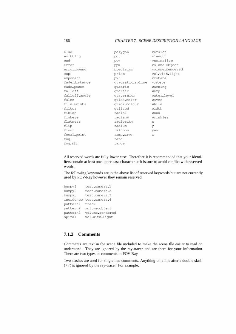
186 CHAPTER 7. SCENE DESCRIPTION LANGUAGE
else polygon versionemitting pot vlengthend pow vnormalizeerror ppm volume objecterror bound precision volume renderedexp prism vol with lightexponent pwr vrotatefade distance quadratic spline v stepsfade power quadric warningfalloff quartic warpfalloff angle quaternion water levelfalse quick color wavesfile exists quick colour whilefilter quilted widthfinish radial woodfisheye radians wrinklesflatness radiosity xflip radius yfloor rainbow yesfocal point ramp wave zfog randfog alt range
All reserved words are fully lower case. Therefore it is recommended that your identi-fiers contain at least one upper case character so it is sure to avoid conflict with reservedwords.
The following keywords are in the above list of reserved keywords but are not currentlyused by POV-Ray however they remain reserved.
bumpy1 test camera 1bumpy2 test camera 2bumpy3 test camera 3incidence test camera 4pattern1 trackpattern2 volume objectpattern3 volume renderedspiral vol with light
7.1.2 Comments
Comments are text in the scene file included to make the scene file easier to read orunderstand. They are ignored by the ray-tracer and are there for your information.There are two types of comments in POV-Ray.
Two slashes are used for single line comments. Anything on a line after a double slash(//) is ignored by the ray-tracer. For example:

7.1. LANGUAGE BASICS 187
// This line is ignored
You can have scene file information on the line in front of the comment as in:
object { FooBar } // this is an object
The other type of comment is used for multiple lines. It starts with ”/*” and ends with”*/”. Everything in-between is ignored. For example:
/* These linesare ignoredby theray-tracer */
This can be useful if you want to temporarily remove elements from a scene file. /*. . . */ comments can comment out lines containing other // comments and thus canbe used to temporarily or permanently comment out parts of a scene. /* . . . */comments can be nested, the following is legal:
/* This is a comment// This too/* This also */*/
Use comments liberally and generously. Well used, they really improve the readabilityof scene files.
7.1.3 Float Expressions
Many parts of the POV-Ray language require you to specify one or more floating pointnumbers. A floating point number is a number with a decimal point. Floats may bespecified using literals, identifiers or functions which return float values. You may alsocreate very complex float expressions from combinations of any of these using variousfamiliar operators.
Where POV-Ray needs an integer value it allows you to specify a float value and ittruncates it to an integer. When POV-Ray needs a logical or boolean value it interpretsany non-zero float as true and zero as false. Because float comparisons are subject torounding errors POV-Ray accepts values extremely close to zero as being false whendoing boolean functions. Typically values whose absolute values are less than a presetvalue epsilon are considered false for logical expressions. The value of epsilon issystem dependent but is generally about 1.0e−10. Two floats a and b are consideredto be euqal if |a−b| < epsilon.

188 CHAPTER 7. SCENE DESCRIPTION LANGUAGE
7.1.3.1 Float Literals
Float literals are represented by an optional sign (”+” or ”–”) digits, an optional decimalpoint and more digits. If the number is an integer you may omit the decimal point andtrailing zero. If it is all fractional you may omit the leading zero. POV-Ray supportsscientific notation for very large or very small numbers. The following are all validfloat literals:
-2.0 -4 34 3.4e6 2e-5 .3 0.6
7.1.3.2 Float Identifiers
Float identifiers may be declared to make scene files more readable and to parameterizescenes so that changing a single declaration changes many values. An identifier isdeclared as follows.
#declare IDENTIFIER = EXPRESSION
Where IDENTIFIER is the name of the identifier up to 40 characters long andEXPRESSION is any valid expression which evaluates to a float value. Here are someexamples.
#declare Count = 0#declare Rows = 5.3#declare Cols = 6.15#declare Number = Rows*Cols#declare Count = Count+1
As the last example shows, you can re-declare a float identifier and may use previouslydeclared values in that re-declaration. There are several built-in identifiers which POV-Ray declares for you. See 7.1.7 on page 197 for details.
7.1.3.3 Float Operators
Arithmetic float expressions can be created from float literals, identifiers or functionsusing the following operators in this order of precedence . . .
() expressions in parentheses first+A unary plus-A unary minus!A logical notA*B multiplication

7.1. LANGUAGE BASICS 189
A/B divisionA+B additionA-B subtraction
Relational, logical and conditional expressions may also be created. However there isa restriction that these types of expressions must be enclosed in parentheses first. Thisrestriction, which is not imposed by most computer languages, is necessary becausePOV-Ray allows mixing of float and vector expressions. Without the parentheses thereis an ambiguity problem. Parentheses are not required for the unary logical not operator”!” as shown above. The operators and their precedence are shown here.
Relational expressions: The operands are arithmetic expressions and the result is al-ways boolean with 1 for true and 0 for false. All relational operators have the sameprecedence.
(A < B) A is less than B(A <= B) A is less than or equal to B(A = B) A is equal to B (actually |A−B| < epsilon)(A != B) A is not equal to B (actually |A−B| ≥ epsilon)(A >= B) A is greater than or equal to B(A > B) A is greater than B
Logical expressions: The operands are converted to boolean values of 0 for false and 1for true. The result is always boolean. All logical operators have the same precedence.Note that these are not bitwise operations, they are logical.
(A & B) true only if both A and B are true, false otherwise(A | B) true if either A or B or both are true
Conditional expressions: The operand C is boolean while operands A and B are anyexpressions. The result is of the same type as A and B.
(C ? A : B) if C then A else B
Assuming the various identifiers have been declared, the following are examples ofvalid expressions . . .
1+2+3 2*5 1/3 Row*3 Col*5
(Offset-5)/2 This/That+Other*Thing
((This<That) & (Other>=Thing)?Foo:Bar)
Expressions are evaluated left to right with innermost parentheses evaluated first, thenunary +, − or !, then multiply or divide, then add or subtract, then relational, thenlogical, then conditional.

190 CHAPTER 7. SCENE DESCRIPTION LANGUAGE
7.1.4 Vector Expressions
POV-Ray often requires you to specify a vector. A vector is a set of related float values.Vectors may be specified using literals, identifiers or functions which return vectorvalues. You may also create very complex vector expressions from combinations ofany of these using various familiar operators.
POV-Ray vectors may have from two to five components but the vast majority of vec-tors have three components. Unless specified otherwise, you should assume that theword vector means a three component vector. POV-Ray operates in a 3D x, y, z coor-dinate system and you will use three component vectors to specify x, y and z values. Insome places POV-Ray needs only two coordinates. These are often specified by a 2Dvector called an UV vector. Fractal objects use 4D vectors. Color expressions use 5Dvectors but allow you to specify 3, 4 or 5 components and use default values for theunspecified components. Unless otherwise noted, all 2, 4 or 5 component vectors workjust like 3D vectors but they have a different number of components.
7.1.4.1 Vector Literals
Vectors consist of two to five float expressions that are bracketed by angle brackets〈 and 〉. The terms are separated by commas. For example here is a typical threecomponent vector:
< 1.0, 3.2, -5.4578 >
The commas between components are necessary to keep the program from thinkingthat the 2nd term is the single float expression 3.2− 5.4578 and that there is no 3rdterm. If you see an error message such as Float expected but ’〉’ found instead youprobably have missed a comma.
Sometimes POV-Ray requires you to specify floats and vectors side-by-side. The rulesfor vector expressions allow for mixing of vectors with vectors or vectors with floatsso commas are required separators whenever an ambiguity might arise. For example〈1,2,3〉−4 evaluates as a mixed float and vector expression where 4 is subtracted fromeach component resulting in 〈−3,−2,−1〉. However the comma in 〈1,2,3〉,−4 meansthis is a vector followed by a float.
Each component may be a full float expression. For example 〈This+ 3,That/3,5 ∗Other Thing〉 is a valid vector.
7.1.4.2 Vector Identifiers
Vector identifiers may be declared to make scene files more readable and to parameter-ize scenes so that changing a single declaration changes many values. An identifier isdeclared as follows . . .

7.1. LANGUAGE BASICS 191
#declare IDENTIFIER = EXPRESSION
Where IDENTIFIER is the name of the identifier up to 40 characters long andEXPRESSION is any valid expression which evaluates to a vector value. Here aresome examples . . .
#declare Here = <1,2,3>#declare There = <3,4,5>#declare Jump = <Foo*2,Bar-1,Bob/3>#declare Route = There-Here#declare Jump = Jump+<1,2,3>
Note that you invoke a vector identifier by using its name without any angle brackets.As the last example shows, you can re-declare a vector identifier and may use previ-ously declared values in that re-declaration. There are several built-in identifiers whichPOV-Ray declares for you. See 7.1.7 on page 197 for details.
7.1.4.3 Vector Operators
Vector literals, identifiers and functions may also be combined in expressions thesame as float values. Operations are performed on a component-by-component basis.For example 〈1,2,3〉+ 〈4,5,6〉 evaluates the same as 〈1+4,2+5,3+6〉 or 〈5,7,9〉.Other operations are done on a similar component-by-component basis. For example(〈1,2,3〉 = 〈3,2,1〉) evaluates to 〈0,1,0〉 because the middle components are equal butthe others are not. Admittedly this isn’t very useful but its consistent with other vectoroperations.
Conditional expressions such as(C ? A : B) require that C is a float expression butA and B may be vector expressions. The result is that the entire conditional evaluatesas a valid vector. For example if Foo and Bar are floats then
Foo < Bar ? <1,2,3> : <5,6,7>
evaluates as the vector 〈1,2,3〉 if Foo is less than Bar and evaluates as 〈5,6,7〉 other-wise.
You may use the dot operator to extract a single component from a vector. Suppose theidentifier Spot was previously defined as a vector. Then Spot.x is a float value thatis the first component of this x, y, z vector. Similarly Spot.y and Spot.z referencethe 2nd and 3rd components. If Spot was a two component UV vector you could useSpot.u and Spot.v to extract the first and second component. For a 4D vector use.x, .y, .z and .t to extract each float component. The dot operator is also used incolor expressions which are covered later.
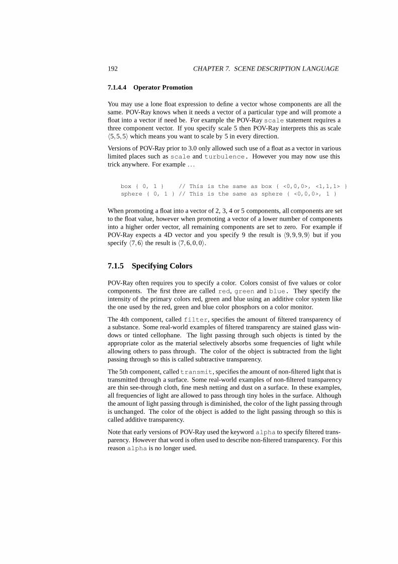
192 CHAPTER 7. SCENE DESCRIPTION LANGUAGE
7.1.4.4 Operator Promotion
You may use a lone float expression to define a vector whose components are all thesame. POV-Ray knows when it needs a vector of a particular type and will promote afloat into a vector if need be. For example the POV-Ray scale statement requires athree component vector. If you specify scale 5 then POV-Ray interprets this as scale〈5,5,5〉 which means you want to scale by 5 in every direction.
Versions of POV-Ray prior to 3.0 only allowed such use of a float as a vector in variouslimited places such as scale and turbulence. However you may now use thistrick anywhere. For example . . .
box { 0, 1 } // This is the same as box { <0,0,0>, <1,1,1> }sphere { 0, 1 } // This is the same as sphere { <0,0,0>, 1 }
When promoting a float into a vector of 2, 3, 4 or 5 components, all components are setto the float value, however when promoting a vector of a lower number of componentsinto a higher order vector, all remaining components are set to zero. For example ifPOV-Ray expects a 4D vector and you specify 9 the result is 〈9,9,9,9〉 but if youspecify 〈7,6〉 the result is 〈7,6,0,0〉.
7.1.5 Specifying Colors
POV-Ray often requires you to specify a color. Colors consist of five values or colorcomponents. The first three are called red, green and blue. They specify theintensity of the primary colors red, green and blue using an additive color system likethe one used by the red, green and blue color phosphors on a color monitor.
The 4th component, called filter, specifies the amount of filtered transparency ofa substance. Some real-world examples of filtered transparency are stained glass win-dows or tinted cellophane. The light passing through such objects is tinted by theappropriate color as the material selectively absorbs some frequencies of light whileallowing others to pass through. The color of the object is subtracted from the lightpassing through so this is called subtractive transparency.
The 5th component, called transmit, specifies the amount of non-filtered light that istransmitted through a surface. Some real-world examples of non-filtered transparencyare thin see-through cloth, fine mesh netting and dust on a surface. In these examples,all frequencies of light are allowed to pass through tiny holes in the surface. Althoughthe amount of light passing through is diminished, the color of the light passing throughis unchanged. The color of the object is added to the light passing through so this iscalled additive transparency.
Note that early versions of POV-Ray used the keyword alpha to specify filtered trans-parency. However that word is often used to describe non-filtered transparency. For thisreason alpha is no longer used.

7.1. LANGUAGE BASICS 193
Each of the five components of a color are float values which are normally in the rangebetween 0.0 and 1.0. However any values, even negatives may be used.
Colors may be specified using vectors, keywords with floats or identifiers. You mayalso create very complex color expressions from combinations of any of these usingvarious familiar operators. The syntax for specifying a color has evolved since POV-Ray was first released. We have maintained the original keyword-based syntax andadded a short-cut vector notation. Either the old or new syntax is acceptable howeverthe vector syntax is easier to use when creating color expressions.
7.1.5.1 Color Vectors
The syntax for a color vector is any of the following . . .
color rgb VECTOR3color rgbf VECTOR4color rgbt VECTOR4color rgbft VECTOR5
where VECTOR3, VECTOR4 or VECTOR5 are any valid vector expressions of 3, 4 or5 components. For example
color rgb <1.0, 0.5, 0.2>
This specifies a color whose red component is 1.0 or 100% of full intensity. The greencomponent is 0.5 or 50% of full intensity and the blue component is 0.2 or 20% of fullintensity. Although the filter and transmit components are not explicitly specified, theyexist and are set to their default values of 0 or no transparency.
The rgbf keyword requires a four component vector. The 4th component is the filtercomponent and the transmit component defaults to zero. Similarly the rgbt keywordrequires four components where the 4th value is moved to the 5th component which istransmit and then the filter component is set to zero.
The rgbft keyword allows you to specify all five components. Internally in expres-sions all five are always used.
Under most circumstances the keyword color is optional and may be omitted. Wealso support the British or Canadian spelling colour. Under some circumstances, ifthe vector expression is a 5 component expression or there is a color identifier in theexpression then the rgbtf keyword is optional.
7.1.5.2 Color Keywords
The older keyword method of specifying a color is still useful and many users prefer it.Like a color vector, you begin with the optional keyword color. This is followed by
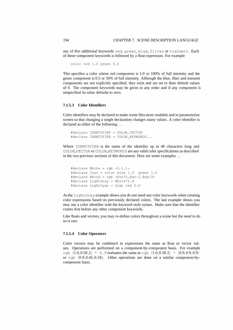
194 CHAPTER 7. SCENE DESCRIPTION LANGUAGE
any of five additional keywords red, green, blue, filter or transmit. Eachof these component keywords is followed by a float expression. For example
color red 1.0 green 0.5
This specifies a color whose red component is 1.0 or 100% of full intensity and thegreen component is 0.5 or 50% of full intensity. Although the blue, filter and transmitcomponents are not explicitly specified, they exist and are set to their default valuesof 0. The component keywords may be given in any order and if any component isunspecified its value defaults to zero.
7.1.5.3 Color Identifiers
Color identifiers may be declared to make scene files more readable and to parameterizescenes so that changing a single declaration changes many values. A color identifier isdeclared as either of the following . . .
#declare IDENTIFIER = COLOR_VECTOR#declare IDENTIFIER = COLOR_KEYWORDS...
Where IDENTIFIER is the name of the identifier up to 40 characters long andCOLOR VECTOR or COLOR KEYWORDS are any valid color specifications as describedin the two previous sections of this document. Here are some examples . . .
#declare White = rgb <1,1,1>#declare Cyan = color blue 1.0 green 1.0#declare Weird = rgb <Foo*2,Bar-1,Bob/3>#declare LightGray = White*0.8#declare LightCyan = Cyan red 0.6
As the LightGray example shows you do not need any color keywords when creatingcolor expressions based on previously declared colors. The last example shows youmay use a color identifier with the keyword style syntax. Make sure that the identifiercomes first before any other component keywords.
Like floats and vectors, you may re-define colors throughout a scene but the need to doso is rare.
7.1.5.4 Color Operators
Color vectors may be combined in expressions the same as float or vector val-ues. Operations are performed on a component-by-component basis. For examplergb 〈1.0,0.50.2〉 * 0.9 evaluates the same as rgb 〈1.0,0.50.2〉 * 〈0.9,0.9,0.9〉or rgb 〈0.9,0.45,0.18〉. Other operations are done on a similar component-by-component basis.

7.1. LANGUAGE BASICS 195
You may use the dot operator to extract a single component from a color. Supposethe identifier Shade was previously defined as a color. Then Shade.red is the floatvalue of the red component of Shade. Similarly Shade.green, Shade.blue,Shade.filter and Shade.transmit extract the float value of the other colorcomponents.
7.1.5.5 Common Color Pitfalls
The variety and complexity of color specification methods can lead to some commonmistakes. Here are some things to consider when specifying a color.
When using filter transparency, the colors which come through are multiplied by theprimary color components. For example if grey light such asrgb 〈0.9,0.9,0.9〉 passesthrough a filter such as rgbf 〈1.0,0.5,0.0,1.0〉 the result is rgb 〈0.9,0.45,0.0〉 withthe red let through 100%, the green cut in half from 0.9 to 0.45 and the blue totallyblocked. Often users mistakenly specify a clear object by
color filter 1.0
but this has implied red, green and blue values of zero. You’ve just specified a totallyblack filter so no light passes through. The correct way is either
color red 1.0 green 1.0 blue 1.0 filter 1.0
or
color transmit 1.0
In the 2nd example it doesn’t matter what the rgb values are. All of the light passesthrough untouched.
Another pitfall is the use of color identifiers and expressions with color keywords. Forexample . . .
color My_Color red 0.5
this substitutes whatever was the red component of My Color with a red componentof 0.5 however . . .
color My_Color + red 0.5
adds 0.5 to the red component of My Color and even less obvious . . .

196 CHAPTER 7. SCENE DESCRIPTION LANGUAGE
color My_Color * red 0.5
that cuts the red component in half as you would expect but it also multiplies the green,blue, filter and transmit components by zero! The part of the expression after themultiply operator evaluates to rgbft 〈0.5,0,0,0,0〉 as a full 5 component color.
The following example results in no change to My Color.
color red 0.5 My_Color
This is because the identifier fully overwrites the previous value. When using identifierswith color keywords, the identifier should be first.
One final issue, some POV-Ray syntax allows full color specifications but only uses thergb part. In these cases it is legal to use a float where a color is needed. For example:
finish { ambient 1 }
The ambient keyword expects a color so the value 1 is promoted to 〈1,1,1,1,1〉 whichis no problem. However
pigment { color 0.4 }
is legal but it may or may not be what you intended. The 0.4 is promoted to〈0.4,0.4,0.4,0.4,0.〉 with the filter and transmit set to 0.4 as well. It is more likelyyou wanted . . .
pigment { color rgb 0.4 }
in which case a 3 component vector is expected. Therefore the 0.4 is promoted to〈0.4,0.4,0.4,0.0,0.0〉 with default zero for filter and transmit.
7.1.6 Strings
The POV-Ray language requires you to specify a string of characters to be used as a filename, text for messages or text for a text object. Strings may be specified using literals,identifiers or functions which return string values. Although you cannot build stringexpressions from symbolic operators such as are used with floats, vectors or colors,you may perform various string operations using string functions. Some applicationsof strings in POV-Ray allow for non-printing formatting characters such as newline orform-feed.
7.1.6.1 String Literals
String literals begin with a double quote mark ’”’ which is followed by up to 256printable ASCII characters and are terminated by another double quote mark. Thefollowing are all valid string literals:
"Here" "There" "myfile.gif" "textures.inc"

7.1. LANGUAGE BASICS 197
7.1.6.2 String Identifiers
String identifiers may be declared to make scene files more readable and to parameter-ize scenes so that changing a single declaration changes many values. An identifier isdeclared as follows . . .
#declare IDENTIFIER = STRING
Where IDENTIFIER is the name of the identifier up to 40 characters long andSTRING is a string literal, string identifier or function which returns a string value.Here are some examples . . .
#declare Font_Name = "ariel.ttf"#declare Inc_File = "myfile.inc"#declare Name = "John"#declare Name = concat(Name," Doe")
As the last example shows, you can re-declare a string identifier and may use previouslydeclared values in that re-declaration.
7.1.7 Built-in Identifiers
There are several built-in float and vector identifiers. You can use them to specifyvalues or to create expressions but you cannot re-declare them to change their values.
7.1.7.1 Constant Built-in Identifiers
Most built-in identifiers never change value. They are defined as though the followinglines were at the start of every scene.
#declare pi = 3.1415926535897932384626#declare true = 1#declare yes = 1#declare on = 1#declare false = 0#declare no = 0#declare off = 0#declare u = <1,0>#declare v = <0,1>#declare x = <1,0,0>#declare y = <0,1,0>#declare z = <0,0,1>#declare t = <0,0,0,1>

198 CHAPTER 7. SCENE DESCRIPTION LANGUAGE
The built-in float identifier pi is obviously useful in math expressions involving circles.
The built-in float identifiers on,off, yes, no, true and false are designed for useas boolean constants.
The built-in vector identifiers x, y and z provide much greater readability for yourscene files when used in vector expressions. For example . . . .
plane { y, 1} // The normal vector is obviously "y".plane { <0,1,0>, 1} // This is harder to read.
translate 5*x // Move 5 units in the "x" direction.translate <5,0,0> // This is less obvious.
An expression like 5*x evaluates to 5〈1,0,0〉 or 〈5,0,0〉.
Similarly u and v may be used in 2D vectors. When using 4D vectors you should usex, y, z, and t and POV-Ray will promote x, y and z to 4D when used where 4D isrequired.
7.1.7.2 Built-in Identifier clock
The built-in float identifier clock is used to control animations in POV-Ray. Unlikesome animation packages, the action in POV-Ray animated scenes does not dependupon the integer frame numbers. Rather you should design your scenes based upon thefloat identifier clock. For non-animated scenes its default value is 0 but you can setit to any float value using the INI file option Clock=n.n or the command-line switch+Kn.n to pass a single float value your scene file.
Other INI options and switches may be used to animate scenes by automatically loop-ing through the rendering of frames using various values for clock. By default, theclock value is 0 for the initial frame and 1 for the final frame. All other frames areinterpolated between these values. For example if your object is supposed to rotate onefull turn over the course of the animation you could specify rotate 360*clock*y.Then as clock runs from 0 to 1, the object rotates about the y-axis from 0 to 360 degrees.
Although the value of clock will change from frame-to-frame, it will never changethroughout the parsing of a scene.
See 6.2.1 on page 151 for more details.
7.1.7.3 Built-in Identifier version
The built-in float identifier version contains the current setting of the version com-patibility option. Although this value defaults to 3 which is the current POV-Ray ver-sion number, the initial value of version may be set by the INI file option Ver-sion=n.n or by the +MVn.n command-line switch. This tells POV-Ray to parse thescene file using syntax from an earlier version of POV-Ray.

7.1. LANGUAGE BASICS 199
The INI option or switch only affects the initial setting. Unlike other built-in identi-fiers, you may change the value of version throughout a scene file. You do not use#declare to change it though. The #version language directive is used to changemodes. Such changes may occur several times within scene files.
Together with the built-in version identifier the #version directive allows you tosave and restore the previous values of this compatibility setting. For example supposeMYSTUFF.INC is in version 1 format. At the top of the file you could put:
#declare Temp_Vers = version // Save previous value#version 1.0 // Change to 1.0 mode
... // Version 1.0 stuff goes here...
#version Temp_Vers // Restore previous version
7.1.8 Functions
POV-Ray defines a variety of built-in functions for manipulating floats, vectors andstrings. The functions are listed grouped according to their usage and not by the typeof value they return. For example vdot computes the dot product of two vectors andis listed as a vector function even though it returns a single float value.
Function calls consist of a keyword which specifies the name of the function followedby a parameter list enclosed in parentheses. Parameters are separated by commas. Forexample:
keyword(param1,param2)
Functions evaluate to values that are floats, vectors or strings and may be used in ex-pressions or statements anywhere that literals or identifiers of that type may be used.
7.1.8.1 Float Functions
The following are the functions which take one or more float parameters and returnfloat values. Assume that A and B are any valid expression that evaluates to a float.See 7.1.8.2 on page 201 and 7.1.8.3 on page 202 for other functions which return floatvalues but whose primary purpose is more closely related to vectors and strings.
abs(A): Absolute value of A. If A is negative, returns --A otherwise re-turns A.
acos(A): Arc-cosine of A. Returns the angle, measured in radians, whosecosine is A.

200 CHAPTER 7. SCENE DESCRIPTION LANGUAGE
asin(A): Arc-sine of A. Returns the angle, measured in radians, whosesine is A.
atan2(A,B): Arc-tangent of (A/B). Returns the angle, measured in ra-dians, whose tangent is (A/B). Returns appropriate value even if B iszero. Use atan2(A,1) to compute usual atan(A) function.
ceil(A): Ceiling of A. Returns the smallest integer greater than A. Roundsup to the next higher integer.
cos(A): Cosine of A. Returns the cosine of the angle A, where A is mea-sured in radians.
degrees(A): Convert radians to degrees. Returns the angle measured indegrees whose value in radians is A. The formula is
Adegrees =180π
Aradians. (7.1)
div(A,B): Integer division. The integer part of (A/B).
exp(A): Exponential of A. Returns the value of e raised to the Apower where e is the non-repeating value approximately equal to2.71828182846 the base of natural logarithms.
floor(A): Floor of A. Returns the largest integer less than A. Roundsdown to the next lower integer.
int(A): Integer part of A. Returns the truncated integer part of A. Roundstowards zero.
log(A): Natural logarithm of A. Returns the natural logarithm base e ofthe value A where e is the non-repeating value approximately equal to2.71828182846.
max(A,B): Maximum of A and B. Returns A if A larger than B. Otherwisereturns B.
min(A,B): Minimum of A and B. Returns A if A smaller than B. Otherwisereturns B.
mod(A,B): Value of A modulo A. Returns the remainder after the integerdivision of A/B. The Formula is1
mod(A,B) =
(AB−
⌊AB
⌋)B. (7.2)
pow(A,B): Exponentiation. Returns the value of A raised to the power B.
radians(A): Convert degrees to radians. Returns the angle measured inradians whose value in degrees is A. The formula is
Aradians =π
180Adegree. (7.3)
1 x� is the smallest integer number larger than x.

7.1. LANGUAGE BASICS 201
rand(A): Returns the next pseudo-random number from the stream speci-fied by the positive integer A. You must call seed() to initialize a randomstream before calling rand(). The numbers are uniformly distributed,and have values between 0.0 and 1.0, inclusively. The numbers gener-ated by separate streams are independent random variables.
seed(A): Initializes a new pseudo-random stream with the initial seedvalue A. The number corresponding to this random stream is returned.Any number of pseudo-random streams may be used as shown in theexample below:
#declare R1 = seed(0)#declare R2 = seed(12345)
#sphere {<rand(R1), rand(R1), rand(R1)>,rand(R2)
}
Multiple random generators are very useful in situations where you userand() to place a group of objects, and then decide to use rand() in an-other location earlier in the file to set some colors or place another groupof objects. Without separate rand() streams, all of your objects wouldmove when you added more calls to rand(). This is very annoying.
sin(A): Sine of A. Returns the sine of the angle A, where A is measuredin radians.
sqrt(A): Square root of A. Returns the value whose square is A.
tan(A): Tangent of A. Returns the tangent of the angle A, where A ismeasured in radians.
7.1.8.2 Vector Functions
The following are the functions which take one or more vector and float parameters andreturn vector or float values. All of these functions support only three component vec-tors. Assume that A and B are any valid expression that evaluates to a three componentvector and that F is any valid expression that evaluates to a float.
vaxis rotate(A,B,F): Rotate A about B by A. Given the x, y, z coor-dinates of a point in space designated by the vector A, rotate that pointabout an arbitrary axis defined by the vector B. Rotate it through anangle specified in degrees by the float value F. The result is a vectorcontaining the new x, y, z coordinates of the point.
vcross(A,B): Cross product of A and B. Returns a vector that is the vec-tor cross product of the two vectors. The resulting vector is perpen-dicular to the two original vectors and its length is proportional to theangle between them. See the animated demo scene VECT2.POV for anillustration.

202 CHAPTER 7. SCENE DESCRIPTION LANGUAGE
vdot(A,B): Dot product of A and B. Returns a float value that is the dotproduct (sometimes called scaler product of A with B). The formula is
vdot = AxBx+AyBy+Az Bz. (7.4)
See the animated demo scene VECT2.POV for an illustration.
vlength(A): Length of A. Returns a float value that is the length of vec-tor A. Can be used to compute the distance between two points. Theformula is
vlength =√
vdot(A,A). (7.5)
vnormalize(A): Normalize vector A. Returns a unit length vector that isthe same direction as A. The formula is vnormalize = A/vlength(A).
vrotate(A,B): Rotate A about origin by B. Given the x, y, z coordinatesof a point in space designated by the vector A, rotate that point aboutthe origin by an amount specified by the vector B. Rotate it about the x-axis by an angle specified in degrees by the float value B.x. SimilarlyB.y and B.z specify the amount to rotate in degrees about the y-axisand z-axis. The result is a vector containing the new x,y,z coordinatesof the point.
7.1.8.3 String Functions
The following are the functions which take one or more string and float parameters andreturn string or float values. Assume that S1 and S2 are any valid strings and that A, Land P are any valid expressions that evaluate to floats.
asc(S1): ASCII value of S1. Returns an integer value in the range 0 to255 that is the ASCII value of the first character of S1. For exampleasc("ABC") is 65 because that is the value of the character ”A”.
chr(A): Character whose ASCII value is A. Returns a single characterstring. The ASCII value of the character is specified by an integer Awhich must be in the range 0 to 255. For example chr(70) is thestring ”F”. If you use chr() when rendering text objects you should beaware that the characters rendered for values of A > 127 are dependenton the (TTF) font being used. Many (TTF) fonts use the Latin-1 (ISO8859-1) character set, but not all do.
concat(S1,S2,[S3 . . . ]): Concatenate strings S1 and S2. Returnsa string that is the concatenation of all parameter strings. Must have atleast 2 parameters but may have more. For example:
concat("Value is ", str(A,3,1), " inches")
7.1. LANGUAGE BASICS 203
If the float value Awas 12.34 the result is ”Value is 12.3 inches”, whichis a string.
file exists(S1): Search for file specified by S1. Attempts to open thefile whose name is specified the string S1. The current directory andall directories specified in any Library Path INI options or +L com-mand line switches are searched. File is immediately closed. Returns aboolean value 1 on success and 0 on failure.
str(A,L,P): Convert float A to formatted string. Returns a formattedstring representation of float value A. The float parameter L specifiesthe minimum length of the string and the type of left padding used ifthe string’s representation is shorter than the minimum. If L is positivethen the padding is with blanks. If L is negative then the padding iswith zeros. The overall minimum length of the formatted string isabs(L). If the string needs to be longer, it will be made as long asnecessary to represent the value.
The float parameter P specifies the number of digits after the decimalpoint. If P is negative then a compiler-specific default precision is use.Here are some examples:
str(123.456,0,3) "123.456"str(123.456,4,3) "123.456"str(123.456,9,3) " 123.456"str(123.456,-9,3) "00123.456"str(123.456,0,2) "123.46"str(123.456,0,0) "123"str(123.456,5,0) " 123"str(123.000,7,2) " 123.00"str(123.456,0,-1) "123.456000" (platform specific)
strcmp(S1,S2): Compare string S1 to S2. Returns a float value zeroif the strings are equal, a positive number if S1 comes after S2 in theASCII collating sequence, else a negative number.
strlen(S1): Length of S1. Returns an integer value that is the numberof characters in the string S1.
strlwr(S1): Lower case of S1. Returns a new string in which all uppercase letters in the string S1 are converted to lower case. The originalstring is not affected. For example strlwr("Hello There!")results in ”hello there!”.
substr(S1,P,L): Sub-string from S1. Returns a string that is a subsetof the characters in parameter S1 starting at the position specified bythe integer value P for a length specified by the integer value L. For ex-ample substr("ABCDEFGHI",4,2) evaluates to the string ”‘EF”.If P+L > strlen(S1) an error occurs.

204 CHAPTER 7. SCENE DESCRIPTION LANGUAGE
strupr(S1): Upper case of S1. Returns a new string in which all lowercase letters in the string S1 are converted to upper case. The originalstring is not affected. For example strupr("Hello There!")results in ”HELLO THERE!”.
val(S1): Convert string S1 to float. Returns a float value that is repre-sented by the text in S1. For example val("123.45") is 123.45 asa float.
7.2 Language Directives
The POV Scene Language contains several statements called language directives whichtell the file parser how to do its job. These directives can appear in almost any place inthe scene file — even in the middle of some other statements. They are used to includeother text files in the stream of commands, to declare identifiers, to define conditionalor looped parsing and to control other important aspects of scene file processing.
Each directive begins with the hash character # (often called a number sign or poundsign). It is followed by a keyword and optionally other parameters.
In versions of POV-Ray prior to 3.0, the use of this # character was optional. Languagedirectives could only be used between objects, camera or light source statements andcould not appear within those statements. The exception was the #include whichcould appear anywhere. Now that all language directives can be used almost anywhere,the # character is mandatory.
The following keywords introduce language directives.
#break #default #statistics#case #else #switch#debug #end #version#declare #render #warning
Earlier versions of POV-Ray considered #max intersections and#max trace level to be language directives but they have been moved tothe global settings statement. Their use as a directive still works but itgenerates a warning and may be discontinued in the future.
7.2.1 Include Files
The language allows include files to be specified by placing the line
#include "filename.inc"
7.2. LANGUAGE DIRECTIVES 205
at any point in the input file. The filename may be specified by any valid string ex-pression but it usually is a literal string enclosed in double quotes. It may be up to 40characters long (or your computer’s limit), including the two double-quote characters.
The include file is read in as if it were inserted at that point in the file. Using include isthe same as actually cutting and pasting the entire contents of this file into your scene.
Include files may be nested. You may have at most 10 nested include files. There is nolimit on un-nested include files.
Generally, include files have data for scenes but are not scenes in themselves. Byconvention scene files end in .POV and include files end with . INC.
It is legal to specify drive and directory information in the file specification however itis discouraged because it makes scene files less portable between various platforms.
It is typical to put standard include files in a special sub-directory. POV-Ray can onlyread files in the current directory or one referenced by the Library Path option (Seesection 6.2.3.2 on page 166).
7.2.2 Declare
Identifiers may be declared and later referenced to make scene files more readable andto parametrize scenes so that changing a single declaration changes many values. Thereare several built-in identifiers which POV-Ray declares for you. See 7.1.7 on page 197for details.
7.2.2.1 Declaring identifiers
An identifier is declared as follows.
#declare IDENTIFIER = ITEM
Where IDENTIFIER is the name of the identifier up to 40 characters long and ITEMis any of the following
float, vector, color or string expressionsobjects (all kinds)texture, pigment, normal, finish or halocolor map, pigment map, slope map, normal mapcamera, light sourceatmospherefograinbowsky spheretransform

206 CHAPTER 7. SCENE DESCRIPTION LANGUAGE
Here are some examples.
#declare Rows = 5#declare Count = Count+1#declare Here = <1,2,3>#declare White = rgb <1,1,1>#declare Cyan = color blue 1.0 green 1.0#declare Font_Name = "ariel.ttf"#declare Ring = torus {5,1}#declare Checks = pigment{ checker White, Cyan }
object{ Rod scale y*5 } // not "cylinder { Rod } "object {
Ringpigment { Checks scale 0.5 }transform Skew
}
Declarations, like most language directives, can appear anywhere in the file — evenwithin other statements. For example:
#declare Here=<1,2,3>#declare Count=0 // initialize Count
union {object { Rod translate Here*Count }#declare Count=Count+1 // re-declare inside unionobject { Rod translate Here*Count }#declare Count=Count+1 // re-declare inside unionobject { Rod translate Here*Count }
}
As this example shows, you can re-declare an identifier and may use previously de-clared values in that re-declaration. However if you attempt to re-declare an identifieras anything other than its original type, it will generate a warning message.
Declarations may be nested inside each other within limits. In the example in theprevious section you could declare the entire union as a object. However for technicalreasons you may not use any language directive inside the declaration of floats, vectorsor color expressions.
7.2.3 Default Directive
POV-Ray creates a default texture when it begins processing. You may change thosedefaults as described below. Every time you specify a texture { . . . } statement,

7.2. LANGUAGE DIRECTIVES 207
POV-Ray creates a copy of the default texture. Anything you put in the texture state-ment overrides the default settings. If you attach a pigment, normal or finishto an object without any texture statement then POV-Ray checks to see if a texture hasalready been attached. If it has a texture then the pigment, normal or finish will modifythe existing texture. If no texture has yet been attached to the object then the defaulttexture is copied and the pigment, normal or finish will modify that texture.
You may change the default texture, pigment, normal or finish using the language di-rective #default { . . . } as follows:
#default {texture {
pigment {...}normal {...}finish {...}
}}
Or you may change just part of it like this:
#default {pigment {...}
}
This still changes the pigment of the default texture. At any time there is only onedefault texture made from the default pigment, normal and finish. The example abovedoes not make a separate default for pigments alone. Note that the special texturestiles and material map or a texture with a texture map may not be used asdefaults.
You may change the defaults several times throughout a scene as you wish. Subse-quent #default statements begin with the defaults that were in effect at the time. Ifyou wish to reset to the original POV-Ray defaults then you should first save them asfollows:
//At top of file#declare Original_Default = texture {}
later after changing defaults you may restore it with . . .
#default {texture {Original_Default}}
If you do not specify a texture for an object then the default texture is attached when theobject appears in the scene. It is not attached when an object is declared. For example:

208 CHAPTER 7. SCENE DESCRIPTION LANGUAGE
#declare My_Object=sphere{ <0,0,0>, 1 } // Default texture not applied
object { My_Object } // Default texture added here
You may force a default texture to be added by using an empty texture statement asfollows:
#declare My_Thing =sphere { <0,0,0>, 1 texture {} } // Default texture applied
The original POV-Ray defaults for all items are given throughout the documentationunder each appropriate section.
7.2.4 Version Directive
While many language changes have been made for POV-Ray 3.0, all of version 2.0syntax and most of version 1.0 syntax still works. Whenever possible we try to maintainbackwards compatibility. One feature introduced in 2.0 that was incompatible with any1.0 scene files is the parsing of float expressions. Setting +MV1.0 command line switchor the Version=1.0 INI option turns off expression parsing as well as many warningmessages so that nearly all 1.0 files will still work. The changes between 2.0 and 3.0are not as extensive. Setting Version=2.0 is only necessary to eliminate some warningmessages. Naturally the default setting for this option is Version=3.0.
The #version language directive is used to change modes within scene files. Thisswitch or INI options only affects the initial setting.
Together with the built-in version identifier the #version directive allows you tosave and restore the previous values of this compatibility setting. For example supposeMYSTUFF.INC is in version 1.0 format. At the top of the file you could put:
#declare Temp_Vers = version // Save previous value#version 1.0 // Change to 1.0 mode
... // Version 1.0 stuff goes here ...
#version Temp_Vers // Restore previous version
Previous versions of POV-Ray would not allow you to change versions inside an objector declaration but that restriction has been lifted for POV-Ray 3.0.
Future versions of POV-Ray may not continue to maintain full backward compatibilityeven with the #version directive. We strongly encourage you to phase in 3.0 syntaxas much as possible.

7.2. LANGUAGE DIRECTIVES 209
7.2.5 Conditional Directives
POV-Ray 3.0 allows a variety of new language directives to implement conditionalparsing of various sections of your scene file. This is especially useful in describingthe motion for animations but it has other uses as well. Also available is a #whileloop directive. You may nest conditional directives 200 levels deep.
7.2.5.1 IF ELSE Directives
The simplest conditional directive is a traditional #if directive. It is of the form . . .
#if (COND)// This section is// parsed if COND is true
#else// This section is// parsed if COND is false
#end // End of conditional part
where (COND) is a float expression that evaluates to a boolean value. A value of 0.0 isfalse and any non-zero value is true. Note that extremely small values of about 1e−10are considered zero in case of round off errors. The parentheses around the conditionare required. The #else directive is optional. The #end directive is required.
7.2.5.2 IFDEF Directives
The #ifdef directive is similar to the #if directive however it is used to determineif an identifier has been previously declared. After the #ifdef directive instead of aboolean expression you put a lone identifier enclosed in parentheses. For example:
#ifdef (User_Thing)// This section is parsed if the// identifier "User_Thing" was// previously declaredobject{User_Thing} // invoke identifier
#else// This section is parsed if the// identifier "User_Thing" was not// previously declaredbox{<0,0,0>,<1,1,1>} // use a default
#end// End of conditional part
The #else directive is optional. The #end directive is required.

210 CHAPTER 7. SCENE DESCRIPTION LANGUAGE
7.2.5.3 IFNDEF Directives
The #ifndef directive is similar to the #ifdef directive however it is used to deter-mine if the given identifier isn’t declared yet. For example:
#ifndef (User_Thing)// This section is parsed if the// identifier "User_Thing" was not// previously declaredbox{<0,0,0>,<1,1,1>} // use a default
#else// This section is parsed if the// identifier "User_Thing" was// previously declaredobject{User_Thing} // invoke identifier
#end// End of conditional part
The #else directive is optional. The #end directive is required.
7.2.5.4 SWITCH CASE and RANGE Directives
A more powerful conditional is the #switch directive. The syntax is as follows . . .
#switch (VALUE)#case (TEST_1)
// This section is parsed if VALUE=TEST_1#break //First case ends
#case (TEST_2)// This section is parsed if VALUE=TEST_2
#break //Second case ends
#range (LOW_1,HIGH_1)// This section is parsed if// (VALUE >= LOW_1) and (VALUE <= HIGH_1)
#break //Third case ends
#range (LOW_2,HIGH_2)// This section is parsed if// (VALUE >= LOW_2) and (VALUE <= HIGH_2)
#break //Fourth case ends
#else// This section is parsed if no other case or// range is true.
#end // End of conditional part

7.2. LANGUAGE DIRECTIVES 211
The float expression VALUE following the #switch directive is evaluated and com-pared to the values in the #case or #range directives. When using #case, it isfollowed by a float expression TEST 1 in parentheses. It is compared to the VALUE.As usual in POV-Ray, float comparisons are considered equal if their difference is under1e−10. If the values are equal, parsing continues normally until a #break, #else or#end directive is reached. If the comparison fails POV-Ray skips until another #caseor #range is found.
If you use the #range directive it is followed by two float expressions LOW 1 andHIGH 1 which are enclosed in parentheses and separated by a comma. If the switchVALUE is in the range specified then parsing continues normally until a #break,#else or #end directive is reached. If the VALUE is outside the range the comparisonfails and POV-Ray skips until another #case or #range is found.
If no #case or #range succeeds the #else section is parsed. The #else directiveis optional. If no #else is specified and no match succeeds then parsing resumes afterthe #end directive.
There may be any number of #case or #range directives in any order you want.If a segment evaluates true but no #break is specified, the parsing will fall throughto the next #case or #range and will continue until a #break, #else or #end.Hitting a #break while parsing a successful section causes an immediate jump to the#end without processing subsequent sections, even if a subsequent condition wouldalso have been satisfied.
7.2.5.5 WHILE Directive
The #while directive is a looping feature that makes it easy to place multiple objectsin a pattern or other uses. The #while directive is followed by a float expression thatevaluates to a boolean value. A value of 0.0 is false and any non-zero value is true.Note that extremely small values of about 1e−10 are considered zero in case of roundoff errors. The parentheses around the expression are required. If the condition istrue parsing continues normally until an #end directive is reached. At the end, POV-Ray loops back to the #while directive and the condition is re-evaluated. Loopingcontinues until the condition fails. When it fails, parsing continues after the #enddirective. For example:
#declare Count=0#while (Count < 5)
object{MyObject translate x*3*Count}#declare Count=Count+1
#end
This example places five copies of MyObject in a row spaced three units apart in thex-direction.
212 CHAPTER 7. SCENE DESCRIPTION LANGUAGE
7.2.6 User Message Directives
With the addition of conditional and loop directives, the POV-Ray language has thepotential to be more like an actual programming language. This means that it will benecessary to have some way to see what is going on when trying to debug loops andconditionals. To fulfill this need we have added the ability to print text messages to thescreen. You have a choice of five different text streams to use including the ability togenerate a fatal error if you find it necessary. Limited formatting is available for stringsoutput by this method.
7.2.6.1 Text Message Streams
The syntax for a text message is any of the following:
#debug STRING#error STRING#error STRING#render STRING#statistics STRING#warning STRING
Where STRING is any valid string of text including string identifiers or functions whichreturn strings. For example:
#switch (clock*360)#range (0,180)
#render "Clock in 0 to 180 range\n"#break
#range (180,360)#render "Clock in 180 to 360 range\n"
#break
#else#warning "Clock outside expected range\n"#warning concat("Value is:",str(clock*360,5,0),"\n")
#end
There are seven distinct text streams that POV-Ray uses for output. You may outputonly to five of them. On some versions of POV-Ray, each stream is designated by aparticular color. Text from these streams are displayed whenever it is appropriate sothere is often an intermixing of the text. The distinction is only important if you chooseto turn some of the streams off or to direct some of the streams to text files. On somesystems you may be able to review the streams separately in their own scroll-backbuffer. See 6.2.5.2 on page 174 for details on re-directing the streams to a text file.

7.2. LANGUAGE DIRECTIVES 213
Here is a description of how POV-Ray uses each stream. You may use them for what-ever purpose you want except note that use of the #error stream causes a fatal errorafter the text is displayed.
DEBUG: This stream displays debugging messages. It was primarily de-signed for developers but this and other streams may also be used bythe user to display messages from within their scene files.
FATAL: This stream displays fatal error messages. After displaying thistext, POV-Ray will terminate. When the error is a scene parsing error,you may be shown several lines of scene text that leads up to the error.
RENDER: This stream displays information about what options you havespecified to render the scene. It includes feedback on all of the ma-jor options such as scene name, resolution, animation settings, anti-aliasing and others.
STATISTICS: This stream displays statistics after a frame is rendered. Itincludes information about the number of rays traced, the length oftime of the processing and other information.
WARNING: This stream displays warning messages during the parsing ofscene files and other warnings. Despite the warning, POV-Ray can con-tinue to render the scene.
The BANNER and STATUS streams can not be accessed by the user.
7.2.6.2 Text Formatting
Some escape sequences are available to include non-printing control characters in yourtext. These sequences are similar to those used in string literals in the C programminglanguage. Note that these control characters only apply in text message directives.They are not implemented for other string usage in POV-Ray such as text objects or filenames. Depending on what platform you are using, they may not be fully supportedfor console output. However they will appear in any text file if you re-direct a streamto a file. The sequences are:
”\a” Bell or alarm, 0x07”\b” Backspace, 0x08”\f” Form feed, 0x0C”\n” New line (line feed) 0x0A”\r” Carriage return 0x0D”\t” Horizontal tab 0x09”\v” Vertical tab 0x0B”\0” Null 0x00”\\” Backslash 0x5C”\’” Single quote 0x27
214 CHAPTER 7. SCENE DESCRIPTION LANGUAGE
”\”” Double quote 0x22
For example:
#debug "This is one line.\nBut this is another"
7.3 POV-Ray Coordinate System
Objects, lights and the camera are positioned using a typical 3D coordinate system. Theusual coordinate system for POV-Ray has the positive y-axis pointing up, the positivex-axis pointing to the right and the positive z-axis pointing into the screen. The negativevalues of the axes point the other direction as shown in the images in section 4.1.1 onpage 33.
Locations within that coordinate system are usually specified by a three componentvector. The three values correspond to the x, y and z directions respectively. For ex-ample, the vector 〈1,2,3〉 means the point that’s one unit to the right, two units up andthree units in front of the center of the universe at 〈0,0,0〉.
Vectors are not always points though. They can also refer to an amount to size, moveor rotate a scene element or to modify the texture pattern applied to an object.
The supported transformations are rotate, scale and translate. They are usedto turn, size and translate an object or texture. A transformation matrix may also beused to specify complex transformations directly.
7.3.1 Transformations
The supported transformations are rotate, scale and translate. They are used to turn,size and translate an object or texture.
rotate <VECTOR>scale <VECTOR>translate <VECTOR>
7.3.1.1 Translate
An object or texture pattern may be moved by adding a translate parameter. It consistsof the keyword translate followed by a vector expression. The terms of the vectorspecify the number of units to move in each of the x, y and z directions. Translatemoves the element relative to it’s current position. For example

7.3. POV-RAY COORDINATE SYSTEM 215
sphere { <10, 10, 10>, 1pigment { Green }translate <-5, 2, 1>
}
will move the sphere from 〈10,10,10〉 to 〈5,12,11〉. It does not move it to the absolutelocation 〈−5,2,1〉. Translating by zero will leave the element unchanged on that axis.For example:
sphere { <10, 10, 10>, 1pigment { Green }translate 3*x // evaluates to <3,0,0> so move 3 units
// in the x direction and none along y or z}
7.3.1.2 Scale
You may change the size of an object or texture pattern by adding a scale parameter.It consists of the keyword scale followed by a vector expression. The 3 terms of thevector specify the amount of scaling in each of the x, y and z directions.
Scale is used to stretch or squish an element. Values larger than one stretch the elementon that axis while values smaller than one are used to squish it. Scale is relative to thecurrent element size. If the element has been previously re-sized using scale then scalewill size relative to the new size. Multiple scale values may used.
For example
sphere { <0,0,0>, 1scale <2,1,0.5>
}
will stretch and smash the sphere into an ellipsoid shape that is twice the original sizealong the x-direction, remains the same size in the y-direction and is half the originalsize in the z-direction.
If a lone float expression is specified it is promoted to a three component vector whoseterms are all the same. Thus the item is uniformly scaled by the same amount in alldirections. For example:
object {MyObjectscale 5 // Evaluates as <5,5,5> so uniformly scale
// by 5 in every direction.}

216 CHAPTER 7. SCENE DESCRIPTION LANGUAGE
7.3.1.3 Rotate
You may change the orientation of an object or texture pattern by adding a rotate pa-rameter. It consists of the keyword rotate followed by a vector expression. Thethree terms of the vector specify the number of degrees to rotate about each of the x-,y- and z-axes.
Note that the order of the rotations does matter. Rotations occur about the x-axis first,then the y-axis, then the z-axis. If you are not sure if this is what you want then youshould only rotate on one axis at a time using multiple rotation statements to get acorrect rotation. As in
rotate <0, 30, 0> // 30 degrees around Y axis then,rotate <-20, 0, 0> // -20 degrees around X axis then,rotate <0, 0, 10> // 10 degrees around Z axis.
Rotation is always performed relative to the axis. Thus if an object is some distancefrom the axis of rotation it will not only rotate but it will orbit about the axis as thoughit was swinging around on an invisible string.
To work out the rotation directions you must perform the famous Computer GraphicsAerobics exercise as explained in the section 4.1.1 on page 33.
7.3.1.4 Matrix Keyword
The matrix keyword can be used to explicitly specify the transformation matrix tobe used for objects or textures. Its syntax is:
matrix < m00, m01, m02,m10, m11, m12,m20, m21, m22,m30, m31, m32 >
Where m00 through m32 are float expressions that specify the elements of a 4 ×4matrix with the fourth column implicitly set to 〈0,0,0,1〉. A point P, P = 〈px, py, pz〉,is transformed into Q, Q = 〈qx,qy,qz〉, by
qx =m0,0 px+m1,0 py+m2,0 pz+m3,0
qy =m0,1 px+m1,1 py+m2,1 pz+m3,1
qz =m0,2 px+m1,2 py+m2,2 pz+m3,2
(7.6)
Normally you won’t use the matrix keyword because it’s less descriptive than the trans-formation commands and harder to visualize. There is an intersecting aspect of thematrix command though. It allows more general transformation like shearing. Thefollowing matrix causes an object to be sheared along the y-axis.

7.3. POV-RAY COORDINATE SYSTEM 217
object {MyObjectmatrix < 1, 1, 0,
0, 1, 0,0, 0, 1,0, 0, 0 >
}
7.3.2 Transformation Order
Because rotations are always relative to the axis and scaling is relative to the origin,you will generally want to create an object at the origin and scale and rotate it first.Then you may translate it into its proper position. It is a common mistake to carefullyposition an object and then to decide to rotate it because a rotation of an object causesit to orbit about the axis, the position of the object may change so much that it orbitsout of the field of view of the camera!
Similarly scaling after translation also moves an object unexpectedly. If you scale afteryou translate the scale will multiply the translate amount. For example
translate <5, 6, 7>scale 4
will translate to 〈20,24,28〉 instead of 〈5,6,7〉. Be careful when transforming to getthe order correct for your purposes.
7.3.3 Transform Identifiers
At times it is useful to combine together several transformations and apply them inmultiple places. A transform identifier may be used for this purpose. Transformidentifiers are declared as follows:
#declare IDENT = transform { TRANSFORMATION... }
Where IDENT is the identifier to be declared and TRANSFORMATION is one or moretranslate, rotate, scale or matrix specifications or a previously declaredtransform identifier. A transform identifier is invoked by the transform keywordwithout any brackets as shown here:
object {MyObject // Get a copy of MyObjecttransform MyTrans // Apply the transformation
218 CHAPTER 7. SCENE DESCRIPTION LANGUAGE
translate -x*5 // Then move it 5 units left}object {
MyObject // Get another copy of MyObjecttransform MyTrans // Apply the same transformationtranslate -x*5 // Then move this one 5 units right
}
On extremely complex CSG objects with lots of components it may speed up parsing ifyou apply a declared transformation rather than the individual translate, rotate,scale or matrix specifications. The transform is attached just once to eachcomponent. Applying each individual translate, rotate, scale or matrixspecifications takes long. This only affects parsing — rendering works the same eitherway.
7.3.4 Transforming Textures and Objects
When an object is transformed all textures attached to the object at that time are trans-formed as well. This means that if you have a translate, rotate, scale ormatrix in an object before a texture the texture will not be transformed. If the trans-formation is after the texture then the texture will be transformed with the object. Ifthe transformation is inside the texture { . . . } statement then only the textureis affected. The shape remains the same. For example:
sphere { 0, 1texture { Jade } // texture identifier from TEXTURES.INCscale 3 // this scale affects both the
// shape and texture}
sphere { 0, 1scale 3 // this scale affects the shape onlytexture { Jade }
}
sphere { 0, 1texture {
Jadescale 3 // this scale affects the texture only
}}
Transformations may also be independently applied to pigment patterns and surfacenormal patterns. Note that scaling a normal pattern affects only the width and spacing.It does not affect the apparent height or depth of the bumps. For example:

7.4. CAMERA 219
box { <0, 0, 0>, <1, 1, 1>texture {
pigment {checker Red, Whitescale 0.25 // This affects only the color pattern
}normal {
bumps 0.3 // This specifies apparent height of bumpsscale 0.2 // Scales diameter and space between bumps
// but not the height. Has no effect on// color pattern.
}rotate y*45 // This affects the entire texture but
} // not the object.}
7.4 Camera
The camera definition describes the position, projection type and properties of the cam-era viewing the scene. Its syntax is:
camera {[ perspective | orthographic | fisheye |
ultra_wide_angle | omnimax | panoramic |cylinder FLOAT ]
location <VECTOR>look_at <VECTOR>right <VECTOR>up <VECTOR>direction <VECTOR>sky <VECTOR>right <VECTOR>angle FLOATblur_samples FLOATaperture FLOATfocal_point <VECTOR>normal { NORMAL }
}
Depending on the projection type some of the parameters are required, some are op-tional and some aren’t used. If no projection type is given the perspective camera willbe used (pinhole camera). If no camera is specified a default camera is used.
Regardless of the projection type all cameras use the location, look at, right,up, direction and sky keywords to determine the location and orientation of the

220 CHAPTER 7. SCENE DESCRIPTION LANGUAGE
camera. Their meaning differs with the projection type used. A more detailed explana-tion of the camera placement follows later.
7.4.1 Type of Projection
The following list explains the different projection types that can be used with thecamera. The most common types are the perspective and orthographic projections.
angle
locationdirection
look_atimage plane
up
right
+0.5
-0.5
+0.5
-0.5
Figure 7.1: The perspective camera.
Perspective projection: This projection represents the classic pinhole cam-era. The (horizontal) viewing angle is either determined by the ratiobetween the length of the direction vector and the length of the rightvector or by the optional keyword angle, which is the preferred way.The viewing angle has to be larger than 0 degrees and smaller than 180degrees. See figure 7.1 for an overview of the perspective camera’sgeometry.
Orthographic projection: This projection uses parallel camera rays to cre-ate an image of the scene. The size of the image is determined by thelengths of the right and up vectors.If you add the orthographic keyword after all other parameters of a per-spective camera you’ll get an orthographic view with the same imagearea, i. e. the size of the image is the same. In this case you needn’tspecify the lengths of the right and up vector because they’ll be calcu-lated automatically. You should be aware though that the visible partsof the scene change when switching from perspective to orthographicview. As long as all objects of interest are near the look at locationthey’ll be still visible if the orthographic camera is used. Objects fareraway may get out of view while nearer objects will stay in view.

7.4. CAMERA 221
Fisheye projection: This is a spherical projection. The viewing angle isspecified by the angle keyword. An angle of 180 degrees creates thestandard fisheye while an angle of 360 degrees creates a super-fisheye(I-see-everything-view). If you use this projection you should get acircular image. If this isn’t the case, i. e. you get an elliptical image,you should read 7.4.4.5.1 on page 225.
Ultra wide angle projection: This projection is somewhat similar to thefisheye but it projects the image onto a rectangle instead of a circle.The viewing angle can be specified using the angle keyword.
Omnimax projection: The omnimax projection is a 180 degrees fisheyethat has a reduced viewing angle in the vertical direction. In realitythis projection is used to make movies that can be viewed in the dome-like Omnimax theaters. The image will look somewhat elliptical. Theangle keyword isn’t used with this projection.
Panoramic projection: This projection is called cylindrical equirectangu-lar projection. It overcomes the degeneration problem of the perspec-tive projection if the viewing angle approaches 180 degrees. It uses atype of cylindrical projection to be able to use viewing angles largerthan 180 degrees with a tolerable lateral-stretching distortion. Theangle keyword is used to determine the viewing angle.
Cylindrical projection: Using this projection the scene is projected onto acylinder. There are four different types of cylindrical projections de-pending on the orientation of the cylinder and the position of the view-point. The viewing angle and the length of the up or right vector deter-mine the dimensions of the camera and the visible image. The camerato use is specified by a number. The types are:
1 vertical cylinder, fixed viewpoint2 horizontal cylinder, fixed viewpoint3 vertical cylinder, viewpoint moves along the cylinder’s
axis4 horizontal cylinder, viewpoint moves along the cylinder’s
axis
If the perspective camera is used the angle keyword overrides the viewing anglespecified by the direction keyword and vice versa. Each time angle is used thelength of the direction vector is adjusted to fit the new viewing angle.
There is no limitation to the viewing angle except for the perspective projection. If youchoose viewing angles larger than 360 degrees you’ll see repeated images of the scene(the way the repetition takes place depends on the camera). This might be useful forspecial effects.
You should note that the vista buffer can only be used with the perspective and ortho-graphic camera.

222 CHAPTER 7. SCENE DESCRIPTION LANGUAGE
7.4.2 Focal Blur
Simulates focal depth-of-field by shooting a number of sample rays from jittered pointswithin each pixel and averaging the results.
The aperture setting determines the depth of the sharpness zone. Large apertures givea lot of blurring, while narrow apertures will give a wide zone of sharpness. Note that,while this behaves as a real camera does, the values for aperture are purely arbitraryand are not related to f-stops.
The center of the zone of sharpness is the focal point vector (the defaultfocal point is 〈0,0,0〉).
The blur samples value controls the maximum number of rays to use for each pixel.More rays give a smoother appearance but is slower, although this is controlled some-what by an adaptive mechanism that stops shooting rays when a certain degree of confi-dence has been reached that shooting more rays would not result in a significant change.
The confidence and variance keywords control the adaptive function. The con-fidence value is used to determine when the samples seem to be close enough to thecorrect color. The variance value specifies an acceptable tolerance on the variance ofthe samples taken so far. In other words, the process of shooting sample rays is ter-minated when the estimated color value is very likely (as controlled by the confidenceprobability) near the real color value.
Since the confidence is a probability its values can range from 0 to 1 (the default is 0.9,i. e. 90%). The value for the variance should be in the range of the smallest displayablecolor difference (the default is 1/128).
Larger confidence values will lead to more samples, slower traces and better images.The same holds for smaller variance thresholds.
By default no focal blur is used, i. e. the default aperture is 0 and the default numberof samples is 0.
7.4.3 Camera Ray Perturbation
The optional keyword normal may be used to assign a normal pattern to the camera.All camera rays will be perturbed using this pattern. This lets you create special effects.See the animated scene CAMERA2.POV for an example.
7.4.4 Placing the Camera
In the following sections the placing of the camera will be further explained.
7.4. CAMERA 223
7.4.4.1 Location and Look At
Under many circumstances just two vectors in the camera statement are all you need toposition the camera: location and look at. For example:
camera {location <3,5,-10>look_at <0,2,1>
}
The location is simply the x, y, z coordinates of the camera. The camera can be locatedanywhere in the ray-tracing universe. The default location is 〈0,0,0〉. The look atvector tells POV-Ray to pan and tilt the camera until it is looking at the specified x, y, zcoordinates. By default the camera looks at a point one unit in the z-direction from thelocation.
The look at specification should almost always be the last item in the camera state-ment. If other camera items are placed after the look at vector then the camera maynot continue to look at the specified point.
7.4.4.2 The Sky Vector
Normally POV-Ray pans left or right by rotating about the y-axis until it lines up withthe look at point and then tilts straight up or down until the point is met exactly.However you may want to slant the camera sideways like an airplane making a bankedturn. You may change the tilt of the camera using the sky vector. For example:
camera {location <3,5,-10>sky <1,1,0>look_at <0,2,1>
}
This tells POV-Ray to roll the camera until the top of the camera is in line with the skyvector. Imagine that the sky vector is an antenna pointing out of the top of the camera.Then it uses the sky vector as the axis of rotation left or right and then to tilt up ordown in line with the sky vector. In effect you’re telling POV-Ray to assume that thesky isn’t straight up. Note that the sky vector must appear before the look at vector.
The sky vector does nothing on its own. It only modifies the way the look at vectorturns the camera. The default value for sky is 〈0,1,0〉.
7.4.4.3 The Direction Vector
The direction vector tells POV-Ray the initial direction to point the camera beforemoving it with look at or rotate vectors (the default is direction 〈0,0,1〉). It
224 CHAPTER 7. SCENE DESCRIPTION LANGUAGE
may also be used to control the (horizontal) field of view with some types of projection.This should be done using the easier to use angle keyword though.
If you are using the ultra wide angle, panoramic or cylindrical projection you shoulduse a unit length direction vector to avoid strange results.
The length of the direction vector doesn’t matter if one of the following projectiontypes is used: orthographic, fisheye or omnimax.
7.4.4.4 Angle
The angle keyword specifies the (horizontal) viewing angle in degress of the cameraused. Even though it is possible to use the direction vector to determine the viewingangle for the perspective camera it is much easier to use the angle keyword.
The necessary calculations to convert from one method to the other are described be-low. These calculations are used to determine the length of the direction vector when-ever the angle keyword is encountered.
The viewing angle is converted to a direction vector length and vice versa using theformula The viewing angle α is given by the formula
α = 2 tan−1 lr2ld
(7.7)
where lr and ld are the lengths of the right and direction vector respectively.
From this the length of the direction vector can be calculated for a given viewing angleand right vector. From this the length of the direction ld vector can be calculated for agiven viewing angle ∠ and right vector.
ld =lr
2 tan(α
2
) . (7.8)
7.4.4.5 Up and Right Vectors
The direction of the up and right vectors (together with the direction vector) deter-mine the orientation of the camera in the scene. They are set implicitly by their defaultvalues of
right 4/3*xup y
or the look at parameter (in combination with location). The directions of anexplicitly specified right and up vector will be overridden by any following look atparameter.

7.4. CAMERA 225
While some camera types ignore the length of these vectors others use it to extractvaluable information about the camera settings. The following list will explain themeaning of the right and up vector for each camera type. Since the direction the vectorsis always used to describe the orientation of the camera it will not be explained again.
Perspective projection: The lengths of the up and right vectors are used toset the size of the viewing window and the aspect ratio as describedin detail in section 7.4.4.5.1. Since the field of view depends on thelength of the direction vector (implicitly set by the angle keyword orexplicitly set by the direction keyword) and the lengths of the rightand up vectors you should carefully choose them in order to get thedesired results.
Orthographic projection: The lengths of the right and up vector set thesize of the viewing window regardless of the direction vector length,which is not used by the orthographic camera. Again the relation of thelengths is used to set the aspect ratio.
Fisheye projection: The right and up vectors are used to set the aspect ratio.
Ultra wide angle projection: The up and right vectors work in a similarway as for the perspective camera.
Omnimax projection: The Omnimax projection is quite similar to the fish-eye and thus the right and up vectors are also used to determine theaspect ratio of the resulting image.
Panoramic projection: The up and right vectors work in a similar way asfor the perspective camera.
Cylindrical projection: In cylinder type one and three the axis of the cylin-der lies along the up vector and the width is determined by the lengthof right vector or it may be overridden with the angle vector. Intype three the up vector determines how many units high the image is.For example if you have up 4*y on a camera at the origin only pointsfrom y =−2 to y = 2 are visible. All viewing rays are perpendicularto the y-axis. For type two and four, the cylinder lies along the rightvector. Viewing rays for type four are perpendicular to the right vec-tor.
Note that the up, right and direction vectors should always remain perpendicular toeach other or the image will be distorted. If this is not the case a warning message willbe printed. The vista buffer will not work for non-perpendicular camera vectors.
7.4.4.5.1 Aspect Ratio
Together the right and up vectors define the aspect ratio (height to width ratio) of theresulting image. The default values up 〈0,1,0rangle and right 〈1.33,0,0〉 resultin an aspect ratio of 4 to 3. This is the aspect ratio of a typical computer monitor. If

226 CHAPTER 7. SCENE DESCRIPTION LANGUAGE
you wanted a tall skinny image or a short wide panoramic image or a perfectly squareimage you should adjust the up and right vectors to the appropriate proportions.
Most computer video modes and graphics printers use perfectly square pixels. Forexample Macintosh displays and IBM S-VGA modes 640x480, 800x600 and 1024x768all use square pixels. When your intended viewing method uses square pixels then thewidth and height you set with the +W and +H switches should also have the same ratioas the right and up vectors. Note that 640/480 = 4/3 so the ratio is proper for this squarepixel mode.
Not all display modes use square pixels however. For example IBM VGA mode320x200 and Amiga 320x400 modes do not use square pixels. These two modes stillproduce a 4/3 aspect ratio image. Therefore images intended to be viewed on suchhardware should still use 4/3 ratio on their up and right vectors but the +W and +Hsettings will not be 4/3.
For example:
camera {location <3,5,-10>up <0,1,0>right <1,0,0>look_at <0,2,1>
}
This specifies a perfectly square image. On a square pixel display like SVGA youwould use +W and +H settings such as +W480 +H480 or +W600 +H600. However onthe non-square pixel Amiga 320x400 mode you would want to use values of +W240+H400 to render a square image.
7.4.4.5.2 Handedness
The right vector also describes the direction to the right of the camera. It tells POV-Ray where the right side of your screen is. The sign of the right vector can be used todetermine the handedness of the coordinate system in use. The default right statementis:
right <1.33, 0, 0>
This means that the +x-direction is to the right. It is called a left-handed system be-cause you can use your left hand to keep track of the axes. Hold out your left hand withyour palm facing to your right. Stick your thumb up. Point straight ahead with yourindex finger. Point your other fingers to the right. Your bent fingers are pointing to the+x-direction. Your thumb now points into +y-direction. Your index finger points intothe +z-direction.

7.4. CAMERA 227
To use a right-handed coordinate system, as is popular in some CAD programs andother ray-tracers, make the same shape using your right hand. Your thumb still pointsup in the +y-direction and your index finger still points forward in the +z-direction butyour other fingers now say the +x-direction is to the left. That means that the rightside of your screen is now in the −x-direction. To tell POV-Ray to act like this this youcan use a negative x value in the right vector like this:
right <-1.33, 0, 0>
Since x increasing to the left doesn’t make much sense on a 2D screen you now ro-tate the whole thing 180 degrees around by using a positive z value in your camera’slocation. You end up with something like this.
camera {location <0,0,10>up <0,1,0>right <-1.33,0,0>look_at <0,0,0>
}
Now when you do your ray-tracer’s aerobics, as explained in the section 4.1.1 onpage 33, you use your right hand to determine the direction of rotations.
In a two dimensional grid, x is always to the right and y is up. The two versions ofhandedness arise from the question of whether z points into the screen or out of it andwhich axis in your computer model relates to up in the real world.
Architectural CAD systems, like AutoCAD, tend to use the God’s Eye orientation thatthe z-axis is the elevation and is the model’s up direction. This approach makes senseif you’re an architect looking at a building blueprint on a computer screen. z means up,and it increases towards you, with x and y still across and up the screen. This is thebasic right handed system.
Stand alone rendering systems, like POV-Ray, tend to consider you as a participant.You’re looking at the screen as if you were a photographer standing in the scene. Up inthe model is now y, the same as up in the real world and x is still to the right, so z mustbe depth, which increases away from you into the screen. This is the basic left handedsystem.
7.4.4.6 Transforming the Camera
The translate and rotate commands can re-position the camera once you’vedefined it. For example:

228 CHAPTER 7. SCENE DESCRIPTION LANGUAGE
camera {location < 0, 0, 0>direction < 0, 0, 1>up < 0, 1, 0>right < 1, 0, 0>rotate <30, 60, 30>translate < 5, 3, 4>
}
In this example, the camera is created, then rotated by 30 degrees about the x-axis,60 degrees about the y-axis and 30 degrees about the z-axis, then translated to anotherpoint in space.
7.4.5 Camera Identifiers
You may declare several camera identifiers if you wish. This makes it easy to quicklychange cameras. For example:
#declare Long_Lens =camera {
location -z*100angle 3
}
#declare Short_Lens =camera {
location -z*50angle 15
}
camera {Long_Lens // edit this line to change lenseslook_at Here
}
7.5 Objects
Objects are the building blocks of your scene. There are a lot of different types ofobjects supported by POV-Ray: finite solid primitives, finite patch primitives, infinitesolid polynomial primitives and light sources. Constructive Solid Geometry (CSG) isalso supported.
The basic syntax of an object is a keyword describing its type, some floats, vectorsor other parameters which further define its location and/or shape and some optional
7.5. OBJECTS 229
object modifiers such as texture, pigment, normal, finish, bounding, clipping or trans-formations.
The texture describes what the object looks like, i. e. its material. Textures are com-binations of pigments, normals, finishes and halos. Pigment is the color or patternof colors inherent in the material. Normal is a method of simulating various patternsof bumps, dents, ripples or waves by modifying the surface normal vector. Finish de-scribes the reflective and refractive properties of a material. The halo is used to describethe interior of the object.
Bounding shapes are finite, invisible shapes which wrap around complex, slow render-ing shapes in order to speed up rendering time. Clipping shapes are used to cut awayparts of shapes to expose a hollow interior. Transformations tell the ray-tracer how tomove, size or rotate the shape and/or the texture in the scene.
7.5.1 Empty and Solid Objects
It is very important that you know the basic concept behind empty and solid objects inPOV-Ray to fully understand how features like halos and translucency are used.
Objects in POV-Ray can either be solid, empty or filled with (small) particles.
A solid object is made from the material specified by its pigment and finish statements(and to some degree its normal statement). By default all objects are assumed to besolid. If you assign a stone texture to a sphere you’ll get a ball made completely ofstone. It’s like you had cut this ball from a block of stone. A glass ball is a massivesphere made of glass.
You should be aware that solid objects are conceptual things. If you e. g. clip awayparts of the sphere you’ll see that the sphere is empty, i. e. you’ll clearly see that theinterior is empty and it just has a very thin surface.
This is not contrary to the concept of a solid object used in POV-Ray. It is assumed thatall space inside the sphere is covered by the sphere’s material. Thus there is no roomfor any other particles like those used by fog or halos.
Empty objects are created by adding the hollow keyword (see 7.5.7.3 on page 276) tothe object statement. An empty (or hollow) object is assumed to be made of a very thinsurface which is of the material specified by the pigment, finish and normal statements.The object’s interior is empty, i. e. it normally contains air molecules.
An empty object can be filled with particles by adding fog or atmosphere to the sceneor by adding a halo to the object. It is very important to understand that in order to fillan object with any kind of particles it first has to be made hollow.
7.5.1.1 Halo Pitfall
There is a piftall in the current empty/solid object implementation that you have to beaware of.

230 CHAPTER 7. SCENE DESCRIPTION LANGUAGE
In order to be able to put solid objects inside a halo (this also holds for fog and atmo-sphere) a test has to be made for every ray that passes through the halo. If this raytravels through a solid object the halo will not be calculated. This is what anyone willexpect.
The problem arises when the camera ray is inside any non-hollow object. In this casethe ray is already travelling through a solid object and even if the halo’s containerobject is hit and it is hollow, the halo will not be calculated. There is no way of tellingbetween these two cases.
POV-Ray has to determine wether the camera is inside any object prior to tracing acamera ray in order to be able to correctly render halos when the camera is inside thecontainer object. There’s no way around doing this.
The solution to this problem (that will often happen with infinite objects like planes) isto make those objects hollow too. Thus the ray will travel through a hollow object, willhit the container object and the halo will be calculated.
Note that the above is also true for atmosphere and fog.
7.5.1.2 Refraction Pitfall
There is a pitfall in the way refractive (and non-refractive translucent) objects are han-dled.
Imagine you want to create an object that’s partially made of glass and stone. You’d usesomething like the following merge because you don’t want to see any inside surfaces.
merge {sphere { <-1,0,0>, 2 texture { Stone } }sphere { <+1,0,0>, 2 texture { Glass } }
}
What’s wrong with this, you may ask? The problem is that there is no way of tellingwhat the interior of the actual object will look like. This is not a problem of POV-Ray,it’s a general problem. You can’t define the interior of any object in a surface basedmodel. You would have to create some (complex) rules to decide what the interior willlook like. Is it made of stone? Is it made of glass? Is it made of some bizarre mixturebetween glass and stone? Is it half stone and half glass? Where is the boundary betweenthe two materials and what does it look like?
You will not be able to answer any of the above questions by just looking at the aboveobject. You need more informations.
If you wanted to create an object made half of stone and half of glass you would haveused the following statements.

7.5. OBJECTS 231
union {intersection {
sphere { <-1,0,0>, 2 }plane { x, 0 }texture { Stone }
}intersection {
sphere { <+1,0,0>, 2 }plane { x, 0 inverse }texture { Glass }
}}
This example is correct because there is one object made only of stone and one madeonly of glass.
You should never use objects whose interior is not well defined, i. e. there must not bedifferent textures for the object having different refractive (and translucent) properties.You should be aware that this holds only for the lowest layer if you use layered textures.
See also 7.5.1.1 on page 229 for a similar problem with halos.
7.5.2 Finite Solid Primitives
There are twelve different solid finite primitive shapes: blob, box, cone, cylinder, frac-tal, height field, lathe, sphere, superellipsoid, surface of revolution, text object andtorus. These have a well-defined inside and can be used in CSG (see section 7.5.5 onpage 261). They are finite and respond to automatic bounding. As with all shapes theycan be translated, rotated and scaled.
7.5.2.1 Blob
Blobs are an interesting and flexible object type. Mathematically they are iso-surfacesof scalar fields, i. e. their surface is defined by the strength of the field in each point. Ifthis strength is equal to a threshold value you’re on the surface otherwise you’re not.
Picture each blob component as an object floating in space. This object is filled witha field that has its maximum at the center of the object and drops off to zero at theobject’s surface. The field strength of all those components are added together to formthe field of the blob. Now POV-Ray looks for points where this field has a given value,the threshold value. All these points form the surface of the blob object. Points witha greater field value than the threshold value are considered to be inside while pointswith a smaller field value are outside.
There’s another, simpler way of looking at blobs. They can be seen as a union offlexible components that attract or repel each other to form a blobby organic looking

232 CHAPTER 7. SCENE DESCRIPTION LANGUAGE
shape. The components’ surfaces actually stretch out smoothly and connect as if theywere made of honey or something like that.
A blob is made up of spherical and cylindrical components and is defined as follows:
blob {threshold THRESHOLD_VALUEcylinder { <END1>, <END2>, RADIUS, [ strength ] STRENGTH }sphere { <CENTER>, RADIUS, [ strength ] STRENGTH }[ component STRENGTH, RADIUS, <CENTER> ][ hierarchy FLAG ][ sturm ]
}
The threshold keyword determines the total field strength value that POV-Ray islooking for. By following the ray out into space and looking at how each blob compo-nent affects the ray, POV-Ray will find the points in space where the field strength isequal to the threshold value. The following list shows some things you should knowabout the threshold value.
1. The threshold value must be positive.2. A component disappears if the threshold value is greater than its
strength.3. As the threshold value gets larger the surface you see gets closer to
the centers of the components.4. As the threshold value gets smaller the surface you see gets closer to
the surface of the components.
Cylindrical components are specified by the keyword cylinder giving a cylinderformed by the base 〈END1〉, the apex 〈END2〉 and the radius. The cylinder has hemi-spherical caps at the base and apex. Spherical components are specified by the keywordsphere forming a sphere at 〈CENTER〉 with the given radius. Each component canbe individually translated, rotated, scaled and textured. The complete syntax for thecylindrical and spherical components is:
sphere { <CENTER>, RADIUS, [strength] STRENGTH[ translate <VECTOR> ][ rotate <VECTOR> ][ scale <VECTOR> ]TEXTURE_MODIFIERS
}
cylinder { <END1>, <END2>, RADIUS, [strength] STRENGTH[ translate <VECTOR> ][ rotate <VECTOR> ][ scale <VECTOR> ]TEXTURE_MODIFIERS
}
7.5. OBJECTS 233
By unevenly scaling a spherical component you can create ellipsoidal components. Thecomponent keyword gives a spherical component and is only used for compatibilitywith earlier POV-Ray versions.
The strength parameter is a float value specifying the field strength at the center ofthe object. The strength may be positive or negative. A positive value will make thatcomponent attract other components while a negative value will make it repel othercomponents. Components in different, separate blob shapes do not affect each other.
You should keep the following things in mind.
1. The strength value may be positive or negative. Zero is a bad value,as the net result is that no field was added — you might just as wellhave not used this component.
2. If strength is positive POV-Ray will add the component’s field to thespace around the center of the component. If this adds enough fieldstrength to be greater than the threshold value you will see a sur-face.
3. If the strength value is negative POV-Ray will subtract the compo-nent’s field from the space around the center of the component. Thiswill only do something if there happen to be positive componentsnearby. What happens is that the surface around any nearby posi-tive components will be dented away from the center of the negativecomponent.
The components of each blob object are internally bounded by a spherical boundinghierarchy to speed up blob intersection tests and other operations. By using the optionalkeyword hierarchy you can switch this hierarchy off.
An example of a three component blob is:
blob {threshold 0.6sphere { <.75, 0, 0>, 1, 1 }sphere { <-.375, .64952, 0>, 1, 1 }sphere { <-.375, -.64952, 0>, 1, 1 }scale 2
}
If you have a single blob component then the surface you see will just look like theobject used, i. e. a sphere or a cylinder, with the surface being somewhere inside thesurface specified for the component. The exact surface location can be determinedfrom the blob equation listed below (you will probably never need to know this, blobsare more for visual appeal than for exact modeling).
For the more mathematically minded, here’s the formula used internally by POV-Rayto create blobs. You don’t need to understand this to use blobs. The formula used for a

234 CHAPTER 7. SCENE DESCRIPTION LANGUAGE
single blob component is:
density = strength(1−radius2)2 (7.9)
This formula has the nice property that it is exactly equal to the strength parameter atthe center of the component and drops off to exactly 0 at a distance from the center ofthe component that is equal to the radius value. The density formula for more than oneblob component is just the sum of the individual component densities:
density =∑i
densityi. (7.10)
The calculations for blobs must be very accurate. If this shape renders improperly youmay add the keyword sturm after the last component to use POV-Ray’s slower-yet-more-accurate Sturmian root solver.
7.5.2.2 Box
A simple box can be defined by listing two corners of the box like this:
box { <CORNER1>, <CORNER2> }
corner 1
corner 2
Figure 7.2: The geometry of a box.
Where 〈CORNER1〉 and 〈CORNER2〉 are vectors defining the x, y, z coordinates ofthe opposite corners of the box. See figure 7.2 for details about the box geometry.
Note that all boxes are defined with their faces parallel to the coordinate axes. Theymay later be rotated to any orientation using the rotate keyword.

7.5. OBJECTS 235
Each element of 〈CORNER1〉 should always be less than the corresponding elementin 〈CORNER2〉. If any elements of 〈CORNER1〉 are larger than 〈CORNER2〉 the boxwill not appear in the scene.
Boxes are calculated efficiently and make good bounding shapes (if manually boundingseems to be necessary).
7.5.2.3 Cone
A finite length cone or a frustum (a cone with the point cut off) may be defined by.
cone {<BASE_POINT>, BASE_RADIUS, <CAP_POINT>, CAP_RADIUS[ open ]
}
cap radius
base radius
cap point
base point
Figure 7.3: The geometry of a cone.
Where 〈BASE POINT 〉 and 〈CAP POINT 〉 are vectors defining the x, y, z coordinatesof the center of the cone’s base and cap and BASE RADIUS and CAP RADIUS arefloat values for the corresponding radii. See figure 7.3 for details about the cone geom-etry.
Normally the ends of a cone are closed by flat planes which are parallel to each otherand perpendicular to the length of the cone. Adding the optional keyword open afterCAP RADIUS will remove the end caps and results in a tapered hollow tube like amegaphone or funnel.
7.5.2.4 Cylinder
A finite length cylinder with parallel end caps may be defined by.

236 CHAPTER 7. SCENE DESCRIPTION LANGUAGE
cylinder {<BASE_POINT>, <CAP_POINT>, RADIUS[ open ]
}
base point
radius
cap point
Figure 7.4: The geometry of a cylinder.
Where 〈BASE POINT 〉 and 〈CAP POINT 〉 are vectors defining the x, y, z coordinatesof the cylinder’s base and cap and RADIUS is a float value for the radius. See figure 7.4for details about the cylinder geometry.
Normally the ends of a cylinder are closed by flat planes which are parallel to eachother and perpendicular to the length of the cylinder. Adding the optional keywordopen after the radius will remove the end caps and results in a hollow tube.
7.5.2.5 Height Field
Height fields are fast, efficient objects that are generally used to create mountains orother raised surfaces out of hundreds of triangles in a mesh. The height field syntax is:
height_field {FILE_TYPE "FILENAME"[ hierarchy BOOL ][ smooth BOOL ][ water_level FLOAT ]
}
A height field is essentially a one unit wide by one unit long square with a mountainoussurface on top. The height of the mountain at each point is taken from the color number
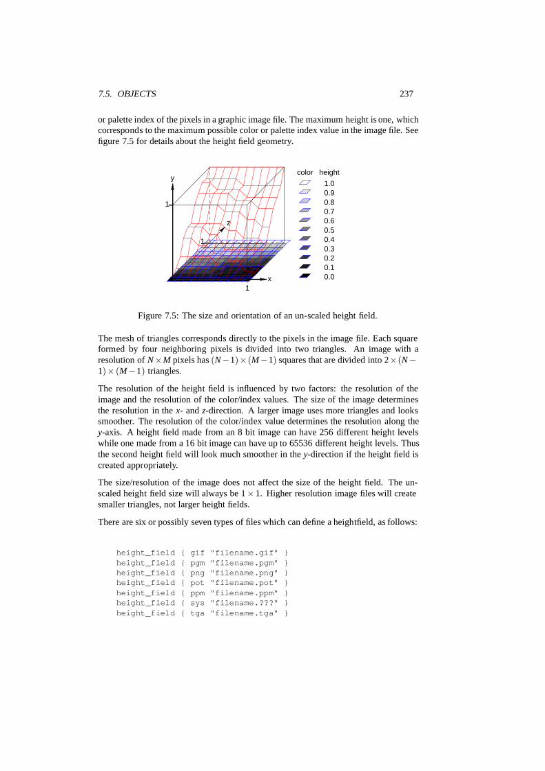
7.5. OBJECTS 237
or palette index of the pixels in a graphic image file. The maximum height is one, whichcorresponds to the maximum possible color or palette index value in the image file. Seefigure 7.5 for details about the height field geometry.
z
1
1.00.90.80.70.60.50.40.30.20.10.0
heightcolor
1
1x
y
Figure 7.5: The size and orientation of an un-scaled height field.
The mesh of triangles corresponds directly to the pixels in the image file. Each squareformed by four neighboring pixels is divided into two triangles. An image with aresolution of N×M pixels has (N−1)×(M−1) squares that are divided into 2×(N−1)× (M−1) triangles.
The resolution of the height field is influenced by two factors: the resolution of theimage and the resolution of the color/index values. The size of the image determinesthe resolution in the x- and z-direction. A larger image uses more triangles and lookssmoother. The resolution of the color/index value determines the resolution along they-axis. A height field made from an 8 bit image can have 256 different height levelswhile one made from a 16 bit image can have up to 65536 different height levels. Thusthe second height field will look much smoother in the y-direction if the height field iscreated appropriately.
The size/resolution of the image does not affect the size of the height field. The un-scaled height field size will always be 1×1. Higher resolution image files will createsmaller triangles, not larger height fields.
There are six or possibly seven types of files which can define a heightfield, as follows:
height_field { gif "filename.gif" }height_field { pgm "filename.pgm" }height_field { png "filename.png" }height_field { pot "filename.pot" }height_field { ppm "filename.ppm" }height_field { sys "filename.???" }height_field { tga "filename.tga" }

238 CHAPTER 7. SCENE DESCRIPTION LANGUAGE
The image file used to create a height field can be a GIF, TGA, POT, PNG, PGM, PPMand possibly a system specific (e. g. Windows BMP or Macintosh Pict) format file.The GIF, PNG, PGM and possibly system format files are the only ones that can becreated using a standard paint program. Though there are paint programs for creatingTGA image files they won’t be of much use for creating the special 16 bit TGA filesused by POV-Ray (see below and 7.8.4 on page 359 for more details).
In an image file like GIF that uses a color palette the color number is the palette index ata given pixel. Use a paint program to look at the palette of a GIF image. The first coloris palette index zero, the second is index one, the third is index two and so on. The lastpalette entry is index 255. Portions of the image that use low palette entries will resultin lower parts of the height field. Portions of the image that use higher palette entrieswill result in higher parts of the height field.
Height fields created from GIF files can only have 256 different height levels becausethe maximum number of colors in a GIF file is 256.
The color of the palette entry does not affect the height of the pixel. Color entry 0could be red, blue, black or orange but the height of any pixel that uses color entry 0will always be 0. Color entry 255 could be indigo, hot pink, white or sky blue but theheight of any pixel that uses color entry 255 will always be 1.
You can create height field GIF images with a paint program or a fractal program likeFRACTINT. You can usually get FRACTINT from most of the same sources as POV-Ray.
A POT file is essentially a GIF file with a 16 bit palette. The maximum number ofcolors in a POT file is 65536. This means a POT height field can have up to 65536possible height values. This makes it possible to have much smoother height fields.Note that the maximum height of the field is still 1 even though more intermediatevalues are possible.
At the time of this writing the only program that created POT files was a freewareIBM-PC program called FRACTINT. POT files generated with this fractal programcreate fantastic landscapes.
The TGA and PPM file formats may be used as a storage device for 16 bit numbersrather than an image file. These formats use the red and green bytes of each pixel tostore the high and low bytes of a height value. These files are as smooth as POT filesbut they must be generated with special custom-made programs. Several programs cancreate TGA heightfields in the format POV uses, such as GFORGE and Terrain Maker.
PNG format heightfields are usually stored in the form of a grayscale image with blackcorresponding to lower and white to higher parts of the height field. Because PNGfiles can store up to 16 bits in grayscale images they will be as smooth as TGA andPPM images. Since they are grayscale images you will be able to view them with aregular image viewer. GFORGE can create 16-bit heightfields in PNG format. ColorPNG images will be used in the same way as TGA and PPM images.
SYS format is a platform specific file format. See your platform specific documentationfor details.

7.5. OBJECTS 239
An optional water level parameter may be added after the file name. It consistsof the keyword water level followed by a float value telling the program to ignoreparts of the height field below that value. The default value is zero and legal valuesare between zero and one. For example water level .5 tells POV-Ray to onlyrender the top half of the height field. The other half is below the water and couldn’tbe seen anyway. This term comes from the popular use of height fields to renderlandscapes. A height field would be used to create islands and another shape would beused to simulate water around the islands. A large portion of the height field would beobscured by the water so the water level parameter was introduced to allow theray-tracer to ignore the unseen parts of the height field. water level is also used tocut away unwanted lower values in a height field. For example if you have an imageof a fractal on a solid colored background, where the background color is palette entry0, you can remove the background in the height field by specifying, water level.001.
Normally height fields have a rough, jagged look because they are made of lots of flattriangles. Adding the keyword smooth causes POV-Ray to modify the surface normalvectors of the triangles in such a way that the lighting and shading of the triangles willgive a smooth look. This may allow you to use a lower resolution file for your heightfield than would otherwise be needed. However, smooth triangles will take longer torender.
In order to speed up the intersection tests an one-level bounding hierarchy is avail-able. By default it is always used but it can be switched off to eventually improve therendering speed for small height fields (i. e. low resolution images).
7.5.2.6 Julia Fractal
A julia fractal object is a 3-D slice of a 4-D object created by generalizing the processused to create the classic Julia sets. You can make a wide variety of strange objectsusing julia fractal, including some that look like bizarre blobs of twisted taffy.
The julia fractal syntax (with default values listed in comments) is:
julia_fractal {4DJULIA_PARAMETER // default is <1,0,0,0>[ quaternion | hypercomplex ] // default is quaternion[ sqr | cube | exp |
reciprocal | sin | asin |sinh | asinh | cos | acos |cosh | acosh | tan | atan |tanh | atanh | log | pwr(X,Y) ] // default is sqr
[ max_iteration MAX_ITERATION ] // default value 20[ precision PRECISION ] // default value 20[ slice 4DNORMAL, DISTANCE ] // default <0,0,0,1>,0
}

240 CHAPTER 7. SCENE DESCRIPTION LANGUAGE
The 4-D vector 4DJULIA PARAMETER is the classic Julia parameter p in the iteratedformula f (h)+ p.
The julia fractal object is calculated by using an algorithm that determines whether anarbitrary point h(0) in 4-D space is inside or outside the object. The algorithm requiresgenerating the sequence of vectors h(0), h(1), . . . by iterating the formula
h(n+1) = f (h(n))+ p, n = 0,1, . . . ,max iteration−1, (7.11)
where p is the fixed 4-D vector parameter of the julia fractal and f () is one of thefunctions sqr, cube, . . . specified by the presence of the corresponding keyword. Thepoint h(0) that begins the sequence is considered inside the julia fractal object if noneof the vectors in the sequence escapes a hypersphere of radius 4 about the origin beforethe iteration number reaches the max iteration value. As you increase max iteration,some points escape that did not previously escape, forming the julia fractal. Dependingon the JULIA PARAMETER, the julia fractal object is not necessarily connected; it maybe scattered fractal dust. Using a low max iteration can fuse together the dust to makea solid object. A high max iteration is more accurate but slows rendering. Even thoughit is not accurate, the solid shapes you get with a low maximum iteration value can bequite interesting.
Since the mathematical object described by this algorithm is four-dimensional andPOV-Ray renders three dimensional objects, there must be a way to reduce the numberof dimensions of the object from four dimensions to three. This is accomplished byintersecting the 4-D fractal with a 3-D plane defined by the slice field and then pro-jecting the intersection to 3-D space. The slice plane is the 3-D space that is perpendic-ular to NORMAL4D and is DISTANCE units from the origin. Zero length NORMAL4Dvectors or a NORMAL4D vector with a zero fourth component are illegal.
You can get a good feel for the four dimensional nature of a julia fractal by using POV-Ray’s animation feature to vary a slice’s DISTANCE parameter. You can make the juliafractal appear from nothing, grow, then shrink to nothing as DISTANCE changes, muchas the cross section of a 3-D object changes as it passes through a plane.
The precision parameter is a tolerance used in the determination of whether pointsare inside or outside the fractal object. Larger values give more accurate results butslower rendering. Use as low a value as you can without visibly degrading the fractalobject’s appearance.
The presence of the keywords quaternion or hypercomplex determine which4-D algebra is used to calculate the fractal. Both are 4-D generalizations of the com-plex numbers but neither satisfies all the field properties (all the properties of real andcomplex numbers that many of us slept through in high school). Quaternions havenon-commutative multiplication and hypercomplex numbers can fail to have a multi-plicative inverse for some non-zero elements (it has been proved that you cannot suc-cessfully generalize complex numbers to four dimensions with all the field propertiesintact, so something has to break). Both of these algebras were discovered in the 19thcentury. Of the two, the quaternions are much better known, but one can argue that
7.5. OBJECTS 241
hypercomplex numbers are more useful for our purposes, since complex valued func-tions such as sin, cos, etc. can be generalized to work for hypercomplex numbers in auniform way.
For the mathematically curious, the algebraic properties of these two algebras can bederived from the multiplication properties of the unit basis vectors 1 = 〈1,0,0,0〉, i =〈0,1,0,0〉, j = 〈0,0,1,0〉 and k = 〈0,0,0,1〉. In both algebras 1x = x1 = x for any x (1is the multiplicative identity). The basis vectors 1 and i behave exactly like the familiarcomplex numbers 1 and i in both algebras.
Quaternion basis vector multiplication rules:
i j = k jk = i ki = j (7.12)
ji=−k k j =−i ik =− j (7.13)
ii = j j= kk =−1 i jk=−1 (7.14)
Hypercomplex basis vector multiplication rules:
i j= k jk =−i ki =− j (7.15)
ji= k k j =−i ik =− j (7.16)
ii= j j= kk =−1 i jk = 1 (7.17)
A distance estimation calculation is used with the quaternion calculations to speed themup. The proof that this distance estimation formula works does not generalize from twoto four dimensions but the formula seems to work well anyway, the absence of proofnotwithstanding!
The presence of one of the function keywords sqr, cube, etc. determines whichfunction is used for f (h) in the iteration formula h(n+ 1) = f (h(n))+ p. Most ofthe function keywords work only if the hypercomplex keyword is present. Only sqrand cube work with quaternions. The functions are all familiar complex functionsgeneralized to four dimensions. See table 7.1 on the following page for a list of theavailable functions.
A simple example of a julia fractal object is:
julia_fractal {<-0.083,0.0,-0.83,-0.025>quaternionsqrmax_iteration 8precision 15
}
The first renderings of julia fractals using quaternions were done by Alan Norton andlater by John Hart in the ’80’s. This new POV-Ray implementation follows FRACTINT
in pushing beyond what is known in the literature by using hypercomplex numbers
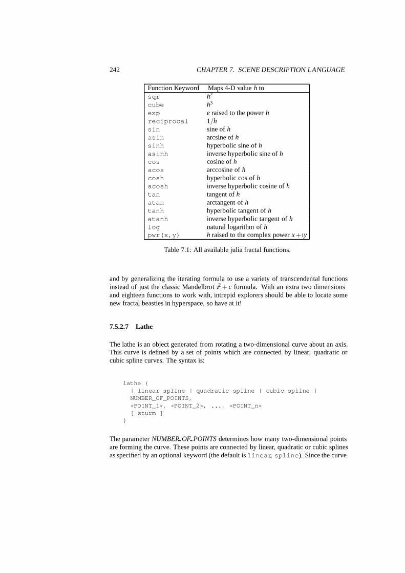
242 CHAPTER 7. SCENE DESCRIPTION LANGUAGE
Function Keyword Maps 4-D value h tosqr h2
cube h3
exp e raised to the power hreciprocal 1/hsin sine of hasin arcsine of hsinh hyperbolic sine of hasinh inverse hyperbolic sine of hcos cosine of hacos arccosine of hcosh hyperbolic cos of hacosh inverse hyperbolic cosine of htan tangent of hatan arctangent of htanh hyperbolic tangent of hatanh inverse hyperbolic tangent of hlog natural logarithm of hpwr(x,y) h raised to the complex power x+ ıy
Table 7.1: All available julia fractal functions.
and by generalizing the iterating formula to use a variety of transcendental functionsinstead of just the classic Mandelbrot z2+ c formula. With an extra two dimensionsand eighteen functions to work with, intrepid explorers should be able to locate somenew fractal beasties in hyperspace, so have at it!
7.5.2.7 Lathe
The lathe is an object generated from rotating a two-dimensional curve about an axis.This curve is defined by a set of points which are connected by linear, quadratic orcubic spline curves. The syntax is:
lathe {[ linear_spline | quadratic_spline | cubic_spline ]NUMBER_OF_POINTS,<POINT_1>, <POINT_2>, ..., <POINT_n>[ sturm ]
}
The parameter NUMBER OF POINTS determines how many two-dimensional pointsare forming the curve. These points are connected by linear, quadratic or cubic splinesas specified by an optional keyword (the default is linear spline). Since the curve
7.5. OBJECTS 243
is not automatically closed, i. e. the first and last points are not automatically connected,you’ll have to do this by your own if you want a closed curve. The curve thus definedis rotated about the y-axis to form the lathe object which is centered at the origin.
The following examples creates a simple lathe object that looks like a thick cylinder,i. e. a cylinder with a thick wall:
lathe {linear_spline5,<2, 0>, <3, 0>, <3, 5>, <2, 5>, <2, 0>pigment {Red}
}
The cylinder has an inner radius of 2 and an outer radius of 3, giving a wall width of1. It’s height is 5 and it’s located at the origin pointing up, i. e. the rotation axis is they-axis. Note that the first and last point are equal to get a closed curve.
The splines that are used by the lathe and prism objects are a little bit difficult to un-derstand. The basic concept of splines is to draw a curve through a given set of pointsin a determined way. The linear spline is the simplest spline because it’s nothing morethan connecting consecutive points with a line. This means that the curve that is drawnbetween two points only depends on those two points. No additional information istaken into account. Quadratic and cubic splines are different in that they do not onlytake other points into account when connecting two points but they also look smootherand — in the case of the cubic spline — produce smoother transitions at each point.
Quadratic splines are made of quadratic curves. Each of them connects two consecutivepoints. Since those two points (call them second and third point) aren’t enough todescribe a quadratic curve the predecessor of the third point is taken into account whenthe curve is drawn. Mathematically the relationship (their location on the 2-D plane)between the third and fourth point determines the slope of the curve at the third point.The slope of the curve at the second point is out of control. Thus quadratic splines lookmuch smoother than linear splines but the transitions at each point are generally notsmooth because the slopes on both sides of the point are different.
Cubic splines overcome the transition problem of quadratic splines because they alsotake the first point into account when drawing the curve between the second and thirdpoint. The slope at the second point is under control now and allows a smooth transitionat each point. Thus cubic splines produce the most flexible and smooth curves.
You should note that the number of spline segments, i. e. curves between two points,depends on the spline type used. For linear splines you get n−1 segments connectingthe points Pi, i = 1, . . . ,n. A quadratic spline gives you n−2 segments because thelast point is only used for determining the slope as explained above (thus you’ll need atleast three points to define a quadratic spline). The same holds for cubic splines whereyou get n− 3 segments with the first and last point used only for slope calculations(thus needing at least four points).

244 CHAPTER 7. SCENE DESCRIPTION LANGUAGE
If you want to get a closed quadratic and cubic spline with smooth transitions at the endpoints you have to make sure that in the cubic case Pn−1 = P2 (to get a closed curve),Pn = P3 and Pn−2 = P1 (to smooth the transition). In the quadratic case Pn−1 = P1 (toclose the curve) and Pn = P2 (for a smooth transition).
The slower but more accurate Sturmian root solver may be used with the quadraticspline lathe if the shape does not render properly. Since a quadratic polynomal has tobe solved for the linear spline lathe the Sturmian root solver is not needed. In case ofcubic splines the Sturmian root solver is always used because a 6th order polynomalhas to be solved.
7.5.2.8 Prism
The prism is an object generated from sweeping one or more two-dimensional, closedcurves along an axis. These curves are defined by a set of points which are connectedby linear, quadratic or cubic splines.
The syntax for the prism is:
prism {[ linear_sweep | conic_sweep ][ linear_spline | quadratic_spline | cubic_spline ]HEIGHT1,HEIGHT2,TOTAL_NUMBER_OF_POINTS,<POINT_1>, <POINT_2>, ..., <POINT_n>[ open ][ sturm ]
}
The prism object allows you to use any number of sub-prisms inside one prism state-ment (they are of the same spline and sweep type). Wherever an even number ofsub-prisms overlaps a whole appears.
The syntax of the prism object depends on the type of spline curve used. Below thesyntax of the linear spline prism is given.
prism {linear_splineHEIGHT1,HEIGHT2,TOTAL_NUMBER_OF_POINTS,<A_1>, <A_2>, ..., <A_na>, <A_1>,<B_1>, <B_2>, ..., <B_nb>, <B_1>,<C_1>, <C_2>, ..., <C_nc>, <C_1>,...
}

7.5. OBJECTS 245
Each of the sub-prisms has to be closed by repeating the first point of a sub-prism atthe end of the sub-prism’s point sequence. If this is not the case a warning is issuedand the prism is ignored (with linear splines automatic closing is used). This impliesthat all points of a prism are different (except the first and last of course). This appliesto all spline types though the control points of the quadratic and cubic splines can bearbitrarily chosen.
The last sub-prism of a linear spline prism is automatically closed — just like the lastsub-polygon in the polygon statement — if the first and last point of the sub-polygon’spoint sequence are not the same. This make it very easy to convert between polygonsand prisms. Quadratic and cubic splines are never automatically closed.
The syntax for quadratic spline prisms is:
prism {quadratic_splineHEIGHT1,HEIGHT2,TOTAL_NUMBER_OF_POINTS,<CL_A>, <A_1>, <A_2>, ..., <A_na>, <A_1>,<CL_B>, <B_1>, <B_2>, ..., <B_nb>, <B_1>,<CL_C>, <C_1>, <C_2>, ..., <C_nc>, <C_1>,...
}
Quadratic spline sub-prisms need an additional control point at the beginning of eachsub-prisms’ point sequence to determine the slope at the start of the curve.
Last but not least the syntax for the cubic spline prism.
prism {cubic_splineHEIGHT1,HEIGHT2,TOTAL_NUMBER_OF_POINTS,<CL_A1>, <A_1>, <A_2>, ..., <A_na>, <A_1>, <CL_A2>,<CL_B1>, <B_1>, <B_2>, ..., <B_nb>, <B_1>, <CL_B2>,<CL_C1>, <C_1>, <C_2>, ..., <C_nc>, <C_1>, <CL_C2>,...
}
In addition to the closed point sequence each cubic spline sub-prism needs two controlpoints to determine the slopes at the start and end of the curve.
The parameter TOTAL NUMBER OF POINTS determines how many two-dimensional points (lying in the x-z-plane) form the curves (this includes allcontrol points needed for quadratic and cubic splines). The curves are swept alongthe y-axis from HEIGHT1 to HEIGHT2 to form the prism object. By default linear
246 CHAPTER 7. SCENE DESCRIPTION LANGUAGE
sweeping is used to create the prism, i. e. the prism’s walls are perpendicular to thex-z-plane (the size of the curve does not change during the sweep). You can also useconic sweeping /conic sweep that leads to a prism with cone-like walls by scalingthe curve down during the sweep.
Like cylinders the prism is normally closed. You can remove the caps on the prismby using the open keyword. If you do so you shouldn’t use it with CSG because theresults may get wrong.
The following example creates a simple prism object that looks like a piece of cake:
prism {linear_sweeplinear_spline0, 1,4,<-1, 0>, <1, 0>, <0, 5>, <-1, 0>pigment {Red}
}
For an explanation of the spline concept read the description of the lathe object.
The slower but more accurate Sturmian root solver may be used with the cubic splineprisms if the shape does not render properly. The linear and quadratic spline prisms donot need the Sturmian root solver.
7.5.2.9 Sphere
The syntax of the sphere object is:
sphere {<CENTER>, RADIUS
}
Where 〈CENTER〉 is a vector specifying the x, y, z coordinates of the center of thesphere and RADIUS is a float value specifying the radius. Spheres may be scaledunevenly giving an ellipsoid shape. See figure 7.6 on the next page for details aboutthe sphere geometry.
Because spheres are highly optimized they make good bounding shapes (if manalbounding seems to be necessary).
7.5.2.10 Superquadric Ellipsoid
The superquadric ellipsoid is an extension of the quadric ellipsoid. It can be used tocreate boxes and cylinders with round edges and other interesting shapes. Mathemati-

7.5. OBJECTS 247
radius
center
Figure 7.6: The geometry of a sphere.
cally it is given by the equation:
f (x,y,z)=(|x|2/e+ |y|2/e
)e/n+ |z|2/n−1 = 0 (7.18)
The values of e and n, called the east-west and north-south exponent, determine theshape of the superquadric ellipsoid. Both have to be greater than zero. The sphere ise. g. given by e= 1 and n = 1.
The syntax of the superquadric ellipsoid, which is located at the origin, is:
superellipsoid { <e, n> }
Two useful objects are the rounded box and the rounded cylinder. These are declaredin the following way.
#declare Rounded_Box = superellipsoid { <r, r> }#declare Rounded_Cylinder = superellipsoid { <1, r> }
The roundedness r determines the roundedness of the edges and has to be greater thanzero and smaller than one. The smaller you choose the values of r the smaller andsharper the edges will get.
Very small values of e and n might cause problems with the root solver (the Sturmianroot solver cannot be used).
7.5.2.11 Surface of Revolution
The surface of revolution (SOR) object is generated by rotating the graph of a functionabout an axis. This function describes the dependence of the radius from the positionon the rotation axis. The syntax of the SOR object is:

248 CHAPTER 7. SCENE DESCRIPTION LANGUAGE
sor {NUMBER_OF_POINTS,<POINT0>, <POINT1>, ..., <POINTn-1>[ open ][ sturm ]
}
The points 〈POINT0〉 through 〈POINT n−1〉 are two-dimensional vectors consistingof the radius and the corresponding height, i. e. the position on the rotation axis. Thesepoints are smoothly connected (the curve is passing through the specified points) androtated about the y-axis to form the SOR object. The first and last points are only usedto determine the slopes of the function at the start and end point. The function used forthe SOR object is similar to the splines used for the lathe object. The difference is thatthe SOR object is less flexible because it underlies the restrictions of any mathematicalfunction, i. e. to any given point y on the rotation axis belongs at most one functionvalue, i. e. one radius value. You can’t rotate closed curves with the SOR object.
The optional keyword open allows you to remove the caps on the SOR object. If youdo this you shouldn’t use it with CSG anymore because the results may be wrong.
The SOR object is useful for creating bottles, vases, and things like that. A simple vasecould look like this:
#declare Vase = sor {7,<0.000000, 0.000000><0.118143, 0.000000><0.620253, 0.540084><0.210970, 0.827004><0.194093, 0.962025><0.286920, 1.000000><0.468354, 1.033755>open
}
One might ask why there is any need for a SOR object if there is already a lathe ob-ject which is much more flexible. The reason is quite simple. The intersection testwith a SOR object involves solving a cubic polynomial while the test with a lathe ob-ject requires to solve of a 6th order polynomial (you need a cubic spline for the samesmoothness). Since most SOR and lathe objects will have several segments this willmake a great difference in speed. The roots of the 3rd order polynomial will also bemore accurate and easier to find.
The slower but more accurate Sturmian root solver may be used with the surface ofrevolution object if the shape does not render properly.
The following explanations are for the mathematically interested reader who wants toknow how the surface of revolution is calculated. Though it is not necessary to read onit might help in understanding the SOR object.

7.5. OBJECTS 249
The function that is rotated about the y-axis to get the final SOR object is given by
r2 = f (h) = Ah3+Bh2+Ch+D (7.19)
with radius r and height h. Since this is a cubic function in h it has enough flexibilityto allow smooth curves.
The curve itself is defined by a set of n points Pi, i = 0 . . .n−1, which are interpolatedusing one function for every segment of the curve. A segment j, j = 1 . . .n−3, goesfrom point Pj to point Pj+1 and uses points Pj−1 and Pj+2 to determine the slopes atthe endpoints. If there are n points we will have n−3 segments. This means that weneed at least four points to get a proper curve.
The coefficients Aj, Bj, Cj and Dj are calculated for every segment using the equation
b =M x (7.20)
that is
r2j
r2j+1
2r jr j+1−r j−1hj+1−hj−1
2r j+1r j+2−r jh j+2−h j
=
h3j h2
j h j 1h3
j+1 h2j+1 hj+1 1
3h2j 2hj 1 0
3h2j+1 2hj+1 1 0
A j
B jCj
D j
(7.21)
where rj is the radius and hj is the height of point Pj.
Figure 7.7 on the following page shows the configuration of the points Pi, the locationof segment j and the curve that is defined by this segment.
7.5.2.12 Text
A text object creates 3-D text as an extruded block letter. Currently only TrueTypefonts are supported but the syntax allows for other font types to be added in the future.The syntax is:
text {ttf "FONTNAME.TTF","STRING_OF_TEXT",THICKNESS_FLOAT, OFFSET_VECTOR
}
Where FONTNAME.TTF is the name of the TrueType font file. It is a quoted stringliteral or string expression. The string expression which follows is the actual text ofthe string object. It too may be a quoted string literal or string expression. See 7.1.6 onpage 196 for more on string expressions.

250 CHAPTER 7. SCENE DESCRIPTION LANGUAGE
−4.0 −2.0 0.0 2.0 4.0Radius r
0.0
2.0
4.0
6.0
8.0
Hei
ght h
P0
Pj−1
Pj
Pj+1
Pj+2
Pn−1
Segment j
P1
Figure 7.7: Segment j of n−3 segments in a point configuration of n points. The pointsdescribe the curve of a surface of revolution
.
The text will start with the origin at the lower left, front of the first character and willextend in the +x-direction. The baseline of the text follows the x-axis and decendersdrop into the −y-direction. The front of the character sits in the x-y-plane and the textis extruded in the +z-direction. The front-to-back thickness is specified by the requiredvalue THICKNESS FLOAT.
Characters are generally sized so that 1 unit of vertical spacing is correct. The charac-ters are about 0.5 to 0.75 units tall.
The horizontal spacing is handled by POV-Ray internally including any kerning infor-mation stored in the font. The required vector OFFSET VECTOR defines any extratranslation between each character. Normally you should specify a zero for this value.Specifing 0.1*x would put additional 0.1 units of space between each character.
Only printable characters are allowed in text objects. Characters such as return, linefeed, tabs, backspace etc. are not supported.
7.5.2.13 Torus
A torus is a 4th order quartic polynomial shape that looks like a donut or inner tube.Because this shape is so useful and quartics are difficult to define, POV-Ray lets youtake a short-cut and define a torus by:
torus {MAJOR, MINOR[ sturm ]
}

7.5. OBJECTS 251
where MAJOR is a float value giving the major radius and MINOR is a float specifyingthe minor radius. The major radius extends from the center of the hole to the mid-lineof the rim while the minor radius is the radius of the cross-section of the rim. The torusis centered at the origin and lies in the x-z-plane with the y-axis sticking through thehole. See fihure 7.8 for details about the torus geometry.
major radius
minor radius
x
z
center line
Figure 7.8: Major and minor radius of a torus.
The torus is internally bounded by two cylinders and two rings forming a thick cylinder.With this bounding cylinder the performance of the torus intersection test is vastlyincreased. The test for a valid torus intersection, i. e. solving a 4th order polynomial,is only performed if the bounding cylinder is hit. Thus a lot of slow root solvingcalculations are avoided.
Calculations for all higher order polynomials must be very accurate. If the torus rendersimproperly you may add the keyword sturm after the MINOR value to use POV-Ray’sslower-yet-more-accurate Sturmian root solver.
7.5.3 Finite Patch Primitives
There are six totally thin, finite objects which have no well-defined inside. They arebicubic patch, disc, smooth triangle, triangle, polygon and mesh. They may be com-bined in CSG union but cannot be use in other types of CSG (or inside a clipped bystatement). Because these types are finite POV-Ray can use automatic bounding onthem to speed up rendering time. As with all shapes they can be translated, rotated andscaled.

252 CHAPTER 7. SCENE DESCRIPTION LANGUAGE
7.5.3.1 Bicubic Patch
A bicubic patch is a 3D curved surface created from a mesh of triangles. POV-Raysupports a type of bicubic patch called a Bezier patch. A bicubic patch is defined asfollows:
bicubic_patch {type PATCH_TYPEflatness FLATNESS_VALUEu_steps NUM_U_STEPSv_steps NUM_V_STEPS<CP1>, <CP2>, <CP3>, <CP4>,<CP5>, <CP6>, <CP7>, <CP8>,<CP9>, <CP10>, <CP11>, <CP12>,<CP13>, <CP14>, <CP15>, <CP16>
}
The keyword type is followed by a float PATCH TYPE which currently must be either0 or 1. For type 0 only the control points are retained within POV-Ray. This means thata minimal amount of memory is needed but POV-Ray will need to perform many extracalculations when trying to render the patch. Type 1 preprocesses the patch into manysubpatches. This results in a significant speedup in rendering at the cost of memory.
The four parameters type, flatness, u steps and v steps may appear in anyorder. They are followed by 16 vectors that define the x, y, z coordinates of the 16control points which define the patch. The patch touches the four corner points 〈CP1〉,〈CP4〉, 〈CP13〉 and 〈CP16〉 while the other 12 points pull and stretch the patch intoshape. The Bezier surface is enclosed by the convex hull formed by the 16 controlpoints, this is known as the convex hull property.
The keywords u steps and v steps are each followed by float values which tellhow many rows and columns of triangles are the minimum to use to create the surface.The maximum number of individual pieces of the patch that are tested by POV-Ray canbe calculated from the following:
pieces = 2u steps 2v steps (7.22)
This means that you really should keep u steps and v steps under 4. Most patcheslook just fine with u steps 3 and v steps 3, which translates to 64 subpatches(128 smooth triangles).
As POV-Ray processes the Bezier patch it makes a test of the current piece of the patchto see if it is flat enough to just pretend it is a rectangle. The statement that controls thistest is flatness. Typical flatness values range from 0 to 1 (the lower the slower).
If the value for flatness is 0 POV-Ray will always subdivide the patch to the extendspecified by u steps and v steps. If flatness is greater than 0 then every time thepatch is split, POV-Ray will check to see if there is any need to split further.

7.5. OBJECTS 253
There are both advantages and disadvantages to using a non-zero flatness. The advan-tages include:
• If the patch isn’t very curved, then this will be detected and POV-Raywon’t waste a lot of time looking at the wrong pieces.
• If the patch is only highly curved in a couple of places, POV-Ray willkeep subdividing there and concentrate it’s efforts on the hard part.
The biggest disadvantage is that if POV-Ray stops subdividing at a particular level onone part of the patch and at a different level on an adjacent part of the patch there is thepotential for cracking. This is typically visible as spots within the patch where you cansee through. How bad this appears depends very highly on the angle at which you areviewing the patch.
Like triangles, the bicubic patch is not meant to be generated by hand. These shapesshould be created by a special utility. You may be able to acquire utilities to generatethese shapes from the same source from which you obtained POV-Ray.
bicubic_patch {type 1flatness 0.01u_steps 4v_steps 4<0, 0, 2>, <1, 0, 0>, <2, 0, 0>, <3, 0,-2>,<0, 1 0>, <1, 1, 0>, <2, 1, 0>, <3, 1, 0>,<0, 2, 0>, <1, 2, 0>, <2, 2, 0>, <3, 2, 0>,<0, 3, 2>, <1, 3, 0>, <2, 3, 0>, <3, 3, -2>
}
The triangles in a POV-Ray bicubic patch are automatically smoothed using nor-mal interpolation but it is up to the user (or the user’s utility program) to create controlpoints which smoothly stitch together groups of patches.
7.5.3.2 Disc
One other flat, finite object available with POV-Ray is the disc. The disc is infinitelythin, it has no thickness. If you want a disc with true thickness you should use a veryshort cylinder. A disc shape may be defined by:
disc {<CENTER>, <NORMAL>, RADIUS [, HOLE_RADIUS ]
}
The vector 〈CENTER〉 defines the x, y, z coordinates of the center of the disc. The〈NORMAL〉 vector describes its orientation by describing its surface normal vector.This is followed by a float specifying the RADIUS. This may be optionally followedby another float specifying the radius of a hole to be cut from the center of the disc.

254 CHAPTER 7. SCENE DESCRIPTION LANGUAGE
7.5.3.3 Mesh
The mesh object can be used to efficiently store large numbers of triangles. Its syntaxis:
mesh {triangle {
<CORNER1>, <CORNER2>, <CORNER3>[ texture { STRING } ]
}smooth_triangle {
<CORNER1>, <NORMAL1>,<CORNER2>, <NORMAL2>,<CORNER3>, <NORMAL3>[ texture { STRING } ]
}[ hierarchy FLAG ]
}
Any number of triangles and/or smooth triangles can be used and each of those trianglescan be individually textured by assigning a texture name to it. The texture has to bedeclared before the mesh is parsed. It is not possible to use texture definitions insidethe triangle or smooth triangle statements. This is a restriction that is necessary for anefficient storage of the assigned textures.
The mesh’s components are internally bounded by a bounding box hierarchy to speedup intersection testing. The bounding hierarchy can be turned off with the hierarchykeyword. This should only be done if memory is short or the mesh consists of only afew triangles.
Copies of a mesh object refer to the same triangle data and thus consume very lit-tle memory. You can easily trace hundred copies of an 10000 triangle mesh withoutrunning out of memory (assuming the first mesh fits into memory).
The mesh object has two advantages over a union of triangles: it needs less memory andit is transformed faster. The memory requierements are reduced by efficiently storingthe triangles vertices and normals. The parsing time for transformed meshes is reducedbecause only the mesh object has to be transformed and not every single triangle as itis necessary for unions.
The mesh object can currently only include triangle and smooth triangle components.That restriction is liable to change, allowing polygonal components, at some point inthe future.
7.5.3.4 Polygon
Polygons are useful for creating rectangles, squares and other planar shapes with morethan three edges. Their syntax is:

7.5. OBJECTS 255
polygon {TOTAL_NUMBER_OF_POINTS,<A_1>, <A_2>, ..., <A_na>, <A_1>,<B_1>, <B_2>, ..., <B_nb>, <B_1>,<C_1>, <C_2>, ..., <C_nc>, <C_1>,...
}
The points 〈A 1〉 through 〈A na〉 describe the first sub-polygon, the points 〈B 1〉through 〈B nb〉 describe the second sub-polygon, and so on. A polygon can containany number of sub-polygons, either overlapping or not. In places where an even num-ber of polygons overlaps a whole appears. You only have to be sure that each of thesepolygons is closed. This is insured by repeating the first point of a sub-polygon at theend of the sub-polygon’s point sequence. This implies that all points of a sub-polygonare different.
If the (last) sub-polygon is not closed a warning is issued and the program automaticallycloses the polygon. This is useful because polygons imported from other programs maynot be closed, i. e. their first and last point are not the same.
All points of a polygon are three-dimensional vectors that have to lay on one plane.If this is not the case an error occurs. You can also use two-dimensional vectors todescribe the polygon. POV-Ray assumes that the z value is zero in this case.
A square polygon that matches the default planar imagemap is simply:
polygon {4,<0, 0>, <0, 1>, <1, 1>, <1, 0>texture {
finish { ambient 1 diffuse 0 }pigment { image_map { gif "test.gif" } }
}//scale and rotate as needed here
}
The sub-polygon feature can be used to generate complex shapes like the letter ”P”,where a whole is cut into another polygon:
#declare P = polygon {12,<0, 0>, <0, 6>, <4, 6>, <4, 3>, <1, 3>, <1, 0>, <0, 0>,<1, 4>, <1, 5>, <3, 5>, <3, 4>, <1, 4>
}
The first sub-polygon (on the first line) describes the outer shape of the letter ”P”. Thesecond sub-polygon (on the second line) describes the rectangular hole that is cut in

256 CHAPTER 7. SCENE DESCRIPTION LANGUAGE
the top of the letter ”P”. Both rectangles are closed, i. e. their first and last points arethe same.
The feature of cutting holes into a polygon is based on the polygon inside/outside testused. A point is considerd to be inside a polygon if a straight line drawn from this pointin an arbitrary direction crosses an odd number of edges (this is known as Jordan’scurve theorem).
Another very complex example showing one large triangle with three small holes andthree seperate, small triangles is given below:
polygon {28,<0,0> <1,0> <0,1> <0,0> // large outer tri.<.3,.7> <.4,.7> <.3,.8> <.3,.7> // small outer tri. #1<.5,.5> <.6,.5> <.5,.6> <.5,.5> // small outer tri. #2<.7,.3> <.8,.3> <.7,.4> <.7,.3> // small outer tri. #3<.5,.2> <.6,.2> <.5,.3> <.5,.2> // inner tri. #1<.2,.5> <.3,.5> <.2,.6> <.2,.5> // inner tri. #2<.1,.1> <.2,.1> <.1,.2> <.1,.1> // inner tri. #3
}
7.5.3.5 Triangle and Smooth Triangle
The triangle primitive is available in order to make more complex objects than thebuilt-in shapes will permit. Triangles are usually not created by hand but are convertedfrom other files or generated by utilities. A triangle is defined by
triangle {<CORNER1>, <CORNER2>, <CORNER3>
}
where 〈CORNERn〉 is a vector defining the x, y, z coordinates of each corner of thetriangle.
Because triangles are perfectly flat surfaces it would require extremely large numbersof very small triangles to approximate a smooth, curved surface. However much of ourperception of smooth surfaces is dependent upon the way light and shading is done. Byartificially modifying the surface normals we can simulate as smooth surface and hidethe sharp-edged seams between individual triangles.
The smooth triangle primitive is used for just such purposes. The smooth triangles usea formula called Phong normal interpolation to calculate the surface normal for anypoint on the triangle based on normal vectors which you define for the three corners.This makes the triangle appear to be a smooth curved surface. A smooth triangle isdefined by

7.5. OBJECTS 257
smooth_triangle {<CORNER1>, <NORMAL1>,<CORNER2>, <NORMAL2>,<CORNER3>, <NORMAL3>
}
where the corners are defined as in regular triangles and 〈NORMALn〉 is a vector de-scribing the direction of the surface normal at each corner.
These normal vectors are prohibitively difficult to compute by hand. Therefore smoothtriangles are almost always generated by utility programs. To achieve smooth results,any triangles which share a common vertex should have the same normal vector at thatvertex. Generally the smoothed normal should be the average of all the actual normalsof the triangles which share that point.
7.5.4 Infinite Solid Primitives
There are five polynomial primitive shapes that are possibly infinite and do not respondto automatic bounding. They are plane, cubic, poly, quadric and quartic. They do havea well defined inside and may be used in CSG and inside a clipped by statement.As with all shapes they can be translated, rotated and scaled..
7.5.4.1 Plane
The plane primitive is a simple way to define an infinite flat surface. The plane isspecified as follows:
plane { <NORMAL>, DISTANCE }
The 〈NORMAL〉 vector defines the surface normal of the plane. A surface normal isa vector which points up from the surface at a 90 degree angle. This is followed bya float value that gives the distance along the normal that the plane is from the origin(that is only true if the normal vector has unit length; see below). For example:
plane { <0, 1, 0>, 4 }
This is a plane where straight up is defined in the positive y-direction. The plane is4 units in that direction away from the origin. Because most planes are defined withsurface normals in the direction of an axis you will often see planes defined using thex, y or z built-in vector identifiers. The example above could be specified as:
plane { y, 4 }

258 CHAPTER 7. SCENE DESCRIPTION LANGUAGE
The plane extends infinitely in the x- and z-directions. It effectively divides the worldinto two pieces. By definition the normal vector points to the outside of the plane whileany points away from the vector are defined as inside. This inside/outside distinctionis only important when using planes in CSG and clipped by.
A plane is called a polynomial shape because it is defined by a first order polynomialequation. Given a plane:
plane { <A, B, C>, D }
it can be represented by the equation
Ax+By+Cz−D√
A2+B2+C2 = 0. (7.23)
Therefore our example plane { y,4 } is actually the polynomial equation y = 4.You can think of this as a set of all x, y, z points where all have y values equal to 4,regardless of the x or z values.
This equation is a first order polynomial because each term contains only single powersof x, y or z. A second order equation has terms like x2, y2, z2, xy, xz and yz. Anothername for a 2nd order equation is a quadric equation. Third order polys are calledcubics. A 4th order equation is a quartic. Such shapes are described in the sectionsbelow.
7.5.4.2 Poly, Cubic and Quartic
Higher order polynomial surfaces may be defined by the use of a poly shape. Thesyntax is
poly { ORDER, <T1, T2, T3, .... Tm> }
where ORDER is a whole number from 2 to 7 inclusively that specifies the order of theequation. T1, T2, . . . Tm are float values for the coefficients of the equation. There arem such terms where
m=((ORDER+1)(ORDER+2)(ORDER+3))
6. (7.24)
An alternate way to specify 3rd order polys is:
cubic { <T1, T2,... T20> }
Also 4th order equations may be specified with:
7.5. OBJECTS 259
quartic { <T1, T2,... T35> }
Here’s a more mathematical description of quartics for those who are interested. Quar-tic surfaces are 4th order surfaces and can be used to describe a large class of shapesincluding the torus, the lemniscate, etc. The general equation for a quartic equation inthree variables is (hold onto your hat):
a00x4+a01x3y+a02x3z+a03x3+a04x2y2+
a05x2yz+a06x2y+a07x2z2+a08x2z+a09x2+
a10xy3+a11xy2z+a12xy2+a13xyz2+a14xyz+
a15xy+a16xz3+a17xz2+a18xz+a19x+
a20y4+a21y3z+a22y3+a23y2z2+a24y2z+
a25y2+a26yz3+a27yz2+a28yz+a29y+
a30z4+a31z3+a32z2+a33z+a34 = 0 (7.25)
To declare a quartic surface requires that each of the coefficients a00 . . .a34 be placedin order into a single long vector of 35 terms.
As an example let’s define a torus the hard way. A Torus can be represented by theequation:
x4+y4+z4+2x2y2+2x2z2+2y2z2−
2(r20+r2
1)x2+2(r2
0−r21)y
2−2(r20+r2
1)z2+(r2
0−r21)
2 = 0 (7.26)
Where r0 is the major radius of the torus, the distance from the hole of the donut to themiddle of the ring of the donut, and r1 is the minor radius of the torus, the distance fromthe middle of the ring of the donut to the outer surface. The following object declarationis for a torus having major radius 6.3 minor radius 3.5 (Making the maximum widthjust under 20).
// Torus having major radius sqrt(40), minor radius sqrt(12)
quartic {< 1, 0, 0, 0, 2, 0, 0, 2, 0,
-104, 0, 0, 0, 0, 0, 0, 0, 0,0, 0, 1, 0, 0, 2, 0, 56, 0,0, 0, 0, 1, 0, -104, 0, 784 >
sturmbounded_by { // bounded_by speeds up the render,
// see bounded_by// explanation later// in docs for more info.
sphere { <0, 0, 0>, 10 }}
}

260 CHAPTER 7. SCENE DESCRIPTION LANGUAGE
Poly, cubic and quartics are just like quadrics in that you don’t have to understand whatone is to use one. The file SHAPESQ.INC has plenty of pre-defined quartics for you toplay with. The syntax for using a pre-defined quartic is:
object { Quartic_Name }
Polys use highly complex computations and will not always render perfectly. If the sur-face is not smooth, has dropouts, or extra random pixels, try using the optional keywordsturm in the definition. This will cause a slower but more accurate calculation methodto be used. Usually, but not always, this will solve the problem. If sturm doesn’t work,try rotating or translating the shape by some small amount. See the sub-directory MATH
in the scene files directory for examples of polys in scenes.
There are really so many different quartic shapes, we can’t even begin to list or describethem all. If you are interested and mathematically inclined, an excellent reference bookfor curves and surfaces where you’ll find more quartic shape formulas is:
The CRC Handbook of Mathematical Curves and SurfacesDavid von SeggernCRC Press, 1990
7.5.4.3 Quadric
Quadric surfaces can produce shapes like ellipsoids, spheres, cones, cylinders,paraboloids (dish shapes) and hyperboloids (saddle or hourglass shapes). Note thatyou do not confuse quaDRic with quaRTic. A quadric is a 2nd order polynomial whilea quartic is 4th order. Quadrics render much faster and are less error-prone.
A quadric is defined in POV-Ray by
quadric { <A,B,C>, <D,E,F>, <G,H,I>, J }
where A through J are float expressions that define a surface of x, y, z points whichsatisfy the equation
Ax2 + By2 + Cz2 + Dxy + Exz + Fyz + Gx + Hy + Iz + J = 0 (7.27)
Different values of A, B, C, . . . J will give different shapes. If you take any threedimensional point and use its x, y and z coordinates in the above equation the answerwill be 0 if the point is on the surface of the object. The answer will be negative if thepoint is inside the object and positive if the point is outside the object. Here are someexamples:
X2+Y 2+Z2−1 = 0 Sphere (7.28)
X2+Y 2−1 = 0 Infinite cylinder along the z-axis (7.29)
X2+Y 2−Z2 = 0 Infinite cone along the z-axis (7.30)
7.5. OBJECTS 261
The easiest way to use these shapes is to include the standard file SHAPES.INC intoyour program. It contains several pre-defined quadrics and you can transform thesepre-defined shapes (using translate, rotate and scale) into the ones you want. You caninvoke them by using the syntax:
object { Quadric_Name }
The pre-defined quadrics are centered about the origin 〈0,0,0〉 and have a radius of 1.Don’t confuse radius with width. The radius is half the diameter or width making thestandard quadrics 2 units wide.
Some of the pre-defined quadrics are,
EllipsoidCylinder_X, Cylinder_Y, Cylinder_ZQCone_X, QCone_Y, QCone_ZParaboloid_X, Paraboloid_Y, Paraboloid_Z
For a complete list, see the file SHAPES.INC.
7.5.5 Constructive Solid Geometry
POV-Ray supports Constructive Solid Geometry (CSG) with five different operations:difference, intersection, merge, union and negation (inversion). While the first fouroperations represent binary operators, i. e. they need two arguments, the negation is aunary operator, it takes only one argument.
7.5.5.1 About CSG
Constructive Solid Geometry is a technique for combining two or more objects to createa new object using the three boolean set operators union, intersection, andnegation. It only works with solid objects, i. e. objects that have a well-definedinterior. This is the case for all objects described in the sections 7.5.2 on page 231and 7.5.4 on page 257.
CSG shapes may be used anywhere a standard shape can be used, even inside otherCSG shapes. They can be translated, rotated or scaled in the same way as any othershape. The shapes making up the CSG shape may be individually translated, rotatedand scaled as well.
7.5.5.2 Inside and Outside
Most shape primitives, like spheres, boxes and blobs divide the world into two regions.One region is inside the object and one is outside.
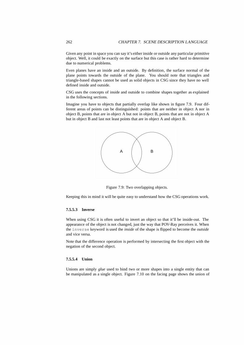
262 CHAPTER 7. SCENE DESCRIPTION LANGUAGE
Given any point in space you can say it’s either inside or outside any particular primitiveobject. Well, it could be exactly on the surface but this case is rather hard to determinedue to numerical problems.
Even planes have an inside and an outside. By definition, the surface normal of theplane points towards the outside of the plane. You should note that triangles andtriangle-based shapes cannot be used as solid objects in CSG since they have no welldefined inside and outside.
CSG uses the concepts of inside and outside to combine shapes together as explainedin the following sections.
Imagine you have to objects that partially overlap like shown in figure 7.9. Four dif-ferent areas of points can be distinguished: points that are neither in object A nor inobject B, points that are in object A but not in object B, points that are not in object Abut in object B and last not least points that are in object A and object B.
A B
Figure 7.9: Two overlapping objects.
Keeping this in mind it will be quite easy to understand how the CSG operations work.
7.5.5.3 Inverse
When using CSG it is often useful to invert an object so that it’ll be inside-out. Theappearance of the object is not changed, just the way that POV-Ray perceives it. Whenthe inverse keyword is used the inside of the shape is flipped to become the outsideand vice versa.
Note that the difference operation is performed by intersecting the first object with thenegation of the second object.
7.5.5.4 Union
Unions are simply glue used to bind two or more shapes into a single entity that canbe manipulated as a single object. Figure 7.10 on the facing page shows the union of
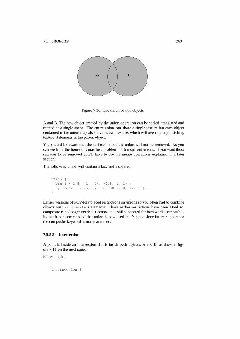
7.5. OBJECTS 263
BA
Figure 7.10: The union of two objects.
A and B. The new object created by the union operation can be scaled, translated androtated as a single shape. The entire union can share a single texture but each objectcontained in the union may also have its own texture, which will override any matchingtexture statements in the parent object.
You should be aware that the surfaces inside the union will not be removed. As youcan see from the figure this may be a problem for transparent unions. If you want thosesurfaces to be removed you’ll have to use the merge operations explained in a latersection.
The following union will contain a box and a sphere.
union {box { <-1.5, -1, -1>, <0.5, 1, 1> }cylinder { <0.5, 0, -1>, <0.5, 0, 1>, 1 }
}
Earlier versions of POV-Ray placed restrictions on unions so you often had to combineobjects with composite statements. Those earlier restrictions have been lifted socomposite is no longer needed. Composite is still supported for backwards compatibil-ity but it is recommended that union is now used in it’s place since future support forthe composite keyword is not guaranteed.
7.5.5.5 Intersection
A point is inside an intersection if it is inside both objects, A and B, as show in fig-ure 7.11 on the next page.
For example:
intersection {
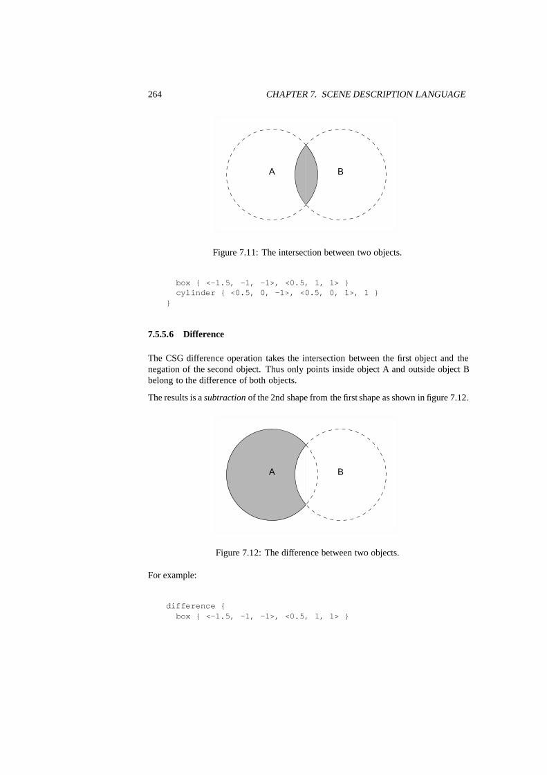
264 CHAPTER 7. SCENE DESCRIPTION LANGUAGE
A B
Figure 7.11: The intersection between two objects.
box { <-1.5, -1, -1>, <0.5, 1, 1> }cylinder { <0.5, 0, -1>, <0.5, 0, 1>, 1 }
}
7.5.5.6 Difference
The CSG difference operation takes the intersection between the first object and thenegation of the second object. Thus only points inside object A and outside object Bbelong to the difference of both objects.
The results is a subtraction of the 2nd shape from the first shape as shown in figure 7.12.
A B
Figure 7.12: The difference between two objects.
For example:
difference {box { <-1.5, -1, -1>, <0.5, 1, 1> }

7.5. OBJECTS 265
cylinder { <0.5, 0, -1>, <0.5, 0, 1>, 1 }}
7.5.5.7 Merge
The union operation just glues objects together, it does not remove the objects’ surfacesinside the union. If a transparent union is used those surface will get visible.
The merge operations can be used to avoid this problem. It works just like union but iteliminates the inner surfaces like shown in figure 7.13.
A B
Figure 7.13: Merge removes inner surfaces.
7.5.6 Light Sources
The last object covered is the light source. Light sources have no visible shape of theirown. They are just points or areas which emit light. Their full syntax is:
light_source {<LOCATION>color <COLOUR>[ spotlight ][ point_at <POINT_AT> ][ radius RADIUS ][ falloff FALLOFF ][ tightness TIGHTNESS ][ area_light <AXIS1>, <AXIS2>, SIZE1, SIZE2 ][ adaptive ADAPTIVE ][ jitter JITTER ][ looks_like { OBJECT } ][ fade_distance FADE_DISTANCE ][ fade_power FADE_POWER ][ atmospheric_attenuation BOOL ]
}
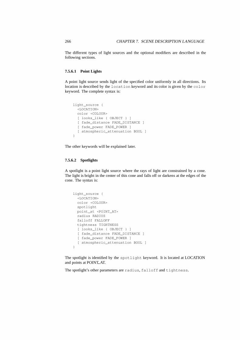
266 CHAPTER 7. SCENE DESCRIPTION LANGUAGE
The different types of light sources and the optional modifiers are described in thefollowing sections.
7.5.6.1 Point Lights
A point light source sends light of the specified color uniformly in all directions. Itslocation is described by the location keyword and its color is given by the colorkeyword. The complete syntax is:
light_source {<LOCATION>color <COLOUR>[ looks_like { OBJECT } ][ fade_distance FADE_DISTANCE ][ fade_power FADE_POWER ][ atmospheric_attenuation BOOL ]
}
The other keywords will be explained later.
7.5.6.2 Spotlights
A spotlight is a point light source where the rays of light are constrained by a cone.The light is bright in the center of this cone and falls off or darkens at the edges of thecone. The syntax is:
light_source {<LOCATION>color <COLOUR>spotlightpoint_at <POINT_AT>radius RADIUSfalloff FALLOFFtightness TIGHTNESS[ looks_like { OBJECT } ][ fade_distance FADE_DISTANCE ][ fade_power FADE_POWER ][ atmospheric_attenuation BOOL ]
}
The spotlight is identified by the spotlight keyword. It is located at LOCATIONand points at POINT AT.
The spotlight’s other parameters are radius, falloff and tightness.
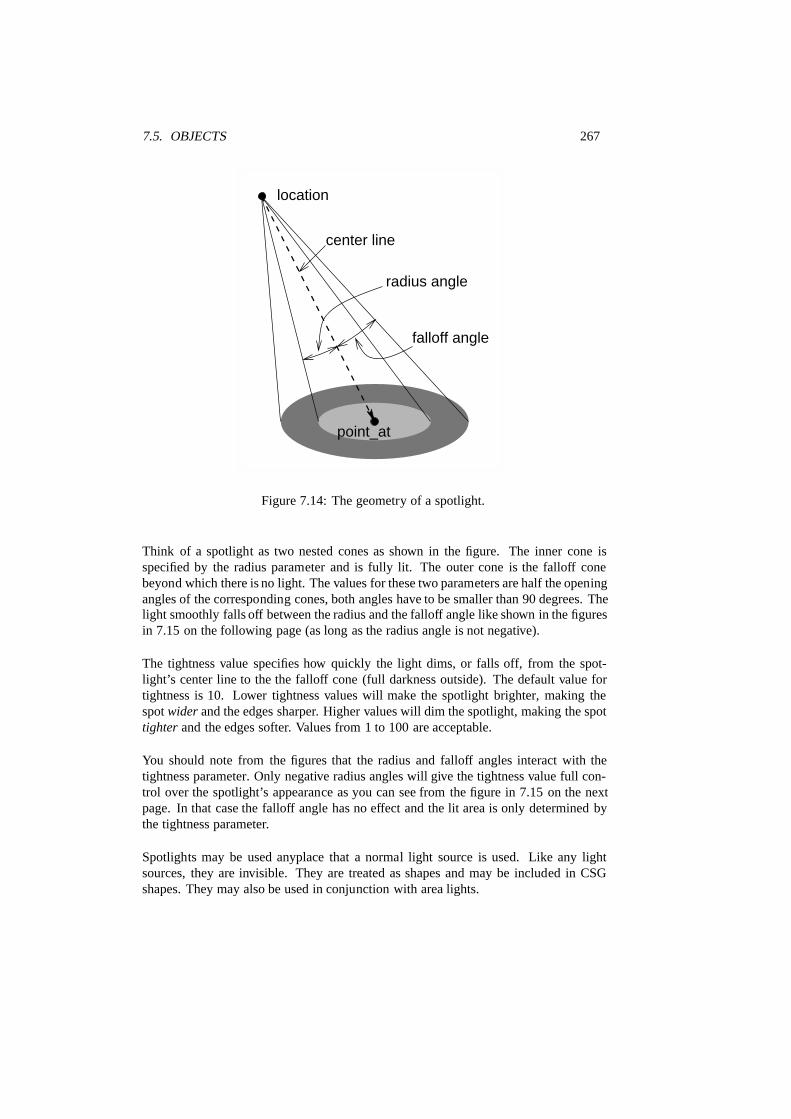
7.5. OBJECTS 267
falloff angle
center line
radius angle
location
point_at
Figure 7.14: The geometry of a spotlight.
Think of a spotlight as two nested cones as shown in the figure. The inner cone isspecified by the radius parameter and is fully lit. The outer cone is the falloff conebeyond which there is no light. The values for these two parameters are half the openingangles of the corresponding cones, both angles have to be smaller than 90 degrees. Thelight smoothly falls off between the radius and the falloff angle like shown in the figuresin 7.15 on the following page (as long as the radius angle is not negative).
The tightness value specifies how quickly the light dims, or falls off, from the spot-light’s center line to the the falloff cone (full darkness outside). The default value fortightness is 10. Lower tightness values will make the spotlight brighter, making thespot wider and the edges sharper. Higher values will dim the spotlight, making the spottighter and the edges softer. Values from 1 to 100 are acceptable.
You should note from the figures that the radius and falloff angles interact with thetightness parameter. Only negative radius angles will give the tightness value full con-trol over the spotlight’s appearance as you can see from the figure in 7.15 on the nextpage. In that case the falloff angle has no effect and the lit area is only determined bythe tightness parameter.
Spotlights may be used anyplace that a normal light source is used. Like any lightsources, they are invisible. They are treated as shapes and may be included in CSGshapes. They may also be used in conjunction with area lights.

268 CHAPTER 7. SCENE DESCRIPTION LANGUAGE
0.0 10.0 20.0 30.0 40.0 50.0 60.0 70.0 80.0 90.0Angle between light ray and spotlight’s centerline
0.0
0.5
1.0
Ligh
t int
ensi
ty m
ultip
lier
radius = 0radius = 15radius = 30radius = 45
(a)
0.0 10.0 20.0 30.0 40.0 50.0 60.0 70.0 80.0 90.0Angle between light ray and spotlight’s centerline
0.0
0.5
1.0
Ligh
t int
ensi
ty m
ultip
lier
falloff = 45falloff = 60falloff = 75falloff = 90
(b)
0.0 10.0 20.0 30.0 40.0 50.0 60.0 70.0 80.0 90.0Angle between light ray and spotlight’s centerline
0.0
0.5
1.0
Ligh
t int
ensi
ty m
ultip
lier
0
1
2
510
2050
100
(c)
0.0 10.0 20.0 30.0 40.0 50.0 60.0 70.0 80.0 90.0Angle between light ray and spotlight’s centerline
0.0
0.5
1.0
Ligh
t int
ensi
ty m
ultip
lier
1
2
510
2050
100
0
(d)
Figure 7.15: Different light intensity multiplier curves: (a) fixed falloff angle of 45degrees; (b) fixed radius angle of 45 degrees; (c) fixed angle and falloff angles of 30and 60 degrees respectively and different tightness values; (d) negative radius angleand different tightness values.
7.5.6.3 Cylindrical Lights
Cylindrical light sources work pretty much like spotlights except that the light rays areconstraint by a cylinder and not a cone. The syntax is:
light_source {<LOCATION>color <COLOUR>cylinderpoint_at <POINT_AT>radius RADIUSfalloff FALLOFFtightness TIGHTNESS[ looks_like { OBJECT } ]

7.5. OBJECTS 269
[ fade_distance FADE_DISTANCE ][ fade_power FADE_POWER ][ atmospheric_attenuation BOOL ]
}
The radius, falloff and tightness keywords control the same features as withthe spotlight.
You should keep in mind that the cylindrical light source is still a point light source.The rays are emitted from one point and are only constraint by a cylinder. The lightrays are not parallel.
7.5.6.4 Area Lights
Area light sources occupy a finite, one- or two-dimensional area of space. They cancast soft shadows because they can partially block light.
The area lights used in POV-Ray are rectangular in shape, sort of like a flat panel light.Rather than performing the complex calculations that would be required to model atrue area light, it is approximated as an array of point light sources spread out over thearea occupied by the light. The intensity of each individual point light in the array isdimmed so that the total amount of light emitted by the light is equal to the light colorspecified in the declaration. The syntax is:
light_source {<LOCATION>color <COLOUR>area_light <AXIS1>, <AXIS2>, SIZE1, SIZE2adaptive ADAPTIVEjitter JITTER[ spotlight ][ point_at <POINT_AT> ][ radius RADIUS ][ falloff FALLOFF ][ tightness TIGHTNESS ][ looks_like { OBJECT } ][ fade_distance FADE_DISTANCE ][ fade_power FADE_POWER ][ atmosphere BOOL ][ atmospheric_attenuation BOOL ]
}
The light’s location and color are specified in the same way as a for a regular lightsource.
The area light command defines the size and orientation of the area light as wellas the number of lights in the light source array. The vectors AXIS1 and AXIS2 specify

270 CHAPTER 7. SCENE DESCRIPTION LANGUAGE
the lengths and directions of the edges of the light. Since the area lights are rectangularin shape these vectors should be perpendicular to each other. The larger the size of thelight the thicker the soft part of shadows will be. The numbers SIZE1 and SIZE2 spec-ify the dimensions of the array of point lights. The more lights you use the smootheryour shadows will be but the longer they will take to render.
The jitter command is optional. When used it causes the positions of the pointlights in the array to be randomly jittered to eliminate any shadow banding that mayoccur. The jittering is completely random from render to render and should not be usedwhen generating animations.
Note that it is possible to specify spotlight parameters along with the area light param-eters to create area spotlights. Using area spotlights is a good way to speed up scenesthat use area lights since you can confine the lengthy soft shadow calculations to onlythe parts of your scene that need them.
An interesting effect can be created using a linear light source. Rather than havinga rectangular shape, a linear light stretches along a line sort of like a thin fluorescenttube. To create a linear light just create an area light with one of the array dimensionsset to 1.
The adaptive command is used to enable adaptive sampling of the light source. Bydefault POV-Ray calculates the amount of light that reaches a surface from an arealight by shooting a test ray at every point light within the array. As you can imaginethis is very slow. Adaptive sampling on the other hand attempts to approximate thesame calculation by using a minimum number of test rays. The number specified afterthe keyword controls how much adaptive sampling is used. The higher the number themore accurate your shadows will be but the longer they will take to render. If you’renot sure what value to use a good starting point is adaptive 1. The adaptivekeyword only accepts integer values and cannot be set lower than 0.
When performing adaptive sampling POV-Ray starts by shooting a test ray at each ofthe four corners of the area light. If the amount of light received from all four cornersis approximately the same then the area light is assumed to be either fully in view orfully blocked. The light intensity is then calculated as the average intensity of the lightreceived from the four corners. However, if the light intensity from the four cornersdiffers significantly then the area light is partially blocked. The area light is split intofour quarters and each section is sampled as described above. This allows POV-Ray torapidly approximate how much of the area light is in view without having to shoot atest ray at every light in the array. Visually the sampling goes like shown in 7.16 on thefacing page.
While the adaptive sampling method is fast (relatively speaking) it can sometimes pro-duces inaccurate shadows. The solution is to reduce the amount of adaptive samplingwithout completely turning it off. The number after the adaptive keyword adjusts thenumber of times that the area light will be split before the adaptive phase begins. Forexample if you use adaptive 0 a minimum of 4 rays will be shot at the light. If youuse adaptive 1 a minimum of 9 rays will be shot (adaptive 2 gives 25 rays,adaptive 3 gives 81 rays, etc). Obviously the more shadow rays you shoot the

7.5. OBJECTS 271
2x2 rayslevel 0 level 1
3x3 rays 5x5 rayslevel 2
samples reused from the previous level
new ray samples
Figure 7.16: Area light adaptive sampling.
slower the rendering will be so you should use the lowest value that gives acceptableresults.
The number of rays never exceeds the values you specify for rows and columns ofpoints. For example area light x,y,4,4 specifies a 4 by 4 array of lights. If youspecify adaptive 3 it would mean that you should start with a 9 by 9 array. In thiscase no adaptive sampling is done. The 4 by 4 array is used.
7.5.6.5 Shadowless Lights
Using the shadowless keyword you can stop a light source from casting shadows.
7.5.6.6 Looks like
Normally the light source itself has no visible shape. The light simply radiates froman invisible point or area. You may give a light source any shape by adding alooks like { OBJECT } statement.
There is an implied no shadow attached to the looks like object so that lightis not blocked by the object. Without the automatic no shadow the light inside theobject would not escape. The object would, in effect, cast a shadow over everything.
If you want the attached object to block light then you should attach it with a union andnot a looks like as follows:
union {light_source { <100, 200, -300> color White }object { My_Lamp_Shape }
}
Presumably parts of the lamp shade are translucent to let some light out.

272 CHAPTER 7. SCENE DESCRIPTION LANGUAGE
7.5.6.7 Light Fading
By default POV-Ray does not diminish light from any light source as it travels throughspace. In order to get a more realistic effect fade distance and fade power canbe used to model the distance based falloff in light intensity.
The fade distance keyword is used to specify the distance at which the full lightintensity arrives, i. e. the intensity which was given by the color keyword. Theactual attenuation is described by the fade power keyword, which determines thefalloff rate. E. g. linear or quadratic falloff can be used by setting FADE POWER to1 or 2 respectively. The complete formula to calculate the factor by which the light isattenuated is
attenuation =2
1+
(d
FADE DISTANCE
)FADE POW ER (7.31)
with d being the distance the light has traveled.
0.0 5.0 10.0Relative distance to light source
0.0
0.5
1.0
1.5
2.0
Ligh
t int
ensi
ty m
ultip
lier
no fadingfading power 1fading power 2fading power 3
Figure 7.17: Light fading functions for different fading powers.
You should note two important facts: First, for FADE DISTANCEs larger than onethe light intensity at distances smaller than FADE DISTANCE actually increases.This is necessary to get the light source color if the distance traveled equals theFADE DISTANCE. Second, only light coming directly from light sources is attenu-ated. Reflected or refracted light is not attenuated by distance.
7.5.6.8 Atmosphere Interaction
By default light sources will interact with an atmosphere added to the scene. Thisbehaviour can be switched off by using the atmosphere keyword inside the lightsource statement.

7.5. OBJECTS 273
light_source {...atmosphere off
}
7.5.6.9 Atmospheric Attenuation
Normally light coming from light sources is not influenced by fog or atmosphere. Thiscan be changed by turning the atmospheric attenuation for a given light source on. Alllight coming from this light source will now be diminished as it travels through the fogor atmosphere. This results in an distance-based, exponential intensity falloff ruled bythe used fog or atmosphere. If there is no fog or atmosphere no change will be seen.
7.5.7 Object Modifiers
A variety of modifiers may be attached to objects. Transformations such as translate,rotate and scale have already been discussed. Textures are in a section of their ownbelow. Here are three other important modifiers: clipped by, bounded by andno shadow. Although the examples below use object statements and object identi-fiers, these modifiers may be used on any type of object such as sphere, box etc.
7.5.7.1 Clipped By
The clipped by statement is technically an object modifier but it provides a type ofCSG similar to CSG intersection. You attach a clipping object like this:
object {My_Thingclipped_by{plane{y,0}}
}
Every part of the object My Thing that is inside the plane is retained while the remain-ing part is clipped off and discarded. In an intersection object the hole is closed off.With clipped by it leaves an opening. For example the figure in 7.18 on the nextpage shows object A being clipped by object B.
clipped by may be used to slice off portions of any shape. In many cases it willalso result in faster rendering times than other methods of altering a shape.
Often you will want to use the clipped by and bounded by options with the sameobject. The following shortcut saves typing and uses less memory.
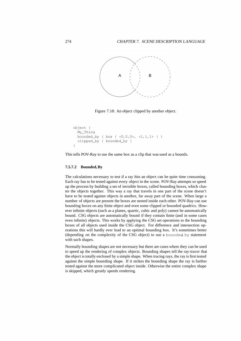
274 CHAPTER 7. SCENE DESCRIPTION LANGUAGE
BA
Figure 7.18: An object clipped by another object.
object {My_Thingbounded_by { box { <0,0,0>, <1,1,1> } }clipped_by { bounded_by }
}
This tells POV-Ray to use the same box as a clip that was used as a bounds.
7.5.7.2 Bounded By
The calculations necessary to test if a ray hits an object can be quite time consuming.Each ray has to be tested against every object in the scene. POV-Ray attempts so speedup the process by building a set of invisible boxes, called bounding boxes, which clus-ter the objects together. This way a ray that travels in one part of the scene doesn’thave to be tested against objects in another, far away part of the scene. When large anumber of objects are present the boxes are nested inside each other. POV-Ray can usebounding boxes on any finite object and even some clipped or bounded quadrics. How-ever infinite objects (such as a planes, quartic, cubic and poly) cannot be automaticallybound. CSG objects are automatically bound if they contain finite (and in some caseseven infinite) objects. This works by applying the CSG set operations to the boundingboxes of all objects used inside the CSG object. For difference and intersection op-erations this will hardly ever lead to an optimal bounding box. It’s sometimes better(depending on the complexity of the CSG object) to use a bounded by statementwith such shapes.
Normally bounding shapes are not necessary but there are cases where they can be usedto speed up the rendering of complex objects. Bounding shapes tell the ray-tracer thatthe object is totally enclosed by a simple shape. When tracing rays, the ray is first testedagainst the simple bounding shape. If it strikes the bounding shape the ray is furthertested against the more complicated object inside. Otherwise the entire complex shapeis skipped, which greatly speeds rendering.

7.5. OBJECTS 275
To use bounding shapes, simply include the following lines in the declaration of yourobject:
bounded_by {object { ... }
}
An example of a bounding shape:
intersection {sphere { <0,0,0>, 2 }plane { <0,1,0>, 0 }plane { <1,0,0>, 0 }bounded_by {sphere { <0,0,0>, 2 } }
}
The best bounding shape is a sphere or a box since these shapes are highly optimized,although, any shape may be used. If the bounding shape is itself a finite shape whichresponds to bounding slabs then the object which it encloses will also be used in theslab system.
CSG shapes can benefit from bounding slabs without a bounded by statement how-ever they may do so inefficiently in intersection, difference and merge. In these threeCSG types the automatic bound used covers all of the component objects in their en-tirety. However the result of these intersections may result in a smaller object. Comparethe sizes of the illustrations for union and intersection in the CSG section above. It ispossible to draw a much smaller box around the intersection of A and B than the unionof A and B yet the automatic bounds are the size of the union of A and B regardless ofthe kind of CSG specified.
While it is almost always a good idea to manually add a bounded by to intersec-tion, difference and merge, it is often best to not bound a union. If a union has nobounded by and no clipped by POV-Ray can internally split apart the compo-nents of a union and apply automatic bounding slabs to any of its finite parts. Note thatsome utilities such as RAW2POV may be able to generate bounds more efficiently thanPOV-Ray’s current system. However most unions you create yourself can be easilybounded by the automatic system. For technical reasons POV-Ray cannot split a mergeobject. It is probably best to hand bound a merge, especially if it is very complex.
Note that if bounding shape is too small or positioned incorrectly it may clip the ob-ject in undefined ways or the object may not appear at all. To do true clipping, useclipped by as explained above. Often you will want to use the clipped by andbounded by options with the same object. The following shortcut saves typing anduses less memory.
object {

276 CHAPTER 7. SCENE DESCRIPTION LANGUAGE
My_Thingclipped_by{ box { <0,0,0>,<1,1,1 > }}bounded_by{ clipped_by }
}
This tells POV-Ray to use the same box as a bounds that was used as a clip.
7.5.7.3 Hollow
POV-Ray by default assumes that objects are made of a solid material that completelyfills the interior of an object. By adding the hollow keyword to the object you canmake it hollow. That is very useful if you want atmospheric effects to exist inside anobject. It is even required for objects containing a halo (see 7.6.4 on page 302 fordetails).
In order to get a hollow CSG object you just have to make the top level object hollow.All children will assume the same hollow state except their state is explicitly set. Thefollowing example will set both spheres inside the union hollow
union {sphere { -0.5*x, 1 }sphere { 0.5*x, 1 }hollow
}
while the next example will only set the second sphere hollow because the first spherewas explicitly set to be not hollow.
union {sphere { -0.5*x, 1 hollow off }sphere { 0.5*x, 1 }hollow
}
7.5.7.4 No Shadow
You may specify the no shadow keyword in an object to make that object cast noshadow. This is useful for special effects and for creating the illusion that a light sourceactually is visible. This keyword was necessary in earlier versions of POV-Ray whichdid not have the looks like statement. Now it is useful for creating things like laserbeams or other unreal effects.
Simply attach the keyword as follows:

7.6. TEXTURES 277
object {My_Thingno_shadow
}
7.5.7.5 Sturm
Some of POV-Ray’s objects allow you to choose between a fast but sometimes inaccu-rate root solver and a slower but more accurate one. This is the case for all objects thatinvolve the solution of a cubic or quartic polynomial. There are analytic mathematicalsolutions for those polynomals that can be used.
Lower order polynomals are trivial to solve while higher order polynomials requireiterative algorithms to solve them. One of those algorithms is the Sturmian root solver.
The following list shows all objects for which the Sturmian root solver can be used.
blobcubiclathe (only with quadratic splines)polyprism (only with cubic splines)quarticsor
7.6 Textures
The texture describes what the object looks like, i. e. its material. Textures are com-binations of pigments, normals, finishes and halos. Pigment is the color or pattern ofcolors inherent in the material. Normal is a method of simulating various patterns ofbumps, dents, ripples or waves by modifying the surface normal vector. Finish de-scribes the reflective and refractive properties of a material. Halo simulates effects likeclouds, fog, fire etc. by using a density field defined inside the object.
A plain texture consists of a single pigment, an optional normal, a single finish andoptionally one or more halos. A special texture combines two or more textures using apattern or blending function. Special textures may be made quite complex by nestingpatterns within patterns. At the innermost levels however, they are made up from plaintextures. Note that allthough we call a plain texture plain it may be a very complextexture. The term plain only means that it has a single pigment, normal, finish andhalo.
The most complete form for defining a plain texture is as follows:

278 CHAPTER 7. SCENE DESCRIPTION LANGUAGE
texture {TEXTURE_IDENTIFIERpigment {..}.normal {..}.finish {..}.halo {..}.TRANSFORMATIONS
}
Each of the items in a texture are optional but if they are present the identifiermust be first and the transformations must be last. The pigment, normal and fin-ish parameters modify any pigment, normal and finish already specified in the TEX-TURE IDENTIFIER. Any halos are added to the already existing halos. If no textureidentifier is specified the pigment, normal and finish statements modify the current de-fault values and any halo is added to the default halo, if any. TRANSFORMATIONsare translate, rotate, scale and matrix statements. They should be specified last.
The sections below describe all of the options available in pigments, normals, finishesand halos. Special textures are covered later.
7.6.1 Pigment
The color or pattern of colors for an object is defined by a pigment statement. Allplain textures must have a pigment. If you do not specify one the default pigment isused. A pigment statement is part of a texture specification. However it can be tediousto type texture { pigment { . . . } } just to add a color to an object. Thereforeyou may attach a pigment directly to an object without explicitly specifying that it aspart of a texture. For example:
//this... //can be shortened to this...
object { object {My_Object My_Objecttexture { pigment {color Red}
pigment {color Red} }}
}
The color you define is the way you want the object to look if fully illuminated. Youpick the basic color inherent in the object and POV-Ray brightens or darkens it de-pending on the lighting in the scene. The parameter is called pigment because we aredefining the basic color the object actually is rather than how it looks.
The most complete form for defining a pigment is as follows:

7.6. TEXTURES 279
pigment {PIGMENT_IDENTIFIERPATTERN_TYPEPIGMENT_MODIFIERS...
}
Each of the items in a pigment are optional but if they are present, they should be inthe order shown above to insure that the results are as expected. Any items after thePIGMENT IDENTIFIER modify or override settings given in the identifier. If no iden-tifier is specified then the items modify the pigment values in the current default tex-ture. Valid PIGMENT MODIFIERS are color map, pigment map, image mapand quick color statements as well as any of the generic PATTERN MODIFIERSsuch as translate, rotate, scale, turbulence, wave shape and warp state-ments. Such modifiers apply only to the pigment and not to other parts of the texture.Modifiers should be specified last.
The various pattern types fall into roughly four categories. Each category is discussedbelow. They are solid color, color list patterns, color mapped patterns and image maps.
7.6.1.1 Solid Color Pigments
The simplest type of pigment is a solid color. To specify a solid color you simply put acolor specification inside a pigment. For example:
pigment {color Orange}
A color specification consists of the option keyword color followed by a color iden-tifier or by a specification of the amount of red, green, blue, filtered and unfilteredtransparency in the surface. See section 7.1.5 on page 192 for more details about col-ors. Any pattern modifiers used with a solid color are ignored because there is nopattern to modify.
7.6.1.2 Color List Pigments
There are three color list patterns: checker, hexagon and brick. The result is apattern of solid colors with distinct edges rather than a blending of colors as with colormapped patterns. Each of these patterns is covered in more detail in a later section.The syntax for each is:
pigment { brick COLOR1, COLOR2 MODIFIERS ... }pigment { checker COLOR1, COLOR2 MODIFIERS ... }pigment { hexagon COLOR1, COLOR2, COLOR3 MODIFIERS ... }
Each COLORn is any valid color specification. There should be a comma betweeneach color or the color keyword should be used as a separator so that POV-Ray candetermine where each color specification starts and ends.

280 CHAPTER 7. SCENE DESCRIPTION LANGUAGE
7.6.1.3 Color Maps
Most of the color patterns do not use abrupt color changes of just two or three colorslike those in the brick, checker or hexagon patterns. They instead use smooth transi-tions of many colors that gradually change from one point to the next. The colors aredefined in a pigment modifier called a color map that describes how the pattern blendsfrom one color to the next.
Each of the various pattern types available is in fact a mathematical function that takesany x, y, z location and turns it into a number between 0.0 and 1.0 inclusive. Thatnumber is used to specify what mix of colors to use from the color map.
A color map is specified by . . .
pigment{PATTERN_TYPEcolor_map {
[ NUM_1 COLOR_1][ NUM_2 COLOR_2][ NUM_3 COLOR_3]...
}PIGMENT_MODIFIERS...
}
Where NUM 1, NUM 2, . . . are float values between 0.0 and 1.0 inclusive. COLOR 1,COLOR 2, . . . are color specifications. Note that the [] brackets are part of the actualstatement. They are not notational symbols denoting optional parts. The bracketssurround each entry in the color map. There may be from 2 to 256 entries in the map.The alternate spelling colour map may be used.
For example
sphere {<0,1,2>, 2pigment {
gradient x //this is the PATTERN_TYPEcolor_map {
[0.1 color Red][0.3 color Yellow][0.6 color Blue][0.6 color Green][0.8 color Cyan]
}}
}
The pattern function is evaluated and the result is a value from 0.0 to 1.0. If the value isless than the first entry (in this case 0.1) then the first color (red) is used. Values from

7.6. TEXTURES 281
0.1 to 0.3 use a blend of red and yellow using linear interpolation of the two colors.Similarly values from 0.3 to 0.6 blend from yellow to blue. Note that the 3rd and 4thentries both have values of 0.6. This causes an immediate abrupt shift of color fromblue to green. Specifically a value that is less than 0.6 will be blue but exactly equal to0.6 will be green. Moving along, values from 0.6 to 0.8 will be a blend of green andcyan. Finally any value greater than or equal to 0.8 will be cyan.
If you want areas of unchanging color you simply specify the same color for two adja-cent entries. For example:
color_map {[0.1 color Red][0.3 color Yellow][0.6 color Yellow][0.8 color Green]
}
In this case any value from 0.3 to 0.6 will be pure yellow.
The color map keyword may be used with any pattern except brick, checker,hexagon and image map. You may declare and use color map identifiers. Forexample:
#declare Rainbow_Colors=color_map {
[0.0 color Magenta][0.33 color Yellow][0.67 color Cyan][1.0 color Magenta]
}
object{My_Objectpigment{
gradient xcolor_map{Rainbow_Colors}
}}
7.6.1.4 Pigment Maps
In addition to specifying blended colors with a color map you may create a blend ofpigments using a pigment map. The syntax for a pigment map is identical to a colormap except you specify a pigment in each map entry (and not a color).
A pigment map is specified by . . .

282 CHAPTER 7. SCENE DESCRIPTION LANGUAGE
pigment{PATTERN_TYPEpigment_map {
[ NUM_1 PIGMENT_BODY_1][ NUM_2 PIGMENT_BODY_2][ NUM_3 PIGMENT_BODY_3]...
}PIGMENT_MODIFIERS...
}
Where NUM 1, NUM 2, . . . are float values between 0.0 and 1.0 inclusive. A PIG-MENT BODY is anything that would normally appear inside a pigment { . . . }statement but the pigment keyword and {} braces are not needed. Note that the []brackets are part of the actual statement. They are not notational symbols denotingoptional parts. The brackets surround each entry in the map. There may be from 2 to256 entries in the map.
For example
sphere {<0,1,2>, 2pigment {
gradient x //this is the PATTERN_TYPEpigment_map {
[0.3 wood scale 0.2][0.3 Jade] //this is a pigment identifier[0.6 Jade][0.9 marble turbulence 1]
}}
}
When the gradient x function returns values from 0.0 to 0.3 the scaled wood pig-ment is used. From 0.3 to 0.6 the pigment identifier Jade is used. From 0.6 up to 0.9 ablend of Jade and a turbulent marble is used. From 0.9 on up only the turbulent marbleis used.
Pigment maps may be nested to any level of complexity you desire. The pigments ina map may have color maps or pigment maps or any type of pigment you want. Anyentry of a pigment map may be a solid color however if all entries are solid colors youshould use a color map which will render slightly faster.
Entire pigments may also be used with the block patterns such as checker, hexagon andbrick. For example . . .
pigment {
7.6. TEXTURES 283
checkerpigment { Jade scale .8 }pigment { White_Marble scale .5 }
}
Note that in the case of block patterns the pigment { . . . } wrapping is requiredaround the pigment information.
A pigment map is also used with the average pigment type. See 7.6.7.2 on page 319for details.
You may not use pigment map or individual pigments with an image map.See 7.6.5.1 on page 313 for an alternative way to do this.
7.6.1.5 Image Maps
When all else fails and none of the above pigment pattern types meets your needs youcan use an image map to wrap a 2-D bit-mapped image around your 3-D objects.
7.6.1.5.1 Specifying an Image Map
The syntax for an image map is . . .
pigment {image_map {
FILE_TYPE "filename"MODIFIERS...
}}
Where FILE TYPE is one of the following keywords gif, tga, iff, ppm, pgm, pngor sys. This is followed by the name of the file in quotes. Several optional modifiersmay follow the file specification. The modifiers are described below. Note that earlierversions of POV-Ray allowed some modifiers before the FILE TYPE but that syntax isbeing phased out in favor of the syntax described here.
Filenames specified in the image map statements will be searched for in the home(current) directory first and, if not found, will then be searched for in directories spec-ified by any –L (library path) options active. This would facilitate keeping all yourimage maps files in a separate subdirectory and giving an –L option on the commandline to where your library of image maps are.
By default, the image is mapped onto the x-y-plane. The image is projected onto theobject as though there were a slide projector somewhere in the−z-direction. The imageexactly fills the square area from (x,y) coordinates (0,0) to (1,1) regardless of the im-age’s original size in pixels. If you would like to change this default you may translate,rotate or scale the pigment or texture to map it onto the object’s surface as desired.
284 CHAPTER 7. SCENE DESCRIPTION LANGUAGE
In section 7.6.7.6 on page 322 the checker pigment pattern is explained. The checksare described as solid cubes of colored clay from which objects are carved. With imagemaps you should imagine that each pixel is a long, thin, square, colored rod that extendsparallel to the z-axis. The image is made from rows and columns of these rods bundledtogether and the object is then carved from the bundle.
If you would like to change this default orientation you may translate, rotate or scalethe pigment or texture to map it onto the object’s surface as desired.
7.6.1.5.2 The map type Option
The default projection of the image onto the x-y-plane is called a planar map type.This option may be changed by adding the map type keyword followed by a numberspecifying the way to wrap the image around the object.
A map type 0 gives the default planar mapping already described.
A map type 1 gives a spherical mapping. It assumes that the object is a sphere of anysize sitting at the origin. The y-axis is the north/south pole of the spherical mapping.The top and bottom edges of the image just touch the pole regardless of any scaling.The left edge of the image begins at the positive x-axis and wraps the image around thesphere from west to east in a −y-rotation. The image covers the sphere exactly once.The once keyword has no meaning for this mapping type.
With map type 2 you get a cylindrical mapping. It assumes that a cylinder of anydiameter lies along the y-axis. The image wraps around the cylinder just like the spher-ical map but the image remains one unit tall from y = 0 to y = 1. This band of color isrepeated at all heights unless the once keyword is applied.
Finally map type 5 is a torus or donut shaped mapping. It assumes that a torusof major radius one sits at the origin in the x-z-plane. The image is wrapped aroundsimilar to spherical or cylindrical maps. However the top and bottom edges of the mapwrap over and under the torus where they meet each other on the inner rim.
Types 3 and 4 are still under development.
Note that the map type option may also be applied to bump map andmaterial map statements.
7.6.1.5.3 The Filter and Transmit Bitmap Modifiers
To make all or part of an image map transparent you can specify filter and/or transmitvalues for the color palette/registers of PNG, GIF or IFF pictures (at least for the modesthat use palettes). You can do this by adding the keyword filter or transmitfollowing the filename. The keyword is followed by two numbers. The first numberis the palette number value and the second is the amount of transparency. The valuesshould be separated by a comma. For example:
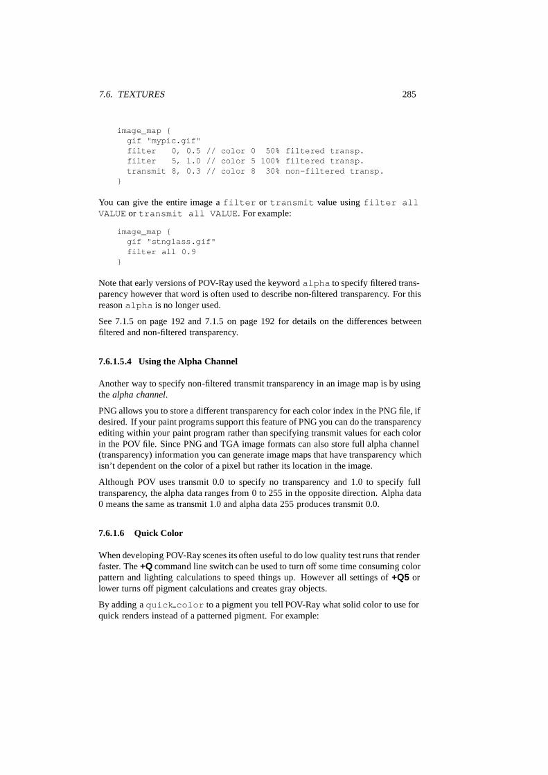
7.6. TEXTURES 285
image_map {gif "mypic.gif"filter 0, 0.5 // color 0 50% filtered transp.filter 5, 1.0 // color 5 100% filtered transp.transmit 8, 0.3 // color 8 30% non-filtered transp.
}
You can give the entire image a filter or transmit value using filter allVALUE or transmit all VALUE. For example:
image_map {gif "stnglass.gif"filter all 0.9
}
Note that early versions of POV-Ray used the keyword alpha to specify filtered trans-parency however that word is often used to describe non-filtered transparency. For thisreason alpha is no longer used.
See 7.1.5 on page 192 and 7.1.5 on page 192 for details on the differences betweenfiltered and non-filtered transparency.
7.6.1.5.4 Using the Alpha Channel
Another way to specify non-filtered transmit transparency in an image map is by usingthe alpha channel.
PNG allows you to store a different transparency for each color index in the PNG file, ifdesired. If your paint programs support this feature of PNG you can do the transparencyediting within your paint program rather than specifying transmit values for each colorin the POV file. Since PNG and TGA image formats can also store full alpha channel(transparency) information you can generate image maps that have transparency whichisn’t dependent on the color of a pixel but rather its location in the image.
Although POV uses transmit 0.0 to specify no transparency and 1.0 to specify fulltransparency, the alpha data ranges from 0 to 255 in the opposite direction. Alpha data0 means the same as transmit 1.0 and alpha data 255 produces transmit 0.0.
7.6.1.6 Quick Color
When developing POV-Ray scenes its often useful to do low quality test runs that renderfaster. The +Q command line switch can be used to turn off some time consuming colorpattern and lighting calculations to speed things up. However all settings of +Q5 orlower turns off pigment calculations and creates gray objects.
By adding a quick color to a pigment you tell POV-Ray what solid color to use forquick renders instead of a patterned pigment. For example:
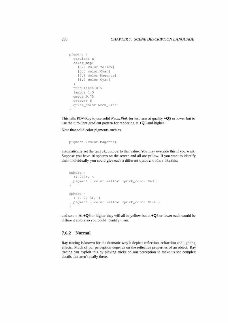
286 CHAPTER 7. SCENE DESCRIPTION LANGUAGE
pigment {gradient xcolor_map{
[0.0 color Yellow][0.3 color Cyan][0.6 color Magenta][1.0 color Cyan]
}turbulence 0.5lambda 1.5omega 0.75octaves 8quick_color Neon_Pink
}
This tells POV-Ray to use solid Neon Pink for test runs at quality +Q5 or lower but touse the turbulent gradient pattern for rendering at +Q6 and higher.
Note that solid color pigments such as
pigment {color Magenta}
automatically set the quick color to that value. You may override this if you want.Suppose you have 10 spheres on the screen and all are yellow. If you want to identifythem individually you could give each a different quick color like this:
sphere {<1,2,3>, 4pigment { color Yellow quick_color Red }
}
sphere {<-1,-2,-3>, 4pigment { color Yellow quick_color Blue }
}
and so on. At +Q6 or higher they will all be yellow but at +Q5 or lower each would bedifferent colors so you could identify them.
7.6.2 Normal
Ray-tracing is known for the dramatic way it depicts reflection, refraction and lightingeffects. Much of our perception depends on the reflective properties of an object. Raytracing can exploit this by playing tricks on our perception to make us see complexdetails that aren’t really there.

7.6. TEXTURES 287
Suppose you wanted a very bumpy surface on the object. It would be very difficult tomathematically model lots of bumps. We can however simulate the way bumps lookby altering the way light reflects off of the surface. Reflection calculations depend ona vector called a surface normal vector. This is a vector which points away from thesurface and is perpendicular to it. By artificially modifying (or perturbing) this normalvector you can simulate bumps.
The normal { . . . } statement is the part of a texture which defines the pattern ofnormal perturbations to be applied to an object. Like the pigment statement, you canomit the surrounding texture block to save typing. Do not forget however that there isa texture implied. For example . . .
// this... // can be shortened to this...
object { object {My_Object My_Objecttexture { pigment { color Purple }
pigment { color Purple } normal { bumps 0.3 }normal { bumps 0.3 } }
}}
Note that attaching a normal pattern does not really modify the surface. It only affectsthe way light reflects or refracts at the surface so that it looks bumpy.
The most complete form for defining a normal is as follows:
normal {NORMAL_IDENTIFIERPATTERN_TYPE FloatValueNORMAL_MODIFIERSTRANSFORMATIONS...
}
Each of the items in a normal are optional but if they are present they should be in theorder shown above to insure that the results are as expected. Any items after the NOR-MAL IDENTIFIER modify or override settings given in the identifier. If no identifieris specified then the items modify the normal values in the current default texture. ThePATTERN TYPE may optionally be followed by a float value that controls the appar-ent depth of the bumps. Typical values range from 0.0 to 1.0 but any value may beused. Negative values invert the pattern. The default value if none is specified is 0.5.
Valid NORMAL MODIFIERS are slope map, normal map, bump map andbump size statements as well as any of the generic PATTERN MODIFIERS suchas translate, rotate, scale, turbulence, wave shape and warp statements. Such modifiersapply only to the normal and not to other parts of the texture. Modifiers should bespecified last.

288 CHAPTER 7. SCENE DESCRIPTION LANGUAGE
There are three basic types of NORMAL PATTERN TYPEs. They are pattern nor-mals, specialized normals and bump maps. They differ in the types of modifiers youmay use with them. Originally POV-Ray had some patterns which were exclusivelyused for pigments while others were exclusively used for normals. Since POV-Ray3.0 you can use any pattern for either pigments or normals. For example it is nowvalid to use ripples as a pigment or wood as a normal type. The patterns bumps,dents, ripples, waves, wrinkles and bump map were once exclusively nor-mal patterns which could not be used as pigments. Because these six types use special-ized normal modification calculations they cannot have slope map, normal map orwave shape modifiers. All other normal pattern types may use them.
7.6.2.1 Slope Maps
A slope map is a normal pattern modifier which gives the user a great deal of controlover the exact shape of the bumpy features. It is best illustrated with a gradient normalpattern. Suppose you have . . .
plane{ z, 0pigment{ White }normal { gradient x }
}
This gives a ramp wave pattern that looks like small linear ramps that climb from thepoints at x = 0 to x = 1 and then abruptly drops to 0 again to repeat the ramp fromx = 1 to x = 2. A slope map turns this simple linear ramp into almost any wave shapeyou want. The syntax is as follows . . .
normal{PATTERN_TYPE Valueslope_map {
[ NUM_1 POINT_SLOPE_1][ NUM_2 POINT_SLOPE_2][ NUM_3 POINT_SLOPE_3]...
}NORMAL_MODIFIERS...
}
Note that the [] brackets are part of the actual statement. They are not notationalsymbols denoting optional parts. The brackets surround each entry in the slope map.There may be from 2 to 256 entries in the map.
The NUM 1, NUM 2, . . . are float values between 0.0 and 1.0 inclusive.POINT SLOPE 1, POINT SLOPE 2, . . . are 2 component vectors such as 〈0,1〉where
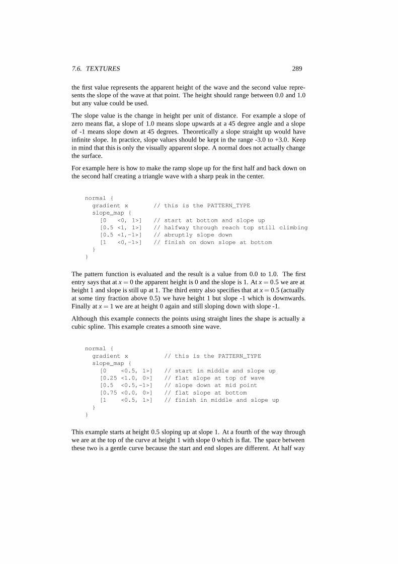
7.6. TEXTURES 289
the first value represents the apparent height of the wave and the second value repre-sents the slope of the wave at that point. The height should range between 0.0 and 1.0but any value could be used.
The slope value is the change in height per unit of distance. For example a slope ofzero means flat, a slope of 1.0 means slope upwards at a 45 degree angle and a slopeof -1 means slope down at 45 degrees. Theoretically a slope straight up would haveinfinite slope. In practice, slope values should be kept in the range -3.0 to +3.0. Keepin mind that this is only the visually apparent slope. A normal does not actually changethe surface.
For example here is how to make the ramp slope up for the first half and back down onthe second half creating a triangle wave with a sharp peak in the center.
normal {gradient x // this is the PATTERN_TYPEslope_map {
[0 <0, 1>] // start at bottom and slope up[0.5 <1, 1>] // halfway through reach top still climbing[0.5 <1,-1>] // abruptly slope down[1 <0,-1>] // finish on down slope at bottom
}}
The pattern function is evaluated and the result is a value from 0.0 to 1.0. The firstentry says that at x = 0 the apparent height is 0 and the slope is 1. At x = 0.5 we are atheight 1 and slope is still up at 1. The third entry also specifies that at x= 0.5 (actuallyat some tiny fraction above 0.5) we have height 1 but slope -1 which is downwards.Finally at x = 1 we are at height 0 again and still sloping down with slope -1.
Although this example connects the points using straight lines the shape is actually acubic spline. This example creates a smooth sine wave.
normal {gradient x // this is the PATTERN_TYPEslope_map {
[0 <0.5, 1>] // start in middle and slope up[0.25 <1.0, 0>] // flat slope at top of wave[0.5 <0.5,-1>] // slope down at mid point[0.75 <0.0, 0>] // flat slope at bottom[1 <0.5, 1>] // finish in middle and slope up
}}
This example starts at height 0.5 sloping up at slope 1. At a fourth of the way throughwe are at the top of the curve at height 1 with slope 0 which is flat. The space betweenthese two is a gentle curve because the start and end slopes are different. At half way

290 CHAPTER 7. SCENE DESCRIPTION LANGUAGE
we are at half height sloping down to bottom out at 3/4ths. By the end we are climbingat slope 1 again to complete the cycle. There are more examples in SLOPEMAP.POV inthe sample scenes.
A slope map may be used with any pattern except brick, checker, hexagon,bumps, dents, ripples, waves, wrinkles and bump map.
You may declare and use slope map identifiers. For example:
#declare Fancy_Wave =slope_map { // Now let’s get fancy
[0.0 <0, 1>] // Do tiny triangle here[0.2 <1, 1>] // down[0.2 <1,-1>] // to[0.4 <0,-1>] // here.[0.4 <0, 0>] // Flat area[0.5 <0, 0>] // through here.[0.5 <1, 0>] // Square wave leading edge[0.6 <1, 0>] // trailing edge[0.6 <0, 0>] // Flat again[0.7 <0, 0>] // through here.[0.7 <0, 3>] // Start scallop[0.8 <1, 0>] // flat on top[0.9 <0,-3>] // finish here.[0.9 <0, 0>] // Flat remaining through 1.0
}
object{ My_Objectpigment { White }normal {
woodslope_map { Fancy_Wave }
}}
7.6.2.2 Normal Maps
Most of the time you will apply single normal pattern to an entire surface but you mayalso create a pattern or blend of normals using a normal map. The syntax for a normalmap is identical to a pigment map except you specify a normal in each map entry.
A normal map is specified by . . .
normal{PATTERN_TYPEnormal_map {
[ NUM_1 NORMAL_BODY_1][ NUM_2 NORMAL_BODY_2][ NUM_3 NORMAL_BODY_3]

7.6. TEXTURES 291
...}NORMAL_MODIFIERS...
}
Where NUM 1, NUM 2, . . . are float values between 0.0 and 1.0 inclusive. A NOR-MAL BODY is anything that would normally appear inside a normal { . . . } state-ment but the normal keyword and {} braces are not needed. Note that the [] bracketsare part of the actual statement. They are not notational symbols denoting optionalparts. The brackets surround each entry in the map. There may be from 2 to 256entries in the map.
For example
normal {gradient x //this is the PATTERN_TYPEnormal_map {
[0.3 bumps scale 2][0.3 dents][0.6 dents][0.9 marble turbulence 1]
}}
When the gradient x function returns values from 0.0 to 0.3 then the scaled bumpsnormal is used. From 0.3 to 0.6 dents are From 0.6 up to 0.9 a blend of dents and aturbulent marble is used. From 0.9 on up only the turbulent marble is used.
Normal maps may be nested to any level of complexity you desire. The normals in amap may have slope maps or normal maps or any type of normal you want.
A normal map is also used with the average normal type. See 7.6.7.2 on page 319for details.
Entire normals may also be used with the block patterns such as checker, hexagon andbrick. For example . . .
normal {checker
normal { gradient x scale .2 }normal { gradient y scale .2 }
}}
Note that in the case of block patterns the normal { . . . } wrapping is requiredaround the normal information.
You may not use normal map or individual normals with a bump map. See 7.6.5.1on page 313 for an alternative way to do this.

292 CHAPTER 7. SCENE DESCRIPTION LANGUAGE
7.6.2.3 Bump Maps
When all else fails and none of the above normal pattern types meets your needs youcan use a bump map to wrap a 2-D bit-mapped bump pattern around your 3-D objects.
Instead of placing the color of the image on the shape like an image map a bumpmap perturbs the surface normal based on the color of the image at that point. Theresult looks like the image has been embossed into the surface. By default, a bumpmap uses the brightness of the actual color of the pixel. Colors are converted to grayscale internally before calculating height. Black is a low spot, white is a high spot.The image’s index values may be used instead (see section 7.6.2.3.3 on the next pagebelow).
7.6.2.3.1 Specifying a Bump Map
The syntax for bump map is . . .
normal {bump_map {
FILE_TYPE "filename"BITMAP_MODIFIERS...
}NORMAL_MODIFIERS...
}
Where FILE TYPE is one of the following keywords gif, tga, iff, ppm, pgm,png or sys. This is followed by the name of the file using any valid string expres-sion. Several optional modifiers may follow the file specification. The modifiers aredescribed below. Note that earlier versions of POV-Ray allowed some modifiers beforethe FILE TYPE but that syntax is being phased out in favor of the syntax describedhere.
Filenames specified in the bump map statement will be searched for in the home (cur-rent) directory first and, if not found, will then be searched for in directories specifiedby any +L switches or Library Path options. This would facilitate keeping all yourbump maps files in a separate subdirectory, and specifying a library path to them. Notethat any operating system default paths are not searched unless you also specify themas a Library Path.
By default, the bump pattern is mapped onto the x-y-plane. The bumps are projectedonto the object as though there were a slide projector somewhere in the −z-direction.The bump pattern exactly fills the square area from (x,y) coordinates (0,0) to (1,1)regardless of the bitmaps’s original size in pixels. If you would like to change thisdefault, you may translate, rotate or scale the normal or texture to map it onto theobject’s surface as desired.
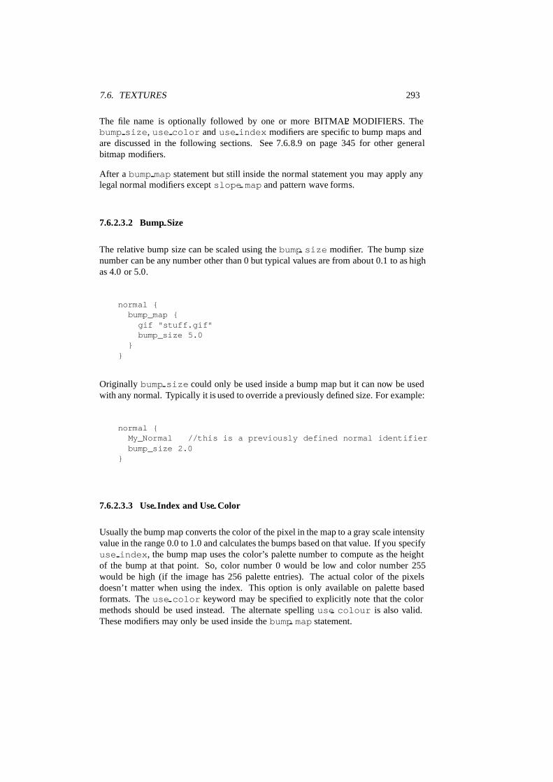
7.6. TEXTURES 293
The file name is optionally followed by one or more BITMAP MODIFIERS. Thebump size, use color and use index modifiers are specific to bump maps andare discussed in the following sections. See 7.6.8.9 on page 345 for other generalbitmap modifiers.
After a bump map statement but still inside the normal statement you may apply anylegal normal modifiers except slope map and pattern wave forms.
7.6.2.3.2 Bump Size
The relative bump size can be scaled using the bump size modifier. The bump sizenumber can be any number other than 0 but typical values are from about 0.1 to as highas 4.0 or 5.0.
normal {bump_map {
gif "stuff.gif"bump_size 5.0
}}
Originally bump size could only be used inside a bump map but it can now be usedwith any normal. Typically it is used to override a previously defined size. For example:
normal {My_Normal //this is a previously defined normal identifierbump_size 2.0
}
7.6.2.3.3 Use Index and Use Color
Usually the bump map converts the color of the pixel in the map to a gray scale intensityvalue in the range 0.0 to 1.0 and calculates the bumps based on that value. If you specifyuse index, the bump map uses the color’s palette number to compute as the heightof the bump at that point. So, color number 0 would be low and color number 255would be high (if the image has 256 palette entries). The actual color of the pixelsdoesn’t matter when using the index. This option is only available on palette basedformats. The use color keyword may be specified to explicitly note that the colormethods should be used instead. The alternate spelling use colour is also valid.These modifiers may only be used inside the bump map statement.

294 CHAPTER 7. SCENE DESCRIPTION LANGUAGE
7.6.3 Finish
The finish properties of a surface can greatly affect its appearance. How does lightreflect? What happens when light passes through? What kind of highlights are visible.To answer these questions you need a finish statement.
The finish { . . . } statement is the part of a texture which defines the variousfinish properties to be applied to an object. Like the pigment or normal statement youcan omit the surrounding texture block to save typing. Do not forget however that thereis a texture implied. For example . . .
// this... // can be shortened to this...
object { object {My_Object My_Objecttexture { pigment { color Purple }
pigment { color Purple } finish { phong 0.3 }finish { phong 0.3 } }
}}
The most complete form for defining a finish is as follows:
finish {FINISH_IDENTIFIER[ ambient COLOR ][ diffuse FLOAT ][ brilliance FLOAT ][ phong FLOAT ][ phong_size FLOAT ][ specular FLOAT ][ roughness FLOAT ][ metallic [ FLOAT ] ][ reflection COLOR ][ refraction FLOAT ][ ior FLOAT ][ caustics FLOAT ][ fade_distance FLOAT ][ fade_power FLOAT ][ irid { thickness FLOAT turbulence VECTOR } ][ crand FLOAT ]
}
The FINISH IDENTIFIER is optional but should proceed all other items. Any itemsafter the FINISH IDENTIFIER modify or override settings given in the IDENTIFIER.If no identifier is specified then the items modify the finish values in the current defaulttexture. Note that transformations are not allowed inside a finish because finish itemscover the entire surface uniformly.
7.6. TEXTURES 295
7.6.3.1 Ambient
The light you see in dark shadowed areas comes from diffuse reflection off of otherobjects. This light cannot be directly modeled using ray-tracing. However we can usea trick called ambient lighting to simulate the light inside a shadowed area.
Ambient light is light that is scattered everywhere in the room. It bounces all overthe place and manages to light objects up a bit even where no light is directly shining.Computing real ambient light would take far too much time, so we simulate ambientlight by adding a small amount of white light to each texture whether or not a light isactually shining on that texture.
This means that the portions of a shape that are completely in shadow will still have alittle bit of their surface color. It’s almost as if the texture glows, though the ambientlight in a texture only affects the shape it is used on.
Usually a single float value is specified even though the syntax calls for a color. Forexample a float value of 0.3 gets promoted to the full color vector 〈0.3,0.3,0.3,0.3,0.3〉which is acceptible because only the red, green and blue parts are used.
The default value is very little ambient light (0.1). The value can range from 0.0 to1.0. Ambient light affects both shadowed and non-shadowed areas so if you turn upthe ambient value you may want to turn down the diffuse value.
Note that this method doesn’t account for the color of surrounding objects. If you walkinto a room that has red walls, floor and ceiling then your white clothing will look pinkfrom the reflected light. POV-Ray’s ambient shortcut doesn’t account for this. Thereis also no way to model specular reflected indirect illumination such as the flashlightshining in a mirror.
You may color the ambient light using one of two methods. You may specify a colorrather than a float after the ambient keyword in each finish statement. For example
finish { ambient rgb <0.3,0.1,0.1> } //a pink ambient
You may also specify the overall ambient light source used when calculating the am-bient lighting of an object using the global ambient light setting. The formula isgiven by
ambient = ambientf inish ambientl ight source (7.32)
See section 7.8.2 on page 356 for details.
7.6.3.2 Diffuse Reflection Items
When light reflects off of a surface the laws of physics say that it should leave the sur-face at the exact same angle it came in. This is similar to the way a billiard ball bounces

296 CHAPTER 7. SCENE DESCRIPTION LANGUAGE
off a bumper of a pool table. This perfect reflection is called specular reflection. How-ever only very smooth polished surfaces reflect light in this way. Most of the time,light reflects and is scattered in all directions by the roughness of the surface. Thisscattering is called diffuse reflection because the light diffuses or spreads in a variety ofdirections. It accounts for the majority of the reflected light we see.
POV-Ray and most other ray-tracers can only simulate directly one of these three typesof illumination. That is the light which comes directly from actual light sources. Lightcoming from other objects such as mirrors via specular reflection (shine a flashlightonto a mirror for example). And last not least light coming from other objects viadiffuse reflections (look at some dark area under a desk or in a corner: even thougha lamp may not directly illuminate that spot you can still see a little bit because lightcomes from diffuse reflection off of nearby objects).
7.6.3.2.1 Diffuse
The keyword diffuse is used in a finish statement to control how much of thelight coming directly from any light sources is reflected via diffuse reflection. Forexample
finish {diffuse 0.7}
means that 70% of the light seen comes from direct illumination from light sources.The default value is diffuse 0.6.
7.6.3.2.2 Brilliance
The amount of direct light that diffuses from an object depends upon the angle at whichit hits the surface. When light hits at a shallow angle it illuminates less. When it isdirectly above a surface it illuminates more. The brilliance keyword can be usedin a finish statement to vary the way light falls off depending upon the angle ofincidence. This controls the tightness of the basic diffuse illumination on objects andslightly adjusts the appearance of surface shininess. Objects may appear more metallicby increasing their brilliance. The default value is 1.0. Higher values from to about10.0 cause the light to fall off less at medium to low angles. There are no limits to thebrilliance value. Experiment to see what works best for a particular situation. This isbest used in concert with highlighting.
7.6.3.2.3 Crand Graininess
Very rough surfaces, such as concrete or sand, exhibit a dark graininess in their apparentcolor. This is caused by the shadows of the pits or holes in the surface. The crandkeyword can be added to cause a minor random darkening in the diffuse reflection

7.6. TEXTURES 297
of direct illumination. Typical values range from crand 0.01 to crand 0.5 orhigher. The default value is 0. For example:
finish { crand 0.05 }
The grain or noise introduced by this feature is applied on a pixel-by-pixel basis. Thismeans that it will look the same on far away objects as on close objects. The effectalso looks different depending upon the resolution you are using for the rendering. Forthese reasons it is not a very accurate way to model the rough surface effect but someobjects still look better with a little crand thrown in.
Note that this should not be used when rendering animations. This is the one of a fewtruly random features in POV-Ray and will produce an annoying flicker of flying pixelson any textures animated with a crand value.
7.6.3.3 Highlights
Highlights are the bright spots that appear when a light source reflects off of a smoothobject. They are a blend of specular reflection and diffuse reflection. They are specular-like because they depend upon viewing angle and illumination angle. However theyare diffuse-like because some scattering occurs. In order to exactly model a highlightyou would have to calculate specular reflection off of thousands of microscopic bumpscalled micro facets. The more that micro facets are facing the viewer the shinier theobject appears and the tighter the highlights become. POV-Ray uses two differentmodels to simulate highlights without calculating micro facets. They are the specularand Phong models.
Note that specular and Phong highlights are not mutually exclusive. It is possible tospecify both and they will both take effect. Normally, however, you will only specifyone or the other.
7.6.3.3.1 Phong Highlights
The phong keyword controls the amount of Phong highlighting on the object. It causesbright shiny spots on the object that are the color of the light source being reflected.
The Phong method measures the average of the facets facing in the mirror directionfrom the light sources to the viewer.
Phong’s value is typically from 0.0 to 1.0, where 1.0 causes complete saturation to thelight source’s color at the brightest area (center) of the highlight. The default phong0.0 gives no highlight.
The size of the highlight spot is defined by the phong size value. The larger thephong size the tighter, or smaller, the highlight and the shinier the appearance. The

298 CHAPTER 7. SCENE DESCRIPTION LANGUAGE
smaller the phong size the looser, or larger, the highlight and the less glossy the ap-pearance.
Typical values range from 1.0 (very dull) to 250 (highly polished) though any valuesmay be used. Default phong size is 40 (plastic) if phong size is not specified. Forexample:
finish { phong 0.9 phong_size 60 }
If phong is not specified phong size has no effect.
7.6.3.3.2 Specular Highlight
A specular highlight is very similar to Phong highlighting but it uses slightly differ-ent model. The specular model more closely resembles real specular reflection andprovides a more credible spreading of the highlights occuring near the object horizons.
The specular value is typically from 0.0 to 1.0, where 1.0 causes complete saturationto the light source’s color at the brightest area (center) of the highlight. The defaultspecular 0.0 gives no highlight.
The size of the spot is defined by the value given for roughness. Typical values rangefrom 1.0 (very rough — large highlight) to 0.0005 (very smooth — small highlight).The default value, if roughness is not specified, is 0.05 (plastic).
It is possible to specify wrong values for roughness that will generate an error whenyou try to render the file. Don’t use 0 and if you get errors check to see if you are usinga very, very small roughness value that may be causing the error. For example:
finish { specular 0.9 roughness 0.02 }
If specular is not specified roughness has no effect.
7.6.3.3.3 Metallic Highlight Modifier
The keyword metallic may be used with Phong or specular highlights. This key-word indicates that the color of the highlights will be calculated by an empirical func-tion that models the reflectivity of metallic surfaces.
White light relfected specularly from a metallic surface takes the color of the surface,except then the incidence angle approaches 90 degrees, where it becomes white again.
The metallic keyword may be follow by a numeric value to specify the influencethe above effect has (the default value is one). For example:

7.6. TEXTURES 299
finish {phong 0.9phong_size 60metallic
}
If phong or specular is not specified metallic has no effect.
7.6.3.4 Specular Reflection
When light does not diffuse and it does reflect at the same angle as it hits an ob-ject, it is called specular reflection. Such mirror-like reflection is controlled by thereflection keyword in a finish statement. For example:
finish { reflection 1.0 ambient 0 diffuse 0 }
This gives the object a mirrored finish. It will reflect all other elements in the scene.Usually a single float value is specified after the keyword even though the syntax callsfor a color. For example a float value of 0.3 gets promoted to the full color vector〈0.3,0.3,0.3,0.3,0.3〉 which is acceptible because only the red, green and blue partsare used.
The value can range from 0.0 to 1.0. By default there is no reflection.
Adding reflection to a texture makes it take longer to render because an additional raymust be traced. The reflected light may be tinted by specifying a color rather than afloat. For example
finish { reflection rgb <1,0,0> }
gives a real red mirror that only reflects red light.
Note that although such reflection is called specular it is not controlled by thespecular keyword. That keyword controls a specular highlight.
7.6.3.5 Refraction
When light passes through a surface either into or out of a dense medium the path of theray of light is bent. Such bending is called refraction. Normally transparent or semi-transparent surfaces in POV-Ray do not refract light. Adding refraction 1.0 tothe finish statement turns on refraction.
Note that it is recommended that you only use refraction 0 or refraction1 (or even better refraction off and refraction on). Values in between
300 CHAPTER 7. SCENE DESCRIPTION LANGUAGE
will darken the refracted light in ways that do not correspond to any physical property.Many POV-Ray scenes were created with intermediate refraction values before this bugwas discovered so the feature has been maintained. A more appropriate way to reducethe brightness of refracted light is to change the filter or transmit value in thecolors specified in the pigment statement. Note also that refraction does not causethe object to be transparent. Transparency only occurs if there is a non-zero filter ortransmit value in the color.
The amount of bending or refracting of light depends upon the density of the material.Air, water, crystal and diamonds all have different densities and thus refract differently.The index of refraction or ior value is used by scientists to describe the relative densityof substances. The ior keyword is used in POV-Ray to specify the value. For example:
texture {pigment { White filter 0.9 }finish {
refraction 1ior 1.5
}}
The default ior value of 1.0 will give no refraction. The index of refraction for air is1.0, water is 1.33, glass is 1.5 and diamond is 2.4. The file CONSTS.INC pre-definesseveral useful values for ior.
Note that if a texture has a filter component and no value for refraction and ior are sup-plied the renderer will simply transmit the ray through the surface with no bending. Inlayered textures, the refraction and ior keywords must be in the last texture, otherwisethey will not take effect.
7.6.3.5.1 Light Attenuation
Light attenuation is used to model the decrease in light intensity as the light travelsthrough a translucent object. Its syntax is:
finish {fade_distance FADE_DISTANCEfade_power FADE_POWER
}
The fade distance keyword determines the distance the light has to travel to reachhalf intensity while the fade power keyword describes how fast the light will falloff. For realistic effects a fade power of 1 to 2 should be used.

7.6. TEXTURES 301
The attenuation is calculated by a formula similar to that used for light source attenua-tion.
attenuation =1
1+
(d
FADE DISTANCE
)FADE POW ER (7.33)
7.6.3.5.2 Faked Caustics
The syntax is:
finish {caustics POWER
}
***STILL BEING WRITTEN***
7.6.3.6 Iridescence
Iridescence, or Newton’s thin film interference, simulates the effect of light on surfaceswith a microscopic transparent film overlay. The effect is like an oil slick on a puddleof water or the rainbow hues of a soap bubble (see also 7.8.5 on page 360).
The syntax is:
finish {irid {
AMOUNTthickness FLOATturbulence VECTOR
}}
This finish modifies the surface color as a function of the angle between the light sourceand the surface. Since the effect works in conjunction with the position and angle ofthe light sources to the surface it does not behave in the same ways as a proceduralpigment pattern.
The AMOUNT parameter is the contribution of the iridescence effect to the overallsurface color. As a rule of thumb keep to around 0.25 (25% contribution) or less, butexperiment. If the surface is coming out too white, try lowering the diffuse and possiblythe ambient values of the surface.
The thickness keyword represents the film’s thickness. This is an awkward param-eter to set, since the thickness value has no relationship to the object’s scale. Changing

302 CHAPTER 7. SCENE DESCRIPTION LANGUAGE
it affects the scale or busy-ness of the effect. A very thin film will have a high frequencyof color changes while a thick film will have large areas of color.
The thickness of the film can be varied with the turbulence keyword. You can onlyspecify the amount of turbulence with iridescence. The octaves, lambda, and omegavalues are internally set and are not adjustable by the user at this time.
In addition, perturbing the object’s surface normal through the use of bump patternswill affect iridescence.
For the curious, thin film interference occurs because, when the ray hits the surface ofthe film, part of the light is reflected from that surface, while a portion is transmittedinto the film. This subsurface ray travels through the film and eventually reflects offthe opaque substrate. The light emerges from the film slightly out of phase with the raythat was reflected from the surface.
This phase shift creates interference, which varies with the wavelength of the compo-nent colors, resulting in some wavelengths being reinforced, while others are cancelledout. When these components are recombined, the result is iridescence.
The concept used for this feature came from the book Fundamentals of Three-Dimensional Computer Graphics by Alan Watt (Addison-Wesley).
7.6.4 Halo
A halo is used to simulate some of the atmospheric effects that occur when small parti-cles interact with light or radiate on their own. Those effects include clouds, fogs, fire,etc.
Halos are attached to an object, the so called container object, which they completelyfill. If the object is partially or completely translucent and the object is specified to behollow (see section 7.5.7.3 on page 276 for more details) the halo will be visible. Thusthe halo effects are limited to the space that the object covers. This should always bekept in mind.
What the halo actually will look like depends on a lot of parameters. First of all youhave to specify which kind of effect you want to simulate. After this you need to definethe distribution of the particles. This is basically done in two steps: a mapping functionis selected and a density function is chosen. The first function maps world coordinatesonto a one-dimensional interval while the later describes how this linear interval ismapped onto the final density values.
The properties of the particles, such as their color and their translucency, are givenby a color map. The density values calculated by the mapping processes are used todetermine the appropriate color using this color map.
A ray marching process is used to volume sample the halo and to accumulate the in-tensities and opacity of each interval.
The following sections will describe all of the halo parameters in more detail. Thecomplete halo syntax is given by:
7.6. TEXTURES 303
halo {attenuating | emitting | glowing | dust[ constant | linear | cubic | poly ][ planar_mapping | spherical_mapping |
cylindrical_mapping | box_mapping ][ dust_type DUST_TYPE ][ eccentricity ECCENTRICITY ][ max_value MAX_VALUE ][ exponent EXPONENT ][ samples SAMPLES ][ aa_level AA_LEVEL ][ aa_threshold AA_THRESHOLD ][ jitter JITTER ][ turbulence <TURBULENCE> ][ octaves OCTAVES ][ omega OMEGA ][ lambda LAMBDA ][ colour_map COLOUR_MAP ][ frequency FREQUENCY ][ phase PHASE ][ scale <VECTOR> ][ rotate <VECTOR> ][ translate <VECTOR> ]
}
7.6.4.1 Halo Mapping
As described above the actual particle distribution and halo appearance is influencedby a lot of parameters. The steps that are performed during the halo calculation will beexplained below. It will also be noted where the different halo keywords will have aneffect on the calculations.
1. Depending on the current sampling position along the ray, pointP (coordinates x, y, z) inside the halo container object is calcu-lated. The actual location is influenced by the jitter keyword, thenumber of samples and the use of anti-aliasing (aa level andaa threshold).
2. Point P is transformed into point Q using the (current) halo’s trans-formation. Here all local halo transformations come into play, i. e. alltransformations specified inside the (current) halo statement.
3. Turbulence is added to point Q. The amount of turbulence is given bythe turbulence keyword. The turbulence calculation is influencedby the octaves, omega and lambda keywords.
4. Radius r is calculated depending on the specified den-sity mapping (planar mapping, spherical mapping,cylindrical mapping or box mapping). The radius isclipped to the range from 0 to 1, i. e. 0 ≤ r ≤ 1.

304 CHAPTER 7. SCENE DESCRIPTION LANGUAGE
5. The density d is calculated from the radius r using the specified den-sity function (constant, linear, cubic or poly) and the max-imum value given by max value. The density will be in the rangefrom 0 to max value.
6. The density d is first multiplied by the frequency value, added tothe phase value and clipped to the range from 0 to 1 before it is usedto get the color from the color map. If an attenuating halo is usedthe color will be determined by the total density along the ray and notby the sum of the colors for each sample.
All steps are repeated for each sample point along the ray that is inside the halo con-tainer object. Steps 2 through 6 are repeated for all halos attached to the halo containerobject.
It should be noted that in order to get a finite particle distribution, i. e. a particledistribution that vanishes outside a finite area, a finite density mapping and a finitedensity function has to be used.
A finite density mapping gives the constant value one for all points outside a finite area.The box and spherical mappings are the only finite mapping types.
A finite density function vanishes for all parameter values above one (there are nonegative parameter values). The only infinte density function is the constant function.
Finite particle distributions are especially useful because they can always be trans-formed to stay inside the halo container object. If particles leave the container objectthey become invisible and the surface of the container will be visible due to the densitydiscontiniuty at the surface.
7.6.4.2 Multiple Halos
It is possible to put more than one halo inside a container object. This is simply doneby putting more than one halo statement inside the container object statement like:
sphere { 0, 1pigment { Clear }halo { here comes halo nr. 1 }halo { here comes halo nr. 2 }halo { here comes halo nr. 3 }...
}
The effects of the different halos are added. This is in fact similar to the CSG unionoperation.
You should note that currently multiple attenuating halos will use the color map of thelast halo only. It is not possible to use different color maps for multiple attenuatinghalos.

7.6. TEXTURES 305
7.6.4.3 Halo Type
The type of the halo is defined by one of the following mutually exclusive keywords (ifmore than one is specified the last will be used). The default is attenuating.
halo {attenuating | emitting | glowing | dust
}
The halo type determines how the light will interact with the particles inside the con-tainer object. There are two basic categories of light interaction: self-illuminated andilluminated. The first type includes the attenuating, emitting and glowing effects whilethe dust effect is of the second type.
The four types will be covered in detail in the next sections.
7.6.4.3.1 Attenuating
The attenuating halo that only absorbs light passing through it is rendered by accumu-lating the particle density along a ray. The total halo color is determined from the total,accumulated density and the specified color map (see section 7.6.4.6 on page 310 fordetails about the color map). The background light, i. e. the light passing through thehalo, is attenuated by the total density and added to the total halo color to get the finalcolor of the halo.
This model is suited to render particle distributions with a high albedo because the finalcolor does not depend on the transparency of single volume elements but only on thetotal transparency along the ray. The albedo of a particle is given by the amount of lightscattered by this particle in all directions in relation to the amount of incoming light. Ifthe particle doesn’t absorb any light the albedo is one.
Clouds and steams are two of the effects that can be rendered quite realistic by addingenough turbulence.
7.6.4.3.2 Dust
The dust halo consists of particles that do not emit any light. They only reflect andabsorb incoming light. Its syntax is:
halo {dust[ dust_type DUST_TYPE ][ eccentricity ECCENTRICITY ]
}
306 CHAPTER 7. SCENE DESCRIPTION LANGUAGE
As the ray marches through the dust all light coming from any light sources is accumu-lated and scattered according to the dust type and the current dust density. Since thislight accumulation includes a test for occlusion, other objects may cast shadows intothe dust.
The same scattering types that are used with the atmosphere in section 7.7.1 onpage 347 can be used with the dust (the default type is isotropic scattering). Theyare:
#declare ISOTROPIC_SCATTERING = 1#declare MIE_HAZY_SCATTERING = 2#declare MIE_MURKY_SCATTERING = 3#declare RAYLEIGH_SCATTERING = 4#declare HENYEY_GREENSTEIN_SCATTERING = 5
The Henyey-Greenstein function needs the additional parameter eccentricity thatis described in the section about atmosphere. This keyword only applies to dust type 5,the Henyey-Greenstein scattering.
7.6.4.3.3 Emitting
Emitting halos only emit light. Every particle is a small light source that emits somelight. This light is not attenuated by the other particles because they are assumed to bevery small.
As the ray travels through the density field of an emitting halo the color of the particlesin each volume element and their differential transparency is determined from the colormap. These intensities are accumulated to get the total color of the density field. Thistotal intensity is added to the light passing through the halo. The background light isattenuated by the total density of the halo.
Since the emitted light is not attenuated it can be used to model effects like fire, ex-plosions, light beams, etc. By choosing a well suited color map those effects can berendered with a high degree of realism.
Fire is best modeled using planar mapping. Spherical mapping and high turbulencevalues can be used to create explosions (it’s best to use a periodic color map and fre-quencies larger than one).
Emitting halos do not cast any light on other objects like light sources do, even thoughthey are made up of small, light-emitting particles. In order to make them actually emitlight hundreds or thousands of small light sources would have to be used. This wouldslow down tracing by a degree that would make it useless.
7.6.4.3.4 Glowing
The glowing halo is similar to the emitting halo. The difference is that the light emittedby the particles is attenuated by the other particles. This can be seen as a combination

7.6. TEXTURES 307
of the attenuating and the emitting model.
7.6.4.4 Density Mapping
The density mapping is used to map points in space onto a linear, one-dimensionalinterval between 0.0 and 1.0, thus describing the appearance of the three-dimensionalparticle distribution. The different mapping types are specified by:
halo {planar_mapping | spherical_mapping |cylindrical_mapping | box_mapping
}
The default mapping type is planar mapping.
Since the mapping takes place in relation to the origin of the world coordinate systemthe following rule must always be kept in mind: Halo container objects ought to beunit sized objects centered at the origin. They can be transformed later to suit theindividuals needs.
The different mapping types are explained in more detail in the following sections.
7.6.4.4.1 Box Mapping
The box mapping can be used to create a box-shaped particle distribution. The mappingis calculated by getting the maximum of the absolute values of each coordinate as givenby the formula:
f (x,y,z)=max (|x|, |y|, |z|) (7.34)
Values larger than one are clipped to one.
7.6.4.4.2 Cylindrical Mapping
The distance r(x,y, z) from the y-axis given by
r(x,y, z)=√
x2+z2 (7.35)
is used to get the interval values. Values larger than one are clipped to one.
7.6.4.4.3 Planar Mapping
The distance r(x,y, z) from the x-z-plane given by
r(x,y, z)= |y| (7.36)
308 CHAPTER 7. SCENE DESCRIPTION LANGUAGE
is used to get the interval values. Values larger than one are clipped to one.
7.6.4.4.4 Spherical Mapping
The distance r(x,y, z) from the origin given by
r(x,y, z)=√
x2+y2+z2 (7.37)
is used to get the interval values. Values larger than one are clipped to one.
7.6.4.5 Density Function
The density function determines how the actual density values are calculated from thelinear, one-dimensional interval that resulted from the density mapping.
The density function is specified by the following keywords:
halo {[ constant | linear | cubic | poly ][ max_value MAX_VALUE ][ exponent EXPONENT ]
}
The exponent keyword is only used together with the poly density function.
The individual functions f (r) are described in the following sections. They all map thevalue r(x,y, z) calculated by the density mapping onto a suitable density range between0 and MAX VALUE (specified with the keyword max value).
7.6.4.5.1 Constant
The constant function gives the constant value MAX VALUE regardless of the intervalvalue and the type of density mapping. It is calculated by the trivial formula
f (r)=MAX VALUE. (7.38)
The constant density function can be used to create a constant particle distribution thatis only constrained by the container object. See figure 7.19 on the facing pagea for aplot of the function.
7.6.4.5.2 Linear
A linear falloff from MAX VALUE at r = 0 to zero at r = 1 is created with the lineardensity function. It is given by:
f (r) =MAX VALUE (1− r) (7.39)

7.6. TEXTURES 309
0.0 0.5 1.0r
0.0
0.5
1.0
f(r)
(a)
0.0 0.5 1.0r
0.0
0.5
1.0
f(r)
(b)
0.0 0.5 1.0r
0.0
0.5
1.0
f(r)
(c)
0.0 0.2 0.4 0.6 0.8r
0.0
0.2
0.4
0.6
0.8f(
r)
0.1
0.4
1
2.5
10
(d)
Figure 7.19: The different halo density functions: (a) constant, (b) linear, (c) cubic,and (d) polynomial.
See figure 7.19b for a plot of the function.
7.6.4.5.3 Cubic
The cubic function gives a smooth blend between the maximum value MAX VALUEat r = 0 and 0 at r = 1. It is given by:
f (r)=MAX VALUE (2r3−3r2+1) (7.40)
This is actually a cubic spline. See figure 7.19a for a plot of the function.
7.6.4.5.4 Poly
A polynomial function can be used to get a large variety of density functions. All havethe maximum value MAX VALUE at r = 0 and the minimum value 0 at r = 1. It is
310 CHAPTER 7. SCENE DESCRIPTION LANGUAGE
given by:
f (r)=MAX VALUE (1−r)EXPONENT (7.41)
The exponent is given by the exponent keyword. In case of EXPONENT = 0 you’llget a linear falloff. See figure 7.19 on the page beforea for a plot of the function.
7.6.4.6 Halo Color Map
The density f (r), which ranges from 0 to MAX VALUE , is mapped onto the colormap to get the color and differential translucency for each volume element as the raymarches through the density field (the final color of attenuating halos is calculated fromthe total density; see section 7.6.4.1 on page 303 and section 7.6.4.3.1 on page 305).The differential translucency determines for each value of f (r) how much the totalopacity has to be increased (or decreased).
The color map is specified by:
halo {[ colour_map COLOUR_MAP ]
}
The differential translucency is stored in the transmittance channel of the map’s colorentries. A simple example is given by
colour_map {[0 rgbt<1, 1, 1, 1>][1 rgbt<1, 1, 1, 0>]
}
In this example areas with a low density (small f (r)) will be translucent (large dif-ferential translucency of 1 = 100%) and areas with a high density (large f (r)) willbe opaque (small differential translucency of 0 = 0%). You should note that negativetransmittance values can be used to create very dense fields.
In the case of the dust halo the filter channels of the colors in the color map are used tospecify the amount of light that will be filtered by the corresponding color map entry.For all other halo types the filter value is ignored.
There is no default color map.
7.6.4.7 Halo Sampling
The halo effects are calculated by marching through the density field along a ray. Atdiscrete steps samples are taken from the density field and evaluated according to the
7.6. TEXTURES 311
color map and all other parameters. The effects of all volume elements are accumulatedto get the total effect.
The following parameters are used to tune the sampling process:
halo {[ samples SAMPLES ][ aa_level AA_LEVEL ][ aa_threshold AA_THRESHOLD ][ jitter JITTER ]
}
The individual sampling parameters are described in the sections below.
7.6.4.7.1 Number of Samples
The number of samples that are taken along the ray inside the halo container objectis specified by the samples keyword. The greater the number of samples the moredenser the density field is sampled and the more accurate but slower the result will be.
The default number of samples is 10. This is sufficient for simple density fields thatdon’t use turbulence.
High turbulence values and dust halos normally need a large number of samples toavoid aliasing artifacts.
7.6.4.7.2 Super-Sampling
The sampling is prone to alias (like the atmosphere sampling in section 7.7.1 onpage 347). One way to reduce possible aliasing artifacts is to use super-sampling. Iftwo neighboring samples differ too much an additional sampling is taken in-between.This process recurses until the values of the samples are close too each other or themaximum recursion level given by AA LEVEL is reached. The threshold to kick super-sampling in is given by AA THRESHOLD.
By default super-sampling is not used. The default values for AA THRESHOLD andAA LEVEL are 0.3 and 3 respectively.
7.6.4.7.3 Jitter
Jitter can be used to introduce some noise to the sampling locations. This may help toreduce aliasing artifacts at the cost of an increased noise level in the image. Since thehuman visual system is much more forgiving to noise than it is to regular patterns thisis not much of a problem.
By default jittering is not used. The values should be smaller than 1.0.
Note that jittering is used even if super-sampling is not used.

312 CHAPTER 7. SCENE DESCRIPTION LANGUAGE
7.6.4.8 Halo Modifiers
This section covers all general halo modifiers. They are:
halo {[ turbulence <TURBULENCE> ][ octaves OCTAVES ][ omega OMEGA ][ lambda LAMBDA ][ frequency FREQUENCY ][ phase PHASE ][ scale <VECTOR> ][ rotate <VECTOR> ][ translate <VECTOR> ]
}
***STILL BEING WRITTEN*** [DB]
7.6.4.8.1 Turbulence Modifier
***STILL BEING WRITTEN*** [DB]
7.6.4.8.2 Octaves Modifier
***STILL BEING WRITTEN*** [DB]
7.6.4.8.3 Omega Modifier
***STILL BEING WRITTEN*** [DB]
7.6.4.8.4 Lambda Modifier
***STILL BEING WRITTEN*** [DB]
7.6.4.8.5 Frequency Modifier
The frequency parameter adjusts the number of times the density interval is mappedonto itself, i. e. the range from 0.0 to 1.0, before it is mapped onto the color map. Theformula doing this is:
f̂ (r)= ( f requency f (r)+ phase) mod 1. (7.42)

7.6. TEXTURES 313
Thus the halo color map will be repeated by the specified frequency.
7.6.4.8.6 Phase Modifier
The phase parameter determines the offset at which the mapping of the density fieldonto itself starts. See equation 7.42 on the preceding page for how the phase is used.
Thus the color entry for density f (r) = 0 can be moved to phase mod 1.
7.6.4.8.7 Transformation Modifiers
Halos can be transformed using the rotate, scale and translate keywords. You have tobe careful that you don’t move the density field out of the container object though.
7.6.5 Special Textures
Special textures are complex textures made up of multiple textures. The componenttextures may be plain textures or may be made up of special textures. A plain texturehas just one pigment, normal and finish statement (and maby some halo statements).Even a pigment with a pigment map is still one pigment and thus considered a plaintexture as are normals with normal map statements.
Special textures use either a texture map keyword to specify a blend or pattern oftextures or they use a bitmap similar to an image map called a material map (specifiedwith the material map keyword).
There are restrictions on using special textures. A special texture may not be used as adefault texture (see section 7.2.3 on page 206). A special texture cannot be used as alayer in a layered texture however you may use layered textures as any of the texturescontained within a special texture.
7.6.5.1 Texture Maps
In addition to specifying blended color with a color map or a pigment map you maycreate a blend of textures using texture map. The syntax for a texture map is iden-tical to the pigment map except you specify a texture in each map entry.
A texture map is specified by . . .
texture{PATTERN_TYPEtexture_map {
[ NUM_1 TEXTURE_BODY_1][ NUM_2 TEXTURE_BODY_2][ NUM_3 TEXTURE_BODY_3]

314 CHAPTER 7. SCENE DESCRIPTION LANGUAGE
...}TEXTURE_MODIFIERS...
}
Where NUM 1, NUM 2, . . . are float values between 0.0 and 1.0 inclusive. A TEX-TURE BODY is anything that would normally appear inside a texture { . . . }statement but the texture keyword and {} braces are not needed. Note that the []brackets are part of the actual statement. They are not notational symbols denotingoptional parts. The brackets surround each entry in the map. There may be from 2 to256 entries in the map.
For example:
texture {gradient x //this is the PATTERN_TYPEtexture_map {
[0.3 pigment{Red} finish{phong 1}][0.3 T_Wood11] //this is a texture identifier[0.6 T_Wood11][0.9 pigment{DMFWood4} finish{Shiny}]
}}
When the gradient x function returns values from 0.0 to 0.3 the red highlightedtexture is used. From 0.3 to 0.6 the texture identifier T Wood11 is used. From 0.6 upto 0.9 a blend of T Wood11 and a shiny DMFWood4 is used. From 0.9 on up only theshiny wood is used.
Texture maps may be nested to any level of complexity you desire. The textures in amap may have color maps or texture maps or any type of texture you want.
The blended area of a texture map works by fully calculating both contributing texturesin their entirety and then linearly interpolating the apparent colors. This means thatreflection, refraction and lighting calculations are done twice for every point. Thisis in contrast to using a pigment map and a normal map in a plain texture, wherethe pigment is computed, then the normal, then reflection, refraction and lighting arecalculated once for that point.
Entire textures may also be used with the block patterns such as checker, hexagon andbrick. For example . . .
texture {checker
texture { T_Wood12 scale .8 }texture { pigment { White_Marble } finish { Shiny } scale .5 }
}}
7.6. TEXTURES 315
Note that in the case of block patterns the texture { . . . } wrapping is requiredaround the texture information. Also note that this syntax prohibits the use of a lay-ered texture however you can work around this by declaring a texture identifier for thelayered texture and referencing the identifier.
A texture map is also used with the average pattern type. See 7.6.7.2 on page 319for details.
7.6.5.2 Tiles
Earlier versions of POV-Ray had a special texture called tiles texture that created acheckered pattern of textures. Although it is still supported for backwards computabil-ity you should use a checker block texture pattern described in section 7.6.5.1 onpage 313 rather than tiles textures.
7.6.5.3 Material Maps
The material map special texture extends the concept of image maps to apply to entiretextures rather than solid colors. A material map allows you to wrap a 2-D bit-mappedtexture pattern around your 3-D objects.
Instead of placing a solid color of the image on the shape like an image map, an entiretexture is specified based on the index or color of the image at that point. You mustspecify a list of textures to be used like a texture palette rather than the usual colorpalette.
When used with mapped file types such as GIF, and some PNG and TGA images, theindex of the pixel is used as an index into the list of textures you supply. For unmappedfile types such as some PNG and TGA images the 8 bit value of the red component inthe range 0-255 is used as an index.
If the index of a pixel is greater than the number of textures in your list then the indexis taken modulo N where N is the length of your list of textures.
7.6.5.3.1 Specifying a Material Map
The syntax of a material map is . . .
texture {material_map {
FILE_TYPE "filename"BITMAP_MODIFIERS...texture {..}. // First used for index 0texture {..}. // Second texture used for index 1texture {..}. // Third texture used for index 2

316 CHAPTER 7. SCENE DESCRIPTION LANGUAGE
texture {..}. // Fourth texture used for index 3// and so on for however many used.
}TRANSFORMATION...
}
Where FILE TYPE is one of the following keywords gif, tga, iff, ppm, pgm,png or sys. This is followed by the name of the file using any valid string expres-sion. Several optional modifiers may follow the file specification. The modifiers aredescribed below. Note that earlier versions of POV-Ray allowed some modifiers beforethe FILE TYPE but that syntax is being phased out in favor of the syntax describedhere.
Filenames specified in the material map statements will be searched for in thehome (current) directory first and, if not found, will then be searched for in directoriesspecified by any +L switches or Library Path options. This would facilitate keepingall your material map files in a separate subdirectory and specifying a library path tothem. Note that any operating system default paths are not searched unless you alsospecify them as a Library Path.
By default, the material is mapped onto the x-y-plane. The material is projected ontothe object as though there were a slide projector somewhere in the −z-direction. Thematerial exactly fills the square area from (x,y) coordinates (0,0) to (1,1) regardless ofthe bitmap’s original size in pixels. If you would like to change this default you maytranslate, rotate or scale the texture to map it onto the object’s surface as desired.
The file name is optionally followed by one or more BITMAP MODIFIERS.See 7.6.8.9 on page 345 for other details.
After a material map statement but still inside the texture statement you may applyany legal texture modifiers. Note that no other pigment, normal, finish or halo state-ments may be added to the texture outside the material map. The following is illegal:
texture {material_map {
gif "matmap.gif"texture {T1}texture {T2}texture {T3}
}finish {phong 1.0}
}
The finish must be individually added to each texture.
Note that earlier versions of POV-Ray allowed such specifications but they were ig-nored. The above restrictions on syntax were necessary for various bug fixes. Thismeans some POV-Ray 1.0 scenes using material maps many need minor modificationsthat cannot be done automatically with the version compatibility mode.
7.6. TEXTURES 317
If particular index values are not used in an image then it may be necessary to supplydummy textures. It may be necessary to use a paint program or other utility to examinethe map file’s palette to determine how to arrange the texture list.
The textures within a material map texture may be layered but material map texturesdo not work as part of a layered texture. To use a layered texture inside a material mapyou must declare it as a texture identifier and invoke it in the texture list.
7.6.6 Layered Textures
It is possible to create a variety of special effects using layered textures. A layeredtexture consists of several textures that are partially transparent and are laid one on topof the other to create a more complex texture. The different texture layers show throughthe transparent portions to create the appearance of one texture that is a combination ofseveral textures.
You create layered textures by listing two or more textures one right after the other. Thelast texture listed will be the top layer, the first one listed will be the bottom layer. Alltextures in a layered texture other than the bottom layer should have some transparency.For example:
object {My_Objecttexture {T1} // the bottom layertexture {T2} // a semi-transparent layertexture {T3} // the top semi-transparent layer
}
In this example T2 shows only where T3 is transparent and T1 shows only where T2and T3 are transparent.
The color of underlying layers is filtered by upper layers but the results do not lookexactly like a series of transparent surfaces. If you had a stack of surfaces with thetextures applied to each, the light would be filtered twice: once on the way in as thelower layers are illuminated by filtered light and once on the way out. Layered texturesdo not filter the illumination on the way in. Other parts of the lighting calculationswork differently as well. The results look great and allow for fantastic looking texturesbut they are simply different from multiple surfaces. See STONES.INC in the standardinclude files directory for some magnificent layered textures.
Note layered textures must use the texture { . . . } wrapped around any pigment,normal or finish statements. Do not use multiple pigment, normal or finish statementswithout putting them inside the texture statement.
Layered textures may be declared. For example

318 CHAPTER 7. SCENE DESCRIPTION LANGUAGE
#declare Layered_Examp =texture {T1}texture {T2}texture {T3}
may be invoked as follows:
object {My_Objecttexture {
Layer_Examp// Any pigment, normal or finish here// modifies the bottom layer only.
}}
If you wish to use a layered texture in a block pattern, such as checker, hexagon, orbrick, or in a material map, you must declare it first and then reference it inside a singletexture statement. A special texture cannot be used as a layer in a layered texturehowever you may use layered textures as any of the textures contained within a specialtexture.
7.6.7 Patterns
POV-Ray uses a method called three-dimensional solid texturing to define the color,bumpiness and other properties of a surface. You specify the way that the texturevaries over a surface by specifying a pattern. Patterns are used in pigments, normalsand texture maps.
All patterns in POV-Ray are three dimensional. For every point in space, each patternhas a unique value. Patterns do not wrap around a surface like putting wallpaper on anobject. The patterns exist in 3d and the objects are carved from them like carving anobject from a solid block of wood or stone.
Consider a block of wood. It contains light and dark bands that are concentric cylindersbeing the growth rings of the wood. On the end of the block you see these concentriccircles. Along its length you see lines that are the veins. However the pattern existsthroughout the entire block. If you cut or carve the wood it reveals the pattern inside.Similarly an onion consists of concentric spheres that are visible only when you sliceit. Marble stone consists of wavy layers of colored sediments that harden into rock.
These solid patterns can be simulated using mathematical functions. Other randompatterns such as granite or bumps and dents can be generated using a random numbersystem and a noise function.
In each case, the x, y, z coordinate of a point on a surface is used to compute somemathematical function that returns a float value. When used with color maps or pigment
7.6. TEXTURES 319
maps, that value looks up the color of the pigment to be used. In normal statementsthe pattern function result modifies or perturbs the surface normal vector to give abumpy appearance. Used with a texture map, the function result determines whichcombinations of entire textures to be used.
The following sections describe each pattern. See the sections 7.6.1 on page 278and 7.6.2 on page 286 for more details on how to use patterns.
7.6.7.1 Agate
The agate pattern is a banded pattern similar to marble but it uses a specialized built-in turbulence function that is different from the traditional turbulence. The traditionalturbulence can be used as well but it is generally not necessary because agate is alreadyvery turbulent. You may control the amount of the built-in turbulence by adding theagate turb keyword followed by a float value. For example:
pigment {agateagate_turb 0.5color_map {
...}
}
The agate pattern uses the ramp wave wave type by default but may use any wavetype. The pattern may be used with color map, pigment map, normal map,slope map and texture map.
7.6.7.2 Average
Technically average is not a pattern type but it is listed here because the syntaxis similar to other patterns. Typically a pattern type specifies how colors or normalsare chosen from a pigment map or normal map, however average tells POV-Ray toaverage together all of the patterns you specify. Average was originally designed to beused in a normal statement with a normal map as a method of specifying more thanone normal pattern on the same surface. However average may be used in a pigmentstatement with a pigment map or in a texture statement with a texture map to averagecolors too.
When used with pigments, the syntax is:
pigment {averagepigment_map
320 CHAPTER 7. SCENE DESCRIPTION LANGUAGE
{[WEIGHT_1 PIGMENT_BODY_1][WEIGHT_2 PIGMENT_BODY_2]...[WEIGHT_n PIGMENT_BODY_n]
}PIGMENT_MODIFIER
}
Similarly you may use a texture map in a texture statement. All textures are fullycomputed. The resulting colors are then weighted and averaged.
When used with a normal map in a normal statement, multiple copies of the originalsurface normal are created and are perturbed by each pattern. The perturbed normalsare then weighted, added and normalized.
See the sections 7.6.1.4 on page 281, 7.6.2.2 on page 290 and 7.6.5.1 on page 313 formore information.
7.6.7.3 Bozo
The bozo pattern is a very smooth, random noise function that is traditionally usedwith some turbulence to create clouds. The spotted pattern is identical to bozo but inearly versions of POV-Ray spotted did not allow turbulence to be added. Turbulencecan now be added to any pattern so these are redundant but both are retained for back-wards compatibility. The bumps pattern is also identical to bozo when used anywhereexcept in a normal statement. When used as a normal, bumps uses a slightly differentmethod to perturb the normal with a similar noise function.
The bozo noise function has the following properties:
1. It’s defined over 3D space, i. e. it takes the x, y and z coordinates andreturns the noise value there.
2. If two points are far apart the noise values at those points are relativelyrandom.
3. If two points are close together the noise values at those points areclose to each other.
You can visualize this as having a large room and a thermometer that ranges from0.0 to 1.0. Each point in the room has a temperature. Points that are far apart haverelatively random temperatures. Points that are close together have close temperatures.The temperature changes smoothly but randomly as we move through the room.
Now let’s place an object into this room along with an artist. The artist measures thetemperature at each point on the object and paints that point a different color dependingon the temperature. What do we get? A POV-Ray bozo texture!
The bozo pattern uses the ramp wave wave type by default but may use any wavetype. The pattern may be used with color map, pigment map, normal map,slope map and texture map.
7.6. TEXTURES 321
7.6.7.4 Brick
The brick pattern generates a pattern of bricks. The bricks are offset by half a bricklength on every other row in the x- and z-directions. A layer of mortar surrounds eachbrick. The syntax is given by
pigment {brick COLOR_1, COLOR_2brick_size VECTORmortar FLOAT
}
where COLOR 1 is the color of the mortar and COLOR 2 is the color of the brickitself. If no colors are specified a default deep red and dark gray are used. The defaultsize of the brick and mortar together is 〈8,3,4.5〉 units. The default thickness of themortar is 0.5 units. These values may be changed using the optional brick sizeand mortar pattern modifiers. You may also use pigment statements in place of thecolors. For example:
pigment {brick pigment{Jade}, pigment{Black_Marble}
}
When used with normals, the syntax is
normal {brick BUMP_FLOAT
}
Where BUMP FLOAT is an optional bump size float value. You may also use fullnormal statements. For example:
normal {brick normal { bumps 0.2 }, normal { granite 0.3 }
}
When used with textures, the syntax is
texture {brick texture { T_Gold_1A }, texture { Stone12 }
}
This is a block pattern which cannot use wave types, color map, or slope map modifiers.

322 CHAPTER 7. SCENE DESCRIPTION LANGUAGE
7.6.7.5 Bumps
The bumps pattern was originally designed only to be used as a normal pattern. It usesa very smooth, random noise function that creates the look of rolling hills when scaledlarge or a bumpy orange peal when scaled small. Usually the bumps are about 1 unitapart.
When used as a normal, bumps uses a specialized normal perturbation function. Thismeans that the bumps pattern cannot be used with normal map, slope map or wavetype modifiers in a normal statement.
When used as a pigment pattern or texture pattern, the bumps pattern is identical tobozo or spotted and is similar to normal bumps but is not identical as are most normalswhen compared to pigments. When used as pigment or texture statements the bumpspattern uses the ramp wave wave type by default but may use any wave type. Thepattern may be used with color map, pigment map, and texture map.
7.6.7.6 Checker
The checker pattern produces a checkered pattern consisting of alternating squaresof COLOR 1 and COLOR 2. If no colors are specified then default blue and greencolors are used.
pigment { checker COLOR_1, COLOR_2 }
The checker pattern is actually a series of cubes that are one unit in size. Imagine abunch of 1 inch cubes made from two different colors of modeling clay. Now imaginearranging the cubes in an alternating check pattern and stacking them in layer afterlayer so that the colors still alternate in every direction. Eventually you would have alarger cube. The pattern of checks on each side is what the POV-Ray checker patternproduces when applied to a box object. Finally imagine cutting away at the cube untilit is carved into a smooth sphere or any other shape. This is what the checker patternwould look like on an object of any kind.
You may also use pigment statements in place of the colors. For example:
pigment { checker pigment { Jade }, pigment { Black_Marble } }
When used with normals, the syntax is
normal { checker BUMP_FLOAT }
Where BUMP FLOAT is an optional bump size float value. You may also use fullnormal statements. For example:
7.6. TEXTURES 323
normal {checker normal { gradient x scale .2 }, normal { gradient y scale .2 }
}
When used with textures, the syntax is . . .
texture { checker texture { T_Wood_3A }, texture { Stone12 } }
This use of checker as a texture pattern replaces the special tiles texture in previousversions of POV-Ray. You may still use tiles but it may be phased out in futureversions so checker textures are best.
This is a block pattern which cannot use wave types, color map, or slope map modifiers.
7.6.7.7 Crackle
The crackle pattern is a set of random tiled polygons. With a large scale and no tur-bulence it makes a pretty good stone wall or floor. With a small scale and no turbulenceit makes a pretty good crackle ceramic glaze. Using high turbulence it makes a goodmarble that avoids the problem of apparent parallel layers in traditional marble.
Mathematically, the set crackle(p) = 0 is a 3D Voronoi diagram of a field of semirandom points and crackle(p) < 0 is the distance from the set along the shortest path(a Voronoi diagram is the locus of points equidistant from their two nearest neighborsfrom a set of disjoint points, like the membranes in suds are to the centers of the bub-bles).
The crackle pattern uses the ramp wave wave type by default but may useany wave type. The pattern may be used with color map, pigment map,normal map, slope map and texture map.
7.6.7.8 Dents
The dents pattern was originally designed only to be used as a normal pattern. It isespecially interesting when used with metallic textures. It gives impressions into themetal surface that look like dents have been beaten into the surface with a hammer.Usually the dents are about 1 unit apart.
When used as a normal pattern, dents uses a specialized normal perturbation function.This means that the dents pattern cannot be used with normal map, slope map or wavetype modifiers in a normal statement.
When used as a pigment pattern or texture pattern, the dents pattern is similar to nor-mal dents but is not identical as are most normals when compared to pigments. Whenused in pigment or texture statements the dents pattern uses the ramp wave wavetype by default but may use any wave type. The pattern may be used with color map,pigment map and texture map.
324 CHAPTER 7. SCENE DESCRIPTION LANGUAGE
7.6.7.9 Gradient
ne of the simplest patterns is the gradient pattern. It is specified as
pigment {gradient VECTOR}
where VECTOR is a vector pointing in the direction that the colors blend. For example
pigment { gradient x } // bands of color vary as you move// along the "x" direction.
LATEX-ONLY\begin{QUOTE}\begin{CF}
produces a series of smooth bands of color that look like layers of colors next to eachother. Points at x = 0 are the first color in the color map. As the x location increasesit smoothly turns to the last color at x = 1. Then it starts over with the first again andgradually turns into the last color at x= 2. The pattern reverses for negative values of x.Using gradient y or gradient z makes the colors blend along the y- or z-axis.Any vector may be used but x, y and z are most common.
As a normal pattern, gradient generates a saw-tooth or ramped wave appearance. Thesyntax is
normal { gradient VECTOR, BUMP_FLOAT}
where the VECTOR giving the orientation is a required parameter but theBUMP FLOAT bump size which follows is optional.
The pattern uses the ramp wavewave type by default but may use any wave type. Thepattern may be used with color map, pigment map, normal map, slope mapand texture map.
7.6.7.10 Granite
This pattern uses a simple 1/ f fractal noise function to give a good granite pattern.This pattern is used with creative color maps in STONES.INC to create some gorgeouslayered stone textures.
As a normal pattern it creates an extremely bumpy surface that looks like a graveldriveway or rough stone.
The pattern uses the ramp wavewave type by default but may use any wave type. Thepattern may be used with color map, pigment map, normal map, slope mapand texture map.
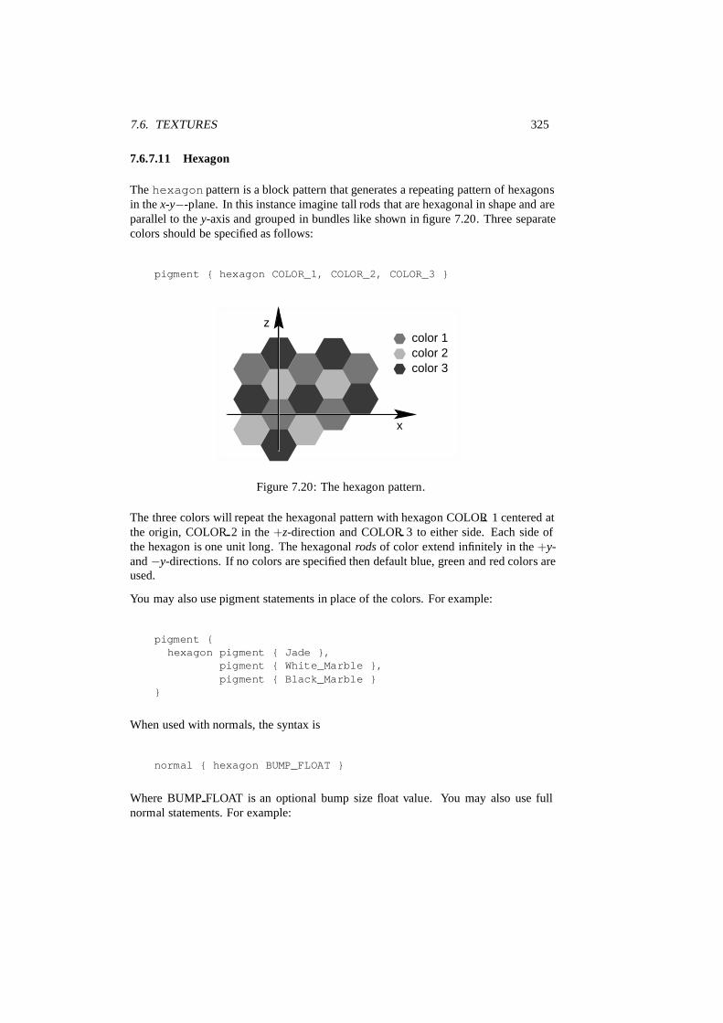
7.6. TEXTURES 325
7.6.7.11 Hexagon
The hexagon pattern is a block pattern that generates a repeating pattern of hexagonsin the x-y−-plane. In this instance imagine tall rods that are hexagonal in shape and areparallel to the y-axis and grouped in bundles like shown in figure 7.20. Three separatecolors should be specified as follows:
pigment { hexagon COLOR_1, COLOR_2, COLOR_3 }
color 1color 2color 3
x
z
Figure 7.20: The hexagon pattern.
The three colors will repeat the hexagonal pattern with hexagon COLOR 1 centered atthe origin, COLOR 2 in the +z-direction and COLOR 3 to either side. Each side ofthe hexagon is one unit long. The hexagonal rods of color extend infinitely in the +y-and −y-directions. If no colors are specified then default blue, green and red colors areused.
You may also use pigment statements in place of the colors. For example:
pigment {hexagon pigment { Jade },
pigment { White_Marble },pigment { Black_Marble }
}
When used with normals, the syntax is
normal { hexagon BUMP_FLOAT }
Where BUMP FLOAT is an optional bump size float value. You may also use fullnormal statements. For example:

326 CHAPTER 7. SCENE DESCRIPTION LANGUAGE
normal {hexagon
normal { gradient x scale .2 },normal { gradient y scale .2 },normal { bumps scale .2 }
}
When used with textures, the syntax is . . .
texture {hexagon
texture { T_Gold_3A },texture { T_Wood_3A },texture { Stone12 }
}
This is a block pattern which cannot use wave types, color map, or slope map modifiers.
7.6.7.12 Leopard
Leopard creates regular geometric pattern of circular spots.
The pattern uses the ramp wavewave type by default but may use any wave type. Thepattern may be used with color map, pigment map, normal map, slope mapand texture map.
7.6.7.13 Mandel
The mandel pattern computes the standard Mandelbrot fractal pattern and projects itonto the x-y-plane. It uses the x and y coordinates to compute the Mandelbrot set. Thepattern is specified with the keyword mandel followed by an integer number. Thisnumber is the maximum number of iterations to be used to compute the set. Typicalvalues range from 10 up to 256 but any positive integer may be used. For example:
pigment {mandel 25color_map {
[0.0 color Cyan][0.3 color Yellow][0.6 color Magenta][1.0 color Cyan]
}scale .5
}
7.6. TEXTURES 327
The value passed to the color map is computed by the formula:
value =number o f iterations
max iterations(7.43)
When used as a normal pattern, the syntax is . . .
normal {mandel ITER, BUMP_AMOUNT
}
where the required integer ITER value is optionally followed by a float bump size.
The pattern extends infinitely in the z-direction similar to a planar image map. Thepattern uses the ramp wave wave type by default but may use any wave type. Thepattern may be used with color map, pigment map, normal map, slope mapand texture map.
7.6.7.14 Marble
The marble pattern is very similar to the gradient x pattern. The gradient patternuses a default ramp wave wave type which means it uses colors from the color mapfrom 0.0 up to 1.0 at location x = 1 but then jumps back to the first color for x >1 and repeats the pattern again and again. However the marble pattern uses thetriangle wave wave type in which it uses the color map from 0 to 1 but then itreverses the map and blends from 1 back to zero. For example:
pigment {gradient xcolor_map {
[0.0 color Yellow][1.0 color Cyan]
}}
This blends from yellow to cyan and then it abruptly changes back to yellow and re-peats. However replacing gradient x with marble smoothly blends from yellowto cyan as the x coordinate goes from 0.0 to 0.5 and then smoothly blends back fromcyan to yellow by x = 1.0.
Earlier versions of POV-Ray did not allow you to change wave types. Now thatwave types can be changed for most any pattern, the distinction between marbleand gradient x is only a matter of default wave types.
When used with turbulence and an appropriate color map, this pattern looks like veinsof color of real marble, jade or other types of stone. By default, marble has no turbu-lence.
The pattern may be used with color map, pigment map, normal map,slope map and texture map.
328 CHAPTER 7. SCENE DESCRIPTION LANGUAGE
7.6.7.15 Onion
Onion is a pattern of concentric spheres like the layers of an onion. Each layer is oneunit thick.
The pattern uses the ramp wavewave type by default but may use any wave type. Thepattern may be used with color map, pigment map, normal map, slope mapand texture map.
7.6.7.16 Quilted
The quilted pattern was originally designed only to be used as a normal pattern.The quilted pattern is so named because it can create a pattern somewhat like a quilt ora tiled surface. The squares are actually 3-D cubes that are 1 unit in size.
When used as a normal pattern it uses a specialized normal perturbation function. Thismeans that the quilted pattern cannot be used with normal map, slope map or wave typemodifiers in a normal statement.
When used as a pigment pattern or texture pattern, the quilted pattern is similar to nor-mal quilted but is not identical as are most normals when compared to pigments. Whenused in pigment or texture statements the quilted pattern uses the ramp wave wavetype by default but may use any wave type. The pattern may be used with color map,pigment map and texture map.
The two parameters control0 and control1 are used to adjust the curvature ofthe seam or gouge area between the quilts. The syntax is:
normal {quilted AMOUNTcontrol0 C0control1 C1
}
The values should generally be kept to around the 0.0 to 1.0 range. The default valueis 1.0 if none is specified. Think of this gouge between the tiles in cross-section as asloped line.
This straight slope can be made to curve by adjusting the two control values. Thecontrol values adjust the slope at the top and bottom of the curve. A control valuesof 0 at both ends will give a linear slope, as shown in figure 7.21 on the facing page,yielding a hard edge. A control value of 1 at both ends will give an ”s” shaped curve,resulting in a softer, more rounded edge.
7.6.7.17 Radial
The radial pattern is a radial blend that wraps around the +y-axis. The color forvalue 0.0 starts at the +x-direction and wraps the color map around from east to west
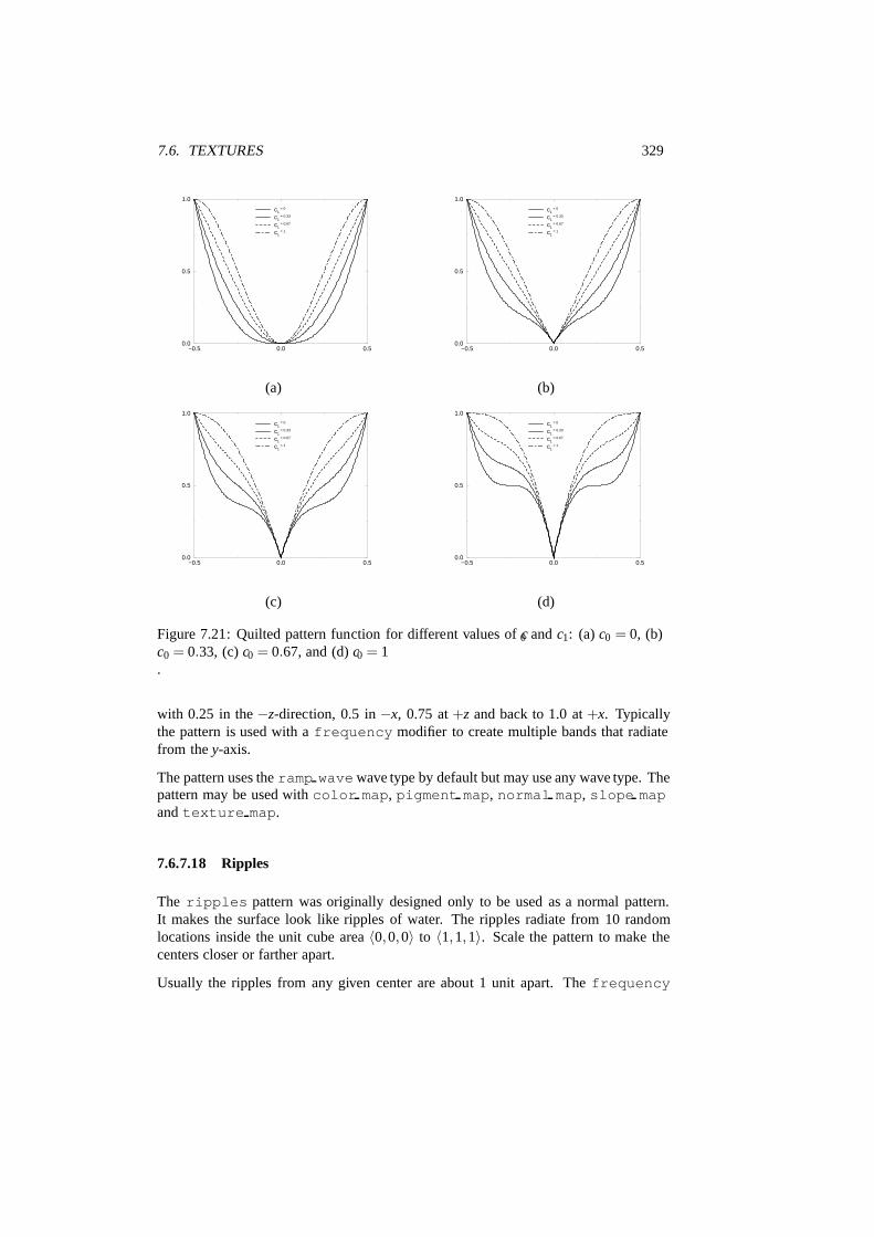
7.6. TEXTURES 329
−0.5 0.0 0.50.0
0.5
1.0
c1 = 0
c1 = 0.33
c1 = 0.67
c1 = 1
(a)
−0.5 0.0 0.50.0
0.5
1.0
c1 = 0
c1 = 0.33
c1 = 0.67
c1 = 1
(b)
−0.5 0.0 0.50.0
0.5
1.0
c1 = 0
c1 = 0.33
c1 = 0.67
c1 = 1
(c)
−0.5 0.0 0.50.0
0.5
1.0
c1 = 0
c1 = 0.33
c1 = 0.67
c1 = 1
(d)
Figure 7.21: Quilted pattern function for different values of c0 and c1: (a) c0 = 0, (b)c0 = 0.33, (c) c0 = 0.67, and (d) c0 = 1.
with 0.25 in the −z-direction, 0.5 in −x, 0.75 at +z and back to 1.0 at +x. Typicallythe pattern is used with a frequency modifier to create multiple bands that radiatefrom the y-axis.
The pattern uses the ramp wavewave type by default but may use any wave type. Thepattern may be used with color map, pigment map, normal map, slope mapand texture map.
7.6.7.18 Ripples
The ripples pattern was originally designed only to be used as a normal pattern.It makes the surface look like ripples of water. The ripples radiate from 10 randomlocations inside the unit cube area 〈0,0,0〉 to 〈1,1,1〉. Scale the pattern to make thecenters closer or farther apart.
Usually the ripples from any given center are about 1 unit apart. The frequency

330 CHAPTER 7. SCENE DESCRIPTION LANGUAGE
keyword changes the spacing between ripples. The phase keyword can be used tomove the ripples outwards for realistic animation.
The number of ripple centers can be changed with the global parameterglobal settings { number of waves FLOAT } somewhere in the scene.This affects the entire scene. You cannot change the number of wave centers on in-dividual patterns. See 7.8.8 on page 362 for details.
When used as a normal pattern, ripples uses a specialized normal perturbation function.This means that the ripples pattern cannot be used with normal map, slope map or wavetype modifiers in a normal statement.
When used in pigment or texture statements the ripples pattern uses theramp wave wave type by default but may use any wave type. The pattern may beused with color map, pigment map and texture map.
7.6.7.19 Spiral1
The spiral1 pattern creates a spiral that winds around the y-axis similar to a screw.Its syntax is:
pigment {spiral1 NUMBER_OF_ARMS
}
The NUMBER OF ARMS value determins how may arms are winding around they-axis.
The pattern uses the triangle wave wave type by default but may use any wavetype. The pattern may be used with color map, pigment map, normal map,slope map and texture map.
7.6.7.20 Spiral2
The spiral2 pattern is a modification of the spiral1 pattern with an extraordinarylook.
The pattern uses the triangle wave wave type by default but may use any wavetype. The pattern may be used with color map, pigment map, normal map,slope map and texture map.
7.6.7.21 Spotted
The spotted pattern is identical to the bozo pattern. Early versions of POV-Ray didnot allow turbulence to be used with spotted. Now that any pattern can use turbulencethere is no difference between bozo and spotted. See 7.6.7.3 on page 320 for details.

7.6. TEXTURES 331
7.6.7.22 Waves
The waves pattern was originally designed only to be used as a normal pattern. Thewaves pattern looks similar to the ripples pattern except the features are rounder andbroader. The effect is to make waves that look more like deep ocean waves. The wavesradiate from ten random locations inside the unit cube area 〈0,0,0〉 to 〈1,1,1〉. Scalethe pattern to make the centers closer or farther apart.
Usually the waves from any given center are about 1 unit apart. The frequencykeyword changes the spacing between waves. The phase keyword can be used tomove the waves outwards for realistic animation.
The number of ripple centers can be changed with the global parameterglobal settings { number of waves FLOAT } somewhere in the scene.This affects the entire scene. You cannot change the number of wave centers on in-dividual patterns. See 7.8.8 on page 362 for details.
When used as a normal pattern, waves uses a specialized normal perturbation function.This means that the waves pattern cannot be used with normal map, slope map or wavetype modifiers in a normal statement.
When used in pigment or texture statements the waves pattern uses the ramp wavewave type by default but may use any wave type. The pattern may be used withcolor map, pigment map and texture map.
7.6.7.23 Wood
The wood pattern consists of concentric cylinders centered on the z-axis. When ap-propriately colored, the bands look like the growth rings and veins in real wood. Smallamounts of turbulence should be added to make it look more realistic. By default, woodhas no turbulence.
Unlike most patterns, the wood pattern uses the triangle wave wave type by de-fault. This means that like marble, wood uses color map values 0.0 to 1.0 then repeatsthe colors in reverse order from 1.0 to 0.0. However you may use any wave type. Thepattern may be used with color map, pigment map, normal map, slope mapand texture map.
7.6.7.24 Wrinkles
The wrinkles pattern was originally designed only to be used as a normal pattern. Ituses a 1/ f noise pattern similar to granite but the features in wrinkles are sharper. Thepattern can be used to simulate wrinkled cellophane or foil. It also makes an excellentstucco texture.
When used as a normal pattern it uses a specialized normal perturbation function. Thismeans that the wrinkles pattern cannot be used with normal map, slope map or wavetype modifiers in a normal statement.

332 CHAPTER 7. SCENE DESCRIPTION LANGUAGE
When used as a pigment pattern or texture pattern, the wrinkles pattern is similarto normal wrinkles but is not identical as are most normals when compared to pig-ments. When used in pigment or texture statements the wrinkles pattern uses theramp wave wave type by default but may use any wave type. The pattern may beused with color map, pigment map and texture map.
7.6.8 Pattern Modifiers
Pattern modifiers are statements or parameters which modify how a pattern is evaluatedor tells what to do with the pattern. The modifiers color map and pigment mapapply only to pigments. See section 7.6.1 on page 278. The modifiers bump size,slope map and normal map apply only to normals. See section 7.6.2 on page 286.The texture map modifier can only be used with textures. See section 7.6.5.1 onpage 313.
The pattern modifiers in the following section can be used with pigment, normal ortexture patterns.
7.6.8.1 Transforming Patterns
The most common pattern modifiers are the transformation modifiers translate,rotate, scale and matrix. For details on these commands see 7.3.1 on page 214.
These modifiers may be placed inside pigment, normal and texture statements tochange the position, size and orientation of the patterns.
In general the order of transformations relative to other pattern modifiers such asturbulence, color map and other maps is not important. For example scalingbefore or after turbulence makes no difference. The turbulence is done first, then thescaling regardless of which is specified first. However the order in which transforma-tions are performed relative to warp statements is important. See 7.6.8.8 on page 336for details.
7.6.8.2 Frequency and Phase
The frequency and phase modifiers act as a type of scale and translate modifiersfor color map, pigment map, normal map, slope map and texture map.This discussion uses a color map as an example but the same principles apply to pig-ment maps, normal maps, slope maps and texture maps.
The frequency keyword adjusts the number of times that a color map repeats overone cycle of a pattern. For example gradient covers color map values 0 to 1 overthe range from x = 0 to x = 1. By adding frequency 2.0 the color map repeatstwice over that same range. The same effect can be achieved using scale 0.5*x sothe frequency keyword isn’t that useful for patterns like gradient.
7.6. TEXTURES 333
However the radial pattern wraps the color map around the +y-axis once. If you wantedtwo copies of the map (or 3 or 10 or 100) you’d have to build a bigger map. Addingfrequency 2.0 causes the color map to be used twice per revolution. Try this:
pigment {radialcolor_map{[0.5 color Red][0.5 color White]}frequency 6
}
The result is six sets of red and white radial stripes evenly spaced around the object.
The float after frequency can be any value. Values greater than 1.0 causes morethan one copy of the map to be used. Values from 0.0 to 1.0 cause a fraction of the mapto be used. Negative values reverses the map.
The phase value causes the map entries to be shifted so that the map starts and endsat a different place. In the example above if you render successive frames at phase0 then phase 0.1, phase 0.2 etc you could create an animation that rotates the stripes.The same effect can be easily achieved by rotating the radial pigment using rotatey*Angle but there are other uses where phase can be handy.
Sometimes you create a great looking gradient or wood color map but you want thegrain slightly adjusted in or out. You could re-order the color map entries but that’s apain. A phase adjustment will shift everything but keep the same scale. Try animatinga mandel pigment for a color palette rotation effect.
Frequency and phase have no effect on block patterns checker, brick and hexagon nordo they effect image maps, bump maps or material maps. They also have no effectin normal statements when used with bumps, dents, quilted or wrinkles because thesenormal patterns cannot use normal map or slope map.
They can be used with normal patterns ripples and waves even though these two pat-terns cannot use normal map or slope map either. When used with ripples orwaves, frequency adjusts the space between features and phase can be adjusted from0.0 to 1.0 to cause the ripple or waves to move relative to their center for animating thefeatures.
These values work by applying the following formula
new value = (old value∗ f requency+ phase) mod 1.0. (7.44)
7.6.8.3 Waveform
Most patterns that take color map, pigment map, slope map, normal map ortexture map use the entries in the map in order from 0.0 to 1.0. The wood andmarble patterns use the map from 0.0 to 1.0 and then reverses it and runs it from 1.0 to
334 CHAPTER 7. SCENE DESCRIPTION LANGUAGE
0.0. The difference can easily be seen when these patterns are used as normal patternswith no maps.
Patterns such as gradient or onion generate a grove or slot that looks like a ramp thatdrops off sharply. This is called a ramp wave wave type. However wood and marbleslope upwards to a peak, then slope down again in a triangle wave. In previousversions of POV-Ray there was no way to change the wave types. You could simulate atriangle wave on a ramp wave pattern by duplicating the map entries in reverse, howeverthere was no way to use a ramp wave on wood or marble.
Now any pattern that takes a map can have the default wave type overridden. Forexample:
pigment { wood color_map { MyMap } ramp_wave }
Also available are sine wave and scallop wave types. These types are of mostuse in normal patterns as a type of built-in slope map. The sine wave takes the zig-zag of a ramp wave and turns it into a gentle rolling wave with smooth transitions. Thescallop wave uses the absolute value of the sine wave which looks like corduroywhen scaled small or like a stack of cylinders when scaled larger.
Although any of these wave types can be used for pigments, normals or textures, thesine wave and scallop wave types are not as noticeable on pigments or texturesas they are for normals.
Wave types have no effect on block patterns checker, brick and hexagon nor do theyeffect image maps, bump maps or material maps. They also have no effect in normalstatements when used with bumps, dents, quilted or wrinkles because these normalpatterns cannot use normal map or slope map.
7.6.8.4 Turbulence
he keyword turbulence followed by a float or vector may be used to stir up anypigment, normal, texture, irid or halo. A number of optional parameters may be usedwith turbulence to control how it is computed. For example:
pigment {wood color_map { MyMap }turbulence TURB_VECTORoctaves FLOATomega FLOATlambda FLOAT
}
Typical turbulence values range from the default 0.0, which is no turbulence, to 1.0 ormore, which is very turbulent. If a vector is specified different amounts of turbulenceare applied in the x-, y- and z-direction. For example

7.6. TEXTURES 335
turbulence <1.0, 0.6, 0.1>
has much turbulence in the x-direction, a moderate amount in the y-direction and asmall amount in the z-direction.
Turbulence uses a random noise function called DNoise. This is similar to the noiseused in the bozo pattern except that instead of giving a single value it gives a direction.You can think of it as the direction that the wind is blowing at that spot. Points closetogether generate almost the same value but points far apart are randomly different.
In general the order of turbulence parameters relative to other pattern modifiers suchas transformations, color maps and other maps is not important. For example scalingbefore or after turbulence makes no difference. The turbulence is done first, then thescaling regardless of which is specified first. See 7.6.8.8 on the next page for a way towork around this behavior.
Turbulence uses DNoise to push a point around in several steps called octaves. Welocate the point we want to evaluate, then push it around a bit using turbulence to getto a different point then look up the color or pattern of the new point.
It says in effect Don’ t give me the color at this spot . . . take a few random steps indifferent directions and give me that color. Each step is typically half as long as theone before.
The magnitude of these steps is controlled by the turbulence value. There are threeadditional parameters which control how turbulence is computed. They are octaves,lambda and omega. Each is optional. Each is followed by a single float value. Eachhas no effect when there is no turbulence.
7.6.8.5 Octaves
he octaves value controls the number of steps of turbulence that are computed. Legalvalues range from 1 to 10. The default value of 6 is a fairly high value; you won’tsee much change by setting it to a higher value because the extra steps are too small.Float values are truncated to integer. Smaller numbers of octaves give a gentler, wavyturbulence and computes faster. Higher octaves create more jagged or fuzzy turbulenceand takes longer to compute.
7.6.8.6 Lambda
he lambda parameter controls how statistically different the random move of an oc-tave is compared to its previous octave. The default value is 2.0 which is quite random.Values close to lambda 1.0 will straighten out the randomness of the path in the di-agram above. The zig-zag steps in the calculation are in nearly the same direction.Higher values can look more swirly under some circumstances.

336 CHAPTER 7. SCENE DESCRIPTION LANGUAGE
7.6.8.7 Omega
he omega value controls how large each successive octave step is compared to theprevious value. Each successive octave of turbulence is multiplied by the omega value.The default omega 0.5 means that each octave is 1/2 the size of the previous one.Higher omega values mean that 2nd, 3rd, 4th and up octaves contribute more turbulencegiving a sharper, crinkly look while smaller omegas give a fuzzy kind of turbulence thatgets blurry in places.
7.6.8.8 Warps
The warp statement is a pattern modifier that is similar to turbulence. Turbulenceworks by taking the pattern evaluation point and pushing it about in a series of randomsteps. However warps push the point in very well-defined, non-random, geometricways. The warp statement also overcomes some limitations of traditional turbulenceand transformations by giving the user more control over the order in which turbulence,transformation and warp modifiers are applied to the pattern.
Currently there are three types of warps but the syntax was designed to allow futureexpansion. The first two, the repeat warp and the black hole warp are new fea-tures for POV-Ray that modify the pattern in geometric ways. The other warp providesan alternative way to specify turbulence.
The syntax for using a warp statement in a pigment is
pigment {PATTERN_TYPEPIGMENT_MODIFIERS...warp { WARP_ITEMS..}.OTHER_PIGMENT_MODIFIERS...
}
Similarly warps may be used in normals and textures. You may have as many sepa-rate warp statements as you like in each pattern. The placement of warp statementsrelative to other modifiers such as color map or turbulence is not important.However placement of warp statements relative to each other and to transformationsis significant. Multiple warps and transformations are evaluated in the order in whichyou specify them. For example if you translate, then warp or warp, then translate, theresults can be different.
7.6.8.8.1 Black Hole Warp
A black hole is so named because of its similarity to real black holes. Just like thereal thing, you cannot actually see a black hole. The only way to detect its presence isby the effect it has on things that surround it. Unlike the real thing, however, it won’t
7.6. TEXTURES 337
swallow you up and compress your entire body to a volume of, say, 2.010−10 micronsin diameter if you get too close (We’re working on that part).
Take, for example, a woodgrain. Using POV-Ray’s normal turbulence and other texturemodifier functions, you can get a nice, random appearance to the grain. But in itsrandomness it is regular — it is regularly random! Adding a black hole allows youto create a localised disturbance in a woodgrain in either one or multiple locations.The black hole can have the effect of either sucking the surrounding texture into itself(like the real thing) or pushing it away. In the latter case, applied to a woodgrain, itwould look to the viewer as if there were a knothole in the wood. In this text we usea woodgrain regularly as an example, because it is ideally suitable to explaining blackholes. However, black holes may in fact be used with any texture.
The effect that the black hole has on the texture can be specified. By default, it suckswith the strength calculated expotentially (inverse-square). You can change this if youlike.
Black holes may be used anywhere a Warp is permitted. The syntax is:
warp{
black_hole <CENTER>, RADIUS[falloff VALUE][strength VALUE][repeat <VECTOR>][turbulence <VECTOR>][inverse]
}
Some examples are given by
warp{
black_hole <0, 0, 0>, 0.5}
warp{
black_hole <0.15, 0.125, 0>, 0.5falloff 7strength 1.0repeat <1.25, 1.25, 0>turbulence <0.25, 0.25, 0>inverse
}
warp{

338 CHAPTER 7. SCENE DESCRIPTION LANGUAGE
black_hole <0, 0, 0>, 1.0falloff 2strength 2inverse
}
In order to fully understand how a black hole works, it is important to know the theorybehind it. A black hole (or any warp) works by taking a point and perturbing it toanother location. The amount of perturbation depends on the strength of the black holeat the original point passed in to it. The amount of perturbation directly relates to theamount of visual movement that you can see occur in a texture. The stronger the blackhole at the input co-ordinate the more that original co-ordinate is moved to anotherlocation (either closer to or further away from the center of the black hole.)
Movement always occurs on the vector that exists between the input point and thecenter of the black hole.
Black holes are considered to be spheres. For a point to be affected by a black hole, itmust be within the sphere’s volume.
Suppose you have a black hole at 〈1,1,1〉 and a point at 〈1,2,1〉. If this point is per-turbed by a total amount of +1 units its new location is 〈1,3,1〉, which is on a directline extrapolated from the vector between 〈1,1,1〉 and 〈1,2,1〉. In this case the pointis pushed away from the black hole, which is not normal behaviour but is good fordemonstration purposes.
The internal properties of a black hole are as follows.
Center The center of the black hole.Radius Its radius.Falloff The power by which the effect falls off (default 2).Strength The magnitude of the transformation effect (see below).
Inverted If set push points away instead of pulling them in.Repeat If set we have many black holes instead of one.Turbulence If set each new repeated black hole’s position is uncer-
tain.
Repeat Vector The 〈x,y, z〉 factor to repeat by.Turbulence Vector The maximum 〈x,y, z〉 factor for turbulence random-
ness.
Each of these are discussed below.
Center: A vector defining the center of the sphere that represents the black hole. If theblack hole has Repeat set it is the offset within each block.
Radius: A number giving the length, in units, of the radius of the sphere that representsthe black hole.
7.6. TEXTURES 339
If a point is not within radius units of 〈center〉 it cannot be affected by the black holeand will not be perturbed.
Falloff: The power by which the effect of the black hole falls off. The default is two.The force of the black hole at any given point, before applying the Strength modifier,is as follows.
First, convert the distance from the point to the center to a proportion (0 to 1) that thepoint is from the edge of the black hole. A point on the perimeter of the black holewill be 0.0; a point at the centre will be 1.0; a point exactly halfway will be 0.5, and soforth.
Mentally you can consider this to be a closeness factor. A closeness of 1.0 is as closeas you can get to the center (i. e. at the center), a closeness of 0.0 is as far away as youcan get from the center and still be inside the black hole and a closeness of 0.5 meansthe point is exactly halfway between the two.
Call this value c. Raise c to the power specified in Falloff . By default Falloff is 2, sothis is c2 or c squared. The resulting value is the force of the black hole at that exactlocation and is used, after applying the Strength scaling factor as described below, todetermine how much the point is perturbed in space.
For example, if c is 0.5 the force is 0.52 or 0.25. If c is 0.25 the force is 0.125. But if cis exactly 1.0 the force is 1.0.
Recall that as c gets smaller the point is farther from the center of the black hole. Usingthe default power of 2, you can see that as c reduces, the force reduces expotentiallyin an inverse-square relationship. Put in plain english, it means that the force is muchstronger (by a power of two) towards the center than it is at the outside.
By increasing Falloff , you can increase the magnitude of the falloff. A large value willmean points towards the perimeter will hardly be affected at all and points towards thecenter will be affected strongly.
A value of 1.0 for Falloff will mean that the effect is linear. A point that is exactlyhalfway to the center of the black hole will be affected by a force of exactly 0.5.
A value of Falloff of less than one but greater than zero means that as you get closerto the outside, the force increases rather than decreases. This can have some uses butthere is a side effect. Recall that the effect of a black hole ceases outside its perimiter.This means that points just within the permiter will be affected strongly and those justoutside not at all. This would lead to a visible border, shaped as a sphere.
A value for Falloff of 0 would mean that the force would be 1.0 for all points withinthe black hole, since any number larger 0 raised to the power of 0 is 1.0.
The magnitude of the movement of the point is determined basically by the value offorce after scaling. We’ll consider scaling later. Lets take an example.
Suppose we have a black hole of radius 2.0 and a point that is exactly 1.0 units fromthe center. That means it is exactly half-way to the center and that c would be 0.5. Ifwe use the default falloff of 2 the force at that point is 0.52 or 0.25. What this means

340 CHAPTER 7. SCENE DESCRIPTION LANGUAGE
is that we must move the point by 0.25 of its distance from the center. In this case it is1.0 units from the center, so we move it by 1.0 ∗0.25 or 0.25 units. This gives a finaldistance of 1.0− (1.0 ∗0.25) or 0.75 units from the center, on a direct line in 3D spacebetween the original position and the center.
If the point were part of, say, a wood grain, the wood grain would appear to bendtowards the (invisible) center of the black hole. If the Inverse flag were set, however, itwould be pushed away, meaning its final position would be 1.0+(1.0 ∗0.25) or 1.25units from the center.
Strength: The Strength gives you a bit more control over how much a point is perturbedby the black hole. Basically, the force of the black hole (as determined above) ismultipled by the value of Strength, which defaults to 1.0. If you set Strength to 0.5, forexample, all points within the black hole will be moved by only half as much as theywould have been. If you set it to 2.0 they will be moved twice as much.
There is a rider to the latter example, though — the movement is clipped to a maximumof the original distance from the center. That is to say, a point that is 0.75 units fromthe center may only be moved by a maximum of 0.75 units either towards the center oraway from it, regardless of the value of Strength. The result of this clipping is that youwill have an exclusion area near the centre of the black hole where all points whosefinal force value exceeded or equalled 1.0 were moved by a fixed amount.
Inverted: If Inverted is set points are pushed away from the center instead of beingpulled in.
Repeat: Repeat allows you to simulate the effect of many black holes without havingto explicitly declare them. Repeat is a vector that tells POV-Ray to use this black holeat multiple locations.
If you’re not interested in the theory behind all this, just skip the following text and usethe values given in the summary below.
Using Repeat logically divides your scene up into cubes, the first being located at〈0,0,0〉 and going to 〈repeat〉. Suppose your repeat vector was 〈1,5,2〉. The firstcube would be from 〈0,0,0〉 to 〈1,5,2〉. This cube repeats, so there would be one at〈−1,−5,−2〉, 〈1,5,2〉, 〈2,10,4〉 and so forth in all directions, ad infinitum.
When you use Repeat, the center of the black hole does not specify an absolute locationin your scene but an offset into each block. It is only possible to use positive offsets.Negative values will produce undefined results.
Suppose your center was 〈0.5,1,0.25〉 and the repeat vector is 〈2,2,2〉. This gives usa block at 〈0,0,0〉 and 〈2,2,2〉, etc. The centers of the black hole’s for these blockswould be 〈0,0,0〉+〈0.5,1.0,0.25〉, i. e. 〈0.5,1.0,0.25〉, and 〈2,2,2〉+〈0.5,1.0,0.25〉,i. e. 〈2,5,3.0,2.25〉.
Due to the way repeats are calculated internally, there is a restriction on the values youspecify for the repeat vector. Basically, each black hole must be totally enclosed withineach block (or cube), with no part crossing into a neighbouring one. This means that,for each of the x, y and z dimensions, the offset of the center may not be less than the
7.6. TEXTURES 341
radius, and the repeat value for that dimension must be ≥ the center plus the radiussince any other values would allow the black hole to cross a boundary. Put anotherway, for each of x, y and z
radius ≤ offset or center <= repeat− radius. (7.45)
If the repeat vector in any dimension is too small to fit this criteria, it will be increasedand a warning message issued. If the center is less than the radius it will also be movedbut no message will be issued.
Note that none of the above should be read to mean that you can’t overlap black holes.You most certainly can and in fact this can produce some most useful effects. Therestriction only applies to elements of the same black hole which is repeating. You candeclare a second black hole that also repeats and its elements can quite happily overlapthe first and causing the appropriate interactions.
It is legal for the repeat value for any dimension to be 0, meaning that POV-Ray willnot repeat the black hole in that direction.
Turbulence: Turbulence can only be used with Repeat. It allows an element of ran-domness to be inserted into the way the black holes repeat, to cause a more naturallook. A good example would be an array of knotholes in wood — it would look ratherartificial if each knothole were an exact distance from the previous.
The turbulence vector is a measurement that is added to each individual back hole in anarray, after each axis of the vector is multipled by a different random amount rangingfrom 0 to 1.
For example, suppose you have a repeating element of a black hole that is supposed tobe at 〈2,2,2〉. You have specified a turbulence vector of 〈4,5,3〉, meaning you wantthe position to be able to vary by no more than 1.0 units in the X direction, 3.0 units inthe Y direction and 2.0 in Z. This means that the valid ranges of the new position areas follows
x can be from 2 to 6.y can be from 2 to 7.z can be from 2 to 5.
The resulting actual position of the black hole’s center for that particular repeat elementis random (but consistent, so renders will be repeatable) and somewhere within theabove co-ordinates.
There is a rider on the use of turbulence, which basically is the same as that of therepeat vector. Yyou can’t specify a value which would cause a black hole to potentiallycross outside of its particular block.
Since POV-Ray doesn’t know in advance how much a position will be changed dueto the random nature of the changes, it enforces a rule that is similar to the one for

342 CHAPTER 7. SCENE DESCRIPTION LANGUAGE
Repeat, except it adds the maximum possible variation for each axis to the center. Forexample, suppose you had a black hole with a center of 〈1.0,1.0,1.0〉, radius of 0.5 anda turbulence of 〈0.5,0.25,0〉— normally, the mimimum repeat would be 〈1.5,1.5,1.5〉.However, now we take into account the turbulence, meaning the minimum repeat vectoris actually 〈2.0,1.75,1.5〉.
Repeat summarized: For each of x, y and z the offset of the center must be ≥ radius andthe value of the repeat must be ≥ center + radius + turbulence. The exception beingthat repeat may be 0 for any dimension, which means do not repeat in that direction.
7.6.8.8.2 Repeat Warp
The repeatwarp causes a section of the pattern to be repeated over and over. It takesa slice out of the pattern and makes multiple copies of it side-by-side. The warp hasmany uses but was originally designed to make it easy to model wood veneer textures.Veneer is made by taking very thin slices from a log and placing them side-by-side onsome other backing material. You see side-by-side nearly identical ring patterns buteach will be a slice perhaps 1/32th of an inch deeper.
The syntax for a repeat warp is
warp { repeat VECTOR offset VECTOR flip VECTOR }
The repeat vector specifies the direction in which the pattern repeats and the width ofthe repeated area. This vector must lie entirely along an axis. In other words, two of itsthree components must be 0. For example
pigment {woodwarp { repeat 2*x }
}
which means that from x= 0 to x= 2 you get whatever the pattern usually is. But fromx = 2 to x = 4 you get the same thing exactly shifted two units over in the x-direction.To evaluate it you simply take the x-coordinate modulo 2. Unfortunately you get exactduplicates which isn’t very realistic. The optional offset vector tells how much totranslate the pattern each time it repeats. For example
pigment {woodwarp { repeat 2*x offset 0.05*z }
}
means that we slice the first copy from x= 0 to x= 2 at z = 0 but at x = 2 to x = 4 weoffset to z= 0.05. In the 4 to 6 interval we slice at z= 0.10. At the n-th copy we slice

7.6. TEXTURES 343
at 0.05nz. Thus each copy is slightly different. There are no restrictions on the offsetvector.
Finally the flip vector causes the pattern to be flipped or mirrored every other copyof the pattern. The first copy of the pattern in the positive direction from the axis is notflipped. The next farther is, the next is not, etc. The flip vector is a three component x,y, z vector but each component is treated as a boolean value that tells if you should orshould not flip along a given axis. For example
pigment {woodwarp { repeat 2*x flip <1,1,0> }
}
means that every other copy of the pattern will be mirrored about the x- and y- axis butnot the z-axis. A non-zero value means flip and zero means do not flip about that axis.The magnitude of the values in the flip vector doesn’t matter.
7.6.8.8.3 Turbulence Warp
The POV-Ray language contains an ambiguity and limitation on the way you specifyturbulence and transformations such as translate, rotate, scale and matrix transforms.Usually the turbulence is done first. Then all translate, rotate, scale and matrix oper-ations are always done after turbulence regardless of the order in which you specifythem. For example this
pigment {woodscale .5turbulence .2
}
works exactly the same as
pigment {woodturbulence .2scale .5
}
The turbulence is always first. A better example of this limitation is with uneven tur-bulence and rotations.

344 CHAPTER 7. SCENE DESCRIPTION LANGUAGE
pigment {woodturbulence 0.5*yrotate z*60
}
// as compared to
pigment {woodrotate z*60turbulence 0.5*y
}
The results will be the same either way even though you’d think it should look different.
We cannot change this basic behavior in POV-Ray now because lots of scenes wouldpotentially render differently if suddenly the order transformation vs turbulence sud-denly mattered when in the past, it didn’t.
However, by specifying our turbulence inside warp statement you tell POV-Ray that theorder in which turbulence, transformations and other warps are applied is significant.Here’s an example of a turbulence warp.
warp { turbulence <0,1,1> octaves 3 lambda 1.5 omega 0.3 }
The significance is that this
pigment {woodtranslate <1,2,3> rotate x*45 scale 2warp { turbulence <0,1,1> octaves 3 lambda 1.5 omega 0.3 }
}
produces different results than this . . .
pigment {woodwarp { turbulence <0,1,1> octaves 3 lambda 1.5 omega 0.3 }translate <1,2,3> rotate x*45 scale 2
}
You may specify turbulence without using a warp statement. However you cannotcontrol the order in which they are evaluated unless you put them in a warp.
The evaluation rules are as follows:

7.6. TEXTURES 345
• First any turbulence not inside a warp statement is applied regardless ofthe order in which it appears relative to warps or transformations.
• Next each warp statement, translate, rotate, scale or matrix one-by-one,is applied in the order the user specifies. If you want turbulence done ina specific order, you simply specify it inside a warp in the proper place.
7.6.8.9 Bitmap Modifiers
A bitmap modifier is a modifier used inside an 7.6.1.5 on page 283, 7.6.2.3 on page 292or 7.6.5.3 on page 315 to specify how the 2-D bitmap is to be applied to the 3-D surface.Several bitmap modifiers apply to specific kinds of maps and they are covered in theappropriate sections. The bitmap modifiers discussed in the following sections areapplicable to all three types of bitmaps.
7.6.8.9.1 The once Option
Normally there are an infinite number of repeating image maps, bump maps or materialmaps created over every unit square of the x-y-plane like tiles. By adding the oncekeyword after a file name you can eliminate all other copies of the map except the oneat (0,0) to (1,1). In image maps, areas outside this unit square are treated as fullytransparent. In bump maps, areas outside this unit square are left flat with no normalmodification. In material maps, areas outside this unit square are textured with the firsttexture of the texture list.
For example:
image_map {gif "mypic.gif"once
}
7.6.8.9.2 The ” map type” Option
The default projection of the bump onto the x-y-plane is called a planar map type.This option may be changed by adding the map type keyword followed by a numberspecifying the way to wrap the bump around the object.
A map type 0 gives the default planar mapping already described.
A map type 1 gives a spherical mapping. It assumes that the object is a sphere of anysize sitting at the origin. The y-axis is the north/south pole of the spherical mapping.The top and bottom edges of the bitmap just touch the pole regardless of any scaling.The left edge of the bitmap begins at the positive x-axis and wraps the pattern around

346 CHAPTER 7. SCENE DESCRIPTION LANGUAGE
the sphere from west to east in a −y-rotation. The pattern covers the sphere exactlyonce. The once keyword has no meaning for this type.
With map type 2 you get a cylindrical mapping. It assumes that a cylinder of anydiameter lies along the y-axis. The bump pattern wraps around the cylinder just like thespherical map but remains one unit tall from y = 0 to y = 1. This band of the pattern isrepeated at all heights unless the once keyword is applied.
Finally map type 5 is a torus or donut shaped mapping. It assumes that a torus ofmajor radius 1 sits at the origin in the x-z-plane. The pattern is wrapped around similarto spherical or cylindrical maps. However the top and bottom edges of the map wrapover and under the torus where they meet each other on the inner rim.
Types 3 and 4 are still under development.
For example:
sphere{<0,0,0>,1pigment{
image_map {gif "world.gif"map_type 1
}}
}
7.6.8.9.3 The interpolate Option
Adding the interpolate keyword can smooth the jagged look of a bitmap. WhenPOV-Ray asks an image map color or a bump amount for a bump map, it often asks fora point that is not directly on top of one pixel but sort of between several differentlycolored pixels. Interpolations returns an in-between value so that the steps between thepixels in the map will look smoother.
Although interpolate is legal in material maps the color index is interpolated be-fore the texture is chosen. It does not interpolate the final color as you might hope itwould. In general, interpolation of material maps serves no useful purpose but this maybe fixed in future versions.
There are currently two types of interpolation:
Bilinear — interpolate 2Normalized Distance — interpolate 4
For example:

7.7. ATMOSPHERIC EFFECTS 347
image_map {gif "mypic.gif"interpolate 2
}
Default is no interpolation. Normalized distance is the slightly faster of the two, bilin-ear does a better job of picking the between color. Normally bilinear is used.
If your map looks jaggy, try using interpolation instead of going to a higher resolutionimage. The results can be very good.
7.7 Atmospheric Effects
Atmospheric effects are a loosely-knit group of features that affect the backgroundand/or the atmosphere enclosing the scene. POV-Ray includes the ability to render anumber of atmospheric effects, such as fog, haze, mist, rainbows and skies.
7.7.1 Atmosphere
Computer generated images normally assume a vacuum space that does not allow therendering of natural phenomena like smoke, light beams, etc. A very simple approachto add fog to a scene is explained in section 7.7.3 on page 351. This kind of fog doesnot interact with any light sources though. It will not show light beams or other effectsand is therefore not very realistic.
The atmosphere effect overcomes some of the fog’s limitations by calculating the inter-action between light and the particles in the atmosphere using volume sampling. Thusshaft of light beams will become visible and objects will cast shadows onto smoke orfog.
The syntax of the atmosphere is:
atmosphere {type TYPEdistance DISTANCE[ scattering SCATTERING ][ eccentricity ECCENTRICITY ][ samples SAMPLES ][ jitter JITTER ][ aa_threshold AA_THRESHOLD ][ aa_level AA_LEVEL ][ colour <COLOUR> ]
}

348 CHAPTER 7. SCENE DESCRIPTION LANGUAGE
The type keyword determines the type of scattering model to be used. There arefive different phase functions representing the different models: isotropic, Rayleigh,Mie (haze and murky atmosphere) and Henyey-Greenstein. The different scatteringfunctions are shown in figure 7.22.
Isotropic scattering is the simplest form of scattering because it is independent of di-rection. The amount of light scattered by particles in the atmosphere does not dependon the angle between the viewing direction and the incoming light.
Rayleigh scattering models the scattering for extremely small particles such asmolecules of the air. The amount of scattered light depends on the incident light angle.It is largest when the incident light is parallel or anti-parallel to the viewing directionand smallest when the incident light is perpendicular to the viewing direction. Youshould note that the Rayleigh model used in POV-Ray does not take the dependency ofscattering on the wavelength into account.
−1.0 −0.5 0.0 0.5 1.0−1.0
−0.5
0.0
0.5
1.0
The
ligh
t is
com
ing
from
her
e
(a)
0.0 0.5 1.0−1.0
−0.5
0.0
0.5
1.0
The
ligh
t is
com
ing
from
her
e
(b)
0.0 0.5 1.0−1.0
−0.5
0.0
0.5
1.0
The
ligh
t is
com
ing
from
her
e
(c)
−1.0 −0.5 0.0 0.5 1.0−1.00
−0.50
0.00
0.50
1.00
The
ligh
t is
com
ing
from
her
e
e = −0.6e = −0.3e = 0.0e = 0.3e = 0.6
(d)
Figure 7.22: The different atmospheric scattering functions: (a) Rayleigh, (b) Mie”haze”, (c) Mie ”murky”, and (d) Heyney-Greenstein.
Mie scattering is used for relatively small particles such as miniscule water droplets offog, cloud particles, and particles responsible for the polluted sky. In this model the

7.7. ATMOSPHERIC EFFECTS 349
scattering is extremely directional in the forward direction i. e. the amount of scatteredlight is largest when the incident light is anti-parallel to the viewing direction (the lightgoes directly to the viewer). It is smallest when the incident light is parallel to theviewing direction. The haze and murky atmosphere models differ in their scatteringcharacteristics. The murky model is much more directional than the haze model.
The Henyey-Greenstein scattering is based on an analytical function and can be usedto model a large variety of different scattering types. The function models an ellipsewith a given eccentricity e. This eccentricity is specified by the optional keywordeccentricity which is only used for scattering type five. An eccentricity value ofzero defines isotropic scattering while positive values lead to scattering in the direc-tion of the light and negative values lead to scattering in the opposite direction of thelight. Larger values of e (or smaller values in the negative case) increase the directionalproperty of the scattering.
The easiest way to use the different scattering types will be to declare some constantsand use those in your atmosphere definition:
#declare ISOTROPIC_SCATTERING = 1#declare MIE_HAZY_SCATTERING = 2#declare MIE_MURKY_SCATTERING = 3#declare RAYLEIGH_SCATTERING = 4#declare HENYEY_GREENSTEIN_SCATTERING = 5
The distance keyword is used to determine the density of the particles in the at-mosphere. This density is constant for the whole atmosphere. The distance parameterworks in the same way as the fog distance.
With the scattering keyword you can change the amount of light that is scatteredby the atmosphere, thus increasing or decreasing the brightness of the atmosphere.Smaller scattering values decrease the brightness while larger values increase it.
The colour or color keyword can be used to create a colored atsosphere, i. e. it canbe used to get particles that filter the light passing through. The default color is black.
The light passing through the atmosphere (either coming from light sources or the back-ground) is filtered by the atmosphere’s color if the specified color has a non-zero filtervalue. In other words, the amount by which the light is filtered by the atmosphere’scolor is given by the filter value (pretty much in the same way as it is done for the fog).Using a color of rgbf 〈1,0,0,0.25〉 will result in a slightly reddish atmosphere be-cause 25% of the light passing through the atmosphere is filtered by (multiplied with)the color of the atmosphere, i. e. rgb 〈1,0,0〉 (and that’s red).
The transmittance channel of the atmosphere’s color is used to specify a minimumtranslucency. If a value larger than zero is used you’ll always see that amount of thebackground through the atmosphere, regardless of how dense the atmosphere is. Thisworks in the same way as it does for fogs.
Since the atmosphere is calculated by sampling along the viewing ray and lookingfor contributions from light sources, it is prone to aliasing (just like any sampling

350 CHAPTER 7. SCENE DESCRIPTION LANGUAGE
technique). There are four parameters to minimize the artifacts that may be visible:samples, jitter, aa level and aa threshold.
The samples keyword determines how many samples are calculated in one intervalalong the viewing ray. The length of the interval is either the distance as given by thedistance keyword or the length of the lit part of the viewing ray, whichever is smaller.This lit part is a section of the ray that is most likely lit by a light source. In the case of aspotlight it is the part of the ray that lies in the cone of light. In other cases it becomesmore difficult. The only thing you should keep in mind is that the actual samplinginterval length is variable but there will never be fewer than the specified samples inthe specified distance.
One technique to reduce the visibility of sampling artifacts is to jitter the sample points,i. e. to add random noise to their location. This can be done with the jitter keyword.
Another technique is super-sampling (an anti-aliasing method). This helps to avoidmissing features by adding additional samples in places were high intensity changesoccur (e. g. the edge of a shadow). The anti-aliasing is turned on by the aa levelkeyword. If this is larger than zero super-sampling will be used. The additional sampleswill be recursively placed between two samples with a high intensity change. The levelto which subdivision takes places is specified by the aa level keyword. Level onemeans one subdivision (one additional sample), level two means two subdivisions (upto three additional samples), etc.
The threshold for the intensity change is given by the aa threshold keyword. If theintensity change is greater than this threshold anti-aliasing will be used for those twosamples.
With spotlights you’ll be able to create the best results because their cone of light willbecome visible. Pointlights can be used to create effects like street lights in fog. Lightscan be made to not interact with the atmosphere by adding atmosphere off to thelight source. They can be used to increase the overall light level off the scene to makeit look more realistic.
You should note that the atmosphere feature will not work if the camera is inside anon-hollow object (see 7.5.1 on page 229 for a detailed explanation).
7.7.2 Background
A background color can be specified if desired. Any ray that doesn’t hit an objectwill be colored with this color. The default background is black. The syntax forbackground is:
background { colour <COLOUR> }

7.7. ATMOSPHERIC EFFECTS 351
7.7.3 Fog
Fog is defined by the following statement:
fog {fog_type FOG_TYPEdistance DISTANCEcolour <COLOUR>[ turbulence <TURBULENCE> ][ turb_depth TURB_DEPTH ][ omega OMEGA ][ lambda LAMBDA ][ octaves OCTAVES ][ fog_offset FOG_OFFSET ][ fog_alt FOG_ALT ][ up <FOG_UP> ][ TRANSFORMATION ]
}
The optional up vector specifies a direction pointing up, generally the same as thecamera’s up vector. All calculations done during the ground fog evaluation are donerelative to this up vector, i. e. the actual heights are calculated along this vector.
The up vector can also be modified using any of the known transformations describedin 7.3.1 on page 214. Though it may not be a good idea to scale the up vector — theresults are hardly predictable — it is quite useful to be able to rotate it. You should alsonote that translations do not affect the up direction (and thus don’t affect the fog).
Currently there are two fog types, constant fog and ground fog. The constant fog has aconstant density everywhere while the ground fog has a constant density for all heightsbelow a given point on the up axis and thins out along this axis. The height belowwhich the fog has constant density is specified by the fog offset keyword. Thefog alt keyword is used to specify the rate by which the fog fades away. At analtitude of f og o f f set+ f og alt the fog has a density of 25%. The density of the fogat a given height y is calculated by the formula:
density =
1(1+
y− f og o f f setf og alt
)2 , y > f og alt
1, y ≤ f og alt
(7.46)
The total density along a ray is calculated by integrating from the height of the startingpoint to the height of the end point.
Two constants are defined for easy use of the fog types in the file CONST.INC:
// FOG TYPE CONSTANTS#declare Constant_Fog = 1#declare Ground_Fog = 2

352 CHAPTER 7. SCENE DESCRIPTION LANGUAGE
The color of a pixel with an intersection depth d is calculated by
Colorpixel = e−dD Colorob ject+
(1− e
−dD
)Color fog (7.47)
where D is the fog distance. At depth 0 the final color is the object’s color. If theintersection depth equals the fog distance the final color consists of 64% of the object’scolor and 36% of the fog’s color.
The fog color that is given by the color keyword has three purposes. First it definesthe color to be used in blending the fog and the background. Second it is used to specifya translucency threshold. By using a transmittance larger than zero one can make surethat at least that amount of light will be seen through the fog. With a transmittance of0.3 you’ll see at least 30% of the background. Third it can be used to make a filteringfog. With a filter value larger than zero the amount of background light given by thefiler value will be multiplied with the fog color. A filter value of 0.7 will lead to a fogthat filters 70% of the background light and leaves 30% unfiltered.
Fogs may be layered. That is, you can apply as many layers of fog as you like. Gen-erally this is most effective if each layer is a ground fog of different color, altitude andwith different turbulence values. To use multiple layers of fogs, just add all of them tothe scene.
You may optionally stir up the fog by adding turbulence. The turbulence keywordmay be followed by a float or vector to specify an amount of turbulence to be used.The omega, lambda and octaves turbulence parameters may also be specified.See section 7.6.8 on page 332 for details on all of these turbulence parameters.
Additionally the fog turbulence may be scaled along the direction of the viewing rayusing the turb depth amount. Typical values are from 0.0 to 1.0 or more. Thedefault value is 0.5 but any float value may be used.
You should note that the fog feature will not work if the camera is inside a non-hollowobject (see 7.5.1 on page 229 for a detailed explanation).
7.7.4 Sky Sphere
The sky sphere is used create a realistic sky background without the need of an addi-tional sphere to simulate the sky. Its syntax is:
sky_sphere {pigment { PIGMENT1 }pigment { PIGMENT2 }pigment { PIGMENT3 }...[ TRANSFORMATION ]
}

7.7. ATMOSPHERIC EFFECTS 353
The sky sphere can contain several pigment layers with the last pigment being at thetop, i. e. it is evaluated last, and the first pigment being at the bottom, i. e. it is evaluatedfirst. If the upper layers contain filtering and/or transmitting components lower layerswill shine through. If not lower layers will be invisible.
The sky sphere is calculated by using the direction vector as the parameter for evaluat-ing the pigment patterns. This leads to results independent from the view point whichpretty good models a real sky where the distance to the sky is much larger than thedistances between visible objects.
If you want to add a nice color blend to your background you can easily do this byusing the following example.
sky_sphere {pigment {
gradient ycolor_map {
[ 0.5 color CornflowerBlue ][ 1.0 color MidnightBlue ]
}scale 2translate -1
}}
This gives a soft blend from CornflowerBlue at the horizon to MidnightBlue at thezenith. The scale and translate operations are used to map the direction vector values,which lie in the range from 〈−1,−1,−1〉 to 〈1,1,1〉, onto the range from 〈0,0,0〉 to〈1,1,1〉. Thus a repetition of the color blend is avoided for parts of the sky below thehorizon.
In order to easily animate a sky sphere you can transform it using the known transfor-mations described in 7.3.1 on page 214. Though it may not be a good idea to translateor scale a sky sphere — the results are hardly predictable — it is quite useful to be ableto rotate it. In an animation the color blendings of the sky can be made to follow therising sun for example.
You should note that only one sky sphere can be used in any scene. It also will notwork as you might expect if you use camera types like the orthographic or cylindricalcamera. The orthographic camera uses parallel rays and thus you’ll only see a verysmall part of the sky sphere (you’ll get one color skies in most cases). Reflections incurved surface will work though, e. g. you will clearly see the sky in a mirrored ball.
7.7.5 Rainbow
The rainbow is a fog-like, circular arc that can be used to create rainbows. The syntaxis:

354 CHAPTER 7. SCENE DESCRIPTION LANGUAGE
rainbow {direction <DIR>angle ANGLEwidth WIDTHdistance DISTANCEcolor_map { COLOUR_MAP }[ jitter JITTER ][ up <UP> ][ arc_angle ARC_ANGLE ][ falloff_angle FALLOFF_ANGLE ]
}
The direction vector determines the direction of the (virtual) light that is respon-sible for the rainbow. Ideally this is an infinitely far away light source like the sunthat emits parallel light rays. The position and size of the rainbow are specified by theangle and width keywords. To understand how they work you should first knowhow the rainbow is calculated.
For each ray the angle between the rainbow’s direction vector and the ray’s directionvector is calculated. If this angle lies in the interval from ANGLE −WIDT H/2 toANGLE +WIDTH/2 the rainbow is hit by the ray. The color is then determined byusing the angle as an index into the rainbow’s colormap. After the color has beendetermined it will be mixed with the background color in the same way like it is donefor fogs.
Thus the angle and width parameters determine the angles under which the rainbowwill be seen. The optional jitter keyword can be used to add random noise to theindex. This adds some irregularity to the rainbow that makes it look more realistic.
The distance keyword is the same like the one used with fogs. Since the rainbow isa fog-like effect it’s possible that the rainbow is noticeable on objects. If this effect isnot wanted it can be avoided by using a large distance value. By default a sufficientlylarge value is used to make sure that this effect does not occure.
The color map keyword is used to assign a color map that will be mapped onto therainbow. To be able to create realistic rainbows it is important to know that the indexinto the color map increases with the angle between the ray’s and rainbow’s directionvector. The index is zero at the innermost ring and one at the outermost ring. The filterand transmittance values of the colors in the color map have the same meaning as theones used with fogs (see section 7.7.3 on page 351).
The default rainbow is a 360 degree arc that looks like a circle. This is no problem aslong as you have a ground plane that hides the lower, non-visible part of the rainbow. Ifthis isn’t the case or if you don’t want the full arc to be visible you can use the optionalkeywords up, arc angle and falloff angle to specify a smaller arc.
The arc angle keyword determines the size of the arc in degrees (from 0 to 360degrees). A value smaller than 360 degrees results in an arc that abruptly vanishes.Since this doesn’t look nice you can use the falloff angle keyword to specify a

7.8. GLOBAL SETTINGS 355
region in which the rainbow will smoothly blend into the background making it vanishsoftly. The falloff angle has to be smaller or equal to the arc angle.
The up keyword determines were the zero angle position is. By changing this vectoryou can rotate the rainbow about its direction. You should note that the arc goes from−ARC ANGLE/2 to +ARC ANGLE/2. The soft regions go from −ARC ANGLE/2to −FALLOFF ANGLE/2 and from +FALLOFF ANGLE/2 to +ARC ANGLE/2.
The following example generates a 120 degrees rainbow arc that has a falloff region of30 degrees at both ends:
rainbow {direction <0, 0, 1>angle 42.5width 5distance 1000jitter 0.01color_map { Rainbow_Color_Map }up <0, 1, 0>arc_angle 120falloff_angle 60
}
It is possible to use any number of rainbows and to combine them with other atmo-spheric effects.
7.8 Global Settings
The global settings statement is a catch-all statement that gathers together anumber of global parameters. The statement may appear anywhere in a scene as longas its not inside any other statement. You may have multiple global settingsstatements in a scene. Whatever values were specified in the last global settingsstatement override any previous settings. Regardless of where you specify the state-ment, the feature applies to the entire scene.
Note that some items which were language directives in previous versions of POV-Ray have been moved inside the global settings statement so that it is moreobvious to the user that their effect is global. The old syntax is permitted but generatesa warning.
global_settings {adc_bailout FLOATambient_light COLORassumed_gamma FLOAThf_gray_16 BOOLEAN
356 CHAPTER 7. SCENE DESCRIPTION LANGUAGE
irid_wavelength COLORmax_intersections INTEGERmax_trace_level INTEGERnumber_of_waves INTEGERradiosity { RADIOSITY_ITEMS... }
}
Each item is optional and may appear in and order. If an item is specified more thanonce, the last setting overrides previous values. Details on each item are given in thefollowing sections.
7.8.1 ADC Bailout
In scenes with many reflective and transparent surfaces, POV-Ray can get bogged downtracing multiple reflections and refractions that contribute very little to the color of aparticular pixel. The program uses a system called Adaptive Depth Control (ADC)to stop computing additional reflected or refracted rays when their contribution is in-significant.
You may use the global setting adc bailout keyword followed by float value tospecify the point at which a ray’s contribution is considered insignificant.
global_settings { adc_bailout FLOAT }
The default value is 1/255, or approximately 0.0039, since a change smaller than thatcould not be visible in a 24 bit image. Generally this setting is perfectly adequate andshould be left alone. Setting adc bailout to 0 will disable ADC, relying completelyon max trace level to set an upper limit on the number of rays spawned.
See 7.8.6 on page 360 for details on how ADC and max trace level interact.
7.8.2 Ambient Light
Ambient light is used to simulate the effect of interdiffuse reflection that is responsiblefor lighting areas that partially or completely lie in shadow. POV-Ray provides anambient light source to let you easily change the brightness of the ambient lightingwithout changing every ambient value in all finish statements. It also lets you createinteresting effects by changing the color of the ambient light source. The syntax is:
global_settings { ambient_light COLOR }
The default is a white ambient light source set at rgb〈1,1,1〉. The actual ambient usedis:
ambient = ambientf inish ambientlight source (7.48)
See section 7.6.3.1 on page 295 for more information.
7.8. GLOBAL SETTINGS 357
7.8.3 Assumed Gamma
Many people may have noticed at one time or another that some images are too brightor dim when displayed on their system. As a rule, Macintosh users find that imagescreated on a PC are too bright, while PC users find that images created on a Macintoshare too dim.
The assumed gamma global setting works in conjunction with the Display GammaINI setting (see section 6.2.2.2.1 on page 158) to ensure that scene files render thesame way across the wide variety of hardware platforms that POV-Ray is used on. Theassumed gamma setting is used in a scene file by adding
global_settings { assumed_gamma FLOAT }
where the assumed gamma value is the correction factor to be applied before the pixelsare displayed and/or saved to disk. For scenes created in older versions of POV-Ray, theassumed gamma value will be the same as the display gamma value of the system thescene was created on. For PC systems, the most common display gamma is 2.2, whilefor scenes created on Macintosh systems should use a scene gamma of 1.8. Anothergamma value that sometimes occurs in scenes is 1.0.
Scenes that do not have an assumed gamma global setting will not have any gammacorrection performed on them, for compatibility reasons. If you are creating new scenesor rendering old scenes, it is strongly recommended that you put in an appropriateassumed gamma global setting. For new scenes, you should use an assumed gammavalue of 1.0 as this models how light appears in the real world more realistically.
The following sections explain more thoroughly what gamma is and why it is impor-tant.
7.8.3.1 Monitor Gamma
The differences in how images are displayed is a result of how a computer actuallytakes an image and displays it on the monitor. In the process of rendering an image anddisplaying it on the screen, several gamma values are important, including the POVscene file or image file gamma and the monitor gamma.
Most image files generated by POV-Ray store numbers in the range from 0 to 255 foreach of the red, green and blue components of a pixel. These numbers represent theintensity of each color component, with 0 being black and 255 being the brightest color(either 100% red, 100% green or 100% blue). When an image is displayed, the graphicscard converts each color component into a voltage which is sent to the monitor to lightup the red, green and blue phosphors on the screen. The voltage is usually proportionalto the value of each color component.
Gamma becomes important when displaying intensities that aren’t the maximum orminimum possible values. For example, 127 should represent 50% of the maximum

358 CHAPTER 7. SCENE DESCRIPTION LANGUAGE
intensity for pixels stored as numbers between 0 and 255. On systems that don’t dogamma correction, 127 will be converted to 50% of the maximum voltage, but becauseof the way the phosphors and the electron guns in a monitor work, this may be only22% of the maximum color intensity on a monitor with a gamma of 2.2. To display apixel which is 50% of the maximum intensity on this monitor, we would need a voltageof 73% of the maximum voltage, which translates to storing a pixel value of 186.
The relationship between the input pixel value and the displayed intensity can be ap-proximated by an exponential function
obright = ibrightdisplay gamma (7.49)
where obright is the output intensity and ibright is the input pixel intensity. Both valuesare in the range from 0 to 1 (0% to 100%). Most monitors have a fixed gamma valuein the range from 1.8 to 2.6. Using the above formula with display gamma valuesgreater than 1 means that the output brightness will be less than the input brightness.In order to have the output and input brightness be equal an overall system gamma of1 is needed. To do this, we need to gamma correct the input brightness in the samemanner as above but with a gamma value of 1/display gamma before it is sent to themonitor. To correct for a display gamma of 2.2, this pre-monitor gamma correctionuses a gamma value of 1.0/2.2 or approximately 0.45.
How the pre-monitor gamma correction is done depends on what hardware and soft-ware is being used. On Macintosh systems, the operating system has taken it upon itselfto insulate applications from the differences in display hardware. Through a gammacontrol panel the user may be able to set the actual monitor gamma and MacOS willthen convert all pixel intensities so that the monitor will appear to have the specifiedgamma value. On Silicon Graphics machines, the display adapter has built-in gammacorrection calibrated to the monitor which gives the desired overall gamma (the defaultis 1.7). Unfortunately, on PCs and most UNIX systems, it is up to the application to doany gamma correction needed.
7.8.3.2 Image File Gamma
Since most PC and UNIX applications and image file formats don’t understand displaygamma, they don’t do anything to correct for it. As a result, users creating images onthese systems adjust the image in such a way that it has the correct brightness whendisplayed. This means that the data values stored in the files are made brighter to com-pensate for the darkening effect of the monitor. In essence, the 0.45 gamma correctionis built in to the image files created and stored on these systems. When these files aredisplayed on a Macintosh system, the gamma correction built in to the file, in addi-tion to gamma correction built into MacOS, means that the image will be too bright.Similarly, files that look correct on Macintosh or SGI systems because of the built-ingamma correction will be too dark when displayed on a PC.
The new PNG format files generated by POV-Ray 3.0 overcome the problem of toomuch or not enough gamma correction by storing the image file gamma (which is

7.8. GLOBAL SETTINGS 359
1.0/display gamma) inside the PNG file when it is generated by POV-Ray. Whenthe PNG file is later displayed by a program that has been set up correctly, it usesthis gamma value as well as the current display gamma to correct for the potentiallydifferent display gamma used when originally creating the image.
Unfortunately, of all the image file formats POV-Ray supports, PNG is the only onethat has any gamma correction features and is therefore preferred for images that willbe displayed on a wide variety of platforms.
7.8.3.3 Scene File Gamma
The image file gamma problem itself is just a result of how scenes themselves aregenerated in POV-Ray. When you start out with a new scene and are placing lightsources and adjusting surface textures and colors, you generally make several attemptsbefore the lighting is how you like it. How you choose these settings depends uponthe preview image or the image file stored to disk, which in turn is dependent upon theoverall gamma of the display hardware being used.
This means that as the artist you are doing gamma correction in the POV-Ray scenefile for your particular hardware. This scene file will generate an image file that isalso gamma corrected for your hardware and will display correctly on systems similarto your own. However, when this scene is rendered on another platform, it may betoo bright or too dim, regardless of the output file format used. Rather than have youchange all the scene files to have a single fixed gamma value (heaven forbid!), POV-Ray 3.0 allows you to specify in the scene file the display gamma of the system thatthe scene was created on.
The assumed gamma global setting, in conjunction with the Display Gamma INIsetting lets POV-Ray know how to do gamma correction on a given scene so that thepreview and output image files will appear the correct brightness on any system. Sincethe gamma correction is done internally to POV-Ray, it will produce output image filesthat are the correct brightness for the current display, regardless of what output formatis used. As well, since the gamma correction is performed in the high-precision dataformat that POV-Ray uses internally, it produces better results than gamma correctiondone after the file is written to disk.
Although you may not notice any difference in the output on your system with andwithout an assumed gamma setting, the assumed gamma is important if the scene isever rendered on another platform.
7.8.4 HF Gray 16
The hf gray 16 setting is useful when using POV-Ray to generate heightfields foruse in other POV-Ray scenes. The syntax is . . .
global_settings { hf_gray_16 BOOLEAN }

360 CHAPTER 7. SCENE DESCRIPTION LANGUAGE
The boolean value turns the option on or off. If the keyword is specified without theboolean value then the option is turned on. If hf gray 16 is not specified in anyglobal settings statement in the entire scene then the default is off.
When hf gray 16 is on, the output file will be in the form of a heightfield, with theheight at any point being dependent on the brightness of the pixel. The brightness of apixel is calculated in the same way that color images are converted to grayscale images:
height = 0.3 red+0.59 green+0.11 blue. (7.50)
Setting the hf gray 16 option will cause the preview display, if used, to be grayscalerather than color. This is to allow you to see how the heightfield will look because somefile formats store heightfields in a way that is difficult to understand afterwards. Seesection 7.5.2.5 on page 236 for a description of how POV-Ray heightfields are storedfor each file type.
7.8.5 Irid Wavelength
Iridescence calculations depend upon the dominant wavelengths of the primary col-ors of red, green and blue light. You may adjust the values using the global settingirid wavelength as follows . . .
global_settings { irid_wavelength COLOR }
The default value is rgb〈0.25,0.18,0.14〉 and any filter or transmit values are ignored.These values are proportional to the wavelength of light but they represent no real worldunits.
In general, the default values should prove adequate but we provide this option as ameans to experiment with other values.
7.8.6 Max Trace Level
In scenes with many reflective and transparent surfaces POV-Ray can get bogged downtracing multiple reflections and refractions that contribute very little to the color of aparticular pixel. The global setting max trace level defines the maximum numberof recursive levels that POV-Ray will trace a ray.
global_settings { max_trace_level INTEGER }
This is used when a ray is reflected or is passing through a transparent object and whenshadow rays are cast. When a ray hits a reflective surface, it spawns another ray tosee what that point reflects. That is trace level one. If it hits another reflective surface

7.8. GLOBAL SETTINGS 361
another ray is spawned and it goes to trace level two. The maximum level by default isfive.
One speed enhancement added to POV-Ray in version 3.0 is Adaptive Depth Control(ADC). Each time a new ray is spawned as a result of reflection or refraction its con-tribution to the overall color of the pixel is reduced by the amount of reflection or thefilter value of the refractive surface. At some point this contribution can be consideredto be insignificant and there is no point in tracing any more rays. Adaptive depth con-trol is what tracks this contribution and makes the decision of when to bail out. Onscenes that use a lot of partially reflective or refractive surfaces this can result in a con-siderable reduction in the number of rays fired and makes it safer to use much highermax trace level values.
This reduction in color contribution is a result of scaling by the reflection amount and/orthe filter values of each surface, so a perfect mirror or perfectly clear surface will notbe optimizable by ADC. You can see the results of ADC by watching the Rays Savedand Highest Trace Level displays on the statistics screen.
The point at which a ray’s contribution is considered insignificant is controlled by theadc bailout value. The default is 1/255 or approximately 0.0039 since a changesmaller than that could not be visible in a 24 bit image. Generally this setting is per-fectly adequate and should be left alone. Setting adc bailout to 0 will disable ADC,relying completely on max trace level to set an upper limit on the number of raysspawned.
If max trace level is reached before a non-reflecting surface is found and if ADChasn’t allowed an early exit from the ray tree the color is returned as black. Raisemax trace level if you see black areas in a reflective surface where there shouldbe a color.
The other symptom you could see is with transparent objects. For instance, try makinga union of concentric spheres with a clear texture on them. Make ten of them in theunion with radius’s from 1 to 10 and render the scene. The image will show the firstfew spheres correctly, then black. This is because a new level is used every time youpass through a transparent surface. Raise max trace level to fix this problem.
Note that raising max trace level will use more memory and time and it couldcause the program to crash with a stack overflow error, although ADC will alleviatethis to a large extent. Values for max trace level are not restricted, so it can beset to any number as long as you have the time and memory. However, increasing itssetting does not necessarily equate to increased image quality unless such depths arereally needed by the scene.
7.8.7 Max Intersections
POV-Ray uses a set of internal stacks to collect ray/object intersection points. Theusual maximum number of entries in these I-Stacks is 64. Complex scenes may causethese stacks to overflow. POV-Ray doesn’t stop but it may incorrectly render your

362 CHAPTER 7. SCENE DESCRIPTION LANGUAGE
scene. When POV-Ray finishes rendering, a number of statistics are displayed. If yousee I-Stack Overflows reported in the statistics you should increase the stack size. Adda global setting to your scene as follows:
global_settings { max_intersections INTEGER }
If the I-Stack Overflows remain increase this value until they stop.
7.8.8 Number Of Waves
The wave and ripples pattern are generated by summing a series of waves, each witha slightly different center and size. By default, ten waves are summed but this amountcan be globally controlled by changing the number of waves setting.
global_settings { number_of_waves INTEGER }
Changing this value affects both waves and ripples alike on all patterns in the scene.
7.8.9 Radiosity
Radiosity is an extra calculation that more realistically computes the diffuse interreflec-tion of light. This diffuse interreflection can be seen if you place a white chair in a roomfull of blue carpet, blue walls and blue curtains. The chair will pick up a blue tint fromlight reflecting off of other parts of the room. Also notice that the shadowed areas ofyour surroundings are not totally dark even if no light source shines directly on thesurface. Diffuse light reflecting off of other objects fills in the shadows. Typicallyray-tracing uses a trick called ambient light to simulate such effects but it is not veryaccurate.
Radiosity is more accurate than simplistic ambient light but it takes much longer tocompute. For this reason, POV-Ray does not use radiosity by default. Radiosity isturned on using the Radiosity INI file option or the +QR command line switch.
The following sections describes how radiosity works, how to control it with variousglobal settings and tips on trading quality vs. speed.
7.8.9.1 How Radiosity Works
The problem of ray-tracing is to figure out what the light level is at each point that youcan see in a scene. Traditionally, in ray tracing, this is broken into the sum of thesecomponents:
Diffuse The effect that makes the side of things facing the light brighter.

7.8. GLOBAL SETTINGS 363
Specular The effect that makes shiny things have dings or sparkles onthem.
Reflection The effect that mirrors give.Ambient The general all-over light level that any scene has, which keeps
things in shadow from being pure black.
POV’s radiosity system, based on a method by Greg Ward, provides a way to replacethe last term — the constant ambient light value — with a light level which is based onwhat surfaces are nearby and how bright in turn they are.
The first thing you might notice about this definition is that it is circular: the light ofeverything is dependent on everything else and vice versa. This is true in real life butin the world of ray-tracing, we can make an approximation. The approximation that isused is: the objects you are looking at have their ambient values calculated for you bychecking the other objects nearby. When those objects are checked during this process,however, a traditional constant ambient term is used.
How does POV-Ray calculate the ambient term for each point? By sending out morerays, in many different directions, and averaging the results. A typical point might use200 or more rays to calculate its ambient light level correctly.
Now this sounds like it would make the ray-tracer 200 times slower. This is true,except that the software takes advantage of the fact that ambient light levels changequite slowly (remember, shadows are calculated separately, so sharp shadow edges arenot a problem). Therefore, these extra rays are sent out only once in a while (about 1time in 50), then these calculated values are saved and reused for nearby pixels in theimage when possible.
This process of saving and reusing values is what causes the need for a variety of tuningparameters, so you can get the scene to look just the way you want.
7.8.9.2 Adjusting Radiosity
As described earlier, radiosity is turned on by using the Radiosity INI file option or the+QR command line switch. However radiosity has many parameters that are specifiedin a radiosity { . . . } statement inside a global settings { . . . } state-ment as follows:
global_settings {radiosity {
brightness FLOATcount INTEGERdistance_maximum FLOATerror_bound FLOATgray_threshold FLOATlow_error_factor FLOATminimum_reuse FLOAT

364 CHAPTER 7. SCENE DESCRIPTION LANGUAGE
nearest_count INTEGERrecursion_limit INTEGER
}}
Each item is optional and may appear in and order. If an item is specified more thanonce the last setting overrides previous values. Details on each item is given in thefollowing sections.
7.8.9.2.1 brightness
This is the degree to which ambient values are brightened before being returned up-wards to the rest of the system. If an object is red 〈1,0,0〉, with an ambient valueof 0.3, in normal situations a red component of 0.3 will be added in. With radiosityon, assume it was surrounded by an object of gra color 〈0.6,0.6,0.6〉. The averagecolor returned by the gathering process will be the same. This will be multiplied bythe texture’s ambient weight value of 0.3, returning 〈0.18,0.18,0.18〉. This is muchdarker than the 0.3 which would be added in normally. Therefore, all returned valuesare brightened by the inverse of the average of the calculated values, so the averageambient added in does not change. Some will be higher than specified (higher than0.3 in this example) and some will be lower but the overall scene brightness will beunchanged.
The default value is 3.3.
7.8.9.2.2 count
The number of rays that are sent out whenever a new radiosity value has to be calculatedis given by count. Values of 100 to 150 make most scenes look good. Higher valuesmight be needed for scenes with high contrast between light levels or small patchesof light causing the illumination. This would be used only for a final rendering on animage because it is very compute intensive. Since most scenes calculate the ambientvalue at 1% to 2% of pixels, as a rough estimate, your rendering will take 1% to 2% ofthis number times as long. If you set it to 300 your rendering might take 3 to 6 timesas long to complete (1% to 2% times 300).
When this value is too low, the light level will tend to look a little bit blotchy, as if thesurfaces you’re looking at were slightly warped. If this is not important to your scene(as in the case that you have a bump map or if you have a strong texture) then by allmeans use a lower number.
The default value is 100.
7.8.9.2.3 distance maximum
The distance maximum is the only tuning value that depends upon the size of theobjects in the scene. This one must be set for scenes to render properly . . . the rest

7.8. GLOBAL SETTINGS 365
can be ignored for a first try. It is difficult to describe the meaning simply but it setsthe distance in model units from a sample at which the error is guaranteed to hit 100%(radiosity error bound ≥ 1): no samples are reused at a distance larger thanthis from their original calculation point.
Imagine an apple at the left edge of a table. The goal is to make sure that samples onthe surface of the table at the right are not used too close to the apple and definitely notunderneath the apple. If you had enough rays there wouldn’t be a problem since one ofthem would be guaranteed to hit the apple and set the reuse radius properly for you. Inpractice, you must limit this.
We use this technique: find the object in your scene which might have the followingproblem: a small object on a larger flatter surface that you want good ambient lightnear. Now, how far from this would you have to get to be sure that one of your rays hada good chance of hitting it? In the apple-on-the-table example, assuming I used onePOV-Ray unit as one inch, I might use 30 inches. A theoretically sound way (when youare running lots of rays) is the distance at which this object’s top is 5 degrees above thehorizon of the sample point you are considering. This corresponds to about 11 timesthe height of the object. So, for a 3-inch apple, 33 inches makes some sense. For goodbehavior under and around a 1/3 inch pea, use 3 inches etc. Another VERY roughestimate is one third the distance from your eye position to the point you are lookingat. The reasoning is that you are probably no more than 90 inches from the apple onthe table, if you care about the shading underneath it.
The default value is 0.
7.8.9.2.4 error bound
The error bound is one of the two main speed/quality tuning values (the other is ofcourse the number of rays shot). In an ideal world, this would be the only value needed.It is intended to mean the fraction of error tolerated. For example, if it were set to 1 thealgorithm would not calculate a new value until the error on the last one was estimatedat as high as 100%. Ignoring the error introduced by rotation for the moment, on flatsurfaces this is equal to the fraction of the reuse distance, which in turn is the distanceto the closest item hit. If you have an old sample on the floor 10 inches from a wall,an error bound of 0.5 will get you a new sample at a distance of about 5 inches fromthe wall. 0.5 is a little rough and ready, 0.33 is good for final renderings. Values muchlower than 0.3 take forever.
The default value is 0.4.
7.8.9.2.5 gray threshold
Diffusely interreflected light is a function of the objects around the point in question.Since this is recursively defined to millions of levels of recursion, in any real life scene,every point is illuminated at least in part by every other part of the scene. Since we

366 CHAPTER 7. SCENE DESCRIPTION LANGUAGE
can’t afford to compute this, we only do one bounce and the calculated ambient lightis very strongly affected by the colors of the objects near it. This is known as colorbleed and it really happens but not as much as this calculation method would have youbelieve. The gray threshold variable grays it down a little, to make your scenemore believable. A value of .6 means to calculate the ambient value as 60% of theequivalent grey value calculated, plus 40% of the actual value calculated. At 0%, thisfeature does nothing. At 100%, you always get white/grey ambient light, with no hue.Note that this does not change the lightness/darkness, only the strength of hue/grayness(in HLS terms, it changes H only).
The default value is 0.5
7.8.9.2.6 low error factor
If you calculate just enough samples, but no more, you will get an image which hasslightly blotchy lighting. What you want is just a few extra interspersed, so that theblending will be nice and smooth. The solution to this is the mosaic preview: it goesover the image one or more times beforehand, calculating radiosity values. To ensurethat you get a few extra, the radiosity algorithm lowers the error bound during thepre-final passes, then sets it back just before the final pass. This tuning value sets theamount that the error bound is dropped during the preliminary image passes. If yourlow error factor is 0.8 and your error bound is set to 0.4 it will really use an error boundof 0.32 during the first passes and 0.4 on the final pass.
The default value is 0.8.
7.8.9.2.7 minimum reuse
The minimum effective radius ratio is set by minimum reuse. This is the fractionof the screen width which sets the minimum radius of reuse for each sample point(actually, it is the fraction of the distance from the eye but the two are roughly equal).For example, if the value is 0.02 the radius of maximum reuse for every sample is set towhatever ground distance corresponds to 2% of the width of the screen. Imagine yousent a ray off to the horizon and it hits the ground at a distance of 100 miles from youreyepoint. The reuse distance for that sample will be set to 2 miles. At a resolution of300×400 this will correspond to (very roughly) 8 pixels. The theory is that you don’twant to calculate values for every pixel into every crevice everywhere in the scene, itwill take too long. This sets a minimum bound for the reuse. If this value is too low,(which is should be in theory) rendering gets slow, and inside corners can get a littlegrainy. If it is set too high, you don’t get the natural darkening of illumination nearinside edges, since it reuses. At values higher than 2% you start getting more just plainerrors, like reusing the illumination of the open table underneath the apple.
Remember that this is a unitless ratio.
The default value is 0.015.

7.8. GLOBAL SETTINGS 367
7.8.9.2.8 nearest count
The nearest count value is the maximum number of old ambient values blendedtogether to create a new interpolated value. It will always be the n geometrically closestreusable points that get used. If you go lower than 4, things can get pretty patchy. Thiscan be good for debugging, though. Must be no more than 10, since that is the size ofthe array allocated.
The default value is 6.
7.8.9.2.9 radiosity quality
This feature is not yet implemented.
7.8.9.2.10 recursion limit
This value determines how many recursion levels are used to calculate the diffuse inter-reflection. Valid values are one and two.
The default value is 1.
7.8.9.3 Tips on Radiosity
If you want to see where your values are being calculated set radiosity countdown to about 20, set radiosity nearest count to 1 and setradiosity grey to 0. This will make everything maximally patchy, so you’ll beable to see the borders between patches. There will have been a radiosity calculationat the center of most patches. As a bonus, this is quick to run. You can then changethe radiosity error bound up and down to see how it changes things. Likewisemodify radiosity reuse dist min and max.
One way to get extra smooth results: crank up the sample count (we’ve gone as high as1300) and drop the low error factor to something small like 0.6. Bump up thereuse count to 7 or 8. This will get better values, and more of them, then interpolateamong more of them on the last pass. This is not for people with a lack of patiencesince it is like a squared function. If your blotchiness is only in certain corners or nearcertain objects try tuning the error bound instead. Never drop it by more than a little ata time, since the run time will get very long.
If your scene looks good but right near some objects you get spots of the right (usuallydarker) color showing on a flat surface of the wrong color (same as far away from theobject), then try dropping reuse dist max. If that still doesn’t work well increaseyour ray count by 100 and drop the error bound just a bit. If you still have problems,drop reuse nearest count to about 4.

368 CHAPTER 7. SCENE DESCRIPTION LANGUAGE

Part IV
Appendix
369


Appendix A
Copyright
The following sections contain the legal information and license for the Persistence ofVision Ray-Tracer, also called POV-Ray .
Before you use this program you have to read the sections below.
A.1 General License Agreement
THIS NOTICE MUST ACCOMPANY ALL OFFICIAL OR CUSTOM PERSIS-TENCE OF VISION FILES. IT MAY NOT BE REMOVED OR MODIFIED.THIS INFORMATION PERTAINS TO ALL USE OF THE PACKAGE WORLD-WIDE. THIS DOCUMENT SUPERSEDES ALL PREVIOUS GENERAL LI-CENSES OR DISTRIBUTION POLICIES. ANY INDIVIDUALS, COMPANIESOR GROUPS WHO HAVE BEEN GRANTED SPECIAL LICENSES MAY CON-TINUE TO DISTRIBUTE VERSION 2.x BUT MUST RE-APPLY FOR VER-SION 3.00 OR LATER.
This document pertains to the use and distribution of the Persistence of Vision Ray-Tracer a. k. a POV-Ray . It applies to all POV-Ray program source files, executable(binary) files, scene files, documentation files, help file, bitmaps and INI files containedin official POV-Ray Team archives. All of these are referred to here as the software.
All of this software is Copyright 1991,1996 by the POV-Ray Team . Although it isdistributed as freeware, it is NOT Public Domain.
The copyrighted package may ONLY be distributed and/or modified according to thelicense granted herein. The spirit of the license is to promote POV-Ray as a standardray-tracer, provide the full POV-Ray package freely to as many users as possible, pre-vent POV-Ray users and developers from being taken advantage of, enhance the lifequality of those who come in contact with POV-Ray. This license was created so thesegoals could be realized. You are legally bound to follow these rules, but we hope youwill follow them as a matter of ethics, rather than fear of litigation.
371
372 APPENDIX A. COPYRIGHT
A.2 Usage Provisions
Permission is granted to the user to use the software and associated files in this packageto create and render images. The use of this software for the purpose of creating imagesis completely free. The creator of a scene file and the image created from the scenefile, retains all rights to the image and scene file they created and may use them for anypurpose commercial or noncommercial.
The user is also granted the right to use the scenes files, fonts, bitmaps, and includefiles distributed in the INCLUDE, TEXSAMPS and POV3DEMO sub- directories in theirown scenes. Such permission does not extend to files in the POVSCN sub-directory.POVSCN files are for your enjoyment and education but may not be the basis of anyderivative works.
A.3 General Rules for All Distributions
The permission to distribute this package under certain very specific conditions isgranted in advance, provided that the following conditions are met.
These archives must not be re-archived using a different method without the explicitpermission of the POV-Team. You may rename the archives only to meet the file nameconventions of your system or to avoid file name duplications but we ask that you tryto keep file names as similar to the originals as possible (for example: POVSRC.ZIP toPOVSRC30.ZIP)
Ready-to-run unarchived distribution on CD-ROM is also permitted if the files arearranged in our standard directory or folder structure as though it had been properlyinstalled on a hard disk.
You must distribute a full package of files as described in the next section. No portionof this package may be separated from the package and distributed separately otherthan under the conditions specified in the provisions given below.
Non-commercial distribution in which no money or compensation is charged (such as auser copying the software for a personal friend or colleague) is permitted with no otherrestrictions.
Teachers and educational institutions may also distribute the material to students andmay charge minimal copying costs if the software is to be used in a course.
A.4 Definition of Full Package
POV-Ray is contained in two sets of archives for each hardware platform. A full pack-age consists of either:
A.5. CONDITIONS FOR SHAREWARE/FREEWARE DISTRIBUTION COMPANIES373
End user executable archives containing an executable program, documenta-tion, and sample scenes but no source.
or
Programmer archives containing full source code but no executable. Alsoyou must include an archive containing documentation, and sample scenes.On some platforms, the documentation and sample scenes are archived sep-arately from the source. Source alone is not sufficient. You must have docsand scenes.
POV-Ray is officially distributed for MS-Dos; Windows 32-bit; Linux for Intel x86series; Apple Macintosh; Apple PowerPC; SunOS; and Amiga. Other systems may beadded in the future.
Distributors need not support all platforms but for each platform you support you mustdistribute a full package. For example a Macintosh only BBS need not distribute theWindows versions.
This software may only be bundled with other software packages according to theconditions specified in the provisions below.
A.5 Conditions for Shareware/Freeware DistributionCompanies
Shareware and freeware distribution companies may distribute the software includedin software-only compilations using media such as, but not limited to, floppy disk,CD-ROM, tape backup, optical disks, hard disks, or memory cards. This section onlyapplies to distributors of collected programs. Anyone wishing to bundle the packagewith a shareware product must use the commercial bundling rules. Any bundling withbooks, magazines or other print media should also use the commercial rules.
You must notify us that you are distributing POV-Ray and must provide us with infor-mation on how to contact you should any support issues arise.
No more than five dollars U.S. ($5) can be charged per disk for the copying of thissoftware and the media it is provided on. Space on each disk must be used as fully aspossible. You may not spread the files over more disks than are necessary.
Distribution on high volume media such as backup tape or CD-ROM is permitted ifthe total cost to the user is no more than $0.08 U.S. dollars per megabyte of data. Forexample a CD-ROM with 600 meg could cost no more than $48.00.
374 APPENDIX A. COPYRIGHT
A.6 Conditions for On-Line Services and BBS’s Includ-ing Internet
On-line services, BBS’s and internet sites may distribute the POV-Ray software underthe conditions in this section. Sites which allow users to run POV-Ray from remotelocations must use separate provisions in the section below.
The archives must all be easily available on the service and should be grouped togetherin a similar on-line area.
It is strongly requested that sites remove prior versions of POV-Ray to avoid user con-fusion and simplify or minimize our support efforts.
The site may only charge standard usage rates for the downloading of this software. Apremium may not be charged for this package. I. e. CompuServe or America On-Linemay make these archives available to their users, but they may only charge regularusage rates for the time required to download.
A.7 Online or Remote Execution of POV-Ray
Some internet sites have been set up so that remote users can actually run POV-Raysoftware on the internet server. Other companies sell CPU time for running POV-Raysoftware on workstations or high-speed computers. Such use of POV-Ray software ispermitted under the following conditions.
Fees or charges, if any, for such services must be for connect time, storage or processorusage ONLY. No premium charges may be assessed for use of POV-Ray beyond thatcharged for use of other software. Users must be clearly notified that they are beingcharged for use of the computer and not for use of POV-Ray software.
Users must be prominently informed that they are using POV-Ray software, that suchsoftware is free, and where they can find official POV-Ray software. Any attempt toobscure the fact that the user is running POV-Ray is expressly prohibited.
All files normally available in a full package distribution, especially a copy of this li-cense and full documentation must be available for download or readable online so thatusers of an online executable have access to all of the material of a full user package.
If the POV-Ray software has been modified in any way, it must also follow the provi-sions for custom versions below.
A.8 Conditions for Distribution of Custom Versions
The user is granted the privilege to modify and compile the source code for their ownpersonal use in any fashion they see fit. What you do with the software in your ownhome is your business.

A.8. CONDITIONS FOR DISTRIBUTION OF CUSTOM VERSIONS 375
If the user wishes to distribute a modified version of the software, documentation orother parts of the package (here after referred to as a custom version) they must followthe provisions given below. This includes any translation of the documentation intoother languages or other file formats. These license provisions have been establishedto promote the growth of POV-Ray and prevent difficulties for users and developersalike. Please follow them carefully for the benefit of all concerned when creating acustom version.
No portion of the POV-Ray source code may be incorporated into another programunless it is clearly a custom version of POV-Ray that includes all of the basic functionsof POV-Ray.
All executables, documentation, modified files and descriptions of the same mustclearly identify themselves as a modified and unofficial version of POV-Ray. Anyattempt to obscure the fact that the user is running POV-Ray or to obscure that this isan unofficial version expressly prohibited.
You must provide all POV-Ray support for all users who use your custom version. Youmust provide information so that user may contact you for support for your customversion. The POV-Ray Team is not obligated to provide you or your users any technicalsupport.
Include contact information in the DISTRIBUTION MESSAGE macros in the sourcefile OPTOUT.H and insure that the program prominently displays this information. Dis-play all copyright notices and credit screens for the official version.
Custom versions may only be distributed as freeware. You must make all of yourmodifications to POV-Ray freely and publicly available with full source code to themodified portions of POV-Ray and must freely distribute full source to any new partsof the custom version. The goal is that users must be able to re-compile the programthemselves and to be able to further improve the program with their own modifications.
You must provide documentation for any and all modifications that you have made tothe program that you are distributing. Include clear and obvious information on how toobtain the official POV-Ray.
The user is encouraged to send enhancements and bug fixes to the POV-Ray Team,but the team is in no way required to utilize these enhancements or fixes. By sendingmaterial to the team, the contributor asserts that he owns the materials or has the rightto distribute these materials. He authorizes the team to use the materials any way theylike. The contributor still retains rights to the donated material, but by donating, grantsunrestricted, irrevocable usage and distribution rights to the POV-Ray Team. The teamdoesn’t have to use the material, but if we do, you do not acquire any rights related toPOV-Ray. The team will give you credit as the creator of new code if applicable.
Include a copy of the POVLEGAL.DOC document.

376 APPENDIX A. COPYRIGHT
A.9 Conditions for Commercial Bundling
Vendors wishing to bundle POV-Ray with commercial software (including shareware)or with publications must first obtain explicit permission from the POV-Ray Team. Thisincludes any commercial software or publications, such as, but not limited to, maga-zines, cover-disk distribution, books, newspapers, or newsletters in print or machinereadable form.
The POV-Ray Team will decide if such distribution will be allowed on a case-by-casebasis and may impose certain restrictions as it sees fit. The minimum terms are givenbelow. Other conditions may be imposed.
• Purchasers of your product must not be led to believe that they are payingfor POV-Ray. Any mention of the POV-Ray bundle on the box, in adver-tising or in instruction manuals must be clearly marked with a disclaimerthat POV-Ray is free software and can be obtained for free or nominalcost from various sources.
• Include clear and obvious information on how to obtain the official POV-Ray.
• You must provide all POV-Ray support for all users who acquired POV-Ray through your product. The POV-Ray Development Team is not ob-ligated to provide you or your customers any technical support.
• Include a credit page or pages in your documentation for POV-Ray.• If you modify any portion POV-Ray for use with your hardware or soft-
ware, you must follow the custom version rules in addition to these rules.• Include contact and support information for your product.• Include a full user package as described above.
A.10 Other Provisions
The team permits and encourages the creation of programs, including commercialpackages, which import, export or translate files in the POV-Ray Scene DescriptionLanguage. There are no restrictions on use of the language itself. We reserve the rightto add or remove or change any part of the language.
”POV-Ray”, ”Persistence of Vision”, ”POV-Ray Team” and ”POV-Help” are trade-marks of the POV-Ray Team.
While we do not claim any restrictions on the letters ”POV” alone, we humbly requestthat you not use POV in the name of your product. Such use tends to imply it is aproduct of the POV-Ray Team. Existing programs which used ”POV” prior to thepublication of this document need not feel guilty for doing so provided that you makeit clear that the program is not the work of the team nor endorsed by us.

A.11. REVOCATION OF LICENSE 377
A.11 Revocation of License
VIOLATION OF THIS LICENSE IS A VIOLATION OF COPYRIGHT LAWS.IT WILL RESULT IN REVOCATION OF ALL DISTRIBUTION PRIVILEGESAND MAY RESULT IN CIVIL OR CRIMINAL PENALTY.
Such violators who are prohibited from distribution will be identified in this document.
In this regard, ”PC Format”, a magazine published by Future Publishing, Ltd. in theUnited Kingdom, distributed incomplete versions of POV-Ray 1.0 in violation the li-cense which was effect at the time. They later attempted to distribute POV-Ray 2.2without prior permission of the POV-Ray Team in violation the license which was ineffect at the time. There is evidence that other Future Publishing companies have alsoviolated our terms. Therefore ”PC Format”, and any other magazine, book or CD-ROMpublication owned by Future Publishing is expressly prohibited from any distributionof POV-Ray software until further notice.
A.12 Disclaimer
This software is provided as is without any guarantees or warranty. Although the au-thors have attempted to find and correct any bugs in the package, they are not respon-sible for any damage or losses of any kind caused by the use or misuse of the package.The authors are under no obligation to provide service, corrections, or upgrades to thispackage.
A.13 Technical Support
We sincerely hope you have fun with our program. If you have any problems with theprogram, the team would like to hear about them. Also, if you have any comments,questions or enhancements, please contact the POV-Ray Team on the CompuServeInformation Service in the GO GRAPHICS forums, GRAPHDEV forum. Also checkus out on the internet at http://www.povray.org or ftp.povray.org. TheUSENET group comp.graphics.rendering.raytracing is a great sourceof information on POV-Ray and related topics.
License enquiries should be made via email and limited technical support is availablevia email to:
Chris YoungPOV-Ray Team CoordinatorCIS: 76702,1655Internet: 76702.1655compuserve.com

378 APPENDIX A. COPYRIGHT
The following postal address is only for official license business and only if email isimpossible.
We do not provide technical support via regular mail, only email. We don’t care ifyou don’t have a modem or online access. We will not mail you disks with updatedversions. Do not send money.
Chris Young3119 Cossell DriveIndianapolis, IN 46224 U.S.A.
The other authors’ contact information may be found in section B on the next page (seealso D on page 387).
Appendix B
Authors
Following is a list in alphabetic order of all people who have ever worked on the POV-Ray Team or who have made a note-worthy contribution. If you want to contact orthank the authors read the sections C on page 385 and D on page 387.
%Steve Anger(POV-Ray 2.0/3.0 developer)CIS: 70714,3113Internet: [email protected]
Randy Antler(IBM-PC display code enhancements)
John Baily(RLE targa code)
Eric Barish(Ground fog code)
Dieter Bayer(POV-Ray 3.0 developer and docs coordinator)CIS: 100255,3074
Kendall Bennett(PMODE library support)
Steve Bennett(GIF support)
379

380 APPENDIX B. AUTHORS
Jeff Bowermaster(Beta test)
David Buck(Original author of DKBTrace)(POV-Ray 1.0 developer)
Chris Cason(POV-Ray 2.0/3.0 developer, POV-Help, Windows port)Internet (preferred): [email protected] or [email protected]: 100032,1644
Aaron Collins(Co-author of DKBTrace 2.12)(POV-Ray 1.0 developer)
Chris Dailey(POV-Ray 3.0 developer)CIS:
Steve Demlow(POV-Ray 3.0 developer)CIS:
Andreas Dilger(POV-Ray 3.0 developer)Internet: [email protected]://www-mddsp.enel.ucalgary.ca/People/adilger/
Joris van Drunen Littel(Mac beta tester)
Alexander Enzmann(POV-Ray 1.0/2.0/3.0 developer)CIS: 70323,2461Internet: [email protected]
Dan Farmer(POV-Ray 1.0/2.0/3.0 developer)CIS: 74431,1075
David Harr(Mac balloon help and palette code)
Jimmy Hoeks(Help file for Windows user interface)

381
Terry Kanakis(Camera fix)
Kari Juharvi Kivisalo(Ground fog code)
Adam Knight(Mac beta tester, Mac Apple Guide developer)CIS:
Lutz Kretzschmar(IBM-PC display code [SS24 truecolor], part of the anti-aliasing code)CIS: 100023,2006
Charles Marslett(IBM-PC display code)
Pascal Massimino(Fractal objects)
Jim McElhiney(POV-Ray 3.0 developer)CIS:
Robert A. Mickelsen(POV-Ray 3.0 docs)CIS:
Mike Miller(Artist, scene files, stones.inc)CIS: 70353,100
Douglas Muir(Bump maps, height fields)
Joel NewKirk(Amiga Version)CIS: 102627,1152
Jim Nitchals(Mac version, scene files)
Paul Novak(Texture contributions)

382 APPENDIX B. AUTHORS
Dave Park(Amiga support, AGA video code)
David Payne(RLE targa code)
Bill Pulver(Time code, IBM-PC compile)
Anton Raves(Beta tester, helping out on several Mac thingies)CIS: 100022,2603
Dan Richardson(Docs)CIS:
Tim Rowley(PPM and Windows-specific BMP image format support)Internet: [email protected]
Robert Schadewald(Beta tester)CIS:
Eduard Schwan(Mac version, mosaic preview, docs)CIS: 71513,2161
Robert Skinner(Noise functions)
Erkki Sondergaard(Scene files)CIS:
Zsolt Szalavari(Halo code)Internet: [email protected]
Scott Taylor(Leopard and onion textures)
Timothy Wegner(Fractal objects, PNG support)CIS: 71320,675

383
Internet: [email protected]
Drew Wells(POV-Ray 1.0 developer, POV-Ray 1.0 team coordinator)
Chris Young(POV-Ray 1.0/2.0/3.0 developer, POV-Ray 2.0/3.0 team coordinator)CIS: 76702,1655

384 APPENDIX B. AUTHORS

Appendix C
Contacting the Authors
The POV-Team is a collection of volunteer programmers, designers, animatorsand artists meeting via electronic mail on Compuserve’s GRAPHDEV forum (GOGRAPHDEV).
The POV-Team’s goal is to create freely distributable, high quality rendering and ani-mation software written in C that can be easily ported to many different computers.
If you have any questions about POV-Ray, please contact
We love to hear about how you’re using and enjoying the program. We also will do ourbest try to solve any problems you have with POV-Ray and incorporate good sugges-tions into the program.
If you have a question regarding commercial use of, distribution of, or anything particu-larly sticky, please contact Chris Young, the development team coordinator. Otherwise,spread the mail around. We all love to hear from you!
The best method of contact is e-mail through CompuServe for most of us. America On-Line and Internet can now send mail to CompuServe, also, just use the Internet addressand the mail will be sent through to CompuServe where we read our mail daily.
Please do not send large files to us through the e-mail without asking first. We pay foreach minute on CompuServe and large files can get expensive. Send a query beforeyou send the file, thanks!
385

386 APPENDIX C. CONTACTING THE AUTHORS
Appendix D
Postcards for POV-Ray TeamMembers
If you want to personally thank some of the POV-Ray Team members you can sendthem a postcard from wherever you are. To avoid invalid addresses from floatingaround (in case some of us move) the addresses listed below (in alphabetical order)are only valid until the given date.
Dieter BayerTaeublingstr. 2691058 ErlangenGermany (until 31. July 1997)
Chris Cason (Windows version)PO Box 407WilliamstownVictoria 3016Australia (until 31. December 1998)
Joel NewKirk255-9 Echelon RdVoorhees, NJ, USA, 08043 (until —)
Eduard Schwan (Macintosh version)1112 Oceanic DriveEncinitas, California, USA, 92024-4007 (until 30. June 1998)
You should also be aware that we do not answer any questions asked by regular mailor phone, we only reply to e-mails. Send any questions you have to the e-mail addressmentioned in section C on page 385.
387

388 APPENDIX D. POSTCARDS FOR POV-RAY TEAM MEMBERS
Appendix E
POV-Ray Output Messages
***STILL BEING WRITTEN***
E.1 Options in Use
***STILL BEING WRITTEN***
E.2 Warning Messages
***STILL BEING WRITTEN***
E.2.1 Warnings during the Parsing Stage
***STILL BEING WRITTEN***
E.2.2 Other Warnings
***STILL BEING WRITTEN***
E.3 Error Messages
***STILL BEING WRITTEN***
389

390 APPENDIX E. POV-RAY OUTPUT MESSAGES
E.3.1 Scene File Errors
***STILL BEING WRITTEN***
E.3.2 Other Errors
***STILL BEING WRITTEN***
E.4 Statistics
***STILL BEING WRITTEN*** [DB]

Appendix F
Tips and Hints
F.1 Scene Design Tips
There are a number of excellent shareware CAD style modelers available on the DOSplatform now that will create POV-Ray scene files. The online systems mentionedelsewhere in this document are the best places to find these.
Hundreds of special-purpose utilities have been written for POV-Ray: data conversionprograms, object generators, shell-style launchers and more. It would not be possibleto list them all here, but again, the online systems listed will carry most of them. Most,following the POV-Ray spirit, are freeware or inexpensive shareware.
Some extremely elaborate scenes have been designed by drafting on graph paper. Ray-tracer Mike Miller recommends graph paper with a grid divided in tenths, allowingnatural decimal conversions.
Start out with a boilerplate scene file, such as a copy of BASICVUE.POV, and editthat. In general, place your objects near and around the origin with the camera in thenegative z-direction, looking at the origin. Naturally, you will break from this rulemany times, but when starting out, keep things simple.
For basic, boring, but dependable lighting, place a light source at or near the positionof the camera. Objects will look flat, but at least you will see them. From there, youcan move it slowly into a better position.
F.2 Scene Debugging Tips
To see a quick version of your picture, render it very small. With fewer pixels tocalculate the ray-tracer can finish more quickly. –W160 –H100 is a good size.
Use the +Q quality switch when appropriate.
391
392 APPENDIX F. TIPS AND HINTS
If there is a particular area of your picture that you need to see in high resolution,perhaps with anti-aliasing on (perhaps a fine-grained wood texture), use the +SC, +EC,+SR and +ER switches to isolate a window.
If your image contains a lot of inter-reflections, set max trace level to a low valuesuch as 1 or 2. Don’t forget to put it back up when you’re finished!
Turn off any unnecessary lights. Comment out extended light keywords when notneeded for debugging. Again, don’t forget to put them back in before you retire for thenight with a final render running!
If you’ve run into an error that is eluding you by visual examination it’s time to startbracketing your file. Use the block comment characters /* . . . */ to disable most ofyour scene and try to render again. If you no longer get an error the problem naturallylies somewhere within the disabled area. Slow and methodical testing like this willeventually get you to a point where you will either be able to spot the bug, or go quietlyinsane. Maybe both.
If you seem to have lost yourself or an object (a common experience for beginners)there are a few tricks that can sometimes help:
1. Move your camera way back or increase the viewing angle to providea long range view. This may not help with very small objects whichtend to be less visible at a distance but it’s a nice trick to keep up yoursleeve.
2. Try setting the ambient value to 1.0 if you suspect that the object maysimply be hidden from the lights. This will make it self-illuminatedand you’ll be able to see it even with no lights in the scene.
3. Replace the object with a larger, more obvious stand-in object likea large sphere or box. Be sure that all the same transformations areapplied to this new shape so that it ends up in the same spot.
F.3 Animation Tips
When animating objects with solid textures, the textures must move with the object,i. e. apply the same rotate or translate functions to the texture as to the object itself.This is now done automatically if the transformations are placed after the texture blocklike the following example
shape { ...pigment { ... }scale < ... >
}
will scale the shape and pigment texture by the same amount.
F.4. TEXTURE TIPS 393
shape { ...scale < ... >pigment { ... }
}
will scale the shape but not the pigment.
Constants can be declared for most of the data types in the program including floatsand vectors. By writing these to include files you can easily separate the parametersfor an animation into a separate file.
Some examples of declared constants would be:
#declare Y_Rotation = 5.0 * clock#declare ObjectRotation = <0, Y_Rotation, 0>#declare MySphere = sphere { <0, 0, 0>, 1.1234 }
Other examples can be found scattered throughout the sample scene files.
A tip for MS-Dos users: Get ahold of DTA.EXE (Dave’s Targa Animator) for creating.FLI/.FLC animations. AAPLAY.EXE and PLAY.EXE are common viewers for this typeof file.
When moving the camera in an animation (or placing one in a still image, for thatmatter) avoid placing the camera directly over the origin. This will cause very strangeerrors. Instead, move off center slightly and avoid hovering directly over the scene.
F.4 Texture Tips
Wood is designed like a log with growth rings aligned along the z-axis. Generally thesewill look best when scaled down by about a tenth (to a unit-sized object). Start out withrather small value for the turbulence too (around 0.05 is good for starters).
The marble texture is designed around a pigment primitive that is much like an x-gradient. When turbulated, the effect is different when viewed from the side or fromthe end. Try rotating it by 90 degrees on the y-axis to see the difference.
You cannot get specular highlights on a totally black object. Try using a very dark gray,say Gray10 or Gray15 (from COLORS.IN), instead.
F.5 Height Field Tips
Try using POV-Ray itself to create images for height fields:

394 APPENDIX F. TIPS AND HINTS
camera { location <0, 0, -2> }plane { z, 0
finish { ambient 1 } // needs no light sourcespigment { bozo } // or whatever. Experiment.
}
That’s all you’ll need to create a .TGA file that can then be used as a height field inanother image!
F.6 Converting ” Handedness”
If you are importing images from other systems you may find that the shapes are back-wards (left-to-right inverted) and no rotation can make them correct.
Often, all you have to do is negate the terms in the right vector of the camera to flip thecamera left-to-right (use the right-hand coordinate system). Some programs seem tointerpret the coordinate systems differently, however, so you may need to experimentwith other camera transformations if you want the y- and z-vectors to work as POV-Raydoes.

Appendix G
Frequently Asked Questions
This is a collection of frequently asked questions and their answers taken directlyfrom messages posted in the Graphic Developer’s Forum on Compuserve and thecomp.graphics.raytracing newsgroup.
This version of the FAQ is heavily biased towards the CompuServe user of the IBMPC version of POV-Ray. Hopefully later revisions will remove some of this bias, but atpresent time, that is the largest audience.
G.1 General Questions
Q: When will POV-Ray 3.0 be released?
A: It is already available.
Q: When will the source code be released?
A: The soruce code available too.
G.2 POV-Ray Option Questions
Q: How can I set mosaic preview to go from 8× straight to final render without goingto 4× and then t× first?A: Use the +SPn or Preview Start Size option to set the starting resolution and the+EPn or Preview End Size option to set the ending resolution. With +SP8 and +EP8it will go from 8×8 down to 8×8 (just one pass) then immediately drop into the finalpass at 1×1.
Q: Should the +MB switch be used in very small scenes, i. e. with a low number ofobjects.
395
396 APPENDIX G. FREQUENTLY ASKED QUESTIONS
A: That depends on the number of objects and their type. Normally it doesn’t hurt toalways use the bounding box hierarchy (+MB0). If you have just one or two objects itmay be better to not use automatic bounding.
Q: Does the +MB switch affect the quality of the image? A: No. It only affects thespeed of the intersection tests.
G.3 Atmosphere Questions
Q: Why is the atmosphere I added not visible?A: The most common error made when adding an atmosphere to a scene is the missinghollow keyword in all objects the camera currently is in. If you are inside a box that isused to model a room you’ll have to add the hollow keyword to the box statement. If aplane is used to model the ground you’ll have to make it hollow (only if you are insidethe plane, but to be sure you can always do it).
If this doesn’t help there may be other problems you’ll have to verify. The distance andscattering values of the atmosphere have to be larger than zero. Light sources that shallinteract with the atmosphere mustn’t contain an atmosphere off statement.
Q: Why can’t I see any atmosphere through my translucent object?A: If you have a translucent object you (almost) always have to make it hollow byadding the hollow keyword. Whenever an intersection is found and the ray is insidea solid object no atmospheric effects will be calculated.
If you have a partially transparent plane for example the atmosphere on the other sideof the plane will only be visible through the plane if this plane is hollow.
Q: Why do the lit parts of the atmosphere amplify the background?
A: First, they don’t.
Second, whenever parts of the background are visible through the atmosphere and thoseareas of the atmosphere are lit by any light source, the scattered light is added to thelight coming from the background. This is the reason why the background seems to beamplified by the atmosphere. Just imagine the followoing example: you have a bluebackground that is attenuated be the atmosphere in a way that the color reaching theviewer is 〈0,0,0.2〉. Now some light coming from a light source is attenuated and scat-tered by the atmosphere and finally reaches the viewer with a color of 〈0.5,0.5,0.5〉.Since we already have light coming from the background, both colors are added to give〈0.5,0.5,0.7〉. Thus the light gets a blue hue. As a result you think that the backgroundlight is amplified but it isn’t as the following scene clearly shows.
ersion 3.0camera {
location <0, 6, -20>

G.3. ATMOSPHERE QUESTIONS 397
look_at <0, 6, 0>angle 48
}
atmosphere {type 1samples 10distance 20scattering 0.3aa_level 3aa_threshold 0.1jitter 0.2
}
light_source { <0, 15, 0> color red .7 green .7 blue .7 shadowless }
light_source {<-5, 15, 0> color rgb <1, 0, 0>spotlightpoint_at <-5, 0, 0>radius 10falloff 15tightness 1atmospheric_attenuation on
}
light_source {<0, 15, 0> color rgb <0, 1, 0>spotlightpoint_at <0, 0, 0>radius 10falloff 15tightness 1atmospheric_attenuation on
}
light_source {<5, 15, 0> color rgb <0, 0, 1>spotlightpoint_at <5, 0, 0>radius 10falloff 15tightness 1atmospheric_attenuation on
}
plane { z, 10pigment { checker color rgb<1, 0, 0> color rgb<0, 1, 0> }hollow
}

398 APPENDIX G. FREQUENTLY ASKED QUESTIONS
In the background you see a red/green checkered plane. The background color visiblethrough the atmosphere is added to the light scattered from the spotlights. You’ll noticethat even though the red squares behind the red spotlight’s cone are brighter than thoseoutside the cone the green ones are not. For the green spotlight the situation is turnedaround: the green squares seem to be amplified while the red are not. The blue spotlightdoesn’t show this effect at all.

Appendix H
Suggested Reading
Beside the POV-Ray specific books mentioned in 2.4.6 on page 20 there are severalgood books or periodicals that you should be able to locate in your local computerbook store or your local university library.
An Introduction to Ray-TracingAndrew S. Glassner (editor)ISBN 0-12-286160-4Academic Press1989
3D Artist Newsletter(The Only Newsletter about Affordable PC 3D Tools and Techniques)Publisher: Bill AllenP.O. Box 4787Santa Fe, NM 87502-4787(505) 982-3532
Image Synthesis: Theory and PracticeNadia Magnenat-Thalman and Daniel ThalmannSpringer-Verlag1987
The RenderMan CompanionSteve UpstillAddison Wesley1989
Graphics GemsAndrew S. Glassner (editor)Academic Press1990
399

400 APPENDIX H. SUGGESTED READING
Fundamentals of Interactive Computer GraphicsJ. D. Foley and A. Van DamISBN 0-201-14468-9Addison-Wesley1983
Computer Graphics: Principles and Practice (2nd Ed.)J. D. Foley, A. van Dam, J. F. HughesISBN 0-201-12110-7Addison-Wesley1990
Computers, Pattern, Chaos, and BeautyClifford PickoverSt. Martin’s Press
SIGGRAPH Conference ProceedingsAssociation for Computing MachinerySpecial Interest Group on Computer Graphics
IEEE Computer Graphics and ApplicationsThe Computer Society10662, Los Vaqueros CircleLos Alamitos, CA 90720
The CRC Handbook of Mathematical Curves and SurfacesDavid von SeggernCRC Press1990
The CRC Handbook of Standard Mathematical TablesCRC PressThe Beginning of Time

Index
#break, 210#case, 210#debug, 212#declare, 188, 190, 194, 197, 198, 205,
206#default, 206#else, 209#end, 211#error, 212#if, 209#ifdef, 209#ifndef, 210#include, 204#max intersections, 361#max trace level, 360#range, 210#render, 212#statistics, 212#switch, 210#version, 167, 208#warning, 212#while, 211
aa level, 311, 349, 350aa threshold, 311, 349, 350abs, 199acos, 199acosh, 241adaptive, 270adaptive sampling, see samplingadaptive super-sampling, see samplingadc bailout, 356, 361agate, 319agate turb, 319albedo, 305all, 285alpha, 192
alpha channel, 285ambient, 295ambient light, 76, 356angle, 221aperture, 222arc angle, 140, 354area light, 79area light, 269asc, 202asin, 200, 241asinh, 241assumed gamma, 357atan, 200, 241atan2, 200atanh, 241atmosphere, 84, 131, 272atmospheric attenuation, 273attenuating, 112, 305average, 319
background, 123BANNER, see streamsbicubic patch, 41, 252bicubic patch, 41, 252black hole, 336blob, 48, 231blue, 36, 192blur samples, 222box, 38, 234box mapping, 307bozo, 320break, 210brick, 88, 321brick size, 321brilliance, 296bump map, 292, 292bumps, 322
401
402 INDEX
bumpy1, 186bumpy2, 186bumpy3, 186
camera, 35case, 210caustics, 301CD, see The Official POV-Ray
CDROMCD-ROM, see The Official POV-Ray
CDROMCDROM, see The Official POV-Ray
CDROMceil, 200checker, 322chr, 202clock, 198color, 192, 279color map, 280colour, 192, 279, 349colour map, 106, 280, 310component, 232, 233composite, 263concat, 202cone, 39, 235confidence, 222conic sweep, 245constant, 308constructive solid geometry, 70control0, 328control1, 328cos, 200, 241cosh, 241crackle, 323crand, 296CSG, 70cube, 241cubic, 258, 309cubic spline, 243cubic spline, 242, 245cylinder, 39, 232, 235, 268cylindrical, 221, 225cylindrical light, 79cylindrical mapping, 307
DEBUG, see streams
debug, 212default, 206degrees, 200difference, 72direction, 223disc, 253distance, 349, 351div, 200dust, 115, 305dust type, 305
eccentricity, 305, 349else, 209emitting, 104, 105, 306end, 211error, 212exp, 200, 241exponent, 309
fade distance, 83, 272, 300fade power, 83, 272falloff, 77, 270falloff angle, 140, 354false, 198FATAL, see streamsfile exists, 203filter, 192, 284fisheye, 221, 225flatness, 252flip, 342floor, 200focal point, 222fog, 127, 351fog alt, 351fog offset, 351fog type, 351frequency, 109, 312, 332
gif, 238, 283, 292, 316global settings, 355glowing, 111, 306granite, 324green, 36, 192
halo, 104, 302aa level, 311

INDEX 403
aa threshold, 311attenuating, 112, 305box mapping, 307colour map, 310constant, 308cubic, 309cylindrical mapping, 307dust, 115, 305dust type, 305eccentricity, 305emitting, 104, 105, 306exponent, 309frequency, 109, 312glowing, 111, 306jitter, 311lambda, 312linear, 105, 308max value, 308multiple halos, 114, 304octaves, 312omega, 312phase, 313planar mapping, 307poly, 309samples, 106, 311scale, 108, 113spherical mapping, 105, 308turbulence, 107, 312
height field, 48, 236height field, 48, 236hexagon, 88, 325hf gray 16, 359hierarchy, 233, 239, 254hollow, 105, 276, 302hypercomplex, 240
if, 209ifdef, 209iff, 283, 292, 316ifndef, 210image map, 283, 283, 292, 315incidence, 186include, 34, 36, 40, 86INI files, 148int, 200interpolate, 346
intersection, 72inverse, 262ior, 300irid, 301irid wavelength, 360
jitter, 180, 270, 311, 349, 350julia fractal, 50, 239julia fractal, 50, 239
lambda, 312, 351lathe, 50, 242leopard, 326light source, 37, 265linear, 105, 308linear spline, 243linear spline, 242, 244linear sweep, 245location, 223log, 200, 241look at, 223looks like, 81
mandel, 326map type, 345marble, 327material map, 315matrix, 216max, 200max intersections, 361max iteration, 240max trace level, 360max value, 308merge, 74, 265mesh, 50, 254metallic, 298min, 200mod, 200mortar, 321
no, 198non-adaptive sampling, see samplingnon-adaptive super-sampling, see sam-
plingnormal, 286normal map, 290

404 INDEX
number of waves, 362
O, 324object, 228octaves, 312, 351off, 198offset, 342omega, 312, 351Omnimax, 225omnimax, 221on, 198once, 345onion, 328open, 235, 236, 248orthographic, 220, 225
panoramic, 221, 225pattern, 323
agate, 319average, 319bozo, 320brick, 321bumps, 322checker, 322crackle, 323dents, 323gradient, 324granite, 324hexagon, 325leopard, 326mandel, 326marble, 327onion, 328quilted, 328radial, 328ripples, 329spiral1, 330spiral2, 330spotted, 330waves, 331wood, 331wrinkles, 331
pattern1, 186pattern2, 186pattern3, 186perspective, 220, 225
pgm, 238, 292, 316phase, 313, 332phong, 297phong size, 297pi, 198pigment, 87, 278pigment map, 92, 281planar mapping, 307plane, 40, 257png, 238, 283, 292, 316point at, 77, 270pointlight, 76poly, 258, 309polygon, 52, 254pot, 238pow, 200ppm, 238, 283, 292, 316precision, 240prism, 54, 244pwr, 241
quadratic spline, 243quadratic spline, 242, 245quadric, 260quartic, 258quaternion, 240quick color, 285quick colour, 285quilted, 328
radial, 328radians, 200radiosity, 362
brightness, 364count, 364distance maximum, 364error bound, 365gray threshold, 365low error factor, 366minimum reuse, 366nearest count, 367radiosity quality, 367recursion limit, 367
radius, 77, 232, 235, 236, 243, 246,247, 251, 253, 259, 266, 284
rainbow, 137

INDEX 405
ramp wave, 333rand, 201range, 210ray-tracing, 5reciprocal, 241red, 36, 192reflection, 299RENDER, see streamsrender, 212repeat, 342rgb, 193rgbf, 193rgbft, 193rgbt, 193right, 34, 224, 394ripples, 329roughness, 296, 298
samples, 106, 311, 349, 350sampling
adaptive, 180non-adaptine, 179
scale, 108, 113scallop wave, 333scattering, 349seed, 201shadowless, 82, 271sin, 201, 241sine wave, 333sinh, 241sky, 223sky sphere, 123sky sphere, 123, 352slice, 239, 240slope map, 288smooth, 239smooth triangle, 256smooth triangle, 256sor, 59, 247specular, 296, 298sphere, 33, 35, 232, 246spherical mapping, 105, 308spiral, 186spiral1, 330spiral2, 330spotlight, 77, 266, 270
spotted, 330sqr, 241sqrt, 201STATISTICS, see streamsstatistics, 212STATUS, see streamsstr, 203strcmp, 203streams
BANNER, 173, 213DEBUG, 173, 213FATAL, 173, 213RENDER, 173, 213STATISTICS, 173, 213STATUS, 173, 213WARNING, 173, 213
strength, 233strlen, 203strlwr, 203strupr, 204sturm, 234, 244, 246, 248, 251, 260substr, 203super-sampling, see samplingsuperellipsoid, 246superquadric ellipsoid, 54surface of revolution, 59, 247switch, 210sys, 238, 283, 292, 316
T, 334–336t, 198tan, 201, 241tanh, 241test camera 1, 186test camera 2, 186test camera 3, 186test camera 4, 186text, 60texture, 36, 37, 40, 84, 86, 229, 277,
392bump map, 292image map, 283, 315layered, 317material map, 315normal map, 290pigment map, 281

406 INDEX
slope map, 288texture map, 313
texture map, 313tga, 238, 283, 292, 316The Official POV-Ray CDROM, 20thickness, 301threshold, 232tightness, 77, 267, 270tile2, 315tiles, 315torus, 64, 250track, 186transform, 217transmit, 192, 284triangle, 256triangle wave, 333true, 198ttf, 249turb depth, 351turbulence, 107, 312, 351type, 252, 348
u, 198u steps, 252ultra wide angle, 221, 225union, 70up, 224, 351use color, 293use colour, 293use index, 293
v, 198v steps, 252val, 204variance, 222vaxis rotate, 201vcross, 201vdot, 202version, 208vlength, 202vnormalize, 202vol with light, 186volume object, 186volume rendered, 186vrotate, 202
WARNING, see streams
warning, 212warp, 336water level, 238waves, 331while, 211width, 354wood, 331wrinkles, 331
x, 198
y, 198yes, 198
z, 198