PESTICIDE RISK ASSESSMENT FOR BIRDS

AND MAMMALS

Selection of relevant species and development of standard

scenarios for higher tier risk assessment in the Northern Zone

in accordance with Regulation EC 1107/2009

24 January 2014

Version 1.1

Editing log – Higher Tier Risk Assessment for Birds and Mammals in Northern zone.Date Version Issues Responsible Implementatio

n date2013-01-23 1.0 First version of Northern zone Higher

tier Risk Assessment for Birds and Mammals

Alf Aagaard (P&G, DK-

EPA)

2013-10

2014-01-24 1.1 Exposure estimate for assessment of long-term (reproductive) risk should be derived using a multiple application factor (MAF) and a time weighted average (TWA) value as described in EFSA guidance (moving time window approach, appendix H, EFSA, 2009).The food category "large seeds (cereal grain)" should be split into two categories: "cereal grain/ear on plant" and "large seeds/cereal grain on ground" with different RUD-values in accordance with EFSA guidance (appendix F, EFSA, 2009).

All PD tables in the GD and the Excel file "PD values_skylark_wood mouse", which accompanies the calculation tool, should be updated to reflect the above-mentioned split.

DT50 for arthropods in calculation tool should be adjustable (as an refinement), if valid data are present

Criteria for refinement of DT50 are only agreed for foliage.

Table 4.2 is removed and the text changed accordingly, as interception values given in table 4.3 and 4.4 are accepted in the Northern zone.

Substantial changes are highlighted

Alf Aagaard (P&G, DK-

EPA)

2014-03-01

0

1

Contents

1 Background and introduction..............................................................................31.1 Background for Danish version..........................................................................4

2 How to use this higher tier guidance...................................................................53 Selection of focal species....................................................................................64 Risk assessment for birds and mammals............................................................8

4.1 Estimation of Daily Dietary Dose.......................................................................84.2 Derivation of crop and growth stage specific PD values....................................94.3 Residue per Unit Dose (RUD)..........................................................................104.4 Recommendation for residue decline refinements (DT50)...............................114.5 Interception.......................................................................................................124.6 Use of PT data...................................................................................................144.7 Dehusking.........................................................................................................15

5 Selected focal species.......................................................................................185.1 Birds..................................................................................................................18

5.1.1 Bean goose Anser fabalis..................................................................................................................185.1.2 Pink-footed goose Anser brachyrhyncus...........................................................................................205.1.3 Grey partridge Perdix perdix.............................................................................................................235.1.4 Woodpigeon Columba palumbus......................................................................................................265.1.5 Skylark Alauda arvensis....................................................................................................................315.1.6 Yellow wagtail Motacilla flava.........................................................................................................375.1.7 White wagtail Motacilla alba............................................................................................................385.1.8 Robin Erithacus rubecula..................................................................................................................415.1.9 Whinchat Saxicola rubetra................................................................................................................435.1.10 Whitethroat Sylvia communis............................................................................................................455.1.11 Willow warbler Phylloscopus trochilus............................................................................................485.1.12 Blue tit Cyanistes caeruleus..............................................................................................................495.1.13 Starling Sturnus vulgaris...................................................................................................................515.1.14 Chaffinch Fringilla coelebs...............................................................................................................545.1.15 Linnet Carduelis cannabina..............................................................................................................575.1.16 Yellowhammer Emberiza citrinella..................................................................................................60

5.2 Mammals...........................................................................................................675.2.1 Common shrew Sorex araneus..........................................................................................................675.2.2 Brown hare Lepus europaeus............................................................................................................695.2.3 Field vole Microtus agrestis..............................................................................................................755.2.4 Wood mouse Apodemus sylvaticus...................................................................................................786 Summary tables.................................................................................................857 References.........................................................................................................98

2

3

1 Background and introduction

Regulation EC 1107/2009 concerning the placing of plant protection products on the market in the EU entered into force on 14 June 2011. A central aspect in the new regulation is the principle of mutual recognition, which aims at reducing the administrative burden for industry and for Member States and also provides for more harmonized availability of plant protection products across the Community. To facilitate this, the Community is divided into three zones with comparable agricultural, plant health and environmental (including climatic) conditions.

Environmental risk assessment is a tiered approach where the initial risk is assessed based on conservative assumptions regarding expected exposure and effects on non-target organisms. If the initial assessment indicates a potential risk, a more refined (“higher tier”) risk assessment is often provided based on more realistic assumptions regarding exposure and/or effects.

The risk assessment for birds and mammals is one of the areas where higher tier risk refinements are often needed. Whereas the initial risk assessment for birds and mammals is common between Member States, based on the EFSA Guidance Document (EFSA 2009), it has been recognized that common ground needs to be developed for the refined risk assessment in order to facilitate a harmonized zonal risk assessment.

The need for a common strategy for higher tier risk assessment for birds and mammals within the Northern Zone was discussed at a workshop held 7-9 June 2011 in Copenhagen. At the meeting it was agreed that the focal species and scenarios described in the Danish report on higher tier risk assessment for birds and mammals (Danish Environmental Protection Agency 2009) and the accompanying calculator tool could be considered a valid starting point for developing a common tool for the Northern Zone (Denmark, Estonia, Finland, Latvia, Lithuania, Norway and Sweden; in the following simply referred to as “the Zone”).

The necessary amendments to the Danish report and calculator tool were discussed at another workshop, held 8-9 May 2012 in Copenhagen with participation of Northern zone member states and ECPA. It was decided to include a number of additional species to ensure proper coverage of the entire Zone. The new species to be included, and the focal species to be used in higher tier risk assessment for each combination of crop and growth stage, were agreed upon at the workshop. It was further agreed that the exposure scenarios, particularly the composition of diet to be used for all relevant combinations of focal species, crop and growth stage, should be specified in more detail than in the Danish report.

The present document is a strongly revised version of the Danish report (Danish Environ-mental Protection Agency 2009), extended and updated to cover the entire Zone and to comply with the decisions at the workshops.

A calculator tool (Excel spreadsheet) was developed for use in connection with the Danish report. Like the report, the calculator tool has been updated to include the new species and to comply with the above-mentioned workshop decisions. The calculator tool is a flexible tool, which complements the EFSA Calculator Tool for Tier 1 risk assessment, providing a wide range of refinement options required for higher tier risk assessment.

Extension and revision of the report and the calculator tool were made possible by a grant from the Nordic Chemical Group under the Nordic Council of Ministers (Project No. 1662).

4

The project was conducted by:

Bo Svenning Petersen, Orbicon A/S (Denmark)

in co-operation with the members of the Steering Group:

Alf Aagaard (Denmark, chairperson) Rasmus Søgaard (Denmark) Rain Reiman (Estonia) Leona Mattsoff (Finland) Dace Bumane (Latvia) Zita Varanaviciene (Lithuania) Marit Randall (Norway) Henrik Sundberg (Sweden) Elisabeth Dryselius (Sweden).

Comments and supplementary information to the report were kindly provided by:

Åke Berg, Swedish University of Agricultural Sciences Juha Tiainen, Finnish Game and Fisheries Research Institute

1.1 Background for Danish version

This document was originally initiated by the Swedish Chemicals Agency (KemI) in December 2004 in order to develop national scenarios for refined risk assessments for birds and mammals at registration of plant protection products in accordance with Directive 91/414. The Swedish project was conducted by Jan Wärnbäck, in co-operation with KemI and the Department of Conservation Biology at the Swedish University of Agricultural Sciences, Uppsala.

Following its publication in 2006, the report by KemI was used also by the Danish Environmental Protection Agency (DEPA). In the autumn of 2008, the DEPA however decided to develop specific Danish scenarios for higher tier risk assessment. This was done with an update of the information in the Swedish report. The project was conducted for DEPA during 2009 by Orbicon A/S.

The original report was prepared for use under Directive 91/414 (SANCO 4145/2000 Guidance Document for Risk Assessment for Birds and Mammals). However, in 2009 SANCO 4145/2000 was replaced by the current GD (EFSA 2009). The associated changes, notably a revision of the standard Residues per Unit Dose, were partly incorporated in the Danish report.

The present document has been updated to be fully consistent with current guidance (EFSA 2009).

5

2 How to use this higher tier guidance

This document on higher tier risk assessment for birds and mammals in the Northern zone comes with a calculator tool which has been developed to provide standard scenarios for higher tier risk assessment in the Nordic Zone. The scenarios shall be used whenever the standard tier 1 scenarios (EFSA calculator tool) do not indicate safe use.

The intention is to provide risk assessments for birds and mammals, based on Northern zone focal species relevant for the crop type and its growth stage. Biological background information on crop stage specific relevant focal species and available refinement options are presented in this document and it is applied in the calculation tool. Guidance on use of the calculation tool is given in an introduction page of the calculation tool (Excel spreadsheet).

All the higher tier refinement options given in this document are agreed among the Northern zone member states and as such accepted in the core assessment. For all Northern zone member states the list of refinement options is considered as exhaustive, i.e. no further refinements are accepted. The only exception is for Denmark where some further refinements may be applicable. Guidance on these further options can be found on the Danish EPA homepage and such refinements should be provided in the national addendum.

Risk assessments for reproductive effects should be provided although exposure window is outside breeding season. Avian gonads are developed during whole season and adverse effects might therefore be manifested from exposure at a sensitive stage during that development. This assessment may be omitted, if clear justification is provided showing that it is not needed.

Following from the section above it is noted that the approaches based on ADME refinements (i.e. according to the Opinion of the Scientific Panel on Plant protection products and their residues (PPR) on a request from EFSA related to the evaluation of pirimicarb) contains several uncertainties (e.g. ADME for birds, unreliable feeding rate data, lack of observations in existing studies). For these reasons refinements based on the body burden approach are not considered appropriate for the Northern zone until validated models and guidance for use are available.

Note that, in the long term risk assessment, a maximum TWA period of 21 days can be used. If the study for deriving the endpoint demonstrates that an exposure time for onset of toxic effect is shorter than 21 days (e.g for developmental studies) this shorter TWA-period should be used.

6

3 Selection of focal species

The agricultural landscape holds a wide range of both bird and mammal species that may be exposed by the use of plant protection products. However, there is a great variation in the use of agricultural land by different species. Some species live their entire life in agricultural habitats while others are mainly present during breeding or migration. Another important factor in determining whether birds and mammals are present and in what densities is the actual crop. Wildlife preference for different crop types varies both between species, geographical areas and seasons. Therefore, some criteria were set up in order to be able to select relevant standard species for higher tier risk assessment of plant protection products.

The species selected as focal species should be:

1. Commonly found in agricultural land across major parts of the Zone.2. Abundant and prevalent in relevant crop types.3. Satisfying a major part of their nutritional need in the crop type at least during parts of

the season. 4. Relatively small in body size since energy expenditure and the exposure are

decreasing in relation to increasing weight. Smaller animals are therefore more worst case.

Although when selecting focal species special consideration needs to be paid to the treatment of the crop, the time of year and the likelihood of finding a species in the treated field, the diet composition also needs to cover potential food items with different residue levels (e.g. vegetative plant tissue, seeds, insects). Thus, not all of the species that have been selected comply with all of the set criteria. In such cases the species have been selected due to other features that are considered important in risk assessment. These features might be feeding habits that make the species particularly exposed (e.g. grazing birds), or species that can be found in a specific form of cultivation (e.g. orchards).

The major challenge when choosing which species should be considered in the risk assessment of birds and mammals is the lack of sufficient data, especially on time budgets, crop use and feeding behaviour of the species in agricultural land (Pascual et al. 1998). Research projects usually have a different aim than trying to establish the behaviour of species and individuals in different crop types. However, useful information is currently available for a number of crops and for a number of both bird and mammal species. In particular several projects conducted by the UK Food and Environment Research Agency (formerly Central Science Laboratory) have proved useful.

For simplicity, the list of focal species should not be too long. Therefore, as a general rule only one representative for each feeding guild has been selected for each crop type and season. The selected species should be those that are considered most worst case, i.e. usually the smallest species fulfilling the above criteria. Larger species and/or species whose diet contains lower pesticide residues will be covered by the risk assessment for more worst case species. In case several species may be equally worst case, the more well-studied species were generally selected.

Using these criteria, species such as lapwing Vanellus vanellus, rook Corvus frugilegus and hooded crow Corvus cornix were eliminated due to their large size, and the well-studied and

7

abundant linnet Carduelis cannabina and yellowhammer Emberiza citrinella were preferred to species such as tree sparrow Passer montanus and goldfinch Carduelis carduelis.

Among the small mammals, the ecological traits within the groups of shrew and mouse species are quite similar. Available data on diet composition and habitat use are however more extensive for common shrew Sorex araneus and wood mouse Apodemus sylvaticus than for their ecologically similar but less well known relatives (pygmy shrew Sorex minutus, various Apodemus species and eastern house mouse Mus musculus), making them more suited as focal species. Furthermore, common shrew and wood mouse are clearly the most abundant representatives of their feeding guild in agricultural land.

For risk assessment of planr protection products used in orchards and nurseries, the true farmland species are usually not relevant. The main bird species to be used for these particular habitats are robin Erithacus rubecula, blue tit Parus caeruleus, chaffinch Fringilla coelebs and linnet, which are common in habitats of similar structure, such as gardens and city parks. Furthermore, information on the time budgets of these species in orchards is available from radio-tracking studies in England (Crocker et al. 1998, Prosser 2010).

A few species, notably pink-footed goose Anser brachyrhyncus and grey partridge Perdix perdix, have been retained from the Danish report although they are absent from large parts of the Zone. The main reason is that they are considered worst case for their feeding guild (herbivores and omnivores, respectively), due to small size (pink-footed goose) or a high proportion of vegetative plant parts in diet (partridge), and thereby cover also the more widespread species. Furthermore, both species are of high conservation interest due to a limited distribution (pink-footed goose) or severe population declines (grey partridge).

Voles. In the EFSA Guidance Document (EFSA 2009) common vole Microtus arvalis is used as generic focal species for Tier 1 in most arable crops. Within the Zone, however, the common vole is either absent (Norway, Sweden, most of Denmark and Finland) or mainly occurs in grassland (Baltic States). Voles are found in arable fields only at peak populations when they immigrate from the grasslands, and the animals occurring in arable fields are probably of little or no importance for the total population. Therefore, no small herbivore is considered relevant for risk assessment in arable crops within the Zone.

The common vole is much less common and widespread within the Zone than the closely related field vole Microtus agrestis. The latter species is very frequent, and may be abundant, in all types of grassland provided the grass is high enough (≥ 10 cm) to provide sufficient cover. It is therefore considered a relevant focal species in grassland and orchards.

Bank vole Myodes glareolus (formerly Clethrionomys glareolus) has a close resemblance to the wood mouse in terms of habitat, size and feeding behaviour (opportunistic and mixed diet). However, wood mouse is more abundant in agricultural fields than bank vole. Taken together, the risk assessment of wood mouse is considered to cover that of bank vole.

Water vole Arvicola terrestris is known to feed on potatoes in autumn but there is no evidence of water voles feeding on newly sown potatoes in spring. It is assumed that residues in potatoes in autumn are low and that toxicological assessments for the sake of consumer safety are sufficient to protect also the water vole. Thus the species is not included as a focal species.

8

4 Risk assessment for birds and mammals

4.1 Estimation of Daily Dietary Dose

Irrespective of the tier (screening step, tier 1 or higher tier), risk assessment for birds and mammals is performed by calculating the toxicity-exposure ratio (TER), which is given by the following equations:

Acute TER = LD50 / DDDReproductive (long-term) TER = NOAELrepro / DDD

Estimation of the Daily Dietary Dose (DDD) of the active substance in question is thus a key element in risk assessment. In higher tier risk assessment, as dealt with in the present document, the DDD is calculated for one or more real species (“focal species”) that are known to occur in the crop(s) in question. Calculation of the DDD shall as far as possible be based on diet compositions, which have actually been measured in the field (as opposed to the generic diets used at tier 1).

Basically the DDD is given by the following equation:

DDD = ((FIR x C x PD) / BW) x PT, where

FIR = Food intake rate of the focal species in question (g fresh weight per day)C = Concentration of active substance in fresh diet (mg/kg)PD = Fraction of a particular food type in dietBW = Body weight of focal species (g)PT = Fraction of diet obtained within treated area.

The food intake rate (FIR) depends on the daily energy expenditure (DEE) of the species, which is again related to the body weight. FIR (g) is calculated by dividing DEE (kJ) by the energy content in 1 g of diet.

The concentration C is directly available in the special case of treated seeds, but in all other cases C must be calculated from the residue per unit dose (RUD), application rate, number of applications1, half-life of compound etc. (cf. EFSA 2009).

For a mixed diet, (FIR x C x PD) must be calculated separately for each food type, and the resulting DDD is the sum of the contributions from each food type in diet.

In the remaining sections of this chapter, estimation of PD and PT and a few other issues of relevance for higher tier risk assessment and the use of this document are briefly discussed.

As mentioned in the introduction, a calculator tool (Excel spreadsheet) has been developed to facilitate the calculation of DDD and TER for each of the selected focal species. Please refer to the introductory page of the calculator tool for specific guidance on how to use this tool.

1 Expressed as a factor for multiple applications (MAF).

9

4.2 Derivation of crop and growth stage specific PD values

In this document, species-specific diets (PD values) to be used in higher tier risk assessment have been defined for each relevant combination of focal species, crop, growth stage and time of the year. This is straightforward for single-diet species and also fairly easy for other species that occupy rather narrow food and/or habitat niches. It is more difficult, however, to specify crop and growth stage specific diets for omnivorous species which have a general occurrence in farmland, e.g. skylark Alauda arvensis and wood mouse Apodemus sylvaticus. This is mainly because the major published studies of diet (e.g. Green 1978 for skylark, Pelz 1989 for wood mouse) elucidate the diet in arable land in general, rather than in specific crops.

The following example illustrates the problem. Skylark diet in April is specified as follows by Green (1978):

Invertebrates 14 % of dry weight Cereal grain 30 % Small seeds (grass and weed seeds) 22 % Monocotyledonous (cereal and grass) leaves 24 % Dicotyledonous leaves 10 %

However, cereal grain and monocotyledonous leaves are mainly available in cereal fields and therefore their share of the diet will probably be much smaller in, e.g., oilseed rape fields where grasses occurring as weeds are the only monocotyledons present and grain is only available as old spillage. The DDD of skylarks foraging in pesticide-treated rape fields will therefore be biased if it is estimated directly from the general PD data above.

Basically, two different (and mutually exclusive) approaches might be used to overcome this problem. One approach would be to assume that the diet in each month is fixed and that those food items which are not available in rape fields will be obtained from elsewhere. Thus PD is retained and a residue of zero is assigned to those food items which are assumed to be obtained outside the treated field. Calculation of DDD is rather straightforward and no PT factor shall be used (because foraging outside the treated area is already accounted for by assuming zero residues in some food items). This approach is not recommended.

The other approach assumes that the animal adjusts its diet according to availability in the crop in question. Therefore PD is adjusted to reflect availability in, e.g., rape fields. This makes estimation of DDD less straightforward and the adjustment may introduce an element of subjectivity. However, this approach is more in line with the official definition of PD (“composition of diet obtained from treated area”, EFSA 2009) and is the approach used in the present context. Standard (or measured) RUD values are used for all food items occurring in the diet. Foraging outside the treated field can be accounted for by applying a PT factor.

Following this approach, the published PD values which apply to arable land in general were adjusted for each relevant combination of crop, growth stage and month, taking the relative availability of different food items in the crop and growth stage in question into account. Furthermore “invertebrates” were split into foliar and ground-dwelling arthropods and “vegetative plant tissue” was split into mono- and dicotyledonous plants because rather different RUD values apply to those groups (cf. the following section).

To deal with this problem in an objective way, a set of fixed criteria was developed and applied to the data. E.g. for skylark, in non-cereal crops the share of cereal grain in diet was

10

reduced to 6 %, corresponding to the minimum level found by Green (1978) 2, and the relative share of the other food items was increased proportionally.

The criteria used for skylark and wood mouse are specified in Appendix 1 and 2, respectively.

The major published studies of the diets of important focal species such as skylark (Green 1978) and wood mouse (Pelz 1989) rely on field data from the 1970s and 1980s. Agricultural conditions have changed profoundly since then and it is highly probable that the diets of key farmland species have changed as well, reflecting changes in food availability. New studies would therefore be welcome.

If new studies are to supersede the old ones, sample sizes must be adequate and should preferably be comparable to those of the old studies. Thus, dietary studies based on 10-20 fecal sacs/droppings, e.g. from animals caught for tagging, will not be accepted. Preferably, data should be peer-reviewed and available for inclusion in future revisions of the present document.

4.3 Residue per Unit Dose (RUD)

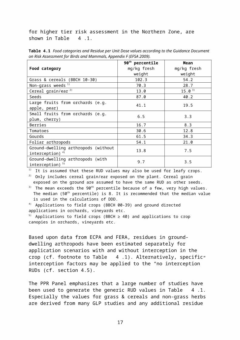
During preparation of the proposal for the current EFSA Guidance Document (EFSA 2009) the food categories and RUD values in SANCO/4145/2000 were revised, based mainly on new or updated databases provided by Baril et al. (2005), ECPA and the UK Food and Environment Research Agency (FERA). The food categories and RUD values, which are included in the EFSA Guidance Document and which shall also be used as the basis for higher tier risk assessment in the Northern Zone, are shown in Table 4.1.

Table 4.1 Food categories and Residue per Unit Dose values according to the Guidance Document on Risk Assessment for Birds and Mammals, Appendix F (EFSA 2009).

Food category 90th percentilemg/kg fresh weight

Meanmg/kg fresh weight

Grass & cereals (BBCH 10-30) 102.3 54.2Non-grass weeds 1) 70.3 28.7Cereal grain/ear 2) 13.0 15.0 3)

Seeds 87.0 40.2Large fruits from orchards (e.g. apple, pear) 41.1 19.5Small fruits from orchards (e.g. plum, cherry) 6.5 3.3Berries 16.7 8.3Tomatoes 30.6 12.8Gourds 61.5 34.3Foliar arthropods 54.1 21.0Ground-dwelling arthropods (without interception) 4) 13.8 7.5Ground-dwelling arthropods (with interception) 5) 9.7 3.5

1) It is assumed that these RUD values may also be used for leafy crops.2) Only includes cereal grain/ear exposed on the plant. Cereal grain exposed on the ground are assumed to have

the same RUD as other seeds.3) The mean exceeds the 90th percentile because of a few, very high values. The median (50th percentile) is 8. It is

recommended that the median value is used in the calculations of DDD.4) Applications to field crops (BBCH 00-39) and ground directed applications in orchards, vineyards etc.5) Applications to field crops (BBCH ≥ 40) and applications to crop canopies in orchards, vineyards etc.

2 The underlying rationale is that 6 % represents the amount of grain which is “always” available in rotational fields due to harvest spillage, turning over of soil, etc.

11

Based upon data from ECPA and FERA, residues in ground-dwelling arthropods have been estimated separately for application scenarios with and without interception in the crop (cf. footnote to Table 4.1). Alternatively, specific interception factors may be applied to the “no interception” RUDs (cf. section 4.5).

The PPR Panel emphasizes that a large number of studies have been used to generate the generic RUD values in Table 4.1. Especially the values for grass & cereals and non-grass herbs are derived from many GLP studies and any additional residue study would tend to rather broaden the existing database than to replace an RUD derived from it (EFSA 2009). Also the RUD values for arthropods are based on a fairly extensive database and it therefore has to be fully justified if new measured data shall override these RUDs. By contrast, EFSA (2009) recognizes that the estimate for seeds, which is unchanged from SANCO/4145/ 2000, is unsatisfactory.

Residues in earthworms and other soil invertebrates, which occur in the diet of species such as common shrew and wood mouse, are not included in the standard tables. The residues in earthworms and other organisms that spend most or all of their time buried in the soil are usually negligible but may be computed from the following equation:

PEC(worm) = PEC(soil) x (0.84 + 0.01 x Pow) / (0.02 x Koc), where

PEC(soil) is calculated as a time-weighted average after the last application, using an averaging period equal to the interval between applications (or 21 d for single application)Pow is selected from the List of Endpoints (Pow = 10log Pow)Koc is selected as the mean Koc value from the List of Endpoints (same value as used for FOCUS groundwater modelling).

Alternatively the pore water approach may be used (see section 5.6 in EFSA 2009).

Estimation of residues in earthworms would be relevant mainly for potentially bioaccumulating substances with high predicted concentrations in soil.

4.4 Recommendation for residue decline refinements (DT50)

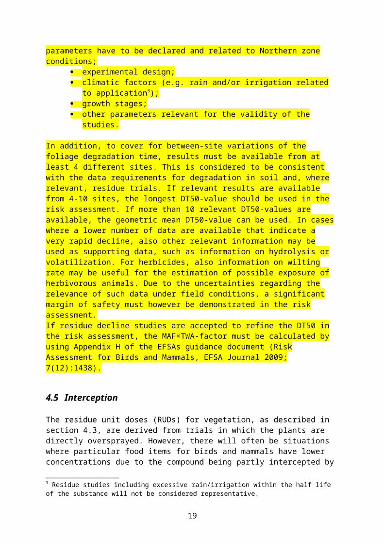
Residue studies used for refinements of the default foliage DT50 of 10 days must be considered representative for the Northern zone conditions according guidance given in EFSAs guidance document (Risk Assessment for Birds and Mammals, EFSA Journal 2009; 7(12):1438). For example, the following parameters have to be declared and related to Northern zone conditions;

experimental design; climatic factors (e.g. rain and/or irrigation related to application3); growth stages; other parameters relevant for the validity of the studies.

In addition, to cover for between-site variations of the foliage degradation time, results must be available from at least 4 different sites. This is considered to be consistent with the data

3 Residue studies including excessive rain/irrigation within the half life of the substance will not be considered representative.

12

requirements for degradation in soil and, where relevant, residue trials. If relevant results are available from 4-10 sites, the longest DT50-value should be used in the risk assessment. If more than 10 relevant DT50-values are available, the geometric mean DT50-value can be used. In cases where a lower number of data are available that indicate a very rapid decline, also other relevant information may be used as supporting data, such as information on hydrolysis or volatilization. For herbicides, also information on wilting rate may be useful for the estimation of possible exposure of herbivorous animals. Due to the uncertainties regarding the relevance of such data under field conditions, a significant margin of safety must however be demonstrated in the risk assessment.If residue decline studies are accepted to refine the DT50 in the risk assessment, the MAF×TWA-factor must be calculated by using Appendix H of the EFSAs guidance document (Risk Assessment for Birds and Mammals, EFSA Journal 2009; 7(12):1438).

4.5 Interception

The residue unit doses (RUDs) for vegetation, as described in section 4.3, are derived from trials in which the plants are directly oversprayed. However, there will often be situations where particular food items for birds and mammals have lower concentrations due to the compound being partly intercepted by the crop before it reaches the food item. It may therefore be appropriate to include an interception factor (or rather its complement, a deposition factor) in the estimation of residues and the Daily Dietary Dose.

Interception by the crop shall be considered as a minimizing factor for residues on plant food items and other food items exposed on or near the ground when canopy-directed applications of insecticides and fungicides to orchards, vineyards etc. are performed and undergrowth vegetation (assumed to be mainly grass) is present. Conversely, no interception factor shall be applied for herbicide applications in those crops, since these are typically made directly to the undergrowth vegetation.

In field crops, the crop itself may be assumed to receive the full application rate. However, other plants will usually also be available as food. At certain stages the crop intercepts some of the applied product and hence the amount of pesticide deposited on food items below the crop will be less than the application rate. Since measured residues of such food items at the appropriate growth stage of the crop are not available, only estimates can be used. Estimates of the deposition on the soil surface below crops of different structure and growth stages are available in the FOCUS reports (FOCUS 2000, 2001). However, deposition on 3-dimensional structures (e.g. weeds) above the ground is probably different from the deposition on the 2-dimensional soil surface.

According to EFSA (2009) estimation of residues on undergrowth vegetation using FOCUS interception factors becomes increasingly uncertain with decreasing soil cover of the crop and increasing height of weeds. Thus, reliable predictions are only deemed possible where the largest part of the soil surface is actually covered by the crop and the undergrowth vegetation is clearly smaller than the crop plants.

Based on this assessment, EFSA (2009) concludes that the crop interception values used in the FOCUS surface water report (FOCUS 2001) for Step 2 PECSW calculations can be considered acceptable also in the context of bird and mammal risk assessment, provided that the growth stage is sufficiently advanced. These figures are likely to be conservative estimates

13

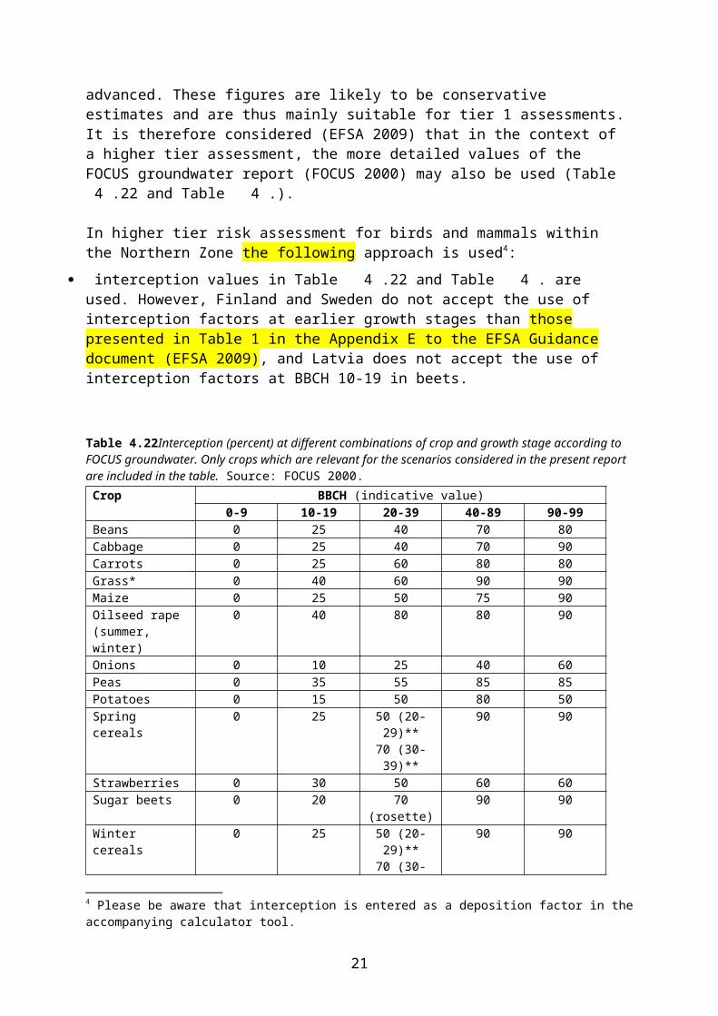
and are thus mainly suitable for tier 1 assessments. It is therefore considered (EFSA 2009) that in the context of a higher tier assessment, the more detailed values of the FOCUS groundwater report (FOCUS 2000) may also be used (Table 4.22 and Table 4.).

In higher tier risk assessment for birds and mammals within the Northern Zone the following approach is used4:

interception values in Table 4.22 and Table 4. are used. However, Finland and Sweden do not accept the use of interception factors at earlier growth stages than those presented in Table 1 in the Appendix E to the EFSA Guidance document (EFSA 2009), and Latvia does not accept the use of interception factors at BBCH 10-19 in beets.

Table 4.22Interception (percent) at different combinations of crop and growth stage according to FOCUS groundwater. Only crops which are relevant for the scenarios considered in the present report are included in the table. Source: FOCUS 2000.

Crop BBCH (indicative value)0-9 10-19 20-39 40-89 90-99

Beans 0 25 40 70 80Cabbage 0 25 40 70 90Carrots 0 25 60 80 80Grass* 0 40 60 90 90Maize 0 25 50 75 90Oilseed rape (summer, winter)

0 40 80 80 90

Onions 0 10 25 40 60Peas 0 35 55 85 85Potatoes 0 15 50 80 50Spring cereals 0 25 50 (20-29)**

70 (30-39)**90 90

Strawberries 0 30 50 60 60Sugar beets 0 20 70 (rosette) 90 90Winter cereals 0 25 50 (20-29)**

70 (30-39)**90 90

* An interception value of 90 % may be used for applications to established turf.** BBCH code of 20-29 for tillering and 30-39 for elongation.

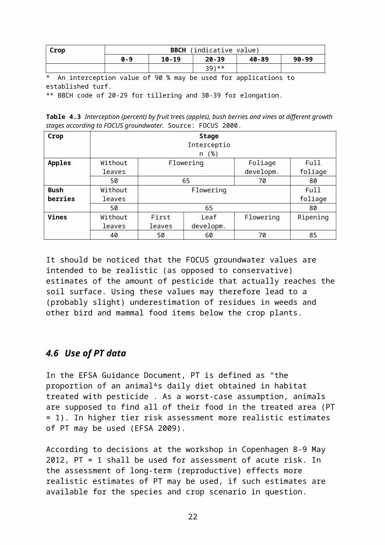
Table 4.3 Interception (percent) by fruit trees (apples), bush berries and vines at different growth stages according to FOCUS groundwater. Source: FOCUS 2000.Crop Stage

Interception (%)Apples Without leaves Flowering Foliage developm. Full foliage

50 65 70 80Bush berries Without leaves Flowering Full foliage

50 65 80Vines Without leaves First leaves Leaf developm. Flowering Ripening

40 50 60 70 85

It should be noticed that the FOCUS groundwater values are intended to be realistic (as opposed to conservative) estimates of the amount of pesticide that actually reaches the soil surface. Using these values may therefore lead to a (probably slight) underestimation of residues in weeds and other bird and mammal food items below the crop plants.

4 Please be aware that interception is entered as a deposition factor in the accompanying calculator tool.

14

4.6 Use of PT data

In the EFSA Guidance Document, PT is defined as “the proportion of an animal’s daily diet obtained in habitat treated with pesticide”. As a worst-case assumption, animals are supposed to find all of their food in the treated area (PT = 1). In higher tier risk assessment more realistic estimates of PT may be used (EFSA 2009).

According to decisions at the workshop in Copenhagen 8-9 May 2012, PT = 1 shall be used for assessment of acute risk. In the assessment of long-term (reproductive) effects more realistic estimates of PT may be used, if such estimates are available for the species and crop scenario in question. Because PT data are generally sparse, some read-across between structurally similar crops is acceptable. All cases of read-across between crops must be duly justified.

PT may be estimated indirectly by radio-tracking of individuals, assuming that the amount of active time spent by an animal in a given crop is directly proportional to the amount of food eaten there. In radio-tracking studies animals may be caught in general farmland or in (or in close proximity to) the crop of concern. In both cases, PT may be estimated for the whole sample of individuals tracked (“all birds/animals”) or only for the subsample of individuals that actually visited the crop of concern during tracking (“consumers”).

EFSA (2009) recommends that for focal species caught within (or in close proximity to) the target crop, PT should be estimated from the total sample of individuals – whether they used the crop of concern or not. For focal species caught in the general farmland, only those individuals proved by radiotracking to visit the crop of concern (consumers) should be included in the estimation of PT.

Irrespective of the above choice (all individuals or consumers) it is necessary to decide what level of protection is required. For example, if the first-tier PT of 1 is replaced by a median or mean value, this would suggest that the risk assessment will only relate to those 50 % individuals that fall under this PT. If the 90th percentile of the PT distribution is used, 90 % of the population will be protected, provided that no other parameters drive the risk assessment5.

At the workshop in Copenhagen 8-9 May 2012 it was agreed to follow the EFSA recommen-dations concerning the use of “all animals” or “consumers”. It was further agreed to use the 90th percentile of the PT distribution for the core risk assessment (Northern Zone registration report).

Refinements of PT in new studies should as a minimum be based on 10 individual animals caught within (or in close proximity to) the target crop or on a minimum of 10 animals tracked to be “consumers” in the target crop. In the available studies (referred in this GD) refinement of PT based on the "consumers" group is accepted also in cases where the number of individual animals in this group is below 10, provided the number of individuals in the "all birds" group studied was above 10.

5 It should be noticed that this assumption will almost never be met, implying that the true level of protection may only be reliably estimated by probabilistic methods.

15

Refinement of PT based on the “home range approach” or calculation of Jacobs’ Index are not accepted. It is considered that firm relationships between these approaches and PT estimates based on traditional (“a day in the life”) sampling protocols have not yet been established.

4.7 Dehusking

Dehusking of seeds may reduce exposure in granivorous birds and mammals. Regardless whether the seed has been subject to seed treatments or has been contaminated during spraying, the substance will be mainly on the outside and dehusking may thus remove the majority of the residue. Based upon experimental (manual) dehusking of seeds, Edwards et al. (1998) suggested that the reduction of exposure may be as high as 85 %. However, even in species which routinely dehusk, dehusking depends on the kind of seed and only a proportion of the seeds are dehusked (SANCO/4145/2000).

In the case of birds, dehusking is mainly observed in smaller species (body weight < 50 g) and chiefly in the specialized granivores (finches, sparrows and buntings). Larger granivorous birds (body weight > 50 g) do not dehusk as they are able to destroy even hard-shelled seeds in their gizzard. Among the small birds, species with a relatively thin bill, such as skylark, wagtails and other insectivores, do not have the capability of dehusking. Even in the small, granivorous species, dehusking is not an all-or-nothing phenomenon; certain species dehusk some but not all seed types, and in the wild the actual proportion of seeds dehusked may depend on stressors such as feeding pressure, predation risk or competition (Prosser 1999). Assuming a standard reduction of 85 % (or any other value) of the theoretical exposure in species that dehusk is therefore not justified.

For granivorous mammals, e.g. wood mouse, dehusking or cracking of seed or fruit shells is often a part of their typical feeding behaviour. Distinct anatomical features such as specialized incisors or folds of skin that prevent material from entering the mouth while being gnawed indicate that most rodents will probably minimise the uptake of husks when eating seeds (DEFRA 2005). Several older studies have demonstrated that dehusking occurs under laboratory as well as under semi-field conditions but do not provide quantitative information on the effect of dehusking. Dehusking efficiency in mice has however been quantified in two new studies.

Ludwigs et al. (2007) quantified the efficiency of dehusking by laboratory mice and wild Apodemus mice. They found that the efficiency was strongly dependent on seed structure. Dehusking of sunflower seeds where the seed coat and the fruit coat are not grown together was highly effective (≥ 90 %). Dehusking of maize seeds was less effective, 62-65 % by Apodemus mice, probably because the outer layer of the seed is firmly adhered to the rest of the kernel. Experimentally induced food shortage reduced the percentage of maize seeds dehusked from 77 % to 65 % but dehusking efficiency, as measured for those seeds where dehusking was actually performed, was unchanged.

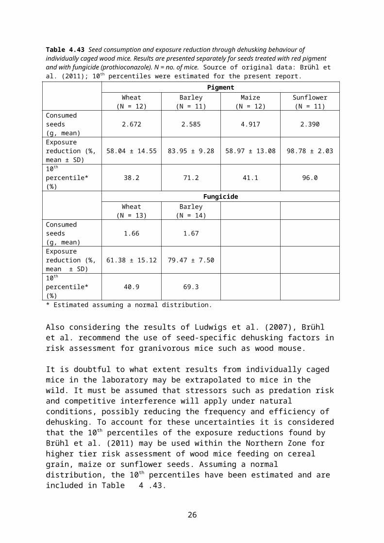
Brühl et al. (2011) studied dehusking by individually caged wood mice and found dehusking efficiencies of 60-80 % in cereals and c. 99 % in sunflower (Table 4.43). Notably dehusking efficiency was higher in barley than in wheat and maize. Dehusking efficiency was approximately the same, no matter if the seed was treated with a fungicide or a generic pigment and no matter whether the mice were starved before the experiment or not.

16

Table 4.43 Seed consumption and exposure reduction through dehusking behaviour of individually caged wood mice. Results are presented separately for seeds treated with red pigment and with fungicide (prothioconazole). N = no. of mice. Source of original data: Brühl et al. (2011); 10th percentiles were estimated for the present report.

PigmentWheat

(N = 12)Barley

(N = 11)Maize

(N = 12)Sunflower(N = 11)

Consumed seeds(g, mean) 2.672 2.585 4.917 2.390

Exposure reduction (%, mean ± SD) 58.04 ± 14.55 83.95 ± 9.28 58.97 ± 13.08 98.78 ± 2.03

10th percentile* (%) 38.2 71.2 41.1 96.0

FungicideWheat

(N = 13)Barley

(N = 14)Consumed seeds(g, mean) 1.66 1.67

Exposure reduction (%, mean ± SD) 61.38 ± 15.12 79.47 ± 7.50

10th percentile* (%) 40.9 69.3* Estimated assuming a normal distribution.

Also considering the results of Ludwigs et al. (2007), Brühl et al. recommend the use of seed-specific dehusking factors in risk assessment for granivorous mice such as wood mouse.

It is doubtful to what extent results from individually caged mice in the laboratory may be extrapolated to mice in the wild. It must be assumed that stressors such as predation risk and competitive interference will apply under natural conditions, possibly reducing the frequency and efficiency of dehusking. To account for these uncertainties it is considered that the 10th percentiles of the exposure reductions found by Brühl et al. (2011) may be used within the Northern Zone for higher tier risk assessment of wood mice feeding on cereal grain, maize or sunflower seeds. Assuming a normal distribution, the 10th percentiles have been estimated and are included in Table 4.43.

EFSA (2009) recommends that dehusking factors are not routinely applied in risk assessment. If dehusking is to be considered in a higher tier risk assessment, except for the wood mouse cases specified above, case-specific evidence must be provided that dehusking actually plays a role under field conditions for the focal species in question, and experimental data must be available for the relevant type of seed. In particular, the use of dehusking factors for weed seeds will not be accepted without case-specific experimental evidence.

It is not known to what extent dehusking is triggered solely by the structure of the seed or to what extent impalability of a seed treatment also plays a role. Also for this reason, particular care should be taken when risk assessment is performed for seed treatments with a high toxicity per single seed.

Especially for birds, a risk assessment for a dehusking species shall always be accompanied by an assessment for a second species that does not dehusk (EFSA 2009).

17

5 Selected focal species

5.1 Birds

5.1.1 Bean goose Anser fabalis

General informationThe bean goose (subspecies A. f. fabalis) breeds in small numbers (few thousand) within the taiga zone of Norway, Sweden and Finland. The main breeding areas are in Russia where it is replaced by the more numerous subspecies rossicus within the tundra zone. Main wintering areas (both subspecies) are in Germany and the Netherlands but some 30-40,000 birds (mainly fabalis), or c. 10 % of the European wintering population, usually winter in Denmark and southern Sweden (BirdLife International 2004). Occurrence in other parts of the Zone is chiefly on passage during spring and autumn (Table 5.4).

Table 5.4. Population size and trends of bean goose (wintering population) in the Nordic and Baltic countries. ”–”: not present. Source: BirdLife International 2004.Country Population size

(midwinter, individuals)*Year(s) of estimate Trend

(1990 – 2000)Denmark 10,000 – 12,000 1999 – 2000 StableEstonia 0 – 5 1998 New occurrenceFinland –Latvia 0 – 10 1990 – 2000 UnknownLithuania 1 – 10 1992 – 2002 Increase; > 80 %Norway –Sweden 15,000 – 30,000 1998 – 2001 Increase; < 20 %* See text for migrant numbers.

Departure from the breeding grounds is usually late August to mid-September, with arrival in winter quarters from late September to early October, but passage may occur throughout October (Cramp & Simmons 1977). Numbers in Sweden peak in September-October (Nilsson 2004). Further dispersal towards southwest may occur during cold spells. In eastern Denmark, most bean geese arrive during December-January, indicating cold flight from Swedish wintering areas. The bean geese depart from the wintering areas from mid-March, with spring numbers in Sweden usually peaking during April (Nilsson 2004). From the beginning of May most birds have left for the breeding grounds.

The number of bean geese staging in Sweden in autumn varies in different years from 40,000 to 80,000 individuals (Nilsson 2004), with a peak in October (Wallin and Millberg 1995). In spring the number of staging birds is much lower (Nilsson and Persson 1984) and the birds also stay for a shorter period of time compared to autumn.

Agricultural associationBean geese use agricultural land for foraging during migration. In a Swedish study, bean geese were found using mainly autumn sown cereals and stubbles in September-October (Axelsson 2004). Stubbles were used mostly in September with a shift towards cereals later in the month (Axelsson 2004). In early autumn (before 10 October) 8 % of the geese were found on autumn sown cereals (Nilsson and Persson 1984), while in late October 60 % of the geese in the study area were found on this habitat (Gezelius 1990). In spring (March-April) the bean

18

geese are mainly found in cereal fields. It is reasonable to assume that the crop type used by foraging geese also constitutes the main nutritional intake.

Body weightBody weight (subspecies fabalis) ♂ 2690–4060 g, ♀ 2220–3470 g (Snow & Perrins 1998). Mean body weight of the smaller sex (♀: 2845 g) may be used for risk assessment.

Energy expenditureNo specific studies of energy demands have been conducted on bean goose, but see below for studies on the closely related pink-footed goose.

Because no species-specific data are available, daily energy expenditure may be calculated allometrically using the equation for non-passerine birds in accordance with the formula in Appendix G of the EFSA Guidance Document (EFSA 2009). The allometric equation gives an estimate of the energy required for subsistence but does not allow for pre-migratory fattening in spring. Using the allometric equation therefore leads to an underestimation of the energy demand in spring, especially in April (cf. pink-footed goose).

It should be noticed, though, that the bean geese wintering in Fennoscandia (including Denmark) mainly breed within the Russian taiga zone; hence their journey towards the breeding grounds is shorter and the possibilities for feeding en route and after arrival to the breeding area are probably better than in the pink-footed goose. Therefore the need for pre-migratory fattening is assumed to be less pronounced in the bean goose.

Diet The feeding during migration and in the winter quarters is performed on arable and pasture-land, and especially in late autumn (from mid-October) cereals are predominantly used (Nilsson and Persson 1984; Axelsson 2004). The main diet is various green plant material and, if available, wheat, rape, and peas (Nilsson and Persson 1984; Axelsson 2004). Also feeds on newly sown grain (cf., e.g., Danish/Swedish/German name “seed goose”).

Risk assessmentThe bean goose is relevant for the following crop scenarios:

winter cereals, freshly drilled (BBCH 0-9) winter cereals, BBCH 10-29 spring cereals, freshly drilled (BBCH 0-9) spring cereals, BBCH 10-29 grass, short

In any case it may be assumed that within the treated area, the birds feed entirely on the treated crop or seed (PD = 1).

A body weight of 2845 g and a Daily Energy Expenditure (DEE) of 1412 kJ/day (from the allometric equation) may be used in risk assessment.

For birds feeding on freshly drilled seeds, a DEE of 1412 kJ/day is equivalent to an intake of 108 g seed/day (fresh weight) 6. However, this is almost certainly an underestimate of the actual intake of birds feeding on new-sown spring cereals (cf. the studies referred below for 6 Calculated using standard values for energy and moisture content and assimilation efficiency for cereal grain, cf. Appendix G (Tables 3 and 4) to the EFSA Guidance Document (EFSA 2009).

19

pink-footed goose). A FIR of 225 g seed/day (fresh weight), as used in the pink-footed goose, will probably also represent the worst case situation for bean goose.

There is no species-specific information allowing a refinement of PT. PT information from other Anser species, e.g. greylag goose Anser anser, may in principle be extrapolated to cover bean goose (Å. Berg pers. comm.). However, the available data on greylag goose (Prosser 2010) do not distinguish between active and inactive time and are therefore not considered suitable for risk assessment.

The relevance of reproductive risk assessment is doubtful as the bean goose does not breed in agricultural areas within the Zone. In any case, reproductive risk assessment will only be relevant for applications performed shortly before departure in spring, i.e. in April.

5.1.2 Pink-footed goose Anser brachyrhyncus

General informationThe pink-footed goose is a fairly common migrant and wintering species in Denmark (mainly in western Jutland where the species is locally abundant) and a fairly common migrant at a few sites in central and northern Norway. It is a rare migrant and winter visitor in Sweden, a rare migrant in Finland, and a rare or very rare visitor in the Baltic countries. In eastern Denmark, Sweden and further east, the pink-footed goose is replaced by the slightly larger bean goose (cf. above), with which it was formerly considered conspecific.

Pink-footed geese breed in Svalbard, Iceland and eastern Greenland, but only birds from the Svalbard population occur regularly within the Zone. The geese arrive to western Norway and Denmark in late September, and by mid-October all of the Svalbard population (c. 50,000 birds) probably stay in Denmark. Previously, most of the population moved further south from mid-October, but during recent decades an increasing part has remained in Denmark in winter, except during cold spells (Table 5.5). During March and the first half of April, the whole Svalbard population is again assembled in Denmark. The departure for the breeding grounds may start in mid-April and the last flocks leave Denmark in early or mid-May. In Norway, 10-20,000 birds stage in the Trondheim Fjord area between late April and mid-May before moving on to staging areas in Lofoten-Vesterålen, where probably the entire population stays at some time during May (although not all birds at the same time) (Fox et al. 1997, Madsen et al. 1997).

Table 5.5. Population size and trends of pink-footed goose (wintering population) in the Nordic and Baltic countries. ”–”: not present. Source: BirdLife International 2004.Country Population size

(midwinter, individuals)Year(s) of estimate Trend

(1990 – 2000)Denmark 21,000 – 23,000* 1999 – 2000 StableEstonia –Finland –Latvia –Lithuania –Norway – *Sweden 30 – 80 1998 – 2001 Increase; < 20 %* See text for migrant numbers.

Agricultural association

20

Pink-footed geese usually occur in flocks of more than 100 individuals and often in flocks of several thousands. The geese prefer to feed in large fields and other areas with an open view. They feed in salt marshes, rough and cultivated pastures, stubble fields (sometimes with undersown grass), winter cereal fields and newly sown cereal and pea fields.

During late winter and spring, the geese use different habitats in sequence. In a Danish study (Madsen et al. 1997), the geese from mid-March to early April were foraging mainly on grassland, followed by stubble and, to a minor degree, winter cereals. From mid-April onwards, stubble fields were ploughed and thus lost importance. The grasslands likewise decreased in importance as the geese increasingly used new-sown cereal or pea fields for feeding. To prevent crop damage, alternative food (cereal grain) is now offered to the geese at several sites.

In a local study at Filsø, Denmark, (Lorenzen & Madsen 1986) the geese used mainly stubble fields in autumn, stubble with undersown seed grass in autumn and spring, and newly sown barley fields in spring.

Time and energy budgets of pink-footed geese have been studied in Denmark (see below).

Body weightBody weight ♂ mostly 1900–3300 g, ♀ 1800–3100 g (Snow & Perrins 1998). Mean body weight of the smaller sex (♀: 2450 g) may be used for standard risk assessment.

The birds put on weight before spring migration. Mean body weight in early May, immediately before departure towards the breeding grounds, has been estimated at 3200 g (population mean) (Madsen et al. 1997).

Energy expenditureThe energy expenditure may be calculated allometrically using the equation for non-passerine birds in accordance with the formula in Appendix G of the EFSA Guidance Document (EFSA 2009); this gives a Daily Energy Expenditure (DEE) of 1277 kJ/day for a 2450 g goose. However, the information below should also be taken into account.

During spring the geese gain weight, partly in preparation for the long-distance migration to their arctic breeding grounds, and partly because the females must bring sufficient energy and nutrient reserves to produce eggs as food is very scarce at their arrival in Svalbard. Thus the birds, and especially the females, experience an increased energy and nutrient demand during their stay in Denmark in spring (Madsen et al. 1997). To meet these requirements, the geese forage on the new growth of grass on pastures and salt marshes and gradually shift to new-sown fields as these become available. The preference for new-sown fields compared to pastures can be explained by the greatly improved daily energy intake rate there (Madsen 1985).

The daily net energy intake of a 2.5 kg goose has been estimated at 1267 kJ/day for a bird feeding on grassland and at 2824 kJ/day for a bird feeding on newly sown spring barley fields; these figures are said to be equivalent to a daily consumption of 793 g (fresh weight) of grass leaves or 225 g (fresh weight) of barley grain, respectively (Madsen 1985).

In another study (Madsen et al. 1997), the daily energy intake in late April was estimated at 1834 – 2011 kJ/day for birds feeding on grassland and newly sown fields. In early May, the

21

corresponding figure was 2238 kJ/day for birds feeding on newly sown cereal fields, grasses, and cereal grain offered as bait.

Diet Pink-footed geese feed exclusively on vegetable material, including parts of plants both above and below ground. In the winter quarters, the geese now feed mainly on farmland, including grassland, but the exact composition of diet differs according to local and seasonal variations in crop-plant availability and nutritional demand.

On pastures, the geese eat leaves of common agricultural grasses and leaves and stolons of clover and other herbs. In the Netherlands, wintering geese (of different species) prefer feeding on improved grassland with short vegetation of grasses and dicotyledons. Pink-footed geese may also feed on roots and tubers (e.g. carrots, potatoes) as well as on leaves of oil-seed rape.

When feeding on newly sown cereal fields in spring, the geese primarily take the ungerminated grain on the surface and in the upper 2-3 cm of the soil (Madsen et al. 1997). In some areas, the geese abandon a site when the grain is sprouting, but in other areas it is reported that the geese also take the sprouting grain but clip off the stem before ingesting the seed (Madsen et al. 1997).

A daily intake of 2238 kJ (cf. above) is equivalent to the consumption of 172 g of grain (fresh weight)7. However, the daily consumption of grain may be even higher as direct observations of geese indicate that they may consume between 179 and 291 g of new-sown grain per day. The latter figures are probably slightly too high, however, as they are based on the assumption that each observed peck represents the ingestion of a grain (Madsen et al. 1997).

Time and energy budgets have been studied in NW Jutland in the second half of April. In the morning, the geese start to feed on newly sown cereal fields and forage intensively here for 2-3 hours. They then move to grassland (either salt marsh or cultivated pasture) and stay there during most of the day, feeding less intensively and spending most of their time roosting. On half of the observation days, the geese returned to the new-sown fields in the evening, to feed intensively for c. 2 hours before flying to the roost. The geese spent 27-48 % of the feeding day length in the new-sown fields, but due to higher feeding intensity and much higher profitability of the grain compared to grass, the geese gained 53-79 % of their daily energy intake from the new-sown fields (Madsen et al. 1997).

In areas where cereal grain is offered as bait this can profoundly change the daily rhythm, time and energy budget of the geese.

Risk assessmentThe pink-footed goose is relevant for the following crop scenarios:

winter cereals, BBCH 10-29 spring cereals, freshly drilled (BBCH 0-9) spring cereals, BBCH 10-29 pulses (peas), freshly drilled (BBCH 0-9) grass, short

7 Calculated using standard values for energy and moisture content and assimilation efficiency for cereal grain.

22

In any case it may be assumed that within the treated area, the birds feed entirely on the treated crop or seed (PD = 1).

A body weight of 2450 g may be used as a worst case assumption.

For birds feeding on plant leaves (cereals BBCH 10-29, short grass) the allometric equation can be used to estimate the DEE and FIR.

For birds feeding on freshly drilled seeds in spring, a 2450 g goose ingesting 225 g seed/day (fresh weight) is assumed to represent the worst case situation.

A PT value of 0.79 may be assumed for birds feeding on new-sown fields. There is no particular information on time budgets of birds feeding on plant leaves in late spring, but a PT of 0.79 will probably also be worst case for these scenarios.

The relevance of reproductive risk assessment is doubtful as the pink-footed goose does not breed in agricultural areas within the Zone. In any case, reproductive risk assessment will only be relevant for applications performed shortly before departure in spring, e.g. in Denmark for applications taking place between mid-April and early May.

5.1.3 Grey partridge Perdix perdix

General informationThe grey partridge is a widespread and fairly common species in Denmark and Lithuania. It also occurs, although more scarcely, in Latvia and Estonia and in farmland areas of southern Sweden and Finland (Table 5.6). Almost everywhere, numbers have declined strongly in recent decades; e.g. in Denmark an average decline of 3.2 % per year was estimated for the period 1976–2011 (Heldbjerg & Lerche-Jørgensen 2012). In many areas the natural population is reinforced by releases for hunting purposes; in Denmark between 20,000 and 70,000 birds are annually released (Kahlert et al. 2008).

Table 5.6. Population size and trends of grey partridge (breeding population) in the Nordic and Baltic countries. ”–”: not present. Sources: BirdLife International/European Bird Census Council (2000), BirdLife International (2004), Tiainen et al. (2010), Ottosson et al. (2012).Country Population size

(breeding pairs)Year(s) of estimate Trend

(1970 – 1990)Trend

(1990 – 2000)Denmark 10,000 – 15,000 2000 Decline; 20–49 % Decline; c. 50 %Estonia 4,000 – 7,000 1998 Decline; 20–49 % FluctuatingFinland > 10,000 2010 Decline; c. 90 % Fluctuating**Latvia 500 – 5,000 1990 – 2000 Decline; ≥ 50 % Decline; < 20 %Lithuania 10,000 – 20,000 1999 – 2001 Decline; 20–49 % Decline; 20–29 %Norway – * Extinct –Sweden 14,000 2008 Decline; 20–49 % Decline; 10–19 %* Re-introduction has been attempted.** C. 50 % increase 1990 – 2010.

Partridges are sedentary birds that gather in small flocks of up to 20-30 birds in winter. Flocks break up in early spring (March – early April) as the territories are established. Breeding is usually in May-June, but re-layings may extend the season into August (Snow & Perrins 1998). Single-brooded; clutch size is usually 10-20, occasionally larger, making quick recovery of populations possible after cold winters.

23

Agricultural associationPartridges are strongly associated with farmland, especially of the “old-fashioned” type with small fields surrounded by stripes of rough vegetation and hedgerows. The species occupies cereals and other arable crops as well as grassland. If present, early successional stages of set-aside (including game stripes) are probably favoured (Kahlert et al. 2008). Crop preferences do not seem strong as different studies have given different results.

In an English study of radio-tagged birds (Green 1984), 97 % of all fixes were from cereal fields and 40 % of fixes were from within 25 m of the field boundary. Unsprayed headlands are preferred (Rands 1986).

Body weightBody weight ♂ mostly 350–450 g, ♀ 340–420 g (Snow & Perrins 1998). Mean body weight of the smaller sex (♀: 380 g) may be used for risk assessment.

Energy expenditureEstimates of daily energy intake in winter for wild birds range between 300 kJ/day at an ambient temperature of +15 °C to 650 kJ/day at −15 °C (Christensen et al. 1996). The energy expenditure can also be calculated allometrically using the equation for non-passerine birds in accordance with the formula in Appendix G of the EFSA Guidance Document (EFSA 2009).

DietThe diet consists chiefly of vegetable matter. Green plant parts are probably staple food of adults throughout the year, but there is a marked annual cycle in the relative importance of food items, partly associated with farming practice. During winter and spring, the diet consists mainly of leaves of cereal crops, grasses and dicotyledonous weeds. In late spring, summer and autumn, seeds are often a major component of the diet and waste grain may dominate for some time after harvest. Insects may also be important in late spring and summer and are the main food of the chicks.

Steenfeldt et al. (1991) studied the diet composition of partridges in Danish farmland during two years. A total of 2112 faeces samples were collected from different crops. The results are expressed as percent of fragment area (roughly equivalent to volume %). The results indicate that the diet composition is highly variable between crops (Table 5.7).

Table 5.7. Grey partridge diet in farmland, analysed from faecal samples (Steenfeldt et al. 1991)1.Time of year Food type % of diet fragment areaAutumn Green plant material 52-73(Aug – Nov) Seeds/grain 23-47

Insects 0-3Flowerbuds/roots –

Winter Green plant material 16-99(Dec – Feb) Seeds/grain 1-83

Insects –Flowerbuds/roots 0-3

Early spring Green plant material 51-99(Mar – Apr) Seeds/grain 1-49

Insects –Flowerbuds/roots –

Late spring Green plant material 11-90(May – June) Seeds/grain 10-84

24

Time of year Food type % of diet fragment areaInsects 0-25Flowerbuds/roots 0-4

Summer Green plant material 19-98(June – July) Seeds/grain 2-74

Insects 0-20Flowerbuds/roots 0-32

1 Percentages calculated approximately from figures 1 and 2 in Steenfeldt et al. (1991). Range shows variation between crop types.

Other studies have shown greater importance of waste grain in autumn (October); from 60-71 % of dry weight of crop contents in Finland (Pulliainen 1984) to 94 % of dry weight in England (Potts 1970).

Insects are an important component of chick diet and contribute more than 50 % (by volume) of the diet in the first few weeks of life. In chicks foraging in cereal fields, the proportion of plant material in diet increases rapidly with age from about 20 % (dry weight) at age 1-5 days to c. 80 % at age 20-25 days (Christensen et al. 1996). Beetles are usually the dominant insect food items, with Chrysomelidae, Curculionidae, Carabidae and Nitidulidae being most important.

The chicks apparantly feed opportunistically. In a Danish study (Rasmussen et al. 1992), the proportion (by volume) of insects in the diet of small chicks varied from 3 % in birds feeding in hedgerows to 69 % in birds feeding in beet fields. Seeds and cereal grain made up between 4 % in spring-sown rape fields and 86 % in field boundaries. The volume of green plant parts in chick diet ranged from 11 % in field boundaries to 88 % in rape fields.

Potts (1970) collated data from studies of chick diet in the UK (Table 5.8). The results are presented as percent of food items; please notice that small items such as aphids and ants are less important in terms of biomass.

Table 5.8. Grey partridge chick diet in cereal fields and grassland, analysed by dissection of crops (Potts 1970).Habitat Food type % of food itemsCereal fields Plant material 47

Aphids 25Other invertebrates 28

Grassland Plant material 14Ants 31Aphids 9Other invertebrates 44

Risk assessmentThe grey partridge is relevant for the following crop scenario:

winter cereals, applications in autumn and winter (BBCH 10-19)

The grey partridge would also be relevant for other crop scenarios and seasons, but in those cases other omnivorous bird species, first of all skylark, are more worst case.

For this particular scenario, the diet composition in Table 5.9 may be used in case refinement of PD is needed.

25

Table 5.9. Estimated diet composition of grey partridges in cereal fields late autumn and winter (expert judgement based upon Table 5.7 and Steenfeldt et al. 1991).

Food category PD (fresh weight)*Grasses & cereals (BBCH 10-30) 0.60Non-grass weeds 0.26Cereal grain on ground 0.06Small seeds 0.08

* In the original study (Steenfeldt et al. 1991), diet composition is presented as “% of fragment area”. It may be assumed that this roughly corresponds to % of fresh weight because the material was soaked in water before analysis.

As 97 % of all fixes in a radio-tracking study were from cereal fields, PT shall not be refined unless fully justified by case-specific data.

5.1.4 Woodpigeon Columba palumbus

General informationThe woodpigeon is a widespread and common or abundant species in agricultural and forested landscapes, and partly also in urban areas, throughout the Zone. It extended its range northward during the 20th century and now also occurs commonly within the boreal zone. Populations are assumed to be stable or increasing throughout the Zone, except in Sweden where the species has apparently declined following an increase until 1970-80 (Snow & Perrins 1998, Table 5.10).

Table 5.10. Population size and trends of woodpigeon (breeding population) in the Nordic and Baltic countries. Sources: BirdLife International/European Bird Census Council (2000), BirdLife International (2004), Ottosson et al. (2012).Country Population size

(breeding pairs)Year(s) of estimate Trend

(1970 – 1990)Trend

(1990 – 2000)Denmark 250,000 – 350,000 2000 Increase; 20–49 % Increase; 10–19 %Estonia 40,000 – 80,000 1998 Stable StableFinland 150,000 – 200,000 1998 – 2002 Stable Increase; c. 10 %Latvia 40,000 – 60,000 1990 – 2000 Stable Increase; 20–29 %Lithuania 80,000 – 120,000 1999 – 2001 Stable Increase; 20–29 %Norway 100,000 – 500,000 1990 – 2002 Increase; 20–49 % StableSweden 980,000 2008 Stable Decline; 28 %

Woodpigeons are migratory in northern and eastern Europe but are partly sedentary in Denmark and in southernmost Norway and Sweden. The northern and eastern boundaries of the normal winter distribution lie close to the 0 °C January isotherm (Snow & Perrins 1998). Northern and eastern populations leave the breeding areas from mid-September to early November, with huge numbers passing through South Sweden and Denmark, and along the eastern Baltic coastline, in October. Spring migration occurs mainly March-April (Cramp 1985).

The breeding season is very long, stretching from mid-February to November in north-west (atlantic) Europe. Urban populations lay significantly earlier than rural populations, the latter usually starting breeding late March to mid-April (Snow & Perrins 1998). In Central Europe laying begins mid-April and in north-eastern Europe even later. In Denmark most layings occur between May and July and nestlings may still be found until October. Breeding pairs make on average 4 breeding attempts per year (information on ringdue (woodpigeon) at http://www.dofbasen.dk/ART).

26

Agricultural associationWoodpigeons occur in most terrestrial habitats but seem to prefer a mosaic landscape with woods and agricultural land. In farmland, woodpigeons breed in hedgerows, coverts etc. but forages in open fields. Woodpigeons breeding in forest or urban areas also frequently fly to adjacent farmland to feed. Broad-leaved crops seem to be preferred feeding sites but crop preferences during summer are not strong (Petersen 1996b). Pigeons foraging in British farmland showed season-dependent preferences: cereal stubble in November - January, winter rape in January - February and pasture in February - May; in addition newly sown cereal and pea fields were exploited when available (October - November and March - May) (Inglis et al. 1990). Woodpigeons have also been recorded feeding in freshly drilled rape fields (Petersen 1996a). In a British study of birds feeding at bait stations with different seeds, pigeons seemed to prefer peas but also took rape and barley (Prosser 1999).

British data on proportion of time (PT) spent by individual woodpigeons in different crops have been consolidated by Prosser (2010) and are summarized in Table 5.11. These data indicate that oilseed rape is a preferred crop during most of the year.

Table 5.11. Percentage of active time spent by radio-tagged woodpigeons in different crops in the UK, presented as 90th percentile of the modelled PT distribution. The birds were caught in general farmland (not in specific crops); it is therefore recommended to use values for the subsample of birds who actually used the crop in question (“consumers only”) (bold).Crop Period No. of birds 90th percentile ReferenceAll birds:(Winter)cereals

Summer(Jun – Aug)

19 0.23 Prosser 2010

Autumn(Sep – Nov)

27 0.07 Prosser 2010

Winter(Dec – Feb)

15 0.42 Prosser 2010

(Winter)oilseed rape

Spring(Mar – May)

13 0.78 Prosser 2010

Summer(Jun & Aug)*

19 0.72 Prosser 2010

Autumn(Sep – Nov)

27 0.17 Prosser 2010

Winter(Dec – Feb)

15 0.59 Prosser 2010

Potatoesand beet

Autumn(Sep – Nov)

27 0.02 Prosser 2010

Consumers only:(Winter)cereals

Summer(Jun – Aug)

8 0.36 Prosser 2010

Autumn(Sep – Nov)

11 0.10 Prosser 2010

Winter(Dec – Feb)

7 0.61 Prosser 2010

(Winter)oilseed rape

Spring(Mar – May)

8 0.84 Prosser 2010

Summer(Jun & Aug)*

13 0.77 Prosser 2010

Autumn(Sep – Nov)

11 0.29 Prosser 2010

Winter(Dec – Feb)

8 0.68 Prosser 2010

27

Crop Period No. of birds 90th percentile ReferencePotatoesand beet

Autumn(Sep – Nov)

18 0.08 Prosser 2010

* July was excluded as oilseed rape is normally harvested during this month in the UK.

Body weightBody weight is rather variable: ♂ 325–614 g, ♀ 284–587 g (Snow & Perrins 1998); low values (< 350 g) are possibly from exhausted birds (Cramp 1985). Mean body weight of the smaller sex (♀: 435 g) may be used for risk assessment.

Energy expenditureThe daily energy expenditure can be calculated allometrically using the equation for non-passerine birds in accordance with the formula in Appendix G of the EFSA Guidance Document (EFSA 2009).

DietWoodpigeons feed on a wide range of plant material, with seeds or green leaves dominating, depending on season. Seeds from newly sown cereal, pea or rape fields and all types of grain from stubble fields are apparently preferred when available. In winter, green leaves of broad-leaved crops (oil-seed rape) and different weeds are important but beech mast, acorns etc. may also be significant during autumn and winter. The summer diet is highly variable and may include up to 5 % invertebrates (Christensen et al. 1996).

Woodpigeons often feed by gorging themselves while on the ground, then moving to safer locations (usually in hedges or trees) to digest their food and rest (Prosser 2010).

Adult pigeons feed their nestlings with a secretion from the crop, amounting to 92 % of the diet in newly hatched chicks and gradually decreasing to 21 % of diet in chicks ≥ 15 days old. The balance is made up by the same food as that of adults, except that invertebrates and weed seeds are more frequent (Christensen et al. 1996).

British studies indicate that a significant shift in the feeding habits of woodpigeons has occurred in recent decades. Before the 1970s, cereal stubbles, clover leys and pasture were preferred foraging sites during winter but as the stubble fields were replaced by autumn-sown crops, woodpigeons moved to newly sown cereal fields in autumn and oil-seed rape in winter (Inglis et al. 1990).

Ljunggren (1968) studied adult crop contents in a rural population of woodpigeons in SW Sweden. The results are presented as percentage of food items (by number) (Table 5.12).

Table 5.12. Woodpigeon diet in SW Sweden, analysed from crop contents (n = 728 crops) (Ljunggren 1968).Time of year Food type % of food itemsJan – Apr Plant leaves 52

Cereal grain 46Weed seeds 2Rape seeds 1Peas 1

May – Aug Rape seeds 28Cereal grain 26Peas 16Weed seeds 15Plant leaves 13

28

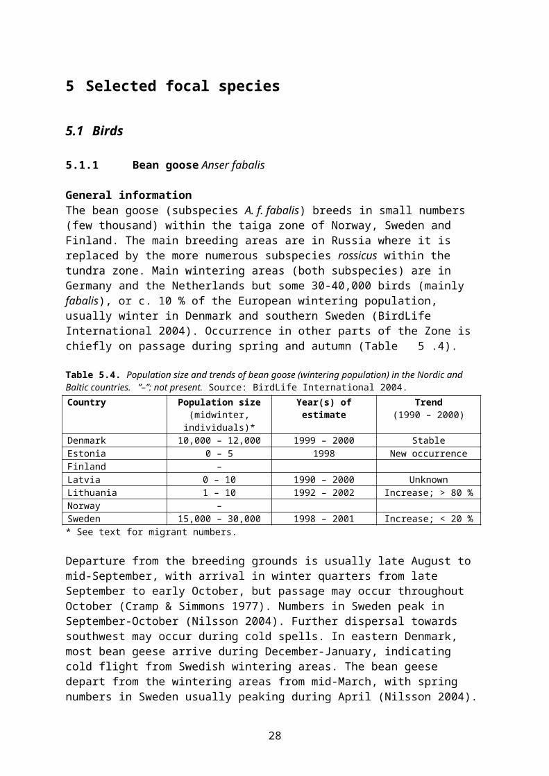
Time of year Food type % of food itemsSep – Nov Cereal grain 68

Peas 12Plant leaves 9Rape seeds 7Weed seeds 3

Schnock & Seutin (1973, cited in Cramp 1985) studied woodpigeon crop contents in Belgium (Table 5.13). The results are presented as percentage of fresh weight.

Table 5.13. Woodpigeon diet in Belgium, analysed from crop contents (n = 673 crops) (Schnock & Seutin 1973 cited in Cramp 1985).Time of year Food type % of fresh weightApril – mid-May Cereals or legumes 91

Leaves of clover and dicot. weeds 4Beech flower buds 3Weed seeds 2

mid-May – mid-July Fruits and seeds (e.g. Caryo-phyllaceae, Ranunculaceae)

45

Leaves (clover, lucerne, Fraxinus) 33Rhizomes and bulbs 10Cereals or legumes 6Flower buds 4Animal matter 3

mid-July – mid-October Cereals or legumes1 97Weed seeds (Vicia) 2Animal matter 1

mid-October – March Fruits and seeds (esp. acorns and beech mast)

45

Cereals or legumes 362

Green leaves 191 Including 53 % wheat, 29 % peas, 11 % barley.2 Up to 83 % during periods of snow cover.

Risk assessmentThe woodpigeon is relevant for the following crop scenarios:

winter cereals, freshly drilled maize, freshly drilled winter rape, BBCH 10-19 spring rape, BBCH 10-19 pulses (peas), BBCH 10-19 pulses (peas), BBCH 80-99

Woodpigeons are highly mobile and may cover large areas of land in their search for food (Prosser 2010). Therefore the available data on diet composition (Table 5.12, Table 5.13) do not reflect foraging in any particular crop. To deal with this, the published diets were used as a starting point, whereupon the food items not available (or less available) in the crop in question were deleted (or their share was reduced) and the relative shares of the other components of diet were increased proportionally. In this process, the generic “pigeon” diets in EFSA 2009 were also taken into account.

It is proposed that the diets specified below (Table 5.14) are used in higher tier risk assessment for sprayed compounds.

29

Table 5.14. Estimated diet composition of woodpigeons feeding in different crops (expert judgement based upon Table 5.12, Table 5.13 and EFSA 2009).

Winter cereals, freshly drilledFood category PD (fresh weight)Large seeds 0.97Small seeds 0.02Ground arthropods 0.01

Maize, freshly drilledFood category PD (fresh weight)Non-grass weeds & leafy crops 0.05Large seeds 0.92Small seeds 0.03

Winter rape, BBCH 10-29Food category PD (fresh weight)Non-grass weeds & leafy crops 0.80Large seeds 0.10Small seeds 0.10

Spring rape, BBCH 10-29Food category PD (fresh weight)Non-grass weeds & leafy crops 0.80Large seeds 0.05Small seeds 0.14Ground arthropods 0.01

Pulses, BBCH 10-19Food category PD (fresh weight)Non-grass weeds & leafy crops 0.60Large seeds 0.25Small seeds 0.14Ground arthropods 0.01

Pulses, BBCH 80-99Food category PD (fresh weight)Non-grass weeds & leafy crops 0.24Large seeds 0.60Small seeds 0.14Ground arthropods 0.02

In risk assessment for seed treatments the following values may be used (Table 5.15).

Table 5.15. Estimated amounts of treated seed consumed by a 435 g woodpigeon fulfilling its daily requirements by feeding on freshly drilled winter cereals or maize. PD for mixed diets as in Table 5.14.

PD (fresh weight)* Fresh weight (g)Winter cereals(autumn)

1.00 33.70.97 32.7

Maize(spring)

1.00 33.70.92 32.2

* PD = 1 may be used in acute risk assessment, PD < 1 in long-term risk assessment.

Due to their high mobility, it is unlikely that woodpigeons will be foraging in any single crop for a longer period of time. It is therefore considered appropriate to refine the risk assessment

30

by adjusting PT, using the radio-tracking data in Table 5.11. PT data are however not available for all relevant crops.

5.1.5 Skylark Alauda arvensis

General informationThe skylark is a widespread and abundant species in farmland across most of Europe. The highest densities are found in lowland areas within the temperate zone. In the boreal zone it occurs wherever there are larger areas of arable land or pasture. Being originally a bird of steppe grasslands the skylark spread with deforestation and the expansion of agriculture, especially during the 19th century. From c. 1970 onwards population declines have been recorded almost everywhere, most probably as a result of agricultural intensification.

Table 5.16. Population size and trends of skylark (breeding population) in the Nordic and Baltic countries. Sources: BirdLife International/European Bird Census Council (2000), BirdLife International (2004), Ottosson et al. (2012).Country Population size

(breeding pairs)Year(s) of estimate Trend

(1970 – 1990)Trend

(1990 – 2000)Denmark 1,100,000 – 1,300,000 2000 Decline; 20–49 % Decline; < 10 %Estonia 150,000 – 300,000 1998 Decline; 20–49 % StableFinland 300,000 – 400,000 1998 – 2002 Decline; 20–49 % Stable*Latvia 1,100,000 – 1,800,000 1990 – 2000 Stable StableLithuania 1,100,000 – 1,500,000 1999 – 2001 Stable Decline; < 20 %Norway 100,000 – 400,000 1990 – 2001 Stable Decline; < 20 %Sweden 800,000 2008 Decline; 20–49 % Decline; 28 %* Increasing after 2000 (Tiainen et al. 2012b).

Skylarks are migratory throughout the Zone, with just some few thousand birds remaining in Denmark and southern Sweden during mild winters (Petersen 2006). The birds arrive at their breeding grounds from late February to early April. In the southern part of the Zone, skylarks breed from April to July and may produce 2 or 3 clutches per year. Further north breeding starts from early May and only one or maybe two clutches are produced. At the end of the breeding season in August the breeding grounds in farmland are almost vacated. Autumn migration takes place during September - early November.

Agricultural associationThe skylark is a pronounced farmland bird and is almost exclusively found in arable land using a wide range of crop types for breeding and foraging (Mason & Macdonald 2000). In a study in Finnish farmland one important factor for the presence of skylarks in fields was the distance to nearest forest and the openness of the area (no birds were found in areas smaller than 11.5 ha), (Piha et al. 2003). In a similar Danish study (Petersen 1998), skylark densities were negatively associated with the presence of buildings, woods, hedgerows, coverts and other habitat islands.

In farmland areas in the southern and central parts of Sweden, mean skylark densities were 0.26 territories/ha (Robertson & Berg 1992). Densities are affected by crop type as shown by inventories in SW Sweden with the highest skylark density in peas (0.82 territories/ha), followed by rape (0.61), winter cereals (0.53), spring sown cereals (0.37), oat (0.32), cabbage (0.25) and flax (0.09) (Lindqvist et al. 2000). Skylarks are also found at high densities in set-asides (0.80) and early stages of energy forest (0.37 territories/ha respectively) (Berg & Pärt 1994, Berg 2002). In Finland the density depends on the size of the farmland patch (Piiroinen

31

et al. 1985). In large open areas, the average density was 0.64 – 0.72 territories/ha in south-western Finland and 0.45 territories/ha in southeastern Finland (Tiainen & Seimola 2010). The density can be as high as 1.2 territories/ha in plots of over 100 ha in organic farms (Tiainen & Seimola 2010). In Åland, the average density of skylarks was 0.68 territories/ha with maxima in winter cereals and winter oilseed rape (> 1,2 territories/ha, Tiainen et al. 2012a). In a Danish study, the highest densities were found on set-aside, followed by cereals and rotational grassland, and the lowest densities were found on permanent grassland (Petersen 1996b).

The home range size of skylarks depends on both crop type and landscape structure (Jenny 1990; Poulsen et al. 1998). Average home range size in winter cereals are 4.6 ha and between 2.4 - 2.6 ha in sprayed spring cereal fields (Odderskær et al. 1997a, Poulsen et al. 1998).

Skylarks are present on arable fields from March until late July and early August when the breeding grounds are largely abandoned (Odderskær et al. 1997b, Esbjerg & Petersen 2002). Densities are changing over the growth period in spring and summer, with decreasing numbers of skylark territories in winter cereals and winter rape and increasing numbers in spring cereals and, towards the end of the season, in sugar beet (e.g. Toepfer & Stubbe 2001, Esbjerg & Petersen 2002). In central Europe (including the British isles) and also in the southern part of the Northern Zone, winter cereal fields usually grow too high and dense for successful skylark breeding early in the season (i.e. during the first half of May), while further north where crop growth is slower, winter cereals may be a suitable breeding habitat until June (Hiron et al. 2012). In autumn, skylarks are commonly recorded on stubble fields (e.g. Esbjerg & Petersen 2002, J. Tiainen pers. comm.) and on winter cereal fields (Crocker & Irving 1999).

The time a bird spends in one field is to some degree depending on where the nest is situated. It has been shown that birds with nests in the centre of a field are more likely to forage in the same field compared to birds nesting closer to the field edge which to a greater extent forage outside the field (Donald et al. 2001). From studies using both radio-telemetry and intensive visual observation, it has been shown that skylarks uses arable crops and single fields for foraging (Crocker et al. 2002; notifier study summarized in EFSA 2004). Thus, skylarks might be present in one field during the whole breeding season spending nearly all time there.

The proportion of time (PT) spent by individual skylarks in different crops has been estimated by Finch & Payne (2006) and Prosser (2010), based upon British radio-tracking data. The results are summarized in Table 5.17. It should be noticed that the British data may under-estimate the skylarks’ use of winter cereals during summer within the Northern Zone (cf. above) and that it is doubtful to what extent PT data for winter cereals may be extrapolated to spring cereals.

Table 5.17. Percentage of active time spent by radio-tagged skylarks in different crops in the UK, presented as mean and 90th percentile of the modelled PT distributions. The birds were caught in general farmland (not in specific crops); it is therefore recommended to use values for the subsample of birds who actually used the crop in question (“consumers only”) (bold).Crop Period No. of birds Mean 90 percentile ReferenceAll birds:Winter cereals

Winter(Sep – Mar)

24 0.14 0.67 Finch & Payne 2006

24 0.63 Prosser 2010Summer 44 0.25 0.92 Finch &

32

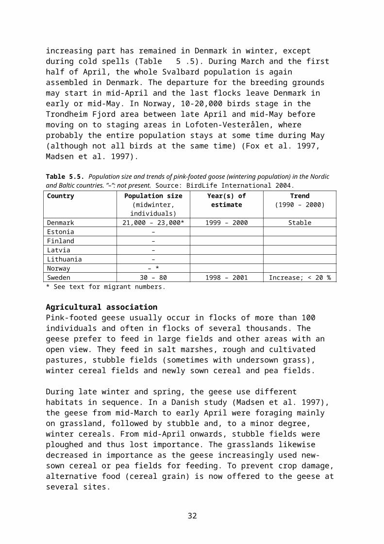
Crop Period No. of birds Mean 90 percentile Reference(Apr – Aug) Payne 2006

44 0.90 Prosser 2010Winter rape Winter

(Aug – Mar)27 0.05 0.10 Finch &

Payne 200627 0.13 Prosser 2010

Summer(Apr – Jul)

41 0.05 0.18 Finch & Payne 2006

41 0.26 Prosser 2010Beet(+ potatoes)

Apr – Nov 59 0.11 0.47 Finch & Payne 2006

59 0.49 Prosser 2010Consumers only:Winter cereals

Winter(Sep – Mar)

10 0.34 0.94 Finch & Payne 2006

10 0.96 Prosser 2010Summer(Apr – Aug)

26 0.42 0.97 Finch & Payne 2006

26 0.99 Prosser 2010Winter rape Winter

(Aug – Mar)4 0.36 0.98 Finch &

Payne 20064 0.89 Prosser 2010

Summer(Apr – Jul)

7 0.33 0.57 Finch & Payne 2006

7 0.57 Prosser 2010Beet(+ potatoes)

Apr – Nov 18 0.35 0.88 Finch & Payne 2006

18 0.84 Prosser 2010

Body weightBody weight ♂ mostly 34–50 g, ♀ 26–43 g (Snow & Perrins 1998). Mean body weight of the smaller sex (♀: 35 g) may be used for risk assessment.

Energy expenditureThe existence metabolism for adult skylarks is given by the formula; 31.2 − 0.440T kcal/birds/day, were T = ambient temperature (Topping and Odderskær 2004, calculated from Kendeigh et al. 1977). Alternatively, the energy expenditure can be calculated allometrically using the equation for passerine birds in accordance with the formula in Appendix G of the EFSA Guidance Document (EFSA 2009).

DietThe diet of skylarks is depending on season and availability of different food types. Cereal grains and leaves form a large part of the diet in winter, while invertebrates are the most important part of the diet in summer (Green 1978). Skylarks do not dehusk seeds before swallowing them (Buxton et al. 1998). The chicks are almost entirely reared on invertebrates (Green 1978; Donald 2004). The diet composition of adults and chicks of skylark in arable land are presented separately for different times of year in the tables below.

Green (1978) studied skylarks in three farmland areas in east England between November 1974 and June 1977. In the three areas the dominating crops were cereals and sugar beet (Table 5.18).

Table 5.18. Skylark diet in arable land (Green 1978)1.

33

Time of year Food type % of diet dry weightApril Invertebrates 14

Cereal grain 30Grass flowers and seeds2 15Dicotyledonous weed seeds2 7Monocotyledonous leaves 24Dicotyledonous leaves 10

May Invertebrates 28Cereal grain 11Grass flowers and seeds2 11Dicotyledonous weed seeds2 12Monocotyledonous leaves 24Dicotyledonous leaves 14

June Invertebrates 40Cereal grain 6Grass flowers and seeds2 6Dicotyledonous weed seeds2 17Monocotyledonous leaves 17Dicotyledonous leaves 14

July Invertebrates 51Cereal grain 27Grass flowers and seeds2 2Dicotyledonous weed seeds2 5Monocotyledonous leaves 10Dicotyledonous leaves 5

August Invertebrates 24Cereal grain 56Grass flowers and seeds2 5Dicotyledonous weed seeds2 9Monocotyledonous leaves 1Dicotyledonous leaves 5

September Invertebrates 13Cereal grain 71Grass flowers and seeds2 1Dicotyledonous weed seeds2 12Monocotyledonous leaves 2Dicotyledonous leaves 1

1 All data on % of diet calculated approximately from figure 3 in Green (1978). 2 For risk assessment purposes, “grass flowers and seeds” and “dicotyledonous weed seeds” may be merged into the category “small seeds”.

Green (1980) studied skylark feeding habits in two consecutive years on nine sugar beet fields in England. Faeces samples were collected from the fields and observations were done in April and May (Table 5.19).

Table 5.19. Skylark diet on sugar beet fields (Green 1980).Time of year Food type % of diet dry weightApril-May Seedlings1 63

Weed seeds 21Invertebrates2 16

1 Weed and sugar beet cotyledons and leaves.2 Ground-dwelling arthropods.

Navntoft et al. (2003) performed a detailed study of the arthropod part of the skylark diet in organic cereal fields (winter wheat and spring barley) in Denmark. A total of 1296 faecal

34

samples were analysed. The results were expressed as both number and biomass of food items and are summarized in Table 5.20.

Table 5.20. Arthropods in the diet of skylarks in cereal fields (Navntoft et al. 2003).Time of year Food type % of diet

by number by biomassMay-July Carabidae img.1 16 25

Staphylinidae img. 1 2 15 8Chrysomelidae img. 2 14 5Syrphidae juv. 2 9 22Symphyta juv. 2 1 16Lepidoptera juv.2 2 8Other arthropods 43 16

1 Ground-dwelling arthropods.2 Foliar arthropods.

Odderskær et al. (1997a) studied the diet of skylark chicks in spring barley fields in a Danish farmland. The food analysis was made from 249 faecal samples and included arthropod food remains only (Table 5.21).

Table 5.21. Arthropods in skylark chick diet in spring barley fields (Odderskær et al. 1997a).Time of year Food type % of diet dry weightMay-June Carabidae1 49

Lepidoptera2 17Heteroptera2 8Coleoptera (Elateridae) 1 2 6Other insects 21

1 Ground-dwelling arthropods.2 Foliar arthropods.

Risk assessmentThe skylark may be a relevant focal species in all field crops including grassland.

For any month, the diet composition (PD values) might in principle be taken directly from Table 5.18. However, these PD values apply to arable land in general and should be adjusted to allow for differences in food availability between crops. Furthermore, the relative amounts of foliar and ground dwelling arthropods in diet do not appear from this table. If foliar arthropods are present in the crop during the period in question, they may be assumed to constitute up to 50 % of the invertebrate part of the diet, or less during the period of crop development. The occurrence of foliar arthropods in diet is documented in Table 5.20 and Table 5.21.

Crop-specific PD adjustments are described in Appendix 1 and the PD values to be used in higher tier risk assessment are shown in Appendix 3 and in the accompanying data sheet.

For those elements of the diet which are obtained from the ground, interception in the crop canopy shall be taken into account as appropriate for the crop and growth stage in question, cf. section 4.5.

In risk assessment for seed treatments the values in Table 5.22 may be used. For each exposure scenario, the amount of ingested seed is computed from PD for cereal grain or small seeds, estimated as described in Appendix 1 (cf. above). PD for grass is calculated from the

35

scenario (April) where grass seeds make up the largest share of the diet, using the ratio between grass and dicotyledonous weed seeds found by Green (Table 5.18).

Table 5.22. Estimated amounts of treated seed consumed by a 35 g skylark fulfilling its daily requirements by feeding in newly sown cereal, rape or grass fields.

PD (dry weight)* Fresh weight (g)Spring cereals 1.00 9.48

0.46 3.98Winter cereals 1.00 9.48

0.74** 6.71**Spring rape 1.00 7.61

0.57 4.39Winter rape 1.00 7.61

0.51 3.93Grass 1.00 7.61

0.42 3.17* PD = 1 may be used in acute risk assessment, PD < 1 in long-term risk assessment.** Includes harvest spillage from a possible preceding cereal crop.

Skylarks may obtain almost all of their food from a single (large) field. If deemed appropriate, PT may be refined using the information in Table 5.17.

5.1.6 Yellow wagtail Motacilla flava

General informationThe yellow wagtail occurs in open country, especially meadows and pastures, across most of the Zone. Most populations have declined in recent decades, and in Denmark – and maybe also in other parts of the Zone – occurrence is now rather scarce and local (Table 5.23).

Table 5.23. Population size and trends of yellow wagtail (breeding population) in the Nordic and Baltic countries. Sources: BirdLife International/European Bird Census Council (2000), BirdLife International (2004), Ottosson et al. (2012).Country Population size

(breeding pairs)Year(s) of estimate Trend

(1970 – 1990)Trend

(1990 – 2000)Denmark 5,000 – 10,000 2000 Decline; 20–49 % Decline; 30–49 %Estonia 10,000 – 20,000 1998 Stable Decline; 20–29 %Finland 250,000 – 400,000 1998 – 2002 Decline; 20–49 % Decline, 50 %Latvia 10,000 – 25,000 1990 – 2000 Stable StableLithuania 20,000 – 30,000 1999 – 2001 Stable Decline; 30–49 %Norway 100,000 – 500,000 1990 – 2002 Stable StableSweden 360,000 2008 Increase; 20–49 % Decline; 55 %

The birds mostly arrive at their breeding grounds during May, with laying occurring mainly in late May and June. Yellow wagtails are usually single-brooded within the Zone, but two broods have been reported from Denmark and may also occur elsewhere in the southern part of the Zone. Autumn migration may begin as early as late July but the bulk of migration occurs from mid-August until late September. European birds winter in sub-Saharan Africa.

Agricultural associationIn the breeding season, yellow wagtails mostly prefer riversides, lakesides, pastures and similar habitats with low, dense and moist herbage or turf (Cramp 1988). In the northern part

36

of the range, the species (subspecies thunbergi) is also found in peat bogs (mires) and grazed fens.

Locally, especially in Central Europe, yellow wagtails seem to have adapted to intensive agriculture and occur in arable fields, particularly in row crops such as potato and beet but also in cereals (Glutz von Blotzheim & Bauer 1985). In North European farmland the species is mainly found in permanent grassland, although before the decline it was common in spring-sown fields in, e.g., southern Finland (Piiroinen et al. 1985, Tiainen et al. 1985).

Population densities in farmland may generally reach 2–4 breeding pairs per 10 ha under optimum conditions, i.e. in extensively managed grassland. In arable fields, maximum densities of 0.5 – 0.7 pairs per 10 ha have been reported from Central Europe (Glutz von Blotzheim & Bauer 1985).

Body weightBody weight of both sexes mostly 14-21 g (Snow & Perrins 1998). Mean body weight (17.5 g) may be used for risk assessment.

Energy expenditureThe energy expenditure may be calculated allometrically using the equation for passerine birds in accordance with the formula in Appendix G of the EFSA Guidance Document (EFSA 2009).

Diet Yellow wagtails feed almost exclusively on arthropods, mainly Diptera. They prefer small food items (2-7 mm) but may also take larger insects such as dragonflies Odonata. Three main foraging techniques are used: (1) picking from ground or water surface while walking; (2) run-picking, where the prey is picked from the surface (ground, plant or water) or when it takes off; (3) flycatching after short flight from ground or perch (Cramp 1988). Occasionally yellow wagtails take insects from plants in hovering flight (Glutz von Blotzheim cited by Camp 1988). Thus, both ground-dwelling and foliar insects occur in the diet.

In England in April-May, birds feeding in flocks at pools took predominantly Diptera (91–98 % by number) and small numbers of Coleoptera, Aphididae and Ichneumonidae. Birds feeding singly at dung pads also took mainly Diptera, with beetles Coleoptera making up 6.4 % of the diet (by number) (Davies 1977). In Russia (Moscow region) in June, jumping plant lice Psyllidae comprised 83 % of the diet (by number), followed by beetles (7 %, mostly Chrysomelidae), while Diptera comprised only 2.3 % of diet (Ptushenko & Inozemtsev cited by Cramp 1988). In other studies, especially from more southern and less humid areas, Coleoptera make up a larger part of the diet (Glutz von Blotzheim & Bauer 1985).

Nestling diet is similar to that of adults. In a study from the St. Petersburg region, Diptera comprised 44.8 % (by number) and Ephemeroptera 24.2 % of nestling diet; other items brought to the nests were mainly Odonata, Coleoptera, Trichoptera and small molluscs (Prokofieva cited by Cramp 1988).

Risk assessmentThe yellow wagtail is relevant for the following crop scenario:

grassland, all stages

37

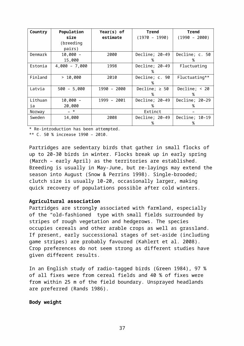
As described above yellow wagtails prefer dipterans, which are partly foliage-dwelling. Populations of foliar insects are however not well developed in short grass and quickly disappears after termination. Therefore the diet is assumed to be composed as shown in Table 5.24.

Table 5.24. Estimated diet composition of yellow wagtails feeding in grassland at different stages.Crop Stage PD (fresh weight)

Foliar arthropods Ground-dwelling arthropodsGrassland Sowing and

pre-emergence 1.00

Short 0.25 0.75Medium and long 0.50 0.50Termination 0.25 0.75

For ground-dwelling arthropods, interception in the crop canopy may be taken into account as appropriate for the growth stage in question.

5.1.7 White wagtail Motacilla alba

General informationThe white wagtail is a widespread and common species across most of Europe and occurs in farmland and other open habitats all over the Zone. European breeding populations appear to be mainly stable (BirdLife International 2004, Table 5.25).

Table 5.25. Population size and trends of white wagtail (breeding population) in the Nordic and Baltic countries. Sources: BirdLife International/European Bird Census Council (2000), BirdLife International (2004), Ottosson et al. (2012).Country Population size

(breeding pairs)Year(s) of estimate Trend

(1970 – 1990)Trend

(1990 – 2000)Denmark 100,000 – 150,000 2000 Increase; 20–49 % StableEstonia 100,000 – 150,000 1998 Stable StableFinland 600,000 – 900,000 1998 – 2002 Stable Decline, 10 % *Latvia 150,000 – 300,000 1990 – 2000 Stable Decline; 30–49 %Lithuania 400,000 – 500,000 1999 – 2001 Increase; 20–49 % StableNorway 100,000 – 500,000 1990 – 2003 Stable StableSweden 410,000 2008 Stable Decline; 19 %* A moderate increase was found for the farmland population 2001 – 2011 (Tiainen et al. 2008, 2012b).

Arrival at the breeding grounds is earlier than in yellow wagtail, the white wagtails arriving during late March and April across most of the Zone, stretching to early May in the northern-most part of the range. In Denmark, white wagtails breed from mid-April or May to July or (rarely) August and usually produce 2 broods per year. In the northern parts of the Zone white wagtails are usually single-brooded although 2 broods may occur. In Central Finland the first eggs are laid in early May, with the main breeding period being mid-May to early June and the last clutches appearing in the 2nd week of July; in southern Finland breeding occurs up to one week earlier (Cramp 1988). Autumn migration occurs from late August until mid-October, usually peaking in mod-September. The winter quarters are in the Mediterranean area and Northern Africa.

Agricultural associationThe white wagtail occurs in a wide range of open habitats, often near water. It is very common in the cultivated landscape, where it is often found in association with human

38

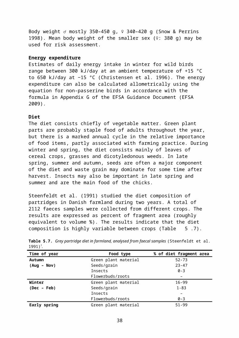
settlements and along roads, tracks and larger ditches. Patches of bare ground or with very low vegetation seem essential. The species is to some extent associated with grazing livestock, also in farmyards and small pens. Tall or dense vegetation is avoided. In farmland, white wagtails tend to prefer grassland with short turf and avoid tall, autumn-sown crops (Cramp 1988, Buxton et al. 1998).

In a Danish study in freshly drilled spring rape (Petersen 1996a), white wagtails were second only to skylarks in prevalence and abundance; the mean number of white wagtails foraging on the study fields was 0.045/ha/minute.

Body weightBody weight of both sexes mostly 17-25 g (Snow & Perrins 1998). Mean body weight (21 g) may be used for risk assessment.

Energy expenditureThe mean BMR of captive birds (mean weight 18.1 g) has been estimated at 25.1 kJ/day (Christensen et al. 1996). Alternatively, the energy expenditure can be calculated allo-metrically using the equation for passerine birds in accordance with the formula in Appendix G of the EFSA Guidance Document (EFSA 2009).

Diet White wagtails feed almost exclusively on invertebrates, mainly Diptera but also Coleoptera and other insects. They prefer small food items (2-7 mm). In farmland, white wagtails frequently forage in pastures, newly sown fields, ploughed fields, along ditches and other waterside habitats, in farmyards and along roads (Christensen et al. 1996).

In Western Europe, major studies of adult diet are available from England in late winter (Davies 1976, 1977) and from Austria all year (Glutz von Blotzheim & Bauer 1985). In England in March, birds feeding in flocks at pools took mainly Diptera (97 % by volume), while the diet of single birds feeding at dung pads comprised more than 75 % Diptera and 13 % Coleoptera (by number). In Austria, all year diet consisted of Diptera (37 % by number), Trichoptera (27 %), Coleoptera (16 %), Lepidoptera (11 %) and Orthoptera (5 %); a few seeds were also found.

There is no information on nestling diet from Western Palearctic. Studies from Kirgiziya indicate that the diet of nestlings is similar to adult diet (Christensen et al. 1996).

Like the yellow wagtail, white wagtails use three main foraging techniques: picking, run-picking and flycatching. In southern England, flock birds feeding at shallow pools employed picking exclusively, while single birds (feeding mainly at dung pads in pasture) used greater variety of techniques: picking (67 %), run-picking (14 %) and flycatching (19 %). Single birds took fewer, but probably larger, food items per minute than flock birds (Davies 1976, 1977).

There is no specific information on the diet of white wagtails feeding in arable land.

Risk assessmentThe white wagtail is a relevant focal species in early stages of all field crops and in most or all stages of crops where bare soil is present between the plants (rows). In grassland, assessment for white wagtail is covered by the smaller yellow wagtail.

39

The diet consists entirely of insects and other arthropods. Many of the preferred prey items, i.e. dipterans, are foliage-dwelling, so foliar arthropods are assumed to be included in the diet as soon as their populations are established in the fields during spring. For risk assessment puposes, their share of the diet may be assumed to be 25 % during development and 50 % at later stages.

The relevant scenarios are specified in Table 5.26.

Table 5.26. Estimated diet composition of white wagtails in different crops and growth stages.Crop Growth stage (BBCH) PD (fresh weight)

Foliar arthropods Ground-dwelling arthropodsWinter cereals 0-9 1Spring cereals 0-9, 10-14* 1Maize 0-9 1

10-29 0.25 0.75Winter rape 0-9, 10-19** 1

Post-harvest (stubble) 1Spring rape 0-9 1

10-19 0.25 0.75Post-harvest (stubble) 1

Beets 0-9 110-19 0.25 0.7520-49 0.50 0.50

Potatoes 0-9 110-19 0.25 0.7520-89 0.50 0.50Pre-harvest desiccation 0.25 0.75

Pulses 0-9 110-19 0.25 0.7520-79 0.50 0.50

Field grown vegetables 0-9 110-19 0.25 0.7520-89 0.50 0.50

Strawberries Planting (10-19) 0.25 0.7520-89 0.50 0.50Post-harvest 0.50 0.50

* Tillering occurs from stage 13-14, making the field unsuitable for white wagtails.** In autumn-sown rape, BBCH 10-19 is passed in autumn or early spring when foliar arthropods are not present in the field.

For ground-dwelling arthropods, interception in the crop canopy shall be taken into account as appropriate for the crop and growth stage in question, cf. section 4.5.

Species-specific data allowing a refinement of PT are not available.

5.1.8 Robin Erithacus rubecula

General informationThe robin is widespread and abundant all over the Zone, except in the northernmost parts. Its primary habitat is forest and woodland (coniferous, deciduous or mixed) but robins are also common in parks, gardens and other humanly managed and disturbed habitats (Snow & Perrins 1998), although not in the north (Finland). Population fluctuations, partly related to

40

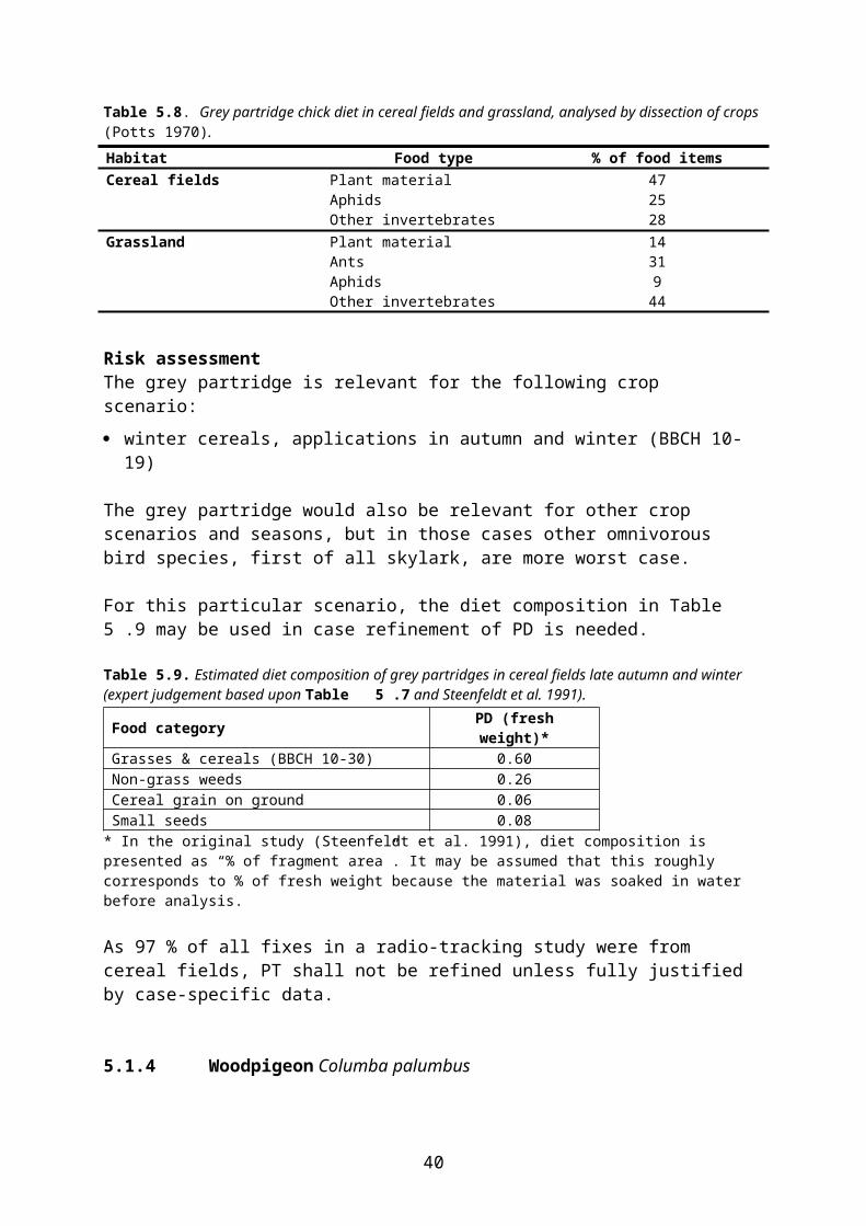
the winter temperatures, are not infrequent, but overall North European breeding populations seem to be largely stable (Table 5.27).

Table 5.27. Population size and trends of robin (breeding population) in the Nordic and Baltic countries. Sources: BirdLife International/European Bird Census Council (2000), BirdLife International (2004), Ottosson et al. (2012).Country Population size

(breeding pairs)Year(s) of estimate Trend

(1970 – 1990)Trend

(1990 – 2000)Denmark 200,000 – 300,000 2000 Fluctuating FluctuatingEstonia 250,000 – 500,000 1998 Stable StableFinland 1,200,000 – 3,300,000 1998 – 2002 Fluctuating Increase; 65 %Latvia 700,000 – 1,000,000 1990 – 2000 Stable StableLithuania 800,000 – 1,500,000 1999 – 2001 Stable StableNorway 500,000 – 1,500,000 1990 – 2002 Increase; 20–49 % StableSweden 3,800,000 2008 Stable Decline; 20 %

Robins breeding within the Zone are generally migratory, but a minor part of the Danish, South Swedish and Norwegian populations stay in the area throughout the year, particularly in mild winters. Winter quarters are in W and SW Europe and NW Africa. The migrants arrive in late March and April and depart from mid-August to mid-November (Snow & Perrins 1998). Breeding is from late April to end of July in the south but does not start until mid- or late May in the northern part of the Zone. Usually double-brooded in the south and single-brooded in the north (Snow & Perrins 1998).

Agricultural associationAlthough robins are not infrequent in hedgerows and coverts in farmland, the species is not considered relevant for field crops due to its habitat preferences of forest, parks and gardens (Svensson et al. 1999, Larsen & Heldbjerg 2009).

The species is, however, fairly common in orchards and nurseries. In a study of orchards in the UK, 29 robins were radio-tracked to estimate the active time spent in this habitat (Crocker et al. 1998, Finch & Payne 2006, Prosser 2010). The results are summarized in Table 5.28.

Table 5.28. Percentage of active time spent by radio-tagged robins in orchards in the UK, presented as 90th percentile of the modelled PT distribution. The birds were caught inside the orchard or along the orchard edge; it is therefore recommended to use the values for the total sample of tracked birds (bold).Crop Period No. of birds Mean 90 percentile ReferenceAll birds:Orchard Apr – Sep 29 0.21 0.53 Finch &

Payne 200629 0.51 Prosser 2010

Consumers only:Orchard Apr – Sep 24 0.25 0.56 Finch &

Payne 200624 0.54 Prosser 2010

Body weightBody weight ♂ mostly 15–21 g, ♀ 14–19 g (Snow & Perrins 1998). Mean body weight of the smaller sex (♀: 16.5 g) may be used for risk assessment.

Energy expenditure

41

No species specific data available, therefore calculated allometrically using the equation for passerine birds in accordance with the formula in Appendix G of the EFSA Guidance Document (EFSA 2009).

Diet The diet during the breeding season consists of invertebrates both for adults and nestlings. Foraging is done mainly on ground living invertebrates, but robins sometimes take prey from branches or leaves. In a study between March-May of hedgerow inhabiting robins in northern Germany, faecal samples showed that Coleoptera constituted the main part of the diet (Table 5.29). Other data from northern Europe are apparently not available.

Table 5.29. Diet composition of adult robins in a hedgerow habitat (Grajetzky 1993).Time of year Food type % of dietMarch-May (n=445) Coleoptera 61

Diptera 18Diplopoda 6Hymenoptera 5Arachnida 4Collembola/Others 6

Risk assessmentThe robin is a relevant focal species in orchards (fruit trees), ornamentals and nursery cultures, as specified below:

Fruit trees: ground directed applications (herbicides) Ornamentals and nursery: pre-emergence, small plants (all treatments), large plants

(ground directed applications)

As a ground feeder, robin is particularly relevant for ground directed applications, including applications to small plants. For canopy directed applications blue tit is more worst case.

For all exposure scenarios the diet may be assumed to consist entirely of ground-dwelling invertebrates (PD = 1). No interception shall be taken into account for the above-mentioned scenarios.

PT may be refined using the information in Table 5.28.

5.1.9 Whinchat Saxicola rubetra

General informationThe whinchat occurs in open areas, from semi-dry heathlands and clear cut forest to humid meadows and edges of marshes with suitable perches such as fences, bushes and tall weeds. It may be found all over the Zone although its occurrence in Denmark is now rather sparse. Whinchat populations have declined strongly across Western and Central Europe during recent decades (BirdLife International 2004); e.g. in Denmark the average annual decline during 1981-2011 was as high as 5.56 % (Heldbjerg & Lerche-Jørgensen 2012). Northern and eastern populations have apparently fared better (Table 5.30), maybe partly as a result of large-scale abandonment of arable land in the Baltic States during the 1990s. In Finland the farmland population has been more or less stable at least since the early 1980s (Tiainen et al. 1985, 2008, 2012a,b), probably due to a still heterogenous landscape structure.

42

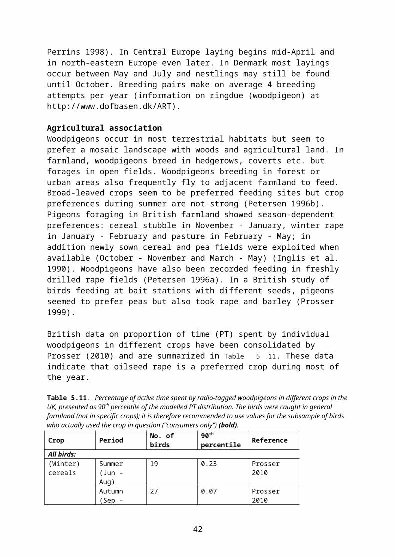
Table 5.30. Population size and trends of whinchat (breeding population) in the Nordic and Baltic countries. Sources: BirdLife International/European Bird Census Council (2000), BirdLife International (2004), Ottosson et al. (2012).Country Population size

(breeding pairs)Year(s) of estimate Trend

(1970 – 1990)Trend

(1990 – 2000)Denmark 5,000 – 10,000 2000 Decline; 20–49 % Decline; 50 %Estonia 50,000 – 150,000 1998 Increase; 20–49 % StableFinland 300,000 – 400,000 1998 – 2002 Decline; 20–49 % * Decline; 30 % *Latvia 300,000 – 500,000 1990 – 2000 Stable Increase; 20–49 %Lithuania 50,000 – 120,000 1999 – 2001 Decline; 20–49 % Increase; < 20 %Norway 50,000 – 300,000 1990 – 2003 Stable StableSweden 250,000 2008 Stable Increase; 11 %* Farmland populations have been more or less stable since at least the early 1980s (Tiainen et al. 2008, 2012b).

Whinchats are long-distance migrants that winter in tropical Africa. They arrive at the breeding grounds mainly during May and depart in August-September. Breeding begins soon after arrival in May, or in early June in the northern part of the Zone. Whinchats are usually single-brooded in Northern Europe, but re-layings occur in case of nest loss, implying that breeding activities may take place until mid-July (Glutz von Blotzheim & Bauer 1988).

Agricultural associationIn Western and Central Europe, whinchats are mainly associated with extensively managed grassland types, especially extensively grazed pasture and hay meadows which are not mown before July. Intensively managed grassland and arable crops are avoided, although exceptional breedings have been recorded in cereal, potato and clover fields (Cramp 1988, Glutz von Blotzheim & Bauer 1988).

Whinchats seem to occur more frequently in arable or mixed farmland in North Europe. In a Latvian study, the species was strongly associated with abandoned fields (Aunins et al. 2001). In Finland the CAP set-asides, and since 2008 the environmental fallow scheme, has favoured the whinchat, which also benefits on eutrofication of verge vegetation of larger drainage ditches (Herzon et al. 2011, Tiainen et al. 2012a). In Norway whinchats were frequently recorded in cereal fields from mid-summer until the onset of autumn migration (Hage et al. 2011).

Population densities in northern Europe are mostly between 0.1 and 1.3 pairs per 10 ha (Glutz von Blotzheim & Bauer 1988).

Body weightBody weight of both sexes mostly 14–19 g (Snow & Perrins 1998). Mean body weight (16.5 g) may be used for risk assessment.

Energy expenditureNo species specific data available, therefore calculated allometrically using the equation for passerine birds in accordance with the formula in Appendix G of the EFSA Guidance Document (EFSA 2009).

Diet The diet in Europe consists almost exclusively of invertebrates. A few seeds also occur in the diet and berries are taken during autumn migration. Hunts from perch, flying to and taking prey mainly from ground or in vegetation (Cramp 1988).

43

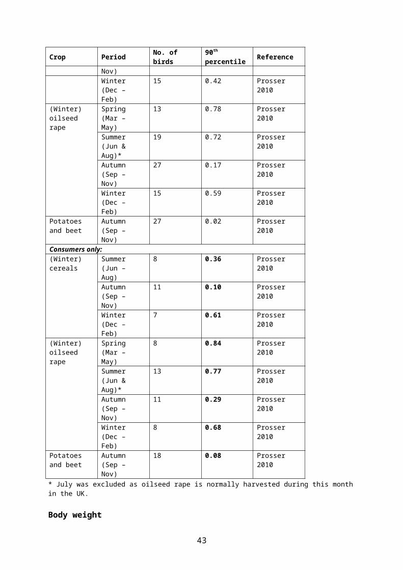
Adult diet is mainly insects and is often dominated by Coleoptera, Hymenoptera and/or Diptera, but also Orthoptera, Dermaptera, Heteroptera and Lepidoptera (imagines and larvae) occur frequently. Other animal food items occurring in adult diet are spiders, snails and Oligochaeta (Glutz von Blotzheim & Bauer 1988). Quantitative studies of adult diet are apparently few; in a Ukranian study 98 % of the food items were insects, mainly Coleoptera (70 %) (n = 14 stomachs, Kusmenko 1977 cited by Glutz von Blotzheim & Bauer 1988).

Nestling diet has been studied in Poland and Switzerland. In the Polish study the most common food items in diet were adult Lepidoptera (24.8 % by number), Lepidoptera and Symphyta larvae (15.9 %), Tipulidae (14.5 %) and Orthoptera (12.8 %) (Steinfatt 1937 cited by Glutz von Blotzheim & Bauer 1988). The results of the Swiss study are summarized in Table 5.31.

Table 5.31. Whinchat nestling diet in two areas of canton Waadt, Switzerland (Labhardt cited by Glutz von Blotzheim & Bauer 1988). Time of year Food type % of diet (by number)

Les Moulins/Pays d’Enhaut (n = 4198)

Les Mosses(n = 1531 items)

Breeding season Hymenoptera1 27 60Coleoptera 27 2Diptera 21 12Lepidoptera2 14 19Orthoptera 3 3Heteroptera 1Gastropoda 3 2Araneidae 2 2Oligochaeta 1

1 almost exclusively Symphyta larvae2 mainly larvae.

Risk assessmentThe whinchat is relevant for the following crop scenarios:

cereals (winter and spring), BBCH 40-89 cereals (winter and spring), pre-harvest desiccation

Based on the studies summarized above, the diet may be assumed to consist of 75 % foliar arthropods and 25 % ground-dwelling arthropods. Following pre-harvest desiccation with herbicides, the crop in most cases will be wilted, and associated foliar arthropods will be gone, within one week. The proportion of foliar arthropods in diet will therefore be strongly reduced; Table 5.32.

Table 5.32. Estimated diet composition of whinchats feeding in cereal fields at different stages.Crop Stage PD (fresh weight)

Foliar arthropods Ground-dwelling arthropodsCereals BBCH 40-89 0.75 0.25

Pre-harvest desiccation 0.35 0.65

Interception shall be considered for ground-dwelling arthropods, as appropriate for the growth stage in question.

There are no species-specific data allowing a refinement of PT.

44

5.1.10 Whitethroat Sylvia communis

General informationThe whitethroat is widespread and abundant in Denmark, the Baltic States, southern and western Norway, southern Sweden and southern Finland. It is generally absent from the boreal and montane parts of the Scandinavian peninsula (north of the 14 °C July isotherm), where its occurrence is largely limited to areas near the coast (Cramp 1992).

Whitethroat populations in western and central Europe crashed around 1970, due to several years of serious drought in their sub-Saharan winter quarters (e.g. Marchant et al. 1990), while east European populations were less affected. Since the mid-1970s whitethroat populations have been rather stable with some tendencies of increase (Table 5.33). Whitethroats in south Finnish farmland show an increasing trend before 1984, stability in 1984-2000 and moderate increase in 2001-2011 (Tiainen et al. 2008, 2012b).

Table 5.33. Population size and trends of whitethroat (breeding population) in the Nordic and Baltic countries. Sources: BirdLife International/European Bird Census Council (2000), BirdLife International (2004), Ottosson et al. (2012).Country Population size

(breeding pairs)Year(s) of estimate Trend

(1970 – 1990)Trend

(1990 – 2000)Denmark 300,000 – 450,000 2000 Decline; 20–49 % FluctuatingEstonia 100,000 – 200,000 1998 Increase; 20–49 % StableFinland 250,000 – 400,000 1998 – 2002 Stable Decline; 10 %Latvia 300,000 – 500,000 1990 – 2000 Stable Increase; 50–79 %Lithuania 400,000 – 500,000 1999 – 2001 Stable StableNorway 50,000 – 300,000 1990 – 2003 Stable StableSweden 250,000 2008 Increase; 20–49 % Increase; 31 %

The whitethroats arrive at their breeding grounds during May, with arrivals stretching into June in the northernmost part of the range. They start breeding shortly after arrival, i.e. from mid-May in Denmark. In Finland, egg-laying may occur from the 3rd week of May and normally peaks during the first half June (von Haartman 1969). Whitethroats are usually single-brooded in northern Europe although two broods may occur. The breeding season ends in July and the birds leave mainly between early August and early September.

Agricultural associationWhitethroats are found chiefly in open countryside with hedgerows, shrubs and bushy verges of larger drainage ditches, but also occupy early successional woodland, forest edges and clearings. In farmland, whitethroats are usually dependent on the presence of hedgerows, scrub or rough herbage for breeding but they may also establish territories and attempt nesting in winter rape (Persson 1971, Cavallin 1988). The species may also occur in orchards (Cramp 1992).

The general density in large agricultural landscapes in Finland was 0.12 – 0.25 territories/ha (Tiainen & Seimola 2010). In Åland the density was 1.7 territories/ha in bushes in open agricultural landscape, 0.6 in environmental fallow fields, 0.55 in dry meadows, 0.12 in field pastures, 0.044 in leys, 0.015 in spring cereals and 0.006 in dicotyledonous crops (Tiainen et al. 2012a).

Whitethroats breeding in winter rape fields probably perform most of their foraging inside the field. Apart from this, the species forages mainly in hedgerows, scrub and tall herbage.

45

Various agricultural crops are also used, especially where adjacent to hedgerows, coverts etc. In a Danish study, whitethroats breeding in hedgerows spent only 8 % of their foraging time in crops (Sell & Odderskær 1990), but the percentage may be somewhat higher where suitable conditions prevail. Esbjerg & Petersen (2002) found that whitethroats increased their use of the fields for feeding significantly if herbicide and insecticide use was reduced.

With the exception of winter rape, the crop preferences of whitethroats are not strong. The main requirement may be that crop density and biomass shall be sufficiently high to provide cover and hold an ample population of arthropods. Leafy crops may be preferred. Esbjerg & Petersen (2002) found densities of foraging whitethroats of up to 1 per ha in beet fields during the 2nd half of July; densities in winter and spring cereals were somewhat lower.

After the breeding season, i.e. from about mid-July, whitethroats frequently feed in orchards with bush berries.

Body weightBody weight of both sexes mostly 13-18 g (Snow & Perrins 1998). Mean body weight (15.5 g) may be used for risk assessment.

Energy expenditureThe daily energy expenditure can be calculated allometrically using the equation for passerine birds in accordance with the formula in Appendix G of the EFSA Guidance Document (EFSA 2009).

Diet In spring and during the breeding season, whitethroats feed almost exclusively on arthropods, particularly Heteroptera, Coleoptera, Hymenoptera and Lepidoptera. In late summer, fruits and berries enter the diet. Nestlings are fed insects and other invertebrates.

Whitethroats forage mainly in low trees, bushes and herbage (including agricultural crops) by searching the foliage and small branches. Less frequently, insects are taken in flight or from the ground (Christensen et al. 1996).

The occurrence of fruits and berries in the diet has been studied in East Germany (Emmrich 1973 cited in Cramp 1988). The results are presented as the percent of stomachs containing the fruit type in question (Table 5.34); all other food items were invertebrates.

Table 5.34. The occurrence of fruits in stomachs of whitethroats from East Germany. n = no. of stomachs analysed. (Emmrich 1973 cited in Cramp 1988).Time of year Food type % of stomachs with food item4-31 May Ribes fruit 18(n = 11)18 Jul – 19 Aug Rubus fruit 52(n = 32) Ribes fruit 28

Hippophaë fruit 6other fruits 3

22 Aug – 11 Sep Sambucus fruit 56(n = 9) Ribes fruit 44

Rubus fruit 22other fruits 11

Risk assessment

46

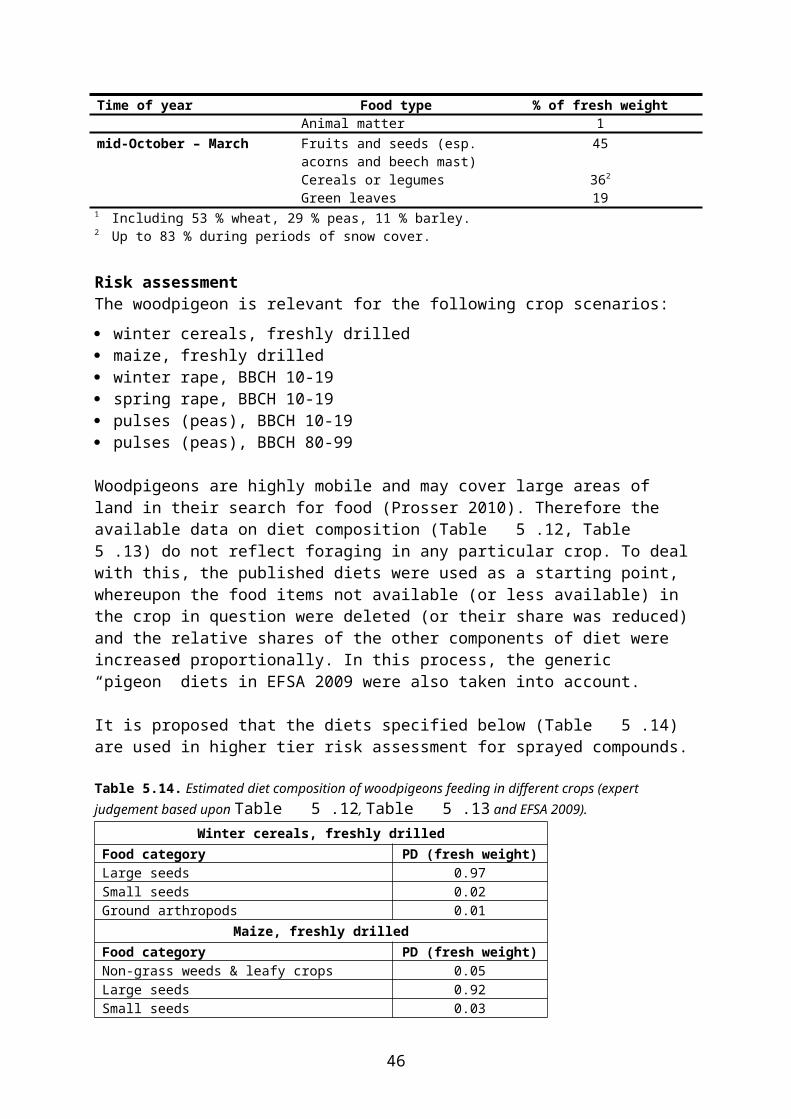
The whitethroat is relevant for the following crop scenarios:

winter rape, from development of flower buds to laying in swaths (BBCH 40-89) spring rape, from development of flower buds to laying in swaths (BBCH 40-89) bush berries, during development and ripening of fruits (BBCH 70-89) (canopy directed

applications)

In rape fields, the diet of whitethroats may be assumed to consist entirely of foliar arthropods (PD = 1). In bush berries, when fruits are present, the diet may be assumed to consist of 50 % berries and 50 % foliar arthropods (by fresh weight).

Whitethroats holding territories in rape fields may be assumed to perform almost all of their feeding within the field (PT ≈ 1), but for the general farmland population PT may be as low as 0.08 (cf. Sell & Odderskær 1990).

There are no species-specific data allowing a refinement of PT for whitethroats feeding in orchards.

5.1.11 Willow warbler Phylloscopus trochilus

General informationThe willow warbler is a widespread and abundant species throughout the zone. Its main habitat is birch forest, where it may be extremely numerous, but it also occurs in other types of forest and woodland, scrub (including willows) and second growth. It is often attracted to fringe areas, including forest clearings, especially with birches. Being a forest generalist species it often fits readily into small and shifting ecological niches (Snow & Perrins 1998).

Willow warblers are trans-Saharan migrants and, as in many other species wintering in tropical Africa, the European populations have suffered some recent declines. Still, it may well be the most numerous bird species in Fennoscandia (Table 5.35).

Table 5.35. Population size and trends of willow warbler (breeding population) in the Nordic and Baltic countries. Sources: BirdLife International/European Bird Census Council (2000), BirdLife International (2004), Ottosson et al. (2012).Country Population size

(breeding pairs)Year(s) of estimate Trend

(1970 – 1990)Trend

(1990 – 2000)Denmark 400,000 – 600,000 2000 Stable Decline; 10–19 %Estonia 800,000 – 2,000,000 1998 Stable Increase; 20–29 %Finland 7,000,000 – 11,000,000 1998 – 2002 Stable Decline; 15 %Latvia 500,000 – 600,000 1990 – 2000 Stable StableLithuania 400,000 – 600,000 1999 – 2001 Stable StableNorway 2,000,000 – 10,000,000 1995 – 2002 Stable StableSweden 13,000,000 2008 Increase; 20–49 % Decline; 14 %

Willow warblers arrive at their breeding grounds from mid-April until the end of May. Main arrival is from 21 April to 15 May in southern and central Sweden, 11-25 May in northern Sweden. At Lake Ladoga, near the Gulf of Finland, most local birds arrive 15-20 May (Snow & Perrins 1998). Egg-laying occurs mainly between late May and mid-June in Fennoscandia, with an average delay of 1,0 – 1.5 days per degree of latitude (Tiainen 1991). Willow warblers are considered single-brooded in Fennoscandia, but in case of nest loss re-layings may occur until early or mid-July (Tiainen 1991). Autumn migration begins in late July,

47

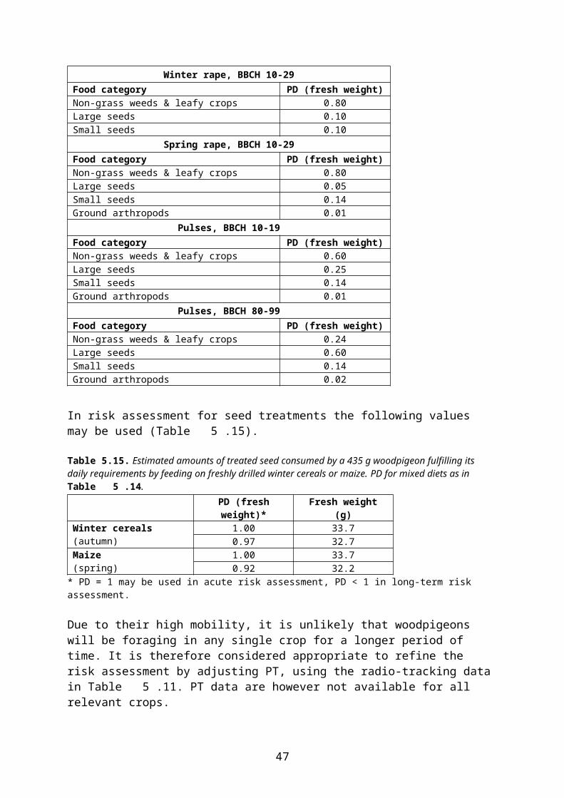
peaks during the 2nd half of August, and the last birds leave the breeding areas in late September.

Agricultural associationIn the Central European lowlands and the British Isles, and also in the southern part of the Northern Zone, willow warblers are linked with arboreal habitats and in farmland areas the species occurs in hedgerows, trees and shrub around ponds, and other non-crop habitats (Glutz von Blotzheim & Bauer 1991, Petersen 1998). Williow warblers may occur in orchards (Cramp 1992) but are apparently not reported from arable crops. Further north the niche is broader, reflecting more generalistic habits. In Norway the species is frequently found in maize fields and also occur, albeit less frequently, in oilseed rape, field grown vegetables and bush berries (Hage et al. 2011).

Body weightBody weight is mostly 7-12 g (Snow & Perrins 1998); females are c. 10 % lighter than males (J. Tiainen pers. comm.). Mean body weight (9.5 g) may be used for risk assessment.

Energy expenditureThe daily energy expenditure can be calculated allometrically using the equation for passerine birds in accordance with the formula in Appendix G of the EFSA Guidance Document (EFSA 2009).

Diet The diet consists of insects and spiders, and in autumn also some berries. Food is obtained mostly by picking from leaves, twigs and branches, but hovering, fly-catching in air and ground feeding are also used (Cramp 1992). Food choice largely reflects availability but Diptera, Hymenoptera and larval Lepidoptera seem to be preferred (Glutz von Blotzheim & Bauer 1991).

Many quantitative studies of diet exist, but in almost all studies diet composition was reported as percent (or number) of food items. Furthermore, these studies are assumed to reflect diet composition in wooded habitats. However, in a study of spring migrants on a Danish island, willow warbler diet composition (as determined by stomach flushing) was also reported as percent of dry weight (Table 5.36).

Table 5.36. Diet composition of willow warblers staging on the island of Hjelm, Denmark (Laursen 1978 cited by Buxton et al. 1998).Time of year Food type % of diet dry weightMay Homoptera (Aphididae, Psylloidea) 37

Diptera 24Lepidoptera larvae 21Coleoptera (mainly Curculionidae) 7Hymenoptera (mainly Tenthredinoidea) 7Araneae 5

Risk assessmentThe willow warbler is relevant for the following crop scenario:

maize, BBCH 30-39

The diet may in be assumed to consist almost entirely of foliar arthropods; judged from the above- metioned study (Table 5.36) ground arthropods make up ≤ 5 % of diet.

48

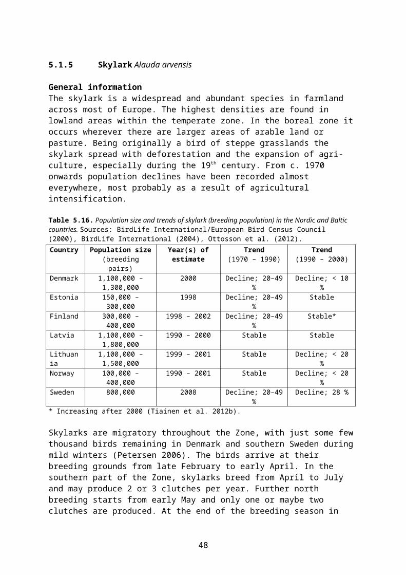
There are no species-specific data allowing a refinement of PT.

5.1.12 Blue tit Cyanistes caeruleus

General informationThe blue tit is widespread and common throughout the Zone south of the July isotherm of 14°C (Snow & Perrins 1998). Its primary habitat is deciduous woodland but it also occurs in coppice, overgrown marshes and mires etc. The species is frequent in parks, gardens and other man-made habitats, provided suitable nest-holes are available.

Blue tits are resident in the southern part of the Zone while birds from northern populations are partial migrants. Northern birds make irregular eruptive movements, mainly towards south-west (Snow & Perrins 1998). Populations may be somewhat fluctuating, perhaps related to winter temperatures, but overall numbers have probably increased during recent decades (Table 5.37).

Table 5.37. Population size and trends of blue tit (breeding population) in the Nordic and Baltic countries. Sources: BirdLife International/European Bird Census Council (2000), BirdLife International (2004), Ottosson et al. (2012).Country Population size

(breeding pairs)Year(s) of estimate Trend

(1970 – 1990)Trend

(1990 – 2000)Denmark 200,000 – 250,000 2000 Fluctuating FluctuatingEstonia 50,000 – 100,000 1998 Increase; 20–49 % Increase; 20–29 %Finland 400,000 – 650,000 1998 – 2002 Increase; ≥ 50 % Increase; 220 %Latvia 100,000 – 140,000 1990 – 2000 Stable StableLithuania 70,000 – 110,000 1999 – 2001 Stable StableNorway 100,000 – 200,000 1990 – 2002 Stable Increase; < 20 %Sweden 700,000 2008 Stable Decline; 3 %

Over much of central and northern Europe egg-laying begins mostly in the last week of April and the first few days of May (Snow & Perrins 1998), maybe a little later further north. Median laying date is 7 May in South-west Sweden and South Finland (Cramp & Perrins 1993, Glutz von Blotzheim & Bauer 1993). Blue tits are usually single-brooded, but in some populations 10 to 50 % of the breeding pairs may produce a 2nd clutch in some years (Cramp & Perrins 1993, Glutz von Blotzheim & Bauer 1993). Clutch size (mostly 10-12, occasionally 16-18) is the largest among European passerines.

Agricultural associationBlue tits are fairly common in rural gardens, deciduous hedgerows and habitat islands, but the species is not considered relevant for field crops due to its habitat preferences of broad-leaved forest, parks and gardens (Svensson et al. 1999, Larsen & Heldbjerg 2009). The habitat preferences include orchards and nurseries, provided suitable nest-holes are available.

In a study of orchards in the UK, 20 blue tits were radio-tracked to estimate the active time spent in this habitat (Crocker et al. 1998, Finch & Payne 2006, Prosser 2010). The results are summarized in Table 5.38.

49

Table 5.38. Percentage of active time spent by radio-tagged blue tits in orchards in the UK, presented as 90th percentile of the modelled PT distribution. The birds were caught inside the orchard or along the orchard edge; it is therefore recommended to use the values for the total sample of tracked birds (bold).Crop Period No. of birds Mean 90 percentile ReferenceAll birds:Orchard Apr – Sep 20 0.21 0.55 Finch &

Payne 200620 0.53 Prosser 2010

Consumers only:Orchard Apr – Sep 16 0.27 0.58 Finch &

Payne 200616 0.57 Prosser 2010

Body weightBody weight of both sexes mostly 9.5 – 12.5 g (Snow & Perrins 1998). Mean body weight (11 g) may be used for risk assessment.

Energy expenditureNo species specific data available, therefore calculated allometrically using the equation for passerine birds in accordance with the formula in Appendix G of the EFSA Guidance Document (EFSA 2009).

Diet Blue tits are mostly foraging in the foliage of trees and bushes (Cramp and Perrins 1993). Ground-feeding occurs mainly in winter, when searching for beech mast etc. In an English study, the percentage of feeding observations on the ground was as follows: January-February 10-15, March 4, April 2, May-August 0, September-October 1, November 5, December 7 (Gibb 1954 cited in Cramp & Perrins 1993).

The diet of blue tits is reflecting seasonal changes with more seeds and fruits in winter and almost exclusively invertebrates in the breeding season (Cramp and Perrins 1993). In SW England, nuts and seeds from trees (beech, oak, chestnut, birch) were found in 13 % of blue tit gizzards in September, 59 % in October, 44 % in November, 40 % in December, 31 % in January, 7 % in February and 0 % in March-August (Betts 1955 cited in Cramp & Perrins 1993). More detailed, quantitative data on diet composition are apparently not available, but invertebrates almost certainly make up the bulk of the diet throughout the year. The nestling diet consists of invertebrates (Cowie and Hinsley 1988).

Risk assessmentThe blue tit is relevant for the following scenarios:

fruit trees, canopy directed applications bush berries, canopy directed applications ornamentals and nursery, canopy directed applications

During March - September, the diet may be assumed to consist entirely of foliage arthropods (PD = 1). Outside this period, nuts and seeds from trees enter the diet but probably never make up more than 50 %; this part of the diet shall be regarded as unsprayed.

For applications in (March) April - September, PT may be refined using the information in Table 5.38.

50

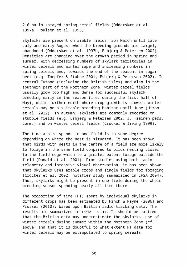
5.1.13 Starling Sturnus vulgaris

General informationNorth European starling populations have suffered pronounced declines in recent decades but the species is still common and widespread across most of the Zone (Table 5.39). Starlings depend on open areas, such as grassland, field crops or floodlands, for foraging, but also need suitable holes (natural or man-made) for nesting. Through more than a century, the starling benefited from the clearing of forests, establishment of human settlements and spread of agriculture in northern Europe. Its range and population size probably reached a maximum during the 1960s, after which most populations have declined (Rintala & Tiainen 2007, 2008). Agricultural intensification in general, and structural changes within farmland in particular, may well be the main reasons for the decline. At least in Finland, the major driver was probably the dramatic decline of dairy husbandry and the consequent decrease in availability of good Starling habitat (Rintala & Tiainen 2007, 2008).

Table 5.39. Population size and trends of starling (breeding population) in the Nordic and Baltic countries. Sources: BirdLife International/European Bird Census Council (2000), BirdLife International (2004), Ottosson et al. (2012).Country Population size

(breeding pairs)Year(s) of estimate Trend

(1970 – 1990)Trend

(1990 – 2000)Denmark 400,000 – 600,000 2000 Decline; 20–49 % Decline; 20–29 %Estonia 20,000 – 50,000 1998 Decline; ≥ 50 % Decline; 20–29 %Finland 30,000 – 60,000 1998 – 2002 Decline; ≥ 50 % Decline; 30 %Latvia 50,000 – 250,000 1990 – 2000 Decline; ≥ 50 % Decline; < 20 %Lithuania 250,000 – 300,000 1999 – 2001 Stable StableNorway 200,000 – 500,000 1990 – 2003 Decline; 20–49 % Decline; 20–29 %Sweden 640,000 2008 Decline; ≥ 50 % Decline; 12 %

The species is generally migratory within the Zone, albeit with an increasing tendency for urban starlings to remain resident in South Sweden, Denmark and southern and western Norway, especially in mild winters (Snow & Perrins 1998). Winter quarters are mainly in the Channel area.

Arrival in spring is in early March in the south, continuing throughout April in the north. Starlings are semi-colonial and breeding is synchronized, with almost all layings occurring in late April and early May in Denmark and southern Sweden and one week later in northern Finland (Cramp & Perrins 1994a). Usually single-brooded but two broods may occur, especially in the southern parts of the Zone. Most young fledge between late May and mid-June. In late June and July juveniles and some adults disperse, mainly in a south-westerly direction and often over several hundred km, to gather at suitable feeding areas, e.g. in the Wadden Sea area. The breeding grounds may thus be vacated after midsummer, but in many areas within the Zone large flocks may be found foraging on pastures until September. Autumn migration takes place mostly between mid-September and early November.

Agricultural associationStarlings are associated with open country, particularly grasslands. They breed in open forest, woodland edge, around farms, in villages and in urban areas, but always near grassland (including lawns, golf courses etc.).

Feeding is mainly on the ground in open areas of short grass, but salt marshes and intertidal zones are also used, particularly during migration. Among the different categories of

51

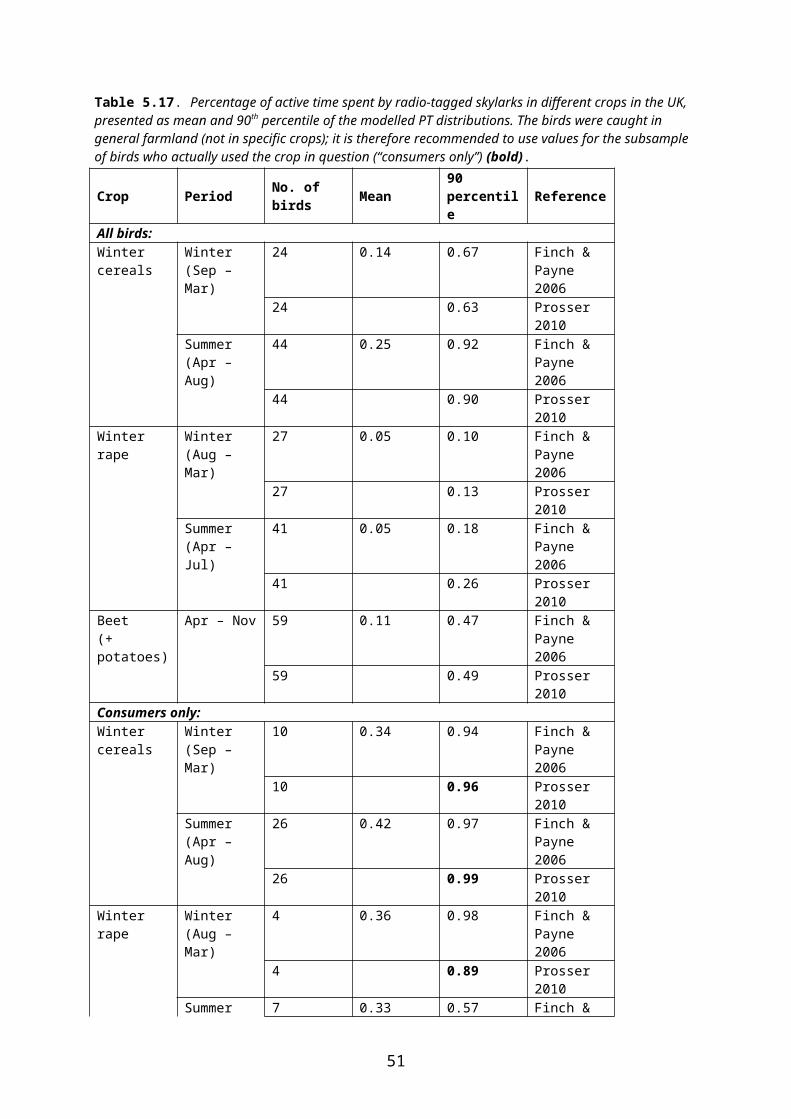
grassland, rotational or permanent pastures and old leys are preferred (Tiainen et al. 1989, Whitehead et al. 1995, Petersen 1996b). In late summer and autumn, stubble fields, newly sown fields, orchards and thickets with berries are also used; e.g., in southern England up to 40 % of the foraging birds were recorded in stubble fields and up to 10 % in trees (Christensen et al. 1996).

Body weightBody weight somewhat variable, ♂ mostly 70–90, ♀ mostly 60–90 g (Snow & Perrins 1998). Mean body weight of the smaller sex (♀: 75 g) may be used for risk assessment.

Energy expenditureAccording to English data, the daily energy expenditure is highest in spring (c. 290 kJ/day) and lowest in summer (c. 200 kJ/day) (Christensen et al. 1996). The intake of captive adult starlings was 210-265 kJ/day if kept on animal food. Alternatively, the energy expenditure can be calculated allometrically using the equation for passerine birds in accordance with the formula in Appendix G of the EFSA Guidance Document (EFSA 2009).

Diet The diet consists of animal as well as vegetable matter throughout the year, but the relative proportions vary with the annual cycle (and are parallelled by changes in the length of the intestine). Invertebrates dominate in spring and summer while vegetable matter comprises a high proportion of the diet during autumn and winter. The proportion of vegetable matter in the diet is less than 50 % from April to June and 50-95 % during the rest of the year (Christensen et al. 1996). In a Polish study of adult diet, 85 % of all food items were animal during February-September (Gromadzki 1969), and in a similar Czech study, 69 % of all food items were animal in March-November (Havlin & Folk 1965), see also Table 15. In both of these studies, almost no vegetable food items were taken between March and June.

Invertebrate food is taken from the soil surface or just below the soil surface by bill-probing. Insects such as Coleoptera, Diptera (e.g. Tipula) larvae, Hymenoptera and Lepidoptera larvae dominate but spiders and earthworms also occur in the diet. Nestling diet consists almost entirely of invertebrates (mainly Coleoptera, Diptera and Lepidoptera).

Vegetable food is mainly seeds, including cereal grain, but also fruits during summer and autumn. In a Polish study of 85 stomachs, cultivated fruits were found in up to 70 % of stomachs (varying proportions in different months), cereal grain in up to 60 %, wild seeds in up to 40 % and wild fruits in up to 30 % (Gromadzki 1969).

Havlin & Folk (1965) studied the composition of diet in adult starlings in Czechoslovakia during March-November by means of stomach analysis. The results are presented as percentage of food items (Table 5.40).

Table 5.40. Diet composition of adult starlings in Czechoslovakia (Havlin & Folk 1965).Time of year Food type % of food itemsMarch – November Hymenoptera (mainly ants) 30.5(n = 9917) Coleoptera 27.0

Wild fruit 19.1Cultivated fruit 7.3Diptera 6.6Ceral grain 3.4Spiders 1.4

52

Lepidoptera 1.4Wild seeds 0.7Others 2.5

Risk assessmentBeing a partial frugivore, the starling is relevant for the following scenarios:

strawberries, BBCH 60-89 fruit trees (cherry, plum), canopy directed applications during BBCH 60-89

The starling would also be relevant in grassland, which is its main foraging habitat, but here smaller species, such as yellow wagtail, are more worst case.

Based on the information presented above, the following composition of diet may be assumed for these scenarios (Table 5.41).

Table 5.41. Estimated diet composition to be used in risk assessment for starlings feeding on strawberries, cherries or plums.

Strawberries, BBCH 60-89Food category PD (fresh weight)Large seeds 0.04Small seeds 0.01Berries 0.27Ground arthropods 0.68

Orchard (plum, cherry), canopy directed applications during BBCH 60-89Food category PD (fresh weight)Large seeds 0.04Small seeds 0.01Small fruit from orchards 0.27Ground arthropods 0.68

For those elements of the diet which are obtained from the ground, i.e. seeds and ground arthropods, interception in the crop or canopy shall be taken into account.

It is highly probable that not all of the food will be obtained within the treated area (PT < 1). However, specific data allowing a refinement of PT are not available.

5.1.14 Chaffinch Fringilla coelebs

General informationThe chaffinch is one of the most numerous breeding bird species in northern Europe. It is widespread and abundant throughout the Zone south of the July isotherm of 12°C (Snow & Perrins 1998). The breeding populations are apparently mainly stable (Table 5.42).

Table 5.42. Population size and trends of chaffinch (breeding population) in the Nordic and Baltic countries. Sources: BirdLife International/European Bird Census Council (2000), BirdLife International (2004), Ottosson et al. (2012).Country Population size

(breeding pairs)Year(s) of estimate Trend

(1970 – 1990)Trend

(1990 – 2000)Denmark 1,500,000 – 2,000,000 2000 Increase; 20–49 % StableEstonia 1,500,000 – 2,500,000 1998 Stable Stable

53

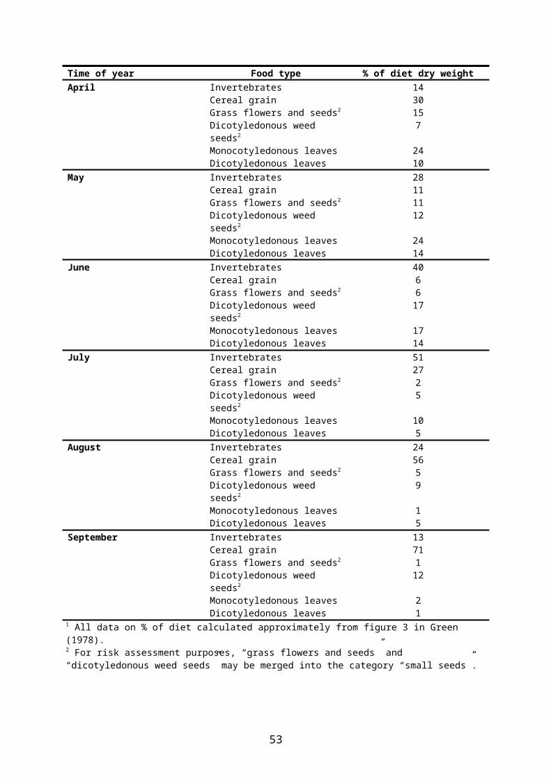
Finland 5,000,000 – 7,000,000 1998 – 2002 Decline; 20–49 % StableLatvia 2,600,000 – 3,200,000 1990 – 2000 Stable StableLithuania 2,500,000 – 3,500,000 1999 – 2001 Stable StableNorway 1,000,000 – 1,500,000 1990 – 2002 Stable StableSweden 8,400,000 2008 Stable Decline; 9 %

Chaffinches are migratory across most of the Zone, but some birds winter in the southern part, especially in years with a high production of beech mast. Most birds arrive at their breeding grounds during March-April and breeding is mainly in May-June. Remarkably for such a small bird, chaffinches are usually single-brooded and produce only 4-5 eggs per clutch. Autumn migration takes place mainly between mid-September and late October.

Agricultural associationChaffinches are essentially forest and woodland birds but are commonly found at almost any site with trees, including orchards, rural gardens, and hedgerows and coverts in farmland. However, breeding populations in farmland are probably small compared with the primary populations in forest.

Chaffinches occur in farmland all year round, and especially during migration periods large flocks are often seen foraging on open fields. Low and open crops that do not impede the birds’ movements on the ground are probably preferred, but crop preferences are not strong (Petersen 1996b). Farmland may be a particularly important feeding habitat in years where the production of beech mast and other forest seeds is small.

In a study of orchards in the UK, 33 chaffinches were radio-tracked to estimate the active time spent in this habitat (Crocker et al. 1998, Finch & Payne 2006, Prosser 2010). The results are summarized in Table 5.43.

Table 5.43. Percentage of active time spent by radio-tagged chaffinches in orchards in the UK, presented as 90th

percentile of the modelled PT distribution. The birds were caught inside the orchard or along the orchard edge; it is therefore recommended to use the values for the total sample of tracked birds (bold).Crop Period No. of birds Mean 90 percentile ReferenceAll birds:Orchard Apr – Sep 33 0.32 0.74 Finch &

Payne 200628 0.77 Prosser 2010

Consumers only:Orchard Apr – Sep 29 0.36 0.76 Finch &

Payne 200624 0.80 Prosser 2010

Body weightMean body weight ♂ 21.9, ♀ 20.9 g (Buxton et al. 1998). A body weight of 21 g may be used for risk assessment.

Energy expenditureOver the year, the Basic Metabolic Rate varies between 32.2 and 41.6 kJ/day (Christensen et al. 1996). Alternatively, the energy expenditure can be calculated allometrically using the equation for passerine birds in accordance with the formula in Appendix G of the EFSA Guidance Document (EFSA 2009).

Diet

54

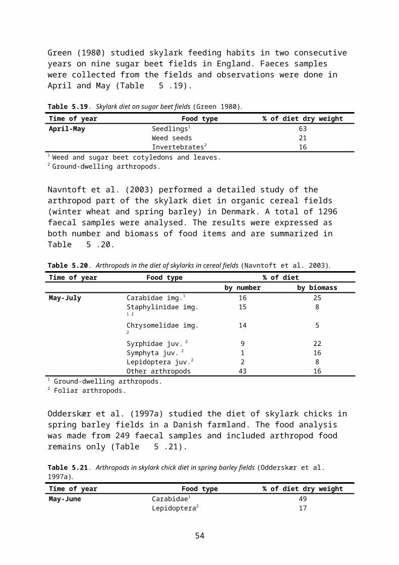
The diet of chaffinches is varied; it consists mainly of seeds and other plant material which are usually taken from the ground. During the breeding season, insects and other invertebrates make up the bulk of the diet and foraging in trees is more frequent. The seeds taken range in weight from 0.1 mg (Artemisia) to 230 mg (beech) (Newton 1967). Seeds are dehusked except for small and long seeds which are crushed (Buxton et al. 1998).

The diet of chaffinches has been investigated in all-year studies in Germany (Eber 1956) and England (Newton 1967). The results are shown in Table 5.44 to Table 5.46.

Table 5.44. Seasonal variation in Chaffinch diet in England, analysed from gut contents (Newton 1967).Time of year Food type % of volumeMay – mid-July Seeds 19

Invertebrates 81mid-July – September Cereal grain 56

Weed seeds 25Other seeds 4Invertebrates 15

October – April Cereal grain 30Weed seeds 65Invertebrates 5

Table 5.45. Seasonal variation in the ratio between plant and animal matter in Chaffinch diet in Germany, analysed from gut contents (Eber 1956).Time of year Food type % of itemsMarch – April Plant 90

Animal 10May – July Plant 30

Animal 70August – September Plant 63

Animal 37October – February Plant 99

Animal 1

Table 5.46. The composition of Chaffinch diet in Schleswig-Holstein, Germany, analysed from feeding observations (Christensen et al. 1996).Time of year Food type % of dietAll year Cereal grain 49

Beech mast 28Invertebrates 9Asteraceae seeds 5Brassicaceae seeds 4Polygonaceae seeds 4

The diet of chaffinch nestlings consists almost exclusively of invertebrates and includes foliage insects (e.g. aphids, Lepidoptera larvae), ground-dwelling invertebrates (e.g. Coleoptera and their larvae, Dermaptera, spiders, snails, earthworm cocoons) and even airborne insects (e.g. Lepidoptera, Diptera). The amount of vegetable matter is < 10 % in all studies.

Risk assessmentThe chaffinch is a relevant focal species for the following scenarios:

55

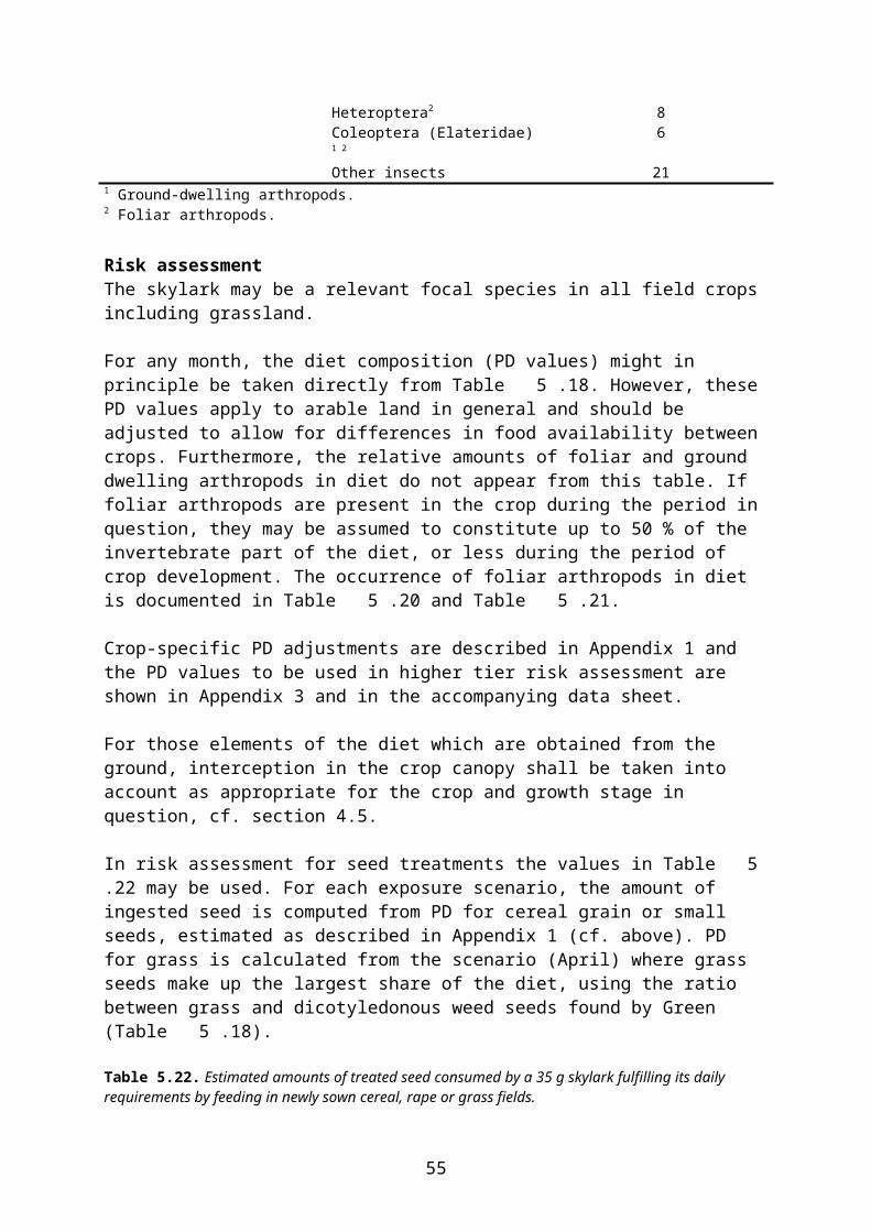
orchards (all applications) bush berries, all season ornamentals/nursey, large plants (canopy and ground directed applications)

The diet of chaffinches is varied and depends on the feeding habitat and the time of year. For the crops/cultures of relevance, the following composition of diet may be assumed (Table 5.47):

Table 5.47. Estimated diet composition of chaffinches feeding in fruit trees, bush berries and ornamentals/nursery cultures (expert judgement based upon Table 5.44, Table 5.45 and Table 5.46).

March – AprilFood category PD (fresh weight)Small (weed) seeds 0.90Ground arthropods 0.10

May – JulyFood category PD (fresh weight)Small (weed) seeds 0.20Foliar arthropods 0.40Ground arthropods 0.40

August – SeptemberFood category PD (fresh weight)Small (weed) seeds 0.75Foliar arthropods 0.10Ground arthropods 0.15

For canopy directed applications, interception in the canopy shall be taken into account for seeds and ground-dwelling arthropods.

Chaffinches are capable of dehusking, but small seeds are usually not dehusked (Buxton et al. 1998). Hence, including a dehusking factor in the calculations of exposure is probably not justified for the above scenarios.

PT may be refined using the information in Table 5.43.

5.1.15 Linnet Carduelis cannabina

General informationThe linnet is widespread and abundant in the southern part of the Zone (Denmark, Lithuania, South Sweden). It is less numerous further north, reaching northwards until central Sweden and Finland and also occurring in a narrow belt along the coast of the Gulf of Bothnia (Snow & Perrins 1998). In Norway linnets are mainly found in the agricultural landscape in the south-eastern part of the country (Gjershaug 1994 cited in Hage et al. 2011).

Like several other farmland birds, linnet populations have declined over large parts of western Europe during recent decades, most probably as a result of agricultural intensification (Table 5.48). In Finland where the species has increased, it has probably been favoured by set-asides,

56

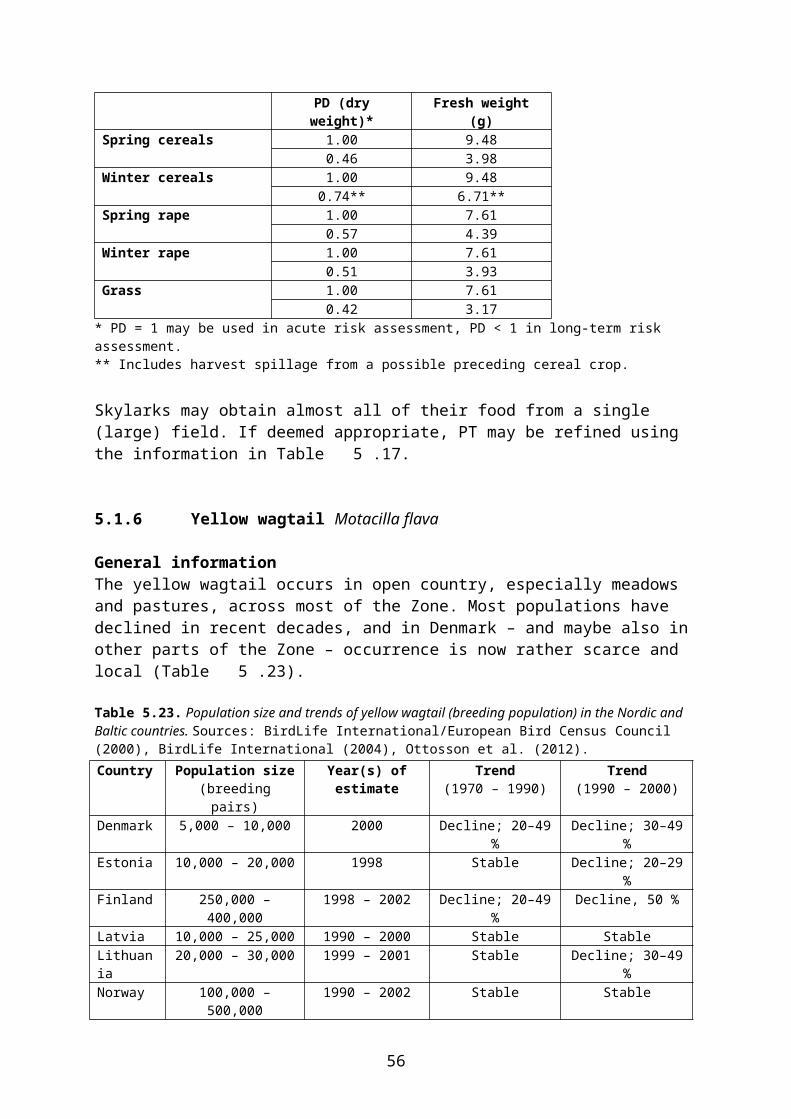
environmental fallows, organic farming and increasing densities of weeds (Hyvönen et al. 2003, Hyvönen & Huusela-Veistola 2008, Tiainen et al. 2008, 2012b).

Table 5.48. Population size and trends of linnet (breeding population) in the Nordic and Baltic countries. Sources: BirdLife International/European Bird Census Council (2000), BirdLife International (2004), Ottosson et al. (2012).Country Population size

(breeding pairs)Year(s) of estimate Trend

(1970 – 1990)Trend

(1990 – 2000)Denmark 150,000 – 300,000 2000 Increase; 20–49 %* Decline; 20–29 %Estonia 20,000 – 40,000 1998 Decline; 20–49 % StableFinland 20,000 – 30,000 1998 – 2002 Decline; ≥ 50 % Increase; 100 %Latvia 10,000 – 25,000 1990 – 2000 Stable StableLithuania 150,000 – 300,000 1999 – 2001 Stable StableNorway 10,000 – 15,000 1990 – 2002 Decline; 20–49 % StableSweden 110,000 2008 Decline; 20–49 % Decline; 37 %* Probably a mistake. Published studies (Petersen & Nøhr 1991, Heldbjerg & Lerche-Jørgensen 2012) indicate strong decline until 1982 followed by a smaller increase.

Linnets are migratory throughout the Zone, except that a few birds may winter in Denmark, especially in mild winters. The winter quarters are in Western Europe, the Mediterranean area and Northern Africa. The birds arrive at their breeding grounds during late March and April. Linnets breed from late April or early May to July or early August and usually produce two broods per year. Autumn migration takes place mainly during September - October.

Agricultural associationLinnets depend on shrubs and bushes for nest-sites and ready access to foodplants and ground foraging areas. Major habitats are scrub and heathland, farmland with hedges and low trees, orchards, uncultivated areas, young plantations, forest clear-cuts adjoining farmland, and suburban gardens. The species is widespread and locally abundant in farmland, where it is largely associated with rough vegetation at field borders, set-aside, rotational fallow and other uncultivated areas.

Within the arable land, several studies have indicated that linnets are to some extent associated with oil-seed rape fields (Petersen 1996b, Crocker & Irving 1999, Mason & Macdonald 2000). Moorcroft et al. (2006) suggest that availability of oilseed rape is important to maintain populations of linnet in intensively managed agricultural systems. In spite of their association with oil-seed rape during late spring and summer it seems that linnets only to a very limited extent use freshly drilled rape fields for feeding, at least in spring (Petersen 1996a).

Crocker & Irving (1999) found linnets to be prevalent and abundant in sugar beet in summer and autumn. Beet fields seem to gain importance from late June onwards, probably as a result of the increasing amounts of available weed seeds (Esbjerg & Petersen 2002). In a Norwegian study, linnets were frequently recorded in field grown vegetables (Hage et al. 2011).

In a British study of radio-tagged birds, linnets using oil-seed rape for foraging (“consumers”) spent on average 44 % of their active time within the rape fields (Finch & Payne 2006). However, some birds spent almost all of their active time in rape fields. Linnets also used sugar beet and/or potato for foraging, but these crops were less intensively used (Table 5.49).

57

Table 5.49. Percentage of active time spent by radio-tagged linnets in different crops in the UK, presented as 90th percentile of the modelled PT distribution. The birds were caught in the general farmland (not in specific crops); it is therefore recommended to use values for the subsample of birds who actually used the crop in question (“consumers only”) (bold).Crop Period No. of birds Mean 90 percentile ReferenceAll birds:Winter rape April – July 22 0.12 0.62 Finch &

Payne 200614 0.81 Prosser 2010

Beet(+ potatoes)

April – Nov 21 0.13 0.43 Finch & Payne 2006

21 0.43 Prosser 2010Consumers only:Winter rape April – July 6 0.44 0.99 Finch &

Payne 20066 0.99 Prosser 2010

Beet(+ potatoes)

April – Nov 11 0.25 0.59 Finch & Payne 2006

11 0.59 Prosser 2010

Body weightBody weight ♂ mostly 17–22 g, ♀ 15–21 g (Snow & Perrins 1998). Mean body weight of the smaller sex (♀: 18 g) may be used for risk assessment.

Energy expenditureA captive linnet (16.9 g) had a BMR of 29.3 kJ/day (Christensen et al. 1996). The daily energy expenditure may also be calculated allometrically using the equation for passerine birds in accordance with the formula in Appendix G of the EFSA Guidance Document (EFSA 2009).

Diet Linnets feed almost exclusively on small to medium-sized seeds and are particularly dependent on weeds of open country and waste ground. Over the full annual cycle, seeds from available Brassicaceae seem to be the most common food, but seeds of Caryophyllaceae (Cerastium, Stellaria), Polygonaceae (Polygonum, Chenopodium) and Asteraceae (e.g. thistles and Taraxacum) are also frequent in diet. The size of seeds taken range from 0.05 to 50 mg, but the main size range is 1-10 mg. Milky seeds are preferred to ripe seeds (Newton 1967). Seeds are dehusked (Buxton et al. 1998).

In an English study, the diet of linnets largely reflected weed abundance and included 25 of the 30 most common weeds in the area but not cereal grains (Newton 1967). By contrast, cereal grain was the most frequent food item in April and in autumn in a study from Schleswig-Holstein (Eber 1956).

Invertebrates, e.g. aphids and Lepidoptera larvae, appear incidentally in adult diet but may be fed more regularly to nestlings. In an English study, insects occurred in only 2 of 62 broods, with aphids making up 15 % of diet during the first 9 days in one brood. In other studies, nestling diet consisted entirely of seeds. According to some early studies, insects may be predominant food of nestlings, but modern studies conclude that the proportion of invertebrates was much overestimated in these early studies (Christensen et al. 1996).

58

Risk assessmentThe linnet is relevant for the following scenarios:

winter rape, from flowering (BBCH 60) to post-harvest spring rape, from flowering (BBCH 60) to post-harvest beets, BBCH 10-49 pulses, BBCH 10-39 field grown vegetables, BBCH 10-89 grass; newly sown, long grass with seed heads, and termination orchards, ground directed applications bush berries, all season ornamentals/nursey, all exposure scenarios

The diet may be assumed to consist entirely of small seeds (PD = 1).

For weed seeds exposed on or near the ground, interception in the crop canopy shall be taken into account as appropriate for the crop and growth stage in question.

There is no information about the relative amounts of rape seeds and weed seeds in the diet of linnets feeding in rape fields. Nor is there any information about the relative amounts of grass seeds and weed seeds in the diet of linnets feeding in grass fields (including grass for seed). In newly sown grass fields, linnets will take the grass seeds but prefer weed seeds if available. Thus, the relative amounts of grass seeds and weed seeds in the diet will vary.

In risk assessment for seed treatments, it may be assumed that the birds feed entirely on grass seed (worst case). An 18 g linnet needs 4.9 g (fresh weight) of small seeds to fulfil its average daily requirements.

Seeds are usually dehusked so a dehusking factor may be applied (cf. section 4.7). Case-specific evidence must be provided that dehusking actually plays a role under field conditions for this species.

For linnets feeding in oil-seed rape or row crops, PT may be refined using the information in Table 5.49; the PT values for beet will probably also apply to pulses and field grown vegetables. There is no information allowing a refinement of PT for linnets feeding in grass fields.

There are no species-specific data allowing a refinement of PT for linnets feeding in orchards, bush berries or ornamentals/nursery cultures. In orchards, PT values are probably close to those found for chaffinch (Table 5.43), and similar values may well apply for bush berries and ornamentals/nursery.

5.1.16 Yellowhammer Emberiza citrinella

General informationThe yellowhammer is a widespread and common or abundant species throughout the Zone. It avoids dense forest, towns and mountain areas but otherwise occurs wherever trees or scrub (including farmland hedges) alternate with open areas. In recent decades, North and West European populations have generally declined while populations in central and eastern Europe

59

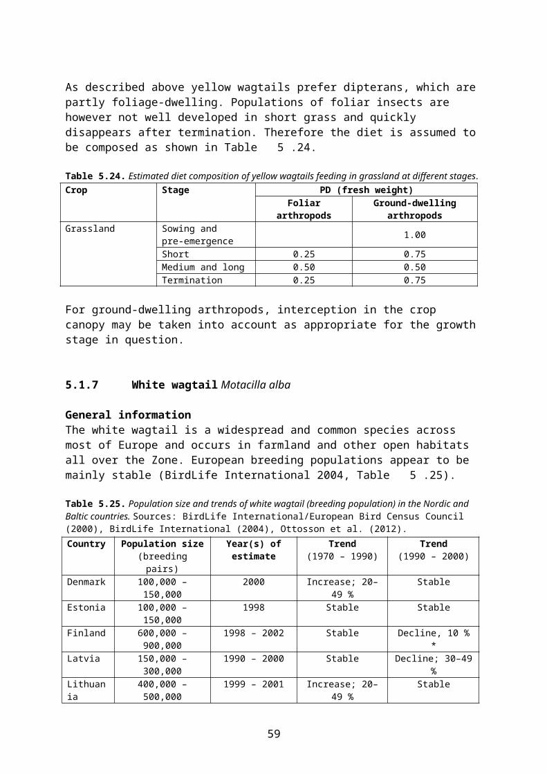
have remained stable or may even have increased slightly (BirdLife International 2004, Table 5.50).

Table 5.50. Population size and trends of yellowhammer (breeding population) in the Nordic and Baltic countries. Sources: BirdLife International/European Bird Census Council (2000), BirdLife International (2004), Ottosson et al. (2012).Country Population size

(breeding pairs)Year(s) of estimate Trend

(1970 – 1990)Trend

(1990 – 2000)Denmark 400,000 – 600,000 2000 Stable Decline; 10–19 %Estonia 100,000 – 200,000 1998 Stable Increase; 20–29 %Finland 700,000 – 1,100,000 1998 – 2002 Stable Decline; 10 % *Latvia 80,000 – 160,000 1990 – 2000 Decline; 20–49 % StableLithuania 600,000 – 750,000 1999 – 2001 Stable StableNorway 150,000 – 500,000 1995 – 2002 Stable Decline; < 20 %Sweden 900,000 2008 Stable Decline; 23 %* Farmland population has been more or less stable, with a moderate increase 2001 – 2011 (Tiainen et al. 2008, 2012b).

In the southern part of the Zone, yellowhammers are mainly resident or dispersive, usually gathering in flocks at good feeding sites during winter. Northern populations are partial migrants, wintering up to 250-500 km SW of the breeding area (Snow & Perrins 1998). Most migrants arrive in March-April and the territories are defended from April until July. Breeding is from late April or May to July or (rarely) August. Yellowhammers usually produce two broods per year. The migrants leave September - November.

Agricultural associationYellowhammers are found in arable landscapes during the breeding season as well as in winter when the species is strongly associated with this habitat (Stolt 1988). Entirely open landscapes are avoided and the preferred arable landscapes consist of habitat islands, forest edges, semi-natural pastures and hedgerows or bushes (Berg and Pärt 1994; Svensson et al. 1999; Bradbury et al. 2000, Vepsäläinen et al. 2010). Open fields are used for foraging (Stoate et al. 1998), but most of the foraging occurs in the vicinity of hedgerows and other kinds of cover.

The mean densities of yellowhammer in Swedish farmland are according to inventories between 0.12 and 0.15 territories/ha (Robertson and Berg 1992; Söderström 2001). Territories are often linear along, e.g., a hedgerow and the territory size is usually less than 1 ha (Söderström and Pärt 2000). Foraging bouts are often done outside the territory with a mean range of 116-184 m (maximum 238 m) (Petersen et al. 1995; Stoate et al. 1998). According to Lille (1996), the foraging range is usually restricted to a radius of 250 m around the nest with a mean foraging distance of 82 m. In a Danish study, differences in foraging range where found in the breeding season with longer foraging distances in May and July compared to June, and males generally moving longer distances than females (Petersen et al. 1995).

In the breeding season different crop types are used for foraging (Petersen et al. 1995; Morris et al. 2001) but in general spring cereals are preferred and grassland is avoided (see also Table 5.52). Crop preferences change during the season, probably due to changes in crop structure and food availability. Yellowhammers are adapted to ground-feeding, leading to a preference for early growth stages of cereals and for other crops that offer access to bare soil (Petersen et al. 1995). Cereals also become important as the grains ripen (Biber 1993, Stoate et al. 1998). Beet fields may be very important feeding sites in July (Petersen et al. 1995, Esbjerg & Petersen 2002). After harvest, cereal stubble is preferred.

60

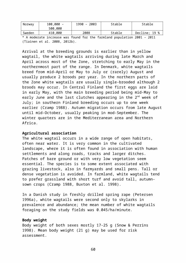
Lille (1996) studied the feeding habitat of 20 pairs of yellowhammer feeding nestlings in farmland in North Germany. He found that cereal fields were most frequently visited (42.5 % of foraging trips), followed by set-aside (21.0 %), hedgerows and other field border vegetation (15.7 %), oilseed rape (12.7 %) and wood (5.3 %).

In a study in England yellowhammers spent on average about 25% of their active time in arable crops (Crocker et al. 2002). However, some individuals spent almost all their active time in cropped habitats (Crocker et al. 2002). It is therefore reasonable to believe that some yellowhammers forage to a large extent in crops.

The proportion of time (PT) spent by individual yellowhammers in different crops has been estimated by the Food and Environment Research Agency (formerly Central Science Laboratory) in the UK. The results are summarized in Table 5.51.

Table 5.51. Percentage of active time spent by radio-tagged yellowhammers in different crops in the UK, presented as 90th percentile of the modelled PT distribution. The birds were caught in the general farmland (not in specific crops); it is therefore recommende to use values for the subsample of birds who actually used the crop in question (“consumers only”) (bold).Crop Period No. of birds Mean 90 percentile ReferenceAll birds:Winter cereals

Winter(Sep – Mar)

44 0.02 0.05 Finch & Payne 2006

44 0.06 Prosser 2010Summer(Apr – Aug)

28 0.21 0.77 Finch & Payne 2006

28 0.70 Prosser 2010Winter rape Winter

(Sep – Mar)44 0.01 0.00 Finch &

Payne 200651 0.00 Prosser 2010

Summer(Apr – Aug)

28 0.11 0.60 Finch & Payne 2006

21 0.61 Prosser 2010Beet(+ potatoes)

Apr – Nov 50 0.12 0.56 Finch & Payne 2006

50 0.55 Prosser 2010Consumers only:Winter cereals

Winter(Sep – Mar)

10 0.02 0.14 Finch & Payne 2006

10 0.14 Prosser 2010Summer(Apr – Aug)

17 0.34 0.87 Finch & Payne 2006

17 0.87 Prosser 2010Winter rape Winter

(Sep – Mar)2 0.01 0.61 Finch &

Payne 20064 0.61 Prosser 2010

Summer(Apr – Aug)

7 0.45 0.86 Finch & Payne 2006

7 0.86 Prosser 2010Beet(+ potatoes)

Apr – Nov 13 0.46 0.94 Finch & Payne 2006

13 0.94 Prosser 2010

In a Danish study, 31 and 23 radio-tagged yellowhammers were tracked on organic and conventional farms, respectively, during May-July (Petersen et al. 1995). The home ranges of

61

birds on organic farms were dominated by grassland, winter cereals, spring cereals and various broad-leaved crops. On the conventional farms, the home ranges were dominated by winter cereals, maize, spring cereals and oil-seed rape. Results are presented as the proportion of records (fixes) in each crop type, which is supposed to be roughly equivalent to the proportion of time spent in each crop (Table 5.52). Comparison of usage and availability indicates crop preferences. Furthermore, the results illustrate how usage (PT) of a certain crop depends on availability.

Table 5.52. The use of different crops by 54 radio-tagged yellowhammers on organic and conventional farms in Denmark. Records (fixes) from off-crop habitats have been excluded (Petersen et al. 1995).

CropAvailability

(proportion ofhome range)

Usage(proportion of crop fixes) (n = 260)

Mean 95 % confidence limits

Conventional farms:Winter cereals 0.30 0.21 0.10 - 0.32Maize 0.30 0.31 0.19 - 0.43Spring cereals 0.13 0.09 0.01 - 0.16Oil-seed rape 0.13 0.24 0.13 - 0.35Grassland 0.07 0.05 0.00 - 0.10Leafy crops 0.05 0.07 0.00 - 0.13Others 0.03 0.04 –Organic farms:Grassland 0.37 0.15 0.07 - 0.22Winter cereals 0.22 0.30 0.20 - 0.40Spring cereals 0.20 0.22 0.13 - 0.31Leafy crops 0.18 0.29 0.20 - 0.39Others 0.03 0.04 –

Body weightMean body weight of both sexes 27 g (24-31 g) (Buxton et al. 1998) or mostly 25-36 g (Snow & Perrins 1998). The mean of these values (29 g) may be used for risk assessment.

Energy expenditureNo species specific data available, therefore calculated allometrically using the equation for passerine birds in accordance with the formula in Appendix G of the EFSA Guidance Document (EFSA 2009).

Diet The diet of yellowhammers consists of seeds and invertebrates in variable proportions over the year. Seeds are usually dehusked (Buxton et al. 1998, Prosser 1999).

The species is foraging in a wide range of crop types such as maize, winter and spring cereals, rape, peas and sugar beet (Petersen et al. 1995; Stoate et al. 1998; Mason & Macdonald 2000; Morris et al. 2001). As cereal grains ripen, fields with these crops may provide food for both adults and young, although invertebrates are the major component of the nestling diet (Stoate et al. 1998).

The food of adult yellowhammers may consist of 80 % invertebrates in May-June (Buxton et al. 1998), although faecal samples from five individuals collected in June in England revealed

62

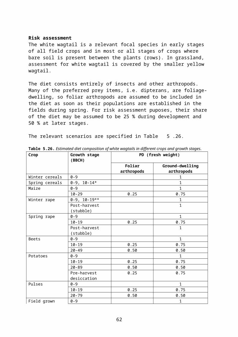
a diet of 100 % cereals (Stoate et al. 1998). In the Moscow region of Russia, the proportion of invertebrates in diet was highest (70% by number) in June; the annual average diet compo-sition is shown in Table 5.53.

Table 5.53. All-year diet composition of adult yellowhammers in Moscow Region, Russia (Inozemtsev 1962 cited by Cramp & Perrins 1994b).Time of year Food type % of food itemsAll year Coleoptera img. 39.3(n = 478) Lepidoptera larvae 1.0

Tipulidae 1.0Seeds:Wheat 12.3Oats 8.8Pine 8.7Spruce 4.6Other seeds 21.1

Prys-Jones (1977, cited in Buxton et al. 1998) studied the relative proportions of seeds and invertebrates in the diet of yellowhammers in the UK. The results are given in Table 5.54.

Table 5.54. Yellowhammer adult diet in the UK (Prys-Jones 1977 cited by Buxton et al. 1998).Time of year food type % of dietMarch – June Seeds 65 1)

Invertebrates 35 1)

July – October Seeds 75 1)

Invertebrates 25 1)

November – February Seeds 99 1)

Invertebrates 1 1)

Seed composition 3)

October – November Cereal 93 2)

Grass 7 2)

December – February Cereal 66 2)

Grass 34 2)

March – April Cereal 91 2)

Grass 9 2)

1) by volume2) by dry weight 3) seeds of dicotyledons also found, especially in April, but negligible in terms of weight.

Some data on the diet of yellowhammer nestlings and the composition of invertebrates in the nestling diet are given in Table 5.55 and Table 5.56.

Stoate et al. (1998) studied yellowhammer during three years in a 292 ha mixed arable landscape in central England. The diet composition of nestlings was calculated from 144 faecal sacs from 56 broods (Table 5.55).

Table 5.55. Yellowhammer nestling diet in the UK (Stoate et al. 1998).Time of year food type % of dietMay-July Cereal seeds 38 1

Invertebrates 62 1

63

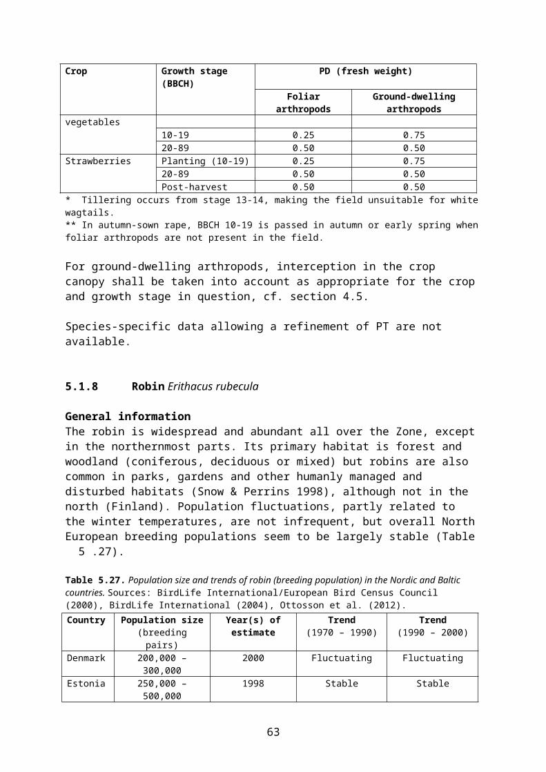
Time of year food type % of dietInvertebrate composition Coleoptera3 4 40 2

Diptera (adults) 3 17 2

Lepidoptera larvae3 13 2

Aranea3 4 10 2

Hemiptera3 7 2

Hymenoptera3 4 2 2

1 by volume2 by number.3 foliar arthropods4 ground-dwelling arthropods.

Lille (1996) studied the diet of yellowhammer nestlings in North German farmland. The diet composition was calculated from identification of 4764 food items brought to 12 broods (Table 5.56).

Table 5.56. Yellowhammer nestling diet in North German farmland (Lille 1996).Time of year Food type % of diet

by number by fresh weightJune-July Cereal grain 15.6 6.7

Lepidoptera larvae1 12.0 46.2Lepidoptera img. 1 2.1 4.4Diptera larvae1 2 46.9 25.7Diptera img. 1 3.7 2.6Coleoptera1 2 6.2 7.1Arachnidae1 2 8.3 3.3Others 5.3 4.0

1 foliar arthropods2 ground-dwelling arthropods.

Risk assessmentThe yellowhammer is relevant for the following scenarios:

winter cereals, freshly drilled (BBCH 0-9) winter cereals; BBCH 70-89, pre-harvest desiccation and post-harvest (stubble) treatments spring cereals, freshly drilled (BBCH 0-9) spring cereals; BBCH 70-89, pre-harvest desiccation and post-harvest (stubble) treatments maize, BBCH 30-39

The yellowhammer would be relevant for other scenarios as well, but in these cases other omnivorous (skylark) or granivorous (linnet) species are more worst case.

The diet is composed of seeds (mainly cereal grain) and invertebrates and varies with the season, cf. Table 5.54, Table 5.55 and Table 5.56. Cereal grain/ear may be picked directly from the growing straw. It is proposed that the diets specified below (Table 5.57) are used in higher tier risk assessment.

Table 5.57. Estimated diet composition of yellowhammers feeding in cereals or maize (expert judgement based mainly upon Table 5.54).

Winter cereals, freshly drilledFood category PD (fresh weight)Large seeds on ground 0.70Small seeds 0.05Ground arthropods 0.25

64

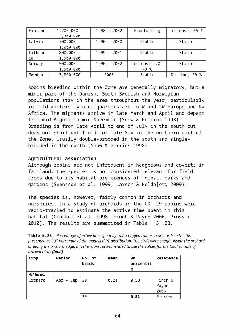
Spring cereals, freshly drilledFood category PD (fresh weight)Large seeds on ground 0.59Small seeds 0.06Ground arthropods 0.35

Winter and spring cereals, BBCH 70-89Food category PD (fresh weight)Cereal grain/ear on plant 0.75Foliar arthropods 0.13Ground arthropods 0.12

Winter and spring cereals, pre-harvest desiccationFood category PD (fresh weight)Cereal grain/ear on plant 0.75Foliar arthropods 0.06Ground arthropods 0.19

Winter and spring cereals, post-harvest (stubble) treatmentsFood category PD (fresh weight)Large seeds on ground 0.75Ground arthropods 0.25

Maize, BBCH 20-39Food category PD (fresh weight)Large seeds on ground 0.35Small seeds 0.03Foliar arthropods 0.16Ground arthropods 0.46

Maize, BBCH ≥ 40Food category PD (fresh weight)Large seeds on ground 0.35Small seeds 0.03Foliar arthropods 0.31Ground arthropods 0.31

For ground arthropods and seeds picked from the ground an interception factor shall be applied as appropriate for the crop and growth stage in question.

In risk assessment for seed treatments the following values may be used (Table 5.58).

Table 5.58. Estimated amounts of treated seed consumed by a 29 g yellowhammer fulfilling its daily requirements by feeding on freshly drilled winter or spring cereals. PD for mixed diets as in Table 5.57.

PD (fresh weight)* Fresh weight (g)Winter cereals 1.00 8.35

0.70 6.72Spring cereals 1.00 8.35

0.59 6.05* PD = 1 may be used in acute risk assessment, PD < 1 in long-term risk assessment.

Seeds are usually dehusked so a dehusking factor may be applied (cf. section 4.7).

PT may be refined using the information in Table 5.51 and Table 5.52.

65

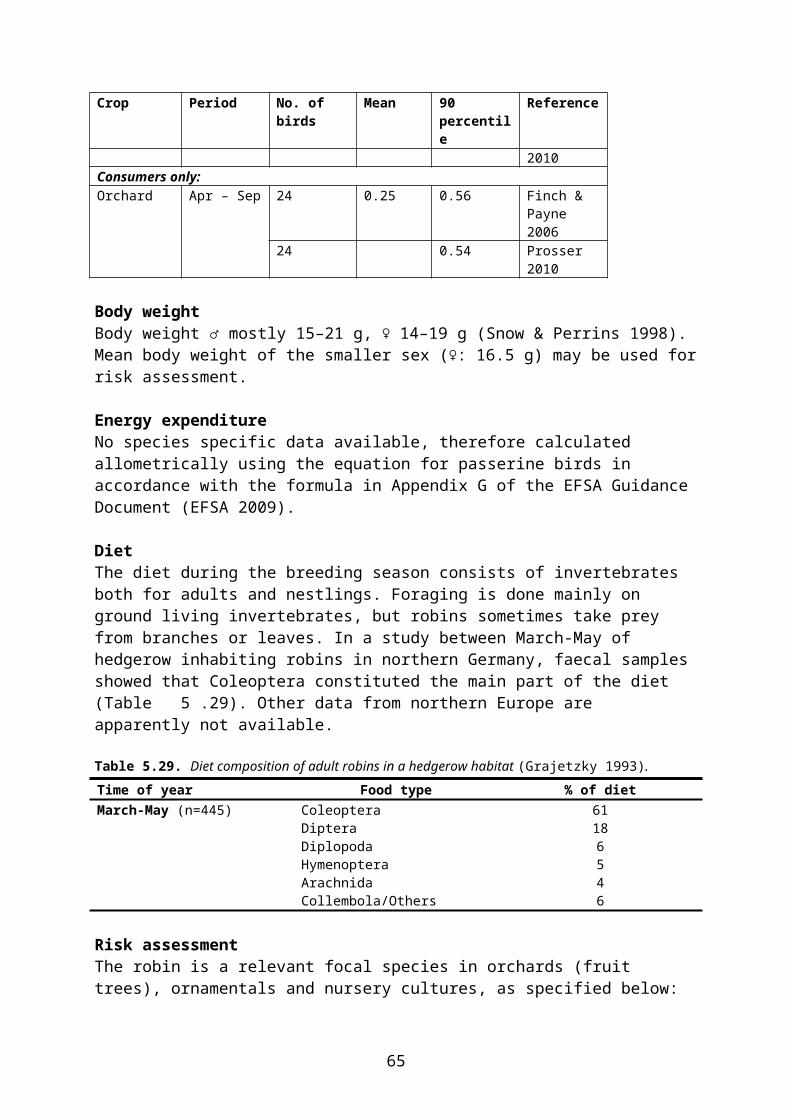
5.2 Mammals

5.2.1 Common shrew Sorex araneus

General informationThe common shrew is a widespread and common species throughout the Zone; apparent gaps in the distribution in Norway are assumed to be the result of patchy information (Mitchell-Jones et al. 1999). The species occurs in a wide range of habitats, including forests and arable land, but prefers moist and cool habitats with dense vegetation cover (Mitchell-Jones et al. 1999, Baagøe & Ujvári 2007). The most important requirement for finding the species in a habitat is that there is a ground cover to minimize visibility for predators. Breeding season is between May and September and usually two litters of young are born per year.

Agricultural associationThe common shrew is widespread in arable landscapes (Tattersall et al. 2002; Huitu et al. 2004) but occurs in low numbers compared to, e.g., wood mouse (Jensen & Hansen 2003). As crops grow higher and ground cover increases common shrews are more likely to be found on arable land. However, this is probably animals nesting in surrounding habitats and making foraging trips to the fields (Tew et al. 1994). In a study in southern Sweden single individuals of common shrew where caught in the fields while more regular captures where made on habitat islands situated in the fields (Loman 1991a). Thus, this shows that the species is present in the agricultural landscape and probably particularly in leys (L. Hansson pers. comm. to KemI).

The home range of the common shrew varies depending on habitat and season and ranges between 0.037 and 0.11 ha (Gurney et al. 1998). In arable landscapes common shrews can live their entire life within approximately one hectare (L. Hansson pers. comm. to KemI).

Common shrews are living in arable habitats and are present in these habitats all year round (Tew et al. 1994; Tattersall et al. 2002). In a Danish study covering summer and autumn, common shrews were regularly trapped in set-aside, permanent grassland and grass in rotation, occasionally in oilseed rape but never in wheat or pea fields (Jensen & Hansen 2003). The number of trapped shrews was generally very low except in some fields with grass in rotation (Jensen & Hansen 2003). Numbers declined from summer to autumn (Jensen & Hansen 2003). As crop cover extends, the species uses arable fields increasingly for foraging (Tew et al. 1994). In a study conducted by Tew et al. (1994) common shrews were caught between April and October away from hedgerows almost exclusively in autumn sown cereal (Tew et al. 1994). It might be assumed that the common shrew spends more time in arable fields from June to harvest. Many individuals spend their entire life foraging in one crop type (L. Hansson pers. comm. to KemI), but no studies have been done on foraging behaviour of the common shrew in arable fields.

The common shrew is a small species with a high metabolic rate forcing it to have several foraging bouts per day (Merritt & Vessey 2000). During foraging sessions shrews might find all their prey in one arable field, although there are no studies on time budgets in arable crops.

Body weightShrews are fluctuating in body weight with a marked decrease in winter (Churchfield 1982).

66

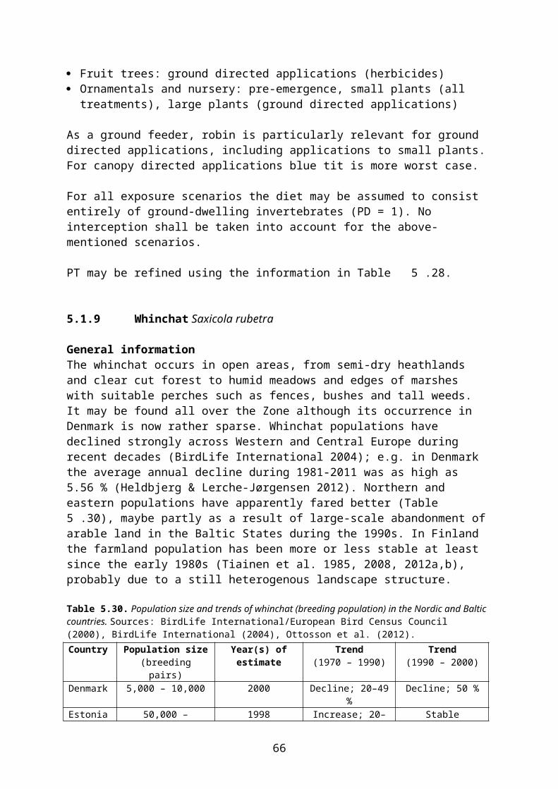
Body weight is reported as follows:

Summer weight 10.4 g (Aitchison 1987) Mean 8.1 (5-14) g (Gurney et al. 1998)

It is recommended that the body weight of 8.1 g from Gurney et al. (1998) is used for risk assessment.

Energy expenditureFor common shrew energy expenditure regardless of season is 39 kJ/day (animal body weight 8.6 g) according to Gebczynski (1965). Alternatively, the energy expenditure can be calculated allometrically using the equation for mammals in accordance with the formula in Appendix G of the EFSA Guidance Document (EFSA 2009).

Diet The common shrew is an opportunistic predator feeding on a wide range of common invertebrates, particularly earthworms, woodlice, spiders, slugs, snails and insect larvae. Only small amounts of vegetative food are consumed (Bjärvall and Ullström 1985). The common shrew finds its prey by encounter (Plesner-Jensen 1993) although some preferences for food items are shown (Churchfield 1982). The prey is found on the ground surface as well as under it, and studies have shown that individuals are able to find food at a depth of 120 mm (Churchfield 1980). The prey size varies from larger than 20 mm to smaller than 3 mm. 41 % of the invertebrates taken have a body size less than or equal to 5 mm and very few are smaller than 3 mm (Churchfield 1982). The diet composition collected from 215 alimentary tracts of common shrews living in grassland is presented in Table 5.59.

Table 5.59. Common shrew diet in grassland (n = 215) (Pernetta 1976)1. Time of year Food type % of diet fresh weightApril Opiliones and Spiders 26

Earthworms 20Coleoptera larvae 20Coleoptera adults 15

May Opiliones and Spiders 15Earthworms 23Coleoptera larvae 17Coleoptera adults 40Chilopods 2Isopoda 3

June Opiliones and Spiders 10Earthworms 7Coleoptera larvae 11Coleoptera adults 57Isopoda 4

July Opiliones and Spiders 9Earthworms 17Coleoptera larvae 21Coleoptera adults 30Slugs and Snails 1Chilopods 23Isopoda 4

August Opiliones and Spiders 13Earthworms 36Coleoptera larvae 3Coleoptera adults 26

September Opiliones and Spiders 14

67

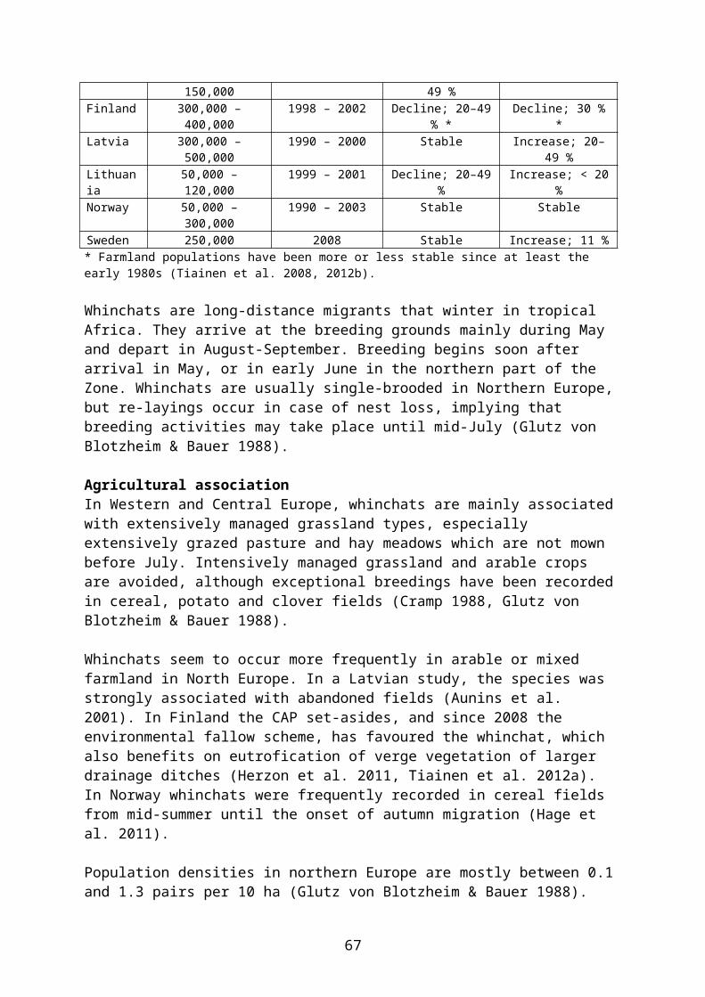
Time of year Food type % of diet fresh weightEarthworms 20Coleoptera larvae 8Coleoptera adults 34Slugs and Snails 2

1 For risk assessment purposes, all food items except earthworms may be assumed to belong to the category “ground-dwelling arthropods”.

In a study in England, Johnson et al. (1992) found that beetles were a major component of the diet with over 40 % of the guts examined containing remains of adult beetles (n = 199). Mollusc remains and aphids were each found in approximately 30 % of the guts examined. The fourth major prey type was dipteran larvae or pupae (chiefly leatherjackets), which were found in 16-40 % of guts. Earthworms were absent from the gut contents examined. This probably reflects the low numbers of worms present at the study site and possibly also the shrews’ difficulty in capturing worms in the heavy soils of the study site.

Risk assessmentThe insectivorous common shrew is relevant for the following crop scenarios:

winter rape, BBCH 80-89 and pre-harvest desiccation spring rape, BBCH 80-89 and pre-harvest desiccation grass (medium and long)

The diet in rape fields may be assumed to consist entirely of ground arthropods (PD = 1).

The diet in grassland also consists mainly of ground arthropods and may be taken from Table 5.59 for the month(s) in question. The proportion of earthworms in diet varies with the soil structure.

Home ranges of common shrews are small (usually ≈ 0.1 ha) and many individuals spend their entire life foraging in a single crop type. Thus, PT shall not be refined unless fully justified by case-specific data.

5.2.2 Brown hare Lepus europaeus

General informationThe brown hare is widespread and common, or fairly common, in open countryside throughout the southern and eastern part of the Zone (Mitchell-Jones et al. 1999). It is absent from northern Finland, Sweden north of limes norrlandicus (Frylestam 1990), and Norway except for a small area in the south-easternmost part of the country. Occurrence in southern Sweden and Norway is due to introduction (Mitchell-Jones et al. 1999). North of its range the brown hare is replaced by the smaller mountain (or snow) hare Lepus timidus, which is the only indigenous lagomorph on the Scandinavian peninsula.

During recent decades, brown hare populations have declined strongly across large areas of western and central Europe, and in Denmark the species is now red listed as vulnerable. The main reason for the decline is probably agricultural intensification, including fertilizer and pesticide use, which causes a shortage of food during the summer half, thereby reducing the fecundity of females and survival of the young (Olesen & Asferg 2006).

68

The principal habitats of the brown hare are open agricultural landscapes with relatively small fields and different crops (Asferg & Madsen 2007). Reproduction starts early in the year, in February in the southern part of the Zone, and ends in September (Frylestam 1980b, Asferg & Madsen 2007). In Denmark the brown hare may have up to 4 or even 5 litters during the breeding season, but due to food shortage the average number of litters per female is now only 2.3 (Olesen & Asferg 2006).

Agricultural association The brown hare is found in all sorts of open agricultural landscape such as intensively farmed areas, areas with mixed farming and pastoral landscapes. Studies of the species have been conducted in a wide range of landscapes with different agricultural practices (Frylestam 1980a, Tapper and Barnes 1986, Pépin 1987, Smith et al. 2004).

Although there are marked variations in home range sizes, the general pattern seems to be large home ranges in areas of intensive agriculture and limited landscape diversity, and small home ranges in areas with a higher degree of natural habitats and thereby landscape diversity (Olesen & Asferg 2006). In intensively managed arable landscapes home range sizes can be as large as 138 ha (Marboutin and Aebischer 1996), while much smaller home ranges are found in mixed farmland and in grass dominated landscapes, 29 ha and 34 ha respectively (Broekhuizen and Maaskamp 1982, Smith et al. 2004).

Brown hare densities are, similar to home ranges, depending on landscape quality. In a quantitative study of brown hare numbers in relation to habitat type, Smith et al. (2005) found that abundance of hares showed a strong positive association with wheat, cereals, and beet. In the same study habitat diversity was also strongly positively associated with hare abundance, while monocultures showed a strong negative association (Smith et al. 2005). In Poland hares that lived in monocultures were only found in areas which offered a variation in vegetation (Lewandowski and Nowakowski 1993). This might be because hares need a variety of vegetation types to ensure access to high quality food during the year and thus large crop fields have a negative impact on their feeding resource (Panek and Kamieniarz 1999). Some mean hare densities (individuals/100 ha) in spring for different landscape types are: Intensive arable land 29 (23-35) (Pépin 1987), for mixed farmland and pastoral land in Sweden 45 (38-55) and 14 (14-15), respectively (Frylestam 1979).

From a study in mixed farmland in England (50 % winter wheat/barley and 50 % grassland) the time (day and night) that brown hares spent in different crops are shown in Table 5.60.

Table 5.60. Time spent (%) in different habitats (Tapper and Barnes 1986).Crop Jan Feb Mars Apr May June July Aug Sept Oct Nov DecWheat 65 50 55 30 15 20 10 2.5 - - 35 45Barley - - - - 20 10 10 5 2.5 - - -Grass 20 35 45 65 60 55 70 67.5 50 52.5 40 30

According to Tapper and Barnes (1986), brown hares have two basic requirements: a feeding area and a resting area. Hares usually feed at night and rest at day, and depending on the habitat quality these areas can either coincide or differ (Tapper and Barnes 1986). In Table 5.60 the brown hare activity is not specified, making such a separation impossible. It has been shown from studies in France, England and Sweden that brown hares favour arable crops in spring, both in intensive arable land and mixed farmland (Frylestam 1980a; Pépin 1985; DEFRA 2002). From a dietary study, Chapuis (1990) showed that the predominant food of brown hare in spring (April and May) consists of wheat (Chapuis 1990). Similarly as in

69

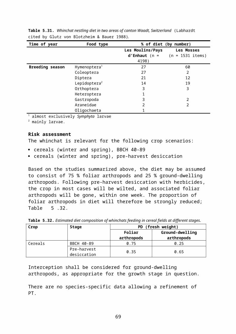
spring, winter cereals are again being favoured in autumn (Chapuis 1990; Frylestam 1992). From these studies it is reasonable to assume that brown hares in the study conducted by Tapper and Barnes (1986) use cereals for the majority of the foraging time when the shoots are young (i.e. April and May in areas where spring cereals dominate). Furthermore, in a more intensive agriculture landscape with a smaller proportion of grasslands the percent time that hares spend in different arable crops are probably higher as the grassland habitat covers a much smaller area or is largely absent. Thus, the numbers in Table 5.60 can be viewed as minimum estimates for the use of wheat and barley since cereal fields are likely to overtake some of the functions of grasslands.

In a study performed by the UK Food and Environment Research Agency, brown hares were caught using walk-in traps set in gaps in hedges, and were fitted with collar-mounted radio tags. A vehicle was used for tracking which was carried out both day and night. The hares’ use of different crops was modelled by fitting a Beta distribution to the radio-tracking data. The results are reported by Prosser (2010); Table 5.61.

Table 5.61. Percentage of active time spent by radio-tagged brown hares in different crops in the UK, presented as 90th percentile of the modelled PT distribution. The hares were caught in the general farmland (not in specific crops); it is therefore recommended to use the subsample of animals who actually used the crop in question (“consumers only”) (bold) (Prosser 2010).

Period Crop No. of animals 90th percentileAll animals:Spring(March - May)

(winter) cereals 19 0.87(winter) oil-seed rape 1.00all crops 1.00

Summer(June - August)*

(winter) cereals 20 0.62(winter) oil-seed rape 0.56non-cereal crops 0.75all crops 0.94

Autumn(September - November)

(winter) cereals 23 0.63(winter) oil-seed rape 0.28non-cereal crops 0.35all crops 0.89

Winter(December - February)

(winter) cereals 23 0.85(winter) oil-seed rape 0.45all crops 1.00

Consumers only:Spring(March - May)

(winter) cereals 14 0.93(winter) oil-seed rape 7 1.00all crops 19 1.00

Summer(June - August)*

(winter) cereals 10 0.89(winter) oil-seed rape 4 0.88non-cereal crops 10 0.95all crops 18 0.99

Autumn(September - November)

(winter) cereals 15 0.69(winter) oil-seed rape 6 0.65non-cereal crops 13 0.47all crops 22 0.91

Winter(December - February)

(winter) cereals 21 0.87(winter) oil-seed rape 8 0.66all crops 21 1.00

* July was excluded from the calculations for oilseed rape because rape is normally harvested during this month in the UK.

70

Body weightMean body weight of brown hares in Sweden is 4.2 kg with a slight increase in weight further north (Frylestam 1990). In the UK, mean body weight is 3.23 - 3.43 kg (Gurney et al. 1998). The body weight of 3.8 kg from the EFSA Guidance Document (EFSA 2009) is probably a realistic estimate (biased low) for the southern part of the Zone and should be used for risk assessment.

Energy expenditureNo species-specific data available, therefore calculated allometrically using the equation for mammals in accordance with the formula in Appendix G of the EFSA Guidance Document (EFSA 2009).

DietThe brown hare is feeding on a wide selection of arable crops (e.g. cereals), grasses and herbs. Cereal crops like winter wheat is a preferred food item but requirements are changing over the season and as cereals grow larger, more weedy grasses and herbs are included in the diet (Frylestam 1980a, Tapper and Barnes 1986, Chapuis 1990). It appears that the diet of hares closely reflects the vegetation available in the specific home range and the phenology of individual plant species (Olesen & Asferg 2006). Hares living in agricultural areas with intensive cereal production preferentially select green parts of cereals (up to 95 %) during the early growth stages of these crops, but in summer when cereals ripen the use of wild dicotyledonous plant species increases in proportion to their appearance and abundance (Olesen & Asferg 2006). In pastoral landscapes, hares have a far more diverse diet of non-grass herbs (weeds) year round and, if present, they feed on root crops, wild grasses, clover and lucerne (Olesen & Asferg 2006). In arable landscapes during late summer, up to 20 % of the stomach content may consist of cereal grain (Olesen & Asferg 2006).

From studies in Swedish farmland brown hares show highest preferences for winter wheat and barley in April and May (Frylestam 1980a). Similarly, preferences are shown for spring cereals from May to July (Tapper and Barnes 1986). Below are listed some brown hare diets from different landscape types and times of year.

Frylestam (1986) studied the winter diet from a total of 120 stomachs of shot hares in three areas with different agricultural practises in southern Sweden (Table 5.62).

Table 5.62. Brown hare diet in different agricultural landscape in southern Sweden (Frylestam 1986).Landscape type Time of year Food type % of food itemsIntensive arable land October – December Wheat 48.5(n=26) Rape 37.8

Poaceae sp (Grasses) 10.6Herbs and woody plants 3.0

Mixed farmland (n=39) October – December Poaceae sp (Grasses) 62.9Wheat 20.5Rape 12.2Herbs and woody plants 4.0

Pastoral land (n=55) October – December Poaceae sp (Grasses) 73.9Herbs and woody plants 16.3Wheat 7.6Rape 1.0

71

Chapuis (1990) studied hare diets in an intensively managed arable landscape in France mainly comprised by winter wheat (40-50%), and maize (30%). The study area was 200 ha and data on hare diet was collected from faeces samples over two annual cycles (Table 5.63). Hansen studied the seasonal variation in dietary composition of brown hare in agricultural areas in Denmark (Table 5.64). Table 5.63. Brown hare diet in arable land (Chapuis 1990)1.Time of year Food type % of dietApril Wheat 90

Other grasses 7Other dicotolydons 2.5Inflorescences of grasses 1

May Wheat 72Other grasses 9Other dicotolydons 2.5Inflorescences of grasses 9

June Wheat 34Other grasses 18Inflorescences of grasses 22.5Maize 14Equisetum arvense2 15Other dicotolydons 5

July Wheat 10Other grasses 11.5Inflorescences of grasses 31Maize 16.5Equisetum arvense2 9Other dicotolydons 5Seeds of grasses 4

August Wheat 24Other grasses 8Inflorescences of grasses 27.5Equisetum arvense2 24Maize 7.5Seeds of grasses 10Other dicotolydons 6

September Wheat 71Other grasses 10Other dicotolydons 7Inflorescences of grasses 5Seeds of grasses 2.5Equisetum arvense2 1

1 All data on percentage of diet calculated approximately from figure 2 and 3 in Chapuis (1990).2 Residues (RUD), energy content, assimilation efficiency etc. of Equisetum may be assumed to be the same as in grasses.

Table 5.64. Brown hare diet, expressed as vol. % of stomach contents, in agricultural areas in Denmark (Hansen 1990). Plant fraction, group or species Winter

Dec-Marvol. %

SpringApr-May

vol. %

SummerJun-Sepvol. %

AutumnOct-Novvol. %

Monocotyledon, cereals 25-65 35-50 8-25 25-50Monocotyledon, wild and domestic grasses 25-60 22-25 25-30 35-55Dicotyledon, wild herbs 2-4 8-20 12-26 3-5Dicotyledon, crops 0 0-15 18-45 2-3Seeds and fruit 0-3 0 0-3 0-1

72

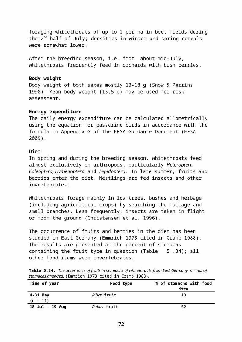
Risk assessmentThe herbivorous brown hare is a relevant focal species in most field crops and grassland, and may also be relevant in orchards:

winter cereals, BBCH 10-29 spring cereals, BBCH 10-29 maize, BBCH 10-29 winter rape, BBCH 10-39 spring rape, BBCH 10-39 beets, BBCH 10-49 pulses, BBCH 10-99 field grown vegetables, BBCH 10-89 strawberries, all stages except termination grass, short orchards, all applications bush berries, all stages

Relevance in orchards and bush berries depends on whether field vole is considered relevant for the situation and Member State in question; in that case field vole will be more worst case.

The diet of brown hares consists almost entirely of green plant parts, with seeds and fruits being present in very small amounts only. The relative amounts of grasses (including cereals) and dicotyledons (leafy crops and weeds) in the diet vary with the crop and the season. In some studies, the diet of hares was found to include sizable amounts of cereal grain in late summer, but these data are not relevant for the scenarios where brown hare has been identified as a focal species.

For the relevant crop and grassland scenarios, the relative amounts of mono- and dicotyledons in the diet may be estimated from Table 5.64 for the crop and time of year in question. Some food items will however not be available in a certain crop, e.g. cereals and dicotyledonous crops will not be available in the same field, and PD has to be adjusted to allow for this. In orchards (fruit trees), the diet consists entirely of grasses and weeds growing beneath the trees. In bush berries, hares will also eat the leaves of the bushes (especially Ribes sp.).

Taking the above considerations into account, the relative amounts of mono- and dicotyle-donous plants in diet may be estimated as follows for use in risk assessment (Table 5.65).

Table 5.65. Estimated diet composition of brown hares feeding in different crops. PD values were calculated from Table 5.64, omitting diet components assumed not be present in the crop in question and increasing the share of the other components proportionally. Spring: April-May; Summer: June-Sept.; Autumn: Oct.-Nov.

Crop Growth stage SeasonPD (fresh weight)

Monocotyledons(cereals, grasses)

Dicotyledons(leafy crops,

non-grass weeds)

Bush berry plants (buds, leaves)

Winter cereals BBCH 10-29 Spring 0.84 0.16Autumn 0.95 0.05

Spring cereals;Maize

BBCH 10-29 Spring 0.84 0.16

Maize BBCH 10-29 Summer 0.72 0.28Oilseed rape BBCH 10-39 Spring &

autumn0.39 0.61

73

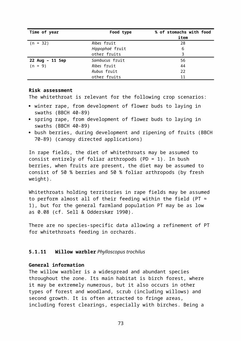
Crop Growth stage SeasonPD (fresh weight)

Monocotyledons(cereals, grasses)

Dicotyledons(leafy crops,

non-grass weeds)

Bush berry plants (buds, leaves)

Beets BBCH 10-19 Spring 0.39 0.61Pulses BBCH 10-39Vegetables BBCH 10-49Beets BBCH 10-49 Summer 0.26 0.74Pulses BBCH 10-99Vegetables BBCH 10-49Strawberries Planting

Pre-floweringSpring 0.44 0.56

PlantingFlowering & fruit develop.Post-harvest

Summer 0.30 0.70

Grass, short;Orchards

Spring & summer

0.64 0.36

Autumn* 0.93 0.07Bush berries Spring 0.54 0.30 0.16

Summer 0.45 0.28 0.27Autumn* 0.93 0.07

* In orchards and bush berries, autumn treatments will always be post-harvest.

For applications in orchards and bush berries, interception in the canopy shall be taken into account as appropriate for the growth stage and type of application.

Brown hares have large home ranges (29-138 ha, cf. above), implying that it will usually be appropriate to refine PT. The values in Table 5.61 may be used for field crops (notice that only 90th percentiles are available) while PT values for grassland may be estimated from Table 5.60. There is no specific information allowing refinement of PT for orchards and bush berries.

5.2.3 Field vole Microtus agrestis

General informationThe field vole is widespread within the Zone, where it occurs from southernmost Denmark and Lithuania to northernmost Norwegian mainland (Mitchell-Jones et al. 1999). Apparent gaps in the distribution in western and northern Norway and northern Finland are probably due to incomplete coverage in the European Atlas (Mitchell-Jones et al. 1999). The species is generally common within its range, except in marginal areas where it may be locally rare. Field voles may occur in woodland, provided there is a good grass cover, but are found mostly in open country where they prefer tall and dense grass vegetation and areas where the vegetation provides good cover, such as meadows, set-asides, river banks, vegetated margins of ditches and hedgerows (Mitchell-Jones et al. 1999, Hansen & Jensen 2007a).

In Denmark, breeding starts in March and ends in September; during this period four to five litters are born (Hansen & Jensen 2007a).

Agricultural association

74

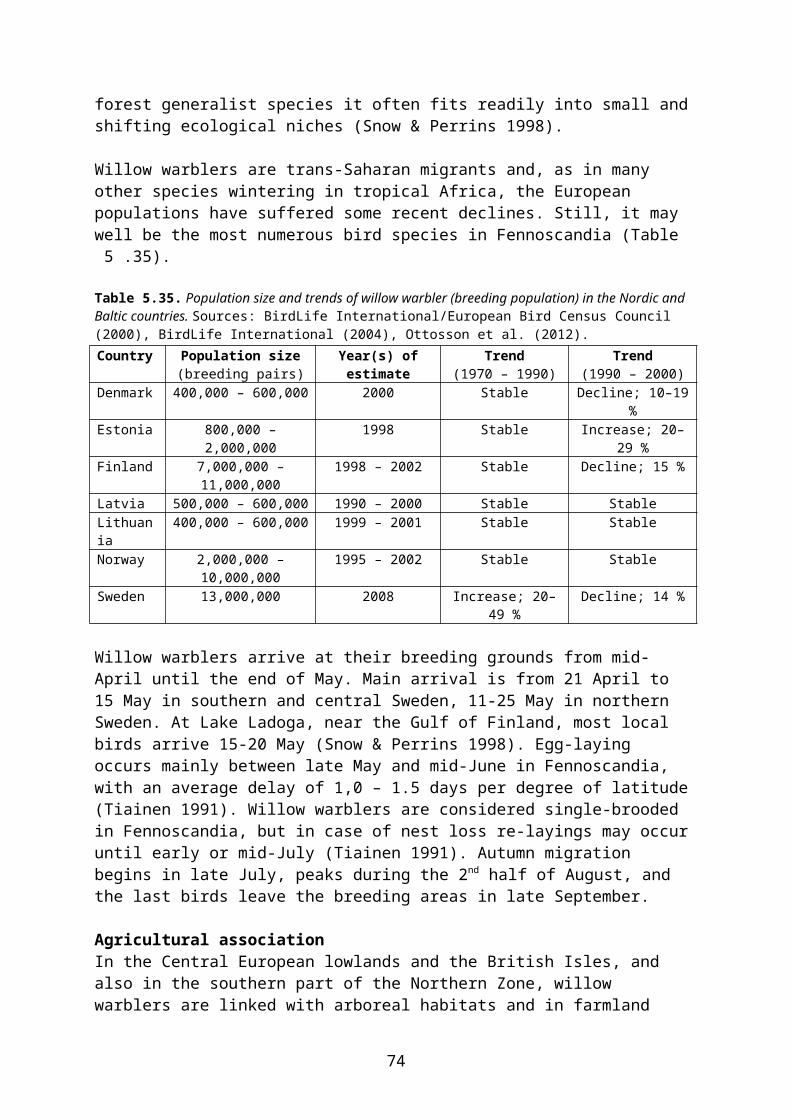
The field vole can be found in farmland (Loman 1991a, Tattersall et al. 2002, Hansen & Jensen 2007a) where it mainly occurs in set-aside and permanent grassland while numbers in cereal fields are low (Jensen & Hansen 2003). For example, in a three years study of small mammals on arable land in England, Tew (1994) failed to capture any field voles away from the hedgerows around cereal fields. In another study in England, field voles were occasionally caught in the fields, but they were usually restricted to areas with dense ground cover, such as patches infested with blackgrass Alopecurus myosuroides (Johnson et al. 1992).

The species requires a vegetation cover for its presence and is therefore – apart from its occurrence in permanent grassland – found mainly in the surroundings of arable crops and not in the crop itself (Gurney et al. 1998, Hansen & Jensen 2007a). The most frequently used habitat in arable landscapes is field boundaries (e.g. ditches) (Huitu et al. 2004, Yletyinen & Norrdahl 2008), and particularly field voles are found in two-year leys and set-asides (Hansson 1977, Rogers and Gorman 1995a, Tattersall et al. 2002). The species also occurs in orchards, provided the grass cover is higher than 10 cm.

The field vole is often found in leys and set-asides where there is a vegetation cover year round, and in such habitats voles can be both nesting and foraging (Hansson 1977, Jensen & Hansen 2003, Huitu et al. 2004). Thus, it is reasonable to believe that field voles can spend their whole life cycle in leys and set-asides, albeit in fairly low densities, compared to the densities in prime habitats such as meadows and other permanent grasslands.

In several studies the captures of field voles in arable crops are few (e.g. Loman 1991a; Rogers and Gorman 1995a, Jensen & Hansen 2003) and the time spent in this habitat is probably low. The home range of field voles varies between 0.02 and 0.1 ha for females and twice that for males (Bjärvall and Ullström 1985).

Body weightThe body weight of field voles is given for males and females separately:

Males mean weight 39.7 (15-42) g, (Gurney et al. 1998). Females mean weight 30.9 (15-32) g, (Gurney et al. 1998).

A body weight of 30 g may be used for risk assessment.

Energy expenditureDaily energy budget has been calculated for the field vole on a summer and a winter day to 51.7 kJ/animal/day (animal weight 23.8 g) and 44.5 kJ/animal/day (animal weight 20.4 g), respectively (Hansson and Grodzínski 1970). Alternatively, the energy expenditure can be calculated allometrically using the equation for mammals in accordance with the formula in Appendix G of the EFSA Guidance Document (EFSA 2009).

DietThe field vole is a herbivore, mainly feeding on green leaves and stems of grasses. Almost no seeds or invertebrates are consumed (Hansson 1971). In a study in England where field voles were occasionally trapped in oilseed rape, a dietary analyses showed that the voles were eating mainly monocotyledons (82 %) and only 3 % oilseed rape (Rogers 1993). In a study in southern Sweden animal food occurred with a maximum of 2 % of total stomach content in any month (Hansson 1971). In the same study the annual food habits of 527 field voles living in grassland was examined (Table 5.66).

75

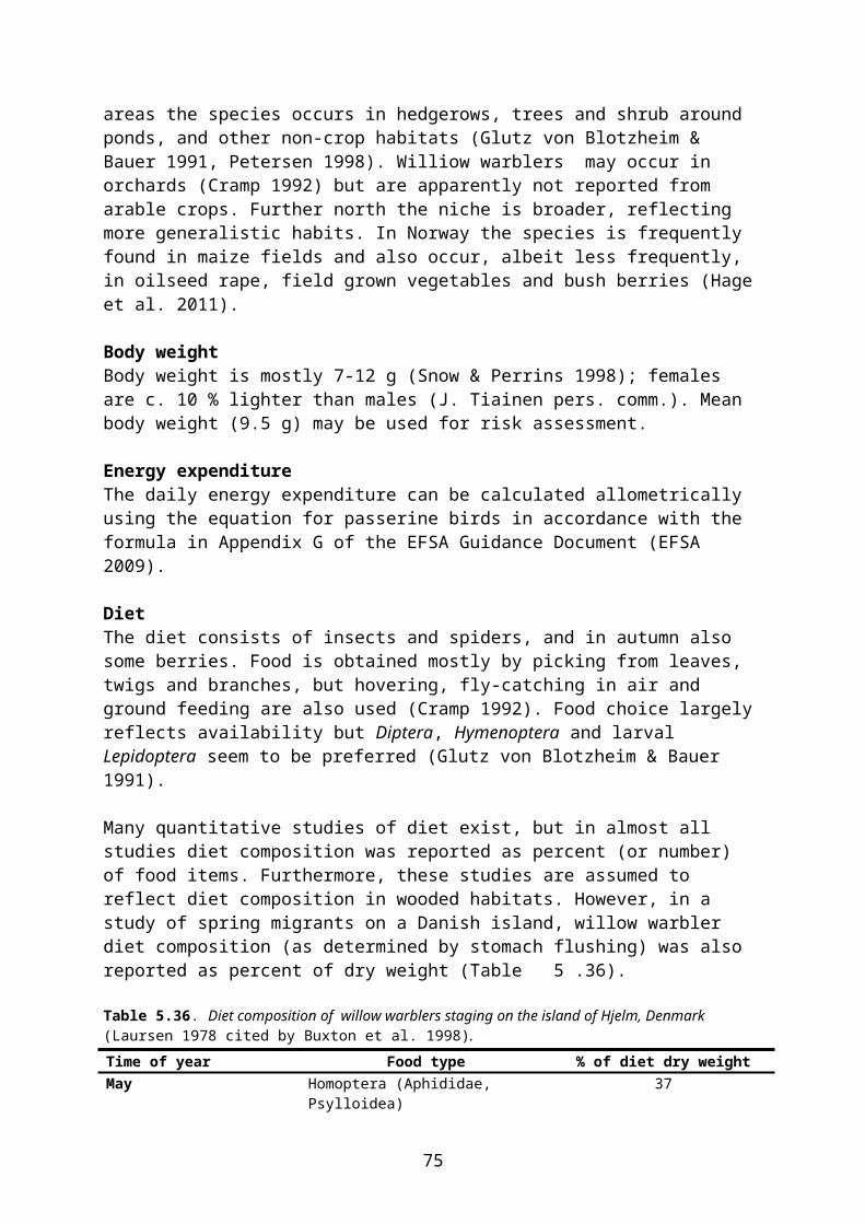
Table 5.66. Field vole diet in grassland of southern Sweden (Hansson 1971).Time of year Food type % of food itemsApril (n=26) Grass (leaves and stems) 71

Herb (leaves and stems) 2Graminoids (leaves and stems) 9Vegetative storage organs* 17

May (n=17) Grass (leaves and stems) 75Herb (leaves and stems) 14Graminoids (leaves and stems) 2Vegetative storage organs* 5

June (n=29) Grass (leaves and stems) 52Herb (leaves and stems) 37Graminoids (leaves and stems) 2Vegetative storage organs* 10

July (n=23) Grass (leaves and stems) 40Herb (leaves and stems) 36Graminoids (leaves and stems) 2Grass seeds 19

August (n=33) Grass (leaves and stems) 30Herb (leaves and stems) 51Grass seeds 12

September (n=22) Grass (leaves and stems) 65Herb (leaves and stems) 25Grass seeds 8

* Mainly underground storage organs, so residues will depend on the mode of action of the compound (systemic or non-systemic).

In a Dutch study, the diet composition was studied throughout the year at two sites (Faber & Ma 1986 cited in Gurney et al. 1998). The results from one of these sites are shown in Table 5.67. At the other site, the diet was dominated by wavy hair-grass Deschampsia flexuosa and also contained mosses (Hypnum cupressiforme) and blueberry Vaccinium myrtillus. Accordingly, this site was probably a grass-dominated heathland, making the results less relevant for risk assessment.

Table 5.67. Stomach contents of field voles collected in grassland near Budel, the Netherlands (Faber & Ma 1986).Time of year Food type % fresh weightMarch Grasses 96.1

Dicotyledons 2.5Undetermined plant material 1.0Fungi 0.3

June Grasses 52.1Dicotyledons 40.5Undetermined plant material 3.0Animal material* 2.0

August Grasses 57.4Dicotyledons 29.0Undetermined plant material 8.3Seeds 4.9Animal material* 1.2

October Grasses 79.0Dicotyledons 17.0Undetermined plant material 2.0Seeds 0.7Other 0.3

December Grasses 96.0

76

Time of year Food type % fresh weightDicotyledons 0.3Undetermined plant material 2.5Other 0.7

* Probably ground-dwelling arthropods.

Risk assessmentThe herbivorous field vole is relevant for the following crop scenarios:

grass, medium and long (all season) orchards, canopy and ground directed treatments (all season) bush berries (all season)

The composition of diet at different times of the year may be taken from Table 5.67 (which is preferred to Table 5.66 because the PD values are expressed in terms of weight). It is considered that the values in Table 5.67 are valid for all of the above-mentioned scenarios. In the calculation of PD, the percent content of “undetermined plant material” and “other” are left out and the shares of the other components increased proportionally to provide a sum of 100 percent; Table 5.68.

Table 5.68. Estimated diet composition (PD values) of field voles feeding in grass-dominated habitats at different times of the year. PD values were calculated from Table 5.67 (see text).

Food typePD (fresh weight)

Spring Summer AutumnMarch June August October

Grasses 0.97 0.55 0.62 0.82Non-grass herbs 0.03 0.43 0.32 0.17Small seeds 0.05 0.01Ground arthropods 0.02 0.01

Home ranges of field voles may be very small (≈ 0.1 ha), so refinement of PT for field voles living in grass is probably not justified. In orchards and bush berries, PT may be refined if justified by case-specific data.

5.2.4 Wood mouse Apodemus sylvaticus

General informationThe wood mouse is common and widespread in Denmark, southern Sweden, South Norway and south-western Lithuania (Mitchell-Jones et al. 1999). The species is found in a wide range of habitats, including both arable land and forest. There may be geographic variation in habitat, with western populations being associated mostly with diverse habitats and eastern populations with woodland edge habitats (Mitchell-Jones et al. 1999). In Denmark wood mice are mainly found in open habitats, including arable land, and rarely occur in forest (Hansen & Jensen 2007b). In north-eastern Lithuania, Latvia, Estonia and southern Finland, the wood mouse is replaced in farmland by the striped field mouse Apodemus agrarius, which is of similar size.

Wood mice are nocturnal and live in well developed burrow systems which can be as deep as 25 cm (Loman 1991a). Young are born from March-April to September-October with two, maximum four, litters during the breeding season (Hansen & Jensen 2007b).

77

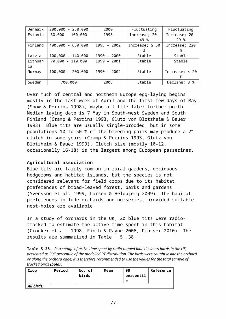
Agricultural associationThe wood mouse is widespread and common in the agricultural landscape and occurs in a number of farmland habitats (Jensen & Hansen 2003). Studies on the species have been conducted in set-asides as well as in arable crops such as wheat (autumn and spring sown), rye, winter barley, potatoes, sugar beet and oilseed rape (Green 1979, Pelz 1989, Loman 1991a, Rogers and Gorman 1995a, Fitzgibbon 1997, Todd et al. 2000, Jensen & Hansen 2003 and notifier study summarized in EFSA Journal 2004). Wood mice are found throughout the year in the fields (Green 1979, Loman 1991b, Rogers 1993) although densities decline following harvest due to predation and migration to hedges (Tew & Macdonald 1993, Tew et al. 1994).

Macdonald et al. (2000) compared the use of wheat, barley and rape fields by wood mice in England and found a tendency for numbers of mice to be lower in rape than in other crops. Jensen & Hansen (2003) on the other hand found that wood mice were trapped more commonly in rape than in other crops, particularly during autumn. In a study in NW France, Ouin et al. (2000) recorded low occurrence of wood mice in maize and carrot fields between May and July compared to fields with wheat and peas.

Wood mice are territorial and individuals have separate home ranges. There is a difference in home range size between breeding season and winter, as well as for males and females. The home range of males during the breeding season has been estimated at 1.22 – 1.87 ha and in winter at 0.34 ha (Green 1979, Tattersall et al. 2001). The corresponding estimates for females are 0.49 – 0.63 ha and in winter 0.46 ha (Green 1979, Tew et al. 1992). In an English study of radio-tracked mice in a winter wheat field, two males had large home ranges of 18.1 ha and 23.3 ha in June-July while a single female had a home-range of only 0.13 ha during the same period (Tew et al. 1992). According to Tew & Macdonald (1994) only females are defending territories, while males have larger undefended ranges overlapping as many female territories as possible (Tattersall et al. 2001). The home range size is also dependent on density. Higher densities lead to decreased home range sizes (Tew & Macdonald 1994). Population densities according to two studies on arable land are 1.14 individuals/ha (Pelz 1989) and 1.17 individuals/ha (Green 1979). Some spring/summer densities for different crop types are: winter wheat 2.30, spring sown cereals 1.02, and sugar beet 0.55 animals/ha (Green 1979). Densities in winter cereal fields in autumn are 5-10 animals/ha (Tew & Macdonald 1993, Hansen & Jensen 2007b).

There are populations of wood mouse that are present in agricultural landscapes and spend their entire life in this habitat. However, wood mice that lived in barley or wheat fields during the summer emigrated to the hedgerows after harvest (Tew et al. 1994) leading to large seasonal variations in population size in field centres (Macdonald et al. 2000). The home ranges for individual mice are likely to be inside the area of a single field and it is therefore reasonable to assume that these mice may spend their entire life cycle in a single field. This assumption is supported by other studies (Plesner-Jensen 1993; notifier study summarized in EFSA 2004).

Radio-tracking studies of wood mice caught in arable land have been conducted in the UK and are reported by Prosser (2010). The mice were equipped with collar-mounted radio tags and were tracked during “a day in the life” – or rather “a night in the life” since tracking was carried out from dusk to dawn to reflect the nocturnal habits of the species. In one project, data were allegedly collected from 20-30 individuals in each of spring (March - May),

78

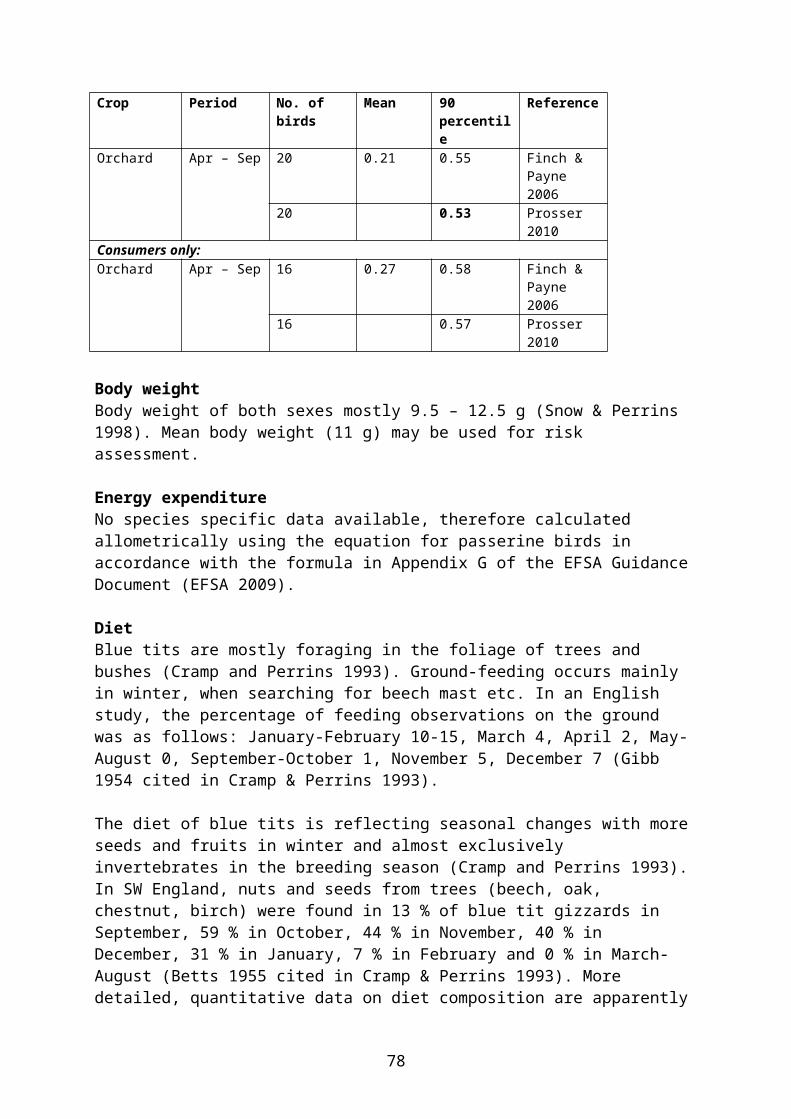
summer (June - August), autumn (September - November) and winter (December - February). However, data are reported for the periods June - September and October - February and only for potatoes (summer) and cereals (winter) (Prosser 2010, Table 5.69). In another study, wood mice were caught on or immediately adjacent to newly-drilled cereal fields in autumn. Tracking followed a protocol similar to that in the first study and the results are also shown in Table 5.69.

Table 5.69. Percentage of active time spent by radio-tagged wood mice in different crops in the UK, presented as 90th percentile of the modelled PT distribution. Results are shown for the total sample of tracked mice (“all animals”) as well as for the subsample of animals who actually used the crop in question (“consumers only”). Recommendations on which data set to use are given below the table and are also shown in bold (Prosser 2010).

Period Crop No. of animals 90th percentile

All animals:Summer(June - September)1 2

Potatoes2 20 0.79 1

Autumn(September - November) 3

Winter cereals,newly drilled3

21 0.37

Winter(October - February)2

Winter cereals2 36 0.70

Consumers only:Summer(June - September)1 2

Potatoes2 17 0.82 1

Autumn(September - November)3

Winter cereals,newly drilled3

12 0.51

Winter(October - February)2

Winter cereals2 10 0.81

1 Although data were only reported for June - September, it is assumed that that these values may be used for the whole growing season.2 Animals were presumably trapped in general farmland; it is recommended to use data for “consumers only”.3 Animals were trapped in or adjacent to newly-drilled cereal fields; it is recommended to use data for “all animals”.

Body weightThe body weight of wood mice shows an annual cycle with higher weights during breeding season compared to other times of year (Rogers & Gorman 1995a).

Body weight is reported as follows:

Summer 25 g (May-August) (L. Hansson pers. comm. to KemI). Year round 18 (13-27) g (Gurney et al 1998).

The latter mean weight (18 g) may be used for risk assessment.

Energy expenditureDaily energy budgets for wood mouse in summer, winter and annually have been calculated by Grodzínski (1985) from several scientific papers. The energy budget for wood mice on a summer and a winter day amount to 43.1 kJ/animal/day (weight 22 g) and 37.1 kJ/animal/day (weight 19 g), respectively (Grodzínski 1985). Alternatively, the energy expenditure can be calculated allometrically using the equation for mammals in accordance with the formula in Appendix G of the EFSA Guidance Document (EFSA 2009).

79

DietThe wood mouse is an opportunistic feeder, taking mainly seeds and invertebrates. The diet depends on the main habitats which exist within the home range of the population, but also on the time of year as availability of food differ during the growth period. Plesner-Jensen (1993) found that seeds of wheat, barley and oil-seed rape were among the five most favoured food items to wood mice, with wheat ranking higher than the other crops. However, crop seeds are only available for a short time, and for most of the year wood mice rely on wild plant seeds (Green 1979, Pelz 1989). During winter, grazing of winter cereals by wood mice may locally cause considerable damage (Roebuck et al. 1944).

The principal diet of wood mouse throughout the year was reported by Hansson (1985) and Tew et al. (1992) to consist of 70 % seeds/cereal grains, 15 % animal matter and 5-10 % vegetative plant tissue. The diet composition for different habitats and time of year for arable dwelling wood mice has been investigated in a number of different studies which are summarized below (Table 5.70, Table 5.71, Table 5.72).

In an English study, Barber et al. (2003) studied the amount of winter wheat seeds consumed by wood mice during a three week period following drilling in October. Two fields of 4.7 and 5.6 ha were examined and mice were caught in transects from the field boundary towards the centre of the field. A total of 90 wood mice were used to establish the proportion of stomach content that consisted of wheat seeds. The amount of wheat seeds, estimated as % of total stomach content (probably by volume), was:

Less than 25 % (90 % of the individuals) Maximum 40 % (10 % of the individuals)

Pelz (1989) studied arable dwelling wood mice in a typical sugar beet growing area in the Rhineland, Germany. In the area a three year crop rotation system with sugar beet, winter wheat and winter barley was employed. The analysis of food consumption was based on 465 wood mice that were caught between 1976-77 and 1980-86 (Table 5.70). Table 5.70. Wood mice diet in intensive arable land dominated by winter cereals and sugar beet (Pelz 1989).Time of year Food type Vol. % of dietMarch (n=56) Insect larvae1 25

Earthworms 23Vegetative plant tissue2 22Cereal grain 23Sugar beet seeds 7

April (n=49) Insect larvae1 45Earthworms 26Vegetative plant tissue2 24Cereal grain 5

May (n=16) Insect larvae1 10Earthworms 40Vegetative plant tissue2 16Cereal grain 30Dicotyledon seeds (herb) 4

June (n=15) Insect larvae1 25Earthworms 9Vegetative plant tissue2 9Cereal grain 32Dicotyledon seeds (herb) 25

July (n=10) Insect larvae1 28Vegetative plant tissue2 8

80

Time of year Food type Vol. % of dietCereal grain 48Dicotyledon seeds (herb) 16

August (n=41) Insect larvae1 28Earthworms 5Vegetative plant tissue2 10Cereal grain 37Dicotyledon seeds (herb) 20

September (n=18) Insect larvae1 25Earthworms 13Vegetative plant tissue2 9Cereal grain 33Dicotyledon seeds (herb) 20

October (n=48) Insect larvae1 30Vegetative plant tissue2 25Cereal grain 30Dicotyledon seeds (herb) 15

November (n=36) Insect larvae1 9Earthworms 3Vegetative plant tissue2 40Cereal grain 40Dicotyledon seeds (herb) 8

1 For risk assessment puposes, the insect larvae may be assumed to be picked from the ground.2 Mono- or dicotyledonous, depending on the crop.

Green (1979) studied arable dwelling wood mice in English farmland. Among the crops grown in the study area were spring barley, spring and winter wheat and sugar beet. Wood mice living in winter wheat fields were caught for food analysis (Table 5.71). Table 5.71. Wood mouse diet in winter wheat fields in England (Green 1979).Time of year Food type Vol. % of dietSeptember – December (n=8) Arthropods1 16

Cereal grain 60Dicotyledon seeds2 24

January – March (n=30) Arthropods1 16Earthworms 16Cereal grain 55Chickweed seed2 2Other dicotyledon seeds2 3Leaf tissue 1Other plant tissue 7

April – June (n=15) Arthropods1 12Cereal grain 6Leaf tissue 1Chickweed seed2 27Grass flowers/green seeds2 53

1 All arthropods may be assumed to be ground-dwelling.2 Small seeds.

Rogers and Gorman (1995b) collected data on wood mice living on set-aside in Scotland. The set-aside included in the study was fallow from barley and regenerated naturally. The diet analysis was performed in 53 wood mice caught over an 18 month period (Table 5.72).

81

Table 5.72. Wood mouse diet on set-aside (n=53) (Rogers & Gorman 1995b).Time of year Food type Vol. % of dietMarch – May Monocotyledons (Grasses) 72

Insects 13Other animal material* 10Dicotyledons (Herbs) 5

June – August Monocotyledons (Grasses) 45Seeds 42Other plant material 5Dicotyledons (Herbs) 3Other animal material* 2Insects 1

September – November Monocotyledons (Grasses) 50Seeds 35Other plant material 6Insects 5Dicotyledons (Herbs) 2Other animal material* 1

* Probably mainly soil invertebrates (earthworms).

Risk assessmentThe omnivorous wood mouse is a relevant focal species in all scenarios. Risk assessment for wood mouse is assumed to cover also the striped field mouse, which replaces the wood mouse in farmland in the Baltic States and Finland.

The diet composition (PD values) may be deduced from Table 5.70 – Table 5.72 for the month(s) in question. The PD values in the tables shall however be adjusted to allow for differences in food availability between crops. Crop-specific PD adjustments are described in Appendix 2 and the resulting PD values are shown in Appendix 4 and in the accompanying data sheet.

All insects and other arthropods listed in the tables may be assumed to be ground-dwelling. A few of the arthropods will be foliar but this is offset by the fact that burrowing arthropods, which probably have very low residues, also occur in the diet.

As wood mice obtain almost all of their food from the ground, interception in the crop canopy shall be taken into account as appropriate for the crop and application scenario in question, cf. section 4.5.

The wood mouse is also relevant for all field scenarios involving seed treatments. The values in Table 5.73 may be used in risk assessment; the PD values to be used in assessment of long-term risk are derived from the adjustments described in Appendix 2.

Table 5.73. Estimated amounts of treated seed consumed by an 18 g wood mouse fulfilling its daily requirements by feeding in newly sown fields.

PD (fresh weight)* Fresh weight (g) NotesSpring cereals** 1.00 3.90

0.29 2.05Winter cereals** 1.00 3.90

0.55 / 0.60 2.45 / 2.41 Values from Pelz/Green. Both values include an unknown amount of harvest spillage

Maize** 1.00 3.900.29 2.18 Includes an unknown amount of cereal grain

82

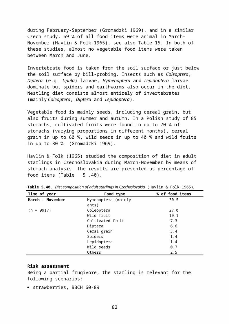
PD (fresh weight)* Fresh weight (g) NotesSpring rape*** 1.00 3.13

0.07 0.59Winter rape*** 1.00 3.13

0.41 2.02 Includes an unknown amount of weed seedsBeets*** 1.00 3.13

0.07 0.59Pulses** 1.00 3.90

0.29 2.18 Includes an unknown amount of cereal grainGrass*** 1.00 3.13

0.42 2.25 Based upon Rogers & Gorman (1995b) data* PD = 1 may be used in acute risk assessment, PD < 1 in long-term risk assessment.** Large seeds. *** Small seeds.

Dehusking or cracking of seeds is part of the typical feeding behaviour of wood mice, so a dehusking factor may be applied, cf. section 4.7. Home ranges of female wood mice are usually small (< 1 ha) and may well be within the area of a single field. For potatoes (all season), cereals in winter (October - February) and newly drilled cereals in autumn, PT may be refined using the data in Table 5.69. In all other cases, PT shall not be refined unless fully justified by case-specific data.

83

6 Summary tables

The selection of relevant focal species for different combinations of crop and growth stage is summarized in this chapter.

The selection is based on the species specific information presented in chapter 5. Because of the different ecological traits of the focal species, only species considered relevant for a specific crop scenario are listed. Species that are not mentioned are assumed to be less frequent in the actual crop at that time of year, or the risk assessment for these species is covered by other, more sensitive species.

The different scenarios within a certain crop are defined by their growth stage (BBCH, ref. Meier 2001). The calendar months mentioned in the tables refer to Danish conditions and are merely indicative. In cases where two time lines are presented, the upper line refers to spring-sown crops and the lower line to autumn-sown crops.

It should be noticed that although most of the focal species are widespread and common across the Northern Zone, not all of the species selected for a certain crop scenario may be relevant in all Member States within the Zone.

84

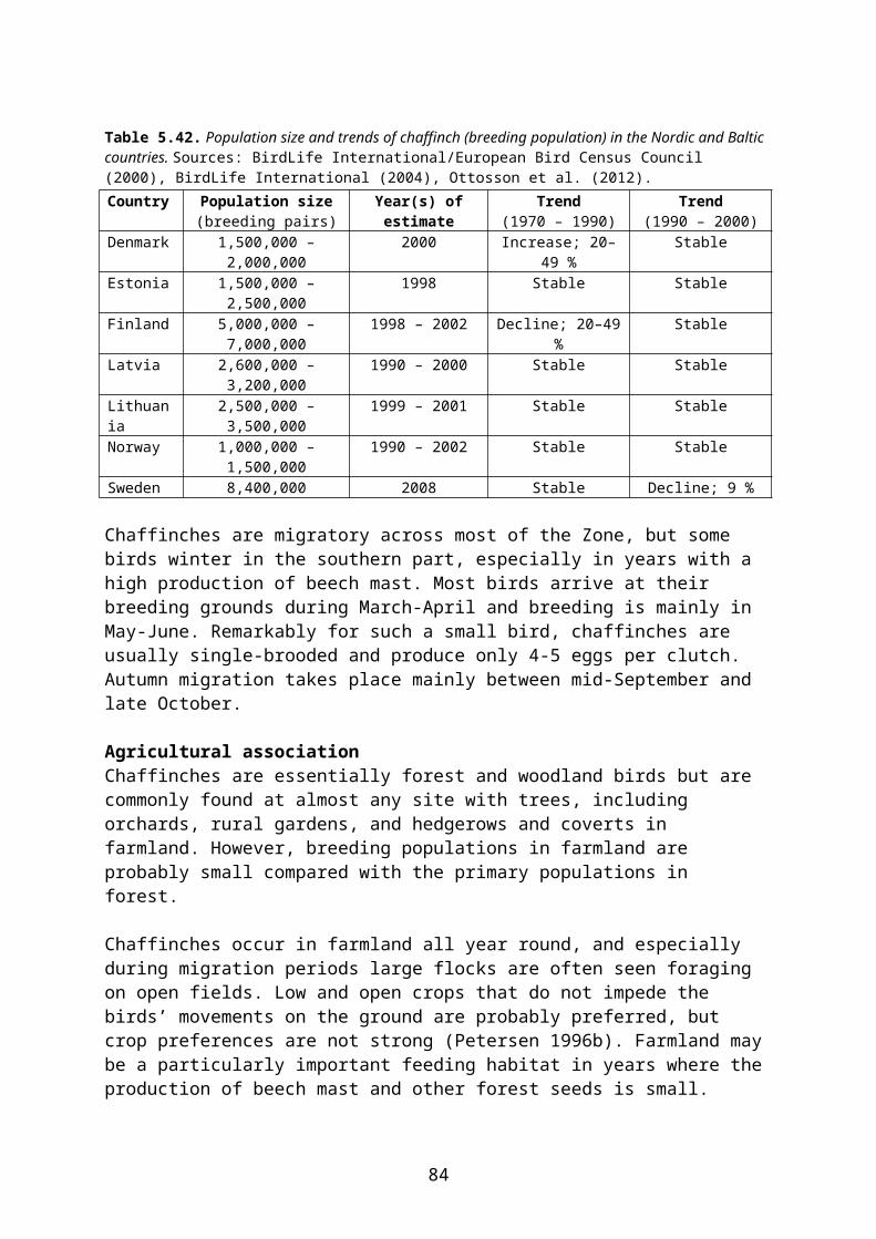
Beets

Beet crops include sugar beet, fodder beet and turnip; they are sown in spring and are subject to various pesticide treatments throughout the growing season.Sowing andpre-emergenceBBCH 0-9

Early growth stages of cropBBCH 10-19

Closing of rows

BBCH 20-39

Final development towards harvestingBBCH 40-49

April May - June June July - OctoberFood types- ground-dwelling arthropods- (treated seeds) 1)

- (weed seeds) 2)

- crop leaves- weeds 3)

- ground-dwelling arthropods- (weed seeds) 2)

- crop leaves- weeds 3)

- weed seeds- ground-dwelling arthropods- foliar arthropods 4)

- crop leaves- weeds 3)

- weed seeds- ground-dwelling arthropods- foliar arthropods

Selected species Skylark White wagtail Wood mouse

Skylark White wagtail Linnet Brown hare Wood mouse

Skylark White wagtail Linnet Brown hare Wood mouse

Skylark White wagtail Linnet Brown hare Wood mouse

1) Pelleted beet seeds may be eaten by mammals (mice) but are little attractive to birds (Prosser 1999) and are usually precision drilled at 2-3 cm depth. In Sweden the risk assessment shall also cover potential spill of treated seeds.2) Availability of weed seeds depends on the soil treatments.3) The relative amounts of grasses and dicotyledonous weeds will vary.4) The population of foliar arthropods in the field develops during this period.

85

Bush berries

Bush berries cultivated in the Northern Zone include red and black currant, raspberry, gooseberry and blackberry. Bush berries are subject to various pesticide treatments throughout the growing season (except during harvest).Pre-floweringand floweringBBCH ≤ 69

Development and ripening of fruitsBBCH 70-89

Post-harvest

Food types- foliar arthropods- ground-dwelling arthropods- grass- dicot. weeds- weed seeds

- fruits- foliar arthropods- ground-dwelling arthropods- grass- dicot. weeds- weed seeds

- foliar arthropods- ground-dwelling arthropods- grass- dicot. weeds- weed seeds

Selected species Blue tit 1)

Chaffinch Linnet Brown hare Field vole 2)

Wood mouse

Whitethroat 1)

Blue tit 1)

Chaffinch Linnet Brown hare Field vole 2)

Wood mouse

Blue tit 1)

Chaffinch Linnet Brown hare Field vole 2)

Wood mouse

1) Canopy directed applications.2) If ground vegetation (grass) height is ≥ 10 cm.

86

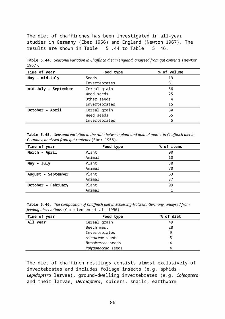
Cereals

Sowing andpre-emergenceBBCH 0-9

Early growth stages of cropBBCH 10-29

Stretching to floweringBBCH 30-39

Stretching to floweringBBCH 40-69

Development and ripening of grainBBCH 70-89

Pre-harvest desiccation 1)

Post-harvest stubble treatments 2)

Sowing andpre-emergenceBBCH 0-9

Early growth stages of cropBBCH 10-19

April(spring cereals)

(April -) May June June - July July - August August August - Sept.

– April / May(winter cereals) 3)

May - June May - June/July July - Aug. July - August August - Sept. Sept. - October Sept./October –

Food types- treated seeds- ground-dwelling arthropods- (weed seeds) 4)

- early growth stages of crop- ground-dwelling arthropods- (weed seeds) 4)

- ground-dwelling arthropods- foliar arthrop.5)

- weeds- crop itself is not attractive as food item

- ground-dwelling arthropods- foliar arthrop.5)

- weeds- crop itself is not attractive as food item

- ground-dwelling arthropods- foliar arthropods- weeds- weed seeds- cereal grain/ear

- ground-dwelling arthropods- foliar arthropods- weeds- weed seeds- cereal grain/ear

- ground-dwelling arthropods- weeds 6)

- weed seeds- waste grain

- treated seeds- ground-dwelling arthropods- (weed seeds) 4)

- (waste grain) 4)

- early growth stages of crop- ground-dwelling arthropods- (weed seeds) 4)

- (waste grain) 4)

Selected species Bean goose Pink-footed g. Skylark White wagtail Yellowhammer Wood mouse

Bean goose Pink-footed g. Skylark White wagtail 7)

Brown hare Wood mouse

Skylark Wood mouse

Skylark Whinchat Wood mouse

Skylark Whinchat Yellowhammer Wood mouse

Skylark Whinchat Yellowhammer Wood mouse

Skylark Yellowhammer Wood mouse

Bean goose Woodpigeon Skylark White wagtail 8)

Yellowhammer Wood mouse

Bean goose Pink-footed g. Grey partridge Brown hare Wood mouse

1) At pre-harvest desiccation with herbicides, in most cases the crop and possible weeds in the field are completely wilted or at least have become unattractive as food within approximately one week. Hence, exposure via green parts of plants and associated foliar arthropods is limited to the first week after treatment. Thereafter, only ground dwelling arthropods and seeds remain attractive as food items in the field.2) At post-harvest stubble treatments with herbicides, in most cases the weeds in the field are completely wilted or at least have become unattractive as food within approximately one week. Hence, exposure via green parts of plants is limited to the first week after treatment. Thereafter, only ground dwelling arthropods and seeds remain attractive as food items in the field.3) The phenology of winter cereals differs between species. In general, rye and winter barley develop earlier than winter wheat.4) Availability of weed seeds and waste grain depends on the soil treatments.5) The population of foliar arthropods in the field develops during this period.6) Grasses or dicotyledonous weeds, depending on the situation.7) BBCH 10-14.8) September.

87

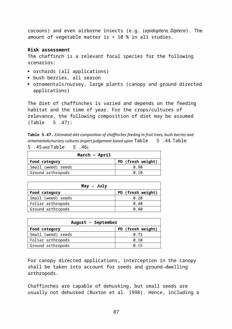
Fruit trees (orchards)

Fruit trees in the Northern Zone include pome fruit (apple, pear) and stone fruit (plum, cherry). Fruit trees are treated with pesticides in spring and early summer, or post-harvest in autumn. Treatments with insecticides, fungicides and growth regulators are directed towards the canopy of the trees, while herbicides are applied to the ground beneath the trees. Generally, herbicide treatments take place in the tree rows, while the strips between the trees may be left untreated.The relevant focal species for risk assessment depend on the kind of treatment (canopy or ground directed) rather than on the season.Herbicide treatments(applied to ground)

Other treatments (applied to canopy)

All seasonFood types- grass- dicot. weeds- weed seeds- ground-dwelling arthropods

- foliar arthropods- fruit- grass 1)

- dicot. weeds 1)

- weed seeds 1)

- ground-dwelling arthropods 1)

Selected species Robin Chaffinch Linnet Brown hare Field vole 2)

Wood mouse

Blue tit Starling 3)

Chaffinch Brown hare Field vole 2)

Wood mouse

1) Interception in the leaf canopy shall be taken into account.2) If ground vegetation (grass) height is ≥ 10 cm. 3) Only in stone fruit (cherry, plum) when fruits are present (BBCH 60-89).

88

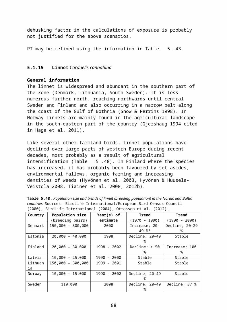
Grass

This group includes grass for seed, grass ley, mixed ley, pasture and turf. Seed grass and leys are usually bi- or tri-annual, whereas pasture and turf are normally permanent.Grass seeds are sown in spring or autumn, often as an undersown crop. Treatments vary depending on type of grassland. Pesticide use is most intensive in grass for seed where intensity of use is comparable to that in cereals. In leys and especially in permanent grassland (except golf courses), treatments are less frequent although herbicides, insecticides and fungicides may all be used.Sowing andpre-emergence

Short grass Medium and long grass, incl. with seed heads

Termination 1)

Food types- grass seeds- weed seeds- ground-dwelling arthropods

- grass- dicot. weeds- weed seeds- ground-dwelling arthropods- (foliar arthropods)2)

- grass- dicot. weeds- grass & weed seeds- ground-dwelling arthropods- foliar arthropods

- grass- dicot. weeds- grass & weed seeds- ground-dwelling arthropods- foliar arthropods

Selected species Skylark Yellow wagtail Linnet Wood mouse

Bean goose Pink-footed g. Skylark Yellow wagtail Brown hare Wood mouse

Skylark Yellow wagtail Linnet Common shrew Field vole Wood mouse

Skylark Yellow wagtail Linnet Wood mouse

1) At termination of leys or permanent grassland with herbicides, in most cases the grass and possible weeds are completely wilted or at least has become unattractive as food within approximately one week. Hence, exposure via green parts of plants and associated leaf-dwelling insects would be limited to the first week after treatment. Thereafter, only ground dwelling insects and seeds would remain attractive as food items in the field.2) The population of foliar arthropods is set back when the grass is mown. Therefore, the shorter the grass and the more frequent the mowings, the smaller the population of foliar arthropods.

89

Maize

Maize is sown in spring and is subject to various pesticide treatments until the crop is too high to allow driving in the field.Sowing andpre-emergenceBBCH 0-9

Early growth stages of cropBBCH 10-29

Stretching

BBCH 30-39April - May May - June June - JulyFood types- ground-dwelling arthropods- (treated seeds) 1)

- (weed seeds) 2)

- crop leaves- weeds 3)

- weed seeds- ground-dwelling arthropods

- crop leaves- weeds 3)

- weed seeds- ground-dwelling arthropods- foliar arthropods 4)

Selected species Woodpigeon Skylark White wagtail Wood mouse

Skylark White wagtail Brown hare Wood mouse

Skylark Willow warbler Yellowhammer Brown hare Wood mouse

1) Maize seeds are usually precision drilled at 5 cm depth. In Sweden the risk assessment shall also cover potential spill of treated seeds.2) Availability of weed seeds depends on the soil treatments.3) The relative amounts of grasses and dicotyledonous weeds will vary.4) The population of foliar arthropods in the field develops during this period.

90

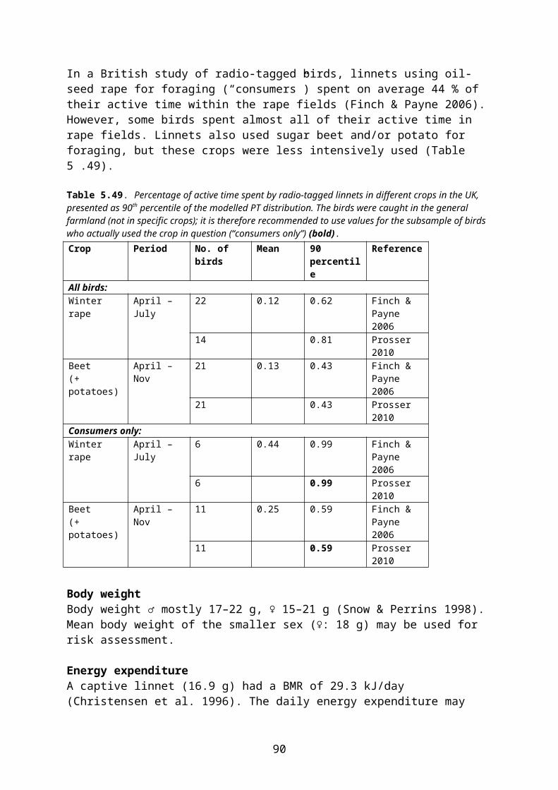
Oilseed rape

Oilseed rape is sown in spring or in early autumn and is subject to various pesticide treatments throughout the season.Sowing andpre-emergence

BBCH 0-9

Early growth stages of crop

BBCH 10-19

Stretching

BBCH 20-39

Development of side shoots and flower budsBBCH 40-59

Flowering, development of fruitsBBCH 60-79

Ripening of seed

BBCH 80-89

Pre-harvest desiccation or laying in swaths 1)

Post-harvest stubble treatments 2)

Sowing andpre-emergence

BBCH 0-9

Early growth stages of crop

BBCH 10-19April(spring-sown )

April - May May May - June June - July July - August July - August August - Sept.

– March/April(autumn-sown)

April April - May May - June June - July July July - August August September –

Food types- treated seeds- ground-dwell. arthropods- (weed seeds) 3)

- ground-dwell. arthropods- crop leaves- (weed seeds) 3)

- ground-dwell. arthropods- foliar arthropods 4)

- crop leaves- weeds

- ground-dwell. arthropods- foliar arthropods- crop leaves- weeds- weed seeds

- ground-dwell. arthropods- foliar arthropods- crop leaves- weeds- weed seeds

- ground-dwell. arthropods- foliar arthropods- crop leaves- weeds- weed seeds- rape seeds

- ground-dwell. arthropods- foliar arthropods- weeds- weed seeds- rape seeds

- ground-dwell. arthropods- weeds 5)

- weed seeds- rape seeds

- treated seeds- ground-dwell. arthropods- (weed seeds) 3)

- (waste grain) 3)

- ground-dwell. arthropods- crop leaves- (weed seeds) 3)

- (waste grain) 3)

Selected species Skylark White wagt. Wood mouse

Woodpigeon Skylark White wagt. Brown hare Wood mouse

Skylark Brown hare Wood mouse

Skylark Whitethroat Wood mouse

Whitethroat Linnet Wood mouse

Whitethroat Linnet Com. shrew Wood mouse

Linnet Com. shrew Wood mouse

Skylark White wagt. Linnet Wood mouse

Skylark White wagt. Wood mouse

Woodpigeon Skylark 6)

White wagt. Brown hare Wood mouse

1) At pre-harvest desiccation with herbicides, in most cases the crop and possible weeds in the field are completely wilted or at least have become unattractive as food within approximately one week. Hence, exposure via green parts of plants and associated foliar arthropods is limited to the first week after treatment. Thereafter, only ground dwelling arthropods and seeds remain attractive as food items in the field.2) At post-harvest stubble treatments with herbicides, in most cases the weeds in the field are completely wilted or at least have become unattractive as food within approximately one week. Hence, exposure via green parts of plants is limited to the first week after treatment. Thereafter, only ground dwelling arthropods and seeds remain attractive as food items in the field.3) Availability of weed seeds and waste grain depends on the soil treatments.4) The population of foliar arthropods in the field develops during this period.5) Grasses or dicotyledonous weeds, depending on the situation.6) September - October.

91

Ornamentals and nursery

Ornamentals and nursery include plants of very different height and structure. They are subject to various pesticide treatments throughout their growth cycle. For larger plants, treatments with insecticides and fungicides are directed towards the canopy of the plants, while herbicides are applied to the ground beneath the plants.Pre-emergence Small plants:

all treatmentsLarge plants:herbicide treatments(applied to ground)

Large plants:insecticide and fungicide treatments (applied to canopy)

All seasonFood types- ground-dwelling arthropods- weeds 1)

- (weed seeds) 2)

- ground-dwelling arthropods- (foliar arthropods)3)

- weeds 1)

- ground-dwelling arthropods- weeds 1)

- weed seeds

- foliar arthropods- ground-dwelling arthropods 4)

- weeds 1) 4)

- weed seeds 4)

Selected species Robin Linnet Wood mouse

Robin Linnet Wood mouse

Robin Chaffinch Linnet Wood mouse

Blue tit Chaffinch Linnet Wood mouse

1) The relative amounts of grasses and dicotyledonous weeds will vary.2) Availability of weed seeds depends on the soil treatments.3) Depending on the culture and the situation.4) Interception in the leaf canopy shall be taken into account.

92

Potatoes

Potato tubers are planted in spring, and the crop is subject to various pesticide treatments throughout the growing season.Planting andpre-emergence

BBCH 0-9

Early growth stages of crop

BBCH 10-19

Development of side shoots, stretching, closing of rowsBBCH 20-39

Development of inflorescences, flowering, develop-ment of tubers BBCH 40-89

Pre-harvest desiccation 1)

BBCH 90-99April May June July - August August - Sept.Food types- ground-dwelling arthropods- (weed seeds) 2)

- ground-dwelling arthropods- (weed seeds) 2)

- potato shoots are inedible and will not be eaten

- ground-dwelling arthropods- foliar arthropods 3)

- weeds 4)

- weed seeds- crop itself is not attractive as food item

- ground-dwelling arthropods- foliar arthropods- weeds 4)

- weed seeds- crop itself is not attractive as food item

- ground-dwelling arthropods- foliar arthropods- weeds 4)

- weed seeds

Selected species Skylark White wagtail Wood mouse

Skylark White wagtail Wood mouse

Skylark White wagtail Wood mouse

Skylark White wagtail Wood mouse

Skylark White wagtail Wood mouse

1) At pre-harvest desiccation with herbicides, in most cases the crop and possible weeds in the field are completely wilted or at least have become unattractive as food within approximately one week. Hence, exposure via green parts of plants and associated foliar arthropods is limited to the first week after treatment. Thereafter, only ground dwelling arthropods and seeds remain attractive as food items in the field.2) Availability of weed seeds depends on the soil treatments.3) The population of foliar arthropods in the field develops during this period.4) The relative amounts of grasses and dicotyledonous weeds will vary.

93

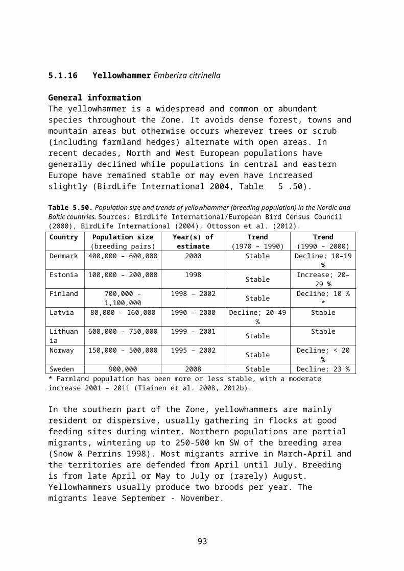
Pulses

This group includes peas and beans, which are sown in spring and are subject to various pesticide treatments throughout the growing season.The approximate time schedule refers to the cultivation of field peas for fodder.Sowing andpre-emergence

BBCH 0-9

Early growth stages of crop

BBCH 10-19

Development of side shoots (bean) and stretchingBBCH 20-39

Development of flower buds

BBCH 40-59

Flowering and developmentof podsBBCH 60-79

Ripening of seeds, pre-harvest desiccation 1)

BBCH 80-99April May May - June June June - July July - AugustFood types- ground-dwelling arthropods- (treated seeds) 2)

- (weed seeds) 3)

- crop leaves- ground-dwelling arthropods- (weed seeds) 3)

- crop leaves- weeds 4)

- weed seeds- ground-dwelling arthropods- foliar arthropods 5)

- crop leaves- weeds 4)

- weed seeds- ground-dwelling arthropods- foliar arthropods

- crop leaves- weeds 4)

- weed seeds- ground-dwelling arthropods- foliar arthropods

- crop leaves- crop (seeds)- weeds 4)

- weed seeds- ground-dwelling arthropods- foliar arthropods

Selected species Pink-footed g. Skylark White wagtail Wood mouse

Woodpigeon Skylark White wagtail Linnet Brown hare Wood mouse

Skylark White wagtail Linnet Brown hare Wood mouse

Skylark White wagtail Brown hare Wood mouse

Skylark White wagtail Brown hare Wood mouse

Woodpigeon Skylark Brown hare Wood mouse

1) At pre-harvest desiccation with herbicides, in most cases the crop and possible weeds in the field are completely wilted or at least have become unattractive as food within approximately one week. Hence, exposure via green parts of plants and associated foliar arthropods is limited to the first week after treatment. Thereafter, only ground dwelling arthropods and seeds (including peas) remain attractive as food items in the field.2) Peas are usually precision drilled at 6-8 cm depth, and thus are generally not accessible to birds (except geese and swans). In Sweden the risk assessment shall also cover potential spill of treated seeds.3) Availability of weed seeds depends on the soil treatments.4) The relative amounts of grasses and dicotyledonous weeds will vary.5) The population of foliar arthropods in the field develops during this period.

94

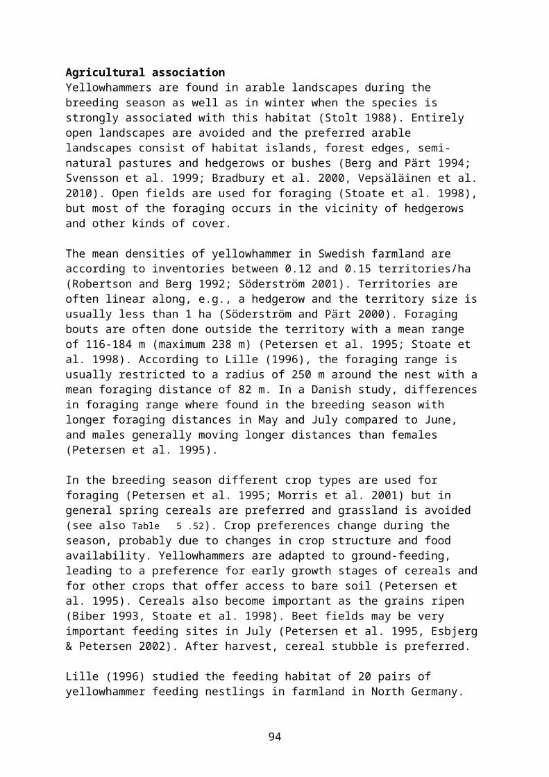
Strawberries

Strawberries are grown for several years in the same field. They are usually planted in spring (April to June), but planting may also occur during summer or autumn. Strawberry plants may be dipped in fungicides before planting, and the fields are subject to various pesticide treatments throughout the season (except during harvest).Planting

BBCH 10-19

Pre-flowering

BBCH 20-59

Flowering, development and ripening of fruitsBBCH 60-89

Post-harvest Termination 1)

Spring Late spring, summer Late summer,autumn

Food types- crop leaves- (weed seeds) 2)

- ground-dwelling arthropods

- crop leaves- weeds 3)

- weed seeds- ground-dwelling arthropods- foliar arthropods

- crop leaves- fruits- weeds 3)

- weed seeds- ground-dwelling arthropods- foliar arthropods

- crop leaves- weeds 3)

- weed seeds- ground-dwelling arthropods- foliar arthropods

- crop leaves- weeds 3)

- weed seeds- ground-dwelling arthropods- foliar arthropods

Selected species Skylark White wagtail Brown hare Wood mouse

Skylark White wagtail Brown hare Wood mouse

Skylark White wagtail Starling Brown hare Wood mouse

Skylark White wagtail 4)

Brown hare Wood mouse

Skylark Wood mouse

1) At termination of strawberry fields with herbicides, in most cases the crop and possible weeds in the field are completely wilted or at least have become unattractive as food within approximately one week. Hence, exposure via green parts of plants and associated foliar arthropods is limited to the first week after treatment. Thereafter, only ground dwelling arthropods and seeds remain attractive as food items in the field.2) Availability of weed seeds depends on the soil treatments.3) The relative amounts of grasses and dicotyledonous weeds will vary.4) Until late September.

95

Vegetables (field grown)

Major field grown vegetables within the Northern Zone include carrots, onions, brassica vegetable crops, lettuce and leek. Most brassica vegetable crops, lettuce and leek and some onions are not sown but are cultivated indoor before planting in the field. Phenology and time schedules vary between crops. Lettuce mature rapidly, in c. 8 weeks, and planting takes place continuously during the summer season. Pesticide treatments take place throughout the growing season.Sowing andpre-emergenceBBCH 0-9

Leaf development

BBCH 10-19

Stretching, development of side shoots 1)

BBCH 20-39

Development of harvestable partsBBCH ≥ 40

Food types- ground-dwelling arthropods- (treated seeds) 2)

- (weed seeds) 3)

- crop leaves- weeds 4)

- ground-dwelling arthropods- (weed seeds) 3)

- crop leaves- weeds 4)

- weed seeds- ground-dwelling arthropods- foliar arthropods

- crop leaves- weeds 4)

- weed seeds- ground-dwelling arthropods- foliar arthropods

Selected species Skylark White wagtail Wood mouse

Skylark White wagtail Linnet Brown hare Wood mouse

Skylark White wagtail Linnet Brown hare Wood mouse

Skylark White wagtail Linnet Brown hare Wood mouse

1) Only relevant for spinach, loosehead lettuce, kale, broccoli and brussel sprouts.2) In crops that are sown (not planted), the seeds are generally too small to be attractive or are pelleted and precision drilled at some cm depth. In Sweden the risk assessment shall also cover potential spill of treated seeds.3) Availability of weed seeds depends on the soil treatments.4) The relative amounts of grasses and dicotyledonous weeds will vary.

96

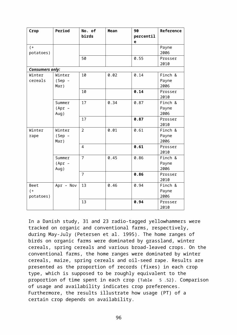
7 References

Aitchison, C.W. 1987. Review of winter trophic relations of soricine shrews. Mammal review 17: 1-24.

Asferg, T. & Madsen, A.B. 2007. Hare. In: Dansk Pattedyratlas (Ed. by Baagøe, H. J. & Jensen, T. S.), pp. 100-103. Gyldendal, København.

Aunins, A., B.S. Petersen, J. Priedniks & E. Prins 2001. Relationships between birds and habitats in Latvian farmland. Acta Ornithologica 36: 55-64.

Axelsson, K-M. 2004. Habitatval hos tranor, gäss och sångsvanar kring Tåkern. Länsstyrelsen Östergötland, Rapport 2004: 14.

Baagøe, H. J. & Ujvári, M. 2007. Almindelig spidsmus. In: Dansk Pattedyratlas (Ed. by Baagøe, H. J. & Jensen, T. S.), pp. 24-27. Gyldendal, København.

Barber, I., Tarrant, K.A. & Thompson, H.M. 2003. Exposure of small mammals, in particular the Wood mouse Apodemus sylvaticus, to pesticide seed treatment. Environmental Toxicology and Chemistry 22: 1134-1139.

Baril, A., Whiteside, M. & Boutin, C. 2005. Analysis of a database of pesticide residues on plants for wildlife risk assessment. Environmental Toxicology and Chemistry 24: 360-371.

Berg, Å. 2002. Composition and diversity of bird communities in Swedish farmland-forest mosaic landscapes. Bird Study 49: 153-165.

Berg, Å. & Pärt, T. 1994. Abundance of breeding farmland birds on arable and set-aside fields at forest edges. Ecography 17: 147-152.

Biber, O. 1993. Raumnutzung der Goldammer Emberiza citrinella für die Nahrungssuche zur Brutzeit in einer intensiv genutzten Agrarlandschaft (Schweizer Mittelland). Der Ornitologische Beobachter 90: 283-296.

BirdLife International/European Bird Census Council 2000. European bird populations: estimates and trends. Cambridge, UK: Birdlife International. (BirdLife Conservation series No. 10).

BirdLife International 2004. Birds in Europe: Population estimates, trends and conservation status. Cambridge, UK: Birdlife International. (BirdLife Conservation series No. 12).

Bjärvall, A. & Ullström, S. 1985. Däggdjur. Alla Europas arter. Wahlström & Widstrand, Stockholm.

Bradbury, R.B., Kyrkos, A., Morris, A.J., Clark, S.C., Perkins, A.J. & Wilson, J.D. 2000 Habitat associations and breeding success of yellowhammers on lowland farmland. Journal of Applied Ecology 37: 789-805.

Broekhuizen, S. & Maaskamp, F. 1982. Movement, home range and clustering in the European hare (Lepus europaeus Pallas) in The Netherlands. Zeitschrift für Säugetierkunde 47: 22-32.

Brühl, C.A., Guckenmus, B., Ebeling, M. & Barfknecht, R. 2011. Exposure reduction of seed treatments through dehusking behaviour of the wood mouse (Apodemus sylvaticus). Environ. Sci. Pollut. Res. 18: 31-37.

Buxton, J.M., Crocker, D.R. & Pascual, J.A. 1998. Birds and farming: information for risk assessment (“Bird Bible”). Report to Pesticides Safety Directorate, Contract PN0919. Central Science Laboratory, UK.

Cavallin, B. 1988. Törnsångare Sylvia c. communis. In: Fåglar i jordbrukslandskapet (ed. Andersson, S.), pp. 307-314. Vår Fågelvärld Supplement No. 12.

97

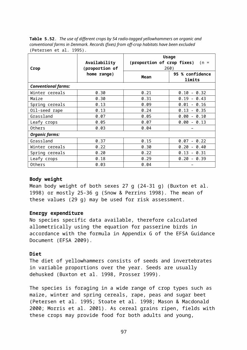
Chapuis, J.L. 1990. Comparison of the diets of two sympatric lagomorphs, Lepus europaeus (Pallas) and Oryctolagus cuniculus (L.) in an agroecosystem of the Ile-de-France. Zeitschrift für Säugetierkunde 55: 176-185.

Christensen, K.D., Falk, K. & Petersen, B.S. 1996: Feeding Biology of Danish Farmland Birds. Working Report No. 12 1996, Danish Environmental Protection Agency.

Churchfield, S. 1980. Subterranean foraging and burrowing activity of the common shrew. Acta Theriologica 25: 451-59.

Churchfield, S. 1982. Food availability and the diet of the common shrew Sorex araneus in Britain. Journal of Applied Ecology 51: 15-28.

Cowie, R.J. & Hinsley, S.A. 1988. Feeding ecology of great tits (Parus major) and Blue tits (Parus caeruleus), breeding in suburban gardens. Journal of Animal Ecology 57: 611-626.

Cramp, S. & Simmons, K.E.L. (eds.) 1977. The birds of the Western Palearctic, Vol. I. Oxford University Press, Oxford, UK.

Cramp, S. (ed.) 1985. The birds of the Western Palearctic, Vol. IV. Oxford University Press, Oxford, UK.

Cramp, S. (ed.) 1988. The birds of the Western Palearctic, Vol. V. Oxford University Press, Oxford, UK.

Cramp, S. (ed.) 1992. The birds of the Western Palearctic, Vol. VI. Oxford University Press, Oxford, UK.

Cramp, S. & Perrins, C.M. (eds.) 1993. The birds of the Western Palearctic, Vol. VII. Oxford University Press, Oxford, UK.

Cramp, S. & Perrins, C.M. (eds.) 1994a. The birds of the Western Palearctic, Vol. VIII. Oxford University Press, Oxford, UK.

Cramp, S. & Perrins, C.M. (eds.) 1994b. The birds of the Western Palearctic, Vol. IX. Oxford University Press, Oxford, UK

Crocker, D.R., Prosser, P., Tarrant, K.A., Irving, P.V., Watola, G., Chandler-Morris, S.A., Hart, J. & Hart, A.D.M. 1998. Improving the assessment of pesticide risk to birds in orchards. Objective 1: Use of radio-telemetry to monitor birds´ use of orchards. Contract PN0903.

Crocker, D.R & Irving, P.V. 1999. Improving estimates of wildlife exposure to pesticides in arable crops. Milestone report 02/01: Variation of bird numbers on arable crops. Central Science Laboratory, Project PN0915.

Crocker, D.R., Prosser, P., Irving, P.V., Bone, P. & Hart, A. 2002. Estimating avian exposure to pesticides on arable crops. Aspects of Applied Biology 67: 237-244.

Danish Environmental Protection Agency 2009. Pesticide Risk Assessment for Birds and Mammals.

Davies, N.B. 1976. Food, flocking and territorial behaviour of the Pied Wagtail in winter. Journal of Animal Ecology 45: 235-253.

Davies, N.B. 1977. Prey selection and social behaviour in Wagtails. Journal of Animal Ecology 46: 37-57.

DEFRA (Department for Environmental, Food and Rural Affairs). 2002. Integrating farm management practices with brown hare conservation in pastoral habitats. Project BD 1436.

DEFRA (Department for Environmental, Food and Rural Affairs) 2005. Risks to small mammals from hoarding of solid pesticide formulations. DEFRA Project Code PS2308 (http://randd.defra.gov.uk/Document.aspx?Document=PS2308_2672_FRP.doc).

Donald, P.F., Muirhead, L.B., Buckingham, D.L. Evans, A.D., Kirby, W.B. & Gruar, D.J. 2001. Body condition, growth rates and diet of Skylark Alauda arvensis nestlings on lowland farmland. Ibis 143: 658-669.

98

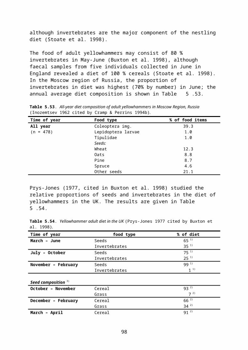
Donald, P.F. 2004. The Skylark. T & AD Poyser, London.Eber, G. 1956. Vergleichende Untersuchungen über die Ernährung einiger Finkenvögel.

Biologische Abhandlungen 13/14: 1-60.Edwards, P.J., Bembridge, J., Jackson, D., Earl, M. & Anderson, L. 1998. Estimation of

pesticides residues on weed seeds for wildlife risk assessment. Poster presentation at the SETAC 19th annual meeting, 1998, Charlotte, NC, USA. (Summary on p. 151 of abstract book).

EFSA 2004. Opinion of the Scientific Panel on Plant Health Protection Products and their Residues on a request from the Commission related to the evaluation of methamidophos in ecotoxicology in the context of Council Directive 91/414/EEC. The EFSA Journal 144: 1-50.

EFSA 2009. Guidance Document on Risk Assessment for Birds and Mammals on request from EFSA. The EFSA Journal 2009; 7(12): 1438 (139 pp.). doi: 10.2903/j.efsa.2009.1438. Available online: www.efsa.europa.eu.

Esbjerg, P. & Petersen, B.S. (ed.) 2002. Effects of reduced pesticide use on flora and fauna in agricultural fields. Pesticides Research No. 58. Danish Environmental Protection Agency.

Faber, J. & Ma, W-C. 1986. Observations on seasonal dynamics in diet composition of the field vole, Microtus agrestis, with some methodological remarks. Acta Theriologica, Vol. 31: 479-490.

Finch, E. & Payne, M. 2006. Bird and mammal risk assessment: refining the proportion of diet obtained in the treated crop area (PT) through the use of radio tracking data. Advisory Committee on Pesticides, Environmental Panel, SC 11449.

Fitzgibbon, C.D. 1997. Small mammals in farm woodlands: the effects of habitat, isolation and surrounding land-use patterns. Journal of Applied Ecology 34: 530-539.

FOCUS 2000. FOCUS groundwater scenarios in the EU review of active substances. Report of the FOCUS Groundwater Scenarios Workgroup, EC Document Reference SANCO/ 321/2000, rev.2.

FOCUS 2001. FOCUS Surface Water Scenarios in the EU Evaluation Process under 91/414/EEC. Report of the FOCUS Working Group on Surface Water Scenarios. EC Document Reference SANCO/4802/2001-rev.2.

Fox, A.D., Mitchell, C., Madsen, J. & Boyd, H. 1997. Anser brachyrhynchus Pink-footed Goose. BWP Update Vol. 1 No. 1: 37-48.

Frylestam, B. 1979. Structure, size, and dynamics of three European hare population in southern Sweden. Acta Theriologica 24: 449-464.

Frylestam, B. 1980a. Utilization of farmland habitats by european hares (Lepus europaeus Pallas) in southern Sweden. Viltrevy 11: 271-284.

Frylestam, B. 1980b. Reproduction in the European hare in southern Sweden. Holarctic Ecology 3: 74-80.

Frylestam, B. 1986. Agricultural land use effects on the winter diet of Brown hares (Lepus europaeus Pallas) in southern Sweden. Mammal Review 16: 157-161.

Frylestam, B. 1990. pp 1-46. Lär känna fältharen. Svenska Jägareförbundet, Stockholm.Frylestam, B. 1992. Utilisation by Brown hares Lepus europaeus, Pallas of field habitats and

complimentary food stripes in Southern Sweden. Pp. 259-261 in Bobek, B., Perzanowski, K. & Regelin, W., Eds. Global trends in wildlife management. Trans. 18th IUGB Congress, Krakow 1987. Swiat Press, Krakow-Warsawa.

Gebczynski, M. 1965. Seasonal and age change in the metabolism and activity of Sorex araneus Linnaeus 1758. Acta Theriologica 22: 303-331.

Gezelius, L. 1990. Sädgässens antal, fördelning och fältval vid Tåkern. Vingspegeln 9: 36-45.

99

Glutz von Blotzheim, U.N. & Bauer, K.M. 1985. Handbuch der Vögel Mitteleuropas, Band 10/II. AULA-Verlag, Wiesbaden, Germany.

Glutz von Blotzheim, U.N. & Bauer, K.M. 1988. Handbuch der Vögel Mitteleuropas, Band 11/I. AULA-Verlag, Wiesbaden, Germany.

Glutz von Blotzheim, U.N. & Bauer, K.M. 1991. Handbuch der Vögel Mitteleuropas, Band 12/II. AULA-Verlag, Wiesbaden, Germany.

Glutz von Blotzheim, U.N. & Bauer, K.M. 1993. Handbuch der Vögel Mitteleuropas, Band 13/I. AULA-Verlag, Wiesbaden, Germany.

Grajetzky, B. 1993. Nahrungsökologie adulter Rotkehlchen (Erithacus rubecula) einer schleswig-holsteinischen Knicklandschaft. Journal für Ornithologie 134: 13-22.

Green, R. 1978. Factors affecting the diet of farmland skylarks, Alauda arvensis. Journal of Animal Ecology 47: 913-928.

Green, R. 1979. The ecology of Wood mice (Apodemus sylvaticus) on arable farmland. Journal of Zoology 188: 357-377.

Green, R.E. 1980. Food selection by skylarks and grazing damage to sugar beet seedlings. Journal of Applied Ecology 17: 613-630.

Green, R.E. 1984. The feeding ecology and survival by partridge chicks (Alectoris rufa and Perdix perdix) on arable farm in East Anglia. Journal of Applied Ecology 21: 817-830.

Grodzínski, W. 1985. Ecological energetics of bank voles and wood mice. Symposium of Zoological Society of London 55: 169-192.

Gromadzki, M. 1969. Composition of food of the Starling Sturnus vulgaris in agrocenoses. Ekologia Polska 17: 287-311.

Gurney, J.E., Peretta, J., Crocker, D.R. & Pascual, J.A. 1998. Mammals and farming: information for risk assessment (“Mammal Bible”). Report to Pesticides Safety Directorate, Contract PN 0910/PN0919. Central Science Laboratory, UK.

von Haartman, L. 1969. The nesting habits of Finnish birds. I. Passeriformes. Commentationes Biologicae 32: 1-187.

Hage, M., Bakken, V. & Isaksen, K. 2011. Risk assessment of agricultural pesticides for birds and mammals in Southeast Norway. Recommendations for focal species. Report to the Norwegian Food Safety Authority.

Hansen, K. 1990. Harens (Lepus europaeus) fødevalg på landbrugsarealer. Unpublished report, NERI.

Hansen, T. S. & Jensen, T. S. 2007a. Almindelig markmus. In: Dansk Pattedyratlas (ed. by Baagøe, H. J. & Jensen, T. S.), pp. 128-131. Gyldendal, København.

Hansen, T. S. & Jensen, T. S. 2007b. Skovmus. In: Dansk Pattedyratlas (ed. by Baagøe, H. J. & Jensen, T. S.), pp. 148-151. Gyldendal, København.

Hansson, L. & Grodzínski, W. 1970. Bioenergetic parameters of the field vole Microtus agrestis L. Oikos 21: 76-82.

Hansson, L. 1971. Habitat, food and population dynamics of the field vole Microtus agrestis (L.) in south Sweden. Viltrevy 8: 290-312.

Hansson, L. 1977. Spatial dynamics of field voles Microtus agrestis in heterogeneous landscapes. Oikos 29: 539-544.

Hansson, L. 1985. The food of bank voles, wood mice and yellow-necked mice. Symposium of Zoological Society of London 55: 141-168.

Havlin, J. & Folk, C. 1965. Potrava a vyznam spacka obecneho, Sturnus vulgaris. Zoologicke Listy 14: 193-208. (Cited in Christensen et al. 1996 and Cramp & Perrins 1994a).

Heldbjerg, H. & Lerche-Jørgensen, M. 2012. Overvågning af de almindelige fuglearter i Danmark 1975-2011. Årsrapport for Punkttællingsprojektet. Dansk Ornitologisk Forening, Copenhagen.

100

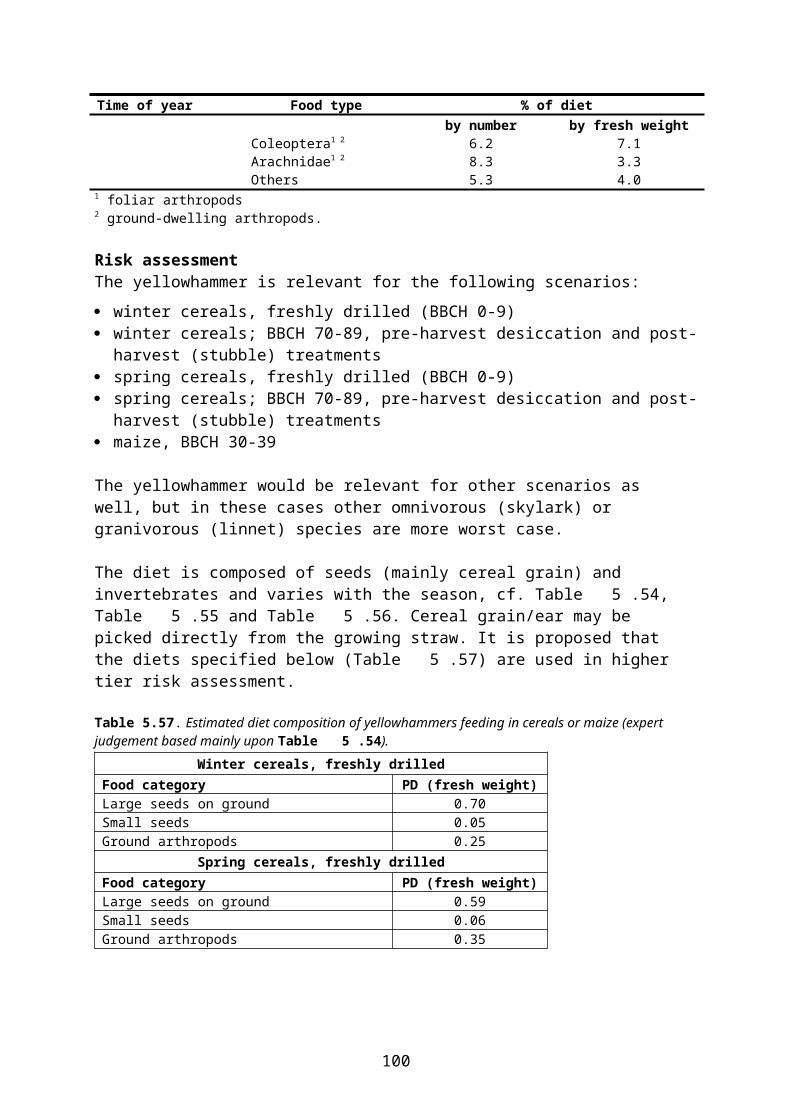
Herzon, I., Ekroos, J., Rintala, J., Tiainen, J., Seimola, T. & Vepsäläinen, V. 2011. Importance of set-aside for birds in Finland: an impact assessment and mitigation solutions. Agriculture, Ecology and Environment 143: 3-7.

Hiron, M., Berg, Å & Pärt, T. 2012. Do skylarks prefer autumn sown cereals? Effects of agricultural land use, region and time in the breeding season on density. Agriculture, Ecosystems and Environment 150: 82-90.

Huitu, O., Norrdahl, K. & Korpimäki, E. 2004. Competition, predation and interspecific synchrony in cyclic small mammal communities. Ecography 27: 197-206.

Hyvönen, T. & Huusela-Veistola, E. 2008. Arable weeds as indicators of agricultural intensity – a case study from Finland. Biological Conservation 141: 2857-2864.

Hyvönen, T., Ketoja, E., Salonen, J., Jalli, H. & Tiainen, J. 2003. Weed species diversity and community composition in organic and conventional cropping of spring cereals. Agriculture, Ecosystems & Environment 97: 131-149.

Inglis, I.R., Isaacson, A.J., Thearle, R.J.P. & Westwood, N.J. 1990. The effects of changing agricultural practice upon Woodpigeon Columba palumbus numbers. Ibis 132: 262-272.

Jenny, M. 1990. Territorialität und Brutbiologie der Feldlerche Alauda arvensis in einer intensiv genutzten Agrarlandschaft. Journal für Ornithologie 131: 241-265.

Jensen, T. S. & Hansen, T.S. 2003. Biodiversitet og biotopsfordeling hos småpattedyr i det åbne land. Flora og fauna 109 (1): 9 – 22.

Johnson, I. P., Flowerdew, J. R. & Hare, R. 1992. Populations and diet of small rodents and shrews in relation to pesticide usage. In: Pesticides and the environment: the Boxworth project (Ed. by P. Greig-Smith, G. Frampton & T. Hardy), pp. 144-157. Her Majesty's Stationary Office, London.

Kahlert, J., Asferg, T. & Odderskær, P. 2008. Agerhønens biologi og bestandsregulering. En gennemgang af den nuværende viden. Faglig rapport fra DMU nr. 666. Danmarks Miljøundersøgelser, Aarhus Universitet.

Kendeigh, S.C., Dol´nik, V.R. & Gavrilov, V.M. 1977. Avian energetics. Pp. 129-197 in Pinowski, J., Kendeigh, S.C., Eds. Granivorous birds in ecosystems. Cambridge University Press, UK.

Larsen, J.L. & Heldbjerg, H. 2009. Udarbejdelse af habitatspecifikke fugleindikatorer. Upubl. notat til Skov- og Naturstyrelsen. Dansk Ornitologisk Forening.

Lewandowski, K. & Nowakowski, J.J. 1993. Spatial distribution of brown hare Lepus europaeus populations in habitats of various types of agriculture. Acta Theriologica 38: 435-442.

Lille, R. 1996. Zur Bedeutung von Bracheflächen für die Avifauna der Agrarlandschaft: Eine nahrungsökologische Studie an der Goldammer Emberiza citrinella. Agrarökologie Bd. 21. Verlag Paul Haupt, Bern, Switzerland.

Lindqvist, M., Svensson, S. & Sjöstedt O. (GF Konsult AB). 2000. Miljöövervakning av fåglar på jordbruksmark i Västra Götalands län – resultat från en inventering 1999 av åtta provrutor, Rapport 2000: 18.

Ljunggren, L. 1968. Seasonal studies of Wood Pigeon populations. I. Body weight, feeding habits, liver and thyroid activity. Viltrevy 5: 435-504.

Loman, J. 1991a. The small mammal fauna in an agriculture landscape in southern Sweden, with special reference to the wood mouse Apodemus sylvaticus. Mammalia 55: 91-96.

Loman, J. 1991b. Do wood mouse Apodemus sylvaticus (L.) abandon fields during autumn Ekologia Polska 39: 221-228.

Lorenzen, B. & Madsen, J. 1986. Feeding by geese on the Filsø farmland, Denmark, and the effects of grazing on yield structure of spring barley. Holarctic Ecology 9: 305-311.

101

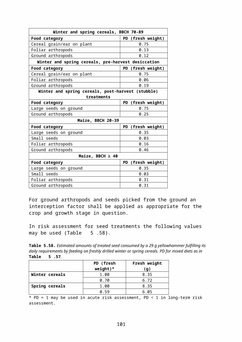
Ludwigs, J.-D., Pascual, J., Wolf, A. & von Blanckenhagen, F. 2007. Comparison of dehusking experiments of laboratory mice and wild Apodemus spec. mice. Poster presented at SETAC Europe Conference, Porto, 2007.

Macdonald, D.W., Tew, T.E., Todd, A., Garner, J.P. & Johnson, P.J. 2000. Arable habitat use by wood mice (Apodemus sylvaticus) 3. A farm-scale experiment on the effects of crop rotation. J. Zool. Lond. 250: 313-320.

Madsen, J. 1985. Relations between change in spring habitat selection and daily energetics of Pink-footed Geese Anser brachyrhynchus. Ornis Scandinavica 16: 222-228.

Madsen, J., Hansen, F. & Kjeldsen, J.P. 1997. Spring Exposure of Pink-footed Geese to Pesticide-Treated Seed. Pesticides Research No. 33. Danish Environmental Protection Agency.

Marboutin, E. & Aebischer, N.J. 1996. Does harvesting arable crops influence the behaviour of the European hare Lepus europaeus. Wildlife Biology 2: 83-91.

Marchant, J.H., Hudson, R., Carter, S.P. & Whittington, P. 1990. Population trends in British breeding birds. British Trust for Ornithology, Tring, UK.

Mason, C.F. & Macdonald, S.M. 2000. Influence of landscape and land-use on the distribution of breeding birds in farmland in eastern England. Journal of Zoology 251: 229-348.

Meier, U (ed.) 2001. Growth stages of mono- and dicotyledonous plants. BBCH Monograph. 2. Edition. Federal Biological Research Centre for Agriculture and Forestry.

Merritt, J.F. & Vessey, S.H. 2000. Shrews – Small insectivores with polyphasic patterns. Pp. 235-251 in Halle, S. & Stenseth, N.C., Eds. Activity patterns in small mammals. Ecological studies 141.

Mitchell-Jones, A.J., Amori, G., Bogdanowicz, W., Krystufek, B., Reijnders, P.J.H., Spitzenberger, F., Stubbe, M., Thissen, J.B.M., Vohralik, V. & Zima, J. 1999. Atlas of European Mammals. Academic Press, London.

Moorcroft, D., Wilson, J.D. & Bradbury, R.B. 2006. Diet of nestling Linnets Carduelis cannabina on lowland farmland before and after agricultural intensification. Bird Study 53: 156-162.

Morris, A.J., Whittingham, M.J., Bradbury, R.B., Wilson, J.D., Kyrkos, A., Buckingham, D.L. & Evans, A.D. 2001. Foraging habitat selection by yellowhammers (Emberiza citrinella) nesting in agriculturally contrasting regions in lowland England. Biolgical Conservation 101: 197-210.

Navntoft, S., Esbjerg, P., Jensen, A.-M.M., Johnsen, I. & Petersen, B.S. 2003. Flora and Fauna Changes During Conversion from Conventional to Organic Farming. Pesticides Research No. 74. Danish Environmental Protection Agency.

Newton, I. 1967. The adaptive radiation and feeding ecology of some British Finches. Ibis 109: 49-53.

Nilsson, L. 2004. www.darwin.biol.lu.se/zooekologi/waterfowl/GooseInv/GRap/ANSINV03-04.pdf 2005-03-30.

Nilsson, L. & Persson, H. 1984. Non-breeding distribution, numbers and ecology of bean goose Anser fabalis in Sweden. Viltrevy 13: 107-170.

Odderskær, P., Prang, A., Elmegaard, N. & Andersen, P.N. 1997a. Skylark reproduction in pesticide treated and untreated fields. Pesticide Research No. 32. Ministry of Environment and Energy, Denmark.

Odderskær, P., Prang, A., Poulsen, J.G., Andersen, P.N. & Elmegaard, N. 1997b. Skylark (Alauda arvensis) utilisation of micro-habitat in spring barley fields. Agriculture, Ecosystems and Environment 62: 21-29.

Olesen, C.R. & Asferg, T. 2006. Assessing potential causes for the population decline of European brown hare in the agricultural landscape of Europe – a review of the current

102

knowledge. National Environmental Research Institute, Denmark. 32 pp. NERI Technical report No. 600.

Ottosson, U., Ottvall, R., Elmberg, J., Green, M., Gustafsson, R., Haas, F., Holmqvist, N., Lindström, Å., Nilsson, L., Svensson, M., Svensson, S. & Tjernberg, M. 2012. Fåglarna i Sverige - antal och förekomst. Sveriges Ornitologiska Förening, Halmstad.

Ouin, A., Paillat, G., Butet, A. & Burel, F. 2000. Spatial dynamics of wood mouse (Apodemus sylvaticus) in an agricultural landscape under intensive use in the Mont Saint Michel Bay (France). Agriculture, Ecosystems and Environment 78: 159-165.

Panek, M. & Kamieniarz, R. 1999. Relationship between density of brown hare Lepus europaeus and landscape structure in Poland in the years 1981-1995. Acta Theriologica 44: 67-75.

Pascual, J., Crocker, J., & Hart, A. 1998. Improving estimates of the exposure of non-target wildlife to pesticides in arable crops – a review of existing data. Project PN0919.

Pelz, H-J. 1989. Ecological aspects of damage to sugar beet seeds by Apodemus sylvaticus. Pp. 34-48 in Putman, R.J., Edt. Mammals as pests. Chapman & Hall, London.

Pépin, D. 1987. Dynamics of a heavily exploited population of brown hare in a large-scale farming area. Journal of Applied Ecology 24: 725-734.

Pernetta, J.C. 1976. Diets of the shrews Sorex araneus L. and Sorex minutus L. in Wytham grassland. Journal of Animal Ecology 45: 899-912.

Persson, B. 1971. Habitat selection and nesting of a South Swedish Whitethroat Sylvia communis Lath. population. Ornis Scandinavica 2: 119-126.

Petersen, B.S. 1996a. Field study of hazards to farmland birds following spring-sowing of Promet 400 CS-treated rape seed. Report to Ciba-Geigy A/S. Ornis Consult, Copenhagen.

Petersen, B.S. 1996b. The Distribution of Birds in Danish Farmland. Pesticides Research No. 17. Danish Environmental Protection Agency.

Petersen, B.S. 1998. The distribution of Danish farmland birds in relation to habitat characteristics. Ornis Fennica 75: 105-118.

Petersen, B.S. 2006. European Union management plan for skylark Alauda arvensis 2007-2009. Prepared by DDH Consulting (Denmark) and Tour du Valat (France) on behalf of the European Commission.

Petersen, B.S., Falk, K. & Bjerre, K.D. 1995. Yellowhammer studies on organic and conventional farms. Pesticides Research No. 15. Ministry of Environment and Energy, Denmark.

Petersen, B.S. & Nøhr, H. 1991. Monitering af agerlandets fugle 1990. Arbejdsrapport fra Miljøstyrelsen nr. 25/1991.

Piha, M., Pakkal, T. & Tiainen, J. 2003. Habitat preferences of the Skylark Alauda arvensis in southern Finland. Ornis Fennica 80: 97-110.

Piiroinen, J., Tiainen, J., Pakkala, T.& Ylimaunu, J. 1985. The avifauna of Finnish farmland in 1984. Lintumies 20: 126-138 (Finnish with English summary).

Plesner-Jensen, S. 1993. Ecology and behaviour of small mammals on expanded field margins. D.Phil.Thesis, University of Oxford.

Potts, G.R. 1970. Recent changes in the farmland with special reference to the decline of the grey partridge. Bird Study 17: 145-166.

Poulsen, J.G., Sotherton, N.W. & Aebisher, N.J. 1998. Comparative nesting and feeding ecology of skylarks Alauda arvensis on arable farmland in southern England with reference to set-aside. Journal of Applied Ecology 35: 131-147.

Prosser, P. 1999. Potential exposure of birds to treated seed. Central Science Laboratory, Project PN0907.

103

Prosser, P. 2010. Consolidation of bird and mammal PT data for use in risk assessment. Food and Environment Research Agency, UK.

Pulliainen, E. 1984. Changes in the composition of the autumn food of Perdix perdix in West Finland over 20 years. Journal of Applied Ecology 21: 133-139.

Rands, M.R.W. 1986. The survival of gamebird (Galliformes) chicks in relation to pesticide use on cereals. Ibis 128: 57-64.

Rasmussen, P.N., Steenfeldt, S. & Jensen, T.S. 1992. Insekter som føde for kyllinger af Agerhøns (Perdix perdix). Flora og Fauna 98: 87-92.

Rintala, J. & Tiainen, J. 2007. Indexing long-term regional bird population dynamics with nestling ringing data. Annales Zoologici Fennici 44: 115-140.

Rintala, J. & Tiainen, J. 2008. A model incorporating a reduction in carrying capacity translates brood size trends into a population decline: the case of the Finnish starlings, 1951-2005. Oikos 117: 47-59.

Robertson, J. & Berg, Å. 1992. Status and population changes of farmland birds in southern Sweden. Ornis Svecica 2: 119-190.

Roebuck, A., Baker, F.T. & White, J.H. 1944. The grazing of winter cereals by the wood-mouse (Apodemus sylvaticus). Journal of Animal Ecology 13: 105-109.

Rogers, L.M. 1993. The ecology of small mammals in set-aside land. D.Phil.Thesis, Aberdeen University.

Rogers, L.M. & Gorman, M.L. 1995a. The population dynamics of small mammals living in set-aside and surrounding semi-natural and crop land. Journal of Zoology 236: 451-464.

Rogers, L.M. & Gorman, M.L. 1995b. The diet of the wood mouse Apodemus sylvaticus on set-aside land. Journal of Zoology 235: 77-83.

Sell, H. & Odderskær, P. 1990. Tornsangerens Sylvia communis ynglebiologi i danske læhegn. Dansk Ornitologisk Forenings Tidsskrift 84: 21-29.

Smith, R.K., Jennings, N.V., Robinson, A. & Harris, S. 2004. Conservation of European hares Lepus europaeus in Britain: is increasing habitat heterogeneity in farmland the answer Journal of Applied Ecology 41: 1092-1102.

Smith, R.K., Vaughan, N. & Harris, S. 2005. A quantitative analysis of the abundance and demography of European hares Lepus europaeus in relation to habitat type, intensity of agriculture and climate. Mammal review 35: 1-24.

Snow, D.W. & Perrins, C.M. 1998. The Birds of the Western Palearctic. Concise Edition. Oxford University Press, Oxford, UK.

Steenfeldt, S., Rasmussen, P.N. & Jensen, T.S. 1991. Food selection in a population of Partridge Perdix perdix in Danish arable farmland. Dansk Ornitologisk Forenings Tidsskrift 85: 67-76.

Stoate, C., Moreby S.J. & Szczur, J. 1998. Breeding ecology of farmland Yellowhammers Emberiza citrinella. Bird Study 45: 109-121.

Stolt, B-O. 1988. Gulsparv Emberiza citrinella L. Pages 363-368 in Andersson S, Edt. Fåglar i jordbrukslandskapet. Vår Fågelvärld Supplement no. 12.

Svensson, S., Svensson, M. & Tjernberg, M. 1999. Svensk fågelatlas. Vår fågelvärld, supplement 31, Stockholm.

Söderström, B. 2001. Fåglar i odlingslandskapet i Värmlands, Västra Götalands och Skånes län – statistiska analyser av data från den regionala miljöövervakningen. Länsstyrelsen i Värmlands län – Miljöenheten, Rapport 2001:3.

Söderström, B. & Pärt, T. 2000. Influence of landscape scale on farmland birds breeding in semi-natural pastures. Conservation Biology 14: 522-533.

Tapper, S.C. & Barnes, R.F.W. 1986. Influence of farming practise on the ecology of the brown hare (Lepus europaeus). Journal of Applied Ecology 23: 39-52.

104

Tattersall, F.H., Macdonald, D.W., Hart, B.J., Manley, W.J. & Feber, R.E. 2001. Habitat use by wood mice (Apodemus sylvaticus) in a changeable landscape. Journal of Zoology 255: 487-494.

Tattersall, F.H., Macdonald, D.W., Hart, B.J., Johnson, P., Manley W. & Feber, R. 2002. Is habitat linearity important for small mammal communities on farmland? Journal of Applied Ecology 39: 643-652.

Tew, T. E. 1994. Farmland hedgerows: habitat, corridors or irrelevant? A small mammal'sperspective. In: Hedgerow Management and Nature Conservation (eds. Watt, T.A. &Buckley, G.P.), pp. 80-94. Wye College Press, Wye.

Tew, T.E., Macdonald, D.W. & Rands, M.R.W. 1992. Herbicide application affects microhabitat use by arable wood mice (Apodemus sylvaticus). Journal of Applied Ecology 29: 532-539.

Tew, T.E. & Macdonald, D.W. 1993. The effects of harvest on arable wood mice Apodemus sylvaticus. Biological Conservation 65: 279-283.

Tew, T.E. & Macdonald, D.W. 1994. Dynamics of space use and male vigour amongst wood mice Apodemus sylvaticus, in the cereal ecosystem. Behavioral Ecology and Sociobiology 34: 337-345.

Tew, T.E., Todd, I.A. & Macdonald, D.W. 1994. Field margins and small mammals. BCPC Monogr. 58: 85-94.

Tiainen, J. 1991: Phylloscopus trochilus (Linnaeus 1758) – Fitis, Fitislaubsänger. Pp. 1292-1357 in: Glutz von Blotzheim, U. N. & Bauer, K. M.( Hrsg.): Handbuch der Vögel Mitteleuropas, Band 12/II. AULA-Verlag, Wiesbaden, Germany.

Tiainen, J., Ekroos, J., Holopainen, J., Piha, M., Rintala, J., Seimola, T. & Vepsäläinen, V. 2008. Maatalousympäristön linnuston muutos ympäristöohjelmakaudella 2000-06. In: Kuussaari, M., Heliölä, J, Tiainen, J. & Helenius, J. (eds.): Significance of the Finnish agri-environment support scheme for biodiversity and landscape: Final report 2000-2006. Suomen ympäristö (The Finnish Environment) 4/2008, pp. 90-109 (in Finnish).

Tiainen, J., Hanski, I. K., Pakkala, T., Piiroinen, J. & Yrjölä R. 1989. Clutch size, nestling growth and nestling mortality of the Starling Sturnus vulgaris in south Finnish agroenvironments. Ornis Fennica 66: 41-48.

Tiainen, J., Pakkala, T., Piiroinen, J., Vickholm, M. & Virolainen, E. 1985. Changes of the avifauna of farmland at Lammi, southern Finland during the past 50 years. Lintumies 20: 30-42 (Finnish with English summary).

Tiainen, J., Rintala, J. & Seimola, T. 2010. Recent changes in distribution and abundance of the Grey Partridge in Finland. Linnut-vuosikirja 2009: 60-63 (Finnish with English summary).

Tiainen, J. & Seimola, T. 2010. Density of breeding farmland birds in large south Finnish agricultural areas. Linnut-vuosikirja 2009: 146-151 (Finnish with English summary).

Tiainen, J., Seimola, T., Holmström, H. & Rintala, J. 2012a. Farmland bird populations in Åland in 2011 with a comparison to 2001 and continental Finland. Linnut-vuosikirja 2011: 48-57 (Finnish with English summary).

Tiainen, J., Seimola, T., Rintala, J. & Holmström, H. 2012b. Changes in farmland bird populations in Finland in 2001-2011. Linnut-vuosikirja 2011: 38-47 (Finnish with English summary).

Todd, I.A., Tew, T.E. & Macdonald, D.W. 2000. Arable habitat use by wood mice (Apodemus sylvaticus). 1. Macrohabitat. Journal of Zoology 250: 299-303.

Toepfer, S. & Stubbe, M. 2001. Territory density of the skylark (Alauda arvensis) in relation to field vegetation in central Germany. Journal für Ornithologie 142: 184-194.

105

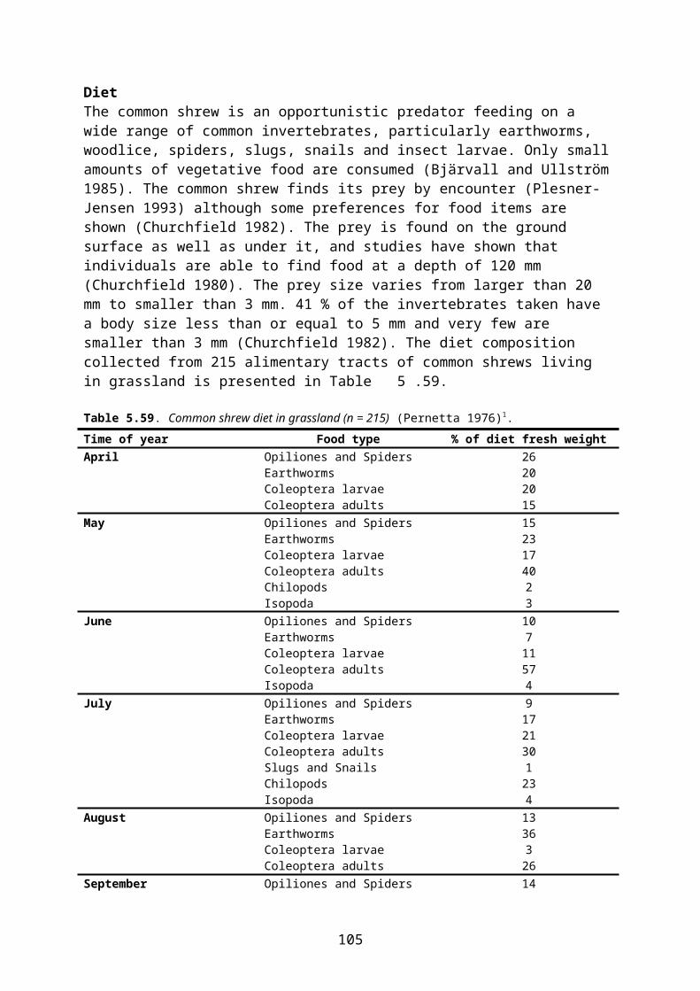
Topping, C.J. & Odderskær, P. 2004. Modeling the influence of temporal and spatial factors on the assessment of impacts of pesticides on skylarks. Environmental Toxicology and Chemistry 23: 509-520.

Vepsäläinen, V., Tiainen, J., Holopainen, J., Piha, M. & Seimola, T. 2010: Improvements in the Finnish agri-environment scheme are needed in order to support rich farmland avifauna. Annales Zoologici Fennici 47: 287-305.

Wallin, E. & Millberg, P. 1995. Effect of bean geese (Anser fabalis) grazing on winter wheat during migration stopover in southern Sweden. Agriculture, Ecosystems and Environment 54: 103-108.

Whitehead, S.C., Wright, J. & Cotton, P.A. 1995. Winter field use by the European Starling Sturnus vulgaris - habitat preferences and the availability of prey. Journal of Avian Biology 26: 193-202.

Yletyinen, S. & Norrdahl, K. 2008. Habitat use of field voles (Microtus agrestis) in wide and narrow buffer zones. Agriculture, Ecosystems and Environment 123: 194-200.

106

Appendix 1

Rules used for crop and growth stage specific adjustment of general PD values in skylark.

The following rules were applied to modify the PD values, as specified by month in Table 5.18. When the share (PD) of one or more food category was reduced (or increased) relative to the values in Table 5.18, the share of the other food categories was increased (or reduced) proportionally.

Monocotyledonous leaves (grasses and cereals)Dicotyledonous leaves (non-grass weeds, leafy crops)

In the study of Green (1978) (Table 5.18), monocotyledons were generally more common than dicotyledons in the diet. This is assumed to reflect availability in a cereal-dominated landscape.

General assumptions: No leaves or shoots are available in BBCH 0-9 (PD = 0). As long as the crop itself is attractive as skylark food, i.e. in BBCH 10-19 (10-29 in

cereals), crop leaves are assumed to make up the entire green plant part of diet, except in potatoes and strawberries.

At pre-harvest desiccation and stubble treatments, proportion of green plant parts in diet is reduced by 50 %. This is because all green parts of plants are assumed to become inattractive as food items within one week after treatment.

Cereals & maize: In BBCH 10-29 (10-19 in maize) all green plants in diet are assumed to be

monocotyledonous, i.e. PD for dicots is added to PD for monocots. After BBCH 29 (19) the monocot:dicot ratio in Table 5.18 is used.

Leafy crops (except potatoes and strawberries): In BBCH 10-19 all green plants in diet are assumed to be dicotyledonous, i.e. PD for

monocots is added to PD for dicots. At later stages the monocot:dicot ratio in Table 5.18 is used, except that PD for monocots is reduced by 50 %.

Potatoes: Potato shoots and leaves are inedible. The monocot:dicot ratio in Table 5.18 is used

for all stages but the PD values are reduced by 50 %.

Strawberries: Strawberry leaves are little attractive and are therefore not assumed to make up the

entire green plant part of diet in early stages. The monocot:dicot ratio in Table 5.18 is used for all stages, except that PD for monocots is reduced by 50 %.

Cereal grain

According to Table 5.18 cereal grain constitutes between 6 and 71 percent of diet dry weight. Again, this is assumed to reflect availability in a cereal-dominated landscape; in non-cereal crops the share of cereal grain in diet will be much less.

107

Leafy crops & maize: The minimum PD recorded by Green (6 %) is assumed to apply to all crops and

months. The underlying rationale is that 6 % represents the amount of grain which is “always” available in rotational fields due to harvest spillage, turning over of soil, etc.

Spring cereals: PD as in Table 5.18, except that the July level of 27 % does not apply for growth stages

(BBCH) ≤ 69 (when the grain is not developed); the June level of 6 % is used instead. At BBCH 70-89 and pre-harvest desiccation, one third of the cereal grain is assumed

to be exposed on the ground while the remainder is exposed on the plant and made available through lodging of straw or loosening of grain.

Winter cereals: PD as in leafy crops in April - July (until and including BBCH 69), thereafter (July -

September) follows Table 5.18. At BBCH 70-89 and pre-harvest desiccation, one third of the cereal grain is assumed

to be exposed on the ground while the remainder is exposed on the plant and made available through lodging of straw or loosening of grain.

Small seeds

All crops except oil-seed rape: PD is assumed to follow Table 5.18; the Green categories ”grass flowers and seeds” and

”dicotyledonous weed seeds” are merged to one class, small seeds.

Oilseed rape: As above, except that PD is assumed to be increased by a factor of 4 in July and a

factor of 2 in August-September. This is because rape seeds are assumed to be attractive food for skylarks.

Foliar arthropodsGround-dwelling arthropods

The Green category “invertebrates” must be split into foliar and ground-dwelling arthropods because the RUD values differ notably.

General: No foliar arthropods are assumed to occur in the diet at BBCH ≤ 19 (BBCH ≤ 29 for

cereals). A foliar:ground-dwelling arthropod ratio of 1:3 in diet is assumed to apply during the

main period of vegetative growth (usually BBCH 20-39). A ratio of 1:1 is assumed to apply at later growth stages (BBCH ≥ 40). A ratio of 1:3 is assumed to apply for pre-harvest desiccation treatments. No foliar arthropods are assumed to be present at stubble (post-harvest) treatments.

In some crops, e.g. most vegetables, BBCH stages 20-39 are not used because the growth pattern differs from the general pattern (no side shoots, no stretching). In these cases, the foliar:ground-dwelling arthropod ratio in skylark diet is assumed to be 1:1 as soon as leaf development is complete.

108

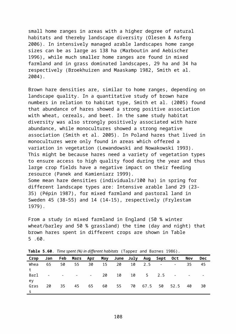
Specific rules for grassland types

The “grassland” category is a rather inhomogeneous mixture of grassland areas within and outside rotation, such as seed grass, leys, pasture and turf. Separate rules for adjustment of PT were defined for rotational and non-rotational grassland, mainly because of differences in availability of cereal grain. The rules are rather briefly presented here but should be easily understandable by comparison with the previous, more detailed accounts. Please also refer to the grassland table in section 6.

Rotational grassland (seed grass and leys)

Sowing and pre-emergence: Grassland within rotation is usually established by undersowing in cereal crops;

therefore no specific scenario is defined for this stage.

Short grass: Monocotyledonous leaves: unchanged from Table 5.18 (short grass may be eaten). Dicotyledonous leaves: PD reduced by 50 % (reduced availability). Cereal grain: PD fixed at 6 % (“background” level). Small seeds: unchanged from Table 5.18. Arthropods: all ground-dwelling.

Medium and long grass: Monocotyledonous leaves: PD reduced by 50 % (medium-long grass is not attractive

skylark food). Dicotyledonous leaves: PD reduced by 50 %. Cereal grain: fixed at 6 %. Small seeds: unchanged from Table 5.18. Arthropods: foliar:ground-dwelling ratio set at 1:1.

Termination: Monocotyledonous leaves: PD reduced by 50 % (the grass quickly becomes

unattractive as food). Dicotyledonous leaves: PD reduced by 75 % (combination of reduced availability and

unattractiveness). Cereal grain: fixed at 6 %. Small seeds: unchanged from Table 5.18. Arthropods: foliar:ground-dwelling ratio set at 1:3.

Non-rotational grassland (pasture and turf)

Sowing and pre-emergence (BBCH 0-9): Mono- and dicotyledonous leaves: none (PD = 0). Cereal grain: none. Small seeds: unchanged from Table 5.18. Arthropods: all ground-dwelling.

Short grass, medium and long grass, termination: As rotational grassland without cereal grain.

109

110

Appendix 2

Rules used for crop and growth stage specific adjustment of general PD values in wood mouse.

The following rules were applied to modify the PD values for wood mouse, as specified by month in Table 5.70 (Pelz 1989) and by period in Table 5.71 (Green 1979) and Table 5.72 (Rogers & Gorman 1995b). The PD values in Table 5.70 are used for arable crops, including seed grass and other short-rotational grasslands, while those in Table 5.72 are used for permanent grasslands, fruit trees, bush berries, ornamentals and nursery cultures. The PD values in Table 5.71 represent an alternative to Table 5.70 for winter cereals (BBCH ≤ 69).

PD values are adjusted to reflect differences in availability between crops and growth stages, taking into account the crop composition (rotational scheme) in the study area. When the share (PD) of one or more food category is reduced (or increased) relative to the values in Table 5.70 – Table 5.72, the share of the other food categories is increased (or reduced) proportionally.

Adjustment of Pelz (1989) data (Table 5.70):

Grasses and cereal shoots (monocotyledonous leaves/shoots)Non-grass weeds, leafy crops (dicotyledonous leaves/shoots)

These food categories were not separated in the Pelz study but were pooled in the category “vegetative plant tissue”. Because standard RUDs in mono- and dicotyledons differ notably a separation is required. This separation is based upon the presumed availability of mono- and dicotyledons in the crop types in question.

General assumptions: No leaves or shoots are available in BBCH 0-9 (PD = 0). As long as the crop itself is very attractive food, i.e. in BBCH 10-19 (10-29 in

cereals), crop leaves are assumed to make up the entire green plant part of diet, except in potatoes, strawberries and grasses.

In later stages, a monocot:dicot ratio of 2:1 is assumed for cereals (including maize) and grass. A monocot:dicot ratio of 1:2 is assumed for other (leafy) crops.

At pre-harvest desiccation, termination and stubble treatments, the proportion of green plant parts in diet is reduced by 50 %. This is because all green parts of plants are assumed to become inattractive as food items within one week after treatment.

Potatoes: Potato shoots and leaves are inedible. The total share of vegetative plant tissue is

reduced by 50 % and a monocot:dicot ratio of 1:1 is assumed for all growth stages.

Strawberries: Strawberry leaves are not assumed to make up the entire green plant part of diet in any

stage, so a monocot:dicot ratio of 1:2 is used for all stages.

Grass: A monocot:dicot ratio of 4:1 is assumed for short grass and a ratio of 2:1 is assumed

for long grass and at termination.

111

Cereal grain

According to Table 5.70 cereal grain constitutes between 5 and 48 percent of diet volume. This is assumed to reflect availability in a cereal-dominated landscape; in non-cereal crops the share of cereal grain in diet will be much less.

Spring and winter cereals: In BBCH 0-9, PD for vegetative plant tissue (which is not available at that stage) is

added to PD for cereal grain. The July PD level of 48 % cereal grain is assumed not to apply for BBCH stages ≤ 69

(when the grain is not developed); the June level of 32 % is used instead. At BBCH 70-89 and pre-harvest desiccation, two thirds of the cereal grain is assumed

to be exposed on the ground while the remainder is exposed on the plant and made available through lodging of straw or loosening of grain.

Leafy crops and grass: The minimum PD recorded by Pelz (5 %) is assumed to apply to all crops and months.

The underlying rationale is that 5 % represents the amount of grain which is “always” available in rotational fields due to harvest spillage, turning over of soil, etc.

Maize: In BBCH 0-9 (April), PD for vegetative plant tissue is added to PD for cereal grain;

the sum (29 %) is assumed to reflect the amount of old cereal grain and fresh maize seed in diet. This value is also used for BBCH 0-9 in May.

In all other stages, maize seed is assumed not to occur in diet and a PD of 5 % cereal grain is used (as in leafy crops).

Other large seeds (peas and beans)

Peas and beans are only available in fields with pulses. If more specific information is not available, residues in peas and beans are assumed to be similar to residues in cereal grain.

In BBCH 0-9 (April and May), PD for large seeds/cereal grain is calculated as described above for maize and includes old cereal grain and newly sown peas (beans).

BBCH 10-79: PD for large seeds is fixed at 5 % as in other leafy crops, reflecting availability of old cereal grain.

PD 80-99 (pre-harvest desiccation): PD is fixed at a level of 10 % (cereal grain x 2), to include seeds in pods.

Beet seeds

Beet seeds are only available in beet fields as pelleted seeds. According to Pelz (Table 5.70) beet seeds constitute 7 % of diet volume immediately after sowing.

A PD of 7 % is assumed to apply to other small, freshly sown seeds as well (cf. below).

Small seeds

PD for small seeds generally follows Table 5.70 (dicotyledon seeds) with the following adjustments:

112

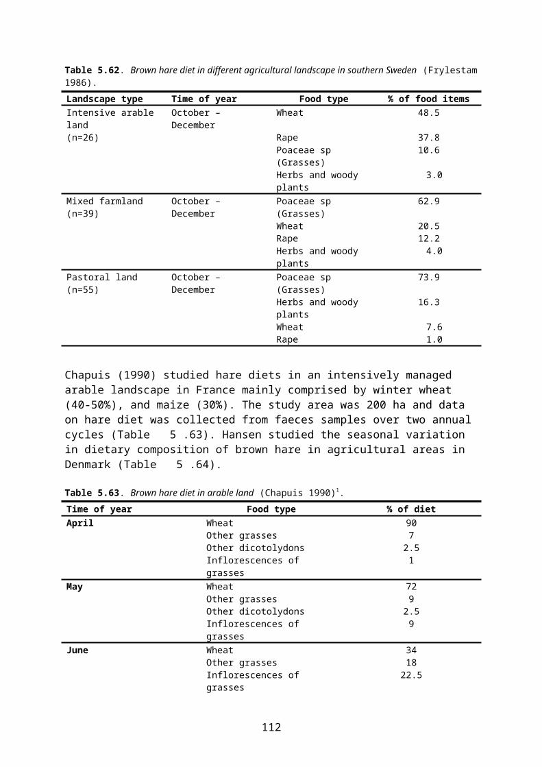
Spring rape: In BBCH 0-9 (April), when weed seeds do not occur in diet according to Pelz (1989),

PD is set at 7 % (as in sugar beet). PD is increased by 25 % in BBCH 80-89 (ripening of fruit) and for stubble treatments

(harvest spillage available). PD is increased by 50 % at pre-harvest desiccation

Winter rape: In BBCH 0-9 (August), PD for dicotyledon seeds is increased by 25 %. For treatments after BBCH 80, PD is adjusted as described for spring rape.

Field grown vegetables: In BBCH 0-9 (April), PD is set at 3.5 % (half of the value in sugar beet and rape). This

value is also added to PD for small seeds in May and June (BBCH 0-9 only). Vegetable seeds are usually pelleted and precision drilled or are too small to be really attractive.

Grass (medium and long): PD for small seeds is increased by 50 % in June, July and August to include grass

seeds.

Insect larvaeEarthworms

No changes from Table 5.70, except for proportional adjustments when PD for other food items is reduced or increased. All insect larvae in diet are assumed to belong to the category “ground-dwelling arthropods”.

Adjustment of Rogers & Gorman (1995b) data (Table 5.72):

All insects occurring in the diet are assumed to be ground-dwelling. The category “other animal material” (2-10 % of diet) is assumed to consist of earthworms, which are a prominent element of wood mouse diet in arable land (cf. Table 5.70).

The category “other plant material” (0-6 % of diet) is assumed to consist mainly of underground plant parts such as rhizomes and various storage organs. Residues in these are generally unknown but are probably lower than residues in leaves and shoots. The category was therefore merged with the “dicotyledon (herb)” category because standard RUDs for dicotyledons are lower than for grasses.

For the periods June-August and September-November the PD values in Table 5.72 do not sum up to 100 %. This is corrected by proportional adjustment and rounding off.

Permanent and semi-permanent grassland (long-lasting leys, pasture and turf)

Sowing and pre-emergence (BBCH 0-9): Diet is specified for two periods where sowing usually takes place: spring (March-

May) and autumn (August-October).

113

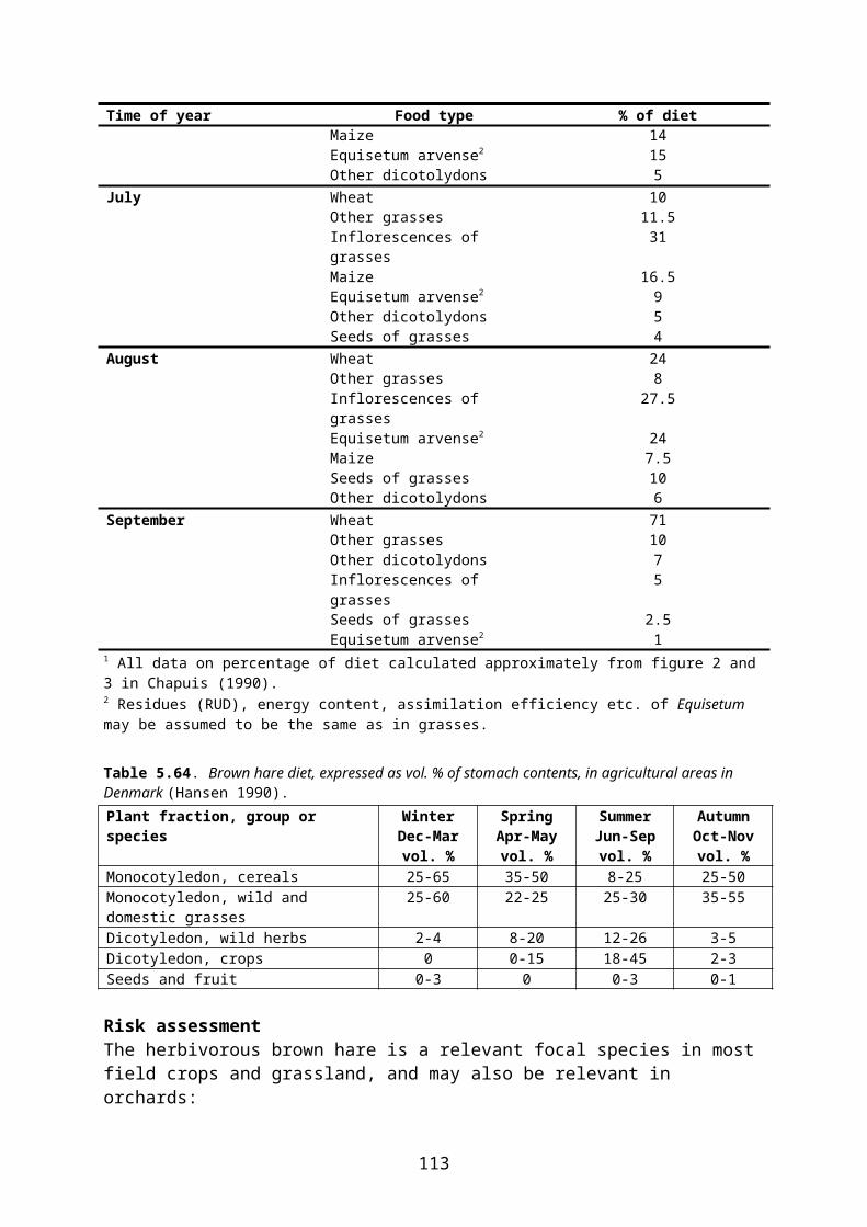
No vegetative plant tissue in diet (PD = 0). Small seeds fixed at maximum level for “seeds” (PD = 42 %). Insects and soil invertebrates (“other animal material”), spring: based on PD for

March-May, adjusted to account for the absence of vegetative plant tissue. Insects and soil invertebrates, autumn: based on average PD for June-August and

September-November, adjusted as above.

Short or long grass: All PD values as in Table 5.72, with “other plant material” being added to “dicotyledons

(herbs)”.

Termination: PD values as described for short and long grass, except that PD for grasses and

dicotyledons (including “other plant material”) are reduced by 50 %.

Fruit trees and bush berries

All stages: All PD values as in Table 5.72, with “other plant material” being added to “dicotyledons

(herbs)”.

Ornamentals and nursery

Vegetative plant tissue (grasses and herbs):

Ornamentals and nursery cultures are very variable; from small plants in nurseries to large plants grown under conditions reminiscent of those in orchards. Accordingly, the ground vegetation may vary from bare soil to grass cover. The following rules attempt to take this variation into account.

Small plants: No grass cover, so the amount of grass in the diet is far below the PD values in Table 5.72. The total amount of vegetative plant material in diet is assumed to be equal to the sum of “dicotyledons (herbs)” and “other plant material”. A monocot:dicot ratio of 1:1 is assumed.

Sowing and pre-emergence (BBCH 0-9): As in small plants, but with total amount of vegetative plant material reduced by 50 %.

Large plants: Some grass cover is asssumed. PD for monocotyledons is based upon the value in Table 5.72, reduced by 75 %; “other plant material” is added to “dicotyledons (herbs)”.

Seeds:

All seeds are assumed to belong to the food category small seeds. Pre-emergence and small plants: PD as in Table 5.72, reduced by 75 %. Large plants: PD is based upon Table 5.72, reduced by 50 %.

Insects and other animal material (earthworms): All PD values are based upon Table 5.72.

114

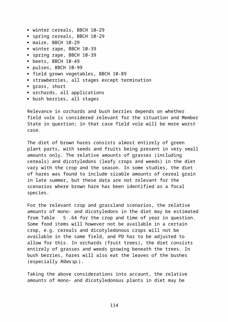
115

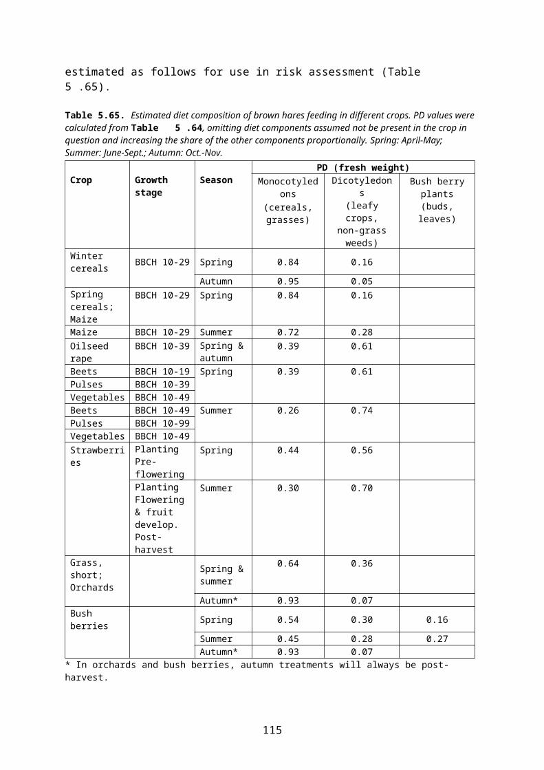
Appendix 3

PD values (dry weight) for skylarks feeding in different crops.

Spring cereals April May June June July July August August August Sept.BBCH 0-9 10-29 30-39 40-69 40-69 70-89 70-89 Pre-harv. Stubble Stubble

desiccat. treatm. treatm.Grasses and cereal shoots 0,38 0,17 0,17 0,13 0,10 0,01 0,01 0,01 0,01Non-grass herbs, leafy crops 0,14 0,14 0,06 0,05 0,05 0,02 0,02 0,01Cereal grain/ear on plant 0,18 0,37 0,39Large seeds/cereal grain on ground 0,46 0,11 0,06 0,06 0,06 0,09 0,19 0,19 0,58 0,72Small seeds (weed seeds) 0,33 0,23 0,23 0,23 0,09 0,07 0,14 0,14 0,14 0,13Large fruit (pome)Small fruit (plum, cherry)BerriesFoliar arthropods 0,10 0,20 0,33 0,25 0,12 0,06Ground-dwelling arthropods 0,21 0,28 0,30 0,25 0,13Ground-dwelling arthropods with intercept. 0,20 0,33 0,26 0,12 0,19Soil invertebrates

Sum 1,00 1,00 1,00 1,00 1,00 1,00 1,00 1,00 1,00 1,00

Maize April May May June June JulyBBCH 0-9 0-9 10-29 10-29 30-39 30-39

Grasses and cereal shoots 0,40 0,31 0,17 0,13Non-grass herbs, leafy crops 0,14 0,06Cereal grain/ear on plantLarge seeds/cereal grain on ground 0,06 0,06 0,06 0,06 0,06 0,06Small seeds (weed seeds) 0,57 0,42 0,24 0,23 0,23 0,09Large fruit (pome)Small fruit (plum, cherry)BerriesFoliar arthropods 0,10 0,17Ground-dwelling arthropods 0,37 0,52 0,30 0,40 0,30 0,49Ground-dwelling arthropods with intercept.Soil invertebrates

Sum 1,00 1,00 1,00 1,00 1,00 1,00

116

Winter cereals Sept. Sept. April May May June May June July July AugustBBCH 0-9 10-19 10-29 10-29 30-39 30-39 40-59 40-69 60-69 70-89 70-89

Grasses and cereal shoots 0,03 0,46 0,40 0,25 0,17 0,25 0,17 0,13 0,10 0,01Non-grass herbs, leafy crops 0,15 0,14 0,15 0,14 0,06 0,05 0,05Cereal grain/ear on plant 0,18 0,37Large seeds/cereal grain on ground 0,74 0,71 0,06 0,06 0,06 0,06 0,06 0,06 0,06 0,09 0,19Small seeds (weed seeds) 0,13 0,13 0,29 0,24 0,24 0,23 0,24 0,23 0,09 0,07 0,14Large fruit (pome)Small fruit (plum, cherry)BerriesFoliar arthropods 0,08 0,10 0,15 0,20 0,33 0,25 0,12Ground-dwelling arthropods 0,13 0,13 0,19 0,30 0,22 0,30Ground-dwelling arthropods with intercept. 0,15 0,20 0,33 0,26 0,12Soil invertebrates

Sum 1,00 1,00 1,00 1,00 1,00 1,00 1,00 1,00 1,00 1,00 1,00

Winter cereals July August August Sept.BBCH Pre-harv. Pre-harv. Stubble Stubble

desiccat. desiccat. treatm. treatm.Grasses and cereal shoots 0,05 0,01 0,01Non-grass herbs, leafy crops 0,03 0,03 0,02 0,01Cereal grain/ear on plant 0,19 0,39Large seeds/cereal grain on ground 0,10 0,19 0,58 0,72Small seeds (weed seeds) 0,08 0,14 0,14 0,13Large fruit (pome)Small fruit (plum, cherry)BerriesFoliar arthropods 0,14 0,06Ground-dwelling arthropods 0,25 0,13Ground-dwelling arthropods with intercept. 0,41 0,19Soil invertebrates

Sum 1,00 1,00 1,00 1,00

117

Spring oilseed rape April April May May May June August Sept.BBCH 0-9 10-19 10-19 20-39 40-59 40-59 Stubble Stubble

treatm. treatm.Grasses and cereal shoots 0,15 0,15 0,09 0,01 0,01Non-grass herbs, leafy crops 0,46 0,40 0,17 0,17 0,16 0,04 0,02Cereal grain/ear on plantLarge seeds/cereal grain on ground 0,06 0,06 0,06 0,06 0,06 0,06 0,06 0,06Small seeds (weed seeds) 0,57 0,29 0,24 0,28 0,28 0,25 0,48 0,61Large fruit (pome)Small fruit (plum, cherry)BerriesFoliar arthropods 0,08 0,17 0,22Ground-dwelling arthropods 0,37 0,19 0,30 0,26 0,41 0,30Ground-dwelling arthropods with intercept. 0,17 0,22Soil invertebrates

Sum 1,00 1,00 1,00 1,00 1,00 1,00 1,00 1,00

Winter oil-seed rape August Sept. April April April May July AugustBBCH 0-9 10-19 10-19 20-39 40-59 40-59 Stubble Stubble

treatm. treatm.Grasses and cereal shoots 0,19 0,19 0,15 0,03 0,01Non-grass herbs, leafy crops 0,10 0,46 0,16 0,16 0,17 0,03 0,04Cereal grain/ear on plantLarge seeds/cereal grain on ground 0,06 0,06 0,06 0,06 0,06 0,06 0,06 0,06Small seeds (weed seeds) 0,51 0,42 0,29 0,36 0,36 0,28 0,31 0,48Large fruit (pome)Small fruit (plum, cherry)BerriesFoliar arthropods 0,06 0,11 0,17Ground-dwelling arthropods 0,43 0,42 0,19 0,17 0,57 0,41Ground-dwelling arthropods with intercept. 0,12 0,17Soil invertebrates

Sum 1,00 1,00 1,00 1,00 1,00 1,00 1,00 1,00

118

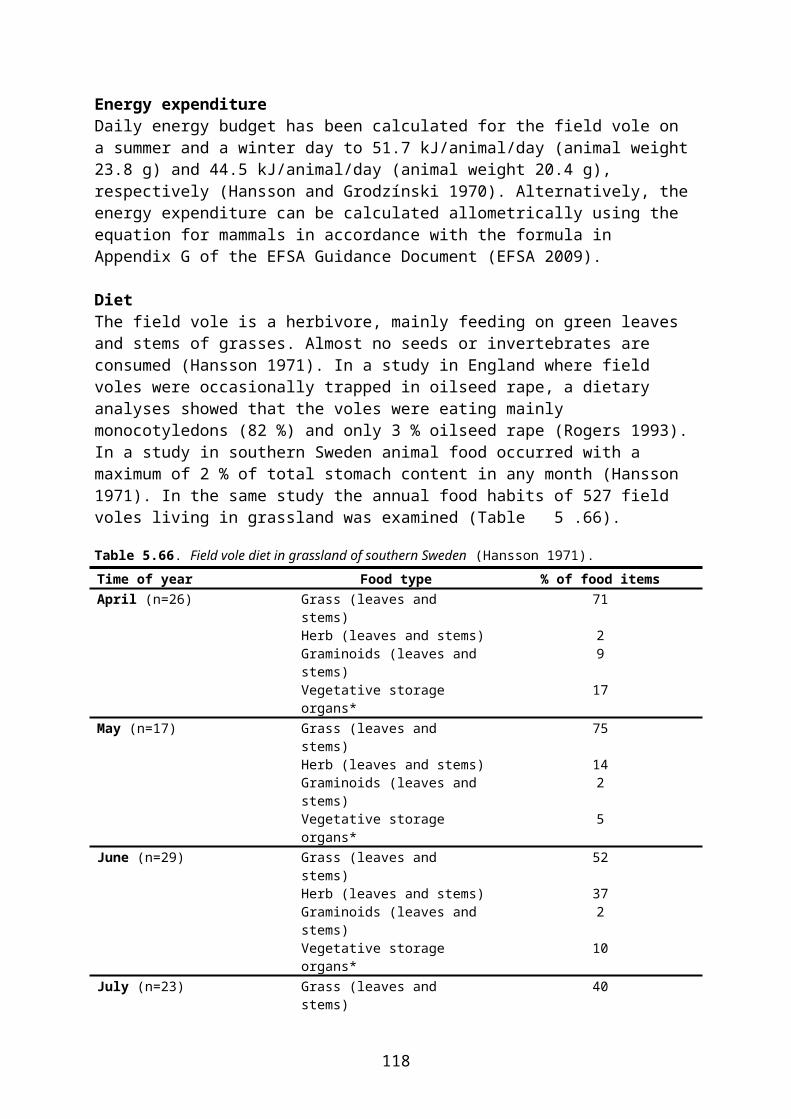
Beets April May* June June July August Sept.BBCH 0-9 10-19 10-19 20-39 40-49 40-49 40-49

Grasses and cereal shoots 0,09 0,07 0,01 0,02Non-grass herbs, leafy crops 0,63 0,31 0,16 0,07 0,11 0,07Cereal grain/ear on plantLarge seeds/cereal grain on ground 0,06 0,06 0,06 0,06 0,06 0,06Small seeds (weed seeds) 0,57 0,21 0,23 0,25 0,10 0,30 0,43Large fruit (pome)Small fruit (plum, cherry)BerriesFoliar arthropods 0,11 0,35 0,26 0,21Ground-dwelling arthropods 0,37 0,16 0,40 0,33Ground-dwelling arthropods with intercept. 0,35 0,26 0,21Soil invertebrates

Sum 1,00 1,00 1,00 1,00 1,00 1,00 1,00

* Values from Green (1980) sugar beet study

Potatoes April May June July August August Sept.BBCH 0-9 10-19 20-39 40-89 45-89 90-99 90-99

(desiccat.) (desiccat.)Grasses and cereal shoots 0,16 0,10 0,07 0,01 0,01 0,01Non-grass herbs, leafy crops 0,09 0,08 0,03 0,05 0,03 0,02Cereal grain/ear on plantLarge seeds/cereal grain on ground 0,06 0,06 0,06 0,06 0,06 0,06 0,06Small seeds (weed seeds) 0,57 0,31 0,28 0,10 0,32 0,33 0,46Large fruit (pome)Small fruit (plum, cherry)BerriesFoliar arthropods 0,12 0,37 0,28 0,14 0,11Ground-dwelling arthropods 0,37 0,38 0,36 0,43* 0,34*Ground-dwelling arthropods with intercept. 0,37 0,28Soil invertebrates

Sum 1,00 1,00 1,00 1,00 1,00 1,00 1,00

* Low interception at this stage according to FOCUS (2000)

119

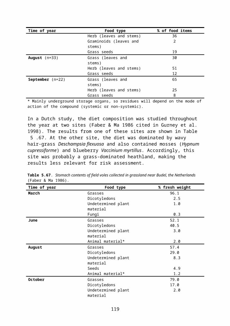
Pulses April May May June May June June July August July AugustBBCH 0-9 0-9 10-19 10-19 20-39 20-39 40-79 40-79 60-79 80-99 80-99

(desiccat.) (desiccat.)Grasses and cereal shoots 0,15 0,09 0,09 0,07 0,01 0,04 0,01Non-grass herbs, leafy crops 0,40 0,31 0,17 0,16 0,16 0,07 0,11 0,04 0,06Cereal grain/ear on plantLarge seeds/cereal grain on ground 0,06 0,06 0,06 0,06 0,06 0,06 0,06 0,06 0,06 0,06 0,06Small seeds (weed seeds) 0,57 0,42 0,24 0,23 0,28 0,25 0,25 0,10 0,30 0,10 0,32Large fruit (pome)Small fruit (plum, cherry)BerriesFoliar arthropods 0,08 0,11 0,22 0,35 0,26 0,19 0,14Ground-dwelling arthropods 0,37 0,52 0,30 0,40 0,26 0,33Ground-dwelling arthropods with intercept. 0,22 0,35 0,26 0,57 0,41Soil invertebrates

Sum 1,00 1,00 1,00 1,00 1,00 1,00 1,00 1,00 1,00 1,00 1,00

120

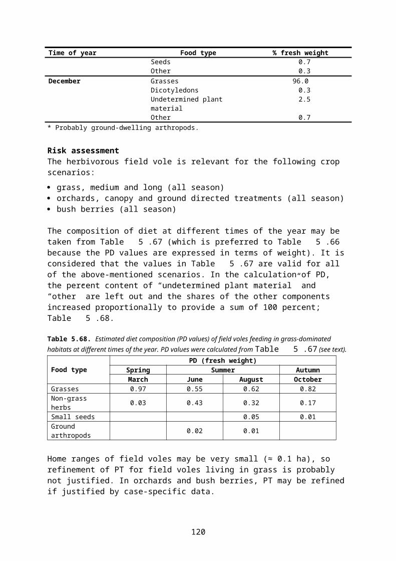
Field grown vegetables April May June May June July August May June July August Sept.BBCH 0-9 0-9 0-9 10-19 10-19 10-19 10-19 20-39 20-39 20-39 20-39 20-39

Grasses and cereal shoots 0,15 0,09 0,07 0,01 0,02Non-grass herbs, leafy crops 0,40 0,31 0,19 0,13 0,17 0,16 0,07 0,11 0,07Cereal grain/ear on plantLarge seeds/cereal grain on ground 0,06 0,06 0,06 0,06 0,06 0,06 0,06 0,06 0,06 0,06 0,06 0,06Small seeds (weed seeds) 0,57 0,42 0,34 0,24 0,23 0,09 0,30 0,28 0,25 0,10 0,30 0,43Large fruit (pome)Small fruit (plum, cherry)BerriesFoliar arthropods 0,17 0,22 0,35 0,26 0,21Ground-dwelling arthropods 0,37 0,52 0,60 0,30 0,40 0,66 0,51 0,17 0,22 0,35 0,26 0,21Ground-dwelling arthropods with intercept.Soil invertebrates

Sum 1,00 1,00 1,00 1,00 1,00 1,00 1,00 1,00 1,00 1,00 1,00 1,00

Field grown vegetables May June July August Sept.BBCH 40+ 40+ 40+ 40+ 40+

Grasses and cereal shoots 0,15 0,09 0,07 0,01 0,02Non-grass herbs, leafy crops 0,17 0,16 0,07 0,11 0,07Cereal grain/ear on plantLarge seeds/cereal grain on ground 0,06 0,06 0,06 0,06 0,06Small seeds (weed seeds) 0,28 0,25 0,10 0,30 0,43Large fruit (pome)Small fruit (plum, cherry)BerriesFoliar arthropods 0,17 0,22 0,35 0,26 0,21Ground-dwelling arthropodsGround-dwelling arthropods with intercept. 0,17 0,22 0,35 0,26 0,21Soil invertebrates

Sum 1,00 1,00 1,00 1,00 1,00

121

Strawberries April May June July August Sept. April May June June JulyStage / BBCH Planting Pre-flowering (20-59) Flowering and fruit

development (60-89)Grasses and cereal shoots 0,19 0,15 0,09 0,07 0,01 0,02 0,20 0,15 0,09 0,09 0,07Non-grass herbs, leafy crops 0,16 0,17 0,16 0,07 0,11 0,06 0,16 0,17 0,16 0,16 0,07Cereal grain/ear on plantLarge seeds/cereal grain on ground 0,06 0,06 0,06 0,06 0,06 0,06 0,06 0,06 0,06 0,06 0,06Small seeds (weed seeds) 0,36 0,28 0,25 0,10 0,30 0,43 0,36 0,28 0,25 0,25 0,10Large fruit (pome)Small fruit (plum, cherry)BerriesFoliar arthropods 0,11 0,17 0,22 0,22 0,35Ground-dwelling arthropods 0,23 0,34 0,44 0,70 0,52 0,43Ground-dwelling arthropods with intercept. 0,11 0,17 0,22 0,22 0,35Soil invertebrates

Sum 1,00 1,00 1,00 1,00 1,00 1,00 1,00 1,00 1,00 1,00 1,00

Strawberries July August Sept. April May June July August Sept.Stage / BBCH Post-harvest treatm. Termination

Grasses and cereal shoots 0,07 0,01 0,02 0,12 0,09 0,05 0,04 0,01 0,01Non-grass herbs, leafy crops 0,07 0,11 0,07 0,10 0,10 0,09 0,04 0,06 0,03Cereal grain/ear on plantLarge seeds/cereal grain on ground 0,06 0,06 0,06 0,06 0,06 0,06 0,06 0,06 0,06Small seeds (weed seeds) 0,10 0,30 0,43 0,44 0,34 0,29 0,10 0,32 0,45Large fruit (pome)Small fruit (plum, cherry)BerriesFoliar arthropods 0,35 0,26 0,21 0,07 0,10 0,13 0,19 0,14 0,11Ground-dwelling arthropodsGround-dwelling arthropods with intercept. 0,35 0,26 0,21 0,21 0,31 0,38 0,57 0,41 0,34Soil invertebrates

Sum 1,00 1,00 1,00 1,00 1,00 1,00 1,00 1,00 1,00

122

Rotational grass (seed grass, leys) April May June July August Sept. April May June July August Sept.Stage Short grass Medium & long grass

Grasses and cereal shoots 0,35 0,28 0,18 0,13 0,02 0,03 0,21 0,16 0,10 0,07 0,01 0,02Non-grass herbs, leafy crops 0,07 0,08 0,08 0,03 0,06 0,03 0,09 0,09 0,08 0,03 0,06 0,03Cereal grain/ear on plantLarge seeds/cereal grain on ground 0,06 0,06 0,06 0,06 0,06 0,06 0,06 0,06 0,06 0,06 0,06 0,06Small seeds (weed seeds) 0,32 0,26 0,25 0,10 0,32 0,44 0,39 0,31 0,28 0,10 0,32 0,45Large fruit (pome)Small fruit (plum, cherry)BerriesFoliar arthropods 0,12 0,19 0,24 0,37 0,27 0,22Ground-dwelling arthropods 0,20 0,32 0,43 0,68 0,54 0,44Ground-dwelling arthropods with intercept. 0,13 0,19 0,24 0,37 0,28 0,22Soil invertebrates

Sum 1,00 1,00 1,00 1,00 1,00 1,00 1,00 1,00 1,00 1,00 1,00 1,00

Rotational grass (seed grass, leys) April May June July August Sept.Stage Termination

Grasses and cereal shoots 0,22 0,17 0,11 0,07 0,01 0,02Non-grass herbs, leafy crops 0,05 0,05 0,04 0,02 0,03 0,02Cereal grain/ear on plantLarge seeds/cereal grain on ground 0,06 0,06 0,06 0,06 0,06 0,06Small seeds (weed seeds) 0,41 0,32 0,29 0,10 0,33 0,45Large fruit (pome)Small fruit (plum, cherry)BerriesFoliar arthropods 0,06 0,10 0,12 0,19 0,14 0,11Ground-dwelling arthropodsGround-dwelling arthropods with intercept. 0,20 0,30 0,38 0,56 0,43 0,34Soil invertebrates

Sum 1,00 1,00 1,00 1,00 1,00 1,00

123

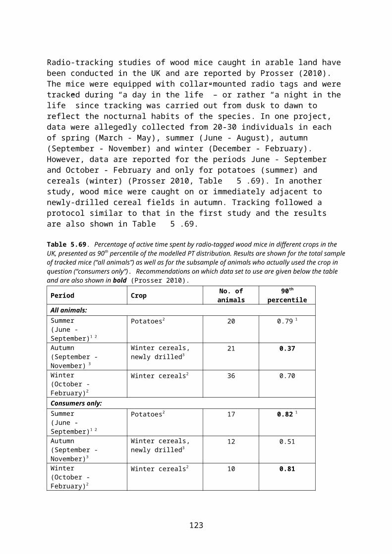
Non-rotational grass (turf, pasture) April May August Sept. April May June July August Sept.Stage Sowing & pre-emergence Short grass

Grasses and cereal shoots 0,37 0,29 0,20 0,14 0,02 0,04Non-grass herbs, leafy crops 0,08 0,09 0,08 0,04 0,06 0,04Cereal grain/ear on plantLarge seeds/cereal grain on groundSmall seeds (weed seeds) 0,61 0,45 0,37 0,50 0,34 0,28 0,26 0,10 0,34 0,46Large fruit (pome)Small fruit (plum, cherry)BerriesFoliar arthropodsGround-dwelling arthropods 0,39 0,55 0,63 0,50 0,21 0,34 0,46 0,72 0,58 0,46Ground-dwelling arthropods with intercept.Soil invertebrates

Sum 1,00 1,00 1,00 1,00 1,00 1,00 1,00 1,00 1,00 1,00

Non-rotational grass (turf, pasture) April May June July August Sept. April May June July August Sept.Stage Medium & long grass Termination

Grasses and cereal shoots 0,23 0,17 0,11 0,07 0,02 0,02 0,24 0,18 0,11 0,08 0,01 0,02Non-grass herbs, leafy crops 0,09 0,10 0,09 0,04 0,06 0,04 0,05 0,05 0,05 0,02 0,03 0,02Cereal grain/ear on plantLarge seeds/cereal grain on groundSmall seeds (weed seeds) 0,42 0,33 0,29 0,11 0,34 0,47 0,43 0,35 0,31 0,11 0,35 0,48Large fruit (pome)Small fruit (plum, cherry)BerriesFoliar arthropods 0,13 0,20 0,25 0,39 0,29 0,23 0,07 0,10 0,13 0,20 0,15 0,12Ground-dwelling arthropodsGround-dwelling arthropods with intercept. 0,13 0,20 0,26 0,39 0,29 0,24 0,21 0,32 0,40 0,59 0,46 0,36Soil invertebrates

Sum 1,00 1,00 1,00 1,00 1,00 1,00 1,00 1,00 1,00 1,00 1,00 1,00

124

Appendix 4

PD values (fresh weight) for wood mice feeding in different crops.

Spring cereals April May June June July July August August August Sept.BBCH 0-9 10-29 30-39 40-69 40-69 70-89 70-89 Pre-harv. Stubble Stubble

desiccat. treatm. treatm.Grasses and cereal shoots 0,16 0,06 0,06 0,07 0,05 0,07 0,04 0,04 0,03Non-grass herbs, leafy crops 0,03 0,03 0,03 0,03 0,03 0,02 0,02 0,02Cereal grain/ear on plant 0,16 0,12 0,13Large seeds/cereal grain on ground 0,29 0,30 0,32 0,32 0,32 0,32 0,25 0,26 0,39 0,34Small seeds (weed seeds) 0,04 0,25 0,25 0,21 0,16 0,20 0,21 0,21 0,21Large fruit (pome)Small fruit (plum, cherry)BerriesFoliar arthropodsGround-dwelling arthropods 0,45 0,10 0,25 0,29 0,26Ground-dwelling arthropods with intercept. 0,25 0,37 0,28 0,28 0,29Soil invertebrates 0,26 0,40 0,09 0,09 0,05 0,05 0,05 0,14

Sum 1,00 1,00 1,00 1,00 1,00 1,00 1,00 1,00 1,00 1,00

Winter cereals Sept. Oct. Sept. Oct. Nov. March April May May JuneBBCH 0-9 0-9 10-19 10-19 10-19 10-19 10-29 10-29 30-39 30-39

Grasses and cereal shoots 0,09 0,25 0,40 0,23 0,24 0,16 0,11 0,06Non-grass herbs, leafy crops 0,05 0,03Cereal grain/ear on plantLarge seeds/cereal grain on ground 0,42 0,55 0,33 0,30 0,40 0,25 0,05 0,30 0,30 0,32Small seeds (weed seeds) 0,20 0,15 0,20 0,15 0,08 0,04 0,04 0,25Large fruit (pome)Small fruit (plum, cherry)BerriesFoliar arthropodsGround-dwelling arthropods 0,25 0,30 0,25 0,30 0,09 0,27 0,45 0,10 0,10 0,25Ground-dwelling arthropods with intercept.Soil invertebrates 0,13 0,13 0,03 0,25 0,26 0,40 0,40 0,09

Sum 1,00 1,00 1,00 1,00 1,00 1,00 1,00 1,00 1,00 1,00

125

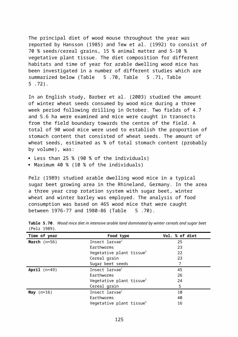
Winter cereals May June July July August July August August Sept.BBCH 40-59 40-69 60-69 70-89 70-89 Pre-harv. Pre-harv. Stubble Stubble

desiccat. desiccat. treatm. treatm.Grasses and cereal shoots 0,11 0,06 0,07 0,05 0,07 0,03 0,04 0,04 0,03Non-grass herbs, leafy crops 0,05 0,03 0,03 0,03 0,03 0,01 0,02 0,02 0,02Cereal grain/ear on plant 0,16 0,12 0,17 0,13Large seeds/cereal grain on ground 0,30 0,32 0,32 0,32 0,25 0,33 0,26 0,39 0,34Small seeds (weed seeds) 0,04 0,25 0,21 0,16 0,20 0,17 0,21 0,21 0,21Large fruit (pome)Small fruit (plum, cherry)BerriesFoliar arthropodsGround-dwelling arthropods 0,29 0,26Ground-dwelling arthropods with intercept. 0,10 0,25 0,37 0,28 0,28 0,29 0,29Soil invertebrates 0,40 0,09 0,05 0,05 0,05 0,14

Sum 1,00 1,00 1,00 1,00 1,00 1,00 1,00 1,00 1,00

Winter cereals Sept. Sept. Jan.- April- April-Green (1979) alternative -Dec. -Dec. Feb. June June

BBCH 0-9 10-19 10-19 14-39 40-69

Grasses and cereal shoots 0,08 0,01 0,01Non-grass herbs, leafy cropsCereal grain/ear on plantLarge seeds/cereal grain on ground 0,60 0,60 0,55 0,06 0,06Small seeds (weed seeds) 0,24 0,24 0,05 0,80 0,80Large fruit (pome)Small fruit (plum, cherry)BerriesFoliar arthropodsGround-dwelling arthropods 0,16 0,16 0,16 0,12Ground-dwelling arthropods with intercept. 0,12Soil invertebrates 0,16 0,01 0,01

Sum 1,00 1,00 1,00 1,00 1,00

126

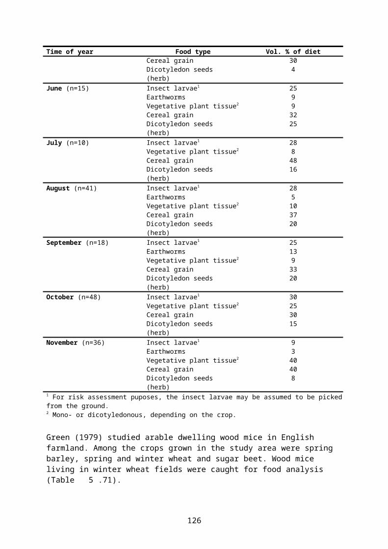
127

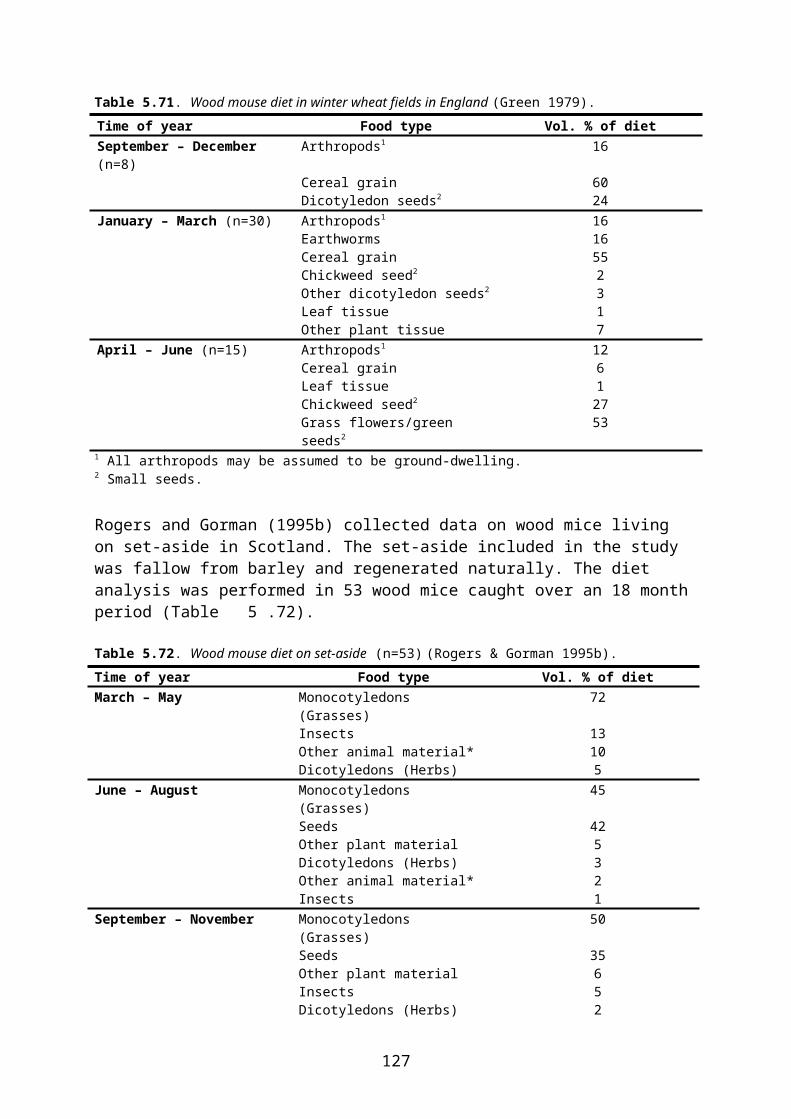
Maize April May May June June JulyBBCH 0-9 0-9 10-29 10-29 30-39 30-39

Grasses and cereal shoots 0,22 0,12 0,08 0,10Non-grass herbs, leafy crops 0,04 0,05Cereal grain/ear on plantLarge seeds/cereal grain on ground 0,29* 0,29* 0,05 0,05 0,05 0,05Small seeds (weed seeds) 0,05 0,05 0,35 0,35 0,29Large fruit (pome)Small fruit (plum, cherry)BerriesFoliar arthropodsGround-dwelling arthropods 0,45 0,13 0,14 0,35 0,35 0,51Ground-dwelling arthropods with intercept.Soil invertebrates 0,26 0,53 0,54 0,13 0,13

Sum 1,00 1,00 1,00 1,00 1,00 1,00

* Cereal grain + maize seeds

Spring oilseed rape April April May May May June July July August July August August Sept.BBCH 0-9 10-19 10-19 20-39 40-59 40-79 60-79 80-89 80-89 Pre-harv. Pre-harv. Stubble Stubble

desiccat. desiccat. treatm. treatm.Grasses and cereal shoots 0,07 0,07 0,04 0,05 0,05 0,05 0,02 0,02 0,02 0,02Non-grass herbs, leafy crops 0,24 0,22 0,15 0,15 0,08 0,10 0,09 0,09 0,05 0,05 0,05 0,04Cereal grain/ear on plantLarge seeds/cereal grain on ground 0,05 0,05 0,05 0,05 0,05 0,05 0,05 0,05 0,05 0,05 0,05 0,05 0,05Small seeds (weed seeds) 0,07* 0,05 0,05 0,05 0,35 0,29 0,34 0,35 0,41 0,42 0,38 0,35Large fruit (pome)Small fruit (plum, cherry)BerriesFoliar arthropodsGround-dwelling arthropods 0,56 0,45 0,14 0,14 0,42 0,35Ground-dwelling arthropods with intercept. 0,14 0,35 0,51 0,47 0,39 0,47 0,39Soil invertebrates 0,32 0,26 0,54 0,54 0,54 0,13 0,07 0,07 0,08 0,19

Sum 1,00 1,00 1,00 1,00 1,00 1,00 1,00 1,00 1,00 1,00 1,00 1,00 1,00

* Rape seeds

128

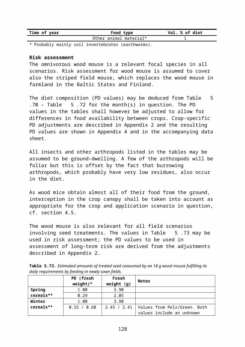
Winter oilseed rape August Sept. Oct. March April Oct. Nov. March AprilBBCH 0-9 10-19 10-19 10-19 10-19 20-39 20-39 20-39 20-39

Grasses and cereal shoots 0,11 0,21 0,09 0,08Non-grass herbs, leafy crops 0,13 0,34 0,27 0,24 0,23 0,42 0,18 0,16Cereal grain/ear on plantLarge seeds/cereal grain on ground 0,05 0,05 0,05 0,05 0,05 0,05 0,05 0,05 0,05Small seeds (weed seeds) 0,41 0,28 0,20 0,09 0,20 0,13 0,09Large fruit (pome)Small fruit (plum, cherry)BerriesFoliar arthropodsGround-dwelling arthropods 0,46 0,36 0,41 0,31 0,45 0,41 0,14 0,31 0,45Ground-dwelling arthropods with intercept.Soil invertebrates 0,08 0,18 0,28 0,26 0,05 0,28 0,26

Sum 1,00 1,00 1,00 1,00 1,00 1,00 1,00 1,00 1,00

Winter oilseed rape April May June June July July July AugustBBCH 40-59 40-79 70-79 80-89 80-89 Pre-harv. Stubble Stubble

desiccat. treatm. treatm.Grasses and cereal shoots 0,08 0,07 0,04 0,04 0,05 0,02 0,02 0,02Non-grass herbs, leafy crops 0,16 0,15 0,08 0,08 0,09 0,05 0,05 0,05Cereal grain/ear on plantLarge seeds/cereal grain on ground 0,05 0,05 0,05 0,05 0,05 0,05 0,05 0,05Small seeds (weed seeds) 0,05 0,35 0,40 0,34 0,41 0,37 0,38Large fruit (pome)Small fruit (plum, cherry)BerriesFoliar arthropodsGround-dwelling arthropods 0,51 0,42Ground-dwelling arthropods with intercept. 0,45 0,14 0,35 0,32 0,47 0,47Soil invertebrates 0,26 0,54 0,13 0,11 0,08

Sum 1,00 1,00 1,00 1,00 1,00 1,00 1,00 1,00

129

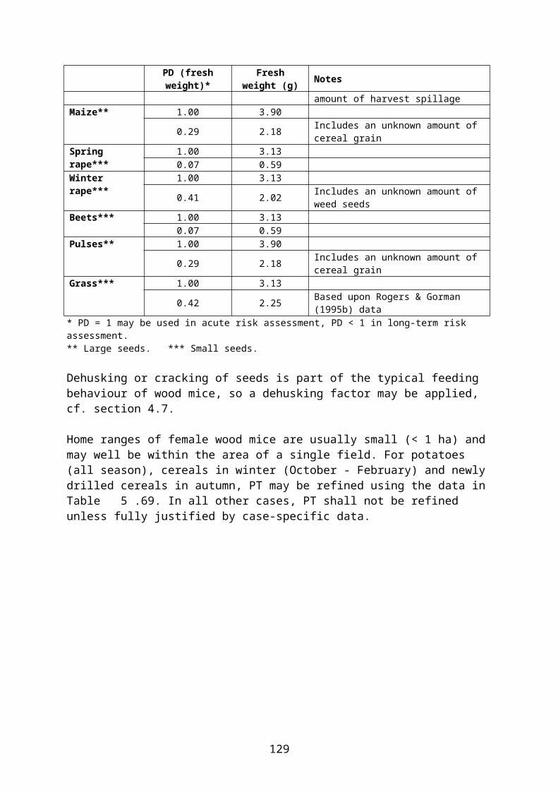
Beets April May June June July August Sept. Oct.BBCH 0-9 10-19 10-19 20-39 40-49 40-49 40-49 40-49

Grasses and cereal shoots 0,04 0,05 0,05 0,04 0,11Non-grass herbs, leafy crops 0,22 0,12 0,08 0,10 0,10 0,09 0,23Cereal grain/ear on plantLarge seeds/cereal grain on ground 0,05 0,05 0,05 0,05 0,05 0,05 0,05 0,05Small seeds (weed seeds) 0,07* 0,05 0,35 0,35 0,29 0,30 0,28 0,20Large fruit (pome)Small fruit (plum, cherry)BerriesFoliar arthropodsGround-dwelling arthropods 0,56 0,14 0,35 0,35Ground-dwelling arthropods with intercept. 0,51 0,42 0,36 0,41Soil invertebrates 0,32 0,54 0,13 0,13 0,08 0,18

Sum 1,00 1,00 1,00 1,00 1,00 1,00 1,00 1,00

* Beet seeds

Potatoes April May June July August August Sept.BBCH 0-9 10-19 20-39 40-89 45-89 90-99 90-99

(desiccat.) (desiccat.)Grasses and cereal shoots 0,06 0,03 0,04 0,04 0,02 0,02Non-grass herbs, leafy crops 0,06 0,03 0,04 0,04 0,02 0,02Cereal grain/ear on plantLarge seeds/cereal grain on ground 0,05 0,05 0,05 0,05 0,05 0,05 0,05Small seeds (weed seeds) 0,06 0,37 0,32 0,33 0,34 0,32Large fruit (pome)Small fruit (plum, cherry)BerriesFoliar arthropodsGround-dwelling arthropods 0,60 0,16 0,38 0,48* 0,39*Ground-dwelling arthropods with intercept. 0,55 0,46Soil invertebrates 0,35 0,61 0,14 0,08 0,09 0,20

Sum 1,00 1,00 1,00 1,00 1,00 1,00 1,00

* Low interception at this stage according to FOCUS (2000)

130

Pulses April May May June May June June July August July AugustBBCH 0-9 0-9 10-19 10-19 20-39 20-39 40-79 40-79 60-79 80-99 80-99

(desiccat.) (desiccat.)Grasses and cereal shoots 0,07 0,04 0,04 0,05 0,05 0,02 0,03Non-grass herbs, leafy crops 0,22 0,12 0,15 0,08 0,08 0,10 0,10 0,05 0,05Cereal grain/ear on plantLarge seeds/cereal grain on ground 0,29* 0,29* 0,05 0,05 0,05 0,05 0,05 0,05 0,05 0,10 0,10Small seeds (weed seeds) 0,05 0,05 0,35 0,05 0,35 0,35 0,29 0,30 0,30 0,31Large fruit (pome)Small fruit (plum, cherry)BerriesFoliar arthropodsGround-dwelling arthropods 0,45 0,13 0,14 0,35 0,14 0,35Ground-dwelling arthropods with intercept. 0,35 0,51 0,42 0,53 0,43Soil invertebrates 0,26 0,53 0,54 0,13 0,54 0,13 0,13 0,08 0,08

Sum 1,00 1,00 1,00 1,00 1,00 1,00 1,00 1,00 1,00 1,00 1,00

* Cereal grain + peas (or beans)

Field grown vegetables April May June May June July August May June July August Sept.BBCH 0-9 0-9 0-9 10-19 10-19 10-19 10-19 20-39 20-39 20-39 20-39 20-39

Grasses and cereal shoots 0,07 0,04 0,05 0,05 0,04Non-grass herbs, leafy crops 0,22 0,12 0,15 0,15 0,15 0,08 0,10 0,10 0,09Cereal grain/ear on plantLarge seeds/cereal grain on ground 0,05 0,05 0,05 0,05 0,05 0,05 0,05 0,05 0,05 0,05 0,05 0,05Small seeds (weed seeds) 0,03 0,08 0,28 0,05 0,35 0,29 0,30 0,05 0,35 0,29 0,30 0,28Large fruit (pome)Small fruit (plum, cherry)BerriesFoliar arthropodsGround-dwelling arthropods 0,58 0,17 0,49 0,14 0,35 0,51 0,42 0,14 0,35 0,51 0,42 0,36Ground-dwelling arthropods with intercept.Soil invertebrates 0,34 0,70 0,18 0,54 0,13 0,08 0,54 0,13 0,08 0,18

Sum 1,00 1,00 1,00 1,00 1,00 1,00 1,00 1,00 1,00 1,00 1,00 1,00

131

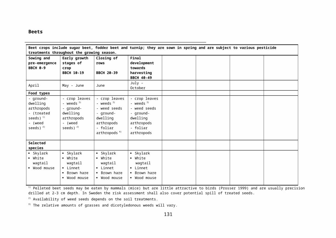
Field grown vegetables May June July August Sept. Oct.BBCH 40-49 40-49 40-49 40-49 40-49 40-49

Grasses and cereal shoots 0,07 0,04 0,05 0,05 0,04 0,11Non-grass herbs, leafy crops 0,15 0,08 0,10 0,10 0,09 0,23Cereal grain/ear on plantLarge seeds/cereal grain on ground 0,05 0,05 0,05 0,05 0,05 0,05Small seeds (weed seeds) 0,05 0,35 0,29 0,30 0,28 0,20Large fruit (pome)Small fruit (plum, cherry)BerriesFoliar arthropodsGround-dwelling arthropodsGround-dwelling arthropods with intercept. 0,14 0,35 0,51 0,42 0,36 0,41Soil invertebrates 0,54 0,13 0,08 0,18

Sum 1,00 1,00 1,00 1,00 1,00 1,00

Strawberries April May June July August Sept. Oct. April May June June JulyStage / BBCH Planting Pre-flowering (20-59) Flowering and fruit

development (60-89)Grasses and cereal shoots 0,08 0,07 0,04 0,05 0,05 0,04 0,11 0,08 0,07 0,04 0,04 0,05Non-grass herbs, leafy crops 0,16 0,15 0,08 0,10 0,10 0,09 0,23 0,16 0,15 0,08 0,08 0,10Cereal grain/ear on plantLarge seeds/cereal grain on ground 0,05 0,05 0,05 0,05 0,05 0,05 0,05 0,05 0,05 0,05 0,05 0,05Small seeds (weed seeds) 0,05 0,35 0,29 0,30 0,28 0,20 0,05 0,35 0,35 0,29Large fruit (pome)Small fruit (plum, cherry)BerriesFoliar arthropodsGround-dwelling arthropods 0,45 0,14 0,35 0,51 0,42 0,36 0,41Ground-dwelling arthropods with intercept. 0,45 0,14 0,35 0,35 0,51Soil invertebrates 0,26 0,54 0,13 0,08 0,18 0,26 0,54 0,13 0,13

Sum 1,00 1,00 1,00 1,00 1,00 1,00 1,00 1,00 1,00 1,00 1,00 1,00

132

Strawberries July August Sept. Oct. March April May June July August Sept. Oct. Nov.Stage / BBCH Post-harvest Termination

Grasses and cereal shoots 0,05 0,05 0,04 0,11 0,05 0,05 0,04 0,02 0,03 0,03 0,02 0,07 0,16Non-grass herbs, leafy crops 0,10 0,10 0,09 0,23 0,11 0,09 0,08 0,05 0,05 0,05 0,05 0,14 0,32Cereal grain/ear on plantLarge seeds/cereal grain on ground 0,05 0,05 0,05 0,05 0,05 0,05 0,05 0,05 0,05 0,05 0,05 0,05 0,05Small seeds (weed seeds) 0,29 0,30 0,28 0,20 0,10 0,06 0,37 0,32 0,33 0,30 0,25 0,19Large fruit (pome)Small fruit (plum, cherry)BerriesFoliar arthropodsGround-dwelling arthropodsGround-dwelling arthropods with intercept. 0,51 0,42 0,36 0,41 0,36 0,51 0,16 0,37 0,55 0,46 0,38 0,49 0,21Soil invertebrates 0,08 0,18 0,33 0,30 0,61 0,14 0,08 0,20 0,07

Sum 1,00 1,00 1,00 1,00 1,00 1,00 1,00 1,00 1,00 1,00 1,00 1,00 1,00

Grassland in short rotation March April May June July August Sept. Oct. Nov.Stage Short grass

Grasses and cereal shoots 0,22 0,19 0,17 0,10 0,12 0,12 0,10 0,27 0,50Non-grass herbs, leafy crops 0,05 0,05 0,04 0,02 0,03 0,03 0,03 0,07 0,13Cereal grain/ear on plantLarge seeds/cereal grain on ground 0,05 0,05 0,05 0,05 0,05 0,05 0,05 0,05 0,05Small seeds (weed seeds) 0,09 0,06 0,35 0,29 0,30 0,28 0,20 0,13Large fruit (pome)Small fruit (plum, cherry)BerriesFoliar arthropodsGround-dwelling arthropods 0,31 0,45 0,14 0,35 0,51 0,42 0,36 0,41 0,14Ground-dwelling arthropods with intercept.Soil invertebrates 0,28 0,26 0,54 0,13 0,08 0,18 0,05

Sum 1,00 1,00 1,00 1,00 1,00 1,00 1,00 1,00 1,00

133

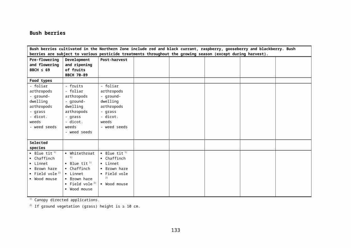
Grassland in short rotation March April May June July August Sept. Oct. Nov.Stage Medium & long grass

Grasses and cereal shoots 0,18 0,16 0,15 0,07 0,09 0,09 0,09 0,23 0,42Non-grass herbs, leafy crops 0,09 0,08 0,07 0,04 0,04 0,04 0,04 0,11 0,21Cereal grain/ear on plantLarge seeds/cereal grain on ground 0,05 0,05 0,05 0,05 0,05 0,05 0,05 0,05 0,05Small seeds (weed seeds) 0,09 0,05 0,44 0,38 0,39 0,28 0,20 0,13Large fruit (pome)Small fruit (plum, cherry)BerriesFoliar arthropodsGround-dwelling arthropodsGround-dwelling arthropods with intercept. 0,31 0,45 0,14 0,29 0,44 0,36 0,36 0,41 0,14Soil invertebrates 0,28 0,26 0,54 0,11 0,07 0,18 0,05

Sum 1,00 1,00 1,00 1,00 1,00 1,00 1,00 1,00 1,00

Grassland in short rotation March April May June July August Sept. Oct. Nov.Stage Termination

Grasses and cereal shoots 0,11 0,09 0,08 0,05 0,05 0,05 0,05 0,14 0,32Non-grass herbs, leafy crops 0,05 0,05 0,04 0,02 0,03 0,03 0,02 0,07 0,16Cereal grain/ear on plantLarge seeds/cereal grain on ground 0,05 0,05 0,05 0,05 0,05 0,05 0,05 0,05 0,05Small seeds (weed seeds) 0,10 0,06 0,37 0,32 0,33 0,30 0,25 0,19Large fruit (pome)Small fruit (plum, cherry)BerriesFoliar arthropodsGround-dwelling arthropodsGround-dwelling arthropods with intercept. 0,36 0,51 0,16 0,37 0,55 0,46 0,38 0,49 0,21Soil invertebrates 0,33 0,30 0,61 0,14 0,08 0,20 0,07

Sum 1,00 1,00 1,00 1,00 1,00 1,00 1,00 1,00 1,00

134

Permanent & perennial grass March Aug. March June Sept. March June Sept. March June Sept.-May -Oct. -May -Aug. -Nov. -May -Aug. -Nov. -May -Aug. -Nov.

Stage Sowing & Short grass Medium & long grass Termination pre-emergence

Grasses and cereal shoots 0,72 0,46 0,51 0,72 0,46 0,51 0,59 0,31 0,36Non-grass herbs, leafy crops 0,05 0,08 0,08 0,05 0,08 0,08 0,04 0,06 0,06Cereal grain/ear on plantLarge seeds/cereal grain on groundSmall seeds (weed seeds) 0,42 0,42 0,43 0,35 0,43 0,35 0,59 0,50Large fruit (pome)Small fruit (plum, cherry)BerriesFoliar arthropodsGround-dwelling arthropods 0,33 0,39 0,13 0,01 0,05Ground-dwelling arthropods with intercept. 0,13 0,01 0,05 0,21 0,01 0,07Soil invertebrates 0,25 0,19 0,10 0,02 0,01 0,10 0,02 0,01 0,16 0,03 0,01

Sum 1,00 1,00 1,00 1,00 1,00 1,00 1,00 1,00 1,00 1,00 1,00

Fruit trees (orchards) March June Sept. March June Sept.-May -Aug. -Nov. -May -Aug. -Nov.

Application / Stage Canopy directed (all stages) Ground directed (all stages)

Grasses and cereal shoots 0,72 0,46 0,51 0,72 0,46 0,51Non-grass herbs, leafy crops 0,05 0,08 0,08 0,05 0,08 0,08Cereal grain/ear on plantLarge seeds/cereal grain on groundSmall seeds (weed seeds) 0,43 0,35 0,43 0,35Large fruit (pome)Small fruit (plum, cherry)BerriesFoliar arthropodsGround-dwelling arthropods 0,13 0,01 0,05Ground-dwelling arthropods with intercept. 0,13 0,01 0,05Soil invertebrates 0,10 0,02 0,01 0,10 0,02 0,01

Sum 1,00 1,00 1,00 1,00 1,00 1,00

135

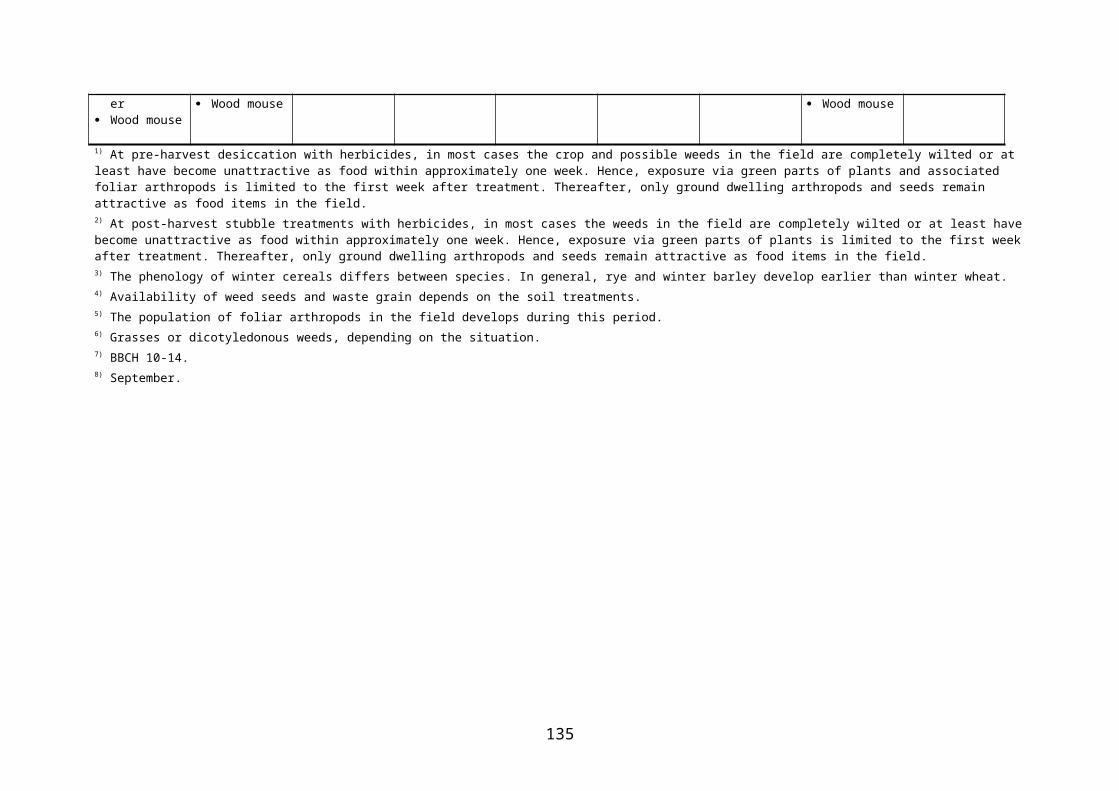
Bush berries March June Sept. March June Sept.-May -Aug. -Nov. -May -Aug. -Nov.

Application / Stage Canopy directed (all stages) Ground directed (all stages)

Grasses and cereal shoots 0,72 0,46 0,51 0,72 0,46 0,51Non-grass herbs, leafy crops 0,05 0,08 0,08 0,05 0,08 0,08Cereal grain/ear on plantLarge seeds/cereal grain on groundSmall seeds (weed seeds) 0,43 0,35 0,43 0,35Large fruit (pome)Small fruit (plum, cherry)BerriesFoliar arthropodsGround-dwelling arthropods 0,13 0,01 0,05Ground-dwelling arthropods with intercept. 0,13 0,01 0,05Soil invertebrates 0,10 0,02 0,01 0,10 0,02 0,01

Sum 1,00 1,00 1,00 1,00 1,00 1,00

Ornamentals and nursery March June Sept. March June Sept. March June Sept. March June Sept.-May -Aug. -Nov. -May -Aug. -Nov. -May -Aug. -Nov. -May -Aug. -Nov.

Stage / Application Pre-emergence Small plants Large plants, canopy directed Large plants, ground directed

Grasses and cereal shoots 0,05 0,11 0,11 0,09 0,19 0,18 0,39 0,32 0,35 0,39 0,32 0,35Non-grass herbs, leafy crops 0,05 0,11 0,11 0,09 0,18 0,18 0,11 0,13 0,11 0,11 0,13 0,11Cereal grain/ear on plantLarge seeds/cereal grain on groundSmall seeds (weed seeds) 0,60 0,47 0,49 0,38 0,48 0,40 0,48 0,40Large fruit (pome)Small fruit (plum, cherry)BerriesFoliar arthropodsGround-dwelling arthropods 0,51 0,06 0,26 0,46 0,05 0,22 0,28 0,02 0,12Ground-dwelling arthropods with intercept. 0,28 0,02 0,12Soil invertebrates 0,39 0,12 0,05 0,36 0,09 0,04 0,22 0,05 0,02 0,22 0,05 0,02

Sum 1,00 1,00 1,00 1,00 1,00 1,00 1,00 1,00 1,00 1,00 1,00 1,00

136