peter benner hermann mena jens saak - tu-chemnitz.de · the numerical treatment of linear-quadratic...
TRANSCRIPT

Peter Benner Hermann Mena Jens Saak
On the Parameter Selection Problem in
the Newton-ADI Iteration for Large Scale
Riccati Equations
CSC06-03
Chemnitz Scientific Computing
Preprints
Impressum
Chemnitz Scientific Computing Preprints mdash ISSN 1864-0087
(1995ndash2005 Preprintreihe des Chemnitzer SFB393)
HerausgeberProfessuren furNumerische und Angewandte Mathematikan der Fakultat fur Mathematikder Technischen Universitat Chemnitz
PostanschriftTU Chemnitz Fakultat fur Mathematik09107 ChemnitzSitzReichenhainer Str 41 09126 Chemnitz
httpwwwtu-chemnitzdemathematikcsc
Chemnitz Scientific Computing
Preprints
Peter Benner Hermann Mena Jens Saak
On the Parameter Selection Problem in
the Newton-ADI Iteration for Large Scale
Riccati Equations
CSC06-03
CSC06-03 ISSN 1864-0087 October 2006
Abstract
The numerical treatment of linear-quadratic regulator problems forparabolic partial differential equations (PDEs) on infinite time horizonsrequires the solution of large scale algebraic Riccati equations (ARE)The Newton-ADI iteration is an efficient numerical method for this taskIt includes the solution of a Lyapunov equation by the alternating di-rections implicit (ADI) algorithm in each iteration step On finite timeintervals the solution of a large scale differential Riccati equation is re-quired This can be solved by a backward differentiation formula (BDF)method which needs to solve an ARE in each time step
Here we study the selection of shift parameters for the ADI methodThis leads to a rational min-max-problem which has been considered bymany authors Since knowledge about the complete complex spectrumis crucial for computing the optimal solution this is infeasible for thelarge scale systems arising from finite element discretization of PDEsTherefore several alternatives for computing suboptimal parameters arediscussed and compared for numerical examples
Contents
1 Introduction 111 Problem background 112 Newton-ADI iteration 4
2 Review of existing parameter selection methods 521 Leja Points 622 Optimal parameters 723 Heuristic parameters 824 Discussion 8
3 Suboptimal parameter computation 9
4 Numerical results 1141 FDM semidiscretized diffusion-convection-reaction equation 1242 FDM semidiscretized heat equation 1343 FEM semidiscretized convection-diffusion equation 14
5 Conclusions 16
Authorrsquos addresses
Peter Benner Jens Saak
Fakultat fur MathematikTechnische Universitat ChemnitzD-09107 Chemnitz[bennerjenssaak]mathematiktu-chemnitzde
Hermann Mena
Departamento de MatematicaEscuela Politecnica NacionalQuito - Ecuadorhmenaserverepneduec
1 Introduction
Optimal control problems governed by partial differential equations are a topic of cur-rent research Many control stabilization and parameter identification problems can bereduced to the linear-quadratic regulator (LQR) problem see [14 24 25 9 10] Par-ticularly LQR problems for parabolic systems have been studied in detail in the past30 years and several results concerning existence theory and numerical approximationcan be found [27 24 25] Gibson [17] and BanksKunisch [3] present an approxima-tion technique to reduce the inherently infinite-dimensional problem of the distributedregulator problem for parabolic PDEs to (large) finite-dimensional analogues
The solution of these finite-dimensional problems can be reduced to the solution of amatrix Riccati equation In the finite-time horizon case this is a first order differentialequation and in the infinitendashtime horizon case an algebraic one see eg [4 37]
In Section 11 we briefly summarize the basic results for the LQR control of parabolicPDEs Then we review the Newton-ADI iteration for the solution of large scale matrixRiccati equations in Section 12 showing how this involves the solution of a Lyapunovequation by the ADI algorithm in every iteration step Furthermore we introduce therational minimax problem related to the parameter selection problem there which isthe main topic of this paper We give a brief summary of Wachspressrsquos results and aheuristic choice of parameters described in [33] as well as a Leja point approach [38 39]in Section 2 In Section 3 we show how the first two of these methods can be combinedto have a parameter computation which can be applied efficiently even in case of verylarge systems The forth section will show the efficiency of our method compared tothe Wachspress parameters for test examples where the complete spectrum can stillbe computed numerically and thus Wachspressrsquos method can be used to compute theoptimal parameters We close this article with some conclusions in Section 5
11 Problem background
Consider nonlinear parabolic diffusion-convection and diffusion-reaction systems of theform
partx
partt+nabla middot (c(x)minus k(nablax)) + q(x) = Bu(t) t isin [0 Tf ] (1)
in Ω sub Rd d = 1 2 3 with appropriate initial and boundary conditions The equationcan be split into the convective term c the diffusive part k and the uncontrolled reactiongiven by q The state x of the system depends on ξ isin Ω and the time t isin [0 Tf ] and isdenoted by x(ξ t)
Notation Note that we use bold letters for the infinite-dimensional setting and regularletters for the discretized case We also write x(t) isin X in the abstract setting whilex(ξ t) is used if concrete problems (PDEs) are considered
We consider applications where the control u(t) is assumed to depend only on thetime t isin [0 Tf ] while the linear operator B may depend on ξ isin Ω Let J(xu) be a given
On the Parameter Selection in the Newton-ADI Iteration for Large Scale Riccati Equations
performance index then the control problem is given as
minuJ(xu) subject to (1) (2)
If (1) is in fact linear then a variational formulation leads to an abstract Cauchy problemfor a linear evolution equation of the form
x = Ax + Bu x(0) = x0 isin X (3)
for linear operators
A dom(A) sub X rarr X B U rarr X (4)
C X rarr Y
where the state space X the observation space Y and the control space U are assumedto be separable Hilbert spaces Additionally U is assumed to be finite dimensional iethere are only a finite number of independent control inputs to (1) Here C maps thestates of the system to its outputs such that
y = Cx (5)
If (1) is nonlinear model predictive control technics can be applied [5 21 22] Therethe equation is linearized at certain working points or around reference trajectories andlinear problems for equations as in (3) have to be solved on subintervals of [0 Tf ]
In many applications in engineering the performance index J(xu) is given in quadraticform We assume (3) to have a unique solution for each input u so that x = x(u) Thuswe can write the cost functional as J(u) = J(x(u)u) Then
J(u) =1
2
Tfint0
〈xQx〉X + 〈uRu〉U dt+ 〈xTfGxTf
〉X (6)
where Q G are selfadjoint operators on the state space X R is a selfadjoint operatoron the control space U and xTf
denotes x( Tf ) To guarantee unique solvability of thecontrol problem R is assumed positive definite Since often only a few measurements ofthe state are available as the outputs of the system the operator Q = ClowastQC (here andin the following lowast denotes the Hilbert space adjoint) generally is only positive semidefiniteas well as G In many applications one simply has Q = I (eg in the examples inSection 4)
If the standard assumptions that
bull A is the infinitesimal generator of a C0-semigroup T(t)
bull BC are linear bounded operators and
bull for every initial value there exists an admissible control u isin L2(0infinU)
2
Peter Benner Hermann Mena and Jens Saak
hold then the solution of the abstract LQR problem can be obtained analogously to thefinite-dimensional case (see [44 13 17]) We then have to consider the operator Riccatiequations
0 = lt(X) = ClowastQC + AlowastX + XAminusXBRminus1BlowastX (7)
andX = minuslt(X) (8)
depending on whether Tf lt infin (8) or not (7) If Tf = infin then G = 0 and the linearoperator X is the solution of (7) ie X domArarr domAlowast and 〈xlt(X)x〉 = 0 for allx x isin dom(A) The optimal control is then given as the feedback control
ulowast(t) = minusRminus1BlowastXinfinxlowast(t) (9)
which has the form of a regulator or closed-loop control Here Xinfin is the minimalnonnegative self-adjoint solution of (7) xlowast(t) = S(t)x0(t) and S(t) is the C0-semigroupgenerated by AminusBRminus1BlowastXinfin In problems where Tf lt infin the optimal control isdefined similarly to (9 ) but then Xinfin represents the unique nonnegative solution of thedifferential Riccati equation (8) with initial condition XTf
= G and therefore dependson time ie it has to be replaced by Xinfin(t) in (9) Most of the required conditionsparticularly the restrictive assumption that B is bounded can be weakened [24 25 35]
In order to solve the infinite-dimensional LQR problem numerically we use a Galerkinprojection of the variational formulation of the PDE (1) onto a finite-dimensional spaceXh spanned by a finite set of basis functions (eg finite element ansatz functions)
If we now choose the space of test functions as the space generated by finite element(fem) ansatz functions for a finite element semidiscretization in space then the operatorsabove have matrix representations in the fem basis So we have to solve the discreteproblem
minuisinL2(0Tf U)
1
2
Tfint0
〈xQx〉Xh+ 〈uRu〉U dt+ 〈xTf
GxTf〉Xh
(10)
with respect to
x = Ax+Bu
x( 0) = Ihx0 (11)
y = Cx
Here Ih is the interpolation operator from the space discretization method (here fem)Approximation results in terms of approximation of the Riccati solution operator X andthe solution semigroup S(t) for the closed loop system validating this technique havebeen considered eg in [25 3 8 20 30 31] Note that the control space is consideredfinite-dimensional and therefore does not change under spatial semi-discretization iewe can directly apply the control computed for the discretized systems (11) to theinfinite-dimensional system (3) although it might be suboptimal there The estimationof the sub-optimality of that approach will be considered elsewhere
3
On the Parameter Selection in the Newton-ADI Iteration for Large Scale Riccati Equations
12 Newton-ADI iteration
In this note we will concentrate on the step of solving the large sparse matrix Riccatiequations
0 = lth(X) = CT QC + ATX +XAminusXBRminus1BTX (12)
orX = minuslth(X) = minusCT QC minus ATX minusXA+XBRminus1BTX (13)
respectively The initial value for the latter initial value problem is X(Tf ) = G Suchinitial value problems can efficiently be solved by BDF methods known from ordinarydifferential equations [7 16 12] This involves solving algebraic equations of type (12) ineach time step The algebraic Riccati equation (ARE) is a nonlinear system of equationsso it is natural to apply Newtonrsquos method to find its solutions This approach has beeninvestigated details and further references can be found in [36 23 29 34 4 15]
Observing that the (Frechet) derivative of lth at P is given by the Lyapunov operator
ltprime
h|P Q 7rarr (Ah minusBhRminus1BT
h P )TQ+Q(Ah minusBhRminus1BT
h P )
Newtonrsquos method for AREs can be written as
N` =(ltprime
h|P`
)minus1
lth(P`)X`+1 = X` +N`
Then one step of the Newton iteration for a given starting matrix can be implementedas follows
Algorithm 11 Newtonrsquos method for AREs
Require Pl such that Al is stable1 A` larr Ah minusBhR
minus1BTh P`
2 Solve the Lyapunov equation AT` N` +N`A` = minuslth(P`)3 P`+1 larr P` +N`
Newtonrsquos iteration for AREs can be reformulated as a one step iteration re-writing itsuch that the next iterate is computed directly from the Lyapunov equation in Step 2of Algorithm 11
(Ah minusBhRminus1BT
h P`)TP`+1 + P`+1(Ah minusBhR
minus1BTh P`) =
minusCTh QhCh minus P`BhR
minus1BTh P` = minusW`W
T`
So we have to solve a Lyapunov equation
F TX +XF = minusWW T (14)
with stable F in each Newton step (14) will be solved using the alternating directionimplicit(ADI) iteration which can be written as [42]
(F T + pjI)Q(jminus1)2 = minusWW T minusQjminus1(F minus pjI)(F T + pjI)Q
Tj = minusWW T minusQ(jminus1)2(F minus pjI)
(15)
4
Peter Benner Hermann Mena and Jens Saak
where p denotes the complex conjugate of p isin C If the shift parameters pj are chosenappropriately then limjrarrinfinQj = Q with a superlinear convergence rate
In order to make this iteration work for large-scale problems we apply the low rankNewton ADI method presented in [6 33] (based upon the iterative technique by Wach-spress [42]) to the AREs
Practical experience shows that it is crucial to have good shift parameters to get fastconvergence in the ADI process The error in iterate j is given by ej = Rjejminus1 where
Rj = (F + pjI)minus1(F T minus pjI)(F T + pjI)
minus1(F minus pjI)
Thus the error after J iterations satisfies
eJ = GJe0 GJ =Jprodj=1
Rj
due to the fact that GJ is symmetric
||eJ || le ρ(GJ)||e0|| ρ(GJ) = k(p)2
where p = p1 p2 pJ and
k(p) = maxλisinσ(F )
∣∣∣∣∣Jprodj=1
(pj minus λ)
(pj + λ)
∣∣∣∣∣ (16)
By this the ADI parameters are chosen in order to minimizes ρ(GJ) which leads to therational minimax problem
minpjisinRj=1J
k(p) (17)
for the shift parameters pj see eg [43] This minimization problem is also known asthe rational Zolotarev problem since in the real case ie σ(F ) sub R it is equivalent tothe third of four approximation problems solved by Zolotarev in the 19th century see[26] For a complete historical overview see [41]
2 Review of existing parameter selection methods
Many procedures for constructing optimal or suboptimal shift parameters have beenproposed in the literature [19 32 39 43] Most of the approaches cover the spectrumof F by a domain Ω sub Cminus and solve (17) with respect to Ω instead of σ(F ) Ingeneral one must choose among the various approaches to find effective ADI iterationparameters for specific problems One could even consider sophisticated algorithms likethe one proposed by Istace and Thiran [19] in which the authors use numerical techniquesfor nonlinear optimization problems to determine optimal parameters However it isimportant to take care that the time spent in computing parameters does not outweighthe convergence improvement derived therefrom
5
On the Parameter Selection in the Newton-ADI Iteration for Large Scale Riccati Equations
Wachspress et al [43] compute the optimum parameters when the spectrum of thematrix F is real or in the complex case if the spectrum of F can be embedded in anelliptic functions region which often occurs in practice These parameters may be chosenreal even if the spectrum is complex as long as the imaginary parts of the eigenvaluesare small compared to their real parts (see [28 43] for details) The method applied byWachspress in the complex case is similar to the technique of embedding the spectruminto an ellipse and then use Chebyshev polynomials In case that the spectrum is not wellrepresented by the elliptic functions region a more general development by Starke [39]describes how generalized Leja points yield asymptotically optimal iteration parametersFinally an inexpensive heuristic procedure for determining ADI shift parameters whichoften works well in practice was proposed by Penzl [32] We will summarize theseapproaches here
21 Leja Points
Gonchar [18] characterizes the general minimax problem and shows how asymptoticallyoptimal parameters can be obtained with generalized Leja or Fejer points Starke [38]applies this theory to the ADI minimax problem (17) The generalized Leja pointsare defined as follows Given ϕ isin E and ψ isin F arbitrarily EF subsets of C forj = 1 2 the new points ϕj isin E and ψj isin F are chosen recursively in such a waythat with
rj(z) =
jprodi=1
z minus ϕjz minus ψj
(18)
the two conditionsmaxxisinE |rj(z)| = |rj(ϕj+1)|maxxisinF |rj(z)| = |rj(ψj+1)|
(19)
are fullfilled Bagby [2] shows that the rational functions rj obtained by this procedureare asymptotically minimal for the rational Zolotarev problem Starke considers a gen-eral ADI iteration so for ADI applied to the Lyapunov equation (15) the generalizedLeja points will be defined as follows
Given p0 isin E E is a complex subset such that σ(F ) sub E for j = 1 2 the newpoints pj isin E are chosen recursively in such a way that with
rj(z) =
jprodi=1
z minus pjz + pj
(20)
the conditionmaxxisinE|rj(z)| = |rj(pj+1)| (21)
holds The generalized Leja points can be determined numerically for a large class ofboundary curves partE When relatively few iterations are needed to attain the prescribedaccuracy the Leja points may be poor Moreover their computation can be quite timeconsuming when the number of Leja points generated is large since the computationgets more and more expensive the more prior Leja points are already calculated
6
Peter Benner Hermann Mena and Jens Saak
22 Optimal parameters
We will briefly summarize the parameter selection procedure given in [43] in this sectionDefine the spectral bounds a b and a sector angle α for the matrix F as
a = mini
(Reλi) b = maxi
(Reλi) α = tanminus1 maxi
∣∣∣∣ImλiReλi
∣∣∣∣ (22)
where λ1 λn are eigenvalues of minusF It is assumed that the spectrum of minusF liesinside the elliptic functions region determined by a b α as defined in [43] Let
cos2 β =2
1 + 12
(ab
+ ba
) m =2 cos2 α
cos2 βminus 1 (23)
If α lt β then m ge 1 and the parameters are real We define
k1 =1
m+radicm2 minus 1
k =radic
1minus k12 (24)
Define the elliptic integrals K and v via
F [ψ k] =
int ψ
0
dxradic1minus k2 sin2 x
(25)
as
K = K(k) = F
[π
2 k
] v = F
[sinminus1
radica
bk1
k1
] (26)
where F is the incomplete elliptic integral of the first kind k is its modulus and ψ is itsamplitude
The number of the ADI iterations required to achieve k(p)2 le ε is J = d K2vπ
log 4εe
and the ADI parameters are given by
pj = minusradicab
k1
dn
[(2j minus 1)K
2J k
] j = 1 2 J (27)
where dn(u k) is the elliptic function (see [1])If m lt 1 the parameters are complex We define the dual elliptic spectrum
aprime = tan
(π
4minus α
2
) bprime =
1
aprime αprime = β
Substituting aprime in (23) we find that
βprime = α mprime =2 cos2 β
cos2 αminus 1
By construction mprime must now be greater than 1 Therefore we may compute the opti-mum real parameters pprimej for the dual problem The corresponding complex parametersfor the actual spectrum can then be computed from
cosαj =2
pprimej + 1pprime
j
(28)
7
On the Parameter Selection in the Newton-ADI Iteration for Large Scale Riccati Equations
for j = 1 2 d1+J2e
p2jminus1 =radicab exp[ıαj] p2j =
radicab exp[minusıαj] (29)
23 Heuristic parameters
The bounds needed to compute optimal parameters are too expensive to be computedexactly in case of large scale systems because they need the knowledge of the wholespectrum of F In fact this computation would be more expensive than the applicationof the ADI method itself
An alternative was proposed by Penzl in [32] He presents a heuristic procedurewhich determines suboptimal parameters based on the idea of replacing σ(F ) by anapproximation R of the spectrum in (17) Specifically σ(F ) is approximated using theRitz values computed by the Arnoldi process (or any other large scale eigensolver) Dueto the fact that the Ritz values tend to be located near the largest magnitude eigenvaluesthe inverses of the Ritz values related to Fminus1 are also computed to get an approximationof the smallest magnitude eigenvalues of F yielding a better approximation of σ(F )The suboptimal parameters P = p1 pk are chosen among the elements of thisapproximation because the function
sP(t) =|(tminus p1) (tminus pk)||(t+ p1) (t+ pk)|
becomes small over σ(F ) if there is one of the shifts pj in the neighborhood of eacheigenvalue The procedure determines the parameters as follows First the elementpj isin R which minimizes the function spj over R is chosen The set P is initialized byeither pj or the pair of complex conjugates pj pj Now P is successively enlargedby the elements or pairs of elements of R for which the maximum of the current sPis attained Doing this the elements of R giving the largest contributions to the valueof sP are successively canceled out Therefore the resulting sP is nonzero only in theelements of R where its value is comparably small anyway In this sense (17) is solvedheuristicly
24 Discussion
We are searching for a parameter set for the ADI method applied to a control prob-lem where in the PDE constraint (1) the diffusive part is dominating the reaction orconvection terms respectively Thus the resulting operator has a spectrum with onlymoderately large imaginary components compared to the real parts In these problemsthe Wachspress approach should always be applicable and lead to real shift parametersin many cases In problems where the reactive and convective terms are absent iewe are considering a plain heat equation and therefore the spectrum is part of the realaxis the Wachspress parameters are proven to be optimal The heuristics proposed byPenzl is more expensive to compute there and Starke notes in [38] that the generalizedLeja approach will not be competitive here since it is only asymptotically optimal For
8
Peter Benner Hermann Mena and Jens Saak
the complex spectra case common strategies to determine the generalized Leja pointsgeneralize the idea of enclosing the spectrum by a polygonal domain where the start-ing roots are placed in the corners So one needs quite exact information about theshape of the spectrum there In practice this would need to be able to compute theeigenvalues with largest imaginary parts already for a simple rectangular enclosure ofthe spectrum Since this still doesnrsquot work reliable we decided to avoid the comparisonwith that approach in this publication although it might proof useful in cases where theWachspress parameters are no longer applicable or one knows some a-priori informationon the spectrum
3 Suboptimal parameter computation
In this section we discuss our new contribution to the parameter selection problem Theidea is to avoid the problems of the methods reviewed in the previous section and onthe other hand combine their advantages
Since the important information that we need to know for the Wachspress approachis the outer shape of the spectrum of the matrix F we will describe an algorithmapproximating the outer spectrum With this approximation the input parameters ab and α for the Wachspress method are determined and the optimal parameters forthe approximated spectrum are computed Obviously these parameters have to beconsidered suboptimal for the original problem but if we can approximate the outerspectrum at a similar cost to that of the heuristic parameter choice we end up with amethod giving nearly optimal parameters at a drastically reduced computational costcompared to the optimal parameters
In the following we discuss the main computational steps in Algorithm 31
Real spectra In the case where the spectrum is real we can simply compute the upperand lower bounds of the spectrum by an Arnoldi process and enter the Wachspresscomputation with these values for a and b and set α = 0 ie we only have to computetwo complete elliptic integrals by an arithmetic geometric mean process This is verycheap since it is a quadratically converging scalar computation (see below)
Complex spectra For complex spectra we introduce an additional shifting step to beable to apply the Arnoldi process more efficiently Since we are dealing with stablesystems1 we compute the largest magnitude and smallest magnitude eigenvalues anduse the arithmetic mean of their real parts as a horizontal shift such that the spectrumis centered around the origin Now Arnoldirsquos method is applied to the shifted spectrumto compute a number of largest magnitude eigenvalues These will now automaticallyinclude the smallest magnitude eigenvalues of the original system after shifting back Sowe can avoid extensive application of the Arnoldi method to the inverse of F We only
1Note that the Newton-ADI-iteration assumes that we know a stabilizing initial feedback or the systemis stable itself
9
On the Parameter Selection in the Newton-ADI Iteration for Large Scale Riccati Equations
Algorithm 31 approximate optimal ADI parameter computation
Require F Hurwitz stable1 if σ(F ) sub R then2 Compute the spectral bounds and set a = minσ(minusF ) and b = maxσ(minusF )3 k1 = a
b k =
radic1minus k2
14 K = F (π
2 k) v = F (π
2 k1)
5 Compute J and the parameters according to (27)6 else7 Compute a = min Re (σ(minusF )) b = max Re (σ(minusF )) and c = a+b
2
8 Compute l largest magnitude eigenvalues λi for the shifted matrix minusF + cI by anArnoldi process or alike
9 Shift these Eigenvalues back ie λi = λi + c10 Compute a b and α from the λi like in (22)11 if m ge 1 in (23) then12 Compute the parameters by (23)ndash(27)13 else The ADI parameters are complex in this case14 Compute the dual variables15 Compute the parameters for the dual variables by (23)ndash(27)16 Use (28) and (29) to get the complex shifts17 end if18 end if
need it to get a rough approximation of the smallest magnitude eigenvalue to determinea and b for the shifting step
The number of eigenvalues we compute can be seen as a tuning parameter here Themore eigenvalues we compute the better the approximation of the shape of the spectrumis and the closer we get to the exact a b and α but obviously the computation becomesmore and more expensive Especially the dimension of the Krylov subspaces is risingwith the number of parameters requested and with it the memory consumption in theArnoldi process But in cases where the spectrum is filling a rectangle or an egg-likeshape a few eigenvalues are sufficient here (compare Section 41)
A drawback of this method can be that in case of small (compared to the real parts)imaginary parts of the eigenvalues one may need a large number of eigenvalue approx-imations to find the ones with large imaginary parts which are crucial to determine αaccurately On the other hand in that case the spectrum is almost real and therefore itwill be sufficient to compute the parameters for the approximate real spectrum in mostapplications
Computation of the elliptic integrals The new as well as the Wachspress parameteralgorithms require the computation of certain elliptic integrals presented in (25) These
10
Peter Benner Hermann Mena and Jens Saak
are equivalent to the integral
F [ψ k] =
int ψ
0
dxradic(1minus k2) sin2 x+ cos2 x
=
int ψ
0
dxradic(k2
1) sin2 x+ cos2 x (30)
In the case of real spectra ψ = π2
and F [π2 k] is a complete elliptic integral of the form
I(a b) =
int π2
0
dxradica2 cos2 x+ b2 sin2 x
and I(a b) = π2M(ab)
where M(a b) is the arithmetic geometric mean of a and b Theproof for the quadratic convergence of the arithmetic geometric mean process is givenin many textbooks (eg[40])
For incomplete elliptic integrals ie the case ψ lt π2 an additional Landenrsquos trans-
formation has to be performed Here first the arithmetic geometric mean is computedas above then a descending Landenrsquos transformation is applied (see [1 Chapter 17])which comes in at the cost of a number of scalar tangent computations equal to thenumber of iteration steps taken in the arithmetic geometric mean process above
The value of the elliptic function dn from equation (27) is also computed by an arith-metic geometric mean process (see [1 Chapter 16])
To summarize the advantages of the proposed method we can say
bull We compute real shift parameters even in case of many complex spectra wherethe heuristic method would compute complex ones This results in a significantlycheaper ADI iteration considering memory consumption and computational effortsince complex computations are avoided
bull We have to compute less Ritz values compared to the heuristic method reducingthe time spent in the computational overhead for the acceleration of the ADImethod
bull We compute a good approximation of the Wachspress parameters at a drasticallyreduced computational cost compared to their exact computation
4 Numerical results
For the numerical tests we used the LyaPack2 software package [33] A test programsimilar to demo r1 from the LyaPack examples is used for the computation where theADI parameter selection is switched between the methods described in the previoussections We are here concentrating on the case where the ADI shift parameters can bechosen real
11
On the Parameter Selection in the Newton-ADI Iteration for Large Scale Riccati Equations
0 10 20 30 40 50 60 70 80
0
10
20
30
40
50
60
70
80
nz = 382
Sparsity pattern of A
(a)
minus1200 minus1100 minus1000 minus900 minus800 minus700 minus600 minus500 minus400 minus300minus80
minus60
minus40
minus20
0
20
40
60
80eigenvalues of a centered FDM semidiscrete diffusionminusreactionminusconvection equation
(b)
0 1 2 3 4 5 6 7 8 9 10 11 12 13 140
50
100
150
200
250
ADI iteration numbers
Newton step
A
DI
ste
ps
optimal
heuristic
semiminusoptimal
(c)
Figure 1 (a) sparsity pattern of the FDM semidiscretized operator for equation (31) and(b) its spectrum (c) Iteration history for the Newton ADI method applied to(31)
41 FDM semidiscretized diffusion-convection-reaction equation
Here we consider the finite difference semidiscretized partial differential equation
partx
parttminus∆xminus
[200
]nablax + 180x = f(ξ)u(t) (31)
where x is a function of time t vertical position ξ1 and horizontal position ξ2 on thesquare with opposite corners (0 0) and (1 1) The example is taken from the SLICOTcollection of benchmark examples for model reduction of linear time-invariant dynamicalsystems (see [11 Section 27] for details) It is given in semidiscretized state space modelrepresentation
x = Ax+Bu y = Cx (32)
The matrices A B C for this system can be found on the NICONET web site3
2available from httpwwwnetliborglyapack or httpwwwtu-chemnitzdesfb393lyapack
3httpwwwicmtu-bsdeNICONETbenchmodredhtml
12
Peter Benner Hermann Mena and Jens Saak
0 50 100 150 200 250 300 350 400
0
50
100
150
200
250
300
350
400
nz = 1920
Sparsity pattern of A
(a)
0 1 2 3 4 5 6 7 8 90
5
10
15
20
25
30
35
40
45
50
Newton step
AD
I ste
ps
ADI iteration numbers
optimal
heuristic
semiminusoptimal
(b)
Figure 2 (a) sparsity pattern of the FDM semidiscretized operator for equation (33) and(b) Iteration history for the Newton ADI
Figure 1 (a)(b) show the spectrum and sparsity pattern of the system matrix A Theiteration history ie the numbers of ADI steps in each step of Newtonrsquos method areplotted in Figure 1 (c) There we can see that in fact the semi-optimal parameters workexactly like the optimal ones by the Wachspress approach This is what we would expectsince the rectangular spectrum is an optimal case for our idea because the parameters ab and α are exactly (to the accuracy of Arnoldirsquos method) met here Note especially thatfor the heuristic parameters even more outer Newton iterations than for our parametersare required
42 FDM semidiscretized heat equation
In this example we tested the parameters for the finite difference semidiscretized heatequation on the unit square (0 1)times (0 1)
partx
parttminus∆x = f(ξ)u(t) (33)
The data is generated by the routines fdm 2d matrix and fdm 2d vector from the ex-amples of the LyaPack package Details on the generation of test problems can be foundin the documentation of these routines (comments and Matlab help) Since the differ-ential operator is symmetric here the matrix A is symmetric and its spectrum is realin this case Hence α = 0 and for the Wachspress parameters only the largest magni-tude and smallest magnitude eigenvalues have to be found to determine a and b Thatmeans we only need to compute two Ritz values by the Arnoldi (which here is in fact aLanczos process because of symmetry) process compared to about 30 (which seems tobe an adequate number of shifts) for the heuristic approach We used a test examplewith 400 unknowns here to still be able to compute the complete spectrum using eig
for comparison
13
On the Parameter Selection in the Newton-ADI Iteration for Large Scale Riccati Equations
(a)
minus3500 minus3000 minus2500 minus2000 minus1500 minus1000 minus500 0minus25
minus20
minus15
minus10
minus5
0
5
10
15
20
25
eigenvalues of MA
Penzl shifts
Wachspress shifts
(b)
Figure 3 (a) A 2d cross-section of the liquid flow in a round tube (b) Eigenvalue andshift parameter distributions
In Figure 2 we plotted the sparsity pattern of A and the iteration history for thesolution of the corresponding ARE We can see (Figure 2 (b)) that iteration numbersonly differ very slightly Hence we can choose quite independently which parametersto use Since the Wachspress approach needs a good approximation of the smallestmagnitude eigenvalue it might be a good idea to choose the heuristic parameters here(even though they are much more expensive to compute) if the smallest magnitudeeigenvalue is known to be close to the origin (eg in case of finite element discretizationswith fine meshes)
43 FEM semidiscretized convection-diffusion equation
The last example is a system appearing in the optimal heatingcooling of a fluid flowin a tube An application is the temperature regulation of certain reagent inflows in
14
Peter Benner Hermann Mena and Jens Saak
0 200 400 600 800 1000
0
100
200
300
400
500
600
700
800
900
1000
nz = 7378
Sparsity pattern of A and M
(a)
0 200 400 600 800 1000
0
100
200
300
400
500
600
700
800
900
1000
nz = 7378
Sparsity pattern of A and M after reordering
(b)
0 200 400 600 800 1000
0
100
200
300
400
500
600
700
800
900
1000
nz = 22846
(c)
1 2 3 4 5 60
10
20
30
40
50
60
70
80
Newton step
AD
I ste
ps
ADI Iteration history
optimalheuristicsemiminusoptimal
(d)
Figure 4 (a) sparsity pattern of A and M in (35) (b) sparsity pattern of A and Min (35) after reordering for bandwidth reduction (c) sparsity pattern of theCholesky factor of reordered M and (d) Iteration history for the Newton ADI
chemical reactors The model equations are
partxparttminus α∆x + v middot nablax = 0 in Ω
x = x0 on Γin
partxpartn
= σ(uminus x) on Γheat1 cup Γheat2
partxpartn
= 0 on Γout
(34)
Here Ω is the rectangular domain shown in Figure 3 (a) The inflow Γin is at the leftpart of the boundary and the outflow Γout the right one The control is applied viathe upper and lower boundaries We can restrict ourselves to this 2d-domain assumingrotational symmetry ie non-turbulent diffusion dominated flows The test matriceshave been created using the COMSOL Multiphysics software and α = 006 resulting inthe Eigenvalue and shift distributions shown in Figure 3 (b)
Since a finite element discretization in space has been applied here the semidiscrete
15
On the Parameter Selection in the Newton-ADI Iteration for Large Scale Riccati Equations
model is of the formMx = Ax+ Bu
y = Cx(35)
This is transformed into a standard system (32) by decomposing M into M = MLMU
where ML = MTU since M is symmetric Then defining x = MUx A = Mminus1
L AMminus1U
B = Mminus1L and C = CMminus1
U (without computing any of the inverses explicitly in thecode) we end up with a standard system for x having the same inputs u as (35)
Note that the heuristic parameters do not appear in the results bar graphics hereThis is due to the fact that the LyaPacksoftware crashed while applying the complex shiftcomputed by the heuristics Numerical tests where only the real ones of the heuristicparameters where used lead to very poor convergence in the inner loop which is generallystopped by the maximum iteration number stopping criterion This resulted in breakingthe convergence in the outer Newton loop
5 Conclusions
In this paper we have reviewed existing methods for determining sets of ADI parametersand based on this review we suggest a new procedure which combines the best featuresof two of those For the real case the parameters computed by the new method areoptimal and in general their performance is quite satisfactory as one can see in thenumerical examples The computational cost depends only on the computation of anArnoldi process for the matrix involved and on the computation of elliptic integralsSince the latter is a quadratically converging scalar iteration the Arnoldi process isthe dominant computation here which makes this method suitable for the large scalesystems arising from finite element discretization of PDEs The main advantages of thenew method are that it is cheaper to compute than the existing ones and that it avoidscomplex computations in the ADI iteration for many cases where the others would resultin complex iterations
Acknowledgements
This work was supported by the DFG project rdquoNumerische Losung von Optimals-teuerungsproblemen fur instationare Diffusions-Konvektions- und Diffusions-Reaktions-gleichungenrdquo grant BE37151-1 and DAAD program rdquoAcciones Integradas Hispano-Alemanasrdquo grant D0525675
16
Peter Benner Hermann Mena and Jens Saak
References
[1] M Abramovitz and I Stegun eds Pocketbook of mathematical functionsVerlag Harry Deutsch 1984 Abridged edition of rdquoHandbook of mathematical func-tionsrdquo (1964)
[2] T Bagby On interpolation by rational functions Duke Math J 36 (1969)pp 95ndash104
[3] H Banks and K Kunisch The linear regulator problem for parabolic systemsSIAM J Cont Optim 22 (1984) pp 684ndash698
[4] P Benner Computational methods for linear-quadratic optimization Supple-mento ai Rendiconti del Circolo Matematico di Palermo Serie II No 58 (1999)pp 21ndash56
[5] P Benner S Gorner and J Saak Numerical solution of optimal con-trol problems for parabolicsystems in Parallel Algorithms and Cluster ComputingImplementationsAlgorithms and Applications K Hoffmann and A Meyer edsvol 52 of Lecture Notes in Computational Science and Engineering Springer-VerlagBerlinHeidelberg Germany 2006
[6] P Benner J-R Li and T Penzl Numerical solution of large Lyapunovequations Riccati equations and linear-quadratic control problems tech rep
[7] P Benner and H Mena BDF methods for large-scale differential Riccati equa-tions in Proc of Mathematical Theory of Network and Systems MTNS 2004 B DMoor B Motmans J Willems P V Dooren and V Blondel eds 2004
[8] P Benner and J Saak Linear-quadratic regulator design for optimal coolingof steel profiles Tech Rep SFB39305-05 Sonderforschungsbereich 393 ParalleleNumerische Simulation fur Physik und Kontinuumsmechanik TU Chemnitz D-09107 Chemnitz (Germany) 2005 Available from httpwwwtu-chemnitzde
sfb393sfb05prhtml
[9] A Bensoussan G D Prato M Delfour and S Mitter Representa-tion and Control of Infinite Dimensional Systems Volume I Systems amp ControlFoundations amp Applications Birkauser Boston Basel Berlin 1992
[10] Representation and Control of Infinite Dimensional Systems Volume II Sys-tems amp Control Foundations amp Applications Birkauser Boston Basel Berlin1992
[11] Y Chahlaoui and P Van Dooren A collection of benchmark examples formodel reduction of linear time invariant dynamical systems SLICOT Working Note2002ndash2 Feb 2002 Available from httpwwwicmtu-bsdeNICONETreports
html
17
On the Parameter Selection in the Newton-ADI Iteration for Large Scale Riccati Equations
[12] C Choi and A Laub Efficient matrix-valued algorithms for solving stiff Riccatidifferential equations IEEE Trans Automat Control 35 (1990) pp 770ndash776
[13] R Curtain and T Pritchard Infinite Dimensional Linear System Theoryvol 8 of Lecture Notes in Control and Information Sciences Springer-Verlag NewYork 1978
[14] R Curtain and H Zwart An Introduction to Infinite-Dimensional Linear Sys-tems Theory vol 21 of Texts in Applied Mathematics Springer-Verlag New York1995
[15] B Datta Numerical Methods for Linear Control Systems Elsevier AcademicPress 2004
[16] L Dieci Numerical integration of the differential Riccati equation and some relatedissues SIAM J Numer Anal 29 (1992) pp 781ndash815
[17] J S Gibson The Riccati integral equation for optimal control problems in Hilbertspaces SIAM J Cont Optim 17 (1979) pp 537ndash565
[18] A A Gonchar Zolotarev problems connected with rational functions MathUSSR Sbornik 7 (1969) pp 623ndash635
[19] M P Istace and J P Thiran On the third and fourth Zoltarev problems incomplex plane Math Comp (1993)
[20] K Ito Finite-dimensional compensators for infinite-dimensional systems viagalerkin-type approximation SIAContOpt 28 (1990) pp 1251ndash1269
[21] K Ito and K Kunisch Receding horizon optimal control for infinite dimensionalsystems ESAIM Control Optim Calc Var 8 (2002) pp 741ndash760
[22] Receding horizon control with incomplete observations SIAM J Control Op-tim 45 (2006) pp 207ndash225
[23] P Lancaster and L Rodman The Algebraic Riccati Equation Oxford Univer-sity Press Oxford 1995
[24] I Lasiecka and R Triggiani Differential and Algebraic Riccati Equations withApplication to BoundaryPoint Control Problems Continuous Theory and Approx-imation Theory no 164 in Lecture Notes in Control and Information SciencesSpringer-Verlag Berlin 1991
[25] Control Theory for Partial Differential Equations Continuous and Approxi-mation Theories I Abstract Parabolic Systems Cambridge University Press Cam-bridge UK 2000
[26] V I Lebedev On a Zolotarev problem in the method of alternating directionsUSSR Comput Math and Math Phys 17 (1977) pp 58ndash76
18
Peter Benner Hermann Mena and Jens Saak
[27] J Lions Optimal Control of Systems Governed by Partial Differential EquationsSpringer-Verlag Berlin FRG 1971
[28] A Lu and E Wachspress Solution of Lyapunov equations by alternating direc-tion implicit iteration Comput Math Appl 21 (1991) pp 43ndash58
[29] V Mehrmann The Autonomous Linear Quadratic Control Problem Theory andNumerical Solution no 163 in Lecture Notes in Control and Information SciencesSpringer-Verlag Heidelberg July 1991
[30] K Morris Convergence of controllers designed using state-space methods IEEETrans Automat Control 39 (1994) pp 2100ndash2104
[31] Design of finite-dimensional controllers for infinite-dimensional systems byapproximation J Math Systems Estim and Control 4 (1994) pp 1ndash30
[32] T Penzl A cyclic low rank Smith method for large sparse Lyapunov equationsSIAM J Sci Comput 21 (2000) pp 1401ndash1418
[33] Lyapack Users Guide Tech Rep SFB39300-33 Sonderforschungsbereich393 Numerische Simulation auf massiv parallelen Rechnern TU Chemnitz 09107Chemnitz Germany 2000 Available from httpwwwtu-chemnitzdesfb393
sfb00prhtml
[34] P Petkov N Christov and M Konstantinov Computational Methods forLinear Control Systems Prentice-Hall Hertfordshire UK 1991
[35] A Pritchard and D Salamon The linear quadratic control problem for infinitedimensional systems with unbounded input and output operators SIAM J ControlOptimization 25 (1987) pp 121ndash144
[36] V Sima Algorithms for Linear-Quadratic Optimization vol 200 of Pure and Ap-plied Mathematics Marcel Dekker Inc New York NY 1996
[37] E D Sontag Mathematical control theory Deterministic finite dimensional sys-tems no 6 in Texts in Applied Mathematics Springer-Verlag New York NY2nd ed 1998
[38] G Starke Rationale Minimierungsprobleme in der komplexen Ebene im Zusam-menhang mit der Bestimmung optimaler ADI-Parameter PhD thesis Fakultat furMathematik Universitat Karlsruhe December 1989
[39] Optimal alternating directions implicit parameters for nonsymmetric systemsof linear equations SIAM J Numer Anal 28 (1991) pp 1431ndash1445
[40] U Storch and H Wiebe Textbook of mathematics Vol 1 Analysis of one vari-able (Lehrbuch der Mathematik Band 1 Analysis einer Veranderlichen) Spek-trum Akademischer Verlag Heidelberg 3 ed 2003 (German)
19
On the Parameter Selection in the Newton-ADI Iteration for Large Scale Riccati Equations
[41] J Todd Applications of transformation theory A legacy from Zolotarev (1847-1878) in Approximation Theory and Spline Functions S P S et al ed no C 136in NATO ASI Ser Dordrecht-Boston-Lancaster 1984 D Reidel Publishing Copp 207ndash245 Proc NATO Adv Study Inst St JohnrsquosNewfoundland 1983
[42] E Wachspress Iterative solution of the Lyapunov matrix equation Appl MathLetters 107 (1988) pp 87ndash90
[43] The ADI model problem 1995 Available from the author
[44] J Zabczyk Remarks on the algebraic Riccati equation Appl Math Optim 2(1976) pp 251ndash258
20
Chemnitz Scientific Computing Preprints ndash ISSN 1864-0087
- Introduction
-
- Problem background
- Newton-ADI iteration
-
- Review of existing parameter selection methods
-
- Leja Points
- Optimal parameters
- Heuristic parameters
- Discussion
-
- Suboptimal parameter computation
- Numerical results
-
- FDM semidiscretized diffusion-convection-reaction equation
- FDM semidiscretized heat equation
- FEM semidiscretized convection-diffusion equation
-
- Conclusions
-

On the Parameter Selection in the Newton-ADI Iteration for Large Scale Riccati Equations
performance index then the control problem is given as
minuJ(xu) subject to (1) (2)
If (1) is in fact linear then a variational formulation leads to an abstract Cauchy problemfor a linear evolution equation of the form
x = Ax + Bu x(0) = x0 isin X (3)
for linear operators
A dom(A) sub X rarr X B U rarr X (4)
C X rarr Y
where the state space X the observation space Y and the control space U are assumedto be separable Hilbert spaces Additionally U is assumed to be finite dimensional iethere are only a finite number of independent control inputs to (1) Here C maps thestates of the system to its outputs such that
y = Cx (5)
If (1) is nonlinear model predictive control technics can be applied [5 21 22] Therethe equation is linearized at certain working points or around reference trajectories andlinear problems for equations as in (3) have to be solved on subintervals of [0 Tf ]
In many applications in engineering the performance index J(xu) is given in quadraticform We assume (3) to have a unique solution for each input u so that x = x(u) Thuswe can write the cost functional as J(u) = J(x(u)u) Then
J(u) =1
2
Tfint0
〈xQx〉X + 〈uRu〉U dt+ 〈xTfGxTf
〉X (6)
where Q G are selfadjoint operators on the state space X R is a selfadjoint operatoron the control space U and xTf
denotes x( Tf ) To guarantee unique solvability of thecontrol problem R is assumed positive definite Since often only a few measurements ofthe state are available as the outputs of the system the operator Q = ClowastQC (here andin the following lowast denotes the Hilbert space adjoint) generally is only positive semidefiniteas well as G In many applications one simply has Q = I (eg in the examples inSection 4)
If the standard assumptions that
bull A is the infinitesimal generator of a C0-semigroup T(t)
bull BC are linear bounded operators and
bull for every initial value there exists an admissible control u isin L2(0infinU)
2
Peter Benner Hermann Mena and Jens Saak
hold then the solution of the abstract LQR problem can be obtained analogously to thefinite-dimensional case (see [44 13 17]) We then have to consider the operator Riccatiequations
0 = lt(X) = ClowastQC + AlowastX + XAminusXBRminus1BlowastX (7)
andX = minuslt(X) (8)
depending on whether Tf lt infin (8) or not (7) If Tf = infin then G = 0 and the linearoperator X is the solution of (7) ie X domArarr domAlowast and 〈xlt(X)x〉 = 0 for allx x isin dom(A) The optimal control is then given as the feedback control
ulowast(t) = minusRminus1BlowastXinfinxlowast(t) (9)
which has the form of a regulator or closed-loop control Here Xinfin is the minimalnonnegative self-adjoint solution of (7) xlowast(t) = S(t)x0(t) and S(t) is the C0-semigroupgenerated by AminusBRminus1BlowastXinfin In problems where Tf lt infin the optimal control isdefined similarly to (9 ) but then Xinfin represents the unique nonnegative solution of thedifferential Riccati equation (8) with initial condition XTf
= G and therefore dependson time ie it has to be replaced by Xinfin(t) in (9) Most of the required conditionsparticularly the restrictive assumption that B is bounded can be weakened [24 25 35]
In order to solve the infinite-dimensional LQR problem numerically we use a Galerkinprojection of the variational formulation of the PDE (1) onto a finite-dimensional spaceXh spanned by a finite set of basis functions (eg finite element ansatz functions)
If we now choose the space of test functions as the space generated by finite element(fem) ansatz functions for a finite element semidiscretization in space then the operatorsabove have matrix representations in the fem basis So we have to solve the discreteproblem
minuisinL2(0Tf U)
1
2
Tfint0
〈xQx〉Xh+ 〈uRu〉U dt+ 〈xTf
GxTf〉Xh
(10)
with respect to
x = Ax+Bu
x( 0) = Ihx0 (11)
y = Cx
Here Ih is the interpolation operator from the space discretization method (here fem)Approximation results in terms of approximation of the Riccati solution operator X andthe solution semigroup S(t) for the closed loop system validating this technique havebeen considered eg in [25 3 8 20 30 31] Note that the control space is consideredfinite-dimensional and therefore does not change under spatial semi-discretization iewe can directly apply the control computed for the discretized systems (11) to theinfinite-dimensional system (3) although it might be suboptimal there The estimationof the sub-optimality of that approach will be considered elsewhere
3
On the Parameter Selection in the Newton-ADI Iteration for Large Scale Riccati Equations
12 Newton-ADI iteration
In this note we will concentrate on the step of solving the large sparse matrix Riccatiequations
0 = lth(X) = CT QC + ATX +XAminusXBRminus1BTX (12)
orX = minuslth(X) = minusCT QC minus ATX minusXA+XBRminus1BTX (13)
respectively The initial value for the latter initial value problem is X(Tf ) = G Suchinitial value problems can efficiently be solved by BDF methods known from ordinarydifferential equations [7 16 12] This involves solving algebraic equations of type (12) ineach time step The algebraic Riccati equation (ARE) is a nonlinear system of equationsso it is natural to apply Newtonrsquos method to find its solutions This approach has beeninvestigated details and further references can be found in [36 23 29 34 4 15]
Observing that the (Frechet) derivative of lth at P is given by the Lyapunov operator
ltprime
h|P Q 7rarr (Ah minusBhRminus1BT
h P )TQ+Q(Ah minusBhRminus1BT
h P )
Newtonrsquos method for AREs can be written as
N` =(ltprime
h|P`
)minus1
lth(P`)X`+1 = X` +N`
Then one step of the Newton iteration for a given starting matrix can be implementedas follows
Algorithm 11 Newtonrsquos method for AREs
Require Pl such that Al is stable1 A` larr Ah minusBhR
minus1BTh P`
2 Solve the Lyapunov equation AT` N` +N`A` = minuslth(P`)3 P`+1 larr P` +N`
Newtonrsquos iteration for AREs can be reformulated as a one step iteration re-writing itsuch that the next iterate is computed directly from the Lyapunov equation in Step 2of Algorithm 11
(Ah minusBhRminus1BT
h P`)TP`+1 + P`+1(Ah minusBhR
minus1BTh P`) =
minusCTh QhCh minus P`BhR
minus1BTh P` = minusW`W
T`
So we have to solve a Lyapunov equation
F TX +XF = minusWW T (14)
with stable F in each Newton step (14) will be solved using the alternating directionimplicit(ADI) iteration which can be written as [42]
(F T + pjI)Q(jminus1)2 = minusWW T minusQjminus1(F minus pjI)(F T + pjI)Q
Tj = minusWW T minusQ(jminus1)2(F minus pjI)
(15)
4
Peter Benner Hermann Mena and Jens Saak
where p denotes the complex conjugate of p isin C If the shift parameters pj are chosenappropriately then limjrarrinfinQj = Q with a superlinear convergence rate
In order to make this iteration work for large-scale problems we apply the low rankNewton ADI method presented in [6 33] (based upon the iterative technique by Wach-spress [42]) to the AREs
Practical experience shows that it is crucial to have good shift parameters to get fastconvergence in the ADI process The error in iterate j is given by ej = Rjejminus1 where
Rj = (F + pjI)minus1(F T minus pjI)(F T + pjI)
minus1(F minus pjI)
Thus the error after J iterations satisfies
eJ = GJe0 GJ =Jprodj=1
Rj
due to the fact that GJ is symmetric
||eJ || le ρ(GJ)||e0|| ρ(GJ) = k(p)2
where p = p1 p2 pJ and
k(p) = maxλisinσ(F )
∣∣∣∣∣Jprodj=1
(pj minus λ)
(pj + λ)
∣∣∣∣∣ (16)
By this the ADI parameters are chosen in order to minimizes ρ(GJ) which leads to therational minimax problem
minpjisinRj=1J
k(p) (17)
for the shift parameters pj see eg [43] This minimization problem is also known asthe rational Zolotarev problem since in the real case ie σ(F ) sub R it is equivalent tothe third of four approximation problems solved by Zolotarev in the 19th century see[26] For a complete historical overview see [41]
2 Review of existing parameter selection methods
Many procedures for constructing optimal or suboptimal shift parameters have beenproposed in the literature [19 32 39 43] Most of the approaches cover the spectrumof F by a domain Ω sub Cminus and solve (17) with respect to Ω instead of σ(F ) Ingeneral one must choose among the various approaches to find effective ADI iterationparameters for specific problems One could even consider sophisticated algorithms likethe one proposed by Istace and Thiran [19] in which the authors use numerical techniquesfor nonlinear optimization problems to determine optimal parameters However it isimportant to take care that the time spent in computing parameters does not outweighthe convergence improvement derived therefrom
5
On the Parameter Selection in the Newton-ADI Iteration for Large Scale Riccati Equations
Wachspress et al [43] compute the optimum parameters when the spectrum of thematrix F is real or in the complex case if the spectrum of F can be embedded in anelliptic functions region which often occurs in practice These parameters may be chosenreal even if the spectrum is complex as long as the imaginary parts of the eigenvaluesare small compared to their real parts (see [28 43] for details) The method applied byWachspress in the complex case is similar to the technique of embedding the spectruminto an ellipse and then use Chebyshev polynomials In case that the spectrum is not wellrepresented by the elliptic functions region a more general development by Starke [39]describes how generalized Leja points yield asymptotically optimal iteration parametersFinally an inexpensive heuristic procedure for determining ADI shift parameters whichoften works well in practice was proposed by Penzl [32] We will summarize theseapproaches here
21 Leja Points
Gonchar [18] characterizes the general minimax problem and shows how asymptoticallyoptimal parameters can be obtained with generalized Leja or Fejer points Starke [38]applies this theory to the ADI minimax problem (17) The generalized Leja pointsare defined as follows Given ϕ isin E and ψ isin F arbitrarily EF subsets of C forj = 1 2 the new points ϕj isin E and ψj isin F are chosen recursively in such a waythat with
rj(z) =
jprodi=1
z minus ϕjz minus ψj
(18)
the two conditionsmaxxisinE |rj(z)| = |rj(ϕj+1)|maxxisinF |rj(z)| = |rj(ψj+1)|
(19)
are fullfilled Bagby [2] shows that the rational functions rj obtained by this procedureare asymptotically minimal for the rational Zolotarev problem Starke considers a gen-eral ADI iteration so for ADI applied to the Lyapunov equation (15) the generalizedLeja points will be defined as follows
Given p0 isin E E is a complex subset such that σ(F ) sub E for j = 1 2 the newpoints pj isin E are chosen recursively in such a way that with
rj(z) =
jprodi=1
z minus pjz + pj
(20)
the conditionmaxxisinE|rj(z)| = |rj(pj+1)| (21)
holds The generalized Leja points can be determined numerically for a large class ofboundary curves partE When relatively few iterations are needed to attain the prescribedaccuracy the Leja points may be poor Moreover their computation can be quite timeconsuming when the number of Leja points generated is large since the computationgets more and more expensive the more prior Leja points are already calculated
6
Peter Benner Hermann Mena and Jens Saak
22 Optimal parameters
We will briefly summarize the parameter selection procedure given in [43] in this sectionDefine the spectral bounds a b and a sector angle α for the matrix F as
a = mini
(Reλi) b = maxi
(Reλi) α = tanminus1 maxi
∣∣∣∣ImλiReλi
∣∣∣∣ (22)
where λ1 λn are eigenvalues of minusF It is assumed that the spectrum of minusF liesinside the elliptic functions region determined by a b α as defined in [43] Let
cos2 β =2
1 + 12
(ab
+ ba
) m =2 cos2 α
cos2 βminus 1 (23)
If α lt β then m ge 1 and the parameters are real We define
k1 =1
m+radicm2 minus 1
k =radic
1minus k12 (24)
Define the elliptic integrals K and v via
F [ψ k] =
int ψ
0
dxradic1minus k2 sin2 x
(25)
as
K = K(k) = F
[π
2 k
] v = F
[sinminus1
radica
bk1
k1
] (26)
where F is the incomplete elliptic integral of the first kind k is its modulus and ψ is itsamplitude
The number of the ADI iterations required to achieve k(p)2 le ε is J = d K2vπ
log 4εe
and the ADI parameters are given by
pj = minusradicab
k1
dn
[(2j minus 1)K
2J k
] j = 1 2 J (27)
where dn(u k) is the elliptic function (see [1])If m lt 1 the parameters are complex We define the dual elliptic spectrum
aprime = tan
(π
4minus α
2
) bprime =
1
aprime αprime = β
Substituting aprime in (23) we find that
βprime = α mprime =2 cos2 β
cos2 αminus 1
By construction mprime must now be greater than 1 Therefore we may compute the opti-mum real parameters pprimej for the dual problem The corresponding complex parametersfor the actual spectrum can then be computed from
cosαj =2
pprimej + 1pprime
j
(28)
7
On the Parameter Selection in the Newton-ADI Iteration for Large Scale Riccati Equations
for j = 1 2 d1+J2e
p2jminus1 =radicab exp[ıαj] p2j =
radicab exp[minusıαj] (29)
23 Heuristic parameters
The bounds needed to compute optimal parameters are too expensive to be computedexactly in case of large scale systems because they need the knowledge of the wholespectrum of F In fact this computation would be more expensive than the applicationof the ADI method itself
An alternative was proposed by Penzl in [32] He presents a heuristic procedurewhich determines suboptimal parameters based on the idea of replacing σ(F ) by anapproximation R of the spectrum in (17) Specifically σ(F ) is approximated using theRitz values computed by the Arnoldi process (or any other large scale eigensolver) Dueto the fact that the Ritz values tend to be located near the largest magnitude eigenvaluesthe inverses of the Ritz values related to Fminus1 are also computed to get an approximationof the smallest magnitude eigenvalues of F yielding a better approximation of σ(F )The suboptimal parameters P = p1 pk are chosen among the elements of thisapproximation because the function
sP(t) =|(tminus p1) (tminus pk)||(t+ p1) (t+ pk)|
becomes small over σ(F ) if there is one of the shifts pj in the neighborhood of eacheigenvalue The procedure determines the parameters as follows First the elementpj isin R which minimizes the function spj over R is chosen The set P is initialized byeither pj or the pair of complex conjugates pj pj Now P is successively enlargedby the elements or pairs of elements of R for which the maximum of the current sPis attained Doing this the elements of R giving the largest contributions to the valueof sP are successively canceled out Therefore the resulting sP is nonzero only in theelements of R where its value is comparably small anyway In this sense (17) is solvedheuristicly
24 Discussion
We are searching for a parameter set for the ADI method applied to a control prob-lem where in the PDE constraint (1) the diffusive part is dominating the reaction orconvection terms respectively Thus the resulting operator has a spectrum with onlymoderately large imaginary components compared to the real parts In these problemsthe Wachspress approach should always be applicable and lead to real shift parametersin many cases In problems where the reactive and convective terms are absent iewe are considering a plain heat equation and therefore the spectrum is part of the realaxis the Wachspress parameters are proven to be optimal The heuristics proposed byPenzl is more expensive to compute there and Starke notes in [38] that the generalizedLeja approach will not be competitive here since it is only asymptotically optimal For
8
Peter Benner Hermann Mena and Jens Saak
the complex spectra case common strategies to determine the generalized Leja pointsgeneralize the idea of enclosing the spectrum by a polygonal domain where the start-ing roots are placed in the corners So one needs quite exact information about theshape of the spectrum there In practice this would need to be able to compute theeigenvalues with largest imaginary parts already for a simple rectangular enclosure ofthe spectrum Since this still doesnrsquot work reliable we decided to avoid the comparisonwith that approach in this publication although it might proof useful in cases where theWachspress parameters are no longer applicable or one knows some a-priori informationon the spectrum
3 Suboptimal parameter computation
In this section we discuss our new contribution to the parameter selection problem Theidea is to avoid the problems of the methods reviewed in the previous section and onthe other hand combine their advantages
Since the important information that we need to know for the Wachspress approachis the outer shape of the spectrum of the matrix F we will describe an algorithmapproximating the outer spectrum With this approximation the input parameters ab and α for the Wachspress method are determined and the optimal parameters forthe approximated spectrum are computed Obviously these parameters have to beconsidered suboptimal for the original problem but if we can approximate the outerspectrum at a similar cost to that of the heuristic parameter choice we end up with amethod giving nearly optimal parameters at a drastically reduced computational costcompared to the optimal parameters
In the following we discuss the main computational steps in Algorithm 31
Real spectra In the case where the spectrum is real we can simply compute the upperand lower bounds of the spectrum by an Arnoldi process and enter the Wachspresscomputation with these values for a and b and set α = 0 ie we only have to computetwo complete elliptic integrals by an arithmetic geometric mean process This is verycheap since it is a quadratically converging scalar computation (see below)
Complex spectra For complex spectra we introduce an additional shifting step to beable to apply the Arnoldi process more efficiently Since we are dealing with stablesystems1 we compute the largest magnitude and smallest magnitude eigenvalues anduse the arithmetic mean of their real parts as a horizontal shift such that the spectrumis centered around the origin Now Arnoldirsquos method is applied to the shifted spectrumto compute a number of largest magnitude eigenvalues These will now automaticallyinclude the smallest magnitude eigenvalues of the original system after shifting back Sowe can avoid extensive application of the Arnoldi method to the inverse of F We only
1Note that the Newton-ADI-iteration assumes that we know a stabilizing initial feedback or the systemis stable itself
9
On the Parameter Selection in the Newton-ADI Iteration for Large Scale Riccati Equations
Algorithm 31 approximate optimal ADI parameter computation
Require F Hurwitz stable1 if σ(F ) sub R then2 Compute the spectral bounds and set a = minσ(minusF ) and b = maxσ(minusF )3 k1 = a
b k =
radic1minus k2
14 K = F (π
2 k) v = F (π
2 k1)
5 Compute J and the parameters according to (27)6 else7 Compute a = min Re (σ(minusF )) b = max Re (σ(minusF )) and c = a+b
2
8 Compute l largest magnitude eigenvalues λi for the shifted matrix minusF + cI by anArnoldi process or alike
9 Shift these Eigenvalues back ie λi = λi + c10 Compute a b and α from the λi like in (22)11 if m ge 1 in (23) then12 Compute the parameters by (23)ndash(27)13 else The ADI parameters are complex in this case14 Compute the dual variables15 Compute the parameters for the dual variables by (23)ndash(27)16 Use (28) and (29) to get the complex shifts17 end if18 end if
need it to get a rough approximation of the smallest magnitude eigenvalue to determinea and b for the shifting step
The number of eigenvalues we compute can be seen as a tuning parameter here Themore eigenvalues we compute the better the approximation of the shape of the spectrumis and the closer we get to the exact a b and α but obviously the computation becomesmore and more expensive Especially the dimension of the Krylov subspaces is risingwith the number of parameters requested and with it the memory consumption in theArnoldi process But in cases where the spectrum is filling a rectangle or an egg-likeshape a few eigenvalues are sufficient here (compare Section 41)
A drawback of this method can be that in case of small (compared to the real parts)imaginary parts of the eigenvalues one may need a large number of eigenvalue approx-imations to find the ones with large imaginary parts which are crucial to determine αaccurately On the other hand in that case the spectrum is almost real and therefore itwill be sufficient to compute the parameters for the approximate real spectrum in mostapplications
Computation of the elliptic integrals The new as well as the Wachspress parameteralgorithms require the computation of certain elliptic integrals presented in (25) These
10
Peter Benner Hermann Mena and Jens Saak
are equivalent to the integral
F [ψ k] =
int ψ
0
dxradic(1minus k2) sin2 x+ cos2 x
=
int ψ
0
dxradic(k2
1) sin2 x+ cos2 x (30)
In the case of real spectra ψ = π2
and F [π2 k] is a complete elliptic integral of the form
I(a b) =
int π2
0
dxradica2 cos2 x+ b2 sin2 x
and I(a b) = π2M(ab)
where M(a b) is the arithmetic geometric mean of a and b Theproof for the quadratic convergence of the arithmetic geometric mean process is givenin many textbooks (eg[40])
For incomplete elliptic integrals ie the case ψ lt π2 an additional Landenrsquos trans-
formation has to be performed Here first the arithmetic geometric mean is computedas above then a descending Landenrsquos transformation is applied (see [1 Chapter 17])which comes in at the cost of a number of scalar tangent computations equal to thenumber of iteration steps taken in the arithmetic geometric mean process above
The value of the elliptic function dn from equation (27) is also computed by an arith-metic geometric mean process (see [1 Chapter 16])
To summarize the advantages of the proposed method we can say
bull We compute real shift parameters even in case of many complex spectra wherethe heuristic method would compute complex ones This results in a significantlycheaper ADI iteration considering memory consumption and computational effortsince complex computations are avoided
bull We have to compute less Ritz values compared to the heuristic method reducingthe time spent in the computational overhead for the acceleration of the ADImethod
bull We compute a good approximation of the Wachspress parameters at a drasticallyreduced computational cost compared to their exact computation
4 Numerical results
For the numerical tests we used the LyaPack2 software package [33] A test programsimilar to demo r1 from the LyaPack examples is used for the computation where theADI parameter selection is switched between the methods described in the previoussections We are here concentrating on the case where the ADI shift parameters can bechosen real
11
On the Parameter Selection in the Newton-ADI Iteration for Large Scale Riccati Equations
0 10 20 30 40 50 60 70 80
0
10
20
30
40
50
60
70
80
nz = 382
Sparsity pattern of A
(a)
minus1200 minus1100 minus1000 minus900 minus800 minus700 minus600 minus500 minus400 minus300minus80
minus60
minus40
minus20
0
20
40
60
80eigenvalues of a centered FDM semidiscrete diffusionminusreactionminusconvection equation
(b)
0 1 2 3 4 5 6 7 8 9 10 11 12 13 140
50
100
150
200
250
ADI iteration numbers
Newton step
A
DI
ste
ps
optimal
heuristic
semiminusoptimal
(c)
Figure 1 (a) sparsity pattern of the FDM semidiscretized operator for equation (31) and(b) its spectrum (c) Iteration history for the Newton ADI method applied to(31)
41 FDM semidiscretized diffusion-convection-reaction equation
Here we consider the finite difference semidiscretized partial differential equation
partx
parttminus∆xminus
[200
]nablax + 180x = f(ξ)u(t) (31)
where x is a function of time t vertical position ξ1 and horizontal position ξ2 on thesquare with opposite corners (0 0) and (1 1) The example is taken from the SLICOTcollection of benchmark examples for model reduction of linear time-invariant dynamicalsystems (see [11 Section 27] for details) It is given in semidiscretized state space modelrepresentation
x = Ax+Bu y = Cx (32)
The matrices A B C for this system can be found on the NICONET web site3
2available from httpwwwnetliborglyapack or httpwwwtu-chemnitzdesfb393lyapack
3httpwwwicmtu-bsdeNICONETbenchmodredhtml
12
Peter Benner Hermann Mena and Jens Saak
0 50 100 150 200 250 300 350 400
0
50
100
150
200
250
300
350
400
nz = 1920
Sparsity pattern of A
(a)
0 1 2 3 4 5 6 7 8 90
5
10
15
20
25
30
35
40
45
50
Newton step
AD
I ste
ps
ADI iteration numbers
optimal
heuristic
semiminusoptimal
(b)
Figure 2 (a) sparsity pattern of the FDM semidiscretized operator for equation (33) and(b) Iteration history for the Newton ADI
Figure 1 (a)(b) show the spectrum and sparsity pattern of the system matrix A Theiteration history ie the numbers of ADI steps in each step of Newtonrsquos method areplotted in Figure 1 (c) There we can see that in fact the semi-optimal parameters workexactly like the optimal ones by the Wachspress approach This is what we would expectsince the rectangular spectrum is an optimal case for our idea because the parameters ab and α are exactly (to the accuracy of Arnoldirsquos method) met here Note especially thatfor the heuristic parameters even more outer Newton iterations than for our parametersare required
42 FDM semidiscretized heat equation
In this example we tested the parameters for the finite difference semidiscretized heatequation on the unit square (0 1)times (0 1)
partx
parttminus∆x = f(ξ)u(t) (33)
The data is generated by the routines fdm 2d matrix and fdm 2d vector from the ex-amples of the LyaPack package Details on the generation of test problems can be foundin the documentation of these routines (comments and Matlab help) Since the differ-ential operator is symmetric here the matrix A is symmetric and its spectrum is realin this case Hence α = 0 and for the Wachspress parameters only the largest magni-tude and smallest magnitude eigenvalues have to be found to determine a and b Thatmeans we only need to compute two Ritz values by the Arnoldi (which here is in fact aLanczos process because of symmetry) process compared to about 30 (which seems tobe an adequate number of shifts) for the heuristic approach We used a test examplewith 400 unknowns here to still be able to compute the complete spectrum using eig
for comparison
13
On the Parameter Selection in the Newton-ADI Iteration for Large Scale Riccati Equations
(a)
minus3500 minus3000 minus2500 minus2000 minus1500 minus1000 minus500 0minus25
minus20
minus15
minus10
minus5
0
5
10
15
20
25
eigenvalues of MA
Penzl shifts
Wachspress shifts
(b)
Figure 3 (a) A 2d cross-section of the liquid flow in a round tube (b) Eigenvalue andshift parameter distributions
In Figure 2 we plotted the sparsity pattern of A and the iteration history for thesolution of the corresponding ARE We can see (Figure 2 (b)) that iteration numbersonly differ very slightly Hence we can choose quite independently which parametersto use Since the Wachspress approach needs a good approximation of the smallestmagnitude eigenvalue it might be a good idea to choose the heuristic parameters here(even though they are much more expensive to compute) if the smallest magnitudeeigenvalue is known to be close to the origin (eg in case of finite element discretizationswith fine meshes)
43 FEM semidiscretized convection-diffusion equation
The last example is a system appearing in the optimal heatingcooling of a fluid flowin a tube An application is the temperature regulation of certain reagent inflows in
14
Peter Benner Hermann Mena and Jens Saak
0 200 400 600 800 1000
0
100
200
300
400
500
600
700
800
900
1000
nz = 7378
Sparsity pattern of A and M
(a)
0 200 400 600 800 1000
0
100
200
300
400
500
600
700
800
900
1000
nz = 7378
Sparsity pattern of A and M after reordering
(b)
0 200 400 600 800 1000
0
100
200
300
400
500
600
700
800
900
1000
nz = 22846
(c)
1 2 3 4 5 60
10
20
30
40
50
60
70
80
Newton step
AD
I ste
ps
ADI Iteration history
optimalheuristicsemiminusoptimal
(d)
Figure 4 (a) sparsity pattern of A and M in (35) (b) sparsity pattern of A and Min (35) after reordering for bandwidth reduction (c) sparsity pattern of theCholesky factor of reordered M and (d) Iteration history for the Newton ADI
chemical reactors The model equations are
partxparttminus α∆x + v middot nablax = 0 in Ω
x = x0 on Γin
partxpartn
= σ(uminus x) on Γheat1 cup Γheat2
partxpartn
= 0 on Γout
(34)
Here Ω is the rectangular domain shown in Figure 3 (a) The inflow Γin is at the leftpart of the boundary and the outflow Γout the right one The control is applied viathe upper and lower boundaries We can restrict ourselves to this 2d-domain assumingrotational symmetry ie non-turbulent diffusion dominated flows The test matriceshave been created using the COMSOL Multiphysics software and α = 006 resulting inthe Eigenvalue and shift distributions shown in Figure 3 (b)
Since a finite element discretization in space has been applied here the semidiscrete
15
On the Parameter Selection in the Newton-ADI Iteration for Large Scale Riccati Equations
model is of the formMx = Ax+ Bu
y = Cx(35)
This is transformed into a standard system (32) by decomposing M into M = MLMU
where ML = MTU since M is symmetric Then defining x = MUx A = Mminus1
L AMminus1U
B = Mminus1L and C = CMminus1
U (without computing any of the inverses explicitly in thecode) we end up with a standard system for x having the same inputs u as (35)
Note that the heuristic parameters do not appear in the results bar graphics hereThis is due to the fact that the LyaPacksoftware crashed while applying the complex shiftcomputed by the heuristics Numerical tests where only the real ones of the heuristicparameters where used lead to very poor convergence in the inner loop which is generallystopped by the maximum iteration number stopping criterion This resulted in breakingthe convergence in the outer Newton loop
5 Conclusions
In this paper we have reviewed existing methods for determining sets of ADI parametersand based on this review we suggest a new procedure which combines the best featuresof two of those For the real case the parameters computed by the new method areoptimal and in general their performance is quite satisfactory as one can see in thenumerical examples The computational cost depends only on the computation of anArnoldi process for the matrix involved and on the computation of elliptic integralsSince the latter is a quadratically converging scalar iteration the Arnoldi process isthe dominant computation here which makes this method suitable for the large scalesystems arising from finite element discretization of PDEs The main advantages of thenew method are that it is cheaper to compute than the existing ones and that it avoidscomplex computations in the ADI iteration for many cases where the others would resultin complex iterations
Acknowledgements
This work was supported by the DFG project rdquoNumerische Losung von Optimals-teuerungsproblemen fur instationare Diffusions-Konvektions- und Diffusions-Reaktions-gleichungenrdquo grant BE37151-1 and DAAD program rdquoAcciones Integradas Hispano-Alemanasrdquo grant D0525675
16
Peter Benner Hermann Mena and Jens Saak
References
[1] M Abramovitz and I Stegun eds Pocketbook of mathematical functionsVerlag Harry Deutsch 1984 Abridged edition of rdquoHandbook of mathematical func-tionsrdquo (1964)
[2] T Bagby On interpolation by rational functions Duke Math J 36 (1969)pp 95ndash104
[3] H Banks and K Kunisch The linear regulator problem for parabolic systemsSIAM J Cont Optim 22 (1984) pp 684ndash698
[4] P Benner Computational methods for linear-quadratic optimization Supple-mento ai Rendiconti del Circolo Matematico di Palermo Serie II No 58 (1999)pp 21ndash56
[5] P Benner S Gorner and J Saak Numerical solution of optimal con-trol problems for parabolicsystems in Parallel Algorithms and Cluster ComputingImplementationsAlgorithms and Applications K Hoffmann and A Meyer edsvol 52 of Lecture Notes in Computational Science and Engineering Springer-VerlagBerlinHeidelberg Germany 2006
[6] P Benner J-R Li and T Penzl Numerical solution of large Lyapunovequations Riccati equations and linear-quadratic control problems tech rep
[7] P Benner and H Mena BDF methods for large-scale differential Riccati equa-tions in Proc of Mathematical Theory of Network and Systems MTNS 2004 B DMoor B Motmans J Willems P V Dooren and V Blondel eds 2004
[8] P Benner and J Saak Linear-quadratic regulator design for optimal coolingof steel profiles Tech Rep SFB39305-05 Sonderforschungsbereich 393 ParalleleNumerische Simulation fur Physik und Kontinuumsmechanik TU Chemnitz D-09107 Chemnitz (Germany) 2005 Available from httpwwwtu-chemnitzde
sfb393sfb05prhtml
[9] A Bensoussan G D Prato M Delfour and S Mitter Representa-tion and Control of Infinite Dimensional Systems Volume I Systems amp ControlFoundations amp Applications Birkauser Boston Basel Berlin 1992
[10] Representation and Control of Infinite Dimensional Systems Volume II Sys-tems amp Control Foundations amp Applications Birkauser Boston Basel Berlin1992
[11] Y Chahlaoui and P Van Dooren A collection of benchmark examples formodel reduction of linear time invariant dynamical systems SLICOT Working Note2002ndash2 Feb 2002 Available from httpwwwicmtu-bsdeNICONETreports
html
17
On the Parameter Selection in the Newton-ADI Iteration for Large Scale Riccati Equations
[12] C Choi and A Laub Efficient matrix-valued algorithms for solving stiff Riccatidifferential equations IEEE Trans Automat Control 35 (1990) pp 770ndash776
[13] R Curtain and T Pritchard Infinite Dimensional Linear System Theoryvol 8 of Lecture Notes in Control and Information Sciences Springer-Verlag NewYork 1978
[14] R Curtain and H Zwart An Introduction to Infinite-Dimensional Linear Sys-tems Theory vol 21 of Texts in Applied Mathematics Springer-Verlag New York1995
[15] B Datta Numerical Methods for Linear Control Systems Elsevier AcademicPress 2004
[16] L Dieci Numerical integration of the differential Riccati equation and some relatedissues SIAM J Numer Anal 29 (1992) pp 781ndash815
[17] J S Gibson The Riccati integral equation for optimal control problems in Hilbertspaces SIAM J Cont Optim 17 (1979) pp 537ndash565
[18] A A Gonchar Zolotarev problems connected with rational functions MathUSSR Sbornik 7 (1969) pp 623ndash635
[19] M P Istace and J P Thiran On the third and fourth Zoltarev problems incomplex plane Math Comp (1993)
[20] K Ito Finite-dimensional compensators for infinite-dimensional systems viagalerkin-type approximation SIAContOpt 28 (1990) pp 1251ndash1269
[21] K Ito and K Kunisch Receding horizon optimal control for infinite dimensionalsystems ESAIM Control Optim Calc Var 8 (2002) pp 741ndash760
[22] Receding horizon control with incomplete observations SIAM J Control Op-tim 45 (2006) pp 207ndash225
[23] P Lancaster and L Rodman The Algebraic Riccati Equation Oxford Univer-sity Press Oxford 1995
[24] I Lasiecka and R Triggiani Differential and Algebraic Riccati Equations withApplication to BoundaryPoint Control Problems Continuous Theory and Approx-imation Theory no 164 in Lecture Notes in Control and Information SciencesSpringer-Verlag Berlin 1991
[25] Control Theory for Partial Differential Equations Continuous and Approxi-mation Theories I Abstract Parabolic Systems Cambridge University Press Cam-bridge UK 2000
[26] V I Lebedev On a Zolotarev problem in the method of alternating directionsUSSR Comput Math and Math Phys 17 (1977) pp 58ndash76
18
Peter Benner Hermann Mena and Jens Saak
[27] J Lions Optimal Control of Systems Governed by Partial Differential EquationsSpringer-Verlag Berlin FRG 1971
[28] A Lu and E Wachspress Solution of Lyapunov equations by alternating direc-tion implicit iteration Comput Math Appl 21 (1991) pp 43ndash58
[29] V Mehrmann The Autonomous Linear Quadratic Control Problem Theory andNumerical Solution no 163 in Lecture Notes in Control and Information SciencesSpringer-Verlag Heidelberg July 1991
[30] K Morris Convergence of controllers designed using state-space methods IEEETrans Automat Control 39 (1994) pp 2100ndash2104
[31] Design of finite-dimensional controllers for infinite-dimensional systems byapproximation J Math Systems Estim and Control 4 (1994) pp 1ndash30
[32] T Penzl A cyclic low rank Smith method for large sparse Lyapunov equationsSIAM J Sci Comput 21 (2000) pp 1401ndash1418
[33] Lyapack Users Guide Tech Rep SFB39300-33 Sonderforschungsbereich393 Numerische Simulation auf massiv parallelen Rechnern TU Chemnitz 09107Chemnitz Germany 2000 Available from httpwwwtu-chemnitzdesfb393
sfb00prhtml
[34] P Petkov N Christov and M Konstantinov Computational Methods forLinear Control Systems Prentice-Hall Hertfordshire UK 1991
[35] A Pritchard and D Salamon The linear quadratic control problem for infinitedimensional systems with unbounded input and output operators SIAM J ControlOptimization 25 (1987) pp 121ndash144
[36] V Sima Algorithms for Linear-Quadratic Optimization vol 200 of Pure and Ap-plied Mathematics Marcel Dekker Inc New York NY 1996
[37] E D Sontag Mathematical control theory Deterministic finite dimensional sys-tems no 6 in Texts in Applied Mathematics Springer-Verlag New York NY2nd ed 1998
[38] G Starke Rationale Minimierungsprobleme in der komplexen Ebene im Zusam-menhang mit der Bestimmung optimaler ADI-Parameter PhD thesis Fakultat furMathematik Universitat Karlsruhe December 1989
[39] Optimal alternating directions implicit parameters for nonsymmetric systemsof linear equations SIAM J Numer Anal 28 (1991) pp 1431ndash1445
[40] U Storch and H Wiebe Textbook of mathematics Vol 1 Analysis of one vari-able (Lehrbuch der Mathematik Band 1 Analysis einer Veranderlichen) Spek-trum Akademischer Verlag Heidelberg 3 ed 2003 (German)
19
On the Parameter Selection in the Newton-ADI Iteration for Large Scale Riccati Equations
[41] J Todd Applications of transformation theory A legacy from Zolotarev (1847-1878) in Approximation Theory and Spline Functions S P S et al ed no C 136in NATO ASI Ser Dordrecht-Boston-Lancaster 1984 D Reidel Publishing Copp 207ndash245 Proc NATO Adv Study Inst St JohnrsquosNewfoundland 1983
[42] E Wachspress Iterative solution of the Lyapunov matrix equation Appl MathLetters 107 (1988) pp 87ndash90
[43] The ADI model problem 1995 Available from the author
[44] J Zabczyk Remarks on the algebraic Riccati equation Appl Math Optim 2(1976) pp 251ndash258
20
Chemnitz Scientific Computing Preprints ndash ISSN 1864-0087
- Introduction
-
- Problem background
- Newton-ADI iteration
-
- Review of existing parameter selection methods
-
- Leja Points
- Optimal parameters
- Heuristic parameters
- Discussion
-
- Suboptimal parameter computation
- Numerical results
-
- FDM semidiscretized diffusion-convection-reaction equation
- FDM semidiscretized heat equation
- FEM semidiscretized convection-diffusion equation
-
- Conclusions
-

Peter Benner Hermann Mena and Jens Saak
hold then the solution of the abstract LQR problem can be obtained analogously to thefinite-dimensional case (see [44 13 17]) We then have to consider the operator Riccatiequations
0 = lt(X) = ClowastQC + AlowastX + XAminusXBRminus1BlowastX (7)
andX = minuslt(X) (8)
depending on whether Tf lt infin (8) or not (7) If Tf = infin then G = 0 and the linearoperator X is the solution of (7) ie X domArarr domAlowast and 〈xlt(X)x〉 = 0 for allx x isin dom(A) The optimal control is then given as the feedback control
ulowast(t) = minusRminus1BlowastXinfinxlowast(t) (9)
which has the form of a regulator or closed-loop control Here Xinfin is the minimalnonnegative self-adjoint solution of (7) xlowast(t) = S(t)x0(t) and S(t) is the C0-semigroupgenerated by AminusBRminus1BlowastXinfin In problems where Tf lt infin the optimal control isdefined similarly to (9 ) but then Xinfin represents the unique nonnegative solution of thedifferential Riccati equation (8) with initial condition XTf
= G and therefore dependson time ie it has to be replaced by Xinfin(t) in (9) Most of the required conditionsparticularly the restrictive assumption that B is bounded can be weakened [24 25 35]
In order to solve the infinite-dimensional LQR problem numerically we use a Galerkinprojection of the variational formulation of the PDE (1) onto a finite-dimensional spaceXh spanned by a finite set of basis functions (eg finite element ansatz functions)
If we now choose the space of test functions as the space generated by finite element(fem) ansatz functions for a finite element semidiscretization in space then the operatorsabove have matrix representations in the fem basis So we have to solve the discreteproblem
minuisinL2(0Tf U)
1
2
Tfint0
〈xQx〉Xh+ 〈uRu〉U dt+ 〈xTf
GxTf〉Xh
(10)
with respect to
x = Ax+Bu
x( 0) = Ihx0 (11)
y = Cx
Here Ih is the interpolation operator from the space discretization method (here fem)Approximation results in terms of approximation of the Riccati solution operator X andthe solution semigroup S(t) for the closed loop system validating this technique havebeen considered eg in [25 3 8 20 30 31] Note that the control space is consideredfinite-dimensional and therefore does not change under spatial semi-discretization iewe can directly apply the control computed for the discretized systems (11) to theinfinite-dimensional system (3) although it might be suboptimal there The estimationof the sub-optimality of that approach will be considered elsewhere
3
On the Parameter Selection in the Newton-ADI Iteration for Large Scale Riccati Equations
12 Newton-ADI iteration
In this note we will concentrate on the step of solving the large sparse matrix Riccatiequations
0 = lth(X) = CT QC + ATX +XAminusXBRminus1BTX (12)
orX = minuslth(X) = minusCT QC minus ATX minusXA+XBRminus1BTX (13)
respectively The initial value for the latter initial value problem is X(Tf ) = G Suchinitial value problems can efficiently be solved by BDF methods known from ordinarydifferential equations [7 16 12] This involves solving algebraic equations of type (12) ineach time step The algebraic Riccati equation (ARE) is a nonlinear system of equationsso it is natural to apply Newtonrsquos method to find its solutions This approach has beeninvestigated details and further references can be found in [36 23 29 34 4 15]
Observing that the (Frechet) derivative of lth at P is given by the Lyapunov operator
ltprime
h|P Q 7rarr (Ah minusBhRminus1BT
h P )TQ+Q(Ah minusBhRminus1BT
h P )
Newtonrsquos method for AREs can be written as
N` =(ltprime
h|P`
)minus1
lth(P`)X`+1 = X` +N`
Then one step of the Newton iteration for a given starting matrix can be implementedas follows
Algorithm 11 Newtonrsquos method for AREs
Require Pl such that Al is stable1 A` larr Ah minusBhR
minus1BTh P`
2 Solve the Lyapunov equation AT` N` +N`A` = minuslth(P`)3 P`+1 larr P` +N`
Newtonrsquos iteration for AREs can be reformulated as a one step iteration re-writing itsuch that the next iterate is computed directly from the Lyapunov equation in Step 2of Algorithm 11
(Ah minusBhRminus1BT
h P`)TP`+1 + P`+1(Ah minusBhR
minus1BTh P`) =
minusCTh QhCh minus P`BhR
minus1BTh P` = minusW`W
T`
So we have to solve a Lyapunov equation
F TX +XF = minusWW T (14)
with stable F in each Newton step (14) will be solved using the alternating directionimplicit(ADI) iteration which can be written as [42]
(F T + pjI)Q(jminus1)2 = minusWW T minusQjminus1(F minus pjI)(F T + pjI)Q
Tj = minusWW T minusQ(jminus1)2(F minus pjI)
(15)
4
Peter Benner Hermann Mena and Jens Saak
where p denotes the complex conjugate of p isin C If the shift parameters pj are chosenappropriately then limjrarrinfinQj = Q with a superlinear convergence rate
In order to make this iteration work for large-scale problems we apply the low rankNewton ADI method presented in [6 33] (based upon the iterative technique by Wach-spress [42]) to the AREs
Practical experience shows that it is crucial to have good shift parameters to get fastconvergence in the ADI process The error in iterate j is given by ej = Rjejminus1 where
Rj = (F + pjI)minus1(F T minus pjI)(F T + pjI)
minus1(F minus pjI)
Thus the error after J iterations satisfies
eJ = GJe0 GJ =Jprodj=1
Rj
due to the fact that GJ is symmetric
||eJ || le ρ(GJ)||e0|| ρ(GJ) = k(p)2
where p = p1 p2 pJ and
k(p) = maxλisinσ(F )
∣∣∣∣∣Jprodj=1
(pj minus λ)
(pj + λ)
∣∣∣∣∣ (16)
By this the ADI parameters are chosen in order to minimizes ρ(GJ) which leads to therational minimax problem
minpjisinRj=1J
k(p) (17)
for the shift parameters pj see eg [43] This minimization problem is also known asthe rational Zolotarev problem since in the real case ie σ(F ) sub R it is equivalent tothe third of four approximation problems solved by Zolotarev in the 19th century see[26] For a complete historical overview see [41]
2 Review of existing parameter selection methods
Many procedures for constructing optimal or suboptimal shift parameters have beenproposed in the literature [19 32 39 43] Most of the approaches cover the spectrumof F by a domain Ω sub Cminus and solve (17) with respect to Ω instead of σ(F ) Ingeneral one must choose among the various approaches to find effective ADI iterationparameters for specific problems One could even consider sophisticated algorithms likethe one proposed by Istace and Thiran [19] in which the authors use numerical techniquesfor nonlinear optimization problems to determine optimal parameters However it isimportant to take care that the time spent in computing parameters does not outweighthe convergence improvement derived therefrom
5
On the Parameter Selection in the Newton-ADI Iteration for Large Scale Riccati Equations
Wachspress et al [43] compute the optimum parameters when the spectrum of thematrix F is real or in the complex case if the spectrum of F can be embedded in anelliptic functions region which often occurs in practice These parameters may be chosenreal even if the spectrum is complex as long as the imaginary parts of the eigenvaluesare small compared to their real parts (see [28 43] for details) The method applied byWachspress in the complex case is similar to the technique of embedding the spectruminto an ellipse and then use Chebyshev polynomials In case that the spectrum is not wellrepresented by the elliptic functions region a more general development by Starke [39]describes how generalized Leja points yield asymptotically optimal iteration parametersFinally an inexpensive heuristic procedure for determining ADI shift parameters whichoften works well in practice was proposed by Penzl [32] We will summarize theseapproaches here
21 Leja Points
Gonchar [18] characterizes the general minimax problem and shows how asymptoticallyoptimal parameters can be obtained with generalized Leja or Fejer points Starke [38]applies this theory to the ADI minimax problem (17) The generalized Leja pointsare defined as follows Given ϕ isin E and ψ isin F arbitrarily EF subsets of C forj = 1 2 the new points ϕj isin E and ψj isin F are chosen recursively in such a waythat with
rj(z) =
jprodi=1
z minus ϕjz minus ψj
(18)
the two conditionsmaxxisinE |rj(z)| = |rj(ϕj+1)|maxxisinF |rj(z)| = |rj(ψj+1)|
(19)
are fullfilled Bagby [2] shows that the rational functions rj obtained by this procedureare asymptotically minimal for the rational Zolotarev problem Starke considers a gen-eral ADI iteration so for ADI applied to the Lyapunov equation (15) the generalizedLeja points will be defined as follows
Given p0 isin E E is a complex subset such that σ(F ) sub E for j = 1 2 the newpoints pj isin E are chosen recursively in such a way that with
rj(z) =
jprodi=1
z minus pjz + pj
(20)
the conditionmaxxisinE|rj(z)| = |rj(pj+1)| (21)
holds The generalized Leja points can be determined numerically for a large class ofboundary curves partE When relatively few iterations are needed to attain the prescribedaccuracy the Leja points may be poor Moreover their computation can be quite timeconsuming when the number of Leja points generated is large since the computationgets more and more expensive the more prior Leja points are already calculated
6
Peter Benner Hermann Mena and Jens Saak
22 Optimal parameters
We will briefly summarize the parameter selection procedure given in [43] in this sectionDefine the spectral bounds a b and a sector angle α for the matrix F as
a = mini
(Reλi) b = maxi
(Reλi) α = tanminus1 maxi
∣∣∣∣ImλiReλi
∣∣∣∣ (22)
where λ1 λn are eigenvalues of minusF It is assumed that the spectrum of minusF liesinside the elliptic functions region determined by a b α as defined in [43] Let
cos2 β =2
1 + 12
(ab
+ ba
) m =2 cos2 α
cos2 βminus 1 (23)
If α lt β then m ge 1 and the parameters are real We define
k1 =1
m+radicm2 minus 1
k =radic
1minus k12 (24)
Define the elliptic integrals K and v via
F [ψ k] =
int ψ
0
dxradic1minus k2 sin2 x
(25)
as
K = K(k) = F
[π
2 k
] v = F
[sinminus1
radica
bk1
k1
] (26)
where F is the incomplete elliptic integral of the first kind k is its modulus and ψ is itsamplitude
The number of the ADI iterations required to achieve k(p)2 le ε is J = d K2vπ
log 4εe
and the ADI parameters are given by
pj = minusradicab
k1
dn
[(2j minus 1)K
2J k
] j = 1 2 J (27)
where dn(u k) is the elliptic function (see [1])If m lt 1 the parameters are complex We define the dual elliptic spectrum
aprime = tan
(π
4minus α
2
) bprime =
1
aprime αprime = β
Substituting aprime in (23) we find that
βprime = α mprime =2 cos2 β
cos2 αminus 1
By construction mprime must now be greater than 1 Therefore we may compute the opti-mum real parameters pprimej for the dual problem The corresponding complex parametersfor the actual spectrum can then be computed from
cosαj =2
pprimej + 1pprime
j
(28)
7
On the Parameter Selection in the Newton-ADI Iteration for Large Scale Riccati Equations
for j = 1 2 d1+J2e
p2jminus1 =radicab exp[ıαj] p2j =
radicab exp[minusıαj] (29)
23 Heuristic parameters
The bounds needed to compute optimal parameters are too expensive to be computedexactly in case of large scale systems because they need the knowledge of the wholespectrum of F In fact this computation would be more expensive than the applicationof the ADI method itself
An alternative was proposed by Penzl in [32] He presents a heuristic procedurewhich determines suboptimal parameters based on the idea of replacing σ(F ) by anapproximation R of the spectrum in (17) Specifically σ(F ) is approximated using theRitz values computed by the Arnoldi process (or any other large scale eigensolver) Dueto the fact that the Ritz values tend to be located near the largest magnitude eigenvaluesthe inverses of the Ritz values related to Fminus1 are also computed to get an approximationof the smallest magnitude eigenvalues of F yielding a better approximation of σ(F )The suboptimal parameters P = p1 pk are chosen among the elements of thisapproximation because the function
sP(t) =|(tminus p1) (tminus pk)||(t+ p1) (t+ pk)|
becomes small over σ(F ) if there is one of the shifts pj in the neighborhood of eacheigenvalue The procedure determines the parameters as follows First the elementpj isin R which minimizes the function spj over R is chosen The set P is initialized byeither pj or the pair of complex conjugates pj pj Now P is successively enlargedby the elements or pairs of elements of R for which the maximum of the current sPis attained Doing this the elements of R giving the largest contributions to the valueof sP are successively canceled out Therefore the resulting sP is nonzero only in theelements of R where its value is comparably small anyway In this sense (17) is solvedheuristicly
24 Discussion
We are searching for a parameter set for the ADI method applied to a control prob-lem where in the PDE constraint (1) the diffusive part is dominating the reaction orconvection terms respectively Thus the resulting operator has a spectrum with onlymoderately large imaginary components compared to the real parts In these problemsthe Wachspress approach should always be applicable and lead to real shift parametersin many cases In problems where the reactive and convective terms are absent iewe are considering a plain heat equation and therefore the spectrum is part of the realaxis the Wachspress parameters are proven to be optimal The heuristics proposed byPenzl is more expensive to compute there and Starke notes in [38] that the generalizedLeja approach will not be competitive here since it is only asymptotically optimal For
8
Peter Benner Hermann Mena and Jens Saak
the complex spectra case common strategies to determine the generalized Leja pointsgeneralize the idea of enclosing the spectrum by a polygonal domain where the start-ing roots are placed in the corners So one needs quite exact information about theshape of the spectrum there In practice this would need to be able to compute theeigenvalues with largest imaginary parts already for a simple rectangular enclosure ofthe spectrum Since this still doesnrsquot work reliable we decided to avoid the comparisonwith that approach in this publication although it might proof useful in cases where theWachspress parameters are no longer applicable or one knows some a-priori informationon the spectrum
3 Suboptimal parameter computation
In this section we discuss our new contribution to the parameter selection problem Theidea is to avoid the problems of the methods reviewed in the previous section and onthe other hand combine their advantages
Since the important information that we need to know for the Wachspress approachis the outer shape of the spectrum of the matrix F we will describe an algorithmapproximating the outer spectrum With this approximation the input parameters ab and α for the Wachspress method are determined and the optimal parameters forthe approximated spectrum are computed Obviously these parameters have to beconsidered suboptimal for the original problem but if we can approximate the outerspectrum at a similar cost to that of the heuristic parameter choice we end up with amethod giving nearly optimal parameters at a drastically reduced computational costcompared to the optimal parameters
In the following we discuss the main computational steps in Algorithm 31
Real spectra In the case where the spectrum is real we can simply compute the upperand lower bounds of the spectrum by an Arnoldi process and enter the Wachspresscomputation with these values for a and b and set α = 0 ie we only have to computetwo complete elliptic integrals by an arithmetic geometric mean process This is verycheap since it is a quadratically converging scalar computation (see below)
Complex spectra For complex spectra we introduce an additional shifting step to beable to apply the Arnoldi process more efficiently Since we are dealing with stablesystems1 we compute the largest magnitude and smallest magnitude eigenvalues anduse the arithmetic mean of their real parts as a horizontal shift such that the spectrumis centered around the origin Now Arnoldirsquos method is applied to the shifted spectrumto compute a number of largest magnitude eigenvalues These will now automaticallyinclude the smallest magnitude eigenvalues of the original system after shifting back Sowe can avoid extensive application of the Arnoldi method to the inverse of F We only
1Note that the Newton-ADI-iteration assumes that we know a stabilizing initial feedback or the systemis stable itself
9
On the Parameter Selection in the Newton-ADI Iteration for Large Scale Riccati Equations
Algorithm 31 approximate optimal ADI parameter computation
Require F Hurwitz stable1 if σ(F ) sub R then2 Compute the spectral bounds and set a = minσ(minusF ) and b = maxσ(minusF )3 k1 = a
b k =
radic1minus k2
14 K = F (π
2 k) v = F (π
2 k1)
5 Compute J and the parameters according to (27)6 else7 Compute a = min Re (σ(minusF )) b = max Re (σ(minusF )) and c = a+b
2
8 Compute l largest magnitude eigenvalues λi for the shifted matrix minusF + cI by anArnoldi process or alike
9 Shift these Eigenvalues back ie λi = λi + c10 Compute a b and α from the λi like in (22)11 if m ge 1 in (23) then12 Compute the parameters by (23)ndash(27)13 else The ADI parameters are complex in this case14 Compute the dual variables15 Compute the parameters for the dual variables by (23)ndash(27)16 Use (28) and (29) to get the complex shifts17 end if18 end if
need it to get a rough approximation of the smallest magnitude eigenvalue to determinea and b for the shifting step
The number of eigenvalues we compute can be seen as a tuning parameter here Themore eigenvalues we compute the better the approximation of the shape of the spectrumis and the closer we get to the exact a b and α but obviously the computation becomesmore and more expensive Especially the dimension of the Krylov subspaces is risingwith the number of parameters requested and with it the memory consumption in theArnoldi process But in cases where the spectrum is filling a rectangle or an egg-likeshape a few eigenvalues are sufficient here (compare Section 41)
A drawback of this method can be that in case of small (compared to the real parts)imaginary parts of the eigenvalues one may need a large number of eigenvalue approx-imations to find the ones with large imaginary parts which are crucial to determine αaccurately On the other hand in that case the spectrum is almost real and therefore itwill be sufficient to compute the parameters for the approximate real spectrum in mostapplications
Computation of the elliptic integrals The new as well as the Wachspress parameteralgorithms require the computation of certain elliptic integrals presented in (25) These
10
Peter Benner Hermann Mena and Jens Saak
are equivalent to the integral
F [ψ k] =
int ψ
0
dxradic(1minus k2) sin2 x+ cos2 x
=
int ψ
0
dxradic(k2
1) sin2 x+ cos2 x (30)
In the case of real spectra ψ = π2
and F [π2 k] is a complete elliptic integral of the form
I(a b) =
int π2
0
dxradica2 cos2 x+ b2 sin2 x
and I(a b) = π2M(ab)
where M(a b) is the arithmetic geometric mean of a and b Theproof for the quadratic convergence of the arithmetic geometric mean process is givenin many textbooks (eg[40])
For incomplete elliptic integrals ie the case ψ lt π2 an additional Landenrsquos trans-
formation has to be performed Here first the arithmetic geometric mean is computedas above then a descending Landenrsquos transformation is applied (see [1 Chapter 17])which comes in at the cost of a number of scalar tangent computations equal to thenumber of iteration steps taken in the arithmetic geometric mean process above
The value of the elliptic function dn from equation (27) is also computed by an arith-metic geometric mean process (see [1 Chapter 16])
To summarize the advantages of the proposed method we can say
bull We compute real shift parameters even in case of many complex spectra wherethe heuristic method would compute complex ones This results in a significantlycheaper ADI iteration considering memory consumption and computational effortsince complex computations are avoided
bull We have to compute less Ritz values compared to the heuristic method reducingthe time spent in the computational overhead for the acceleration of the ADImethod
bull We compute a good approximation of the Wachspress parameters at a drasticallyreduced computational cost compared to their exact computation
4 Numerical results
For the numerical tests we used the LyaPack2 software package [33] A test programsimilar to demo r1 from the LyaPack examples is used for the computation where theADI parameter selection is switched between the methods described in the previoussections We are here concentrating on the case where the ADI shift parameters can bechosen real
11
On the Parameter Selection in the Newton-ADI Iteration for Large Scale Riccati Equations
0 10 20 30 40 50 60 70 80
0
10
20
30
40
50
60
70
80
nz = 382
Sparsity pattern of A
(a)
minus1200 minus1100 minus1000 minus900 minus800 minus700 minus600 minus500 minus400 minus300minus80
minus60
minus40
minus20
0
20
40
60
80eigenvalues of a centered FDM semidiscrete diffusionminusreactionminusconvection equation
(b)
0 1 2 3 4 5 6 7 8 9 10 11 12 13 140
50
100
150
200
250
ADI iteration numbers
Newton step
A
DI
ste
ps
optimal
heuristic
semiminusoptimal
(c)
Figure 1 (a) sparsity pattern of the FDM semidiscretized operator for equation (31) and(b) its spectrum (c) Iteration history for the Newton ADI method applied to(31)
41 FDM semidiscretized diffusion-convection-reaction equation
Here we consider the finite difference semidiscretized partial differential equation
partx
parttminus∆xminus
[200
]nablax + 180x = f(ξ)u(t) (31)
where x is a function of time t vertical position ξ1 and horizontal position ξ2 on thesquare with opposite corners (0 0) and (1 1) The example is taken from the SLICOTcollection of benchmark examples for model reduction of linear time-invariant dynamicalsystems (see [11 Section 27] for details) It is given in semidiscretized state space modelrepresentation
x = Ax+Bu y = Cx (32)
The matrices A B C for this system can be found on the NICONET web site3
2available from httpwwwnetliborglyapack or httpwwwtu-chemnitzdesfb393lyapack
3httpwwwicmtu-bsdeNICONETbenchmodredhtml
12
Peter Benner Hermann Mena and Jens Saak
0 50 100 150 200 250 300 350 400
0
50
100
150
200
250
300
350
400
nz = 1920
Sparsity pattern of A
(a)
0 1 2 3 4 5 6 7 8 90
5
10
15
20
25
30
35
40
45
50
Newton step
AD
I ste
ps
ADI iteration numbers
optimal
heuristic
semiminusoptimal
(b)
Figure 2 (a) sparsity pattern of the FDM semidiscretized operator for equation (33) and(b) Iteration history for the Newton ADI
Figure 1 (a)(b) show the spectrum and sparsity pattern of the system matrix A Theiteration history ie the numbers of ADI steps in each step of Newtonrsquos method areplotted in Figure 1 (c) There we can see that in fact the semi-optimal parameters workexactly like the optimal ones by the Wachspress approach This is what we would expectsince the rectangular spectrum is an optimal case for our idea because the parameters ab and α are exactly (to the accuracy of Arnoldirsquos method) met here Note especially thatfor the heuristic parameters even more outer Newton iterations than for our parametersare required
42 FDM semidiscretized heat equation
In this example we tested the parameters for the finite difference semidiscretized heatequation on the unit square (0 1)times (0 1)
partx
parttminus∆x = f(ξ)u(t) (33)
The data is generated by the routines fdm 2d matrix and fdm 2d vector from the ex-amples of the LyaPack package Details on the generation of test problems can be foundin the documentation of these routines (comments and Matlab help) Since the differ-ential operator is symmetric here the matrix A is symmetric and its spectrum is realin this case Hence α = 0 and for the Wachspress parameters only the largest magni-tude and smallest magnitude eigenvalues have to be found to determine a and b Thatmeans we only need to compute two Ritz values by the Arnoldi (which here is in fact aLanczos process because of symmetry) process compared to about 30 (which seems tobe an adequate number of shifts) for the heuristic approach We used a test examplewith 400 unknowns here to still be able to compute the complete spectrum using eig
for comparison
13
On the Parameter Selection in the Newton-ADI Iteration for Large Scale Riccati Equations
(a)
minus3500 minus3000 minus2500 minus2000 minus1500 minus1000 minus500 0minus25
minus20
minus15
minus10
minus5
0
5
10
15
20
25
eigenvalues of MA
Penzl shifts
Wachspress shifts
(b)
Figure 3 (a) A 2d cross-section of the liquid flow in a round tube (b) Eigenvalue andshift parameter distributions
In Figure 2 we plotted the sparsity pattern of A and the iteration history for thesolution of the corresponding ARE We can see (Figure 2 (b)) that iteration numbersonly differ very slightly Hence we can choose quite independently which parametersto use Since the Wachspress approach needs a good approximation of the smallestmagnitude eigenvalue it might be a good idea to choose the heuristic parameters here(even though they are much more expensive to compute) if the smallest magnitudeeigenvalue is known to be close to the origin (eg in case of finite element discretizationswith fine meshes)
43 FEM semidiscretized convection-diffusion equation
The last example is a system appearing in the optimal heatingcooling of a fluid flowin a tube An application is the temperature regulation of certain reagent inflows in
14
Peter Benner Hermann Mena and Jens Saak
0 200 400 600 800 1000
0
100
200
300
400
500
600
700
800
900
1000
nz = 7378
Sparsity pattern of A and M
(a)
0 200 400 600 800 1000
0
100
200
300
400
500
600
700
800
900
1000
nz = 7378
Sparsity pattern of A and M after reordering
(b)
0 200 400 600 800 1000
0
100
200
300
400
500
600
700
800
900
1000
nz = 22846
(c)
1 2 3 4 5 60
10
20
30
40
50
60
70
80
Newton step
AD
I ste
ps
ADI Iteration history
optimalheuristicsemiminusoptimal
(d)
Figure 4 (a) sparsity pattern of A and M in (35) (b) sparsity pattern of A and Min (35) after reordering for bandwidth reduction (c) sparsity pattern of theCholesky factor of reordered M and (d) Iteration history for the Newton ADI
chemical reactors The model equations are
partxparttminus α∆x + v middot nablax = 0 in Ω
x = x0 on Γin
partxpartn
= σ(uminus x) on Γheat1 cup Γheat2
partxpartn
= 0 on Γout
(34)
Here Ω is the rectangular domain shown in Figure 3 (a) The inflow Γin is at the leftpart of the boundary and the outflow Γout the right one The control is applied viathe upper and lower boundaries We can restrict ourselves to this 2d-domain assumingrotational symmetry ie non-turbulent diffusion dominated flows The test matriceshave been created using the COMSOL Multiphysics software and α = 006 resulting inthe Eigenvalue and shift distributions shown in Figure 3 (b)
Since a finite element discretization in space has been applied here the semidiscrete
15
On the Parameter Selection in the Newton-ADI Iteration for Large Scale Riccati Equations
model is of the formMx = Ax+ Bu
y = Cx(35)
This is transformed into a standard system (32) by decomposing M into M = MLMU
where ML = MTU since M is symmetric Then defining x = MUx A = Mminus1
L AMminus1U
B = Mminus1L and C = CMminus1
U (without computing any of the inverses explicitly in thecode) we end up with a standard system for x having the same inputs u as (35)
Note that the heuristic parameters do not appear in the results bar graphics hereThis is due to the fact that the LyaPacksoftware crashed while applying the complex shiftcomputed by the heuristics Numerical tests where only the real ones of the heuristicparameters where used lead to very poor convergence in the inner loop which is generallystopped by the maximum iteration number stopping criterion This resulted in breakingthe convergence in the outer Newton loop
5 Conclusions
In this paper we have reviewed existing methods for determining sets of ADI parametersand based on this review we suggest a new procedure which combines the best featuresof two of those For the real case the parameters computed by the new method areoptimal and in general their performance is quite satisfactory as one can see in thenumerical examples The computational cost depends only on the computation of anArnoldi process for the matrix involved and on the computation of elliptic integralsSince the latter is a quadratically converging scalar iteration the Arnoldi process isthe dominant computation here which makes this method suitable for the large scalesystems arising from finite element discretization of PDEs The main advantages of thenew method are that it is cheaper to compute than the existing ones and that it avoidscomplex computations in the ADI iteration for many cases where the others would resultin complex iterations
Acknowledgements
This work was supported by the DFG project rdquoNumerische Losung von Optimals-teuerungsproblemen fur instationare Diffusions-Konvektions- und Diffusions-Reaktions-gleichungenrdquo grant BE37151-1 and DAAD program rdquoAcciones Integradas Hispano-Alemanasrdquo grant D0525675
16
Peter Benner Hermann Mena and Jens Saak
References
[1] M Abramovitz and I Stegun eds Pocketbook of mathematical functionsVerlag Harry Deutsch 1984 Abridged edition of rdquoHandbook of mathematical func-tionsrdquo (1964)
[2] T Bagby On interpolation by rational functions Duke Math J 36 (1969)pp 95ndash104
[3] H Banks and K Kunisch The linear regulator problem for parabolic systemsSIAM J Cont Optim 22 (1984) pp 684ndash698
[4] P Benner Computational methods for linear-quadratic optimization Supple-mento ai Rendiconti del Circolo Matematico di Palermo Serie II No 58 (1999)pp 21ndash56
[5] P Benner S Gorner and J Saak Numerical solution of optimal con-trol problems for parabolicsystems in Parallel Algorithms and Cluster ComputingImplementationsAlgorithms and Applications K Hoffmann and A Meyer edsvol 52 of Lecture Notes in Computational Science and Engineering Springer-VerlagBerlinHeidelberg Germany 2006
[6] P Benner J-R Li and T Penzl Numerical solution of large Lyapunovequations Riccati equations and linear-quadratic control problems tech rep
[7] P Benner and H Mena BDF methods for large-scale differential Riccati equa-tions in Proc of Mathematical Theory of Network and Systems MTNS 2004 B DMoor B Motmans J Willems P V Dooren and V Blondel eds 2004
[8] P Benner and J Saak Linear-quadratic regulator design for optimal coolingof steel profiles Tech Rep SFB39305-05 Sonderforschungsbereich 393 ParalleleNumerische Simulation fur Physik und Kontinuumsmechanik TU Chemnitz D-09107 Chemnitz (Germany) 2005 Available from httpwwwtu-chemnitzde
sfb393sfb05prhtml
[9] A Bensoussan G D Prato M Delfour and S Mitter Representa-tion and Control of Infinite Dimensional Systems Volume I Systems amp ControlFoundations amp Applications Birkauser Boston Basel Berlin 1992
[10] Representation and Control of Infinite Dimensional Systems Volume II Sys-tems amp Control Foundations amp Applications Birkauser Boston Basel Berlin1992
[11] Y Chahlaoui and P Van Dooren A collection of benchmark examples formodel reduction of linear time invariant dynamical systems SLICOT Working Note2002ndash2 Feb 2002 Available from httpwwwicmtu-bsdeNICONETreports
html
17
On the Parameter Selection in the Newton-ADI Iteration for Large Scale Riccati Equations
[12] C Choi and A Laub Efficient matrix-valued algorithms for solving stiff Riccatidifferential equations IEEE Trans Automat Control 35 (1990) pp 770ndash776
[13] R Curtain and T Pritchard Infinite Dimensional Linear System Theoryvol 8 of Lecture Notes in Control and Information Sciences Springer-Verlag NewYork 1978
[14] R Curtain and H Zwart An Introduction to Infinite-Dimensional Linear Sys-tems Theory vol 21 of Texts in Applied Mathematics Springer-Verlag New York1995
[15] B Datta Numerical Methods for Linear Control Systems Elsevier AcademicPress 2004
[16] L Dieci Numerical integration of the differential Riccati equation and some relatedissues SIAM J Numer Anal 29 (1992) pp 781ndash815
[17] J S Gibson The Riccati integral equation for optimal control problems in Hilbertspaces SIAM J Cont Optim 17 (1979) pp 537ndash565
[18] A A Gonchar Zolotarev problems connected with rational functions MathUSSR Sbornik 7 (1969) pp 623ndash635
[19] M P Istace and J P Thiran On the third and fourth Zoltarev problems incomplex plane Math Comp (1993)
[20] K Ito Finite-dimensional compensators for infinite-dimensional systems viagalerkin-type approximation SIAContOpt 28 (1990) pp 1251ndash1269
[21] K Ito and K Kunisch Receding horizon optimal control for infinite dimensionalsystems ESAIM Control Optim Calc Var 8 (2002) pp 741ndash760
[22] Receding horizon control with incomplete observations SIAM J Control Op-tim 45 (2006) pp 207ndash225
[23] P Lancaster and L Rodman The Algebraic Riccati Equation Oxford Univer-sity Press Oxford 1995
[24] I Lasiecka and R Triggiani Differential and Algebraic Riccati Equations withApplication to BoundaryPoint Control Problems Continuous Theory and Approx-imation Theory no 164 in Lecture Notes in Control and Information SciencesSpringer-Verlag Berlin 1991
[25] Control Theory for Partial Differential Equations Continuous and Approxi-mation Theories I Abstract Parabolic Systems Cambridge University Press Cam-bridge UK 2000
[26] V I Lebedev On a Zolotarev problem in the method of alternating directionsUSSR Comput Math and Math Phys 17 (1977) pp 58ndash76
18
Peter Benner Hermann Mena and Jens Saak
[27] J Lions Optimal Control of Systems Governed by Partial Differential EquationsSpringer-Verlag Berlin FRG 1971
[28] A Lu and E Wachspress Solution of Lyapunov equations by alternating direc-tion implicit iteration Comput Math Appl 21 (1991) pp 43ndash58
[29] V Mehrmann The Autonomous Linear Quadratic Control Problem Theory andNumerical Solution no 163 in Lecture Notes in Control and Information SciencesSpringer-Verlag Heidelberg July 1991
[30] K Morris Convergence of controllers designed using state-space methods IEEETrans Automat Control 39 (1994) pp 2100ndash2104
[31] Design of finite-dimensional controllers for infinite-dimensional systems byapproximation J Math Systems Estim and Control 4 (1994) pp 1ndash30
[32] T Penzl A cyclic low rank Smith method for large sparse Lyapunov equationsSIAM J Sci Comput 21 (2000) pp 1401ndash1418
[33] Lyapack Users Guide Tech Rep SFB39300-33 Sonderforschungsbereich393 Numerische Simulation auf massiv parallelen Rechnern TU Chemnitz 09107Chemnitz Germany 2000 Available from httpwwwtu-chemnitzdesfb393
sfb00prhtml
[34] P Petkov N Christov and M Konstantinov Computational Methods forLinear Control Systems Prentice-Hall Hertfordshire UK 1991
[35] A Pritchard and D Salamon The linear quadratic control problem for infinitedimensional systems with unbounded input and output operators SIAM J ControlOptimization 25 (1987) pp 121ndash144
[36] V Sima Algorithms for Linear-Quadratic Optimization vol 200 of Pure and Ap-plied Mathematics Marcel Dekker Inc New York NY 1996
[37] E D Sontag Mathematical control theory Deterministic finite dimensional sys-tems no 6 in Texts in Applied Mathematics Springer-Verlag New York NY2nd ed 1998
[38] G Starke Rationale Minimierungsprobleme in der komplexen Ebene im Zusam-menhang mit der Bestimmung optimaler ADI-Parameter PhD thesis Fakultat furMathematik Universitat Karlsruhe December 1989
[39] Optimal alternating directions implicit parameters for nonsymmetric systemsof linear equations SIAM J Numer Anal 28 (1991) pp 1431ndash1445
[40] U Storch and H Wiebe Textbook of mathematics Vol 1 Analysis of one vari-able (Lehrbuch der Mathematik Band 1 Analysis einer Veranderlichen) Spek-trum Akademischer Verlag Heidelberg 3 ed 2003 (German)
19
On the Parameter Selection in the Newton-ADI Iteration for Large Scale Riccati Equations
[41] J Todd Applications of transformation theory A legacy from Zolotarev (1847-1878) in Approximation Theory and Spline Functions S P S et al ed no C 136in NATO ASI Ser Dordrecht-Boston-Lancaster 1984 D Reidel Publishing Copp 207ndash245 Proc NATO Adv Study Inst St JohnrsquosNewfoundland 1983
[42] E Wachspress Iterative solution of the Lyapunov matrix equation Appl MathLetters 107 (1988) pp 87ndash90
[43] The ADI model problem 1995 Available from the author
[44] J Zabczyk Remarks on the algebraic Riccati equation Appl Math Optim 2(1976) pp 251ndash258
20
Chemnitz Scientific Computing Preprints ndash ISSN 1864-0087
- Introduction
-
- Problem background
- Newton-ADI iteration
-
- Review of existing parameter selection methods
-
- Leja Points
- Optimal parameters
- Heuristic parameters
- Discussion
-
- Suboptimal parameter computation
- Numerical results
-
- FDM semidiscretized diffusion-convection-reaction equation
- FDM semidiscretized heat equation
- FEM semidiscretized convection-diffusion equation
-
- Conclusions
-

On the Parameter Selection in the Newton-ADI Iteration for Large Scale Riccati Equations
12 Newton-ADI iteration
In this note we will concentrate on the step of solving the large sparse matrix Riccatiequations
0 = lth(X) = CT QC + ATX +XAminusXBRminus1BTX (12)
orX = minuslth(X) = minusCT QC minus ATX minusXA+XBRminus1BTX (13)
respectively The initial value for the latter initial value problem is X(Tf ) = G Suchinitial value problems can efficiently be solved by BDF methods known from ordinarydifferential equations [7 16 12] This involves solving algebraic equations of type (12) ineach time step The algebraic Riccati equation (ARE) is a nonlinear system of equationsso it is natural to apply Newtonrsquos method to find its solutions This approach has beeninvestigated details and further references can be found in [36 23 29 34 4 15]
Observing that the (Frechet) derivative of lth at P is given by the Lyapunov operator
ltprime
h|P Q 7rarr (Ah minusBhRminus1BT
h P )TQ+Q(Ah minusBhRminus1BT
h P )
Newtonrsquos method for AREs can be written as
N` =(ltprime
h|P`
)minus1
lth(P`)X`+1 = X` +N`
Then one step of the Newton iteration for a given starting matrix can be implementedas follows
Algorithm 11 Newtonrsquos method for AREs
Require Pl such that Al is stable1 A` larr Ah minusBhR
minus1BTh P`
2 Solve the Lyapunov equation AT` N` +N`A` = minuslth(P`)3 P`+1 larr P` +N`
Newtonrsquos iteration for AREs can be reformulated as a one step iteration re-writing itsuch that the next iterate is computed directly from the Lyapunov equation in Step 2of Algorithm 11
(Ah minusBhRminus1BT
h P`)TP`+1 + P`+1(Ah minusBhR
minus1BTh P`) =
minusCTh QhCh minus P`BhR
minus1BTh P` = minusW`W
T`
So we have to solve a Lyapunov equation
F TX +XF = minusWW T (14)
with stable F in each Newton step (14) will be solved using the alternating directionimplicit(ADI) iteration which can be written as [42]
(F T + pjI)Q(jminus1)2 = minusWW T minusQjminus1(F minus pjI)(F T + pjI)Q
Tj = minusWW T minusQ(jminus1)2(F minus pjI)
(15)
4
Peter Benner Hermann Mena and Jens Saak
where p denotes the complex conjugate of p isin C If the shift parameters pj are chosenappropriately then limjrarrinfinQj = Q with a superlinear convergence rate
In order to make this iteration work for large-scale problems we apply the low rankNewton ADI method presented in [6 33] (based upon the iterative technique by Wach-spress [42]) to the AREs
Practical experience shows that it is crucial to have good shift parameters to get fastconvergence in the ADI process The error in iterate j is given by ej = Rjejminus1 where
Rj = (F + pjI)minus1(F T minus pjI)(F T + pjI)
minus1(F minus pjI)
Thus the error after J iterations satisfies
eJ = GJe0 GJ =Jprodj=1
Rj
due to the fact that GJ is symmetric
||eJ || le ρ(GJ)||e0|| ρ(GJ) = k(p)2
where p = p1 p2 pJ and
k(p) = maxλisinσ(F )
∣∣∣∣∣Jprodj=1
(pj minus λ)
(pj + λ)
∣∣∣∣∣ (16)
By this the ADI parameters are chosen in order to minimizes ρ(GJ) which leads to therational minimax problem
minpjisinRj=1J
k(p) (17)
for the shift parameters pj see eg [43] This minimization problem is also known asthe rational Zolotarev problem since in the real case ie σ(F ) sub R it is equivalent tothe third of four approximation problems solved by Zolotarev in the 19th century see[26] For a complete historical overview see [41]
2 Review of existing parameter selection methods
Many procedures for constructing optimal or suboptimal shift parameters have beenproposed in the literature [19 32 39 43] Most of the approaches cover the spectrumof F by a domain Ω sub Cminus and solve (17) with respect to Ω instead of σ(F ) Ingeneral one must choose among the various approaches to find effective ADI iterationparameters for specific problems One could even consider sophisticated algorithms likethe one proposed by Istace and Thiran [19] in which the authors use numerical techniquesfor nonlinear optimization problems to determine optimal parameters However it isimportant to take care that the time spent in computing parameters does not outweighthe convergence improvement derived therefrom
5
On the Parameter Selection in the Newton-ADI Iteration for Large Scale Riccati Equations
Wachspress et al [43] compute the optimum parameters when the spectrum of thematrix F is real or in the complex case if the spectrum of F can be embedded in anelliptic functions region which often occurs in practice These parameters may be chosenreal even if the spectrum is complex as long as the imaginary parts of the eigenvaluesare small compared to their real parts (see [28 43] for details) The method applied byWachspress in the complex case is similar to the technique of embedding the spectruminto an ellipse and then use Chebyshev polynomials In case that the spectrum is not wellrepresented by the elliptic functions region a more general development by Starke [39]describes how generalized Leja points yield asymptotically optimal iteration parametersFinally an inexpensive heuristic procedure for determining ADI shift parameters whichoften works well in practice was proposed by Penzl [32] We will summarize theseapproaches here
21 Leja Points
Gonchar [18] characterizes the general minimax problem and shows how asymptoticallyoptimal parameters can be obtained with generalized Leja or Fejer points Starke [38]applies this theory to the ADI minimax problem (17) The generalized Leja pointsare defined as follows Given ϕ isin E and ψ isin F arbitrarily EF subsets of C forj = 1 2 the new points ϕj isin E and ψj isin F are chosen recursively in such a waythat with
rj(z) =
jprodi=1
z minus ϕjz minus ψj
(18)
the two conditionsmaxxisinE |rj(z)| = |rj(ϕj+1)|maxxisinF |rj(z)| = |rj(ψj+1)|
(19)
are fullfilled Bagby [2] shows that the rational functions rj obtained by this procedureare asymptotically minimal for the rational Zolotarev problem Starke considers a gen-eral ADI iteration so for ADI applied to the Lyapunov equation (15) the generalizedLeja points will be defined as follows
Given p0 isin E E is a complex subset such that σ(F ) sub E for j = 1 2 the newpoints pj isin E are chosen recursively in such a way that with
rj(z) =
jprodi=1
z minus pjz + pj
(20)
the conditionmaxxisinE|rj(z)| = |rj(pj+1)| (21)
holds The generalized Leja points can be determined numerically for a large class ofboundary curves partE When relatively few iterations are needed to attain the prescribedaccuracy the Leja points may be poor Moreover their computation can be quite timeconsuming when the number of Leja points generated is large since the computationgets more and more expensive the more prior Leja points are already calculated
6
Peter Benner Hermann Mena and Jens Saak
22 Optimal parameters
We will briefly summarize the parameter selection procedure given in [43] in this sectionDefine the spectral bounds a b and a sector angle α for the matrix F as
a = mini
(Reλi) b = maxi
(Reλi) α = tanminus1 maxi
∣∣∣∣ImλiReλi
∣∣∣∣ (22)
where λ1 λn are eigenvalues of minusF It is assumed that the spectrum of minusF liesinside the elliptic functions region determined by a b α as defined in [43] Let
cos2 β =2
1 + 12
(ab
+ ba
) m =2 cos2 α
cos2 βminus 1 (23)
If α lt β then m ge 1 and the parameters are real We define
k1 =1
m+radicm2 minus 1
k =radic
1minus k12 (24)
Define the elliptic integrals K and v via
F [ψ k] =
int ψ
0
dxradic1minus k2 sin2 x
(25)
as
K = K(k) = F
[π
2 k
] v = F
[sinminus1
radica
bk1
k1
] (26)
where F is the incomplete elliptic integral of the first kind k is its modulus and ψ is itsamplitude
The number of the ADI iterations required to achieve k(p)2 le ε is J = d K2vπ
log 4εe
and the ADI parameters are given by
pj = minusradicab
k1
dn
[(2j minus 1)K
2J k
] j = 1 2 J (27)
where dn(u k) is the elliptic function (see [1])If m lt 1 the parameters are complex We define the dual elliptic spectrum
aprime = tan
(π
4minus α
2
) bprime =
1
aprime αprime = β
Substituting aprime in (23) we find that
βprime = α mprime =2 cos2 β
cos2 αminus 1
By construction mprime must now be greater than 1 Therefore we may compute the opti-mum real parameters pprimej for the dual problem The corresponding complex parametersfor the actual spectrum can then be computed from
cosαj =2
pprimej + 1pprime
j
(28)
7
On the Parameter Selection in the Newton-ADI Iteration for Large Scale Riccati Equations
for j = 1 2 d1+J2e
p2jminus1 =radicab exp[ıαj] p2j =
radicab exp[minusıαj] (29)
23 Heuristic parameters
The bounds needed to compute optimal parameters are too expensive to be computedexactly in case of large scale systems because they need the knowledge of the wholespectrum of F In fact this computation would be more expensive than the applicationof the ADI method itself
An alternative was proposed by Penzl in [32] He presents a heuristic procedurewhich determines suboptimal parameters based on the idea of replacing σ(F ) by anapproximation R of the spectrum in (17) Specifically σ(F ) is approximated using theRitz values computed by the Arnoldi process (or any other large scale eigensolver) Dueto the fact that the Ritz values tend to be located near the largest magnitude eigenvaluesthe inverses of the Ritz values related to Fminus1 are also computed to get an approximationof the smallest magnitude eigenvalues of F yielding a better approximation of σ(F )The suboptimal parameters P = p1 pk are chosen among the elements of thisapproximation because the function
sP(t) =|(tminus p1) (tminus pk)||(t+ p1) (t+ pk)|
becomes small over σ(F ) if there is one of the shifts pj in the neighborhood of eacheigenvalue The procedure determines the parameters as follows First the elementpj isin R which minimizes the function spj over R is chosen The set P is initialized byeither pj or the pair of complex conjugates pj pj Now P is successively enlargedby the elements or pairs of elements of R for which the maximum of the current sPis attained Doing this the elements of R giving the largest contributions to the valueof sP are successively canceled out Therefore the resulting sP is nonzero only in theelements of R where its value is comparably small anyway In this sense (17) is solvedheuristicly
24 Discussion
We are searching for a parameter set for the ADI method applied to a control prob-lem where in the PDE constraint (1) the diffusive part is dominating the reaction orconvection terms respectively Thus the resulting operator has a spectrum with onlymoderately large imaginary components compared to the real parts In these problemsthe Wachspress approach should always be applicable and lead to real shift parametersin many cases In problems where the reactive and convective terms are absent iewe are considering a plain heat equation and therefore the spectrum is part of the realaxis the Wachspress parameters are proven to be optimal The heuristics proposed byPenzl is more expensive to compute there and Starke notes in [38] that the generalizedLeja approach will not be competitive here since it is only asymptotically optimal For
8
Peter Benner Hermann Mena and Jens Saak
the complex spectra case common strategies to determine the generalized Leja pointsgeneralize the idea of enclosing the spectrum by a polygonal domain where the start-ing roots are placed in the corners So one needs quite exact information about theshape of the spectrum there In practice this would need to be able to compute theeigenvalues with largest imaginary parts already for a simple rectangular enclosure ofthe spectrum Since this still doesnrsquot work reliable we decided to avoid the comparisonwith that approach in this publication although it might proof useful in cases where theWachspress parameters are no longer applicable or one knows some a-priori informationon the spectrum
3 Suboptimal parameter computation
In this section we discuss our new contribution to the parameter selection problem Theidea is to avoid the problems of the methods reviewed in the previous section and onthe other hand combine their advantages
Since the important information that we need to know for the Wachspress approachis the outer shape of the spectrum of the matrix F we will describe an algorithmapproximating the outer spectrum With this approximation the input parameters ab and α for the Wachspress method are determined and the optimal parameters forthe approximated spectrum are computed Obviously these parameters have to beconsidered suboptimal for the original problem but if we can approximate the outerspectrum at a similar cost to that of the heuristic parameter choice we end up with amethod giving nearly optimal parameters at a drastically reduced computational costcompared to the optimal parameters
In the following we discuss the main computational steps in Algorithm 31
Real spectra In the case where the spectrum is real we can simply compute the upperand lower bounds of the spectrum by an Arnoldi process and enter the Wachspresscomputation with these values for a and b and set α = 0 ie we only have to computetwo complete elliptic integrals by an arithmetic geometric mean process This is verycheap since it is a quadratically converging scalar computation (see below)
Complex spectra For complex spectra we introduce an additional shifting step to beable to apply the Arnoldi process more efficiently Since we are dealing with stablesystems1 we compute the largest magnitude and smallest magnitude eigenvalues anduse the arithmetic mean of their real parts as a horizontal shift such that the spectrumis centered around the origin Now Arnoldirsquos method is applied to the shifted spectrumto compute a number of largest magnitude eigenvalues These will now automaticallyinclude the smallest magnitude eigenvalues of the original system after shifting back Sowe can avoid extensive application of the Arnoldi method to the inverse of F We only
1Note that the Newton-ADI-iteration assumes that we know a stabilizing initial feedback or the systemis stable itself
9
On the Parameter Selection in the Newton-ADI Iteration for Large Scale Riccati Equations
Algorithm 31 approximate optimal ADI parameter computation
Require F Hurwitz stable1 if σ(F ) sub R then2 Compute the spectral bounds and set a = minσ(minusF ) and b = maxσ(minusF )3 k1 = a
b k =
radic1minus k2
14 K = F (π
2 k) v = F (π
2 k1)
5 Compute J and the parameters according to (27)6 else7 Compute a = min Re (σ(minusF )) b = max Re (σ(minusF )) and c = a+b
2
8 Compute l largest magnitude eigenvalues λi for the shifted matrix minusF + cI by anArnoldi process or alike
9 Shift these Eigenvalues back ie λi = λi + c10 Compute a b and α from the λi like in (22)11 if m ge 1 in (23) then12 Compute the parameters by (23)ndash(27)13 else The ADI parameters are complex in this case14 Compute the dual variables15 Compute the parameters for the dual variables by (23)ndash(27)16 Use (28) and (29) to get the complex shifts17 end if18 end if
need it to get a rough approximation of the smallest magnitude eigenvalue to determinea and b for the shifting step
The number of eigenvalues we compute can be seen as a tuning parameter here Themore eigenvalues we compute the better the approximation of the shape of the spectrumis and the closer we get to the exact a b and α but obviously the computation becomesmore and more expensive Especially the dimension of the Krylov subspaces is risingwith the number of parameters requested and with it the memory consumption in theArnoldi process But in cases where the spectrum is filling a rectangle or an egg-likeshape a few eigenvalues are sufficient here (compare Section 41)
A drawback of this method can be that in case of small (compared to the real parts)imaginary parts of the eigenvalues one may need a large number of eigenvalue approx-imations to find the ones with large imaginary parts which are crucial to determine αaccurately On the other hand in that case the spectrum is almost real and therefore itwill be sufficient to compute the parameters for the approximate real spectrum in mostapplications
Computation of the elliptic integrals The new as well as the Wachspress parameteralgorithms require the computation of certain elliptic integrals presented in (25) These
10
Peter Benner Hermann Mena and Jens Saak
are equivalent to the integral
F [ψ k] =
int ψ
0
dxradic(1minus k2) sin2 x+ cos2 x
=
int ψ
0
dxradic(k2
1) sin2 x+ cos2 x (30)
In the case of real spectra ψ = π2
and F [π2 k] is a complete elliptic integral of the form
I(a b) =
int π2
0
dxradica2 cos2 x+ b2 sin2 x
and I(a b) = π2M(ab)
where M(a b) is the arithmetic geometric mean of a and b Theproof for the quadratic convergence of the arithmetic geometric mean process is givenin many textbooks (eg[40])
For incomplete elliptic integrals ie the case ψ lt π2 an additional Landenrsquos trans-
formation has to be performed Here first the arithmetic geometric mean is computedas above then a descending Landenrsquos transformation is applied (see [1 Chapter 17])which comes in at the cost of a number of scalar tangent computations equal to thenumber of iteration steps taken in the arithmetic geometric mean process above
The value of the elliptic function dn from equation (27) is also computed by an arith-metic geometric mean process (see [1 Chapter 16])
To summarize the advantages of the proposed method we can say
bull We compute real shift parameters even in case of many complex spectra wherethe heuristic method would compute complex ones This results in a significantlycheaper ADI iteration considering memory consumption and computational effortsince complex computations are avoided
bull We have to compute less Ritz values compared to the heuristic method reducingthe time spent in the computational overhead for the acceleration of the ADImethod
bull We compute a good approximation of the Wachspress parameters at a drasticallyreduced computational cost compared to their exact computation
4 Numerical results
For the numerical tests we used the LyaPack2 software package [33] A test programsimilar to demo r1 from the LyaPack examples is used for the computation where theADI parameter selection is switched between the methods described in the previoussections We are here concentrating on the case where the ADI shift parameters can bechosen real
11
On the Parameter Selection in the Newton-ADI Iteration for Large Scale Riccati Equations
0 10 20 30 40 50 60 70 80
0
10
20
30
40
50
60
70
80
nz = 382
Sparsity pattern of A
(a)
minus1200 minus1100 minus1000 minus900 minus800 minus700 minus600 minus500 minus400 minus300minus80
minus60
minus40
minus20
0
20
40
60
80eigenvalues of a centered FDM semidiscrete diffusionminusreactionminusconvection equation
(b)
0 1 2 3 4 5 6 7 8 9 10 11 12 13 140
50
100
150
200
250
ADI iteration numbers
Newton step
A
DI
ste
ps
optimal
heuristic
semiminusoptimal
(c)
Figure 1 (a) sparsity pattern of the FDM semidiscretized operator for equation (31) and(b) its spectrum (c) Iteration history for the Newton ADI method applied to(31)
41 FDM semidiscretized diffusion-convection-reaction equation
Here we consider the finite difference semidiscretized partial differential equation
partx
parttminus∆xminus
[200
]nablax + 180x = f(ξ)u(t) (31)
where x is a function of time t vertical position ξ1 and horizontal position ξ2 on thesquare with opposite corners (0 0) and (1 1) The example is taken from the SLICOTcollection of benchmark examples for model reduction of linear time-invariant dynamicalsystems (see [11 Section 27] for details) It is given in semidiscretized state space modelrepresentation
x = Ax+Bu y = Cx (32)
The matrices A B C for this system can be found on the NICONET web site3
2available from httpwwwnetliborglyapack or httpwwwtu-chemnitzdesfb393lyapack
3httpwwwicmtu-bsdeNICONETbenchmodredhtml
12
Peter Benner Hermann Mena and Jens Saak
0 50 100 150 200 250 300 350 400
0
50
100
150
200
250
300
350
400
nz = 1920
Sparsity pattern of A
(a)
0 1 2 3 4 5 6 7 8 90
5
10
15
20
25
30
35
40
45
50
Newton step
AD
I ste
ps
ADI iteration numbers
optimal
heuristic
semiminusoptimal
(b)
Figure 2 (a) sparsity pattern of the FDM semidiscretized operator for equation (33) and(b) Iteration history for the Newton ADI
Figure 1 (a)(b) show the spectrum and sparsity pattern of the system matrix A Theiteration history ie the numbers of ADI steps in each step of Newtonrsquos method areplotted in Figure 1 (c) There we can see that in fact the semi-optimal parameters workexactly like the optimal ones by the Wachspress approach This is what we would expectsince the rectangular spectrum is an optimal case for our idea because the parameters ab and α are exactly (to the accuracy of Arnoldirsquos method) met here Note especially thatfor the heuristic parameters even more outer Newton iterations than for our parametersare required
42 FDM semidiscretized heat equation
In this example we tested the parameters for the finite difference semidiscretized heatequation on the unit square (0 1)times (0 1)
partx
parttminus∆x = f(ξ)u(t) (33)
The data is generated by the routines fdm 2d matrix and fdm 2d vector from the ex-amples of the LyaPack package Details on the generation of test problems can be foundin the documentation of these routines (comments and Matlab help) Since the differ-ential operator is symmetric here the matrix A is symmetric and its spectrum is realin this case Hence α = 0 and for the Wachspress parameters only the largest magni-tude and smallest magnitude eigenvalues have to be found to determine a and b Thatmeans we only need to compute two Ritz values by the Arnoldi (which here is in fact aLanczos process because of symmetry) process compared to about 30 (which seems tobe an adequate number of shifts) for the heuristic approach We used a test examplewith 400 unknowns here to still be able to compute the complete spectrum using eig
for comparison
13
On the Parameter Selection in the Newton-ADI Iteration for Large Scale Riccati Equations
(a)
minus3500 minus3000 minus2500 minus2000 minus1500 minus1000 minus500 0minus25
minus20
minus15
minus10
minus5
0
5
10
15
20
25
eigenvalues of MA
Penzl shifts
Wachspress shifts
(b)
Figure 3 (a) A 2d cross-section of the liquid flow in a round tube (b) Eigenvalue andshift parameter distributions
In Figure 2 we plotted the sparsity pattern of A and the iteration history for thesolution of the corresponding ARE We can see (Figure 2 (b)) that iteration numbersonly differ very slightly Hence we can choose quite independently which parametersto use Since the Wachspress approach needs a good approximation of the smallestmagnitude eigenvalue it might be a good idea to choose the heuristic parameters here(even though they are much more expensive to compute) if the smallest magnitudeeigenvalue is known to be close to the origin (eg in case of finite element discretizationswith fine meshes)
43 FEM semidiscretized convection-diffusion equation
The last example is a system appearing in the optimal heatingcooling of a fluid flowin a tube An application is the temperature regulation of certain reagent inflows in
14
Peter Benner Hermann Mena and Jens Saak
0 200 400 600 800 1000
0
100
200
300
400
500
600
700
800
900
1000
nz = 7378
Sparsity pattern of A and M
(a)
0 200 400 600 800 1000
0
100
200
300
400
500
600
700
800
900
1000
nz = 7378
Sparsity pattern of A and M after reordering
(b)
0 200 400 600 800 1000
0
100
200
300
400
500
600
700
800
900
1000
nz = 22846
(c)
1 2 3 4 5 60
10
20
30
40
50
60
70
80
Newton step
AD
I ste
ps
ADI Iteration history
optimalheuristicsemiminusoptimal
(d)
Figure 4 (a) sparsity pattern of A and M in (35) (b) sparsity pattern of A and Min (35) after reordering for bandwidth reduction (c) sparsity pattern of theCholesky factor of reordered M and (d) Iteration history for the Newton ADI
chemical reactors The model equations are
partxparttminus α∆x + v middot nablax = 0 in Ω
x = x0 on Γin
partxpartn
= σ(uminus x) on Γheat1 cup Γheat2
partxpartn
= 0 on Γout
(34)
Here Ω is the rectangular domain shown in Figure 3 (a) The inflow Γin is at the leftpart of the boundary and the outflow Γout the right one The control is applied viathe upper and lower boundaries We can restrict ourselves to this 2d-domain assumingrotational symmetry ie non-turbulent diffusion dominated flows The test matriceshave been created using the COMSOL Multiphysics software and α = 006 resulting inthe Eigenvalue and shift distributions shown in Figure 3 (b)
Since a finite element discretization in space has been applied here the semidiscrete
15
On the Parameter Selection in the Newton-ADI Iteration for Large Scale Riccati Equations
model is of the formMx = Ax+ Bu
y = Cx(35)
This is transformed into a standard system (32) by decomposing M into M = MLMU
where ML = MTU since M is symmetric Then defining x = MUx A = Mminus1
L AMminus1U
B = Mminus1L and C = CMminus1
U (without computing any of the inverses explicitly in thecode) we end up with a standard system for x having the same inputs u as (35)
Note that the heuristic parameters do not appear in the results bar graphics hereThis is due to the fact that the LyaPacksoftware crashed while applying the complex shiftcomputed by the heuristics Numerical tests where only the real ones of the heuristicparameters where used lead to very poor convergence in the inner loop which is generallystopped by the maximum iteration number stopping criterion This resulted in breakingthe convergence in the outer Newton loop
5 Conclusions
In this paper we have reviewed existing methods for determining sets of ADI parametersand based on this review we suggest a new procedure which combines the best featuresof two of those For the real case the parameters computed by the new method areoptimal and in general their performance is quite satisfactory as one can see in thenumerical examples The computational cost depends only on the computation of anArnoldi process for the matrix involved and on the computation of elliptic integralsSince the latter is a quadratically converging scalar iteration the Arnoldi process isthe dominant computation here which makes this method suitable for the large scalesystems arising from finite element discretization of PDEs The main advantages of thenew method are that it is cheaper to compute than the existing ones and that it avoidscomplex computations in the ADI iteration for many cases where the others would resultin complex iterations
Acknowledgements
This work was supported by the DFG project rdquoNumerische Losung von Optimals-teuerungsproblemen fur instationare Diffusions-Konvektions- und Diffusions-Reaktions-gleichungenrdquo grant BE37151-1 and DAAD program rdquoAcciones Integradas Hispano-Alemanasrdquo grant D0525675
16
Peter Benner Hermann Mena and Jens Saak
References
[1] M Abramovitz and I Stegun eds Pocketbook of mathematical functionsVerlag Harry Deutsch 1984 Abridged edition of rdquoHandbook of mathematical func-tionsrdquo (1964)
[2] T Bagby On interpolation by rational functions Duke Math J 36 (1969)pp 95ndash104
[3] H Banks and K Kunisch The linear regulator problem for parabolic systemsSIAM J Cont Optim 22 (1984) pp 684ndash698
[4] P Benner Computational methods for linear-quadratic optimization Supple-mento ai Rendiconti del Circolo Matematico di Palermo Serie II No 58 (1999)pp 21ndash56
[5] P Benner S Gorner and J Saak Numerical solution of optimal con-trol problems for parabolicsystems in Parallel Algorithms and Cluster ComputingImplementationsAlgorithms and Applications K Hoffmann and A Meyer edsvol 52 of Lecture Notes in Computational Science and Engineering Springer-VerlagBerlinHeidelberg Germany 2006
[6] P Benner J-R Li and T Penzl Numerical solution of large Lyapunovequations Riccati equations and linear-quadratic control problems tech rep
[7] P Benner and H Mena BDF methods for large-scale differential Riccati equa-tions in Proc of Mathematical Theory of Network and Systems MTNS 2004 B DMoor B Motmans J Willems P V Dooren and V Blondel eds 2004
[8] P Benner and J Saak Linear-quadratic regulator design for optimal coolingof steel profiles Tech Rep SFB39305-05 Sonderforschungsbereich 393 ParalleleNumerische Simulation fur Physik und Kontinuumsmechanik TU Chemnitz D-09107 Chemnitz (Germany) 2005 Available from httpwwwtu-chemnitzde
sfb393sfb05prhtml
[9] A Bensoussan G D Prato M Delfour and S Mitter Representa-tion and Control of Infinite Dimensional Systems Volume I Systems amp ControlFoundations amp Applications Birkauser Boston Basel Berlin 1992
[10] Representation and Control of Infinite Dimensional Systems Volume II Sys-tems amp Control Foundations amp Applications Birkauser Boston Basel Berlin1992
[11] Y Chahlaoui and P Van Dooren A collection of benchmark examples formodel reduction of linear time invariant dynamical systems SLICOT Working Note2002ndash2 Feb 2002 Available from httpwwwicmtu-bsdeNICONETreports
html
17
On the Parameter Selection in the Newton-ADI Iteration for Large Scale Riccati Equations
[12] C Choi and A Laub Efficient matrix-valued algorithms for solving stiff Riccatidifferential equations IEEE Trans Automat Control 35 (1990) pp 770ndash776
[13] R Curtain and T Pritchard Infinite Dimensional Linear System Theoryvol 8 of Lecture Notes in Control and Information Sciences Springer-Verlag NewYork 1978
[14] R Curtain and H Zwart An Introduction to Infinite-Dimensional Linear Sys-tems Theory vol 21 of Texts in Applied Mathematics Springer-Verlag New York1995
[15] B Datta Numerical Methods for Linear Control Systems Elsevier AcademicPress 2004
[16] L Dieci Numerical integration of the differential Riccati equation and some relatedissues SIAM J Numer Anal 29 (1992) pp 781ndash815
[17] J S Gibson The Riccati integral equation for optimal control problems in Hilbertspaces SIAM J Cont Optim 17 (1979) pp 537ndash565
[18] A A Gonchar Zolotarev problems connected with rational functions MathUSSR Sbornik 7 (1969) pp 623ndash635
[19] M P Istace and J P Thiran On the third and fourth Zoltarev problems incomplex plane Math Comp (1993)
[20] K Ito Finite-dimensional compensators for infinite-dimensional systems viagalerkin-type approximation SIAContOpt 28 (1990) pp 1251ndash1269
[21] K Ito and K Kunisch Receding horizon optimal control for infinite dimensionalsystems ESAIM Control Optim Calc Var 8 (2002) pp 741ndash760
[22] Receding horizon control with incomplete observations SIAM J Control Op-tim 45 (2006) pp 207ndash225
[23] P Lancaster and L Rodman The Algebraic Riccati Equation Oxford Univer-sity Press Oxford 1995
[24] I Lasiecka and R Triggiani Differential and Algebraic Riccati Equations withApplication to BoundaryPoint Control Problems Continuous Theory and Approx-imation Theory no 164 in Lecture Notes in Control and Information SciencesSpringer-Verlag Berlin 1991
[25] Control Theory for Partial Differential Equations Continuous and Approxi-mation Theories I Abstract Parabolic Systems Cambridge University Press Cam-bridge UK 2000
[26] V I Lebedev On a Zolotarev problem in the method of alternating directionsUSSR Comput Math and Math Phys 17 (1977) pp 58ndash76
18
Peter Benner Hermann Mena and Jens Saak
[27] J Lions Optimal Control of Systems Governed by Partial Differential EquationsSpringer-Verlag Berlin FRG 1971
[28] A Lu and E Wachspress Solution of Lyapunov equations by alternating direc-tion implicit iteration Comput Math Appl 21 (1991) pp 43ndash58
[29] V Mehrmann The Autonomous Linear Quadratic Control Problem Theory andNumerical Solution no 163 in Lecture Notes in Control and Information SciencesSpringer-Verlag Heidelberg July 1991
[30] K Morris Convergence of controllers designed using state-space methods IEEETrans Automat Control 39 (1994) pp 2100ndash2104
[31] Design of finite-dimensional controllers for infinite-dimensional systems byapproximation J Math Systems Estim and Control 4 (1994) pp 1ndash30
[32] T Penzl A cyclic low rank Smith method for large sparse Lyapunov equationsSIAM J Sci Comput 21 (2000) pp 1401ndash1418
[33] Lyapack Users Guide Tech Rep SFB39300-33 Sonderforschungsbereich393 Numerische Simulation auf massiv parallelen Rechnern TU Chemnitz 09107Chemnitz Germany 2000 Available from httpwwwtu-chemnitzdesfb393
sfb00prhtml
[34] P Petkov N Christov and M Konstantinov Computational Methods forLinear Control Systems Prentice-Hall Hertfordshire UK 1991
[35] A Pritchard and D Salamon The linear quadratic control problem for infinitedimensional systems with unbounded input and output operators SIAM J ControlOptimization 25 (1987) pp 121ndash144
[36] V Sima Algorithms for Linear-Quadratic Optimization vol 200 of Pure and Ap-plied Mathematics Marcel Dekker Inc New York NY 1996
[37] E D Sontag Mathematical control theory Deterministic finite dimensional sys-tems no 6 in Texts in Applied Mathematics Springer-Verlag New York NY2nd ed 1998
[38] G Starke Rationale Minimierungsprobleme in der komplexen Ebene im Zusam-menhang mit der Bestimmung optimaler ADI-Parameter PhD thesis Fakultat furMathematik Universitat Karlsruhe December 1989
[39] Optimal alternating directions implicit parameters for nonsymmetric systemsof linear equations SIAM J Numer Anal 28 (1991) pp 1431ndash1445
[40] U Storch and H Wiebe Textbook of mathematics Vol 1 Analysis of one vari-able (Lehrbuch der Mathematik Band 1 Analysis einer Veranderlichen) Spek-trum Akademischer Verlag Heidelberg 3 ed 2003 (German)
19
On the Parameter Selection in the Newton-ADI Iteration for Large Scale Riccati Equations
[41] J Todd Applications of transformation theory A legacy from Zolotarev (1847-1878) in Approximation Theory and Spline Functions S P S et al ed no C 136in NATO ASI Ser Dordrecht-Boston-Lancaster 1984 D Reidel Publishing Copp 207ndash245 Proc NATO Adv Study Inst St JohnrsquosNewfoundland 1983
[42] E Wachspress Iterative solution of the Lyapunov matrix equation Appl MathLetters 107 (1988) pp 87ndash90
[43] The ADI model problem 1995 Available from the author
[44] J Zabczyk Remarks on the algebraic Riccati equation Appl Math Optim 2(1976) pp 251ndash258
20
Chemnitz Scientific Computing Preprints ndash ISSN 1864-0087
- Introduction
-
- Problem background
- Newton-ADI iteration
-
- Review of existing parameter selection methods
-
- Leja Points
- Optimal parameters
- Heuristic parameters
- Discussion
-
- Suboptimal parameter computation
- Numerical results
-
- FDM semidiscretized diffusion-convection-reaction equation
- FDM semidiscretized heat equation
- FEM semidiscretized convection-diffusion equation
-
- Conclusions
-

Peter Benner Hermann Mena and Jens Saak
where p denotes the complex conjugate of p isin C If the shift parameters pj are chosenappropriately then limjrarrinfinQj = Q with a superlinear convergence rate
In order to make this iteration work for large-scale problems we apply the low rankNewton ADI method presented in [6 33] (based upon the iterative technique by Wach-spress [42]) to the AREs
Practical experience shows that it is crucial to have good shift parameters to get fastconvergence in the ADI process The error in iterate j is given by ej = Rjejminus1 where
Rj = (F + pjI)minus1(F T minus pjI)(F T + pjI)
minus1(F minus pjI)
Thus the error after J iterations satisfies
eJ = GJe0 GJ =Jprodj=1
Rj
due to the fact that GJ is symmetric
||eJ || le ρ(GJ)||e0|| ρ(GJ) = k(p)2
where p = p1 p2 pJ and
k(p) = maxλisinσ(F )
∣∣∣∣∣Jprodj=1
(pj minus λ)
(pj + λ)
∣∣∣∣∣ (16)
By this the ADI parameters are chosen in order to minimizes ρ(GJ) which leads to therational minimax problem
minpjisinRj=1J
k(p) (17)
for the shift parameters pj see eg [43] This minimization problem is also known asthe rational Zolotarev problem since in the real case ie σ(F ) sub R it is equivalent tothe third of four approximation problems solved by Zolotarev in the 19th century see[26] For a complete historical overview see [41]
2 Review of existing parameter selection methods
Many procedures for constructing optimal or suboptimal shift parameters have beenproposed in the literature [19 32 39 43] Most of the approaches cover the spectrumof F by a domain Ω sub Cminus and solve (17) with respect to Ω instead of σ(F ) Ingeneral one must choose among the various approaches to find effective ADI iterationparameters for specific problems One could even consider sophisticated algorithms likethe one proposed by Istace and Thiran [19] in which the authors use numerical techniquesfor nonlinear optimization problems to determine optimal parameters However it isimportant to take care that the time spent in computing parameters does not outweighthe convergence improvement derived therefrom
5
On the Parameter Selection in the Newton-ADI Iteration for Large Scale Riccati Equations
Wachspress et al [43] compute the optimum parameters when the spectrum of thematrix F is real or in the complex case if the spectrum of F can be embedded in anelliptic functions region which often occurs in practice These parameters may be chosenreal even if the spectrum is complex as long as the imaginary parts of the eigenvaluesare small compared to their real parts (see [28 43] for details) The method applied byWachspress in the complex case is similar to the technique of embedding the spectruminto an ellipse and then use Chebyshev polynomials In case that the spectrum is not wellrepresented by the elliptic functions region a more general development by Starke [39]describes how generalized Leja points yield asymptotically optimal iteration parametersFinally an inexpensive heuristic procedure for determining ADI shift parameters whichoften works well in practice was proposed by Penzl [32] We will summarize theseapproaches here
21 Leja Points
Gonchar [18] characterizes the general minimax problem and shows how asymptoticallyoptimal parameters can be obtained with generalized Leja or Fejer points Starke [38]applies this theory to the ADI minimax problem (17) The generalized Leja pointsare defined as follows Given ϕ isin E and ψ isin F arbitrarily EF subsets of C forj = 1 2 the new points ϕj isin E and ψj isin F are chosen recursively in such a waythat with
rj(z) =
jprodi=1
z minus ϕjz minus ψj
(18)
the two conditionsmaxxisinE |rj(z)| = |rj(ϕj+1)|maxxisinF |rj(z)| = |rj(ψj+1)|
(19)
are fullfilled Bagby [2] shows that the rational functions rj obtained by this procedureare asymptotically minimal for the rational Zolotarev problem Starke considers a gen-eral ADI iteration so for ADI applied to the Lyapunov equation (15) the generalizedLeja points will be defined as follows
Given p0 isin E E is a complex subset such that σ(F ) sub E for j = 1 2 the newpoints pj isin E are chosen recursively in such a way that with
rj(z) =
jprodi=1
z minus pjz + pj
(20)
the conditionmaxxisinE|rj(z)| = |rj(pj+1)| (21)
holds The generalized Leja points can be determined numerically for a large class ofboundary curves partE When relatively few iterations are needed to attain the prescribedaccuracy the Leja points may be poor Moreover their computation can be quite timeconsuming when the number of Leja points generated is large since the computationgets more and more expensive the more prior Leja points are already calculated
6
Peter Benner Hermann Mena and Jens Saak
22 Optimal parameters
We will briefly summarize the parameter selection procedure given in [43] in this sectionDefine the spectral bounds a b and a sector angle α for the matrix F as
a = mini
(Reλi) b = maxi
(Reλi) α = tanminus1 maxi
∣∣∣∣ImλiReλi
∣∣∣∣ (22)
where λ1 λn are eigenvalues of minusF It is assumed that the spectrum of minusF liesinside the elliptic functions region determined by a b α as defined in [43] Let
cos2 β =2
1 + 12
(ab
+ ba
) m =2 cos2 α
cos2 βminus 1 (23)
If α lt β then m ge 1 and the parameters are real We define
k1 =1
m+radicm2 minus 1
k =radic
1minus k12 (24)
Define the elliptic integrals K and v via
F [ψ k] =
int ψ
0
dxradic1minus k2 sin2 x
(25)
as
K = K(k) = F
[π
2 k
] v = F
[sinminus1
radica
bk1
k1
] (26)
where F is the incomplete elliptic integral of the first kind k is its modulus and ψ is itsamplitude
The number of the ADI iterations required to achieve k(p)2 le ε is J = d K2vπ
log 4εe
and the ADI parameters are given by
pj = minusradicab
k1
dn
[(2j minus 1)K
2J k
] j = 1 2 J (27)
where dn(u k) is the elliptic function (see [1])If m lt 1 the parameters are complex We define the dual elliptic spectrum
aprime = tan
(π
4minus α
2
) bprime =
1
aprime αprime = β
Substituting aprime in (23) we find that
βprime = α mprime =2 cos2 β
cos2 αminus 1
By construction mprime must now be greater than 1 Therefore we may compute the opti-mum real parameters pprimej for the dual problem The corresponding complex parametersfor the actual spectrum can then be computed from
cosαj =2
pprimej + 1pprime
j
(28)
7
On the Parameter Selection in the Newton-ADI Iteration for Large Scale Riccati Equations
for j = 1 2 d1+J2e
p2jminus1 =radicab exp[ıαj] p2j =
radicab exp[minusıαj] (29)
23 Heuristic parameters
The bounds needed to compute optimal parameters are too expensive to be computedexactly in case of large scale systems because they need the knowledge of the wholespectrum of F In fact this computation would be more expensive than the applicationof the ADI method itself
An alternative was proposed by Penzl in [32] He presents a heuristic procedurewhich determines suboptimal parameters based on the idea of replacing σ(F ) by anapproximation R of the spectrum in (17) Specifically σ(F ) is approximated using theRitz values computed by the Arnoldi process (or any other large scale eigensolver) Dueto the fact that the Ritz values tend to be located near the largest magnitude eigenvaluesthe inverses of the Ritz values related to Fminus1 are also computed to get an approximationof the smallest magnitude eigenvalues of F yielding a better approximation of σ(F )The suboptimal parameters P = p1 pk are chosen among the elements of thisapproximation because the function
sP(t) =|(tminus p1) (tminus pk)||(t+ p1) (t+ pk)|
becomes small over σ(F ) if there is one of the shifts pj in the neighborhood of eacheigenvalue The procedure determines the parameters as follows First the elementpj isin R which minimizes the function spj over R is chosen The set P is initialized byeither pj or the pair of complex conjugates pj pj Now P is successively enlargedby the elements or pairs of elements of R for which the maximum of the current sPis attained Doing this the elements of R giving the largest contributions to the valueof sP are successively canceled out Therefore the resulting sP is nonzero only in theelements of R where its value is comparably small anyway In this sense (17) is solvedheuristicly
24 Discussion
We are searching for a parameter set for the ADI method applied to a control prob-lem where in the PDE constraint (1) the diffusive part is dominating the reaction orconvection terms respectively Thus the resulting operator has a spectrum with onlymoderately large imaginary components compared to the real parts In these problemsthe Wachspress approach should always be applicable and lead to real shift parametersin many cases In problems where the reactive and convective terms are absent iewe are considering a plain heat equation and therefore the spectrum is part of the realaxis the Wachspress parameters are proven to be optimal The heuristics proposed byPenzl is more expensive to compute there and Starke notes in [38] that the generalizedLeja approach will not be competitive here since it is only asymptotically optimal For
8
Peter Benner Hermann Mena and Jens Saak
the complex spectra case common strategies to determine the generalized Leja pointsgeneralize the idea of enclosing the spectrum by a polygonal domain where the start-ing roots are placed in the corners So one needs quite exact information about theshape of the spectrum there In practice this would need to be able to compute theeigenvalues with largest imaginary parts already for a simple rectangular enclosure ofthe spectrum Since this still doesnrsquot work reliable we decided to avoid the comparisonwith that approach in this publication although it might proof useful in cases where theWachspress parameters are no longer applicable or one knows some a-priori informationon the spectrum
3 Suboptimal parameter computation
In this section we discuss our new contribution to the parameter selection problem Theidea is to avoid the problems of the methods reviewed in the previous section and onthe other hand combine their advantages
Since the important information that we need to know for the Wachspress approachis the outer shape of the spectrum of the matrix F we will describe an algorithmapproximating the outer spectrum With this approximation the input parameters ab and α for the Wachspress method are determined and the optimal parameters forthe approximated spectrum are computed Obviously these parameters have to beconsidered suboptimal for the original problem but if we can approximate the outerspectrum at a similar cost to that of the heuristic parameter choice we end up with amethod giving nearly optimal parameters at a drastically reduced computational costcompared to the optimal parameters
In the following we discuss the main computational steps in Algorithm 31
Real spectra In the case where the spectrum is real we can simply compute the upperand lower bounds of the spectrum by an Arnoldi process and enter the Wachspresscomputation with these values for a and b and set α = 0 ie we only have to computetwo complete elliptic integrals by an arithmetic geometric mean process This is verycheap since it is a quadratically converging scalar computation (see below)
Complex spectra For complex spectra we introduce an additional shifting step to beable to apply the Arnoldi process more efficiently Since we are dealing with stablesystems1 we compute the largest magnitude and smallest magnitude eigenvalues anduse the arithmetic mean of their real parts as a horizontal shift such that the spectrumis centered around the origin Now Arnoldirsquos method is applied to the shifted spectrumto compute a number of largest magnitude eigenvalues These will now automaticallyinclude the smallest magnitude eigenvalues of the original system after shifting back Sowe can avoid extensive application of the Arnoldi method to the inverse of F We only
1Note that the Newton-ADI-iteration assumes that we know a stabilizing initial feedback or the systemis stable itself
9
On the Parameter Selection in the Newton-ADI Iteration for Large Scale Riccati Equations
Algorithm 31 approximate optimal ADI parameter computation
Require F Hurwitz stable1 if σ(F ) sub R then2 Compute the spectral bounds and set a = minσ(minusF ) and b = maxσ(minusF )3 k1 = a
b k =
radic1minus k2
14 K = F (π
2 k) v = F (π
2 k1)
5 Compute J and the parameters according to (27)6 else7 Compute a = min Re (σ(minusF )) b = max Re (σ(minusF )) and c = a+b
2
8 Compute l largest magnitude eigenvalues λi for the shifted matrix minusF + cI by anArnoldi process or alike
9 Shift these Eigenvalues back ie λi = λi + c10 Compute a b and α from the λi like in (22)11 if m ge 1 in (23) then12 Compute the parameters by (23)ndash(27)13 else The ADI parameters are complex in this case14 Compute the dual variables15 Compute the parameters for the dual variables by (23)ndash(27)16 Use (28) and (29) to get the complex shifts17 end if18 end if
need it to get a rough approximation of the smallest magnitude eigenvalue to determinea and b for the shifting step
The number of eigenvalues we compute can be seen as a tuning parameter here Themore eigenvalues we compute the better the approximation of the shape of the spectrumis and the closer we get to the exact a b and α but obviously the computation becomesmore and more expensive Especially the dimension of the Krylov subspaces is risingwith the number of parameters requested and with it the memory consumption in theArnoldi process But in cases where the spectrum is filling a rectangle or an egg-likeshape a few eigenvalues are sufficient here (compare Section 41)
A drawback of this method can be that in case of small (compared to the real parts)imaginary parts of the eigenvalues one may need a large number of eigenvalue approx-imations to find the ones with large imaginary parts which are crucial to determine αaccurately On the other hand in that case the spectrum is almost real and therefore itwill be sufficient to compute the parameters for the approximate real spectrum in mostapplications
Computation of the elliptic integrals The new as well as the Wachspress parameteralgorithms require the computation of certain elliptic integrals presented in (25) These
10
Peter Benner Hermann Mena and Jens Saak
are equivalent to the integral
F [ψ k] =
int ψ
0
dxradic(1minus k2) sin2 x+ cos2 x
=
int ψ
0
dxradic(k2
1) sin2 x+ cos2 x (30)
In the case of real spectra ψ = π2
and F [π2 k] is a complete elliptic integral of the form
I(a b) =
int π2
0
dxradica2 cos2 x+ b2 sin2 x
and I(a b) = π2M(ab)
where M(a b) is the arithmetic geometric mean of a and b Theproof for the quadratic convergence of the arithmetic geometric mean process is givenin many textbooks (eg[40])
For incomplete elliptic integrals ie the case ψ lt π2 an additional Landenrsquos trans-
formation has to be performed Here first the arithmetic geometric mean is computedas above then a descending Landenrsquos transformation is applied (see [1 Chapter 17])which comes in at the cost of a number of scalar tangent computations equal to thenumber of iteration steps taken in the arithmetic geometric mean process above
The value of the elliptic function dn from equation (27) is also computed by an arith-metic geometric mean process (see [1 Chapter 16])
To summarize the advantages of the proposed method we can say
bull We compute real shift parameters even in case of many complex spectra wherethe heuristic method would compute complex ones This results in a significantlycheaper ADI iteration considering memory consumption and computational effortsince complex computations are avoided
bull We have to compute less Ritz values compared to the heuristic method reducingthe time spent in the computational overhead for the acceleration of the ADImethod
bull We compute a good approximation of the Wachspress parameters at a drasticallyreduced computational cost compared to their exact computation
4 Numerical results
For the numerical tests we used the LyaPack2 software package [33] A test programsimilar to demo r1 from the LyaPack examples is used for the computation where theADI parameter selection is switched between the methods described in the previoussections We are here concentrating on the case where the ADI shift parameters can bechosen real
11
On the Parameter Selection in the Newton-ADI Iteration for Large Scale Riccati Equations
0 10 20 30 40 50 60 70 80
0
10
20
30
40
50
60
70
80
nz = 382
Sparsity pattern of A
(a)
minus1200 minus1100 minus1000 minus900 minus800 minus700 minus600 minus500 minus400 minus300minus80
minus60
minus40
minus20
0
20
40
60
80eigenvalues of a centered FDM semidiscrete diffusionminusreactionminusconvection equation
(b)
0 1 2 3 4 5 6 7 8 9 10 11 12 13 140
50
100
150
200
250
ADI iteration numbers
Newton step
A
DI
ste
ps
optimal
heuristic
semiminusoptimal
(c)
Figure 1 (a) sparsity pattern of the FDM semidiscretized operator for equation (31) and(b) its spectrum (c) Iteration history for the Newton ADI method applied to(31)
41 FDM semidiscretized diffusion-convection-reaction equation
Here we consider the finite difference semidiscretized partial differential equation
partx
parttminus∆xminus
[200
]nablax + 180x = f(ξ)u(t) (31)
where x is a function of time t vertical position ξ1 and horizontal position ξ2 on thesquare with opposite corners (0 0) and (1 1) The example is taken from the SLICOTcollection of benchmark examples for model reduction of linear time-invariant dynamicalsystems (see [11 Section 27] for details) It is given in semidiscretized state space modelrepresentation
x = Ax+Bu y = Cx (32)
The matrices A B C for this system can be found on the NICONET web site3
2available from httpwwwnetliborglyapack or httpwwwtu-chemnitzdesfb393lyapack
3httpwwwicmtu-bsdeNICONETbenchmodredhtml
12
Peter Benner Hermann Mena and Jens Saak
0 50 100 150 200 250 300 350 400
0
50
100
150
200
250
300
350
400
nz = 1920
Sparsity pattern of A
(a)
0 1 2 3 4 5 6 7 8 90
5
10
15
20
25
30
35
40
45
50
Newton step
AD
I ste
ps
ADI iteration numbers
optimal
heuristic
semiminusoptimal
(b)
Figure 2 (a) sparsity pattern of the FDM semidiscretized operator for equation (33) and(b) Iteration history for the Newton ADI
Figure 1 (a)(b) show the spectrum and sparsity pattern of the system matrix A Theiteration history ie the numbers of ADI steps in each step of Newtonrsquos method areplotted in Figure 1 (c) There we can see that in fact the semi-optimal parameters workexactly like the optimal ones by the Wachspress approach This is what we would expectsince the rectangular spectrum is an optimal case for our idea because the parameters ab and α are exactly (to the accuracy of Arnoldirsquos method) met here Note especially thatfor the heuristic parameters even more outer Newton iterations than for our parametersare required
42 FDM semidiscretized heat equation
In this example we tested the parameters for the finite difference semidiscretized heatequation on the unit square (0 1)times (0 1)
partx
parttminus∆x = f(ξ)u(t) (33)
The data is generated by the routines fdm 2d matrix and fdm 2d vector from the ex-amples of the LyaPack package Details on the generation of test problems can be foundin the documentation of these routines (comments and Matlab help) Since the differ-ential operator is symmetric here the matrix A is symmetric and its spectrum is realin this case Hence α = 0 and for the Wachspress parameters only the largest magni-tude and smallest magnitude eigenvalues have to be found to determine a and b Thatmeans we only need to compute two Ritz values by the Arnoldi (which here is in fact aLanczos process because of symmetry) process compared to about 30 (which seems tobe an adequate number of shifts) for the heuristic approach We used a test examplewith 400 unknowns here to still be able to compute the complete spectrum using eig
for comparison
13
On the Parameter Selection in the Newton-ADI Iteration for Large Scale Riccati Equations
(a)
minus3500 minus3000 minus2500 minus2000 minus1500 minus1000 minus500 0minus25
minus20
minus15
minus10
minus5
0
5
10
15
20
25
eigenvalues of MA
Penzl shifts
Wachspress shifts
(b)
Figure 3 (a) A 2d cross-section of the liquid flow in a round tube (b) Eigenvalue andshift parameter distributions
In Figure 2 we plotted the sparsity pattern of A and the iteration history for thesolution of the corresponding ARE We can see (Figure 2 (b)) that iteration numbersonly differ very slightly Hence we can choose quite independently which parametersto use Since the Wachspress approach needs a good approximation of the smallestmagnitude eigenvalue it might be a good idea to choose the heuristic parameters here(even though they are much more expensive to compute) if the smallest magnitudeeigenvalue is known to be close to the origin (eg in case of finite element discretizationswith fine meshes)
43 FEM semidiscretized convection-diffusion equation
The last example is a system appearing in the optimal heatingcooling of a fluid flowin a tube An application is the temperature regulation of certain reagent inflows in
14
Peter Benner Hermann Mena and Jens Saak
0 200 400 600 800 1000
0
100
200
300
400
500
600
700
800
900
1000
nz = 7378
Sparsity pattern of A and M
(a)
0 200 400 600 800 1000
0
100
200
300
400
500
600
700
800
900
1000
nz = 7378
Sparsity pattern of A and M after reordering
(b)
0 200 400 600 800 1000
0
100
200
300
400
500
600
700
800
900
1000
nz = 22846
(c)
1 2 3 4 5 60
10
20
30
40
50
60
70
80
Newton step
AD
I ste
ps
ADI Iteration history
optimalheuristicsemiminusoptimal
(d)
Figure 4 (a) sparsity pattern of A and M in (35) (b) sparsity pattern of A and Min (35) after reordering for bandwidth reduction (c) sparsity pattern of theCholesky factor of reordered M and (d) Iteration history for the Newton ADI
chemical reactors The model equations are
partxparttminus α∆x + v middot nablax = 0 in Ω
x = x0 on Γin
partxpartn
= σ(uminus x) on Γheat1 cup Γheat2
partxpartn
= 0 on Γout
(34)
Here Ω is the rectangular domain shown in Figure 3 (a) The inflow Γin is at the leftpart of the boundary and the outflow Γout the right one The control is applied viathe upper and lower boundaries We can restrict ourselves to this 2d-domain assumingrotational symmetry ie non-turbulent diffusion dominated flows The test matriceshave been created using the COMSOL Multiphysics software and α = 006 resulting inthe Eigenvalue and shift distributions shown in Figure 3 (b)
Since a finite element discretization in space has been applied here the semidiscrete
15
On the Parameter Selection in the Newton-ADI Iteration for Large Scale Riccati Equations
model is of the formMx = Ax+ Bu
y = Cx(35)
This is transformed into a standard system (32) by decomposing M into M = MLMU
where ML = MTU since M is symmetric Then defining x = MUx A = Mminus1
L AMminus1U
B = Mminus1L and C = CMminus1
U (without computing any of the inverses explicitly in thecode) we end up with a standard system for x having the same inputs u as (35)
Note that the heuristic parameters do not appear in the results bar graphics hereThis is due to the fact that the LyaPacksoftware crashed while applying the complex shiftcomputed by the heuristics Numerical tests where only the real ones of the heuristicparameters where used lead to very poor convergence in the inner loop which is generallystopped by the maximum iteration number stopping criterion This resulted in breakingthe convergence in the outer Newton loop
5 Conclusions
In this paper we have reviewed existing methods for determining sets of ADI parametersand based on this review we suggest a new procedure which combines the best featuresof two of those For the real case the parameters computed by the new method areoptimal and in general their performance is quite satisfactory as one can see in thenumerical examples The computational cost depends only on the computation of anArnoldi process for the matrix involved and on the computation of elliptic integralsSince the latter is a quadratically converging scalar iteration the Arnoldi process isthe dominant computation here which makes this method suitable for the large scalesystems arising from finite element discretization of PDEs The main advantages of thenew method are that it is cheaper to compute than the existing ones and that it avoidscomplex computations in the ADI iteration for many cases where the others would resultin complex iterations
Acknowledgements
This work was supported by the DFG project rdquoNumerische Losung von Optimals-teuerungsproblemen fur instationare Diffusions-Konvektions- und Diffusions-Reaktions-gleichungenrdquo grant BE37151-1 and DAAD program rdquoAcciones Integradas Hispano-Alemanasrdquo grant D0525675
16
Peter Benner Hermann Mena and Jens Saak
References
[1] M Abramovitz and I Stegun eds Pocketbook of mathematical functionsVerlag Harry Deutsch 1984 Abridged edition of rdquoHandbook of mathematical func-tionsrdquo (1964)
[2] T Bagby On interpolation by rational functions Duke Math J 36 (1969)pp 95ndash104
[3] H Banks and K Kunisch The linear regulator problem for parabolic systemsSIAM J Cont Optim 22 (1984) pp 684ndash698
[4] P Benner Computational methods for linear-quadratic optimization Supple-mento ai Rendiconti del Circolo Matematico di Palermo Serie II No 58 (1999)pp 21ndash56
[5] P Benner S Gorner and J Saak Numerical solution of optimal con-trol problems for parabolicsystems in Parallel Algorithms and Cluster ComputingImplementationsAlgorithms and Applications K Hoffmann and A Meyer edsvol 52 of Lecture Notes in Computational Science and Engineering Springer-VerlagBerlinHeidelberg Germany 2006
[6] P Benner J-R Li and T Penzl Numerical solution of large Lyapunovequations Riccati equations and linear-quadratic control problems tech rep
[7] P Benner and H Mena BDF methods for large-scale differential Riccati equa-tions in Proc of Mathematical Theory of Network and Systems MTNS 2004 B DMoor B Motmans J Willems P V Dooren and V Blondel eds 2004
[8] P Benner and J Saak Linear-quadratic regulator design for optimal coolingof steel profiles Tech Rep SFB39305-05 Sonderforschungsbereich 393 ParalleleNumerische Simulation fur Physik und Kontinuumsmechanik TU Chemnitz D-09107 Chemnitz (Germany) 2005 Available from httpwwwtu-chemnitzde
sfb393sfb05prhtml
[9] A Bensoussan G D Prato M Delfour and S Mitter Representa-tion and Control of Infinite Dimensional Systems Volume I Systems amp ControlFoundations amp Applications Birkauser Boston Basel Berlin 1992
[10] Representation and Control of Infinite Dimensional Systems Volume II Sys-tems amp Control Foundations amp Applications Birkauser Boston Basel Berlin1992
[11] Y Chahlaoui and P Van Dooren A collection of benchmark examples formodel reduction of linear time invariant dynamical systems SLICOT Working Note2002ndash2 Feb 2002 Available from httpwwwicmtu-bsdeNICONETreports
html
17
On the Parameter Selection in the Newton-ADI Iteration for Large Scale Riccati Equations
[12] C Choi and A Laub Efficient matrix-valued algorithms for solving stiff Riccatidifferential equations IEEE Trans Automat Control 35 (1990) pp 770ndash776
[13] R Curtain and T Pritchard Infinite Dimensional Linear System Theoryvol 8 of Lecture Notes in Control and Information Sciences Springer-Verlag NewYork 1978
[14] R Curtain and H Zwart An Introduction to Infinite-Dimensional Linear Sys-tems Theory vol 21 of Texts in Applied Mathematics Springer-Verlag New York1995
[15] B Datta Numerical Methods for Linear Control Systems Elsevier AcademicPress 2004
[16] L Dieci Numerical integration of the differential Riccati equation and some relatedissues SIAM J Numer Anal 29 (1992) pp 781ndash815
[17] J S Gibson The Riccati integral equation for optimal control problems in Hilbertspaces SIAM J Cont Optim 17 (1979) pp 537ndash565
[18] A A Gonchar Zolotarev problems connected with rational functions MathUSSR Sbornik 7 (1969) pp 623ndash635
[19] M P Istace and J P Thiran On the third and fourth Zoltarev problems incomplex plane Math Comp (1993)
[20] K Ito Finite-dimensional compensators for infinite-dimensional systems viagalerkin-type approximation SIAContOpt 28 (1990) pp 1251ndash1269
[21] K Ito and K Kunisch Receding horizon optimal control for infinite dimensionalsystems ESAIM Control Optim Calc Var 8 (2002) pp 741ndash760
[22] Receding horizon control with incomplete observations SIAM J Control Op-tim 45 (2006) pp 207ndash225
[23] P Lancaster and L Rodman The Algebraic Riccati Equation Oxford Univer-sity Press Oxford 1995
[24] I Lasiecka and R Triggiani Differential and Algebraic Riccati Equations withApplication to BoundaryPoint Control Problems Continuous Theory and Approx-imation Theory no 164 in Lecture Notes in Control and Information SciencesSpringer-Verlag Berlin 1991
[25] Control Theory for Partial Differential Equations Continuous and Approxi-mation Theories I Abstract Parabolic Systems Cambridge University Press Cam-bridge UK 2000
[26] V I Lebedev On a Zolotarev problem in the method of alternating directionsUSSR Comput Math and Math Phys 17 (1977) pp 58ndash76
18
Peter Benner Hermann Mena and Jens Saak
[27] J Lions Optimal Control of Systems Governed by Partial Differential EquationsSpringer-Verlag Berlin FRG 1971
[28] A Lu and E Wachspress Solution of Lyapunov equations by alternating direc-tion implicit iteration Comput Math Appl 21 (1991) pp 43ndash58
[29] V Mehrmann The Autonomous Linear Quadratic Control Problem Theory andNumerical Solution no 163 in Lecture Notes in Control and Information SciencesSpringer-Verlag Heidelberg July 1991
[30] K Morris Convergence of controllers designed using state-space methods IEEETrans Automat Control 39 (1994) pp 2100ndash2104
[31] Design of finite-dimensional controllers for infinite-dimensional systems byapproximation J Math Systems Estim and Control 4 (1994) pp 1ndash30
[32] T Penzl A cyclic low rank Smith method for large sparse Lyapunov equationsSIAM J Sci Comput 21 (2000) pp 1401ndash1418
[33] Lyapack Users Guide Tech Rep SFB39300-33 Sonderforschungsbereich393 Numerische Simulation auf massiv parallelen Rechnern TU Chemnitz 09107Chemnitz Germany 2000 Available from httpwwwtu-chemnitzdesfb393
sfb00prhtml
[34] P Petkov N Christov and M Konstantinov Computational Methods forLinear Control Systems Prentice-Hall Hertfordshire UK 1991
[35] A Pritchard and D Salamon The linear quadratic control problem for infinitedimensional systems with unbounded input and output operators SIAM J ControlOptimization 25 (1987) pp 121ndash144
[36] V Sima Algorithms for Linear-Quadratic Optimization vol 200 of Pure and Ap-plied Mathematics Marcel Dekker Inc New York NY 1996
[37] E D Sontag Mathematical control theory Deterministic finite dimensional sys-tems no 6 in Texts in Applied Mathematics Springer-Verlag New York NY2nd ed 1998
[38] G Starke Rationale Minimierungsprobleme in der komplexen Ebene im Zusam-menhang mit der Bestimmung optimaler ADI-Parameter PhD thesis Fakultat furMathematik Universitat Karlsruhe December 1989
[39] Optimal alternating directions implicit parameters for nonsymmetric systemsof linear equations SIAM J Numer Anal 28 (1991) pp 1431ndash1445
[40] U Storch and H Wiebe Textbook of mathematics Vol 1 Analysis of one vari-able (Lehrbuch der Mathematik Band 1 Analysis einer Veranderlichen) Spek-trum Akademischer Verlag Heidelberg 3 ed 2003 (German)
19
On the Parameter Selection in the Newton-ADI Iteration for Large Scale Riccati Equations
[41] J Todd Applications of transformation theory A legacy from Zolotarev (1847-1878) in Approximation Theory and Spline Functions S P S et al ed no C 136in NATO ASI Ser Dordrecht-Boston-Lancaster 1984 D Reidel Publishing Copp 207ndash245 Proc NATO Adv Study Inst St JohnrsquosNewfoundland 1983
[42] E Wachspress Iterative solution of the Lyapunov matrix equation Appl MathLetters 107 (1988) pp 87ndash90
[43] The ADI model problem 1995 Available from the author
[44] J Zabczyk Remarks on the algebraic Riccati equation Appl Math Optim 2(1976) pp 251ndash258
20
Chemnitz Scientific Computing Preprints ndash ISSN 1864-0087
- Introduction
-
- Problem background
- Newton-ADI iteration
-
- Review of existing parameter selection methods
-
- Leja Points
- Optimal parameters
- Heuristic parameters
- Discussion
-
- Suboptimal parameter computation
- Numerical results
-
- FDM semidiscretized diffusion-convection-reaction equation
- FDM semidiscretized heat equation
- FEM semidiscretized convection-diffusion equation
-
- Conclusions
-

On the Parameter Selection in the Newton-ADI Iteration for Large Scale Riccati Equations
Wachspress et al [43] compute the optimum parameters when the spectrum of thematrix F is real or in the complex case if the spectrum of F can be embedded in anelliptic functions region which often occurs in practice These parameters may be chosenreal even if the spectrum is complex as long as the imaginary parts of the eigenvaluesare small compared to their real parts (see [28 43] for details) The method applied byWachspress in the complex case is similar to the technique of embedding the spectruminto an ellipse and then use Chebyshev polynomials In case that the spectrum is not wellrepresented by the elliptic functions region a more general development by Starke [39]describes how generalized Leja points yield asymptotically optimal iteration parametersFinally an inexpensive heuristic procedure for determining ADI shift parameters whichoften works well in practice was proposed by Penzl [32] We will summarize theseapproaches here
21 Leja Points
Gonchar [18] characterizes the general minimax problem and shows how asymptoticallyoptimal parameters can be obtained with generalized Leja or Fejer points Starke [38]applies this theory to the ADI minimax problem (17) The generalized Leja pointsare defined as follows Given ϕ isin E and ψ isin F arbitrarily EF subsets of C forj = 1 2 the new points ϕj isin E and ψj isin F are chosen recursively in such a waythat with
rj(z) =
jprodi=1
z minus ϕjz minus ψj
(18)
the two conditionsmaxxisinE |rj(z)| = |rj(ϕj+1)|maxxisinF |rj(z)| = |rj(ψj+1)|
(19)
are fullfilled Bagby [2] shows that the rational functions rj obtained by this procedureare asymptotically minimal for the rational Zolotarev problem Starke considers a gen-eral ADI iteration so for ADI applied to the Lyapunov equation (15) the generalizedLeja points will be defined as follows
Given p0 isin E E is a complex subset such that σ(F ) sub E for j = 1 2 the newpoints pj isin E are chosen recursively in such a way that with
rj(z) =
jprodi=1
z minus pjz + pj
(20)
the conditionmaxxisinE|rj(z)| = |rj(pj+1)| (21)
holds The generalized Leja points can be determined numerically for a large class ofboundary curves partE When relatively few iterations are needed to attain the prescribedaccuracy the Leja points may be poor Moreover their computation can be quite timeconsuming when the number of Leja points generated is large since the computationgets more and more expensive the more prior Leja points are already calculated
6
Peter Benner Hermann Mena and Jens Saak
22 Optimal parameters
We will briefly summarize the parameter selection procedure given in [43] in this sectionDefine the spectral bounds a b and a sector angle α for the matrix F as
a = mini
(Reλi) b = maxi
(Reλi) α = tanminus1 maxi
∣∣∣∣ImλiReλi
∣∣∣∣ (22)
where λ1 λn are eigenvalues of minusF It is assumed that the spectrum of minusF liesinside the elliptic functions region determined by a b α as defined in [43] Let
cos2 β =2
1 + 12
(ab
+ ba
) m =2 cos2 α
cos2 βminus 1 (23)
If α lt β then m ge 1 and the parameters are real We define
k1 =1
m+radicm2 minus 1
k =radic
1minus k12 (24)
Define the elliptic integrals K and v via
F [ψ k] =
int ψ
0
dxradic1minus k2 sin2 x
(25)
as
K = K(k) = F
[π
2 k
] v = F
[sinminus1
radica
bk1
k1
] (26)
where F is the incomplete elliptic integral of the first kind k is its modulus and ψ is itsamplitude
The number of the ADI iterations required to achieve k(p)2 le ε is J = d K2vπ
log 4εe
and the ADI parameters are given by
pj = minusradicab
k1
dn
[(2j minus 1)K
2J k
] j = 1 2 J (27)
where dn(u k) is the elliptic function (see [1])If m lt 1 the parameters are complex We define the dual elliptic spectrum
aprime = tan
(π
4minus α
2
) bprime =
1
aprime αprime = β
Substituting aprime in (23) we find that
βprime = α mprime =2 cos2 β
cos2 αminus 1
By construction mprime must now be greater than 1 Therefore we may compute the opti-mum real parameters pprimej for the dual problem The corresponding complex parametersfor the actual spectrum can then be computed from
cosαj =2
pprimej + 1pprime
j
(28)
7
On the Parameter Selection in the Newton-ADI Iteration for Large Scale Riccati Equations
for j = 1 2 d1+J2e
p2jminus1 =radicab exp[ıαj] p2j =
radicab exp[minusıαj] (29)
23 Heuristic parameters
The bounds needed to compute optimal parameters are too expensive to be computedexactly in case of large scale systems because they need the knowledge of the wholespectrum of F In fact this computation would be more expensive than the applicationof the ADI method itself
An alternative was proposed by Penzl in [32] He presents a heuristic procedurewhich determines suboptimal parameters based on the idea of replacing σ(F ) by anapproximation R of the spectrum in (17) Specifically σ(F ) is approximated using theRitz values computed by the Arnoldi process (or any other large scale eigensolver) Dueto the fact that the Ritz values tend to be located near the largest magnitude eigenvaluesthe inverses of the Ritz values related to Fminus1 are also computed to get an approximationof the smallest magnitude eigenvalues of F yielding a better approximation of σ(F )The suboptimal parameters P = p1 pk are chosen among the elements of thisapproximation because the function
sP(t) =|(tminus p1) (tminus pk)||(t+ p1) (t+ pk)|
becomes small over σ(F ) if there is one of the shifts pj in the neighborhood of eacheigenvalue The procedure determines the parameters as follows First the elementpj isin R which minimizes the function spj over R is chosen The set P is initialized byeither pj or the pair of complex conjugates pj pj Now P is successively enlargedby the elements or pairs of elements of R for which the maximum of the current sPis attained Doing this the elements of R giving the largest contributions to the valueof sP are successively canceled out Therefore the resulting sP is nonzero only in theelements of R where its value is comparably small anyway In this sense (17) is solvedheuristicly
24 Discussion
We are searching for a parameter set for the ADI method applied to a control prob-lem where in the PDE constraint (1) the diffusive part is dominating the reaction orconvection terms respectively Thus the resulting operator has a spectrum with onlymoderately large imaginary components compared to the real parts In these problemsthe Wachspress approach should always be applicable and lead to real shift parametersin many cases In problems where the reactive and convective terms are absent iewe are considering a plain heat equation and therefore the spectrum is part of the realaxis the Wachspress parameters are proven to be optimal The heuristics proposed byPenzl is more expensive to compute there and Starke notes in [38] that the generalizedLeja approach will not be competitive here since it is only asymptotically optimal For
8
Peter Benner Hermann Mena and Jens Saak
the complex spectra case common strategies to determine the generalized Leja pointsgeneralize the idea of enclosing the spectrum by a polygonal domain where the start-ing roots are placed in the corners So one needs quite exact information about theshape of the spectrum there In practice this would need to be able to compute theeigenvalues with largest imaginary parts already for a simple rectangular enclosure ofthe spectrum Since this still doesnrsquot work reliable we decided to avoid the comparisonwith that approach in this publication although it might proof useful in cases where theWachspress parameters are no longer applicable or one knows some a-priori informationon the spectrum
3 Suboptimal parameter computation
In this section we discuss our new contribution to the parameter selection problem Theidea is to avoid the problems of the methods reviewed in the previous section and onthe other hand combine their advantages
Since the important information that we need to know for the Wachspress approachis the outer shape of the spectrum of the matrix F we will describe an algorithmapproximating the outer spectrum With this approximation the input parameters ab and α for the Wachspress method are determined and the optimal parameters forthe approximated spectrum are computed Obviously these parameters have to beconsidered suboptimal for the original problem but if we can approximate the outerspectrum at a similar cost to that of the heuristic parameter choice we end up with amethod giving nearly optimal parameters at a drastically reduced computational costcompared to the optimal parameters
In the following we discuss the main computational steps in Algorithm 31
Real spectra In the case where the spectrum is real we can simply compute the upperand lower bounds of the spectrum by an Arnoldi process and enter the Wachspresscomputation with these values for a and b and set α = 0 ie we only have to computetwo complete elliptic integrals by an arithmetic geometric mean process This is verycheap since it is a quadratically converging scalar computation (see below)
Complex spectra For complex spectra we introduce an additional shifting step to beable to apply the Arnoldi process more efficiently Since we are dealing with stablesystems1 we compute the largest magnitude and smallest magnitude eigenvalues anduse the arithmetic mean of their real parts as a horizontal shift such that the spectrumis centered around the origin Now Arnoldirsquos method is applied to the shifted spectrumto compute a number of largest magnitude eigenvalues These will now automaticallyinclude the smallest magnitude eigenvalues of the original system after shifting back Sowe can avoid extensive application of the Arnoldi method to the inverse of F We only
1Note that the Newton-ADI-iteration assumes that we know a stabilizing initial feedback or the systemis stable itself
9
On the Parameter Selection in the Newton-ADI Iteration for Large Scale Riccati Equations
Algorithm 31 approximate optimal ADI parameter computation
Require F Hurwitz stable1 if σ(F ) sub R then2 Compute the spectral bounds and set a = minσ(minusF ) and b = maxσ(minusF )3 k1 = a
b k =
radic1minus k2
14 K = F (π
2 k) v = F (π
2 k1)
5 Compute J and the parameters according to (27)6 else7 Compute a = min Re (σ(minusF )) b = max Re (σ(minusF )) and c = a+b
2
8 Compute l largest magnitude eigenvalues λi for the shifted matrix minusF + cI by anArnoldi process or alike
9 Shift these Eigenvalues back ie λi = λi + c10 Compute a b and α from the λi like in (22)11 if m ge 1 in (23) then12 Compute the parameters by (23)ndash(27)13 else The ADI parameters are complex in this case14 Compute the dual variables15 Compute the parameters for the dual variables by (23)ndash(27)16 Use (28) and (29) to get the complex shifts17 end if18 end if
need it to get a rough approximation of the smallest magnitude eigenvalue to determinea and b for the shifting step
The number of eigenvalues we compute can be seen as a tuning parameter here Themore eigenvalues we compute the better the approximation of the shape of the spectrumis and the closer we get to the exact a b and α but obviously the computation becomesmore and more expensive Especially the dimension of the Krylov subspaces is risingwith the number of parameters requested and with it the memory consumption in theArnoldi process But in cases where the spectrum is filling a rectangle or an egg-likeshape a few eigenvalues are sufficient here (compare Section 41)
A drawback of this method can be that in case of small (compared to the real parts)imaginary parts of the eigenvalues one may need a large number of eigenvalue approx-imations to find the ones with large imaginary parts which are crucial to determine αaccurately On the other hand in that case the spectrum is almost real and therefore itwill be sufficient to compute the parameters for the approximate real spectrum in mostapplications
Computation of the elliptic integrals The new as well as the Wachspress parameteralgorithms require the computation of certain elliptic integrals presented in (25) These
10
Peter Benner Hermann Mena and Jens Saak
are equivalent to the integral
F [ψ k] =
int ψ
0
dxradic(1minus k2) sin2 x+ cos2 x
=
int ψ
0
dxradic(k2
1) sin2 x+ cos2 x (30)
In the case of real spectra ψ = π2
and F [π2 k] is a complete elliptic integral of the form
I(a b) =
int π2
0
dxradica2 cos2 x+ b2 sin2 x
and I(a b) = π2M(ab)
where M(a b) is the arithmetic geometric mean of a and b Theproof for the quadratic convergence of the arithmetic geometric mean process is givenin many textbooks (eg[40])
For incomplete elliptic integrals ie the case ψ lt π2 an additional Landenrsquos trans-
formation has to be performed Here first the arithmetic geometric mean is computedas above then a descending Landenrsquos transformation is applied (see [1 Chapter 17])which comes in at the cost of a number of scalar tangent computations equal to thenumber of iteration steps taken in the arithmetic geometric mean process above
The value of the elliptic function dn from equation (27) is also computed by an arith-metic geometric mean process (see [1 Chapter 16])
To summarize the advantages of the proposed method we can say
bull We compute real shift parameters even in case of many complex spectra wherethe heuristic method would compute complex ones This results in a significantlycheaper ADI iteration considering memory consumption and computational effortsince complex computations are avoided
bull We have to compute less Ritz values compared to the heuristic method reducingthe time spent in the computational overhead for the acceleration of the ADImethod
bull We compute a good approximation of the Wachspress parameters at a drasticallyreduced computational cost compared to their exact computation
4 Numerical results
For the numerical tests we used the LyaPack2 software package [33] A test programsimilar to demo r1 from the LyaPack examples is used for the computation where theADI parameter selection is switched between the methods described in the previoussections We are here concentrating on the case where the ADI shift parameters can bechosen real
11
On the Parameter Selection in the Newton-ADI Iteration for Large Scale Riccati Equations
0 10 20 30 40 50 60 70 80
0
10
20
30
40
50
60
70
80
nz = 382
Sparsity pattern of A
(a)
minus1200 minus1100 minus1000 minus900 minus800 minus700 minus600 minus500 minus400 minus300minus80
minus60
minus40
minus20
0
20
40
60
80eigenvalues of a centered FDM semidiscrete diffusionminusreactionminusconvection equation
(b)
0 1 2 3 4 5 6 7 8 9 10 11 12 13 140
50
100
150
200
250
ADI iteration numbers
Newton step
A
DI
ste
ps
optimal
heuristic
semiminusoptimal
(c)
Figure 1 (a) sparsity pattern of the FDM semidiscretized operator for equation (31) and(b) its spectrum (c) Iteration history for the Newton ADI method applied to(31)
41 FDM semidiscretized diffusion-convection-reaction equation
Here we consider the finite difference semidiscretized partial differential equation
partx
parttminus∆xminus
[200
]nablax + 180x = f(ξ)u(t) (31)
where x is a function of time t vertical position ξ1 and horizontal position ξ2 on thesquare with opposite corners (0 0) and (1 1) The example is taken from the SLICOTcollection of benchmark examples for model reduction of linear time-invariant dynamicalsystems (see [11 Section 27] for details) It is given in semidiscretized state space modelrepresentation
x = Ax+Bu y = Cx (32)
The matrices A B C for this system can be found on the NICONET web site3
2available from httpwwwnetliborglyapack or httpwwwtu-chemnitzdesfb393lyapack
3httpwwwicmtu-bsdeNICONETbenchmodredhtml
12
Peter Benner Hermann Mena and Jens Saak
0 50 100 150 200 250 300 350 400
0
50
100
150
200
250
300
350
400
nz = 1920
Sparsity pattern of A
(a)
0 1 2 3 4 5 6 7 8 90
5
10
15
20
25
30
35
40
45
50
Newton step
AD
I ste
ps
ADI iteration numbers
optimal
heuristic
semiminusoptimal
(b)
Figure 2 (a) sparsity pattern of the FDM semidiscretized operator for equation (33) and(b) Iteration history for the Newton ADI
Figure 1 (a)(b) show the spectrum and sparsity pattern of the system matrix A Theiteration history ie the numbers of ADI steps in each step of Newtonrsquos method areplotted in Figure 1 (c) There we can see that in fact the semi-optimal parameters workexactly like the optimal ones by the Wachspress approach This is what we would expectsince the rectangular spectrum is an optimal case for our idea because the parameters ab and α are exactly (to the accuracy of Arnoldirsquos method) met here Note especially thatfor the heuristic parameters even more outer Newton iterations than for our parametersare required
42 FDM semidiscretized heat equation
In this example we tested the parameters for the finite difference semidiscretized heatequation on the unit square (0 1)times (0 1)
partx
parttminus∆x = f(ξ)u(t) (33)
The data is generated by the routines fdm 2d matrix and fdm 2d vector from the ex-amples of the LyaPack package Details on the generation of test problems can be foundin the documentation of these routines (comments and Matlab help) Since the differ-ential operator is symmetric here the matrix A is symmetric and its spectrum is realin this case Hence α = 0 and for the Wachspress parameters only the largest magni-tude and smallest magnitude eigenvalues have to be found to determine a and b Thatmeans we only need to compute two Ritz values by the Arnoldi (which here is in fact aLanczos process because of symmetry) process compared to about 30 (which seems tobe an adequate number of shifts) for the heuristic approach We used a test examplewith 400 unknowns here to still be able to compute the complete spectrum using eig
for comparison
13
On the Parameter Selection in the Newton-ADI Iteration for Large Scale Riccati Equations
(a)
minus3500 minus3000 minus2500 minus2000 minus1500 minus1000 minus500 0minus25
minus20
minus15
minus10
minus5
0
5
10
15
20
25
eigenvalues of MA
Penzl shifts
Wachspress shifts
(b)
Figure 3 (a) A 2d cross-section of the liquid flow in a round tube (b) Eigenvalue andshift parameter distributions
In Figure 2 we plotted the sparsity pattern of A and the iteration history for thesolution of the corresponding ARE We can see (Figure 2 (b)) that iteration numbersonly differ very slightly Hence we can choose quite independently which parametersto use Since the Wachspress approach needs a good approximation of the smallestmagnitude eigenvalue it might be a good idea to choose the heuristic parameters here(even though they are much more expensive to compute) if the smallest magnitudeeigenvalue is known to be close to the origin (eg in case of finite element discretizationswith fine meshes)
43 FEM semidiscretized convection-diffusion equation
The last example is a system appearing in the optimal heatingcooling of a fluid flowin a tube An application is the temperature regulation of certain reagent inflows in
14
Peter Benner Hermann Mena and Jens Saak
0 200 400 600 800 1000
0
100
200
300
400
500
600
700
800
900
1000
nz = 7378
Sparsity pattern of A and M
(a)
0 200 400 600 800 1000
0
100
200
300
400
500
600
700
800
900
1000
nz = 7378
Sparsity pattern of A and M after reordering
(b)
0 200 400 600 800 1000
0
100
200
300
400
500
600
700
800
900
1000
nz = 22846
(c)
1 2 3 4 5 60
10
20
30
40
50
60
70
80
Newton step
AD
I ste
ps
ADI Iteration history
optimalheuristicsemiminusoptimal
(d)
Figure 4 (a) sparsity pattern of A and M in (35) (b) sparsity pattern of A and Min (35) after reordering for bandwidth reduction (c) sparsity pattern of theCholesky factor of reordered M and (d) Iteration history for the Newton ADI
chemical reactors The model equations are
partxparttminus α∆x + v middot nablax = 0 in Ω
x = x0 on Γin
partxpartn
= σ(uminus x) on Γheat1 cup Γheat2
partxpartn
= 0 on Γout
(34)
Here Ω is the rectangular domain shown in Figure 3 (a) The inflow Γin is at the leftpart of the boundary and the outflow Γout the right one The control is applied viathe upper and lower boundaries We can restrict ourselves to this 2d-domain assumingrotational symmetry ie non-turbulent diffusion dominated flows The test matriceshave been created using the COMSOL Multiphysics software and α = 006 resulting inthe Eigenvalue and shift distributions shown in Figure 3 (b)
Since a finite element discretization in space has been applied here the semidiscrete
15
On the Parameter Selection in the Newton-ADI Iteration for Large Scale Riccati Equations
model is of the formMx = Ax+ Bu
y = Cx(35)
This is transformed into a standard system (32) by decomposing M into M = MLMU
where ML = MTU since M is symmetric Then defining x = MUx A = Mminus1
L AMminus1U
B = Mminus1L and C = CMminus1
U (without computing any of the inverses explicitly in thecode) we end up with a standard system for x having the same inputs u as (35)
Note that the heuristic parameters do not appear in the results bar graphics hereThis is due to the fact that the LyaPacksoftware crashed while applying the complex shiftcomputed by the heuristics Numerical tests where only the real ones of the heuristicparameters where used lead to very poor convergence in the inner loop which is generallystopped by the maximum iteration number stopping criterion This resulted in breakingthe convergence in the outer Newton loop
5 Conclusions
In this paper we have reviewed existing methods for determining sets of ADI parametersand based on this review we suggest a new procedure which combines the best featuresof two of those For the real case the parameters computed by the new method areoptimal and in general their performance is quite satisfactory as one can see in thenumerical examples The computational cost depends only on the computation of anArnoldi process for the matrix involved and on the computation of elliptic integralsSince the latter is a quadratically converging scalar iteration the Arnoldi process isthe dominant computation here which makes this method suitable for the large scalesystems arising from finite element discretization of PDEs The main advantages of thenew method are that it is cheaper to compute than the existing ones and that it avoidscomplex computations in the ADI iteration for many cases where the others would resultin complex iterations
Acknowledgements
This work was supported by the DFG project rdquoNumerische Losung von Optimals-teuerungsproblemen fur instationare Diffusions-Konvektions- und Diffusions-Reaktions-gleichungenrdquo grant BE37151-1 and DAAD program rdquoAcciones Integradas Hispano-Alemanasrdquo grant D0525675
16
Peter Benner Hermann Mena and Jens Saak
References
[1] M Abramovitz and I Stegun eds Pocketbook of mathematical functionsVerlag Harry Deutsch 1984 Abridged edition of rdquoHandbook of mathematical func-tionsrdquo (1964)
[2] T Bagby On interpolation by rational functions Duke Math J 36 (1969)pp 95ndash104
[3] H Banks and K Kunisch The linear regulator problem for parabolic systemsSIAM J Cont Optim 22 (1984) pp 684ndash698
[4] P Benner Computational methods for linear-quadratic optimization Supple-mento ai Rendiconti del Circolo Matematico di Palermo Serie II No 58 (1999)pp 21ndash56
[5] P Benner S Gorner and J Saak Numerical solution of optimal con-trol problems for parabolicsystems in Parallel Algorithms and Cluster ComputingImplementationsAlgorithms and Applications K Hoffmann and A Meyer edsvol 52 of Lecture Notes in Computational Science and Engineering Springer-VerlagBerlinHeidelberg Germany 2006
[6] P Benner J-R Li and T Penzl Numerical solution of large Lyapunovequations Riccati equations and linear-quadratic control problems tech rep
[7] P Benner and H Mena BDF methods for large-scale differential Riccati equa-tions in Proc of Mathematical Theory of Network and Systems MTNS 2004 B DMoor B Motmans J Willems P V Dooren and V Blondel eds 2004
[8] P Benner and J Saak Linear-quadratic regulator design for optimal coolingof steel profiles Tech Rep SFB39305-05 Sonderforschungsbereich 393 ParalleleNumerische Simulation fur Physik und Kontinuumsmechanik TU Chemnitz D-09107 Chemnitz (Germany) 2005 Available from httpwwwtu-chemnitzde
sfb393sfb05prhtml
[9] A Bensoussan G D Prato M Delfour and S Mitter Representa-tion and Control of Infinite Dimensional Systems Volume I Systems amp ControlFoundations amp Applications Birkauser Boston Basel Berlin 1992
[10] Representation and Control of Infinite Dimensional Systems Volume II Sys-tems amp Control Foundations amp Applications Birkauser Boston Basel Berlin1992
[11] Y Chahlaoui and P Van Dooren A collection of benchmark examples formodel reduction of linear time invariant dynamical systems SLICOT Working Note2002ndash2 Feb 2002 Available from httpwwwicmtu-bsdeNICONETreports
html
17
On the Parameter Selection in the Newton-ADI Iteration for Large Scale Riccati Equations
[12] C Choi and A Laub Efficient matrix-valued algorithms for solving stiff Riccatidifferential equations IEEE Trans Automat Control 35 (1990) pp 770ndash776
[13] R Curtain and T Pritchard Infinite Dimensional Linear System Theoryvol 8 of Lecture Notes in Control and Information Sciences Springer-Verlag NewYork 1978
[14] R Curtain and H Zwart An Introduction to Infinite-Dimensional Linear Sys-tems Theory vol 21 of Texts in Applied Mathematics Springer-Verlag New York1995
[15] B Datta Numerical Methods for Linear Control Systems Elsevier AcademicPress 2004
[16] L Dieci Numerical integration of the differential Riccati equation and some relatedissues SIAM J Numer Anal 29 (1992) pp 781ndash815
[17] J S Gibson The Riccati integral equation for optimal control problems in Hilbertspaces SIAM J Cont Optim 17 (1979) pp 537ndash565
[18] A A Gonchar Zolotarev problems connected with rational functions MathUSSR Sbornik 7 (1969) pp 623ndash635
[19] M P Istace and J P Thiran On the third and fourth Zoltarev problems incomplex plane Math Comp (1993)
[20] K Ito Finite-dimensional compensators for infinite-dimensional systems viagalerkin-type approximation SIAContOpt 28 (1990) pp 1251ndash1269
[21] K Ito and K Kunisch Receding horizon optimal control for infinite dimensionalsystems ESAIM Control Optim Calc Var 8 (2002) pp 741ndash760
[22] Receding horizon control with incomplete observations SIAM J Control Op-tim 45 (2006) pp 207ndash225
[23] P Lancaster and L Rodman The Algebraic Riccati Equation Oxford Univer-sity Press Oxford 1995
[24] I Lasiecka and R Triggiani Differential and Algebraic Riccati Equations withApplication to BoundaryPoint Control Problems Continuous Theory and Approx-imation Theory no 164 in Lecture Notes in Control and Information SciencesSpringer-Verlag Berlin 1991
[25] Control Theory for Partial Differential Equations Continuous and Approxi-mation Theories I Abstract Parabolic Systems Cambridge University Press Cam-bridge UK 2000
[26] V I Lebedev On a Zolotarev problem in the method of alternating directionsUSSR Comput Math and Math Phys 17 (1977) pp 58ndash76
18
Peter Benner Hermann Mena and Jens Saak
[27] J Lions Optimal Control of Systems Governed by Partial Differential EquationsSpringer-Verlag Berlin FRG 1971
[28] A Lu and E Wachspress Solution of Lyapunov equations by alternating direc-tion implicit iteration Comput Math Appl 21 (1991) pp 43ndash58
[29] V Mehrmann The Autonomous Linear Quadratic Control Problem Theory andNumerical Solution no 163 in Lecture Notes in Control and Information SciencesSpringer-Verlag Heidelberg July 1991
[30] K Morris Convergence of controllers designed using state-space methods IEEETrans Automat Control 39 (1994) pp 2100ndash2104
[31] Design of finite-dimensional controllers for infinite-dimensional systems byapproximation J Math Systems Estim and Control 4 (1994) pp 1ndash30
[32] T Penzl A cyclic low rank Smith method for large sparse Lyapunov equationsSIAM J Sci Comput 21 (2000) pp 1401ndash1418
[33] Lyapack Users Guide Tech Rep SFB39300-33 Sonderforschungsbereich393 Numerische Simulation auf massiv parallelen Rechnern TU Chemnitz 09107Chemnitz Germany 2000 Available from httpwwwtu-chemnitzdesfb393
sfb00prhtml
[34] P Petkov N Christov and M Konstantinov Computational Methods forLinear Control Systems Prentice-Hall Hertfordshire UK 1991
[35] A Pritchard and D Salamon The linear quadratic control problem for infinitedimensional systems with unbounded input and output operators SIAM J ControlOptimization 25 (1987) pp 121ndash144
[36] V Sima Algorithms for Linear-Quadratic Optimization vol 200 of Pure and Ap-plied Mathematics Marcel Dekker Inc New York NY 1996
[37] E D Sontag Mathematical control theory Deterministic finite dimensional sys-tems no 6 in Texts in Applied Mathematics Springer-Verlag New York NY2nd ed 1998
[38] G Starke Rationale Minimierungsprobleme in der komplexen Ebene im Zusam-menhang mit der Bestimmung optimaler ADI-Parameter PhD thesis Fakultat furMathematik Universitat Karlsruhe December 1989
[39] Optimal alternating directions implicit parameters for nonsymmetric systemsof linear equations SIAM J Numer Anal 28 (1991) pp 1431ndash1445
[40] U Storch and H Wiebe Textbook of mathematics Vol 1 Analysis of one vari-able (Lehrbuch der Mathematik Band 1 Analysis einer Veranderlichen) Spek-trum Akademischer Verlag Heidelberg 3 ed 2003 (German)
19
On the Parameter Selection in the Newton-ADI Iteration for Large Scale Riccati Equations
[41] J Todd Applications of transformation theory A legacy from Zolotarev (1847-1878) in Approximation Theory and Spline Functions S P S et al ed no C 136in NATO ASI Ser Dordrecht-Boston-Lancaster 1984 D Reidel Publishing Copp 207ndash245 Proc NATO Adv Study Inst St JohnrsquosNewfoundland 1983
[42] E Wachspress Iterative solution of the Lyapunov matrix equation Appl MathLetters 107 (1988) pp 87ndash90
[43] The ADI model problem 1995 Available from the author
[44] J Zabczyk Remarks on the algebraic Riccati equation Appl Math Optim 2(1976) pp 251ndash258
20
Chemnitz Scientific Computing Preprints ndash ISSN 1864-0087
- Introduction
-
- Problem background
- Newton-ADI iteration
-
- Review of existing parameter selection methods
-
- Leja Points
- Optimal parameters
- Heuristic parameters
- Discussion
-
- Suboptimal parameter computation
- Numerical results
-
- FDM semidiscretized diffusion-convection-reaction equation
- FDM semidiscretized heat equation
- FEM semidiscretized convection-diffusion equation
-
- Conclusions
-

Peter Benner Hermann Mena and Jens Saak
22 Optimal parameters
We will briefly summarize the parameter selection procedure given in [43] in this sectionDefine the spectral bounds a b and a sector angle α for the matrix F as
a = mini
(Reλi) b = maxi
(Reλi) α = tanminus1 maxi
∣∣∣∣ImλiReλi
∣∣∣∣ (22)
where λ1 λn are eigenvalues of minusF It is assumed that the spectrum of minusF liesinside the elliptic functions region determined by a b α as defined in [43] Let
cos2 β =2
1 + 12
(ab
+ ba
) m =2 cos2 α
cos2 βminus 1 (23)
If α lt β then m ge 1 and the parameters are real We define
k1 =1
m+radicm2 minus 1
k =radic
1minus k12 (24)
Define the elliptic integrals K and v via
F [ψ k] =
int ψ
0
dxradic1minus k2 sin2 x
(25)
as
K = K(k) = F
[π
2 k
] v = F
[sinminus1
radica
bk1
k1
] (26)
where F is the incomplete elliptic integral of the first kind k is its modulus and ψ is itsamplitude
The number of the ADI iterations required to achieve k(p)2 le ε is J = d K2vπ
log 4εe
and the ADI parameters are given by
pj = minusradicab
k1
dn
[(2j minus 1)K
2J k
] j = 1 2 J (27)
where dn(u k) is the elliptic function (see [1])If m lt 1 the parameters are complex We define the dual elliptic spectrum
aprime = tan
(π
4minus α
2
) bprime =
1
aprime αprime = β
Substituting aprime in (23) we find that
βprime = α mprime =2 cos2 β
cos2 αminus 1
By construction mprime must now be greater than 1 Therefore we may compute the opti-mum real parameters pprimej for the dual problem The corresponding complex parametersfor the actual spectrum can then be computed from
cosαj =2
pprimej + 1pprime
j
(28)
7
On the Parameter Selection in the Newton-ADI Iteration for Large Scale Riccati Equations
for j = 1 2 d1+J2e
p2jminus1 =radicab exp[ıαj] p2j =
radicab exp[minusıαj] (29)
23 Heuristic parameters
The bounds needed to compute optimal parameters are too expensive to be computedexactly in case of large scale systems because they need the knowledge of the wholespectrum of F In fact this computation would be more expensive than the applicationof the ADI method itself
An alternative was proposed by Penzl in [32] He presents a heuristic procedurewhich determines suboptimal parameters based on the idea of replacing σ(F ) by anapproximation R of the spectrum in (17) Specifically σ(F ) is approximated using theRitz values computed by the Arnoldi process (or any other large scale eigensolver) Dueto the fact that the Ritz values tend to be located near the largest magnitude eigenvaluesthe inverses of the Ritz values related to Fminus1 are also computed to get an approximationof the smallest magnitude eigenvalues of F yielding a better approximation of σ(F )The suboptimal parameters P = p1 pk are chosen among the elements of thisapproximation because the function
sP(t) =|(tminus p1) (tminus pk)||(t+ p1) (t+ pk)|
becomes small over σ(F ) if there is one of the shifts pj in the neighborhood of eacheigenvalue The procedure determines the parameters as follows First the elementpj isin R which minimizes the function spj over R is chosen The set P is initialized byeither pj or the pair of complex conjugates pj pj Now P is successively enlargedby the elements or pairs of elements of R for which the maximum of the current sPis attained Doing this the elements of R giving the largest contributions to the valueof sP are successively canceled out Therefore the resulting sP is nonzero only in theelements of R where its value is comparably small anyway In this sense (17) is solvedheuristicly
24 Discussion
We are searching for a parameter set for the ADI method applied to a control prob-lem where in the PDE constraint (1) the diffusive part is dominating the reaction orconvection terms respectively Thus the resulting operator has a spectrum with onlymoderately large imaginary components compared to the real parts In these problemsthe Wachspress approach should always be applicable and lead to real shift parametersin many cases In problems where the reactive and convective terms are absent iewe are considering a plain heat equation and therefore the spectrum is part of the realaxis the Wachspress parameters are proven to be optimal The heuristics proposed byPenzl is more expensive to compute there and Starke notes in [38] that the generalizedLeja approach will not be competitive here since it is only asymptotically optimal For
8
Peter Benner Hermann Mena and Jens Saak
the complex spectra case common strategies to determine the generalized Leja pointsgeneralize the idea of enclosing the spectrum by a polygonal domain where the start-ing roots are placed in the corners So one needs quite exact information about theshape of the spectrum there In practice this would need to be able to compute theeigenvalues with largest imaginary parts already for a simple rectangular enclosure ofthe spectrum Since this still doesnrsquot work reliable we decided to avoid the comparisonwith that approach in this publication although it might proof useful in cases where theWachspress parameters are no longer applicable or one knows some a-priori informationon the spectrum
3 Suboptimal parameter computation
In this section we discuss our new contribution to the parameter selection problem Theidea is to avoid the problems of the methods reviewed in the previous section and onthe other hand combine their advantages
Since the important information that we need to know for the Wachspress approachis the outer shape of the spectrum of the matrix F we will describe an algorithmapproximating the outer spectrum With this approximation the input parameters ab and α for the Wachspress method are determined and the optimal parameters forthe approximated spectrum are computed Obviously these parameters have to beconsidered suboptimal for the original problem but if we can approximate the outerspectrum at a similar cost to that of the heuristic parameter choice we end up with amethod giving nearly optimal parameters at a drastically reduced computational costcompared to the optimal parameters
In the following we discuss the main computational steps in Algorithm 31
Real spectra In the case where the spectrum is real we can simply compute the upperand lower bounds of the spectrum by an Arnoldi process and enter the Wachspresscomputation with these values for a and b and set α = 0 ie we only have to computetwo complete elliptic integrals by an arithmetic geometric mean process This is verycheap since it is a quadratically converging scalar computation (see below)
Complex spectra For complex spectra we introduce an additional shifting step to beable to apply the Arnoldi process more efficiently Since we are dealing with stablesystems1 we compute the largest magnitude and smallest magnitude eigenvalues anduse the arithmetic mean of their real parts as a horizontal shift such that the spectrumis centered around the origin Now Arnoldirsquos method is applied to the shifted spectrumto compute a number of largest magnitude eigenvalues These will now automaticallyinclude the smallest magnitude eigenvalues of the original system after shifting back Sowe can avoid extensive application of the Arnoldi method to the inverse of F We only
1Note that the Newton-ADI-iteration assumes that we know a stabilizing initial feedback or the systemis stable itself
9
On the Parameter Selection in the Newton-ADI Iteration for Large Scale Riccati Equations
Algorithm 31 approximate optimal ADI parameter computation
Require F Hurwitz stable1 if σ(F ) sub R then2 Compute the spectral bounds and set a = minσ(minusF ) and b = maxσ(minusF )3 k1 = a
b k =
radic1minus k2
14 K = F (π
2 k) v = F (π
2 k1)
5 Compute J and the parameters according to (27)6 else7 Compute a = min Re (σ(minusF )) b = max Re (σ(minusF )) and c = a+b
2
8 Compute l largest magnitude eigenvalues λi for the shifted matrix minusF + cI by anArnoldi process or alike
9 Shift these Eigenvalues back ie λi = λi + c10 Compute a b and α from the λi like in (22)11 if m ge 1 in (23) then12 Compute the parameters by (23)ndash(27)13 else The ADI parameters are complex in this case14 Compute the dual variables15 Compute the parameters for the dual variables by (23)ndash(27)16 Use (28) and (29) to get the complex shifts17 end if18 end if
need it to get a rough approximation of the smallest magnitude eigenvalue to determinea and b for the shifting step
The number of eigenvalues we compute can be seen as a tuning parameter here Themore eigenvalues we compute the better the approximation of the shape of the spectrumis and the closer we get to the exact a b and α but obviously the computation becomesmore and more expensive Especially the dimension of the Krylov subspaces is risingwith the number of parameters requested and with it the memory consumption in theArnoldi process But in cases where the spectrum is filling a rectangle or an egg-likeshape a few eigenvalues are sufficient here (compare Section 41)
A drawback of this method can be that in case of small (compared to the real parts)imaginary parts of the eigenvalues one may need a large number of eigenvalue approx-imations to find the ones with large imaginary parts which are crucial to determine αaccurately On the other hand in that case the spectrum is almost real and therefore itwill be sufficient to compute the parameters for the approximate real spectrum in mostapplications
Computation of the elliptic integrals The new as well as the Wachspress parameteralgorithms require the computation of certain elliptic integrals presented in (25) These
10
Peter Benner Hermann Mena and Jens Saak
are equivalent to the integral
F [ψ k] =
int ψ
0
dxradic(1minus k2) sin2 x+ cos2 x
=
int ψ
0
dxradic(k2
1) sin2 x+ cos2 x (30)
In the case of real spectra ψ = π2
and F [π2 k] is a complete elliptic integral of the form
I(a b) =
int π2
0
dxradica2 cos2 x+ b2 sin2 x
and I(a b) = π2M(ab)
where M(a b) is the arithmetic geometric mean of a and b Theproof for the quadratic convergence of the arithmetic geometric mean process is givenin many textbooks (eg[40])
For incomplete elliptic integrals ie the case ψ lt π2 an additional Landenrsquos trans-
formation has to be performed Here first the arithmetic geometric mean is computedas above then a descending Landenrsquos transformation is applied (see [1 Chapter 17])which comes in at the cost of a number of scalar tangent computations equal to thenumber of iteration steps taken in the arithmetic geometric mean process above
The value of the elliptic function dn from equation (27) is also computed by an arith-metic geometric mean process (see [1 Chapter 16])
To summarize the advantages of the proposed method we can say
bull We compute real shift parameters even in case of many complex spectra wherethe heuristic method would compute complex ones This results in a significantlycheaper ADI iteration considering memory consumption and computational effortsince complex computations are avoided
bull We have to compute less Ritz values compared to the heuristic method reducingthe time spent in the computational overhead for the acceleration of the ADImethod
bull We compute a good approximation of the Wachspress parameters at a drasticallyreduced computational cost compared to their exact computation
4 Numerical results
For the numerical tests we used the LyaPack2 software package [33] A test programsimilar to demo r1 from the LyaPack examples is used for the computation where theADI parameter selection is switched between the methods described in the previoussections We are here concentrating on the case where the ADI shift parameters can bechosen real
11
On the Parameter Selection in the Newton-ADI Iteration for Large Scale Riccati Equations
0 10 20 30 40 50 60 70 80
0
10
20
30
40
50
60
70
80
nz = 382
Sparsity pattern of A
(a)
minus1200 minus1100 minus1000 minus900 minus800 minus700 minus600 minus500 minus400 minus300minus80
minus60
minus40
minus20
0
20
40
60
80eigenvalues of a centered FDM semidiscrete diffusionminusreactionminusconvection equation
(b)
0 1 2 3 4 5 6 7 8 9 10 11 12 13 140
50
100
150
200
250
ADI iteration numbers
Newton step
A
DI
ste
ps
optimal
heuristic
semiminusoptimal
(c)
Figure 1 (a) sparsity pattern of the FDM semidiscretized operator for equation (31) and(b) its spectrum (c) Iteration history for the Newton ADI method applied to(31)
41 FDM semidiscretized diffusion-convection-reaction equation
Here we consider the finite difference semidiscretized partial differential equation
partx
parttminus∆xminus
[200
]nablax + 180x = f(ξ)u(t) (31)
where x is a function of time t vertical position ξ1 and horizontal position ξ2 on thesquare with opposite corners (0 0) and (1 1) The example is taken from the SLICOTcollection of benchmark examples for model reduction of linear time-invariant dynamicalsystems (see [11 Section 27] for details) It is given in semidiscretized state space modelrepresentation
x = Ax+Bu y = Cx (32)
The matrices A B C for this system can be found on the NICONET web site3
2available from httpwwwnetliborglyapack or httpwwwtu-chemnitzdesfb393lyapack
3httpwwwicmtu-bsdeNICONETbenchmodredhtml
12
Peter Benner Hermann Mena and Jens Saak
0 50 100 150 200 250 300 350 400
0
50
100
150
200
250
300
350
400
nz = 1920
Sparsity pattern of A
(a)
0 1 2 3 4 5 6 7 8 90
5
10
15
20
25
30
35
40
45
50
Newton step
AD
I ste
ps
ADI iteration numbers
optimal
heuristic
semiminusoptimal
(b)
Figure 2 (a) sparsity pattern of the FDM semidiscretized operator for equation (33) and(b) Iteration history for the Newton ADI
Figure 1 (a)(b) show the spectrum and sparsity pattern of the system matrix A Theiteration history ie the numbers of ADI steps in each step of Newtonrsquos method areplotted in Figure 1 (c) There we can see that in fact the semi-optimal parameters workexactly like the optimal ones by the Wachspress approach This is what we would expectsince the rectangular spectrum is an optimal case for our idea because the parameters ab and α are exactly (to the accuracy of Arnoldirsquos method) met here Note especially thatfor the heuristic parameters even more outer Newton iterations than for our parametersare required
42 FDM semidiscretized heat equation
In this example we tested the parameters for the finite difference semidiscretized heatequation on the unit square (0 1)times (0 1)
partx
parttminus∆x = f(ξ)u(t) (33)
The data is generated by the routines fdm 2d matrix and fdm 2d vector from the ex-amples of the LyaPack package Details on the generation of test problems can be foundin the documentation of these routines (comments and Matlab help) Since the differ-ential operator is symmetric here the matrix A is symmetric and its spectrum is realin this case Hence α = 0 and for the Wachspress parameters only the largest magni-tude and smallest magnitude eigenvalues have to be found to determine a and b Thatmeans we only need to compute two Ritz values by the Arnoldi (which here is in fact aLanczos process because of symmetry) process compared to about 30 (which seems tobe an adequate number of shifts) for the heuristic approach We used a test examplewith 400 unknowns here to still be able to compute the complete spectrum using eig
for comparison
13
On the Parameter Selection in the Newton-ADI Iteration for Large Scale Riccati Equations
(a)
minus3500 minus3000 minus2500 minus2000 minus1500 minus1000 minus500 0minus25
minus20
minus15
minus10
minus5
0
5
10
15
20
25
eigenvalues of MA
Penzl shifts
Wachspress shifts
(b)
Figure 3 (a) A 2d cross-section of the liquid flow in a round tube (b) Eigenvalue andshift parameter distributions
In Figure 2 we plotted the sparsity pattern of A and the iteration history for thesolution of the corresponding ARE We can see (Figure 2 (b)) that iteration numbersonly differ very slightly Hence we can choose quite independently which parametersto use Since the Wachspress approach needs a good approximation of the smallestmagnitude eigenvalue it might be a good idea to choose the heuristic parameters here(even though they are much more expensive to compute) if the smallest magnitudeeigenvalue is known to be close to the origin (eg in case of finite element discretizationswith fine meshes)
43 FEM semidiscretized convection-diffusion equation
The last example is a system appearing in the optimal heatingcooling of a fluid flowin a tube An application is the temperature regulation of certain reagent inflows in
14
Peter Benner Hermann Mena and Jens Saak
0 200 400 600 800 1000
0
100
200
300
400
500
600
700
800
900
1000
nz = 7378
Sparsity pattern of A and M
(a)
0 200 400 600 800 1000
0
100
200
300
400
500
600
700
800
900
1000
nz = 7378
Sparsity pattern of A and M after reordering
(b)
0 200 400 600 800 1000
0
100
200
300
400
500
600
700
800
900
1000
nz = 22846
(c)
1 2 3 4 5 60
10
20
30
40
50
60
70
80
Newton step
AD
I ste
ps
ADI Iteration history
optimalheuristicsemiminusoptimal
(d)
Figure 4 (a) sparsity pattern of A and M in (35) (b) sparsity pattern of A and Min (35) after reordering for bandwidth reduction (c) sparsity pattern of theCholesky factor of reordered M and (d) Iteration history for the Newton ADI
chemical reactors The model equations are
partxparttminus α∆x + v middot nablax = 0 in Ω
x = x0 on Γin
partxpartn
= σ(uminus x) on Γheat1 cup Γheat2
partxpartn
= 0 on Γout
(34)
Here Ω is the rectangular domain shown in Figure 3 (a) The inflow Γin is at the leftpart of the boundary and the outflow Γout the right one The control is applied viathe upper and lower boundaries We can restrict ourselves to this 2d-domain assumingrotational symmetry ie non-turbulent diffusion dominated flows The test matriceshave been created using the COMSOL Multiphysics software and α = 006 resulting inthe Eigenvalue and shift distributions shown in Figure 3 (b)
Since a finite element discretization in space has been applied here the semidiscrete
15
On the Parameter Selection in the Newton-ADI Iteration for Large Scale Riccati Equations
model is of the formMx = Ax+ Bu
y = Cx(35)
This is transformed into a standard system (32) by decomposing M into M = MLMU
where ML = MTU since M is symmetric Then defining x = MUx A = Mminus1
L AMminus1U
B = Mminus1L and C = CMminus1
U (without computing any of the inverses explicitly in thecode) we end up with a standard system for x having the same inputs u as (35)
Note that the heuristic parameters do not appear in the results bar graphics hereThis is due to the fact that the LyaPacksoftware crashed while applying the complex shiftcomputed by the heuristics Numerical tests where only the real ones of the heuristicparameters where used lead to very poor convergence in the inner loop which is generallystopped by the maximum iteration number stopping criterion This resulted in breakingthe convergence in the outer Newton loop
5 Conclusions
In this paper we have reviewed existing methods for determining sets of ADI parametersand based on this review we suggest a new procedure which combines the best featuresof two of those For the real case the parameters computed by the new method areoptimal and in general their performance is quite satisfactory as one can see in thenumerical examples The computational cost depends only on the computation of anArnoldi process for the matrix involved and on the computation of elliptic integralsSince the latter is a quadratically converging scalar iteration the Arnoldi process isthe dominant computation here which makes this method suitable for the large scalesystems arising from finite element discretization of PDEs The main advantages of thenew method are that it is cheaper to compute than the existing ones and that it avoidscomplex computations in the ADI iteration for many cases where the others would resultin complex iterations
Acknowledgements
This work was supported by the DFG project rdquoNumerische Losung von Optimals-teuerungsproblemen fur instationare Diffusions-Konvektions- und Diffusions-Reaktions-gleichungenrdquo grant BE37151-1 and DAAD program rdquoAcciones Integradas Hispano-Alemanasrdquo grant D0525675
16
Peter Benner Hermann Mena and Jens Saak
References
[1] M Abramovitz and I Stegun eds Pocketbook of mathematical functionsVerlag Harry Deutsch 1984 Abridged edition of rdquoHandbook of mathematical func-tionsrdquo (1964)
[2] T Bagby On interpolation by rational functions Duke Math J 36 (1969)pp 95ndash104
[3] H Banks and K Kunisch The linear regulator problem for parabolic systemsSIAM J Cont Optim 22 (1984) pp 684ndash698
[4] P Benner Computational methods for linear-quadratic optimization Supple-mento ai Rendiconti del Circolo Matematico di Palermo Serie II No 58 (1999)pp 21ndash56
[5] P Benner S Gorner and J Saak Numerical solution of optimal con-trol problems for parabolicsystems in Parallel Algorithms and Cluster ComputingImplementationsAlgorithms and Applications K Hoffmann and A Meyer edsvol 52 of Lecture Notes in Computational Science and Engineering Springer-VerlagBerlinHeidelberg Germany 2006
[6] P Benner J-R Li and T Penzl Numerical solution of large Lyapunovequations Riccati equations and linear-quadratic control problems tech rep
[7] P Benner and H Mena BDF methods for large-scale differential Riccati equa-tions in Proc of Mathematical Theory of Network and Systems MTNS 2004 B DMoor B Motmans J Willems P V Dooren and V Blondel eds 2004
[8] P Benner and J Saak Linear-quadratic regulator design for optimal coolingof steel profiles Tech Rep SFB39305-05 Sonderforschungsbereich 393 ParalleleNumerische Simulation fur Physik und Kontinuumsmechanik TU Chemnitz D-09107 Chemnitz (Germany) 2005 Available from httpwwwtu-chemnitzde
sfb393sfb05prhtml
[9] A Bensoussan G D Prato M Delfour and S Mitter Representa-tion and Control of Infinite Dimensional Systems Volume I Systems amp ControlFoundations amp Applications Birkauser Boston Basel Berlin 1992
[10] Representation and Control of Infinite Dimensional Systems Volume II Sys-tems amp Control Foundations amp Applications Birkauser Boston Basel Berlin1992
[11] Y Chahlaoui and P Van Dooren A collection of benchmark examples formodel reduction of linear time invariant dynamical systems SLICOT Working Note2002ndash2 Feb 2002 Available from httpwwwicmtu-bsdeNICONETreports
html
17
On the Parameter Selection in the Newton-ADI Iteration for Large Scale Riccati Equations
[12] C Choi and A Laub Efficient matrix-valued algorithms for solving stiff Riccatidifferential equations IEEE Trans Automat Control 35 (1990) pp 770ndash776
[13] R Curtain and T Pritchard Infinite Dimensional Linear System Theoryvol 8 of Lecture Notes in Control and Information Sciences Springer-Verlag NewYork 1978
[14] R Curtain and H Zwart An Introduction to Infinite-Dimensional Linear Sys-tems Theory vol 21 of Texts in Applied Mathematics Springer-Verlag New York1995
[15] B Datta Numerical Methods for Linear Control Systems Elsevier AcademicPress 2004
[16] L Dieci Numerical integration of the differential Riccati equation and some relatedissues SIAM J Numer Anal 29 (1992) pp 781ndash815
[17] J S Gibson The Riccati integral equation for optimal control problems in Hilbertspaces SIAM J Cont Optim 17 (1979) pp 537ndash565
[18] A A Gonchar Zolotarev problems connected with rational functions MathUSSR Sbornik 7 (1969) pp 623ndash635
[19] M P Istace and J P Thiran On the third and fourth Zoltarev problems incomplex plane Math Comp (1993)
[20] K Ito Finite-dimensional compensators for infinite-dimensional systems viagalerkin-type approximation SIAContOpt 28 (1990) pp 1251ndash1269
[21] K Ito and K Kunisch Receding horizon optimal control for infinite dimensionalsystems ESAIM Control Optim Calc Var 8 (2002) pp 741ndash760
[22] Receding horizon control with incomplete observations SIAM J Control Op-tim 45 (2006) pp 207ndash225
[23] P Lancaster and L Rodman The Algebraic Riccati Equation Oxford Univer-sity Press Oxford 1995
[24] I Lasiecka and R Triggiani Differential and Algebraic Riccati Equations withApplication to BoundaryPoint Control Problems Continuous Theory and Approx-imation Theory no 164 in Lecture Notes in Control and Information SciencesSpringer-Verlag Berlin 1991
[25] Control Theory for Partial Differential Equations Continuous and Approxi-mation Theories I Abstract Parabolic Systems Cambridge University Press Cam-bridge UK 2000
[26] V I Lebedev On a Zolotarev problem in the method of alternating directionsUSSR Comput Math and Math Phys 17 (1977) pp 58ndash76
18
Peter Benner Hermann Mena and Jens Saak
[27] J Lions Optimal Control of Systems Governed by Partial Differential EquationsSpringer-Verlag Berlin FRG 1971
[28] A Lu and E Wachspress Solution of Lyapunov equations by alternating direc-tion implicit iteration Comput Math Appl 21 (1991) pp 43ndash58
[29] V Mehrmann The Autonomous Linear Quadratic Control Problem Theory andNumerical Solution no 163 in Lecture Notes in Control and Information SciencesSpringer-Verlag Heidelberg July 1991
[30] K Morris Convergence of controllers designed using state-space methods IEEETrans Automat Control 39 (1994) pp 2100ndash2104
[31] Design of finite-dimensional controllers for infinite-dimensional systems byapproximation J Math Systems Estim and Control 4 (1994) pp 1ndash30
[32] T Penzl A cyclic low rank Smith method for large sparse Lyapunov equationsSIAM J Sci Comput 21 (2000) pp 1401ndash1418
[33] Lyapack Users Guide Tech Rep SFB39300-33 Sonderforschungsbereich393 Numerische Simulation auf massiv parallelen Rechnern TU Chemnitz 09107Chemnitz Germany 2000 Available from httpwwwtu-chemnitzdesfb393
sfb00prhtml
[34] P Petkov N Christov and M Konstantinov Computational Methods forLinear Control Systems Prentice-Hall Hertfordshire UK 1991
[35] A Pritchard and D Salamon The linear quadratic control problem for infinitedimensional systems with unbounded input and output operators SIAM J ControlOptimization 25 (1987) pp 121ndash144
[36] V Sima Algorithms for Linear-Quadratic Optimization vol 200 of Pure and Ap-plied Mathematics Marcel Dekker Inc New York NY 1996
[37] E D Sontag Mathematical control theory Deterministic finite dimensional sys-tems no 6 in Texts in Applied Mathematics Springer-Verlag New York NY2nd ed 1998
[38] G Starke Rationale Minimierungsprobleme in der komplexen Ebene im Zusam-menhang mit der Bestimmung optimaler ADI-Parameter PhD thesis Fakultat furMathematik Universitat Karlsruhe December 1989
[39] Optimal alternating directions implicit parameters for nonsymmetric systemsof linear equations SIAM J Numer Anal 28 (1991) pp 1431ndash1445
[40] U Storch and H Wiebe Textbook of mathematics Vol 1 Analysis of one vari-able (Lehrbuch der Mathematik Band 1 Analysis einer Veranderlichen) Spek-trum Akademischer Verlag Heidelberg 3 ed 2003 (German)
19
On the Parameter Selection in the Newton-ADI Iteration for Large Scale Riccati Equations
[41] J Todd Applications of transformation theory A legacy from Zolotarev (1847-1878) in Approximation Theory and Spline Functions S P S et al ed no C 136in NATO ASI Ser Dordrecht-Boston-Lancaster 1984 D Reidel Publishing Copp 207ndash245 Proc NATO Adv Study Inst St JohnrsquosNewfoundland 1983
[42] E Wachspress Iterative solution of the Lyapunov matrix equation Appl MathLetters 107 (1988) pp 87ndash90
[43] The ADI model problem 1995 Available from the author
[44] J Zabczyk Remarks on the algebraic Riccati equation Appl Math Optim 2(1976) pp 251ndash258
20
Chemnitz Scientific Computing Preprints ndash ISSN 1864-0087
- Introduction
-
- Problem background
- Newton-ADI iteration
-
- Review of existing parameter selection methods
-
- Leja Points
- Optimal parameters
- Heuristic parameters
- Discussion
-
- Suboptimal parameter computation
- Numerical results
-
- FDM semidiscretized diffusion-convection-reaction equation
- FDM semidiscretized heat equation
- FEM semidiscretized convection-diffusion equation
-
- Conclusions
-

On the Parameter Selection in the Newton-ADI Iteration for Large Scale Riccati Equations
for j = 1 2 d1+J2e
p2jminus1 =radicab exp[ıαj] p2j =
radicab exp[minusıαj] (29)
23 Heuristic parameters
The bounds needed to compute optimal parameters are too expensive to be computedexactly in case of large scale systems because they need the knowledge of the wholespectrum of F In fact this computation would be more expensive than the applicationof the ADI method itself
An alternative was proposed by Penzl in [32] He presents a heuristic procedurewhich determines suboptimal parameters based on the idea of replacing σ(F ) by anapproximation R of the spectrum in (17) Specifically σ(F ) is approximated using theRitz values computed by the Arnoldi process (or any other large scale eigensolver) Dueto the fact that the Ritz values tend to be located near the largest magnitude eigenvaluesthe inverses of the Ritz values related to Fminus1 are also computed to get an approximationof the smallest magnitude eigenvalues of F yielding a better approximation of σ(F )The suboptimal parameters P = p1 pk are chosen among the elements of thisapproximation because the function
sP(t) =|(tminus p1) (tminus pk)||(t+ p1) (t+ pk)|
becomes small over σ(F ) if there is one of the shifts pj in the neighborhood of eacheigenvalue The procedure determines the parameters as follows First the elementpj isin R which minimizes the function spj over R is chosen The set P is initialized byeither pj or the pair of complex conjugates pj pj Now P is successively enlargedby the elements or pairs of elements of R for which the maximum of the current sPis attained Doing this the elements of R giving the largest contributions to the valueof sP are successively canceled out Therefore the resulting sP is nonzero only in theelements of R where its value is comparably small anyway In this sense (17) is solvedheuristicly
24 Discussion
We are searching for a parameter set for the ADI method applied to a control prob-lem where in the PDE constraint (1) the diffusive part is dominating the reaction orconvection terms respectively Thus the resulting operator has a spectrum with onlymoderately large imaginary components compared to the real parts In these problemsthe Wachspress approach should always be applicable and lead to real shift parametersin many cases In problems where the reactive and convective terms are absent iewe are considering a plain heat equation and therefore the spectrum is part of the realaxis the Wachspress parameters are proven to be optimal The heuristics proposed byPenzl is more expensive to compute there and Starke notes in [38] that the generalizedLeja approach will not be competitive here since it is only asymptotically optimal For
8
Peter Benner Hermann Mena and Jens Saak
the complex spectra case common strategies to determine the generalized Leja pointsgeneralize the idea of enclosing the spectrum by a polygonal domain where the start-ing roots are placed in the corners So one needs quite exact information about theshape of the spectrum there In practice this would need to be able to compute theeigenvalues with largest imaginary parts already for a simple rectangular enclosure ofthe spectrum Since this still doesnrsquot work reliable we decided to avoid the comparisonwith that approach in this publication although it might proof useful in cases where theWachspress parameters are no longer applicable or one knows some a-priori informationon the spectrum
3 Suboptimal parameter computation
In this section we discuss our new contribution to the parameter selection problem Theidea is to avoid the problems of the methods reviewed in the previous section and onthe other hand combine their advantages
Since the important information that we need to know for the Wachspress approachis the outer shape of the spectrum of the matrix F we will describe an algorithmapproximating the outer spectrum With this approximation the input parameters ab and α for the Wachspress method are determined and the optimal parameters forthe approximated spectrum are computed Obviously these parameters have to beconsidered suboptimal for the original problem but if we can approximate the outerspectrum at a similar cost to that of the heuristic parameter choice we end up with amethod giving nearly optimal parameters at a drastically reduced computational costcompared to the optimal parameters
In the following we discuss the main computational steps in Algorithm 31
Real spectra In the case where the spectrum is real we can simply compute the upperand lower bounds of the spectrum by an Arnoldi process and enter the Wachspresscomputation with these values for a and b and set α = 0 ie we only have to computetwo complete elliptic integrals by an arithmetic geometric mean process This is verycheap since it is a quadratically converging scalar computation (see below)
Complex spectra For complex spectra we introduce an additional shifting step to beable to apply the Arnoldi process more efficiently Since we are dealing with stablesystems1 we compute the largest magnitude and smallest magnitude eigenvalues anduse the arithmetic mean of their real parts as a horizontal shift such that the spectrumis centered around the origin Now Arnoldirsquos method is applied to the shifted spectrumto compute a number of largest magnitude eigenvalues These will now automaticallyinclude the smallest magnitude eigenvalues of the original system after shifting back Sowe can avoid extensive application of the Arnoldi method to the inverse of F We only
1Note that the Newton-ADI-iteration assumes that we know a stabilizing initial feedback or the systemis stable itself
9
On the Parameter Selection in the Newton-ADI Iteration for Large Scale Riccati Equations
Algorithm 31 approximate optimal ADI parameter computation
Require F Hurwitz stable1 if σ(F ) sub R then2 Compute the spectral bounds and set a = minσ(minusF ) and b = maxσ(minusF )3 k1 = a
b k =
radic1minus k2
14 K = F (π
2 k) v = F (π
2 k1)
5 Compute J and the parameters according to (27)6 else7 Compute a = min Re (σ(minusF )) b = max Re (σ(minusF )) and c = a+b
2
8 Compute l largest magnitude eigenvalues λi for the shifted matrix minusF + cI by anArnoldi process or alike
9 Shift these Eigenvalues back ie λi = λi + c10 Compute a b and α from the λi like in (22)11 if m ge 1 in (23) then12 Compute the parameters by (23)ndash(27)13 else The ADI parameters are complex in this case14 Compute the dual variables15 Compute the parameters for the dual variables by (23)ndash(27)16 Use (28) and (29) to get the complex shifts17 end if18 end if
need it to get a rough approximation of the smallest magnitude eigenvalue to determinea and b for the shifting step
The number of eigenvalues we compute can be seen as a tuning parameter here Themore eigenvalues we compute the better the approximation of the shape of the spectrumis and the closer we get to the exact a b and α but obviously the computation becomesmore and more expensive Especially the dimension of the Krylov subspaces is risingwith the number of parameters requested and with it the memory consumption in theArnoldi process But in cases where the spectrum is filling a rectangle or an egg-likeshape a few eigenvalues are sufficient here (compare Section 41)
A drawback of this method can be that in case of small (compared to the real parts)imaginary parts of the eigenvalues one may need a large number of eigenvalue approx-imations to find the ones with large imaginary parts which are crucial to determine αaccurately On the other hand in that case the spectrum is almost real and therefore itwill be sufficient to compute the parameters for the approximate real spectrum in mostapplications
Computation of the elliptic integrals The new as well as the Wachspress parameteralgorithms require the computation of certain elliptic integrals presented in (25) These
10
Peter Benner Hermann Mena and Jens Saak
are equivalent to the integral
F [ψ k] =
int ψ
0
dxradic(1minus k2) sin2 x+ cos2 x
=
int ψ
0
dxradic(k2
1) sin2 x+ cos2 x (30)
In the case of real spectra ψ = π2
and F [π2 k] is a complete elliptic integral of the form
I(a b) =
int π2
0
dxradica2 cos2 x+ b2 sin2 x
and I(a b) = π2M(ab)
where M(a b) is the arithmetic geometric mean of a and b Theproof for the quadratic convergence of the arithmetic geometric mean process is givenin many textbooks (eg[40])
For incomplete elliptic integrals ie the case ψ lt π2 an additional Landenrsquos trans-
formation has to be performed Here first the arithmetic geometric mean is computedas above then a descending Landenrsquos transformation is applied (see [1 Chapter 17])which comes in at the cost of a number of scalar tangent computations equal to thenumber of iteration steps taken in the arithmetic geometric mean process above
The value of the elliptic function dn from equation (27) is also computed by an arith-metic geometric mean process (see [1 Chapter 16])
To summarize the advantages of the proposed method we can say
bull We compute real shift parameters even in case of many complex spectra wherethe heuristic method would compute complex ones This results in a significantlycheaper ADI iteration considering memory consumption and computational effortsince complex computations are avoided
bull We have to compute less Ritz values compared to the heuristic method reducingthe time spent in the computational overhead for the acceleration of the ADImethod
bull We compute a good approximation of the Wachspress parameters at a drasticallyreduced computational cost compared to their exact computation
4 Numerical results
For the numerical tests we used the LyaPack2 software package [33] A test programsimilar to demo r1 from the LyaPack examples is used for the computation where theADI parameter selection is switched between the methods described in the previoussections We are here concentrating on the case where the ADI shift parameters can bechosen real
11
On the Parameter Selection in the Newton-ADI Iteration for Large Scale Riccati Equations
0 10 20 30 40 50 60 70 80
0
10
20
30
40
50
60
70
80
nz = 382
Sparsity pattern of A
(a)
minus1200 minus1100 minus1000 minus900 minus800 minus700 minus600 minus500 minus400 minus300minus80
minus60
minus40
minus20
0
20
40
60
80eigenvalues of a centered FDM semidiscrete diffusionminusreactionminusconvection equation
(b)
0 1 2 3 4 5 6 7 8 9 10 11 12 13 140
50
100
150
200
250
ADI iteration numbers
Newton step
A
DI
ste
ps
optimal
heuristic
semiminusoptimal
(c)
Figure 1 (a) sparsity pattern of the FDM semidiscretized operator for equation (31) and(b) its spectrum (c) Iteration history for the Newton ADI method applied to(31)
41 FDM semidiscretized diffusion-convection-reaction equation
Here we consider the finite difference semidiscretized partial differential equation
partx
parttminus∆xminus
[200
]nablax + 180x = f(ξ)u(t) (31)
where x is a function of time t vertical position ξ1 and horizontal position ξ2 on thesquare with opposite corners (0 0) and (1 1) The example is taken from the SLICOTcollection of benchmark examples for model reduction of linear time-invariant dynamicalsystems (see [11 Section 27] for details) It is given in semidiscretized state space modelrepresentation
x = Ax+Bu y = Cx (32)
The matrices A B C for this system can be found on the NICONET web site3
2available from httpwwwnetliborglyapack or httpwwwtu-chemnitzdesfb393lyapack
3httpwwwicmtu-bsdeNICONETbenchmodredhtml
12
Peter Benner Hermann Mena and Jens Saak
0 50 100 150 200 250 300 350 400
0
50
100
150
200
250
300
350
400
nz = 1920
Sparsity pattern of A
(a)
0 1 2 3 4 5 6 7 8 90
5
10
15
20
25
30
35
40
45
50
Newton step
AD
I ste
ps
ADI iteration numbers
optimal
heuristic
semiminusoptimal
(b)
Figure 2 (a) sparsity pattern of the FDM semidiscretized operator for equation (33) and(b) Iteration history for the Newton ADI
Figure 1 (a)(b) show the spectrum and sparsity pattern of the system matrix A Theiteration history ie the numbers of ADI steps in each step of Newtonrsquos method areplotted in Figure 1 (c) There we can see that in fact the semi-optimal parameters workexactly like the optimal ones by the Wachspress approach This is what we would expectsince the rectangular spectrum is an optimal case for our idea because the parameters ab and α are exactly (to the accuracy of Arnoldirsquos method) met here Note especially thatfor the heuristic parameters even more outer Newton iterations than for our parametersare required
42 FDM semidiscretized heat equation
In this example we tested the parameters for the finite difference semidiscretized heatequation on the unit square (0 1)times (0 1)
partx
parttminus∆x = f(ξ)u(t) (33)
The data is generated by the routines fdm 2d matrix and fdm 2d vector from the ex-amples of the LyaPack package Details on the generation of test problems can be foundin the documentation of these routines (comments and Matlab help) Since the differ-ential operator is symmetric here the matrix A is symmetric and its spectrum is realin this case Hence α = 0 and for the Wachspress parameters only the largest magni-tude and smallest magnitude eigenvalues have to be found to determine a and b Thatmeans we only need to compute two Ritz values by the Arnoldi (which here is in fact aLanczos process because of symmetry) process compared to about 30 (which seems tobe an adequate number of shifts) for the heuristic approach We used a test examplewith 400 unknowns here to still be able to compute the complete spectrum using eig
for comparison
13
On the Parameter Selection in the Newton-ADI Iteration for Large Scale Riccati Equations
(a)
minus3500 minus3000 minus2500 minus2000 minus1500 minus1000 minus500 0minus25
minus20
minus15
minus10
minus5
0
5
10
15
20
25
eigenvalues of MA
Penzl shifts
Wachspress shifts
(b)
Figure 3 (a) A 2d cross-section of the liquid flow in a round tube (b) Eigenvalue andshift parameter distributions
In Figure 2 we plotted the sparsity pattern of A and the iteration history for thesolution of the corresponding ARE We can see (Figure 2 (b)) that iteration numbersonly differ very slightly Hence we can choose quite independently which parametersto use Since the Wachspress approach needs a good approximation of the smallestmagnitude eigenvalue it might be a good idea to choose the heuristic parameters here(even though they are much more expensive to compute) if the smallest magnitudeeigenvalue is known to be close to the origin (eg in case of finite element discretizationswith fine meshes)
43 FEM semidiscretized convection-diffusion equation
The last example is a system appearing in the optimal heatingcooling of a fluid flowin a tube An application is the temperature regulation of certain reagent inflows in
14
Peter Benner Hermann Mena and Jens Saak
0 200 400 600 800 1000
0
100
200
300
400
500
600
700
800
900
1000
nz = 7378
Sparsity pattern of A and M
(a)
0 200 400 600 800 1000
0
100
200
300
400
500
600
700
800
900
1000
nz = 7378
Sparsity pattern of A and M after reordering
(b)
0 200 400 600 800 1000
0
100
200
300
400
500
600
700
800
900
1000
nz = 22846
(c)
1 2 3 4 5 60
10
20
30
40
50
60
70
80
Newton step
AD
I ste
ps
ADI Iteration history
optimalheuristicsemiminusoptimal
(d)
Figure 4 (a) sparsity pattern of A and M in (35) (b) sparsity pattern of A and Min (35) after reordering for bandwidth reduction (c) sparsity pattern of theCholesky factor of reordered M and (d) Iteration history for the Newton ADI
chemical reactors The model equations are
partxparttminus α∆x + v middot nablax = 0 in Ω
x = x0 on Γin
partxpartn
= σ(uminus x) on Γheat1 cup Γheat2
partxpartn
= 0 on Γout
(34)
Here Ω is the rectangular domain shown in Figure 3 (a) The inflow Γin is at the leftpart of the boundary and the outflow Γout the right one The control is applied viathe upper and lower boundaries We can restrict ourselves to this 2d-domain assumingrotational symmetry ie non-turbulent diffusion dominated flows The test matriceshave been created using the COMSOL Multiphysics software and α = 006 resulting inthe Eigenvalue and shift distributions shown in Figure 3 (b)
Since a finite element discretization in space has been applied here the semidiscrete
15
On the Parameter Selection in the Newton-ADI Iteration for Large Scale Riccati Equations
model is of the formMx = Ax+ Bu
y = Cx(35)
This is transformed into a standard system (32) by decomposing M into M = MLMU
where ML = MTU since M is symmetric Then defining x = MUx A = Mminus1
L AMminus1U
B = Mminus1L and C = CMminus1
U (without computing any of the inverses explicitly in thecode) we end up with a standard system for x having the same inputs u as (35)
Note that the heuristic parameters do not appear in the results bar graphics hereThis is due to the fact that the LyaPacksoftware crashed while applying the complex shiftcomputed by the heuristics Numerical tests where only the real ones of the heuristicparameters where used lead to very poor convergence in the inner loop which is generallystopped by the maximum iteration number stopping criterion This resulted in breakingthe convergence in the outer Newton loop
5 Conclusions
In this paper we have reviewed existing methods for determining sets of ADI parametersand based on this review we suggest a new procedure which combines the best featuresof two of those For the real case the parameters computed by the new method areoptimal and in general their performance is quite satisfactory as one can see in thenumerical examples The computational cost depends only on the computation of anArnoldi process for the matrix involved and on the computation of elliptic integralsSince the latter is a quadratically converging scalar iteration the Arnoldi process isthe dominant computation here which makes this method suitable for the large scalesystems arising from finite element discretization of PDEs The main advantages of thenew method are that it is cheaper to compute than the existing ones and that it avoidscomplex computations in the ADI iteration for many cases where the others would resultin complex iterations
Acknowledgements
This work was supported by the DFG project rdquoNumerische Losung von Optimals-teuerungsproblemen fur instationare Diffusions-Konvektions- und Diffusions-Reaktions-gleichungenrdquo grant BE37151-1 and DAAD program rdquoAcciones Integradas Hispano-Alemanasrdquo grant D0525675
16
Peter Benner Hermann Mena and Jens Saak
References
[1] M Abramovitz and I Stegun eds Pocketbook of mathematical functionsVerlag Harry Deutsch 1984 Abridged edition of rdquoHandbook of mathematical func-tionsrdquo (1964)
[2] T Bagby On interpolation by rational functions Duke Math J 36 (1969)pp 95ndash104
[3] H Banks and K Kunisch The linear regulator problem for parabolic systemsSIAM J Cont Optim 22 (1984) pp 684ndash698
[4] P Benner Computational methods for linear-quadratic optimization Supple-mento ai Rendiconti del Circolo Matematico di Palermo Serie II No 58 (1999)pp 21ndash56
[5] P Benner S Gorner and J Saak Numerical solution of optimal con-trol problems for parabolicsystems in Parallel Algorithms and Cluster ComputingImplementationsAlgorithms and Applications K Hoffmann and A Meyer edsvol 52 of Lecture Notes in Computational Science and Engineering Springer-VerlagBerlinHeidelberg Germany 2006
[6] P Benner J-R Li and T Penzl Numerical solution of large Lyapunovequations Riccati equations and linear-quadratic control problems tech rep
[7] P Benner and H Mena BDF methods for large-scale differential Riccati equa-tions in Proc of Mathematical Theory of Network and Systems MTNS 2004 B DMoor B Motmans J Willems P V Dooren and V Blondel eds 2004
[8] P Benner and J Saak Linear-quadratic regulator design for optimal coolingof steel profiles Tech Rep SFB39305-05 Sonderforschungsbereich 393 ParalleleNumerische Simulation fur Physik und Kontinuumsmechanik TU Chemnitz D-09107 Chemnitz (Germany) 2005 Available from httpwwwtu-chemnitzde
sfb393sfb05prhtml
[9] A Bensoussan G D Prato M Delfour and S Mitter Representa-tion and Control of Infinite Dimensional Systems Volume I Systems amp ControlFoundations amp Applications Birkauser Boston Basel Berlin 1992
[10] Representation and Control of Infinite Dimensional Systems Volume II Sys-tems amp Control Foundations amp Applications Birkauser Boston Basel Berlin1992
[11] Y Chahlaoui and P Van Dooren A collection of benchmark examples formodel reduction of linear time invariant dynamical systems SLICOT Working Note2002ndash2 Feb 2002 Available from httpwwwicmtu-bsdeNICONETreports
html
17
On the Parameter Selection in the Newton-ADI Iteration for Large Scale Riccati Equations
[12] C Choi and A Laub Efficient matrix-valued algorithms for solving stiff Riccatidifferential equations IEEE Trans Automat Control 35 (1990) pp 770ndash776
[13] R Curtain and T Pritchard Infinite Dimensional Linear System Theoryvol 8 of Lecture Notes in Control and Information Sciences Springer-Verlag NewYork 1978
[14] R Curtain and H Zwart An Introduction to Infinite-Dimensional Linear Sys-tems Theory vol 21 of Texts in Applied Mathematics Springer-Verlag New York1995
[15] B Datta Numerical Methods for Linear Control Systems Elsevier AcademicPress 2004
[16] L Dieci Numerical integration of the differential Riccati equation and some relatedissues SIAM J Numer Anal 29 (1992) pp 781ndash815
[17] J S Gibson The Riccati integral equation for optimal control problems in Hilbertspaces SIAM J Cont Optim 17 (1979) pp 537ndash565
[18] A A Gonchar Zolotarev problems connected with rational functions MathUSSR Sbornik 7 (1969) pp 623ndash635
[19] M P Istace and J P Thiran On the third and fourth Zoltarev problems incomplex plane Math Comp (1993)
[20] K Ito Finite-dimensional compensators for infinite-dimensional systems viagalerkin-type approximation SIAContOpt 28 (1990) pp 1251ndash1269
[21] K Ito and K Kunisch Receding horizon optimal control for infinite dimensionalsystems ESAIM Control Optim Calc Var 8 (2002) pp 741ndash760
[22] Receding horizon control with incomplete observations SIAM J Control Op-tim 45 (2006) pp 207ndash225
[23] P Lancaster and L Rodman The Algebraic Riccati Equation Oxford Univer-sity Press Oxford 1995
[24] I Lasiecka and R Triggiani Differential and Algebraic Riccati Equations withApplication to BoundaryPoint Control Problems Continuous Theory and Approx-imation Theory no 164 in Lecture Notes in Control and Information SciencesSpringer-Verlag Berlin 1991
[25] Control Theory for Partial Differential Equations Continuous and Approxi-mation Theories I Abstract Parabolic Systems Cambridge University Press Cam-bridge UK 2000
[26] V I Lebedev On a Zolotarev problem in the method of alternating directionsUSSR Comput Math and Math Phys 17 (1977) pp 58ndash76
18
Peter Benner Hermann Mena and Jens Saak
[27] J Lions Optimal Control of Systems Governed by Partial Differential EquationsSpringer-Verlag Berlin FRG 1971
[28] A Lu and E Wachspress Solution of Lyapunov equations by alternating direc-tion implicit iteration Comput Math Appl 21 (1991) pp 43ndash58
[29] V Mehrmann The Autonomous Linear Quadratic Control Problem Theory andNumerical Solution no 163 in Lecture Notes in Control and Information SciencesSpringer-Verlag Heidelberg July 1991
[30] K Morris Convergence of controllers designed using state-space methods IEEETrans Automat Control 39 (1994) pp 2100ndash2104
[31] Design of finite-dimensional controllers for infinite-dimensional systems byapproximation J Math Systems Estim and Control 4 (1994) pp 1ndash30
[32] T Penzl A cyclic low rank Smith method for large sparse Lyapunov equationsSIAM J Sci Comput 21 (2000) pp 1401ndash1418
[33] Lyapack Users Guide Tech Rep SFB39300-33 Sonderforschungsbereich393 Numerische Simulation auf massiv parallelen Rechnern TU Chemnitz 09107Chemnitz Germany 2000 Available from httpwwwtu-chemnitzdesfb393
sfb00prhtml
[34] P Petkov N Christov and M Konstantinov Computational Methods forLinear Control Systems Prentice-Hall Hertfordshire UK 1991
[35] A Pritchard and D Salamon The linear quadratic control problem for infinitedimensional systems with unbounded input and output operators SIAM J ControlOptimization 25 (1987) pp 121ndash144
[36] V Sima Algorithms for Linear-Quadratic Optimization vol 200 of Pure and Ap-plied Mathematics Marcel Dekker Inc New York NY 1996
[37] E D Sontag Mathematical control theory Deterministic finite dimensional sys-tems no 6 in Texts in Applied Mathematics Springer-Verlag New York NY2nd ed 1998
[38] G Starke Rationale Minimierungsprobleme in der komplexen Ebene im Zusam-menhang mit der Bestimmung optimaler ADI-Parameter PhD thesis Fakultat furMathematik Universitat Karlsruhe December 1989
[39] Optimal alternating directions implicit parameters for nonsymmetric systemsof linear equations SIAM J Numer Anal 28 (1991) pp 1431ndash1445
[40] U Storch and H Wiebe Textbook of mathematics Vol 1 Analysis of one vari-able (Lehrbuch der Mathematik Band 1 Analysis einer Veranderlichen) Spek-trum Akademischer Verlag Heidelberg 3 ed 2003 (German)
19
On the Parameter Selection in the Newton-ADI Iteration for Large Scale Riccati Equations
[41] J Todd Applications of transformation theory A legacy from Zolotarev (1847-1878) in Approximation Theory and Spline Functions S P S et al ed no C 136in NATO ASI Ser Dordrecht-Boston-Lancaster 1984 D Reidel Publishing Copp 207ndash245 Proc NATO Adv Study Inst St JohnrsquosNewfoundland 1983
[42] E Wachspress Iterative solution of the Lyapunov matrix equation Appl MathLetters 107 (1988) pp 87ndash90
[43] The ADI model problem 1995 Available from the author
[44] J Zabczyk Remarks on the algebraic Riccati equation Appl Math Optim 2(1976) pp 251ndash258
20
Chemnitz Scientific Computing Preprints ndash ISSN 1864-0087
- Introduction
-
- Problem background
- Newton-ADI iteration
-
- Review of existing parameter selection methods
-
- Leja Points
- Optimal parameters
- Heuristic parameters
- Discussion
-
- Suboptimal parameter computation
- Numerical results
-
- FDM semidiscretized diffusion-convection-reaction equation
- FDM semidiscretized heat equation
- FEM semidiscretized convection-diffusion equation
-
- Conclusions
-

Peter Benner Hermann Mena and Jens Saak
the complex spectra case common strategies to determine the generalized Leja pointsgeneralize the idea of enclosing the spectrum by a polygonal domain where the start-ing roots are placed in the corners So one needs quite exact information about theshape of the spectrum there In practice this would need to be able to compute theeigenvalues with largest imaginary parts already for a simple rectangular enclosure ofthe spectrum Since this still doesnrsquot work reliable we decided to avoid the comparisonwith that approach in this publication although it might proof useful in cases where theWachspress parameters are no longer applicable or one knows some a-priori informationon the spectrum
3 Suboptimal parameter computation
In this section we discuss our new contribution to the parameter selection problem Theidea is to avoid the problems of the methods reviewed in the previous section and onthe other hand combine their advantages
Since the important information that we need to know for the Wachspress approachis the outer shape of the spectrum of the matrix F we will describe an algorithmapproximating the outer spectrum With this approximation the input parameters ab and α for the Wachspress method are determined and the optimal parameters forthe approximated spectrum are computed Obviously these parameters have to beconsidered suboptimal for the original problem but if we can approximate the outerspectrum at a similar cost to that of the heuristic parameter choice we end up with amethod giving nearly optimal parameters at a drastically reduced computational costcompared to the optimal parameters
In the following we discuss the main computational steps in Algorithm 31
Real spectra In the case where the spectrum is real we can simply compute the upperand lower bounds of the spectrum by an Arnoldi process and enter the Wachspresscomputation with these values for a and b and set α = 0 ie we only have to computetwo complete elliptic integrals by an arithmetic geometric mean process This is verycheap since it is a quadratically converging scalar computation (see below)
Complex spectra For complex spectra we introduce an additional shifting step to beable to apply the Arnoldi process more efficiently Since we are dealing with stablesystems1 we compute the largest magnitude and smallest magnitude eigenvalues anduse the arithmetic mean of their real parts as a horizontal shift such that the spectrumis centered around the origin Now Arnoldirsquos method is applied to the shifted spectrumto compute a number of largest magnitude eigenvalues These will now automaticallyinclude the smallest magnitude eigenvalues of the original system after shifting back Sowe can avoid extensive application of the Arnoldi method to the inverse of F We only
1Note that the Newton-ADI-iteration assumes that we know a stabilizing initial feedback or the systemis stable itself
9
On the Parameter Selection in the Newton-ADI Iteration for Large Scale Riccati Equations
Algorithm 31 approximate optimal ADI parameter computation
Require F Hurwitz stable1 if σ(F ) sub R then2 Compute the spectral bounds and set a = minσ(minusF ) and b = maxσ(minusF )3 k1 = a
b k =
radic1minus k2
14 K = F (π
2 k) v = F (π
2 k1)
5 Compute J and the parameters according to (27)6 else7 Compute a = min Re (σ(minusF )) b = max Re (σ(minusF )) and c = a+b
2
8 Compute l largest magnitude eigenvalues λi for the shifted matrix minusF + cI by anArnoldi process or alike
9 Shift these Eigenvalues back ie λi = λi + c10 Compute a b and α from the λi like in (22)11 if m ge 1 in (23) then12 Compute the parameters by (23)ndash(27)13 else The ADI parameters are complex in this case14 Compute the dual variables15 Compute the parameters for the dual variables by (23)ndash(27)16 Use (28) and (29) to get the complex shifts17 end if18 end if
need it to get a rough approximation of the smallest magnitude eigenvalue to determinea and b for the shifting step
The number of eigenvalues we compute can be seen as a tuning parameter here Themore eigenvalues we compute the better the approximation of the shape of the spectrumis and the closer we get to the exact a b and α but obviously the computation becomesmore and more expensive Especially the dimension of the Krylov subspaces is risingwith the number of parameters requested and with it the memory consumption in theArnoldi process But in cases where the spectrum is filling a rectangle or an egg-likeshape a few eigenvalues are sufficient here (compare Section 41)
A drawback of this method can be that in case of small (compared to the real parts)imaginary parts of the eigenvalues one may need a large number of eigenvalue approx-imations to find the ones with large imaginary parts which are crucial to determine αaccurately On the other hand in that case the spectrum is almost real and therefore itwill be sufficient to compute the parameters for the approximate real spectrum in mostapplications
Computation of the elliptic integrals The new as well as the Wachspress parameteralgorithms require the computation of certain elliptic integrals presented in (25) These
10
Peter Benner Hermann Mena and Jens Saak
are equivalent to the integral
F [ψ k] =
int ψ
0
dxradic(1minus k2) sin2 x+ cos2 x
=
int ψ
0
dxradic(k2
1) sin2 x+ cos2 x (30)
In the case of real spectra ψ = π2
and F [π2 k] is a complete elliptic integral of the form
I(a b) =
int π2
0
dxradica2 cos2 x+ b2 sin2 x
and I(a b) = π2M(ab)
where M(a b) is the arithmetic geometric mean of a and b Theproof for the quadratic convergence of the arithmetic geometric mean process is givenin many textbooks (eg[40])
For incomplete elliptic integrals ie the case ψ lt π2 an additional Landenrsquos trans-
formation has to be performed Here first the arithmetic geometric mean is computedas above then a descending Landenrsquos transformation is applied (see [1 Chapter 17])which comes in at the cost of a number of scalar tangent computations equal to thenumber of iteration steps taken in the arithmetic geometric mean process above
The value of the elliptic function dn from equation (27) is also computed by an arith-metic geometric mean process (see [1 Chapter 16])
To summarize the advantages of the proposed method we can say
bull We compute real shift parameters even in case of many complex spectra wherethe heuristic method would compute complex ones This results in a significantlycheaper ADI iteration considering memory consumption and computational effortsince complex computations are avoided
bull We have to compute less Ritz values compared to the heuristic method reducingthe time spent in the computational overhead for the acceleration of the ADImethod
bull We compute a good approximation of the Wachspress parameters at a drasticallyreduced computational cost compared to their exact computation
4 Numerical results
For the numerical tests we used the LyaPack2 software package [33] A test programsimilar to demo r1 from the LyaPack examples is used for the computation where theADI parameter selection is switched between the methods described in the previoussections We are here concentrating on the case where the ADI shift parameters can bechosen real
11
On the Parameter Selection in the Newton-ADI Iteration for Large Scale Riccati Equations
0 10 20 30 40 50 60 70 80
0
10
20
30
40
50
60
70
80
nz = 382
Sparsity pattern of A
(a)
minus1200 minus1100 minus1000 minus900 minus800 minus700 minus600 minus500 minus400 minus300minus80
minus60
minus40
minus20
0
20
40
60
80eigenvalues of a centered FDM semidiscrete diffusionminusreactionminusconvection equation
(b)
0 1 2 3 4 5 6 7 8 9 10 11 12 13 140
50
100
150
200
250
ADI iteration numbers
Newton step
A
DI
ste
ps
optimal
heuristic
semiminusoptimal
(c)
Figure 1 (a) sparsity pattern of the FDM semidiscretized operator for equation (31) and(b) its spectrum (c) Iteration history for the Newton ADI method applied to(31)
41 FDM semidiscretized diffusion-convection-reaction equation
Here we consider the finite difference semidiscretized partial differential equation
partx
parttminus∆xminus
[200
]nablax + 180x = f(ξ)u(t) (31)
where x is a function of time t vertical position ξ1 and horizontal position ξ2 on thesquare with opposite corners (0 0) and (1 1) The example is taken from the SLICOTcollection of benchmark examples for model reduction of linear time-invariant dynamicalsystems (see [11 Section 27] for details) It is given in semidiscretized state space modelrepresentation
x = Ax+Bu y = Cx (32)
The matrices A B C for this system can be found on the NICONET web site3
2available from httpwwwnetliborglyapack or httpwwwtu-chemnitzdesfb393lyapack
3httpwwwicmtu-bsdeNICONETbenchmodredhtml
12
Peter Benner Hermann Mena and Jens Saak
0 50 100 150 200 250 300 350 400
0
50
100
150
200
250
300
350
400
nz = 1920
Sparsity pattern of A
(a)
0 1 2 3 4 5 6 7 8 90
5
10
15
20
25
30
35
40
45
50
Newton step
AD
I ste
ps
ADI iteration numbers
optimal
heuristic
semiminusoptimal
(b)
Figure 2 (a) sparsity pattern of the FDM semidiscretized operator for equation (33) and(b) Iteration history for the Newton ADI
Figure 1 (a)(b) show the spectrum and sparsity pattern of the system matrix A Theiteration history ie the numbers of ADI steps in each step of Newtonrsquos method areplotted in Figure 1 (c) There we can see that in fact the semi-optimal parameters workexactly like the optimal ones by the Wachspress approach This is what we would expectsince the rectangular spectrum is an optimal case for our idea because the parameters ab and α are exactly (to the accuracy of Arnoldirsquos method) met here Note especially thatfor the heuristic parameters even more outer Newton iterations than for our parametersare required
42 FDM semidiscretized heat equation
In this example we tested the parameters for the finite difference semidiscretized heatequation on the unit square (0 1)times (0 1)
partx
parttminus∆x = f(ξ)u(t) (33)
The data is generated by the routines fdm 2d matrix and fdm 2d vector from the ex-amples of the LyaPack package Details on the generation of test problems can be foundin the documentation of these routines (comments and Matlab help) Since the differ-ential operator is symmetric here the matrix A is symmetric and its spectrum is realin this case Hence α = 0 and for the Wachspress parameters only the largest magni-tude and smallest magnitude eigenvalues have to be found to determine a and b Thatmeans we only need to compute two Ritz values by the Arnoldi (which here is in fact aLanczos process because of symmetry) process compared to about 30 (which seems tobe an adequate number of shifts) for the heuristic approach We used a test examplewith 400 unknowns here to still be able to compute the complete spectrum using eig
for comparison
13
On the Parameter Selection in the Newton-ADI Iteration for Large Scale Riccati Equations
(a)
minus3500 minus3000 minus2500 minus2000 minus1500 minus1000 minus500 0minus25
minus20
minus15
minus10
minus5
0
5
10
15
20
25
eigenvalues of MA
Penzl shifts
Wachspress shifts
(b)
Figure 3 (a) A 2d cross-section of the liquid flow in a round tube (b) Eigenvalue andshift parameter distributions
In Figure 2 we plotted the sparsity pattern of A and the iteration history for thesolution of the corresponding ARE We can see (Figure 2 (b)) that iteration numbersonly differ very slightly Hence we can choose quite independently which parametersto use Since the Wachspress approach needs a good approximation of the smallestmagnitude eigenvalue it might be a good idea to choose the heuristic parameters here(even though they are much more expensive to compute) if the smallest magnitudeeigenvalue is known to be close to the origin (eg in case of finite element discretizationswith fine meshes)
43 FEM semidiscretized convection-diffusion equation
The last example is a system appearing in the optimal heatingcooling of a fluid flowin a tube An application is the temperature regulation of certain reagent inflows in
14
Peter Benner Hermann Mena and Jens Saak
0 200 400 600 800 1000
0
100
200
300
400
500
600
700
800
900
1000
nz = 7378
Sparsity pattern of A and M
(a)
0 200 400 600 800 1000
0
100
200
300
400
500
600
700
800
900
1000
nz = 7378
Sparsity pattern of A and M after reordering
(b)
0 200 400 600 800 1000
0
100
200
300
400
500
600
700
800
900
1000
nz = 22846
(c)
1 2 3 4 5 60
10
20
30
40
50
60
70
80
Newton step
AD
I ste
ps
ADI Iteration history
optimalheuristicsemiminusoptimal
(d)
Figure 4 (a) sparsity pattern of A and M in (35) (b) sparsity pattern of A and Min (35) after reordering for bandwidth reduction (c) sparsity pattern of theCholesky factor of reordered M and (d) Iteration history for the Newton ADI
chemical reactors The model equations are
partxparttminus α∆x + v middot nablax = 0 in Ω
x = x0 on Γin
partxpartn
= σ(uminus x) on Γheat1 cup Γheat2
partxpartn
= 0 on Γout
(34)
Here Ω is the rectangular domain shown in Figure 3 (a) The inflow Γin is at the leftpart of the boundary and the outflow Γout the right one The control is applied viathe upper and lower boundaries We can restrict ourselves to this 2d-domain assumingrotational symmetry ie non-turbulent diffusion dominated flows The test matriceshave been created using the COMSOL Multiphysics software and α = 006 resulting inthe Eigenvalue and shift distributions shown in Figure 3 (b)
Since a finite element discretization in space has been applied here the semidiscrete
15
On the Parameter Selection in the Newton-ADI Iteration for Large Scale Riccati Equations
model is of the formMx = Ax+ Bu
y = Cx(35)
This is transformed into a standard system (32) by decomposing M into M = MLMU
where ML = MTU since M is symmetric Then defining x = MUx A = Mminus1
L AMminus1U
B = Mminus1L and C = CMminus1
U (without computing any of the inverses explicitly in thecode) we end up with a standard system for x having the same inputs u as (35)
Note that the heuristic parameters do not appear in the results bar graphics hereThis is due to the fact that the LyaPacksoftware crashed while applying the complex shiftcomputed by the heuristics Numerical tests where only the real ones of the heuristicparameters where used lead to very poor convergence in the inner loop which is generallystopped by the maximum iteration number stopping criterion This resulted in breakingthe convergence in the outer Newton loop
5 Conclusions
In this paper we have reviewed existing methods for determining sets of ADI parametersand based on this review we suggest a new procedure which combines the best featuresof two of those For the real case the parameters computed by the new method areoptimal and in general their performance is quite satisfactory as one can see in thenumerical examples The computational cost depends only on the computation of anArnoldi process for the matrix involved and on the computation of elliptic integralsSince the latter is a quadratically converging scalar iteration the Arnoldi process isthe dominant computation here which makes this method suitable for the large scalesystems arising from finite element discretization of PDEs The main advantages of thenew method are that it is cheaper to compute than the existing ones and that it avoidscomplex computations in the ADI iteration for many cases where the others would resultin complex iterations
Acknowledgements
This work was supported by the DFG project rdquoNumerische Losung von Optimals-teuerungsproblemen fur instationare Diffusions-Konvektions- und Diffusions-Reaktions-gleichungenrdquo grant BE37151-1 and DAAD program rdquoAcciones Integradas Hispano-Alemanasrdquo grant D0525675
16
Peter Benner Hermann Mena and Jens Saak
References
[1] M Abramovitz and I Stegun eds Pocketbook of mathematical functionsVerlag Harry Deutsch 1984 Abridged edition of rdquoHandbook of mathematical func-tionsrdquo (1964)
[2] T Bagby On interpolation by rational functions Duke Math J 36 (1969)pp 95ndash104
[3] H Banks and K Kunisch The linear regulator problem for parabolic systemsSIAM J Cont Optim 22 (1984) pp 684ndash698
[4] P Benner Computational methods for linear-quadratic optimization Supple-mento ai Rendiconti del Circolo Matematico di Palermo Serie II No 58 (1999)pp 21ndash56
[5] P Benner S Gorner and J Saak Numerical solution of optimal con-trol problems for parabolicsystems in Parallel Algorithms and Cluster ComputingImplementationsAlgorithms and Applications K Hoffmann and A Meyer edsvol 52 of Lecture Notes in Computational Science and Engineering Springer-VerlagBerlinHeidelberg Germany 2006
[6] P Benner J-R Li and T Penzl Numerical solution of large Lyapunovequations Riccati equations and linear-quadratic control problems tech rep
[7] P Benner and H Mena BDF methods for large-scale differential Riccati equa-tions in Proc of Mathematical Theory of Network and Systems MTNS 2004 B DMoor B Motmans J Willems P V Dooren and V Blondel eds 2004
[8] P Benner and J Saak Linear-quadratic regulator design for optimal coolingof steel profiles Tech Rep SFB39305-05 Sonderforschungsbereich 393 ParalleleNumerische Simulation fur Physik und Kontinuumsmechanik TU Chemnitz D-09107 Chemnitz (Germany) 2005 Available from httpwwwtu-chemnitzde
sfb393sfb05prhtml
[9] A Bensoussan G D Prato M Delfour and S Mitter Representa-tion and Control of Infinite Dimensional Systems Volume I Systems amp ControlFoundations amp Applications Birkauser Boston Basel Berlin 1992
[10] Representation and Control of Infinite Dimensional Systems Volume II Sys-tems amp Control Foundations amp Applications Birkauser Boston Basel Berlin1992
[11] Y Chahlaoui and P Van Dooren A collection of benchmark examples formodel reduction of linear time invariant dynamical systems SLICOT Working Note2002ndash2 Feb 2002 Available from httpwwwicmtu-bsdeNICONETreports
html
17
On the Parameter Selection in the Newton-ADI Iteration for Large Scale Riccati Equations
[12] C Choi and A Laub Efficient matrix-valued algorithms for solving stiff Riccatidifferential equations IEEE Trans Automat Control 35 (1990) pp 770ndash776
[13] R Curtain and T Pritchard Infinite Dimensional Linear System Theoryvol 8 of Lecture Notes in Control and Information Sciences Springer-Verlag NewYork 1978
[14] R Curtain and H Zwart An Introduction to Infinite-Dimensional Linear Sys-tems Theory vol 21 of Texts in Applied Mathematics Springer-Verlag New York1995
[15] B Datta Numerical Methods for Linear Control Systems Elsevier AcademicPress 2004
[16] L Dieci Numerical integration of the differential Riccati equation and some relatedissues SIAM J Numer Anal 29 (1992) pp 781ndash815
[17] J S Gibson The Riccati integral equation for optimal control problems in Hilbertspaces SIAM J Cont Optim 17 (1979) pp 537ndash565
[18] A A Gonchar Zolotarev problems connected with rational functions MathUSSR Sbornik 7 (1969) pp 623ndash635
[19] M P Istace and J P Thiran On the third and fourth Zoltarev problems incomplex plane Math Comp (1993)
[20] K Ito Finite-dimensional compensators for infinite-dimensional systems viagalerkin-type approximation SIAContOpt 28 (1990) pp 1251ndash1269
[21] K Ito and K Kunisch Receding horizon optimal control for infinite dimensionalsystems ESAIM Control Optim Calc Var 8 (2002) pp 741ndash760
[22] Receding horizon control with incomplete observations SIAM J Control Op-tim 45 (2006) pp 207ndash225
[23] P Lancaster and L Rodman The Algebraic Riccati Equation Oxford Univer-sity Press Oxford 1995
[24] I Lasiecka and R Triggiani Differential and Algebraic Riccati Equations withApplication to BoundaryPoint Control Problems Continuous Theory and Approx-imation Theory no 164 in Lecture Notes in Control and Information SciencesSpringer-Verlag Berlin 1991
[25] Control Theory for Partial Differential Equations Continuous and Approxi-mation Theories I Abstract Parabolic Systems Cambridge University Press Cam-bridge UK 2000
[26] V I Lebedev On a Zolotarev problem in the method of alternating directionsUSSR Comput Math and Math Phys 17 (1977) pp 58ndash76
18
Peter Benner Hermann Mena and Jens Saak
[27] J Lions Optimal Control of Systems Governed by Partial Differential EquationsSpringer-Verlag Berlin FRG 1971
[28] A Lu and E Wachspress Solution of Lyapunov equations by alternating direc-tion implicit iteration Comput Math Appl 21 (1991) pp 43ndash58
[29] V Mehrmann The Autonomous Linear Quadratic Control Problem Theory andNumerical Solution no 163 in Lecture Notes in Control and Information SciencesSpringer-Verlag Heidelberg July 1991
[30] K Morris Convergence of controllers designed using state-space methods IEEETrans Automat Control 39 (1994) pp 2100ndash2104
[31] Design of finite-dimensional controllers for infinite-dimensional systems byapproximation J Math Systems Estim and Control 4 (1994) pp 1ndash30
[32] T Penzl A cyclic low rank Smith method for large sparse Lyapunov equationsSIAM J Sci Comput 21 (2000) pp 1401ndash1418
[33] Lyapack Users Guide Tech Rep SFB39300-33 Sonderforschungsbereich393 Numerische Simulation auf massiv parallelen Rechnern TU Chemnitz 09107Chemnitz Germany 2000 Available from httpwwwtu-chemnitzdesfb393
sfb00prhtml
[34] P Petkov N Christov and M Konstantinov Computational Methods forLinear Control Systems Prentice-Hall Hertfordshire UK 1991
[35] A Pritchard and D Salamon The linear quadratic control problem for infinitedimensional systems with unbounded input and output operators SIAM J ControlOptimization 25 (1987) pp 121ndash144
[36] V Sima Algorithms for Linear-Quadratic Optimization vol 200 of Pure and Ap-plied Mathematics Marcel Dekker Inc New York NY 1996
[37] E D Sontag Mathematical control theory Deterministic finite dimensional sys-tems no 6 in Texts in Applied Mathematics Springer-Verlag New York NY2nd ed 1998
[38] G Starke Rationale Minimierungsprobleme in der komplexen Ebene im Zusam-menhang mit der Bestimmung optimaler ADI-Parameter PhD thesis Fakultat furMathematik Universitat Karlsruhe December 1989
[39] Optimal alternating directions implicit parameters for nonsymmetric systemsof linear equations SIAM J Numer Anal 28 (1991) pp 1431ndash1445
[40] U Storch and H Wiebe Textbook of mathematics Vol 1 Analysis of one vari-able (Lehrbuch der Mathematik Band 1 Analysis einer Veranderlichen) Spek-trum Akademischer Verlag Heidelberg 3 ed 2003 (German)
19
On the Parameter Selection in the Newton-ADI Iteration for Large Scale Riccati Equations
[41] J Todd Applications of transformation theory A legacy from Zolotarev (1847-1878) in Approximation Theory and Spline Functions S P S et al ed no C 136in NATO ASI Ser Dordrecht-Boston-Lancaster 1984 D Reidel Publishing Copp 207ndash245 Proc NATO Adv Study Inst St JohnrsquosNewfoundland 1983
[42] E Wachspress Iterative solution of the Lyapunov matrix equation Appl MathLetters 107 (1988) pp 87ndash90
[43] The ADI model problem 1995 Available from the author
[44] J Zabczyk Remarks on the algebraic Riccati equation Appl Math Optim 2(1976) pp 251ndash258
20
Chemnitz Scientific Computing Preprints ndash ISSN 1864-0087
- Introduction
-
- Problem background
- Newton-ADI iteration
-
- Review of existing parameter selection methods
-
- Leja Points
- Optimal parameters
- Heuristic parameters
- Discussion
-
- Suboptimal parameter computation
- Numerical results
-
- FDM semidiscretized diffusion-convection-reaction equation
- FDM semidiscretized heat equation
- FEM semidiscretized convection-diffusion equation
-
- Conclusions
-

On the Parameter Selection in the Newton-ADI Iteration for Large Scale Riccati Equations
Algorithm 31 approximate optimal ADI parameter computation
Require F Hurwitz stable1 if σ(F ) sub R then2 Compute the spectral bounds and set a = minσ(minusF ) and b = maxσ(minusF )3 k1 = a
b k =
radic1minus k2
14 K = F (π
2 k) v = F (π
2 k1)
5 Compute J and the parameters according to (27)6 else7 Compute a = min Re (σ(minusF )) b = max Re (σ(minusF )) and c = a+b
2
8 Compute l largest magnitude eigenvalues λi for the shifted matrix minusF + cI by anArnoldi process or alike
9 Shift these Eigenvalues back ie λi = λi + c10 Compute a b and α from the λi like in (22)11 if m ge 1 in (23) then12 Compute the parameters by (23)ndash(27)13 else The ADI parameters are complex in this case14 Compute the dual variables15 Compute the parameters for the dual variables by (23)ndash(27)16 Use (28) and (29) to get the complex shifts17 end if18 end if
need it to get a rough approximation of the smallest magnitude eigenvalue to determinea and b for the shifting step
The number of eigenvalues we compute can be seen as a tuning parameter here Themore eigenvalues we compute the better the approximation of the shape of the spectrumis and the closer we get to the exact a b and α but obviously the computation becomesmore and more expensive Especially the dimension of the Krylov subspaces is risingwith the number of parameters requested and with it the memory consumption in theArnoldi process But in cases where the spectrum is filling a rectangle or an egg-likeshape a few eigenvalues are sufficient here (compare Section 41)
A drawback of this method can be that in case of small (compared to the real parts)imaginary parts of the eigenvalues one may need a large number of eigenvalue approx-imations to find the ones with large imaginary parts which are crucial to determine αaccurately On the other hand in that case the spectrum is almost real and therefore itwill be sufficient to compute the parameters for the approximate real spectrum in mostapplications
Computation of the elliptic integrals The new as well as the Wachspress parameteralgorithms require the computation of certain elliptic integrals presented in (25) These
10
Peter Benner Hermann Mena and Jens Saak
are equivalent to the integral
F [ψ k] =
int ψ
0
dxradic(1minus k2) sin2 x+ cos2 x
=
int ψ
0
dxradic(k2
1) sin2 x+ cos2 x (30)
In the case of real spectra ψ = π2
and F [π2 k] is a complete elliptic integral of the form
I(a b) =
int π2
0
dxradica2 cos2 x+ b2 sin2 x
and I(a b) = π2M(ab)
where M(a b) is the arithmetic geometric mean of a and b Theproof for the quadratic convergence of the arithmetic geometric mean process is givenin many textbooks (eg[40])
For incomplete elliptic integrals ie the case ψ lt π2 an additional Landenrsquos trans-
formation has to be performed Here first the arithmetic geometric mean is computedas above then a descending Landenrsquos transformation is applied (see [1 Chapter 17])which comes in at the cost of a number of scalar tangent computations equal to thenumber of iteration steps taken in the arithmetic geometric mean process above
The value of the elliptic function dn from equation (27) is also computed by an arith-metic geometric mean process (see [1 Chapter 16])
To summarize the advantages of the proposed method we can say
bull We compute real shift parameters even in case of many complex spectra wherethe heuristic method would compute complex ones This results in a significantlycheaper ADI iteration considering memory consumption and computational effortsince complex computations are avoided
bull We have to compute less Ritz values compared to the heuristic method reducingthe time spent in the computational overhead for the acceleration of the ADImethod
bull We compute a good approximation of the Wachspress parameters at a drasticallyreduced computational cost compared to their exact computation
4 Numerical results
For the numerical tests we used the LyaPack2 software package [33] A test programsimilar to demo r1 from the LyaPack examples is used for the computation where theADI parameter selection is switched between the methods described in the previoussections We are here concentrating on the case where the ADI shift parameters can bechosen real
11
On the Parameter Selection in the Newton-ADI Iteration for Large Scale Riccati Equations
0 10 20 30 40 50 60 70 80
0
10
20
30
40
50
60
70
80
nz = 382
Sparsity pattern of A
(a)
minus1200 minus1100 minus1000 minus900 minus800 minus700 minus600 minus500 minus400 minus300minus80
minus60
minus40
minus20
0
20
40
60
80eigenvalues of a centered FDM semidiscrete diffusionminusreactionminusconvection equation
(b)
0 1 2 3 4 5 6 7 8 9 10 11 12 13 140
50
100
150
200
250
ADI iteration numbers
Newton step
A
DI
ste
ps
optimal
heuristic
semiminusoptimal
(c)
Figure 1 (a) sparsity pattern of the FDM semidiscretized operator for equation (31) and(b) its spectrum (c) Iteration history for the Newton ADI method applied to(31)
41 FDM semidiscretized diffusion-convection-reaction equation
Here we consider the finite difference semidiscretized partial differential equation
partx
parttminus∆xminus
[200
]nablax + 180x = f(ξ)u(t) (31)
where x is a function of time t vertical position ξ1 and horizontal position ξ2 on thesquare with opposite corners (0 0) and (1 1) The example is taken from the SLICOTcollection of benchmark examples for model reduction of linear time-invariant dynamicalsystems (see [11 Section 27] for details) It is given in semidiscretized state space modelrepresentation
x = Ax+Bu y = Cx (32)
The matrices A B C for this system can be found on the NICONET web site3
2available from httpwwwnetliborglyapack or httpwwwtu-chemnitzdesfb393lyapack
3httpwwwicmtu-bsdeNICONETbenchmodredhtml
12
Peter Benner Hermann Mena and Jens Saak
0 50 100 150 200 250 300 350 400
0
50
100
150
200
250
300
350
400
nz = 1920
Sparsity pattern of A
(a)
0 1 2 3 4 5 6 7 8 90
5
10
15
20
25
30
35
40
45
50
Newton step
AD
I ste
ps
ADI iteration numbers
optimal
heuristic
semiminusoptimal
(b)
Figure 2 (a) sparsity pattern of the FDM semidiscretized operator for equation (33) and(b) Iteration history for the Newton ADI
Figure 1 (a)(b) show the spectrum and sparsity pattern of the system matrix A Theiteration history ie the numbers of ADI steps in each step of Newtonrsquos method areplotted in Figure 1 (c) There we can see that in fact the semi-optimal parameters workexactly like the optimal ones by the Wachspress approach This is what we would expectsince the rectangular spectrum is an optimal case for our idea because the parameters ab and α are exactly (to the accuracy of Arnoldirsquos method) met here Note especially thatfor the heuristic parameters even more outer Newton iterations than for our parametersare required
42 FDM semidiscretized heat equation
In this example we tested the parameters for the finite difference semidiscretized heatequation on the unit square (0 1)times (0 1)
partx
parttminus∆x = f(ξ)u(t) (33)
The data is generated by the routines fdm 2d matrix and fdm 2d vector from the ex-amples of the LyaPack package Details on the generation of test problems can be foundin the documentation of these routines (comments and Matlab help) Since the differ-ential operator is symmetric here the matrix A is symmetric and its spectrum is realin this case Hence α = 0 and for the Wachspress parameters only the largest magni-tude and smallest magnitude eigenvalues have to be found to determine a and b Thatmeans we only need to compute two Ritz values by the Arnoldi (which here is in fact aLanczos process because of symmetry) process compared to about 30 (which seems tobe an adequate number of shifts) for the heuristic approach We used a test examplewith 400 unknowns here to still be able to compute the complete spectrum using eig
for comparison
13
On the Parameter Selection in the Newton-ADI Iteration for Large Scale Riccati Equations
(a)
minus3500 minus3000 minus2500 minus2000 minus1500 minus1000 minus500 0minus25
minus20
minus15
minus10
minus5
0
5
10
15
20
25
eigenvalues of MA
Penzl shifts
Wachspress shifts
(b)
Figure 3 (a) A 2d cross-section of the liquid flow in a round tube (b) Eigenvalue andshift parameter distributions
In Figure 2 we plotted the sparsity pattern of A and the iteration history for thesolution of the corresponding ARE We can see (Figure 2 (b)) that iteration numbersonly differ very slightly Hence we can choose quite independently which parametersto use Since the Wachspress approach needs a good approximation of the smallestmagnitude eigenvalue it might be a good idea to choose the heuristic parameters here(even though they are much more expensive to compute) if the smallest magnitudeeigenvalue is known to be close to the origin (eg in case of finite element discretizationswith fine meshes)
43 FEM semidiscretized convection-diffusion equation
The last example is a system appearing in the optimal heatingcooling of a fluid flowin a tube An application is the temperature regulation of certain reagent inflows in
14
Peter Benner Hermann Mena and Jens Saak
0 200 400 600 800 1000
0
100
200
300
400
500
600
700
800
900
1000
nz = 7378
Sparsity pattern of A and M
(a)
0 200 400 600 800 1000
0
100
200
300
400
500
600
700
800
900
1000
nz = 7378
Sparsity pattern of A and M after reordering
(b)
0 200 400 600 800 1000
0
100
200
300
400
500
600
700
800
900
1000
nz = 22846
(c)
1 2 3 4 5 60
10
20
30
40
50
60
70
80
Newton step
AD
I ste
ps
ADI Iteration history
optimalheuristicsemiminusoptimal
(d)
Figure 4 (a) sparsity pattern of A and M in (35) (b) sparsity pattern of A and Min (35) after reordering for bandwidth reduction (c) sparsity pattern of theCholesky factor of reordered M and (d) Iteration history for the Newton ADI
chemical reactors The model equations are
partxparttminus α∆x + v middot nablax = 0 in Ω
x = x0 on Γin
partxpartn
= σ(uminus x) on Γheat1 cup Γheat2
partxpartn
= 0 on Γout
(34)
Here Ω is the rectangular domain shown in Figure 3 (a) The inflow Γin is at the leftpart of the boundary and the outflow Γout the right one The control is applied viathe upper and lower boundaries We can restrict ourselves to this 2d-domain assumingrotational symmetry ie non-turbulent diffusion dominated flows The test matriceshave been created using the COMSOL Multiphysics software and α = 006 resulting inthe Eigenvalue and shift distributions shown in Figure 3 (b)
Since a finite element discretization in space has been applied here the semidiscrete
15
On the Parameter Selection in the Newton-ADI Iteration for Large Scale Riccati Equations
model is of the formMx = Ax+ Bu
y = Cx(35)
This is transformed into a standard system (32) by decomposing M into M = MLMU
where ML = MTU since M is symmetric Then defining x = MUx A = Mminus1
L AMminus1U
B = Mminus1L and C = CMminus1
U (without computing any of the inverses explicitly in thecode) we end up with a standard system for x having the same inputs u as (35)
Note that the heuristic parameters do not appear in the results bar graphics hereThis is due to the fact that the LyaPacksoftware crashed while applying the complex shiftcomputed by the heuristics Numerical tests where only the real ones of the heuristicparameters where used lead to very poor convergence in the inner loop which is generallystopped by the maximum iteration number stopping criterion This resulted in breakingthe convergence in the outer Newton loop
5 Conclusions
In this paper we have reviewed existing methods for determining sets of ADI parametersand based on this review we suggest a new procedure which combines the best featuresof two of those For the real case the parameters computed by the new method areoptimal and in general their performance is quite satisfactory as one can see in thenumerical examples The computational cost depends only on the computation of anArnoldi process for the matrix involved and on the computation of elliptic integralsSince the latter is a quadratically converging scalar iteration the Arnoldi process isthe dominant computation here which makes this method suitable for the large scalesystems arising from finite element discretization of PDEs The main advantages of thenew method are that it is cheaper to compute than the existing ones and that it avoidscomplex computations in the ADI iteration for many cases where the others would resultin complex iterations
Acknowledgements
This work was supported by the DFG project rdquoNumerische Losung von Optimals-teuerungsproblemen fur instationare Diffusions-Konvektions- und Diffusions-Reaktions-gleichungenrdquo grant BE37151-1 and DAAD program rdquoAcciones Integradas Hispano-Alemanasrdquo grant D0525675
16
Peter Benner Hermann Mena and Jens Saak
References
[1] M Abramovitz and I Stegun eds Pocketbook of mathematical functionsVerlag Harry Deutsch 1984 Abridged edition of rdquoHandbook of mathematical func-tionsrdquo (1964)
[2] T Bagby On interpolation by rational functions Duke Math J 36 (1969)pp 95ndash104
[3] H Banks and K Kunisch The linear regulator problem for parabolic systemsSIAM J Cont Optim 22 (1984) pp 684ndash698
[4] P Benner Computational methods for linear-quadratic optimization Supple-mento ai Rendiconti del Circolo Matematico di Palermo Serie II No 58 (1999)pp 21ndash56
[5] P Benner S Gorner and J Saak Numerical solution of optimal con-trol problems for parabolicsystems in Parallel Algorithms and Cluster ComputingImplementationsAlgorithms and Applications K Hoffmann and A Meyer edsvol 52 of Lecture Notes in Computational Science and Engineering Springer-VerlagBerlinHeidelberg Germany 2006
[6] P Benner J-R Li and T Penzl Numerical solution of large Lyapunovequations Riccati equations and linear-quadratic control problems tech rep
[7] P Benner and H Mena BDF methods for large-scale differential Riccati equa-tions in Proc of Mathematical Theory of Network and Systems MTNS 2004 B DMoor B Motmans J Willems P V Dooren and V Blondel eds 2004
[8] P Benner and J Saak Linear-quadratic regulator design for optimal coolingof steel profiles Tech Rep SFB39305-05 Sonderforschungsbereich 393 ParalleleNumerische Simulation fur Physik und Kontinuumsmechanik TU Chemnitz D-09107 Chemnitz (Germany) 2005 Available from httpwwwtu-chemnitzde
sfb393sfb05prhtml
[9] A Bensoussan G D Prato M Delfour and S Mitter Representa-tion and Control of Infinite Dimensional Systems Volume I Systems amp ControlFoundations amp Applications Birkauser Boston Basel Berlin 1992
[10] Representation and Control of Infinite Dimensional Systems Volume II Sys-tems amp Control Foundations amp Applications Birkauser Boston Basel Berlin1992
[11] Y Chahlaoui and P Van Dooren A collection of benchmark examples formodel reduction of linear time invariant dynamical systems SLICOT Working Note2002ndash2 Feb 2002 Available from httpwwwicmtu-bsdeNICONETreports
html
17
On the Parameter Selection in the Newton-ADI Iteration for Large Scale Riccati Equations
[12] C Choi and A Laub Efficient matrix-valued algorithms for solving stiff Riccatidifferential equations IEEE Trans Automat Control 35 (1990) pp 770ndash776
[13] R Curtain and T Pritchard Infinite Dimensional Linear System Theoryvol 8 of Lecture Notes in Control and Information Sciences Springer-Verlag NewYork 1978
[14] R Curtain and H Zwart An Introduction to Infinite-Dimensional Linear Sys-tems Theory vol 21 of Texts in Applied Mathematics Springer-Verlag New York1995
[15] B Datta Numerical Methods for Linear Control Systems Elsevier AcademicPress 2004
[16] L Dieci Numerical integration of the differential Riccati equation and some relatedissues SIAM J Numer Anal 29 (1992) pp 781ndash815
[17] J S Gibson The Riccati integral equation for optimal control problems in Hilbertspaces SIAM J Cont Optim 17 (1979) pp 537ndash565
[18] A A Gonchar Zolotarev problems connected with rational functions MathUSSR Sbornik 7 (1969) pp 623ndash635
[19] M P Istace and J P Thiran On the third and fourth Zoltarev problems incomplex plane Math Comp (1993)
[20] K Ito Finite-dimensional compensators for infinite-dimensional systems viagalerkin-type approximation SIAContOpt 28 (1990) pp 1251ndash1269
[21] K Ito and K Kunisch Receding horizon optimal control for infinite dimensionalsystems ESAIM Control Optim Calc Var 8 (2002) pp 741ndash760
[22] Receding horizon control with incomplete observations SIAM J Control Op-tim 45 (2006) pp 207ndash225
[23] P Lancaster and L Rodman The Algebraic Riccati Equation Oxford Univer-sity Press Oxford 1995
[24] I Lasiecka and R Triggiani Differential and Algebraic Riccati Equations withApplication to BoundaryPoint Control Problems Continuous Theory and Approx-imation Theory no 164 in Lecture Notes in Control and Information SciencesSpringer-Verlag Berlin 1991
[25] Control Theory for Partial Differential Equations Continuous and Approxi-mation Theories I Abstract Parabolic Systems Cambridge University Press Cam-bridge UK 2000
[26] V I Lebedev On a Zolotarev problem in the method of alternating directionsUSSR Comput Math and Math Phys 17 (1977) pp 58ndash76
18
Peter Benner Hermann Mena and Jens Saak
[27] J Lions Optimal Control of Systems Governed by Partial Differential EquationsSpringer-Verlag Berlin FRG 1971
[28] A Lu and E Wachspress Solution of Lyapunov equations by alternating direc-tion implicit iteration Comput Math Appl 21 (1991) pp 43ndash58
[29] V Mehrmann The Autonomous Linear Quadratic Control Problem Theory andNumerical Solution no 163 in Lecture Notes in Control and Information SciencesSpringer-Verlag Heidelberg July 1991
[30] K Morris Convergence of controllers designed using state-space methods IEEETrans Automat Control 39 (1994) pp 2100ndash2104
[31] Design of finite-dimensional controllers for infinite-dimensional systems byapproximation J Math Systems Estim and Control 4 (1994) pp 1ndash30
[32] T Penzl A cyclic low rank Smith method for large sparse Lyapunov equationsSIAM J Sci Comput 21 (2000) pp 1401ndash1418
[33] Lyapack Users Guide Tech Rep SFB39300-33 Sonderforschungsbereich393 Numerische Simulation auf massiv parallelen Rechnern TU Chemnitz 09107Chemnitz Germany 2000 Available from httpwwwtu-chemnitzdesfb393
sfb00prhtml
[34] P Petkov N Christov and M Konstantinov Computational Methods forLinear Control Systems Prentice-Hall Hertfordshire UK 1991
[35] A Pritchard and D Salamon The linear quadratic control problem for infinitedimensional systems with unbounded input and output operators SIAM J ControlOptimization 25 (1987) pp 121ndash144
[36] V Sima Algorithms for Linear-Quadratic Optimization vol 200 of Pure and Ap-plied Mathematics Marcel Dekker Inc New York NY 1996
[37] E D Sontag Mathematical control theory Deterministic finite dimensional sys-tems no 6 in Texts in Applied Mathematics Springer-Verlag New York NY2nd ed 1998
[38] G Starke Rationale Minimierungsprobleme in der komplexen Ebene im Zusam-menhang mit der Bestimmung optimaler ADI-Parameter PhD thesis Fakultat furMathematik Universitat Karlsruhe December 1989
[39] Optimal alternating directions implicit parameters for nonsymmetric systemsof linear equations SIAM J Numer Anal 28 (1991) pp 1431ndash1445
[40] U Storch and H Wiebe Textbook of mathematics Vol 1 Analysis of one vari-able (Lehrbuch der Mathematik Band 1 Analysis einer Veranderlichen) Spek-trum Akademischer Verlag Heidelberg 3 ed 2003 (German)
19
On the Parameter Selection in the Newton-ADI Iteration for Large Scale Riccati Equations
[41] J Todd Applications of transformation theory A legacy from Zolotarev (1847-1878) in Approximation Theory and Spline Functions S P S et al ed no C 136in NATO ASI Ser Dordrecht-Boston-Lancaster 1984 D Reidel Publishing Copp 207ndash245 Proc NATO Adv Study Inst St JohnrsquosNewfoundland 1983
[42] E Wachspress Iterative solution of the Lyapunov matrix equation Appl MathLetters 107 (1988) pp 87ndash90
[43] The ADI model problem 1995 Available from the author
[44] J Zabczyk Remarks on the algebraic Riccati equation Appl Math Optim 2(1976) pp 251ndash258
20
Chemnitz Scientific Computing Preprints ndash ISSN 1864-0087
- Introduction
-
- Problem background
- Newton-ADI iteration
-
- Review of existing parameter selection methods
-
- Leja Points
- Optimal parameters
- Heuristic parameters
- Discussion
-
- Suboptimal parameter computation
- Numerical results
-
- FDM semidiscretized diffusion-convection-reaction equation
- FDM semidiscretized heat equation
- FEM semidiscretized convection-diffusion equation
-
- Conclusions
-

Peter Benner Hermann Mena and Jens Saak
are equivalent to the integral
F [ψ k] =
int ψ
0
dxradic(1minus k2) sin2 x+ cos2 x
=
int ψ
0
dxradic(k2
1) sin2 x+ cos2 x (30)
In the case of real spectra ψ = π2
and F [π2 k] is a complete elliptic integral of the form
I(a b) =
int π2
0
dxradica2 cos2 x+ b2 sin2 x
and I(a b) = π2M(ab)
where M(a b) is the arithmetic geometric mean of a and b Theproof for the quadratic convergence of the arithmetic geometric mean process is givenin many textbooks (eg[40])
For incomplete elliptic integrals ie the case ψ lt π2 an additional Landenrsquos trans-
formation has to be performed Here first the arithmetic geometric mean is computedas above then a descending Landenrsquos transformation is applied (see [1 Chapter 17])which comes in at the cost of a number of scalar tangent computations equal to thenumber of iteration steps taken in the arithmetic geometric mean process above
The value of the elliptic function dn from equation (27) is also computed by an arith-metic geometric mean process (see [1 Chapter 16])
To summarize the advantages of the proposed method we can say
bull We compute real shift parameters even in case of many complex spectra wherethe heuristic method would compute complex ones This results in a significantlycheaper ADI iteration considering memory consumption and computational effortsince complex computations are avoided
bull We have to compute less Ritz values compared to the heuristic method reducingthe time spent in the computational overhead for the acceleration of the ADImethod
bull We compute a good approximation of the Wachspress parameters at a drasticallyreduced computational cost compared to their exact computation
4 Numerical results
For the numerical tests we used the LyaPack2 software package [33] A test programsimilar to demo r1 from the LyaPack examples is used for the computation where theADI parameter selection is switched between the methods described in the previoussections We are here concentrating on the case where the ADI shift parameters can bechosen real
11
On the Parameter Selection in the Newton-ADI Iteration for Large Scale Riccati Equations
0 10 20 30 40 50 60 70 80
0
10
20
30
40
50
60
70
80
nz = 382
Sparsity pattern of A
(a)
minus1200 minus1100 minus1000 minus900 minus800 minus700 minus600 minus500 minus400 minus300minus80
minus60
minus40
minus20
0
20
40
60
80eigenvalues of a centered FDM semidiscrete diffusionminusreactionminusconvection equation
(b)
0 1 2 3 4 5 6 7 8 9 10 11 12 13 140
50
100
150
200
250
ADI iteration numbers
Newton step
A
DI
ste
ps
optimal
heuristic
semiminusoptimal
(c)
Figure 1 (a) sparsity pattern of the FDM semidiscretized operator for equation (31) and(b) its spectrum (c) Iteration history for the Newton ADI method applied to(31)
41 FDM semidiscretized diffusion-convection-reaction equation
Here we consider the finite difference semidiscretized partial differential equation
partx
parttminus∆xminus
[200
]nablax + 180x = f(ξ)u(t) (31)
where x is a function of time t vertical position ξ1 and horizontal position ξ2 on thesquare with opposite corners (0 0) and (1 1) The example is taken from the SLICOTcollection of benchmark examples for model reduction of linear time-invariant dynamicalsystems (see [11 Section 27] for details) It is given in semidiscretized state space modelrepresentation
x = Ax+Bu y = Cx (32)
The matrices A B C for this system can be found on the NICONET web site3
2available from httpwwwnetliborglyapack or httpwwwtu-chemnitzdesfb393lyapack
3httpwwwicmtu-bsdeNICONETbenchmodredhtml
12
Peter Benner Hermann Mena and Jens Saak
0 50 100 150 200 250 300 350 400
0
50
100
150
200
250
300
350
400
nz = 1920
Sparsity pattern of A
(a)
0 1 2 3 4 5 6 7 8 90
5
10
15
20
25
30
35
40
45
50
Newton step
AD
I ste
ps
ADI iteration numbers
optimal
heuristic
semiminusoptimal
(b)
Figure 2 (a) sparsity pattern of the FDM semidiscretized operator for equation (33) and(b) Iteration history for the Newton ADI
Figure 1 (a)(b) show the spectrum and sparsity pattern of the system matrix A Theiteration history ie the numbers of ADI steps in each step of Newtonrsquos method areplotted in Figure 1 (c) There we can see that in fact the semi-optimal parameters workexactly like the optimal ones by the Wachspress approach This is what we would expectsince the rectangular spectrum is an optimal case for our idea because the parameters ab and α are exactly (to the accuracy of Arnoldirsquos method) met here Note especially thatfor the heuristic parameters even more outer Newton iterations than for our parametersare required
42 FDM semidiscretized heat equation
In this example we tested the parameters for the finite difference semidiscretized heatequation on the unit square (0 1)times (0 1)
partx
parttminus∆x = f(ξ)u(t) (33)
The data is generated by the routines fdm 2d matrix and fdm 2d vector from the ex-amples of the LyaPack package Details on the generation of test problems can be foundin the documentation of these routines (comments and Matlab help) Since the differ-ential operator is symmetric here the matrix A is symmetric and its spectrum is realin this case Hence α = 0 and for the Wachspress parameters only the largest magni-tude and smallest magnitude eigenvalues have to be found to determine a and b Thatmeans we only need to compute two Ritz values by the Arnoldi (which here is in fact aLanczos process because of symmetry) process compared to about 30 (which seems tobe an adequate number of shifts) for the heuristic approach We used a test examplewith 400 unknowns here to still be able to compute the complete spectrum using eig
for comparison
13
On the Parameter Selection in the Newton-ADI Iteration for Large Scale Riccati Equations
(a)
minus3500 minus3000 minus2500 minus2000 minus1500 minus1000 minus500 0minus25
minus20
minus15
minus10
minus5
0
5
10
15
20
25
eigenvalues of MA
Penzl shifts
Wachspress shifts
(b)
Figure 3 (a) A 2d cross-section of the liquid flow in a round tube (b) Eigenvalue andshift parameter distributions
In Figure 2 we plotted the sparsity pattern of A and the iteration history for thesolution of the corresponding ARE We can see (Figure 2 (b)) that iteration numbersonly differ very slightly Hence we can choose quite independently which parametersto use Since the Wachspress approach needs a good approximation of the smallestmagnitude eigenvalue it might be a good idea to choose the heuristic parameters here(even though they are much more expensive to compute) if the smallest magnitudeeigenvalue is known to be close to the origin (eg in case of finite element discretizationswith fine meshes)
43 FEM semidiscretized convection-diffusion equation
The last example is a system appearing in the optimal heatingcooling of a fluid flowin a tube An application is the temperature regulation of certain reagent inflows in
14
Peter Benner Hermann Mena and Jens Saak
0 200 400 600 800 1000
0
100
200
300
400
500
600
700
800
900
1000
nz = 7378
Sparsity pattern of A and M
(a)
0 200 400 600 800 1000
0
100
200
300
400
500
600
700
800
900
1000
nz = 7378
Sparsity pattern of A and M after reordering
(b)
0 200 400 600 800 1000
0
100
200
300
400
500
600
700
800
900
1000
nz = 22846
(c)
1 2 3 4 5 60
10
20
30
40
50
60
70
80
Newton step
AD
I ste
ps
ADI Iteration history
optimalheuristicsemiminusoptimal
(d)
Figure 4 (a) sparsity pattern of A and M in (35) (b) sparsity pattern of A and Min (35) after reordering for bandwidth reduction (c) sparsity pattern of theCholesky factor of reordered M and (d) Iteration history for the Newton ADI
chemical reactors The model equations are
partxparttminus α∆x + v middot nablax = 0 in Ω
x = x0 on Γin
partxpartn
= σ(uminus x) on Γheat1 cup Γheat2
partxpartn
= 0 on Γout
(34)
Here Ω is the rectangular domain shown in Figure 3 (a) The inflow Γin is at the leftpart of the boundary and the outflow Γout the right one The control is applied viathe upper and lower boundaries We can restrict ourselves to this 2d-domain assumingrotational symmetry ie non-turbulent diffusion dominated flows The test matriceshave been created using the COMSOL Multiphysics software and α = 006 resulting inthe Eigenvalue and shift distributions shown in Figure 3 (b)
Since a finite element discretization in space has been applied here the semidiscrete
15
On the Parameter Selection in the Newton-ADI Iteration for Large Scale Riccati Equations
model is of the formMx = Ax+ Bu
y = Cx(35)
This is transformed into a standard system (32) by decomposing M into M = MLMU
where ML = MTU since M is symmetric Then defining x = MUx A = Mminus1
L AMminus1U
B = Mminus1L and C = CMminus1
U (without computing any of the inverses explicitly in thecode) we end up with a standard system for x having the same inputs u as (35)
Note that the heuristic parameters do not appear in the results bar graphics hereThis is due to the fact that the LyaPacksoftware crashed while applying the complex shiftcomputed by the heuristics Numerical tests where only the real ones of the heuristicparameters where used lead to very poor convergence in the inner loop which is generallystopped by the maximum iteration number stopping criterion This resulted in breakingthe convergence in the outer Newton loop
5 Conclusions
In this paper we have reviewed existing methods for determining sets of ADI parametersand based on this review we suggest a new procedure which combines the best featuresof two of those For the real case the parameters computed by the new method areoptimal and in general their performance is quite satisfactory as one can see in thenumerical examples The computational cost depends only on the computation of anArnoldi process for the matrix involved and on the computation of elliptic integralsSince the latter is a quadratically converging scalar iteration the Arnoldi process isthe dominant computation here which makes this method suitable for the large scalesystems arising from finite element discretization of PDEs The main advantages of thenew method are that it is cheaper to compute than the existing ones and that it avoidscomplex computations in the ADI iteration for many cases where the others would resultin complex iterations
Acknowledgements
This work was supported by the DFG project rdquoNumerische Losung von Optimals-teuerungsproblemen fur instationare Diffusions-Konvektions- und Diffusions-Reaktions-gleichungenrdquo grant BE37151-1 and DAAD program rdquoAcciones Integradas Hispano-Alemanasrdquo grant D0525675
16
Peter Benner Hermann Mena and Jens Saak
References
[1] M Abramovitz and I Stegun eds Pocketbook of mathematical functionsVerlag Harry Deutsch 1984 Abridged edition of rdquoHandbook of mathematical func-tionsrdquo (1964)
[2] T Bagby On interpolation by rational functions Duke Math J 36 (1969)pp 95ndash104
[3] H Banks and K Kunisch The linear regulator problem for parabolic systemsSIAM J Cont Optim 22 (1984) pp 684ndash698
[4] P Benner Computational methods for linear-quadratic optimization Supple-mento ai Rendiconti del Circolo Matematico di Palermo Serie II No 58 (1999)pp 21ndash56
[5] P Benner S Gorner and J Saak Numerical solution of optimal con-trol problems for parabolicsystems in Parallel Algorithms and Cluster ComputingImplementationsAlgorithms and Applications K Hoffmann and A Meyer edsvol 52 of Lecture Notes in Computational Science and Engineering Springer-VerlagBerlinHeidelberg Germany 2006
[6] P Benner J-R Li and T Penzl Numerical solution of large Lyapunovequations Riccati equations and linear-quadratic control problems tech rep
[7] P Benner and H Mena BDF methods for large-scale differential Riccati equa-tions in Proc of Mathematical Theory of Network and Systems MTNS 2004 B DMoor B Motmans J Willems P V Dooren and V Blondel eds 2004
[8] P Benner and J Saak Linear-quadratic regulator design for optimal coolingof steel profiles Tech Rep SFB39305-05 Sonderforschungsbereich 393 ParalleleNumerische Simulation fur Physik und Kontinuumsmechanik TU Chemnitz D-09107 Chemnitz (Germany) 2005 Available from httpwwwtu-chemnitzde
sfb393sfb05prhtml
[9] A Bensoussan G D Prato M Delfour and S Mitter Representa-tion and Control of Infinite Dimensional Systems Volume I Systems amp ControlFoundations amp Applications Birkauser Boston Basel Berlin 1992
[10] Representation and Control of Infinite Dimensional Systems Volume II Sys-tems amp Control Foundations amp Applications Birkauser Boston Basel Berlin1992
[11] Y Chahlaoui and P Van Dooren A collection of benchmark examples formodel reduction of linear time invariant dynamical systems SLICOT Working Note2002ndash2 Feb 2002 Available from httpwwwicmtu-bsdeNICONETreports
html
17
On the Parameter Selection in the Newton-ADI Iteration for Large Scale Riccati Equations
[12] C Choi and A Laub Efficient matrix-valued algorithms for solving stiff Riccatidifferential equations IEEE Trans Automat Control 35 (1990) pp 770ndash776
[13] R Curtain and T Pritchard Infinite Dimensional Linear System Theoryvol 8 of Lecture Notes in Control and Information Sciences Springer-Verlag NewYork 1978
[14] R Curtain and H Zwart An Introduction to Infinite-Dimensional Linear Sys-tems Theory vol 21 of Texts in Applied Mathematics Springer-Verlag New York1995
[15] B Datta Numerical Methods for Linear Control Systems Elsevier AcademicPress 2004
[16] L Dieci Numerical integration of the differential Riccati equation and some relatedissues SIAM J Numer Anal 29 (1992) pp 781ndash815
[17] J S Gibson The Riccati integral equation for optimal control problems in Hilbertspaces SIAM J Cont Optim 17 (1979) pp 537ndash565
[18] A A Gonchar Zolotarev problems connected with rational functions MathUSSR Sbornik 7 (1969) pp 623ndash635
[19] M P Istace and J P Thiran On the third and fourth Zoltarev problems incomplex plane Math Comp (1993)
[20] K Ito Finite-dimensional compensators for infinite-dimensional systems viagalerkin-type approximation SIAContOpt 28 (1990) pp 1251ndash1269
[21] K Ito and K Kunisch Receding horizon optimal control for infinite dimensionalsystems ESAIM Control Optim Calc Var 8 (2002) pp 741ndash760
[22] Receding horizon control with incomplete observations SIAM J Control Op-tim 45 (2006) pp 207ndash225
[23] P Lancaster and L Rodman The Algebraic Riccati Equation Oxford Univer-sity Press Oxford 1995
[24] I Lasiecka and R Triggiani Differential and Algebraic Riccati Equations withApplication to BoundaryPoint Control Problems Continuous Theory and Approx-imation Theory no 164 in Lecture Notes in Control and Information SciencesSpringer-Verlag Berlin 1991
[25] Control Theory for Partial Differential Equations Continuous and Approxi-mation Theories I Abstract Parabolic Systems Cambridge University Press Cam-bridge UK 2000
[26] V I Lebedev On a Zolotarev problem in the method of alternating directionsUSSR Comput Math and Math Phys 17 (1977) pp 58ndash76
18
Peter Benner Hermann Mena and Jens Saak
[27] J Lions Optimal Control of Systems Governed by Partial Differential EquationsSpringer-Verlag Berlin FRG 1971
[28] A Lu and E Wachspress Solution of Lyapunov equations by alternating direc-tion implicit iteration Comput Math Appl 21 (1991) pp 43ndash58
[29] V Mehrmann The Autonomous Linear Quadratic Control Problem Theory andNumerical Solution no 163 in Lecture Notes in Control and Information SciencesSpringer-Verlag Heidelberg July 1991
[30] K Morris Convergence of controllers designed using state-space methods IEEETrans Automat Control 39 (1994) pp 2100ndash2104
[31] Design of finite-dimensional controllers for infinite-dimensional systems byapproximation J Math Systems Estim and Control 4 (1994) pp 1ndash30
[32] T Penzl A cyclic low rank Smith method for large sparse Lyapunov equationsSIAM J Sci Comput 21 (2000) pp 1401ndash1418
[33] Lyapack Users Guide Tech Rep SFB39300-33 Sonderforschungsbereich393 Numerische Simulation auf massiv parallelen Rechnern TU Chemnitz 09107Chemnitz Germany 2000 Available from httpwwwtu-chemnitzdesfb393
sfb00prhtml
[34] P Petkov N Christov and M Konstantinov Computational Methods forLinear Control Systems Prentice-Hall Hertfordshire UK 1991
[35] A Pritchard and D Salamon The linear quadratic control problem for infinitedimensional systems with unbounded input and output operators SIAM J ControlOptimization 25 (1987) pp 121ndash144
[36] V Sima Algorithms for Linear-Quadratic Optimization vol 200 of Pure and Ap-plied Mathematics Marcel Dekker Inc New York NY 1996
[37] E D Sontag Mathematical control theory Deterministic finite dimensional sys-tems no 6 in Texts in Applied Mathematics Springer-Verlag New York NY2nd ed 1998
[38] G Starke Rationale Minimierungsprobleme in der komplexen Ebene im Zusam-menhang mit der Bestimmung optimaler ADI-Parameter PhD thesis Fakultat furMathematik Universitat Karlsruhe December 1989
[39] Optimal alternating directions implicit parameters for nonsymmetric systemsof linear equations SIAM J Numer Anal 28 (1991) pp 1431ndash1445
[40] U Storch and H Wiebe Textbook of mathematics Vol 1 Analysis of one vari-able (Lehrbuch der Mathematik Band 1 Analysis einer Veranderlichen) Spek-trum Akademischer Verlag Heidelberg 3 ed 2003 (German)
19
On the Parameter Selection in the Newton-ADI Iteration for Large Scale Riccati Equations
[41] J Todd Applications of transformation theory A legacy from Zolotarev (1847-1878) in Approximation Theory and Spline Functions S P S et al ed no C 136in NATO ASI Ser Dordrecht-Boston-Lancaster 1984 D Reidel Publishing Copp 207ndash245 Proc NATO Adv Study Inst St JohnrsquosNewfoundland 1983
[42] E Wachspress Iterative solution of the Lyapunov matrix equation Appl MathLetters 107 (1988) pp 87ndash90
[43] The ADI model problem 1995 Available from the author
[44] J Zabczyk Remarks on the algebraic Riccati equation Appl Math Optim 2(1976) pp 251ndash258
20
Chemnitz Scientific Computing Preprints ndash ISSN 1864-0087
- Introduction
-
- Problem background
- Newton-ADI iteration
-
- Review of existing parameter selection methods
-
- Leja Points
- Optimal parameters
- Heuristic parameters
- Discussion
-
- Suboptimal parameter computation
- Numerical results
-
- FDM semidiscretized diffusion-convection-reaction equation
- FDM semidiscretized heat equation
- FEM semidiscretized convection-diffusion equation
-
- Conclusions
-
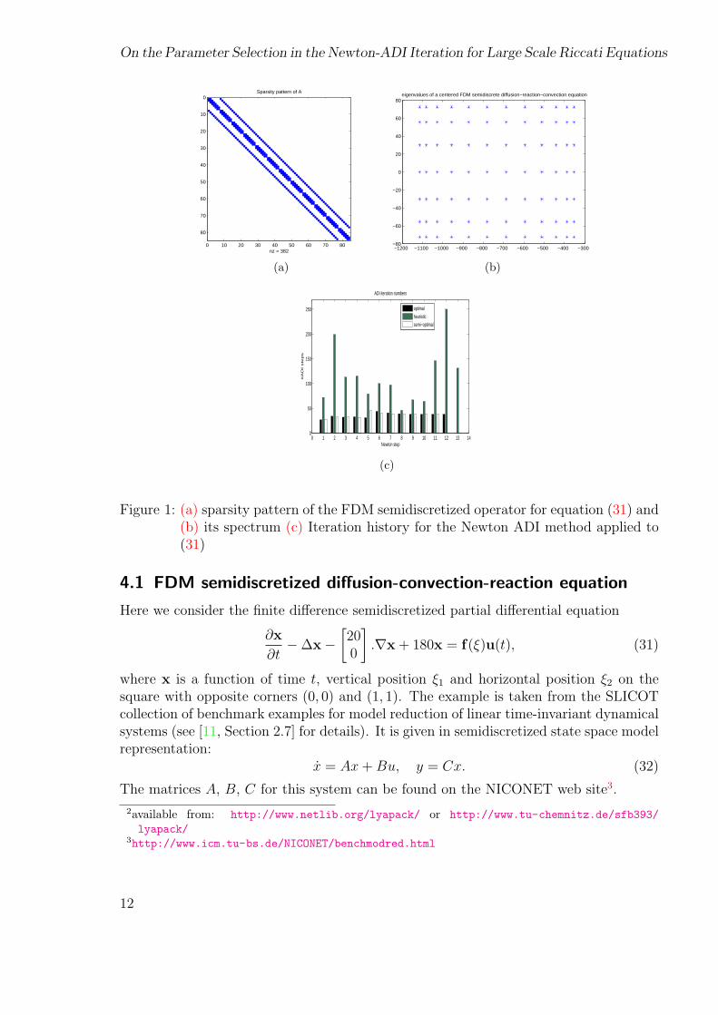
On the Parameter Selection in the Newton-ADI Iteration for Large Scale Riccati Equations
0 10 20 30 40 50 60 70 80
0
10
20
30
40
50
60
70
80
nz = 382
Sparsity pattern of A
(a)
minus1200 minus1100 minus1000 minus900 minus800 minus700 minus600 minus500 minus400 minus300minus80
minus60
minus40
minus20
0
20
40
60
80eigenvalues of a centered FDM semidiscrete diffusionminusreactionminusconvection equation
(b)
0 1 2 3 4 5 6 7 8 9 10 11 12 13 140
50
100
150
200
250
ADI iteration numbers
Newton step
A
DI
ste
ps
optimal
heuristic
semiminusoptimal
(c)
Figure 1 (a) sparsity pattern of the FDM semidiscretized operator for equation (31) and(b) its spectrum (c) Iteration history for the Newton ADI method applied to(31)
41 FDM semidiscretized diffusion-convection-reaction equation
Here we consider the finite difference semidiscretized partial differential equation
partx
parttminus∆xminus
[200
]nablax + 180x = f(ξ)u(t) (31)
where x is a function of time t vertical position ξ1 and horizontal position ξ2 on thesquare with opposite corners (0 0) and (1 1) The example is taken from the SLICOTcollection of benchmark examples for model reduction of linear time-invariant dynamicalsystems (see [11 Section 27] for details) It is given in semidiscretized state space modelrepresentation
x = Ax+Bu y = Cx (32)
The matrices A B C for this system can be found on the NICONET web site3
2available from httpwwwnetliborglyapack or httpwwwtu-chemnitzdesfb393lyapack
3httpwwwicmtu-bsdeNICONETbenchmodredhtml
12
Peter Benner Hermann Mena and Jens Saak
0 50 100 150 200 250 300 350 400
0
50
100
150
200
250
300
350
400
nz = 1920
Sparsity pattern of A
(a)
0 1 2 3 4 5 6 7 8 90
5
10
15
20
25
30
35
40
45
50
Newton step
AD
I ste
ps
ADI iteration numbers
optimal
heuristic
semiminusoptimal
(b)
Figure 2 (a) sparsity pattern of the FDM semidiscretized operator for equation (33) and(b) Iteration history for the Newton ADI
Figure 1 (a)(b) show the spectrum and sparsity pattern of the system matrix A Theiteration history ie the numbers of ADI steps in each step of Newtonrsquos method areplotted in Figure 1 (c) There we can see that in fact the semi-optimal parameters workexactly like the optimal ones by the Wachspress approach This is what we would expectsince the rectangular spectrum is an optimal case for our idea because the parameters ab and α are exactly (to the accuracy of Arnoldirsquos method) met here Note especially thatfor the heuristic parameters even more outer Newton iterations than for our parametersare required
42 FDM semidiscretized heat equation
In this example we tested the parameters for the finite difference semidiscretized heatequation on the unit square (0 1)times (0 1)
partx
parttminus∆x = f(ξ)u(t) (33)
The data is generated by the routines fdm 2d matrix and fdm 2d vector from the ex-amples of the LyaPack package Details on the generation of test problems can be foundin the documentation of these routines (comments and Matlab help) Since the differ-ential operator is symmetric here the matrix A is symmetric and its spectrum is realin this case Hence α = 0 and for the Wachspress parameters only the largest magni-tude and smallest magnitude eigenvalues have to be found to determine a and b Thatmeans we only need to compute two Ritz values by the Arnoldi (which here is in fact aLanczos process because of symmetry) process compared to about 30 (which seems tobe an adequate number of shifts) for the heuristic approach We used a test examplewith 400 unknowns here to still be able to compute the complete spectrum using eig
for comparison
13
On the Parameter Selection in the Newton-ADI Iteration for Large Scale Riccati Equations
(a)
minus3500 minus3000 minus2500 minus2000 minus1500 minus1000 minus500 0minus25
minus20
minus15
minus10
minus5
0
5
10
15
20
25
eigenvalues of MA
Penzl shifts
Wachspress shifts
(b)
Figure 3 (a) A 2d cross-section of the liquid flow in a round tube (b) Eigenvalue andshift parameter distributions
In Figure 2 we plotted the sparsity pattern of A and the iteration history for thesolution of the corresponding ARE We can see (Figure 2 (b)) that iteration numbersonly differ very slightly Hence we can choose quite independently which parametersto use Since the Wachspress approach needs a good approximation of the smallestmagnitude eigenvalue it might be a good idea to choose the heuristic parameters here(even though they are much more expensive to compute) if the smallest magnitudeeigenvalue is known to be close to the origin (eg in case of finite element discretizationswith fine meshes)
43 FEM semidiscretized convection-diffusion equation
The last example is a system appearing in the optimal heatingcooling of a fluid flowin a tube An application is the temperature regulation of certain reagent inflows in
14
Peter Benner Hermann Mena and Jens Saak
0 200 400 600 800 1000
0
100
200
300
400
500
600
700
800
900
1000
nz = 7378
Sparsity pattern of A and M
(a)
0 200 400 600 800 1000
0
100
200
300
400
500
600
700
800
900
1000
nz = 7378
Sparsity pattern of A and M after reordering
(b)
0 200 400 600 800 1000
0
100
200
300
400
500
600
700
800
900
1000
nz = 22846
(c)
1 2 3 4 5 60
10
20
30
40
50
60
70
80
Newton step
AD
I ste
ps
ADI Iteration history
optimalheuristicsemiminusoptimal
(d)
Figure 4 (a) sparsity pattern of A and M in (35) (b) sparsity pattern of A and Min (35) after reordering for bandwidth reduction (c) sparsity pattern of theCholesky factor of reordered M and (d) Iteration history for the Newton ADI
chemical reactors The model equations are
partxparttminus α∆x + v middot nablax = 0 in Ω
x = x0 on Γin
partxpartn
= σ(uminus x) on Γheat1 cup Γheat2
partxpartn
= 0 on Γout
(34)
Here Ω is the rectangular domain shown in Figure 3 (a) The inflow Γin is at the leftpart of the boundary and the outflow Γout the right one The control is applied viathe upper and lower boundaries We can restrict ourselves to this 2d-domain assumingrotational symmetry ie non-turbulent diffusion dominated flows The test matriceshave been created using the COMSOL Multiphysics software and α = 006 resulting inthe Eigenvalue and shift distributions shown in Figure 3 (b)
Since a finite element discretization in space has been applied here the semidiscrete
15
On the Parameter Selection in the Newton-ADI Iteration for Large Scale Riccati Equations
model is of the formMx = Ax+ Bu
y = Cx(35)
This is transformed into a standard system (32) by decomposing M into M = MLMU
where ML = MTU since M is symmetric Then defining x = MUx A = Mminus1
L AMminus1U
B = Mminus1L and C = CMminus1
U (without computing any of the inverses explicitly in thecode) we end up with a standard system for x having the same inputs u as (35)
Note that the heuristic parameters do not appear in the results bar graphics hereThis is due to the fact that the LyaPacksoftware crashed while applying the complex shiftcomputed by the heuristics Numerical tests where only the real ones of the heuristicparameters where used lead to very poor convergence in the inner loop which is generallystopped by the maximum iteration number stopping criterion This resulted in breakingthe convergence in the outer Newton loop
5 Conclusions
In this paper we have reviewed existing methods for determining sets of ADI parametersand based on this review we suggest a new procedure which combines the best featuresof two of those For the real case the parameters computed by the new method areoptimal and in general their performance is quite satisfactory as one can see in thenumerical examples The computational cost depends only on the computation of anArnoldi process for the matrix involved and on the computation of elliptic integralsSince the latter is a quadratically converging scalar iteration the Arnoldi process isthe dominant computation here which makes this method suitable for the large scalesystems arising from finite element discretization of PDEs The main advantages of thenew method are that it is cheaper to compute than the existing ones and that it avoidscomplex computations in the ADI iteration for many cases where the others would resultin complex iterations
Acknowledgements
This work was supported by the DFG project rdquoNumerische Losung von Optimals-teuerungsproblemen fur instationare Diffusions-Konvektions- und Diffusions-Reaktions-gleichungenrdquo grant BE37151-1 and DAAD program rdquoAcciones Integradas Hispano-Alemanasrdquo grant D0525675
16
Peter Benner Hermann Mena and Jens Saak
References
[1] M Abramovitz and I Stegun eds Pocketbook of mathematical functionsVerlag Harry Deutsch 1984 Abridged edition of rdquoHandbook of mathematical func-tionsrdquo (1964)
[2] T Bagby On interpolation by rational functions Duke Math J 36 (1969)pp 95ndash104
[3] H Banks and K Kunisch The linear regulator problem for parabolic systemsSIAM J Cont Optim 22 (1984) pp 684ndash698
[4] P Benner Computational methods for linear-quadratic optimization Supple-mento ai Rendiconti del Circolo Matematico di Palermo Serie II No 58 (1999)pp 21ndash56
[5] P Benner S Gorner and J Saak Numerical solution of optimal con-trol problems for parabolicsystems in Parallel Algorithms and Cluster ComputingImplementationsAlgorithms and Applications K Hoffmann and A Meyer edsvol 52 of Lecture Notes in Computational Science and Engineering Springer-VerlagBerlinHeidelberg Germany 2006
[6] P Benner J-R Li and T Penzl Numerical solution of large Lyapunovequations Riccati equations and linear-quadratic control problems tech rep
[7] P Benner and H Mena BDF methods for large-scale differential Riccati equa-tions in Proc of Mathematical Theory of Network and Systems MTNS 2004 B DMoor B Motmans J Willems P V Dooren and V Blondel eds 2004
[8] P Benner and J Saak Linear-quadratic regulator design for optimal coolingof steel profiles Tech Rep SFB39305-05 Sonderforschungsbereich 393 ParalleleNumerische Simulation fur Physik und Kontinuumsmechanik TU Chemnitz D-09107 Chemnitz (Germany) 2005 Available from httpwwwtu-chemnitzde
sfb393sfb05prhtml
[9] A Bensoussan G D Prato M Delfour and S Mitter Representa-tion and Control of Infinite Dimensional Systems Volume I Systems amp ControlFoundations amp Applications Birkauser Boston Basel Berlin 1992
[10] Representation and Control of Infinite Dimensional Systems Volume II Sys-tems amp Control Foundations amp Applications Birkauser Boston Basel Berlin1992
[11] Y Chahlaoui and P Van Dooren A collection of benchmark examples formodel reduction of linear time invariant dynamical systems SLICOT Working Note2002ndash2 Feb 2002 Available from httpwwwicmtu-bsdeNICONETreports
html
17
On the Parameter Selection in the Newton-ADI Iteration for Large Scale Riccati Equations
[12] C Choi and A Laub Efficient matrix-valued algorithms for solving stiff Riccatidifferential equations IEEE Trans Automat Control 35 (1990) pp 770ndash776
[13] R Curtain and T Pritchard Infinite Dimensional Linear System Theoryvol 8 of Lecture Notes in Control and Information Sciences Springer-Verlag NewYork 1978
[14] R Curtain and H Zwart An Introduction to Infinite-Dimensional Linear Sys-tems Theory vol 21 of Texts in Applied Mathematics Springer-Verlag New York1995
[15] B Datta Numerical Methods for Linear Control Systems Elsevier AcademicPress 2004
[16] L Dieci Numerical integration of the differential Riccati equation and some relatedissues SIAM J Numer Anal 29 (1992) pp 781ndash815
[17] J S Gibson The Riccati integral equation for optimal control problems in Hilbertspaces SIAM J Cont Optim 17 (1979) pp 537ndash565
[18] A A Gonchar Zolotarev problems connected with rational functions MathUSSR Sbornik 7 (1969) pp 623ndash635
[19] M P Istace and J P Thiran On the third and fourth Zoltarev problems incomplex plane Math Comp (1993)
[20] K Ito Finite-dimensional compensators for infinite-dimensional systems viagalerkin-type approximation SIAContOpt 28 (1990) pp 1251ndash1269
[21] K Ito and K Kunisch Receding horizon optimal control for infinite dimensionalsystems ESAIM Control Optim Calc Var 8 (2002) pp 741ndash760
[22] Receding horizon control with incomplete observations SIAM J Control Op-tim 45 (2006) pp 207ndash225
[23] P Lancaster and L Rodman The Algebraic Riccati Equation Oxford Univer-sity Press Oxford 1995
[24] I Lasiecka and R Triggiani Differential and Algebraic Riccati Equations withApplication to BoundaryPoint Control Problems Continuous Theory and Approx-imation Theory no 164 in Lecture Notes in Control and Information SciencesSpringer-Verlag Berlin 1991
[25] Control Theory for Partial Differential Equations Continuous and Approxi-mation Theories I Abstract Parabolic Systems Cambridge University Press Cam-bridge UK 2000
[26] V I Lebedev On a Zolotarev problem in the method of alternating directionsUSSR Comput Math and Math Phys 17 (1977) pp 58ndash76
18
Peter Benner Hermann Mena and Jens Saak
[27] J Lions Optimal Control of Systems Governed by Partial Differential EquationsSpringer-Verlag Berlin FRG 1971
[28] A Lu and E Wachspress Solution of Lyapunov equations by alternating direc-tion implicit iteration Comput Math Appl 21 (1991) pp 43ndash58
[29] V Mehrmann The Autonomous Linear Quadratic Control Problem Theory andNumerical Solution no 163 in Lecture Notes in Control and Information SciencesSpringer-Verlag Heidelberg July 1991
[30] K Morris Convergence of controllers designed using state-space methods IEEETrans Automat Control 39 (1994) pp 2100ndash2104
[31] Design of finite-dimensional controllers for infinite-dimensional systems byapproximation J Math Systems Estim and Control 4 (1994) pp 1ndash30
[32] T Penzl A cyclic low rank Smith method for large sparse Lyapunov equationsSIAM J Sci Comput 21 (2000) pp 1401ndash1418
[33] Lyapack Users Guide Tech Rep SFB39300-33 Sonderforschungsbereich393 Numerische Simulation auf massiv parallelen Rechnern TU Chemnitz 09107Chemnitz Germany 2000 Available from httpwwwtu-chemnitzdesfb393
sfb00prhtml
[34] P Petkov N Christov and M Konstantinov Computational Methods forLinear Control Systems Prentice-Hall Hertfordshire UK 1991
[35] A Pritchard and D Salamon The linear quadratic control problem for infinitedimensional systems with unbounded input and output operators SIAM J ControlOptimization 25 (1987) pp 121ndash144
[36] V Sima Algorithms for Linear-Quadratic Optimization vol 200 of Pure and Ap-plied Mathematics Marcel Dekker Inc New York NY 1996
[37] E D Sontag Mathematical control theory Deterministic finite dimensional sys-tems no 6 in Texts in Applied Mathematics Springer-Verlag New York NY2nd ed 1998
[38] G Starke Rationale Minimierungsprobleme in der komplexen Ebene im Zusam-menhang mit der Bestimmung optimaler ADI-Parameter PhD thesis Fakultat furMathematik Universitat Karlsruhe December 1989
[39] Optimal alternating directions implicit parameters for nonsymmetric systemsof linear equations SIAM J Numer Anal 28 (1991) pp 1431ndash1445
[40] U Storch and H Wiebe Textbook of mathematics Vol 1 Analysis of one vari-able (Lehrbuch der Mathematik Band 1 Analysis einer Veranderlichen) Spek-trum Akademischer Verlag Heidelberg 3 ed 2003 (German)
19
On the Parameter Selection in the Newton-ADI Iteration for Large Scale Riccati Equations
[41] J Todd Applications of transformation theory A legacy from Zolotarev (1847-1878) in Approximation Theory and Spline Functions S P S et al ed no C 136in NATO ASI Ser Dordrecht-Boston-Lancaster 1984 D Reidel Publishing Copp 207ndash245 Proc NATO Adv Study Inst St JohnrsquosNewfoundland 1983
[42] E Wachspress Iterative solution of the Lyapunov matrix equation Appl MathLetters 107 (1988) pp 87ndash90
[43] The ADI model problem 1995 Available from the author
[44] J Zabczyk Remarks on the algebraic Riccati equation Appl Math Optim 2(1976) pp 251ndash258
20
Chemnitz Scientific Computing Preprints ndash ISSN 1864-0087
- Introduction
-
- Problem background
- Newton-ADI iteration
-
- Review of existing parameter selection methods
-
- Leja Points
- Optimal parameters
- Heuristic parameters
- Discussion
-
- Suboptimal parameter computation
- Numerical results
-
- FDM semidiscretized diffusion-convection-reaction equation
- FDM semidiscretized heat equation
- FEM semidiscretized convection-diffusion equation
-
- Conclusions
-

Peter Benner Hermann Mena and Jens Saak
0 50 100 150 200 250 300 350 400
0
50
100
150
200
250
300
350
400
nz = 1920
Sparsity pattern of A
(a)
0 1 2 3 4 5 6 7 8 90
5
10
15
20
25
30
35
40
45
50
Newton step
AD
I ste
ps
ADI iteration numbers
optimal
heuristic
semiminusoptimal
(b)
Figure 2 (a) sparsity pattern of the FDM semidiscretized operator for equation (33) and(b) Iteration history for the Newton ADI
Figure 1 (a)(b) show the spectrum and sparsity pattern of the system matrix A Theiteration history ie the numbers of ADI steps in each step of Newtonrsquos method areplotted in Figure 1 (c) There we can see that in fact the semi-optimal parameters workexactly like the optimal ones by the Wachspress approach This is what we would expectsince the rectangular spectrum is an optimal case for our idea because the parameters ab and α are exactly (to the accuracy of Arnoldirsquos method) met here Note especially thatfor the heuristic parameters even more outer Newton iterations than for our parametersare required
42 FDM semidiscretized heat equation
In this example we tested the parameters for the finite difference semidiscretized heatequation on the unit square (0 1)times (0 1)
partx
parttminus∆x = f(ξ)u(t) (33)
The data is generated by the routines fdm 2d matrix and fdm 2d vector from the ex-amples of the LyaPack package Details on the generation of test problems can be foundin the documentation of these routines (comments and Matlab help) Since the differ-ential operator is symmetric here the matrix A is symmetric and its spectrum is realin this case Hence α = 0 and for the Wachspress parameters only the largest magni-tude and smallest magnitude eigenvalues have to be found to determine a and b Thatmeans we only need to compute two Ritz values by the Arnoldi (which here is in fact aLanczos process because of symmetry) process compared to about 30 (which seems tobe an adequate number of shifts) for the heuristic approach We used a test examplewith 400 unknowns here to still be able to compute the complete spectrum using eig
for comparison
13
On the Parameter Selection in the Newton-ADI Iteration for Large Scale Riccati Equations
(a)
minus3500 minus3000 minus2500 minus2000 minus1500 minus1000 minus500 0minus25
minus20
minus15
minus10
minus5
0
5
10
15
20
25
eigenvalues of MA
Penzl shifts
Wachspress shifts
(b)
Figure 3 (a) A 2d cross-section of the liquid flow in a round tube (b) Eigenvalue andshift parameter distributions
In Figure 2 we plotted the sparsity pattern of A and the iteration history for thesolution of the corresponding ARE We can see (Figure 2 (b)) that iteration numbersonly differ very slightly Hence we can choose quite independently which parametersto use Since the Wachspress approach needs a good approximation of the smallestmagnitude eigenvalue it might be a good idea to choose the heuristic parameters here(even though they are much more expensive to compute) if the smallest magnitudeeigenvalue is known to be close to the origin (eg in case of finite element discretizationswith fine meshes)
43 FEM semidiscretized convection-diffusion equation
The last example is a system appearing in the optimal heatingcooling of a fluid flowin a tube An application is the temperature regulation of certain reagent inflows in
14
Peter Benner Hermann Mena and Jens Saak
0 200 400 600 800 1000
0
100
200
300
400
500
600
700
800
900
1000
nz = 7378
Sparsity pattern of A and M
(a)
0 200 400 600 800 1000
0
100
200
300
400
500
600
700
800
900
1000
nz = 7378
Sparsity pattern of A and M after reordering
(b)
0 200 400 600 800 1000
0
100
200
300
400
500
600
700
800
900
1000
nz = 22846
(c)
1 2 3 4 5 60
10
20
30
40
50
60
70
80
Newton step
AD
I ste
ps
ADI Iteration history
optimalheuristicsemiminusoptimal
(d)
Figure 4 (a) sparsity pattern of A and M in (35) (b) sparsity pattern of A and Min (35) after reordering for bandwidth reduction (c) sparsity pattern of theCholesky factor of reordered M and (d) Iteration history for the Newton ADI
chemical reactors The model equations are
partxparttminus α∆x + v middot nablax = 0 in Ω
x = x0 on Γin
partxpartn
= σ(uminus x) on Γheat1 cup Γheat2
partxpartn
= 0 on Γout
(34)
Here Ω is the rectangular domain shown in Figure 3 (a) The inflow Γin is at the leftpart of the boundary and the outflow Γout the right one The control is applied viathe upper and lower boundaries We can restrict ourselves to this 2d-domain assumingrotational symmetry ie non-turbulent diffusion dominated flows The test matriceshave been created using the COMSOL Multiphysics software and α = 006 resulting inthe Eigenvalue and shift distributions shown in Figure 3 (b)
Since a finite element discretization in space has been applied here the semidiscrete
15
On the Parameter Selection in the Newton-ADI Iteration for Large Scale Riccati Equations
model is of the formMx = Ax+ Bu
y = Cx(35)
This is transformed into a standard system (32) by decomposing M into M = MLMU
where ML = MTU since M is symmetric Then defining x = MUx A = Mminus1
L AMminus1U
B = Mminus1L and C = CMminus1
U (without computing any of the inverses explicitly in thecode) we end up with a standard system for x having the same inputs u as (35)
Note that the heuristic parameters do not appear in the results bar graphics hereThis is due to the fact that the LyaPacksoftware crashed while applying the complex shiftcomputed by the heuristics Numerical tests where only the real ones of the heuristicparameters where used lead to very poor convergence in the inner loop which is generallystopped by the maximum iteration number stopping criterion This resulted in breakingthe convergence in the outer Newton loop
5 Conclusions
In this paper we have reviewed existing methods for determining sets of ADI parametersand based on this review we suggest a new procedure which combines the best featuresof two of those For the real case the parameters computed by the new method areoptimal and in general their performance is quite satisfactory as one can see in thenumerical examples The computational cost depends only on the computation of anArnoldi process for the matrix involved and on the computation of elliptic integralsSince the latter is a quadratically converging scalar iteration the Arnoldi process isthe dominant computation here which makes this method suitable for the large scalesystems arising from finite element discretization of PDEs The main advantages of thenew method are that it is cheaper to compute than the existing ones and that it avoidscomplex computations in the ADI iteration for many cases where the others would resultin complex iterations
Acknowledgements
This work was supported by the DFG project rdquoNumerische Losung von Optimals-teuerungsproblemen fur instationare Diffusions-Konvektions- und Diffusions-Reaktions-gleichungenrdquo grant BE37151-1 and DAAD program rdquoAcciones Integradas Hispano-Alemanasrdquo grant D0525675
16
Peter Benner Hermann Mena and Jens Saak
References
[1] M Abramovitz and I Stegun eds Pocketbook of mathematical functionsVerlag Harry Deutsch 1984 Abridged edition of rdquoHandbook of mathematical func-tionsrdquo (1964)
[2] T Bagby On interpolation by rational functions Duke Math J 36 (1969)pp 95ndash104
[3] H Banks and K Kunisch The linear regulator problem for parabolic systemsSIAM J Cont Optim 22 (1984) pp 684ndash698
[4] P Benner Computational methods for linear-quadratic optimization Supple-mento ai Rendiconti del Circolo Matematico di Palermo Serie II No 58 (1999)pp 21ndash56
[5] P Benner S Gorner and J Saak Numerical solution of optimal con-trol problems for parabolicsystems in Parallel Algorithms and Cluster ComputingImplementationsAlgorithms and Applications K Hoffmann and A Meyer edsvol 52 of Lecture Notes in Computational Science and Engineering Springer-VerlagBerlinHeidelberg Germany 2006
[6] P Benner J-R Li and T Penzl Numerical solution of large Lyapunovequations Riccati equations and linear-quadratic control problems tech rep
[7] P Benner and H Mena BDF methods for large-scale differential Riccati equa-tions in Proc of Mathematical Theory of Network and Systems MTNS 2004 B DMoor B Motmans J Willems P V Dooren and V Blondel eds 2004
[8] P Benner and J Saak Linear-quadratic regulator design for optimal coolingof steel profiles Tech Rep SFB39305-05 Sonderforschungsbereich 393 ParalleleNumerische Simulation fur Physik und Kontinuumsmechanik TU Chemnitz D-09107 Chemnitz (Germany) 2005 Available from httpwwwtu-chemnitzde
sfb393sfb05prhtml
[9] A Bensoussan G D Prato M Delfour and S Mitter Representa-tion and Control of Infinite Dimensional Systems Volume I Systems amp ControlFoundations amp Applications Birkauser Boston Basel Berlin 1992
[10] Representation and Control of Infinite Dimensional Systems Volume II Sys-tems amp Control Foundations amp Applications Birkauser Boston Basel Berlin1992
[11] Y Chahlaoui and P Van Dooren A collection of benchmark examples formodel reduction of linear time invariant dynamical systems SLICOT Working Note2002ndash2 Feb 2002 Available from httpwwwicmtu-bsdeNICONETreports
html
17
On the Parameter Selection in the Newton-ADI Iteration for Large Scale Riccati Equations
[12] C Choi and A Laub Efficient matrix-valued algorithms for solving stiff Riccatidifferential equations IEEE Trans Automat Control 35 (1990) pp 770ndash776
[13] R Curtain and T Pritchard Infinite Dimensional Linear System Theoryvol 8 of Lecture Notes in Control and Information Sciences Springer-Verlag NewYork 1978
[14] R Curtain and H Zwart An Introduction to Infinite-Dimensional Linear Sys-tems Theory vol 21 of Texts in Applied Mathematics Springer-Verlag New York1995
[15] B Datta Numerical Methods for Linear Control Systems Elsevier AcademicPress 2004
[16] L Dieci Numerical integration of the differential Riccati equation and some relatedissues SIAM J Numer Anal 29 (1992) pp 781ndash815
[17] J S Gibson The Riccati integral equation for optimal control problems in Hilbertspaces SIAM J Cont Optim 17 (1979) pp 537ndash565
[18] A A Gonchar Zolotarev problems connected with rational functions MathUSSR Sbornik 7 (1969) pp 623ndash635
[19] M P Istace and J P Thiran On the third and fourth Zoltarev problems incomplex plane Math Comp (1993)
[20] K Ito Finite-dimensional compensators for infinite-dimensional systems viagalerkin-type approximation SIAContOpt 28 (1990) pp 1251ndash1269
[21] K Ito and K Kunisch Receding horizon optimal control for infinite dimensionalsystems ESAIM Control Optim Calc Var 8 (2002) pp 741ndash760
[22] Receding horizon control with incomplete observations SIAM J Control Op-tim 45 (2006) pp 207ndash225
[23] P Lancaster and L Rodman The Algebraic Riccati Equation Oxford Univer-sity Press Oxford 1995
[24] I Lasiecka and R Triggiani Differential and Algebraic Riccati Equations withApplication to BoundaryPoint Control Problems Continuous Theory and Approx-imation Theory no 164 in Lecture Notes in Control and Information SciencesSpringer-Verlag Berlin 1991
[25] Control Theory for Partial Differential Equations Continuous and Approxi-mation Theories I Abstract Parabolic Systems Cambridge University Press Cam-bridge UK 2000
[26] V I Lebedev On a Zolotarev problem in the method of alternating directionsUSSR Comput Math and Math Phys 17 (1977) pp 58ndash76
18
Peter Benner Hermann Mena and Jens Saak
[27] J Lions Optimal Control of Systems Governed by Partial Differential EquationsSpringer-Verlag Berlin FRG 1971
[28] A Lu and E Wachspress Solution of Lyapunov equations by alternating direc-tion implicit iteration Comput Math Appl 21 (1991) pp 43ndash58
[29] V Mehrmann The Autonomous Linear Quadratic Control Problem Theory andNumerical Solution no 163 in Lecture Notes in Control and Information SciencesSpringer-Verlag Heidelberg July 1991
[30] K Morris Convergence of controllers designed using state-space methods IEEETrans Automat Control 39 (1994) pp 2100ndash2104
[31] Design of finite-dimensional controllers for infinite-dimensional systems byapproximation J Math Systems Estim and Control 4 (1994) pp 1ndash30
[32] T Penzl A cyclic low rank Smith method for large sparse Lyapunov equationsSIAM J Sci Comput 21 (2000) pp 1401ndash1418
[33] Lyapack Users Guide Tech Rep SFB39300-33 Sonderforschungsbereich393 Numerische Simulation auf massiv parallelen Rechnern TU Chemnitz 09107Chemnitz Germany 2000 Available from httpwwwtu-chemnitzdesfb393
sfb00prhtml
[34] P Petkov N Christov and M Konstantinov Computational Methods forLinear Control Systems Prentice-Hall Hertfordshire UK 1991
[35] A Pritchard and D Salamon The linear quadratic control problem for infinitedimensional systems with unbounded input and output operators SIAM J ControlOptimization 25 (1987) pp 121ndash144
[36] V Sima Algorithms for Linear-Quadratic Optimization vol 200 of Pure and Ap-plied Mathematics Marcel Dekker Inc New York NY 1996
[37] E D Sontag Mathematical control theory Deterministic finite dimensional sys-tems no 6 in Texts in Applied Mathematics Springer-Verlag New York NY2nd ed 1998
[38] G Starke Rationale Minimierungsprobleme in der komplexen Ebene im Zusam-menhang mit der Bestimmung optimaler ADI-Parameter PhD thesis Fakultat furMathematik Universitat Karlsruhe December 1989
[39] Optimal alternating directions implicit parameters for nonsymmetric systemsof linear equations SIAM J Numer Anal 28 (1991) pp 1431ndash1445
[40] U Storch and H Wiebe Textbook of mathematics Vol 1 Analysis of one vari-able (Lehrbuch der Mathematik Band 1 Analysis einer Veranderlichen) Spek-trum Akademischer Verlag Heidelberg 3 ed 2003 (German)
19
On the Parameter Selection in the Newton-ADI Iteration for Large Scale Riccati Equations
[41] J Todd Applications of transformation theory A legacy from Zolotarev (1847-1878) in Approximation Theory and Spline Functions S P S et al ed no C 136in NATO ASI Ser Dordrecht-Boston-Lancaster 1984 D Reidel Publishing Copp 207ndash245 Proc NATO Adv Study Inst St JohnrsquosNewfoundland 1983
[42] E Wachspress Iterative solution of the Lyapunov matrix equation Appl MathLetters 107 (1988) pp 87ndash90
[43] The ADI model problem 1995 Available from the author
[44] J Zabczyk Remarks on the algebraic Riccati equation Appl Math Optim 2(1976) pp 251ndash258
20
Chemnitz Scientific Computing Preprints ndash ISSN 1864-0087
- Introduction
-
- Problem background
- Newton-ADI iteration
-
- Review of existing parameter selection methods
-
- Leja Points
- Optimal parameters
- Heuristic parameters
- Discussion
-
- Suboptimal parameter computation
- Numerical results
-
- FDM semidiscretized diffusion-convection-reaction equation
- FDM semidiscretized heat equation
- FEM semidiscretized convection-diffusion equation
-
- Conclusions
-
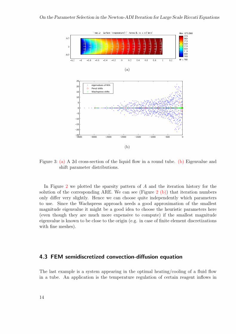
On the Parameter Selection in the Newton-ADI Iteration for Large Scale Riccati Equations
(a)
minus3500 minus3000 minus2500 minus2000 minus1500 minus1000 minus500 0minus25
minus20
minus15
minus10
minus5
0
5
10
15
20
25
eigenvalues of MA
Penzl shifts
Wachspress shifts
(b)
Figure 3 (a) A 2d cross-section of the liquid flow in a round tube (b) Eigenvalue andshift parameter distributions
In Figure 2 we plotted the sparsity pattern of A and the iteration history for thesolution of the corresponding ARE We can see (Figure 2 (b)) that iteration numbersonly differ very slightly Hence we can choose quite independently which parametersto use Since the Wachspress approach needs a good approximation of the smallestmagnitude eigenvalue it might be a good idea to choose the heuristic parameters here(even though they are much more expensive to compute) if the smallest magnitudeeigenvalue is known to be close to the origin (eg in case of finite element discretizationswith fine meshes)
43 FEM semidiscretized convection-diffusion equation
The last example is a system appearing in the optimal heatingcooling of a fluid flowin a tube An application is the temperature regulation of certain reagent inflows in
14
Peter Benner Hermann Mena and Jens Saak
0 200 400 600 800 1000
0
100
200
300
400
500
600
700
800
900
1000
nz = 7378
Sparsity pattern of A and M
(a)
0 200 400 600 800 1000
0
100
200
300
400
500
600
700
800
900
1000
nz = 7378
Sparsity pattern of A and M after reordering
(b)
0 200 400 600 800 1000
0
100
200
300
400
500
600
700
800
900
1000
nz = 22846
(c)
1 2 3 4 5 60
10
20
30
40
50
60
70
80
Newton step
AD
I ste
ps
ADI Iteration history
optimalheuristicsemiminusoptimal
(d)
Figure 4 (a) sparsity pattern of A and M in (35) (b) sparsity pattern of A and Min (35) after reordering for bandwidth reduction (c) sparsity pattern of theCholesky factor of reordered M and (d) Iteration history for the Newton ADI
chemical reactors The model equations are
partxparttminus α∆x + v middot nablax = 0 in Ω
x = x0 on Γin
partxpartn
= σ(uminus x) on Γheat1 cup Γheat2
partxpartn
= 0 on Γout
(34)
Here Ω is the rectangular domain shown in Figure 3 (a) The inflow Γin is at the leftpart of the boundary and the outflow Γout the right one The control is applied viathe upper and lower boundaries We can restrict ourselves to this 2d-domain assumingrotational symmetry ie non-turbulent diffusion dominated flows The test matriceshave been created using the COMSOL Multiphysics software and α = 006 resulting inthe Eigenvalue and shift distributions shown in Figure 3 (b)
Since a finite element discretization in space has been applied here the semidiscrete
15
On the Parameter Selection in the Newton-ADI Iteration for Large Scale Riccati Equations
model is of the formMx = Ax+ Bu
y = Cx(35)
This is transformed into a standard system (32) by decomposing M into M = MLMU
where ML = MTU since M is symmetric Then defining x = MUx A = Mminus1
L AMminus1U
B = Mminus1L and C = CMminus1
U (without computing any of the inverses explicitly in thecode) we end up with a standard system for x having the same inputs u as (35)
Note that the heuristic parameters do not appear in the results bar graphics hereThis is due to the fact that the LyaPacksoftware crashed while applying the complex shiftcomputed by the heuristics Numerical tests where only the real ones of the heuristicparameters where used lead to very poor convergence in the inner loop which is generallystopped by the maximum iteration number stopping criterion This resulted in breakingthe convergence in the outer Newton loop
5 Conclusions
In this paper we have reviewed existing methods for determining sets of ADI parametersand based on this review we suggest a new procedure which combines the best featuresof two of those For the real case the parameters computed by the new method areoptimal and in general their performance is quite satisfactory as one can see in thenumerical examples The computational cost depends only on the computation of anArnoldi process for the matrix involved and on the computation of elliptic integralsSince the latter is a quadratically converging scalar iteration the Arnoldi process isthe dominant computation here which makes this method suitable for the large scalesystems arising from finite element discretization of PDEs The main advantages of thenew method are that it is cheaper to compute than the existing ones and that it avoidscomplex computations in the ADI iteration for many cases where the others would resultin complex iterations
Acknowledgements
This work was supported by the DFG project rdquoNumerische Losung von Optimals-teuerungsproblemen fur instationare Diffusions-Konvektions- und Diffusions-Reaktions-gleichungenrdquo grant BE37151-1 and DAAD program rdquoAcciones Integradas Hispano-Alemanasrdquo grant D0525675
16
Peter Benner Hermann Mena and Jens Saak
References
[1] M Abramovitz and I Stegun eds Pocketbook of mathematical functionsVerlag Harry Deutsch 1984 Abridged edition of rdquoHandbook of mathematical func-tionsrdquo (1964)
[2] T Bagby On interpolation by rational functions Duke Math J 36 (1969)pp 95ndash104
[3] H Banks and K Kunisch The linear regulator problem for parabolic systemsSIAM J Cont Optim 22 (1984) pp 684ndash698
[4] P Benner Computational methods for linear-quadratic optimization Supple-mento ai Rendiconti del Circolo Matematico di Palermo Serie II No 58 (1999)pp 21ndash56
[5] P Benner S Gorner and J Saak Numerical solution of optimal con-trol problems for parabolicsystems in Parallel Algorithms and Cluster ComputingImplementationsAlgorithms and Applications K Hoffmann and A Meyer edsvol 52 of Lecture Notes in Computational Science and Engineering Springer-VerlagBerlinHeidelberg Germany 2006
[6] P Benner J-R Li and T Penzl Numerical solution of large Lyapunovequations Riccati equations and linear-quadratic control problems tech rep
[7] P Benner and H Mena BDF methods for large-scale differential Riccati equa-tions in Proc of Mathematical Theory of Network and Systems MTNS 2004 B DMoor B Motmans J Willems P V Dooren and V Blondel eds 2004
[8] P Benner and J Saak Linear-quadratic regulator design for optimal coolingof steel profiles Tech Rep SFB39305-05 Sonderforschungsbereich 393 ParalleleNumerische Simulation fur Physik und Kontinuumsmechanik TU Chemnitz D-09107 Chemnitz (Germany) 2005 Available from httpwwwtu-chemnitzde
sfb393sfb05prhtml
[9] A Bensoussan G D Prato M Delfour and S Mitter Representa-tion and Control of Infinite Dimensional Systems Volume I Systems amp ControlFoundations amp Applications Birkauser Boston Basel Berlin 1992
[10] Representation and Control of Infinite Dimensional Systems Volume II Sys-tems amp Control Foundations amp Applications Birkauser Boston Basel Berlin1992
[11] Y Chahlaoui and P Van Dooren A collection of benchmark examples formodel reduction of linear time invariant dynamical systems SLICOT Working Note2002ndash2 Feb 2002 Available from httpwwwicmtu-bsdeNICONETreports
html
17
On the Parameter Selection in the Newton-ADI Iteration for Large Scale Riccati Equations
[12] C Choi and A Laub Efficient matrix-valued algorithms for solving stiff Riccatidifferential equations IEEE Trans Automat Control 35 (1990) pp 770ndash776
[13] R Curtain and T Pritchard Infinite Dimensional Linear System Theoryvol 8 of Lecture Notes in Control and Information Sciences Springer-Verlag NewYork 1978
[14] R Curtain and H Zwart An Introduction to Infinite-Dimensional Linear Sys-tems Theory vol 21 of Texts in Applied Mathematics Springer-Verlag New York1995
[15] B Datta Numerical Methods for Linear Control Systems Elsevier AcademicPress 2004
[16] L Dieci Numerical integration of the differential Riccati equation and some relatedissues SIAM J Numer Anal 29 (1992) pp 781ndash815
[17] J S Gibson The Riccati integral equation for optimal control problems in Hilbertspaces SIAM J Cont Optim 17 (1979) pp 537ndash565
[18] A A Gonchar Zolotarev problems connected with rational functions MathUSSR Sbornik 7 (1969) pp 623ndash635
[19] M P Istace and J P Thiran On the third and fourth Zoltarev problems incomplex plane Math Comp (1993)
[20] K Ito Finite-dimensional compensators for infinite-dimensional systems viagalerkin-type approximation SIAContOpt 28 (1990) pp 1251ndash1269
[21] K Ito and K Kunisch Receding horizon optimal control for infinite dimensionalsystems ESAIM Control Optim Calc Var 8 (2002) pp 741ndash760
[22] Receding horizon control with incomplete observations SIAM J Control Op-tim 45 (2006) pp 207ndash225
[23] P Lancaster and L Rodman The Algebraic Riccati Equation Oxford Univer-sity Press Oxford 1995
[24] I Lasiecka and R Triggiani Differential and Algebraic Riccati Equations withApplication to BoundaryPoint Control Problems Continuous Theory and Approx-imation Theory no 164 in Lecture Notes in Control and Information SciencesSpringer-Verlag Berlin 1991
[25] Control Theory for Partial Differential Equations Continuous and Approxi-mation Theories I Abstract Parabolic Systems Cambridge University Press Cam-bridge UK 2000
[26] V I Lebedev On a Zolotarev problem in the method of alternating directionsUSSR Comput Math and Math Phys 17 (1977) pp 58ndash76
18
Peter Benner Hermann Mena and Jens Saak
[27] J Lions Optimal Control of Systems Governed by Partial Differential EquationsSpringer-Verlag Berlin FRG 1971
[28] A Lu and E Wachspress Solution of Lyapunov equations by alternating direc-tion implicit iteration Comput Math Appl 21 (1991) pp 43ndash58
[29] V Mehrmann The Autonomous Linear Quadratic Control Problem Theory andNumerical Solution no 163 in Lecture Notes in Control and Information SciencesSpringer-Verlag Heidelberg July 1991
[30] K Morris Convergence of controllers designed using state-space methods IEEETrans Automat Control 39 (1994) pp 2100ndash2104
[31] Design of finite-dimensional controllers for infinite-dimensional systems byapproximation J Math Systems Estim and Control 4 (1994) pp 1ndash30
[32] T Penzl A cyclic low rank Smith method for large sparse Lyapunov equationsSIAM J Sci Comput 21 (2000) pp 1401ndash1418
[33] Lyapack Users Guide Tech Rep SFB39300-33 Sonderforschungsbereich393 Numerische Simulation auf massiv parallelen Rechnern TU Chemnitz 09107Chemnitz Germany 2000 Available from httpwwwtu-chemnitzdesfb393
sfb00prhtml
[34] P Petkov N Christov and M Konstantinov Computational Methods forLinear Control Systems Prentice-Hall Hertfordshire UK 1991
[35] A Pritchard and D Salamon The linear quadratic control problem for infinitedimensional systems with unbounded input and output operators SIAM J ControlOptimization 25 (1987) pp 121ndash144
[36] V Sima Algorithms for Linear-Quadratic Optimization vol 200 of Pure and Ap-plied Mathematics Marcel Dekker Inc New York NY 1996
[37] E D Sontag Mathematical control theory Deterministic finite dimensional sys-tems no 6 in Texts in Applied Mathematics Springer-Verlag New York NY2nd ed 1998
[38] G Starke Rationale Minimierungsprobleme in der komplexen Ebene im Zusam-menhang mit der Bestimmung optimaler ADI-Parameter PhD thesis Fakultat furMathematik Universitat Karlsruhe December 1989
[39] Optimal alternating directions implicit parameters for nonsymmetric systemsof linear equations SIAM J Numer Anal 28 (1991) pp 1431ndash1445
[40] U Storch and H Wiebe Textbook of mathematics Vol 1 Analysis of one vari-able (Lehrbuch der Mathematik Band 1 Analysis einer Veranderlichen) Spek-trum Akademischer Verlag Heidelberg 3 ed 2003 (German)
19
On the Parameter Selection in the Newton-ADI Iteration for Large Scale Riccati Equations
[41] J Todd Applications of transformation theory A legacy from Zolotarev (1847-1878) in Approximation Theory and Spline Functions S P S et al ed no C 136in NATO ASI Ser Dordrecht-Boston-Lancaster 1984 D Reidel Publishing Copp 207ndash245 Proc NATO Adv Study Inst St JohnrsquosNewfoundland 1983
[42] E Wachspress Iterative solution of the Lyapunov matrix equation Appl MathLetters 107 (1988) pp 87ndash90
[43] The ADI model problem 1995 Available from the author
[44] J Zabczyk Remarks on the algebraic Riccati equation Appl Math Optim 2(1976) pp 251ndash258
20
Chemnitz Scientific Computing Preprints ndash ISSN 1864-0087
- Introduction
-
- Problem background
- Newton-ADI iteration
-
- Review of existing parameter selection methods
-
- Leja Points
- Optimal parameters
- Heuristic parameters
- Discussion
-
- Suboptimal parameter computation
- Numerical results
-
- FDM semidiscretized diffusion-convection-reaction equation
- FDM semidiscretized heat equation
- FEM semidiscretized convection-diffusion equation
-
- Conclusions
-

Peter Benner Hermann Mena and Jens Saak
0 200 400 600 800 1000
0
100
200
300
400
500
600
700
800
900
1000
nz = 7378
Sparsity pattern of A and M
(a)
0 200 400 600 800 1000
0
100
200
300
400
500
600
700
800
900
1000
nz = 7378
Sparsity pattern of A and M after reordering
(b)
0 200 400 600 800 1000
0
100
200
300
400
500
600
700
800
900
1000
nz = 22846
(c)
1 2 3 4 5 60
10
20
30
40
50
60
70
80
Newton step
AD
I ste
ps
ADI Iteration history
optimalheuristicsemiminusoptimal
(d)
Figure 4 (a) sparsity pattern of A and M in (35) (b) sparsity pattern of A and Min (35) after reordering for bandwidth reduction (c) sparsity pattern of theCholesky factor of reordered M and (d) Iteration history for the Newton ADI
chemical reactors The model equations are
partxparttminus α∆x + v middot nablax = 0 in Ω
x = x0 on Γin
partxpartn
= σ(uminus x) on Γheat1 cup Γheat2
partxpartn
= 0 on Γout
(34)
Here Ω is the rectangular domain shown in Figure 3 (a) The inflow Γin is at the leftpart of the boundary and the outflow Γout the right one The control is applied viathe upper and lower boundaries We can restrict ourselves to this 2d-domain assumingrotational symmetry ie non-turbulent diffusion dominated flows The test matriceshave been created using the COMSOL Multiphysics software and α = 006 resulting inthe Eigenvalue and shift distributions shown in Figure 3 (b)
Since a finite element discretization in space has been applied here the semidiscrete
15
On the Parameter Selection in the Newton-ADI Iteration for Large Scale Riccati Equations
model is of the formMx = Ax+ Bu
y = Cx(35)
This is transformed into a standard system (32) by decomposing M into M = MLMU
where ML = MTU since M is symmetric Then defining x = MUx A = Mminus1
L AMminus1U
B = Mminus1L and C = CMminus1
U (without computing any of the inverses explicitly in thecode) we end up with a standard system for x having the same inputs u as (35)
Note that the heuristic parameters do not appear in the results bar graphics hereThis is due to the fact that the LyaPacksoftware crashed while applying the complex shiftcomputed by the heuristics Numerical tests where only the real ones of the heuristicparameters where used lead to very poor convergence in the inner loop which is generallystopped by the maximum iteration number stopping criterion This resulted in breakingthe convergence in the outer Newton loop
5 Conclusions
In this paper we have reviewed existing methods for determining sets of ADI parametersand based on this review we suggest a new procedure which combines the best featuresof two of those For the real case the parameters computed by the new method areoptimal and in general their performance is quite satisfactory as one can see in thenumerical examples The computational cost depends only on the computation of anArnoldi process for the matrix involved and on the computation of elliptic integralsSince the latter is a quadratically converging scalar iteration the Arnoldi process isthe dominant computation here which makes this method suitable for the large scalesystems arising from finite element discretization of PDEs The main advantages of thenew method are that it is cheaper to compute than the existing ones and that it avoidscomplex computations in the ADI iteration for many cases where the others would resultin complex iterations
Acknowledgements
This work was supported by the DFG project rdquoNumerische Losung von Optimals-teuerungsproblemen fur instationare Diffusions-Konvektions- und Diffusions-Reaktions-gleichungenrdquo grant BE37151-1 and DAAD program rdquoAcciones Integradas Hispano-Alemanasrdquo grant D0525675
16
Peter Benner Hermann Mena and Jens Saak
References
[1] M Abramovitz and I Stegun eds Pocketbook of mathematical functionsVerlag Harry Deutsch 1984 Abridged edition of rdquoHandbook of mathematical func-tionsrdquo (1964)
[2] T Bagby On interpolation by rational functions Duke Math J 36 (1969)pp 95ndash104
[3] H Banks and K Kunisch The linear regulator problem for parabolic systemsSIAM J Cont Optim 22 (1984) pp 684ndash698
[4] P Benner Computational methods for linear-quadratic optimization Supple-mento ai Rendiconti del Circolo Matematico di Palermo Serie II No 58 (1999)pp 21ndash56
[5] P Benner S Gorner and J Saak Numerical solution of optimal con-trol problems for parabolicsystems in Parallel Algorithms and Cluster ComputingImplementationsAlgorithms and Applications K Hoffmann and A Meyer edsvol 52 of Lecture Notes in Computational Science and Engineering Springer-VerlagBerlinHeidelberg Germany 2006
[6] P Benner J-R Li and T Penzl Numerical solution of large Lyapunovequations Riccati equations and linear-quadratic control problems tech rep
[7] P Benner and H Mena BDF methods for large-scale differential Riccati equa-tions in Proc of Mathematical Theory of Network and Systems MTNS 2004 B DMoor B Motmans J Willems P V Dooren and V Blondel eds 2004
[8] P Benner and J Saak Linear-quadratic regulator design for optimal coolingof steel profiles Tech Rep SFB39305-05 Sonderforschungsbereich 393 ParalleleNumerische Simulation fur Physik und Kontinuumsmechanik TU Chemnitz D-09107 Chemnitz (Germany) 2005 Available from httpwwwtu-chemnitzde
sfb393sfb05prhtml
[9] A Bensoussan G D Prato M Delfour and S Mitter Representa-tion and Control of Infinite Dimensional Systems Volume I Systems amp ControlFoundations amp Applications Birkauser Boston Basel Berlin 1992
[10] Representation and Control of Infinite Dimensional Systems Volume II Sys-tems amp Control Foundations amp Applications Birkauser Boston Basel Berlin1992
[11] Y Chahlaoui and P Van Dooren A collection of benchmark examples formodel reduction of linear time invariant dynamical systems SLICOT Working Note2002ndash2 Feb 2002 Available from httpwwwicmtu-bsdeNICONETreports
html
17
On the Parameter Selection in the Newton-ADI Iteration for Large Scale Riccati Equations
[12] C Choi and A Laub Efficient matrix-valued algorithms for solving stiff Riccatidifferential equations IEEE Trans Automat Control 35 (1990) pp 770ndash776
[13] R Curtain and T Pritchard Infinite Dimensional Linear System Theoryvol 8 of Lecture Notes in Control and Information Sciences Springer-Verlag NewYork 1978
[14] R Curtain and H Zwart An Introduction to Infinite-Dimensional Linear Sys-tems Theory vol 21 of Texts in Applied Mathematics Springer-Verlag New York1995
[15] B Datta Numerical Methods for Linear Control Systems Elsevier AcademicPress 2004
[16] L Dieci Numerical integration of the differential Riccati equation and some relatedissues SIAM J Numer Anal 29 (1992) pp 781ndash815
[17] J S Gibson The Riccati integral equation for optimal control problems in Hilbertspaces SIAM J Cont Optim 17 (1979) pp 537ndash565
[18] A A Gonchar Zolotarev problems connected with rational functions MathUSSR Sbornik 7 (1969) pp 623ndash635
[19] M P Istace and J P Thiran On the third and fourth Zoltarev problems incomplex plane Math Comp (1993)
[20] K Ito Finite-dimensional compensators for infinite-dimensional systems viagalerkin-type approximation SIAContOpt 28 (1990) pp 1251ndash1269
[21] K Ito and K Kunisch Receding horizon optimal control for infinite dimensionalsystems ESAIM Control Optim Calc Var 8 (2002) pp 741ndash760
[22] Receding horizon control with incomplete observations SIAM J Control Op-tim 45 (2006) pp 207ndash225
[23] P Lancaster and L Rodman The Algebraic Riccati Equation Oxford Univer-sity Press Oxford 1995
[24] I Lasiecka and R Triggiani Differential and Algebraic Riccati Equations withApplication to BoundaryPoint Control Problems Continuous Theory and Approx-imation Theory no 164 in Lecture Notes in Control and Information SciencesSpringer-Verlag Berlin 1991
[25] Control Theory for Partial Differential Equations Continuous and Approxi-mation Theories I Abstract Parabolic Systems Cambridge University Press Cam-bridge UK 2000
[26] V I Lebedev On a Zolotarev problem in the method of alternating directionsUSSR Comput Math and Math Phys 17 (1977) pp 58ndash76
18
Peter Benner Hermann Mena and Jens Saak
[27] J Lions Optimal Control of Systems Governed by Partial Differential EquationsSpringer-Verlag Berlin FRG 1971
[28] A Lu and E Wachspress Solution of Lyapunov equations by alternating direc-tion implicit iteration Comput Math Appl 21 (1991) pp 43ndash58
[29] V Mehrmann The Autonomous Linear Quadratic Control Problem Theory andNumerical Solution no 163 in Lecture Notes in Control and Information SciencesSpringer-Verlag Heidelberg July 1991
[30] K Morris Convergence of controllers designed using state-space methods IEEETrans Automat Control 39 (1994) pp 2100ndash2104
[31] Design of finite-dimensional controllers for infinite-dimensional systems byapproximation J Math Systems Estim and Control 4 (1994) pp 1ndash30
[32] T Penzl A cyclic low rank Smith method for large sparse Lyapunov equationsSIAM J Sci Comput 21 (2000) pp 1401ndash1418
[33] Lyapack Users Guide Tech Rep SFB39300-33 Sonderforschungsbereich393 Numerische Simulation auf massiv parallelen Rechnern TU Chemnitz 09107Chemnitz Germany 2000 Available from httpwwwtu-chemnitzdesfb393
sfb00prhtml
[34] P Petkov N Christov and M Konstantinov Computational Methods forLinear Control Systems Prentice-Hall Hertfordshire UK 1991
[35] A Pritchard and D Salamon The linear quadratic control problem for infinitedimensional systems with unbounded input and output operators SIAM J ControlOptimization 25 (1987) pp 121ndash144
[36] V Sima Algorithms for Linear-Quadratic Optimization vol 200 of Pure and Ap-plied Mathematics Marcel Dekker Inc New York NY 1996
[37] E D Sontag Mathematical control theory Deterministic finite dimensional sys-tems no 6 in Texts in Applied Mathematics Springer-Verlag New York NY2nd ed 1998
[38] G Starke Rationale Minimierungsprobleme in der komplexen Ebene im Zusam-menhang mit der Bestimmung optimaler ADI-Parameter PhD thesis Fakultat furMathematik Universitat Karlsruhe December 1989
[39] Optimal alternating directions implicit parameters for nonsymmetric systemsof linear equations SIAM J Numer Anal 28 (1991) pp 1431ndash1445
[40] U Storch and H Wiebe Textbook of mathematics Vol 1 Analysis of one vari-able (Lehrbuch der Mathematik Band 1 Analysis einer Veranderlichen) Spek-trum Akademischer Verlag Heidelberg 3 ed 2003 (German)
19
On the Parameter Selection in the Newton-ADI Iteration for Large Scale Riccati Equations
[41] J Todd Applications of transformation theory A legacy from Zolotarev (1847-1878) in Approximation Theory and Spline Functions S P S et al ed no C 136in NATO ASI Ser Dordrecht-Boston-Lancaster 1984 D Reidel Publishing Copp 207ndash245 Proc NATO Adv Study Inst St JohnrsquosNewfoundland 1983
[42] E Wachspress Iterative solution of the Lyapunov matrix equation Appl MathLetters 107 (1988) pp 87ndash90
[43] The ADI model problem 1995 Available from the author
[44] J Zabczyk Remarks on the algebraic Riccati equation Appl Math Optim 2(1976) pp 251ndash258
20
Chemnitz Scientific Computing Preprints ndash ISSN 1864-0087
- Introduction
-
- Problem background
- Newton-ADI iteration
-
- Review of existing parameter selection methods
-
- Leja Points
- Optimal parameters
- Heuristic parameters
- Discussion
-
- Suboptimal parameter computation
- Numerical results
-
- FDM semidiscretized diffusion-convection-reaction equation
- FDM semidiscretized heat equation
- FEM semidiscretized convection-diffusion equation
-
- Conclusions
-

On the Parameter Selection in the Newton-ADI Iteration for Large Scale Riccati Equations
model is of the formMx = Ax+ Bu
y = Cx(35)
This is transformed into a standard system (32) by decomposing M into M = MLMU
where ML = MTU since M is symmetric Then defining x = MUx A = Mminus1
L AMminus1U
B = Mminus1L and C = CMminus1
U (without computing any of the inverses explicitly in thecode) we end up with a standard system for x having the same inputs u as (35)
Note that the heuristic parameters do not appear in the results bar graphics hereThis is due to the fact that the LyaPacksoftware crashed while applying the complex shiftcomputed by the heuristics Numerical tests where only the real ones of the heuristicparameters where used lead to very poor convergence in the inner loop which is generallystopped by the maximum iteration number stopping criterion This resulted in breakingthe convergence in the outer Newton loop
5 Conclusions
In this paper we have reviewed existing methods for determining sets of ADI parametersand based on this review we suggest a new procedure which combines the best featuresof two of those For the real case the parameters computed by the new method areoptimal and in general their performance is quite satisfactory as one can see in thenumerical examples The computational cost depends only on the computation of anArnoldi process for the matrix involved and on the computation of elliptic integralsSince the latter is a quadratically converging scalar iteration the Arnoldi process isthe dominant computation here which makes this method suitable for the large scalesystems arising from finite element discretization of PDEs The main advantages of thenew method are that it is cheaper to compute than the existing ones and that it avoidscomplex computations in the ADI iteration for many cases where the others would resultin complex iterations
Acknowledgements
This work was supported by the DFG project rdquoNumerische Losung von Optimals-teuerungsproblemen fur instationare Diffusions-Konvektions- und Diffusions-Reaktions-gleichungenrdquo grant BE37151-1 and DAAD program rdquoAcciones Integradas Hispano-Alemanasrdquo grant D0525675
16
Peter Benner Hermann Mena and Jens Saak
References
[1] M Abramovitz and I Stegun eds Pocketbook of mathematical functionsVerlag Harry Deutsch 1984 Abridged edition of rdquoHandbook of mathematical func-tionsrdquo (1964)
[2] T Bagby On interpolation by rational functions Duke Math J 36 (1969)pp 95ndash104
[3] H Banks and K Kunisch The linear regulator problem for parabolic systemsSIAM J Cont Optim 22 (1984) pp 684ndash698
[4] P Benner Computational methods for linear-quadratic optimization Supple-mento ai Rendiconti del Circolo Matematico di Palermo Serie II No 58 (1999)pp 21ndash56
[5] P Benner S Gorner and J Saak Numerical solution of optimal con-trol problems for parabolicsystems in Parallel Algorithms and Cluster ComputingImplementationsAlgorithms and Applications K Hoffmann and A Meyer edsvol 52 of Lecture Notes in Computational Science and Engineering Springer-VerlagBerlinHeidelberg Germany 2006
[6] P Benner J-R Li and T Penzl Numerical solution of large Lyapunovequations Riccati equations and linear-quadratic control problems tech rep
[7] P Benner and H Mena BDF methods for large-scale differential Riccati equa-tions in Proc of Mathematical Theory of Network and Systems MTNS 2004 B DMoor B Motmans J Willems P V Dooren and V Blondel eds 2004
[8] P Benner and J Saak Linear-quadratic regulator design for optimal coolingof steel profiles Tech Rep SFB39305-05 Sonderforschungsbereich 393 ParalleleNumerische Simulation fur Physik und Kontinuumsmechanik TU Chemnitz D-09107 Chemnitz (Germany) 2005 Available from httpwwwtu-chemnitzde
sfb393sfb05prhtml
[9] A Bensoussan G D Prato M Delfour and S Mitter Representa-tion and Control of Infinite Dimensional Systems Volume I Systems amp ControlFoundations amp Applications Birkauser Boston Basel Berlin 1992
[10] Representation and Control of Infinite Dimensional Systems Volume II Sys-tems amp Control Foundations amp Applications Birkauser Boston Basel Berlin1992
[11] Y Chahlaoui and P Van Dooren A collection of benchmark examples formodel reduction of linear time invariant dynamical systems SLICOT Working Note2002ndash2 Feb 2002 Available from httpwwwicmtu-bsdeNICONETreports
html
17
On the Parameter Selection in the Newton-ADI Iteration for Large Scale Riccati Equations
[12] C Choi and A Laub Efficient matrix-valued algorithms for solving stiff Riccatidifferential equations IEEE Trans Automat Control 35 (1990) pp 770ndash776
[13] R Curtain and T Pritchard Infinite Dimensional Linear System Theoryvol 8 of Lecture Notes in Control and Information Sciences Springer-Verlag NewYork 1978
[14] R Curtain and H Zwart An Introduction to Infinite-Dimensional Linear Sys-tems Theory vol 21 of Texts in Applied Mathematics Springer-Verlag New York1995
[15] B Datta Numerical Methods for Linear Control Systems Elsevier AcademicPress 2004
[16] L Dieci Numerical integration of the differential Riccati equation and some relatedissues SIAM J Numer Anal 29 (1992) pp 781ndash815
[17] J S Gibson The Riccati integral equation for optimal control problems in Hilbertspaces SIAM J Cont Optim 17 (1979) pp 537ndash565
[18] A A Gonchar Zolotarev problems connected with rational functions MathUSSR Sbornik 7 (1969) pp 623ndash635
[19] M P Istace and J P Thiran On the third and fourth Zoltarev problems incomplex plane Math Comp (1993)
[20] K Ito Finite-dimensional compensators for infinite-dimensional systems viagalerkin-type approximation SIAContOpt 28 (1990) pp 1251ndash1269
[21] K Ito and K Kunisch Receding horizon optimal control for infinite dimensionalsystems ESAIM Control Optim Calc Var 8 (2002) pp 741ndash760
[22] Receding horizon control with incomplete observations SIAM J Control Op-tim 45 (2006) pp 207ndash225
[23] P Lancaster and L Rodman The Algebraic Riccati Equation Oxford Univer-sity Press Oxford 1995
[24] I Lasiecka and R Triggiani Differential and Algebraic Riccati Equations withApplication to BoundaryPoint Control Problems Continuous Theory and Approx-imation Theory no 164 in Lecture Notes in Control and Information SciencesSpringer-Verlag Berlin 1991
[25] Control Theory for Partial Differential Equations Continuous and Approxi-mation Theories I Abstract Parabolic Systems Cambridge University Press Cam-bridge UK 2000
[26] V I Lebedev On a Zolotarev problem in the method of alternating directionsUSSR Comput Math and Math Phys 17 (1977) pp 58ndash76
18
Peter Benner Hermann Mena and Jens Saak
[27] J Lions Optimal Control of Systems Governed by Partial Differential EquationsSpringer-Verlag Berlin FRG 1971
[28] A Lu and E Wachspress Solution of Lyapunov equations by alternating direc-tion implicit iteration Comput Math Appl 21 (1991) pp 43ndash58
[29] V Mehrmann The Autonomous Linear Quadratic Control Problem Theory andNumerical Solution no 163 in Lecture Notes in Control and Information SciencesSpringer-Verlag Heidelberg July 1991
[30] K Morris Convergence of controllers designed using state-space methods IEEETrans Automat Control 39 (1994) pp 2100ndash2104
[31] Design of finite-dimensional controllers for infinite-dimensional systems byapproximation J Math Systems Estim and Control 4 (1994) pp 1ndash30
[32] T Penzl A cyclic low rank Smith method for large sparse Lyapunov equationsSIAM J Sci Comput 21 (2000) pp 1401ndash1418
[33] Lyapack Users Guide Tech Rep SFB39300-33 Sonderforschungsbereich393 Numerische Simulation auf massiv parallelen Rechnern TU Chemnitz 09107Chemnitz Germany 2000 Available from httpwwwtu-chemnitzdesfb393
sfb00prhtml
[34] P Petkov N Christov and M Konstantinov Computational Methods forLinear Control Systems Prentice-Hall Hertfordshire UK 1991
[35] A Pritchard and D Salamon The linear quadratic control problem for infinitedimensional systems with unbounded input and output operators SIAM J ControlOptimization 25 (1987) pp 121ndash144
[36] V Sima Algorithms for Linear-Quadratic Optimization vol 200 of Pure and Ap-plied Mathematics Marcel Dekker Inc New York NY 1996
[37] E D Sontag Mathematical control theory Deterministic finite dimensional sys-tems no 6 in Texts in Applied Mathematics Springer-Verlag New York NY2nd ed 1998
[38] G Starke Rationale Minimierungsprobleme in der komplexen Ebene im Zusam-menhang mit der Bestimmung optimaler ADI-Parameter PhD thesis Fakultat furMathematik Universitat Karlsruhe December 1989
[39] Optimal alternating directions implicit parameters for nonsymmetric systemsof linear equations SIAM J Numer Anal 28 (1991) pp 1431ndash1445
[40] U Storch and H Wiebe Textbook of mathematics Vol 1 Analysis of one vari-able (Lehrbuch der Mathematik Band 1 Analysis einer Veranderlichen) Spek-trum Akademischer Verlag Heidelberg 3 ed 2003 (German)
19
On the Parameter Selection in the Newton-ADI Iteration for Large Scale Riccati Equations
[41] J Todd Applications of transformation theory A legacy from Zolotarev (1847-1878) in Approximation Theory and Spline Functions S P S et al ed no C 136in NATO ASI Ser Dordrecht-Boston-Lancaster 1984 D Reidel Publishing Copp 207ndash245 Proc NATO Adv Study Inst St JohnrsquosNewfoundland 1983
[42] E Wachspress Iterative solution of the Lyapunov matrix equation Appl MathLetters 107 (1988) pp 87ndash90
[43] The ADI model problem 1995 Available from the author
[44] J Zabczyk Remarks on the algebraic Riccati equation Appl Math Optim 2(1976) pp 251ndash258
20
Chemnitz Scientific Computing Preprints ndash ISSN 1864-0087
- Introduction
-
- Problem background
- Newton-ADI iteration
-
- Review of existing parameter selection methods
-
- Leja Points
- Optimal parameters
- Heuristic parameters
- Discussion
-
- Suboptimal parameter computation
- Numerical results
-
- FDM semidiscretized diffusion-convection-reaction equation
- FDM semidiscretized heat equation
- FEM semidiscretized convection-diffusion equation
-
- Conclusions
-

Peter Benner Hermann Mena and Jens Saak
References
[1] M Abramovitz and I Stegun eds Pocketbook of mathematical functionsVerlag Harry Deutsch 1984 Abridged edition of rdquoHandbook of mathematical func-tionsrdquo (1964)
[2] T Bagby On interpolation by rational functions Duke Math J 36 (1969)pp 95ndash104
[3] H Banks and K Kunisch The linear regulator problem for parabolic systemsSIAM J Cont Optim 22 (1984) pp 684ndash698
[4] P Benner Computational methods for linear-quadratic optimization Supple-mento ai Rendiconti del Circolo Matematico di Palermo Serie II No 58 (1999)pp 21ndash56
[5] P Benner S Gorner and J Saak Numerical solution of optimal con-trol problems for parabolicsystems in Parallel Algorithms and Cluster ComputingImplementationsAlgorithms and Applications K Hoffmann and A Meyer edsvol 52 of Lecture Notes in Computational Science and Engineering Springer-VerlagBerlinHeidelberg Germany 2006
[6] P Benner J-R Li and T Penzl Numerical solution of large Lyapunovequations Riccati equations and linear-quadratic control problems tech rep
[7] P Benner and H Mena BDF methods for large-scale differential Riccati equa-tions in Proc of Mathematical Theory of Network and Systems MTNS 2004 B DMoor B Motmans J Willems P V Dooren and V Blondel eds 2004
[8] P Benner and J Saak Linear-quadratic regulator design for optimal coolingof steel profiles Tech Rep SFB39305-05 Sonderforschungsbereich 393 ParalleleNumerische Simulation fur Physik und Kontinuumsmechanik TU Chemnitz D-09107 Chemnitz (Germany) 2005 Available from httpwwwtu-chemnitzde
sfb393sfb05prhtml
[9] A Bensoussan G D Prato M Delfour and S Mitter Representa-tion and Control of Infinite Dimensional Systems Volume I Systems amp ControlFoundations amp Applications Birkauser Boston Basel Berlin 1992
[10] Representation and Control of Infinite Dimensional Systems Volume II Sys-tems amp Control Foundations amp Applications Birkauser Boston Basel Berlin1992
[11] Y Chahlaoui and P Van Dooren A collection of benchmark examples formodel reduction of linear time invariant dynamical systems SLICOT Working Note2002ndash2 Feb 2002 Available from httpwwwicmtu-bsdeNICONETreports
html
17
On the Parameter Selection in the Newton-ADI Iteration for Large Scale Riccati Equations
[12] C Choi and A Laub Efficient matrix-valued algorithms for solving stiff Riccatidifferential equations IEEE Trans Automat Control 35 (1990) pp 770ndash776
[13] R Curtain and T Pritchard Infinite Dimensional Linear System Theoryvol 8 of Lecture Notes in Control and Information Sciences Springer-Verlag NewYork 1978
[14] R Curtain and H Zwart An Introduction to Infinite-Dimensional Linear Sys-tems Theory vol 21 of Texts in Applied Mathematics Springer-Verlag New York1995
[15] B Datta Numerical Methods for Linear Control Systems Elsevier AcademicPress 2004
[16] L Dieci Numerical integration of the differential Riccati equation and some relatedissues SIAM J Numer Anal 29 (1992) pp 781ndash815
[17] J S Gibson The Riccati integral equation for optimal control problems in Hilbertspaces SIAM J Cont Optim 17 (1979) pp 537ndash565
[18] A A Gonchar Zolotarev problems connected with rational functions MathUSSR Sbornik 7 (1969) pp 623ndash635
[19] M P Istace and J P Thiran On the third and fourth Zoltarev problems incomplex plane Math Comp (1993)
[20] K Ito Finite-dimensional compensators for infinite-dimensional systems viagalerkin-type approximation SIAContOpt 28 (1990) pp 1251ndash1269
[21] K Ito and K Kunisch Receding horizon optimal control for infinite dimensionalsystems ESAIM Control Optim Calc Var 8 (2002) pp 741ndash760
[22] Receding horizon control with incomplete observations SIAM J Control Op-tim 45 (2006) pp 207ndash225
[23] P Lancaster and L Rodman The Algebraic Riccati Equation Oxford Univer-sity Press Oxford 1995
[24] I Lasiecka and R Triggiani Differential and Algebraic Riccati Equations withApplication to BoundaryPoint Control Problems Continuous Theory and Approx-imation Theory no 164 in Lecture Notes in Control and Information SciencesSpringer-Verlag Berlin 1991
[25] Control Theory for Partial Differential Equations Continuous and Approxi-mation Theories I Abstract Parabolic Systems Cambridge University Press Cam-bridge UK 2000
[26] V I Lebedev On a Zolotarev problem in the method of alternating directionsUSSR Comput Math and Math Phys 17 (1977) pp 58ndash76
18
Peter Benner Hermann Mena and Jens Saak
[27] J Lions Optimal Control of Systems Governed by Partial Differential EquationsSpringer-Verlag Berlin FRG 1971
[28] A Lu and E Wachspress Solution of Lyapunov equations by alternating direc-tion implicit iteration Comput Math Appl 21 (1991) pp 43ndash58
[29] V Mehrmann The Autonomous Linear Quadratic Control Problem Theory andNumerical Solution no 163 in Lecture Notes in Control and Information SciencesSpringer-Verlag Heidelberg July 1991
[30] K Morris Convergence of controllers designed using state-space methods IEEETrans Automat Control 39 (1994) pp 2100ndash2104
[31] Design of finite-dimensional controllers for infinite-dimensional systems byapproximation J Math Systems Estim and Control 4 (1994) pp 1ndash30
[32] T Penzl A cyclic low rank Smith method for large sparse Lyapunov equationsSIAM J Sci Comput 21 (2000) pp 1401ndash1418
[33] Lyapack Users Guide Tech Rep SFB39300-33 Sonderforschungsbereich393 Numerische Simulation auf massiv parallelen Rechnern TU Chemnitz 09107Chemnitz Germany 2000 Available from httpwwwtu-chemnitzdesfb393
sfb00prhtml
[34] P Petkov N Christov and M Konstantinov Computational Methods forLinear Control Systems Prentice-Hall Hertfordshire UK 1991
[35] A Pritchard and D Salamon The linear quadratic control problem for infinitedimensional systems with unbounded input and output operators SIAM J ControlOptimization 25 (1987) pp 121ndash144
[36] V Sima Algorithms for Linear-Quadratic Optimization vol 200 of Pure and Ap-plied Mathematics Marcel Dekker Inc New York NY 1996
[37] E D Sontag Mathematical control theory Deterministic finite dimensional sys-tems no 6 in Texts in Applied Mathematics Springer-Verlag New York NY2nd ed 1998
[38] G Starke Rationale Minimierungsprobleme in der komplexen Ebene im Zusam-menhang mit der Bestimmung optimaler ADI-Parameter PhD thesis Fakultat furMathematik Universitat Karlsruhe December 1989
[39] Optimal alternating directions implicit parameters for nonsymmetric systemsof linear equations SIAM J Numer Anal 28 (1991) pp 1431ndash1445
[40] U Storch and H Wiebe Textbook of mathematics Vol 1 Analysis of one vari-able (Lehrbuch der Mathematik Band 1 Analysis einer Veranderlichen) Spek-trum Akademischer Verlag Heidelberg 3 ed 2003 (German)
19
On the Parameter Selection in the Newton-ADI Iteration for Large Scale Riccati Equations
[41] J Todd Applications of transformation theory A legacy from Zolotarev (1847-1878) in Approximation Theory and Spline Functions S P S et al ed no C 136in NATO ASI Ser Dordrecht-Boston-Lancaster 1984 D Reidel Publishing Copp 207ndash245 Proc NATO Adv Study Inst St JohnrsquosNewfoundland 1983
[42] E Wachspress Iterative solution of the Lyapunov matrix equation Appl MathLetters 107 (1988) pp 87ndash90
[43] The ADI model problem 1995 Available from the author
[44] J Zabczyk Remarks on the algebraic Riccati equation Appl Math Optim 2(1976) pp 251ndash258
20
Chemnitz Scientific Computing Preprints ndash ISSN 1864-0087
- Introduction
-
- Problem background
- Newton-ADI iteration
-
- Review of existing parameter selection methods
-
- Leja Points
- Optimal parameters
- Heuristic parameters
- Discussion
-
- Suboptimal parameter computation
- Numerical results
-
- FDM semidiscretized diffusion-convection-reaction equation
- FDM semidiscretized heat equation
- FEM semidiscretized convection-diffusion equation
-
- Conclusions
-

On the Parameter Selection in the Newton-ADI Iteration for Large Scale Riccati Equations
[12] C Choi and A Laub Efficient matrix-valued algorithms for solving stiff Riccatidifferential equations IEEE Trans Automat Control 35 (1990) pp 770ndash776
[13] R Curtain and T Pritchard Infinite Dimensional Linear System Theoryvol 8 of Lecture Notes in Control and Information Sciences Springer-Verlag NewYork 1978
[14] R Curtain and H Zwart An Introduction to Infinite-Dimensional Linear Sys-tems Theory vol 21 of Texts in Applied Mathematics Springer-Verlag New York1995
[15] B Datta Numerical Methods for Linear Control Systems Elsevier AcademicPress 2004
[16] L Dieci Numerical integration of the differential Riccati equation and some relatedissues SIAM J Numer Anal 29 (1992) pp 781ndash815
[17] J S Gibson The Riccati integral equation for optimal control problems in Hilbertspaces SIAM J Cont Optim 17 (1979) pp 537ndash565
[18] A A Gonchar Zolotarev problems connected with rational functions MathUSSR Sbornik 7 (1969) pp 623ndash635
[19] M P Istace and J P Thiran On the third and fourth Zoltarev problems incomplex plane Math Comp (1993)
[20] K Ito Finite-dimensional compensators for infinite-dimensional systems viagalerkin-type approximation SIAContOpt 28 (1990) pp 1251ndash1269
[21] K Ito and K Kunisch Receding horizon optimal control for infinite dimensionalsystems ESAIM Control Optim Calc Var 8 (2002) pp 741ndash760
[22] Receding horizon control with incomplete observations SIAM J Control Op-tim 45 (2006) pp 207ndash225
[23] P Lancaster and L Rodman The Algebraic Riccati Equation Oxford Univer-sity Press Oxford 1995
[24] I Lasiecka and R Triggiani Differential and Algebraic Riccati Equations withApplication to BoundaryPoint Control Problems Continuous Theory and Approx-imation Theory no 164 in Lecture Notes in Control and Information SciencesSpringer-Verlag Berlin 1991
[25] Control Theory for Partial Differential Equations Continuous and Approxi-mation Theories I Abstract Parabolic Systems Cambridge University Press Cam-bridge UK 2000
[26] V I Lebedev On a Zolotarev problem in the method of alternating directionsUSSR Comput Math and Math Phys 17 (1977) pp 58ndash76
18
Peter Benner Hermann Mena and Jens Saak
[27] J Lions Optimal Control of Systems Governed by Partial Differential EquationsSpringer-Verlag Berlin FRG 1971
[28] A Lu and E Wachspress Solution of Lyapunov equations by alternating direc-tion implicit iteration Comput Math Appl 21 (1991) pp 43ndash58
[29] V Mehrmann The Autonomous Linear Quadratic Control Problem Theory andNumerical Solution no 163 in Lecture Notes in Control and Information SciencesSpringer-Verlag Heidelberg July 1991
[30] K Morris Convergence of controllers designed using state-space methods IEEETrans Automat Control 39 (1994) pp 2100ndash2104
[31] Design of finite-dimensional controllers for infinite-dimensional systems byapproximation J Math Systems Estim and Control 4 (1994) pp 1ndash30
[32] T Penzl A cyclic low rank Smith method for large sparse Lyapunov equationsSIAM J Sci Comput 21 (2000) pp 1401ndash1418
[33] Lyapack Users Guide Tech Rep SFB39300-33 Sonderforschungsbereich393 Numerische Simulation auf massiv parallelen Rechnern TU Chemnitz 09107Chemnitz Germany 2000 Available from httpwwwtu-chemnitzdesfb393
sfb00prhtml
[34] P Petkov N Christov and M Konstantinov Computational Methods forLinear Control Systems Prentice-Hall Hertfordshire UK 1991
[35] A Pritchard and D Salamon The linear quadratic control problem for infinitedimensional systems with unbounded input and output operators SIAM J ControlOptimization 25 (1987) pp 121ndash144
[36] V Sima Algorithms for Linear-Quadratic Optimization vol 200 of Pure and Ap-plied Mathematics Marcel Dekker Inc New York NY 1996
[37] E D Sontag Mathematical control theory Deterministic finite dimensional sys-tems no 6 in Texts in Applied Mathematics Springer-Verlag New York NY2nd ed 1998
[38] G Starke Rationale Minimierungsprobleme in der komplexen Ebene im Zusam-menhang mit der Bestimmung optimaler ADI-Parameter PhD thesis Fakultat furMathematik Universitat Karlsruhe December 1989
[39] Optimal alternating directions implicit parameters for nonsymmetric systemsof linear equations SIAM J Numer Anal 28 (1991) pp 1431ndash1445
[40] U Storch and H Wiebe Textbook of mathematics Vol 1 Analysis of one vari-able (Lehrbuch der Mathematik Band 1 Analysis einer Veranderlichen) Spek-trum Akademischer Verlag Heidelberg 3 ed 2003 (German)
19
On the Parameter Selection in the Newton-ADI Iteration for Large Scale Riccati Equations
[41] J Todd Applications of transformation theory A legacy from Zolotarev (1847-1878) in Approximation Theory and Spline Functions S P S et al ed no C 136in NATO ASI Ser Dordrecht-Boston-Lancaster 1984 D Reidel Publishing Copp 207ndash245 Proc NATO Adv Study Inst St JohnrsquosNewfoundland 1983
[42] E Wachspress Iterative solution of the Lyapunov matrix equation Appl MathLetters 107 (1988) pp 87ndash90
[43] The ADI model problem 1995 Available from the author
[44] J Zabczyk Remarks on the algebraic Riccati equation Appl Math Optim 2(1976) pp 251ndash258
20
Chemnitz Scientific Computing Preprints ndash ISSN 1864-0087
- Introduction
-
- Problem background
- Newton-ADI iteration
-
- Review of existing parameter selection methods
-
- Leja Points
- Optimal parameters
- Heuristic parameters
- Discussion
-
- Suboptimal parameter computation
- Numerical results
-
- FDM semidiscretized diffusion-convection-reaction equation
- FDM semidiscretized heat equation
- FEM semidiscretized convection-diffusion equation
-
- Conclusions
-