petroacoustics - ifp energies...
TRANSCRIPT

ISBN: 2-901638-14-7 Book DOI : 10.2516/ifpen/2014002 EAN: 9782901638148 Chapter 1 DOI : 10.2516/ifpen/2014002.c001
PETROACOUSTICS - A TOOL FOR APPLIED SEISMICS -
Patrick Rasolofosaon and Bernard Zinszner
(:IF~""~ .n,,gl .. \~ noUVEllES

2
PETROACOUSTICS
- A TOOL FOR APPLIED SEISMICS –
Patrick Rasolofosaon and Bernard Zinszner
DOI: 10.2516/ifpen/2014002
PETROACOUSTICS
The book "PETROACOUSTICS" consists of 8 chapters intended to be published
independently on the Internet:
Chapter 1 - Some more or less basic notions (and General Introduction)
Chapter 2 - Petroacoustics laboratory measurements
Chapter 3 - Elastic waves in isotropic, homogeneous rocks
Chapter 4 - Elastic anisotropy
Chapter 5 - Frequency/wavelength dependence (impact of fluids and heterogeneities)
Chapter 6 - Poroelasticity applied to petroacoustics
Chapter 7 - Nonlinear elasticity
Chapter 8 - Applications to seismic interpretation
A detailed Table of Content, Nomenclature, Reference List, Subject Index and Author Index
is annexed to each Chapter
Each chapter is published independently as a pdf file. To comply with the rules of copyright
no modification is allowed after the publication on the web, this is the reason why no
information regarding the other chapters, which are subject to changes (e.g. the precise table
of content or expected date of publication), are given in a published Chapter. These updated
data are shown on a dedicated web site: http://books.ifpenergiesnouvelles.fr
I
This work is dedicated to the memory of Olivier Coussy (1953-2010), who, in the beginning
of his career, enormously contributed to popularizing Poromechanics among petroleum
geoscientists, through numerous fruitful collaborations with IFP Energies nouvelles. At that
time we were incredibly lucky to be witnesses and sometimes actors, with Olivier’s help, in
this revolution.

I

1
ACKNOWLEDGMENTS
We are highly indebted to many of our colleagues for their contribution to this work.
Firstly a word of thanks to those who, at IFP Energies nouvelles (IFPEN) contributed directly
(review, assistance in computing): Jean Francois Nauroy, Laurence Nicoletis, Noalwenn
Dubos-Sallée and Olivier Vincké.
At IFPEN Rock Physics Laboratory, a lot of work was done by PhD students and Interns.
Many quotes in this book are testimony to the contribution of Rob Arts, Louanas Azoune,
Ana Bayon, Thierry Cadoret, Nathalie Lucet, Didier Martin, Bruno Pouet, Hocine Tabti,
Pierre Tarif. For many years, Michel Masson was of great help for the experiments.
The Rock Acoustics courses taught at IFP School and at the Universities Pierre et Marie Curie
and Denis Diderot of Paris, and the numerous questions of the students have greatly
stimulated the writing of this book.
We are indebted to many of our colleagues (or professors!) for the indirect but invaluable
contributions made over the years during discussions or collaborative works. We are grouping
them according to their institutions:
- IFPEN: Olga Vizika, Gérard Grau, Christian Jacquin
- Beicip-Franlab: Bernard Colletta
- IPGP and French Universities: Maria Zamora, Mathias Fink, Daniel Royer, Jean-Paul
Poirier, Daniel Broseta, André Zarembowitch, Michel Dietrich, Pascal Challande
- IRSN: Justo Cabrera, Philippe Volant
- Stanford University: Amos Nur, Gary Mavko
- Colorado School of Mines: Mike Batzle, Manika Prasad
- Oil and Service companies (CGG, GdFSuez, Petrobras, Schlumberger, Statoil, Shell,
Total): Ivar Brevik, Lucia Dillon, Dominique Marion, Eric De Bazelaire, Christian
Hubans, Jean Arnaud, Colin Sayers, Thierry Coléou, Arnoult Colpaert, Ronny Hofmann,
Mark Kittridge, Salvador Rodriguez.
We wish to express our deepest gratitude to Klaus Helbig for longtime collaboration on
Seismic Anisotropy, and even far beyond. Also, within the global community of volunteering
Anisotropists, special mention goes to the late Mike Schoenberg, Ivan Psencik, Evgeny
Chesnokov, Leon Thomsen, Erling Fjaer, Joe Dellinger, Véronique Farra, Boris Gurevich,
Michael Slawinski, and Ilya Tsvankin.
Paul Johnson, of Los Alamos National Laboratory, introduced us to the frightning field of
Nonlinear Elasticity. We gratefully acknowledge him and the active community of Nonlinear
Elasticity in Geomaterials, including Tom Shankland, Jim TenCate, Koen Van den Abelee,
Katherine McCall, Robert Guyer, for long time and fruitful collaboration.
Thanks to Lionel Jannaud, inspired by the great pioneering seismologist Keiti Aki in his
work on wave propagation in random media, for allowing us to use some of his results for the
writing of chapter 5 on Frequency/wavelength dependence.
Finally we would like to give special thanks to Thierry Bourbié. This book is an offshoot of
our first textbook "Acoustics of Porous Media", and we gained great experience from him.

2

3
GENERAL INTRODUCTION
Petroacoustics, or more commonly Rock Acoustics, is the study of mechanical wave propagation in rocks. It is one of the most prolific branches of 'Rock Physics', aiming itself to make the link between the rock response to remote physical solicitations (often by wave methods or by potential methods) and the physical properties of rocks (such as mineralogy, porosity, permeability, fluid content…). Rock physics is a very active field, which has early evolved from a sophisticated curiosity for specialists to a mainstream research topic leading to practical tools now routinely integrated in oil exploration and exploitation. On the leading edge of this wave, volunteering groups of specialists of Rock Physics constituting a global community meet during the International Workshop on Rock Physics (IWRP), involving both industry and academia, and not associated with any formal organisation or institution, as documented on their website http://www.rockphysicists.org/Home.
After this website, many references on petroacoustics are already available for decades. For the 1990s numerous experimental and theoretical works have accumulated and new books have been published, for instance 'The Rock Physics Handbook' of Gary Mavko, Tapan Mukerji and Jack Dvorkin, among the most recommended. So one could fairly ask why a new book in the field?
This book can be considered as a natural continuation of the book entitled 'Acoustics of Porous Media', co-authored by Thierry Bourbié, Olivier Coussy and Bernard Zinszner, and issued by our laboratory in 1986 for the French version, and in 1987 for the English version.
However, here the clear guideline is experimentation. In contrast to previous books, all the techniques, from the most conventional (using piezoelectric transducers) to the most recent space-age methods (as laser ultrasonics) are detailed. Furthermore the book is mainly based on experimental data allowing to select the most appropriate theories for describing elastic wave propagation in rocks. Emphasis on Nonlinear elasticity and Seismic anisotropy are also originality of the book. A part of the book also focuses on the history of the different sub-fields dealt with, having in mind that the knowledge of the history of a field contributes to understanding the field itself. For instance, in spite of the clear anteriority of their work the names of the Persian mathematician, physicist and optics engineer Ibn Sahl, and of the English astronomer and mathematician Thomas Harriot are unfairly not, or rarely, associated with the law of refraction, compared to the names of the Dutch astronomer and mathematician Willebrord Snell van Royen, known as Snellius, and of the French philosopher and writer René Descartes, as detailed in the first chapter.

4
The book is divided into eight chapters.
The first chapter deals with what we call some more or less basic notions that will be used in the following chapters. Some notions described in this chapter are well know and/or straightforward and can be found in any classical textbook on Continuum Mechanics or on Acoustics. Some other notions are unfortunately not commonly appreciated and need to be introduced for studying physics in geological media. The chapter is divided into three sections. First we introduce Petroacoustics, or more commonly Rock acoustics, and Geoacoustics, that is to say acoustics of geological media, as particular branches of Acoustics (section 1.1). Then we give the basics of classical Mechanics in Continuous Media, including the description of stress, strain and elastic wave propagation, together with the main deviations from the ideal homogeneous isotropic linearly elastic behaviour, that is to
say heterogeneity, dispersion, attenuation, anisotropy, and nonlinearity possibly with the presence of
hysteresis (section 1.2). Last, because natural media are all but continuous media at many scales, we describe in section 1.3 the way to adapt the previous descriptions to the case of discontinuous media with hierarchal structure, such as geological media, with the introduction of fundamental notions such as Representative Elementary Volume and Continuum Representation in such media. These are precisely the less obvious notions that are referred to in the title of this chapter.
In Chapter 2, we describe the most common techniques for performing acoustic experiments on rocks in the laboratory. The chapter is divided into three sections. First we discuss the reliability of petroacoustic measurements, we introduce the main petrophysical parameters (porosity, permeability), and we emphasize various experimental cautions (damage, saturation process…) (section 2.1). Then we introduce the two main types of experiments performed in petroacoustic laboratories, characterized by contrasted aims. The first type experiment, described in section 2.2, aims to measure the acoustic properties of geological materials. In this case it is important that the measured sample is representative of the studied geological formation. Another important aspect is the physical state of the rock sample. Obviously altered and/or damaged samples must be avoided. Finally the pressure and temperature state have to be as close as possible to the in-situ condition. Section 2.3 deals with the second type of experiments in rocks, aiming to better understand physical phenomena involved in elastic wave propagation, or to study wave propagation on scaled-down physical models in the laboratory. In this case, temperature and pressure condition, have less importance, unless these parameters are precisely in the central parameters of the study. The chosen materials, possibly artificial materials (such as sintered glass beads), can be chosen according to the purpose of the physical study.
Chapter 3 addresses the dependence of the acoustic parameters (mainly velocity and attenuation) of geomaterials on their lithologic nature (mineralogy, porosity) and on physical parameters (fluid saturation, pressure, and temperature). All these relationships are obviously at the height of applications of petroacoustics to the interpretation of seismic data in a broad sense (i.e., seismological data, applied seismic data, acoustic logs data…). As a matter of fact, it is from the quantitative knowledge of these relationships that we can hope to extract information such as porosity or saturation state of underground formations.
5
In chapter 4 we discuss elastic anisotropy under different points of view but, as in the other chapters, always more or less in relation with experimental aspects. The chapter is divided into seven sections. In the first section (4.1), we summarize the history of seismic anisotropy. Section 4.2 introduces the symmetry principles in physical phenomena, due to the great scientist Pierre Curie, and the way they can simplify the description of elastic anisotropy. In the next section 4.3 we introduce the classical theory of static and dynamic elasticity in anisotropic media, and we describe and illustrate the main manifestations of elastic anisotropy in rock (i.e. directional dependence of the elastic wave velocities, shear-wave splitting of shear-wave birefringence, and the fact that the seismic rays are generally not normal to the wavefronts). Because rocks generally exhibit moderate to weak anisotropy strength it is possible to use perturbation theories to simplify the exact theoretical derivation as described in the next section (4.4). This is followed by a description of the main causes of elastic anisotropy and the corresponding rock physics models (section 4.5). In addition to elastic anisotropy, experimental studies have unambiguously other robust results, namely porous nature (poroelasticity), frequency dependence (viscoelasticity), or the dependence on stress-strain level (nonlinearity) which lead to use more sophisticated models as pointed out in the next part (section 4.6). The last section (4.7) explains how elastic anisotropy alters the seismic response and necessitates the adaptation of existing seismic processing tools to take into account the anisotropic case. Conversely it also explains how seismic response can be analyzed in order to characterize the studied rocks.
The dependence of the mechanical properties of geological media with respect to frequency, or equivalently with wavelength, is illustrated by countless examples at various scales and is discussed in Chapter 5. This chapter also describes and details the main causes of this dependence. The chapter is divided into five sections. We start (section 5.1) by distinguishing the geometry-induced, or extrinsic, frequency/wavelength dependence from the intrinsic one, due to the property of the rock itself. The rest of the chapter is focused on intrinsic frequency/wavelength dependence. Next we describe the main causes of intrinsic frequency/wavelength dependence in rocks, which can be summarized in two words, namely fluids and heterogeneities. In the third section we describe the frequency/wavelength dependence due to the presence of fluid. It is essentially an anelastic mechanism (see Chapter 1 section 1.2.3.5), where the energy dissipation (conversion of wave energy to heat) is due to the viscosity of the saturating fluid. In contrast, the frequency/wavelength dependence due to the presence of heterogeneities described in section 4 is not due to energy dissipation but, rather, to energy redistribution from the first arriving coherent waves to the later chaotic arrivals, or codas, the total wave-field energy being conserved. Finally, instead of specifying the physical mechanisms involved in the frequency/wavelength dependence, an alternative way is to phenomenologically describe the mechanical behaviour of rock as done in the last section, by studying the empirical relation between the applied stress and the resulting strain. We shall see that, among the large class of phenomenological models, the sub-class of linear viscoelastic models can closely mimic the behaviour of a broad class of dissipative processes, resulting from rapid and small-amplitude variations in strain due to waves that propagate in rocks.
Chapter 6 deals with the poroelastic description of rock behaviour. In other words the chapter describes the elasticity of rocks considered as porous media. The chapter is divided into four sections. First we introduce the general field of Poromechanics, that is to say Mechanics in porous media, including the sub-fields of Poroelasticity and Poroacoustics, that is to say, respectively, Elasticity and Acoustics of porous media (section 6.1). Then we give the basics of the classical theory of poroelasticity, including the description of the stresses and the strains in porous media, of the static couplings (i.e., change of fluid pressure or mass due to applied stress, or change of porous frame
volume due to fluid pressure or mass change]) and of the dynamic couplings (i.e., viscous and inertial couplings). The section ends with wave propagation (section 6.2), emphasizing the influence of the

6
presence of macroscopic mechanical discontinuities, that is to say interfaces, and of fluid transfer
through these interfaces on the observed wavefields. The next section (section 6.3) describes the various sophistications of the initial model imposed by experimental reality, mainly the necessity of integrating viscoelasticity [mainly due to the presence of compliant features (e.g., cracks, micro fractures)] and/or anisotropy into the poroelastic model. This leads to a new classification of wave
propagation regimes in fluid-saturated porous media distinguishing four regimes represented in a
(crack density)- Sk (interface permeability) diagram [ Sk characterizing the fluid exchange through the
macroscopic mechanical discontinuities (or interfaces)]. The last section explains how poroelastic signature of rocks can be used to characterize fluid substitution in different context of underground exploitation (section 6.4).
The perfect linear relation between stress and strain is often a convenient simplification in most real media, but does not reflect experimental reality. In fact, nonlinear elasticity is a pervasive characteristic of rocks, mainly due to the presence of compliant porosity (e.g., cracks, microfractures), but not only, and is addressed in Chapter 7. The chapter is divided into six parts. First we introduce the multiple aspects of nonlinear science and briefly introduce the history of nonlinear elasticity (section 7.1). Then we give the basics of nonlinear elasticity. This include the description of stresses in the presence of finite deformations, that is to say Cauchy stress relative to the present configuration and Piola-Kirchhoff stress relative to the reference configuration.
The classical third order nonlinear elasticity (implying expansion of the elastic deformation energy to the third power of the strain components) is detailed in the static case and in the dynamic case, especially wave propagation (section 7.2). Section 3 describes the main experimental manifestations of nonlinear elasticity, namely the stress-dependence of the velocities/moduli, the generation of harmonic frequency not present in the source frequency spectrum, and wave-to-wave interaction (section 7.3). Then we detail the two main fields of nonlinear elasticity in rocks (section 7.4), namely nonlinear acoustics (i.e., the study of wave of finite amplitude) and acoustoelasticity (i.e., the study perturbative waves in statically pre-stressed media). In the next section we introduce the most used sophistications of the nonlinear elastic model, namely the higher order nonlinear models and nonlinear hysteretic models of Preisach type. Associated to Kelvin's description in eigenstresses and eigenstrains, the last approach demonstrates that there seems to be no limit in the sophistication of the models with media exhibiting simultaneously dispersion/attenuation, anisotropy, and nonlinearity possibly with the presence of hysteresis (section 7.5). In the last section (section 7.6) we illustrate how the multiple ramifications of nonlinear response of rocks may affect various areas of research in Geosciences. These include Rock mechanics, and more generally speaking material science, where the nonlinear response of material may be used for characterization purposes, and Seismology, where the spectral distorsion of seismic waves has to be considered. The characterization of material property change by monitoring the nonlinear response may be valuable (e.g., changes due to fluid saturation, to stress variations or to damage induced by fatigue…).
Finally, in Chapter 8, we describe some case histories showing practical applications of each of the
theories introduced in the previous chapters. The chapter is divided into four sections. In the first part
(section 8.1) we deal with fracture characterization from the analysis of seismic anisotropy. Section 8.2 illustrates the application of Poroelasticity theory to seismic monitoring of subsurface exploitation with Hydrocarbon Reservoir monitoring and CO2 geological storage. This will be followed in the section 8.3 by the exploitation of the scattered seismic wavefields for the characterization of heterogeneity in the subsurface. The last section (8.4) illustrates by field examples

7
how the principle of nonlinear elasticity can be exploited for inverting the stress state in the subsurface.
Lastly, we wrote the book as if it were the book we wished we had available on our shelf at the time we were newcomers in the field. That is why we make it freely downloadable on the internet in order to facilitate sharing our experimental and theoretical expertise of these last decades with the community, and above all to encourage young newcomers to the fascinating field of Petroacoustics. We hope that some readers will actually experience as much pleasure as we experienced when writing this book.
Rueil-Malmaison, April 2014
Patrick Rasolofosaon and Bernard Zinszner

8
9
PETROACOUSTICS - A TOOL FOR APPLIED SEISMICS-
CHAPTER 1 SOME MORE OR LESS BASIC NOTIONS
Patrick Rasolofosaon and Bernard Zinszner

10
PETROACOUSTICS – CHAPTER 1
SOME MORE OR LESS BASIC NOTIONS 1-i
1- SOME MORE OR LESS BASIC NOTIONS .............................................................. 1.1-1
1.1 Petroacoustics and Geoacoustics: Definition, etymology and particular branches of Acoustics .......................................................................................................................... 1.1-2
1.1.1 Acoustics, Geoacoustics and Petroacoustics: Definitions and etymology ..... 1.1-2
1.1.2 Petroacoustics and Geoacoustics as particular branches of Acoustics ........... 1.1-3
1.2 Mechanics of continuous media ........................................................................... 1.2-5
1.2.1 Stress tensor, strain tensor and stress-strain law of linear elasticity .............. 1.2-5
1.2.1.1 Strain tensor ............................................................................................ 1.2-5
1.2.1.2 Stress tensor .......................................................................................... 1.2-10
1.2.1.3 Hooke's law and Elastic constants ........................................................ 1.2-15
1.2.2 Elastic wave propagation and reflection/refraction at interfaces ................. 1.2-24
1.2.2.1 Elastic wave equation ........................................................................... 1.2-24
1.2.2.2 Energy considerations, Impedance and reflection/transmission ........... 1.2-33
1.2.2.3 Wavelength, frequency/period and spatial resolution ........................... 1.2-45
1.2.3 Heterogeneity, dispersion, anisotropy and attenuation in continuous media ... 1.2-56
1.2.3.1 Heterogeneity ........................................................................................ 1.2-56
1.2.3.2 Anisotropy ............................................................................................. 1.2-57
1.2.3.3 Dispersion ............................................................................................. 1.2-59
1.2.3.4 Attenuation ............................................................................................ 1.2-63
1.2.3.5 Elasticity (linear, nonlinear possibly with hysteresis) and Anelasticity 1.2-64
1.3 Physics in real media – Hierarchical structure of Geological media and continuum mechanics in such media ................................................................................................ 1.3-65
1.3.1 Physics in simple real media and continuum representation ........................ 1.3-66
1.3.2 Specificity of the geological media: the hierarchical structure .................... 1.3-68
1.3.3 Representative Elementary volume, Continuum representation of geological media and Mechanics in such media .......................................................................... 1.3-70
1.3.3.1 Local Representative Elementary Volume (REV) ................................ 1.3-70
1.3.3.2 The hierarchical structure of geological media and seismic resolution 1.3-73
1.3.3.3 Overall Representative Elementary Volume (REV) ............................. 1.3-77
1.3.3.4 Continuum representation of geological media .................................... 1.3-78
1.3.3.5 Characteristic lengths and representative samples ................................ 1.3-78
1.3.4 Heterogeneity, anisotropy, attenuation/dispersion, nonlinearity and hysteresis in geological media ........................................................................................................ 1.3-84
References ...................................................................................................................... 1.3-87
Subject Index .................................................................................................................. 1.3-93
Authors Index ....................................................................................................................... 95

PETROACOUSTICS – CHAPTER 1
SOME MORE OR LESS BASIC NOTIONS 1-a
Nomenclature
The notations div , grad , curl and 2∇ designate the divergence, gradient, curl and Laplacian operators, namely in Cartesian coordinates:
yx zdivx y z
∂ Ψ∂ Ψ ∂ Ψ= + +∂ ∂ ∂
Ψ
, ,x y z
∂ϕ ∂ϕ ∂ϕϕ = ∂ ∂ ∂ grad
, ,y yx xz z
y z z x x y
∂ Ψ ∂ Ψ ∂ Ψ ∂ Ψ∂ Ψ ∂ Ψ= − − − ∂ ∂ ∂ ∂ ∂ ∂ curl Ψ
2 2 2
22 2 2x y z
∂ ϕ ∂ ϕ ∂ ϕ∇ ϕ = + +∂ ∂ ∂
The real and imaginary parts of a complex quantity are indicated by:
Real part = ( )R or ( )Re
Imaginary part = ( )I or ( )Im
A dot above a quantity denotes a derivative with respect to time
Symbols
The nomenclature below does not include the multiple constants used in the text. These are generally represented by the Characters A, B, C... a, b, c...etc.
ijklC components of the elasticity tensor
wd density of liquid water
atomicD interatomic distance

PETROACOUSTICS – CHAPTER 1
SOME MORE OR LESS BASIC NOTIONS 1-b
dl , 'dl infinitesimal distances beween two points
E Young's modulus
E total energy density per unit volume,
f frequency
iF components of a force vector
H elastic modulus (generic) (2)1H Hankel function of the second kind, of order 1
I Kronecker's identity tensor of rank 2
K wave vector
K bulk modulus
k wave number
Bk Boltzmann constant
Pk P-wave number or longitudinal wave number
Sk S-wave number or shear wave number
pathfreeL mean free path
M P-wave or longitudinal wave modulus
wM molecular weight of water
moleculem mass of an individual molecule
n unit vector
N Avogadro number
P energy flux vector, Umov-Poynting-Heaviside vector, or UPH vector
r radial distance in polar or cylindrical coordinates
R radial distance in spherical coordinates
R reflection coefficient
ideal gasR molar universal or ideal gas constant
Rv Vertical resolution
Rh Horizontal resolution
T transmission coefficient
T period
KT temperature in Kelvin degree
xxu −= ' displacement vector
V velocity of propagation a wave
eV energy velocity vector phV phase velocity vector

PETROACOUSTICS – CHAPTER 1
SOME MORE OR LESS BASIC NOTIONS 1-c
PV P-wave or longitudinal wave velocity
RMSV root mean square velocity
SV S-wave or shear wave velocity
V , 'V volumes of elements
W strain energy density
x , 'x
position vectors
1x , 2x , 3x components of the position vector x
1'x , 2'x , 3'x components of the position vector 'x
Z depth
PZ P-wave impedance, or longitudinal wave impedance
SZ S-wave impedance, or shear wave impedance
V wave equation operator or d'Alembertian operator of velocity V δik components of Kroneker identity tensor I
ε strain tensor
ikε components of the strain tensor ε
ς ratio of shear wave modulus and P-wave modulus
λ first Lamé's parameter
Λ wavelength
µ second Lamé's parameter, shear modulus, or S-wave modulus
ν Poisson's ratio
ϖ nanoscopic scale
ρ density
σ stress tensor
ijσ components of the stress tensor σ
τm collision time in statistical mechanics
ijθ angle between the directions i and j
Θ relative variation of an elementary volume
θ incidence, reflection or transmission angle

PETROACOUSTICS – CHAPTER 1
SOME MORE OR LESS BASIC NOTIONS 1-d
Acronyms
AVA amplitude versus angle
AVO amplitude versus offset
IHSD Ibn Sahl–Harriot-Snell–Descartes (refraction law)
PREM primary reference earth model
REV representative elementary volume
SAM Scanning Acoustic Microscopy
UPH Umov-Poynting-Heaviside (energy flux vector)

PETROACOUSTICS – CHAPTER 1
SOME MORE OR LESS BASIC NOTIONS 1.1-1
1- SOME MORE OR LESS BASIC NOTIONS
"Why a four-year-old child could understand this report.
Run out and find me a four-year-old child,
I can't make head or tail out of it" §
Groucho Marx (1895-1977) in 'Duck soup' (1933)
The chapter is divided into three parts. First we introduce Petroacoustics and
Geoacoustics as particular branches of Acoustics. Then we give the basics of classical
Mechanics in continuous media, including the description of stress, strain and elastic wave
propagation, together with the main deviations from the ideal homogeneous isotropic linearly
elastic behaviour, that is to say heterogeneity, dispersion, attenuation, anisotropy, and
nonlinearity possibly with the presence of hysteresis. Last, because natural media are all
but continuous media at many scales, we describe the way to adapt the previous descriptions
to the case of discontinuous media with hierarchical structure, such as geological media,
with the introduction of fundamental notions such as Representative Elementary Volume
and Continuum Representation in such media.
§ This is the exact quote of Groucho Marx, in the role of Rufus T. Firefly, excerpt from the Marx Brothers anarchic comedy film 'Duck soup' written by Bert Kalmar and Harry Ruby in 1933. The following wrong alternate quotes attributed to Groucho Marx can be found on the internet: "A child of five could understand this. Fetch me a child of five." or "A child of five would understand this. Send someone to fetch a child of five."

PETROACOUSTICS – CHAPTER 1
SOME MORE OR LESS BASIC NOTIONS 1.1-2
1.1 Petroacoustics and Geoacoustics: Definition, etymology and particular
branches of Acoustics
1.1.1 Acoustics, Geoacoustics and Petroacoustics: Definitions and etymology
According to the popular dictionary Merriam-Webster, "acoustics" is defined as the science that deals with the production, control, transmission, reception, and effects of sound. Because the word "sound" often refers in common language only to the mechanical vibrations that can be heard by humans, we suggest to extend the above definition by replacing the word "sound" by the words "mechanical vibrations" in order to include, as usually done in modern acoustics, not only audible sounds but also ultrasounds and infrasound (i.e. mechanical waves characterized by frequencies respectively above and below the frequency hearing range of humans) and mechanical vibrations of much lower frequency, such as seismic waves or even earth tides (see sub-section 1.2.2.3). After the website of Etimonline, the adjective "acoustic" ("acoustique" in French, and "akustisch" in German) appeared around the beginning of the 17th century and is derived from the Greek word ἀκουστικός (akoustikos), meaning "pertaining to hearing", itself derived from the word ἀκουστός (akoustos), meaning "heard, audible". In geophysics [e.g., Sheriff, 2002] one uses to call an "acoustic medium" a medium that only supports P-wave (see sub-section 1.2.2.1), such as liquids or gases. In contrast a medium that support both P- and S-waves is usually called an "elastic medium" (for the word "elasticity" see sub-section 1.2.2.5), such as solids. After the same reference, the noun "acoustics" ("acoustique" in French and "akustik" in German), initially meaning the science of sound, appeared in the 1680s and is derived from the adjective "acoustic" with the suffix "-ics". This latter is often used in the names of sciences or disciplines (e.g., physics, genetics, economics, aerobics...) and represents a 16th century revival of the classical custom of using the neuter plural of adjectives with the Greek suffix –ικός (-ikos), as in ἀκουστικός (akoustikos), to mean "matters relevant to" and also as the titles of treatises about them. Two neologisms are used in this book, namely "geoacoustics" and "petroacoustics".
The noun "geoacoustics" ("géoacoustique" in French and "geoakustik" in German) seems to appear in the mid 1960s [e.g., Hamilton, 1965]. It is derived from the Greek prefix "geo-", meaning earth, and the noun "acoustics", and simply designates the specific branch of acoustics applied to earth sciences. This specific branch, which could also be called acoustics of the earth, mainly includes seismics, seismology and also acoustical oceanography [Rasolofosaon, 2010] (see sub-section 1.1.2). The adjective "petroacoustic" ("pétroacoustique" in French and "petroakustisch" in German), seems to be more recent and has been used since the 1970s in the german literature (e.g., Kopf
PETROACOUSTICS – CHAPTER 1
SOME MORE OR LESS BASIC NOTIONS 1.1-3
et al., [1970]). It is derived from the Latin prefix "petr-", meaning "rock", and the adjective "acoustic". The corresponding discipline is "petroacoustics" ("pétroacoustique" in French and "petrooakustik" in German), which is simply the specific branch of geoacoustics restricted to the study of rocks. An equivalent terminology for "petroacoustics" is "rock acoustics", which is widely used in the literature (Lin [1982]; Fjaer et al. [1989]; Rasolofosaon [1991]; Winkler and Murphy [1995]; Carcione [2007]; etc...).
1.1.2 Petroacoustics and Geoacoustics as particular branches of Acoustics
A popular representation of the scope of acoustics in the acoustical community is the "wheel of acoustics" of Robert Bruce Lindsay [Lindsay, 1973] illustrated by Figure 1.1.2-1. The wheel is constituted by concentric circles and rings. The inner most disk in brown in the centre of the wheel is occupied by fundamental physical acoustics, which constitutes the common theoretical background or the core of all the fields of acoustics. The four broad fields of Life Sciences, Earth Sciences, Engineering and the Arts are distributed clockwise on the outer most circle.
The outer ring in cold colours lists the areas of application of acoustics, namely:
- for Life Sciences: Medicine, Physiology and part of Psychology,
- for Earth Sciences: Atmospheric Physics, Solid Earth Geophysics and Oceanography, and - for the Arts: Visual arts, Musics, Speech and part of Psychology.
The inner ring in warm colours is composed of the various divisions of acoustics, following terminologies close to those of the Physics and Astronomy Classification Scheme of the American Institute of Physics.
According to this latter, regarding Geoacoustics, the specific branch of acoustics applied to Earth Sciences, the major divisions are:
- Aeroacoustics: gathering topics as various as Outdoor sound source and propagation, Shock and blast waves, Interaction of fluid motion and sound, Interaction of sound with ground surfaces, ground cover and topography, scattering of sound by a turbulent atmosphere, among others.
- Underwater acoustics: including Normal mode and Ray propagation of sound in water, Underwater applications of nonlinear acoustics, Scattering, echoes, and reverberation in water due to various obstacles, Ocean parameter estimation by acoustical methods, Acoustical detection of marine life, Various aspects of sonar acoustics, among others
- Solid earth acoustics: gathering Seismology, the study of the Earth at the global scale, and Applied Seismics, which aims to explore/exploit the earth's subsurface and upper crust for economical and/or environmental purposes?

PETROACOUSTICS – CHAPTER 1
SOME MORE OR LESS BASIC NOTIONS 1.1-4
Figure 1.1.2-1: The "wheel of acoustics", created by R. Bruce Lindsay in J. Acoust. Soc. Am. V. 36, p. 2242 [1964] summarizing the divisions of modern acoustics and including Geoacoustics, the special branch of acoustics applied to Earth Sciences (Modified after Lindsay [1973] and Kallistratova [2002])

PETROACOUSTICS – CHAPTER 1
SOME MORE OR LESS BASIC NOTIONS 1.2-5
1.2 Mechanics of continuous media
In contrast with mechanics of discrete particles, Continuum Mechanics, formally initiated by the French mathematician Augustin-Louis Cauchy (1789 –1857) (see Box 1.2.1-1), deals with the mechanical behavior of media considered as continuous. Obviously, this is an ideal representation of real media, which are composed of atoms and molecules and which, as a consequence, are all but continuous media. The link between this ideal mathematical view point, ignoring the 'atomistic' structure of matter, and the physical view point of real media, including continuum representation, is detailed in the next section 1.3.
In the present section, we introduce the basics of the ideal approach of continuum mechanics.
Within this framework, the fields (displacement, strain, stress ...) and the physical properties (density, elastic moduli, velocities...), all introduced in this section, are all assumed continuous and even analytic functions of both time and space variables (except at a limited number of surfaces of discontinuities, see for instance §1.2.2.2 on reflection/transmission of elastic waves at interfaces).
The section is divided into three parts. First we introduce strain and stress, and the simplest behavior law linking them, namely Hooke's law. Then elastic wave propagation and reflection/transmission of waves at interfaces are described. Finally we define the characters that deviate from the common ideal homogeneous isotropic linearly elastic behaviour, namely, heterogeneity, anisotropy, nonlinearity, attenuation and dispersion.
1.2.1 Stress tensor, strain tensor and stress-strain law of linear elasticity
1.2.1.1 Strain tensor
Subject to forces, solid bodies are deformed, and the distances between the material points and the angles between couples of material points vary. Let us consider any point M of a solid body, represented by its position vector x
of components ( )zxyxxx === 321 ,,
which, after deformation, becomes the point 'M represented by its position vector 'x , as
illustrated by Figure 1.2.1-1

PETROACOUSTICS – CHAPTER 1
SOME MORE OR LESS BASIC NOTIONS 1.2-6
Figure 1.2.1-1: Deformation of a solid body
Displacement during transformation is therefore characterized by the vector:
(1.2.1-1) xxu −= ' .
The distance between two infinitely close points in the undeformed state was:
(1.2.1-2) 23
22
21 dxdxdxdl ++=
and becomes in the deformed state:
(1.2.1-3) 23
22
21 '''' dxdxdxdl ++=
which, after Equation (1.2.1-1), can be written:
(1.2.1-4) ( ) ( ) ( )2332
222
11' dudxdudxdudxdl +++++=
Substituting3
1
ii k
kk
udu dx
x=
∂=∂∑ , or more concisely k
k
ii dx
x
udu
∂∂
= , with summation convention
on the repeated indices, one then obtains:
(1.2.1-5) ( ) ( ) kiik dxdxdldl ε2' 22 =−
where ikε is defined by:
(1.2.1-6)
∂∂
∂∂+
∂∂+
∂∂=
k
l
i
l
i
k
k
iik x
u
x
u
x
u
x
u
2
1ε
( ikε ) is called the Green-Lagrangian strain tensor (after the British mathematical physicist
George Green (1793-1841) and the mathematician and astronomer Joseph-Louis Lagrange (1736 – 1813), born Giuseppe Lodovico (Luigi) Lagrangia) (e.g., Salençon [2002]).

PETROACOUSTICS – CHAPTER 1
SOME MORE OR LESS BASIC NOTIONS 1.2-7
The summation convention on the repeated indices used in the two previous equations, and in the remaining part of book, is also called Einstein's summation convention on repeated indices, after the famous German-born theoretical physicist Albert Einstein (1879-1955) who first introduced it in his milestone paper on the general theory of relativity [Einstein, 1916]. According to this convention, when subscripts are repeated in an equation on the same side of an equality sign (for instance i and k on the right hand side of Equation (1.2.1-5), and l on the right hand side of Equation (1.2.1-6)) the summation on these indices are understood. Thus
2 ik i kdx dxε in Equation (1.2.1-5) concisely stands for 3 3
1 1
2 ik i ki k
dx dx= =
ε∑∑ , and
1
2i k l l
k i i k
u u u u
x x x x
∂ ∂ ∂ ∂+ + ∂ ∂ ∂ ∂ for
3
1
1
2i k l l
k i i kl
u u u u
x x x x=
∂ ∂ ∂ ∂+ + ∂ ∂ ∂ ∂ ∑ in Equation (1.2.1-
6).
In solids exhibiting large deformations and mostly in fluids, because it is impossible to follow the motion of each individual particle, it is difficult to refer to an undeformed initial state. Thus Green-Lagrangian formulation is not relevant. An alternative formalism called the Eulerian formalism, after the Swiss mathematician and physicist Leonhard Euler (1707 -1783), is more relevant and uses the deformed state, instead of the undeformed state, as the reference state. The explicit expressions of the components of the Eulerian strain slightly differ from those of the Green-Lagrangian strain tensor in Equation (1.2.1-6) (e.g., Salençon [2002]):
(1.2.1-6bis)
∂∂
∂∂
−∂∂
+∂∂
=k
l
i
l
i
k
k
iik x
u
x
u
x
u
x
u
2
1ε
For small deformations, the only case considered here in contrast with what will be assumed in Chapter 7 on Nonlinear Elasticity, the variation in distance between material points, and hence the variation in displacement, is small compared with the distance itself. In other words, the product of derivatives can be neglected in comparison with the derivatives themselves in both Equations (1.2.1-6) and (1.2.1-6bis). In this special case the Green-Lagrangian formalism and the Eulerian formalism are equivalent. Hence the components of the linearized strain tensor can be written:
(1.2.1-7)
∂∂+
∂∂≈
i
k
k
iik x
u
x
u
2
1ε
Let us now consider the variation in length in the direction 1x . This consists in making in
Equation (1.2.1-5): ( ) ( )212 '' dxdl = , ( ) ( )21
2 dxdl = and ( ) 02 =kdx if 1≠k .
This immediately gives:
(1.2.1-8) ( ) ( ) ( )112
12
1 21' ε+= dxdx
If ( )1xδ is the relative difference between the norm of 1xd
and the norm of 1'xd
, one obtains:

PETROACOUSTICS – CHAPTER 1
SOME MORE OR LESS BASIC NOTIONS 1.2-8
(1.2.1-9) ( ) ( ) [ ]212
12
1 )(1' xdxdx δ+=
Equations (1.2.1-8) and (1.2.1-9) then give:
(1.2.1-10) [ ] 112
1 21)(1 εδ +=+ x
Assuming small deformations, )( 1xδ is infinitely small and Equation (1.2.1-10) leads to:
(1.2.1-11) 111)( εδ ≈x .
This shows that, assuming small deformations, the diagonal elements iiε (without summation
on the repeated indices) are equal to the linear dilatation in the corresponding direction i.
Equation (1.2.1-3) showing that the strain tensor defines the bilinear form such that 2/).''.(),( ydxdydxdydxd
−=ε , if we now examine the transformation of the scalar product of two vectors xd
and yd
, which after deformation become 'xd
and 'yd , a similar
argument as the one leading to Equation (1.2.1-5) gives:
(1.2.1-12) jiij dxdxydxdydxd ε2.''. += .
Assuming 1xdxd = and 2xdyd
= , initially orthogonal, Equation (1.2.1-12), added to the
interpretation of 11ε and 22ε , gives:
(1.2.1-13) 12212211 2)','(cos)1()1( εεε =++ xdxd
.
Assuming once again small deformations:
(1.2.1-14) 12121221 sin)2
(cos)','(cos θθθπ ≈=−=xdxd
.
Equations (1.2.1-13) and (1.2.1-14) lead to:
(1.2.1-15) 1212 2εθ ≈
Thus the non-diagonal elements of the tensor ε of rank 2 characterize the change in angle between two coordinate axes.
After Equations (1.2.1-6) and (1.2.1-7) the strain tensor is a symmetrical tensor.
This allows mapping the strain tensor to single-column matrix of dimension 6 using the following correspondence [Voigt, 1910]:
(1.2.1-16)
======
612513423
333222111
2;2;2
;;
εεεεεεεεεεεε
The single index notation, replacing the two-indices notation, is called Voigt notation, after the German physicist Woldemar Voigt (1850-1919).
As for any symmetrical tensor, the strain tensor has real eigenvectors which are mutually orthogonal. The directions corresponding to the eigenvectors are called the principal strain

PETROACOUSTICS – CHAPTER 1
SOME MORE OR LESS BASIC NOTIONS 1.2-9
BOX 1.2.1-1
Stress tensor: Historical aspects
The French mathematician Augustin-Louis Cauchy (1789 – 1857) introduced the notion of stress, according to the British mathematician Augustus Edward Hough Love (1863-1940) in the outstanding historical introduction to the mathematical theory of elasticity of his famous textbook [Love, 1944], of which we give here an excerpt (also quoted by Salençon [2002]):
"By the autumn of 1822 Cauchy had discovered most of the elements of the pure theory of elasticity. He had introduced the notion of stress at a point determined by the tractions per unit of area across all plane elements through the point. For this purpose he had generalized the notion of hydrostatic pressure, and he had shown that the stress is expressible by means of six component stresses, and also by means of three purely normal tractions across a certain triad of planes which cut each other at right angles – the 'principal planes of stress' ".
Also according to Love [1944], Cauchy's memoir was communicated during that year to the Académie des Sciences of Paris, but was published later in different volumes of Cauchy's "Exercices de mathématiques" in 1827 and 1828 [Cauchy 1827a; 1827b and 1828], the last reference containing the correct equations of elasticity.
This is all the more remarkable that the modern tensorial formalism, now commonly used in physics in general, was unavailable at Cauchy's time and was introduced much later by the Italian mathematicians Tullio Levi Civita (1873-1941) and Gregorio Ricci-Curbastro (1853-1925) (e.g., Levi-Civita [1926]).
PETROACOUSTICS – CHAPTER 1
SOME MORE OR LESS BASIC NOTIONS 1.2-10
directions. These principal directions are mutually orthogonal and remain so throughout the deformation process, since, in the reference system built on these directions, the strain tensor is diagonal. In this reference system, the diagonal terms that we note Iε , IIε and IIIε represent the linear dilatations in the principal directions, and are thus called the principal strains.
The elementary volume, built on the principal directions, is IIIIII dxdxdxd =V and is transformed into:
(1.2.1-17) VV dd IIIIII )1()1()1(' εεε +++=
The relative variation of the elementary volume, or volumetric strain, VVV ddd /)'( −=Θ , to the nearest second order, is therefore:
(1.2.1-18) 332211)(' εεεεεεε ++==++≈−=Θ Tr
d
ddIIIIII
V
VV
where )(εTr designates the trace of the strain tensor, which is invariant with respect to any rotation of the coordinate system. This justifies the last equality of Equation (1.2.1-18).
Owing to Equation (1.2.1-7), we therefore have:
(1.2.1-19) )(udiv=Θ .
Hence assuming small deformations, the volumetric strain corresponds to the displacement divergence.
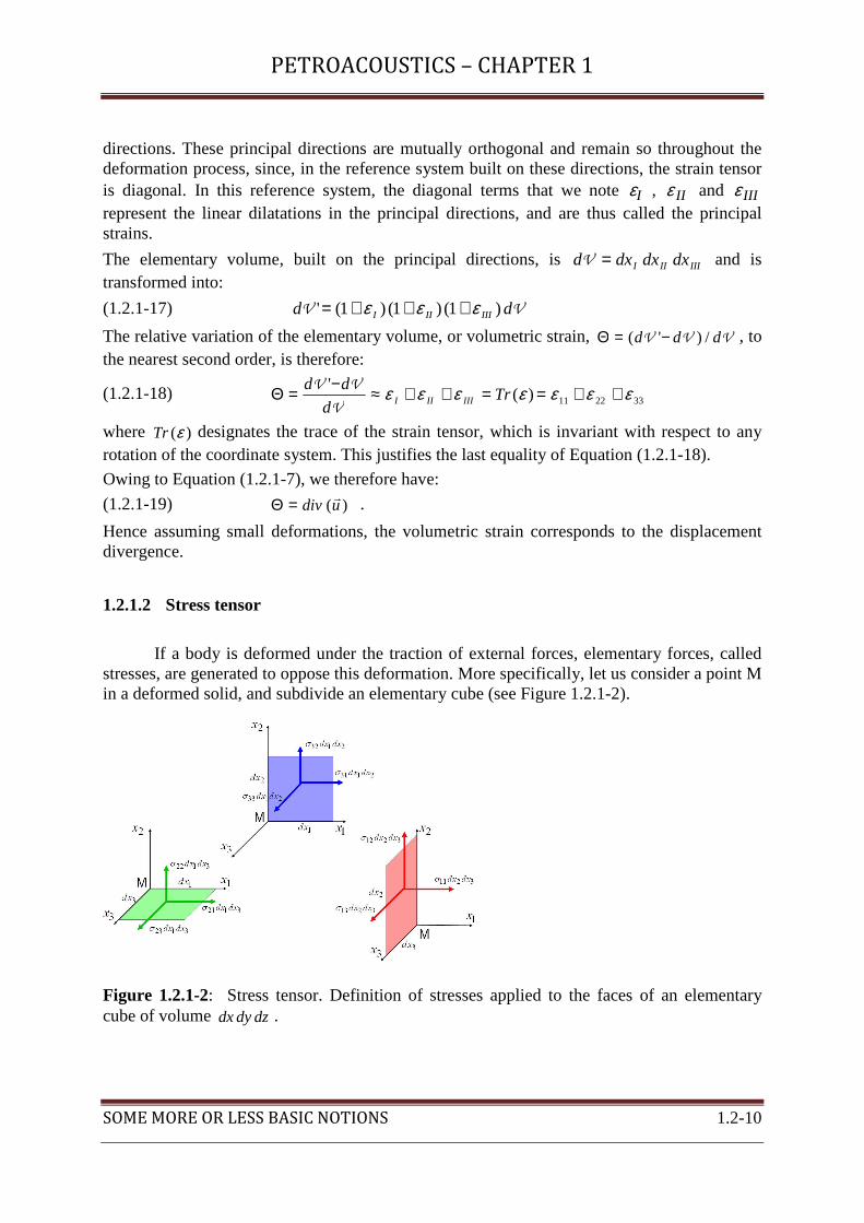
1.2.1.2 Stress tensor
If a body is deformed under the traction of external forces, elementary forces, called stresses, are generated to oppose this deformation. More specifically, let us consider a point M in a deformed solid, and subdivide an elementary cube (see Figure 1.2.1-2).
Figure 1.2.1-2: Stress tensor. Definition of stresses applied to the faces of an elementary cube of volume dzdydx .
PETROACOUSTICS – CHAPTER 1
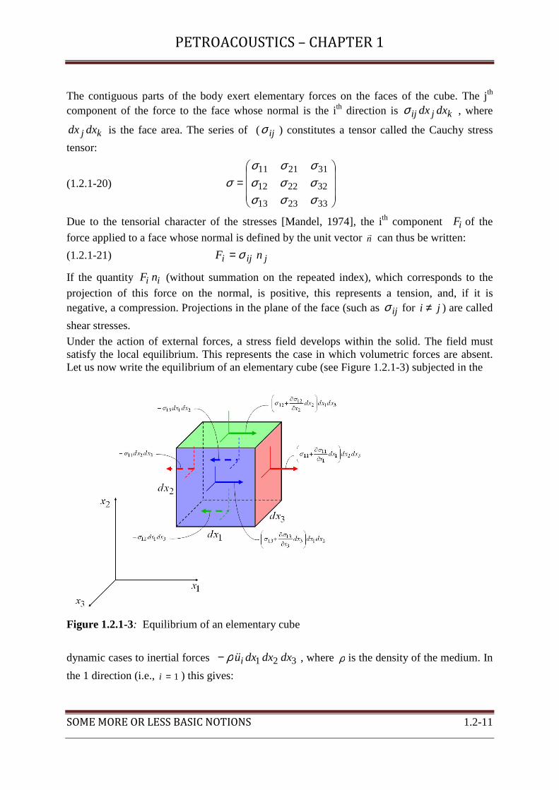
SOME MORE OR LESS BASIC NOTIONS 1.2-11
The contiguous parts of the body exert elementary forces on the faces of the cube. The jth component of the force to the face whose normal is the ith direction is kjij dxdxσ , where
kj dxdx is the face area. The series of (ijσ ) constitutes a tensor called the Cauchy stress
tensor:
(1.2.1-20)
=
332313
322212
312111
σσσσσσσσσ
σ
Due to the tensorial character of the stresses [Mandel, 1974], the ith component iF of the
force applied to a face whose normal is defined by the unit vector n can thus be written:
(1.2.1-21) jiji nF σ=
If the quantity ii nF (without summation on the repeated index), which corresponds to the
projection of this force on the normal, is positive, this represents a tension, and, if it is negative, a compression. Projections in the plane of the face (such as ijσ for ji ≠ ) are called
shear stresses.
Under the action of external forces, a stress field develops within the solid. The field must satisfy the local equilibrium. This represents the case in which volumetric forces are absent. Let us now write the equilibrium of an elementary cube (see Figure 1.2.1-3) subjected in the
Figure 1.2.1-3: Equilibrium of an elementary cube
dynamic cases to inertial forces 321 dxdxdxuiɺɺρ− , where ρ is the density of the medium. In
the 1 direction (i.e., 1=i ) this gives:
PETROACOUSTICS – CHAPTER 1
SOME MORE OR LESS BASIC NOTIONS 1.2-12
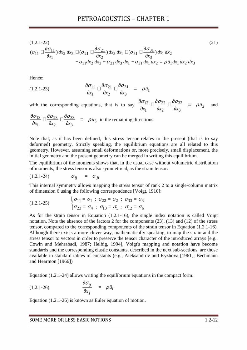
(1.2.1-22) (21)
3211213113213211
213
313113
2
212132
1
1111 )()()(
dxdxdxudxdxdxdxdxdx
dxdxx
dxdxx
dxdxx
ɺɺρσσσ
σσσσσσ
=−−−∂
∂++
∂∂
++∂
∂+
Hence:
(1.2.1-23) 13
31
2
21
1
11 uxxx
ɺɺρσσσ=
∂∂
+∂
∂+
∂∂
with the corresponding equations, that is to say 23
32
2
22
1
12 uxxx
ɺɺρσσσ=
∂∂
+∂
∂+
∂∂
and
33
33
2
23
1
13 uxxx
ɺɺρσσσ=
∂∂
+∂
∂+
∂∂
in the remaining directions.
Note that, as it has been defined, this stress tensor relates to the present (that is to say deformed) geometry. Strictly speaking, the equilibrium equations are all related to this geometry. However, assuming small deformations or, more precisely, small displacement, the initial geometry and the present geometry can be merged in writing this equilibrium.
The equilibrium of the moments shows that, in the usual case without volumetric distribution of moments, the stress tensor is also symmetrical, as the strain tensor:
(1.2.1-24) jiij σσ =
This internal symmetry allows mapping the stress tensor of rank 2 to a single-column matrix of dimension 6 using the following correspondence [Voigt, 1910]:
(1.2.1-25)
======
612513423
333222111
;;
;;
σσσσσσσσσσσσ
As for the strain tensor in Equation (1.2.1-16), the single index notation is called Voigt notation. Note the absence of the factors 2 for the components (23), (13) and (12) of the stress tensor, compared to the corresponding components of the strain tensor in Equation (1.2.1-16). Although there exists a more clever way, mathematically speaking, to map the strain and the stress tensor to vectors in order to preserve the tensor character of the introduced arrays [e.g., Cowin and Mehrabadi, 1987; Helbig, 1994], Voigt's mapping and notation have become standards and the corresponding elastic constants, described in the next sub-sections, are those available in standard tables of constants (e.g., Aleksandrov and Ryzhova [1961]; Bechmann and Hearmon [1966])
Equation (1.2.1-24) allows writing the equilibrium equations in the compact form:
(1.2.1-26) ij
iju
xɺɺρ
σ=
∂
∂
Equation (1.2.1-26) is known as Euler equation of motion.
PETROACOUSTICS – CHAPTER 1
SOME MORE OR LESS BASIC NOTIONS 1.2-13
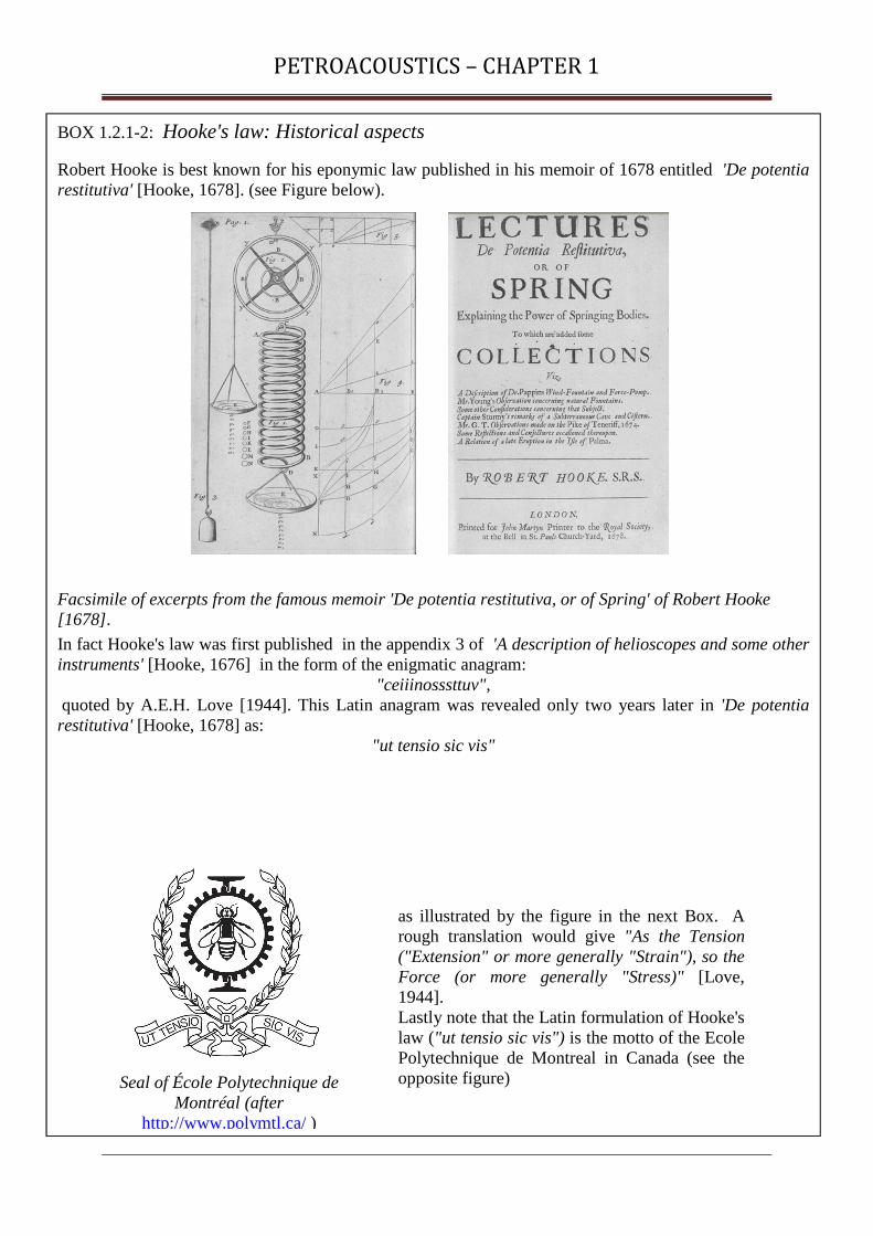
BOX 1.2.1-2: Hooke's law: Historical aspects
Robert Hooke is best known for his eponymic law published in his memoir of 1678 entitled 'De potentia restitutiva' [Hooke, 1678]. (see Figure below).
Facsimile of excerpts from the famous memoir 'De potentia restitutiva, or of Spring' of Robert Hooke [1678].
In fact Hooke's law was first published in the appendix 3 of 'A description of helioscopes and some other instruments' [Hooke, 1676] in the form of the enigmatic anagram:
"ceiiinosssttuv", quoted by A.E.H. Love [1944]. This Latin anagram was revealed only two years later in 'De potentia restitutiva' [Hooke, 1678] as:
"ut tensio sic vis"
Seal of École Polytechnique de Montréal (after
http://www.polymtl.ca/ )
as illustrated by the figure in the next Box. A rough translation would give "As the Tension ("Extension" or more generally "Strain"), so the Force (or more generally "Stress)" [Love, 1944]. Lastly note that the Latin formulation of Hooke's law ("ut tensio sic vis") is the motto of the Ecole Polytechnique de Montreal in Canada (see the opposite figure)

PETROACOUSTICS – CHAPTER 1
SOME MORE OR LESS BASIC NOTIONS 1.2-14
BOX 1.2.1-3
Hooke's law: Historical aspects (continued)
Hooke's law was erroneously published as the anagram "ceiiinosssttuu" instead of "ceiiinosssttuv", as corrected in "modern" Latin in the epigraph of Arts [1993]. In effect, in the old Latin alphabet before the introduction of the letter "u" by Petrus Ramus (1515-1572) in the 16th century, the modern letters "u" and "v" were not established as separate letters and were transcribed "v" so that the correct old transcription of the anagram would have been "ceiiinosssttvv".
Facsimile of the published original versions of Hooke's law (top) in the form of an anagram
in 1676, and (bottom) in the unravelled and most popular form of 1678.
Regarding publishing in the form of anagrams in general, as noted by Salençon [2002], the Italian physicist, mathematician and philosopher Galileo Galiei (1564 -1642) himself used this type of stratagem to secretly inform the German mathematician and astronomer Johannes Kepler (1571 – 1630) about his discovery of the phases of Venus as "Haec immatura a me iam frustra leguntur - oy" (translation: In vain these things are read by me prematurely), which when deciphered gives "Cynthia figuras aemulatur mater amorum" (translation: the Mother of Loves (Venus) imitates the figures of Diane (the moon)). From another point of view, as noted by Little [1973], Hooke' experiments only related force to extension. No account was taken of the shape of the tested samples. The law which bears Hooke's name postulate a linear relationship between stress and strain. In the early nineteenth century the French mathematicians Augustin Louis Cauchy (1789-1857) and Claude-Louis Navier (1785-1836) developed more completely this relation which is often called generalized Hooke's law. The modern tensorial formalism, now commonly used in all the branches of physics but unavailable at that time, was introduced much later by the Italian mathematicians Tullio Levi Civita (1873-1941) and Gregorio Ricci-Curbastro (1853-1925) [e.g., Levi-Civita, 1926].

PETROACOUSTICS – CHAPTER 1
SOME MORE OR LESS BASIC NOTIONS 1.2-15
Since the stress tensor is symmetrical, a principal reference system can be defined at each point in which the stress tensor is diagonal. The diagonal terms Iσ , IIσ and IIIσ are called the principal stresses.
1.2.1.3 Hooke's law and Elastic constants
A. Theoretical formulation of generalized Hooke's law of linear elasticity.
In a perfectly elastic medium the elementary work done per unit volume ijij dεσ derives from
a potential W , called the strain energy density, which writes:
(1.2.1-27) ijij ddW εσ=
which implies:
(1.2.1-28) ij
ijW
εσ
∂∂=
In the case of linear elasticity W is a quadratic function of the components of the strain tensor. If the strain energy density is normalized in a way that the undeformed state, corresponding to
0=ε , corresponds to zero energy, and if W is also minimal in this state (stability condition), then the strain energy density takes the simplified form (e.g., Ben-Menahem and Singh [1981]):
(1.2.1-29) klijijklCW εε2
1=
with implicit summation on the repeated indices. Inserting Equation (1.2.1-29) into Equation (1.2.1-28) gives:
(1.2.1-30) klijklij C εσ =
which is the generalized Hooke's law, or the modern form of the law of linear elasticity. In other words it is the most general linear relation between the components ijσ of the stress
tensor and the components klε of the strain tensor. The coefficientsijklC are the
components of the elasticity tensor. In the most general case this fourth rank tensor is defined by 34=81 coefficients. Due to the internal symmetries of the stress tensor (i.e., jiij σσ = ) and
of the strain tensor (i.e., lkkl εε = ) each of these tensors is defined by 6 independent
coefficients, as pointed out in the previous sub-sections. As a consequence the array of the coefficients ijklC exhibits the symmetries:
(1.2.1- 31) ijlkjiklijkl CCC ==
and can be put in one-to-one relation with a square matrix of dimension 6, which reduces the number of independent coefficients to 6×6=36. Furthermore, deriving each member of Equation (1.2.1-30) with respect to klε gives the:
PETROACOUSTICS – CHAPTER 1
SOME MORE OR LESS BASIC NOTIONS 1.2-16
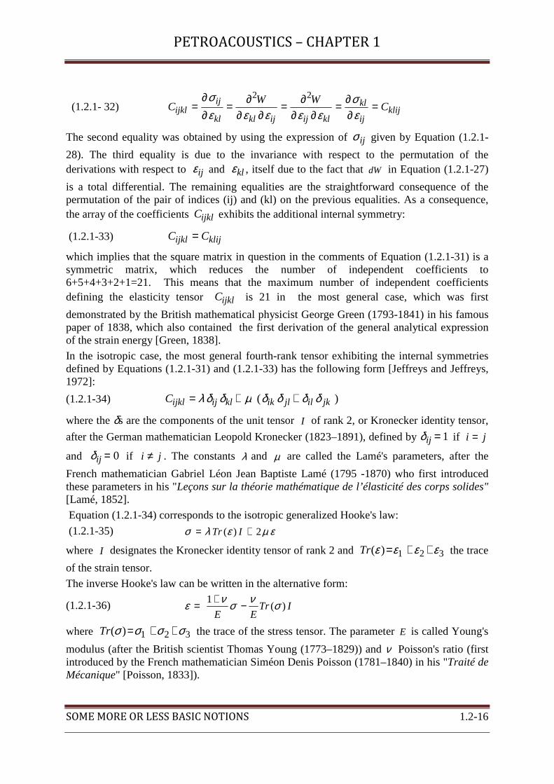
(1.2.1- 32) klijij
kl
klijijklkl
ijijkl C
WWC =
∂∂=
∂∂∂=
∂∂∂=
∂∂
=εσ
εεεεεσ 22
The second equality was obtained by using the expression of ijσ given by Equation (1.2.1-
28). The third equality is due to the invariance with respect to the permutation of the derivations with respect to ijε and klε , itself due to the fact that dW in Equation (1.2.1-27)
is a total differential. The remaining equalities are the straightforward consequence of the permutation of the pair of indices (ij) and (kl) on the previous equalities. As a consequence, the array of the coefficients ijklC exhibits the additional internal symmetry:
(1.2.1-33) klijijkl CC =
which implies that the square matrix in question in the comments of Equation (1.2.1-31) is a symmetric matrix, which reduces the number of independent coefficients to 6+5+4+3+2+1=21. This means that the maximum number of independent coefficients defining the elasticity tensor ijklC is 21 in the most general case, which was first
demonstrated by the British mathematical physicist George Green (1793-1841) in his famous paper of 1838, which also contained the first derivation of the general analytical expression of the strain energy [Green, 1838].
In the isotropic case, the most general fourth-rank tensor exhibiting the internal symmetries defined by Equations (1.2.1-31) and (1.2.1-33) has the following form [Jeffreys and Jeffreys, 1972]:
(1.2.1-34) )( jkiljlikklijijklC δδδδµδδλ ++=
where the δs are the components of the unit tensor I of rank 2, or Kronecker identity tensor,
after the German mathematician Leopold Kronecker (1823–1891), defined by 1=ijδ if ji =
and 0=ijδ if ji ≠ . The constants λ and µ are called the Lamé's parameters, after the
French mathematician Gabriel Léon Jean Baptiste Lamé (1795 -1870) who first introduced these parameters in his "Leçons sur la théorie mathématique de l’élasticité des corps solides" [Lamé, 1852].
Equation (1.2.1-34) corresponds to the isotropic generalized Hooke's law:
(1.2.1-35) εµελσ 2)( += ITr
where I designates the Kronecker identity tensor of rank 2 and 321)( εεεε ++=Tr the trace
of the strain tensor.
The inverse Hooke's law can be written in the alternative form:
(1.2.1-36) ITrEE
)(1 σνσνε −+=
where 321)( σσσσ ++=Tr the trace of the stress tensor. The parameter E is called Young's
modulus (after the British scientist Thomas Young (1773–1829)) and ν Poisson's ratio (first introduced by the French mathematician Siméon Denis Poisson (1781–1840) in his "Traité de Mécanique" [Poisson, 1833]).

PETROACOUSTICS – CHAPTER 1
SOME MORE OR LESS BASIC NOTIONS 1.2-17
B. Physical interpretation of all the elasticity parameters
The physical interpretations of the different elasticity parameters introduced in the two previous equations are the followings.
First let us consider an isotropic elastic cylinder submitted to a uniaxial stress, as illustrated by Figure 1.2.1-4
Figure 1.2.1-4: Young's modulus and Poisson's ratio
.
If the uniaxial stress is along the x-axis, i.e. 01 ≠= σσ and all the other components of the stress tensor being equal to zero, Equation (1.2.1-36) gives:
(1.2.1-37) E
σε =1 and σνεεE
−== 32
Thus Young's modulus E is simply the coefficient of proportionality between the uniaxial
stress σ and the axial strain 1∆ε = l
l. Thus E can be interpreted as the uniaxial stress
necessary to produce a unit axial strain.
After Equation (1.2.1-37):
(1.2.1-38) 32
1 1
( / )
( / )
εε ∆ν = − = − = −ε ε ∆
D D
l l
Thus Poisson's ratio ν can be interpreted as the opposite of the ratio between the radial strain
DD /32 ∆== εε and the axial strain 1∆ε = l
l of a sample under a uniaxial stress.

PETROACOUSTICS – CHAPTER 1
SOME MORE OR LESS BASIC NOTIONS 1.2-18
Figure 1.2.1-5: Shear modulus and Bulk modulus
Now let us conduct a pure shear experiment, as illustrated by the left side of Figure 1.2.1-5. For instance let us consider a shear stress in the xy-plane, i.e. 0612 ≠== τσσ all the other
components of the stress tensor being equal to zero, Equation (1.2.1-35) gives:
(1.2.1-39) 1212 2 εµσ = or in contracted notations 66 εµσ =
Thus the second Lamé parameter µ is simply the coefficient of proportionality between the
shear stress τσσ == 612 and the corresponding distortion εεε == 126 2 , ε designating the
angular distortion on the left side of Figure 1.2.1-5. That is why µ is also called the shear modulus. Note that µ can also be interpreted as the shear stress necessary to produce a unit angular distortion.
The right side of Figure 1.2.1-5 introduces a new elastic parameterK , called the bulk modulus. For this we conduct a hydrostatic experiment, i.e. 0321 ≠−=== pσσσ all the
other components of the stress tensor being equal to zero. The parameter p designates the exerted external pressure. The volume of the sample is initially V , and becomes + ∆V V under pressure. By definition the bulk modulus K is the coefficient of proportionality between the applied pressure p and the relative variation of volume /∆V V of the sample. In other words, K can be interpreted as the pressure necessary to produce a unit relative variation of volume.
In order to make the link between K and Lamé's parameters we can take the trace of each member of Equation (1.2.1-35):
(1.2.1-40) )()23()( εµλσ TrTr +=
For the hydrostatic experiment pTr 3)( −=σ and 1 2 3( ) /ε = ε + ε + ε = ∆Tr V V which
inserted in the previous equation gives:
(1.2.1-41) ( 2 / 3) / /= − λ + µ ∆ = − ∆p KV V V V
which gives by identification:
PETROACOUSTICS – CHAPTER 1
SOME MORE OR LESS BASIC NOTIONS 1.2-19
(1.2.1-42) 3/2µλ +=K
Similarly, for the link between K and Young's modulus E and Poisson's ratio ν we take the trace of each member of Equation (1.2.1-36):
(1.2.1-43) )(21
)( σνε TrE
Tr−=
which after Equations (1.2.1-40) to (1.2.1-42) gives:
(1.2.1-44) )21(3 ν−
= EK
The physical interpretation of the 1st Lamé parameter λ is not as straightforward.
Let us consider a uniaxial strain 1ε along the x-axis in an isotropic elastic sample, all the other components of the strain tensor being equal to zero. This is the strain state corresponding to the classical oedometer test in soil mechanics (e.g., Lambe and Whitman [1979]). In order to maintain these strains, after Equation (1.2.1-35) we need to apply the three following stresses 11 )2( εµλσ += along the x-axis, 12 ελσ = along the y-axis and
13 ελσ = along the z-axis. Thus the parameter λ can be defined as the stress required to
maintain a vanishing lateral strain on a sample under imposed unit uniaxial strain. In addition, note that the stress necessary to produce a unit strain in the direction of the imposed uniaxial strain is equal to µλ 2+ . Thus the ratio 1312 // σσσσ = of the lateral stress and the axial
stress necessary to impose a uniaxial strain is equal to )1/()2/( ννµλλ −=+ (the last equality is obtained from the table of Figure 1.2.1-6, extensively commented in the next sub-section), and only depends on the elastic property of the medium.
C. Link between all the elastic parameters
The considered elastic parameters are Young's modulus E, the bulk modulus K, the P-wave modulus M, the first Lamé's parameter λ, the second Lamé's parameter (or shear modulus or S-wave modulus) µ, and Poisson's ratio ν. Note that the P-wave modulus µλ 2+=M and the shear wave modulus µ , which is equal to the shear modulus or to the second Lamé's parameter, will be studied in the sub-section on wave propagation.
In addition to Equations (1.2.1-42) and (1.2.1-44) and to the above definitions of the P-wave and S-wave moduli we can obtain new relations by inserting the expression (1.2.1-43) of
)(σTr as function of )(εTr into Equation (1.2.1-36) and identify the result with Equation (1.2.1-35). This gives:
(1.2.1-45) )21()1( νν
νλ−+
= E and
)1(2 νµ
+= E
With all the previous equations it is possible to express any elastic parameters function of any pair of elastic parameter.
Figure 1.2.1-6 contains a table precisely giving the explicit expressions of the elastic parameters listed in the first row, as functions of any pair of these elastic parameters listed in the first column. For instance if one needs the expression of the P-wave modulus M (4th column) as function of Young's modulus E and Poisson's ratio ν (6th row) one reads the table

PETROACOUSTICS – CHAPTER 1
SOME MORE OR LESS BASIC NOTIONS 1.2-20
element at the intersection of 4th column and of the 6th row: )21()1(/)1( ννν −×+−= EM .
Similarly, for the expression of Poisson's ratio ν (last column) as function of P-wave modulus M and S-wave modulus µ (11th row) one reads: )(2/)2( µµν −×−= MM .
Note that the table of Fig. 1.2.1-6 is exhaustive. Indeed, the number of ways of selecting two
parameters among the six parameters listed in the first row of the table is 152
6=
, which is
exactly the number of pair of elastic parameters listed in the first column.
Figure 1.2.1-6: Link between the pairs of elastic constants in an isotropic linearly elastic medium (after Gassmann [1951]; Gassmann [1972]). We choose to reproduce Gassmann's table as a fac simile thus a change in typographic characters have to be noticed: k is the bulk modulus (K elsewhere in the text) and ω1, ω2 have nothing in common with angular frequency.

PETROACOUSTICS – CHAPTER 1
SOME MORE OR LESS BASIC NOTIONS 1.2-21
Furthermore it is straightforward to deduce the explicit expression of the P-wave velocity PV
and the S-wave velocity SV as functions of any pair of the elastic parameters. For this we
simply use the classical expressions ρ/MVP = and ρµ /=SV of these velocities (see
sub-section 1.2.2), ρ being the density of the medium, and the explicit expressions M and µ
of the wave moduli in the table. For instance, one can deduce the expressions of PV and SV
as functions of the bulk modulus K and Poisson's ratio ν (9th row). One reads )1/()1(3 νν +−= KM and )1(2/)21(3 ννµ +−= K , and one deduces
)1(/)1(3 νρν +−= KVP and )1(2/)21(3 νρν +−= KVS .
Lastly, the ratio of any pair of the elastic parameters listed in the first row of the table, for instance µλ / , can be expressed as the ratio of any other pair of these parameters, for instance MK / . For this, first one takes the expressions 2/)3( MK −=λ and
4/)(3 KM −=µ as functions of K and M on the 6th row of the table. Then one straightforwardly deduces the ratio
/ 2 (3 ) / 3 ( ) 2 (3 1) / 3 (1 )K M M Kλ µ ι ι= − − = − − , where /k Mι = .
D. Upper and lower bounds for all the elastic parameters.
The stability of an elastic material imposes that the material cannot deform spontaneously without energy input from outside. In other words the strain energy density W defined by Equation (1.2.1-29) must be positive for any deformation. In the special cases of the pure shear experiment and of the hydrostatic stress experiment in isotropic media illustrated by Figure 1.2.1-5 this implies:
(1.2.1-46) 0>K and 0>µ
The following expressions of the remaining elastic parameters as function of the pair of parameters ),( µk are given in the 8th row of the table on Figure 1.2.1-6:
(1.2.1-47) µ
µ+
=K
KE
3
9 , 3/4µ+= KM , 3/2µλ −= K and
)3(2
23
µµν
+−=
K
K
The conditions (1.2.1-46) on the bulk modulus k and on the shear modulus µ and Equation (1.2.1-47) imply the following bounds for the remaining elastic parameters:
(1.2.1-48) 0>E , 0>M , +∞<<∞− λ and 2
11 <<− ν
In summary the bulk modulus K, the shear modulus µ , Young's modulus E and the P-wave modulus M can have any positive value. The first Lamé's parameter λ can have any real value, either positive or negative. And Poisson's ratio ν is bounded by the values -1 and 1/2.
Furthermore, according to the expression of Poisson's ratio ν in Equation (1.2.1-47), materials having Poisson's ratio tending to 1/2 exhibit either finite shear modulus µ and infinitely large bulk modulus K, or vanishing shear modulus µ but finite bulk modulus K. Typically this last case corresponds to non-viscous liquids and gases.

PETROACOUSTICS – CHAPTER 1
SOME MORE OR LESS BASIC NOTIONS 1.2-22
In contrast, materials having Poisson's ratio tending to -1 exhibit either vanishing bulk modulus K but finite shear modulus µ , or finite bulk modulus k and infinitely large shear modulus µ . From a more general point of view, nearly all (?) natural isotropic material have positive Poisson's ratio, that is to say when cylinders made of such materials are uniaxially compressed they increase in cross-section, as illustrated by Figure 1.2.1-4 (on Poisson's ratio). However thermodynamic stability does not impede negative Poisson's ratio. The corresponding materials are sometimes called "auxetic" (e.g., Evans et al. [1991]), a word derived from the Greek word αὐξητικός (auxetikos) which means "that which tends to increase". Examples of such unusual materials, which become thicker in lateral directions when pulled, are for instance various manufactured foams (e.g., Lakes [1987]) characterized by Poisson's ratio ν values down to -0.7. The study of auxetic materials is a relatively new field of research and development (e.g., Stott et al. [2000]).
Lastly, note that the ratio M
µς = of the S-wave and P-wave moduli can be written as:
(1.2.1-49) 3/4µ
µµς+
==KM
After Equation (1.2.1-46) the bulk modulus K and the shear modulus µ can have any positive value. As a consequence ς must be positive and smaller than the limit value 4/3 :
(1.2.1-50) 4
30 <=<
M
µς
A ratio M
µς = tending to 0 corresponds to media exhibiting either finite shear modulus µ
and infinitely large bulk modulus K , or vanishing shear modulus µ but finite bulk modulus K (typically non-viscous liquids and gases), which all also correspond to Poisson's ratio tending to 1/2 as said in the comments of Equation (1.2.1-49).
In contrast, a ratio M
µς = tending to 4/3 corresponds to media exhibiting either vanishing
bulk modulus K but finite shear modulus µ , or finite bulk modulus K and infinitely large shear modulus µ , which all also correspond to Poisson's ratio tending to -1 as said in the comments of Equation (1.2.1-49).

PETROACOUSTICS – CHAPTER 1
SOME MORE OR LESS BASIC NOTIONS 1.2-23
BOX 1.2.2-1
The wave equation: Historical aspects
The formulation of the 1D wave equation and its solution are due to the French scientist, philosopher and music theorist Jean-Baptiste le Rond d'Alembert (1717–1783), in the context of the study of vibrating strings (d'Alembert [1747]).
After Boussinesq [1906], much later, the French mathematician and physicist Siméon Denis Poisson (1781–1840) and the Russian mathematician and physicist Mikhail Vasilyevich Ostrogradsky (1801–1862) first studied, around 1830, elastic waves generation from a small spherical source and propagation of two spherical wavefronts centered at the source location in a homogeneous isotropic elastic medium of infinite extension (e.g., Poisson [1830]; Ostrogradsky [1831]), which is the basis of modern seismological/seismic theory.
These authors also demonstrate that the largest sphere is the first wavefront and corresponds to the P-wave, or primary wave, that is to say the first to be recorded in seismics/seismology because of its highest velocity. This wave is also called the longitudinal wave because the particle displacement associated with the wave is parallel to the direction of propagation of the wave. The second wavefront is the smaller sphere and corresponds to the S-wave, or secondary wave. This wave is also called the transverse wave because the particle displacement associated with the wave is perpendicular to the direction of propagation of the wave (see details in the next sub-section).

PETROACOUSTICS – CHAPTER 1
SOME MORE OR LESS BASIC NOTIONS 1.2-24
1.2.2 Elastic wave propagation and reflection/refraction at interfaces
1.2.2.1 Elastic wave equation
Figure 1.2.2-1: 1D problem of wave propagation
Let us consider the equilibrium of an element of length dx in blue. The average particle displacement associated with this element is ),( txU which is a function of the single space variable x and timet . Neglecting any force acting at distance (e.g., gravimetric, magnetic etc...), for fixed time t the only applied forces are Sσ on the left side and S)( σσ d+ on
the right side of the element, where dxx
d∂∂= σσ because the stress ),( txσ is only function of
the single space variable x and time t . Finally Newton's second law applied to the element gives the equation of motion:
(1.2.2-1) 2
2
t
Udxdx
x ∂∂=−
∂∂+ SSS ρσσσ
where ρ designates the density of the medium, and dxS and dxSρ the volume and the mass of the element.
A. 1D wave propagation
First let us consider a wave propagating in one dimension, for instance in a beam of sectionS , along the x-axis as illustrated by Figure 1.2.2-1.
Simplifying and dividing each member of the previous equation by dxS leads to:
(1.2.2-2) 2
2
t
U
x ∂∂=
∂∂ ρσ
Inserting the unidimensional stress-strain relation εσ H= , with x
U
∂∂=ε , into Equation
(1.2.2-2) gives the general equation of 1D-motion:
PETROACOUSTICS – CHAPTER 1
SOME MORE OR LESS BASIC NOTIONS 1.2-25
(1.2.2-3) 2
2
t
U
x
UH
x ∂∂=
∂∂
∂∂ ρσ
where H is an elastic modulus which will be specified later. If the medium is assumed homogeneous, then H does not depend on the space variable x, as a consequence the previous equation simplifies in the following way:
(1.2.2-4) 2
2
2
2
t
U
x
UH
∂∂=
∂∂ ρ
which is the wave equation, of which two solutions are:
(1.2.2-5) )(),(V
xttxU ξψ +=
where ψ is an arbitrary function describing the wave shape and 1±=ξ .
If one inserts the expression of the displacement ),( txU from Equation (1.2.2-5) into Equation (1.2.2-4), one obtains:
(1.2.2-6) ""2
ψρψ =V
H
If one rejects the obvious solution 0=ψ corresponding to the space at rest, and the unphysical affine solution BAx +=ψ , A and B being arbitrary constants, which would lead to infinite amplitude at distance x tending to infinity, Equation (1.2.2-6) is verified if the following equality is verified:
(1.2.2-7) ρ/HV =
V is the velocity of propagation of the wave. As illustrated by Figure 1.2.2-2 Equation (1.2.2-5) describes a disturbance that travels with no change of shape at the velocity V given by Equation (1.2.2-7). Because all natural media, including geological media, are more or less attenuating with respect to wave propagation, elastic waveforms change during propagation due to attenuation/dispersion as will be detailed in the next chapters.
Also note the absence of permanent particle displacement after the passage of the wave. This is due to the fact that the medium is conservative and releases all the elastic energy contained in the wave.

PETROACOUSTICS – CHAPTER 1
SOME MORE OR LESS BASIC NOTIONS 1.2-26
Figure 1.2.2-2: Wave propagation without distorsion of the wave shape. On the left side: propagation in the direction of decreasing values of the space variable x [ξ=+1 in Equation (1.2.2-5)], and on the right side: propagation in the direction of increasing values of the space variable x [ξ=-1 in Equation (1.2.2-5)]. Case of a Gaussian-like waveform. The colour scale for the amplitudes is in the center of the figure.
Now let us examine the exact expression of the modulus H for specific wave types.
In the case of a uniaxial stress along the x-axis, i.e. 01 ≠σ and all the components of the
stress tensor equal to zero, after Equation (1.2.1-36) one has 11 εσ E= . Thus EH = and
ρ/EV = , which corresponds to the velocity of an extensional wave propagating along a
beam or a rod of small section.
In the case of a uniaxial strain along the x-axis, i.e. 01 ≠ε and all the components of the strain
tensor equal to zero, after Equation (1.2.1-35) one has 11 )2( εµλσ += and 132 ελσσ == .
Thus µλ 2+=H and ρµλ /)2( +=V , which corresponds to the velocity of a
longitudinal wave propagating along the x-axis.
In the case of a shear stress in the direction perpendicular to the x-axis, say in the yz-plan i.e. 05 ≠ε and all the components of the stress tensor equal to zero, after Equation (1.2.1-35) one
has 55 εµσ = . Note that in this case the displacement U is no longer parallel but
perpendicular to the x-axis, say along the z-axis. Thus µ=H and ρµ /=V , which
corresponds to the velocity of a transverse, or shear, wave propagating along the x-axis.

PETROACOUSTICS – CHAPTER 1
SOME MORE OR LESS BASIC NOTIONS 1.2-27
B. 3D wave propagation and general formalism
By introducing the expression of linearized strains given by Equation (1.2.1-7) into the isotropic constitutive equation (1.2.1-35) and then the result into Euler's equation (1.2.1-26) the following equations of motion are obtained:
(1.2.2-8) uucurlcurlugrad ɺɺρµµλ =−+ div)2(
where grad (.) and curl (.) designate the gradient and the rotational of the considered scalar and vector fields respectively, and u the displacement field induced by the wave.
Then, assuming that the vector field u, is defined everywhere in space and smooth enough, and vanishes at infinity together with its first derivatives, we can use Helmholtz's theorem, after the German physicist and physiologist Hermann Ludwig Ferdinand von Helmholtz (1821–1894). The theorem says that the vector field u can be decomposed into a rotational part Ψcurl and an irrotational part ϕgrad :
(1.2.2-9) = ϕ +u grad curl Ψ
where ϕ and Ψ are called the scalar and the vector potential.
All the equations being linear and the medium linearly elastic we can study separately the effect of each field which have no interaction on the remaining field. The superposition principle, applicable here, guarantees that the net response of the medium caused by two fields is the sum of the responses which would have been caused by each field individually.
Thus, first let us consider irrotational displacements (i.e., 0=ucurl ) defined by a scalar potential ϕ such that:
(1.2.2-10) = ϕu grad
This equation inserted into Equation (1.2.2-9) gives:
(1.2.2-11) PV ( ) 0ϕ =
where (.))(
1(.)(.)
2
2
22
tVPVP ∂
∂−∇= designates the wave equation operator or
d'Alembertian operator [after the French mathematician, mechanician, physicist, philosopher and music theorist Jean-Baptise le Rond d’Alembert (1717 – 1783)], of velocity PV given by:
(1.2.2-12) ρµλ /)2( +=PV .
The operator (.)(.)2 graddiv=∇ designates the Laplacian of the considered quantity, after the French mathematician and astronomer Pierre-Simon de Laplace (1749 – 1827).
Equation (1.2.2-11) generalizes to 3D Equation (1.2.2-4) which was restricted to 1D. It defines waves propagating at the velocity PV . Note that we find the same result as the 1D case with a wave modulus equal to µλ 2+ . These waves are called dilatational waves because they correspond to the propagation of volumetric strain. Indeed, by applying the Laplacian
operator (.)2∇ to Equation (1.2.2-8) for u satisfying Equation (1.2.2-10) and using Equation (1.2.1-18) we actually obtain:

PETROACOUSTICS – CHAPTER 1
SOME MORE OR LESS BASIC NOTIONS 1.2-28
(1.2.2-13) 0)( =ΘPV
These waves are also called P-waves, where P corresponds to "primary", because these are the fastest waves likely to propagate in an isotropic linear elastic solid and, as a consequence, the first waves to be recorded by the seismic/seismological receivers.
Let us now consider rotational displacements defined by a vector potential Ψ such that:
(1.2.2-14) Ψcurlu =
These movements correspond to motion without volume change or equivolumetric motion, because:
(1.2.2-15) 0===Θ Ψcurlu divdiv
Inserting (1.2.2-14) into Equation (1.2.2-8) gives:
(1.2.2-16) 0)( =ΨSV
where (.))(
1(.)(.)
2
2
22
tVSVS ∂
∂−∇= designates the wave equation operator or
d'Alembertian operator, of velocity SV given by:
(1.2.2-17) ρµ /=PV .
Equation (1.2.2-16) defines waves propagating with the velocity SV . These are called shear
waves. They are also called S-waves, where S stands for secondary, because they are slower than the P-waves.
Note that, after the table contained on Figure 1.2.1-6 the ratio MV
V
P
S µς =
=
2
of the S-
wave velocity squared and of the P-wave velocity squared, which is equal to the ratio of the S-wave and P-wave moduli, can be written as a function of Poisson's ratio ν in the form:
(1.2.2-18) )1(2
21
ννς
−−=
Also note the following surprising result. After the same table the inverse relation giving
Poisson's ratio ν as a function of M
µς = is formally identical to the previous equation after
inverting the variables ν and ς :
(1.2.2-19) )1(2
21
ςςν
−−= .
According to Equation (1.2.1-50) M
µς = is bounded by the values 0 and 4/3 , which implies
that the ratio of the S-wave and P-wave velocities verifies the relation:
(1.2.2-20) 2
30 <<
P
S
V
V

PETROACOUSTICS – CHAPTER 1
SOME MORE OR LESS BASIC NOTIONS 1.2-29
As said in the comments of Equation (1.2.1-50), a ratio P
S
V
V tending to
2
3, or equivalently
a ratio M
µς = tending to 4
3, corresponds to media exhibiting Poisson's ratio tending to -1.
Since nearly all (?) natural isotropic material exhibit positive Poisson's ratio ν , after Equation (1.2.2-18) the general bounds given by Equation (1.2.2-20) are expected to be narrower for natural media:
(1.2.2-21) 2
10 <=<
M
µς or equivalently 2
20 <<
P
S
V
V
a. Plane waves
Now, studying the motion of material particles due to the propagation of the wave, by using the change in variables:
(1.2.2-22) Vnzmylxt /)( ++−=α and Vnzmylxt /)( ++−=β
with 1222 =++ nml and PVV = or SV , the position vector being defined by its
coordinates ),,( zyx in an orthonormal trihedron ),,( zyx .
Noting that, for any function ),( βαF :
(1.2.2-23) βα ∂
∂+∂∂= FF
Fɺ ,
∂∂−
∂∂=
∂∂
αβFF
V
l
x
F etc.
we obtain that a solution of Equations (1.2.2-11) and (1.2.2-16) of the type ),( βαF will verify:
(1.2.2-24) βα ∂∂
∂ F24
where φ=F or Ψ . When integrated, this equation implies that:
(1.2.2-25) [ ] [ ]VnzmylxtgVnzmylxtfF /)(/)( ++++++−=
where f and g are arbitrary functions describing the wave shape as the function ψ in the case of 1D propagation in Equation (1.2.2-5).
For fixed time t , F is constant for the plane constantnzmylx =++ .
As illustrated by Figure 1.2.2-3, for φ=F , Equations (1.2.2-10) and (1.2.2-25) show that the particle motion is perpendicular to the wave fronts, which are planes normal to the direction
),,( nml=n . In the 1D case of Figure 1.2.2-3 and Equation (1.2.2-5), one has )0,0,1(=n , the function f of Equation (1.2.2-25) would correspond to the case 1−=ξ of Equation (1.2.2-5) , that is to say waves propagating in the direction of )0,0,1(=n .

PETROACOUSTICS – CHAPTER 1
SOME MORE OR LESS BASIC NOTIONS 1.2-30
Figure 1.2.2-3: Sketch of 3D Wave propagation of P- and S-waves showing the wavefronts, the wave normal and the particle displacement.
This is a general result in 3D geometry. That is to say, the function [ ]Vnzmylxtf /)( ++− of Equation (1.2.2-25) corresponds to waves propagating in a
direction parallel to ),,( nml=n and in the same direction as n . In contrast, the function
[ ]Vnzmylxtg /)( +++ of Equation (1.2.2-25) corresponds to waves propagating in a direction parallel to ),,( nml=n but in the opposite direction from n . In the 1D case of Figure 1.2.2-3 and Equation (1.2.2-5) the function g of Equation (1.2.2-25) would correspond to the case 1+=ξ of Equation (1.2.2-5) , that is to say waves propagating in the direction opposite from )0,0,1(=n in the 1D-case.
The vector nV Vph = , where n is the normal to the wavefront illustrated by Figure 1.2.2-3, is called the phase velocity vector. The velocity V , is equal either to the P-wave velocity PV or to the S-wave velocity SV , is called the phase velocity. In later sections it
will be designated by phV in order not to be confused with the energy velocity eV of
section 1.2.2.2 and the group velocity grV of section 1.2.3.3. In homogenous linear elastic media of infinite extension all these velocities are equal.
The wave polarization is called longitudinal, and the P-waves are also called longitudinal waves. Finally, note that the popular analogy of P-waves and compressional waves in a spring has unfortunately lead some authors to call erroneously P-waves compressional waves. This is misleading because, after the table contained on Figure 1.2.1-6 , the P-wave modulus is 3/4µ+= KM is composed of more shear modulus µ than incompressibility modulus, or bulk modulus,K .

PETROACOUSTICS – CHAPTER 1
SOME MORE OR LESS BASIC NOTIONS 1.2-31
For Ψ=F , Equations (1.2.2-14) and (1.2.2-25) show that the particle motion is parallel to the wave fronts as illustrated by Figure 1.2.2-3. The wave polarization is called transverse, and the S-waves are also called transverse waves.
These results, obtained for plane waves, are actually generally applicable to any wave fronts since any wave front can be decomposed in a superposition of plane wave fronts (e.g., Aki and Richards [1980]; Ben-Menahem and Singh [1998]). Polarization is either normal to the wave front for P-waves or parallel to the wave front for S-waves.
In this first chapter we have assumed that the medium is isotropic. This is not verified in general because most rocks more or less exhibit anisotropic behaviour as will be detailed in Chapter 4 on elastic anisotropy.
b. Cylindrical waves
If the considered wave problem exhibits a rotational symmetry about an axis, for instance the vertical z-axis, the waves are called cylindrical waves, as in the case of waves generated by a line source located at the z-axis in a homogeneous isotropic elastic medium.. In such case it is appropriate to express the D'Alembertian of Equations (1.2.2-11) and (1.2.2-13) in cylindrical coordinates (e.g., Morse and Feshbach [1953])
(1.2.2-26) (.))(
1(.)
11(.) 2
2
2,
2
2
2
2
22
2
, tVzrrrr SPV SP ∂
∂−
∂∂+
∂∂+
∂∂+
∂∂=
θ
where the position vector is defined by its cylindrical coordinates ),,( zr θ with the equivalence ),sin,cos(),,( zrrzyx θθ= with the Cartesian coordinates ),,( zyx . The wave velocity is noted SPV , with the index P for P-wave and S for S-wave. In the case of
rotational symmetry about the z-axis and of invariance with respect to any translation along the z-axis the derivations with respect to the variables θ and z must vanish in Equation (1.2.2-26). In other words the wave field only depends on the distance r from the z-axis and on the time t . As a consequence the general harmonic solution of Equation (1.2.2-11) and Equation (1.2.2-13), corresponding to an outgoing wave, can be written (e.g., Kinsler et al. [2000]):
(1.2.2-27) tjSPSP erkHutru ω)(),( ,
)2(10, =
where SPu , designates the particle displacement associated with the P-wave (index P)
or with the S-wave (index S), 0u a complex constant, ).()2(1H the Hankel function of
the second kind, of order 1 (e.g., Abramowitz and Stegun [1965]), SPSP Vk ,, /ω= the
wave number associated with the distance r from the z-axis, and ω the pulsation of the wave. Using the asymptotic form of the Hankel functions for large rk SP, found in the last
reference, the solution defined by Equation (1.2.2-27) has the asymptotic behaviour:
(1.2.2-28) ( )4/3
,0,
,2
),( πω
π−−≈ rktj
SPSP
SPerk
utru
Because the particle displacement decreases as 2/1−r , the energy flux of the wave field, crossing a fixed unit surface parallel to the wave front proportional to the square of the
PETROACOUSTICS – CHAPTER 1
SOME MORE OR LESS BASIC NOTIONS 1.2-32
particle displacement (as detailed in sub-section 1.2.2.2) decreases as 1−r . This effect is commonly called the 2D geometrical spreading [e.g., Sheriff and Geldart, 1995]. This was expected since the wavefront is a cylinder of axis the z-axis and of radius r , which increases with time as tV SP, . The total amount of energy transported by the whole
cylindrical wavefront of increasing radius r per unit length along the z-axis being constant (i.e. energy provided by the source), the energy per unit surface decreases as r/1
and as a consequence the particle displacement decreases as r/1 .
The harmonic solution given by Equation (1.2.2-27) is important because any time signal can be decomposed in a sum of such elementary solutions using Fourier transform (e.g., Bracewell [1965]; also see Box 1.2.2-4).
c. Spherical waves
If the considered wave problem exhibits a spherical symmetry, the waves are called spherical waves, as in the case of waves generated by a point source in a homogeneous isotropic elastic medium. In such case it is appropriate to express the D'Alembertian of Equations (1.2.2-11) and (1.2.2-13) in spherical coordinates (e.g., Morse and Feshbach [1953]):
(1.2.2-29)
P,S
2 2 2
V 2 2 2 2 2 2 2P,S
2 1 1 1(.) sin (.) (.)
R RR R sin R sin (V ) t
∂ ∂ ∂ ∂ ∂ ∂ = + + θ + − ∂ ∂θ ∂θ∂ θ θ ∂ϕ ∂
where the position vector is defined by its spherical coordinates (R , , )θ ϕ with the equivalence(x , y, z) (R sin cos , R sin sin , R cos )= θ ϕ θ ϕ θ with the Cartesian coordinates ),,( zyx . In the case of spherical symmetry the derivations with respect to the variables θ and ϕ must vanish in Equation (1.2.2-29). In other words the wave field only depends on the distance R and on the time t . As a consequence the wave equation takes the simple form:
(1.2.2-30) [ ] [ ]),()(
1),(
2,2
2
2,
,2
2
trutV
truRRR
SPSP
SP ∂∂−
∂∂+
∂∂
which further simplifies if the new variable SPuR , is introduced:
(1.2.2-31) [ ] [ ]
2
,2
2,
2
,2 ),(
)(
1),(
t
truR
VR
truR SP
SP
SP
∂∂
−∂
∂
One recognizes the classical 1D-wave equation except that the variable is no longer the particle displacement SPu , but the product SPuR , of the radial distance R and of the particle
displacement. As a consequence, after Equation (1.2.2-25) the general solution of Equation (1.2.2-31) simply writes:
(1.2.2-32) ( ) ( )SPSPSP VRtgR
VRtfR
tru ,,, /1
/1
),( ++−=

PETROACOUSTICS – CHAPTER 1
SOME MORE OR LESS BASIC NOTIONS 1.2-33
where f and g are arbitrary functions describing the wave shape as the function ψ in the case of 1D propagation in Equation (1.2.2-5). The solution defined by Equation (1.2.2-32) holds for any strictly positive value of the radial distanceR . Obviously the solution is not valid for vanishingR. The first term of the right hand member of Equation (1.2.2-32) describes a wave propagating in the direction of increasing values of the radial distanceR, that is to say a diverging wave or an outgoing wave. The second term of the right hand member of Equation (1.2.2-32) describes a wave propagating in the direction of decreasing values of the radial distanceR, that is to say a converging wave or an incoming wave. As for the cylindrical waves of Equation (1.2.2-27), particular classes of solution are the outcoming or diverging harmonic waves:
(1.2.2-33) ( )
R
eAtru
SPVRtj
SP
,/
, ),(−
=ω
where A is an arbitrary complex constant.
Because the particle displacement decreases as 1R− , the energy flux of the wave field, crossing a fixed unit surface parallel to the wave front proportional to the square of the particle displacement (as detailed in sub-section 1.2.2.2) decreases as 2−R . As in the 2D case, this effect is commonly called the 3D geometrical spreading (e.g., Sheriff and Geldart [1995]). This was expected since the wavefront is a sphere of radius R, which increases with time as tV SP, . The total amount of energy transported by the whole spherical wavefront of
increasing radius R being constant (i.e. energy provided by the source), the energy per unit surface decreases as 2/1 R and as a consequence the particle displacement decreases as R/1 .
1.2.2.2 Energy considerations, Impedance and reflection/transmission
A. Energy flux associated to the elastic wave and elastic impedance
The amount of energy transported per unit time by the elastic wave, or the energy flux of the wave field, crossing a fixed unit surface parallel to the wave front is equal to the norm of the vector P of components (e.g., Dieulesaint and Royer [1974]):
(1.2.2-34) t
uP i
ikk ∂∂−= σ
PETROACOUSTICS – CHAPTER 1
SOME MORE OR LESS BASIC NOTIONS 1.2-34
where ikσ and t
ui∂
∂ are the components of the stress and the particle velocity induced
by the elastic wave. We call the vector P the Umov-Poynting-Heaviside vector, or in a shorter way the UPH vector (see box 1.2.2-2).
BOX 1.2.2-2
The energy flux vector: Historical aspects
The energy flux vector P is often called Poynting vector [Auld, 1973; Dieulesaint and Royer, 1974], sometimes Poynting-Heaviside vector [Unz, 1963] and sometimes Umov-Poynting vector [Carcione, 2007], after the Russian physicist and mathematician Nikolay Alekseevich Umov (1846-1915), the British physicist John Henry Poynting (1852-1914) and the British physicist and mathematician Oliver Heaviside (1850-1925).
According to Kiselev [1982], Umov first introduced the concept of the energy flux vector P in his doctoral thesis [Umov, 1874] in the following way:
"… the quantity of energy, which takes place through the infinitely small flat element in the infinitely short time, is equal to the negative work of the elastic forces, which act on this element."
Then ten years later, Poynting [1884] and Heaviside [1884] independently re-discovered the concept, more in the context of electromagnetic wave propagation.
Considering the independent enormous contributions of these three brilliant scientists we suggest to call the vector P the Umov-Poynting-Heaviside vector, or in a shorter way the UPH vector. More general considerations on the UPH vector, even in anisotropic media, are well documented in Carcione [2007].
PETROACOUSTICS – CHAPTER 1
SOME MORE OR LESS BASIC NOTIONS 1.2-35
If E designates the total energy density per unit volume, the velocity vector of energy
transport or energy velocity vector eV is given by (e.g., Dieulesaint and Royer [1974]):
(1.2.2-35) PV =e /E In isotropic media of infinite extension the energy velocity vector is equal to the phase
velocity vector nV Vph = , where n is the normal to the wavefront illustrated by Figure
1.2.2-3, and V , either the P-wave velocity PV or the S-wave velocity SV introduced in the
previous sections. Thus the UPH vector is collinear to the energy velocity vector eV and to
the phase velocity vector phV and, as a consequence is normal to the wavefront.
Let us consider the particle displacement associated to a monofrequency plane P-wave propagating in an isotropic medium of infinite extension, say in the x-direction, without loss of generality. The only non-vanishing component is:
(1.2.2-36) ( )[ ]PVxtjuu /exp)0(11 −= ω
where fπω 2= is the angular frequency (f being the frequency) and j the complex number
such that 12 −=j .
The only non-zero component of the UPH vector is:
(1.2.2-37) t
uP
∂∂
−= 1111 σ
After Equation (1.2.2-36), one has 11 ujt
u ω=∂
∂. And after the sub-section 1.2.2.1.B the
axial stress associated to the P-wave is 1111 )2( εµλσ += where 11
11 uV
jx
u
P
ωε −=∂∂
= , the
last equality being due to Equation (1.2.2-36). As a consequence the absolute value of the stress is given by:
(1.2.2-38) PV
µλσ 211
+= v1
where v1 is the absolute value of the particle velocity associated to the elastic wave.
Because ρµλ /)2( +=PV , After Equation (1.2.2-38) the ratio of the stress and the particle
velocity is PP
P VV
Z ρµλ =+= 2 is called the P-wave impedance.
Inserting the expression 11σ of Equation (1.2.2-38) and the above expressions into the
absolute value of each member of Equation (1.2.2-36) leads to:
(1.2.2-39) PZP =1 v12 PZ/211σ=
Similarly the complex particle displacement associated to a monofrequency plane S-wave propagating in an isotropic medium of infinite extension, for instance in the x-direction, and polarized along the y-direction, without loss of generality. The only non-vanishing component is:

PETROACOUSTICS – CHAPTER 1
SOME MORE OR LESS BASIC NOTIONS 1.2-36
(1.2.2-40) ( )[ ]SVxtjuu /exp)0(22 −= ω .
The only non-zero component of the UPH vector is:
(1.2.2-41) t
uP
∂∂−= 2
121 σ .
After the sub-section 1.2.2.1.B the shear stress associated to the S-wave is 1212 2 εµσ =
where 22
122 uV
jx
u
S
ωε −=∂
∂= . As a consequence the absolute value of the stress is given
by:
(1.2.2-42) SV
µσ =12 v2
where v2 is the absolute value of the particle velocity associated to the elastic wave.
Because ρµ /=SV , After Equation (1.2.2-42) the ratio of the stress and the particle velocity
is SS
S VV
Z ρµ == it is called the S-wave impedance.
Inserting the expression 12σ of Equation (1.2.2-42) and the above expressions into the
absolute value of each member of Equation (1.2.2-41) leads to:
(1.2.2-43) SZP =1 v22 SZ/212σ=
B. Reflection and transmission of elastic waves at interfaces
a. Case on normal incidence
The elastic impedances Z (that is to say, either the P-wave impedancePZ or the S-wave
impedance SZ ) are important parameters because any elastic wave striking a macroscopic
surface of discontinuity of the impedance, and more exactly of the density ρ and/or of the
velocity V (that is to say, either the P-wave velocityPV or the S-wave velocity SV ), within
the earth generate transmitted and reflected waves at this interface that allow for instance to image the earth's interior in seismics and in seismology.
Let us consider the simplest case of a plane P-wave (or S-wave) of unit amplitude (this can be either the stress or the particle velocity induced by the wave) striking at normal incidence the plane surface separating two media of impedances 1Z and 2Z , as illustrated by Figure 1.2.2-4

PETROACOUSTICS – CHAPTER 1
SOME MORE OR LESS BASIC NOTIONS 1.2-37
Figure 1.2.2-4: Reflection and transmission of a plane wave of unit amplitude normally incident at a plane discontinuity of impedance.
In the case of an incident P-wave (respectively S-wave) two P-waves (resp. S-waves) are generated at the interface and go away from the interface, namely the reflected and the transmitted wave of amplitude R and T respectively. In order to derive the unknowns R and T two equations are necessary. The first equation is the condition of the continuity either of the stress or of the particle velocity induced by the wave at the interface, which writes:
(1.2.2-44) T=+R1
The left-hand member of this equation is the cumulative amplitude of the incident wave and of the reflected wave in the medium 1, and the right-hand member the amplitude of the transmitted wave in the medium 2.
The second equation is the condition of conservation of the energy which writes:
(1.2.2-45) 22
21
21 1 TR ×+×=× YYY
where, according to Equations (1.2.2-39) for P-wave and (1.2.2-43) for S-wave, the parameter Y designates either the impedance Z , if the considered amplitude is the particle velocity induced by the wave, or the reciprocal Z/1 of the impedance, if the considered amplitude is the stress induced by the wave. The left-hand member of Equation (1.2.2-44) is the incident energy. The right-hand member is the sum of the reflected energy (first term) and the transmitted energy (second term). Note the indices for the parameterY . The incident energy
21 1×Y and the reflected energy 2
1 R×Y contain the factor 1Y , which correspond to waves
propagating in medium 1. In contrast the transmitted energy 22 T×Y contains the factor 2Y
because the transmitted wave propagates in medium 2.
Inserting the expression of T from Equation (1.2.2-44) into Equation (1.2.2-45) and solving for the parameter R gives:
PETROACOUSTICS – CHAPTER 1
SOME MORE OR LESS BASIC NOTIONS 1.2-38
(1.2.2-46) 21
21
YY
YY
+−
=R
which inserted into Equation (1.2.2-44) allows solving for the parameterT :
(1.2.2-47) 21
12
YY
Y
+=T
The two previous equations give the explicit expressions of the reflection and transmission coefficients of elastic waves at normal incidence (e.g., Aki and Richards [1980]; Auld [1973]; Ben-Menahem and Singh [1998]; Dieulesaint and Royer [1974]). More precisely, if the considered amplitude is the particle velocity induced by the wave, which is commonly measured in land seismics with the seismic receivers or geophones (e.g., Sheriff and Geldart [1995]), then the parameter Y designates the impedanceZ . In this case the reflection and the transmission coefficients ntdisplacemeR and ntdisplacemeT relative to the particle velocity (or
displacement) are given by:
(1.2.2-48) 21
21
ZZ
ZZntdisplaceme +
−=R and
21
12
ZZ
Zntdisplaceme +
=T
In contrast, if the considered amplitude is the stress induced by the wave, which is commonly measured in marine seismics with the seismic receivers or hydrophones (e.g., Sheriff and Geldart [1995]), then the parameter Y the impedanceZ . In this case the reflection and the transmission coefficients stressR and stressT relative to the stress induced by the wave are
given by:
(1.2.2-49) 12
12
ZZ
ZZstress +
−=R and
21
22
ZZ
Zstress +
=T
First note that the above analysis and Equations (1.2.2-48) and (1.2.2-49) hold for both P-waves (replace Z by PZ ) and S-waves (replace Z by SZ ).
Note that the reflection coefficients stressR and ntdisplacemeR are of equal absolute value but of
opposite sign. In contrast the transmission coefficients ntdisplacemeT and stressT are unequal in
absolute value, their ratio being given by 21 // ZZstressntdisplaceme =TT .
If the impedance increases with the depth, which occurs in most of the cases in the earth,
21 ZZ < on Figure 1.2.2-5, the reflection coefficient relative to the particle velocity (or
displacement) ntdisplacemeR is negative in the convention of Equation (1.2.2-48), which is the
European convention. In order to deal with positive reflection coefficients in most of the cases the American and Australian convention take the same absolute value but the opposite sign for ntdisplacemeR in Equation (1.2.2-48).
b. Case of oblique incidence
In the case of an oblique incidence the problem is more complex. The generated rays (reflected and refracted) have orientations different from the incident ray, and the explicit expressions of the reflection/transmission coefficients are substantially more complex. The

PETROACOUSTICS – CHAPTER 1
SOME MORE OR LESS BASIC NOTIONS 1.2-39
orientations of the different rays are explained by kinematic arguments and the reflection/transmission coefficients must be derived by dynamic equations.
1.2.2.2.B.b.1 Kinematic aspect: Laws of reflection and refraction
The adopted description is essentially that of Helbig [2001].
First let us introduce the wave vector ( ) nK V/ω= , where V and ω are the velocity and the pulsation of the wave, andn the normal to the wave front. The vector K is also normal to the wave front and has a norm equal toV/ω , that is to say the product of the pulsation of the wave and the reciprocal V/1 of the velocity, also called the wave slowness.
Let us consider a wave intersecting the plane surface of contact between two media. Since the intersection of the incident wave with the contact surface is the cause of the reflected and refracted waves, the reflected and refracted wave fronts intersect the contact surface together with the incident wave front. And this must hold at any time. As a consequence the incident wave front and the reflected/refracted wave front must be continuous across the contact surface. As a consequence the apparent slowness, as well as the projection of the wave vector, of the incident wave and of all the generated waves (reflected and refracted) along the contact surface must be the same, which is illustrated by Figure 1.2.2-5.
Figure 1.2.2-5: Sketch of the reflection/refraction of a wave at the plane surface of contact
between two elastic media. See detail in the text.

PETROACOUSTICS – CHAPTER 1
SOME MORE OR LESS BASIC NOTIONS 1.2-40
BOX 1.2.2-3
The laws of reflection and refraction: Historical aspects
The law of reflection was known from the ancient Greeks. It was formulated in the textbook "Elements" of the famous Greek mathematician, Euclide (around 300 BC), and demonstrated by the Greek mathematician and engineer Hero of Alexandria (c. 10–70 AD) using geometrical arguments and assuming that light travels along the shortest path. The refraction law first published around 984 by the Persian mathematician, physicist and optics engineer Ibn Sahl (c.940-1000) in his treatise "On Burning Mirrors and Lenses" (e.g., Rashed [1993]; Wolf and Krötzsch [1995]; Cerantola [2004]) (see Figure).
(Left) Facsimile of a page of Ibn Sahl's treatise showing the discovery of the law of refraction, and (Right) Magnification of the left top part of this page showing the modern interpretation. The incident ray and the refracted ray intersect at points E and H respectively a normal HG to the interface between the two media in contact. According to Ibn Sahl, the rays verify the refraction law if the ratio EC/HC is constant whatever the
incidence angle )1(θ . The rectangular triangles HGC and EGC having the common side GC , this constant ratio is equal to the ratio )1()2( sin/sin θθ of the sines of the angles of refraction )2(θ and of incidence )1(θ , which is nothing but the law of sines for refraction if EC and HC are identified with the norms of the incident wave vector
)1(K and of the refracted wave vector )2(K , and the ratio EC/HC with the ratio of the wave velocities )1()2( /VV . However note that Ibn Sahl never explicitly refer to the velocities nor to the indices of the media in contact. The law was first rediscovered by the English astronomer and mathematician Thomas Harriot (1560-1621) by 1602, but remained unpublished during his lifetime (e.g., Lohne [1959]; Bruin [1981]). Then the Dutch astronomer and mathematician Willebrord Snell van Royen (1580-1626), known as Snellius, and the French philosopher and writer René Descartes (1596–1650) also rediscovered the law. The former also died before he could publish the law and the latter published it in his Treatise "La Dioptrique" [Descartes, 1637]. The French lawyer and mathematician Pierre de Fermat (1601-1665) rejected Descartes' heuristic approach and published in 1658 a demonstration of the law based on the principle of extremum time, that bears his name. In English the law is called "Snell's law", and in French, "loi de Descartes" or less often "loi de Snell-Descartes". In contrast, in spite of the clear anteriority of their work the names Ibn Sahl and Harriot are unfairly not, or rarely, associated with the law of refraction. Considering the independent enormous contributions of these four brilliant scientists we strongly suggest to call the refraction law the "Ibn Sahl–Harriot-Snell–Descartes refraction law", or in a shorter way the IHSD refraction law.

PETROACOUSTICS – CHAPTER 1
SOME MORE OR LESS BASIC NOTIONS 1.2-41
More precisely, the incident wave is characterized by the wave vector )1(PI K (case of an
incident P-wave) in red, the reflected waves by the wave vectors )1(PRK (for P-wave) in red
and )1(SRK (for S-wave) in blue, and the refracted waves by the wave vectors )1(
PT K (for P-
wave) in yellow and )1(ST K (for S-wave) in green. The continuity of the wave fronts imply that
the projection MI of the incident wave vector )1(PI K on the contact surface is equal to the
projection IN of the wave vectors corresponding to all the reflected/refracted waves, I being the point of incidence. The first consequence is that all the wave vectors, as well as all the corresponding rays, are contained in the same plane, called the incidence plane, defined by the incident wave vector and the normal to the contact surface at the incidence point I .
Furthermore, more quantitatively this simply writes in terms of the velocities and of the angles between each wave vector and the normal to the contact surface (after simplification by the pulsationω ):
(1.2.2-50) pVVVV S
S
P
P
S
S
P
P ==== )2(
)2(
)2(
)2(
)1(
)1(
)1(
)1( sinsinsinsin θθθθ
The common value of these projections, usually designated byp , is the ray parameter extensively used in seismic ray theory (e.g., Aki and Richards [1980]; Ben Menahem and Singh [1981]).
Apart from the fact that the incident ray and all the generated rays (reflected and refracted) are contained in the same plane, called the incidence plane, Equation (1.2.2-50), often called the law of sines, summarizes quantitatively the laws of reflection and refraction (see Box 1.2.2-3 for historical aspects).
Note that the direction of the incident wave vector )1(PI K , or ray, and the direction of the
reflected wave vector )1(PRK of the same wave type (here the P-wave), or ray, are symmetric
with respect to the normal to the contact surface as indicated on Figure 1.2.2-5. The angle between )1(
PI K and the normal to the interface, and the angle between )1(PRK and the normal to
the interface are equal and designated by the same letter )1(Pθ .
1.2.2.2.B.b.2 Dynamic aspect: General case R and T expression
Many textbooks deal with the classical problem of the computation of the reflection /transmission of plane waves at the plane interface between two elastic solids (e.g., Ewing et al. [1957]; Achenbach [1975]; Miklowitz [1978]; Aki and Richards [1980]; Ben-Menahem and Singh [1998]). These coefficients were first derived by Knott [1899] in terms of the normalized potential amplitudes, the potentials being the Helmholtz potentials introduced in sub-section 1.2.2.1. Later Zöppritz [1919] independently derived these coefficients in terms of the normalized displacement amplitudes. Although the reflection /transmission coefficients are often called the Zöppritz coefficients in the seismological literature, considering the

PETROACOUSTICS – CHAPTER 1
SOME MORE OR LESS BASIC NOTIONS 1.2-42
enormous contributions of these two brilliant scientists we rather recommend to call the reflection /transmission coefficients the Knott-Zöppritz coefficients. Here we use the reflection/transmission coefficients in terms of amplitude or stress. These coefficients can be converted in the corresponding coefficients in potentials (e.g., Achenbach [1975]).
Suppose that the plane surface of contact between the two media of Figure 1.2.2-6 is horizontal, that is to say parallel to the local Earth surface two types of S-wave, exhibiting contrasted behaviours can be distinguished. More precisely, the first type of S-wave is horizontally polarized (along the y-axis) normal to the incidence xz-plane. It is called the SH-wave (H standing for "horizontal"). The second type of S-wave is vertically polarized in the incidence xz-plane. It is called the SV-wave (V standing for "vertical").
Figure 1.2.2-6: The two types of S-waves in the presence of a horizontal interface, namely
(Left) SH-waves horizontally polarized normal to the incidence plane (a SH incident wave only generate a reflected SH-wave and a refracted SH-wave), and
(Right) SV-waves vertically polarized in the plane of incidence (a SV incident wave can generate not only a reflected SV-wave and a refracted SV-wave, but also a reflected P-wave and a refracted P-wave not represented on the Figure for simplification).
For reason of continuity of the wave-induced displacement and stress an incident SH-wave cannot generate reflected/refracted P or SV-waves, but only generates a reflected SH-wave and a refracted SH-wave. In contrast an incident P or SV-wave can generate P- and SV-waves by reflection and refraction. Note that for simplification the P-waves, although actually generated at the interface, are not represented on the Figure for simplification.
PETROACOUSTICS – CHAPTER 1
SOME MORE OR LESS BASIC NOTIONS 1.2-43
Aki and Richards [1980] give the explicit expressions of the reflection and transmission coefficients of the SH-wave in displacement:
(1.2.2-51)
+=
+−=
)2()2()1()1(
)1()1(
)2()2()1()1(
)2()2()1()1(
coscoscos2
coscoscoscos
SHSSHS
SHSHH
SHSSHS
SHSSHSHH
ZZ
ZSS
ZZ
ZZSS
θθθ
θθθθ
where HH SS
and HH SS
respectively designate the reflection coefficient and the transmission coefficient of the SH-wave, the first letter designating the type of incident wave and the second letter the type of the reflected/transmitted wave. The symbol above each letter indicates the orientation of the wavefront either upward ( HS
) or downward ( HS
) propagation,
the index H standing for "horizontal" shear-wave. The symbols )1(SHθ and )2(
SHθ indifferently
designate the angles of incidence, reflection or transmission respectively in the medium 1 and 2. Note these equations are very similar to the corresponding equations (1.2.2-48) for the case of normal incidence. Only the impedances are replaced by the angle dependent corrected impedances )()( cos i
SHi
SZ θ ( 2,1=i is the index of the considered medium), which is equal to
the S-wave impedance )( iSZ of the medium i times the cosine of the corresponding angle of
incidence, reflection or refraction. Obviously the reflection/transmission coefficients for normal incidence can be recovered by vanishing the angles (thus the cosines tends to 1) of incidence, reflection and transmission, which is a consistent result.
Aki and Richards [1980] also give the explicit expressions of the reflection/transmission coefficients of P- and SV-waves in displacement in matrix form (using the notations of Mavko et al. [2003] slightly modified):
(1.2.2-52) NM 1
PP
PPPPPP
PP
PPPPP
−=
SSSSSS
SS
SSSSSS
SPS
where each element of the matrix in the left-hand member is a reflection/transmission coefficient. The first letter designates the type of incident wave and the second letter the type of the reflected/transmitted wave. As for Equation (1.2.2-51) the symbol above each
letter indicates the orientation of the wavefront either upward (P
orS
) or downward (P
orS
) propagation. The detailed expressions of the matrices M and N are the followings:
(1.2.2-53)
−−
−−−−
=
)2()2()2()2()1()1()1()1(
)2()2()2()2()2()1()1()1()1()1(
)2()2()1()1(
)2()2()1()1(
2sin2cos2sin2cos
2coscossin22coscossin2
sincossincos
cossincossin
SSSPSSSP
SSPSSSSPSS
SPSP
SPSP
ZZZZ
ZZZZ
θθθθθθθθθθ
θθθθθθθθ
M
PETROACOUSTICS – CHAPTER 1
SOME MORE OR LESS BASIC NOTIONS 1.2-44
(1.2.2-54)
−−−
−−−−
=
)2()2()2()2()1()1()1()1(
)2()2()2()2()2()1()1()1()1()1(
)2()2()1()1(
)2()2()1()1(
2sin2cos2sin2cos
2coscossin22coscossin2
sincossincos
cossincossin
SSSPSSSP
SSPSSSSPSS
SPSP
SPSP
ZZZZ
ZZZZ
θθθθθθθθθθ
θθθθθθθθ
N
All the reflection/transmission coefficients obtained by these equations can easily be evaluated numerically. In contrast, the exact explicit expressions of the reflection and transmission coefficients are so complex that it is difficult to get further physical insight. Fortunately, in the case of weak contrast between the media in contact, that is to say if
1<<∆
P
P
V
V, 1<<∆
ρρ and as a consequence if 1<<∆
P
P
Z
Z (where ).(∆ designates the
difference of value of the considered parameter across the interface, and a bar (-) above any parameter the averaging value of the considered parameter of both sides of the interface), the reflection and transmission coefficients of the P-wave, for instance, greatly simplify. Aki and Richards (1980) derived simple approximate expressions of the reflection coefficient PP
and
of the transmission coefficient PP
of the P-wave, which can be re-written in the more compact forms (e.g., Thomsen [1993]; Rüger [1997]; Rasolofosaon [2000]):
(1.2.2-55)
∆+∆+∆−≈
∆+
∆
−∆+∆≈
θθθ
θθθµµ
222
222
2
tansin21
sin21
21
1PP
tansin21
sin421
21
PP
P
P
P
P
P
P
P
P
P
S
P
P
P
P
V
V
V
V
Z
Z
V
V
V
V
V
V
Z
Z
where µ is the shear modulus. This compact form is convenient because the dependence with the angle of incidence θ is ranked by increasing power ofθ . Indeed, for small angle of incidence, that is to say for 1<<θ , 22sin θθ ≈ and 422 tansin θθθ ≈ . So the terms independent of θ in the right-hand members of Equation (1.2.2-55) are the reflection/transmission coefficients for normal incidence. From the equations corresponding to normal incidence one has
(1.2.2-56) ( ) P
P
PP
PP
PP
PP
Z
Z
ZZ
ZZ
ZZ
ZZ
22/2PP
)1()2(
)1()2(
)1()2(
)1()2( ∆≈+−=
+−=
, and
(1.2.2-57) ( ) ( )
( ) P
P
PP
PPPP
PP
P
Z
Z
ZZ
ZZZZ
ZZ
Z
21
2/2
2PP
)1()2(
)1()2()1()2(
)1()2(
)2( ∆−≈+
−++=+
=
,
where )(iPZ designates the P-wave impedance in the medium )2,1( =ii and the approximate
equality ( ≈ ) is due to the weak contrast assumption.
All the angle-dependent correcting terms are even functions ofθ , at any order, due to the symmetry of the problem with respect to the plan normal to the incidence plane and containing the incidence point. The term in θ2sin in the right hand members of Equation (1.2.2-55) can be interpreted as the first correcting term at small anglesθ . For the reflection
coefficient PP
it is the classical gradient term with respect to θ2sin , which is commonly used in the study of the variation in the amplitude of seismic reflection Amplitude versus the

PETROACOUSTICS – CHAPTER 1
SOME MORE OR LESS BASIC NOTIONS 1.2-45
Angle of incidence or source-geophone Offset (or distance). The technique is commonly called AVA (for "Amplitude Versus Angle") and AVO (for "Amplitude Versus Offset") in Applied Geophysics (e.g., Castagna and Backus [1993]). In contrast with the reflectivity at normal incidence, the gradient term contains information on the S-wave through the parameters SV andµ . Because variations of P SV V are often related to variations of fluid
content (see Chapter 6 on Poroelasticity) and/or to lithology variations, AVO studies can provide detailed information on lithology and/or on porefill of reservoirs (e.g., see details in the previous reference).
Note that the gradient term for the approximate transmission coefficient PP
is surprisingly independent of the S-wave parameters, which is not the case for the exact expression. The additional correction term in θθ 22 tansin for 1<<θ substantially contributing for large
angle of incidence, is equal to the P-wave velocity contrast P
P
V
V∆ for both the transmission
coefficient PP
and the reflection coefficientPP
.
1.2.2.3 Wavelength, frequency/period and spatial resolution
A. Frequency/period and Wavelength: Definitions
Now let us consider a plane sine wave of single frequency f propagating for instance in the x-direction, as illustrated by Figure 1.2.2-7. The recorded signal at a receiver R is a sine function u(xR, t). In land seismics the receivers are geophones and are sensitive to the particle velocity induced by the wave (e.g., Sheriff and Geldart [1995]), which is the recorded waveform u (xR, t). In contrast, in marine seismics, the recorded waveform u (xR, t) is the pressure induced by the wave because the seismic receiver is a hydrophone sensitive to pressure.
The period fT /1= of the sine function is the reciprocal of the frequency f, and is the smallest time interval on which the periodic function repeats its value. The unit for the period T is the second (symbol s). The frequency unit is hertz (symbol Hz), after the German physicist Heinrich Rudolf Hertz (1857-1894). A periodic vibration of n Hz exhibits n cycles per second.
The time-varying field of particle velocity, or pressure, induced by the wave is also a periodic field in space as illustrated by Figure 1.2.2-7. More precisely, the sine wave propagating at a velocity V induces a mechanical perturbation u(x, t1) exhibiting a sinusoidal shape for fixed time t1. The spatial period Λ of u(x, t1) is called the wavelength , and is linked to the period T and frequency f of the recorded waveform u(xR, t) by the relation fVTV /==Λ .
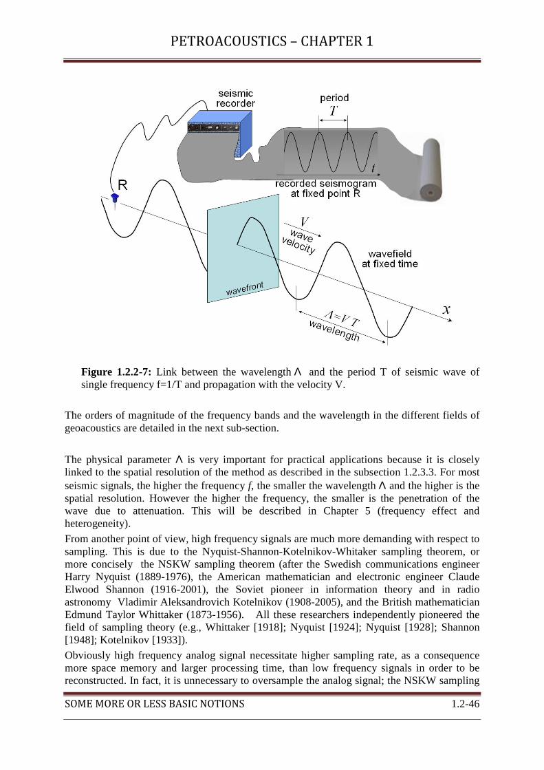
PETROACOUSTICS – CHAPTER 1
SOME MORE OR LESS BASIC NOTIONS 1.2-46
Figure 1.2.2-7: Link between the wavelength Λ and the period T of seismic wave of single frequency f=1/T and propagation with the velocity V.
The orders of magnitude of the frequency bands and the wavelength in the different fields of geoacoustics are detailed in the next sub-section.
The physical parameter Λ is very important for practical applications because it is closely linked to the spatial resolution of the method as described in the subsection 1.2.3.3. For most seismic signals, the higher the frequency f, the smaller the wavelength Λ and the higher is the spatial resolution. However the higher the frequency, the smaller is the penetration of the wave due to attenuation. This will be described in Chapter 5 (frequency effect and heterogeneity).
From another point of view, high frequency signals are much more demanding with respect to sampling. This is due to the Nyquist-Shannon-Kotelnikov-Whitaker sampling theorem, or more concisely the NSKW sampling theorem (after the Swedish communications engineer Harry Nyquist (1889-1976), the American mathematician and electronic engineer Claude Elwood Shannon (1916-2001), the Soviet pioneer in information theory and in radio astronomy Vladimir Aleksandrovich Kotelnikov (1908-2005), and the British mathematician Edmund Taylor Whittaker (1873-1956). All these researchers independently pioneered the field of sampling theory (e.g., Whittaker [1918]; Nyquist [1924]; Nyquist [1928]; Shannon [1948]; Kotelnikov [1933]).
Obviously high frequency analog signal necessitate higher sampling rate, as a consequence more space memory and larger processing time, than low frequency signals in order to be reconstructed. In fact, it is unnecessary to oversample the analog signal; the NSKW sampling
PETROACOUSTICS – CHAPTER 1
SOME MORE OR LESS BASIC NOTIONS 1.2-47
theorem gives the optimum sampling frequency allowing a complete reconstruction of the continuous-time function from the digitized function. The NSKW sampling theorem states that a band-limited analog signal must be sampled at a rate NSKWf at least equal to twice the
highest frequency maxf contained in the spectrum of the input analog signal, the optimum
sampling rate being max2 ffNSKW= .
For instance, the commercial audio Compact Discs (CD) have a specification of roughly kHzfNSKW 44≈ sampling rate, which correspond to a maximum reconstructed frequency of
specification of roughly kHzff NSKW 222/max ≈= , which is slightly larger than the
maximum audible frequency by humans (that is to say roughly kHz20 ) (see Figure 1.2.2-8 and the corresponding comments). As a consequence, high-fidelity sound systems with sampling rate higher than kHzfNSKW 44≈ , proposed by some commercial manufacturer, can
be considered as selling points, and are obviously useless except maybe for music-loving bats or cats, as illustrated in the next subsection.
Besides, in seismics applied to the oil industry the sampling rate ranges from 2ms to 4ms, depending on the resolution needed. This corresponds to a sampling rate in frequency of
HzHzfNSKW 500250 −= , which corresponds to a maximum reconstructed frequency of
roughly HzHzff NSKW 2501252/max −≈= , which is slightly larger than the maximum
frequency present in recorded seismic signals (e.g., Sheriff and Geldart [1995]).
B. The different frequency/wavelength bands of Geoacoustics
The frequency bands of geoacoustical measurements are illustrated by Figure 1.2.2-8. The whole experimental spectrum roughly covers ten orders of magnitude, from 10-4 Hz to 106 Hz. Note that for completeness, earth tides (mainly involving semi-diurnal processes (e.g., Melchior [1974]) and corresponding to frequencies of the order of 10-5 Hz) and crustal deformations [with time constants of the order of days to years (e.g., Kobayashi and Yoshida [2004]; Sato et al. [2007]) and corresponding to frequencies of the order of 10-7 Hz to 10-5 Hz) have also been included as dynamical mechanical processes, even if they cannot be considered stricto sensu as geoacoustical experiments. With this proviso the frequency spectrum covers up to thirteen orders of magnitude.

PETROACOUSTICS – CHAPTER 1
SOME MORE OR LESS BASIC NOTIONS 1.2-48
Figure 1.2.2-8: The frequency bands of geoacoustics measurements compared to the frequency hearing ranges, and the corresponding wavelengths.
The overall spectrum can be roughly divided into three groups: :
The frequency spectrum of global seismology ranges from 10-4 Hz to 100 Hz, with three types of waves encountered, namely (e.g., Fowler [1990]; Press and Siever [2000]; Stein and Wysession [2003]):
- The body waves, corresponding to bulk P- and S-waves are characterized typically by periods of the order of 1s to 10s, corresponding to frequencies from 10-1 Hz to 100 Hz, - The surface waves, that is to say Love and Rayleigh waves, are confined to the outer layers of the Earth and are characterized typically by periods of roughly 10s to a few 100s, that is to say to frequencies from a few 10-3 Hz to 10-1 Hz, and - The normal modes are the free oscillations of the earth and are mainly excited by large earthquakes. They are characterized typically by periods of the order of 102 s to 104 s, corresponding to frequencies from 10-4 Hz to 10-2 Hz.
The frequency spectrum of applied seismics roughly ranges from 101 Hz to 104 Hz (e.g., Sheriff and Geldart [1995]; Boyer and Mari [1997]) and covers three types of experiments, namely :
PETROACOUSTICS – CHAPTER 1
SOME MORE OR LESS BASIC NOTIONS 1.2-49
- Surface seismics, equivalent to medical echography but transposed at kilometric scale to probe the earth subsurface. The sources and the receivers are located at the surface of the earth. The seismic signals are characterized by frequencies roughly higher than a few Hz-101 Hz and hardly exceeding 102 Hz, - Well seismics, using receivers in a well and sources at the surface (Vertical Seismic Profile or VSP) or both receivers and sources in two different wells (Well-to-Well seismics), is characterized typically by frequencies from a few 102 Hz to 103 Hz, and - Sonic logging (acoustic logs), using mostly piezoelectric sources and receivers on a probe lowered by a cable into a borehole. Generated waves are P- or S-waves refracted at the borehole wall and guided waves (Stoneley, Pseudo-Rayleigh) frequencies from 103 Hz to 104 Hz.
The frequency spectrum of ultrasonic laboratory experiments is characterized
typically by frequencies of 105 Hz to 106 Hz. Sources and receivers for rock acoustics are piezoelectric transducers.
The frequency spectrum of laboratory experiments can be divided into four groups (e.g., Bourbié et al. [1987]; Johnson and Rasolofosaon [1996]):
Quasi-static stress-strain tests that are performed in rock mechanics and/or geomechanical laboratories of oil companies, research institutes or universities. They are conducted over frequency interval of near zero to a few Hz.
Torsional oscillator experiments used in a few university laboratories and research institutes. They are conducted over frequency interval of 0.1 Hz to 100 Hz. This is close to the frequency interval of seismic experiments.
Resonant-bar experiments used in some research institutes and universities. They take place over the frequency interval of 102 Hz to 104 Hz, that is to say the frequency interval encountered in acoustic logging in the field.
Dynamic and propagative ultrasonic waves that are used in the rock acoustics (or petroacoustics) laboratories of oil companies, research institutes, or universities. They are characterized typically by frequencies of 105 Hz to 106 Hz,
For comparison the frequency hearing ranges of humans and of a couple of animals are plotted in the bottom part of Figure 1.2.2-8. Human frequency hearing range is typically considered to be between 20 Hz and 20 kHz. This range significantly varies with age and professional hearing damage. Ultrasounds and infrasounds are mechanical vibrations of frequencies respectively higher and lower than audible frequencies. Animals such as elephants, giraffes and whales use infrasounds to communicate even over large distances (e.g., Garstang et al. [1995]; McComb et al. [2003]; Tomecek [2009]). Other animals such as cats and dogs are able to hear ultrasounds, and some others such as bats use them for echolocation (e.g., Fenton and Bell [1981]; Barclay [1999]).

PETROACOUSTICS – CHAPTER 1
SOME MORE OR LESS BASIC NOTIONS 1.2-50
BOX 1.2.2-4
Time width and Frequency bandwidth – Fourier transform
The frequency content of a time function can be analyzed by Fourier transformation
(noted ), after the French mathematician and Physicist Jean Baptiste Joseph Fourier (1768–1830), defined by (e.g., Bracewell [1965]):
↔ .
designates the frequency, the inverse Fourier transform, and the Fourier transform of . Note that the opposite sign convention for all the terms in power of the exponential exist (e.g., Cerveny [2001]). We use the present convention consistently with Equations (1.2.2-28), (1.2.2-33), (1.2.2-36) and (1.2.2-40) for instance. The concept is commonly used in many fields including data processing and analysis, image processing and filtering, antennas designing and using, and differential equation solving, to name a few (e.g., Bracewell [1965]).
The general result , being a constant, means that if the time scale
of the function is contracted by a factor (shortening of the pulse duration) the frequency spectrum expands by the factor , and vice-versa. In other words the shorter the pulse the larger its bandwidth, and vice-versa. As a consequence the signal and its Fourier transform cannot be stretched or compressed simultaneously, which implies an uncertainty relation of the same type as Heisenberg's uncertainty relation in quantum mechanics [De Bruijn, 1967] [named after the German theoretical physicist Werner Karl Heisenberg (1901–1976)].
As an example, let us consider the Gaussian function [after the famous German mathematician and scientist Johann Carl Friedrich Gauss (1777-1855)], known as the bell-shape function, and
defined by: .
The corresponding Fourier transform is , which is also a
Gaussian function. The frequency bandwidth of at -8.68dB below the maximum is
given by which is indeed inversely proportional to the time width of .
Time dependence of the Gaussian function
is the time width of the
signal at an amplitude equal to its maximum divided by Euler's number [named after the Swiss mathematician and physicist Leonhard Euler (1707-1783)]
, which roughly corresponds to -8.68dB below the maximum.

PETROACOUSTICS – CHAPTER 1
SOME MORE OR LESS BASIC NOTIONS 1.2-51
C. Spatial resolution
According to Sheriff [2002] the resolution of a system in geophysics is the ability to separate two features that are close together. Similarly, in radar science resolution is defined as the ability to distinguish between targets that are very close (e.g., Skolnik [1970]). In this section we will see that the spatial resolution is closely linked with the seismic wavelength.
Applied seismologists distinguish vertical resolution from horizontal resolution as illustrated
by the two next sub-sections and the corresponding figures.
a. Vertical resolution
The spatial resolution vR in reflection in a given direction of observation, or range resolution,
is well known from radar technology and is given by [Barton and Leonov, 1998]:
(1.2.2-58) )2/(2/ BWVVR sv ×≈≈ τ
where V is the average velocity of wave propagation in the medium, Sτ the time-width of the
source signal, andBW the corresponding frequency bandwidth. Note that in radar science, the electromagnetic rays can come from any direction in the aerial half space. In contrast, in surface-reflection seismics the vertical direction is the average direction of the seismic rays and the targets are in the earth subsurface. That is why vR will be called here the vertical
resolution.
The second equality (≈) in the previous equation is due to the classical result that the time-width sτ of a pulse signal is inversely proportional to the frequency bandwidth BW of this
signal, as illustrated for a Gaussian signal in Box 1.2.2-4, a good approximation for the pulse radar signals.
This is also roughly the case for the Ricker signal, the second derivative of the Gaussian function well-known as the Mexican-hat function and commonly used as a wavelet in seismic modelling for computing synthetic seismograms (e.g., Sheriff and Geldart [1995]; Yilmaz [2001]; Liner [2004]) as illustrated by Fig. 1.2.2-9.

PETROACOUSTICS – CHAPTER 1
SOME MORE OR LESS BASIC NOTIONS 1.2-52
Figure 1.2.2-9: Vertical resolution illustrated by the reflection of seismic signal (here Ricker wavelet) at the top and the bottom of a wedge layer in light brown pinching out to the left. The vertical resolution limit vR occurs when the layer is one-quarter of wavelength thick
(modified after Liner [2004] and Widess [1973])
On this figure, the vertical resolution is illustrated by the reflection of a seismic signal, namely a Ricker wavelet, at the top and the bottom (in brown solid line) of a wedge layer (in light brown) pinching out to the left. Because for the special case of Ricker wavelet, as well as for typical seismic signal in general, the frequency bandwidth BW does not differ much from the central frequency MAXf of the wavelet. As a consequence the last equation implies that
the vertical resolution is proportional to the average wavelength Λ. More precisely the vertical resolution limit vR occurs when the layer is one-quarter of wavelength Λ thick, as shown by
Fig. 1.2.2-9. As pointed out by Liner [2004], when the bed is thinner than this limit the top and the bottom reflections merge into a single signal. Distinct peaks are observed when the layer is thicker than Λ /4.
b. Horizontal resolution
Let us consider a surface seismics experiment with a coincident source-receiver (E/G) couple located at the origin of a trihedron xyz and at the free surface of a 3D isotropic homogeneous medium as shown by Fig. 1.2.2-10. Now let us analyze the wave reflection at a plane horizontal interface located at depth z, not only through the specular vertical ray GH but also

PETROACOUSTICS – CHAPTER 1
SOME MORE OR LESS BASIC NOTIONS 1.2-53
through non-specular rays such as EB or EA. Although this figure only represents a two-dimensional cut of the geometrical configuration, the overall problem is three-dimensional and exhibits the vertical axis EH (normal to the interface) as an axis of rotational invariance.
Figure 1.2.2-10: The horizontal resolution limit hR before seismic migration is equal to the
diameter of the first Fresnel zone
The positions of the points A and B are such that the seismic path difference between the vertical ray EH and the oblique rays EA or EB is equal to Λ/4 , a quarter of the dominant seismic wavelength, which corresponds to a total path difference of Λ/2 in reflection (i.e. Λ/4 for the way down and Λ/4 for the way back up) and equivalently a time-lag of half a period. The horizontal disk of diameter AB constitutes the first Fresnel zone, of which all the points interfere constructively for reflection. Only this portion of the reflector contributes constructively to the reflection (e.g., Sheriff and Geldart [1995]). Thus the distance AB=hR
quantifies the horizontal resolution limit or the size of the smallest elementary reflector detectable by the seismic set-up. The explicit expression of hR can be found by applying
Pythagoras' theorem to the triangle EHB:
(1.2.2-59) ( ) ( )222 4/2/ Λ+=+ zRz h
which gives:
(1.2.2-60) ( ) ( ) Λ≈−Λ+= zzzRh 24/4 222 or Λ≈ zRh 2
The approximate equality (≈) holds if we assume that the reflector depth z is much larger than the dominant wavelengthΛ .
All the above description is made before a special type of data processing called seismic migration (see Box 1.2.2-5). Just as migration collapses the diffraction patterns by focusing the seismic energy on the elementary diffraction points composing the reflectors, migration

PETROACOUSTICS – CHAPTER 1
SOME MORE OR LESS BASIC NOTIONS 1.2-54
BOX 1.2.2-5
Seismic migration: Concise description and Illustration
Seismic migration is a common type of seismic data processing for imaging (e.g. Yilmaz [2001]) that can be simply described in the following way. Suppose that the reflector plotted on Fig.1.2.2-10 is replaced by the single point at depth Z [see Fig. (a)] the only reflected signal recorded by all the receivers (case of coincident source and receiver) located at the surface in the xy-plane would come from this single diffraction point. Diffraction waves are recorded by all the receivers and appear as a special diffraction pattern, namely a diffraction hyperbola, on the seismograms (e.g., Sheriff and Geldart [1995]), as illustrated by Fig. (b).
(a) The 2D earth model consisting of a single diffraction point, and
(b) The corresponding zero-offset (coincident source and receiver) seismic section, constituted of a display along a line of the signals recorded by all the receivers located at the surface along the x-axis, the vertical axis being the arrival time. The typical figure obtained is the diffraction pattern (after Yilmaz [2001] and Sheriff [2002])
(c) Raw data corresponding to Physical modeling of marine seismic reflection experiment (zero-offset) in the laboratory on a scale model immersed in a water tank, and
(d) Same data as in (c) after seismic migration allowing to reconstruct a correct image of the reflector.
Seismic migration consists in focusing all the diffraction energy exactly on the single point H at the correct location. Furthermore the plane reflector of Fig.1.2.2-10, as well as any curved reflector, can be decomposed in an infinite number of points, which can be considered as potential diffraction points. Obviously in practice the reflector surfaces are pixelized and decomposed in a finite number of points. The elementary migration operation previously described is repeated on each individual point, considered as a diffraction point. The main role of migration is to correct for the distorsion and artifacts images observed on the raw seismic sections, as those shown on the data of Fig.(c). The main effects are, from one hand the reconstruction of the true shape of the reflectors and the correct positioning of these reflectors at their true location in the subsurface, and from another hand to wipe out the remaining diffraction patterns interfering with the rest of the display. This is illustrated by Fig.(d) and by the more detailed laboratory results on seismic imaging with scale models in section 2.3.2.3.
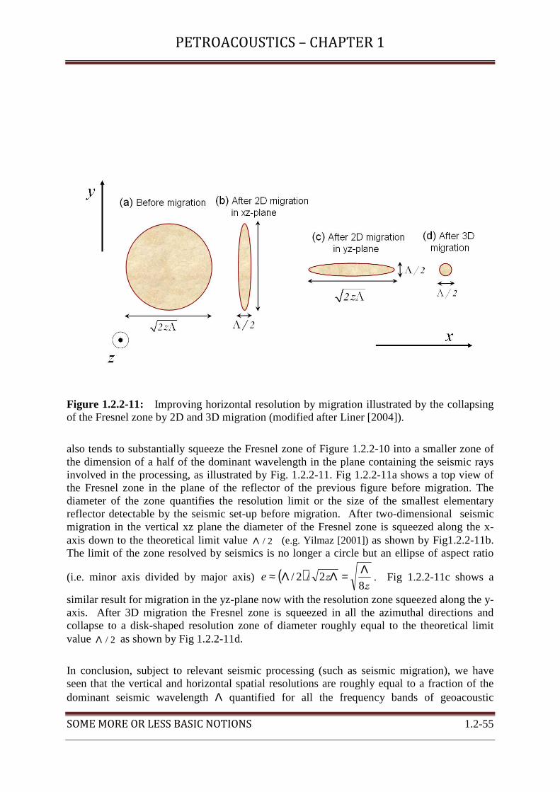
PETROACOUSTICS – CHAPTER 1
SOME MORE OR LESS BASIC NOTIONS 1.2-55
Figure 1.2.2-11: Improving horizontal resolution by migration illustrated by the collapsing of the Fresnel zone by 2D and 3D migration (modified after Liner [2004]).
also tends to substantially squeeze the Fresnel zone of Figure 1.2.2-10 into a smaller zone of the dimension of a half of the dominant wavelength in the plane containing the seismic rays involved in the processing, as illustrated by Fig. 1.2.2-11. Fig 1.2.2-11a shows a top view of the Fresnel zone in the plane of the reflector of the previous figure before migration. The diameter of the zone quantifies the resolution limit or the size of the smallest elementary reflector detectable by the seismic set-up before migration. After two-dimensional seismic migration in the vertical xz plane the diameter of the Fresnel zone is squeezed along the x-axis down to the theoretical limit value 2/Λ (e.g. Yilmaz [2001]) as shown by Fig1.2.2-11b. The limit of the zone resolved by seismics is no longer a circle but an ellipse of aspect ratio
(i.e. minor axis divided by major axis) ( )z
z8
2/2/Λ=ΛΛ≈e . Fig 1.2.2-11c shows a
similar result for migration in the yz-plane now with the resolution zone squeezed along the y-axis. After 3D migration the Fresnel zone is squeezed in all the azimuthal directions and collapse to a disk-shaped resolution zone of diameter roughly equal to the theoretical limit value 2/Λ as shown by Fig 1.2.2-11d.
In conclusion, subject to relevant seismic processing (such as seismic migration), we have seen that the vertical and horizontal spatial resolutions are roughly equal to a fraction of the dominant seismic wavelength Λ quantified for all the frequency bands of geoacoustic

PETROACOUSTICS – CHAPTER 1
SOME MORE OR LESS BASIC NOTIONS 1.2-56
measurements in section 1.2.2.3. We emphasized that this is the case for typical seismic signals, as for the classical Ricker wavelet, because the corresponding frequency bandwidth BW does not differ much from the central frequency. However, more correctly seismic time resolution, as in radar science, is essentially determined by the time-width (or pulse width) of the source signal, and thus by the corresponding frequency bandwidth as described by Equation (1.2.2-58) and the corresponding comments.
1.2.3 Heterogeneity, dispersion, anisotropy and attenuation in continuous media
Most of classical textbooks in mechanics start by assuming a homogeneous isotropic linearly elastic medium. These are only convenient assumptions in order to simplify the theoretical derivations. In detail most natural media, including geological media, do not strictly verify these simplifying assumptions, at least weakly. The mechanical properties can vary with parameter as different as the observation point P, the direction of observation, or the frequency among others. In this sub-section we define the characters that deviate from the ideal homogeneous isotropic linearly elastic behaviour.
1.2.3.1 Heterogeneity
According to Etimonline, the adjective "homogeneous" comes from the Latin adjective "homogeneus" and from the Greek adjective "homogenes", meaning "of the same kind", itself a combination of the prefix "homo-" (coming from the Greek adjective "homos", meaning "same", and the Greek noun "genos " , meaning "kind, gender, race, stock". The suffix "-ity" of the noun ""homogeneity" is the usual suffix forming abstract nouns from adjectives (here "homogeneous"), meaning "condition or quality of being..." The words "heterogeneous" and "heterogeneity" are the contrary of the words "homogeneous" and "homogeneity" respectively, and are constructed by substituting the prefix "hetero-" (coming from the Greek adjective "heteros", meaning "different").
A medium exhibits heterogeneity, with respect to a given physical property (elastic or electromagnetic wave velocity, electric or thermal conductivity, mechanical strength...) and to corresponding measurement accuracy, if this property depends on the observation point P at the considered accuracy level, the other parameters remaining fixed. The medium is said to be heterogeneous with respect to the considered physical property at the considered measurement accuracy. In the opposite case the medium exhibits homogeneity, and is said to be homogeneous with respect to the considered physical property at the considered measurement accuracy. In the special case of acoustics the physical property is elastic wave velocity, density and/or impedance.
Note that, if the accuracy level of physical measurements were infinite, any real material would be virtually heterogeneous with respect to any physical property due to possible infinitesimal spatial variation of the physical properties resulting from possible infinitesimal spatial variation of the local physical conditions (e.g., stress, temperature...). Correlatively, for instance, because the major mineral constituents of rocks have densities roughly ranging from
32200 /kg m to 33500 /kg m (e.g., Bass [1995]; Clark [1966]), if the accuracy level of density measurement were not better than roughly 60%, any rock formation would be virtually

PETROACOUSTICS – CHAPTER 1
SOME MORE OR LESS BASIC NOTIONS 1.2-57
homogeneous with respect to density. That is why, in general, the specification of the accuracy level of the physical measurement to be considered is important.
1.2.3.2 Anisotropy
The noun "isotropy" is derived from the Greek words "iso", meaning same, and "tropos" meaning direction. Note that the noun "anisotropy" is defined as the negative of the noun "isotropy", with the Greek privative prefix an-, meaning not or without.
A medium exhibits anisotropy, with respect to a given physical property (elastic or electromagnetic wave velocity, electric or thermal conductivity, mechanical strength...) and to corresponding measurement accuracy, if this property depends on the direction of observation at the considered accuracy level, the other parameters remaining fixed. In this case the medium is said to be anisotropic with respect to the considered physical property at the considered accuracy level. In the opposite case the medium exhibits isotropy, and is said to be isotropic with respect the considered physical property at the considered accuracy level. In the special case of acoustics the physical property is elastic wave velocity, density and/or impedance.
As for heterogeneity, if the accuracy level of physical measurements were infinite, any real material would be virtually anisotropic with respect to any physical property due to possible infinitesimal directional variation of the physical properties resulting from possible infinitesimal directional variation of the physical conditions (e.g., stress ...). Correlatively, for instance, because the directional dependence of the elastic wave velocities hardly exceed roughly 50% in the major mineral constituents of rocks (e.g., Babuska and Cara [1991]), if the accuracy level of velocity measurement were not better than roughly 50%, any rock formation would virtually be isotropic with respect to elastic wave propagation. Here again we emphasize the necessity of specifying the accuracy level of the physical measurement.
Some authors used the terms aeolotropy and aeolotropic (e.g., Love [1944]; Stoneley [1949]), instead of anisotropy and anisotropic respectively, but both of these terms are now quite uncommon.
Because heterogeneity and anisotropy are sometimes erroneously mixed up, Figure 1.2.3-1 illustrates the difference between heterogeneity and anisotropy with respect to elastic wave propagation [Gassmann, 1972]. Four elastic media labelled from (a) to (d) are considered, namely (a) an isotropic and homogeneous medium, (b) an isotropic but heterogeneous medium, (c) a homogeneous but anisotropic medium, and (d) an anisotropic and heterogeneous medium. All exhibit an increase of the wave velocity with depth. On the right part of each cartoon, a seismic source is located at mid-depth of each medium and different snapshots of the seismic wavefronts at regular time interval are plotted, together with the corresponding seismic rays. In homogeneous media, corresponding to cases a and c, all the seismic rays, that is to say the lines normal to the wavefronts, are straight lines and are all the
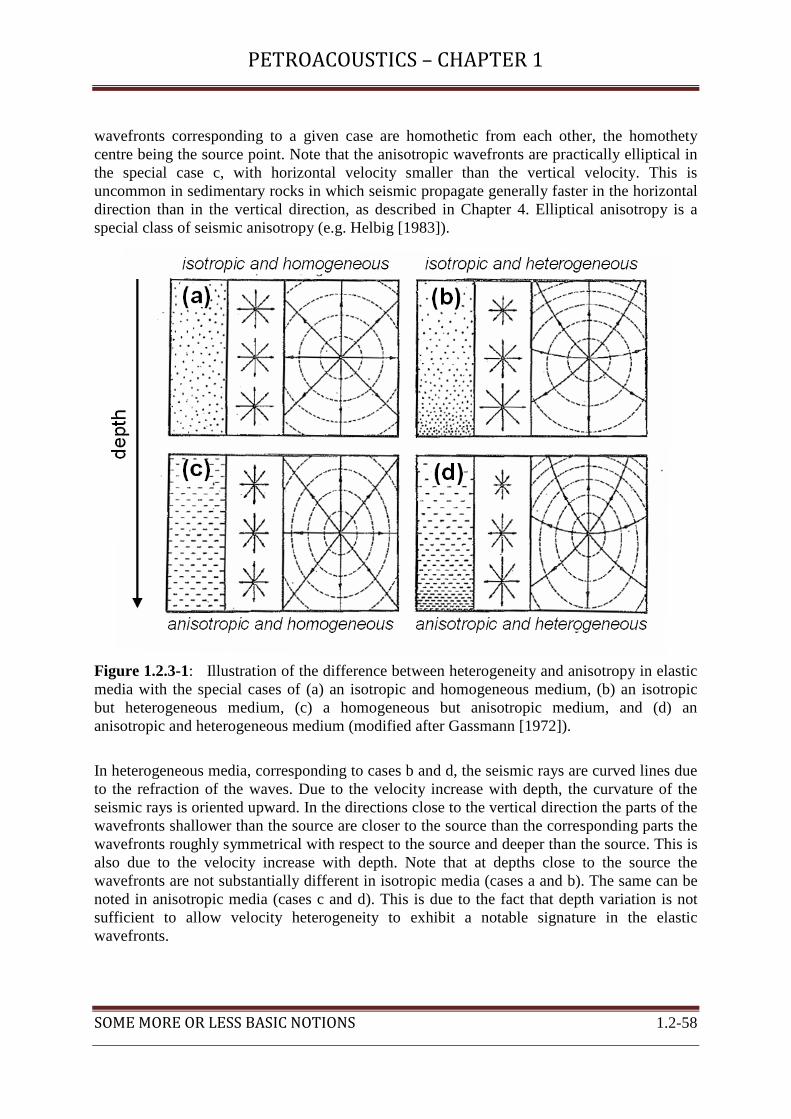
PETROACOUSTICS – CHAPTER 1
SOME MORE OR LESS BASIC NOTIONS 1.2-58
wavefronts corresponding to a given case are homothetic from each other, the homothety centre being the source point. Note that the anisotropic wavefronts are practically elliptical in the special case c, with horizontal velocity smaller than the vertical velocity. This is uncommon in sedimentary rocks in which seismic propagate generally faster in the horizontal direction than in the vertical direction, as described in Chapter 4. Elliptical anisotropy is a special class of seismic anisotropy (e.g. Helbig [1983]).
Figure 1.2.3-1: Illustration of the difference between heterogeneity and anisotropy in elastic media with the special cases of (a) an isotropic and homogeneous medium, (b) an isotropic but heterogeneous medium, (c) a homogeneous but anisotropic medium, and (d) an anisotropic and heterogeneous medium (modified after Gassmann [1972]).
In heterogeneous media, corresponding to cases b and d, the seismic rays are curved lines due to the refraction of the waves. Due to the velocity increase with depth, the curvature of the seismic rays is oriented upward. In the directions close to the vertical direction the parts of the wavefronts shallower than the source are closer to the source than the corresponding parts the wavefronts roughly symmetrical with respect to the source and deeper than the source. This is also due to the velocity increase with depth. Note that at depths close to the source the wavefronts are not substantially different in isotropic media (cases a and b). The same can be noted in anisotropic media (cases c and d). This is due to the fact that depth variation is not sufficient to allow velocity heterogeneity to exhibit a notable signature in the elastic wavefronts.
PETROACOUSTICS – CHAPTER 1
SOME MORE OR LESS BASIC NOTIONS 1.2-59
The heterogeneous, anisotropic, dispersive or attenuative characters of a medium are not absolute characters of the medium but are relative to the considered physical phenomenon, and to the scale of observation, namely to the elastic wavelength Λ for elastic wave propagation.
Regarding anisotropy, for instance cubic crystals are isotropic with respect to optical or electromagnetic waves but anisotropic with respect to elastic waves (e.g., Voigt [1910]; Sirotine and Chaskolskaya [1975]; Nye [1985]). Regarding anisotropic rocks, Rasolofosaon and Zinszner [2002] observed that the elastic anisotropy and the hydraulic anisotropy are closely correlated in some rocks, especially when these physical properties share the same cause (e.g., layering, fractures). In contrast, in some other rocks, hydraulic properties and elastic properties are clearly uncorrelated, which highlights the difficulties for estimating permeability anisotropy from elastic anisotropy in rocks.
Regarding the characteristic scale of the phenomenon, namely the wavelength Λ for wave propagation, for instance a crystal does not behave in the same manner with Electromagnetic X-ray commonly used for crystallography, of wavelengths around 0.1nm, and with Electromagnetic visible light waves of wavelengths roughly from 0.4µm to 0.8µm. X-ray diffractometers can detail the arrangement of atoms (of typical dimension ~0.1nm) in crystals, allowing to identify the crystal symmetry (e.g., Hammond [1997]; Rhodes [2000]). In contrast, crystals behave as homogeneous anisotropic media with optical waves (e.g., Born and Wolf [1986]; Nye [1985]). With respect to elastic waves, a 1D stratified medium with isotropic constituents behaves as an anisotropic medium if the elastic wavelength Λ is much larger than the thicknesses of the constituent layers (e.g., Bruggeman [1937]; Riznichenko [1948]; Riznichenko [1949]; Postma [1955]; Helbig [1958]; Backus [1962]). If the elastic wavelength Λ is much smaller than the thicknesses of the constituent layers the medium behave as a vertically heterogeneous medium composed of isotropic layers. This model is chosen by Helbig [2009] to illustrate the close link between anisotropy and dispersion as detailed in section 1.2.3.3.
1.2.3.3 Dispersion
The noun "dispersion" comes from the Latin noun "dispersio", meaning a scattering. Note that, in contrast with the noun "anisotropy", the noun "dispersion" is not defined as the negation of another noun.
A medium exhibits dispersion, with respect to a physical property involving wave propagation (i.e., elastic or electromagnetic wave propagation), and to the corresponding measurement accuracy, if the physical property depends on the wavelength Λ at the considered accuracy level, the other parameters remaining fixed. In such case the medium is said to be dispersive with respect to the physical property at the considered accuracy level. In the opposite case the medium does not exhibit any dispersion, and is said to be non-dispersive with respect the considered physical property at the considered accuracy level. In the special case of acoustics the physical properties considered are elastic wave velocity, density or impedance (see Boxes 1.2.3-1 and 1.2.3-2)

PETROACOUSTICS – CHAPTER 1
SOME MORE OR LESS BASIC NOTIONS 1.2-60
The induced dispersion is extrinsic (or of geometric type) if the velocity dependence on the wavelength Λ is due to geometrical effects (for instance length of the sample, radius of a borehole, thickness of a plate…). Such type of dispersion is exhibited by waves propagating in waveguides, for instance the guided elastic waves in boreholes encountered in acoustic logging (e.g., Paillet and White [1982]; White [1983]) or the guided electromagnetic or optical waves in the different waveguides components of communication and radar antenna systems (e.g., Mahmoud [1991]; Okamoto [2000]). Note that such kind of dispersion is not necessarily associated with attenuation.

PETROACOUSTICS – CHAPTER 1
SOME MORE OR LESS BASIC NOTIONS 1.2-61
BOX 1.2.3-1
Group velocity, phase velocity and dispersion: Concise description and
Illustration
Let us consider the behaviour of a wave packet ( , )u x t during its propagation illustrated by the figure below in a dispersive medium (figure on the left-hand side) and in a non-dispersive medium (figure on the right-hand side). The figure displays the wavefield amplitude ( , )u x t for
Variation in time of a wave packet, group velocity and phase velocity in a dispersive medium (on the left hand side) and in a non-dispersive medium (on the right hand side) for five time values t1 to t5). Note the change of shape of the waveform during the propagation in the dispersive medium.
any distance x from the source but for fixed time t, here t1 to t5. For instance, the function ( , )u x t for fixed time t, often called a snapshot in seismics [Sheriff, 2002], could correspond for fixed time t to the shape of a vibrating string in one dimension or to the shape of the surface of a pond in two dimension in which a pebble has been thrown. In a dispersive medium the maximum of the envelope of the wave
packet (materialized by the red dots and referenced by the positions'1E to
'5E ), travels at the group
velocity grV , different from the phase velocity
phV of an individual peak within the wave packet
(referenced by the positions '1P to
'5P and materialized by the green dots). In the considered case
ph grV V< (the red dots travel faster than the green dots), which is not a rule. Because the velocity of each individual peak, or each phase, or more exactly of each frequency component is different from the velocity of the other frequency components, the shape of the wave packet changes during the propagation in a dispersive medium. In contrast, in non-dispersive media (figure on the right-hand
side) all the frequency components travel at the same speed ph grV V= (the red dots and the green
dots travel at the same speed). As a consequence the shape of the wave packet is unchanged during the propagation. A more detailed mathematical description is proposed in Box 1.2.3-2.

PETROACOUSTICS – CHAPTER 1
SOME MORE OR LESS BASIC NOTIONS 1.2-62
BOX 1.2.3-2
Group velocity, phase velocity and dispersion: Analytical description
Let us consider the wave packet ( , )u x t as a superposition of waves of different amplitude and frequency, according to the following equation:
[ ] ( , ) ( ) exp ( )u x t U k i k t k x dk+∞
−∞= ω −∫ ,
where ( )U k is the Fourier transform (FT) of the function ( , )u x t for fixed time t (see Box 1.2.2-4 ; note that in that box the conjugate variables for the FT were the time t and the frequency f. In contrast, here the conjugate variables are the space variable x and the wave number k , but the formulation is identical). Note that in general, that is to say in dispersive media, the angular frequency 2 fω = π is a function of
the wavenumber / phk V= ω , where phV is the frequency-dependent phase velocity (see section 1.2.2.1).
Let us assume that the Fourier spectrum amplitude ( )U k slowly varies with k and is non-zero over a
narrow band centered at 0k . This is the case for the signals of Box 1.2.3-1 and in most of the cases in
practice where the central frequency 0f of the carrier signal, that is to say the high-frequency signal
modulated in amplitude, is much larger than the frequency of the envelope of the wave packet or the amplitude-modulation signal. As a consequence the Fourier spectrum amplitude ( )U k only takes
notable values over a narrow band centered at 0 0 0/ ( )phk V= ω ω , where 0 02 fω = π is the angular
frequency of the carrier signal and 0( )phV ω the phase velocity at this frequency. Thus the dispersion
relation can be developed in the vicinity of 0k :
( )0
0 0( ) ( )k k
dk k k k
dk =
ω ω ≈ ω + − ,
which inserted in the integral definition of ( , )u x t leads to [Dieulesaint and Royer, 1974]:
00( , ) ( ( ) ,0)i t gru x t e u x V k tΩ= −
where 0
0( )gr
k k
dV k
dk =
ω = and 0 0 0 0( ) ( )grk k V kΩ = ω − . The previous equation shows that the
wave packet travelled the distance 0( )grV k t during the time t with the velocity 0( )grV k , called the
group velocity. More detailed considerations on the mathematical methods used here for the integration near a stationary point, such as the so-called stationary phase method, steepest descent method or saddle point method can be found in classical textbooks on physical mathematics (e.g., Morse and Feshbach [1953]).
In non-dispersive media the angular frequency ω is independent of the wave number k , or equivalently
the phase velocity phV does not depend on the frequency. As a consequence the phase lag due to a
travel distance x is equal to / phx V−ω and is proportional to the frequency. Lastly the dispersion
relation simply writes:[ ] ( )0 0 0 0( ) ( ) / /k k k k kω −ω − = ω or equivalently
( )0 0( ) ( ) phk k V k kω = ω + − (note that it is an exact equality “=” and not an approximate equality
“≈”). As a consequence the group velocity grV is equal to the phase velocity phV and is independent of the frequency.
PETROACOUSTICS – CHAPTER 1
SOME MORE OR LESS BASIC NOTIONS 1.2-63
In contrast, the induced dispersion is intrinsic if the velocity dependence on the wavelength Λ is due to the medium of propagation itself excluding any of the aforementioned geometrical effects. Such type of dispersion is always associated with attenuation (see next sub-section) and is exhibited by viscoelastic models (see Chapter 5 on Frequency dependence) or Biot poroelastic model (see Chapter 6 on Poroelasticity) for instance.
Here again we insist on the fact that the intrinsic or extrinsic character of dispersion is not absolute but relative to the considered physical phenomenon, and to the scale of observation, namely to the elastic wavelength Λ for elastic wave propagation.
The dispersion is said to be normal if shorter wavelengths travel slower than longer wavelengths. In other words normal dispersion occurs if the group velocity decreases with the frequency, or equivalently increases with the wavelength [Bourbié et al., 1987]. Conversely, if high frequency components travel faster than the lower ones, the medium is anomalously dispersive. The dispersion is said to be inverse or anomalous, and the group velocity increases with the frequency. This is the case for any viscoelastic medium [Bourbié et al., 1987], as detailed in Chapter 5 on Frequency dependence. Lastly, as pointed out by Helbig [2009], dispersion and anisotropy which may appear as disjoint phenomena are closely linked. More precisely by considering a common independent variable, namely the wave vector K , the vector normal to the wavefront with length proportional to the wave number k , linked to the wavelength Λ , to the frequency f and to the wave velocity V by the relations Λ== /2/2 ππ Vfk (see also sub-section 1.2.2.2.B.b.1). Anisotropy and dispersion are simply the dependences of the velocity V on the direction and on the length, respectively, of the wave vector K.
1.2.3.4 Attenuation
According to Etimonline, the noun "attenuation" is derived from the verb "attenuate", itself coming from the Latin word "attenuatus" (meaning "enfeebled, weak"), preterit of the Latin verb "attenuare" (meaning "to make thin, lessen, diminish").
A medium exhibits attenuation, with respect to wave propagation (i.e., elastic or electromagnetic wave) at a given measurement accuracy, if the amount of energy transported per unit time by the wave, or the energy flux of the wave field, crossing a fixed unit surface parallel to the wave front, that is to say the norm of the Umov-Poynting-Heaviside vector P(see §1.2.2.2 and box 1.2.2-2) decreases during propagation at the considered accuracy level, the other parameters remaining fixed. In such case the medium is said to be attenuative with respect to wave propagation at the considered accuracy level. In the opposite case the medium does not exhibit any attenuation, and is said to be non-attenuative with respect to wave propagation at the considered accuracy level. In the special case of acoustics the wave considered are elastic waves.

PETROACOUSTICS – CHAPTER 1
SOME MORE OR LESS BASIC NOTIONS 1.2-64
The induced attenuation is extrinsic (or of geometric type) if the energy decrease is due to is due to geometrical effects. This is caused by the deformation of the wavefront induced by local heterogeneities (defocusing of the wave rays) at these scales. Note that the energy flux of the wave field can also increase locally due to local focusing of the seismic rays. In contrast, the induced attenuation is intrinsic if the energy decrease is due to the medium of propagation itself excluding any geometrical effect.
As for dispersion we insist on the fact that the intrinsic or extrinsic character of attenuation is not absolute but relative to the considered physical phenomenon, and to the scale of observation, namely to the elastic wavelength Λ for elastic wave propagation.
Intrinsic dispersion and intrinsic attenuation are not independent in causal systems, such as physical media. A system is causal if it is unable to respond to a solicitation force before this latter is applied. The frequency dependences of the dispersion function and of the attenuation function are necessarily linked by the Kramers-Kronig relations (e.g., Aki and Richards, [1980]) through a Hilbert transform as detailed in Chapter 5 on Frequency dependence. This has been checked experimentally in various materials by Pouet and Rasolofosaon [1993] using wide bandwidth experimental system such as laser ultrasonics, as illustrated in §2.3.3.3.
1.2.3.5 Elasticity (linear, nonlinear possibly with hysteresis) and Anelasticity
According to Etimonline, the adjective "elastic" is coined in French since 1650s as the adjective "élastique" as a scientific term to describe gases, from the modern Latin adjective "elasticus" and from the Greek adjective "elastos", meaning "ductile, flexible". The adjective "linear" comes from the Latin word "linearis", meaning "belonging to a line", the latter coming from the Latin noun "linea" meaning "string, line". Lastly the noun "hysteresis" is derived the ancient Greek word ὑστέρησις (hysteresis) variously meaning "deficiency, shortcoming, or lagging behind".
The medium exhibits elasticity, or an elastic behaviour, if it instantaneously deforms reversibly under stress at the accuracy level of the measurement, the other parameters remaining fixed. In such case the medium is said to be elastic at the considered accuracy level.
In other words, in such media the stress is an analytic function of the strain at the considered accuracy level. If this functional dependence is linear the medium exhibits linear elasticity, and the medium is said to be linearly elastic at the considered accuracy level. Otherwise one deal with nonlinear elasticity and the medium considered is said to be nonlinear elastic at the considered accuracy level. Furthermore if the stress-strain curve between an initial state A and a final state B depends not only on the states A and B but also on the stress history at the considered accuracy level, the stress-strain is said to exhibit stress-history dependence, path-dependence or hysteresis at the considered accuracy level. The medium is said to be hysteretic (see Chapter 7 on nonlinear elasticity) at the considered accuracy level. Hysteresis phenomenon is encountered in various fields, including mechanics, physics (friction, ferromagnetic and ferroelectric hysteresis, superconductivity, supercooling), hydrology (soil-
PETROACOUSTICS – CHAPTER 1
SOME MORE OR LESS BASIC NOTIONS 1.3-65
moisture hysteresis), economics, chemistry, biology, to name a few (e.g., O'Donnagain [2004]; Bertotti and Mayergoyz [2006]).
The noun "anelasticity" is defined as the negative of the noun "elasticity", with the Greek privative prefix an-, meaning not or without. A medium exhibits anelasticity if the deformation reversibly depends on the time rate of change of stress as well as on the stress itself (e.g., James [1989]) at the considered accuracy level. In such case the medium is said to be anelastic at the considered accuracy level. Viscoelastic media (see Chapter 5 on Frequency dependence) are examples of such media. Due to reversibility, the medium recovers its original shape if the stress is removed. Time dependence means that the strain response to an applied stress is not instantaneous. It takes finite time for the strain to reach its equilibrium value for a given stress.
According to Etimonline, the adjective "plastic" comes from the Latin "plasticus" and from the Greek. “plastiko” meaning "able to be molded, pertaining to molding", itself coming from “plastos” meaning "molded," and from “plassein" meaning “to mold". A medium is plastic, or exhibits “plasticity” if its strain response to an applied stress is both time dependent and irreversible at the considered accuracy level (e.g., James [1989]). Time dependence means that the strain continuously changes with time without reaching an equilibrium level for a given stress. Due to irreversibility, the medium also do not recover its original shape if the stress is removed, even after long times. Note that above a certain level of applied stress virtually any real material more or less exhibits such type of behaviour. Such stress levels are seldom reached in mechanical wave phenomena but in nuclear explosions or big earthquakes not too far from the sources.
Lastly, regarding all these deviations from the ideal homogeneous isotropic linearly elastic behaviour, all the mixed behaviours are possible. For instance Carcione [2007] describes media exhibiting attenuation/dispersion and anisotropy. Attenuation/dispersion, heterogeneity and anisotropy are dealt with by Cerveny et al. [2008]. There even seems to be no limit in the sophistication of the models with media exhibiting simultaneously dispersion/attenuation, anisotropy, and nonlinearity possibly with the presence of hysteresis [Rasolofosaon, 2009].
1.3 Physics in real media – Hierarchical structure of Geological media and continuum mechanics in such media
In the previous section all the fields (displacement, strain, stress ...) and physical properties (density, elastic moduli, velocities...) were assumed to be continuous and even analytic functions of both time and space variables (except at a limited number of surfaces of discontinuities, see for instance §1.2.2.2 on reflection/transmission at interfaces). However real media, which are composed of atoms and molecules, are all but continuous media. In this section we first describe how to make the link between this ideal mathematical view point and the physical view point. Then we show how to adapt the ideal mathematical tool to the description of mechanics, first in simple real media, then in more complicate media such as geological media.

PETROACOUSTICS – CHAPTER 1
SOME MORE OR LESS BASIC NOTIONS 1.3-66
The section is organized in the following way. First we introduce the specificity of physics in real media and the continuum representation of such media. Then we introduce a particular class of complicate real media, namely geological media. We show the specific hierarchical structure (multi-scale heterogeneity) of geological media and their continuum representation for mechanics.
1.3.1 Physics in simple real media and continuum representation
This sub-section is inspired by Challande [2004]. Here we shall consider only simple real media, such homogeneous fluid (liquid or gas), homogeneous amorphous solids or monocrystals.
In mathematics a point, although not given a precise definition as any primitive notion, is a geometrical element of vanishing dimension, i.e., it has no length, area or volume (e.g., Hartshorne [2000]). In physics, material points have a finite dimension. A physical material point is a sphere of diameter much larger than the nanoscopic scale ϖ of the interatomic distances in solids or of the mean free path in gases, in order to ensure the stability of the averages of all the considered quantities (strain, stress, elastic constant and density) of the mechanics of continuous media. In other words, the stability of theses averages means that the spatial evolution of these quantities is "slower" at the scale of the material point than at the nanoscopic scale ϖ. A quick estimation of the nanoscopic scale ϖ can be made. In solids ϖ is the size of inter-atomic distances, that is to say of the order of atomicD ≈ 0.1nm (e.g., Kittel [1967]). In gases
the molecular volume at normal conditions of pressure and temperature is 22.4 dm3 and roughly contains N≈6.022×10²³ atoms, N being Avogadro number [after the Italian chemist Lorenzo Romano Amedeo Carlo Avogadro (1776-1856)]. Here the word "atom" is taken in a generic sense to designate the smallest unit in the gas, which may in fact be two atoms in diatomic gas (such as nitrogen, oxygen or hydrogen) [Huang, 2001]. As a consequence each atom of gas occupies an average volume of 37.2×10⁻²⁷ dm3, which corresponds to an average distance between each atom of gas of ϖ≈3.3nm. In liquids, which exhibit an intermediate state between the gas and the solids, the interatomic distance ϖ is of the order of the interatomic distance in solids. For instance, we can consider liquid water of density wd≈103kg/m3 at normal condition of pressure and temperature. The molecular weight of water being wM ≈18g/mole, the average volume occupied by a molecule of water is
w
w
dN
M≈ 29.9×10⁻³⁰ m3 (N being Avogadro number) which corresponds to an average
interatomic distance of ϖ≈3.1nm, which is quite comparable to the average distance between atoms in gases.
The same reasoning has to be applied to the time variable. More precisely, we previously emphasized the non-vanishing size of the physical material point. Similarly the physical instant of time t must have a non-vanishing "duration", typically much larger than characteristic time of molecular phenomena, for instance the average duration between two successive collisions of gas molecules in Brownian motion (after the Scottish botanist Robert Brown (1773–1858)) (e.g., Rosser [1982]; Huang [2001]), classically denoted collision time

PETROACOUSTICS – CHAPTER 1
SOME MORE OR LESS BASIC NOTIONS 1.3-67
in statistical mechanics, is of the order of τm ≈ 0.1ns (e.g., Huang [1987]; Bloch [2000]) in gases (such as nitrogen, oxygen or hydrogen) at normal conditions, but is function of pressure and temperature.
The "duration" of the physical instant of continuum mechanics is much larger than the molecular time scale τm in order to ensure the stability of the averages of all the considered quantities (strain, stress, elastic constant and density) of the mechanics of continuous media over the time "duration" of the physical instant. In other words, the stability of theses averages means that the temporal evolution of these quantities are "slower" at the scale of the physical instant than at the molecular time scale τm. The frequencies involved in conventional continuum mechanics and acoustics hardly exceeds 10MHz, in ultrasonic experiments, which corresponds to a period of 100ns, a time scale much larger than the molecular time scale
τm ≈ 0.1ns. This last value can roughly be obtained by dividing the mean free path pathfreeL of a molecule,
that is to say the average distance covered by a molecule between the successive collisions with other moving molecules in Brownian motion, by the root mean square velocity RMSV of
a molecule. The mean free path pathfreeL corresponds to the number n of cells of dimension
equal to the average interatomic distance ϖ≈3.1nm crossed between two collisions:
(1.3.1-1) atomic
pathfree DnL
2ϖϖ ≈=
the number of cells n being approximated byatomicD
ϖ, the ratio between the average
interatomic distance ϖ and the characteristic dimension of a molecule atomicD . This roughly
gives ≈L 0.1nm.
The root mean square velocity RMSV of a molecule can be obtained from classical kinetic
theory of gases (e.g., Jeans [1960]; Huang, 1987) by linking the absolute temperature T , a property at the bulk level, to the average (translational) kinetic energy per molecule
( )2
2
1RMSmolecule Vm , which is a property at the individual molecule level ( moleculem being the
mass of an individual molecule):
(1.3.1-2) ( ) KBRMSmolecule TkVm2
3
2
1 2 = or mole
Kgasideal
molecule
KBRMS M
TR
m
TkV
33==
12310380.1 −−×≈ KJkB and 11314.8 −−≈ KmoleJR gasideal being respectively Boltzmann
constant (after the Austrian physicist Ludwig Eduard Boltzmann (1844–1906)) and the molar universal or ideal gas constant, these two quantities being linked by the relation
N/gasidealB Rk = ( N is Avogadro number). This leads to 480≈RMSV m/s for oxygen gas at
standard condition of temperature, that is to say ≈KT 293.15 K (corresponding to 20 °C). As
a consequence the molecular time scale is given by ≈= RMSpathfreem VL /τ 0.1ns as previously
mentioned.

PETROACOUSTICS – CHAPTER 1
SOME MORE OR LESS BASIC NOTIONS 1.3-68
As pointed out by Challande [2004], both of the above threshold conditions in time and in space have to be fulfilled in order to make the predictions of continuum mechanics representative of the experimental reality. For instance, applying continuum mechanics to study the interaction between the upper most layers of the earth atmosphere on satellites can lead to erroneous results because the mean free path of the molecules pathfreeL becomes of the
order of the macroscopic dimensions. The same situation occurs at the nanometer-scale for the problem of fluid flow in nanotubes. Here again the mean free path of the fluid molecules are comparable to the diameter of the nanotubes which implies that continuum mechanics is not applicable.
In contrast with the scale of description of continuum mechanics in simple media, for continuum mechanics in rocks the scale of description is considerably larger and does not consist in a single scale but a hierarchical structure of multiple scales as detailed in the next sections.
1.3.2 Specificity of the geological media: the hierarchical structure
Figure 1.3.2-1 illustrates the wide range of scales in geological media characterized by a hierarchical structure. In contrast to biological media, such as wood (e.g., Bucur [1995], Bucur and Rasolofosaon [1998]) exhibiting "intrinsic" scales of heterogeneity with the cellobiose molecules, the fibrils, the cell walls and the annual rings, the description of the heterogeneity scales of geological media is often closely linked to the field of investigation, for instance reservoir engineering (e.g., Krause et al. [1987]), sedimentary geology (e.g., Miall [1991]), geomorphology (e.g., Griffiths and Stoke [2008]) or hydrology (e.g., Huggenberger and Aigner [1999]).
In a classification clearly oriented toward the description of reservoir rocks Krause et al. (1987) suggest the following hierarchical structure of the heterogeneity scales:
Microscopic scale: it is the smallest scale, the scale of the microscopic
observations in petrography on thin sections or pore casts (e.g., Williams et al. [1954]; Zinszner and Pellerin [2007]), namely the scale of the grains and the pores. The typical size is smaller than 1 mm.
Mesoscopic scale: it is the scale of petrophysical measurements (porosity, permeability, capillary pressure curves, ultrasonic velocities,) and lithofacies studies on samples in the laboratory (e.g., Bourbié et al. [1987]; Gluyas and Swarbrick [2004]; Zinszner and Pellerin [2007]). Its typical dimensions are larger than 1 cm, but substantially smaller than 1 m.

PETROACOUSTICS – CHAPTER 1
SOME MORE OR LESS BASIC NOTIONS 1.3-69
Figure 1.3.2-1: The hierarchical structure of geological media exhibiting multi-scale heterogeneity (modified after Krause et al. [1987]).
Macroscopic scale: it is the scale of the ‘elements’ typical of interwell distances which determine how a reservoir drains and where for instance hydrocarbons are not recovered. It is basically the scale of the ‘blocks’ used in the numerical simulations of oil reservoir performance (e.g., Ewing [1983]; Chavent and Jaffre [1986]; Watts [1997]; Fanchi [2006]), for instance, and is typically larger than 1 m, but smaller than a few 100m.
Megascopic scale: it considers elements of field-wide character, such as compartments or hydrocarbon traps (e.g., Selley [1998]; Gluyas and Swarbrick [2004]) which are typically larger than 1 km but often smaller than a few 10 km.
Gigascopic scale: it is a scale added in this work. It is the regional scale and also the scale of basin modelling (e.g., Doligez et al. [1986]; Schneider et al. [2000]). It is typically larger than 10 km
As pointed out by Bucur and Rasolofosaon [1998], the above classification is not standard. For instance, some authors use gigascopic for megascopic, and megascopic for macroscopic (e.g., Haldorsen and Damsleth [1993]). Note that, smaller than the microscopic scale, the
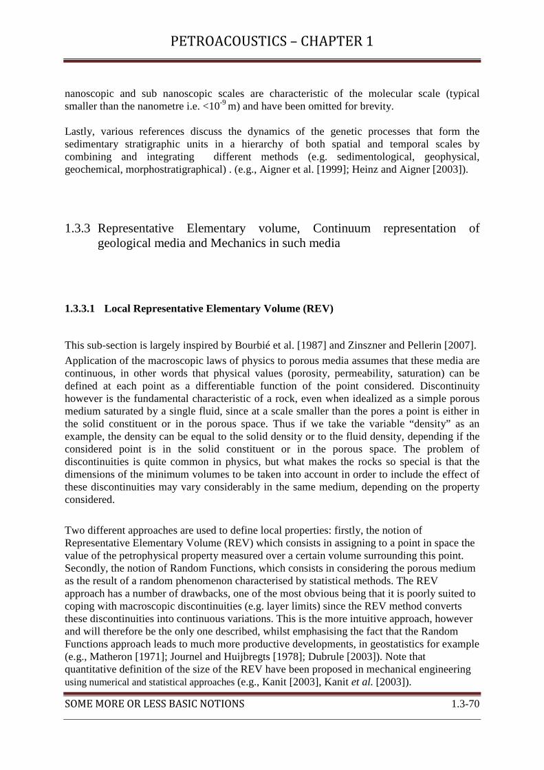
PETROACOUSTICS – CHAPTER 1
SOME MORE OR LESS BASIC NOTIONS 1.3-70
nanoscopic and sub nanoscopic scales are characteristic of the molecular scale (typical smaller than the nanometre i.e. <10-9 m) and have been omitted for brevity. Lastly, various references discuss the dynamics of the genetic processes that form the sedimentary stratigraphic units in a hierarchy of both spatial and temporal scales by combining and integrating different methods (e.g. sedimentological, geophysical, geochemical, morphostratigraphical) . (e.g., Aigner et al. [1999]; Heinz and Aigner [2003]).
1.3.3 Representative Elementary volume, Continuum representation of geological media and Mechanics in such media
1.3.3.1 Local Representative Elementary Volume (REV)
This sub-section is largely inspired by Bourbié et al. [1987] and Zinszner and Pellerin [2007].
Application of the macroscopic laws of physics to porous media assumes that these media are continuous, in other words that physical values (porosity, permeability, saturation) can be defined at each point as a differentiable function of the point considered. Discontinuity however is the fundamental characteristic of a rock, even when idealized as a simple porous medium saturated by a single fluid, since at a scale smaller than the pores a point is either in the solid constituent or in the porous space. Thus if we take the variable “density” as an example, the density can be equal to the solid density or to the fluid density, depending if the considered point is in the solid constituent or in the porous space. The problem of discontinuities is quite common in physics, but what makes the rocks so special is that the dimensions of the minimum volumes to be taken into account in order to include the effect of these discontinuities may vary considerably in the same medium, depending on the property considered.
Two different approaches are used to define local properties: firstly, the notion of Representative Elementary Volume (REV) which consists in assigning to a point in space the value of the petrophysical property measured over a certain volume surrounding this point. Secondly, the notion of Random Functions, which consists in considering the porous medium as the result of a random phenomenon characterised by statistical methods. The REV approach has a number of drawbacks, one of the most obvious being that it is poorly suited to coping with macroscopic discontinuities (e.g. layer limits) since the REV method converts these discontinuities into continuous variations. This is the more intuitive approach, however and will therefore be the only one described, whilst emphasising the fact that the Random Functions approach leads to much more productive developments, in geostatistics for example (e.g., Matheron [1971]; Journel and Huijbregts [1978]; Dubrule [2003]). Note that quantitative definition of the size of the REV have been proposed in mechanical engineering using numerical and statistical approaches (e.g., Kanit [2003], Kanit et al. [2003]).
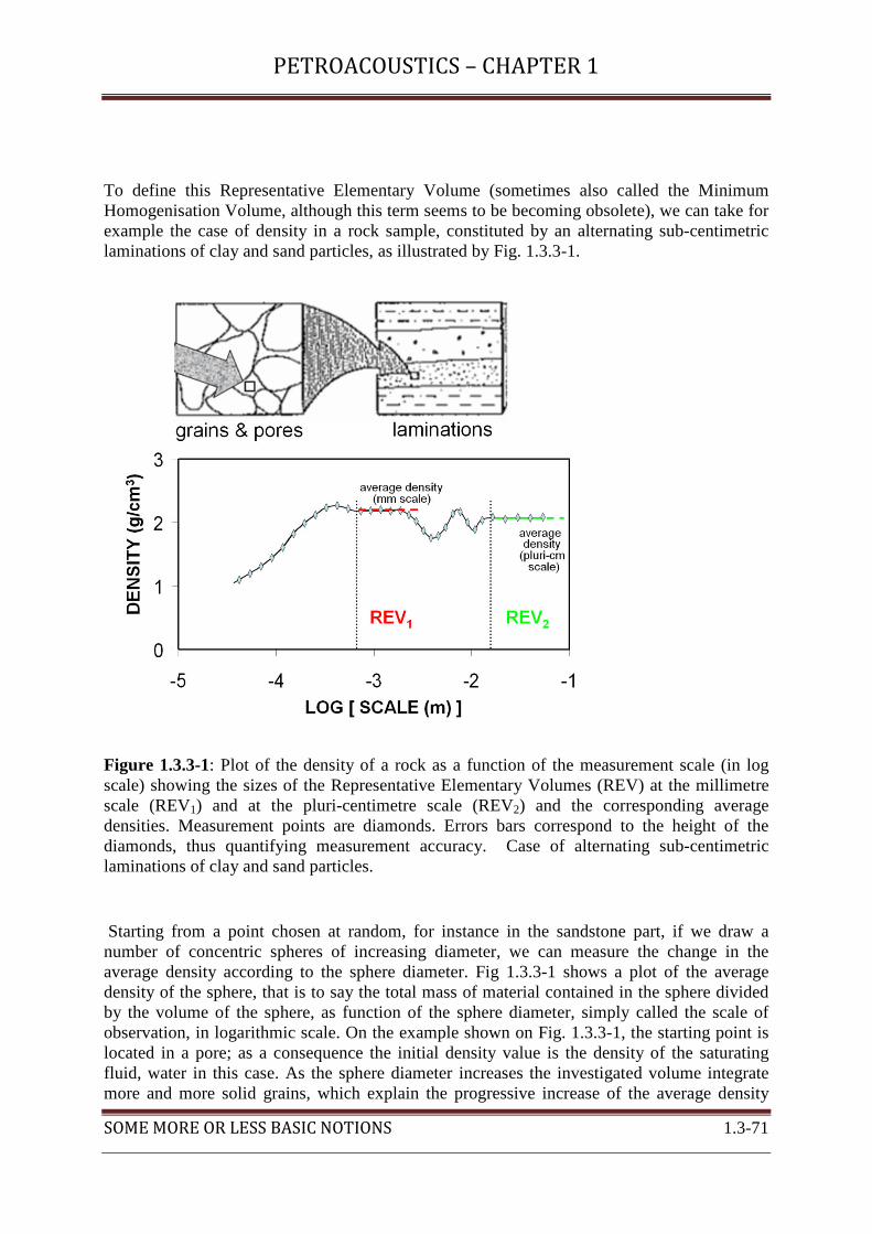
PETROACOUSTICS – CHAPTER 1
SOME MORE OR LESS BASIC NOTIONS 1.3-71
To define this Representative Elementary Volume (sometimes also called the Minimum Homogenisation Volume, although this term seems to be becoming obsolete), we can take for example the case of density in a rock sample, constituted by an alternating sub-centimetric laminations of clay and sand particles, as illustrated by Fig. 1.3.3-1.
Figure 1.3.3-1: Plot of the density of a rock as a function of the measurement scale (in log scale) showing the sizes of the Representative Elementary Volumes (REV) at the millimetre scale (REV1) and at the pluri-centimetre scale (REV2) and the corresponding average densities. Measurement points are diamonds. Errors bars correspond to the height of the diamonds, thus quantifying measurement accuracy. Case of alternating sub-centimetric laminations of clay and sand particles.
Starting from a point chosen at random, for instance in the sandstone part, if we draw a number of concentric spheres of increasing diameter, we can measure the change in the average density according to the sphere diameter. Fig 1.3.3-1 shows a plot of the average density of the sphere, that is to say the total mass of material contained in the sphere divided by the volume of the sphere, as function of the sphere diameter, simply called the scale of observation, in logarithmic scale. On the example shown on Fig. 1.3.3-1, the starting point is located in a pore; as a consequence the initial density value is the density of the saturating fluid, water in this case. As the sphere diameter increases the investigated volume integrate more and more solid grains, which explain the progressive increase of the average density

PETROACOUSTICS – CHAPTER 1
SOME MORE OR LESS BASIC NOTIONS 1.3-72
with the scale of observation. At the accuracy level of the measurement, quantified by the height of the diamonds materializing the measurement points, we reach a mean density value of the rock for spheres of diameter slightly smaller than 1 millimetre. Using this method, we can calculate the volume required to obtain a stable value of the variable at the considered accuracy level. and thereby define a first local Representative Elementary Volume REV1. For the density variable, the order of magnitude of this diameter is 1 to 3 grain diameters in the well-sorted intergranular spaces. As soon as the porous structure becomes more complex (as in some limestone rocks, for example), the dimension of the local REV may be very large compared with that of the petrological grain. If we go on the process of increasing the diameter of the concentric spheres the average density is no longer constant but varies again for sphere diameters larger than a few millimetres, in the case considered. In fact, as the sphere diameter increases the investigated volume integrates heterogeneities at a larger scale, such as the alternating sub-centimetric laminations of clay and sand particles in the case considered. At the considered accuracy level, we reach a second stable value of the density for spheres of diameter slightly larger than a few centimetres and thereby define a second local Representative Elementary Volume REV2. The common centre of all the spheres on which the physical property is averaged and on which the size of the local REV is deduced is fixed in the medium. That is why we talk of a "local" REV, in contrast with an "overall" REV that will be introduced in sub-section 1.3.3.3. In this last case the centre of the concentric spheres can have any position in a volume Ω of the geological medium. Note that at for the definitions of heterogeneity, anisotropy, dispersion and attenuation (see §1.2.3) the notion of Representative Elementary Volume (REV) is relative both to a given physical property and to the corresponding measurement accuracy. Obviously, if the accuracy level of physical measurement were infinite, no stable value of the corresponding physical property would be reached. As a consequence no REV could virtually be found for any real material. Correlatively, if the measurements are not accurate enough to be sensitive to the measurement scale, any volume dimension would be apparently representative of the physical property at the considered accuracy level. That is why, here again, the specification of the accuracy level of the physical measurement to be considered is important.
The above simple example illustrates the hierarchical structure of the different REV for the considered parameter "density".
Furthermore, as pointed out by Bourbié et al. [1987], for the same very simple medium, a clear variation in REV dimension for the “density” parameter and for another parameter such as “the fluid saturation”, in the case of the medium is saturated by several fluids. Thus when a physical phenomenon, for instance elastic wave propagation, involves not a single physical property of the medium but several, such as density and elastic moduli for elastic wave propagation (EWP), the Representative Elementary Volume REVEWP to be chosen at a given scale is the largest of the REV associated to each physical property.

PETROACOUSTICS – CHAPTER 1
SOME MORE OR LESS BASIC NOTIONS 1.3-73
Lastly, in the empirical definition of the REV, we implicitly accepted that above a certain investigation radius, the value of the studied variable stabilises at the considered accuracy level (at least over a dimensional interval) and that an REV can therefore be determined for the property concerned. Frequently, however, the values of some properties of natural media do not exhibit this stabilisation. When the investigation volume increases, the value of the characteristic varies continuously. It is no longer possible to define a REV, with the previous common meaning. This is the case for self-similar media, exemplified by some fractured formations, of which the structure reproduces itself during the scale change (see examples and link with REV in Zinszner and Pellerin [2007]), as a consequence no REV can be found.
1.3.3.2 The hierarchical structure of geological media and seismic resolution
The procedure described in the previous sub-section can be applied at much smaller
and much larger scales and is illustrated by Fig. 1.3.3-2.
Figure1.3.3-2: The evolution of the average density as a function of the measurement scale and of the heterogeneity scale of geological media. Measurement points are diamonds. Errors bars correspond to the height of the diamonds, thus quantifying measurement accuracy. For convenience the wavelength bands of the complete set of geoacoustical measurements and ultra-high frequency acoustic measurements (on top of the figure) can be compared with the measurement scale (on the bottom of the figure) (modified after Krause et al. [1987]; Bourbié et al. [1987]; Zinszner and Pellerin [2007]).
PETROACOUSTICS – CHAPTER 1
SOME MORE OR LESS BASIC NOTIONS 1.3-74
As previously, we still focus on the density of the medium. Note that the whole experimental spectrum has considerably increased and now covers many orders of magnitude, roughly seventeen orders of magnitude (from the molecular scale 10-10m to the global earth scale slightly smaller than 107m). As in the previous sub-section we plot the average density of the medium over a sphere of increasing diameter (the centre of the concentric spheres of investigation being randomly chosen in the saturating fluid) as a function of the scale of investigation (that is to say the diameter of the investigation sphere) in log scale. The measurement points are diamonds, and measurement accuracy is quantified by the height of the diamonds. Note that when the scale is larger than say hm/km the sphere of investigation reaches the surface of the earth. In these cases we compute the average density only over the part of the investigation sphere contained in the earth. Note that, in contrast with Fig. 1.3.2-1, the nanoscopic and sub nanoscopic scales, which are characteristic of the molecular scale (typical smaller than the nanometre i.e. <10-9 m), are represented. If we start from the latter scale the fluctuations of the average density are very large when the size of the investigation sphere is smaller than the molecular scale. If a very large number of molecules are included in the investigation sphere the volume required to obtain a stable value of the density variable is reached. We have reached the Representative Elementary Volume (REV) at a scale much above the molecular scale, roughly around 10-8m. The average density is simply the density of the single saturating fluid. As pointed out at the end of the previous sub-section, if the rock is saturated by several fluids other fluctuations of the average density are observed at a larger scale with possibly a new stabilization of the average density when reaching a new larger REV (not considered in the Figure). The variations of the average density at the grain/pore scale and at the scale of the laminations (typically from 10-5m to 10-1m) with two REVs have been already detailed in the previous sub-section.

PETROACOUSTICS – CHAPTER 1
SOME MORE OR LESS BASIC NOTIONS 1.3-75
BOX 1.3.3-1
Structure of the Earth's interior and Preliminary Reference Earth Model
(PREM)
The structure of the Earth's interior is known by us mainly by seismology, in particular its spherically symmetric structure with 3D small perturbations (e.g., Musset and Khan [2000]). Apart from the small 3D perturbations the radial structure of the earth was known by the 1930s from famous seismologists such as Harold Jeffreys (1891-1989), Beno Gutenberg (1889-1960), Inge Lehmann (1888-1993), and Keith Bullen (1906-1976). The nomenclature of the subdivisions of the Earth's interior is due to the latter geoscientist.
(Right) The spherically symmetric structure of the Earth's interior, (Middle) The major discontinuities exhibited by the Earth's interior, and (Left) Depth dependence of P-wave velocity and S-wave velocity, density after the PREM
From the surface to the centre of the Earth the different layers are the crust (~10-~70km thick), the mantle (~2800km thick), the outer core (~2200km thick), and the inner core (~1500km thick). The major discontinuities have been discovered by major geophysicists, such Andrija Mohorovicic (1857-1936) for the crust/mantle boundary, Beno Gutenberg for the mantle/outer core boundary, and Inge Lehmann for the boundary between the outer core and the inner core. Each of these major discontinuities bears the name of its discoverer. The inversion of a huge set of seismological data led to the Preliminary Reference Earth Model (PREM), which is the first complete and consistent model of a radial earth for different physical parameters, such the P-wave and S-wave velocities, the density and the attenuations [Dziewonski and Anderson, 1981]. This model exhibits a rough systematic increase of the density with the depth, with abrupt variations at the main inner boundaries introduced previously.

PETROACOUSTICS – CHAPTER 1
SOME MORE OR LESS BASIC NOTIONS 1.3-76
From pluri-decimetric scale to the hectometric scale (typically the scale of the well logs) fluctuations of the average density with increasing scale of observation can be due, for instance to alternating succession of formations of different types (e.g. sandstones and shale) but following one another repetitively with more or less regularity. If the investigation sphere include a sufficient number of constituent layers a new stable value of the average density is reached for spheres of diameter typically larger than many layers and thereby define a new REV at the macro scale, that is to say around a few metres to a decametre in the case considered. The average density is simply the average rock density at the macro scale. The example shown on the figure corresponds to an alternation of sandstone beds and shale beds of centimetric to decimetric size. Because the shale/sandstone sequence is followed by a more compact carbonate sequence at larger depth the average density tends to slightly increase when the investigation sphere start to include more and more carbonate beyond the size of the REV at the macroscale.
At the megascale, that is to say from 102 m to a few 103 m, the variation of the average density of sedimentary formations with the scale of investigation can be computed from typical depth dependence curves of the density in sediments (e.g., Faust [1951]; Gardner et al. [1974]). Note that at these scales the density of the sediments continuously increases with depth. As a consequence the curve of the average density versus the scale of observation does not exhibit any stabilization. In other words, it is no longer possible to define a REV, with the previous common meaning. The same phenomenon is observed at the next larger scale or gigascopic scale. The variation of the average density of the earth with the scale of investigation can be computed from the large-scale structure of the Earth's interior described for instance by the so-called Preliminary Reference Earth Model (PREM) of Dziewonski and Anderson [1981], extensively used in Global geophysics (see Box 1.3.3-1). The curve of the scale dependence of the average density computed from this model monotonously increases and exhibits slope discontinuities due to the presence of the major discontinuities in the Earth's interior. As a consequence the curve of the average density versus the scale of observation does not exhibit any stabilization. In other words, here again it is not possible to define a REV, with the previous common meaning. The last point of the plot corresponds to the largest scale, that is to say the Earth's radius, and to the average density of the Earth, that is roughly 5500 kg/m3.
PETROACOUSTICS – CHAPTER 1
SOME MORE OR LESS BASIC NOTIONS 1.3-77
Because the spatial resolution of acoustical methods in general is roughly equal to a fraction of the dominant wavelength Λ we have also plotted on the top of the previous figure the wavelength bands of the complete set of geoacoustical measurements and hypersounds and ultra-high frequency acoustic measurements, for instance in the domain of Scanning Acoustic Microscopy (SAM) operating in frequencies between 100 MHz and 2 GHz (e.g., Briggs [1992]; Briggs and Arnold [1996]). The comparison between the typical wavelength band of geoacoustical measurements (see Figure 1.2.2-8 and the corresponding comments) and the different scales of heterogeneity of geological media (see Figure 1.3.2-1 and the corresponding comments) straightforwardly allows choosing the type of measurement that is appropriate to resolve a considered heterogeneity scale. For instance mesoscopic heterogeneities can be resolved by ultrasonic methods. In contrast, macroscopic heterogeneities can hardly be resolved by conventional surface seismics but can easily be seen by acoustic logs and well logging methods in general.
1.3.3.3 Overall Representative Elementary Volume (REV)
In the two previous sub-sections the common centre of all the spheres on which the physical property is averaged and on which the size of the local REV is deduced is fixed in the medium considered. If the concentric spheres are centered on another point the size of the new local REV, if it exists at this point, is not necessarily equal to the size of the previous local REV.
In the present sub-section the centre of the spheres for the analysis of the local REV vary in a given volumeΩ of which the size is much larger than the size of the local REV. In case a local REV for the physical property considered, as described in the previous subsections, can be defined at each point of Ω one can define an overall REV on Ω for the physical property under consideration. The size of this overall REV is simply the largest size among the sizes of the local REV corresponding to all the points of Ω . Obviously, by definition, at any point of Ω the size of the local REV is smaller than or equal to the size of the overall REV. That is to say, at any point of Ω the curve of the physical property under consideration versus the scale of observation (as illustrated by Figure 1.3.3-1) exhibits a stabilization for scales larger than the size of the overall REV, however smaller than the size of the next larger overall REV.
Note that, at the considered level of measurement accuracy, the stabilization value of the physical property is not necessarily identical for all the points ofΩ . If the stabilization value is identical for all the points ofΩ , the medium is said to be homogeneous with respect to the physical property considered (at the considered accuracy level) and at a scale equal to the size of the overall REV. If this is not the case, the medium is heterogeneous with respect to the physical property considered (at the considered accuracy level) and at a scale equal to the size of the overall REV (for detailed descriptions of homogeneity and heterogeneity in continuous media see § 1.2.3.1, and in geological media see §1.3.4).
In the following, for brevity, instead of "overall REV" we shall simply use "REV", the adjective "overall" being omitted but always implicit. We also assume that a level of measurement accuracy is given.

PETROACOUSTICS – CHAPTER 1
SOME MORE OR LESS BASIC NOTIONS 1.3-78
1.3.3.4 Continuum representation of geological media
In the case where the scale length characteristic of the experiment, namely the elastic wavelength Λ , in natural media, such as geological media, is much larger than the size of the largest Representative Elementary Volumes REVlargest common to all the physical properties involved in elastic wave propagation, namely the density and the elastic moduli of the medium (after sub-section 1.2.2.1), a continuum representation of the analyzed medium can be achieved with physical material points of the size of the REVlargest . The size of this point is much larger than the size of the physical point in simple real media (see detail in section 1.3.1), and depends on the scale of observation.
Regarding the time variable, we know from section 1.3.1 that the physical instant of time t in simple real media must have a non-vanishing "duration", typically much larger than the molecular time scale τ=0.1ns. We can keep the same duration for the physical instant of times t in simple real media and in natural media, such as geological media.
1.3.3.5 Characteristic lengths and representative samples
A. Characteristic lengths
We can understand the importance of the notion of REV dimension, which is a fundamental characteristic when studying a physical property of geological media. We can also appreciate that a second type of characteristic dimension is involved: dimensions related the physical phenomenon itself. In the following lines we will use empirical definitions to describe notions which would require a more rigorous approach. However, we consider that by so doing we will provide a few basic ideas, necessary in this field to correctly interpret the results of acoustical experiments. Failure to respect the conditions concerning the characteristic lengths is the main cause of numerous experimental errors, leading to apparently inconsistent acoustical behaviour.
The three types of dimension to be taken into account are represented diagrammatically on Figure 1.3.3-3: – The characteristic dimension of sample homogeneity for a property and in a given petrophysical state. The REV dimension gives an approximation of this dimension (d on the diagram). In practice, accurate measurement of this dimension involves the use of (geo)statistical methods (range of the variogram, for example) (e.g., Matheron [1971]; Journel and Huijbregts [1978]; Dubrule [2003]) but we will not develop this point since we have not

PETROACOUSTICS – CHAPTER 1
SOME MORE OR LESS BASIC NOTIONS 1.3-79
described the Random Functions method. We can therefore see the limits of our qualitative approach, but in fact it is often sufficient to detect the largest risks of error. – The characteristic dimension of the physical phenomenon itself. The simplest example amongst the properties described in sub-section 1.2.2.3 is that of the wavelength Λ of elastic waves. – The sample size C. In a given experiment, this characteristic length is always easy to find! However, it generates challenging practical problems when, in order to perform a rigorous analysis of the other characteristic dimensions, very large samples are required.
Figure 1.3.3-3: Diagrammatic representation of various types of characteristic dimension in a petrophysical experiment.
B. Notion of valid sample
Acoustical measurements in the laboratory are taken for two main reasons: – To characterise a geological formation by means of a limited number of samples, combining their individual properties in up-scaling processes to best define the layer parameters.

PETROACOUSTICS – CHAPTER 1
SOME MORE OR LESS BASIC NOTIONS 1.3-80
– To study the relations between acoustical properties and other petrophysical properties in a particular geological formation. In both cases, the sample must satisfy certain validity conditions. Firstly, it must be homogeneous and implicitly its volume must be much larger than the REV for the phenomenon considered (in other words C >> d, using the notation given on Fig. 1.3.3-3). The need for a homogeneous sample is quite obvious since, if we are studying the relations between the physical properties A and B and the sample is the combination of two parts of properties A1, B1 and A2, B2, the measurement result will be a combination of relations A1B1 and A2B2 which is difficult to generalise! The measurement must also have a physical meaning, in other words the REV dimension must be very small compared with the characteristic length of the physical phenomenon being studied.
For experiments concerning elastic waves, the wavelength Λ must be compared with the REV. The cases studied are the following: – If Λ is significantly larger than the diameter of this volume, then the vibration will exhibit macroscopic homogeneous behaviour insensitive to microscopic discontinuities in the porous medium. Valid experimental results can be deduced from the characteristic values of the medium studied. – If Λ has the same order of magnitude as this representative dimension, we observe scattering phenomena which radically change the behaviour of the wave in the porous medium. – If Λ is significantly smaller, the porous medium “no longer exists” as such and the analysis must be repeated at a much smaller scale: the medium to be studied consists of individual grains and pores. More detailed considerations on the frequency dependence of the elastic properties of rocks due to the presence of heterogeneities will be found in Chapter 5 on Frequency dependence. In conclusion, to perform good acoustical experiments, it is important to respect certain basic validity conditions: – the sample must be homogeneous; – the relations of scale C >>d and Λ >>d must be respected. Apart from practical considerations, there are a priori no special difficulties in satisfying these conditions, as long as the REV does not vary during the experiment. This is not always the case, however, and we may be faced with a difficult problem when varying a parameter such as saturation. For instance low saturations may in some cases generate REV values much greater than that of the porosity as such: during an experiment, the REV may therefore vary to such an extent that the entire experiment could be invalidated [Cadoret, 1993]. An example of this type of situation is given below.
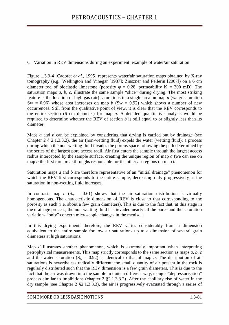
PETROACOUSTICS – CHAPTER 1
SOME MORE OR LESS BASIC NOTIONS 1.3-81
C. Variation in REV dimensions during an experiment: example of water/air saturation
Figure 1.3.3-4 [Cadoret et al., 1995] represents water/air saturation maps obtained by X-ray tomography (e.g., Wellington and Vinegar [1987]; Zinszner and Pellerin [2007]) on a 6 cm diameter rod of bioclastic limestone (porosity φ = 0.28, permeability K = 300 mD). The saturation maps a, b, c, illustrate the same sample “slice” during drying. The most striking feature is the location of high gas (air) saturations in a single area on map a (water saturation Sw = 0.96) whose area increases on map b (Sw = 0.92) which shows a number of new occurrences. Still from the qualitative point of view, it is clear that the REV corresponds to the entire section (6 cm diameter) for map a. A detailed quantitative analysis would be required to determine whether the REV of section b is still equal to or slightly less than its diameter. Maps a and b can be explained by considering that drying is carried out by drainage (see Chapter 2 § 2.1.3.3.2), the air (non-wetting fluid) expels the water (wetting fluid); a process during which the non-wetting fluid invades the porous space following the path determined by the series of the largest pore access radii. Air first enters the sample through the largest access radius intercepted by the sample surface, creating the unique region of map a (we can see on map a the first rare breakthroughs responsible for the other air regions on map b. Saturation maps a and b are therefore representative of an “initial drainage” phenomenon for which the REV first corresponds to the entire sample, decreasing only progressively as the saturation in non-wetting fluid increases. In contrast, map c (Sw = 0.61) shows that the air saturation distribution is virtually homogeneous. The characteristic dimension of REV is close to that corresponding to the porosity as such (i.e. about a few grain diameters). This is due to the fact that, at this stage in the drainage process, the non-wetting fluid has invaded nearly all the pores and the saturation variations “only” concern microscopic changes in the menisci. In this drying experiment, therefore, the REV varies considerably from a dimension equivalent to the entire sample for low air saturations up to a dimension of several grain diameters at high saturations. Map d illustrates another phenomenon, which is extremely important when interpreting petrophysical measurements. This map strictly corresponds to the same section as maps a, b, c and the water saturation (Sw = 0.92) is identical to that of map b. The distribution of air saturations is nevertheless radically different: the small quantity of air present in the rock is regularly distributed such that the REV dimension is a few grain diameters. This is due to the fact that the air was drawn into the sample in quite a different way, using a “depressurisation” process similar to imbibitions (chapter 2 §2.1.3.3.2). After the capillary rise of water in the dry sample (see Chapter 2 §2.1.3.3.3), the air is progressively evacuated through a series of

PETROACOUSTICS – CHAPTER 1
SOME MORE OR LESS BASIC NOTIONS 1.3-82
depressurisation phases under increasing vacuum, followed each time by repressurisation to atmospheric pressure.
Figure 1.3.3-4: Water/air saturation map for the same slice of bioclastic limestone. Maps a, b and c correspond to water displacement using a drying process. For map d, water displacement occurred via a “depressurisation” process (after Cadoret et al. [1995]). (the speckled patterns at the scale visible on d map are not a sign of variation of saturation but an experimental noise).

PETROACOUSTICS – CHAPTER 1
SOME MORE OR LESS BASIC NOTIONS 1.3-83
This is a clear illustration of the principle whereby, in experiments involving multi-phase equilibria, the fluid displacement method may have extremely important consequences on the location of the fluids and therefore on the petrophysical characteristics. The quantitative saturation data alone is far from being sufficient to describe the state of a sample.
D. Consequences of REV variation during an experiment: case of seismic velocities of samples in water/gas saturation
The relations between the seismic wave velocities and the gas saturation are extremely valuable when interpreting reservoir seismics. Some laboratory results may appear to be contradictory, producing different types of V vs. Sw relations depending on the experiments and not corresponding to the values predicted by the Biot-Gassmann equation (see Chapter 6). This phenomenon illustrates the practical consequences of the previous remarks. Some data extracted from Cadoret et al. [1995] are given below. The results shown on Figure 1.3.3-5 concern elastic wave velocities measured using the resonant bar technique (§ 2.2.2) applied to a large sample (length 100 cm, diameter 6 cm). This method consists in bringing the sample into resonance in extension or torsion mode. The resonance frequency is such that the half wavelength is equal to the bar length (or to an integer fraction of this length). Sonic frequency (in the kilohertz range) wave velocities can therefore be measured extremely accurately on rock volumes of pluridecimetric dimension. In this experiment, the air saturation variation was obtained using the two methods described in the previous paragraph: drying and depressurisation. Note that the lowest water saturation which can be obtained easily by depressurisation is equal to the Hirschwald coefficient (§2.1.2.3.2), which explains why the lowest saturations in the depressurisation series are approximately 0.65. The results are quite clear: – Concerning the shear wave, we observe that the fluid displacement method used has no effect whatsoever on the velocity. The S-wave velocity (Vs on the graph) decreases slowly and regularly as the water saturation increases. In compliance with the theory, the shear modulus is unaffected by the presence of fluid (and therefore the fluid displacement method). We only observe a density effect due to the higher water content. – The situation is quite different for the E-wave velocities (Ve on the graph) similar at this stage of the analysis to compression waves. When the saturation variation is obtained using the depressurisation method, the experimental result shows excellent agreement with the predictions of the Biot-Gassmann equation: as the water content increases, the E-velocity decreases regularly (density effect). It is only when the last air bubbles have disappeared (total saturation) that the sudden increase in saturating fluid incompressibility causes in a correlative increase in velocity. In contrast, when the saturation variation is obtained by drying, the velocities no longer follow the Biot-Gassmann equation and vary progressively between minimum values at around Sw = 0.8 and the maximum value at Sw = 1.
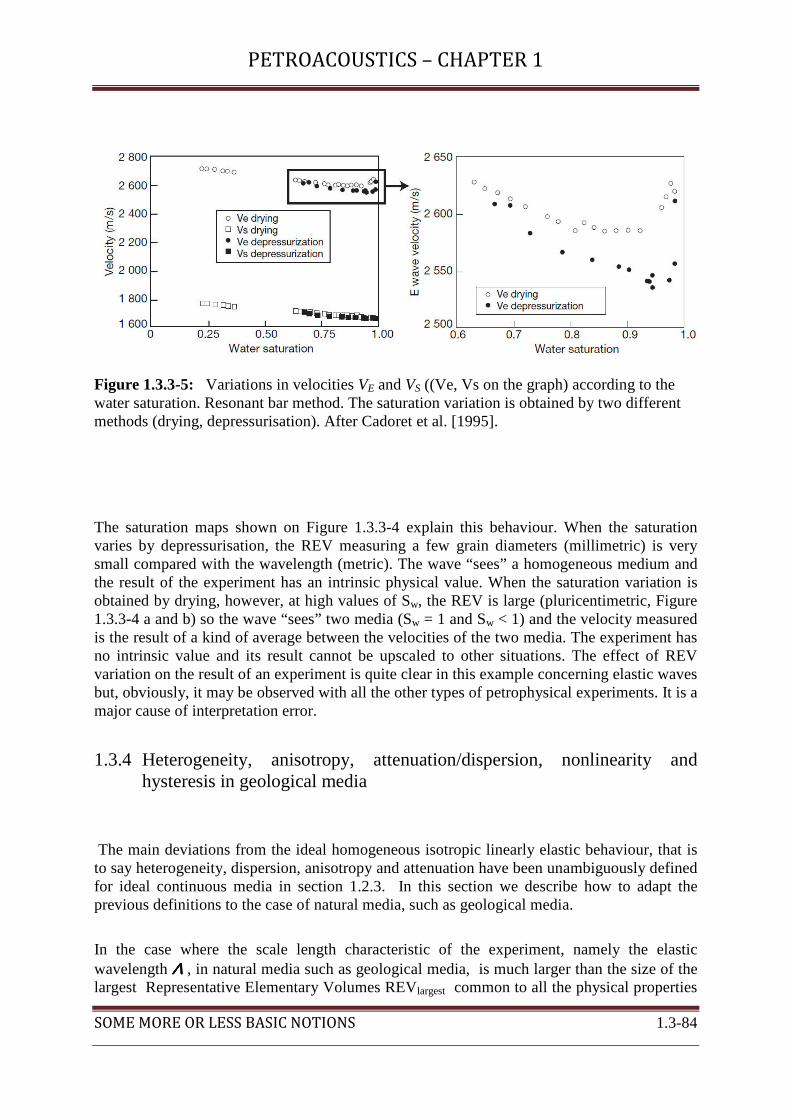
PETROACOUSTICS – CHAPTER 1
SOME MORE OR LESS BASIC NOTIONS 1.3-84
Figure 1.3.3-5: Variations in velocities VE and VS ((Ve, Vs on the graph) according to the water saturation. Resonant bar method. The saturation variation is obtained by two different methods (drying, depressurisation). After Cadoret et al. [1995].
The saturation maps shown on Figure 1.3.3-4 explain this behaviour. When the saturation varies by depressurisation, the REV measuring a few grain diameters (millimetric) is very small compared with the wavelength (metric). The wave “sees” a homogeneous medium and the result of the experiment has an intrinsic physical value. When the saturation variation is obtained by drying, however, at high values of Sw, the REV is large (pluricentimetric, Figure 1.3.3-4 a and b) so the wave “sees” two media (Sw = 1 and Sw < 1) and the velocity measured is the result of a kind of average between the velocities of the two media. The experiment has no intrinsic value and its result cannot be upscaled to other situations. The effect of REV variation on the result of an experiment is quite clear in this example concerning elastic waves but, obviously, it may be observed with all the other types of petrophysical experiments. It is a major cause of interpretation error.
1.3.4 Heterogeneity, anisotropy, attenuation/dispersion, nonlinearity and hysteresis in geological media
The main deviations from the ideal homogeneous isotropic linearly elastic behaviour, that is to say heterogeneity, dispersion, anisotropy and attenuation have been unambiguously defined for ideal continuous media in section 1.2.3. In this section we describe how to adapt the previous definitions to the case of natural media, such as geological media.
In the case where the scale length characteristic of the experiment, namely the elastic wavelength ΛΛΛΛ , in natural media such as geological media, is much larger than the size of the largest Representative Elementary Volumes REVlargest common to all the physical properties

PETROACOUSTICS – CHAPTER 1
SOME MORE OR LESS BASIC NOTIONS 1.3-85
involved in elastic wave propagation, namely the density and the elastic moduli of the medium (after sub-section 1.2.2.1), a continuum representation of the analyzed medium can be achieved with physical material points of the size of the REVlargest . The size of this point is much larger than the size of the physical point in simple real media (see detail in section 1.3.1), and depends on the scale of observation.
Regarding the time variable, we know from section 1.3.1 that the physical instant of time t in simple real media must have a non-vanishing "duration", typically much larger than the molecular time scale τ≈0.1ns. We can keep the same duration for the physical instants of time t in simple real media and in natural media, such as geological media.
At these space and time scales any property of the medium involved in elastic wave propagation, namely the density and the elastic moduli, can be represented by continuous functions of space and time. Therefore when we talk about a physical property at a certain scale we actually refer to the corresponding continuous function representing the considered physical property, associated with physical material points of the size of the REV largest.
As a consequence, provided the continuum representation of the medium at the considered scale, all the definitions and descriptions of the behaviours deviating from the ideal homogeneous isotropic linearly elastic behaviour given for continuous media in section 1.2.3 (heterogeneity, anisotropy, dispersion, attenuation, elasticity (linear or nonlinear possibly with hysteresis)) remain valid but are relative to the scale of observation.
For instance, regarding heterogeneity, the generalized definition in natural media is the following: "A medium exhibits heterogeneity at a given scale, with respect to a given physical property (elastic or electromagnetic wave velocity, electric or thermal conductivity, mechanical strength...) and to a corresponding measurement accuracy, if this property depends on the observation physical point P at this scale at the considered accuracy level, the other parameters remaining fixed. The medium is said to be heterogeneous at this scale, with respect to the considered physical property at the considered accuracy level. In the opposite case the medium exhibits homogeneity, and is said to be homogeneous at this scale with respect to the considered physical property at the considered accuracy level. In the special case of acoustics the physical properties are elastic wave velocities and density."
Regarding anisotropy, the generalized definition in natural media is the following: "A medium exhibits anisotropy at a given scale, with respect to a given physical property (elastic or electromagnetic wave velocity, electric or thermal conductivity, mechanical strength...) and to a corresponding measurement accuracy, if this property depends on the direction of observation at this scale and at the considered accuracy level, the other parameters remaining fixed. In such case the medium is said to be anisotropic at this scale with respect to the considered physical property at the corresponding accuracy level. In the opposite case the medium exhibits anisotropy, and is said to be anisotropic at this scale with respect to the considered physical property at the corresponding accuracy level, In the opposite case the medium exhibits isotropy, and is said to be isotropic at this scale with respect to the
PETROACOUSTICS – CHAPTER 1
SOME MORE OR LESS BASIC NOTIONS 1.3-86
considered physical property. In the special case of acoustics the physical properties are elastic wave velocities and density."
A natural medium exhibits dispersion at a given scale, with respect to a physical property involving wave propagation (i.e., elastic or electromagnetic wave propagation), and to the corresponding measurement accuracy, if the physical property depends on the wavelength Λ at this scale and at the considered accuracy level, the other parameters remaining fixed. In such case the medium is said to be dispersive at this scale with respect to the considered physical property at the considered accuracy level. In the opposite case the medium do not exhibit any dispersion, and is said to be non-dispersive at this scale with respect the considered physical property at the considered accuracy level. In the special case of acoustics the physical property is elastic wave velocity, density and/or impedance.
Lastly, a natural medium exhibits attenuation at a given scale, with respect to wave propagation (i.e., elastic or electromagnetic wave) at a given measurement accuracy, if the amount of energy transported per unit time by the wave, or the energy flux of the wave field, crossing a fixed unit surface parallel to the wave front, that is to say the norm of the Umov-Poynting-Heaviside vector P (see §1.2.2.2 and box 1.2.2-2) decreases during propagation at the considered accuracy level, the other parameters remaining fixed. In such case the medium is said to be attenuative at this scale with respect to wave propagation at the considered accuracy level. In the opposite case the medium does not exhibit any attenuation at this scale, and is said to be non-attenuative at this scale with respect to wave propagation at the considered accuracy level. In the special case of acoustics the wave considered are elastic waves.

PETROACOUSTICS – CHAPTER 1
SOME MORE OR LESS BASIC NOTIONS 1.3-87
References
Abramowitz M and Stegun I A, 1965, Handbook of Mathematical Functions: Dover, New York. Achenbach, J.D., 1975, Wave Propagation in Elastic Solids, Elsevier Science Publishers B.V., Amsterdam. Aigner, T., Heinz, J., Hornung, J., and Asprion, U., 1999, A hierarchical process-approach to reservoir heterogeneity:
examples from outcrop analogues. Bulletin des Centres de Recherches Exploration-Production Elf-Aquitaine, 22, 1–11.
Aki, K., and Richards, P., 1980, Quantitative seismology, theory and methods: W. H. Freeman & Co Alexandrov, K.S. and T.V. Ryzhova, 1961, The elastic properties of crystals., Sov. Phys.Cry, 6, 228-252. Arts, R. J., 1993, A study of general anisotropic elasticity in rocks by wave propagation – theoretical and
experimental aspects-. Ph. D. thesis, Université Pierre et Marie Curie (Paris 6), Paris, France. Ed. Technip. Auld, B. A. , 1973, Acoustic Fields and Waves in Solids, Wiley-Interscience publication. Babuska, V., and M. Cara, 1991, Seismic Anisotropy in the Earth: Kluwer Academic, Dordrecht, Netherlands. Backus, G. E., 1962, Long-wave elastic anisotropy produced by horizontal layering: Journal of Geophysical Research,
67, 4427–4440. Barclay, R. M. R., 1999. Bats are not birds—a cautionary note on using echolocation calls to identify bats: a comment.
Journal of Mammalogy , 80: 290–296. Barton, D. K. and S. A. Leonov, 1998, Radar Technology Encyclopedia , Artech House Inc. Bass, J.D, , 1995. Elasticity of minerals, glasses, and melts, in Mineral Physics and Crystallography: A Handbook of
Physical Constants, pp. 45–63, ed. Ahrens T.J., American Geophysical Union, Washington, DC. Bechmann, R. and A. M. Hearmon, 1966, in Elastic, Piezoelectric, Piezooptic, and Electrooptic Constants of
Crystals, edited by K.H. Hellwege and A. Hellwege, Landolt-Börnstein, New Series, Group III, Vol. 1, Springer Verlag, Berlin,
Ben Menahem, A. and S. J. Singh, 1981. Seismic waves and sources. Springer-Verlag, Heidelberg. Bertotti , G. .and I. Mayergoyz, 2006, The Science of Hysteresis. Academic Press. Bloch, F., 2000, Fundamentals of statistical mechanics: manuscript and notes of Felix Bloch. Imperial College Press;
World Scientific; London: Singapore. Born, M. and Wolf, W. 1986. Principles of Optics, Pergamon Press: Sixth (corrected) Edition. Bourbie, T., Coussy, O. and B. Zinszner, 1987, Acoustics of Porous Media, Editions Technip, Paris. Boussinesq, J.,1906, Propagation du mouvement autour d'un centre, dans un millieu élastique, homogène et isotrope:
Annales scientifiques de l'É.N.S, 3e série, tome 23, p. 225-261. Boyer, S. and Mari, J.L, 1997. Seismic Surveying and well logging. Oil and Gas Exploration Techniques. Editions
Technip. ISBN: 2-7108-0712-2. Bracewell, R. N. , 1965, The Fourier Transform and Its Applications. New-York: McGraw-Hill. Briggs, A., 1992, Acoustic Microscopy : Clarendon Press, Oxford. Briggs, A. and W. Arnold, 1996, Advances in Acoustic Microscopy: Plenum Press, New York. Bruggeman, D. A. G., 1937, Berechnung der verschiedenen physikalischen Konstanten von heterogenen Substanzen:
Annalen der Physik, 29, 160–165. Bruin, F., 1981, “Atmospheric refraction and extinction near the horizon,” Archive for History of Exact Sciences 25,
1–17. Bucur V., 1995, Acoustics of wood. CRC Press. Boca Raton, New York, London, Tokyo. Bucur, V., and P.N.J. Rasolofosaon, 1998. Dynamic elastic and nonlinearity in wood and rock. Ultrasonics 36:813–
824. Cadoret, T., 1993, Effet de la saturation eau/gaz sur les pr acoustiques des roches,aux sonores et ultrasonores. Ph.D.
Dissertation, Univ. de Paris VII, Paris, France. Cadoret, T., D. Marion, and B. Zinszner, 1995, Influence of frequency and fluid distribution on elastic wave velocities
in partially saturated limestones: Journal of Geophysical Research-Solid Earth, v. 100, no. B6. Carcione J.-M., 2007, Wave Fields in Real Media : Wave Propagation in Anisotropic, Anelastic, Porous and
Electromagnetic Media, vol. 38 of Hanbook of Geophysical Exploration : Seismic Exploration, second : revised and extended edn, Elsevier, 2007.
Castagna J. and Backus M.M. , 1993, Offset-Dependent Reflectivity - Theory and Practice of AV0 Analysis. SEG Special Publication.
Cauchy, A., 1827a, De la pression ou tension dans un corps solide. Exercices de Mathématiques, 2, 42-56; Addition, 57-59
Cauchy, A., 1827b, Sur la condensation et la dilatation des corps solides, Exercices de Mathématiques, 2, 60-69.

PETROACOUSTICS – CHAPTER 1
SOME MORE OR LESS BASIC NOTIONS 1.3-88
Cauchy, A., 1828, Sur les équations qui expriment les conditions d'équilibre ou les lois du mouvement intérieur d'un corps solide, élastique, ou non élastique, Exercices de Mathématiques, 3, 160-187.
Cerantola, S., 2004, La ley física de Ibn Sahl:estudio y traducción parcial de su Kitāb al-harraqāt, Anaquel de Estudios Árabes, vol. 15, 57-95.
Cerveny, V., 2001, Seismic Ray Theory: Cambridge University Press, Cambridge. Cerveny, V., Klimes, L. and I. Psencık, I., 2008. Attenuation vector in heterogeneous, weakly dissipative, anisotropic
media, Geophys. J. Int., 175, 346–355. Challande, P., 2004, Rappels de mécanique des milieux continus, Cours de Master 2, Parcours "Acoustique Physique",
Université Pierre et Marie Curie, Paris 6. Chavent, G. and J. Jaffre, 1986, Mathematical models and Finite Elements for Reservoir Simulation, Studies in
Mathematics and its Applications, Vol. 17, North-Holland, Amsterdam. Clark Jr., S.P., (Ed.), 1966. Handbook of Physical Constants. The Geological Society of America, Inc., New York. Cowin SC, Mehrabadi MM., 1987, On the identification of material symmetry for anisotropic elastic material. J Mech
Appl Math. 1987;40:451–475. D’Alembert, J. l. R., 1747, Recherches sur la courbe que forme une corde tendue mise en vibration, Hist. Acad. Roy.
Sci. et Belles Let. Berlin, 214-219. DeBruijn, N. C., 1967, ”Uncertainty principles in Fourier analysis,” in Inequalities, 0. Shisha, Ed., New York, NY:
Academic Press, pp. 57-71. Descartes R., 1637, La Dioptrique, re-publishd in 1963. Dioptrique, in Œuvres philosophiques I, Paris, Garnier.
available at http://classiques.uqac.ca/classiques/Descartes/dioptrique/dioptrique.html Dieulesaint, E. and D. Royer, 1974, Ondes élastiques dans les solides. Masson, Paris. Doligez, B., Bessis, F., Burrus, J., Ungerer, P. and Chenet, P.Y., 1986, Integrated Numerical Simulation of
Sedimentation, Heat Transfer, Hydrocarbon Formation and Fluid Migration in a Sedimentary Basin: the Themis Model. Thermal Modelling in Sedimentary Basins, Proceedings of the 1st IFP Research Conference on Exploration, Carcans, June 3-7, 1985, 173-195.
Dubrule, O., 2003. Geostatistics for Seismic Data Integration in Earth Models, Distinguished Instructor Series, No. 6, Society of Exploration Geophysicists.
Dziewonski A. M. and Anderson D. L., 1981, Preliminary reference Earth model. Phys. Earth Planet. Int., 25, 297-356.
Einstein, A , 1916, Die Grundlage de Allgememen Relativitatstheone," 1916 (in Ferret, W , and Jeffery, G , Side Lights on Relativitt/, London, Methuen, 1922)
Evans, K. E. , Nkansah, M. A., Hutchinson, I. J. and S. C. Rogers, 1991, "Molecular network design", Nature , 1991, 353, 124.
Ewing, R., 1983, The mathematics of reservoir simulation. SIAM, Philadelphia. Ewing, W.M. , Jardetzky, W.S. and F. Press, 1957, Elastic Waves in Layered Media: McGraw-Hill, New York . Fanchi, J. R., 2006, Principles of applied reservoir simulation. Elsevier, Oxford. ISBN 13: 978-0-7506-7933-6. Faust, L. Y., 1951, Seismic velocity as a function of depth and geologic time: Geophysics, v. 16, p. 192-206 Fenton, M. B. and Bell, G. P., 1981. Recognition of species of insectivorous bats by their echolocation calls.
Journal of Mammalogy, 62, 233–243. Fjaer, E., Holt, R.M., & Raaen, A.M. 1989. Rock mechanics and rock acoustics, in Rock at Great Depth, V.
Maury and Fourmaintraux (eds.), Balkema, Rotterdam, pp. 355-362. Fowler, C. M. R., 1990, The Solid Earth: An introduction to Global Geophysics, Cambridge Univ. Press, New
York. Gardner,G.H. F., Gardner, L.W., and Gregory,A. R., 1974, Formation velocity and density—The diagnostic
basis for stratigraphic traps: Geophysics, 39, 770–780. Garstang, M., Larom, D., Raspet, R. & Lindeque, M., 1995, Atmospheric controls on elephant communication.
Journal of Experimental Biology, 198, 939–951. Gassmann, F. 1951. Über die elastizität poröser medien: Vierteljahrsschrift der Naturforschenden Geselschaft in
Zürich , 96, 1-23. translated as "On elasticity of porous media," by F. Gassmann, in Classics of Elastic Wave Theory, Geophysics reprint series No. 24, edited by M. A. Pelissier, H. Hoeber, N. van de Coevering, I. F. Jones, SEG, Tulsa, OK, 2007, 389-407.
Gassmann, F. 1972. Seismische prospektion – Ein lehr- und hilfsbuch zur auswertung von laufzeitmessungen: Birkhäuser Verlag, Basel, Switzerland.
Gluyas, J.G., and R.E. Swarbrick, 2004, Petroleum geoscience. Blackwell Pub, IBSN: 0-632-03767-9. Green, G., 1838, "On the laws of reflection and refraction of light at the common surface of two non-
crystallized media " Transactions of the Cambridge Philosophical Society, 6, part III, 403-413.
PETROACOUSTICS – CHAPTER 1
SOME MORE OR LESS BASIC NOTIONS 1.3-89
Griffiths, J.S. and Stokes, M., 2008. Engineering geomorphological input to ground models: an approach based on Earth systems. Quarterly Journal of Engineering Geology and Hydrogeology, 41, 73–91.
Haldorsen, H.H. and Damsleth, E. (1993) Challenges in reservoir characterization. AAPG Bull., 77, 541–551 Hamilton, E.L., 1965, Geoacoustic models of the sea floor. I- Shallow Bering Sea; 2- Mohole (Guadalupe site):
Navy Electronics Lan San Diego CA Navy report #AD0466064. Hammond, C., 1997, The Basics of Crystallography and Diffraction, Oxford University Press, New York. Hartshorne, R., 2000, Geometry- Euclid and Beyond, Springer, New-York Heaviside, O., 1884. The induction of currents in cores, The Electrician, pp. 583 et seq. Heinz, J. and T. Aigner, 2003, Hierarchical dynamic stratigraphy in various Quaternary gravel deposits, Rhine
glacier area (SW Germany): implications for hydrostratigraphy. International Journal of Earth Sciences (Geol Rundsch), 92, 923-938.
Helbig, K., 1958, Elastische Wellen in anisotropen medien: Gerlands Beiträge zur Geophysik, 67, 177–211. Helbig, K., 1983, Elliptical anisotropy-its significance and meaning. Geophysics, 48, 825-832. Helbig, K., 1994, Foundations of anisotropy for exploration seismics Pergamon. Helbig, K., 2001, Anisotropy for the rest of us, 50th EAGE conference and Exhibition, Amsterdam. Course
manual. Helbig, K., 2009, Anisotropy and dispersion – Two sides of a coin: Geophysics, v. 74; no. 2; p. WA15-WA23;
DOI: 10.1190/1.3052114 Hooke, R., 1676, A description of helioscopes and some other instruments, Ed. John Martyn, Royal Society,
London. Fac-simile of the book is downloadable at http://posner.library.cmu.edu/Posner/ Hooke, R., 1678, De potentia restitutiva, or of Springs, Ed. John Martyn, Royal Society, London. Fac-simile of
the book is downloadable at http://posner.library.cmu.edu/Posner/ Huang K. , 1987, Statistical Mechanics. Wiley, New-York. Huang K. , 2001, Introduction to Statistical Physics. Taylor & Francis, London. Huggenberger, P., Aigner, T., 1999. Introduction to the special issue on aquifer sedimentology: problems,
perspectives and modern approaches. Sediment. Geol. 129, 179–186. James, D. E. , 1989, The Encyclopedia of Solid Earth Geophysics, Van Nostrand Reinhold, New York. Jeans, J., 1960, An Introduction to the Kinetic Theory of Gases, Cambridge: Cambridge University Press. Jeffreys, H. and B.S. Jeffreys, 1972, Methods of Mathematical Physics (3rd edition). Cambridge University
Press. Johnson, P. A., and P. N. J. Rasolofosaon, 1996, Manifestation of nonlinear elasticity in rock: Convincing
evidence over large frequency and strain intervals from laboratory studies, Nonlinear Processes Geophys., 3, 77– 88, 1996.
Journel, A. G. and Huijbregts, C., 1978, Mining Geostatistics, 1978, Academic Press, 600pp. Kallistratova, M. A., 2002, Acoustic Waves in the Turbulent Atmosphere: A Review, J. of Atmos. Oceanic
Technol., Vol. 19, pp.1139-1149. Kanit, T. 2003. Notion de volume élémentaire représentatif pour les matériaux hétérogènes: approche
statistique et numérique Thèse de Doctorat de l'Ecole Nationale Supérieure des Mines de Paris, Paris. Kanit, T., Forest, S., Mounoury, V. and D. Jeulin, 2003, Determination of the size of the representative volume
element for random composites: statistical and numerical approach, Int. J. Solids Struct. 40, 3647–3679. Kinsler L. E., Frey A. R., Coppens A. B. and J.V. Sanders, 2000. Fundamentals of Acoustics, Ed. John Wiley &
Sons, 4th Ed., New York. Kiselev, A. P., 1982, Energy flux of elastic waves. Journal of Soviet Mathematics, V. 19, No.4, pp. 1372-1375. Kittel, C., 1967, Introduction to Solid State Physics, 3rd Ed., Wiley, New-York. Knott, C.G., 1899, “Reflection and refraction of elastic waves with seismological applications”, Phil. Mag. 48,
64-97. Kobayashi, A. and A. Yoshida, 2004, Crustal Deformation in and extended Area after the 1946 Nankai
Earthquake Deduced from Tide Gauge Records, Journal of the Geodetic Society of Japan, 50(1), 39-42. Kopf, M., Schrage, I.and F. Schuppe, 1970, Petrophysics--An Aid to Seismic Investigation: Geophys. Geol.,
NO 15, PP 24-35 (in german). Kotelnikov V.A., 1933, On the transmission capacity of "ether" and wire in electrocommunications: in Material
for the First All-Union Conference of Questions of Communication, Izd. Red. Upr. Svyazi RKKA (in russian), Reprinted in Modern Sampling Theory: Mathematics and Applications, Editors: J. J. Benedetto und PJSG Ferreira, Birkhauser (Boston) 2000, ISBN 0-8176-4023-1
Krause, F.F., H.N. Collins, D.A. Nelson, S.D.Machemer, and P.R. French, 1987, Multiscale Anatomy of a Reservoir: Geological Characterization of Pembina-Cardium Pool, West-Central Alberta, Canada: The American Association of Petroleum Geologists Bulletin, 71; 10: 1233-1260.
PETROACOUSTICS – CHAPTER 1
SOME MORE OR LESS BASIC NOTIONS 1.3-90
Lakes, R., 1987, “Foam structures with negative Poisson’s ratio,” Science, vol. 235, p. 1038, Feb. 1987. Lambe, T. W., and R. V. Whitman, 1979, Soil Mechanics, John Wiley, New York. Lamé, G., 1852, Leçons sur la théorie mathématique de l’élasticité des corps solides. Bachelier, Paris: Levi-Civita, T., 1926, The absolute differential calculus (Calculus of tensors). Blackie & Son Limited, London and
Glasgow, also re-published by Dover, New-York, 1977. Lin, C., 1982, Microgeometry II: Testing for homogeneity in Berea sandstone. Mathematical Geology, 14, (Number 4
/ August, 1982): p. 361-370. Liner, C. L., 2004, Elements of 3D Seismology, 450 pp., PennWell Corp., Tulsa, Okla. Lindsay, R. B., 1973: Acoustics: Historical and Philosophical Development. Benchmark Papers in Acoustics,
Dowden, Hutchinson and Ross, 120 pp. Little, R.W., 1973, Elasticity, , Prentice-Hall Ed., Englewood Cliffs, New Jersey. Lohne, J., 1959, “Thomas Harriott (1560-1621), the Tycho Brahe of optics,” Centaurus 6, no. 2, 113–121. Love A.E.H., 1944, A Treatise on the Mathematical Theory of Elasticity, Dover, New York, 4th Edition. Mahmoud, S. F. , 1991, Electromagnetic Waveguides Theory and Applications, Peter Peregrinus Ltd. Mandel J., 1974, Introduction à la mécanique des milieux continus déformables, Academie Polonaise des Sciences,
Varszawa. Matheron, G., 1971, The Theory of Regionalised Variables and its Applications, Cahier No. 5, Centre de Morphologie
Mathématique de Fontainebleau, 211 pp. Mavko, G., Mukerji, T., and Dvorkin, J., 2003, The rock physics handbook: Cambridge Univ. Press. McComb, K., Reby, D., Baker, L., Moss, C., Sayialel, S., 2003. Long-distance communication of acoustic cues to
social identity in African elephants. Anim. Behav. 65, 317–329. Melchior, P., 1974, Earth Tides: Surveys in Geophysics, 1, pp. 275-303. Miall, A.D., 1991, Hierarchies of architectural units in clastic rocks, and their relationship to sedimentation rate. In:
Miall AD, Tyler N (eds) The three-dimensional facies architecture of terrigenous clastic sediments, and its implications for hydrocarbon discovery and recovery. Soc Econ Paleontol Mineral Conc Sedimentol Paleontol 3:224–232.
Miklowitz, J., 1978, The Theory of Elastic Waves and Waveguides, North-Holland, Amsterdam. Morse P. M. and H. Feshbach, 1953, Methods of Theoretical Physics: McGraw-Hill, New-York Musset A.E. and Khan M.A. 2000. Looking Into The Earth: An Introduction to Geological Geophysics. Cambridge
University Press. Nye,, J. F. , 1985, Physical properties of crystals: Oxford U.P., Oxford. Nyquist, H., 1924, Certain factors affecting telegraph speed. Bell System Technical Journal, 3, 324–346. Nyquist, H., 1928, Certain topics in telegraph transmission theory, Trans. AIEE, Vol. 47, pp. 363-390. O'Donnagain, M., 2004, Semi-linear Duffing Equation with Discrete Preisach Nonlinearity: M.S. thesis, National
University of Ireland, Cork. Okamoto, K., 2000, Fundamentals of Optical Waveguides, Academic Press, San Diego, CA. Ostrogradsky, M.V., 1831, Sur l'intégration des équations aux différences partielles, relatives aux petites vibrations
d'un milieu élastique: Mémoires de l'Académie des Sciences de Saint-Petersbourg, tome I, 455-461. Paillet, F.L., and White, J.E., 1982, Acoustic modes of propagation in the borehole and their relationship to rock
properties: Geophysics, v. 47, no. 8, p. 1215-1228. Poisson, S.D., 1830, Sur la propagation des mouvements dans un milieu élastique: Mémoires de l'Académie des
Sciences de Paris, tome X, 578-605. Poisson, S.D., 1833, Traité de Mécanique, 2nd ed., Bachelier, Paris. Postma, G. W., 1955, Wave propagation in a stratified medium: Geophysics, 20, 780–806. Pouet B. and P.N.J. Rasolofosaon, 1993, Measurement of broadband intrinsic ultrasonic attenuation and dispersion in
solids with laser techniques, J. Acoust. Soc. Am. 93, 3, 1286-1292. Poynting, J.H., 1884, On the Transfer of Energy in the Electromagnetic Field: Philosophical Trans. 175, 343-361; also,
pp. 174-193, Collected Scientific Papers (CambridgeU. Press, 1920). Press, F. and R. Siever, 2000, Understanding Earth (third edition): New York, W.H. Freeman and Co., 573 p. Rashed R , 1993, Géométrie et dioptrique au Xe siècle: Ibn Sahl, al‐Qūhī et Ibn al‐Haytham. Paris: Les Belles
Lettres, see also 1940, A pioneer in anaclastics-Ibn Sahl on burning mirrors and lenses: ISIS, 81, 464-491 Rasolofosaon, P.N.J., 1991, Rock acoustics: relevance of the porous viscoelastic model. Hovem, J. Shear waves in
marine sediments. 157-166. 1991. Kluwer Academic Publishers Rasolofosaon, P.N.J., 2000, From transverse isotropy to arbitrary anisotropy for qP-waves in weakly anisotropic
media, in Ikelle, L., and Gangi, A., Eds., Anisotropy 2000: Fractures, converted waves and case studies: Proceedings of the Ninth International Workshop on Seismic Anisotropy (9IWSA), Soc. Expl. Geophys.

PETROACOUSTICS – CHAPTER 1
SOME MORE OR LESS BASIC NOTIONS 1.3-91
Rasolofosaon, P. N. J., 2009, Unified phenomenological model for the mechanical behavior of rocks:Geophysics, 74, WB107-WB116.
Rasolofosaon, P.N.J., 2010, Geoacoustics –From global seismology to applied seismics – (in french), Course of Master 2 in Physical Acoustics, Université Pierre et Marie Curie (Paris VI) and Université Denis Diderot (Paris VII).
Rasolofosaon P N J and Zinszner B E 2002 Comparison between permeability anisotropy and elasticity anisotropy of reservoir rocks; Geophysics 67 230–240.
Rosser, W. G. V. , 1982, An Introduction to Statistical Physics, Horwood, Chichester.. Rhodes, G., 2000, Crystallography made crystal clear: A guide for users of macromolecular models. Academic Press,
San Diego, CA. Riznichenko, I. V., 1948, The propagation of seismic waves in discrete and heterogeneous media: Bulletin of the
Academy of Science of USSR, Geographical and Geophysical Series, 13, 115–128. Riznichenko, Iu. V., 1949, Seismic quasi-anisotropy: Bulletin of the Academy of Science of USSR, Geographical and
Geophysical Series, 13, 518–544. Rosser, W. G. V., 1982, An Introduction to Statistical Physics. Ellis Horwood Limited, UK. Rüger, A., 1997, P-wave reflection coefficients for transversely isotropic models with vertical and horizontal axis of
symmetry: Geophysics, 62, 713-722. Salençon, J., 2002, Mécanique des Milieux continus, Ed. Ellipses and Editions de l'Ecole Polytechnique, Paris. Sato, K., Hashimoto, M. and Y. Hoso, 2007, Development of a monitoring technique of anomalous crustal
deformations by the application of kinematic GPS – Part II. The experiment of a long baseline and construction of a semi-real time monitoring system -, Annuals of Disaster Prev. Res. Inst. Kyoto Univ., No 50 C., pp. 141-147.
Schneider, F., Wolf, S., Faille, I. and Pot, D., 2000, A 3D-Basin Model for Hydrocarbon Potential Evaluation: Application to Congo Offshore. Oil & Gas Science Technology – Revue de l’Institut Français du Pétrole, 55, 1, 3-13.
Selley, R.C., 1998. Elements of Petroleum Geology. Academic Press, London. Shannon, C. E., 1948, A mathematical theory of communication, Bell System Technical Journal, Vol. 27, pp. 379-423,
623-56. Sheriff, R.E., 2002. Encyclopedic Dictionary of Applied Geophysics. Society of Exploration Geophysicists, Tulsa,
Oklahoma, U.S.A. Sheriff, R. E. and L. P. Geldart, 1995, Exploration Seismology, 592 pp., Cambridge Univ. Press, New York. Sirotine, Y. I., and M. P. Chaskolskaya, 1975, Fundamentals of crystal physics: Nauka, Moscow. Skolnik, M.I., 1970, Radar Handbook. McGraw-Hill, New York. Stein, S. and M. Wysession, 2003, An Introduction to Seismology, Earthquakes, and the Earth Structure, Blackwell,
Oxford. Stoneley, R., 1949, The seismological implications of aelotropy in continental structure, Mon. Not. R. Astron. Soc.,
Geophys. Suppl., 5, 222-232, 1949. Stott, P.J, Mitchell, R., Alderson, K. and A. Alderson, 2000, Growth industry.
Materials World. Vol. 8, no. 10, pp. 12-14. Thomsen, L., 1993, Weak anisotropic reflections, in Castagna, J. P., and Backus, M. M., Eds., Offset-dependent
reflectivity—Theory and practice of AVO analysis: Soc. Expl. Geophys., 103–111. Tomecek, S.M., 2009, Animal behavior: Animal communication, Infobase publishing, Umov, N.A., 1874, Equations of the energy flows in bodies. Doctorate Sciences thesis, Odessa; Articles in the
collection “ Selected compositions”. - М.: State publishing house of technical-theoretical science, 1930; Experience of the terrestrial magnetism magnetic images research. - «Bulletin de la Sociéte Impériale des Naturalistes de Moscou», 1902.
Unz, H., 1963, ”Oliver Heaviside (1850-1925)”, IEEE Transactions on Education, pp. 30-33. Voigt, W., 1910, Lehrbuch der Kristallphysik: B. G. Teubner, Leipzig, First Edition, 1910; Second edition 1928. Watts, J. W. , 1997, Reservoir simulation: past, present and future. SPE Computer Applications, 12(4):171–176. Wellington, S.L., Vinegar, H.J., 1987. X-ray computerized tomography. Journal of Petroleum Technology 39 (8),
885–898. White, J. E., 1983, Underground sound: Elsevier Science Publ. Co. Whittaker, E. T. , 1918, On the Numerical Solution of Integral-Equations: Proc. R. Soc. Lond. A, June 1, 1918,
94:367-383; doi:10.1098/rspa.1918.0024. Widess, M. B., 1973, How thin is a thin bed ?: Geophysics, v. 38, p. 1176-1180. Williams, H., Turner, F. J., and Gilbert, C. M., 1954, Petrography - An introduction to the study of rocks in thin
sections: W. H. Freeman and Co., San Francisco, California, 406 p.

PETROACOUSTICS – CHAPTER 1
SOME MORE OR LESS BASIC NOTIONS 1.3-92
Winkler, K. W., and Murphy, W. F., III, 1995, Acoustic velocity and attenuation in porous rocks, in Ahrens, T. J., Ed., Rock physics and phase relations: A handbook of physical constants: Am. Geophys. Union, 20–34.
Wolf, K. B. and G. Krötzsch, 1995, ‘‘Geometry and dynamics in refracting systems,’’ Eur. J. Phys. 16, 14–20. Yilmaz, O., 2001, Seismic data analysis, 2nd. ed.: Soc. Expl. Geophys., Tulsa. Zinszner, B., and F. M. Pellerin, 2007, A geoscientist's guide to petrophysics. Editions Technip. Paris. Zoppritz, K., 1919. Uber Erdbebenwellen VIIb, Gottinger Nachrichren, p. 66-84.

PETROACOUSTICS – CHAPTER 1
SOME MORE OR LESS BASIC NOTIONS 1.3-93
Subject Index
acoustic logs frequency spectrum 1.2-49
acoustics, Definition 1.1-2
aeolotropy 1.2-5
anelasticity 1.2-64
anisotropy 1.2-57
elastic vs. Hydraulic 1.2-59
geological media 1.3-85
attenuation 1.2-63,
extrinsic 1.2-64
geological media 1.3-85
intrinsic 1.2-64
auxetics material 1.2-22
AVA - amplitude versus angle 1.2-45
AVO - amplitude versus offset 1.2-45
Avogadro number 1.3-66
body waves 1.2-48
Boltzmann constant 1.3-67
Brownian motion 1.3-66
bulk modulus 1.2-18
Cauchy stress tensor 1.2-11
causal systems1.2-64
characteristic lengths 1.3-78
continuum representation 1.3-66
geological media 1.3-78
cylindrical waves 1.2-31
D'Alembertian operator 1.2-27
depressurisation experiment 1.3-81, 1.3-84
dilatational wave cf. P-waves
dispersion 1.2-59,
anomalous 1.2-63
extrinsic 1.2-60
geological media 1.3-85
intrinsic 1.2-63
inverse 1.2-63
normal 1.2-63
drainage 1.3-81, 1.3-84
drying experiment 1.3-81, 1.3-84
Einstein’s summation 1.2-7
elastic constants 1.2-15
link between 1.2-19
upper and lower bounds 1.2-21
elastic impedance 1.2-36
elastic wave equation 1.2-24
Historical aspects 1.2-23
elasticity 1.2-64
linear 1.2-64
nonlinear 1.2-64
energy flux vector 1.2-33
Historical aspects 1.2-34
Euler equation of motion. 1.2-12
Eulerian formalism 1.2-7
E-wave 1.3-83
Fourier transform 1.2-50
frequency
audible 1.2-49
bandwidth 1.2-50
definition1.2-45
geoacoustics 1.2-47
spectrum 1.2-48
geoacoustics , definition 1.1-2
geometrical spreading 1.2-33
global seismology frequency spectrum 1.2-48
Green-Lagrangian strain tensor 1.2-6
group velocity 1.2-61
Gutenberg discontinuity 1.3-75
Helmholtz's theorem 1.2-27
heterogeneity 1.2-56
geological media 1.3-85
multi-scale 1.3-69
scales 1.3-68
heterogeneity scales 1.2-68
multi-scale1.2-69
hierarchichal structure 1.3-68
homogeneity 1.2-56
geological media 1.3-85
Hooke's law: 1.2-15
Historical aspects 1.2-13
hysteresis 1.2-64
Ibn Sahl–Harriot-Snell–Descartes refraction
law 1.2-40
imbibitions 1.3-82, 1.3-84
Impedance 1.2-36
interface 1.2-36
Isotropy 1.2-57
geological media 1.3-85
Knott-Zöppritz coefficients 1.2-42
Kramers-Kronig relations 1.2-64
Kronecker identity tensor1.2-16
PETROACOUSTICS – CHAPTER 1
SOME MORE OR LESS BASIC NOTIONS 94
Lamé's parameters 1.2-16
Laplacian operator 1.2-27
Lehmann boundary 1.3-75
Love wave 1.2-48
material points 1.3-66
mean free path 1.2-67
migration (seismics) 1.2-54
minimum homogenisation volume 1.3-71
Mohorovicic discontinuity 1.3-75
nanoscopic scale 1.3-66
NSKW sampling theorem 1.2-46
period, definition 1.2-45
Petroacoustics, Definition 1.1-2
phase velocity 1.2-61
plane waves 1.2-29
plasticity 1.2-65
Poisson's ratio 1.2-16
Poynting vector 1.2-34
Poynting-Heaviside vector 1.2-34
PREM (Preliminary Reference Earth Model)
1.3-75
primary wave 1.2-28
P-waves Definition 1.2-28
quasi-static stress-strain tests frequency
spectrum 1.2-49
random functions 1.3-70
Rayleigh wave 1.2-48
reflection and refraction laws 1.2-39
historical aspects 1.2-40
Reflection coefficient 1.2-38
Reflection Transmission at interface 1.2-36
representative samples 1.3-79
resolution
horizontal 1.2-52
spatial 1.2-51
vertical 1.2-51
resonant-bar frequency spectrum 1.2-49
REV (representative elementary volume) 1.3-
70
local 1.3-70
overall 1.3-77
variation during experiments 1.3-81
saturation maps 1.3-81
scales (of heterogeneity) 1.3-68, 1.3-85
multi-scale 1.3-69,
seismic frequency spectrum 1.2-48
seismic migration 1.2-54
self-similar media 1.3-73
shear modulus 1.2-18
shear waves cf S-waves
SH-wave 1.2-42
Snell–Descartes refraction law 1.2-40
sonic logging frequency spectrum 1.2-49
spherical waves 1.2-32
spreading (geometrical )1.2-33
strain tensor 1.2-5
stress tensor 1.2-10
historical aspects 1.2-9
stress-strain law of linear elasticity
stress-strain tests frequency spectrum 1.2-49
surface seismic frequency spectrum 1.2-49
surface waves 1.2-48
SV-wave 1.2-42
S-wave 1.3-83
S-waves definition 1.2-28
torsional oscillator frequency spectrum 1.2-
49
transmission reflection at interface 1.2-36
transmission coefficient 1.2-38
ultrasonic laboratory experiments 1.2-49
Umov-Poynting-Heaviside vector 1.2-34, 1.3-
86
Voigt notation 1.2-8
volume
minimum homogenisation 1.3-71
representative elementary 1.3-70
wave slowness 1.2-39
wave vector 1.2-39
wave vector 1.2-63
wavelength: Definitions 1.2-45
well seismics frequency spectrum 1.2-49
wheel of acoustics 1.1-3
wood texture 1.3-68
X-ray tomography 1.3-81
Young's modulus 1.2-16
Zöppritz coefficients 1.2-42
PETROACOUSTICS – CHAPTER 1
SOME MORE OR LESS BASIC NOTIONS 95
Authors Index
Abramowitz M., 31
Achenbach, J.D., 41, 42
Aigner, T., 68, 70
Aki, K., 31, 38, 41, 43, 44, 64
Alderson, A. 23
Alderson, K. 23
Alexandrov, K.S.
Anderson D. L., 75, 76
Arnold W., 77
Arts, R. J., 14
Asprion, U. 68, 70
Auld, B. A. , 34, 38
Babuska, V., 57
Backus, G. E., 45, 59
Backus, M.M., 45
Baker, L., 49
Barclay, R. M. R. 49
Barton, D. K.
Bass, J.D., 56
Bechmann, R., 12
Bell, G. P., 49
Ben Menahem, A., 41
Bertotti , G., 65
Bessis, F., 69
Bloch, F., 67
Born, M., 59
Bourbié, T., I-II, 49, 63, 68, 70, 72, 73
Boussinesq, J., 23
Boyer, S., 48
Bracewell, R. N., 32, 50
Briggs, A., 77
Bruggeman, D. A. G., 59
Bruin, F., 40
Bucur V., 68, 69
Burrus, J., 69
Cadoret, T., 80, 81, 83, 84
Cara, M., 57
Carcione, J.M., 3, 34, 65
Castagna, J., 45
Cauchy, A., I-V, 5, 9,
Cerantola, S., 40
Cerveny, V., 50
Challande, P., 66
Chaskolskaya, P., 59
Chavent, G., 69
Chenet, P.Y., 69
Clark Jr., S.P, 69
Collins, H.N., 68, 69, 73
Coppens, A. B., 31
Coussy, O., I-II, 49, 63, 68, 70, 72, 73
Cowin S.C., 12
D’Alembert, J. l. R., 23
Damsleth, E. 69
DeBruijn, N. C., 50
Descartes, R., 40
Dieulesaint, E., 33, 34, 35, 62
Doligez, B., 69
Dubrule, O., 70, 79
Dvorkin, J I-II, 43
Dziewonski A. M., 75, 76
Einstein, A. , 7
Evans, K. E., 22
Ewing, R., 69
Ewing, W.M. , 41
Faille, I. 69
Fanchi, J. R., 69
Faust, L. Y., 76
Fenton, M. B., 49
Feshbach, H., 31, 32
Fjaer, E., 3
Forest, S., 70
Fowler, C. M. R., 68
French, P.R., 68, 69, 73
Frey A. R., 31
Gardner, L.W., 76
Gardner,G.H. F.,76
Garstang, M., 49
Gassmann, F., 20, 57, 58
Geldart, L.P., 33, 38, 45, 47, 48, 51, 53, 54
Gilbert, C. M., 68
Gluyas, J.G., 68, 69
Green, G., 6, 16
Gregory,A. R., 76
Griffiths, J.S., 68
Haldorsen, H.H., 69
Hamilton, E.L., 2.
Hammond, C., 59
Hartshorne, R., 68
Hashimoto, M. 47
Hearmon, A. M, 12
Heaviside, O.,. 34, 59, 63
Heinz, J. 70
Heinz, J., 68, 70
Helbig, K., 12, 39, 58, 59, 63
Holt, R.M., 3
Hooke, R., 13, 14
PETROACOUSTICS – CHAPTER 1
SOME MORE OR LESS BASIC NOTIONS 96
Hornung, J., 68, 70
Hoso, Y., 47
Huang K. , 66, 67
Huggenberger, P., 68
Huijbregts, C., 79
Hutchinson, I. J. , 22
Jaffre, J.,69
James, D. E., 65
Jardetzky, W.S., 41
Jeans, J., 67
Jeffreys, B.S. ,16
Jeffreys, H., 16
Jeulin, D., 70
Johnson, P. A., 49
Journel, A. G., 79
Kallistratova, M. A., 4
Kanit, T., 70
Khan, M.A., 75
Kinsler L. E., 31
Kiselev, A. P., 34
Kittel, C., 66
Knott, C.G.,.41
Kobayashi, A. 47
Kopf, M., 2
Kotelnikov V.A., 46
Krause, F.F., 68, 69, 73
Krötzsch, G., 40, 59
Lakes, R., 62
Lambe, T. W., 19
Lamé, G., 1852, 16
Larom, D., 49
Levi-Civita, T 9, 14
Lin, C., 1982. 3
Lindeque, M., 49
Lindsay, R. B., 3, 4
Liner, C. L.,.51, 52, 55
Little, R.W., 1973, 14
Lohne, J., 1959, 40
Love A.E.H., 9, 14, 57
Machemer, S.D., 68, 69, 73
Mahmoud, S. F. , 60
Mandel J., 11
Mari, J.L, 48
Marion, D., 81, 83, 84
Matheron, G., 70, 79
Mavko, G., I-II, 43
Mayergoyz I., 65
McComb, K.,49
Mehrabadi M.M., 12
Melchior, P., 47
Miall, A.D., 68
Miklowitz, J.,. 41
Mitchell, R., 23
Morse P. M. 31, 32
Moss, C., 49
Mounoury, V. 70
Mukerji, T., I-II, 43
Murphy, W. F., 3
Musset A.E., 75
Nelson, D.A. , 68, 69, 73
Nkansah, M. A., 22
Nye, J. F. , 59
Nyquist, H., 46
O'Donnagain, M.,. 65
Okamoto, K.,. 60
Ostrogradsky, M.V.,.23
Paillet, F.L., 60
Pellerin, F. M., 68, 70, 73, 81
Poisson, S.D 16, 23
Postma, G. W., 59
Pot, D., 69
Pouet B., 64
Poynting, J.H., 34
Press, F. 48
Press, F., 41
Raaen, A.M., 3
Rashed R 40
Rasolofosaon, P.N.J., 2, 3, 44, 49, 59, 64, 65, 69
Raspet, R., 49
Reby, D.,49
Rhodes, G., 59
Richards, P., 31, 38, 41, 43, 44, 64
Riznichenko, I. V 59
Rogers, S. C., 22
Rosser, W. G. V. , 66
Royer, D., 33, 34, 35, 62
Rüger, A., 1997,. 44
Salençon, J., 6, 7, 9, 14
Sanders, J.V. 31
Sato, K., 69
Sayialel, S.,. 49
Schneider, F., 69
Schrage, I., 2
Schuppe, F., 2
Selley, R.C., 69
Shannon, C. E., 46
Sheriff, R. E. 2, 32, 33, 38, 45, 47, 48, 51, 53, 54,
61
Siever, R., 48
Singh, S. J., 41
Sirotine, Y. I., 59
Skolnik, M.I., 51
Stegun I. A., 31
Stein, S. 48
Stokes, M.,.68
Stoneley, R 57
Stott, P.J, 23
Swarbrick, R.E., 68, 69,
PETROACOUSTICS – CHAPTER 1
SOME MORE OR LESS BASIC NOTIONS 97
Thomsen, L., 44
Tomecek, S.M., 49
Turner, F. J., 68
Umov, N.A., 34
Ungerer, P., 69
Unz, H., 34
Vinegar, H.J., 81
Voigt, W., 8, 12, 59
Wellington, S.L., 81
White, J. E., 1983, 60
White, J.E.,.60
Whitman, R. V. , 19
Whittaker, E. T 46
Widess, M. B., 52
Williams, H.,68
Winkler, K. W., 3
Wolf, K. B. 40, 59
Wolf, S., 69
Wolf, W., 59
Wysession, M., 48
Yilmaz, O., 51, 54, 55
Yoshida, A., 47
Zinszner, B., I-II, 49, 59, 63, 68, 70, 72, 73, 81, 83,
84
Zoppritz, K., 42