petrophysics of carbonates.pdf
TRANSCRIPT
Petrophysics of Carbonates
Presented by
Michael Holmes, Digital Formation Presentation and graphics by:
Jennifer Bartell, Digital Formation
Analysis and output created in LESA, Digital Formation Petrophysical Software

Outline
Calculating VSH
□ GR
□ SP
□ Porosity
Lithology
Interpretation
Cores vs. Wells Logs
Carbonates and Seismic
Reservoir Characterization
GR
Gamma ray – identify clean formation and shale volume
Measures naturally occurring gamma ray activity in the formation from:
□ Potassium: clay minerals, evaporates
□ Thorium: clay minerals
□ Uranium: minerals and organic matter (uranium not necessarily associated with clay)
Regular (non-spectral) GR measures all activity, and is most common GR run
Spectral GR separates and isolates K, Th, and U responses, can be very beneficial in distinguishing clay minerals from charging by the presence of uranium

Calculating VSH: GR
For each zone, GRclean and GRshale baselines are chosen by the interpreter
Two common models to calculate shale volume (VSH) using GR:
Krygowski, 2012i

Calculating VSH: SP
Identify intervals of clean formation and shale volume
Identify permeable intervals
Estimate formation water salinity, knowing mud filtrate resistivity
Correlate formations from well to well
As with GR, the interpreter must chose SPshale and SPclean baselines
The common model used to calculate VSH from SP:
Krygowski, 2012 Clean baseline Shale baseline
Porosity
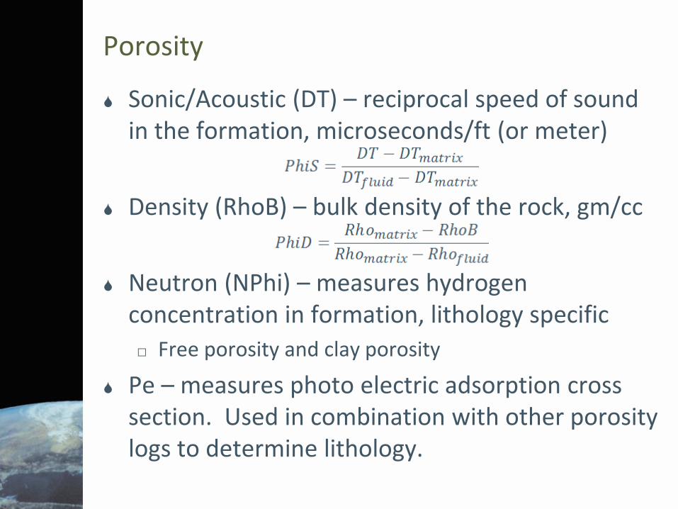
Sonic/Acoustic (DT) – reciprocal speed of sound in the formation, microseconds/ft (or meter)
Density (RhoB) – bulk density of the rock, gm/cc
Neutron (NPhi) – measures hydrogen concentration in formation, lithology specific
□ Free porosity and clay porosity
Pe – measures photo electric adsorption cross section. Used in combination with other porosity logs to determine lithology.

Porosity
Cross plots of density vs. neutron and sonic vs. neutron yield porosity with no requirement for matrix and fluid input
VSH is also available from a density/neutron combination:
This calculation is unreliable in gas-bearing formations
Porosity
All porosity logs measure total porosity
Of equal, probably greater importance, is effective porosity
The two porosity measurements are related as follows:
Total Porosity = Effective Porosity + (VSH×Shale Porosity)
This means that effective porosity is influenced by both the choice of VSH and of shale porosity
As well as any influence of changing matrix and fluid properties in the total porosity calculation
Porosity
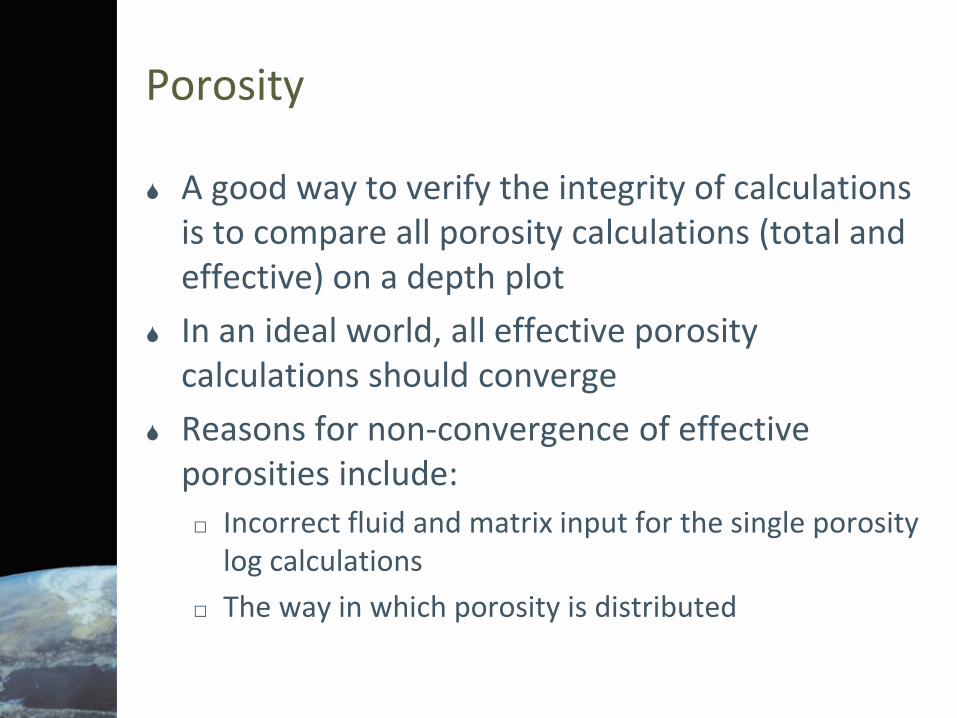
A good way to verify the integrity of calculations is to compare all porosity calculations (total and effective) on a depth plot
In an ideal world, all effective porosity calculations should converge
Reasons for non-convergence of effective porosities include:
□ Incorrect fluid and matrix input for the single porosity log calculations
□ The way in which porosity is distributed

Moldic Porosity • Density/neutron porosity measures
the entire pore network where as acoustic porosity is directional and does not “see” moldic porosity
• The example shows where acoustic porosity is less than density/neutron porosity, implying moldic porosity – illustrated with yellow color fill
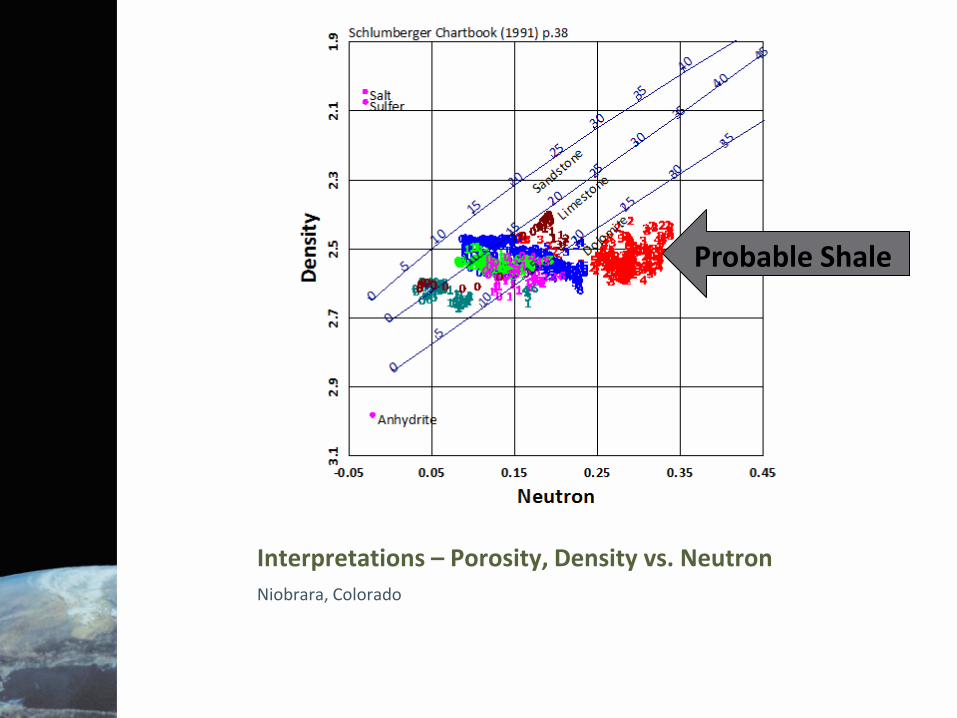
Interpretations – Porosity, Density vs. Neutron
Niobrara, Colorado
Probable Shale

Interpretations – Density vs. Pe
Niobrara, Colorado

Interpretations – Density vs. Sonic
Niobrara, Colorado
Probable Shale

Interpretations – Sonic vs. Neutron
Niobrara, Colorado
Probable Shale

Lithology
As with porosity calculations, the starting point for lithologic differentiation are porosity cross plots:
□ Density vs. neutron
□ Acoustic vs. neutron
□ Density vs. Pe
□ Rho matrix vs. DT matrix
□ Rho matrix vs. U matrix
This presentation focuses on the Density vs. Neutron and Rho matrix vs. U matrix plots since they give the most rigorous results

Lithology – Density vs. Neutron
The density vs. neutron is the most commonly used
Wide-spread application because of abundance of measurements
□ Most wells since the 1980’s have these measurements
In addition to a good measure of cross plot porosity, the plots yield lithologic information
Sandstone, limestone, dolomite, and anhydrite each have distinct grain densities – extrapolation to zero porosity

Lithology – Density vs. Neutron
Pitfalls of using this plot in isolation:
□ Gas effects reduce apparent grain densities
□ In the absence of other information, gas bearing limestones can be misinterpreted as sandstone, and gas-bearing dolomite as limestones. In the case of very high gas saturation, as sandstones.
□ Dolomite cemented sandstones will be misinterpreted as carbonates with no silica

Lithology – Rho matrix vs. U matrix
Rho matrix vs. U matrix is the most powerful cross plot for lithologic differentiation
□ Caveat being the Pe issue with barite drilling mud
Quantitative distinction among quartz, calcite, dolomite, and anhydrite are possible
Dolomite-cemented sandstone can be unequivocally distinguished from carbonate only assemblages

Lithology
Example of a calcium carbonate sequence Kansas
Courtesy of Lynn Watney, KGS
Mostly limestone,
minor sandstone
and dolomite
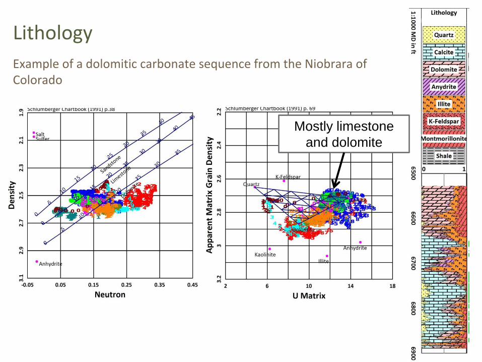
Lithology
Example of a dolomitic carbonate sequence from the Niobrara of Colorado
Mostly limestone
and dolomite

Lithology
Example of a cherty carbonate sequence from Kansas
Courtesy of Lynn Watney, KGS
Mostly dolomite and
quartz, minor
limestone
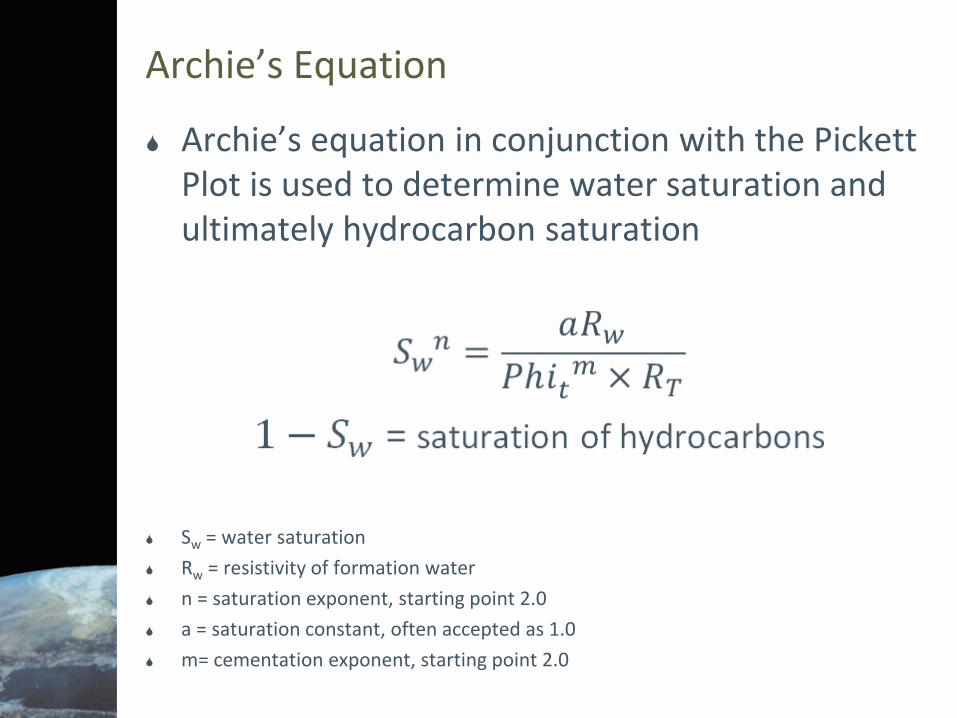
Archie’s Equation
Archie’s equation in conjunction with the Pickett Plot is used to determine water saturation and ultimately hydrocarbon saturation
Sw = water saturation
Rw = resistivity of formation water
n = saturation exponent, starting point 2.0
a = saturation constant, often accepted as 1.0
m= cementation exponent, starting point 2.0

Pickett Plot – Resistivity vs. Porosity
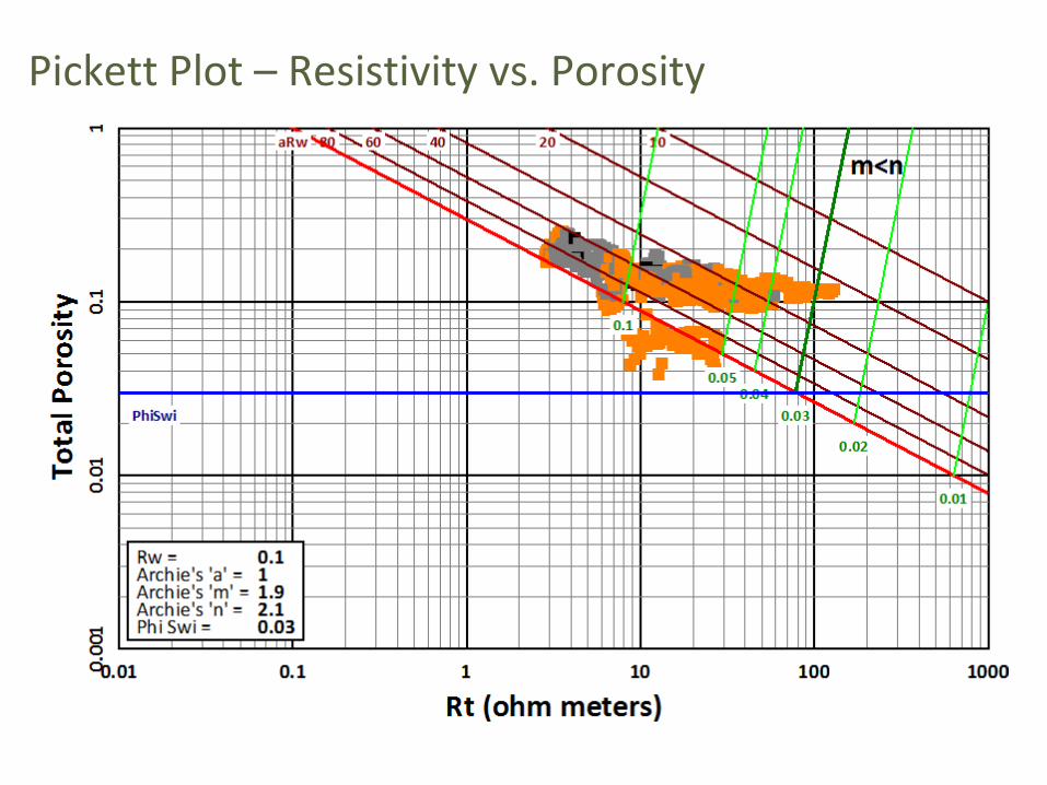
Pickett Plot – Resistivity vs. Porosity
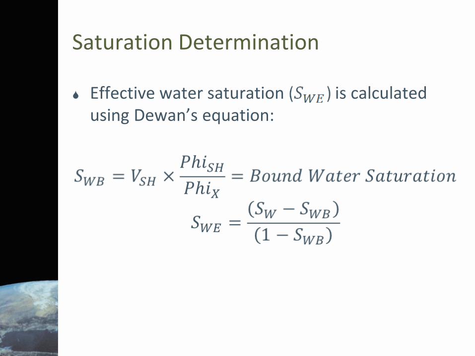
Saturation Determination
Effective water saturation is calculated using Dewan’s equation:

Permeability
Permeability is determined using a modified Timur equation:
is the lower of log-calculated or theoretical from a Buckles equation:

Interpretation – Example
Niobrara, Colorado

Cores vs. Well Logs – Porosity
Most likely a measurement of connected porosity only
There are no service company standards in place, as a result, procedures for measuring porosity vary
Generally, core porosities equates well with petrophysically defined effective porosity

Cores vs. Well Logs – Fluid Saturation
Measurements are made at the surface, following decompression as the core is brought to the surface
In general, one might anticipate: □ Oil saturation to be reduced due to mud filtrate invasion
□ Gas saturation to be increased in volatile oil reservoirs, due to gas generation as pressure is reduced
□ Water saturation to increase do to mud filtrate invasion as well

Cores vs. Well Logs – Grain Density
Core measurements clearly eliminate any influence of fluid saturation (gas effect)
Closest comparisons should be in in clean oil or water bearing sandstones and carbonates
Cores vs. Well Logs – Permeability
There are many different ways of measuring core permeability:
□ Air, at ambient conditions
□ Klinkenberg – extrapolation to infinite pressure. This is preferred, and will be lower than air permeability
□ Permeability at various overburden pressure ■ Can have extreme influence, reducing permeabilities by
orders of magnitude in tight gas sand

Cores vs. Well Logs – Permeability
Correlation with petrophysically-defined permeability is hazardous
Petrophysical estimates involve empirical relations between porosity and irreducible water saturation
□ This is only applicable when the reservoir is indeed at Swi
Core Shifting
It is imperative to try to shift the core data to agree with logs
For sidewall cores, this should not be an issue
For continuous coring it is essential □ Core depth made by the driller may have discrepancies with log depth –
sometimes up to 10 feet or more!
□ For core recoveries of less than 100%, the assumption is frequently made that loss has occurred at the base of the cores as the core barrel is brought to the surface. This might not be a valid assumption as loss could occur by “rubble-izing” incomplete levels at any location
Core vs. Log Scale
Core plug samples are usually about 2 cubic inches (33 cubic cm) in volume. On the other hand, log measurements sample at least a cubic foot (0.03 cubic meter) at a time.
The difference in volume measurements, logs to cores is at a minimum close to 1000. For some logging tools with poor vertical resolution and deeper depths of investigation, that difference could be as high as 1,000,000!

Vertical Resolution of Wireline Logs
Courtesy of Schlumberger

Vertical Resolution of Wireline Logs
Approximate volumes measured by wireline logs:
Log Vertical, ft. Depth, ft. Approximate
Volume, ft3
GR 0.75 1 2.36
Density 1 0.5 0.78
Neutron 2 0.75 3.53
Acoustic 2 2 25.13
Laterolog 2 4 100.5
Induction 7 7 1077.56
Methodology of Upscaling
The basic methodology is to "upscale" the core data measurements to the approximate level of the log measurements, to improve the correlations between the core and log data
Evaluation of correlation coefficients between the upscaled core data and the log measurements to find suggested depth shifts in a rigorous manner

Applications
Aid in depth shifting
The upscaled core data output is a continuous curve – it is much easier to compare wireline logs with upscaled core curves rather than discrete core data points

Example
Texas Panhandle
Data shift
Data shift

Carbonate Unconventional Reservoirs
The Bakken and Niobrara are two examples of carbonate reservoirs undergoing active development
Both produce from carbonate intervals with organic-rich shales in close proximity

Carbonate Unconventional Reservoirs
Carbonate conventional reservoir model:
Matrix Effective Porosity Shale
Water Oil/Gas
The Reservoir

Carbonate Unconventional Reservoirs
Elements of unconventional reservoirs, both carbonate and clastic:
Matrix Effective Porosity
Silt
The Reservoir
TOC
Cla
y So
lids
Cla
y W
ate
r
Fre
e S
hal
e
Po
rosi
ty
Shale

Carbonate Unconventional Reservoirs
Digital Formation has developed a deterministic petrophysical model, which is designed to identify four porosity components:
□ Effective Porosity
□ TOC
□ Clay Porosity
□ Free Shale Porosity
Both adsorbed and free hydrocarbons are also determined
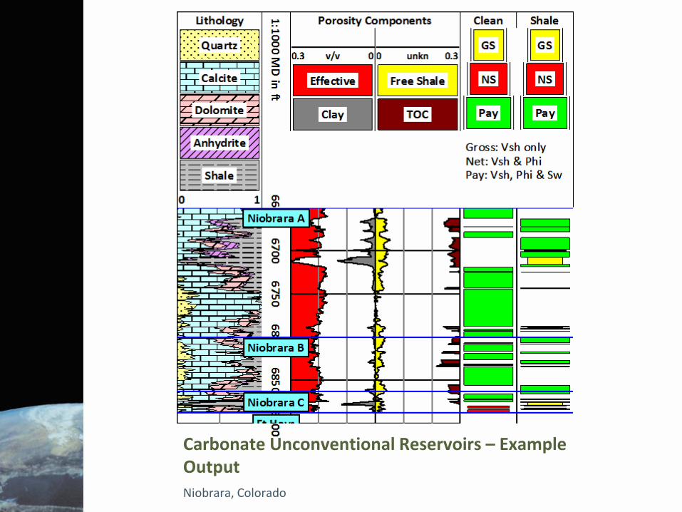
Carbonate Unconventional Reservoirs – Example Output
Niobrara, Colorado

Carbonate Unconventional Reservoirs – Example Output, Adsorbed vs. Free Hydrocarbons
Niobrara, Colorado
Adsorbed oil in
Niobrara Shale
intervals

Carbonate Unconventional Reservoirs – Example Output
Bakken, Montana

Carbonate Unconventional Reservoirs – Example Output, Adsorbed vs. Free Hydrocarbons
Bakken, Montana
Adsorbed oil in
Bakken Shale

Rock Physics Modeling
The Rock Physics Model Digital Formation has developed involves solution to the Gassmann and Krief geophysical models
The Rock Physics Model uses density and neutron logs to mimic both compressional and shear acoustic data
In the absence of shear measurements, the pseudo shear log can be reliable
Texas Panhandle

Rock Physics Modeling
By applying changing fluid properties to both density and neutron curves, which is particularly important in gas reservoirs, the effects of fluid substitution can be quantified
This technique can also be applied to the effects of pressure reduction on pseudo log responses
From the pseudo acoustic and density logs, synthetic seismograms at different saturation or pressure levels can be created, and related to measured seismic responses
Texas Panhandle
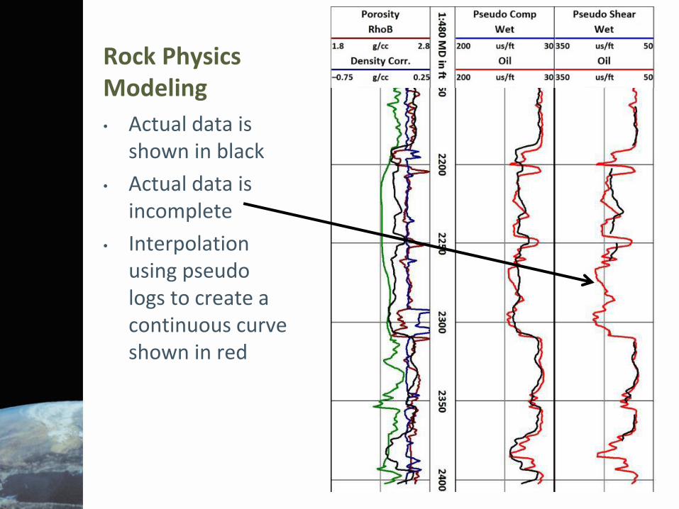
Rock Physics Modeling
• Actual data is shown in black
• Actual data is incomplete
• Interpolation using pseudo logs to create a continuous curve shown in red
Texas Panhandle

Reservoir Characterization
In a reservoir sequence, levels at irreducible water saturation (and a singular rock type) can be distinguished from other levels:
□ Belonging to a different rock type
□ Due to the presence of mobile water
Can be shown on a log Phi vs. log Sw cross plot
Texas Panhandle
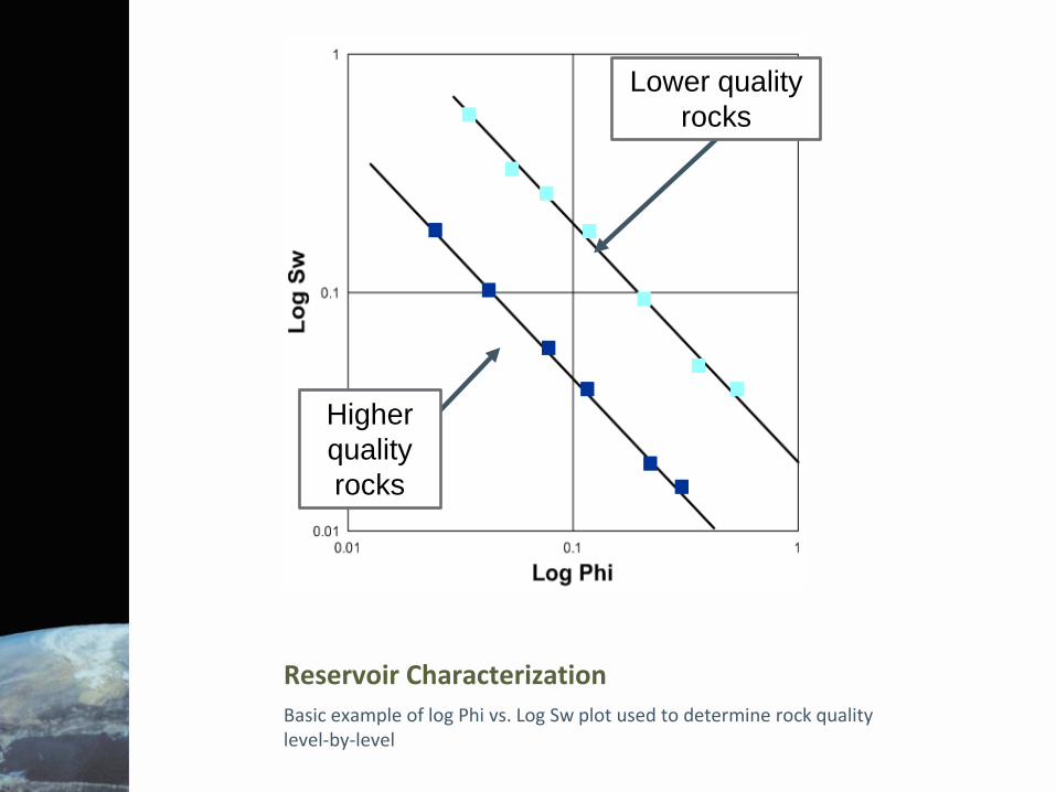
Reservoir Characterization
Basic example of log Phi vs. Log Sw plot used to determine rock quality level-by-level
Lower quality
rocks
Higher
quality
rocks
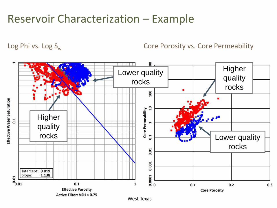
Reservoir Characterization – Example
Log Phi vs. Log Sw Core Porosity vs. Core Permeability
West Texas
Lower quality
rocks
Higher
quality
rocks Lower quality
rocks
Higher
quality
rocks

References
Bond, D.C. "Determination of residual oil saturation." Oklahoma City, Interstate Oil Compact Commission Report (1978): n. pag. Print.
Buckles, R.S. "Correlating and averaging connate water saturation data." Journal of Canadian Petroleum Technology 9.1 (1965): 42-52. Print.
Chilingar, George V, Robert W. Mannon, and Herman H. Rieke. Oil and Gas Production from Carbonate Rocks. New York: American Elsevier Pub. Co, 1972. Print.
Dewan, John T. Essentials of Modern Open-Hole Log Interpretation. Tulsa, Okla: PennWell Books, 1983. Print.
Doveton, John H. Geologic Log Analysis Using Computer Methods. Tulsa, Okla: American Association of Petroleum Geologists, 1994. Print.
Ellis, Darwin V, and Julian M. Singer. Well Logging for Earth Scientists. Dordrecht: Springer, 2007. Print.
Holmes, Michael, et al. "A Petrophysical Model to Estimate Relative and Effective Permeabilities in Hydrocarbon Water Systems." Oral presentation given at the SPE Annual Technical Conference and Exhibition held in San Antonio, Texas, USA, 8-10 October (2012): n. pag. Print.
Holmes, Michael, et al. "A Petrophysical Model to Estimate Free hydrocarbons in Organic Shales." Poster Prestentation given at the AAPG Annual Conference and Exhibition, Houston, TX (2011): n. pag. Print.
References
Holmes, Michael, et al. "Relationship Between Porosity and Water Saturation: Methodology to Distinguish Mobile from Capillary Bound Water." Oral presentation given at the AAPG ACE, Denver, Colorado 7-10 June (2009): n. pag. Print.
Krygowski, Dan. Basic Openhole Log Interpretation. Golden, CO: Petrolium Technology Transfer Council, 2013. Print.
Morris, R.L., and W.P. Biggs. "Using log-derived values of water saturation and porosity." ransactions of the SPWLA 8th Annual Logging Symposium Paper X, 26 p (1967): n. pag. Print.
Passey, Q.R., et al. "From Oil-Prone Source Rock to hydrocarbons-Producing Shale Reservoir ? Geologic and Petrophysical Characterization of Unconventional Shale-hydrocarbons Reservoirs." SPE 131350 (2010): n. pag. Web.
Passey, Q.R. "A Practical Model for Organic Richness from Porosity and Resistivity Logs." AAPG Bulletin 74.12 (1990): 1777-1794. Print.
"Shale Petrophysics." Denver Well Logging Society 2010 Fall Workshop, Golden CO (2010): n. pag. Print.
"Special Core Analysis." DWLS Spring Workshop, Golden CO (2008): n. pag. Web.

Petrophysics of Carbonates Q&A
Presented by
Michael Holmes, Digital Formation Presentation and graphics by:
Jennifer Bartell, Digital Formation
Analysis and output created in LESA, Digital Formation Petrophysical Software