ph36010 mathcad worksheet advanced graphics...

PH36010 MathCAD worksheetAdvanced Graphics and Animation

In this worksheet we examine some more of mathCAD's graphing capabilitiesand use animation to illustrate aspects of physics.

Polar Plots

A polar plot is simply an x-y graph wrapped around into a circle.

After the wrapping, the x-axis represents the angles between 0 and 360 degand the y-axis the radius.

To illustrate a simple polar plot, we will examine the curve known as theCardoid. This is a common curve that appears in the directional response ofmicrophones and antennae.

The Cardoid curve gives a radius, r, and a function of an angle, θ.The equation of the curve is given by:

r(θ)=a[cos(θ)+1]where a is a constant, in this case we will take a=1

First define the function r(θ)

a 1:=

r θ( ) a cos θ( ) 1+( )⋅:=

Now call up a Polar plot (Insert|Graph|Polar Plot) and fill in the placeholders for

θ and r

0

30

60

90

120

150

180

210

240

270

300

330

2

1.5

1

0.5

0r θ( )

θ

Note:MathCAD automatically

creates a range for θ going

from 0 to 2π (0-360)

Although mathCAD is workingin radians, the polar plot isscaled in degrees. This is aslight inconsistency withinmathCAD, but don't worry.

(C) dpl 2002 1/18

PH36010 MathCAD Example Sheet 7

As well as displaying continuous functions of angle like we did above, polarplots can also display discrete points of data stored in vectors, in the sameway as x-y plots.

In the photon scattering example, experimental data of scattering angles wasgiven in a text file containing 2 columns of values.

Read data into matrix

NB. If you are copying this worksheet intoyour own directory, you will need to copy thedata file and change the file read componentto point to it. Follow link from users.aber.ac.uk/dpl-> Course Material -> PH36010 -> Phase.csv

Data

...\phase.csv

:=

Angle Data0⟨ ⟩

deg⋅:= First column contains angles in degrees

LogPhase Data1⟨ ⟩

:= Second column contains log10of response

0 1 2 3 40

2

4

6

8

LogPhase

Angle

X Y plot ofdata

We can plot the same data as a polar plot

0

30

60

90

120

150

180

210

240

270

300

330

6

4

2

LogPhase

Angle

(C) dpl 2002 2/18


0

30

60

90

120

150

180

210

240

270

300

330

6

4

2

LogPhase

Angle

Change the trace tostem in order to plotlines from the origin toeach data point.

Note how the data only gives the response for half the circle, which isreflected in the plot. It is assumed that the response in the 180-360 range isthe same as that in the 0-180 range.

Using matrix functions from the f(x) toolbar button, create two vectors,LogPhase360 and Angle360 which represent the data for the angles -180 to180.

Create a plot showing the complete polar scattering function.

Hints:Create the Angle360 vector first, then you can easily check you have asensible looking answer before using similar steps to create theLogPhase360.

Angle contains the anlges between 0 and 180, so the reverse of Angle willcontain the angles between 180 and 0.You can stack two vectors together to make a single long one.You need to make sure that you don't get two zeroes in the middle of yourresult vector.How would you use submatrix() to return a vector missing its first row ?If V is a vector, then what is -V ?Functions that may be useful are: reverse(), stack(), submatrix()

(C) dpl 2002 3/18


Simple 3D surface plots

Here we will use a simple 3D surface plot to show the profile of a gaussiansurface.Gaussian surfaces arising as a result of many natural processes, for example ifwe shine a narrow beam of ions or photons onto a flat plate and measure theintensity of the beam at different places on the plate, we will find the resultusually looks like a gaussian.

The gaussian functions we will plot is a function of x- and y- and looks like:

k 1:=

k is a constant which determine the width ofour beam.Gaussian2D x y,( ) e

x2

y2

+( )−

k:=

In plotting, we frequently need to fill a vector with a range of values. Thismakes it easy to scale our plots as required.Since we will be doing this several times in this sheet, it makes sense todefine a program to do it for us...

FillSeries Min Max, N,( ) ∆Max Min−

N←

Resulti Min ∆ i⋅+←

i 0 N..∈for

Result

:= Calculate the increment

Loop through the number ofincrements, adding each one tothe result

When finished looping, return theresult

Having created the program, test it to check it works before moving on.

Returns a vector going from -1 to 1in 10 steps.

Notice that in order to take 10 steps, wevisit 11 points

FillSeries 1− 1, 10,( )

0

0

1

2

3

4

5

6

7

8

9

10

-1

-0.8

-0.6

-0.4

-0.2

0

0.2

0.4

0.6

0.8

1

=

Now the FillSeries() functions appears to be OK, we can move on...

(C) dpl 2002 4/18


We will plot our Gaussian2D() function over x and y values going from -5 to+5 in 100 steps.Create variable to hold the minimum and maximum values for x and y and also the number of steps in each direction.

N 100:=

xmin 5−:= xmax 5:= ymin 5−:= ymax 5:=

Use the FillSeries() function to create vectors X and Y which hold the x and yvalues we wish to plot the function at

X FillSeries xmin xmax, N,( ):= Y FillSeries ymin ymax, N,( ):=

Use the space on the right of the page to print out the 2 vectors and assureyourselves that they look OK.

We now wish to fill a matrix, Z, with the values of the Gaussian2D function atthe corresponding point. To do this we create 2 range variables, i & j, which weuse to step through the X & Y vectors

i 0 N..:= i is used to step the the X vector

j 0 N..:= j is used to step the the Y vector

Filling the Z matrix is done with the range variables i & j

Zi j, Gaussian2D Xi Y j,( ):=

Now insert a 3D surface plot and display the Z-matrix

Z

This is the default plotformat. The surface is notfilled in and the lines are allblack

Bring up the format box andon the Appearance tab page,change the surface to befilled with a colourmap andjust contour lines to bedrawn.

(C) dpl 2002 5/18


Z

Experiment withdifferent options onthe pages on theformat dialog box

Try dragging themouse over the plotto get different viewangles.

Hold <shift> whilstdragging the mouseto start the plotrotating.

Experiment with changing the values above for xmin,xmax,ymin and ymax aswell as the k constant.

(C) dpl 2002 6/18


The following segment of mathCAD will plot a cone

a 2:= Base radius

b 5:= Height of cone

Function h(x,y) gives height ofslope

h x y,( )b−

ax

2y

2+⋅ b+:=

Function cone(x,y) uses a conditionalto restrict the points on the cone tothose above the xy plane

cone x y,( ) if x2

y2

+( ) a2

> 0, h x y,( ), :=

Zi j, cone Xi Y j,( ):= Fill the Z matrix with the cone() function,using the same range of X & Y valuesas before.

Z

Use the plot format options to display the cone with a colourmap over thesurface.

On the advanced tab-page of the format dialog box, you can select differentcolour maps to use.

A truncated cone is simply a cone with the top sliced off. Create a functionTruncCone(x,y) that uses the definitions of h(x,y) and cone(x,y) togther with anif() function to give a cone with the top sliced off at a height of zz.

Plot your truncated cone with zz set to 3

Try and create a function to plot a hemisphere. You may need to adjust thescaling on the z-axis so that it looks like a hemisphere.

(C) dpl 2002 7/18


Advanced 3D surface plots

So far the 3D surface plots have lacked any scaling in the x and y axes. Thenumbers appearing on the plot axes have related to the indices of the z matrixrahter than 'real world' co-ordinates.

In this section we will combine 3 matrices together in order to give plotswhere the X and Y axes are scaled in real world co-ordinates.

We will use the X and Y vectors we created earlier, together with the rangevariables for indexing them.

XXi j, Xi:= YYi j, Y j:=

XX

0 1 2 3 4

0

1

2

3

4

5

-5 -5 -5 -5 -5

-4.9 -4.9 -4.9 -4.9 -4.9

-4.8 -4.8 -4.8 -4.8 -4.8

-4.7 -4.7 -4.7 -4.7 -4.7

-4.6 -4.6 -4.6 -4.6 -4.6

-4.5 -4.5 -4.5 -4.5 -4.5

= YY

0 1 2 3

0

1

2

3

4

5

-5 -4.9 -4.8 -4.7

-5 -4.9 -4.8 -4.7

-5 -4.9 -4.8 -4.7

-5 -4.9 -4.8 -4.7

-5 -4.9 -4.8 -4.7

-5 -4.9 -4.8 -4.7

=

ZZi j, Gaussian2D XXi j, YYi j,,( ):=

The XX and YY matrices hold the real world co-ordinates of the points we wish toplot.

Note how the indices are used.

Here is a section of the XX and YY matrices. See how each column of the XX matrixis identical and each row of the YY matrix is identical.

When we fill the Z matrix using the range variables, the Gaussian2D function iscalled with the x and y values from the corresponding point in the XX and YY tables.

Thus Z0,0 becomes Gaussian2D(-5,-5)

Z0,1 becomes Gaussian2D(-5,-4.9)

Z0,2 becomes Gaussian2D(-5,-4.8)

...Z1,0 becomes Gaussian2D(-4.9,-5)

...Z100,99 becomes Gaussian2D(5,4.9)

Z becomes Gaussian2D(5,5)

(C) dpl 2002 8/18


Z100,100 becomes Gaussian2D(5,5)

Once we have filled the matrices we can plot the function by putting the 3matrices in the 3D plot placeholder, seperated with commas and surrounded inbrackets.

XX YY, ZZ,( )

Notice how the axes are now scaled in real numbers over the range wespecified earlier.

Experiment with the shading and colourmap options as before

(C) dpl 2002 9/18


Polar plots in 3D

In the above example, we used a simple scaling relationship to create the XXand YY matrices. We can use more complicated relationships to make plotsand surfaces to fit in with our problems.

In this example we will map our XP and YP matrices onto polar co-ordinates,enabling us to plot functions which are essentially polar in nature. In this casewe will plot the electron probability function for the 100 electron in theHydrogen atom.

The first step is to define our range of r and θ values we are going to beplotting

If you are pusing a version of mathCAD prior to v13, you will need to define

nm as 10-9m and a0 as 5.292 10

11−× m. a

0 is the bohr radius of the atom

RSteps 30:= We will plot 30 steps in the radial direction

Create a vector Radius holding a series of radii from 0m to 6 Bohr radii.

Radius FillSeries 0m 6 a0⋅, RSteps,( ):=

ri 0 RSteps..:= Range variable ri for indexing radii

θSteps 20:= 20 steps in angular direction

Create vector Theta holding a series of angles from -π to π

Theta FillSeries π− π, θSteps,( ):=

θi 0 θSteps..:= Range variable θi for indexing angles

Now, once we've created the Theta and Radius vectors, along with the rangevariables for indexing them, we can fill our XP and YP matrices with polarcoordinates.

XPri θi,

Radiusri cos Thetaθi( )⋅:= NB If you try and re-use the XX or YY

matrices, you will get a Units error - why ?

YPri θi,

Radiusri sin Thetaθi( )⋅:=

(C) dpl 2002 10/18


We can examine the XP and YP matrices asbefore:

XP

0 1 2 3

0

1

2

3

4

5

6

7

8

9

0 0 0 0-11-1.058·10 -11-1.007·10 -12-8.562·10 -12-6.221·10-11-2.117·10 -11-2.013·10 -11-1.712·10 -11-1.244·10-11-3.175·10 -11-3.02·10 -11-2.569·10 -11-1.866·10-11-4.233·10 -11-4.026·10 -11-3.425·10 -11-2.488·10-11-5.292·10 -11-5.033·10 -11-4.281·10 -11-3.11·10-11-6.35·10 -11-6.039·10 -11-5.137·10 -11-3.733·10-11-7.408·10 -11-7.046·10 -11-5.994·10 -11-4.355·10-11-8.467·10 -11-8.052·10 -11-6.85·10 -11-4.977·10-11-9.525·10 -11-9.059·10 -11-7.706·10 -11-5.599·10

m=

YP

0 1 2 3

0

1

2

3

4

5

6

7

8

9

0 0 0 0

0 -12-3.27·10 -12-6.221·10 -12-8.562·10

0 -12-6.541·10 -11-1.244·10 -11-1.712·10

0 -12-9.811·10 -11-1.866·10 -11-2.569·10

0 -11-1.308·10 -11-2.488·10 -11-3.425·10

0 -11-1.635·10 -11-3.11·10 -11-4.281·10

0 -11-1.962·10 -11-3.733·10 -11-5.137·10

0 -11-2.289·10 -11-4.355·10 -11-5.994·10

0 -11-2.616·10 -11-4.977·10 -11-6.85·10

0 -11-2.943·10 -11-5.599·10 -11-7.706·10

m=

In the XP and YP matrices, the angular values go across and the radius valuesgo down the page.

The XP matrix holds the x-coordinates of the points in the plane and the YPmatrix holds the y- co-ordinates of the points.

Thus, at an angle of -π radians (first column) all the x-coordinates are negativeand the y co-ords zero.

At an angle of -90 deg (column 5) the x-coordinates are zero and the y valuesnegative.

Having created our XP and YP matrices, we can see about plotting a functionon our 3D polar graph.

The wave function ψ of the 100 electron as afunction of radius

ψ100 r( )1

πa03

e

r−

a0⋅:=

(C) dpl 2002 11/18


We can start by plotting ψ100() in two dimensions. This is easily achived usingthe Radius vector we defined earlier, along with the ri range variable

0 5 .1011

1 .1010

1.5 .1010

2 .1010

2.5 .1010

3 .1010

0

1 .1015

2 .1015

ψ100 Radiusri( )

Radiusri

Now we can fill a matrix with the result of applying our function

Z100ri θi,

πa03

ψ100 Radiusri( )⋅:=

XP

m

YP

m, Z100,

XP

a0

YP

a0

, Z100,

In the left hand plot we have divided the XP and YP matrices by m to scale the plot inmetersIn the right hand plot, we have divided the XP and YP matrices by a0, in orderto scale the axes in Bohr radii.

The ψ100 and ψ200 functions are both symetrical about the axis and do not

depend on θ. The ψ210 function depends on θ as well as r and is given below

ψ210 r θ,( ) 1

32 π⋅ a05

⋅

r⋅ e

r−

2 a0⋅⋅ cos θ( )⋅:= Create a matrix Z210 and fill it with

the ψ210 function over the range ofvalues before plotting it.

(C) dpl 2002 12/18


Plotting a sphere and other surfaces

The following snippet is taken from the resource centre and shows how to plota sphere by the simple application of spherical co-ordinates.

Note that I've changed the names of the matrices to avoid conflicting with theX,Y and Z matrices we used earlier in this sheet.

Np 25:=

i 0 Np..:= φi iπ

Np⋅:= Could use

FillSeries here.

j 0 Np..:= θ j j 2⋅π

Np⋅:=

SphereXi j, sin φi( ) cos θ j( )⋅:= These are simply the equations toconvert spherical coordinates intocartesian.

SphereYi j, sin φi( ) sin θ j( )⋅:=

SphereZi j, cos φi( ):=

SphereX SphereY, SphereZ,( )

Play with plot options

(C) dpl 2002 13/18


Having created a single sphere, it is trivial to plot two of them on the samegraph. Here the second sphere is moved 2.1 units along the x-axis

SphereX SphereY, SphereZ,( ) SphereX 2.1+ SphereY, SphereZ,( ),

Try selecting 'Equal Scales' from the plot formatting options to get a gooddisplay.

You can select different fill options for each plot on the graph.

The resource centre has quicksheets which act as a starting point forplotting spheres, tori and other more complex surfaces.

(C) dpl 2002 14/18


Animation in mathCAD

Animations consist of a number of pictures shown one after another insuccession. this fools the eye into believing that it is observingcontinuous motion.

MathCAD performs animations by means of a system variable called FRAME.When you ask mathCAD to animate a region of the worksheet, it takes asnapshow of the region before incrementing FRAME and taking anothersnapshot. When all the snapshots are combined together they give theimpression of continuous motion.

As a trivial, if not particularly exciting example, bring up the animation dialogbox (Tools|Animation|Record...)When the dialog box is displayed, use the mouse to drag a box around theregion where the value of FRAME is displayed below. Once you have selected the region to animate, press the Animate button inthe dialog box.After a while, you should see the windows media player and be able to playback a little animation showing how FRAME changes from 0 to 9

FRAME 0=

Colngratulations, you have created your first animation. More excitinganimations usually contain graphs.

Have a look at some of the examples in the Resource Centre. There is acomplete tutorial guide in Advanced Topics|Treasury Guide to Animations anda few very useful examples in Quicksheets|Animations

(C) dpl 2002 15/18


The following example shows how simple it is to animate the spheres wecreated earlier. Try animating the video for FRAME going from 0 to 20

∆π

10:= Displacement t( ) 2 sin ∆ t⋅( )+:=

t FRAME:=

Before you begin animation, select format the graph and fix the x axis scale to -4 to +4

SphereX Displacement t( )− SphereY, SphereZ,( ) SphereX Displacement t( )+ SphereY, SphereZ,( ),

Experiment with lighting, appearance, surface plot and other options

(C) dpl 2002 16/18


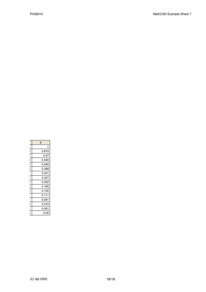
Z100

0 1 2 3 4 5

0

1

2

3

4

5

6

7

8

9

10

11

12

13

14

15

1 1 1 1 1 1

0.819 0.819 0.819 0.819 0.819 0.819

0.67 0.67 0.67 0.67 0.67 0.67

0.549 0.549 0.549 0.549 0.549 0.549

0.449 0.449 0.449 0.449 0.449 0.449

0.368 0.368 0.368 0.368 0.368 0.368

0.301 0.301 0.301 0.301 0.301 0.301

0.247 0.247 0.247 0.247 0.247 0.247

0.202 0.202 0.202 0.202 0.202 0.202

0.165 0.165 0.165 0.165 0.165 0.165

0.135 0.135 0.135 0.135 0.135 0.135

0.111 0.111 0.111 0.111 0.111 0.111

0.091 0.091 0.091 0.091 0.091 0.091

0.074 0.074 0.074 0.074 0.074 0.074

0.061 0.061 0.061 0.061 0.061 0.061

0.05 0.05 0.05 0.05 0.05 0.05

=

(C) dpl 2002 17/18


6

1 1

0.819 0.819

0.67 0.67

0.549 0.549

0.449 0.449

0.368 0.368

0.301 0.301

0.247 0.247

0.202 0.202

0.165 0.165

0.135 0.135

0.111 0.111

0.091 0.091

0.074 0.074

0.061 0.061

0.05 0.05

(C) dpl 2002 18/18

ph36010 mathcad worksheet advanced graphics...

Documents