Pharmacokinetics of Current and Future Drugs for TIVASteven L. Shafer, M.D.Palo Alto, California

Lecture goals: 1) To introduce the basic pharmacokinetic concepts that apply to intravenous drugs, 2) to explain how these concepts can be used to develop rational dosing guidelines for intravenous anesthetic drugs, 3) to provide insight into rational selection of drugs for intravenous anesthesia, and 4) to provide nomograms showing how to administer intravenous anesthetic drugs in ways that take advantage of their pharmacokinetic properties. The goal is not to provide YATOUPN (yet another table of interpretable pharmacokinetic numbers).

Pharmacokinetics are classically represented by compartment models, such as the one-compartment model shown to the right. This model has a single volume and flow. The attraction of the one-compartment model is its simplicity. It is easy to visualize the body as a one-compartment model (particularly when it is wrapped in Spandex), into which we inject drug. The mathematics of the one compartment model are easy also. The initial loading dose to achieve a concentration is simply your target times V, the volume of the compartment. The infusion rate to maintain a target concentration is simply your target times Q, clearance.

If we were built like buckets, we would have a single volume and a single clearance. The math would be easy, but life would be dull. For all intravenous anesthetic drugs, we behave as if we were several buckets connected together by pipes, as shown in figure 2 (two compartment model) and figure 3 (three compartment model). The volume to the left in the two compartment model, and in the center of the three compartment model, is called the “central volume.” The other volumes are called “peripheral volumes,” and the sum of the all the volumes is the volume of distribution at steady state (or Vdss). The clearances leaving the central compartment for the outside is the “central” or “metabolic” clearance. The clearances between the central compartment and the peripheral compartments are called “intercompartmental clearances.”

Figure 1: The one compartment model, with a single volume and flow term.

What do the volumes and clearances estimated by pharmacokinetic modeling mean? It is likely that the central (or “metabolic”) clearance estimated by pharmacokinetic modeling has a true physiologic basis. It is also conceivable that the volume of distribution at steady state (Vdss) has a physiological basis: the partitioning of drug into all body structures at steady state.

For three compartment models, it is tempting to speculate that the rapidly equilibrating volume (V2) corresponds to vessel rich group and the slowly equilibrating volume (V3) corresponds to the fat and vessel poor group. In fact, many authors discuss drugs in exactly this way. This may provide some insight, particularly for highly lipophilic drugs in which a large V3 may be explained by extensive distribution of the drug into fat. However, for the most part the volumes and clearances (except central clearance and Vdss) developed in pharmacokinetic models are simply mathematical constants derived from equations that describe the plasma drug concentrations over time. They are not direct measures of anatomic structures or human physiology.

The reason we use multicompartment models for the intravenous anesthetic drugs is that the plasma concentrations over time following a bolus of an intravenous drug resemble the curve in figure 5. For many drugs, three distinct phases can be distinguished. There is a rapid “distribution” phase (solid line) that begins immediately after the bolus injection. This phase is characterized by very rapid movement of the drug from the plasma to the rapidly equilibrating tissues. Often there is a slower second distribution phase (dashed line) that is characterized by movement of drug into more slowly equilibrating tissues, and return of drug to the plasma from the most rapidly equilibrating tissues (i.e, those that reached equilibrium with the plasma during phase 1). The terminal phase

Figure 2: Two compartment pharmacokinetic model, with two volumes, (central and peripheral) and two clearances (central, and intercompartmental).

Figure 3: Three compartment model, with three volumes, (central, rapidly equilibrating peripheral and slowly equilibrating peripheral) and three clearances (central, rapid and slow intercompartmental).

Figure 4: Shape of curve following intravenous bolus injection.

(dotted line) is a straight line when plotted on a semilogarithmic graph. The terminal phase is often called the “elimination phase” because the primary mechanism for decreasing drug concentration during the terminal phase is drug elimination from the body. The distinguishing characteristic of the terminal elimination phase is that the relative proportion of drug in the plasma and peripheral volumes of distribution remains constant. During this “terminal phase” drug returns from the rapid and slow distribution volumes to the plasma, and is permanently removed from the plasma by metabolism or renal excretion.

Curves which continuously decrease over time, with a continuously increasing slope (i.e., curves that look like figure 5), can be described by a sum of exponentials. In pharmacokinetics, one way of notating this sum of exponentials is to say that the plasma

concentration over time is: where t is the time since the bolus, C(t) is the drug concentration following a bolus dose, and A, , B, , C, and are parameters of a pharmacokinetic model.

We use equation 1 in modeling pharmacokinetics because it describes the data. In particular, we can use it to describe both the onset and offset of drug effect. The “classic” method of describing the offset of drug effect is to use the terminal half-life. This is not a good idea for drugs described by multicompartmental pharmacokinetics, because the half-life relates only to 1 parameter, , while all 6 parameters in equation 1 influence the rate of offset of drug effect.

Before we discuss how to use pharmacokinetics to design rational dosing guidelines, we must understand how pharmacokinetics relate to the onset and offset of drug effect. Dr. Stanki’s lecture will discuss the biophase, which is the essential pharmacokinetic concept to understanding drug onset. Therefore, we will limit the discussion here to the offset of drug effect.

The offset of drug affect

In anesthesia, the offset of drug effect governs awakening from the anesthetic state. The rate at which drug decreases is dependent both on elimination and distribution of the drug from the central compartment. Drug that has distributed into peripheral tissues is partly sequestered from the plasma, in that a gradient must be established between the concentration in the central compartment and in the peripheral tissues plasma before a net flow will be established between the peripheral tissues and the plasma. The contribution of redistribution, elimination, and sequestration towards the rate of decrease of drug concentration varies according to the duration of drug delivery. As a result the time for the drug concentration to decrease a set percentage varies according to the duration of drug administration.

C(t) = Ae + B e + C e- t - t - t Equation 1

Because half-lives tell us almost nothing about the time required for the concentrations to fall by 50%, Hughes et al introduced the term “context-sensitive half-time” to describe the time required for a 50% decrease in plasma concentration following infusions of varying duration.35 The context is the duration of an infusion that maintains a steady drug concen-tration. Figure 5 shows the context sensitive half-times for two opioids popular in anesthesia practice: alfentanil, and sufentanil. The terminal half-lives for these drugs are 2 hours and 9 hours, respectively. Even though sufentanil has terminal half-life that is nearly 5 times longer than that of alfentanil, the sufentanil concentrations will fall much faster than the alfentanil concentrations for infusions of less than 8 hours duration. This illustrates that terminal half-lives are misleading: the 9 hour terminal half-life of sufentanil provides virtually no insight (actually, it is misleading) into how long it will take the plasma concentrations to fall by 50% following drug administration.

The clinical setting determines the percent decrease necessary to produce a given change in drug effect. Again, to use an example from anesthesia, let's say that we are running a very light anesthetic. Let us postulate that the anesthetic is so light that just a a 20% decrease in opioid concentration would produce emergence from anesthesia. Conversely, let's say that we are running a very deep anesthetic (e.g., an opioid anesthetic for cardiac surgery). In this case, we may need an 80% decrease in concentration for the patient to awaken. Figure 6 shows the times required for the sufentanil concentration to fall by 20, 50, and 80% as a function of the infusion duration. We can infusion sufentanil for 10 hours, and still et a 20% decrease within a few minutes of turning off the infusion. However, a 50% decrease will take an hour after a 10 hour infusion. If we need an 80% decrease, then after just 3 hours of drug administration we will need another 3 hours for the patient to awaken!

Designing dosing regimens

Now that we have reviewed the basics of pharmacokinetics and the mathematical models, it is time to ask: how do we actually calculate drug dosages? Again, I use anesthetic drugs as examples, because these are the drugs with which I am the most familiar.

Initial bolus dose

Let's start by computing how to give the first dose of intravenous drug (although the same concepts apply to giving the first dose of an orally administered drug). The definition of

Figure 5: Context sensitive half-times (vertical axis) for sufentanil and alfentanil, as a function of infusion duration (horizontal axis).

Figure 6: The times for a 20%, 50%, and 80% decrease in sufentanil concentration, as a function of infusion duration.

concentration is amount divided by volume. We can rearrange the definition of concentration to find the amount of drug required to produce any desired concentration for a known volume:

Many introductory pharmacokinetic texts suggest using this formula to calculate the “loading bolus” required to achieve a given concentration. This concept is often applied to theophylline and digitalis. The problem with applying this concept is that there are several volumes: V1 (central compartment), V2 and V3 (the peripheral compartments), and Vdss, the sum of the individual volumes. V1 is usually much smaller than Vdss, and so it is tempting to say that the loading dose should be something between, Concentration V 1 2 and Concentration Vd ss 3.

As shown in figure 7, with multicompartment drugs administering a bolus of Concentration V 1 4will achieve the desired concentration for an initial instant, but the levels will rapidly decrease below the desired target. Administering a bolus of Concentration Vd ss 5will produce an overshoot in the plasma that may persist for many minutes. One resolution is to suggest that the dose be between these extremes.

Again, using an anesthetic drug as an example, consider the dose of fentanyl required to attenuate the hemodynamic response to intubation when combined with thiopental. The target concentration for this is approximately 3 g/ml. The V1 and Vdss for fentanyl are 13 liters and 360 liters, respectively. The above equations can thus be interpreted as suggesting that an appropriate dose of fentanyl to attenuate the hemodynamic response is between 39 g (3 ng/ml 13 liters) and 1,080 g (3 ng/ml 360 liters) (figure 7). Personally, I don't need equations to tell me that the right fentanyl dose is somewhere between 39 and 1080 g!

The usual dosing guidelines for bolus injection, as presented above, are oriented towards producing a specific plasma concentrations. Since the plasma is not the site of drug effect, it is illogical to base the calculation of the initial bolus on a plasma concentration. As pointed out previously, by knowing the ke0 of an intravenous anesthetic, we can design a dosing regimen to that yields the desired concentration at the site of drug effect. If one turns to Figure 1 of Dr. Stanki’s biophase lecture, we can see the relative plasma and effect site concentrations following an IV bolus of fentanyl. The plasma concentration decreases continuously, while the effect site concentration rises until it reaches the plasma concentration, at which point both decrease continuously. If we do not want to overdose the patient, we should select the bolus that produces the desired peak concentration in the effect site.

The decline in plasma concentration between the initial concentration following the bolus (amount / V1) and the concentration at the time of peak effect can be thought of as a dilution of the bolus into a larger volume than the volume of the central compartment. This introduces the concept of Vdpeak effect, which is the volume of distribution at the time of peak effect. The size of

Amount = Concentration Volume

Figure 7: Plasma drug concentrations following bolus doses based on target concentration times V1 and target concentration times Vdss.

this volume can be readily calculated from the observation that the plasma and effect site concentrations are the same at the time of peak effect:

Vdloading dose

C (peak effect)plasmapeak effect =

where Cplasma (peak effect) is the plasma concentration at the time of peak effect. Remembering that concentration is amount over volume, we can rearrange the above equation by substituting the initial plasma concentration times V1 for the loading dose. This gives the relationship:

where Cplasma (initial) is the initial concentration following a bolus, Cplasma (peak effect) is the concentration at the time of peak effect, and the ratio of these is the percent decrease in plasma concentration between the initial concentration and the concentration at the time of peak effect.

Returning to the goal of selecting the dose to produce a certain given effect without producing an overdose: by definition the plasma concentration at the time of peak effect is the loading dose / Vd (peak effect). This can be rearranged to calculate the size of the initial bolus:

loading dose desired concentration Vd peak effect =

The Vdpeak effect for fentanyl is 75 liters. To produce a peak fentanyl effect site concentration of 3.0 ng/ml requires 225 g, which will produce a peak effect in 3.6 minutes. This is a clinically reasonable suggestion, compared with the absurd suggestion, based upon V1 and Vdss, of simply picking a dose between 39 and 1080 g.

The exact same concept applies to oral dosage. Measure the plasma drug concentration at the time of oral dosage, and calculate Vdpeak effect as the oral dose divided by the concentration at the time of peak effect. The dose necessary to produce any desired concentration is then the target times Vdpeak effect.

Maintenance infusion rate

As previously pointed out, the rate at which drug exits from the body is the systemic clearance, Q, times the plasma concentration. To maintain a steady concentration, CT (for target concentration), drug must be delivered at the same rate that drug is exiting the body. Thus, the maintenance infusion rate is often presented as:

Maintenance infusion rate = CT Q

For drugs with multicompartmental pharmacokinetics, which includes all of the drugs used in anesthetic practice, drug is distributed into the peripheral tissues as well as cleared from the body. The rate of distribution into tissues changes over time as the tissue concentrations equilibrates with the plasma. The above equation is only correct after the peripheral tissues have equilibrated with the plasma, which requires many hours. At all other times, this maintenance infusion rate will be too slow.

VdC

C percent decreasepeak effect

(initial)(peak effect)

= V = V 1

plasma

plasma

1

However, in some situations this simple maintenance rate calculation may be acceptable when combined with a bolus based on Vdpeak effect. For drugs with a long delay between the bolus dose and peak effect, much of the distribution of drug into the tissues may have occurred by the time the effect site concentration reaches a peak. In this case, the maintenance infusion rate calculated as CT Q may be fairly accurate because Vdpeak effect was sufficiently higher then V1 to account for the much of the distribution of drug into peripheral tissues. This is the reason that the loading infusion-maintenance infusion concepts works modestly well for theophylline.

This leads us to consider a more sophisticated approach in designing infusion rates to maintain target concentrations for drugs with multicompartment pharmacokinetics. Since the net flow of drug into peripheral tissues decreases over time, the infusion rate to maintain any desired concentration also decreases over time. If the initial bolus has been based on Vdpeak effect, no infusion need be administered until the effect site concentration peaks. Following the peak in effect site concentration, the equation to maintain the desired concentration is (unfortunately):

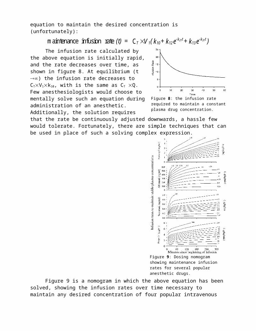
maintenance infusion rate C (t) = V ( k + k e + k e )T 1 10 12-k t

13-k t21 31

The infusion rate calculated by the above equation is initially rapid, and the rate decreases over time, as shown in figure 8. At equilibrium (t ) the infusion rate decreases to CTV1k10, with is the same as CT Q. Few anesthesiologists would choose to mentally solve such an equation during administration of an anesthetic. Additionally, the solution requires that the rate be continuously adjusted downwards, a hassle few would tolerate. Fortunately, there are simple techniques that can be used in place of such a solving complex expression.

Figure 8: the infusion rate required to maintain a constant plasma drug concentration.

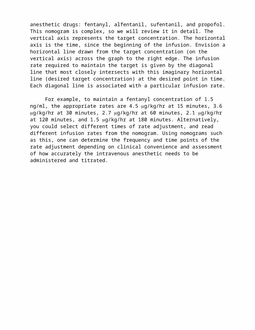
Figure 9 is a nomogram in which the above equation has been solved, showing the infusion rates over time necessary to maintain any desired concentration of four popular intravenous anesthetic drugs: fentanyl, alfentanil, sufentanil, and propofol. This nomogram is complex, so we will review it in detail. The vertical axis represents the target concentration. The horizontal axis is the time, since the beginning of the infusion. Envision a horizontal line drawn from the target concentration (on the vertical axis) across the graph to the right edge. The infusion rate required to maintain the target is given by the diagonal line that most closely intersects with this imaginary horizontal line (desired target concentration) at the desired point in time. Each diagonal line is associated with a particular infusion rate.

For example, to maintain a fentanyl concentration of 1.5 ng/ml, the appropriate rates are 4.5 g/kg/hr at 15 minutes, 3.6 g/kg/hr at 30 minutes, 2.7 g/kg/hr at 60 minutes, 2.1 g/kg/hr at 120 minutes, and 1.5 g/kg/hr at 180 minutes. Alternatively, you could select different times of rate adjustment, and read different infusion rates from the nomogram. Using nomograms such as this, one can determine the frequency and time points of the rate adjustment depending on clinical convenience and assessment of how accurately the intravenous anesthetic needs to be administered and titrated.

Figure 9: Dosing nomogram showing maintenance infusion rates for several popular anesthetic drugs.

Drugs in the future: remifentanil

There are only two intravenous anesthetics on the horizon, remifentanil and eltanolone. I am unable to generate any personal enthusiasm for eltanolone, because I haven’t seen any data suggesting it offers any advantage over presently available hypnotics. Also, I’m not sure how seriously it is being developed, and whether it will even reach a formal FDA review. So I have chosen to ignore it, and will focus on a drug that will be available very soon: remifentanil.

Remifentanil’s unique characteristic is its metabolism.1,2,3

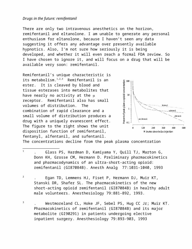
Remifentanil is an ester. It is cleaved by blood and tissue esterases into metabolites that have nearly no activity at the receptor. Remifentanil also has small volumes of distribution. The combination of rapid clearance and a small volume of distribution produces a drug with a uniquely evanescent effect. The figure to the right shows the unit disposition function of remifentanil, fentanyl, alfentanil, and sufentanil. The concentrations decline from the peak plasma concentration immediately following an intravenous bolus. We can see in the figure how the pharmacokinetics of remifentanil differ from those of the other opioids. A bolus of remifentanil disappears from the plasma more rapidly than a comparable bolus of fentanyl, alfentanil, or sufentanil.

1 . Glass PS, Hardman D, Kamiyama Y, Quill TJ, Marton G, Donn KH, Grosse CM, Hermann D. Preliminary pharmacokinetics and pharmacodynamics of an ultra-short-acting opioid: remifentanil (GI87084B). Anesth Analg 77:1031-1040, 1993

2 . Egan TD, Lemmens HJ, Fiset P, Hermann DJ, Muir KT, Stanski DR, Shafer SL. The pharmacokinetics of the new short-acting opioid remifentanil (GI87084B) in healthy adult male volunteers. Anesthesiology 79:881-892, 1993.

3 . Westmoreland CL, Hoke JF, Sebel PS, Hug CC Jr; Muir KT. Pharmacokinetics of remifentanil (GI87084B) and its major metabolite (GI90291) in patients undergoing elective inpatient surgery. Anesthesiology 79:893-903, 1993

Minutes since bolus injection0 120 240 360 480 600

Perc

ent o

f pea

k pl

asm

a op

ioid

con

cent

ratio

n

0.1

1

10

100

fentanyl

sufentanil

alfentanil

remifentanil

Minutes since bolus injection0 2 4 6 8 10

Percent of peak effect site opioid concentration

0

20

40

60

80

100

fentanyl

sufentanil

alfentanil

remifentanil

Remifentanil has an onset that resembles the onset of alfentanil. For the past 15 years we have used the EEG as a measure of opioid drug effect to measure the rate of equilibration between the plasma and the site of opioid drug effect within the brain. Dr. Talmage Egan recently characterized this equilibration delay for remifentanil. The results of his work, shown to the right, suggest that remifentanil will have an alfentanil-like onset. The peak effect-site concentration following a bolus of remifentanil will be observed within 1.5 minutes following a bolus injection. However, the effect will be more transient than for a similar bolus of alfentanil. Six minutes following a bolus injection, the alfentanil concentration in the effect site will be approximately 40% of the peak concentration, while the remifentanil concentration will be about 20% of the peak concentration.

Remifentanil’s rapid metabolism and small volume of distribution means that remifentanil will accumulate less than other opioids. This has a profound influence on the relationship between infusion duration and the time required for the plasma and effect-site concentrations to decrease by any given percent when the infusion is terminated. Using the computer simulations4 we can examine the time required for decreases of 20, 50, and 80% in the effect-site opioid concentration for remifentanil, fentanyl, alfentanil, and sufentanil. The simulations assume that a pseudo-steady state concentration has been maintained in the effect-site. The time for 50% recovery is similar to the “context-sensitive half-time” proposed by Hughes and colleagues.5 The pharmacokinetic/pharmacodynamic model predicts that the effect-site remifentanil concentration

4 . Shafer SL, Varvel JR. Pharmacokinetics, pharmacodynamics, and rational opioid selection. Anesthesiology 74:53-63, 1991

5 . Hughes MA, Glass PS, Jacobs JR. Context-sensitive half-time in multicompartment pharmacokinetic models for intravenous anesthetic drugs. Anesthesiology 76:334-341,1992

0

20

40

60

Min

utes

requ

ired

for a

giv

en p

erce

nt d

ecre

ase

in e

ffec

t site

con

cent

ratio

n

0

30

60

90

120

Minutes since beginning of infusion0 120 240 360 480 600

0

60

120

180

240

300

20% decrease

50% decrease

80% decrease

fentanyl

fentanyl

fentanyl

alfentanil

alfentanil

alfentanil

sufentanil

sufentanil

sufentanil

remifentanil

remifentanil

remifentanil

will decrease by 80% within 10 minutes of turning off a continuous, pseudo-steady state infusion, regardless of the infusion duration. Remifentanil is described by a three-compartment pharmacokinetic model, which implies some tissue accumulation. However, since the time for an 80% decrease in effect-site concentration appears independent of concentration, this implies that the tissue accumulation of remifentanil is clinically insignificant.

The pharmacokinetics of remifentanil suggest that within 10 minutes of starting an infusion remifentanil will nearly reach steady state. The figure to the right shows the effect-site concentrations of fentanyl, alfentanil, sufentanil, and remifentanil during a zero-order (i.e., constant rate) infusion. The concentrations are expressed as a percent of the eventual steady-state concentration. Within 4 minutes of starting an infusion rate the remifentanil concentration in the effect site is already within 50% of the steady-state concentration, while the fentanyl, alfentanil, and sufentanil concentrations are below 15% of the steady-state concentration. By 10-15 minutes the effect-site concentrations of remifentanil are 80% of the steady-state concentration, while the concentrations of the other opioids are still less than 30% of the steady-state concentration. Thus, the very rapid clearance, combined with the rapid blood-brain equilibration, result in rapid changes in drug effect following adjustments in infusion rate.

Since the variability in steady state concentrations reflect the variability in clearance, the variability in remifentanil concentration during clinical care will almost totally reflect variability in remifentanil clearance. Esterase metabolism appears to be a very well-preserved metabolic system with little variability between individuals. In our studies, remifentanil concentrations have shown about 30% less residual variability than we have observed with other opioids, and about 50% less variability than we have observed with hypnotics (thiopental, propofol). Additionally, it is likely that remifentanil’s pharmacokinetics will be unchanged by renal or hepatic failure, or by pseudocholinesterase deficiency, as esterase metabolism is usually preserved in these states. As Carl Rosow pointed out in his elegant editorial, remifentanil may finally give us a truly predictable opioid.6

1) To summarize the pharmacokinetic and pharmacodynamic differences between remifentanil

6 . Rosow C. Remifentanil: a unique opioid analgesic. Anesthesiology 79:875-876, 1993.

Minutes since beginning of continuous infusion0 10 20 30 40 50 60

Perc

ent o

f ste

ady-

stat

e ef

fect

site

opi

oid

conc

entra

tion

0

20

40

60

80

100

fentanyl

sufentanil

alfentanil

remifentanil

and the presently available opioids: 1) the drug is cleared extremely rapidly from the plasma, 2) the plasma-effect site equilibration is very rapid, 3) the rate of decline in plasma and effect-site remifentanil concentration will be nearly independent of the infusion duration, 4) a remifentanil infusion rate will rapidly approach steady-state in the plasma and effect site, and 5) the relationship between infusion rate and opioid concentration will be less variable for remifentanil than for other available opioids.

So, how might remifentanil change how we practice anesthesia? In the July issue of Anesthesiology, Vuyk and colleagues develop a model of the interaction between propofol and alfentanil during intubation, maintenance, and emergence of anesthesia.7 In an accompanying editorial Donald Stanski and I used Vuyk’s interaction model to define the infusion rates and concentrations of propofol and alfentanil that would be used to maintain patients at an IC50 for hemodynamic responsiveness during anesthesia (a “light” anesthetic by definition) and would provide for the most rapid possible awakening at the conclusion of anesthesia.8 The figure to the upper right shows the results of our modeling exercise. The maintenance infusion rates for propofol and alfentanil appear in Panel A. Following intubation the propofol infusion starts at 180 mg/kg/min for 10 min, decreases to 140 mg/kg/min from 10-30 min, and then decreases to approximately 100 mg/kg/min for the next 9.5 hours. The alfentanil infusion rate for the first hour is approximately 350 ng/kg/min, and is then decreased to about 250 ng/kg/min for the remainder of the anesthetic. Panels B and C show the propofol and alfentanil concentrations during maintenance (solid lines) and upon emergence following termination of the infusion (dotted lines) based upon the dosing guidelines from panel A. The interaction models favor a relatively high effect-site alfentanil concentration (344 ng/ml) and a modest propofol concentration (1.44 mg/ml) for the noxious stimulation of intubation. Following intubation, the propofol level is raised to 3-3.5 mg/ml, while the alfentanil concentration is immediately lowered to 85-100 ng/ml. The dashed lines in panels B and C show the predicted concentration when the patients awaken as a function of infusion duration. Panel D shows the number of minutes from the end of the infusion to awakening, as a function of the duration of drug administration. The simulation shows that when carefully constructed dosing guidelines are

7 . Vuyk J, Lim T, Engbers FHM, Burm AGL, Vletter AA, Bovill JG. The pharmacodynamic interaction of propofol and alfentanil during lower abdominal surgery in women. Anesthesiology 83:8-22, 1995

8 . Stanski DR, Shafer SL. Quantifying anesthetic drug interaction: implications for drug dosing. Anesthesiology 83:1-5, 1995

Time (Minutes)0 120 240 360 480 600

Rec

over

y Pe

rcen

t

0255075

100

Alfe

ntan

il (n

g/m

l)

0100200300400

Prop

ofol

(g/

ml)

0

2

4

6

Infu

sion

Rat

es

0100200300400

Rec

over

y Ti

me

05

101520

Minutes from ending the infusions to awakening

Maintenance concentrationConcentration on emergence

Maintenance concentrationConcentration on emergence

Propofol (g/kg/min)

Alfentanil (ng/kg/min)

Propofol percent decrement for emergence

Alfentanil percent decrement for emergence

A

B

C

D

E

used, the typical patient will awaken from a total intravenous anesthetic with propofol and alfentanil within 20 minutes of terminating the infusions. Panel E of shows the percent decrease in propofol and alfentanil concentration required for emergence at the conclusion of the “optimal” anesthetic developed from the interaction models. The propofol concentration at the effect site must decrease by 50%, while the alfentanil concentration decreases by 25-35%.

How will remifentanil change total intravenous anesthesia? Because remifentanil and alfentanil are both pure agonists, I will assume that the interaction between remifentanil and propofol is the same as that demonstrated by Vuyk and colleagues between alfentanil and propofol, adjusted for the different potency and pharmacokinetics of remifentanil. Repeating the modeling exercise produces the results shown to the right. When combined with remifentanil, propofol becomes the drug whose pharmacokinetics limit the rate of recovery. The balance shifts to a lower dose of propofol and a higher opioid concentration. Panel B shows a lower propofol concentration during maintenance than in the prior panel B above. Panel B also shows how little the propofol must decrease for patients to awaken. Because of remifentanil’s rapid metabolism and blood-brain equilibration, the remifentanil concentration during anesthesia is well in excess of the concentration required for emergence (panel D). The net effect of this changed balance is that recovery will typically be expected within 5 minutes (panel D), during which time the remifentanil concentration decreases by 60% while the propofol concentration decreases by only 25% (panel E). The modeling exercise shows that remifentanil used for total intravenous anesthesia may produce a shift in the anesthetic balance towards relatively higher opioid concentrations and lower hypnotic concentrations. The advantage of such a shift is a more rapid emergence on conclusion of the anesthetic. Of course, there may be disadvantages as well, and thus the predictions of this modeling exercise must be rigorously tested prospectively.

How will remifentanil change titration? One possibility is that titration may become totally unnecessary in the anesthetized, ventilated patient because of the rapid clearance and plasma-effect site equilibration of remifentanil. We may elect to give all of our patients an ED99.99,

knowing that a gross overdose will result in little additional time for emergence at the conclusion of the anesthetic. For patients who are breathing spontaneously (e.g., patients requiring sedation and analgesia), titration will remain an important concern. Remifentanil may offer benefits in ease of titration because of the close link between infusion rate and effect site concentration. This link is sometimes referred to as “real-time pharmacodynamics.”

Time (Minutes)0 120 240 360 480 600

Rec

over

y Pe

rcen

t

0255075

100

Rem

ifent

anil

(ng/

ml)

05

101520

Prop

ofol

(g/

ml)

0

2

4

6

Infu

sion

Rat

es

0100200300400

Rec

over

y Ti

me

05

101520

Minutes from ending the infusions to awakening

Maintenance concentrationConcentration on emergence

Maintenance concentrationConcentration on emergence

Propofol (g/kg/min)

Remifentanil (ng/kg/min)

Propofol percent decrement for emergence

Remifentanil percent decrement for emergence

A

B

C

D

E

The figure to the right is an example of the linkage between infusion rate and effect-site concentration for remifentanil. In this simulation the infusion rate, shown as the dotted line, is stepped up and down over 60 minutes. Each step is followed by a rapid response in the effect site concentration. Within 10 minutes of the step change, the effect site concentration has started to level off at the new concentration. The rapid response to an increase in infusion rate is a consequence of remifentanil’s rapid plasma-effect-site equilibration. However, it is the rapid response to the decrease in infusion rate, as shown here, that really sets the remifentanil apart from the other opioids. This rapid response to a decrease in infusion rate is a function of both the very rapid ester hydrolysis and the rapid blood-brain equilibration.

Conclusion:The pharmacokinetics of the intravenous anesthetic drugs are best characterized by multicompartment pharmacokinetics. With computer simulations it is possible to place the pharmacokinetics into perspective, and to develop dosing guidelines for selection and titration of the intravenous drugs. Individuals interested in doing simulations such as these are welcome to download the program STANPUMP for the WWW at the following URL: http://pkpd.icon.palo-alto.med.va.gov.

References

Minutes Since Beginning Infusion

0 15 30 45 60 75 90

Rem

ifent

anil

Effe

ctSi

te C

once

ntra

tion

(ng/

ml)

0

1

2

3

4

5

Rem

ifent

anil

Infu

sion

R

ate

(g/

min

)

0

5

10

15