Phase Center Stabilization of a Horn Antenna and its

Application in a Luneburg Lens Feed Array

by

Brian H. Simakauskas

B.S., University of Massachusetts, 2010

A thesis submitted to the

Faculty of the Graduate School of the

University of Colorado in partial fulfilment

of the requirement for the degree of

Master of Science

Department of Electrical, Computer, and Energy Engineering

2015

This thesis entitled:

Phase Center Stabilization of a Horn Antenna and its Application in a Luneburg Lens Feed Array

written by Brian H. Simakauskas

has been approved for the Department of Electrical, Computer, and Energy Engineering

______________________________________

Dejan S. Filipović

______________________________________

Maxim Ignatenko

Date ________________

The final copy of this thesis has been examined by the signatories, and we

find that both the content and the form meet acceptable presentation standards

of scholarly work in the above mentioned discipline.

iii

Simakauskas, Brian H. (M.Sc., Electrical, Computer, and Energy Engineering)

Phase Center Stabilization of a Horn Antenna and its Application in a Luneburg Lens Feed Array

Thesis directed by Professor Dejan S. Filipović

With any reflecting or refracting structure, such as a parabolic reflector or lens antenna, the

knowledge of the focal point is critical in the design as it determines the point at which a feeding signal

should originate for proper operation. Spherically symmetrical lenses have a distinct advantage over

other structure types in that there exists an infinite number of focal points surrounding the lens. Due to

this feature, a spherical lens can remain in a fixed position while a beam can be steered to any direction

by movement of the feed only. Unlike phased arrays that beam-steer electronically, a spherical lens

exhibits no beam deterioration at wide angles. The lens that accomplishes this is in practice called the

Luneburg lens which has been studied since the 1940s.

Due to the electromechanical properties of the horn antenna, it is often used to feed the above

mentioned configurations. In the focusing of any feed antenna, its phase center is an approximate point in

space that should be coincident with a reflector or lens’s focal point to minimize phase error over the

radiating aperture. Although this is often easily accomplished over a narrow bandwidth, over wide

bandwidths some antennas have phase centers that vary significantly, making their focusing a challenge.

This thesis seeks to explain the problem with focusing a Luneburg lens with a canonical horn

antenna and offers a modified horn design that remains nearly focused over a frequency band of 18 – 45

GHz. In addition to simulating the feed / lens configurations, the lens and feed horn will be fabricated

and mounted for far field measurements to be taken in an anechoic antenna range. A final feed design

will be implemented in an array configuration with the Luneburg lens, capable of transmitting and

receiving multiple beams without requiring any moving parts or complex electronic beam-forming

networks. As a tradeoff, a separate receiver or switching network is required to accommodate each feed

antenna. This aspect of the system, however, is outside the scope of research for this thesis.

iv

Acknowledgements

To the US Navy’s Office of Naval Research, I am extremely thankful for their support of this

research and for my position with the Antenna Research Group. I know that I have taken a lot away from

this experience and I hope my work will contribute to the long-term goals of the CIA project.

I owe my advisor, Professor Dejan Filipović, a great deal of thanks for giving me the opportunity

to work with the Antenna Research Group. During my tenure here, I not only gained invaluable

experience and knowledge related to antennas and EM concepts, but through working with Filip and my

peers I am privileged to have participated in an active research environment with such great people.

Thanks to those who served on my thesis committee: Filip, Dr. Maxim Ignatenko, Dr. Neill

Kefauver, and Dr. James Mead all who have provided much appreciated and useful feedback. Maxim’s

guidance was extremely valuable throughout this entire project. I owe Dr. Nathan Jastram many thanks

for his help with the antenna range in getting the measurements necessary for this thesis. I am also

thankful to Jim, Ivan, and Andy of ProSensing. My experiences while working there are what motivated

me to continue my education over three years ago.

I owe my lovely fiancée Luella an enormous gratitude for her constant support throughout my

graduate school career. From day one, she has not only tolerated my busy workload but has remained

supportive and kept me motivated to see this through to the best of my abilities. I truly could not have

asked for anyone better to share this experience with.

Lastly, a thank you to my parents, brother, and sister for their unconditional support over all the

years.

v

Contents

Chapter 1 Introduction .................................................................................................................................. 1

1.1 Background ....................................................................................................................... 1

1.2 Luneburg Lens .................................................................................................................. 2

1.3 Horn Antennas .................................................................................................................. 4

1.4 Application ........................................................................................................................ 5

1.5 Phase Center Definition .................................................................................................... 6

Chapter 2 Extraction of Phase Center Position ........................................................................................... 10

2.1 Coordinate System / Geometry ....................................................................................... 10

2.2 Slope Method .................................................................................................................. 12

2.3 Least Mean Squares Solution .......................................................................................... 14

2.4 Exact Solution Using an Iterative Approach ................................................................... 16

2.5 Summary ......................................................................................................................... 18

Chapter 3 Phase Center of Horn Antennas ................................................................................................. 20

3.1 Introduction ..................................................................................................................... 20

3.2 Analytical Derivations .................................................................................................... 21

3.3 Example Horn Simulations ............................................................................................. 22

Chapter 4 Phase Stabilized Horn Design and Fabrication .......................................................................... 26

vi

4.1 Introduction ..................................................................................................................... 26

4.2 Methods for Phase Center Stabilization .......................................................................... 27

4.2.1 Flare Angle Design .................................................................................................... 27

4.2.2 Corrugations ............................................................................................................... 27

4.2.3 Flare Profile Design ................................................................................................... 30

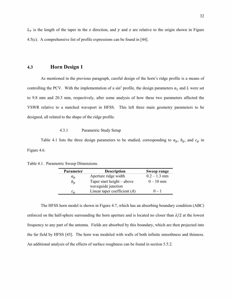
4.3 Horn Design 1 ................................................................................................................. 32

4.3.1 Parametric Study Setup .............................................................................................. 32

4.3.2 Parametric Study Results ........................................................................................... 34

4.3.3 Fabrication ................................................................................................................. 36

4.3.4 Performance ............................................................................................................... 37

4.4 Horn Design 2 ................................................................................................................. 40

4.4.1 Parametric Study Results ........................................................................................... 41

4.4.2 Fabrication ................................................................................................................. 41

4.4.3 Performance ............................................................................................................... 43

4.5 Summary ......................................................................................................................... 45

Chapter 5 Luneburg Lens / Feed Horn Implementation ............................................................................. 47

5.1 Introduction ..................................................................................................................... 47

5.2 Luneburg Lens Simulation – Open-Ended Waveguide................................................... 48

5.3 Luneburg Lens with Single Feed Antenna ...................................................................... 50

5.3.1 Horn 1 ........................................................................................................................ 51

5.3.2 Horn 2 ........................................................................................................................ 56

vii

5.4 Luneburg Lens with Multiple Feeds ............................................................................... 57

5.4.1 S-Parameters .............................................................................................................. 59

5.4.2 Simulations / Measurements ...................................................................................... 61

5.5 Analysis ........................................................................................................................... 65

5.5.1 Primary / Secondary Feed Patterns ............................................................................ 65

5.5.2 Horn Loss Analysis .................................................................................................... 68

5.5.3 2-Layer Lens Loss Analysis ....................................................................................... 71

5.6 Summary ......................................................................................................................... 72

Chapter 6 Conclusions ................................................................................................................................ 73

6.1 Phase Center of Horn Antennas ...................................................................................... 73

6.2 Design of a Luneburg Lens Feed .................................................................................... 74

6.3 Future Work .................................................................................................................... 75

6.4 Original Contributions .................................................................................................... 76

Bibliography ............................................................................................................................................... 77

Appendix A Phase Center Measurements ................................................................................................... 81

Appendix B Lens / Feed Mounting ............................................................................................................. 85

Appendix C 10-Layer LL Simulation ......................................................................................................... 89

viii

Figures

Figure 1.1. Concept of the Luneburg lens using ray tracing. In this example, the focal point is located a

distance outside the lens surface (� > 1)................................................................................. 3

Figure 1.2. A Luneburg lens operating with five feeds in a single plane. ................................................... 5

Figure 1.3. (a) Directivity of a LL vs the positioning of a Hertzian dipole simulated at 45 GHz in HFSS

and (b) the model showing the spacing of the Hertzian dipole. ............................................... 6

Figure 1.4. Reflector antenna, with the PC of the feeding antenna located at its focal point. ..................... 7

Figure 2.1. (a) Geometry considered when using far field data (red solid line) at a distance � to determine

�, the distance to the PC on the z-axis of the �� plane. The PC is defined as the center of

radii of the phase front (dashed blue line). (b) The far field phase coincides with the phase

front when the origin is placed at the PC. .............................................................................. 10

Figure 2.2. Half-wavelength dipole (� = 30 GHz) placed 1 cm above the origin in HFSS. ..................... 13

Figure 2.3. (a) Far field phase profile of a 30 GHz /2dipole placed 1 cm above the origin. (b) The

phase pattern plotted versus cos( ). ...................................................................................... 13

Figure 2.4. Geometry considered when using far field data (red solid line) to determine phase center that

is offset in the � and � dimensions. The PC is defined as the center of radii of the phase

front (dashed blue line). ......................................................................................................... 15

Figure 3.1. Horn antenna design parameters (a) isometric view (b) E-plane dimensions and (c) H-plane

dimensions. ............................................................................................................................ 21

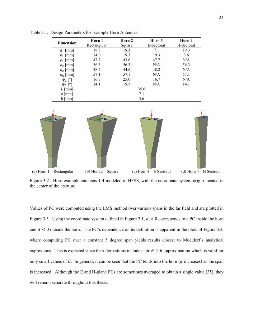
Figure 3.2. Horn example antennas 1-4 modeled in HFSS, with the coordinate system origin located in

the center of the aperture. ...................................................................................................... 23

ix

Figure 3.3. E and H-plane PC location versus frequency of the modeled horn antennas given in Table 3.1

using beamwidths of 3 dB, 10 dB, and constant 5° compared to the analytical model. A

value of � > 0 corresponds to a PC location located inside the horn relative to the aperture

plane. ...................................................................................................................................... 24

Figure 3.4. Horn 2 aperture fields, normalized amplitude (left column) and phase (50° range, right

column). ................................................................................................................................. 25

Figure 4.1. (a) WRD-1845 cross section dimensions and (b) 3D model of the double-ridged waveguide.

............................................................................................................................................... 27

Figure 4.2. (a) Corrugation design parameters and (b) HFSS corrugated square horn model. .................. 28

Figure 4.3. Aperture E-field intensity of the standard square horn (horn 2) vs. the corrugated horn. ....... 29

Figure 4.4. E / H plane PC location � vs. frequency of the corrugated horn (solid lines), compared to the

identical horn without corrugations (dashed lines). ............................................................... 30

Figure 4.5. Profile types that were considered for the feed horn design. ................................................... 31

Figure 4.6. Schematic of the horn antenna, with parametric study parameters labeled �� − �� .............. 33

Figure 4.7. Horn design 1 as modeled in HFSS for the parametric sweep. ............................................... 33

Figure 4.8. (a) PCV (b) and VSWR profiles for a single geometry of the parametric sweep, with the

sampled frequency points labeled. ......................................................................................... 34

Figure 4.9. Images showing the PCV performance as a function of parameters ��, ��, and ��. ............. 35

Figure 4.10. PCV of the chosen design simulated in HFSS, as computed over the 3dB beamwidth. ....... 36

Figure 4.11. Prototypes of horn design 1, fabricated using CNC machining (a) disassembled, (b)

assembled with adhesive absorber and (c) fabricated using DMLS. ..................................... 37

Figure 4.12. Horn 1 Simulations / Measurements: (a) Reflection coefficient (b) Directivity (c) E-Plane

PC and (d) H-Plane PC computed over the 10 dB beamwidth using amplitude weighting... 38

Figure 4.13. Simulated (red) and measured (blue, black) normalized radiation patterns of horn 1 at

various frequencies. ............................................................................................................... 39

x

Figure 4.14. (a) Prototype horn 2 full model and (b) defined using E and H symmetry planes. ............... 40

Figure 4.15. (a) Horn 2 design features (b) top view showing ridges (c) bottom view of waveguide

junction. ................................................................................................................................. 42

Figure 4.16. Prototype horn 2 (a) isometric view (b) waveguide junction flange. .................................... 42

Figure 4.17. Horn 2 Simulations / Measurements: (a) Reflection coefficient (b) Directivity / Gain (c) E-

Plane PC and (d) H-Plane PC. PCs were computed over the 10 dB beamwidth using

amplitude weighting. ............................................................................................................. 43

Figure 4.18. Prototype horn 2 mounted in the antenna range, with microwave absorber placed below the

aperture opening. ................................................................................................................... 44

Figure 4.19. Simulated (red) and measured (blue) normalized radiation patterns of horn 2 at various

frequencies. ............................................................................................................................ 45

Figure 5.1. (a) 2-layer LL HFSS model with transparent outer layer and (b) manufactured lens. ............ 48

Figure 5.2. HFSS model of an open-ended waveguide feeding the LL, separated by a distance ��......... 48

Figure 5.3. Simulated 2-layer LL performance when fed with an OE-WG, as a function of aperture

distance from the surface (��) and frequency, (a) normalized directivity and (b) peak SLL

normalized to 0 dB at each frequency. .................................................................................. 49

Figure 5.4. �� and ���� as determined using (5.1) and (5.2) for the OE-WG / LL simulation. .............. 50

Figure 5.5. Expected optimum horn feed position with respect to its PC offset ���, the lens focal point

��, and the LL / feed separation ��. ..................................................................................... 51

Figure 5.6. Horn 1 / LL performance vs position in terms of (a) directivity and (b) peak SLL. The focal

point in terms of �� and ���� is found as the minimum of the plots in (c). ........................ 52

Figure 5.7. Horn 1 VSWR (simulated) versus the horn / lens separation �� and frequency. .................... 53

Figure 5.8. CNC horn 1 mounted with LL (a) on bench and (b) installed in antenna range, before

wrapping the lower mount with microwave absorber............................................................ 54

xi

Figure 5.9. Simulations / measurements of horn 1 (CNC) mounted with the LL, (a) reflection coefficient

(b) directivity / gain (c) HPBW and (d) peak SLL. ............................................................... 54

Figure 5.10. E / H-plane antenna patterns of prototype horn 1 (CNC) mounted with the LL. .................. 55

Figure 5.11. Horn 2 / LL performance vs position in terms of (a) directivity and (b) peak SLL. The focal

point in terms of �� and ���� is found as the minimum of the plots in (c). ........................ 56

Figure 5.12. Horn 2 VSWR (simulated) versus the horn / lens separation �� and frequency. .................. 57

Figure 5.13. (a) Feed manifold CAD model pictured without the lens or supports, (b) feed array labeling

as the array ordering would appear looking from the bottom of (a). ..................................... 58

Figure 5.14. Feed separation angle ℎ. ...................................................................................................... 58

Figure 5.15. Feed manifold (a) without LL (b) with LL installed. ............................................................ 59

Figure 5.16. S-measurements between numerous feed element combinations: (a) Reflection coefficient

(S11), (b) E-array element coupling, (c) H-array element coupling, (d) cross coupling

between E/H-plane elements. ................................................................................................ 60

Figure 5.17. E-field magnitude when fed by the center element F0 in (a) E-array and (b) H-array cross

sections at 18 GHz, normalized to the E-field intensity incident on the LL. ......................... 61

Figure 5.18. Lens manifold mounted in antenna chamber (a) front view (b) side view with F11 connected

as the AUT feed. .................................................................................................................... 62

Figure 5.19. (a) All feeds excited in HFSS and (b) E-plane of the three unique E-array feeds measured in

the antenna range. .................................................................................................................. 62

Figure 5.20. Normalized radiation patterns of F0, F12, and F11. ................................................................. 63

Figure 5.21. F0 Simulated and measured E / H plane (a) peak SLL and (b) HPBW. ................................ 64

Figure 5.22. (a) Gain of the three measured / simulated elements and (b) normalized E-plane radiation

pattern corresponding with the dip at 39 GHz. ...................................................................... 65

Figure 5.23. (a) Geometry showing the LL aperture plane in relation to the primary and secondary

radiation patterns. .................................................................................................................. 67

Figure 5.24. Zeroth Bessel function of the first kind. ................................................................................ 68

xii

Figure 5.25. Horn 1 conductor loss due to the finite conductivity of aluminum, plotted for multiple values

of �. ....................................................................................................................................... 69

Figure 5.26. Two-dimensional rectangular groove dimensions. ................................................................ 70

Figure 5.27. Attenuation constant ratio for various square groove roughnesses. ...................................... 70

Figure 5.28. Loss of the 2-layer LL fed by horn 1, where tan �� is the assumed loss tangent of the LL

layer materials. ....................................................................................................................... 71

Figure A.1. Antenna range setup geometry, where � and �! refer to the PC position when the AUT is

positioned at = 0. ............................................................................................................... 82

Figure A.2. Distance error given in (A.3). ................................................................................................. 83

Figure A.3. E-plane PC measurement of horn 1 mounted 13.5 cm from the center of rotation, computed

using the least mean squares error (red solid) which is susceptible to the rotational phase

error versus the iterative method (blue dashed) which corrects for the error. ....................... 84

Figure B.1. (a) Indent on the equator of the LL and (b) mating ring designed onto the lens bracket. ....... 85

Figure B.2. Horn 1 (alternate exterior design) simulated (a) with bracket in place and (b) without bracket.

............................................................................................................................................... 86

Figure B.3. Normalized radiation patterns at the low / high frequencies to check the effects of the lens

mounting bracket. .................................................................................................................. 87

Figure B.4. (a) Measurement of the horn/lens spacer and (b) alignment of the F0 feed antenna. .............. 88

Figure C.1. Models of the (a) 2-layer LL and (b) 10-layer LLs. ................................................................ 89

Figure C.2. Scale used in Table C.1 – Table C.6 ....................................................................................... 90

Figure C.3. (a) Directivity and (b) SLL comparison between the 2 and 10-layer LLs as fed by horn 1. .. 93

Figure C.4. Reflection coefficient of horn 1 with and without the 2 and 10-layer LLs. ............................ 93

xiii

Tables

Table 3.1. Design Parameters for Example Horn Antennas. ..................................................................... 23

Table 4.1. Parametric Sweep Dimensions. ................................................................................................ 32

Table 4.2. Horn antenna design specifications. ......................................................................................... 35

Table 4.3. Horn 1 design dimensions. ........................................................................................................ 36

Table 4.4. Horn 2 Dimensions (Swept parameters shaded). ...................................................................... 41

Table 4.5. Summary of Design Changes Implemented in Horn 2. ............................................................ 41

Table C.1. Horn 1 / LL fields at 18 GHz. .................................................................................................. 90

Table C.2. Horn 1 / LL fields at 23 GHz. .................................................................................................. 90

Table C.3. Horn 1 / LL fields at 27 GHz. .................................................................................................. 91

Table C.4. Horn 1 / LL fields at 33 GHz. .................................................................................................. 91

Table C.5. Horn 1 / LL fields at 40 GHz. .................................................................................................. 92

Table C.6. Horn 1 / LL fields at 45 GHz. .................................................................................................. 92

1

Chapter 1

Introduction

1.1 Background

The need for highly directive antennas exists in many applications, most notably in radio

astronomy, communications, radar, and remote sensing where, in a perfect world, an antenna’s radiation

would be confined to the shape of a pencil beam. Reflector antennas are a common means of transmitting

and receiving directive radiation patterns, generally operating with some type of feed antenna. Similarly,

lenses can also collimate a feed antenna’s radiation into a highly directive beam, which for some

applications may be more compatible than a reflector-type design. While lenses require edge mounting

and the use of dielectrics which may lead to higher losses and undesired reflections, at microwave

frequencies lenses can have better wide-angle scanning performance [1]. The application driving the

writing of this thesis involves a wideband (18-45 GHz) military decoy system that must be capable of

receiving and transmitting a high power directive beam at any angle in a 2# steradian, or a half-space,

field of view. Accomplishing this with a reflector is impractical as it would involve extremely fast

mechanical steering. In contrast, a spherically symmetrical lens allows for the placement of numerous

feeds in its bottom half space for propagation from its upper half-space, resulting in the desired field of

view without requiring any mechanical movement or any blockage to the radiating aperture. This type of

lens is known as a Luneburg lens.

2

1.2 Luneburg Lens

Described by Carl Luneburg in 1944 [2], the standard Luneburg Lens (LL) was designed such

that a focal point, located on the surface of the spherical lens, is focused to infinity on the opposite side of

the lens. Due to the spherical symmetry of the LL, a high-gain antenna can be realized at any angle by

changing only the feed position to coincide with the focal point for that given direction. Unlike other

focusing structures, e.g. parabolic reflectors or non-spherical lenses, the lens itself can remain stationary

while having its beam steered by only its feed antenna.

The LL has a useful application in the area of radar calibration, where an object of known radar

cross section (RCS) at a given angle is desired. To create a radar calibration target, a portion (e.g. half) of

the spherical lens’s surface is fit with a highly conducting material. Every point on the conductor is then

a focal point for a plane wave incident on the opposite side of the lens. The lens not only increases the

RCS of the conductor, but it also creates a target that is insensitive to alignment angle relative to other

types of calibration targets [3].

In communications, the LL can provide large angular coverage with broad bandwidth, low cross

polarization, and high gain to increase data capacity. For example, in one implementation, a twelve-feed

LL was implemented into a 120° sector cellular base station and was found to increase the data capacity

by almost a factor of twelve as compared to the standard antenna configuration [4]. The LL is also of

great interest for on-the-move communication platforms that must maintain limited antenna profiles.

High speed trains, aircraft, and maritime applications are examples where a steerable highly directive

antenna is required for a two-way communication link with a satellite, for example. To limit its profile

size, a single hemisphere of the LL can be used in conjunction with a ground plane with the use of image

theory [5].

3

A LL is constructed such that the index of refraction varies as a function of the radius �, where

� = 0 is at the center of the sphere and � = � is at the outer surface. The index of refraction $ is given as

[6]

$%�) = 1�&1 ' �( − �(�( (1.1)

For a standard LL � = 1, however this value can be changed to move the focal point either inside or

outside the LL which commonly deems it a modified LL. Practical applications may desire the focal point

to be located at a point distant from the lens surface, in which case � is chosen such that

� = �)� (1.2)

where �) is the focal point relative to the center of the lens. A two-dimensional depiction of a LL with

� > 1 is shown in Figure 1.1.

$

1

$*+,

Figure 1.1. Concept of the Luneburg lens using ray tracing. In this example, the focal point is located a

distance outside the lens surface (� > 1).

An ideal implementation assumes a continuously varying $ within the lens, but in practice its

profile is typically discretized into - shells to allow for practical fabrication techniques. For example,

4

LL designs may include - = 2, 5, 10, or more shells of different refractive indices $., with the innermost

section comprising the core of the sphere. The variation of $ can be realized by use of different materials

for each layer or by dielectric mixing techniques. Dielectric mixing is often accomplished using pockets

of air as described in [7] [8]. This method can pose challenges in the precise control of dielectric

constants and maintaining lens uniformity and low loss. For ease in fabrication, it is often desired to

choose existing low-loss dielectric materials to comprise each shell layer, with careful selection of each

shell thickness as demonstrated in [9] with the development of a two-shell LL. A method for

implementing a genetic algorithm to determine both the layer thicknesses and the $. is given in [10],

where the values of $. can be limited to correspond with readily available materials. Because the $. differ from the values obtained in (1.1), lenses designed in this manner are referred to as nonuniform LLs.

Common feed antennas to the LL include open-ended waveguide (OE-WG) [8] [11], horn

antennas [5], and patch antennas [12] [13]. For the application discussed herein, the horn antenna is most

appropriate due to the wide bandwidth required.

1.3 Horn Antennas

The electromagnetic horn as it applies to microwaves has been studied and experimented

extensively with since the late 1930s, driven by developing technology during the World War II era [14].

High performance feed horns have a large presence in satellite communication antennas, radar antennas,

and radio-astronomy antennas. The most basic types of feed horns are the E-plane sectoral horn, H-plane

sectoral horn, pyramidal horn, square horn, and conical horn. The cross section of a conical horn is

circularly symmetric and the other three horns have rectangular or square cross sections. The pyramidal

and sectoral horns are characterized by which plane of the horn is flared, meaning that the dimension in

that plane increases along the axis that runs from the throat of the horn to its aperture. The E/H planes of

horn antennas are specified as the planes parallel to the fundamental mode’s E/H fields, respectively.

5

Early thorough analyses of the canonical electromagnetic horn were given in the 1930s by

Barrow and Chu [15] and Southworth [16]. The relationship between horn geometry and performance

parameters such as the gain then became well understood thanks to the many studies that followed [17]

[18] [19]. Since then, numerous features have been developed to improve performance aspects such as

transmission of wider bandwidths, reduced cross polarization, and increased beam symmetry, to name a

few. Such features directly applicable to the design goals herein will be discussed in chapter 4.

1.4 Application

The LL to be studied has a radius � = 36 mm with a focal point ideally located 5 mm from the

lens surface. From (1.1) and (1.2), � = 1.139 for such a lens and $ = √23 varies between 1 and 1.33,

where 23 is the relative permittivity and $ is the index of refraction. A two-layer lens is analyzed in this

research, whose inner core consists of a greater $ than that of the outer layer [9].

The feeding horn antenna is to operate in a single polarization over the 18-45 GHz range,

employing a square aperture to allow for a dual polarized version in a future design iteration. Several

feed / lens mounting configurations will be examined in order of increasing complexity, from a single

feed mount to a manifold consisting of an array of feeds equally spaced below the lower half space of the

lens. With an array of feeds, a directive beam can be transmitted or received in multiple directions

(Figure 1.2) without mechanical scanning or complex electrical beam steering.

Figure 1.2. A Luneburg lens operating with five feeds in a single plane.

6

If it were practical to feed the LL with a point source, such as a small dipole antenna, focusing

such a feed antenna would be straightforward and its center would be positioned at the focal point of the

lens. Positioning a practical horn antenna, however, is more difficult since its radiation pattern is not an

ideal spherical wave with a well-defined center point. In the next section, the antenna phase center will

be discussed, which is a metric that approximates such a point in which radiation seems to emanate from

an antenna.

Although not practically realizable, the Hertzian dipole is a convenient method for simulating a

point source using CEM (computational electromagnetics) software. To demonstrate the LL’s

dependence on its feed’s position, an excited 45 GHz Hertzian dipole was swept in distance relative to the

LL’s surface and simulated using the finite element method (FEM) solver HFSS [20]. The effect on LL

directivity is shown in Figure 1.3, where it is clear that its focal point is located 5 mm from its surface.

(a) (b)

Figure 1.3. (a) Directivity of a LL vs the positioning of a Hertzian dipole simulated at 45 GHz in HFSS

and (b) the model showing the spacing of the Hertzian dipole.

1.5 Phase Center Definition

The phase center (PC) of an antenna is generally not understood as well as the more traditional

measurements like directivity, beamwidth, axial ratio, etc. In many cases, knowledge of the PC is simply

not of interest in an antenna design and for some antenna types the term is not even applicable. Others,

7

however, require its full consideration but care must be taken to define the PC appropriately when used

since its definition has subjective qualities. Given by IEEE, its definition is [21]:

Phase center: The location of a point associated with an antenna such that if it is taken as the center of

a sphere the radius of which extends into the far field, the phase of a given field component over the

surface of the radiation sphere is essentially constant, at least over that portion of the surface where

the radiation is significant.

More briefly, the PC defines a point in space at which an antenna’s radiation seems to originate and is

found at the radial center of a surface consisting of constant phase in the far field. For a point source

radiating a spherical wave, the PC is simply at the exact location of the source regardless of frequency.

However, a true spherical phase front is not realizable for a physical antenna and can only be

approximated over a certain viewing angle, resulting in the qualitative nature of IEEE’s definition.

The knowledge or design of an antenna’s PC is important in many different applications.

Antenna designs often require a feeding antenna to be used in conjunction with a reflector or a lens. For

example, the parabolic reflector antenna shown in Figure 1.4 shows transmission of a plane wave due to

correct positioning of the feed horn.

Figure 1.4. Reflector antenna, with the PC of the feeding antenna located at its focal point.

8

It is well known from a geometrical optics standpoint that maximum antenna directivity is achieved when

a spherical wave originates from the focal point of the reflecting structure. Analogously, a plane wave

incident on a reflector will converge at its focal point [14]. For this reason, positioning the PC of the feed

is an essential component in the design and construction of a reflector antenna since the PC is the point

that best approximates the origin of a spherical wave. In narrowband applications, it may be possible to

simply tune the feed position mechanically, affixing it at the point that results in maximum directivity of

the system. In a wideband system, however, the PC of the feeding antenna tends to vary as a function of

frequency [22] and a more careful approach must be considered to avoid defocusing at some frequencies.

Not only does the PC tend to vary with frequency, but it may also vary as a function of angle

[23]. The knowledge of PC versus angle is imperative to time-based correlation receivers such as those

used in the Global Positioning System (GPS), where a receiver antenna receives signals from at least four

different transmitting antennas whose signals are likely arriving from different elevation angles [24].

Using a simple lookup-table, PC corrections can be made for the different signals based on their angle of

arrival such that all distance computations are made relative to a single reference point on the antenna.

The same process may be used to correct for PC variation of the transmitting antennas as well.

The PC, as it is discussed in this introduction, is most easily applied to linearly polarized antennas

radiating a major lobe in one direction. For many antennas, however, defining the PC is not

straightforward even with further clarification. For example, mobile phone or laptop antennas do not

have an obvious direction or main lobe in which to find the center of curvature with respect to phase. A

more general term “radiation center” has been defined using angular momentum of the far field [25].

This research, however, will primarily concern horn antennas and the traditional definition of PC will be

suitable with proper clarification.

Other definitions of PC have been developed for specific applications. Kildal, for example,

defined the PC as the point in a feed antenna which, when placed at the focal point of a parabolic

9

reflector, maximizes its aperture efficiency [26]. Although this objective may seem obvious, arbitrary

definitions of PC (using the 3 dB or 10 dB beamwidth, e.g.) may not lead to maximum aperture efficiency

and thus having a mathematical expression to determine this location is convenient for applications

involving single or multi-reflector antenna systems. These types of antennas require constant phase

across the reflector’s surface to achieve maximum aperture efficiency and minimize cross polarization.

This relation can be used to compute PC for practical designs because reflectors only involve one

significant degree of freedom in their construction: the reflecting surface. Defining a feed’s PC specific

for operation with a LL, however, is a much more difficult task as there are up to four degrees of freedom

in their construction that will affect performance such as the index of refraction $, inner and outer surface

characteristics, and surface reflection losses [1]. For this reason, experimentally determining the PC for a

LL is most appropriate for the purposes of this research.

10

Chapter 2

Extraction of Phase Center Position

2.1 Coordinate System / Geometry

For an antenna in which the definition of phase center (PC) is applicable, the PC can be derived directly

from the shape of the radiated far field phase pattern 4% ) which does not depend on the 2# modulus of

the phase. Most commonly, the PC is considered within a single plane, e.g. the �� plane in Figure 2.1,

where a known far field exists at a distance � from a reference origin.

(a) (b)

Figure 2.1. (a) Geometry considered when using far field data (red solid line) at a distance � to determine �, the distance to the PC on the z-axis of the �� plane. The PC is defined as the center of radii of the

phase front (dashed blue line). (b) The far field phase coincides with the phase front when the origin is

placed at the PC.

11

Before discussing different methods for computing the PC, it is worthwhile to recognize that if the

reference origin is displaced from the PC, then the far field phase function 5% ) will vary as a function of

angle at any far field distance � [Figure 2.1(a)]. In contrast, a sampled 5% ) that is constant over

corresponds to the phase front and indicates that the origin coincides with the PC of the radiating source

[Figure 2.1(b)].

The phase front in Figure 2.1 is defined as having a nearly constant phase at some arbitrary

distance in the far field whose corresponding PC is located at its center of radii. The generalized far field

for an antenna can be written as

6 = |6% , 9)| :;<%=,>)� = |6% , 9)| :;[@%=,>)AB3]� (2.1)

where D = 2#/ is the wavenumber and 4% , 9) is the portion of the phase function 5 that is dependent

on the and 9 spherical coordinates and will contain information leading to the PC location, as the shape

of this function will vary depending on the choice of coordinate system origin with respect to the PC.

In general, the PC (and thus �) is a function of 9 as it will vary depending on the plane in which

the far field is measured. Throughout this thesis, the PC will be computed in the two principal planes: the

9 = 0° and 9 = 90° planes which correspond to a horn antenna’s H and E-planes, respectively. When

using terms such as PC, �, or 4% ), the plane being considered will be explicitly stated. As described in

[27], the PC can be defined for an arbitrary plane 9 = 9E once it has been measured in the two principle

planes, i.e.

�%9 = 9E) = cos(%9E) �%9 = 0°) ' sin(%9E)�%9 = 90°). (2.2)

Referring to the geometry in Figure 2.1(a), the distance K changes with and can be written

using the law of cosines:

K% ) = L�( ' �( ' 2���MN% ). (2.3)

12

This distance is important, as it represents the measured far field relative to the antenna’s radiation point

of origin rather than to the arbitrary reference origin. For far field amplitude calculations, this distance is

often approximated equal to � which is sufficient when the far-field criteria of � ≥ 2�(/ is met, where

� is the largest dimension of the antenna aperture. Because the phase is periodic, however, this

approximation cannot be used when the reference origin and PC do not coincide (� ≠ 0). A more

accurate approximation for K% ) can be derived using Taylor’s first order approximation:

K% ) ≅ � ' ��MN% ) (2.4)

which is valid for � ≪ �.

2.2 Slope Method

A simple, closed form method for computing the PC was published by Hu in 1961 who was

concerned about the positioning of a horn antenna feed for a parabolic reflector [28]. When referenced to

the PC, the same field given at some distance � relative to the origin in Figure 2.1 can be expressed as

6 = |6% , 9)| :A;BS%=)� = |6% , 9)| :A;B[3TUVWX%=)]� (2.5)

which assumes the portion of the field being considered is within the main radiation lobe such that an

approximate spherical phase front exists. Equating the phase terms in (2.1) and (2.5), Hu showed that

@%=)YZ[%=) = D� = (\] �. (2.6)

In other words, by plotting the far field phase pattern versus �MN% ) and measuring the slope of the

resulting line, the PC location can be obtained from an arbitrarily placed origin with respect to the

wavelength. It should be noted that this method assumes symmetry in two of the planes, such that the PC

is known to vary in only one dimension (e.g. the axial dimension of a horn antenna). The inclusion of a

13

phase time dependency or offset by the phase’s D� term will have no effect on the measured slope and

thus only knowledge of the phase pattern shape 4% ) is required.

Using HFSS, a 30 GHz half-wavelength dipole, whose PC is known to be at its center due to

symmetry in all three planes, was placed at (0,0,1) cm in Cartesian coordinate space as shown in Figure

2.2.

Figure 2.2. Half-wavelength dipole (� = 30 GHz) placed 1 cm above the origin in HFSS.

The phase pattern of the 9 = 0 plane is plotted in Figure 2.3(a). The same phase profile, when plotted

versus cos% ), becomes linear and is shown in Figure 2.3(b).

(a) (b)

Figure 2.3. (a) Far field phase profile of a 30 GHz /2dipole placed 1 cm above the origin. (b) The

phase pattern plotted versus cos% ).

() [rad]

() [rad]

-

14

The slope - in Figure 2.3(b) is found to be - = 6.28. With - = @%`)YZ[%=) and D substituted into (2.6), the

PC location is found at � = 0.999 cm, which is within 10am (1 × 10Ac) of the dipole center.

This method has been dubbed the two-point method [29] because Hu calculated the slope using

two points, only defining the PC when a straight line could be plotted. With today’s abundance of line-

fitting algorithms, a linear fit can be applied to simulated or measured data which allows for the

computation of the “best fit” PC even when plotting 4% ) vs cos% ) does not result in a perfectly straight

line.

2.3 Least Mean Squares Solution

A least mean squares (LMS) solution for PC was described by Rusch and Potter [30] and later

simplified specifically for an antenna range setting [31]. Unlike the previous method, this solution

decomposes the PC offset distance � into two components (�d and �e – referring to Figure 2.4). In the

9 = 90° (��) plane,

�%9 = 90°) = �e cos% ) ' �d sin% ) . (2.7)

Similarly, if � were being computed in the 9 = 0° (f�) plane,

�%9 = 0°) = �e cos% ) ' �g sin% ) (2.8)

although for the remainder of this chapter the �� plane will be assumed and all 9 dependency will

continue to be neglected. For any antenna mounted such that �d ≠ 0, a linear slope will be induced into

4% ) which will compromise the accuracy of the slope method, therefore compensation in both directions

is desired for a measurement setup which will inevitably contain some offset in the f or � direction due to

imperfect alignment of two antennas on the �-axis.

15

Figure 2.4. Geometry considered when using far field data (red solid line) to determine phase center that

is offset in the � and � dimensions. The PC is defined as the center of radii of the phase front (dashed

blue line).

Given a set of discretely measured far field phase samples 4. within the main lobe, a sum of

squares difference (SSD) model can be defined as:

��� =h[4. − %4E ' D%�i cos% .) ' �d sin% .)))](. (2.9)

where 4E = D� is the unwrapped phase at = 0 and D is the wavenumber. While the phase values

4.%� = 1…$) must be unwrapped, any modulo of 2# is acceptable which is useful when the exact phase

is unknown. Equation (2.9) uses the approximation given in (2.4) with � composed into its � and �

components. Setting the derivatives of (2.9) with respect to the unknowns (�d, �e, and 4E) to zero, a

system can be assembled in matrix form for straightforward solution in an environment such as

MATLAB. The resulting system is [31]

16

klllllm −Dhn. sin( . .

Dhn. sin% .) cos% .).−hn.sin% .).−Dhn.sin% .)cos% .).

Dhn. �Ms( . .−hn.�Ms% .).−Dhn.sin% .).

Dhn.cos% .).−hn.. op

ppppqr�d�e4E

s =klllllm−hn.4.sin% .).−hn.4.cos% .).−hn.4.. op

ppppq (2.10)

where the n. terms correspond to an optional weighting function t that can be used to assign

“importance” to portions of the phase pattern as it applies to the PC computation. Traditional weighting

functions (Gaussian, e.g.) will be maximum at boresight and taper toward the edges of the beam similar to

the behavior of the antenna’s amplitude pattern. Since the reason for weighting is based on the tapering

of radiation intensity at off-boresight angles, it is logical to simply use the antenna’s amplitude pattern as

the weighting function. This will be referred to as amplitude weighting throughout this thesis. For a

planar E-field pattern, the amplitude weighting function is defined as

n+u = v6.(v∑ v6.(vx.yz . (2.11)

where the 6. are the far field electric field samples corresponding with the . and 4. used in (2.10).

2.4 Exact Solution Using an Iterative Approach

As discussed in the previous two sections, an approximation (2.4) was made in order to allow for

the differentiation of field components and for mathematical convenience. In certain situations, however,

this approximation can lead to significant phase errors, particularly if the ratio �/� is not small enough.

This error is discussed in more detail in Appendix A and a method for solving for PC while avoiding this

error is shown below. The far field approximation relative to the PC can be written using the exact

solution for K% ) which was given in (2.3):

6 = |6% )| :A;BS%=)� = |6% )| :A;B3&zT%U{|TU}|)3| T(%U{X.x=TU}VWX=)3

� (2.12)

17

where (2.7) was used to decompose � into its � and � components. It should be emphasized that the

phase expression in (2.12) is valid within the antenna main lobe and it is assumed that values of have

been limited to within the first pattern null. For � ≪ �, (2.12) reduces to (2.5) with the use of a first order

Taylor series expansion.

Unlike the previous PC solution methods, the phase term in (2.12) does not allow for a closed-

form solution for �d and �e, suggesting an iterative approach. As described in [30], the PC can be found

by minimization of the phase pattern variance computed with respect to an origin adjusted by �d and �e.

The measured phase pattern 5*~+X (with 2# modulus adjusted to −D� at boresight) whose origin is

adjusted by �d and �e will be referred to as 5VW33 and is given by

5VW33%�d, �e, ) = 5*~+X% ) − D� �1 − &1 ' %�d( ' �e()�( ' 2%�dN�$ ' �e�MN )� �. (2.13)

As opposed to the previous methods, the knowledge of � is required in (2.13) and must be used to ensure

the 2# modulus of 5*~+X% ) is accurate. In an antenna range, � corresponds to the distance between the

probe antenna’s PC and center of rotation (Appendix A). For simulations which typically project the far

field to � = ∞, simply using a large value of � will suffice.

A quasi-Newton method was implemented in MATLAB to find the minimum variance of (2.13)

for a given phase pattern measurement, i.e. to find �d and �e that results in the “flattest” phase pattern.

To minimize the variation of 5VW33 over all of interest, a cost function �%�) is defined as

�%�) = 1$hn.|5VW33%�, .) − ⟨5VW33%�)⟩|(x.yz (2.14)

where � = ��d�e�. Equation (2.14) is similar to the variance �( of the phase pattern but includes an

optional weighting vector t as described in the last section. The brackets in the term ⟨5VW33%�)⟩ indicate

18

the mean value of 5VW33 over all . being considered. If the weighting function is used, then a weighted

arithmetic mean should also be used, i.e.

⟨5VW33%�)⟩ = ∑ n.5VW33%�, .)x.yz ∑ n.x.yz . (2.15)

The cost function �%�) can be minimized by iteratively solving

��T� = �� − [�%��)]Az��%��) (2.16)

until � converges [32]. � is the Hessian matrix and is equal to

� =klllm �(���d( �(��d�e�(��d�e �(���e( op

ppq (2.17)

and the gradient vector ��%��) is equal to

��%��) = � ���U{���U}�. (2.18)

When applied to simulated data, a �%�) of nearly zero is easily obtainable upon finding the PC. Due to

uncertainties rising from a finite signal to noise ratio, range measurements will tend to converge with a

greater value of �%�).

2.5 Summary

For most simulations and measurements conducted in this research, the LMS method will suffice

to provide an accurate PC location. In cases where an antenna under test (AUT) incurs a large rotational

scanning error as discussed in Appendix A, the iterative approach should be used and careful

measurements should be taken between the AUT, probe antenna, and scanning center of rotation. In all

cases, amplitude weighting will be applied to the field of view being considered in the PC computation.

19

Because any nonzero �g or �d will be attributed to mounting misalignments since the antennas in this

research are symmetric around the �-axis, reported values of � in future chapters are simply equal to �e

as discussed in this chapter.

20

Chapter 3

Phase Center of Horn Antennas

3.1 Introduction

The phase center of a canonical horn antenna is dependent on horn dimensions such as flare angle

4~ and 4�, aperture size �z × �z, and length � (Figure 3.1). Generally, for a smaller flare angle the PC

tends toward the aperture of the horn. In contrast, the PC in horns having wide flare angles is located

more toward the throat, or apex, of the horn [14]. The reason for this behavior is inherent to the geometry

of the horn and is illustrated in Figure 3.1(b), where the difference between �~ and �z leads to a phase

error �~ in the E-plane of the aperture. As the flare angle 4~ tends to zero, �~ = �z and �~ = 0 as in an

open-ended waveguide [33]. The same is true in the H-plane, whose phase error �� is shown in Figure

3.1(c). The tangential fields in the pyramidal horn’s aperture plane are given by the approximation [14]

6��%f�, ��) = 6E cos � #�z f�� :A;�B�,�|�| T��|�� �/(�, (3.1)

where the prime symbol indicates a coordinate system centered in the aperture plane of the horn. The

phase in a horn aperture has a quadratic distribution in both the f′ and �′ directions which describes

mathematically �~ and �� shown in Figure 3.1. Note that as frequency increases ( decreases), D = 2#/

becomes larger and enhances the phase term in (3.1). One may expect similar PC behavior in both E and

H planes due to the similar quadratic phase dependence of f and � in (3.1), however because the aperture

amplitude tapers in the f direction (H-plane), the extent to which �� influences the H-plane PC is less

than that of �~ in the uniformly illuminated E-plane.

21

(a)

(b) E-plane

(c) H-plane

Figure 3.1. Horn antenna design parameters (a) isometric view (b) E-plane dimensions and (c) H-plane

dimensions.

3.2 Analytical Derivations

Muehldorf analytically derived expressions for the PC location in square, diagonal, and

rectangular horns as functions of their electrical dimensions [27]. These expressions were developed

using equivalent aperture electric and magnetic currents while considering the spherical phase error �~

and �� in the horn aperture. The analysis assumes a single TE10 waveguide mode feeding the antenna and

is valid only for angles near boresight due to approximations used within the derivations. After deriving

the far field patterns, Muehldorf determined the PC as the center of radii of a far field equiphase surface

near boresight. It is shown that the PC can be found as the second derivative of the phase front at

boresight ( = 0). While the boresight approximation and single propagating mode limit the usefulness

22

of the analytical expressions, they are nonetheless a valuable tool for validating empirical models used for

determining the PC in standard horn antennas.

As an extension to Muehldorf’s work, Teichman derived the PC in horn antennas using edge

diffraction theory and included measurements for comparison [34]. Edge diffraction theory uses a

superposition of the main geometrical optics field and two diffracted signals (on the two E-plane edges)

which are taken as the sources of radiation from which to derive the far fields. To characterize both horn

size and the frequency’s influence on PC, Teichman successively shaved down the length of an X-band

horn and measured over 7.5-10 GHz. Close agreement was observed for large horns (D�~ > 50) but as the

horn was trimmed to shorter lengths the measured PC location began to vary widely with respect to the

theoretical results. Teichman theorized that in the case of shorter horns, higher-order modes excited

within the horn may not have had sufficient length to attenuate as they would have in the longer horns.

3.3 Example Horn Simulations

A set of horns were designed in HFSS with the parameters shown in Table 3.1. The set consists

of a rectangular horn, square horn, and sectoral horns of both E and H-planes. Dimensions of the

rectangular horn (Horn 1) are consistent with Ka-band standard gain horns that are commercially

available and the three other geometries are extensions of Horn 1. All dimensions in Table 3.1

correspond with those labeled in Figure 3.1 and are fed with WR28 rectangular waveguide. The

dimensions of Table 3.1 were used to obtain the PC over frequencies of 26 – 40 GHz using Muehldorf’s

analytical models. As seen in Figure 3.2, the coordinate system origin is located in the center of the

aperture which is consistent with Muehldorf’s point of reference.

23

Table 3.1. Design Parameters for Example Horn Antennas.

Dimension Horn 1 Horn 2 Horn 3 Horn 4

Rectangular Square E-Sectoral H-Sectoral �z [mm] 19.3 19.3 7.1 19.3 �z [mm] 14.0 19.3 19.3 3.6 �z [mm] 47.7 43.6 47.7 N/A �( [mm] 56.3 56.3 N/A 56.3 �~ [mm] 48.2 44.6 48.2 N/A �� [mm] 57.1 57.1 N/A 57.1 4~ [°] 16.7 25.0 16.7 N/A 4� [°] 14.1 19.5 N/A 14.1 � [mm] 35.6

a [mm] 7.1

b [mm] 3.6

(a) Horn 1 – Rectangular (b) Horn 2 – Square (c) Horn 3 – E Sectoral (d) Horn 4 – H Sectoral

Figure 3.2. Horn example antennas 1-4 modeled in HFSS, with the coordinate system origin located in

the center of the aperture.

Values of PC were computed using the LMS method over various spans in the far field and are plotted in

Figure 3.3. Using the coordinate system defined in Figure 2.1, � > 0 corresponds to a PC inside the horn

and � < 0 outside the horn. The PC’s dependence on its definition is apparent in the plots of Figure 3.3,

where computing PC over a constant 5 degree span yields results closest to Mueldorf’s analytical

expressions. This is expected since their derivations include a sin ≅ approximation which is valid for

only small values of . In general, it can be seen that the PC tends into the horn (� increases) as the span

is increased. Although the E and H-plane PCs are sometimes averaged to obtain a single value [35], they

will remain separate throughout this thesis.

24

(a) Horn 1 – Rectangular

(b) Horn 2 – Square

(c) Horn 3 – E Sectoral

(d) Horn 4 – H Sectoral

Figure 3.3. E and H-plane PC location versus frequency of the modeled horn antennas given in Table 3.1

using beamwidths of 3 dB, 10 dB, and constant 5° compared to the analytical model. A value of � > 0

corresponds to a PC location located inside the horn relative to the aperture plane.

The aperture fields for horn 1 were acquired in method of moments (MoM) software FEKO [36]

and are plotted in Figure 3.4. Though they are not an exact representation of (3.1), the general features in

both amplitude and phase are present. That is, the amplitude tapers in the f direction (H-plane) and the

phase changes quadratically in both f and � directions. With the scale of the phase remaining constant

for all frequencies, the phase error �~ and �� can be easily visualized in the right column of Figure 3.4,

d [mm]

d [mm]

Frequency [GHz]

26 28 30 32 34 36 38 40

0

5

10

d [mm]

25

which becomes less uniform as the frequency increases and corresponds with a PC located further into the

horn, as was seen in Figure 3.3(a).

Frequency Amplitude (Normalized) Phase (50° range)

26.5 GHz

33 GHz

40 GHz

Figure 3.4. Horn 2 aperture fields, normalized amplitude (left column) and phase (50° range, right

column).

The examples in this section, particularly when the horn’s E-plane is flared significantly (horns 2

and 3), demonstrate the extent to which the PC can be expected to vary over a wide frequency band.

Fortunately, there are horn design features that can be implemented to minimize the PC’s movement with

respect to frequency.

26

Chapter 4

Phase Stabilized Horn Design and Fabrication

4.1 Introduction

For operation with a LL having a fixed focal point, the main design goal of the feeding antenna

involves stabilizing its PC, or minimizing the PC’s variation in space, over frequency. This metric will be

referred to as phase center variation with respect to frequency PCV(�) and should not be confused with

PCV( , 9) as it refers to the PC variation over angle, typically a design concern for antennas used in

ranging applications [23] [29]. It is well known that the PC of an open-ended waveguide is near the

aperture center and is not sensitive to frequency since there is a uniform phase distribution across the

aperture [37]. While open-ended waveguide has been used to feed a LL [11], a custom horn antenna is

required here due to the wide operating bandwidth. In addition, designing a custom antenna allows for a

lower VSWR and improved E/H plane symmetry.

The horn antenna is to be fed with a custom feed waveguide WRD-1845 [38], consisting of a

dual-ridge cross-section (Figure 4.1) for propagation over the 18-45 GHz band. These ridges must extend

into the horn’s flared section to maintain a good impedance match. Several methods for stabilizing the

PC will be discussed in the next section while taking into account the limitations and requirements

specific to the constraints of the application.

27

(a) (b)

Figure 4.1. (a) WRD-1845 cross section dimensions and (b) 3D model of the double-ridged waveguide.

4.2 Methods for Phase Center Stabilization

Chapter 3 discussed several tendencies of PC behavior that can be expected in standard horn

antennas. Any movement in PC as a function of frequency is generally undesired for a feed antenna since

it will cause defocusing at some portions of the band. Fortunately, there are several design features that

can be exploited for their PC stabilization with respect to frequency.

4.2.1 Flare Angle Design

It was mentioned in section 3.1 that as a horn’s flare angle 4 is decreased the PC will tend toward

the aperture. Careful design of the flare angle in both E and H-plane can be a straightforward approach

for achieving low PCV while maintaining a nearly identical E/H-plane PC. In Figure 3.3, the square

horn’s (horn 2) E-plane PC is much further into the horn than the H plane PC. The rectangular horn (horn

1), however, has an E-plane PC much closer to the aperture as a result of the smaller dimension �z which

also reduces the flare angle 4~. Because the feed horn for this study requires a horn that can be modified

to support dual-polarization, a square aperture will be used despite the advantages of using rectangular in

terms of PCV and E/H-plane PC coincidence when transmitting / receiving a single polarization.

4.2.2 Corrugations

Corrugations in the horn sidewall are a useful feature for achieving E/H-plane beam symmetry

and low cross-polarization, and for this reason they are extremely common feed antennas for reflector

28

antennas used in radar and communications [39]. Each corrugation can be viewed as an individual

transmission line. If designed correctly, the transmission lines can be designed such that there is a

negative reactance (capacitance) seen by a surface wave on the sidewall of the horn. Surfaces satisfying

this requirement are often referred to as soft surfaces and are described in detail in [40].

A correct corrugation design will force the E-field to zero on the E-plane walls of the horn. This

behavior is similar to that expected on the horn H-plane edges where the E-field component is tangential

to the wall. For perfect conductors, it is well known that the tangential component of the E-field will be

zero. The tapering of the E-field amplitude in both f and �, as a result, reduces the far field sidelobes and

causes the E/H beams to be more symmetric [14]. In a similar manner, the E-plane PC will behave more

like the H-plane PC which tends to remain closer to the aperture over frequency.

Referring to the geometry in Figure 4.2(a), maintaining a capacitive surface reactance requires

(4.1) – (4.3) to be satisfied across the frequency band [14]:

4 < �V < 2 (4.1)

n � 10 (4.2)

� � n10 (4.3)

(a) (b)

Figure 4.2. (a) Corrugation design parameters and (b) HFSS corrugated square horn model.

29

Corrugations were implemented into all four walls of the square example antenna (horn 2)

discussed in section 3.3 [Figure 4.2(b)] and the aperture fields were obtained in HFSS. The tapering of

the E-field in the � direction of the aperture plane can clearly be seen in the right column of Figure 4.3.

Frequency Amplitude (Normalized)

Standard Horn Corrugated Horn

26.5 GHz

33 GHz

40 GHz

Figure 4.3. Aperture E-field intensity of the standard square horn (horn 2) vs. the corrugated horn.

The corrugated horn’s impact on PC is evident in Figure 4.4, where the E-plane PCV is reduced from 6.2

mm to 1.9 mm. The E and H-plane PCs are also closer to each other than they are in the standard square

horn.

30

Figure 4.4. E / H plane PC location � vs. frequency of the corrugated horn (solid lines), compared to the

identical horn without corrugations (dashed lines).

Although corrugations have some clear advantages, there are also exist some impracticalities that may

limit their use. In this application, for example, (4.1) cannot be satisfied over the required bandwidth of

18 – 45 GHz. In addition, the increase in sidewall depth of at least �V makes this design a challenge

where space is a premium.

4.2.3 Flare Profile Design

The most basic explanation for PCV behavior of a horn antenna is due to the differing lengths of

the horn axis and sidewall, �z and �~ [Figure 3.1(b)]. The addition of a flaring profile to the horn

sidewall, however, invalidates this simple relation since higher order modes will be excited and the fields

within the horn become much more complex than the single moded cylindrical wave that is often assumed

when computing the aperture fields analytically [34].

Specific flaring profiles have been used for various performance features in the past. For

example, exponential ridge flares have been used as a means of matching a horn’s 50Ω coax transition to

377Ω (free space) over wide bandwidths [41]. A number of successive linear flares of varying flare angle

may be used to excite specific modes leading to E/H-plane symmetry in the far field pattern [42]. The

31

sin2 profile was used on a corrugated sidewall and was found to match well to the feeding

coax/waveguide transition while reducing phase error across the aperture [43]. Figure 4.5 shows some

different flaring profiles that were considered in this antenna design.

(a) Linear (b) Exponential

(c) Sin2 (d) Hyperbolic

(e) Tangent (f) f)

Figure 4.5. Profile types that were considered for the feed horn design.

Because the dual waveguide ridges (Figure 4.1) must be extended into the horn aperture, the profiles

shown in Figure 4.5 were applied to the horn ridges themselves and it was found that both the radiation

characteristics and the VSWR of the horn are very sensitive to both the profile type and the design

parameters associated with it. Like in [43], the sin2 profile was found to have a beneficial effect on

equalizing the aperture phase distribution and thus helps to stabilize the PC over frequency. This profile,

shown in Figure 4.5(c), is given by the expression

�%�) = �E ' %�+) − �E) �%1 −  ) ��¡ '   sin( � #�2�¡�� (4.4)

where �E and �+) are the ridge � dimensions at the beginning of the taper and at the aperture,

respectively,   is a coefficient between [0-1] controlling the amount of linear taper added to the profile,

32

�¡ is the length of the taper in the � direction, and � and � are relative to the origin shown in Figure

4.5(c). A comprehensive list of profile expressions can be found in [44].

4.3 Horn Design 1

As mentioned in the previous paragraph, careful design of the horn’s ridge profile is a means of

controlling the PCV. With the implementation of a sin2 profile, the design parameters �z and � were set

to 9.8 mm and 20.3 mm, respectively, after some analysis of how these two parameters affected the

VSWR relative to a matched waveport in HFSS. This left three main geometry parameters to be

designed, all related to the shape of the ridge profile.

4.3.1 Parametric Study Setup

Table 4.1 lists the three design parameters to be studied, corresponding to �), �), and �) in

Figure 4.6.

Table 4.1. Parametric Sweep Dimensions.

Parameter Description Sweep range �) Aperture ridge width 0.2 – 1.3 mm �) Taper start height – above

waveguide junction

0 – 10 mm

�) Linear taper coefficient ( ) 0 – 1

The HFSS horn model is shown in Figure 4.7, which has an absorbing boundary condition (ABC)

enforced on the half-sphere surrounding the horn aperture and is located no closer than /2 at the lowest

frequency to any part of the antenna. Fields are absorbed by this boundary, which are then projected into

the far field by HFSS [45]. The horn was modeled with walls of both infinite smoothness and thinness.

An additional analysis of the effects of surface roughness can be found in section 5.5.2.

33

Figure 4.6. Schematic of the horn antenna, with parametric study parameters labeled �) − �) .

Figure 4.7. Horn design 1 as modeled in HFSS for the parametric sweep.

Although the implementation of a true optimization could save computational resources if implemented

correctly, it was not attempted for this design due to the difficulty in defining a cost function involving

computed PCs at various frequencies. Because HFSS does not intrinsically return the PC of an antenna,

an external environment such as MATLAB would be required to interact with HFSS for full execution of

the optimization. Furthermore, an optimizer would have a high probability of getting trapped in the cost

34

function’s local minima. When computationally viable, the parametric sweep allows all data to be taken

then analyzed from multiple angles to determine a suitable design while capturing all local minima of the

cost function. In this exercise, seven different frequencies were sampled for each geometry and an

estimated PCV was determined as the maximum deviation over the seven samples. As an example,

Figure 4.8 shows the PCV and VSWR for a geometry that was part of the parametric sweep with the

seven sampled frequency points labeled. Although the actual PCV can be seen to be approximately 3.3

mm, the PCV as seen at the 7 simulation points, or PCVest, is 3 mm.

(a) (b)

Figure 4.8. (a) PCV (b) and VSWR profiles for a single geometry of the parametric sweep, with the

sampled frequency points labeled.

It is important to note that due to limited frequency sampling, the estimated PCV can only appear to be

lower than the actual PCV and thus no “good” designs will be neglected because of coarse frequency

sampling. While this reduces simulation time, the tradeoff is the time required to manually simulate the

highest performing geometries to determine which is truly the best performing when finer frequency

points are sampled.

4.3.2 Parametric Study Results

After simulating the 780 geometries in HFSS, the geometry with the lowest E-plane PCV was

chosen given that multiple other required specifications were met, as summarized in Table 4.2.

35

Table 4.2. Horn antenna design specifications.

Specification Value

VSWR < 2

X-pol Isolation > 30 dB

Peak sidelobe level > 20 dB

Front to back ratio > 10 dB

PCV results in terms of the swept parameters can be visualized as a heat map, where parameters �) and

�) are varied on the f and � axes, respectively, and an individual plot is created for each value of the

1 mm 2 mm 3 mm 4 mm 5+ mm

Phase Center Variation

(estimated)

Figure 4.9. Images showing the PCV performance as a function of parameters �), �), and �).

Design Geometry

36

third parameter, �) (Figure 4.9). The “hot spot” in the �) = 0.8 plot was chosen as the design geometry

due to its PCV performance as well as the satisfaction of the requirements listed in Table 4.2. In addition

to displaying the best geometric parameters in terms of PCV, viewing the results in this manner also

reveals the effect that fabrication tolerances can have on the PCV of a machined or printed antenna. After

running a second parametric sweep of finer parameter increments, the design in Table 4.3 was chosen.

Table 4.3. Horn 1 design dimensions (Swept parameters shaded).

Dimension Value �) 1.0 mm �) 7.1 mm �) 0.79 �z, �z 9.8 mm � 20.3 mm

When simulated at finer frequency points (500 MHz spacing), this geometry yielded an E-plane PCV of

~1.2 mm as computed over the 3 dB beamwidth, plotted in Figure 4.10.

Figure 4.10. PCV of the chosen design simulated in HFSS, as computed over the 3dB beamwidth.

4.3.3 Fabrication

The horn antenna was fabricated of aluminum using reductive and additive methods: 1) CNC

(Computer Numerical Control) milling and 2) DMLS (Direct Metal Laser Sintering), which is a form of

metal 3D-printing. The split-block design in Figure 4.11(a) was required for machining the interior horn

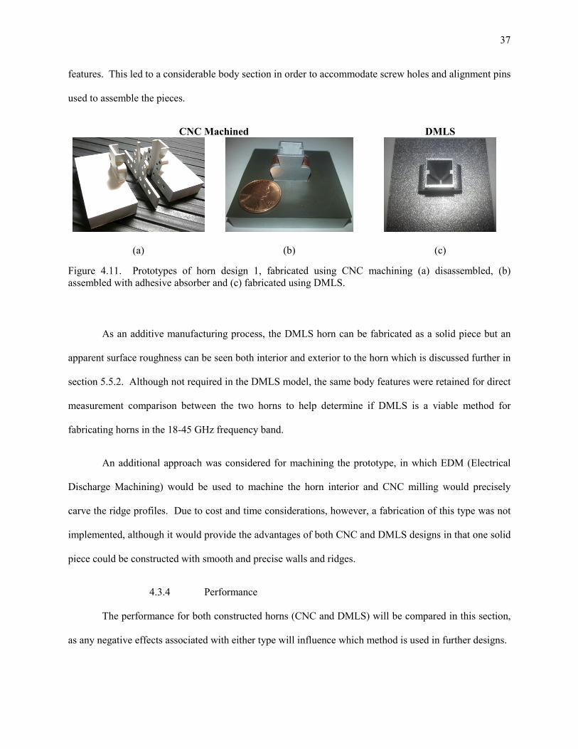
37

features. This led to a considerable body section in order to accommodate screw holes and alignment pins

used to assemble the pieces.

CNC Machined DMLS

(a) (b) (c)

Figure 4.11. Prototypes of horn design 1, fabricated using CNC machining (a) disassembled, (b)

assembled with adhesive absorber and (c) fabricated using DMLS.

As an additive manufacturing process, the DMLS horn can be fabricated as a solid piece but an

apparent surface roughness can be seen both interior and exterior to the horn which is discussed further in

section 5.5.2. Although not required in the DMLS model, the same body features were retained for direct

measurement comparison between the two horns to help determine if DMLS is a viable method for

fabricating horns in the 18-45 GHz frequency band.

An additional approach was considered for machining the prototype, in which EDM (Electrical

Discharge Machining) would be used to machine the horn interior and CNC milling would precisely

carve the ridge profiles. Due to cost and time considerations, however, a fabrication of this type was not

implemented, although it would provide the advantages of both CNC and DMLS designs in that one solid

piece could be constructed with smooth and precise walls and ridges.

4.3.4 Performance

The performance for both constructed horns (CNC and DMLS) will be compared in this section,

as any negative effects associated with either type will influence which method is used in further designs.

38

Reflection coefficient measurements were taken using an Agilent Vector Network Analyzer

(VNA) with a maximum frequency of 40 GHz. A custom waveguide TRL (Thru – Reflect – Line)

calibration kit was used to calibrate the VNA to a reference plane at the antenna waveguide junction. Far

field radiation measurements were taken in the Antenna Research Group’s NSI millimeter antenna range

at the University of Colorado Boulder, which employs a roll over azimuth positioner and was set up with

a wideband horn antenna probe. The 10 dB beamwidth with amplitude weighting was applied in the

computation of the PC. Measurements and HFSS simulations (assuming a perfectly matched waveport)

are plotted in Figure 4.12.

(a) (b)

(c) (d)

Figure 4.12. Horn 1 Simulations / Measurements: (a) Reflection coefficient (b) Directivity (c) E-Plane

PC and (d) H-Plane PC computed over the 10 dB beamwidth using amplitude weighting.

Directivity [dBi]

Frequency [GHz]

20 25 30 35 40 45-1

0

1

2

3

HFSS

CNC Measured

DMLS Measured

Frequency [GHz]

20 25 30 35 40 45-1

0

1

2

3

HFSS

CNC Measured

DMLS Measured

E-Plane H-Plane

PCVE = 2 mm PCVH = 0.7 mm

39

PCVE and PCVH of 2 mm and 0.7 mm can be seen in Figure 4.12(c) and (d), respectively. Figure

4.12 (c) and (d) differ from the PCs of Figure 4.10 for several reasons: 1) the 3 dB beamwidth was used

when evaluating PC in the parametric sweeps and 2) practical horn features such as a non-zero wall

thickness at the aperture were not modeled in the parametric sweep simulation. Normalized radiation

patterns at various frequencies are plotted below.

E-Plane H-Plane

18 GHz

26 GHz

34 GHz

42 GHz

Figure 4.13. Simulated (red) and measured (blue, black) normalized radiation patterns of horn 1 at

various frequencies.

Antenna range measurements are plotted up to 42 GHz, the point at which the SNR becomes too

low to yield reliable data due to limited bandwidth of the up/downconverter modules. It is apparent in the

40

above results that neither fabrication method seems to have adverse effects on the radiation patterns,

matching performance, directivity, or PCV.

4.4 Horn Design 2

A second iteration of a feed horn design was completed for the purpose of constructing an array

beneath the bottom half-space of the LL. The aperture dimensions �z and �z were reduced by more than

1 mm and the flared section length of the horn � was lengthened by approximately 6 mm to allow for

improved impedance matching of the antenna, particularly at the lower part of the band as compared to

horn 1.

In contrast to the horn 1 parametric study discussed in 4.3.1, aluminum horn walls of 0.4 mm

thickness were used in the model of horn 2, whereas a fictitious horn with zero wall thickness was used in

the first iteration. In the last section, it was found that wall thickness and other practical design

characteristics had an effect both on PC and reflection coefficient, making it a goal in this iteration to

design the ridge profile while considering the effects of all design features. The horn 2 model is pictured

in Figure 4.14a. E and H-plane symmetry planes [Figure 4.14(b)] were utilized to reduce runtime of the

parametric sweep. The same ABC boundary (not shown) used for horn 1 was also used for

transformation to the far fields.

(a) (b)

Figure 4.14. (a) Prototype horn 2 full model and (b) defined using E and H symmetry planes.

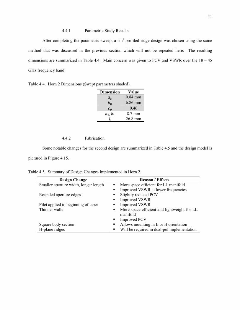
41

4.4.1 Parametric Study Results

After completing the parametric sweep, a sin2 profiled ridge design was chosen using the same

method that was discussed in the previous section which will not be repeated here. The resulting

dimensions are summarized in Table 4.4. Main concern was given to PCV and VSWR over the 18 – 45

GHz frequency band.

Table 4.4. Horn 2 Dimensions (Swept parameters shaded).

Dimension Value �) 0.84 mm �) 6.86 mm �) 0.46 �z, �z 8.7 mm � 26.8 mm

4.4.2 Fabrication

Some notable changes for the second design are summarized in Table 4.5 and the design model is

pictured in Figure 4.15.

Table 4.5. Summary of Design Changes Implemented in Horn 2.

Design Change Reason / Effects

Smaller aperture width, longer length � More space efficient for LL manifold

� Improved VSWR at lower frequencies

Rounded aperture edges � Slightly reduced PCV

� Improved VSWR

Filet applied to beginning of taper � Improved VSWR

Thinner walls � More space efficient and lightweight for LL

manifold

� Improved PCV

Square body section

H-plane ridges

� Allows mounting in E or H orientation

� Will be required in dual-pol implementation

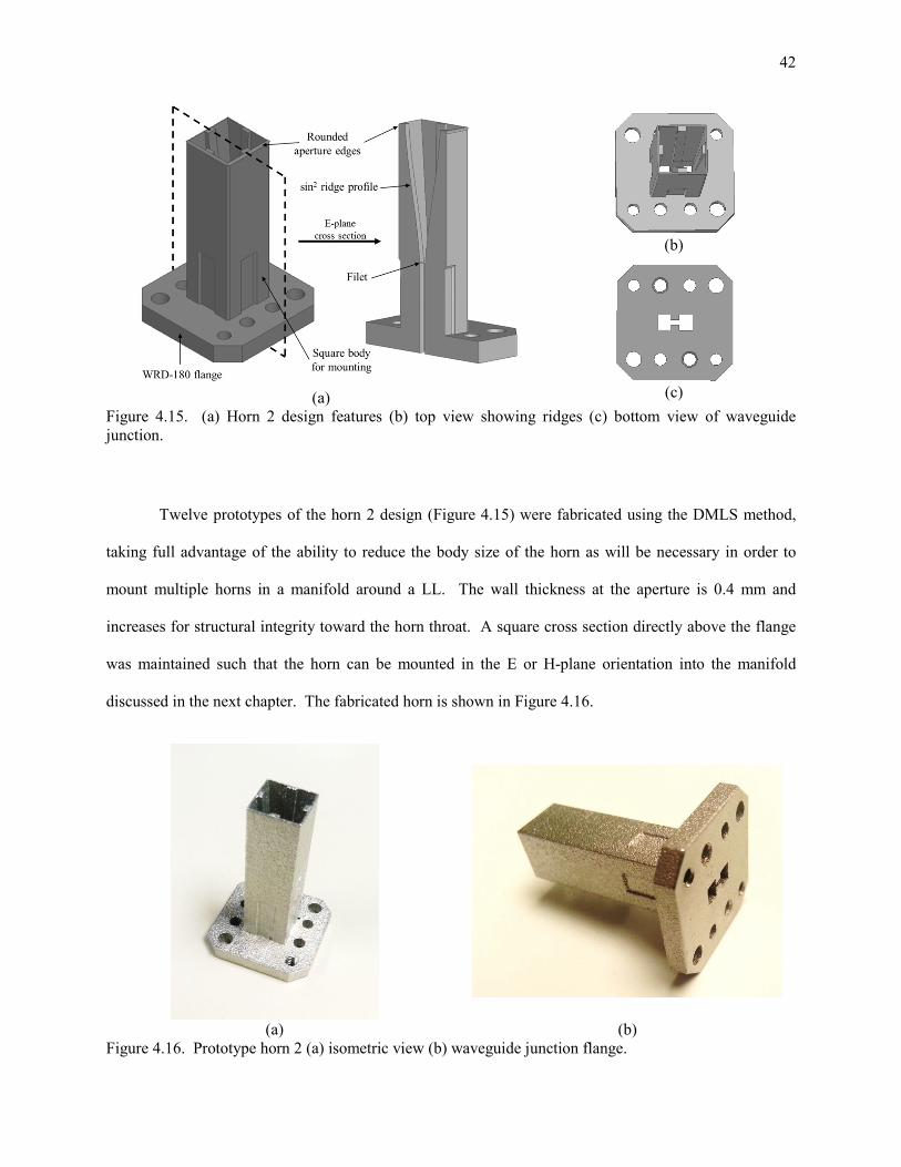
42

(a)

(b)

(c)

Figure 4.15. (a) Horn 2 design features (b) top view showing ridges (c) bottom view of waveguide

junction.

Twelve prototypes of the horn 2 design (Figure 4.15) were fabricated using the DMLS method,

taking full advantage of the ability to reduce the body size of the horn as will be necessary in order to

mount multiple horns in a manifold around a LL. The wall thickness at the aperture is 0.4 mm and

increases for structural integrity toward the horn throat. A square cross section directly above the flange

was maintained such that the horn can be mounted in the E or H-plane orientation into the manifold

discussed in the next chapter. The fabricated horn is shown in Figure 4.16.

(a) (b)

Figure 4.16. Prototype horn 2 (a) isometric view (b) waveguide junction flange.

43

4.4.3 Performance

Of the twelve feed horns, nine were installed into the manifold discussed in the next chapter. The

remaining three were used for measurements taken in this section and are designated H1, H2, and H3.

Reflection coefficient measurements were taken using a VNA (Vector Network Analyzer) with a

maximum frequency of 40 GHz. A custom waveguide TRL (Thru – Reflect – Line) calibration kit was

used to calibrate the VNA to a reference plane at the antenna waveguide junction. Measurements and

HFSS simulations (assuming a matched waveport) are plotted in Figure 4.17.

(a) (b)

(c) (d)

Figure 4.17. Horn 2 Simulations / Measurements: (a) Reflection coefficient (b) Directivity / Gain (c) E-

Plane PC and (d) H-Plane PC. PCs were computed over the 10 dB beamwidth using amplitude weighting.

Frequency [GHz]

20 25 30 35 40 45-2

-1

0

1

2

HFSS

H1Meas

Frequency [GHz]

20 25 30 35 40 45-2

-1

0

1

2

HFSS

H1Meas

E-Plane H-Plane

PCVE=1.5 mm

PCVH=0.8 mm

44

Reference gain measurements were required to compute gain of the AUT in Figure 4.17(b). The

reference measurements were acquired using standard gain horns in the 18 – 26.5 GHz and 26.5 – 45 GHz

bands. The inconsistent gain offset (relative to directivity) in the AUT data on either side of 26.5 GHz

indicates there may be a deviation between the assumed gain and actual gain exhibited by the standard

gain horns.

The PCV was measured to be 1.5 mm in the E-plane and 0.8 mm in the H-plane. While there was

some slight disagreement between PC at the lower frequencies, the overall PCV expected from the

simulations was observed in the measurement. At lower frequencies, the antenna pattern is more

susceptible to impacts from the mounting hardware and absorber due to the wider beamwidth. For these

measurements, absorber was placed 5 mm below the aperture.

Figure 4.18. Prototype horn 2 mounted in the antenna range, before placing microwave absorber below

the aperture opening.

Simulated and measured radiation patterns are plotted in Figure 4.19.

45

E-Plane H-Plane

18 GHz

26 GHz

34 GHz

42 GHz

Figure 4.19. Simulated (red) and measured (blue) normalized radiation patterns of horn 2 at various

frequencies.

4.5 Summary

During the design process of horn 1, some valuable insight was gained which led to a second

design more suited to the application at hand. Some main observations with respect to the two horns are

as follows:

� Horn 1 prototypes as manufactured using CNC and DMLS both perform similarly, despite the

undesired features inherent to each method.

� The directivity and gain, as expected, is lower for horn 2 due to the smaller aperture size.

46

� PCVE is lower for prototype horn 2 (1.5 mm) as a result of reducing the aperture size and

conducting the parametric sweep while considering the wall thickness at the aperture of the horn.

� The mean value of PC over frequency is located closer to the aperture of horn 2.

� The maximum reflection coefficient measured for horn 2 is 3 dB lower than for horn 1.

Both designs will be mounted for measurement with the LL in the next chapter for comparison, however

only horn 2 is intended to be mounted as a feed array to the LL.

47

Chapter 5

Luneburg Lens / Feed Horn Implementation

5.1 Introduction

Throughout the feed antenna design process, a stable LL focal point has been assumed over the

bandwidth of interest. This, in turn, made a feed antenna with minimal PCV over frequency highly

desirable. It will be shown in section 5.2, however, that the focal point of the two-layer nonuniform LL

can vary with frequency, further complicating the relationship between feed position, feed PC, and LL

focal point. In addition, reflections between the lens, feed antenna, and within the lens itself can cause

additional scattering and coupling between multiple feeds placed in the vicinity of one another. This will

affect system performance such as gain, sidelobe level (SLL), and reflection coefficient. Due to the very

complex nature of the problem at hand, a numerical approach is most appropriate for determining the

optimal placement of the feed horns with respect to the LL surface.

The LL being used in this study is a two layer lens as pictured in Figure 5.1. Using known

permittivities of each layer, this lens was able to be modeled using the finite element method (FEM)

solver within HFSS with losses neglected in the initial analysis. A loss analysis of the lens is discussed in

section 5.5.3. The actual lens used for measurements was designed and supplied by Lun’ Tech of Perols,

France.

48

(a) (b)

Figure 5.1. (a) 2-layer LL HFSS model with transparent outer layer and (b) manufactured lens.

5.2 Luneburg Lens Simulation – Open-Ended Waveguide

The aperture of an open-ended waveguide (OE-WG) was swept in distance from the LL surface

as a means of determining the lens’s focal point numerically.

Figure 5.2. HFSS model of an open-ended waveguide feeding the LL, separated by a distance �+.

The focal point is determined as the OE-WG aperture location that results in maximum directivity

and peak sidelobe level (SLL), where SLL is positive and is relative to the maximum directivity. Figure

5.3(a) and (b) show maximum directivity and peak SLL as functions of lens / OE-WG separation (�+) and

frequency. To cover the 18 – 45 GHz bandwidth, three waveguide cross sections (WR-42, WR-28, and

WR-22) were used over their respective operation bandwidths. The values in each frequency column of

Figure 5.3 are normalized to 0 dB.

49

(a) (b)

Figure 5.3. Simulated 2-layer LL performance when fed with an OE-WG, as a function of aperture

distance from the surface (�+) and frequency, (a) normalized directivity and (b) peak SLL normalized to

0 dB at each frequency.

Note that the scale is larger for SLL since it is more sensitive to waveguide separation �+ than is

directivity. Although the focal point for this lens appears to be in the region between 4-5 mm, it will be

defined formally as the point that maximizes performance over the frequency band as determined by �¢,

defined as

�¢%�+) = 1£h |1 − �x%�, �+)|(¤¥¤y¤� (5.1)

where £ is the number of frequencies simulated and �x%�, �U) = ¢%¤,U¦)¢%¤)§¨© is the normalized directivity

(linear form) as a function of frequency � and �+. The distance �+ at which �¢ is minimum will reveal

the optimum placement of the horn aperture according to (5.1). Similarly, �ª«« can be defined in terms of

peak SLL performance:

�ª««%�+) = 1£h |1 − ���x%�, �+)|(¤¥¤y¤� (5.2)

where again, the peak SLL is normalized at each frequency and is in linear form spanning (0 – 1). �¢ and

�ª«« for the OE-WG simulation are plotted in Figure 5.4.

dB dB

50

Figure 5.4. �¢ and �ª«« as determined using (5.1) and (5.2) for the OE-WG / LL simulation.

The minimums of �¢ and �ª«« are separated by about 1 mm. For this reason, the focal point of a non-

ideal lens, like the definition of the PC of the feed antenna, is not trivial and must be determined using

specific design requirements.

5.3 Luneburg Lens with Single Feed Antenna

The aperture of prototype horn 1 was positioned under the LL according to Figure 5.5 for

simulation in HFSS. Neglecting effects such as reflections and coupling, at a single frequency �. one

would expect an optimum aperture location of

�+u = �)u − �¬­. (5.3)

where �+u is the distance between feed aperture center and lens surface, �)u is the focal point of the lens at

frequency �., and �¬­. is the computed phase center offset relative to the horn’s aperture at frequency �..

(da)

51

Figure 5.5. Expected optimum horn feed position with respect to its PC offset �¬­, the lens focal point �), and the LL / feed separation �+.

5.3.1 Horn 1

Like the OE-WG simulation, the horn was swept in distance �+ from the surface of the lens in

HFSS. Results are shown in Figure 5.6, with the optimum horn location determined using the metrics

given in (5.1) and (5.2). Ideally, the best performance at each frequency in Figure 5.6(a) and (b) would

correspond to (5.3). There exist several obstacles in determining the feed position using (5.3), however.

First is that �¬­ will vary depending on how it is computed. Unlike for a reflector antenna [26], an

“appropriate” definition pertaining to the LL has yet to be developed. Second, the focal point was

measured using an OE-WG, which illuminates the lens differently than the horn. Since the horn is more

directive, a smaller portion of the lens will be illuminated as the frequency increases. Lastly and most

importantly, the focal point and PC were both computed in separate simulations of the lens and horn,

respectively. When arranging the two structures less than 1 cm from each other there is an interaction

that will invalidate the simple relationship in (5.3) due to reflections, scattering, and coupling if other feed

antennas are present.

52

(a) (b)

(c)

Figure 5.6. Horn 1 / LL performance vs position in terms of (a) directivity and (b) peak SLL. The focal

point in terms of �¢ and �ª«« is found as the minimum of the plots in (c).

The interaction between feed and LL is evident in plotting the feed VSWR as a function of �+

and frequency (Figure 5.7). Ideally, the inner and outer boundaries of the lens would be well matched

and VSWR would not change with �+, as is true with for LL with more layers (Appendix C). A clear

variation, however, can be seen in the �-axis of Figure 5.7 and is at its worse at 27 GHz between 4 – 5

mm. This is not surprising since the outer layer of a 2 layer LL is not as well matched to free space as

say, a 10 layer lens would be. Although the lens’s contribution to VSWR at a given frequency will

ultimately decrease with increasing distance �+, there exists a periodicity in the VSWR that can be seen

dB dB

53

in Figure 5.7 depending on the phase of the reflected fields. The feed horn by itself will have internal

reflections and in some cases, the reflection from the lens may add destructively to lower the overall

VSWR as measured at the feed input. Conversely, the reflections add constructively to raise the VSWR

at some frequency / distance combinations.

Figure 5.7. Horn 1 VSWR (simulated) versus the horn / lens separation �+ and frequency.

A bracket (Figure 5.8) was designed and fabricated with the use of 3D printing to secure the LL

and allow for the mounting of the horn 1 prototype antenna a fixed distance from the LL surface. Thin

shims were used to set the distance of the feed aperture to �+ = 4.3 mm. The bracket material consists of

PLA (polylactic acid) type plastic. When simulated with and without the mounting bracket, the radiation

pattern revealed no significant impact due to its presence. Further discussion of the mounting bracket can

be found in Appendix B. Simulated versus measured performance is shown below.

54

(a) (b)

Figure 5.8. CNC horn 1 mounted with LL (a) on bench and (b) installed in antenna range before

wrapping the lower mount with microwave absorber.

(a) (b)

(c) (d)

Figure 5.9. Simulations / measurements of horn 1 (CNC) mounted with the LL, (a) reflection coefficient

(b) directivity / gain (c) HPBW and (d) peak SLL.

Frequency [GHz]

20 25 30 35 40 450

5

10

15

20

HFSS E-Plane

HFSS H-Plane

Meas E-Plane

Meas H-Plane

SLL [dB]

55

The drop-off in directivity [Figure 5.9(b)] above 40 GHz corresponds with a widening of the E-

plane HPBW [Figure 5.9(c)]. Note that horn 1, when measured without the lens, does not have the same

drop in directivity [Figure 4.12(b)]. This effect, as it pertains to both the lens and the feed, will be

discussed later in the chapter. Measured antenna patterns at several frequencies are compared to the

HFSS simulation in Figure 5.10.

E-Plane H-Plane

18 GHz

26 GHz

34 GHz

42 GHz

Figure 5.10. E / H-plane antenna patterns of prototype horn 1 (CNC) mounted with the LL.

In most cases, the sidelobes were exacerbated in the measurements by 1 – 2 dB but for the most part the

measurements maintained the same features as the simulations.

56

5.3.2 Horn 2

Horn 2 was also swept in distance �+ in HFSS to determine an ideal mounting position for use in

the manifold discussed in the next section. Results are plotted in Figure 5.11.

(a) (b)

(c)

Figure 5.11. Horn 2 / LL performance vs position in terms of (a) directivity and (b) peak SLL. The focal

point in terms of �¢ and �ª«« is found as the minimum of the plots in (c).

Note a more overall stability in terms of both directivity and peak SLL as a function of position

than for horn 1. The minima of �¢ and �ª«« coincide at the same distance of �+ = 4.2 mm. The

position’s effect on VSWR is shown in Figure 5.12.

(da)

dB dB

57

Figure 5.12. Horn 2 VSWR (simulated) versus the horn / lens separation �+ and frequency.

The “hot spots” in Figure 5.12 are similar to those seen in Figure 5.7 which indicates the behavior to be

more dependent on lens characteristics than on the feeds. A new metric, �S® , can also be considered

which is similar to �¢ but instead plots the realized gain which includes mismatch loss corresponding to

the VSWR profile in Figure 5.12. The minimum of �S® is located at 4.28 mm which is only 0.08 mm

from the minimum of �¢.

5.4 Luneburg Lens with Multiple Feeds

A feed manifold was designed for use with prototype horn 2 enabling the assembly of two

curvilinear 1x5 arrays, one along the f� plane and one along the �� plane as shown in Figure 5.13

requiring nine feeds in all. Figure 5.13(b) shows the labeling convention for the different feeds, as

viewed from the bottom of the manifold where the waveguide flanges are visible.

58

(a) (b)

Figure 5.13. (a) Feed manifold CAD model pictured without the lens or supports, (b) feed array labeling

as the array ordering would appear looking from the bottom of (a).

The feed F0 is the bottom center feed and will radiate maximally at the lens’s boresight ( = 0). Throughout this chapter, the two arrays will be referred to as the E-plane array (F11 – F15) and H-plane

array (F21 – F25) indicating that the E or H-planes of the feed horns are in the same plane for the given

array. The horns in both arrays are separated by an angle � (Figure 5.14).

Figure 5.14. Feed separation angle �.

59

With the directivity of the lens expected to be > 20 dBi, the five element array will not provide

continuous beam coverage in the lens’s far field. The prime purpose for this implementation, however, is

to study the effects of coupling and demonstrate the mounting of multiple feeds in the vicinity of one

another under a LL. The fully assembled manifold is pictured in Figure 5.15.

(a) (b)

Figure 5.15. Feed manifold (a) without LL (b) with LL installed.

5.4.1 S-Parameters

The feeds in the manifold are separated by � = 25° in both E and H arrays. With the E and H

arrays populated, S-parameter measurements were taken using an Agilent VNA up to its maximum of 40

GHz. The measurements are plotted in Figure 5.16 and are organized into reflection coefficient, E-plane

element coupling, H-plane element coupling, and cross coupling between elements in the two curvilinear

arrays. Redundant measurements are omitted from the plots below, e.g. the coupling between feeds F21

and F24 (S24_21) is assumed to be the same as the coupling between F22 and F25 (S25_22) due to symmetry

and therefore only one of the measurements is plotted.

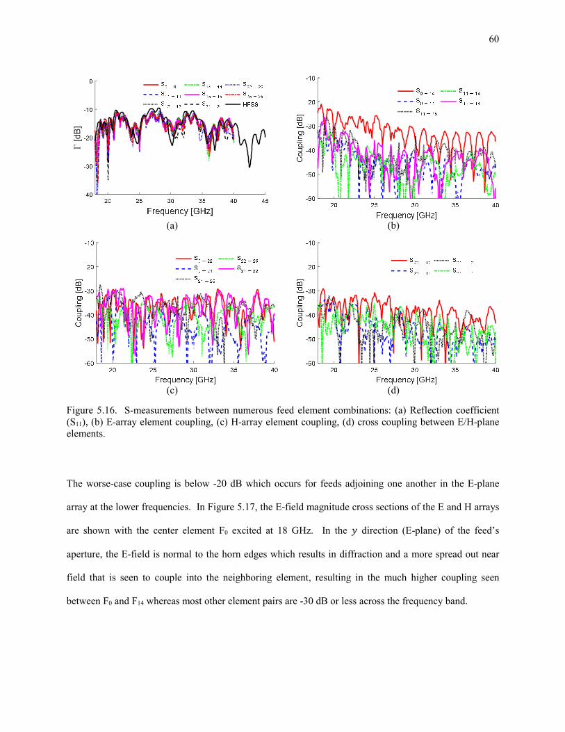
60

(a) (b)

(c) (d)

Figure 5.16. S-measurements between numerous feed element combinations: (a) Reflection coefficient

(S11), (b) E-array element coupling, (c) H-array element coupling, (d) cross coupling between E/H-plane

elements.

The worse-case coupling is below -20 dB which occurs for feeds adjoining one another in the E-plane

array at the lower frequencies. In Figure 5.17, the E-field magnitude cross sections of the E and H arrays

are shown with the center element F0 excited at 18 GHz. In the � direction (E-plane) of the feed’s

aperture, the E-field is normal to the horn edges which results in diffraction and a more spread out near

field that is seen to couple into the neighboring element, resulting in the much higher coupling seen

between F0 and F14 whereas most other element pairs are -30 dB or less across the frequency band.

[dB]

61

(a) (b)

Figure 5.17. E-field magnitude when fed by the center element F0 in (a) E-array and (b) H-array cross

sections at 18 GHz, normalized to the E-field intensity incident on the LL.

The two outer horns are separated by � = 100° and it can be expected that S15_11 and S25_21 will increase

as � approaches 180°. HFSS simulations reveal coupling levels on the order of -10 dB for � = 180°. 5.4.2 Simulations / Measurements

In both HFSS simulations and range measurements of the feed manifold, the horns were

positioned a distance �+ = 4.2 mm from the lens surface as a result of the �¢ and �ª«« plots in Figure

5.11. The process of mounting the feed horns is discussed in Appendix B. Absorber was lined on the top

surface of the manifold [Figure 5.15(a)] in an attempt to mitigate effects from the mounting hardware

beneath the manifold surface during the initial analysis of the system. The manifold as mounted in the

anechoic chamber is pictured in Figure 5.18.

|6| [V/m] > 1

0

62

(a) (b)

Figure 5.18. Lens manifold mounted in antenna chamber (a) front view (b) side view with F11 connected

as the AUT feed and microwave absorber removed.

In post-processing, HFSS can excite the desired number of feeds to view any combination of beams. The

36 GHz 3D polar gain pattern with all feeds excited is shown in Figure 5.19(a). Due to symmetry, only

three beams were measured in the antenna range: F0, F12, and F11 and their individual patterns are

superimposed onto each other as shown in Figure 5.19(b).

(a) (b)

Figure 5.19. (a) All feeds excited in HFSS and (b) E-plane of the three unique E-array feeds measured in

the antenna range at 36 GHz.

63

Because the antenna range employs a roll-over-azimuth positioner for scanning the AUT, only one

principal plane of the off-axis feeds (F11 and F12) will be measured in one continuous scan and the H-

plane will be plotted for F0 only. Patterns for the three measured beams are plotted in Figure 5.20.

E-Plane H-Plane

18 GHz

26 GHz

34 GHz

42 GHz

Figure 5.20. Normalized radiation patterns of F0, F12, and F11.

The peak SLL and HPBW measured for F0 are plotted in Figure 5.21.

64

(a) (b)

Figure 5.21. F0 Simulated and measured E / H plane (a) peak SLL and (b) HPBW.

As in the horn 1 / LL measurements, the maximum SLL occurs in the H-plane at most

frequencies. The highest sidelobes that can be expected for the given configuration are located at about

14 dB when simulated, but are likely closer to 10 dB when measured up to 45 GHz. SLL measurements

were only plotted to 43 GHz, above which the measurement SNR was too low to accurately measure the

sidelobes.

The gain was measured and compared to HFSS simulations and is plotted in Figure 5.22(a). The

dip at 39 GHz is thought to be from an external factor in the measurement, given that horn 2 exhibited no

obvious losses at this frequency and it was not measured in the F0 measurement. As an additional check,

the normalized radiation patterns are plotted in Figure 5.22(b) at that frequency. The fact that the

reflection coefficient was average at this frequency and the radiation patterns show no abnormalities

further supports that the gain dip at 39 GHz is due to measurement effects.

Frequency [GHz]

20 25 30 35 40 455

10

15

20

25

HFSS E-Plane

HFSS H-Plane

Meas E-Plane

Meas H-Plane

HPBW [deg]

65

(a) (b)

Figure 5.22. (a) Gain of the three measured / simulated elements and (b) normalized E-plane radiation

pattern corresponding with the dip at 39 GHz.

5.5 Analysis

5.5.1 Primary / Secondary Feed Patterns

Minimizing the PCV of the feed horn will minimize the LL’s aperture phase error since the feed

will be approximately focused across all frequencies. The amplitude distribution of the feed, however,

will also have a direct impact on the LL radiation pattern. For this analysis, the feed’s radiation will be

referred to as the primary pattern and the LL’s radiation the secondary pattern.

It can be noticed in the gain of the LL fed by horn 1 [Figure 5.9(b)] that the directivity peaks at

about 40 GHz then drops about 1.5 dB over the next 5 GHz. Horn 2 / LL gain begins to drop at 44 GHz

[Figure 5.22(a)] but is less obvious since it is near the maximum plotted frequency. It can also be seen in

each configuration’s corresponding HPBW plots that the E-plane HPBW begins to increase at the same

frequency while the H-plane HPBW does not. This behavior is observed both in the simulations and the

measurements.

66

For aperture antennas, the maximum directivity is related to the antenna’s area  )��X by [14]

� = 4# )��X:+( (5.4)

where :+ � 1 is the aperture efficiency. For the LL,  )��X is simply the cross sectional area of the

sphere. In the case of a reflector antenna, for example, an aperture efficiency of one occurs when its

aperture is uniformly illuminated in terms of both amplitude and phase. The dependency on wavelength

in the denominator of (5.4) describes an antenna’s increase in directivity with frequency due to an

increasing electrical size of the aperture. This is observed up to 40 GHz for horn1 / LL. At frequencies

greater than 40 GHz, :+ begins decreasing with frequency by a factor greater than the increase caused by

1/(, causing an overall decrease in the directivity.

Two basic trends were observed in the 2-layer LL’s peak sidelobe level (SLL) behavior: 1) The

SLL worsened as frequency increased and 2) the feed’s H-plane had worse sidelobes than in the E-plane

at most frequencies. The latter effect can be explained with some analysis of the feed antenna pattern.

An analysis conducted in [46] approximates the primary feed pattern as

�¤ = cos% �)x (5.5)

where ′ is the primary pattern angle and $ describes the directivity of the feed. That is, a higher value of

$ corresponds with a narrower feed beamwidth incident on the LL. Assuming a feed with a pattern given

in (5.5) and the geometry in Figure 5.23, the relationship between aperture plane power �+%�) and the

feed’s pattern is given by [47]

�+%�) = cos �sinAz � ��)��x�)(°�)( − �( . (5.6)

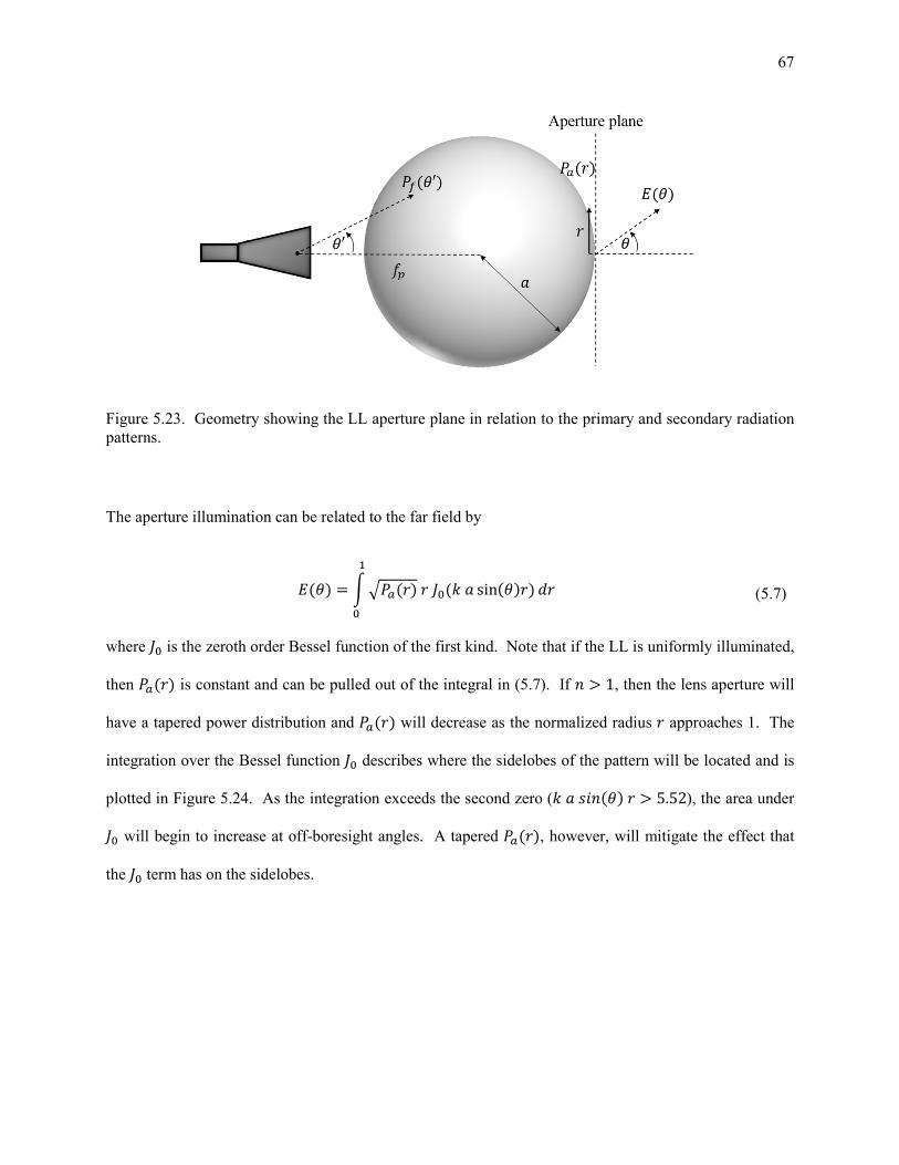
67

Figure 5.23. Geometry showing the LL aperture plane in relation to the primary and secondary radiation

patterns.

The aperture illumination can be related to the far field by

6% ) = ±L�+%�)�²E%D� sin% )�) ��zE

(5.7)

where ²E is the zeroth order Bessel function of the first kind. Note that if the LL is uniformly illuminated,

then �+%�) is constant and can be pulled out of the integral in (5.7). If $ > 1, then the lens aperture will

have a tapered power distribution and �+%�) will decrease as the normalized radius � approaches 1. The

integration over the Bessel function ²E describes where the sidelobes of the pattern will be located and is

plotted in Figure 5.24. As the integration exceeds the second zero (D�N�$% )� > 5.52), the area under

²E will begin to increase at off-boresight angles. A tapered �+%�), however, will mitigate the effect that

the ²E term has on the sidelobes.

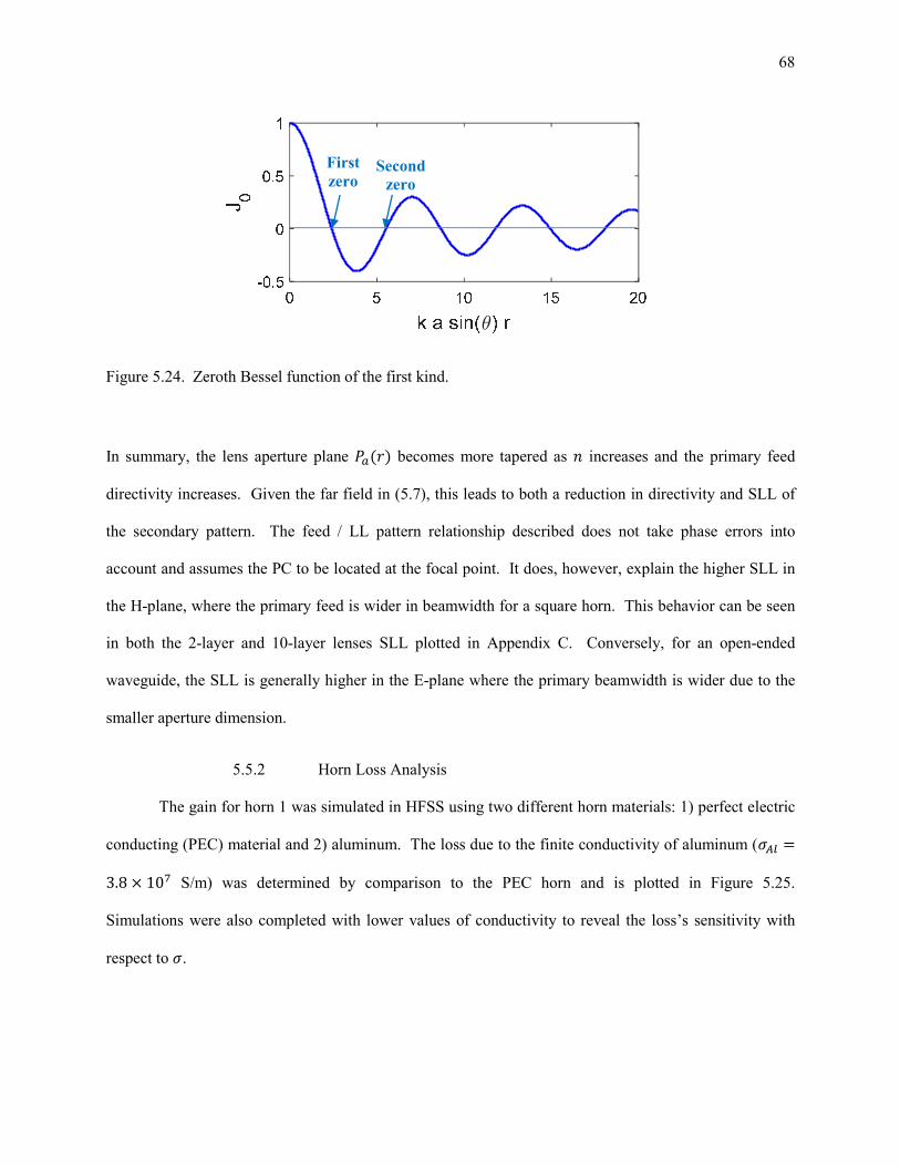
68

Figure 5.24. Zeroth Bessel function of the first kind.

In summary, the lens aperture plane �+%�) becomes more tapered as $ increases and the primary feed

directivity increases. Given the far field in (5.7), this leads to both a reduction in directivity and SLL of

the secondary pattern. The feed / LL pattern relationship described does not take phase errors into

account and assumes the PC to be located at the focal point. It does, however, explain the higher SLL in

the H-plane, where the primary feed is wider in beamwidth for a square horn. This behavior can be seen

in both the 2-layer and 10-layer lenses SLL plotted in Appendix C. Conversely, for an open-ended

waveguide, the SLL is generally higher in the E-plane where the primary beamwidth is wider due to the

smaller aperture dimension.

5.5.2 Horn Loss Analysis

The gain for horn 1 was simulated in HFSS using two different horn materials: 1) perfect electric

conducting (PEC) material and 2) aluminum. The loss due to the finite conductivity of aluminum (�³´ =3.8 × 10µ S/m) was determined by comparison to the PEC horn and is plotted in Figure 5.25.

Simulations were also completed with lower values of conductivity to reveal the loss’s sensitivity with

respect to �.

First

zero Second

zero

69

Figure 5.25. Horn 1 conductor loss due to the finite conductivity of aluminum, plotted for multiple values

of �.

The DMLS method contained a visible surface roughness, specified to be 5-15am Ra1. As fields

propagate through the horn, the surface roughness changes the path in which eddy currents will travel in

the horn ridges and sidewalls depending on the skin depth � relative to the roughness. Much interest has

been given to the area of conductor loss over a rough surface. Morgan [48] solved this problem for

square and triangular shaped grooves both parallel and transverse to the direction of current flow.

Additional computations for expected conductor loss was provided and verified by rough surface

modeling in HFSS [49]. For two-dimensional grooves transverse to current flow, increased conductor

loss per unit length is given by

¶V¶VE = 1 ' 2# tanAz ¹1.4 �Δ��(» (5.8)

¶V = Attenuation constant with surface roughness

¶VE = Attenuation constant for smooth surface

Δ = RMS roughness value

� = Skin depth

1 Ra is a metric used to describe surface roughness. It is the arithmetic average of surface height deviation.

Loss [dB]

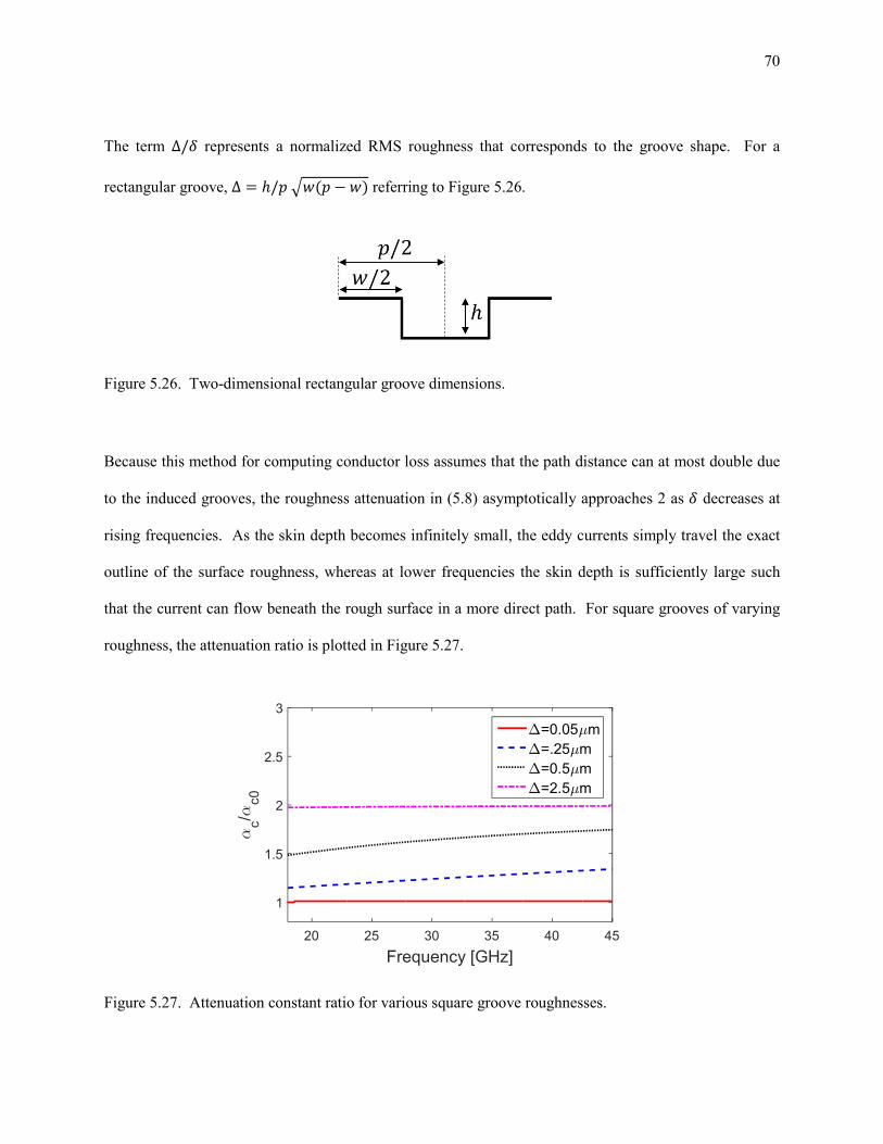
70

The term Δ/� represents a normalized RMS roughness that corresponds to the groove shape. For a

rectangular groove, Δ = ℎ/�Ln%� − n) referring to Figure 5.26.

Figure 5.26. Two-dimensional rectangular groove dimensions.

Because this method for computing conductor loss assumes that the path distance can at most double due

to the induced grooves, the roughness attenuation in (5.8) asymptotically approaches 2 as � decreases at

rising frequencies. As the skin depth becomes infinitely small, the eddy currents simply travel the exact

outline of the surface roughness, whereas at lower frequencies the skin depth is sufficiently large such

that the current can flow beneath the rough surface in a more direct path. For square grooves of varying

roughness, the attenuation ratio is plotted in Figure 5.27.

Figure 5.27. Attenuation constant ratio for various square groove roughnesses.

Frequency [GHz]

20 25 30 35 40 45

c/c0

1

1.5

2

2.5

3

=0.05 m

=.25 m

=0.5 m

=2.5 m

71

The skin depth for aluminum over 18-45 GHz varies from about 0.4 – 0.6 am and it can be seen that as

the roughness Δ enters this range the surface attenuation is expected to rise. Assuming a worst case Δ of

15am, the surface roughness loss will reach the asymptotic limit of 2 across the frequency band. Even

though the DMLS surface resembles a periodic structure whose behavior, based on the model, would

resemble that of Figure 5.27, a safety factor of ¶V/¶VE = 4 will be used herein since exact surface

properties are unknown. In addition, a second safety factor will be used for the assumed conductivity, in

which the loss computed with � = 0.5 × �³´ in Figure 5.25 yielded a maximum of about 0.05 dB.

Multiplying by a surface roughness attenuation factor of 4, a maximum surface loss of 0.2 dB is expected

due to the combined surface roughness and limited conductivity of the horn surface.

5.5.3 2-Layer Lens Loss Analysis

Using the loss tangents tan �. of the inner and outer LL layers given in [33], the loss was

computed for the 2-layer LL when fed by horn 1 in HFSS by comparison with the gain for the lossless

lens. Multiples of tan �. were also applied to the lens and plotted in Figure 5.28 as a means for showing

the sensitivity of the material properties in terms of the loss tangent.

Figure 5.28. Loss of the 2-layer LL fed by horn 1, where tan �. is the assumed loss tangent of the LL

layer materials.

2-Layer LL Loss [dB]

72

For the given loss tangents of the materials, a maximum of 0.24 dB loss was observed. Doubling

the loss tangents in each material results in a maximum loss of 0.52 dB. Due to uncertainties in the

materials, the loss tangent’s frequency dependency, and on disagreement within the literature on the

material properties, a maximum of 0.52 dB loss will be assumed for the 2-layer LL, where a factor of 2

was used in the loss tangents to account for any such errors that may exist. For a high power application,

the difference between 0.24 dB and 0.52 dB of loss can translate into a significant amount of heat and a

more thorough study of the material properties may be needed to determine the power handling

capabilities of the lens.

5.6 Summary

Both feed antennas were positioned under the LL according to metrics that were developed to

optimize the system’s radiation characteristics in terms of directivity and SLL over the frequency band.

Each configuration was measured and results were confirmed to closely resemble the radiation patterns

given in HFSS, establishing confidence in the described methods for simulating, mounting, and

measuring the lens / feed system. Nine feeds of the second prototype design were implemented into two

curvilinear arrays and S-parameters of the numerous feeds were measured. Although no obvious

excessive losses due to the surface roughness of the DMLS aluminum fabrication method were observed,

an additional analysis was completed which predicts a worst case of 0.2 dB loss, although this value could

be more effectively determined (and likely reduced) if a more complete set of surface statistics were

known. Similarly, a maximum LL loss of 0.52 dB has been given through simulations with the

assumption that the loss tangent is at most double the values given in literature at the simulated

frequencies.

73

Chapter 6

Conclusions

6.1 Phase Center of Horn Antennas

Chapter 2 discussed several methods for computing the PC of any antenna radiating a well-defined

main lobe in the boresight direction. As a design specification that is very qualitative in nature, it is

important to understand the implications of the different factors affecting the computation of PC. The

beamwidth and choice of weighting function are two of the main aspects affecting its computation, but

other subjective qualities may be necessary to yield results that are of interest for the given application.

For example, while testing horn 2 which had a wider beamwidth than the first horn, it was realized that

spillover portions (i.e. edges of the 10 dB beamwidth that do not intersect the lens) of the beam were

being used in the PC computation at low frequencies. It was decided that it was more rational to limit the

far field to angles of the pattern that are within the subtended angle of the lens, about 122° at the

mounting distance that was used.

The simulation of four example horn antennas showed some general tendencies of the PC in horn

antennas and how its definition can have a large impact in its determined location. Although at the time

of the feed antenna designs it was not well-understood how important PC stabilization would be for

performance of the LL, the examples nonetheless were a motivation for the design of an antenna whose

PC remained as stable as possible across frequency. To avoid losing the distinction between E and H

plane PCs, they were plotted separately throughout this thesis. The averaging of the two surely would

74

have lowered the PCV of any designed antennas and may have looked better on paper, but generalizing

the PC in this sense can be deceiving in that a horn with a zero PCV could still have E and H-plane PCs

far apart from one another and thus the lens aperture phase error would not be minimized. If an averaged

E/H-plane PC had been used, a separate metric indicating the separation between E and H PCs would

have also been included.

6.2 Design of a Luneburg Lens Feed

After exploring several PC stabilization methods, the horn interior ridges were designed with a

sin2 profile and the PC was stabilized to less than 2 mm over the 18 – 45 GHz frequency range in the first

design iteration, prototype horn 1. This design was fabricated with aluminum using both subtractive and

additive techniques and similar performance was seen between both prototype implementations.

Mounting a single feed under the LL, it was shown that models of the LL in HFSS produced accurate

performance results in terms of reflection coefficient, directivity, and radiation patterns. In most cases,

sidelobes were higher in the measurements by 1-2 dB. Measurements, however, are subject to finite

accuracy in the feed / LL spacing, fabrication imperfections, and misalignment error therefore it should

not be surprising that the modeled results appear slightly better.

A second design horn comprising a smaller aperture was designed for mounting in a LL feed

manifold in its lower half-space. Both the smaller aperture and lessons learned from the parametric

sweep conducted in the first iteration helped reduce the PCV to 1.5 mm in the E-plane and 0.8 mm in the

H-plane while maintaining closer E/H PCs at each frequency. Although the PC measurements yielded

overall less agreement with simulations for horn 2, its performance as measured with the LL supports a

lower PCV as compared to horn 1. With nine feeds installed into the lens manifold, three of the feeds in

the E-plane array were measured and compared with the HFSS simulation. Like in horn 1, higher

sidelobes were seen in the measured radiation patterns.

75

6.3 Future Work

From the beginning of this project, the top priority concerning the feed antenna involved

minimizing its PCV with the assumption that the LL focal point was stable. With a maximum PCV of 1.5

mm, near-maximum directivity (within 0.5 dB) was achieved across all frequencies as determined when

sweeping horn 2 in distance from the lens surface in HFSS. It was seen that the sidelobe level, however,

was more sensitive to the horn positioning. It may be worthwhile in the future to attempt to design a

varying PC that coincides with movement of the LL focal point to further minimize the peak SLL across

all frequencies. In addition, as the 2-layer LL becomes better understood it may be beneficial to prioritize

other feed characteristics before stabilizing the PC, such as fine control of the feed beamwidth and thus

the LL illumination and aperture efficiency.

While only nine feeds were mounted in the LL manifold, eventually 36 such feeds will be

required to span the bottom hemisphere of the lens. The positioning of curvilinear arrays across a

spherical surface is simple, however equally spacing 36 elements to maximize beam coverage is a much

more complicated task as there is no obvious way in which to organize them. Even with their spacing

optimized, the beamwidth of the LL may be too narrow to allow for continuous coverage at higher

frequencies and it may be necessary to limit the directivity of the feed / LL combination if beam

overlapping is desired at, for example, the 3 dB beamwidths. With each of the 36 elements requiring

dual-pol operation, 36 orthomode transducers (OMTs) must also fit into the lower hemisphere of the lens.

The mechanical design in itself of the end product will be very challenging.

In addition to the lens considered in this research, alternative lens options may provide improved

radiation characteristics. A LL consisting of additional layers may help to reduce sidelobes while

mitigating the reflections at layer boundaries. With today’s 3D-printing capabilities, printing a LL with

precise control of air-to-plastic ratio (and thus permittivity) may also be a conceivable method for

producing a LL if internal losses can be kept to a minimum.

76

6.4 Original Contributions

The following original contributions of this thesis are listed below:

� Demonstrated a method for stabilizing the PC of a square horn antenna over a wide

bandwidth, where corrugations were not a practical design option.

� Implemented an alternative method for computing the PC for an antenna whose PC is not

located sufficiently close to the center of rotation of a roll-over-azimuth positioner. This

was done iteratively to avoid using approximations that can lead to large errors at

millimeter wavelengths.

� Designed a manifold consisting of two curvilinear arrays of feed horn antennas for a LL

whose design focal point is 5 mm from its surface. Each feed horn can be adjusted

approximately ±2 mm relative to the lens surface and a method for setting the lens /

horn spacing was demonstrated using a spacer constructed of two pieces of acrylic.

� Fabricated a small horn antenna using aluminum direct metal laser sintering and

demonstrated that results similar to previously proven fabrication methods were

obtainable with modest losses.

77

Bibliography

[1] J. L. Volakis, Antenna Engineering Handbook, New York: McGraw-Hill, 2007.

[2] R. K. Luneburg, The Mathematical Theory of Optics, Providence, RI: Brown Univ. Press, 1944.

[3] F. T. Ulaby and D. G. Long, Microwave Radar and Radiometric Remote Sensing, Ann Arbor: The

Univ. of Michigan Press, 2014.

[4] P. Afanasyev, S. Matitsine, V. Sledkov, P. Lagoiski, L. Matytsine, T. DeMarco, and T. Chia,

"Multi-beam Luneburg Lens Antenna for Cellular Communications," in EuCAP, Lisbon, 2015.

[5] J. Thorton, D. Smith, S. J. Foti, and Y. Y. Jiang, "Reduced Height Luneburg Lens Antennas for

Satellite Communications-on-the-move," in COMITE, Pardubice, 2015.

[6] J. A. Lock, "Scattering of an Electromagnetic Plane Wave by a Luneburg Lens. I. Ray Theory,"

Journal of the Optical Society of America, vol. 25, pp. 2971-2979, 2008.

[7] J. Reinholdt, "Cylindrical Luneburg Lens Antenna for Multi-Beam Small Cell Wireless Backhaul

Applications," M.Sc. Thesis, Dept. of Eng. Physics and Elec. Eng., Lulea Univ. of Tech., 2014.

[8] S. Rondineau, M. Himdi, and Jacques Sorieux, "A Sliced Spherical Luneburg Lens," IEEE

Antennas Wireless Propag. Lett., vol. 2, pp. 163-166, 2003.

[9] A. V. Boriskin, A. Vorobyov, and R. Sauleau, "Two-Shell Radially Symmetric Dielectric Lenses

as Low-Cost Analogs of the Luneburg Lens," IEEE Trans. Antennas Propag., vol. 59, no. 8, pp.

3089-3093, 2011.

[10] H. Mosallaei and Y. Rahmat-Samii, "Nonuniform Luneburg and Two-Shell Lens Antennas:

Radiation Characteristics and Deisgn Optimization," IEEE Trans. Antennas Propag., vol. 49, no. 1,

pp. 60-69, 2001.

[11] M. Liang, X. Yu, R. Sabory-Garcia, W. Ng, M. E. Gehm, and H. Xin, "Broadband Electronically

Beam Scanning Structure Using Luneburg Lens," in MTT-S Int. Microwave Symp., 2013.

[12] Q. Xu and J. Thorton, "Report on Steerable Antenna Architectures and Critical RF Circuits

Performance," CAPANINA, 2006.

[13] M. J. Goonan, "A novel Luneburg lens feed for multiple beam antennas," in Antennas and Propag.

Soc. Int. Symposium, Ann Arbor, MI, 1993.

[14] C. Balanis, Antenna Theory, 3rd Ed., Hoboken, NJ: John Wiley & Sons, Inc., 2005.

[15] W. L. Barrow and L. J. Chu, "Theory of the Electromagnetic Horn," Proc. IRE, pp. 51-64, 1939.

78

[16] G. C. Southworth, "Hyper frequency wave guides - General considerations and experimental

results," Bell Syst. Tech. J., vol. 15, pp. 284-309, 1936.

[17] W. T. Slayton, "Design and Calibration of Microwave Antenna Gain Standards," US Naval

Research Lab, Washington, DC, 1954.

[18] E. H. Braun, "Gain of Electromagnetic Horns," Proc. IRE, vol. 41, pp. 109-115, 1953.

[19] E. H. Braun, "Some Data for the Design of Electromagnetic Horns," IEEE Trans. Antennas

Proagat., Vols. AP-4, pp. 29-31, 1956.

[20] HFSS v.15.0, ANSYS, Inc., 2015.

[21] IEEE Standard for Definitions of Terms for Antennas, New York, NY, 2013.

[22] M. J. Radway, T. P. Cencich, and D. S. Filipovic, "Phase Center Stability of Planar Spiral

Antennas," in Antenna Applications Symposium, Monticello, IL, 2009.

[23] S. R. Best, "Distance-Measurement Error Associated with Antenna Phase-Center Displacement in

Time-Reference Radio Positioning Systems," IEEE Antennas Propagat. Mag., vol. 46, no. 2, pp.

13-22, 2004.

[24] T. Wei and Z. Xin, "Research on the High Precise Calibration of the GPS Receiving Antenna

Phase Center," in ISAPE, Guangzhou, 2010.

[25] J. Friden and G. Kristensson, "Calculation of Antenna Radiation Center Using Angular

Momentum," IEEE Trans. Antennas Propag., vol. 61, no. 12, pp. 5923-5930, 2013.

[26] P. Kildal, "Combined E- and H-Plane Phase Centers of Antenna Feeds," IEEE Trans. Antennas

Propag., Vols. AP-31, no. 1, 1983.

[27] E. I. Muehldorf, "The Phase Center of Horn Antennas," IEEE Trans. Antennas Propag., Vols. AP-

22, pp. 753-750, 1970.

[28] Y. Y. Hu, "A Method of Determining PHase Centers and its Application to Electromagnetic

Horns," Journal of the Franklin Institute, vol. 271, no. 1, pp. 31-39, 1961.

[29] W. Kunysz, "Antenna Phase Center Effects and Measurements in GNSS Ranging Applications," in

ANTEM-AMEREM, Ottawa, ON, 2010.

[30] W. V. T. Rusch and P. D. Potter, Analysis of Reflector Antennas, New York: Academic Press,

Inc., 1970.

[31] P. N. Betjes, "An Algorithm for Automated Phase Center Determination and its Implementation,"

in AMTA, St. Louis, 2007.

[32] W. H. Press, S. A. Teukolsky, W. T. Vetterling, B. P. Flannery, Numerical Recipes, The Art of

Scientific Computing, 3rd ed., Cambridge, MA: Cambridge Univ. Press, 2007.

79

[33] D. M. Pozar, Microwave Engineering, 3rd Ed., John Wiley & Sons, Inc., 2005.

[34] M. Teichman, "Determination of Horn Antenna Phase Centers by Edge Diffraction Theory," IEEE

Trans. Aerosp. Elecron. Syst., Vols. AES-9, no. 6, pp. 875-882, 1973.

[35] C. Ehrenborg, Investigation and Comparison Between Radiation and Phase Center for Canonical

Antennas, M.Sc. Thesis: Dept of Elec. and Info. Tech., Lund Univ. 2014..

[36] FEKO Suite 6.2, EM Software & Systems S.A. Ltd, 2013.

[37] K. Harima, "Accurate Gain Measurement for Millimeter-Wave Horn and Open-Ended Waveguide

Antennas," in Int. Symp. on Antennas and Prop., Nagoya, Japan, 2012.

[38] N. Jastram and D. S. Filipovic, "Development of Integrated High Power Passive Front-Ends for

Towed Decoys," in GOMACTech 15, St. Louis, 2015.

[39] A. D. Olver, P. J. B. Clarricoats, A. A. Kishk, and L. Shafai, Microwave Horns and Feeds, New

York: IEEE Press, 1994.

[40] P. Kildal, "Artificially soft and hard surfaces in electromagnetics and their application to antenna

design," in Microwave Conf. Proc, Madrid, Spain, 1993.

[41] K. L. Walton and V. C. Sundberg, "Broadband Ridged Horn Design," Microwave Journal, vol. 7,

pp. 96-101, 1964.

[42] S. B. Cohn, "Flare-Angle Changes in a Horn as a Means of Pattern Control," Microwave Journal,

vol. 13, pp. 41-46, 1970.

[43] A. X. a. J. Olver, "Design of Profiled Corrugated Horns," IEEE Trans. Antennas Propag., vol. 36,

no. 7, 1988.

[44] A. H. Akgiray, "New Technologies Driving Decade-Bandwidth Radio Astronomy," Ph.D.

dissertation, California Inst. of Tech., Pasadena, CA, 2013.

[45] ANSYS, "HFSS Online Help," 2012.

[46] J. Thorton, "Properties of Spherical Lens Antennas for High Altitude Platform Communications,"

in EMPS/ASMS, Noordwijk, 2004.

[47] S. P. Morgan, "General Solution to the Luneburg Lens Problem," Journal of Applied Physics, vol.

29, no. 9, pp. 1358-1368, 1958.

[48] S. P. Morgan, Jr., "Effect of Surface Roughess on Eddy Current Losses at Microwave

Frequencies," Bell Telephone Laboratories, Murray Hill, NJ, 1948.

[49] M. V. Lukic and D. S. Filipovic, "Modeling of 3-D Surface Roughness Effects with Application to

u-Coaxial Lines," IEEE Trans. Microw. Theory Techn., vol. 55, no. 3, pp. 518-525, 2007.

[50] P. A. Beeckman, "Analysis of phase errors in antenna-measurements applications to phase-pattern

80

corrections and phase-centre determination," IRE Proceedings, vol. 132, no. 6, pp. 391-394, 1985.

[51] P. I. Deffenbaugh, R. C. Rumpf, and K. H. Church, "Broadband Microwave Frequency

Characterization of 3D Printed Materials," IEEE Trans. Compon. Packag. Manuf. Technol., vol. 3,

no. 12, pp. 2147-2155, 2013.

[52] Z. Sipus, D. Bojanjac, and T. Komljenovic, "Electromagnetic Modeling of Spherically Stratified

Lenses Illuminated by Arbitrary Sources," IEEE Trans. Antennas Propag., vol. 63, no. 4, pp. 1837-

1843, 2015.

81

Appendix A

Phase Center Measurements

When using a CEM (computational electromagnetic) simulation tool to obtain the far field phase

of a horn antenna, phase symmetry about the �-axis is easily maintained to within 0.5 degrees when using

reasonable solution settings. Because HFSS projects the far field to � → ∞, the approximation given in

(2.4) remains very accurate and any of the PC extraction methods discussed in Chapter 2 will yield

practically the same values for the PC offset �. When taking measured data, however, care must be taken

to consider the effects of the finite far field distance in which the measurements are taking place.

A.1 Rotational Scanning Error

In the ideal case, the antenna under test (AUT) is mounted with its PC located on the axis

containing the center of rotation (� = 0), corresponding to Figure A.1. In some cases, however, the size

of the AUT or other mounting limitations may require an antenna to be located a distance from the center

of rotation. Referring to Figure A.1, it is evident that the farther the AUT is from the center of rotation,

the greater distance it will physically move in the antenna range as it scans in .

82

Figure A.1. Antenna range setup geometry, where �d and �e refer to the PC position when the AUT is

positioned at = 0.

While this simple fact is often disregarded when taking more common amplitude-based measurements, it

can have a significant impact in the PC computation due to the rotational phase error incurred when

scanning the AUT in [50]. During the first set of measurements completed with horn 1, the aperture of

the AUT was mounted a distance of 13.5 cm from the center of rotation, i.e. �~13.5 cm. In this case, it

was discovered that unlike CEM simulations, the method used to extract the PC can have a significant

impact on the values obtained. In the antenna range geometry shown in Figure A.1, the wideband

observation antenna was set up such that � = 2.2 m and �/�~0.06. Evaluating the true value of K% ) using the law of cosines:

K% ) = L�( ' �( ' 2���MN% ). (A.1)

The approximation for � ≪ � is

K¿% ) ≅ � ' ��MN% ). (A.2)

With respect to the horn 1 measurement setup, the deviation between (A.1) and (A.2) is

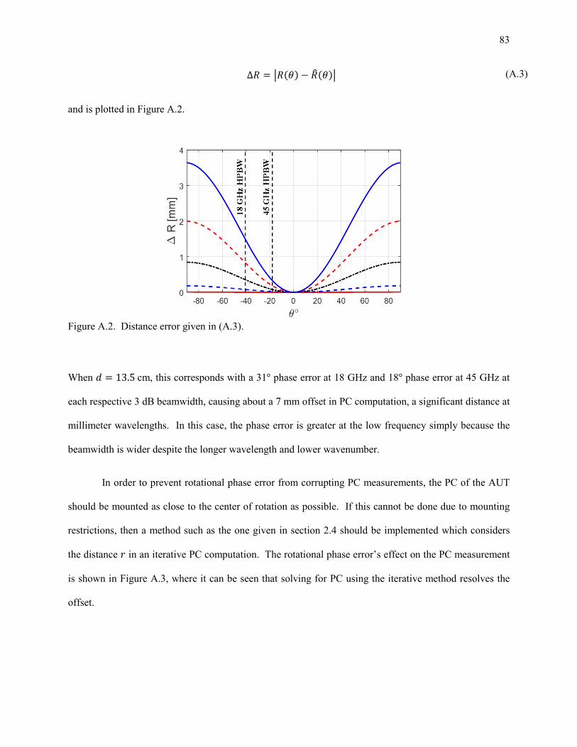
83

ΔK = vK% ) − K¿% )v (A.3)

and is plotted in Figure A.2.

Figure A.2. Distance error given in (A.3).

When � = 13.5cm, this corresponds with a 31° phase error at 18 GHz and 18° phase error at 45 GHz at

each respective 3 dB beamwidth, causing about a 7 mm offset in PC computation, a significant distance at

millimeter wavelengths. In this case, the phase error is greater at the low frequency simply because the

beamwidth is wider despite the longer wavelength and lower wavenumber.

In order to prevent rotational phase error from corrupting PC measurements, the PC of the AUT

should be mounted as close to the center of rotation as possible. If this cannot be done due to mounting

restrictions, then a method such as the one given in section 2.4 should be implemented which considers

the distance � in an iterative PC computation. The rotational phase error’s effect on the PC measurement

is shown in Figure A.3, where it can be seen that solving for PC using the iterative method resolves the

offset.

84

Figure A.3. E-plane PC measurement of horn 1 mounted 13.5 cm from the center of rotation, computed

using the least mean squares error (red solid) which is susceptible to the rotational phase error versus the

iterative method (blue dashed) which corrects for the error.

While � generally can only be approximated since its true measurement is relative to the observation

antenna’s PC which can also vary with frequency and scan angle ′, � determined to within 1 cm was

easily obtained which will determine the PC to within 0.3 mm for the given mounting setup of � = 13.5

cm. However, as � increases the computation becomes more sensitive to the measurement of �, therefore

it is always good practice to minimize � when mounting the AUT regardless of the method used.

85

Appendix B

Lens / Feed Mounting

The LL was constructed using a solid core and outer shell of different indices of refraction.

Because of a very thin layer of glue adhering the two halves of the outer shell, a small indent of less than

0.5 mm circles the lens equator. A small ring was placed around the lens bracket to grip the lens in the

indent. This was advantageous in that if the lens were a perfect sphere without an indent, the bracket

would likely have needed to be wider to ensure the lens did not slip out during measurements. Both the

indent and mating ring are pictured in Figure B.1.

(a) (b)

Figure B.1. (a) Indent on the equator of the LL and (b) mating ring designed onto the lens bracket.

B.1 Materials

The material of the 3D-printed mounting bracket and manifold was chosen mainly for its

electrical properties. Somos Watershed 11122 was used which has a dielectric constant of 2.6 and loss

Indent Mating

ring

86

tangent of 0.027 at the highest measured frequency of 11 GHz in [51]. Mechanically, a polypropylene or

true ABS plastic would be more durable but the available types had higher loss tangents.

Before printing the horn 1 single feed mount bracket, an HFSS simulation was run with and

without the bracket as shown in Figure B.2. The bracket was assumed to be ABS-like with 23 = 3 and

the two screws were modeled as nylon with 23 = 4.

(a) (b)

Figure B.2. Horn 1 (alternate exterior design) simulated (a) with bracket in place and (b) without bracket.

Normalized radiation patterns are plotted in Figure B.3 for comparison of sidelobe performance with and

without the lens mounting bracket. As expected, the mounting brackets have no discernable impact on

the 45 GHz antenna pattern since both the feed and lens beamwidths are narrow at the high frequency. At

18 GHz, however, the fields are more spread and there is more interaction with the bracket. The 18 GHz

E-plane far sidelobes (> 45 °) are seen to be higher by 2-4 dB, while the first and second H-plane

sidelobes are raised by about 1 dB.

Nylon

screw

87

E-Plane H-Plane

18 GHz

45 GHz

Figure B.3. Normalized radiation patterns at the low / high frequencies to check the effects of the lens

mounting bracket.

B.2 Feed Horn Positioning

The feed horns were designed to slide up and down in their mounting brackets by ±2 mm,

allowing for accurate placement of the feeds with respect to the lens surface even in the presence of small

fabrication errors. One difficult task when populating the feed array was spacing the hollow horn

apertures to the curved spherical surface of the lens. To accomplish this to a reasonable level of accuracy,

a fixed spacer was created for the desired aperture to lens surface distance. A small piece of acrylic was

cut such that it fit over on the horn aperture, with additional pieces on three of the sides to keep it from

sliding off. A nylon screw was then threaded and glued into the top and filed down until the desired

distance was obtained as measured using a digital caliper [Figure B.4(a)]. The horn position could then

be set and tightened with the spacer in place [Figure B.4(b)]. Once the horn was secured using the nylon

set screws, the spacer was then slid out.

88

(a) (b)

Figure B.4. (a) Measurement of the horn/lens spacer and (b) alignment of the F0 feed antenna.

To populate the array, it is required to install the feed elements starting with the center element (F0) and

work outward in order to be able to access the three set screws for each element.

Set screws

4.2 mm spacer

89

Appendix C

10-Layer LL Simulation

A 10-layer LL was modeled in HFSS as a means for comparing performance of the 2-layer LL

(Figure C.1). The 10-layer LL is a much closer approximation to an ideal uniform LL than is the 2-layer

and their direct comparison can help to recognize certain effects caused by the 2-layer construction type.

(a) (b)

Figure C.1. Models of the (a) 2-layer LL and (b) 10-layer LLs.

C.1 E-Fields – Horn 1

The following plots show the E-fields resulting from the 2 and 10-layer LLs excited with horn 1

at various frequencies. The E-fields are plotted in log scale (Figure C.2), normalized to the E-field

intensity at the feed aperture.

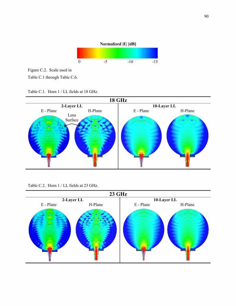
90

Normalized |E| [dB]

0 -5 -10 -15

Figure C.2. Scale used in

Table C.1 through Table C.6.

Table C.1. Horn 1 / LL fields at 18 GHz.

18 GHz 2-Layer LL 10-Layer LL

E - Plane H-Plane E - Plane H-Plane

Table C.2. Horn 1 / LL fields at 23 GHz.

23 GHz 2-Layer LL 10-Layer LL

E - Plane H-Plane E - Plane H-Plane

Lens

Surface

91

Table C.3. Horn 1 / LL fields at 27 GHz.

27 GHz 2-Layer LL 10-Layer LL

E - Plane H-Plane E - Plane H-Plane

Table C.4. Horn 1 / LL fields at 33 GHz.

33 GHz 2-Layer LL 10-Layer LL

E - Plane H-Plane E - Plane H-Plane

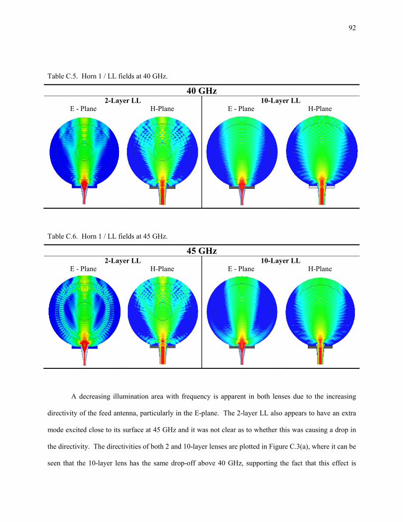
92

Table C.5. Horn 1 / LL fields at 40 GHz.

40 GHz 2-Layer LL 10-Layer LL

E - Plane H-Plane E - Plane H-Plane

Table C.6. Horn 1 / LL fields at 45 GHz.

45 GHz 2-Layer LL 10-Layer LL

E - Plane H-Plane E - Plane H-Plane

A decreasing illumination area with frequency is apparent in both lenses due to the increasing

directivity of the feed antenna, particularly in the E-plane. The 2-layer LL also appears to have an extra

mode excited close to its surface at 45 GHz and it was not clear as to whether this was causing a drop in

the directivity. The directivities of both 2 and 10-layer lenses are plotted in Figure C.3(a), where it can be

seen that the 10-layer lens has the same drop-off above 40 GHz, supporting the fact that this effect is

93

solely due to the feed’s influence on the aperture efficiency. Note that there are also no ripples present in

the 10-layer LL directivity plot.

(a) (b)

Figure C.3. (a) Directivity and (b) SLL comparison between the 2 and 10-layer LLs as fed by horn 1.

C.2 Reflection Coefficient – Horn 1

Both simulations and measurements of the 2-layer LL reflection coefficient contained ripples, as

seen in the 2-layer trace of Figure C.4.

Figure C.4. Reflection coefficient of horn 1 with and without the 2 and 10-layer LLs.

94

When the 10-layer lens was placed in front of horn 1, the improved matching behavior to free space and

between each layer resulted in a reflection coefficient plot very similar to that of the horn by itself. The

ripples were also eradicated with the 10-layer LL as was seen in the directivity.