phase change thermal energy storage for the … · symposium 2013, liverpool john moore’s...

PHASE CHANGE THERMAL ENERGY STORAGE

FOR THE THERMAL CONTROL OF LARGE

THERMALLY LIGHTWEIGHT INDOOR SPACES

A thesis submitted for the degree of

Doctor of Philosophy (PhD)

By

GOWREESUNKER, Baboo Lesh S. (BEng)

School of Engineering and Design

Brunel University

June 2013

i

ABSTRACT

Energy storage using Phase Change Materials (PCMs) offers the advantage of higher

heat capacity at specific temperature ranges, compared to single phase storage.

Incorporating PCMs in lightweight buildings can therefore improve the thermal mass,

and reduce indoor temperature fluctuations and energy demand. Large atrium buildings,

such as Airport terminal spaces, are typically thermally lightweight structures, with

large open indoor spaces, large glazed envelopes, high ceilings and non-uniform

internal heat gains. The Heating, Ventilation and Air-Conditioning (HVAC) systems

constitute a major portion of the overall energy demand of such buildings.

This study presented a case study of the energy saving potential of three different PCM

systems (PCM floor tiles, PCM glazed envelope and a retrofitted PCM-HX system) in

an airport terminal space. A quasi-dynamic coupled TRNSYS®-FLUENT® simulation

approach was used to evaluate the energy performance of each PCM system in the

space. FLUENT® simulated the indoor air-flow and PCM, whilst TRNSYS® simulated

the HVAC system. Two novel PCM models were developed in FLUENT® as part of

this study. The first model improved the phase change conduction model by accounting

for hysteresis and non-linear enthalpy-temperature relationships, and was developed

using data from Differential Scanning Calorimetry tests. This model was validated with

data obtained in a custom-built test cell with different ambient and internal conditions.

The second model analysed the impact of radiation on the phase change behaviour. It

was developed using data from spectrophotometry tests, and was validated with data

from a custom-built PCM-glazed unit. These developed phase change models were

found to improve the prediction errors with respect to conventional models, and

together with the enthalpy-porosity model, they were used to simulate the performance

of the PCM systems in the airport terminal for different operating conditions.

This study generally portrayed the benefits and flexibility of using the coupled

simulation approach in evaluating the building performance with PCMs, and showed

that employing PCMs in large, open and thermally lightweight spaces can be beneficial,

depending on the configuration and mode of operation of the PCM system. The

simulation results showed that the relative energy performance of the PCM systems

relies mainly on the type and control of the system, the night recharge strategy, the

latent heat capacity of the system, and the internal heat gain schedules. Semi-active

systems provide more control flexibility and better energy performance than passive

systems, and for the case of the airport terminal, the annual energy demands can be

reduced when night ventilation of the PCM systems is not employed. The semi-active

PCM-HX-8mm configuration without night ventilation, produced the highest annual

energy and CO2 emissions savings of 38% and 23%, respectively, relative to a

displacement conditioning (DC) system without PCM systems.

ii

PUBLICATIONS

Published Journal Papers

Gowreesunker BL, Tassou SA, Kolokotroni M (2012), Improved simulation of phase

change processes in applications where conduction is the dominant heat transfer

mode, Energy and Buildings 47: 353-359

Gowreesunker BL, Tassou SA (2013), Effectiveness of CFD simulation for the

performance prediction of phase change building boards in the thermal

environment control of indoor spaces, Building and Environment 59: 612-625

Gowreesunker BL, Stankovic SB, Tassou SA, Kyriacou PA (2013), Experimental and

numerical investigations of the optical and thermal aspects of a PCM-Glazed

unit, Energy and Buildings 61: 239-249

Gowreesunker BL, Tassou SA, Kolokotroni M (2013), Coupled TRNSYS-CFD

simulations evaluating the performance of PCM plate heat exchangers in an

Airport Terminal building displacement conditioning system, Building and

Environment 65: 132-145

Published Conference Papers

Gowreesunker BL, Tassou SA (2012), The energy storage capabilities of clay boards

with phase change materials in building applications, In Proceedings of the 12th

International Conference on Energy Storage, Innostock 2012, Lleida, Spain, 16-

18 May 2012, Paper no. INNO-SP-117 (ISBN: 9788493879334).

Gowreesunker BL, Tassou SA (2013), Evaluation of the energy impact of PCM tiles in

an Airport Terminal Departure Hall, In Proceedings of the CIBSE Technical

Symposium 2013, Liverpool John Moore’s University, Liverpool, UK, 11-12

April 2013, www.cibse.org.

Gowreesunker BL, Tassou SA (2013-Accepted), A TRNSYS-FLUENT coupled

simulation of the thermal environment of an airport terminal space with a

mixing and displacement air conditioning system, 13th

International Conference

of the International Building Performance Simulation Association, Chambéry,

France, 25-28 August 2013.

iii

ACKNOWLEDGEMENTS

I would like to express my appreciation and gratitude to Prof. Savvas Tassou for

allowing me to work on this project, and for extending and guiding my potential; both

intellectually and tactfully. I am also very grateful to Prof. Maria Kolokotroni for

constantly supporting my professional development since my undergraduate years.

Although both being very busy with administrative matters, their organisation, hard-

work and dedication to research are inspiring.

I would like to thank the UK Engineering and Physical Sciences Research Council

(EPSRC Grant no: EP/H004181/1), through Prof. Tassou, for financially supporting this

research study. I am also thankful for the discussions with the other collaborating

universities (City, Reading, Loughborough and Kent) at our regular meetings at Brunel,

which facilitated the collaborative research paper with City University.

I am thankful to my colleagues in the Brunel Refrigeration Laboratory: IDewa, Emily,

INyoman, Giovanna, Kostas and Amir, amongst others; and the technicians, Mr. C.

Xanthos and K. Withers; for their help and enlivening conversations, not always related

to Thermodynamics.

Finally, I would like to express my very special gratitude to my Father, Mother, Sister,

Prabhupada, Radha and Krsna for their constant moral and emotional support. I dedicate

this thesis to them.

iv

TABLE OF CONTENTS

ABSTRACT ....................................................................................................................... i

PUBLICATIONS .............................................................................................................. ii

ACKNOWLEDGEMENTS ............................................................................................. iii

TABLE OF CONTENTS ................................................................................................. iv

LIST OF FIGURES ....................................................................................................... viii

LIST OF TABLES ......................................................................................................... xiv

NOMENCLATURES ..................................................................................................... xv

ABBREVIATIONS ....................................................................................................... xix

CHAPTER 1 – INTRODUCTION ................................................................................... 1

1.1 Problem Definition .................................................................................................. 1

1.2 The Airport Terminal Environment......................................................................... 5

1.3 Research Aims and Objectives ................................................................................ 8

1.4 Structure of Thesis ................................................................................................... 9

CHAPTER 2 – BACKGROUND TO STUDY ............................................................... 10

2.1 Phase Change Materials (PCMs) ........................................................................... 10

2.1.1 Introduction to Latent Heat Storage ................................................................ 10

2.1.2 Classification of PCM ..................................................................................... 15

2.1.3 Thermal Analysis Techniques ........................................................................ 20

2.1.4 Introduction to PCM related systems ............................................................. 25

2.1.5 Micro-encapsulated PCM systems.................................................................. 26

2.1.6 PCM panels and boards .................................................................................. 30

2.1.7 PCM-Air heat exchanger type systems ........................................................... 34

2.1.8 PCM Glazing units.......................................................................................... 38

2.1.9 PCM in Heat/Cold Storage Units.................................................................... 40

2.2 Thermal Comfort ................................................................................................... 43

2.2.1 Thermal Comfort conditions ........................................................................... 45

2.3 Summary of Chapter 2 .......................................................................................... 48

CHAPTER 3 – THERMAL MODELLING OF PHASE CHANGE .............................. 51

3.1 Importance of Numerical Modelling ..................................................................... 51

3.2 Common Phase Change Models ............................................................................ 53

3.2.1 The Enthalpy-Porosity Method ....................................................................... 54

v

3.2.2 The Effective Heat Capacity Method ............................................................. 57

3.3 Enhancements to Phase Change Models ............................................................... 59

3.3.1 Enhanced Phase Change Conduction Model .................................................. 60

3.3.2 Validity of Model............................................................................................ 61


CHAPTER 4 – MODELLING OF INDOOR THERMAL ENVIRONMENT AND PCM

......................................................................................................................................... 66

4.1 Introduction to Computational Fluid Dynamics (CFD) ........................................ 66

4.1.1 Governing Equations ...................................................................................... 68

4.1.2 Turbulence Modelling..................................................................................... 71

4.1.3 Renormalisation Group (RNG) k-ε Turbulence Model .................................. 76

4.1.4 Near-Wall Treatment ...................................................................................... 78

4.2 Modelling of Indoor Environment and PCM boards ............................................. 79

4.3 Validity of CFD ..................................................................................................... 83

4.4 Effectiveness of CFD ............................................................................................ 87

4.4.1 Impact of PCM boards .................................................................................... 87

4.4.2 Ventilation heat transfer rates ......................................................................... 89

4.4.3 Effective use of PCM boards .......................................................................... 91


CHAPTER 5 – OPTICAL MODELLING OF PCM ...................................................... 95

5.1 Development of Optical Model ............................................................................. 96

5.2 Validity of Optical Model ................................................................................... 100

5.3 Design Implications ............................................................................................. 104

5.4 Summary of Chapter 5 ........................................................................................ 107

CHAPTER 6 – NUMERICAL CONSIDERATIONS FOR AIRPORT TERMINAL . 109

6.1 Overview of Modelling Strategy ......................................................................... 109

6.2 Introduction to TRNSYS ..................................................................................... 110

6.3 Coupling of CFD & TRNSYS ............................................................................. 112

6.4 CFD Numerical Considerations .......................................................................... 114

6.4.1 Radiation Modelling ..................................................................................... 117

6.5 TRNSYS HVAC System ..................................................................................... 119

6.6 L2 Norm – CFD Temporal and Spatial Convergence Study ............................... 121

6.7 Coupled Model .................................................................................................... 127


vi

CHAPTER 7 – AIRPORT PCM SYSTEMS ................................................................ 130

7.1 PCM Floor Tiles .................................................................................................. 131

7.2 PCM Glazing Envelope ....................................................................................... 134

7.2.1 PCM Glazing Model ..................................................................................... 134

7.2.2 TRNSYS-FLUENT Coupling for PCM Glazing .......................................... 136

7.3 PCM Heat-Exchanger (PCM-HX) ...................................................................... 138

7.3.1 PCM-HX Model ........................................................................................... 139

7.3.2 TRNSYS-FLUENT Coupling for PCM-HX ................................................ 142

7.3.3 PCM-HX Control Strategies ......................................................................... 143

7.4 Pressure Drop Calculations ................................................................................. 144

7.5 Total Annual Energy Demand ............................................................................. 145


CHAPTER 8 – PERFORMANCE OF PCM SYSTEMS IN AIRPORT TERMINAL

SPACE .......................................................................................................................... 149

8.1 Seasonal Performance of stand-alone DC system ............................................... 150

8.2 Seasonal Performance of DC system and PCM Tiles ......................................... 155

8.2.1 ‘Ebb’ Tiles .................................................................................................... 155

8.2.2 ‘Energain’ Tiles ............................................................................................ 158

8.3 Seasonal Performance of DC system and PCM Glazing .................................... 161

8.4 Seasonal Performance of DC system with retrofitted PCM-HX ......................... 164

8.4.1 DC-PCM-HX-16mm .................................................................................... 164

8.4.2 DC-PCM-HX-8mm ...................................................................................... 168

8.5 Annual Energy Performance ............................................................................... 172

8.5.1 Relative Energy Performance ....................................................................... 174

8.5.2 Assessment of the Control Method ............................................................... 176

8.5.3 Cost and CO2 Emissions Analysis ................................................................ 178


CHAPTER 9 – CONCLUSIONS AND RECOMMENDATIONS FOR FUTURE

WORK .......................................................................................................................... 181

9.1 Concluding Remarks ........................................................................................... 183

9.2 Recommendations for Future Work .................................................................... 190

REFERENCES .............................................................................................................. 192

Appendix A: Development of phase change conduction model ................................... 207

Appendix B: Validity and effectiveness of CFD .......................................................... 212

vii

Appendix C: Development of optical phase change model .......................................... 223

Appendix D: Numerical conditions .............................................................................. 230

Appendix E: Pressure drop calculations for the Airport Terminal space ...................... 244

Appendix F: Annual Energy calculation procedure ...................................................... 248

Appendix G: Assumptions for costs and CO2 emissions analysis ................................ 250

viii

LIST OF FIGURES

Fig. 2.1 Solid-Liquid phase change ……………………………………........ 11

Fig. 2.2 Classification of Phase Change Materials …………………………. 15

Fig. 2.3 Typical curve of a DSC plot .………………………………………. 21

Fig. 2.4 Heat Flow DSC …………………………………………………….. 22

Fig. 2.5 Heat Flux DSC ……………………………………………………... 22

Fig. 2.6 PCM Microcapsules ………………………………………………... 27

Fig. 2.7 Powdered PCM ……………………………………………………. 28

Fig. 2.8 Rubitherm CSM® Panel …………………………………………… 30

Fig. 2.9 TROX system …………………………………………………….... 37

Fig. 2.10 PCM nodule by Cristopia …………………………………………... 41

Fig. 3.1 Solid-liquid interface ………………………………………………. 53

Fig. 3.2 Enthalpy-temperature relation ……………………………………... 55

Fig. 3.3 The Enthalpy method of representing phase change ………………. 56

Fig. 3.4 Effective heat capacity curve (cp liq = cp sol) ………………………… 57

Fig. 3.5 DSC graph of investigated PCM composite .………………………. 62

Fig. 3.6(a) Experimental, UDF and Enthalpy-porosity temperatures of a

representative point during the melting process …………………....

63

Fig. 3.6(b) Experimental, UDF and Enthalpy-porosity temperatures of a

representative point during the freezing process ...…………………

63

Fig. 4.1 Schematic of CFD solution process ………………………………... 66

Fig. 4.2 Grid discretisation schematic ……………………………………..... 69

Fig. 4.3 Velocity fluctuations ……………………………………………….. 71

Fig. 4.4(a) Experimental Test cell and Wall construction ……………………... 80

Fig. 4.4(b) Locations of temperature sensors in experimental test cell ………... 81

Fig. 4.5 Environmental chamber/ External air temperature ………………… 81

Fig. 4.6(a) Mesh in main air-domain …………………………………………... 83

Fig. 4.6(b) Mesh distribution in walls and air boundary layer ……………….... 83

Fig. 4.7 Local error analysis for non-ventilated scenario …………………… 84

Fig. 4.8 Local error analysis for ventilated scenario ………………………... 85

ix

Fig. 4.9 Comparison of Temperature evolutions at 3 points in the test cell,

and Temperature contours (K) at the end of the heating period with

PCM-Clay board and Plasterboard on the walls ……………………

88

Fig. 4.10 Area-weighted wall heat flux with PCM and plaster boards, and

with different night ventilation rates for PCM boards only ………...

89

Fig. 4.11 Liquid fraction change for different ventilation rates …………….... 91

Fig. 4.12 Velocity streams for ventilation rates of 12 ACH and 46 ACH ........ 92

Fig. 5.1 Spectral transmittance of RT27 in solid, liquid and mushy phases ... 97

Fig. 5.2(a) Schematic of Experimental setup …………………………………... 98

Fig. 5.2(b) Actual setup in Environmental chamber …………………………… 98

Fig. 5.3 Enthalpy-temperature curve of RT27 …………………………….... 98

Fig. 5.4 Absorption (σa), scattering (σs) and extinction (σε) coefficients

during phase change ………………………………………………...

99

Fig. 5.5 PCM finite volume model in PCM-glazed unit ….……………….... 102

Fig. 5.6(a) Transmittance (with experimental error curves) of the PCM filled

glazing under 950 W/m2 irradiation and 13°C ……………………...

102

Fig. 5.6(b) Numerical progression of PCM Temperature ..…………………….. 103

Fig. 5.7 Model Temperature and transmittance progression for a PCM-

glazed and a standard double glazed unit under 950 W/m2

irradiation and 13°C air/initial glazing temperature ..……………....

105

Fig. 5.8 Visual aspect of phase change ……………………………………... 106

Fig. 6.1 London Heathrow Terminal 5 Departure Hall ……………………... 114

Fig. 6.2 CFD representation of investigated airport departure hall ……….... 115

Fig. 6.3 Internal heat gains schedule ………………………………………... 116

Fig. 6.4 Schematic of HVAC system ……………………………………….. 119

Fig. 6.5(a) External temperatures schedule input for L2 norm study ………….. 122

Fig. 6.5(b) Heat gains schedule input for L2 norm study ……………………..... 122

Fig. 6.5(c) Ventilation input schedule input for L2 norm study ………………... 122

Fig. 6.6 Scaled residuals for the benchmark model only, over the course of

the simulation ……………………………………………………….

123

Fig. 6.7(a) L2 norm for Temperature …………………………………………... 124

Fig. 6.7(b) L2 norm for x-velocity ...…………………………………………… 124

Fig. 6.7(c) L2 norm for y-velocity ……………………………………………... 125

x

Fig. 6.8 Airport Terminal Space Model Grid ……………………………….. 126

Fig. 6.9 Generic flow of information in TRNSYS-FLUENT coupling for

normal HVAC system ………………………………………………

128

Fig. 7.1 PCM tiles grid ……………………………………………………… 131

Fig. 7.2 Flow of information in TRNSYS-FLUENT coupling for the PCM-

glazed model ………………………………………………………..

136

Fig. 7.3 Temperature nodes used in calculating the radiation properties of

RT27 ………………………………………………………………..

137

Fig. 7.4 Rubitherm GmbH CSM ® plate …………………………………… 138

Fig. 7.5 Actual Heathrow Terminal 5 diffuser ……………………………… 138

Fig. 7.6 Schematic of DV diffuser, CSM® plate arrangement, and supply

and by-pass ducts inside diffuser …………………………………...

139

Fig. 7.7 Model description of CSM® Plate …………………………………. 140

Fig. 7.8 Heat transfer rates of PCM-HX unit for different air-gaps between

plates at a total mass flow rate of 6 kg/s. ΔT is the temperature

difference between the incoming air and the PCM plate …………...

141

Fig. 7.9 Modified information flow for DC with PCM-HX ………………… 142

Fig. 7.10 HVAC ducting for airport terminal space ………………………….. 144

Fig. 7.11 Generic Ambient temperatures for different seasons …………….... 146

Fig. 8.1(a) Ambient and zone temperature (Tf) profiles for the three distinct

seasons in ‘DC-only’ Case ………………………………………….

150

Fig. 8.1(b) Heating (+) and Cooling (-) Energy Load Profile for ‘DC-only’

case for 2D geometry ……………………………………………….

150

Fig. 8.2(a) Temperature contour (°C) still-frame during the DC unit cooling

mode ………………………………………………………………...

151

Fig. 8.2(b) Temperature contour (°C) still-frame during the DC unit heating

mode ………………………………………………………………...

151

Fig. 8.3(a) Velocity vectors (m/s) in airport domain during DC cooling mode .. 152

Fig. 8.3(b) Velocity vectors (m/s) in airport domain during DC heating mode .. 153

Fig. 8.4 Seasonal heating (+) and cooling (-) demands of Airport space for

stand-alone DC case ………………………………………………...

153

Fig. 8.5(a) Ambient and zone temperature (Tf) profiles with and without night

ventilation for the Ebb-Tiles’ case ……………………………........

155

xi

Fig. 8.5(b) Heating (+) and cooling (-) load profiles for the Ebb-Tiles’ case,

with and without night ventilation, for 2D geometry ………………

156

Fig. 8.6 Heating (+) and cooling (-) demands with and without night

ventilation, with Ebb floor tiles …………………………………….

157


ventilation for the Energain-Tiles’ case ………………………….....

158

Fig. 8.7(b) Heating (+) and cooling (-) load profiles for the Energain-Tiles’

case, with and without night ventilation, for 2D geometry …………

159

Fig. 8.8 Heating (+) and cooling (-) demands with/without night ventilation,

with Energain floor tiles ……………………………………….........

160


ventilation for the PCM-glazing’s case ……………………………..

161

Fig. 8.9(b) Heating (+) and cooling (-) load profiles for the PCM glazing’s

case, with and without night ventilation, for 2D geometry …………

161

Fig. 8.10 Heating (+) and cooling (-) demands with and without night

ventilation, with the PCM-glazing envelope ……………………….

162

Fig.

8.11(a)

Ambient and zone temperature (Tf) profiles, with different night

ventilation charging strategies for the PCM-HX-16mm case ………

164

Fig.

8.11(b)

Heating (+) and cooling (-) load profiles for the PCM-HX-16mm

case, with different night ventilation charging strategies, for 2D

geometry ……………………………………………………………

165

Fig. 8.12 Heating (+) and cooling (-) demands with different night ventilation

strategies, with PCM-HX-16mm ……………………….………….

166

Fig.

8.13(a)

Zone temperatures (Tf) and PCM temperatures during one day in

the intermediate season ……..……………………………………..

167

Fig.

8.13(b)

Heating (+) and cooling (-) load trends for one day in the

intermediate season ………………………………………………....

167

Fig.

8.14(a)

Ambient and zone temperature (Tf) profiles, with different night

ventilation charging strategies for the PCM-HX-8mm case ……….

168

Fig.

8.14(b)

Heating (+) and cooling (-) load profiles for the PCM-HX-8mm

case, with different night ventilation charging strategies, for 2D

geometry ……………………………………………………………

169

xii

Fig. 8.15 Heating (+) and cooling (-) demands with different night ventilation

strategies, with PCM-HX-16mm …..……………………………….

170

Fig. 8.16

Load comparison of PCM-HX-8mm and PCM-HX-16mm for a day

in the intermediate season, under the limiting night control

ventilation charging strategy ……………………………………….

171

Fig. 8.17 Annual energy demand of the entire Airport Terminal Space for the

different PCM system configurations …..…………………………..

172

Fig. 8.18 Total annual energy demands of PCM System configurations

relative to the ‘DC-only’ case ………………………………………

174

Fig. 8.19 Indoor temperature (Tf) for a typical summer day for the ‘DC-only’

case ………………………………………………………………….

176

In Appendices

Fig. A1.1 Environmental Chamber Air temperature surrounding the PCM

composite sample …………………………………………………...

207

Fig.

A1.2(a)

DSC, UDF and Enthalpy-Porosity curves used in the simulations

for the melting process ……………………………………………...

208

Fig.

A1.2(b)

DSC, UDF and Enthalpy-Porosity curves used in the simulations

for the freezing process ……………………………………………..

209

Fig. A1.3 CFD model grid and monitored points’ locations ………………….. 210

Fig. B1.1 Test Cell Wall Configuration ……………………………………..... 212

Fig. B1.2 Location, description and uncertainty of air and surface

thermocouples ………………………………………………………

214

Fig. B1.3 Melting and freezing curves of sample S-3 and the enthalpy-

porosity model ……………………………………………………...

216

Fig. B1.4 L2-planes and L2-norm for temperature and velocities ………….... 218

Fig. B1.5 TA-4 Non-ventilated experimental and simulated temperatures …... 220

Fig. B1.6 TS-5 Non-ventilated experimental and simulated temperatures …… 221

Fig. B1.7 TS-6 Non-ventilated experimental and simulated temperatures …… 221

Fig. B1.8 TA-4 Ventilated experimental and simulated temperatures ….……. 221

Fig. B1.9 TS-5 Ventilated experimental and simulated temperatures ………... 222

Fig. B1.10 TS-6 Ventilated experimental and simulated temperatures ………... 222

xiii

Fig. C1.1 Experimental setup for optical tests ………………………………... 223

Fig.

C1.2(a)

Heat released-stored in given temperature intervals for RT27; HR –

Heat released; HS – Heat stored …………………………………....

225

Fig.

C1.2(b)

Mean experimental extinction coefficients and extinction

coefficients using the relationship Eq. (C1.6) and Eq. (C1.12) ….....

227

Fig. E1.1 Main Supply Duct dP ……………………………………………... 244

Fig. E1.2 Branch Supply Duct dP …………………………………………… 245

Fig. E1.3 Main Return Duct dP ………………………………………………. 245

Fig. E1.4 DC Diffuser Return Path ………………………………………….. 246

xiv

LIST OF TABLES

Table 2.1 List of some Organic Paraffin PCMs ……………………………… 16

Table 2.2 List of some non paraffin organic PCMs ………………………….. 17

Table 2.3 List of Salt hydrates PCMs ………………………………………... 18

Table 2.4 List of common commercial PCMs ……………………………...... 19

Table 2.5 Differences between heat flow and heat flux DSC ………………... 23

Table 2.6 Comfort criteria for Airport Terminals ……………………………. 46

Table 3.1 User defined source terms required to fully defining the conduction

phase change process ……………………………………………....

61

Table 4.1 PCM DSC enthalpy, onset and end temperatures for different

PCM-Clay board samples and heating/cooling rates ...………….....

82

Table 5.1 Viscosity and density variation of RT27 during phase change ……. 100

Table 6.1 Building envelope physical and thermal properties ………….......... 117

Table 6.2 Information exchanged in coupled simulation …………………...... 128

Table 7.1 Floor tiles physical and thermal characteristics ………………........ 132

Table 7.2 Discrete Simulation times ………………………………………..... 146

Table 7.3 Simulated and yearly Degree days for 15°C and 18°C base

temperatures …………………………………………………….....

146

Table 8.1 Payback period and CO2 emissions of PCM systems for the entire

airport …………….

178

In Appendices

Table A1.1 Additional CFD inputs …………………………………………….. 210

Table B1.1 Dynamic thermal properties of Walls …………………………..…. 213

Table B1.2 Material properties from manufacturer …………………………..... 213

Table B1.3 Regression coefficient, enthalpy uncertainty in h-T curve fits and

total uncertainty in enthalpy at heating/cooling rate of 0.5 K/min ...

215

Table C1.1 Sensor uncertainties and sensitivities ……………………………… 228

xv

NOMENCLATURES

A Area (m2)

C Heat capacity (J/K)

C1ε, C2ε, C3ε, Cμ, β0 and η0 Empirical constants (-)

clo Clothing factor (-)

cp Specific heat capacity (J/kgK)

d Optical depth (-)

f Friction factor (-)

G Irradiation (W/m2)

g or gi,j Gravity (m/s2)

Gb and Gk Turbulence generation rate (1/s2)

h Specific enthalpy (J/kg)

H Enthalpy (J)

hc Convection heat transfer coefficient (W/m2K)

L Length (m)

Lf Latent enthalpy (J/kg)

m Mass (kg)

met Metabolic rate (W)

n Refractive index (-)

P Pressure (Pa)

Pr Prandtl number (-)

Area-weighted wall heat flux (W/m2)

Q Heat flow / Power (W)

q Heat flux (W/m2)

R Molecular gas constant (-)

Rε Additional term in turbulence equation

Re Reynolds number (-)

s Physical depth (m)

SE Energy source term (W/m3)

SM Mass source term (kg/m3)

xvi

T Temperature (°C or K)

t Time (s)

Tamb Ambient air temperature (°C or K)

Tc Comfort temperature (°C or K)

Texh Exhaust air temperature (°C or K)

Text External surface temperature (°C or K)

Tf Feedback temperature (°C or K)

Tm Mixed air temperature (°C or K)

Tpcm Mean PCM temperature (°C or K)

Tr Return air temperature (°C or K)

Ts Supply air temperature (°C or K)

Tsky Sky temperature (°C or K)

U Uncertainty (-)

u i, j Velocity vectors – u, v, w (m/s)

U-value Overall heat transfer coefficient (W/m2K)

uτ Friction velocity (m/s)

Vi Volume of cell (m3)

x i,j Direction vectors – x, y (m)

y+ Dimensionless wall thickness (-)

∇ Vector differential (-)

α Gray radiation absorptance (-)

β Liquid fraction (-)

δ Ratio of radiation absorption and scattering (-)

Δh Change in specific enthalpy (J/kg)

ΔT Change in temperature (K)

ε Radiation emissivity (-)

λ Thermal conductivity (W/mK)

μ Dynamic viscosity (kg/m.s)

μt Turbulent viscosity (kg/m.s)

ξ Specific friction loss coefficient (-)

ρ Density (kg/m3)

σ Stefan-Boltzmann constant (W/m2K

4)

σa Gray radiation absorption coefficient (m-1

)

xvii

σs Gray radiation scattering coefficient (m-1

)

σε Gray radiation extinction coefficient (m-1

)

τ Gray radiation transmittance (-)

τw Wall shear stress (Pa)

φ Cell Parameter (-)

Volume flow rate (m3/s)

Subscripts:

amb Ambient air

d Dynamic friction losses

discrete Discrete solution of Navier-Stokes Equation

eff Effective

exact Exact solution of Navier-Stokes Equation

ext External surface

f Freezing

fl Airport floor

gl Airport glazing / glass

gl-pcm PCM-glazed unit

i Cell

int Internal surface

l Lower limit

L Friction head loss

liq Liquid PCM phase

m Melting

pcm Phase Change Material

rad Radiation

ref Reference

ro Airport roof

sam Sample

sol Solid PCM phase

sp Specific friction losses

t Current time step

t+1 Next time step

xviii

t –1 Previous time step

u Upper limit

unit Overall glazing unit

τ Transmitted radiation

Superscripts:

ˉ Average

´ Instantaneous fluctuations

th Reference of time-steps

xix

ABBREVIATIONS

ACH Air Change per Hour

ACI Airports Council International

ASHRAE American Society of Heating, Refrigeration and Air-

conditioning Engineers

BATA British Air Transport Association

CAA Civil Aviation Authority

CDD Cooling Degree Days

CFD Computational Fluid Dynamics

CIBSE Chartered Institute of Building Services Engineering

DC Displacement Conditioning

DC - Only Stand-alone/ Conventional displacement diffuser

DC + Ebb tiles Displacement diffuser and Ebb tiles in airport, without night

ventilation recharge

DC + Ebb tiles Vent Displacement diffuser and Ebb tiles in airport, with full

night ventilation recharge

DC + Energain tiles Displacement diffuser and Energain tiles in airport, without


DC + Energain tiles Vent Displacement diffuser and Energain tiles in airport, with full


DC-PCM-HX-16mm Displacement diffuser retrofitted with PCM-HX of 16 mm

air gaps in between plates

DC-PCM-HX-8mm Displacement diffuser retrofitted with PCM-HX of 8 mm air

gaps in between plates

DD Degree Days

DEC Display Energy Performance Certificate

DECC UK Department of Energy and Climate Change

DLL Dynamic Link Library

DO Discrete Ordinates radiation model

DSC Differential Scanning Calorimetry

DTRM Direct Transfer Radiation Model

DV Displacement Ventilation

xx

Ebb Eco-Building boards Co. Ltd: produces the Ebb boards

Energain Energain boards produced by DuPont Co. Ltd.

EPC UK Energy Performance Certificate

ES Energy Simulation tool

FLUENT CFD software

Full-Ventilation / ‘Full’ The scenario where the PCM systems are ventilated

throughout the entire night period when the airport is closed.

GHG Greenhouse Gas

HDD Heating Degree Days

HDPE High Density Polythene

HVAC Heating Ventilation and Air-Conditioning

IEA International Energy Agency

LES Large Eddy Simulations

Limiting control /

control

The scenario where limiting night ventilation control

strategy is employed for the PCM-HX systems when the

airport is closed.

NoVent No night ventilation recharge when the airport is closed.

SSPCM Shaped Stabilised Phase Change Materials

PCM Phase Change Materials

PCS Phase Change Slurries

PCM-HX Phase Change Material Heat Exchanger

PID Proportional, Integral and Differential controller

PMV Predictive Mean Vote

PPD Percentage of People Dissatisfied

PV Photovoltaic

RANS Reynolds-Average Navier Stokes

RHI UK Renewable Heat Incentive

RMS Root Mean Square

RNG The Re-Normalisation Group Theory

RSM Reynolds Stress turbulence Model

SST Shear-Stress Transport turbulence model

TRNSYS TRaNsient SYstem Simulation software

UDF User Defined Functions

1

CHAPTER 1 – INTRODUCTION

1.1 Problem Definition

Following the Copenhagen Summit on Climate Change in 2009 and the Climate Change

Act 2008, the UK Department of Energy and Climate Change (DECC) has set a 34%

greenhouse gas emission reduction target for 2020 and 80% for 2050, relative to the

1990 levels (DECC, 2009). Greenhouse Gases (GHG) consist of mainly nitrogen

oxides, carbon dioxide, methane and sulphur oxides, which are primarily a result of

combustion of fossil fuels and the release of the combustion gases into the atmosphere.

The impact of increasing concentrations of GHG in the atmosphere results in global

warming, i.e. the effect of solar radiation being trapped in the earth’s atmosphere

causing an increase in global temperature.

The concept of global warming does not impact only the environment (rise in sea levels,

more hurricanes or more intense droughts), but also affects countries from an economic

point of view. Due to the rapid depletion of crude oil and its increased usage, the price

of crude oil has been increasing at fast rates; $15 per barrel in 1990 to $80 per barrel in

2010 (Roper, 2010). Energy companies and governments have thus been shifting

attention from oil-produced energy to more renewable sources of energy such as solar,

wind or tidal. For instance, the UK renewable energy industry has received investments

of up to £ 10.4 billion, intended towards the development, implementation and research

of renewable energy technologies (HM Government, 2009).

In the UK, domestic, commercial and industrial buildings account for almost 50% of the

total energy consumption and carbon emissions (DFPNI, 2010). Public and commercial

buildings (e.g. retail, commercial office, hotel, education spaces) account for ~36% of

the total building energy demand and emissions; industrial buildings account for ~12%

and domestic buildings account for the rest (Delay et al, 2009). Heating, lighting and

space cooling account for 46%, 23% and 11% of the public and commercial emissions,

respectively, although cooling emissions may be more significant in air-conditioned

buildings (Delay et al, 2009). In order to reduce carbon emissions, the UK government

has implemented various measures to monitor and reduce the energy demand of

2

buildings and their dependencies on fossil fuels. The ‘display energy performance

certificate’ (DEC) for large non-domestic buildings; the use of Energy Performance

Certificate (EPC); the Low Carbon Homes Scheme; and the Renewable Heat Incentive

(RHI) are some of the policies introduced. The Carbon Trust further recommends the

use of passive features (daylighting, shading and natural ventilation); improvements in

building fabric and equipments; and the use of on-site low energy technologies for both

energy generation and storage, in order to meet the emissions reduction target for 2050

(Ashcroft et al, 2013; Strbac et al, 2012).

Recently, the trends in building design have been shifting towards the design of large

glazed buildings such as atria (Bostick, 2009). Hotels, office buildings, shopping malls

and other multi-purpose mega-structures have extensively exploited the atrium concept

(Hung and Chow, 2001). The main benefits of the atrium concept are that they allow

architects to incorporate the outdoor environment into the building design in such a way

that the occupants do not feel confined to a closed space, and they provide day-lighting,

which were found to create a more pleasing and productive environment (Ander, 2003).

As a result, atrium buildings have become very popular with building designers and

owners, and have found an increasing frequency of application (Hung, 2003; Bostick,

2009). However, a major drawback of using such structures relates to the reduction in

the thermal mass of the building. For the case of the UK weather, it is accepted that

thermal mass is beneficial to buildings with respect to increasing thermal comfort and

reducing energy consumption (Pochee et al, 2012). Hence, although atrium buildings

can provide some advantages, these come with an increased energy demand with

respect to the HVAC system.

This study aims at reducing the energy demand and associated carbon emissions of

large and thermally lightweight buildings. It focuses on the case of airport terminal

buildings, which is assumed to serve as a template for atrium buildings with large open

spaces, glazed envelope and high ceilings. These features were found to be common for

most major modern airports around the world, including London Heathrow, Bangkok

Suvarnabhumi International Airport, Chengdu Shuangliu International Airport, Dubai

International Airport, amongst others.

The UK aviation industry comprises of 25 top airports and allows the traffic of

approximately 200 million passengers per year (CAA, 2011). The total UK emissions

3

from the aviation industry in 2008 was 36.2 million tonnes of CO2e representing 6.3%

of UK’s total emissions, while emissions from domestic aviation amounted to 2.3

million tonnes of CO2e (BATA, 2008). Emissions from energy consumption of airport

buildings contribute to 0.1-0.3% of global GHG emissions (ACI, 2009), amounting to

an approximate annual 0.6-1.7 million tonnes of CO2e for UK airports. The energy

consumption is mainly gas for heating, and electricity for lighting, cooling, ventilation

and other electrical equipment. On a global level, the recognition of the need for

reduction of energy demand and carbon emissions by the aviation industry (ACI, 2009)

has led to the development of various state-of-the-art systems.

For instance; Malaysian Airports have implemented intelligent natural lighting systems

to control lighting but also internal gains (www.malaysiaairports.com, 2013); Italy’s

Fiumicino Airport uses tri-generation and LED lamps (Gregori, 2010); Australia’s Alice

Springs Airport uses PV concentrator systems to reduce emissions (ACI, 2010);

Melbourne International Airport incorporated cool roofs with albedo of 0.95 to reduce

cooling loads (SkyCool Pty, 2011); London Stansted Airport uses biomass boilers to

reduce emissions (Stansted Energy Strategy, 2011); and London Heathrow Terminal 5

uses displacement conditioning system and solar shading by canopies and low eaves, to

reduce HVAC energy consumption (UKTI, 2010).

This study aims at reducing the energy consumption and associated carbon emissions,

with regards to heating, ventilation and air-conditioning (HVAC) systems, by

implementing latent heat storage systems into airport terminal buildings. The concept of

phase change materials (PCMs) for thermal storage in buildings has received

considerable attention over recent years. Their ability to store large quantity of heat at

narrow temperature ranges have made them popular with energy storage systems and

for the passive control of thermal comfort in buildings. PCMs have allowed the effect of

high thermal mass to be integrated into lightweight buildings, resulting in improved

thermal comfort in free-floating buildings and reduced energy consumption in air-

conditioned buildings. Extensive research is currently being undertaken on PCM

systems for relatively small office buildings. The concept has not yet been applied to

larger open spaces, with large glazing areas and highly variable occupancy, such as

airport terminal buildings.

4

It is emphasised that although the emissions from airport terminal buildings are

relatively small compared to global GHG emissions, many improvements can still be

made with regards to a more efficient use of energy (ACI, 2009). Furthermore, the

findings and methods used in this study are not limited to only airports, but can also be

applied to other similar large buildings with low thermal mass. The typical airport

environment is described in the next section.

5

1.2 The Airport Terminal Environment

Airport terminals can be separated into 5 main parts: baggage reclaim areas; check-in

areas; concourses; customs area; and departure lounges (CIBSE A, 2006). Envelope

heat transfers, occupancy heat gains, solar gains, lighting gains, electrical and

mechanical appliance gains constitute the major heat gains in the space, often unwanted

during the summer, while useful during the winter. Referring to CIBSE guide A (2006),

it can be observed that the thermal comfort criteria may vary quite significantly within

an airport terminal: from 12-19 °C for baggage reclaim areas to 21-23 °C for check-in

areas. This is anticipated due to the large size and variety of activities encountered in

airport terminal buildings.

One of the more noticeable features of modern airport terminals is the glass curtain

walls. These glass walls are used for aesthetic and daylight reasons, and to improve the

overall ‘experience’ of passengers. However, glass behaves in a similar way to

greenhouse gases in the atmosphere, i.e. they transmit shorter wave radiation, but are

opaque to long wave radiation. The radiation energy is therefore effectively trapped into

the space, increasing the cooling load in the summer. Most common glass types used in

airports are double or triple insulated glass units (IGU), with U-values usually in the

range of 1.5 - 2.5 W/m2K (Piechowski et al, 2007; Meng et al, 2007). The drawback of

such glazing units relates to their relatively low thermal mass compared to conventional

brick or timber frame walls (CIBSE A, 2006), resulting in a low thermal mass in the

building envelope which is detrimental for UK weather conditions (Pochee et al, 2012).

Accordingly, the UK Building Regulations (2010) have limited the proportion of

windows in the extension of existing or new large places of assembly to a maximum of

40% on exposed walls and 20% for roof-lights, with maximum solar transmittance of

0.46 and maximum U-values of 1.8 - 2.2 W/m2K.

Additionally, airport terminals generally possess high ceilings, usually for aesthetic

reasons, with large volumes of empty space. Adopting an air-conditioning system that

only conditions occupied spaces has therefore been of importance for energy efficiency

(ACI, 2009). In the case of Heathrow Terminal 5, the airport design adopts an energy-

efficient strategy using a displacement air conditioning system and shading by means of

canopies and low eaves to reduce solar gain (UK Trade and Investment, 2010). Radiant

floor/ ceiling systems (such as in the New Bangkok International Airport) have also

6

been used for airports, depicting the shift from the use of conventional mixed

conditioning systems (such as in Barcelona International Airport).

Conventional mixing systems employ long-throw nozzles which supply air at relatively

high levels and velocities, generating mixing in the space. On the other hand,

displacement diffusers supply cold air at low velocities and levels, whereby upon

reaching a heat source, the warm plume rises, displacing the air to higher regions where

it is removed. The latter method enables for a more localised ventilation approach,

where the supply air is specifically targeted to the conditioned zone. For heating

purposes, both systems behave in the mixing conditioning mode (Gowreesunker and

Tassou, 2013d). Furthermore, both lateral and vertical stratification has been optimised

in various innovative designs such that the indoor temperatures near the building

envelope is adjusted to match the external temperatures, reducing heat transfer with the

external environment.

In general, modern airport spaces are complex indoor environments to control. The heat

loads do not follow a uniform schedule (Parker et al, 2011), the terminal buildings

usually have large open spaces and high ceilings (Simmonds and Gaw, 1996), different

comfort conditions are required for different areas of the airport (CIBSE A, 2006), and

the thermal mass of the terminal buildings is relatively low due to the large glazed areas.

As a result, the indoor thermal control system (HVAC and control systems) employed

in airports plays a significant role in both the distribution of comfort and the overall

energy demand of the building. Furthermore, although the number of passengers

passing through UK airports continues to increase, existing airports will continue to be

in operations due to land space constraints (CAA, 2011). It is expected that UK airports

for the next 40 years have already been built (Parker et al, 2012). Refurbishments of

these existing airports will therefore be of considerable importance, and it is imperative

that energy efficient solutions can be easily retrofitted to such buildings.

This research study will focus on the thermal conditioning of an airport terminal

departure hall, with a large, glazed and open space, with high ceiling. The airport

terminal geometry considered in this study is similar to London Heathrow Terminal 5

departure hall, which consists of a constant cross-sectional geometry (Designbuild-

network, 2012). This terminal hall consists of a large glazed envelope which produces a

relatively low thermal mass compared to conventional buildings, and the indoor space is

7

conditioned via a displacement conditioning (DC) system. The DC system provides

both cooling and heating. This scenario therefore assumes a suitable template for the

performance evaluation of energy storage systems using PCM for airports with large,

open and glazed spaces.

Three types of PCM systems are investigated in this study: two passive systems and a

semi-active system. The former systems consist of PCM floor tiles and PCM glazed

units, while the latter system is a PCM heat exchanger system (PCM-HX) retrofitted in

the airport DC diffuser. The passive systems have been chosen based on the simplicity

of use, while the semi-active PCM-HX system was chosen on the basis of potential

enhanced performance, control and retrofitting abilities, compared to the passive

systems.

The aims and objectives for this research study are shown in the next section.

8

1.3 Research Aims and Objectives

The primary objective of this study is to obtain the relative energy impact of the

different investigated PCM systems, which will require the use of valid numerical

models to predict the relative energy performances of each system. Furthermore,

because of the importance of the indoor air-movement on the energy demands of the

airport terminal space, CFD must also be integrated in the simulations (Heiselberg et al,

1998), as opposed to only using simpler zonal models. Thus, the main aims and

objectives of this study can be summarised as follows:

Conduct an exhaustive literature review of the different PCMs and PCM systems

employed in the thermal conditioning of buildings, including their modes of

operation and associated performance.

Analyse different phase change modelling approaches used in past studies, and

assess their relevance for this study. Develop and validate new phase change

models or enhance existing models, if necessary, in order to adequately simulate

each PCM system.

Integrate indoor air-movement aspects with the performance of HVAC systems,

by coupling CFD with conventional energy simulation tools. It is known that

such coupled approach usually requires the development of custom-built

coupling codes between the CFD and Energy simulation tools. Therefore, the

writing and debugging of such codes should also be investigated, and adequately

interpreted for the simulation of each PCM system.

Employ the coupled simulation approach to evaluate the relative energy

performance of the PCM systems, and depict their energy saving potential.

9

1.4 Structure of Thesis

This thesis consists of nine chapters. Chapter 1 provides an introduction and a general

description of the work carried out in the project, including the main aims and

objectives of the study. Chapter 2 presents an overview of the concept of latent heat

storage in buildings, and also evaluates different experimental and commercial PCMs

and PCM systems used in buildings. The chapter additionally presents suitable thermal

comfort conditions for airport terminal spaces.

Chapter 3 introduces the concept of numerical modelling when employed in energy

performance evaluations. It also describes two conventional phase change models, and

presents a new and validated enhanced phase change model suited specifically for

thermal conduction dominant phase changes. Chapter 4 describes the modelling

approaches used in CFD, and presents the validity of CFD to simulate both the indoor

environment and the phase change process. The chapter also portrays the benefits of

using CFD in the building design process, especially when PCMs are involved.

Chapter 5 introduces a novel phase change model which considers the impact of

radiation on the PCM. The chapter also presents the experimental validation of the

model, and portrays its performance when used to investigate PCM-glazed units.

Chapter 6 provides a general introduction to the energy simulation tool TRNSYS, and

the coupling between CFD and TRNSYS. This chapter describes: the considered airport

terminal space; the boundary conditions used in the CFD model; the L2 norm method

used to evaluate the errors in the CFD model; and the general coupled strategy and

exchanged parameters between the two simulation tools. Chapter 7 extends on chapter

6 and provides a more detailed description of the coupling strategy and models used for

each PCM system. Chapter 7 also presents the method of calculating the annual energy

performance of the systems.

Chapter 8 presents the seasonal energy and temperature trends of the different PCM

systems in an airport case study, and discusses the relative annual energy performance

of the different systems and the associated payback period and CO2 emissions. Chapter

9 finally concludes the research work by describing the outcomes of the study, and

provides recommendations for further work in this field.

10

CHAPTER 2 – BACKGROUND TO STUDY

This chapter provides a general understanding of the use of PCMs to provide thermal

comfort in building spaces. It focuses on: the characterisation of PCMs; the description

of some PCM-related systems; and the clarification of thermal comfort within buildings.

It aims at providing background information for this study, and concentrates on solid-

liquid PCMs.

2.1 Phase Change Materials (PCMs)

2.1.1 Introduction to Latent Heat Storage

In thermodynamics, a phase is defined as a state of matter which is homogeneous

throughout, not only in chemical composition, but also in physical state (Wunderlich,

2005). The concept of solids and liquids is related primarily to the kinetics (or energy)

of the molecules. Solids consist of molecular structures where the mobility is effectively

zero and the molecules only vibrate, while liquids possess larger amplitude motion and

a higher degree of disorder compared to solids (Wunderlich, 2005). Changing between a

low energy phase and a higher energy phase therefore requires the addition or removal

of energy. The addition of energy to a material leading to melting is known as an

endothermic process, while the removal of energy leading to freezing is known as an

exothermic process.

Melting/ crystallisation/ vaporisation/ condensation are 1st order transitions. These

transitions are explained simply as involving a latent heat and a change in heat capacity

of the material. 2nd

order transitions, such as glass transitions involve only changes in

heat capacity (Chung, 2010). The concept of latent heat storage is therefore limited to 1st

order transitions, and in this study, ‘phase change’ will relate to 1st order transitions.

These phase changes involve a re-arrangement of particles at a molecular level within a

material, with heat storage/release taking place at a specific range of temperatures (the

phase change temperature range). Intermolecular forces or potential forces dictate many

chemical properties such as reactivity and stability of the material, but more

importantly, they represent the high energy bonds between molecules, which when

11

broken or formed during phase change, involve a large amount of heat transfer known

as latent heat. During phase change, the heat/energy transfer serves mainly to influence

the potential forces between the molecules, i.e. the material absorbs energy for melting

or releases energy for freezing.

As the molecular kinetics are slightly affected during phase changes, the result is large

transfers of energy within a quasi-constant range of temperature (Evola et al, 2013), as

shown in Fig. 2.1. Including the sensible heat capacity of a material, the total heat

stored/released by a material during phase change can be expressed by:

Q = (m · cp · ∆T)PCM + (m · ∆hm )PCM - Eq. (2.1)

Q Amount of heat stored/released [kJ]

∆T Temperature change of storage material [K]

m Mass of storage material [kg]

∆hm Specific melting enthalpy of storage material [kJ/kg]

cp Storage material specific heat capacity [kJ/kgK]

Fig. 2.1 Solid-Liquid phase change

The phase changes that can occur in a

material are:

Solid – Liquid Phase change (Fusion)

Liquid – Vapour Phase change

(Vapourisation)

Solid – Vapour Phase change

(Sublimation)

Solid – Solid Phase change

In building services engineering, emphasis has been placed on the solid-liquid phase

change, and more recently on solid-solid phase change, as they both offer the smallest

volume changes; in the order of 10% (Raoux and Wuttig, 2008) and are chemically and

physically more stable. For the purpose of this study, only solid-liquid PCMs will be

considered.

Two further important considerations in the behaviour of PCMs relate to the hysteresis

and nucleation phenomena. It is conventional to assume that for instance, the enthalpy

12

changes for melting and freezing are equal; however in some PCMs, hysteresis occurs,

whereby the two temperature ranges and enthalpy changes differ (Bony and Citherlet,

2007). Nucleation, on the other hand, is a more design dependent effect. During phase

changes, the new crystals (solid) or droplets (liquid), jointly called nuclei, are formed by

a physical reaction – known as the nucleation process. In most cases, the nucleation

process will occur at the standard phase change temperature to form the new phase,

however in some cases, the process does not start until the phase change temperature

has passed, and nucleation begins at a new temperature known as the nucleation

temperature (Gunther et al, 2007). This difference in temperature is known as the

degree of subcooling or superheating. Nucleation is thus a design dependent issue

because nuclei tend to grow at corners, imperfections or impurities, i.e. physical aspects

of the design.

These two phenomena (hysteresis and nucleation) considerably increase the complexity

in modelling phase change processes. Additionally, the heat transfer process during

phase change is also complex and is dealt later, in relation to the Stefan problem.

For an optimum performance and use of a PCM, its properties have to be identified. The

important properties for a PCM to be used in building environments can be separated

into the following thermophysical, kinetic and chemical properties (Sharma et al, 2004):

13

Thermophysical Properties Kinetic Properties Chemical Properties

Melting temperature in

desired range

High Latent heat per

unit volume

High specific heat

capacity

High decomposition

temperature

High thermal

conductivity

Small volume change

during phase change

Congruent melting

High nucleation rate to

avoid subcooling/

superheating

High rate of crystal

growth to enhance phase

change

Chemical stability

Maintains properties

for long lifecycles

No chemical

decomposition over

freeze/melt cycles

Non-corrosiveness to

the container

Non-toxic, non-

flammable and non-

explosive

Moreover low cost, good recyclability and large scale availability are also important.

For the purpose of passive thermal comfort, phase change temperatures in the range of

18°C to 25°C have been deemed satisfactory (Mehling et al, 2002), while the required

melting enthalpy depends on the heat loads of the specific buildings. For active systems,

the temperature ranges are more system and situation dependent.

Not all PCMs possess these desirable thermophysical properties, and the limitations of

the PCMs may be compensated with adequate system design. The main problems

relating to the thermal aspects of PCM are low conductivity, incongruent melting, phase

segregation, superheating and subcooling, as described by the following:

Low thermal conductivity of PCMs is a very common disadvantage. Thermal

conductivity varies between 0.1 - 0.2 W/mK for organic PCMs and between 0.4 – 0.6

W/mK for other PCMs (Lamberg, 2004b). During phase change, the solid-liquid

interface moves away from the heat transfer surface, and the heat transfer resistance

gradually increases due to the increased thickness of the molten/solidified medium. As a

result, heat transfer enhancements are often required, and usually take the form of fins,

carbon nanotubes, metal honeycombs, metal/graphite matrices, lessing rings (Lamberg,

2004b) or through the use of direct contact heat transfer methods, or appropriate types

14

of heat exchangers. Furthermore, the heat transfer area of the PCM can be increased by

using slurries or granules in order to promote heat transfer.

Congruent melting refers to the melting of a compound without decomposition.

Incongruent melting implies that the solid does not simply melt, but reacts and

decomposes to form another substance of different composition (Weisstein, 2010).

Semi-congruent melting implies that a salt hydrate compound breaks down into a low

concentration solid salt hydrate and an aqueous solution of the salt. The original salt

hydrate can however be re-formed upon freezing (Mehling and Cabeza, 2008).

Incongruent melting affects the thermal properties of the material due to the new

composition formed. This phenomenon can be suppressed by the use of suitable

thicknesses (Sharma et al, 2004).

Phase segregation occurs in the solidification process. The molecules in the material

must have time to diffuse in order to achieve a uniform composition. If cooling is done

too fast, a non-uniform material composition will result in a process known as

segregation (Ravikumar and Srinivasan, 2005). For instance, one phase may contain a

higher proportion of water and another, a higher salt concentration (Raoux and Wuttig,

2008). This affects the thermal performance of the PCM by reducing the active volume

used for heat storage, and prevents repetition of identical melt/freeze cycles required by

the PCM. Phase segregation can be minimised through the use of nucleating, thickening

agents (Farid et al, 2004) and artificial mixing, as well as by thickening the PCM with

additional material to increase its viscosity (Raoux and Wuttig, 2008).

Some materials undergo phase changes at their standard melting/freezing temperatures

only under very fast heating/cooling conditions, which is not always the case. For these

materials, under ‘normal’ conditions, subcooling will occur as solidification takes place

below the freezing temperature. Some salt hydrates can be cooled to 50°C below their

freezing point without crystallisation (PCM Products Ltd, 2010). Similarly,

superheating refers to the melting process taking place above the melting temperature.

The degree of subcooling/superheating is obtained by the difference between the

nucleation temperature and peak crystallisation/melting temperature, respectively. The

heat transfer between these two temperatures is satisfied through sensible heat, and the

actual latent heat capacity might be reduced with these phenomena (Sandnes and

15

Rekstad, 2006). Thus, the studies described in Callister (2006) are being conducted in

relation to investigating different nucleating agents to minimise the risks of subcooling

and superheating, through the promotion of heterogeneous nucleation. Stable subcooled

PCMs can however also be employed in system designs (Sandnes and Rekstad, 2006).

2.1.2 Classification of PCM

With increasing research in the field of latent heat storage, developments in both

experimental and commercial PCMs are expanding. PCMs are generally classified as

organic, inorganic and eutectics. Each of these classifications contains sub-categories as

portrayed in Fig. 2.2, with specific advantages and disadvantages, taken into

consideration when choosing a specific type of PCM. The following Tables 2.1 - 2.4

present the melting enthalpy and the melting temperature of some common PCMs. Fig.

2.2 shows the general classification of PCMs.

Fig. 2.2. Classification of Phase Change Materials (Sharma et al, 2004)

The main focus of this work will be on solid-liquid PCMs, which are largely available

on the market. It should however be noted that melting happens in a range of

temperature (either narrow or large), instead of the single value portrayed in the tables.

These are only indicative values.

Latent Heat Storage Materials

Organic

Paraffin

Non-Paraffin

Inorganic

Salt Hydrates

Metallic

Eutectics

16

Eutectics refer to a composition of two or more components (organic or inorganic)

which melt and freeze congruently, without segregation since the mixture crystals melt

and freeze simultaneously. The properties of eutectics therefore depend on the specific

constituents of the mixture (Sharma et al, 2004).

Organic - Paraffin

Paraffin consists of hydrocarbon chains of alkanes with the general monomer formula

CnH2n+2. They exist mainly as liquids and waxy solids and are one of the most

commonly used commercial organic PCMs (Sharma et al, 2004). Commercial grade

paraffins are obtained from petroleum distillation and are not pure substances, but a

mixture of different hydrocarbons. Some examples are given in Table 2.1.

Table 2.1. List of some organic pure paraffin PCMs (Sharma et al, 2004)

Material Melting point (°C) Latent heat (kJ/kg)

N-tetradecane 5.5 226

N-pentadecane 10 205

N-hexadecane 16.7 237

N-henicosane 40.5 161

N-pentacosane 53.7 164

N-hexacosane 56.3 255

The advantages of paraffins are that: they are more chemically stable than inorganic

substances due to the strong chemical alkane bonds; they melt congruently and

subcooling does not pose a problem, hence nucleating agents are not usually employed

(Kelly, 2000); they show high heats of fusion and they are safe and non-reactive.

Conversely, paraffins have low thermal conductivity; they have a relatively higher solid

– liquid volume change compared to other PCM; they are flammable (Sharma et al,

2004); and because commercial grade paraffin contains various hydrocarbons, the

melting temperature ranges are not clearly defined.

17

Organic – Non Paraffin

Organic non paraffin is the largest sub-category of PCM available. They consist of

esters, fatty acids, alcohols and glycols suitable for latent heat storage (Sharma et al,

2004). Some examples are given in Table 2.2.

Table 2.2. List of some non paraffin organic PCMs (Sharma et al, 2004)


Formic acid 7.8 247

Acetic acid 16.7 187

Glycerin 17.9 198.7

Butyl stearate 19 140

Polyethylene Glycol-600 20-25 146

D-Lattic Acid 26 184

Myristic acid + Capric acid 24 147.7

1-3 Methyl pentacosane 29 197

These materials are flammable and should not be exposed to high temperatures. Fatty

acids have similar physical and chemical characteristics as paraffins, but have sharper

phase transformations. Furthermore, non paraffins are mildly corrosive and are about

three times more expensive than paraffins (Sharma et al, 2004).

Inorganic PCM – Salt Hydrates

Salt hydrates are the most studied group of PCM. They consist of salts and water which

combine in a crystalline matrix when the material solidifies. Salt hydrates behave in

three different ways: congruent, incongruent and semi-congruent (Sharma et al, 2004),

as explained section 2.1.1.

Some common salt hydrates can be found in Table 2.3.

18

Table 2.3. List of Salt hydrates PCMs (Sharma et al, 2004)


K2HO4.6H2O 14 108

KF.4H2O 18 330

K2HO4.4H2O 18.5 231

LiBO2.8H2O 25.7 289

FeBr3.6H2O 27 105

CaCl2.6H2O 29-30 170-192

Na2SO4.10H2O

(Glaubeur’s salt) 32 251-254

Salt hydrates: are cheaper; tend to have relatively higher heat storage capacity per unit

volume; and have higher thermal conductivity, than organic PCMs. They are the best

options for low temperature ranging from 0oC to 99

oC, based on their thermal

properties. However, they have a tendency to subcool and not melt congruently

(Ravikumar and Srinivasan, 2005). They also have sharp melting points and low

volume change during phase transformation, but tend to corrode metal containers that

are commonly used in thermal storage (Sharma et al, 2004).

Commercial PCMs

Some common commercial PCMs are presented in Table 2.4. These include organic

paraffins, salt hydrates and blends of paraffins and salt hydrates.

19

Table 2.4. List of common commercial PCMs (Waqas and Din, 2013)

Name of PCM Type of

PCM

Melting

point (°C)

Latent heat

(kJ/kg)

Manufacturing

Company

SP22 A4 Blends 24 165 Rubitherm GmbH



RT27 Paraffin 27 184 Rubitherm GmbH

RT21 Paraffin 22 134 Rubitherm GmbH

A26 Paraffin 26 150 PCM products Ltd



S21 Salt hydrate 22 170 PCM products Ltd

S23 Salt hydrate 23 175 PCM products Ltd

Micronal® PCM Paraffin 21; 23; 26 90-110 BASF Ltd

Commercial PCMs are being increasingly used in the development of thermal storage

systems because of the different variety of commercial PCMs available in the thermal

comfort range of buildings. Paraffinic PCMs are preferred to salt hydrates or blends, as

they do not react with the encapsulating material (Waqas and Din, 2013).

20

2.1.3 Thermal Analysis Techniques

In order to optimally implement PCMs into the design of energy efficient systems, the

selection of a suitable material is important. This requires the measurement of the

PCMs’ thermophysical properties (Yinping et al, 1999). Other physical and chemical

properties in regards to density, chemical stability, etc. are also important, but these can

be obtained with reasonable accuracy from the manufacturers. ‘Thermophysical

properties’ are defined as the material properties affecting the transfer and storage of

heat which vary with the state variables temperature, pressure, composition and other

relevant variables, without altering the material's chemical identity (NPL, 2010). Past

literatures have reported that the phase change temperature, latent heat, heat capacity

and thermal conductivity are the most important parameters in the experimental and

numerical study of PCMs (Dolado et al, 2011; Yinping et al, 1999, 2006). The most

commonly used thermal analysis techniques to evaluate these parameters are the DSC

and the T-history methods.

Differential Scanning Calorimetry (DSC)

Differential Scanning Calorimetry (DSC) refers to a technique whereby the thermal

properties of a material can be determined through the analysis of heat flows into and

out of the sample material relative to a reference sample, under different heating/cooling

temperature rates. The reference is usually an empty pan identical to the sample pan.

The differential heat flows are plotted against temperature, and various micro-structural

transitions and thermophysical properties can be deduced from the plot. The test is done

in an inert atmosphere usually nitrogen gas, which is used to remove any corrosive

gases from the sample (MRFN, 2010) and to minimise the risk of condensation inside

the DSC instrument when the temperature gets below the air dew point.

The heating/cooling temperature rates are important features of the analysis. These are

usually limited to 40°C/min, above which the effects of non-linearity becomes dominant

and the calibration parameters become no longer applicable (Bershtein and Egorov,

1994). Faster temperature rates give more inherent sensitivity, but better resolution can

be obtained at lower temperature rates. Resolution refers to the ability to separate close

thermal events, while sensitivity refers to the ability to detect weak events. Increased

resolution is always at the expense of sensitivity, and vice versa (Verdonck et al, 1999).

21

Furthermore, the mass of the sample, i.e. thermal inertia of the material should also be

considered before choosing a rate. Small samples (< 10 - 30mg) can have faster rates,

while heavier samples should have a slower rate (Bershtein and Egorov, 1994) in order

to allow for uniformity in temperature distribution in the sample and improved

resolution.

Because of the differential nature of the technique, the heat flow during phase

transitions in the sample is composed of (Bershtein and Egorov, 1994) (Eq. 2.2):

As depicted in Fig. 2.3;

- I: is dq/dt, the recorded heat flux from zero line, i.e. the experimental DSC curve.

- II: is (Csam –Cref) dT/dt, the displacement of the baseline from the zero level; here

Csam and Cref are the heat capacity of the sample and reference respectively, and

dT/dt is the rate of change of temperature.

- III: is RCsam d2q/dt

2, which represents the slope of the experimental curve at any

point, characterising the effect of thermal lag.

Fig. 2.3. Typical curve of a DSC plot (Bershtein and Egorov, 1994)

There exist two types of DSC: heat-flow DSC and heat-flux DSC as explained in the

following sections.

The distinguishing aspect of a heat flow DSC is the double-furnace, where heating is

done through the individual heaters mainly by conduction, and cooling is done through

a refrigeration system.

22

Fig. 2.4. Heat Flow DSC (source: www.pedia.educdz.com, 2010)

This type of DSC operates by maintaining the sample and reference at the same

temperature by modulating the heat flow directly, hence the name ‘heat flow’ DSC.

This allows for very precise control of temperature, very accurate enthalpy and heat

capacity measurements, and true isothermal performance (Ye et al, 2010). Apparatus

from PerkinElmer Ltd. claim an accuracy of <±0.2% and a precision of <±0.03% for

calorific values of their heat flow DSC 8000/8500®, with temperatures ranging from -

180°C to 750°C, and heating/cooling rates varying from 0.01°C/min to 750°C/min (Ye

et al, 2010).

Heat flux DSCs also work on the principle of heat flows, however they operate by

measuring temperature differences and changes between a sample and a reference (ΔT),

and calculate heat flux from calibration data. Because of their single furnace design,

heat flux DSCs are less sensitive to small transitions, heat and cool at slower rates than

heat flow DSC, and give less accurate values for specific heat capacity and enthalpy (Ye

et al, 2010).

Fig. 2.5. Heat Flux DSC (source: www.pedia.educdz.com, 2010)

23

The DSC 6000® from PerkinElmer, employed in this study, is a heat flux DSC which

provides a ± 2% accuracy in enthalpy change and ± 0.1K accuracy, with a temperature

range of -180°C to 450°C, and heating/cooling rate of 0.1°C/min to 100°C/min. This

provides an adequate range of parameters, suitable for the analysis of materials to be

used in buildings.

In essence, both types of DSC give comparable and good data, and allow the sample to

undergo lifecycle tests. Table 2.5 summarises the main differences between them:

Table 2.5. Differences between heat flow and heat flux DSC

(Ye et al, 2010)

Heat Flow DSC Heat Flux DSC

Fast heating (> 250°C/min) Yes No

Modulated Techniques Yes Yes

Accuracy of cp values High Moderate

Delta H values High Moderate

Isotherm performance Excellent Affected by

sample

To an extent, only the validity of the results ± an error margin from the DSC plot is of

interest to the research engineer. As a result, calibration of the DSC instrument is of

vital importance. In the case of DSCs, a successful calibration will result in good data

agreement with the standards, a smooth baseline and a reasonable separation of sample

peak from any noise in the baseline (Ye et al, 2010). The DSC used in this study is

industry-calibrated for temperature and enthalpy using Indium, which has stable

properties and can be manufactured to a high level of purity.

The limitations of DSC are that it is often difficult to interpret the heat flow from a DSC

experiment if multiple processes overlap over the same temperature range (Verdonck et

al, 1999), and as the samples are very small, the thermophysical properties may be

different from those in bulk materials used in practical systems (Yinping et al, 1999).

Furthermore, with conventional DSCs, the distinction between hysteresis and

subcooling/superheating during phase change is usually unobservable, and thus the

difference between the melting and freezing peaks is globally termed ‘subcooling’ for

DSC experiments.

24

The T- History method

DSC has been a popular and efficient method of determining the thermal properties of

materials. However, one limitation put forward by many researchers is the inability of

DSC results to represent the actual bulk properties of the materials which may be

different to the small samples used in DSCs (Yinping et al, 1999). As a result, Yinping

et al. (1999) developed the T-history method of determining the melting point, degree

of subcooling, heat of fusion, specific heat capacities and thermal conductivity of

several PCMs simultaneously.

The principle consists of a rapid change of environment of liquid PCM in a test tube

from a temperature above its melting point to a temperature below the melting point.

The test tube is connected to a temperature sensor and a data logger which records the

changes in temperature that occurs during the process, i.e. the Temperature (T) - history.

The method uses the lumped capacity concept, whereby all temperatures in the test

sample are assumed to be uniform. This is true for Biot number < 0.1. The unknowns

developed in the process, such as the heat convection coefficient outside the test tube,

are calculated through a simultaneous test, under similar conditions, but with a test tube

containing water. By a process of elimination, all unknowns, including thermal

conductivity are obtained.

Compared with conventional DSC methods, the T-history method has the advantages of

having a simple experimental setup; of analysing several PCMs at the same time; and of

measuring various thermal properties simultaneously. Furthermore, the distinction

between hysteresis and subcooling/superheating parameters is also possible. The results

obtained from the T-history method agree well with the literature and the precision

obtained from the measurements satisfies the requirements for engineering purposes. On

the other hand, tests such as repeating charging and discharging cycles cannot be easily

performed and the thermal conductivity of PCM can only be deduced for material that

have a clear interface, which is not the case for some salt hydrates (Yinping et al, 1999).

Nevertheless, this technique has received considerable attention in the engineering

sector, partly because of its simplicity, adaptability and reasonable accuracy. As a result,

it is constantly being improved, as shown by the works of Kravvaritis et al. (2010) and

Stankovic et al. (2012).

25

In this study, it is not essential to obtain the detailed phenomena occurring within the

PCM as it changes phase. A global perspective of the latent enthalpy, phase change

temperature range and the variation of the enthalpy with temperature are more

important. As a result, the Perkin Elmer DSC 6000® was employed for the thermal

characterisations of all PCMs in this study, due to its availability and simplicity of use.

2.1.4 Introduction to PCM related systems

PCM systems developed in the market tend to focus on PCM as a medium: to recover

waste or ‘free’ energy; to act as a means of heat transport (i.e. to move thermal energy

from one place to another); and to store large quantities of heat at specific temperatures.

These systems are designed to operate in a passive or active mode. Passive systems

refer to systems in which the charging/discharging of the PCM is done without any

mechanical equipment, such as thermosyphons or night cooling, whilst active systems

refer to systems in which the operation of the PCM is directly influenced by mechanical

means, such as auxiliary heaters/coolers (Zhu et al, 2009). In some cases, semi-active

systems have also been introduced, referring to a combination of active and passive

systems. These involve the minimal use of mechanical means in the system, where the

mechanical components usually do not affect the PCM directly, but rather, influence the

performance of the overall system design; such as the use of ‘active’ fans blowing air on

a ‘passive’ PCM panel.

In order to allow repetitive operation of PCM systems, the energy potential of the PCM

must be adequately recharged. Although earth to air heat exchangers and evaporative

cooling have been used for PCM recharge, ventilation strategies have been the most

popular (Raj and Velraj, 2010). Ventilation charging commonly takes the form of

passing cold night ambient air to the PCM to restore its cooling potential which can be

later used for cooling purposes during the day – ‘free-cooling’. A diurnal temperature

fluctuation of 12-15°C is usually considered appropriate for an effective use of free-

cooling systems (Waqas and Din, 2013). Recharging PCMs, with respect to heating, can

be done by solar energy or low cost night-time electricity, although the specific

systems/strategies employed can vary. For the purpose of passive or semi-active PCM

systems in buildings, it has been argued that materials with peak melting temperature in

26

the range of 18°C – 25°C are most appropriate (Mehling et al, 2002; Dimaano and

Watanabe, 2002; Raj and Velraj, 2010). For active systems, the PCM temperature

ranges may differ depending on the application.

This study excludes phase change slurries (PCS); because the thermophysical and

rheological properties of such heat transfer fluids are still not fully understood (Delgado

et al, 2011). Thus, PCS have received little attention to date in terms of their

implementation into actual building system designs. The following sub-sections

describe some experimental and commercial PCM systems that have been employed in

building scenarios.

2.1.5 Micro-encapsulated PCM systems

Microencapsulated PCM is a term that refers to two types of PCM containment; shape-

stabilised (powder) and granular (microcapsule) forms. Their uses in buildings have

been primarily oriented towards their integration into wall structures; such as

wallboards or concrete, and in the development of phase change slurries (PCS).

Microencapsulation is limited to organic materials, because although salt hydrates

would be desirable, the mobility of the water crystals prevents their encapsulation

(Mehling et al, 2002).

The methods of incorporating PCMs into building fabric include direct incorporation

(adding PCM to the mix when creating the fabric), and immersion (placing the block or

board in liquid PCM at specific temperatures and for specific time period). In the case

of wallboards, direct incorporation is a more economical process, while both methods

are satisfactory for concrete blocks (Kelly, 2000).

PCM microcapsules

Microcapsules commonly refer to impermeable solid-shelled containers ranging from 1-

1000 µm in diameter with the PCM enclosed inside. The PCM microcapsules can be

manufactured using physical processes such as spray-drying, or by chemical processes

(Jahns, 2010).

27

Paraffins can be filled inside the capsules, while the

outer shell may consist of various formaldehydes or

polyacrylates (Mehling et al, 2002). The outer shell

is designed to be highly resistant to thermal and

mechanical stresses, which depends on the material

and the micro-encapsulation technique (Boh and

Sumiga, 2008), and to be chemically compatible

with the PCM. Heat transfer in PCM microcapsules

is improved due to the high surface area to volume

ratio, relative to macro-encapsulated PCMs.

Fig. 2.6. PCM Microcapsules

(Uddin et al, 2002)

Bentz and Turpin (2007) investigated the incorporation of granular PCMs into concrete.

The high thermal mass of concrete is advantageous as it stores heat during the day and

releases it at night. However in tropical climates, the nocturnal release of heat can be

uncomfortable without forced cooling. The incorporation of PCM therefore adjusts the

heat absorption and temperature of the wall to comfortable values. Butyl stearate and

other paraffin microcapsules were impregnated in concrete and tested using computer

simulations. The results showed a 30% annual reduction in freeze/thaw cycles with the

addition of PCM to concrete, for several American regions. This shows promising

enhancement in the thermal properties of concrete through the incorporation of PCM

microcapsules.

Castellon et al (2007) studied the effects of Micronal® PCM in concrete for a small

cubicle in Spain. The PCM had a melting point of 26°C and melting enthalpy of 110

kJ/kg. They observed that the passive cooling impact of the PCM was most prominent

with the windows closed during the day and opened at night, to allow for better

charging and discharging. A reduction of 4°C in temperatures and a peak temperature

shift of 2 hours were observed with the use of PCM in the concrete. They also studied

the heating potential of the PCM-wall through the use of a Trombe Wall. The Trombe

wall consisted of an external glass panel separated from the PCM wall by 10cm; in

order to allow solar radiation to penetrate through, but minimise heat losses by

conduction and convection. As opposed to cooling, heating is more efficient by closing

all windows for the whole day and night, in order to allow the appropriate charging of

the PCM in winter. They therefore concluded that for continental weather conditions, it

28

is best to have a Trombe wall installed for the winter, which has to be de-activated /

removed over the summer period.

Shape-Stabilised PCM

As opposed to granular PCM, shape stabilised PCM (SSPCM) refers to the PCM being

embedded in a support matrix, which allows it to keep its shape during phase

transitions. The leakage of PCM, the selection of suitable container material, the

additional thermal resistance of the container and container cost are often problematic

when using granular forms of PCM, but shape stabilised PCM eliminates these

drawbacks (Yinping et al, 2006). In the case of building walls, it should be noted that

the effect of surface tension in the host material prevents the PCM from leaking from

the wall, even in the liquid phase (Kelly, 2000).

Fig. 2.7. Powdered PCM

(Rubitherm GmbH, 2010)

The common PCMs used in SSPCMs consist mainly of

various types of paraffin with different melting

temperature, due to their stable properties (Kelly, 2000).

The supporting material matrix essentially provides a

form of encapsulation to the PCM during phase change.

Common supporting materials include high density

polythene (HDPE), silica and carbon graphite (which

also enhances the thermal conductivity), and these

should have a melting temperature higher than the PCM.

Miao et al (2007) conducted experiments using different paraffins, with HDPE as the

supporting structure, to determine the performance of PCMs suitable for building walls.

The PCMs had a melting temperature range of 21°C - 27°C and melting enthalpy in the

range of 95 kJ/kg - 140 kJ/kg. Experiments were conducted using DSC, and they

concluded that: increasing the mass content of PCM increases the heat storage capacity

of the wall; HDPE and paraffin form a homogeneous structure; the structure has good

stability; a melting range of 21°C - 27°C is satisfactory for thermal comfort and, that

SSPCMs provide large heat storage capability, good uniformity and stability when used

in building walls.

29

Guobing et al (2007) performed a set of experiments to determine whether

incorporating SSPCM plates in walls or using PCM-gypsum wallboards, with the same

amount of PCM, is more effective. HDPE was used as the supporting structure and

PCMs of various melting points were studied. They found that both methods help in

reducing temperature swings in a passive environment, but using the SSPCM plates

improves the thermal response and better utilises the latent heat capacity of the PCM.

They also emphasised the importance of the location of the PCM plates/boards in the

building.

Micro-encapsulation enhances the heat transfer abilities compared to macro-

encapsulated PCMs. The larger heat transfer area to volume ratio improves heat transfer

and compensates for the low thermal conductivity of the PCM (Castellon et al, 2007).

Incorporating PCMs in building structures saves on space, and does not impact on the

mechanical properties of the host material, which opens opportunities for structural

applications (Kelly, 2000). The porosity of the host material plays an important role in

the amount of PCM that can be incorporated. The higher the amount of PCM

incorporated, the higher the heat storage capacity of the overall material. Wallboards

can absorb a maximum of 50% of its mass in PCM, and depending on the type of

concrete, a maximum of 20% by mass of PCM can be absorbed (Kelly, 2000). It is

important to note that micro-encapsulated PCMs are not only used in structural

components, but also as replacements in some applications for macro-encapsulated

PCM and in heat/cold stores. However, uneven porosity distribution in a

microencapsulated PCM system prevents the exact determination of the heat transfer

properties of the entire composite, which increases the modelling complexity.

Rubitherm GmbH and BASF Co Ltd. manufacture a wide range of commercially

available microencapsulated PCMs, as well as different passive systems that can be

used in buildings (Rubitherm GmbH, 2010; BASF, 2010). The performance of micro-

encapsulated PCM in wallboards is discussed in section 2.1.6.

30

2.1.6 PCM panels and boards

PCM panels consist of the PCM inside a thermally conductive container, while PCM

boards generally imply the PCM being embedded in building wallboards. They can both

be used in various similar ways depending on the design of the building, but are usually

added or substituted in the building envelope.

Fig. 2.8. Rubitherm CSM® Panel (Rubitherm GmbH, 2010)

A popular PCM panel employed in various studies is the Rubitherm CSM® panel as

shown in Fig. 2.8. This plate consists of an aluminium casing and contains PCM

developed by Rubitherm GmbH. Castell et al (2010) incorporated these CSM® panels

(with RT-27® and SP-25 A8®) in the design of a Mediterranean style cubicle in Spain

with conventional bricks and alveolar bricks. The results show that under free-floating

conditions, the peak temperatures inside the closed cubicle reduced by 1°C and the

temperature fluctuations were significantly reduced, relative to a cubicle without PCM.

The importance of night ventilation during successively hot days is emphasised, in order

to optimise the recharging process of the PCM. Furthermore, employing the PCM

panels in an air-conditioned cubicle showed that a reduction of 15% in the energy

consumption was possible, compared to cubicles without PCM. The popularity of the

Rubitherm CSM® plates can be largely associated to their relative ease of use, wide

variety of PCM available from Rubitherm GmbH and the enhanced heat transfer

properties due to its surface design (Dolado et al, 2011). Although these can be

31

successfully employed in building envelopes, the CSM® plates have also been used as

heat exchangers, as discussed in section 2.1.7.

Kuznik et al (2009a) tested the DuPont Energain® panel in a MICROBAT test-cell,

where the panels are placed on the internal side of the walls. The results showed that the

indoor air temperature of the test cell without the PCM closely follows the outdoor air

temperature for both heating and cooling. Employing the PCM panel increases the time

delay and reduces the peak air temperature in the test cell. Furthermore, the effects of

temperature hysteresis in predicting the performance of the panels were also

emphasised.

Kuznik et al (2009b) further extended their studies to the MINIBAT test-cell,

investigating the performance of the DuPont Energain® panel and the effect of solar

radiation over three seasons. The application of the PCM panels during summer caused

the maximum air temperature to decrease by 3.9°C while the minimum air temperature

increased by 0.8°C. During mid-season, the maximum air temperature decreased by

2.3°C, while the minimum air temperature increased by 0.4°C. And similarly during

winter, the PCM effectively reduces the temperature swing within the space, by

preventing overheating due to solar radiation. These results show that the main effect of

the PCM panels was to maintain the indoor air temperature within comfortable levels.

Furthermore, the study also showed the importance of free-cooling during summer, and

the reduction in indoor air temperature stratification when employing the PCM panels.

PCM wallboards have clearly defined uses. They can substitute or complement the

commonly employed gypsum plasterboard, improving the energy storage potential of a

lightweight building envelope. Gowreesunker and Tassou (2013a) investigated the

performance of a PCM-Clay composite board placed on the walls of a custom built test-

cell, with wall properties similar to a timber frame wall. The board contained 21%

Micronal® PCM, with a mean enthalpy of 16.5 kJ/kg over a temperature range of 12-

22°C. The study consisted of the experimental validation of a CFD numerical model of

the test-cell, later used to investigate different aspects of the PCM boards’ performance.

Firstly, applying the PCM boards resulted in 3°C reduction in peak air and surface

temperatures, relative to gypsum plasterboards, preventing the overheating propensity

of the building space. Secondly, the study portrayed the importance of night ventilation

in the recharging process of the PCM boards. For the studied ventilation air inlet/outlet

32

configuration, a flow rate greater than 93 ACH would recharge the boards within 9hrs.

The authors also showed that as the ventilation flow rate increases, the reduction in

charging time decreases, due to the low conduction of the PCM board dominating the

overall heat transfer process. Hence, in order to further reduce the charging times after a

‘threshold’ air-flow rate, the PCM board itself has to be modified.

Shilei et al (2007) experimentally investigated a PCM wallboard consisting of 82%

Capric acid and 18% Lauric acid, impregnated to 26% by mass into gypsum

plasterboard. The boards were tested in an experimental test room, with similar size to a

common office. The experimental results agreed with DSC results, demonstrating the

energy storage potential of the PCM boards. The authors concluded that the use of

PCMs in the building envelope can shift heating and cooling loads to off-peak electrical

hours.

Athienitis et al (1997) experimentally investigated the performance of PCM-gypsum

boards used as wall linings in an outdoor full-scale test-room in Montreal, Canada. The

PCM board consisted of butyl stearate, with a phase change range of 16-20.8 °C and a

latent enthalpy of 30.7 kJ/kg. The boards were tested under typical Canadian winter

conditions. The main conclusion was that the application of the PCM boards reduced

the risk of overheating of the space by about 4°C, as it absorbed the excess solar heat

during winter. Furthermore, the authors also developed a validated mathematical model

that can be used to evaluate the performance of PCM boards.

As a variation to PCM boards, Cerón et al (2011) incorporated the ACUAL 20 PCM®

into clay floor tiles and experimentally tested the tiles in a solar house in Madrid. Their

results showed that during winter, under an incident solar radiation intensity of 1026

W/m2, employing the PCM floor tiles limited the indoor temperature rise when the

ambient temperature increased to above 17 °C because of the additional energy storage

potential. Hence, the overall temperature swing within the space reduced compared to a

non-PCM tiled floor. For summer purposes however, the authors suggest a PCM with

higher phase change temperature. This PCM tile has been patented, patent no.

P200501263.

Although PCM boards tend to be mostly used as passive systems, some researchers

have explored the improved performance of these boards when used in semi-active

33

systems. Kondo et al (2002) designed and incorporated a rock wool PCM ceiling board

in the false ceiling of an office building in Japan, to minimise the Air Handling Unit

(AHU) running costs. During peak operating conditions, the room air is passed through

the PCM board in order to pre-cool the air before it reaches the AHU, thus allowing for

a smaller size AHU and reduction in running costs. After experiments in an

environmental chamber, a reduction of 14.8% was obtained in the thermal load of the

AHU when using the PCM board. Furthermore, using low cost night-time electricity in

the recharging process resulted in an overall reduction of 91.6% in the running costs of

the system, when employing the PCM ceiling board relative to a normal rock-wool

board.

Koschenz and Lehmann (2004) developed a thermally activated PCM ceiling panel,

employing capillary tubes to pass water for the recharging process of the PCM, and

aluminium fins to improve the conductivity of the panel. The authors showed that

employing such a system only required a 5 cm layer of microencapsulated PCM to

maintain a comfortable room temperature in standard office spaces.

Lin et al (2007) studied an underfloor electric heating system fitted with shaped-

stabilised PCM floor boards at Tsinghua University, China. The concept employed

cheaper night time electricity to recharge the PCM floor boards in order to reduce the

peak load during the day. For different Chinese regions, different phase change

temperature ranges and different latent enthalpies were suggested. The results showed

that: the PCM system is able to provide comfortable indoor environments at off peak

hours and; the maximum electricity consumption was shifted from peak to off-peak

hours.

The limitations associated with such concepts are due to the low conductivity of the

PCM. Large surface areas must be available to passively control the thermal

environment. Furthermore, incorporating PCM panels in the interior design of a space

might affect aesthetics and compromise acoustics. PCMs incorporated in chilled cooling

systems should have a temperature above the air dew point temperature to avoid

condensation inside the conditioned space.

Although most studies tend to focus on PCM panels/boards for cooling, the use of PCM

panels/boards in buildings can also be extended to reduce heating energy consumption.

34

This approach seeks to maximise the benefits of solar gain during winter, by allowing

the PCM inside the conditioned space to absorb solar heat. The heat is then slowly

released when the temperature drops, helping to keep the building warm and reduce the

need for supplementary heating (De Saulles, 2009). This approach is effectively

distributing the stored heat throughout the day to provide a lower temperature swing,

improving thermal comfort in the building.

The benefits of adopting PCM panels and boards have been clearly portrayed in the

literatures. However, they have all been applied to relatively small spaces, with rather

uniform heat gains, as opposed to this study. This therefore reinforces the need for the

study in this thesis, in reference to the performance of PCM systems when applied in

larger and more open spaces. Commercial PCM panels/boards can be found from BASF

Ltd, Eco Building Boards Ltd, Datum Phase change Ltd, Delta Membrane systems Ltd

and Rubitherm GmbH.

2.1.7 PCM-Air heat exchanger type systems

PCMs used in heat exchangers are a relatively new concept, with few commercial

products available on the market. Contrary to PCM panels and boards, the phase change

properties of PCMs employed in AC units are more dependent on the AC system

design. Nonetheless, as shown by the following literatures, because these systems

mainly operate under the free-cooling principle, the PCM phase change temperatures

are close to the comfort conditions. This aids in the maximisation of the energy saving

potential of PCMs.

Dolado et al. (2009) numerically studied an energy storage device consisting of a PCM

plate arrangement placed in an air duct system under free cooling. The candidate PCMs

were E21® (from EPS Ltd), RT27® (from Rubitherm GmbH) and C32® (from Climator

AB). The authors conveyed the importance of the encapsulation geometry and chemical

compatibility of different PCMs with their encapsulation. Aluminium encapsulation was

used in their study. The PCM was used to collect ‘cold’ from the ambient air during the

night to be released during the day (free-cooling), in a semi-active way to minimise

overheating of the conditioned space and maintain comfortable indoor thermal

35

conditions. The simulation results showed that the selected PCMs were not suitable for

general rooms (comfort temperature of 20°C to 24°C) and ‘biotech labs’ (comfort

temperature of 17°C to 27°C). They were however better suited to computer rooms

requiring temperatures of 21°C to 40°C. This is because commercial PCMs tend to

have large melting temperature ranges, and the associated latent capacity within the

comfort temperature range is not always enough to maintain thermal comfort. This

emphasises the fact that it is not the peak phase change temperature which is the crucial

parameter, but rather, the melting range and enthalpy within the required comfort

temperature limits.

Vakilaltojjar et al (2001) studied semi-analytically the heat transfer properties of an

arrangement consisting of PCM plates placed in an air-conditioning system. The PCMs

considered were calcium chloride hexahydrate and potassium fluoride tetrahydrate. The

authors showed that for the same mass of PCM, increasing the plate thickness and air

gap resulted in poorer heat transfer properties. Conversely, smaller air gaps and thinner

PCM plates enhanced the heat transfer performance, at the expense of higher number of

PCM containers, larger volume of the overall storage device and higher pressure drop.

Furthermore, it was found that the air velocity profile at the inlet did not affect the heat

transfer characteristics considerably.

Medved and Arkar (2008) numerically investigated the free-cooling performance of

PCM RT20® spheres packed in a cylinder to be incorporated into air conditioning

system ducts, for six European cities. They found that a PCM with broader temperature

range is more favourable for such applications due to the large variations in ambient air

temperature. For the cases studied, the authors showed that the PCM peak melting

temperature should not differ by more than ±2°C from the optimum indoor temperature

in order to allow an effective use of the PCM. They showed that the optimum size of the

PCM unit for free-cooling should be between 1 and 1.5 kg of PCM per m3/hr of fresh

ventilation air, while the night ventilation rate should be approximately thrice the

daytime flow rate.

Nagano et al (2006) experimentally studied the design of a floor supply AC system with

granular PCM for the metropolitan area of Japan. The authors produced their own

granules from a mixture of hexadecane and octadecane that were evenly distributed in

the floor. The experiments were conducted in a test-cell mimicking an office building.

36

The results showed that employing a PCM packed bed in the floor AC system improved

the time constant of the room temperature by a factor 1.5-2.1, and that the use of night-

ventilation at a rate of 16.3 m3/hr allowed 89% of the daytime cooling energy to be

provided by the PCM.

Gowreesunker and Tassou (2013b) numerically investigated a CSM® panel arrangement

retrofitted inside an airport’s displacement ventilation diffuser, using a TRNSYS-CFD

quasi-dynamic simulation method. TRNSYS® was used to simulate the AC unit and

control system, while the airflow and radiation within the airport terminal was simulated

using CFD FLUENT®. The PCM system operated under the free-cooling principle

during summer and mid-seasons, while the indoor air was re-circulated for winter

recharge. The results showed that annual energy savings in the range of 22-34% are

possible, and because of the operation schedule of the airport terminal, limiting the use

of night ambient air for the PCM recharge is more beneficial.

Zalba et al (2004) experimentally studied an arrangement of PCM plates with RT-25®

and C-22® inside air conditioning ducts. They found that the heat transfer rate was faster

with thinner plates, higher air flow rates, and greater temperature difference between the

PCM and the incoming air. They further employed the Design of Experiment (DoE)

statistical method to formulate the relationship between these three variables and the

melting/solidification times. Using these relations to size the PCM system, an economic

analysis was conducted to depict the performance of the system. This showed that using

the PCM plate system would require an additional 9% investment, but will have a

payback period of 3-4 years and will consume 9.4 times less energy than a conventional

AC system.

Dolado et al (2011) studied a real scale PCM-air heat exchanger in a laboratory

experimental setup. They used the Ruitherm CSM® plates with an organic PCM of

mean phase change temperature of 26.5°C. They quantified the surface of the plates in

terms of rugosity, and convection heat transfer analyses in the PCM were simplified

using an effective thermal conductivity. The authors showed that for a constant PCM

mass, although increasing the PCM thickness increases the air convective heat transfer

coefficient due to an increase in the air velocity, the solidification/melting process is

delayed. Conversely, decreasing the PCM thickness improves the absorption/release of

heat because of the larger heat transfer unit area, for a given volume.

37

A commercially available air-conditioning product with PCM is the TROX Type FSL-

B-PCM® (see Fig. 2.9), which is a semi active system that can be placed in suspended

ceilings or under-window sill.

Fig. 2.9. TROX system

(www.troxuk.co.uk, 2013)

The charging process occurs at night with cold air

passing through the PCM, and the discharging

process happens during the day, with hot outside air

passing through the unit (free-cooling) before

entering the space. The product uses either paraffin

or salt hydrates with melting points between 20°C

to 25°C. The manufacturer claims a cooling

capacity of 280W when used for 5 hours, and an

auxiliary heating capacity of 2 kW, done by electric

heating (TROX UK Ltd, 2013).

TROX Technik® produces other variations of AC units, comprising mainly of under-sill

units and under floor units. During the UK-summer, the diurnal temperature fluctuation

is around 10°C (De Saulles, 2009), which suggests that these systems may also provide

semi-active heating at night, if a uniform temperature profile for both the day and night

is required, without the need of electric heating. Nonetheless, auxiliary heating will be

required for winter.

The Monodraught COOL-PHASE® unit is another commercially available AC unit,

which incorporates PCM. The unit is placed on the ceiling and comprises of PCM plate

heat exchangers. It operates by the free-cooling principle, using cold night air to

recharge the PCM. For heating purposes, the unit recirculates indoor air to recharge the

PCM accordingly. The manufacturer claims a reduction of 90% in the energy

consumption relative to a conventional cooling system (MONODRAUGHT Ltd, 2013).

The introduction of these commercial PCM units shows the market’s interest in the

concept of energy storage in reducing the energy consumption and CO2 emissions in

buildings, with regards to the 2020 UK emission reduction targets.

38

2.1.8 PCM Glazing units

It can be inferred from the literature that PCMs have received most attention in relation

to their application to plasterboards, wallboards or concrete, as well as active systems

such as PCM-heat exchangers (Gowreesunker et al, 2013c). These systems have already

been shown to be effective for different building spaces, as described in sections 2.1.6

and 2.1.7, and resulted in various commercial products such as Dupont Energain®,

Monodraught Cool-Phase® or Ebb PCM-Clay® boards. Most of the commercial and

experimental systems are opaque, and therefore the understanding and consideration of

the radiation aspect of PCM have been largely neglected in past research studies.

However more recently, new commercially available types of glazing such as

Delta®Cool-28 or GlassX®, which incorporate PCMs have been developed, showing the

market interest for more thermally massive glazing.

Weinläder et al (2005) optically tested RT25® (paraffin), S27® and L30® (salt hydrates)

placed in transparent plastic containers behind a double glazed window. The optical

tests revealed that the PCMs have higher transmittance values in the liquid state relative

to the solid states. In liquid phase, the PCMs are clear, transparent and non-scattering,

while the solid phase is translucent and scattering. Nonetheless, the color of the

transmitted light is constant for all phases, making PCMs viable options for day-lighting

purposes. The authors further evaluated the thermal performance of such glazed systems

in German weather conditions. During winter, the PCM improves the insulating effect

of a double glazed window and shifts the heat gains to the evening, thus leveling the

temperature of the space over an entire day/night period. During summer, a PCM façade

can reduce the overall heat gains by 25 % and can provide a lower indoor temperature

relative to conventional double glazed units. The authors concluded that facade panels

with PCM can be very advantageous to office buildings, although the change in visual

appearance in the PCM during phase change may be a drawback.

Gowreesunker et al (2013c) studied the optical and thermal aspects of a double glazed

unit, where the cavity was filled with RT27®. The optical properties of the PCM-glazed

unit were experimentally evaluated, and several relationships describing the variations

of the absorption and scattering coefficients of the PCM during phase change were

developed. Using a validated numerical model, they showed that employing the PCM

39

enhances the thermal mass of the window during phase change, relative to a standard

double glazed unit. However, because of the higher radiation absorption coefficient of

the PCM in the liquid phase, relative to air, overheating may be a limitation once the

PCM has melted. The visual aspect of the PCM was found to be similar to observations

by Weinläder et al (2004), where a PCM-glazed unit is suitable for day-lighting

purposes, but depending on the application, the change in visual appearance during

phase change may have to be concealed.

The Delta Cool-28® is a commercial PCM glazed unit, consisting of salt hydrates with a

phase change temperature between 26 and 30 °C, and total heat capacity of 1.2 kWh/m2

during phase change. The manufacturer claims an indoor temperature reduction of 4 °C

to 6 °C during summer months, improving the thermal comfort of the occupants and

reducing the building cooling loads. During winter, the PCM absorbs and stores solar

gains, aiding in the reduction of heating loads (www.cosella-dorken.com, 2013).

Similarly, GlassX® is another commercial PCM glazed product incorporating calcium

chloride hexahydrate within their glazing units. The manufacturer claims a reduction of

7 °C in indoor temperature with the application of GlassX® during summer. Up to 70%

savings in cooling energy and 6% in heating load are anticipated through the use of

GlassX® (www.glassx.ch, 2013). This product has already been fitted in various

buildings in Switzerland and Germany, with very favourable outcomes. As a result,

GlassX® Ltd has developed various other optimised products including: double and

triple glazed units; a prismatic reflector pane at 35° to optimize reflection of solar

radiation during winter and summer at high altitudes; and screen-printing options to

mask the changing appearance of the PCM as it changes phase.

40

2.1.9 PCM in Heat/Cold Storage Units

Energy storage systems are crucial for the successful implementation of renewable

energy technologies so as to ensure sufficient energy when the renewable energy is not

available. Conventional storage of heat/cold is done in water tanks/towers, or

electrically using PV cells, and has applications extending from building air-

conditioning to nuclear reactors. Although water has been the main medium used in

heat/cold stores, PCM can also be considered as a strong alternative due to its high

energy density (Sharma et al, 2004).

Cold stores with PCMs work in a similar manner to PCM panels, i.e. they are charged

by cool air/water or electricity at night, and discharged when needed. Ice has been

commonly employed in cold stores, however, because of its fixed melting point at 0 °C,

ice has limited applications. Other PCMs such as inorganic salt hydrates, organic

paraffin waxes and eutectics have thus been investigated, and considered suitable for

cold stores. For instance, RT5® (peak melting point 7 °C and latent heat of fusion 158

kJ/kg) was proposed to be a suitable candidate for cooling applications, because of its

congruent melting, no subcooling, its stability after several heating and cooling cycles,

and its self-nucleating properties (Sharma et al, 2004).

Additionally, Bo et al (1999) suggested the use of hexadecane and tetradecane, as well

as mixtures of both for cold stores. The phase change temperatures of the different

mixtures ranged from 1.7 °C to 17.9 °C, and latent heat from 146 kJ/kg to 227 kJ/kg.

The thermal properties were measured using DSC. The paraffins showed stable

chemical and thermal properties, and the volume change during phase changes was

below 10%. They concluded that the studied materials qualify for cool storage.

Tay et al (2012) experimentally investigated a tube-in-tank design filled with a salt

hydrate with phase change temperature of -27 °C. They based the performance of the

PCM on the compact factor and heat exchanger effectiveness of the tank design, and

proposed an equation for the average effectiveness of such tanks up to a tube spacing of

70 mm. They concluded that this tank design can deliver a high energy storage density

with compactness factors above 90%.

Cristopia Ltd. developed an encapsulated nodule storage, or mini plastic PCM spheres,

ranging from diameters of 77mm to 98mm, and phase change temperature of -33 °C to

41

0 °C. An example of such PCM nodule is shown in Fig. 2.10 (www.cristopia.com,

2010).

Fig. 2.10. PCM nodule by Cristopia

(Cristopia Co. Ltd, 2010)

These PCM nodules are put directly

into the storage tank and the secondary

heat transfer medium exchanges

thermal energy by direct contact with

the nodule. This nodular storage

system has proven to be very effective,

due to its low operating temperatures

and high mechanical strength

(Cristopia Co Ltd, 2010).

Heat stores are mainly used to capture solar energy for use in water and air heating

systems, and sometimes in cooling applications (through absorption chillers) (Godarzi

et al, 2013). The Solar Heating and Cooling (SHC) programme (Citherlet et al, 2007)

investigated the use of PCM together with water as heat stores. One of the advantages

of using water as the heat storage medium is that it can store heat at different

temperatures due to stratification. Thus Citherlet et al (2007) designed a water tank with

PCM at the top, operating at a relatively high melting temperature. When the water

temperature at the top of the tank reaches the PCM melting point, the latter starts

charging, therefore maintaining temperature stratification in the water as well as

increasing the overall heat capacity of the tank. The PCM used was 90% sodium acetate

and 10% graphite, with a melting point of 58°C, melting enthalpy of 180-200 kJ/kg and

enhanced conductivity (due to graphite) of 2-5 W/m⋅K.

Other types of configurations may include entire heat stores filled with PCM, with the

secondary fluid (water) passing through heat exchangers. Such studies include

Mettawee and Assassa (2006) who experimentally investigated a paraffin wax with

melting temperature of 54°C and melting enthalpy of 266 kJ/kg in a solar collector.

Their study showed that the low thermal conductivity of the PCM is a limitation at the

start of the melting process, which lowers the heat transfer coefficient. However, as the

PCM melts and convection becomes more dominant, the heat transfer properties

improve. During the discharging process, increasing the water flow rate improves heat

transfer. Glauber's salt, calcium chloride hexahydrate, sodium thiosulfate penthydrate,

42

sodium carbonate decahydrate, fatty acids, and paraffin waxes were found to be

important PCMs for solar heating applications (Koca et al, 2008).

Due to the popularity of PCM heat stores, their application has been extended from the

air conditioning of buildings to district heating and cooling, waste heat recovery and

heat transportation. The TransHeat® system combines the advantages of district heating

with those of latent heat storage. This allows industrial waste heat to be used for other

applications such as water heating or cooling (through absorption chillers) at other

places. The PCM used in TransHeat® systems is sodium acetate trihydrate with melting

point of 58°C but most PCMs in the melting temperature range of 58°C – 180°C have

been deemed satisfactory (Mehling et al, 2002), with higher importance placed on the

melting enthalpy.

A common drawback for both heat and cold stores is the low conductivity of PCMs.

Direct contact improves the heat transfer properties, but cannot be used for all PCMs.

As a result, appropriate heat exchangers must be used. Furthermore, the use of heat

transfer enhancements such as fins, high conductivity metal matrices, etc. were also

found to be effective (Sharma et al, 2004). For heat exchangers, the heat transfer

coefficient can also be enhanced by using a rough surface between air and the

encapsulation (Dolado et al, 2011), promoting turbulence. Medrano et al (2009)

experimentally investigated the thermal performance of five conventional heat

exchangers working as latent energy storage devices, with RT35® and water as the heat

transfer fluid. The authors concluded that a double pipe heat exchanger and a plate heat

exchanger are not effective as heat stores. A compact heat exchanger, with PCM

between the coils and fins provided the best performance, with 1kW heat transfer at a

temperature difference of 25°C.

A report by the International Energy Agengy (IEA) Task 32 (Steicher, 2008) showed

that the performance of storage tanks is strongly dependent on the temperature

variations in the tank. For temperature variations from 50 °C to 70 °C, a PCM tank with

a heat exchanger can be sized to 1/3 of a conventional water tank. However, for macro-

encapsulated PCM and a temperature variation of 25-85 °C or 20-70 °C, the PCM store

will have the same size as water stores. Hence, hot water designs requiring large

variations in temperature will have limited benefits with respect to store size when

PCMs are employed.

43

2.2 Thermal Comfort

Thermal comfort is generally defined as the ‘condition of mind which expresses

satisfaction with the thermal environment’ (Fanger, 1970). From this definition, thermal

comfort is dependent on both the environment and the occupant, making it a subjective

concept, whereby its evaluation can differ significantly between different studies. Two

distinctive approaches to assessing thermal comfort are the heat balance model and the

thermal adaptive model (Brager and de Dear, 1998), with a common index of thermal

neutrality, referring to the conditions where the occupant would prefer neither a cooler

or warmer surroundings (Fanger, 1970).

The heat balance model, also known as the static/ constancy model, is the basis of early

works on thermal comfort (Gagge et al, 1967). The model consists of determining the

energy balance between the occupant and its surrounding, such that the internal body

temperature is constant, attaining thermal neutrality. The model has undergone

extensive laboratory testing, identifying the main variables as (Fanger, 1970):

- Activity level (heat production in the body)

- Thermal resistance of clothing (clo-value)

- Air temperature

- Mean radiant temperature

- Relative air velocity

- Air Humidity

The activity level, consisting of the mean skin temperature and sweat secretion values,

are used as basic parameters for thermal comfort, as only these two factors relate to the

human physiological variables influencing the comfort equation (Fanger, 1970). These

two variables combined with the heat transfer theory led to the formation of the general

Fanger’s comfort equation. The activity level and clothing factor, obtainable from

guides such as CIBSE or ASHRAE, together with the other parameters can thus be used

in Fanger’s comfort equation to determine an optimal thermal condition for building

occupants.

The thermal sensation of the occupants, i.e. ‘the condition of mind’ aspect from the

definition of thermal comfort is quantified through the Predictive Mean Vote (PMV) or

Environment conditions

44

Percentage of People Dissatisfied (PPD) indices under different conditions. These are

statistical analyses showing the deviation in thermal neutrality for a large group of

people for particular environmental conditions. An acceptable thermal environment

would have a PMV of less than ± 0.5, with PPD < 10% (Fanger, 1970). This

mechanistic approach of the comfort equation has received numerous criticisms due to

the simplicity in which the ‘condition of mind’ of the occupant is evaluated.

The limitations of the heat balance model have therefore led to the development of the

thermal adaptive model, aiming at enhancing the evaluation of comfort by considering

the active customization of humans in different environment. Human interaction with

the environment has been separated into 3 groups (Brager and de Dear, 1998):

- Behavioural response

- Physiological response

- Psychological response

Behavioural response consists of either conscious or unconscious modifications

brought about by the occupant. This includes personal adjustments (e.g. adjusting

clothes, postures, etc.), technological adjustments (e.g. opening/closing windows) and

cultural adjustments (e.g. adapting dress codes), which modify the heat transfer with the

surrounding environment, enhancing comfort (Brager and de Dear, 1998).

Physiological response refers to the acclimatization of the human body leading to a

gradual reduction in the strain induced by the exposure to the environment. This is done

through the thermoregulatory system of the human body (Brager and de Dear, 1998).

Psychological response relates to the habituation and expectation of a particular

thermal environment. A person’s reaction to a temperature which is less than perfect

will depend very much on his/ her expectations (McIntyre, 1980). The psychological

aspect is thought to be the most influencing aspect in the adaptivity of occupants to their

environment (Brager and de Dear, 1998).

Although the thermal adaptive model’s results are a better representation of the state of

mind of the occupants, the complexity of the procedure makes its application to

building design difficult (McCartney and Nicol, 2002). For this reason, international

standards have been slow in implementing the adaptive theory in their guides, staying

with Fanger’s equation to evaluate thermal comfort.

45

From the previous discussion, the evaluation of design parameters for thermal comfort

of a building, or even the assessment of thermal comfort is very complex. Brager and de

Dear, (1998) suggested that both the heat balance and the adaptive models should be

used complementarily, and showed that behavioural and psychological responses are

more influential in determining thermal comfort. De Dear et al. (1997) suggested that

the PMV model should be used for air-conditioned buildings, while the adaptive model

should be employed for naturally ventilated buildings.

In the case of this study, the airport terminal occupancy is chaotic, and no specific

parameters can be appropriately evaluated due to the diversity in occupants and sub-

environments within the terminal. However, as suggested by Milne (1995), by

providing occupants with greater control over their own indoor environment, and

allowing temperatures to closely track patterns of the outdoor climate, significant

energy savings can be obtained together with enhanced thermal comfort. The centrally

air-conditioned terminal building provides passengers with an expectation (equivalent to

values obtained from the CIBSE or ASHRAE guides, which are for a large group of

people in the corresponding environment), and they therefore come prepared. Thus by

allowing the indoor environment to vary in phase with the outdoor conditions, within

the ‘expected’ norms described by the guides, and assuming that the passengers will

adapt themselves toward thermal comfort, an acceptable indoor thermal environment

can be produced.

Comfort also comprises of pollutant levels, noise, etc, in the building, but these non-

thermal factors will not be considered in this study. As a result, the main parameters

monitored for thermal comfort are the air temperature and velocity, while relative

humidity is assumed constant at 50%.

2.2.1 Thermal Comfort conditions

The thermal comfort approach employed in this study is similar to the works of

Piechowski and Rowe (2007), whereby thermal comfort was evaluated for a combined

radiant floor and air ventilation system for an airport terminal in the tropical climate in

Northern Australia, through CFD. The concept of adaptivity of occupants is

incorporated into the determination of thermal comfort by allowing the indoor

46

conditions to vary in phase with the outdoor conditions, but maintaining a PPD < 10%.

Piechowski and Rowe (2007) identified the appropriate parameters for comfort and

obtained a summer design air temperature for the Australian Climate of 25-28 °C. These

conditions are relaxed in areas where the occupancy is short and transient, in order to

save energy, in relation to the adaptivity model. They also pointed out that many spaces

in airport terminals are without occupants (e.g. high ceilings), and therefore thermally

conditioning these unoccupied spaces results in waste of energy. In the works of

Piechowski and Rowe (2007), a height of 2m from the ground is considered essential

for conditioning.

The balance between thermal comfort and energy requirements is of prime importance

in selecting an appropriate air-conditioning system, especially for large spaces. Energy

demand relates primarily to the sensible and latent thermal loads of spaces, but also to

the mechanical energy and efficiency of air-conditioning components. By maintaining

the indoor conditions close to the outdoor conditions, significant energy savings can be

achieved, provided thermal comfort limits are respected (Piechowski and Rowe, 2007).

The airport thermal comfort criteria prescribed by the CIBSE standards are given in

Table 2.6, for a clothing factor of 0.65-1.15 clo, metabolic rate of 1.3-1.8 met, relative

humidity of 50% and air velocity of 0.15 m/s to provide a PMV of ±0.5.

Table 2.6. Comfort criteria for Airport Terminals (CIBSE A, 2006)

Airport Terminal

Sectors

CIBSE Winter

comfort operative

temp (°C)

CIBSE Summer

operative temp (°C)

Baggage Reclaim 12 - 19 21 - 25

Check-in areas 18 - 20 21 - 23

Concourse (no seats) 19 - 24 21 - 25

Customs area 17 - 21 20 - 24

Departure lounges 18 - 22 21 - 25

In airport terminals, there are transient passengers, but also staff members that are in the

environment for longer periods of time. Depending on the rules and regulations of the

airport, the latter occupants may be more flexible in their adaptation than the

passengers. For the case of the ‘check-in areas’, considered in this study, the design

comfort temperature range is 18-23°C, which is obtained from CIBSE Guide A (2006).

47

Furthermore, the movement of air is important in buildings as it provides fresh air,

removes odours, and satisfies significant proportions of thermal loads (Piechowski and

Rowe, 2007). Meng et al (2007) suggests that occupants do not feel air speeds lower

than 0.5 m/s, whilst air speed over 5 m/s are very uncomfortable.

An interpretation of the adaptive comfort model would be a relaxation of the

mechanistic comfort temperatures, described in Table 2.6. However the complexity lies

in determining the extent to which the temperatures can be relaxed. Unfortunately, more

research is required into the thermal comfort of airport terminals, considering the

adaptation model and the requirements of different groups of people, in order to

accurately quantify and relax the thermal comfort requirements. This is beyond the

scope of this study.

48

2.3 Summary of Chapter 2

Chapter 2 introduced the concept of phase change materials, with a focus on solid-liquid

PCMs. The important aspect of high heat content at narrow ranges of temperature

supports the use of PCM in buildings, but various other thermo-physical, kinetic and

chemical properties have also been identified as essential to the proper utilisation of

PCMs. The lack of certain desired properties can be overcome through appropriate

system design. The classification of PCMs into organic, inorganic and eutectics has

been presented, with a description of some commonly employed experimental and

commercial PCMs. Classical thermal analysis techniques consisting of the DSC and T-

history methods have also been described.

The choice of PCMs is primarily related to the comfort temperatures required in the

conditioned space. In passive systems, PCMs are generally chosen such that the peak

phase change temperature lies within the comfort temperature range; although this does

not imply that the PCM is most effectively used. The overall phase change temperature

range should also ensure that most of the phase change occurs within the desired

temperature range, in order to improve the effectiveness of the PCM and prevent energy

‘wastage’. In semi-active or active systems, the phase change temperature and enthalpy

ranges are more system dependent. The phase change enthalpies are determined based

on the heat loads of the building, and are also system dependent. Thus, as the

performance of PCM systems depends on the type of building, weather conditions,

thermal comfort conditions, etc., the sizing of PCM systems is also case-dependent.

Solid-liquid PCMs are found to have poor heat transfer properties and hence are not

used directly as a heat transfer medium. Micro-encapsulation, heat transfer

enhancements and efficient system designs have been popular methods to improve the

heat transfer properties. The application of PCMs to buildings has mainly been through

their incorporation into the building envelope or their use in air-conditioned related

systems. They are used to shift the thermal loads by providing additional thermal

inertia. They have also been incorporated in gypsum wallboards, wooden structures and

concrete, with very encouraging results.

The Rubitherm CSM® plates have been popular in the design of semi-active AC-related

systems, where they have been used to provide free-conditioning or to reduce the size

49

and energy consumption of the AHU. Cold night ambient air is commonly used for

recharging the PCMs in cooling applications, while for heating purposes, the relatively

warmer room air can be re-circulated to restore the heating potential of the PCM. Other

less popular PCM heat exchanger systems include the use of PCM spheres in the AC

ducts, or the use of conventional heat exchangers with PCM incorporated in them. In

passive systems, the PCM is allowed to operate on its own, based on the physics of the

building, and therefore emphasising the importance of appropriately sizing the passive

PCM system. Conversely, the employment of semi-active systems offers more

flexibility in the performance of the PCM, as secondary parameters such as flow rates or

temperatures can be further controlled during the operation of the PCM system. With

regards to costs, the capital costs of implementing PCM systems in AC buildings may

be high, but compared to conventional AC systems, the running costs are very

favourable, with encouraging payback periods (Zalba et al, 2004).

Other uses of PCMs include heat/cold stores and PCM glazed units. Heat/cold stores

can consist of macro- or microencapsulated PCM, possibly combined with water to

allow for stratification. Direct contact methods were found to be more efficient than

indirect methods. In general, the stores can be found to have enhanced thermal storage

capacity, thus enabling smaller store sizes to be used. PCM glazed units can be mainly

used to improve the thermal mass of lightweight and glazed structures by absorbing

solar radiation and providing a thermally stable indoor climate. However, the optical

properties of PCMs may affect the aesthetics of the space, and PCM-glazed units may

therefore require concealment.

The majority of PCM systems encountered in the literature have been studied for

relatively small indoor spaces such as offices, and for intermittently occupied buildings.

The performance of PCM systems were found to be heavily dependent on the phase

change temperatures, thermophysical properties, melting enthalpy, amount and type of

PCM, orientation of the building, climatic conditions, type of systems (passive, active

or semi-active), design of the system and building operation (ventilation schedules and

heat loads) – i.e. a PCM system’s performance is case dependent. Therefore, this

emphasises the use of numerical models in the prediction and optimization of the

performance of PCM systems.

50

Section 2.2 provides a general understanding of the thermal comfort criteria for airport

terminal buildings – the two comfort models, i.e. Fanger’s equation and the adaptive

model are described. As specified in section 2.2.1, the combined use of both models is a

more accurate way of quantifying thermal comfort. The adaptive model basically

specifies that occupants can adapt themselves to a specific environment, while Fanger’s

equation of comfort provides a mechanistic approach to comfort. Using both methods

simultaneously enables a relaxation of the thermal comfort requirements by closely

tracking the external temperature patterns. This allows reduction in the AC running

costs.

The following chapters describe the numerical methodologies employed in this study to

evaluate the performance of PCM systems in the airport terminal space.

51

CHAPTER 3 – THERMAL MODELLING OF PHASE CHANGE

3.1 Importance of Numerical Modelling

Numerical modelling generally refers to the process of employing mathematical models

or relations to describe the dynamic behaviour of a real system. Numerical models aid

in the conceptualisation of a physical system into mathematical terms (Barbour and

Krahn, 2004), and therefore, depending on the complexity of the actual problem,

various assumptions may be present in the model. Numerical modelling has been

popular in a wide variety of fields, ranging between quantum dynamics,

thermodynamics, structural analysis, geotechnical engineering and climate modelling

(ScienceDirect, 2013).

In the engineering field, numerical models are commonly employed for interpretative,

design or predictive studies (Barbour and Krahn, 2004):

- Interpretation: refers to the use of numerical models to help in understanding

field or laboratory data.

- Design: refers to the use of numerical models in comparative analyses. It helps

in determining the relative performance of different systems, with less emphasis

on the final absolute values.

- Prediction: refers to the use of numerical models to provide a final quantifiable

performance of the investigated system.

In all cases, it is important to have a valid numerical model that reflects the physical

reality. Validation refers to an iterative procedure where the model outputs are

compared to experimental data, until the errors are justified within the limits of

confidence (Thompson, 2005). Suitable validation metrics should be employed to

quantify these errors and to provide a measure of the accuracy of the models

(Oberkampf and Barone, 2006).

Once a model is validated, it can be used in parametric analyses, where specific model

parameters are varied and their respective impacts on the main variables investigated.

For instance, Li et al. (2012) validated a numerical model investigating the heat and

moisture transfer in a test cell. The model was then used to study a further 12 cases with

52

different test cell configurations, monitoring the humidity and temperature levels as the

main parameters. Gutiérrez-Montes et al. (2008) validated a numerical model in relation

to the fire propagation in a test cell. Employing the validated model, they investigated

the performance of different fans in order to extract the noxious fumes from the

building. Gowreesunker and Tassou (2013a) validated a numerical model to investigate

PCM building boards in a test cell. Using the model, they studied the effect of

ventilation flow rates on the charging performance of the boards. Employing numerical

models can therefore prevent the construction of expensive experimental setups for

parametric studies, as well as save considerable amount of time and resources.

In this study, numerical models will be used to explore the phase change process of

PCMs, and to model the indoor environment. Phase change simulations can be

performed using finite volume methods (such as CFD) or lumped capacity methods.

Both methods have been found to be effective; however finite volume methods are more

detailed. Indoor environments can be simulated using zonal, multi-zonal or

computational fluid dynamics (CFD) models (Chen, 2009). However, in cases with

large indoor spaces, the International Energy Agency (IEA) suggests that the air-flow

inside the space is crucial, and recommends the use of CFD for performance evaluations

(Heiselberg et al, 1998). Thus, for the purpose of this study, CFD will be used to model

both the phase change process and the indoor space of the airport terminal, in order to

improve on the accuracy of the simulation results.

53

3.2 Common Phase Change Models

Phase change consists of a heat transfer process involving sensible and latent heat,

within a quasi-constant temperature range. Based on the first law of thermodynamics;

the conservation of energy, Eq. (3.1), is employed to model the heat transfer process

involved in phase change.

Governing Energy Equation:

(3.1)

Referring to Eq. (3.1), in the Eulerian context;

accounts for the total energy of the fluid in the control volume

accounts for the energy transfer due to movement of fluid into and

out of the control volume (convection)

accounts for the heat transfer by conduction at the surfaces of the

control volume

accounts for other energy sources such as chemical, electrical, etc

In a non-phase change problem, a solution can be obtained relatively simply by

applying the boundary and initial conditions to the discretised energy equation.

However, in problems involving phase changes, there exists additional boundary

conditions at the phase change interface (Kowalewski and Gobin, 2004), as shown in

Fig. 3.1 for a one dimensional problem.

Fig. 3.1 Solid-liquid interface

54

For such problems, it is commonly assumed that the heat transfer at the interface is by

conduction only, perpendicular to the interface, and that the homogeneous material has

a single melting temperature. These are known as the Stefan conditions (Eq. (3.2)) for

phase change, expressed as (Kowalewski and Gobin, 2004):

(3.2a)

(3.2b)

The Stefan conditions represent the energy conservation at the phase change interface,

and relate to discrete phase change temperatures. The solution of the energy equation

with these additional boundary conditions would describe the temperature distribution

within the material. However, the ambiguity with this process is that the boundary

conditions at the interface are constantly changing with the progression of phase

change, implying that they have to be found as part of the final solution (Esen and

Kutluay, 2004). This is known as the Stefan problem. Analytical solutions of the Stefan

problem such as the Neumann solution do exist, but are limited to simple situations

(Esen and Kutluay, 2004). In practical applications, the boundary conditions are more

stochastic and the phase change region is mushy, therefore limiting the use of simplified

analytical solutions, and preventing the use of the Stefan problem in its classical form.

More recently, an increasing number of numerical methods have attempted to avoid

explicitly tracking the phase change interface in numerical models. However, although

these methods have simplified the modelling of phase change, the numerical

simulations still remain a challenging task, especially with regards to hysteresis, sub-

cooling and nucleation. Common ‘non-explicit’ phase change tracking models include

the enthalpy-porosity method and the effective heat capacity method, described in

sections 3.2.1 and 3.2.2, respectively.

3.2.1 The Enthalpy-Porosity Method

The enthalpy of a material refers to the energy contained in a certain amount of that

material, relative to a reference temperature. The enthalpy-porosity method does not

aim at explicitly tracking the location of the phase change interface as proposed by the

55

classical Stefan problem, but instead uses a defined enthalpy-temperature relation, ΔH =

f(T), to model the effect of phase change (Voller and Shadabi, 1984). This

simplification has considerably increased the popularity of this method.

Early research by Voller and Shadabi (1984) mainly focused on materials with discrete

phase change temperatures, where the enthalpy-temperature relation was a step function

(see Fig 3.2). However, as most materials possess a phase change temperature range

(i.e. a mushy region), with the enthalpy changing with different temperatures within the

mushy region (see Fig 3.2), the problem becomes more complex.

Fig. 3.2 Enthalpy-temperature relation

The effects of the mushy region are modelled through a parameter known as the liquid

fraction (β) proposed by Voller and Prakash (1987), which has been adopted by various

commercial packages, such as ANSYS FLUENT®. The liquid fraction is defined as:

(3.3)

From Eq. (3.3), β is obtained by the lever rule and the latent heat content of the material

can be expressed as ΔH = β⋅Lf (where Lf is the total latent heat). The lever rule assumes

56

that the enthalpy-temperature relation is linear, as opposed to the actual curvature

obtained from experimental data.

Fig. 3.3. The Enthalpy method of representing phase change

Fig. 3.3 shows that the linear approximation of the enthalpy-temperature relation may

be satisfactory in some cases. However, as the enthalpy curvature for the actual material

increases, the validity of the lever rule may then become questionable. Hence, the

critical aspect to the accuracy of the method relates to the determination of an accurate

enthalpy-temperature relation of the PCM, which can be obtained through heat analysis

techniques such as the DSC or T-history method (Rady, 2009), described in section

2.1.3.

As previously explained, the additional thermal effect of phase change is the

introduction of the latent heat, which refers to an additional heat storage capacity in the

differential control volume. The latent heat can therefore be incorporated into the

governing energy equation (Eq. (3.1)) as follows (ANSYS FLUENT theory guide,

2010):

The total energy in the control volume with phase change is given by:

(3.4)

57

Hence by replacing Eq. (3.4) into the governing energy equation (Eq. (3.1)), the effect

of phase change can be modelled as follows:

(3.5)

In the case of FLUENT®, the solver operates by iterating between equations Eqs. (3.3),

(3.4) and (3.5). The effect of convection during phase change can also be appropriately

modelled using the enthalpy-porosity model (Voller and Prakash, 1987).

3.2.2 The Effective Heat Capacity Method

The effective heat capacity method was proposed by Poirier and Salcudean (1988) to

simulate phase change. The basis for this method is similar to the enthalpy-porosity

method, but instead of directly influencing the enthalpy of the PCM as in Eq. (3.4), it

models phase change as a sensible process with an increased (effective) heat capacity.

This can be visualised in Fig 3.4.

Fig 3.4. Effective heat capacity curve (cp liq = cp sol)

The effective heat capacity method, similar to the enthalpy-porosity method, defines a

new parameter known as the ‘effective heat capacity’ (cp eff) as follows (Yang and He,

2010):

58

(3.6)

Where ‘β’ is the liquid fraction defined by Eq. (3.3).

Thus by substituting Eq. (3.6) into Eq. (3.1), the following expression can be obtained:

(3.7)

As a result, another method of simulating a numerical phase change problem without

explicitly tracking the phase front can be obtained by iterating between Eqs. (3.3), (3.6)

and (3.7).

A limitation of the effective heat capacity method is that in the event that the total phase

change occurs in one time-step, its effect will not be captured. Thus, small time steps

are required, increasing the computational time. Furthermore, for materials with single

phase change temperature, a virtual temperature range must be used, leading to poor

results and simulation distortion of the real problem (Hu and Argyropoulos, 1996).

The choice of using either the enthalpy method or the heat capacity method is largely

based on the numerical package used to solve the problem. For instance, it is

recommended to use the enthalpy method with COMSOL® (Srinivas and

Ananthasuresh, 2006), the effective heat capacity method with FEMLAB® (Lamberg et

al, 2004a), either technique with ESP-r® (Heim, 2005), while FLUENT® only uses the

enthalpy-porosity method. Both methods are physically and thermally valid, with the

only distinctions relating to the stability and convergence of the numerical solution.

59

3.3 Enhancements to Phase Change Models

Two common limitations in both the enthalpy-porosity and the effective heat capacity

methods, although employed in various studies such as: Susman et al. (2010), Sharma et

al. (2006), Silva et al. (2012) or Chen et al. (2008), are that in their default states, they

assume a linear enthalpy/cp – temperature relationship and no hysteresis in the PCM.

Hysteresis refers to the phenomenon whereby the PCM melts and freezes in different

temperature ranges and with different enthalpies, i.e. different temperature–enthalpy

curves for melting and freezing. Hysteresis is related to the chemical and kinetic

properties of the material (Mehling and Cabeza, 2008).

Although these two assumptions used in the previously described methods may be

justified for certain PCMs; they do not represent the actual heat transfer process within

the material. As portrayed in the works of Kuznik and Virgone (2009a, b) and Dolado et

al. (2011), these effects are crucial in the appropriate performance evaluation of PCM

systems, especially since a large proportion of PCMs available for building applications

shows hysteresis in the charge and discharge cycles (Soares et al, 2013). As a result,

this shows the importance of developing new phase change simulation models, such as

the sigmoid function based smooth effective heat capacity by Yang et al. (2010) or the

continuous-properties model by Egolf and Manz (1994), and the need for further work

in evaluating the real performance of PCMs (Soares et al, 2013).

The following section 3.3.1 depicts a model developed as part of this study, which aims

at improving the simulation of phase change in commercial PCM systems. It focuses on

the simulation of PCM boards or panels, where thermal conduction is the dominant heat

transfer process. This model is further documented in Gowreesunker et al. (2012).

60

3.3.1 Enhanced Phase Change Conduction Model

As elaborated in section 2.1, PCM boards and panels constitute a large proportion of

passive PCM systems employed in buildings. Being a passive system, where the actual

conditioning of the indoor environment is based solely on the thermodynamics of the

boards, the appropriate representation of the phase change process is crucial in

determining the overall performance of PCM boards.

The model developed in this section enhances the conventional enthalpy-porosity and

effective heat capacity methods, by allowing user defined enthalpy-temperature curves

to be separately defined for melting and freezing processes. In doing so, both the non-

linearity and hysteresis involved in phase change processes can be modelled. This

method was inspired by similar works performed on evaporation/condensation by De

Schepper et al. (2009). The works of De Schepper et al. (2009) focused on a single

phase change temperature, incorporating source terms in the energy and momentum

equations to simulate phase change in pure water. This study, on the other hand, focuses

on phase change mushy regions and only influences the energy equation. The method

may be thought of as an extrapolation of the enthalpy-porosity method, but instead of

explicitly calculating the enthalpy of the PCM at each time-step, it relies on the addition

of a heat source term SE in Eq. (3.1) to account for the extra latent energy involved in

the melting and solidification processes. At this moment, this method has been

developed for conduction dominant phase change processes only, as is the case in PCM

boards.

The source terms for the melting and solidification processes are defined in Table 3.1.

The functions f(T)m and f(T)f relates to the amount of heat stored/released by the PCM

at each temperature during the melting and freezing processes, respectively. They can

be obtained from heat analysis techniques such as DSC or the T-history method. For

completeness, the source terms must be defined for all the conditions described in Table

3.1.

61

Table 3.1. User defined source terms required to fully

defining the conduction phase change process

Heat sink conditions for Melting ( )

( Tt ≤ Tliq, m ) & ( Tt –1 ≥ Tsol, m ) SE, m =

Eq.(3.8)

( Tt > Tliq, m ) & ( Tt –1 < Tsol, m ) SE, m =

Eq.(3.9)

( Tsol, m ≤ Tt ≤ Tliq, m ) & ( Tt –1 < Tsol, m ) SE, m =

Eq.(3.10)

( Tt > Tliq, m ) & ( Tsol, m ≤ Tt –1 ≤ Tliq, m ) SE, m =

Eq.(3.11)

Heat source conditions for Freezing (Tt –1 > Tt )

( Tt ≥ Tsol, f ) & ( Tt –1 ≤ Tliq, f )

SE, f =

Eq.(3.12)

( Tt < Tsol, f ) & (Tt –1 > Tliq, f ) SE, f =

Eq.(3.13)

( Tsol, f ≤ Tt ≤ Tliq, f ) & ( Tt –1 > Tliq, f ) SE, f =

Eq.(3.14)

( Tt < Tsol, f ) & ( Tsol, f ≤ Tt –1 ≤ Tliq, f ) SE, f =

Eq.(3.15)

3.3.2 Validity of Model

This model was validated with 0.5 kg of macro-encapsulated PCM encased in a

100×70×80 mm thin aluminium box. The sample was a composite of low density

polyethylene and organic PCM with phase change behaviour shown in Fig. 3.5,

obtained via DSC.

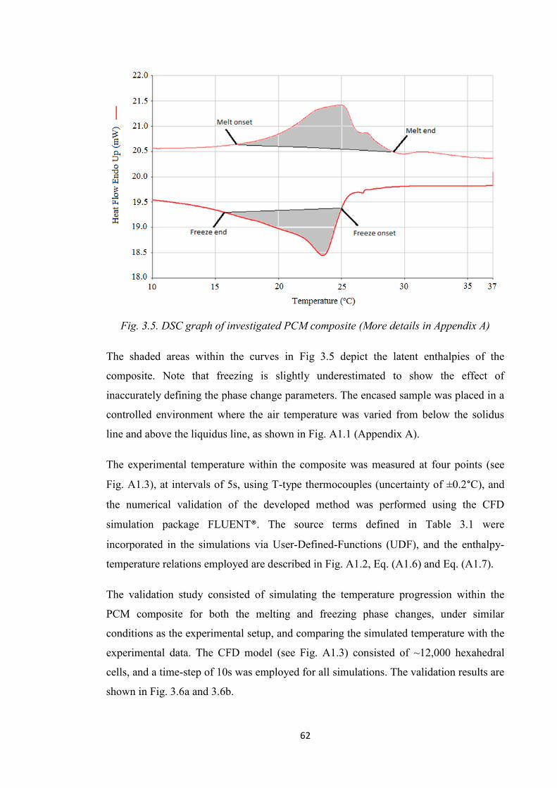
62

Fig. 3.5. DSC graph of investigated PCM composite (More details in Appendix A)

The shaded areas within the curves in Fig 3.5 depict the latent enthalpies of the

composite. Note that freezing is slightly underestimated to show the effect of

inaccurately defining the phase change parameters. The encased sample was placed in a

controlled environment where the air temperature was varied from below the solidus

line and above the liquidus line, as shown in Fig. A1.1 (Appendix A).

The experimental temperature within the composite was measured at four points (see

Fig. A1.3), at intervals of 5s, using T-type thermocouples (uncertainty of ±0.2°C), and

the numerical validation of the developed method was performed using the CFD

simulation package FLUENT®. The source terms defined in Table 3.1 were

incorporated in the simulations via User-Defined-Functions (UDF), and the enthalpy-

temperature relations employed are described in Fig. A1.2, Eq. (A1.6) and Eq. (A1.7).

The validation study consisted of simulating the temperature progression within the

PCM composite for both the melting and freezing phase changes, under similar

conditions as the experimental setup, and comparing the simulated temperature with the

experimental data. The CFD model (see Fig. A1.3) consisted of ~12,000 hexahedral

cells, and a time-step of 10s was employed for all simulations. The validation results are

shown in Fig. 3.6a and 3.6b.

63

Fig. 3.6(a). Experimental, UDF and Enthalpy-porosity temperatures

of a representative point during the melting process

Fig. 3.6(b). Experimental, UDF and Enthalpy-porosity temperatures

of a representative point during the freezing process

(The details of the simulations are given in Appendix A)

Fig. 3.6 shows that the User Defined Function (UDF) models more accurately predict

the temperature trends in both the melting and freezing cases than the enthalpy-porosity

model. In the melting case, the UDF model produces a more gradual change in the

temperature trend due to the smoothness in the enthalpy-temperature relationship

described in Fig. A1.2a, compared to the enthalpy porosity method which assumes the

64

linear relationship. Overall, for the melting case, the UDF model produced a Root Mean

Square (RMS) error of 1.3% (0.36K), whilst the enthalpy-porosity model produced a

higher RMS error of 12.3% (3.5K), calculated using Eq. (A1.8) and Eq. (A1.9).

In the freezing case, Fig. 3.6b shows that the experimental approximation of the

enthalpy-temperature curve in Fig. A1.2b and Eq. (A1.7) is not accurate enough to

predict the exact temperature trend in the composite material. This is due to the

deliberate slightly inaccurate freezing onset and end temperatures, and curvatures

employed in the simulations. The results showed that for the freezing case, employing

the UDF model produces an RMS error of 0.5% (0.2K), while the default enthalpy-

porosity model produces a higher error of 6.3% (2.6K).

In general, it was found that employing the UDF model, which accounts for the

enthalpy-temperature curvature and hysteresis in the PCM during phase change is more

accurate than the default enthalpy-porosity method employed in FLUENT®.

Furthermore, the validation study showed that the predicted temperature trends are

dependent on the thermal properties of phase change, but also on the curvatures

assigned to the SE equations. For instance in the freezing case, because of the higher

gradient in the f(T)f curve (see Fig. A1.2b) at the freezing onset, relative to the DSC

curve, the temperature trend is different at the start of freezing. These effects are

particularly important when simulating the cyclic operation (charge/discharge) of PCM

systems.

65


This chapter provides an understanding of the numerical modelling of phase change

processes. The enthalpy-porosity method and the effective-heat capacity method are

described, and their limitations in terms of the linear evaluation of the liquid fraction are

emphasised. For the case of phase change processes where thermal conduction is

dominant, such as in PCM boards, an enhanced method of simulation is presented. This

method employs User Defined Functions (UDF) obtained from experimental phase

change characterisation techniques to mimic the enthalpy-temperature relationships of

the PCM during phase change. The overall simulation errors were reduced when

employing the enhanced method, due to the more accurate representation of phase

change.

This method is fully documented in Gowreesunker et al. (2012), and more details are

given in Appendix A. The following chapter describes the numerical procedure used to

account for air-movement in indoor spaces, and depicts the application and validation of

the enhanced conduction-dominant phase change model described in this chapter, in a

CFD environment.

66

CHAPTER 4 – MODELLING OF INDOOR THERMAL

ENVIRONMENT AND PCM

4.1 Introduction to Computational Fluid Dynamics (CFD)

Indoor thermal environments can be simulated with zonal, multi-zonal or

Computational Fluid Dynamics (CFD) models. Zonal or multi-zonal modelling refers to

the situation where the properties of a macroscopic volume of air are concentrated at

one node in the investigated zone. It assumes that the volume of air for this node is fully

mixed, and the properties are uniform throughout the zone. For large and open spaces,

such as Airport Terminals, the International Energy Agency (IEA) recommends the use

of CFD because of the importance of air-flow within the building (Heiselberg et al,

1998). CFD is a finite volume method that solves the discretised form of the governing

Navier-Stokes equations in order to produce solution fields describing the fluid motion,

heat transfer and/or chemical reactions in a particular domain.

Fig. 4.1. Schematic of CFD solution process

Post-processor - Generation of variable contours / vectors - Export of numeric solutions

Model Generator - Geometry modeller - Grid generator - Identification of Boundary conditions

CFD Solver - Grid importation - Set-up of CFD models - Description of materials and fluids - Set-up of Boundary conditions - Set-up of Solution methods - Solution generation

67

The general set-up for a CFD simulation consists of a model generator, a CFD solver

and a post-processor, schematically represented in Fig 4.1. In this study, ANSYS

FLUENT® is used as the CFD solver. The aims of using CFD are to obtain a localised

solution of the variables (pressure, temperature, density and velocities) and to obtain an

adequate visualisation of the variable fields in the solution domain, otherwise not

possible in zonal models. The potential of CFD extends into many disciplines, and has

been employed in research studies, ranging from oxygen generation (Matsui et al,

2004), thermal comfort in buildings (Tye-Gingras and Gosselin, 2012) and atmospheric

simulations (Gousseau et al, 2011).

The level of precision possible from CFD varies depending on the level of grid and

model refinement, whereby increasing the level of details increases the computing costs.

For instance, the number of grid cells required to calculate the smallest eddies in a

turbulent flow with Re in the order of 104, would be of the order of 10

8 cells and would

require a supercomputer (Stribling, 2000). Generally, for engineering problems, it is

more important to obtain a solution where the general numerical solution accuracy is

within the real-life uncertainties of the adequate sensors (Gowreesunker et al, 2013a), as

opposed to having a solution with very small-scale details. This allows for a quicker and

more efficient use of the CFD tool for engineering purposes.

68

4.1.1 Governing Equations

The main variables involved in the governing equations are pressure (P), temperature

(T), density (ρ) and velocities (u, v, w), and therefore six equations are required to

describe a particular flow problem. These equations are known as the Navier-Stokes set

of equations (Eqs. 4.1-4.3) and the equation of state (Eq. 4.4). The Navier-Stokes

equations are non-linear, coupled and partial differential equations which represent the

physical laws governing the motion of fluids. They are difficult to solve using

conventional mathematical methods, and are therefore discretised, linearised, and solved

in a CFD solver through iterative methods. Convergence of a solution is obtained after

the residuals between successive iterations are within the limits defined in the solver.

Momentum equation:

(4.1)

Continuity equation:

(4.2)

Energy equation:

(4.3)

Equation of state:

(4.4)

Discretisation refers to the process of breaking down the terms of the governing

equations into simpler discrete algebraic forms. It can also refer to the breaking down of

the flow domain into separate control volumes, i.e. meshes, as shown in Fig. 4.2, which

allows the production of localised solution fields for a particular domain.

69

Fig. 4.2. Grid discretisation schematic

In Fig. 4.2, the cell centre values are noted by block letters (P, E, N, W, S), while the

face values are denoted by the small-case letters (e, n, w, s). The approximate form of

the governing equations is applied to each control volume and the face values are

required to obtain a solution.

The following shows a simple example of the discretisation for the diffusion term in the

governing energy equation (Eq. 4.3) with respect to the y-direction for the control

volume in Fig 4.2 (Beausoleil-Morrison, 2000).

(4.5)

Eq. (4.3) is given in terms of the face values. However, CFD stores cell-centre values as

opposed to face values. Thus, in order to appropriately use the governing equations, the

face values have to be computed from the cell centre values (ANSYS FLUENT theory

guide, 2010). This is accomplished by a linearisation process, which simplifies the

governing equation terms into linear algebraic terms through various gradient

computation schemes. For instance, the least-square cell based gradient assumes a linear

variation of the surrounding cell variables with respect to the control volume (P), as

shown by Eq. (4.6).

(4.6a)

70

(4.6b)

Applying the results from Eq. (4.6) to Eq. (4.5), we obtain the following Eq. (4.7):

(4.7)

The general form of the discretised equation is given as Eq. (4.8) (Fluent theory guide,

2010):

(4.8)

Where ‘nc’ represents the neighbouring cell, ‘a’ are linearised coefficients and ‘φ’ is the

scalar quantity at the cell centre. The processes of discretisation and linearisation can

both be commonly referred to as ‘discretisation’, and will henceforth be implied in this

manner for this study. Thus, this discretised form of the governing equations is

employed in the CFD solver to generate solution fields for a specified problem.

71

4.1.2 Turbulence Modelling

Air-flows inside built environments consist of different flow regimes ranging from low-

Reynolds flows (wall boundary layers) to more turbulent flows (near HVAC

inlets/outlets) (Heiselberg et al, 1998). The adequate modelling of turbulence is

therefore one of the most important aspects in appropriately defining the velocities and

stresses involved in the flow, and thus the actual building air movement itself.

Turbulence is a complex phenomenon, referring to small scale random variations in

fluid motion, for which the direct simulation is not possible under the current level of

technology (ANSYS FLUENT theory guide, 2010). Its modelling is instead conducted

with the Reynolds-Averaged Navier-Stokes (RANS) or the Large Eddy Simulation

(LES) methods, through a filter which limits the size of turbulence in the flow domain.

In the case of LES, eddies larger than the size of the filter are explicitly resolved to

improve accuracy, at the expense of large computational costs. The RANS models

separate the solution variables into mean (time-averaged) and fluctuating components as

shown in Fig. 4.3 and Eq. (4.9). Both the RANS and LES models introduce additional

unknowns in the approximate form of the governing equations, which must be solved to

close the overall system of equations (Fluent theory guide, 2010).

The following sections focus on the RANS turbulence models, which are more

commonly employed because of the relatively lower computational effort required.

Fig 4.3. Velocity fluctuations

(4.9)

The velocities at a point in time and space are defined by , with a time-averaged value

of and fluctuation of , as defined by Eq. (4.9). This averaging process introduces

some new unknowns – known as the Reynolds stresses – into the governing equations

(ANSYS FLUENT theory guide, 2010) – Reynolds Stresses: .

72

These stresses represent the rate at which momentum is transported or diffused by

turbulent fluctuations, and they have to be solved in order to satisfy ‘closure’ of the

system of equations. The Reynolds stresses can be evaluated by two methods: the Eddy

viscosity models or the Reynolds Stress Models (RSM). The Eddy-viscosity models

relate the Reynolds stresses to the mean velocity gradient and produce a relatively low

computationally expensive process. Examples of the Eddy-viscosity models are the

Spalart-Allmaras model, the k-ε models and the k-ω models. The alternative Reynolds

Stress Model aims at solving the differential transport equations for each term in the

Reynolds stresses, considerably increasing the solution complexity and computational

time (ANSYS FLUENT theory guide, 2010).

Various studies have employed CFD to simulate the air-flows in built environments,

and because of the different flow regimes encountered in buildings, the choice of a

turbulence model is crucial, as elaborated by the following studies. Zhang et al. (2007)

evaluated eight turbulence models, including the Re-Normalisation Group (RNG) k-ε,

the low-Reynolds number k-ε and the Shear-Stress Transport (SST) k-ω models, in the

prediction of air-flow, temperature and turbulence in four indoor geometries, under

forced, natural and mixed forced/natural convection. They found that in general, LES

provides the most detailed flow features, but considerably increases the computational

time relative to the RANS models. Among the RANS models, the V2-f and the RNG k-ε

models have the best accuracy, computing effort and robustness. The authors stress that

each airflow category favours a particular turbulence model, but recommend the V2-f

and the RNG k-ε models for indoor airflow simulations.

Gebremedhin and Wu (2003) studied the airflow characteristics of a ventilated cattle

facility to evaluate the thermal interaction between the cattle and the indoor

environment. The standard k-ε model, the RNG k-ε model, the Low-Reynolds number

k-ε model, the k-ω model and the Reynolds stress model (RSM) were employed in the

CFD simulations. The authors concluded that the RNG k-ε model provided the most

accurate, stable and computationally efficient solution.

Rohdin and Moshfegh (2007) compared the standard k-ε, RNG k-ε and realizable k-ε

models for the temperature and air-flow simulation in a mechanically ventilated large

and complex industrial facility. The comparison was relative to field measurements.

They found that the RNG k-ε turbulence model produced the lowest validation errors in

73

the simulation, with deviations of 0.04 m/s and 0.3 °C from the experimental results, at

the expense of slightly higher computational time than the other models.

Hara and Kato (2004) validated a CFD simulation for the movement of smoke in a fire

using the standard k-ε model. Deviations of 5% were obtained for both the velocity and

temperature fields in the simulations, with respect to experimental correlations. They

showed that modifying the buoyancy production term of the turbulence dissipation (ε)

equation does not significantly affect the results, but an appropriate grid near the heat

source is crucial for the accurate representation of the thermal plume.

Leenknegt et al. (2012) conducted a sensitivity analysis for the convective heat

exchange between the room air and the envelope thermal mass. The standard, realizable

and RNG k-ε models, and the standard and SST k-ω models were studied in their

analysis. The authors showed that similar results are obtained for the standard and RNG

k-ε models, as well as the standard and SST k-ω models, respectively. The RNG k-ε

model was adopted for the final model, based on the results of their literature survey.

Hussain et al. (2012) investigated six RANS models, including the one-equation model

(Spallart–Allamaras), together with the Discrete Transfer Radiation Model (DTRM) in

the natural and forced ventilation simulation of atria. In comparison with experimental

results, they concluded that the two equation models (the standard k-ε, RNG k-ε,

realizable k-ε, standard k-ω and SST k-ω models) provided better results compared to

the one-equation model, and that SST k-ω model showed relatively better prediction

than the other models.

Awbi (1998) investigated the natural convection heat transfer coefficients for walls,

ceiling and floor of a building space, using the standard k-ε model with logarithmic wall

function and the low-Reynolds number k-ε model. The author found that the standard k-

ε model does not generally predict accurate heat transfer, whilst the low-Reynolds

number k-ε model performs much better. The low-Reynolds turbulence model however

requires fine grid points which increases computational time. The author suggests

finding the convective heat transfer coefficients from empirical equations, and applying

them directly to the simulation, instead of calculating them for every iteration.

Kuznik et al. (2007) conducted a steady-state validation study of a mechanically

ventilated test cell, using the realizable k-ε, RNG k-ε, standard k-ω and SST k-ω

74

turbulence models. They found that only the realizable k-ε and the k-ω models provided

appropriate numerical results, of which the k-ω model was in better agreement with the

experimental temperature progression. Furthermore, the realizable k-ε and the k-ω

models also appropriately predicted the jet expansion rate of the inlet fan, whilst none of

the models properly predicted the jet profiles.

Tanasic et al. (2011) investigated the airflow in a mechanically ventilated large

industrial hall, including buoyancy, using the standard k-ε model for turbulence. They

concluded that the model did not provide adequate quantitative results as the simulation

values differed significantly from the measured values.

Suarez et al. (2011) investigated the forced/buoyant airflow in a glazed gallery using the

RNG k-ε, standard k-ε and the k-ω models. They concluded that there were no major

air-flow differences between the models, and on the basis of stability and simulation

time, the RNG k-ε model was employed in their final simulations.

Gowreesunker and Tassou (2013a) investigated the performance of PCM boards in a

test cell using the RNG k-ε model. The model’s air and surface temperatures were

compared to experimental data, and were found to have a mean error of 1.0 °C for a

total of 23 thermocouples. Local absolute errors in the air temperature values varied

between 0.6-1.5 °C, including the uncertainty in the thermocouples. The models were

considered to be accurate enough based on the relative errors obtained in the study.

Zhai et al. (2007) studied turbulence models for enclosed indoor environments. They

identified that each turbulence model has its advantages and limitations under different

situations, and that no universal turbulence model exists for indoor airflow simulations.

75

This literature survey shows that the most popular and accurate RANS models are the

RNG k-ε and the SST k-ω turbulence models, although each model may provide

relatively different results in some cases. Generally, the RNG k-ε turbulence model was

found to be equally valid for both low and strong turbulence flows, due to various

improvements from the standard model, resulting in a better modelling of separating

and near-wall flows (Leenknegt et al, 2012). Thus, even though there is not a universal

turbulence model, there is a general consensus from the literature that the RNG k-ε

model produces adequate flow fields for simulations involving buoyant, forced or

forced/buoyant flows in buildings, under reasonable simulation times (Gowreesunker

and Tassou, 2013a; Chen, 1995; Zhang et al, 2007).

76

4.1.3 Renormalisation Group (RNG) k-ε Turbulence Model

This section describes the RNG k-ε turbulence model which is employed in this study.

Following the Boussinesq approach for the k-ε turbulence models, two additional sets of

equations are to be solved: one for the turbulent kinetic energy (k); and one for the

dissipation rate of kinetic energy (ε) (Launder and Spalding, 1972), which are then used

to obtain the turbulent/eddy viscosity (μt) of the flow, as shown by Eq. (4.10).

(4.10a)

(4.10b)

(4.10c)

The coefficients C1ε, C2ε, C3ε and Cμ are empirical constants; σk and σε are the inverse

effective Prandtl numbers for the turbulent kinetic energy and dissipation rate,

respectively; Gb is the turbulent kinetic energy generation due to buoyancy; Gk is the

kinetic energy generation due to the mean velocity gradients; and μt is the eddy

viscosity. The default values for the coefficients are 1.42, 1.68, 0.0, 0.0845, 0.7178 and

0.7178 for C1ε, C2ε, C3ε, Cμ, σk and σε, respectively (Rohdin and Moshfegh, 2007).

The RNG k-ε turbulence model has been developed following a statistical study known

as the renormalisation group theory. It filters out small scale turbulence to a degree that

the remaining scales can be resolved (Rohdin and Moshfegh, 2007). The turbulence

dissipation rate (ε) equation is modified as shown by Eq. (4.11a) and Rε is defined by

Eq. (4.11b).

(4.11a)

77

(4.11b)

The values of the additional constants in Eq. (4.11) are 0.012 and 4.38 for β0 and η0,

respectively. The RNG k-ε model enhances the standard model, through the use of an

analytically derived function to calculate the effective turbulent viscosity, separating

low Re-number flows from high Re-number flows. This allows a more accurate

representation of turbulence for different types of flows, instead of assuming high Re-

number flows for all types flows, as in the case of the standard model (ANSYS

FLUENT theory guide, 2010).

78

4.1.4 Near-Wall Treatment

Wall functions are empirical relationships that are used to simplify the prediction of

flows within the boundary layer at the near wall grid cells. Instead of attempting to

resolve the different flow regimes within the boundary layer through the use of many

grid cells, wall functions allow a relaxation of the grid size near the wall by permitting

the near wall grid points to be relatively further from the wall.

The standard wall functions simplify the near wall flows into two distinct regions:

laminar dominated flow and the log-law region, requiring different empirical

relationships. These two regions are separated based on the dimensionless distance from

the wall (y+).

(4.12)

Where:

(4.13)

By appropriately placing grid points in the respective regions of the boundary layers,

the near-wall model employ different methods to obtain an equilibrium solution. For

cases where (y+>11.225), the standard wall model employs the logarithmic law:

(4.14)

For cases where (y+<11.225), the following laminar stress-strain relationship is

employed:

(4.15)

ĸ is the Von Kármán constant (0.4187), E is an empirical constant (9.793), u is the mean

fluid velocity, τw is the wall shear stress and uτ is the friction velocity. Although, the

standard model represents an ideal approach to modelling the near-wall phenomena, it

has been found to work well with various wall-bounded flows (ANSYS FLUENT User

guide, 2010) and in some building simulations (Blocken and Carmeliet, 2007).

Nonetheless, FLUENT also offers various other near-wall treatments, including the

enhanced-wall treatment which is more suited to different flow regimes, as explained in

the ANSYS FLUENT theory and user guides (2010).

79

4.2 Modelling of Indoor Environment and PCM boards

In this study, in order to further validate the use of CFD in the simulation of indoor

thermal environments, its effectiveness was extended to the simulation of PCM boards

within the built environment. Hence, the next section depicts the experimental

validation and usefulness of CFD when employed in the performance evaluation of

PCM boards applied to a test-cell’s walls.

PCM boards are becoming a popular passive method for controlling the indoor

temperature, as confirmed by the number of commercial products available on the

market. They are being currently marketed as an energy-efficient alternative to gypsum

plasterboards, with the PCM preventing overheating and reducing the temperature

swings in thermally lightweight buildings. Conventionally, commercial simulation tools

such as ESP-r (Heim and Clarke, 2003) and TRNSYS (Bony and Citherlet, 2007),

amongst others, possess phase change modelling capabilities. However, in addition to

not allowing for detailed air-flow analyses, the percentage of PCM being used cannot be

determined with these default multi-zonal models. Thus, in order to appropriately

evaluate the performance of PCM boards and the indoor environment air-flow, both

aspects should be simultaneously simulated in a CFD environment. The validation of

such simulations has not been previously reported in the literature.

To accomplish this validation study, the test cell shown in Fig. 4.4 was constructed with

internal dimensions of 1.3×0.8×1.4m and a glazed area of 1.3×0.8m. This test cell was

then placed inside an environmental chamber where the air temperature was controlled.

In essence, the test cell represents a built environment whilst the environmental

chamber provides the ambient conditions. The material configuration of the walls

provided an overall U-value of 0.21 W/m2K, a decrement factor of 0.81 and a time lag

of 4.8h, which is similar to a timber frame wall with plasterboard (CIBSE A, 2006). The

glazing U-value is 1.2 W/m2K.

(Refer to Appendix B for more construction and experimental details)

80

Fig. 4.4a. Experimental test cell and wall construction

Twenty three type-T thermocouples were uniformly distributed inside the test cell and

on the walls (see Fig B1.2). The air sensors were placed 5cm from the wall and the

surface sensors were covered with a thin layer of plaster. The test cell was assumed to

be intermittently occupied and a 200×100 mm, 100 W mica plate heater was employed

to produce the internal heat gains during the day-time occupied hours. During night-

time, the heater was turned off.

Day-time was defined as the hours where the external ambient temperature increases,

and vice-versa for night-time, as shown in Fig. 4.5. Two sets of experiments were

performed: a non-ventilated case where the inlet and outlet were closed during night-

time; and a ventilated case, where external air was blown into the test cell during night-

time at a rate of 0.045 kg/s via the 100 mm diameter inlet shown in Fig. B1.2. The air

velocity was measured with a TSI hot-wire velocity meter with an accuracy of ±0.015

m/s. The two different ventilation scenarios were investigated in order to show the

importance of night charging on the performance of the PCM boards. Before each

experiment was started, it was ensured that all temperatures in the test-cell were at the

same steady value, for the valid initialisation of the CFD models. Each experiment

recorded the temperatures at locations shown in Fig. 4.4b, at intervals of 30 s for 24 h

using Pico data loggers.

81

Fig. 4.4b. Locations of temperature sensors in experimental test cell

Fig. 4.5. Environmental chamber/ External air temperature

82

The PCM board investigated in this study is a commercial 13 mm clay board

impregnated with 21% (by volume) Micronal® PCM. These EBB™ PCM clay boards

are manufactured by mixing the PCM microcapsules and clay, before being compacted

and embedded in a polythene matrix. As a result, this does not always result in a

uniform distribution of the PCM granules in the board. Three random sample locations

were therefore chosen from the boards to conduct the DSC characterisation analysis,

shown in Table 4.1.

Table 4.1. PCM DSC enthalpy, onset and end temperatures for

different PCM-Clay board samples and heating/cooling rates

Heating

/

cooling

Rate

Melting Freezing

Onset

Temperature

(K)

End

Temperature

(K)

Enthalpy

(kJ/kg)

Onset

Temperature

(K)

End

Temperature

(K)

Enthalpy

(kJ/kg)

1st Sample (S-1)

0.5

K/min 285.4 295.5 14.7 295.4 284.4 17.0

1 K/min 285.3 295.5 14.8 295.3 284.2 17.1

2 K/min 284.9 296.0 15.6 294.8 283.8 17.7

2nd

Sample (S-2)

0.5

K/min 284.9 296.1 16.3 294.9 284.9 17.9

1 K/min 284.8 295.9 16.3 294.9 284.8 18.0

2 K/min 284.1 296.4 17.0 293.8 283.8 18.8

3rd

Sample (S-3)

0.5

K/min 285.2 295.8 15.6 295.2 284.7 17.4

1 K/min 285.1 295.9 15.7 295.1 284.6 17.5

2 K/min 284.5 296.3 16.1 294.6 283.8 18.5

Enthalpy Porosity Model

- 284.9 295.5 16.5 295.5 284.9 16.5

Table 4.1 shows that as the heating/cooling rates of each sample are lowered, the

melting/freezing enthalpy and phase change temperatures tend towards a constant value.

The lowest investigated heating/cooling rate of 0.5 K/min provides values which are

within the uncertainty of ±0.1 K and ±2% of the enthalpy change for the DSC, and are

therefore considered for further analysis. Between the 3 samples at 0.5 K/min, a mean

melting enthalpy of 15.6 kJ/kg and mean freezing enthalpy of 17.4 kJ/kg are obtained,

with a deviation of ±0.9 kJ/kg between samples. A mean melting onset temperature of

83

285.2 K, and end temperature of 295.8 K are obtained, while a mean freezing onset

temperature of 295.2 K and end temperature of 284.7 K are obtained. The deviation in

temperature between the 3 samples is ±0.6 K. The enthalpy–porosity model is defined

as the average values of the onset and end temperatures, and enthalpy of all the samples

at 0.5 K/min for both freezing and melting.

4.3 Validity of CFD

The validation study was conducted in ANSYS FLUENT® where all the domains of the

test-cell were modelled. The final mesh was obtained following an L2 norm study to test

for the spatial and temporal convergence of the model (see Appendix B), and is shown

in Fig. 4.6. The external surfaces of the test-cell are bounded by convective heat transfer

conditions, which were determined by a separate CFD investigation, modelling the

external surface of the test-cell and the environmental chamber. This resulted in values

of 5.3 W/m2 K for the bottom and right surfaces, 2.8 W/m

2 K for the glazing, left and

top surfaces, and 2.4 W/m2 K for the back surface, with reference to Fig. B1.2. A heat

generation rate of 500,000 W/m3 is applied to model the 10 mm thick plate heater. The

mass-flow inlet and pressure outlet are closed during the day-time heating period. The

RNG k–ɛ turbulence model, with non-slip enhanced wall functions were used and air

was considered as an ideal gas. The body-force weighted discretisation scheme was

employed for pressure, and the second order upwind scheme was used for momentum,

density and energy. The SIMPLE algorithm was used for the pressure–velocity

coupling.

Fig. 4.6(a). Mesh in main air-domain Fig. 4.6(b). Mesh distribution in walls

and air boundary layer

84

The mesh was designed using the in-built ANSYS design modeller meshing algorithm,

and the resulting mesh comprised of hexahedral cells in the near-wall inflated layers and

wall domains, with tetrahedral and hexahedral cells in the air domain. Eight inflation

layers were used near the walls, with a first grid size of 2 mm and growth ratio of 1.3.

The mesh size increases towards the bulk of the air domain to 40 mm. The wall-solid

domains contain 3–4 mesh intervals along the thickness, with a face cell size of 20–

50 mm. The inlet and outlet domains contain four inflation layers with a first grid size

of 1.5 mm, growth ratio of 1.2 and an average of 10 mm cells in the main fluid flow.

The mesh at the heater has a face size of 10 mm and 8 inflation layers with a first grid

size of 1.5 mm and growth ratio of 1.1. The enhanced phase change model described in

chapter 3 is employed to simulate the boards (the equations for the S-3 enthalpy-

temperature curves are given by Eq. (B1.2) and Eq. (B1.3) in Appendix B).

The validation errors from the simulations are shown in Fig. 4.7 and Fig. 4.8. The

validity of the models was based on the relative RMS errors of each model with respect

to the experimental data. (Refer to Appendix B for details of the error calculations)

Fig. 4.7. Local error analysis for non-ventilated scenario

85

Fig. 4.8. Local error analysis for ventilated scenario

In the non-ventilated case (see Fig 4.7), the absolute errors vary between 0.7-1.5 K and

0.8-2.1 K, corresponding to relative errors of 7.3-20.8% and 8.5-27 %, for the air and

surface temperatures, respectively. The higher errors for surface temperatures can be

attributed to the uneven distribution of PCM in the boards. Overall mean errors of

11.92% (1.07 K), 11.73% (1.02 K) and 10.8% (0.96 K) are obtained for sample-1 (S-1),

sample-2 (S-2) and sample-3 (S-3), respectively. It can also be seen from Fig. 4.7 that

the enthalpy-porosity model produces higher errors of 11-27% with a mean of 18.5%

(1.5 K), than the UDF models that incorporates the hysteresis and non-linearity effects

in the PCM simulation.

For the ventilated case (see Fig 4.8), the local absolute error varies between 0.7-1.5 K

and 0.8-2.0 K, corresponding to relative errors of 5.4-13.4% and 6.0-19.6 % for the air

and surface temperatures, respectively. Similarly in this case, the higher surface errors

can be attributed to the uneven distribution of PCM in the boards. The overall mean

errors are found to be 9.25% (1.03 K), 8.8% (0.97 K) and 8.06% (0.91 K) for S-1, S-2

and S-3, respectively, while the mean error for the enthalpy porosity model is again

higher, at 12.5% (1.3 K), than the curved-fit models. As the relative errors in both

scenarios are lower than 30%, using a similar justification as proposed in the works of

86

Zhang et al. (2007), the validation of the CFD modelling study is considered acceptable

(Gowreesunker and Tassou, 2013a).

It is interesting to note that the choice of PCM sample does not impact heavily the

overall errors when the UDF models are used. However, a mean improvement of 0.5 K

is obtained with the implementation of the S-3 model relative to the enthalpy–porosity

model. Depending on the type of building, with different comfort temperature ranges,

the importance of appropriately simulating phase change will become higher as the

building temperature range becomes smaller. These errors should therefore be carefully

considered when applying CFD to the thermal evaluation of built environments with

PCM. In this validation study, the main errors can be attributed to: the uncertainty in the

thermocouples (see Fig. B1.2); the uncertainty in the curve-fits for the external air

temperature, PCM enthalpy and temperature data (see Table B1.3); the non-uniformity

in PCM distribution; the uncertainty in the ventilation flow rate; and the non-

consideration of radiation.

87

4.4 Effectiveness of CFD

As mentioned previously, passive PCM systems rely on cool night ventilation for

adequate charging. This section describes the effectiveness of CFD to predict the

performance of PCM boards for the more popular ventilated case, in terms of: the

impact of the PCM boards in the test-cell, the heat transfer rates with different night

ventilation rates, and the effective use of PCM boards. The results are for the PCM

sample S-3 which produced the lowest errors in the validation study.

4.4.1 Impact of PCM boards

The test cell was closed during the heating period, and thus buoyancy due to the heater

is the dominant force in the indoor air flow, as shown in the temperature contours of Fig

4.9. The experimental study from Hunt et al. (2001) suggests that an aspect ratio

(height/width) <1 causes stable stratification, as the propensity for turbulent mixing and

overturning at the top of the air domain is lower. In this study, the aspect ratios of the

test cell were 1.08 and 1.75. The qualitative results from Fig. 4.9 therefore abide by the

empirical observations made by Hunt et al. (2001), as although the aspect ratios of the

cell are slightly higher than 1, they are not high enough to completely destroy

stratification. Thus, both stratification and a slight overturning near the walls are

observed in this simulation.

88

Fig. 4.9. Comparison of Temperature evolutions at 3 points in the test cell, and

Temperature contours (K) at the end of the heating period with PCM-Clay board

and Plasterboard on the walls

It can also be observed from Fig 4.9 that a reduction of 3 K in the peak air temperature

and a lower temperature swing are obtained with the addition of the PCM-Clay board,

relative to plasterboard. Vertical temperature stratification in the air domain of the PCM

cell is ~3 K/m compared to ~4 K/m in the plasterboard cell, and stratification in the

PCM cell is more uniform compared to the plasterboard cell. A more uniform and less

stratified environment in the occupied zone provides better thermal comfort (Chao and

89

Wan, 2004). Furthermore, the determination of the velocity, temperature and turbulence

fields from the CFD results may improve the evaluation of local thermal comfort

(ANSI/ASHRAE 55-2004), which is otherwise not available for zonal models.

4.4.2 Ventilation heat transfer rates

While conduction is the dominant heat transfer mechanism within the boards,

convection occurs between the boards and the air domain (natural convection during the

heating/occupied period and forced convection during the night ventilation period). Fig.

4.10 shows the area-weighted heat flux on the internal side of the test cell walls, which

aims at determining the energy impact of PCM-clay boards and plasterboards during the

day, and the effects of different ventilation rates on the PCM boards during night

ventilation charging.

Fig. 4.10. Area-weighted wall heat flux with PCM and plaster boards, and with

different night ventilation rates for PCM boards only (The calculation method for ‘hc’ is

given in Appendix B)

Fig. 4.10 shows that in the heating phase, the heat flux to the PCM wall is higher than

the plasterboard wall, due to the lower wall temperatures of the PCM board during

phase change. The average increase in wall heat flux into the walls of 5W/m2 with the

90

addition of the PCM-board signifies that the building envelope is providing an extra

5W/m2 of cooling, compared to plasterboard. This corresponds to an extra cooling effect

of 25W for this test cell, compared to plasterboards, with an internal heat gain of 100W

and without air-conditioning systems. Fig. 4.10 also depicts the impact of night

ventilation on the PCM boards. As the wall heat transfer coefficient, hc, increases with

increasing ventilation rates, the heat flux out of the walls also increases. This

corresponds to a faster re-charge of the PCM boards, improving their efficiency. By

employing heat transfer coefficients of 5.07, 2.83, 0.91 and 0.28 W/m2K, the PCM

boards are fully recharged after 9, 11, 17 and 23 hrs, respectively (Note that the last two

charging times have been linearly extrapolated).

In this study, as the externally blown air is just below the freezing end temperature of

the PCM, can be used to justify full-recharge of the boards. In other cases,

monitoring the liquid fraction may be more appropriate. The relatively low reduction in

charging times as hc increases from 2.83 to 5.07 W/m2K is explained by the fact that as

hc increases, the low thermal diffusivity of the PCM board becomes more dominant and

limits the heat transfer rates in the boards. In this case, a wall heat transfer coefficient

greater than 2.83 W/m2K (46 ACH) would be adequate, as it would completely recharge

the PCM boards before the end of the simulation period.

91

4.4.3 Effective use of PCM boards

In order to extract the full potential of PCM boards, they have to be suitably placed

within the building, and the liquid fraction is a useful parameter to quantify their

effective use.

Fig. 4.11. Liquid fraction change for different ventilation rates

The qualitative observations from Fig. 4.11 infer that the top part of the test-cell

undergoes full phase change after the heating period. The liquid fraction in the lower

portion of the cell is 0.8-0.9, signifying that only 80-90% of the PCM has been used in

the cooling process. This is due to temperature stratification in the space. In order to

optimise the boards’ performance, air mixing strategies can be considered for the space

or the PCM could be concentrated at the top part of the wall and ceiling of the cell.

Fig. 4.11 also shows the re-charging effects of different ventilation rates at the end of

the simulations. Using 46 ACH reduces the overall liquid fraction to 0, and hence

completely recharges the PCM boards. Conversely, using 12ACH recharges the PCM to

30-50% for the same time period. For this latter ventilation rate, the wall temperatures

92

near the outlet are affected by the airflow, as shown by an area of higher liquid fraction

in Fig. 4.11.

Fig. 4.12. Velocity streams for ventilation rates of 12 ACH and 46 ACH

Fig. 4.12 shows that the air movement at this area near the outlet is low at 12ACH

compared to the mixing propensity of 46ACH, and hence the low heat transfer from the

wall. The ventilation rate can therefore be increased or an air inlet with swirl diffusers

can be used to generate mixing in the space at 12 ACH, and further reduce the liquid

fraction in the recharging process.

93


This chapter describes the use of CFD in the simulation of indoor environments and

also validates the application of the enhanced conduction-dominant phase change model

developed in chapter 3. The experimental tests used for the validation study were

conducted in a test cell, placed inside an environmental chamber, where the ambient

conditions of the test cell were controlled and monitored. In general, the results showed

that:

the PCM clay wall boards can provide up to 3 K reduction in the peak

temperature of indoor spaces compared to conventional plasterboard, and can

prevent overheating. The performance depends on the quantity of PCM used, the

characteristics of the building fabric and the internal and external heat gains.

the performance of the CFD simulations depends to a certain extent on the

approach used for the simulation of the PCM in the board. Using the enhanced

phase change model improves the simulation accuracy compared to the standard

enthalpy–porosity by a mean 0.5 K.

the average absolute error in the simulations compared to the experimental

results was found to be 1.0 K, including the uncertainties of the thermocouples.

These errors are acceptable judged by other studies and uncertainties in the

measurements.

the qualitative results show that the temperature stratification effects can be

adequately predicted with CFD models and together with the liquid fraction

term, can enable more efficient building design using PCM boards for both

natural and forced convection scenarios.

due to the extensive simulation times required, CFD can mainly be used as a

design tool to determine areas of concern and to investigate improvements in the

design with PCM boards over a short period of time. A number of discrete time

dependent simulations, however, can be used with different weather data to gain

an understanding of the influence of the variation in external conditions on the

thermal response of indoor spaces equipped with PCM boards.

94

Furthermore, this chapter shows that the RNG k-ε turbulence model can be successfully

used in the air-flow modelling within built environments, as suggested by past

literature, and demonstrates the higher potential of CFD for detailed analysis, relative to

zonal or multi-zonal models. This research is further documented in Gowreesunker et

al. (2013a)

The next chapter extends the application of PCM modelling further, to large glazed

buildings, with relatively low thermal mass. It addresses the performance of PCM-

glazed units, and provides various relationships that can be employed in the numerical

modelling of such systems.

95

CHAPTER 5 – OPTICAL MODELLING OF PCM

The low thermal mass or capacitance of building envelopes is progressively becoming a

growing issue due to the increasing trend of designing buildings with maximum

exposure to the outdoor environment (Bostick, 2009), such as for airport terminal

buildings. One approach to increasing the thermal mass of low thermal mass buildings

is to incorporate PCM in the glazing structure (Goia et al, 2012).

Weinläder et al. (2005) investigated the optical properties of RT25®, S27® and L30®,

placed in transparent plastic containers behind a double glazed window. The optical

tests revealed that the PCMs have higher transmittance values in the liquid state than the

solid states. In the liquid phase, the PCMs are clear, transparent and non-scattering,

while the solid phase is translucent and scattering. Nonetheless, the colour of the

transmitted light is constant for all phases, making PCMs viable options for day-lighting

purposes. The authors also numerically showed that a PCM façade reduces the overall

heat gains by 25 % and provides a lower indoor temperature relative to conventional

double glazed units in a German summer condition, whilst it increases the insulating

effect during winter.

Regarding the optical modelling of the PCM, Weinläder et al. (2005) assumed identical

refractive indices for the solid and liquid phases, which varied with the radiation

wavelength; and found that the radiation scattering coefficient is a function of only the

PCM thickness. The numerical model employed in their study is unclear, and the

authors do not comment on the variation of the optical properties as the PCM changes

phase.

Ismail and Henriquez (2002) adopted a 1-D mathematical model to simulate the

behaviour of a PCM-glazed unit. The PCM was placed within the gap of a double

glazed unit, where it was assumed to have constant thermophysical properties, a single

phase change temperature and no convection in the liquid phase. The optical modelling

was relatively simple as the optical properties were considered constant during phase

change, and the scattering effects were neglected. Nonetheless, the authors claim that

the model was validated with experimental data.

96

Goia et al. (2012) also investigated the 1-D mathematical modelling of a PCM double

glazed unit. The thermophysical properties of the PCM were considered constant in all

phases, convection was ignored in the liquid phase and phase change was simulated

using the effective heat capacity method. The optical properties of the PCM were

constant in the fully liquid and solid phases, but varied with the temperature during

phase change. This variation in optical properties with temperature/ liquid-fraction was

an assumption from the authors. The PCM domain was segmented into different nodes,

each with lumped value parameters. The model showed good validity with respect to

experimental data, but the authors acknowledge the limitations associated with their

assumptions. They further suggest the need for a better and more reliable modelling of

short wave radiation within the PCM.

As seen in section 2.1.8 and as depicted by the previously referred literature, PCM

glazed units have received relatively less research attention compared to other PCM

systems. However more recently, new commercially available types of glazing such as

Delta Cool-28® or GlassX®, which incorporate PCMs, have been developed, which

indicates an increasing market interest for more thermally massive glazing. As a result,

the accurate modelling of radiation through PCMs is growing in importance, especially

with regards to the appropriate performance evaluation of PCM-glazed units.

One of the limiting aspects of PCM optical modelling encountered in the literature is the

inability of the models to fully simulate the radiation behaviour of PCMs during the

phase change process. Thus, in order to understand and improve the performance/

modelling of PCMs in glazed structures, knowledge of the optical properties (scattering

and absorption) during phase change is required. These properties are characterised as

follows.

5.1 Development of Optical Model

This model was largely developed from empirical data from a spectroscopy analysis and

an actual double glazed unit. It aims at defining the variation of the extinction

coefficient (i.e. sum of the scattering and absorption coefficients) of the PCM during

phase change. This model is published in Gowreesunker et al. (2013c).

97

The optical characterisation of the PCM was first performed with a spectrophotometer,

which measured the spectral radiation transmittance for different PCM phases, as shown

in Fig. 5.1. However, due to the inability to control and monitor the temperature within

the spectrophotometer, a specific spectrum could only be assigned to the fully solid and

liquid phases (under visual inspection), while the spectrum for the mushy region only

depicts the relative differences. The investigated PCM was RT27®.

Fig 5.1. Spectral transmittance of RT27 in solid, liquid and mushy phases (The

measurement uncertainty is ±2% for the liquid samples and ±10% for the solid samples)

(Gowreesunker et al, 2013c)

Using Fig. 5.1, it was estimated that the extinction coefficients for the solid and liquid

phases of RT27® were 30.1-52.3 m-1

and 3.6-5.5 m-1

, respectively, (using Eq. (C1.7))

for the visible range (350-850 nm) of the spectrum. Furthermore, it was also observed

that in the visible range, the transmittance / optical thickness is nearly independent of

the wavelength. This accounts for the unchanged colour in the transmitted light

(therefore, suitable for day-lighting), and also allows for gray modelling of PCM in the

visible range.

Due to the lack of temperature control in the spectrophotometer, the following

experimental setup was therefore devised in order to quantify the variation in the optical

properties during phase change (see Fig. 5.2).

98

Fig. 5.2(a). Schematic of Experimental setup Fig. 5.2(b). Actual setup in

Environmental chamber

The entire setup was placed inside an environmental chamber where the air temperature

was controlled. A Kipp & Zonen CMA-6® pyranometer was used to measure the

radiation heat flux (W/m2) transmitted through the glazed surface test specimens. A 150

W metal halide (Iodide discharge) lamp producing a diffuse light with a spectrum

ranging mainly from 350 nm to 850 nm was employed. The irradiation intensity was

varied by varying the distance between the glazing and the lamp. Three types of

surfaces were investigated: a standard double-glazed unit, a PCM-double glazed unit

(PCM within glazing) and ‘no-glazing’. The main objective was to measure the gray

radiation transmission for the different surfaces at different temperatures during phase

change, and using the procedure described in Appendix C to obtain the variation in

absorption, scattering and extinction coefficients of RT27®.

Fig. 5.3. Enthalpy-temperature curve of RT27(Gowreesunker et al, 2013c)

99

Fig. 5.4. Absorption (σa), scattering (σs) and extinction (σε) coefficients

during phase change

Fig. 5.3 shows that the latent heat capacities of RT27® were found to be 165 kJ/kg and

191 kJ/kg for the cooling and heating cycles, respectively, evaluated between 15 and

27.8 °C using the T-history method (Appendix C). Correspondingly, Fig. 5.4 shows the

variation in the absorption, scattering and extinction coefficients during the phase

change process of RT27 (Gowreesunker et al, 2013c). As anticipated from previous

studies (Weinläder et al. 2005 and Goia et al. 2012), the scattering coefficient is more

prominent in the solid phase, while absorption dominates in the liquid phase. Within the

mushy phase, the scattering effect is higher for the major part until a temperature 24.5

°C, after which, absorption dominates until phase change is complete.

The relationships developed are as follows:

σε = (β⋅σε,liq) + (1-β)⋅(σε,sol) (5.1)

(5.2)

(5.3)

Where:

(5.4)

δ defines the ratio between the absorption and scattering coefficients for the fully solid

phase of the PCM. Eqs. (5.1-5.4) describe the change in optical properties as a PCM

100

changes phase. They employ the liquid fraction term or temperature (as β= f (T)) to vary

the optical properties, and therefore portray the importance of the thermal

characterisation of the PCM. The following section shows the implication and

validation of Eqs. (5.1-5.4) in an actual PCM-glazed unit.

5.2 Validity of Optical Model

The numerical validation of the optical model / relations developed (Eqs. 5.1-5.4) was

performed using the CFD package FLUENT®. The PCM-double glazed unit was

simulated at an irradiation level of 950 W/m2 and a surrounding temperature of 13°C,

until the PCM completely changed phase from solid to liquid. The overall gray

transmittance value was the main variable monitored for validation.

The effective heat capacity method was employed to simulate the phase change process:

because of the relative ease to incorporate the variation of specific heat capacity with a

temperature profile in FLUENT using UDF and; to account for the effect of natural

convection. The variation in cp is determined from Eqs. (5.5) and (5.6). The derivation

of the equations is detailed in Appendix C. In addition, the density and viscosity of the

PCM were varied in the simulations as shown in Table 5.1. The thermal conductivity of

RT27® is 0.2 W/mK.

Table 5.1. Viscosity and density variation of RT27® during phase change

(Gowreesunker et al. 2013c)

Temperature range Viscosity (Pa⋅s) Density (kg/m3)

T < Tsol - 880

Tsol ≤ T ≤ Tliq 0.031 880 – (120⋅β)

T > Tliq

For 15°C ≤ T < 26 °C;

cp(T) = 0.012 T4 - 0.911 T

3 + 25.835 T

2 - 323.96 T + 1519.21 (kJ/kg⋅K)

(R2 = 0.994)

(5.5)

101

For 26 °C ≤ T ≤ 27.94°C; cp(T) =-7.34 T2 + 376.55 T - 4786.72 (kJ/kg⋅K)

(R2=1.000)

(5.6)

The change in viscosity in the liquid phase was obtained using the approach employed

by Reid et al. (1987), which suggests a form of exp(A + (B/T)), whilst the change in

liquid density is obtained from the works of Ye et al. (2012).

The radiation modelling of the glazed unit was performed using the gray Discrete-

Ordinates (DO) radiation model as it is the most detailed model in FLUENT. It allows

for the simulation of radiation scattering and absorption effects, and is applicable for a

wide range of optical thicknesses. The DO model solves the radiation heat transfer

equation for a finite number of discrete solid angles by transforming it into a transport

equation for radiation intensity (ANSYS FLUENT theory guide, 2010). The angular

discretisation for radiation transport was separated into 3×3 divisions and 2×2 pixels,

and the irradiation is diffuse and gray. The two glass layers in the double glazed

window were modelled as thin walls, with thermal conductivity of 1.3 W/mK, density

of 140 kg/m3, specific heat capacity of 840 J/kgK, σa of 19 m

-1, non-scattering

properties and a constant refractive index of 1.5. The equations of the absorption and

scattering coefficients for the PCM are implemented as UDFs, varying with the

temperature of the cells. The refractive index of the PCM was constant at 1.3.

The front and back faces were defined as semi-transparent walls, with convective

thermal boundary conditions to the ambient environmental chamber air. A heat transfer

coefficient of 5.1 W/m2K was applied to the front face, while 1.1 W/m

2K was used for

the back face (These coefficients were obtained from a separate simulation between the

experimental setup and the environment chamber). The sides of the glazed units were

assumed to be adiabatic and reflective. A time-step of 10s was employed for the

simulation and the model consisted of 10,000 structured hexahedral cells (see Fig. 5.5).

102

Fig. 5.5. PCM finite volume model in PCM-glazed unit

Fig. 5.6a shows the progression of the transmittance (τ gl-PCM) of the PCM filled glazed

unit, and portrays a comparison with the experimental results. Fig. 5.6b shows the

numerical volume weighted temperature of the PCM, depicting the state of the PCM.

Fig. 5.6(a). Transmittance (with experimental error bars) of the PCM filled

glazing under 950 W/m2 irradiation and 13°C

103

Fig. 5.6(b). Numerical progression of PCM Temperature

Fig. 5.6a shows that at the beginning of the experiment, the transmittance value of the

PCM glazing is lowest due to the opacity associated with the solid PCM. In the solid

state, the scattering effect dominates as described in Fig. 5.4, and thus most irradiation

is reflected. The relatively small absorption effect of ~6 m-1

allows the temperature to

gradually increase until the phase change onset temperature of 15°C (at ~750s). In the

beginning of phase change, the absorption effects are constant, while the change in the

scattering coefficient is relatively more pronounced. Therefore, in the early stages of

phase change, the change in transmittance can be mainly associated to scattering.

Subsequently, upon reaching a temperature of ~20°C (at ~2000s) the rate of increase in

transmittance decreases due to a lower rate of temperature increase, whereby the phase

change effect of the PCM becomes more evident. In this temperature range, although

the optical thickness has a high rate of change (see Fig. 5.4), the variation in effective

heat capacity of the PCM dominates the overall change in transmittance. In the final

stages of phase change (between 25-28°C), where the effective heat capacity of the

PCM is at its maximum, the rate of increase of both the temperature and the

transmittance decreases further. Fig. 5.6a shows that the transmittance values obtained

from the simulation are within the errors of the experimental results, and that the trends

are also similar. As the numerical results match the experimental data within the error

limits, the model is considered to be valid.

104

5.3 Design Implications

The purpose of incorporating PCM within a glazed unit is to increase the thermal mass

of the glazed system. However, because of the transparency of glazed units, the

radiation effects of the PCM are also crucial. This section aims at comparing the

performance of a PCM-glazed unit with an ordinary double glazed unit.

The application of PCM increases the overall heat capacity within a double glazed unit.

In this case, with a mean effective heat capacity of 10 kJ/kgK for RT27® during phase

change, the decrement delay of the overall PCM-glazed unit is approximately 2h

(decrement factor of 0.9), compared to 0.03h (decrement factor of 1.0) for an ordinary

double glazed unit, calculated using the CIBSE admittance method. These imply that

employing PCM within a glazed unit will improve the thermal mass by delaying the

impact and reducing the effect of the outdoor conditions on the indoor environment.

As elaborated in section 5.2, the reduction in transmittance of the PCM-glazed unit

during phase change is mainly due to the scattering and absorption properties of the

PCM. However, when the PCM is melted, radiation absorption is then the dominant

effect resulting in an increase in the temperature of the unit. On the other hand, in a

standard double glazed unit, the radiation absorption properties of air in the cavity are

negligible, and the dominant effect resulting in the reduction in transmittance is the

reflection due to changes in refractive indices and the radiation absorption properties of

the glass. The differences in behaviour for these two systems are shown in Fig. 5.7. The

standard glazing temperature profile is obtained from a separate CFD simulation, with

similar parameters to those described in section 5.2, but with an air-cavity.

105

Fig. 5.7. Model Temperature and transmittance progression for a PCM-glazed and a

standard double glazed unit under 950 W/m2 irradiation and 13°C air/initial glazing

temperature.

Fig. 5.7 shows that in the phase change region of the PCM-glazed unit, the PCM

provides a higher reduction in transmittance and a lower rise in temperature than the

standard double glazed unit. This implies that the radiation heat transfer rate is reduced

and the effect of the extra thermal mass due to the PCM can be clearly observed. The

discrepancy in the glazing performance occurs after the phase change process, where

the temperature of the PCM increases above that of standard glazing. This is due to the

constant radiation absorption coefficient (4 m-1

) of the PCM in the liquid phase, as

opposed to no absorption by the air-cavity. As a result, a steady-state temperature of 40

°C is obtained for the standard glazing, while a higher steady temperature of 70 °C is

obtained for the PCM-glazed unit after the phase change process.

Furthermore, it can be seen that the steady-state transmittance of the PCM-glazed (0.47)

and standard glazed units (0.56) are relatively close, even though more radiation is

absorbed by the liquid PCM. This similarity in transmittance can be explained with

reference to the different refractive indices of a normal glazing and PCM-filled glazing.

In the case of the standard glazing, the greater difference between the refractive indices

of the glass (n=1.5) and air-cavity (n≈1) implies that the overall diffuse reflection

propensity of the glazed unit is higher (Siegel and Spuckler, 1994). Conversely, as the

difference in refractive indices between the PCM (n=1.3) and the glass (n=1.5) in the

106

PCM-glazing is lower, less reflection is induced. Thus, although the steady-state

transmittances are similar, the dominant radiation effects are different; the irradiation is

mostly absorbed in the liquid PCM (leading to increase in temperatures), whilst it is

mainly reflected in a normal air-cavity glazing. This therefore stresses the importance of

proper sizing of such PCM-systems in order to avoid overheating.

Moreover, the visual aspect of a PCM-glazed unit is also very important with regards to

aesthetics. As observed in this study, PCMs are fully transparent in the liquid phase, but

are translucent in the solid/mushy phase, as shown in Fig. 5.8.

Fig. 5.8. Visual aspect of phase change

The colour of the transmitted light is the same at any phase of the PCM as the spectral

distribution in Fig. 5.1 is the same at all phases, making it acceptable for daylight

purposes. However the radiation intensity is different. Furthermore, the change in

opacity and scattering of light can be an architectural drawback. This can however be

minimised by employing concealing measures such as screen-prints or translucent

containers (Weinlader et al, 2005), if the application permits it.

107


This chapter analysed the optical and thermal aspects of a PCM-glazed unit with

RT27®, and compared its performance with a standard double glazed unit. The optical

properties were evaluated using spectrophotometry and a custom-built experimental

setup, whilst the thermal properties were evaluated using the T-history method. Various

relationships were developed based on observations from the experimental results,

which allowed the description and modelling of the optical aspects of PCM during

phase change. The experimental results and relationships developed were also employed

in a finite volume model, which was validated over the entire phase change process.

This research is further documented in Gowreesunker et al. (2013c).

The main results showed that:

during rapid changes in temperature or phase of the PCM, the transmittance

spectra are unstable. Conversely, under stable conditions, visual transmittance

values of 90 % and 40 % are obtained for the liquid and solid phases,

respectively. It was also observed that the changes in transmittance spectrum at

different PCM phases are quasi-uniform under stable conditions.

the scattering effects are more prominent in the solid phase, while absorption

dominates in the liquid phase. Within the mushy phase, the optical properties of

PCM that are non-scattering in the liquid phase can be described with relation to

the liquid fraction.

employing the relationships developed from this study allows a successful and

valid representation of the radiation propagation within a PCM, over the entire

phase change range.

the use of PCM within a double-glazed unit improves the thermal mass during

phase change, relative to a standard double glazed unit. After phase change,

although providing a similar transmittance to a standard glazed unit, the

absorption process dominates in the PCM-glazed unit, compared to reflection in

the standard glazed unit. Thus, in using PCM-glazed units, adequate emphasis

must be placed on the overheating aspects of PCM-glazed units after the PCM

has melted.

108

the PCM visual aspect changes as the material changes phase. It is translucent in

the solid phase and transparent in the liquid phase. Thus, depending on the

application, this may be acceptable, or the PCM may have to be concealed.

This next chapter describes the methodology used for the performance evaluation of the

different PCM systems in the airport terminal space. It describes the coupling between

the CFD tool and the Energy Simulation (ES) tool.

109

CHAPTER 6 – NUMERICAL CONSIDERATIONS FOR

AIRPORT TERMINAL

6.1 Overview of Modelling Strategy

As alluded to in the previous chapter, a coupled simulation method will be employed in

this study. This is particularly important in order to accurately represent the air-

movement within the airport terminal and calculate the HVAC energy impact of the

different PCM systems. This study focused on a case similar to London Heathrow

Terminal 5 departure hall which is a large and open space, with a glazed envelope. The

departure hall is fitted with displacement conditioning (DC) diffusers on the floor,

which provide both heating and cooling.

This study investigated the relative energy saving potential of PCM systems in the

airport DC system. The input parameters used were obtained from the validated works

of other authors and CIBSE and ASHRAE guides, as described in the following

sections. The accuracy of the models was obtained from an L2 norm study using the

widely validated RNG k-ε turbulence model for buildings. The coupling strategy is

similar to that employed in the models of Zhai and Chen (2005), and Fan and Ito

(2012). The PCM models have all been validated as discussed in Chapters 3 to 5 and

using the data from the works of Dolado et al. (2011).

In effect, the modelling strategy employs several validated models (including the

validated phase change models from this study) to quantify the performance of each

PCM system when employed in the airport terminal. The results from this study will be

used for comparative analyses rather than the absolute characterisation of the energy

performance of the HVAC system. A similar approach can be found in the works of

Oikonomou et al. (2012).

In the coupled simulations for this study, the departure hall and PCM systems are

simulated in FLUENT. TRNSYS is used to simulate the control system, provide the

necessary boundary conditions required by the FLUENT model, and calculate the

energy requirements of the building.

110

6.2 Introduction to TRNSYS

TRNSYS® (TRaNsient SYstem Simulation) is a modular simulation program that

allows the evaluation of various energy systems, including HVAC analysis and sizing,

multi-zone airflow analyses, electric power simulation, building thermal performance,

and analysis of control schemes. It consists of a Graphical User Interface (GUI), a

simulation kernel and different simulation components (Types). The kernel reads the

project description file or deck file (*.dck), and adjusts the simulation components’

order so as to ensure adequate transfer of information between the components.

The components used in TRNSYS can be written in various languages such as

FORTRAN, PASCAL or C++, that allows the creation of a Windows DLL (Dynamic

Link Library, *.dll). These components contain the programming subroutines which

describe the function of the component. The DLL refers to a shared library with the

main TRNSYS kernel, and because of the modular approach employed in TRNSYS, the

new component DLL can be externally incorporated into the simulation without the

need for recompiling the entire TRNSYS software for each new component added. This

provides the flexibility for the user to easily create different simulation components

which are not present in the default simulation studio.

The components in TRNSYS are interlinked in the graphical interface, whereby the

solution can be obtained either through the successive substitution method or the

Powell’s method (TRNEdit, 2010). The successive substitution method refers to the

method where the outputs of a component are fed/ substituted as the inputs to another

component. A component is called only if its inputs change during a particular time-

step, and convergence is reached when the outputs vary within the tolerance limits

defined in the deck file. The successive substitution method calls a component as many

times as required by the simulation during a time-step and then proceeds to the next

time-step after convergence. The Powell’s method, on the other hand, has been

developed for back-solving and oscillatory data limitations of the successive

substitution method. This latter method is mainly used for controller research (TRNEdit,

2010). The time-stepping in TRNSYS is constant during a simulation, and, the

successive substitution method is used in this study.

111

The incorporation of weather files, different control systems, HVAC systems, different

scheduling strategy and the modelling of multi-zone buildings makes TRNSYS a

complete and powerful tool in the evaluation of building energy systems. Nonetheless,

similar to other multi-zone simulation tools, it is not recommended for cases where the

geometry and size of a building largely influence the performance of the HVAC

systems, such as in Atria, Airports, or other large open spaces. In these cases, the

modelling of air-flow in the building is crucial and therefore zonal representations do

not provide adequate results (Heiselberg et al, 2008; Gowreesunker and Tassou, 2013a).

112

6.3 Coupling of CFD & TRNSYS

Common simulation tools such as TRNSYS®, EnergyPlus® and ESP-r® typically

employ zonal or multi-zonal models to simulate buildings and HVAC systems. This

approach eliminates the necessity to model the airflow distribution in the zone,

considerably simplifying the model through the use of empirical equations to mimic air-

flow. These simulation tools have been more focused on the simulation of building

services systems than the air flow and temperature variation within a space. In doing so,

the simulation times and computer costs are kept low, at the expense of accuracy in the

determination of air flow and temperature in the building.

On the other hand, CFD tools such as ANSYS FLUENT® or CFX® have been mainly

developed as general purpose simulation softwares. These tools employ the finite

volume principle, which requires the generation and discretisation of the building

volume and solution of the approximate form of the Navier-Stokes equations. The

simulation results can therefore be of high accuracy, at the expense of high computing

time and costs.

It can thus be claimed that CFD provides detailed air-flow simulations, whilst TRNSYS

provides the platform to simulate the mechanical systems used for indoor thermal

environment control. In other words, the benefits provided by one tool are missing in

the other tool, such that an ‘optimum’ model would be the complement of both tools,

requiring a coupling strategy (Zhai and Chen, 2005). As a result, some commercial

simulation packages such as Integrated Environmental Solution Virtual Environment®

(IES-VE) (IES, 2012) and Design builder® (DesignBuilder, 2012) have introduced CFD

components to their interface. The CFD capability on these tools, is however simpler

than actual CFD solvers, but the resulting simulation outputs are more detailed than

those of zonal models. The limitations of these packages are that: i) the grids are

uniform hexahedral cells, suited mainly to rectangular geometries; ii) there are

limitations in the turbulence models employed; and iii) the coupling between the

building space and the control systems is done at the end of the simulation

(Gowreesunker et al, 2013b).

In this study, the advantages of both TRNSYS and CFD modelling are utilised through

the development of a coupling code that dynamically links TRNSYS to the CFD

113

package FLUENT. At the moment, because of the respective architecture of the

softwares, it is simpler to allow TRNSYS to control the entire coupling, as it is easier to

integrate new components in TRNSYS than to modify the FLUENT kernel. This

coupling can be done via a script and results file (Arias, 2006; Fan and Ito, 2012).

A script file is a *.in file, created by TRNSYS, which is read by FLUENT. It contains

the journal file with all the inputs to the CFD simulation which include: specific models

to be used, boundary conditions, and which outputs to be produced. A results file is a

*.txt file, created by FLUENT, containing the outputs from the CFD tool which can be

read by TRNSYS. These outputs can be localised or mean values.

Zhai and Chen (2005) generally classified the coupling methods as either static or

dynamic. A static coupling consists of ‘one-step’ or ‘two-step’ data exchange between

the CFD and the Energy Simulation (ES) tools. This is suitable for cases where the

solution is not very sensitive to the data being exchanged. Alternatively, a dynamic

coupling strategy is proposed, which refers to a continuous exchange of data for each

time-step in the simulation. The latter strategy can be further sub-divided into quasi-

dynamic and fully-dynamic coupling.

A quasi-dynamic coupling involves no iterations between ES and CFD at each time-

step. Instead CFD receives the boundary conditions from the ES time-step (tth

), and

returns the results to the ES tool for the next time-step (t+1)th

. Conversely, a fully-

dynamic coupling iterates ES and CFD a number of times during each time-step, until a

converged coupled solution is reached, before moving to the next time-step. The latter

method is more time-consuming because of the relatively higher number of coupled

iterations between the ES and CFD tools during each time-step.

A quasi-dynamic coupling strategy is employed in this study so as to minimise the

computational effort of the coupled simulation. However, when using such a strategy, it

is important that the accuracy of the models is not sacrificed to an extent where the

results become non-representative of the actual scenario. Sections 6.6 and 6.7 therefore

depict the numerical considerations for operating such coupled simulations in the

performance evaluation of PCM systems in the Airport Terminal.

114

6.4 CFD Numerical Considerations

FLUENT was used to simulate the indoor environment because of its ability to solve the

discretised form of the Navier-Stokes equations, and provide velocity and temperature

fields within the terminal space. The London Heathrow Terminal 5 is shown in Fig. 6.1.

Fig. 6.1. London Heathrow Terminal 5 Departure Hall

An accurate model of the airport terminal, generated in FLUENT must capture the

essential aspects of such a space, which includes: a high ceiling space; a large glazed

envelope and a large open floor space. These characteristic aspects can also be found in

several other modern airports such as Bangkok International Airport (Simmonds et al,

2000), Chengdu Shuangliu International Airport (Liu et al, 2009) and Dubai

International Airport, amongst others. As a result, a 2D transient model of the departure

hall which includes these characteristic features was developed. The 2D analysis is

justified based on the constant cross-sectional area of the departure hall, and to

minimise computational effort. The 2D depth of the model is 1 m, however, each

diffuser actually serves a depth of 12 m at London Heathrow Terminal 5.

The CFD model boundary of the airport terminal is shown in Fig. 6.2.

115

Fig. 6.2. CFD representation of investigated airport departure hall

The geometry consists of a fully glazed surface at one extremity, a partially glazed roof

and tiled floor. All the domains (Air/Roof/Floor/Glazing) are explicitly modelled and

discretised in FLUENT so as to account for their thermal inertia. The roof is assumed to

be 25% glazed; the external surface of the roof and glazing are bounded by convection

and radiation conditions and the floor external surface is adiabatic. The external

convection heat transfer coefficient is 25 W/m2K (CIBSE A, 2006), with a mean annual

wind speed of ~5ms-1

at London Heathrow (DECC, 2013). The internal occupancy heat

gains are mimicked by each square (0.25 m2), with the uniform heat flux boundary

conditions shown in Fig. 6.3. The passenger zone spreads along half of the floor area at

a height of 2 m, as shown by the shaded area in Fig. 6.2, and consists of the crucial part

of the departure hall to be conditioned (Liu et al, 2009). As a result, Tf, the feedback

temperature node for the HVAC control system is located within this conditioned space.

Owing to the chaotic nature of passenger traffic within the terminal building, the

occupancy heat gain schedule is shown in Fig. 6.3. This schedule is adapted from Parker

et al. (2011), with the heat fluxes obtained from Simmonds et al. (2000).

116

Fig. 6.3. Internal heat gains schedule (Parker et al, 2011; Simmonds et al, 2000)

The lighting gain is constant at 5 W/m2 during the occupied hours and is applied at the

internal surface of the roof (Simmonds et al, 2000). The DC diffuser inlet has a height

of 2m and is bounded by a ‘mass-flow inlet’ condition. The return/ exhaust from the

airport terminal has a height of 4m and is bounded by an ‘outwards mass-flux inlet’

conditions, with a total mass flow rate equal to the inlet mass flow rate, so as to allow

for conservation of mass.

As elaborated in sections 4.1 and 4.3, the RNG k-ε turbulence model has been shown to

be appropriate in a number of air-flow simulations in buildings, and will thus be

employed in this study. The walls are considered non-slip. Air is modelled as an ideal

gas to account for the buoyancy effects within the space. The effect of humidity is

neglected in this study because PCM systems only affect the sensible load of a building.

The SIMPLE algorithm is used for the pressure-velocity coupling and the Body-Force

Weighted pressure interpolation scheme is employed to account for the buoyancy

effects. These assumptions are based on the recommendations of ANSYS FLUENT®

(FLUENT User guide, 2010) for problems involving large body forces (such as natural

convection), and the work of Gowreesunker and Tassou (2013a), Schellen et al. (2013)

and Schellen et al. (2012). The enhanced wall treatment is used to model the near-wall

flows, because the enhanced-wall function in FLUENT allows an adequate

representation of the velocity and thermal profiles for different near-wall flow regimes,

including the buffer region (3 < y+ < 10) (ANSYS FLUENT Theory guide, 2010).

117

The material properties of the building envelope are given in Table. 6.1, and are

obtained from a combination of CIBSE Guide A (2006) and the works of Simmonds et

al. (2000).

Table 6.1. Building envelope physical and thermal properties

Thickness

(mm)

ρ

(kg/m3)

λ

(W/mK)

cp

(J/kgK) εext εint τ

Floor 13 1700 0.8 850 - 0.5 -

Glazing 30 140 0.03 840 0.16 0.2 0.5

Roof 30 140 0.03 840 0.16 0.2 0.01

All radiation properties are based on Kirchhoff’s radiation law, which states that at

equilibrium, the emissivity equals the absorptivity of a surface (Modest, 2003).

6.4.1 Radiation Modelling

Five different radiation models are available in FLUENT. In this study, the Discrete

Ordinate (DO) radiation model is employed to simulate the radiation heat exchange

between the airport terminal internal surfaces, as it is a more generic radiation model

and is more accommodating to complex geometries (ANSYS FLUENT theory guide,

2010). This model solves the radiative heat transfer equation Eq. (6.1) for a finite

number of discrete solid angles.

⋅

(6.1)

All surfaces are treated as opaque and diffuse in CFD, and the effect of solar radiation is

incorporated in the form of heat fluxes and generation rates in the building envelope, as

recommended by the International Energy Agency (IEA) Task 12 Report (Bryn and

Schiefloe, 2006). An explicit modelling of radiation propagation through the building

envelope would result in the inappropriate representation of long-wave radiation at

night, and would require the non-gray segmentation of radiation. This is beyond the

scope of this study. Instead, Kirchhoff’s law is used to account for the radiation

exchange between the external surface of the airport terminal and the sky, whilst the

118

DO-model is used to calculate the radiation exchange between the internal surfaces of

the airport terminal. The radiative properties are given in Table 6.1.

The radiative heat exchange between the external surface and the sky is obtained from

Eq. (6.2).

(6.2)

Where Tsky is obtained from TRNSYS:

At night; from TRNSYS Type 69b which calculates the night-sky temperature based on

the dry bulb and dew point temperatures.

During the day (based on the assumption that the external surface temperature is close

to the ambient temperature);

(6.3)

The total heat exchange between the external surface and the ambient environment is

therefore given by Eq. (6.4):

(6.4)

Furthermore, the heat load on the floor due to the transmitted solar radiation from the

roof and side glazing is calculated from Eq. (6.5), and applied to the internal side of the

floor as a heat generation rate:

(6.5)

It should be noted that all radiation properties are gray.

119

6.5 TRNSYS HVAC System

The HVAC system simulated in TRNSYS is a constant air volume system, whereby the

conditioning of the airport terminal is done via adjustments of the supply air

temperature. The overall system is schematically shown in Fig. 6.4.

Fig. 6.4. Schematic of HVAC system

Return air at temperature Tr is extracted from the airport and partially mixed with

incoming ambient air at temperature Tamb. The mixed air at temperature Tm then passes

through the heating and cooling coils, where the PID control system adjusts the amount

of either cooling or heating required by the space, based on the feedback temperature Tf.

The sensor position for Tf can be found in Fig. 6.2. Thus, the PID controller is

effectively providing thermal comfort in the space by adjusting the supply temperature

Ts. The PID set point temperature is maintained at 21 °C, and the integral, derivative

and gain constants are 0.1 hour, 0.1 hour and 10% respectively, for all simulations. The

PID set point temperature is maintained constant for all seasons, as it can be considered

a mean optimum thermal comfort temperature condition (Auliciems and Szokolay, 2007).

This was verified for the case of an airport terminal space in the UK, based on: 1.15 clo,

1.4 met and air velocity of 0.15 ms-1

for winter conditions; and 0.65 clo, 1.4 met and air

velocity of 0.15 ms-1

for summer conditions (CIBSE A, 2006); whereby a temperature

of 21 °C is found to provide an adequate PMV of ±0.5 for the occupants in both

seasons, using the Fanger’s equation of thermal comfort (Fanger, 1970).

The mode of operation of the HVAC system and the PID controller is as follows; where

Tc,l and Tc,u are the lower and upper limits of comfort temperature, respectively.

If Tf > Tc, u ; The PID controller will calculate a supply temperature Ts < 21°C so as

- + Tm

Ts

Tr

Tamb

Texh

Tf

Ts

Tr

Tamb

Texh

AIRPORT

DOMAIN

IN FLUENT

PID

120

to satisfy the cooling requirement of the space.

If Tc, l ≤ Tf ≤ Tc, u ; The PID controller is non-operational and air is supplied at Tm to the

space, in order to reduce the HVAC energy consumption.

If Tf < Tc, l ; The PID controller will calculate a supply temperature Ts > 21°C so as

to satisfy the heating load.

During its normal mode, the HVAC system is operational only during the occupied

hours, i.e. between 04:00 and 24:00 (see Fig. 6.3), whilst the entire airport is assumed

closed during the non-occupied hours. For the case of the 2D geometry shown in Fig.

6.2, the total inlet ventilation flow rate is 0.5 kg/s, comprising of 0.2 kg/s fresh air flow

rate. This mixing ratio is constant. This results in a heating and cooling capacity of 4

kW each, with a temperature difference of 8K across the units. Note that the cross-

sectional thickness of the 2D geometry is 1m and that the HVAC sizing methodology is

more thoroughly described in Appendix D.

121

6.6 L2 Norm – CFD Temporal and Spatial Convergence Study

The CFD model of the airport terminal space simulated in FLUENT is the more

important part of the coupled simulation, because the temperature data obtained from

the FLUENT building model controls the entire simulation. As a result, it is important

to ensure that the data obtained from FLUENT is accurate enough, so that it represents

the actual behaviour of the airport terminal space.

The validity of CFD in building simulations has already been confirmed in a wide range

of studies, described in section 4.1, as well as the validation study conducted in section

4.3. However, because of the influence of the mesh size and time-step on the final

results of a particular geometry (Gowreesunker et al, 2013 a, b), it is important to

design a CFD model whereby the errors associated with these aforementioned

parameters are justified within the limits of accuracy and adequate computing power.

This error analysis is performed following an L2 norm study for the temperature and

velocities in the model. The L2 norm study is essentially a sensitivity analysis of the

mesh size and time-step, with the temperature and velocities variables as the monitored

parameters. It quantifies the errors in the model based on the difference between the

exact solution of the governing differential equations and the solution of the discrete

governing equations. However as the exact solution of the governing equations is not

known, the results of a simulation with a uniformly very fine mesh and small time-step

are taken as the benchmark (Gowreesunker and Tassou, 2013a; Alauzet et al, 2007).

The L2 norm errors are calculated from Eq. (6.6) (Veluri et al, 2012):

L2 norm =

(6.6)

The inputs to the L2 norm simulation are described in Figs. 6.5, representing typical

values for airports (Parker et al, 2011; Simmonds et al, 2000).

122

Fig. 6.5(a). External temperatures schedule input for L2 norm study

Fig. 6.5(b). Heat gains schedule input for L2 norm study

Fig. 6.5(c). Ventilation input schedule for L2 norm study

123

In this case, the results of a simulation with very fine-uniform mesh (307,000) and time-

step (10 s) are taken as the benchmark. This benchmark model employs second-order

discretisation schemes (as proposed by Ramponi and Blocken (2012)), has a mean y+

value of 3.2 and a global Courant number of 1.55. Furthermore, the scaled residuals are

10-4

for continuity; 10-5

for x/y velocities, k and ε; and 10-7

for energy and DO intensity,

as shown in Fig. 6.6.

Three meshes: coarse (≈26,000 cells), medium (≈40,000 cells) and fine (≈61,000 cells);

and four time-steps: 60s, 120s, 360s and 720s were evaluated in this model

independence study. Mesh refinement was performed by varying all mesh sizes by the

same ratio. Apart from the benchmark model simulation, the default FLUENT residual

convergence criteria and first-order discretisation schemes were employed for all other

investigated models. Furthermore, air is modelled as an ideal gas to account for

buoyancy effects, the body-force weighted scheme was used for the pressure

discretisation, the RNG k-ε model non-slip wall conditions were used for turbulence

and the SIMPLE algorithm was used for the pressure-velocity coupling. The enhanced

wall treatment is used to model the near-wall flows, because the enhanced-wall function

in FLUENT allows an adequate representation of the velocity and thermal profiles for

different flow regimes, including in the buffer region (3 < y+ < 10) (ANSYS FLUENT

theory guide, 2010).

Fig. 6.6. Scaled residuals for the benchmark model only,

over the course of the simulation

124

The mean errors and standard deviations from the L2 norm study shown in Figs. 6.7 are

determined from 36 uniformly distributed points in the comfort zone at heights of 0.3

m, 1.2 m, and 2 m, and time intervals of 1 hour.

Fig. 6.7(a). L2 norm for Temperature

Fig. 6.7(b). L2 norm for x-velocity

125

Fig. 6.7(c). L2 norm for y-velocity

In order to enhance the practicality and realism of this study, the maximum errors are

taken to be similar to the uncertainty of real-life sensors. Hence, the error requirements

are taken to be 0.5K (similar to errors in K-type thermocouples) and 0.15 m/s (similar to

errors in the TSI VelociCalc 8386® Pitot-tube velocity meter). Figs. 6.7 show that

although the scaled residuals convergence criteria is relaxed for the investigated models,

relative to the benchmark model, the errors for the different mesh sizes and time-steps

are still within reasonable margins. The use of first order discretisation schemes in the

investigated models improved the residual convergence stability in this case.

For the case of the simulated models, the velocity error requirement is satisfied with the

Coarse-60s/120s, and all the medium and fine configurations. However, the temperature

error requirement is only satisfied with the Coarse-60s/120s, Medium-60s/120s/360s

and Fine-60s/120s/360s configurations. As a result, the medium mesh with 360s time-

step was finally chosen for the CFD model, on the basis of a temperature error level

lower than 0.5K and the relatively lower computing times. The resulting CFD grid is

shown in Fig. 6.8 (Gowreesunker et al, 2013b).

126

Fig. 6.8. Airport Terminal Space Model Grid

The mesh shown in Fig. 6.8 is designed using the in-built ANSYS® design modeller

meshing algorithm, and consists of mainly hexahedral cells. The air domain is made of

unstructured mesh, with a face cell size of 5 cm and growth rate of 1.1 at the internal

gains; a face cell size of 10 cm and growth rate of 1.05 at the envelope surfaces,

producing a first inflated layer of 4 cm; and a face cell size at the inlet and outlet of 6

cm. The mesh gradually increases towards the bulk of the air domain producing a

maximum cell size of 75 cm. The roof, glazing and floor domains are made of

structured hexahedral cells ranging from 3 cm to 10 cm, with 2-5 mesh intervals, with

the finest meshes in the floor domain to appropriately account for the solar heat fluxes.

127

6.7 Coupled Model

As elaborated in section 6.3, the coupling between an ES tool (TRNSYS) and a CFD

package (FLUENT) is essential in order to account for the impact of air-movement in

the airport terminal space on the energy consumption of the HVAC system. This

coupling can be accomplished through the use of a script and results file which transfers

the required information between the two software. At present, it is simpler to allow

TRNSYS to control the entire coupling, due to the ease of incorporating a user-built

component in its architecture. Modifying the FLUENT kernel would be beyond the

scope of this study.

A quasi-dynamic coupling method is employed in this study, where the transfer of

information between the two tools is done at the end of each time-step. This method is

chosen based on its practicality of use and much lower simulation times than fully-

dynamic simulations. Furthermore, as shown in the works of Zhai and Chen (2006),

quasi-dynamic coupling can provide very similar results to fully-dynamic coupling for

cases where the thermal behaviour of the building does not change significantly within a

time-step. It is therefore important to determine the maximum time-steps allowed in the

simulations, whereby the prediction errors are acceptable.

In this study, it has already been confirmed in section 6.6 that a time-step of 360s in

CFD is appropriate for the terminal space, because the temperature and velocity norms

vary within the error limits of actual sensors. The coupled simulation should however

also ensure a small enough time-step so that the switching effects of the PID controller

are accounted for in the simulations. This is also justified with regards to the

performance of real-life sensors, such as the Siemens REV200® or the REV23RF® PID

building temperature controllers. These controllers are employed for both massive and

lightweight structures, and operate with switching cycles of 360s or 720s, depending on

the size and thermal response of the building (Siemens, 2001). This implies that the

time-step of the TRNSYS PID controller should also be in the range of 360s to 720s, so

that the effect of the switching cycles of the PID controller is not lost in the quasi-

dynamic coupling. Thus, considering the maximum time-step of the CFD model and the

switching cycles of the PID controller, 360s (0.1 hr) is chosen as the time-step for both

the CFD and TRNSYS models.

128

The general transfer of information between the two simulation tools is shown in Fig.

6.9.

Fig. 6.9. Generic flow of information in TRNSYS-FLUENT

coupling for normal HVAC system

The ‘inputs’ from TRNSYS at time tth

are passed as boundary conditions to the

FLUENT model, where the latter solves the discretised governing equations, and the

‘CFD-outputs’ results are returned to TRNSYS at tth

. However, because of the

successive substitution method used by TRNSYS, the ‘CFD-outputs’ are actually used

at time t+1th

for the ‘updated ventilation temperature’, hence completing the information

loop.

Table 6.2. Information exchanged in coupled simulation

TRNSYS inputs (Boundary conditions)

- (Script file)

CFD Outputs

- (Results file)

Linearly interpolated weather data

(ambient temperature (Tamb),

sky temperatures (Tsky), floor solar gains)

Feedback temperature

(Tf)

Internal heat gains

(lighting, occupancy gain)

Return air temperature

(Tr)

Ventilation conditions (supply air temperature

(Ts), supply air mass flow rate)

The TRNSYS screen-shot and program files can be found in Appendix D. This coupled

model is also described in Gowreesunker et al (2013b).

FLUENT-

Airport

terminal

TRNSYS-

Inputs

TRNSYS -

HVAC

+Controls

Boundary conditions

tth

CFD Outputs

tth

Updated Ventilation temperature

(t+1)th

time

129


This chapter explains the quasi-dynamic coupling method employed between FLUENT

and TRNSYS. It describes the L2 norm procedure used to obtain a CFD model of the

airport terminal space, where the errors associated with the time-steps and mesh sizes

are within the uncertainties of real-life sensors. It also describes the flow of information

between the two simulation tools, as well as the parameters exchanged. Furthermore,

the HVAC and control systems are also described.

The chapter also provides the settings employed in the quasi-dynamic simulations of the

airport terminal in order to determine the energy consumption. Further details of the

TRNSYS model are provided in Appendix D. The following chapter describes the

actual PCM systems and models investigated in this study which includes two passive

systems and a semi-active system. The parameters exchanged and the flow of

information between the simulation tools can be slightly different depending on the

PCM system investigated.

130

CHAPTER 7 – AIRPORT PCM SYSTEMS

Although the number of passengers travelling through UK airports keeps increasing,

existing airport terminals will continue to be in operations due to land space constraints

(CAA, 2011). It can therefore be anticipated that refurbishment of these existing airports

will become more frequent, emphasising the importance of retrofitting using novel

energy saving systems. Thus, in addition to providing adequate energy savings to the

airport terminal, the ease of retrofitting the PCM systems into existing airports was also

considered in the choice of the investigated PCM systems.

This chapter describes the different PCM systems investigated for the airport terminal

space described in Chapter 6. Two passive systems, PCM floor tiles and a PCM glazing

envelope, as well as a semi-active PCM heat-exchanger system are investigated. These

systems are studied for the case of displacement conditioning, which is more popular

for large indoor spaces with high ceilings, due to their lower cooling energy

consumption (Gowreesunker and Tassou, 2013 d, e).

Each of the PCM systems are modelled in FLUENT using the phase change models

described later in this chapter. The PCMs are discretised in order to obtain a more

accurate representation of the internal heat transfer processes. The flow of information

and parameters exchanged in the TRNSYS-FLUENT coupling may differ depending on

the particular PCM system modelled.

Additionally, because the FLUENT model requires extensive simulation times, discrete

time-dependent simulations will be performed for generic weather patterns. The yearly

energy demands are determined using the concept of Degree Days, as explained in

section 7.5. Sections 7.1 to 7.3 describe the models of the PCM tiles, PCM glazing and

PCM-HX system, respectively.

131

7.1 PCM Floor Tiles

The use of the PCM floor tiles implies replacing the normal floor tiles described in

Table 6.1 by modified floor tiles impregnated with PCM. The PCM tiles are explicitly

discretised in the FLUENT model as shown in Fig. 7.1, and the enhanced phase change

conduction model described in section 3.3 is used to simulate the thermal performance.

This enhanced phase change method is employed here, because such passive systems

operate mainly on the thermodynamics of the PCM, in order to dampen the indoor

temperature fluctuations (Zhou et al, 2012), and therefore require a detailed

representation of phase change.

Fig. 7.1 PCM tiles grid

The phase change characteristics of the tiles are the same as commercial PCM products,

such as the EBB-PCM-Clay® boards (as used in section 4.2) and the Dupont Energain®,

but have the same physical dimensions as the normal floor tiles. These products have

been chosen as the peak phase change temperature is near the optimum comfort

temperature of 21°C and the overall phase change temperature range spans the comfort

temperature range. However, the two PCM tiles have relatively different latent heat

capacity. The physical and thermal characteristics of the different floor tiles are shown

in Table 7.1.

Air

PCM

tile

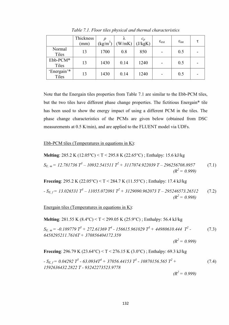
132

Table 7.1. Floor tiles physical and thermal characteristics

Thickness

(mm)

ρ

(kg/m3)

λ

(W/mK)

cp

(J/kgK) εext εint τ

Normal

Tiles 13 1700 0.8 850 - 0.5 -

Ebb-PCM®

Tiles 13 1430 0.14 1240 - 0.5 -

‘Energain’®

Tiles 13 1430 0.14 1240 - 0.5 -

Note that the Energain tiles properties from Table 7.1 are similar to the Ebb-PCM tiles,

but the two tiles have different phase change properties. The fictitious Energain® tile

has been used to show the energy impact of using a different PCM in the tiles. The

phase change characteristics of the PCMs are given below (obtained from DSC

measurements at 0.5 K/min), and are applied to the FLUENT model via UDFs.

Ebb-PCM tiles (Temperatures in equations in K):

Melting: 285.2 K (12.05°C) < T < 295.8 K (22.65°C) ; Enthalpy: 15.6 kJ/kg

SE, m = 12.781736 T3 – 10932.541511 T

2 + 3117074.922039 T – 296256708.8957

(R2 = 0.999)

(7.1)

Freezing: 295.2 K (22.05°C) < T < 284.7 K (11.55°C) ; Enthalpy: 17.4 kJ/kg

- SE, f = 13.026531 T3 – 11055.072091 T

2 + 3129090.962073 T – 295246573.26512

(R2 = 0.998)

(7.2)

Energain tiles (Temperatures in equations in K):

Melting: 281.55 K (8.4°C) < T < 299.05 K (25.9°C) ; Enthalpy: 56.4 kJ/kg

SE, m = -0.189779 T5 + 272.61369 T

4 - 156615.961029 T

3 + 44980610.444 T

2 -

6458295211.7616T + 370856404172.359

(R2 = 0.999)

(7.3)

Freezing: 296.79 K (23.64°C) < T < 276.15 K (3.0°C) ; Enthalpy: 69.3 kJ/kg

- SE, f = 0.04292 T5 - 63.0934T

4 + 37056.44153 T

3 - 10870156.565 T

2 +

1592636432.2822 T - 93242273523.9778

(R2 = 0.999)

(7.4)

133

Furthermore, two night ventilation recharge strategies are investigated for the recharge

of the PCM tiles: no-night ventilation; and night ventilation during the non-occupied

hours of the airport (between 24:00 and 04:00). As the PCM tiles are located within the

terminal space, the ventilated night air must pass through the indoor space in order to

re-charge the tiles (i.e. flush the airport indoor space). Hence, during the summer or

intermediate periods, outdoor air is assumed to pass through the airport at night; and

during the winter period, the indoor air is re-circulated through the DC diffuser to

provide air movement in the terminal space to re-charge the tiles. The night ventilation

rate through the diffuser for the 2D airport geometry is maintained at 0.5 kg/s for all

cases.

For the PCM tiles simulations, the TRNSYS-FLUENT coupling is similar to the normal

DC simulation described in section 6.7, and the phase change effect is accounted for in

the FLUENT model.

134

7.2 PCM Glazing Envelope

As indicated in chapter 5, past research in the field of PCM glazing has been relatively

scarce. However more recently, with the advent of commercial PCM glazed units, it has

generated renewed attention. Thus, because of the large glazed areas in Airport terminal

buildings, the energy performance of such systems is of interest to this study.

7.2.1 PCM Glazing Model

A PCM glazing envelope involves replacing the partly-glazed roof and side-glazing of

the terminal space with modified glazing units with PCM. Hence, the 30 mm thick

glazing and roof units described in Table 6.1 are replaced with double glazing units with

two 8 mm glass encapsulation panels and PCM RT27® in the 30 mm cavity, (in a

similar manner to Fig. 5.8). This configuration is similar to commercial structural

glazing products such as the SunGuard® (Guardian Industries Corp., 2012), which

roughly uses glass dimensions twice the size of conventional double glazing units for

structural purposes. The PCM RT27® is employed here based on the specifications of

commercial products such as the Delta-Cool 28®, which employ PCM with phase

change temperatures in the range of 26 – 30 °C, and which were shown to be adequate

for the European climate (DELTA, 2013).

The modelling of PCM glazing is more complex than ordinary PCM systems (such as

PCM tiles) because the heat transfer process within the PCM constitutes of both

conduction and radiation. Convection within the PCM is neglected in this case because

the two 8mm glass panels provide the dominant thermal resistance in the overall glazing

unit. The validated method described in chapter 5 and Gowreesunker et al. (2013c) is

employed to simulate the thermal and optical aspects of the PCM glazing envelope. The

thermophysical and phase change properties of RT27® can be found in chapter 5, and

the glass properties in Table 6.1, noting that ε = α according to Kirchhoff’s Radiation

law (Siegel and Spuckler, 1994).

It should be noted that because radiation transfer between the sky and the external

surface of the glazing is not explicitly modelled in FLUENT, the relationships for the

radiation properties (scattering, absorption and extinction coefficients) of the PCM

135

described by Eqs. (5.1-5.3) are not used. Instead, a more lumped approach is employed,

as described by Eqs. (7.5-7.8) (Gowreesunker et al, 2013c):

The transmittance of the PCM is:

τPCM = 10 -d

(7.5)

where d = [ β⋅σε,liq + (1-β)⋅σε,sol ]⋅s (7.6)

The absorption of the PCM is:

αPCM = [δ⋅β +(1-δ)] ⋅ (1-τPCM) (7.7)

The reflectance of the PCM due to scattering is:

ρPCM = [δ - δ⋅β] ⋅ (1-τPCM) (7.8)

Referring to Fig. 5.1, with a transmittance value of 0.4 and 0.9 for the solid and liquid

phases, respectively, δ is found to be 0.83 using Eq. (5.4). The physical thickness ‘s’ of

the PCM is 30 mm; the extinction coefficients are 30 m-1

and 4 m-1

for the solid (σε,sol)

and liquid phases (σε,liq), respectively obtained from Fig. 5.4, and the variation of the

liquid fraction term (β) is obtained from Eq. (C1.6) in Appendix C.

The overall transmittance and absorptance of the glazing units are obtained according to

the conservation of energy principle, as follows:

Transmittance of overall glazing unit (τunit) = (τ gl ⋅ τ PCM) (7.9)

Absorptance of overall glazing unit (αunit) = (α gl + α PCM – α gl⋅α PCM) (7.10)

The transmitted energy is applied as a heat generation rate on the floor of the terminal

space, whilst the absorbed radiation in the glazed units is implemented as described in

section 6.4.1. The glazing and roof radiation properties are modified according to Eqs.

(7.9 and 7.10). At night, emission from the glazing and roof surfaces occurs according

the external surface emittance only, as described in section 6.4.1, and the radiation

interaction between different PCM phases is ignored.

Phase change is simulated with the effective heat capacity method, according to the

variation of cp obtained from Eqs. (C1.4 - 1.5) in Appendix C. The variation of cp is

implemented as User Defined Function (UDF) in FLUENT.

136

7.2.2 TRNSYS-FLUENT Coupling for PCM Glazing

In this case, because the solar heat fluxes and the radiation boundary conditions are

calculated directly in TRNSYS and then passed to FLUENT, the radiation

characteristics of the PCM were also calculated in TRNSYS. As a result, although the

overall coupling strategy remained unchanged from the normal DC case, the exchanged

parameters are different as shown in Fig. 7.2.

Fig. 7.2. Flow of information in TRNSYS-FLUENT

coupling for the PCM-glazed model

Furthermore, expanding on the lumped-radiation modelling approach of the PCM, the

temperature at 11 segments/ nodes inside the roof and glazing are used in the calculation

of the radiation characteristics of the PCM-glazed envelope. The nodes shown in Fig.

7.3 are chosen for segments where the temperatures are observed to be quasi-uniform

(i.e. <0.4°C difference). The roof and glazing domains were refined to 6 mesh intervals

in order to increase the simulation accuracy for the phase change.

(t+1)th

FLUENT-

Airport

terminal

Boundary conditions

tth

CFD Outputs

tth

Updated Ventilation temperature

(t+1)th

time

Temperature nodes

values

TRNSYS –

Liquid

fraction

calculation

TRNSYS-

Inputs

TRNSYS -

HVAC

+Control

Transmittance calculation

Absorptance calculation

137

Fig. 7.3. Temperature nodes used in calculating the radiation properties of RT27

Referring to Fig. 7.2, in addition to the normal parameters produced by FLUENT at tth

,

the 11 extra temperatures from the nodes in Fig. 7.3 are also returned to TRNSYS.

TRNSYS then employs these temperatures at tth

to calculate the liquid fraction of the

PCM for each node using Eq. (C1.6), and subsequently, the transmittance and

absorptance of the glazing units, using Eq. (7.9) and Eq. (7.10). These radiation

parameters are then used to adjust the floor solar heat flux and external surface

absorptivities for the FLUENT model at (t+1)th

, therefore completing the information

loop. Note that the surface absorptances are separately supplied by TRNSYS to each

segment in the FLUENT model, and that the overall transmitted radiation is uniformly

distributed on the floor. Furthermore, the two night ventilation recharge strategies

employed for the PCM tiles are also used for this PCM-glazed envelope.

In essence, TRNSYS is used to calculate the radiation transmittance and absorptance of

the PCM-glazed envelope for every PCM state, and to provide the floor solar heat flux.

FLUENT simulates the phase change process of the PCM and the indoor air movement.

It can be argued that the lumped approach used to simulate radiation in the PCM is

limited by the fact that it assumes uniform properties for each node. However, referring

to Fig. C1.2b, where the uncertainty in the temperature values is ±0.4°C, this approach

can be justified as the temperature difference over each segment in the model is also

within this uncertainty margin.

138

7.3 PCM Heat-Exchanger (PCM-HX)

This PCM-HX system represents a semi-active arrangement to provide free

conditioning of the airport space. The arrangement consists of the Rubitherm GmbH

CSM® plates (see Fig. 7.4) retrofitted inside the displacement DC diffuser in the airport

departure hall shown in Fig. 7.5. The plates are symmetrically arranged as shown in Fig.

7.6.

Fig. 7.4. Rubitherm GmbH CSM ® plate

Fig. 7.5. Actual Heathrow Terminal 5 diffuser

139

Fig. 7.6. Schematic of DV diffuser, CSM plate arrangement, and supply and by-pass

ducts inside diffuser

Due to the large air volume flow rate supplied by each diffuser to the space, the surface

area of the diffusers has to be large in order to satisfy the low velocity requirements of

displacement ventilation system (CIBSE B, 2006). The volume inside the diffuser is

however mainly empty space, which provides the opportunity to retrofit the PCM-HX

system.

7.3.1 PCM-HX Model

Due to the symmetry of the PCM-HX arrangement, a 2D model of the PCM plates is

employed. The protrusions of the plate surface into the air stream, shown in Fig. 7.4, are

crucial in the heat transfer calculations from the plates, and are incorporated as a surface

roughness of 0.25 mm in the FLUENT model (Dolado et al, 2011).

The mesh employed in the CSM® plate model consists of structured 1.0×3.0 mm

hexahedral cells in the PCM domain, and hexahedral cells with a face size of 2mm with

growth ratio of 1.2 in the air domain, as shown in Fig. 7.7. The RNG k-ε turbulence

model was used, as it is adaptable to both high and low turbulence scenarios. The phase

140

change process was modelled with the enthalpy porosity method, and the properties of

the PCM used are: λ = 0.2 W/mK; ρ = 820 kg/m3; cp = 2100 J/kgK; phase change range

= 16 - 25 °C; and latent enthalpy = 180 kJ/kg, similar to the phase change properties of

RT25® used in the experimental free-cooling system of Zalba et al. (2004).

Furthermore, the adequacy of the enthalpy-porosity method for PCM heat exchanger

systems is confirmed by the studies of Ye et al. (2011).

Fig. 7.7. Model description of CSM Plate

To allow for appropriate residual convergence, a time-step of 20 s was employed for the

plate model. Hence, for one time-step in the Airport-CFD and TRNSYS models, 18 sub

time-steps were performed for the PCM plate model to ensure that all the simulation

components were at the same time, i.e. to produce a coherent overall time-step of 360 s.

In order to size the system, the following set of simulations was performed to gain an

understanding of the heat transfer rates associated with the plate arrangements within

the diffuser. This was done by varying the air gap between the plates in the model of

Fig. 7.7, and computing the total heat transfer rate for an entire diffuser, according to

the scenario presented in Fig. 7.6. The results are shown in Fig. 7.8.

141

Fig. 7.8. Heat transfer rates of PCM-HX unit for different air-gaps between plates at a

total mass flow rate of 6 kg/s (i.e. (0.5 kg/s/m in the 2D geometry) × (12m served by 1

diffuser)). ΔT is the temperature difference between the incoming air and the PCM

plate.

According to the HVAC size in section 6.5, 48 kW of conditioning is required per

diffuser to fully satisfy the conditioning load of the airport terminal. Fig. 7.8 shows that

employing an air-gap of 8mm produces a heat transfer rate of 47.9kW per diffuser,

while using an air-gap of 16mm produces a heat transfer rate of 30 kW, at a temperature

difference of 7K. Hence, an air-gap of 8mm should be adequate for this study.

However, for completeness, an air-gap of 16mm is also studied so as to investigate the

energy impact of adequately sizing the PCM-HX. This amounts to a total PCM latent

heat capacity of 202MJ (190 rows) and 133MJ (125 rows) for air-gaps of 8mm and

16mm, respectively. The air convection heat transfer coefficient for the plates in the

16mm air gap configuration is 14.3 W/m2K and in the 8mm air gap configuration is

16.05 W/m2K. Furthermore, the pressure drops across the plates with an air-gap of 8mm

and 16mm are 45Pa and 10Pa, respectively.

As the HVAC system is a constant air-volume system, the air-mass flow rate passing

through the PCM plate arrangement is also constant. This amounts to 0.048 kg/s (i.e. 6

kg/s ÷ 125 rows) and 0.032 kg/s (i.e. 6 kg/s ÷ 190 rows) per row, for each air-gap case.

These mass flow rates are applied to the model in Fig. 7.7.

142

7.3.2 TRNSYS-FLUENT Coupling for PCM-HX

The TRNSYS-FLUENT coupling for the PCM-HX system is done via a secondary

custom built component in TRNSYS that transfers the required parameters to the

separate PCM plate FLUENT model (see Fig. 7.7). The flow of information is shown in

Fig. 7.9.

Fig. 7.9. Modified information flow for DC with PCM-HX

Fig 7.9 shows that the flow of information consists of the similar exchange of

parameters as in the normal DC case described in Fig. 6.9, but additionally includes the

‘Boundary Conditions-2’ and ‘CFD Outputs-2’ with the PCM-HX plate model.

Boundary Conditions-2 comprises the air mass flow rate and the mixed air temperature

Tm (see Fig. 6.4), while CFD Outputs-2 consists of the PCM mean temperature and the

outlet air temperature from the PCM-HX.

In this case, TRNSYS provides the boundary conditions for both the airport model and

the PCM-HX model, and uses the CFD outputs to control both the airport and the PCM-

HX system, as described in the next section. FLUENT is used to simulate both the

building and the PCM-HX model, including the phase change process.

Due to the successive substitution method, each CFD component built in TRNSYS is

simulated sequentially. Thus, the overall simulation time in running the airport model

with the PCM-HX model is the addition of the individual simulation times of the two

custom-built CFD components.

tth

Boundary

Conditions -2

Updated Ventilation Inputs

(t+1)th

time

CFD Outputs -2

tth

Boundary Conditions-1

tth

CFD Outputs -1

tth

FLUENT:

Airport

terminal

FLUENT:

PCM-HX

TRNSYS:

HVAC +

Controls

TRNSYS: Inputs

143

7.3.3 PCM-HX Control Strategies

The PCM-HX system is employed here for free-conditioning the airport terminal space.

This generally refers to relying on the PCM plate arrangement to adequately condition

the mixed air at temperature Tm (see Fig. 6.4), without the need for auxiliary heating or

cooling. However, as the PCM-HX system is located in the diffuser, at the end of the

HVAC line, and because of the irregularities in the internal heat gains, the air

temperature leaving the PCM-HX is unpredictable. Hence, for this case, the following

control strategies were employed:

If Tf > Tc, u ;

The PID controller will calculate a supply temperature Ts < 21°C

to satisfy the cooling load, and the supply air bypasses the PCM-

HX (see Fig. 7.6).

If Tc, l ≤ Tf ≤ Tc, u ; The heating/cooling coils are non-operational, and air at Tm

passes through the PCM-HX before being supplied to the space.

If Tf < Tc, l ;

The PID controller will calculate a supply temperature Ts > 21°C

to satisfy the heating load, and the supply air bypasses the PCM-

HX.

The PCM-HX is effectively used only when the indoor temperature is within the

comfort level, where the PCM-HX aims at prolonging the duration of comfort, by

providing suitable temperature dampening effects. An indication of the air-by-pass route

inside the diffuser can be observed in Fig. 7.6.

In this study, three different night charging strategies are investigated for the PCM-HX

when the airport terminal building is closed between 24:00 and 04:00: i) no night

ventilation; ii) ‘non-stop’ full ventilation; and iii) a limiting ventilation control. During

the summer and intermediate periods, cold ambient air is used for charging. The

limiting control is done by monitoring the PCM temperature, and stopping night

ventilation when the PCM temperature drops below the lower comfort level. The night

outdoor-recharge air is used to simply flush the PCM-HX in the diffuser, and does not

affect the indoor airport terminal space at night.

144

During winter, the return air from the airport is re-circulated through the PCM-HX to

store the extra heat from the space (i.e. flushing the airport indoor space). In the winter

case, the limiting control is performed by monitoring the difference between the return

air temperature (Tr) and the mean PCM temperature (Tpcm), such that night ventilation is

active only when there is a net positive heat transfer into the PCM, i.e. Tr > Tpcm. As

mentioned earlier, the night ventilation rate for the 2D geometry is maintained at 0.5

kg/s for all cases.

7.4 Pressure Drop Calculations

The boundary used to calculate the pressure drops across the HVAC ducts is shown in

Fig. 7.10.

Fig. 7.10. HVAC ducting for airport terminal space

The sizing of the ducts was based on the velocity criteria provided by CIBSE guide B

(2006), and the pressure drops are calculated from equations given in Idelchik (1994). A

velocity of 15 m/s was used for the main ducts giving a diameter of 0.65 m, and a

velocity of 10 m/s with a duct diameter of 0.45 m was used for the 3 final ducts run to

the diffuser, as shown in Fig. 7.6. The detailed pressure drop calculations are shown in

Appendix E.

Note that the air duct design serves only as an approximate means of quantifying the

pressure drop for the different DC configurations, and that the same ducting

configuration is employed for all DC and PCM system cases in order to abide by the

comparative nature of this study.

145

7.5 Total Annual Energy Demand

The annual HVAC energy demand is obtained through the concept of Heating Degree

Days (HDD) and Cooling Degree Days (CDD), as proposed by CIBSE TM-41 (Day,

2006). Degree days are a measure of how much (in degrees), and for how long (in

days), the external air temperature is lower than a specific base temperature in the case

of heating or above a specific base temperature in the case of cooling. It is used as a

means of estimating the amount cooling/heating required by a building, as well as for

energy management purposes (Day, 2006).

The key issue in employing this method relates to the choice of the base temperatures

(i.e. reference temperatures), which allows the determination of the energy consumption

of the building (Day, 2006). The base temperature refers to the external ambient

temperature whereby the building does not require any energy to maintain the indoor

comfort conditions. Hence, for HDD, the base temperature will be the ambient

temperature above which heating is not required, and for CDD, it will be the ambient

temperature below which cooling is not required.

This method is employed here mainly due to the extensive computing times associated

with the CFD models, whereby the running of yearly simulations in CFD would be

impractical. As suggested in Gowreesunker and Tassou (2013a), discrete and generic

time dependent situations can be simulated to quantify the behaviour of the building and

the HVAC system. The energy demand per degree day can be calculated for each of

these simulated periods, and the total annual HDD and CDD are then used to

extrapolate for the yearly energy demand. The base temperatures are obtained by

analysing the energy demand and ambient temperature patterns of the stand-alone DC

cases.

The simulations are therefore run for peak summer and winter conditions, and an

intermediate condition, as described in Table 7.2 and Fig. 7.11, in order to obtain the

behaviour of the building under different weather conditions. The Meteonorm C-37790

weather files for London are used for the simulations, and the weather data values for

the 360s time-steps employed in this study are linearly interpolated between the hourly

values. The intermediate conditions are obtained based on a probabilistic study of the

146

most frequent ambient air temperature ranges occurring during the year; which was

found to be in the range of 10-23°C for this weather file.

Table 7.2 Discrete Simulation times

Intermediate 4500 – 4600 hrs

Summer 5434 – 5534 hrs

Winter 8576 – 8676 hrs

Fig. 7.11. Generic ambient temperatures for the different seasons

Table. 7.3. Simulated and yearly Degree days for 15°C and 18°C base temperatures

(The base temperatures presented in Table 7.3 are obtained based on the energy

demands, as explained in Appendix F)

Seasons HDD CDD

Simulated Winter 46.35 0.00

Simulated Summer 0.29 13.79

Simulated Intermediate 2.49 6.27

Entire Year 1859.12 120.10

-5

0

5

10

15

20

25

30

35

0 20 40 60 80 100

Tem

pera

ture

(°C

)

Hours

Intermediate Summer Winter

147

HDD and CDD have been employed in several studies such as Kolokotroni et al. (2010)

and Bolatturk (2008), in the prediction of building energy consumption. This is due to

its simplicity and speed of use, as well as the possibility to easily estimate the building

energy performance for different weather conditions. This concept is therefore adopted

for this study as it is an adequate method to estimate the annual energy demand for

simulations requiring long computing times. It is also adequate for comparative

analyses.

148


This chapter describes the numerical models of the PCM systems studied for the airport

terminal space. Two passive and one semi-active system are presented, which have been

chosen based on their energy storage potential as well as suitability and ease-of-retrofit

in the airport terminal. The implementation of the PCM tiles, PCM glazing and PCM-

HX systems in the respective models, the thermo-physical properties of the PCMs, and

the flow of information in the TRNSYS-FLUENT coupling are described. Furthermore,

the control strategies involved with each system in terms of both the HVAC control

system and the night recharge methods are also explained.

The layout for the air ducts is presented in section 7.4, and is maintained for all

simulation scenarios, for comparative purposes. The pressure drops involved with each

PCM system can be found in Appendix E. Because of the extensive simulation times

involved in the CFD models, the concept of Degree Days was employed in the annual

energy calculations.

The next chapter describes the air conditioning performance of the stand-alone DC

system as well as each PCM system, when employed in the airport terminal space.

149

CHAPTER 8 – PERFORMANCE OF PCM SYSTEMS IN

AIRPORT TERMINAL SPACE

This chapter presents a case study, depicting the numerical results obtained using the

previously described models in the airport terminal space, with the TRNSYS-FLUENT

coupled simulation method. The comfort temperature range is taken to be 18-23°C, as

defined in Table 2.6 (CIBSE A, 2006). The HVAC mode of operation, described in

section 6.5, allows the indoor temperature to closely follow the ambient conditions, and

improve both the energy consumption and thermal comfort of the space, by providing

the flexibility of the occupants to adapt to the indoor conditions.

In addition it also shows the thermal performance of the conventional stand-alone

Displacement Conditioning (DC) system, and each of the PCM systems, namely: the

PCM tiles (‘Ebb’ and ‘Energain’ tiles), the PCM-glazed envelope, and the retrofitted

PCM-HX system (with 8mm and 16mm air gaps), described in Chapter 7. The

simulations are run for discrete weather conditions and the annual energy demands are

computed using the Degree Day concept. The first day of each simulation is neglected

in the analysis, so as to avoid initialisation errors. The results include the indoor

temperature progression as well as the energy demand trends for each system. These

results are aimed at providing the relative energy performances of each PCM system.

150

8.1 Seasonal Performance of stand-alone DC system

This scenario involves the modelling of the conventional DC system using the CFD and

TRNSYS HVAC models, without the use of PCM systems. A time-step of 360s was

used for both TRNSYS and CFD, as explained in section 6.7, with an average of 40

iterations per time-step for the CFD simulation to satisfy the convergence criteria. All

simulations are initialised at 21°C, and the overall actual simulation time for each

season was 13 hrs with a 3GHz i7 processor. The results are given in Fig. 8.1.

Fig. 8.1(a). Ambient and zone temperature (Tf) profiles for the

three distinct seasons in ‘DC-only’ Case

Fig. 8.1(b). Heating (+) and cooling (-) energy load Profile

for ‘DC-only’ case for 2D geometry

151

During the intermediate period, the DC system successfully controls Tf within the

comfort temperature range of 18-23 °C. The majority of the energy requirement is for

cooling, with a relatively small amount for heating during the early hours of the

morning. During the summer period, the zone temperature is less effectively controlled

compared to the intermediate season, where the temperature reaches ~26 °C at mid-day.

Similar to the intermediate season, the majority of the load is for cooling during

summer, but heating is also required on a small number of occasions when the ambient

temperature is low during early mornings.

During winter, only heating is required by the space. However, Fig. 8.1(a) shows that

based on the control strategy used, the DC system is unable to satisfy the comfort

requirements in winter; where the zone temperature varies between 15 °C and 18 °C.

This anomaly is further explained in section 8.5.2.

Fig. 8.2(a). Temperature contour (°C) still-frame during the DC unit cooling mode

Fig. 8.2(b). Temperature contour (°C) still-frame during the DC unit heating mode

152

Fig. 8.2 demonstrates why DC is more suitable for cooling purposes, rather than heating

large spaces. During the cooling mode, Fig. 8.2 (a) shows the buoyancy effects of the

DC system enhance cooling in the space, with the cold air spreading on the floor until it

reaches a heat source. This enables the cooling potential of the DC system to be

specifically directed to the occupied space and avoid unnecessary conditioning of

unoccupied areas. Furthermore, the temperature stratification effect in the space

prevents further heat gains from the higher levels in the building envelope by reducing

the temperature difference with the external conditions. In the case of heating, the DC

system behaviour resembles a mixed ventilation system (Gowreesunker et al, 2013d).

Fig. 8.2(b) shows that the warm air supplied by the displacement diffuser rises quickly

and mixes with the indoor air due to its dominant buoyant force, hence failing to

establish the temperature stratification benefits in the space.

Fig. 8.3(a). Velocity vectors (m/s) in airport domain during DC cooling mode

153

Fig. 8.3(b). Velocity vectors (m/s) in airport domain during DC heating mode

Additionally, Fig. 8.3 shows the velocity vectors in the entire airport domain and in the

conditioned zone, which is naturally influenced by the geometry of the airport. The

main observation from this velocity plot relates to the air velocities in the conditioned

zone, which was found to be in the range of 0.1 - 0.3 m/s, hence abiding by the velocity

comfort criteria of < 0.5 m/s, described in section 2.2.1. Being a constant air volume

HVAC system, the temperature and velocity plots from Figs. 8.2 and 8.3 are similar for

all systems, and hence these plots can be taken as the generic air-movement plots for the

airport terminal.

Fig. 8.4. Seasonal heating (+) and cooling (-) demands of the

airport space for stand-alone DC case

154

It can be observed from Fig. 8.4 that the space requires heating for all three seasons:

during the early morning hours of the day for the summer and intermediate season (due

to the airport operating hours described in Fig. 6.3), and for the entire day in the winter

season. Consequently, cooling is required only during the mid hours of the day for the

summer and intermediate periods. Hence for the ‘DC-only’ case, it can be observed that

under UK weather conditions, heating is more prominent than cooling, and that the

indoor stratification benefits associated with the DC cooling mode can only be obtained

for the summer and intermediate weather conditions.

155

8.2 Seasonal Performance of DC system and PCM Tiles

This section depicts the energy impact of the PCM floor tiles on the airport terminal

space, and is divided into the performance of the Ebb® tiles and the Energain® tiles. A

time-step of 360s is employed for both the CFD and TRNSYS models, with an average

of 40 iterations per time-step for the CFD model. The simulation time for each season

was 14 hours with a 3GHz i7 processor. The contour and vector plots for the indoor air-

movement are similar to Figs. 8.2 and 8.3.

8.2.1 ‘Ebb’ Tiles

The Ebb tiles are placed on the floor of the airport terminal space as described in section

7.1, and the enhanced phase change model developed in this study is used to simulate

phase change. The temperature and load trends of the zone, with the Ebb floor tiles, are

shown in Fig. 8.5.

Fig. 8.5(a). Ambient and zone temperature (Tf) profiles with and without

night ventilation for the Ebb-Tiles’ case

156

Fig. 8.5(b). Heating (+) and cooling (-) load profiles for the Ebb-Tiles’ case,

with/ without night ventilation, for 2D geometry

It can be observed from Fig 8.5(a) that the general temperature trends for the Ebb tiles’

for all seasons are similar to the ‘DC-only’ case, whereby: the indoor space is

maintained in the comfort range only for the intermediate season; whilst the space

overheats for part of the summer. The temperature impact of the PCM tiles in the

summer can be quantified by the fact that the indoor space overheats (i.e. Tf > 23°C) for

22% and 21.5% of the time for the non ventilated ‘DC + Ebb tiles’ and the ‘DC + Ebb

tiles Vent’ cases, respectively, compared to 23% for the ‘DC-only’ case. Furthermore,

the zone temperature during the winter season is below the comfort requirements,

similar to the ‘DC-only’ case.

The load profiles for both the ‘DC-only’ and the non-ventilated ‘DC + Ebb tiles’ cases

are very similar, as shown in Fig. 8.5(b). During the intermediate season, heating is

required during the early morning hours, while cooling dominates during the day.

During summer, heating may be required, but cooling is most prominent, whilst in

winter, the airport terminal requires only heating. For the ‘DC + Ebb tiles Vent’ case, a

noticeable change in the load profile can be observed. The time of maximum cooling

load for both the summer and intermediate seasons is found to shift by an average of 0.8

hrs, whilst the heating load for these two seasons is found to increase in the early

157

morning hours compared to the ‘DC-only’ and ‘DC + Ebb tiles’ cases. During winter,

the heating load trends for all configurations are similar.

Thus, the addition of the Ebb tiles without ventilation is found not to have a major

impact on both the temperature and energy load profiles of the airport terminal, whilst

recharging the Ebb tiles through night-ventilation shifts the time of maximum cooling

load during the day by 0.8 hours during the intermediate and summer seasons.

However, night-ventilating the indoor space also increases the heating load required by

the space during the early morning hours in the intermediate and summer seasons.

Hence, although the percentage overheating time in the summer is similar for the non-

ventilated and ventilated cases, the overheating of the space occurs 0.8 hrs later when

ventilating the indoor space at night. There is no apparent impact of the Ebb tiles during

the winter season.

Fig. 8.6. Heating (+) and cooling (-) demands with and without night ventilation,

with Ebb floor tiles

Fig. 8.6 shows that employing night ventilation in the space reduces slightly the cooling

demand during the summer and intermediate seasons, but at the same time, increases the

heating demand. Thus, night ventilation is effectively shifting the load from cooling to

heating, and therefore the annual energy savings will depend on the balance between the

two opposing loads. Furthermore, compared to the ‘DC-only’ case from Fig. 8.4, it can

be observed that the cooling loads are lower when employing the Ebb floor tiles, whilst

158

heating load increases when using night ventilation with the Ebb floor tiles. During

winter, the heating loads for the Ebb floor tiles are slightly lower compared to the ‘DC-

only’ case.

8.2.2 ‘Energain’ Tiles

The thermophysical properties of the Energain tiles are given in section 7.1. This tile is

used to show the impact of floor tiles with higher latent enthalpy than the Ebb tile, on

the energy performance of the indoor space. The temperature and load trends of the

zone for the Energain floor tiles are shown in Fig. 8.7.


night ventilation for the Energain-Tiles’ case

159

Fig. 8.7(b). Heating (+) and cooling (-) load profiles for the Energain-Tiles’ case,

with and without night ventilation, for 2D geometry

The general observations from the trends in Fig. 8.7 are similar to the Ebb tiles’ case,

that is: the comfort conditions are satisfied for the intermediate season; there is

overheating in the summer; and the indoor temperatures are below the comfort

requirements during winter. However, the swing in the indoor temperature is more

noticeable when employing the Energain floor tiles. For instance, the summer indoor

temperatures are found to increase at a slower rate compared to the ‘DC-only’ case,

whilst the reduction in the winter indoor temperatures during the night is lower when

the Energain tiles are used, compared to the ‘DC-only’ case.

Consequently, the temperature impact of the PCM tiles in the summer can be quantified

by the fact that the indoor space overheats (i.e. Tf > 23°C) for 19.7% and 19.0% of the

time for the non ventilated ‘DC + Energain tiles’ and the ‘DC + Energain tiles Vent’

cases, respectively, compared to 23% for the ‘DC-only’ case. This also shows an

improvement in indoor thermal comfort, compared to using the Ebb floor tiles.

Similar to the Ebb tiles case, the heating energy load is found to increase (when night

ventilating the space) in the early morning due to the higher thermal mass of the

building that needs heating, while the cooling energy decreases during the day,

compared to the ‘DC-only’ case. However, when using the Energain tiles, the reduction

in cooling energy during the day is more prominent for both the non-ventilated and

160

ventilated cases, compared to both the ‘DC-only’ and Ebb-tile cases. Additionally, the

time of maximum cooling load is found to shift by an average of 1.3 hrs for both the

non-ventilated and ventilated scenarios, compared to the ‘DC-only’ case. During winter,

there are no apparent changes in the energy demand for the space.


with Energain floor tiles

Fig. 8.8 shows that similar to the Ebb tiles, using the Energain tiles reduces the cooling

load during the day for the intermediate and summer seasons, compared to the ‘DC-

only’ case. However, the reduction in cooling load is more pronounced when using the

Energain tiles, due to the higher latent heat capacity of the PCM. The heating demand

for the summer and intermediate seasons is reduced when employing the Energain tiles

in the non-ventilated mode, whilst ventilation significantly increases the heating load,

compared to the ‘DC-only’ case. It can also be observed that the winter heating load is

reduced when employing the Energain tiles, compared to both the Ebb-tiles and the

‘DC-only’ cases.

Generally, it was found that increasing the latent heat capacity of the floor tiles reduces

the cooling load during the summer and intermediate seasons, but ventilating the space

at night increases the heating loads for these two seasons. In winter, the heating load

also decreases with the use of higher latent heat capacity PCM in the floor tiles, and

ventilating the space at night has a very low impact on the heating energy demand of the

space.

161

8.3 Seasonal Performance of DC system and PCM Glazing

This section describes the performance of the PCM-glazed envelope. A time-step of

360s is employed for both the CFD and TRNSYS models, with an average of 50

iterations per time-step for the CFD model. The simulation time for each season was 17

hours with a 3GHz i7 processor. The thermophysical properties of the PCM-glazing are

detailed in section 7.2. Fig 8.9 shows the temperature and load trends of the zone, with a

PCM glazed envelope.


night ventilation for the PCM-glazing’s case

Fig. 8.9(b). Heating (+) and cooling (-) load profiles for the PCM glazing’s case,

with and without night ventilation, for 2D geometry

162

The overall temperature trends obtained from using the PCM-glazed envelope are

similar to the trends when using the Energain tiles, i.e. there is a noticeable reduction in

the rate of increase of temperature during the summer and intermediate seasons, as well

as relatively higher night temperatures during winter, compared to the ‘DC-only’ case.

Furthermore, the %-overheating hours (i.e. Tf > 23°C) during summer is also reduced to

20.3% and 18.1%, for the non-night ventilated and night ventilated PCM-glazing cases,

respectively.

The heating energy load during the intermediate and summer seasons is found to

increase in the early morning hours, similar to the ‘PCM floor tiles’ cases, due to the

higher thermal mass of the building that requires heating, compared to the ‘DC-only’

case. During the day, the cooling load is found to decrease relative to the ‘DC-only’

case, portraying the effectiveness of the PCM. Furthermore, the time of maximum

cooling energy load during the intermediate and summer days is shifted to later in the

day by an average of 1.6 hrs, for both the ventilated and non-ventilated cases, compared

to the ‘DC-only’ case. During winter, there is no apparent change in the heating energy

demand, when using the PCM-glazed envelope.


with the PCM-glazing envelope

163

Fig. 8.10 shows that the summer and intermediate cooling loads are reduced with the

use of the PCM-glazing compared to the ‘DC-only’ case, because of the higher solar

radiation absorption rate of the PCM compared to the normal glazing; and that the

employment of night ventilation has a beneficial impact in this regard. Night ventilation

however also increases the heating loads for these two seasons. During winter, the

heating energy demand also decreases with the use of the PCM-glazing compared to the

‘DC-only’ case, due to the lower heat loss rates through the glazed envelopes. However,

using night ventilation in winter increases the heating load compared to a non-ventilated

case. The latter observation can be explained by the fact that compared to the floor tiles;

the PCM-glazing envelope has a direct contact with the external ambient air conditions.

Hence, increasing convection within the building also increases the heat transfer with

the outdoor air which increases the heating requirement during the winter occupied

hours.

164

8.4 Seasonal Performance of DC system with retrofitted PCM-HX

This section describes the impact of retrofitting the PCM heat exchanger (PCM-HX)

system in the displacement diffuser of the airport terminal. Compared to the PCM tiles

and glazing, this is a semi-active system, whereby the PCM influences the air supplied

into the space. The control strategies are described in section 7.3.3, and both

configurations of the PCM-HX, i.e. the 16mm and the 8mm air gaps between successive

PCM plate rows, are evaluated in this section. In this case, the airport CFD model

employed a time-step of 360s and 40 iterations per time-step, and the PCM-HX CFD

model employed a time-step of 20s to satisfy the convergence criteria. Thus for every

time-step of the airport model, 18 sub time-steps were performed for the PCM plate in

order to allow coherency in the simulation times. The overall computing time was 19

hrs for each season, with a 3GHz i7 processor.

8.4.1 DC-PCM-HX-16mm

Fig. 8.11 shows the temperature and energy trends for the different seasons using a

16mm air gap for the PCM-HX, and the different night charging strategies described in

section 7.3.3.

Fig. 8.11(a). Ambient and zone temperature (Tf) profiles, with different

night ventilation charging strategies for the PCM-HX-16mm case

165

Fig. 8.11(b). Heating (+) and cooling (-) load profiles for the PCM-HX-16mm case,

with different night ventilation charging strategies, for 2D geometry

Fig. 8.11(a) shows that the PCM-HX-16mm system is able to satisfy the comfort

conditions only during the intermediate season whilst produces slight overheating

during the summer, and the temperature during the winter drops outside the comfort

region. The overall temperature performance of the three control strategies is very

similar. The employment of the PCM-HX-16mm shows an average shift of 1.8 hrs in

the intermediate and summer peak temperatures, as well as lower peak summer

temperatures, compared to the ‘DC-only’ case. The %-overheating summer hours (i.e. Tf

> 23°C) are 21.6%, 21.5% and 21.1% for the ‘noVent’, ‘limiting control’ and ‘full

ventilation’ night charging strategies, respectively, compared to 23% for the ‘DC-only’

case.

With regards to energy demand (see Fig. 8.11(b)), it can be seen that the ‘full

ventilation’ strategy increases the early morning peak heating demands during both the

intermediate and summer periods due to PCM over-cooling at night, relative to the other

strategies. The use of the PCM-HX-16mm produces an average shift of 1.8 hrs in the

time of peak cooling energy demand, compared to the ‘DC-only’ case. The winter

heating load trends are similar for all control strategies.

166

Fig. 8.12. Heating (+) and cooling (-) demands with different night ventilation

strategies, with PCM-HX-16mm

Fig. 8.12 shows that the night charging strategies of the PCM-HX-16mm have a greater

relative effect on the heating energy requirement than the cooling energy requirement,

in the summer and intermediate seasons. It can be seen that reducing night ventilation to

recharge the PCM, reduces the heating demand in the intermediate and summer periods

as overcooling in the morning is reduced. The use of the PCM-HX-16mm has little

effect on the heating demand in winter, due to the fact that the temperature of the air (Tm

or Tr, in Fig. 6.4) passing through the PCM-HX-16mm is in the lower range (15-18°C)

of the PCM phase change temperature range of 16-26 °C, as shown in Fig. 8.11(a). The

latent storage capacity of the PCM is therefore inefficiently used during winter.

On the other hand, the cooling demand in both the summer and intermediate seasons is

reduced with the addition of the PCM-HX-16mm, relative to the ‘DC-only’ system.

However, the different ventilation charging strategies do not significantly affect the

cooling performance. Previous studies have primarily shown that PCM free-

conditioning systems mainly reduce cooling demands and temperature swings in

intermittently occupied buildings. However, as the airport schedule is less uniform and

different to intermittently occupied buildings, this study shows that the PCM-HX-16mm

has a higher impact on the heating demand of the space during the intermediate and

summer periods. This is explained below.

167

Fig. 8.13(a). Zone temperatures (Tf) and PCM mean temperatures

during one day in the intermediate season

Fig. 8.13(b). Heating (+) and cooling (-) load trends

for one day in the intermediate season

(Note that: (4559-4564) hrs is the night charging/ ventilation period; the daytime period

is during (4565-4579) hrs; and (4583) hrs is 24:00, when the airport closes. The

specifics of the weather data can be obtained from the Meteonorm C-37790 weather

files for London)

Fig. 8.13(a) shows that during the early hours of the morning, the zone temperature for

most cases is less than the lower comfort limit of 18°C, with the space requiring

heating. Employing a full night ventilation charging strategy implies that the

168

temperature being supplied to the space from the PCM-HX-16mm in the early morning

hours is lower compared to the other configurations, hence increasing the heating

demands. Preventing night ventilation or limiting the PCM temperature to 18°C will

reduce the need for heating in the early hours (from 4564 hr) of the morning, because of

the relatively higher supply temperature compared to the full ventilation strategy.

Furthermore, Fig. 8.13(a) shows that the use of the PCM-HX-16mm shifts the

occurrence of high space temperature from the morning to later hours, reducing the

cooling energy requirements in the morning (see Fig. 8.13(b)), but increasing it in the

late afternoon hours. Nonetheless, as shown by Figs. 8.12 and 8.4, the overall cooling

energy requirement of the space is reduced with the use of the PCM-HX-16mm

compared to a ‘DC-only’ system.

8.4.2 DC-PCM-HX-8mm

Fig. 8.14 shows the temperature and energy trends for the different seasons using an

8mm air gap for the PCM-HX, including the different night charging strategies.

Fig. 8.14(a). Ambient and zone temperature (Tf) profiles, with different

night ventilation charging strategies for the PCM-HX-8mm case

169

Fig. 8.14(b). Heating (+) and cooling (-) load profiles for the PCM-HX-8mm case,

with different night ventilation charging strategies, for 2D geometry

The observations for the temperature and energy trends of the PCM-HX-8mm case are

similar to the PCM-HX-16mm case, where: the comfort conditions are satisfied only for

the intermediate season; overheating occurs in the summer; the indoor temperatures are

below the comfort criteria for winter; there is a reduction in the peak summer

temperatures, relative to the ‘DC-only’ case; and a shift in the time for peak cooling

demand by 2.0 hrs, compared to the ‘DC-only’ case. There is also no major change in

the winter temperature and energy trends when using the PCM-HX-8mm.

Furthermore, the %-overheating summer hours (i.e. Tf > 23°C) are 21.4%, 21.1% and

19.5% for the ‘noVent’, ‘limiting control’ and ‘full ventilation’ night charging

strategies, respectively.

170

Fig. 8.15. Heating (+) and cooling (-) demands with different night ventilation

strategies, with PCM-HX-16mm

The observations from Fig. 8.15 imply that the effect of the PCM-HX-8mm on the

energy performance of the DC system is again similar to the PCM-HX-16mm case.

However, the cooling loads of the PCM-HX-8mm are relatively lower than the PCM-

HX-16mm configuration in the summer and intermediate seasons, whilst the PCM-HX-

8mm configuration improves the heating performance only for the ‘non-ventilated’ and

‘limiting control’ night charging strategies, compared to the PCM-HX-16mm for the

summer and intermediate seasons. There is no major difference in the performance of

the PCM-HX-8mm and PCM-HX-16mm during winter, because the indoor temperature

fluctuates in the lower levels of the phase change temperature range, inefficiently

exploiting the energy storage potential of the PCM, as explained in section 8.4.1.

Thus, in general, the PCM-HX-8mm is found to have a similar impact on the Airport

space as the PCM-HX-16mm case, except that the effects are more prominent due to the

higher latent heat capacity of the PCM-HX-8mm configuration. This observation is

exemplified in Fig. 8.16, for the case of limiting night ventilation control.

171

Fig. 8.16. Load comparison of PCM-HX-8mm and PCM-HX-16mm for a day in the

intermediate season, under the limiting night control ventilation charging strategy

It can be observed from Fig. 8.16 that: employing the PCM-HX systems reduces the

heating load during the early morning hours; and employing a higher latent heat

capacity in the diffuser, in the form of the PCM-HX-8mm configuration, improves the

heating energy demand even further. This is explained by the fact that due to the higher

heat capacity of the diffuser, the PCM temperature is maintained closer to the lower

limit of comfort during the early morning hours, requiring less auxiliary heating when

the HVAC system starts to operate (from 4564 hr).

During the day, there is a shift in the peak cooling load from the early morning hours to

later hours in the day when using the DC-PCM-HX system, relative to the ‘DC-only’

case. Furthermore, there is a net reduction in the cooling loads when employing the DC-

PCM-HX system relative to the ‘DC-only’ system, due to the increased thermal mass.

This increase in heat capacity is effectively prolonging the period for which the indoor

temperature is within the comfort region of 18-23 °C. In this regard, increasing the

latent heat capacity of the system from the PCM-HX-16mm to PCM-HX-8mm

configuration improves this effect and reduces the cooling loads even further, as shown

in Fig. 8.16.

172

8.5 Annual Energy Performance

This section presents the annual energy demands of the space when using each PCM

system. The energy is divided into annual heating and cooling load, extrapolated using

the Degree Day concept explained in section 7.5, and the fan powers described in

Appendix E. (The annual energy calculation method is explained in Appendix F)

Fig. 8.17. Annual energy demand of the entire Airport Terminal Space

for the different PCM system configurations

Fig. 8.17 shows that heating constitute a major portion of the annual energy demand for

the airport terminal space in UK weather conditions, whilst cooling is the least

significant portion of the annual energy demand. This is due to the relatively higher

number of annual Heating Degree Days (HDD) compared to Cooling Degree Days

(CDD) for the UK weather conditions (see Table 7.3). As a result, in order to

significantly influence the energy performance of the airport space, the PCM system

must influence the heating load of the building relatively more than the cooling load.

173

This is a rather counter-intuitive ideology, because PCMs have been mainly appreciated

in past studies for their cooling energy savings potential.

From the previous sections, it has been observed that employing the PCM systems

during winter has a relatively low influence on the heating demand. Hence, in order to

improve the annual total energy demand, the heating loads during the summer and

intermediate seasons must instead be reduced. For these two latter seasons, heating is

mainly required during the early morning hours when the airport opens. Thus, an

efficient PCM system would either limit the reduction in temperatures during the night

or satisfy the early morning heating requirements, reducing the dependency on energy-

consuming auxiliary heating units.

Fig. 8.17 shows that employing full night ventilation for recharge actually reduces the

energy saving potential of the PCM systems. This is because night-ventilating the PCM

systems without any control produces lower temperatures during the early hours of the

morning, which have to be compensated through the use of increased amount of

auxiliary heating. Conversely, not providing night ventilation, provides the maximum

heating energy savings potential as the morning supply/indoor temperatures are higher.

In cases without night-ventilation, the recharging process of the PCM systems

adequately occurs within the operating hours of the airport. For instance, referring to

Fig. 8.13(a), it can be seen that the PCM temperature decreases during the early

occupied hours of the day, when the airport starts to operate (i.e. the PCM charging

phase). Although the PCM temperature decreases to a slightly higher value without

night-ventilation, compared to the night-ventilation strategies, the PCM is still

adequately recharged to ~80% without any ventilation in the intermediate season. Thus,

using the non-ventilated strategies allows a reduced heating load in the early morning

(due to the higher PCM temperatures), without extensively sacrificing the cooling

potential of the PCM during the day. This observation is confirmed in the annual energy

demands of the different PCM configurations, whereby not employing night ventilation

provides energy savings for all the investigated PCM systems.

174

8.5.1 Relative Energy Performance

In order to analyse the energy impact of the different PCM systems, Fig. 8.18 shows the

energy performance of the PCM systems relative to the ‘DC-only’ case.

Fig. 8.18. Total annual energy demands of PCM System configurations relative to the

‘DC-only’ case

Employing the retrofitted PCM-HX configurations reduces the annual energy demands

only for the cases of ‘noVent’ and ‘Limiting control’ night ventilation strategies. These

cases reduce the heating requirements in the early morning hours of the summer and

intermediate seasons, and thus provide with the highest energy savings compared to the

‘Full’ night ventilation strategy. Employing the latter night charging strategy produces

annual energy losses. Additionally, using the PCM-HX-8mm configuration produces

higher energy savings compared to the PCM-HX-16mm configuration due its higher

latent heat capacity, even though the fan power is higher for the PCM-HX-8mm

configuration. Thus, in this case, employing an extra 150% latent heat capacity in the

PCM-HX system of the DC diffuser produces an extra annual energy savings of 4%.

175

Using PCM floor tiles also produces energy savings only for the cases where night

ventilation is not employed. The energy saving potential of the tiles is less than the

PCM-HX systems, partly because of the relatively lower latent heat capacity of the tiles,

and partly due to the passive nature of the PCM system. Using a passive system

produces a lower heat transfer rate due to the lower air velocities (heat transfer

coefficients) with the PCM. Additionally, using a PCM tile with higher latent heat

capacity produces higher energy savings. However, Fig. 8.18 shows that employing a

PCM tile that contains about an extra 350% latent heat capacity, only produces a

supplementary reduction of 2% in the annual energy demand.

Similarly, utilising the PCM glazed envelope produces energy savings only for the case

without night ventilation. In this case, the energy saving potential is similar to using the

non ventilated Ebb floor tiles, and lower than the other PCM configurations. This can be

explained by the fact that although the higher thermal mass and the lower solar

transmission of the PCM glazing reduces the cooling energy load during the day, a

higher thermal mass also requires relatively higher heating in the early morning hours,

compared to the other PCM systems. Also, because the PCM glazed envelope is located

adjacent to the external air, the entire PCM thermal mass is not solely employed in the

conditioning of the indoor space, but is also directly influenced by the external

conditions. Conversely, ventilating the PCM-glazed system at night significantly

amplifies the early morning heating load (especially during the summer and

intermediate seasons), making the combination of PCM glazing and night ventilation

the worst annual energy performing configuration. (The optical change in the PCM

during phase change must also be considered in the application of such PCM-glazed

structures.)

Thus, for the PCM system configurations studied, employing the PCM-HX-8mm

without night ventilation provides the highest energy savings of 38%, whilst employing

the PCM glazing with night ventilation produces the highest energy losses of 69%,

compared to the ‘DC-only’ case. The employment of PCM systems, without night

ventilation is found to shift the peak cooling energy demand to later hours in the day,

while also reducing the early morning heating and overall energy demands.

176

8.5.2 Assessment of the Control Method

The use of the PID controller and the HVAC control strategy described in section 6.5,

leads to a poor performance for the displacement conditioning system during the winter

season (i.e. the indoor temperatures are below the comfort requirements) and the

overheating propensity during the summer season. This is explained with reference to

Fig. 8.19.

Fig. 8.19. Indoor temperature (Tf) for a typical summer day for the ‘DC-only’ case

(Airport opens at 5476 hrs and closes at 5495 hrs)

As observed in Fig. 8.19, the cooling capacity of the HVAC system at 4 kW for the

section considered, is justified by the fact that when the indoor temperature is outside

the comfort range, providing 4kW of cooling brings the indoor temperature back to

within comfort. Overheating occurs due to the cyclic behaviour of the PID controller

and HVAC control strategy, whereby when the indoor temperature reaches the comfort

conditions of 18 – 23 °C, cooling is switched off, and the mixed air at temperature (Tm –

see Fig. 6.4) is then supplied to the space. The same explanation applies to the poor

heating performance during the winter season. This combination of PID and HVAC

control method represents a relatively simple control strategy, and was adopted mainly

to allow free-conditioning of the space within the comfort temperature range and to

reduce the energy demand.

177

Nonetheless, although the indoor temperatures in the peak summer and winter seasons

are slightly out of the comfort requirements, they can be justified based on the adaptive

thermal comfort approach employed by CIBSE guide A (2006). This approach allows

an overheating of 3°C (i.e. indoor temperatures of up to 26°C) for summer days, which

corresponds to a relaxation of the Percentage of People Dissatisfied (PPD) value to 20%

(Holmes and Hacker, 2008). Similarly, for the thermal conditions of 1.15 clo, 1.4 met

and 0.2 m/s (i.e. the winter criteria for airport check-in areas – set by CIBSE guide A

(2006)), a PPD value of 20% (PMV of ±0.8) allows a minimum temperature of ~15°C

(Fanger, 1970), i.e. an undercooling of 3°C, to account for the adaptive thermal comfort

aspect of the occupants.

178

8.5.3 Cost and CO2 Emissions Analysis

This section describes the payback periods and CO2 emissions for each of the

investigated PCM systems. The analysis is based on the additional costs of the PCM in

the individual systems and the energy cost savings provided by each system, with

respect to the DC-only case.

The costs and CO2 emissions analysis are shown in Table 8.1. More details can be

found in Appendix G.

Table 8.1. Payback period and CO2 emissions of PCM systems for the entire airport

Total running

costs (£/year)

Savings (£/year)

Additional PCM

Investment (£)

Payback (years)

Annual CO2 emissions

(kgCO2)

CO2 emissions reduction

(%)

DC Only 293,788 - - - 1,066,777 -

PCM-HX-16-NoVent

234,546 59,243 495,360 8.36 829,889 22

PCM-HX-16-control

250,932 42,856 495,360 11.56 945,360 11

PCM-HX-16-full

352,054 - 58,266 495,360 NA 1,327,929 - 24

PCM-HX-8-NoVent

232,312 61,477 752,947 12.25 817,637 23

PCM-HX-8-control

247,956 45,832 752,947 16.43 931,266 13

PCM-HX-8-full

370,856 - 77,068 752,947 NA 1,400,526 - 31

Ebb tiles - NoVent

271,242 22,546 150,703 6.68 977,107 8

Ebb tiles - Vent

348,363 - 54,575 150,703 NA 1,317,627 - 24

Energain - NoVent

268,064 25,725 572,670 22.26 965,152 10

Energain - Vent

387,592 - 93,804 572,670 NA 1,474,815 - 38

PCM-glaze - NoVent

272,966 20,822 2,449,607 117.64 984,813 8

PCM-glaze-Vent

430,495 - 136,706 2,449,607 NA 1,645,827 - 54

CO2 emissions reduction is calculated relative to the ‘DC-only’ case. The calculations

assume that heating is done with gas boilers with efficiency of 80% (Energy Saving

Trust, 2013), cooling is done by chillers with COP of 5.0 (source:

179

www.mitsubishirenewables.eu, 2013), and the efficiency of the fan is 70% (CIBSE B,

2006). CO2 emission factors for natural gas and electricity are 0.517 kgCO2/kWh and

0.185 kgCO2/kWh, respectively (Energy Saving Trust, 2013).

Table 8.1 shows that the Ebb tiles have the shortest payback period, whilst the PCM

glazing units have the highest payback period. It can be seen that the semi-active PCM

system configurations of ‘PCM-HX-16-NoVent’ and ‘PCM-HX-8-NoVent’ produce the

lowest CO2 emissions as well as the highest energy savings, and have relatively average

payback periods, compared to the other systems. The ‘Ebb tiles-NoVent’ produces

higher CO2 emissions than the PCM-HX systems. This may present a dilemma:

whereby if CO2 emissions are crucial, then the ‘PCM-HX-8-NoVent’ is the most

appropriate system; whilst if payback is more important, the ‘Ebb tiles-NoVent’ system

may be the more appropriate system.

Nonetheless, considering both the carbon emissions and energy demand of the airport to

be the crucial parameters, the ‘PCM-HX-8-NoVent’ system configuration is the most

energy efficient system, producing a reasonable payback period of 12.25 years. This

configuration also produces about 23% lower annual CO2 emissions compared to the

DC-only case. Furthermore, it is also expected that as the quantities of PCM purchased

increase and PCM technologies become more mature, the investment costs and payback

periods will also decrease.

180


This chapter presents a case study of the energy performance obtained from applying

the different PCM configurations to an airport terminal space. The results are obtained

from the numerical models described in Chapters 6 and 7. In general, it was found that

using night ventilation as a charging strategy when the airport is closed, has a negative

impact on the PCM system performances because of the higher heating requirements in

the early morning hours. The use of the semi-active PCM-HX systems provides higher

energy savings compared to the passive PCM floor tiles and glazing envelope, and the

PCM-HX-8mm without night ventilation is found to be the most energy efficient

configuration. This chapter also presents the results of a simplified cost and CO2

emissions analysis of the different PCM systems.

Chapter 9 will summarise the results and findings obtained from this study, and provide

recommendations for future research.

181

CHAPTER 9 – CONCLUSIONS AND RECOMMENDATIONS

FOR FUTURE WORK

Airport terminal spaces can be generally classified as large open spaces with high

ceilings and glazed envelope, resulting in a thermally lightweight building structure. For

UK weather conditions, thermal mass has been found to be advantageous as it reduces

thermal comfort by limiting the temperature fluctuations in the indoor environment,

thus keeping the HVAC energy costs and associated carbon emissions low.

In this study, Phase Change Material (PCM) systems have been proposed to increase the

thermal mass of airport terminal spaces, without significantly affecting the aesthetics

and design of the building. Three systems: PCM tile; PCM glazed unit; and a retrofitted

PCM-HX system were investigated. This thesis describes the numerical procedure

employed to determine the performance of these systems and presents a case study of

the associated HVAC and PCM energy performance in an airport terminal space.

A quasi-dynamic coupled TRNSYS and FLUENT simulation approach was used to

evaluate the performance of the PCM systems. The use of computational fluid dynamics

(CFD - FLUENT) was imperative in this study due to the large indoor space of airport

terminals, whereby the indoor air movement is a significant factor in the energy demand

of the HVAC system. Hence, an in-house coupling code was developed and used to

enhance the potential of the multi-zonal simulation software TRNSYS, where the

HVAC and control system was simulated.

The phase change processes in the PCM systems were simulated in FLUENT, due to the

flexibility and accuracy provided by finite volume methods. An improved simulation

method was developed to simulate the conduction dominant phase change process in

PCM tiles; a novel simulation method, describing the impact of incident radiation on

PCMs, was developed to evaluate the performance of the PCM-glazed unit, and the

enthalpy-porosity method was used to simulate the PCM-HX behaviour. The phase

change models developed in this study have been experimentally validated, and were

found to improve the prediction results compared to more conventional simulation

methods.

182

The work carried out as part of this thesis can be summarised as follows:

A literature review of the different types, benefits and drawbacks of commercial

and experimental PCMs and PCM systems that are employed in the thermal

conditioning of buildings is presented in Chapter 2.

An enhanced phase change conduction model was developed in Chapter 3,

specifically aimed at the simulations of PCM boards or tiles, and was

experimentally validated. This model allows the simulation of non-linear

enthalpy-temperature relationships as well as hysteresis, and is published in

Gowreesunker et al. (2012).

The effectiveness of CFD in the prediction of air-flow in indoor environments

has been explored in Chapter 4. The extended potential and benefits of CFD in

determining the impact of PCM boards on the indoor environment has also been

explored and validated in a test cell environment. This is published in

Gowreesunker and Tassou (2013a).

Due to the large glazed structure of airport terminals, the behaviour of PCMs

under incident radiation was also investigated in Chapter 5. This resulted in the

development of a model to define the radiation and thermal behaviour of PCMs

in a PCM-glazed structure. This model has been experimentally validated in a

PCM-glazed unit, and is published in Gowreesunker et al. (2013c).

Employing these validated phase change models and the conventional enthalpy-

porosity model, the energy performance of two PCM tile systems, a PCM-glazed

envelope, and two retrofitted PCM-HX systems were numerically evaluated for

the airport terminal space. The simulations were performed using a quasi-

dynamic coupled TRNSYS-FLUENT method, via a coupling code developed in

this study. The coupling strategies and PCM systems are described in Chapters 6

and 7. The general coupled modelling approach is published in Gowreesunker et

al. (2013b).

The impact of each PCM system in the airport terminal space under

displacement conditioning, was evaluated in terms of the indoor temperature and

energy demands trends for three distinct seasons. The overall impacts were then

evaluated based on their relative annual energy demands, computed using the

degree day concept, and the associated CO2 emissions. This is described in

Chapter 8.

183

9.1 Concluding Remarks

1. The literature survey showed that PCM systems have been largely investigated

for relatively small indoor spaces, such as offices, and for intermittently occupied

buildings. The high heat content at a narrow range of temperatures supports the use of

PCMs to improve the thermal mass of lightweight buildings, but other thermophysical,

kinetic and chemical properties are also important for the proper implementation of

PCM systems. The limitations of certain properties can be overcome through adequate

system design. In general, the literature survey showed that:

a. PCMs with phase change temperatures in the range of 18°C to 25°C have been

deemed appropriate for both passive and free-conditioning of spaces.

b. Although the T-history method has been proposed as more accurate for the

thermal characterisation of PCMs due to the larger sample size, the use of

Differential Scanning Calorimetry (DSC) has also been found to be satisfactory

for engineering purposes, when evaluating the overall performance of PCM

systems.

c. PCM systems have been mainly found to reduce the temperature swing in free-

floating indoor spaces, and reduce energy consumption in air-conditioned

buildings. However, PCMs have to be recharged to allow the repetitive

functioning of the system. This has mainly been done through the use of outdoor

night air ventilation for cooling, or through the storage of excess heat for heating

purposes.

d. PCM boards and panels have been the most extensively studied passive systems

in the literature, and have resulted in various commercial products. Similarly,

PCM heat exchanger (PCM-HX) type systems have been the most widely

studied semi-active systems and have also resulted in several commercial

products. PCM-glazed units have only recently attracted both research and

commercial attention. Semi-active systems offer more flexibility in operation,

compared to passive systems.

e. Numerical modelling is important for the energy evaluation of PCM systems in

buildings, because of the large number of variables encountered in system

design and control.

184

2. The adequate modelling of phase change is essential in determining the

performance of PCM systems, especially for passive systems, where the

thermodynamics of the PCM is solely responsible for the overall performance of the

system. Hence, the phase change conduction model developed as part of this study was

aimed at improving the simulations of such passive systems, through the consideration

of non-linear enthalpy-temperature relationships and hysteresis of the PCM, using User

Defined Functions (UDF) in FLUENT. The model was experimentally validated, and

the results showed that:

a. For a PCM with temperature hysteresis of 2°C, the RMS prediction errors for

melting were found to be 0.36°C for the UDF models, compared to 3.5°C for the

enthalpy-porosity model.

b. For freezing, the RMS prediction errors were found to be 0.2°C for the UDF

models, compared to the 2.6°C for the enthalpy-porosity model.

c. The PCM temperature trends were also found to be more accurate when

employing the UDF models, compared to the conventional enthalpy-porosity

model.

3. Due to the renewed research and commercial attention on PCM-glazed units,

and the typical large glazed envelope of airport terminal spaces, the impact of a PCM-

glazed envelope was considered to be of interest for this study. However, as the

behaviour of PCMs under an incident radiation has not been extensively studied and

reported in the literature, the radiation and thermal aspects of PCM RT27® was also

explored in more detail in this thesis. The main outcomes of this analysis showed that:

a. Radiation scattering is more prominent in the solid phase of the PCM, while

radiation absorption dominates in the liquid phase. In the mushy phase, the

radiation scattering and absorption behaviours can be described by the liquid

fraction term.

b. The models developed in this study are able to adequately predict the radiation

and thermal behaviour of the PCM as it undergoes phase change. The simulation

results were successfully validated with experimental data.

185

c. The use of PCM within a double-glazed unit increases the thermal mass during

phase change relative to a standard double glazed unit. After phase change,

although providing a similar overall transmittance value to a standard glazed

unit, the absorption process dominates in the PCM-glazed unit, compared to

reflection in a standard glazed unit. Thus, when using PCM-glazed units,

adequate emphasis must be placed on the overheating aspects after the PCM has

melted.

d. The PCM visual aspect changes as the material changes phase. It is translucent

in the solid phase and transparent in the liquid phase. Thus, depending on its

application, this may be acceptable, or should be considered in greater detail in

architectural design.

4. Airport environments require the use of CFD to predict the indoor air-flow

which is required for the appropriate energy evaluation of HVAC systems for large

spaces. In this regard, although several past studies have shown the adequacy of CFD to

predict indoor air-flows, the effectiveness of CFD in this study is further extended to the

simulation of indoor air-flow and PCM boards. This was done by applying the PCM

boards on the internal sides of the walls of an experimental test-cell, and monitoring the

indoor air and surface temperatures for different ventilation configurations, in order to

validate the CFD model. The results showed that:

a. The performance of the CFD simulations depends to a certain extent on the

approach used for the simulation of the PCM in the board. Using the enhanced

phase change conduction model improves the simulation accuracy compared to

the standard enthalpy–porosity by about 0.5 °C.

b. The qualitative results show that the temperature stratification effects can be

adequately predicted with CFD models, and the liquid fraction term can enable

more efficient building design using PCM boards for both natural and forced

convection scenarios.

c. Due to the extensive simulation times required, CFD can mainly be used as a

design tool to determine areas of concern and to investigate improvements in

building design over a short period of time. A number of discrete time

dependent simulations, can however be used with different weather data to gain

186

an understanding of the influence of the variation in external conditions on the

thermal response of indoor spaces equipped with PCM boards.

5. The performance evaluation of the PCM systems in the airport terminal space

was carried out using a numerical approach, whereby the main aim was to obtain the

relative performance of the different systems instead of their absolute quantifiable

performances.

Furthermore, because of the requirement to simulate the indoor air-flow, multi-zonal

simulation tools could not be employed in isolation due to their simplistic approach to

air-flow modelling. As a result, a coupled simulation approach was adopted to study the

performance of the PCM systems in the airport terminal space. The CFD model was

developed following an L2 norm approach in order to adequately relax and justify the

errors encountered in the simulations. It was found that using such a coupled simulation

approach provides a greater flexibility in terms of: designing different PCM systems,

control systems and indoor geometries; implementing detailed simulation models and

boundary conditions; combining different mechanical systems and CFD; and providing

a detailed visualisation and understanding of the heat transfer processes involved in

both the building and the HVAC system.

6. The performance evaluation of the DC (Displacement Conditioning) system was

done in terms of the heating and cooling energy demands of the building, the fan power

required by the DC system, and the indoor temperature trends. The results showed that:

a. The use of DC is more effective for cooling purposes rather than heating

purposes. This is due to the stratification benefits provided by the buoyancy

effects of cold supply air, compared to the mixing propensity of hot supply air.

Temperature stratification allows the cooling potential of the supply air to be

specifically targeted to the conditioned zone and to reduce the heat gains from

higher levels in the building envelope, improving the air distribution in the

indoor space and reducing the overall HVAC energy demand.

187

b. The combination of the cyclic operation of the PID controller and the free-

conditioning HVAC control strategy used in this study was able to satisfy the

comfort conditions only during the intermediate seasons. Slight over-heating

was noted during summer, whilst slight under-cooling was obtained in winter.

Nonetheless, the indoor temperatures can still be justified based on the adaptive

thermal comfort approach by CIBSE. This control strategy represents a

relatively simple control method, and was mainly adopted to allow free-

conditioning of the space and reduce energy requirements.

c. The majority of the annual energy demand is for heating the space. This was

mainly due to the: operating hours of the airport terminal building, whereby

heating was sometimes required even during the early morning hours in the

summer; and the UK weather conditions. As a result, it was observed that in

order to significantly reduce the energy demand of the airport terminal space, the

PCM systems must influence the heating demand of the building relatively more

than the cooling demand.

7. Three different PCM systems were studied for this airport terminal space,

together with different night charging strategies for each system. The relative

performance of the systems was then compared to each other, and with the ‘DC-only’

diffuser. The results showed that:

a. The use of the retrofitted semi-active PCM-HX system in the DC diffuser

improves the overall performance of the HVAC system by providing the

intended improved free-conditioning aspect. The indoor temperature within the

comfort range of 18-23°C is thus effectively prolonged as the supply air is kept

closer to the comfort temperature range for a longer duration of time, compared

to the ‘DC-only’ case. Hence, it was found that by increasing the overall heat

capacity of the PCM-HX configuration from PCM-HX-16mm to PCM-HX-

8mm, the temperature swing in the space was further reduced and the overall

energy demand improved, even though the fan power increased.

b. The use of passive PCM floor tiles was found to increase the overall thermal

mass of the building envelope. In doing so, the cooling energy demand of the

building is reduced, and depending on the night charging strategy employed,

188

heating demand can also be reduced, compared to the ‘DC-only’ case. It was

also found that increasing the latent heat capacity of the PCM floor tiles simply

made a more pronounced reduction in the space overheating and overall energy

demand.

c. The use of the passive PCM-glazed envelope slightly improved the indoor

temperature swing compared to the PCM floor tiles during the summer and

intermediate periods. Similarly, the cooling loads also reduced for the majority

of cases, relative to the PCM floor tiles and ‘DC-only’ case, mainly due to the

lower solar transmission. In winter, the heating loads reduced compared to the

‘DC-only’ case, depicting the insulating effect of the PCM in the glazing. The

optical change of the PCM during phase change must also be taken into account

when applying such PCM-glazed structures to the building envelopes.

d. In general, employing night ventilation produced a negative impact on the

annual energy demand of the airport terminal space when using the PCM

systems. This is due to the early morning heating demands of the building;

ventilating the PCM at night without any control, produces lower PCM

temperatures in the morning, requiring additional heating. Conversely, avoiding

or limiting night ventilation increases the PCM temperatures in the morning,

reducing the early morning heating demand and overall fan power. The recharge

of the PCM systems can be adequately implemented within the early operating

hours of the airport terminal space.

8. The use of the PCM systems investigated in this study smoothed out the

variation of energy demand across the operating hours of the airport. This was observed

by the fact that both the early morning heating demands and the cooling demands

during daytime were reduced with the use of the PCM systems without night-

ventilation, in the summer and intermediate periods. Additionally, there was a net shift

of the peak temperatures to later in the day when using the PCM systems.

During winter, the PCM systems were found to have a relatively lower impact on both

the indoor temperature and heating demands, compared to the summer and intermediate

periods. This was mainly due to the fact that the phase change temperatures of the

PCMs were slightly outside the indoor temperature fluctuation range, resulting in the

189

slightly inefficient use of the latent heat capacity. This shows the importance of

appropriately choosing the PCM for each investigated scenario.

This study generally showed that employing PCMs in an airport terminal space can be

beneficial, depending on the type of system and the night recharge strategy employed.

Using the semi-active PCM-HX system without night ventilation can provide up to 38%

and 23% in annual energy and CO2 emissions savings, respectively, whilst using the

passive PCM floor tiles and PCM-glazed envelope without night-ventilation can

provide up to 15% and 10% in annual energy and CO2 emissions savings, relative to the

‘DC-only’ case. Employing ‘full night’ ventilation strategies produces energy losses for

all PCM systems, whilst using controlled night ventilation strategies provides relatively

lower energy savings compared to ‘noVent’ ventilation strategies.

For the case of this airport departure hall, this study showed that the use of the semi-

active ‘PCM-HX-8mm’ system without night ventilation produces the lowest energy

demand (38%), lowest CO2 emissions (23%) and a payback period of 12.25 years,

compared to the ‘DC-only’ case.

190

9.2 Recommendations for Future Work

The modelling approaches to simulate phase change processes are constantly being

improved, especially with regards to simulating convection, hysteresis and nucleation.

The enhanced phase change model developed in this study is currently limited to

conduction dominant phase change only, due to the nature of the UDF equations

employed in the model. This model can however be improved by adequately modifying

these UDF equations to account for convection, and by undergoing further validation

studies. Nucleation, on the other hand, is a more design dependent problem and may

require the use of statistical approaches to quantify the surface parameters.

The test cell and environmental chamber facilities developed as part of this study may

be used to provide further experimental results to validate different numerical scenarios,

not limited to PCM boards. For instance, the large glazed surface in the test cell can be

used to study radiation models such as the Discrete Ordinates or Surface-2-Surface

models. Because of the growing use of numerical models in the design process,

engineers and manufacturers are constantly looking for simpler and more accurate

models to quickly evaluate the impact of different building phenomena (such as

stratification, dynamic heat transfer rates or thermal mass). The developed facilities can

be therefore used to validate such simple models, in order to facilitate the design

process. Validation studies are very important in order to improve confidence in

numerical modelling approaches.

The PCM radiation modelling approach developed in this study is aimed at primarily

providing a method to quantify the radiation performance of PCMs, but also to provide

a platform for further research in this field. The relationships developed can be further

verified for a wider range of PCMs and wavelengths, or be further improved by

accounting for the radiation transfer between different phases at the material phase

change interface. Additionally, the behaviour of PCM-glazed units during night cooling

can also be further explored, or the model can be employed in the design of thermally

massive glazed units with PCM.

The coupled simulation approach between TRNSYS and FLUENT provides a very

flexible simulation tool to analyse different complex scenarios, because it combines the

zonal approach of TRNSYS with the finite volume method of FLUENT. However, at

191

the moment, due to extensive computing times, this coupled approach is limited to

research studies, and even then, requires some simplifications to make it practical.

These simplifications can introduce uncertainties with the real situation and can

therefore be further improved. For instance: a more explicit modelling of radiation

through the glazing structure, considering the absorption, scattering and reflection

properties of the glass can be used, instead of employing the lumped parameters; the

simulation domain can be extended from 2D to 3D; or longer time periods can be

simulated to improve the prediction accuracy of the Degree Day concept. The effects of

these simplifications can be further investigated, in the form of parametric analyses of

the different simulation variables.

This study provides a platform for investigating the relative performance of PCM

systems for large and thermally lightweight indoor spaces. The performance of the PCM

systems can however be further investigated for various different scenarios, including:

different ventilation systems; different comfort temperature ranges; different night

control strategies, including pre-heating of the airport in the morning; different heat gain

profiles; intelligent HVAC control systems; different heating and cooling set-points;

different PCMs for summer, intermediate and winter seasons; and different PCM

configurations or inter-operation of different PCM systems. Furthermore, a more

extensive costs and CO2 emissions analysis can be performed, depending on the quality

of information available.

192

REFERENCES

Airports Council International – ACI (2009), ACI Policies and Recommended Practices

Handbook, Seventh Edition, ACI, Geneva

Airports Council International – ACI, Green Flight Times, Edition 4 (Sept-Nov 2010)

Alauzet F, Frey PJ, George PL, Mohammadi B (2007), 3D transient fixed point mesh

adaptation for time-dependent problems: application to CFD simulations,

Journal of Computational Physics 222: 592-623

Ander GD (2003), Daylighting performance and design, John Wiley & Sons, Inc. 2nd

Edition. USA. ISBN: 0-471-26299-4.

ANSI/ASHRAE Standard 55-2004: Thermal environmental conditions for human

occupancy (2004) pp. 8

ANSYS FLUENT theory guide (Nov 2010), Release 13.0.

ANSYS FLUENT user guide (Nov 2010), Release 13.0.

Arias DA (2006), Advances on the coupling between a commercial CFD package and a

component-based simulation program, Second National IBPSA-USA

Conference (SimBuild 2006), Cambridge, MA, August 2-4, 2006

Athienitis AK, Liu C, Hawes D, Banu D, Feldman D (1997), Investigation of the

thermal performance of a passive solar test-room with wall latent heat storage,

Building and Environment 2(5):3405–3410

Auliciems A, Szokolay SV (2007). Thermal comfort: Passive and low energy

Architecture International design tools and techniques, PLEA Note 3. ISBN:

0867767294. 2nd Edition. The University of Queensland; 2007

Awbi HB (1998), Calculation of convective heat transfer coefficients of room surfaces

for natural convection, Energy and Buildings 28: 219–227

Barbour SL, Krahn J (2004), Numerical modelling – Prediction or Process?,

Geotechnical News, December Issue, pp. 44-52

BATA-The Voice of UK Airlines, The Environment, Fuel and Fuel Efficiency (2008), 5

pgs

Beausoleil-Morrison I (2000), The adaptive coupling of heat and air flow modelling

within dynamic whole-building simulation, PhD Thesis, University of

Strathclyde, Glasgow UK.

Bentz DP, Turpin R (2007), Potential applications of phase change materials in concrete

technology, Cement & Concrete composites, 29, 527 – 532

193

Bershtein VA, Egorov VM (1994), Differential Scanning Calorimetry of polymers, Ellis

Horwood, ISBN: 0-13-218215-7

Blocken B, Carmeliet J (2007), Validation of CFD simulations of wind-driven rain on a

low-rise building façade, Building and Environment 42: 2530–2548

Bo H, Gustafsson EM, Setterwall F (1999), Tetradecane and hexadecane binary

mixtures as phase change materials for cool storage in district cooling systems,

Energy 24(12): 1015 – 1028

Boh B, Sumiga B (2008), Microencapsulation technology and its applications in

building construction materials, Materials and Geoenvironment, 55(30): 329 –

344

Bolatturk A (2008), Optimum insulation thickness for building walls with respect to

cooling and heating degree-hours in the warmest zone of Turkey, Building and


Bony J, Citherlet S (2007), Numerical model and experimental validation of heat

storage with phase change materials Energy and Buildings 39: 1065–1072

Bostick CW (2009), Architectural trend through the looking glass, In Proceedings of the

Glass performance days 2009, Tampere, Finland, pp. 860-866

Brager GS, De Dear RJ (1998), Thermal adaptation in the built environment: a literature

review, Energy and Buildings 27: 83-96

Bryn I, Schiefloe PA (2006), Atrium models for the analysis of thermal comfort and

energy use, A report of the International Energy Agency (IEA) Task 12 –

Building Energy analysis and design tools for solar applications, Project A.3,

March 2006

Building Research Establishment (BRE) – Carbon emissions from non-domestic

buildings (BR442), Published in 2000.

Callister WD (2006), Materials Science and Engineering: An Introduction, 6th Edition,

Wiley International Edition

Castell A, Martorell I, Medrano M, Perez G, Cabeza LF (2010), Experimental study of

using PCM in brick constructive solutions for passive cooling, Energy and

Buildings 42: 534–540

Castellon C, Medrano M, Roca J, Nogues M, Castell A, Cabeza LF (2007), Use of

microencapsulated phase change materials in building applications, ASHRAE,

2007

Cerón I, Neila J, Khayet M (2011), Experimental tile with phase change materials

(PCM) for building use, Energy and Buildings 43: 1869–1874

194

Chao CYH, Wan MP (2004), Airflow and air temperature distribution in the occupied

region of an underfloor ventilation system, Building and Environment, 39: 749–

762

Chartered Institute of Building Services Engineering (CIBSE) Guide A, 2006

Chartered Institute of Building Services Engineering (CIBSE) Guide B, 2006

Chen C, Guo H, Liu Y, Yue H, Wang C (2008), A new kind of phase change material

(PCM) for energy-storing wallboard, Energy and Buildings 40(5): 882-890

Chen Q (1995), Comparison of different k-ε models for indoor air flow computations,

Numerical Heat Transfer, Part B, 28(3): 353-369

Chen Q (2009), Ventilation performance prediction for buildings: A method overview

and recent applications, Building and Environment 44(4): 848–858

Chung DDL (2010), Composite Materials – Science and Applications, 2nd Edition,

Springer Verlag (ISBN: 9781848828308)

Citherlet BJ, Cabeza LF, Streicher W (2007), Laboratory prototypes of PCM storage

units, Project report 4 of subtask C 2007, Solar Heating and cooling Programme

Civil Aviation Authority – CAA (2011) – Airport market power assessments; UK

Airports Market - General Context; Working Paper September 2011

Day T (2006), Degree days: Theory and Applications, CIBSE TM-41

De Dear R, Brager G, Cooper D (1997), Developing an adaptive model of thermal

comfort and preference, Final Report, ASHRAE RP-884

De Saulles T (2009), The Concrete Centre, Thermal mass explained, ISBN: 978-1-

904818-71-7

De Schepper SCK, Heynderickx GJ, Marin GB (2009), Modeling the evaporation of a

hydrocarbon feedstock in the convection section of a steam cracker, Computers

and Chemical Engineering, 33: 122-132

Delgado M, Lázaro A, Mazo J, Zalba B (2011), Review on phase change material

emulsions and microencapsulated phasechange material slurries: Materials, heat

transfer studies and applications, Renewable and Sustainable Energy Reviews

16: 253– 273

Dimaano MNR, Watanabe T (2002), Performance investigation of the capric and lauric

acid mixture as latent heat energy storage for a cooling system, Solar energy

72(3): 205-215

195

Dolado P, Lazaro A, Marin JM, Zalba B (2011), Characterization of melting and

solidification in a real scale PCM-air heat exchanger: Numerical model and

experimental validation, Energy Conversion and Management 52: 1890–1907

Dolado P, Lazaro A, Zalba B, Marin JM, (2009) Numerical simulation of the thermal

behaviour of an energy storage unit with phase change materials for air

conditioning applications between 17°C and 40°C, Thermal Engineering

Division, Department of Mechanical Engineering, University of Zaragoza, Spain

Egolf PW, Manz H (1994), Theory and modeling of phase change materials with and

without mushy regions, International Journal of Heat Transfer, 37(18): 2917-

2924

Esen A, Kutluay S (2004), A numerical solution of the Stefan problem with a

Neumann-type boundary condition by enthalpy method, Applied Mathematics

and Computation 148: 321–329

Evola G, Marletta L, Sicurella F (2013), A methodology for investigating the

effectiveness of PCM wallboards for summer thermal comfort in buildings,

Building and Environment 59:517-527

Fan Y, Ito K (2012), Energy consumption analysis intended for real office space with

energy recovery ventilator by integrating BES and CFD approaches, Building

and Environment 52: 57-67

Fanger PO (1970), Thermal Comfort: Analysis and applications in Environmental

Engineering, McGraw-Hill Book Company, USA

Farid MM, Khudhair AM, Razack SAK, Hallaj SA (2004) A review on phase change

energy storage: materials and applications, Energy Conversion and Management

45, 1597–1615

Gagge AP, Stolwijk JAJ, Hardy JD (1967), Comfort and thermal responses at various

ambient temperatures, Environmental Research 1(1): 1-20

Gebremedhin KG, Wu BX (2003), Characterization of flow field in a ventilated space

and simulation of heat exchange between cows and their environment, Journal

of Thermal Biology, 28: 301–319

Godarzi AA, Jalilian M, Samimi J, Jokar A, Vesaghi MA (2013), Design of a PCM

storage system for a solar absorption chiller based on exergo-economic analysis

and genetic algorithm, International Journal of Refrigeration 36: 88-101

Goia F, Perino M, Haase M (2012), A numerical model to evaluate the thermal

behaviour of PCM glazing system configurations, Energy and Buildings 54:

141–153

196

Gousseau P, Blocken B, Stathopoulos T, van Heijst GJF (2011), CFD simulation of

near-field pollutant dispersion on a high-resolution grid: A case study by LES

and RANS for a building group in downtown Montreal, Atmospheric

Environment 45(2): 428-438

Gowreesunker BL, Tassou SA, Kolokotroni M (2012), Improved simulation of phase

change processes in applications where conduction is the dominant heat transfer

mode, Energy and Buildings 47: 353-359

Gowreesunker BL and Tassou SA (2013a), Effectiveness of CFD simulation for the

performance prediction of phase change building boards in the thermal

environment control of indoor spaces, Building and Environment 59: 612-625

Gowreesunker BL, Tassou SA, Kolokotroni M (2013b), Coupled TRNSYS-CFD

simulations evaluating the performance of PCM plate heat exchangers in an

Airport Terminal building displacement conditioning system, Building and


Gowreesunker BL, Stankovic SB, Tassou SA, Kyriacou PA (2013c), Experimental and

numerical investigations of the optical and thermal aspects of a PCM-Glazed

unit, Energy and Buildings 61: 239-249

Gowreesunker BL and Tassou SA (2013d), Evaluation of the energy impact of PCM

tiles in an Airport Terminal Departure Hall, In Proceedings of the CIBSE

Technical Symposium 2013, Liverpool John Moore’s University, Liverpool,

UK, 11-12 April 2013

Gowreesunker BL and Tassou SA (2013e), A TRNSYS-FLUENT coupled simulation

of the thermal environment of an airport terminal space with a mixing and

displacement air conditioning system, 13th International Conference of the

International Building Performance Simulation Association, Chambéry, France,

25-28 August 2013.

Gregori G (2010), Technology on Energy saving – Airports going green, “Leonardo da

Vinci” Fiumicino Airport, Chicago Nov 2010

Gunther E, Mehling H, Hiebler S (2007), Modeling the subcooling and solidification of

phase change materials, Modelling and Simulation in Materials Science and

Engineering. 15: 879-892, IOP Publishing

Guobing Z, Yinping Z, Xin W, Kunping L, Wei X (2007), An assessment of mixed type

PCM-gypsum and shape-stabilized PCM plates in a building for passive solar

heating, Solar Energy, 81(11), 1351-1360

Gutiérrez-Montes C, Sanmiguel-Rojas E, Kaiser AS, Viedma A (2008), Numerical

model and validation experiments of atrium enclosure fire in a new fire test

facility, Building and Environment 43(11): 1912-1928

197

Hara T, Kato S (2004), Numerical simulation of thermal plumes in free space using the

standard k-ε model, Fire Safety Journal 39: 105-129

Heim D (2005), Two solution methods of heat transfer with phase change within whole

building dynamic simulation, Building Simulation 2005, Ninth International

IBPSA Conference, Montreal, Canada, 15-18 August 2005

Heim D, Clarke J (2003), Numerical modelling and thermal simulation of phase change

materials within ESP-r. In: Eighth international IBPSA conference, Eindhoven,

Netherlands, August 11–14, 2003

Heiselberg P, Murakami S, Roulet CA (1998), Ventilation of large spaces in building –

Analysis and prediction techniques, International Energy Agency (IEA) Energy

Conservation in Buildings and Community systems, Annex 26: Energy Efficient

Ventilation of Large Enclosures, 1998

Holmes M, Hacker J (2008), The problem of summertime overheating prediction,

Proceedings of Conference: Air Conditioning and the Low Carbon Cooling

Challenge, Cumberland Lodge, Windsor, UK, 27-29 July 2008. London:

Network for Comfort and Energy Use in Buildings

http://glassx.ch/index.php?id=314, Accessed on 09 Jan. 2013

http://pedia.educdz.com/Encyclopedia_of_Chemical_Physics_and_Physical_Chemistry/

b1_27.htm, Accessed on 12 Oct. 2010

Weisstein EW (2010),

http://scienceworld.wolfram.com/chemistry/IncongruentMelting.html, Accessed

on 09 Oct. 2010

SkyCool Pty (2011), http://www.airport-technology.com/contractors/terminal/skycool/,

Accessed on 17 Mar. 2011

DELTA (2013), http://www.cosella-dorken.com/bvf-ca-en/products/pcm/products/

cool28.php, Accessed on 09 Jan. 2013

Cristopia Co Ltd (2010),

http://www.cristopia.com/cristopia/english/products/indproducts. html,

Accessed on 16 Oct. 2010

DECC – UK Department of Energy and Climate Change (2009),

http://www.decc.gov.uk/en/ content/cms/what_we_do/lc_uk/lc_uk.aspx ,


DesignBuilder (2012), http://www.designbuilder.co.uk/content/view/40/61/, Accessed

on 22 Dec. 2012

198

Designbuild-network (2012), http://www.designbuild-network.com/projects/terminal-5-

heathrow/terminal-5-heathrow4.html , Accessed on 20 Sep. 2012

DFPNI – UK Department of Finance and Personnel (2010),

http://www.dfpni.gov.uk/energy-performance-of-buildings, Accessed on 06 Oct.

2010

Energy Saving Trust (2013), http://www.energysavingtrust.org.uk/Energy-Saving-

Trust/Our-calculations, Accessed on 15 Apr. 2013

IES (2012), http://www.iesve.com/news, Accessed on 22 Dec. 2012

http://www.malaysiaairports.com.my/index.php/environment/534, Accessed on 28 Mar.

2013

http://www.mitsubishirenewables.eu/downloads.php, Accessed on the 16 Apr. 2013

MONODRAUGHT Ltd (2013), http://www.monodraught.com/, Accessed on 08 Jan.

2013

MRFN – Materials Research Facilities Network (2010),

http://www.mrfn.org/ucsb/polym/DSC-Manual.pdf, Accessed on 12 Oct. 2010

NPL – National Physical Laboratory (2010), http://www.npl.co.uk/engineering-

measurements/thermal/temperature/faqs, Accessed on 12 Oct. 2010

PCM Products Ltd (2010), http://www.pcmproducts.net/products_pcm_solutions.htm,


Ye P, McCorkle J, Cassel B (2010), http://www.perkinelmer.co.uk, Accessed on 12 Oct.

2010

Roper, LD (2010), http://www.roperld.com/science/minerals/fossilfuels.htm, Accessed

on 06 Oct. 2010

Rubitherm GmbH (2010), http://www.rubitherm.com/english/index.htm, Accessed on

19 Oct. 2010

BASF (2010), http://www.basf.com/group/corporate/en_GB/brand/MICRONAL_PCM ,


ScienceDirect (2013), http://www.sciencedirect.com, Accessed on the 01 Feb. 2013

Guardian Industries Corporation (2012), http://www.sunguardglass.co.uk/

SpecificationsResources/ProductSpecifications/index.htm, Accessed on 24 Aug.

2012

TROX UK Ltd (2013), http://www.troxuk.co.uk/uk/service/download_center/structure/

technical_documents/air_water_systems/index.html, Accessed on 22 Jan. 2013

199

DECC-UK Department of Energy and Climate Change (2013),

https://restats.decc.gov.uk /cms/ annual-mean-wind-speed-map, Accessed on 14

Mar. 2013

Hu H, Argyropoulos SA (1996), Mathematical modelling of solidification and melting:

a review, Modelling and Simulation in Materials Science and Engineering. 4:

371-396

Hung WY (2003), Architectural aspects of atrium, International Journal on Engineering

Performance-Based Fire Codes, 5(4):131-137

Hung WY and Chow WK (2001), A Review on Architectural Aspects of Atrium

Buildings, Architectural Science Review, 44(3): 285-295

Hunt GR, Cooper P, Linden PF (2001), Thermal stratification produced by plumes and

jets in enclosed spaces, Building and Environment 36: 871–882

Hussain S, Oosthuizen PH, Kalendar A (2012), Evaluation of various turbulence models

for the prediction of the airflow and temperature distributions in atria, Energy

and Buildings 48: 18-28

Idelchik IE (1994), Handbook of hydraulic resistance. 3rd Edition. CRC Press; 1994

HM Government (2009), Investing in a Low Carbon Britain, initiative of ‘Building

Britain’s Future’ 2009, HM Government, Crown Copyright. URN 09D/544

Ismail KAR, Henriquez JR (2002), Parametric study on composite and PCM glass

systems, Energy Conversion and Management 43: 973–993

Jahns E (2010), Microencapsulated phase change material, BASF AG, Germany

Kelly R (2000), Latent Heat Storage in Building Materials, International Conference on

Sustainable Building 2000, 22-25 October 2000, Maastricht, The Netherlands.

Koca A, Oztop HF, Koyun T, Varol Y (2008), Energy and exergy analysis of a latent

heat storage system with phase change materials for a solar collector, Renewable

Energy 33(4):567-574

Kolokotroni M, Davies M, Croxford B, Bhuiyan S, Mavrogianni A (2010), A validated

methodology for the prediction of heating and cooling energy demand for

buildings with the Urban Heat Island: Case-study of London, Solar Energy 84:

2246-2255

Kondo T, Iwamoto T. Research on using the PCM for ceiling board. IEA ECESIA,

Annex 17, 3rd workshop, Tokyo, Japan; 2002

Koschenz M, Lehmann B (2004), Development of a thermally activated ceiling panel

with PCM for application in lightweight and retrofitted buildings, Energy and


200

Kowalewski T. A., Gobin D. (2004) Phase change with convection: modelling and

validation, Springer-Verlag Wien New York, ISBN: 3211208917

Kravvaritis E D, Antonopoulos K A , Tzivanidis C (2010), Improvements to the

measurement of the thermal properties of phase change materials, Measurement

Science and Technology 21 (2010) 045103 (9pp)

Kuznik F, Rusaouën G, Brau J (2007), Experimental and numerical study of a full scale

ventilated enclosure: comparison of four two equations closure turbulence

models, Building and Environment 42: 1043–1053

Kuznik F, Virgone J (2009a), Experimental investigation of wallboard containing phase

change material: Data for validation of numerical modelling, Energy and


Kuznik F, Virgone J (2009b), Experimental assessment of a phase change material for

wall building use, Applied Energy 86: 2038–2046

Lamberg P, Lehtiniemi R, Henell AM (2004a), Numerical and experimental

investigation of melting and freezing processes in phase change materials

storage, International Journal of thermal Sciences 43: 277-287

Lamberg P (2004b), Approximate analytical model for two phase solidification problem

in a finned phase-change-material storage, Applied Energy 77: 131-152

Launder BE, Spalding DB (1972), Lectures in Mathematical Models of Turbulence,

Academic Press, London, England.

Leenknegt S, Wagemakers R, Bosschaerts W, Saelens D (2012), Numerical sensitivity

study of transient surface convection during night cooling, Energy and Buildings

53: 85-95

Li Y, Fazio P, Rap J (2012), Numerical investigation of the influence of room factors on

HAM transport in a full-scale experimental room, Building and Environment 50:

114-124

Lin K, Zhang Y, Di H, Yang R (2007), Study of an electrical heating system with

ductless air supply and shape-stabilized PCM for thermal storage, Energy

Conversion and Management 48: 2016–2024

Liu J, Yu N, Lei B, Rong X, Yang L (2009), Research on indoor environment for the

terminal 1 of Chengdu Shuangliu International airport, Proceedings of the

Eleventh International IBPSA Conference, Glasgow, Scotland, 27-30 July 2009

Matsui M, Takayanagi H, Oda Y, Komurasaki K, Arakawa Y (2004), Performance of

arcjet-type atomic-oxygen generator by laser absorption spectroscopy and CFD

analysis, Vacuum 73(3-4): 341-346

201

McCartney KJ, Nicol JF (2002), Developing an adaptive control algorithm for Europe,

Energy and Buildings, 34(6): 623-635

McIntyre DA (1980), Design requirements for a comfortable environment, in: Cena K,

Clark JA (Eds), Bioengineering Thermal Physiology and Comfort, Elsevier,

Amsterdam: 157-168

Medrano M, Yilmaz MO, Nogués M, Martorell I, Roca J, Cabeza LF (2009),

Experimental evaluation of commercial heat exchangers for use as PCM thermal

storage systems, Applied Energy 86: 2047–2055

Medved S, Arkar C (2008), Correlation between the local climate and the free-cooling

potential of latent heat storage, Energy and Buildings 40: 429–437

Mehling H, Cabeza LF (2008), Heat and cold storage with PCM: An up to date

introduction into basics and applications, Springer, ISBN: 978-3-540-68556-2

Mehling H, Hiebler S, Cabeza LF (2002), News on the application of PCMs for heating

and cooling of buildings, IEA, ECESIA Annex 17

Meng Q, Li Q, Zhao L, Li L, ChenY, Wang S (2007), Numerical study on airflow and

temperature distribution in an airport terminal building under natural

ventilation, 6th International Conference on Indoor Air Quality, Ventilation &

Energy Conservation in Buildings IAQVEC 2007, Oct. 28 - 31 2007, Sendai,

Japan

Mettawee EBS, Assassa GMR (2006), Experimental study of a compact PCM solar

collector, Energy 31(14): 2958-2968

Miao C, Lu G, Yao Y, Tang G, Weng D (2007), Preparation of shape-stabilized phase

change materials as temperature-adjusting powder, Frontiers of materials science

in China 2007, 1(3): 284–287

Milne GR (1995), The energy implications of a climate-based indoor air temperature

standard, in: Nicol, Humphreys, Sykes, Roaf (Eds), Standards for thermal

comfort, E and FN Spon, London, pp 182-189

Modest MF (2003), Radiative heat transfer, 2nd Edition, Elsevier Science, USA

Nagano K, Takeda S, Mochida T, Shimakura K, Nakamura T (2006), Study of a floor

supply air conditioning system using granular phase change material to augment

building mass thermal storage—Heat response in small scale experiments,

Energy and Buildings 38: 436–446

Oberkampf WL, Barone MF (2006), Measures of agreement between computation and

experiment: validation metrics, Journal of Computational Physics 217(1): 5–36

202

Oikonomou E, Davies M, Mavrogianni A, Biddulph P, Wilkinson P, Kolokotroni M

(2012), Modelling the relative importance of the urban heat island and the

thermal quality of dwellings for overheating in London, Building and


Parker J, Cropper P, Shao L (2011), Using building simulation to evaluate low carbon

refurbishment options for airport buildings, Proceedings of Building Simulation

2011: 12th Conference of International Building Performance Simulation

Association, Sydney, 14-16 November 2011, pp. 554-561

Parker J, Cropper P, Shao L (2012), Retrofit of airport terminals: Using building

simulation to evaluate environmental and economic impacts. Retrofit 2012,

Salford University, 24th – 26th January 2012. Available at:

www.energy.salford.ac.uk (Accessed 28th March 2013)

Piechowski M, Rowe A (2007), Building design for hot and humid climates –

Implications on thermal comfort and energy efficiency, Proceedings: Building

Simulation 2007

Pochee H, Dawson G, Burgon P, Bentham T (2012), An analysis of the benefits and

drawbacks of exposed thermal mass in modern, well-insulated buildings, World

Renewable Energy Forum, Denver, Colorado, 13-17 May 2012, Paper 0964

Poirier D, Salcudean M (1988), On numerical methods used in mathematical modelling

of phase change in liquid metals, ASME Journal of Heat Transfer 110: 562–70

Rady M (2009), Granular phase change materials for thermal energy storage:

Experiments and numerical simulations, Applied Thermal Engineering, 29:

3149-3159

Raj VAA, Velraj R (2010), Review on free cooling of buildings using phase change

materials, Renewable and Sustainable Energy Reviews 14: 2819-2829

Ramponi R, Blocken B (2012), CFD simulation of cross-ventilation for a generic

isolated building: Impact of computational parameters, Building and

Environment 53: 34–48

Raoux S, Wuttig M (2008), Phase change materials: Science and applications, Springer

Ravikumar M, Srinivasan PSS (2005), Phase change material as a thermal energy

storage material for cooling of building, Journal of Theoretical and Applied

Information Technology, 503-511

Reid RC, Prausnitz JM, Poling BE (1987), The Properties of Gases and Liquids.

McGraw-Hill, New York, 1987

203

Rohdin P, Moshfegh B (2007), Numerical predictions of indoor climate in large

industrial premises. A comparison between different k-ε models supported by

field measurements, Building and Environment 42: 3872-3882

Sandnes B, Rekstad J (2006), Supercooling salt hydrates: Stored enthalpy as a function

of temperature, Solar Energy 80:616-625

Schellen L, Loomans MGLC, Kingma RMN, de Wit MH, Frijns AJH, van Marken

Lichtenbelt WD (2013), The use of a thermophysiological model in the built

environment to predict thermal sensation: Coupling with the indoor environment

and thermal sensation, Building and Environment 59: 10-22

Schellen L, Timmers S, Loomans M, Nelissen E, Hensen JLM, van Marken Lichtenbelt

W (2012), Downdraught assessment during design: Experimental and numerical

evaluation of a rule of thumb, Building and Environment 57: 290-301

Sharma A, Sharma SD, Buddhi D, Won LD (2006), Effect of thermo physical properties

of heat exchanger material on the performance of latent heat storage system

using an enthalpy method, International Journal of Energy Research 30 (3):

191–201

Sharma SD, Kitano H, Sagara K (2004), Phase change materials for low temperature

solar thermal applications, Department of Agricultural Engineering, Osaka

University, Japan, Vol. 29, pp 31 – 64

Shilei L, Guohui F, Neng Z, Li D (2007), Experimental study and evaluation of latent

heat storage in phase change materials wallboards, Energy and Buildings 39:

1088–1091

Siegel R, Spuckler CM (1994), Effects of refractive index and diffuse or specular

boundaries on a radiating isothermal layer, Journal of Heat Transfer 116: 787-

790

Siemens REV200: Room Temperature Controller, CE1N2212en Data Sheet (2001)

Silva T, Vicente R, Soares N, Ferreira V (2012) Experimental testing and numerical

modelling of masonry wall solution with PCM incorporation: A passive

construction solution, Energy and Buildings 49: 235-24

Simmonds P, Gaw W (1996), Using a constant volume displacement ventilation system

to create a micro climate in a large airport terminal in Bangkok, Proceedings of

the Tenth Symposium on Improving Building Systems in Hot and Humid

Climates, Fort Worth, TX, May 13-14, 1996, pp. 217-227

Simmonds P, Holst S, Reuss S (2000), Using radiant cooled floors to condition large

spaces and maintain comfort conditions, ASHRAE Transactions 106 (2000), pp.

695–701

204

Soares N, Costa JJ, Gaspar AR, Santos P (2013), Review of passive PCM latent heat

thermal energy storage systems towards buildings’ energy efficiency, Energy

and Buildings 59: 82-103

Srinivas VSS, Ananthasuresh GK (2006), Analysis and Topology Optimization of Heat

Sinks with a Phase Change Material on COMSOL Multiphysics™ Platform,

Excerpt from the Proceedings of the COMSOL Users Conference 2006

Bangalore

Stankovic SB, Kyriacou PA (2012), The effects of thermistor linearization techniques

on the T-history characterization of phase change materials, Applied Thermal

Engineering 44: 78–84

Stansted Airport Energy Strategy 2011-2016: Renewing our approach to Energy

Management, Published by London Stansted – Go Discover, Sept 2011

Steicher W (2008), Laboratory prototypes of PCM storage units; A Report of IEA Solar

Heating and Cooling programme - Task 32: Advanced storage concepts for solar

and low energy buildings, Report C4 of Subtask C

Strbac G, Aunedi M, Pudjianto D, Djapic P, Teng F, Sturt A, Jackravut D, Sansom R,

Yufit V, Brandon N (2012), Strategic Assessment of the Role and Value of

Energy Storage Systems in the UK Low Carbon Energy Future, Report for the

Carbon Trust, Energy Futures Lab, Imperial College London.

Stribling D, Tassou SA (2000), Investigation into the design and optimisation of

multideck refrigerated display cases, PhD Thesis, Brunel University, UK

Suarez MJ, Gutierrez AJ, Pistono J, Blanco E (2011), CFD analysis of heat collection in

a glazed gallery, Energy and Buildings 43: 108-116

Susman G, Dehouche Z, Cheechern T, Craig S (2010), Tests of prototype PCM ‘sails’

for office cooling, Applied Thermal Engineering 31(5): 717-726

Tanasic N, Jankes G, Skistad H (2011), CFD analysis and airflow measurements to

approach large industrial halls energy efficiency: A case study of a cardboard

mill hall, Energy and Buildings 43: 1200-1206

Tay NHS, Belusko M, Bruno F (2012), Experimental investigation of tubes in a phase

change thermal energy storage system, Applied Energy 90: 288–297

The Building Regulations 2010, Conservation of fuel and power, Part L2B, HM

Government.

Delay T, Farmer S, Jennings T (2009), Building the future, today. The Carbon Trust,

Report No. CTC765.

205

Ashcroft M, Rugg R (2013), http://www.carbontrust.com/news/2012/05/building-for-

the-future, Accessed on the 10 April 2013.

Thompson DE (2005), Verification, Validation, and Solution Quality in Computational

Physics: CFD Methods Applied to Ice Sheet Physics, NASA/TM-2005-213453

TRNSYS 17 Manual (2010), TRNEdit: Editing the input file and creating TRNSED

application, Vol. 6

Tye-Gingras M, Gosselin L (2012), Comfort and energy consumption of hydronic

heating radiant ceilings and walls based on CFD analysis, Building and

Environment 54: 1- 13

Uddin MS, Zhu HJ, Hawlader MNA (2002) Effects of cyclic operation on the

characteristics of a microencapsulated PCM storage material, International

Journal of Solar Energy, 2002, 22(3-4),105–114

UKTI - UK Trade & Investment, Sustainable airports: Benefitting from the UK’s world-

class expertise, Sept 2010, Crown Copyright.

Vakilaltojjar SM, Saman W (2001), Analysis and modelling of a phase change storage

system for air conditioning applications, Applied Thermal Engineering 21: 249-

263

Veluri SP, Roy CJ, Luke EA (2012), Comprehensive code verification techniques for

finite volume CFD codes, Computers & Fluids 70: 59-72

Verdonck E, Schaap K, Thomas LC (1999), A discussion of the principles and

applications of Modulated Temperature DSC (MTDSC), International Journal of

Pharmaceutics 192 (1999), 3–20

Voller VR, Prakash C (1987), A fixed grid numerical modelling methodology for

convection-diffusion mushy region phase-change problems, International

Journal of Heat and Mass Transfer 30(8): 1709-1719

Voller VR, Shadabi L (1984), Enthalpy methods for tracking a phase change boundary

in two dimensions, International Communications in Heat and Mass Transfer

11(1): 239-249

Waqas A, Din ZU (2013), Phase change material (PCM) storage for free cooling of

buildings-A review, Renewable and Sustainable Energy Reviews 18: 607–625

Weinläder H, Beck A, Fricke J (2005), PCM-façade-panel for daylighting and room

heating, Solar Energy 78: 177-186

Wunderlich B (2005), Thermal Analysis of Polymeric Materials, Springer, ISBN:

3540236295

206

Yang H, He Y (2010), Solving heat transfer problems with phase change via smoothed

effective heat capacity and element-free Galerkin methods, International

Communications in Heat and Mass Transfer, 37: 385-392

Ye WB, Zhu DS, Wang N (2011), Numerical simulation on phase-change thermal

storage/release in a plate-fin unit, Applied Thermal Engineering 31: 3871-3884

Ye WB, Zhu DS, Wang N (2012), Fluid flow and heat transfer in a latent thermal

energy unit with different change material (PCM) cavity volume fractions,

Applied Thermal Engineering 42: 49-57

Yinping Z, Xu X, Hongfa D, Kunping L, Rui Y (2006), Experimental Study on the

Thermal Performance of the Shape-Stabilized Phase Change Material Floor

Used in Passive Solar Buildings, J. Sol. Energy Eng. 128(2): 255-257

Yinping Z, Yi J and Yi J, (1999), A simple method, the T-history method, of and

determining the heat of fusion, specific heat and thermal conductivity of phase

change materials, Measurement Science and Technology. 10 (1999) 201 – 205

Zalba B, Marin JM, Cabeza LF, Mehling H (2004), Free-cooling of buildings with

phase change materials, International Journal of Refrigeration 27: 839–849

Zhai Z, Zhang Z, Zhang W, Chen Q (2007), Evaluation of various turbulence models in

predicting air airflow and turbulence in enclosed environments by CFD. Part-1:

Summary of prevent turbulence models, HVAC&R Research 13: 853-870

Zhai ZJ, Chen QY (2005), Performance of coupled building energy and CFD

simulations, Energy and Buildings 37: 333-344

Zhai ZJ, Chen QY (2006), Sensitivity analysis and application guides for integrated

building energy and CFD simulation, Energy and Buildings 38: 1060-1068

Zhang Z, Zhang W, Zhai Z, Chen Q (2007), Evaluation of various turbulence models in

predicting airflow and turbulence in enclosed environments by CFD. Part-2:

Comparison with experimental data from literature, HVAC&R Research 13(6):

871-886

Zhou D, Zhao CY, Tian Y (2012), Review on thermal energy storage with phase change

materials (PCMs) in building applications, Applied Energy 92: 593–605

Zhu N, Ma Z, Wang S (2009), Dynamic characteristics and energy performance of

buildings using phase change materials: A review, Energy Conversion and

Management 50: 3169–3181

207

Appendix A: Development of phase change conduction model

This appendix provides supporting information used in the development of the phase

change conduction model described in Chapter 3.

A1. Surrounding air temperature

The surrounding air temperature employed in the experimental setup is shown in Fig.

A1.1. The same temperature profiles are used in the validation study.

Fig. A1.1 – Environmental Chamber Air temperature

surrounding the PCM composite sample

The heating curve air temperature equations are (Temperature in K):

For: 0< t ≤ 2000s ; T = 0.000000012144889 t3 - 0.000053128368077 t

2 +

0.081766346914520 t + 278.297052966762 (R2 = 0.997) (A1.1)

For: t > 2000s ; T = 0.000460672416241 t + 326.288171300508 (R2 = 0.972) (A1.2)

The cooling curve air temperature equations are (Temperature in K):

For 0 < t ≤ 3150s ; T = -0.000000001487132 t3 + 0.000009870224848 t

2 -

0.025669068823511 t + 330.967748978315 (R2 = 0.997) (A1.3)

208

For t > 3150s ; T = -0.000000000002492 t3 + 0.000000150684968 t

2 -

0.003125442202782 t + 310.139061137967 (R2 = 0.992) (A1.4)

A2. The enthalpy-temperature curves and PCM composite properties

The melting and freezing curves are obtained from the Differential Scanning

Calorimetry (DSC) at a temperature rate of 0.5K/min. Heat flow DSCs provide the heat

flow in the material in terms of mW. However, when extracting the numerical data from

the Perkin Elmer DSC6000® curves, the values are given in terms of mW for every

second. Hence, the final numerical value obtained from the DSC is equivalent to mJ.

The following procedure was then employed to obtain the enthalpy (J/kg) values for the

PCM at each temperature.

Enthalpy @ T (in mJ/g or J/kg) = q / m (A1.5)

Where:

q: Energy (mJ)

m: Mass of PCM sample in DSC (g)

Hence, the following enthalpy curves were obtained for the melting and freezing

processes.

Fig. A1.2(a). DSC, UDF and Enthalpy-Porosity curves used

in the simulations for the melting process

209

Fig. A1.2(b). DSC, UDF and Enthalpy-Porosity curves used

in the simulations for the freezing process

The onset of melting is taken to be 290 K (16.85 °C) and the end temperature 302 K

(28.85 °C), with a latent heat capacity of 44,360 J/kg, based on the original DSC curves

in Fig. 3.5. The equation (J/kg) of the UDF curve is given by:

f (T)m = −38.23834 T3

+ 34027.216359 T2

− 10088202.17 T +

996484631.167432 (R2=0.992)

(A1.6)

Similarly, the onset of freezing is taken to be 298.15 K (25 °C) and the end temperature

at 289 K (15.85 °C), producing an average hysteresis of ≈2 K, based on the energy

curves. The latent heat capacity for freezing is 44,117 J/kg. The equation of the UDF

curve (J/kg) was determined to be:

- f (T)f 0.09683 T3

+ 394.481059 T2

− 201586.679029 T +

27601496.324826 (R2=0.997)

(A1.7)

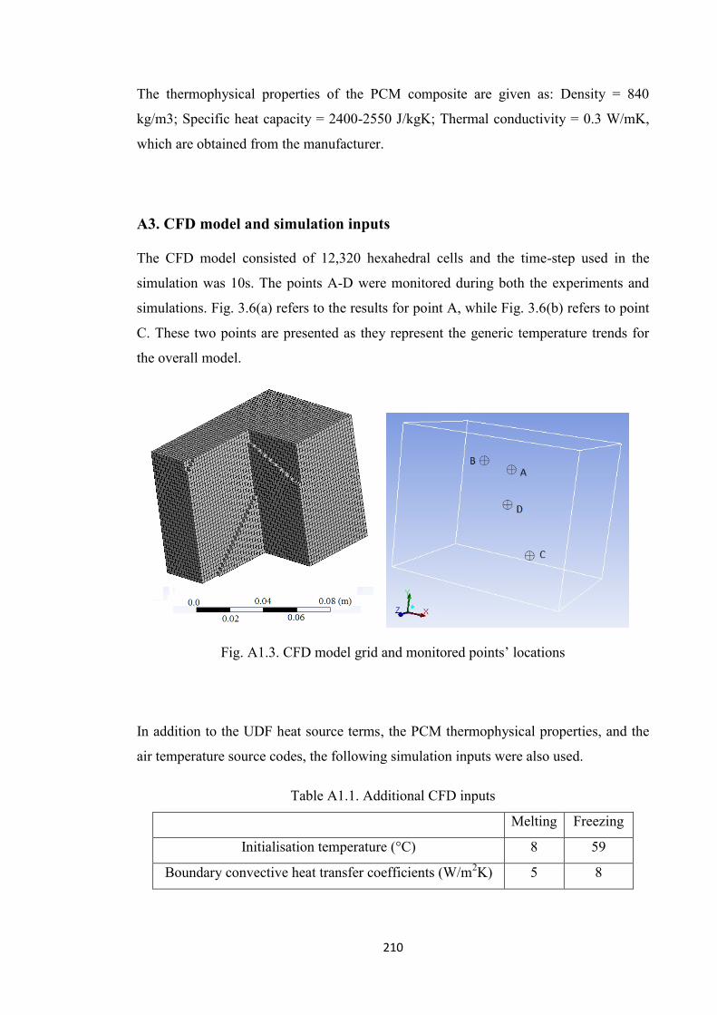
210

The thermophysical properties of the PCM composite are given as: Density = 840

kg/m3; Specific heat capacity = 2400-2550 J/kgK; Thermal conductivity = 0.3 W/mK,

which are obtained from the manufacturer.

A3. CFD model and simulation inputs

The CFD model consisted of 12,320 hexahedral cells and the time-step used in the

simulation was 10s. The points A-D were monitored during both the experiments and

simulations. Fig. 3.6(a) refers to the results for point A, while Fig. 3.6(b) refers to point

C. These two points are presented as they represent the generic temperature trends for

the overall model.

Fig. A1.3. CFD model grid and monitored points’ locations

In addition to the UDF heat source terms, the PCM thermophysical properties, and the

air temperature source codes, the following simulation inputs were also used.

Table A1.1. Additional CFD inputs

Melting Freezing

Initialisation temperature (°C) 8 59

Boundary convective heat transfer coefficients (W/m2K) 5 8

211

The boundary convective heat transfer coefficients were obtained as part of the

validation process.

A4. RMS error equations

The mean absolute RMS error is obtained by comparing the numerical (num) and

experimental (exp) temperatures of the PCM for the same time (t).

Mean absolute RMS error =

(A1.8)

The mean relative RMS error was obtained by dividing the mean absolute RMS error by

the mean absolute overall temperature difference over the four monitored points.

Relative RMS error= [Mean absolute RMS error / –

]×100 (A1.9)

Where ‘np’ refers to the points (A-D) monitored. In this case, the total number for np =

4.

212

Appendix B: Validity and effectiveness of CFD

This appendix provides supporting information on the validation study conducted in

chapter 4. It describes the experimental procedure and the numerical model employed.

(Note that this study is fully published in Gowreesunker and Tassou (2013a) –

“Effectiveness of CFD simulation for the performance prediction of phase change

building boards in the thermal environment control of indoor spaces”.

B1. Description of Experimental Test Cell

This test cell was constructed so as to provide experimental data to allow an appropriate

validation of the CFD model. It was therefore constructed to closely match the thermal

properties of an actual building.

One of the main aims of employing PCM panels is to enhance the thermal mass of a

particular building. As a result, the choice of material combination for the test cell

envelope was highly emphasised. The thermal mass was quantified in terms of the

decrement factor and the time lag of the wall, calculated using the CIBSE admittance

method. To simplify the calculation of the dynamic thermal properties, the Dynamic

Thermal Property Calculator V1.0 (developed by ‘The Concrete Centre’) was

employed. After various material combinations, the following wall configuration was

chosen (see Fig. B1.1). The internal wall surfaces were plastered and painted white.

Fig. B1.1. Test Cell Wall Configuration

213

Adopting such material configuration provided thermal properties close to a Timber

Frame Wall with plasterboard (CIBSE guide A, 2006), as shown in Table B1.1.

Table B1.1. Dynamic thermal properties of Walls

Thermal Properties CIBSE Timber Frame Wall Experimental Test Cell

U-value (W/m2K) 1.14 0.21

Decrement Factor (-) 0.7 0.81

Time lag (hr) 4.9 4.8

Note that in this case, the U-value of the test cell walls was adjusted to abide by the

2010 Building Regulations Part L2A: Notional U-value of < 0.26 W/m2K for non-

dwellings’ walls. Nonetheless, Table B1.1 shows that the dynamic properties of the test

cell wall are relatively close to those of an actual wall.

A glazing of U-value 1.2 W/m2K (4-16-4 mm, Argon filled) was incorporated in the

design in order to represent the large glazed areas usually found in Airport Terminals.

The thermophysical properties of the materials are shown in Table B1.2.

Table B1.2. Material properties from manufacturer

Properties PCM

board Wood

Rigid PIR

Insulation

Glazing –

24mm (90% Ar

filled)

Plaster

Density (kg/m3) 1430 500 40 140 950

Specific heat capacity

(J/kgK) 1240 1300 1600 840 840

Thermal conductivity

(W/mK) 0.14 0.13 0.023 0.03 0.16

214

B2. Equipment used and Uncertainties

The main parameter monitored during the experiments was the surface and air

temperatures, where various Type T thermocouples were uniformly placed within the

test cell as shown in Fig. B1.2. The environmental chamber air temperature was also

monitored using a Type T thermocouple with an error of ± 0.2K.

Fig. B1.2. Location, description and uncertainty of air and surface thermocouples

These thermocouples were calibrated together with their respective Pico TC-08® data

loggers using a F250 mk2® precision thermometer (±0.1K) in a water/glycol bath for a

temperature range of 2-50 °C. The air thermocouples in the test cell were placed at 5cm

from the wall surface, whilst the surface thermocouples were covered with a thin layer

of plaster.

An axial fan was placed at the inlet to blow external air into the chamber for the night

ventilation recharge. The air velocity was measured using a TSI hot-wire velocity meter

with an accuracy of ± 0.015m/s. The inlet and outlet were sealed during the heating

period and the non-ventilated night condition.

215

B3. Phase change implementation of PCM board

Due to the non-uniform distribution of the Micronal® PCM granules in the clay board,

three different random samples were taken from the boards and used in the DSC

characterisation of the phase change. The phase change properties of the board were

analysed using the Perkin Elmer DSC 6000®, which possess an uncertainty of ±0.1 K

for the temperature and ±2 % of the enthalpy change. The DSC was industry calibrated

using Indium and Zinc standards.

The DSC data for each sample are shown in Table 4.1. The phase change temperatures

and enthalpies at a heating/cooling rate were considered for each sample, as the data

were within the error limits of the DSC.

The enhanced phase change model described in chapter 3 and Appendix A was

employed in this simulation. Polynomials were fitted to the melting and freezing curves

of each sample, and were implemented in the CFD model as User Defined Functions

(UDF). The errors associated with the curve fits are shown in Table B1.3.

Table B1.3. Regression coefficient, enthalpy uncertainty in h-T curve fits and total

uncertainty in enthalpy at heating/cooling rate of 0.5 K/min

Melting Freezing

Sample R2 ∆hcurve-fit ∆htotal R

2 ∆hcurve-fit ∆htotal

S-1 0.999 ± 0.065 kJ/kg ±0.360 kJ/kg 0.998 ± 0.350 kJ/kg ±0.700 kJ/kg



∆htotal = ∆hcurve-fit + ∆hDSC (B1.1)

Where:

∆hcurve-fit = uncertainty in enthalpy associated with the curve fitting of the experimental

DSC data for different samples over the phase change range. This is obtained through

the comparison of the DSC data and data calculated by the curve-fit equation

∆hDSC = uncertainty associated with the DSC or 2% of enthalpy value

216

The resulting enthalpy-temperature curves for sample S-3 (with the lowest errors) are

given in Fig. B1.3.

Fig. B1.3. Melting and freezing curves of sample S-3 and the enthalpy-porosity model

Correspondingly, the equations for the polynomial curves for S-3 h-T relations are:

f(T)m = 12.781736 T3 – 10932.541511 T

2 + 3117074.922039 T –

296256708.8957 (R2 = 0.999)

(B1.2)

- f(T)f = 13.026531 T3 – 11055.072091 T

2 + 3129090.962073 T –

295246573.26512 (R2 = 0.998)

(B1.3)

B4. L2 norm study

In building simulations especially, because of the large spaces to be simulated, it is

inconvenient to abide by the usual grid and time-step criteria of Courant number < 5

(FLUENT User guide, 2010), which often require very small grid size and small time-

steps. These would significantly impact on the simulation times, or even make the use

of CFD impractical.

The L2 norm study is a grid and time-step sensitivity analysis to determine the

appropriate mesh and time-step levels appropriate for a particular model. It was

employed here to determine the errors associated with different grid sizes and time-

217

steps, and to justify the use of larger grid and time-step sizes. (The temperature and

velocity norms are considered in this study)

L2 norm =

(B1.4)

Where:

Vi = volume of cells

φi discrete = Temperature or velocities obtained from the discretised Governing Equations

φi exact = Temperature or velocities obtained from the exact solution of the Governing

Equations

As the exact solution of the governing equations is not known, the results of a

simulation with a uniformly very fine mesh (850,000 elements) and time step (10s)

were taken as the benchmark. Three meshes: coarse (140,000 elements); medium

(212,500 elements); and fine (283,000 elements), and three time-steps: 500s; 200s; and

100s were considered in this model independence study. Mesh refinement was

performed by varying all mesh sizes by the same ratio, but maintaining the inflation

parameters (Gowreesunker and Tassou, 2013a).

The L2 norm was computed for uniformly distributed points, 0.2m apart, over the three

planes (across the inlet, outlet and heater) shown in Fig. B1.4, and for 1000s intervals

for the ventilated case, which consists of both buoyancy driven and forced convection

flows. The default FLUENT residual convergence criteria were employed for all

simulations.

218

Fig. B1.4. L2-planes and L2-norm for temperature and velocities

Fig. B1.4 shows that the temperature and velocity norms are more dependent on the

time-step than the mesh size. A temperature convergence criteria of 0.2-0.4 K was used,

based on the uncertainty of the thermocouples, while 0.015 m/s was used for the

velocity convergence criteria based on the accuracy of the TSI velocity meter used in

the experiment. Under these conditions, the temperature criterion is satisfied with the

Fine-100s, Fine-200s and Medium-100s setups, and the velocity criterion is satisfied by

the Medium-100s and Fine-100s setups. Thus to minimise computational time, the

Medium-100s setup was employed for the simulations. Both the ventilated and non-

ventilated cases were simulated on the same grid with an average y+ value of 6. The

employed mesh is shown in Fig. 4.6.

219

B5. Numerical considerations

The validation errors were quantified in terms of the absolute Root Mean Square (RMS)

error and the relative RMS errors, for each thermocouple and for each sample modelled.

(B1.5)

The relative error is defined by Eq. (B1.6):

(B1.6)

Where:

Texp: Experimental Temperature (K or °C)

Tnum: Numerical Temperature (K or °C)

U thermocouple: Uncertainty of Local thermocouple (K or °C)

t: time (s)

Nt: Number of time-steps

The relative RMS error represents the overall local relative error in the transient

simulation and is based on the smallest peak local experimental temperature difference

obtained during the test cell heating/cooling cycle. This calculation method is analogous

to the validation procedure used in Zhang et al. (2007), where the authors based the

steady state relative errors on the temperature difference between the outlet/inlet,

local/environment or cold/hot surfaces. However due to the transient nature of this

study, the relative errors are hereby defined in a different way. The smallest local

experimental temperature difference in Eq. (B1.6) refers to the smallest difference

between the start/peak or peak/end temperatures of the experiment, where the ‘small’

nature of the difference provides a more conservative error evaluation. The errors can be

found in Fig. 4.7 and Fig. 4.8.

Furthermore, the convective heat transfer coefficient for the ventilated night charging is

given by Eq. (B1.7)

220

(B1.7)

Where:

: Area-weighted walls’ heat flux (W/m2)

Tinlet : Air inlet/ Reference temperature (K)

: Area-weighted walls’ surface temperature (K)

Nt : Number of time-steps

Figs. B1.5 to B1.10 show some generic temperature trends obtained in the validation

process.

For the Non-Ventilated Scenario:

Fig. B1.5. TA-4 Non-ventilated experimental and simulated temperatures

221

Fig. B1.6. TS-5 Non-ventilated experimental and simulated temperatures

Fig. B1.7. TS-6 Non-ventilated experimental and simulated temperatures

For the Ventilated Scenarios:

Fig. B1.8. TA-4 Ventilated experimental and simulated temperatures

222

Fig. B1.9. TS-5 Ventilated experimental and simulated temperatures

Fig. B1.10. TS-6 Ventilated experimental and simulated temperatures

223

Appendix C: Development of optical phase change model

This appendix provides supporting information used in the development of the optical

phase change model described in chapter 5.

C1. Description of experimental setup and procedure

The experimental setup was devised in order to obtain the gray transmittance values of

the PCM for different irradiation level and at different temperatures. The setup

consisted of a 150W metal halide lamp, a reflector casing, a pyranometer and the

investigated glazed surface, as shown in Fig. C1.1, placed inside an environmental

chamber where the surrounding temperature was monitored and controlled. The internal

side of the reflector casing had a dimension of 200×200×500mm, and was lined with

reflective aluminium tape. The double glazing was air filled, with dimensions 4-16-4

mm and a U-value of 2.8 W/m2K. The purpose of the reflector casing was to limit the

loss in radiation transfer between the glazed surface and the pyranometer. Furthermore,

it also served to ‘focus’ the transmitted radiation to the pyranometer.

Fig. C1.1 Experimental

setup for optical tests

The tests were conducted by placing the entire setup in the environmental chamber for

24 hours prior to the start of the test. This allowed the temperature of all the components

to reach the same steady level, which is essential for the appropriate initialisation of the

numerical model and to ensure that the temperature of the PCM is known. Note that

there were no thermocouples within the PCM so as to avoid nucleation issues.

224

The irradiation levels were recorded with a ‘no-glazed’ surface, a standard double

glazed unit and the PCM glazed unit (for a period varying between 5-9 hrs, or until

steady state). The main parameter employed for the development of the model is the

radiation transmittance, which is obtained from Eqs. C(1.1-1.3), where the transmitted

radiation intensity for non-glazed/empty specimen, double glazed and PCM-glazed

surfaces are (G), (Gτ-gl) and (Gτ-gl-PCM), respectively (Gowreesunker et al. 2013c).

(C1.1)

(C1.2)

(C1.3)

The transmitted radiation for the PCM-glazed unit (Gτ-gl-PCM) was taken at the beginning

of each experiment, after having applied stable irradiation to the glazing. It corresponds

to the lowest transmitted irradiation level at the corresponding surrounding

environmental chamber temperature, before the PCM starts to melt. In this way, a

transmittance value was assigned to the temperature of the PCM, which then allowed

calculating the extinction coefficients.

C2. Thermal characterisation of RT27

The thermal characterisation of RT27 was conducted by Stanislava B. Stankovic (from

City University), according to the University Collaboration scheme under which this

Project was based on.

Having obtained the enthalpy-temperature curves (shown in Fig. 5.3), the effective heat

capacity was calculated from the derivative of the mean enthalpy curve. The liquid

fraction variation was obtained by fitting a polynomial to the curvature of the mean

enthalpy curve from Fig. 5.3, using the method described in Gowreesunker et al.

(2012). Hysteresis was neglected.

225

These resulted in the following equations employed in the numerical validation of the

study (The cp in the fully liquid and solid states are constant) – Temperatures (T) in °C:

For 15°C ≤ T < 26 °C;

cp eff (T) = 0.01202 T4 - 0.9113 T

3 + 25.83499 T

2 - 323.96615 T + 1519.21328

(kJ/kg⋅K) (R2 = 0.994)

(C1.4)

For 26 °C ≤ T ≤ 27.94°C;

cp eff (T) =-7.34132 T2 + 376.54918 T - 4786.72094

(kJ/kg⋅K) (R2=1.000)

(C1.5)

β = (4.39×10-5⋅T4

) – (2.92×10-3⋅T3

) + (7.38×10-2⋅T2

) – (8.25×10-1⋅T) + 3.42

(R2= 0.991)

(C1.6)

The onset and end temperatures of the phase change process can be verified from Fig.

C1.2(a).

Fig. C1.2(a). Heat released-stored in given temperature intervals for RT27; HR – Heat

released; HS – Heat stored.(Gowreesunker et al, 2013c)

13 15 17 19 21 23 25 27 29 31 33 350

10

20

30

40

Hea

t re

leas

ed-s

tore

d/k

Jkg-1

13 15 17 19 21 23 25 27 29 31 33 350

10

20

30

40

Temperature/°C

HR

HS

226

C3. Calculation of the optical properties of RT27

(The following relations have been fully explained in the published paper from the

author; Gowreesunker et al. (2013c) – “Experimental and numerical investigations of

the optical and thermal aspects of a PCM-Glazed unit” – and all references can be found

in the mentioned paper.)

This section aims at showing the general procedure followed for the development of the

optical model of phase change. The experiments were carried out with irradiation

intensities of 950 W/m2, 550 W/m

2 and 260 W/m

2, and temperatures ranging from 13

°C to 29 °C, in order to span the entire phase change range of the PCM. Employing Eq.

(C1.7), the extinction coefficients (σε) of RT27 at different temperatures and irradiation

level were calculated (where ‘s’ is the physical thickness of the PCM: 16mm for the

PCM-glazed unit; or 10mm for the spectrophotometry measurements). Furthermore, it

is known that the extinction coefficient is the sum of the absorption (σa) and scattering

coefficients (σs), hence Eq. (C1.8).

Log10 (τpcm) = -(σε × s) (C1.7)

σε = σs + σa (C1.8)

However the issue in this formulation lies in the separation of the σa and σs terms in

order to understand the thermal aspect of the radiation process. From the study by

Weinlader et al. (2004) and as observed from this study, the PCM is non-scattering,

clear and transparent in the liquid phase, and the increase in opacity as the PCM

changes to solid is largely associated to the scattering process. This observation was

subsequently adopted to dissect the extinction coefficient into the scattering and

absorption coefficients, by assuming that the scattering process dominates during the

solid phase and that the liquid phase is non-scattering.

This led to the definition of a new parameter (δ) which represents the minimum

radiation absorption in the solid phase of the PCM. Thus, working from the hypothesis

that the change of transmittance varies with the liquid fraction, and that scattering

dominates in the solid phase whilst absorption dominates in the liquid phase, the

following relations were developed.

227

(C1.9)

(C1.10)

Where:

(C1.11)

σε = (β⋅σε,liq) + (1-β)⋅(σε,sol) (C1.12)

It can be implied that the development of the optical relations followed a reverse

engineering approach, where the relations were postulated from previous studies and

hypotheses, and the verification process was then based on experimental data and

numerical simulations. The experimental verification of the variation in extinction

coefficient is shown in Fig. C1.2b, and the numerical validation is shown in section 5.2.

Fig. C1.2(b) Mean experimental extinction coefficients and extinction coefficients using

the relationship Eq. (C1.6) and Eq. (C1.12)

228

C4. Error calculations

The experimental calculation for the extinction coefficient (σε) absolute uncertainty was

determined from the general uncertainty propagation equation, in reference to Eq.

(C1.7), producing Eq. (C1.13).

(C1.13)

Where Uσε is the absolute uncertainty in the scattering coefficient, τ is the transmittance

value, and Uτ is the absolute uncertainty in transmittance.

The error from the thickness was neglected because it could not be obtained from the

glass manufacturer. The uncertainty in the transmittance Uτ for each irradiation level

was calculated as follows, based on the uncertainties of the employed apparatus.

Table C1.1. Sensor uncertainties and sensitivities

Sensors uncertainty and sensitivity

Sensitivity of pyranometer (η) 0.0137 mV / Wm-2

Uncertainty in pyranometer ± 0.03 mV

Accuracy of data logger 0.2% + 0.01 mV

Uncertainty in Air Temperature ± 0.4 °C

The following equations were developed based on Eq. (C1.1) – Eq. (C1.3), where ‘V’ is

the recorded voltage from the pyranometer and ‘G’ are the respective irradiation

intensities;

(C1.14)

(C1.15)

229

(C1.16)

The experimental uncertainties presented in Fig. 5.6a were obtained from Eq. (C1.15).

The uncertainties in the extinction coefficient presented in Fig. C1.2b were obtained

from Eq. (C1.13), where the absolute mean uncertainty in transmittance (Uτ) was

calculated from Eq. (C1.16).

230

Appendix D: Numerical conditions

This appendix provides supporting material for chapter 6 of this study, relating to the

numerical procedure employed for the performance evaluation of the PCM systems.

D1. HVAC sizing methodology

The sizing of the HVAC system was performed based on the mean steady state thermal

loads of the airport terminal departure hall. Displacement conditioning systems are

more efficient than mixed conditioning systems, because they are able to direct their

cooling potential towards the conditioned space, as opposed to conditioning the entire

space. According to Simmonds et al. (2000), 1 person occupies 4 m2 in an airport

terminal, and therefore based on the 48 m2 floor area simulated in the 2D case, there are

12 persons at any one time in the terminal. However, the heat gains provided by these

occupants vary according to Fig. 6.3. Furthermore, based on the fresh air requirement

from CIBSE guide A (2006) of 15 L/s/person for a high indoor air quality, the total

fresh air requirement of 0.2 kg/s for the 12 occupants. (Note that the 2D thickness of the

CFD case is 1m)

Hence, for cooling purposes, the sizing is done mainly by focusing on the heat loads in

the conditioned space i.e. up to a height of 2m from the floor:

1. Mean internal heat gains = 25 W/m2 ×48 m

2 = 1200 W

2. Mean solar gains on the floor from glazing and roof for UK weather = 350 W/m2

× [(9×0.5)+(62×0.01)] m2

× 0.5 = 896 W

3. Ambient air ventilation heat gain = 8 K × 0.2 kg/s × 1002 J/kgK= 1603 W

Hence the mean cooling load is found to be: 3.7 kW

Conversely, for heating purposes, the displacement conditioning system behaves similar

to a mixed ventilation system, due to the buoyancy effects of the low velocity inlet air at

high temperature. Hence for heating purposes:

1. Mean Convective heat losses from roof and glazing = 20 K × 1 W/m2K × (9+62)

m2 = - 1420 W

2. Solar gains are neglected

3. Mean internal heat gains = 25 W/m2 ×48 m

2 = 1200 W

231

4. Ambient air ventilation heat loss = 18 K × 0.2 kg/s × 1002 J/kgK = - 3608 W

Hence the mean heating load is found to be - 3.8 kW

(Where: 8 K and 18 K are assumed temperature difference between the ambient and the

indoor environments for cooling and heating purposes, respectively; 1002 J/kgK is the

specific heat capacity of air; 0.5 is the radiation transmittance of the glazing and the

radiation absorption of the floor; 0.01 is the radiation transmittance of the roof; 48, 9

and 62 m2 are the floor, glazing and roof areas, respectively – refer to Table 6.1 for

more information)

As a result, in order to allow the control system to have more flexibility on its influence

on the indoor environment, both the heating and cooling units were sized at 4 kW. In

this way, the controller could have a higher potential in controlling the indoor thermal

environment, by having a higher range to adjust the supply air temperature.

Considering a load of 4kW and a temperature difference of 8K across the heating and

cooling coils, the total mass flow rate across both units was found to be 0.5 kg/s.

Furthermore, in displacement conditioning systems, because the diffusers are relatively

close to the occupants, the air supply velocity is important in providing adequate

thermal comfort. In this case, the air velocity in the conditioned zone should not

generally exceed 0.25 m/s for moderate thermal environments (CIBSE B, 2006),

although Fanger’s equation allows a maximum of 0.4 m/s (Fanger, 1970) for a clothing

factor of 1.15 and temperatures of 18-23 °C, typical of an airport terminal building

(CIBSE A, 2006). Thus, as shown in the results section of the study, the mean velocities

of the air in the conditioned zone are in the range of 0.15 and 0.3 m/s, abiding by the

velocity comfort requirements and confirming the velocity comfort aspect of the

Displacement Conditioning system.

Furthermore, as this HVAC system is a constant air volume (CAV) system, the mixing

ratio of fresh and return air, in the supply air is constant. Thus: Fresh air flow rate = 0.2

kg/s; Return supply air flow rate = 0.3 kg/s; and Total air flow rate = 0.5 kg/s, with a 4

kW cooling and heating capacity.

232

D2. TRNSYS Screen-Shot for the normal DV HVAC system

233

D3. TRNSYS program file

TRNSYS - the TRaNsient SYstem Simulation program

The Solar Energy Lab at the University of Wisconsin - Madison, USA

Le Centre Scientifique et Technique du Batiment, Sophia Antipolis, France

Transsolar Energietechnik GmBH, Stuttgart, Germany

Thermal Energy System Specialists, LLC, Madison Wisconsin, USA

Release 17.00.0019

Listing file for: "D:\ACTIVEsystem\DV-freshair-floor\DV-HVAC-after-mixing.dck"

*** Notice at time : 0.000000

Generated by Unit : Not applicable or not available

Generated by Type : Not applicable or not available

Message : The TRNSYS Executable (TRNExe.exe) and main DLL (TRNDll.dll) are located in

"C:\Trnsys17\Exe"



Generated by Type : 208

TRNSYS Message 75 : The Type referenced below requires descriptors instead of initial values.

Reported information : Type 208




TRNSYS Message 75 : The Type referenced below requires descriptors instead of initial values.





TRNSYS Message 76 : The following Type has been identified as allowing the unit specifications

(kg/h for example) after the input specifications and initial values for the inputs. The critical parameter

number, and the value of this critical parameter that indicates that the units will be supplied is also listed.

This information was retrieved from the VarUnits.dat file located in the \Exe directory of your TRNSYS

16 installation.

Reported information : Type 580, Critical Parameter 11, Parameter Value 1




TRNSYS Message 88 : The following Type has been identified as allowing FORMAT statements.

This information was retrieved from the Formats.dat file located in the \Exe directory of your TRNSYS

16 installation.


*** Pre-Processing the TRNSYS EQUATIONs and CONSTANTs to check for fatal errors.

*** Pre-Processing of EQUATIONs and CONSTANTs completed with no fatal errors found.

*** Evaluating the EQUATIONs and CONSTANTs to determine their initial values.

*** Finished evaluating the EQUATIONs and CONSTANTs and ready to begin processing the

remainder of the TRNSYS input file.

234

VERSION 17

*******************************************************************************

*** TRNSYS input file (deck) generated by TrnsysStudio

*** on Tuesday, February 19, 2013 at 10:27

*** from TrnsysStudio project: D:\ACTIVEsystem\DV-freshair-floor\DV-HVAC-after-mixing.tpf

***

*** If you edit this file, use the File/Import TRNSYS Input File function in

*** TrnsysStudio to update the project.

***

*** If you have problems, questions or suggestions please contact your local

*** TRNSYS distributor or mailto:[email protected]

***

*******************************************************************************

*******************************************************************************

*** Units

*******************************************************************************

*******************************************************************************

*** Control cards

*******************************************************************************

* START, STOP and STEP

CONSTANTS 3

START=4500

STOP=4600

STEP=0.1

* User defined CONSTANTS

! Start time End time Time step

SIMULATION 4.5000000000000000E+03 4.6000000000000000E+03 1.0000000000000001E-

01

! Integration Convergence

TOLERANCES 1.0000000000000002E-03 1.0000000000000002E-03

! Max iterations Max warnings Trace limit

LIMITS 30 500 51

! TRNSYS numerical integration solver method

DFQ 1

! TRNSYS output file width, number of characters

WIDTH 80

! NOLIST statement

LIST

! MAP statement

! Solver statement Minimum relaxation factor Maximum relaxation factor

SOLVER 0

1.000000000000000

1.000000000000000

! Nan DEBUG statement

NAN_CHECK 0

! Overwrite DEBUG statement

OVERWRITE_CHECK 0

! disable time report

TIME_REPORT 0

235

! EQUATION SOLVER statement

EQUATION SOLVING METHOD 0

* Model "Type15-6" (Type 15)

*

UNIT 3 TYPE 15

*$UNIT_NAME Type15-6

*$MODEL .\Weather Data Reading and Processing\Standard Format\Meteonorm Files (TM2)\Type15-

6.tmf

*$POSITION 93 468

*$LAYER Weather - Data Files #

PARAMETERS 9

! 1 File Type

! 2 Logical unit

! 3 Tilted Surface Radiation Mode

! 4 Ground reflectance - no snow

! 5 Ground reflectance - snow cover

! 6 Number of surfaces

! 7 Tracking mode

! 8 Slope of surface

! 9 Azimuth of surface

6.0000000000000000E+00 3.4000000000000000E+01 3.0000000000000000E+00

2.0000000000000001E-01 7.0000000000000007E-01

1.0000000000000000E+00 1.0000000000000000E+00 9.0000000000000000E+01

0.0000000000000000E+00

*** External files

ASSIGN C:\Trnsys17\Weather\Meteonorm\Europe\GB-London-Weather-C-37790 - Copy - Copy.tm2

34

*|? Which file contains the Meteonorm weather data? |1000

*------------------------------------------------------------------------------

* Model "Type25c" (Type 25)

*

UNIT 16 TYPE 25

*$UNIT_NAME Type25c

*$MODEL .\Output\Printer\Unformatted\No Units\Type25c.tmf

*$POSITION 1030 244

*$LAYER Outputs #

PARAMETERS 10

! 1 Printing interval

! 2 Start time

! 3 Stop time

! 4 Logical unit

! 5 Units printing mode

! 6 Relative or absolute start time

! 7 Overwrite or Append

! 8 Print header

! 9 Delimiter

! 10 Print labels

1.0000000000000001E-01 4.5000000000000000E+03 4.6000000000000000E+03

3.6000000000000000E+01 0.0000000000000000E+00

0.0000000000000000E+00 -1.0000000000000000E+00 -1.0000000000000000E+00

0.0000000000000000E+00 1.0000000000000000E+00

INPUTS 10

! Controller ratio:AmbientinK ->Input to be printed-1

! Controller ratio:Teff ->Input to be printed-2

! Controller ratio:Actualheating ->Input to be printed-3

! Controller ratio:ActualCooling ->Input to be printed-4

! MainFan:Outlet flow rate ->Input to be printed-5

236

! Recirculating fan:Outlet flow rate ->Input to be printed-6

! Controller ratio:Tm ->Input to be printed-7

! Controller ratio:Treturnn ->Input to be printed-8

! Energy consumption:Energy ->Input to be printed-9

! Energy consumption:TotalEnergy ->Input to be printed-10

AMBIENTINK TEFF ACTUALHEATING ACTUALCOOLING

15,2

19,2 TM TRETURNN ENERGY

TOTALENERGY

*** INITIAL INPUT VALUES

ambient effecttemp Heating Cooli

ng mainfanflow

recirculatingfanflow Tm Treturn Chill

erBoilerJ Total_energy

*** External files

ASSIGN heterar.out 36

*|? Output file for printed results |1000

*------------------------------------------------------------------------------

* Model "Type65c" (Type 65)

*

UNIT 12 TYPE 65

*$UNIT_NAME Type65c

*$MODEL .\Output\Online Plotter\Online Plotter With File\No Units\Type65c.tmf

*$POSITION 934 618

*$LAYER Main #

PARAMETERS 12

! 1 Nb. of left-axis variables

! 2 Nb. of right-axis variables

! 3 Left axis minimum

! 4 Left axis maximum

! 5 Right axis minimum

! 6 Right axis maximum

! 7 Number of plots per simulation

! 8 X-axis gridpoints

! 9 Shut off Online w/o removing

! 10 Logical Unit for output file

! 11 Output file units

! 12 Output file delimiter

1.0000000000000000E+00 2.0000000000000000E+00 2.8000000000000000E+02

3.1000000000000000E+02 -1.0000000000000000E+01

1.8000000000000000E+03 1.0000000000000000E+00 1.2000000000000000E+01

0.0000000000000000E+00 3.5000000000000000E+01

0.0000000000000000E+00 0.0000000000000000E+00

INPUTS 3

! Type425:Point_1 ->Left axis variable

! heater:Control signal ->Right axis variable-1

! Cooler:Control signal ->Right axis variable-2

24,1 8,1 6,1


Zone heat cool

LABELS 3

Temperatures

Heat transfer rates

Graph 1

*** External files

ASSIGN D:\ACTIVEsystem\DV-freshair-floor\DV-HVAC-after-mixing.plt 35

*|? What file should the online print to? |1000

*------------------------------------------------------------------------------

* Model "Cooler" (Type 23)

237

*

UNIT 6 TYPE 23

*$UNIT_NAME Cooler

*$MODEL .\Controllers\PID Controller\Type23.tmf

*$POSITION 483 607

*$LAYER Main #

PARAMETERS 2

! 1 mode

! 2 Maximum number of oscillations

1.0000000000000000E+00 3.0000000000000000E+00

INPUTS 13

! Feedback temp:Tset ->Setpoint

! Feedback temp:Feedback ->Controlled variable

! Feedback temp:cooler ->On / Off signal

! [unconnected] Minimum control signal

! [unconnected] Maximum control signal

! [unconnected] Threshold for non-zero output

! [unconnected] Gain constant

! [unconnected] Integral time

! [unconnected] Derivative time

! [unconnected] Tracking time for anti-windup

! [unconnected] Fraction of ySet for proportional effect

! [unconnected] Fraction of ySet for derivative effect

! [unconnected] High-frequency limit on derivative

TSET FEEDBACK COOLER CONST ING CONST

CONST CONST CONST CONST CONST Y

CONST CONST CONST


0.0000000000000000E+00 0.0000000000000000E+00 0.0000000000000000E+00

0.0000000000000000E+00 1.0000000000000000E+00

0.0000000000000000E+00 -1.0000000000000001E-01 1.0000000000000001E-01

1.0000000000000001E-01 -1.0000000000000000E+00

1.0000000000000000E+00 1.0000000000000000E+00 1.0000000000000000E+01

*------------------------------------------------------------------------------

* Model "heater" (Type 23)

*

UNIT 8 TYPE 23

*$UNIT_NAME heater

*$MODEL .\Controllers\PID Controller\Type23.tmf

*$POSITION 419 692

*$LAYER Main #

PARAMETERS 2

! 1 mode

! 2 Maximum number of oscillations

1.0000000000000000E+00 3.0000000000000000E+00

INPUTS 13

! Feedback temp:Tset ->Setpoint

! Feedback temp:Feedback ->Controlled variable

! Feedback temp:heater ->On / Off signal

! [unconnected] Minimum control signal

! [unconnected] Maximum control signal

! [unconnected] Threshold for non-zero output

! [unconnected] Gain constant

! [unconnected] Integral time

! [unconnected] Derivative time

! [unconnected] Tracking time for anti-windup

! [unconnected] Fraction of ySet for proportional effect

! [unconnected] Fraction of ySet for derivative effect

238

! [unconnected] High-frequency limit on derivative

TSET FEEDBACK HEATER CONST ING CONST

CONST CONST CONST CONST CONST Y

CONST CONST CONST


0.0000000000000000E+00 0.0000000000000000E+00 0.0000000000000000E+00

0.0000000000000000E+00 1.0000000000000000E+00

0.0000000000000000E+00 1.0000000000000001E-01 1.0000000000000001E-01

1.0000000000000001E-01 -1.0000000000000000E+00

1.0000000000000000E+00 1.0000000000000000E+00 1.0000000000000000E+01

*------------------------------------------------------------------------------

* EQUATIONS "Feedback temp"

*

EQUATIONS 9

heater = (LT([24,1], 293))*[17,3]

Tset = 294

cooler = (GT([24,1], 295))*[17,3]

intermediate = (1-(heater+cooler))*[17,3]

! Mass flow rate of air - mass flow rate of fresh air

Massflowrate = 0.3

!mass flow rate of fresh air

freshmass = 0.2

Ventflow = (Massflowrate+freshmass)*[17,3]

Feedback = [24,1]

! because outlet is 4 m^2 surface area

MassFlux = Ventflow/4

Lightgain = (5/0.008)*[17,3]

*$UNIT_NAME Feedback temp

*$LAYER Main

*$POSITION 359 509

*------------------------------------------------------------------------------

* Model "Type9e" (Type 9)

*

UNIT 17 TYPE 9

*$UNIT_NAME Type9e

*$MODEL .\Utility\Data Readers\Generic Data Files\Expert Mode\Free Format\Type9e.tmf

*$POSITION 90 75

*$LAYER Main #

PARAMETERS 22

! 1 Mode

! 2 Header Lines to Skip

! 3 No. of values to read

! 4 Time interval of data

! 5 Interpolate or not-1

! 6 Multiplication factor-1

! 7 Addition factor-1

! 8 Average or instantaneous value-1












239


! 21 Logical unit for input file

! 22 Free format mode

5.0000000000000000E+00 0.0000000000000000E+00 4.0000000000000000E+00

1.0000000000000000E+00 -1.0000000000000000E+00

1.0000000000000000E+00 0.0000000000000000E+00 1.0000000000000000E+00

1.0000000000000000E+00 1.0000000000000000E+00

0.0000000000000000E+00 1.0000000000000000E+00 -1.0000000000000000E+00

1.0000000000000000E+00 0.0000000000000000E+00

1.0000000000000000E+00 -1.0000000000000000E+00 1.0000000000000000E+00

0.0000000000000000E+00 1.0000000000000000E+00

3.7000000000000000E+01 -1.0000000000000000E+00

*** External files

ASSIGN Trial.txt 37

*|? Input file name |1000

*------------------------------------------------------------------------------

* EQUATIONS "Controller ratio"

*

EQUATIONS 19

!Converts ambient temperature in Kelvin

AmbientinK = [3,1]+273.15

QheatSet = heater*2000

!Maximum cooling capacity of auxiliary cooling coil

QcoolSet = cooler*(-4000)

Returnflow = Massflowrate

!Mass flow rate of fresh air

mf = freshmass

Ratiofresh = (mf/(mf+Returnflow))*[17,3]

Ratioreturn = (1-Ratiofresh)*[17,3]

ActualCooling = QcoolSet*[6,1]

Actualheating = QheatSet*[8,1]

Totalmassflow = mf+Returnflow

!Specific heat of air

cpa = 1002

Tm = (Ratiofresh*AmbientinK)+((Ratioreturn)*[24,2])

Tsupheat = heater*((Actualheating/(Totalmassflow*cpa))+Tm)

Tsupcool = cooler*((ActualCooling/(Totalmassflow*cpa))+Tm)

Tsupinter = Tm*intermediate

Treturnn = [24,2]

Teff = ((Tsupheat+Tsupcool+Tsupinter)*[17,3])+([17,4]*[24,2])

intermmediatecf = intermediate

Acnorrmal = [17,3]

*$UNIT_NAME Controller ratio

*$LAYER Main

*$POSITION 605 392

*------------------------------------------------------------------------------

* Model "MainFan" (Type 3)

*

UNIT 15 TYPE 3

*$UNIT_NAME MainFan

*$MODEL .\Hydronics\Fans\Variable Speed\No Humidity\Type3a.tmf

*$POSITION 815 394

*$LAYER Air Loop #

PARAMETERS 5

! 1 Maximum flow rate

! 2 Fluid specific heat

! 3 Maximum power

! 4 Conversion coefficient

240

! 5 Power coefficient

1.8000000000000000E+03 1.0000000000000000E+00 3.5999999046330000E+06

1.0000000000000001E-01 0.0000000000000000E+00

INPUTS 3

! [unconnected] Inlet fluid temperature

! [unconnected] Inlet mass flow rate

! Controller ratio:Ratiofresh ->Control signal

CONST CONST RATIOFRESH


2.0000000000000000E+01 0.0000000000000000E+00 0.0000000000000000E+00

*------------------------------------------------------------------------------

* Model "Recirculating fan" (Type 3)

*

UNIT 19 TYPE 3 fan

*$UNIT_NAME Recirculating fan

*$MODEL .\Hydronics\Fans\Variable Speed\No Humidity\Type3a.tmf

*$POSITION 823 500

*$LAYER Air Loop #

PARAMETERS 5

! 1 Maximum flow rate

! 2 Fluid specific heat

! 3 Maximum power

! 4 Conversion coefficient

! 5 Power coefficient

1.8000000000000000E+03 1.0000000000000000E+00 3.5999999046330000E+06

1.0000000000000001E-01 0.0000000000000000E+00

INPUTS 3

! [unconnected] Inlet fluid temperature

! [unconnected] Inlet mass flow rate

! Controller ratio:Ratioreturn ->Control signal

CONST CONST RATIORETURN


2.0000000000000000E+01 0.0000000000000000E+00 0.0000000000000000E+00

*------------------------------------------------------------------------------

* EQUATIONS "Energy consumption"

*

EQUATIONS 4

Energy = Acnorrmal*(ActualCooling+Actualheating)

MainFanP = [15,3]

AuxFanP = [19,3]

TotalEnergy = Energy+MainFanP+AuxFanP

*$UNIT_NAME Energy consumption

*$LAYER Main

*$POSITION 1111 562

*------------------------------------------------------------------------------

* EQUATIONS "Heat Gains"

*

EQUATIONS 5

Source = [17,2]*2

!to get W/m2 from kJ/hr m2

Solargain = [3,24]*0.277777778

! glass transmittance * Glass area

Glazeprop = 0.5*9

!Ceiling transmittance * Ceiling area

Ceilingprop = 0.00875*62

Floorflux = (Glazeprop+Ceilingprop)*(Solargain/48)*(1/0.1)*(0.5)

*$UNIT_NAME Heat Gains

241

*$LAYER Main

*$POSITION 273 40

*------------------------------------------------------------------------------

* Model "Type69b" (Type 69)

*

UNIT 22 TYPE 69

*$UNIT_NAME Type69b

*$MODEL .\Physical Phenomena\Sky Temperature\calculate cloudiness factor\Type69b.tmf

*$POSITION 71 255

*$LAYER Main #

PARAMETERS 2

! 1 mode for cloudiness factor

! 2 height over sea level

0.0000000000000000E+00 0.0000000000000000E+00

INPUTS 4

! Type15-6:Dry bulb temperature ->Ambient temperature

! Type15-6:Dew point temperature ->Dew point temperature at ambient conditions

! Type15-6:Horizontal beam radiation ->Beam radiation on the horizontal

! Type15-6:Sky diffuse radiation on the horizontal ->Diffuse radiation on the horizontal

3,1 3,2 3,19 3,20


0.0000000000000000E+00 2.0000000000000000E+01 0.0000000000000000E+00

0.0000000000000000E+00

*------------------------------------------------------------------------------

* EQUATIONS "Radiation"

*

EQUATIONS 8

AmbientK = [3,1]+273.15

sigma = 5.67/(10*10*10*10*10*10*10*10)

!Converting to W/m2

Solar = [3,24]* 0.277777778

RadT4 = (Solar/sigma)+(AmbientK**4)

RadT = RadT4**0.25

skysignal = LE(Solar,1)

NightskytempK = [22,1]+273.15

effectiveskyTK = ((skysignal*NightskytempK)+((1-skysignal)*RadT))

*$UNIT_NAME Radiation

*$LAYER Main

*$POSITION 313 136

*------------------------------------------------------------------------------

* Model "CFD" (Type 425)

*

UNIT 24 TYPE 425

*$UNIT_NAME Type425

*$MODEL .\My Components\Type425.tmf

*$POSITION 550 148

*$LAYER Main #

PARAMETERS 4

! 1 Mode

! 2 No_of_inputs

! 3 No_of_outputs

! 4 Calling_mode

1.0000000000000000E+00 8.0000000000000000E+00 2.0000000000000000E+00

1.0000000000000000E+00

INPUTS 9

! [unconnected] Control_function

! Radiation:AmbientK ->Outside_air_temp

242

! Heat Gains:Source ->People_gain

! Radiation:effectiveskyTK ->Solar_gain

! Feedback temp:Ventflow ->Mass_flow_rate

! Controller ratio:Teff ->Vent_temp

! Feedback temp:MassFlux ->Out_mass_flux

! Heat Gains:Floorflux ->Floor_gain

! Feedback temp:Lightgain ->light

CONST AMBIENTK SOURCE EFFECTIVESKYTK

VENTFLOW

TEFF MASSFLUX FLOORFLUX LIGHTGAIN


1.0000000000000000E+00 2.9300000000000000E+02 1.0000000000000001E-01

1.0000000000000001E-01 1.0000000000000001E-01

2.9300000000000000E+02 1.0000000000000001E-01 1.0000000000000001E-01

6.2500000000000000E+02

LABELS 4

C:\Program Files\ANSYS Inc\v130\fluent\ntbin\win64\fluent.exe

-r13.0.0 2d -i

waza.in

result.txt

*------------------------------------------------------------------------------

END

TRANSIENT SIMULATION STARTING AT TIME = 4.5000000000000000E+03

STOPPING AT TIME = 4.6000000000000000E+03

TIMESTEP = 1 / 10

DIFFERENTIAL EQUATION ERROR TOLERANCE = 1.0000000000000002E-03

ALGEBRAIC CONVERGENCE TOLERANCE = 1.0000000000000002E-03

DIFFERENTIAL EQUATIONS SOLVED BY MODIFIED EULER




TRNSYS Message 89 : TRNDll.dll is compiled in debug mode. External DLLs will be loaded from

the .\UserLib\DebugDLLs\ directory.

Reported information : Not available




Message : The following Types were loaded from TRNDll.dll: Type15, Type23, Type65,

Type3, Type25, Type9, Type69




Message : "FileReader.dll" was found but did not contain any components from the input file.




Message : "type127.dll" was found but did not contain any components from the input file.

243




Message : "Type157_demo_debug.dll" was found but did not contain any components from

the input file.




Message : "Type412.dll" was found but did not contain any components from the input file.




Message : The following Types were loaded from "Type425.dll": Type425




Message : "Type76Lib.dll" was found but did not contain any components from the input file.




Message : "Type82Lib.dll" was found but did not contain any components from the input file.




TRNSYS Message 199 : TRNSYS found at least one user DLL in the UserLib directory. (Note: Only

DLL's including Types that are used in the simulation are loaded)

Reported information : 1 user DLL was loaded after searching in "C:\Trnsys17\UserLib\DebugDLLs"

244

Appendix E: Pressure drop calculations for the Airport Terminal

space

This appendix provides supporting materials used in the calculation of the HVAC duct

pressure drop. The specific loss coefficients used were obtained from Idelchik (1994).

The different duct-sections can be referred back to Fig. 7.6 and Fig. 7.10, and all ducts

are assumed to be made of galvanised steel. The calculations are for each diffuser, with

an air mass flow rate of 6 kg/s.

Static losses are obtained from (m):

(E1.1)

Specific losses (m):

(E1.2)

Dynamic losses (m):

(E1.3)

Power losses (W): (E1.3)

Where ‘f’ is the friction factor; ‘L’ is the pipe length (m); ‘u’ is the air velocity (m/s);

‘g’ is gravity (9.81 m/s2); ‘ρ’ is the density of air (1.22 kg/m

3); ‘ξ’ is the specific loss

coefficient; ‘h’ is the head loss (m); and is the air volumetric flow rate (m3/s).

E1. Main Supply Duct

Fig. E1.1. Main Supply Duct dP

Diameter of pipe = 0.645m ; Air-velocity = 15 m/s ; Re = 6.17×105 ; (k/d) = 0.00023 ; f

= 0.00385 ; Specific loss coefficient at ‘a’ = 0.22 (for 90° bend).

(hL = 9.44 m) + (hsp = 2.53 m) + (hd = 11.47 m) = (htotal = 23.44 m)

Qloss = 1346.5 W

245

E2. Branch Supply Duct

Fig. E1.2. Branch Supply Duct dP

The dominant static pressure loss was found to be for the route a-b-c.

(Same pressure drops are assumed for the by-pass routes)

Air velocity = 10 m/s ; (k/d) = 0.00033 ; Re = 2.9×105 ; f = 0.0044 ; ξa = 0.49 ; ξb = 0.55

and ξc = 0.672 (for a 71° expansion joint).

(hL, a-b = 0.591 m) + (hL, b-c = 0.31 m) + (hsp, a-c = 12.94 m) + (hsp, c = 3.43 m) =

(htotal = 17.27 m)

Qloss = 992.1 W

E3. Main Return Duct

Fig. E1.3. Main Return Duct dP

Air velocity = 15 m/s ; ξa = 0.04 (for a 40°

contraction) ; ξb = 1.707 (for a T-joint) ; ξc =

0.22 (for a T-joint) ; f = 0.00385; g´ = 0.71 ;

and Lb-exit = 2m.

(hsp, a = 0.459 m) + (hsp, b = 19.58 m) + (hsp, c

= 2.525 m) + (hL, b-c = 7.3 m) + (hpotential, b-c =

10.606 m) = (htotal = 40.47 m)

Qloss = 2333 W

246

E4. DC Diffuser Return dP

Fig. E1.4. DC Diffuser Return Path

Air velocity = 10 m/s ; ξ = 0.08 (for a 60° contraction) and ξreturn branch = 0.4

htotal = 2.448 m

Qloss = 138.3 W (This path is used during night recharge of the PCM-HX system only

and follows the same path as the main supply branch)

247

E5. Total Power Losses

Normal DC case

Total Supply Loss = 992.1 W + 1346.5 W = 2.34 kW

Total Return Loss = 2.33 kW

PCM Tiles and PCM-glazed envelope

Total Supply Loss = 2.34 kW

Total Return Loss during normal operation and winter night recharge = 2.33 kW

Total Return Loss during night ventilation (Summer/Intermediate) = 25W+31W = 56W

PCM-HX - 16mm air gap (10Pa pressure drop across plates)

Total Supply Loss = 2.34 kW + 48 W = 2.39 kW


Total Return Loss during night ventilation (Summer/Intermediate) = 138.3W +

1346.5W = 1.48 kW

PCM-HX - 8 mm air gap (45Pa pressure drop across plates)

Total Supply Loss = 2.34 kW + 216 W = 2.56 kW


Total Return Loss during night ventilation (Summer/Intermediate) = 138.3W +

1346.5W = 1.48 kW

248

Appendix F: Annual Energy calculation procedure

This appendix aims at describing the calculation procedure used to obtain the annual

energy values presented in section 8.5.

The thermal loads are obtained using the concept of degree days, which are presented in

section 7.5. Based on the definition of the distinct seasons described in Table 7.2, the

seasonal Heating degree days (HDD) and Cooling Degree days (CDD) have been

calculated for these periods, as shown in Table 7.3. The annual HDD and CDD are also

presented in Table 7.3, and will be used to obtain the annual thermal loads. The base

temperatures for the degree day calculation were obtained with reference to Figs. 8.1,

whereby it was observed that heating is required for average temperature below 15°C

and cooling is required for an average temperature above 18°C.

F1. Degree day (DD) procedure for each system

Having obtained the heating and cooling thermal loads results from TRNSYS in

kWh/m, the thermal loads/DD are calculated for each season and for heating and

cooling separately:

(F1.1)

(F1.2)

The annual thermal loads are then obtained, based on the average seasonal

heating/cooling per DD, as follow:

(F1.3)

(F1.4)

249

Where ‘3’ is the number of seasons investigated; ‘300m’ is the overall length of the

Airport Terminal space considered. The results from Eq. (F1.3) and (F1.4) are shown in

Fig. 8.17.

F2. Annual Fan Powers’ calculations

The method of calculating the fan powers presented in Fig. 8.17 are explained here. The

power losses of each diffuser due to pressure drops in the HVAC and the DC diffuser

are individually explored in Appendix E. These same values are used here for each of

the different PCM systems’ configuration investigated.

In this study, it is assumed that each DC diffuser serves a 2D thickness (or length) of

12m. Hence based on the overall length of the airport terminal space of 300m, 24

diffusers are found in this airport terminal space. The power loss for each diffuser is

explained in Appendix E.

The extrapolation for the annual power demand is done based on the probabilities that

the fans are used for each season. The annual fan power for each system is obtained as

follows:

(F1.5)

Where: ‘8760’ is the total hours per year; and ‘24’ is the total number of diffusers in the

entire airport. The results from Eq. (F1.5) are shown in Fig. 8.17.

It should be noted that the same extrapolation procedure to obtain both the annual

thermal loads and annual fan powers are employed for all PCM system configurations,

in order to abide by the comparative nature of the study.

250

Appendix G: Assumptions for costs and CO2 emissions analysis

This appendix shows the assumptions used in the calculations of the costs and CO2

emissions of the different PCM systems in section 8.5.3. Heating is done with gas,

while chillers and fans use electricity. The energy demands are obtained from Fig. 8.17,

adjusted for the respective efficiencies of the components. This analysis considers the

‘DC-only’ system as the base system, and all payback periods are calculated with

reference to that base system.

Payback [years] = (PCM Investment [£]) / (Energy Savings [£/year])

Assumptions for the price and CO2 emissions factor of consumed energy:

(www.energysavingtrust.org.uk, 2013)

Price

(pence/kWh)

CO2 emissions

(kgCO2/ kWh)

Natural Gas: 4.64 0.185

Electricity (Standard rate): 15.32 0.517

Electricity (Economy/ night rate): 9.08 0.514

Costs of PCM systems (Investments):

The prices of the PCMs are obtained from Rubitherm GmbH

(These prices are expected to be lower as the quantities ordered increase and as the

PCM technology becomes more mature).

1. PCM-HX-16 configuration

- 1 diffuser contains (12 plates per row*125 rows) 1500 plates @ 13.76 [£/plate].

- 24 diffusers found in airport amounting to £495,360 of additional investment.

2. PCM-HX-8 configuration

- 1 diffuser contains (12 plates per row*190 rows) 2280 plates @ 13.76 [£/plate].

- 24 diffusers found in airport amounting to £752,947 of additional investment.

3. Ebb tiles

- Average price of paraffin blend PCMs = 10.47 [£/ m2 of floor area].

- Total floor area = 14400 m2; amounting to additional investment of £150,703.

251

4. ‘Theoretical’ Energain tiles

- Average price of paraffin blend PCMs = 3.8*10.47 [£/ m2 of floor area].

- Total floor area = 14400 m2; amounting to additional investment of £572,670.

5. PCM Glazing

- Price of RT27 = 4.675 [£/kg].

- Total mass of RT27 in glazing and ceiling = (62+9)*(300)*0.03 [m3] * 820 [kg/m

3] =

523,980 kg.

- Total additional costs of PCM in glazing = 523,980[kg] * 4.675 [£/kg] = £2,449,607.

phase change thermal energy storage for the … · symposium 2013, liverpool john moore’s...

Documents