phase diagram for two-layer relu neural networks at in

Journal of Machine Learning Research 22 (2021) 1-47 Submitted 10/20; Revised 1/21; Published 2/21

Phase Diagram for Two-layer ReLU Neural Networks atInfinite-width Limit

Tao Luoa,∗ [email protected]

Zhi-Qin John Xua,∗ [email protected]

Zheng Maa [email protected]

Yaoyu Zhanga,b,† [email protected] of Mathematical Sciences, Institute of Natural Sciences, MOE-LSC and Qing Yuan Research

Institute, Shanghai Jiao Tong University, Shanghai, 200240, ChinabShanghai Center for Brain Science and Brain-Inspired Technology, Shanghai, 200031, China

Editor: Ohad Shamir

Keywords: two-layer ReLU neural network, infinite-width limit, phase diagram, dynam-ical regime, condensation

Abstract

How neural network behaves during the training over different choices of hyperparametersis an important question in the study of neural networks. In this work, inspired by thephase diagram in statistical mechanics, we draw the phase diagram for the two-layer ReLUneural network at the infinite-width limit for a complete characterization of its dynamicalregimes and their dependence on hyperparameters related to initialization. Through bothexperimental and theoretical approaches, we identify three regimes in the phase diagram,i.e., linear regime, critical regime and condensed regime, based on the relative change ofinput weights as the width approaches infinity, which tends to 0, O(1) and +∞, respectively.In the linear regime, NN training dynamics is approximately linear similar to a randomfeature model with an exponential loss decay. In the condensed regime, we demonstratethrough experiments that active neurons are condensed at several discrete orientations.The critical regime serves as the boundary between above two regimes, which exhibits anintermediate nonlinear behavior with the mean-field model as a typical example. Overall,our phase diagram for the two-layer ReLU NN serves as a map for the future studies andis a first step towards a more systematical investigation of the training behavior and theimplicit regularization of NNs of different structures.

1. Introduction

It has been widely observed that, given training data, neural networks (NNs) may exhibitdistinctive dynamical behaviors during the training, depending on the choices of hyperpa-rameters. As an example, we consider a two-layer NN with m hidden neurons

fαθ (x) =1

α

m∑k=1

akσ(wᵀkx), (1)

∗. The first two authors contributed equally.†. Corresponding author.

c©2021 Tao Luo, Zhi-Qin John Xu, Zheng Ma, and Yaoyu Zhang.

License: CC-BY 4.0, see https://creativecommons.org/licenses/by/4.0/. Attribution requirements are providedat http://jmlr.org/papers/v22/20-1123.html.

https://creativecommons.org/licenses/by/4.0/

http://jmlr.org/papers/v22/20-1123.html

Luo, Xu, Ma, and Zhang

where x ∈ Rd, α is the scaling factor, θ = vec(θa,θw) with θa = vec(akmk=1), θw =vec(wkmk=1) is the set of parameters initialized by a0

k ∼ N(0, β21), w0

k ∼ N(0, β22Id). The

bias term bk can be incorporated by expanding x and wk to (xᵀ, 1)ᵀ and (wᵀk, bk)

ᵀ. Atthe infinite-width limit m → ∞, given β1, β2 ∼ O(1), for α ∼

√m, the gradient flow of

NN can be approximated by a linear dynamics of neural tangent kernel (NTK) (Jacotet al., 2018; Arora et al., 2019; Zhang et al., 2020), whereas for α ∼ m, gradient flow ofNN exhibits highly nonlinear mean-field dynamics (Mei et al., 2018; Rotskoff and Vanden-Eijnden, 2018; Chizat and Bach, 2018; Sirignano and Spiliopoulos, 2020). The currentsituation of NN study is similar to an early era of statistical mechanics, when we observedifferent states of a matter at several discrete conditions without the guidance of a unifiedphase diagram.

In this work, we present the first phase diagram for the two-layer neural networks withrectified linear units (ReLU NN). To this end, two difficulties need to be overcome. The firstdifficulty is that one can not identify sharply distinctive regimes/states required for a phasediagram with finite neurons. This situation is similar to the analysis in statistical mechanics,e.g., Ising model, where phase transition can not happen with finite particles. Therefore, inanalogy to the thermodynamic limit, we take the infinite-width limit m→∞ as our startingpoint and successfully identify three dynamical regimes of NNs, i.e., linear regime, criticalregime, and condensed regime. In the linear regime, θw almost does not change and NNtraining dynamics can be linearized around the initialization similar to an NTK or a randomfeature model. In the condensed regime, the relative change of θw tends to infinity and iscondensed at several discrete directions in the feature space. In the critical regime, whichserves as the boundary between above two regimes, relative change of θw is O(1) with themean-field model as an example. The second difficulty is the identification of phase diagramcoordinates. For the vanilla gradient flow training dynamics of NN in Eq. (1), there arethree hyperparameters α, β1 and β2, which in general are functions of m. However, throughappropriate rescaling and normalization of the gradient flow dynamics, which accounts forthe dynamical similarity up to a time scaling, we arrive at two independent coordinates

γ = limm→∞

− log β1β2/α

logm, γ′ = lim

m→∞− log β1/β2

logm. (2)

The resulting phase diagram is shown in Fig. 1. Examples studied in previous literatureare also marked, for example, Ref. E et al. (2020) studied NNs with settings represented bythe red dashed line.

This phase diagram is obtained through experimental and theoretical approaches. Wefirst present an intuitive scaling analysis to provide a rationale for the boundary that sep-arates the linear regime and the condensed regime. Then, we experimentally demonstratethe transition across this boundary in the phase diagram for an 1-d data set. Finally, weestablish a rigorous theory for general data sets.

Our work is a first step towards a systematical effort in drawing the phase diagrams forNNs of different structures. With the guidance of these phase diagrams, detailed experi-mental ∗ and theoretical works can be done to further characterize the dynamical behaviorand the corresponding implicit regularization effect at each of the identified regime.

∗. Code can be found in https://github.com/xuzhiqin1990/phasediagram_twolayerNN

2

https://github.com/xuzhiqin1990/phasediagram_twolayerNN

Phase Diagram for Two-layer ReLU Neural Networks at Infinite-width Limit

Linearregime

Condensedregime

Examples:

Xavier,Meanfield

Criticalregime

PhaseDiagram

NTK

Eatel.(2020)

LeCun,He

Figure 1: Phase diagram of two-layer ReLU NNs at infinite-width limit. The marked ex-amples are studied in existing literature (see Table 1 for details.)

2. Related Works

The study of regimes in the literature usually revolves around the choice of scaling factor α inspecific power-law relations to the width m. For example, the NTK scaling α ∼

√m (Jacot

et al., 2018; Arora et al., 2019; Zhang et al., 2020) and the mean-field scaling α ∼ m (Meiet al., 2018; Rotskoff and Vanden-Eijnden, 2018; Chizat and Bach, 2018; Sirignano andSpiliopoulos, 2020) has been studied extensively. In Chizat et al. (2019), the authors identifythe lazy training behavior for limm→∞m/α = ∞, by which NN parameters stay close toinitialization during the training. In Williams et al. (2019), for two-layer ReLU network,lazy and active regimes and their corresponding regularization effect are studied for 1-dproblems. Their analysis uses different quantities for regime separation, which cannot serveas coordinates for a phase diagram. In Geiger et al. (2020), the authors show empiricallythat the mean-field scaling of α ∼ m for β1, β2 ∼ O(1) fixed (i.e., γ = 1 for γ′ = 0 fixedin our phase diagram Fig. 1) is critical for regime separation. All above works do notaccount for the effect of specific power-law scaling of initialization over different layers usedin practice. Note that, in Woodworth et al. (2020), for the matrix factorization problem, asimilar critical scaling of 1/m is identified for regime separation.

In E et al. (2020), for two-layer NNs with α = 1, β2 ∼ O(1), the authors study theeffect of β (∼ β1) in relation to m. Specifically, they prove that NN training dynamicscan be linearized for β = o(m−1/6) as m → ∞, which constitutes a line in Fig. 1. In Maet al. (2020), they further study such cases in the under-parameterized and mildly over-parameterized settings and experimentally identified the quenching-activation behavior for

3


finite m, which phenomenologically is closely related to the condensed regime we identifiedat m→∞.

Another work related to the condensed regime is Maennel et al. (2018). The authorsstudy the two-layer ReLU NNs and prove that, as the initialization of parameters goes tozero, a quantization effect emerges, that is, the weight vectors tend to concentrate at asmall number of orientations determined by the input data at an early stage of training.However, the limit of m→∞ is not considered in their work.

Our linear regime is closely related to NTK, kernel and lazy regimes, which, despitedefined under different settings, exhibit the same characteristic linear training dynamics;our critical regime and condensed regime are related to mean-field, active, adaptive, deep,rich or feature-learning regimes, which characterizes nonlinear training dynamics of NNsfrom different perspectives (Jacot et al., 2018; Chizat et al., 2019; Mei et al., 2019; Williamset al., 2019; Woodworth et al., 2020; Moroshko et al., 2020; Geiger et al., 2020; Chen et al.,2020).

3. Rescaling and the Normalized Model

Identification of the coordinates is important for drawing the phase diagram. Unlike insome thermodynamic systems where temperature and pressure are natural choices, for NNs,it is not obvious which quantities of hyperparameters are keys to the regime separation.However, there are some guiding principles for finding the coordinates of a phase diagramat m→∞:

(i) They should be effectively independent.

(ii) Given a specific coordinate in the phase diagram, the learning dynamics of all thecorresponding NNs statistically should be similar up to a time scaling.

(iii) They should well differentiate dynamical differences except for the time scaling.

Guided by above principles, in this section, we perform the following rescaling procedurefor a fair comparison between different choices of hyperparameters and obtain a normalizedmodel with two independent quantities irrespective of the time scaling of the gradient flowdynamics. We start with the original model (1)

fαθ (x) =1

α

m∑k=1

akσ(wᵀkx), (3)

defined on a given sample set S = (xi, yi)ni=1 where xi ∈ Rd, i ∈ [n], network width mand a scaling parameter 1/α and σ = ReLU. The parameters are initialized by

a0k ∼ N(0, β2

1), w0k ∼ N(0, β2

2Id), (4)

where ak and wk are separated into different scales β1 and β2. The empirical risk is

RS(θ) =1

2n

n∑i=1

(fαθ (xi)− yi)2. (5)

4


Then the training dynamics based on gradient descent (GD) at the continuous limit obeysthe following gradient flow of θ,

dθ

dt= −∇θRS(θ). (6)

More precisely, θ = vec(qkmk=1) with qk = (ak,wᵀk)ᵀ, k ∈ [m] solves

dakdt

= − 1

n

n∑i=1

1

ασ(wᵀ

kxi)

(1

α

m∑k′=1

ak′σ(wᵀk′xi)− yi

)dwk

dt= − 1

n

n∑i=1

1

αakσ

′(wᵀkxi)xi

(1

α

m∑k′=1


).

Let

ak = β−11 ak, wk = β−1

2 wk, t =1

β1β2t, (7)

then

dakdt

= −β2

β1

1

n

n∑i=1

β1β2

ασ(wᵀ

kxi)

(β1β2

α

m∑k′=1


),

dwk

dt= −β1

β2

1

n

n∑i=1

β1β2

αakσ

′(wᵀkxi)xi

(β1β2

α

m∑k′=1


).

We introduce two scaling parameters

κ :=β1β2

α, κ′ :=

β1

β2, (8)

where κ and κ′ are called the energetic scaling parameter and the dynamical scaling pa-rameter, respectively. Then the above dynamics can be written as

dakdt

= − 1

κ′1

n

n∑i=1

κσ(wᵀkxi)

(κ

m∑k′=1


),

dwk

dt= −κ′ 1

n

n∑i=1

κakσ′(wᵀ

kxi)xi

(κ

m∑k′=1


).

The above recaled dynamics can be treated as a weighted gradient flow of NN scaled by κequipped with the empirical risk

fκθ (x) = κm∑k=1

akσ(wᵀkx), (9)

RS,κ(θ) =1

2n

n∑i=1

(fκθ (xi)− yi)2, (10)

5


with the following initialization

a0k ∼ N(0, 1), w0

k ∼ N(0, Id), (11)

where we can see they are of standard normal distributions. The weighted GD dynamicsthen can be written simply as

dqkdt

= −Mκ′∇qkRS,κ(θ), (12)

where the mobility matrix

Mκ′ =

(1/κ′

κ′Id

). (13)

In the following discussion throughout this paper, we will refer to this rescaled model (9)as normalized model and drop superscript κ and all the “bar”s of ak, wk, t for simplicity.Note that κ and κ′ do not follow principle (ii) and (iii) above at infinite-width limit. Theyare in general functions of m, which attains 0, O(1), +∞ at m → ∞. For example, κ = 0and κ′ = 1 for both the NTK and mean-field model, however, they are known to havedistinctive training behaviors. To account for such dynamical difference under differentwidely considered power-law scalings of α, β1 and β2 shown in Table. 1, we arrive at

γ = limm→∞

− log κ

logm, γ′ = lim

m→∞− log κ′

logm, (14)

which meets all above principles as demonstrated later by theory and experiments.

Remark 1. We remark that the above rescaling technique can be viewed in analogy to thenondimensionalization in physics, which is the partial or full removal of physical dimensionsfrom an equation involving physical quantities by a suitable substitution of variables. In moregeneral point of view, nondimensionalization can also recover characteristic properties of asystem, which in our case recovers the different behaviors of training dynamics for differentregimes.

More specifically, we can view, in the original model (1), qk = (ak,wᵀk)ᵀ, k ∈ [m] as the

generalized coordinates which have the unit of “length” denoted as [L]. Then in the two-layerNN (1), α should have the unit of “volume” as a normalization factor depending on m toavoid blowing up of the model. Particularly, if σ is ReLU then we can think α’s unit is [L]2

(unit of area on a plane).Finally, following above analysis, κ = β1β2

α and κ′ = β1β2

are two nondimensional param-

eters (without unit) so as for γ and γ′, which are suitable to serve as the coordinations ofour phase diagram.

Remark 2. Here we list some commonly-used initialization methods and/or related workswith their scaling parameters as shown in Table 1.

6


Nameα β1 β2

κ κ′ γ γ′

(related works) (β1β2α ) (β1β2

) ( limm→∞

log 1/κlogm

) ( limm→∞

log 1/κ′logm

)

LeCun1

√1m

√1d

√1md

√dm

12

12(LeCun et al., 2012)

He1

√2m

√2d

√4md

√dm

12

12(He et al., 2015)

Xavier1

√2

m+1

√2

m+d

√4

(m+1)(m+d)

√m+dm+1

1 0(Glorot and Bengio, 2010)

NTK √m 1 1

√1m

1 12 0

(Jacot et al., 2018)

Mean-fieldm 1 1 1

m 1 1 0(Mei et al., 2018)

(Sirignano and Spiliopoulos, 2020)

(Rotskoff and Vanden-Eijnden, 2018)

E et al.1 β 1 β β lim

m→∞log 1/βlogm

limm→∞

log 1/βlogm(E et al., 2020)

Table 1: Initialization methods with their scaling parameters

3.1 Typical Cases over the Phase Diagram

With γ and γ′ as coordinates, in this subsection, we illustrate through experiments thebehavior of a diversity of typical cases over the phase diagram using a simple 1-d problemof 4 training points, which allows easy visualization.

The first row in Fig. 2 shows typical learning results over different γ’s, from a relativelyjagged interpolation (NTK scaling) to a smooth cubic-spline-like interpolation (mean-fieldscaling) and further to a linear spline interpolation. To probe into details of their parameterspace representation, we notice for the ReLU activation that the parameter pair (ak,wk)of each neuron can be separated into a unit orientation feature w = w/‖w‖2 and anamplitude A = |a|‖w‖2 indicating its contribution to the output, that is, (A, w). For theone-dimensional input, w is two dimensional due to the incorporation of bias. Therefore,we use the angle to the x-axis in [−π, π) to indicate the orientation of each w. The scatterplot of (Ak, wk)mk=1 is shown in the second row in Fig. 2. Clearly, the evolution of theparameters of the examples in the first row of Fig. 2 are different. For γ = 0.5, the initialscatter plot is very close to the one after training. However, for γ = 1.75, active neurons(i.e., neurons with significant amplitude A) are condensed at a few orientations, whichstrongly deviates from the initial scatter plot.

4. Phase Diagram

In this section, with γ and γ′ as coordinates, we characterize at m → ∞ the dynamicalregimes of NNs and identify their boundaries in the phase diagram through experimentaland theoretical approaches. How to characterize and classify different types of trainingbehaviors of NNs is an important open question. Currently, a behavior of NN dynamics,by which gradient flow of the NN can be effectively linearized around initialization duringthe training, has been extensively studied both empirically and theoretically (Jacot et al.,2018; Lee et al., 2019; Arora et al., 2019; E et al., 2020). We refer to the regime withthis behavior as the linear regime. As shown in Fig. 1, many works have proved that a

7


0.5 0.0 0.5x

0.1

0.2y

(a) γ = 0.5

0.5 0.0 0.5x

0.0

0.2y

(b) γ = 1

0.5 0.0 0.5x

0.1

0.2y

(c) γ = 1.75

2 0 2orientation

0.0

0.5

1.0

A

(d) γ = 0.5

2 0 2orientation

0.0

0.5

1.0

A

(e) γ = 1

2 0 2orientation

0.0

0.5

1.0

A

(f) γ = 1.75

Figure 2: Learning four data points by two-layer ReLU NNs with different γ’s shown inthe first row. The corresponding scatter plots of initial (cyan) and final (red)(Ak, wk)mk=1 are shown in the second row. γ′ = 0 (β1 = β2 = 1), hidden neuronnumber m = 1000.

specific point or line in the phase diagram belong to the linear regime. However, its exactrange in the phase diagram remains unclear. On the other hand, NN training dynamics canalso be highly nonlinear at m → ∞ as widely studied for the mean-field model as a pointshown in the phase diagram (Mei et al., 2018; Sirignano and Spiliopoulos, 2020; Rotskoffand Vanden-Eijnden, 2018). However, whether there are other points in the phase diagramthat has similar training behavior is not well understood. In addition, it is not clear ifthere are other regimes in the phase diagram that are nonlinear but behaves distinctivelycomparing to the mean-field model. In the following, we will address these problems anddraw the phase diagram.

4.1 Regime Identification and Separation

The linear regime refers to the set of coordinates with which the gradient flow of fθ at anyt is well approximated by gradient flow of its linearized model, i.e.,

f linθ = ∇θfθ(0) · (θ(t)− θ(0)). (15)

Note that, the zeroth order term fθ(0) does not appear because, without loss of generality, itis always offset to 0 by the ASI trick to eliminate the extra generalization error induced bya random initial function as studied in Zhang et al. (2020). In general, this linear behavioronly happens when θ(t) always stays within a small neighbourhood of θ(0) such that the firstorder Taylor expansion is a good approximation. For a two-layer NN, because its outputlayer is always linear w.r.t. output weights, this requirement of small neighbourhood isreduced to the one for the input weights, that is, θw(t) always stays within a neighbourhood

8


of θw(0). Since the size of this neighbourhood of good linear approximation scales with‖θw(0)‖2, therefore we use the following relative distance as an indicator of how far θw(t)deviates from θw(0) during the training

RD(θw(t)) =‖θw(t)− θw(0)‖2‖θw(0)‖2

. (16)

Specifically, we focus on quantity supt∈[0,+∞)

RD(θw(t)), which is the maximum deviation of

θw(t) from initialization during the training. As m → ∞, if supt∈[0,+∞)

RD(θw(t)) → 0, then

the NN training dynamics falls into the linear regime. Otherwise, if it approaches O(1) or+∞, then NN training dynamics is nonlinear. Note that, for the latter case, in which θwdeviates infinitely far away from initialization, a very strong nonlinear dynamical behaviorof condensation in feature space can be observed as illustrated in Fig. 2f. We refer to theregime of sup

t∈[0,+∞)RD(θw(t))→ +∞ the condensed regime, which is justified latter in Sec.

4.2 by detailed experiments. For supt∈[0,+∞)

RD(θw(t)) → O(1), NNs exhibit an intermediate

level of nonlinear behavior. We refer to this regime as the critical regime.In the following, we will separate exactly the linear regime and the condensed regime

in the phase diagram through experimental and theoretical approaches. We first presentan intuitive scaling analysis to provide a rationale for the boundary that separates thesetwo regimes in the phase diagram. Then, we experimentally demonstrate the validity ofthis boundary in regime separation in the phase diagram for an 1-d data set. Finally, weestablish a rigorous theory which proves the transition across this boundary for two-layerReLU NNs at m→∞ for general data sets.

4.1.1 Intuitive Scaling Analysis

Before we jump into a detailed analysis, through an intuitive scaling analysis, we first illus-trate the separation between the linear regime and the condensed regime. The capability,i.e., the magnitude of target function that can be fitted, of the two-layer ReLU NN aroundinitialization can be roughly estimated as

C = mβ1β2/α = mκ.

Without loss of generality, the target function is always O(1). Therefore, a necessarycondition for the linear regime is that NN has the capability of fitting the target in thevicinity of initialization, i.e., C & O(1). Therefore,

κ & 1/m,

yielding γ ≤ 1 at m → ∞. We further notice that, the output layer is always linear.Therefore, even when the output weight θa changes significantly, the dynamics can still belinearized if the input layer weight θw stays in the vicinity of its initialization. As indicatedby the dynamics Eq. (12), this is possible when (i) κ′ 1 at initialization and (ii) the scaleof a, say quantified by expectation E(|a|), satisfies E(|a|) β2 throughout the training. Inthis case, at the end of the training,

C = mβ2E(|a|)/α mβ22/α = mκ/κ′. (17)

9


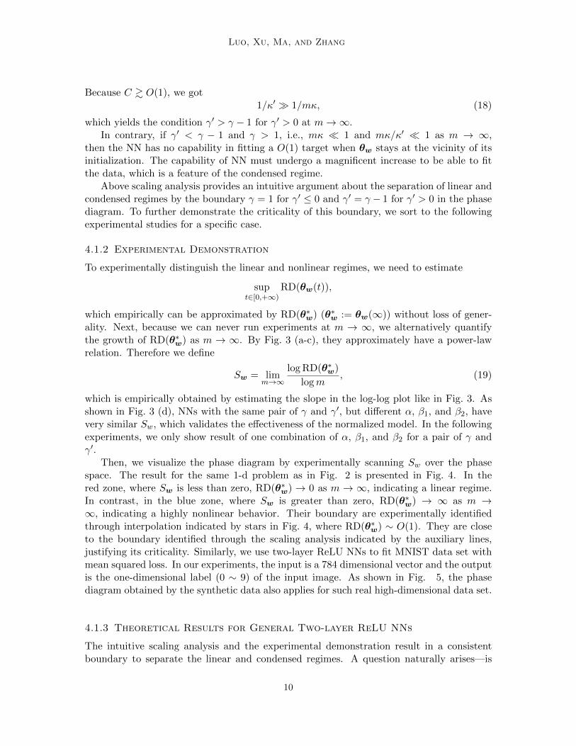
Because C & O(1), we got1/κ′ 1/mκ, (18)

which yields the condition γ′ > γ − 1 for γ′ > 0 at m→∞.In contrary, if γ′ < γ − 1 and γ > 1, i.e., mκ 1 and mκ/κ′ 1 as m → ∞,

then the NN has no capability in fitting a O(1) target when θw stays at the vicinity of itsinitialization. The capability of NN must undergo a magnificent increase to be able to fitthe data, which is a feature of the condensed regime.

Above scaling analysis provides an intuitive argument about the separation of linear andcondensed regimes by the boundary γ = 1 for γ′ ≤ 0 and γ′ = γ − 1 for γ′ > 0 in the phasediagram. To further demonstrate the criticality of this boundary, we sort to the followingexperimental studies for a specific case.

4.1.2 Experimental Demonstration

To experimentally distinguish the linear and nonlinear regimes, we need to estimate

supt∈[0,+∞)

RD(θw(t)),

which empirically can be approximated by RD(θ∗w) (θ∗w := θw(∞)) without loss of gener-ality. Next, because we can never run experiments at m → ∞, we alternatively quantifythe growth of RD(θ∗w) as m → ∞. By Fig. 3 (a-c), they approximately have a power-lawrelation. Therefore we define

Sw = limm→∞

log RD(θ∗w)

logm, (19)

which is empirically obtained by estimating the slope in the log-log plot like in Fig. 3. Asshown in Fig. 3 (d), NNs with the same pair of γ and γ′, but different α, β1, and β2, havevery similar Sw, which validates the effectiveness of the normalized model. In the followingexperiments, we only show result of one combination of α, β1, and β2 for a pair of γ andγ′.

Then, we visualize the phase diagram by experimentally scanning Sw over the phasespace. The result for the same 1-d problem as in Fig. 2 is presented in Fig. 4. In thered zone, where Sw is less than zero, RD(θ∗w) → 0 as m → ∞, indicating a linear regime.In contrast, in the blue zone, where Sw is greater than zero, RD(θ∗w) → ∞ as m →∞, indicating a highly nonlinear behavior. Their boundary are experimentally identifiedthrough interpolation indicated by stars in Fig. 4, where RD(θ∗w) ∼ O(1). They are closeto the boundary identified through the scaling analysis indicated by the auxiliary lines,justifying its criticality. Similarly, we use two-layer ReLU NNs to fit MNIST data set withmean squared loss. In our experiments, the input is a 784 dimensional vector and the outputis the one-dimensional label (0 ∼ 9) of the input image. As shown in Fig. 5, the phasediagram obtained by the synthetic data also applies for such real high-dimensional data set.

4.1.3 Theoretical Results for General Two-layer ReLU NNs

The intuitive scaling analysis and the experimental demonstration result in a consistentboundary to separate the linear and condensed regimes. A question naturally arises—is

10


103 104

m

10 3

10 2 RD( *w)

dataslope=-0.506

(a) γ = 0.5

103 104

m

10 1

100

RD( *w)

dataslope=0.007

(b) γ = 1

103 104

m

101

102 RD( *w)

dataslope=0.372

(c) γ = 1.75

0.5 1.0 1.50.5

0.0

0.5 Sw

(d) Sw vs. γ

Figure 3: Growth of RD(θ∗w) w.r.t. m→∞ with γ′ = 0. For (a-c), β1 = 1, β2 = 1, and theplot is RD(θ∗w) vs. m of NNs with 1000, 5000, 10000, 20000, 40000 hidden neuronsindicated by five blue dots, respectively. The gray line is a linear fit with slopeindicated. For (d), the plot is Sw vs. γ for γ′ = 0. Each line is for a pair of β1 andβ2: Blue: β1 = 1, β2 = 1; Orange: β1 = m−1/2, β2 = m−1/2; Green: β1 = m−1,β2 = m−1. Note that α is determined by α = β1β2m

γ .

0.6 0.8 1.0 1.2 1.40.40.30.20.10.00.10.20.30.4

′

Sw

0.4

0.2

0.0

0.2

0.4

Figure 4: For synthetic data, Sw estimated on two-layer ReLU NNs of 1000, 5000, 10000,20000, 40000 hidden neurons over γ (ordinate) and γ′ (abscissa). The stars arezero points obtained by the linear interpolation over different γ for each fixed γ′.Dashed lines are auxiliary lines indicating the theoretically obtained boundary.

11


0.7 0.8 0.9 1.0 1.1 1.2 1.30.30.20.10.00.10.20.3

′

Sw

0.4

0.2

0.0

0.2

0.4

Figure 5: For MNIST data, Sw estimated on two-layer ReLU NNs of 1000, 10000, 50000,250000, 40000 hidden neurons over γ (ordinate) and γ′ (abscissa). The stars arezero points obtained by the linear interpolation over different γ for each fixed γ′.Dashed lines are auxiliary lines indicating the theoretically obtained boundary.

there a theory that makes the intuitive scaling analysis rigorous and generalizes aboveempirical phase diagram for an 1-d example to general high-dimensional data for two-layer ReLU NNs. In the following, we address this question by providing two theoremsin informal statements, which proves the criticality of lim

m→+∞sup

t∈[0,+∞)RD(θw(t)) at above

identified boundary in the phase diagram. Their rigorous statements can be found in Section5.

Theorem 1*. (Informal statement of Theorem 6) If γ < 1 or γ′ > γ − 1, then with a highprobability over the choice of θ0, we have

limm→+∞

supt∈[0,+∞)

RD(θw(t)) = 0. (20)

Theorem 2*. (Informal statement of Theorem 8) If γ > 1 and γ′ < γ − 1, then with ahigh probability over the choice of θ0, we have

limm→+∞

supt∈[0,+∞)

RD(θw(t)) = +∞. (21)

Remark 3. limm→+∞

supt∈[0,+∞)

RD(θw(t)) is like an order parameter in the analysis of phase

transition in statistical mechanics, which is key to the regime separation and exhibits dis-continuity at the boundary.

In Theorem 1*, focusing on the linear regime, the negligible relative change of w isessentially proved by showing the kernel of the training dynamics undergoes no significantchange during the whole dynamics. However, the kernel of the training dynamics mightbe out of control for the condensed regime. This difficulty makes the result of Theorem2* nontrivial. Instead of studying the kernel, more detailed information of the dynamicsshould be used. Indeed, we establish a neural-wise estimate, |ak(t)| ≤ 1

κ′ ‖wk(t)‖2 + |a0k|,

12


which holds for any κ, κ′ and any t ≥ 0. We believe that this estimate can be extendedto other network structures and general activation functions for the regimes of nonlineardynamics.

Above two theorems complete the phase diagram of two-layer ReLU NN with distinctivedynamical regimes separated based on lim

m→+∞sup

t∈[0,+∞)RD(θw(t)). The behavior of NN

in the linear regime, e.g., exponential decay of loss, implicit regularization in terms of aRKHS norm, and etc., is very well studied. However, the critical and condense regimes islargely not understood. In the following, we make a further step to unravel a signaturenonlinear behavior—condensation as m → ∞ through experiments, which sheds light onfuture theoretical study.

4.2 Critical and Condensed Regimes

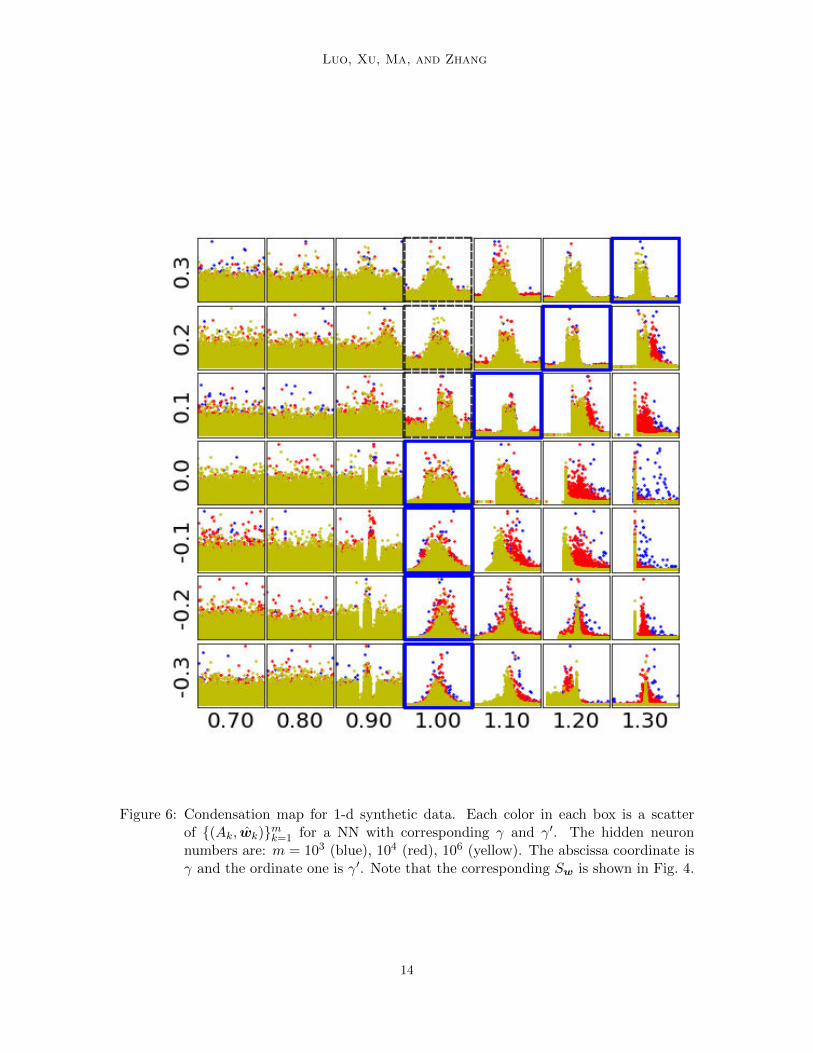
By Fig. 2 (d-f) in previous section, it can be observed that the condensation of NN represen-tation in feature space (Ak, wk)mk=1 comparing to initialization is a distinctive feature forthe nonlinear training dynamics of NNs. Specifically, we care about this condensation at them → ∞ limit when relative change of θw approaches +∞. Therefore, using the same 1-ddata as in Fig. 2, we scan the learned distribution of (Ak, wk) pair for m = 103, 104, 106 overthe phase diagram to experimentally find out the limiting behavior. The result is shown inFig. 6 with the corresponding Sw shown in Fig. 4. It is easy to observe that, right to theboundary indicated by blue boxes, the condensation becomes stronger for larger Sw and asm → ∞, implying a delta-function-like condensation behavior in the limit. This conformswith our intuition that the farther away θw deviates from initialization, the stronger nonlin-earity of NNs exhibited here in the form of condensation. Therefore, as introduced before,we refer to this regime as the condensed regime. In the critical regime as the boundarybetween the linear and the condensed regimes, the level of condensation is almost fixed asm→∞, which resembles a mean-field behavior. Indeed, the well-studied mean-field modelis one point in the critical regime shown in the phase diagram Fig. 1. In general, the mech-anism of condensation as well as its implicit regularization effect is not well understood,which remain as important open questions for the future research.

We also examine the condensation of NNs for MNIST data set. For such high-dimensionaldata, it is impossible to directly visualize the distribution in the high-dimensional featurespace like above 1-d case. Therefore, we consider a projection approach, by which weproject each w to a reference direction p and plot Ak vs. Iw = w · p. Note that the refer-ence direction can be arbitrary selected and does not affect our conclusion. Without loss ofgenerality, we pick p = 1/

√n. Clearly, if neurons indeed condensed at several directions in

the high-dimensional feature space, then their 1-d projection should also condense at severalpoints. As shown in Fig. 7 (corresponding Sw is shown in Fig. 5), similar to the 1-d case,condensation behavior can be observed in the condensed regime identified above. As theparameters move further away from the boundary in the condensed regime, condensationbecomes more salient.

13


Figure 6: Condensation map for 1-d synthetic data. Each color in each box is a scatterof (Ak, wk)mk=1 for a NN with corresponding γ and γ′. The hidden neuronnumbers are: m = 103 (blue), 104 (red), 106 (yellow). The abscissa coordinate isγ and the ordinate one is γ′. Note that the corresponding Sw is shown in Fig. 4.

14


Figure 7: Condensation map for MNIST data set. Each color in each box is a scatter of(Ak, Iwmk=1 for a NN with corresponding γ and γ′. The hidden neuron numbersare: m = 103 (blue), 104 (red), 2.5 × 105 (yellow). The abscissa coordinate is γand the ordinate one is γ′. Note that the corresponding Sw is shown in Fig. 5.

15


5. Theoretical Regime Characterization

We illustrate above how our phase diagram Fig. 1 is obtained through experimental andtheoretical approaches. To obtain a more detailed understanding of general properties ofthese regimes, we present our theoretical results in detail in this section, which follows arigorous description of our notations and definitions in the beginning. The proofs can befound in the appendix.

To start with, let us consider a two layer neural network

fθ(x) :=1

κfκθ (x) =

m∑k=1

akσ(wᵀkx), (22)

with the activation function σ(z) = ReLU(z) = max(z, 0). Denote the data set

S = (xi, yi)ni=1, (23)

where xi’s are i.i.d. sampled from the (unknown) distribution D over Ω = [0, 1]d with(xi)d = 1 and yi = f(xi) ∈ [0, 1] for all i ∈ [n].

We denote ei = κfθ(xi)− yi = κfθ(xi)− f(xi), i ∈ [n] and e = (e1, e2, . . . , en)ᵀ. Thenthe empirical risk can be written as

RS(θ) := RS,κ(θ) =1

2n

n∑i=1

(κfθ(xi)− yi)2 =1

2neᵀe. (24)

Its gradient flow isθ = −Mκ′∇θRS(θ), (25)

with a more explicit form for ak and wk respectivelyak = − 1

κ′∇akRS(θ) = − κ

κ′n

n∑i=1

eiσ(wᵀkxi),

wk = −κ′∇wkRS(θ) = −κκ′

n

n∑i=1

eiaiσ′(wᵀ

kxi)xi.

(26)

Here κ, κ′ are scaling parameters proposed in Section 3. The parameters are initialized as

a0k := ak(0) ∼ N(0, 1), (27)

w0k := wk(0) ∼ N(0, Id), (28)

θ0 := θ(0) = vec(a0k,w

0kmk=1). (29)

The kernels k[a] and k[w] of the GD dynamics are

k[a](x,x′) = Ewσ(wᵀx)σ(wᵀx′),

k[w](x,x′) = E(a,w)a2σ′(wᵀx)σ′(wᵀx′)x · x′.

(30)

16


The Gram matrices K [a] and K [w] of an infinite width two-layer network are

K[a]ij = k[a](xi,xj), K [a] = (K

[a]ij )n×n,

K[w]ij = k[w](xi,xj), K [w] = (K

[w]ij )n×n.

(31)

For the simplicity of proof, we now define the normalized Gram matrices G[a], G[w], andG for a finite width two-layer network as follows:

G[a]ij (θ) =

1

κ′m

m∑k=1

∇akκfθ(xi) · ∇akκfθ(xj) =κ2

κ′m

m∑k=1

σ(wᵀkxi)σ(wᵀ

kxj),

G[w]ij (θ) =

κ′

m

m∑k=1

∇wkκfθ(xi) · ∇wkκfθ(xj) =κ2κ′

m

m∑k=1

a2kσ′(wᵀ

kxi)σ′(wᵀ

kxj)xi · xj ,

G = G[a] +G[w].

(32)

Assumption 1. Suppose that the Gram matrices are strictly positive definite. In otherwords,

λ := minλa, λw > 0, (33)

whereλa := λmin

(K [a]

), λw := λmin

(K [w]

). (34)

We remark that if for any i 6= j, xi 6‖ xj , then Assumption 1 holds. This follows theproof of (Du et al., 2019, Theorem 3.1). Indeed, we do have the fact that, for any i 6= j, ifxi 6= xj then xi 6‖ xj , because in our paper the notation xi means the augmented vector(xᵀ

i , 1)ᵀ (See the first paragraph in Section 1).

Assumption 2. Suppose that the following limits exist

γ := limm→∞

− log κ

logm, γ′ := lim

m→∞− log κ′

logm. (35)

Remark 4. We expect that

G[a](θ0) ≈ κ2

κ′K [a], G[w](θ0) ≈ κ2κ′K [w], (36)

and these will be rigorously achieved in the following proofs. We also remark that λ ≤ d,which will be used in the following proofs.

Remark 5. When γ ≤ 12 , we consider NNs with non-zero initial parameters and zero initial

output, which can be achieved in NNs by applying the AntiSymmetrical Initialization (ASI)trick (Zhang et al., 2020).

Our main results are as follows.

Theorem 6 (linear regime). Given δ ∈ (0, 1) and the sample set S = (xi, yi)ni=1 ⊂ Ωwith xi’s drawn i.i.d. from some unknown distribution D. Suppose that Assumption 1 andAssumption 2 hold. ASI is used when γ ≤ 1

2 . Suppose that γ < 1 or γ′ > γ − 1 and thedynamics (26)–(29) is considered. Then for sufficiently large m, with probability at least1− δ over the choice of θ0, we have

17


(a) (changes of θ and θw)

supt∈[0,+∞)

‖θw(t)− θ0w‖2 ≤ sup

t∈[0,+∞)‖θ(t)− θ0‖2 .

1√mκ

logm. (37)

(b) (linear convergence rate)

RS(θ(t)) ≤ exp

(−2mκ2λt

n

)RS(θ0). (38)

Moreover, for sufficiently large m, with probability at least 1− δ− 2 exp

(−C0m(d+1)

4C2ψ,1

)over

the choice of θ0, we have

(c) (relative change of θ)

supt∈[0,+∞)

‖θ(t)− θ0‖2‖θ0‖2

.1

mκlogm. (39)

In particular, if γ < 1, supt∈[0,+∞)

‖θ(t)−θ0‖2‖θ0‖2 1.

(d) (relative change of θw)

supt∈[0,+∞)

RD(θw(t)) = supt∈[0,+∞)

‖θw(t)− θ0w‖2

‖θ0w‖2

.

1mκ logm, γ < 1,κ′

mκ logm, γ′ > γ − 1.(40)

In particular, if either γ < 1 or γ′ > γ−1, supt∈[0,+∞)

RD(θw(t)) = supt∈[0,+∞)

‖θw(t)−θ0w‖2‖θ0w‖2

1.

Remark 7. In the regions γ < 1 or γ′ > γ−1, Theorem 6 shows that with a high probabilityover the initialization, the relative changes of wk’s are negligible. This implies that thefeatures change only slightly during the whole gradient flow dynamics. Therefore, in thisregime and with large width m, one can expect the training result to be close to that of someproper linear regression model. Note that the relative change of θ is negligible only in thesub-region γ < 1. For γ ≥ 1 and γ′ > γ − 1, the relative changes of ak’s can be fairly large,which may lead to unbounded relative change of θ. The relative changes of θ and ak’s arealso empirically validated in Appendix D.

In order to obtain the theorem that characterize the condensed regime, we need furtherassumption as follows,

Assumption 3. We assume that, without loss of generality,

maxi∈[n]

yi ≥1

2, (41)

and that the neural network can be well-trained to the empirical risk less than O( 1n). More

quantitatively, we require that there exists a T ∗ > 0 such that

RS(θ(T ∗)) ≤ 1

32n. (42)

18


Then we can get the following theorem

Theorem 8 (condensed regime). The sample set S = (xi, yi)ni=1 ⊂ Ω with xi’s drawni.i.d. from some unknown distribution D. Suppose that Assumption 2 and Assumption 3hold. Suppose that γ > 1 and γ′ < γ − 1 and the dynamics (26)–(29) is considered. Then

for sufficiently large m, with probability at least 1 − 2 exp

(−C0m(d+1)

4C2ψ,1

)over the choice of

θ0, we have

supt∈[0,+∞)

RD(θw(t)) = supt∈[0,+∞)

‖θw(t)− θ0w‖2

‖θ0w‖2

1. (43)

To end this section, we provide a sketch of the proofs for the main theorems. In particu-lar, two schematic diagrams 8 and 9 are provided for the proofs of Theorem 6 (Theorem 1*)and Theorem 8 (Theorem 2*), respectively, since they are proved in totally different ways.For Theorem 6, we first establish bounds and concentration inequalities for initial parame-ters. Then the lower bound for the minimal eigenvalue of initial Gram matrix is obtained,which leads to a local in time linear convergence result for the empirical risk. Finally, forsufficiently wide neural networks, we show that the previous estimate is essentially globalin time. We remark that for different (γ, γ′)’s, the details are quite different in the proofsof Theorem 6, which causes the two branches shown in Figure 8. For Theorem 8, as shownin Figure 9, the schematic diagram of the proof is short and straightforward, thanks to akey observation of the neuron-wise estimate, i.e., Proposition 27.

6. Conclusions and Discussion

In this paper, we characterized the linear, critical, and condensed regimes with distinctivefeatures and draw the phase diagram for the two-layer ReLU NN at the infinite-width limit.We experimentally demonstrate and theoretically prove the transition across the boundary(critical regime) in the phase diagram. Through experiments, we further identify the con-densation as the signature behavior in the condensed regime of very strong nonlinearity.Note that, the phenomenon of condensation in a broad sense is observed in several earlystudies of nonlinear training dynamics of NNs in different settings (Maennel et al., 2018;Chizat and Bach, 2018; Ma et al., 2020).

A phase diagram serves as a map that guides the future research. In our phase diagramfor two-layer ReLU NNs, the linear regimes is very well understood both theoretically andexperimentally. However, the critical and condensed regimes are still largely not understoodfrom both experimental and theoretical perspectives. The following problems for theseregimes requires further studies: (i) whether the dynamics always converges to a globalminimizer; (ii) what is the convergence rate; (iii) what is the mechanism of condensation;(iv) how to characterize the implicit regularization of condensation.

Our phase diagram is obtained specifically for the ReLU activation, however, our method-ology and thus obtained regime characterization can be naturally extended to more generalactivations, which is an immediate next step of this work. In addition, how to character-ize the effect of other hyperparameters, e.g., choice of optimization method, learning rate,regularization techniques, and etc., to the NN training dynamics requires future studies.

19


Initial bounds(Lemma 9 & 10)

Concentration(Lemma 14 & 16, Theorem 15)

(Proposition 17) (Proposition 20)

(Proposition 18) (Proposition 21)

bounds on (Proposition 19)

bounds on (Proposition 22)

case of Thm (Theorem 6)(Proposition 23)

case of Thm (Theorem 6)（Proposition 25）

Schematic Diagram for Proof ofTheorem 1*

Figure 8: Sketch of proof for Theorem 1*.

20


(Proposition 27)

Theorem 2* (Theorem 8)

and

Schematic Diagram for Proof ofTheorem 2*

Figure 9: Sketch of proof for Theorem 2*.

Other important future problems include drawing the phase diagram for NNs of three ormore layers or for convolutional networks.

In analogy to statistical mechanics, a clean regime separation may be only possibleat the infinite width limit, which is not realistic in practice. Nevertheless, rich insightabout a finite size system often can be derived from the analysis at the limit, which isusually much easier. Therefore, we believe it is an important task to systematically drawsuch phase diagrams for NNs of different structures through a combination of theoreticaland experimental approaches as demonstrated in this work. These phase diagrams can becontinuously refined and provides a clear pathway to open the black box of deep learning.

Acknowledgments

This work is sponsored by the National Key R&D Program of China Grant No. 2019YFA0709503(Z. X.), the Shanghai Sailing Program, the Natural Science Foundation of Shanghai GrantNo. 20ZR1429000 (Z. X.), the National Natural Science Foundation of China Grant No.62002221 (Z. X.), Shanghai Municipal of Science and Technology Project Grant No. 20JC1419500(Y.Z.), and the HPC of School of Mathematical Sciences and the Student Innovation Centerat Shanghai Jiao Tong University.

21


Appendix A. Technical Lemmas

This section collects some technical lemmas and propositions. For convenience, we definethe two quantities

α(t) := maxk∈[m],s∈[0,t]

|ak(s)|, ω(t) := maxk∈[m],s∈[0,t]

‖wk(s)‖∞. (44)

Lemma 9 (bounds of initial parameters). Given δ ∈ (0, 1), we have with probability at least1− δ over the choice of θ0

maxk∈[m]

|a0k|, ‖w0

k‖∞≤√

2 log2m(d+ 1)

δ, (45)

Proof If X ∼ N(0, 1), then P(|X| > ε) ≤ 2e−12ε2 for all ε > 0. Since a0

k ∼ N(0, 1),(w0

k)α ∼ N(0, 1) for k = 1, 2, . . . ,m, α = 1, . . . , d and they are all independent, by setting

ε =

√2 log

2m(d+ 1)

δ,

one can obtain

P(

maxk∈[m]

|a0k|, ‖w0

k‖∞> ε

)= P

(max

k∈[m],α∈[d]

|a0k|, |(w0

k)α|> ε

)= P

(m⋃k=1

(|a0k| > ε

)⋃(d⋃

α=1

(|(w0

k)α| > ε)))

≤m∑k=1

P(|a0k| > ε

)+

m∑k=1

d∑α=1

P(|(w0

k)α| > ε)

≤ 2me−12ε2 + 2mde−

12ε2

= 2m(d+ 1)e−12ε2

= δ.

Lemma 10 (bound of initial empirical risk). Given δ ∈ (0, 1) and the sample set S =(xi, yi)ni=1 ⊂ Ω with xi’s drawn i.i.d. from some unknown distribution D. Suppose thatAssumption 1 holds. We have with probability at least 1− δ over the choice of θ0

RS(θ0) ≤ 1

2

[1 + 2d

(log

4m(d+ 1)

δ

)(2 + 3

√2 log(8/δ)

)κ√m

]2

. (46)

Proof LetG = gx(a,w) | gx(a,w) := aσ(wᵀx),x ∈ Ω. (47)

Lemma 9 implies that with probability at least 1− δ/2 over the choice of θ0, we have

|gx(a0k,w

0k)| ≤ d|a0

k|‖w0k‖ ≤ 2d log

4m(d+ 1)

δ

22


Then1

msupx∈Ω|fθ0(x)| = sup

x∈Ω

∣∣∣∣∣ 1

m

m∑k=1

a0kσ(w0

k · x)− E(a,w)aσ(wᵀx)

∣∣∣∣∣≤ 2Radθ0(G) + 6d

(log

4m(d+ 1)

δ

)√2 log(8/δ)

m.

The Rademacher complexity can be estimated by

Radθ0(G) =1

mEτ

[supx∈Ω

m∑k=1

τka0kσ(w0

k · x)

]

≤ 1

m

√2 log

4m(d+ 1)

δEτ

[supx∈Ω

m∑k=1

τkw0k · x

]

≤√

2 log4m(d+ 1)

δ

√2d log

4m(d+ 1)

δ

√d√m

=2d log 4m(d+1)

δ√m

.

Therefore

supx∈Ω|fθ0(x)| ≤ 2d

(log

4m(d+ 1)

δ

)(2 + 3

√2 log(8/δ)

√m),

and

RS(θ0) ≤ 1

2n

n∑i=1

(1 + κ|fθ(xi)|)2

≤ 1

2

[1 + 2d

(log

4m(d+ 1)

δ

)(2 + 3

√2 log(8/δ)κ

√m)]2

.

Remark 11. If γ > 12 , then κ = o( 1√

m logm) and RS(θ0) = O(1). One can use ASI

trick (Zhang et al., 2020) to guarantee RS(θ0) ≤ 12 for any κ.

Next we introduce the sub-exponential norm of a random variable and the sub-exponentialBernstein’s inequality.

Definition 12 (sub-exponential norm (Vershynin, 2018)). The sub-exponential norm of arandom variable X is defined as

‖X‖ψ1 := infs > 0 | EX[e|X|/s] ≤ 2. (48)

In particular, we denote the sub-exponential norm of a χ2(d) random variable X by Cψ,d :=‖X‖ψ1. Here the χ2 distribution with d degrees of freedom has the probability density function

fX(z) =1

2d/2Γ(d/2)zd/2−1e−z/2.

23


Remark 13. Note that

EX∼χ2(d)e|X|/2 =

∫ +∞

0

1

2d/2Γ(d/2)zd/2−1 dz = +∞,

lims→+∞

EX∼χ2(d)e|X|/s = lim

s→+∞

∫ +∞

0

1

2d/2Γ(d/2)zd/2−1e−z/2+z/s dz = 1 < 2.

These imply that 2 ≤ Cψ,d < +∞.

Lemma 14. Suppose that w ∼ N(0, Id), a ∼ N(0, 1) and given xi,xj ∈ Ω. Then we have

(i) if X := σ(wᵀxi)σ(x · xj), then ‖X‖ψ1 ≤ dCψ,d.

(ii) if X := a2σ′(wᵀxi)σ′(wᵀxj)xi · xj, then ‖X‖ψ1 ≤ dCψ,d.

Proof Let Z := ‖w‖22 = χ2(d).(i) |X| ≤ d‖w‖22 = dZ and

‖X‖ψ1 = infs > 0 | EX exp(|X|/s) ≤ 2= infs > 0 | Ew exp (|σ(wᵀxi)σ(wᵀxj)|/s) ≤ 2≤ infs > 0 | Ew exp(d‖w‖22/s) ≤ 2= infs > 0 | EZ exp(d|Z|/s) ≤ 2= d infs > 0 | EZ exp(|Z|/s) ≤ 2= d‖χ2(d)‖ψ1

≤ dCψ,d.

(ii) |X| ≤ d|a|2 ≤ dZ and ‖X‖ψ1 ≤ dCψ,d.

Theorem 15 (sub-exponential Bernstein’s inequality (Vershynin, 2018)). Suppose thatX1, . . . ,Xm are i.i.d. sub-exponential random variables with EX1 = µ, then for any s ≥ 0we have

P

(∣∣∣∣∣ 1

m

m∑k=1

Xk − µ

∣∣∣∣∣ ≥ s)≤ 2 exp

(−C0mmin

(s2

‖X1‖2ψ1

,s

‖X1‖ψ1

)), (49)

where C0 is an absolute constant.

Proposition 16 (norm of initial parameters). Given δ ∈ (0, 1), we have with probability at

least 1− 2 exp

(−C0m(d+1)

4C2ψ,1

)over the choice of θ0

√m(d+ 1)

2≤ ‖θ0‖2 ≤

√3m(d+ 1)

2, (50)√

md

2≤ ‖θ0

w‖2 ≤√

3md

2. (51)√

m

2≤ ‖θ0

a‖2 ≤√

3m

2. (52)

24


Proof Let X1, . . . ,Xm(d+1) be the squares of the entries of θ0, which are drawn i.i.d. fromχ2(1). The latter is sub-exponential and EXk = 1. Then by Theorem 15

P

∣∣∣∣∣∣ 1

m(d+ 1)

m(d+1)∑k=1

Xk − 1

∣∣∣∣∣∣ ≥ s ≤ 2 exp

(−C0m(d+ 1) min

(s2

C2ψ,1

,s

Cψ,1

)).

Setting s = 12 , we have s

Cψ,1≤ 1/2

2 < 1 and

P

1

2≤ 1

m(d+ 1)

m(d+1)∑k=1

Xk ≤3

2

≤ 2 exp

(−C0m(d+ 1) min

(1

4C2ψ,1

,1

2Cψ,1

))

= 2 exp

(−C0m(d+ 1)

4C2ψ,1

).

Therefore, with probability at least 1− 2 exp

(−C0m(d+1)

4C2ψ,1

)over the choice of θ0,

1

2≤ 1

m(d+ 1)

m(d+1)∑k=1

Xk =1

m(d+ 1)‖θ0‖22 ≤

3

2.

In other words, (50) holds. The proofs of (51) and (52) are similar.

Proposition 17 (minimal eigenvalue of Gram matrix G at initial). Given δ ∈ (0, 1) andthe sample set S = (xi, yi)ni=1 ⊂ Ω with xi’s drawn i.i.d. from some unknown distribution

D. Suppose that Assumption 1 holds. If m ≥ 16n2d2Cψ,dC0λ2

log 4n2

δ then with probability at least

1− δ over the choice of θ0, we have

λmin

(G(θ0)

)≥ 3

4κ2

(1

κ′λa + κ′λw

). (53)

Proof For any ε > 0, we define

Ω[a]ij :=

θ0 |

∣∣∣∣ κ′κ2G

[a]ij (θ0)−K [a]

ij

∣∣∣∣ ≤ ε

n

,

Ω[w]ij :=

θ0 |

∣∣∣∣ 1

κ2κ′G

[w]ij (θ0)−K [w]

ij

∣∣∣∣ ≤ ε

n

.

By Theorem 15 and Lemma 14, if εndCψ,d

≤ 1, then

P(Ω[a]ij ) ≥ 1− 2 exp

(− mC0ε

2

n2d2C2ψ,d

),

P(Ω(w)ij ) ≥ 1− 2 exp

(− mC0ε

2

n2d2C2ψ,d

),

25


so with probability at least

[1− 2 exp

(− mC0ε2

n2d2C2ψ,d

)]2n2

≥ 1 − 4n2 exp

(− mC0ε2

n2d2C2ψ,d

)over

the choice of θ0, we have ∥∥∥∥ κ′κ2G[a](θ0)−K [a]

∥∥∥∥F

≤ ε,∥∥∥∥ 1

κ2κ′G[w](θ0)−K [w]

∥∥∥∥F

≤ ε,

Hence by taking ε = λ/4, that is, δ = 4n2 exp

(− mC0λ2

16n2d2C2ψ,d

)λmin

(G(θ0)

)≥ λmin

(G[a](θ0)

)+ λmin

(G[w](θ0)

)≥ κ2

κ′λa −

κ2

κ′

∥∥∥∥ κ′κ2G[a](θ0)−K [a]

∥∥∥∥F

+ κ2κ′λw − κ2κ′∥∥∥∥ 1

κ2κ′G[w](θ0)−K [w]

∥∥∥∥F

≥ κ2

κ′(λa − ε) + κ2κ′(λw − ε)

≥ 3

4κ2

(1

κ′λa + κ′λw

).

We remark that for ε = λ/4, we have εndCψ,d

= λ8nd ≤

18 < 1.

In the following we denotet∗ = inft | θ(t) /∈ N (θ0), (54)

where

N (θ0) :=

θ | ‖G(θ)−G(θ0)‖F ≤

1

4κ2

(1

κ′λa + κ′λw

). (55)

Then we have the following lemma.

Proposition 18 (local in time exponential decay of RS , θ-lazy training). Given δ ∈ (0, 1)and the sample set S = (xi, yi)ni=1 ⊂ Ω with xi’s drawn i.i.d. from some unknown distri-

bution D. Suppose that Assumption 1 holds. If m ≥ 16n2d2C2ψ,d

λ2C0log 4n2

δ , then with probability

at least 1− δ over the choice of θ0, we have for any t ∈ [0, t∗)

RS(θ(t)) ≤ exp

(−mκ

2

n

(1

κ′λa + κ′λw

))RS(θ0). (56)

Proof Prop. 17 implies that for any δ ∈ (0, 1), with probability at least 1 − δ over thechoice of θ0 and for any θ ∈ N (θ0), we have

λmin (G(θ)) ≥ λmin

(G(θ0)

)− ‖G(θ)−G(θ0)‖F

≥ 3

4κ2

(1

κ′λa + κ′λw

)− 1

4κ2

(1

κ′λa + κ′λw

)=

1

2κ2

(1

κ′λa + κ′λw

).

26


Note that

Gij = G[a]ij +G

[w]ij =

κ2

κ′m

m∑k=1

∇akfθ(xi) · ∇akfθ(xj) +κ2κ′

m

m∑k=1

∇wkfθ(xi) · ∇wkfθ(xj),

and

∇akRS(θ) =1

n

n∑i=1

eiκ∇akfθ(xi),

∇wkRS(θ) =1

n

n∑i=1

eiκ∇wkfθ(xi).

Thus

m

n2eᵀGe =

1

κ′

m∑k=1

∇akRS(θ) · ∇akRS(θ) + κ′m∑k=1

∇wkRS(θ) · ∇wkRS(θ).

Then finally we get

d

dtRS(θ(t)) = −

(1

κ′

m∑k=1

∇akRS(θ) · ∇akRS(θ) + κ′m∑k=1

∇wkRS(θ) · ∇wkRS(θ)

),

= −mn2eᵀGe,

≤ −2m

nλmin (G(θ(t)))RS(θ(t))

≤ −mκ2

n

(1

κ′λa + κ′λw

)RS(θ(t)),

and an integration yields the result.

Proposition 19 (bounds on the change of parameters, θ-lazy training). Given δ ∈ (0, 1)and the sample set S = (xi, yi)ni=1 ⊂ Ω with xi’s drawn i.i.d. from some unknown distribu-

tion D. Suppose that Assumption 1 holds. If m ≥ max

16n2d2C2

ψ,d

λ2C0log 8n2

δ ,4√

2dn√RS(θ0)

κ(λa/κ′+κ′λw)

,

then with probability at least 1− δ over the choice of θ0, for any t ∈ [0, t∗) and any k ∈ [m],

maxk∈[m]

|ak(t)− ak(0)| ≤ 2 max

1

κ′, 1

√2 log

4m(d+ 1)

δp, (57)

maxk∈[m]

‖wk(t)−wk(0)‖∞ ≤ 2 maxκ′, 1√

2 log4m(d+ 1)

δp, (58)

and

maxk∈[m]

|ak(0)|, ‖wk(0)‖∞ ≤√

2 log4m(d+ 1)

δ, (59)

where p :=2√

2dn√RS(θ0)

mκ(λa/κ′+κ′λw) .

27


Proof Since

α(t) = maxk∈[m],s∈[0,t]

|ak(s)|, ω(t) = maxk∈[m],s∈[0,t]

‖wk(s)‖∞,

we obtain

|∇akRS |2 =

∣∣∣∣∣ 1nn∑i=1

eiκσ(wᵀkxi)

∣∣∣∣∣2

≤ 2‖wk‖21κ2RS(θ) ≤ 2d2(ω(t))2κ2RS(θ),

‖∇wkRS‖2 =

∥∥∥∥∥ 1

n

n∑i=1

eiκakσ′(wᵀ

kxi)xi

∥∥∥∥∥2

∞

≤ 2|ak|2κ2RS(θ) ≤ 2(α(t))2κ2RS(θ).

By Prop. 18, we have if m ≥ 16n2d2C2ψ,d

λ2C0log 8n2

δ , then with probability at least 1− δ/2 over

the choice of θ0,

|ak(t)− ak(0)| ≤ 1

κ′

∫ t

0|∇akRS(θ(s))| ds

≤√

2dκ

κ′

∫ t

0ω(s)

√RS(θ(s)) ds

≤√

2dκ

κ′ω(t)

∫ t

0

√RS(θ0) exp

(−mκ

2

2n

(1

κ′λa + κ′λw

)s

)ds

≤2√

2dn√RS(θ0)

mκκ′(λ

[a]S /κ

′ + κ′λw

)ω(t)

=p

κ′ω(t).

On the other hand,

‖wk(t)−wk(0)‖∞ ≤ κ′∫ t

0‖∇wkRS(θ(s))‖∞ ds

≤√

2κκ′∫ t

0α(s)

√RS(θ(s)) ds

≤√

2κκ′α(t)

∫ t

0

√RS(θ0) exp

(−mκ

2

2n

(1

κ′λa + κ′λw

)s

)ds

≤2√

2n√RS(θ0)κ′

mκ(λ

[a]S /κ

′ + κ′λw

)α(t)

≤ pκ′α(t).

Thus

α(t) ≤ α(0) + pω(t)1

κ′,

ω(t) ≤ ω(0) + pα(t)κ′.

28


By Lemma 9, we have with probability at least 1− δ/2 over the choice of θ0,

maxk∈[m]

|ak(0)|, ‖wk(0)‖∞ ≤√

2 log4m(d+ 1)

δ.

If

m ≥4√

2dn√RS(θ0)

κ (λa/κ′ + κ′λw),

then we have

p =2√

2dn√RS(θ0)

mκ (λa/κ′ + κ′λw)≤ 1

2.

Thus

α(t) ≤ α(0) +p

κ′ω(0) + p2α(t),

α(t) ≤ 4

3α(0) +

2

3

1

κ′ω(0).

Therefore

α(t) ≤ 2 max

1,

1

κ′

√2 log

4m(d+ 1)

δ.

Similarly, one can obtain the estimate of ω(t) as

ω(t) ≤ 2 max1, κ′√

2 log4m(d+ 1)

δ.

Finally we have for any t ∈ [0, t∗) with probability at least 1− δ over the choice of θ0,

maxk∈[m]

|ak(t)− ak(0)| ≤ 2 max

1

κ′, 1

√2 log

4m(d+ 1)

δp,

maxk∈[m]

‖wk(t)−wk(0)‖∞ ≤ 2 maxκ′, 1√

2 log4m(d+ 1)

δp,

which completes the proof.

To show our main results with γ′ > γ − 1, we further define

t∗a = inft | θ(t) ∈ Na(θ0), t∗w = inft | θ(0) ∈ Nw(θ0), (60)

where

Na(θ0) :=

θ | ‖G[a](θ)−G[a](θ0)‖F ≤

1

4

κ2

κ′λa

, (61)

Nw(θ0) :=

θ | ‖G[w](θ)−G[w](θ0)‖F ≤

1

4κ2κ′λw

. (62)

29


Proposition 20 (minimal eigenvalue of Gram matrix G[a] at initial). Given δ ∈ (0, 1) andthe sample set S = (xi, yi)ni=1 ⊂ Ω with xi’s drawn i.i.d. from some unknown distribution

D. Suppose that Assumption 1 holds. If m ≥ 16n2d2C2ψ,d

C0λ2alog 2n2

δ , then we have with probability

at least 1− δ over the choice of θ0,

λmin

(G[a](θ0)

)≥ 3

4

κ2

κ′λa. (63)

Proof For any ε > 0 define

Ω[a]ij :=

θ0 |

∣∣∣∣ κ′κ2G

[a]ij (θ0)−K [a]

ij

∣∣∣∣ ≤ ε

n

. (64)

By Theorem 15 and Lemma 14, if εndCψ,d

≤ 1 then

P(Ω[a]ij ) ≥ 1− 2 exp

(− mC0ε

2

n2d2C2ψ,d

),

with probability at least[1− 2 exp

(− mC0ε

2

n2d2C2ψ,d

)]n2

≥ 1− 2n2 exp

(− mC0ε

2

n2d2C2ψ,d

)

over the choice of θ0, we have ∥∥∥∥ κ′κ2G[a](θ0)−K [a]

∥∥∥∥F

≤ ε.

Taking ε = λa/4, i.e., δ = 2n2 exp

(− mC0λ2a

16n2d2C2ψ,d

), we obtain the estimate

λmin(G[a](θ0) ≥ κ2

κ′λa −

κ2

κ′

∥∥∥∥ κ′κ2G[a](θ0)−K [a]

∥∥∥∥F

≥ κ2

κ′(λa − ε)

≥ 3

4

κ2

κ′λa.

Proposition 21 (local in time exponential decay of RS , w-lazy training). Given δ ∈(0, 1) and the sample set S = (xi, yi)ni=1 ⊂ Ω with xi’s drawn i.i.d. from some unknown

distribution D. Suppose that Assumption 1 holds. If m ≥ 16n2d2C2ψ,d

C0λ2alog 2n2

δ , then with

probability at least 1− δ over the choice of θ0, for t ∈ [0, t∗a),

RS(θ(t)) ≤ exp

(−mκ

2

κ′nλat

)RS(θ0). (65)

30


Proof By Prop. 20, for any δ ∈ (0, 1) with probability 1− δ over the choice of θ0 and forany θ ∈ Na(θ0),

λmin(G[a](θ)) ≥ λmin(G[a](θ0))− ‖G(θ)−G(θ0)‖F

≥ 3

4

κ2

κ′λa −

1

4

κ2

κ′λa

=1

2

κ2

κ′λa.

Therefored

dtRS(θ(t)) = −m

n2eᵀGe

≤ −mn2eᵀG[a]e

≤ −2m

nλmin

(G[a](θ(t))

)RS(θ(t))

≤ −mκ2

κ′nλaRS(θ(t)).

This leads to the linear convergence rate.

Proposition 22 (bounds on the change of parameters, w-lazy training). Given δ ∈ (0, 1)and the sample set S = (xi, yi)ni=1 ⊂ Ω with xi’s drawn i.i.d. from some unknown distribu-

tion D. Suppose that Assumption 1 holds. If m ≥ 16n2d2C2ψ,d

C0λ2alog 4n2

δ and mκκ′ ≥

4√

2dn√RS(θ0)

λa

and κ′ ≤ 1, then with probability at least 1− δ over the choice of θ0 and for any t ∈ [0, t∗a),k ∈ [m],

maxk∈[m]

|ak(t)− ak(0)| ≤ 21

κ′

√2 log

4m(d+ 1)

δpa, (66)

maxk∈[m]

‖wk(t)−wk(0)‖∞ ≤ 2

√2 log

4m(d+ 1)

δpa, (67)

and

maxk∈[m]

|ak(0)|, ‖wk(0)‖∞ ≤√

2 log4m(d+ 1)

δ, (68)

where pa =2√

2dn√RS(θ0)

mκλa/κ′.

Proof Since

α(t) = maxk∈[m],s∈[0,t]

|ak(s)|, ω(t) = maxk∈[m],s∈[0,t]

‖wk(s)‖∞,

then

|∇akRS |2 =

∣∣∣∣∣ 1nn∑i=1

eiκσ(wᵀkxi)

∣∣∣∣∣2

≤ 2‖wk‖21κ2RS(θ) ≤ 2d2(ω(t))2κ2RS(θ),

‖∇wkRS‖2 =

∥∥∥∥∥ 1

n

n∑i=1

eiκakσ′(wᵀ

kxi)xi

∥∥∥∥∥2

∞

≤ 2|ak|2κ2RS(θ) ≤ 2(α(t))2κ2RS(θ).

31


By Prop. 18, we have if m ≥ 16n2d2C2ψ,d

λ2C0log 8n2

δ , then with probability at least 1− δ/2 over

the choice of θ0,

|ak(t)− ak(0)| ≤ 1

κ′

∫ t

0|∇akRS(θ(s))| ds

≤√

2dκ

κ′

∫ t

0ω(s)

√RS(θ(s)) ds

≤√

2dκ

κ′ω(t)

∫ t

0

√RS(θ0) exp

(−mκ

2

2n

(1

κ′λa + κ′λw

)s

)ds

≤2√

2dn√RS(θ0)

mκκ′(λ

[a]S /κ

′ + κ′λw

)ω(t)

=paκ′ω(t).

On the other hand,

‖wk(t)−wk(0)‖∞ ≤ κ′∫ t

0‖∇wkRS(θ(s))‖∞ ds

≤√

2κκ′∫ t

0α(s)

√RS(θ(s)) ds

≤√

2κκ′α(t)

∫ t

0

√RS(θ0) exp

(−mκ

2

2n

(1

κ′λa + κ′λw

)s

)ds

≤2√

2n√RS(θ0)κ′

mκ(λ

[a]S /κ

′ + κ′λw

)α(t)

≤ paκ′α(t).

Thus

α(t) ≤ α(0) + paω(t)1

κ′,

ω(t) ≤ ω(0) + paα(t)κ′.

By Lemma 9, we have with probability at least 1− δ/2 over the choice of θ0,

maxk∈[m]

|ak(0)|, ‖wk(0)‖∞ ≤√

2 log4m(d+ 1)

δ.

If

m ≥4√

2dn√RS(θ0)

κ (λa/κ′ + κ′λw),

then

pa =2√

2dn√RS(θ0)

mκλa/κ′≤ 1

2.

32


Thus

α(t) ≤ α(0) +paκ′ω(0) + p2

aα(t),

α(t) ≤ 4

3α(0) +

2

3

1

κ′ω(0),

Therefore

α(t) ≤ 21

κ′

√2 log

4m(d+ 1)

δ.

Similarly, one can obtain the estimate of ω(t) as

ω(t) ≤ 2

√2 log

4m(d+ 1)

δ.

Finally, with probability at least 1− δ over the choice of θ0 and for any t ∈ [0, t∗a), we have

maxk∈[m]

|ak(t)− ak(0)| ≤ 21

κ′

√2 log

4m(d+ 1)

δpa,

maxk∈[m]

‖wk(t)−wk(0)‖∞ ≤ 2

√2 log

4m(d+ 1)

δpa,


Appendix B. Proof of Theorem 6

We further divide the linear regime into two part: γ < 1 where the training dynamics isθ-lazy and γ′ > γ − 1 where the training dynamics is w-lazy. Theorem 6 is hence coveredby Proposition 23 and Proposition 25 whose proofs are given in this section.

Proposition 23 (θ-lazy training). Given δ ∈ (0, 1) and the sample set S = (xi, yi)ni=1 ⊂Ω with xi’s drawn i.i.d. from some unknown distribution D. Suppose that Assumption 1 andAssumption 2 hold. ASI is used if γ ≤ 1

2 . Suppose that γ < 1 and the dynamics (26)–(29)is considered. Then for sufficiently large m, with probability at least 1 − δ over the choiceof θ0, we have

(a) supt∈[0,+∞)

‖θ(t)− θ0‖2 . 1√mκ

logm.

(b) RS(θ(t)) ≤ exp(−2mκ2λt

n

)RS(θ0).

Moreover, we have with probability at least 1− δ − 2 exp

(−C0m(d+1)

4C2ψ,1

).

(c) supt∈[0,+∞)

‖θ(t)−θ0‖2‖θ0‖2 . 1

mκ logm.

Proof Let t ∈ [0, t∗), p =2√

2dn√RS(θ0)

mκ(λa/κ′+κ′λw) and ξ =

√2 log 8m(d+1)

δ .

33


(a) From Proposition 19 we have with probability at least 1− δ/2 over the choice of θ0,

supt∈[0,t∗]

‖θ(t)− θ0‖2 ≤

m(d+ 1)

(2

√2 log

8m(d+ 1)

δ

√2dn

√RS(θ0)

mκ (λa/κ′ + κ′λw)

)2 1

2

= max

κ′,

1

κ′

√m(d+ 1)2

√2 log

8m(d+ 1)

δ

√2dn

√RS(θ0)


≤ max

κ′,

1

κ′

4√d+ 1dn

√log 8m(d+1)

δ

√RS(θ0)

√mκ (λa/κ′ + κ′λw)

≤4√d+ 1dn

√log 8m(d+1)

δ

√RS(θ0)

√mκλ

.1√mκ

logm,

where we use the fact

maxκ′, 1

κ′

λa/κ′ + κ′λw

≤ max

κ′

κ′λw,

1/κ′

λa/κ′

≤ 1

λ.

(b) The linear convergence rate is essentially proved by Prop. 18 with t∗ = +∞. Wedivide the proof into the following three steps. In particular, t∗ = +∞ is proved inthe step (iii).

(i) Let

g[a]ij (w) := σ(wᵀxi)σ(wᵀxj),

then ∣∣∣G[a]ij (θ(t))−G[a]

ij (θ(0))∣∣∣ ≤ κ2

mκ′

m∑k=1

∣∣∣g[a]ij (wk(t))− g

[a]ij (wk(0))

∣∣∣ .By mean value theorem, for somce c ∈ (0, 1),∣∣∣g[a]ij (wk(t))− g

[a]ij (wk(0))

∣∣∣ ≤ ‖∇g[a]ij (cwk(t) + (1− c)wk(0))‖∞‖wk(t)−wk(0)‖1,

where∇g[a]

ij (w) = σ′(w · ξi)σ(wᵀxj)xi + σ(wᵀxi)σ′(wᵀxj)xj ,

and‖∇g[a]

ij (w)‖∞ ≤ 2‖w‖1.

From Proposition 19 we have with probability at least 1− δ/2 over the choice ofθ0,

‖wk(t)−wk(0)‖∞ ≤ pα(t)κ′ ≤ 2 maxκ′, 1ξp,‖wk(t)−wk(0)‖1 ≤ 2dmaxκ′, 1ξp.

34


Thus

‖cwk(t) + (1− c)wk(0)‖1 ≤ d (‖wk(0)‖∞ + ‖wk(t)−wk(0)‖∞)

≤ d(ξ + 2 maxκ′, 1ξp

)≤ 2dξmaxκ′, 1.

Then

|G[a]ij (θ(t))−G[a]

ij (θ(0))| ≤ 8d2κ2ξ2 max

κ′,

1

κ′

p,

and

‖G[a](θ(t))−G[a](θ(0))‖F ≤ 8d2nκ2 max

κ′,

1

κ′

(2 log

8m(d+ 1)

δ

)2√

2dn√RS(θ0)


≤ κmax

κ′,

1

κ′

32√

2d3n2(

log 8m(d+1)δ

)√RS(θ0)

m (λa/κ′ + κ′λw).

If we choose

mκ ≥128√

2d3n2(

log 8m(d+1)δ

)√RS(θ0)

λ2, (69)

then noticing that1

λ2≥ 1(

4(

127λa(λw)3

)1/4)2

≥ 1(λa/(κ′)3/2 +

√κ′λw

)2

=κ′

(λa/κ′ + κ′λw)2

and1

λ2≥ 1(

4(

127(λa)3λw

)1/4)2

≥ 1(λa/√κ′ + (κ′)3/2λw

)2

=1

(λa/κ′ + κ′λw)2 κ′,

we have

mκ ≥ max

κ′,

1

κ′

256√

2d3n2(

log 8m(d+1)δ

)√RS(θ0)

(λa/κ′ + κ′λw)2 .

Therefore

‖G[a](θ(t))−G[a](θ(0))‖F ≤1

8κ2

(1

κ′λa + κ′λw

). (70)

35


(ii) Define

Di,k = ωk(0) | ‖wk(t)−wk(0)‖∞ ≤ 2ξmaxκ′, 1p,σ′(wk(t

∗) · xi) 6= σ′(wk(0) · xi).

If |wk(0) · xi| > 4dmaxκ′, 1ξp, then

|wk(t) · xi −wk(0) · xi| ≤ ‖xi‖1‖wk(t)−wk(0)‖∞ ≤ 2d

√2 log

8m(d+ 1)

δp,

thus wk(t) · xi and wk(0) · xi have the same sign which means Di,k is empty.Recall that xi ∈ [0, 1]d with (xi)d = 1, then ‖xi‖2 ≥ 1. Let xi = xi

‖xi‖2 then

|wk(0) · xi| ≥ |xk(0) · xi| and

P(Di,k) ≤ P(|wk(0) · xi| ≤ 4dmaxκ′, 1ξp)≤ P(|wk(0) · xi| ≤ 4dmaxκ′, 1ξp)= P(|wk(0) · (1, 0, 0, . . . , 0)ᵀ| ≤ 4dmaxκ′, 1ξp)= P(|(wk(0))1| ≤ 4dmaxκ′, 1ξp)

= 2

∫ 4dmaxκ′,1ξp

0

1√2π

e−x2

2 dx

≤ 8√2πdmaxκ′, 1ξp

≤ 4dmaxκ′, 1ξp.

Then

|G[w]ij (θ(t))−G[w]

ij (θ(0))| ≤ κ2κ′|xi · xj |m

m∑k=1

∣∣∣a2k(t∗)σ′(wk(t) · xi)σ′(wk(t) · xj)

− a2k(0)σ′(wk(0) · xi)σ′(wk(0) · xj)

∣∣∣≤ κ2κ′d

m

m∑k=1

[a2k(t)|Dk,i,j |+ |a2

k(t)− a2k(0|

],

where

Dk,i,j := σ′(wk(t) · xi)σ′(wk(t) · xj)− σ′(wk(0) · xi)σ′(wk(0) · xj).

ThusE|Dk,i,j | ≤ P(Dk,i ∪Dk,j) ≤ 8dmaxκ′, 1ξp.

At the same time

|a2k(t)− a2

k(0)| ≤ |ak(t)− ak(0)|2 + 2|ak(0)||ak(t)− ak(0)|

≤(

2 max

1

κ′, 1

ξp

)2

+ 2ξ

(2 max

1

κ′, 1

ξp

)≤ 6ξ2 max

1

κ′2, 1

p,

36


so

a2k(t) ≤ |a2

k(t)− a2k(0)|+ a2

k(0) ≤(

2 max

1

κ′, 1

ξp

)2

+ 2ξ

(2 max

1

κ′, 1

ξp

)+ ξ2

≤ 4 max

1

κ′2, 1

ξ2.

Then

En∑

i,j=1

∣∣∣G[w]ij (θ(t))−G[w]

ij (θ(0))∣∣∣

≤n∑

i,j=1

κ2κ′d

m

m∑k=1

(4 max

1

κ′2, 1

ξ2E|Dk,i,j |+ 6 max

1

κ′2, 1

ξ2p

)

≤n∑

i,j=1

κ2κ′d

m

m∑k=1

(4 max

1

κ′2, 1

ξ28dmaxκ′, 1ξp+ 6 max

1

κ′2, 1

ξ2p

)

≤ κ2κ′dn2

(32dξmaxκ′, 1

κ′2+ 6 max

1

κ′2, 1

)ξ2p

≤ 40κ2d2n2

(2 log

8m(d+ 1)

δ

)3/2

maxκ′2, 1

κ′p.

By Markov’s inequality, with probability at least 1 − δ/2 over the choice of θ0,we have

‖G[w](θ(t))−G[w](θ(0))‖F

≤n∑

i,j=1

∣∣∣G[w]ij (θ(t))−G[w]

ij (θ(0))∣∣∣

≤ max

κ′2,

1

κ′

40κ2d2n2(

2 log 8m(d+1)δ

)3/2p

δ/2

≤ max

κ′2,

1

κ′

80κ2d2n22

√2

δ

(log

8m(d+ 1)

δ

)3/2 2√

2dn√RS(θ0)


≤ κmax

κ′2,

1

κ′

640d3n3(

log 8m(d+1)δ

)3/2√RS(θ0)δ−1

m (λa/κ′ + κ′λw).

If

m ≥5120δ−1d3n3

(log 8m(d+1)

δ

)3/2√RS(θ0)

λ2,

then noticing that1

λ2≥ κ′2

(κ′λw)2 ≥κ′2

(λa/κ′ + κ′λw)2

37


and1

λ2≥ 1(

4(

127(λa)3λw

)1/4)2

≥ 1(λa/√κ′ + (κ′)3/2λw

)2

=1

(λa/κ′ + κ′λw)2 κ′,

we have

‖G[w](θ(t))−G[w](θ(0))‖F ≤1

8κ2

(1

κ′λa + κ′λw

). (71)

(iii) For t ∈ [0, t∗),

RS(θ(t)) ≤ exp

(−mκ

2

n

(1

κ′λa + κ′λw

)t

)RS(θ0) ≤ exp

(−2mκ2λ

n

)RS(θ0).

Suppose that t∗ < +∞ then one can take the limit t→ t∗ in (70) and (71). Thiswill lead to a contradiction with the definition of t∗. Therefore t∗ = +∞.

(c) By Proposition 16, we have with probability at least 1− 2 exp

(−C0m(d+1)

4C2ψ,1

)over the

choice of θ0,

‖θ0‖ ≥√m(d+ 1)

2,

Therefore, with probability at least 1− δ − 2 exp

(−C0m(d+1)

4C2ψ,1

)over the choice of θ0,

we have

supt∈[0,+∞)

‖θ(t)− θ0‖2‖θ0‖2

≤

√2

m(d+ 1)sup

t∈[0,+∞)‖θ(t)− θ0‖2

≤

√2

m(d+ 1)

4√d+ 1dn

√log 8m(d+1)

δ

√RS(θ0)

√mκλ

≤ 1

mκ

4√

2dn

√log 8m(d+1)

δ

√RS(θ0)

λ

.1

mκlogm.

Remark 24. The proof indicates more quantitative conditions on m and κ for Proposi-tion 23 to hold:

m ≥16n2d2C2

ψ,d

λ2C0log

16n2

δ, (72)

38


and

mκ ≥ max

2√

2dn√RS(θ0)

λ,

128√

2d3n2(

log 8m(d+1)δ

√RS(θ0)

)λ2

,

5120δ−1d3n3(

log 8m(d+1)δ

)3/2√RS(θ0)

λ2

.

(73)

Proposition 25 (w-lazy training). Given δ ∈ (0, 1) and the sample set S = (xi, yi)ni=1 ⊂Ω with xi’s drawn i.i.d. from some unknown distribution D. Suppose that Assumption 1and Assumption 2 hold. Suppose that γ′ > γ − 1, γ′ > 0, and the dynamics (26)–(29) isconsidered. Then for sufficiently large m, with probability at least 1 − δ over the choice ofθ0, we have

(a)

supt∈[0,+∞)


t∈[0,+∞)‖θ(t)− θ0‖2 .

1√mκ

logm.

(b) RS(θ(t)) ≤ exp(−mκ2λat

κ′n

)RS(θ0).

Moreover we have with probability at least 1− δ − 2 exp

(−C0m(d+1)

4C2ψ,1

).

(c)

supt∈[0,+∞)

‖θ(t)− θ0‖2‖θ0‖2

.1

mκlogm, (not 1),

supt∈[0,+∞)

‖θw(t)− θ0w‖2

‖θw‖2.

κ′

mκlogm, ( 1).

Proof Let t ∈ [0, t∗a), pa =2√

2dn√RS(θ0)

mκλa/κ′, and ξ =

√2 log 8m(d+1)

δ .

(a) From Proposition 19 we have with probability at least 1− δ/2 over the choice of θ0

supt∈[0,t∗a)


t∈[0,t∗a)‖θ(t)− θ0‖2

≤

( mκ′2

+md)(

2

√2 log

8m(d+ 1)

δpa

)2 1

2

=√m(d+ 1)2

1

κ′

√2 log

8m(d+ 1)

δ

√2dn

√RS(θ0)

mκλa/κ′

≤ max

κ′,

1

κ′

4√d+ 1dn

√log 8m(d+1)

δ

√RS(θ0)

√mκ (λa/κ′ + κ′λw)

≤8√d+ 1dn

√log 8m(d+1)

δ

√RS(θ0)

√mκλa

.

39


(b) We divide this proof into the following two steps.

(i) Let

G[a]ij (w) := σ(wᵀxi)σ(wᵀxj),

then


ij (θ(0))| ≤ κ2

mκ′

m∑k=1

|g[a]ij (wk(t))− g

[a]ij (wk(0))|.

By the mean value theorem, for somce c ∈ (0, 1),

|g[a]ij (wk(t))− g

[a]ij (wk(0))| ≤ ‖∇gij (cwk(t) + (1− c)wk(0))‖∞‖wk(t)−wk(0)‖1,

where∇g[a]

ij (w) = σ′(w · ξi)σ(wᵀxj)xi + σ(wᵀxi)σ′(wᵀxj)xj ,

and‖∇g[a]

ij (w)‖∞ ≤ 2‖w‖1.

From Proposition 19 we have with probability at least 1− δ/2 over the choice ofθ0,

‖wk(t)−wk(0)‖∞ ≤ paα(t)κ′ ≤ 2ξpa,

‖wk(t)−wk(0)‖1 ≤ 2dξpa.

Thus

‖cwk(t) + (1− c)wk(0)‖1 ≤ d (‖wk(0)‖∞ + ‖wk(t)−wk(0)‖∞)

≤ d (ξ + 2ξpa)

≤ 2dξ.

Then


ij (θ(0))| ≤ 8d2κ2

κ′ξ2pa,

and

‖G[a](θ(t))−G[a](θ(0))‖F ≤ 16d2n

(log

8m(d+ 1)

δ

)κ2

κ′pa

≤32√

2d3n2(

log 8m(d+1)δ

)√RS(θ0)κ

mλa.

If

mκ

κ′≥

256√

2d3n2(

log 8m(d+1)δ )

)√RS(θ0)

λ2a

,

then we have

‖G[a](θ(t))−G[a](θ(0))‖F ≤1

8

κ2

κ′λa. (74)

40


(ii) For t ∈ [0, t∗a) by Prop. 18,

RS(θ(t)) ≤ exp

(−mκ

2λat

nκ′

)RS(θ0).

Suppose that t∗a < +∞ then one can take the limit t→ t∗a in (74). This will leadto a contradiction with the definition of t∗a. Therefore t∗a = +∞.

(c) By Proposition 16, we have with probability at least 1 − 2 exp(−C0m(d+1)4C2

ψ,1) over the

choice of θ0,

‖θ0‖22 ≥d+ 1

2m.

So with probability at least 1− δ− 2 exp

(−C0m(d+1)

4C2ψ,1

)over the choice of θ0, we have

supt∈[0,+∞)

‖θ(t)− θ0‖2‖θ0‖2

≤

√2

m(d+ 1)sup

t∈[0,+∞)‖θ(t)− θ0‖2

≤

√2

m(d+ 1)

8√d+ 1dn

√log 8m(d+1)

δ

√RS(θ0)

√mκλ

≤ 1

mκ

8√

2dn

√log 8m(d+1)

δ

√RS(θ0)

λa

.1

mκlogm.

Similarly, by Proposition 16, we have with probability at least 1 − 2 exp(−C0m(d+1)4C2

ψ,1)

over the choice of θ0,

‖θ0w‖22 ≥

d

2m.

So with probability at least 1− δ − 2 exp

(−C0md

4C2ψ,1

)over the choice of θ0, we have

supt∈[0,+∞)

‖θw(t)− θ0w‖2

‖θ0w‖2

≤√

2

dmsup

t∈[0,+∞)‖θw(t)− θ0

w‖2

≤√

2

dm

κ′√mκ

8√ddn

√log 8m(d+1)

δ

√RS(θ0)

λ

.κ′

mκlogm.

We remark that in fact we can prove a similar result about the change of parameter ak’s.We state this result as follows without proof.

41


Proposition 26 (a-lazy training). Given δ ∈ (0, 1) and the sample set S = (xi, yi)ni=1 ⊂Ω with xi’s drawn i.i.d. from some unknown distribution D. Suppose that Assumption 1and Assumption 2 hold. Suppose that γ′ < γ − 1, γ′ < 0, and the dynamics (26)–(29) isconsidered. Then for sufficiently large m, with probability at least 1 − δ over the choice ofθ0, we have

(a)

supt∈[0,+∞)

‖θa(t)− θ0a‖2 ≤ sup

t∈[0,+∞)‖θ(t)− θ0‖2 .

1√mκ

logm.

(b) RS(θ(t)) ≤ exp(−mκ2κ′λwt

n

)RS(θ0).

Moreover we have with probability at least 1− δ− 2 exp

(−C0m(d+1)

4C2ψ,1

)over the choice

of θ0, we have

(c)

supt∈[0,+∞)

‖θ(t)− θ0‖2‖θ0‖2

.1

mκlogm, (not 1),

supt∈[0,+∞)

‖θa(t)− θ0a‖2

‖θa‖2.

1

mκκ′logm, ( 1).

Appendix C. Proof of Theorem 8

In order to characterize the condensed regime, we need a crucial proposition that ravels anatrual relation between ak(t) and wk(t) during the GD training dynamics.

Proposition 27. Consider the GD training dynamics (26)–(29), then we have

|ak(t)| ≤1

κ′‖wk(t)‖2 + |a0

k|, (75)

which holds for any t ≥ 0 and k ∈ [m].

Proof Multiplying equations in (26) by κ′ak and wkκ′ respectively, we obtain

κ′akak = −κn

n∑i=1

eiakσ(wᵀkxi),

1

κ′wkwk = −κ

n

n∑i=1

eiakσ′(wᵀ

kxi)wᵀkxi.

(76)

Notice that for ReLU activation σ(z) = zσ′(z), z ∈ R. by comparing the right hand sideof (76), one can obtain

κ′2d

dt|ak|2 =

d

dt‖wk‖22. (77)

Integrating this from 0 to t leads to

κ′2(|ak(t)|2 − |a0

k|2)

= ‖wk(t)‖22 − ‖w0k‖22,

42


which then can be written as

|ak(t)|2 =1

κ′2(‖wk(t)‖22 − ‖w0

k‖22)

+ |a0k|2. (78)

Finally we have

|ak(t)| ≤√

1

κ′2‖wk(t)‖22 + |a0

k|2 ≤1

κ′‖wk(t)‖2 + |a0

k|.

We remark that the key identity (77) in the proof of Proposition 27 has been previouslyproved in (Du et al., 2018, Theorem 2.1). A special case of it is (Williams et al., 2019,Lemma 3).Proof [Proof of Theorem 8] By Assumption 3, there exits a T ∗ > 0 such that

RS(θ(T ∗)) ≤ 1

32n.

Without loss of generality, we assume f(x1) ≥ 12 . Therefore

1

2ne1(T ∗)2 ≤ 1

2ne(T ∗)ᵀe(T ∗) = RS(θ(T ∗)) ≤ 1

32n,

which means

|e1(T ∗)| ≤ 1

4.

Recalling the definition that e1 = κfθ(x1)− f(x1), we have

κm∑k=1

ak(T∗)σ(wk(T

∗)ᵀx1) ≥ f(x1)− 1

4≥ 1

4.

So1

4κ≤

m∑k=1

ak(T∗)σ(wk(T

∗)ᵀx1)

≤√d

m∑k=1

|ak(T ∗)|‖wk(T∗)‖2

≤√d

m∑k=1

(1

κ′‖wk(T

∗)‖2 + |a0k|)‖wk(T

∗)‖2

=√d

(1

κ′

m∑k=1

‖wk(T∗)‖22 +

m∑k=1

|a0k|‖wk(T

∗)‖2

)

≤√d

(1

κ′‖θw(T ∗)‖22 +

1

4‖θ0

a‖22 + ‖θw(T ∗)‖22)

≤ 2√dmax

1

κ′, 1

‖θw(T ∗)‖22 +

√d

4‖θ0

a‖22,

43


where we have used Proposition 27. By Proposition 16, we have with probability at least1− 2 exp(−C0m(d+1)

4C2ψ,1

) over the choice of θ0,

‖θ0a‖ ≤

√3

2m,

‖θ0w‖ ≤

√3

2dm.

If mκ ≤ 13√d, then 3

√dm8 ≤ 1

8κ and

1

8κ≤ 1

4κ− 3√dm

8≤ 1

4κ−√d

4‖θ0

a‖22

≤ 2√dmax

1

κ′, 1

‖θw(T ∗)‖22.

Thusmin1, κ′

16√dκ

≤ ‖θw(T ∗)‖22.

Therefore

supt∈[0,+∞)

‖θw(t)− θ0w‖2

‖θ0w‖2

≥ ‖θw(T ∗)− θ0w‖2

‖θ0‖2

≥

√√√√ min1,κ′16√dκ

32dm

− 1

&

√min1, κ′

κm.

If γ′ < γ − 1, thenmin1, κ′

κm 1,


Remark 28. Suppose that Assumption 1 and 2 hold. If γ > 1 and γ′ < 1 − γ, thenTheorem 8 can hold without taking Assumption 3. Actually, for any δ ∈ (0, 1), Proposi-tion 26 guarantees the Assumption 3 with probability at least 1 − δ over the choice of θ0,when m is sufficiently large. Therefore, under Assumptions 1 and 2, if m is sufficientlylarge, then we have with probability at least 1− δ over the choice of θ0, the relative change

supt∈[0,+∞)

RD(θw(t)) 1.

Appendix D. Relative Deviation of Parameters

For completion, we can also similarly define the slope of the relative deviation for θ anda denoted by Sθ and Sa, respectively. As shown in Fig. 10 (a), the boundary for the θ is

44


0.6 0.8 1.0 1.2 1.40.40.30.20.10.00.10.20.30.4

′

S

0.4

0.2

0.0

0.2

0.4

(a)

0.6 0.8 1.0 1.2 1.40.40.30.20.10.00.10.20.30.4

′

Sw

0.4

0.2

0.0

0.2

0.4

(b)

Figure 10: Sθ in (a) and Sw in (b) estimated on NNs of 1000, 5000, 10000, 20000, 40000neurons over γ (ordinate) and γ′ (abscissa). The stars are zero points obtainedby the linear interpolation over different γ for each fixed γ′. Dashed lines areauxiliary lines.

γ = 1, regardless of γ′, that is, all parameters are close to their initialization after training.For output weight a, as shown in Fig. 10(b), the boundary consists of two rays, one is γ = 1and γ′ ≥ 0, the other is γ+ γ′ = 1 and γ′ ≤ 0. This verifies that, in the area between γ = 1and γ−γ′ = 1 of γ′ ≤ 0, the change of scatter plot from a Gaussian initialization is inducedby the change of a.

References

Sanjeev Arora, Simon S. Du, Wei Hu, Zhiyuan Li, Ruslan Salakhutdinov, and RuosongWang. On exact computation with an infinitely wide neural net. In NeurIPS 2019, 2019.

Zhengdao Chen, Grant M. Rotskoff, Joan Bruna, and Eric Vanden-Eijnden. A dynamicalcentral limit theorem for shallow neural networks. In NeurIPS 2020, 2020.

Lenaıc Chizat and Francis R. Bach. On the global convergence of gradient descent forover-parameterized models using optimal transport. In NeurIPS 2018, 2018.

Lenaıc Chizat, Edouard Oyallon, and Francis R. Bach. On lazy training in differentiableprogramming. In NeurIPS 2019, 2019.

Simon S. Du, Wei Hu, and Jason D. Lee. Algorithmic regularization in learning deephomogeneous models: Layers are automatically balanced. In NeurIPS 2018, 2018.

Simon S. Du, Xiyu Zhai, Barnabas Poczos, and Aarti Singh. Gradient descent provablyoptimizes over-parameterized neural networks. In ICLR 2019, 2019.

Weinan E, Chao Ma, and Lei Wu. A comparative analysis of optimization and generalizationproperties of two-layer neural network and random feature models under gradient descentdynamics. Sci. China Math., 63, 2020.

45


Mario Geiger, Stefano Spigler, Arthur Jacot, and Matthieu Wyart. Disentangling featureand lazy training in deep neural networks. Journal of Statistical Mechanics: Theory andExperiment, 2020(11):113301, 2020.

Xavier Glorot and Yoshua Bengio. Understanding the difficulty of training deep feedforwardneural networks. In Proceedings of the thirteenth international conference on artificialintelligence and statistics, pages 249–256, 2010.

Kaiming He, Xiangyu Zhang, Shaoqing Ren, and Jian Sun. Delving deep into rectifiers:Surpassing human-level performance on imagenet classification. In ICCV 2015, 2015.

Arthur Jacot, Clement Hongler, and Franck Gabriel. Neural tangent kernel: Convergenceand generalization in neural networks. In NeurIPS 2018, 2018.

Yann A LeCun, Leon Bottou, Genevieve B Orr, and Klaus-Robert Muller. Efficient back-prop. In Neural networks: Tricks of the trade, pages 9–48. Springer, 2012.

Jaehoon Lee, Lechao Xiao, Samuel S. Schoenholz, Yasaman Bahri, Roman Novak, JaschaSohl-Dickstein, and Jeffrey Pennington. Wide neural networks of any depth evolve aslinear models under gradient descent. In NeurIPS 2019, 2019.

Chao Ma, Lei Wu, and Weinan E. The quenching-activation behavior of the gradient descentdynamics for two-layer neural network models. arXiv preprint arXiv:2006.14450, 2020.

Hartmut Maennel, Olivier Bousquet, and Sylvain Gelly. Gradient descent quantizes relunetwork features. arXiv preprint arXiv:1803.08367, 2018.

Song Mei, Andrea Montanari, and Phan-Minh Nguyen. A mean field view of the landscapeof two-layer neural networks. Proceedings of the National Academy of Sciences, 115(33):E7665–E7671, 2018.

Song Mei, Theodor Misiakiewicz, and Andrea Montanari. Mean-field theory of two-layersneural networks: dimension-free bounds and kernel limit. In COLT 2019, 2019.

Edward Moroshko, Suriya Gunasekar, Blake Woodworth, Jason Lee, Nati Srebro, andDaniel Soudry. Implicit bias in deep linear classification: Initialization scale vs train-ing accuracy. In NeurIPS 2020, 2020.

Grant M. Rotskoff and Eric Vanden-Eijnden. Parameters as interacting particles: long timeconvergence and asymptotic error scaling of neural networks. In NeurIPS 2018, 2018.

Justin Sirignano and Konstantinos Spiliopoulos. Mean field analysis of neural networks:A central limit theorem. Stochastic Processes and their Applications, 130(3):1820–1852,2020.

Roman Vershynin. High-dimensional probability: An introduction with applications in datascience, volume 47. Cambridge university press, 2018.

Francis Williams, Matthew Trager, Daniele Panozzo, Claudio T. Silva, Denis Zorin, andJoan Bruna. Gradient dynamics of shallow univariate relu networks. In NeurIPS 2019,2019.

46


Blake E. Woodworth, Suriya Gunasekar, Jason D. Lee, Edward Moroshko, Pedro Savarese,Itay Golan, Daniel Soudry, and Nathan Srebro. Kernel and rich regimes in over-parametrized models. In COLT 2020, 2020.

Yaoyu Zhang, Zhi-Qin John Xu, Tao Luo, and Zheng Ma. A type of generalization errorinduced by initialization in deep neural networks. In MSML 2020, 2020.

47

phase diagram for two-layer relu neural networks at in

Documents