phase equilibrium modeling for binary systems …. atashrouz, h. mirshekar: phase equilibrium...

104

Bulgarian Chemical Communications, Volume 46, Number 1 (pp. 104 – 116) 2014

Phase equilibrium modeling for binary systems containing CO2 using artificial neural networks

S. Atashrouz*, H. Mirshekar Department of Chemical Engineering, Amirkabir University of Technology (Tehran Polytechnic), Mahshahr Campus,

Mahshahr, P.O. Box 415, Iran.

Received January 7, 2013; Revised May 28, 2013

In this study, two mathematical models based on the Feed-Forward Back Propagation Artificial Neural Network (FFBP-ANN) are employed for the prediction of CO2 mole fraction in liquid (x1) and vapor (y1) phases in the Vapor Liquid Equilibrium (VLE) for fifty-six CO2-containing binary mixtures. 2104 data sets from the open literature have been used to construct the models. Furthermore, some new experimental data (not applied in ANN training) have been used to examine the reliability of the model. Predictions using ANN were compared with available literature data and the results confirm that there is a reasonable conformity between the predicted values and the experimental data. The average absolute deviation percent (AAD (%)) for ANN model I (x1 prediction) and ANN model II (y1 prediction) are 1.572 and 0.848 respectively. The study shows that the neural network model is a good alternative method for the estimation of phase equilibrium properties for this type of mixtures.

Key words: vapor liquid equilibria; carbon dioxide; modeling; artificial neural network, supercritical fluid extraction, refrigerant

INTRODUCTION Prediction of vapor liquid equilibrium data is a

necessary need in chemical engineering processes. Carbon dioxide (CO2) is an important component in binary mixtures and estimation of VLE data for binary mixtures containing CO2 is necessary in different processes such as supercritical extraction, refrigeration, absorption and more recently, in the development of new and improved methods for carbon capture and storage [1]. Supercritical fluid extraction processes for selectively recovering high purity active principles from biological substrates is a technology of interest to the food, cosmetics and pharmaceutical industries. Extraction using supercritical fluids is now being used in the industry because it is non-flammable, non-toxic and it is available in a highly purified form at low cost and it can be employed at near-environmental temperatures [2–4]. However, the design of this type of processes requires the knowledge of phase equilibrium diagrams over a vast range of temperatures and pressures [5]. From this point of view, knowledge of the phase behavior of systemscontaining carbon dioxide is of growing importance due to the increased use of supercritical CO2 as an

environmentally benign solvent alternative to volatile organics in chemical processes [1]. Another application of carbon dioxide is recently in binary systems that have been utilized for crystallization, purification of solids and reaction media. CO2 and methanol binary mixture is an example of this type of systems [6]. Also binary mixtures containing CO2

and refrigerant mixtures are recently of great importance. For nearly 60 years, chlorofluoro-carbons (CFCs) have been widely used as solvents, foam-blowing agents, aerosols and especially refrigerants due to their stability, non-toxicity, non-flammability, good thermodynamic properties and so on. However, they also have a harmful effect on the earth’s protective ozone layer. So, they have been regulated internationally by Montreal Protocol since 1989. Much effort has been made to find the suitable replacement for CFCs. Initial CFC alternatives included some hydro chlorofluoro-carbons (HCFCs) but they will be also phased out internationally because their ozone depletion potentials (ODPs) and global warming potentials (GWPs) are significant though less than those of CFCs. Hydrofluorocarbons (HFCs) synthetic refrigerants which have zero ODPs were proposed as promising replacements for CFCs and HCFCs. HFC-134a (1,1,1,2-tetrafluoroethane; CF3CH2F) is an environmentally acceptable refrigerant, which

© 2014 Bulgarian Academy of Sciences, Union of Chemists in Bulgaria

* To whom all correspondence should be sent:E-mail: [email protected]

S. Atashrouz, H. Mirshekar: Phase equilibrium modeling for binary systems containing CO2 …

105

has replaced the ozone-depleting dichlorodifluoro-methane (CFC-12) in a wide range of applications especially in automotive air-conditioning and domestic refrigeration [7]. In order to develop refrigeration processes estimation of VLE data for binary mixtures containing CO2 and HFCs has a great importance. Furthermore for the new total flooding clean agents that were being developed to replace certain Halon fire extinguishing agents, the discharge time required to achieve 95% of the minimum design concentration shall not exceed 10 s and the expellant gas is needed for their lack of vapor pressure. Generally, Nitrogen is used as an expellant gas because it does not be liquefied at high pressure, but carbon dioxide has some merits to nitrogen such as price, storage area and supplementary extinguishing effect for R123 and R124 as fire extinguishing agents [8]. In another environmentally view, the emission of carbon dioxide has been identified as the main contributor to global warming and climate change. The challenge for modern industry is to find cost effective solutions that will reduce the release of CO2

into the atmosphere. Reduction of CO2 emissions can be achieved by a variety of means. A physical absorption process is one of the most important possibilities. The advantage of this method is that it requires relatively little energy. Diisopropylether, an excellent solvent, is expected to absorb CO2 [9]. So in this point of view, knowledge of VLE data for binary mixtures that has a solvent for absorption of CO2 is important. In another application the high-pressure phase equilibrium information of mixtures composed of CO2 and alcohols is of particular importance and has been actively studied for various utilities. For example, the phase equilibrium behaviors of low-molecular weight alcohols such as methanol and ethanol in CO2 are essential for the effective evaluation of cosolvents to CO2-based supercritical solvents. Also the phase equilibrium information of high molecular weight alcohols such as 2-ethoxyethanol with CO2 is valuably used to processes in the food and cosmetic industries [10].

Information about the phase behavior of fluid mixtures can be obtained from direct measurement of phase equilibrium data or by the use of equation of state based thermodynamic models. Direct measurement of precise experimental data is often difficult and expensive, while in the second method Several conventional thermodynamic models such as equations of state (EoS) are used for estimating the VLE [11]. A thermodynamic model provides the necessary relationships between thermodynamic properties and can be used in combination with

fundamental relations to generate all the properties required to perform phase equilibrium calculations. The most common thermodynamic models are equations of state and among them cubic equations of state are the most popular. Although thermodynamic models have been derived from strong theoretical principles these methods include a large number of equation of states and excess Gibbs free energy models. that are tedious and involve a certain amount of empiricism to determine mixture constants, through fitting experimental data and using various arbitrary mixing rules, making difficult the selection of the appropriate model for a particular case [12].

On the other hand artificial neural networks(ANN), which can be viewed as an universal approximation tool with an inherent ability to extract from experimental data the highly non-linear and complex relationships between the variables of the problem handled, have gained broad attention within process engineering as a robust and efficient computational tool [12]. Recently, ANN has found extensive application in the field of thermodynamics and transport properties such as the estimation of VLE, viscosity, density, vapor pressure, compressibility factor and thermal conductivity and etc [13–18].

In this research, two comprehensive models based on multi-layer FFBP-ANN were developed to estimate VLE data for fifty-six binary mixtures containing CO2, the importance of which was mentioned above. Model I and model II predict CO2

mole fractions in the liquid (x1) and vapor (y1)phases respectively. The mixtures include 1-butanol, 1-heptanol , 1-hexanol, 1-octanol, 1-pentanol, 1-propanol, 2-butanol, 2-ethoxyethanol, 2-methoxyethanol, 2-methyl-1-propanol, 2-pentanol, 2-propanol, 3-methyl-1-butanol, 3-methyl-2-butanol , 3-pentanol, acetic acid, a-pinene, benzene, chloroform, cyclohexanol, cyclohexanone, cyclopentanol, decanal, DHAEE, DIPE, ethyl butyrate, EPAEE, ethanol, fenchone, H2, limonene, methanol, methyl acetate, methyl linoleate, methyl oleate, methyl propionate, m-xylene, n-hexane , dimethylformamide, n-octacosane, n-octane, o-xylene, propylene carbonate, perfluorohexane, propane, p-xylene, R32, R116, R123, R134a, R152a, R610, styrene, tertpentanol, tetrahydrofuran and water. The developed models were trained and evaluated by using the experimental data for binary mixtures reported by [1–3], [5–9], [19–50] and properties for fifty-six pure components reported by [19], [20], [51]. The experimental data were divided into three groups in the random manner for the


106

development of the ANN models. One part of the experimental data (60%) was used to train the networks and the rest was used to evaluate the performance of the networks for the test (20%) and validation (20%) of the model. Finally, for the model validation, the prediction of the ANN models was compared with the experimental data.

Applications of ANN for the prediction of VLE

Applications of ANN for the prediction of VLE have been reported in a number of papers. Application of ANNs to predict VLE was first conducted by Petersen et al. [52]. They have developed an ANN with aim of estimating activity coefficient based on group contribution methods. After that ANN has been used to estimate bubble point conditions of the benzene-toluene binary mixture by Guimaraes and McGreavy [53]. Sharma et al. [54] have reported the use of ANN models to predict the liquid and vapor phase compositions for VLE calculation of methane-ethane and ammonia-water binary mixtures. Urata et al. [55] have developed a new way for prediction of VLE using ANN in three steps. In the first step, the sign of logarithm of activity coefficient (γ ) is estimated for each binary system using ANN. In the second step, two sets of relation between liquid mole fraction and ln (γ) are constructed. And finally in the third step,vapor–liquid composition and equilibrium temperature are calculated using the estimated activity coefficient. The researches that were mentioned above have used multilayer perceptron(MLP) network for VLE calculation but Ganguly [56] has developed ANN with radial basis function (RBF) network to predict VLE of binary and ternary systems. Piowtrowski et al. [57] have used a feed forward multilayer neural network to simulate complex VLE in an industrial process of urea synthesis from ammonia and carbon dioxide. Bilgin [58] employed a FFBP neural network to estimate the isobaric VLE data for the methylcyclohexane-toluene and isopropanol-methyl isobutyl ketone binary mixtures. Mohanty [59] has used multilayer perceptron ANN to predict liquid and vapor phase compositions for CO2- ethylcaprate, CO2-ethylcaproate and CO2- ethylcaprylate binaries. Also Mohanty [60] in another paper has reported the use of ANN to estimate the bubble pressure and the vapor phase composition of the CO2–difluoromethane with this aim that difluoromethane was an attractive alternative to chlorofluorocarbons (CFCs) and hydro chlorofluorocarbons (HCFCs). Karimi and Yousefi [11] have developed four ANNs for estimating VLE data for four binary refrigerant

mixtures. Yamamoto and Tochigi [61] have used a reconstruction-learning neural network to estimating margules parameters and then they used of the margules parameters to estimate VLE for binary mixtures mentioned in their work. Ghanadzadeh and Ahmadifar [62] have used ANN for prediction of boiling temperature of two binary alcohol mixtures. Si-Mousa et al. [12] have used ANN to correlate VLE of CO2- esters mixtures in high pressure condition. Faúndez et al. [13] have applied an ANN for Phase equilibrium modeling in ethanol- congener mixtures in the alcoholic beverage production. Also Faúndez et al. [63] have empoloyed ANN to estimate water- congener mixtures found in alcoholic beverages. Zarenezhad and Aminian [64] have developed a feed forward neural network model with four hidden layers to predict the vapor-liquid equilibrium of seven binary mixtures of CO2- alkanols. Abedini et al. [4] have used ANN to estimate VLE data of six CO2- alcohol systems include CO2- methanol, CO2- ethanol, CO2- 1-butanol, CO2- 2-butanol, CO2-1-pentanol and CO2- 2-pentanol.

As it is mentioned, information about phase behavior for binary mixtures containing CO2 has a great importance in different processes. The previous works do not develop a widespread model, as an example, they only develop models containing CO2 and alcohols or esters. This type of modeling is not a model which corresponds to different binary systems and is limited to especially binary mixtures, with the same chemical groups. The present work, with the aim of developing a comprehensive model, corresponds to different binary systems and has not been presented in the literature.

Artificial Neural Network

Neural networks consist of arrays of simple active units linked by weighted connections. ANN consists of multiple layers of neurons arranged in such a way that each neuron in one layer is connected with each neuron in the next layer. The network used in this study is a multi-layer feed forward neural network with a learning scheme of the Back-Propagation (BP) of errors and the Levenberg- Marquardt algorithm for the adjustment of the connecting weights. Neurons are the fundamental processing element of an ANN, which are arranged in layers that make up the global architecture[11].

The main advantage of using ANNs to predict the VLE data lies in their ability to learn the relationship between the complex VLE data for different binary mixtures. The ANN input is the first layer in the network through which the information is supplied.


107

The number of neurons in the input layer depends on the network input parameters. Hidden layers connect the input and output layers. Hidden layers enrich the network for learning the relation between input and output data. In theory, ANN with only one hidden layer and enough neurons in the hidden layer, has the ability to learn any relation between the input and output data. Transfer function is the mathematic function that determines the relation between neuron output and the network. In other words, transfer function indicates the degree of nonlinearity in the network. Practically, in the feed forward BP-ANN model some limited functions are used as transfer functions[65]. Normally, the transfer functions of all neurons in the hidden layers are similar. Also, for all neurons in the output layer, the same transfer function is used. For the prediction of phenomena, logistic transfer function is the most conventional transfer function that is used in the hidden layers, because it is very easy to differentiate the sigmoid transfer function for using in the BP algorithm [66–68]. The sigmoid transfer function is as follows:

��(��) = �� (1-a)

�� = ∑ �� (1-b)

Which "n" in Eq. (1) is the number of inputs to the neuron. "wi" is the weight coefficient corresponding to the input "xi" and "Opj" is the output corresponding to the "j" neuron. For completion of this section, we illustrate the learning BP algorithm.

ANN Training Algorithm

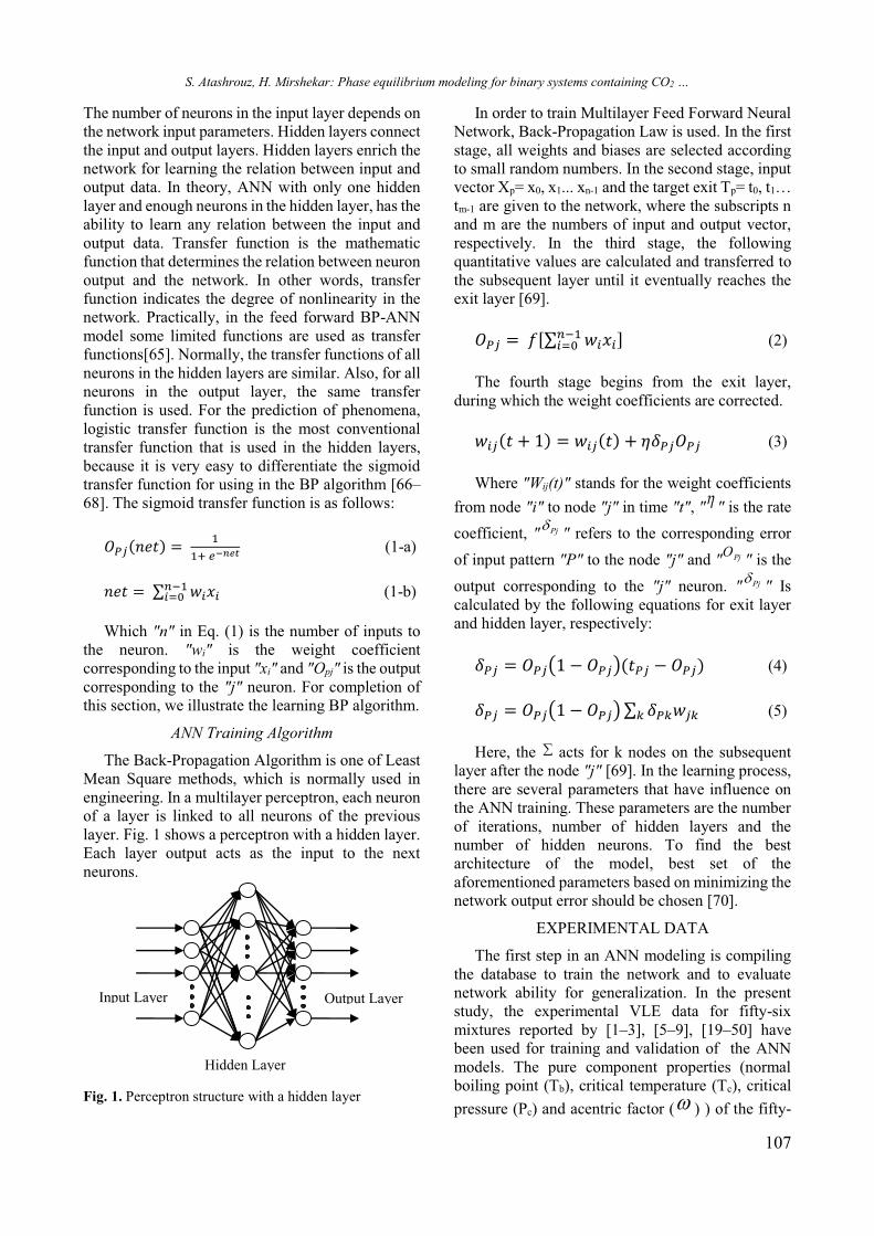
The Back-Propagation Algorithm is one of Least Mean Square methods, which is normally used in engineering. In a multilayer perceptron, each neuron of a layer is linked to all neurons of the previous layer. Fig. 1 shows a perceptron with a hidden layer. Each layer output acts as the input to the next neurons.

Fig. 1. Perceptron structure with a hidden layer

In order to train Multilayer Feed Forward Neural Network, Back-Propagation Law is used. In the first stage, all weights and biases are selected according to small random numbers. In the second stage, input vector Xp= x0, x1... xn-1 and the target exit Tp= t0, t1… tm-1 are given to the network, where the subscripts n and m are the numbers of input and output vector, respectively. In the third stage, the following quantitative values are calculated and transferred tothe subsequent layer until it eventually reaches the exit layer [69].

�� = �[∑ �� ] (2)

The fourth stage begins from the exit layer, during which the weight coefficients are corrected.

��(� + 1) = ��(�) + �� (3)

Where "Wij(t)" stands for the weight coefficients from node "i" to node "j" in time "t", "� " is the rate coefficient, " Pj� " refers to the corresponding error of input pattern "P" to the node "j" and " PjO " is the output corresponding to the "j" neuron. " Pj� " Is calculated by the following equations for exit layer and hidden layer, respectively:

�� = ��1 − ��(�� − ��) (4)

�� = ��1 − �� ∑ �� (5)

Here, the � acts for k nodes on the subsequent layer after the node "j" [69]. In the learning process, there are several parameters that have influence on the ANN training. These parameters are the number of iterations, number of hidden layers and the number of hidden neurons. To find the best architecture of the model, best set of the aforementioned parameters based on minimizing the network output error should be chosen [70].

EXPERIMENTAL DATA

The first step in an ANN modeling is compiling the database to train the network and to evaluate network ability for generalization. In the present study, the experimental VLE data for fifty-six mixtures reported by [1–3], [5–9], [19–50] have been used for training and validation of the ANN models. The pure component properties (normal boiling point (Tb), critical temperature (Tc), critical pressure (Pc) and acentric factor ( ) ) of the fifty-�

Input Layer

Hidden Layer

Output Layer


108

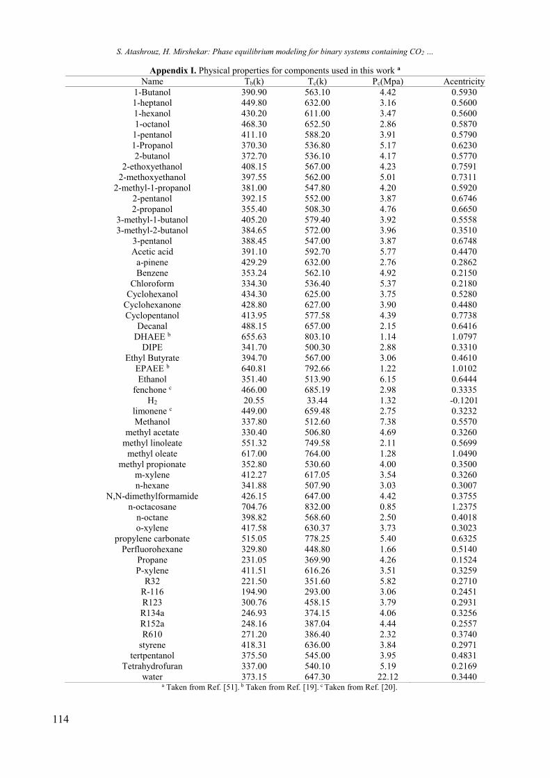
six Pure component used in this work were collected from different literature [19], [20], [51] and the collection was listed in Appendix I. also the range of T, P, x1 and y1 is reported in Appendix II.

Development of the ANN Model

In estimating VLE by using ANN, most of the previous works predict two VLE parameters, and all of them use only one ANN model for predicting these two VLE parameters. The use of only one ANN for the prediction of two VLE parameters leads to the complexity of the network and also reduces the network accuracy. This is because of the order of standard deviation for the output parameters.

Standard deviation (STD) for a number of data sets defines as: �� = �

� ∑ (�� − �� ̅)! (6)

Where

�̅ = �� ∑ �� (7)

In Eq. (6) and Eq. (7) "n" is the number of data point and "�̅" is the average of data sets.

When the order of standard deviation of an output parameter is higher than the other, the error of the higher standard deviation output, affects the other output parameter and this problem reduces accuracy of ANN model.

To investigate this influence, with the aim of calculating x1 and y1, three models were considered:

Model I (x1 prediction), model II (y1 prediction) and the model III (x1 and y1 prediction). The inputs of the all models are P, T, Tc, Pc, � . The standard deviation of y1 and x1 is 0.1794 and 0.2751 respectively. Model I and model II with 339 and 310 parameters respectively and model III with different structure has been developed and the results were shown in Table 1. As shown model I that predicts only x1 has more accuracy in comparison with other structures of model III. The accuracy of this model is better than even the ANN structures with more parameters in model III. Also in regard to model II the accuracy of this model is better in predicting of y1 than the entire model III structures. So according to Table 1 for VLE modeling by ANN for have more accuracy we should develop two separate ANN for every VLE parameter

Two ANN models were considered for the prediction of CO2 mole fraction in the vapor and liquid phases. In order to describe the phase behavior of the fifty-six CO2 (1) - component (2) binaries by two ANN models, eight variables have been selected in this work: four intensive state variables (equilibrium temperature, equilibrium pressure and equilibrium CO2 mole fractions in the liquid and vapor phases) and four pure component properties of the components (normal boiling point, critical temperature, critical pressure and acentric factor). The choice of the input and output variables was based on the phase rule. Therefore, the equilibrium temperature and pressure, together with the pure

Table 1. AAD (%) for model I, model II and different structure of model III.

Number of ANN parametersAAD (%)

x1

AAD (%)

y1

339a 1.572 -310b - 0.848101 4.781 2.425182 3.674 2.283275 2.556 1.580321 2.405 1.601460 2.109 1.373671 2.033 1.270839 2.069 1.248911 1.776 1.319959 2.014 1.416

1103 2.092 1.3131962 1.658 1.0874438 2.085 1.253

amodel I: predicting only x1 bmodel II: predicting only y1


109

Table 2. Architecture of the optimized ANN models. Hidden layer 1 Hidden layer 2 Output layer

Network Type

Training Algorithm

No. of neurons

Activation function No. of neurons Activation

functionNo. of

neuronsActivation function

FFBP-ANNa

BRBP usingLevenberg-Marquardt

optimizationb

Model I: 14Model II: 15

tansigMATLABfunction

Model I:15

Model II:12

tansigMATLABfunction

1

Linear(purelin

MATLAB function)

anewff MATLAB function. btrainbr MATLAB function.component properties have been selected as input variables and the CO2 mole fraction in the liquid and vapor phases as output variables. A simple scheme of inputs and output to the developed ANN models was shown in Fig. 2.

Fig. 2. A simple scheme of inputs and output to the models, output for the model I and model II are x1 and y1respectively

In the training phase, the number of neurons in the hidden layers was important for the network optimization. However, decision on the number of hidden layers neurons is difficult because it depends on the specific problem being solved using ANN. With too few neurons, the network may not be powerful enough for a given learning task. With a large number of neurons, the ANN may memorize the input training data very well so that the network tends to perform poorly on new test data and is called “over-fitting”. To prevent the over-fitting issue, we should evaluate average absolute deviation percent (AAD (%)) for train set, validation set and test set and they must be in the same order of magnitude. Average absolute deviation percent (AAD (%)) was calculated from the following relation:

AAD (%) = �� ∑ "#�

$%& − #�'*,-"�� (8)

Where "n" is the number of data point, "Exp" and "Calc" superscripts stand for the experimental and calculated CO2 mole fraction respectively.

ANN modeling for the VLE of fifty-six CO2 (1)-component (2) binaries was carried out in MATLAB ver. 7.9.0 program. Initially, the program starts with the default FFBP-ANN type (newff MATLAB function), the Levenberg-Marquardt BPtraining algorithm (trainlm MATLAB training function) and one hidden layer. Once the topology is specified the starting and ending number(s) of neurons in the hidden layer(s) have to be specified.

The number of neurons in hidden layer(s) is then modified by adding neurons one at a time. The procedure begins with the logarithmic sigmoid activation function and then the hyperbolic tangent sigmoid activation function for the hidden layers and the linear activation function for the output layer. The results of different runs of the program show that the Bayesian Regularization Back Propagation (BRBP), using Levenberg-Marquardtoptimization models, train more successfully than models using attenuated training. Table 2 shows the structure of the optimized ANN models.

RESULTS AND DISCUSSION

Using the random selection method, 60% of all data were assigned to the training set, 20% of all data were assigned to the validation set and the rest of the data were used as the test set. In the training process, different hidden layers and neurons were tried and finally the optimized ANN obtained for this study were two networks with two hidden layers containing 14 neurons in layer 1 and 15 neurons in layer 2 for model I and two hidden layers containing 15 neurons in layer 1 and 12 neurons in layer 2 for model II. In an optimized ANN, the AAD (%) for the train, validation and test data sets are in the same order of magnitude. AAD (%) and also, network performance, sum of squares error (SSE) for the train, validation and test sets of data were listed in Table 3.

Table 3. SSE and AAD (%) for the models. Model SSE AAD (%)

trainAAD (%)

testAAD (%) validation

I 0.38097 1.603 1.497 1.572II 0.26887 0.864 0.751 0.896

The ability of the models for the prediction of CO2 mole fraction in the vapor and liquid phases are shown in the Fig. 3 and Fig. 4. Where “R” is correlation coefficient and defined by:

. = /022�3(�, #) = ∑ (%�% 5 )(6�67)�89:;∑ (%�%̅)< ∑ (6�67)<�89:�89:

(9)


110

Where "n" is the number of data point, "x" and "y" are target and output parameters respectively and "� 5" and "#5 " are the average of the target and output.

Fig. 3. Comparison of the experimental and modeling results for the mole fraction in liquid phase of CO2 in fifty-six binary mixtures by ANN model I.

Fig. 4. Comparison of the experimental and modeling results for the mole fraction in vapor phase of CO2 in fifty-six binary mixtures by ANN model II.

As shown, good agreement for the prediction of ANN model and the experimental data are observed. So the ANN models can be reliably used to estimate x1 and y1 for CO2- binary systems within the ranges of parameters considered in this work.

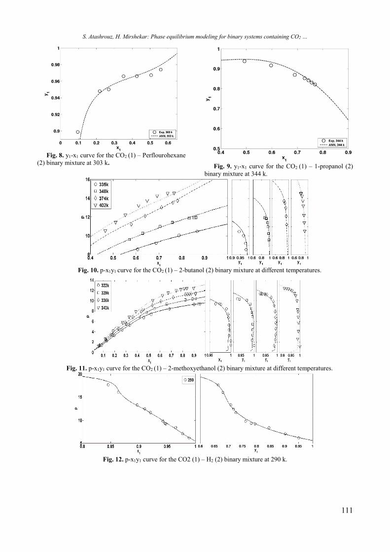
Figs. 5 to 9 show the y1-x1 curves for the five CO2-containing binary mixtures including 1-butanol, propane, R610, perflourohexane and 1-propanol and also Figs. 10 to 14 show the p-x1y1

curves for five CO2-containing binary mixtures including 2-butanol, 2-methoxyethanol, H2, R123, R152a at different temperatures. The lines are the results of ANN models. They include a comparison between experimental data and ANN results. As shown, the Figures show good agreement between experimental data and the prediction of the ANN models. By comparing the behavior of Fig. 12 with that of other p-x1y1 Figures, it can be seen that

Fig. 5. y1-x1 curve for the CO2 (1) – 1-butanol (2) binary mixture at 354 k.

Fig. 6. y1-x1 curve for the CO2 (1)–Propane (2) binary mixture at 253 k.

Fig. 7. y1-x1 curve for the CO2 (1) – R610 (2) binary mixture at 263 k.

treatment of H2-CO2 system is completely different from others, while the ANN models with a good reliability predict this treatment and this shows that ANN models are strong models to predict VLE data even with completely different treatment.


111

Fig. 8. y1-x1 curve for the CO2 (1) – Perflourohexane (2) binary mixture at 303 k. Fig. 9. y1-x1 curve for the CO2 (1) – 1-propanol (2)

binary mixture at 344 k.

Fig. 10. p-x1y1 curve for the CO2 (1) – 2-butanol (2) binary mixture at different temperatures.

Fig. 11. p-x1y1 curve for the CO2 (1) – 2-methoxyethanol (2) binary mixture at different temperatures.

Fig. 12. p-x1y1 curve for the CO2 (1) – H2 (2) binary mixture at 290 k.


112

Fig. 13. p-x1y1 curve for the CO2 (1) – R123 (2) binary mixture at different temperatures.

Fig. 14. p-x1y1 curve for the CO2 (1) – R152a (2) binary mixture at different temperatures.CONCLUSIONS

In this work, two comprehensive FFBP-ANN models were developed for the prediction of x1 and y1 data for fifty-six CO2-containing binary mixtures at different temperature range. It was shown that good agreement between the model predictions and the experimental data was achieved.

The study and its results allow us to obtain these conclusions:

1. It was shown that in prediction of two VLE parameters by use of ANN for reducing the errors and increases the accuracy of ANN, two separate ANN for every parameter should be used.

2. The advantage of the ANN model is its applicability for the all fifty-six CO2-containing binary mixtures in just two models, while the thermodynamic models are used for an especially binary mixture.

3. Use of ANN models for prediction of VLE data is less cumbersome way in comparison with thermodynamic models, especially in cases with no information about appropriate thermodynamic model.

4. The AAD (%) for the model I and model II were obtained 1.572 and 0.848 respectively. Therefore, the ANN model can be reliably used to estimate x1 and y1 for CO2- binary systems within the ranges of parameters considered in this work.

Acknowledgements: The authors gratefully acknowledge to amir abbas pouladi for his help in this work.

REFERENCES 1.K. Tochigi, T. Namae, T. Suga, H. Matsuda, K.

Kurihara, M. C. Ramos, C. McCabe, J. Supercrit. Fluid, 55, 682, ( 2010).

2.A. Bejarano, J. E. Gutiérrez, K. a. Araus, J. C. de la Fuente, J. Chem. Thermodyn., 43, 759, (2011).

3. J.E. Gutiérrez, A. Bejarano, J.C.D.L. Fuente, J. Chem. Thermodyn., 42, 591, (2010).

4. R. Abedini, I. Zanganeh, M. Mohagheghian, J. Phase Equilib. Diff., 32, 105, (2011).

5. G. Silva-Oliver, L.A. Galicia-Luna, Fluid Phase Equilibr., 182, 145, (2001).

6. K. Bezanehtak, G.B. Combes, F. Dehghani, N. R. Foster, D. L. Tomasko, J. Chem. Eng. Data, 47, 161, (2002).

7. J.S. Lim, J.M. Jin, K.P. Yoo, J. Supercrit. Fluid, 44,279, (2008).

8. K. Jeong, J. Im, G. Lee, Y.J. Lee, H. Kim, Fluid Phase Equilibr., 251, 63, (2007).

9. C. Zhu, X. Wu, D. Zheng, W. He, S. Jing, Fluid Phase Equilibr., 264, 259, (2008).

10. I.P. Koronaki, E. Rogdakis, T. Kakatsiou, Energ. Convers. Manage., 60, 152, (2012).

11. H. Karimi, F. Yousefi, Chinese J. Chem. Eng., 15,765, (2007).

12. C. Si-Moussa, S. Hanini, R. Derriche, M. Bouhedda, A. Bouzidi, Braz. J. Chem. Eng., 25, 183, (2008).

13. C.A. Faúndez, F.A. Quiero, J.O. Valderrama, Fluid Phase Equilibr., 292, 29, (2010).

14. M. Safamirzaei, H. Modarress, Mohsen-Nia, Fluid Phase Equilibr., 289, 32, (2010).

15. F. Eslamimanesh, A. Gharagheizi, A.H. Mohammadi, D. Richon, Chem. Eng. Sci., 66, 3039, (2011).


113

16. A. Sencan, , I.I. Köse, R. Selbas, Energ. Convers. Manage., 52, 958, (2011).

17. A. Sozen, E. Arcaklioglu, T. Menlík, Expert Syst. Appl., 37, 1158, (2010).

18. Y. Bakhbakhi, Expert Syst. Appl., 38, 11355, (2011). 19. C. Ming J. Chang, M. Shian Lee, B. chin Li, P.yen

Chen, Fluid Phase Equilibr., 233, 56, (2005). 20. M. Akgu, N. A. Akgu, S. Dinc, J. Supercrit. Fluid,

15, 117, (1999). 21. G. Silva-Oliver, L.A. Galicia-Luna, Fluid Phase

Equilibr., 199, 213, (2002). 22. Ž. Knez, M. Škerget, L. Ilič, C. Lütge, J. Supercrit.

Fluid, 43, 383, (2008). 23. . O. Elizalde-Solis, L.A. Galicia-Luna, S. I. Sandler,

J. G. Sampayo-Hernández, Fluid Phase Equilibr.,210, 215, (2003).

24. W.H. Hwu, J.S. Cheng, K.W. Cheng, Y.P. Chen, J. Supercrit. Fluid, 28, 1, (2004).

25. O. Elizalde-Solis, L.A. Galicia-Luna, L.E. Camacho-Camacho, Fluid Phase Equilibr., 259, 23, (2007).

26. T. Hiaki, H. Miyagi, T. Tsuji, M. Hongo, J. Supercrit. Fluid, 13, 23, (1998).

27. S. N. Joung, C. W. Yoo, H. Y. Shin, S. Y. Kim, K. P. Yoo, C. S. Lee, W. S. Huh, Fluid Phase Equilibr.,185, 219, (2001).

28. W. Lin, H. Xiaosong, Z. Lan, C. Kaixun, Chinese J. Chem. Eng., 17, 642, (2009).

29. H. S. Lee, H. Lee, Fluid Phase Equilibr., 150, 695, (1998).

30. A. Bamberger, G. Sieder, G. Maurer, J. Supercrit. Fluid, 17, 97, (2000).

31. 31. K. Ohgaki and T. Katayama, J. Chem. Eng. Data,21, 53, (1976).

32. A. M. Scurto, C. M. Lubbers, G. Xu, J. F. Brennecke, Fluid Phase Equilibr., 190, 135, (2001).

33. S. Laugier, D. Richon, J. Chem. Eng. Data, 42, 155, (1997).

34. P. Naidoo, J. D. Raal, D. Ramjugernath, J. Chem. Eng. Data, 55, 196, (2010).

35. M. V. da Silva, D. Barbosa, P. O. Ferreira, J. Chem. Eng. Data, 47, 1171, (2002).

36. L. Hongling, Z. Rongjiao, X. Wei, L. Yanfen, S. Yongju, T. Yiling, J. Chem. Eng. Data, 56, 1148, (2011).

37. F. Gironi, M. Maschietti, J. Supercrit. Fluid, 70, 8, ( 2012).

38. S. Schwinghammer, M. Siebenhofer, R. Marr, J. Supercrit. Fluid, 38, 1, (2006).

39. L. Hongling, Z. Rongjiao, X. Wei, X. Hongfei, D. Zeliang, T. Yiling, J. Chem. Eng. Data, 54, 1510, (2009).

40. C. Duran-Valencia, A. Valtz, L.A. Galicia-Luna, D. Richon, J. Chem. Eng. Data, 46, 1589, (2001).

41. S.H. Huang, H.M. Lin, K.C. Chao, J. Chem. Eng. Data, 33, 143, (1988).

42. J.H. Kim, M.S. Kim, Fluid Phase Equilibr., 238, 13, (2005).

43. F. Rivollet, A. Chapoy, C. Coquelet, D. Richon, Fluid Phase Equilibr., 218, 95, (2004).

44. A. Valtz, C. Coquelet, D. Richon, Fluid Phase Equilibr., 258, 179, (2007).

45. C. Duran-Valencia, G. Pointurier, A. Valtz, P. Guilbot, D. Richon, J. Chem. Eng. Data, 47, 59, (2002).

46. H. Madani, A. Valtz, C. Coquelet, A. H. Meniai, D. Richon, J. Chem. Thermodyn., 40, 1490, (2008).

47. A. Valtz, X. Courtial, E. Johansson, C. Coquelet, D. Ramjugernath, Fluid Phase Equilibr., 304, 44, (2011).

48. M. Akgün, D. Emel, N. Baran, N.A. Akgün, S. Deniz, S. Dinçer, J. Supercrit. Fluid, 31, 27, (2004).

49. W. Lin, L. Jian-cheng, Y. Hao, C. Kai-xun, Chem. Res. Chinese U., 27, 678, (2011).

50. D. Kodama, T. Yagihashi, T. Hosoya, M. Kato, Fluid Phase Equilibr., 297, 168, (2010).

51. Aspen Hysys 2006 Software- aspenONE. 52. P. Petersen, R. Fredenslund, A. Rasmussen, Comput.

Chem. Eng., 18, 63, (1994). 53. C. Guimaraes, P.R.B. McGreavy, Comput. Chem.

Eng., 19, 741, (1995). 54. R. Sharma, D. Singhal, R. Ghosh, A. Dwivedi,

Comput. Chem. Eng., 23, 385, (1999). 55. S. Urata, A. Takada, J. Murata, T. Hiaki, A. Sekiya,

Fluid Phase Equilibr., 199, 63, (2002). 56. S. Ganguly, Comput. Chem. Eng., 27, 1445, (2003). 57. K. Piotrowski, J. Piotrowski, J. Schlesinger, Chem.

Eng. Process., 42, 285, (2003). 58. M. Bilgin, J. Serb. Chem. Soc., 69, 669, (2004). 59. S. Mohanty, Fluid Phase Equilibr., 235, 92, (2005). 60. S. Mohanty, Int. J. Refrig., 29, 243, (2006).61. H. Yamamoto, K. Tochigi, Fluid Phase Equilibr.,

257, 169, (2007). 62. H. Ghanadzadeh, H. Ahmadifar, J. Chem.

Thermodyn., 40, 1152, (2008). 63. C.A. Faúndez, F.A. Quiero, J. O. Valderrama, Chem.

Eng. Commun., 198, 102, (2011). 64. B. Zarenezhad and A. Aminian, Korean J. Chem.

Eng., 28, 1286, (2011). 65. G. Zhang, B. E. Patuwo, M. Y. Hu, Int. J.

Forecasting, 14, 35, (1998). 66. H.J. Manohar, R. Saravanan, S. Renganarayanan,

Energ. Convers. Manage., 47, 2202, (2006). 67. A. Malallah, I.S. Nashawi, J. Petrol. Sci. Eng., 49,

193, (2005). 68. M. Chakraborty, C. Bhattacharya, S. Dutta, J.

Membrane Sci., 220, 155, (2003). 69. R. Beale, T. Jackson, Neural Computing: An

Introduction, Institute of Physics Publishing, London, 1998.

70. A.R. Moghadassi, M.R. Nikkholgh, S.M. Hosseini, F. Parvizian, A. Sanaeirad, Arpn-Jeas, 6, 100, (2011).


114

Appendix I. Physical properties for components used in this work a

Name Tb(k) Tc(k) Pc(Mpa) Acentricity1-Butanol 390.90 563.10 4.42 0.59301-heptanol 449.80 632.00 3.16 0.56001-hexanol 430.20 611.00 3.47 0.56001-octanol 468.30 652.50 2.86 0.5870

1-pentanol 411.10 588.20 3.91 0.57901-Propanol 370.30 536.80 5.17 0.62302-butanol 372.70 536.10 4.17 0.5770

2-ethoxyethanol 408.15 567.00 4.23 0.75912-methoxyethanol 397.55 562.00 5.01 0.7311

2-methyl-1-propanol 381.00 547.80 4.20 0.59202-pentanol 392.15 552.00 3.87 0.67462-propanol 355.40 508.30 4.76 0.6650

3-methyl-1-butanol 405.20 579.40 3.92 0.55583-methyl-2-butanol 384.65 572.00 3.96 0.3510

3-pentanol 388.45 547.00 3.87 0.6748Acetic acid 391.10 592.70 5.77 0.4470

a-pinene 429.29 632.00 2.76 0.2862Benzene 353.24 562.10 4.92 0.2150

Chloroform 334.30 536.40 5.37 0.2180Cyclohexanol 434.30 625.00 3.75 0.5280

Cyclohexanone 428.80 627.00 3.90 0.4480Cyclopentanol 413.95 577.58 4.39 0.7738

Decanal 488.15 657.00 2.15 0.6416DHAEE b 655.63 803.10 1.14 1.0797

DIPE 341.70 500.30 2.88 0.3310Ethyl Butyrate 394.70 567.00 3.06 0.4610

EPAEE b 640.81 792.66 1.22 1.0102Ethanol 351.40 513.90 6.15 0.6444

fenchone c 466.00 685.19 2.98 0.3335H2 20.55 33.44 1.32 -0.1201

limonene c 449.00 659.48 2.75 0.3232Methanol 337.80 512.60 7.38 0.5570

methyl acetate 330.40 506.80 4.69 0.3260methyl linoleate 551.32 749.58 2.11 0.5699

methyl oleate 617.00 764.00 1.28 1.0490methyl propionate 352.80 530.60 4.00 0.3500

m-xylene 412.27 617.05 3.54 0.3260n-hexane 341.88 507.90 3.03 0.3007

N,N-dimethylformamide 426.15 647.00 4.42 0.3755n-octacosane 704.76 832.00 0.85 1.2375

n-octane 398.82 568.60 2.50 0.4018o-xylene 417.58 630.37 3.73 0.3023

propylene carbonate 515.05 778.25 5.40 0.6325Perfluorohexane 329.80 448.80 1.66 0.5140

Propane 231.05 369.90 4.26 0.1524P-xylene 411.51 616.26 3.51 0.3259

R32 221.50 351.60 5.82 0.2710R-116 194.90 293.00 3.06 0.2451R123 300.76 458.15 3.79 0.2931R134a 246.93 374.15 4.06 0.3256R152a 248.16 387.04 4.44 0.2557R610 271.20 386.40 2.32 0.3740

styrene 418.31 636.00 3.84 0.2971tertpentanol 375.50 545.00 3.95 0.4831

Tetrahydrofuran 337.00 540.10 5.19 0.2169water 373.15 647.30 22.12 0.3440

a Taken from Ref. [51]. b Taken from Ref. [19]. c Taken from Ref. [20].


115

Appendix II. Range of data used for developing of the ANN models. Systems: CO2 (1) + T/K ΔP/Mpa Δx1 Δy1

1-butanol 354,398,430,324,333,355,392,426,313 2.067-16.939 0.074-0.9031 0.7976-0.99591-heptanol 374,411,431 4.038-21.391 0.2173-0.87 0.8932-0.99781-hexanol 324,353,397,403,431,432 2.268-20.128 0.035-0.9008 0.801-0.99741-octanol 328 4-15 0.2406-0.7772 0.9435-0.99971-pentanol 313,323,333 1.81-11.72 0.091-0.76 0.968-0.9981-propanol 344,373,397,426,313,323,333 2.15-15.769 0.095-0.835 0.54-0.9932-butanol 335,348,374,402,431,313 4.03-14.536 0.2906-0.8965 0.7082-0.99462-ethoxyethanol 323,330,337,344 1.29-12.37 0.0788-0.969 0.9052-0.99992-methoxyethanol 322,329,336,343 1.19-12.4 0.0576-0.9535 0.9105-0.99992-methyl-1-propanol 313,323,333,313,323,333,343,353 2.11-14.04 0.094-0.9328 0.9294-0.99612-pentanol 313,313,323,333 1-10.587 0.025-0.985 0.9645-0.9972-propanol 334,344,353,378,398,413,432,443 2.03-13.788 0.06-0.888 0.443-0.9753-methyl-1-butanol 313,323,333 2.08-10.68 0.111-0.895 0.97-0.9943-methyl-2-butanol 313,323,333 2.147-10.249 0.105-0.9055 0.9681-0.99563-pentanol 313,323,333 1.942-10.207 0.0957-0.9072 0.9678-0.9942acetic acid 313,333,353 1.1-11.1 0.0964-0.7098 0.948-0.9952a-pinene 313,323,333 7.15-10.93 0.478-0.908 0.983-0.9983benzene 298,313 0.89383-7.7504 0.1063-0.9327 0.9754-0.9959Chloform 303,313,323,333 0.032416-9.9689 0-1 0-1cyclohexanol 433,473 3.55-21.5 0.089-0.602 0.84-0.947Cyclohexanone 433,453 3.03-21.52 0.103-0.736 0.843-0.962cyclopentanol 373,403 0.914-11.838 0.0177-0.3942 0.9264-0.9891decanal 288,303,313 1.68-8.22 0.28-0.96 0.989-0.998DHAEE 313,333 4.24-23.54 0.5325-0.9443 0.9822-0.9999diisopropyl ether 265,273,293,313,333 0.547-2.554 0.1127-0.7589 0.9269-0.9998EB 313,333,353,373 2-12 0.18-0.9495 0.8153-0.9978EPAEE 313,333 2.86-20.79 0.2842-0.9402 0.979-0.9999ethanol 313,333,353,313,313,322,333,338,344 0.57-13.9 0.0269-0.9668 0.8068-0.9948Fenchone 313,323,333 7.04-11.2 0.606-0.92 0.9808-0.9997H2 278,290 4.805-19.253 0.8455-0.9912 0.4945-0.9575limonene 313,323,333,323,343 7.04-13.5 0.429-0.93156 0.96053-0.9996methanol 313,278,288,298,308,313,320,330,335,342,303 0.573-12.39 0.0247-0.935 0.0977-0.9982methyl acetate 308,318,328 0.7-9 0.128-0.9802 0.892-0.9978methyl linoleate 313,333 2.86-18.03 0.5217-0.9509 0.9806-0.9999methyl oleate 313,333 2.86-18.03 0.4876-0.943 0.9812-0.9999methyl propionate 313,333,353,373 1-12 0.3125-0.9058 0.3282-0.9887m-xylene 313,333,353 0.7-10.37 0.04-0.6971 0.951-0.9754n-hexane 298,313 0.44372-7.6578 0.0495-0.924 0.9253-0.9904dimethylformamide 293,313,338 0.43-11.05 0.0345-0.8823 0.9874-0.9998n-octacosane 573 0.99405-5.0574 0.0596-0.27 0.9957-0.9983n-octane 313 0.52-3.522 0.0588-0.3905 0.9966-0.9979o-xylene 313,333,353 0.79-14.86 0.0536-0.8345 0.8469-0.9756PC 313,333,353,373 1-13 0.081-0.7279 0.952-0.9968perfluorohexane 303,313,323 0.479-3.454 0.0911-0.5588 0.8467-0.9806propane 253,263,273,283,293,303,313,323 0.2442-7.2062 0-1 0-1P-xylene 313,333,353 0.61-12.37 0.04-0.8377 0.8228-0.9748R32 283,293,303,305,313,323,333,343 1.106-7.464 0-1 0-1R116 253,273,283,291,294,296 1.051-6.448 0-1 0-1R123 313,323,333 0.873-8.074 0.1219-0.9209 0.7352-0.9788R134a 252, 272, 292, 323,328,329,333,338,339,354 0.131-7.369 0-0.867 0-0.983R152a 258,278,298,308,323,343 0.144-7.6482 0-1 0-1R610 263,283,303,308,323,338,352 0.1823-6.8628 0.0218-0.9473 0.2418-0.983styrene 333,338,343,348 6-13.42 0.428-0.932 0.895-0.998tertpentanol 313,323,333,345 4.56-11.44 0.2409-0.9236 0.9253-0.9977tetrahydrofuran 313,333,353,298,313 0.47-10.29 0.0687-0.983 0.9347-0.998water 323,333,353 4.05-14.11 0.008-0.0217 0.9857-0.9966


116

МОДЕЛИРАНЕ ЧРЕЗ ИЗКУСТВЕНИ НЕВРОННИ МРЕЖИ НА БИНАРНИ СИСТЕМИ,СЪДЪРЖАЩИ ВЪГЛЕРОДЕН ДИОКСИД

С.Аташруз*, Х. МишекарДепартамент по инженерна химия, Технологичен университет Амиркабир (Политехнически университет в

Техеран), Кампус Махшахр, Махшахр, Иран.

Постъпила на 7 януари, 2013 г.; коригирана на 28 май, 2013 г.

Използвани се два математични модела, базирани на FFBP-ANN-невронни мрежи за предсказването на молните части на CO2 в течна (x1) и парова (y1) фаза при равновесието течност-пари (VLE) за петдесет и шест бинарни смеси, съдържащи CO2. За съставяне на моделите са използвани 2104 групи от данни, намерени в литературата. За тестването на моделите са използвани експериментални данни, неприлагани при ANN-тренирането. Предсказаните резултати, получени чрез невронните мрежи са сравнени с достъпни литературни данни и е намерено резонно съгласие с тях. Средните абсолютни отклонения, получени с модела ANN-I за молните части x1 и с модела ANN-II за молните части y1 са съответно 1.572 % и 0.848 %. Изследването показва, че моделирането с невронни мрежи е добър алтернативен метод за оценяването на фазовите равновесия за този тип системи.

phase equilibrium modeling for binary systems …. atashrouz, h. mirshekar: phase equilibrium...

Documents