phase i experimental testing of a generic submarine model ... · further experimental testing of...

UNCLASSIFIED

Phase I Experimental Testing of a Generic Submarine Model in the DSTO Low Speed Wind Tunnel

Howard Quick1, Ronny Widjaja2, Brendon Anderson2, Bruce Woodyatt1, Andrew D. Snowden1 and Stephen Lam1

1Air Vehicles Division 2Maritime Platforms Division

Defence Science and Technology Organisation

DSTO-TN-1101

ABSTRACT DSTO has conducted Phase I of planned experimental testing of a generic submarine model in its low speed wind tunnel. These wind tunnel tests aimed to gather steady-state aerodynamic force and moment data and to investigate the flow-field characteristics on and around the bare-hull. Further experimental testing is planned, extending the range of model configurations tested to include the addition of hull-casing, fin and control surfaces to the model. These experimental data will complement computational and experimental hydrodynamic analysis of the generic submarine shape.

Approved for public release

RELEASE LIMITATION

UNCLASSIFIED

UNCLASSIFIED

Published by Air Vehicles Division DSTO Defence Science and Technology Organisation 506 Lorimer St Fishermans Bend, Victoria 3207 Australia Telephone: (03) 9626 7000 Fax: (03) 9626 7999 © Commonwealth of Australia 2012 AR-015-344 July 2012 APPROVED FOR PUBLIC RELEASE

UNCLASSIFIED

UNCLASSIFIED

UNCLASSIFIED

Phase I Experimental Testing of a Generic Submarine Model in the DSTO Low Speed Wind Tunnel

Executive Summary Through the DSTO Corporate Enabling Research Programme (CERP) – Future Undersea Warfare, researchers are applying computational and experimental methods to explore the flow-field characteristics on and around a modern generic submarine shape. This comprehensive research study involves the use of high-fidelity computational fluid dynamic (CFD) methods, as well as experimental hydrodynamic and experimental aerodynamic test techniques to investigate a (common) generic shape. A substantial body of data will be gathered, enhancing DSTO knowledge and understanding of these complex flows, and providing researchers with a valuable database compiled from disparate sources. This report documents Phase I testing of the generic submarine in the DSTO low speed wind tunnel. The Phase I low speed wind tunnel experiments involved the testing of a 1.35 m long aluminium model of the generic submarine in its bare-hull configuration, that is, without the hull-casing, fin, and control surfaces attached. The submarine model was pitched and yawed through a large range of attitudes, to gather gross steady-state aerodynamic force and moment data, and to explore the characteristics of the flow-field using several different flow visualization techniques such as tufting and smoke. The experiments also included the use of a thermal imaging camera to study boundary layer transition. The report describes the experimental equipment used during the tests, along with the test methodology. A sub-set of the data gathered is also presented and briefly discussed. Overall, the force and moment data were consistent, exhibiting expected and predictable trends. Whilst thermal imaging of boundary layer transition proved problematical, the use of conventional flow visualization techniques were more successful, allowing researchers to visualize the flow-field in regions of interest, including the tail-cone. Further experimental testing of the model in the DSTO low speed wind tunnel is planned, and will include a detailed study of the boundary layer profile, the use of particle image velocimetry (PIV) to study the off-body flow-field, as well as additional force and moment testing with the hull-casing, fin, and the control surfaces attached.

UNCLASSIFIED

UNCLASSIFIED

This page is intentionally blank

UNCLASSIFIED DSTO-TN-1101

Contents

NOTATION..............................................................................................................................IV

1. INTRODUCTION............................................................................................................... 1

2. EXPERIMENTAL EQUIPMENT ...................................................................................... 1 2.1 Generic Submarine Model...................................................................................... 1 2.2 DSTO Low Speed Wind Tunnel............................................................................ 3

2.2.1 Blockage Ratio.......................................................................................... 3 2.3 Strain Gauge Balance ............................................................................................... 4

3. EXPERIMENTAL METHOD ............................................................................................ 4 3.1 Axes System ............................................................................................................... 5 3.2 Reference Coordinates ............................................................................................. 6 3.3 Data Reduction.......................................................................................................... 6 3.4 Flow Offset Tests ...................................................................................................... 7 3.5 Test Conditions ......................................................................................................... 8

3.5.1 Boundary Layer Transition .................................................................... 8 3.5.1.1 Boundary Layer Transition Check Method ......................................... 9

3.6 Test Schedule............................................................................................................. 9 3.6.1 Reference Runs ........................................................................................ 9 3.6.2 Bare-Hull – Boundary Layer Transition Strips-Off ............................ 9 3.6.3 Bare-Hull – Boundary Layer Transition Strips-On........................... 10 3.6.4 Flow Visualisation Testing................................................................... 10 3.6.5 Thermal Imaging of Boundary Layer Transition.............................. 10

4. RESULTS ............................................................................................................................ 10 4.1 Force and Moment Tests........................................................................................ 11

4.1.1 Reference Runs ...................................................................................... 11 4.1.2 Bare-Hull – Boundary Layer Transition Strips-Off .......................... 11 4.1.3 Bare-Hull – Boundary Layer Transition Strips-On........................... 12 4.1.4 Bare-Hull – Comparison of Boundary Layer Transition Strips-Off

and On..................................................................................................... 13 4.2 Assessment of Data Quality.................................................................................. 14 4.3 Flow Visualisation.................................................................................................. 16

4.3.1 Smoke Generator and Probe ................................................................ 16 4.3.2 Tufting..................................................................................................... 17

4.4 Thermal Imaging of Boundary Layer Transition.............................................. 17

5. CONCLUSION .................................................................................................................. 19

6. ACKNOWLEDGEMENTS .............................................................................................. 19

UNCLASSIFIED i


7. REFERENCES .................................................................................................................... 20

APPENDIX A - TECHNICAL SPECIFICATIONS ....................................................... 21

APPENDIX B - PHASE I TEST SCHEDULE................................................................. 23

APPENDIX C - DETERMINATION OF FLOW OFFSET ANGLES ......................... 24 C.1. Experimental Method.................................................................... 24 C.2. Computational Analysis ............................................................... 24

APPENDIX D - REFERENCE RUNS ............................................................................... 26

APPENDIX E - BARE-HULL – BOUNDARY LAYER TRANSITION STRIPS-OFF .............................................................................................................. 27

APPENDIX F - BARE-HULL – BOUNDARY LAYER TRANSITION STRIPS-ON ............................................................................................................... 29

APPENDIX G - BARE-HULL – COMPARISON OF BOUNDARY LAYER TRANSITION STRIPS-OFF AND ON ................................................ 31

List of Figures

Figure 1 - Generic submarine model mounted in the DSTO low speed wind tunnel............ 2 Figure 2 - Schematic cut-away drawing of the generic submarine model ............................... 3 Figure 3 - Strain gauge balance DSTO-BAL-04 ............................................................................ 4 Figure 4 - Axes system..................................................................................................................... 5 Figure 5 - Model reference coordinates......................................................................................... 6 Figure 6 - Boundary layer transition strip attached circumferentially at 5% of its body length (l) ......................................................................................................................................................... 8 Figure 7 - Boundary layer transition strips attached longitudinally down the constant diameter section of the body........................................................................................................... 9 Figure 8 - A typical smoke flow visualisation result showing the vortex flow around the model at high-incidence (Test condition: α = 25°, β= 0°, U= 10 m/s)................................................. 16 Figure 9 - A typical tufting flow visualisation result showing unsteady flow over the aft-body of the model at high-incidence ..................................................................................................... 17 Figure 10 - Thermal image of the model at zero-incidence and zero-sideslip in a free-stream flow of 60 m/s................................................................................................................................. 18

UNCLASSIFIED ii


List of Tables

Table 1 - Reference parameters for the generic submarine model ........................................... 6 Table 2 - Flow offset angles............................................................................................................. 7 Table 3 - Estimated uncertainties for the instrumentation and data acquisition system ..... 14 Table 4 - Estimated uncertainties for selected parameters ....................................................... 15

UNCLASSIFIED iii


Notation

CD Drag force coefficient

qS

D

[CK, CM, CN] Rolling, Pitching and Yawing moment coefficients

qSl

N

qSl

M

qSl

K,,

CL Lift force coefficient

qS

L

[CX, CY, CZ] Longitudinal, Side and Vertical force coefficients

qS

Z

qS

Y

qS

X,,

CG Centre of gravity d Body diameter (m)

D Drag force (N)

X Longitudinal force (N)

Y Side force (N)

Z Vertical force (N)

K Moment about the x-axis (Nm)

l Model reference length (1.35 m)

L Lift force (N)

M Moment about the z-axis (Nm)

MRP Moment Reference Point

N Moment about the y-axis (Nm)

q Dynamic pressure

2

2

1U (Pa)

Rel Reynolds number

Ul

S Model reference area (1.8225 m2, where S = l2)

u Velocity component along x-axis

v Velocity component along y-axis

U Free-stream wind tunnel air velocity (m/s)

w Velocity component along z-axis

UNCLASSIFIED iv


UNCLASSIFIED v

α Angle-of-attack (º)

β Angle-of-sideslip (º)

ρ Density (kg/m3)

μ Viscosity (kg/(s m))

σ Standard deviation


1. Introduction

This report describes the experimental testing of a generic submarine model in the DSTO low speed wind tunnel (LSWT). Researchers are using these tests to enhance their knowledge and understanding of the complex flow physics around modern submarine shapes, as well as to investigate and assess the relative merits of various experimental test techniques. This report documents Phase I of a larger experimental test programme, where the results gathered will complement a body of information being compiled for the generic submarine shape from various sources including computational fluid dynamic (CFD) methods and experimental hydrodynamic testing. The Phase I wind tunnel tests aimed to gather steady-state aerodynamic force and moment data, and to investigate the flow characteristics on and around the bare-hull, that is, the generic submarine without a body-casing, fin, or control surfaces attached. The model with these appendages fitted will be experimentally tested and reported at a later date. This report describes the experimental equipment used during Phase I including the wind tunnel model, the test facility, and the instrumentation used to gather the data. A section on experimental method defines the axes systems and reference coordinates used, the data reduction methods, the corrections applied to the results, the test conditions, and the test schedule. The results of the main test configurations are presented graphically, and briefly discussed. Selected CFD substantiation data are also included in the appendices.

2. Experimental Equipment

2.1 Generic Submarine Model

The generic submarine model was designed and manufactured to be suitable for testing in both a wind tunnel, and with minor modifications, a water tunnel. Machined from aluminium, the bare-hull model comprises a cylindrical centre-body with an ellipsoid nose, and a streamlined tail section (i.e. boat-tail). When fully assembled the model has a fineness ratio of approximately 7.3. Although the generic submarine model incorporates many geometric design features of modern submarines, the test article is a generic model design that has no full-scale equivalent.

UNCLASSIFIED 1


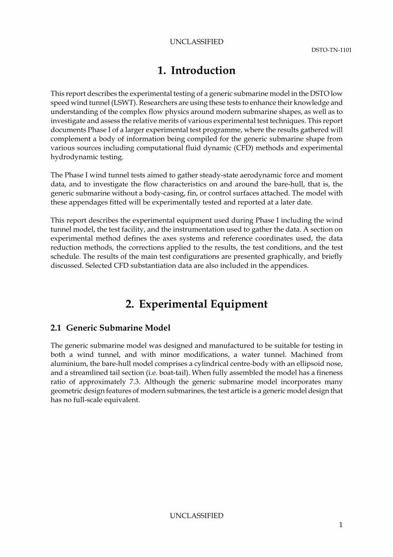
Figure 1 - Generic submarine model mounted in the DSTO low speed wind tunnel

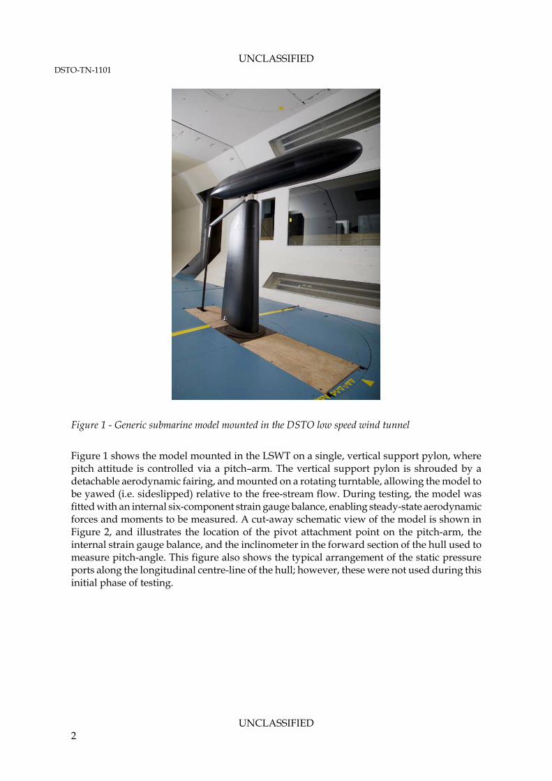
Figure 1 shows the model mounted in the LSWT on a single, vertical support pylon, where pitch attitude is controlled via a pitch–arm. The vertical support pylon is shrouded by a detachable aerodynamic fairing, and mounted on a rotating turntable, allowing the model to be yawed (i.e. sideslipped) relative to the free-stream flow. During testing, the model was fitted with an internal six-component strain gauge balance, enabling steady-state aerodynamic forces and moments to be measured. A cut-away schematic view of the model is shown in Figure 2, and illustrates the location of the pivot attachment point on the pitch-arm, the internal strain gauge balance, and the inclinometer in the forward section of the hull used to measure pitch-angle. This figure also shows the typical arrangement of the static pressure ports along the longitudinal centre-line of the hull; however, these were not used during this initial phase of testing.

UNCLASSIFIED 2


Figure 2 - Schematic cut-away drawing of the generic submarine model

2.2 DSTO Low Speed Wind Tunnel

The Phase I experimental tests were conducted in the DSTO LSWT located at Fishermans Bend in Melbourne. This facility is a conventional subsonic, closed-circuit wind tunnel that is capable of airspeeds up to 100 m/s. The test-section has an irregular octagonal cross-section measuring 2.74 m (wide) by 2.13 m (high). The maximum unit Reynolds number per metre is approximately 6 x 106 based on the maximum airspeed achievable during a test. Further technical specifications for the wind tunnel and its data acquisition system are provided in Table A1 and Table A2 respectively of Appendix A. 2.2.1 Blockage Ratio

The overall blockage ratio for the model at zero-incidence was estimated to be 2.1%. This value represents the sum of the frontal area of the model (i.e. 0.5%) and the vertical pylon fairing (i.e. 1.6%). This total figure is lower than the 7.5% blockage ratio regarded as acceptable in subsonic wind tunnel testing [1].

UNCLASSIFIED 3


2.3 Strain Gauge Balance

A six-component strain gauge balance was fitted inside the model, and used to measure gross steady-state aerodynamic forces and moments as the model was pitched and yawed through various discrete angles. Figure 3 shows the DSTO-BAL-04 strain gauge balance used throughout the tests, whilst details of its calibrated load range are provided in Table A3 of Appendix A.

Figure 3 - Strain gauge balance DSTO-BAL-04

3. Experimental Method

The experimental method used during these wind tunnel tests is described below, and includes details of the axes system and reference coordinates, data reduction, and flow offset testing. The test conditions are also reported, along with a brief description of the test schedule. Issues pertinent to data processing and data accuracy are also canvassed. A complete copy of the test schedule is included in Table B1 and Table B2 of Appendix B.

UNCLASSIFIED 4


3.1 Axes System

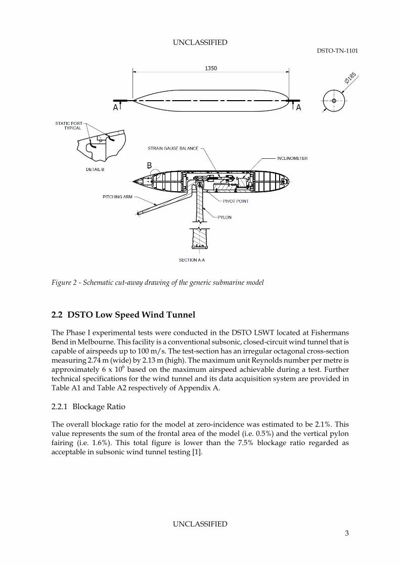
The model was tested at various attitudes, defined by combinations of angle-of-attack (α) and angle-of-sideslip (β). An inclinometer, a Jewel Instruments LCF-3000 unit, was fitted inside the model to measure α, whilst β was measured by the turntable encoder. Aerodynamic force and moment data were gathered in both wind and body-axes systems, and reduced to their non-dimensional coefficient form. Figure 4 defines the axes system used during these tests.

Figure 4 - Axes system

UNCLASSIFIED 5


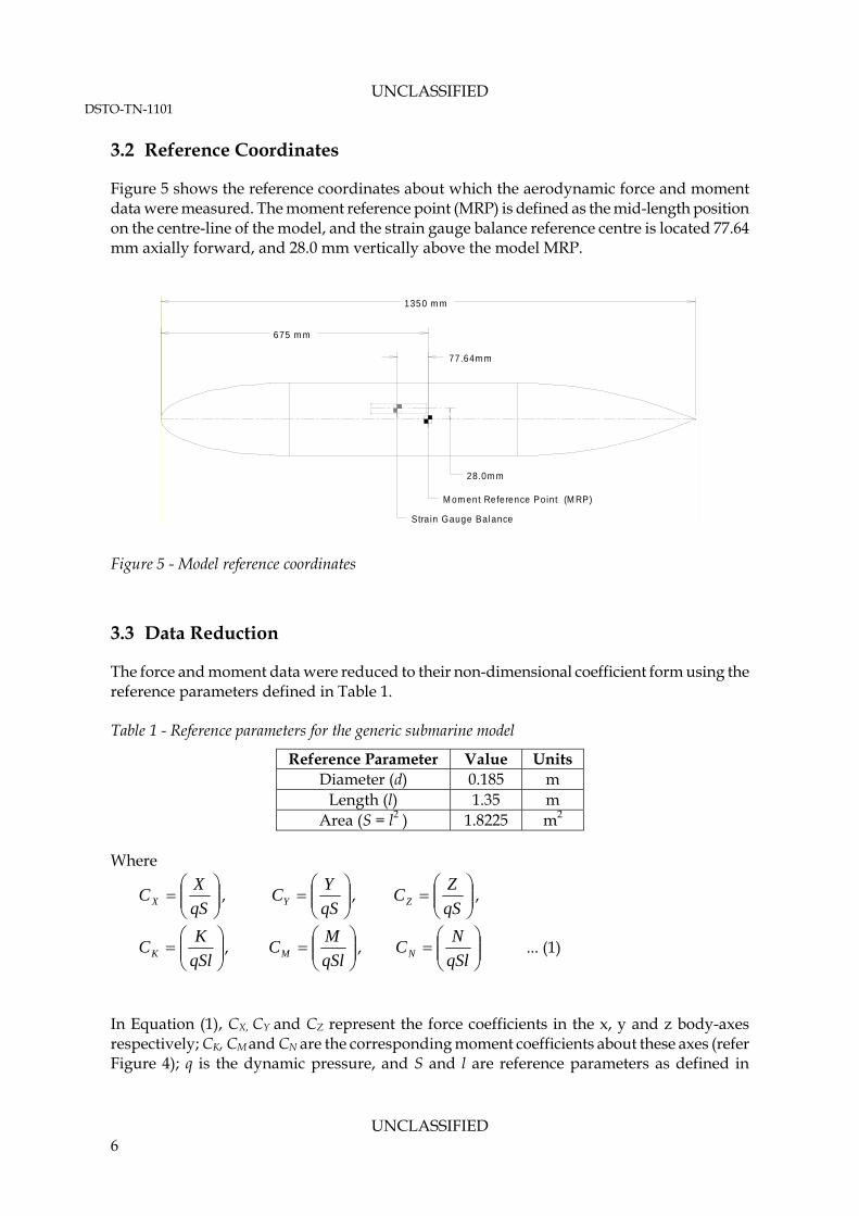
3.2 Reference Coordinates

Figure 5 shows the reference coordinates about which the aerodynamic force and moment data were measured. The moment reference point (MRP) is defined as the mid-length position on the centre-line of the model, and the strain gauge balance reference centre is located 77.64 mm axially forward, and 28.0 mm vertically above the model MRP.

1350 m m

675 m m

Stra in Gauge Balance

28.0m m

M om ent Reference Point (M RP)

77.64m m

Figure 5 - Model reference coordinates

3.3 Data Reduction

The force and moment data were reduced to their non-dimensional coefficient form using the reference parameters defined in Table 1. Table 1 - Reference parameters for the generic submarine model

Reference Parameter Value Units Diameter (d) 0.185 m

Length (l) 1.35 m Area (S = l2 ) 1.8225 m2

Where

qS

XCX ,

qS

YCY ,

qS

ZCZ ,

qSl

KCK ,

qSl

MCM ,

qSl

NCN ... (1)

In Equation (1), CX, CY and CZ represent the force coefficients in the x, y and z body-axes respectively; CK, CM and CN are the corresponding moment coefficients about these axes (refer Figure 4); q is the dynamic pressure, and S and l are reference parameters as defined in

UNCLASSIFIED 6


Table 1. Similarly, the lift and drag coefficients CL and CD respectively are defined in Equation (2) as:

qS

LCL ,

qS

DCD ... (2)

3.4 Flow Offset Tests

A limited number of tests were conducted to quantify the flow offsets, or flow angularities, in the wind tunnel test-section due to the presence of the model and its support equipment in the flow-field. With the model installed in the test-section, and using a method described in [1], the flow offset angles were estimated at a free-stream velocity of 60 m/s. The flow offset angles are presented as up-flow and cross-flow components. The estimated flow offset values are shown in Table 2, whilst a more detailed description of the method used is provided in Section C.1 of Appendix C.

Table 2 - Flow offset angles

Flow Direction Value Cross-flow 0.24° Up-flow 1.8°

The results in Table 2 show an order of magnitude difference between the cross-flow and up-flow angles. This discrepancy was unexpected, but is indicative of the adverse influence that the vertical pylon fairing and the pitch-arm have on the flow. This conclusion was subsequently confirmed by CFD, and is briefly discussed in section C.2 of Appendix C. Importantly, the force and moment data gathered during these tests will form part of a larger incremental database, that is, the hull-casing, fin, and the control surfaces will be considered as aerodynamic increments to the bare-hull. Therefore, there is no immediate requirement to correct the bare-hull force and moment data for the effects of up-flow and cross-flow, since all subsequent testing will be performed using the same model and mounting arrangement. However, the information does provide valuable insight into the effects that model suspension equipment can have on the flow-field. An experimental assessment of the support pylon is planned. This will involve the use of a dummy (mirror) pylon positioned above the model. Pitching and yawing the model in the presence of this mirror pylon, and then differencing the force and moment data gathered from the results for the conventional (single) support pylon arrangement, will provide an estimate of the aerodynamics for the model in a free-stream flow. The outcomes from these tests will be documented in a subsequent report.

UNCLASSIFIED 7


3.5 Test Conditions

The force and moment tests were conducted at a nominal airspeed of 60 m/s representing a Reynolds number Rel of 5.2 x 106, based on body length (l). Note for comparison, a typical full size submarine operating in seawater at 20 knots would have a corresponding Reynolds number of approximately 6 x 108. 3.5.1 Boundary Layer Transition

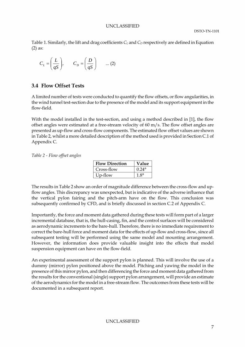
To better approximate the behaviour of the boundary layer over a typical, full-scale, submarine, transition strips were attached to the model. An empirical method, described in reference [2], was used to determine the appropriate carborundum grit size (ie. size 80, or an average particle diameter of 0.21 mm) for this test programme. As Figure 6 shows, a 3 mm wide transition strip was attached circumferentially around the body of the model, approximately 67.5 mm downstream from the nose, or at 5% of the reference body length (l).

Figure 6 - Boundary layer transition strip attached circumferentially at 5% of its body length (l)

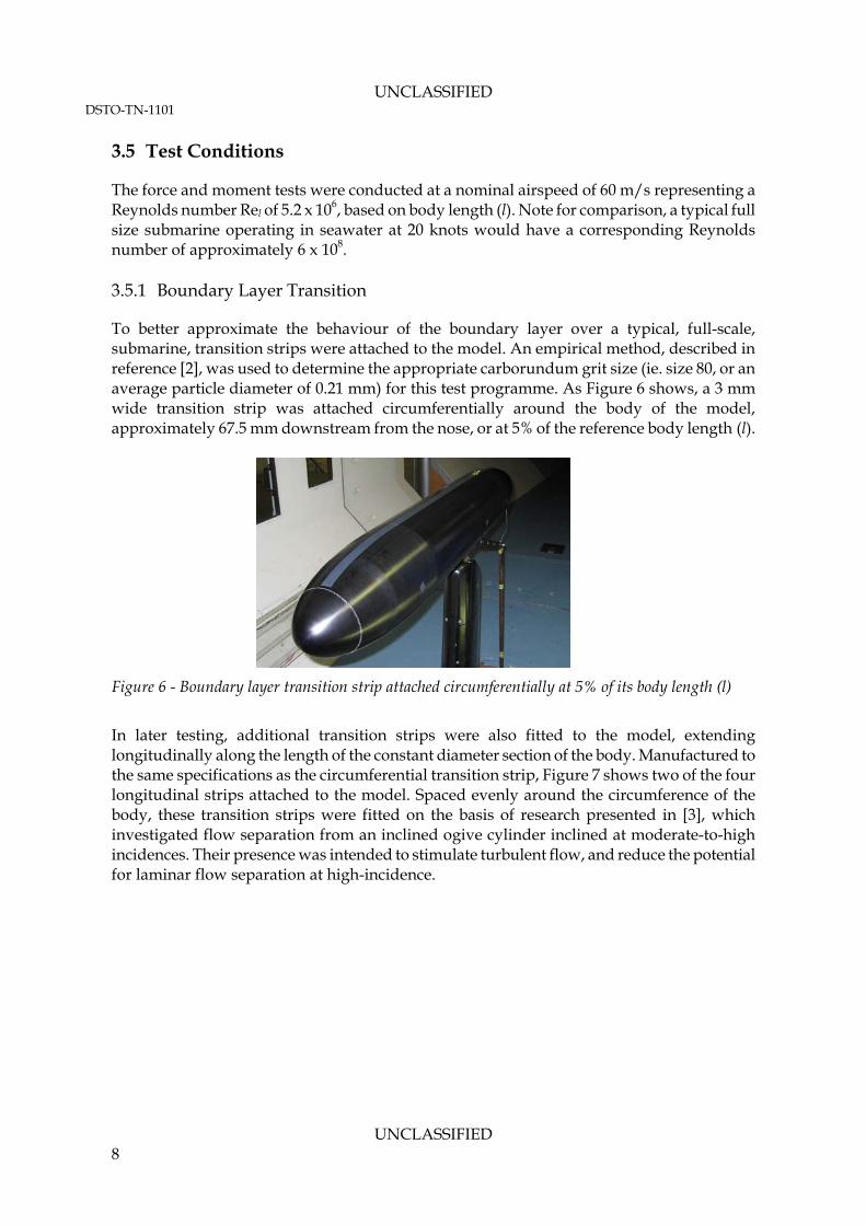
In later testing, additional transition strips were also fitted to the model, extending longitudinally along the length of the constant diameter section of the body. Manufactured to the same specifications as the circumferential transition strip, Figure 7 shows two of the four longitudinal strips attached to the model. Spaced evenly around the circumference of the body, these transition strips were fitted on the basis of research presented in [3], which investigated flow separation from an inclined ogive cylinder inclined at moderate-to-high incidences. Their presence was intended to stimulate turbulent flow, and reduce the potential for laminar flow separation at high-incidence.

UNCLASSIFIED 8


Figure 7 - Boundary layer transition strips attached longitudinally down the constant diameter section

of the body

3.5.1.1 Boundary Layer Transition Check Method A qualitative check of the effectiveness of the transition strips was conducted prior to commencing the test programme. This involved the use of a stethoscope connected to a total pressure probe located in the region of interest. As there are audible differences between a laminar and a turbulent boundary layer, this method involves listening to the flow both up-stream and down-stream of the transition strip. This test confirmed the effectiveness of the transition strips to artificially induce transition on the model. 3.6 Test Schedule

The primary aims of the Phase I tests were to gather steady-state force and moment data for the bare-hull configuration, and to investigate the flow characteristics on and around the model using different flow visualisation techniques. These test objectives are reflected in the schedule included in Table B1 and Table B2 of Appendix B. 3.6.1 Reference Runs

Reference Runs were included throughout the test programme to enable the consistency and repeatability of the experimental method to be quantitatively assessed. Reference Runs involved pitching the model through a range of discrete angles (α) from -15° to +15° at zero β and airspeed of 60 m/s. Reference Runs were conducted with both transitions strips-on1 and off. 3.6.2 Bare-Hull – Boundary Layer Transition Strips-Off

The model was tested at 60 m/s with boundary layer transition strips-off, where force and moment data were gathered at various combinations of α between ±15º and β between ±30º. This model configuration provided the baseline data for comparison with subsequent boundary layer transition strips-on test data.

1 Reference Runs with transition strips-on refers only to the attachment of a transition strip around the circumference of the model at 5% of its body length.

UNCLASSIFIED 9


3.6.3 Bare-Hull – Boundary Layer Transition Strips-On

The model was also extensively tested at 60 m/s with boundary layer transition strips-on. Initially, transition strips were attached only around the circumference of the model at 5% of its body length, but later in the programme, transition strips were also attached longitudinally along the length constant diameter section of the body (as described in section 3.5.1). In both cases, the model was tested at combinations of α between ±15º and β between ±30º. 3.6.4 Flow Visualisation Testing

Several different flow visualisation techniques were used to investigate areas of interest on and around the model. Surface flows were investigated using tufts attached to the model surface, whilst off-body flows were investigated using a smoke generator and probe. In both cases the model was pitched and yawed to different angles to highlight interesting flow phenomenon; however, these tests were conducted at reduced airspeeds. For tufting tests, the airspeed was decreased to approximately 45 m/s, whereas for the smoke flow visualisation tests, the airspeed was further reduced to 10 m/s. A reduction in airspeed was necessary in both cases to maximise the effectiveness of the test method. Two digital cameras captured the flow visualisation results, with the data recorded and processed using a digital imaging system. The main camera provided a port-side view of the model, whilst the second camera, located downstream from the model and slightly elevated, captured the starboard view. 3.6.5 Thermal Imaging of Boundary Layer Transition

Further to the qualitative method described in section 3.5.1.1, an alternative method that used thermal imaging equipment to investigate the effectiveness of the boundary layer transition strips was also trialled. This involved heating the model, so as to elevate its temperature slightly above the ambient air temperature, and then using an infrared (IR) camera mounted above the test-section (external to the flow), to monitor the surface temperature of the model as it cooled in the free-stream. Theoretically, thermal imaging will show a temperature gradient, where the model cools more slowly in the presence of a laminar boundary layer than it does in a turbulent boundary layer. Although technically more complex, thermal imaging is less intrusive on the flow-field compared to the physical presence of a total pressure probe when positioned close to the model.

4. Results

Selected results from the testing of the generic submarine model in the DSTO LSWT are briefly discussed below, and also presented graphically in Appendix D to Appendix G. Whilst these results represent only a subset of the data gathered, the main elements of the test programme are covered. The discussion of the results is intentionally brief, and of a qualitative nature, restricted to general observations regarding data trends. A more thorough analysis and assessment of the data will be the subject of future reports.

UNCLASSIFIED 10


4.1 Force and Moment Tests

4.1.1 Reference Runs

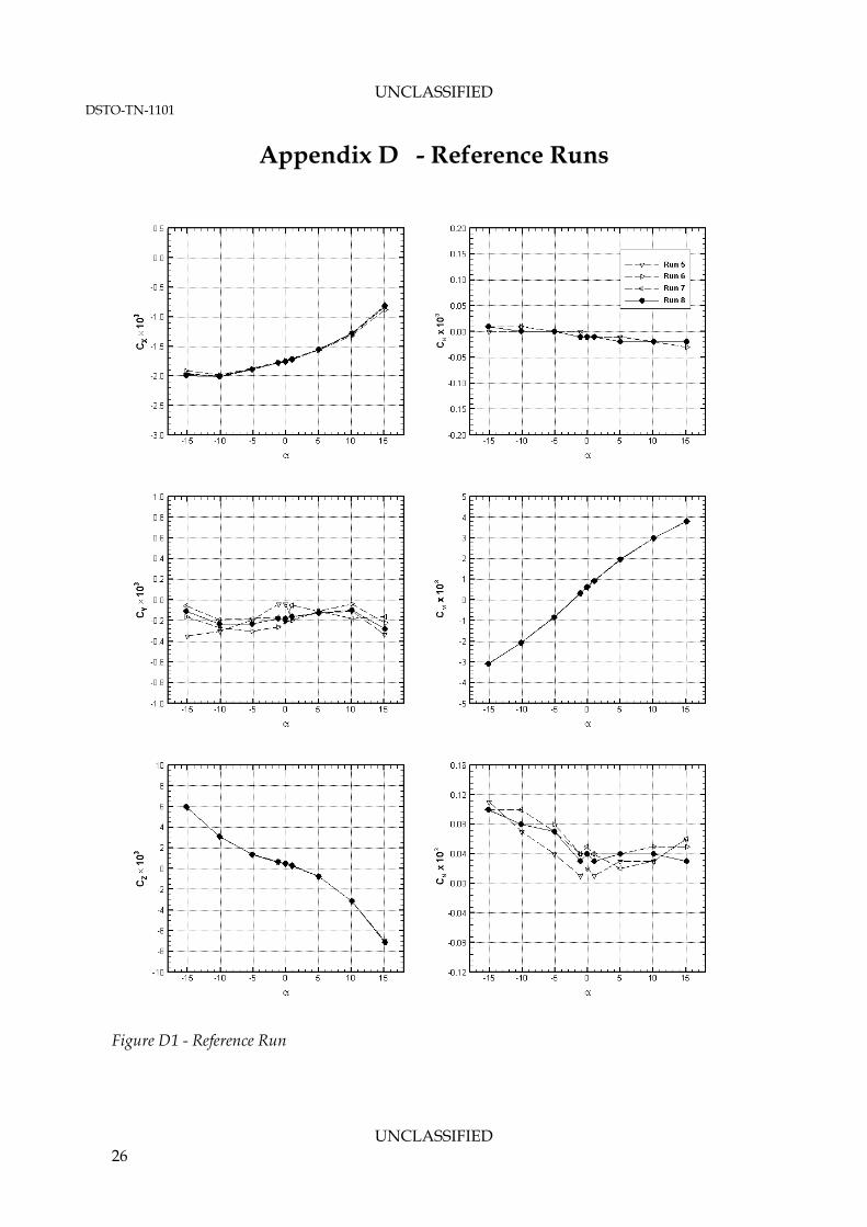
Appendix D shows force and moment data gathered during the Reference Runs included in the test programme. Plotted in their coefficient form, the results represent the model in the bare-hull configuration, with transitions strips-on (i.e. attached around the circumference of the model at 5% of its body length). In general, the results are consistent and repeatable. The longitudinal coefficients CX, CZ and CM are expressed as a function of α over the range ±15º at zero β. The X force coefficient in the body-axis (CX) displays a positive, non-linear gradient, with the minimum value occurring at α =-10º. Given the symmetric hull geometry under test, the CX data was expected to be approximately symmetric about the flow offset value, so the offset apparent in the CX data suggests a possible wake effect from the model support and fairing. In contrast, the Z force coefficient in the body-axis (CZ) is relatively symmetric about zero-incidence, with the results predictably showing a non-linear, negative gradient. This is consistent with increased body lift for increasing α. The pitching moment coefficient (CM) has a positive gradient, that is, the model is unstable in pitch, with CM increasing with α. These results also show a small offset in CM at zero-incidence, or an asymmetry in the flow, inducing a nose-up pitch tendency at this attitude. Whilst it may appear that there is less consistency and repeatability in the lateral coefficients, the variations in these data are comparatively small when compared to the longitudinal coefficients. There is some variability in the data for the Y force coefficient in the body-axis (CY); however, overall the trends remain consistent. The rolling moment coefficient (CK) is relatively insensitive to changes in α, albeit the data does show a small negative change in gradient over the range of conditions tested. This result is indicative of a lateral asymmetry in the flow. The results for the yawing moment coefficient (CN) are also relatively consistent, but similarly highlighting an asymmetry about zero-incidence. 4.1.2 Bare-Hull – Boundary Layer Transition Strips-Off

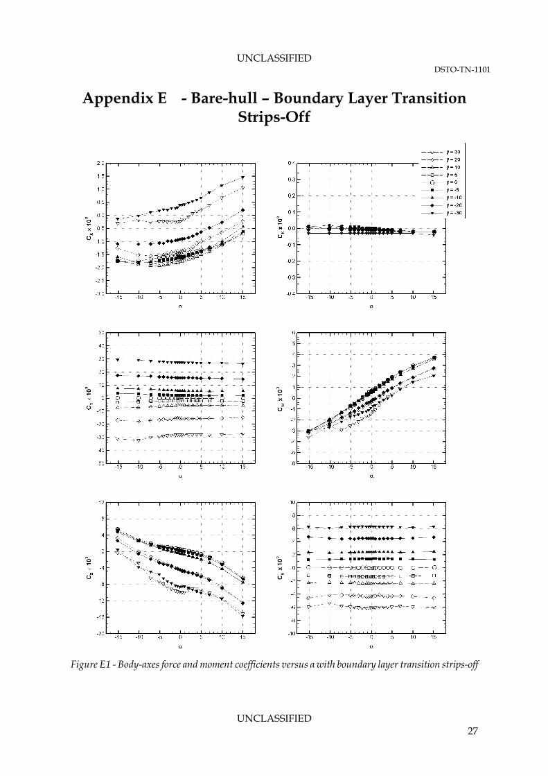
Appendix E shows data gathered for the model with boundary layer transition strips-off. These results cover a broad range of α and β conditions at the free-stream airspeed of 60 m/s. Specifically Figure E1 and Figure E2 show the coefficients plotted as a function of α and β respectively. Figure E1 shows that the trends in the data are relatively consistent. At each discrete β condition there is an expected and predictable variation in the coefficient. For example, the longitudinal coefficients, CZ and CM exhibit largely linear behaviour over the range of α tested, with noticeable groupings in the data at corresponding values of positive and negative β (i.e. the results for each discrete ±β value correlate reasonably well, particularly for -10º < β < 10º). The results show CX has a positive gradient, increasing with increasing α, but is non-linear about zero-incidence. This trend in the CX results is most likely caused by the pylon fairing and model pitch-arm mechanism influencing the flow around the model. The CM results show

UNCLASSIFIED 11


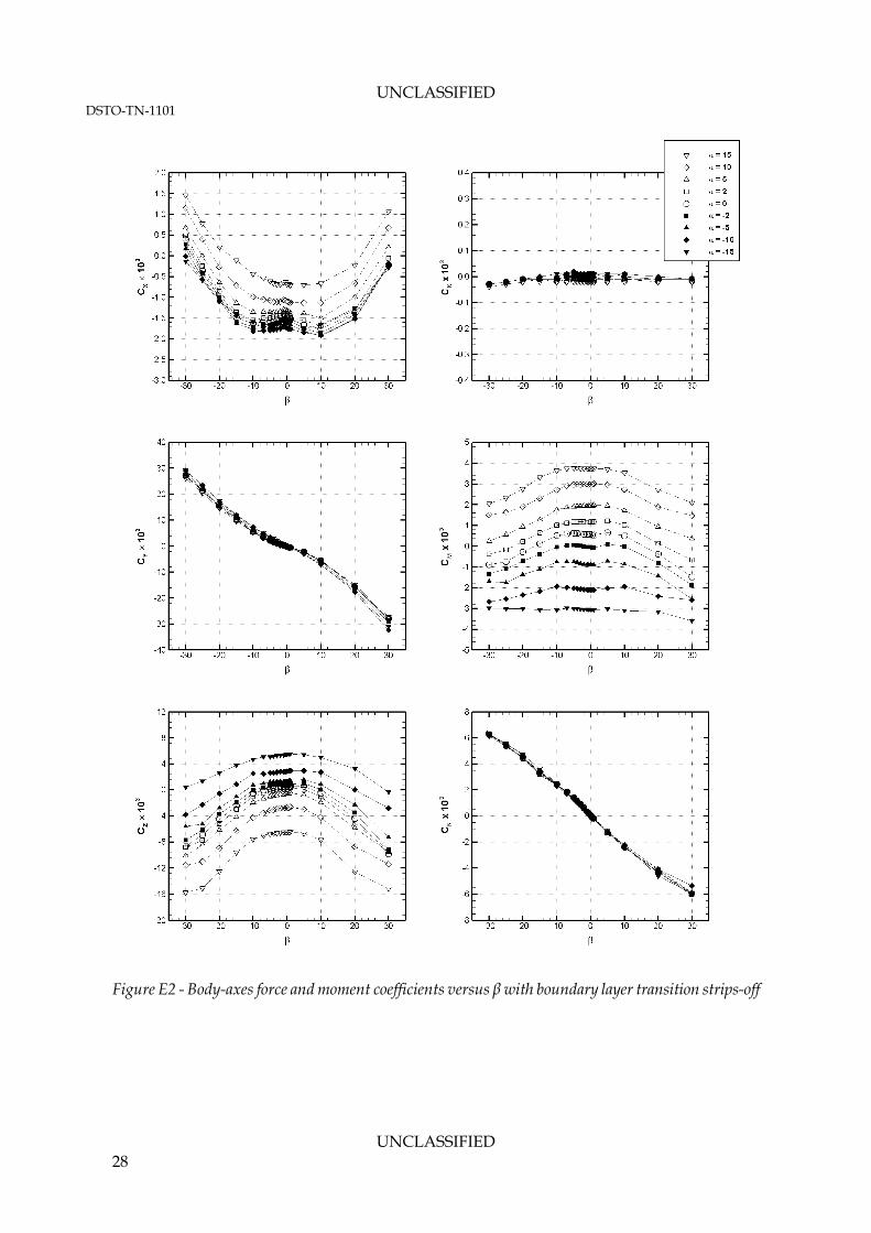
the model is unstable in pitch, with CM increasing with α. Once more, there is a small offset in CM at zero-incidence, that is, the model has a nose-up pitch tendency at this attitude. Predictably, the lateral coefficients, CY, CK, and CN are relatively insensitive to variations in pitch. However, there is a change in the nominal values of both CY and CN as the magnitude of β is increased. These trends are also consistent with expectations. CK is relatively insensitive to changes in α; however, the data does show a small negative change in gradient over the range of conditions tested, indicative of a lateral asymmetry in the flow. Figure E2 shows the coefficients plotted as a function of β for constant values of α. Again, the trends in the data are relatively consistent, where for each discrete α condition, there is an expected and predictable variation in the coefficient. The CX results highlight an asymmetry in the flow. At negative values of β, the magnitude of this coefficient is greater than for (equivalent) positive values. The pitch characteristics of the model were relatively consistent, that is, when the model was yawed about a zero-sideslip for a constant value of α, the magnitude of CM decreased. The vertical force is reduced with increasing β, or the value of CZ decreases. This trend is consistent with a reduction in lift with increasing sideslip. In the case of the lateral coefficients, both CY and Cn are approximately linear, increasing in magnitude with increasing β, whilst remaining invariant with α. The rolling characteristics of the model were not influenced significantly by changes in either α or β. 4.1.3 Bare-Hull – Boundary Layer Transition Strips-On

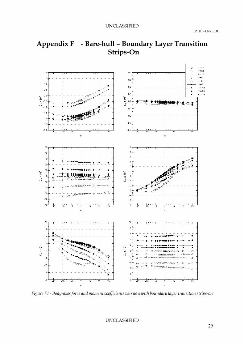
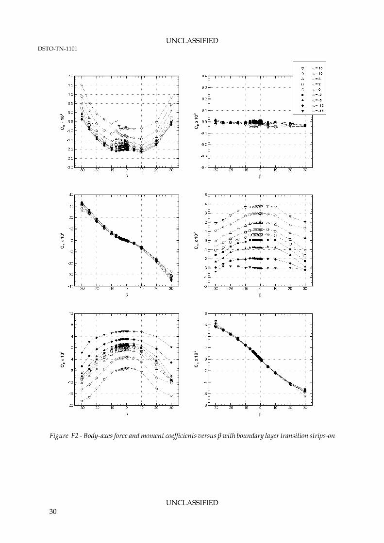
Appendix F shows data gathered for the model with boundary layer transition strips-on, specifically, the boundary layer strip was attached at 5% of the body-length around the circumference of the model. Figure F1 and Figure F2 show the coefficients plotted as a function of α and β respectively at the free-stream airspeed of 60 m/s. Figure F1 shows that the trends in the data are consistent for -10º < β < 10º, where for each discrete β condition there is an expected and predictable variation in the coefficient. Predictably, the transition strip has increased the magnitude of CX, but has not changed the overall trend in the data. For the cases where β = 20º and β = 30º, the results for the longitudinal coefficients (ie. CX, CZ, CM) indicate pronounced differences between the data sets. This suggests the results are sensitive to the presence of the transition strip in combination with these β angles. The lateral coefficients, CY, CK, and CN remain relatively insensitive to variations in pitch, and are not affected by the addition of the transition strip. Figure F2 shows the coefficients plotted as a function of β for constant values of α. Similarly, these data, with the exception of CX, were not noticeably impacted by the addition of the boundary layer transition strip.

UNCLASSIFIED 12


4.1.4 Bare-Hull – Comparison of Boundary Layer Transition Strips-Off and On

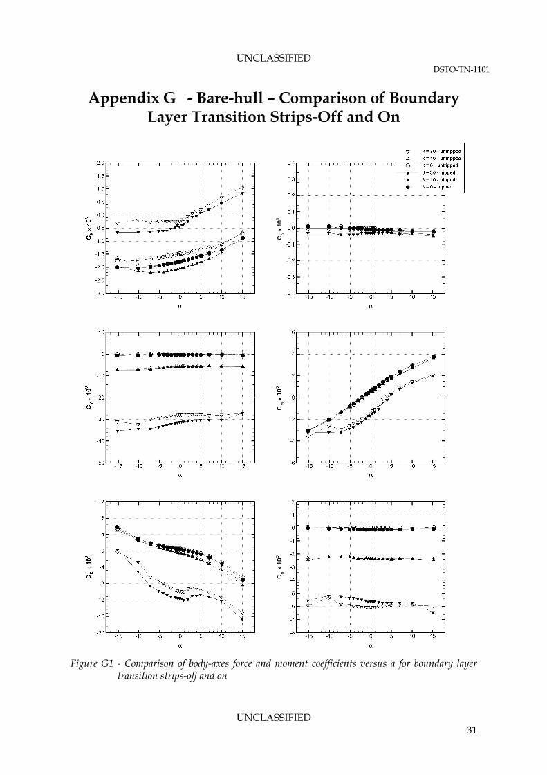
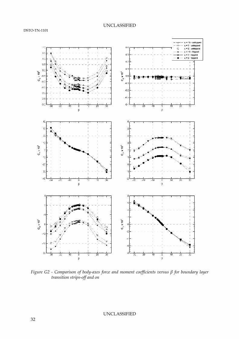
For completeness, Appendix G shows selected comparative results for the model with boundary layer transition strips-off and on. Figure G1 and Figure G2 show the coefficients plotted as a function of α and β respectively at the free-stream airspeed of 60 m/s. The effects of the boundary layer transition strip are clearly indicated in the comparative results for the longitudinal coefficient CX (i.e. there is an increase in drag with the transition strip-on). Whilst there are some observable differences in the two sets of results for other coefficients, these differences correlate with expected trends in the data at higher incidence and/or high sideslip conditions.

UNCLASSIFIED 13


4.2 Assessment of Data Quality

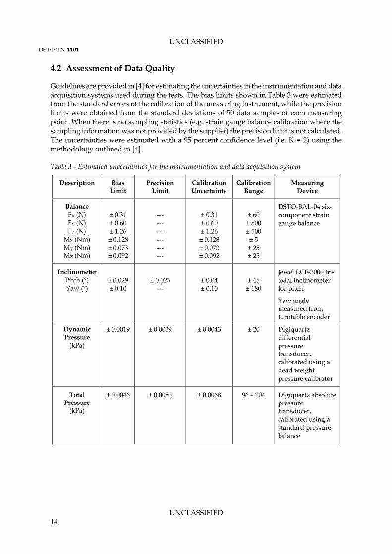
Guidelines are provided in [4] for estimating the uncertainties in the instrumentation and data acquisition systems used during the tests. The bias limits shown in Table 3 were estimated from the standard errors of the calibration of the measuring instrument, while the precision limits were obtained from the standard deviations of 50 data samples of each measuring point. When there is no sampling statistics (e.g. strain gauge balance calibration where the sampling information was not provided by the supplier) the precision limit is not calculated. The uncertainties were estimated with a 95 percent confidence level (i.e. K = 2) using the methodology outlined in [4]. Table 3 - Estimated uncertainties for the instrumentation and data acquisition system

Description Bias Limit

Precision Limit

Calibration Uncertainty

Calibration Range

Measuring Device

Balance FX (N) FY (N) FZ (N)

MX (Nm) MY (Nm) MZ (Nm)

± 0.31 ± 0.60 ± 1.26 ± 0.128 ± 0.073 ± 0.092

--- --- --- --- --- ---

± 0.31 ± 0.60 ± 1.26 ± 0.128 ± 0.073 ± 0.092

± 60

± 500 ± 500

± 5 ± 25 ± 25

DSTO-BAL-04 six-component strain gauge balance

Inclinometer Pitch (°) Yaw (°)

± 0.029 ± 0.10

± 0.023

---

± 0.04 ± 0.10

± 45

± 180

Jewel LCF-3000 tri-axial inclinometer for pitch.

Yaw angle measured from turntable encoder

Dynamic Pressure

(kPa)

± 0.0019 ± 0.0039 ± 0.0043 ± 20 Digiquartz differential pressure transducer, calibrated using a dead weight pressure calibrator

Total Pressure

(kPa)

± 0.0046 ± 0.0050

± 0.0068 96 – 104 Digiquartz absolute pressure transducer, calibrated using a standard pressure balance

UNCLASSIFIED 14


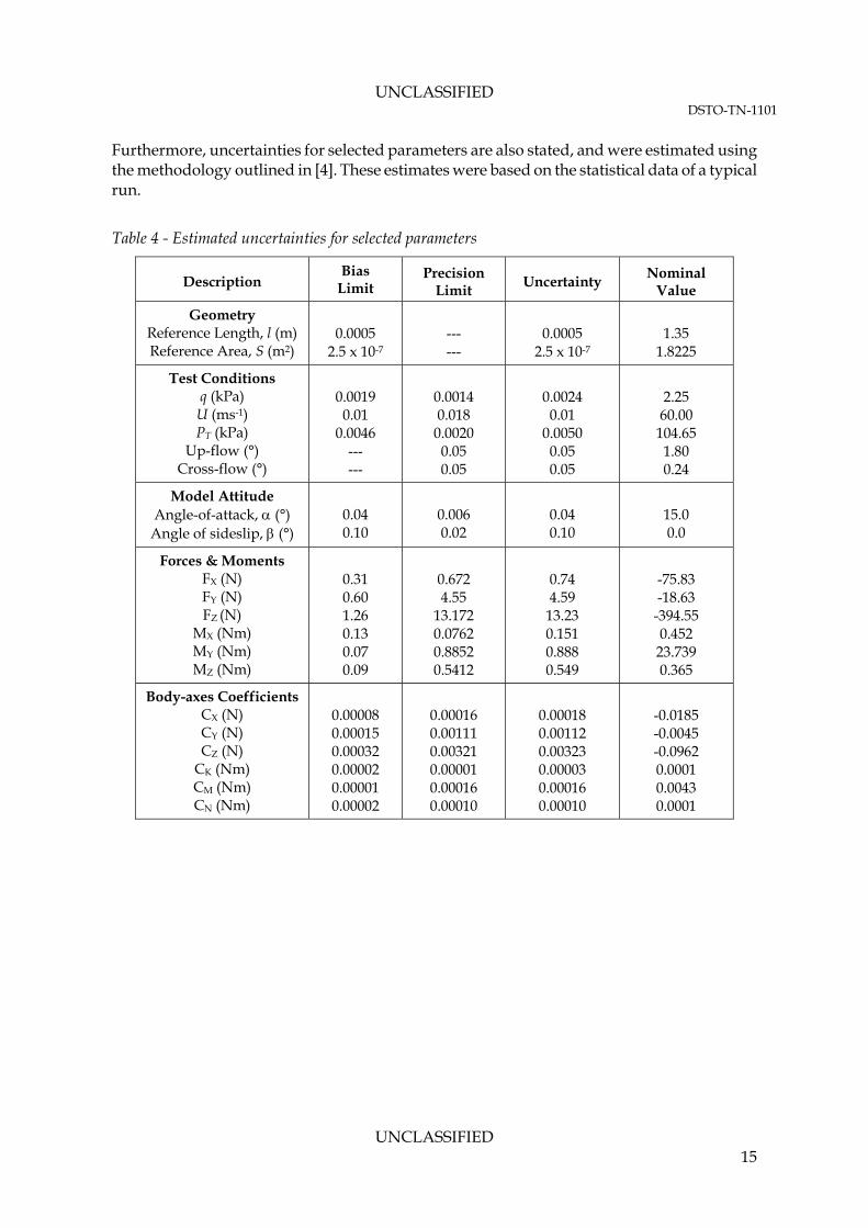
Furthermore, uncertainties for selected parameters are also stated, and were estimated using the methodology outlined in [4]. These estimates were based on the statistical data of a typical run.

Table 4 - Estimated uncertainties for selected parameters

Bias Description Limit

Precision Limit Uncertainty Nominal

Value

Geometry Reference Length, l (m) Reference Area, S (m2)

0.0005

2.5 x 10-7

--- ---

0.0005

2.5 x 10-7

1.35

1.8225

Test Conditions q (kPa)

U (ms-1) PT (kPa)

Up-flow (°) Cross-flow (°)

0.0019 0.01

0.0046 --- ---

0.0014 0.018

0.0020 0.05 0.05

0.0024 0.01

0.0050 0.05 0.05

2.25 60.00

104.65 1.80 0.24

Model Attitude Angle-of-attack, (°)

Angle of sideslip, (°)

0.04 0.10

0.006 0.02

0.04 0.10

15.0 0.0

Forces & Moments FX (N) FY (N) FZ (N)

MX (Nm) MY (Nm) MZ (Nm)

0.31 0.60 1.26 0.13 0.07 0.09

0.672 4.55

13.172 0.0762 0.8852 0.5412

0.74 4.59

13.23 0.151 0.888 0.549

-75.83 -18.63

-394.55 0.452

23.739 0.365

Body-axes Coefficients CX (N) CY (N) CZ (N)

CK (Nm) CM (Nm) CN (Nm)

0.00008 0.00015 0.00032 0.00002 0.00001 0.00002

0.00016 0.00111 0.00321 0.00001 0.00016 0.00010

0.00018 0.00112 0.00323 0.00003 0.00016 0.00010

-0.0185 -0.0045 -0.0962 0.0001 0.0043 0.0001

UNCLASSIFIED 15


4.3 Flow Visualisation

Several flow visualisation methods were used to investigate the flow characteristics on and around the model. Tufts were attached to the body to study surface flow behaviour, while a smoke generator and probe were used to investigate off-body flows. Both methods provided qualitative insights as to the nature of the flow, and Table B2 of Appendix B summaries the test conditions. 4.3.1 Smoke Generator and Probe

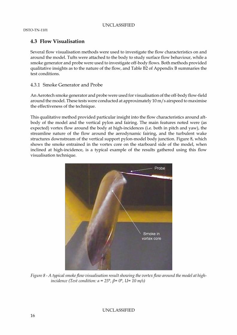
An Aerotech smoke generator and probe were used for visualisation of the off-body flow-field around the model. These tests were conducted at approximately 10 m/s airspeed to maximise the effectiveness of the technique. This qualitative method provided particular insight into the flow characteristics around aft-body of the model and the vertical pylon and fairing. The main features noted were (as expected) vortex flow around the body at high-incidences (i.e. both in pitch and yaw), the streamline nature of the flow around the aerodynamic fairing, and the turbulent wake structures downstream of the vertical support pylon-model body junction. Figure 8, which shows the smoke entrained in the vortex core on the starboard side of the model, when inclined at high-incidence, is a typical example of the results gathered using this flow visualisation technique.

Figure 8 - A typical smoke flow visualisation result showing the vortex flow around the model at high-

incidence (Test condition: α = 25°, β= 0°, U= 10 m/s)

UNCLASSIFIED 16


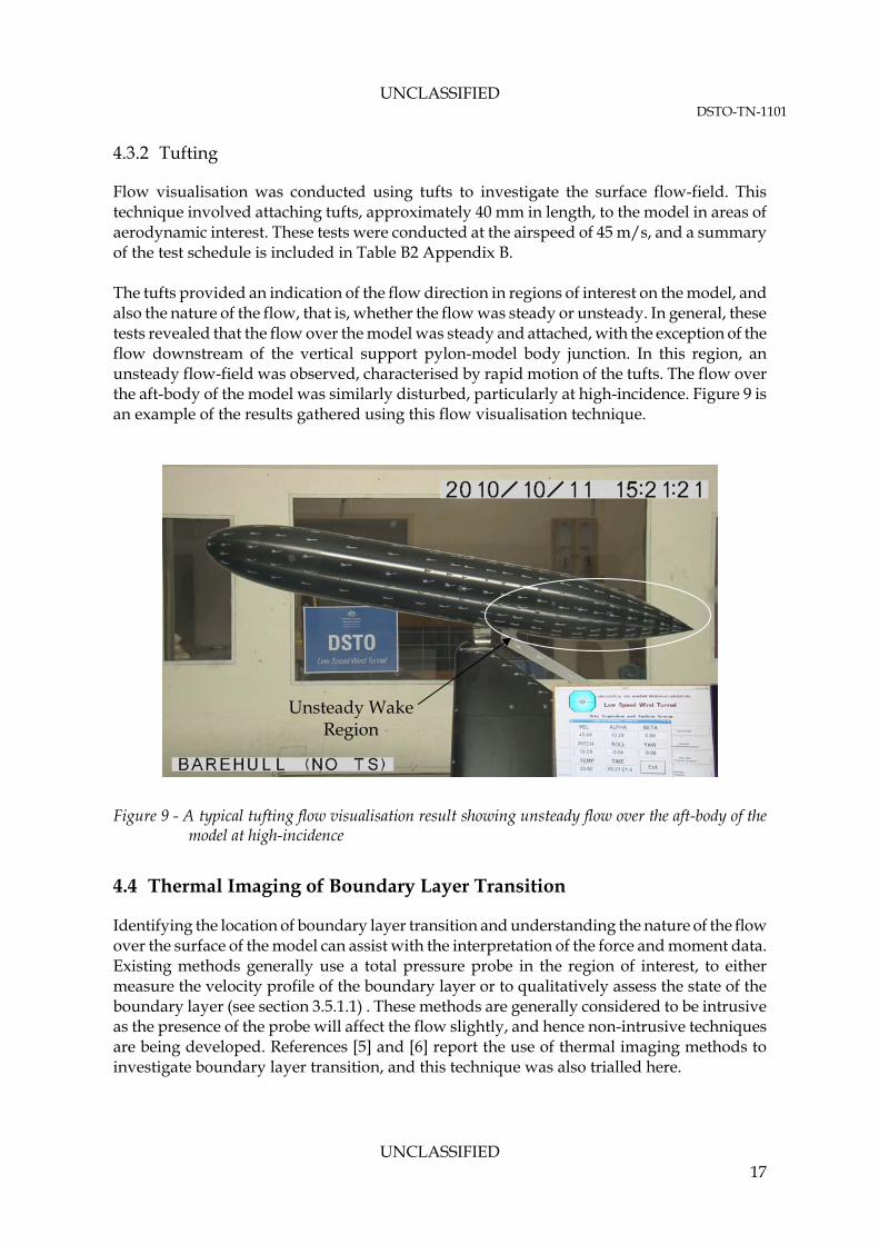
4.3.2 Tufting

Flow visualisation was conducted using tufts to investigate the surface flow-field. This technique involved attaching tufts, approximately 40 mm in length, to the model in areas of aerodynamic interest. These tests were conducted at the airspeed of 45 m/s, and a summary of the test schedule is included in Table B2 Appendix B. The tufts provided an indication of the flow direction in regions of interest on the model, and also the nature of the flow, that is, whether the flow was steady or unsteady. In general, these tests revealed that the flow over the model was steady and attached, with the exception of the flow downstream of the vertical support pylon-model body junction. In this region, an unsteady flow-field was observed, characterised by rapid motion of the tufts. The flow over the aft-body of the model was similarly disturbed, particularly at high-incidence. Figure 9 is an example of the results gathered using this flow visualisation technique.

Unsteady Wake Region

Figure 9 - A typical tufting flow visualisation result showing unsteady flow over the aft-body of the model at high-incidence

4.4 Thermal Imaging of Boundary Layer Transition

Identifying the location of boundary layer transition and understanding the nature of the flow over the surface of the model can assist with the interpretation of the force and moment data. Existing methods generally use a total pressure probe in the region of interest, to either measure the velocity profile of the boundary layer or to qualitatively assess the state of the boundary layer (see section 3.5.1.1) . These methods are generally considered to be intrusive as the presence of the probe will affect the flow slightly, and hence non-intrusive techniques are being developed. References [5] and [6] report the use of thermal imaging methods to investigate boundary layer transition, and this technique was also trialled here.

UNCLASSIFIED 17


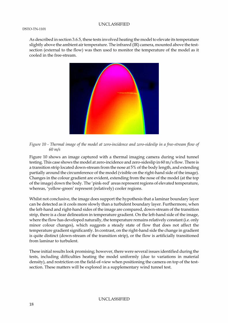
As described in section 3.6.5, these tests involved heating the model to elevate its temperature slightly above the ambient air temperature. The infrared (IR) camera, mounted above the test-section (external to the flow) was then used to monitor the temperature of the model as it cooled in the free-stream.

Figure 10 - Thermal image of the model at zero-incidence and zero-sideslip in a free-stream flow of 60 m/s

Figure 10 shows an image captured with a thermal imaging camera during wind tunnel testing. This case shows the model at zero-incidence and zero-sideslip in 60 m/s flow. There is a transition strip located down-stream from the nose at 5% of the body length, and extending partially around the circumference of the model (visible on the right-hand side of the image). Changes in the colour gradient are evident, extending from the nose of the model (at the top of the image) down the body. The ‘pink-red’ areas represent regions of elevated temperature, whereas, ‘yellow-green’ represent (relatively) cooler regions. Whilst not conclusive, the image does support the hypothesis that a laminar boundary layer can be detected as it cools more slowly than a turbulent boundary layer. Furthermore, when the left-hand and right-hand sides of the image are compared, down-stream of the transition strip, there is a clear delineation in temperature gradient. On the left-hand side of the image, where the flow has developed naturally, the temperature remains relatively constant (i.e. only minor colour changes), which suggests a steady state of flow that does not affect the temperature gradient significantly. In contrast, on the right-hand side the change in gradient is quite distinct (down-stream of the transition strip), or the flow is artificially transitioned from laminar to turbulent. These initial results look promising; however, there were several issues identified during the tests, including difficulties heating the model uniformly (due to variations in material density), and restriction on the field-of-view when positioning the camera on top of the test-section. These matters will be explored in a supplementary wind tunnel test.

UNCLASSIFIED 18


5. Conclusion

DSTO researchers have completed Phase I of a series of planned low speed wind tunnel tests of a generic submarine model. These tests were used to gather steady-state aerodynamic force and moment data for the model at various attitudes, to trial a new method to detect boundary layer transition using thermal imaging equipment and to use flow visualisation methods to investigate areas of particular aerodynamic interest. This report documents the experimental equipment and method used during the tests to gather and process the data, and also presents selected results. The experimental results satisfied the test requirements in terms of data quality and repeatability, although the significant influence of the model support equipment on the flow angularity in the wind tunnel test-section was noted. This finding does not affect the intended use of the aerodynamic data set, which is planned to provide an incremental data set, but rather is noted for the benefit of designing future wind tunnel model support equipment. Satisfied with the experimental results obtained, researchers are now planning follow-on wind tunnel experiments to further characterise the aerodynamic properties of the generic submarine in different configurations. The experimental data will also complement a body of information being compiled for the generic submarine shape from various sources including computational methods and experimental hydrodynamic testing.

6. Acknowledgements

The authors would like to thank John Clayton, Paul Jacquemin, Kevin Desmond, Alberto Gonzalez, Peter O’Connor, and Chris Rider for their assistance in preparing the model and conducting the wind tunnel tests. In addition, the significant contribution by staff from Propulsion Branch, in particular Michael Posadowski and Nigel Smith, for the setup, operation and post-test analysis of the infrared-red camera results is gratefully acknowledged.

UNCLASSIFIED 19


7. References

[1] Barlow, J. B., Rae, W. H. and Pope, A., Low Speed Wind Tunnel Testing, John Wiley & Sons, 1999.

[2] Braslow, A. L., and Knox, E. C., Simplified Method for Determination of Critical Height of

Distributed Roughness Particles for Boundary Layer Transition at Mach Numbers from 0 to 5, NACA TN 4363, 1958.

[3] Lamont, P.J., Pressures Around an Inclined Ogive Cylinder with Laminar, Transitional, or

Turbulent Separation, AIAA Journal, Vol. 20, No. 11, Nov. 1982, pp. 1492-1499. [4] American Institute of Aeronautics and Astronautics (AIAA), Standard – Assessment of

Experimental Uncertainty with Application to Wind Tunnel Testing, AIAA S-071A-1999. [5] Montelpare, S. and Ricci, R., A Thermographic Method to Evaluate the Local Boundary

Layer Separation Phenomena on Aerodynamic Bodies Operating at Low Reynolds Number, International Journal of Thermal Sciences, July, 2003.

[6] de Luca, L., Carlomagno, G., M. and Buresti, G., Boundary Layer Diagnostics by Means of

an Infrared Scanning Radiometer, Experiments in Fluids, 1990 [7] Snowden, A. D. and Widjaja, R., CFD Modelling of the DARPA SUBOFF Submarine in Bare

Hull Configuration, DSTO Technical Report, Air Vehicles Division, DSTO, Australia, 2011, In Preparation.

UNCLASSIFIED 20


Appendix A - Technical Specifications

Table A1 - DSTO low speed wind tunnel

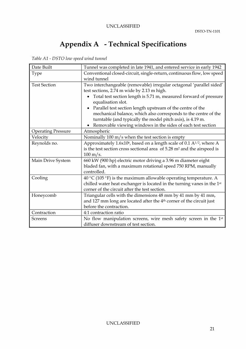
Date Built Tunnel was completed in late 1941, and entered service in early 1942 Type Conventional closed-circuit, single-return, continuous flow, low speed

wind tunnel Test Section Two interchangeable (removable) irregular octagonal ‘parallel sided’

test sections, 2.74 m wide by 2.13 m high. Total test section length is 5.71 m, measured forward of pressure

equalisation slot. Parallel test section length upstream of the centre of the

mechanical balance, which also corresponds to the centre of the turntable (and typically the model pitch axis), is 4.19 m.

Removable viewing windows in the sides of each test section Operating Pressure Atmospheric Velocity Nominally 100 m/s when the test section is empty Reynolds no. Approximately 1.6x106, based on a length scale of 0.1 A1/2, where A

is the test section cross sectional area of 5.28 m2 and the airspeed is 100 m/s.

Main Drive System 660 kW (900 hp) electric motor driving a 3.96 m diameter eight bladed fan, with a maximum rotational speed 750 RPM, manually controlled.

Cooling 40 C (105 F) is the maximum allowable operating temperature. A chilled water heat exchanger is located in the turning vanes in the 1st corner of the circuit after the test section.

Honeycomb Triangular cells with the dimensions 48 mm by 41 mm by 41 mm, and 127 mm long are located after the 4th corner of the circuit just before the contraction.

Contraction 4:1 contraction ratio Screens No flow manipulation screens, wire mesh safety screen in the 1st

diffuser downstream of test section.

UNCLASSIFIED 21


Table A2 - DSTO LSWT data acquisition system

Data Acquisition System

Intel Xeon computer running Red Hat Fedora Linux, providing real-time graphical display, data processing, data storage and printer output.

Force and moment data acquisition provided by Vishay Strain Gauge Amplifiers, using a VXI system controller with Ethernet connection to the main computer.

Data acquisition modules to control the facility equipment (pitch-arm and turntable), and to acquire data from the wind tunnel instrumentation using PC-based modules.

Table A3 - Strain gauge balance (DSTO-BAL-04)

Strain Gauge Balance (DSTO-BAL-04)

A six-component internal strain gauge balance with the load range: Range Axial force (X) 100N Side force (Y) 1000N Normal force (Z) 1000N Rolling moment (K) 12Nm Pitching moment (M) 50Nm Yawing moment (N) 50Nm

Standard Errors Axial force (X) 0.154% F.S. Side force (Y) 0.030% F.S. Normal force (Z) 0.063% F.S. Rolling moment (K) 0.534% F.S. Pitching moment (M) 0.073% F.S. Yawing moment (N) 0.092% F.S

UNCLASSIFIED 22


Appendix B - Phase I Test Schedule

Table B1 - Phase I force and moment testing of the generic submarine model

Table B2 - Phase I flow visualisation testing of the generic submarine model

UNCLASSIFIED 23


Appendix C - Determination of Flow Offset Angles

C.1. Experimental Method

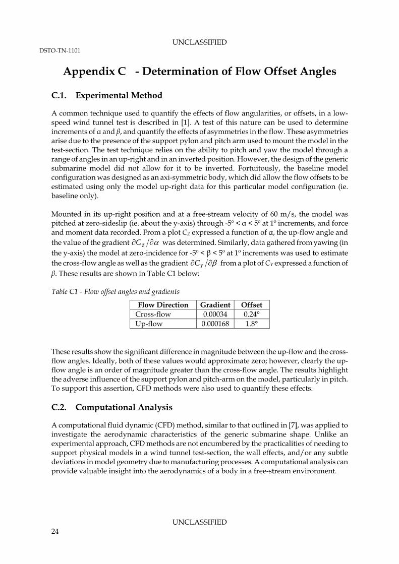
A common technique used to quantify the effects of flow angularities, or offsets, in a low-speed wind tunnel test is described in [1]. A test of this nature can be used to determine increments of α and β, and quantify the effects of asymmetries in the flow. These asymmetries arise due to the presence of the support pylon and pitch arm used to mount the model in the test-section. The test technique relies on the ability to pitch and yaw the model through a range of angles in an up-right and in an inverted position. However, the design of the generic submarine model did not allow for it to be inverted. Fortuitously, the baseline model configuration was designed as an axi-symmetric body, which did allow the flow offsets to be estimated using only the model up-right data for this particular model configuration (ie. baseline only). Mounted in its up-right position and at a free-stream velocity of 60 m/s, the model was pitched at zero-sideslip (ie. about the y-axis) through -5º < α < 5º at 1º increments, and force and moment data recorded. From a plot CZ expressed a function of α, the up-flow angle and the value of the gradient ZC was determined. Similarly, data gathered from yawing (in the y-axis) the model at zero-incidence for -5º < β < 5º at 1º increments was used to estimate the cross-flow angle as well as the gradient YC from a plot of CY expressed a function of β. These results are shown in Table C1 below: Table C1 - Flow offset angles and gradients

Flow Direction Gradient Offset Cross-flow 0.00034 0.24° Up-flow 0.000168 1.8°

These results show the significant difference in magnitude between the up-flow and the cross-flow angles. Ideally, both of these values would approximate zero; however, clearly the up-flow angle is an order of magnitude greater than the cross-flow angle. The results highlight the adverse influence of the support pylon and pitch-arm on the model, particularly in pitch. To support this assertion, CFD methods were also used to quantify these effects. C.2. Computational Analysis

A computational fluid dynamic (CFD) method, similar to that outlined in [7], was applied to investigate the aerodynamic characteristics of the generic submarine shape. Unlike an experimental approach, CFD methods are not encumbered by the practicalities of needing to support physical models in a wind tunnel test-section, the wall effects, and/or any subtle deviations in model geometry due to manufacturing processes. A computational analysis can provide valuable insight into the aerodynamics of a body in a free-stream environment.

UNCLASSIFIED 24


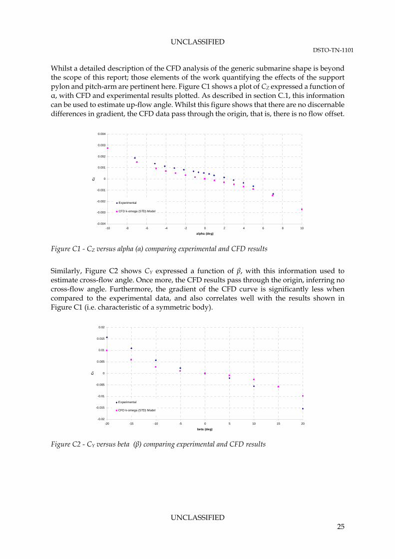
Whilst a detailed description of the CFD analysis of the generic submarine shape is beyond the scope of this report; those elements of the work quantifying the effects of the support pylon and pitch-arm are pertinent here. Figure C1 shows a plot of CZ expressed a function of α, with CFD and experimental results plotted. As described in section C.1, this information can be used to estimate up-flow angle. Whilst this figure shows that there are no discernable differences in gradient, the CFD data pass through the origin, that is, there is no flow offset.

-0.004

-0.003

-0.002

-0.001

0

0.001

0.002

0.003

0.004

-10 -8 -6 -4 -2 0 2 4 6 8 10

alpha (deg)

CZ

Experimental

CFD k-omega (STD) Model

Figure C1 - CZ versus alpha (α) comparing experimental and CFD results

Similarly, Figure C2 shows CY expressed a function of β, with this information used to estimate cross-flow angle. Once more, the CFD results pass through the origin, inferring no cross-flow angle. Furthermore, the gradient of the CFD curve is significantly less when compared to the experimental data, and also correlates well with the results shown in Figure C1 (i.e. characteristic of a symmetric body).

-0.02

-0.015

-0.01

-0.005

0

0.005

0.01

0.015

0.02

-20 -15 -10 -5 0 5 10 15 20

beta (deg)

CY

Experimental

CFD k-omega (STD) Model

Figure C2 - CY versus beta (β) comparing experimental and CFD results

UNCLASSIFIED 25


Appendix D - Reference Runs

Figure D1 - Reference Run

UNCLASSIFIED 26


Appendix E - Bare-hull – Boundary Layer Transition Strips-Off

Figure E1 - Body-axes force and moment coefficients versus α with boundary layer transition strips-off

UNCLASSIFIED 27


Figure E2 - Body-axes force and moment coefficients versus β with boundary layer transition strips-off

UNCLASSIFIED 28


Appendix F - Bare-hull – Boundary Layer Transition Strips-On

Figure F1 - Body-axes force and moment coefficients versus α with boundary layer transition strips-on

UNCLASSIFIED 29


Figure F2 - Body-axes force and moment coefficients versus β with boundary layer transition strips-on

UNCLASSIFIED 30


Appendix G - Bare-hull – Comparison of Boundary Layer Transition Strips-Off and On

Figure G1 - Comparison of body-axes force and moment coefficients versus α for boundary layer

transition strips-off and on

UNCLASSIFIED 31


UNCLASSIFIED 32

Figure G2 - Comparison of body-axes force and moment coefficients versus β for boundary layer transition strips-off and on

Page classification: UNCLASSIFIED

DEFENCE SCIENCE AND TECHNOLOGY ORGANISATION

DOCUMENT CONTROL DATA 1. PRIVACY MARKING/CAVEAT (OF DOCUMENT)

2. TITLE Phase I Experimental Testing of a Generic Submarine Model in the DSTO Low Speed Wind Tunnel

3. SECURITY CLASSIFICATION (FOR UNCLASSIFIED REPORTS THAT ARE LIMITED RELEASE USE (L) NEXT TO DOCUMENT CLASSIFICATION) Document (U) Title (U) Abstract (U)

4. AUTHOR(S) Howard Quick, Ronny Widjaja, Brendon Anderson, Bruce Woodyatt, Andrew D. Snowden and Stephen Lam

5. CORPORATE AUTHOR DSTO Defence Science and Technology Organisation 506 Lorimer St Fishermans Bend Victoria 3207 Australia

6a. DSTO NUMBER DSTO-TN-1101

6b. AR NUMBER AR-015-344

6c. TYPE OF REPORT Technical Note

7. DOCUMENT DATE July 2012

8. FILE NUMBER M1/9/3065

9. TASK NUMBER ERP 07/299

10. TASK SPONSOR DSTO

11. NO. OF PAGES 32

12. NO. OF REFERENCES 7

13. DSTO Publications Repository http://dspace.dsto.defence.gov.au/dspace/

14. RELEASE AUTHORITY Chief, Air Vehicles Division

15. SECONDARY RELEASE STATEMENT OF THIS DOCUMENT

Approved for public release OVERSEAS ENQUIRIES OUTSIDE STATED LIMITATIONS SHOULD BE REFERRED THROUGH DOCUMENT EXCHANGE, PO BOX 1500, EDINBURGH, SA 5111 16. DELIBERATE ANNOUNCEMENT No Limitations 17. CITATION IN OTHER DOCUMENTS Yes 18. DSTO RESEARCH LIBRARY THESAURUS Submarine hulls; Wind tunnel tests; Aerodynamic loads; Boundary layer transition; Flow visualisation 19. ABSTRACT DSTO has conducted Phase I of planned experimental testing of a generic submarine model in its low speed wind tunnel. These wind tunnel tests aimed to gather steady-state aerodynamic force and moment data and to investigate the flow-field characteristics on and around the bare-hull. Further experimental testing is planned, extending the range of model configurations tested to include the addition of hull-casing, fin and control surfaces to the model. These experimental data will complement computational and experimental hydrodynamic analysis of the generic submarine shape.

Page classification: UNCLASSIFIED

phase i experimental testing of a generic submarine model ... · further experimental testing of...

Documents