Phase II Final Report

“Creation of a Dynamical Stratospheric Turbulence Forecasting and Nowcasting Tool

for High Altitude Airships and Other Aircraft"

Phase II Contract No. HQ0006-06-C-7328

MDA POC: Mr. Mike Lee

Technical Point of Contact: Dr. David C. Fritts (303) 415-9701 x205

Contractual Point of Contact: Ms. Donna Romeo (425) 556-9055 x220

Prepared for Missile Defense Agency 7100 Defense Pentagon

Washington DC 20301-7100

Approved for public release; distribution is unlimited

20 October 2008

Report Documentation Page Form ApprovedOMB No. 0704-0188

Public reporting burden for the collection of information is estimated to average 1 hour per response, including the time for reviewing instructions, searching existing data sources, gathering andmaintaining the data needed, and completing and reviewing the collection of information. Send comments regarding this burden estimate or any other aspect of this collection of information,including suggestions for reducing this burden, to Washington Headquarters Services, Directorate for Information Operations and Reports, 1215 Jefferson Davis Highway, Suite 1204, ArlingtonVA 22202-4302. Respondents should be aware that notwithstanding any other provision of law, no person shall be subject to a penalty for failing to comply with a collection of information if itdoes not display a currently valid OMB control number.

1. REPORT DATE 20 OCT 2008 2. REPORT TYPE

3. DATES COVERED 00-00-2008 to 00-00-2008

4. TITLE AND SUBTITLE Creation of a Dynamical Stratospheric Turbulence Forecasting andNowcasting Tool for High Altitude Airships and Other Aircraft

5a. CONTRACT NUMBER

5b. GRANT NUMBER

5c. PROGRAM ELEMENT NUMBER

6. AUTHOR(S) 5d. PROJECT NUMBER

5e. TASK NUMBER

5f. WORK UNIT NUMBER

7. PERFORMING ORGANIZATION NAME(S) AND ADDRESS(ES) NorthWest Research Associates, Inc.,4118 148th Ave. NE,Redmond,WA,98052

8. PERFORMING ORGANIZATIONREPORT NUMBER

9. SPONSORING/MONITORING AGENCY NAME(S) AND ADDRESS(ES) 10. SPONSOR/MONITOR’S ACRONYM(S)

11. SPONSOR/MONITOR’S REPORT NUMBER(S)

12. DISTRIBUTION/AVAILABILITY STATEMENT Approved for public release; distribution unlimited

13. SUPPLEMENTARY NOTES

14. ABSTRACT

15. SUBJECT TERMS

16. SECURITY CLASSIFICATION OF: 17. LIMITATION OF ABSTRACT Same as

Report (SAR)

18. NUMBEROF PAGES

8

19a. NAME OFRESPONSIBLE PERSON

a. REPORT unclassified

b. ABSTRACT unclassified

c. THIS PAGE unclassified

Standard Form 298 (Rev. 8-98) Prescribed by ANSI Std Z39-18

2

1. Introduction We have now completed a Phase II development of an atmospheric decision aid (ADA)

forecasting methodology for military, civilian, and commercial aircraft for which significant wave and turbulence activity may pose an operational or functional risk. The specific goal for MDA purposes was to create a forecasting methodology for turbulence activity at the expected High Altitude Airship (HAA) flight altitude of 22 km that specifically addresses all of the dominant sources of turbulence in the clear atmosphere. These include turbulence accompanying gravity waves arising from deep convection, those arising due to air flow over significant terrain, and turbulence due to Kelvin-Helmholtz instability (KHI) accompanying wind shears arising from jet stream flows and inertia-gravity wave motions in the lower stratosphere.

Given the expected deployment of HAAs over specific sites, our implementation for HAA purposes provides forecast options extending up to 72 hours within a user-selected domain either 500 or 1000 km across centered at any point on Earth. Forecasts are based on National Center for Environmental Prediction (NCEP) initial conditions and NCEP forecasts at 6-hour intervals thereafter. As with any forecasting methodology, however, we have the greatest confidence in the forecasts based on direct measurements at the earliest forecast times.

The motivations for our approach and the specific methodologies employed for each component of the turbulence forecast were described in previous reports. This final report summarizes our development effort and the resulting turbulence forecast product that accompanies it and which is provided as a suite of operational scripts and executable files. The operational and support environment for the forecasting methodology are described in Section 2. Examples of the forecast output for various sources and environments are provided in Section 3. Section 4 briefly describes the required operational environment. A separate HAA/TURBO Users Manual also accompanies this report and the scripts and executable forecasting files.

2. HAA/TURBO Operational and Support Environment

The computational and data access requirements necessary to perform turbulence forecasts with our HAA/TURBO software are described in the User Manual accompanying the executable codes. The nominal data feed requires input from a NOAAport downlink of initialization data or other suitable data source providing input data in the same formats. Additional details are provided in the User Manual. 3. HAA/TURBO Methodologies, Turbulence Intensities, and Example Forecasts

a. HAA/TURBO forecast methodologies Four specific methodologies underpin our HAA/TURBO turbulence forecasting

procedure. As described in our previous reports, these include

1. a Fourier-Laplace (FL) method developed by Vadas and Fritts (2001, 2002, 2004, 2008) for the description of the gravity waves arising from deep convection with fast embedded convective plumes (Lane and Sharman, 2006) and their propagation to higher altitudes in varying environments;

2. a Fourier-ray (FR) method describing transient and steady gravity wave responses to complex 3D terrain and their propagation to high altitudes (Broutman et al., 2003, 2006, 2008; Eckermann et al., 2006);

3

3. characterization of the statistical potential for KHI due to wind shears and based on the dependence of such instabilities on the mean and low-frequency wave environment at HAA altitudes; and

4. characterization of turbulence intensities for both gravity wave breaking and KHI based on direct numerical simulations (DNS) of these dynamics that specifically resolve the large-scale instability dynamics, the inertial range of turbulence, and the turbulence variability throughout the domain and the event evolution (Werne and Fritts, 1998, 1999a, b, 2000, 2001; Werne et al., 2005; Fritts et al., 2008a, b).

These individual methods vary greatly, but they have each enabled development of a quantitative method for forecasting turbulence intensities that allow a merged forecasting scheme accounting for all important turbulence sources based on NCEP initial conditions and/or forecasts. These modules are linked in order to provide a combined forecast for mean turbulence intensities and their expected hazards for HAA operations as shown in Figure 1. For each module, we have employed the best and most quantitative data available for assessing the individual contributions to the total expected mean turbulence intensity at 50-km resolution across the forecasting domain. Examples of the turbulence structures for KHI and GW breaking from which we determine turbulence statistics are shown in Figure 2.

Figure 1. Schematic of the merged forecasting methodology employing modular assessments of mean turbulence due to each of the three primary sources of clear air turbulence at the HAA flight altitude of 22 km: mountain waves (MWs), gravity waves (GWs) generated by deep convection, and KHI occurring due to strong wind shears. The modular approach both accounts for all of the major turbulence sources and allows for forecast updates as new data are available and forecast improvements in each module as initial data or forecast capabilities improve.

deterministic

MW and turbulence forecast

statistical

convective GW and turbulence forecast

statistical

jet stream GW and turbulence forecast

comprehensive mixed

deterministic/statistical GW and turbulence forecast

4

Figure 2. Examples of turbulence due to KHI (upper left), mountain wave or convective gravity wave breaking (right, times are in buoyancy periods and turbulence initiation occurred at t ~ 10), and the distributions of log10 ε for the GW breaking event (lower left). Characteristic vertical depths of these turbulent regions are ~100 m to 1 km for KHI and ~1 to 10 km for GW breaking. The distributions of turbulence intensities within each type of event indicate a wide range of values, with the statistics dependent on the event scale and environmental factors.

Turbulence statistics for both mountain waves (MWs) and the convective gravity waves

(GWs) are based on high-resolution DNS of these dynamics. These statistics (see the lower left panel of Figure 2) indicate a broad range of turbulence intensities, with mean values at each time far above minimum values and also well below maximum local values. Following conventional usage for aircraft, we will categorize turbulence as “very light”, “light”, “moderate”, “severe”, or “extreme”, with each category spanning a decade or more of turbulence intensities. Hence, “extreme” turbulence intensities may occur in localized regions when mean turbulence intensities are “severe”, “severe” turbulence may occur in localized regions when mean turbulence intensities are “moderate”, and so on, with the probability of local values greater than 10 times the mean value (i.e., “severe” rather than “moderate” or “moderate” rather than “light”) of ~1%. Thus, we have designed a forecasting procedure for anticipated mean turbulence intensities, but we note that extrema within each category are an unavoidable consequence of the natural variability within any turbulence field. We also note that the potential for the extrema within each category to impact HAA flight operations or task performance depends on the spatial scales of the turbulence and that this increases with mean turbulence intensity.

5

b. Mean turbulence intensities Measurements of stratospheric turbulence over many years have led to a qualitative

understanding of the mean and extreme turbulence intensities due to the various sources posing the greatest risks to aircraft in the clear atmosphere. These include aircraft measurements at altitudes as high as 21 km and balloon measurements extending to similar altitudes (Lilly and Kennedy, 1973; Lilly et al., 1974; Cadet, 1977; Cot and Barat, 1986). Based on these measurements, and their stratification by meteorological conditions, we estimate a mean turbulence intensity due to background shear instability having a mechanical energy dissipation rate of ε ~ 10-4 m2s-3. Trout and Panofsky (1969) related energy dissipation rates to aircraft assessments of turbulence intensities in the categories identified above, and these are the basis for our relation to potential flight hazards displayed in Table 1. We note, however, based on both our DNS of turbulence sources and evolutions and more recent high-resolution measurements at small scales, that turbulence is virtually always present at some level. Thus we have departed from the terminology of Trout and Panofsky (1969) by defining categories of “very light turbulence” rather than “no turbulence” and “extreme” turbulence higher than “severe” levels.

Turbulence intensities

Very Light Turb. (VLT)

Light Turb. (LT)

Moderate Turb. (MT)

Severe Turb. (ST)

Extreme Turb. (ET)

ε (m2s-3) < 3x10-4 3x10-4 - 3x10-3 3x10-3 - 3x10-2 3x10-2 - 3x10-1 > 3x10-1

Table 1. Correspondence of mechanical energy dissipation rate to defined level of flight hazard. The turbulence intensities defined as “severe” turbulence contain all of the estimates listed by Trout and Panofsky (1969) and those provided by Lilly and Kennedy (1973) in this category. They have also been confirmed and further quantified through scaling of our DNS results to the Lilly and Kennedy (1973) observations, which were found to be in good agreement for the mountain wave spatial and temporal scales indicated by these observations. We also note, however, that assessments of turbulence intensity are likely to be airframe dependent. As such, specific applications to HAA may require further quantification and validation when these systems are deployed. Applications for other military aircraft may likewise benefit from further evaluation of turbulence impacts on aircraft having very different aerodynamic responses than the aircraft yielding data from which the current thresholds were derived.

c. Example forecasts Our methodologies for assessing mean

turbulence intensities arising from the three sources also lead to statistical distributions of mean turbulence that are dependent on the scales and environmental conditions of the individual events. An example of the mean turbulence statistics obtained from our KHI turbulence module for NCEP balloon soundings is shown in Figure 3. The mean is ε = 10-4 m2s-3, but the distribution spans 5 decades of mean turbulence intensities. Figure 3. Histogram of mean turbulence forecasts based on ~5 million NCEP balloon soundings. Only ~5%, 0.6%, and 0.01% of these values correspond to “light”, “moderate”, and “severe” turbulence, respectively. Turbulence due to MWs and convective GWs is significantly stronger.

6

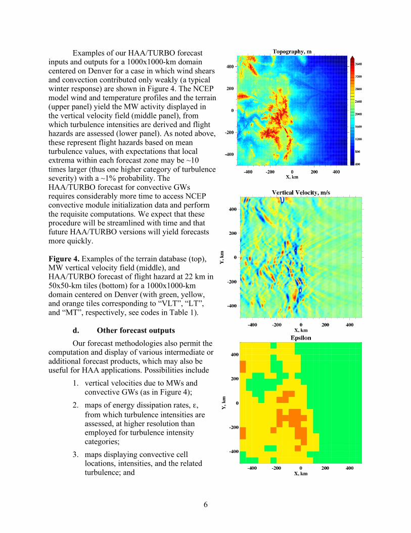
Examples of our HAA/TURBO forecast inputs and outputs for a 1000x1000-km domain centered on Denver for a case in which wind shears and convection contributed only weakly (a typical winter response) are shown in Figure 4. The NCEP model wind and temperature profiles and the terrain (upper panel) yield the MW activity displayed in the vertical velocity field (middle panel), from which turbulence intensities are derived and flight hazards are assessed (lower panel). As noted above, these represent flight hazards based on mean turbulence values, with expectations that local extrema within each forecast zone may be ~10 times larger (thus one higher category of turbulence severity) with a ~1% probability. The HAA/TURBO forecast for convective GWs requires considerably more time to access NCEP convective module initialization data and perform the requisite computations. We expect that these procedure will be streamlined with time and that future HAA/TURBO versions will yield forecasts more quickly. Figure 4. Examples of the terrain database (top), MW vertical velocity field (middle), and HAA/TURBO forecast of flight hazard at 22 km in 50x50-km tiles (bottom) for a 1000x1000-km domain centered on Denver (with green, yellow, and orange tiles corresponding to “VLT”, “LT”, and “MT”, respectively, see codes in Table 1).

d. Other forecast outputs Our forecast methodologies also permit the

computation and display of various intermediate or additional forecast products, which may also be useful for HAA applications. Possibilities include

1. vertical velocities due to MWs and convective GWs (as in Figure 4);

2. maps of energy dissipation rates, ε, from which turbulence intensities are assessed, at higher resolution than employed for turbulence intensity categories;

3. maps displaying convective cell locations, intensities, and the related turbulence; and

7

4. various meteorological fields, possibly including NCEP horizontal winds, frontal systems, etc., surface maps showing roads boundaries, infrastructure, and/or other user-defined fields.

Hence, feedback providing preferences or suggestions for additional fields that would be valuable to HAA forecasters are encouraged and will be considered for inclusion in future HAA/TURBO software updates. 4. HAA/TURBO Operational Factors

Our HAA/TURBO software has been configured, compiled, and tested on a Linux platform having 1 GB of memory. However, we recommend a minimum of 2 GB of memory to ensure that the software has sufficient memory resources, given other processes that may also be running in parallel. We have configured the software to provide what we consider to be optimal resolution for the convective GW computation, and this requires approximately 30 min to execute for each forecast time desired. This can be changed to require significantly less computational resources, but at some cost in forecast sensitivity to all GW spatial scales. Our graphical display package currently employs IDL software and routines, but can likewise be reconfigured with other public-domain software if desired. These and other operational aspects of the HAA/TURBO forecast software are described in greater detail in the accompanying User Manual.

5. References Cadet, D., 1977: Energy dissipation within intermittent clear air turbulence patches, J. Atmos.

Sci., 34, 137-142. Cot, C. E., and J. Barat, 1986: Wave-turbulence interaction in the stratosphere: A case study, J.

Geophys. Res., 91, 2749-2756. Broutman, D., J. Ma, S. D. Eckermann, and J. Lindeman, 2006: Fourier-ray modeling of trapped

lee waves: theory for wave transience, Mon. Wea. Rev., 143, 2849–2856. Broutman, D., J. W. Rottman and S. D. Eckermann, 2003: A simplified Fourier method for

nonhydrostatic mountain waves, J. Atmos. Sci., 60, 2686-2696. Broutman, D., S. D. Eckermann, and J. W. Rottmann, 2008: Practical application of two turning-

point theory to mountain-wave transmission through a wind jet, J. Atmos. Sci. in press. Eckermann, S. D., D. Broutman, J. Ma, and J. Lindeman, 2006: Fourier-ray modeling of short

wavelength trapped lee waves observed in infrared satellite imagery near Jan Mayen, Mon. Wea. Rev., 143, 2830–2848.

Fritts, D. C., L. Wang, J. Werne, T. Lund, and K. Wan, 2008a: Gravity wave instability dynamics at high Reynolds numbers, 1: Wave field evolution at large amplitudes and high frequencies, J. Atmos. Sci., in press.

Fritts, D. C., L. Wang, J. Werne, T. Lund, and K. Wan, 2008b: Gravity wave instability dynamics at high Reynolds numbers, 2: Turbulence evolution, structure, and anisotropy, J. Atmos. Sci., in press.

Lane, T.P., and R. D. Sharman, 2006: Gravity wave breaking, secondary wave generation, and mixing above deep convection in a three-dimensional cloud model, Geophys. Res. Lett., 33, L23813, doi:10.1029/2006GL027988.

8

Lilly, D. K., and P. J. Kennedy, 1973: Observations of a stationary mountain wave and its associated momentum flux and energy dissipation, J. Atmos. Sci., 30, 1135-1152.

Lilly, D. K., D. E. Waco, and S. I. Adelfang, 1974: Stratospheric mixing estimated from high-altitude turbulence measurements, J. Appl. Meteorol., 13, 488-493.

Trout, D, and H. A. Panofsky, 1969: Energy dissipation near the tropopause, Tellus, 21, 355-358. Vadas, S. L, and D. C. Fritts, 2001: Gravity wave radiation and mean responses to local body

forces in the atmosphere, J. Atmos. Sci., 58, 2249-2279. Vadas, S. L., and D. C. Fritts, 2002: The importance of spatial variability in the generation of

secondary gravity waves from local body forces , Geophys. Res. Lett., 29 (20), 10.1029/2002GL015574.

Vadas, S. L., and D. C. Fritts, 2004: Thermospheric responses to gravity waves arising from mesoscale convective complexes, J. Atmos. Solar Terres. Phys., 66, 781-804.

Vadas, S. L., and D. C. Fritts, 2008: Reconstruction of the gravity wave field excited by convective plumes via ray tracing in real space, Ann. Geophys., SpreadFEx special issue, in press.

Werne, J. A., and D. C. Fritts, 1998: Turbulence in stratified and sheared fluids: T3E simulations, 8th DoD HPC User Group Symposium.

Werne, J. A., and D. C. Fritts, 1999a: Stratified shear turbulence: Evolution and statistics, Geophys. Res. Lett., 26, 439-442.

Werne, J. A., and D. C. Fritts, 1999b: Anisotropy in stratified shear turbulence , 9th DoD HPC User Group Symposium, Monterey, CA.

Werne, J. A., and D. C. Fritts, 2000: Structure functions in stratified shear turbulence , 10th DoD HPC User Group Symposium, Albequerque, NM.

Werne, J. A., and D. C. Fritts, 2001: Anisotropy in a stratified shear layer, Phys. Chem. Earth, 26, 263-268.

Werne, J. T. Lund, B. A. Pettersson-Reif, P. Sullivan, and D. C. Fritts, 2005: CAP Phase II simulations for the Air Force HEL-JTO project: Atmospheric turbulence simulations on NAVO's 3000-processor IBM P4+ and ARL's 2000-processor Intel Xeon EM64T cluster, DoD HPCMO Conference, July.