PHASE RECOVERY, MAXCUTAND COMPLEX SEMIDEFINITE PROGRAMMING

IRENE WALDSPURGER, ALEXANDRE D’ASPREMONT, AND STEPHANE MALLAT

ABSTRACT. Phase retrieval seeks to recover a signal x ∈ Cp from the amplitude |Ax| of linear measure-ments Ax ∈ Cn. We cast the phase retrieval problem as a non-convex quadratic program over a complex phasevector and formulate a tractable relaxation (called PhaseCut) similar to the classical MaxCut semidefinite pro-gram. We solve this problem using a provably convergent block coordinate descent algorithm whose structureis similar to that of the original greedy algorithm in Gerchberg and Saxton [1972], where each iteration is amatrix vector product. Numerical results show the performance of this approach over three different phaseretrieval problems, in comparison with greedy phase retrieval algorithms and matrix completion formulations.

1. INTRODUCTION

The phase recovery problem, i.e. the problem of reconstructing a complex phase vector given only themagnitude of linear measurements, appears in a wide range of engineering and physical applications. Itis needed for example in X-ray and crystallography imaging [Harrison, 1993], diffraction imaging [Bunket al., 2007] or microscopy [Miao et al., 2008]. In these applications, the detectors cannot measure the phaseof the incoming wave and only record its amplitude. Recovering the complex phase of wavelet transformsfrom their amplitude also has applications in audio signal processing [Griffin and Lim, 1984].

In all these problems, complex measurements of a signal x ∈ Cp are obtained from a linear injectiveoperator A, but we can only measure the magnitude vector |Ax|. Depending on the properties of A, thephase of Ax may or may not be uniquely characterized by the magnitude vector |Ax|, up to an additiveconstant, and it may or may not be stable. For example, if A is a one-dimensional Fourier transform, thenthe recovery is not unique but it becomes unique almost everywhere for an oversampled two-dimensionalFourier transform, although it is not stable. Uniqueness is also obtained with an oversampled wavelettransform operator A, and the recovery of x from |Ax| is then continuous [Waldspurger and Mallat, 2012].If A consists in random Gaussian measurements then uniqueness can be proved, together with stabilityresults [Candes et al., 2011b; Candes and Li, 2012].

Recovering the phase of Ax from |Ax| is a nonconvex optimization problem. Until recently, this prob-lem was solved using various greedy algorithms [Gerchberg and Saxton, 1972; Fienup, 1982; Griffin andLim, 1984], which alternate projections on the range of A and on the nonconvex set of vectors y such that|y| = |Ax|. However, these algorithms often stall in local minima. A convex relaxation called PhaseLiftwas introduced in [Chai et al., 2011] and [Candes et al., 2011b] by observing that |Ax|2 is a linear functionof X = xx∗ which is a rank one Hermitian matrix. The recovery of x is thus expressed as a rank minimiza-tion problem over positive semidefinite Hermitian matrices X satisfying some linear conditions. This lastproblem is approximated by a semidefinite program. It has been shown that this program recovers x withhigh probability when A has gaussian independant entries [Candes et al., 2011b,a]. Numerically, the sameresult seems to hold for several classes of linear operators A.

Our main contribution here is to formulate phase recovery as a quadratic optimization problem overthe unit complex torus. We then write a convex relaxation to phase recovery very similar to the MaxCutsemidefinite program (we call this relaxation PhaseCut in what follows). While the resulting SDP is typically

Date: July 24, 2013.2010 Mathematics Subject Classification. 94A12, 90C22, 90C27.Key words and phrases. Phase Recovery, MaxCut, Semidefinite Programming, Convex Relaxation, Scattering.

1

larger than the PhaseLift relaxation, its simple structure (the constraint matrices are singletons) allows us tosolve it very efficiently. In particular, this allows us to use a provably convergent block coordinate descentalgorithm whose iteration complexity is similar to that of the original greedy algorithm in Gerchberg andSaxton [1972] (each iteration is a matrix vector product, which can be computed efficiently). We also showthat tightness of PhaseLift implies tightness of a modified version of PhaseCut. Furthermore, under thecondition thatA is injective and b has no zero coordinate, we derive an equivalence result between PhaseLiftand a modified version of PhaseCut, in the noiseless setting. This result implies that both algorithms aresimultaneously tight (an earlier version of this paper showed PhaseLift tightness implies PhaseCut tightnessand the reverse direction was then proved in [Voroninski, 2012] under mild additional assumptions). In anoisy setting, one can show that PhaseCut is at least as stable as a variant of PhaseLift, while PhaseCutempirically appears to be more stable in some cases, e.g. when b is sparse.

Seeing the MaxCut relaxation emerge in a phase recovery problem is not entirely surprising: it appears,for example, in an angular synchronization problem where one seeks to reconstruct a sequence of angles θi(up to a global phase), given information on pairwise differences θi−θj mod. 2π, for (i, j) ∈ S [see Singer,2011], the key difference between this last problem and the phase recovery problem in (1) is that the signinformation is lost in the input to (1). Complex MaxCut-like relaxations of decoding problems also appearin maximum-likelihood channel detection [Luo et al., 2003; Kisialiou and Luo, 2010; So, 2010]. Froma combinatorial optimization perspective, showing the equivalence between phase recovery and MaxCutallows us to expose a new class of nontrivial problem instances where the semidefinite relaxation for aMaxCut-like problem is tight, together with explicit conditions for tightness directly imported from thematrix completion formulation of these problems (these conditions are of course also hard to check, buthold with high probability for some classes of random experiments).

The paper is organized as follows. Section 2 explains how to factorize away the magnitude informationto form a nonconvex quadratic program on the phase vector u ∈ Cn satisfying |ui| = 1 for i = 1, . . . , n,and a greedy algorithm is derived in Section 2.3. We then derive a tractable relaxation of the phase recoveryproblem, written as a semidefinite program similar to the classical MaxCut relaxation in [Goemans andWilliamson, 1995], and detail several algorithms for solving this problem in Section 3. Section 4 provesthat a variant of PhaseCut and PhaseLift are equivalent in the noiseless case and thus simultaneously tight.We also prove that PhaseCut is as stable as a weak version of PhaseLift and discuss the relative complexityof both algorithms. Finally, Section 5 performs a numerical comparison between the greedy, PhaseLift andPhaseCut phase recovery algorithms for three phase recovery problems, in the noisy and noiseless case. Inthe noisy case, these results suggest that if b is sparse, then PhaseCut may be more stable than PhaseLift.

Notations. We write Sp (resp. Hp) the cone of symmetric (resp. Hermitian) matrices of dimension p ; S+p

(resp. H+p ) denotes the set of positive symmetric (resp. Hermitian) matrices. We write ‖ · ‖p the Schatten

p-norm of a matrix, that is the p-norm of the vector of its eigenvalues (in particular, ‖ · ‖∞ is the spectralnorm). We write A† the (Moore-Penrose) pseudoinverse of a matrix A and ‖A‖`1 the sum of the modulus ofthe coefficients of A. For x ∈ Rp, we write diag(x) the matrix with diagonal x. When X ∈ Hp however,diag(X) is the vector containing the diagonal elements of X . For X ∈ Hp, X∗ is the Hermitian transposeof X , with X∗ = (X)T . Finally, we write b2 the vector with components b2i , i = 1, . . . , n.

2. PHASE RECOVERY

The phase recovery problem seeks to retrieve a signal x ∈ Cp from the amplitude b = |Ax| of n linearmeasurements, solving

find xsuch that |Ax| = b,

(1)

in the variable x ∈ Cp, where A ∈ Cn×p and b ∈ Rn.2

2.1. Greedy Optimization in the Signal. Approximate solutions x of the recovery problem in (1) areusually computed from b = |Ax| using algorithms inspired from the alternating projection method in [Ger-chberg and Saxton, 1972]. These algorithms compute iterates yk in the set F of vectors y ∈ Cn such that|y| = b = |Ax|, which are getting progressively closer to the image of A. The Gerchberg-Saxton algorithmprojects the current iterate yk on the image of A using the orthogonal projector AA† and adjusts to bi theamplitude of each coordinate. We describe this method explicitly below.

Algorithm 1 Gerchberg-Saxton.

Input: An initial y1 ∈ F, i.e. such that |y1| = b.1: for k = 1, . . . , N − 1 do2: Set

yk+1i = bi

(AA†yk)i|(AA†yk)i|

, i = 1, . . . , n. (Gerchberg-Saxton)

3: end forOutput: yN ∈ F.

Because F is not convex however, this alternating projection method usually converges to a stationarypoint y∞ which does not belong to the intersection of F with the image of A, and hence |AA†y∞| 6= b.Several modifications proposed in [Fienup, 1982] improve the convergence rate but do not eliminate theexistence of multiple stationary points. To guarantee convergence to a unique solution, which hopefully be-longs to the intersection of F and the image of A, this non-convex optimization problem has recently beenrelaxed as a semidefinite program [Chai et al., 2011; Candes et al., 2011b], where phase recovery is formu-lated as a matrix completion problem (described in Section 4). Although the computational complexity ofthis relaxation is much higher than that of the Gerchberg-Saxton algorithm, it is able to recover x from |Ax|(up to a multiplicative constant) in a number of cases [Chai et al., 2011; Candes et al., 2011b].

2.2. Splitting Phase and Amplitude Variables. As opposed to these strategies, we solve the phase recov-ery problem by explicitly separating the amplitude and phase variables, and by only optimizing the valuesof the phase variables. In the noiseless case, we can write Ax = diag(b)u where u ∈ Cn is a phase vector,satisfying |ui| = 1 for i = 1, . . . , n. Given b = |Ax|, the phase recovery problem can thus be written as

minu∈Cn, |ui|=1,

x∈Cp

‖Ax− diag(b)u‖22,

where we optimize over both variables u ∈ Cn and x ∈ Cp. In this format, the inner minimization problemin x is a standard least squares and can be solved explicitly by setting

x = A† diag(b)u,

which means that problem (1) is equivalent to the reduced problem

min|ui|=1u∈Cn

‖AA† diag(b)u− diag(b)u‖22.

The objective of this last problem can be rewritten as follows

‖AA† diag(b)u− diag(b)u‖22 = ‖(AA† − I)diag(b)u‖22= u∗ diag(bT )M diag(b)u.

where M = (AA† − I)∗(AA† − I) = I−AA†. Finally, the phase recovery problem (1) becomes

minimize u∗Musubject to |ui| = 1, i = 1, . . . n,

(2)

3

in the variable u ∈ Cn, where the Hermitian matrix

M = diag(b)(I−AA†)diag(b)

is positive semidefinite. The intuition behind this last formulation is simple, (I − AA†) is the orthogonalprojector on the orthogonal complement of the image of A (the kernel of A∗), so this last problem simplyminimizes in the phase vector u the norm of the component of diag(b)u which is not in the image of A.

2.3. Greedy Optimization in Phase. Having transformed the phase recovery problem (1) in the quadraticminimization problem (2), suppose that we are given an initial vector u ∈ Cn, and focus on optimizing overa single component ui for i = 1, . . . , n. The problem is equivalent to solving

minimize uiMiiui + 2 Re(∑

j 6=i ujMjiui

)subject to |ui| = 1, i = 1, . . . n,

in the variable ui ∈ C where all the other phase coefficients uj remain constant. Because |ui| = 1 this thenamounts to solving

min|ui|=1

Re

ui∑j 6=i

Mjiuj

which means

ui =−∑

j 6=iMjiuj∣∣∣∑j 6=iMjiuj

∣∣∣ (3)

for each i = 1, . . . , n, when u is the optimum solution to problem (2). We can use this fact to deriveAlgorithm 2, a greedy algorithm for optimizing the phase problem.

Algorithm 2 Greedy algorithm in phase.

Input: An initial u ∈ Cn such that |ui| = 1, i = 1, . . . , n. An integer N > 1.1: for k = 1, . . . , N do2: for i = 1, . . . n do3: Set

ui =−∑

j 6=iMjiuj∣∣∣∑j 6=iMjiuj

∣∣∣4: end for5: end for

Output: u ∈ Cn such that |ui| = 1, i = 1, . . . , n.

This greedy algorithm converges to a stationary point u∞, but it is generally not a global solution of prob-lem (2), and hence |AA† diag(u∞)b| 6= b. It has often nearly the same stationary points as the Gerchberg-Saxton algorithm. One can indeed verify that if u∞ is a stationary point then y∞ = diag(u∞)b is astationary point of the Gerchberg-Saxton algorithm. Conversely if b has no zero coordinate and y∞ is astable stationary point of the Gerchberg-Saxton algorithm then u∞i = y∞i /|y∞i | defines a stationary point ofthe greedy algorithm in phase.

IfAx can be computed with a fast algorithm usingO(n log n) operations, which is the case for Fourier orwavelets transform operators for example, then each Gerchberg-Saxton iteration is computed withO(n log n)operations. The greedy phase algorithm above does not take advantage of this fast algorithm and requiresO(n2) operations to update all coordinates ui for each iteration k. However, we will see in Section 3.6 thata small modification of the algorithm allows for O(n log n) iteration complexity.

4

2.4. Complex MaxCut. Following the classical relaxation argument in [Shor, 1987; Lovasz and Schrijver,1991; Goemans and Williamson, 1995; Nesterov, 1998], we first write U = uu∗ ∈ Hn. Problem (2), written

QP (M) , min. u∗Musubject to |ui| = 1, i = 1, . . . n,

in the variable u ∈ Cn, is equivalent to

min. Tr(UM)subject to diag(U) = 1

U � 0, Rank(U) = 1,

in the variable U ∈ Hn. After dropping the (nonconvex) rank constraint, we obtain the following convexrelaxation

SDP (M) , min. Tr(UM)subject to diag(U) = 1, U � 0,

(PhaseCut)

which is a semidefinite program (SDP) in the matrix U ∈ Hn and can be solved efficiently. When thesolution of problem PhaseCut has rank one, the relaxation is tight and the vector u such that U = uu∗ is anoptimal solution of the phase recovery problem (2). If the solution has rank larger than one, a normalizedleading eigenvector v of U is used as an approximate solution, and diag(U − vvT ) gives a measure of theuncertainty around the coefficients of v.

In practice, semidefinite programming solvers are rarely designed to directly handle problems writtenover Hermitian matrices and start by reformulating complex programs in Hn as real semidefinite programsover S2n based on the simple facts that follow. For Z, Y ∈ Hn, we define T (Z) ∈ S2n as in [Goemans andWilliamson, 2004]

T (Z) =

(Re(Z) − Im(Z)Im(Z) Re(Z)

)(4)

so that Tr(T (Z)T (Y )) = 2Tr(ZY ). By construction, Z ∈ Hn iff T (Z) ∈ S2n. One can also check thatz = x+ iy is an eigenvector of Z with eigenvalue λ if and only if(

xy

)and

(−yx

)are eigenvectors of T (Z), both with eigenvalue λ (depending on the normalization of z, one correspondsto (Re(z), Im(z)), the other one to (Re(i z), Im(i z)). This means in particular that Z � 0 if and only ifT (Z) � 0.

We can use these facts to formulate an equivalent semidefinite program over real symmetric matrices,written

minimize Tr(T (M)X)subject to Xi,i +Xn+i,n+i = 2

Xi,j = Xn+i,n+j , Xn+i,j = −Xi,n+j , i, j = 1, . . . , n,X � 0,

in the variable X in S2n. This last problem is equivalent to PhaseCut. In fact, because of symmetries inT (M), the equality constraints enforcing symmetry can be dropped, and this problem is equivalent to aMaxCut like problem in dimension 2n, which reads

minimize Tr(T (M)X)subject to diag(X) = 1, X � 0,

(5)

in the variable X in S2n. As we will see below, formulating a relaxation to the phase recovery problem as acomplex MaxCut-like semidefinite program has direct computational benefits.

5

3. ALGORITHMS

In the previous section, we have approximated the phase recovery problem (2) by a convex relaxation,written

minimize Tr(UM)subject to diag(U) = 1, U � 0,

which is a semidefinite program in the matrix U ∈ Hn. The dual, written

maxw∈Rn

nλmin(M + diag(w))− 1Tw, (6)

is a minimum eigenvalue maximization problem in the variablew ∈ Rn. Both primal and dual can be solvedefficiently. When exact phase recovery is possible, the optimum value of the primal problem PhaseCut iszero and we must have λmin(M) = 0, which means that w = 0 is an optimal solution of the dual.

3.1. Interior Point Methods. For small scale problems, with n ∼ 102, generic interior point solvers suchas SDPT3 [Toh et al., 1999] solve problem (5) with a complexity typically growing as O

(n4.5 log(1/ε)

)where ε > 0 is the target precision [Ben-Tal and Nemirovski, 2001, §4.6.3]. Exploiting the fact that the2n equality constraints on the diagonal in (5) are singletons, Helmberg et al. [1996] derive an interior pointmethod for solving the MaxCut problem, with complexity growing as O

(n3.5 log(1/ε)

)where the most

expensive operation at each iteration is the inversion of a positive definite matrix, which costs O(n3) flops.

3.2. First-Order Methods. When n becomes large, the cost of running even one iteration of an interiorpoint solver rapidly becomes prohibitive. However, we can exploit the fact that the dual of problem (5)can be written (after switching signs) as a maximum eigenvalue minimization problem. Smooth first-orderminimization algorithms detailed in [Nesterov, 2007] then produce an ε-solution after

O

(n3√

log n

ε

)floating point operations. Each iteration requires forming a matrix exponential, which costs O(n3) flops.This is not strictly smaller than the iteration complexity of specialized interior point algorithms, but matrixstructure often allows significant speedup in this step. Finally, the simplest subgradient methods produce anε-solution in

O

(n2 log n

ε2

)floating point operations. Each iteration requires computing a leading eigenvector which has complexityroughly O(n2 log n).

3.3. Block Coordinate Descent. We can also solve the semidefinite program in PhaseCut using a blockcoordinate descent algorithm. While no explicit complexity bounds are available for this method in ourcase, the algorithm is particularly simple and has a very low cost per iteration (it only requires computinga matrix vector product). We write ic the index set {1, . . . , i − 1, i + 1, . . . , n} and describe the method asAlgorithm 3.

Block coordinate descent is widely used to solve statistical problems where the objective is separable(LASSO is a typical example) and was shown to efficiently solve semidefinite programs arising in covarianceestimation [d’Aspremont et al., 2006]. These results were extended by [Wen et al., 2012] to a broader classof semidefinite programs, including MaxCut. We briefly recall its simple construction below, applied to abarrier version of the MaxCut relaxation PhaseCut, written

minimize Tr(UM)− µ log det(U)subject to diag(U) = 1

(7)

which is a semidefinite program in the matrix U ∈ Hn, where µ > 0 is the barrier parameter. As in interiorpoint algorithms, the barrier enforces positive semidefiniteness and the value of µ > 0 precisely controls the

6

distance between the optimal solution to (7) and the optimal set of PhaseCut. We refer the reader to [Boydand Vandenberghe, 2004] for further details. The key to applying coordinate descent methods to problemspenalized by the log det(·) barrier is the following block-determinant formula

det(U) = det(B) det(y − xTB−1x), when U =

(B xxT y

), U � 0. (8)

This means that, all other parameters being fixed, minimizing the function det(X) in the row and columnblock of variables x, is equivalent to minimizing the quadratic form y − xTZ−1x, arguably a much simplerproblem. Solving the semidefinite program (7) row/column by row/column thus amounts to solving thesimple problem (9) described in the following lemma.

Lemma 3.1. Suppose σ > 0, c ∈ Rn−1, and B ∈ Sn−1 are such that b 6= 0 and B � 0, then the optimalsolution of the block problem

minx

cTx− σ log(1− xTB−1x) (9)

is given by

x =

√σ2 + γ − σ

γBc

where γ = cTBc.

Proof. As in [Wen et al., 2012], a direct consequence of the first order optimality conditions for (9).

Here, we see problem (7) as an unconstrained minimization problem over the off-diagonal coefficientsof U , and (8) shows that each block iteration amounts to solving a minimization subproblem of the form (9).Lemma 3.1 then shows that this is equivalent to computing a matrix vector product. Linear convergenceof the algorithm is guaranteed by the result in [Boyd and Vandenberghe, 2004, §9.4.3] and the fact thatthe function log det is strongly convex over compact subsets of the positive semidefinite cone. So thecomplexity of the method is bounded by O

(log 1

ε

)but the constant in this bound depends on n here, and

the dependence cannot be quantified explicitly.

Algorithm 3 Block Coordinate Descent Algorithm for PhaseCut.

Input: An initial X0 = In and ν > 0 (typically small). An integer N > 1.1: for k = 1, . . . , N do2: Pick i ∈ [1, n].3: Compute

x = Xkic,icMic,i and γ = x∗Mic,i

4: If γ > 0, set

Xk+1ic,i = Xk+1∗

i,ic = −√

1− νγ

x

elseXk+1ic,i = Xk+1∗

i,ic = 0.

5: end forOutput: A matrix X � 0 with diag(X) = 1.

7

3.4. Initialization & Randomization. Suppose the Hermitian matrix U solves the semidefinite relax-ation PhaseCut. As in [Goemans and Williamson, 2004; Ben-Tal et al., 2003; Zhang and Huang, 2006;So et al., 2007], we generate complex Gaussian vectors x ∈ Cn with x ∼ NC(0, U), and for each sample x,we form z ∈ Cn such that

zi =xi|xi|

, i = 1, . . . , n.

All the sample points z generated using this procedure satisfy |zi| = 1, hence are feasible points for prob-lem (2). This means in particular that QP (M) ≤ E[z∗Mz]. In fact, this expectation can be computedalmost explicitly, using

E[zz∗] = F (U), with F (w) = 12ei arg(w)

∫ π

0cos(θ) arcsin(|w| cos(θ))dθ

where F (U) is the matrix with coefficients F (Uij), i, j = 1, . . . , n. We then get

SDP (M) ≤ QP (M) ≤ Tr(MF (U)) (10)

In practice, to extract good candidate solutions from the solution U to the SDP relaxation in PhaseCut, wesample a few points from NC(0, U), normalize their coordinates and simply pick the point which mini-mizes z∗Mz.

This sampling procedure also suggests a simple spectral technique for computing rough solutions to prob-lem PhaseCut: compute an eigenvector of M corresponding to its lowest eigenvalue and simply normalizeits coordinates (this corresponds to the simple bound on MaxCut by [Delorme and Poljak, 1993]). The infor-mation contained in U can also be used to solve a robust formulation [Ben-Tal et al., 2009] of problem (1)given a Gaussian model u ∼ NC(0, U).

3.5. Approximation Bounds. The semidefinite program in PhaseCut is a MaxCut-type graph partitioningrelaxation whose performance has been studied extensively. Note however that most approximation resultsfor MaxCut study maximization problems over positive semidefinite or nonnegative matrices, while we areminimizing in PhaseCut so, as pointed out in [Kisialiou and Luo, 2010; So and Ye, 2010] for example, wedo not inherit the constant approximation ratios that hold in the classical MaxCut setting.

3.6. Exploiting Structure. In some instances, we have additional structural information on the solution ofproblems (1) and (2), which usually reduces the complexity of approximating PhaseCut and improves thequality of the approximate solutions. We briefly highlight a few examples below.

3.6.1. Symmetries. In some cases, e.g. signal processing examples where the signal is symmetric, theoptimal solution u has a known symmetry pattern. For example, we might have u(k− − i) = u(k+ + i)for some k−, k+ and indices i ∈ [0, k− − 1]. This means that the solution u to problem (1) can be writtenu = Pv, where v ∈ Cq with q < n, and we can solve (1) by focusing on the smaller problem

minimize v∗P ∗MPvsubject to |(Pv)i| = 1, i = 1, . . . n,

in the variable v ∈ Cq. We reconstruct a solution u to (1) from a solution v to the above problem as u = Pv.This produces significant computational savings.

3.6.2. Alignment. In other instances, we might have prior knowledge that the phases of certain samples arealigned, i.e. that there is an index set I such that ui = uj , for all i, j ∈ I , this reduces to the symmetriccase discussed above when the phase is arbitrary. W.l.o.g., we can also fix the phase to be one, with ui = 1for i ∈ I , and solve a constrained version of the relaxation PhaseCut

min. Tr(UM)subject to Uij = 1, i, j ∈ I,

diag(U) = 1, U � 0,

which is a semidefinite program in U ∈ Hn.8

3.6.3. Fast Fourier transform. If the product Mx can be computed with a fast algorithm in O(n log n)operations, which is the case for Fourier or wavelet transform operators, we significantly speed up theiterations of Algorithm 3 to update all coefficients at once. Each iteration of the modified Algorithm 3 thenhas cost O(n log n) instead of O(n2).

3.6.4. Real valued signal. In some cases, we know that the solution vector x in (1) is real valued. Prob-lem (1) can be reformulated to explicitly constrain the solution to be real, by writing it

minu∈Cn, |ui|=1,

x∈Rp

‖Ax− diag(b)u‖22

or again, using the operator T (·) defined in (4)

minimize∥∥∥∥T (A)

(x0

)− diag

(bb

)(Re(u)Im(u)

)∥∥∥∥22

subject to u ∈ Cn, |ui| = 1x ∈ Rp.

The optimal solution of the inner minimization problem in x is given by x = A†2B2v, where

A2 =

(Re(A)Im(A)

), B2 = diag

(bb

), and v =

(Re(u)Im(u)

)hence the problem is finally rewritten

minimize ‖(A2A†2B2 −B2)v‖22

subject to v2i + v2n+i = 1, i = 1, . . . , n,

in the variable v ∈ R2n. This can be relaxed as above by the following problem

minimize Tr(VM2)subject to Vii + Vn+i,n+i = 1, i = 1, . . . , n,

V � 0,

which is a semidefinite program in the variable V ∈ S2n, whereM2 = (A2A†2B2−B2)

T (A2A†2B2−B2) =

BT2 (I−A2A

†2)B2.

4. MATRIX COMPLETION & EXACT RECOVERY CONDITIONS

In [Chai et al., 2011; Candes et al., 2011b], phase recovery (1) is cast as a matrix completion problem.We briefly review this approach and compare it with the semidefinite program in PhaseCut. Given a signalvector b ∈ Rn and a sampling matrix A ∈ Cn×p, we look for a vector x ∈ Cp satisfying

|a∗ix| = bi, i = 1, . . . , n,

where the vector a∗i is the ith row of A and x ∈ Cp is the signal we are trying to reconstruct. The phaserecovery problem is then written as

minimize Rank(X)subject to Tr(aia

∗iX) = b2i , i = 1, . . . , n

X � 0

in the variable X ∈ Hp, where X = xx∗ when exact recovery occurs. This last problem can be relaxed as

minimize Tr(X)subject to Tr(aia

∗iX) = b2i , i = 1, . . . , n

X � 0(PhaseLift)

9

which is a semidefinite program (called PhaseLift by Candes et al. [2011b]) in the variable X ∈ Hp. Recentresults in [Candes et al., 2011a; Candes and Li, 2012] give explicit (if somewhat stringent) conditions onA and x under which the relaxation is tight (i.e. the optimal X in PhaseLift is unique, has rank one, withleading eigenvector x).

4.1. Weak Formulation. We also introduce a weak version of PhaseLift, which is more directly relatedto PhaseCut and is easier to interpret geometrically. It was noted in [Candes et al., 2011a] that, whenI ∈ span{aia∗i }ni=1, the condition Tr(aia

∗iX) = b2i , i = 1, ..., n determines Tr(X), so in this case the trace

minimization objective is redundant and PhaseLift is equivalent to

find Xsubject to Tr(aia

∗iX) = b2i , i = 1, . . . , n

X � 0.(Weak PhaseLift)

When I /∈ span{aia∗i }ni=1 on the other hand, Weak PhaseLift and PhaseLift are not equivalent: solutionsof PhaseLift solve Weak PhaseLift too but the converse is not true. Interior point solvers typically pick asolution at the analytic center of the feasible set of Weak PhaseLift which in general can be significantlydifferent from the minimum trace solution.

However, in practice, the removal of trace minimization does not really seem to alter the performancesof the algorithm. We will illustrate this affirmation with numerical experiments in §5.4 and a formal proofis given in [Demanet and Hand, 2012] who showed that, in the case of Gaussian random measurements, therelaxation of Weak PhaseLift was tight with high probability under the same conditions as PhaseLift.

4.2. Phase Recovery as a Projection. We will see in what follows that phase recovery can interpreted asa projection problem. These results will prove useful later to study stability. The PhaseCut reconstructionproblem defined in PhaseCut is written

minimize Tr(UM)subject to diag(U) = 1, U � 0,

with M = diag(b)(I−AA†)diag(b). In what follows, we assume bi 6= 0, i = 1, ..., n, which means that,after scaling U , solving PhaseCut is equivalent to solving

minimize Tr(V (I−AA†))subject to diag(V ) = b2, V � 0.

(11)

In the following lemma, we show that this last semidefinite program can be understood as a projectionproblem on a section of the semidefinite cone using the trace (or nuclear) norm. We define

F = {V ∈ Hn : x∗V x = 0, ∀x ∈ R(A)⊥}which is also F = {V ∈ Hn : (I − AA†)V (I − AA†) = 0}, and we now formulate the objective ofproblem (11) as a distance.

Lemma 4.1. For all V ∈ Hn such that V � 0,

Tr(V (I−AA†)) = d1(V,F) (12)

where d1 is the distance associated to the trace norm.

Proof. Let B1 (resp. B2) be an orthonormal basis of rangeA (resp. (rangeA)⊥). Let T be the transfor-mation matrix from canonical basis to orthonormal basis B1 ∪ B2. Then

F = {V ∈ Hn s.t. T−1V T =(S1 S2S∗2 0

), S1 ∈ Hp, S2 ∈Mp,n−p}

As the transformation X → T−1XT preserves the nuclear norm, for every matrix V � 0, if we write

T−1V T =(V1 V2V ∗2 V3

)10

FIGURE 1. Schematic representation of the sets involved in equations (13) and (14) : thecone of positive hermitian matrices H+

n (in light grey), its intersection with the affine sub-spaceHb, and F ∩H+

n , which is a face of H+n .

then the orthogonal projection of V onto F is

W = T(V1 V2V ∗2 0

)T−1,

so d1(V,F) = ‖V −W‖1 = ‖(0 00 V3

)‖1. As V � 0,

(V1 V2V ∗2 V3

)� 0 hence

(0 00 V3

)� 0, so d1(V,F) =

Tr(0 00 V3

). Because AA† is the orthogonal projection ontoR(A), we have T−1(I−AA†)T =

(0 00 I

)hence

d1(V,F) = Tr(0 00 V3

)= Tr((T−1V T )(T−1(I−AA†)T )) = Tr(V (I−AA†))

which is the desired result.

This means that PhaseCut can be written as a projection problem, i.e.

minimize d1(V,F)subject to V ∈ H+

n ∩Hb(13)

in the variable V ∈ Hn, where Hb = {V ∈ Hn s.t. Vi,i = b2i , i = 1, ..., n}. Moreover, with ai the i-throw of A, we have for all X ∈ H+

p , Tr(aia∗iX) = a∗iXai = diag(AXA∗)i, i = 1, . . . , n, so if we call

V = AXA∗ ∈ F , when A is injective, X = A†V A†∗ and Weak PhaseLift is equivalent to

find V ∈ H+n ∩ F

subject to diag(V ) = b2.

First order algorithms for Weak PhaseLift will typically solve

minimize d(diag(V ), b2)subject to V ∈ H+

n ∩ F

for some distance d over Rn. If d is the ls-norm, for any s ≥ 1, d(diag(V ), b2) = ds(V,Hb), where ds isthe distance generated by the Schatten s-norm, the algorithm becomes

minimize ds(V,Hb)subject to V ∈ H+

n ∩ F(14)

which is another projection problem in V .Thus, PhaseCut and Weak PhaseLift are comparable, in the sense that both algorithms aim at finding a

point of H+n ∩ F ∩ Hb but PhaseCut does so by picking a point of H+

n ∩ Hb and moving towards F whileWeak PhaseLift moves a point of H+

n ∩ F towards Hb. We can push the parallel between both relaxationsmuch further. We will show in what follows that, in a very general case, PhaseLift and a modified version

11

of PhaseCut are simultaneously tight. We will also be able to compare the stability of Weak PhaseLift andPhaseCut when measurements become noisy.

4.3. Tightness of the Semidefinite Relaxation. We will now formulate a refinement of the semidefiniterelaxation in PhaseCut and prove that this refinement is equivalent to the relaxation in PhaseLift under mildtechnical assumptions. Suppose u is the optimal phase vector, we know that the optimal solution to (1)can then be written x = A† diag(b)u, which corresponds to the matrix X = A† diag(b)uu∗ diag(b)A†∗

in PhaseLift, henceTr(X) = Tr(diag(b)A†∗A† diag(b)uu∗).

Writing B = diag(b)A†∗A† diag(b), when problem (1) is solvable, we look for the “minimum trace”solution among all the optimal points of relaxation PhaseCut by solving

SDP2(M) , min. Tr(BU)subject to Tr(MU) = 0

diag(U) = 1, U � 0,(PhaseCutMod)

which is a semidefinite program in U ∈ Hn. When problem (1) is solvable, then every optimal solutionof the semidefinite relaxation PhaseCut is a feasible point of relaxation PhaseCutMod. In practice, thesemidefinite program SDP (M + γB), written

minimize Tr((M + γB)U)subject to diag(U) = 1, U � 0,

obtained by replacing M by M + γB in problem PhaseCut, will produce a solution to PhaseCutMod when-ever γ > 0 is sufficiently small (this is essentially the exact penalty method detailed in [Bertsekas, 1998,§4.3] for example). This means that all algorithms (greedy or SDP) designed to solve the original PhaseCutproblem can be recycled to solve PhaseCutMod with negligible effect on complexity. We now show thatthe PhaseCutMod and PhaseLift relaxations are simultaneously tight when A is injective. An earlier ver-sion of this paper showed PhaseLift tightness implies PhaseCut tightness and the argument was reversed in[Voroninski, 2012] under mild additional assumptions.

Proposition 4.2. Assume that bi 6= 0 for i = 1, . . . , n, that A is injective and that there is a solution xto (1). The function

Φ : Hp → Hn

X 7→ Φ(X) = diag(b)−1AXA∗ diag(b)−1

is a bijection between the feasible points of PhaseCutMod and those of PhaseLift.

Proof. Note that Φ is injective whenever b > 0 and A has full rank. We have to show that U is afeasible point of PhaseCutMod if and only if it can be written under the form Φ(X), where X is feasiblefor PhaseLift. We first show that

Tr(MU) = 0, U � 0, (15)is equivalent to

U = Φ(X) (16)for some X � 0. Observe that Tr(UM) = 0 means UM = 0 because U,M � 0, hence Tr(MU) = 0in (15) is equivalent to

AA† diag(b)U diag(b) = diag(b)U diag(b)

because b > 0 and M = diag(b)(I − AA†)diag(b). If we set X = A† diag(b)U diag(b)A†∗, this lastequality implies both

AX = AA† diag(b)U diag(b)A†∗ = diag(b)U diag(b)A†∗

andAXA∗ = diag(b)U diag(b)A†∗A∗ = diag(b)U diag(b)

12

which is U = Φ(X), and shows (15) implies (16). Conversely, if U = Φ(X) then diag(b)U diag(b) =AXA∗ and using AA†A = A, we get AXA∗ = AA†AXA∗ = AA† diag(b)U diag(b) which meansMU = 0, hence (15) is in fact equivalent to (16) since U � 0 by construction.

Now, if X is feasible for PhaseLift, we have shown Tr(MΦ(X)) = 0 and φ(X) � 0, moreoverdiag(Φ(X))i = Tr(aia

∗iX)/b2i = 1, so U = Φ(X) is a feasible point of PhaseCutMod. Conversely,

if U is feasible for PhaseCutMod, we have shown that there exists X � 0 such that U = Φ(X) whichmeans diag(b)U diag(b) = AXA∗. We also have Tr(aia

∗iX) = b2iUii = b2i , which means X is feasible

for PhaseLift and concludes the proof.

We now have the following central corollary showing the equivalence between PhaseCutMod and PhaseLiftin the noiseless case.

Corollary 4.3. If A is injective, bi 6= 0 for all i = 1, ..., n and if the reconstruction problem (1) admits anexact solution, then PhaseCutMod is tight (i.e. has a unique rank one solution) whenever PhaseLift is.

Proof. When A is injective, Tr(X) = Tr(BΦ(X)) and Rank(X) = Rank(Φ(X)).

This last result shows that in the noiseless case, the relaxations PhaseLift and PhaseCutMod are in factequivalent. In the same way, we could have shown that Weak PhaseLift and PhaseCut were equivalent. Theperformances of both algorithms may not match however when the information on b is noisy and perfectrecovery is not possible.

Remark 4.4. Note that Proposition 4.2 and corollary 4.3 also hold when the initial signal is real and themeasurements are complex. In this case, we define the B in PhaseCutMod by B = B2A

†∗2 A†2B2 (with

the notations of paragraph 3.6.4). We must also replace the definition of Φ by Φ(X) = B−12 A2XA∗2B−12 .

Furthermore, all steps in the proof of proposition 4.2 are still valid if we replace M by M2, A by A2 anddiag(b) by B2. The only difference is that now 1

b2iTr(aia

∗iX) = diag(Φ(X))i + diag(Φ(X))n+i.

4.4. Stability in the Presence of Noise. We now consider the case where the vector of measurements bis of the form b = |Ax0| + bnoise. We first introduce a definition of C-stability for PhaseCut and WeakPhaseLift. The main result of this section is that, when the Weak PhaseLift solution in (14) is stable at apoint, PhaseCut is stable too, with a constant of the same order. The converse does not seem to be true whenb is sparse.

Definition 4.5. Let x0 ∈ Cn, C > 0. The algorithm PhaseCut (resp. Weak PhaseLift) is said to be C-stableat x0 iff for all bnoise ∈ Rn close enough to zero, every minimizer V of equation (13) (resp. (14)) withb = |Ax0|+ bnoise, satisfies

‖V − (Ax0)(Ax0)∗‖2 ≤ C‖Ax0‖2‖bnoise‖2.

The following matrix perturbation result motivates this definition, by showing that a C-stable algorithmgenerates a O(C‖bnoise‖2)-error over the signal it reconstructs.

Proposition 4.6. Let C > 0 be arbitrary. We suppose that Ax0 6= 0 and ‖V − (Ax0)(Ax0)∗‖2 ≤

C‖Ax0‖2‖bnoise‖2 ≤ ‖Ax0‖22/2. Let y be V ’s main eigenvector, normalized so that (Ax0)∗y = ‖Ax0‖2.

Then‖y −Ax0‖2 = O(C‖bnoise‖2),

and the constant in this last equation does not depend upon A, x0, C or ‖b‖2.

Proof. We use [El Karoui and d’Aspremont, 2009, Eq.10] for

u =Ax0‖Ax0‖2

v =y

‖Ax0‖2E =

V − (Ax0)(Ax0)∗

‖Ax0‖2213

This result is based on [Kato, 1995, Eq. 3.29], which gives a precise asymptotic expansion of u− v. For ourpurposes here, we only need the first-order term. See also Bhatia [1997], Stewart and Sun [1990] or Stewart[2001] among others for a complete discussion. We get ‖v − u‖ = O(‖E‖2) because if M = uu∗, then‖R‖∞ = 1 in [El Karoui and d’Aspremont, 2009, Eq.10]. This implies

‖y −Ax0‖2 = ‖Ax0‖2‖u− v‖ = O

(‖V − (Ax0)(Ax0)

∗‖2‖Ax0‖2

)= O(C‖bnoise‖)

which is the desired result.

Note that normalizing y differently, we would obtain ‖y−Ax0‖2 ≤ 4C‖bnoise‖2. We now show the mainresult of this section, according to which PhaseCut is “almost as stable as” Weak PhaseLift. In practice ofcourse, the exact values of the stability constants has no importance, what matters is that they are of thesame order.

Theorem 4.7. Let A ∈ Cn×m, for all x0 ∈ Cn, C > 0, if Weak PhaseLift is C-stable in x0, then PhaseCutis (2C + 2

√2 + 1)-stable in x0.

Proof. Let x0 ∈ Cn, C > 0 be such that Weak PhaseLift is C-stable in x0. Ax0 is a non-zero vector(because, with our definition, neither Weak PhaseLift nor PhaseCut may be stable in x0 if Ax0 = 0 andA 6= 0). We set D = 2C + 2

√2 + 1 and suppose by contradiction that PhaseCut is not D-stable in x0.

Let ε > 0 be arbitrary. Let bn,PC ∈ Rn be such that ‖bn,PC‖2 ≤ max(‖Ax0‖2, ε/2) and such that, forb = |Ax0|+ bn,PC, the minimizer VPC of (13) verifies

‖VPC − (Ax0)(Ax0)∗‖2 > D‖Ax0‖2‖bn,PC‖2

Such a VPC must exist or PhaseCut would be D-stable in x0. We call V �PC the restriction of VPC to

range(A) (that is, the matrix such that x∗(V �PC)y = x∗(VPC)y if x, y ∈ range(A) and x∗(V �

PC)y = 0 if x ∈

range(A)⊥ or y ∈ range(A)⊥) and V ⊥PC the restriction of VPC to range(A)⊥. Let us set bn,PL =

√V

�PC ii−

|Ax0|ii for i = 1, ..., n. As V �PC ∈ H+

n ∩F , V �PC minimizes (14) for b = |Ax0|+bn,PL (because V �

PC ∈ Hb).Lemmas A.1 and A.2 (proven in the appendix) imply that ‖V �

PC − (Ax0)(Ax0)∗‖2 > C‖Ax0‖2‖bn,PL‖2

and ‖bn,PL‖2 ≤ ε. As ε is arbitrary, Weak PhaseLift is not C-stable in x0, which contradicts our hypotheses.Consequently, PhaseCut is (2C + 2

√2 + 1)-stable in x0.

Theorem 4.7 is still true if we replace 2C + 2√

2 + 1 by any D > 2C +√

2. We only have toreplace, in the demonstration, the inequality ‖bn,PC‖2 ≤ ‖Ax0‖2 by ‖bn,PC‖2 ≤ α‖Ax0‖2 with α =

D − (2C +√

2)/(1 +√

2). Also, the demonstration of this theorem is based on the fact that, when VPCsolves (13), one can construct some VPL = V

�PC close to VPC , which is an approximate solution of (14).

It is natural to wonder whether, conversely, from a solution VPL of (14), one can construct an approx-imate solution VPC of (13). It does not seem to be the case. One could for example imagine settingVPC = diag(R)VPL diag(R), where Ri = bi/

√VPL ii. Then VPC would not necessarily minimize (13)

but at least belong to Hb. But ‖VPC − VPL‖2 might be quite large: (14) implies that ‖diag(VPL) − b2‖sis small but, if some coefficients of b are very small, some Ri may still be huge, so diag(R) 6≈ I. This doeshappen in practice (see § 5.5).

To conclude this section, we relate this definition of stability to the one introduced in [Candes and Li,2012]. Suppose that A is a matrix of random gaussian independant measurements such that E[|Ai,j |2] = 1for all i, j. We also suppose that n ≥ c0p (for some c0 independent of n and p). In the noisy setting, Candesand Li [2012] showed that the minimizerX of a modified version of PhaseLift satisfies with high probability

||X − x0x∗0||2 ≤ C0|| |Ax0|2 − b2 ||1

n(17)

14

for some C0 independent of all variables. Assuming that the Weak PhaseLift solution in (14) behavesas PhaseLift in a noisy setting and that (17) also holds for Weak PhaseLift, then

||AXA∗ − (Ax0)(Ax0)∗||2 ≤ ||A||2∞||X − x0x∗0||2

≤ C0||A||2∞n|| |Ax0|2 − b2 ||1

≤ C0||A||2∞n

(2||Ax0||2 + ||bnoise||2)||bnoise||2

Consequently, for anyC > 2C0||A||2∞n , Weak PhaseLift isC-stable in all x0. With high probability, ||A||2∞ ≤

(1 + 1/8)n (it is a corollary of [Candes and Li, 2012, Lemma 2.1]) so Weak PhaseLift (and thus alsoPhaseCut) is C-stable with high probability for some C independent of all parameters of the problem.

4.5. Perturbation Results. We recall here sensitivity analysis results for semidefinite programming fromTodd and Yildirim [2001]; Yildirim [2003], which produce explicit bounds on the impact of small pertur-bations in the observation vector b2 on the solution V of the semidefinite program (11). Roughly speaking,these results show that if b2 + bnoise remains in an explicit ellipsoid (called Dikin’s ellipsoid), then interiorpoint methods converge back to the solution in one full Newton step, hence the impact on V is linear, equalto the Newton step. These results are more numerical in nature than the stability bounds detailed in theprevious section, but they precisely quantify both the size and, perhaps more importantly, the geometry ofthe stability region.

4.6. Complexity Comparisons. Both the relaxation in PhaseLift and that in PhaseCut are semidefiniteprograms and we highlight below the relative complexity of solving these problems depending on algorith-mic choices and precision targets. Note that, in their numerical experiments, [Candes et al., 2011b] solve apenalized formulation of problem PhaseLift, written

minX�0

n∑i=1

(Tr(aia∗iX)− b2i )2 + λTr(X) (18)

in the variable X ∈ Hp, for various values of the penalty parameter λ > 0.The trace norm promotes a low rank solution, and solving a sequence of weighted trace-norm problems

has been shown to further reduce the rank in [Fazel et al., 2003; Candes et al., 2011b]. This method replacesTr(X) by Tr(WkX) whereW0 is initialized to the identity I . Given a solutionXk of the resulting semidef-inite program, the weighted matrix is updated to Wk+1 = (Xk + ηI)−1 (see Fazel et al. [2003] for details).We denote by K the total number of such iterations, typically of the order of 10. Trace minimization isnot needed for the semidefinite program (PhaseCut), where the trace is fixed because we optimize over anormalized phase vector. However, weighted trace-norm iterations could potentially improve performancein PhaseCut as well.

Recall that p is the size of the signal and n is the number of measured samples with n = Jp in theexamples reviewed in Section 5. In the numerical experiments in [Candes et al., 2011b] as well as in thispaper, J = 3, 4, 5. The complexity of solving the PhaseCut and PhaseLift relaxations in PhaseLift usinggeneric semidefinite programming solvers such as SDPT3 [Toh et al., 1999], without exploiting structure, isgiven by

O

(J4.5 p4.5 log

1

ε

)and O

(K J2 p4.5 log

1

ε

)for PhaseCut and PhaseLift respectively [Ben-Tal and Nemirovski, 2001, § 6.6.3]. The fact that the constraintmatrices have only one nonzero coefficient in PhaseCut can be exploited (the fact that the constraints aia∗iare rank one in PhaseLift helps, but it does not modify the principal complexity term) so we get

O

(J3.5 p3.5 log

1

ε

)and O

(K J2p4.5 log

1

ε

)15

for PhaseCut and PhaseLift respectively using the algorithm in Helmberg et al. [1996] for example. If weuse first-order solvers such as TFOCS [Becker et al., 2012], based on the optimal algorithm in [Nesterov,1983], the dependence on the dimension can be further reduced, to become

O

(J3 p3

ε

)and O

(KJ p3

ε

)for solving a penalized version of the PhaseCut relaxation and the penalized formulation of PhaseLift in (18).While the dependence on the signal dimensions p is somewhat reduced, the dependence on the target pre-cision grows from log(1/ε) to 1/ε. Finally, the iteration complexity of the block coordinate descent Al-gorithm 3 is substantially lower and its convergence is linear, but no fully explicit bounds on the numberof iterations are known in our case. The complexity of the method is then bounded by O

(log 1

ε

)but the

constant in this bound depends on n here, and the dependence cannot be quantified explicitly.Algorithmic choices are ultimately guided by precision targets. If ε is large enough so that a first-order

solver or a block coordinate descent can be used, the complexity of PhaseCut is not significantly betterthan that of PhaseLift. On the contrary, when ε is small, we must use an interior point solver, for whichPhaseCut’s complexity is an order of magnitude lower than that of PhaseLift because its constraint matricesare singletons. In practice, the target value for ε strongly depends on the sampling matrix A. For example,when A corresponds to the convolution by 6 Gaussian random filters (§5.2), to reconstruct a Gaussian whitenoise of size 64 with a relative precision of η, we typically need ε ∼ 2.10−1η. For 4 Cauchy wavelets (§5.3),it is twenty times less, with ε ∼ 10−2η. For other types of signals than Gaussian white noise, we may evenneed ε ∼ 10−3η.

4.7. Greedy Refinement. If the PhaseCut or PhaseLift algorithms do not return a rank one matrix thenan approximate solution of the phase recovery problem is obtained by extracting a leading eigenvector v.For PhaseCut and PhaseLift, x = A† diag(b)v and x = v are respectively approximate solutions of thephase recovery problem with |Ax| 6= b = |Ax|. This solution is then refined by applying the Gerchberg-Saxton algorithm initialized with x. If x is sufficiently close to x then, according to numerical experimentsof Section 5, this greedy algorithm converges to λx with |λ| = 1. These greedy iterations require muchless operations than PhaseCut and PhaseLift algorithms, and thus have no significant contribution to thecomputational complexity.

4.8. Sparsity. Minimizing Tr(X) in the PhaseLift problem means looking for signals which match themodulus constraints and have minimum `2 norm. In some cases, we have a priori knowledge that the signalwe are trying to reconstruct is sparse, i.e. Card(x) is small. The effect of imposing sparsity was studied ine.g. [Moravec et al., 2007; Osherovich et al., 2012; Li and Voroninski, 2012].

Assuming n ≤ p, the set of solutions to ‖Ax − diag(b)u‖2 is written x = A† diag(b)u + Fv whereF is a basis for the nullspace of A. In this case, when the rows of A are independent, AA† = I and thereconstruction problem with a `1 penalty promoting sparsity is then written

minimize ‖A† diag(b)u+ Fv‖21subject to |ui| = 1,

in the variables u ∈ Cp and y ∈ Cp−n. Using the fact that ‖y‖21 = ‖yy∗‖`1 , this can be relaxed as

minimize ‖V UV ∗‖`1subject to U � 0, |Uii| = 1, i = 1, . . . , n,

which is a semidefinite program in the (larger) matrix variable U ∈ Hp and V = (A† diag(b), F ).On the other hand, when n > p and A is injective, the matrix F disappears, taking sparsity into account

simply amounts to adding an l1 penalization to PhaseCut. As noted in [Voroninski, 2012] however, the effectof an `1 penalty on least-squares solutions is not completely clear.

16

20 40 60 80 100 120−3

−2

−1

0

1

2

3

4

0 50 100−0.05

0

0.05

0 50 1000

0.2

0.4

0.6

0.8

1

(a) (b) (c)

FIGURE 2. Real parts of sample test signals. (a) Gaussian white noise. (b) Sum of 6sinuoids of random frequency and random amplitudes. (c) Scan-line of an image.

5. NUMERICAL RESULTS

In this section, we compare the numerical performance of the Gerchberg-Saxton (greedy), PhaseCutand PhaseLift algorithms on various phase recovery problems. As in [Candes et al., 2011b], the PhaseLiftproblem is solved using the package in [Becker et al., 2012], with reweighting, usingK = 10 outer iterationsand 1000 iterations of the first order algorithm. The PhaseCut and Gerchberg-Saxton algorithms describedhere are implemented in a public software package available at

http://www.cmap.polytechnique.fr/scattering/code/phaserecovery.zip

These phase recovery algorithms computes an approximate solution x from |Ax| and the reconstructionerror is measured by the relative Euclidean distance up to a complex phase given by

ε(x, x) , minc∈C,|c|=1

‖x− c x‖‖x‖

. (19)

We also record the error over measured amplitudes, written

ε(|Ax|, |Ax|) , ‖|Ax| − |Ax|‖‖Ax‖

. (20)

Note that when the phase recovery problem either does not admit a unique solution or is unstable, we usu-ally have ε(|Ax|, |Ax|) � ε(x, x). In the next three subsections, we study these reconstruction errors forthree different phase recovery problems, where A is defined as an oversampled Fourier transform, as mul-tiple filterings with random filters, or as a wavelet transform. Numerical results are computed on threedifferent types of test signals x: realizations of a complex Gaussian white noise, sums of complex exponen-tials aω eiωm with random frequencies ω and random amplitudes aω (the number of exponentials is random,around 6), and signals whose real and imaginary parts are scan-lines of natural images. Each signal hasp = 128 coefficients. Figure 2 shows the real part of sample signals, for each signal type.

5.1. Oversampled Fourier Transform. The discrete Fourier transform y of a signal y of q coefficients iswritten

yk =

q−1∑m=0

ym exp(−i2πkm

q) .

In X-ray crystallography or diffraction imaging experiments, compactly supported signals are estimatedfrom the amplitude of Fourier transforms oversampled by a factor J ≥ 2. The corresponding operator Acomputes an oversampled discrete Fourier transform evaluated over n = Jp coefficients. The signal x ofsize p is extended into xJ by adding (J − 1)p zeros and

(Ax)k = xJk =

p∑m=1

xm exp(− i2πkmn

).

17

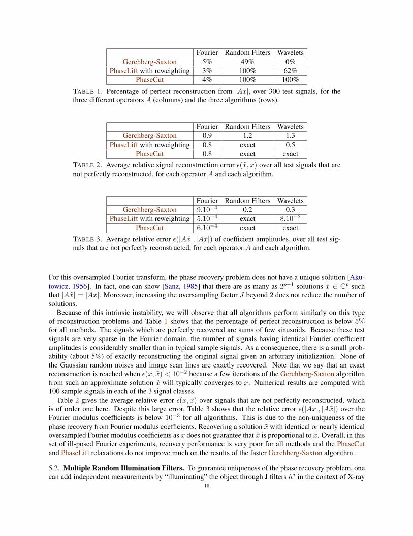
Fourier Random Filters WaveletsGerchberg-Saxton 5% 49% 0%

PhaseLift with reweighting 3% 100% 62%PhaseCut 4% 100% 100%

TABLE 1. Percentage of perfect reconstruction from |Ax|, over 300 test signals, for thethree different operators A (columns) and the three algorithms (rows).

Fourier Random Filters WaveletsGerchberg-Saxton 0.9 1.2 1.3

PhaseLift with reweighting 0.8 exact 0.5PhaseCut 0.8 exact exact

TABLE 2. Average relative signal reconstruction error ε(x, x) over all test signals that arenot perfectly reconstructed, for each operator A and each algorithm.

Fourier Random Filters WaveletsGerchberg-Saxton 9.10−4 0.2 0.3

PhaseLift with reweighting 5.10−4 exact 8.10−2

PhaseCut 6.10−4 exact exact

TABLE 3. Average relative error ε(|Ax|, |Ax|) of coefficient amplitudes, over all test sig-nals that are not perfectly reconstructed, for each operator A and each algorithm.

For this oversampled Fourier transform, the phase recovery problem does not have a unique solution [Aku-towicz, 1956]. In fact, one can show [Sanz, 1985] that there are as many as 2p−1 solutions x ∈ Cp suchthat |Ax| = |Ax|. Moreover, increasing the oversampling factor J beyond 2 does not reduce the number ofsolutions.

Because of this intrinsic instability, we will observe that all algorithms perform similarly on this typeof reconstruction problems and Table 1 shows that the percentage of perfect reconstruction is below 5%for all methods. The signals which are perfectly recovered are sums of few sinusoids. Because these testsignals are very sparse in the Fourier domain, the number of signals having identical Fourier coefficientamplitudes is considerably smaller than in typical sample signals. As a consequence, there is a small prob-ability (about 5%) of exactly reconstructing the original signal given an arbitrary initialization. None ofthe Gaussian random noises and image scan lines are exactly recovered. Note that we say that an exactreconstruction is reached when ε(x, x) < 10−2 because a few iterations of the Gerchberg-Saxton algorithmfrom such an approximate solution x will typically converges to x. Numerical results are computed with100 sample signals in each of the 3 signal classes.

Table 2 gives the average relative error ε(x, x) over signals that are not perfectly reconstructed, whichis of order one here. Despite this large error, Table 3 shows that the relative error ε(|Ax|, |Ax|) over theFourier modulus coefficients is below 10−3 for all algorithms. This is due to the non-uniqueness of thephase recovery from Fourier modulus coefficients. Recovering a solution x with identical or nearly identicaloversampled Fourier modulus coefficients as x does not guarantee that x is proportional to x. Overall, in thisset of ill-posed Fourier experiments, recovery performance is very poor for all methods and the PhaseCutand PhaseLift relaxations do not improve much on the results of the faster Gerchberg-Saxton algorithm.

5.2. Multiple Random Illumination Filters. To guarantee uniqueness of the phase recovery problem, onecan add independent measurements by “illuminating” the object through J filters hj in the context of X-ray

18

imaging or crystallography [Candes et al., 2011a]. The resulting operatorA is the discrete Fourier transformof x multiplied by each filter hj of size p

(Ax)k+pj = (xhj)k = (x ? hj)k for 1 ≤ j ≤ J and 0 ≤ k < p,

where x ? hj is the circular convolution between x and hj . Candes et al. [2011a] proved that, for someconstantC > 0 large enough, CpGaussian independent measurements are sufficient to perfectly reconstructa signal of size p, with high probability. Similarly, we would expect that, picking the filters hj as realizationsof independent Gaussian random variables, perfect reconstruction will be guaranteed with high probabilityif J is large enough (and independent of p). This result has not yet been proven because Gaussian filters donot give independent measurements but Candes et al. [2011b] observed that, empirically, for signals of sizep = 128, with J = 4 filters, perfect recovery is achieved in 100% of experiments.

Table 1 confirms this behavior and shows that the PhaseCut algorithm achieves perfect recovery in allour experiments. As predicted by the equivalence results presented in the previous section, we observe thatPhaseCut and PhaseLift have identical performance in these experiments. With 4 filters, the solutions ofthese two SDP relaxations are not of rank one but are “almost” of rank one, in the sense that their firsteigenvector v has an eigenvalue much larger than the others, by a factor of about 5 to 10. Numerically, weobserve that the corresponding approximate solutions, x = diag(v)b, yield a relative error ε(|Ax|, |Ax|)which, for scan-lines of images and especially for Gaussian signals, is of the order of the ratio between thelargest and the second largest eigenvalue of the matrix U . The resulting solutions x are then sufficientlyclose to x so that a few iterations of the Gerchberg-Saxton algorithm started at x will converge to x.

Table 1 shows however that directly applying the Gerchberg-Saxton algorithm starting from a randominitialization point yields perfect recovery in only about 50% of our experiments. This percentage decreasesas the signal size p increases. The average error ε(x, x) on non-recovered signals in Table 2 is 1.3 whereason the average error on the modulus ε(|Ax|, |Ax|) is 0.2.

5.3. Wavelet Transform. Phase recovery problems from the modulus of wavelet coefficients appear inaudio signal processing where this modulus is used by many audio and speech recognition systems. Thesemoduli also provide physiological models of cochlear signals in the ear [Chi et al., 2005] and recoveringaudio signals from wavelet modulus coefficients is an important problem in this context.

To simplify experiments, we consider wavelets dilated by dyadic factors 2j which have a lower frequencyresolution than audio wavelets. A discrete wavelet transform is computed by circular convolutions withdiscrete wavelet filters, i.e.

(Ax)k+jp = (x ? ψj)k =

p∑m=1

xmψjk−m for 1 ≤ j ≤ J − 1 and 1 ≤ k ≤ p

where ψjm is a p periodic wavelet filter. It is defined by dilating, sampling and periodizing a complex waveletψ ∈ L2(C), with

ψjm =∞∑

k=−∞ψ(2j(m/p− k)) for 1 ≤ m ≤ p.

Numerical computations are performed with a Cauchy wavelet whose Fourier transform is

ψ(ω) = ωd e−ω 1ω>0,

up to a scaling factor, with d = 5. To guarantee thatA is an invertible operator, the lowest signal frequenciesare carried by a suitable low-pass filter φ and

(Ax)k+Jp = (x ? φ)k for 1 ≤ k ≤ p.

One can prove that x is always uniquely determined by |Ax|, up to a multiplication factor. When x is real,the reconstruction appears to be numerically stable. Recall that the results of §3.6.4 allow us to explicitlyimpose the condition that x is real in the PhaseCut recovery algorithm. For PhaseLift in Candes et al.

19

[2011b], this condition is enforced by imposing that X = xx∗ is real. For the Gerchberg-Saxton algorithm,when x is real, we simply project at each iteration on the image of Rp by A, instead of projecting on theimage of Cp by A.

Numerical experiments are performed on the real part of the complex test signals. Table 1 shows thatGerchberg-Saxton does not reconstruct exactly any real test signal from the modulus of its wavelet coeffi-cients. The average relative error ε(x, x) in Table 2 is 1.2 where the coefficient amplitudes have an averageerror ε(|Ax|, |Ax|) of 0.3 in Table 3.

PhaseLift reconstructs 62% of test signals, but the reconstruction rate varies with signal type. The pro-portions of exactly reconstructed signals among random noises, sums of sinusoids and image scan-lines are27%, 60% and 99% respectively. Indeed, image scan-lines have a large proportion of wavelet coefficientswhose amplitudes are negligible. The proportion of phase coefficients having a strong impact on the recon-struction of x is thus much smaller for scan-line images than for random noises, which reduces the numberof significant variables to recover. Sums of sinuoids of random frequency have wavelet coefficients whosesparsity is intermediate between image scan-lines and Gaussian white noises, which explains the interme-diate performance of PhaseLift on these signals. The overall average error ε(x, x) on non-reconstructedsignals is 0.5. Despite this relatively important error, x and x are usually almost equal on most of theirsupport, up to a sign switch, and the importance of the error is precisely due to the local phase inversions(which change signs).

The PhaseCut algorithm reconstructs exactly all test signals. Moreover, the recovered matrix U is alwaysof rank one and it is therefore not necessary to refine the solution with Gerchberg-Saxton iterations. At firstsight, this difference in performance between PhaseCut and PhaseLift may seem to contradict the equiva-lence results of §4.3 (which are valid when x is real and when x is complex). It can be explained howeverby the fact that 10 steps of reweighing and 1000 inner iterations per step are not enough to let PhaseLiftfully converge. In these experiments, the precision required to get perfect reconstruction is very high and,consequently, the number of first-order iterations required to achieve it is too large (see §4.6). With aninterior-point-solver, this number would be much smaller but the time required per iteration would becomeprohibitively large. The much simpler structure of the PhaseCut relaxation allows us to solve these largerproblems more efficiently.

5.4. Impact of Trace Minimization. We saw in §4.1 that, in the absence of noise, PhaseCut was verysimilar to a simplified version of PhaseLift, Weak PhaseLift, in which no trace minimization is performed.Here, we confirm empirically that Weak PhaseLift and PhaseLift are essentially equivalent. Minimizing thetrace is usually used as rank minimization heuristic, with recovery guarantees in certain settings [Fazel et al.,2003; Candes and Recht, 2008; Chandrasekaran et al., 2012] but it does not seem to make much differencehere. In fact, Demanet and Hand [2012] recently showed that in the independent experiments setting, WeakPhaseLift has a unique (rank one) solution with high probability, i.e. the feasible set of PhaseLift is asingleton and trace minimization has no impact. Of course, from a numerical point of view, solving thefeasibility problem Weak PhaseLift is about as hard as solving the trace minimization problem PhaseLift, sothe result [Demanet and Hand, 2012] simplifies analysis but does not really affect numerical performance.

Figure 3 compares the performances of PhaseLift and Weak PhaseLift as a function of n (the numberof measurements). We plot the percentage of successful reconstructions (left) and the percentage of caseswhere the relaxation was exact, i.e. the reconstructed matrix X was rank one (right). The plot shows aclear phase transitions when the number of measurements increases. For PhaseLift, these transitions happenrespectively at n = 155 ≈ 2.5p and n = 285 ≈ 4.5p, while for Weak PhaseLift, the values becomen = 170 ≈ 2.7p and n = 295 ≈ 4.6p, so the transition thresholds are very similar. Note that, in the absenceof noise, Weak PhaseLift and PhaseCut have the same solutions, up to a linear transformation (see §4.2), sowe can expect the same behavior in the comparison PhaseCut versus PhaseCutMod.

20

100 150 200 250 300 350 4000

0.2

0.4

0.6

0.8

1

Number of measurements

Rec

onst

ruct

ion

rate

Weak PhaseLiftPhaseLift

100 150 200 250 300 350 4000

0.2

0.4

0.6

0.8

1

Number of measurements

Prop

ortio

nof

rank

one

sols

.

Weak PhaseLiftPhaseLift

FIGURE 3. Comparison of PhaseLift and Weak PhaseLift performance, for 64-sized sig-nals, as a function of the number of measurements. Reconstruction rate, after Gerchberg-Saxton iterations (left) and proportion of rank one solutions (right).

5.5. Reconstruction in the Presence of Noise. Numerical stability is crucial for practical applications. Inthis last subsection, we suppose that the vector b of measurements is of the form

b = |Ax|+ bnoise

with ‖bnoise‖2 = o(‖Ax‖2). In our experiments, bnoise is always a Gaussian white noise. Two reasons canexplain numerical instabilities in the solution x. First, the reconstruction problem itself can be unstable,with ‖x − cx‖ � ‖|Ax| − |Ax|‖ for all c ∈ C. Second, the algorithm may fail to reconstruct x suchthat ‖|Ax| − b‖ ≈ ‖bnoise‖. No algorithm can overcome the first cause but good reconstruction methodswill overcome the second one. In the following paragraphs, to complement the results in §4.4, we willdemonstrate empirically that PhaseCut is stable, and compare its performances with PhaseLift. We willobserve in particular that PhaseCut appears to be more stable than PhaseLift when b is sparse.

5.5.1. Wavelet transform. Figure 4 displays the performance of PhaseCut in the wavelet transform case. Itshows that PhaseCut is stable up to around 5 − 10% of noise. Indeed, the reconstructed x usually satisfiesε(|Ax|, |Ax|) = ‖ |Ax|−|Ax| ‖2 ≤ ‖bnoise‖2, which is the best we can hope for. Wavelet transform is a casewhere the underlying phase retrieval problem may present instabilities, therefore the reconstruction errorε(x, x) is sometimes much larger than ε(|Ax|, |Ax|). This remark applies especially to sums of sinusoids,which represent the most unstable case.

When all coefficients of Ax have approximately the same amplitude, PhaseLift and PhaseCut producesimilar results, but when Ax is sparse, PhaseLift appears less stable. We gave a qualitative explanation ofthis behavior at the end of §4.4 which seems to be confirmed by the results in Figure 4. This boils down tothe fact that the values of the phase variables in PhaseCut corresponding to zeros in b can be set to zero sothe problem becomes much smaller. Indeed, the performance of PhaseLift and PhaseCut are equivalent inthe case of Gaussian random filters (where measurements are never sparse), they are a bit worse in the caseof sinusoids (where measurements are sometimes sparse) and quite unsatisfactory for scan-lines of images(where measurements are always sparse).

5.5.2. Multiple random illumination filters. Candes and Li [2012] proved that, if A was a Gaussian matrix,the reconstruction problem was stable with high probability, and PhaseLift reconstructed a x such that

ε(x, x) ≤ O(‖bnoise‖2‖Ax‖2

).

21

Gaussian Sinusoids

−3 −2.5 −2 −1.5 −1 −0.5−3

−2.5

−2

−1.5

−1

−0.5

0

Amount of noise

Rel

ativ

eer

ror

−3 −2.5 −2 −1.5 −1 −0.5−3

−2.5

−2

−1.5

−1

−0.5

0

Amount of noise

Rel

ativ

eer

ror

Image Scan-Lines

−3 −2.5 −2 −1.5 −1 −0.5−3

−2.5

−2

−1.5

−1

−0.5

0

Amount of noise

Rel

ativ

eer

ror

Reconstruction error (PhaseCut)

Modulus error (PhaseLift)

Modulus error (PhaseCut)

FIGURE 4. Mean reconstruction errors versus amount of noise for PhaseLift and PhaseCut,both in decimal logarithmic scale, for three types of signals: Gaussian white noises, sumsof sinusoids and scan-lines of images. Both algorithms were followed by a few hundredGerchberg-Saxton iterations.

The same result seems to hold forA corresponding to Gaussian random illumination filters (cf. §5.2). More-over, PhaseCut is as stable as PhaseLift. Actually, up to 20% of noise, when followed by some Gerchberg-Saxton iterations, PhaseCut and PhaseLift almost always reconstruct the same function. Figure 5 displaysthe corresponding empirical performance, confirming that both algorithms are stable. The relative recon-struction errors are approximately linear in the amount of noise, with

ε(|Ax|, |Ax|) ≈ 0.8× ‖bnoise‖2‖Ax‖2

and ε(x, x) ≈ 2× ‖bnoise‖2‖Ax‖2

in our experiments.The impact of the sparsity of b discussed in the last paragraph may seem irrelevant here: if A and x are

independently chosen, Ax is never sparse. However, if we do not choose A and x independently, we mayachieve partial sparsity. We performed tests for the case of five Gaussian random filters, where we chosex ∈ C64 such that (Ax)k = 0 for k ≤ 60. This choice has no particular physical interpretation but it allowsus to check that the influence of sparsity in |Ax| over PhaseLift is not specific to the wavelet transform.Figure 5 displays the relative error over the reconstructed matrix in the sparse and non-sparse cases. If wedenote by Xpl ∈ Cp×p (resp. Xpc ∈ Cn×n) the matrix reconstructed by PhaseLift (resp. PhaseCut), this

22

0 0.05 0.1 0.15 0.2 0.25 0.3 0.35 0.40

0.1

0.2

0.3

0.4

0.5

0.6

0.7

0.8

0.9

1

Amount of noise

Rel

ativ

eer

ror

Reconstr. error (PhaseLift)Reconstr. error (PhaseCut)Modulus error (PhaseLift)Modulus error (PhaseCut)

−4 −3.5 −3 −2.5 −2 −1.5 −1−4

−3.5

−3

−2.5

−2

−1.5

−1

−0.5

PhaseLift (non−sparse)PhaseCut (non−sparse)PhaseLift (sparse)PhaseCut (sparse)

Rec

onst

ruct

ion

erro

r

Amount of noise(sparse)

FIGURE 5. Left: Mean performances of PhaseLift and PhaseCut, followed by Gerchberg-Saxton iterations, for four Gaussian random illumination filters. The x-axis represents therelative noise level, ‖bnoise‖2/‖Ax‖2 and the y-axis the relative error on the result, whichis either ε(x, x) or ε(|Ax|, |Ax|). Right: Loglog plot of the relative error over the matrixreconstructed by PhaseLift (resp. PhaseCut) when A represents the convolution by fiveGaussian filters. Black curves correspond to Ax non-sparse, red ones to sparse Ax.

relative error is defined by

ε =‖AXplA

∗ − (Ax)(Ax)∗‖2‖(Ax)(Ax)∗‖2

(for PhaseLift)

ε =‖diag(b)Xpc diag(b)− (Ax)(Ax)∗‖2

‖(Ax)(Ax)∗‖2(for PhaseCut)

In the non-sparse case, both algorithms yield very similar error ε ≈ 7‖bnoise‖2/‖Ax‖2 (the differencefor a relative noise of 10−4 may come from a computational artifact). In the sparse case, there are lessphases to reconstruct, because we do not need to reconstruct the phase of null measurements. Consequently,the problem is better constrained and we expect the algorithms to be more stable. Indeed, the relativeerrors over the reconstructed matrices are smaller. However, in this case, the performance of PhaseLiftand PhaseCut do not match anymore: ε ≈ 3‖bnoise‖2/‖Ax‖2 for PhaseLift and ε ≈ 1.2‖bnoise‖2/‖Ax‖2for PhaseCut. This remark has no practical impact in our particular example here because taking a fewGerchberg-Saxton iterations would likely make both methods converge towards the same solution, but itconfirms the importance of accounting for the sparsity of |Ax|.

ACKNOWLEDGMENTS

The authors are grateful to Richard Baraniuk, Emmanuel Candes, Rodolphe Jenatton, Amit Singer andVlad Voroninski for very constructive comments. In particular, Vlad Voroninski showed in [Voroninski,2012] that the argument in the first version of this paper, proving that PhaseCutMod is tight when PhaseLiftis, could be reversed under mild technical conditions and pointed out an error in our handling of sparsityconstraints. AA would like to acknowledge support from a starting grant from the European ResearchCouncil (project SIPA), and SM acknowledges support from ANR grant BLAN 012601.

APPENDIX A. TECHNICAL LEMMAS

We now prove two technical lemmas used in the proof of Theorem 4.7.

Lemma A.1. Under the assumptions and notations of Theorem 4.7, we have

‖V �PC − (Ax0)(Ax0)

∗‖2 > 2C‖Ax0‖2‖bn,PC‖2

23

Proof. We first give an upper bound of ‖VPC − V �PC‖2. We use the Cauchy-Schwarz inequality : for

every positive matrix X and all x, y, |x∗Xy| ≤√x∗Xx

√y∗Xy. Let {fi} be an hermitian base of range(A)

diagonalizing V �PC and {gi} an hermitian base of range(A)⊥ diagonalizing V ⊥PC . As {fi} ∩ {gi} is an

hermitian base of Cn, we have

‖VPC − V �PC‖

22 =

∑i,i′

|f∗i (VPC − V �PC)fi′ |2 +

∑i,j

|f∗i (VPC − V �PC)gj |2

+∑i,j

|g∗j (VPC − V�PC)fi|2 +

∑j,j′

|g∗j (VPC − V�PC)gj′ |2

= 2∑i,j

|f∗i (VPC)gj |2 +∑i

|g∗i (V ⊥PC)gi|2

≤ 2∑i,j

|f∗i (VPC)fi‖g∗j (VPC)gj |+ (∑i

g∗i (V⊥PC)gi)

2

= 2TrV�PC TrV ⊥PC + (TrV ⊥PC)2

≤(√

2

√TrV

�PC

√TrV ⊥PC + TrV ⊥PC

)2

(21)

Let us now bound TrV ⊥PC . We first note that TrV ⊥PC = Tr((I−AA†)VPC(I−AA†)) = Tr(VPC(I−AA†)) = d1(VPC ,F) (according to lemma 4.1). Let u ∈ Cn be such that, for all i, |ui| = 1 and (Ax0)i =ui|Ax0|i. We set b = |Ax0|+ bn,PC and V = (b× u)(b× u)∗. As V ∈ H+

n ∩Hb and VPC minimizes (13),

TrV ⊥PC = d1(VPC ,F) ≤ d1(V,F) = d1((Ax0 + bn,PCu)(Ax0 + bn,PCu)∗,F)

= d1((bn,PCu)(bn,PCu)∗,F)

≤ ‖(bn,PCu)(bn,PCu)∗‖1 = Tr(bn,PCu)(bn,PCu)∗ = ‖bn,PC‖22

We also have TrV�PC = TrVPC −TrV ⊥PC . This equality comes from the fact that, if {fi} is an hermitian

base of range(A) and {gi} an hermitian base of range(A)⊥, then

TrVPC =∑i

fiVPCf∗i +

∑i

giVPCg∗i =

∑i

fiV�PCf

∗i +

∑i

giV⊥PCg

∗i = TrV

�PC + TrV ⊥PC

As V ⊥PC � 0, TrV �PC ≤ TrVPC = ‖|Ax0|+ bn,PC‖22 and, by combining this with relations (21) and (22),

we get

‖VPC − V �PC‖2 ≤

√2‖|Ax0|+ bn,PC‖2‖bn,PC‖2 + ‖bn,PC‖22

≤√

2‖Ax0‖2‖bn,PC‖2 + (1 +√

2)‖bn,PC‖22

And, by reminding that we assumed ‖bn,PC‖2 ≤ ‖Ax0‖2,

‖V �PC − (Ax0)(Ax0)

∗‖2 ≥ ‖VPC − (Ax0)(Ax0)∗‖2 − ‖V �

PC − VPC‖2> D‖Ax0‖2‖bn,PC‖2 −

√2‖Ax0‖2‖bn,PC‖2 − (1 +

√2)‖bn,PC‖22

≥ (D − 2√

2− 1)‖Ax0‖2‖bn,PC‖2 = 2C‖Ax0‖2‖bn,PC‖2

which concludes the proof.

Lemma A.2. Under the assumptions and notations of Theorem 4.7, we have ‖bn,PL‖2 ≤ 2‖bn,PC‖.24

Proof. Let ei be the i-th vector of Cn’s canonical base. We set ei = fi + gi where fi ∈ range(A) andgi ∈ range(A)⊥.

VPC ii = e∗iVPCei

= f∗i V�PCfi + 2 Re(f∗i VPCgi) + g∗i V

⊥PCgi

= V�PC ii + 2 Re(f∗i VPCgi) + V ⊥PC ii

Because |f∗i VPCgi| ≤√f∗i VPCfi

√g∗i VPCgi =

√V

�PC ii

√V ⊥PC ii,

(

√V

�PC ii −

√V ⊥PC ii)

2 ≤ VPC ii ≤ (

√V

�PC ii +

√V ⊥PC ii)

2

⇒√V

�PC ii −

√V ⊥PC ii ≤

√VPC ii ≤

√V

�PC ii +

√V ⊥PC ii

So

|bn,PL,i| = |√V

�PC ii − |Ax0|i|

≤ |√V

�PC ii −

√VPC ii|+ |

√VPC ii − |Ax0|i|

≤√V ⊥PC ii + bn,PC,i

and, by (22),

‖bn,PL‖2 ≤ ‖{√

V ⊥PC ii

}i

‖2 + ‖bn,PC‖2

=√TrV ⊥PC + ‖bn,PC‖2 ≤ 2‖bn,PC‖2

which concludes the proof.

REFERENCES

E. J. Akutowicz. On the determination of the phase of a Fourier integral, I. Trans. Am. Math. Soc., 83:179–192, 1956.

S. Becker, E.J. Candes, and M. Grant. Tfocs v1. 1 user guide. 2012.

A. Ben-Tal and A. Nemirovski. Lectures on modern convex optimization : analysis, algorithms, and engineeringapplications. MPS-SIAM series on optimization. Society for Industrial and Applied Mathematics : MathematicalProgramming Society, Philadelphia, PA, 2001.

A. Ben-Tal, A. Nemirovski, and C. Roos. Extended matrix cube theorems with applications to µ-theory in control.Mathematics of Operations Research, 28(3):497–523, 2003.

A. Ben-Tal, L. El Ghaoui, and A.S. Nemirovski. Robust optimization. Princeton University Press, 2009.

D. Bertsekas. Nonlinear Programming. Athena Scientific, 1998.

R. Bhatia. Matrix analysis, volume 169. Springer Verlag, 1997.

S. Boyd and L. Vandenberghe. Convex Optimization. Cambridge University Press, 2004.

O. Bunk, A. Diaz, F. Pfeiffer, C. David, B. Schmitt, D.K. Satapathy, and JF Veen. Diffractive imaging for periodicsamples: retrieving one-dimensional concentration profiles across microfluidic channels. Acta CrystallographicaSection A: Foundations of Crystallography, 63(4):306–314, 2007.

E. J. Candes, T. Strohmer, and V. Voroninski. Phaselift : exact and stable signal recovery from magnitude measure-ments via convex programming. To appear in Communications in Pure and Applied Mathematics, 2011a.

E.J. Candes and X. Li. Solving quadratic equations via phaselift when there are about as many equations as unknowns.Arxiv preprint arXiv:1208.6247, 2012.

25

E.J. Candes and B. Recht. Exact matrix completion via convex optimization. preprint, 2008.

E.J. Candes, Y. Eldar, T. Strohmer, and V. Voroninski. Phase retrieval via matrix completion. Arxiv preprintarXiv:1109.0573, 2011b.

A. Chai, M. Moscoso, and G. Papanicolaou. Array imaging using intensity-only measurements. Inverse Problems,27:015005, 2011.

V. Chandrasekaran, B. Recht, P. Parrilo, and A.S. Willsky. The convex geometry of linear inverse problems. Founda-tions of Computational Mathematics, 12(6):805–849, 2012.

T. Chi, P. Ru, and S. Shamma. Multiresolution spectrotemporal analysis of complex sounds. J. of Acoustic. Societ. ofAmerica, 118:887–906, 2005.

A. d’Aspremont, O. Banerjee, and L. El Ghaoui. First-order methods for sparse covariance selection. SIAM Journalon Matrix Analysis and Applications, 30(1):56–66, 2006.

C. Delorme and S. Poljak. Laplacian eigenvalues and the maximum cut problem. Mathematical Programming, 62(1):557–574, 1993.

L. Demanet and P. Hand. Stable optimizationless recovery from phaseless linear measurements. Arxiv preprintarXiv:1208.1803, 2012.

N. El Karoui and A. d’Aspremont. Approximating eigenvectors by subsampling. ArXiv:0908.0137, 2009.

M. Fazel, H. Hindi, and S.P. Boyd. Log-det heuristic for matrix rank minimization with applications to hankel andeuclidean distance matrices. In American Control Conference, 2003. Proceedings of the 2003, volume 3, pages2156–2162. Ieee, 2003.

J.R. Fienup. Phase retrieval algorithms: a comparison. Applied Optics, 21(15):2758–2769, 1982.

R. Gerchberg and W. Saxton. A practical algorithm for the determination of phase from image and diffraction planepictures. Optik, 35:237–246, 1972.

Michel X Goemans and David P Williamson. Approximation algorithms for max-3-cut and other problems via com-plex semidefinite programming. Journal of Computer and System Sciences, 68(2):442–470, 2004.

M.X. Goemans and D.P. Williamson. Improved approximation algorithms for maximum cut and satisfiability problemsusing semidefinite programming. J. ACM, 42:1115–1145, 1995.

D. Griffin and J. Lim. Signal estimation from modified short-time fourier transform. Acoustics, Speech and SignalProcessing, IEEE Transactions on, 32(2):236–243, 1984.

R.W. Harrison. Phase problem in crystallography. JOSA A, 10(5):1046–1055, 1993.

C. Helmberg, F. Rendl, R. J. Vanderbei, and H. Wolkowicz. An interior–point method for semidefinite programming.SIAM Journal on Optimization, 6:342–361, 1996.

T. Kato. Perturbation theory for linear operators. Springer, 1995.

M. Kisialiou and Z.Q. Luo. Probabilistic analysis of semidefinite relaxation for binary quadratic minimization. SIAMJournal on Optimization, 20:1906, 2010.

X. Li and V. Voroninski. Sparse signal recovery from quadratic measurements via convex programming. arXiv preprintarXiv:1209.4785, 2012.

L. Lovasz and A. Schrijver. Cones of matrices and set-functions and 0-1 optimization. SIAM Journal on Optimization,1(2):166–190, 1991.

Z.Q. Luo, X. Luo, and M. Kisialiou. An efficient quasi-maximum likelihood decoder for psk signals. In Acous-tics, Speech, and Signal Processing, 2003. Proceedings.(ICASSP’03). 2003 IEEE International Conference on,volume 6, pages VI–561. IEEE, 2003.

J. Miao, T. Ishikawa, Q. Shen, and T. Earnest. Extending x-ray crystallography to allow the imaging of noncrystallinematerials, cells, and single protein complexes. Annu. Rev. Phys. Chem., 59:387–410, 2008.

26

M.L. Moravec, J.K. Romberg, and R.G. Baraniuk. Compressive phase retrieval. In Proc. of SPIE Vol, volume 6701,pages 670120–1, 2007.

Y. Nesterov. A method of solving a convex programming problem with convergence rateO(1/k2). Soviet MathematicsDoklady, 27(2):372–376, 1983.

Y. Nesterov. Semidefinite relaxation and nonconvex quadratic optimization. Optimization methods and software, 9(1):141–160, 1998.

Y. Nesterov. Smoothing technique and its applications in semidefinite optimization. Mathematical Programming, 110(2):245–259, 2007.

E. Osherovich, Y. Shechtman, A. Szameit, P. Sidorenko, E. Bullkich, S. Gazit, S. Shoham, E.B. Kley, M. Zibulevsky,I. Yavneh, et al. Sparsity-based single-shot subwavelength coherent diffractive imaging. In CLEO: Science andInnovations. Optical Society of America, 2012.

J. L. C. Sanz. Mathematical considerations for the problem of fourier transform phase retrieval from magnitude. SIAMJournal on Applied Mathematics, 45:651–664, 1985.

N.Z. Shor. Quadratic optimization problems. Soviet Journal of Computer and Systems Sciences, 25:1–11, 1987.

A. Singer. Angular synchronization by eigenvectors and semidefinite programming. Applied and computationalharmonic analysis, 30(1):20–36, 2011.

A.M.C. So. Non–asymptotic performance analysis of the semidefinite relaxation detector in digital communications.2010.

A.M.C. So, J. Zhang, and Y. Ye. On approximating complex quadratic optimization problems via semidefinite pro-gramming relaxations. Mathematical Programming, 110(1):93–110, 2007.

Anthony Man-Cho So and Yinyu Ye. Probabilistic analysis of semidefinite relaxation detectors for multiple-input,multiple-output. Convex Optimization in Signal Processing and Communications, page 166, 2010.

G.W. Stewart. Matrix Algorithms Vol. II: Eigensystems. Society for Industrial Mathematics, 2001.

G.W. Stewart and J. Sun. Matrix perturbation theory. 1990.

M. Todd and E. A. Yildirim. Sensitivity analysis in linear programming and semidefinite programming using interior-points methods. Mathematical Programming, 90(2):229–261, 2001.

K. C. Toh, M. J. Todd, and R. H. Tutuncu. SDPT3 – a MATLAB software package for semidefinite programming.Optimization Methods and Software, 11:545–581, 1999.

V. Voroninski. A comparison between the phaselift and phasecut algorithms. Working paper, 2012.

I. Waldspurger and S. Mallat. Time-frequency phase recovery. Working paper, 2012.

Z. Wen, D. Goldfarb, and K. Scheinberg. Block coordinate descent methods for semidefinite programming. InHandbook on Semidefinite, Conic and Polynomial Optimization, pages 533–564. Springer, 2012.

EA Yildirim. An interior-point perspective on sensitivity analysis in semidefinite programming. Mathematics ofOperations Research, 28(4):649–676, 2003.

S. Zhang and Y. Huang. Complex quadratic optimization and semidefinite programming. SIAM Journal on Optimiza-tion, 16(3):871–890, 2006.

D.I., ECOLE NORMALE SUPERIEURE, PARIS.E-mail address: waldspur@clipper.ens.fr

CNRS & D.I., ECOLE NORMALE SUPERIEURE, PARIS. UMR 8548.E-mail address: alexandre.daspremont@m4x.org

D.I., ECOLE NORMALE SUPERIEURE, PARIS.E-mail address: mallat@cmap.polytechnique.fr

27