phase space structures causing the reaction rate decrease ... · the collinear hydrogen exchange...

Kraják, V., & Waalkens, H. (2020). Phase space structures causing thereaction rate decrease in the collinear hydrogen exchange reaction. Journal ofMathematical Chemistry, 1-48. https://doi.org/10.1007/s10910-019-01083-4

Publisher's PDF, also known as Version of record

License (if available):CC BY

Link to published version (if available):10.1007/s10910-019-01083-4

Link to publication record in Explore Bristol ResearchPDF-document

This is the final published version of the article (version of record). It first appeared online via Springer athttps://doi.org/10.1007/s10910-019-01083-4 . Please refer to any applicable terms of use of the publisher.

University of Bristol - Explore Bristol ResearchGeneral rights

This document is made available in accordance with publisher policies. Please cite only the publishedversion using the reference above. Full terms of use are available: http://www.bristol.ac.uk/pure/user-guides/explore-bristol-research/ebr-terms/

https://doi.org/10.1007/s10910-019-01083-4

https://doi.org/10.1007/s10910-019-01083-4

https://research-information.bris.ac.uk/portal/en/publications/phase-space-structures-causing-the-reaction-rate-decrease-in-the-collinear-hydrogen-exchange-reaction(ff55e966-3ef3-428a-9a7b-a773a2eb4e03).html

https://research-information.bris.ac.uk/portal/en/publications/phase-space-structures-causing-the-reaction-rate-decrease-in-the-collinear-hydrogen-exchange-reaction(ff55e966-3ef3-428a-9a7b-a773a2eb4e03).html

Journal of Mathematical Chemistry (2020) 58:292–339https://doi.org/10.1007/s10910-019-01083-4

ORIG INAL PAPER

Phase space structures causing the reaction rate decreasein the collinear hydrogen exchange reaction

Vladimír Krajnák1,2 · Holger Waalkens1

Received: 24 September 2019 / Accepted: 15 November 2019 / Published online: 25 November 2019© The Author(s) 2019

AbstractThe collinear hydrogen exchange reaction is a paradigm system for understandingchemical reactions. It is the simplest imaginable atomic system with 2 degrees offreedom modeling a chemical reaction, yet it exhibits behaviour that is still not wellunderstood—the reaction rate decreases as a function of energy beyond a criticalvalue. Using lobe dynamics we show how invariant manifolds of unstable periodicorbits guide trajectories in phase space. From the structure of the invariant manifoldswe deduce that insufficient transfer of energy between the degrees of freedom causesa reaction rate decrease. In physical terms this corresponds to the free hydrogen atomrepelling the whole molecule instead of only one atom from the molecule. We furtherderive upper and lower bounds of the reaction rate, which are desirable for practicalreasons.

Keywords Hydrogen exchange · Invariant manifolds · Phase space structures ·Reaction dynamics · Transition state theory

1 Introduction

Westudy the dynamics of the collinear hydrogen exchange reactionH2+H → H+H2,which is an invariant subsystem of the spatial hydrogen exchange reaction, usingthe potential provided by Porter and Karplus in [34]. In literature it is considered aparadigm system for understanding chemical reactions due to its simplicity and varietyof exhibited dynamics. Because the system consists of three identical atoms confinedto a line, it is the simplest imaginable system with 2 degrees of freedom modeling achemical reaction.

B Vladimír Krajná[email protected]

1 Bernoulli Institute for Mathematics, Computer Science and Artificial Intelligence, University ofGroningen, Nijenborgh 9, 9747 AG Groningen, The Netherlands

2 School of Mathematics, University of Bristol, Fry Building, Woodland Road, Bristol BS8 1UG, UK

123

http://crossmark.crossref.org/dialog/?doi=10.1007/s10910-019-01083-4&domain=pdf

http://orcid.org/0000-0001-6052-7531

Journal of Mathematical Chemistry (2020) 58:292–339 293

The hydrogen atoms themselves are the simplest atoms in the universe. Becauseeach consist of one proton and one electron only, an accurate potential energy surfacefor this reaction can be obtained via the Born–Oppenheimer approximation. Intrigu-ingly enough, this system exhibits behaviour that is still not well understood.

The phenomenon we examine here is the counterintuitive observation that the reac-tion rate decreases as energy increases beyond a critical value. After all, one wouldexpect to break bonds more easily using more energy. So far a satisfactory explana-tion of this phenomenon is missing and only an upper bound and a lower bound tothe rate have been found. The upper bound is obtained by means of transition statetheory (TST), due to [49]. TST is a standard tool for studying reaction rates due toits simplicity and accuracy for low energies, but it does not capture the decline of thereaction rate. The improvement brought by variational transition state theory (VTST)[13], does not capture this behaviour either.

Unified statistical theory, due to [23], which is in a certain sense an extension ofTST to more complicated system, does capture the culmination of the reaction rate,but does not yield higher accuracy. The lower bound on the other hand does comequite close. It is obtained using the so-called simple-minded unified statistical theory[32].

A review of reaction rate results including TST can be found in [16]. Pechukas [28]and Truhlar and Garrett [40] review various extensions of TST.

Using lobe dynamics (introduced in [35]) we show how invariant manifolds ofunstable periodic orbits guide trajectories in phase space. From the structure of theinvariant manifolds we deduce that insufficient transfer of energy between the degreesof freedom causes a reaction rate decrease. In physical terms this corresponds tothe free hydrogen atom repelling the whole molecule instead of only one atom fromthe molecule. We further derive bounds of the reaction rate, which are desirable forpractical reasons.

In the remainder of this section we introduce the system, give an overview of TSTand explain the current state of affairs with regards to the collinear hydrogen exchangereaction. Section 2 focuses on relevant periodic orbits and definition of regions of phasespace. In Sect. 3 we introduce new coordinates using which we define a surface ofsection. In Sect. 4 we explain how we study invariant manifolds on the surface ofsection. In Sect. 5 we give a detailed insight into the structures formed by invariantmanifolds and their role in the reaction. Section 6 is devoted to a novel way of breakingdown heteroclinic tangles to provide a better understanding of the interplay of invariantmanifolds of three TSs. In Sect. 7 we calculate various upper and lower bounds of thereaction rate.

1.1 Porter–Karplus potential

The collinear hydrogen exchange system consists of three hydrogen atoms confined toa line, as shown in Fig. 1, where r1 and r2 denote the distances in atomic units betweenneighbouring atoms. Forces between the atoms are given by the Porter and Karpluspotential [34] is the standard potential for the hydrogen exchange reaction (collinearand spatial) used for example in [5,6,14,24,31–33]. The system is considered to react,

123

294 Journal of Mathematical Chemistry (2020) 58:292–339

Fig. 1 Collinear hydrogen atoms and distances

Fig. 2 The Porter–Karplus potential energy surface with contours and its cross sections for fixed values ofr2 = 1.70083 (cyan), 2 (blue), 2.5 (red), 3 (green), 4 (black), 50 (yellow) (Color figure online)

if it passes from the region of reactants (r1 > r2) to the region of products (r1 < r2)and remains there.

We point out two key properties of the Porter–Karplus potential:

– the discrete reflection symmetry with respect to the line r1 = r2,– the saddle point at r1 = r2 = Rs := 1.70083.

The symmetry expresses the fact that we cannot distinguish between three identicalhydrogen atoms, we can only measure distances between them. Hence, any statementreferring to r1 < r2 automatically also holds for r1 > r2.

Potential saddle points represent the activation energy needed for a reaction to bepossible. In the all of this work we give energies as values in atomic units above theminimum of the system. In this convention the energy of the saddle point is 0.01456.

From a configuration space perspective, such a potential barrier is the sole structureseparating reactants from products and the sole obstacle the system needs to overcomein order to react. This perspective implicitly assumes that the system does not recrossthe potential barrier back into reactants. Dynamical structures that cause recrossingsare only visible from a phase space perspective.

Figure 2 shows the potential energy surface near the potential saddle and crosssections of the potential at various values of r2. Due to diminishing forces between theatom and the molecule over large distances the differences between the cross sectionsfade after r2 = 4 and are indistinguishable in double precision beyond r2 = 40.

123


1.2 Definitions

The collinear hydrogen exchange reaction is described by the Hamiltonian

H(r1, pr1 , r2, pr2) = p2r1 + p2r2 − pr1 pr2mH

+U (r1, r2), (1)

where pr1 , pr2 are the momenta conjugate to interatomic distances r1, r2, mH is themass of a hydrogen atom and U is the Porter–Karplus potential described above.

The equations of motion associated to H are as follows:

r1 = 2pr1 − pr2mH

,

pr1 = −∂U (r1, r2)

∂r1,

r2 = 2pr2 − pr1mH

,

pr2 = −∂U (r1, r2)

∂r2.

(2)

The discrete symmetry of the potential translates into the invariance of H and theequations of motion under the map (r1, pr1 , r2, pr2) �→ (r2, pr2 , r1, pr1).

TheHamiltonian flow generated by equations (2) preserves the energy of the systemE = H(r1, pr1 , r2, pr2) and the phase space of this system is therefore foliated byenergy surfaces H = E .

Definition 1 A trajectory passing through the point(r01 , p0r1 , r

02 , p0r2

)is said to be a

reactive trajectory if the solution (r1(t), pr1(t), r2(t), pr2(t)) of the system with theinitial condition

(r1(0), pr1(0), r2(0), pr2(0)) = (r01 , p0r1 , r

02 , p0r2

),

satisfies r1(t) < ∞ and r2(t) → ∞ as t → ∞ and r1(t) → ∞ and r2(t) < ∞ ast → −∞ or vice versa.

A nonreactive trajectory is one for which the solution satisfies r1(t) → ∞ andr2(t) < ∞ as t → ±∞ or r1(t) < ∞ and r2(t) → ∞ as t → ±∞.

Examples of reactive and nonreactive trajectories are shown in Fig. 3. Note thatnonreactive trajectories may cross the potential barrier in the sense that they cross theline r1 = r2.

From the above it follows that the reaction rate at a fixed energy E can be calculatedusing a brute force Monte Carlo method as the proportion of initial conditions ofreactive trajectories at infinity. Since the system decouples in a numerical sense aroundr2 = 40, it is enough to sample a sufficiently remote surface in the reactants (r1 > r2)that is transversal to the flow, for example

r1 + r22

= 50, pr2 < 0. (3)

123


Fig. 3 Examples of reactive (black) and nonreactive (red, blue) trajectories in configuration space at energy0.02400 (Color figure online)

Since r1, r2 is not a centre of mass frame, r2 = const is not transversal to the flow.We remark that (r2, pr2 − pr1

2 ) are canonical coordinates on r1 + r22 = 50 that yield a

uniform random distribution of initial conditions.

1.3 Transition state theory

Since its formulation in [49], TST became the standard tool for estimating rates ofvarious processes not only in chemical reactions [16]. It has found use in many fieldsof physics and chemistry, such as celestial mechanics [10,15], plasma confinement[22] and fluid mechanics [25].

Key element of TST is the transition state (TS), a structure that is between reactantsand products. There is no single generally accepted definition unfortunately, becausein some publications concerning systems with 2 degrees of freedom TS refers to anunstable periodic orbit while in others TS is a dividing surface (DS) associated withthe unstable periodic orbit. We adopt the following definition of a TS from [20]:

Definition 2 (TS) A transition state for a Hamiltonian system is a closed, invariant,oriented, codimension-2 submanifold of the energy surface that can be spanned bytwo surfaces (the TS is the surfaces’ boundary) of unidirectional flux, whose uniondivides the energy surface into two components and has no local recrossings.

For a system with 2 degrees of freedom as considered in this work, a closed, invariant,oriented, codimension-2 submanifold of the energy surface is a periodic orbit and itcan be shown that the periodic orbit must be unstable [27,31,39]. In general, the TS hasto be a normally hyperbolic invariant manifolds (NHIM), an invariant manifolds withlinearised transversal instabilities that dominate the linearised tangential instabilities([8,11]).

123


Theorem 1 (TST) In a system that admits a TS and all trajectories that pass fromreactants to products the DS precisely once, the flux across a DS is precisely thereaction rate.

We remark that in general the flux through a DS associated with a TS is an upperbound to the reaction rate [28,49].

Since its early applications, developments in the field led to a shift in the under-standing of the TS to be an object in phase space rather than configuration space[41–48].

All relevant periodic orbits in this system are self-retracing orbits whose configu-ration space projections oscillate between equipotential lines, so called brake orbits([36]). As suggested by Pollak and Pechukas [31], let (r po1 , r po2 ) be the configurationspace projection of a brake orbit at energy E , then the associated DS is the set ofall phase space points (r po1 , pr1 , r

po2 , pr2) that satisfy H(r po1 , pr1 , r

po2 , pr2) = E . For

constructions of a DS near a saddle type equilibrium point in systems with more than2 degrees of freedom see [41,47,48].

Hydrogen exchange results and evolution of understanding of TST follow.

1.4 Known results

In 1971, Morokuma and Karplus [24] evaluated three representatives of differentclasses of reactions. They found the collinear hydrogen exchange reaction to be thebest suited for a study of the accuracy of TST due to smoothness, symmetry andsimplicity. They found that TST agreed with Monte Carlo calculations up to a certainenergy, but became inaccurate rather quickly after that.

In 1973 [29] Pechukas and McLafferty stated that for TST to be exact, every tra-jectory passing through the DS does so only once. In other words, TST fails in thepresence of trajectories that oscillate between reactants and products.

In 1975 Chapman, Hornstein and Miller [5] present numerical results showingthat transition state theory “fails substantially” for the hydrogen exchange reaction(collinear and spatial) above a certain threshold.

Pollak and Pechukas [31] proved in 1978 that flux through a DS constructed usingan unstable brake orbit gives the best approximation of the reaction rate. In the presenceof multiple TSs the authors introduceVariational TST (VTST)—using the DSwith thelowest flux to approximate the reaction rate. These results detach TST from potentialsaddle points. The authors find for the collinear hydrogen exchange reaction that whenTST breaks down, VTST can be significantly more accurate, even though both fail tocapture the reaction rate decrease.

In 1979 Pollak and Pechukas [30] proved that TST is exact provided there is onlyone periodic orbit. Simultaneously, they derived the best estimate of the reaction rateso far for the collinear hydrogen exchange reaction in [32] using what they calledSimple-minded unified statistical theory (SMUST).

Unified statistical theory (UST), due to Miller [23], attempts to take advantage ofthe difference of fluxes through all DSs and essentially treat regions of simple andcomplicated dynamics separately. The authors of [32] found that UST captures thedrop in the reaction rate and elaborate on the deviation ofUST from the actual rate. The

123


derivation of a lower bound (subject to assumptions) of the rate using the differencebetween TST and VTST is presented in the appendix of [32].

A rigorous lower bound is presented in [33]. It uses a DS constructed using a stableperiodic orbit between two TS to estimate the error of TST. The accuracy of this lowerbound for the hydrogen exchange reaction is remarkable.

In 1987 Davis [6] studied the hydrogen exchange reaction in phase space andconsidered the role of invariant structures. For low energies he showed that TST canbe exact even if several TSs are present, provided that their invariant manifolds donot intersect. At higher energies he made some numerical observations of heteroclinictangles of invariant manifolds and nearby dynamics. At high energies Davis foundthat a particular heteroclinic tangle grows in size and by assuming that it containsexclusively nonreactive trajectories he found a very accurate lower bound. The ideaof this lower bound is very similar to [33], but Davis endures a computational cost toquantify trajectories instead of fluxes through DSs.

Davis also formulated an estimate of the reaction rate based on the observationthat not many trajectories undergo a complicated evolution, as found by Pollak andPechukas [32]. The estimate assumes that beyond a certain time dynamics in theheteroclinic tangle is randomised and 50% of the remaining trajectories are reactive.

Davis’ observations hint at the crucial role played by invariant manifolds, but theprecise manner in which this happens is not understood. Our aim is to explain the roleof invariantmanifolds in the reactionmechanism and extending it to the energy intervalthat Davis did not study, the interval with three TSs. We provide new understanding ofthe interactions between invariant manifolds of two and three TSs and consequentlyexplain the counterintuitive reaction rate decrease.

2 Periodic orbits and geometry

2.1 Local geometry

Before we introduce periodic orbits that are relevant to the reaction mechanism, wedescribe the local energy surface geometry near a potential saddle point. We show thatthe neighbourhood necessarily contains an unstable periodic orbit and we highlightthe importance of invariant manifolds to the local dynamics. The description remainstrue near unstable periodic orbits that do not lie near saddle points.

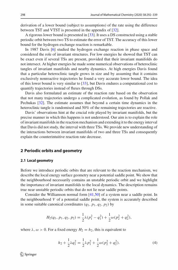
Consider the Williamson normal form [41,50] of a system near a saddle point. Inthe neighbourhood V of a potential saddle point, the system is accurately describedin some suitable canonical coordinates (q1, p1, q2, p2) by

H2(q1, p1, q2, p2) = 1

2λ(p21 − q21 ) + 1

2ω(p22 + q22 ),

where λ, ω > 0. For a fixed energy H2 = h2, this is equivalent to

h2 + 1

2λq21 = 1

2λp21 + 1

2ω(p22 + q22 ). (4)

123


Fig. 4 Illustration of local energy surface geometry in the neighbourhood of a saddle point. Sections forfixed values of q1 define spheres (with ±p1 given implicitly by H2(q1, p1, q2, p2) = h2), shown areq1 = 1.5,−.25,−2

For a each fixed q1 such that h2 + 12λq

21 > 0 this defines a sphere, as shown in Fig. 4.

Depending on h2, the energy surface has the following characteristics:

– If h2 < 0, the energy surface consists of two regions locally disconnected nearq1 = 0, reactants (q1 > 0) and products (q1 < 0).

– Reactants and products are connected by the saddle point for h2 = 0.– For h2 > 0, the energy surface is foliated by spheres. The radius of the spheresincreases with |q1|. Locally the energy surface has a wide-narrow-wide geometryusually referred to as a bottleneck.

We remark that q1 can be referred to as a reaction coordinate. To understand transportthrough a bottleneck, fix an energy h2 slightly above 0 and consider the Hamiltonianequations for H2:

q1 = λp1, q2 = ωp2,

p1 = λq1, p2 = −ωq2.

The degrees of freedom are decoupled with hyperbolic dynamics in (q1, p1) andelliptic in (q2, p2). Moreover q1 = p1 = 0 defines an unstable periodic orbit andq1 = 0 defines a DS separating reactants from products. This DS, similarly to the onedefined in Sect. 1.3, is a sphere that is due to the instability of q1 = p1 = 0 transversalto the flow and does not admit local recrossings. The sphere itself is divided by itsequator q1 = p1 = 0 into two hemispheres with unidirectional flux - trajectoriespassing from reactants to products cross the hemisphere p1 > 0, while trajectoriesfromproducts to reactants cross p1 < 0. Therefore q1 = p1 = 0 satisfies the definition

123


of a TS. We remark that the DS can be perturbed and as long as its boundary remainsfixed and transversality is not violated, the flux through the perturbed and unperturbedDS remains the same.

This description breaks down at high energies, when the periodic orbit may becomestable, an event commonly referred to as loss of normal hyperbolicity. Then TST isinaccurate due to local recrossings of the DS. Loss of normal hyperbolicity occursin the hydrogen exchange reaction, yet TST breaks down at lower energies due thepresence of multiple transition states.

Having the same energy distribution between the degrees of freedom as the periodicorbit q1 = p1 = 0, its invariant manifolds are given by

p21 − q21 = 0,

the stable being q1 = −p1 and the unstable q1 = p1. They consist of two brancheseach—one on the reactant sidewith q1 > 0, one on the product sidewith q1 < 0. Thesemanifolds are cylinders with the periodic orbit as its base. They are codimension-1 inthe energy surface and separate reactive and nonreactive trajectories - reactive onesinside the cylinders

1

2λ(p21 − q21 ) > 0,

and nonreactive outside

1

2λ(p21 − q21 ) < 0.

Only reactive trajectories reach the DS.Note that in a configuration space projection, the separation between reactive and

nonreactive trajectories is not as natural/obvious as in a phase space perspective.Thereforewe study the structuresmadeupof invariantmanifolds that cause the reactionrate decrease in phase space.

We remark that bottlenecks are related to TSs rather than potential saddle points.Section 5 contains examples of bottlenecks unrelated to potential saddle points and asaddle point without a bottleneck.

2.2 Periodic orbits

For energies E above 0.01456, the energy of the saddle point, the system (1) admitsperiodic orbits that come in one-parameter families parametrised by energy. Initiallywe focus on each family separately and subsequently we investigate the interplay thatgoverns the complicated dynamics exhibited by this system. We adopt the notation of[14] for different families of periodic orbits Fn , where n ∈ N, and briefly describetheir evolution with increasing energy. We remark that many families come in pairsrelated by symmetry and for simplicity we restrict ourselves to the r1 ≥ r2 half plane.We will refer to orbits of the family Fn on the other half plane by Fn .

123


Fig. 5 The projections of the periodic orbits of F0 (black), F1 (blue) and F2 (green) onto configurationspace at energies 0.02210, 0.02300, 0.02400, 0.02500 and 0.02600 and the corresponding equipotentiallines (grey) (Color figure online)

By F0 we denote the family of Lyapunov orbits associated with the potential saddle,which as explained in Sect. 2.1 must be unstable for energies slightly above the saddle.The orbits lie on the axis of symmetry of the system r1 = r2, see Fig. 5. Orbits of thisfamily were used in TST calculations in many of the previous works.

A saddle-centre bifurcation at approximately 0.02204 results in the creation oftwo families—the unstable F1 and the initially stable F2. The configuration spaceprojections of these orbits are shown in Fig. 5. The unstable family F1 is the furthestaway from F0 and does not undergo any further bifurcations. The F2 family is initiallystable, but undergoes a period doubling bifurcation at 0.02208 creating the doubleperiod families F21 and F22. Unlike reported by Iñarrea and Palacián [14], we donot find these families disappear in an inverse period doubling bifurcation of F2 at0.02651. Instead F21 and F22 persist with double period until 0.02654, when theycollide together with F2 and F0, see Fig. 7. Consequently F0 becomes stable. Wewould like to enhance the findings of [14] by remarking that F21 and F22 are brieflystable between switching from hyperbolic to inverse hyperbolic and vice versa, seeFig. 6.

At 0.02661, F0 is involved in a bifurcation with a double period family F4 thatoriginates in a saddle-centre bifurcation at 0.02254. F4 is a family symmetric withrespect to r1 = r2. For dynamical purposes we point out that above 0.02661 F0 isinverse hyperbolic.

Figures 6 and 7 show bifurcation diagrams of most of the families on the energy-residue and the energy-action plane. By residue R we mean the Greene residue asintroduced by Greene in [9], where R < 0 means that the periodic orbit is hyperbolic,0 < R < 1 means it is elliptic and R > 1 means it is inverse hyperbolic.

The residue is derived fromamatrix that describes the local dynamics near a periodicorbit—the monodromymatrix. Let Γ be a periodic orbit with the parametrisation γ (t)and period T , and M(t) be the matrix satisfying the variational equation

123


Fig. 6 Bifurcation diagrams showing the evolution of F0 (black), F1 (blue), F2 (light green), F21 (darkgreen), F22 (red) and F4 (orange) on the energy-residue (E, R) and the energy-action (E, S) plane. Theresidues of other families and the action of orbits of period higher than 1 are omitted for the sake of clarity(Color figure online)

Fig. 7 Details of the evolution of F0 (black), F1 (blue), F2 (light green), F21 (dark green), F22 (red, identicalwith F21) and F4 (orange) on the energy-residue (E, R) plane (Color figure online)

M(t) = J D2H(γ (t))M(t), (5)

where J =(

0 I d−I d 0

), with the initial conditionM(0) = I d.Themonodromymatrix

is defined by M = M(T ) and it describes how a sufficiently small initial deviation δ

from γ (0) changes after a full period T :

ΦTH (γ (0) + δ) = γ (T ) + Mδ + O(δ2),

where Φ tH is the Hamiltonian flow.

According to Eckhardt and Wintgen, [7], if δ is an initial displacement along theperiodic orbit δ ‖ J∇H , then δ is preserved after a full period T , i.e. Mδ = δ.Similarly an initial displacement perpendicular to the energy surface δ ‖ ∇H ispreserved. Consequently, two of the eigenvalues of M are

λ1 = λ2 = 1. (6)

123


As (5) is Hamiltonian, the preservation of phase space volume following Liouville’stheorem implies det M(t) = det M(0) = 1 for all t . Therefore the two remainingeigenvalues must satisfy λ3λ4 = 1 and we can write them as λ and 1

λ. Γ is hyperbolic

if λ > 1, it is elliptic if |λ| = 1 and it is inverse hyperbolic if λ < −1.

Definition 3 The Greene residue of Γ is defined as R = 14 (4 − TrM), where M is

the monodromy matrix corresponding to the periodic orbit Γ .

Using (6) we can write R as

R = 1

4

(2 − λ − 1

λ

).

By definition R < 0 if Γ is hyperbolic, 0 < R < 1 if it is elliptic and R > 1 if it isinverse hyperbolic.

Davis [6] mostly focused on the energy interval below 0.02214 and above 0.02655,the interval where TST is exact and the interval where two TSs exist, respectively.

In the light of normal form approximation described in Sect. 2.1, we remark thatthe approximation breaks down completely when F0 loses normal hyperbolicity at0.02655 at the latest. The loss of normal hyperbolicity is not the cause for the overes-timation of the reaction rate by TST as it starts to deviate from the Monte Carlo ratewell before 0.02300.

2.3 Phase space regions

Wewould like to give up the binary partitioning of an energy surface into reactants andproducts in favour of defining an interaction region inbetween into which trajectoriescan only enter once.

As explained in Sect. 2.1, TSs give rise to bottlenecks in phase space. Because F1gives rise to the bottleneck the furthest away from the potential barrier, we use it todelimit regions as follows. Denote DS1 and DS1 the DSs constructed using F1 andF1 according to Sect. 1.3. The interaction region is the region of the energy surfacebetween the two DSs and it contains all other periodic orbits. Reactants and productsare the regions on the r1 > r2-side and the r1 < r2-side of the interaction regionrespectively, see Fig. 8.

The advantages of this partition of space are immediate.

– All TSs and bottlenecks are in the interaction region or on its boundary. Thedynamics in reactants and products has no influence on reactivity and to fullyunderstand the hydrogen exchange reaction, it is enough to restrict the study to theinteraction region.

– Trajectories that leave the interaction region never return. This is true in forwardand backward time.

– It is impossible for a trajectory to enter reactants and products in the sametime direction, unlike in the binary partitioning, where trajectories may oscillatebetween reactants and products.

123


Fig. 8 Regions in configuration space at energy 0.02400. The interaction region (red) bounded by two orbitfrom the family F1 (blue), the region of reactants (blue) and the region of products (green). The orbit F0(black) is also included (Color figure online)

3 Definition of a Poincaré surface of section

Invariant manifolds are 2 dimensional objects on the 3 dimensional energy surfaceembedded in 4 dimensional phase space. To facilitate the study of intersections ofinvariant manifolds, we define a 2 dimensional surface of section on the energy surfacethat is transversal to theflowand intersects invariantmanifolds in 1 dimensional curves.

3.1 Reaction coordinate andminimum energy path

Here we define a reaction coordinate, using which we can monitor the progress alonga reaction pathway. Frequently a reaction coordinate is closely related to a minimumenergy path (MEP) connecting the potential wells of reactants and products via thepotential saddle. The coordinate as such is not a solution of the Hamiltonian systemand, as remarked in [26], is of no dynamical significance to the system.

A MEP can be defined as the union of two paths of steepest descend, the uniquesolutions of the gradient system

r1 = −∂U

∂r1, r2 = −∂U

∂r2,

one connecting the saddle (Rs, Rs) to the potential well (∞, Rmin), the other connect-ing (Rs, Rs) to (Rmin,∞). Figure 9 shows the MEP on a contour plot of U .

3.2 Surface of section

The MEP as defined above does not have an analytic expressing, but can be approxi-mated using q1 = 0, where

123


Fig. 9 Comparison of the MEP (red), the coordinate line q1 = 0 (black) and the coordinate line q1 = 0(cyan). Equipotential lines of the potential energy surface correspond to energies 0.01200, 0.01456, 0.02000,0.02800 and 0.03500 (Color figure online)

q1 = (r1 − Rmin)(r2 − Rmin) − (Rs − Rmin)2,

as used by Davis [6] and shown in Fig. 9. Invariant manifolds are always transversalto the MEP and transversal to q1 = 0 for the energy interval considered in this work.At higher energies Davis used q1 = −0.04, q1 = −0.07 and q1 = −0.084 to avoidtangencies.

We found that

q1 = (r1 − Rmin)(r2 − Rmin) − (Rs − Rmin)2e−2((r1−Rs )

2+(r2−Rs )2), (7)

approximates the MEP significantly better, but a coordinate system involving q1 israther challenging to work with.

Throughout this work we use the surface of section Σ0 defined by q1 = 0, q1 > 0.The condition q1 > 0 determines the sign of the momenta and guarantees that eachpoint on Σ0 corresponds to a unique trajectory. We remark that the boundary of Σ0does not consist of invariant manifolds and therefore it is not a surface of section inthe sense of Birkhoff [4, Chapter 5].

For the sake of utility, we define the other coordinate q2 such that (q1, q2) is anorthogonal coordinate system onR2 and the coordinate lines of q2 are symmetric withrespect to r1 = r2. These conditions are satisfied by

q2 = 1

2(r1 − Rmin)

2 − 1

2(r2 − Rmin)

2. (8)

Note that q2 = 0 is equivalent to r1 = r2 and q2 is a reaction coordinate—it capturesprogress along q1 = 0 and q2 > 0 contains reactants, while q2 < 0 contains products.

123


We remark that q1 can locally considered a bath coordinate capturing oscillatorymotion near the potential barrier. For a fixed energy, the energy surface is bounded inq1 and unbounded in q2.

3.3 Symplectic coordinate transformation

Herewedefine a coordinate system in phase space, such that the coordinate transforma-tion is symplectic. This requires finding the conjugate momenta p1, p2 correspondingto q1, q2. For this purpose we use the following generating function (type 2 in [2]):

G(r1, r2, p1, p2) = ((r1 − Rmin)(r2 − Rmin) − (Rs − Rmin)

2)p1

+ 1

2

((r1 − Rmin)

2 − (r2 − Rmin)2)p2.

Then∂G

∂ri= pri ,

∂G

∂ pi= qi .

One finds that

pr1 = ∂G

∂r1= (r2 − Rmin)p1 + (r1 − Rmin)p2,

pr2 = ∂G

∂r2= (r1 − Rmin)p1 − (r2 − Rmin)p2.

From this we obtain

p1 = (r2 − Rmin)pr1 + (r1 − Rmin)pr2(r1 − Rmin)2 + (r2 − Rmin)2

,

p2 = (r1 − Rmin)pr1 − (r2 − Rmin)pr2(r1 − Rmin)2 + (r2 − Rmin)2

.

This transformation has a singularity at r1 = r2 = Rmin , but U (Rmin, Rmin) =0.03845 is inaccessible at energies we consider. By straightforward calculation onefinds that the symplectic 2-form ω2 is indeed preserved:

ω2 = dpr1 ∧ dr1 + dpr2 ∧ dr2 = dp1 ∧ dq1 + dp2 ∧ dq2.

We remark that (q2, p2) as defined above are the canonical coordinates on Σ0.

4 Transport and barriers

In this section we discuss the dynamics on the surface of section q1 = 0 under thereturn map. This involves investigating structures formed by invariant manifolds vialobe dynamics due to [35].

123


4.1 Structures on the surface of section

The return map P associated with Σ0 is defined as follows. Every point (q0, p0) onΣ0 is mapped to

P(q0, p0) = (q2(T ), p2(T )),

where T > 0 is the smallest for which q1(T ) = 0 along the solution

(q1(t), p1(t), q2(t), p2(t)),

with the initial condition

(q1(0), p1(0), q2(0), p2(0)) = (0, p1, q0, p0),

where p1 is given implicitly by the fixed energy E . P is symplectic because it preservesthe canonical 2-form restricted to Σ0,

ω2∣∣Σ0

= dp2 ∧ dq2, (9)

see [3]. Because the Hamiltonian flow is reversible, P−1 is well defined.Each periodic orbit intersectsΣ0 in a single point that is a fixed point of P . Its stabil-

ity follows from the eigenvalues of the monodromy matrix, as explained in Sect. 2.2.Due to conservation laws, the eigenvalues can be written as λ, 1

λ, 1, 1, see [7]. For TSs,

the eigenvectors corresponding to λ, 1λdefine stable and unstable invariant manifolds

under the linearisation of P near a fixed point.

4.2 Barriers formed by invariant manifolds

In the following we discuss invariant manifolds of TSs and their impact on dynam-ics with increasing energy. Let Fi be a TS, we denote WFi its invariant manifoldsas a whole, stable and unstable invariant manifolds are denoted Ws

Fiand Wu

Firespec-

tively. An additional+/− subscript indicates the branch of the invariant manifold withlarger/smaller q2 coordinate in the neighbourhood of Fi , for exampleWs

Fi+ andWsFi−.

Recall from Sect. 2.1 that invariant manifolds of unstable brake orbits are cylinders ofcodimension-1 on the energy surface and they intersect Σ0 in curves that divide Σ0into two disjoint parts each.

Asmentioned in Sect. 2.2, the systemhas a single periodic orbit F0 between 0.01456and 0.02204. Its invariant manifolds do not intersect and act as separatrices or barriersbetween reactive and nonreactive trajectories, as shown at 0.01900 in Fig. 10. Reactivetrajectories are characterised by a large |p2| momentum and are located above andbelowWF0 . Nonreactive ones have a smaller |p2|momentum and are located betweenWs

F0andWu

F0. ConsequentlyDS0, theDSassociatedwith F0, has the no-return property

and TST is exact ([6]).

123


Fig. 10 Disjoint invariantmanifolds of F0 forming a barrier onΣ0 at 0.01900 and examples of a nonreactive(black) and a reactive (blue) trajectory on Σ0 and in configuration space (Color figure online)

F1 and F2 come into existence at 0.02204, but the reaction mechanism is governedentirely byWF0 .WF1 form a homoclinic tangle, but it only contains nonreactive trajec-tories. TST remains exact until 0.02215, when a heteroclinic intersection of WF0 andWF1 first appears. In the following we introduce the notation for homoclinic and hete-roclinic tangles and subsequently introduce lobe dynamics due to [35] on the exampleof the homoclinic tangle formed by WF1 , the F1 tangle.

4.3 Definitions and notations

Let Fi and Fj be fixed points and assume WsFi

and WuFj

intersect transversally, as isthe case in this system. The heteroclinic point Q ∈ Ws

Fi∩ Wu

Fjconverges to Fi as

t → ∞ and to Fj as t → −∞. The images and preimages of Q under P are alsoheteroclinic points and thereforeWs

FiandWu

Fjintersect infinitely many times creating

a heteroclinic tangle. If i = j , we speak of homoclinic points and homoclinic tangles.Homoclinic and heteroclinic tangles are chaotic, since dynamics near its fixed points

is locally conjugate to Smale’s horseshoe dynamics (see [12]).Denote the segment ofWs

Fibetween Fi and Q by S[Fi , Q] and the segment ofWu

Fj

between Fj and Q by U [Fj , Q].Definition 4 If S[Fi , Q] and U [Fj , Q] only intersect at Q (and Fi if i = j), then Qis a primary intersection point (pip).

It should be clear that every tangle necessarily has pips. If Q is a pip, then PQ0 isa pip too, because if S[Fi , Q] ∩ U [Fj , Q] = {Q}, then S[Fi , PQ] ∩ U [Fj , PQ] ={PQ}. Similarly P−1Q is a pip.We remark that by definition all pips lie on S[Fi , Q]∪U [Fj , Q].Definition 5 Let Q0 and Q1 be pips such that S[Q1, Q0] andU [Q0, Q1] do not inter-sect in pips except for their end points. The set bounded by S[Q1, Q0] andU [Q0, Q1]is called a lobe.

Note that the end points of the segments are ordered, the first being closer to thefixed point along corresponding the manifold in terms of arclength on Σ0. Clearly P

123


Fig. 11 Invariant manifolds of F0, F1 and F1 at 0.02206

preserves this ordering. It follows that if S[Q1, Q0] and U [Q0, Q1] do not intersectin pips except for the endpoints, S[PQ1, PQ0] and U [PQ0, PQ1] cannot intersectin pips other than the end points. Therefore P always maps lobes to lobes.

4.4 A partial barrier

Without knowing about invariant manifolds, the influence of a tangle on transportbetween regions of a Hamiltonian system may seem unpredictable and random. Therole of invariantmanifolds iswell knownand the transportmechanismmaybe intricate,yet understandable.

We explain this mechanism on the example of the F1 tangle. The analogue inheteroclinic tangleswill be apparent. The choice of the F1 tangle at 0.02206 is due to thelogical order in terms of increasing energy and its relative simplicity. Of the invariantmanifolds, Ws

F1+ and WuF1+ form barriers similar to those discussed in Sect. 4.2 at all

energies, while WsF1− and Wu

F1− form a homoclinic tangle. All branches of WF1 lie inthe region of nonreactive trajectories on the reactant side of F0, see Fig. 11.

Choose a pip Q0 ∈ WsF1−∩Wu

F1−, wewill comment on the negligible consequencesof choice later. The segments S[F1, Q0] andU [F1, Q0] delimit a region that we denotein reference to F1 by R1. The complement to R1 in the region bounded by Ws

F0+ andWu

F0+ is denoted R0, see Fig. 12.There is only one pip between Q0 and PQ0, denote it Q1. In general the number

of pips between Q0 and PQ0 is always odd (see [35]).We define lobes using Q0, Q1 and all of their (pre-)images. The way lobes guide

trajectories in and out of regions can be seen on the lobe bounded by S[Q1, Q0] andU [Q0, Q1]. The lobe is located in R0, but its preimage boundedby S[P−1Q1, P−1Q0]andU [P−1Q0, P−1Q1] lies in R1. This area escapes from R1 to R0 after 0 iterationsof the map P , we denote the lobe by L1,0(0). Analogously, by L0,1(0) we denote the

123


Fig. 12 Definition of a region and highlighted lobes in the F1 tangle at 0.02206

lobe that is captured in R1 from R0 after 0 iterations and is bounded by S[PQ0, Q1]andU [Q1, PQ0]. We refer to images and preimages of L1,0(0) and L0,1(0) as escapelobes and capture lobes respectively. Note that due to the no-return property of theinteraction region, escape and capture lobes cannot intersect beyond DS1.

Denote the lobe that leaves Ri for R j , i �= j , immediately after n iterations of themap P by

Li, j (n).

In this notation we have for all k, n ∈ Z the relation

PkLi, j (n) = Li, j (n − k). (10)

Transition between R0 and R1 is closely connected to Q0 and the transition fromLi, j (1) to Li, j (0). All other lobes are confined by the barrier consisting of invariantmanifolds to their respective regions. Near Q0, however, the barrier has a gap throughwhich trajectories can pass. MacKay et al. [19] described this mechanism by sayingthat it “acts like a revolving door or turnstile.” The term turnstile was born and liveson, see [21].

While WsF1− contracts exponentially near the F1, Wu

F1− stretches out. It is easy tosee that S[F1, Q0] is a rigid barrier—nearly linear and guiding all trajectories in itsvicinity. Wu

F1− is a more flexible barrier in forward time - the manifold itself twistsand stretches, alternately lying in R0 and R1. The fluid shape of Wu

F1− is the resultof complicated dynamics and the influence of S[F1, Q0]. Stable manifolds behavesimilarly in backward time and the transition from rigid to flexible results in theturnstile mechanism.

The same is true for heteroclinic tangles. These imperfect barriers are responsiblefor nonreactive trajectorieswith high translational energy and reactive trajectorieswithsurprisingly low translational energy. Due to this strangely selective mechanism wespeak of a partial barrier.

Choosing any other pip than Q0 for the definition of the regions merely affects thetime in which lobes escape. Compared to definitions based on Q0, if we chose PQ0instead, escape/capture of lobes would be delayed by P , if we chose Q1, only escape

123


lobes would be affected. This has implications for notation, not for dynamics or itsunderstanding.

4.5 Properties of lobes

Herewe state some of the basic properties of lobes that will be relevant in the followingsections. The following statements assume thatwe study transport between two regionsthat are separated by a homoclinic tangle or a heteroclinic tangle and involves noother invariant manifolds. This provides useful insight into the complex dynamics ofhomoclinic and heteroclinic tangles.

If the intersection Li, j (0) ∩ L j,i (0) is non-empty, it does not leave the respectiveregion and is not subject to transport. In this case we may redefine lobes to be

Li, j (k) := Li, j (k)\(Li, j (k) ∩ L j,i (k)

),

where Li, j (k) ∩ L j,i (k) = ∅. This justifies the following assumption.

Assumption 1 We assume that the lobes Li, j (0) and L j,i (0) are disjoint.

Equivalently we could assume Li, j (1) ⊂ Ri and Li, j (0) ⊂ R j . In case of transportbetween several regions, we can only make statements based on the two regions thatare separated by manifolds of the given tangle.

Each homoclinic and heteroclinic tangle involves a region bounded by segments ofinvariant manifolds, such as R1 in Sect. 4.4. Since P is symplectic, almost all trajec-tories that enter the bounded region must eventually leave it. This can be formulatedas

Lemma 1 Let at least one of Ri and R j be bounded. Then Li, j (0) can be partitioned,except for a set of measure zero O, as

Li, j (0)\O =⋃

n∈ZLi, j (0) ∩ L j,i (n).

Remark 1 The region R j has the no-return property iff escape lobes (L j,i ) are disjoint,or equivalently iff capture lobes are disjoint. Automatically then for all n > 0

Li, j (0) ∩ L j,i (−n) = ∅.

Some of the intersections in Lemma 1 Li, j (0) ∩ L j,i (n) for n > 0 are empty sets.We are going to show that finitely many are empty at most.

Lemma 2 For all n0 > 0

Li, j (0) ∩ L j,i (n0) �= ∅ ⇒ Li, j (0) ∩ L j,i (n0 + 1) �= ∅.

Using Fig. 12 as an example,

L0,1(−1) ∩ L1,0(2) �= ∅ ⇒ L0,1(−1) ∩ L1,0(3) �= ∅,

123


because L0,1(0) ∩ L1,0(3) �= ∅ and WsF1− can only reach L0,1(0) by passing through

L0,1(−1).

Proof Without loss of generality assume R j is bounded and fix n0 > 0. If

Li, j (0) ∩ L j,i (n0) �= ∅,

then its image under P

Li, j (−1) ∩ L j,i (n0 − 1) �= ∅.

We are going to argue that the only way for Li, j (−1) to reach L j,i (n0 − 1) is byintersecting L j,i (n0).

Denote Q1 and Q2 the pips that define Li, j (0) and P−n0Q0 and P−n0Q1 the pipsthat define L j,i (n0). Let Q ∈ U [Q1, Q2] ∩ S[P−n0Q1, P−n0Q0].

Li, j (−1) lies inside R j (possibly partially in Ri via another escape lobe) and sodoes U [PQ1, PQ2], the part of ∂Li, j (−1) that does not coincide with ∂R j . Notethat as all pips, PQ1, PQ2 ∈ ∂R j . The intersection point Q lies in the interior ofthe region bounded by U [P−n0Q1, Q] and S[P−n0Q1, Q], while PQ1 is locatedoutside. Because a invariant manifold cannot reintersect itself, U [PQ1, P Q] has tocross S[P−n0Q1, Q], which is part of ∂L j,i (−n0). Therefore

Li, j (−1) ∩ L j,i (n0) �= ∅,

and when mapped backward,

Li, j (0) ∩ L j,i (n0 + 1) �= ∅.

��Note for n0 < 0, time reversal yields using a similar argument

Li, j (0) ∩ L j,i (n0) �= ∅ ⇒ Li, j (0) ∩ L j,i (n0 − 1) �= ∅.

Following Lemmas 1 and 2, for k large enough Li, j (k) lies simultaneously in bothregions forming a complicated structure. Since pips are mapped exclusively on ∂R j ,they aid identification of parts of lobes.

Due to (10), for n small we may study lobe intersections of the form

L0,1(k) ∩ L1,0(k + n),

that tend to be heavily distorted by the flow simply by mapping them forward orbackward to less distorted intersections. However this does not work for

L0,1(−k) ∩ L1,0(k),

123


for large k. On the other hand, we can expect the area of this intersection to shrinkconsiderably with k, so their quantitative impact is limited.

We remark that while almost the entire area of a capture lobe must escape at somepoint, this does not apply to entire regions. Regions may contain stable fixed pointssurrounded by KAM curves (sections of KAM tori) that never escape.

The picture of a heteroclinic tangle as a structure consisting of only twomanifolds isoversimplified. In general heteroclinic tangles in a Hamiltonian system with 2 degreesof freedom can be expected to involve four branches of invariant manifolds. It takesfour segments and two pips to define a region and consequently there will always betwo turnstiles. The oversimplification is justified for tangles where the two turnstilesare made up of mutually disjoint lobes. Tangles with two intersecting turnstiles admittransport between non-neighbouring regions and we approach them differently.

4.6 Content of a lobe

In this section we use show how lobes guide trajectories in their interior.Denote by μ the measure on Σ0, that is proportional to ω2

∣∣Σ0

(9). Under areapreservation we understand that for any set A and for all k ∈ Z

μ (A) = μ(Pk A

).

As a direct consequence of area preservation of a region we have for all k, n ∈ Z

μ(Li, j (n)

) = μ(L j,i (k)

).

Assumption 2 Throughout this work we assume that μ(Li, j (0)) �= 0.

Combining Assumptions 1 and 2 implies that Li, j (0), L j,i (1) ⊂ R j and if

2μ(Li, j (0)

)> μ

(R j

),

then necessarily Li, j (0) ∩ L j,i (1) �= ∅.All other lobes may partially lie in both Ri and R j , depending on the intersections

of escape and capture lobes.

Definition 6 Assume R j is bounded. The shortest residence time in a tangle is anumber ksrt ∈ N, such that

Li, j (0) ∩ L j,i (k) = ∅,

for 0 < k < ksrt and

Li, j (0) ∩ L j,i (ksrt ) �= ∅.

Remark 2 The first lobe to lie partially outside R j is Li, j (−ksrt ), because it intersectsL j,i (0) ⊂ Ri . The lobes Li, j (−k) and L j,i (k) are entirely contained in R j for 0 ≤k < ksrt .

123


Note that in a homoclinic tangle, since Li, j (−k) for 0 ≤ k < ksrt must be mutuallydisjoint and all contained in R j , necessarily

μ(R j

)> ksrtμ

(Li, j (0)

).

Once Li, j (−ksrt ) where ksrt > 0 lies partially in Ri by Lemma 2

Li, j (−ksrt ) ∩ L j,i (n) �= ∅,

for all n > 0 and therefore Li, j (−k) intersects L j,i (0) ⊂ Ri for all k > ksrt . Due toreentries and Assumption 1, the statement is not true for Li, j (k) with k > 0, but ananalogue holds in reverse time.

Reentries are possible in tangles where escape (and capture) lobes are not mutuallydisjoint, hence the following Lemma.

Lemma 3 Let k1 < k3 be such that Li, j (k1)∩Li, j (k3) �= ∅with i = 0, 1 and j = 1−i .Then

Li, j (k1) ∩ Li, j (k3) =k3−1⋃

k2=k1+1

Li, j (k1) ∩ L j,i (k2) ∩ Li, j (k3).

Proof Let p ∈ Li, j (k1) ∩ Li, j (k3), Pk1 p ∈ R j and Pk3−1 p ∈ Ri follow fromAssumption 1. Necessarily there exists k2, such that k1 < k2 < k3 and p ∈ L j,i (k2).Since k2 may be different for every p, the union over k2 follows. ��

The argument can be easily generalised for tangles that govern transport betweenmultiple regions. One only needs to observe that p can return to Ri from any region.

In the F1 tangle at 0.02215, reentries can be deduced from the intersection L0,1(1)∩L1,0(0) that lies completely in R0. See Fig. 13 for comparison of a tangle at 0.02215with reentries and at 0.02210 without. Note that both tangles have ksrt = 1.

Instantaneous transport between regions is described by the turnstile mechanism.Transport on a larger time scale can be studied using a measureless and weightlessentity (species, passive scalars or contaminants [37,38]) that is initially contained anduniformly distributed in a region, as done in [35]. Its role is to retain information aboutthe initial state without influencing dynamics indicate escapes and reentries via lobes.

The challenge of studying lobes over large timescales is to determine which regionsa lobe lies in and correctly identifying the interior of a lobe. For this we propose apartitioning of heteroclinic tangles into regions of no return outside of which theevolution of lobes is of no interest.

5 Influence of tangles on the reaction rate

In this section we discuss the evolution of homoclinic and heteroclinic tangles inthe entire energy interval 0 < E ≤ 0.03000 and their influence on dynamics in theinteraction region. The dynamics for higher energies is due to the lack of bifurcationsanalogous. The study of invariant manifolds employs lobe dynamics and a new parti-tioning based on dynamical properties. An in-depth review of invariant manifolds in

123


Fig. 13 The F1 tangle at 0.02210 (above) and at 0.02215 (below). Both homoclinic tangles have ksrt = 1,that can be seen by L0,1(0) ∩ L1,0(1) �= ∅ shown in cyan. At 0.02215 the tangle admits reentries

a chemical system and structural changes in tangles caused by bifurcations has to ourknowledge not been done before.

5.1 Energy interval where TST is exact

TST is exact in the presence of a single TS (due to [30]) and remains exact in case ofmultiple TSs provided their invariant manifolds do not intersect (due to [6]). Thereforeresults of TST and Monte Carlo agree on the interval from 0 to 0.02215. WF0 sepa-rate reactive and nonreactive trajectories, see Sect. 4.2, while the F1 tangle capturesnonreactive trajectories only.

123


Fig. 14 Invariant manifolds at 0.02206 and 0.02214

Some properties of the F1 tangle are carried over to higher energies, such as shapeof lobes or ksrt . Figure 14 shows WF0 and WF1 approaching prior to the intersectionat 0.02215 and the failure of TST.

Each change of structure seems to coincide with a bifurcation of a periodic orbit.The decrease ksrt from 3 to 1 over the energy interval, shown in Fig. 15, coincides withthe period doubling of F2 at 0.02208 and the period doubling of F21 before 0.02209.From a quantitative perspective, the tangle and its lobes grow larger in area.

123


Fig. 15 Lobe structure of the F1 tangle at 0.02206 and 0.02214

5.2 Point where TST fails

At 0.02215,WF0 andWF1 interact through heteroclinic intersections. Instead of minorchanges in the overall topology of the invariant manifolds, we come across somethingthat is better described as a chain reaction.

Firstly, we observe that WF0+ and WF1− intersect forming a heteroclinic tangle,see Fig. 16. Consequently, TST starts to fail (see [6]) and the Monte Carlo reactionrate is lower than TST. Ws

F0and Wu

F0form a partial barrier and this enables the F1

tangle to capture reactive trajectories. We also find heteroclinic intersections ofWF1−and WF1+ as shown in Fig. 17, as well as WF1− and WF0−. Recall that statements forF1 also hold for F1.

Choose two pips in the F0–F1 tangle, so that the region bounded by WF0+ andWF1− denoted R0 satisfies R1 ⊂ R0 (Fig. 16) and define R0 using symmetry.

123


Fig. 16 The regions R0 and R1 at 0.02230

Fig. 17 The F1–F1 tangle at 0.02230, WF1 are shown as solid lines, WF1as dashed

As L0,1(0) and L1,0(1) in the F1 tangle contain heteroclinic points that convergetowards F0 (forward or backward time), they necessarily intersect in R0 (see Fig. 13).By definition, L0,1(0) ∩ L1,0(1) contains trajectories that reenter R1 after they haveescaped and consequently R1 (and R1) loses its no-return property. In particular,trajectories that periodically reenter R1 may exist and if they do, they will be locatedin L0,1(0) ∩ L1,0(k) ∩ . . . for some k.

By symmetry L 0,1(0) and L 0,1(1) also contain heteroclinic points that convergetowards F0 and they cannot avoid intersecting L1,0(1) and L0,1(0) respectively.Figure 17 portraits the intersecting invariant manifolds. These intersections guide

123


trajectories that may cross DS0 multiple times and result in an overestimation of thereaction rate by TST. Due to the size of the lobe intersections, the overestimation issmall but increases with energy. VTST suffers from recrossings too as it estimates therate using the DS with lowest flux, but none of the DSs is recrossing-free.

Due to a high ksrt and small area of lobes, we avoid details of the F1–F1 tangle untilhigher energies. We remark that lobes in the F1–F1 tangle do not intersect outside ofthe bounded region.

5.3 Definitions of important regions

We have established that TST fails at 0.02215 due to recrossings. In this section wegive a detailed description of homoclinic and heteroclinic tangles at 0.02230 andexplain the transport mechanism in these tangles using lobes. The energy 0.02230 isrepresentative for the interval betweenTST failure at 0.02215 and one of several perioddoubling bifurcations of F21 at 0.02232. Moreover, lobes at 0.02230 are sufficientlylarge to study.

For the sake of simple notation, in what follows Q0, Q1, Q2 and Q3 denote pipsthat differ from tangle to tangle. To avoid confusion, we always clearly state whichtangle is discussed.

First we discuss the homoclinic tangles of F0, F1 and F1 at 0.02230. We defineregions relevant to these homoclinic tangles shown in Fig. 18 as follows.

Denote R0, the region bounded byWF0+ andWF1−. The F0–F1 tangle is responsiblefor most of the complicated evolution of reactive trajectories at 0.02230. The regionsabove and below the F0–F1 tangle are R2 and R3 respectively.

The region inside the F1 tangle bounded byWF1− is denoted R1. Further we denoteR4 the region bounded by WF0+ that is relevant for the F0 tangle. A near-intersectionofWF0+ in R1 suggests that R4 is smaller after the period doubling bifurcation of F21at 0.02232.

5.4 Homoclinic tangles

First we concentrate on the F0 tangle at 0.02230, followed by the F1 tangle, bothdepicted in Fig. 19. In both it is possible to identify a number of lobes that explain thedynamics within.

The F0 tangle govern transport from R3 to R4 and from R4 to R2. The lobes in thistangle consist of two disjoint parts. L3,4(0), for example, is bounded by S[Q1, Q0] ∪U [Q0, Q1] and S[Q3, Q2]∪U [Q2, Q3]. Note that L4,2(1) and L3,4(1) intersect nearQ0 and recall that L4,2(1) ∩ L3,4(1) does not leave R4. L3,4(0) ∩ L4,2(1) near Q3implies ksrt = 1.

By far the largest intersection in the F0 tangle is L3,4(−1) ∩ L4,2(2). It comprisesmost of the white area in R4 occupied by nonreactive trajectories and we can deducethe structure of the intersection from L3,4(0) and L4,2(1) as follows. As an image ofL3,4(0), the larger part of L3,4(−1) is bounded by S[PQ1, PQ0] ∪ U [PQ0, PQ1]with pips indicated in Fig. 19. This is nearly a third of the entire region R4. Similarly thelarger part of L4,2(1) is bounded by S[Q0, P−1Q3] ∪U [P−1Q3, Q0]. Its preimage,

123


Fig. 18 Various region at 0.02230

the larger part of L4,2(2), is bounded by S[P−1Q0, P−2Q3] ∪ U [P−2Q3, P−1Q0].Thanks to pips we are able to deduce that the majority of trajectories in the F0 tangleis due to the intersection of these two lobes.

Note that part of an escape lobe extends to the product side of F0 and containsreactive trajectories. This part of the lobe enters R4 via L3,4(1), most of which ismapped to L3,4(0) ∩ L4,2(2) and escapes into R2 via L4,2(1). Using an analogousargument we find that the part of a capture lobe lies on the product side of F0 andcarries reactive trajectories that escaped from R4.

The F1 tangle has only one pip between Q0 and PQ0 and therefore a simplerstructure. L0,1(0) ∩ L1,0(1) implies ksrt = 1, therefore trajectories pass through thistangle quickly. Most nonreactive trajectories of the F0 tangle pass inbetween L1,0(0)and L0,1(1) and avoid the F1 tangle. This follows from its adjacency to Q0, which isonly mapped along the boundary of R1 always on the reactant side of F0. Similarlywe can follow the area between L1,0(0) and L0,1(2) on the product side of F0 usingthe F1 tangle and symmetry.

The considerable size of lobes on the product side of F0 carries information aboutnonreactive trajectories. The part of L0,1(1) on the product side of F0 enters R1 via theupper part of L0,1(0), just above the indicated intersection with L1,0(−1). Since thisarea does not lie in L1,0(1), it is has to be mapped to L0,1(−1)\L1,0(0) that remainsin R1 and is defined by the pips PQ1 and P2Q0 located on S[F1, PQ0]. Furtherthis area will be mapped in L1,0(1)\L0,1(0) and, unlike the part of L1,0(1) borderingS[P−1Q1, P−1Q0], back into products.

In contrast, we can follow the part of L0,1(2) near its boundaryU [P−1Q0, P−2Q1]in reactants beingmapped to L0,1(1) near its boundaryU [Q0, P−1Q1] and via L0,1(0)near its boundary U [PQ0, Q1] into products.

As energy increases, we observe that the nonreactive mechanism of the F0 tanglegrows slower than the nonreactive mechanism in the F1 tangle or even shrinks. The

123


Fig. 19 Homoclinic tangles associated with F0 and F1 respectively at 0.02230

later involves crossing the axis q2 = 0, which on Σ0 coincides DS0. Due to symmetrythe same happens in the F1 tangle. Therefore the flux across DS0 grows twice asquickly as across DS1. Therefore eventually DS1 becomes the surface of minimalflux.

5.5 Heteroclinic tangles

Heteroclinic tangles partially share shapes, lobes and boundaries with homoclinictangles and their description of transport must agree. Recall heteroclinic tangles havetwo turnstiles and two sets of escape and capture lobes.

For the sake of simplicity, we rely on pips and prior knowledge from Sect. 5.4 tointerpret Fig. 20. Define R0 in the F0–F1 tangle using WF0+ and WF1− and the pips

123


Fig. 20 The F0–F1 tangle and the outline of F1–F1 tangle at 0.02230

Q0 and Q2. A single pip is located on ∂R0 between Q0 and its image, the same is truefor Q2.

L3,0(0) bounded by S[Q1, Q0] ∪ U [Q0, Q1] is significantly larger than L0,3(1)bounded by S[Q0, P−1Q1]∪U [P−1Q1, Q0]. Similarly L0,2(1) is larger than L2,0(0).Also note that L3,0(0) ∩ L0,2(1) takes up most of R0. Hence most of R0 originatesin R3 and escapes into R2 after 1 iteration. The trajectories contained therein arenonreactive.

It is worth mentioning that the lobes governing transport from R2 to R3, L0,3(1)and L2,0(0), are disjoint. Nonreactive trajectories originating in R2 spend some time inR0. This agrees with our conclusions on the nonreactive mechanism in the F1 tangle.

123


The reactive mechanism in the F0–F1 tangle involves the capture lobe L3,0(1) partof which is mapped to L3,0(0) \ L0,2(1) and on to L3,0(1) ∩ R0, part of which lies inL0,3(1). The area of this intersection is small in R0.

Understanding the F1–F1 tangle is very involved, as the boundary of the tanglerequires several segments of WF1− and WF1+. We propose a different point of view.In all tangles above, we have found that escape from the bounded region in a tan-gle, all area above the uppermost and below the lowermost stable invariant manifoldescapes without further delay. For example in the F0–F1 tangle, L0,2(1) located aboveWs

F1− and L0,3(1) located below WsF0+ escape to reactants and products respectively,

because as the stable manifold bounding the lobe contracts, the unstable manifold isunobstructed to leave the interaction region. In this sense that we propose only stableinvariant manifolds to be considered a barrier in forward time.

Using this reasoning, concentrate on the area between S[F1, Q0] and S[F1, Q0]in the F1–F1 tangle. Everything above S[Q3, Q2] and below S[Q3, Q2] may passthrough the tangle, but evolves in a regular and predictable manner from R3 to R2or vice versa. We remark that this area is the intersection of two turnstiles. The sameargument applies to the areas above S[Q1, Q0] and below S[Q1, Q0]. Complicateddynamics is restricted to R1, as defined in the F1 tangle, R1 and an island near F0 andshould be treated separately from predictable areas.

Using this line of thought enables us to formulate bounds and estimates of thereaction rate. Before we proceed to quantitative results, we conclude this section bydescribing the evolution of tangles with increasing energy.

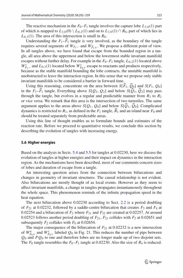
5.6 Higher energies

Based on the analysis in Sects. 5.4 and 5.5 for tangles at 0.02230, here we discuss theevolution of tangles at higher energies and their impact on dynamics in the interactionregion. As the mechanisms have been described, most of our comments concern sizesof lobes and duration of escape from a tangle.

An interesting question arises from the connection between bifurcations andchanges in geometry of invariant structures. The causal relationship is not evident.Also bifurcations are mostly thought of as local events. However as they seem toaffect invariant manifolds, a change in tangles propagates instantaneously throughoutthe whole space. This phenomenon reminds of the infinite propagation speed in theheat equation.

The next bifurcation above 0.02230 according to Sect. 2.2 is a period doublingof F21 at 0.02232, followed by a saddle-centre bifurcation that creates F3 and F4 at0.02254 and a bifurcation of F3 where F31 and F32 are created at 0.02257. At around0.02523 follows another period doubling of F21, F21 collides with F2 at 0.02651 andsubsequently F2 collides with F0 at 0.02654.

The major consequence of the bifurcation of F21 at 0.02232 is a new intersectionof Wu

F0+ and WsF0+ labeled Q0 in Fig. 21. This reduces the number of pips between

Q0 and PQ0 to one and therefore lobes are no longer made up of two disjoint sets.The F0 tangle resembles the F0–F1 tangle at 0.02230. Also the size of R4 is reduced.

123


Fig. 21 The F0 tangle and the F1 tangle at 0.02253

In the F1 tangle we see L0,1(2) cross DS0 twice as shown in Fig. 21. All L0,1(k)for k > 2 and also L1,0(k) with k < −2 therefore pass through R1. Moreover, the tipof L0,1(2) approaching R1 can be expected to pass cross R1 after the bifurcations at0.02254 and 0.02257.

A small remark regarding notation. At this energy L0,1(2) lies in R0, R0, R1, R1,R2 and R3, but we maintain the notation for consistency.

At 0.02400, L0,1(2) in the F1 tangle passes through R1 twice and the numberincreases at higher energies. Almost all lobes lie in almost all regions, but the mecha-nism for fast entry and exit of the tangles remain the same. Figure 22 shows R0 and R0.While R4 is considerably larger than R1 at 0.02253, the opposite is true at 0.02400.Recall that R4 contains predominantly nonreactive trajectories that do not cross DS0,

123


Fig. 22 Indication of boundaries of R0 and R4 (above) and the F1 tangle at 0.02400 (below). The area inthe F1 tangle highlighted in cyan is the part of L0,1(0) ∩ L1,0(1) that originates in products and is guidedby Ws

F1+ (dashed) into products (Color figure online)

whereas R1 mostly contains ones that do. The overestimation of the reaction ratefollows.

The capture lobes in the F1 tangle guide predominantly trajectories from productsinto R1, as shown in Fig. 22.A significant portion of R1 is taken up by L0,1(0)∩L1,0(1)and it is prevented by Ws

F1− from escaping into reactants. Moreover, the a large partof the intersection lies below Ws

F1+, see Fig. 22, that guides it into back products as

WsF1+ contracts.Heteroclinic tangles mirror the changes of the homoclinc tangles (Fig. 23).

123


Fig. 23 Structure of the heteroclinic tangles at 0.02400. WF0+ and WF1− making up the F0–F1 tangle(left) and the F1–F1 tangle (right). Unstable invariant manifolds are as indicated red and green, stable areblue and orange (Color figure online)

5.7 Loss of normal hyperbolicity

F0 loses normal hyperbolicity andbecomes stable at 0.02654, in a bifurcation involvingF2, F2, F21, F21. TST cannot be based on F0 and WF0 cease to exist. The sudden dis-appearance of invariant manifolds has no dramatic consequences. As can be deducedfrom Fig. 23, WF0 are at energies below 0.02654, very close to WF1− and WF1+ andnaturally take over the role of WF0 . Throughout the energy interval from 0.02206when F1 appears to the loss of normal hyperbolicity at 0.02654, we see a transition ofdominance from F0 to F1–F1.

The loss of normal hyperbolicity of F0 simplifies dynamics due to the presence offewer TSs, for example compare Figs. 23 and 24.

At 0.02661, F0 collides with F4 and becomes inverse hyperbolic. Due to the inversehyperbolicity,WF0 exist, but they must contain a twist that is manifested as a reflectionacross the F0 (see [1]), i.e. have the geometry of a Möbius strip. At the same timeWF0 are enclosed between WF1− along with WF1+, but with cylindrical structure.Consequences of the geometry of WF0 are unknown.

There are no more significant bifurcations above 0.02661 and therefore apart fromgrowing tangles and lobes, the tangles remains structurally the same.

Together with WF0 we observe the disappearance of R4 and of the mechanism thatcarries nonreactive trajectories through the F0 tangle without crossing DS0. Conse-quently, all trajectories that pass through the F1−F1 tangle cross DS0 at least twice.Each hemisphere of DS1 still possesses the no-return property, which means trajecto-ries cross DS1 at most twice. Trajectories that avoid the tangle cross both DSs onceor not at all.

Similarly to lower energies, R1 is predominantly made up of L0,1(0) ∩ L1,0(1)in the F1 tangle or L2,0(0) ∩ L0,3(1) in the F1–F1 tangle, as shown in Fig. 24. Theargument that trajectories in the F1–F1 tangle below and above all stable manifoldsleave the interaction region is still valid. Capture lobes are disjoint, therefore it is notpossible to reenter the bounded region. Although R1 and R1 admit return, R1 ∪ R1possesses the no-return property.

123


Fig. 24 The F1–F1 tangle at 0.02700 and an indication how certain parts of lobes are mapped in this tangle

5.8 Known estimate

Davis [6] formulated bounds and an estimate of the reaction rate based on numericalobservation of dynamics. He observed that a significant portion of trajectories leavethe heteroclinic tangle above 0.02654 after one iteration and imposed the assumptionof fast randomization on the remaining trajectories.

As described above, Davis’ observation is due a property of the F1–F1 tangle—R1is mostly occupied by L0,1(0) ∩ L1,0(1). We quantify this proportion below.

The assumption of fast randomization of the other trajectories and a 50%probabilityof them reacting is more difficult to support. From the analysis of lobes we knowthat however intricate the dynamics is, there is no reason for precisely half of theremaining trajectories to leave to reactants and half to products. Instead we find that

123


for small energies, trajectories that spend 2 and more iterations R0 and R0 make up asignificant part of the tangles (up to half at 0.02350), but their total proportion is verysmall and only grows slowly with increasing energy. In the interval up to 0.03000,these trajectories make up at most 3% of the total, 2% below 0.02650, see Table 1.Consequently, any estimate of the reaction rate that takes trajectories escaping after 1iteration into account is accurate to within 3% below 0.03000 and when we includetrajectories escaping after 2 iterations, this number drops to less than 1%.

The difficulty lies in accurately calculating the amount of trajectories. At the costof accuracy, Davis used VTST as a measure of trajectories entering the interactionregion, μ(L3,0(0)) to estimate the size of the tangle and μ(L3,0(0) ∩ L0,2(1)) tosubtract trajectories escaping after 1 iteration. The upper and lower estimates assumeall, respectively none, of the trajectories that escape after 2 or more iterations arereactive.

6 The intricate energy interval

The energy interval 0.02215 < E < 0.02654, when TST is not exact and F0 is a TS,has been largely avoided in the past. The interaction of invariant manifolds of twoTSs posed enough difficulties. Dividing tangles using pieces of invariant manifoldsand following pips to understand dynamics within make this task possible. We dividetangles differently to the lobe dynamics approach, because we aim to describe andmeasure parts of heteroclinic tangles that do not necessarily fall into a single lobe.

6.1 Division of a tangle

Davis [6] calculated pieces of invariant manifolds in this interval at an energy of0.7 eV ≈ 0.02572, but complexity of their intersections did not admit deeper insight.With current understanding it is not possible to consider all the invariant manifolds atonce, because even identifying lobes is challenging, not to speak of their intersections.

We use the approach outlined in Sect. 5.5 and concentrate on WF1 and WF1 , whilekeeping WF0 in mind near F0. A similar approach may be used for homoclinic tan-gles. We separate predictably evolving trajectories from chaotic ones, for exampletrajectories escaping after 1, 2 or 3 iterations from the rest of the tangle. To our knowl-edge, tools for identifying particular lobe intersections and determining the area, aheteroclinic tangle surgery toolbox, have not been previously presented or reported.

There is one more important property of the manifolds that stands out from allprevious figures. Inside the F1–F1 tangle, Wu

F1− and WuF1+ are restricted to the stripe

between two pieces of unstable manifold, e.g. U [F1, Q3] and U [F1, Q1] at 0.02700in Fig. 24 orU [F1, PQ1] andU [F1, P Q1] at 0.02400 in Fig. 25. SimilarlyWs

F1− andWs

F1+ are confined to a single stripe. We remark that WF0 are located between WF1−and WF1+ and thereby confined as well. It therefore makes sense to study this stripein detail.

123


Fig. 25 The F1–F1 tangle at 0.02400 (left) and its simplification (right). WF1− are drawn with solid lines,WF1+ are dashed

Consider the F1–F1 tangle at 0.02400, where R1 and R4 are reasonably sized andnonreactive trajectories that do not cross DS0 exist. Following the motto divide etimpera, we take the following steps:

– We identify new regions that have the no-return property.– We use as few pieces of invariant manifolds as possible.– We define subsets of regions containing reactive/nonreactive trajectories.

Define R5 as the bounded region inside the tangle, the upper part of the boundaryis made up ofU [F1, Q2], S[Q2, Q3],U [Q3, PQ0] and S[PQ0, F1], see Fig. 25, andthe lower part is symmetric to it. Each lobe consists of two disjoint sets, for example,L2,5(0) is bounded by S[PQ1, PQ0], U [PQ0, PQ1] and S[Q3, Q2], U [Q2, Q3].We remark that lobes do not intersect outside R5 and leave the interaction region.Disjoint capture lobes imply:

Remark 3 R5 has the no-return property.

As found in Sect. 5.6, a large part of R5 behaves regularly and leaves the tangle within1 iteration. As argued in Sect. 5.5, stable manifolds contract in forward time andthereby act as a barrier. Everything aboveWs

F1− leaves at the next iteration to reactants,everything below Ws

F1+ leaves to products. This agrees with the lobes L5,3(1) andL5,2(1) that leave R5 by definition.

The remainder of R5 is the stripe between WsF1− and Ws

F1+, the only part of R5

where stable manifolds can lie. We refer to it as the capture stripe and denote it R6, seeFig. 25. Its boundary consists of S[F1, Q1], U [F1, Q1], S[F1, Q1] and U [F1, Q1].

In backward time, the roles of stable and unstable manifolds switch—everythingbelow Wu

F1− and above WuF1+ escapes R5. Define R7, the escape stripe bounded by

S[F1, P Q1], U [F1, P Q1], S[F1, PQ1] and U [F1, PQ1]. R5\R7 escapes R5 after 1iteration in backward time.

We conclude that all complicated and chaotic dynamics is confined to R6 ∩ R7 anddue to the no-return property of R5:

Remark 4 R6 and R7 have the no-return property.

123


Fig. 26 The F1−F1 tangle at 0.02500 and a detail of the diminishing part of R5\(R6 ∪ R7) highlighted incyan (Color figure online)

Note that the boundary of R7 is the image of the boundary of R6. Necessarily

PR6 = R7,

and due to preservation of area μ(R6) = μ(R7).There are more regions with the no-return property in the F1–F1 tangle. Obviously,

R5\(R6 ∪ R7) must be a no-return region as it escapes the R5 immediately afterentering. Also R6\R5 as the entry point to R7 must have the no-return property as wellas capture and escape lobes.

6.2 Dynamical properties

To shorten and facilitate the description of reactive and dynamical properties of R5,R6 and R7, we introduce the following classification of trajectories.

Definition 7 We call the set of trajectories:

directly reactive (DR) if they remain in R2 or R3,directly nonreactive (DN ) if they do not enter the interaction region,captured reactive after n iterations (CRn) if they react after n iterations in R5,captured nonreactive after n iterations (CNn) if they return to the region of originafter n iterations in R5.

Clearly DR and DN never enter R5. Following Sects. 5.6 and 6.1, R5\(R6 ∪ R7) isthe region of CN1 and CR1 is always empty. CR2 and CN2 are pass through R6\R7and R7\R6 and therefore never enter R6 ∩ R7.

This leaves the complicated evolution and chaotic behaviour restricted to R6 ∩ R7.Below 0.02500, R6 ∩ R7 consists of 5 squares near F0, F1, F1, F2 and F2. As F2and F2 approach the bifurcation with F0, the three squares near them merge into onearound 0.02523 when F21 bifurcates, see Figs. 26 and 27.

Trajectories enter R5 via R6\R7 and escape via R7\R6, hence every trajectorycrosses R6\R7 and R7\R6 at most once. The same is true for R5\(R6∪ R7) consistingofCN1. Therefore of R5 only the size R6∩R7 does not reflect the number of trajectories

123


Fig. 27 The F1−F1 tangle at 0.02550 and a detail of the diminished part of R5\(R6 ∪ R7)

it contains. It follows that the area of R6\R7, R7\R6 and R5\(R6 ∪ R7) on the surfaceof section Σ0 is the same of their images on DS1 and DS1.

Figure 28 shows amore detailed partitioning of R6 and R7. Essentially, R6 is dividedinto finer stripes by pieces ofWs

F1− andWsF1+ that are nearly parallel to the boundary.

The boundary of R6 illustrates how the content of the stripe is deformed when mappedinto R7. It is compressed along the stable manifolds towards the fixed points, e.g.

P(S[F1, Q1]) = S[F1, PQ1],

and stretched along the unstable manifolds away from the fixed points. We remark thatthe whole highlighted set in R5\R7 of Fig. 28 is connected, only separated by stableinvariant manifolds. When mapped forward it is stretched, but remains connected.The sets labeled by yellow, red and green are alternately mapped above and below thecapture stripe.

There is a connection between these coloured stripes and lobe intersections, butlobes do not distinguish how often trajectories cross DS0, which is necessary to under-stand overestimation of the reaction rate by TST.

The connected components of R6 ∩ R7 contain dynamics similar to Smale’s horse-shoe dynamics, [12]. As a consequence we observe a fractal structure, as can be seen inFig. 29. R6 ∩ R7 accounts for less than 12% of the all trajectories that pass through R5below 0.02400 when the dynamics is relatively slow. The proportion drops to roughly7% of R5 at 0.03000 and remains below 1% of the total amount of trajectories.

6.3 Areas

In this system, determining the area of R5, R6, R7, R5\(R6∪ R7), R6\R7 and R6∩ R7,is significantly easier than calculating lobe intersections. We employ a Monte Carlobased method that is expensive, yet simple. Ultimately the cost and accuracy dependon the level of detail in R6 ∩ R7, i.e. it can be determined a priori. We also tune initialand terminal conditions to obtain a high accuracy at a reasonable cost.

Previous works seem to consider initial conditions on r1+ r22 = 50, pr1 < 0, which

is a surface near q2 = 1181. We prefer to sample the hemisphere of DS1, throughwhich trajectories enter the interaction region. Directly we have that the difference

123


Fig. 28 Coloured sets in R6 showing how part of the capture stripe is mapped at 0.02400.WF1− are drawnwith solid lines, WF1+ are dashed. CN1 are shown in orange, CR2 green and yellow, CN2 red. Part ofblue also belongs to CN2. Blue, yellow, red and green are separated by white stripes that are mapped toR6 ∩ R7 (Color figure online)

between the inward hemisphere of DS1 and r1 + r22 = 50, pr1 < 0 corresponds to DN

trajectories.The slowest of DR are located near the boundary of R5, and those near pips evolve

similarly to pips. Using pips on WuF1

we define checkpoints, that mark distance thesepips aremapped, i.e. the least distance DR cover in the interaction region in 1 iteration.Then all trajectories that pass the second checkpoint 1 iteration after they pass thefirst checkpoint, are DR and are not captured in R5. Recall that all captured reactivetrajectories spend at least 2 iterations in R5. Trajectories that have a delay of n iterationbetween crossing of the checkpoints are CRn . Since R5 is symmetric, we use thesymmetric counterpart of the second checkpoint to identify CNn .

123


Fig. 29 Detail of the island near F1 and its content at 0.02500. CN3 are purple, CR3 are magenta and therest of the island is plain. CN2 (green) and CR2 (cyan) contained in the adjacent regions R6 and R7 areshown for completeness (Color figure online)

Fig. 30 Checkpoints defined in the F1–F1 tangle at 0.02400

At 0.02400, Q1 and PQ1 are the natural choice for checkpoints, because mark theendpoints of R6\R7 via which trajectories enter R5, see Fig. 30. We define checkpointChQ1 as a vertical line passing through Q1. It is necessary that ChQ1 avoids capturelobes, therefore at energies above 0.02900 the computationally most efficient solutionis to use another vertical line between Q1 and F0.

The role of the second checkpoint, ChPQ1 , is to distinguish trajectories in R5 fromthose outside R5.We use a linear approximation of S[F1, PQ1], the boundary betweenthe escape lobe and R5, in conjunction with a vertical line passing through PQ1.

123


The checkpoint symmetric to ChPQ1 is defined analogously and denoted ChPQ1. If

desired, we can track the number crossings of DS0 using the sign of q2.We can measure individual components of R5: μ(R5\R7) corresponds to the num-

ber of captured trajectories, μ(R5\(R6 ∪ R7)) is given by CN1. Then

μ(R6\R7) = μ(R5\R7) − μ(R5\(R6 ∪ R7)),

and R6 ∩ R7 can be deduced from CRn and CNn where n ≥ 3. The latter followsfrom the fact that CR2 and CN2 do not pass through R6 ∩ R7.

This method is not computationally cheap, but the computational difficulty can beeasily estimated a priori. Determining the distribution up to CRn and CNn with Ninitial conditions requires approximately nN iterations of the map P , but consideringthe prevalence of DR and DN , this number will be considerably lower.

Alternative approaches to calculating lobe areas face the obstacle in distinguishingthe inside from the outside of a lobe, not to mention their intersections. Recent devel-opments [17,18] suggest that a reactive island approach can be used to calculate areasof intersections in a cheaper and simpler manner.

7 Bounds of the reaction rate

7.1 Quantification

In Table 1 we present proportions of areas of classes of trajectories on the planer1 + r2

2 = 50, pr1 < 0. Between 107 and 2.108 initial conditions were used to obtainthese values.

The proportion of DN decreases steadily over the whole interval presented inTable 1 and beyond. This is not surprising given that widening bottlenecks allowmore trajectories enter the interaction region. Thereby nonreactive heavily oscillatingtrajectories enter the interaction region and consequently R5\(R6 ∪ R7) grows fasterthan the rest of R5.

Note that the proportion of DR culminates between 0.02500 and 0.02550. Atthis energies the geometry of the F1−F1 tangle simplifies with the consequence thatall captured trajectories cross DS1. The proportion of DR above 0.02550 decreasespredominantly in favour ofCN1.We observe the growth of capture lobes mainly in thearea of large |p2| momentum, containing predominantly CN1 trajectories (Table 1),approaching the maximal values of |p2| at the given energy. This implies that for agiven (small) |p1| momentum, trajectories are more likely to react at a lower energydue to smaller capture lobes.

In the physical world large values of |p2| correspond by definition (Sect. 3.3) tolarge |pr1 | on the reactant side and large |pr2 | on the product side. Since trajectoriesare less likely to react at higher energies, the mechanism for transfer of kinetic energybetween the degrees of freedom in the interaction region must be failing at highenergies. Consequently, the energy passed from the incoming H to the H2 may be sohigh, that it repels the whole molecule instead of breaking its bond. This may be true

123


Table 1 Proportions of areas ofclasses of trajectories on theplane r1 + r2

2 = 50, pr1 < 0

Energy DR DN CR2 CN1 CN2 Other

0.02205 0.590 0.410 0 0 0 0

0.02214 0.595 0.405 0 0 0 0

0.02215 0.687 0.296 0 0.016 0.001 0.000

0.02230 0.693 0.290 0.001 0.013 0.001 0.001

0.02253 0.703 0.282 0.001 0.011 0.001 0.002

0.02300 0.717 0.266 0.003 0.008 0.003 0.002

0.02350 0.725 0.255 0.004 0.010 0.005 0.003

0.02400 0.733 0.239 0.004 0.015 0.006 0.003

0.02450 0.737 0.227 0.005 0.021 0.006 0.004

0.02500 0.739 0.216 0.006 0.028 0.007 0.005

0.02550 0.739 0.206 0.006 0.037 0.008 0.006

0.02600 0.737 0.197 0.007 0.046 0.008 0.006

0.02650 0.734 0.188 0.007 0.055 0.009 0.007

0.02662 0.734 0.186 0.008 0.057 0.009 0.007

0.02700 0.731 0.180 0.008 0.064 0.010 0.007

0.02800 0.723 0.166 0.009 0.083 0.011 0.008

0.02900 0.714 0.153 0.010 0.101 0.012 0.009

0.03000 0.705 0.145 0.011 0.116 0.013 0.010

Directly reactive (DR) and directly nonreactive (DN ) trajectories donot enter R5. Captured reactive (CR2) and captured nonreactive (CN1,CN2) enter and leave R5 after 1 or 2 iterations. Other trajectories donot leave R5 within 2 iterations after their entry and are inside R6∩R7.Horizontal lines represent the creation of the homoclinic tangles andloss of normal hyperbolicity of F0

for a whole class of collinear atom-diatom reactions, provided it is possible to definean interaction region multiple TSs.

7.2 MC based bounds

Using Table 1 we are able to formulate estimates of the reaction rate up to arbitraryprecision. The idea is similar to [6]. An upper/lower bound on the reaction rate isobtained by assuming that all/none of the trajectories that remain in R5 after n iterationsreact. Table 2 contains the resulting bounds.

DenoteU1 the rate estimate obtained by assuming all trajectories in R5\(R6 ∪ R7)

react, or equivalently only CN1 do not react. Since CN2 and some of Other do notreact, the true reaction rate is lower.

Lemma 4 U1 = μ(DR) + μ(CR2) + μ(CN2) + μ(Other) is an upper bound of thereaction rate.

U1 can be easily improved by acknowledging thatCN2 are nonreactive. Denote thisbound byU2. Because the R6 ∩ R7 contain reactive as well as nonreactive trajectories,the true reaction rate is lower.

123


Table 2 Comparison of resultsof TST and VTST with theactual reaction rate computedvia Monte Carlo and our upperand lower estimates

Energy PTST PVTST PMC L2 U2 U1

0.01600 0.181 0.181 0.181

0.01800 0.383 0.383 0.383

0.01900 0.469 0.469 0.469

0.02000 0.545 0.545 0.545

0.02100 0.615 0.615 0.615

0.02205 0.681 0.681 0.681

0.02215 0.687 0.687 0.687 0.687 0.687 0.689

0.02230 0.696 0.696 0.695 0.694 0.696 0.697

0.02253 0.709 0.709 0.705 0.704 0.706 0.707

0.02300 0.736 0.734 0.721 0.720 0.722 0.725

0.02350 0.763 0.748 0.732 0.728 0.731 0.736

0.02400 0.789 0.761 0.739 0.737 0.741 0.746

0.02450 0.814 0.773 0.744 0.742 0.746 0.753

0.02500 0.838 0.784 0.746 0.744 0.749 0.756

0.02550 0.860 0.794 0.747 0.744 0.750 0.758

0.02600 0.883 0.804 0.747 0.743 0.750 0.758

0.02650 0.904 0.812 0.745 0.742 0.748 0.757

0.02662 0.909 0.814 0.744 0.741 0.748 0.757

0.02700 0.924 0.820 0.743 0.739 0.746 0.756

0.02800 0.963 0.835 0.736 0.732 0.740 0.751

0.02900 0.999 0.847 0.729 0.725 0.734 0.746

0.03000 1.033 0.858 0.720 0.716 0.726 0.739

0.04000 1.278 0.960 0.626

0.05000 1.428 1.002 0.542

Lemma 5 U2 = μ(DR) + μ(CR2) + μ(Other) is an upper bound of the reactionrate.

A lower bound L2 is obtained assuming all of R6 ∩ R7 are nonreactive trajectories.

Lemma 6 L2 = μ(DR) + μ(CR2) is a lower bound of the reaction rate.

The difference between L2 and U2 is precisely μ(Other). This gives us an upperbound on the error of both estimates. An estimate of the reaction rate can be obtainedusing L2 and U2.

8 Conclusion

We have studied invariant manifolds of TSs to find an explanation for the decrease ofthe reaction rate. In the process of understanding how energy surface volume passesthrough homoclinic and heteroclinic tangles formed by these invariant manifolds we

123


found the need for tools that would allow us to work with the tangles and not get lostin details of its chaotic structure. We introduced a suitable division of homoclinic andheteroclinic tangles that is simple and understandable based on reactive properties oftrajectories.

Once divided, the heteroclinic tangles decompose into areas of simple and morecomplicated dynamics. We were able to identify a large class of trajectories that aremerely diverted by the tangles and areas of fractal horseshoe-like structure near hyper-bolic or inverse-hyperbolic periodic orbits. In addition to a better understanding, thedivision provides an easy way calculating the corresponding areas.

Contrary to expectations, the decline of the reaction rate is not a result of lossof normal hyperbolicity. We may consider the decrease of the reaction rate and lossof normal hyperbolicity to be consequences of insufficient transfer of kinetic energybetween the degrees of freedom. In physical terms, the single atom has somuch kineticenergy, that it repels the whole molecule instead of becoming part of it.

Open Access This article is distributed under the terms of the Creative Commons Attribution 4.0 Interna-tional License (http://creativecommons.org/licenses/by/4.0/), which permits unrestricted use, distribution,and reproduction in any medium, provided you give appropriate credit to the original author(s) and thesource, provide a link to the Creative Commons license, and indicate if changes were made.

References

1. A.M. Ozorio de Almeida, N. de Leon, M.A. Mehta, C.C. Marston, Geometry and dynamics of stableand unstable cylinders in Hamiltonian systems. Physica D 46(2), 265–285 (1990). https://doi.org/10.1016/0167-2789(90)90040-V

2. V.I. Arnold, Les méthodes mathématiques de la mécanique classique (Nauka, Éditions Mir, Moscow,1976)

3. J. Binney, O.E. Gerhard, P. Hut, Structure of surfaces of section. Mon. Not. R. Astron. Soc. 215(1),59–65 (1985). https://doi.org/10.1093/mnras/215.1.59

4. G.D. Birkhoff, Dynamical Systems (AMS, Providence, 1927)5. S. Chapman, S.M. Hornstein, W.H. Miller, Accuracy of transition state theory for the threshold of

chemical reactions with activation energy. Collinear and three-dimensional H + H2. J. Am. Chem.Soc. 97(4), 892–894 (1975). https://doi.org/10.1021/ja00837a035

6. M.J. Davis, Phase space dynamics of bimolecular reactions and the breakdown of transition statetheory. J. Chem. Phys. 86(7), 3978–4003 (1987). https://doi.org/10.1063/1.451908

7. B. Eckhardt, D. Wintgen, Indices in classical mechanics. J. Phys. A 24(18), 4335 (1991). https://doi.org/10.1088/0305-4470/24/18/020

8. N. Fenichel, Persistence and smoothness of invariant manifolds for flows. Indiana Univ. Math. J. 21,193–226 (1971). https://doi.org/10.1512/iumj.1972.21.21017

9. J.M. Greene, Two-dimensional measure-preserving mappings. J. Math. Phys. 9(5), 760–768 (1968).https://doi.org/10.1063/1.1664639

10. J. Henrard, Capture into resonance: an extension of the use of adiabatic invariants. Celest. Mech. 27(1),3–22 (1982). https://doi.org/10.1007/BF01228946

11. M.W. Hirsch, C.C. Pugh, M. Shub, Invariant Manifolds. Lecture Notes in Mathematics (Springer,Berlin, 1977)

12. M.W.Hirsch, S. Smale, R.L. Devaney,Differential Equations, Dynamical Systems, and an Introductionto Chaos (Elsevier, Amsterdam, 2004)

13. J. Horiuti, On the statistical mechanical treatment of the absolute rate of chemical reaction. Bull. Chem.Soc. Jpn. 13(1), 210–216 (1938). https://doi.org/10.1246/bcsj.13.210

14. M. Iñarrea, J.F. Palacián,A.I. Pascual, J.P. Salas,Bifurcations of dividing surfaces in chemical reactions.J. Chem. Phys. 135(1), 014110 (2011). https://doi.org/10.1063/1.3600744

123

http://creativecommons.org/licenses/by/4.0/

https://doi.org/10.1016/0167-2789(90)90040-V

https://doi.org/10.1016/0167-2789(90)90040-V

https://doi.org/10.1093/mnras/215.1.59

https://doi.org/10.1021/ja00837a035

https://doi.org/10.1063/1.451908

https://doi.org/10.1088/0305-4470/24/18/020

https://doi.org/10.1088/0305-4470/24/18/020

https://doi.org/10.1512/iumj.1972.21.21017

https://doi.org/10.1063/1.1664639

https://doi.org/10.1007/BF01228946

https://doi.org/10.1246/bcsj.13.210

https://doi.org/10.1063/1.3600744


15. C. Jaffé, S.D. Ross, M.W. Lo, J. Marsden, D. Farrelly, T. Uzer, Statistical theory of asteroid escaperates. Phys. Rev. Lett. 89, 011101 (2002). https://doi.org/10.1103/PhysRevLett.89.011101

16. J.C. Keck, Variational theory of reaction rates. Adv. Chem. Phys. 13, 85 (1967). https://doi.org/10.1002/9780470140154.ch5

17. V. Krajnák, H. Waalkens, The phase space geometry underlying roaming reaction dynamics. J. Math.Chem. 56, 2341–2378 (2018)

18. V. Krajnák, S. Wiggins, Influence of mass and potential energy surface geometry on roaming inChesnavich’s CH+

4 model. J. Chem. Phys. 149(9), 094109 (2018)19. R.S. MacKay, J.D. Meiss, I.C. Percival, Transport in Hamiltonian systems. Physica D 13(1–2), 55–81

(1984). https://doi.org/10.1016/0167-2789(84)90270-720. R.S. MacKay, D.C. Strub, Bifurcations of transition states: Morse bifurcations. Nonlinearity 27(5),

859–895 (2014). https://doi.org/10.1088/0951-7715/27/5/85921. J.D. Meiss, Thirty years of turnstiles and transport. Chaos 25(9), 097602 (2015). https://doi.org/10.

1063/1.491583122. J.D. Meiss, J.R. Cary, D.F. Escande, R.S. MacKay, I.C. Percival, J.L. Tennyson, Dynamical theory of

anomalous particle transport. Plasma Phys. Control. Nucl. Fusion Res. 1984 3, 441–448 (1985)23. W.H.Miller, Unified statistical model for “complex” and “direct” reactionmechanisms. J. Chem. Phys.

65(6), 2216–2223 (1976). https://doi.org/10.1063/1.43337924. K. Morokuma, M. Karplus, Collision dynamics and the statistical theories of chemical reactions. II.

Comparison of reaction probabilities. J. Chem. Phys. 55(1), 63–75 (1971). https://doi.org/10.1063/1.1675562

25. J.M. Ottino, The Kinematics of Mixing: Stretching, Chaos, and Transport. Cambridge Texts in AppliedMathematics (Cambridge Univiversity Press, Cambridge, 1989)

26. P. Pechukas, On simple saddle points of a potential surface, the conservation of nuclear symmetryalong paths of steepest descent, and the symmetry of transition states. J. Chem. Phys. 64, 1516–1521(1976). https://doi.org/10.1063/1.432370

27. P. Pechukas, Statistical approximations in collision theory, in Dynamics of Molecular Collisions PartB, ed. by H.W. Miller (Plenum Press, New York, 1976), pp. 269–322

28. P. Pechukas, Transition state theory. Ann. Rev. Phys. Chem. 32(1), 159–177 (1981). https://doi.org/10.1146/annurev.pc.32.100181.001111

29. P. Pechukas, F.J. McLafferty, On transition-state theory and the classical mechanics of collinear colli-sions. J. Chem. Phys. 58, 1622–1625 (1973). https://doi.org/10.1063/1.1679404

30. P. Pechukas, E. Pollak, Classical transition state theory is exact if the transition state is unique. J. Chem.Phys. 71(5), 2062–2068 (1979). https://doi.org/10.1063/1.438575

31. E. Pollak, P. Pechukas, Transition states, trapped trajectories, and classical bound states embedded inthe continuum. J. Chem. Phys. 69(3), 1218–1226 (1978). https://doi.org/10.1063/1.436658

32. E. Pollak, P. Pechukas, Unified statistical model for “complex” and “direct” reaction mechanisms: atest on the collinear H + H2 exchange reaction. J. Chem. Phys. 70(1), 325–333 (1979). https://doi.org/10.1063/1.437194

33. P. Pollak, M.S. Child, P. Pechukas, Classical transition state theory: a lower bound to the reactionprobability. J. Chem. Phys. 72(3), 1669–1678 (1980). https://doi.org/10.1063/1.439276

34. R.N. Porter, M. Karplus, Potential energy surface for H3. J. Chem. Phys. 40(4), 1105–1115 (1964).https://doi.org/10.1063/1.1725256

35. V. Rom-Kedar, S. Wiggins, Transport in two-dimensional maps. Arch. Ration. Mech. Anal. 109(3),239–298 (1990). https://doi.org/10.1007/BF00375090

36. O.R. Ruiz, Existence of brake-orbits in Finsler mechanical systems. Ph.D. Thesis (1975)37. K.R. Sreenivasan, On local isotropy of passive scalars in turbulent shear flows. Proc. R. Soc. Lond.

Ser. A 434(1890), 165–182 (1991). https://doi.org/10.1098/rspa.1991.008738. K.R. Sreenivasan, R.A. Antonia, The phenomenology of small-scale turbulence. Annu. Rev. Fluid

Mech. 29(1), 435–472 (1997). https://doi.org/10.1146/annurev.fluid.29.1.43539. D.I. Sverdlik, G.W.Koeppl, An energy limit of transition state theory. Chem. Phys. Lett. 59(3), 449–453

(1978). https://doi.org/10.1016/0009-2614(78)85017-940. G.D. Truhlar, B.C. Garrett, Variational transition state theory. Ann. Rev. Phys. Chem. 35, 159–189

(1984). https://doi.org/10.1146/annurev.pc.35.100184.00111141. T. Uzer, C. Jaffé, J. Palacián, P. Yanguas, S.Wiggins, The geometry of reaction dynamics. Nonlinearity

15, 957–992 (2002). https://doi.org/10.1088/0951-7715/15/4/301

123

https://doi.org/10.1103/PhysRevLett.89.011101

https://doi.org/10.1002/9780470140154.ch5

https://doi.org/10.1002/9780470140154.ch5

https://doi.org/10.1016/0167-2789(84)90270-7

https://doi.org/10.1088/0951-7715/27/5/859

https://doi.org/10.1063/1.4915831

https://doi.org/10.1063/1.4915831

https://doi.org/10.1063/1.433379

https://doi.org/10.1063/1.1675562

https://doi.org/10.1063/1.1675562

https://doi.org/10.1063/1.432370

https://doi.org/10.1146/annurev.pc.32.100181.001111


https://doi.org/10.1063/1.1679404

https://doi.org/10.1063/1.438575

https://doi.org/10.1063/1.436658

https://doi.org/10.1063/1.437194

https://doi.org/10.1063/1.437194

https://doi.org/10.1063/1.439276

https://doi.org/10.1063/1.1725256

https://doi.org/10.1007/BF00375090

https://doi.org/10.1098/rspa.1991.0087

https://doi.org/10.1146/annurev.fluid.29.1.435

https://doi.org/10.1016/0009-2614(78)85017-9


https://doi.org/10.1088/0951-7715/15/4/301


42. H. Waalkens, A. Burbanks, S. Wiggins, A computational procedure to detect a new type of high-dimensional chaotic saddle and its application to the 3D Hill’s problem. J. Phys. A 37, L257–L265(2004). https://doi.org/10.1088/0305-4470/37/24/L04

43. H.Waalkens, A. Burbanks, S.Wiggins, Phase space conduits for reaction inmultidimensional systems:HCN isomerization in three dimensions. J. Chem. Phys. 121(13), 6207–6225 (2004). https://doi.org/10.1063/1.1789891

44. H. Waalkens, A. Burbanks, S. Wiggins, Efficient procedure to compute the microcanonical volume ofinitial conditions that lead to escape trajectories from a multidimensional potential well. Phys. Rev.Lett. 95, 084,301 (2005). https://doi.org/10.1103/PhysRevLett.95.084301

45. H. Waalkens, A. Burbanks, S. Wiggins, A formula to compute the microcanonical volume of reactiveinitial conditions in transition state theory. J. Phys. A 38, L759–L768 (2005). https://doi.org/10.1088/0305-4470/38/45/L03

46. H. Waalkens, R. Schubert, S. Wiggins, Wigner’s dynamical transition state theory in phase space:classical and quantum. Nonlinearity 21, R1–R118 (2008). https://doi.org/10.1088/0951-7715/21/1/R01

47. H.Waalkens, S.Wiggins, Direct construction of a dividing surface of minimal flux for multi-degree-of-freedom systems that cannot be recrossed. J. Phys. A 37, L435 (2004). https://doi.org/10.1088/0305-4470/37/35/L02

48. S. Wiggins, L. Wiesenfeld, C. Jaffé, T. Uzer, Impenetrable barriers in phase-space. Phys. Rev. Lett.86, 5478–5481 (2001). https://doi.org/10.1103/PhysRevLett.86.5478

49. E. Wigner, Calculation of the rate of elementary association reactions. J. Chem. Phys. 5, 720–725(1937). https://doi.org/10.1063/1.1750107

50. J. Williamson, On the algebraic problem concerning the normal forms of linear dynamical systems.Am. J. Math. 58(1), 141–163 (1936). https://doi.org/10.2307/2371062

Publisher’s Note Springer Nature remains neutral with regard to jurisdictional claims in published mapsand institutional affiliations.

123

https://doi.org/10.1088/0305-4470/37/24/L04

https://doi.org/10.1063/1.1789891

https://doi.org/10.1063/1.1789891


https://doi.org/10.1088/0305-4470/38/45/L03

https://doi.org/10.1088/0305-4470/38/45/L03

https://doi.org/10.1088/0951-7715/21/1/R01

https://doi.org/10.1088/0951-7715/21/1/R01

https://doi.org/10.1088/0305-4470/37/35/L02

https://doi.org/10.1088/0305-4470/37/35/L02


https://doi.org/10.1063/1.1750107

https://doi.org/10.2307/2371062

phase space structures causing the reaction rate decrease ... · the collinear hydrogen exchange...

Documents