phase-space wavepacket dynamics of internal conversion via...
TRANSCRIPT

Contents lists available at ScienceDirect
Chemical Physics
journal homepage: www.elsevier.com/locate/chemphys
Phase-space wavepacket dynamics of internal conversion via conicalintersection: Multi-state quantum Fokker-Planck equation approach
Tatsushi Ikeda, Yoshitaka Tanimura⁎
Department of Chemistry, Graduate School of Science, Kyoto University, Kyoto 606-8502, Japan
A R T I C L E I N F O
Keywords:Internal conversionConical intersectionAvoided crossingNon-adiabatic transitionCondensed phaseWavepacket dynamicsMulti-state quantum Fokker-Planck equation
A B S T R A C T
We theoretically investigate internal conversion processes of a photoexcited molecule in a condensed phase. Themolecular system is described by two-dimensional adiabatic ground and excited potential energy surfaces thatare coupled to heat baths. We quantify the role of conical intersection (CI) and avoided crossing (AC) in the PESsin dissipative environments by simulating the time evolution of wavepackets to compute the lifetime of theexcited wavepacket, yield of the product, and adiabatic electronic coherence. For this purpose, we employ themulti-state quantum Fokker-Planck equation (MSQFPE) for a two-dimensional Wigner space utilizing theWigner–Moyal expansion for the potential term and the Brinkman hierarchy expression for the momentum. Wefind that the calculated results are significantly different between the CI and AC cases due to the transition in thetuning mode and vibrational motion in the coupling mode.
1. Introduction
Internal conversion (IC) of a photoexcited molecule through conicalintersection (CI) points plays an important role in photochemical pro-cesses, such as ultrafast electronic and vibrational transitions [1–16].Such systems are characterized by adiabatic ground and excited po-tential energy surfaces (PESs) that are functions of multi-dimensionalreaction coordinates. Conical intersections arise at the intersections ofthe PESs, where the Born-Oppenheimer (BO) approximation breaksdown. As a result, efficient non-adiabatic transitions occur through CIs.Experimentally, the roles of CIs are not easy to explore, because excitedwavepackets at the CI points are in transition states exhibiting veryshort lifetimes. Fort this reason, theoretical input regarding de-excita-tion processes via CIs are important for analyzing such experimentalresults.
Theoretically, investigations of this kind are carried out by ob-taining the profiles of the multi-dimensional PESs and then performingquantum kinetic simulations running the wavepackets in the PESs.However, the existence of singular points at CI points make it difficultto obtain accurate static structures of the PESs and to carry out reliablekinetic simulations. For kinetic simulations, because the momentumand lifetime of the wavepackets in excited states are also determined bythermal activation and relaxation processes, environmental effects mustbe described in terms of open quantum dynamics; quantum mechani-cally consistent treatments of the system and environment are essential
to obtain reliable results. The excited state dynamics of such systemsthat explicitly take into account nuclear degrees of freedom and elec-tronic states have been investigated using approaches that employequations of motion for the density matrices or phase space distribu-tions [13–24], mixed quantum-classical trajectories [25–30], andGaussian quantum wavepackets [31–33]. Many of these approaches,however, involve non-trivial assumptions, in particular, those regardingthe quantum dynamical treatment of the couplings between electronicstates and reaction coordinates, without careful verification of theirvalidity.
In this paper, we investigate the role of CI and avoided crossing (AC)in dissipative environments. Although the qualitative analysis has beendone from a perturbative approach [34], here we carry out a quanti-tative analysis using a numerically accurate approach with system-atically changing diabatic coupling parameters. For this purpose, weemploy the multi-state quantum Fokker-Planck equation (MSQFPE)approach, which is an extension of the quantum Fokker-Planck equa-tion for a Wigner distribution function (WDF) to a multi-state system[18–21]. While this technique allows us to treat systems with arbitraryPESs by taking into account the electric coherence explicitly, solvingthe MSQFPE is numerically demanding, in particular, in the case ofmulti-dimensional PESs. For this reason, we apply the Wigner-Moyalexpansion to a multi-state Wigner distribution function (MSWDF) inorder to evaluate the quantum Liouvillian for the multi-state systemand the Brinkman hierarchy for the momentum space of the MSWDF.
https://doi.org/10.1016/j.chemphys.2018.07.013Received 29 May 2018; Accepted 17 July 2018
⁎ Corresponding author.E-mail addresses: [email protected] (T. Ikeda), [email protected] (Y. Tanimura).
Chemical Physics 515 (2018) 203–213
Available online 26 July 20180301-0104/ © 2018 Elsevier B.V. All rights reserved.
T

Then, we explore the interplay between thermal relaxation and de-ex-citation dynamics via the CI and AC by studying wavepackets dynamicson PESs (see Fig. 1).
We employed a general-purpose graphics processing unit (GPGPU)to carry out the numerical integrations of the MSQFPE in this work.
The organization of this paper is as follows: In Section 2, we explainthe features of a Hamiltonian used to model a molecular system de-scribed by the PESs of the electronic states and introduce the multi-statequantum Fokker-Planck equation. In Section 3, we present models fortwo-dimensional IC processes. In Section 4, we present the results forwavepacket dynamics that we obtained using the method introduced inSection 2 and the models presented in Section 3, and we analyze thecomputed wavepacket profiles. Section 5 is devoted to concluding re-marks.
2. Theory
2.1. Hamiltonian
We consider a molecular system with multiple electronic states ⟩j{| }coupled to N dimensionless reaction coordinates→ = … …q q( , , )s , where jrepresents the electronic diabatic states and s is the index for the re-action coordinates. Here and hereafter, we employ dimensionless co-ordinate and a dimensionless momentum defined in terms of the actualcoordinates and momentum qs and ps, as ≡q q m ω /ℏs s s s and≡p p m ω/ ℏs s s s , where ωs is the characteristic frequency and ms is the
effective mass of the sth mode. The system Hamiltonian is expressed as[18–21]
∑ ∑→ → = + ⟩ → ⟨H p q ω p j U q k( , ) ℏ2
| ( ) |,s
ss
j k
jk2
,
(1)
where → = … …p p( , , )s represents the momentum conjugate to the co-ordinates. Here, the nuclear and electronic operators are denoted byhats, and we omit direct products with the identity, ⊗1 , in the kineticterm. The electronic potential is also expressed in matrix form as
→ = →U q U q{ ( )} ( )jkjk , where the diagonal element →U q( )jj and the off-di-
agonal element →U q( )jk ≠j k( ) represent the diabatic PES of the jthelectronic state and the diabatic coupling between the jth and kthstates, respectively. Note that the frequency ωs is determined by thecurvature of the potential →U q( ) as
∼ ∂∂
→→=→
ωq
U qℏ ( ) ,ss
j j
q q
2
2j
0 0
00 (2)
where j0 is a primary state of the vibrational dynamics and→q j0 is a local
minimum of the primary PES.
2.2. Quantum Liouvillian and Wigner distribution functions
Under the canonical quantization of the dimensionless momentumand coordinates, given by
→ ∂∂
→pi z
q z1 and ,ss
s s (3)
the state of the system at time t is described using the density matrix→ →′ρ z z t( , , ), where → →′ρ z z( , )jj and → →′ρ z z( , )jk ≠j k( ) represent the po-
pulation of ⟩j| and the coherence between ⟩j| and ⟩k| , respectively. Thetime evolution of the system is described by the Liouville-von Neumannequation as
→ →′ = − → →′ → →′ρ ρddt
z z t z z z z t( , , ) ( , ) ( , , ),L(4a)
where → →′z z( , )L is the quantum Liouvillian defined as
∑ ⎜ ⎟→ →′ → →′ ≡ − ⎛
⎝
∂∂
− ∂∂ ′
⎞⎠
→ →′
+ → → →′ − → →′ →′
ρ ρ
U ρ ρ U
z z z z i ωz z
z z
i z z z z z z
( , ) ( , )2
( , )
ℏ[ ( ) ( , ) ( , ) ( )].
s
s
s s
2
2
2
2L
(4b)
We now introduce the multi-state Wigner distribution function(MSWDF) for a multi-electronic state system [18]:
∫ ⎜ ⎟→ → ≡ → ⎛
⎝
→ +→ →−
→⎞⎠
−→ →W ρp q t
πd r e q r q r t( , , ) 1
(2 ) 2,
2, ,N
ip r·
(5)
where → ≡ → +→′q z z( )/2 and → ≡→−→′r z z . Both →p and →q are now c-numbers in this phase space representation. The distribution→ →W p q t( , , ) always satisfies the normalization condition
∫ ∫∑ → → → → =dp dq W p q t( , , ) 1.j
jj
(6)
The MSWDF is ideal for studying quantum transport systems, because itallows for the treatment of continuous systems, utilizing open boundaryconditions and periodic boundary conditions. In addition, the form-alism can accommodate the inclusion of an arbitrary time-dependentexternal field [19,20]. Moreover, because we can compare quantumresults with classical results obtained in the classical limit of theequation of motion for the WDF, this approach is effective for identi-fying purely quantum effects [35–38].
Using → →W p q t( , , ), the equation of motion (4) can be expressed inthe Wigner–Moyal expansion form as
∂∂
→ → = − → → → →W Wt
p q t p q p q t( , , ) ( , ) ( , , ),WL (7a)
Fig. 1. Adiabatic BO PESs for our models. (i) The adiabatic ground and excitedBO PESs, →U q( )g
a and →U q( )ea , are depicted for the CI1 model with =d 1.5. The
red, green, and purple curves represent the mean coordinates ⟨→ ⟩q t( ) e for theexcited state, ⟨→ ⟩q t( ) 0 for the reactant region of the ground state, and ⟨→ ⟩q t( ) 1 forthe product region of the ground state, respectively, for the photo-excitedprocess.The symbols × and ▵ represent the CI point and the minimum of →U q( )e
a ,respectively. (ii) The right-side view of (i). (iii) The right-side view of thecrossing region of the AC1 model with = −a 500 cm 1. (For interpretation of thereferences to colour in this figure legend, the reader is referred to the webversion of this article.)
T. Ikeda, Y. Tanimura Chemical Physics 515 (2018) 203–213
204

where → →p q( , )L is the quantum Liouvillian for the MSWDF, defined as
∑
→ → → →
≡ → →
+ → ★ → → − → → ★ →
∂∂
W
W
U W W U
p q p q
ω p p q
q p q p q q
( , ) ( , )
( , )
[ ( ) ( , ) ( , ) ( )],
W
ss s q
iℏ
s
L
(7b)
where the star operator, ★, represents the Moyal product defined as[39,40]
∑★ ≡ ⎡
⎣⎢ ∂ ∂ − ∂ ∂ ⎤
⎦⎥
← ⎯⎯⎯⎯⎯ ⎯ →⎯⎯⎯⎯ ⎯ →⎯⎯⎯⎯ ← ⎯⎯⎯⎯⎯
iexp2
( ) .s
q p q ps s s s(8)
Here we have introduced the differentiation operations from the leftand right, which are defined by
∂ = ∂ ≡∂∂⎯ →⎯⎯ ← ⎯⎯⎯
f x f xf x
x( ) ( )
( ).x x (9)
The details of the derivation of Eq. (7) are presented in SupplementalInformation S1 (Available at: http://dx.doi.org/10.17632/w9k8hxd34t.2).
Note that, as seen from Eqs. (7b) and (8), the Moyal product itselfdoes not explicitly involve the Planck constant ℏin its exponent whenwe adopt the dimensionless coordinates→q and→p . Higher-order termscan be omitted when the wavepackets in the momentum space arenearly Gaussian or the anharmonicity of the potential is weak. In thiscase, Eq. (7b) can be approximated by
∑
→ ★ → → − → → ★ →
= → → → − → → →
− +∂ →
∂∂ → →
∂∂ → →
∂∂ →
∂( )
U W W U
U W W U
q p q p q q
q p q p q q
[ ( ) ( , ) ( , ) ( )]
( ( ) ( , ) ( , ) ( ))
.U W W U
i
i
s
p qp
p qp
ℏ
ℏ
12ℏ
( ) ( , ) ( , ) ( )
s s s s (10)
The above is often used as the mixed quantum classical Liouvilleequation. While verification of the validity of Eq. (10) has been made inthe large mass limit [22], the validity of the numerical approximationin Eq. (8) must be examined case by case, because anharmonicity andthe profiles of the wavepackets play roles in the approximation. In thecase of harmonic potentials, the above expression is exact [18], whilewe have to employ an integral convolution form of the potential termsin the full quantum case described by arbitrary PESs and diabaticcoupling [19–21].
2.3. The multi-state quantum Fokker-Plank equation
We consider the situation in which each reaction coordinate qs in-teracts with its own heat bath. This represents coupling to other inter-and intra-molecular modes. The total Hamiltonian is then expressed as[41]
∑ ∑ ⎜ ⎟→ → → ⎯→⎯
= → → + ⎡
⎣⎢ + ⎛
⎝− ⎞
⎠
⎤
⎦⎥H p q P X H p q P X
gq( , , , ) ( , )
ℏΩ2 Ω
,s ξ
s ξs ξ s ξ
s ξ
s ξstot
,,2
,,
,
2
(11)
where XΩ ,s ξ s ξ, , , and are the vibrational frequency, dimensionless co-ordinate, and its conjugate momentum of the ξ th bath mode coupled toqs, respectively. The coefficient gs ξ, is the coupling constant betweenXs ξ, and qs. Each bath is independent and is characterized by a spectraldistribution function defined as
∑≡ −ωg
δ ω( )2
( Ω ).sξ
s ξs ξ
,2
,J(12)
Here, we assume that each spectral distribution function ω( )sJ has theOhmic form
=ωζ
πωω( ) ,s
s
sJ
(13)
where ζs is the system-bath coupling strength for the sth mode. For theharmonic PES with frequency ωs, the conditions < =ζ ω ζ ω2 , 2s s s s, and>ζ ω2s s for the sth mode correspond to the underdamped, critically
damped, and overdamped cases, respectively.The total system is described by → → → ⎯→⎯
W p q P X t( , , , , )tot , where⎯→⎯
= … …X X( , , )s ξ, and→= … …P P( , , )s ξ, . The reduced MSWDF is then given
by
∫ ∫→ → ≡→ ⎯→⎯ → → → ⎯→⎯
W Wp q t dP d X p q P X t( , , ) ( , , , , ).tot (14)
In general, the equations of motion for the reduced system are ex-pressed in the hierarchical form [19–21,42–44]. In the Markovian case(i.e. the case of an Ohmic distribution, Eq. (13), with the high-tem-perature approximation ∼β ω β ωcoth( ℏ /2) 2/ ℏs s, where β is the inversetemperature divided by the Boltzmann constant, ≡β k T1/ B ), theequations of motion reduce to the quantum Fokker-Planck equation[41]. In the present case, this is expressed as [18]
∑ ⎜ ⎟
∂∂
→ → = − → → → →
+ ∂∂
⎛⎝
+ ∂∂⎞⎠
→ →
W W
W
tp q t p q p q t
ζp
pβ ω p
p q t
( , , ) ( , ) ( , , )
1ℏ
( , , ).
W
ss
ss
s s
L
(15)
The above equation is the MSQFPE, which is a generalization of thequantum Fokker-Planck equation for multiple modes and multipleelectronic states.
2.4. The adiabatic representation
We now introduce electronic adiabatic states, → ⟩q|Φ ( )a . In the fol-lowing, a b, , and c refer to electronic adiabatic states and j k, , and lrefer to electronic diabatic states. The ath electronic adiabatic state isan eigenfunction of the time-independent Schrödinger equation
→ → ⟩ = → → ⟩U q q U q q( )|Φ ( ) ( )|Φ ( ) ,a a aa (16)
where → ≡ ∑ ⟩ → ⟨U q j U q k( ) | ( ) |j kjk
, , and →U q( )a
a is the ath adiabatic BOPES. The diabatic and adiabatic states are related through the trans-formation matrix expressed as
→ ≡ ⟨ → ⟩Z q j q( ) |Φ ( ) .ja a (17)
Using the matrix → = →Z q Z q{ ( )} ( )jaja , Eq. (16) can be written in the form
of a diagonal matrix as
→ → → = →Z U Z Uq q q q( ) ( ) ( ) ( ),†a (18)
where → ≡ →U q δ U q{ ( )} ( )ab aba
a a , and δab is the Kronecker delta. Theadiabatic representation of the (reduced) density matrix, → →′ρ z z( , )a , isdefined through application of the transformation matrix →Z q( ) to→ →′ρ z z( , ) as
→ →′ ≡ → → →′ →′ρ Z ρ Zz z z z z z( , ) ( ) ( , ) ( ).a† (19)
The adiabatic representation of the MSWDF, → →W p q t( , , )a , is defined as
∫ ⎜ ⎟→ → ≡ → ⎛
⎝
→ +→ →−
→⎞⎠
−→ →W ρp q t
πd r e q r q r t( , , ) 1
(2 ) 2,
2, ,N
ip ra
·a
(20)
where the diagonal element → →W p q t( , , )aaa and the off-diagonal element
→ →W p q t( , , )aba ≠a b( ) represent the population of → ⟩q|Φ ( )a and the co-
herence between → ⟩q|Φ ( )a and → ⟩q|Φ ( )b , respectively.The adiabatic representation of the MSWDF can also be obtained by
applying →Z q( ) to → →W p q t( , , ) as
→ → = → ★ → → ★ →W Z W Zp q t q p q t q( , , ) ( ) ( , , ) ( ).a† (21a)
The inverse transformation is expressed as
T. Ikeda, Y. Tanimura Chemical Physics 515 (2018) 203–213
205

→ → = → ★ → → ★ →W Z W Zp q t q p q t q( , , ) ( ) ( , , ) ( ) .a† (21b)
Details regarding Eqs. (17), (19), (21a), and (21b) are presented inSupplemental Information S2 (Available at: http://dx.doi.org/10.17632/w9k8hxd34t.2).
Integrating Eq. (15) with the Liouvillian Eq. (7), we obtain theMSWDF in the diabatic representation, → →W p q t( , , ). Then, using thetransformation (21a), we obtain the MSWDF in the adiabatic re-presentation, → →W p q t( , , )a . Although we can construct the MSQFPE for
→ →W p q t( , , )a , numerical integration of this equation is difficult, becausethe present PESs in the adiabatic basis → ⟩q|Φ ( )a have a singularity at theCI point. For this reason, in the present work, we solve Eq. (15) for→ →W p q t( , , ) to obtain → →W p q t( , , )a .
2.5. Brinkman hierarchy
While the quantum dynamics for an N-dimensional system can bestudied by solving the Schrödinger equation for N-dimensional wavefunctions, we must treat N2 -dimensional reduced density matrices orWigner functions in the study of open quantum dynamics evolving to-ward the thermal equilibrium state. Although the present approachallows us to obtain accurate results, solving the MSQFPE is numericallydemanding, in particular for multi-dimensional PESs. Thus, to reducethe numerical cost, here we describe the momentum space of→ →W p q t( , , ) using a series expansion in terms of Hermite functions
expressed as
∑→ → = → → →→⩾→
− →→ − →
→ →W cp q t e q t e ψ p ψ p( , , ) ( , ) ( ) ( ),U U
n
εβ qn
εβ qn
0
( )/2 ( )/20
0 0
(22a)
where the function of the coordinates in matrix form,→ = →→ →{ ( )}c q t c q t, ( , )n jk n
jk , is defined as
∫→ ≡ → → → → →→ + → + →→ → −c Wq t dp e p q t e ψ p ψ p( , ) ( , , ) ( ) ( ) .U U
nεβ q εβ q
n( )/2 ( )/2
010 0
(22b)
Here, the vector → ≡ … …n n( , , )s represents the momentum state of theHermite function →→ψ p( )n , where → ≡ ∏→ψ p ψ p( ) ( )n s n
ss
( )s
, with
⎜ ⎟⎜ ⎟≡ ⎛⎝
⎞⎠
⎛
⎝− ⎞
⎠ψ p
n α πH
pα
pα
( ) 12 !
exp2
.ns
s ns s
ns
s
s
s
( )2
2s s(23)
Here, ≡α β ω2/ ℏs s , and the nth Hermite polynomial is defined as≡ − ∂ ∂ −H x e x e( ) ( 1) ( / )n
n x n n x2 2. In Eqs. (22a) and (22b), →U q( )0 is the di-agonal matrix whose diagonal elements are identical to those of →U q( ),and εis an arbitrary constant. Because of Eq. (6), →→c q t( , )n always sa-tisfies
∫∑ → → =− →→dq e c q t( , ) 1.
j
εβU q jj( )0
jj
(24)
The notation employed here is defined in Table 1. Note that the zerothorder expansion term is proportional to the classical Boltzmann dis-tribution: ∝ −ψ p e( )s
sβ ω p
0( ) ℏ /2s
s s2
.
The MSQFPE (15) for →→c q t( , )n can be expressed in the form of si-multaneous differential equations as
∑
∑
∑
→ = − → + → + →
− → →→−⎯→⎯
→
− →
→ →+→ →−→
→⩽⎯→⎯ ⩽→⎯→⎯ →−⎯→⎯
→
c c c
c
c
ddt
q t q n q t n q t
q nn m
q t
ζ n q t
( , ) ( )[ 1 ( , ) ( , )]
( ) !( )!
( , )
( , ),
ns
s s n e s n e
m nm n m
ss s n
0
s sA
B
(25)
where→es is the sth unit vector and ⎯→⎯ ≡ … …m m( , , )s is the multi-index forthe Moyal product (8). Here, we have introduced the superoperators
→q( )sA and →⎯→⎯ q( )mB defined as
→ → ≡∂ →
∂− → → + → →→
→→ →c
cA c c Aq q α ω q
qq q q q( ) ( )
2( ) 1
ℏ[ ( ) ( ) ( ) ( )]s n
s s n
ss n n sA
(26a)
and
→ → ≡ − → → − → + →⎯→⎯ →⎯→⎯
⎯→⎯ → →⎯→⎯
⎯→⎯c B c c Bq q i i q q q i q( ) ( )ℏ
[( ) ( ) ( ) ( )( ) ( ) ],m nm
m n nm
m| | | | †B
(26b)
with the auxiliary matrices
→ ≡∂ →
∂A
Uq ε
αq
q( )
2( )
ss s
0
(27a)
and
→ ≡ → ⎯→⎯ ×∂ →
∂→⎯→⎯ ⎯→⎯ ⎯→⎯
+ →⎯→⎯
⎯→⎯− →
BU
qα m
eq
qe( ) 1
2 !
( ).U U
m m mεβ q
m
mεβ q
| |( )/2
| |( )/20 0
(27b)
Details regarding the derivation of Eq. (25) are presented in Supple-mental Information S3 (Available at: http://dx.doi.org/10.17632/w9k8hxd34t.2).
We note that Eq. (25) has been employed as the equations of motionfor the Brinkman hierarchy to describe a classical Fokker-Planckequation [45–47]. The first and second terms in Eq. (25) are the kineticand potential terms. The potential term involves the higher-order Moyalexpansion terms. The last term in Eq. (25) describes the fluctuation anddissipation that arise from the heat baths. While ε is an arbitrary con-stant, we found that the best choice to enhance the numerical stabilityof Eq. (25) is =ε 1/2, as in a case of the single PES [45]. Note that theBrinkman hierarchy representation is suitable for the case that the forcedescribed by the PESs is not strong, i.e. the case in which wavepacketsin the momentum space is close to the thermal equilibrium state and thewavepackets can be described by a small number of coefficients
→→c q t( , )n .
3. Models
3.1. Potential energy surfaces and diabatic coupling
We consider an IC system with two diabatic states, ⟩|0 and ⟩|1 , thereactant and product states, respectively. These states are stronglycoupled to two reaction coordinates, qt and qc, corresponding to thetuning and coupling modes, respectively. The tuning mode tunes theenergy gap between two electronic states, while the coupling modecouples two electronic diabatic state in the CI case [3,4]. The diabaticPESs are described by the following combinations of the Morse andharmonic potential curves:
→ = − + − +− −U q D e ω q q E( ) (1 ) ℏ2
( )ω D q q00 0 ℏ /2 ( ) 2 cc c
0 2 0t 0t t
0
(28a)
and
→ = − + − ++ −U q D e ω q q E( ) (1 ) ℏ2
( ) ,ω D q q11 1 ℏ /2 ( ) 2 cc c
1 2 1t 1t t
1
(28b)
where D j is the dissociation energy, E q,j jt , and q j
c are the equilibriumminima and displacements of the diabatic PES for =j 0 and1, respec-tively, and ωt and ωc are the vibrational frequencies at the minimum of
Table 1The multi-index notation we used in this paper. Note that→n and ⎯→⎯m representthe multi-indexes … …n( , , )s and … …m( , , )s , and→α and→q are real vectors.
Notation Meaning Notation Meaning
→ ⩽ ⎯→⎯n m ⋀ ⩽n ms
s s →n| | ∑ ns s
→→α n ∏ αs s
ns ∂ ∂→→ →
q/n n| | ∏ ∂ ∂q/sns
sns
→n ! ∏ n !s s
T. Ikeda, Y. Tanimura Chemical Physics 515 (2018) 203–213
206

the PESs in the qt and qc directions. Note that when a molecule weconsider obeys a certain point-group symmetry, we can clearly separatethe vibrational modes into the tuning and coupling modes [3,4]. In ourmodel, this condition is expressed as =q qc
0c1. When the molecule is
non-symmetric, however, the mixing of the tuning and coupling modesoccurs. In our model, this condition is expressed as ≠q qc
0c1, which
implies that the coupling mode qc also tunes the energy gap, and theposition of the stable points in the qc direction change during the re-action processes.
For the case <q qt0
t1, the crossing curve of the diabatic PESs is de-
fined as→ ≡∗ ∗ ∗q q q( , )t c , where ∗qt and ∗qc satisfy → = →∗ ∗U q U q( ) ( )00 11 and< <∗q q qt
0t t
1. We chose the parameter values of the PESs such that thiscrossing curve exists. Then, we define the reactant and product regions,R and P , as ⩽ ∗q qt t and > ∗q qt t , respectively, under the condition= ∗q qc c .We introduce the diabatic coupling function as→ = → ≡ →U q U q σ q( ) ( ) ( )10 01 , and consider the CI and AC models in which
→ = −σ q c q q( ) ( )c cCI (29a)
and
→ =σ q a( ) , (29b)
where ≠c 0 and ≠a 0 are the coupling constants, and qcCI is the CI
point in the qc direction. Here, the adiabatic PESs cross at a point in theCI case, whereas they do not cross in the AC case, while the diabaticPESs cross in both CI and AC cases.
In terms of → → →U q U q U q( ), ( ), ( )00 11 01 , and →U q( )10 , the adiabatic BOPESs on the adiabatic ground and excited states, → ⟩q|Φ ( )g and → ⟩q|Φ ( )e ,are given by
→ = → − →U q U q χ q( ) ( ) ( )ga
11 (30a)
and
→ = → + →U q U q χ q( ) ( ) ( ),ea
00 (30b)
where
→ ≡→ − →
+ → − → + →χ qU q U q
U q U q U q( )( ) ( )
212
( ( ) ( )) 4 ( ) .11 00
11 00 2 10 2(31)
In this case, the transformation matrix given in Eq. (17) is expressed as
⎛
⎝⎜
→ →→ →
⎞
⎠⎟ = → + →
⎛
⎝⎜
→ + →
− → →⎞
⎠⎟
Z q Z qZ q Z q χ q σ q
χ q σ qσ q χ q
( ) ( )( ) ( )
1
( ) ( )
( ) ( )( ) ( )
.g e
g e
0 0
1 1 2 2 (32)
Details of Eqs. (30a), (30b), (31), and (32) are presented in Supple-mental Information S4 (Available at: http://dx.doi.org/10.17632/w9k8hxd34t.2). The minimum point of the adiabatic excited PES,→ ≡q q q( , )e e e,min
t,min
c,min , is determined as the minimum point of Eq.
(30b).
3.2. Distributions
We define the expectation value of the kinetic energy for the modeqs as
∫ ∫ ∑≡ → → → →K t dp dqω p
W p q t( )ℏ
2( , , ).s
s s
a
aa2
a(33)
We also define the ground and excited state distributions,→ → ≡ → →W p q t W p q t( , , ) ( , , )g gg
a and → → ≡ → →W p q t W p q t( , , ) ( , , )e eea . The
ground state distribution is further divided into the reactant and pro-duct states, → →W p q t( , , )0 and → →W r q t( , , )1 , for→q in the regions R andP , respectively. Accordingly, we introduce the probability distributionand population for =ϕ e g, , 0, and 1 as
∫→ ≡ → → →F q t dp W p q t( , ) ( , , ),ϕ ϕ(34)
and
∫≡ → →u t dq F q t( ) ( , ),ϕ ϕ(35)
where = +u t u t u t( ) ( ) ( )g 0 1 and + =u t u t( ) ( ) 1g e . Then the expectationvalue of qs at time t is defined as
∫⟨ ⟩ ≡ → →q t dq q F q t u t( ) ( , )/ ( ).sϕ
sϕ ϕ
(36)
The Brinkman hierarchy representation of these conditions and ex-pectation values are presented in Supplemental Information S5(Available at: http://dx.doi.org/10.17632/w9k8hxd34t.2).
4. Numerical results
We carried out numerical simulations for the system described bythe diabatic PESs, Eqs. (28a) and (28b). Next, we introduce the CI andAC models described by the diabatic coupling given in Eqs. (29a) and(29b). For each model, we consider the case with and without dis-placements in the tuning mode qt. Thus, we have four models, which wecall CI0, CI1, AC0, and AC1, where 0 and 1 correspond to the cases− =q q 0c
1c0 and − =q q 1c
1c0 . For − ≠q q 0c
1c0 , the coupling mode also
tunes the energy gap. To investigate the efficiency of the IC process, weintroduce the CI-minimum distance defined as
≡ −d q q ,ecCI
c,min (37)
where qcCI and q e
c,min are the CI point and the minimum of the adiabatic
excited PES. The parameter values for the system and the heat baths arelisted in Table 2.
Numerical calculations were carried out to integrate Eq. (25) usingthe fourth-order low-storage Runge-Kutta method with a time step=δt 0.2 fs [48,49]. The finite difference calculations for the→q deriva-
tives in Eq. (25) were performed using the first-order difference methodwith ninth-order accuracy [50]. The numerical integrations of theMSWDF in →q space were performed using the trapezoidal rule. Themesh size in →q space was × = ×N N 128 48t c with mesh ranges− ⩽ ⩽ +q20 20t and − ⩽ ⩽ +q8 8c . The depth of the Brinkman hier-archy was 40 and 32 for nt and nc, respectively. We introduced artificialviscosity terms in Eq. (25) to enhance the stability of the numericalintegrations. The details regarding the finite differences and artificialviscosity terms are explained in Supplemental Information S6 (Avail-able at: http://dx.doi.org/10.17632/w9k8hxd34t.2).
It has been shown that a GPGPU, which utilizes fast access memoryand super parallel architecture, is a powerful device to integrate si-multaneous differential equations for systems with many degrees offreedom, as Eq. (25). We carried out the time integration of Eq. (25)using the first-order form of Eq. (7b) given in Eq. (10) for 1000 fs em-ploying C++/CUDA codes with an NVIDIA Tesla P100 and employingsingle thread C++ codes with an Intel Xeon CPU E5-2667. The com-putation times were approximately 15min for the former and 16 h forthe latter.
4.1. Verification of the truncated Moyal expansion
We introduce the truncated Moyal product defined as
∑ ∑★ ≡ ⎡
⎣⎢ ∂ ∂ − ∂ ∂ ⎤
⎦⎥
= ← ⎯⎯⎯⎯⎯ ⎯ →⎯⎯⎯⎯ ⎯ →⎯⎯⎯⎯ ← ⎯⎯⎯⎯⎯mi1
! 2( ) ,M
m
M
sq p q p
m
( )0
s s s s(38)
where M is the order of the truncation. Then Eqs. (7b) and (21) can bewritten as
∑→ → → → = ∂∂
→ →
+ → ★ → →
− → → ★ →
W W
U W
W U
p q p q ω pq
p q
i q p q
p q q
( , ) ( , ) ( , )
ℏ[ ( ) ( , )
( , ) ( )],
Ws
s ss
( )
( )
L
M
M (39a)
and
T. Ikeda, Y. Tanimura Chemical Physics 515 (2018) 203–213
207
∑→ → = → ★ → → ★ →
+ ′= −′W Z W Zp q t q p q t q( , , ) ( ) ( , , ) ( ),
M MM Ma
1
†( ) ( )
M (39b)
respectively, where ⩾ 1M . Before carrying out the full analysis, weexamine the accuracy of the above expressions. For this purpose, weconsider the AC0 case, in which the coupling mode, qc, decouples fromthe tuning mode, qt, and the electronic states. For this reason, we canignore the dynamics in the qc direction and regard the AC0 model as aone-dimensional system.
To obtain a proper initial distribution that is consistent with thetruncation Eq. (38) and the high-temperature approximation, we firstset the initial distribution as the classical Boltzmann distribution of thereactant adiabatic ground state, which is expressed as
− = − = −
= − = − −
W p q t W p q t W p q t
W p q t e e
( , , ) ( , , ) ( , , )
0, ( , , ) /
ee eg ge
gg β ω p βU q
a t t eq a t t eq a t t eq
a t t eqℏ /2 ( )g
t t2
a t Z
for qt in
the region R , and as − =W p q t( , , ) 0gga t t eq otherwise, where Z is the
partition function. Then we integrate Eq. (15) for a sufficiently longtime teq to obtain a stationary solution, expressed as W p q( , )t t .
We assume that the reaction process is initiated by photo-excitationcreated by a pair of impulsive pulses at =t 0 described by the dipolemoment ≡ ⟨ ⟩μ j μ k{ } | |jk for =j k, 0, 1 as
= + ⎡⎣
⎤⎦
W W μ μ Wp q p q E τ i i p q( , , 0) ( , ) ( Δ )ℏ
,ℏ
[ , ( , )] ,t t t t2
t t (40)
where E and τΔ are the electric field amplitude and pulse duration ofthe two pulses, and the square brackets represent the ordinary com-mutator, defined as ≡ −A B AB BA[ , ] . Eq. (40) consists of the zeroth-order and second-order perturbative expansion terms of theelectric field, and the excited wavepacket dynamics measured inimpulsive pump–probe spectroscopy can be simulated from the
second-order term [51]. For the elements ≡W W p q( , )jk jkt t with
= ⟩⟨ + ⟩⟨ Wμ μ p q(|0 1| |1 0|), ( , , 0)t t is given in matrix form as
⎜ ⎟= ⎛⎝
+ − + −+ − + −
⎞⎠
W p qW A W W W A W WW A W W W A W W
( , , 0)( ) ( )( ) ( )
,t t
00 11 00 01 10 01
10 01 10 11 00 11 (41)
where ≡A E μ τ2( Δ ) /ℏ2 2. Thus, when we choose the dimensionlessconstant A to be =A 1, the excitation pulses cause the populations of ⟩|0and ⟩|1 states to be exchanged.
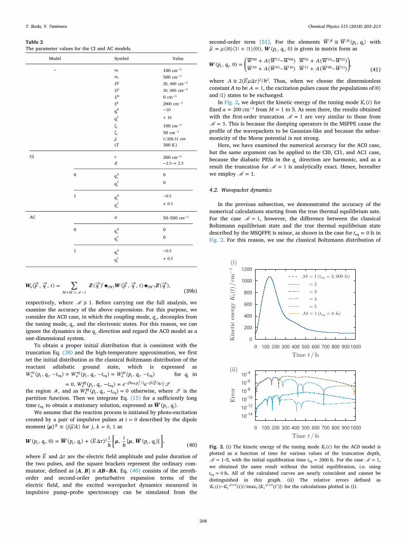
In Fig. 2, we depict the kinetic energy of the tuning mode K t( )t forfixed = −a 200 cm 1 from =M 1 to 5. As seen there, the results obtainedwith the first-order truncation = 1M are very similar to those from= 5M . This is because the damping operators in the MSFPE cause the
profile of the wavepackets to be Gaussian-like and because the anhar-monicity of the Morse potential is not strong.
Here, we have examined the numerical accuracy for the AC0 case,but the same argument can be applied to the CI0, CI1, and AC1 case,because the diabatic PESs in the qc direction are harmonic, and as aresult the truncation for = 1M is analytically exact. Hence, hereafterwe employ = 1M .
4.2. Wavepacket dynamics
In the previous subsection, we demonstrated the accuracy of thenumerical calculations starting from the true thermal equilibrium sate.For the case = 1M , however, the difference between the classicalBoltzmann equilibrium state and the true thermal equilibrium statedescribed by the MSQFPE is minor, as shown in the case for =t 0 fseq inFig. 2. For this reason, we use the classical Boltzmann distribution of
Table 2The parameter values for the CI and AC models.
Model Symbol Value
– ωt 100 −cm 1
ωc 500 −cm 1
D0 20, 000 −cm 1
D1 20, 000 −cm 1
E0 0 −cm 1
E1 2000 −cm 1
qt0 −10
qt1 + 10
ζt 100 −cm 1
ζc 50 −cm 1
β 1/208.51 cm(T 300 K)
CI c 200 −cm 1
d −2.5–+ 2.5
0 qc0 0
qc1 0
1 qc0 −0.5
qc1 + 0.5
AC a 50–500 −cm 1
0 qc0 0
qc1 0
1 qc0 −0.5
qc1 + 0.5
Fig. 2. (i) The kinetic energy of the tuning mode K t( )t for the AC0 model isplotted as a function of time for various values of the truncation depth,= 1M –5, with the initial equilibration time =t 2000 fseq . For the case = 1M ,
we obtained the same result without the initial equilibration, i.e. using=t 0 fseq . All of the calculated curves are nearly coincident and cannot be
distinguished in this graph. (ii) The relative errors defined as− ′=
′=K t K t K t| ( ) ( )|/|max { ( )}|tt t
5t
5M M for the calculations plotted in (i).
T. Ikeda, Y. Tanimura Chemical Physics 515 (2018) 203–213
208

the adiabatic ground state as the initial state. We thus set the initialdistribution for→q in the region R as
→ → = − + + →W p q e( , , 0) 1 ,ee β ω p ω p U q
a(ℏ /2 ℏ /2 ( ))g
t t2 c c
2a
Z (42)
and as → → =W p q( , , 0) 0a otherwise.Fig. 3 illustrates the time evolution of the populations in the excited,
ground reactant, and ground product states, u t u t( ), ( )e 0 , and u t( )1 , withthe CI-minimum distance =d 1.5. For the excited state, the excitedwavepacket is initially in the reactant region on the excited state, andthen the wavepacket arrives at the crossing region at approximately=t 100 fs. Because the excited wavepacket has kinetic energy obtained
from the potential in the direction of the product region at the CI point,most of the population quickly transfers to the product region in theground state.
For the time evolution of u t( )0 , we observe slight oscillatory beha-vior at approximately =t 200 fs, when the wavepackets are in thecrossing region. To analyze this point more closely, we display snap-shots of wavepackets in the ground and excited adiabatic states,→ →F p q t( , , )g and → →F p q t( , , )e , in Fig. 4. Due to the difference between
the stable points for the adiabatic ground and excited states in the di-rection of qc, the wavepacket exhibits vibrational motion in the direc-tion of the coupling mode, qc. As depicted in Fig. 4(ii), the wavepacketcannot be centered at the CI point because of this vibrational motion. Asa result, the population of the reactant also exhibits oscillatory motion,as observed in Fig. 3. Note that the vibrational motions in the couplingmode induce non-adiabatic transitions for the case ≠q qc
0c1, because
the coupling mode also couples to the electronic states. After the os-cillatory motion of the excited state wavepacket in the qc direction andthe motion in the qt direction relax, a small portion of the wavepacket istrapped at the local minimum in the crossing region. This wavepacketslowly relaxes to both the reactant and product regions in the groundstate. By =t 500 fs, illustrated in Fig. 4(iii), has excited wavepacket isrelaxed and has mostly transferred to the product states.
4.3. The lifetime of the adiabatic excited state
We next investigate the lifetime of the adiabatic excited state for theCI and AC models with various values of the diabatic coupling para-meters. We define the lifetime τ e as
∫≡ −−
τ dt u t u tu u t
( ) ( )(0) ( )
,e t e e
e e0f
f
f
(43)
where tf is a sufficiently long time to evaluate the entire de-excitation
Fig. 3. The time evolution of the population in the CI1 model with =d 1.5. Thered, green, and purple curves represent the populations for the excited, groundreactant, and ground product states, u t u t( ), ( )e 0 , and u t( )1 , respectively. Here,the lifetime of the excited population, given in Eq. (43), and the yield, given inEq. (44), are evaluated as =τ 235 fse and =y 0.788p , respectively. (For inter-pretation of the references to colour in this figure legend, the reader is referredto the web version of this article.)
Fig. 4. Snapshots of excited wavepackets in CI1 model with waiting times (i)=t 0 fs, (ii) 250 fs, and (iii) 500 fs. The CI-minimum distance is =d 1.5. The red,
green, and purple curves represent the mean coordinates for the excited, groundreactant, and ground product states, ⟨→ ⟩ ⟨→ ⟩q t q t( ) , ( )e 0, and ⟨→ ⟩q t( ) 1, respectively.The contours of the adiabatic BO PESs for every −1000 cm 1 are represented bythe black curves in the two-dimensional plates. The symbols × and ▵ representthe CI point and the minimum of →U q( )e
a , respectively. Videos of excited wa-vepackets in CI1( = +d 1.5), CI1( = −d 1.5) and AC1( = −a 300 cm 1) models arepresented in Supplemental Information (Available at: http://dx.doi.org/10.17632/w9k8hxd34t.2). (For interpretation of the references to colour in thisfigure legend, the reader is referred to the web version of this article.)
T. Ikeda, Y. Tanimura Chemical Physics 515 (2018) 203–213
209

dynamics. In the following calculations, we set =t 10, 000 fsf .Fig. 5(i) plots τ e as a function of the CI-minimum distance
≡ −d q q ecCI
c,min for the CI model, where qc
CI and q ec
,min are the CI pointand the minimum of the adiabatic excited PES. The lifetime τ e isshortest at =d 0, while it increases with the absolute value of d, be-cause the center of the excited wavepackets is away from the CI pointfor larger d. In the CI1 case, τ e is not symmetric as a function of d,because the diabatic PESs are not symmetric in the qc direction for
≠q qc0
c1. Fig. 5(ii) depicts τ e as a function of the diabatic coupling a in
the AC model. Because the energy gap between the adiabatic groundand excited PESs increases as the diabatic coupling increases, the life-time τ e increases monotonically as a increases. In the case ≠q qc
0c1, the
motion of the coupling mode is excited in the qc direction due to thedifference between the stable points of the PESs. Because of this motion,the BO approximation breaks down. As a result, the lifetimes are shorterin the CI1 and AC1 cases than in the CI0 and AC0 cases.
4.4. The yield
In Fig. 6, we illustrate the relationship between the lifetime τ e andthe yields at the final time, tf , defined as
≡y u t u t( )/ ( ),gp 1f f (44)
using the same parameter values as in the calculations considered inFig. 5.
We observe large yields in the CI0, AC0, and AC1 cases, in ac-cordance with their lifetimes τ e. Note that a short τ e implies that theexcited wavepackets move smoothly across the crossing region whilemaintaining a large momentum in the direction of the product region,
as explained in Section 4.2. The yields yp in the CI0 and AC1 cases aresmaller than in the AC0 case due to the contributions from non-adia-batic transitions in the coupling mode. The similarity between the CI0and AC0 cases indicates that when the adiabatic excited PESs aresmooth and there is no displacement in the coupling mode, and hence=q qc
0c1, the CI does not play an important role. In such cases, the re-
sults of the IC processes via the CI are described by an AC model that ischaracterized by an effectively weak diabatic coupling constant, a.
Contrastingly, the τ e-yp curve in the CI1 case exhibits a bifurcationfor negative and positive d. The yields yp in the case of negative d aresmaller than in the other three cases, while the lifetimes τ e are short.This is because, for negative d, the excited wavepackets first passthrough the crossing region away from the CI point. Then, afterbouncing off of the barrier of the excited PES in the product region andlosing energy due to dissipation, the wavepacket encounters the CIpoint on the way back from the reactant region. Therefore, although thelifetimes for = ±d 1.5 in the CI1 case are similar, ∼τ 250 fse , the yieldin the negative d case is much lower. This indicates that the photo-isomerization process is sensitive to the profiles of the PESs, in parti-cular when the CI plays a significant role.
4.5. Kinetic energy and momentum distribution of the coupling mode
In Fig. 7, we plot the kinetic energy of the coupling mode, K t( )c , as afunction of time for the CI and AC models. In these calculations, weadjusted the diabatic coupling parameters so as to have lifetimes∼τ 200 fse and 300 fs. The parameter sets we used are listed in Table 3.
Fig. 5. (i) The lifetime of the adiabatic excited state τ e as a function of≡ −d q q e
cCI
c,min in the CI0 (the dashed curve) and CI1 (the solid curve) cases,
where qcCI and q e
c,min are the CI point and the minimum of the adiabatic excited
PES. (ii) The lifetime of the adiabatic excited state τ e as a function of the dia-batic coupling a in the AC0 (the dashed curve) and AC1 (the solid curve) cases.
Fig. 6. The yield yp as a function of the lifetime τ e in (i) the CI0 (the dashedcurve) and CI1 (the solid curve) cases and (ii) the AC0 (the dashed curve) andAC1 (the solid curve) cases. Symbol has the same meaning as in Fig. 5 fordifferent d and a.
T. Ikeda, Y. Tanimura Chemical Physics 515 (2018) 203–213
210

In the CI0 cases, the excitation energy and the kinetic energy K t( )t areconverted to K t( )c during the non-adiabatic transition process, andK t( )c reaches the equilibrium value ∼ = −k T/2 104 cmB
1 due to thermalrelaxation. In the AC0 cases, in which the coupling mode qc is in-dependent of the tuning mode qt and the electronic states, K t( )c doesnot change during the non-adiabatic transition process. In the CI1 andAC1 cases, vibrational motion in the coupling mode arises due to thedisplacement between the adiabatic ground and excited PESs,− =q q 1c
1c0 . Because K t( )c is proportional to pc
2, we observe the vibra-tional peaks with frequency = −ω2 1000 cmc
1 that corresponds theperiod of 33.4 fs. Then the vibrational peaks become larger as a functionof time due to the non-adiabatic transitions, and subsequently decreasesdue to the relaxation induced by the environments. The maximumvalue of K t( )c is large for the long lifetime cases in Fig. 7(ii), becausethe wavepackets are trapped in the crossing region and the kineticenergy of the excited state converts to the vibrational energy of thetuning mode, while the wavepackets pass through the crossing regionwithout exciting the coupling mode for the short lifetime cases inFig. 7(i). These results indicate that, the vibrational dynamics of thecoupling mode through the non-adiabatic transition processes are dif-ferent even when the lifetimes of the excited population are similar.
To analyze this point more closely, in Fig. 8, we present snapshots ofthe momentum distributions of the coupling mode as functions of pc andqt in the excited adiabatic state, defined as
∫ ∫≡ → →f p q t dp dq W p q t( , , ) ( , , ),e ec t t c (45)
in the CI0 and AC0 cases at =t 200 fs for ∼τ 200 fse . In the AC0 case,because the coupling mode qc is independent of the electronic states aswell as the tuning mode q f p q t, ( , , )e
t c t exhibits a simple Gaussian-likeshape in the pc direction. Contrastingly, in the CI0 case, f p q t( , , )e
c t hastwo peaks in the positive and negative regions of pc near the crossingregion, due to the role of the CI.
4.6. Electronic coherence
Finally, we investigate the electronic coherence between the adia-batic ground and excited states for the CI and AC models, defined as
∫→ ≡ → → →C q t dp W p q t( , ) ( , , ).eg ega (46)
In order to illustrate the details of the coherent elements of the wave-packets, here we employed a fine mesh, with × = ×N N 256 128t c , al-though we had to use a smaller timestep δt for this smaller mesh, be-cause the information representing the wavepacket propagates faster asthe grid becomes finer. We employed =δt 0.1 fs for these calculations.
In Figs. 9(i) and 9(ii), we display the real parts of the electroniccoherence →C q t( , )eg for the CI0 and AC0 cases at =t 200 fs. The lifetimein each case was adjusted to be ∼τ 200 fse using the values of thediabatic coupling parameters listed in Table 3. In the AC0 case, inwhich the coupling mode qc is independent of the electronic states aswell as the tuning mode qt and →C q t( , )eg , we observe characteristicfeatures only in the qt direction. Contrastingly, in the CI0 case, →C q t( , )eg
exhibits nodes at = =q d 0c , which arise from the qc-dependence of thediabatic coupling. These clear differences between the CI and ACmodels, however, become blurred by the vibrational dynamics in the
Fig. 7. The kinetic energy of the coupling mode K t( )c as a function of t for (i)∼τ 200 fse and (ii) ∼τ 300 fse in the CI0 (the red dashed curve), CI1 (the orange
solid curve), AC0 (the blue dashed curve), and AC1 (the cyan solid curve) cases.In each case, the lifetime was controlled by adjusting the diabatic couplingparameters.
Table 3Parameters values that we used to investigate the time evolution of K t( )c andelectronic coherence →C q t( , )eg .
Lifetime τ e CI0 CI1 AC0 AC1
∼ 200 fs =d 0.0 0.0 =−a/cm 1 100 100∼ 300 fs −1.5 −2.0 220 350
Fig. 8. Snapshots of momentum distributions of the coupling mode as functionsof pc and qt in the excited adiabatic state, f p q t( , , )e
c t , for (i) the CI0 case and(ii) the AC0 case at =t 200 fs. The lifetime in each case was adjusted to be∼τ 200 fse using the diabatic coupling parameters listed in Table 3. The black
dashed lines represent the crossing regions.
T. Ikeda, Y. Tanimura Chemical Physics 515 (2018) 203–213
211
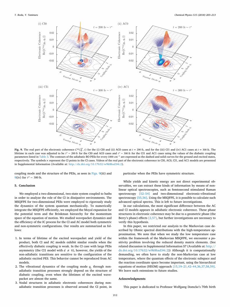
coupling mode and the structure of the PESs, as seen in Figs. 9(iii) and9(iv) for ∼τ 300 fse .
5. Conclusion
We employed a two-dimensional, two-state system coupled to bathsin order to analyze the role of the CI in dissipative environments. TheMSQFPE for two-dimensional PESs were employed to rigorously studythe dynamics of the system quantum mechanically. To numericallyintegrate the MSQFPE efficiently, we employed the Moyal expansion forthe potential term and the Brinkman hierarchy for the momentumspace of the equation of motion. We studied wavepacket dynamics andthe efficiency of the IC process for the CI and AC model both symmetricand non-symmetric configurations. Our results are summarized as fol-lows:
1. In terms of lifetime of the excited wavepacket and yield of theproduct, both CI and AC models exhibit similar results when theeffectively diabatic coupling is weak. In the CI case with large PESsasymmetry (the CI1 model with ≠d 0), however, the yields of thenon-adiabatic transitions are sensitive to the configuration of theadiabatic excited PES. This behavior cannot be reproduced from ACmodels.
2. The vibrational dynamics of the coupling mode qc through non-adiabatic transition processes strongly depend on the structure ofdiabatic coupling, even when the lifetimes of the excited wave-packet are almost the same.
3. Nodal structures in adiabatic electronic coherences during non-adiabatic transition processes is observed around the CI point, in
particular when the PESs have symmetric structure.
While yields and kinetic energy are not direct experimental ob-servables, we can extract these kinds of information by means of non-linear optical spectroscopies, such as femtosecond stimulated Ramanspectroscopy [52–54] and two-dimensional electronic-vibrationalspectroscopy [55,56]. Using the MSQFPE, it is possible to calculate suchadvanced optical spectra. This is left to future investigations.
In our calculations, the most significant difference between the ACand CI models appears in adiabatic electronic coherence. These phasestructures in electronic coherence may be due to a geometric phase (theBerry’s phase) effects [2,57], but further investigations are necessary toverify this hypothesis.
In this paper, we restricted our analysis to the Markovian case de-scribed by Ohmic spectral distributions with the high-temperature ap-proximation. We note that when we study the low temperature casewithin the framework of the Markovian MSQFPE, we encounter a po-sitivity problem involving the reduced density matrix elements. (Seerelated discussion in Supplemental Information S7 (Available at: http://dx.doi.org/10.17632/w9k8hxd34t.2)) Although it is computationallydemanding, we often have to study the non-Markovian case at lowtemperature, where the quantum effects of the electronic subspace andthe reaction coordinate space become important, using the hierarchicalequations of motion (HEOM) approach [15,19–21,42–44,36,37,58,59].We leave such extensions to future studies.
Acknowledgments
This paper is dedicated to Professor Wolfgang Domcke’s 70th birth
Fig. 9. The real part of the electronic coherence →C q t( , )eg for the (i) CI0 and (ii) AC0 cases at =t 200 fs, and for the (iii) CI1 and (iv) AC1 cases at =t 300 fs. Thelifetime in each case was adjusted to be ∼τ 200 fse for the CI0 and AC0 cases and ∼τ 300 fse for the CI1 and AC1 cases using the values of the diabatic couplingparameters listed in Table 3. The contours of the adiabatic BO PESs for every −1000 cm 1 are expressed as the dashed and solid curves for the ground and excited states,respectively. The symbols × represent the CI points in the CI cases. Videos of the real part of the electronic coherence in CI0, AC0, CI1, and AC1 models are presentedin Supplemental Information (Available at: http://dx.doi.org/10.17632/w9k8hxd34t.2).
T. Ikeda, Y. Tanimura Chemical Physics 515 (2018) 203–213
212

anniversary. T. I. is supported by Research Fellowships of the JSPS anda Grant-in-Aid for JSPS Fellows (16J10099). Y. T. is supported by JSPSKAKENHI Grant No. A26248005.
References
[1] W. Domcke, D.R. Yarkony, Conical Intersections: Electronic Structure, Dynamics &Spectroscopy vol. 15, World Scientific, 2004.
[2] W. Domcke, D.R. Yarkony, H. Köppel, Conical Intersections: Theory, Computationand Experiment vol. 17, World Scientific, 2011.
[3] H. Köppel, W. Domcke, L.S. Cederbaum, Adv. Chem. Phys. 57 (1984) 59.[4] W. Domcke, G. Stock, Adv. Chem. Phys. 100 (1997) 1.[5] R. Gonzlez-Luque, M. Garavelli, F. Bernardi, M. Merchn, M.A. Robb, M. Olivucci,
Proc. Natl. Acad. Sci. U.S.A. 97 (2000) 9379.[6] G.A. Worth, L.S. Cederbaum, Annu. Rev. Phys. Chem. 55 (2004) 127.[7] D. Polli, P. Alto, O. Weingart, K.M. Spillane, C. Manzoni, D. Brida, G. Tomasello,
G. Orlandi, P. Kukura, R.A. Mathies, M. Garavelli, G. Cerullo, Nature 467 (2010)440.
[8] P. Hamm, G. Stock, Phys. Rev. Lett. 109 (2012) 173201.[9] Y. Harabuchi, R. Yamamoto, S. Maeda, S. Takeuchi, T. Tahara, T. Taketsugu, J.
Phys. Chem. A 120 (2016) 8804.[10] V.I. Prokhorenko, A. Picchiotti, M. Pola, A.G. Dijkstra, R.J.D. Miller, J. Phys. Chem.
Lett. 7 (2016) 4445.[11] A.G. Dijkstra, V.I. Prokhorenko, J. Chem. Phys. 147 (2017) 064102.[12] M. Kowalewski, B.P. Fingerhut, K.E. Dorfman, K. Bennett, S. Mukamel, Chem. Rev.
117 (2017) 12165.[13] M. Thoss, W.H. Miller, G. Stock, J. Chem. Phys. 112 (2000) 10282.[14] A. Kühl, W. Domcke, J. Chem. Phys. 116 (2002) 263.[15] L. Chen, M.F. Gelin, V.Y. Chernyak, W. Domcke, Y. Zhao, Faraday Discuss. 194
(2016) 61.[16] K. Miyata, Y. Kurashige, K. Watanabe, T. Sugimoto, S. Takahashi, S. Tanaka,
J. Takeya, T. Yanai, Y. Matsumoto, Nat. Chem. 9 (2017) 983.[17] S.J. Cotton, R. Liang, W.H. Miller, J. Chem. Phys. 147 (2017) 064112.[18] Y. Tanimura, S. Mukamel, J. Chem. Phys. 101 (1994) 3049–3061.[19] Y. Tanimura, Y. Maruyama, J. Chem. Phys. 107 (1997) 1779.[20] Y. Maruyama, Y. Tanimura, Chem. Phys. Lett. 292 (1998) 28.[21] T. Ikeda, Y. Tanimura, J. Chem. Phys. 147 (2017) 014102.[22] R. Kapral, G. Ciccotti, J. Chem. Phys. 110 (1999) 8919.[23] K. Ando, M. Santer, J. Chem. Phys. 118 (2003) 10399.[24] G. Hanna, R. Kapral, J. Chem. Phys. 122 (2005) 244505.[25] J.B. Delos, W.R. Thorson, S.K. Knudson, Phys. Rev. A 6 (1972) 709.
[26] J.C. Tully, J. Chem. Phys. 93 (1990) 1061.[27] S. Hammes-Schiffer, J.C. Tully, J. Chem. Phys. 101 (1994) 4657.[28] D.F. Coker, L. Xiao, J. Chem. Phys. 102 (1995) 496.[29] M. Santer, U. Manthe, G. Stock, J. Chem. Phys. 114 (2001) 2001.[30] J.E. Subotnik, A. Jain, B. Landry, A. Petit, W. Ouyang, N. Bellonzi, Annu. Rev. Phys.
Chem. 67 (2016) 387.[31] M. Ben-Nun, T.J. Martnez, J. Chem. Phys. 108 (1998) 7244.[32] M. Ben-Nun, J. Quenneville, T.J. Martnez, J. Phys. Chem. A 104 (2000) 5161.[33] D.V. Makhov, W.J. Glover, T.J. Martinez, D.V. Shalashilin, J. Chem. Phys. 141
(2014) 054110.[34] B. Balzer, S. Hahn, G. Stock, Chem. Phys. Lett. 379 (2003) 351.[35] K. Anatole, Z. Karol, J. Opt. B 6 (2004) 396.[36] A. Kato, Y. Tanimura, J. Phys. Chem. B 117 (2013) 13132.[37] A. Sakurai, Y. Tanimura, New J. Phys. 16 (2014) 015002.[38] R. Cabrera, D.I. Bondar, K. Jacobs, H.A. Rabitz, Phys. Rev. A 92 (2015) 042122.[39] J.E. Moyal, Math. Proc. Camb. Philos. Soc. 45 (1949) 99.[40] K. İmre, E. Özizmir, M. Rosenbaum, P.F. Zweifel, J. Math. Phys. 8 (1967) 1097.[41] A.O. Caldeira, A.J. Leggett, Physica A 121 (1983) 587.[42] Y. Tanimura, R. Kubo, J. Phys. Soc. Jpn. 58 (1989) 101.[43] Y. Tanimura, J. Phys. Soc. Jpn. 75 (2006) 082001.[44] Y. Tanimura, J. Chem. Phys. 142 (2015) 144110.[45] H. Risken, The Fokker-Planck equation vol. 18, Springer-Verlag, Berlin, 1989.[46] T. Ikeda, H. Ito, Y. Tanimura, J. Chem. Phys. 142 (2015) 212421.[47] H. Ito, Y. Tanimura, J. Chem. Phys. 144 (2016) 074201.[48] J.H. Williamson, J. Comput. Phys. 35 (1980) 48.[49] Y.-A. Yan, Chin. J. Chem. Phys. 30 (2017) 277.[50] B. Fornberg, Math. Comput. 51 (1988) 699.[51] S. Mukamel, Principles of Nonlinear Optical Spectroscopy, Oxford University Press,
1999.[52] P. Kukura, D.W. McCamant, R.A. Mathies, Annu. Rev. Phys. Chem. 58 (2007) 461.[53] S. Takeuchi, S. Ruhman, T. Tsuneda, M. Chiba, T. Taketsugu, T. Tahara, Science 322
(2008) 1073.[54] M. Iwamura, H. Watanabe, K. Ishii, S. Takeuchi, T. Tahara, J. Am. Chem. Soc. 133
(2011) 7728.[55] T.A.A. Oliver, N.H.C. Lewis, G.R. Fleming, Proc. Natl. Acad. Sci. U.S.A. 111 (2014)
10061.[56] N.H.C. Lewis, G.R. Fleming, J. Phys. Chem. Lett. 7 (2016) 831.[57] A. Bohm, A. Mostafazadeh, H. Koizumi, Q. Niu, J. Zwanziger, The Geometric Phase
in Quantum Systems: Foundations, Mathematical Concepts, and Applications inMolecular and Condensed Matter Physics, Springer Science & Business Media, 2013.
[58] A. Ishizaki, Y. Tanimura, J. Phys. Soc. Jpn. 74 (2005) 3131.[59] J. Hu, M. Luo, F. Jiang, R.-X. Xu, Y. Yan, J. Chem. Phys. 134 (2011) 244106.
T. Ikeda, Y. Tanimura Chemical Physics 515 (2018) 203–213
213