phase transitions and reflection positivity. i. general

Communications inCommun. math. Phys. 62, 1—34 (1978) Mathematical

Physics© by Springer-Verlag 1978

Phase Transitions and Reflection Positivity. I.General Theory and Long Range Lattice Models

Jίirg Frδhlich1***, Robert Israel2***, Elliot H. Lieb3t, and Barry Simon3**1 Department of Mathematics, Princeton University, Princeton, NJ 08540, USA2 Department of Mathematics, University of British Columbia, Vancouver, B.C., Canada3 Departments of Mathematics and Physics, Princeton University, Princeton, NJ 08540, USA

Abstract. We systematize the study of reflection positivity in statisticalmechanical models, and thereby two techniques in the theory of phasetransitions: the method of infrared bounds and the chessboard method ofestimating contour probabilities in Peierls arguments. We illustrate the ideasby applying them to models with long range interactions in one and twodimensions. Additional applications are discussed in a second paper.

1. Introduction

Among the recent developments in the rigorous theory of phase transitions havebeen the introduction of two powerful techniques motivated in part by ideas fromconstructive quantum field theory: the method of infrared bounds [10, 4] whichprovides the only presently available tool for proving that phase transitions occurin situations where a continuous symmetry is broken, and the chessboard estimatemethod of estimating contour probabilities in a Peierls' argument [14, 9]. This isthe first of three papers systematizing, extending and applying these methods. Inthis paper, we present the general theory and illustrate it by considering phasetransitions in one and two dimensional models with long range interactions. In II,[7], we will consider a large number of applications to lattice models and in III,[8] some continuous models including Euclidean quantum field theories. Reviewsof some of our ideas and those in [4, 9, 10, 14] can be found in [5, 6, 23, 27, 43]. Anapplication can be found in [19].

Three themes are particularly emphasized in these papers. The first, §§2—4, isthe presentation of a somewhat abstract framework, partly for clarification (e.g.

* Present address: Institute des Hautes Etudes Scientifiques, 35, Route de Chartres, F-91440 Bures-sur-Yvette, France** Research partially supported by US National Science Foundation under Grant MPS-75-11864*** Research partially supported by Canadian National Research Council under Grant A4015f Research partially supported by US National Science Foundation under Grant MCS-75-21684-A01

0010-3616/78/0062/0001/S06.80

2 J. Frόhhch et al.

the tricks in [4] to handle the quantum antiferromagnet may appear more naturalin the light of §§2, 3 below) but mainly for the extensions of the theory therebysuggested (e.g. the second theme below and the use, for classical systems, ofreflections in planes containing sites: this idea, occurring already in [9], will becritical for many of our applications, e.g. to the classical antiferromagnets inexternal field). The abstract framework also clarifies various limitations of thetheory such as its present inapplicability to the quantum Heisenberg ferromagnetsand its restriction to reflections in planes between lattice planes for quantumsystems. The second theme is the extension of the methods beyond the nearestneighbor simple cubic models emphasized in [10, 4, 9]. It will turn out (§3) thatrather few additional short range interactions can be accomodated but that alarger variety of long range interactions can be treated. This extension will allowus (§5) to recover and extend to suitable quantum models the results of Dyson [3](resp. Kunz-Pfister [26]) on long range one (resp. two) dimensional systems. It willalso allow us (see II) to discuss a number of lattice Coulomb gases: for example, a"hard core model" where each site can have charge 0, +1 or — I will have two"crystal phases" for sufficiently low temperatures and large fugacity and, forsufficiently low temperatures and suitable fugacity, a third phase which can bethought of as a "plasma" or "gas" phase. Finally it will allow us to construct (seeIII) a two dimensional quantum field theory (a φ4 perturbation of a generalizedfree field) with a spontaneously broken continuous symmetry.

For pair interactions, Hegerfeldt and Nappi [18] have proposed our sufficientcondition for reflection positivity but they did not discuss the connection withphase transitions or the quantum case see also their footnote on p. 4 of theirpaper.

The final theme involves the development of an idea in [10, 5] for proving thatphase transitions occur in a situation where there is no symmetry broken and thusno a priori clear value of external field or fugacity for the multiple phase point. Inall cases, the value can be computed for zero-temperature and one shows thatthere are multiple phases at some nearby value for low temperature, although ourmethods do not appear to specify the value by any computationally explicitprocedure. This technique, which we do not discuss until Paper II, allows us inparticular to recover some results of Pirogov-Sinai [33-35] including the occur-rence of transitions in the triangle model (ordinary Ising ferromagnet in externalfield but with an additional interaction K^σίθjσk over all triples ijk where i and kare nearest neighbors of j in orthogonal directions) and the occurrence of threephases in the Fisher stabilized antiferromagnet in suitable magnetic field (ordinaryIsing antiferromagnet but with additional next nearest neighbor ferromagneticcoupling). As another example we mention an analysis of some models of Ginibre,discussed by Kim-Thompson [32] in the mean field approximation, with theproperty that at low temperatures there are an infinite number of external fieldvalues with multiple phases.

Next we want to make some remarks on the limitations, advantages anddisadvantages of the reflection positivity (RP) methods. As regards the chessboardPeierls argument, it is useful to compare it with the most sophisticated Peierls typemethod that we know of, that of Pirogov-Sinai (PS method) [33-35, 20] (acomparison with the "naive" Peierls argument can be found in [27]):

Phase Transitions and Reflection Positivity. I 3

1) The most serious defect in the RP method is that the requirement ofreflection positivity places rather strong restrictions on the interactions, especiallyfor finite range interactions. For example, the PS analysis of the Fisher anti-ferromagnet would not be affected if one added an additional ferromagneticcoupling σfij for pairs ij with /—y' = (8, 10) (for example) while our argument wouldbe destroyed no matter how small the coupling! More significantly, the RPanalysis in this case requires that σ(0 0)σ(1 1} and σ(0 0)cr(1 _ 1} have equal couplingsPS does not. Similarly in the triangle model, an RP argument requires the fourkinds of triangles to have equal couplings while PS does not.

2) RP can handle certain, admittedly special, long range couplings, amongthem interactions of physical interest such as Coulomb monopole and dipolecouplings. PS in its present form is restricted to finite range interactions.

3) Inherent in the PS method is the notion that one is looking at a system witha "finitely degenerate ground state". This is not inherent in the RP method: all thatis important is that a finite number of specific periodic states have a larger internalenergy per unit volume than the true ground states. In some cases, e.g. theantiferromagnet without Fisher stabilization, there is no practical difference sincethe finite number of states of importance in RP are among the infinitely manyground states that prevent the application of PS. However, there is a model (of aliquid crystal) with an infinitely degenerate ground state to which Heilmann andLieb [19] have applied the RP method with success. This model has only twoground states in finite volume with suitable boundary conditions, but infinitelymany ground states in the PS sense in infinite volume.

4) The PS method gives much more detailed information than the RP methodon the manifold of coexisting phases. For example in the Fisher antiferromagnet,there is, for T small, an external field, μ(Γ), near the computable number μ(0), sothat there are three (or more) phases at that value of T and μ. PS obtain continuityof μ(T) in T while RP does not, but shows only that μ(T)—»μ(0) as T^O.

5) While neither PS nor we have tried hard to optimize the lower bounds ontransition temperatures, it seems reasonably clear that RP methods wouldproduce better bounds.

6) PS require the number of values that a given spin takes to be finite. RPmethods effortlessly extend to models like the anisotropic classical Heisenbergmodel (see [9]).

7) PS can only handle classical models, at least in its present version. RPmethods can handle certain quantum models quite efficiently (see [9]).

8) RP works most naturally for states with periodic boundary conditions. Thiscan occasionally be awkward.

9) PS obtain the exact number of phases at the maximum phase points whileRP only yields a lower bound. This difference is probably not intrinsic, and RPmethods could probably be combined with [11] to yield the exact number ofphases.

10) To our, admittedly biased, tastes the RP method seems considerablysimpler than the PS method.

As regards the infrared bounds method, there is no comparable method withwhich to compare it, but we note it is most unfortunate that the only available

4 J. Frohlich et al.

method for proving phase transitions depends so strongly on reflection positivity.We mention two examples to illustrate this remark:

1) In [10], it is proven that the classical Heisenberg ferromagnet with nearestneighbor interaction has a phase transition for a simple cubic lattice. The methodsof §§2-4 easily extend this result to face centered cubic and many other lattices, butnot to the body centered cubic lattice. This remains an open problem.

2) There has been some discussion recently (see [36] and references therein) ofan intriguing model, originally due to Elliott [28], which should have "helical"long range order: consider a one dimensional plane rotor or N-vector, N^3model with nearest neighbor ferromagnet coupling, J, and somewhat strongersecond neighbor antiferromagnet coupling, K. It will have a helical ground state,i.e. in a ground state σ f σί + t =cosO for some ΘΦO, π depending on the exact valueof J/K. Of course, this helical ordering won't persist to finite temperature in theone dimensional case, but if one adds two more dimensions with conventionalnearest neighbor ferromagnetic couplings one expects helical order will persist. Wedo not see how to prove this with RP methods indeed, infrared bounds obtainedby RP methods always seem to blow up at a single p while at least two p's areinvolved here due to the evenness of the function Ep. We note that if one couldprove an infrared bound, helical order would be proven since Ep vanishes atprecisely two p's with a zero of order p2.

Finally, we summarize the contents of the remaining sections. In §2, we presentan abstract framework for reflection positivity and provide the basic perturbationcriteria which allow one to go from reflection positivity for uncoupled spins toreflection positivity for suitably coupled spins. In §3, we specialize to spin systemsand examine two questions: about what kinds of planes does one have reflectionpositivity for the system of uncoupled spins, and what kinds of interactions obeythe basic perturbation criteria of §2? In §4, we review and describe the two basicRP methods of proving phase transitions when one has reflection positivity aboutthe large family of planes obtained by translating a basic family of planes. In §5, wediscuss the applications to recover the Dyson and Kunz-Pfister results alreadymentioned.

2. Abstract Theory of Reflection Positivity

Reflection positivity was introduced in quantum field theory by Osterwalder andSchrader [30] and it has continued to play an important role there. Its significancein the study of phase transitions for lattice gases was realized in [10, 5, 9], althoughwe must emphasize that transfer matrix ideas are intimately connected withreflection positivity. Klein [25] has considered other abstractions in somewhatdifferent contexts.

To understand the framework we are about to describe, it is useful to keep inmind a particular example, describing a chain of Ising spins, that is essentially thatgiven in [10, 9] (we describe the example after the basic framework).

91 will be a real algebra (with unit) of observables. (We note that to say 9J is areal algebra does not preclude 91 from being, say, an algebra of complex valuedfunctions: ς'reaΓ means that we only suppose that one can multiply by realscalars.) Below we will freely use and expand exponentials and use the Trotter-


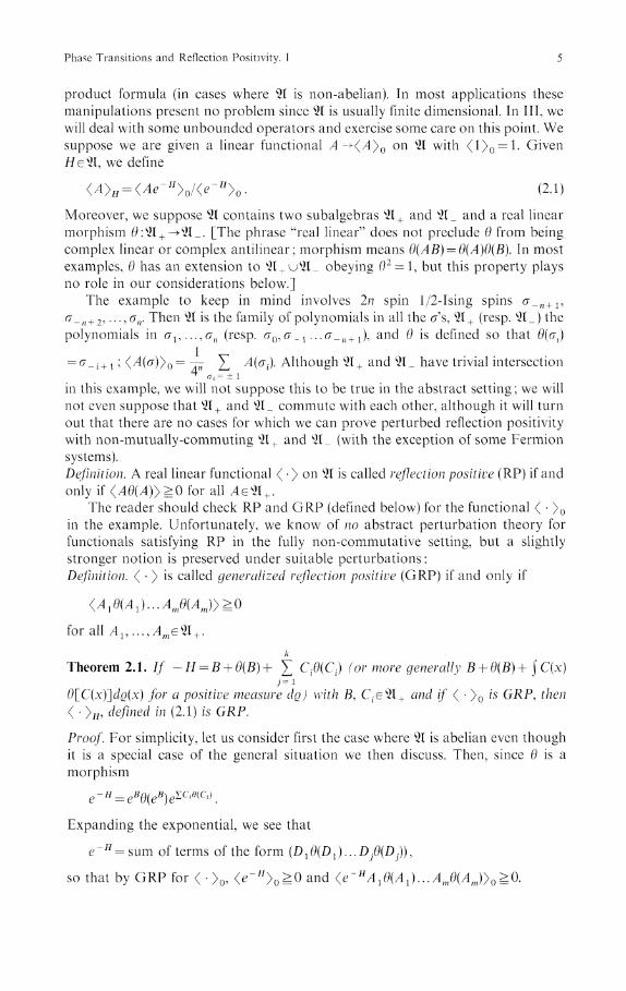
product formula (in cases where 5ί is non-abelian). In most applications thesemanipulations present no problem since 51 is usually finite dimensional. In III, wewill deal with some unbounded operators and exercise some care on this point. Wesuppose we are given a linear functional A -><^>0 on 51 with <1>0 = 1. GivenHE 51, we define

(AyH = (Ae-Hyo/(e~Hyo. (2.1)

Moreover, we suppose 51 contains two subalgebras 51 + and 51 _ and a real linearmorphism 0:S2I+-»21_. [The phrase "real linear" does not preclude Θ from beingcomplex linear or complex antilinear; morphism means θ(AB) = θ(A)θ(B). In mostexamples, Θ has an extension to 5ί+u5I_ obeying Θ2 = \, but this property playsno role in our considerations below.]

The example to keep in mind involves 2n spin 1/2-Ising spins σ_, J + 1 ,ίi_π + 2, . . . ,σ π . Then 51 is the family of polynomials in all the σ's, 51 + (resp. 5ί_) thepolynomials in σ l 5 . . . , σ n (resp. σ0, σ _ l ...σ_n+ 1), and Θ is defined so that θ(σl)

= σ_i+l <^(σ)>0= — £ A(σi). Although 5ί + and 5l_ have trivial intersection4 < τ t = ± l

in this example, we will not suppose this to be true in the abstract setting we willnot even suppose that 51 + and 51 _ commute with each other, although it will turnout that there are no cases for which we can prove perturbed reflection positivitywith non-mutually-commuting 51 + and 51 _ (with the exception of some Fermionsystems).Definition. A real linear functional < > on 51 is called reflection positive (RP) if andonly if <AΘ(>1)>^0 for all ,4e5ί + .

The reader should check RP and GRP (defined below) for the functional < >0

in the example. Unfortunately, we know of no abstract perturbation theory forfunctionals satisfying RP in the fully non-commutative setting, but a slightlystronger notion is preserved under suitable perturbations :Definition. < > is called generalized reflection positive (GRP) if and only if

for all X 1 , . . . , A w e 2 I + .

k

Theorem 2.1. // -H = B + Θ(B}+ £ C fθ(C f) (or more generally B + Θ(B) + j C(x)7 = 1

0[C(x)~]dρ(x) for a positive measure dρ) with B, C e5l+ and if < >0 is GRP, then< >H, defined in (2.1) is GRP.

Proof. For simplicity, let us consider first the case where 51 is abelian even thoughit is a special case of the general situation we then discuss. Then, since Θ is amorphism

Expanding the exponential, we see that

e~ H =sum of terms of the form (Dlθ(D})...Djθ(D^),

so that by GRP for < >0, <e-J/>0^


For the general non-abelian case, we first use the Trotter product formula towrite

H= limg iί — ht-r, Λ u/κ,£_j/^.o/κ.\ i i ^lΌ\^l)iK.kΓT ^C.Θ

fc->oe

and then expand to get e~H as a limit of sums of π[_Djθ(D •}]. DIn the next section, we will give a relevant example (Example 6) of a situation

with < >0 RP but not GRP. There is one case where RP implies GRP (this, in fact,is the only case for which we know how to prove GRP!):

Theorem 2.2. // 91+ and 91 _ commute with each other, a linear functional is RP ifand only if it is GRP.

Proof. πAiθ(Ai) = (πAi)θ(πAί) since the Aj and θ(Aί) commute and θ is amorphism. D

We will also need:

Theorem 2.3. // 91+ and 91 _ commute with each other and if < >0 is RP, then forany A, B, C , D e91 + :

B + ΘB+ΣDlθ(Dl)\

Proof. For simplicity of notation we suppose that 91 is abelian. The general casefollows by using the Trotter formula as in the proof of Theorem 2.1. Since < >0 isRP, we have a Schwarz inequality \(AθByo

2 ^(AΘAyo(BθByo and so (here weuse that 91+ and 91 _ commute)

\(Alθ(Bί)...AjO(Bj)\\2

^(Alθ(Aί)...Ajθ(Aj)yo(Blθ(Bl)...Bjθ(Bj)yo. (2.2)

Now

so expanding the sums we can write it as sum of terms of the formEίθ(Fί)...Elθ(Fl). Using (2.2), we see that

K«>ol ̂ Σ

so using the Schwarz inequality for sums

K*>ol 2 ̂ E <nEiθ(Ei)yo] [Σ <πFίθ(Fί)>0] -

We can now resum the exponential and so obtain the desired result. D

Remarks. Notice that only (2.2) was needed to obtain the result, so we could haveparalleled the discussion of GRP and given (2.2) a name. We only know how toprove (2.2) when 91+ and 91 _ commute.

The theorems in this section are only mild abstractions of ideas in [10, 4]. Infact, [4] already noted the importance of inequalities like those in Theorem 2.3and of Hamiltonians of the form singled out in Theorem 2.1.

Remark. Independently, Osterwalder and Seiler have discussed RP for EuclideanFermi lattice field theories [31] using ideas similar to ours.


There is a generalization of Theorem 2.3, which, while it will not be used in thesequel, is potentially of interest.

Theorem 2.4. // 21 + and 21 _ commute with each other and < >0 is RP, then for any

el

Proof. The same as for Theorem 2.3. One merely has to notice that the first term(namely 1) in the expansion of the exponential cancels. D

Remark. Theorem 2.3 is a Corollary of Theorem 2.4. Merely add(λ~lA + λ)x(λ~lθB + λ) to the exponential in Theorem 2.4 and then let Λ->OG.

3. Reflections in a Single Plane

In this section, we consider the case where 21 is an algebra of observables for aclassical or quantum spin system on a lattice, < >0 is an uncoupled expectationand θ is a reflection in a plane. We concentrate on two distinct questions which areconnected with our discussion in the last section: a) When is < >0 RP and/orGRP? b) What interactions lead to a Hamiltonian with -H = B + ΘB+ XQ0Q?We discuss the first question in a series of examples.

1) Reflections in a Plane Without Sites-Classical Case

We imagine the finite lattice A (which may be a torus) being divided by a plane πinto two subsets Λ+ (to the "right" of π) and A_, with no sites on π. There is some"reflection" r on A such that r takes A+ into A_ and r2 = 1. The "spin" at each siteis a random variable taking values in a compact set K with some "a priori" Borelprobability distribution dρ. Let KΛ= [\Kt and K+ = [| Kt (where each Kt is a

copy of K). For xeK_, define Θ^K+ by (θ^x^x^. We take 21 to be allreal-valued continuous functions on KΛ with 21 + the subalgebras of functionsdepending only on the spins in A±. Define θ : 21+->2I_ by

Finally, we let <F>0= J F(x)[\dρ(xi). Then < >0 is RP sinceKΛ ίeΛ

F(x) Π Φίe/U

Since S2ί is abelian, < >0 is GRP. This example includes the kind of classical systemin [10]. Alternatively, we could allow 21, $1+ to be complex valued and then define


2) Reflections in a Plane Without Sites-" Real" Quantum Case

The setup is very similar to 1) but now for each IE A, we take a copy ̂ of IRm withthe natural inner product. One defines .$? =- (X) ̂ i and #?_ (resp. Jf+) as the tensor

te/l

product of the spaces associated with sites in Λ_ (resp. Λ + ). 91 is now all matriceson ̂ and <A>0=Tr^(/l)/Tr^(l). 91 + (resp. 9Ϊ_) consists of all operators of theform I® A (resp. A® I] under the tensor decomposition .^ = ̂ _®^+. Finallyθ(l®A} = A®\. Then for B = l®A

since Ίΐ(A) is real Thus < >0 is RP and, since 91 + and 91 _ commute, GRP. This

example includes the quantum xy model [4] in the realization σx =

σy = (n A Alternatively, we could take Jf. = (Γm and θ(l®A) = Ά®l where "is

complex conjugation.

3) Reflections in a Plane Without Sites-General Quantum Case

This is identical to the setup in (2) except for the fact that J^ is a copy of (Γm. If wetake θ(i®A) = A® I, then < >0 is not RP since Ύr(A) may not be real. Indeed if 91and θ are chosen in some other way so that Tr is GRP, then the ferromagneticHeisenberg Hamiltonian will not be expressible as —H = B + ΘB+ ^C^C , sinceTr(σ1 σ0)

3 <0, while (σ1 σ0)3 is a sum of AlΘAl ...A3ΘA3. Of course, if one takes

01(1®A) = A®1 where ~ is ordinary matrix complex conjugation, then for

So one recovers RP and GRP, but the usual Heisenberg ferromagnet is no longerof the form ^C^C-, since σ1 •Θ1σ1 =σ l x σ 0 x + σ l zσ 0 z — σ l y σ 0 v in the usual re-alization of the σ's.

The fact that < >0 is not RP does not stop it from being RP on a subalgebraindeed in the Heisenberg case, for functions of σzs alone, it is RP. It could happenthat for the usual (anisotropic) Heisenberg case, < >H is also RP on thissubalgebra and this would lead to phase transitions in the two dimensionalanisotropic case [9]. However, the failure of full GRP implies that our simpleperturbation scheme of §2 will not yield a proof of this type of restricted RP.

4) Twisted Reflections in a Plane Without Sites

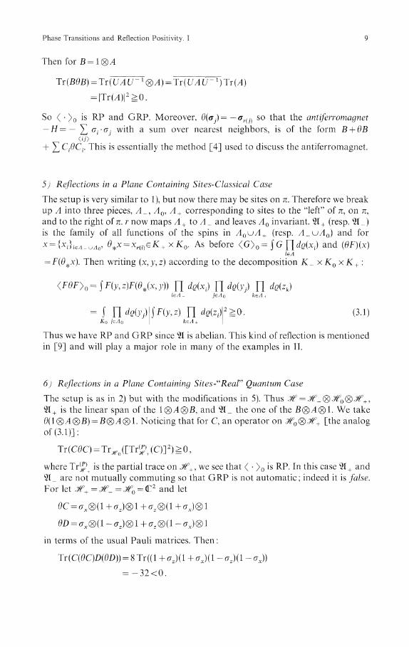
It is sometimes useful to define Θ with a "twist". For example, in the setup of 3),take m = 25+1 and take σx, σ , σz as the usual spin S spins i.e. σz is diagonal andσx±iσy are raising and lowering operators. Thus σx, σz are real and σy is pureimaginary. Let U be the operator on jfL which rotates about the y axis by 180° ateach site. Let

Phase Transitions and Reflection Positivity. I

Then for B =

So < >0 is RP and GRP. Moreover, 0(0^) = ~ σ

r ( j ) so that the antiferromagnet— H= — Σ σί σj with a sum over nearest neighbors, is of the form B + ΘB

<u>+ Σ CβC^ This is essentially the method [4] used to discuss the antiferromagnet.

5} Reflections in a Plane Containing Sites-Classical Case

The setup is very similar to 1), but now there may be sites on π. Therefore we breakup A into three pieces, A_9 /t0, A+ corresponding to sites to the "left" of π, on π,and to the right of π. r now maps A+ to A_ and leaves AQ invariant. 21 + (resp. 21 _)is the family of all functions of the spins in AQuA+ (resp. ΛLu/l 0) and for

* = KWuΛo> θ*x = Xrv>eK+xK0. As before <G>0= f G Π^) and (θF)(x)ieΛ

= F(θ^.x). Then writing (x,y\z) according to the decomposition K_ x K0 x K+ :

=lF(y,z)F(θt(x,y)) Π <*<?(**) Π ^(>'j) Π (̂̂ )ie/l - jeA0 kεΛ 4

= ί Π ^09 Jfί^.z) Π di?(z ;)2^0. (3.1)

Thus we have RP and GRP since 21 is abelian. This kind of reflection is mentionedin [9] and will play a major role in many of the examples in II.

6) Reflections in a Plane Containing Sites- "ReaΓ Quantum Case

The setup is as in 2) but with the modifications in 5). Thus ,̂ = J>f_® Jf0®21+ is the linear span of the 1®A®B, and 2ί_ the one of the β® A® 1. We take0(1®A®B) = B(S)A®1. Noticing that for C, an operator on ̂ 0®^+ [the analogof (3.1)]:

where Tr^ is the partial trace on J f + , we see that < >0 is RP. In this case 21 + and21 _ are not mutually commuting so that GRP is not automatic; indeed it is false.For let Jf+ =JV_ =j^0 = (L2 and let

ΘC = σx®(i + σz)® 1 + σz® (1 + σx)® 1

in terms of the usual Pauli matrices. Then :

= -32<0.


Since this example is not so far from what could arise when expanding realisticspin systems, we conclude that reflections in planes containing sites are not likelyto be permitted for quantum spin systems, even "real" ones.

We summarize the above examples in :

Theorem 3.1. <( >0 is GRP for conventional reflections in planes without sites forclassical and simultaneously real quantum systems and for reflections in planes withsites (lattice planes) for classical systems.

Now we turn to the question of which interactions lead to Hamiltonians of theform

- H = ΘB + B + J C(x)θ[C(x)]dρ(x) . (3.2)

To illustrate the ideas, we will first consider the case of pair interactions in onedimension and then more general cases. The main result is that the interaction hasto be "reflection positive" for (3.2) to hold. The net result of the analysis andTheorem 2.1 is that < >H is RP if and only if the interaction is reflection positive.This is very reminiscent of theorems of Schoenberg [40] (see also [2, 12, 38])relating positive definiteness of e + tF to (conditional) positive definίteness of F, and,indeed, our results can be viewed as a special case of that circle of ideas (seeTheorem 3.5).

We begin with consideration of spins σ _ n + 1 , ...,σn.

Definition. A function (J(/))/> i W1U be called reflection positive if and only if for allpositive integers m and z1? ... ,zwe(C:

X ziZjJ(i+j-l)^0. (3.3)U^i

If we know a priori that J is real-valued [it is by (3.3)] (3.3) need only bechecked for z real. In this case the left side of (3.3) can be viewed as the interactionbetween spins at sites 1, . . . , m with values z1? . . . , zm and the reflections of these spins

at j = \ if the basic interaction is £ J(% — β}σxσβ This explains the name given.'

The following comes from the realization of (3.3) as the condition of solvabilityof the Hamburger moment problem. For the readers ease, we sketch a standardproof ([37]):

Proposition 3.2. Let (J(/'))/>i be a real-valued bounded function. Then (3.3) holds ifand only if

(3.4)- 1

for a positive measure dρ and c g; 0.

Remark. If we interpret Oj~1 as δ^ then cδjί is just the contribution of a δ(λ] pieceof dρ. We write it as cδ^ to be explicit.

Proof. If (3.4) holds, theni

i , / ^ l -1


so (3.3) holds. Conversely, if (3.3) holds, form a Hubert space, J^, by starting withfinite sequence (z l5 ...,zm) (arbitrary in) and letting

and then dividing out by z's with <(z),(z)> = 0 and completing. For a finitesequence (z1? . . . , zm), let /I(z1? . . . , zm) = (0, z l 5 . . . , zm) and note that by repeated use ofthe Schwarz inequality :

\\Az\\ ^ \\z\\ ll2\\A2z\\ 1/2 ̂ ||z|| 1 - l'2n\\A2nz\\

But

so, l im| |^ 2 M z| | 1 / 2 n ^l as n->oo. We conclude that ||^z|| rg | |z| |, so ,4 extends to amap of Jf7 to Jf7. Moreover, by a direct calculation (z,Az) = (Az,w). We concludethat A is self-adjoint. Thus for any z

- 1

by the spectral theorem, where O7'"1 =5^. Let z = (l,0, ...) so that (z,AJ'1z) = J(j)and (3.4) holds. D

We want to emphasize two features of (3.4). First JÔ is not required. Secondlyonly the function J(j) = cδji obeys (3.4) and has bounded support.

In order to obtain the simplest result relating (3.2) to (3.3) we consider freeboundary conditions :

Proposition 3.3. Let («/(/))/ >ι be given. For each m, consider spin 1/2 I sing spins,

-Hm(σ)= Σ J(i-J}°i<?j-i,j— —m+ 1

ί<j

Then Hm has the form (3. 2) for every m if and only if J obeys (3.3).

Remark. One half of this theorem is also contained in Hegerfeldt and Nappi [18].

Proof. If J obeys (3.3), then J has a representation (3.4), so that

-Hm(σ) = Bm + ΘBm+ } Cm(λ)θlCm(λ)-]dρ(λ),- 1

m

where Bm= £ J(i-j}σiσj and Cm(λ)= £ λj~1σj. Conversely, suppose thatl < i < j < m m j = l

Hm has the form (3.2). Then C(x)= X μ^σ^ and so J C(x)[ΘC(x)]dρ(x)i = l

= Σ J(i—J)σiσp where, for lîj '^m: J(ί+j— 1)= J μί(x)μj(x)dρ(x) because^ 0 < 1 g i

if F(σ)= Y^Kâ^p then X f j is unique. Thus Σ ziZj1 îj^m

_ ΓΣ and therefore J is reflection positive. D


This proposition is the basic result we present a number of extensions andvariations :

A) In applications, it is useful to know that periodic boundary consitions leadto a state obeying OS positivity. Given m as above, we define for /' = 1, 2, . . . , 2m — 1.

J»(ί)= Σ J(\i + 2km\). (3.5)fc= - oc

The Hamiltonian

-HIΓ= Σ ^(/->>Λ- m + 1 ̂ i < j 5Ξ m

is the Hamiltonian with periodic boundary conditions. If J has the form (3.4), then

Όθ = c[δn + a,2m- J + J [A- ' +;. -t+1λ2ar}(\ - A2T ldρ(x)

so by the above arguments, -H = B + ΘB+ J [C(x)0C(x)]d^ (x) for suitable C's. Wesummarize in :

Proposition 3.4. Under the hypothesis above, if J obeys (3.3), then H^τ has the form(3.2).

B) We could consider reflections about a plane containing a site. Then thei

above arguments imply that J(l) is arbitrary and J(ϊ) = cδi2 4- j λl~2dQ(x) for ί^2.- 1

In particular, in that case, one can have second "linear" neighbor coupling.C) If one considers a multidimensional cubic system and considers reflection

in the plane i x = 1/2, the kind of analysis above shows that what one needs is that

X z^Jί/ ! +Λ - 1, Ϊ2 -72, . . . , iv -Λ) ̂ 0 (3.6)M . / i ^ i

which leads to the requirement that for il ̂ 1

where c iv is a positive definite function on Zv 1 and dρ obeys a similarcondition. In particular, if

J(i) = α if i^ + . - . + liJ^l

= /? if μ ι |2 + ... + |ίv|

2 = 2,

= 0 otherwise

(i.e. nearest neighbor coupling α, next nearest /?), then one will have RP about anyplane bisecting a nearest neighbor bond as long as

(3.7)

In particular, β can be negative. The case β = — α/2(v — 1) is of some subtlety and is

discussed in detail in Paper II. To check (3.7) is equivalent to RP, we note that the


function c, which has to be positive definite on ZΓ"1, has a Fourier transformv- 1

pj so that the infimum occurs at Py = 0 (all 7) if β^O and at

D) Some clarity is obtained by considering a lattice gas in a very generallanguage, i.e. by allowing multi-particle interactions. We will not explicitly useTheorem 2.1, and the connection with Schoenberg's work on conditionallypositive definite functions will be manifest.

At each sitejeZΓ we are given a copy K of some configuration space K and afixed probability measure dρ(xj) on K Xj denotes a point in K . (For themathematically inclined reader we remark that K is assumed to be a compactHausdorff space, and dρ is chosen to be a regular Borel measure. In fact all ourspaces, resp. measures will have these properties.)

It helps one's intuition to imagine that K is the two point set {1, — 1), and dρthe measure assigning probability \ to 1 and — 1. This will correspond to Isingmodels (see also Corollary 3.6, below).

Given a subset XζZv, we define

(Since K is a compact Hausdorff space, so is Kx, for all X ζ Zv.)To each bounded subset AC%V there corresponds a finite system in A with

configuration space KΛ, an algebra of "observables" C(KΛ\ and whose states arethe probability measures on KΛ. [These are precisely the continuous, normalized,positive linear functionals on C(KΛ)J]

We denote by tr the expectation on C(X°°) given by the product measureY\ dρ(Xj). Clearly tr defines a state of the finite system in A, denoted tr^, by

restriction to C(KΛ).The dynamics of such systems is given in terms of an interaction, Φ. This is a

map from bounded subsets X C%v to C(X°°) with the properties that

(3.8)

and

Q9 (3.9)

for all Y with YπX Φ 0 x = {xj} /ez v.Condition (3.9) is not loss of generality: given an arbitrary interaction Φ

satisfying (3.8), one can always find a physically equivalent interaction Φ obeying(3.8) and (3.9)1

The Hamilton function of a finite system in A with interaction Φ is given by


and the Gibbs equilibrium state with boundary condition ρ^εL1 lKA, |~[ dρ(Xj)\

describing the interactions of the system in A with its complement in Λc (recall theDobrushin-Lanford-Ruelle equations [39,22]), is given by

,J = Z;HrΛFe-H*ρ,J, (3.10)

for arbitrary FeC(KΛ). Here

We now consider a decomposition of Zv into two disjoint sublattices Γ+,Γ_(generally separated by a hyperplane) r is the reflection taking Γ_ to Γ+ and Q^the obvious reflection map from KΓ~ to KΓ * . For FeC(KΓ + \ we set

where x± = {xj}jeΓ± we set /L ± =/lnΓ ± , and if Λ+=rA_ we say that A isreflection symmetric (RS).

Our previous notion of RP is equivalent to

<FΘF>(Φ,ρe Ί y l)^0, (3.11)

for all FεCCR?1*). In this case <->(Φ,ρ?J is said to be RP.We say that a b.c. ρ?yl satisfies RP iff tτΛ(FΘFρ?Λ)^0, (3.12)

for all FeC(KΛ^).Clearly there are b.c. ρdΛ which are not RP, but there are also plenty of b.c.

which are /e.g. ρdΛ = £ GkΘGk, Gke C(KA > ) for all k] Ik

Remark. Consider two b.c. ρeΛ and ρ'dΛ such that

If QdΛ and ρ^Ίyl are RP then so is

by Schur's theorem.From now on we shall always assume that Φ is reflection covariant, i.e.

(3.14)

for arbitrary X C Γ+ .Our aim is to state and prove a necessary and sufficient condition on an

interaction Φ such that < — > (Φ, ρdΛ) is RP, for all RP b.c. ρdΛ and all bounded, RSregions A.

We call an interaction CRN (for "conditionally reflection negative") if and onlyif

X tr(FΘFΦ(X))^0, (3.15)Φ 0

Yfor all FeC(KY\ with Y an arbitrary bounded subset of Γ+, obeying tr(F) = 0.


We call an interaction Φ RN (for "reflection negative") if and only if

X tr(FΘFΘ(X))^0, (3.16)XnΓ± Φ 0

for all FeC(KY) and for arbitrary, bounded YcΓ+.Let diamX = max{|i— j\ :ίJeX}, letX + α denote the translate oϊX by a vector

αeZv, and let τα denote the natural isomorphism from C(KX] to C(Kx + a), forarbitrary^, i.e. {τa} are the translations. Finally, let || || denote the supnorm on

Theorem 3.5. 1) The Gibbs state < — > (βΦ, ρdΛ) is RP, for all inverse temperaturesβ^O, all RP b.c. ρdΛ and all RS regions A if and only if Φ is CRN.

2) Suppose an interaction Φ fulfills (3.9) and has the property that

sup{||ΦpO|| :diamAΓ^r}-»0, (3.17)

as r— »GG (this condition is fulfilled if Φ obeys any reasonable condition ofΐhermodynamic stability!) Then Φ is CRN if and only if Φ is RN.

3) // Φ is RN and A some RS bounded set then

Σ φ(x)XnΛ± Φ 0

is a weak limit of functions of the form

where G£εC(KΛ + ), for all k. An analogous statement holds for RP b.c. ρdΛ.

Remarks. 1) The class of (C)RN interactions Φ forms a convex cone. An analogousstatement holds for RP b.c. By (3.13), the convex cone of RP b.c. is multiplicative.Furthermore, note that RP is stable under taking the thermodynamic limit A\TΓthrough a sequence of RS regions A, with RP b.c. ρdΛ.

These facts and Theorem 3.5 represent a rather complete, mathematicalcharacterization of RP Gibbs states in the classical case see also Corollary 3.6.

2) Generally, CRN interactions and periodic b.c. lead to RP Gibbs states (seealso Proposition 3.4). If Φ obeys (3.17) and the periodic Gibbs states are RP, for allbounded hyper cubes A, then Φ must be RN.

Clearly, periodic b.c. lead to translation invariance, so that A is RS with respectto many different pairs of hyperplanes, and — if Φ(X + a) = τa(Φ(X)} (translationinvariance) — the Gibbs state is translation invariant. For these reasons translationinvariant Φ's and periodic b.c. play an (annoyingly) important role in our theory.

Proof of Theorem 3.5. 1) First we choose ρdΛ = l. This b.c. is clearly RP. In thiscase, the Gibbs state < - > (βΦ, 1) is RP if and only if

XCΛϊ Γ + Φ O

has the property


for all FeC(KΛ + ). This follows easily from (3.14) and the definition of the Gibbsstate. If Rβ®(x +, x _) denotes the integral kernel of R^φ the above inequality takesthe form

ί Π dQ(x]}dQ(yj}F(x + )F(y + )Rf(x + , θ ί f y + )^ (3.18)

for allFEC(KΛ<).Assuming that (3.18) holds for arbitrary RS regions A and all β^O and using a

straight forward extension of Schoenberg's theorem [38] (Theorem XIII. 52) weconclude that Φ must be CRN, i.e.

for all FeC(KΛ + ) with tr(F) = 0 and arbitrary, bounded A + CΓ+. [Here we haveused (3.9) to include regions X f /I in the summation. We recall that Schoenberg'stheorem says that a matrix (btj) has the property that (eβblj) is positive definite forall β^O if and only if £χ.z;.bfj.^0 for all z's with Σzf = 0.] This proves onedirection of Theorem 3.5(1). Conversely suppose now that Φ is CRN. Then

£ tr(F0FΦpO)^0, for all FεC(KΛ + ) with tr(F) = 0, for any RS region A.X n Γ i Φ 0

Now fix some RS, bounded A. By (3.9), it follows that

Σ iΐ(FΘFΦ(X))= X irΛ(FΘFΦ(X))^ΰ,X n Λ ± Φ 0 X n / l i Φ O

XCΛ

for all FGC(KΛ + ) with trΛ(F) = 0. If we write this out as an integral and useSchoenberg's theorem in the other direction we immediately conclude that

^ΦOx + ,6^}' + ) is a positive definite kernel.Next, if ρdΛ is RP then the kernel of ρdΛ, QdΛ(x + ,θ^y + ) is positive definite. By

Schur's theorem, Rβ^(x + ,θ^y + )ρdΛ(x + ,θ^y + ) is positive definite, so that

J Πye/1 4

for aSince, by condition (3.14), e-βH^ = e~H^ is obviously of the form GΛΘGΛRβ

Λ

φ,with GAeC(KΛ^\ Theorem 3.5.1) is now proven.

2) It is trivial that if Φ is RN then Φ is CRN. Therefore we must only show thatif Φ is CRN and satisfies (3.9) and (3.17) then Φ is RN. For this purpose, letFeC(KY\ for an arbitrary, but hence forth fixed YCΓ+. We define

G = F-τf l(F),


where a is a translation such that Y+αcF + , i.e. GeC(K y u y + α) with Yu Y-hαCΓ + .Clearly lr(G) = tr(F)-tr(τβ(F)) = tr(F)-tr(F) = 0. Hence if Φ is CRN then

X tr(GΘGΦpO)^0, i.e.^nΓ± Φ 0

Σ tr(F0FΦ(χ ))- Σ trίFθτ^FJΦίXΊ))X n Γ ± Φ 0 X ! n Γ ± Φ 0

- Σ tr(τβ(F)0FΦ(Y2))* 2nΓi Φ 0

Φ 0

tr(τβ(F)θτβ(F)Φ(Ϊ3))gO.

By condition (3.9), the only non-vanishing terms in the last three sums on thel.s. of this inequality fulfill the conditions J^ C Yur(Y+α), A ^ C Y + α u r Y andX3C(Y+a)ur(Y-\-a). Moreover XjnΓ+ Φ0, j = 1,2, 3. Applying now condition(3.17) we see that these three sums thend to 0 as a tends to oo in a direction forwhich F+ + 0CF+, for all a of this direction. Thus

± Φ 0

Yfor all FeC(KY). Since Y i s an arbitrary, bounded set in F+, this proves Theorem3.5(2).

3) Let P be an orthogonal projection on L2

+ =L2 IKΛ + , £ dρ(Xj)\. Then the\ JeΛ+ I

distribution kernel of P,P(x + ,y + ), is a weak limit of functions of the form

X !Ffc(x + ) Ψ^) , where Ψk e L2

+ , for all fc ./c

This observation combined with the spectral theorem for negative, (resp. positive)bounded operators and the relation Ψk(Θ^y_) = (ΘΨk)(y_) clearly proves Theorem3.5(3). Π

As an application of this general theory we consider a classical spin systemwith many body interactions. The classical spin at site i is denoted σ , and σx

= Π σt. The expectation tr is chosen such that tr (σx) = 0 and tr (σ|) > 0, for all non-ieX

empty X. The interaction Φ is given by

Φ:X^-Jxσx, (3.19)

where J = {Jx} is a family of real numbers indexed by the bounded subsets of TD .The interaction Φ is translation invariant if Jx + a = Jx, for all αeZv, and reflectioncovariant, see (3.14), if Jx = JrX, for all X CΓ+.

Example, Ising model with multi-spin interactions.

Definition. We say that J is RP if and only if

Σ ZXZγJχurY^> (3'2°)X.YCΛ +

for arbitrary, finite sequences {zx}XcΓ+ of complex numbers.


Corollary 3.6. 1) Let Φ be given by (3.19). Then Φ is CRN if and only if J is RP.2) The family of all RP fs forms a convex, multiplicative cone.

Proof. 1) It is not hard to see that if J is RP then Φ, given by (3.19), is RN, thusCRN. Conversely, if Φ is CRN then, for an arbitrary function F of {σ/}/e Γ + withtr(F) = 0

Σ JXuryt?(Fί7)tr(Fσy)^0. (3.21)x,

~ 1

Now choose F = ̂ zxσx, where zΛ = zxtr(σ|)~1, and {zx}XcΓ+ is a finite sequenceof complex numbers. Then

and

tr (Fσx) = Σ ZY tr (σyσx) - £ zy tr (σynX)tr (σyzjχ) = zxtr (σ2

x) = zx , (3.22)y y

so

χΣr/x.

and, by (3.21) and (3.22), this is non-negative. Since {zx} is arbitrary, it follows thatJ is RP.

2) Convexity is obvious. Given J and J', both RP, we define J" by

Jχ = Jx J'x, for a l l X .

By Schur's theorem Jx is then also RP. ΠRemark. There are plenty of RP J's with the property that JXΦO, for subsets Xcontaining an arbitrarly large number of sites. (As an excercise we recommend thatthe reader construct some explicit examples of this type.) As a largely openproblem we propose to investigate the detailed geometric properties of the cone ofRN interaction within one of the standard Banach spaces of interactions, [39].

Theorem 3.5 and Corollary 3.6 provide a rather satisfactory, general theory ofRP Gibbs states for classical systems. See also [6]. In the quantum case nocomplete characterization of RP Gibbs states is available, yet.

The reader can check that Theorem 3.5/Corollary 3.6 includes results inProposition 3.3 and its consequences via Theorem 2.1 as a special case. Inparticular, the following should be noted. In Proposition 3.3, we assumed that Hhas the form (3.2). This form was chosen so that the Gibbs state < >^H is RP for allβ. If, instead, one starts with the apparently weaker requirement that < yβH is RPfor all β, then Theorem 3.5.3) tells us that H has to be of the form (3.2).

Example. Consider a two-dimensional Ising model with 2, 3, and 4 bodyinteractions. Let

~σ(0,0)σ(l,0)Lσ(i, l

~σ(0,0)σ(l, 1)


Let —H=Σ τα[JX + K7 + LZ] where J, K, L are numbers and τα representsaeΛ

translation by a unit. H will be RN with reflection about the plane i1 = 1/2 ifK2=JL and J, L^O. To see this, note that in this case — H has the form

5 + Θ5+ ΣQflCi, where Cασ ( 1 > 0)σ ( 1 > 1 ) + jβσ ( 1 > 0 ) and hence CΘC = y2X + o>βY

+ /?2Z], and the sum on i is over translations in the plane /\ = 1/2.

4. Chessboard Estimates and Infrared Domination

In this section, we review, systematize and extend the basic methods of [10, 4, 14,9] which are based on the use of RP about a large number of planes. For thisreason, we will have to work with periodic boundary conditions or directly ininfinite volume. We begin by describing "chessboard estimates", then mention theway these can be used in connection with a Peierls argument, and finally discussthe method of infrared bounds.

Theorem 4.1. (Abstract Chessboard Estimates [9] ). Let S210 be a real vector space,let r:2I0-»9I0 be a real linear map with r2 = i and let F(a1, ...,a2n) be a complex-valued multilinear map obeying :

F(al9 . ..,a2n) = F(a29 . . ., a2n, aj (4.1)

and

^F(aί,,..,an,mn,...,m1)F(bί,...,bn,rbn,...,rbί}. (4.2)

Then \\a\\ =\F(a,ra,a, ...,rα)|1/2" is a semi-norm and

\F(aί,...,a2n)\ίf[\\aί\\. (4.3)i= 1

Remarks. 1. In the example of 2n spins on a line, one should think of $ί0 asi n \

functions of a spin ata single site, and F(a 1 , . . . , a2n) = ( Y[ ai + n(at} ) r(α) = a (or\i=-n+l I

a if we take complex valued functions) so that (4.1) is true if periodic boundaryconditions are used and (4.2) is an expression of RP.

2. The statement and proof are patterned on [9]. For a discussion of its fieldtheory forebears see [43]. For applications to Holder's inequality for matrices, see

[6].3. It is a worthwhile exercise to prove this directly for the case 2n = 4, see

[6, 43].4. By (4.2) the F(aί,...,an,ran,...,ral) are either all ^0 or all ^0. We can

suppose the former without loss.

Proof. We first prove (4.3) and then it follows that || || is a semi-norm, since (4.3)implies the triangle inequality. Let α l 9 . . . , f l 2 « ^e giγen and suppose that \\at\\ φO forall i. Let bl, ...,b2n be any 2n elements each of which is either an α or an r(α ). Let

g ( b i 9 . . . 9 b 2 n ) = F(bl9...,b2n) I f[ \\bt\\I i=l


and let g 0=max |g(b-)| as the bt run through the (4n)2n possibilities. Among allchoices with \g(bi)\=g0, pick one with the longest string of the form ai9 r(α ),α , ...,r(c/.) for ϊ ? l 5 . . . , & 2 / . Since (4.1) implies that HK^OII = l l f l i l l > (4.2) shows that gobeys the same Schwarz inequality as F. Thus, iϊ\g(b^ - ,b2n)\=g0, we must havethat |g(b1? . . .,bM, rbπ, ...,rb1)| = 00. If 2/ is not 2π in the above choice, let b\, •• ,b'2n bea cyclic permutation of έ> l r . . . ,έ> 2 π with α , r(c/f), . . .,α ,r(αt) occuring as b'n_p ...,b'nwhere j = n — 1 if2l>n and otherwise j = 2l—l. But then 6 x , . . . , έ>n, rήπ,..., rft t has astring of the form at, r(α f),.. . of length 2/ + 2. It follows that g0 = \g(a^ r(a^ ..., r(at))\for some α t. But such a </ is always 1 so #0 ̂ i. This implies (4.3) if each \\at\\ φO.

If some \\cii\\ =0, we claim that F(ai) = Q. For, if not, let b l 9 ...,b2n be a sequencewith some bj = al so that the longest string av r(α ), ...,r(α.) occurs consistent withF(bj)ή=Q. As above bi,...,b2n must be αt, r(α ), ...,r(a f) so there is acontradiction. Π

Typical of the explicit versions of Theorem 4.1 are the following:

Theorem 4.2. Let Λ be a rectangular subset of TΓ with sides 2nlx ... x 2nγ

(n},...,nv positive integers}. Let <•> be an expectation value for a classical spinsystem which is invariant under translations mod^ (periodic boundary conditions)and which is RP with respect to (untwisted) reflections (modπ-) in all planesperpendicular to coordinate axes running mid-way between neighboring points of A.Then for any functions {Gy}yeΛ:

αe/1 \βεΛ

Proof. Let s#0 be the functions of spins {tfα}αe/1 αι = ι and let

' 2 m

Using the assumed RP and Theorem 4.1, and setting a = Y[ GJΆ2 αv, weobtain α 2 . . . . ,α v

2«ι / 2«ι

Π G > α ) \ ^ Π ( Π Π GM2,...,>M2,....αv;αe/1

Repeating the argument in the other v — 1 directions, (4.4) results. DNow let j be an element of the dual lattice, /I, to A, i.e. j is the center of a unit

cube, Δ contained in A. Let F be a function of the spins in A. We say that FeΣ ifand only if F is only a function of spins at the corners of A .. Given such an F we set

where F(ί) is F for ί=j and for nearest neighbor cubes Δί and zlr, F(0 = θίΓ[F(ί)] withθίr untwisted reflection in the plane separating zl . and Δv. Thus, if 1—7 has all evencomponents, then F(ί) is a translate of F and if i—j has v0 odd components F is atranslate of F reflected in v0 orthogonal planes. The proof of Theorem 4.2 extendsto:


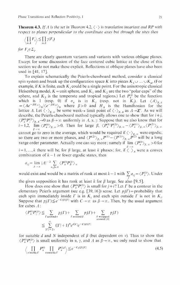
Theorem 4.3. If A is the set in Theorem 4.2, < > is translation invariant and RP withrespect to planes perpendicular to the coordinate axes but through the sites then

for F.eΣ,

There are clearly quantum variants and variants with various oblique planes.Except for some discussion of the face centered cubic lattice at the close of thissection we do not make these explicit. Reflections at oblique planes have also beenused in [41, 17].

To explain schematically the Peierls-chessboard method, consider a classicalspin system and break up the configuration space K into pieces K l u . . . uKm. (Forexample, if K is finite, each K could be a single point. For the anisotropic classicalHeisenberg model, K = unit sphere, and K1 and K2 are the two "polar caps" of thesphere, and K3 is the temperate and tropical regions.) Let P(i} be the functionwhich is 1 (resp. 0) if σα is in Kj (resp. not in K.). Let <^4>^ Λ

= (Ae~βIίΛyo/(e~βHΛyo where β>0 and HΛ is the Hamiltonian for trielattice A. Let < >yβ ^ be some weak-* limit point of < yβ Λ as Λ-+TD '. As we willdescribe, the Peierls-chessboard method typically allows one to show that for / Φj,(P(*]P(j}yβ Λ-^Q as β-ôo uniformly in A, α, y. Suppose that we also know that for

i = l,2,' lim<P^> / ? o o>0. Then for large β <P^Pf]yβ^-<P(^yβ^<P^yβ^/?-»oocannot go to zero in the average, which would be required if < >^ ̂ were ergodic,so there are two or more phases, and <P(2)>/j>ocP

(1)-<ί>(1)>/j?00^>(2) will be a long

range order parameter. Actually one can say more namely if lim (P(ί]yβ >0 for/ j > o c - / j ? 0 0

( ί ]

β->oo

z = l, . . . , / c there will be, for β large, at least k phases; for, if <( >yl were a convexcombination of k — 1 or fewer ergodic states, then

Λ-+CC oc,βeΛ

would exist and would be a matrix of rank at most k — 1 with Σ aίj = (Py^ Underj

the given supposition it has rank at least k for β large. See also [9,5].How does one show that (P(

y

l}P(j}y is small f o r j ' Φ f ? Let Γ be a contour in theelementary Peierls argument (see e.g. [39,16]) sense. Let pi (Γ) = probability thateach spin immediately inside Γ is in Kί and each spin outside Γ is not in Kt.Suppose that p f(Γ)ê~C(/ϊ) |Γ | with C->oc as β-+cc. Then, by the usual argumentfor cubes A :

<pί;>p</>>^ X p.(r)+ Σ Pt(n+ Σ Pi(nΓaroundα Γ around β /wrapped

around \Λ\

^ Σ (|Γ| + i)ViΓ^-C(/?)iΓι|Γ| = 2v

for suitable d and N independent of β (but dependent on v). Thus to show thatis small uniformly in α, 7, and A as β^^, we only need to show that

Π pΐ Π P^ê-^^l (4.5)αins ideΓ αouts ideΓ


for any choice of the jα's (all distinct from i), for then

Finally (4.5) is proven by using chessboard estimates, either directly in the form ofTheorem 4.2 or an extended form of Theorem 4.2 which exploits a two site basicelement. The net result is that the left side of (4.5) is dominated by the product of\Λ\ terms (or in the two site picture of \Λ\/2 terms) most of which are 1. But 0(|Γ|) ofthem are of the form / = /Π p^Λ1^! where α^/cα is a function that has to be

worked out in each case. Typically / can be easily estimated to be small byenergetic considerations. See [14, 9, 5, 19] and Paper II for explicit examples.

Of course, that leaves the questions of showing that

lim <Pj(

/)>yl = ̂ >0 for several Γs .β^cc

We discuss this in detail in Paper II, but note that this often follows fromsymmetry, or by applying the chessboard estimate to obtain an upper bound on

Σ p(a]\Λ = π which is small> see also P> 5> 19]

Thus far, Peierls-type arguments have not been applicable in cases where aphase transition is accompanied by a spontaneously broken continuous symmetry.The only tool available is that invented in [10] : in the notation of Example 1 of § 3,let σ be a function on K, and let σα be the function σ on the αth copy of K. For Aa cube, let p be in A*, the Fourier dual for A ( = 1st Brillouin zone = dual group toA viewed as a torus) and define

p αY\Λ\ *eΛ

9Λ(P} = (dp°-p>β,Λ

Suppose that one can prove that for

(4.6)

for Ep a function satisfying

(2πΓv j E-ldvp = C0<ao (4.7)I P . I ^ π

i = 1 , . . . , v

and that for β^β0

<σ α

2 >^D>0. (4.8)

Then (following the version of the argument in [4]) for ^>max(j80,^1) whereβ1 =C0/2D, we will have (assuming some regularity on Ep)

0)]>0 (4.9)/ - > o o

since

MΓ1^(P=0) = MΓ1 Σ £»-Mr Σ 0»peΛ* p Φ O

^σ^Λ-lΛΓ1 Σ 1/2/ΪJΪ,, (4.10)


where the first sum is controlled by a Plancherel formula, and the second by (4.6).With minimal regularity assumptions on £,

so (4.9) holds. By an argument of Griffiths (see e.g. [4]), (4.9) implies a first orderphase transition with σα as order parameter.

In certain quantum cases /where £ σα and H do not commuted and, as we

shall see below, for some other than simple, cubic lattices like the face centeredcubic lattices, it is necessary or more convenient to rely not on (4.9) but rather on adirect infinite volume argument which is explained in detail in [5, 6, 4].

We note that sometimes (4.8) follows by a symmetry argument (e.g. in theclassical Heisenberg model) but that in general one can try to use a chessboardargument to show, e.g. that Prob(σ^2D)^l/2 for β^β0.

The only known way of proving (4.6) is via a "Gaussian domination" orrelated estimate : Let K be a compact subset of IRN and let dρ be a measure on K.Let σ(1), ... ,σ(]V) be the coordinate functions on K. Suppose that H has the form

H=- Σ Λcy(σα~σv)2 (each pair counted once)

and define for {/ιαy}αΦy real,

Z(ΛaWexp[-i/? Σ ΛvK-Tr-Λ./ϊ) '\ L Z α * y J/0

where < >0 = j πdρ(σα) as usual. We claim that the two conditions: Jαy = J α _ y

= Jγ-y and

Z(/ιαy)^Z(0) (Gaussian domination) (4.11)

imply (4.6) with

Ep=ίΣ(l-e ί ;"α)Jαo (4.12)^ aeΛ

Before proving this, we note that one point of the Definition (3.5) is that it makesEp independent of A for peΛ*.

Since the argument to go from (4.11) to (4.6) is only a mild extension of that in

[10], we only sketch the details. By translation invariance, —rZ(λhΛy)\λ = 0 = Q so

d2

that (4.11) implies that — τZ(/Jιαy); = 0^0. This is equivalent to:—

Σ •y Φ y

\ ± Σ Wα Φ y


(4.13) only holds apriori for real hΛy but it extends to complex h. Now takehΛy = (eίp'Λ-eίp'y)\Λ\~ίl2 and find that (4.13) implies (4.8) with Ep given by (4.12).We summarize :

Theorem 4.4. The Gaussian domination bound Z(/z )rgZ(0) together withJΰly = JΛ-γto = Jy-Λ,Q implies the infrared bound gΛ(p)^(2βEp)~1 with

We next turn to a detailed investigation of (4.11).

Proposition 4.5. Suppose that Jαy^0. Then it suffices to check (4.11) for hΛy of theform ha-hy.

Proof. Since Jαy^0, Z-»0 as any /ιαy-»oo and thus Z takes its maximum at somefinite point. But dZ/dhΛγ = 0 implies that

for the obvious expectation. Thus, letting /zαΞ<σα>, we see that Jιαy = foα — fcy forthose αy with Jα yφO. Z is independent of the other hxy so we can take hΛy = hΛ — hy

for such (αy) without changing Z; i.e. Z takes its maximum value at a pointhay = h,-hr D

Remark. The proof of Theorem 4.4 only used (4. 1 1) for the special case hay = ha — hy

so that Proposition 4.5 is, at this stage, primarily of academic interest. Indeed,there are Jα? not all non-negative so that (4.11) holds for hxy of the form hΛ — hy, andthus (4.6) holds, even though for such J's, Z-»oo for a suitable choice of hay not ofthe form hy — hy.

It is an important and interesting open question to characterize the fer-romagnetic interactions for which the spin 1/2 Ising model obeys Gaussiandomination. We only have partial results on this question relying on reflectionpositivity. We begin with some examples which delimit the class and, in particular,demonstrate the falseness of the apriori attractive conjecture that Gaussiandomination holds for all ferromagnets :

Example 1. Consider two spins, one σ1 ? with values +1 and the other, σ2 withvalues ±2, all values having equal apriori weight. Then <e~ J ( ( T 2~σ ι~ / ί ) 2> has itsmaximum near h= ±1 as J->oo. This shows that equality of the single spindistributions is essential for Gaussian domination in general (but see Examples 5and 6).

Example 2. Let σ1 = + 1, σ2 = -f 1, then

has its maximum near h = 1 as J—>0. The given distribution for σ2 can be thoughtof as that of an Ising spin in an intense positive magnetic field. The failure of RP inthis case shows that even equality of the magnetic fields at each point is alsoessential for Gaussian domination.

Phase Transitions and Reflection Positivity. 1 25

Example 3. (Mean field model.) This is the most involved but also themost significant of the examples we present. Z(/ι)^Z(0) implies that

^2 1 'Ύ

is positive semi-definite. For a spin 1/2 model withJι« = 0δh,dhβ

L y Φ α

a simple calculation shows that (set Jαα = 0)

M,, = δ,γ (Σ JΛ6] - J,γ - Σ ΛΛ^K - σ4χσ, - σ;)> .\ <5 / <5, λ

Take 77 + 1 spins, σ0, ... ,σ,7 with only J0l φO, all equal to απ. Then

M00 = /1απ ~ αn IV

( 1 " \~^Σσi +const an<d thus, as n-^oo, a coupling,]/Π 1 '

of a Gaussian and a spin 1/2 spin. Thus as n-+cc

1 / 1 "

for finite non-zero, c and d. Thus

M 0 0 = - H - l + 2 c ] / π

is negative for n large and therefore Mα_, is not positive definite for n large.Our next example, while a trivial extension of RP ideas illustrates that

Gaussian domination can hold in some cases where RP fails :

Example 4. Let < > be an expectation for a string of 6π spins with third neighborferromagnetic coupling. Then RP fails both for reflections about the midpoint ofbonds and for reflections on sites. Since Z(/ι) is a product of three nearest neighbor2π-point Z's, Gaussian domination for that case yields it for the case at hand.

Our final three examples show that special features of the J's and/or the singlespin distributions can allow one to prove Gaussian domination without RPand/or translation invariance. We hasten to add that phase transitions will notoccur in Examples 5-7.

Example 5. Suppose that H=^Jyβ(σy — σβ)2 with Jyβ arbitrary positive numbers

and that each single spin measures dρy(σy) equals Fydσy with Fαlog concave and

even, but not necessarily α independent. Since e-H(σ*~h*] Y\F^ is a log concave

α

function of {σα,/ιj, Z(/7α) is log concave in hx by a general theorem (see e.g. [1]).Since cZ/dha = Q, all /ια = 0, by symmetry, log concavity implies that Z(/7a) rg Z(0).

26 J. Frόhhch et al.

Example 6. Suppose that H = J^β(σ^ — σβ)2 with Jaβ arbitrary positive numbers and

that each single spin measure dρα(σα) equals Fadσ^ with Fα positive definite and real(hence even), but not necessarily α independent. Then

Z(Λa) = J e-«('»-».> ft [(j ̂ -̂ (/O^ σ Jα

= j Π dμ(kyt'h' j Π (ί*σαeί)l*<r«)e-H(<τ«)

is positive definite in the /z's since the Fourier transform of a Gaussian is aGaussian. In particular, Z(h7) takes its maximum value at hy = 0 (in essence, theabove calculation is proving that the convolution of positive definite functions ispositive definite).

Example 7. Consider an array of n spin 1/2 ίsing spins, s l 5 . . . ,sn on a line witharbitrary positive, nearest neighbor couplings, Jί2,J2^,... ,/π l. Let T(JJή be thetwo by two matrix

e~l/2Jh2

e-l/2J(2-h)*

e-lί2J(2 + h}2

e-ί/2Jh2

i.e. if we label matrices as ^ + + ~ , then Tf J, h)Λ „ =exp J(σ,—σ^—h}2

\ f l _ + ^--/ \ 2We want to note two critical facts about these matrices: first T(J,0) is positivedefinite and Γ(J,0)~ 1 / 2Γ(J,fc)T(J,0)~ 1 / 2 is a contraction in the norm | |(α,/?) | |= (α2 + /J2)1/2—this is proven in [10]. Secondly, the T(J,0) all commute, arepositive definite and when diagonalized simultaneously their largest eigenvalues

correspond to a common eigenvector—this follows by noting that ^— and

1 / 1\—— are the eigenvectors, and the eigenvalue for the first eigenvector is always1/2 \ ~ / ^largest. Since Z(/? 1 ? . . . ,hn) = Ύr(T(J 12,h2 — h1)... T(Jnl,hί —hn)) we can write

where A{ = T(J{_ lΛ^}l!2T(JiΛ+l,ty112 (where J01 =Jnl) and Bt is a contraction, by

the first fact noted above. Let μ^C),... ,μm(C) be the singular values of an m x mmatrix [eigenvalues of (C*C)1/2 ordered so that μ1 ̂ μ2 ̂ ^0]. An inequalityof Horn [21] (see Corollary II.4.1 of [15]) asserts that

Σμl(Cl...Ck)^ Σμi(Cί)...μi(Ck).i=l i=l

Thus, we have that

Z(hι,...,hn)^ ΣμJ(A1...Bn)ί=l

2

^ Σμί(Al)μί(A2)...μί(A,l)


where we use the fact that μ7 (# ):gl, since Bl is a contraction, in the secondinequality, and use the second noted fact in the equality that follows.

To illustrate the close connection between chessboard estimates and Gaussiandomination, we note :

Theorem 4.6. Let A be a 2n1 x ... x 2nv rectangle in TD . Lei J y., be a given on A so

that the chessboard estimate (Theorem 4.1) holds for (-^Z"1 j <?~H(σα) Y\ dρ(σy)for all dρ in 1RN and y-εΛ

Then the Gaussian domination estimate Z(/?J:gZ(0) holds for arbitrary dρ and, inparticular, gΛ(p)^(2βEp)~1.

Proof. By a limiting argument, we can suppose that dρ(σ) = F(σ}dNσ with F > 0 onall of R*. Then, if we define Gx(σ) = F(σ + hΛ)/F(σ) we have that

where the inequality is a chessboard estimate and the last equality comes fromH(σy - h) = H(σΛ) for constant h. D

Remark. Using the Dobrushin-Lanford-Ruelle equations one can prove Theorem4.6 directly in infinite volume for RP Gibbs states.

The above argument has a defect : it does not obviously extend to the quantumcase.

Fortunately, one can use a version of the original argument given in [10],based on Theorem 2.3 : Namely, in the case of 2n spins, Theorem 2.3 says that

.z(h π Λ_ 1 , . . .AA,...Λ)so that translation invariance and the argument in Theorem 4.1 show thatmax|Z(Jz f)| occurs when all /ι's are equal. Since Z(/1, . . . , h) = Z(0), the maximum isZ(0). As of now, this is the most widely applicable proof of Gaussian dominationwe know of.

We remind the reader that in the quantum case there is one additionalcomplication in that Gaussian domination does not lead to a bound on <σ pσ_ p>but rather on a "Duhamel two point function", (σ p,σ_ p). This problem and itsresolution are discussed in [4], for the case of nearest neighbor interactions. Thepresent generalization is straight forward.


The argument based on Theorem 2.3 has an additional advantage, even in the

classical case. Suppose that H=~Σ Λ-(σα~σ

7)2 +^' where <•>#> is RP and J

2- α Φ •/

obeys (3.3). If Z(h)= ( exp- Lγjy,,(σy-σ.,-ha + h^2 + HΊ ) then, as above,' ' '

Theorem 2.3 implies that Z(/ια)^Z(0), and infrared bounds follow. We summarizewith

Theorem 4.7. Let H have the form of Theorem 4.6 with J RP. Let H = H + H' with

H' RN. Let Z(hα) = <exp(H(σα-hα) + H')>0. Then Z(ΛJ^Z(0) and gΛ(p)^(2βEpΓ1

with Ep depending on Jα,,, as in Theorem 4.4.

Finally, we want to mention a problem (and its resolution) that occurs forcertain special models like the ones on face centered cubic lattices. The infinitevolume lattice is reflection invariant about any plane which is the perpendic-ular bisector of a bond, but any finite volume cutoff will destroy many of thesesymmetries. The resolution is the following : Let < ) denote an infinite volumeexpectation and, given, {/?7}7 e Zv with only finitely many non-zero ή"s, let

0(Λ») = ( exP Σ JαV[(σ, - σ./ - (σy - σ, - hΛ + /ιy)\ \^ α Φ y

If we can show that |#(/2α)| ̂ 1 for all hy, then by following the arguments in [10]one will get infinite volume infrared bounds and therefore long range order. Toprove that |g(/7α) |gl, one need only show that <•> has a kind of RP about each"bond" plane, i.e. that

g(hy)\2^g(h'Λ)gyW) (4.14)

where h'x (resp h'^) is obtained by taking hx on the left (resp. right) side of the planeand reflecting in the plane. Given (4.14) it is not hard to reduce the proof ofθ(hy)\ = 1 1° showing that \g(hy)\l i"1'-*! for a set of /?7

α's constant at hQ on a nice setA. But it is easy to see that \cj(hy)\ ^ec\( A\ for such /?'s. (Instead one can use Theorem4.6 in infinite volume; see e.g. [6]).

We can see two ways of proving (4.14). In cases where correlation inequalitiesare available, one can prove (4.14) for a given plane by taking a suitable sequenceof " + boundary condition states" where the given plane cuts A exactly in half.Since the limit is independent of the sequence, (4.14) holds for the + boundarycondition state. When correlation inequalities are not available, one can at leastprove there are multiple phases for, if not, then all periodic states converge to aunique state which would then obey (4.14). If (σ^ x has a lower bound that isuniform in β one would obtain long range order : a contradiction !

5. Long Range Models

In [3], Dyson showed that a spin 1/2 Ising model with J(n) = (l +|/7|)~α has a phasetransition if 1 <α<2 (α> 1 is needed for sensible thermodynamics), and did not if2 < α. His method works for any classical model with correlation inequalities suchas the plane rotor model [13]. Using similar ideas, Kunz and Pfister [26] treated


the two dimensional plane rotor model with J(n) = (\ + \n\)~\ proving a phasetransition if 2 < α < 4.

In this section, we illustrate the general methods of this paper by recoveringthese results (many more examples are presented in [7, 8]) and extending them inseveral directions: a) cases where correlation inequalities are unknown such as theclassical Heisenberg model can be accomodated b) logarithmic improvements inDyson's conditions are given c) certain quantum models are accomodated.

We give details in the one dimensional classical case and then treat twodimensions and quantum models in a few remarks. When correlation inequalitiesof Griffiths type are available, improvements of our results of the following sort arepossible: If a phase transition is known for an RP J0 which is also positive, it holdsfor any larger J even if the larger J is not RP. We suppose in all cases that£|J(π)|<x.

We begin our analysis with:

Theorem 5.1. Let K be a compact subset of IRA and let do be a measure different

from δ(σ\ invariant under σ-»—σ. Let — βH = β ̂ J(l-j}σί σ j and let

Ep = ]Γ J(π)(l — cosp/?). // 0 ̂ J(n) and J is RP, and if g = §dp/Ep < x, then there isn= 1

a first order phase transition with σ as order parameter, at some sufficiently large,finite β.

Theorem 5.2. Let J(i—j) be RP. Then the classical isotropic Pleisenberg model has afir si order phase transition for β large if and only if g = \dp/Ep< x.

Proofs. The absence of a first order phase transition (asserted in Theorem 5.2) ifg=^c follows from a slight extension of an argument of Mermin [29], so weconcentrate on the existence question. Since g< x, this follows, according to thestrategy of §4, if we show that (σpσ_pypQrioά{c ζl/2βEp and lim (H2)^ α >0. J

being RP implies that ( )pcriodic is RP by Theorems 2.1 and 3.4. The method of §4then yields the infrared bounds. In the case of Theorem 5.2, <|σ|2>x = 1 while in thecase of Theorem 5.1, choose r 0>0 so that j dρ>Q and use a chessboard

estimate to see that <(|σ|^r0))^ ΓJ.->0, as /?—>x. The right side of this chessboardestimate is controlled by noting that RP implies that the ground state with therestriction \σy ^r0 has all spins equal, and then by noting that the energy when all(τy = r is strictly monotone increasing in |r|, since J(n)^0. D

These theorems reduce the study of the long range one dimensional case to thestudy of two questions : 1) When is J RP? 2) When is \E~ldp< x. In studying thefirst question the following is useful:

Definition. A distribution F on IR v \fO} is called OS positive (for Osterwalder-Schrader [30]) if and only if F is continuous and

j F(x - y)g(x)g(y)dxdy ^ 0 (5.1)

for all g e C£(x l > 0) where g(y t , . . . , j\,) = g( — y l, y2,..., vv).


Theorem 5.3. a) // F is an OS positive distribution on Rv then J, defined on{(ni,...,nj\nί>0}by

J(n) = F(nί,... ,n v) nΐ >0,

is RP.b) // J-L and J2 are RP on {nί >0} CZV, then so is J VJ 2

OC

c) // J(n)= J e-nydρ(y), (n^ 1), then J is RP on TL\o

Proof, a) In (5.1), let g approach a sum of delta functions. This shows at once that Jis RP.

b) Follows from the fact (Schur's theorem) that iίa^ and btj are positive definitematrices, so is ctj with cij = a ί j b ί ]

c) A restatement of Proposition 3.2; it also follows from a) and well-knownstructure theorems for OS positive distributions. D

Proposition 5.4. The following functions on TL are RP in the region n ̂ 1 :

a) J(π) = n ~ α , b) J(n) = ( l+n)~ α

for all α>0.oc

Proof, a) J e - M ϊ y ~ 1 r f y = Aα)π~α [use Theorem 5.3c];

b) J e nve vyy ldy = Γ ( a ) ( n + l ) y [use Theorem 5.3c] . Do

As for the second question, we note:

oc

Theorem 5.5. Let Ep= ^ J(n)(\ — cospπ) with J(π)^0.n= 1

X'

a) // Σ n~3J(n)~l < x, then \dpE~ l<oo.

b) // limsup(log]V)"Λί-^oo

ΣnJ(n) \dpEv

l = cc.

Remarks. 1. The condition in a) is slightly weaker than the one that Dyson [3]needs for a phase transition. The condition in b) is slightly weaker than the onethat Dyson [3] needs to prove that there is no phase transition in the I sing modelb) will only imply the absence of continuous symmetry breaking. This is as it mustbe if the n~2 ίsing model has a phase transition (as is believed), since J(n) = n~2

obeys the conditions of b).2. b) includes the case J(n) = n~2. This case can be done by explicit calculation

of E (contained in the tables, e.g. (516) of [24]) or by noting that E =/(0)-/(p)X j

with f(p)= Σn~2cospn obeying f"(p) = πδ(p)— with periodic boundary condi-i 2

tions at +π. One sees that E(p)^\p\ in that case.3. If J(/?)~/7~α at infinity, we are in case (a) if α<2 and in case b) if α^2.

Actually with regard to a) one cannot improve even logs, since for J(n)


~n 2(log7i)...(logmft)1 + ε, then Ep~\p\(logp) ...(log^)1"*"8. For b), improvementsare presumably possible: with little change (logN)"1 can be replaced by[(log]Y)(log2)(N)...logm(7V)]-1 which allows only 7t- 2(log 2π)...(logmn) 1 + ε .

1 oo

4. If J(n)= J λ\n\~ldρ, then Ep= £ J(n)(l —cospn) increases when dg- 1 n = 1

increases.This remark allows one to obtain results for J's which are RP but not positive

from those in this theorem.cc

Proof, a) We need a lower bound on Ep=^J(n)(\ — cosnp). For |x| rgπ, (1 — cosx)i

2^ -^-x2 so that

£» = Σ ~ ~ ? p 2 n 2 J ( n ) ,1 i π

where [x] = greatest integer less than x. Thus we need only show that

\ni\p\] -1

Σ P2n2J(n)i

By the Schwarz inequality

/fπ/p]

[π/p]2 =

^ Σ «2 ̂ (») Σ (":

so that

4 π [π/p]

^-τί^p Σ ("o i

since n2[n]~2^([n] + l)2[n]~2^4 for n ^ l and π/p^l for O^p^π. Finally wenote that

\ dp Σ0 1

^ Σ (n2J(n)Γl ίn = 1 0

b) We need an upper bound on E . Since (1 — cosx)^|x| we have that

32 J. Frδhhch et al.

for any N. To estimate the second term, let K(j)= ΣnJ(n) so thati

M

77—1

Thus, if — KYM)->0 as M->x, we have thatM

If K(π)rgClog/7, we see that

Ep ^ C\p\ logJV + CN~ 1 logN .

Choosing JV = [|pΓ1], we see that E^CΊplClogdpΓ1)), so that \Ep

ldp= x, DBy combining the previous results of this section we conclude that

Theorem 5.6. // dρή=δ(p) is a measure on IRN symmetric under σ-+ — σ andJ(n) = n~*, then there is a first order phase transition for the one dimensional spinmodel when l<α<2.

Remark. If N = 1 (or if dρ is anisotropic in a suitable sense) but dρ is not even, therewill be a phase transition in suitable external magnetic field when 1 < α < 2 see[10] or [7].

We describe the extensions in a series of remarks :A) In two dimensions, the functions p*"1 have OS positive Fourier transforms

for α> — 1. This follows from

and the fact that (p2 +m2)' 1 has an OS positive Fourier transform (free Euclideanfield [30, 42]). Since x~β (0</3<2) has a Fourier transform cβp

2~β, we see that77 1 "^ is RP for 0<β<2 by Theorem 5.3a). Then by Theorem 5.3b), we conclude

that \n\~β is RP for all /?>0. Calculations similar to those above show that in 2

dimensions, §dp/Ep<cc if ^ 77~ 6 J(77)~ 1 <oc and for J(/7) = /t~ 4 , an explicit

calculation involving periodic Green's functions for —A [and the fact thatzl(r - 2)-r~ 4 at x] shows that Ep ̂ p 2 logp + 0(p2) at p = 0, so Jrfp/£ p =x in thatcase. We thus obtain :

Theorem 5.7. // dρ^6(p) is a measure on IRN symmetric under σ-*—σ, andJ(n) = n~y\ then there is a first order phase transition for 2<α<4, in the two-dimensional spin model


This result is of interest only in isotropic cases.

B) It is easy to prove first order phase transitions in suitable quantum systems

which are simultaneously real by using the method of [4]. In order for that

method to be applicable one must check an algebraic condition; in particular

some double commutator should not be large. There are two cases where this

condition is easy to verify: in anisotropic models, such as σxσx + εσyσv with ε<l ,

the double commutator is always small at low temperatures, and in a classical

limit, like S->oo in Heisenberg models, the double commutator is small, for S

sufficiently large, [4]. We conclude:

Theorem 5.8. Fix J(n) = n~* for 1 <α<2. Then the isotropic antiferromagnet with

— H= ]Γ (— l)n~mJ(\n — m\)Sn'Sm for quantum spins Sn of spin S has a first ordern Φ m

phase transition if S is sufficiently large (at some β sufficiently large). Moreover, for

any ε with 0 < ε < 1, f/u? spin 1/2 model with -H = £ J(\n-m|)(S*S* + εSy

nSy

m) has an Φ m

first order phase transition at some β sufficiently large.

Acknowledgements. It is a pleasure to thank F. Dyson, O. Heilmann, L. Rosen, E. Seiler, J. Slawny, andT. Spencer for valuable discussions.

References

1. Brascamp,H., Lιeb,E.H.: Some inequalities for Gaussian measures and the long range order of theone dimensional plasma. In: Functional integration and its applications (ed. A. M. Arthurs),pp. 1—14. Oxford: Clarendon Press 1975

2. Donoghue,W.F.,Jr.: Monotone matrix functions and analytic continuation. Berlin-Heidelberg-New York: Springer 1974

3. Dyson, F.: Existence of a phase transition in a one-dimensional ising ferromagnet. Commun. math.Phys. 12, 91 (1969). Non-existence of spontaneous magnetization in a one-dimensional isingferromagnet. Commun. math. Phys. 12, 212 (1969)

4. Dyson,F., Lieb,E.H., Simon,B.: Phase transitions in quantum spin systems with isotropic andnonisotropic interactions. J. Stat. Phys. 18, 335—383 (1978). See also: Phase transitions in thequantum Heisenberg model. Phys. Rev. Letters 37, 120—123 (1976)

5. Frohlich,!.: Phase transitions, goldstone bosons and topological superselection rules. Acta Phys.Austriaca Suppl. XV, 133—269 (1976)

6. Frόhlιch,J.: The pure phases (harmonic functions) of generalized processes. Or: mathematicalphysics of phase transitions and symmetry breaking. Invited talk at Jan. 1977 A.M.S., St. Louismeeting. Bull. Am. Math. Soc. (in press)

7. FrδhlichJ., Israel,R., Lieb,E.H., Simon,B.: Phase transitions and reflection positivity. II. Shortrange lattice models. J. Stat. Phys. (to be submitted)

8. FrόhhchjJ., Israel,R., Lieb,E.H., Simon,B.: Phase transitions and reflection positivity. III.Continuous models. Commun. math. Phys. (to be submitted)

9. Frohlich,J., Lieb, E.H.: Phase transitions in anisotropic lattice spin systems. Commun. math. Phys60, 233—267 (1978)

10. Frohlich,J., Simon,B., Spencer,T.: Infrared bounds, phase transitions, and continuous symmetrybreaking. Commun. math. Phys. 50, 79 (1976)

11. Gallavotti,G., Miracle-Sole, S.: Equilibrium states of the Ising model in the two-phase region. Phys.Rev. 5, 2555—2559 (1972)

12. GeΓfand,I.M., Vilinkin,N. Ya.: Generalized functions, Vol. 4. New York: Academic Press 196413. GinibreJ.: General formulation of Griffiths1 inequality. Commun. math. Phys. 16, 310—328 (1970)14. Glimm,J., Jaffe, A., Spencer,T.: Phase transitions for φ* quantum fields. Commun. math. Phys. 45.

203 (1975)15. GohbergJ.C., Krein,M.G.: Introduction to the theory of linear non-selfadjoint operators.

Providence, RI: American Mathematical Society 1969

34 J. Frδhlich et al.

16. Griffiths,R.: Phase transitions. In: Statistical mechanics and quantum field theory, Les Houches,1970, pp. 241—280. New York: Gordon and Breach 1971

17. Hegerfeldt,G.C.: Correlation inequalities for ίsing ferromagnets with symmetries. Commun. math.Phys. 57, 259—266(1977)

18. Hegerfeldt.G.C, Nappi,C.: Mixing properties in lattice systems. Commun. math. Phys. 53, \—7(1977)

19. Heιlmann,O.J., Lieb, E. H.: Lattice models for liquid crystals (in preparation)20. Holsztynski,W., SlawnyJ.: Peierls condition and number of ground states. Commun. math. Phys.

61, 177—190(1978)21. Horn, A.: On the singular values of a product of completely continuous operators. Proc. Nat. Acad.

Sci. USA 36, 374—375 (1950)22. Israel,R.: Convexity and the theory of lattice gases. Princeton, NJ: Princeton University Press

197823. Israel, R.: Phase transitions in one-dimensional lattice systems. Proc. 1977 IUPAP Meeting, Haifa24. Jolley,C.B.W.: Summation of series. New York: Dover 196125. Klein,A.: A characterization of Osterwalder-Schrader path spaces by the associated semigroup.

Bull. Am. Math. Soc. 82, 762—764 (1976)26. Kunz,H., Pfister,C.E.: First order phase transition in the plane rotor ferromagnetic model in two

dimensions. Commun. math. Phys. 46, 245 (1976)27. Lieb, E. H.: New proofs of long range order. Proceedings of the International Conference on the

Mathematical Problems in Theoretical Physics, Rome, 1977. Lecture notes in physics. Berlin-Heidelberg-New York: Springer (in press)

28. Elliott, R.J.: Phenomenological discussion of magnetic ordering in the rare-earth metals. Phys.Rev. 124, 346-353 (1961)

29. Mermin,N.D.: Absence of ordering in certain classical systems. J. Math. Phys. 8, 1061—1064(1967)

30. Osterwalder,K., Schrader,R. Axioms for Euclidean green's functions. Commun math. Phys. 31,83(1973)Osterwalder,K., Seiler,E.: Gauge field theories on the lattice. Ann. Phys. ί 10, 440---471 (1978)Kim,D., Thompson, C.J.: A lattice model with an infinite numbei of phase transitions. J. Phys. A :Math. Gen. 9, 2097-2103 (1976)

33. Pirogov,S. A., Sinai, Ya.G.: Phase transitions of the first kind for small perturbations of the Isingmodel. Funct. Anal. Pril. 8, 25—30 (1974). [Engl. translation: Funct. Anal. Appl. 8, 21—25 (1974)]

34. Pirogov,S. A., Sinai,Ya.G.: Phase diagrams of classical lattice systems. Teor. Mat. Fiz. 25, 358—369 (1975). [Engl. translation: Theor. Math. Phys. 25, 1185—1192 (1975)]

35. Pirogov,S. A., Sinai, Ya.G.: Phase diagrams of classical lattice systems. Continuation. Theor. Mat.Fiz. 26, 61—76 (1976). [Engl. translation: Theor. Math. Phys. 26, 39—49 (1971)]

36. Redner,S., Stanley,H.E : The R-S model for magnetic systems with competing interactions: seriesexpansions and some rigorous results. J. Phys. C. Solid State Phys. 10, 4765—4784 (1977)

37. Reed,M., Simon,B.: Methods of modern mathematical physics. Vol. II: Fouiier analysis, self-adjointness. New York: Academic Press 1975

38. Reed,M., Simon,B.: Methods of modern mathematical physics. Vol. IV : Analysis of operators.New York: Academic Press 1978

39. Ruelle,D.: Statistical mechanics. New Y o r k : Benjamin 196940. Schoenberg,!. J.: Metric spaces and positive definite functions. Trans. Am. Math. Soc. 44, 522—536

(1938)41. Schrader, R.: New Correlation inequalities for the Ising model and P(φ] theories. Phys. Rev. B 15,

2798—2803 (1977)42. Simon, B.: The P(φ}2 Euclidean (quantum) field theory. Princeton, NJ : Princeton University Press

197443. Simon,B.: New rigorous existence theorems for phase transitions in model systems. Proc. 1977

IUPAP Meeting, Haifa

Communicated by J. Ghmm

Received April 24, 1978

phase transitions and reflection positivity. i. general

Documents