phd 2011_quality of service for voip in wireless communications
TRANSCRIPT

Quality of Service for VoIP in
Wireless Communications
by
Iban Lopetegui Cincunegui
A thesis submitted to the School of Electrical Electronic & Computer Engineering
in partial fulfilment of the requirements for the degree of
Doctor of Philosophy
Faculty of Science, Agriculture and Engineering
Newcastle University March 2011

Abstract
EVER since telephone services were available to the public, technologies have
evolved to more efficient methods of handling phone calls. Originally circuit
switched networks were a breakthrough for voice services, but today most technologies
have adopted packet switched networks, improving efficiency at a cost of Quality of
Service (QoS). A good example of packet switched network is the Internet, a resource
created to handle data over an Internet Protocol (IP) that can handle voice services,
known as the Voice over the Internet Protocol (VoIP).
The combination of wireless networks and free VoIP services is very popular,
however its limitations in security and network overload are still a handicap for most
practical applications. This thesis investigates network performance under VoIP ses-
sions. The aim is to compare the performance of a variety of audio codecs that
diminishes the impact of VoIP in the network. Therefore the contribution of this re-
search is twofold: To study and analyse the extension of speech quality predictors by
a new speech quality model to accurately estimate whether the network can handle a
VoIP session or not and to implement a new application of network coding for VoIP
to increase throughput.
The analysis and study of speech quality predictors is based on the mathematical
model developed by the E-model. A case study of an embedded Session Initiation
Protocol (SIP) proxy, merged with a Media Gateway that bridges mobile networks to
wired networks has been developed to understand its effects on QoS. Experimental
speech quality measurements under wired and wireless scenarios were compared with
the mathematical speech predictor resulting in an extended mathematical solution
of the E-model. A new speech quality model for cascaded networks was designed
and implemented out of this research. Provided that each channel is modelled by a
Markov Chain packet loss model the methodology can predict expected speech quality
and inform the QoS manager to take action.
From a data rate perspective a VoIP session has a very specific characteristic;
exchanged data between two end nodes is often symmetrical. This opens up a new
opportunity for centralised VoIP sessions where network coding techniques can be
applied to increase throughput performance at the channel. An application layer has
been implemented based on network coding, fully compatible with existing protocols
and successfully achieves the network capacity.
ii

Acknowledgements
I would like to express my gratitude to my supervisor Prof. Rolando Carrasco for
giving me the opportunity and support to pursue this PhD. His encouragement and
insights have always been inspiring. I would also like to thank my second supervisor
Prof. Said Boussakta for his help and valuable advice.
I have been part of the research group of Prof. Rolando Carrasco at Newcastle
University including research associate Dr. Martin Johnston, assistant professor Dr.
Li Chen, Dr. Norrozila Sulaiman, Miss Oihana Azpitarte, Dr Tao Guo, Dr. Ioan-
nis Vasalos, Dr. Shaopeng Wu, Dr. Astrid Oddershede, Dr. Vajira Ganepola and
Dr. Ming Kwan Somphruek. I would like to thank them all for being a lively and
entertaining part of the journey.
Finally, I dedicate this thesis to my parents Guillermo Lopetegi and Hirune
Zinkunegi, to my brothers Guillermo and Lander, and friends with special mention
to Lee Morgan-Thomas.
iii

Contents
Abstract ii
Acknowledgements iii
List of Tables viii
List of Figures ix
List of Abbreviations and Symbols xii
1 Introduction 21
1.1 Introduction . . . . . . . . . . . . . . . . . . . . . . . . . . . . . . . . 22
1.2 Motivation . . . . . . . . . . . . . . . . . . . . . . . . . . . . . . . . . 23
1.3 Aims and Objectives . . . . . . . . . . . . . . . . . . . . . . . . . . . 24
1.4 Statement of Originality . . . . . . . . . . . . . . . . . . . . . . . . . 25
1.5 Publications arising from this research . . . . . . . . . . . . . . . . . 26
1.6 Organization of the Thesis . . . . . . . . . . . . . . . . . . . . . . . . 27
2 Literature Review 28
2.1 Introduction . . . . . . . . . . . . . . . . . . . . . . . . . . . . . . . . 29
2.2 VoIP Protocols . . . . . . . . . . . . . . . . . . . . . . . . . . . . . . 29
iv

2.2.1 Signalling Protocol: SIP . . . . . . . . . . . . . . . . . . . . . 29
2.2.1.1 SIP routing methods . . . . . . . . . . . . . . . . . . 32
2.2.1.2 SIP Proxy and Media Gateway . . . . . . . . . . . . 34
2.2.2 Real-Time Protocol . . . . . . . . . . . . . . . . . . . . . . . . 35
2.2.3 Audio Codecs . . . . . . . . . . . . . . . . . . . . . . . . . . . 36
2.2.3.1 G.711 codec . . . . . . . . . . . . . . . . . . . . . . . 38
2.2.3.2 GSM 06.10 codec . . . . . . . . . . . . . . . . . . . . 39
2.2.3.3 Speex codec . . . . . . . . . . . . . . . . . . . . . . . 40
2.2.3.4 Codec Comparison . . . . . . . . . . . . . . . . . . . 41
2.3 VoIP Quality of Service . . . . . . . . . . . . . . . . . . . . . . . . . . 42
2.3.1 Mean Opinion Score . . . . . . . . . . . . . . . . . . . . . . . 44
2.3.2 Speech Quality Predictor: E-model . . . . . . . . . . . . . . . 45
2.4 Fundamentals of Network Coding . . . . . . . . . . . . . . . . . . . . 50
2.4.1 Network Coding Theory . . . . . . . . . . . . . . . . . . . . . 53
2.4.1.1 Single Source Single Sink . . . . . . . . . . . . . . . 53
2.4.1.2 Single Source Multiple Sinks . . . . . . . . . . . . . . 55
2.4.1.3 Linear Network Codes . . . . . . . . . . . . . . . . . 56
2.5 Conclusion . . . . . . . . . . . . . . . . . . . . . . . . . . . . . . . . . 61
3 VoIP Quality in Heterogeneous Networks 62
3.1 Introduction . . . . . . . . . . . . . . . . . . . . . . . . . . . . . . . . 63
3.2 FEC for VoIP . . . . . . . . . . . . . . . . . . . . . . . . . . . . . . . 64
3.2.1 Channel estimation with Markov Chain Theory . . . . . . . . 65
3.2.2 FEC Algorithms . . . . . . . . . . . . . . . . . . . . . . . . . 67
3.3 System Implementation . . . . . . . . . . . . . . . . . . . . . . . . . . 69
3.3.0.1 Embedded SIP Server merged with a Media Gateway 69
3.3.0.2 FEC with piggy backing algorithm . . . . . . . . . . 72
3.3.0.3 Synchronisation . . . . . . . . . . . . . . . . . . . . . 76
3.4 Testing and Results . . . . . . . . . . . . . . . . . . . . . . . . . . . . 77
3.5 Conclusion . . . . . . . . . . . . . . . . . . . . . . . . . . . . . . . . . 80
4 Speech Quality Prediction for Heterogeneous Networks 82
4.1 Introduction . . . . . . . . . . . . . . . . . . . . . . . . . . . . . . . . 83
4.2 New Simulation Design for Multiple Channels . . . . . . . . . . . . . 84
4.2.1 Markov Based Channel Modelling . . . . . . . . . . . . . . . . 85
v

4.2.2 Simulation Tool . . . . . . . . . . . . . . . . . . . . . . . . . . 86
4.3 Proposed Extended E-model . . . . . . . . . . . . . . . . . . . . . . . 87
4.3.1 Methodology to determine audio codecs’ parameters . . . . . . 89
4.4 Results . . . . . . . . . . . . . . . . . . . . . . . . . . . . . . . . . . . 90
4.4.1 Validating the Model . . . . . . . . . . . . . . . . . . . . . . . 91
4.4.2 New Parameters for Audio Codecs . . . . . . . . . . . . . . . 92
4.4.3 Speech Quality Prediction for a Two Hop Connection . . . . . 93
4.4.3.1 Equal Audio Codecs per Hop . . . . . . . . . . . . . 93
4.4.3.2 Different Codecs per Hop . . . . . . . . . . . . . . . 95
4.5 Conclusion . . . . . . . . . . . . . . . . . . . . . . . . . . . . . . . . . 98
5 Network Coding on VoIP 99
5.1 Introduction . . . . . . . . . . . . . . . . . . . . . . . . . . . . . . . . 100
5.2 An algorithm for VoIP with Network Coding . . . . . . . . . . . . . . 101
5.2.1 Packet Flow . . . . . . . . . . . . . . . . . . . . . . . . . . . . 103
5.2.2 Packet Layout . . . . . . . . . . . . . . . . . . . . . . . . . . . 104
5.3 Theoretical Minimum Delay . . . . . . . . . . . . . . . . . . . . . . . 106
5.3.1 Minimum Delay for IEEE 802.11b . . . . . . . . . . . . . . . . 110
5.3.2 Full Duplex Networks with Network Coding . . . . . . . . . . 114
5.4 Implementation of VoIP services with Network Coding . . . . . . . . 115
5.4.1 Implementation Setup . . . . . . . . . . . . . . . . . . . . . . 116
5.5 Experimental Results for VoIP with Network Coding . . . . . . . . . 117
5.5.1 Feasibility of Network Coding . . . . . . . . . . . . . . . . . . 117
5.5.2 Capacity of Network Coding on IEEE 802.11b . . . . . . . . . 121
5.5.3 Mean Opinion Score for Network Coding . . . . . . . . . . . . 124
5.6 Conclusion . . . . . . . . . . . . . . . . . . . . . . . . . . . . . . . . . 126
6 Conclusion and Future Work 128
6.1 Conclusion . . . . . . . . . . . . . . . . . . . . . . . . . . . . . . . . . 129
6.2 Future Work . . . . . . . . . . . . . . . . . . . . . . . . . . . . . . . . 131
Appendices 132
A Calculation of parameters for the E-model with default values . . . . 133
A.I Basic Signal To Noise Ration, R0 . . . . . . . . . . . . . . . . 134
A.II Simultaneous Impairment Factor, IS . . . . . . . . . . . . . . 134
vi

A.III Default parameter values of the Emodel . . . . . . . . . . . . 135
B Hardware Specification for the development of an embedded SIP proxy
Gateway . . . . . . . . . . . . . . . . . . . . . . . . . . . . . . . . . . 136
Bibliography 141
vii
List of Tables
2.1 Used Codecs Characteristics . . . . . . . . . . . . . . . . . . . . . . . 42
3.1 Results For A Wire to Wireless VoIP Session with FEC . . . . . . . 80
4.1 Statistical values for the MOS test, where Diff. refers to Different and
En. to English. . . . . . . . . . . . . . . . . . . . . . . . . . . . . . . 90
4.2 Codec Measurement Results. . . . . . . . . . . . . . . . . . . . . . . . 93
5.1 Parameter values for IEEE 802.11b . . . . . . . . . . . . . . . . . . . 113
5.2 Minimum Delay Bounds and Capacity for IEEE 802.11. . . . . . . . 113
5.3 Efficiency of Network Coding Decision (NCD) %. . . . . . . . . . . . 119
1 Default values and permitted ranges for parameters of the Emodel . . 133
2 Values of described equation in this appendix using default values from
Table 1 . . . . . . . . . . . . . . . . . . . . . . . . . . . . . . . . . . 136
3 Components of designed board . . . . . . . . . . . . . . . . . . . . . . 138
viii

List of Figures
1.1 Example of a current network topology integrating a variety of tech-
nologies. . . . . . . . . . . . . . . . . . . . . . . . . . . . . . . . . . . 24
2.1 SIP method 1. . . . . . . . . . . . . . . . . . . . . . . . . . . . . . . . 33
2.2 SIP method 2. . . . . . . . . . . . . . . . . . . . . . . . . . . . . . . . 33
2.3 SIP method 3. . . . . . . . . . . . . . . . . . . . . . . . . . . . . . . . 34
2.4 RTP packet header. V = version, P = Padding, X = extension, CC =
CSRC Count , M = Marker, PT = Payload Type. . . . . . . . . . . . 36
2.5 GSM 06.10 codec’s general block diagram for encoder, top, and de-
coder, bottom. . . . . . . . . . . . . . . . . . . . . . . . . . . . . . . . 39
2.6 Speex codec’s general block diagram for encoder, top, and decoder,
bottom. . . . . . . . . . . . . . . . . . . . . . . . . . . . . . . . . . . . 40
2.7 Objective method, i.e. R-value, versus subjective method, i.e. MOS. . 46
2.8 E-model communication system. . . . . . . . . . . . . . . . . . . . . . 47
2.9 R-value comparison for a delay only and packet loss only increase sce-
narios. . . . . . . . . . . . . . . . . . . . . . . . . . . . . . . . . . . . 50
2.10 Throughput and robustness improvement examples with network coding. 51
2.11 The single source single sink example. . . . . . . . . . . . . . . . . . . 54
2.12 The butterfly example is a single source two sink example. . . . . . . 56
2.13 The acyclic network model for a wireless network. . . . . . . . . . . . 57
ix

3.1 Speech quality prediction for a RanDomly interpreted channel (RD)
versus a Markov Chain (MC) based model. . . . . . . . . . . . . . . . 65
3.2 Fist-Order Finite State Markov Chain model. . . . . . . . . . . . . . 66
3.3 2-state-Markov Chain loss model, q=0.7. . . . . . . . . . . . . . . . . 67
3.4 Different Forward Error Correction algorithms for VoIP. . . . . . . . 68
3.5 Block diagram of the SIP server merged with a Media Gateway con-
nected to a mobile network. . . . . . . . . . . . . . . . . . . . . . . . 70
3.6 Flow chart for a wire to mobile network VoIP call. . . . . . . . . . . . 71
3.7 FEC encoder with piggy backing. . . . . . . . . . . . . . . . . . . . . 73
3.8 SIP thread state machine. . . . . . . . . . . . . . . . . . . . . . . . . 76
3.9 Modem thread state machine. . . . . . . . . . . . . . . . . . . . . . . 77
3.10 MOS test with q=0.7 for wire-to-wireless connection and single network
connection. . . . . . . . . . . . . . . . . . . . . . . . . . . . . . . . . 78
3.11 Received VoIP packet sequence result. . . . . . . . . . . . . . . . . . 79
4.1 Comparison of the conventional E-model and extended E-model for
multiple channels. . . . . . . . . . . . . . . . . . . . . . . . . . . . . . 85
4.2 N number of independent FSMC channels. . . . . . . . . . . . . . . . 86
4.3 VoIP session model for Multiple channels. . . . . . . . . . . . . . . . 87
4.4 Comparison of Hardware vs Model. . . . . . . . . . . . . . . . . . . . 91
4.5 Single Network codec performance results. . . . . . . . . . . . . . . . 92
4.6 MOS versus proposed E-model, 2 channel-FSMC, q1=q2=0.7. . . . . 94
4.7 MOS versus proposed E-model, 2 channel-FSMC, q1=0.7, q2=0.1492. 97
5.1 Scenario where Network Coding for VoIP is an improvement. . . . . . 101
5.2 Design comparison between conventional method and our proposed
method over a half duplex channel. . . . . . . . . . . . . . . . . . . . 102
5.3 Packet flow of multicasting VoIP with network coding schemes. . . . 104
5.4 Our proposed packet format for RTP. V = version, P = Padding, X =
extension, CC = CSRC Count , M = Marker, PT = Payload Type. . 106
5.5 Transmission of a packet with network coding. . . . . . . . . . . . . . 108
5.6 Transmission of a packet in IEEE 802.11. . . . . . . . . . . . . . . . . 112
5.7 Design comparison between the conventional method and our proposed
method with a full duplex channel. . . . . . . . . . . . . . . . . . . . 115
5.8 Throughput Performance Comparison. . . . . . . . . . . . . . . . . . 119
x
5.9 Delay comparison for a single VoIP system. CM= Conventional Method,
NC= Newtwork Coding method. . . . . . . . . . . . . . . . . . . . . 120
5.10 Inter-Arrival Delay for Network Coding over IEEE 802.3 and IEEE
802.11b. . . . . . . . . . . . . . . . . . . . . . . . . . . . . . . . . . . 122
5.11 Capacity results for IEEE 802.11b. . . . . . . . . . . . . . . . . . . . 124
5.12 Mean Opinion Score (MOS) results for IEEE 802.11b. . . . . . . . . . 126
1 SIP Proxy GW hardware platform. . . . . . . . . . . . . . . . . . . . 137
2 PCB Schematic Part 1, main board . . . . . . . . . . . . . . . . . . . 139
3 PCB Schematic Part 2, RS-232 serial Link . . . . . . . . . . . . . . . 140
xi

List of Abbreviations and Symbols
List of Abbreviations -
A/D - Analogue to Digital converter
ACK - Acknowledgement
AIFS - Arbitration inter-frame space
AP - Access Point
AR - Auto Regression
ATM - Asynchronous Transfer Mode
AuC - Authentication Centre
AVP - Audio Video Protocol
BER - Bit Error Rates
BSC - Base Station Controller
BSS - Basic Service Set
BW - Bandwidth
xii

CBR - Constant Bit Rate
CELP - Code Excited Linear Prediction
CFP - Contention Free Period
CM - Conventional Method
CP - Contention Period
CSMA/CA - Carrier Sense Multiple Access protocol with Collision Avoidance
CSN - Circuit Switched Network
CSRC - Contributing Source Identifier
CTS - Clear to Send
CZ - Concatenated Zigzag
DCF - Distributed Coordination Function
DiffServ - Differentiated Services
DIFS - DCF inter-frame space
DLL - Delay Lower Limit
EIFS - Extended inter-framed space
FCS - Frame Check Sequence
FEC - Forward Error Correction
FR - Frame Relay
FSMC - Finite State Markov Chain
GSM - Global System of Mobile Communications
GW - Gateway
HDR - Packet Header
xiii

HLR - Home Location Register
HTTP - Hipertext Transfer Protocol
IDE - Integrated Design Environment
IEEE - Institute of Electrical and Electronic Engineers
IETF - Internet Engineering Task Force
IFS - Inter-frame space
IntServ - Integrated Services
ISP - Internet Service Provider
ITU - International Union of Telecommunications
LBP - Leader Base Protocol
LP - Linear Prediction
LPC - Linear Prediction Coefficients
LS - Location Server
LSTR - Listener Sidetone Rating
MC - Markov Chains
MCC - Mobile Control Centre
MCU - Micro-controller unit
MD - Minimum Delay
MEGACO - Media Gateway Controller
MGCP - Media Gateway Control Protocol
MIME - Multi-purpose Internet Mail Extensions
MOS - Mean Opinion Score
xiv
MPLS - Multi protocol Label Switching
MS - Mobile Stations
MSB - Most Significant Bit
MSC - Mobile Switching Centre
MSDU - MAC Service Data Unit
NAV - Network Allocation Vector
NC - Network Coding method
NCD - Network Coding Decision
OS - Operation System
OSI - Open System Interconnection
PAMS - Perceptual Analysis Measurement System
PBX - Private Branch Extensions
PCF - Point Coordination Function
PCM - Pulse Code Modulation
PDF - Probability Distribution Function
PER - Packet Error Rates
PESQ - Perceptual Evaluation Speech Quality
PIFS - PCF inter-frame interval
PL - Payload
PLCP - Physical Layer Convergence Protocol
POTS - Plain Old Telephony System
Ppc - Packets Per Conversation
xv

PPDU - PLCP Data Unit
PSN - Packet Switched Network
PSTN - Public Switched Telephone
QDU - Quantization Distortion Units
QoS - Quality of Service
RFC - Request for Comments
RLR - Receiver Loudness Rating
RPE-LTP - Regular-pulse-excited long-term prediction
RS - Redirect Server
RSVP - Resource Reservation Protocol
RTCP - Real Time Control Protocol
RTP - Real time Transport Protocol
RTS - Request to Sent
RTT - Round Trip Time
SDP - Session Description Protocol
SFD - Start of Frame Delimiter
SIFS - Short Inter-frame Space
SIP - Session Initiation Protocol
SLR - Sender Loudness Rating
SOHO - Small Office/Home Office
SS7 - Signalling System 7
SSRC - Synchronisation source identifiers
xvi

STMR - Side tone Masking Rating
TELR - Talker Echo Loudness Rating
UA - User Agent
UAC - User Agent Client
UAS - User Agent Server
UDP - User Datagram Protocol
URI - Uniform Resource Identifier
VLR - Visitor Location Register
VoIP - Voice over Internet Protocol
WAN - Wide Area Network
List of Symbols -
γ - Information rate received by each sink
Txor - Time to compute the operation itself which is dependant on hardware
processors
ρ - Channel factor for concatenated systems with different audio codecs
η - FEC efficiency
F - Field
τ - Refer to the number of independent packets required to perform net-
work coding
~x - Source information vector
A - Advantage factor
Bpl - Packet-loss robustness
xvii
BurstR - Average length of observed burst in an arrival sequence over the av-
erage length of a expected burst under a random loss channel
Ccalls - Capacity of the network to handle VoIP calls within a BSS
Cij - Capacity of an edge
CWmin - Minimum contention window
Ds - Sender distortion value of the telephon
E - Edges
F - The flow of the graph
fij - The information units that are sent from node i to node j
G - Graph
ID - Delay impairment factor
Ie - Equipment impairment factor
IS - Simultaneous impairment factor
Idd - Impairment for too long absolute delay
Idle - Listener Echo impairment
Idte - Talker Echo impairment
Ie−eff - Effective equipment impairment factor
Ieq - Distortion equaliser impairment factor
Mi,j - Encoder matrix for node i connected to j number of output nodes
N0 - Sum of all noises
Nc - Circuit noise
P - Probability of being in one state
p - Probability of moving from a GOOD state to BAD state
xviii

Pn - Packets sent from a single VoIP UAC
Ppl - Packet-loss probability
Pr - Room noise at the receiver side
Ps - Room noise at the sender side
q - Probability of moving from a BAD state to GOOD state
qmin - The minimum number of packets that has to be in the queue to per-
form the modulo two addition
R - R factor
R0 - Signal to noise impairment factor
RAP - Data rate agreed between a the AP and the mobile stations
s - Source node
T - One way delay
t - Sink node
Ta - absolute delay
Tg - Packetization delay
Tp - Conventional single VoIP packet delay
Tr - Round trip delay
Ts - Refers to slot time
Tt - Total transmission delay of one voice packet per user
tw - Waiting time for efficient network coding design for VoIP communi-
cations
Tarr - Delay introduced by the waiting time to receive a second packet to
perform the modulo two addition of the packets
xix

Tbackoff - Back-off time period introduced by IEEE 802.11b to prevent collisions
Tdata - Delay introduced by the IP/UDP/RTP/Payload
Tldata - Time associated with larger packet data due to synchronisation
Tmax - Maximum waiting time allowed by the algorithm to perform network
coding at at the AP
Tntw - Delay introduced by network coding,
Toh - Delay introduced by the MAC overhead of the packet
Tsync - Time associated with additional header introduced in network coding
to achieve synchronisation
V - Vertices
Xd - Input Symbols to a node
zi - Symbol over a field F
xx

CHAPTER 1
Introduction

1.1 Introduction
1.1 Introduction
VOICE over Internet Protocol (VoIP) substantially increases traffic load and can
become a problem if it is not addressed in advance. One possible but expensive
solution would be to set up an entire new data network dedicated to VoIP. A more
sensible approach however is to combine the data network with the VoIP service which
requires a monitoring system if customer satisfaction has to be delivered.
Quality of Service (QoS) is the requirement to guarantee good customer experience
as well as fairness in network allocation, but what is a good customer experience? The
International Union of Telecommunications (ITU) has developed a recommendation
called the Mean Opinion Score (MOS) [1] describing a procedure to validate voice
quality perception throughout large number of customers assessment. A more efficient
approach is to use known communication parameters to set a mathematical model to
predict VoIP call quality. For example, if parameters such as delay and packet losses
are known, a prediction of voice quality can be computed using the E-model [2].
This model analytically clarifies the feedback received from the MOS experiments,
consequently becoming apparent that the prediction of phone quality is feasible and
very important aspect when designing more efficient network architectures. This is
the main reason why in the last decade QoS has become such important topic since
it is known that the customer is always right.
Managing VoIP in wire networks with QoS is already a challenge [3], thus the
emergence of wireless networks, whilst making it more attractive to customers, has
increased complexity in allocating resources to guarantee good quality. At the same
time, customer awareness of the technological issues related to wireless networks has
brought down the expectations of a good quality VoIP experience. This fact opens
an opportunity to network managers to use more efficient though less accurate audio
codecs with higher compression rates to maximise the throughput of the network.
Hence, in this thesis, speech prediction is considered when improving VoIP com-
munications implementing a test-bench for wire to wireless networks with Forward
Error Correction (FEC) algorithms. Furthermore, the current E-model is extended
to predict VoIP quality over heterogeneous networks which is a key feature for future
network design.
Whilst researching these future architecture designs, network coding will play
an important part as its major achievement, the gain in network throughput, has
22
1.2 Introduction
shown great potential to change the paradigm of broadcast communications. At the
moment, conventional nodes within the network are initially set to route information
according to the shortest path or fixed tables since this method focuses on maximising
the highest throughput of point to point communication. A new point of view, is to
consider network resources as a whole rather than a single path to the destination.
Hence, the new system has multiple information sources to be delivered to multiple
destinations thus creating opportunities to insert encoding methods at nodes that
were previously just storing and forwarding information. In this thesis, network
coding schemes for VoIP sessions over a Basic Service Set have been designed and
implemented in a hardware platform to investigate the performance of these methods
over real-time services.
1.2 Motivation
Most research in VoIP has been dedicated to the study of performance from a single
network point of view but real world network and usage scenarios are more likely
to be deployed as depicted in Figure 1.1. This illustration shows a global network
where customers are connected via different technologies; Example A represents a
VoIP call from a soft-phone to a wireless connected cell phone, example B reflects
the communication between two wireless nodes and example C is a soft-phone to soft-
phone connection through a Wide Area Network (WAN). The cross interaction shown
in these examples has an impact on call quality performance. For example, consider
example A where a soft-phone might be using a low data rate audio codec and the
receiver in a wireless network has a fixed audio codec. In this case, the Gateway
(GW) has to decode the codec only to encode again according to the specifications of
that network and in doing so becomes a critical node of the system. If example B is
considered, mobility issues related to channel performance or handover can lead to an
increase on delay and packet loss rates becoming the base station a bottleneck. Finally
the WAN connection in example C can be exposed to packet drops whenever Internet
servers have to deal with large queues. Hence, from a network designer perspective, it
is crucial to know how a network will perform before allocating the required resources.
An experimental case scenario and a deep understanding of speech prediction models
under heterogeneous networks can give an answer to this problem. Furthermore, in
order for future networks to become more efficient, intermediate nodes will have to
23

1.3 Introduction
Figure 1.1: Example of a current network topology integrating a variety of technolo-gies.
take a more active role than simply store, translate and forward the information.
1.3 Aims and Objectives
The aim of this project is to investigate the prediction of VoIP performance over
heterogeneous networks incorporating forward error correction and network coding
schemes to real-case scenarios. A SIP proxy GW to a mobile network is implemented
as starting point of this research where MOS tests are performed to assess VoIP calls.
This implementation is improved by developing active VoIP nodes with awareness of
end-to-end QoS. The results obtained are used to design and implement a new math-
ematical model based on the current E-model [2] to predict speech performance under
heterogeneous networks. This thesis is also focused on improving VoIP efficiency. As
a matter of fact, research is performed on network coding schemes to be applied to
VoIP systems. The investigation aims to improve substantially throughput and delay
24
1.4 Introduction
performance of VoIP calls over wireless broadcast networks without dependency of
the physical layer.
The primary objectives of this research can be summarised as follows:
• Understand and investigate on SIP proxy GWs to connect wire networks to
wireless networks with special attention to Small Office Home Office (SOHO)
applications.
• Implement an algorithm that improves speech quality performance over bursty
networks using active SIP proxy GWs in a test-bench platform.
• Investigate analytical models to assess VoIP quality performance.
• Expand current analytical models to predict VoIP quality over a number of
heterogeneous networks.
• Understand and investigate network coding schemes
• Design and implement in hardware, a network coding based VoIP system that
improves the throughput performance without undermining QoS criteria.
1.4 Statement of Originality
This research has designed and created an embedded system test-bed for a portable
SIP Proxy Gateway to diagnose QoS requirements. This system adopted a FEC al-
gorithm, therefore becoming an active node capable of outperforming conventional
GW but at the cost of extra throughput. The study of speech quality from this
research resulted in an analytical model to extend the E-model [2] predicting VoIP
performance under concatenated networks. Within this procedure, new codecs based
on Linear Prediction (LP) have been tested and parametrised to fit the E-model stan-
dard. The proposed model adds a new equalization impairment factor to distinguish
between poor and bad speech prediction and in addition a methodology to achieve
good prediction under two channel communication with a different audio codec. The
importance of forecasting VoIP performance under different case scenarios brings the
last contribution of this thesis: VoIP with network coding. Recent research carried
out in the field of Information Theory suggests that network coding can increase the
25

1.5 Introduction
throughput of a network. In this last chapter, an application layer based VoIP sys-
tem has been designed and developed to prove the efficiency of network coding. The
proposed system concludes that the same speech quality can be obtained even with
a larger number of users in a Basic Service Set.
1.5 Publications arising from this research
All technical chapters presented in this thesis resulted in a number of tutorials related
to VoIP implementation as well as the following IEEE papers:
1. I. Lopetegui , R. A. Carrasco and S. Boussakta, ”Speech Quality Prediction
in VoIP Concatenating Multiple Markov-Based Channels”, in Proc. IEEE 6th
Advanced International Conference on Telecommunications (AICT 10), May
2010, pp 226-230.
2. I. Lopetegui , R. A. Carrasco and S. Boussakta, ”Embedded Implementation
of a SIP Server Gateway with Forward Error Correction to a Mobile Network”,
in Proc. IEEE 10th International Conference on Computer and Information
Technology (CIT 10), June 2010, pp 2415 -2420.
3. I. Lopetegui , R. A. Carrasco and S. Boussakta, ”VoIP design and implemen-
tation with network coding schemes for wireless networks”, in Proc. IEEE 7th
International Symposium on Communication Systems, Networks and Digital
Signal Processing (CSNDSP10),July 2010, pp 857 -861.
4. I. Lopetegui , R. A. Carrasco and S. Boussakta, ”Experimental measurements
for VoIP with network coding in IEEE 802.11”, in Proc. IEEE 7th International
Symposium on Wireless Communication Systems (ISWCS10), September 2010,
pp795 -799.
5. I. Lopetegui , R. A. Carrasco and S. Boussakta, ”Multicasting VoIP packets
with network coding”, IEEE Trans. Multimedia, submitted (February 2011).
26
1.6 Introduction
1.6 Organization of the Thesis
This thesis is divided into four chapters. Chapter 2 presents a literature review and
introduces VoIP architecture including protocols, topologies and references to the
audio codecs utilised throughout this thesis. E-model and MOS methods are described
to enable understanding the subsequent chapters as part of the QoS measurement
methodologies. This chapter is concluded with an introduction to network coding.
In Chapter 3, the implementation of a SIP proxy GW for embedded systems
introduces the test bed utilised to perform MOS experiments. The SIP proxy is
equipped with FEC correction to overcome a self developed on board packet loss
model based on Markov Chain (MC) theory. Results are compared and discussed
with a conventional SIP proxy GW resulting in a favourable performance for the
active SIP proxy GW. This study leads to a speech prediction model, explained in
the following chapter.
Chapter 4 proposes an extension to the E-model to predict speech quality un-
der heterogeneous networks. The audio codecs chosen at Chapter 2 are tested to
measure their equipment impairment factor and robustness. These audio codecs are
applied into a set of experiments including two independent networks where all possi-
ble combinations are carried out and assessed by the MOS. The experimental results
are utilised to investigate an analytical formula in order to achieve the lowest error-
margin possible between the subjective speech quality predictor and the mathematical
model. The mathematical model and its results are discussed showing a high accuracy
with very low error factor.
In Chapter 5, the understanding of speech prediction is used to assess the impact
of a network coding based VoIP system. A new VoIP design based on an application
layer network coding is described. The design is implemented to corroborate the
advantages of network coding in a single Basic Service Set (BSS) where the results
reveal a great improvement in throughput performance. These results are discussed
alongside speech prediction algorithms where a larger number of VoIP calls have been
performed without loosing speech quality performance.
Finally, the conclusion of the research along with the contributions from this thesis
is presented in Chapter 6, followed by a set of possible future research directions.
27

CHAPTER 2
Literature Review

2.1 Literature Review
2.1 Introduction
THIS chapter provides a general overview of VoIP protocols, quality of service
algorithms and network coding schemes. In Section 2.2, Session Initiation Pro-
tocol (SIP) and Real time Transport Protocol (RTP) are described and it is followed
by an insight of utilised audio codecs in this thesis. In Section 2.3, both subjective
and objective methods to assess speech quality are discussed. Section 2.4 gives an
extensive overview of network coding fundamentals and finally Section 2.5 concludes
the chapter.
2.2 VoIP Protocols
Voice over Internet Protocol (VoIP) is a technology that can be divided in two fun-
damental theoretical aspects: the signalling system and the delivery of audio packets.
The former refers to the signalling protocol responsible to initiate, control and finish
a session of a voice call. The latter is the protocol for transferring voice data through
the network. There are a number of alternatives developed for each cornerstone but
overall a synergy of protocols around SIP and RTP have become the most popular
ones due to its simplicity.
2.2.1 Signalling Protocol: SIP
Originally the signalling systems for VoIP was taken from the Signalling System
7 (SS7) and adapted to the packet switched domain. The development started
with the Media Gateway Control Protocol (MGCP), informally defined in Request
for Comments (RFC) 3435 [4] that later evolved into Media Gateway Controller
(MEGACO) [5]. These protocols are based on a master/slave architecture oriented
to the integration of the Public Switched Telephone (PSTN) and VoIP. Further devel-
opments led to a Peer-to-Peer orientated signalling system with two known protocols:
H.323 and SIP. H.323 is designed to work with local and wide area networks that do
not guarantee QoS. It was developed by the ITU-T and unifies older standards into
a single one [6]. The high complexity and scalability of H.323, made SIP an easier
and faster approach as an alternative to the signalling system over Packet Switched
Networks (PSN).
29

2.2 Literature Review
SIP [7] has been developed and planned within the Internet Engineering Task
Force (IETF). The protocol has been designed with easy implementation, good scal-
ability, and flexibility in mind. SIP is specified mostly in the RFC 3261 and it defines
the creation, modification and termination of a session with one or more participants.
A session is a set of senders and receivers that communicate the state kept in those
senders and receivers during the communication. These entities with SIP support are
defined as User Agents (UA). Each UA is self-sufficient in creating a session with any
other node of the network. Hence, it is said that each node has two key components,
User Agent Server (UAS) and User Agent Client (UAC). The UAS handles any con-
nection request whereas UAC is responsible for creating any new connection. Four
type of entities are defined to route different UA within the network [7]:
• Location Server (LS): A service used by a SIP Proxy server to obtain information
regarding callees possible location(s). Sometimes can be found within the SIP
Proxy server.
• Proxy Server : An intermediary program that acts as both a server and a client
for the purpose of making requests on behalf of other clients.
• Redirect Server (RS): A server that accepts a SIP request, maps the address
into zero or more new addresses, and returns these addresses to the client.
• Gateway Server (GW): A intermediate server that acts on behalf of the SIP
agent to facilitate access to other existing technologies that do not support SIP
signalling system.
SIP is designed to interact with nodes in the same way as Hipertext Transfer
Protocol (HTTP) does, i.e. in a request-response method [8]. Hence, SIP defines six
request methods,
• REGISTER: used to register the users or a third party to the servers.
• INVITE: initiates the call signalling sequence.
• ACK and CANCEL: used to support session setup.
• BYE: terminates a session.
• OPTIONS: queries a server about its capabilities.
30

2.2 Literature Review
Request methods are replied with one of the following six main response codes,
• 1xx: Provisional responses, for instance 180 Ringing.
• 2xx: Dialogue acceptance response, for instance 200 OK.
• 3xx: Response with the new address where the UA might be reached, for in-
stance 302 Moved.
• 4xx: Non accepted final response for a dialogue with information for resubmis-
sion the request, for instance 407 Proxy Authentication Required.
• 5xx: Non accepted final response for a dialogue due to server failure, for instance
503 Service Unavailable.
• 6xx: Non accepted final response for a dialogue although the server has all the
information to proceed with the request, for instance 603 Decline.
SIP uses Uniform Resource Identifier (URI) [9] to identify a logical destination
instead of using IP addresses. It consists of three parts; the protocol that communi-
cates UAs with the SIP server, the name of the server (domain.com) and the name of
the resource. The name of the resource can be defined as an email address, telephone
number or nickname. An example of that could be SIP:[email protected]. Addition-
ally, a SIP message includes other headers such as To, From, Via etc. to facilitate
the description of the request. The readers are referred to [7] for further details on
the subject.
Digital era facilitates audio compressions of different data rate to maximise the
throughput performance of VoIP sessions. This implies that if two UAs are about to
start a VoIP session both have to support the same audio codec since asymmetrical
audio codecs are not allowed. Session Description Protocol (SDP) [10] is commonly
used along with SIP to inform other UAs supported audio/video codecs. SDP is a
challenge/response method based on priority ordering, i.e. the order of the offered
audio codec matters. An example of an SDP message is shown below.
v= 0
o= -7 2 IN IP4 10.12.9.10
s= myphone
c= IN IP4 10.12.9.10
31

2.2 Literature Review
m= audio 65312 RTP/AVP 0 3 38
a= rtpmap:38 SPEEX mode/4
There are five main headers in this example, v,o,s,c,m standing for version, origin-
field, session name, connection-field and media. Version header is a single digit value
and origin-field specifies four parameters: user name space, -7, session identification
, 2, network type, IN IP4 and address of sender, 10.12.9.10. Session name refers to
the name of the phone and media header defines supported audio/video codecs. In
this case audio is supported at port 65312 with RTP protocol running as an Audio
Video Protocol (AVP), followed by a set of numbers that describe the audio codecs
supported by the node in priority order. The audio codecs ciphering are defined in [11]
where 0 and 3 stand for PCMu and GSM codecs. SDP can add other codecs not
specified in RFC 1890 by using Multi-purpose Internet Mail Extensions (MIME) [12].
Such example is the codec defined here as 38. The codec description is followed by an
optional attribute a= rtpmap: 38 SPEEX mode/4, where rtpmap defines the format
and parameters of Speex codec including the supported mode, i.e. mode/4. Further
details on audio codecs are covered at Section 2.2.3.
2.2.1.1 SIP routing methods
Depending on the request methods there are three SIP models for connecting UAs:
Method 1, Method 2 and Method 3 [7].
Method 1: In this method, two UAs take part in the communication process as
seen in Figure 2.1 on the following page and no intermediate nodes are used. Note that
in this case the UA does not need to be registered in any place. The Invite message is a
session initialization packet from SIP in which UAC sends the information such as who
this invite is sent from, to whom and which SDP is supported for the communication.
Once this packet is received by the recipient, a 180 Ringing message is sent saying
that the phone of the destination is ringing. If the recipient answers the phone call,
an 200 OK is sent with the SDP features that the recipient can support. If the caller
agrees, an ACK is sent and RTP packets are exchanged. The phone call is finished
by sending a Bye message.
Method 2: In the following method, the UA is registered in a LS connected to a
SIP Proxy as shown in Figure 2.2 on the next page. Since both servers are connected,
32

2.2 Literature Review
Figure 2.1: SIP method 1.
Figure 2.2: SIP method 2.
the caller is redirected to the destination with a 302 Moved response message. Once
the UAC learns the new destination, it reproduces the request with the new informa-
tion following the same steps as method 1. With this method if a SIP account moves
33

2.2 Literature Review
from one network to another it can be tracked down. This is a more scalable choice
than method 1 since Alice does not need to know where Bob is located.
Method 3: In this method, the SIP Proxy interacts with the LS to generate a par-
allel Invite request on behalf of Alice to Bob as illustrated in Figure 2.3. Thus, the
SIP proxy is responsible for finding the next hop, which in this case is the destination
itself, and routing all pertinent messages. Once the end user is found, packets are
routed via the SIP proxy which monitors the process of the entire conversation. This
method is a general case of interaction where Bob and Alice are part of a heteroge-
neous network, where the bridging of the networks is carried out with a SIP proxy
and a Media Gateway.
Figure 2.3: SIP method 3.
2.2.1.2 SIP Proxy and Media Gateway
SIP protocol is designed to work with PSN but not all PSN nodes use SIP protocol
nor all networks are PSN. If a universal communication system based on PSN is to
34

2.2 Literature Review
take over current telecommunication networks, it has to provide gateways to interact
with other technologies. The entity responsible of that interaction within SIP is the
SIP Proxy with a merged Media Gateway server.
Two main distinction can be made within these servers: SIPs that interact within
PSN or within Circuit Switched Networks (CSN). The former is an example of a
gateway that interacts between H.323 protocol and SIP. In this case, the signalling
system differs from one protocol to another but RTP packets remain the same. Thus
as long as both parties agree on the audio codec parameters the call established is
essentially a VoIP call over a PSN. The latter requires a more thorough understanding
of the CSN technology. Consider that a phone call from the Plain Old Telephony
System (POTS) is routed over a PSN. At some point of the network the Gateway
has to convert SS7 signalling system’s messages into SIP messages. In addition, once
the call is established, voice from the POTS has to be packetised and converted to an
agreed audio codec between the Gateway and the UA at the PSN side. Consequently
the Gateway server becomes a potential bottle neck of the communication system if
it does not deliver packets fast enough. In this thesis, Chapter 3 presents an analysis
and implementation of a SIP proxy with a merged Media Gateway on an embedded
platform to connect IEEE 802.3 and Global System of Mobile Communications (GSM)
network which leads to a speech prediction model in Chapter 4. The GSM is a mobile
network specifically designed for voice communication and thus it is based on a CSN.
Although, fourth generation mobile phone networks are already under development,
there are many services that might not be adopted yet to PSN. For example, the
European Commission for Rail communications requires the use of GSM networks as
a communication system for trains [13]. Equally emergency communication systems
such as lift communications require a robust network for critical calls, where GSM is
a possible solution fulfilling the requirements of the European Norm EN 81-28 [14]. In
conclusion the need of interaction between PSN and CSN is a subject in an ongoing
study and it is also analysed in this thesis.
2.2.2 Real-Time Protocol
Voice packets are moved from source to destination with Real-time Transport Protocol
(RTP) [15] and controlled by Real Time Control Protocol (RTCP) [16]. RTP provides
end-to-end delivery services with a header specification as illustrated in Figure 2.4 on
35

2.2 Literature Review
the following page. The header has initially two octets describing session’s version,
padding, extension, number of Contributing Source Identifier (CSRC), marker and
Payload Type. The first four bytes are completed by the sequence number of the
packet. The header is followed by a time stamp, Synchronisation Source (SSRC)
identifiers and CSRC. This last identifier defines the source identifier of the packet
which in this thesis is always set to zero, leaving a 12 byte packet header. RTP
typically runs on top of User Datagram Protocol (UDP), although the specification
is general enough to support other transport protocols. RTP does not intrinsically
provide any mechanism to ensure timely delivery or any QoS. It relies on lower-
layers to prevent out-of order packets and delivery acknowledgement. Thus, in an
IP network voice commonly travels as IP/UDP/RTP, equivalent to 20 + 8 + 12 = 40
bytes header, without delivery control and maximising the best effort characteristic of
the network. Simultaneously, at a default five second frequency, RTCP sends control
packets to all participants in the session. Its main function is to offer feedback on
the quality of the data distribution, having the chance to advise RTP of any features
that may have to be changed.
Figure 2.4: RTP packet header. V = version, P = Padding, X = extension, CC =CSRC Count , M = Marker, PT = Payload Type.
2.2.3 Audio Codecs
Audio codecs play a very important role in VoIP performance. There are three type
of audio codecs: Waveform codecs, parametric codecs and hybrid codecs. Waveform
codecs shape the original message by digital values, resulting in a high quality per-
formance for high bit-rate coding. One example of this is Pulse Code Modulation
36

2.2 Literature Review
(PCM) [17]. Parametric codecs estimate speech signal based on digital models and
only the parameters of such model are encoded in the bit-stream. This reproduces
a very low bit rate output but the perceptual quality can be very low. A commonly
used digital model is the Linear Prediction (LP) model that uses a time variant filter
whereby the parameters that define the filter are encoded in the bit-stream. Finally,
hybrid codecs are a combination of both waveform and parametric codecs. Hybrid
codecs use digital models, such as LP, with an error correction system that approaches
the model to real speech. An example of this model is Code Excited Linear Prediction
(CELP). In this thesis, one waveform codec and two hybrid codecs, named as PCM,
Regular-Pulse-Excited Long-Term Prediction (RPE-LTP) and CELP are used [17].
All codecs have to sample and quantify voice before any compression is applied. If
voice is considered as a band limited signal of 4Khz, by Nyquist theory the sampling
rate has to be 8Khz, which is the common choice for VoIP. Samples are quantified
according to the resolution of the Analogue to Digital converter, typically 16 or 8 bit
per sample. PCM is based on a 8Khz, 8 bit sampling codec resulting in a 64kbps
audio codec. Codified audio speech is packetised and delivered by the IP network
where the number of samples per packet is a trade-off between efficiency and delay.
Using a small packet size minimizes the delay between the parties, but the bandwidth
efficiency becomes poor. In the case of PCM, if just a sample is sent within a single
RTP packet, the packet delay would be 0.125 ms but the efficiency is 2.43% calculated
as follows [3].
RTP/UDP/IP header is equal to 40 bytes equal to 320 bits
Payload is 8 bit, with a Fs=8000 Hz equal to Ts = 0.125 ms
Required BW=328(bit)/(0.125 (ms)) = 2.624Mbps
Packet efficiency= (8/328)·100 = 2.43%
It is clear that using a 2.624 Mbps for a PCM encoding voice system does not
provide an efficient trade-off. In [18] it is demonstrated that most of the encoding
systems need to have around 20 ms payload to achieve their best relationship between
packetising/delay and utilised bandwidth. Both hybrid codecs utilised in this thesis
use 8Khz sampling rate, 16 bit quantifying speech input and 20 ms payload size.
Equally both of them are based on LP and Long term LP models which are described
next.
37

2.2 Literature Review
LP is a model based on predicting the signal x[n] by using past samples. LP uses
an Auto Regression (AR) model to predict x[n] so that y[n] =N∑
i=1
aix[n−i] where y[n]
is the prediction of x[n], N is the number of samples considered for the prediction
and ai are the coefficients of the prediction, also named Linear Prediction Coefficients
(LPC). The error introduced by this model is e[n] = x[n] − y[n] and the objective
is to keep this error as low as possible. If LP attempts to model speech based on a
variant filter, Long Term LP uses the characteristic of pitch period implicit in speech
to produce a Long Term LP gain. Here different designs have different performance
as explained in the following codec by codec description.
Often speech algorithms are confused by patents and names that belong to dif-
ferent standards. In this research, next three codecs have been chosen: G.711, GSM
06.10 and Speex which use PCM, RPE-LTP and CELP algorithms respectively.
2.2.3.1 G.711 codec
G.711 is defined by the ITU-T Recommendation [19] and uses a non-uniform PCM
model to take the advantage of the statistical distribution of voice, where large ampli-
tudes diminishes with an increase in audio magnitude. Two algorithms are defined:
µ-law and A-law. Since the distortion comparison of these two algorithms is mini-
mum the use of any of them results in a similar performance. Thus, in this thesis
µ-law algorithm is used where the input variable x is captured with 14 bits of uni-
form quantification, and transformed with a memoryless function f(x) that reduces
the distortion error for speech as shown next [17].
f(x) = Aln(1 + µ|x|/A)
ln(1 + µ)sgn(x), |x| <= A (2.1)
where A is the input magnitude’s peak and µ is a compression control degree. To
decode such output, the inverse function is applied by using [17]
f−1(y) =A
µ
[
exp
(
ln(1 + µ) · |y|
A
)
− 1
]
sgn(y), |y| <= A (2.2)
Real implementation for G.711 adopts a linear approximation through tables with
µ = 255 where only 8 Most Significant bits (MSB) are taken into consideration,
resulting in a bit rate of 64 kbps at 8Khz. The algorithm library for this thesis is
taken from [20].
38
2.2 Literature Review
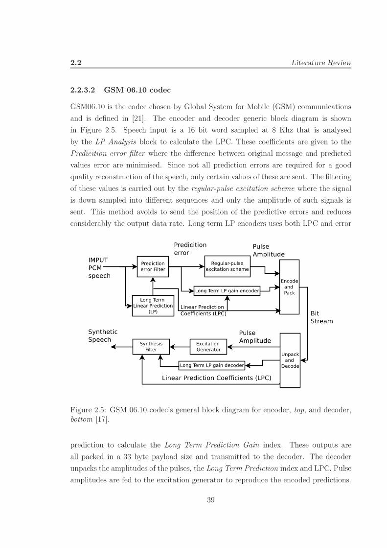
2.2.3.2 GSM 06.10 codec
GSM06.10 is the codec chosen by Global System for Mobile (GSM) communications
and is defined in [21]. The encoder and decoder generic block diagram is shown
in Figure 2.5. Speech input is a 16 bit word sampled at 8 Khz that is analysed
by the LP Analysis block to calculate the LPC. These coefficients are given to the
Predicition error filter where the difference between original message and predicted
values error are minimised. Since not all prediction errors are required for a good
quality reconstruction of the speech, only certain values of these are sent. The filtering
of these values is carried out by the regular-pulse excitation scheme where the signal
is down sampled into different sequences and only the amplitude of such signals is
sent. This method avoids to send the position of the predictive errors and reduces
considerably the output data rate. Long term LP encoders uses both LPC and error
Figure 2.5: GSM 06.10 codec’s general block diagram for encoder, top, and decoder,bottom [17].
prediction to calculate the Long Term Prediction Gain index. These outputs are
all packed in a 33 byte payload size and transmitted to the decoder. The decoder
unpacks the amplitudes of the pulses, the Long Term Prediction index and LPC. Pulse
amplitudes are fed to the excitation generator to reproduce the encoded predictions.
39
2.2 Literature Review
These predictions are given to the synthesiser that at the same time receives LPCs
and the long term gain decoders’ output. This output is a set of synthetic speech
values in the form of 16 bit PCM samples. The algorithm library for this thesis is
taken from [22].
2.2.3.3 Speex codec
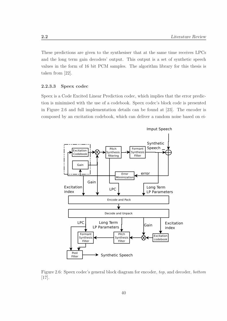
Speex is a Code Excited Linear Prediction codec, which implies that the error predic-
tion is minimised with the use of a codebook. Speex codec’s block code is presented
in Figure 2.6 and full implementation details can be found at [23]. The encoder is
composed by an excitation codebook, which can deliver a random noise based on ei-
Figure 2.6: Speex codec’s general block diagram for encoder, top, and decoder, bottom[17].
40
2.2 Literature Review
ther fixed or adaptable codebook. This output is then filtered and cascaded with the
input gain coefficients relative to the last sample measurement. The pitch synthesis
filter is a short term LP that provides the LPCs and creates the periodicity of the
signal. The signal is then passed through the formant synthesis filter that gives the
envelope to the signal, producing the long term prediction parameters. The output
signal is compared with the original speech using a weighted error system where the
output is fed back to the gain and codebook. The process is repeated for all code-
book’s code vectors creating the commonly known analysis by synthesis process of an
audio codec. The complexity of the codec and bit rate output is determined by the
number of code vectors and therefore it can vary depending on the setup. The process
to decode the encoded bit stream follows the inverse steps of the coding process. The
difference is that the excitation index facilitates the search of the code vector at the
codebook. The gain, LPCs and long term LP parameters are applied to the filters
with no major complexity than that of multiplying vectors. The post filter inserted
before the synthetic output enhances overall performance by smoothing the increased
noise introduced by the error predictor at the encoder side. In this thesis, Speex has
been set to Mode 4 delivering 11,000 bps data rate and the algorithm library is taken
from [23].
2.2.3.4 Codec Comparison
The three codecs described above represent a wide range of current audio codecs.
G.711 is an example of wideband codec with 64 kbps data rate. Although it is not
often used as VoIP audio codec it represents the best voice performance for packet
switched networks and therefore is a reference for the rest of codecs. GSM 06.10 and
Speex represent narrow band audio codecs. On one side, GSM 06.10 is the officially
regulated codec for GSM networks and hence any network willing to interact with it
has to support this codec which is the case of the implementation shown in Chapter 3.
On the other hand, Speex is part of a last generation of codecs where analysis by
synthesis methods are utilised. This codec guarantees good performance over packet
losses and high delays, since long term and short term predictions are taken into
account and fed back to the error predictor. Current state of the art codecs are often
based on CELP.
The performance and characteristics of each audio codec is summarised in Table
2.1 where each encoder’s and decoder’s delay has been extensively tested, over 20
41

2.3 Literature Review
Table 2.1: Used Codecs Characteristics
Codec G.711 GSM 06.10 Speex-mod4
Bit rate(kbps) 64 13.2 11.2Frame interval (ms) 20 20 20Payload Size (Byte) 160 33 28Encoding Delay (ms) 0.0231 0.1444 0.4314Decoding Delay (ms) 0.0169 0.0591 0.0772
times. As expected, codecs with LP have larger encoder values than the waveform
based codec.
2.3 VoIP Quality of Service
VoIP technology enables real-time transmission for voice through PSNs using the
IP network. This network is known as a Best Effort network because each packet is
independently routed to its destination. Hence, packets transmitted by a single source
can take different paths to reach the destination while traversing the network. The
network performance compromises VoIP in four main aspects: Latency, Queueing
and Processing, Packet losses and Jitter [3].
Latency is defined as the delay that the voice data has while crossing the IP
network without including any processing or queuing. This parameter is a measure
of the propagation delay of the data through the wires.
Queuing and processing is the delay associated with the processing in the
router/switches that need to read the IP destination to route the packets to their
next hop. Sometimes, as the propagation delay can be assumed as zero, the concept
latency is used to express the delay of the propagation plus the queuing and processing
delay.
Assuming Latency as the summation of both delays it is necessary to distinguish
that in voice communication there are two latencies, one per voice direction. Round
trip latency is the summation of the two way latency. The ITU Recommendation
G.114 [24] says that the round trip latency range is acceptable when it is less than
150 ms for most user applications. Relatively between 150 and 400 ms is acceptable
for administrators that are aware of which connectivity they are using; over 400 ms is
42

2.3 Literature Review
unacceptable. Likewise, different latency ranges can cause echo and talker overlap. If
the round trip latency is more than 50 ms, the echo from one of the speaker appears
in the communication, thus an echo canceller must be implemented in the vocoder.
The talker overlap is considered when the one-way delay is greater than 250 ms.
Packet losses occur mainly for two reasons; the first cause is related to a phys-
ical layer problem where too many bits are corrupted forcing the receiver to reject
the message. The second reason is due to finite memory space at the routers that
eventually can not allocate more space for incoming packets failing to deliver the
information to its destination.
Jitter is the variation of packets’ delay that reach their destination. The variation
of inter-packets arrival rate makes the conversation unbearable. This problem is
commonly solved by introducing a buffering system to reduce the effect of this feature.
The necessity to guarantee certain QoS might not affect to a well organised net-
work scheme within a LAN. The high speed connection of the typical Ethernet inter-
face of the PC makes the voice communication just as effective as it is with analogue
phones. However, to guarantee the same level of QoS over the Internet requires allo-
cating resources that might not belong to the end users any more, inducing the need
of extra protocols to overcome the problem. There are two different approaches at
this stage.
First option is to offer QoS with protocols working within the IP layer where two
alternatives are available: Integrated Services (IntServ) [25] and Differentiated Ser-
vices (DiffServ) [26]. IntServ is a model that guarantees the QoS between end nodes.
To cope with this task every single hop of the network must agree with the requirement
of the session initiation host. If these parameters are not satisfied the communica-
tion would not be started. IntServ was originally developed by Cisco System and
its corresponding signalling protocol is Resource Reservation Protocol (RSVP) [27].
The protocol defines a signalling system to reserve resources for both multicast and
unicast communications with a request-response methodology. In DiffServ model,
QoS is defined by classifying the traffic and adopting different priorities accordingly.
Therefore it is more scalable than IntServ because each router decides the priority
associated to the data. However in real case scenarios using DiffServ might not be as
effective as it seems. If a company agrees to use DiffServ with an ISP it can not be
guaranteed that all data is going to be routed by this ISP’s routers. Thus, crossing
different ISPs can not guarantee that the priorities are accomplished from the source
43

2.3 Literature Review
to the destination, compromising the desirable QoS.
The second option to provide QoS is within the second layer of the OSI model.
Three possible options are available; Frame Relay (FR) [28], Asynchronous Transfer
Mode (ATM) [29] and Multi protocol Label Switching (MPLS) [30]. FR and MPLS
technologies are based on creating virtual circuits on the network and guarantee a
minimum bandwidth. ATM differs from the other solutions because it offers different
way of organizing the traffic of your network depending on the requirements. If a
parallelism is to be made, IntServ is equivalent to FR and MPLS at a higher layer
and DiffServ is an ATM/MPLS service above the IP layers. Although these solutions
are accessible, they are often expensive or simply not feasible. Subsequently VoIP
traffic is often routed on a Best Effort basis without considering network resource
allocation. Therefore the constraints of PSNs must be considered to understand the
quality performance of VoIP communications as it is shown in the following subsection
with subjective and objective methods to assess VoIP calls.
2.3.1 Mean Opinion Score
Mean Opinion Score (MOS) [1] is a subjective methodology in which a large number
of people (over twenty according to the recommendation) are interviewed and asked
to assess the quality of a voice call. Calls are rated from 5 to 1 where 5 is excellent
quality and 1 represents bad quality.
5. EXCELLENT: The call has excellent sound quality resulting in no technical diffi-
culties.
4. GOOD: The call has good sound quality with audio similar to a long distance
phone call.
3. FAIR: The call has fair sound quality with some interruptions requiring one or
both parties to repeat what they said in the call.
2. POOR: The call has poor sound quality with each party having difficulties hearing
the other speak clearly.
1. BAD: The call has such bad sound quality that neither party can communicate
effectively.
For instance, Public Switched Networks is a CSN using PCM and scores 4.3 out of
44
2.3 Literature Review
5. The advantage of the method is that obtained results represent real voice quality
perception by human beings. Conversely the method is time-consuming and thus
alternative methods based on objective measurements are accepted to asses VoIP
phone calls.
2.3.2 Speech Quality Predictor: E-model
There are two types of objective methods: intrusive and non-intrusive. On one hand,
intrusive methods utilise a reference source to compare it with the degraded signal
where the larger the difference the worst is the quality. For example Perceptual
Evaluation Speech Quality (PESQ) and Perceptual Analysis Measurement System
(PAMS) are based in such method. The problem of this procedure is that the source
information or original voice, has to be compared with the received voice which in
most cases is impossible since users are physically apart. On the other hand, non-
intrusive methods observe parameters that interact with the VoIP call to predict the
quality. ITU-T’s G.107 defines the E-model [2] where speech quality is assessed by a
set of none time-varying additive impairments. This method allows to measure the
quality independently where the users are located which is essential for VoIP calls.
In this thesis, the E-model has been chosen as VoIP call quality assessment method
along with the MOS tests.
The E-model is an objective computational model to assess the transmission vari-
ations for a voice conversation of 3.1 KHz. The model is based on a mouth to ear
system that generates a rating factor namely, R-value. The model takes into account
impairment factors from an end-to-end perspective to conform the R-value which has
a range starting from 0 to 100. The model was developed in accordance to exten-
sive subject laboratory tests and it can be transformed to the MOS values with next
equation [2].
MOS =
1 for R = 0
1 + 0.035R +R(R− 60)(100− R)7 · 10−6 for 0 < R < 100
4.5 for R ≥ 100
(2.3)
Figure 2.7 shows the conversion from one model to another. Note that the max-
imum value of R corresponds to a 4.5 value of the MOS score which means that
45

2.3 Literature Review
regardless how good the voice has been digitalised it is never as good as the original.
Bad - 1
Poor - 2
Fair - 3
Good - 4
Excellent - 5
0 20 40 60 80 100
MO
S
R-value
MOS=1+0.035R+R(R-60)(100-R)7´•10(-6)
Figure 2.7: Objective method, i.e. R-value, versus subjective method, i.e. MOS.
The R-value is defined as follows [2]:
R = R0 − IS − ID − Ie−eff + A (2.4)
where R0 is the basic signal to noise ratio, IS represents decrease in quality more
or less simultaneously with the voice transmission, ID is responsible for any kind
of delay and echo in the system without including the coding delay, Ie−eff denotes
the impairments due to audio codec and channel constraints and A is the advantage
factor related to the service convenience.
Figure 2.8 is the general schematic used by [2] to assess the R-value. The sig-
nal to noise parameter R0, describes the noisiness of the systems including: Sender
Loudness Rating (SLR), room noise at the sender side (Ps), sender distortion value
of the telephone (Ds), Receiver Loudness Rating (RLR), room noise at the receiver
side (Pr) and Listener Sidetone Rating (LSTR). Equally, simultaneous impairment
factor IS, depends on signal to noise parameter (R0), Sender Loudness Rating (SLR),
Receiver Loudness Rating (RLR), Side tone Masking Rating (STMR) and Talker
Echo Loudness Rating (TELR). The advantage factor, A, refers to the fact that users
perception of complex communications affects the expectation of voice quality. For
46

2.3 Literature Review
Figure 2.8: E-model [2] communication system.
instance, this factor equalises the R-value when users are aware of speaking to some-
body in the other side of the Atlantic sea, where greater delays are more tolerated.
These parameters described so far, can be difficult to measure and in most of the
cases constitute invariant values throughout a call. Thus the ITU-T recommends the
use of default parameters (see Appendix A for a detailed description of default values
and formulae for these parameters) to facilitate the calculation of VoIP call quality
where equation (2.4) can be reduced to [2]
R = 93.3− ID − Ie−eff (2.5)
The reduced formula allows us to obtain a valid value of the quality of service
of our system focusing on two cornerstones for voice over packetised systems; delay
and packet loss. In our case, default parameters are used as specified in Appendix A
Table 1 with exception to those parameters referring to delay, channel status and
audio codec type. Delay parameters are defined in ID and are denoted following the
figure as follows : T is one-way delay, Ta is the absolute delay and Tr refers to the
round trip delay. In this thesis, the approximation of Tr = 2 · Ta is considered valid
and is used unless otherwise stated. Channel status and audio codec conform the
47

2.3 Literature Review
Ie−eff where Ppl refers to packet-loss probability, Bpl is packet-loss robustness and Ie
is the equipment impairment factor. Note that the Ie value is a given parameter by
the ITU-T G.113 recommendation [31] whereby codecs are tested under experimental
scenarios to assess their performance.
ID has a different mathematical expression depending on Ta and STMR. While
Ta is considered as a variable parameter, STMR is set as a default parameter (15
dB). Setting STMR to a static value means that VoIP prediction is carried out under
devices that perform ideally with side tones and echo cancellation. ID is therefore
defined as [2]:
ID = Idte + Idle + Idd (2.6)
where Idte, Idle and Idd refer to impairments related to the Talker Echo, Listeners
Echo and too long absolute delay (Ta), respectively. At the same time, Idte is defined
as [2]:
For 9dB ≤ STMR ≤ 20dB
Idte =
(
Roe−Re
2+
2
√
(Roe−Re)2
4+ 100− 1
)
(
1− e−T)
(2.7)
where, Roe and Re are [2]
Roe = −1.5(N0 − RLR)
Re = 80 + TERV − 14
TERV = TELR− 40 log101 + T
10
1− T150
+ 6e−0.3T 2
N0 = −61.16, from Appendix A (2.8)
where N0 refers to the power addition of different noises calculated with R0 using
default values specified in [2] and the rest of parameters are intermediate variables.
The Idle factor is calculated using the following equation [2]:
Idle =R0 − Rle
2+
2
√
(R0 − Rle)2
4+ 169 (2.9)
48

2.3 Literature Review
where R0 = 94.74 is calculated using default values from Appendix A and Rle is [2]
Rle = 10.5 · (WEPL+ 7)(Tr + 1)−0.25
where WEPL is a default value from Appendix A . Finally Idd is a value that depends
upon the absolute delay value, whereby even with perfect echo cancelling the VoIP
call can be perturbed. Idd is set to 0 if Ta ≤ 100 and if not Idd is set to [2]
Idd = 25
(1 +X6)1
6 − 3
(
1 +
(
X
6
)6) 1
6
+ 2
(2.10)
where
X =log10
(
Ta
100
)
log10 2(2.11)
Following the illustration in Figure 2.8, where it is shown that Ie−eff depends on
Ie, Ppl and Bpl, the E-model’s channel modelling is based on the interpretation of
Ppl under different burstiness scenarios. Hence Ie−eff is defined as follows [2]:
Ie−eff = Ie + (95− Ie) ·Ppl
Ppl
BurstR+Bpl
(2.12)
where BurstR refers to a Burst Ratio, defined as the average length of observed
burst in an arrival sequence over the average length of a expected burst under a ran-
dom loss channel. In other words, if a random channel is considered then BurstR = 1
which is a rare case for channel modelling. In the following chapters, channel models
based on experimental data are introduced and applied to different experiments to
investigate the performance of VoIP under heterogeneous networks.
In order to understand the impact of delay and packet losses, Figure 2.9 shows only
delay increasing versus only packet loss rate increasing performance. The prediction
is calculated for a G.711 case scenario where Bpl = 4.3, Ie = 0 and BurstR = 1.
The illustration shows that the increase of packet loss produces a severe quality drop
whereas delay increase has a smoother repercussion. In conclusion, it is visible that
a network should consider minimising the packet loss percentage.
The E-model describes a method to estimate the speech quality over different case
scenarios, whereby using delay and packet loss parameters, quality performance is
assessed. The great advantage of such this method is the rapid evaluation it provides
49

2.4 Literature Review
0
20
40
60
80
100
0 50 100 150 200 250 300 350 400 450 500
0 1 2 3 4 5 6 7 8 9 10 11 12 13 14 15 16 17 18 19 20
R-v
alue
One Way Delay (ms)
Packet Loss (%)
Delay Loss PerformancePacket Loss Performance
Figure 2.9: R-value comparison for a delay only and packet loss only increase scenar-ios.
to both end users and intermediate nodes. Conversely, the model remains limited.
For instance not all codecs are available in [31] nor is the method prepared to handle
multiple network channels. For these reasons Chapter 3 and Chapter 4 are dedicated
to the implementation and modelling of a SIP servers with two different link layers
that cover some of the existing limitations of the model.
2.4 Fundamentals of Network Coding
Previous sections introduced VoIP protocols and QoS assessment methods. In this
section, the literature review is concluded with an introduction to a set of schemes
that is highly promising to radically change the paradigm of future networks. A recent
breakthrough in an Information Theory paper showed that network coding techniques
can considerably improve throughput efficiency of the channel [32]. Essentially, the
theorem states that by combining existing packets in the network, the maximum flow
can be achieved, i.e. an encoding system within intermediate nodes can achieve the
capacity of the network. The following subsections describe network coding theory
and the network topology used in this thesis for a VoIP system with network coding
support.
In a point-to-point connection, information theory divides a communication in
50

2.4 Literature Review
source and channel coding. The former aims to achieve the highest compression of
raw data, good examples are audio codecs used by VoIP services. The latter enables
transmission over the channel essentially error free providing that extra information
has to be added to the original information. For example, in the Internet itself raw
information is packetised (source coding) and transmitted (channel coding) from node
to node according to routing tables that provide the next hop address. This store
and forward method considers source information to be completely independent and
if the same information has to be delivered to two different destinations, then the
source has to be duplicated. In other words, if there are n receivers, the source
information is repeated n times overloading the network considerably. This problem
can be solved if intermediate nodes are actively used rather than simply store and
forward packets where such nodes would combine the incoming information, i.e. store,
code and forward. The method brings several enhancements: throughput efficiency,
robustness to packet loss, reduction of complexity and security [33].
Throughput performance is the best known characteristic of network coding. The
butterfly illustration, on Figure 2.10 (a), is an example of a set of nodes interconnected
with directed links of unit capacity, where bi stands for bit. This example shows that
by encoding bits in node 3, two information units can be exchanged from source to
destination at the same time. Network Coding can also achieve higher robustness by
adopting distributive communications. Consider a relay system where the source node
Figure 2.10: Throughput and robustness improvement examples with network coding.
51

2.4 Literature Review
sends a packet to an intermediate node that stores and forwards the information to
the destination. With network coding the system can be changed so that the source
sends information units to the relay as well as to the destination itself, reducing
packet loss probabilities as seen in Figure 2.10 (b). The advantages of distributive
networks with network coding can also be applied to reduce complexity [33]. Multicast
sub-graphs, require Steiner tree computations [34] that can be simplified in certain
scenarios by distributive systems with network coding. Finally, from a security point
of view, network coding encodes packets that can only be decoded at the destination.
This has two sides; from one side, discourages the spoofing of packets throughout the
network since they are not decodable. From the other side, if an intermediate node
is a malicious node, encoded packets will be delivered to the destination as source
information, breaking the confidentiality of the information.
Considering the network coding evolution time line, although network coding has
been attributed to Ahlswede et al. [32], Yeung and Zhang were first suggesting net-
work coding features for satellite communications in 1998 [35]. Since then, network
coding research in the field has been expanding mainly in encoding/decoding sys-
tems for a large number of nodes to achieve larger throughput values. Li, Yeung
and Cai [36] found that linear encoding at the interior nodes is sufficient to achieve
better performance. Koetter and Medard [37] expanded the work in [36] with linear
encoder/decoder functions by finding polynomial coefficients and Ho et al. [38] im-
proved this result by applying random linear codes for reliable communication. A
more recent research approach proposed Physical Network Coding (PNC) [39] which
has been widely researched with publications including [40] and [41].
The above work is based on theoretical and simulation results assuming combina-
tions of multicast traffic, optimal scheduling and channel models with steady rates.
Another approach to this method has shown a more practical angle; a widely known
application is Avalanche [42], a peer to peer content distribution network. A similar
suggestion was developed by Chung et al. who designed a peer to peer Streaming Sys-
tem named PNECOS that showed a reduction of bandwidth consumption for servers
with network coding techniques [43]. Katti et al. presented COPE, a new architecture
for wireless mesh networks, applicable to technologies such as IEEE 802.11 (Wi-Fi)
and IEEE 802.16 (WiMax) [44]. Vingelman et al. developed a random linear network
coding application based on OpenGl software that takes advantage of graphic cards
to perform calculations related to network coding [45].
52

2.4 Literature Review
2.4.1 Network Coding Theory
In this subsection, network coding theory is explained by means of graphical examples.
Single source single destination model is used to introduce network coding followed
by single source multiple destinations models which leads to a wireless model utilised
in our proposed design in Chapter 5.
2.4.1.1 Single Source Single Sink
A graph G = (V,E) consists of a set of vertices, V , and a set of unidirectional
connecting lines called edges, E. There are three type of vertices: the source , the
intermediate node and the sink represented by s, a numbered circle and t respectively.
Source node is essentially the transmitter of a communication system and does not
receive any input edge. Intermediate nodes act as routing nodes and the sink is the
receiver of the information generated by the transmitter. Nodes are connected by
directional arrows that are defined by a numerical value, the capacity of the edge C.
An edge is denoted as e(i, j) with a direction from its ”initial point” i to its ”terminal
point” j. The flow of an edge, fij , are the information units that are sent from node
i to node j. In our graphs two conditions are imposed.
• The flow of an edge (i, j) in G is positive and equal or less than the capacity of
the edge [46].
0 ≤ fij ≤ Cij (2.13)
• Each vertex i, excluding s and t, has an input flow the same as the output flow
following the conservation law [46]. Inflow(F+(i)) = Outflow(F−(i))
F+(i) =n∑
k∈In(i)
fki (2.14)
and
F−(i) =
n∑
j∈Out(i)
fij (2.15)
The conservation law requires that the output flow from s has to be equal to the
input flow of the sink t which defines the flow of the graph, F . The goal is to maximise
53

2.4 Literature Review
the flow of G given different sets of Cij , in order to achieve the MAX-flow. F has to
be then greater or equal than any capacity in the network.
A cut set is a set of edges of the network whereby the network is divided into two
sets, one of them containing the source and the other the sink. The idea is to find
out what is the flow of the graph by cutting the network because any flow from s to
t must sometimes pass through some of theses edges. We denoted a cut set by (S, T )
where S is a set of vertices that lies on the source side and T is a set of vertices that
lies on the sink side. Figure 2.11 (a) shows an example of a single source single sink
graph. The dotted line expresses a cut set on the graph. In this example S = {s, 1, 2}
and T = {t}. The capacity of a cut, with respect to the capacity of each edge, is
defined as the sum of forward edges in the cut (S, T ) and only the forward edges,
where forward edges are defined as the edges of the direction from the source to the
sink [46].
capacity(S, T ) =∑
i∈S,j∈T
Cij (2.16)
A MIN−cut is therefore a cut set where the capacity is less or equal than any other
cut set of the graph. The illustration in Figure 2.11 (a) shows a minimum cut set of
capacity 3. If the cut set is carried out in the same direction but above the nodes 1
and 2 the capacity is 4. Clearly the edges (s, 1) and (s, 2) with capacity 2 are actually
not contributing in anything to the maximum flow of the graph because edges (1, t)
and (2, t) can not handle more than 3 units of information per time. This intuitive
example led to the MAX-flow MIN-cut theorem presented by Ford and Fulkerson at
Figure 2.11: The single source single sink example. a) Capacities of the network, b)Max-flow network, c) Example with binary units to achieve max-flow [46].
54

2.4 Literature Review
the Canadian Journal of Mathematics [47].
Theorem 1. The maximum flow in any network G is equal to the minimum cut set
of the graph.
In Figure 2.11 (a) an initial graph with different capacities is shown. The mea-
surement of the cut sets proves that the minimum cut set is 3 and therefore the graph
is adapted to Figure 2.11 (b). The exchange of information at the maximum rate
is shown in Figure 2.11 (c) where 3 bits are sent from source to destination. It is
important to point out that the delay introduced by each edge is considered as non
existing. If other network topologies of single source single sink are studied it can be
proved that the max-flow bound is always achieved [46].
2.4.1.2 Single Source Multiple Sinks
The butterfly graph example of Figure 2.12 shows an example of single source multiple
sink graphs. In a graph G with sinks t1,t2, ... tL , we denote the information rate
received by each sink as γ. Hence we must have [46]
γ ≤ Fmax(tl) (2.17)
and
γ ≤ minl{Fmax(tl)} (2.18)
where Fmax is the maximum flow of a sink and equation (2.18) is the minimum
flow of all maximum flows of the graph. This is explained in Figure 2.12. The first
graph, Figure 2.12 (a), shows the capacity of the edges of the butterfly and the cuts
required to compute the Fmax of each sink. Recall that the max flow is the sum of the
edge capacities going forward to the sink. It can be seen that Fmax(t1) = 1+1 = 2 and
Fmax(t2) = 2 where the max flow of the graph is then γ = 2. Figure 2.12 (b) shows
how to achieve such max flow. The source sends two information bits simultaneously
from (s, 1) and (s, 2). b1 and b2 are replicated by nodes 1 and 2 respectively. At this
point node 3 disposes of two bit of information but only one can be sent. Since the
routing scheme for the sinks is fixed, node 3 can combine both bits and send them
to node 4 where they are forwarded to the sinks. If no network coding schemes were
55
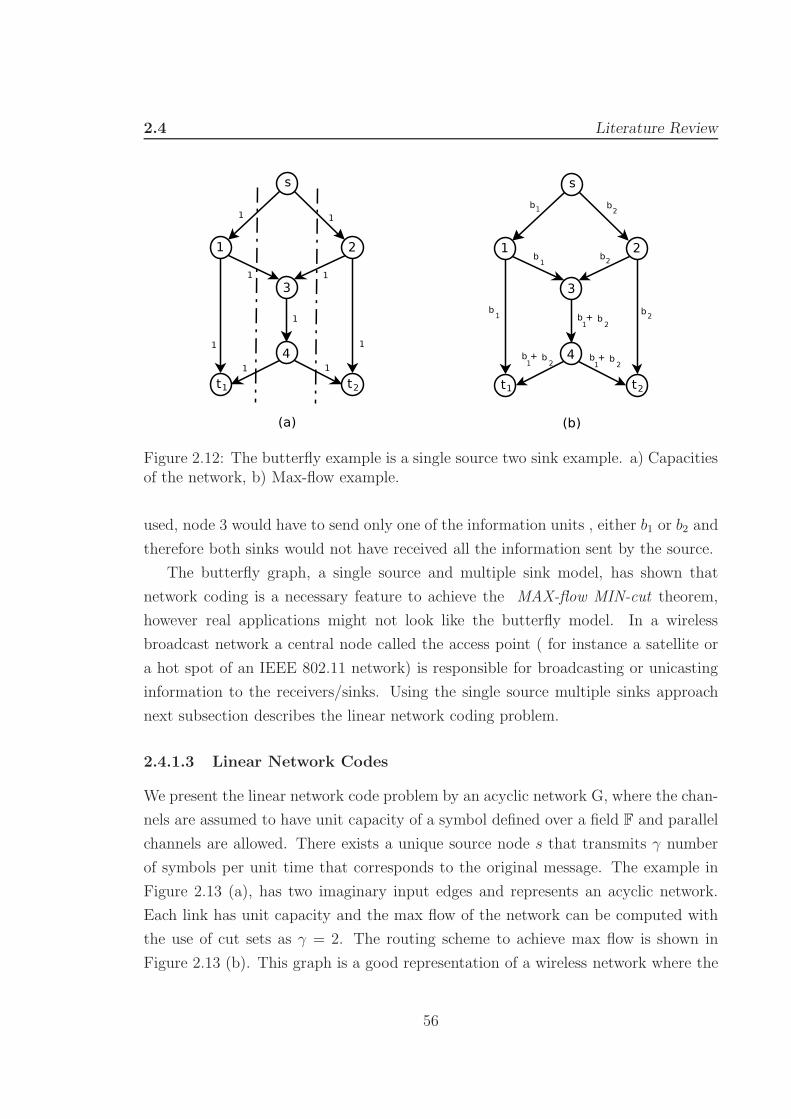
2.4 Literature Review
Figure 2.12: The butterfly example is a single source two sink example. a) Capacitiesof the network, b) Max-flow example.
used, node 3 would have to send only one of the information units , either b1 or b2 and
therefore both sinks would not have received all the information sent by the source.
The butterfly graph, a single source and multiple sink model, has shown that
network coding is a necessary feature to achieve the MAX-flow MIN-cut theorem,
however real applications might not look like the butterfly model. In a wireless
broadcast network a central node called the access point ( for instance a satellite or
a hot spot of an IEEE 802.11 network) is responsible for broadcasting or unicasting
information to the receivers/sinks. Using the single source multiple sinks approach
next subsection describes the linear network coding problem.
2.4.1.3 Linear Network Codes
We present the linear network code problem by an acyclic network G, where the chan-
nels are assumed to have unit capacity of a symbol defined over a field F and parallel
channels are allowed. There exists a unique source node s that transmits γ number
of symbols per unit time that corresponds to the original message. The example in
Figure 2.13 (a), has two imaginary input edges and represents an acyclic network.
Each link has unit capacity and the max flow of the network can be computed with
the use of cut sets as γ = 2. The routing scheme to achieve max flow is shown in
Figure 2.13 (b). This graph is a good representation of a wireless network where the
56

2.4 Literature Review
Figure 2.13: The acyclic network model for a wireless network. a) Capacities of thenetwork, b) Max-flow example, c) The encoding system for a wireless communicationmodel.
source node and node 1 are the central node, i.e. the access point, and t1, t2 are the
receivers or users of the network.
Focusing on Figure 2.13 (c) where the wireless network graph has been dissemi-
nated to describe linear network coding. The source node in this case receives two
flows, f(0,s) and f(0′,s) that represent the source information ~x where ~x = Xd · fd,s,
d ∈ In(s) and Xd ∈ Fγ. The output of s is received by k nodes in the form of
(fs,j)i,k ·Ms,j, where j ∈ Out(s), i and k represent the rows and columns of the out-
put matrix fs,j and M is the mapping encoder of each node. Since the conservation
law has to be accomplished, next hop symbol can be calculated as follows.
(fs,j)i,k =∑
k∈Out(s)
~x ·Ms,j =∑
k∈Out(s)
(Xd · fd,s) ·Ms,j =∑
k∈Out(s)
Xd · (fd,s ·Ms,j) (2.19)
In this way, the original message is transmitted from node to node and can be
decoded as long as the mapping of each encoder, i.e. Ms,j in this case, is known. In
Figure 2.13 (c) there are two encoding nodes ( s and node 1) and 7 flows. The two
sources received at the source form a matrix such that
57

2.4 Literature Review
fd,s =[
f(0,s) f(0′,s)
]
=
[
1 0
0 1
]
Xd =[
z1 z2
]
,where zi ∈ Fγ (2.20)
The encoders Ms,j and M1,l are constructed by rows that define the input symbol
and columns representing the next hop channel. Hence, Ms,j with a two input node
has two rows and since it is connected to 3 nodes it is constructed with 3 columns.
The same construction method is applied to node 1 where there is one input symbol,
thus one row, and two output channels giving two columns. The encoding system is
associative, i.e. the order of the operations can be changed, thus the mapping system
in Figure 2.13 (c) can be defined without considering the input symbols:
(fs,j)i,k = fd,s ·Ms,j =
[
1 0
0 1
]
×
[
1 1 0
0 1 1
]
=
[
1 1 0
0 1 1
]
, (2.21)
fs,t1 = (fs,j)i,1 =
[
1
0
]
, (2.22)
fs,1 = (fs,j)i,2 =
[
1
1
]
, (2.23)
fs,t2 = (fs,j)i,3 =
[
0
1
]
, (2.24)
(f1,j)i,k = fs,1 ×M1,l =
[
1
1
]
×[
1 1]
=
[
1 1
1 1
]
, (2.25)
f1,t1 = (f1,j)i,1 = f1,t2 = (f1,j)i,2 =
[
1
1
]
, (2.26)
On one hand, the encoder system is a set of linear equations where the symbols
are defined at the field specified by the designer. On the other hand, the decoder of
the system can be defined by a set of equations received at the sink. For instance,
sink t1 receives two flows, f(s,t1) and f(1,t1). Each row of received matrix flow is the
combination of the initial message. Therefore the decoder has to solve the following
58

2.4 Literature Review
equations
f(s,t1) ⇒ (f(s,j))1,1 + (f(s,j))2,1 = symbol1 (2.27)
f(1,t1) ⇒ (f(1,j))1,1 + (f(1,j))2,1 = symbol2 (2.28)
where + is the sum in the base field defined by the designer. The set of lin-
ear equations can be solved because (f(s,j))2,1 = 0 and (f(s,j))1,1 = (f(1,j))1,1. Thus
equation (2.28) can be rewritten as symbol1 + (f(1,j))2,1 = symbol2 and solved as
(f(1,j))2,1 = symbol2 − symbol1 (2.29)
Accordingly, to decode the information in sink t2 the step process is the same as
sink t1.
Example: Let us now consider that the source wants to send two symbols z1 and
z2 defined over a field F2 = {0, 1}. The source will then receive two information units
defined as Xd · f(d,s) which produces a matrix such that
~x = Xd · fd,s =[
z1 z2
]
·
[
1 0
0 1
]
=[
z1 z2
]
(2.30)
the output flow of the source node is calculated using equation (2.19) and the
output of node 1 using the mapping in equation (2.25).
(fs,j)i,k = ~x ·Ms,j =[
z1 z2
]
×
[
1 1 0
0 1 1
]
=[
z1 z1 + z2 z2
]
(2.31)
(f1,j)i,k = fs,1 ·M1,l =[
z1 + z2
]
×[
1 1]
=[
z1 + z2 z1 + z2
]
(2.32)
using equations (2.27) and (2.28) the set of equations that are solved for t1 are
symbol1 = fs,t1 = z1
symbol2 = f1,t1 = (z1 + z2) (2.33)
solving the set of equations as
symbol2 = (z1 + z2)− z1 = (z1 + z2) + z1 = z2, from 2.33 (2.34)
59

2.4 Literature Review
where minus sign is substituted by a sum because in F2 + = -. Equally the set
of equations to be solved by sink t2 are
symbol1 = fs,t2 = z2
symbol2 = f1,t2 = (z1 + z2) (2.35)
solving the set of equations as
symbol2 = (z1 + z2)− z2 = (z1 + z2) + z2 = z1, from 2.35 (2.36)
Hence, if the mapping system is known, i.e. Ms,j and M1,l, each sink can decode
sent information. This graph (see Figure 2.13 (c) ) is a representation itself of a
wireless broadcast network. On one hand, the base station offering a connection to
the users is equivalent to nodes s and 1 where received information or uplinks are the
inputs to node s and the sent information or downlinks are the outputs of node 1.
On the other hand, the users are represented by the sinks and the set of edges that
connect them to the source, i.e. e(s, ti). In other words, f0,s and f0′,s are known to
t1 and t2 respectively. In a real scenario this means that a user of a BSS has a buffer
of sent information allowing the receivers to decode incoming packets from node 1.
This is the key feature to understand network coding over wireless networks.
Consider that the encoder matrices are known by both, the end user and the access
point. An end user sends bits of information to the access point and keeps a buffer
memory with what has been sent. This means that end user has either z1 or z2 stored.
At this point the access point is aware that the end node is storing sent information
and proceeds to encode received information before transmitting it to all users. The
end nodes have stored sent information which means equation (2.27) is already at
the receiver. If the access point sends the encoded message in equation (2.28) the
user can retrieve the information by solving the system. The procedure guarantees a
remarkable gain in throughput but there is still a fact that has not been considered
so far, the delay. The graphs presented here have an ideal propagation feature free
of delay. In reality, delay can restrict a service where if exceeds a maximum value
might not be feasible to perform. Since VoIP is one of these services, the study of its
performance is analysed over a wireless network such as IEEE 802.11b in Chapter 5.
60

2.5 Literature Review
2.5 Conclusion
In this chapter, SIP/SDP and RTP/RTCP are described to understand the signalling
system and audio exchange procedures within a VoIP network. State of the art audio
codecs G.711, GSM 06.10 and Speex are chosen because they are a good represen-
tation from the variety of codecs currently available. VoIP phone calls are assessed
throughout this thesis with the MOS and the E-model as presented in this chapter.
The speech prediction model is followed by a network coding introduction that gives
an insight to the design of these network architectures. The study of heterogeneous
network performance is addressed in the following chapter with a MOS test for an
active SIP proxy GW.
61

CHAPTER 3
VoIP Quality in Heterogeneous
Networks

3.1 VoIP Quality in Heterogeneous Networks
3.1 Introduction
NOWADAYS due to the multiplicity of network communication solutions there
is an increased possibility that VoIP calls not only take part within a single
network but rather within a number of networks that often function using different
standards and link layers. SIP has been widely adopted as the signalling system
for PSN and thus the integration with existing technologies is important in order to
offer full services. From an end-to-end user perspective SIP GWs are SIP entities
that cross interact with these technologies and their performance can become critical.
Consider that Alice uses a soft phone at her office desktop to call Bob whose location
is unknown to Alice, as shown in Figure 1.1 on page 24. In an ideal scenario, Alice
would call the UA corresponding to Bob and so the task that the network has to
proceed is to locate Bob. Regardless of Bob using a land line, a cell phone or an office
computer, Alice expects good phone call quality. Therefore, the critical subject is
to know what are the requirements from the network’s perspective to achieve such
transparency.
Firstly, the signalling systems from the differing technologies must be translated
to guarantee that the location and availability of Bob can be determined. Secondly,
voice data is exchanged between end nodes through the GW, but the quality degrada-
tion of a single network can affect the whole conversation. For example, the fact that
Bob may be on a mobile network which guarantees a minimum QoS will not be suffi-
cient if Alice’s network is overloaded (consider example A at Figure 1.1 on page 24).
This could eventually lead to a drop in a number of packets during the conversation.
Heterogeneous network communications require that gateways not only provide sim-
ple forwarding methods but also end-to-end VoIP quality performance. Furthermore,
if a SIP GW can sense the end-to-end speech quality then it can enforce entities to
use methods such as Forward Error Correction (FEC) to overcome the situation.
The development of SIP entities have been growing in the last decade. Hyun
et al. presented a SIP implementation and design of proxy and registrar in [48].
In [49] Huy et al. described User Agent (UA) implementation for voice services
including call establishment, termination, registration and capability of negotiation.
Other implementations take advantage of Private Branch Exchange (PBX) to develop
an integrated telecommunication system. A recognised approach was achieved by
Anjum et al. who developed ChaiTime [50], a Java Telephony API along with SIP to
63

3.2 VoIP Quality in Heterogeneous Networks
design an integrated system. Asterisk [51], an open source software implementation,
is another example of a PBX that offers multiple protocol integration such as H.323,
SIP and self developed IAX [52]. Although the developments above achieve different
technological integration none of them considers the VoIP communication quality
performance as a whole.
In this chapter, a SIP proxy emerged with a Media Gateway is presented as a test-
bed implementation system to bridge IEEE 802.3 (wired) to GSM networks (wireless)
and vice-versa. The platform senses in real-time the quality delivered to end users
using the packet loss rate and supports FEC to overcome conditional scenarios where
the wire section shows low end-to-end VoIP quality performance. This development
is based on an embedded platform to provide the system with higher mobility and
integration for future implementations. The comparison of the passive GW versus
the active GW, i.e. with FEC system integrated, results in a better performance for
active nodes according to the MOS rates.
The remainder of this chapter is organized as follows. Section 3.2 describes FEC
for VoIP with an overview to channel estimations. Section 3.3 presents implementa-
tion tools and software architecture. Section 3.4, discusses the Mean Opinion Score
(MOS) test results, and finally, Section 3.5 concludes the chapter.
3.2 FEC for VoIP
FEC for VoIP services was initially presented by Bolot [53] proving that, even at high
packet loss probabilities, speech quality is maintained satisfactorily. More recently,
advanced FEC methods have been tested for VoIP services; Wenyu et al. showed the
feasibility of FEC under bursty loss Gilbert Elliot Model [54]. Sheng et al. presented
a combination of FEC mechanism for wireless methods, including iterative decoders
such as concatenated zigzag (CZ) [55]. Although most of this research focuses on FEC
for VoIP they do not consider the whole communication system with a combination
of wired and wireless networks, i.e. heterogeneous networks. In our integrated SIP
server GW with FEC, the results in [53] are corroborated and its usage is extended
to a wire-to-wireless network application. In addition, our application includes an
integrated Markov Chain theory based loss model for test purposes; this allows us to
emulate the behaviour of a multiplicity of channels.
64

3.2 VoIP Quality in Heterogeneous Networks
0
20
40
60
80
100
0 1 2 3 4 5 6 7 8 9 10 11 12 13 14 15 16 17 18 19 20
R-v
alue
Packet Loss Percentage (%)
G.711-MCG.711-RDGSM-MCGSM-RD
Figure 3.1: Speech quality prediction for a RanDomly interpreted channel (RD) versusa Markov Chain (MC) based model with codec parameters defined as Bpl = 4.3,Ie = 0 for G.711 and Bpl = 39, 32,Ie = 24.3 for GSM as specified in Chapter 4.FSMC is defined with q = 0.7.
3.2.1 Channel estimation with Markov Chain Theory
From a channel estimation point of view, channels are often modelled based on Bit
Error Rates (BER) that consequently lead to frame errors. From a network point
of view, channels are often modelled as Packet Error Rates (PER) or packet loss
percentage. In Section 2.2.2 on Page 35 it is mentioned that RTCP exchanges the
value of packet loss rate in relation to the link between end users. This percentage
can have different interpretations, but mainly there are two schemes to follow. The
packet loss percentage is either random or non-random. In case of a non random
process, different mathematical models can be applied, where a widely applied model
is Finite State Markov Chain (FSMC) models. Figure 3.1 represents the difference
of both interpretations using the E-model for G.711 and GSM. From the illustration
it is shown that the performance of Markov Chain (MC) based models has worse
performance than RanDom (RD) based interpretation, reaching to a conclusion that
the use of random packet loss model can be misleading in VoIP quality performance
prediction.
FSMC are channel loss models often utilised in network modelling for wired and
wireless communications. In wireless communications, FSMC models have been used
65

3.2 VoIP Quality in Heterogeneous Networks
p
q
1−q
G B1−p
Figure 3.2: Fist-Order Finite State Markov Chain model [62].
to model error burst in fading channels, facilitating designers to analyse and improve
performance measurements in both physical and medium access control services. In
[56] it was proven that higher information rates can be achieved if FSMC memory
is taken into account. A common approximation for fading channels is Rayleigh
Probability Distribution Function (PDF). This PDF is divided into Markovian states
depending on the nature of the fading channel [57], i.e. the higher the number of
states the greater the complexity. Although higher order FSMC models have proven
better in performance, they considerably increase the complexity which for a real-time
channel modelling is not desirable. Hence in this thesis first order FSMC models are
used due to their computational simplicity and accuracy [58].
In wired communications performance of the Internet is affected by routing schemes.
Packet loss due to congestions in routers, delay or priority policies are every-day con-
straints. In [59–61] it is shown that the Internet packet loss can be represented as on
and off states, whereby on refers to all packets being dropped and off signifies no
packets are lost. This behaviour is well suited for a first order FSMC.
A single first order Markov Chain is shown in Figure 3.2 where P (G− > B) = p
represents the probability of moving from the Good state to the Bad State and
P (B− > G) = q the probability of moving from the Bad state to the Good.
If the channel is in the Good state packets are delivered to their destination
whereas within the Bad state packets are dropped. The average probability of being
in each state is then given by equation (3.1), where π0 and π1 are the Good and Bad
states respectively [62].
π0 = (q/(p+ q)), π1 = (p/(p+ q)) (3.1)
Figure 3.3 illustrates the packet loss probability for packets lost in a row with
q = 0.7. The graph demonstrates that the probability of loosing the first packet
is always the highest provided that previous packet was not lost. Consequently,
the probability of loosing yet another packet in a row diminishes as the number of
66
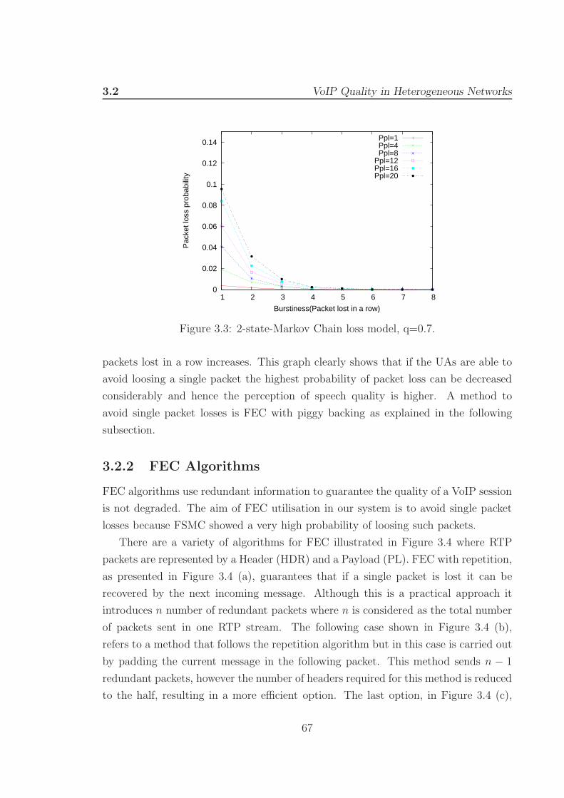
3.2 VoIP Quality in Heterogeneous Networks
0
0.02
0.04
0.06
0.08
0.1
0.12
0.14
1 2 3 4 5 6 7 8
Pac
ket l
oss
prob
abili
ty
Burstiness(Packet lost in a row)
Ppl=1Ppl=4Ppl=8
Ppl=12Ppl=16Ppl=20
Figure 3.3: 2-state-Markov Chain loss model, q=0.7.
packets lost in a row increases. This graph clearly shows that if the UAs are able to
avoid loosing a single packet the highest probability of packet loss can be decreased
considerably and hence the perception of speech quality is higher. A method to
avoid single packet losses is FEC with piggy backing as explained in the following
subsection.
3.2.2 FEC Algorithms
FEC algorithms use redundant information to guarantee the quality of a VoIP session
is not degraded. The aim of FEC utilisation in our system is to avoid single packet
losses because FSMC showed a very high probability of loosing such packets.
There are a variety of algorithms for FEC illustrated in Figure 3.4 where RTP
packets are represented by a Header (HDR) and a Payload (PL). FEC with repetition,
as presented in Figure 3.4 (a), guarantees that if a single packet is lost it can be
recovered by the next incoming message. Although this is a practical approach it
introduces n number of redundant packets where n is considered as the total number
of packets sent in one RTP stream. The following case shown in Figure 3.4 (b),
refers to a method that follows the repetition algorithm but in this case is carried out
by padding the current message in the following packet. This method sends n − 1
redundant packets, however the number of headers required for this method is reduced
to the half, resulting in a more efficient option. The last option, in Figure 3.4 (c),
67

3.2 VoIP Quality in Heterogeneous Networks
Figure 3.4: Different Forward Error Correction algorithms where HDR stands forheader and PL payload.
depicts a FEC system where packets are xor -ed and padded to the third payload.
This method also named as FEC with piggy backing, ensures that a single packet is
not lost with a probability of [54]
π1.FEC =p
(p+ q)((1− q)2 + pq + q(1− q)) (3.2)
where the equation is constructed by starting at the Bad state, i.e. one packet
is already lost, and multiplying it with the addition of three possible cases where
recovering lost packets is not possible; the first case refers to loosing the following
two packets, (1−q)2; the second represents the case when the second packet is received
but the third is lost, pq and finally the last possibility is to loss the second packet
but receive the third one, (1 − q)p. This method only requires (n − 1)/2 number
of redundant packets, which is a considerable gain in comparison to the other two
options. For this reason, the following SIP proxy GW is implemented using FEC with
piggy backing.
68

3.3 VoIP Quality in Heterogeneous Networks
3.3 System Implementation
In this chapter, an embedded SIP proxy GW connected to a GSM capable of working
on a Small Office/Home Office (SOHO) environment written in C code is presented.
The implementation is based on a general purpose board, a GSM modem and an
expansion board, specifically designed for this implementation.
The test board is based on NGW100, a general purpose development board for the
AT32AP7000 processor [63]. The 32-bit Micro-Controller Unit (MCU) is a processor
core with an architecture created specifically for cost-sensitive embedded applications
that require both high performance and low power consumption. This architecture is
based on a RISC processor core designed to do more processing per clock cycle so that
the same throughput can be achieved at a lower clock frequency with substantially
less power consumption. The NGW100 is equipped with a 8MB Parallel flash, a
non-volatile flash memory reloaded with the U-Boot boot loader for Linux, 8MB
Serial flash dedicated to store permanent code and 32MB SDRAM used to store
temporary data. The expansion board has a CS4202 mixed-signal serial audio codec
with an integrated headphone power amplifier compliant with the Intel Audio Codec
97 specification, referred as AC 97 capable of supporting PCM. Finally, the GSM
modem is controlled by a level converter from a serial port from the NGW100 and its
audio input/output are connected to the expansion board. Telit has been chosen for
this development [64]. The embedded SIP server incorporates Linux 2.6.23 Operation
System (OS) and this can be controlled by both serial port and Telnet. Vendors cross
compiler and Integrated Design Environment (IDE) has been used in a Fedora Core
8 to develop the software. Further description of the implementation can be found at
Appendix B .
Software implementation is based on three main sections: Firstly the SIP server
Gateway’s functionality and the call flow of a VoIP session is described, secondly, our
algorithm to support FEC with piggy backing (encoder/decoder) is presented and
thirdly, state machines synchronisation for the SIP and Modem network is explained.
3.3.0.1 Embedded SIP Server merged with a Media Gateway
The Embedded SIP server GW has two main tasks; on one hand it must control the
signalling system from both VoIP and Mobile network, and on the other hand it must
handle the RTP protocol and translate it to the GSM network audio input. oRtp [65]
69

3.3 VoIP Quality in Heterogeneous Networks
Figure 3.5: Block diagram of the SIP server merged with a Media Gateway connectedto a mobile network.
and oSIP [66] libraries are used to implement the SIP server. The block diagram
of the implementation is presented in Figure 3.5. The figure shows the set up for
VoIP calls carried out in the experiments where Alice is connected to the SIP proxy
merged with the Media Gateway. The gateway includes a monitoring system that
allows to the entity to react under poor quality circumstances. The media gateway
is connected to the mobile network through a modem that provides a communication
system from Alice to Bob through the base station. The flow chart of a current VoIP
call is presented next.
Figure 3.6 shows the signalling flow of the embedded SIP server merged with a Me-
dia Gateway. Several assumptions are made for simplicity; Mobile Stations (MS) have
already been assigned their channel number to guarantee synchronisation with the
Base Station (BS) and Authentication and Ciphering processes have been discarded.
In the graph the Mobile Control Centre (MCC) is a unified concept that includes;
Base Station Controller (BSC), Mobile Switching Centre (MSC), Visitor Location
Register (VLR), Home Location Register (HLR) and Authentication Centre (AuC).
BSC is in charge of several BS, MSC is responsible for switching routing and control-
ling a call, VLR stores all relevant information related to the user, HLR is responsible
for the user location information and the AUC is in control of authentication. Readers
are referred to [67] for further details.
This flow chart starts with the registration from Alice’s UA to the Embedded SIP
70

3.3 VoIP Quality in Heterogeneous Networks
Figure 3.6: Flow chart for a wire to mobile network VoIP call [68].
Server GW. If this person has permission to be registered, the server will reply with
a 200 OK accepting the request or it will be rejected. Alice generates a phone call to
Bob by sending an Invite request including its options for audio codecs, i.e. SDP. The
embedded SIP server checks its Register Servers entrance and codec compatibility.
Bob is not in the local area network and therefore a mobile network session is initiated
by sending a request call to the Mobile Gateway (Mobile GW), see Figure 3.6. The
Mobile GW is connected through the Base Station 1 (BS1) to the MCC and forwards
a Call request to contact Bob. MCC checks in the routing tables to track down Bob’s
Mobile Station. Bob’s MS receives a Connection Request while the Mobile GW sends
a 100 Trying response to advise Alice’s UA that the call has been processed. Bob’s
MS confirms that the call has gone through and starts ringing and in return the
71

3.3 VoIP Quality in Heterogeneous Networks
Embedded Server SIP GW sends a 180 Ringing to Alice. If Bob’s phone is switched
off or not available, then this will be noticed by the Embedded Server to Alice and
the phone call will be finished. In this case, Bob accepts the phone call and a 200 OK
message is sent to Alice with codec priorities. It is after this process when Alice and
Bob can talk through the Embedded SIP Server GW. The conversation is finished in
this example by Alice sending a Bye request. This request is forwarded to the MCC
and Bob is informed that Alice has hung the phone up. Confirmation is received at
the embedded Server and a response with a 200 OK is sent.
The embedded SIP server GW allows a routing scheme to track down the user
location. If the user is not logged in, the phone call is routed to the mobile network.
This internal routing system is a very useful feature that always makes sure a cheaper
phone call will be performed, avoiding any extra action from the end user and blindly
integrating both technologies.
As mentioned in the introduction of this chapter, it is possible that Alice’s side
(wired communication) might not be able to deliver packets degrading the VoIP
performance. This problem can be tackled with the use of FEC algorithms as shown
next.
3.3.0.2 FEC with piggy backing algorithm
FEC with piggy backing improves the quality of an end-to-end VoIP session. In
this chapter, the SIP server GW is presented with the support of FEC with piggy
backing. The GW becomes an active node within the network that sensing the QoS
of the communication can enforce the use of FEC.
Both FEC encoder and decoder have been developed in C programming language
at the wire network section. The encoder block code algorithm for Figure 3.4 (c)
is presented in Figure 3.7. Once all variables are set to their default values, the
algorithm starts reading voice frames from the Analogue to Digital (A/D) converter,
Praw and encodes them in G.711 audio codec, Pn. If this is the first packet then
Pfirst = 1 and the packet is sent using conventional method after being copied to an
internal buffer (cpy(Pn, Pa)). At the time of reading the second packet, Pfirst = 2
the packet is sent conventionally as well as being copied to a different internal buffer
(cpy(Pn, Pb)). Third packet’s case is different because Pfirst = 3. Therefore the
xor of previous two packets is performed and the output is concatenated with the
original message, i.e. Pxor = xor(Pa, P b) and Pfec = conc(Pn, Pxor). The new
72

3.3 VoIP Quality in Heterogeneous Networks
Figure 3.7: FEC encoder with piggy backing [68].
packet is sent with the FEC padding and the third packet is copied to the internal
buffer Pa. Since the variable Pfirst is set to zero the forth packet takes diagram’s
right tree in Pfirst > 0. In this case fec = 0 and hence, forth packet is sent without
FEC but it is copied to the internal buffer Pb. Consequently the fifth packet follows
the path of the forth packet but this time FEC is added entering in a loop that sends
packets with FEC as piggy backing.
The decoder reads the sequence number of received packets, decides whether a
73

3.3 VoIP Quality in Heterogeneous Networks
packet is lost or not and if possible implements the xor to recover the lost packet.
The pseudo code for this algorithm is presented in Algorithm 3.1. Received packets
are divided into a set of three packets called fecblocks as shown in Figure 3.4 c), so
that synchronisation within received packets is not lost. A socket is the source of
received packets which are copied to an internal buffer, Prx, where the payload and
the sequence number are stored in Prx.buf and Prx.seq, respectively. Consider that
the first FEC block does not loose any packet; Since the first received packet opens a
new FEC block, it is copied by the ADD function to the FEC buffer. This function
takes the payload and sequence number from Prx and copies them to Pfec.buf and
Pfec.seq. Pfec is considered as an auxiliary buffer to perform FEC when necessary.
Once the first packet of the block is received the second packet arrives to the socket.
In this case, the sequence number of the received packet is compared with the one
in Pfec and stored as diff = Packet2 − Packet1 = 1. Because the received packet
does not contain FEC, the program jumps from line 8 to line 26 where diff value
is checked to be equal or greater than two. If the latter occurs it means that several
packet looses have happened. Since this is not the case, the payload retained at the
FEC buffer and the received payload are copied to the jitter buffer in this order by
using the ADDtoJitter function. Note that the order of adding the payloads to the
jitter buffer have to be respected. Before closing the loop, the initiation of a new
FEC block is allowed in line 32. Consequently the third packet received is stored at
Pfec. Consider that the new FEC block losses the forth packet, which means that
the following received packet is the fifth which contains a FEC padded payload. Line
8 is then true and the difference between sequence numbers is considered. In this
case, because packet four is lost, diff = 5 − 3 = 2 and the recovery of the packet is
performed with the third and the fifth packets, namely Pnew (see line 10). At this
point, there are two possibilities: the first or the second packet of a FEC block is lost,
which means that diff = 1 or diff = 2, respectively.
It is important to determine the order in which payloads are copied to the jitter
buffer. In our case the second packet is lost and therefore FEC buffer, i.e. packet
three, is copied before Pnew. There is also the case that several packets have been
lost having no chance of packet recovery. This is reflected in line 22 where only the
FEC buffer is copied to the jitter buffer. The system continuous the loop until the
socket is closed.
74

3.3 VoIP Quality in Heterogeneous Networks
Algorithm 3.1 FEC Decoder with piggy backing [68].
1: newfecblock = 12: � Synchronisation3: while Prx = packet received do
4: if newfecblock then
5: ADD(Prx to Pfec)6: newfecblock = 07: else
8: diff = Prx.seq − Pfec.seq9: if Prx with FEC == (True) then10: if diff ≤ 2 then
11: Pnew = XOR(Prx.buf, Pfec.buf)12: � Recover Lost packet13: if diff == 2 then
14: ADDtoJitter(Pfec.buf)15: ADDtoJitter(Pnew.buf)16: else
17: ADDtoJitter(Pnew.buf)18: ADDtoJitter(Pfec.buf)19: end if
20: ADD (Prx to Pfec)21: else
22: � Several packets lost23: ADDtoJitter(Pfec.buf)24: ADD (Prx to Pfec)25: end if
26: else
27: if diff ≥ 2 then
28: ADDtoJitter(Pfec.buf)29: ADD (Prx to Pfec)30: else
31: ADDtoJitter(Pfec.buf)32: ADDtoJitter(Prx.buf)33: newfecblock = 134: end if
35: end if
36: end if
37: end while
75

3.3 VoIP Quality in Heterogeneous Networks
3.3.0.3 Synchronisation
The software uses dynamically allocated threads to handle both the signalling system
and audio packets. There are two audio threads: RTP packet receiver and RTP packet
sender. Similarly, the signalling system is comprised of two threads SIP thread and
Modem thread.
Figure 3.8 depicts the finite state machine for the SIP thread responsible for in-
coming calls (SIP fsm) whereas Figure 3.9 shows the modem finite state machine
(GSM fsm). The former’s initial status is at Invite Received and the latter’s is at
Checking Status. When a call request is received and a mobile phone call is initiated,
codec type and modem availability are checked before SIP fsm changes to Trying.
With regards to the modem thread, Invite is a call event that changes the status
to Dialling provided that the modem is not in use by any other previous thread. If
no other event occurs during this process, GSM fsm changes to Ringing Status and
subsequently makes the SIP fsm’s status shift to Ringing. At this stage, the mo-
bile station is ringing. If the end user accepts the phone call the GSM fsm and the
SIP fsm switch to connected status. The conversation can be finished by any of the
two end users returning back to the Checking Status and Terminated for GSM fsm
and SIP fsm respectively. The colours of Figure 3.8 and 3.9 illustrate the follow up
of the status of each synchronisation state-machine.
ED
status
statusringing
connected
status
nected
statusunavai− lable
codec notaccepted
status disconnectedor Bye received
acceptedcodec
CONNECT
discon−
RINGING
TRYING
MINATED
TER
INVITERCVD
Figure 3.8: SIP thread state machine [68].
76
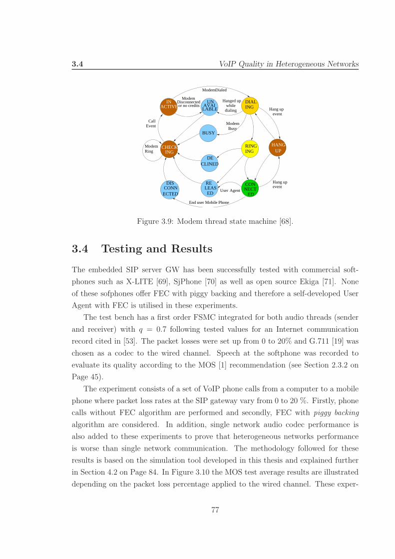
3.4 VoIP Quality in Heterogeneous Networks
ING
AVAIUN
LABLE
DIALING
BUSY
DECLINED
RINGING
CONNECT ED
RELEAS ED
DIS
ModemRing
Modem Busy
End user Mobile Phone
DialedModem
ECTEDCONN
EventCall
Hanged upwhile
dialing Hang up
Hang upevent
event
ACTIVEIN
CHECK HANGUP
ModemDisconnectedor no credits
User Agent
Figure 3.9: Modem thread state machine [68].
3.4 Testing and Results
The embedded SIP server GW has been successfully tested with commercial soft-
phones such as X-LITE [69], SjPhone [70] as well as open source Ekiga [71]. None
of these sofphones offer FEC with piggy backing and therefore a self-developed User
Agent with FEC is utilised in these experiments.
The test bench has a first order FSMC integrated for both audio threads (sender
and receiver) with q = 0.7 following tested values for an Internet communication
record cited in [53]. The packet losses were set up from 0 to 20% and G.711 [19] was
chosen as a codec to the wired channel. Speech at the softphone was recorded to
evaluate its quality according to the MOS [1] recommendation (see Section 2.3.2 on
Page 45).
The experiment consists of a set of VoIP phone calls from a computer to a mobile
phone where packet loss rates at the SIP gateway vary from 0 to 20 %. Firstly, phone
calls without FEC algorithm are performed and secondly, FEC with piggy backing
algorithm are considered. In addition, single network audio codec performance is
also added to these experiments to prove that heterogeneous networks performance
is worse than single network communication. The methodology followed for these
results is based on the simulation tool developed in this thesis and explained further
in Section 4.2 on Page 84. In Figure 3.10 the MOS test average results are illustrated
depending on the packet loss percentage applied to the wired channel. These exper-
77

3.4 VoIP Quality in Heterogeneous Networks
Bad - 1
Poor - 2
Fair - 3
Good - 4
Excellent - 5
0 5 10 15 20
MO
S v
alue
Packet loss (%)
G.711 to GSM with FECG.711 to GSM with no-FEC
Single Network G.711Single Network GSM
Figure 3.10: MOS test with q=0.7 for wire-to-wireless connection and single networkconnection [68].
iments have been assessed by over 20 people, in English, with both native and non
native listeners following the MOS standard requirements.
On one hand, the illustration shows FEC and no-FEC sessions perform equally
when the channel is free of packet losses. As the packet loss rate increases, FEC’s in-
fluence is more noticeable. This reveals that with a 10% of packet losses, FEC registers
a performance of a fairly good connection whereas the no-FEC channel is evaluated
as worse than poor. Even when considering a 20% packet loss rate, FEC shows a
poor performance but still achieves adequate speech quality. On the other hand,
single network VoIP performance for G.711 and GSM 06.10 is depicted. The com-
parison between cascaded two network performance and single network performance
highlights the impact of dual codec connection and corroborates that the awareness
of cascaded two networks connection can be advantageous to improve over all perfor-
mance. Consider the case of five percent of packet loss; a single network performance
for G.711 is 3.2 whereas double channel connection, i.e. G.711 to GSM with no-FEC,
shows a 2.3. This difference means that if a node is not aware that there is more
than one audio codec taking part in the communication, it could believe that overall
performance value is fair, i.e. 3.2, in stead of poor, i.e. 2.3. Hence, if intermediate
78

3.4 VoIP Quality in Heterogeneous Networks
0
200
400
600
800
0 200 400 600 800
Pac
ket N
umbe
r
Packet Sequence Number
Ppl-0%Ppl-5%
Ppl-10%Ppl-15%Ppl-20%
105 109 113
90 94 98
Ppl-15%
Figure 3.11: Received VoIP packet sequence result.Received VoIP packet sequence result.
nodes are aware of the communication system their assessment of the quality is more
accurate and the decision of considering FEC methods is more accurate.
One of the drawbacks related to FEC in addition to the redundant information
is the delay introduced to the communication. In this case, the microcontroller reg-
istered a delay that never exceeds 35 ms. With regards to the jitter performance 12
ms for a non FEC connection and at 13.5 ms for a FEC connection are recorded.
Although these values could influence a session’s quality, they are compensated by a
jitter buffer in the program.
A comparable result to data shown above is derived from the analysis of the
received sequence number in real-time versus the number of received packets, as seen
in Figure 3.11. As expected the greater the packet loss rate, the greater the slope of
the response is. This is shown in the expanded figure of 15% of packet loss where a
packet is lost between the sequences 90 and 100. Furthermore, TABLE 3.1 shows the
recorded values for the experiments where the benefits of using FEC in percentages
can be seen. In the packet loss column, the captured packet loss percentage in a
real scenario matches the theoretical values corroborating that the system is running
correctly. In the packet recovered column, values are almost halved in comparison to
79

3.5 VoIP Quality in Heterogeneous Networks
Table 3.1: Results For A Wire to Wireless VoIP Session with FEC
Sent Lost (%) Packet Loss Recovered with FEC Efficien-Packets Packets Recorded Recorded (%) Recorded Recorded(%) cy (η)1304 0 0 0.00 0 0 0.041028 5 62 6.03 30 2.91 0.751162 10 110 9.47 66 5.67 0.97874 15 110 12.59 72 8.23 0.88808 20 163 20.17 89 11.01 0.81
the packet loss rate value, leading to the conclusion that an extra 64/3 = 21.33 kbps
throughput required by FEC noticeably improves the system’s overall performance.
Therefore the FEC efficiency is defined from equation (3.3).
η =(△MOS)
(△BW )(MOS/Kbps) (3.3)
The numerator (△MOS) is the difference of FEC and non-FEC based MOS test
normalized to the maximum value of MOS. The denominator (△BW ) is the band-
width difference between FEC and non FEC system for a specific codec. In order to
associate each codec’s performance the numerator value is normalised to the band-
width of the codec itself, i.e 64 in case of G.711. The equation represents how valuable
is the extra information sent through FEC over the quality of voice received. Exper-
imental results show that with 0% of packet loss the efficiency proves to be very low
where theoretical response should be 0. However, the higher the packet loss the bet-
ter the efficiency, in other words, the higher the losses the more worthy is to send
redundant data. This efficiency parameter can be considered as a regulator for end
nodes to evaluate the use of FEC under bursty losses.
3.5 Conclusion
In this chapter, an embedded SIP server Gateway to mobile networks with FEC
is presented. Wired and wireless networks have been interfaced by developing an
expansion board and integrating FEC system for VoIP sessions as an example of
a heterogeneous network connection. Our development demonstrates that utilising
FEC for a wired to wireless system, performs satisfactorily even under high packet
80
3.5 VoIP Quality in Heterogeneous Networks
loss channels. Furthermore, the efficiency cost of such model, as shown in TABLE
3.1, determines that under poor channel conditions the implementation of FEC is
beneficial if action is taken by the gateway. Consequently it is proved that active
SIP GWs can enhance end-to-end speech quality, however this is only approved for a
single case scenario. Hence, an analytical model to predict speech quality perception
under a number of different networks is required for the rapid assessment of QoS
which is presented in the following chapter.
81

CHAPTER 4
Speech Quality Prediction for
Heterogeneous Networks
4.1 Speech Quality Prediction for Heterogeneous Networks
4.1 Introduction
IN the previous chapter a VoIP GW implementation proved that passive GWs, i.e.
only store and forward GWs, perform worse when compared to GW’s with FEC
that are aware of channel conditions. The results gained from such implementation
highlight the advantage of intelligent networks to improve QoS. In next generation
networks, end-to-end communications will utilise a variety heterogeneous technolo-
gies and consequently predicting quality performance can play an important role in
network design. In Section 2.3, MOS and E-model showed that VoIP calls can be
rated with subjective and objective methodologies respectively. In Chapter 3 the
MOS model is used to present the results while in this chapter the E-model is con-
sidered to predict speech quality in heterogeneous networks. However, this analytical
model presents a number of limitations where the restricted number of parametrised
audio codecs , see recommendation [31], narrows down the scope of further research
to be carried out. In addition, the model is based on a single audio codec connection
from an end-to-end perspective which is acceptable for an Internet core soft-phone
to soft-phone call but not for a heterogeneous communication system. Considering
the implementation in Chapter 3 for a wired-to-wireless communication, where the
wired network is provided with G.711 audio codec, packet losses rate clearly have an
impact on overall performance. The crucial question is what happens if the wired
network uses another audio codec? Is it necessary to set the implementation again or
can speech quality perception be predicted? Current state of the art models do not
provide a straight forward solution to this problem, however the analytical model pre-
sented in this chapter can predict speech quality perception under two independent
channels using a self developed simulation tool.
In this chapter, the proposed model provides up to three audio codes and two
cascaded network estimations at a time. Simulator response is tested with MOS and
results are compared to the proposed E-model extension where the lower the error-
margin the better the prediction. Channels are modelled through the Finite State
Markov Chain (FSMC) analytical model due to extensive literary research that has
proved it highly successful [72]. The analysis of the effect of multiple channels on
speech quality is carried out in two parts. Firstly, single network tests are performed
to compute codec specific parameters, i.e Ie and Bpl for G.711, GSM06.10 and Speex.
Recall that the E-model uses Ie ( equipment impairment factor) and Bpl ( packet
83
4.2 Speech Quality Prediction for Heterogeneous Networks
loss robustness factor) to parametrise an audio codec (see equation (2.12)). Secondly,
double channel tests with codec and packet loss variations are tested and analysed
following the implementation presented in the previous chapter. The results proved
that low error-margins are achieved with the proposed method.
The remainder of the chapter is organised as follows. Section 4.2 describes the
simulation system design, utilising audio codecs and the packet loss dependency over
multiple channels for VoIP session. Section 4.3 presents the proposed formula to ex-
tend the E-model. Section 4.4 validates the proposed analytical model and evaluates
the performance to predict speech quality under heterogeneous networks. Finally
Section 4.5 concludes the chapter.
4.2 New Simulation Design for Multiple Channels
In this section, a new simulation design for multiple channels is presented. The
idea is to design a generic system capable of modelling the behaviour of multiple
different sub-networks that take part in an heterogeneous communication network
as long as these sub-networks can be mathematically modelled. Figure 4.1 depicts
the comparison between the conventional E-model and the proposed system in this
chapter. The conventional E-model is based on a single network single audio codec
prediction system. The model has been widely researched and its performance has
been agreed to have a fair accuracy in the prediction of speech quality. The proposed
model expands the conventional method to adopt a multiple number of networks and
audio codecs where a Gateway provides the communication to the differing networks.
Consider the implementation in Chapter 3 where a VoIP connection from a soft
phone to a mobile phone using a SIP proxy GW crossing IEEE 802.3 and the GSM
networks is presented. Currently such connection can not be modelled using con-
ventional E-model. To solve this problem audio codecs described in Section 2.2.3
on Page 36 are used with FSMC channel models to set a MOS test. Initially, the
analytical model for multiple independent FSMC networks is shown and then the
simulation tool is described.
84

4.2 Speech Quality Prediction for Heterogeneous Networks
Figure 4.1: Comparison of the conventional E-model and extended E-model for mul-tiple channels.
4.2.1 Markov Based Channel Modelling
In the previous chapter, the use of FSMC [62] has been presented as a model for
bursty networks, where network’s packet loss probability is related to the delivery
or not of last packet. Recall from Figure 3.2 on page 66 that P (G → B) = p
represents the probability of moving from the Good state to the Bad State whereas
P (B → G) = q represents the probability of moving from the Bad to the Good state.
Hence, the probability of being in either the Good or the Bad is calculated using
π0 = (q/(p + q)), π1 = (p/(p + q)) respectively. Considering that the actual path of
communication must travel across multiple channels, each of them can be represented
by a first order FSMC as seen in Figure 4.2. This figure illustrates n number of two
state Markov Chain model. The analytical expression of this communication system
is defined by the transition matrix in equation (4.1) [73].
This matrix is a multiple independent FSMCs gathered in a single matrix where
πi is P (Gi− > Bi) of the ith channel and qi P (Bi− > Gi) for (i = 1, 2, ...n). The
average packet loss probability per channel is independent and therefore the overall
average packet loss probability, Pplt, is calculated by equation (4.2) where ppli is
85

4.2 Speech Quality Prediction for Heterogeneous Networks
1− p1 q1 0 0 0 0
p1 1− q1 0 0 0 0
0 0 1− p2 q2 0 0
0 0 p2 1− q2 0 0
0 0 0 0 . .
0 0 0 0 1− pn qn
0 0 0 0 pn 1− qn
π1.0
π1.1
π2.0
π2.1
.
πn.0
πn.1
=
π1.0
π1.1
π2.0
π2.1
.
πn.0
πn.1
(4.1)
p
q
1−q
G B1−p
p
q
1−q
G B1−p
p
q
1−q
G B1−p
1
1
11
2
2
2
2
n
n
n
n
Figure 4.2: N number of independent FSMC channels.
FSMCi’s average packet loss probability which depends on πi.0 taken from equation
(4.1) defined from equation (3.1) [73].
Pplt = 1−∏
(1− ppli) (4.2)
4.2.2 Simulation Tool
Figure 4.3 on the next page shows the developed simulation tool for speech prediction
tests, written in C language. Voice is sampled to 8 KHz, 16 bit, Little Endian, grouped
in 160 samples for a 20ms packet size. Packets are encoded, filtered by Markov Chain
(MCi) model and buffered at the receiver side to avoid jitter distortion. A decoder
is applied (if necessary) and encoded again to be filtered by the next channel model.
Note that the process to exchange different codec types is done by an entity called
86

4.3 Speech Quality Prediction for Heterogeneous Networks
Figure 4.3: VoIP session model for Multiple channels [73].
Gateway (GW). When the packets arrive at the final destination they are decoded
and played back as 16 bit, 8KHz sampled signal. The model is flexible to be set from
1 to n number of channels, although in these experiments only up to two channels
have been investigated.
4.3 Proposed Extended E-model
The new simulation design in the previous section, presents an scenario where n
number of channels with n number of audio codecs is possible. This new paradigm
introduces a number of constraints to predict speech quality where conventional E-
model described in [2] is not valuable any more. In this section, the conventional
E-model is extended based on extended trial and error approaches that minimises the
difference between subjective experiments and the mathematical model itself. The
proposed new R-value is defined as follows [73]:
R = R0 − IS − ID − Ie−efft + Ieq + A (4.3)
where the signal to noise ratio, R0, the simultaneous impairment factors, IS, and
the advantage factor , A, are evaluated using default values as shown in equation
(2.5). Equally, the delay impairment factor, ID, is also defined according to the
conventional method (see equation (2.6)). This is conceivable because this impairment
87

4.3 Speech Quality Prediction for Heterogeneous Networks
is independent of channel status or utilised audio codec type. Hence, the extended
R-value can be rewritten as [73]
R = 93.3− ID − Ie−efft + Ieq (4.4)
The proposed equation differs in a number of aspects from the conventional E-
model. The effective equipment impairment factor, Ie−efft, is defined as the number of
factors that predicts the impairment factor related to channel response with different
audio codecs. Recall that Ie−eff uses Ppl and BurstR to model the channel and
Ie and Bpl for audio codec performance (see equation (2.12)). In a communication
system with multiple channels and multiple audio codecs, the overall performance is
always dependant on the poorest audio codec and channel. In a parallelism with a
production line, the poorest audio codec is presumably the bottleneck of the system
whereby productions maximum output is the output of the bottle neck production.
Consequently, the proposed analytical model for Ie−efft is based on the poorest Ie−effi
within the communication system to predict over all performance where the poorest
audio codec is determined from the Ie values [73].
Ie−efft = Ie−eff1 +n∑
i=1
ρi × Ie−effi+1(4.5)
where
ρi =
1 for Iei = Ie1
IeiIei+1
× 100 for Iei 6= Iei+1
(4.6)
and
Ie1 > Ie2 > ...Ien (4.7)
BurstRi =pi
pi + qi(4.8)
In this case, Ie−eff1 refers to the poorest audio codec out of n number of channels
and ρ is a factor that allows diminishing the impact of other codecs degradation in
comparison with the performance of Ie1 . It is important to note that multiple channels
with the same audio codec, i.e. Iei = Ie1 , are predicted as a sum of independent
effective equipment factors. The burstiness modelled with FSMC is represented by
88

4.3 Speech Quality Prediction for Heterogeneous Networks
equation 4.8 where pi refers to the average packet loss percentage of the channel and
qi is the parameter that defines the channel itself.
In addition to the extended effective equipment factor, the proposed analytical
model adds a new impairment factor, defined as the distortion equaliser impairment
factor, Ieq. This factor has been incorporated to the analytical model due to inaccu-
racies obtained with very high packet losses, i.e. packet losses above 15%. The main
reason behind this parameter is that human perception barely distinguishes between
a communication system with 20 % and 15 % of packet looses resulting in large differ-
ence between MOS tests and proposed analytical model. The new impairment factor
is defined as [73]:
Ieq = 1 + ePplt−15
15 (4.9)
where Pplt follows equation (4.2) and 15 refers to a fixed numerical value defined
after substantial experimental results.
4.3.1 Methodology to determine audio codecs’ parameters
The above formula extends the conventional E-model prediction to heterogeneous
networks which is tested in the following section. Nevertheless, the audio codecs
described in Section 2.2.3 are not defined by the ITU-T recommendation [31] and
hence experimental measurements are required to determine their parameters.
An audio codec in the E-model is defined by Ie and Bpl. To determine the value
of Ie, MOS tests for each audio codec are carried out with zero delay and zero packet
loss. The experimental values are converted to the R-value which is set with default
values. Since Ppl = 0 and the rest of the parameters are known, Ie is calculated by
using the following equation:
Ie = 93.3−R− ID (4.10)
Once Ie is defined, the value of Bpl is determined. In this case, MOS tests are
performed for each audio codec with a variety of packet loss percentages using a
MC model with q = 0.7. The reason behind this q value is that previous chapter’s
implementation is based on this parameter which provides results with a closer match
to real implementations. The packet loss range is varied from 5% to 20% where each
time the Bpl value is measured as
89
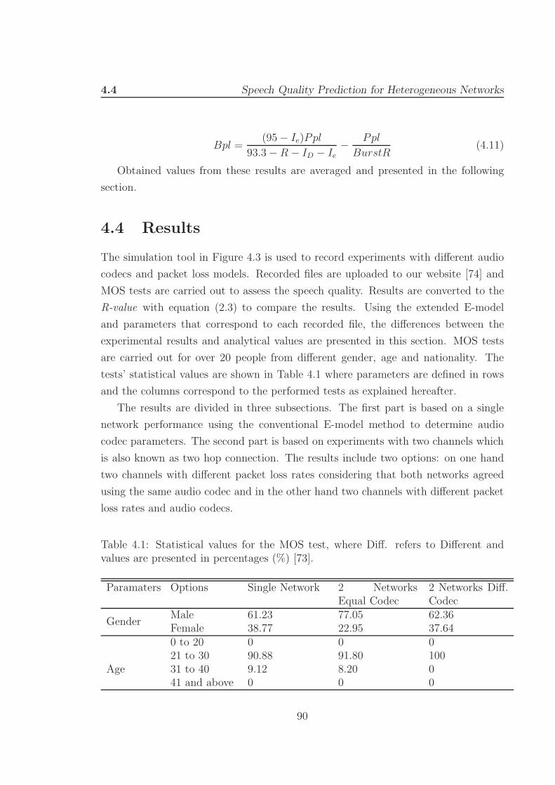
4.4 Speech Quality Prediction for Heterogeneous Networks
Bpl =(95− Ie)Ppl
93.3−R − ID − Ie−
Ppl
BurstR(4.11)
Obtained values from these results are averaged and presented in the following
section.
4.4 Results
The simulation tool in Figure 4.3 is used to record experiments with different audio
codecs and packet loss models. Recorded files are uploaded to our website [74] and
MOS tests are carried out to assess the speech quality. Results are converted to the
R-value with equation (2.3) to compare the results. Using the extended E-model
and parameters that correspond to each recorded file, the differences between the
experimental results and analytical values are presented in this section. MOS tests
are carried out for over 20 people from different gender, age and nationality. The
tests’ statistical values are shown in Table 4.1 where parameters are defined in rows
and the columns correspond to the performed tests as explained hereafter.
The results are divided in three subsections. The first part is based on a single
network performance using the conventional E-model method to determine audio
codec parameters. The second part is based on experiments with two channels which
is also known as two hop connection. The results include two options: on one hand
two channels with different packet loss rates considering that both networks agreed
using the same audio codec and in the other hand two channels with different packet
loss rates and audio codecs.
Table 4.1: Statistical values for the MOS test, where Diff. refers to Different andvalues are presented in percentages (%) [73].
Paramaters Options Single Network 2 NetworksEqual Codec
2 Networks Diff.Codec
GenderMale 61.23 77.05 62.36Female 38.77 22.95 37.64
Age
0 to 20 0 0 021 to 30 90.88 91.80 10031 to 40 9.12 8.20 041 and above 0 0 0
90

4.4 Speech Quality Prediction for Heterogeneous Networks
4.4.1 Validating the Model
The proposed model for heterogeneous networks is validated with the hardware im-
plementation presented in Chapter 3 as shown in Figure 4.4. On one hand, the results
that refer to G.711-GSM 0610 Hardware are taken from Figure 3.10 on page 78 using
the data with regards to G711 to GSM with no-FEC. These values have been trans-
lated to the E-model using equation 2.3. On the other hand, the results obtained by
the proposed model for cascaded network performance using the mathematical model
described in previous section, are represented under the name of G.711-GSM06.10
Model. Comparing the results of both experiments, it is concluded that the model is
a good and fair approach of the hardware model since the differences between both
results is negligible. Hence the variety of the results obtained throughout this chap-
ter are considered as realistic as hardware implementation results for speech quality
prediction.
0
10
20
30
40
50
60
70
80
90
100
1 2 3 4 5 6 7 8 9 10 11 12 13 14 15 16 17 18 19 20
R-v
alue
Packet loss percentage (Ppl) %
G711-GSM06.10 HardwareG711-GSM06.10 Model
Figure 4.4: Comparison of Hardware vs Model.
91

4.4 Speech Quality Prediction for Heterogeneous Networks
4.4.2 New Parameters for Audio Codecs
In these tests a single network with single audio codec is tested in order to define
the parameters for G.711, GSM and Speex audio codecs. The simulation tool is set
to q = 0.7 [53] and no delay is introduced. The obtained results are presented in
Figure 4.5 and Table 4.2 following the formulae in Section 4.3.1. On one hand, the
figure illustrates the average performance of each codec whereas the table presents
Ie and Bpl parameters for each audio codec which are divided in two columns. First
column represents the already available parameters from ITU-T recommendation [31]
where unknown values are shown with ’-’ symbol. Second column is the experimental
results obtained using equations (4.10) and (4.11). Note that the Ie difference for
G.711 between the experimental results and values from [31] is negligible whereas the
Bpl shows higher differences. This is due to the fact that measurements are carried
out with FSMC models rather than random losses. Regarding to GSM audio codec it
can be seen that the Ie differs slightly from the values provided by the ITU-T, which
ensures that the experimental results and the methodology to obtain the values are
accurate. Overall, robustness values appear to have high value for linear predictive
codes (Speex and GSM06.10) however, the codec performance adjusts to the obtained
0
10
20
30
40
50
60
70
80
90
100
0 1 2 3 4 5 6 7 8 9 10 11 12 13 14 15 16 17 18 19 20
R-v
alue
Packet loss (%)
Single Network G.711Single Network GSM 06.10
Single Network SPEEX(MOD4)
Figure 4.5: Single Network codec performance results [73].
92

4.4 Speech Quality Prediction for Heterogeneous Networks
measurements as seen in the following subsections.
Table 4.2: Codec Measurement Results [73].
ReferenceITU-T [31] ExperimentalIe Bpl Ie Bpl
GSM06.10 20 - 24.37 39.32Speex-MOD4 - - 5.37 37.82G.711 0 4.3 0.37 12.92
4.4.3 Speech Quality Prediction for a Two Hop Connection
In this set of experiments, two channels are tested with MOS, converted to the R-
value and compared to our proposed model. The results are based on two independent
FSMC models with two variations: one for equal codecs per channel and the other
for different codecs.
4.4.3.1 Equal Audio Codecs per Hop
Equal codecs per hop experiment is based on two FSMC models where qi value is
fixed to 0.7 in both channels and two different packet losses per channel, ppl1 and
ppl2, are configured at the simulation tool. Pplt is calculated using equation (4.2)
with i = 2 whereas Ie− efft is calculated with equation (4.5) where ρ = 1 since both
channels’ Ie is the same. Finally, audio codec parameters are taken from Table 4.2.
Figure 4.6 shows the performance graphs for different packet loss channels and
audio codecs. Each graph is represented by a fixed packet loss rate depicted in the
upper left label and a variable packet loss rate in the x axis. In the y axis the R-value
of the analytical model versus the experimental results is illustrated. All graphs
include the three audio codecs: G.711, GSM and Speex, where audio˙codec˙name
E-model refers to the proposed extended model and audio˙codec˙name MOS is the
experimental result obtained through the website.
G.711 performance with an error-margin average of 5.02R and a maximum error
of 9.54R shows the consistency of the proposed formula. The maximum error appears
at Ppl1 = 20% & Ppl2 = 5% where a rather exceptional case occurs. In this error
percentage, the tested file suffers from a combination of packet losses where a number
93
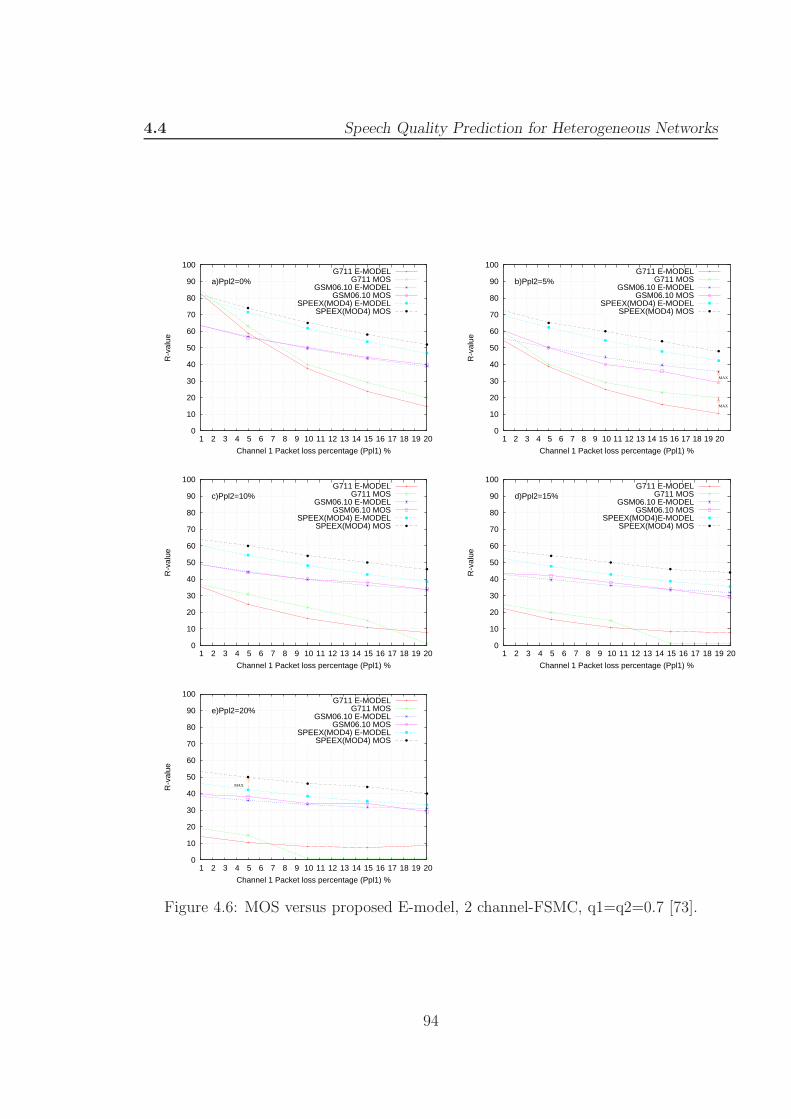
4.4 Speech Quality Prediction for Heterogeneous Networks
0
10
20
30
40
50
60
70
80
90
100
1 2 3 4 5 6 7 8 9 10 11 12 13 14 15 16 17 18 19 20
R-v
alue
Channel 1 Packet loss percentage (Ppl1) %
a)Ppl2=0%G711 E-MODEL
G711 MOSGSM06.10 E-MODEL
GSM06.10 MOSSPEEX(MOD4) E-MODEL
SPEEX(MOD4) MOS
0
10
20
30
40
50
60
70
80
90
100
1 2 3 4 5 6 7 8 9 10 11 12 13 14 15 16 17 18 19 20
R-v
alue
Channel 1 Packet loss percentage (Ppl1) %
b)Ppl2=5%
MAX
MAX
G711 E-MODELG711 MOS
GSM06.10 E-MODELGSM06.10 MOS
SPEEX(MOD4) E-MODELSPEEX(MOD4) MOS
0
10
20
30
40
50
60
70
80
90
100
1 2 3 4 5 6 7 8 9 10 11 12 13 14 15 16 17 18 19 20
R-v
alue
Channel 1 Packet loss percentage (Ppl1) %
c)Ppl2=10%G711 E-MODEL
G711 MOSGSM06.10 E-MODEL
GSM06.10 MOSSPEEX(MOD4) E-MODEL
SPEEX(MOD4) MOS
0
10
20
30
40
50
60
70
80
90
100
1 2 3 4 5 6 7 8 9 10 11 12 13 14 15 16 17 18 19 20
R-v
alue
Channel 1 Packet loss percentage (Ppl1) %
d)Ppl2=15%G711 E-MODEL
G711 MOSGSM06.10 E-MODEL
GSM06.10 MOSSPEEX(MOD4)E-MODEL
SPEEX(MOD4) MOS
0
10
20
30
40
50
60
70
80
90
100
1 2 3 4 5 6 7 8 9 10 11 12 13 14 15 16 17 18 19 20
R-v
alue
Channel 1 Packet loss percentage (Ppl1) %
e)Ppl2=20%
MAX
G711 E-MODELG711 MOS
GSM06.10 E-MODELGSM06.10 MOS
SPEEX(MOD4) E-MODELSPEEX(MOD4) MOS
Figure 4.6: MOS versus proposed E-model, 2 channel-FSMC, q1=q2=0.7 [73].
94

4.4 Speech Quality Prediction for Heterogeneous Networks
of short words (1 syllable) are lost and the comprehension of the speech becomes hard,
resulting in a lower rate in the MOS test. Conversely the mathematical models do
not distinguish between words or packets and therefore the estimated speech quality
is slightly better than that of users perception. As the packet percentages increases,
MOS tests show that users barely distinguish tests with 15% of packet loss rates or
higher rates. This can be seen with Ppl1 = 15% & Ppl2 = 15% and Ppl1 = 10%
& Ppl2 = 20% where the MOS is dropped to one which is equivalent to the lowest
value of the MOS system.
GSM 06.10 codec error-margin average is 1.68R the lowest of all of them. The
smooth response obtains the largest error in Ppl1 = 20% & Ppl2 = 5% where the
value rises to 6.84R. Again this is related to the same problem described for G.711,
where the loss of a number of consequent words generates a bad performance for the
users. Despite of it all, the performance of the analytical model is very accurate in
this case.
Finally, Speex performance shows an average error-margin value of 3.03R with a
maximum peak of 4.92R recorded at Ppl1 = 5% & Ppl2 = 20%. In this case, the
error average of the analytical model is always marginally more positive than the
actual user perception but due to low error differences this is considered insignificant.
These experiments demonstrate that in the scenarios where both channels have the
same audio compressors, predictions are accurate compared to those values obtained
through subjective testing.
4.4.3.2 Different Codecs per Hop
Different codecs per hop experiment is based on two FSMC models where q1 and q2
values are set to 0.7 and 0.1492, respectively. The former value represents an Internet
connection [53] whereas the later is taken from research based on GSM networks [75].
Different packet losses and audio codecs per channel are utilised as input sources
of the simulation tool. Pplt is calculated using equation (4.2) with i = 2 whereas
Ie− efft is calculated with equation (4.5) where ρ value depends upon the audio
codecs considered per channel.
Figure 4.7 shows the performance graphs for different packet loss channels and
audio codecs. The representation of each graph follows the equal codecs graphs
shown in the previous experiment. In this case, experiments for G.711 with GSM,
G.711 with Speex and Speex with GSM are presented. It is important to point out
95

4.4 Speech Quality Prediction for Heterogeneous Networks
that the order of the audio codecs is considered irrelevant since the analytical model
takes into consideration the poorest audio codec to predict speech quality.
G.711 with GSM error-margin shows an average of 8.35R and a maximum error
peak of 22R. This combination of codecs illustrate the poorest performance all results
for the proposed analytical model where the peak can be found at ppl1 = 15% & ppl2 =
20%. There are two main reasons related to this discrepancy: firstly from previous
experiments is understood that human perception for very high packet losses tends
to be distorted due to the incapacity of humans to distinguish between bad and very
bad quality. Secondly, it is believed that the combination of LP codecs with waveform
codecs is expected to perform poorly due to the difference in the Ie parameter which
is reflected in the lower values obtained by the mathematical model.
The combination of G.711 and Speex presents a performance of 2.28R average
error-margin with a maximum peak of 8.05R. The peak is found at ppl1 = 20% &
ppl2 = 0% which if compared with the performance of G.711 with GSM it can be seen
that the high percentage of packet losses in G.711 has an impact on LP based audio
codecs. Nevertheless, the performance of the analytical model can be considered as
fair due to low average error-margin.
Finally Speex with GSM shows a performance of 3.71R error-margin error with a
peak of 8.55R at ppl1 = 15% & ppl2 = 0%. In this case, the lower quality obtained
through Speex codec affects the natural performance of GSM and therefore the MOS
test shows lower values than the analytical model. Despite of it, the average error-
margin is low and proves the proposed analytical model to be a good approach.
Considering all the results, several conclusions that can be drawn. Initially, wave-
length based speech codecs always have the best audio performance. This is observed
in both cases where ppl1 = 0% & ppl2 = 0% where results with G.711 codec show
the best R-value. The second conclusion is that very high packet loss rates are not
distinguishable by human perception regardless of the audio codec utilised. This is
interesting because intermediate nodes could take action by forcing to either end a
VoIP session or consider FEC systems if the expected overall quality drops down to
40R or below. The third conclusion refers to cases with different audio codecs are
utilised where two LP based audio codecs perform worse than a wavelength and a LP
based calls. In fact, throughout all these experiments the best performance is given
to G.711 with Speex codec. Finally, although few examples of high error-margins are
found, it is expected that the on going test results will corroborate even greater the
96

4.4 Speech Quality Prediction for Heterogeneous Networks
0
10
20
30
40
50
60
70
80
90
100
1 2 3 4 5 6 7 8 9 10 11 12 13 14 15 16 17 18 19 20
R-v
alue
Channel 1 Packet loss percentage (Ppl1) %
a)Ppl2=0%
MAX
MAX
G711-GSM06.10 E-MODELG711-GSM06.10 MOS
G711-SPEEX(MOD4) E-MODELG711-SPEEX(MOD4) MOS
SPEEX(MOD4)-GMS06.10 E-MODELSPEEX(MOD4)-GMS06.10 MOS
0
10
20
30
40
50
60
70
80
90
100
1 2 3 4 5 6 7 8 9 10 11 12 13 14 15 16 17 18 19 20
R-v
alue
Channel 1 Packet loss percentage (Ppl1) %
a)Ppl2=5%G711-GSM06.10 E-MODEL
G711-GSM06.10 MOSG711-SPEEX(MOD4) E-MODEL
G711-SPEEX(MOD4) MOSSPEEX(MOD4)-GMS06.10 E-MODEL
SPEEX(MOD4)-GMS06.10 MOS
0
10
20
30
40
50
60
70
80
90
100
1 2 3 4 5 6 7 8 9 10 11 12 13 14 15 16 17 18 19 20
R-v
alue
Channel 1 Packet loss percentage (Ppl1) %
a)Ppl2=10%G711-GSM06.10 E-MODEL
G711-GSM06.10 MOSG711-SPEEX(MOD4) E-MODEL
G711-SPEEX(MOD4) MOSSPEEX(MOD4)-GMS06.10 E-MODEL
SPEEX(MOD4)-GMS06.10 MOS
0
10
20
30
40
50
60
70
80
90
100
1 2 3 4 5 6 7 8 9 10 11 12 13 14 15 16 17 18 19 20
R-v
alue
Channel 1 Packet loss percentage (Ppl1) %
a)Ppl2=15%G711-GSM06.10 E-MODEL
G711-GSM06.10 MOSG711-SPEEX(MOD4) E-MODEL
G711-SPEEX(MOD4) MOSSPEEX(MOD4)-GMS06.10 E-MODEL
SPEEX(MOD4)-GMS06.10 MOS
0
10
20
30
40
50
60
70
80
90
100
1 2 3 4 5 6 7 8 9 10 11 12 13 14 15 16 17 18 19 20
R-v
alue
Channel 1 Packet loss percentage (Ppl1) %
a)Ppl2=20%
MAX
G711-GSM06.10 E-MODELG711-GSM06.10 MOS
G711-SPEEX(MOD4) E-MODELG711-SPEEX(MOD4) MOS
SPEEX(MOD4)-GMS06.10 E-MODELSPEEX(MOD4)-GMS06.10 MOS
Figure 4.7: MOS versus proposed E-model, 2 channel-FSMC, q1=0.7, q2=0.1492 [73].
formula presented in this thesis.
97

4.5 Speech Quality Prediction for Heterogeneous Networks
4.5 Conclusion
In this chapter, an analytical study for VoIP with two network channels is presented
based on the current E-model. Firstly, the study presented single network results
where three audio codecs are tested. Ie and Bpl values for them are measured using
FSMC models and validated with the current G.711 codecs parameters as defined
by the ITU-T. Secondly, two channel network experiments are carried out with two
major set-ups:
1. Equal audio codecs in both channels
2. Different audio codecs per channel
The proposed extended E-model is used to match the MOS test by introducing two
main variables: a new impairment factor to equalise results with high packet loss
rates, and the ρ factor which balances the performance of independent channels with
different audio codecs. The average error-margin of the analytical model compared
with the MOS values shows a reasonable 1.68R to 8.35R error-range.
98
CHAPTER 5
Network Coding on VoIP

5.1 Network Coding on VoIP
5.1 Introduction
IN telecommunications there are three types of communication methods: unicast-
to-unicast, unicast-to-multicast and multicast-to-multicast. The telephone net-
work is based on a unicast-to-unicast method belonging to a hierarchical topology
whereas a broadcast network, based in a flat topology, allows communications be-
tween all peers facilitating unicast-to-multicast and multicast-to-multicast methods.
Nowadays, broadcast networks are preferred, specially wireless broadcast networks
because they cut down costs to service providers for the last mile connection.
Wireless networks often function on omnidirectional basis however, rather than
making use of such beneficial characteristics, most technology has been designed to
achieve unicast-to-unicast communications. This is understandable when taking into
consideration the security issues relating to private or personal information and its
protection against fraudulent use. This can be seen in home networks where the core
of the Internet remains mainly unicast communication. Conversely services such as
satellite TV have already developed a unicast-to-multicast service.
Network coding addresses unicast-to-multicast and multicast-to-multicast commu-
nications from an unknown angle, as seen in Section 2.4. Initially Yeung and Zhang
presented a pioneering research on unicast-to-multicast for satellite communications
in [35]. This concept was further developed by Ahlswede et al. in [32] in a later
paper naming the method as ”network coding”. This inspiring method makes use of
coding theory to increase channel throughput by combining existing packets in the
network and multicast them so that receivers can decode the message. This theory is
particularly encouraging for an increase in performance of half duplex networks and
it is not restricted to any particular layer of the Open System Interconnection (OSI)
model.
VoIP suffers from long delays caused by queues that converge into packet losses
resulting in poor call performance. To insert network coding schemes and create
even more delays at first glance might appear counterproductive but in this chapter,
a new proposal to use network coding theory for VoIP services is presented without
dependency on the physical layer. The block diagram of a possible case scenario where
the proposed model can be implemented is shown in Figure 5.1. In this illustration
a base station with multiple cells is connected to a network with a SIP proxy and
a Media Gateway that provides VoIP services. The users are connected to the base
100

5.2 Network Coding on VoIP
Figure 5.1: Scenario where Network Coding for VoIP is an improvement.
station which divides the geographical area into cells. In particular, one of the cells,
registers a large number of user as it could be the case when popular events happen in
a concentrated area, for example, a football match or a music concert. Subsequently
the aim of this research is to improve the performance of conventional VoIP services
with special care at last mile wireless networks. The theoretical overview described in
Section 2.4, presents a broadcast network graph model using acyclic networks. One
such network, as shown in Figure 2.13 on page 57, was considered whilst designing a
new paradigm for VoIP communications to support network coding techniques. This
paradigm requires a set of changes: a packet modification, queue systems and call
flow synchronisation. This new algorithm for VoIP, remarkably increases by 100 %
the number of VoIP calls that a Basic Service Set (BSS) can handle.
The remainder of this chapter is organised as follows. Section 5.2 presents the
proposed algorithm for VoIP with network coding. Section 5.3 defines theoretical
minimum delays for VoIP with QoS followed by an applied analysis to IEEE 802.11b
networks. Section 5.4 implementation and 5.5 its results, describe and discuss the
theoretical models and obtained performance. Finally, Section 5.6 concludes the
chapter.
5.2 An algorithm for VoIP with Network Coding
In this section, a new proposal for VoIP services is presented, fully compliant with
current state of the art and independent of the physical layer.
VoIP requires a large scale of network resources to both Internet Core and end
users. The traditional method for VoIP is based on central nodes called SIP Proxies
with user Registrar and Location Service (LS) capabilities. End users make use of
101

5.2 Network Coding on VoIP
Figure 5.2: Design comparison between conventional method and our proposedmethod over a half duplex channel [76].
SIP Proxies to locate the call receiver; depending on session features, calls would
be routed either from end user to end user (Peer to Peer system as seen Figure 2.2
on page 33) or through a centralised server as seen in Figure 2.3 on page 34. The
former releases the traffic load to the central server and the latter keeps control of all
data exchanged between users. In some cases, such as wireless communications, end
users are connected to their base station and communication between end nodes must
go through a centralised node. Conventional base stations will simply forward the
message, missing the opportunity to maximise throughput of the channel applying
network coding techniques.
Consider a SIP Proxy that acts as information relay between two end nodes. The
conventional method would only forward packets from node A to node B by simply
repeating them. With network coding central node can combine received packets to
create a new set of outgoing packets reducing the usage of the network as explained
in Section 2.4 on Page 50. In this case, we use the model of Figure 2.13 on page 57
to represent the real environment depicted by Figure 5.2 [76].
In this figure, Alice and Bob are defined as the sink nodes from Figure 2.13 on
page 57 and the SIP server is the central node that acts on behalf of the source
node and node 1. The information units are set with the simplest field, F2 = {0, 1},
the matrix encoders Ms,j and M1,l are used as defined in equation (2.21) and (2.25),
respectively and hence the broadcasted information is a modulo two addition in ac-
cordance with equation (2.29).
Illustration on Figure 5.2, compares the packet flow for a conventional centralised
VoIP session against network coding method. The former implies that all packets
102
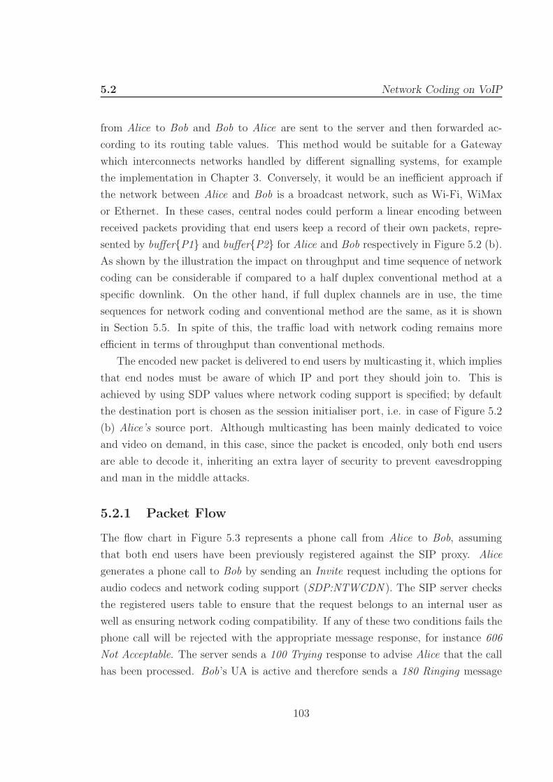
5.2 Network Coding on VoIP
from Alice to Bob and Bob to Alice are sent to the server and then forwarded ac-
cording to its routing table values. This method would be suitable for a Gateway
which interconnects networks handled by different signalling systems, for example
the implementation in Chapter 3. Conversely, it would be an inefficient approach if
the network between Alice and Bob is a broadcast network, such as Wi-Fi, WiMax
or Ethernet. In these cases, central nodes could perform a linear encoding between
received packets providing that end users keep a record of their own packets, repre-
sented by buffer{P1} and buffer{P2} for Alice and Bob respectively in Figure 5.2 (b).
As shown by the illustration the impact on throughput and time sequence of network
coding can be considerable if compared to a half duplex conventional method at a
specific downlink. On the other hand, if full duplex channels are in use, the time
sequences for network coding and conventional method are the same, as it is shown
in Section 5.5. In spite of this, the traffic load with network coding remains more
efficient in terms of throughput than conventional methods.
The encoded new packet is delivered to end users by multicasting it, which implies
that end nodes must be aware of which IP and port they should join to. This is
achieved by using SDP values where network coding support is specified; by default
the destination port is chosen as the session initialiser port, i.e. in case of Figure 5.2
(b) Alice’s source port. Although multicasting has been mainly dedicated to voice
and video on demand, in this case, since the packet is encoded, only both end users
are able to decode it, inheriting an extra layer of security to prevent eavesdropping
and man in the middle attacks.
5.2.1 Packet Flow
The flow chart in Figure 5.3 represents a phone call from Alice to Bob, assuming
that both end users have been previously registered against the SIP proxy. Alice
generates a phone call to Bob by sending an Invite request including the options for
audio codecs and network coding support (SDP:NTWCDN ). The SIP server checks
the registered users table to ensure that the request belongs to an internal user as
well as ensuring network coding compatibility. If any of these two conditions fails the
phone call will be rejected with the appropriate message response, for instance 606
Not Acceptable. The server sends a 100 Trying response to advise Alice that the call
has been processed. Bob’s UA is active and therefore sends a 180 Ringing message
103
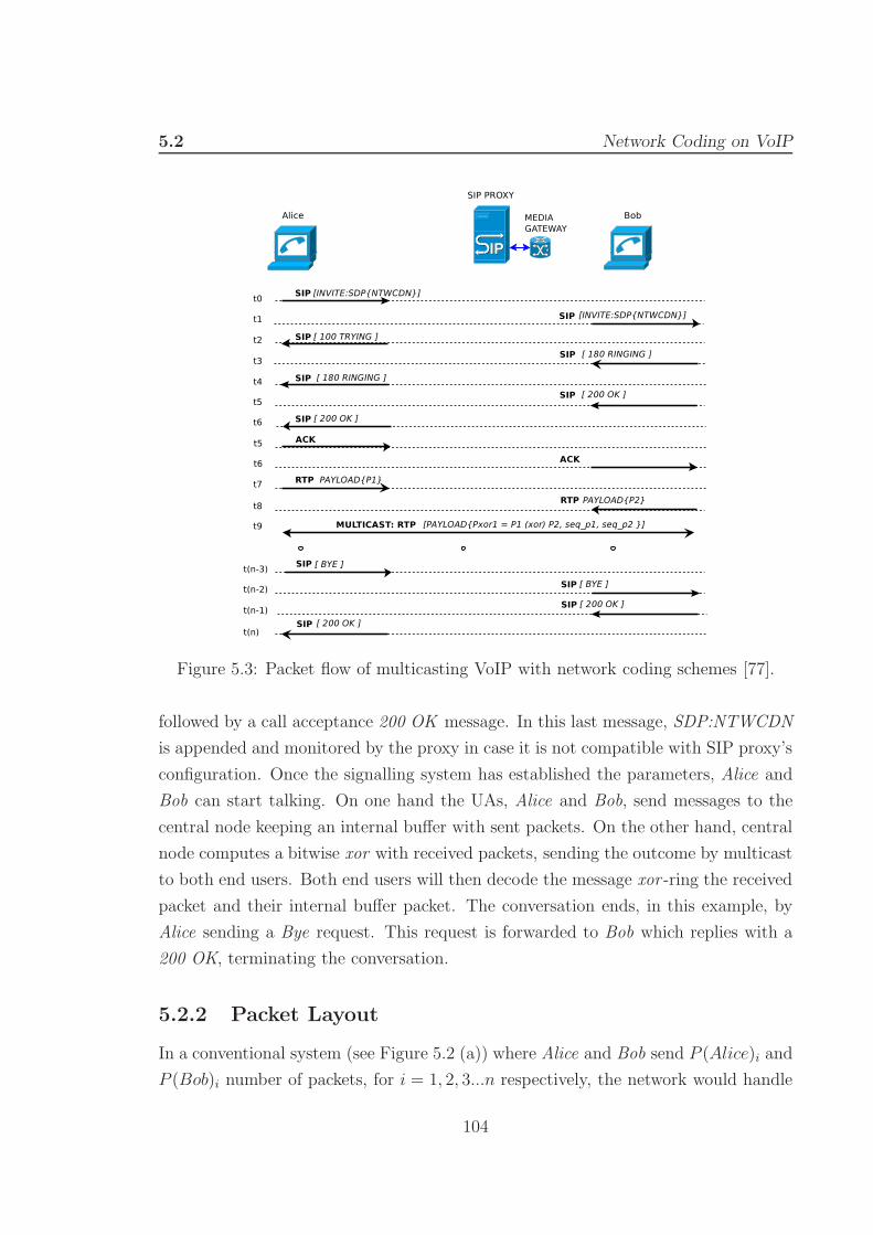
5.2 Network Coding on VoIP
Figure 5.3: Packet flow of multicasting VoIP with network coding schemes [77].
followed by a call acceptance 200 OK message. In this last message, SDP:NTWCDN
is appended and monitored by the proxy in case it is not compatible with SIP proxy’s
configuration. Once the signalling system has established the parameters, Alice and
Bob can start talking. On one hand the UAs, Alice and Bob, send messages to the
central node keeping an internal buffer with sent packets. On the other hand, central
node computes a bitwise xor with received packets, sending the outcome by multicast
to both end users. Both end users will then decode the message xor -ring the received
packet and their internal buffer packet. The conversation ends, in this example, by
Alice sending a Bye request. This request is forwarded to Bob which replies with a
200 OK, terminating the conversation.
5.2.2 Packet Layout
In a conventional system (see Figure 5.2 (a)) where Alice and Bob send P (Alice)i and
P (Bob)i number of packets, for i = 1, 2, 3...n respectively, the network would handle
104

5.2 Network Coding on VoIP
2(P (Alice)n+P (Bob)n) Packets per conversation (Ppc). Since the number of packets
on a constant bit rate is equal for both users, i.e. P (Alice)n = P (Bob)n = Pn, then
Ppc = 4·Pn where Pn is the number of packets sent from a single user. In this chapter,
UAs uplink is considered as regular VoIP session that sends packets to the central
server, thus Alice and Bob are sending packets as they would in the conventional
format to their servers. The SIP Proxy uses the messages obtained from Alice and
Bob to generate a new information packet P (xor)i = P (Alice)i⊕P (Bob)i sent to end
user by multicast. Network load is then given by equation (5.1) where P (xor)n is the
number of packets sent from the proxy to the UAs. This is in accordance with the
theory described in Section 2.4 on Page 50 whereby the maximum flow of the network
is achieved by the new proposal [78].
Ppc = P (Alice)n + P (Bob)n + P (xor)n = 3 · Pn (5.1)
In order to retrieve P (xor)i packets, Alice needs to know which P (Alice)i was used
by the server. This is important as packets sent by the UA might be lost, forcing
the SIP Proxy to use a previous packet for the encoder. Figure 5.4 illustrates the
modified packet format to be applied to downlink packets; The RTP header follows
the recommendation in [16] and adds, by padding, two numbers at the end of the
packet: source sequence number and destination sequence number. These sequence
numbers are the packets sent from the UAs that were captured and used for the
encoder, i.e P (Alice)i for Alice’s case. The node that initiates the session (sending an
Invite request to SIP Proxy) is considered to be the source node whereas the receiver
is the destination. Finally, following the recommendation from RFC 3551 [16] a last
padding octet is added to specify the number of octets added to the standard payload
size. This design allows the end node to synchronise received values with those stored
at a local buffer.
Multicasting xor-ed packets adds an extra delay at the proxy server but does not
overshadow its multiple advantages. The method is independent of the link layer
and therefore easily applicable to any environment where a broadcast network is
the medium. From previous research of VoIP capacity in broadcast network and
primarily in wireless networks, down link throughput and delay is the bottle neck
of the system [79]. Although extra 5 bytes at the header level is introduced to
achieve synchronisation, throughput maximisation is guaranteed reaching a reduced
load of %50 for a full VoIP session in the downlink. Furthermore the proposed design
105
5.3 Network Coding on VoIP
Figure 5.4: Our proposed packet format for RTP [76]. V = version, P = Padding, X= extension, CC = CSRC Count , M = Marker, PT = Payload Type.
is fully compatible with existing RTP and SIP/SDP packet headers and could be
implemented with no major changes.
Although throughput performance is a clear advantage when network coding is in
use, delay introduced by the network propagation and encoders must be considered.
In the next section minimum delay analysis is applied to IEEE 802.11b networks.
5.3 Theoretical Minimum Delay
In this section, we analyse the theoretical Minimum Delay (MD) of the proposed
design and compare it with the MD of the conventional method for a Constant Bit
Rate (CBR) VoIP session. Since MD determines the performance of a single VoIP
session, the number of calls that the network can handle can be derived from it, i.e.
the capacity of the network.
To derive the Delay Lower Limit (DLL) for a VoIP system with network coding
it is necessary to define the achievable MD. This is only possible if the system is in
the best case scenario, i.e. the channel is an ideal channel with no errors and at each
transmission cycle there is only one active station to transmit a packet while other
stations can only receive packets and provide acknowledgements if required by the
link layer.
In a CBR system VoIP stations generate a packet every packetization interval.
For an infinite long phone call if this packet is not transmitted before a new packet
106

5.3 Network Coding on VoIP
is generated the queue at the source station will be infinite too. Since this is not
realistic it is assumed that transmission delay must be lower than the transmission
time [79].
Tt < Tg (5.2)
where Tg stands for packetization delay and Tt for total transmission delay of one
voice packet per user including all overhead. Considering that our case scenario is a
star topology network where an Access Point (AP) is the central node and users are
within the service set (see Figure 5.2), then each VoIP packet has to be transmitted
from one station to the AP firstly and from the AP to the next station secondly. On
one hand, on a half duplex network this means that the network is busy four times
for a packet exchange between users and therefore Tt = 4 · Tp where Tp is the delay
introduced by a single standard packet. On the other hand, a full duplex network
requires Tt = 3 · Tp because packet exchange between pair of network users can be
done simultaneously and bidirectionally as described in Section 5.5. Network coding
method implies that two packets are sent through the network as it would be the
case in a conventional system. There is an additional delay of waiting time until both
packets are received and a response message with the modulo two addition of both
messages, including the extra overhead i.e. 5 bytes in our proposal. Equation (5.2)
for network coding can be rewritten as [78]:
Tg > (τ · Tp) + Tntw (5.3)
where τ is the number of independent packets required to perform network coding,
i.e. τ = 2 in our case, but it could be larger if other coding methods are used at the
central node and Tntw refers to network coding delay introduced by the waiting time
of two arrival packets and the encoded message response with extra overhead. Figure
5.5 illustrates a generic packet transmission for a network coding system. Packets are
received in two different queues but from the same broadcast network which means
that packets to these queues can not arrive at the same time. Once a packet is received
modulo two addition is performed and the new packet with synchronisation overhead
is sent as a multicast to all stations. The illustration shows that the transmission delay
of a conventional voice packet, received at each input queue, consists of a MAC layer
overhead Toh and voice packet delay Tdata. Toh depends on the physical and link layers
whereas voice packet delay is considered as the addition of overheads from the network
107

5.3 Network Coding on VoIP
Figure 5.5: Transmission of a packet with network coding [78].
layer and above i.e. IP/UDP/RTP/PAYLOAD. Our proposed system requires the
following new delay parameters: Tarr is the delay introduced by the waiting time to
receive a second packet to perform the modulo two addition of the packets; Txor is
the time to compute the operation itself which is dependant on hardware processors
and Tldata is the time associated with larger packet data due to synchronisation that
consists of Tsync, the delay introduced by additional header for synchronisation and
Tdata. Equation (5.4) defines the values for a single standard packet, Tp, and a single
network coding packet, Tntw [78].
Tp = Toh + Tdata
Tntw = Tarr + Txor + Toh + Tdata + Tsync (5.4)
Two types of delays can be seen from Figure 5.5: fixed and variable. Overhead
and data delays are related to standard specification and do not vary within a VoIP
session. Similarly Txor depends upon the hardware chosen for the encoder system
which without loss of generality can be considered a fixed delay. Conversely delay
introduced by network coding varies upon Tarr and it is derived from the design of
our proposed system which maximises the probability of performing network coding.
The system is based on two independent queues which theoretically receive packets
at average time equal to the packetization interval time. Consider that the arrival of
a packet is modelled as two independent Poisson processes with a single service time.
From queueing theory it is known that two joined Poisson processes is also a Poisson
108
5.3 Network Coding on VoIP
processes [80]. Therefore, since the minimum number of received packets has to be
two, one packet per station, our queueing design can be modelled as follows [80]:
P2(tw) =(λtw)
2
2e−λt (5.5)
where the maximun probability of having two packets is defined as dP2(tw)dt
= 0 and
calculated asdP2(tw)
dt=
λ2
2
(
2te−λtw − λt2e−λtw)
(5.6)
the equation has a solution of
tw =2
λ(5.7)
In a generic Poisson process, λ is the average arrival time which is equivalent to
the average of generating one packet per packetization time. Since the system is a
joined Poisson process the average arrival time is now doubled, which by considering
a commonly used 20 ms per packet packetization time gives λ = 1/10 ms. This
concludes that the maximum probability of having two packets in the queue is every
tw = 20 ms. In other words, the minimum time that the server has to wait to maximise
network coding performance is 20 ms which has been adopted in our implementation
as seen in the next section. Although the waiting time for a network coding process in
VoIP holds at most 20 ms, it does not mean that if two packets arrive one after each
other with Tarr → 0 the real delay introduced by network coding simply depends
on Txor and the extra overhead introduced by synchronisation. This is interesting
because the capacity of a broadcast network changes if MD of a network coding
system is lower than the MD of the conventional method. From equation (5.2) the
capacity of the network can be derived as the number of sessions that can be placed
in a packetization interval.
Ccalls =Tg
Tt
(5.8)
Many papers including [81], [82], [83], [84] and [79] used equation (5.8) to measure
the capacity a network utilising the IEEE 802.11 protocol. Although this formula
can be used to any type of network, these papers always address the capacity of the
wireless channel to host VoIP session based on a point-to-point topology from a wire
to wireless network, similar to a peer-to-peer system. Conversely in this chapter, we
focus on a star-based protocol which changes the values we introduce for Tt. If the
109
5.3 Network Coding on VoIP
network is half duplex there is a threshold to reach in order to be more efficient than
the conventional method and this is shown in next theorem [78].
Theorem 1. A VoIP single packet’s delay has to be greater than the delay introduced
by network coding in order to ensure a feasible VoIP communication with network
coding schemes.
Tp > Tarr + Txor + Tsync (5.9)
In order to corroborate our method we solve the equations for IEEE 802.11 [85], a
half duplex wireless broadcast network and the results are compared to a full duplex
network such as IEEE 802.3 [86]. Since different type of codecs result in different
Tdata values, three audio codecs described in Section 2.2.3 on Page 36 are considered.
5.3.1 Minimum Delay for IEEE 802.11b
The link layer at IEEE 802.11 is based on a Carrier Sense Multiple Access protocol
with Collision Avoidance (CSMA/CA). This protocol is designed for networks where
sensing the network and sending information at the same time is not compatible which
is the case of wireless networks. The standard defines a binary exponential backoff
method named Distributed Coordination Function (DCF) which allows stations to
transmit data units over a Contention Period (CP). Optionally a Point Coordination
Function (PCF) is described as a guarantor of a minimum QoS per station. This
method uses an AP to manage a Basic Service Set (BSS) in a round robin pooling
system to synchronise with the stations and offers a Contention Free Period (CFP)
to each and one of them. A VoIP Proxy server is connected via a wire to an AP
that gives, in DCF mode, access to multiple stations where all nodes compete for the
channel including the AP.
Priority access to the wireless medium is controlled by a time interval defined
as Inter-Frame Space (IFS). Every sent frame has to wait at least a period of time
before transmitting a message named Short Inter-frame Space (SIFS), TSIFS. The
next longest interval is the PCF Inter-Frame Space (PIFS), an interval designed to
give priority to an access point over the next station at a BSS. At a lower priority,
and therefore longer waiting period, it is defined as DCF Inter-Frame Space (DIFS),
110

5.3 Network Coding on VoIP
TDIFS. Next longer interval time is Arbitration Inter-Frame Space (AIFS) followed
by the Extended Inter-Framed Space (EIFS).
One of the drawbacks of using wireless channels over centralised nodes is that
exchanged packets between stations and AP might not be read by all stations arising
the hidden station problem. IEEE 802.11 overcomes this issue by using Request To
Sent (RTS) frame before any data is sent. RTS is confirmed by a Clear To Send
(CTS) message followed by the data unit and the correspondent Acknowledgement
(ACK) frame, TACK . Although this solution solves the problem it requires a large
overhead. Instead, a basic frame exchange can be done in IEEE 802.11 so that no RTS
or CTS packets are exchanged before each transmission cycle. This requires a timing
interval protocol to maximise the usage of the channel diminishing the probabilities
of a collision. An example of such transmission is illustrated in Figure 5.6. Any
station willing to send a data frame has to sense the medium for DIFS period. If the
channel is free the station will generate a random backoff period (Tbackoff) additional
to DIFS. In this case, Tbackoff = rand(0, CWmin) · Ts where CWmin is the minimum
contention window, rand is a uniform random function between 0 and CWmin with
an average of CWmin/2 and Ts refers to the slot time. If after the backoff time the
channel is free data is transmitted. AP receives the frame and responds after a SIFS
period with an ACK frame confirming the delivery of the frame. Meanwhile other
stations such as Bob’s, generate a Network Allocation Vector (NAV) indicating the
period the medium will be busy.
IEEE 802.11 physical overhead is defined as a computational of Physical Layer
Convergence Protocol (PLCP) Data Unit (PPDU) as seen in the upper graph of
Figure 5.6. The preamble is required at the receiver side for synchronization purposes
and it comprises a set of synchronisation bits plus a Start of Frame Delimiter (SFD).
There are two optional preamble sizes: either short with 56 bit or long with 128
but in both cases the preamble will be sent at 1 Mbps. PLCP header consists of 48
bits that allows the receiver to know the physical specification of the frame such as
modulation type and it is vendor’s choice to choose the data rate which in our case
is set to 2 Mbps. The rest of the headers are sent at the rate agreed between AP and
stations which we define as RAP and is set to 11 Mbps. The frame control provides
the specifications of sent frame, duration is a field of 2 bytes that includes Frame
Check Sequence (FCS) and Address 1 is referred as the source address. These fields
compose the minimal frame size. Address 2, 3 and 4 refer to the destination addresses,
111

5.3 Network Coding on VoIP
Figure 5.6: Transmission of a packet in IEEE 802.11 [85].
transmitting station and receiving station respectively but these are optional. Finally
the sequence number is associated to the MAC Service Data Unit (MSDU).
To compute MD and considering the above description of IEEE 802.11, we define
the delay introduced by this overhead as follows [78]
Toh = TDIFS + TCW + Theader + TSIFS + TACK (5.10)
where Theader is the time interval of PLCP preamble at 1 Mbps, PLCP header
at 2 Mbps and the rest of the frame header at the data rate agreed between station
and AP i.e RAP . TACK is a 14 byte frame transmitted at 2 Mbps and TCW is the
average time before any packet is sent. In this case, the waiting time introduced by
the contention window is compulsory for all the peers and therefore its average value
is considered. Hence, definition of the time delay introduced by IEEE 802.11 can be
read as follows considering Tarr → 0, RAP in bits per second and Bpayload and Bsync
in bytes [78]:
Tt = (2 · Tp) + Tntw, from (5.4)
= 2 · (Toh + Tdata) +
(Tarr + Txor + Toh + Tdata + Tsync)
= 3 · (Toh + Tdata) + (Tsync + Txor)
112

5.3 Network Coding on VoIP
Table 5.1: Parameter values for IEEE 802.11b
Parameters Time (µs ) Size (bytes)PLCP Preamble (short) 72.00 9PLCP Header 24.00 6MAC Header + FCS 20.36 28ACK 56 14SIFS 10.00DIFS 50.00Slot 20CWmin 31 slots
= 3 · Toh +8
RAP
(3Bpayload +Bsync) + Txor (5.11)
which means that the minimum delay is not only dependant on the data rate
of the network but a fixed delay is introduced by the MAC layer, highlighting the
limitations that IEEE 802.11 has when sending packets with an increasing throughput.
A summary of utilised IEEE 802.11b parameters is presented in Table 5.1.
Table 5.2: Minimum Delay Bounds and Capacity for IEEE 802.11 [78].
-G.711 GSM 06.10 Speex-mod4
CM NC CM NC CM NCTt(ms) 2.751 2.067 2.382 1.790 2.367 1.779Ccalls 7.26 9.67 8.39 11.17 8.45 11.24
CM = Conventional Method, NC=Network Coding method
A comparison between conventional method and network coding is shown in Table
5.2 using values from Table 5.1. The assumption made in this method is that multicast
networks provide an ACK frame after a packet is sent. According to [85] multicast
networks do not conceive ACK frames due to obvious congestion if all receivers decide
to acknowledge the delivery of the packet. Thus, the research presented in [87] proved
that the use of a Leader Base Protocol (LBP) on the BSS outperforms conventional
multicasting. The method works as follows; The AP sends a multicast RTS (m-RTS)
that is only replied by the leader with an (m-CTS). The leader is selected according to
113

5.3 Network Coding on VoIP
first in first served method, in other words, the first station connected to the service
set and willing to listen to multicast packets becomes the leader. Once the leader is
chosen, packets are exchanged without RTS/CTS messages. Every packet received
by the leader is acknowledged. In this chapter, the destination port of the multicast
server is decided by the station that started the VoIP session. Equally this station is
the only station sending acknowledgements back to the AP. This method ensures that
the packet loss rate can be reduced to a minimum ensuring a good quality service.
Alternatives to this multicasting method can be found in [88], however, most of the
solutions are either for lower layers or upper layers of RTP.
Values at Table 5.2 present the theoretical boundaries for three audio codecs. As
it can be seen, network coding in comparison to conventional method improves the
number of VoIP calls a BSS can handle. G.711 can handle two more VoIP calls
and the other two codecs, GSM and Speex, are improved by three VoIP calls. The
main reason behind this improvement is the fact that the wireless channel acts as a
half duplex channel, making the network coding method more efficient for real-time
services.
5.3.2 Full Duplex Networks with Network Coding
The advantages of network coding along with our system have been explained in
Section 2.4 on Page 50 , however it is important to put into contest real case scenarios
where network coding is advantageous to network performance. IEEE 802.11b is a
broadcast wireless network that acts as a half duplex channel where clearly network
coding can overcome some of the maximum flow graph problems, however this is not
applicable to all broadcast networks. Full duplex networks perform as shown in Figure
5.7. In this scenario, packets between the SIP proxy and Alice can be exchanged at
the same time as network coding does. The example shows Alice sending a message
to the SIP proxy at t0. In the next time unit, Bob sends a packet to the SIP proxy
but now it is also used by the SIP server to send a packet to Bob. This is only
possible if Bob and Alice have a full duplex channel. Equally in the next time frame,
t2, Alice receives a packet at the same time it sends a new packet to the proxy. This
conventional method exchanges more packets than network coding and therefore is
less efficient as is the case of IEEE 802.3 Ethernet connections. In conclusion full
duplex networks do not have better performance in terms of time units if network
114
5.4 Network Coding on VoIP
Figure 5.7: Design comparison between the conventional method and our proposedmethod with a full duplex channel [78].
coding is utilised.
5.4 Implementation of VoIP services with Network
Coding
In this section, detailed specifications of the experiments are presented. Utilised
hardware, queueing system parameters and delays related to the codecs are discussed
in order to understand the performance of network coding over IEEE 802.11b.
Our proposed method has been carried out with a D-link G604T AP, a SIP proxy
running a Fedora core 8 with Linux kernel 2.6.26 and a laptop with Ubuntu OS, Linux
kernel 2.6.31 running multiple UA, i.e VoIP users. The AP includes 4 Ethernet ports
and a IEEE 802.11b compatible wireless card that has been set to transmit with full
power, sending beacon frames every 100 ms and RTS/CTS are enabled only if packet
size exceeds 4096 bits. With this set-up, RTS/CTS are never sent and introduced
overhead by beacon frames can be dismissed. The distance between stations has been
kept in a range of 5 meters and therefore no major interference is considered. The
SIP proxy station has two Ethernet cards whereas the laptop is provided with four
cards; two Ethernet cards and two wireless cards that give us access to low level frame
spoofing. SIP proxy and RTP clients are written in C code using gcc compiler.
Analysis of packets is carried out using Tcpdump [89] in monitor mode to capture
packets as well as internal timers at each station. Capacity is measured capturing
end-to-end delay of packets. This is possible due to the fact that each station has
115

5.4 Network Coding on VoIP
a dual interface and thus the same C programming process can capture sent and
received packets from different network cards. Sequence numbers are used to confirm
the packet loss as well as end-to-end delay. All phone calls have been performed over
20 times with a duration of 60 seconds and presented results are averaged values of
the experimental results unless otherwise stated. Note that during CBR phone calls,
the length of the conversation does not have any influence in throughput.
The system is based on a SIP Proxy connected to an AP through an IEEE 802.3
(Ethernet) 100 Mbps link and a wireless station connected to the BSS at a rate of
11 Mbps. Each VoIP call, referred as a pair of users since each VoIP call requires
two UAs, generates one sender and two receivers threads at the SIP proxy and two
senders with two receivers at the mobile station. Note that the UA’s receiver is a
multicast receiver joined to the corresponding IP and port number. The receivers
are joined to the multicasting service on a single IP and an odd number of port
destination starting at 7861 which is incremented by four each time a new VoIP call
is generated. Other parameters in our experiments are shown in Table 5.1.
5.4.1 Implementation Setup
Queueing design has been based on the theoretical result obtained from equation (5.7)
and its pseudo algorithm is shown in Algorithm 5.1. The waiting time that ensures
the highest probability of having received one packet per station station is 20 ms,
therefore the queue system has to satisfy Tlimit = qmin · (20 ms) where qmin defines
the minimum number of packets that has to be in the queue to perform the modulo
two addition, qmin ∈ N. This value ensures that most of the packets in the queues are
xor -red. When a VoIP session is started the SIP proxy allocates two queues shown
as Alice’s queue , Q1, and Bob’s queue, Q2. The queues are standard First In First
Out queues where each time qget function is called the packet in the first position of
the queue is retrieved. The algorithm sets a timer, Tmax, and checks whether Alice’s
queue has as many packets as qmin. If this is true, Bob’s queue is checked and if
both queues contain more packets than qmin, they are sent by multicast xor -ing the
payloads. If not enough packets have been received by Bob’s queue then the timer
is checked. On the contrary, if Alice’s queue has not received enough packets Bob’s
queue is checked and if the timer is over, Tmax > Tmin, it will empty the queue by
multicasting the packets, this is the case where Alice’s sequence number is set to null.
116

5.5 Network Coding on VoIP
It must be noted that in this algorithm qmin is not specified as different values achieve
different performances.
Capacity measurements have been conducted for the wireless channel but a clarify-
ing experiment for a full duplex channel is also carried out to point out that delay-wise
the performance of network coding does not improved conventional methods, as seen
in the next section. Capacity values have been obtained by generating consecutive
threads in the wireless station. The fact that a single laptop is used reduces the
chances of packet collision since only two stations at the BSS compete for the chan-
nel. Therefore the saturation limit of the network is a good reflection of networks
maximum throughput.
5.5 Experimental Results for VoIP with Network
Coding
Three main aspects are discussed in this section, throughput gain of network coding,
efficiency of our proposed queueing system and delay limits calculated as described
in the previous section. Firstly, a single VoIP session is captured and analysed to
corroborate that network coding is feasible, i.e. equation (5.9) can be achieved.
Secondly, the capacity of network coding is shown and discussed.
5.5.1 Feasibility of Network Coding
The network coding throughput gain is clearly shown in Figure 5.8 on a single VoIP
phone call of 15 seconds where qmin = 1. This illustration corroborates equation (5.1)
and confirms that in terms of throughput, the gain in network coding is of 50% if
downlink interface is considered which is represented by the filtered results from the
VoIP calls. The spikes shown every 5 seconds are the RTCP packet required by the
standard. It is important to understand that the throughput performance is shown
in Packets/second which is independent of the link layer and audio codec utilised.
Throughput performance also reveals the efficiency of our proposed method. As
mentioned in the previous section qmin can be varied to achieve higher or lower effi-
ciency in network coding, where efficiency is defined as the number of packets received
with an xor applied to the total number of packets received. Table 5.3 shows the ef-
ficiency of a single VoIP session in percentages for both Ethernet IEEE 802.3 and
117
5.5 Network Coding on VoIP
Algorithm 5.1 Network Coding Decision
Tlimit = qmin · (20ms)StartTime(Tmax)while 1 do
� Check Queue for Aliceif Q1 ≥ qmin then
� Check Queue for Bobif Q2 ≥ qmin then
while ((Q2 >= qmin)and(Q1 >= qmin)) dop1 = qget(Q1)p2 = qget(Q2)send(p1(xor)p2)
end while
StopTime(Tmax)StartTime(Tmax)
else
if Tmax > Tlimit then
while Q1 ≥ qmin do
p1 = qget(Q1)send(p1)
end while
StopTime(Tmax)StartTime(Tmax)
end if
end if
else
if ((Q2 >= qmin)and(Tmax > Tlimit)) thenwhile Q2 ≥ qmin do
p2 = qget(Q1)send(p2)
end while
StopTime(Tmax)StartTime(Tmax)
end if
end if
end while
118

5.5 Network Coding on VoIP
0
50
100
150
200
250
300
350
400
0 5 10 15
Pac
kets
/sec
ond
Time (seconds)
SIP Proxy Interface Throughput
Conventional MethodConventional Method, filtered Downlink
Proposed MethodProposed Method, filtered Downlink
Figure 5.8: Throughput Performance Comparison [78].
Table 5.3: Efficiency of Network Coding Decision (NCD) % [78].
Tlimit(ms)IEEE 802.3 NCD (%) IEEE 802.11b NCD (%)
G.711 GSM Speex G.711 GSM Speex20 99.86 98.81 99.80 99.10 98.48 98.6340 99.10 99.27 99.77 99.04 98.03 98.87
Wireless LAN IEEE 802.11b. It can be observed that with qmin = 1, Tlimit = 20 ms,
efficiency is already very close to 100%. In fact, as it is monitored which packets were
not xor -ed it can be seen that 2% of packets sent unchanged are at the beginning
and end of the experiment which is due to both stations start sending packets at the
same time but with a slight difference. Another important fact is that there is no
major difference between codecs which fortifies the robustness of the design.
The critical parameter for a VoIP session is the delay. High delays induce packet
losses since queues have finite size and the variation of delay causes jitter. In both
cases the perception of voice quality is distorted if any of these occurs. In our exper-
iments UA’s queues are as large as the entire conversation which leaves the AP as
the only bottle neck of the system rather than the end users or SIP Proxy. Jitter is
compensated by an internal buffer set to ten payload packets, however this has not
been taken into account for an end-to-end delay. Obtained results are presented in
Figure 5.9.
119

5.5 Network Coding on VoIP
0
10
20
30
40
50
60
70
CM 802.3 NC 802.3 CM 802.11b NC 802.11b
End
To
End
Del
ay (
ms)
G.711GSM
SPEEX
20.19 20.14
53.69
35.05
19.69 19.48
53.22
33.98
19.84 19.32
50.70
30.14
Figure 5.9: Delay comparison for a single VoIP system [78]. CM= ConventionalMethod, NC= Newtwork Coding method.
First two histograms refers to IEEE 802.3 Ethernet link layer results. Figure 5.7
forecasts that the delay comparison of network coding with conventional method is
minimal in full duplex channels which is corroborated by first two histogram sets at
Figure 5.9. In all cases, a single VoIP session’s end-to-end delay is similar to the
packetization delay Tg which is understandable since Tt values for the wire link are
lower than a millisecond. Although theoretically G.711 should always have larger
delay values, the slight variation within different codecs is considered insignificant
since they all are very close to Tt. Conversely, last two histograms present the results
for IEEE 802.11b link layer. These graphs prove one of the important achievements
of this research where most importantly network coding does not only achieve better
performance in terms of throughput but also in terms of delay. This difference between
network coding and conventional method can be clearly seen by the delay difference,
where the average delay of G.711 codec varies from 53.69 to 35.05. Equally the
differences between the rest of the codecs change accordingly which corroborates the
robustness of the method.
The average value of end-to-end delay is not meaningful if the inter-arrival time
is not under certain levels. The inter-arrival time is defined as the time between the
arrival of two consecutive packets. Conventional methods have an inter arrival of
20 ms since the packetization interval is 20 ms, however the performance of network
coding has not been studied yet.
120

5.5 Network Coding on VoIP
Figure 5.10 illustrates the inter arrival time of three randomly chosen phone calls,
for both IEEE 802.3 and IEEE 802.11b channels. The full duplex channel results, left
column, show a very steady delay values averaged to 20 ms. Each graph shows an inner
graph with a higher resolution to give a full understanding of the performance. In
reality, since the physical layer at IEEE 802.3 can sense the network while transmitting
it does not have to wait until the network is idle. This explains the steady response
in inter-arrival time and can be extended to any codec type.
The half duplex channel, right column, show a slight different panorama. From
illustrations it can be seen that the average performance is 20 ms but maximum values
are 112, 100 and 89 milliseconds for Speex, GSM and G.711 respectively. Since the
channel acquisition is preceded by a randomly generated Contention Window (see
equation (5.10)) the end-to-end packet delivery depends upon three times randomly
generated value (one per station plus the response from the proxy). In addition the
propagation delay introduced by the wireless channel has a negative effect on the
performance in comparison to a wired channel. The inner pictures of each figure
show a closer plot where the variation of such delay can be seen to fluctuate from
almost 0 ms up to 40 ms. This is an expected variation since the SIP server has to
wait for two packets before performing the joint packet. The high variation of the
inter-arrival time compromises the receiver where jitter buffers have to be increased
to achieve good quality of service. However, results clearly demonstrate that high
peaks appear occasionally and do not dominate the general performance.
The proposed design confirms that Network Coding is a feasible method even
for real-time services and unveils the need of a large jitter buffer to overcome the
invariance introduced by the combination of wireless channel access and network
coding itself.
5.5.2 Capacity of Network Coding on IEEE 802.11b
The comparison of capacity measurements for IEEE 802.11b wireless network with
Conventional Method (CM) and Network Coding (NC) method are presented in this
subsection. The theoretical results summarised in Table 5.2 asserts that conventional
method can handle up to 7 VoIP users for G.711 and 8 for GSM and Speex codecs.
Figure 5.11 (a) shows our experimental measurements obtained with regards to the
CM and NC method. The x axis represent the number of VoIP pair of users (recall
121

5.5 Network Coding on VoIP
IEEE 802.3 Network IEEE 802.11b Network
0
40
80
120
160
200
240
280
0 500 1000 1500 2000 2500 3000
Inte
r-A
rriv
al D
elay
(ms)
Sequence Number
a) G.711
0 15 30 45
200 205 210
0
40
80
120
160
200
240
280
0 500 1000 1500 2000 2500 3000
Inte
r-A
rriv
al T
ime(
ms)
Sequence Number
d) G.711Max
Average
0 20 40 60 80
200 205 210
0
40
80
120
160
200
240
280
0 500 1000 1500 2000 2500 3000
Inte
r-A
rriv
al D
elay
(ms)
Sequence Number
b) GSM
0 15 30 45
200 205 210
0
40
80
120
160
200
240
280
0 500 1000 1500 2000 2500 3000
Inte
r-A
rriv
al T
ime(
ms)
Sequence Number
e) GSMMax
Average
0 20 40 60 80
200 205 210
0
40
80
120
160
200
240
280
0 500 1000 1500 2000 2500 3000
Inte
r-A
rriv
al D
elay
(ms)
Sequence Number
c) SPEEX
0 15 30 45
200 205 210
0
40
80
120
160
200
240
280
0 500 1000 1500 2000 2500 3000
Inte
r-A
rriv
al T
ime(
ms)
Sequence Number
f) SPEEXMax
Average
0 20 40 60 80
200 205 210
Figure 5.10: Inter-Arrival Delay for Network Coding over IEEE 802.3, full duplexchannel (left column), and over IEEE 802.11b, half duplex channel, right column
122

5.5 Network Coding on VoIP
that a session involves two VoIP users) and y axis shows the end-to-end delay values.
Each value has its standard deviation plotted along giving a full understanding of the
overall performance of the phone call. The illustration also shows an ideal maximum
delay given by the quality of service requirements stated by the E-model [2] for VoIP
services. If this delay limit of 150 ms is taken as a guide line to determine whether
the number of VoIP sessions are feasible or not, then CM experimental results show
that G.711 GSM and Speex can achieve 6 VoIP pair of users. Comparing these results
with the theoretical bound in Table 5.2, it can be seen that G.711, GSM and Speex
are expected to achieve 7,8 and 8 VoIP calls respectively. This is understandable
because the theoretical bound assumes an ideal scenario where there is no collision at
all, i.e. a perfect channel. Nevertheless, as the number of pair user increases G.711
shows a higher delay than GSM and Speex as verified by the theoretical analysis.
The NC performance depicts capacity values of 9 for G.711 codec and 10 for GSM
and Speex. If these values are compared with the Table 5.2 where the theoretical
boundaries are 9, 11 and 11 for G.711, GSM and Speex respectively, it can be seen
that there is a close match between the theory and experimental measurements. In
fact, network coding experiments are arguably a closer match to the theory than
conventional method. We attribute this variation to the fact that network coding
requires to access the channel 25 % less than the CM and therefore the performance
of the model can achieve a better match with theoretical boundaries.
The flat characteristic of the overall performance of VoIP user pairs is a particular
feature of the Internet Protocol and in general of broadcast networks. Recall that IP
is designed for bursty load networks whereby users send a high load of information
in a short period of time. This can also be understood if the broadcast network is
compared to a water pipe, where the users traffic is the incoming water. The water
flowing through the pipe is the same for any user as long as we do not exceed the
maximum capacity of it, at which point the pipe is flooded. Figures in 5.11 are not
any different. Delay performance is fairly stable until it reaches the boundaries of the
link layer and delays increase significantly.
Illustrations from Figure 5.11 (b) to (d) are codec based comparisons, whereby
G.711, GSM and Speex performance is contrasted individually for both conventional
and network coding methods. Figure 5.11 (b) shows the comparison of the G.711
codec. In this graph, if strict delays below 150 ms are considered, it can be seen that
5 and 8 VoIP pair of users are the limits to CM and NC method respectively. This
123

5.5 Network Coding on VoIP
0
50
100
150
200
250
300
350
400
450
500
1 2 3 4 5 6 7 8 9 10 11
End
to E
nd D
elay
(ms)
VoIP Pair of Users
CM-G.711CM-GSM
CM-SPEEXNC-G.711NC-GSM
NC-SPEEXQoS Limit
0
50
100
150
200
250
300
350
400
450
500
1 2 3 4 5 6 7 8 9 10
End
to E
nd D
elay
(ms)
VoIP Pair of Users
G.711 Network CodingG.711 Conventional
Quality of Service Limit
a) Full Results for CM and NC methods b) Comparison of CM vs NC for G.711
0
50
100
150
200
250
300
350
400
450
500
1 2 3 4 5 6 7 8 9 10 11
End
to E
nd D
elay
(ms)
VoIP Pair of Users
GSM Network CodingGSM Conventional
Quality of Service Limit
0
50
100
150
200
250
300
350
400
450
500
1 2 3 4 5 6 7 8 9 10 11
End
to E
nd D
elay
(ms)
VoIP Pair of Users
SPEEX Network CodingSPEEX conventional
Quality of Service Limit
c) Comparison of CM vs NC for GSM d) Comparison of CM vs NC for Speex
Figure 5.11: Capacity results for IEEE 802.11b, where CM refers to ConventionalMethod and NC to Network Coding method [78].
proves that at least a 60 % of improvement over the conventional method is obtained
which is considered a remarkable achievement. For the case of GSM, see Figure 5.11
(c), the strict difference between both methods proves to be 100 % of improved, a
result that is also achieved for Speex codec as shown in Figure 5.11 (d).
5.5.3 Mean Opinion Score for Network Coding
As mentioned in Section 2.3.2 on Page 45 VoIP call quality is often rated using the
MOS method. Due to the limitations of this subjective method, the E-model is an
elegant alternative to predict speech quality performance. In this section, the delay
and packet loss results are utilised to calculate the R-value (see equation (2.4)) and
transformed to the MOS value using equation (2.3). It is important to note that there
124

5.5 Network Coding on VoIP
are not packet losses in these experiments except last phone call of capacity where
very large delays produce packet losses higher than one percent.
Figure 5.12 (a) illustrates the quality response for both conventional and network
coding methods. In the conventional method the codecs in descending order of qual-
ity are: G.711, Speex and GSM. This is due to the fact that there are no lost packets
in the experiments for G.711 which being a lossless audio codec, will always achieve
the best voice quality under ideal circumstances. For lossy compression audio codecs
with the CM, it is remarkable that the performance of Speex, a CELP based audio
codec with a payload size five times smaller than G.711, still achieves a very good
performance. In this figure, rather than having a steady loss of quality, as would be
the case for an increasing loss of packets, quality is kept stable until a breaking point
(5th phone call) where the QoS has dropped to minimal values for a VoIP call and
further values are considered unsatisfactory. Results for NC method clearly show the
better performance in comparison to CM. The breaking point is at 8th phone call for
G.711 and 11th for Speex and GSM, standing out as the better choice of compressing
audio codecs for higher capacity, a feature not seen in the conventional method due
to the nature of IEEE 802.11b medium access time delay.
Figure 5.12 (b) to (d) depict the comparison of each codec individually. From
these illustrations, it can be seen that network coding is a better choice with any
of the audio codecs chosen. In Figure 5.12 (b), G.711’s difference between breaking
points can be considered 9 to 5 for NC and the CM respectively, where VoIP QoS
is improved 100%. The GSM performance, see Figure 5.12 (c), where the breaking
points are 5 to 11 shows a 125 % improvement which is also the case for Speex as
seen in Figure 5.12 (d). If experimental results are compared with the theoretical
response it can be seen that overall performance is slightly below expected capacity
measurements (see Table 5.2). This difference is believed to be the difference between
real experiments and ideal theoretical response where collision free links are expected.
This study clearly clarifies that network coding for VoIP services not only is fea-
sible but it improves the overall performance in throughput, delay and consequently
QoS.
125
5.6 Network Coding on VoIP
0
1
2
3
4
5
1 2 3 4 5 6 7 8 9 10 11
MO
S
VoIP Pair of Users
CM-G.711CM-GSM
CM-SPEEXNC-G.711NC-GSM
NC-SPEEX
0
1
2
3
4
5
1 2 3 4 5 6 7 8 9 10 11
MO
S
VoIP Pair of Users
G.711 Network CodingG.711 Conventional
a) Full Results for CM and NC methods b) Comparison of CM vs NC for G.711
0
1
2
3
4
5
1 2 3 4 5 6 7 8 9 10 11
MO
S
VoIP Pair of Users
GSM Network CodingGSM Conventional
0
1
2
3
4
5
1 2 3 4 5 6 7 8 9 10 11
MO
S
VoIP Pair of Users
SPEEX Network CodingSPEEX conventional
c) Comparison of CM vs NC for GSM d) Comparison of CM vs NC for Speex
Figure 5.12: Mean Opinion Score (MOS) results for IEEE 802.11b, where CM refersto Conventional Method and NC to Network Coding method [78].
5.6 Conclusion
Network coding introduces new opportunities to maximise the throughput perfor-
mance adding an extra cost of computation. Combining VoIP services and network
coding is an innovative idea to reduce the network load. In this chapter, an application
layer coding method is presented to handle unicast VoIP calls where packet multicas-
ting results in remarkable gains in throughput and delay over half duplex channels.
The method involves a queuing system and synchronisation packet designed to be
fully compliant with current VoIP services but satisfying QoS requirements at the
same time. Experimental results are based on an extensively used wireless network
standard, IEEE 802.11b, proving the trade-off between network coding and addi-
126

5.6 Network Coding on VoIP
tional delays as seen in equation (5.9). Furthermore, a maximum 100% improvement
of VoIP call throughput over conventional methods, as shown in Figure 5.11 (a), is
evidence that network coding enhances network performance.
127

CHAPTER 6
Conclusion and Future Work

6.1 Conclusion and Future Work
6.1 Conclusion
NEXT generation of VoIP communications will involve a mixture of current and
future technologies where customer satisfaction will play a key role. As more
technologies are developed the likelihood of using SIP proxy with a merged Media
Gateway that interact within different networks increases substantially. The nature of
this real-time service over heterogeneous networks depends on the performance that
the Media Gateway can deliver. Current intermediate nodes simply store and forward
the message to minimise end to end delay and packet loss probabilities. Although
initially this method reduces the size of the queue at the node it is not always the best
solution to guarantee specific QoS. Hence, in this thesis the SIP proxy with a merged
Media Gateway is considered as an active entity aware of customer satisfaction where
QoS performance is a priority of the network.
State of the art speech prediction algorithms do not consider heterogeneous net-
works and as a consequence of that each technology tackles QoS individually. In this
thesis, VoIP performance is studied for a variety of network topologies and structures,
based on real case scenarios implemented in hardware. The analysis of heterogeneous
networks is divided in two parts: firstly, a SIP proxy with a merged Media Gate-
way with awareness of global speech quality is investigated to activate FEC systems
that overcome with high packet losses; secondly, an new analytical model to predict
speech quality over cascaded networks is researched and compared with customers
quality perception. This model provides a fast assessment of speech quality over het-
erogeneous networks. In addition, a more efficient VoIP method based on network
coding schemes is developed without dependency on the physical layer. This inde-
pendence ensures that VoIP can take advantage of any broadcast network with minor
modifications, maximising the throughput of current and future broadcast networks.
In Chapter 3, a SIP proxy with a merged Media Gateway is implemented with
a new perspective of quality degradation in VoIP communications. In this chapter,
based on a real case scenarios where VoIP is bridged to different technologies, end-
to-end VoIP quality is monitored from the Media Gateway that connects both end
users. As it is common for Media Gateways, each users sits in a different link layer
with different audio codec characteristics which results in a performance that only
the intermediate node can assess since it has access to both network features. Con-
ventional methods have not considered a global VoIP performance but in this chapter
129
6.1 Conclusion and Future Work
the awareness of global QoS is considered to configure a FEC system avoiding single
packet losses. The results shown in Figure 3.10 on page 78 not only asserts that
FEC improves the performance but also proves that if the communication between
end users is considered or modelled as a single network, the quality estimation of
the session is clearly far from realistic values. The experiments from this chapter are
investigated using the MOS test which demands a large number of people and time.
Taking this into consideration a more efficient approach to predict VoIP performance
under heterogeneous networks is required.
In Chapter 4, a new analytical model is presented to predict speech quality per-
formance over n number of networks providing the network can be mathematically
modelled by FSMC. The proposed model expands the limitations shown by the cur-
rent E-model by two means: new audio codecs are measured and new formulae is
introduced to cope with n networks. On one hand, GSM and SPEEX, in MOD 4,
have been tested and analysed to obtained their Ie and Bpl parameters. On the
other hand, the new formulae includes: a new impairment factor to equalise high
packet losses and a definition of a new effective equipment impairment factor based
on ρ factor that uses the Ie value of the channel. Experimental results based on two
independent channels are carried out through the MOS test method and compared
to the proposed analytical model where each network is modelled using FSMC chan-
nel models with q = 0.7 and q = 0.1492. The difference between the MOS and the
analytical model showed low average error-margins between 1.68R and 8.35R.
If active GW’s have a better quality performance at the cost of higher throughput
then a more efficient approach with the same speech quality performance is desired.
To achieve this, Chapter 5 proposes an active proxy that encodes packets. The
new algorithm uses network coding schemes at the application layer to implement a
new approach to VoIP communications over a single Basic Service Set (BSS), where
unicast packets are encoded and multicasted to all users. The method requires a new
payload header compliant with current protocols to achieve users synchronisation.
The theoretical study developed for IEEE 802.11b predicates that there is a maximum
waiting time for network coding to be performed or other wise queue sizes tend to
increase infinitely. Considering this investigation, queue systems in the SIP proxy to
encode packets are implemented where VoIP call throughput is increased by 100% for
G.711 and 125% for GSM and Speex without undermining the quality of the phone
call, a remarkable improvement from conventional methods.
130
6.2 Conclusion and Future Work
In conclusion, this thesis shows evidences that active nodes in VoIP networks
enhance both throughput efficiency and speech quality.
6.2 Future Work
The emergence of new technologies with different features is leading to a heteroge-
neous network where the end-to-end QoS has to be considered in order to satisfy the
customer. Although the proposed algorithms in this thesis significantly facilitate the
incorporation of two networks to a VoIP quality prediction there is still potential to
further exploit these benefits. It should be noted however that the trade off between
quality and throughput performance is an ongoing issue. Consequently the following
points are viable future research ideas:
1. E-model optimisation for further audio codecs and technologies: The
methods proposed in this thesis could be expanded further to a number of
heterogeneous networks whereby cases such as wireless-wire-wireless communi-
cations are considered with wider audio codec range and more realistic wireless
channel models.
2. VoIP with network coding. The potential of active SIP proxy GW has
been demonstrated throughout this thesis to outperform conventional servers.
A key feature of the proposed methods is to apply network coding schemes
at the SIP proxy. This type of server can achieve up to 50% of throughput
increase without loosing speech quality at all. This outstanding achievement has
not been fully exploited because more complex coding algorithms and resource
allocation techniques have not yet been applied.
131

Appendices

A
Appendix A
A Calculation of parameters for the E-model with
default values
The Impairment factors R0 and IS are dependant on default values shown in Table
1, where abbreviations and units have been clarified. In this appendix, the formulae
to calculate these values is described following the specification in [2].
Table 1: Default values and permitted ranges for parameters of the Emodel [2]Parameter Abbr. Unit Default Permitted range
Send Loudness Rating SLR dB +8 0...+ 18Receive Loudness Rating RLR dB +2 −5...+ 14Sidetone Masking Rating STMR dB 15 10...20Listener Sidetone Rating LSTR dB 18 13...23D-Value of Telephone, Send Side Ds - 3 −3... + 3D-Value of Telephone, Receive Side Dr - 3 −3... + 3Talker Echo Loudness Rating TELR dB 65 5...65Weighted Echo Path Loss WEPL dB 110 5...110Mean One WayDelay of the Echo Path T ms 0 0...500Round-Trip Delay in a 4-wire Loop Tr ms 0 0...1000Absolute Delay in echo-free Connection Ta ms 0 0...500Number of Quantisation Distortion Units qdu - 1 1...14Equipment Impairment Factor Ie - 0 0...40Packet Loss Robustness Factor Bpl - 1 1...40Random Packet-Loss Probability Ppl % 0 0...20Burst Radio BurstR - 1 1...2Circuit Noise referred to 0 dBr-point Nc dBm0p −70 −80...− 40Noise Floor at the Receive Side Nfor dBm0p −64 -Room Noise at the Send Side Ps dB(A) 35 35...85Room Noise at the Receive Side Pr dB(A) 35 35...85Advantage Factor A - 0 0...20
133
A
A.I Basic Signal To Noise Ration, R0
R0 is defined as [2]:
R0 = 15− 1.5(SLR +N0) (A.I)
where N0 is the sum of noise sources Nc, Nos, Nor and Nfo , referred as all circuit noise
powers, sender side’s room noise, receiver side’s room noise and noise floor at the receiver
side, respectively [2]:
N0 = 10 log10
(
10Nc10 + 10
Nos10 + 10
Nor10 + 10
Nfo
10
)
(A.II)
Nos = Ps− SLR−Ds− 100 + 0.004(Ps −OLR−Ds− 14)2 (A.III)
Nos = RLR− 121 + Pre+ 0.008(Pre − 35)2 (A.IV)
where Pre is the effective room noise defined as [2]
Pre = Pr + 10 log10
(
1 + 1010−LSTR
10
)
Nfo = Nfor +RLR (A.V)
A.II Simultaneous Impairment Factor, IS
IS is the sum of three impairment factors that happen simultaneously with the voice trans-
mission [2].
IS = Iolr + Ist+ Iq (A.VI)
where Iolr, Ist and Iq stand for the decrease in quality caused by too-low values of OLR,
non-optimum sidetone, and quantising distortion, respectively. They are computed with
the following equations [2]:
Iolr = 20
{
1 +
(
Xolr
8
)8} 1
8
−Xolr
8
(A.VII)
134

A
where
Xolr = OLR+ 0.2(64 +N0 −RLR)N (A.VIII)
Ist = 12
[
1 +
(
STRM0 − 13
6
)8] 1
8
− 28
[
1 +
(
STRM0 + 1
19.4
)35] 1
35
−13
[
1 +
(
STRM0 − 3
33
)13] 1
13
+ 29 (A.IX)
where
STMR0 = −10 log10
(
10−STMR
10 + e−T4 10
−TELR10
)
(A.X)
Iq = 15 log10(
1 + 10Y + 10Z)
(A.XI)
where
Y =R0− 100
15+
46
8.4−
G
9(A.XII)
Z =46
30−
G
40(A.XIII)
G = 1.07 + 0.258Q + 0.0602Q2 (A.XIV)
Q = 37 − 15 log10(qdu) (A.XV)
A.III Default parameter values of the Emodel
Using formulae from previous subsection and the default values in Table 1, the R-factor can
be reduced as follows where the calculation of equations are summarised in Table 2.
R = R0 − IS − ID − Ie−eff +A,using values from Table 1
R = 94.74 − 1.41 − ID − Ie−eff
R = 93.33 − ID − Ie−eff
(A.XVI)
135
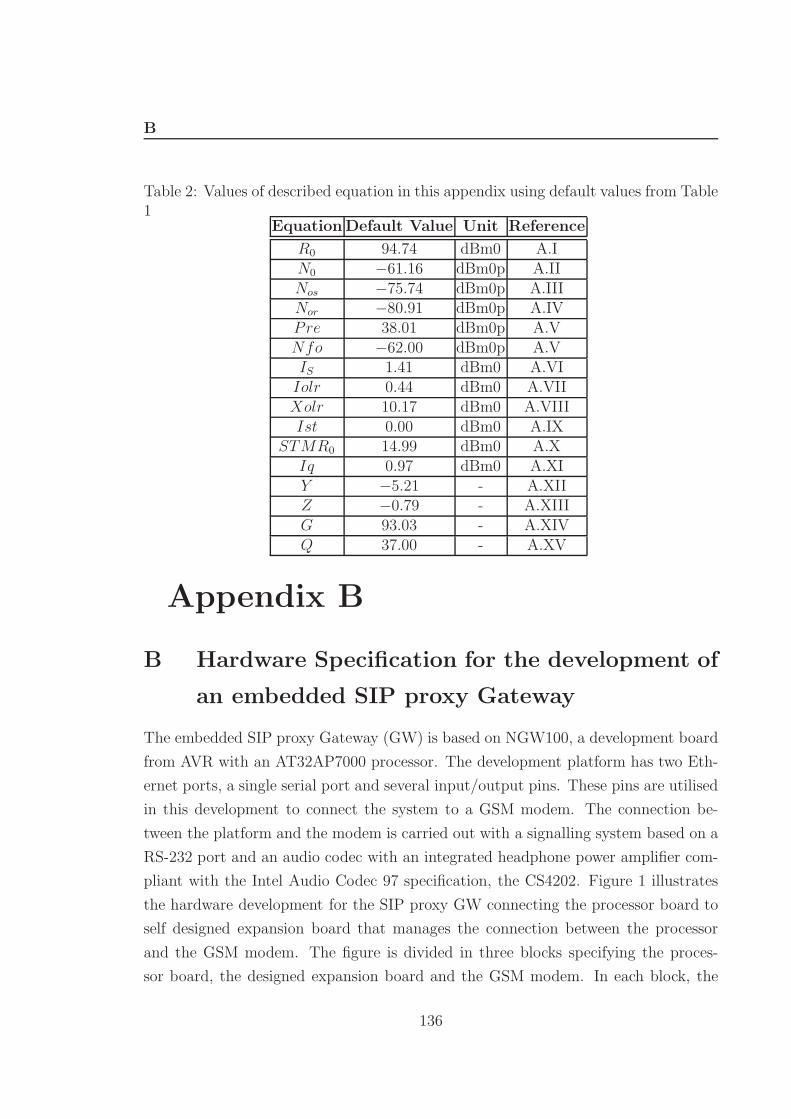
B
Table 2: Values of described equation in this appendix using default values from Table1
EquationDefault Value Unit Reference
R0 94.74 dBm0 A.IN0 −61.16 dBm0p A.IINos −75.74 dBm0p A.IIINor −80.91 dBm0p A.IVPre 38.01 dBm0p A.VNfo −62.00 dBm0p A.VIS 1.41 dBm0 A.VIIolr 0.44 dBm0 A.VIIXolr 10.17 dBm0 A.VIIIIst 0.00 dBm0 A.IX
STMR0 14.99 dBm0 A.XIq 0.97 dBm0 A.XIY −5.21 - A.XIIZ −0.79 - A.XIIIG 93.03 - A.XIVQ 37.00 - A.XV
Appendix B
B Hardware Specification for the development of
an embedded SIP proxy Gateway
The embedded SIP proxy Gateway (GW) is based on NGW100, a development board
from AVR with an AT32AP7000 processor. The development platform has two Eth-
ernet ports, a single serial port and several input/output pins. These pins are utilised
in this development to connect the system to a GSM modem. The connection be-
tween the platform and the modem is carried out with a signalling system based on a
RS-232 port and an audio codec with an integrated headphone power amplifier com-
pliant with the Intel Audio Codec 97 specification, the CS4202. Figure 1 illustrates
the hardware development for the SIP proxy GW connecting the processor board to
self designed expansion board that manages the connection between the processor
and the GSM modem. The figure is divided in three blocks specifying the proces-
sor board, the designed expansion board and the GSM modem. In each block, the
136

B
main components described in this paragraph are highlighted. The expansion board
is designed with Multisim software and the schematic of the entire development is
divided in two figures. Figure 2 depicts the main schematic for the CS4202 whereas
Figure 3 shows the RS232 connection for the modem control. The specifications of
each component of the Printed Circuit Board (PCB) can be found in Table 3.
Figure 1: SIP Proxy GW hardware platform.
137

B
Table 3: Components of designed board
VALUE SHAPE N. REFDES1.5k RES1300- 700X250 1 R161nF KERKO5X4R5 6 C22,C23,C24,C25,C39,C401uF ELKO5R5 2 C5,C261uF KERKO5X4R5 1 C201uF TANKO4˙5R5 1 C151uF ELKO5R5 1 C271uF TANKO4˙5R5 1 C142.2k RES1300- 700X250 1 R172.2uF TANKO4˙5R5 1 C196.8k RES1300- 700X250 4 R10,R11,R12,R1310k RES1300- 700X250 2 R18,R1910uF ELKO5R5 3 C18,C37,C3822pF KERKO5X4R5 2 C1,C247 RES1300- 700X250 2 R1,R2100 RES1300- 700X250 1 R25100nF KERKO5X4R5 13 C6,C7,C8,C17,C21,C30,
C31,C32,C33,C34,C35,C36,C41220k RES1300- 700X250 2 R21,R22220uF ELKO5R5 2 C28,C29470 RES1300- 700X250 2 R23,R24AC97˙LINK HDR1X5 1 U10ANALOG Pwr.Sup. HDR1X2 1 U8CS4202b TSQFP50-P900X 1 U2DIGITAL PwrSup. HDR1X2 1 U9DSUB9F DB9FL 1 J1HC-49/US 25MHz QUARZ˙HC49 1 X1LM7805CT TO220 1 U5MAX3232 DIP16300 1 U7Stereo Socket 3.5mm Stereo socket 4 U1,U3,U4,U6USART HDR1X5 1 U11
138

B
Figure 2: PCB Schematic Part 1, main board
139
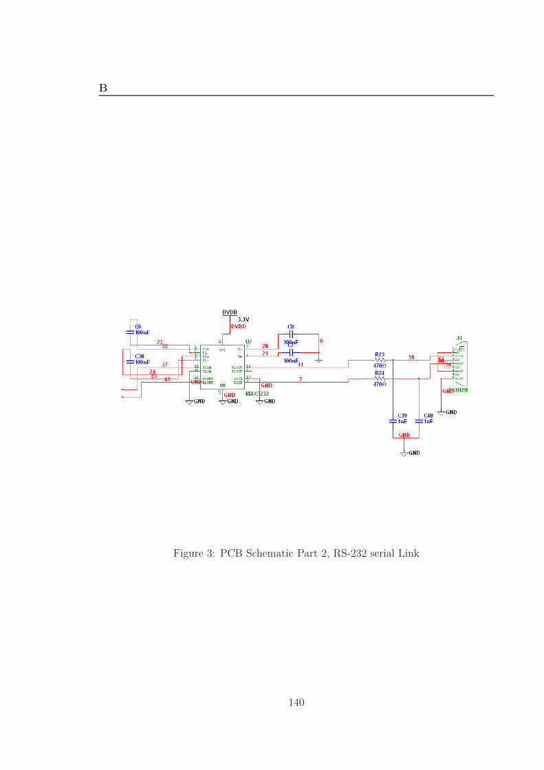
B
Figure 3: PCB Schematic Part 2, RS-232 serial Link
140

Bibliography
[1] J. A. Bergstra and C. A. Middelburg, “ITU-T Recommendation P.800.1 : Mean
Opinion Score terminology,” July 2006.
[2] J. A. Bergtra and C. A. Middelburg, “ITU-T Recommendation G.107 : The
E-Model, a computational model for use in transmission planning,” March 2005.
[3] B. Goode, “Voice over Internet Protocol (VoIP),” Proceedings of the IEEE,
vol. 90, no. 9, pp. 1495 – 1517, Sep. 2002.
[4] F. Andreasen and B. Foster, “Media Gateway Control Protocol (MGCP) Version
1.0,” RFC 3435 (Informational), Internet Engineering Task Force, Jan. 2003,
updated by RFC 3661. [Online]. Available: http://www.ietf.org/rfc/rfc3435.txt
[5] C. Groves, M. Pantaleo, T. Anderson, and T. Taylor, “Gateway Control Protocol
Version 1,” RFC 3525 (Historic), Internet Engineering Task Force, Jun. 2003,
obsoleted by RFC 5125. [Online]. Available: http://www.ietf.org/rfc/rfc3525.txt
[6] C. M. Systems and S. Coursework, “The H.323 Standard, Packet-based multi-
media communications systems,” June 2006.
[7] J. Rosenberg, H. Schulzrinne, G. Camarillo, A. Johnston, J. Peterson, R. Sparks,
M. Handley, and E. Schooler, “SIP: Session Initiation Protocol,” RFC 3261

BIBLIOGRAPHY BIBLIOGRAPHY
(Proposed Standard), Internet Engineering Task Force, Jun. 2002, updated
by RFCs 3265, 3853, 4320, 4916, 5393, 5621, 5626, 5630, 5922, 5954, 6026.
[Online]. Available: http://www.ietf.org/rfc/rfc3261.txt
[8] R. Fielding, J. Gettys, J. Mogul, H. Frystyk, L. Masinter, P. Leach, and
T. Berners-Lee, Hypertext Transfer Protocol – HTTP/1.1, Std., 1999. [Online].
Available: http://www.ietf.org/rfc/rfc2616.txt
[9] M. Nottingham and E. Hammer-Lahav, “Defining Well-Known Uniform
Resource Identifiers (URIs),” RFC 5785 (Proposed Standard), Internet
Engineering Task Force, Apr. 2010. [Online]. Available: http://www.ietf.org/
rfc/rfc5785.txt
[10] M. Handley, V. Jacobson, and C. Perkins, “SDP: Session Description Protocol,”
RFC 4566 (Proposed Standard), Tech. Rep. 4566, July 2006. [Online]. Available:
http://www.ietf.org/rfc/rfc4566.txt
[11] H. Schulzrinne, “Rtp profile for audio and video conferences with minimal con-
trol,” RFC 1890, Tech. Rep., January 1996.
[12] J. K. N. Freed and J. Postel, “Multi-purpose Internet Mail Extensions (MIME),”
RFC 2048, Tech. Rep., November 1996.
[13] ETSI, “http://www.etsi.org/website/technologies/railwaytelecoms.aspx.”
[14] E. Norm, “http://ec.europa.eu/enterprise/policies/european-standards/
documents/harmonised-standards-legislation/list-references/lifts/.”
[15] H. Schulzrinne, S. Casner, R. Frederick, and V. Jacobson, “RTP: A
Transport Protocol for Real-Time Applications,” RFC 3550 (Standard),
Internet Engineering Task Force, Jul. 2003, updated by RFCs 5506, 5761, 6051.
[Online]. Available: http://www.ietf.org/rfc/rfc3550.txt
[16] H. Schulzrinne and S. Casner, “RTP Profile for Audio and Video
Conferences with Minimal Control,” RFC 3551 (Standard), Internet
Engineering Task Force, Jul. 2003, updated by RFC 5761. [Online].
Available: http://www.ietf.org/rfc/rfc3551.txt
142

BIBLIOGRAPHY BIBLIOGRAPHY
[17] W. C. CHU, Speech Coding Algorithms. San Jose, CA, USA: John Wiley &
Sons, Inc., 2003.
[18] M. Baldi and F. Risso, “Efficiency of packet voice with deterministic delay,” in
IEEE Communications Magazine, vol. 38, no. 5, 2000, pp. 170–177.
[19] “ITU-T Recommendation G.711: Pulse Code Modulation (PCM) of voice fre-
quencies,” 1972.
[20] www.sun.com.
[21] “ETSI GSM 06.10 Recommendation GMS 06.10 Full-Rate Speech Transcoding,”
November 2000.
[22] “Jutta Degener and Carsten Bormann, Technische Universitaet Berlin,” 1992.
[23] Jean-marc Valin, “Speex: A free codec for free speech, [online]. available at
www.speex.org.”
[24] “ITU-T Recommendation G.114 : One way transmission time,” May 2003.
[25] R. Braden, D. Clark, and S. Shenker, “Integrated Services in the Internet
Architecture: an Overview,” RFC 1633 (Informational), Tech. Rep. 1633, June
1994. [Online]. Available: http://www.ietf.org/rfc/rfc1633.txt
[26] S. Blake, D. Black, M. Carlson, E. Davies, Z. Wang, and W. Weiss, “An
Architecture for Differentiated Service,” RFC 2475 (Informational), Tech.
Rep. 2475, December 1998, updated by RFC 3260. [Online]. Available:
http://www.ietf.org/rfc/rfc2475.txt
[27] R.Barden, “Resource Reservation Allocation Protocol,” RFC 2205, Tech. Rep.
2205, September 1997. [Online]. Available: http://www.ietf.org/rfc/rfc2205.txt
[28] U. D. Black, Frame Relay Networks: Specifications and Implementations. New
York, NY, USA: McGraw-Hill, Inc., 1998.
[29] R. Handel and M. N. Huber, Integrated Broadband Networks; An Introduction to
ATM-Based Networks. Boston, MA, USA: Addison-Wesley Longman Publishing
Co., Inc., 1991.
143
BIBLIOGRAPHY BIBLIOGRAPHY
[30] E. Rosen, A. Viswanathan, and R. Callon, “Multiprotocol label switching
architecture,” RFC 3031, Tech. Rep. 3031, January 2001. [Online]. Available:
http://www.ietf.org/rfc/rfc3031.txt
[31] “ITU-T Recommendation G.113 : Transmission impairments due to speech pro-
cessing,” November 2007.
[32] R. Ahlswede, N. Cai, S. yen Robert Li, R. W. Yeung, S. Member, and S. Member,
“Network information flow,” IEEE Transactions on Information Theory, vol. 46,
pp. 1204–1216, 2000.
[33] Tracey Ho and Desmond S. Lun, Network coding, An Introduction. Cambridge
University Press, 2008.
[34] M. Hazewinkel and E. Kluwer, Encyclopaedia of Mathematics. Springer, 2002.
[35] R. Yeung and Z. Zhang, “Distributed source coding for satellite communica-
tions,” Information Theory, IEEE Transactions on, vol. 45, no. 4, pp. 1111
–1120, May 1999.
[36] S. yen Robert Li, S. Member, R. W. Yeung, and N. Cai, “Linear network coding,”
IEEE Transactions on Information Theory, vol. 49, pp. 371–381, 2003.
[37] R. Koetter, M. Mdard, and S. Member, “An algebraic approach to network
coding,” IEEE/ACM Transactions on Networking, vol. 11, pp. 782–795, 2003.
[38] T. Ho, M. Mdard, and R. Koetter, “A coding view of network recovery and
management for single-receiver communications,” 2002.
[39] S. Zhang, S. C. Liew, and P. P. Lam, “Hot topic: physical-layer network coding,”
in MobiCom ’06: Proceedings of the 12th annual international conference on
Mobile computing and networking. New York, NY, USA: ACM Press, 2006,
pp. 358–365. [Online]. Available: http://dx.doi.org/10.1145/1161089.1161129
[40] S. Katti, I. Maric, A. Goldsmith, D. Katabi, and M. Medard, “Joint relaying and
network coding in wireless networks,” in Information Theory, 2007. ISIT 2007.
IEEE International Symposium on, 2007, pp. 1101 –1105.
144

BIBLIOGRAPHY BIBLIOGRAPHY
[41] S. Fu, K. Lu, T. Zhang, Y. Qian, and H.-H. Chen, “Cooperative wireless net-
works based on physical layer network coding,”Wireless Communications, IEEE,
vol. 17, no. 6, pp. 86 –95, 2010.
[42] L. F. September and L. Fernandez, “Avalanche modelling,” 2003.
[43] Y.-M. C. Y.-H. C. Tein-Yaw Chung, Chih-Cheng Wang, “Pnecos: A peer-to-peer
network coding streaming system,” June 2008, pp. 379 –384.
[44] S. Katti, H. Rahul, W. Hu, D. Katabi, M. Mdard, and J. Crowcroft, “Xors in
the air: practical wireless network coding,” in In Proc. ACM SIGCOMM, 2006,
pp. 243–254.
[45] P. Vingelmann, P. Zanaty, F. Fitzek, and H. Charaf, “Implementation of random
linear network coding on opengl-enabled graphics cards,” inWireless Conference,
2009. EW 2009. European, May 2009, pp. 118 –123.
[46] R. W. Yeung, Information Theory and Network Coding. Springer, 2008.
[47] L. R. Ford and D. R. Fulkerson, “Maximal flow through a network,” Canadian
Journal of Mathematics, no. 8, pp. 399–404, 1956.
[48] W. Hyun, M. Hub, and S. Kang, “An implementation of sip servers for internet
telephony,” in High Speed Networks and Multimedia Communications 5th IEEE
International Conference on, July 2002, pp. 61–65.
[49] M. Huh, W. Hyun, S. Kang, and P. Kim, “Call management mechanism for
internet phone services based on sip,” in High Speed Networks and Multimedia
Communications 5th IEEE International Conference on, July 2002, pp. 66–70.
[50] F. Anjum, F. Caruso, R. Jain, P. Missier, and A. Zordanand, “Chai time, a
system for rapid creation of portable next-generation telephony services using
third-party software components,” in Open Architectures and Network Program-
ming Proceedings, OPENARCH, March 1999, pp. 22 – 31.
[51] M. Spencer, “Asterisk,” 1999.
[52] M. Spencer, B. Capouch, E. Guy, F. Miller, and K. Shumard, “IAX: Inter-
Asterisk eXchange Version 2,” RFC 5456 (Informational), Internet Engineering
Task Force, Feb. 2010. [Online]. Available: http://www.ietf.org/rfc/rfc5456.txt
145

BIBLIOGRAPHY BIBLIOGRAPHY
[53] J.-C. Bolot, S. Fosse-Parisis, and D. Towsley, “Adaptive fec-based error control
for internet telephony,” in INFOCOM ’99. Eighteenth Annual Joint Conference
of the IEEE Computer and Communications Societies. Proceedings. IEEE, vol. 3,
March 1999, pp. 1453 – 1460.
[54] W. Jiang and H. Schulzrinne, “Comparison and optimization of packet loss repair
methods on voip perceived quality under bursty loss,” in NOSSDAV ’02. New
York, NY, USA: ACM, 2002, pp. 73–81.
[55] S. Tong, D. Lin, A. Kavcic, B. Bai, and L. Ping, “On short forward error-
correcting codes for wireless communication systems,” in Computer Commu-
nications and Networks, 2007. ICCCN 2007. Proceedings of 16th International
Conference on, aug. 2007, pp. 391 –396.
[56] M. Mushkin and I. Bar-David, “Capacity and coding for the gilbert-elliot chan-
nels,” Trans. Inf. Theory, IEEE, vol. 35, no. 6, pp. 1277–1290, Nov 1989.
[57] B. Sklar, “Rayleigh fading channels in mobile digital communication systems .i.
characterization,” Communications Magazine, IEEE, vol. 35, no. 7, pp. 90–100,
Jul 1997.
[58] P. Sadeghi, R. Kennedy, P. Rapajic, and R. Shams, “Finite-state markov model-
ing of fading channels - a survey of principles and applications,” Signal Processing
Magazine, IEEE, vol. 25, no. 5, pp. 57–80, September 2008.
[59] J. Andren, M. Hilding, and D. Veitch, “Understanding end-to-end internet traffic
dynamics,” in Global Telecommunications Conference, 1998. GLOBECOM 98.
The Bridge to Global Integration. IEEE, vol. 2, no. 6, Nov 1998, pp. 1118 – 1122.
[60] W. Jiang and H. Schulzrinne, “Modeling of packet loss and delay and their effect
on real-time multimedia service quality,” in PROCEEDINGS OF NOSSDAV,
2000.
[61] M. Yajnik, S. Moon, J. Kurose, and D. Towsley, “Measurement and modelling
of the temporal dependence in packet loss,” 1999, pp. 345–352.
[62] M. Iosifescu, Finite Markov processes and their applications / Marius Iosifescu.
Wiley, Chichester ; New York :, 1980.
146
BIBLIOGRAPHY BIBLIOGRAPHY
[63] www.atmel.com.
[64] www.telit.com.
[65] S. Morlat, “ortp,” 2001.
[66] A. Moizard, “osip,” 2002.
[67] A. Brand and A. Hamid Aghvami, Multiple Access Protocols for Mobile Commu-
nications. John Wiley & Sons, 2002.
[68] I. Lopetegui, R. Carrasco, S. Boussakta, and O. Azpitarte, “Embedded Imple-
mentation of a SIP Server Gateway with Forward Error Correction to a Mobile
Network,” in Computer and Information Technology (CIT), 2010 IEEE 10th
International Conference on, 29 2010.
[69] www.counterpath.com.
[70] www.sjlabs.com.
[71] www.ekiga.org.
[72] M. Iosifescu, Finite Markov Processes and Their Applications. John Wiley &
Sons, 1980.
[73] I. Lopetegui, R. A. Carrasco, and S. Boussakta, “Speech Quality Prediction in
VoIP Concatenating Multiple Markov-Based Channels,” Advanced International
Conference on Telecommunications, vol. 0, pp. 226–230, 2010.
[74] www.nitazu.com.
[75] A. Konrad, A. Konrad, A. D. Joseph, A. D. Joseph, R. Ludwig, R. Ludwig, B. Y.
Zhao, and B. Y. Zhao, “A markov-based channel model algorithm for wireless
networks,” in Wireless Networks, 2001, pp. 189–199.
[76] I. Lopetegui, R. A. Carrasco, and S. Boussakta, “VoIP Design and Implementa-
tion with Network Coding Schemes for Wireless Networks,” in Communication
Systems Networks and Digital Signal Processing (CSNDSP), 2010 7th Interna-
tional Symposium on, 2010, pp. 857 –861.
147

BIBLIOGRAPHY BIBLIOGRAPHY
[77] I. Lopetegui, R. Carrasco, and S. Boussakta, “Experimental Measurements for
VoIP with Network Coding in IEEE 802.11,” in Wireless Communication Sys-
tems (ISWCS), 2010 7th International Symposium on.
[78] I. Lopetegui, R. A. Carrasco, and S. Boussakta, “Multicasting voip with network
coding,” IEEE Multimedia Trans., submitted.
[79] S. Shin and H. Schulzrinne, “Measurement and analysis of the voip capacity in
ieee 802.11 wlan,” Mobile Computing, IEEE Transactions on, vol. 8, no. 9, pp.
1265 –1279, 2009.
[80] T. G. Robertazzi, Computer Networks and Systems / Thomas G. Robertazzi.
Springer; New York :, 2000.
[81] D. Hole and F. Tobagi, “Capacity of an ieee 802.11b wireless lan supporting
voip,” in Communications, 2004 IEEE International Conference on, vol. 1, 2004,
pp. 196 – 201.
[82] X. W. N.T. Dao and R. Malaney, “The voice capacity of wifi for best effort and
prioritized traffic,” in Proc. Auswireless Conf., vol. 1, 2006, pp. 196 – 201.
[83] W. Wang, S. C. Liew, and V. Li, “Solutions to performance problems in voip
over a 802.11 wireless lan,” Vehicular Technology, IEEE Transactions on, vol. 54,
no. 1, pp. 366 – 384, 2005.
[84] A. Trad, F. Munir, and H. Afifi, “Capacity evaluation of voip in ieee 802.11e
wlan environment,” in Consumer Communications and Networking Conference,
2006. CCNC 2006. 3rd IEEE, vol. 2, 2006, pp. 828 – 832.
[85] “Wireless Lan Medium Access Control (MAC) and Physical Layer (PHY) specifi-
cations. Standard specification, ieee 802.11,” ISO/IEC 8802-11 IEEE Std 802.11
Second edition 2005-08-01 ISO/IEC 8802 11:2005(E) IEEE Std 802.11i-2003
Edition, 2005.
[86] “IEEE local and metropolitan area networks, Carrier Sense Multiple Access with
Collision Detection (CSMA/CD) Access Method and Physical Layer Specifica-
tions,” IEEE Std 802.3-2005 (Revision of IEEE Std 802.3-2002 including all
approved amendments), 2005.
148

BIBLIOGRAPHY BIBLIOGRAPHY
[87] J. Kuri and S. Kasera, “Reliable multicast in multi-access wireless lans,” in
INFOCOM ’99. Eighteenth Annual Joint Conference of the IEEE Computer and
Communications Societies. Proceedings. IEEE, vol. 2, Mar. 1999, pp. 760 –767
vol.2.
[88] R. Rummler, A. Gluhak, and A. Hamid Aghvami, Multicast in Third-Generation
of Mobile Networks. John Wiley & Sons, 2009.
[89] http://www.tcpdump.org/.
149