ph.d. dissertation - connecting repositories · boldrini, g. benedetti, and a. massa, wsn-based...
TRANSCRIPT

Ph.D. Dissertation
International Do toral S hool in Information
and Communi ation Te hnology
DISI - University of Trento
Innovative Inversion Approa hes for
Buried Obje ts Dete tion and Imaging
Mar o Salu i
Tutor:
Andrea Massa, Professor
University of Trento
Advisor:
Gia omo Oliveri, Aggregate Professor
University of Trento
Co-Advisor:
Paolo Ro a, Aggregate Professor
University of Trento
November 2014


To my parents Fran a and Massimo, and to my olleagues and friends of the
ELEDIA Resear h Center. Thank you all.


Abstra t
The study, development, and analysis of innovative inversion te hniques for the
dete tion and imaging of buried obje ts is addressed in this thesis. The proposed
methodologies are based on the use of mi rowave radiations and radar te hniques
for subsurfa e prospe ting, su h as, for example, the Ground Penetrating Radar
(GPR). More pre isely, the re onstru tion of shallow buried obje ts is rstly ad-
dressed by an ele tromagneti inverse s attering method based on the integration
of the inexa t Newton (IN) method with an interative multis aling approa h.
The performan es of su h an inversion approa h are analyzed both when onsid-
ering the use of a se ond-order Born approximation (SOBA) and when exploitingthe full set of non-linear equations governing the s attering phenomena for the
buried s enario. The presented methodologies are parti ularly suitable for ap-
pli ations su h as demining (e.g., for the dete tion of unexploded ordnan es,
UXOs, and improvised explosive devi es, IEDs), for ivil engineering appli a-
tions (e.g., for the investigation of possible stru tural damages, voids, ra ks or
water inltrations in walls, pillars, bridges) as well as for biomedi al imaging
(e.g., for early an er dete tion).
Keywords
Ground Penetrating Radar (GPR), Inverse S attering, Mi rowave Imaging, Iter-
ative Multi-S aling Approa h, Inexa t Newton, Conjugate Gradient, Frequen y
Hopping


Published Conferen e Papers
[C1 F. Viani, M. Donelli, M. Salu i, P. Ro a, and A. Massa, Oppor-
tunisti exploitation of wireless infrastru tures for homeland se u-
rity, Pro . 2011 IEEE AP-S International Symposium, Spokane,
Washington, USA, pp. 3062-3065, July 3-8, 2011.
[C2 F. Viani, M. Salu i, P. Ro a, G. Oliveri, and A. Massa, A multi-
sensor WSN ba kbone for museum monitoring and surveillan e, Eu-
CAP 2012, Prague, Cze h Republi , Mar h 26-30, 2012.
[C3 A. Saverio, T. Cadili, G. Liborio, M. Russo, G. Oliveri, M. Salu i,
and A. Massa, A GA-based strategy for the alibration of satellite
ommuni ation phased array antennas, EuCAP 2013, Gothenburg,
Sweden, April 8-12, 2013.
[C4 G. Oliveri, M. Salu i, A. Massa, D. Gonzalez-Ovejero, and C. Cra-
eye, Analyti ally designed planar aperiodi arrays in the presen e
of mutual oupling, EuCAP 2013, Gothenburg, Sweden, April 8-12,
2013.
[C5 F. Viani, F. Robol, M. Salu i, E. Giarola, S. De Vigili, M. Ro a,
F. Boldrini, G. Benedetti, and A. Massa, WSN-based early alert
system for preventing wildlife-vehi le ollisions in Alps regions - From
the laboratory test to the real-world implementation, EuCAP 2013,
Gothenburg, Sweden, April 8-12, 2013.
[C6 L. Mani a, P. Ro a, M. Salu i, M. Carlin, and A. Massa, S atter-
ing data inversion through interval analysis under Rytov approxima-
tion, EuCAP 2013, Gothenburg, Sweden, April 8-12, 2013.
[C7 M. Salu i, D. Sartori, N. Anselmi, A. Randazzo, G. Oliveri, and A.
Massa, Imaging buried obje ts within the se ond-order Born ap-
proximation through a multiresolution-regularized inexa t-Newton
method, 2013 International Symposium on Ele tromagneti Theory
(EMTS 2013), Hiroshima, Japan, May 20-24, 2013 (Invited).
[C8 G. Oliveri, P. Ro a, M. Salu i, E. T. Bekele, D. H. Werner, and A.
Massa, Design and synthesis of innovative metamaterial-enhan ed
i

arrays, Pro . 2013 IEEE AP-S International Symposium, Lake
Buena Vista, Florida, USA, July 7-12, 2013.
[C9 M. Salu i, P. Ro a, G. Oliveri, and A. Massa, "An innovative
frequen y hopping multizoom inversion strategy for GPR subsur-
fa e imaging," 15th International Conferen e on Ground Penetrating
Radar (GPR 2014), Brussels, Belgium, June 30 - July 04, 2014.
[C10 M. Salu i, G. Oliveri, A. Randazzo, M. Pastorino, and A. Massa,
"Multi-Fo using Pro edure based on the Inexa t-Newton Method
for Ele tromagneti Subsurfa e Prospe ting," European Geos ien es
Union General Assembly (EGU2014), Vienna, Austria, April 27 -
May 2, 2014.
[C11 M. Salu i, L. Tenuti, C. Nardin, G. Oliveri, F. Viani, P. Ro a,
and A. Massa , "Civil engineering appli ations of ground penetrating
radar re ent advan es the ELEDIA Resear h Center," European
Geos ien es Union General Assembly (EGU2014), Vienna, Austria,
April 27 - May 2, 2014.
[C12 M. Salu i, L. Tenuti, C. Nardin, M. Carlin, F. Viani, G. Oliveri and
A. Massa, "Gpr survey through a multi-resolution deterministi ap-
proa h," IEEE AP-S International Symposium, Memphis, Tennessee,
USA, July 6-12, 2014.
[C13 L. Mani a, G. Oliveri, E. Bekele, M. Carlin, M. Salu i, C. Nardin,
E. Martini, S. Ma i, and A. Massa, Optimized synthesis of wave-
manipulating devi es within the system-by-design paradigm, IEEE
AP-S International Symposium, Memphis, Tennessee, USA, July 6-
12, 2014.
[C14 A. Massa, G. Oliveri, M. Salu i, C. Nardin, and P. Ro a, Dealing
with EM fun tional optimization through new generation evolutionary-
based methods, IEEE International Conferen e on Numeri al Ele -
tromagneti Modeling and Optimization for RF, Mi rowave and Ter-
ahertz Appli ations, Pavia, Italy, May 14-16, 2014 (Invited).
[C15 M. Salu i, G. Oliveri, M. Gregory, D. Werner, and A. Massa, A
frequen y-tunable metamaterial-based antenna using a re ongurable
AMC groundplane, 8th European Conferen e on Antennas and Prop-
agation (EuCAP 2014), The Hague, The Netherlands, Apr. 6-11,
2014.
[C16 L. Poli, M. Salu i, P. Ro a, and A. Massa, Adaptive GA-based
thinning strategy for pattern nulling in sub-arrayed phased arrays,
8th European Conferen e on Antennas and Propagation (EUCAP
2014), The Hague, The Netherlands, Apr. 6-11, 2014.
ii

[C17 T. Moriyama, M. Salu i, G. Oliveri, L. Tenuti, P. Ro a, and A.
Massa, Multi-s aling deterministi imaging for GPR survey, IEEE
International Conferen e on Antenna Measurements & Appli ations
(IEEE CAMA 2014), (Antibes Juan-les-Pins, Fran e), Nov. 16-19
2014.
[C18 G. Oliveri, P. Ro a, M. Salu i, and A. Massa, E ient synthesis
of omplex antenna devi es through system-by-design, Pro . 2014
IEEE Symposium Series on Computational Intelligen e (IEEE SSCI
2014), Orlando, Florida, USA, De ember 9-12, 2014 (A epted).
[C19 G. Oliveri, P. Ro a, M. Salu i, and A. Massa, Evolution of nature-
inspired optimization for new generation antenna design, Pro . 2014
IEEE Symposium Series on Computational Intelligen e (IEEE SSCI
2014), Orlando, Florida, USA, De ember 9-12, 2014 (A epted).
[C20 G. Oliveri, P. Ro a, D. H. Werner, E. Bekele, M. Salu i, and A.
Massa, Design and synthesis of innovative metamaterial-enhan ed
arrays, 2013 IEEE Antennas and Propagation So iety International
Symposium, (Orlando, USA), pp. 972-973, July 7-13, 2013.
[C21 M. Carlin, M. Salu i, L. Tenuti, P. Ro a, and A. Massa, E ient
radome optimization through the system-by-design methodology,
9th European Conferen e on Antennas and Propagation (EUCAP
2015), Lisbon, Portugal, April 12-17, 2015 (Submitted).
[C22 L. Tenuti, M. Salu i, L. Poli, G. Oliveri, and A. Massa, Physi al-
information exploitation in inverse s attering approa hes for GPR
survey, 9th European Conferen e on Antennas and Propagation (EU-
CAP 2015), Lisbon, Portugal, April 12-17, 2015 (Submitted).
[C23 F. Viani, M. Salu i, F. Robol, E. Giarola, and A. Massa, WSNs as
enabling tool for next generation smart systems, Atti XIX Riunione
Nazionale di Elettromagnetismo (XIX RiNEm), Roma, pp. 393-396,
10-14 Settembre 2012.
iii

iv

Published Journals Papers
[R1 F. Viani, M. Salu i, F. Robol, G. Oliveri, and A. Massa, Design of a
UHF RFID/GPS fra tal antenna for logisti s management, Journal
of Ele tromagneti Waves and Appli ations, vol. 26, no. 4, pp. 480-
492, 2012.
[R2 F. Viani, M. Salu i, F. Robol, and A. Massa, Multiband Fra -
tal ZigBee/WLAN Antenna for Ubiquitous Wireless Environments,
Journal of Ele tromagneti Waves and Appli ations, vol. 26, no. 11-
12, pp. 1554-1562, 2012.
[R3 L. Poli, P. Ro a, M. Salu i, and A. Massa, "Re ongurable thin-
ning for the adaptive ontrol of linear arrays," IEEE Transa tions on
Antennas and Propagation, vol. 61, no. 10, pp. 5068-5077, 2013.
[R4 B. Majone, F. Viani, E. Filippi, A. Bellin, A. Massa, G. Toller, F.
Robol and M. Salu i, "Wireless sensor network deployment for mon-
itoring soil moisture dynami s at the eld s ale," Pro edia Environ-
mental S ien es, vol. 19, pp. 426-435, 2013.
[R5 M. Salu i, G. Oliveri, A. Randazzo, M. Pastorino, and A. Massa,
Ele tromagneti subsurfa e prospe ting by a multi-fo using inexa t
Newton method within the se ond-order Born approximation, Jour-
nal of Opti al So iety of Ameri a A, vol. 31, no. 6, pp. 1167-1179,
2014.
[R6 T. Moriyama, G. Oliveri, M. Salu i, and T. Takenaka, A multi-
s aling forward-ba kward timestepping method for mi rowave imag-
ing, IEICE Ele troni s Express, vol. 11, no. 16, id. 20140569, pp.
1-10, Aug. 2014. doi:10.1587/elex.11.20140578.
[R7 T. Moriyama, E. Giarola, M. Salu i, and G. Oliveri, On the ra-
diation properties of ADS thinned dipole arrays, IEICE Ele tron-
i s Express, vol. 11, no. 16, id. 20140578, pp. 1-12, Aug. 2014.
doi:10.1587/elex.11.20140569.
v

[R8 M. Salu i, G. Oliveri, A. Randazzo, M. Pastorino, and A. Massa,
Ele tromagneti subsurfa e prospe ting by a fully nonlinear multi-
fo using inexa t Newton method, Journal of Opti al So iety of Amer-
i a A, vol. 31, no. 12, pp. 2618-2629, 2014.
vi

Contents
1 Introdu tion 1
2 Inverse S attering Equations for the Subsurfa e Problem 5
2.1 Geometry of the Problem . . . . . . . . . . . . . . . . . . . . . . 6
2.2 Mathemati al Formulation . . . . . . . . . . . . . . . . . . . . . . 6
3 Multi-Fo using Inexa t NewtonMethod within the Se ond-Order
Born Approximation 13
3.1 Introdu tion . . . . . . . . . . . . . . . . . . . . . . . . . . . . . . 14
3.2 Problem Formulation . . . . . . . . . . . . . . . . . . . . . . . . . 14
3.3 Re onstru tion Method . . . . . . . . . . . . . . . . . . . . . . . . 15
3.4 Numeri al Assessment . . . . . . . . . . . . . . . . . . . . . . . . 18
3.4.1 Calibration of the IMSA− IN − SOBA . . . . . . . . . . 18
3.4.2 Homogeneous Square and L-shaped Cylinders . . . . . 24
3.4.3 O-shaped Cylinder . . . . . . . . . . . . . . . . . . . . . 24
3.4.4 Inhomogeneous Cylinders . . . . . . . . . . . . . . . . . . 28
3.4.5 Square Cylinder with strong ondu tivity . . . . . . . . . 30
3.5 Dis ussions . . . . . . . . . . . . . . . . . . . . . . . . . . . . . . 32
4 Ele tromagneti Subsurfa e Prospe ting by a Fully Nonlinear
Multi-fo using Inexa t Newton Method 33
4.1 Introdu tion and motivation . . . . . . . . . . . . . . . . . . . . . 34
4.2 Mathemati al formulation . . . . . . . . . . . . . . . . . . . . . . 35
4.3 Numeri al Results . . . . . . . . . . . . . . . . . . . . . . . . . . 37
4.3.1 Calibration . . . . . . . . . . . . . . . . . . . . . . . . . . 39
4.3.2 Ee ts of Noise . . . . . . . . . . . . . . . . . . . . . . . . 42
4.3.3 Ee ts of the Diele tri Properties of the Target . . . . . . 47
4.3.4 Re onstru tion of Targets with Small Details . . . . . . . . 50
4.3.5 Re onstru tion of Targets with Higher Condu tivity . . . . 51
4.4 Dis ussions . . . . . . . . . . . . . . . . . . . . . . . . . . . . . . 52
5 GPR Prospe ting through an Inverse S attering Frequen y-Hopping
Multi-Fo using Approa h 53
5.1 Introdu tion and Rationale . . . . . . . . . . . . . . . . . . . . . . 54
vii

5.2 GPR Prospe ting - Inverse S attering Formulation . . . . . . . . 55
5.3 FHMF-CG Inversion Pro edure . . . . . . . . . . . . . . . . . . . 58
5.4 Numeri al and Experimental Validation . . . . . . . . . . . . . . . 62
5.4.1 Rationale and Figures of Merit . . . . . . . . . . . . . . . 62
5.4.2 Numeri al Validation . . . . . . . . . . . . . . . . . . . . . 63
5.4.3 Experimental Validation . . . . . . . . . . . . . . . . . . . 75
5.5 Dis ussions . . . . . . . . . . . . . . . . . . . . . . . . . . . . . . 79
6 Con lusions 81
6.1 Comparison Between Dierent Approa hes . . . . . . . . . . . . . 82
6.2 Final Remarks . . . . . . . . . . . . . . . . . . . . . . . . . . . . . 89
A Derivation of Eq. (4.5) and Eq. (4.6) 103
viii

List of Tables
3.1 Performan e Assessment (O-Shaped S atterer ℓ ≈ λb
2, SNR ∈
[10, 30] dB) - Error values and omputational indexes. . . . . . . 26
4.1 Performan e vs. Noise (Square S atterer - L = 0.32 λb, (xc =−0.16 λb, yc = −0.58 λb), εr = 5.5, σ = 0.01 S/m [τ = 1.5,εrB =4.0, σB =0.01 S/m) - Total number of performed outer iter-
ations, nal tness values, and re onstru tion errors for the BARE
and the IMSA (s = S = 4) IN approa hes. Total exe ution time
on a PC with Intel(R) Core(TM)2 CPU 6600 2.40GHz, 2GB
RAM. . . . . . . . . . . . . . . . . . . . . . . . . . . . . . . . . . 43
4.2 Performan e vs. Target Condu tivity (Square S atterer - L =0.32 λb, (xc = −0.16 λb, yc = −0.58 λb), εr = 5.5, σ = 0.1 S/m
[τ = 1.5 − j5.39, εrB =4.0, σB =0.01 S/m) - Re onstru tion
errors for the bare IN and the IMSA-IN (at step s = S = 4)approa hes. . . . . . . . . . . . . . . . . . . . . . . . . . . . . . . 52
5.1 Illustrative Example [Hollow square prole, εrB = 4.0, σB = 10−3
S/m, τ = 1.0, Noiseless data Figures of merit. . . . . . . . . . . . 72
ix

LIST OF TABLES
x

List of Figures
2.1 Geometry of a subsurfa e imaging problem. (a) Cross-borehole
and (b) half spa e setup. λb is the wavelength in the ba kground
material. . . . . . . . . . . . . . . . . . . . . . . . . . . . . . . . 6
3.1 Geometry of the problem and imaging setup. . . . . . . . . . . . . 15
3.2 Sensitivity Analysis (Homogeneous Square S atterer - ℓ ≈ λb
3, τ =
1.5, SNR = 20 dB) - Behaviour of the integral error Ξtot versus
η and W when Q = Q∗, S = S∗
(a), and versus K when η = η∗,W =W ∗
, and S = S∗(b). Plot of the total, internal, and external
error as a fun tion of S when Q = Q∗, η = η∗, and W = W ∗
( ). . 19
3.3 Sensitivity Analysis (Homogeneous Square S atterer - ℓ ≈ λb
3, τ =
1.5, SNR = 20 dB, S = S∗) - A tual (a) and retrieved (b)( )
ontrast proles when (b) Q = Q∗, W = W ∗
, η = 10−4; ( )
K = K∗, W = 40, η = η∗. . . . . . . . . . . . . . . . . . . . . . . 21
3.4 Sensitivity Analysis (Homogeneous Square S atterer - ℓ ≈ λb
3, τ =
1.5, SNR = 20 dB, Q = Q∗, W = W ∗
, η = η∗) - Behaviour of Φand ζ versus the IMSA − IN iteration number (a). Plot of the
retrieved ontrast proles when (b) S = 1, ( ) S = 2, (d) S = 3,(e) S = 4 = S∗
. . . . . . . . . . . . . . . . . . . . . . . . . . . . . 23
3.5 Performan e Assessment (τ = 1.5, SNR ∈ [10, 40] dB) - Be-
haviour of the Ξtot as a fun tion of SNR when dealing with Square
or L-Shaped targets (a). Plot of the ontrast proles retrieved
by (b)( ) BARE−IN−SOBA and (d)(e) IMSA−IN−SOBAwhen SNR = 10 dB. (b)(d) Square s atterer; ( )(e) L-Shapeds atterer. . . . . . . . . . . . . . . . . . . . . . . . . . . . . . . . . 25
3.6 Performan e Assessment (O-Shaped S atterer ℓ ≈ λb
2, SNR ∈
[10, 30] dB) - Behaviour of the Ξtot as a fun tion of τ obtained by
BARE − IN − SOBA and IMSA− IN − SOBA. . . . . . . . . 26
3.7 Performan e Assessment (O-Shaped S atterer ℓ ≈ λb
2, SNR =
20 dB) - Plot of the ontrast proles retrieved by (a)( )(e)BARE−IN − SOBA and (b)(d)(f ) IMSA − IN − SOBA when (a)(b)
τ = 0.2, ( )(d) τ = 1.0, and (e)(f ) τ = 2.2. . . . . . . . . . . . . . 27
xi
LIST OF FIGURES
3.8 Performan e Assessment (Inhomogeneous S atterers, SNR = 20dB) - Plot of the a tual (a)(b) and retrieved ( )-(f ) ontrast pro-
les by ( )(d) BARE − IN − SOBA and (e)(f ) IMSA − IN −SOBA for (a)( )(e) Double-L and (b)(d)(f ) Con entri tar-
gets. . . . . . . . . . . . . . . . . . . . . . . . . . . . . . . . . . . 29
3.9 Performan e Assessment (Homogeneous Square S atterer - ℓ ≈λb
3, Rτ = 1.5, SNR ∈ [10, 30] dB) - Behaviour of the Ξtot as a
fun tion of σc (a). Plot of the real (b)( ) and imaginary (d)(e)
parts of the ontrast proles retrieved by (b)(d) BARE − IN −SOBA and ( )(e) IMSA− IN − SOBA when SNR = 20 dB. . . 31
4.1 Cross-borehole imaging onguration. . . . . . . . . . . . . . . . . 35
4.2 Calibration (Square S atterer - L = 0.32 λb, (xc = −0.16 λb, yc =−0.58 λb), εr = 5.5, σ = 0.01 S/m [τ = 1.5, εrB =4.0, σB =0.01S/m, SNR = 20 dB) - A tual target used for the algorithm ali-
bration. . . . . . . . . . . . . . . . . . . . . . . . . . . . . . . . . 39
4.3 Calibration (Square S atterer - L = 0.32 λb, (xc = −0.16 λb, yc =−0.58 λb), εr = 5.5, σ = 0.01 S/m [τ = 1.5, εrB =4.0, σB =0.01S/m, SNR = 20 dB) - Total re onstru tion error vs. α (α ∈[0.1, 0.9]) for dierent values of Q in the range Q ∈ [10, 100]. . . . 40
4.4 Calibration (Square S atterer - L = 0.32 λb, (xc = −0.16 λb, yc =−0.58 λb), εr = 5.5, σ = 0.01 S/m [τ = 1.5, εrB =4.0, σB =0.01S/m, SNR = 20 dB) - Best tness value for dierent (Q,α) pairs. 40
4.5 Calibration (Square S atterer - L = 0.32 λb, (xc = −0.16 λb, yc =−0.58 λb), εr = 5.5, σ = 0.01 S/m [τ = 1.5, εrB =4.0, σB =0.01S/m, SNR = 20 dB) - (a) Real and (b) imaginary parts of the re-
onstru ted distribution of the ontrast fun tion when Q = Qopt =50 and α = αopt = 0.9. . . . . . . . . . . . . . . . . . . . . . . . . 41
4.6 Calibration (Square S atterer - L = 0.32 λb, (xc = −0.16 λb, yc =−0.58 λb), εr = 5.5, σ = 0.01 S/m [τ = 1.5, εrB =4.0, σB =0.01S/m, SNR = 20 dB) - Re onstru tion errors for dierent values
of ∆εrB. . . . . . . . . . . . . . . . . . . . . . . . . . . . . . . . . 42
4.7 Performan e vs. Noise (Square S atterer - L = 0.32 λb, (xc =−0.16 λb, yc = −0.58 λb), εr = 5.5, σ = 0.01 S/m [τ = 1.5,εrB =4.0, σB =0.01 S/m, SNR =10 dB) - Re onstru ted dis-
tributions of the ontrast fun tion (real part) when using (a)( )
IMSA-IN and (b)(d) IN under (a)(b) full-nonlinear and ( )(d)
approximate onditions (SOBA). . . . . . . . . . . . . . . . . . . 44
4.8 Performan e vs. Noise (Square S atterer - L = 0.32 λb, (xc =−0.16 λb, yc = −0.58 λb), εr = 5.5, σ = 0.01 S/m [τ = 1.5,εrB =4.0, σB =0.01 S/m, SNR =10 dB) - Re onstru ted dis-
tributions of the ontrast fun tion (imaginary part) when using
(a)( ) IMSA-IN and (b)(d) IN under (a)(b) full-nonlinear and
( )(d) approximate onditions (SOBA). . . . . . . . . . . . . . . . 45
xii

LIST OF FIGURES
4.9 Performan e vs. Noise (Square S atterer - L = 0.32 λb, (xc =−0.16 λb, yc = −0.58 λb), εr = 5.5, σ = 0.01 S/m [τ = 1.5,εrB =4.0, σB =0.01 S/m, SNR = 10 dB) - Fitness (a) and re-
onstru tion errors (b) versus outer iterations index, i. ( ) Errorindex values at ea h fo using step s (s = 1, ..., S). . . . . . . . . . 46
4.10 Performan e vs. Target Permittivity (Hollow Cylinder - Lext =0.48 λb, Lint = 0.16 λb, (xc = 0.08 λb, yc = −0.48 λb), σ = 0.01S/m, εrB =4.0, σB =0.01 S/m, SNR = 20 dB) - Re onstru tion
errors for dierent values of τ . . . . . . . . . . . . . . . . . . . . . 47
4.11 Performan e vs. Target Permittivity (Hollow Cylinder - Lext =0.48 λb, Lint = 0.16 λb, (xc = 0.08 λb, yc = −0.48 λb), εr = 6.2,σ = 0.01 S/m [τ = 2.2, εrB =4.0, σB =0.01 S/m, SNR = 10 dB)
- Re onstru ted distribution of the ontrast fun tion. (a) A tual
onguration and (b) real and (d) imaginary parts provided by the
IMSA-IN strategy and ( ) real and (e) imaginary parts obtained
by the BARE-IN. . . . . . . . . . . . . . . . . . . . . . . . . . . . 48
4.12 Performan e vs. Target S ales (E-Shaped S atterer - εr = 5.5,σ = 0.01 S/m [τ = 1.5, εrB =4.0, σB =0.01 S/m, SNR =20 dB)
- Re onstru ted distribution of the ontrast fun tion (real part).
(a) A tual onguration and re onstru tions with (b)(d) IMSA-IN
and ( )(e) IN under (b)( ) full-nonlinear and (d)(e) approximate
onditions (SOBA). . . . . . . . . . . . . . . . . . . . . . . . . . . 49
4.13 Performan e vs. Target S ales (E-Shaped S atterer - εr = 5.5,σ = 0.01 S/m [τ = 1.5, εrB =4.0, σB =0.01 S/m, SNR =20dB) - Re onstru ted distribution of the ontrast fun tion (imag-
inary part) with (a)( ) IMSA-IN and (b)(d) IN under (a)(b)
full-nonlinear and ( )(d) approximate onditions (SOBA). . . . . 50
4.14 Performan e vs. Target Condu tivity (Square S atterer - L =0.32 λb, (xc = −0.16 λb, yc = −0.58 λb), εr = 5.5, σ = 0.1 S/m
[τ = 1.5 − j5.39, εrB =4.0, σB =0.01 S/m, SNR =10 dB) -
Re onstru ted distribution of the ontrast fun tion. (a) Real and
(b) imaginary parts provided by the IMSA-IN strategy and ( )
real and (d) imaginary parts obtained with the bare IN. . . . . . 51
5.1 Problem denition - Geometry of the problem (a), plot of the
ex itation signal in (b) time domain (i.e., χ (t)) and ( ) frequen y
domain (i.e., X (f)), and of a typi al GPR tra e uv (rm, t) (d) andasso iated s attered eld sv (rm, t) (e). . . . . . . . . . . . . . . . 56
5.2 FHMF-CG Inversion Pro edure - Flow hart of the GPR prospe t-
ing method. . . . . . . . . . . . . . . . . . . . . . . . . . . . . . 59
5.3 Illustrative Example [Hollow square prole, εrB = 4.0, σB = 10−3
S/m, τ = 1.0, Noiseless data, f1 = 200 MHz, k = 1 A tual (a)and FHMF-CG retrieved diele tri proles when (b) s = 1, (b)s = 2, (b) s = 3, (e) s = S = 4. . . . . . . . . . . . . . . . . . . . 64
xiii

LIST OF FIGURES
5.4 Illustrative Example [Hollow square prole, εrB = 4.0, σB = 10−3
S/m, Noiseless data Diele tri proles retrieved by (a)( )(e)(g)
FH-CG and (b)(d)(f )(h) FHMF-CG when (a)(b) q = 2 (f2 = 300MHz), (a)(b) q = 3 (f3 = 400 MHz), (a)(b) q = 4 (f4 = 500MHz), (a)(b) q = 5 (f5 = 600 MHz). . . . . . . . . . . . . . . . . 65
5.5 Performan e Assessment [Hollow square prole, εrB = 4.0, σB =10−3
S/m, τ = 1.0 Behaviour of the integral error vs. the SNR(a), and diele tri proles retrieved by (b)(d) FH-CG and ( )(e)
FHMF-CG when (b)( ) SNR = 30 dB, (d)(e) SNR = 10 dB. . . 66
5.6 Performan e Assessment [Square prole, εrB = 4.0, σB = 10−3
S/m Behaviour of the integral error vs. τ (a), and diele tri
proles retrieved by (b)(d) FH-CG and ( )(e) FHMF-CG when
(b)( ) τ = 1.0, (d)(e) τ = 2.2 when SNR = 30 dB. . . . . . . . . 68
5.7 Performan e Assessment [Two-bar prole, εrB = 4.0, σB = 10−3
S/m, τ = 1.4 Behaviour of the total integral error versus M and
SNR for (a) FH-CG and (b) FHMF-CG . . . . . . . . . . . . . . 70
5.8 Performan e Assessment [Two-bar prole, εrB = 4.0, σB = 10−3
S/m, τ = 1.4, SNR = 20 dB A tual (a) and diele tri proles
retrieved by (b)(d) FH-CG and ( )(e) FHMF-CG when (b)( )
M = 19, (d)(e) M = 76. . . . . . . . . . . . . . . . . . . . . . . 71
5.9 Comparative Assessment [Cir le prole [96, εrB = 9.0, σB =10−2
S/m, ε = 9.05, σ = 0.0, k = K = 3 Real (a)( ) and imag-
inary parts (b)(d) of the a tual (a)(b) and FHMF-CG retrieved
prole when SNR = 50 dB ( )(d), and (e) behaviour of the inte-
gral error vs. the SNR. . . . . . . . . . . . . . . . . . . . . . . . 73
5.10 Comparative Assessment [Large square prole [87, εrB = 9.0,σB = 10−2
S/m, τ = 3.0, k = K = 6 (a) Behaviour of the integralerror vs. the SNR and (b) a tual and ( ) FHMF-CG retrieved
proles when SNR = 50 dB. . . . . . . . . . . . . . . . . . . . . . 74
5.11 Experimental Validation -Dataset [97 - Photo of the experimental
setup ( ourtesy of Prof. M. Guy) (a), geometry of the problem
(b), and full measured radargram available in [97 ( ). . . . . . . 76
5.12 Experimental Validation - Dataset [97 [V = 21 Real (a) and
imaginary parts (b) of the FHMF-CG retrieved prole. . . . . . . 77
5.13 Experimental Validation - Dataset [97 - Real (a)( )(e) and imag-
inary parts (b)(d)(f ) of the FHMF-CG retrieved proles when
(a)(b) V = 5, ( )(d) V = 11, and (e)(f ) V = 41. . . . . . . . . . . 78
6.1 Comparative Assessment (Square S atterer at Dierent Depths -
L = 0.16m, (xc = 0.0m, εr = 5.5, σ = 0.01 S/m [τ = 1.5,εrB =4.0, σB =0.01 S/m, SNR = 20 dB) - Lo ation of the illumi-
nating sour es and of the measurement points for the (a) ross-
borehole and (b) half spa e ongurations. . . . . . . . . . . . . . 82
xiv

LIST OF FIGURES
6.2 Comparative Assessment (Square S atterer at Dierent Depths -
L = 0.16m, (xc = 0.0m, εr = 5.5, σ = 0.01 S/m [τ = 1.5,εrB =4.0, σB =0.01 S/m, SNR = 20 dB) - A tual target used for
the omparison for (a) top (yc = −0.16m), (b) intermediate
(yc = −0.4m) and ( ) bottom (yc = −0.64m) ongurations. . . 83
6.3 Comparative Assessment (Square S atterer at Dierent Depths -
L = 0.16m, (xc = 0.0m, εr = 5.5, σ = 0.01 S/m [τ = 1.5,εrB =4.0, σB =0.01 S/m, SNR = 20 dB) - Final re onstru tion
obtained by the IMSA−IN method when onsidering a (a)(b)( )
ross-borehole and (d)(e)(f ) an half spa e setup. . . . . . . . . . . 85
6.4 Comparative Assessment (Square S atterer at Dierent Depths -
L = 0.16m, (xc = 0.0m, εr = 5.5, σ = 0.01 S/m [τ = 1.5,εrB =4.0, σB =0.01 S/m, SNR = 20 dB) - Final re onstru tion
obtained by the (a)(b)( ) single-frequen y MF − CG and by the
(d)(e)(f ) multi-frequen y FHMF −CG methods when onsider-
ing a half spa e measurement setup. . . . . . . . . . . . . . . . . . 88
xv

LIST OF FIGURES
xvi

Chapter 1
Introdu tion
In re ent years, there has been a growing interest in the development of imag-
ing systems based on the use of mi rowave radiations [1-[5. Due to the ompa-
rable values of the in ident wavelength and obje t linear dimensions, the phys-
i al phenomenon involved in these systems is the s attering of ele tromagneti
waves. Approa hes based on mi rowaves an be protably employed in several
diagnosti s enarios, su h as nondestru tive testing and evaluation (NDT/NDE )
of materials in ivil engineering [6-[9, medi al imaging for breast an er dete -
tion [10-[12, shallow investigation of Earth's subsurfa e [13 as well as retrieval
of ele tromagneti and geometri al hara teristi s of s atterers buried under the
air-soil interfa e [14[18.
One of the key instruments for subsurfa e monitoring and imaging is the ground
penetrating radar (GPR) [13[19 whi h an be used, for example, for verifying
the stru tural stability of on rete stru tures and for ra k dete tion inside ina -
essible materials. Although very good results have been obtained by usingGPR,the solution of inverse s attering problems for buried dete tion is still a halleng-
ing issue, espe ially onsidering the need for fast and a urate apparatuses for
illuminating the target under test and measuring the s attered radiation, as well
as for e ient pro edures to retrieve the geometri al and diele tri properties of
obje ts buried under ground with an a eptable level of resolution. In parti -
ular, on erning the inversion pro edures, it seems that further resear hes are
required in order to over ome the limitations arising from the well known issues
of non-linearity and ill-posedness hara terizing the basi ele tromagneti formu-
lation [5. The non-linearity is dire tly linked to the dependen e of the unknown
total eld inside the investigation area on the s atterer properties [20, while
the ill-posedness auses the solution to be extremely sensitive to noise ae ting
available data for the inversion. Moreover, the available measured data are lim-
ited and pra ti al measurements are arried out from limited transmitter-re eiver
positions, resulting in limited data diversity [20. For these reasons, e ient reg-
ularization te hniques [21-[23 apable to mitigate the above mentioned issues
are needed. Approa hes based on Rytov [24 and Tikhonov strategies [2 have
1

been exploited, along with numeri al approximations su h as rst-order [25[26
and se ond-order [27-[29 Born approximations.
In this ontext, it has also been proved that deterministi inversion pro edures
[30-[32 an provide very a urate re onstru tion results, although they suer
from a strong dependen e on the initialization phase. On the other hand, the use
of sto hasti te hniques has also been proposed [33-[38. Sto hasti approa hes
an e iently over ome the above limitation, but they exhibit a signi antly
higher omputational ost [41[42.
Among deterministi approa hes, inexa t-Newton (IN) methods [28[29[43-[49
have been proven to be ee tive as linearization and regularization tools for solv-
ing inverse-s attering problems, both numeri ally and experimentally [44. Ba-
si ally, these methods provide a linearization of the imaging equations by means
of a Newton's expansion through the Fré het derivative, and solve them in an
approximate way [29. However, the appli ation of su h an approa h has been
mainly limited to the free-spa e s enario, while a more omplex formulation is
needed when dealing with subsurfa e prospe ting [50. The IN method has been
preliminary applied to retrieve buried obje ts in [28 within the se ond-order
Born approximation (SOBA) [27. By exploiting su h a se ond-order approx-
imation, a signi ant redu tion of the omputational burden an be a hieved,
thanks to a redu tion of the problem unknowns (the diele tri parameters), sin e
the internal total ele tri eld is written as the sum of the known in ident eld
and the internal linearized s attered eld (whi h is also expressed in terms of the
transmitted eld) [29.
It must be also noti ed that multi-resolution approa hes [51-[53 have been
proven to be very ee tive in redu ing the amount of lo al minima arising from
the non-linearity of the free-spa e inverse-s attering problem, bringing a bet-
ter exploitation of the available information from olle ted data and yielding
both a urate re onstru tions and high omputational e ien y. The synergeti
integration of a dire t regularization te hnique, su h as the IN method, and
the iterative multi-s aling approa h (IMSA) [54 has been shown to ee tively
ta kle both the non-linearity and the ill-posedness/ill- onditioning of mi rowave
imaging problems by exploiting the best properties of the two strategies and
mutually over oming their intrinsi limitations in tomographi imaging [48-[47.
As a matter of fa t the exploitation of su h an approa h leads to a strong simpli-
ation of the problem, thanks its apability to enfor e a higher resolution only
in the so- alled regions-of-interest (RoIs) [54.
Moreover, a signi ant advantage in using GPR as the subsurfa e prospe ting
tool is represented by the availability of wide-band measurements [59, overing
a wide range of the mi rowave radiation spe trum. In fa t, pulsed GPR systems
are based on the transmission of short ele tromagneti pulses in time-domain
[59, whi h penetrate inside the host medium and are partially ree ted towards
the re eiving antennas ea h time a dis ontinuity of the diele tri hara teristi s
is found. Given that, the apabilities of standard single-frequen y inverse s at-
2

CHAPTER 1. INTRODUCTION
tering approa hes an be further extended by introdu ing additional information
oming from the intrinsi frequen y diversity of the olle ted data. In su h a way,
the exploitation of wide-band GPR measurements requires the development of
multi-frequen y te hniques whi h are able to protably exploit the information
asso iated to dierent omponents of the measured spe trum.
Following the above onsiderations, this thesis presents two e ient single-
frequen y te hniques based on the integration of the inexa t-Newton (IN) method
with a multifo using te hnique, and then a multi-frequen y approa h whi h is
able to ee tively exploit the frequen y diversity of GPR measurements through
a Frequen y-Hopping (FH) s heme.
Thesis outline
The thesis is organized as follows. Firstly, the basi equation governing in fre-
quen y domain the s attering phenomena in subsurfa e problems are introdu ed
in Chapter 2. Then, a single-frequen y approa h based on the IN method under
the se ond order Born approximation (SOBA) is presented in Chapter 3. An
improved version of this te hnique, treating the full non-linear inverse s atter-
ing problem is shown in Chapter 4, extending to strong s atterers the imaging
apabilities of the rst approximated approa h. Finally, Chapter 5 presents an
innovative mi rowave inverse-s attering nested approa h ombining a Frequen y-
Hopping (FH) pro edure and a Multi-Fo using (MF ) te hnique for dealing withmulti-frequen y GPR measurements. Finally, a omparison among the dierent
presented te hniques is given and some nal on lusions are drawn in Chapter
6.
3

4

Chapter 2
Inverse S attering Equations for
the Subsurfa e Problem
In this hapter, the basi equations mathemati ally modeling the subsurfa e
inverse s attering problem in frequen y domain are presented. More pre isely,
the two equations ompletely des ribing the elds measured within and outside
the buried investigation domain are referred to as state and data equations.
It is shown that the problem of retrieving the ele tromagneti hara teristi s
of unknown obje ts buried below the interfa e in a half spa e s enario an be
reformulated as the minimization of a suitable ost fun tion. Su h a ost fun tion
a ounts for both the mismat h between the measured and omputed s attered
eld over a given observation domain and for the mismat h between the measured
and the omputed in ident eld within the investigation domain.
5

2.1. GEOMETRY OF THE PROBLEM
2.1 Geometry of the Problem
Let us onsider a set of ylindri al s atterers buried in a homogeneous, isotropi
and non-magneti half spa e medium [Fig. 2.1. The upper medium (i.e., y > 0)is supposed to be air, with diele tri properties equal to those of the va uum
(ε0 = 8.85× 10⁻¹²Farad/m, µ0 = 1.26× 10⁻⁶
Henry/m and σ0 = 0 S/m). The
lossy lower half spa e of ba kground relative permittivity εrB and ba kground
ondu tivity σB S/m, ontains a set of s atterers lo ated within the known in-
vestigation domain Dinv [Fig. 2.1 and des ribed by dis ontinuous (wrt the ba k-
ground) proles of permittivity εr (r) and ondu tivity σ (r), where the positionve tor r denotes a point in the transverse plane (i.e., r = (x, y)).
-2.5
-2
-1.5
-1
-0.5
0
0.5
-1.5 -1 -0.5 0 0.5 1 1.5
y/λ b
x/λb
Measurement points Source locations
Dinv
Free Space
Soil εrB, σB, µ0
ε0, µ0
τ(x,y)
τ(x,y)
-2.5
-2
-1.5
-1
-0.5
0
0.5
-1.5 -1 -0.5 0 0.5 1 1.5
y/λ b
x/λb
Measurement points Source locations
Dinv
Free Space
Soil εrB, σB, µ0
ε0, µ0
τ(x,y)
τ(x,y)
(a) (b)
Figure 2.1: Geometry of a subsurfa e imaging problem. (a) Cross-borehole and
(b) half spa e setup. λb is the wavelength in the ba kground material.
2.2 Mathemati al Formulation
In the following, we assume that the unknown buried targets are illuminated by a
set of V in ident mono hromati waves produ ed by a set of innite line urrents
oriented along the z axis, whi h an be arranged in both half spa e [Fig. 2.1(a)
or ross-borehole [Fig. 2.1(b) setup
1
. Given that, the generated in ident waves
are of transverse magneti (TM) type, su h that
E(v)inc (r) = E
(v)inc (r) z, v = 1, ..., V. (2.1)
1
Hybrid ongurations an exist, too, where the sour es of em waves are displa ed both
above and below the interfa e separating the two homogeneous media.
6

CHAPTER 2. INVERSE SCATTERING EQUATIONS FOR THE
SUBSURFACE PROBLEM
Moreover, we assume that for ea h v-th illumination the longitudinal ompo-
nent of the s attered ele tri eld ve tor is olle ted at M measurement points
lo ated at position r(v)m , m = 1, ...,M dening the observation domain Dobs.
Following the lassi al inverse s attering approa h [5, the problem of retrieving
the shape, the position and the ele tromagneti hara teristi s of the targets
buried within Dinv is formulated as the problem of re onstru ting the so- alled
ontrast fun tion, dened as
τ (r) =εeq (r)− εB,eq
ε0(2.2)
where
εeq (r) = ε0εr (r)− jσ (r)
ω(2.3)
and
εB,eq = ε0εrB − jσBω
. (2.4)
Given (2.3) and (2.4), it is easy to verify that the real part of the ontrast is
given by
ℜτ (r) = εr (r)− εrB (2.5)
while the imaginary part depends on the frequen y via the angular speed
ω = 2πf as
ℑτ (r) = σB − σ (r)ωε0
. (2.6)
Denoting with υ(j) the ross-se tion of the j-th target buried within Dinv (j =1, ..., J , being J the total number of s atterers), we then have
τ (r) =
0 r /∈∑J
j=1 υ(j)
τ (r) r ∈∑Jj=1 υ
(j)
(2.7)
sin e outside the support of the J buried targets the equivalent permittivity
and the ondu tivity is that of the ba kground medium (i.e., εeq (r) = εB,eq and
σ (r) = σB) and no dis ontinuity an be observed by the propagating impinging
waves.
As a matter of fa t, the total eld measured at position r when the J targets
are buried inside the investigation domain an be de omposed as the sum of
two separate ontributions, represented by the in ident eld and by the so- alled
s attered eld, respe tively
E(v)tot (r) = E
(v)inc (r) + E
(v)scatt (r) , v = 1, ..., V. (2.8)
Given the ylindri al symmetry of the problem [Fig. 2.1 and the isotropi
hara teristi s of the medium at hand, also the total eld and the s attered
eld result z-oriented (i.e., E(v)tot (r) = E
(v)tot (r) z and E
(v)scatt (r) = E
(v)scatt (r) z, for
7

2.2. MATHEMATICAL FORMULATION
v = 1, ..., V ). If on the one hand the in ident eld E(v)inc (r) is referred to the
half spa e s enario when no obje ts are lo ated below the interfa e [Fig. 2.1,
on the other hand the s attered eld is the ontribution to the total eld due to
the presen e of s atterers buried within Dinv. More pre isely, the total eld is
ompletely des ribed by means of the following set of Maxwell equations [59
×E(v)tot (r) = −jωµ0H
(v)tot (r)
×H(v)tot (r) = jωεeq (r)E
(v)tot (r) + I0δ
(x− x(v)
)δ(y − y(v)
)z
· εeq (r)E(v)tot (r) = 0
· µ0H(v)tot (r) = 0
(2.9)
where H(v)tot (r) is the total magneti eld at position r
H(v)tot (r) = H
(v)tot,x (r) x+H
(v)tot,y (r) y (2.10)
and the impressed urrent for the v-th illumination is expressed in expli it
form as
J0 (r) = I0δ(x− x(v)
)δ(y − y(v)
)z (2.11)
where I0 is the amplitude of the urrent owing along an innite z-orientedline lo ated at position
(x(v), y(v)
). In (2.9), the divergen e of εeq (r)E
(v)tot is set
to null (i.e., εeq (r)E(v)tot is solenoidal) sin e it is easily veried that
· εeq (r)E(v)tot =
∂
∂z
εeq (x, y)E
(v)tot (x, y)
= 0. (2.12)
Similarly, in absen e of targets within Dinv, the in ident eld satises the
following set of equations [59
×E(v)inc (r) = −jωµ0H
(v)inc (r)
×H(v)inc (r) = jωεhsE
(v)inc (r) + I0δ
(x− x(v)
)δ(y − y(v)
)z
· εhsE(v)inc (r) = 0
· µ0H(v)inc (r) = 0
(2.13)
where H(v)inc (r) is the in ident magneti eld at position r
H(v)inc (r) = H
(v)inc,x (r) x+H
(v)inc,y (r) y (2.14)
8

CHAPTER 2. INVERSE SCATTERING EQUATIONS FOR THE
SUBSURFACE PROBLEM
and εhs is a pie e-wise onstant fun tion dening the (possibly omplex)
diele tri permittivity of the half spa e s enario at hand
εhs =
ε0 y > 0
εB,eq y < 0.(2.15)
Given that, it follows that the s attered eld satises the following set of equa-
tions [59
×E(v)scatt (r) = −jωµ0H
(v)scatt (r)
×H(v)scatt (r) = jωεhsE
(v)scatt (r) + jω∆ε (r)E
(v)tot (r)
· εhsE(v)scatt (r) = 0
· µ0H(v)scatt (r) = 0
(2.16)
where H(v)scatt (r) is the s attered magneti eld at position r
H(v)scatt (r) = H
(v)scatt,x (r) x +H
(v)scatt,y (r) y (2.17)
and ∆ε (r) models the dis ontinuity between the diele tri permittivity of the
s atterers and the surrounding homogeneous medium
∆ε (r) = εeq (r)− εhs. (2.18)
By looking at (2.16) we an observe that the s attered eld is due to an equivalent
sour e that models the presen e of the unknown s atterers inside Dinv, dened
as [59
Jeq (r) = jω∆ε (r)E(v)tot (r) . (2.19)
By re-arranging (2.16) and imposing the ontinuity of the tangential omponents
of both the ele tri and magneti elds at the interfa e (i.e., at y = 0), eventually[59 the z- omponent of the s attered eld for points lo ated below the interfa e
[i.e., y < 0, Fig. 2.1 an be omputed as
E(v)scatt (r) = k2B
∫
Dinv
τ (r′)E(v)tot (r
′)Gburied (r, r′) dr′ (2.20)
while the s attered eld for points lo ated above the interfa e [i.e., y > 0,Fig. 2.1 is expressed as
E(v)scatt (r) = k2B
∫
Dinv
τ (r′)E(v)tot (r
′)Ghalf−space (r, r′) dr′. (2.21)
9
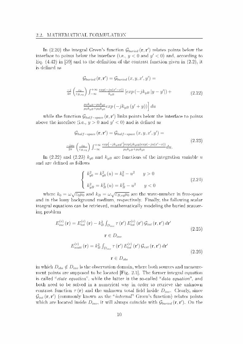
2.2. MATHEMATICAL FORMULATION
In (2.20) the integral Green's fun tion Gburied (r, r′) relates points below the
interfa e to points below the interfa e (i.e., y < 0 and y′ < 0) and, a ording to
Eq. (4.42) in [59 and to the denition of the ontrast fun tion given in (2.2), it
is dened as
Gburied (r, r′) = Gburied (x, y, x′, y′) =
−j4π
(ε0
εB,eq
) ∫ +∞
−∞exp(−ju(x′−x))
kyB[exp (−jkyB |y − y′|)+
µ0kyB−µ0ky0µ0kyB+µ0ky0
exp (−jkyB (y′ + y))]du
(2.22)
while the fun tion Ghalf−space (r, r′) links points below the interfa e to points
above the interfa e (i.e., y > 0 and y′ < 0) and is dened as
Ghalf−space (r, r′) = Ghalf−space (x, y, x
′, y′) =
−jµ0
2π
(ε0
εB,eq
) ∫ +∞
−∞
exp(−jkyBy′)exp(jky0y)exp(−ju(x′−x))
µ0kyB+µ0ky0du.
(2.23)
In (2.22) and (2.23) ky0 and kyB are fun tions of the integration variable uand are dened as follows
k2y0 = k2y0 (u) = k20 − u2 y > 0
k2yB = k2B (u) = k2B − u2 y < 0(2.24)
where k0 = ω√ε0µ0 and kB = ω
√εB,eqµ0 are the wave-number in free-spa e
and in the lossy ba kground medium, respe tively. Finally, the following s alar
integral equations an be retrieved, mathemati ally modeling the buried s atter-
ing problem
E(v)inc (r) = E
(v)tot (r)− k2B
∫Dinv
τ (r′)E(v)tot (r
′)Gint (r, r′) dr′
r ∈ Dinv
(2.25)
E(v)scatt (r) = k2B
∫Dinv
τ (r′)E(v)tot (r
′)Gext (r, r′) dr′
r ∈ Dobs
(2.26)
in whi h Dobs /∈ Dinv is the observation domain, where both sour es and measure-
ment points are supposed to be lo ated [Fig. 2.1. The former integral equation
is alled state equation, while the latter is the so- alled data equation, and
both need to be solved in a numeri al way in order to retrieve the unknown
ontrast fun tion τ (r) and the unknown total eld inside Dinv. Clearly, sin e
Gint (r, r′) ( ommonly known as the internal Green's fun tion) relates points
whi h are lo ated inside Dinv, it will always oin ide with Gburied (r, r′). On the
10
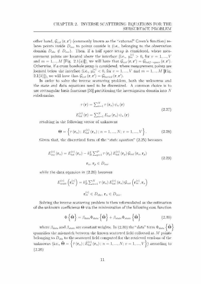
CHAPTER 2. INVERSE SCATTERING EQUATIONS FOR THE
SUBSURFACE PROBLEM
other hand, Gext (r, r′) ( ommonly known as the external Green's fun tion) re-
lates points inside Dinv to points outside it (i.e., belonging to the observation
domain Dobs /∈ Dinv). Then, if a half spa e setup is onsidered, where mea-
surement points are lo ated above the interfa e (i.e., y(v)m > 0, for v = 1, ..., V
and m = 1, ..,M [Fig. 2.1(a)), we will have that Gext (r, r′) = Ghalf−space (r, r′).
Otherwise, if a ross-borehole setup is onsidered, where measurement points are
lo ated below the interfa e (i.e., y(v)m < 0, for v = 1, ..., V and m = 1, ..,M [Fig.
2.1(b)), we will have that Gext (r, r′) = Gburied (r, r′).In order to solve the inverse s attering problem, both the unknowns and
the state and data equations need to be dis retized. A ommon hoi e is to
use re tangular basis fun tions [56 partitioning the investigation domain into Nsubdomains
τ (r) =∑N
n=1 τ (rn)ψn (r)
E(v)tot (r) =
∑Nn=1Etot (rn)ψn (r)
(2.27)
resulting in the following ve tor of unknowns
Θ =τ (rn) ; E
(v)tot (rn) ; n = 1, ..., N ; v = 1, ..., V
. (2.28)
Given that, the dis retized form of the state equation (2.25) be omes
E(v)inc (rn) = E
(v)tot (rn)− k2B
∑Pp=1 τ (rp)E
(v)tot (rp)Gint (rn, rp)
rn, rp ∈ Dinv
(2.29)
while the data equation in (2.26) be omes
E(v)scatt
(r(v)m
)= k2B
∑Nn=1 τ (rn)E
(v)tot (rn)Gext
(r(v)m , rn
)
r(v)m ∈ Dobs, rn ∈ Dinv.
Solving the inverse s attering problem is then reformulated as the estimation
of the unknown oe ients Θ via the minimization of the following ost fun tion
ΦΘ= βdataΦdata
Θ+ βstateΦstate
Θ
(2.30)
where βdata and βstate are onstant weights. In (2.30) the data termΦdata
Θ
quanties the mismat h between the known s attered eld olle ted atM points
belonging to Dobs to the s attered eld omputed for the retrieved versions of the
unknowns (i.e., Θ =τ (rn) ; E
(v)tot (rn) ; n = 1, ..., N ; v = 1, ..., V
) a ording to
(2.26)
11

2.2. MATHEMATICAL FORMULATION
Φdata
Θ=
∑Vv=1
∑Mm=1
∣∣∣E(v)scatt
(r(v)m
)− E(v)
scatt
(r(v)m
)∣∣∣2
∑Vv=1
∑Mm=1
∣∣∣E(v)scatt
(r(v)m
)∣∣∣2 (2.31)
where E(v)scatt
(r(v)m
)is the omputed s attered eld for the m-th probe under
the v-th illumination. Similarly, the state term of the ost fun tion dened in
(2.30) measures the dieren e between the known in ident eld insideDinv to the
retrieved in ident eld omputed a ording (2.25) on the basis of the estimated
Θ
Φstate
Θ=
∑Vv=1
∑Nn=1
∣∣∣E(v)inc (rn)− E
(v)inc (rn)
∣∣∣2
∑Vv=1
∑Nn=1
∣∣∣E(v)inc (rn)
∣∣∣2 (2.32)
where E(v)inc (rn) is the omputed s attered eld for the n-th point in Dinv
under the v-th illumination.
12
Chapter 3
Multi-Fo using Inexa t Newton
Method within the Se ond-Order
Born Approximation
In this hapter, the re onstru tion of a shallow buried obje t is addressed by an
ele tromagneti inverse s attering method based on ombining dierent imag-
ing modalities. In parti ular, the proposed approa h integrates the inexa t-
Newton method with an iterative multi-s aling approa h. Moreover, the use of
the se ond-order Born approximation (SOBA) is exploited. A numeri al val-
idation is provided on erning the potentialities arising by ombining the reg-
ularization apabilities of the inexa t-Newton method and the ee tiveness of
the multi-fo using strategy to mitigate the non-linearity and ill-posedness of the
inversion problem. Comparisons with the standard "bare" approa h in terms of
a ura y, robustness, noise levels, and omputational e ien y are also in luded.
13

3.1. INTRODUCTION
3.1 Introdu tion
The aim of this hapter is to reformulate the integrated IMSA − IN inver-
sion te hnique [48 in order to deal with subsurfa e imaging and to evaluate the
ee tiveness of su h an approa h when the se ond-order Born approximation
(SOBA) is applied. Moreover, a dire t omparison in terms of a ura y, ro-
bustness against dierent onditions and noise levels, as well as omputational
e ien y is given when dire tly omparing the proposed IMSA− IN − SOBAapproa h with its standard bare implementation (BARE − IN − SOBA), asdes ribed in [28.
Towards this end, se tion 3.2 provides the basi mathemati al formulation used to
model the buried problem under the SOBA. In Se t. 3.3 the ombined IMSA−IN − SOBA is des ribed. An in-depth numeri al validation is then provided in
Se t. 3.4 in order to analyze the performan e of the proposed approa h and to
demonstrate its ee tiveness and advantages over the BARE − IN − SOBA,under mono hromati transverse magneti (TM) illumination onditions in a
ross-borehole setup similar to that used in [37. Finally, some on lusions are
drawn (Se t. 3.5).
3.2 Problem Formulation
Let us onsider a ylindri al s atterer buried in a homogeneous half spa e medium.
A ross-borehole measurement onguration is assumed [Fig. 3.1. Let τ (r) de-note the ontrast fun tion inside the inspe ted area Dinv, as dened in equation
(2.2). The upper medium is supposed to be air, with diele tri properties equal
to those of the va uum and the position ve tor r denotes a point in the transverse
plane, i.e., r = (x, y).
The target, whose ross se tion is in luded in the inspe ted area Dinv is illu-
minated by V in ident waves, whi h are produ ed by a set of innite line ur-
rents. They generate in ident waves of transverse magneti type, su h that
E(v)inc(r) = E
(v)inc(r)z, v = 1, . . . , V . Due to the ylindri al geometry, the s attered
and total elds results to be z-polarized, too.
The basi equation for this inverse problem is therefore the following s alar in-
tegral one
E(v)scatt (r) = E
(v)tot (r)− E(v)
inc(r) = k2B
∫
Dinv
τ (r′)E(v)tot (r
′)Gburied (r, r′) dr′, (3.1)
whi h is a nonlinear ill-posed Lippman-S hwinger equation, whose kernel is the
Green's fun tion for the half spa e [55 with denition given in equation (2.22).
In equation (3.1), E(v)tot and E
(v)scatt are the z- omponents of the total and s at-
tered ele tri elds (for the v-th illumination), respe tively. Su h equation is
approximated by using a se ond-order Born expansion [27, i.e.,
14

CHAPTER 3. MULTI-FOCUSING INEXACT NEWTON METHOD
WITHIN THE SECOND-ORDER BORN APPROXIMATION
-2.5
-2
-1.5
-1
-0.5
0
0.5
-1.5 -1 -0.5 0 0.5 1 1.5
y/λ b
x/λb
Measurement pointsSource locations
Dinv
Figure 3.1: Geometry of the problem and imaging setup.
E(v)scatt (r)
∼= F(v)B1 τ (r) + k2B
∫
Dinv
τ (r′)F(v)B1 τ (r
′)Gburied (r, r′) dr′ = F(v)B2 (τ) (r) ,
(3.2)
where F(v)B1 denotes the rst order Born operator dened as
F(v)B1 τ (r) = k2B
∫
Dinv
τ (r′)E(v)inc (r
′)Gburied (r, r′) dr′. (3.3)
Consequently, sin e the ontrast fun tion is independent of v, the inverse s at-
tering problem an be formulated as the solution of the following set of equations
with respe t to the unknown τ
FB2 (τ) =
F
(1)B2 (τ).
.
.
F(V )B2 (τ)
=
E
(1)scatt.
.
.
E(V )scatt
= Escatt (3.4)
The dis rete ounterparts of the above equations an be obtained by partitioning
them in square subdomains in order to obtain pixelated images of the retrieved
distributions of the diele tri parameters inside the inspe ted area.
3.3 Re onstru tion Method
In order to solve equation (3.4), an inner/outer iterative s heme based on an INmethod is applied [28. The operator equation (3.4) is iteratively linearized by
using the Fre hét derivative of the operator FB2. This step leads to the following
linear operator equation
F′
τiu = Escatt − FB2 (τi) (3.5)
15

3.3. RECONSTRUCTION METHOD
where τi is the ontrast fun tion at the i-th iteration and F′
τidenotes the Fre hét
derivative of the operator FB2 at τi. As detailed in [29, F′
τiis given by
F′
τiu =
F
′(1)τi u.
.
.
F′(V )τi u
(3.6)
where
F′(v)τi u (r) = F
(v)B1 u (r) + k2B
∫Dinv
τi (r′)F
(v)B1 u (r
′)Gburied (r, r′) dr′+k2B
∫Dinv
u (r′)F(v)B1 τi (r
′)Gburied (r, r′) dr′(3.7)
As it is well known, equation (3.5) turns out the be ill-posed. Consequently,
its solution an be obtained in a regularization sense by using a regularization
method. In parti ular, following the approa h in [44, a good hoi e seems to be
the use of the Landweber iterative method [61. In this ase, a se ond loop is
obtained by means of the following s heme
ui,0 = 0ui,q+1 = ui,q − ρiF
′∗τi
(F
′
τiui,q − Escatt + FB2 (τi)
),
(3.8)
where F′∗τiis the the adjoint of F
′
τiand 0 < ρi < 2
∥∥F ′
τi
∥∥−2
s, being ‖·‖s the spe tral
norm. A regularized solution ui is obtained by trun ating the iterations after a
predened number of steps Q. After the linearized problem is solved, the urrent
ontrast fun tion is updated as
τi+1 = τi + ui (3.9)
and the algorithm is iterated until a predened stopping riteria is fullled. It
requires of ourse an initialization phase, in whi h an estimate of the diele tri
properties of the inspe ted area is hosen. In most ases, an empty domain is
used as initial guess.
As mentioned in Se tion 3.1, the ee tiveness of an integrated pro edure that
protably exploits the regularization apabilities of the IN method and the a-
pability of the iterative multi-s aling approa h (IMSA) [54 to redu e the o ur-ren e of lo al minima has been already assessed in [48[49 for free-spa e imaging.
Issues su h as numeri al instabilities aused by the presen e of noise on measured
data, as well as the ill- onditioned and non-linear nature of the inversion prob-
lem are thus jointly addressed, throughout the synergeti ombination of both
te hniques.
In parti ular, at ea h s-th step of the IMSA (s = 1, ..., S; s being the step
index), the RoI Ω(s)(Ω(1)
oin iding with Dinv) is dened and partitioned a -
ording to the Ri hmond's pro edure [56 into N square sub-domains (N being
the estimated number of degrees of freedom of the measured data [57[58) en-
tered at r(s)n (r
(s)n ∈ Ω(s)
, n = 1, ..., N). Following the IN method formulation, the
non-linear equation (3.4) is iteratively linearized in order to obtain the following
16

CHAPTER 3. MULTI-FOCUSING INEXACT NEWTON METHOD
WITHIN THE SECOND-ORDER BORN APPROXIMATION
linear operator equation (note the addition of the supers ript
(s)with respe t to
(3.5) to indi ate the iterative nature of the multi-s aling approa h)
(F (s)τi
)′
u(s) = Escatt − F (s)B2
(τ(s)i
)(3.10)
As previously detailed, at ea h IN step, equation (3.10) is solved in a regularized
sense by means of an inner trun ated Landweber loop, omposed by the following
loop (initialized with u(s)i,0 = 0)
u(s)i,q+1 = u
(s)i,q − ρ
(s)i
(F (s)τi
)′∗[(F (s)τi
)′
u(s)i,q −Escatt + F
(s)B2
(τ(s)i
)], q = 0, ..., Q− 1
(3.11)
The urrent solution is updated as τ(s)i+1 = τ
(s)i + u
(s)i,Q and the IN method is
iterated (i.e., by letting i = i + 1) until a suitable predened stop riterion is
rea hed. On e the IN loop has been terminated, a new IMSA step is initialized
(i.e., by letting s = s + 1), throughout the update of Ω(s)and its dis retization
with a ner resolution. This step requires to update the bary enters r(s)n ∈ Ω(s)
,
n = 1, ..., N .
The multi-step pro ess is iterated until the veri ation of a suitable termination
ondition (e.g., s = S), and u(S) = τ (S) is nally assumed as the IMSA− IN −SOBA solution.
It has been pointed out in [49 the importan e of dening an e ient stopping
riterion for the IMSA − IN − SOBA when no a-priori information on the
obje t under test is available. To monitor the evolution of the re onstru tion
residual, a parameter is introdu ed, whi h is dened at ea h IN iteration i as thedis repan y between measured and retrieved s attered eld at M measurement
lo ations:
Φi =
∑Vv=1
∑Mm=1
∥∥∥E(v)scatt(r
(v)m )− E(v)
scatt,i(r(v)m )
∥∥∥2
2
∑Vv=1
∑Mm=1
∥∥∥E(v)scatt(r
(v)m )
∥∥∥2
2
(3.12)
where E(v)scatt(r
(v)m ) and E
(v)scatt,i(r
(v)m ) denote the measured and estimated s attered
elds at the measurement point m (m = 1, ...,M) for the v-th illumination
(v = 1, ..., V ), while ‖.‖2 denotes the l2-norm operator. The following stationary
ondition, based on su essive observations of the estimated residual, an then
be dened in order to adaptively terminate the IN pro edure at ea h s-th step
of the multi-fo using s heme:
ζi =
∣∣∣WΦi −∑W
j=1Φi−j
∣∣∣Φi
≤ η (3.13)
where η and W denote a xed numeri al threshold and a xed number of INiterations, respe tively. The denition of suitable values for both η and W has
learly a riti al impa t on the overall performan es of the IMSA−IN−SOBA,
17

3.4. NUMERICAL ASSESSMENT
sin e both parameters are essential to identify a stagnating behaviour of the
residual, whi h is a tually strongly linked to the semi onvergen e property of the
IN method when dealing with the regularization of noisy data [29. Con erning
the regularization apability of IN method algorithm, the number of iterations
Q for the Landweber method should also be arefully hosen, as well as the
number of multi-s aling iterations S should be set in order to su essfully balan e
omputational e ien y and overall quality of the retrieved images.
3.4 Numeri al Assessment
This se tion is aimed at illustrating the potentialities of the proposed IMSA−IN−SOBAmethod when dealing with the pro essing of syntheti data produ ed
by both homogeneous and inhomogeneous s atterers buried in a lossy homoge-
neous half spa e medium. The signi ant advantage of the IMSA − IN over
the standard IN method has been already highlighted and well do umented in
[48[49 for the free-spa e s enario. The appli ability of the IN method within
the se ond-order Born approximation to the retrieval of buried obje ts has been
su essfully demonstrated in [28, as well. The analysis will thus fo us on the
advantages of employing the iterative multi-resolution inversion s heme over the
bare IN method implementation within the SOBA (BARE − IN − SOBA),both in terms of a ura y, robustness when dealing with dierent s atterers and
dierent noise onditions. Besides the pi torial representation of the retrieved
diele tri distributions, the following error indexes will be used in the following
to give a quantitative evaluation of the re onstru tion a ura y:
Ξreg =1
Nreg
Nreg∑
n=1
|τ (xn, yn)− τ(xn, yn)||τ(xn, yn) + 1| reg = tot, ext, int (3.14)
where Nreg indi ates the number of ells overing the whole inspe ted area Dinv
(reg = tot, Ntot = N), or belonging to the ba kground region (reg = ext), or tothe support of the buried s atterer (reg = int; Ntot = Next+Nint). Moreover, the
terms τ and τ in equation (3.14) indi ate the retrieved and the a tual ontrast
fun tion for the n-th ell belonging to the investigation domain.
The rst part of this Se tion is devoted to a sensitivity analysis of the IMSA−IN − SOBA algorithm, aimed at investigating the ee t of ea h ontrol param-
eter on the nal quality of the retrieved distributions when dealing with noisy
data, in order to dene a suitable and general setup.
3.4.1 Calibration of the IMSA− IN − SOBAIt should be stressed that, as already dis ussed in Se tion 3.3, the hoi e of the
ontrol parameters η, W , Q and S should be arefully performed in order to
protably exploit the apabilities of the IMSA− IN − SOBA.
18

CHAPTER 3. MULTI-FOCUSING INEXACT NEWTON METHOD
WITHIN THE SECOND-ORDER BORN APPROXIMATION
Square - l ≈ λb/3, τ = 1.5, Q = Q*, S = S*, SNR = 20[dB]
W*, η*
10-5
10-4
10-3
10-2
10-1
η 0 10 20 30 40 50 60 70 80W
0
0.02
0.04
0.06
0.08
0.1
Ξtot 0
0.02
0.04
0.06
0.08
0.1
Ξ tot
(a)
0
0.005
0.01
0.015
0.02
0.025
0.03
10 20 30 40 50 60 70 80 90 100
Ξ tot
Q
Square - l ≈ λb/3, τ = 1.5, η = η*, W = W*, SNR = 20[dB]
(b)
10-3
10-2
10-1
100
1 2 3 4 5 6
Rec
onst
ruct
ion
Err
ors
IMSA Step, s
Square - l ≈ λb/3, τ = 1.5, Q = Q*, η = η*, W = W*, SNR = 20[dB]
Ξtot Ξint Ξext
( )
Figure 3.2: Sensitivity Analysis (Homogeneous Square S atterer - ℓ ≈ λb
3, τ = 1.5,
SNR = 20 dB) - Behaviour of the integral error Ξtot versus η and W when
Q = Q∗, S = S∗
(a), and versus K when η = η∗, W = W ∗, and S = S∗
(b).
Plot of the total, internal, and external error as a fun tion of S when Q = Q∗,
η = η∗, and W = W ∗( ).
19

3.4. NUMERICAL ASSESSMENT
Towards this end, an exhaustive sensitivity analysis on the impa t of ea h on-
trol parameter has been performed on noisy eld data (SNR = 20 dB) olle tedfor an homogeneous lossy o- entered square ylinder, with side l ≈ λb/3,λb being the wavelength inside the ba kground, and τ = 0.5 [Fig. 3.3 (a).
Moreover, a square investigation domain of side 1.6λb lo ated 0.1λb under theair-soil interfa e has has been assumed as referen e s enario (Fig. 3.1). The
homogeneous half spa e medium, inside whi h the s atterer is buried, is har-
a terized by a relative diele tri permittivity εrB = 4.0 and by a ondu tivity
σB = 10−2S/m. The investigation domain Dinv is sequentially illuminated by a
set of V = 16 transverse-magneti (TM) mono hromati plane waves generated
by two verti al rows of eld sour es ongured in a ross-borehole setup [Fig.
3.1 working at the frequen y of f = 300 MHz. For ea h view, the syntheti ally
generated s attered eld is olle ted at M = 15 equally spa ed measurement
points (with ±0.2λb oset along x with respe t to the investigation domain [Fig.
3.1). It is worthwhile to noti e that that the values of V and M have been
hosen following the guidelines in [57[58 to olle t all the available information
on Dinv from the measured s attered radiation. Moreover, the investigation area
has been partitioned into N = 100 square sub-domains.
In order to investigate the impa t of η and W on the a hievable performan es
of the IMSA− IN − SOBA, Fig. 3.2(a) reports the total re onstru tion error
Ξtot as a two dimensional fun tion of both parameters, when the number of
Landweber and IMSA iterations are respe tively set to their optimal values Q∗
and S∗.
As it an be observed, a low value of the threshold η (e.g., η = 10−4) results
ompletely inappropriate, leading to a signi ant degradation of the quality of
the re onstru tions, due the so- alled semi onvergen e property of the IN regu-
larization te hnique [29.
A tually, the best re onstru tion is obtained after a given number of IN iter-
ations, while subsequent iterations give rise to worse solutions, sin e data are
ae ted by noise [28. Similarly, an high value of η also leads to ina urate re-
sults, ausing the premature termination of the inversion pro edure. Therefore,
a good hoi e for η is
η∗ = 10−2(3.15)
and it has been assumed hereinafter for the IMSA− IN − SOBA inversions.
Even if less riti al, a suitable value for W should also be arefully sele ted. As
shown in equation (3.13), W denes the number of IN iterations whi h should
be taken into a ount for the identi ation of a stagnating behaviour on the
residual Φ. Although a small value of W an redu e the apability of ltering
out numeri al errors ae ting the omputation of the residual, high values of Wgive rise to a remarkable degradation of the performan es, as depi ted in Fig.
3.2(a), whatever the value of the threshold η. Given the above onsiderations,
the optimal value of W has been set to
W ∗ = 5 (3.16)
20

CHAPTER 3. MULTI-FOCUSING INEXACT NEWTON METHOD
WITHIN THE SECOND-ORDER BORN APPROXIMATION
-1.7
-1.3
-0.9
-0.5
-0.1
-0.8 -0.4 0 0.4 0.8
y/λ b
x/λb
0
0.3
0.6
0.9
1.2
1.5
1.8
Re
τ(x,
y)
(a)
-1.7
-1.3
-0.9
-0.5
-0.1
-0.8 -0.4 0 0.4 0.8
y/λ b
x/λb
0
0.3
0.6
0.9
1.2
1.5
1.8
Re
τ(x,
y)
(b)
-1.7
-1.3
-0.9
-0.5
-0.1
-0.8 -0.4 0 0.4 0.8
y/λ b
x/λb
0
0.3
0.6
0.9
1.2
1.5
1.8
Re
τ(x,
y)
( )
Figure 3.3: Sensitivity Analysis (Homogeneous Square S atterer - ℓ ≈ λb
3, τ = 1.5,
SNR = 20 dB, S = S∗) - A tual (a) and retrieved (b)( ) ontrast proles when
(b) Q = Q∗, W = W ∗
, η = 10−4; ( ) K = K∗
, W = 40, η = η∗.
and it will be used in the following of the dis ussion. For ompleteness, and
to give the reader a pi torial example of what is the impa t of a wrong hoi e
of η and W on the IMSA − IN − SOBA performan es, the retrieved proles
21
3.4. NUMERICAL ASSESSMENT
for the square ylinder of Fig. 3.3(a) are shown for η = 10−4[Fig. 3.3(b)
and W = 40 [Fig. 3.3( ), being the other parameters xed to their optimal
values. The omputed total error indexes are Ξtot⌋η=10−4,W=W ∗ ≈ 1.27 × 10⁻¹
and Ξtot⌋η=η∗,W=40 ≈ 2.12 × 10⁻¹, while a redu tion of more than one order of
magnitude on Ξtot an be a hieved when jointly setting η andW to their optimal
values (Ξtot⌋η=η∗ ,W=W ∗ ≈ 7.92× 10⁻³) [Fig. 3.2(a).
Con erning the dependen e of the inversion quality on the number of Landweber
iterations, Fig. 3.2(b) shows the behaviour of Ξtot as a fun tion of Q, when all
remaining parameters are set to their optimal values. As a matter of fa t, the
number of iterations plays the role of a regularization parameter in the iterative
Landweber regularization method, representing a heuristi ompromise between
fast onvergen e of the IN method (for low values of Q) and noise ltering
(for high values of Q) [28. Therefore, given the above onsiderations and also
following the out ome of the performed sensitivity analysis (Fig. 3.2(b)), the
number of inner iterations has been to
Q∗ = 60 (3.17)
an it will be onsidered for the su essive analysis of the algorithm performan es.
Con erning the stop riterion for the iterative multi-zooming s heme, Fig. 3.2( )
reports the omputed error indexes as a fun tion of the IMSA step s (s = 1, .., 6)in the ase η = η∗, W = W ∗
and Q = Q∗.
As it an be observed, the total error shows a rapid des ent until step s = 4is rea hed (Ξs=1
tot ≈ 9.73 × 10⁻²vs. Ξs=4
tot ≈ 7.92 × 10⁻³), while a progressive
degradation of the a ura y hara terizes the remaining su essive steps, as ver-
ied by the error indexes (Ξs=5tot ≈ 2.15 × 10⁻²
and Ξs=6tot ≈ 3.52 × 10⁻²
). It is
worth noti ing that, although the external error rea hes its null even before step
s = 4, the suppression of artifa ts inside the ba kground region omes at the
ost of a slight in rement of the internal error. Given the above onsiderations,
the optimal number of IMSA steps has been identied as
S∗ = 4 (3.18)
and it will be employed as a good ompromise for su essive test ases. Fig-
ures 3.4(b)-3.4(e) illustrate the evolution of the re onstru tion throughout the
IMSA− IN −SOBA steps, when the optimal values of ea h ontrol parameter
is set to its optimal value. As shown by the single plots, the retrieved prole
improves step-by-step, starting from a rough estimation of the buried obje t
support and diele tri hara teristi s [s = 1 - Fig. 3.4(b) until a satisfa tory
re onstru tion is rea hed [s = 4 = S∗- Fig. 3.4(e). A pi torial representation
of the evolution of the residual (equation (3.12)) and of the stationary index
(equation(3.13)) throughout the multi-zooming steps is given Fig. 3.4(a).
22

CHAPTER 3. MULTI-FOCUSING INEXACT NEWTON METHOD
WITHIN THE SECOND-ORDER BORN APPROXIMATION
10-3
10-2
10-1
100
77 1 11 21 31 41 51 61 71
[arb
itrar
y un
it]
Iteration Index, i
Square - l ≈ λb/3, τ = 1.5, K = K*, W = W*, η = η*, SNR = 20[dB]
40 59
φi ζi
(a)
-1.7
-1.3
-0.9
-0.5
-0.1
-0.8 -0.4 0 0.4 0.8
y/λ b
x/λb
0
0.3
0.6
0.9
1.2
1.5
1.8
Re
τ(x,
y)
-1.7
-1.3
-0.9
-0.5
-0.1
-0.8 -0.4 0 0.4 0.8
y/λ b
x/λb
0
0.3
0.6
0.9
1.2
1.5
1.8
Re
τ(x,
y)
(b) ( )
-1.7
-1.3
-0.9
-0.5
-0.1
-0.8 -0.4 0 0.4 0.8
y/λ b
x/λb
0
0.3
0.6
0.9
1.2
1.5
1.8
Re
τ(x,
y)
-1.7
-1.3
-0.9
-0.5
-0.1
-0.8 -0.4 0 0.4 0.8
y/λ b
x/λb
0
0.3
0.6
0.9
1.2
1.5
1.8
Re
τ(x,
y)
(d) (e)
Figure 3.4: Sensitivity Analysis (Homogeneous Square S atterer - ℓ ≈ λb
3, τ = 1.5,
SNR = 20 dB, Q = Q∗, W = W ∗
, η = η∗) - Behaviour of Φ and ζ versus the
IMSA − IN iteration number (a). Plot of the retrieved ontrast proles when
(b) S = 1, ( ) S = 2, (d) S = 3, (e) S = 4 = S∗.
23

3.4. NUMERICAL ASSESSMENT
3.4.2 Homogeneous Square and L-shaped Cylinders
The rst set of numeri al experiments deals with two o- entered lossy homoge-
neous s atterers having dierent ross-se tions and hara terized by a ontrast
τ = 1.5 [Square and L-shaped proles, - Fig. 3.5. The BARE−IN−SOBAre onstru tions have been arried out by setting Q = 20 and I = 20 [28,
while for the IMSA − IN − SOBA the following parameters have been ho-
sen, a ording to the previously dis ussed sensitivity analysis: η = 10−2 = η∗,W = 5 = W ∗
, Q = 60 = Q∗, and S = 4 = S∗
. Moreover, the investigation do-
main Dinv has been partitioned into N = 400 and N = 100 square sub-domains
for BARE − IN − SOBA and IMSA− IN − SOBA inversion te hniques, re-
spe tively. All remaining parameters are kept equal to those employed in the
previous paragraph.
Figs. 3.5(b)-3.5( ) show the retrieved proles by the BARE−IN−SOBA, whileFigs. 3.5(d)-3.5(e) the orresponding IMSA − IN − SOBA re onstru tions,
in ase the s attered eld data is orrupted by an additive zero mean omplex
Gaussian noise, raising a signal-to-noise ratio equal to SNR = 10 dB. As it an beobserved, the IMSA−IN−SOBA is able to provide a remarkable improvement
in terms of a ura y over the bare ounterpart even in the presen e of a strong
noisy omponent on measurements, as quantitatively onrmed by the lower
error (Ξtot⌋BARE−IN−SOBA”Square” ≈ 1.46× 10⁻¹
vs. Ξtot⌋IMSA−IN−SOBA”Square” ≈ 1.24× 10⁻¹
and Ξtot⌋BARE−IN−SOBA”L−shaped” ≈ 1.23× 10⁻¹
vs. Ξtot⌋IMSA−IN−SOBA”L−shaped” ≈ 1.19× 10⁻¹
).
To further validate these out omes, the results from a more exhaustive set of
noisy ases have been summarized in Fig. 3.5(a), showing the a hieved total
re onstru tion error Ξtot for dierent values of SNR for both the onsidered
homogeneous s atterers. The result is that the IMSA− IN −SOBA over omes
the bare IN method implementation in terms of re onstru tion a ura y, as
pointed out by the error urves in Fig. 3.5(a). Although the re onstru tion
quality degrades for both BARE − IN − SOBA and IMSA− IN − SOBA for
lower signal-to-noise ratios, it turns out that ΞIMSA−IN−SOBAtot < ΞBARE−IN−SOBA
tot
whatever the noise ondition.
3.4.3 O-shaped Cylinder
In order to prove the general validity of the previously dis ussed out omes on
the IMSA − IN − SOBA approa h when dealing with the retrieval of more
omplex diele tri shapes with dierent values of τ , an homogeneous hollow
square ylinder (O-shaped prole) with an outer side equal to l ≈ λb/2 has been hosen as a more hallenging ben hmark geometry. In order to give the reader a
full pi ture on the performan e improvement of the IMSA− IN − SOBA over
the BARE − IN − SOBA, Fig. 3.6 illustrates the behaviour of the total error
Ξtot as a fun tion of τ , for dierent signal-to-noise ratios on s attered data.
24

CHAPTER 3. MULTI-FOCUSING INEXACT NEWTON METHOD
WITHIN THE SECOND-ORDER BORN APPROXIMATION
0
0.05
0.1
0.15
0.2
0.25
0 10 20 30 40
Ξ tot
SNR [dB]
τ = 1.5
Square - BARE-INSquare - IMSA-IN
L-Shaped - BARE-INL-Shaped - IMSA-IN
(a)
Square L-Shaped
BARE−IN−SOBA
-1.7
-1.3
-0.9
-0.5
-0.1
-0.8 -0.4 0 0.4 0.8
y/λ b
x/λb
0
0.3
0.6
0.9
1.2
1.5
1.8
Re
τ(x,
y)
-1.7
-1.3
-0.9
-0.5
-0.1
-0.8 -0.4 0 0.4 0.8
y/λ b
x/λb
0
0.3
0.6
0.9
1.2
1.5
1.8
Re
τ(x,
y)
(b) ( )
IMSA−IN−SOBA
-1.7
-1.3
-0.9
-0.5
-0.1
-0.8 -0.4 0 0.4 0.8
y/λ b
x/λb
0
0.3
0.6
0.9
1.2
1.5
1.8
Re
τ(x,
y)
-1.7
-1.3
-0.9
-0.5
-0.1
-0.8 -0.4 0 0.4 0.8
y/λ b
x/λb
0
0.3
0.6
0.9
1.2
1.5
1.8R
eτ(
x,y)
(d) (e)
Figure 3.5: Performan e Assessment (τ = 1.5, SNR ∈ [10, 40] dB) - Behaviourof the Ξtot as a fun tion of SNR when dealing with Square or L-Shaped targets
(a). Plot of the ontrast proles retrieved by (b)( ) BARE − IN − SOBA and
(d)(e) IMSA − IN − SOBA when SNR = 10 dB. (b)(d) Square s atterer;
( )(e) L-Shaped s atterer.
25

3.4. NUMERICAL ASSESSMENT
0
0.05
0.1
0.15
0.2
0.25
0.3
0.35
0.2 0.6 1 1.4 1.8 2.2
Ξ tot
τ
O-Shaped - l ≈ λb/2
BARE-IN - SNR=10[dB]IMSA-IN - SNR=10[dB]
BARE-IN - SNR=20[dB]IMSA-IN - SNR=20[dB]
BARE-IN - SNR=30[dB]IMSA-IN - SNR=30[dB]
Figure 3.6: Performan e Assessment (O-Shaped S atterer ℓ ≈ λb
2, SNR ∈
[10, 30] dB) - Behaviour of the Ξtot as a fun tion of τ obtained by BARE−IN−SOBA and IMSA− IN − SOBA.
Although the re onstru tion a ura y degrades as τ in reases, the IMSA −IN − SOBA always provides the lowest error (e.g., ΞBARE−IN−SOBA
tot
⌋τ=2.2
≈2.14× 10⁻¹
vs. ΞIMSA−IN−SOBAtot
⌋τ=2.2
≈ 4.42× 10⁻²).
It is also worth to noti e that, as reported in Fig. 3.6, the error index of the
IMSA− IN −SOBA for SNR = 10 dB is always lower than the error provided
by the bare IN method implementation for a signi antly higher signal-to-
noise ratio (SNR = 30 dB). For ompleteness, the error indexes in Fig. 3.6 are
also reported in Tab. 3.1.
BARE − IN − SOBASNR dB τ = 0.2 τ = 0.6 τ = 1.0 τ = 1.4 τ = 1.8 τ = 2.2
30 1.98× 10⁻² 5.68× 10⁻² 9.18× 10⁻² 1.22× 10⁻¹ 1.56× 10⁻¹ 1.92× 10⁻¹
20 2.20× 10⁻² 6.12× 10⁻² 9.79× 10⁻² 1.37× 10⁻¹ 1.74× 10⁻¹ 2.14× 10⁻¹
10 3.52× 10⁻² 8.74× 10⁻² 8.87× 10⁻² 2.01× 10⁻¹ 2.69× 10⁻¹ 3.15× 10⁻¹
IMSA− IN − SOBASNR dB τ = 0.2 τ = 0.6 τ = 1.0 τ = 1.4 τ = 1.8 τ = 2.2
30 1.18× 10⁻² 3.59× 10⁻² 5.63× 10⁻² 6.24× 10⁻² 8.03× 10⁻² 9.06× 10⁻²
20 1.29× 10⁻² 2.72× 10⁻² 3.64× 10⁻² 4.88× 10⁻² 5.20× 10⁻² 4.42× 10⁻²
10 1.28× 10⁻² 3.95× 10⁻² 8.26× 10⁻² 9.21× 10⁻² 1.15× 10⁻¹ 1.54× 10⁻¹
Table 3.1: Performan e Assessment (O-Shaped S atterer ℓ ≈ λb
2, SNR ∈
[10, 30] dB) - Error values and omputational indexes.
26

CHAPTER 3. MULTI-FOCUSING INEXACT NEWTON METHOD
WITHIN THE SECOND-ORDER BORN APPROXIMATION
BARE − IN − SOBA IMSA− IN − SOBAτ=
0.2
-1.7
-1.3
-0.9
-0.5
-0.1
-0.8 -0.4 0 0.4 0.8
y/λ b
x/λb
0
0.05
0.1
0.15
0.2
0.25
0.3
Re
τ(x,
y)
-1.7
-1.3
-0.9
-0.5
-0.1
-0.8 -0.4 0 0.4 0.8
y/λ b
x/λb
0
0.05
0.1
0.15
0.2
0.25
0.3
Re
τ(x,
y)
(a) (b)
τ=
1.0
-1.7
-1.3
-0.9
-0.5
-0.1
-0.8 -0.4 0 0.4 0.8
y/λ b
x/λb
0
0.2
0.4
0.6
0.8
1
1.2R
eτ(
x,y)
-1.7
-1.3
-0.9
-0.5
-0.1
-0.8 -0.4 0 0.4 0.8
y/λ b
x/λb
0
0.2
0.4
0.6
0.8
1
1.2
Re
τ(x,
y)
( ) (d)
τ=
2.2
-1.7
-1.3
-0.9
-0.5
-0.1
-0.8 -0.4 0 0.4 0.8
y/λ b
x/λb
0
0.4
0.8
1.2
1.6
2
2.4
Re
τ(x,
y)
-1.7
-1.3
-0.9
-0.5
-0.1
-0.8 -0.4 0 0.4 0.8
y/λ b
x/λb
0
0.4
0.8
1.2
1.6
2
2.4
Re
τ(x,
y)
(e) (f )
Figure 3.7: Performan e Assessment (O-Shaped S atterer ℓ ≈ λb
2, SNR = 20
dB) - Plot of the ontrast proles retrieved by (a)( )(e) BARE − IN − SOBAand (b)(d)(f ) IMSA − IN − SOBA when (a)(b) τ = 0.2, ( )(d) τ = 1.0, and(e)(f ) τ = 2.2.
To further onrm the above onsiderations and provide a qualitative pi ture
27

3.4. NUMERICAL ASSESSMENT
of the retrieved proles, Fig. 3.7 shows a dire t omparison between the re on-
stru tions provided by both BARE − IN − SOBA and IMSA− IN − SOBAfor dierent values of ontrast [Figs. 3.7(a)-3.7(b) - τ = 0.2, Figs. 3.7( )-3.7(d)- τ = 1.0, Figs. 3.7(e)-3.7(f ) - τ = 2.2, when SNR = 20 dB. As it an be
observed, thanks to the in reased level of resolution inside the orre tly identi-
ed RoI, the IMSA− IN −SOBA outperforms its bare ounterpart, showing
not only the apability of better retrieving the external boundaries of the s at-
terer, suppressing the undesired artifa ts inside the ba kground region, but also
of re ognizing position and shape of the internal avity.
3.4.4 Inhomogeneous Cylinders
To assess the performan es of the IMSA−IN−SOBA when dealing with buried
obje ts hara terized by non-homogeneous diele tri distributions, this Se tion
onsiders the analysis of the two referen e proles in Figs. 3.8(a)-3.8(b). The rst
inhomogeneous geometry (Fig. 3.8(a), Double-L ylinder) is hara terized by
τup = 0.5 and τlow = 1.5 in the upper and lower portions, respe tively, while the
se ond referen e distribution (Fig. 3.8(b), Con entri ylinder) is hara terized
by τext = 0.5 and τin = 1.0. The se ond and third rows of Fig. 3.8 illustrate the
retrieved diele tri distributions by the BARE− IN −SOBA [Figs. 3.8( )-(d)
and by the IMSA − IN − SOBA [Fig. 3.8(e)-(f ), when SNR = 20 dB. As
a matter of fa t, the bare IN method implementation provides mu h more
smoothed proles than the multi-s aling s heme.
Considering the retrieved proles for the Double-L s atterer, the improvement
in terms of a ura y provided by the IMSA− IN − SOBA [Fig. 3.8(e) is on-
rmed by a remarkable redu tion of the re onstru tion error (ΞBARE−IN−SOBAtot ≈
1.03× 10⁻¹vs. ΞIMSA−IN−SOBA
tot ≈ 3.35× 10⁻²). Still onsidering this parti ular
example, it is quite interesting to noti e that the BARE − IN − SOBA seems
almost ompletely unable to identify the presen e of two distin t geometri ally
adja ent distributions of the ontrast [Fig. 3.8( ).
Similar on lusions an be also formulated for the Con entri onguration
[Figs. 3.8(d)-(f ). Dierently from the bare ounterpart, the IMSA − IN −SOBA orre tly identies the squared shape and the ontrast of the inner ore, as
veried by the lower internal re onstru tion error (ΞBARE−IN−SOBAint ≈ 1.19×10⁻¹
vs. ΞIMSA−IN−SOBAint ≈ 7.45× 10⁻²
).
Besides the dis ussed aspe ts, it is important to remark that the improved a u-
ra y showed by the IMSA−IN−SOBA omes together with an in reased om-
putational e ien y, as emphasized by the evaluation of the inversion times on a
standard laptop with 3.20 GHz CPU lo k and 4GB of RAM memory. The total
time required to obtain the re onstru tions in Fig. 3.8 are ∆tIMSA−IN−SOBA =80 [s and ∆tIMSA−IN−SOBA = 57 [s for Double-L and Con entri pro-
les, respe tively, while the time required by the BARE − IN − SOBA is
∆tBARE−IN−SOBA = 256 [s for both distributions.
28

CHAPTER 3. MULTI-FOCUSING INEXACT NEWTON METHOD
WITHIN THE SECOND-ORDER BORN APPROXIMATION
Double-L Con entri
A
t
u
a
l
-1.7
-1.3
-0.9
-0.5
-0.1
-0.8 -0.4 0 0.4 0.8
y/λ b
x/λb
0
0.2
0.4
0.6
0.8
1
1.2
1.4
1.6
1.8
Re
τ(x,
y)
-1.7
-1.3
-0.9
-0.5
-0.1
-0.8 -0.4 0 0.4 0.8
y/λ b
x/λb
0
0.2
0.4
0.6
0.8
1
1.2
Re
τ(x,
y)
(a) (b)
BARE−IN−SOBA
-1.7
-1.3
-0.9
-0.5
-0.1
-0.8 -0.4 0 0.4 0.8
y/λ b
x/λb
0
0.2
0.4
0.6
0.8
1
1.2
1.4
1.6
1.8R
eτ(
x,y)
-1.7
-1.3
-0.9
-0.5
-0.1
-0.8 -0.4 0 0.4 0.8
y/λ b
x/λb
0
0.2
0.4
0.6
0.8
1
1.2
Re
τ(x,
y)
( ) (d)
IMSA−IN−SOBA
-1.7
-1.3
-0.9
-0.5
-0.1
-0.8 -0.4 0 0.4 0.8
y/λ b
x/λb
0
0.2
0.4
0.6
0.8
1
1.2
1.4
1.6
1.8
Re
τ(x,
y)
-1.7
-1.3
-0.9
-0.5
-0.1
-0.8 -0.4 0 0.4 0.8
y/λ b
x/λb
0
0.2
0.4
0.6
0.8
1
1.2
Re
τ(x,
y)
(e) (f )
Figure 3.8: Performan e Assessment (Inhomogeneous S atterers, SNR = 20dB) - Plot of the a tual (a)(b) and retrieved ( )-(f ) ontrast proles by ( )(d)
BARE−IN−SOBA and (e)(f ) IMSA−IN−SOBA for (a)( )(e) Double-L
and (b)(d)(f ) Con entri targets.
29

3.4. NUMERICAL ASSESSMENT
3.4.5 Square Cylinder with strong ondu tivity
The last test ase is aimed at further assessing whether the previously dis ussed
performan es of the IMSA−IN−SOBA are still valid when the unknown obje t
is hara terized by a ondu tivity σc higher than the surrounding ba kground
medium. As for the previous results, the geometry and measurement setup of
Se t. 3.4 have been maintained, while dierent values of ondu tivity σc ≥ σB =10−2
have been onsidered for the Square ylinder in Fig. 3.3(a). Considering
this spe i test ase, the real part of the s atter ontrast is thus kept onstant
to Rτ = 1.5, while the ee t of onsidering dierent values of the imaginary
part I τ =[σB−σc
2πfε0
]is hereinafter investigated. In order to give the reader a full
overview of the ee tiveness of the IMSA−IN−SOBA and to provide a pi torial
omparison in terms of a ura y with respe t to the BARE− IN −SOBA, Fig.3.9(a) depi ts the behaviour of Ξtot as a fun tion of the obje t ondu tivity σc.
In a ordan e to what has been already observed when onsidering dierent val-
ues of Rτ [Fig. 3.6, the error in reases for both methods as the s atterer
be omes stronger (i.e., the value of σc is in reased with respe t to the on-
du tivity of the ba kground medium). However, the error urves in Fig. 3.6
learly highlight the advantages of the IMSA − IN − SOBA when applied to
the dete tion of buried s atterers with strong ondu tivity, whatever the on-
sidered SNR on measured eld data. Moreover, the performan e gap between
the two implementations be omes even more evident as the value of σc is in-
reased (ΞBAREtot
⌋σc=10−2 ≈ 9.72 × 10⁻²
vs. ΞIMSAtot
⌋σc=10−2 ≈ 1.83 × 10⁻²
and
ΞBAREtot
⌋σc=10−1 ≈ 3.12 × 10⁻¹
vs. ΞIMSAtot
⌋σc=10−1 ≈ 7.33 × 10⁻²
, for SNR = 20
dB). For ompleteness, the retrieved distributions when σc = 10−1(I τ =
−5.39) are also reported for both BARE − IN − SOBA [Fig. 3.9(b)-(d) and
IMSA − IN − SOBA [Fig. 3.9( )-(e), for blurred data with SNR = 20 dB.
As onrmed by the presented out omes, the linearization properties of the INare enhan ed when exploiting a multi-resolution approa h intrinsi ally devoted
to mitigate the undesired ee ts of a high-nonlinearity (e.g., the o urren e of
lo al minima), as for the ase of strong s atterers. The artifa ts hara teriz-
ing the re onstru tions of the bare IN method (both present in the real [Fig.
3.9(b) and imaginary [Fig. 3.9(d) parts of the retrieved ontrast) are almost
ompletely suppressed by the IMSA− IN − SOBA, as veried by a redu tion
of the external error by an order of magnitude (ΞBARE−IN−SOBAext
⌋≈ 1.73× 10⁻¹
vs. ΞIMSA−IN−SOBAext
⌋≈ 2.25× 10⁻²
). Moreover, the total inversion time needed
by the multi-zooming te hnique is signi antly redu ed when ompared to the
single-step ounterpart (∆tBARE−IN−SOBA = 259 [s vs. ∆tIMSA−IN−SOBA = 79[s).
30
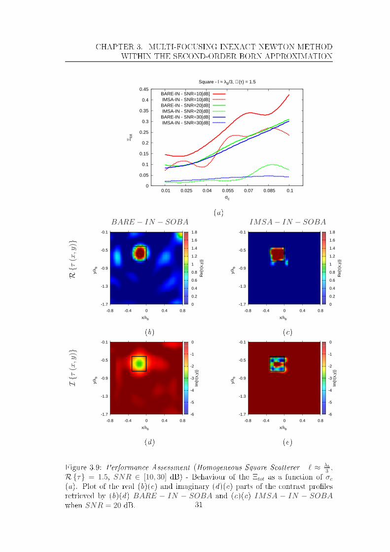
CHAPTER 3. MULTI-FOCUSING INEXACT NEWTON METHOD
WITHIN THE SECOND-ORDER BORN APPROXIMATION
0
0.05
0.1
0.15
0.2
0.25
0.3
0.35
0.4
0.45
0.01 0.025 0.04 0.055 0.07 0.085 0.1
Ξ tot
σc
Square - l ≈ λb/3, ℜ τ = 1.5
BARE-IN - SNR=10[dB]IMSA-IN - SNR=10[dB]
BARE-IN - SNR=20[dB]IMSA-IN - SNR=20[dB]
BARE-IN - SNR=30[dB]IMSA-IN - SNR=30[dB]
(a)
BARE − IN − SOBA IMSA− IN − SOBA
Rτ
(x,y)
-1.7
-1.3
-0.9
-0.5
-0.1
-0.8 -0.4 0 0.4 0.8
y/λ b
x/λb
0
0.2
0.4
0.6
0.8
1
1.2
1.4
1.6
1.8
Re
τ(x,
y)
-1.7
-1.3
-0.9
-0.5
-0.1
-0.8 -0.4 0 0.4 0.8
y/λ b
x/λb
0
0.2
0.4
0.6
0.8
1
1.2
1.4
1.6
1.8
Re
τ(x,
y)
(b) ( )
Iτ
(x,y)
-1.7
-1.3
-0.9
-0.5
-0.1
-0.8 -0.4 0 0.4 0.8
y/λ b
x/λb
-6
-5
-4
-3
-2
-1
0
Imτ
(x,y
)
-1.7
-1.3
-0.9
-0.5
-0.1
-0.8 -0.4 0 0.4 0.8
y/λ b
x/λb
-6
-5
-4
-3
-2
-1
0
Imτ
(x,y
)
(d) (e)
Figure 3.9: Performan e Assessment (Homogeneous Square S atterer - ℓ ≈ λb
3,
Rτ = 1.5, SNR ∈ [10, 30] dB) - Behaviour of the Ξtot as a fun tion of σc(a). Plot of the real (b)( ) and imaginary (d)(e) parts of the ontrast proles
retrieved by (b)(d) BARE − IN − SOBA and ( )(e) IMSA − IN − SOBAwhen SNR = 20 dB.
31

3.5. DISCUSSIONS
3.5 Dis ussions
In this hapter, a new mi rowave imaging method for subsurfa e prospe ting has
been proposed. The approa h ombines a multi-fo using strategy with a regu-
larization solution based on the use of an inexa t-Newton method. In parti ular,
the inverse problem has been addressed by numeri ally solving the Lippmann-
S hwinger equation under the se ond-order Born approximation (SOBA). Theproposed re onstru tion method has been validated through an extended set
of numeri al results involving dierent types of s atterers and noise onditions.
Simulations have highlighted the following key results:
• the proposed te hnique is able to protably ombine the well assessed reg-
ularization apabilities of the adopted lo al sear h te hnique (the inexa t-
Newton method) with the enhan ed exploitation of available information
provided by the multi-fo using strategy, whi h is able to redu e the prob-
lem of lo al minima arising from the non-linearity of the involved set of
equations.
• Moreover, the ombined strategy exhibits advantages over its standard
"bare" implementation in terms of a hieved a ura y and resolution, what-
ever the ontrast distribution (homogeneous/inhomogeneous), the ross-
se tion geometry and the noise level on measured data.
• Furthermore, the proposed multi-fo using approa h over omes the stan-
dard "bare" implementation also in terms of the omputational e ien y,
thanks to the signi ant redu tion of the problem unknowns at ea h itera-
tive step, whi h arises from the use of an adaptive oarse-to-ne dis retiza-
tion of the investigation areas at dierent levels of resolution.
32

Chapter 4
Ele tromagneti Subsurfa e
Prospe ting by a Fully Nonlinear
Multi-fo using Inexa t Newton
Method
In this hapter, an ele tromagneti inverse s attering pro edure for the re on-
stru tion of shallow buried obje ts in a homogeneous half-spa e is proposed. The
approa h is based on the numeri al solution of the integral equations modelling
the inverse s attering relationships and it extends to strong s atterers the imag-
ing apabilities of the approa h presented in Chapter 3 relying on approximated
formulations (i.e., the SOBA). The inversion is based on the synergi appli ationof a multi-fo using strategy based on the iterative multi-s aling approa h (IMSA)
along with an e ient regularization s heme based on the inexa t-Newton (IN )
method. Numeri al results orroborate the mathemati al des ription to assess
apabilities and urrent limitations of the proposed fully-nonlinear te hnique.
33

4.1. INTRODUCTION AND MOTIVATION
4.1 Introdu tion and motivation
Mi rowave methods for retrieving buried obje ts are a key topi of the resear h
area on erned with inversion methods as onrmed by the s ienti literature
[1-[4. Appli ations range from ivil and industrial non-destru tive testing [6-
[9 to medi al imaging [10-[12 as well as geophysi al appli ations [13-[18. As
for these latter, inverse s attering te hniques have been widely proposed for the
shallow investigation of the Earth's subsurfa e to extend/better-exploit the apa-
bilities/features of ground penetrating radars (GPRs) [13-[19. However, despite
several and important results, mi rowave methods are still quite hallenging and
far from a real-life use mainly due to the ill-posedness and the nonlinearity of the
mathemati al relationships that relate the s attered elds to the unknown dis-
tributions of the diele tri parameters of the investigation region. Moreover, the
information ontent available from s attered-eld data is low [70, espe ially when
dealing with aspe t-limited ongurations su h as those in subsurfa e prospe t-
ing, leading to a redu ed data diversity [20. To properly address these issues,
many inversion strategies, both sto hasti [34[36[37[40[42[62[71 and deter-
ministi [26[32[63-[68, have been proposed along with approximate models
(e.g., based on Rytov [48 and [26 Born linearizations).
In a re ent paper, the authors have introdu ed the use of a multi-fo using ap-
proa h asso iated with an inexa t-Newton (IN ) method [48. Indeed, the use of
multi-resolution methods has been found to be an ee tive way to redu e the
number of lo al minima arising in ele tromagneti inverse problems due to the
severe ill-posedness of the integral equations at hand [54[72. On the other hand,
the IN method has proven to be a regularization approa h e ient in several
ele tromagneti appli ations, mainly related to tomography in free-spa e ondi-
tions [44[43. In Chapter 3, the synergi ombination of the two methods has
been exploited in an ee tive approa h for the re onstru tion of buried targets
in a shallow subsurfa e under the se ond-order Born approximation (SOBA) ondition [73 by assuming the s attering eld nonlinearly depending on the di-
ele tri parameters of the obje t under test, but independent on the internal
total ele tri eld. While su h an approximation resulted in a non-negligible
omputational saving be ause of the redu tion of the problem unknowns (i.e.,
the diele tri distribution only), the reliability of the re onstru tion turns out
limited to weak s atterers. Moreover, it is worth pointing out that in pra ti al
appli ations the SOBA extends only partially the range of retrievable diele tri
permittivities ompared to the lassi rst order Born approximation where the
s attered ele tri eld is expressed in terms of the known in ident eld (i.e., the
eld radiated by the sour e in the ba kground without the unknown s atterer).
In this hapter, the integrated multi-fo using-IN (IMSA − IN) strategy is ap-
plied for the rst time to the exa t equations of the inverse s attering problem
for buried obje ts by extending the range of validity of the formulation presented
in Chapter 3 as well as the possibility to retrieve strong s atterers. The outline of
34

CHAPTER 4. ELECTROMAGNETIC SUBSURFACE PROSPECTING BY
A FULLY NONLINEAR MULTI-FOCUSING INEXACT NEWTON
METHOD
the hapter is as follows. In Se t. 4.2, the approa h is mathemati ally des ribed.
Se tion 4.3 reports representative results from several numeri al simulations de-
voted to validate the proposed approa h illustrating its potentials and urrent
limitations. Finally, some on lusions are drawn (Se t. 4.4).
4.2 Mathemati al formulation
Let us onsider the same ylindri al geometry already onsidered in Chapter 3
whose des ription is just summarized here. By assuming transmitting and mea-
surement points arranged in a ross-borehole onguration (Fig. 4.1), let V be
the set of time-harmoni line urrents that generate the in ident elds prob-
ing the investigation region Dinv. For ea h v-th illumination, the longitudinal
omponent of the s attered ele tri eld ve tor is olle ted at M measurements
lo ations (D(v)obs, v = 1, ..., V , being the set of measurement points at the v-th
view).
y/λ b
x/λb
Measurement pointsSource locations
-2.5
-2
-1.5
-1
-0.5
0
0.5
-1.5 -1 -0.5 0 0.5 1 1.5
Dinv
Figure 4.1: Cross-borehole imaging onguration.
To retrieve the unknown diele tri properties of the investigation domain, the
inverse s attering problem mathemati ally des ribed in terms of the following
two integral equations of rst- ( alled state equation) and se ond-kind ( alled
data equation), respe tively [2,
E(v)tot (x, y) = E
(v)inc (x, y) + k2B
∫Dinv
τ (x′, y′)E(v)tot (x
′, y′)Gint (x, y, x′, y′) dx′dy′(x, y) ∈ Dinv
(4.1)
E(v)scatt (x, y) = k2B
∫Dinv
τ (x′, y′)E(v)tot (x
′, y′)Gext (x, y, x′, y′) dx′dy′(x, y) ∈ D(v)
obs
(4.2)
35

4.2. MATHEMATICAL FORMULATION
need to be solved. In (4.1) and (4.2), E(v)tot , E
(v)inc, and E
(v)scatt denote the z-
omponents of the total, in ident, and s attered eld ve tors for the v-th view,
respe tively. Moreover, Gext is the Sommerfeld's Green's fun tion for the half
spa e [55, while the ontrast fun tion τ is dened in equation (2.2).
Unlike the theory presented in Chapter 3, where the SOBA approximated for-
mulation has been assumed, the two s attering equations are ontemporarily
exploited to inspe t buried strong s atterers. Towards this end, let us put (4.1)
and (4.2) in a fun tional form as
A(v)(τ ;E
(v)tot
)= b(v) v = 1, ..., V (4.3)
where b(v) in ludes the known terms (i.e., the in ident eld in the state equation
and the measured s attered ele tri eld in the data equation)
b(v) =
[E
(v)scatt
E(v)inc
], (4.4)
and let us ombine the V equations (4.3) to re ast the inverse problem as the
solution of the following fun tional equation
A(v)(τ ;E
(1)tot , ..., E
(V )tot
)=
E(1)scatt
E(1)inc.
.
.
E(V )scatt
E(V )inc
=
b(1)
.
.
.
b(V )
. (4.5)
By dis retizing (4.5) with square sub-domains and point mat hing, a nonlinear
systems of dis rete equations is yielded
A (τ ;Etot) = b (4.6)
where τ is an array whose n-th entry (n = 1, ..., N) is the value of the ontrast
fun tion at the n-th sub-domain in whi h the investigation domainDinv has been
partitioned, Etot is an array ontaining the V ×N values of the ele tri eld in the
investigation area, and b is an array of size V × (N +M) ontaining the valuesof the known samples of the in ident and s attered ele tri elds (see Appendix
A).
To properly and e iently solve (4.6), some hallenging omputational issues
have to be arefully addressed. To redu e the omputational burden and there-
fore fo using the attention only on parts of the investigation domain where s at-
terers are supposed to be present, the IMSA approa h is adopted. Su h a multi-
fo using te hnique has been rstly developed by A. Massa and o-workers in [54
and su essively deeply analyzed in other papers [48[72[74[75. At ea h step
36

CHAPTER 4. ELECTROMAGNETIC SUBSURFACE PROSPECTING BY
A FULLY NONLINEAR MULTI-FOCUSING INEXACT NEWTON
METHOD
of the IMSA (s = 1, ..., S), a zoomed investigation domain Ωs, omposed by the
ombination of the region of interests dened at step s − 1, is onsidered (Ω1
oin ides with the whole investigation area - see Fig. 4.1). Equation (4.6) is
then solved by using the IN method [44[43 for re onstru ting the distributions
of the diele tri properties in Ωs. Su h an inversion method is omposed by two
nested loops. In the external loop, (4.6) is rst linearized by means of a Newton
approximation, whereas the resulting linear system of equations is solved in a
regularized sense with a trun ated Landweber method [61. A maximum number
of iterations, Imax,s, is set for the external loop, while the number of iterations,
Q, of the inner loop is xed for any re onstru tion pro ess. A omplete dis us-
sion on the appli ation of the IN method an be found in [45 where it has been
shown that the number of external iterations plays the role of a regularization
parameter ontrolling the so- alled semi- onvergen e. Therefore, it is ne essary
to dene a suitable strategy for terminating the iterations in order to guarantee
onvergen e towards the global solution of the fun tional problem at hand. To
this end, let us rst dene the following residual fun tion
Φis =
∑Vv=1
∑Mm=1
∣∣∣E(v)scatt
(x(v)m , y
(v)m
)−E(v)
i
(x(v)m , y
(v)m
)∣∣∣∑V
v=1
∑Mm=1
∣∣∣E(v)scatt
(x(v)m , y
(v)m
)∣∣∣(4.7)
where E(v)scatt
(x(v)m , y
(v)m
)denotes the s attered eld omponent measured at the
m-th measurement point
(x(v)m , y
(v)m
)(m = 1, ...,M) for the v-th illumination
(v = 1, ..., V ), and E(v)i
(x(v)m , y
(v)m
)indi ates the same quantity estimated at the
i-th iteration of the imaging pro ess. Then, at ea h IMSA step, s (s > 1), theIN solver is stopped when one of the following onditions holds true:
• the tness goes below the threshold omputed at the step s (i.e., φis ≤ φth
s );
• the number of outer iterations rea hes its maximum (i.e., Imax,s>1).
As for the threshold at the s-th step, Φths , it is obtained as
Φths ≤ αφfinal
s−1 , s = 2, ..., S (4.8)
where Φfinals−1 is the nal residual at the step s−1, α is a setup s aling fa tor, and
S is the total number of IMSA steps. Con erning the rst IMSA step (s = 1),the stopping riterion is only determined by the user-dened number of outer
iterations (i.e., Imax,s=1).
4.3 Numeri al Results
The proposed approa h has been validated by means of several numeri al sim-
ulations referring to the following ben hmark s enario. The investigation area
37

4.3. NUMERICAL RESULTS
has been hosen as a square domain of side 1.6 λb entered at (0.0, −0.9 λb) withthe diele tri properties of the lower half spa e set to εrB = 4.0 and σB = 0.01S/m. A set of V = 16 TX/RX antennas, modeled as line- urrent sour es with
unit amplitude, has been onsidered at a working frequen y of 300 MHz. The
antennas have been supposed to be lo ated into two boreholes beside Dinv (as
shown in Fig. 4.1) at positions
(xv, yv) =
(−λb, −0.1 λb − 2 λb
v−1v2−1
)if v ≤ V
2(−λb, −0.1 λb − 2 λb
v−− v2−1
v2−1
)if v > V
2
, v = 1, ..., V. (4.9)
When a radiator a ted as transmitter, the remaining M = V − 1 olle ted the
s attered ele tri eld. The number of views and measurement points has been
hosen as suggested in [57[58.
The s attering eld samples (i.e., the data of the inversion pro edure) have been
numeri ally omputed by using a forward solver based on the Method of Moments
[76 with a mesh of Nfwd = 40 × 40 square subdomains. To simulate a more
realisti measurement setup, a Gaussian noise with zero mean value has been
added to the omputed data. Unless otherwise spe ied, the signal-to-noise ratio
on the total ele tri eld data has been set to SNR = 20 dB. As for the inversionpro edure, a oarser mesh has been used to avoid inverse rimes. More in detail,
N IMSAinv = 10×10 subdomains have been adopted at ea h s-th s aling step of the
IMSA, whereas the number of partitions has been set to N bareinv = 20 × 20 pixels
for the bare IN approa h.
To quantitatively evaluate the performan e of the approa h, the same error g-
ures used in Chapter 3 have been adopted and are here reported, for ompleteness
Ξreg =1
Nreg
Nreg∑
n=1
|τ (xn, yn)− τ(xn, yn)||τ(xn, yn) + 1| reg = tot, ext, int (4.10)
where τ and τ are the a tual and re onstru ted values of the ontrast fun tion in
the n-th sub-domain
1
and Nreg indi ates the number of ells overing the whole
inspe ted area Dinv (reg = tot, Ntot = N), or belonging to the ba kground
region (reg = ext), or to the support of the buried s atterer (reg = int; Ntot =Next +Nint).
1
The re onstru tions have been obtained by averaging the results over 100 dierent noise
realizations.
38

CHAPTER 4. ELECTROMAGNETIC SUBSURFACE PROSPECTING BY
A FULLY NONLINEAR MULTI-FOCUSING INEXACT NEWTON
METHOD
4.3.1 Calibration
-1.7
-1.3
-0.9
-0.5
-0.1
-0.8 -0.4 0 0.4 0.8
y/λ b
x/λb
0
0.3
0.6
0.9
1.2
1.5
1.8
Re
τ(x,
y)
Figure 4.2: Calibration (Square S atterer - L = 0.32 λb, (xc = −0.16 λb, yc =−0.58 λb), εr = 5.5, σ = 0.01 S/m [τ = 1.5, εrB =4.0, σB =0.01 S/m, SNR = 20dB) - A tual target used for the algorithm alibration.
As already stated in Chapter 3, the hoi e of the orre t parameters of the in-
version pro edure is of fundamental importan e, thus an analysis of the per-
forman es versus su h parameters has been rstly performed to identify the
best setup. The goal of this alibration has been that of determining the op-
timal (Q,α) pair for the IMSA-IN approa h, while the other parameters have
been set a ording to the guidelines already devised in previous works [43[69,
namely Imax,s=1 = 20, Imax,s>1 = 1000, and S = 4. More in detail, Q and
the tness s aling fa tor α have been varied within the range 10 − 100 and be-
tween 0.1 and 0.9, respe tively. As a referen e target, a square ylinder lo ated
at (−0.16 λb, −0.58 λb) with side L = 0.32 λb, relative diele tri permittivity
εr = 5.5, and ele tri ondu tivity σ = 0.01 S/m (i.e., τ = 1.5) has been onsid-
ered (Fig. 4.2).
39

4.3. NUMERICAL RESULTS
10-3
10-2
10-1
0 0.1 0.2 0.3 0.4 0.5 0.6 0.7 0.8 0.9 1
Rec
onst
ruct
ion
Err
or, Ξ
tot
Fitness Scaling Factor, α
Q=10Q=30Q=50Q=70Q=90
Q=100
Figure 4.3: Calibration (Square S atterer - L = 0.32 λb, (xc = −0.16 λb, yc =−0.58 λb), εr = 5.5, σ = 0.01 S/m [τ = 1.5, εrB =4.0, σB =0.01 S/m, SNR = 20dB) - Total re onstru tion error vs. α (α ∈ [0.1, 0.9]) for dierent values of Q in
the range Q ∈ [10, 100].
0
0.005
0.01
0.015
0.02
0 0.1 0.2 0.3 0.4 0.5 0.6 0.7 0.8 0.9 1
Fitn
ess,
φ
Fitness Scaling Factor, α
Q=10Q=30Q=50Q=70Q=90
Q=100
Figure 4.4: Calibration (Square S atterer - L = 0.32 λb, (xc = −0.16 λb, yc =−0.58 λb), εr = 5.5, σ = 0.01 S/m [τ = 1.5, εrB =4.0, σB =0.01 S/m, SNR = 20dB) - Best tness value for dierent (Q,α) pairs.
40

CHAPTER 4. ELECTROMAGNETIC SUBSURFACE PROSPECTING BY
A FULLY NONLINEAR MULTI-FOCUSING INEXACT NEWTON
METHOD
-1.7
-1.3
-0.9
-0.5
-0.1
-0.8 -0.4 0 0.4 0.8
y/λ b
x/λb
0
0.3
0.6
0.9
1.2
1.5
1.8
Re
τ(x,
y)
(a)
-1.7
-1.3
-0.9
-0.5
-0.1
-0.8 -0.4 0 0.4 0.8
y/λ b
x/λb
-0.5
-0.25
0
0.25
0.5
Imτ
(x,y
)
(b)
Figure 4.5: Calibration (Square S atterer - L = 0.32 λb, (xc = −0.16 λb, yc =−0.58 λb), εr = 5.5, σ = 0.01 S/m [τ = 1.5, εrB =4.0, σB =0.01 S/m, SNR = 20dB) - (a) Real and (b) imaginary parts of the re onstru ted distribution of the
ontrast fun tion when Q = Qopt = 50 and α = αopt = 0.9.
The results of the IMSA-IN re onstru tions are summarized in Fig. 4.3, whi h
reports the values of the total error Ξtot versus the tness s aling fa tor and
for dierent values of the inner iterations of the IN algorithm when setting
Imax,s=1 = 20 and S = 4, being SNR = 20 dB. Sin e the best pair of parameters
is dened as that with the minimum value of the total re onstru tion error Ξtot,
41

4.3. NUMERICAL RESULTS
the optimal setup turned out to be: Q = 50 and α = 0.9. For ompleteness,
Figure 4.4 reports the values of the residual Φ on the data, while Figure 4.5 shows
the distribution of the ontrast fun tion [real part - Fig. 4.5(a); imaginary part
- Fig. 4.5(b) re onstru ted with the optimal parameters.
As it an be observed, the s atterer is faithfully re onstru ted with a areful
identi ation of the target shape as well as an estimation of the ontrast very
lose to the a tual one.
0
1
2
3
4
5
6
7
-1 -0.5 0 0.5 1
Tot
al R
econ
stru
ctio
n E
rror
, Ξto
t (×1
0-2)
∆εb,r
SNR=20 [dB]
Figure 4.6: Calibration (Square S atterer - L = 0.32 λb, (xc = −0.16 λb, yc =−0.58 λb), εr = 5.5, σ = 0.01 S/m [τ = 1.5, εrB =4.0, σB =0.01 S/m, SNR = 20dB) - Re onstru tion errors for dierent values of ∆εrB.
To assess the robustness of the optimal alibration setup against the un ertain-
ties in the medium ele tromagneti parameters, the same target has been imaged
by assuming that the relative diele tri permittivity εrB used by the inversion
method is dierent from its a tual value εrB. The behaviour of the total re on-stru tion error versus ∆εrB , εrB− εrB shows that the a ura y of the proposed
approa h smoothly degrades as the un ertainty in reases (e.g.,
Ξtot|∆εrB=0.8
Ξtot|∆εrB=0.2≈ 2.83
- Fig. 4.6), and that the total error is below 7% even in the worst ase onditions
(i.e., when ∆εrB ≈ −1.0 - Fig. 4.6).
4.3.2 Ee ts of Noise
To evaluate the ee t of the noise on the re onstru tions and the robustness of
the proposed approa h, a set of simulations with levels of noise varying from
SNR = 5 dB down to ∞ has been performed.
42

CHAPTER 4. ELECTROMAGNETIC SUBSURFACE PROSPECTING BY
A FULLY NONLINEAR MULTI-FOCUSING INEXACT NEWTON
METHOD
SNR Itot Φfinal Ξtot Ξint Ξext ∆t [s
BARE∞ (Noiseless) 600 1.28× 10⁻³ 9.46× 10⁻² 2.17× 10⁻¹ 6.94× 10⁻² 4041
30 [dB 600 1.80× 10⁻³ 9.44× 10⁻² 2.17× 10⁻¹ 7.04× 10⁻² 404520 [dB 600 4.07× 10⁻³ 9.83× 10⁻² 2.21× 10⁻¹ 7.25× 10⁻² 404210 [dB 600 1.25× 10⁻² 1.35× 10⁻¹ 2.17× 10⁻¹ 1.00× 10⁻¹ 40385 [dB 600 2.20× 10⁻² 1.91× 10⁻¹ 2.31× 10⁻¹ 1.37× 10⁻¹ 4023
IMSA∞ (Noiseless) 450 4.45× 10⁻³ 5.61× 10⁻³ 1.36× 10⁻¹ 0.00 211
30 [dB 461 4.53× 10⁻³ 5.60× 10⁻³ 1.36× 10⁻¹ 0.00 21220 [dB 827 5.39× 10⁻³ 2.89× 10⁻³ 6.87× 10⁻² 0.00 28810 [dB 3020 1.41× 10⁻² 5.21× 10⁻³ 1.17× 10⁻¹ 0.00 7955 [dB 3020 2.43× 10⁻² 1.46× 10⁻² 1.97× 10⁻¹ 5.96× 10⁻³ 776
Table 4.1: Performan e vs. Noise (Square S atterer - L = 0.32 λb, (xc =−0.16 λb, yc = −0.58 λb), εr = 5.5, σ = 0.01 S/m [τ = 1.5, εrB =4.0, σB =0.01S/m) - Total number of performed outer iterations, nal tness values, and re-
onstru tion errors for the BARE and the IMSA (s = S = 4) IN approa hes.
Total exe ution time on a PC with Intel(R) Core(TM)2 CPU 6600 2.40GHz,
2GB RAM.
Still onsidering the same target of the previous Se tion, the inversion results
are summarized in Tab. 4.1 where the total number of outer iterations needed
to rea h the onvergen e
2
, the nal residual on the data Φfinal, and the re on-
stru tion errors Ξreg are given along with the inversion time
3
. For omparison
purposes, the out omes from the appli ation of the bare IN approa h (i.e., the
single-step uniform resolution IN ) is also reported. It is worth noti ing that for
a fair omparison, the alibration of the ontrol parameters has been arried out
for the bare algorithm, as well, with the identi ation of the following optimal
values: Imax = 600 and Q = 100.
As it an noti ed (Tab. 4.1), the IMSA-IN approa h proves to be quite robust
to the noise on the data sin e, even for heavy noise onditions, the arising er-
rors turns out to be quite small and the multi-resolution implementation always
outperforms its orresponding single-step uniform resolution ounterpart. These
indi ations are also onrmed by the re onstru ted distributions of the ontrast
fun tion (real part - Fig. 4.7; imaginary part - Fig. 4.8).
2
As for the IMSA, this number orresponds to the sum of the outer iterations performed
on the whole set of iterative s aling steps.
3
The IMSA inversion time is omputed as the sum of the exe ution time for ea h iterative
s aling step.
43

4.3. NUMERICAL RESULTS
IN IN − SOBA
IMSA
-1.7
-1.3
-0.9
-0.5
-0.1
-0.8 -0.4 0 0.4 0.8
y/λ b
x/λb
0
0.3
0.6
0.9
1.2
1.5
1.8
Re
τ(x,
y)
-1.7
-1.3
-0.9
-0.5
-0.1
-0.8 -0.4 0 0.4 0.8
y/λ b
x/λb
0
0.3
0.6
0.9
1.2
1.5
1.8
Re
τ(x,
y)
(a) ( )
BARE
-1.7
-1.3
-0.9
-0.5
-0.1
-0.8 -0.4 0 0.4 0.8
y/λ b
x/λb
0
0.3
0.6
0.9
1.2
1.5
1.8
Re
τ(x,
y)
-1.7
-1.3
-0.9
-0.5
-0.1
-0.8 -0.4 0 0.4 0.8
y/λ b
x/λb
0
0.3
0.6
0.9
1.2
1.5
1.8
Re
τ(x,
y)
(b) (d)
Figure 4.7: Performan e vs. Noise (Square S atterer - L = 0.32 λb, (xc =−0.16 λb, yc = −0.58 λb), εr = 5.5, σ = 0.01 S/m [τ = 1.5, εrB =4.0, σB =0.01S/m, SNR =10 dB) - Re onstru ted distributions of the ontrast fun tion (real
part) when using (a)( ) IMSA-IN and (b)(d) IN under (a)(b) full-nonlinear and
( )(d) approximate onditions (SOBA).
As a representative example, let us refer to the plots in Fig. 4.7 on erned with
the inversion of s attering data blurred with a noise hara terized by SNR = 10dB. In parti ular, Figures 4.7(a) and 4.8(a) show the result yielded with the
IMSA-IN algorithm, while Figures 4.7(b) and 4.8(b) plot the re onstru tion from
the bare approa h. Figures 4.7( )-4.7(d) and 4.8( )-4.8(d) omplete the overview
by presenting the results under se ond order Born approximation (i.e., SOBA
method). As expe ted, the IMSA-IN better shapes the target and the estimated
values of the ontrast fun tion are loser to the a tual ones. On the other hand,
the full-approa h signi antly improves the performan e of the approximated
one in both IMSA [Fig. 4.7(a) vs. Fig. 4.7( ) - ΞIMSA−INtot = 5.21 × 10⁻³
vs. ΞIMSA−SOBAtot = 1.83 × 10⁻²
and single-step [Fig. 4.7(b) vs. Fig. 4.7(d) -
ΞINtot = 1.35× 10⁻¹
vs. ΞSOBAtot = 1.46× 10⁻¹
versions.
44

CHAPTER 4. ELECTROMAGNETIC SUBSURFACE PROSPECTING BY
A FULLY NONLINEAR MULTI-FOCUSING INEXACT NEWTON
METHOD
IN IN − SOBA
IMSA
-1.7
-1.3
-0.9
-0.5
-0.1
-0.8 -0.4 0 0.4 0.8
y/λ b
x/λb
-0.5
-0.25
0
0.25
0.5
Imτ
(x,y
)
-1.7
-1.3
-0.9
-0.5
-0.1
-0.8 -0.4 0 0.4 0.8
y/λ b
x/λb
-0.5
-0.25
0
0.25
0.5
Imτ
(x,y
)
(a) ( )
BARE
-1.7
-1.3
-0.9
-0.5
-0.1
-0.8 -0.4 0 0.4 0.8
y/λ b
x/λb
-0.5
-0.25
0
0.25
0.5
Imτ
(x,y
)
-1.7
-1.3
-0.9
-0.5
-0.1
-0.8 -0.4 0 0.4 0.8
y/λ b
x/λb
-0.5
-0.25
0
0.25
0.5
Imτ
(x,y
)
(b) (d)
Figure 4.8: Performan e vs. Noise (Square S atterer - L = 0.32 λb, (xc =−0.16 λb, yc = −0.58 λb), εr = 5.5, σ = 0.01 S/m [τ = 1.5, εrB =4.0,σB =0.01 S/m, SNR =10 dB) - Re onstru ted distributions of the ontrast
fun tion (imaginary part) when using (a)( ) IMSA-IN and (b)(d) IN under
(a)(b) full-nonlinear and ( )(d) approximate onditions (SOBA).
For ompleteness, Figures 4.9(a)-4.9(b) show the residual on the data and the
re onstru tion errors versus the outer iteration number, while the behavior of the
re onstru tion errors at ea h resolution step of the s aling pro ess is reported in
Fig. 4.9( ). As it an be observed, the multi-resolution pro edure allows a
signi ant improvement of the re onstru tion quality throughout the iterative
zooming.
45

4.3. NUMERICAL RESULTS
10-3
10-2
10-1
100
1 21 1021 3021
Φ
Iteration Index, i
2021
(a)
10-3
10-2
10-1
100
1 21 1021 3021
Rec
onst
ruct
ion
Err
ors
Iteration Index, i
2021
Ξtot Ξint Ξext
(b)
10-3
10-2
10-1
100
1 2 3 4
Rec
onst
ruct
ion
Err
ors
IMSA Step, s
Ξtot Ξint Ξext
( )
Figure 4.9: Performan e vs. Noise (Square S atterer - L = 0.32 λb, (xc =−0.16 λb, yc = −0.58 λb), εr = 5.5, σ = 0.01 S/m [τ = 1.5, εrB =4.0, σB =0.01S/m, SNR = 10 dB) - Fitness (a) and re onstru tion errors (b) versus outer
iterations index, i. ( ) Error index values at ea h fo using step s (s = 1, ..., S).
46

CHAPTER 4. ELECTROMAGNETIC SUBSURFACE PROSPECTING BY
A FULLY NONLINEAR MULTI-FOCUSING INEXACT NEWTON
METHOD
Finally, it is worth pointing out that the IMSA-IN approa h requires less CPU
time than the bare method to rea h the onvergen e solution (Tab. 4.1) sin e a
smaller problem has to be solved at ea h resolution step.
4.3.3 Ee ts of the Diele tri Properties of the Target
This Se tion is aimed at giving some insights on the dependen e of the re on-
stru tion a ura y of the proposed approa h on the ontrast values of the imaged
target.
10-5
10-4
10-3
10-2
10-1
100
0.2 0.6 1 1.4 1.8 2.2
Rec
onst
ruct
ion
Err
ors
Reτ(x,y)
SNR=20 [dB]
Ξtot - BARE-IN
Ξint - BARE-IN
Ξext - BARE-IN
Ξtot - IMSA-IN
Ξint - IMSA-IN
Ξext - IMSA-IN
Figure 4.10: Performan e vs. Target Permittivity (Hollow Cylinder - Lext =0.48 λb, Lint = 0.16 λb, (xc = 0.08 λb, yc = −0.48 λb), σ = 0.01 S/m, εrB =4.0,σB =0.01 S/m, SNR = 20 dB) - Re onstru tion errors for dierent values of τ .
A hollow square ylinder has been onsidered [Fig. 4.11(a) entered at
(0.08 λb, −0.48 λb) with external side Lext = 0.48 λb and internal side Lint =0.16 λb. The values of the ontrast have been hanged in the range τ ∈ [0.2, 2.2].Figure 4.10 gives the inversion results in terms of the total re onstru tion error
for both the bare and the IMSA-IN approa hes. It turns out that the two
implementations are quite robust against the ontrast even though the IMSA-
IN is able to provide a smaller value of re onstru tion error. For illustrative
purposes, Figs. 4.11(b) and 4.11( ) show the real part of the ontrast fun tion
retrieved by the IMSA-IN and the bare approa hes when τ = 2.2, while Figs.
4.11(d) and 4.11(e) show the imaginary parts. The plots outline the ee tiveness
of the multi-resolution approa h in both qualitatively and quantitatively imaging
the target, while the single-step te hnique only lo alizes the target.
47

4.3. NUMERICAL RESULTS
-1.7
-1.3
-0.9
-0.5
-0.1
-0.8 -0.4 0 0.4 0.8
y/λ b
x/λb
0
0.4
0.8
1.2
1.6
2
2.4
Re
τ(x,
y)
(a)
Rτ (x, y) I τ (x, y)
IMSA−IN
-1.7
-1.3
-0.9
-0.5
-0.1
-0.8 -0.4 0 0.4 0.8
y/λ b
x/λb
0
0.4
0.8
1.2
1.6
2
2.4
Re
τ(x,
y)
-1.7
-1.3
-0.9
-0.5
-0.1
-0.8 -0.4 0 0.4 0.8
y/λ b
x/λb
-0.5
-0.25
0
0.25
0.5
Imτ
(x,y
)
(b) (d)
BARE−IN
-1.7
-1.3
-0.9
-0.5
-0.1
-0.8 -0.4 0 0.4 0.8
y/λ b
x/λb
0
0.4
0.8
1.2
1.6
2
2.4
Re
τ(x,
y)
-1.7
-1.3
-0.9
-0.5
-0.1
-0.8 -0.4 0 0.4 0.8
y/λ b
x/λb
-0.5
-0.25
0
0.25
0.5
Imτ
(x,y
)
( ) (e)
Figure 4.11: Performan e vs. Target Permittivity (Hollow Cylinder - Lext =0.48 λb, Lint = 0.16 λb, (xc = 0.08 λb, yc = −0.48 λb), εr = 6.2, σ = 0.01 S/m
[τ = 2.2, εrB =4.0, σB =0.01 S/m, SNR = 10 dB) - Re onstru ted distribution
of the ontrast fun tion. (a) A tual onguration and (b) real and (d) imaginary
parts provided by the IMSA-IN strategy and ( ) real and (e) imaginary parts
obtained by the BARE-IN.
48

CHAPTER 4. ELECTROMAGNETIC SUBSURFACE PROSPECTING BY
A FULLY NONLINEAR MULTI-FOCUSING INEXACT NEWTON
METHOD
-1.7
-1.3
-0.9
-0.5
-0.1
-0.8 -0.4 0 0.4 0.8
y/λ b
x/λb
0
0.2
0.4
0.6
0.8
1
1.2
1.4
1.6
1.8
Re
τ(x,
y)
(a)
IN IN − SOBA
IMSA
-1.7
-1.3
-0.9
-0.5
-0.1
-0.8 -0.4 0 0.4 0.8
y/λ b
x/λb
0
0.2
0.4
0.6
0.8
1
1.2
1.4
1.6
1.8
Re
τ(x,
y)
-1.7
-1.3
-0.9
-0.5
-0.1
-0.8 -0.4 0 0.4 0.8
y/λ b
x/λb
0
0.2
0.4
0.6
0.8
1
1.2
1.4
1.6
1.8
Re
τ(x,
y)
(b) (d)
BARE
-1.7
-1.3
-0.9
-0.5
-0.1
-0.8 -0.4 0 0.4 0.8
y/λ b
x/λb
0
0.2
0.4
0.6
0.8
1
1.2
1.4
1.6
1.8
Re
τ(x,
y)
-1.7
-1.3
-0.9
-0.5
-0.1
-0.8 -0.4 0 0.4 0.8
y/λ b
x/λb
0
0.2
0.4
0.6
0.8
1
1.2
1.4
1.6
1.8
Re
τ(x,
y)
( ) (e)
Figure 4.12: Performan e vs. Target S ales (E-Shaped S atterer - εr = 5.5,σ = 0.01 S/m [τ = 1.5, εrB =4.0, σB =0.01 S/m, SNR =20 dB) - Re onstru teddistribution of the ontrast fun tion (real part). (a) A tual onguration and
re onstru tions with (b)(d) IMSA-IN and ( )(e) IN under (b)( ) full-nonlinear
and (d)(e) approximate onditions (SOBA).
49

4.3. NUMERICAL RESULTS
4.3.4 Re onstru tion of Targets with Small Details
The apabilities of the approa h in re onstru ting target details at dimensions
omparable to the inversion grid of the bare te hnique have been assessed then
by onsidering the obje t in Fig. 4.12(a). The ontrast fun tion retrieved by the
IMSA-IN algorithm is shown in Fig. 4.12(b) and Fig. 4.13(a) and ompared to
that from the IN method [Fig. 4.12( ) and Fig. 4.13(b).
IN IN − SOBA
IMSA
-1.7
-1.3
-0.9
-0.5
-0.1
-0.8 -0.4 0 0.4 0.8
y/λ b
x/λb
-0.5
-0.25
0
0.25
0.5
Imτ
(x,y
)
-1.7
-1.3
-0.9
-0.5
-0.1
-0.8 -0.4 0 0.4 0.8
y/λ b
x/λb
-0.5
-0.25
0
0.25
0.5
Imτ
(x,y
)
(a) ( )
BARE
-1.7
-1.3
-0.9
-0.5
-0.1
-0.8 -0.4 0 0.4 0.8
y/λ b
x/λb
-0.5
-0.25
0
0.25
0.5
Imτ
(x,y
)
-1.7
-1.3
-0.9
-0.5
-0.1
-0.8 -0.4 0 0.4 0.8
y/λ b
x/λb
-0.5
-0.25
0
0.25
0.5
Imτ
(x,y
)
(b) (d)
Figure 4.13: Performan e vs. Target S ales (E-Shaped S atterer - εr = 5.5,σ = 0.01 S/m [τ = 1.5, εrB =4.0, σB =0.01 S/m, SNR =20 dB) - Re on-
stru ted distribution of the ontrast fun tion (imaginary part) with (a)( ) IMSA-
IN and (b)(d) IN under (a)(b) full-nonlinear and ( )(d) approximate onditions
(SOBA).
As expe ted, the multi-s aling strategy provides a quite good re onstru tion
of the long arms of the E-shaped target be ause of its intrinsi multi-resolution
nature, although the smallest detail in the internal region is not dete ted probably
due to the masking ee ts of the external region of the s atterer. On the ontrary,
50

CHAPTER 4. ELECTROMAGNETIC SUBSURFACE PROSPECTING BY
A FULLY NONLINEAR MULTI-FOCUSING INEXACT NEWTON
METHOD
the single-step re onstru tion signi antly gets worse loosing all the obje t details
[Fig. 4.12( ) and Fig. 4.13(b). For ompleteness, the orresponding SOBA
implementations are reported in Figs. 4.12(d)-4.12(e) and Figs. 4.13( )-4.13(d),
as well.
4.3.5 Re onstru tion of Targets with Higher Condu tivity
Finally, the ee ts of the ondu tivity of the target have been evaluated. The
square obje t imaged in Se ts. 4.3.1 and 4.3.2 has been again onsidered, but its
ele tri ondu tivity has been in reased to σ = 0.1 (i.e., I τ = −5.39).
Rτ (x, y) I τ (x, y)
IMSA−IN
-1.7
-1.3
-0.9
-0.5
-0.1
-0.8 -0.4 0 0.4 0.8
y/λ b
x/λb
0
0.2
0.4
0.6
0.8
1
1.2
1.4
1.6
1.8
Re
τ(x,
y)
-1.7
-1.3
-0.9
-0.5
-0.1
-0.8 -0.4 0 0.4 0.8
y/λ b
x/λb
-6
-5
-4
-3
-2
-1
0
Imτ
(x,y
)
(a) (b)
BARE−IN
-1.7
-1.3
-0.9
-0.5
-0.1
-0.8 -0.4 0 0.4 0.8
y/λ b
x/λb
0
0.2
0.4
0.6
0.8
1
1.2
1.4
1.6
1.8
Re
τ(x,
y)
-1.7
-1.3
-0.9
-0.5
-0.1
-0.8 -0.4 0 0.4 0.8
y/λ b
x/λb
-6
-5
-4
-3
-2
-1
0Im
τ(x
,y)
( ) (d)
Figure 4.14: Performan e vs. Target Condu tivity (Square S atterer - L =0.32 λb, (xc = −0.16 λb, yc = −0.58 λb), εr = 5.5, σ = 0.1 S/m [τ = 1.5− j5.39,εrB =4.0, σB =0.01 S/m, SNR =10 dB) - Re onstru ted distribution of the
ontrast fun tion. (a) Real and (b) imaginary parts provided by the IMSA-IN
strategy and ( ) real and (d) imaginary parts obtained with the bare IN.
51

4.4. DISCUSSIONS
SNR Ξtot BARE Ξtot IMSA
∞ (Noiseless) 3.07× 10⁻¹ 4.01× 10⁻²
30 [dB 3.07× 10⁻¹ 3.98× 10⁻²
20 [dB 3.14× 10⁻¹ 1.61× 10⁻²
10 [dB 3.60× 10⁻¹ 2.26× 10⁻²
5 [dB 4.21× 10⁻¹ 3.97× 10⁻²
Table 4.2: Performan e vs. Target Condu tivity (Square S atterer - L = 0.32 λb,(xc = −0.16 λb, yc = −0.58 λb), εr = 5.5, σ = 0.1 S/m [τ = 1.5−j5.39, εrB =4.0,σB =0.01 S/m) - Re onstru tion errors for the bare IN and the IMSA-IN (at
step s = S = 4) approa hes.
The re onstru tion errors for dierent values of the signal-to-noise ratio are re-
ported in Tab. 4.2 to assess in this ase, too, the IMSA-IN strategy improve-
ments over to the bare method. This is also visually onrmed by the representa-
tive distributions of the ontrast fun tion shown in Fig. 4.14, whi h refer to the
ase SNR = 10 dB. Indeed, both real and imaginary parts of the ontrast fun -
tion are su essfully retrieved by the IMSA-IN strategy [Figs. 4.14(a)-4.14(b)
being loser to the a tual ones. The same a ura y is not a hieved by the bare
implementation [Figs. 4.14( )-4.14(d).
4.4 Dis ussions
In this hapter, a mi rowave imaging te hnique for the re onstru tion of shallow
buried obje ts has been presented. The proposed approa h extends the strat-
egy presented in Chapter 3 by employing the full non-linear formulation of the
s attering problem. In this way, the method is potentially able to deal with
strong s atterers, too. The re onstru tion performan es have been evaluated by
means of several numeri al simulations. It has been found that the proposed
approa h provides quite good re onstru tions of the onsidered targets showing
a good robustness to the noise, as well. Moreover, the results from the multi-
fo using strategy turned out to be better both in terms of re onstru tion errors
and omputational resour es than the standard bare inexa t-Newton algorithm
when applied to the same s attering ongurations. Future works will be devoted
to an experimental validation of the proposed inversion algorithm.
52

Chapter 5
GPR Prospe ting through an
Inverse S attering
Frequen y-Hopping Multi-Fo using
Approa h
In this hapter, an innovative information-a quisition approa h to 2D Ground-
Penetrating Radar (GPR) prospe ting is presented. A mi rowave inverse-s attering
nested approa h ombining a frequen y-hopping (FH ) pro edure and a multi-
fo using (MF ) te hnique is proposed. On the one hand, the FH s heme ef-
fe tively handles multi-frequen y GPR data, while mitigating the non-linearity
issues. On the other, MF te hniques have proved to be ee tive tools for re-
du ing the o urren e of multi-lo al-minima ae ting GPR investigations then
allowing the use of a lo al sear h te hnique based on the Conjugate Gradient
(CG) method to iteratively solve the inverse problem at hand. Sele ted results
are reported and analyzed to give some insights to the interested readers on the
advantages and the limitations of su h an approa h when handling syntheti ally-
generated and experimental GPR data, as well.
53

5.1. INTRODUCTION AND RATIONALE
5.1 Introdu tion and Rationale
In the last de ades, ground penetrating radars (GPRs) have been widely used
in subsurfa e non-destru tive testing (NDT ) problems [1[13[77[78 arising in
ar haeology, geology, demining, pavement survey, tunnel dete tion, and poli e
investigation [59[79-[83. Su h a popularity mainly derives from the superior
performan e in terms of resolution, depth of investigation, speed, and osts om-
pared to other NDT te hnologies [59[79[80[83. Unfortunately, retrieving the
diele tri properties of buried obje t from GPR data, usually olle ted in the
time domain, is a very hallenging task be ause of the theoreti al properties of
the asso iated inverse problems (i.e., ill posedness and non-linearity [84[85) as
well as the dimensionality of the problem at hand [86. To fa e su h hallenges,
several GPR prospe ting algorithms have been proposed in the state-of-the-art
literature. Approximate formulations of the omplete non-linear problem have
been often taken into a ount [84[86-[88. More spe i ally, weak s atterers
have been su essfully retrieved through Born [84[86[88[89 or distorted-Born
GPR approximations [87 by solving the arising linear problem with trun ated
singular value de omposition (TSVD) algorithms [84[86-[88. Nevertheless, the
derivation of GPR prospe ting te hniques able to faithfully handle strong and/or
extended s atterers and deal with related multi-minima issues is still an open
hallenge [83. Indeed, even though global sear h strategies based on Evolution-
ary Algorithms (EAs) ould, in prin iple, su essfully address nonlinear problems
[34[41, their bare use is generally prevented in subsurfa e imaging be ause of
the size of the domains under investigations and the arising onvergen e and
omputational loads.
On the other hand, the generalization of multi-fo using (MF ) inversion te h-
niques borrowed from free-spa e imaging [54[72[75 is a potentially appealing
approa h to be adopted sin e GPR time-domain signals are intrinsi ally multi-
frequen y data. Histori ally,MF iterative strategies have been spe i ally intro-
du ed to mitigate lo al minima problems in inverse s attering [51[54[72. By
keeping at ea h MF iteration the number of unknowns as lose as possible to the
available data information [90, the original omplex imaging problem is re ast
to a sequen e of simpler data-mismat hing ost fun tion minimizations where
the o urren e of lo al minima is strongly redu ed [54[72. This latter enables
as an interesting by-produ t the possibility to use lo al optimization strategies
that allow a signi ant omputational saving with respe t to EAs [34[41.
This hapter is then aimed at introdu ing a robust and e ient omplement
to existing GPR prospe ting strategies based on the multi-minima mitigation
apabilities of MF pro edures. Towards this end, subsurfa e imaging from
time-domain GPR data is rstly re ast to a multi-frequen y inversion then a
frequen y-hopping (FH ) [91-[93 iterative s heme is adopted. Sin e ea h GPR
frequen y data is asso iated to a dierent level of spatial resolution [92, the FH
approa h is suitably integrated in a hierar hi al multi-resolution s heme that ex-
54

CHAPTER 5. GPR PROSPECTING THROUGH AN INVERSE
SCATTERING FREQUENCY-HOPPING MULTI-FOCUSING APPROACH
ploits a Conjugate Gradient (CG) [30[94 lo al strategy as optimization solver.
The outline of the hapter is as follows. After the formulation of the GPR
prospe ting problem (Se t. 5.2), the proposed FHMF-CG method is introdu ed
and dis ussed (Se t. 5.3). It is then assessed against syntheti data generated
through GprMax software [95 and omparisons with state-of-the-art te hniques
[87[96 are also dis ussed, while experimental validations [97 follow (Se t. 5.4).
Eventually, some on lusions are reported (Se t. 5.5).
5.2 GPR Prospe ting - Inverse S attering For-
mulation
Let us onsider the GPR transverse-magneti problem sket hed in Fig. 5.1(a)
where two homogeneous, isotropi , and non-magneti half-spa es are separated
by an interfa e at y = 0. The lower half spa e of ba kground relative permittivity
εrB and ba kground ondu tivity σB, ontains a set of s atterers lo ated within
the investigation domain Dinv [Fig. 5.1(a) and des ribed by dis ontinuous (wrt
the ba kground) proles of permittivity εr (r) and ondu tivity σ (r). The free-spa e (ε0 and σ0 = 0) upper half spa e omprises a set of V z-dire ted ideal
line sour es lo ated at rv = (xv, yv > 0), v = 1, .., V and ex ited with the time-
domain urrent χ (t) [Fig. 5.1(b) to generate in free spa e the radiated eld
[98[99
wv (r, t) z =
[1
2π |r− rv| c0δ
(t− |r− rv|
c0
)∗ h (r− rv, t) ∗
∂χ (t)
∂t
]z (5.1)
where t stands for the time variable, ∗ is the onvolution operator, c0 is the free-spa e speed of light, δ (·) the Dira 's delta, and h (r, t) is the transient responseof the antenna sour e lo ated in r [99.
From the intera tions between the V line sour es and the lower half spa e (i.e.,
the ba kground and the s atterers) the signal (i.e., the GPR radargram) olle ted
by the M ideal probes lo ated in the upper half-spa e at rm = (xm, ym > 0),m = 1, ...,M , [Fig. 5.1(d) is given by
uv (rm, t) = uv (rm, t) + qv (rm, t) = ev (rm, t) + sv (rm, t) + qv (rm, t)m = 1, ...,M ; v = 1, ..., V
(5.2)
where sv is the s attered ele tri eld, qv is a zero-mean additive Gaussian noise
term modelling the measurement/environment noise, and ev is the in ident (i.e.,the ele tromagneti eld of the same s enario but without the s atterers) ele tri
eld.
55
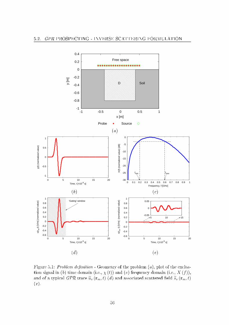
5.2. GPR PROSPECTING - INVERSE SCATTERING FORMULATION
-1
-0.8
-0.6
-0.4
-0.2
0
0.2
0.4
-1 -0.5 0 0.5 1
y [m
]
x [m]
Probe Source
D
Free space
Soil
(a)
-1
-0.5
0
0.5
1
0 5 10 15 20
χ(t)
(no
rmal
ized
val
ue)
Time, t [×10-9 s]
-30
-25
-20
-15
-10
-5
0
0 0.1 0.2 0.3 0.4 0.5 0.6 0.7 0.8 0.9 1
Χ(f
) (n
orm
aliz
ed v
alue
) [d
B]
Frequency, f [GHz]
fmin fmax
(b) ( )
-0.6
-0.4
-0.2
0
0.2
0.4
0.6
0.8
1
0 5 10 15 20
u(r m
,t) [V
/m] (
norm
aliz
ed v
alue
)
Time, t [×10-9 s]
’Gating’ window
-0.6
-0.4
-0.2
0
0.2
0.4
0.6
0.8
1
0 5 10 15 20
s(r m
, t)
[V/m
] (n
orm
aliz
ed v
alue
)
Time, t [×10-9 s]
-0.05
0
0.05
5 10 15
(d) (e)
Figure 5.1: Problem denition - Geometry of the problem (a), plot of the ex ita-
tion signal in (b) time domain (i.e., χ (t)) and ( ) frequen y domain (i.e., X (f)),and of a typi al GPR tra e uv (rm, t) (d) and asso iated s attered eld sv (rm, t)(e).
56

CHAPTER 5. GPR PROSPECTING THROUGH AN INVERSE
SCATTERING FREQUENCY-HOPPING MULTI-FOCUSING APPROACH
In order to retrieve the s atterers prole starting from the GPR radargrams,
the s attered eld data [88 [sv (rm, t) , uv (rm, t) − ev (rm, t) - Fig. 5.1(e) arerstly determined by temporal muting the rst part of the GPR tra e uv (rm, t),m = 1, ...,M , v = 1, ..., V , that a ounts for the dire t oupling between the
transmitting sour e antenna and the air-soil interfa e [Fig. 5.1(d)
sv (rm, t) = Γ [uv (rm, t)] v = 1, ..., V, (5.3)
Γ [·] being the gating operator [Fig. 5.1(e). Indeed, su h a pre-pro essing pro-
edure is equivalent, for the half-spa e s enario at hand, to the subtra tion of
the in ident (or unperturbed) eld, ev, from the total eld, uv, whi h is a us-
tomary operation in mi rowave inverse s attering experiments under ontrolled
onditions.
Afterwards, the Fourier transform of the time s attered data is omputed in Kfrequen y samples
S(k)v (rm) ,
∫∞
−∞sv (rm, t) exp
(j2πf (k)t
)dt
m = 1, ...,M ; v = 1, ..., V ; k = 1, ..., K(5.4)
to avoid both 'insu ien y' and redundan y in the data as well as redu ing the
omputational osts and the measurement burden, thus making it possible to
investigate wider domains Dinv. In (5.4), f (k) ∈ [fmin, fmax] is the k-th sam-
pling frequen y, [fmin, fmax] being the 3dB bandwidth of the spe trum of the
illuminating pulse X (f) =∫∞
−∞χ (t) exp (j2πft) dt [Fig. 5.1( ) [88.
In frequen y-domain framework, the original retrieval problem be omes then that
of retrieving, in the investigation domain Dinv, the obje t fun tion [84[?
τ (k) (r) ,(εr (r)− εrB)− j σ(r)−σB
2πf(k)ε0
ε0, k = 1, ..., K (5.5)
and the total eld
U (k)v (r) ,
∫ ∞
−∞
uv (r, t) exp(j2πf (k)t
)dt v = 1, ..., V ; k = 1, ..., K (5.6)
starting from the s attered , S(k)v (rm),m = 1, ...,M , v = 1, ..., V , k = 1, ..., K, and
the radiated , E(k)v (r) ,
∫∞
−∞ev (rm, t) exp
(j2πf (k)t
)dt, v = 1, ..., V , k = 1, ..., K,
eld frequen y samples. Mathemati ally, su h a problem an be re ast to the
minimization of the data-mismat h ost fun tion [84
Φ(k) =∑V
v=1
∑Mm=1
∣∣∣S(k)v (rm)−S
(k)v (rm)
∣∣∣2
∑Vv=1
∑Mm=1
∣∣∣S(k)v (rm)
∣∣∣2 +
∑Vv=1
∫Dinv
∣∣∣E(k)v (r)−E
(k)v (r)
∣∣∣2dr
∑Vv=1
∫Dinv
∣∣∣E(k)v (r)
∣∣∣2dr
k = 1, .., K
(5.7)
where S(k)v (r) and E
(k)v (r) stand for the retrieved versions of S
(k)v (r) and E
(k)v (r),
respe tively, and they are related to the estimated quantities τ (k) (r) and U(k)v (r)
57

5.3. FHMF-CG INVERSION PROCEDURE
through the data [84
S(k)v (rm) = k2B
∫DinvG(k)ext (rm, r
′) U(k)v (r′) τ (k) (r′) dr′
m = 1, ..,M, k = 1, ..., K, v = 1, ..., V(5.8)
and the state equations [84
E(k)v (r) = U
(k)v (r)− k2B
∫DinvG(k)int (r, r
′) U(k)v (r′) τ (k) (r′) dr′
r ∈ Dinv, k = 1, ..., K, v = 1, ..., V(5.9)
G(k)int (r, r′) and G(k)ext (r, r
′) being the 2D internal and external half-spa e Green's
fun tions for the k-th frequen y [84, respe tively.
The problem of interest an be now summarized/stated as follows
GPR Inverse S attering Prospe ting Problem - Given E(k)v (r)
and S(k)v (rm), m = 1, ...,M , v = 1, ..., V , k = 1, ..., K, nd τ (k) (r)
and U(k)v (r), v = 1, ..., V , k = 1, ..., K, within Dinv su h that (5.7) is
minimized.
5.3 FHMF-CG Inversion Pro edure
The proposed solution pro edure is a nested iterative algorithm omposed by an
external loop (k = 1, ..., K) implementing the FH strategy, while the internal
loop (s = 1, ..., S) performs the MF (Fig. 5.2).
The external FH s heme is essentially an information a quisition pro ess on-
sisting of K su essive solutions of (5.7), ea h y le being related to the k-thfrequen y. Although the ontrast is a dispersive quantity whether lossy mate-
rials are at hand
1
(5.5), the re onstru tion yielded at the (k − 1)-th step an
be exploited to provide a protable initialization for the su essive k-th one
[91[92[93 (e.g., the s atterer support generally does not hange):
τ (k) (r)
∣∣guess = 0 k = 1
τ (k) (r)∣∣guess = ℜ
τ (k−1) (r)
+jℑ
τ (k−1) (r)
f(k−1)
f(k) k = 2, ..., K.(5.10)
In (5.10) the ontrast fun tion retrieved at the (k−1)-th step is res aled to the k-th frequen y by multiplying its imaginary part by the ratio f (k−1)/f (k)
. Moreover,
the guess total eld distribution at the k-th external iteration is omputed, unlike
state-of-the-art FH methods [91, as follows
U(k)v (r)
∣∣∣guess
= E(k)v (r) k = 1
U(k)v (r)
∣∣∣guess
= Ψ[E
(k)v (r) , τ (k) (r)
∣∣guess]
k = 2, ..., K(5.11)
1
Lossy s enarios are ommon in GPR appli ations be ause of the ondu tive nature of the
materials and the soils at hand [79[80[81[82[83.
58
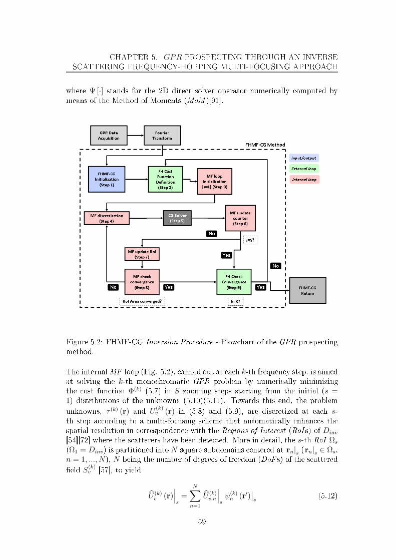
CHAPTER 5. GPR PROSPECTING THROUGH AN INVERSE
SCATTERING FREQUENCY-HOPPING MULTI-FOCUSING APPROACH
where Ψ [·] stands for the 2D dire t solver operator numeri ally omputed by
means of the Method of Moments (MoM )[91.
Figure 5.2: FHMF-CG Inversion Pro edure - Flow hart of the GPR prospe ting
method.
The internalMF loop (Fig. 5.2), arried out at ea h k-th frequen y step, is aimed
at solving the k-th mono hromati GPR problem by numeri ally minimizing
the ost fun tion Φ(k)(5.7) in S zooming steps starting from the initial (s =
1) distributions of the unknowns (5.10)(5.11). Towards this end, the problem
unknowns, τ (k) (r) and U(k)v (r) in (5.8) and (5.9), are dis retized at ea h s-
th step a ording to a multi-fo using s heme that automati ally enhan es the
spatial resolution in orresponden e with the Regions of Interest (RoI s) of Dinv
[54[72 where the s atterers have been dete ted. More in detail, the s-th RoI Ωs
(Ω1 = Dinv) is partitioned into N square subdomains entered at rn|s (rn|s ∈ Ωs,
n = 1, ..., N), N being the number of degrees of freedom (DoF s) of the s attered
eld S(k)v [57, to yield
U (k)v (r)
∣∣∣s=
N∑
n=1
U (k)v,n
∣∣∣sψ(k)n (r′)
∣∣s
(5.12)
59

5.3. FHMF-CG INVERSION PROCEDURE
and
τ (k) (r)∣∣s=
N∑
n=1
τ (k)n
∣∣sψ(k)n (r)
∣∣s
(5.13)
where ψ(k)n (r)
∣∣∣sis the n-th re tangular pulse basis fun tion at the s-th MF step
of the k-th frequen y, while U(k)v,n
∣∣∣sand τ
(k)n
∣∣∣sare the orresponding eld and
ontrast unknown oe ients, respe tively. By substituting (5.12) and (5.13) in
(5.8) and (5.9), the following dis retized form of the data
S(k)v (rm) =
∑Nn=1 U
(k)v,n
∣∣∣sτ(k)n
∣∣∣s
∫DinvG(k)ext (rm, r
′) ψ(k)n (r′)
∣∣∣sdr′
m = 1, ..,M, k = 1, ..., K, v = 1, ..., V(5.14)
and the state equations
E(k)v (rn|s) = U
(k)v,n
∣∣∣s−
∑Nn=1 U
(k)v,n
∣∣∣sτ(k)n
∣∣∣s
∫DinvG(k)int (rn|s , r′) ψ
(k)n (r′)
∣∣∣sdr′
r ∈ Dinv, k = 1, ..., K, v = 1, ..., V(5.15)
are obtained to dedu e the dis retized version of (5.7), Φ(k)∣∣s, to be minimized
with a numeri ally e ient lo al sear h algorithm. Owing to the suitable hoi e
of the ratio between measurement data and unknowns a ording to the DoF
riterion [57 and the ( onsequent) redu ed o urren e of lo al minima [90, a
CG-based deterministi optimization strategy [30[94 is here adopted. Starting
from (5.10) and (5.11), su h a minimization te hnique is dened through by the
following update equations [30[94
U(k)v
∣∣∣i+1
s= U
(k)v
∣∣∣i
s+ α
(k)v
∣∣∣i
sa(k)v
∣∣∣i
s
τ(k)v
∣∣∣i+1
s= τ
(k)v
∣∣∣i
s+ β
(k)v
∣∣∣i
sb(k)v
∣∣∣i
s
(5.16)
where i = 1, ..., I is the minimization iteration index,
U(k)v
∣∣∣i
s,
U (k)v,n
∣∣∣i
s, n = 1, ..., N
(5.17)
and
τ(k)v
∣∣is,
τ (k)n
∣∣is, n = 1, ..., N
(5.18)
are the unknown total eld and ontrast ve tors, respe tively, a(k)v
∣∣∣i
sand b
(k)v
∣∣∣i
s
are the orresponding sear h dire tions proportional to the gradient of Φ(k)∣∣s
[30[94), while α(k)v
∣∣∣i
sand β
(k)v
∣∣∣i
sare the asso iated step lengths.
On e i = I or the ost fun tion stagnation arises[54), the minimization loop
(5.16) is stopped and a new internal MF step is performed (s ← s + 1) to up-
date the lo alization and the size of Ωs through ltering and lustering [54.
60
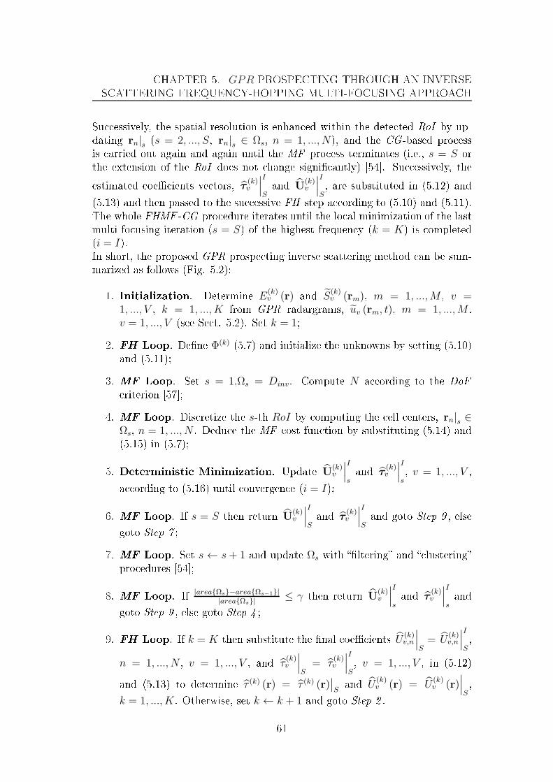
CHAPTER 5. GPR PROSPECTING THROUGH AN INVERSE
SCATTERING FREQUENCY-HOPPING MULTI-FOCUSING APPROACH
Su essively, the spatial resolution is enhan ed within the dete ted RoI by up-
dating rn|s (s = 2, ..., S, rn|s ∈ Ωs, n = 1, ..., N), and the CG-based pro ess
is arried out again and again until the MF pro ess terminates (i.e., s = S or
the extension of the RoI does not hange signi antly) [54. Su essively, the
estimated oe ients ve tors, τ(k)v
∣∣∣I
Sand U
(k)v
∣∣∣I
S, are substituted in (5.12) and
(5.13) and then passed to the su essive FH step a ording to (5.10) and (5.11).
The whole FHMF -CG pro edure iterates until the lo al minimization of the last
multi-fo using iteration (s = S) of the highest frequen y (k = K) is ompleted
(i = I).In short, the proposed GPR prospe ting inverse s attering method an be sum-
marized as follows (Fig. 5.2):
1. Initialization. Determine E(k)v (r) and S
(k)v (rm), m = 1, ...,M , v =
1, ..., V , k = 1, ..., K from GPR radargrams, uv (rm, t), m = 1, ...,M ,
v = 1, ..., V (see Se t. 5.2). Set k = 1;
2. FH Loop. Dene Φ(k)(5.7) and initialize the unknowns by setting (5.10)
and (5.11);
3. MF Loop. Set s = 1,Ωs = Dinv. Compute N a ording to the DoF
riterion [57;
4. MF Loop. Dis retize the s-th RoI by omputing the ell enters, rn|s ∈Ωs, n = 1, ..., N . Dedu e the MF ost fun tion by substituting (5.14) and
(5.15) in (5.7);
5. Deterministi Minimization. Update U(k)v
∣∣∣I
sand τ
(k)v
∣∣∣I
s, v = 1, ..., V ,
a ording to (5.16) until onvergen e (i = I);
6. MF Loop. If s = S then return U(k)v
∣∣∣I
Sand τ
(k)v
∣∣∣I
Sand goto Step 9 , else
goto Step 7 ;
7. MF Loop. Set s← s+ 1 and update Ωs with ltering and lustering
pro edures [54;
8. MF Loop. If
|areaΩs−areaΩs−1||areaΩs|
≤ γ then return U(k)v
∣∣∣I
sand τ
(k)v
∣∣∣I
sand
goto Step 9 , else goto Step 4 ;
9. FH Loop. If k = K then substitute the nal oe ients U(k)v,n
∣∣∣S= U
(k)v,n
∣∣∣I
S,
n = 1, ..., N , v = 1, ..., V , and τ(k)v
∣∣∣S
= τ(k)v
∣∣∣I
S, v = 1, ..., V , in (5.12)
and (5.13) to determine τ (k) (r) = τ (k) (r)∣∣Sand U
(k)v (r) = U
(k)v (r)
∣∣∣S,
k = 1, ..., K. Otherwise, set k ← k + 1 and goto Step 2 .
61
5.4. NUMERICAL AND EXPERIMENTAL VALIDATION
It is worth observing that the FHMF -CG approa h turns out very exible sin e
ea h pro edural blo k (i.e., FH s heme, MF te hnique, minimizer) an be easily
modied, updated, or substituted without altering the other ones. Analogously,
the ost fun tion (5.7) an be easily adapted to take into a ount additional reg-
ularization terms (e.g., multipli ative [101 or sparseness terms [?[23). However,
these investigations are beyond the s ope of the urrent resear h work and they
will be properly addressed in future investigations.
5.4 Numeri al and Experimental Validation
5.4.1 Rationale and Figures of Merit
In this se tion, a set of illustrative experiments is presented to assess the features
and the potentialities of the proposed FHMF-CG inversion pro edure in terms of
a ura y, numeri al e ien y, and robustness both onsidering syntheti (Se t.
5.4.2) and measured data (Se t. 5.4.3). Towards this end, the appli ation of
the proposed MF s heme has been arried out by prepro essing the GPR time-
domain signals
2
[Fig. 5.1(b) through a dis rete Fourier transform (Fig. 5.2),
and then extra ting the data sets at K equispa ed frequen ies within the 3dBbandwidth of the illuminating pulse [Fig. 5.1( ). As regards the numeri al
examples, time-domain syntheti data generated by means of GprMax software
[95 have been orrupted by zero-mean additive Gaussian noise, and the signal-
to-noise ratio (SNR) has been referred to the total eld as [102
SNR ,
∑Vv=1
∑Mm=1
∑Kk=1
∣∣∣T (k)v (rm)
∣∣∣2
∑Vv=1
∑Mm=1
∑Kk=1
∣∣∣N (k)v (rm)
∣∣∣2 . (5.19)
To assess the quality and e ien y of the method, beyond the visual represen-
tation of the retrieved ontrast proles, the integral error gures [54
Ξ(k)reg =
1
Nreg
Nreg∑
n=1
∣∣τ (k) (rn)− τ (k) (rn)∣∣
|τ (k) (rn) + 1| (5.20)
[where reg indi ates if the error omputation overs the overall investigation
domain (reg ⇒ tot), the a tual s atterer support (reg ⇒ int) or the ba k-
ground region (reg ⇒ ext) have been reported, along with the inversion time
∆t. Furthermore, the ontrol parameters of the MF and CG pro edures have
been sele ted a ording to the guidelines in [30[54[72.
2
It is worth remarking that GPR time-domain data, usually available in radargrams , have
been onsidered in both syntheti and experimental examples.
62
CHAPTER 5. GPR PROSPECTING THROUGH AN INVERSE
SCATTERING FREQUENCY-HOPPING MULTI-FOCUSING APPROACH
5.4.2 Numeri al Validation
5.4.2.1 Performan e Assessment
The rst set of examples is devoted to assess the performan e of the proposed
FHMF-CG method when pro essing syntheti data. The ben hmark 2D GPR
s enario onsists of a square investigation domain of side 0.8 m entered at
(0.00,−0.4) m whi h is illuminated by V = 20 sour es radiating a time-domain
Gaussian mono y le pulse [Fig. 5.1(b) with spe trum entered at 300 MHz and
3 dB bandwidth overing the [200.0, 600.0]MHz range [Fig. 5.1( ). The sour es
are equally spa ed on a 1 m line whi h is lo ated at y = 0.1 m above the soil
[Fig. 5.1(a), whi h is hara terized by εrB = 4.0, σB = 10−3S/m. A set of
M = 19 probes [ o-lo ated with the sour es
3
- Fig. 5.1(a) olle t the total eld,
and the Fourier transform is arried out assuming K = 5 frequen ies.
In order to illustrate the FHMF-CG pro edure (Se t. 5.3) on a step-by-step basis,
a hollow square prole (internal side 0.08 m, external side 0.24 m) entered at
(0.12,−0.36) m and hara terized by τ = 1.0 [Fig. 5.3(a) has been imaged in
noiseless onditions (Fig. 5.3). The re onstru tions obtained at the k = 1 FH
iteration ( orresponding to the lowest frequen y, fk = 200 MHz - Fig. 5.3) show
that the multi-fo using pro edure starts from the rough s = 1 re onstru tion
[Fig. 5.3(b), and then progressively zooms on the s atterer support [s = 2, Fig.5.3( ); s = 3, Fig. 5.3(d) until the onvergen e of the MF loop is rea hed [i.e.,
s = S = 4, Fig. 5.3(e). Afterwards, the FH loop iterates on the subsequent
frequen y (k = 2, fk = 300 MHz), performing the same iterative pro ess [but
exploiting the gathered information from the k − 1 step - see (5.10) and (5.11)
to yield the k = 2 retrieved prole [Fig. 5.4(b). The pro edure is then repeated
[k = 3 - Fig. 5.4(d); k = 4 - Fig. 5.4(f ) until k = K = 5 [Fig. 5.4(h). As
regards the a ura y evolution during the FH steps, the re onstru tions obtained
for ea h k shows that the GPR image quality improves as su essive iterations
are performed [e.g., k = 1, Fig. 5.3(e) vs. k = 5, Fig. 5.4(h), as it is also
onrmed by the orresponding total error gures (i.e., Ξ(k)tot
∣∣∣k=1
= 3.96 × 10⁻²
vs. Ξ(k)tot
∣∣∣k=5
= 1.81 × 10⁻²- Tab. 5.1). Indeed, the size and permittivity of the
internal hollow region is orre tly dete ted only at the highest frequen y [i.e.,
k = 5, fk = 600 MHz - Fig. 5.4(h), while it appears distorted at the previous
FH steps [e.g., it seems narrower at k = 2, fk = 300 MHz - Fig. 5.4(b) despite
the noiseless s enario.
3
The GPR multi-view multi-stati setup operates so that when one sour e is a tive, the
remaining V − 1 = M = 19 a t as ideal eld probes [Fig. 5.1(a).
63

5.4. NUMERICAL AND EXPERIMENTAL VALIDATION
-0.8
-0.6
-0.4
-0.2
0
-0.4 -0.2 0 0.2 0.4
y [m
]
x [m]
0
0.2
0.4
0.6
0.8
1
1.2
Re
τ(x,
y)
(a)
s = 1 s = 2
-0.8
-0.6
-0.4
-0.2
0
-0.4 -0.2 0 0.2 0.4
y [m
]
x [m]
0
0.2
0.4
0.6
0.8
1
1.2
Re
τ(x,
y)
-0.8
-0.6
-0.4
-0.2
0
-0.4 -0.2 0 0.2 0.4
y [m
]
x [m]
0
0.2
0.4
0.6
0.8
1
1.2
Re
τ(x,
y)
(b) ( )
s = 3 s = 4
-0.8
-0.6
-0.4
-0.2
0
-0.4 -0.2 0 0.2 0.4
y [m
]
x [m]
0
0.2
0.4
0.6
0.8
1
1.2
Re
τ(x,
y)
-0.8
-0.6
-0.4
-0.2
0
-0.4 -0.2 0 0.2 0.4
y [m
]
x [m]
0
0.2
0.4
0.6
0.8
1
1.2
Re
τ(x,
y)
(d) (e)
Figure 5.3: Illustrative Example [Hollow square prole, εrB = 4.0, σB = 10−3
S/m, τ = 1.0, Noiseless data, f1 = 200 MHz, k = 1 A tual (a) and FHMF-CG
retrieved diele tri proles when (b) s = 1, (b) s = 2, (b) s = 3, (e) s = S = 4.
64

CHAPTER 5. GPR PROSPECTING THROUGH AN INVERSE
SCATTERING FREQUENCY-HOPPING MULTI-FOCUSING APPROACH
FH-CG FHMF-CG
f 2=
300[MHz]
-0.8
-0.6
-0.4
-0.2
0
-0.4 -0.2 0 0.2 0.4
y [m
]
x [m]
0
0.2
0.4
0.6
0.8
1
1.2
Re
τ(x,
y)
-0.8
-0.6
-0.4
-0.2
0
-0.4 -0.2 0 0.2 0.4
y [m
]
x [m]
0
0.2
0.4
0.6
0.8
1
1.2
Re
τ(x,
y)
(a) (b)
f 3=
400[MHz]
-0.8
-0.6
-0.4
-0.2
0
-0.4 -0.2 0 0.2 0.4
y [m
]
x [m]
0
0.2
0.4
0.6
0.8
1
1.2R
eτ(
x,y)
-0.8
-0.6
-0.4
-0.2
0
-0.4 -0.2 0 0.2 0.4
y [m
]
x [m]
0
0.2
0.4
0.6
0.8
1
1.2
Re
τ(x,
y)
( ) (d)
f 4=
500[MHz]
-0.8
-0.6
-0.4
-0.2
0
-0.4 -0.2 0 0.2 0.4
y [m
]
x [m]
0
0.2
0.4
0.6
0.8
1
1.2
Re
τ(x,
y)
-0.8
-0.6
-0.4
-0.2
0
-0.4 -0.2 0 0.2 0.4
y [m
]
x [m]
0
0.2
0.4
0.6
0.8
1
1.2
Re
τ(x,
y)
(e) (f )
f 5=
600[MHz]
-0.8
-0.6
-0.4
-0.2
0
-0.4 -0.2 0 0.2 0.4
y [m
]
x [m]
0
0.2
0.4
0.6
0.8
1
1.2
Re
τ(x,
y)
-0.8
-0.6
-0.4
-0.2
0
-0.4 -0.2 0 0.2 0.4
y [m
]
x [m]
0
0.2
0.4
0.6
0.8
1
1.2
Re
τ(x,
y)
(g) (h)
Figure 5.4: Illustrative Example [Hollow square prole, εrB = 4.0, σB = 10−3
S/m, Noiseless data Diele tri proles retrieved by (a)( )(e)(g) FH-CG and
(b)(d)(f )(h) FHMF-CG when (a)(b) q = 2 (f2 = 300 MHz), (a)(b) q = 3(f3 = 400 MHz), (a)(b) q = 4 (f4 = 500 MHz), (a)(b) q = 5 (f5 = 600 MHz).
65

5.4. NUMERICAL AND EXPERIMENTAL VALIDATION
10-2
10-1
100
∞ 10 20 30 40 50
Ξ(K)
tot
SNR [dB]
FH-CG
FHMF-CG
(a)
FH-CG FHMF-CG
SNR
=30
d
B
-0.8
-0.6
-0.4
-0.2
0
-0.4 -0.2 0 0.2 0.4
y [m
]
x [m]
0
0.2
0.4
0.6
0.8
1
1.2
Re
τ(x,
y)
-0.8
-0.6
-0.4
-0.2
0
-0.4 -0.2 0 0.2 0.4
y [m
]
x [m]
0
0.2
0.4
0.6
0.8
1
1.2
Re
τ(x,
y)
(b) ( )
SNR
=10
d
B
-0.8
-0.6
-0.4
-0.2
0
-0.4 -0.2 0 0.2 0.4
y [m
]
x [m]
0
0.2
0.4
0.6
0.8
1
1.2
Re
τ(x,
y)
-0.8
-0.6
-0.4
-0.2
0
-0.4 -0.2 0 0.2 0.4
y [m
]
x [m]
0
0.2
0.4
0.6
0.8
1
1.2
Re
τ(x,
y)
(d) (e)
Figure 5.5: Performan e Assessment [Hollow square prole, εrB = 4.0, σB =10−3
S/m, τ = 1.0 Behaviour of the integral error vs. the SNR (a), and
diele tri proles retrieved by (b)(d) FH-CG and ( )(e) FHMF-CG when (b)( )
SNR = 30 dB, (d)(e) SNR = 10 dB.
66

CHAPTER 5. GPR PROSPECTING THROUGH AN INVERSE
SCATTERING FREQUENCY-HOPPING MULTI-FOCUSING APPROACH
The re onstru tions obtained with a bare FH approa h (i.e., FH-CG), re-
ported in Fig. 5.4 for omparison purposes, remark the ee tiveness of the MF
paradigm. Indeed, even exploiting all the frequen y data [i.e., k = K, the single-
resolution method is only able to roughly dete t the lo ation of the s atterer,
but ompletely misses its shape and ontrast [i.e., Fig. 5.4(g) vs. Fig. 5.4(h).
This is further remarked by the orresponding total (e.g., Ξ(k)tot
∣∣∣FHMF−CG
k=K= 1.81×
10−2vs. Ξ
(k)tot
∣∣∣FH−CG
k=K= 1.11 × 10⁻¹
- Tab. 5.1), internal (e.g., Ξ(k)int
∣∣∣FHMF−CG
k=K=
1.24×10⁻¹vs. Ξ
(k)int
∣∣∣FH−CG
k=K= 2.81×10⁻¹
- Tab. 5.1), and external integral errors
(e.g., Ξ(k)ext
∣∣∣FHMF−CG
k=K= 8.71 × 10⁻³
vs. Ξ(k)ext
∣∣∣FH−CG
k=K= 8.78 × 10⁻²
- Tab. 5.1).
Even more impressively, the re onstru tion obtained at the k = 1 step of the
FHMF-CG are signi antly better than those a hieved at the k = K step of the
bare method [i.e.,
Ξ(k)tot
∣∣∣FH−CG
k=K
Ξ(k)tot
∣∣∣FHMF−CG
k=1
≈ 2.8 - Fig. 5.3(e) vs. Fig. 5.4(g). These results
support the previous laim on erning the apability of multifo using approa hes
to redu e non-linearity issues arising in GPR imaging (see Se t. 5.3).
To assess proposed method against noisy data, the same s enario has been inves-
tigated assuming SNR ∈ [10, 50] dB (Fig. 5.5). The plots of the total integral
error vs. the noise level show that the FHMF-CG provides an a ura y equal to
that of the noiseless ase until SNR ≈ 40 dB [i.e.,
Ξ(K)tot
∣∣∣SNR=40 dB
Ξ(K)tot
∣∣∣Noiseless ≈ 1.01 - Fig.
5.5(a), while it smoothly degrades for lower SNR values [e.g.,
Ξ(K)tot
∣∣∣SNR=30 dB
Ξ(K)tot
∣∣∣Noiseless ≈
1.2 - Fig. 5.5(a), as it is also onrmed by the prole retrieved when SNR = 30dB [Fig. 5.5( ) vs. Fig. 5.4(h). Moreover, the proposed method is able to de-
te t the presen e and position of the s atterer even in extreme noise onditions
[i.e., SNR = 10 dB - Fig. 5.5(e), although the shape turns out distorted in this
ase [Ξ(K)tot
∣∣∣SNR=10 dB
≈ 2.31× 10⁻¹- Fig. 5.5(a). On the ontrary, the FH-CG
single-resolution approa h provide unsatisfa tory proles even with moderate
noise [Ξ(K)tot
∣∣∣SNR=30 dB
FH−CG≈ 1.1 × 10⁻¹
- Fig. 5.5(b), and it be omes ompletely
unreliable for lower SNR values [Ξ(K)tot
∣∣∣SNR=10 dB
FH−CG≈ 7.4× 10⁻¹
- Fig. 5.5(d).
The robustness of the proposed FHMF-CG s heme is then evaluated against a
variation of the s atterer ontrast. Towards this end, a square prole of side
0.16 m entered at (−0.08,−0.24) m has been simulated assuming τ ∈ [1.0, 2.2]for dierent SNR values (Fig. 5.6).
67

5.4. NUMERICAL AND EXPERIMENTAL VALIDATION
0
0.5
1
1.5
2
2.5
3
3.5
1 1.2 1.4 1.6 1.8 2 2.2
Ξ(K)
tot (
×10-1
) [n
orm
aliz
ed v
alue
]
τ [arbitrary unit]
FH-CG, NoiselessFH-CG, SNR=30 [dB]FH-CG, SNR=20 [dB]
FHMF-CG, NoiselessFHMF-CG, SNR=30 [dB]FHMF-CG. SNR=20 [dB]
(a)
FH-CG FHMF-CG
τ=
1.0
-0.8
-0.6
-0.4
-0.2
0
-0.4 -0.2 0 0.2 0.4
y [m
]
x [m]
0
0.2
0.4
0.6
0.8
1
1.2
Re
τ(x,
y)
-0.8
-0.6
-0.4
-0.2
0
-0.4 -0.2 0 0.2 0.4
y [m
]
x [m]
0
0.2
0.4
0.6
0.8
1
1.2
Re
τ(x,
y)
(b) ( )
τ=
2.2
-0.8
-0.6
-0.4
-0.2
0
-0.4 -0.2 0 0.2 0.4
y [m
]
x [m]
0
0.5
1
1.5
2
2.5
Re
τ(x,
y)
-0.8
-0.6
-0.4
-0.2
0
-0.4 -0.2 0 0.2 0.4
y [m
]
x [m]
0
0.5
1
1.5
2
2.5
Re
τ(x,
y)
(d) (e)
Figure 5.6: Performan e Assessment [Square prole, εrB = 4.0, σB = 10−3
S/m Behaviour of the integral error vs. τ (a), and diele tri proles retrieved
by (b)(d) FH-CG and ( )(e) FHMF-CG when (b)( ) τ = 1.0, (d)(e) τ = 2.2when SNR = 30 dB.
68
CHAPTER 5. GPR PROSPECTING THROUGH AN INVERSE
SCATTERING FREQUENCY-HOPPING MULTI-FOCUSING APPROACH
The behaviour of Ξ(K)tot obtained by the FHMF-CG in the noiseless ase [dashed
blue line - Fig. 5.6(a) shows that an extremely good delity is a hieved whatever
the target ontrast [i.e., Ξ(K)tot
∣∣∣FHMF−CG
∈ [8.7× 10⁻³, 1.2× 10⁻²] - Fig. 5.6(a),
whi h is always signi antly better than that shown by the single-resolution
method [e.g., Ξ(K)tot
∣∣∣FH−CG
≈ 8.2 × 10⁻²when τ = 2.2 - Fig. 5.6(a). However,
the FHMF-CG a ura y signi antly worsens when low τ with moderate noise
levels are at hand [SNR = 30 dB - green lines, Fig. 5.6(a).
More in detail, the integral error in reases of almost one order of magnitude
when τ = 2.2→ 1.0 [i.e.,
Ξ(K)tot
∣∣∣τ=1.0
FHMF−CG
Ξ(K)tot
∣∣∣τ=2.2
FHMF−CG
≈ 9.1 when SNR = 30 dB- Fig. 5.6(a),
rea hing a value whi h is even above that of the orresponding single-resolution
method [i.e., Ξ(K)tot
∣∣∣τ=1.0
FHMF−CG≈ 1.16 × 10⁻¹
vs. Ξ(K)tot
∣∣∣τ=1.0
FH−CG≈ 9.8× 10⁻²
- Fig.
5.6(a). This behaviour, whi h is also onrmed when lower SNR values are at
hand [SNR = 20 dB - red lines, Fig. 5.6(a), suggests that the multifo using
pro edure an exhibit sub-optimal performan e when handling low ontrast s at-
terers in high noise s enarios. By analyzing the orresponding re onstru tions
[SNR = 30 dB, τ = 1.0 - Fig. 5.6( ), it turns out that in this ase the MF
pro edure is not able to orre tly lo ate the RoI be ause the artifa ts have a
ontrast whose magnitude is lose to that of the a tual target [Fig. 5.6( ). A -
ordingly, the FHMF-CG method does not ee tively allo ate the DoF s within
the domain, resulting in a delity similar to that of the single-resolution te h-
nique [Fig. 5.6( ) vs. Fig. 5.6(b). On the ontrary, higher ontrast targets
are a urately retrieved by the FHMF-CG method, sin e the zooming pro edure
orre tly identies the RoI [e.g., SNR = 30 dB, τ = 2.2 - Fig. 5.6(e) vs. Fig.
5.6(d).
The next set of numeri al experiments is devoted to the analysis of the FHMF-
CG sensitivity to the number of available measurements M (Fig. 5.7). To
this end, the retrieval of a two-bar prole entered in (0.16,−0.24) m and
hara terized by τ = 1.4 [Fig. 5.8(a) has been arried out assuming an in reasing
number of probes (i.e., M ∈ [19, 76]) in dierent noise onditions. By observing
the plots of the total integral error obtained by the FHMF-CG method [Fig.
5.7(b) for a xed number of measurements, it turns out that, as expe ted, the
a ura y improves as the SNR enhan es [e.g., Ξ(K)tot
∣∣∣SNR=20 dB
FHMF−CG≈ 8.9 × 10⁻²
vs. Ξ(K)tot
∣∣∣SNR=50 dB
FHMF−CG≈ 3.2 × 10⁻²
when M = 38 - Fig. 5.7(b). Analogously,
in reasing the number of measurements redu es the error for a xed SNR [e.g.,
Ξ(K)tot
∣∣∣M=19
FHMF−CG≈ 5.1× 10⁻²
vs. Ξ(K)tot
∣∣∣M=76
FHMF−CG≈ 2.9 × 10⁻²
when SNR = 30
dB - Fig. 5.7(b).
69
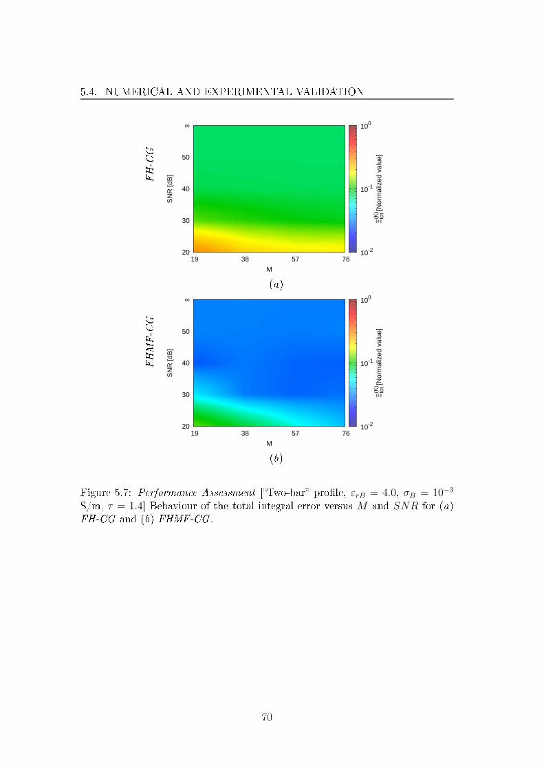
5.4. NUMERICAL AND EXPERIMENTAL VALIDATION
F
H
-
C
G
20
30
40
50
∞
19 38 57 76
SN
R [d
B]
M
10-2
10-1
100
Ξ(K)
tot [
Nor
mal
ized
val
ue]
(a)
F
H
M
F
-
C
G
20
30
40
50
∞
19 38 57 76
SN
R [d
B]
M
10-2
10-1
100
Ξ(K)
tot [
Nor
mal
ized
val
ue]
(b)
Figure 5.7: Performan e Assessment [Two-bar prole, εrB = 4.0, σB = 10−3
S/m, τ = 1.4 Behaviour of the total integral error versus M and SNR for (a)
FH-CG and (b) FHMF-CG .
70

CHAPTER 5. GPR PROSPECTING THROUGH AN INVERSE
SCATTERING FREQUENCY-HOPPING MULTI-FOCUSING APPROACH
-0.8
-0.6
-0.4
-0.2
0
-0.4 -0.2 0 0.2 0.4
y [m
]
x [m]
0
0.25
0.5
0.75
1
1.25
1.5
Re
τ(x,
y)
(a)
FH-CG FHMF-CG
M=
19
-0.8
-0.6
-0.4
-0.2
0
-0.4 -0.2 0 0.2 0.4
y [m
]
x [m]
0
0.25
0.5
0.75
1
1.25
1.5R
eτ(
x,y)
-0.8
-0.6
-0.4
-0.2
0
-0.4 -0.2 0 0.2 0.4
y [m
]
x [m]
0
0.25
0.5
0.75
1
1.25
1.5
Re
τ(x,
y)
(b) ( )
M=
76
-0.8
-0.6
-0.4
-0.2
0
-0.4 -0.2 0 0.2 0.4
y [m
]
x [m]
0
0.25
0.5
0.75
1
1.25
1.5
Re
τ(x,
y)
-0.8
-0.6
-0.4
-0.2
0
-0.4 -0.2 0 0.2 0.4
y [m
]
x [m]
0
0.25
0.5
0.75
1
1.25
1.5
Re
τ(x,
y)
(d) (e)
Figure 5.8: Performan e Assessment [Two-bar prole, εrB = 4.0, σB = 10−3
S/m, τ = 1.4, SNR = 20 dB A tual (a) and diele tri proles retrieved by
(b)(d) FH-CG and ( )(e) FHMF-CG when (b)( ) M = 19, (d)(e) M = 76.
Moreover, the plots in Fig. 5.7 show that (i) the FHMF-CG approa h never
ex eeds a ≈ 10% re onstru tion error, even in the worst onditions [i.e., SNR =20 dB, M = 19 - Fig. 5.7(b), and (ii) whatever the noise level and M value,
the multifo using pro edure outperforms the FH-CG one [Fig. 5.7(b) vs. Fig.
71
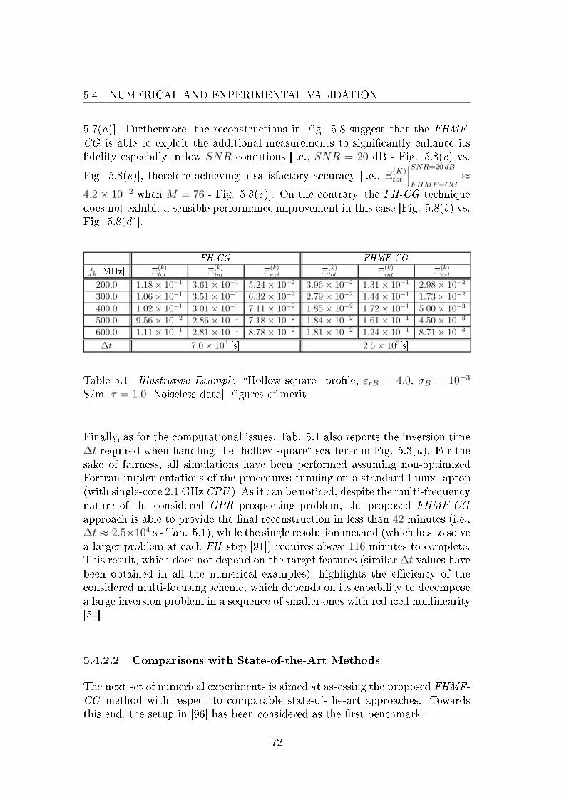
5.4. NUMERICAL AND EXPERIMENTAL VALIDATION
5.7(a). Furthermore, the re onstru tions in Fig. 5.8 suggest that the FHMF-
CG is able to exploit the additional measurements to signi antly enhan e its
delity espe ially in low SNR onditions [i.e., SNR = 20 dB - Fig. 5.8( ) vs.
Fig. 5.8(e), therefore a hieving a satisfa tory a ura y [i.e., Ξ(K)tot
∣∣∣SNR=20 dB
FHMF−CG≈
4.2 × 10⁻²when M = 76 - Fig. 5.8(e). On the ontrary, the FH-CG te hnique
does not exhibit a sensible performan e improvement in this ase [Fig. 5.8(b) vs.
Fig. 5.8(d).
FH-CG FHMF-CG
fk [MHz Ξ(k)tot Ξ
(k)int Ξ
(k)ext Ξ
(k)tot Ξ
(k)int Ξ
(k)ext
200.0 1.18× 10⁻¹ 3.61× 10⁻¹ 5.24× 10⁻² 3.96× 10⁻² 1.31× 10⁻¹ 2.98× 10⁻²
300.0 1.06× 10⁻¹ 3.51× 10⁻¹ 6.32× 10⁻² 2.79× 10⁻² 1.44× 10⁻¹ 1.73× 10⁻²
400.0 1.02× 10⁻¹ 3.01× 10⁻¹ 7.11× 10⁻² 1.85× 10⁻² 1.72× 10⁻¹ 5.00× 10⁻³
500.0 9.56× 10⁻² 2.86× 10⁻¹ 7.18× 10⁻² 1.84× 10⁻² 1.61× 10⁻¹ 4.50× 10⁻³
600.0 1.11× 10⁻¹ 2.81× 10⁻¹ 8.78× 10⁻² 1.81× 10⁻² 1.24× 10⁻¹ 8.71× 10⁻³
∆t 7.0× 10³ [s 2.5× 10³[s
Table 5.1: Illustrative Example [Hollow square prole, εrB = 4.0, σB = 10−3
S/m, τ = 1.0, Noiseless data Figures of merit.
Finally, as for the omputational issues, Tab. 5.1 also reports the inversion time
∆t required when handling the hollow-square s atterer in Fig. 5.3(a). For the
sake of fairness, all simulations have been performed assuming non-optimized
Fortran implementations of the pro edures running on a standard Linux laptop
(with single- ore 2.1GHz CPU ). As it an be noti ed, despite the multi-frequen y
nature of the onsidered GPR prospe ting problem, the proposed FHMF-CG
approa h is able to provide the nal re onstru tion in less than 42 minutes (i.e.,
∆t ≈ 2.5×10⁴ s - Tab. 5.1), while the single resolution method (whi h has to solve
a larger problem at ea h FH step [91) requires above 116 minutes to omplete.
This result, whi h does not depend on the target features (similar∆t values havebeen obtained in all the numeri al examples), highlights the e ien y of the
onsidered multi-fo using s heme, whi h depends on its apability to de ompose
a large inversion problem in a sequen e of smaller ones with redu ed nonlinearity
[54.
5.4.2.2 Comparisons with State-of-the-Art Methods
The next set of numeri al experiments is aimed at assessing the proposed FHMF-
CG method with respe t to omparable state-of-the-art approa hes. Towards
this end, the setup in [96 has been onsidered as the rst ben hmark.
72
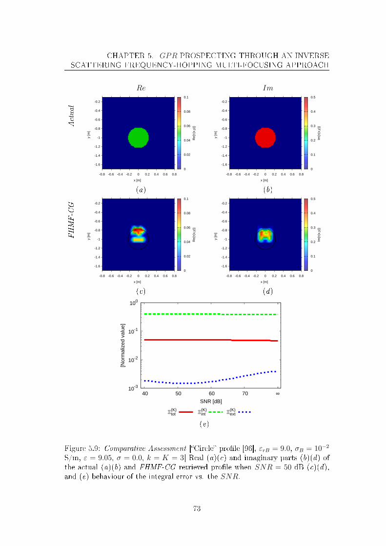
CHAPTER 5. GPR PROSPECTING THROUGH AN INVERSE
SCATTERING FREQUENCY-HOPPING MULTI-FOCUSING APPROACH
Re Im
A
t
u
a
l
-1.6
-1.4
-1.2
-1
-0.8
-0.6
-0.4
-0.2
-0.8 -0.6 -0.4 -0.2 0 0.2 0.4 0.6 0.8
y [m
]
x [m]
0
0.02
0.04
0.06
0.08
0.1
Re
τ(x,
y)
-1.6
-1.4
-1.2
-1
-0.8
-0.6
-0.4
-0.2
-0.8 -0.6 -0.4 -0.2 0 0.2 0.4 0.6 0.8
y [m
]
x [m]
0
0.1
0.2
0.3
0.4
0.5
Imτ
(x,y
)
(a) (b)
F
H
M
F
-
C
G
-1.6
-1.4
-1.2
-1
-0.8
-0.6
-0.4
-0.2
-0.8 -0.6 -0.4 -0.2 0 0.2 0.4 0.6 0.8
y [m
]
x [m]
0
0.02
0.04
0.06
0.08
0.1
Re
τ(x,
y)
-1.6
-1.4
-1.2
-1
-0.8
-0.6
-0.4
-0.2
-0.8 -0.6 -0.4 -0.2 0 0.2 0.4 0.6 0.8
y [m
]
x [m]
0
0.1
0.2
0.3
0.4
0.5
Imτ
(x,y
)
( ) (d)
10-3
10-2
10-1
100
∞ 40 50 60 70
[Nor
mal
ized
val
ue]
SNR [dB]
Ξ(K)tot Ξ(K)
int Ξ(K)ext
(e)
Figure 5.9: Comparative Assessment [Cir le prole [96, εrB = 9.0, σB = 10−2
S/m, ε = 9.05, σ = 0.0, k = K = 3 Real (a)( ) and imaginary parts (b)(d) of
the a tual (a)(b) and FHMF-CG retrieved prole when SNR = 50 dB ( )(d),
and (e) behaviour of the integral error vs. the SNR.
73

5.4. NUMERICAL AND EXPERIMENTAL VALIDATION
0
0.1
0.2
0.3
0.4
0.5
0.6
0.7
∞ 30 40 50 60 70
[Nor
mal
ized
val
ue]
SNR [dB]
Ξ(Κ)tot Ξ(Κ)
int Ξ(Κ)ext
(a)
A tual FHMF-CG
-2
-1.75
-1.5
-1.25
-1
-0.75
-0.5
-0.75 -0.5 -0.25 0 0.25 0.5 0.75
y [m
]
x [m]
0
0.5
1
1.5
2
2.5
3
Re
τ(x,
y)
-2
-1.75
-1.5
-1.25
-1
-0.75
-0.5
-0.75 -0.5 -0.25 0 0.25 0.5 0.75
y [m
]
x [m]
0
0.5
1
1.5
2
2.5
3
Re
τ(x,
y)
(b) ( )
Figure 5.10: Comparative Assessment [Large square prole [87, εrB = 9.0,σB = 10−2
S/m, τ = 3.0, k = K = 6 (a) Behaviour of the integral error vs. theSNR and (b) a tual and ( ) FHMF-CG retrieved proles when SNR = 50 dB.
More spe i ally, a ir le-shaped target entered at (0.0,−1.0) m and with
radius 0.23 m [Figs. 5.9(a)-5.9(b), hara terized by ε = 9.05 and σ = 0.0,has been pla ed in a square investigation domain of side 1.6 m, entered at
(0.0,−0.9) m (i.e., with a −0.1 m oset with respe t to the air-soil interfa e)
with ba kground diele tri properties εrB = 9.0, σB = 10−2S/m [96. The
s enario has been illuminated by V = 21 sour es equispa ed on a 2 m line pla ed
on the air-soil interfa e, and the obtained eld has been sampled by M = 25probes equally spa ed on the same line [96.
The plots of the real [Fig. 5.9( ) and imaginary part [Fig. 5.9(d) of the ontrast
prole obtained at the k = K = 3 step assuming the same SNR levels of [96
4
point out that the proposed approa h is able to orre tly retrieve the number and
4
Sin e the SNR in [96 is not dened as in (5.19), the translation of the employed SNR
numeri al values has been arried out before performing the numeri al simulations, for onsis-
74

CHAPTER 5. GPR PROSPECTING THROUGH AN INVERSE
SCATTERING FREQUENCY-HOPPING MULTI-FOCUSING APPROACH
position the s atterers, and to approximatively yield also its shape and ontrast
[e.g., Fig. 5.9(d) vs. Fig. 5.9(b) despite the signi ant losses in the soil (i.e.,
σB = 10−2S/m). By omparing these results with the one obtained with the
linear TSVD-based inversion approa h dis ussed in [96, it turns out that the
proposed method yield a more a urate estimation of the size and lo ation of the
target, as well as a less blurred ba kground [i.e., Fig. 12 in [96 vs. Fig. 5.9(d).
Indeed, the s atterer enter is reliably approximated by the FHMF-CG [Figs.
5.9( )-5.9(d), while a non-negligible oset was shown in [96. Moreover, a similar
a ura y an be obtained in a wide set of noise onditions [i.e., SNR ≥ 40 dB
- Fig. 5.9(e). These results suggests that using a fully non-linear methodology
(handled through a multi-fo using approa h) an provide an improved a ura y
with respe t to approximated formulations (i.e., distorted Born [96) even in
s enarios where these approximations are a eptable.
Analogous onsiderations arise when applying the FHMF-CG method to the test
ase presented in [87. In this ase, a square s atterer of side 0.5 m entered at
(0.0,−1.45) m [τ = 3.0 - Fig. 5.10(b) has been imaged assuming V = 21 sour esand M = 20 probes displa ed on a 3 m-long line on the air-soil interfa e [87.
Towards this end, a 1.5 × 2.0 m D (εRb = 9.0, σB = 10−2S/m) entered at
(0.00,−1.25) m (0.5 m depth) has been onsidered [87. By omparing the plot
of the retrieved prole at the k = K = 6 FH step [SNR = 50 dB - Fig. 5.10( )
with the orresponding re onstru tion shown obtained with a linear inversion
algorithm under the Distorted Born Approximation (i.e., Fig. 7 in [87) it turns
out that both the shape and the size of the target are more a urately retrieved
by the FHMF-CG method.
Moreover, the plot of the integral errors vs. the SNR show that the obtained
performan e is quite stable with respe t to the noise level [i.e., Ξ(K)tot < 2.1×10⁻¹
when SNR > 50 dB - Fig. 5.10(a), and it smoothly degrades for lower and
lower SNRs [Fig. 5.10(a). The redu ed FHMF-CG a ura y when SNR < 50dB [Fig. 5.10(a) is a tually aused by the depth of the onsidered investigation
domain (i.e., y ∈ [−2,−0.5]m) and by the lossy nature of the soil (i.e., σB = 10−2
S/m), whi h ause a very low s attered eld to be re eived by the probes (i.e.,
at SNR = 30 dB, the signal-to-noise ratio omputed over the s attered eld
turns out equal to ≈ 10 dB in this ase), despite the non-negligible ontrast [i.e.,
τ = 3.0 - Fig. 5.10(b).
5.4.3 Experimental Validation
The last validations are on erned with the inversion of experimental data. To-
wards this end, the measured GPR radargrams in Area 5 of the Near Surfa e
Geophysi al Group (NSGG) Test Site 2 [97 using theMalaX3M GPR equipment
[103 have been onsidered [Fig. 5.11( ).
ten y.
75

5.4. NUMERICAL AND EXPERIMENTAL VALIDATION
(a)
y [m
]
x [m]
TX1 RX1 TX2 RX2
TX21 RX21
0.2 [m]
-1
-0.8
-0.6
-0.4
-0.2
0
0.2
0.4
-1 -0.5 0 0.5 1
Dinv
(b)
Tim
e [n
sec]
Position [m]
0
5
10
15
20
25
30 0 2.5 5 7.5 10 12.5 15 17.5
-10
-8
-6
-4
-2
0
2
4
6
Mea
sure
d S
igna
l Am
plitu
de ×
103
( )
Figure 5.11: Experimental Validation - Dataset [97 - Photo of the experimental
setup ( ourtesy of Prof. M. Guy) (a), geometry of the problem (b), and full
measured radargram available in [97 ( ).
76

CHAPTER 5. GPR PROSPECTING THROUGH AN INVERSE
SCATTERING FREQUENCY-HOPPING MULTI-FOCUSING APPROACH
-0.85
-0.75
-0.65
-0.55
-0.45
-0.35
-0.25
-0.15
-0.05
-0.4 -0.2 0 0.2 0.4
y [m
]
x [m]
-4
-3.5
-3
-2.5
-2
-1.5
-1
-0.5
0
Re
τ(x,
y)
(a)
-0.85
-0.75
-0.65
-0.55
-0.45
-0.35
-0.25
-0.15
-0.05
-0.4 -0.2 0 0.2 0.4
y [m
]
x [m]
0
0.5
1
1.5
2
2.5
Imτ
(x,y
)
(b)
Figure 5.12: Experimental Validation - Dataset [97 [V = 21 Real (a) and
imaginary parts (b) of the FHMF-CG retrieved prole.
77

5.4. NUMERICAL AND EXPERIMENTAL VALIDATION
Re Im
V=
5
-0.85
-0.75
-0.65
-0.55
-0.45
-0.35
-0.25
-0.15
-0.05
-0.4 -0.2 0 0.2 0.4
y [m
]
x [m]
-4
-3.5
-3
-2.5
-2
-1.5
-1
-0.5
0
Re
τ(x,
y)
-0.85
-0.75
-0.65
-0.55
-0.45
-0.35
-0.25
-0.15
-0.05
-0.4 -0.2 0 0.2 0.4
y [m
]
x [m]
0
0.5
1
1.5
2
2.5
Imτ
(x,y
)
(a) (b)
V=
11
-0.85
-0.75
-0.65
-0.55
-0.45
-0.35
-0.25
-0.15
-0.05
-0.4 -0.2 0 0.2 0.4
y [m
]
x [m]
-4
-3.5
-3
-2.5
-2
-1.5
-1
-0.5
0
Re
τ(x,
y)
-0.85
-0.75
-0.65
-0.55
-0.45
-0.35
-0.25
-0.15
-0.05
-0.4 -0.2 0 0.2 0.4
y [m
]
x [m]
0
0.5
1
1.5
2
2.5
Imτ
(x,y
)
( ) (d)
V=
41
-0.85
-0.75
-0.65
-0.55
-0.45
-0.35
-0.25
-0.15
-0.05
-0.4 -0.2 0 0.2 0.4
y [m
]
x [m]
-4
-3.5
-3
-2.5
-2
-1.5
-1
-0.5
0
Re
τ(x,
y)
-0.85
-0.75
-0.65
-0.55
-0.45
-0.35
-0.25
-0.15
-0.05
-0.4 -0.2 0 0.2 0.4
y [m
]
x [m]
0
0.5
1
1.5
2
2.5
Imτ
(x,y
)
(e) (f )
Figure 5.13: Experimental Validation - Dataset [97 - Real (a)( )(e) and imag-
inary parts (b)(d)(f ) of the FHMF-CG retrieved proles when (a)(b) V = 5,( )(d) V = 11, and (e)(f ) V = 41.
The experimental data refer to the setup in Fig. 5.11(a), in whi h an empty box
(εr = 1.0, σ = 0.0 S/m) of size 0.32×0.25×0.15 m is buried 0.15 m below the soil
surfa e [104, whi h is assumed to be hara terized by εrB = 5.0, σB = 38×10−3
S/m. The s enario is investigated through a single pair of transmitting-re eiving
antennas positioned at the air-soil interfa e, whi h is moved over the investigation
domain [one tra e every 0.02 m - Fig. 5.11(b). The transmitter radiates a
Gaussian mono y le pulse with [100, 300]MHz 3 dB bandwidth [97[104, and the
78

CHAPTER 5. GPR PROSPECTING THROUGH AN INVERSE
SCATTERING FREQUENCY-HOPPING MULTI-FOCUSING APPROACH
resulting eld is olle ted by the built-in re eiver (M = 1) whi h is horizontally
separated by 0.2 m [Fig. 5.11(b). A square investigation domain D of side 0.8m and entered at (0.00,−0.45) m is onsidered for the inversion [Fig. 5.11(b).
The plot of the retrieved real [Fig. 5.12(a) and imaginary parts of the ontrast
[Fig. 5.12(b) obtained using V = 21sour e positions [uniformly pla ed over a 0.8m range - Fig. 5.11(b) show that the proposed FHMF-CG approa h is able to
orre tly identify the presen e, horizontal extension, and depth of the target [e.g.,
Fig. 5.12(a), while the verti al extension is overestimated [e.g., Fig. 5.12(b).
However, this behaviour is mainly related to low number of measurements (M =1), and to the fa t that the method does not a ount for the non-ideal nature of
the sour e/probe antennas (i.e., shielded bowties [97[104), and well as for any
roughness or non-homogeneity in the soil.
In order to assess the variation in the retrieval a ura y with the number of a -
quisitions, the same experiment has been repeated onsidering V = 5, 11, 41sour e positions uniformly distributed in the 0.8 m range (Fig. 5.13). By om-
paring the plots of the retrieved proles when V = 11 [Figs. 5.13( )-5.13(d)
and V = 41 [Figs. 5.13(e)-5.13(f ) it turns out that the number of views does
not signi antly ae t the GPR prospe ting a ura y, unless a very few data are
used [V = 5 - Figs. 5.13(a)-5.13(b). Moreover, it is worth observing that V = 11measurements, orresponding to a spatial sampling rate of 0.08 m, are su ient
for the FHMF-CG method to retrieve the diele tri properties, horizontal size,
and depth of the buried target illuminated through standard GPR instruments.
5.5 Dis ussions
An innovative information a quisition approa h based on a nested frequen y-
hopping multi-fo using inversion te hnique has been introdu ed for the solution
of 2D GPR prospe ting problems. Towards this end, an external iterative FH
pro edure has been proposed to handle multi-frequen y GPR data, and its om-
bination with an internal multi-resolution loop able to mitigate lo al minima
issues in the asso iated inverse s attering problem has been presented. To min-
imize the arising multi-fo using ost fun tion, a lo al sear h strategy based on
CG has been implemented and integrated. The proposed FHMF-CG method
has been validated against syntheti and measured GPR data, and a ompara-
tive assessment has been dis ussed.
From the methodologi al viewpoint, the main ontributions of the present work
in lude (i) the derivation of a multi-fo using s heme that, unlike state-of-the-art
methods [54[72, is suitable for GPR prospe ting and an handle time-domain
data through Fourier pro essing, and (ii) the introdu tion of a frequen y-hopping
te hnique whi h, at ea h frequen y step, suitably initializes both the total eld
[Eq. (5.11) and the ontrast [Eq. (5.10) using the a quired information, unlike
[91-[93.
The numeri al and experimental validation has pointed out the following main
79

5.5. DISCUSSIONS
out omes:
• the FHMF-CG method outperforms its single-resolution ounterpart in
terms of a ura y whatever the noise level, ontrast, measurement setup,
and target properties, ex ept for very weak s atterers in low SNR s enarios
in whi h the two methods provide omparable delities;
• thanks to its multi-fo using nature, the proposed approa h is signi antly
more numeri ally e ient than a bare FH-CG te hnique (Tab. 5.1);
• the introdu ed algorithm favourably ompares with state-of-the-art te h-
niques based on linear formulations and TSVD solvers (Se t. 5.4.2.2);
• the FHMF-CG te hnique an be ee tively used to dete t the position,
depth, and diele tri properties of buried obje ts starting from few raw
GPR experimental measurements without the need to a urately model
the a tual soil properties and antenna geometries (Se t. 5.4.3).
Future works, beyond the s ope of this thesis, will be aimed at extending the
proposed methodology to full 3D GPR s enarios. Moreover, the possibility to
improve the method a ura y through a urate modelling of the employed trans-
mitting/re eiving antennas within the inversion pro ess is urrently under inves-
tigation.
80

Chapter 6
Con lusions
In this hapter, a nal numeri al set of simulations is provided and ommented
with the aim of omparing the dierent inversion strategies presented in this
thesis. Moreover, some nal onsiderations on the presented methodologies for
subsurfa e imaging are drawn, highlighting potentialities and limits of ea h te h-
nique.
81

6.1. COMPARISON BETWEEN DIFFERENT APPROACHES
6.1 Comparison Between Dierent Approa hes
In order to assess what are the potentialities as well as the limits of the proposed
inversion te hniques presented in this thesis, a nal numeri al assessment is here
presented. The onsidered ben hmark s enario onsists of a square investigation
domain of side 0.8 m entered at (0.00,−0.4) m whi h is illuminated by V = 16sour es radiating a time-domain Gaussian mono y le pulse [Fig. 5.1(b) with
spe trum entered at 300 MHz and 3 dB bandwidth overing the [200.0, 600.0]MHz range [Fig. 5.1( ). The lower half spa e is o upied by soil, with εrB = 4.0and σB = 10−3
S/m.
y [m
]
x [m]
Measurement PointsSource Locations
-1.2
-1
-0.8
-0.6
-0.4
-0.2
0
0.2
0.4
-1 -0.5 0 0.5 1
Dinv y [m
]
x [m]
Measurement PointsSource Locations
-1.2
-1
-0.8
-0.6
-0.4
-0.2
0
0.2
0.4
-1 -0.5 0 0.5 1
Dinv
(a) (b)
Figure 6.1: Comparative Assessment (Square S atterer at Dierent Depths - L =0.16m, (xc = 0.0m, εr = 5.5, σ = 0.01 S/m [τ = 1.5, εrB =4.0, σB =0.01 S/m,
SNR = 20 dB) - Lo ation of the illuminating sour es and of the measurement
points for the (a) ross-borehole and (b) half spa e ongurations.
For omparison purposes, two measurement ongurations are onsidered,
both onsidering a set of M = 15 probes
1
, o-lo ated with the sour es to form
a ross-borehole [Fig. 6.1(a) and a half spa e [Fig. 6.1(b) setup. Con erning
the ross-borehole setup [Fig. 6.1(a), the sour es/probes are equally spa ed
along two verti al lines at oordinates x = ±0.5 m, starting from a depth of
ymin = −1.0 [m up to a depth of ymax = 0.0 m. For the half spa e setup [Fig.
6.1(b) the sour es/probes are equally spa ed on a 1 m line whi h is lo ated at
y = 0.04 m above the interfa e. As a ben hmark prole, a square prole of
side 0.16 m [Fig. 6.2 entered at xc = 0.0 m and lo ated at dierent depths
inside Dinv has been simulated assuming a ontrast fun tion of τ = 1.5. More
pre isely, the target bary entre is lo ated at a depth of yc = −0.16m for the top
onguration [Fig. 6.2(a), yc = −0.4m for the intermediate onguration [Fig.
6.2(b) and yc = −0.64 m for the bottom onguration.
1
The GPR multi-view multi-stati setup operates so that when one sour e is a tive, the
remaining V − 1 = M = 15 a t as ideal eld probes.
82

CHAPTER 6. CONCLUSIONS
-0.8
-0.6
-0.4
-0.2
0
-0.4 -0.2 0 0.2 0.4
y [m
]
x [m]
0
0.2
0.4
0.6
0.8
1
1.2
1.4
1.6
Re
τ(x,
y)
(a)
-0.8
-0.6
-0.4
-0.2
0
-0.4 -0.2 0 0.2 0.4
y [m
]
x [m]
0
0.2
0.4
0.6
0.8
1
1.2
1.4
1.6
Re
τ(x,
y)
(b)
-0.8
-0.6
-0.4
-0.2
0
-0.4 -0.2 0 0.2 0.4
y [m
]
x [m]
0
0.2
0.4
0.6
0.8
1
1.2
1.4
1.6
Re
τ(x,
y)
( )
Figure 6.2: Comparative Assessment (Square S atterer at Dierent Depths -
L = 0.16m, (xc = 0.0m, εr = 5.5, σ = 0.01 S/m [τ = 1.5, εrB =4.0, σB =0.01S/m, SNR = 20 dB) - A tual target used for the omparison for (a) top (yc =−0.16m), (b) intermediate (yc = −0.4m) and ( ) bottom (yc = −0.64m)
ongurations.
The SNR omputed a ording to (5.19) is su h that a resulting SNR = 20dB an be estimated on the s attered eld at the entral frequen y of 300 MHz.
83

6.1. COMPARISON BETWEEN DIFFERENT APPROACHES
As a rst analysis, we onsider the retrieved proles when the single-frequen y
IMSA−IN te hnique presented in Chapter 4 is employed in order to re over the
ele tromagneti distributions of the investigated targets [Fig. 6.3. The IMSA−IN −SOBA method presented in Chapter 3 will not be onsidered here, sin e it
has been already widely veried in Chapter 4 that its performan es are lower wrt
the full non-linear approa h (i.e., without the SOBA approximation). Moreover,
the same parameters onsidered for the numeri al results shown in Chapter 4
are onsidered (i.e., N = 100, Q = 50, α = 0.9, Imax,s=1 = 20, Imax,s>1 =1000 and S = 4). In parti ular, the retrieved proles are shown when using
both a ross-borehole [Fig. 6.3(a)(b)( ) and a half spa e [Fig. 6.3(d)(e)(f )
measurement onguration. By looking at the retrieved proles in Fig. 6.3, it is
lear that the performan es a hievable with a ross-borehole setup signi antly
over ome those obtainable with a half spa e setup. Moreover, if on the one
hand the performan es for the ross-borehole setup seem quite onstant when
hanging the depth of the unknown target, on the other hand the retrieved
ontrasts when using a half spa e setup undergo a signi ant and progressive
degradation when in reasing the depth of the s atterer inside Dinv [i.e., passing
from Fig. 6.3(d) to Fig. 6.3(e) and to Fig. 6.3(f ). As a matter of fa t, when
the s atterer is at a depth of yc = −0.64 m [i.e., orresponding to 1.28λb at the onsidered frequen y of 300 MHz, Fig. 6.3(f ), the inversion te hnique turns
out to be absolutely un apable to re over the shape and the ele tromagneti
hara teristi s of the target. Su h a behaviour an be motivated by the fa t
that half spa e setups are strongly aspe t-limited, given the fa t that sour es
and measurement points are both lo ated only above the interfa e [Fig. 6.1(b),
thus allowing the olle tion of a very limited amount of information to perform
the inversion. On the ontrary, a ross-borehole setup [Fig. 6.1(a), even if still
aspe t-limited, allows the olle tion of a larger amount of information with the
same number of sour es V and measurements M , sin e transmissions an ross
the investigation domain Dinv and hen e the targets buried within it. Moreover,
sour es and measurement points are lo ated at dierent depths inside the soil, so
that more information an be olle ted for targets whi h are buried at signi ant
depths inside Dinv. The above onsiderations are further onrmed by the total
re onstru tion error Ξtot obtained by the IMSA−IN method for the two setups.
In fa t, we have for the top onguration [Fig. 6.2(a) Ξtot|”top”cross−borehole ≈8.66 × 10⁻³
[Fig. 6.3(a) vs. Ξtot|”top”half space ≈ 1.83 × 10⁻²[Fig. 6.3(d), for
the intermediate onguration [Fig. 6.2(b) Ξtot|”intermediate”cross−borehole ≈ 3.72 × 10⁻³
[Fig. 6.3(b) vs. Ξtot|”intermediate”half space ≈ 2.91 × 10⁻²
[Fig. 6.3(e), while for the
bottom onguration [Fig. 6.2( ) Ξtot|”bottom”cross−borehole ≈ 4.12 × 10⁻³
[Fig. 6.3( )
vs. Ξtot|”bottom”half space ≈ 4.22 × 10⁻²
[Fig. 6.3(f ). The re onstru tion error obtained
for this latter onguration appears more that one order of magnitude larger
when onsidering an half spa e setup wrt a ross-borehole setup.
84

CHAPTER 6. CONCLUSIONS
IMSA− IN ross-borehole IMSA− IN half spa e
-0.8
-0.6
-0.4
-0.2
0
-0.4 -0.2 0 0.2 0.4
y [m
]
x [m]
0
0.2
0.4
0.6
0.8
1
1.2
1.4
1.6
Re
τ(x,
y)
-0.8
-0.6
-0.4
-0.2
0
-0.4 -0.2 0 0.2 0.4
y [m
]
x [m]
0
0.2
0.4
0.6
0.8
1
1.2
1.4
1.6
Re
τ(x,
y)
(a) (d)
-0.8
-0.6
-0.4
-0.2
0
-0.4 -0.2 0 0.2 0.4
y [m
]
x [m]
0
0.2
0.4
0.6
0.8
1
1.2
1.4
1.6
Re
τ(x,
y)
-0.8
-0.6
-0.4
-0.2
0
-0.4 -0.2 0 0.2 0.4
y [m
]
x [m]
0
0.2
0.4
0.6
0.8
1
1.2
1.4
1.6
Re
τ(x,
y)
(b) (e)
-0.8
-0.6
-0.4
-0.2
0
-0.4 -0.2 0 0.2 0.4
y [m
]
x [m]
0
0.2
0.4
0.6
0.8
1
1.2
1.4
1.6
Re
τ(x,
y)
-0.8
-0.6
-0.4
-0.2
0
-0.4 -0.2 0 0.2 0.4
y [m
]
x [m]
0
0.2
0.4
0.6
0.8
1
1.2
1.4
1.6
Re
τ(x,
y)
( ) (f )
Figure 6.3: Comparative Assessment (Square S atterer at Dierent Depths -
L = 0.16m, (xc = 0.0m, εr = 5.5, σ = 0.01 S/m [τ = 1.5, εrB =4.0, σB =0.01S/m, SNR = 20 dB) - Final re onstru tion obtained by the IMSA−IN method
when onsidering a (a)(b)( ) ross-borehole and (d)(e)(f ) an half spa e setup.
It is however mandatory to remember that ross-borehole setups (as the one
depi ted in Fig. 6.1(a)) require in real appli ations the drilling of the ba kground
medium in order to displa e the probes below the interfa e. However, there are
85

6.1. COMPARISON BETWEEN DIFFERENT APPROACHES
a lot of pra ti al s enarios when drilling is a tually impossible (e.g., for the
investigation of an ient ruins or histori al buildings) or, even more, it an ause
severe safety problems to the involved operators in riti al appli ations su h as
demining [16. For these reasons, in a lot of pra ti al s enarios a half spa e [Fig.
6.1(b) is not only preferrable but it is also the only possible hoi e. Given that,
the strongly limited amount of information that an be olle ted by using su h
a prospe ting onguration should be improved by trying to add information
oming from other information sour es. In this thesis, this is ee tively done by
exploiting the available frequen y diversity of real GPR measurements through
the use of the FHMF − CG te hnique presented in Chapter 5. In order to
give the reader a more lear idea of what is the a hievable performan e when
using the multi-frequen y FHMF −CG method, the same ben hmark s enario
onsidered for the previous analysis is used hereinafter (i.e., by keeping the same
position and number of the V sour es andM probes), but fo using the attention
only on the half spa e setup [Fig. 6.1(b). More in details, Figs. 6.4(a)(b)( )
show the re onstru tions obtained by using the single-frequen y version of this
te hnique, denoted as MF − CG2
. As it an be observed, the overall quality
of the re onstru tions obtained for dierent depths of the unknown s atterer
is higher wrt that of the re onstru tions obtained by the IMSA − IN [Figs.
6.3(d)(e)(f ). It is also evident that, even for the bottom s enario, the single-
frequen y MF − CG is able to orre tly identify the lo ation of the target,
even if it fails in properly re onstru ting its ele tromagneti hara teristi s [Fig.
6.4( ). These onsiderations are onrmed by the lower internal re onstru tion
error Ξint: Ξint|”bottom”MF−CG ≈ 4.21 × 10⁻¹
[Fig. 6.4( ) vs. Ξint|”bottom”IMSA−IN ≈ 6.04 ×
10−1[Fig. 6.3(f ). The performan e improvement in this ase is due to the
approximated nature of the IN method, as the inexa t word suggests, while
the CG approa h handles the full derivation of the ost fun tion without any
kind of approximation.
Last but not least, the remarkable improvement in terms of re onstru tion
a ura y oming from the exploitation of multi-frequen y data is visually on-
rmed by the re onstru tions obtained by the FHMF − CG method (Chapter
5) shown in Figs. 6.4(d)(e)(f ). Thanks to the exploitation of K = 5 equally
spa ed frequen y omponents of the GPR measured spe trum via the Frequen y-
Hopping (FH) s heme, the FHMF − CG te hnique is able to orre tly deter-
mine both the shape and the diele tri hara teristi s of the buried target [Figs.
6.4(d)(e)(f ) with an overall re onstru tion a ura y signi antly higher wrt its
single-frequen y ounterpart [Figs. 6.4(a)(b)( ). Moreover, the information
oming from dierent frequen ies is able to balan e the loss of information due
to the use of a half spa e measurement onguration, as veried by the re on-
stru tion obtained for the deepest target [bottom, Fig. 6.4(f ). In this ase,
2
In order to allow a fair omparison between the dierent inversion approa hes, the same
number of dis retization ells N = 100 has been assumed for all the test ases presented in
this se tion.
86

CHAPTER 6. CONCLUSIONS
the internal error is Ξint|”bottom”FHMF−CG ≈ 2.21× 10⁻¹
, whi h is signi antly lower if
ompared to the re onstru tion obtained by the single-frequen y IMSA − IN[Fig. 6.3(f ) and by the single-frequen y MF − CG [Fig. 6.4( ).
87

6.1. COMPARISON BETWEEN DIFFERENT APPROACHES
MF − CG half spa e FHMF − CG half spa e
-0.8
-0.6
-0.4
-0.2
0
-0.4 -0.2 0 0.2 0.4
y [m
]
x [m]
0
0.2
0.4
0.6
0.8
1
1.2
1.4
1.6
Re
τ(x,
y)
-0.8
-0.6
-0.4
-0.2
0
-0.4 -0.2 0 0.2 0.4
y [m
]
x [m]
0
0.2
0.4
0.6
0.8
1
1.2
1.4
1.6
Re
τ(x,
y)
(a) (d)
-0.8
-0.6
-0.4
-0.2
0
-0.4 -0.2 0 0.2 0.4
y [m
]
x [m]
0
0.2
0.4
0.6
0.8
1
1.2
1.4
1.6
Re
τ(x,
y)
-0.8
-0.6
-0.4
-0.2
0
-0.4 -0.2 0 0.2 0.4
y [m
]
x [m]
0
0.2
0.4
0.6
0.8
1
1.2
1.4
1.6
Re
τ(x,
y)
(b) (e)
-0.8
-0.6
-0.4
-0.2
0
-0.4 -0.2 0 0.2 0.4
y [m
]
x [m]
0
0.2
0.4
0.6
0.8
1
1.2
1.4
1.6
Re
τ(x,
y)
-0.8
-0.6
-0.4
-0.2
0
-0.4 -0.2 0 0.2 0.4
y [m
]
x [m]
0
0.2
0.4
0.6
0.8
1
1.2
1.4
1.6
Re
τ(x,
y)
( ) (f )
Figure 6.4: Comparative Assessment (Square S atterer at Dierent Depths -
L = 0.16m, (xc = 0.0m, εr = 5.5, σ = 0.01 S/m [τ = 1.5, εrB =4.0, σB =0.01S/m, SNR = 20 dB) - Final re onstru tion obtained by the (a)(b)( ) single-
frequen yMF−CG and by the (d)(e)(f ) multi-frequen y FHMF−CGmethods
when onsidering a half spa e measurement setup.
88

CHAPTER 6. CONCLUSIONS
6.2 Final Remarks
In this thesis, a new set of mi rowave imaging methods for subsurfa e prospe t-
ing has been introdu ed. Chapters 3 and 4 presented two single-frequen y ap-
proa hes based on the use of an inexa t-Newton method. In parti ular, the
inverse problem has been addressed in Chapter 3 by numeri ally solving the
Lippmann-S hwinger equation under the se ond-order Born approximation. The
proposed IMSA−IN−SOBA re onstru tion method has been validated through
an extended set of numeri al results involving dierent types of s atterers and
noise onditions. Simulations have highlighted the following key results
• the proposed te hnique is able to protably ombine the well assessed reg-
ularization apabilities of the adopted lo al sear h te hnique (the inexa t-
Newton method) with the enhan ed exploitation of available information
provided by the multi-fo using strategy, whi h is able to redu e the prob-
lem of lo al minima arising from the non-linearity of the involved set of
equations.
• Moreover, the ombined strategy exhibits advantages over its standard
"bare" implementation in terms of a hieved a ura y and resolution, what-
ever the ontrast distribution (homogeneous/inhomogeneous), the ross-
se tion geometry and the noise level on measured data.
• Furthermore, the proposed multi-fo using approa h over omes the stan-
dard "bare" implementation also in terms of the omputational e ien y,
thanks to the signi ant redu tion of the problem unknowns at ea h itera-
tive step, whi h arises from the use of an adaptive oarse-to-ne dis retiza-
tion of the investigation areas at dierent levels of resolution.
The approa h presented in Chapter 4 extends this approximated strategy by
employing the full non-linear formulation of the s attering problem. In this
way, the IMSA− IN method is potentially able to deal with strong s atterers,
too. The re onstru tion performan es have been evaluated by means of several
numeri al simulations. It has been found that
• the proposed approa h provides quite good re onstru tions of the onsid-
ered targets showing a good robustness to the noise, as well;
• a signi ant performan e improvement in terms of re onstru tion a ura y
an be observed wrt the SOBA-based approa h presented in Chapter 3,
espe ially for the retrieval of targets hara terized by high values of the
ontrast fun tion;
• the results from the multi-fo using strategy turned out to be better both in
terms of re onstru tion errors and omputational resour es than the stan-
dard bare inexa t-Newton algorithm when applied to the same s attering
ongurations.
89

6.2. FINAL REMARKS
Finally, Chapter 5 presented an innovative information a quisition approa h
based on a nested frequen y-hopping multi-fo using inversion te hnique for the
solution of 2D GPR prospe ting problems. Towards this end, an external itera-
tive FH pro edure has been proposed to handle multi-frequen y GPR data, and
its ombination with an internal multi-resolution loop able to mitigate lo al min-
ima issues in the asso iated inverse s attering problem has been presented. To
minimize the arising multi-fo using ost fun tion, a lo al sear h strategy based
on CG has been implemented and integrated. The proposed FHMF-CG method
has been validated against syntheti and measured GPR data, and a ompar-
ative assessment has been dis ussed. From the methodologi al viewpoint, the
main ontributions of this thesis in lude
1. the derivation of a multi-fo using s heme that, unlike state-of-the-art meth-
ods [54[72, is suitable for GPR prospe ting and an handle time-domain
data through Fourier pro essing;
2. the introdu tion of a frequen y-hopping te hnique whi h, at ea h frequen y
step, suitably initializes both the total eld [Eq. (5.11) and the ontrast
[Eq. (5.10) using the a quired information, unlike [91-[93.
The numeri al and experimental validation has pointed out the following main
out omes:
• the FHMF-CG method outperforms its single-resolution ounterpart in
terms of a ura y whatever the noise level, ontrast, measurement setup,
and target properties, ex ept for very weak s atterers in low SNR s enarios
in whi h the two methods provide omparable delities;
• thanks to its multi-fo using nature, the proposed approa h is signi antly
more numeri ally e ient than a bare FH-CG te hnique;
• the introdu ed algorithm favourably ompares with state-of-the-art te h-
niques based on linear formulations and TSVD solvers;
• the FHMF-CG te hnique an be ee tively used to dete t the position,
depth, and diele tri properties of buried obje ts starting from few raw
GPR experimental measurements without the need to a urately model
the a tual soil properties and antenna geometries.
Moreover, it has been demonstrated that exploiting dierent frequen y ompo-
nents of the measured GPR spe trum an ee tively ounterbalan e the loss of
information due to a strongly aspe t-limited measurement setup, where sour es
and probes are both lo ated above the interfa e. In pra ti al s enarios where
the drilling of the ba kground medium for installing a ross-borehole measure-
ment system is forbidden or simply prohibitive, an half spa e is the only possibile
90

CHAPTER 6. CONCLUSIONS
hoi e. Given that, it has been proven that the apabilities of single-frequen y
approa hes an be signi antly enhan ed by using multi-frequen y strategies, as
onrmed by the numeri al results in Se t. 6.1.
Future works, beyond the s ope of this thesis, will be aimed at extending the
proposed methodologies to full 3D GPR s enarios, as well as at further assess
their potentialities and limitations in dealing with experimental data of dierent
nature. Moreover, the possibility to improve the a ura y of the methods through
a urate modelling of the employed transmitting/re eiving antennas within the
inversion pro ess is urrently under investigation.
91

6.2. FINAL REMARKS
92

Bibliography
[1 R. Zoughi, Mi rowave nondestru tive testing and evaluation (Kluwer A a-
demi , 2000).
[2 M. Pastorino, Mi rowave imaging (John Wiley, 2010).
[3 G. C. Giakos, M. Pastorino, F. Russo, S. Chiwdhury, N. Shah and D.
Davros, Noninvasive imaging for the new entury, IEEE Instrum. Meas.
Mag. 2, 32-35 (1999).
[4 O. Dorn and D. Lesselier, Spe ial issue on Ele tromagneti inverse prob-
lems: emerging methods and novel appli ations, Inverse Probl. 26 (2010).
[5 M. Bertero and P. Bo a i, Introdu tion to inverse problems in imaging
(IOP Press, 1998).
[6 Y. J. Kim, L. Jofre, F. De Flaviis, and M. Q. Feng, Mi rowave ree tion
tomographi array for damage dete tion of ivil stru tures, IEEE Trans.
Antennas Propag. 51, 3022-3032 (2003).
[7 S. Kharkovsky and R. Zoughi, Mi rowave and millimeter wave nonde-
stru tive testing and evaluation - overview and re ent advantages, IEEE
Instrum. Meas. Mag. 10, 26-38 (2007).
[8 G. Bozza, C. Estati o, M. Pastorino, and A. Randazzo, Mi rowave Imag-
ing for Nondestru tive Testing of Diele tri Stru tures: Numeri al Sim-
ulations Using an Inexa t Newton Te hnique, Materials Evaluation 65,
917-922 (2007).
[9 M. Benedetti, M. Donelli, A. Martini, M. Pastorino, A. Rosani, and A.
Massa, An innovative mi rowave-imaging te hnique for nondestru tive
evaluation: Appli ations to ivil stru tures monitoring and biologi al bod-
ies inspe tion, IEEE Trans. Instrum. Meas. 55, 1878-1883 (2006).
[10 P. Kosmas, C. M. Rappaport, and E. Bishop, Modeling with the FDTD
method for mi rowave breast an er dete tion, IEEE Trans. Mi row. The-
ory Te hn. 52, 1890-1897 (2004).
93

BIBLIOGRAPHY
[11 P. Kosmas and C. M. Rappaport, FDTD-based time reversal for mi rowave
breast an er dete tion-lo alization in three dimensions, IEEE Trans. Mi-
row. Theory Te hn. 54, 1921- 1927 (2006).
[12 G. Bozza, M. Brignone and M. Pastorino, Appli ation of the no-sampling
linear sampling method for breast an er dete tion, IEEE Trans. Biomed.
Eng. 57, 2525-2534 (2010).
[13 C.-C. Chen, J. T. Johnson, M. Sato and A. G. Yarovoy, Spe ial issue on
Subsurfa e sensing using ground penetrating radar, IEEE Trans. Geos i.
Remote Sensing, 45 (2007).
[14 R. Firoozabadi, E. L. Miller, C. M. Rappaport, and A. W. Morgenthaler,
Subsurfa e sensing of buried obje ts under a randomly rough surfa e using
s attered ele tromagneti eld data, IEEE Trans. Geos i. Remote Sensing
45, 104-117 (2007).
[15 T. Isernia, L. Cro o, and M. D'Urso, New tools and series for forward and
inverse s attering problems in lossy media, IEEE Geos i. Remote Sensing
Lett. 1, 327- 331 (2004).
[16 F. Soldovieri, O. Lopera, S. Lambot, Combination of advan ed inversion
te hniques for an a urate target lo alization via GPR for demining appli-
ations, IEEE Trans. Geos i. Remote Sensing 49, 451-461 (2011).
[17 I. Catapano, L. Cro o, and T. Isernia, Improved sampling methods for
shape re onstru tion of 3-D buried targets, IEEE Trans. Geos i. Remote
Sensing, 46, 3265-3273 (2008).
[18 A. P. Anderson and P. J. Ri hards, Mi rowave imaging of subsurfa e ylin-
dri al s atters from rosspolar ba ks atter, Ele tron. Lett. 13, 617-619
(1977).
[19 F. Soldovieri, R. Solimene, L. Lo Monte, M. Bavusi, Sparse re onstru tion
from GPR data with appli ations to rebar dete tion, IEEE Trans. Instr.
Meas. 60, 1070-1079 (2011).
[20 T. M. Habashy and A. Abubakar, A general framework for onstraint
minimization for the inversion of ele tromagneti measurements, PIER
46, 265-312 (2004).
[21 G. Oliveri, P. Ro a, and A. Massa, A Bayesian ompressive sampling-
based inversion for imaging sparse s atterers, IEEE Trans. Geos i. Remote
Sens. 49, 3993-4006 (2011).
94

BIBLIOGRAPHY
[22 L. Poli, G. Oliveri, P. Ro a, and A. Massa, Bayesian Compressive Sensing
approa hes for the re onstru tion of two-dimensional sparse s atterers un-
der TE illuminations, IEEE Trans. Geos i. Remote Sens., 51, 2920-2936
(2013).
[23 L. Poli, G. Oliveri, F. Viani, and A. Massa, MT-BCS-based mi rowave
imaging approa h through minimum-norm urrent expansion, IEEE
Trans. Antennas Propag. 61, 4722-4732 (2013).
[24 G. Oliveri, L. Poli, P. Ro a, and A. Massa, Bayesian ompressive opti al
imaging within the Rytov approximation, Opt. Lett. 37, 1760-1762 (2012).
[25 L. Poli, G. Oliveri, and A. Massa Mi rowave imaging within the rst-order
Born approximation by means of the ontrast-eld Bayesian ompressive
sensing, IEEE Trans. Antennas Propag. 60, 2865-2879 (2012).
[26 T. J. Cui, W. C. Chew, A. A. Aydiner and S. Chen, Inverse s attering
of two-dimensional diele tri obje ts in a lossy earth using the distorted
Born iterative method, IEEE Trans. Geos i. Remote Sensing 39, 339-346
(2001).
[27 R. Pierri and G. Leone, Inverse s attering of diele tri ylinders by a
se ond-order Born approximation, IEEE Trans. Geos i. Remote Sens. 37,
374-382 (1999).
[28 G. Bozza, C. Estati o, M. Pastorino, and A. Randazzo, Appli ation of an
inexa t-Newton method within the se ond-order Born approximation to
buried obje ts, IEEE Geos i. Remote Sensing Lett. 4, 51-55 (2007).
[29 C. Estati o, M. Pastorino, and A. Randazzo, An inexa t-Newton method
for short-range mi rowave imaging within the se ond-order Born approxi-
mation, IEEE Trans. Geos i. Remote Sensing 43, 2593-2605 (2005).
[30 H. Harada, D. J. N. Wall, T. Takenaka, and T. Tanaka, Conjugate gradient
method applied to inverse s attering problems, IEEE Trans. Antennas
Propag. 43, 784-792 (1995).
[31 T. Takenaka, H. Zhou and T. Tanaka, Inverse s attering for a three-
dimensional obje t in the time domain, J. Opt. So . Am. A 20, 1867-1874
(2003).
[32 P. M. van Den Berg and A. Abubakar, Contrast sour e inversion method:
state of the art, PIER 34, 189-218 (2001).
[33 S. Caorsi, A. Massa, M. Pastorino, and A. Randazzo, Ele tromagneti
dete tion of diele tri s atterers using phaseless syntheti and real data
and the memeti algorithm, IEEE Trans. Geos i Remote Sens 41, 2745-
2753 (2003).
95

BIBLIOGRAPHY
[34 P. Ro a, G. Oliveri, and A. Massa, Dierential evolution as applied to
ele tromagneti s, IEEE Antennas Propag. Magazine 53, 38-49 (2011).
[35 M. Pastorino, A. Massa, and S. Caorsi, A mi rowave inverse s attering
te hnique for image re onstru tion based on a geneti algorithm, IEEE
Trans. Instrum. Meas. 49, 573- 578 (2000).
[36 S. Caorsi, A. Massa, and M. Pastorino, A omputational te hnique based
on a real- oded geneti algorithm for mi rowave imaging purposes, IEEE
Trans. Geos i. Remote Sens. 38, 1697-1708 (2000).
[37 A. Massa, M. Pastorino, and A. Randazzo, Re onstru tion of two-
dimensional buried obje ts by a hybrid dierential evolution method, In-
verse Probl. 20, 135-150 (2004).
[38 M. Pastorino, S. Caorsi, A. Massa, and A. Randazzo, Re onstru tion al-
gorithms for ele tromagneti imaging, IEEE Trans. Instrum. Meas. 53,
692-699 (2004).
[39 A. Qing, Dynami dierential evolution strategy and appli ations in ele -
tromagneti inverse s attering problems, IEEE Trans. Geos i. Remote
Sensing 44, 116-125 (2005).
[40 A. Semnani, I. T. Rekanos, M. Kamyab and T. G. Papadopoulos, Two-
dimensional mi rowave imaging based on hybrid s atterer representation
and dierential evolution, IEEE Trans. Antenas Propag. 58, 3289-3298
(2010).
[41 P. Ro a, M. Benedetti, M. Donelli, D. Fran es hini, and A. Massa, Evo-
lutionary optimization as applied to inverse s attering problems, Inverse
Problems 25, 1-41 (2009).
[42 M. Pastorino, Sto hasti optimization methods applied to mi rowave
imaging: A review, IEEE Trans. Antennas Propag. 55, 538-548 (2007).
[43 G. Bozza, C. Estati o, M. Pastorino, and A. Randazzo, An inexa t Newton
method for mi rowave re onstru tion of strong s atterers, IEEE Antennas
Wireless Propag. Lett. 5, 61-64 (2006).
[44 C. Estati o, G. Bozza, A. Massa, M. Pastorino, and A. Randazzo, A
two-step iterative inexa t-Newton method for ele tromagneti imaging of
diele tri stru tures from real data, Inverse Problems 43, S81-S94 (2005).
[45 G. Bozza, C. Estati o, A. Massa, M. Pastorino, and A. Randazzo, Short-
range image-based method for the inspe tion of strong s atterers using
mi rowaves, IEEE Trans. Instrum. Meas. 56, 1181-1188 (2007).
96

BIBLIOGRAPHY
[46 G. Bozza and M. Pastorino, An inexa t Newton-based approa h to mi-
rowave imaging within the ontrast sour e formulation, IEEE Trans.
Antennas Propag. 57, 1122-1132 (2009).
[47 A. Randazzo, G. Oliveri, A. Massa, and M. Pastorino, Ele tromagneti
inversion with the multis aling inexa t-Newton method - experimental val-
idation, Mi row. Opt. Te h. Lett. 53, 2834-2838 (2011).
[48 G. Oliveri, L. Lizzi, M. Pastorino and A. Massa, A nested multi-s aling
inexa t-Newton iterative approa h for mi rowave imaging, IEEE Trans.
Antennas Propag. 60, 971-983 (2012).
[49 G. Oliveri, A. Randazzo, M. Pastorino and A. Massa, Ele tromagneti
imaging within the ontrast-sour e formulation by means of the multis al-
ing inexa t Newton method, J. Opt. So . Ameri a A 29, 945-958 (2012).
[50 M. Lambert and D. Lesselier, Binary- onstrained inversion of a buried
ylindri al obsta le from omplete and phaseless magneti elds, Inv.
Probl. 16, 563-576 (2000).
[51 A. Baussard, E. L. Miller, and D. Lesselier, Adaptive multis ale re on-
stru tion of buried obje ts, Inverse Problems 20, S1-S15 (2004).
[52 D. Fran es hini, A. Massa, M. Pastorino, and A. Zanetti, Multi-resolution
iterative retrieval of real inhomogeneous targets, Inverse Problems 21, 51-
63 (2005).
[53 G. Oliveri, Y. Zhong, X. Chen, and A. Massa, Multi-resolution subspa e-
based optimization for inverse s attering, J. Opt. So . Ameri a A 28,
2057-2069 (2011).
[54 S. Caorsi, M. Donelli, D. Fran es hini, and A. Massa, A new methodology
based on an iterative multis aling for mi rowave imaging, IEEE Trans.
Mi rowave Theory Te h. 51, 1162-1173 (2003).
[55 D. C. Stinson, Intermediate mathemati s of ele tromagneti s (Prenti e-
Hall, 1976).
[56 J. H. Ri hmond, S attering by a diele tri ylinder of arbitrary ross
shape, IEEE Trans. Antennas Propag. 13, 334-341 (1965).
[57 O. M. Bu i and G. Fran es hetti, On the degrees of freedom of s attered
elds, IEEE Trans. Antennas Propag. 37, 918- 926 (1989).
[58 O. M. Bu i, L. Cro o, T. Isernia and V. Pas azio, Subsurfa e inverse
s attering problems: quantifying qualifying and a hieving the available
information, IEEE Trans. Geos i. Remote Sensing 39, 2527-2538 (2001).
97
BIBLIOGRAPHY
[59 R. Persi o, Introdu tion to Ground Penetrating Radar: Inverse S attering
and Data Pro essing , London, (Wiley-IEEE Press, 2014).
[60 C. A. Balanis, Advan ed Engineering Ele tromagneti s (John Wiley &
Sons, 1989).
[61 L. Landweber, An iteration formula for Fredholm integral equations of the
rst kind, Ameri an Journal of Mathemati s 73, 615-624 (1951).
[62 C.-H. Huang, C.-C. Chiu, C.-L. Li, and K.-C. Chen, "Time domain inverse
s attering of a two-dimensional homogenous diele tri obje t with arbitrary
shape by parti le swarm optimization," Prog. Ele tromagn. Res. 82, 381-
400 (2008).
[63 F. Li, Q. H. Liu, and L.-P. Song, "Three-dimensional re onstru tion of
obje ts buried in layered media using Born and distorted Born iterative
methods," IEEE Geos i. Remote Sens. Lett. 1, 107-111 (2004).
[64 T. G. Papadopoulos and I. T. Rekanos, "Time-domain mi rowave imag-
ing of inhomogeneous Debye dispersive s atterers," IEEE Trans. Antennas
Propag. 60, 1197-1202 (2012).
[65 C. Yu, M. Yuan, and Q. H. Liu, "Re onstru tion of 3D obje ts from multi-
frequen y experimental data with a fast DBIM-BCGS method," Inverse
Probl. 25, 024007 (2009).
[66 D. W. Winters, B. D. Van Veen, and S. C. Hagness, "A sparsity regular-
ization approa h to the ele tromagneti inverse s attering problem," IEEE
Trans. Antennas Propag. 58, 145-154 (2010).
[67 C. Gilmore, P. Mojabi, and J. LoVetri, "Comparison of an enhan ed dis-
torted Born iterative method and the multipli ative-regularized ontrast
sour e inversion method," IEEE Trans. Antennas Propag. 57, 2341-2351
(2009).
[68 C. Estati o, M. Pastorino, and A. Randazzo, "A novel mi rowave imag-
ing approa h based on regularization in Lp bana h spa es," IEEE Trans.
Antennas Propag. 60, 3373-3381 (2012).
[69 M. Salu i, G. Oliveri, A. Randazzo, M. Pastorino, and A. Massa, "Ele -
tromagneti subsurfa e prospe ting by a multifo using inexa t Newton
method within the se ond-order Born approximation," J. Opt. So . Am. A
31, 1167-1179 (2014).
[70 R. Solimene, M. A. Maisto, and R. Pierri, Role of diversity on the singular
values of linear s attering operators: The ase of strip obje ts, J. Opt. So .
Am. A 30, 2266-2272 (2013).
98

BIBLIOGRAPHY
[71 J. M. Johnson and V. Rahmat-Samii, "Geneti algorithms in engineering
ele tromagneti s," IEEE Antennas Propag. Mag. 39, 7-21 (1997).
[72 S. Caorsi, M. Donelli, and A. Massa, "Dete tion, lo ation, and imaging of
multiple s atterers by means of the iterative multis aling method," IEEE
Trans. Mi row. Theory Te h. 52, 1217-1228 (2004).
[73 G. Leone, R. Persi o, R. Solimene, A quadrati model for ele tromagneti
subsurfa e prospe ting, AEU-Int. J. Ele tron. Commun. 57, 33-46 (2003).
[74 M. Donelli, G. Fran es hini, A. Martini, and A. Massa, "An integrated
multis aling strategy based on a parti le swarm algorithm for inverse s at-
tering problems," IEEE Trans. Geos i. Remote Sens. 44, 298-312 (2006).
[75 D. Fran es hini, M. Donelli, R. Azaro, and A. Massa, "Dealing with mul-
tifrequen y s attering data through the IMSA," IEEE Trans. Antennas
Propag. 55, 2412-2417 (2007).
[76 R. Harrington, Field Computation by Moment Methods (IEEE Press, 1993).
[77 D. Lesselier and T. Habashy, Spe ial issue on Ele tromagneti imaging
and inversion on the Earth's subsurfa e, Inverse Prob. 16 (2000).
[78 W. C. Chew and D. Lesselier, Spe ial issue on Ele tromagneti hara ter-
ization of buried obsta les, Inverse Prob. 20 (2004).
[79 L. Peters, J. J. Daniels, and J. D. Young, Ground penetrating radar as a
subsurfa e environmental sensing tool, IEEE Pro . 82, 1802-1822 (1994).
[80 X. Xu, E. L. Miller, C. M. Rappaport, and G. D. Sower, Statisti al method
to dete t subsurfa e obje ts using array ground-penetrating radar data,
IEEE Trans. Geos i. Remote Sens. 40, 963-976 (2002).
[81 R. Wu, X. Li, and J. Li, Continuous pavement proling with ground-
penetrating radar, IEE Pro . Radar Sonar Navig., vol. 149, no. 4, pp.
183-193, Aug. 2002.
[82 C. Le Bastard, V. Baltazart, Y. Wang, and J. Saillard, Thin-pavement
thi kness estimation using GPR with high-resolution and superresolution
methods, IEEE Trans. Geos i. Remote Sens. 45, 2511-2519 (2007).
[83 L. Cro o, M. Piera ini, M. Sato, and F. Soldovieri, Foreword to the spe-
ial issue on Ground Penetrating Radar: modeling tools, imaging methods
and systems on epts, IEEE J. Sel. Topi s Appl. Earth Obs. 4, 735-738
(2011).
99
BIBLIOGRAPHY
[84 R. Persi o, R. Bernini, and F. Soldovieri, The role of the measurement
onguration in inverse s attering from buried obje ts under the Born ap-
proximation, IEEE Trans. Antennas Propag . 53, 1875-1887 (2005).
[85 R. Persi o, On the role of measurement onguration in onta tless GPR
data pro essing by means of linear inverse s attering, IEEE Trans. An-
tennas Propag . 54, 2062-2071 (2006).
[86 R. Persi o and F. Soldovieri, A mi rowave tomography approa h for a
dierential onguration in GPR prospe ting, IEEE Trans. Antennas
Propag . 54, 3541-3548 (2006).
[87 F. Soldovieri, R. Persi o, and G. Leone, Frequen y diversity in a linear
inversion algorithm for GPR prospe ting, Pro . 10th International Con-
feren e on GPR, 21-24 June, Delft, The Netherlands, pp. 87-90, 2004.
[88 R. Persi o and F. Soldovieri, Ee ts of ba kground removal in linear in-
verse s attering, IEEE Trans. Geos i. Remote Sens. 46, 1104-1114 (2008).
[89 P. Mein ke, E ient al ulation of Born s attering for xed-oset ground-
penetrating radar surveys, IEEE Geos i. Remote Sensing Lett . 4, 88-92
(2007).
[90 T. Isernia, V. Pas azio, and R. Pierri, "On the lo al minima in a tomo-
graphi imaging te hnique," IEEE Trans. Geos i. Remote Sens. 39, 1596-
1607 (2001).
[91 W. C. Chew and J.-H. Lin, A frequen y-hopping approa h for mi rowave
imaging of large inhomogeneous bodies, IEEE Mi row. Guided Wave Lett.
5, 439-441 (1995).
[92 R. Ferraye, J. Dauvigna , and C. Pi hot, An inverse s attering method
based on ontour deformations by means of a level set method using fre-
quen y hopping te hnique, IEEE Trans. Antennas Propag. 51, 1100-1113
(2003).
[93 D. A. Woten, M. R. Hajihashemi, A. M. Hassan, and M. El-Shenawee,
Experimental mi rowave validation of level set re onstru tion algorithm,
IEEE Trans. Antennas Propag. 58, 230-233 (2010).
[94 W. H. Press, S. A. Teukolsky, W. T. Vetterling, and B. P. Flannery, Nu-
meri al Re ipes: The Art of S ienti Computing , 3rd Edition (Cambridge
University Press, 2007).
[95 A. Giannopoulos (2014), GprMax Software [Online Available online:
http://www.see.ed.a .uk/drupal/gprmax
100

BIBLIOGRAPHY
[96 F. Soldovieri, R. Persi o, and G. Leone, Frequen y diversity in a linear
inversion algorithm for GPR prospe ting, Subsurfa e Sensing Te hnol.
Appl ., 6, 25-42 (2005).
[97 I. Hill (2013), NSGG Geophysi s Test Sites [online Available:
www.nsgg.org.uk/test-sites
[98 G. Fran es hetti and C. H. Papas, Pulsed antennas, IEEE Trans. Anten-
nas Propag. 22, 651-661 (1974).
[99 W. Wiesbe k, G. Adamiuk, and C. Sturm, Basi properties and design
prin iples of UWB antennas, Pro . IEEE 97, 372-385 (2009).
[100 F. Soldovieri, G. Pris o, and R. Persi o, A strategy for the determina-
tion of the diele tri permittivity of a lossy soil exploiting GPR surfa e
measurements and a ooperative target, J. Appl. Geophys. 64, 288-295
(2009).
[101 P. M. van den Berg and A. Abubakar, Linear and nonlinear inversion of
GPR data, Pro . International Workshop on Advan ed Ground Penetrat-
ing Radar , pp. 156-163, 14-16 May 2003.
[102 T. Tanaka, N. Kuroki, and T. Takenaka, Filtered forward-ba kward time-
stepping method applied to re onstru tion of diele tri ylinders, J. Ele -
tromagn. Waves Appl. 17, 253-270 (2003).
[103 MALA GPR Australia (2014), MALA X3M system datasheet [online.
Available: malagpr. om.au/produ ts/mala-x3m
[104 Geomatrix Earth S ien e Ltd. (2013), NSGG UXO Test Site [online Avail-
able: www.geomatrix. o.uk/tools/nsgg-uxo-test-site.php
101

BIBLIOGRAPHY
102
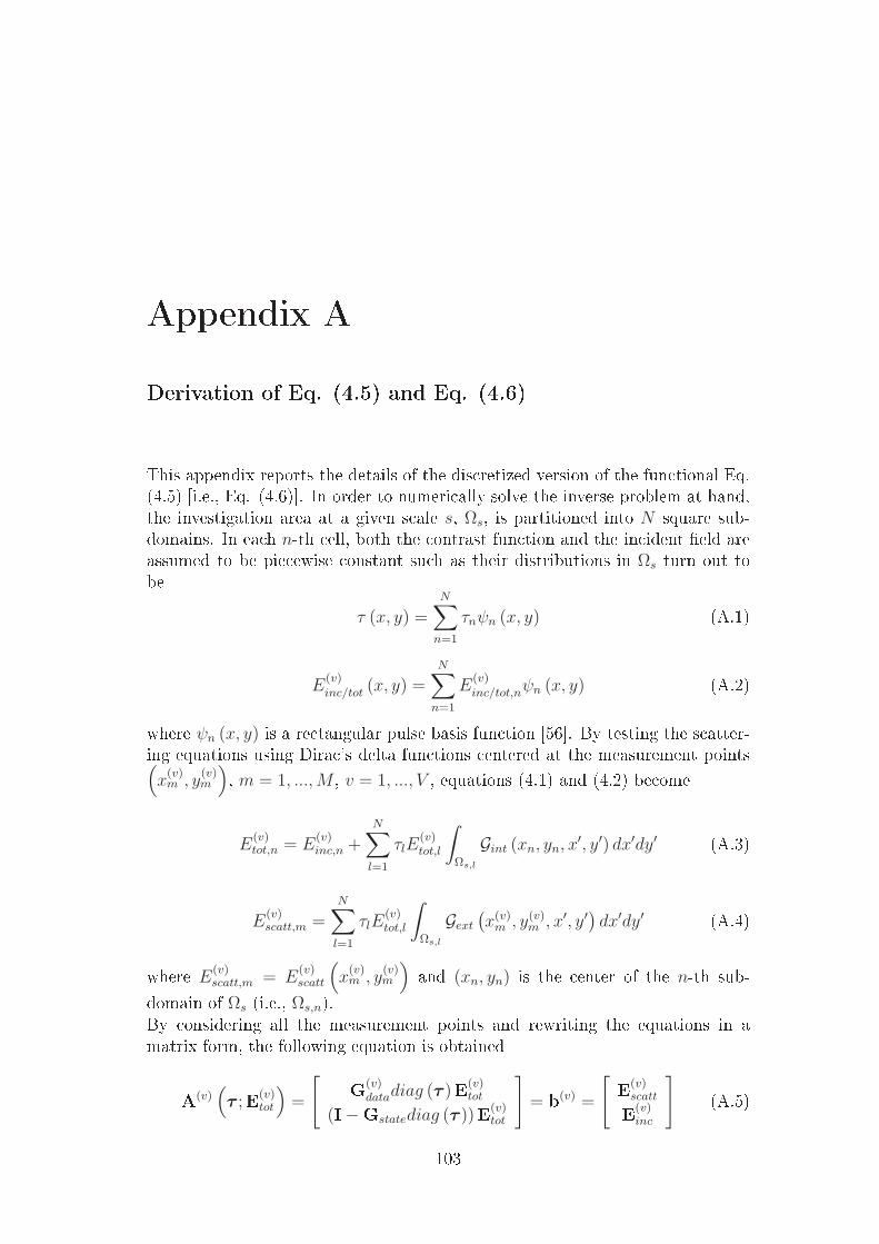
Appendix A
Derivation of Eq. (4.5) and Eq. (4.6)
This appendix reports the details of the dis retized version of the fun tional Eq.
(4.5) [i.e., Eq. (4.6). In order to numeri ally solve the inverse problem at hand,
the investigation area at a given s ale s, Ωs, is partitioned into N square sub-
domains. In ea h n-th ell, both the ontrast fun tion and the in ident eld are
assumed to be pie ewise onstant su h as their distributions in Ωs turn out to
be
τ (x, y) =
N∑
n=1
τnψn (x, y) (A.1)
E(v)inc/tot (x, y) =
N∑
n=1
E(v)inc/tot,nψn (x, y) (A.2)
where ψn (x, y) is a re tangular pulse basis fun tion [56. By testing the s atter-
ing equations using Dira 's delta fun tions entered at the measurement points(x(v)m , y
(v)m
), m = 1, ...,M , v = 1, ..., V , equations (4.1) and (4.2) be ome
E(v)tot,n = E
(v)inc,n +
N∑
l=1
τlE(v)tot,l
∫
Ωs,l
Gint (xn, yn, x′, y′) dx′dy′ (A.3)
E(v)scatt,m =
N∑
l=1
τlE(v)tot,l
∫
Ωs,l
Gext(x(v)m , y(v)m , x′, y′
)dx′dy′ (A.4)
where E(v)scatt,m = E
(v)scatt
(x(v)m , y
(v)m
)and (xn, yn) is the enter of the n-th sub-
domain of Ωs (i.e., Ωs,n).
By onsidering all the measurement points and rewriting the equations in a
matrix form, the following equation is obtained
A
(v)(τ ;E
(v)tot
)=
[G
(v)datadiag (τ )E
(v)tot
(I−Gstatediag (τ ))E(v)tot
]= b
(v) =
[E
(v)scatt
E
(v)inc
](A.5)
103
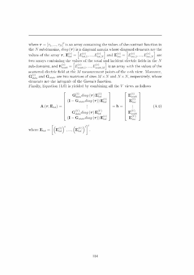
where τ = [τ1, ..., τN ]tis an array ontaining the values of the ontrast fun tion in
the N subdomains, diag (τ ) is a diagonal matrix whose diagonal elements are the
values of the array τ , E(v)tot =
[E
(v)tot,1, ..., E
(v)tot,N
]and E
(v)inc =
[E
(v)inc,1, ..., E
(v)inc,N
]are
two arrays ontaining the values of the total and in ident ele tri elds in the N
sub-domains, and E
(v)scatt =
[E
(v)scatt,1, ..., E
(v)scatt,M
]is an array with the values of the
s attered ele tri eld at the M measurement points of the v-th view. Moreover,
G
(v)data and Gstate are two matri es of sizesM×N and N×N , respe tively, whose
elements are the integrals of the Green's fun tion.
Finally, Equation (4.6) is yielded by ombining all the V views as follows
A (τ ;Etot) =
G
(1)datadiag (τ )E
(1)tot
(I−Gstatediag (τ ))E(1)tot
.
.
.
G
(V )datadiag (τ )E
(V )tot
(I−Gstatediag (τ ))E(v)tot
= b =
E
(1)scatt
E
(1)inc.
.
.
E
(V )scatt
E
(V )inc
(A.6)
where Etot =
[(E
(1)tot
)t
, ...,(E
(V )tot
)t]t.
104