ph.d. thesis dissertation: image super resolution using
TRANSCRIPT

School of Computer Engineering and
Telecommunications
Department of Computer Science and Artificial Intelligence
University of Granada
Ph.D. Thesis Dissertation:
Image Super Resolution UsingCompressed Sensing Observations
Written by: Supervised by:
Wael H. AlSaafin Dr. Miguel Vega
Dr. Rafael Molina
Doctorate Program in Information and
Communication Technologies


El doctorando D. Wael H. AlSaafin y los directores de la tesis Dr. MiguelVega y Dr. Rafael Molina, Profesores Titular y Catedratico de Universidad, re-spectivamente, del Departamento de Lenguajes y Sistemas Informaticos y Cien-cias de la Computacion e Inteligencia Artificial respectivamente, de la Univer-sidad de Granada
GARANTIZAMOS AL FIRMAR ESTA TESIS DOCTORAL
que el trabajo ha sido realizado por el doctorando bajo nuestra direccion y,hasta donde nuestro conocimiento alcanza, en la realizacion del trabajo se hanrespetado los derechos de otros autores a ser citados, cuando se han utilizadosus resultados o publicaciones.
Granada, a 28 de Marzo de 2016
Directores de la Tesis
Dr. Miguel Vega Dr. Rafael Molina
El Doctorando
D. Wael H. AlSaafin


Dedications
To my family...Especially Ahmad, Mohammad, and Saad


Acknowledgements
It was a great job, full of hardworking and determination. It could not succeed without the helpand support I could receive. Thanks to my supervisors Rafael Molina and Miguel Vega. Thanksalso to Aggelos Katssagelos, Javier Mateos, Salvador Villena, Bruno Amizic, and Gokhan Bil-gin, and my colleagues in CITIC for their cooperation and assistance. Thanks to University ofGranada, Yildiz Technical University and Erasmus Mundus program.Thank you all, you have made it an unforgettable successful period.
Wael

Contents
Resumen y Conclusiones xxi
Summary and Conclusions xxv
1 Introduction 1
1.1 Background . . . . . . . . . . . . . . . . . . . . . . . . . . . . . . . . . . . . . . . 2
1.1.1 Classical Digital Imaging . . . . . . . . . . . . . . . . . . . . . . . . . . . . 2
1.1.2 Color Images . . . . . . . . . . . . . . . . . . . . . . . . . . . . . . . . . . . 3
1.1.3 Millimeter Wave Images . . . . . . . . . . . . . . . . . . . . . . . . . . . . 4
1.1.4 Super Resolution . . . . . . . . . . . . . . . . . . . . . . . . . . . . . . . . 6
1.1.5 Compressed Sensing . . . . . . . . . . . . . . . . . . . . . . . . . . . . . . 11
1.2 Objectives and Hypothesis . . . . . . . . . . . . . . . . . . . . . . . . . . . . . . . 14
1.3 Methodology and Contributions . . . . . . . . . . . . . . . . . . . . . . . . . . . . 14
1.4 Thesis Document Structure . . . . . . . . . . . . . . . . . . . . . . . . . . . . . . . 15
2 State of the Art 17
2.1 Image Super Resolution Works . . . . . . . . . . . . . . . . . . . . . . . . . . . . . 17
2.1.1 Image Regularizers . . . . . . . . . . . . . . . . . . . . . . . . . . . . . . . 18
2.1.2 Image Registration . . . . . . . . . . . . . . . . . . . . . . . . . . . . . . . 20
2.1.3 Blur Model . . . . . . . . . . . . . . . . . . . . . . . . . . . . . . . . . . . . 21
2.2 Compressed Sensing Works . . . . . . . . . . . . . . . . . . . . . . . . . . . . . . 22

x Contents
2.3 CSSR Modeling and Formulation . . . . . . . . . . . . . . . . . . . . . . . . . . . 23
3 Compressive Sensing Super Resolution Algorithm 33
3.1 Preliminary Work . . . . . . . . . . . . . . . . . . . . . . . . . . . . . . . . . . . . 33
3.2 The Proposed CSSR Approach . . . . . . . . . . . . . . . . . . . . . . . . . . . . . 39
3.2.1 HR Image Estimation . . . . . . . . . . . . . . . . . . . . . . . . . . . . . . 40
3.2.2 Transformed Coefficient Estimation . . . . . . . . . . . . . . . . . . . . . . 41
3.2.3 Registration from Estimated HR Image . . . . . . . . . . . . . . . . . . . . 42
3.2.4 Registration from Estimated LR Reference Image . . . . . . . . . . . . . . 43
3.2.5 CSSR Algorithm Statement . . . . . . . . . . . . . . . . . . . . . . . . . . 44
3.3 Proposed Color CSSR (CCSSR) . . . . . . . . . . . . . . . . . . . . . . . . . . . . . 44
3.3.1 Modeling and Problem Formulation . . . . . . . . . . . . . . . . . . . . . 44
3.3.2 CCSSR Optimization Approach . . . . . . . . . . . . . . . . . . . . . . . . 45
3.3.3 CCSSR Algorithm Statement . . . . . . . . . . . . . . . . . . . . . . . . . . 48
4 Experimental Results 49
4.1 Quality Assessment . . . . . . . . . . . . . . . . . . . . . . . . . . . . . . . . . . . 49
4.2 Intra CSSR Analysis . . . . . . . . . . . . . . . . . . . . . . . . . . . . . . . . . . . 50
4.2.1 CS Reconstruction . . . . . . . . . . . . . . . . . . . . . . . . . . . . . . . . 50
4.2.2 Registration Estimation . . . . . . . . . . . . . . . . . . . . . . . . . . . . . 54
4.3 CSSR vs ID Works . . . . . . . . . . . . . . . . . . . . . . . . . . . . . . . . . . . . 59
4.4 CSSR vs SR Works . . . . . . . . . . . . . . . . . . . . . . . . . . . . . . . . . . . . 59
4.5 CSSR: The General Case . . . . . . . . . . . . . . . . . . . . . . . . . . . . . . . . 71
4.5.1 CSSR from a single image . . . . . . . . . . . . . . . . . . . . . . . . . . . 74
4.5.2 CSSR vs Sequential Approach . . . . . . . . . . . . . . . . . . . . . . . . . 85
4.5.3 CSSR1 vs CSSR2 . . . . . . . . . . . . . . . . . . . . . . . . . . . . . . . . . 86
4.6 CSSR of PMMW Images . . . . . . . . . . . . . . . . . . . . . . . . . . . . . . . . . 92
4.7 CCSSR of Color Images . . . . . . . . . . . . . . . . . . . . . . . . . . . . . . . . . 94
5 Conclusions and Future Work 103
5.1 Conclusions . . . . . . . . . . . . . . . . . . . . . . . . . . . . . . . . . . . . . . . 103

Contents xi
5.2 Future work . . . . . . . . . . . . . . . . . . . . . . . . . . . . . . . . . . . . . . . 104
Bibliography 105

xii Contents

List of Figures
1.1 Image representation: (a) gray scale image for the letter ’a’, (b) exaggerated ver-sion of the image (×16), (c) the corresponding pixel values. . . . . . . . . . . . . 3
1.2 RGB color Image. (a) Original RGB image, (b) Red channel, (c) Green channel,(d) Blue channel. (Adapted from [1]). . . . . . . . . . . . . . . . . . . . . . . . . . 4
1.3 YCbCr colored image. . . . . . . . . . . . . . . . . . . . . . . . . . . . . . . . . . 5
1.4 Electromagnetic wave spectrum . . . . . . . . . . . . . . . . . . . . . . . . . . . . 5
1.5 PMMW threat detect system. . . . . . . . . . . . . . . . . . . . . . . . . . . . . . . 6
1.6 Sample PMMW image of a man. . . . . . . . . . . . . . . . . . . . . . . . . . . . . 7
1.7 Illustartion of SR process . . . . . . . . . . . . . . . . . . . . . . . . . . . . . . . . 7
1.8 Degradation process illustrative example. (a) 256×256 Original Cameraman im-age, (b) Warped image, θ = −0.1047rad, c = 3, d = 2, (c) Blurred image, Gaussianblur with variance 3, (d) 64 × 64 Down-sampled image, P=4, (e) Noised image,white Gaussian noise SNR=40dB . . . . . . . . . . . . . . . . . . . . . . . . . . . 8
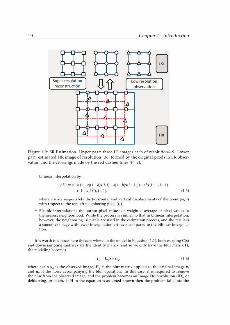
1.9 SR Estimation. Upper part: three LR images each of resolution= 9. Lower part:estimated HR image of resolution=36, formed by the original pixels in LR obser-vation and the crossings made by the red dashed lines (P=2). . . . . . . . . . . . 10
1.10 Bilinear interpolation. Given x at four neighboring pixels, find the intensityvalue at (m,n) . . . . . . . . . . . . . . . . . . . . . . . . . . . . . . . . . . . . . . 11
1.11 Typical CS camera . . . . . . . . . . . . . . . . . . . . . . . . . . . . . . . . . . . . 12
1.12 Compressed sensing acquisition model. Measurement matrix Φ with real en-tries, M=8, N=16 . . . . . . . . . . . . . . . . . . . . . . . . . . . . . . . . . . . . 13
2.1 q-th HR grid calculation. (a) HR grid (in black) and the q-th image grid (in red),(b) Detailed view of (a), with the pixel notation used for the bilinear interpolationof grid element (uq,vq) . . . . . . . . . . . . . . . . . . . . . . . . . . . . . . . . . 25

xiv List of Figures
2.2 Simulation process. Warped with motion vectors (0,0,0)t , (.0524,2,−3)t ,(−.0698,−1,−2)t , (−.0349,3,−1)t , Gaussian blur of variance 5, zooming factor 2,compression ratio R=0.6, SNR of added noise 30dB (a) Original Shepp-Logan im-age, (b) Four simulated LR images., (c) Four CS observations, (d) Original Lenaimage, (e) Four simulated LR images, (f) Four CS observations. . . . . . . . . . . 26
2.3 1-level discrete wavelet transform. (a) Barbara image (b) DWT decomposition . 30
2.4 3-level discrete wavelet transform decomposition. . . . . . . . . . . . . . . . . . 30
3.1 Sequential estimation process. Observations have been simulated using GaussianBlur of variance 3, zooming factor P=2, Gaussian circulant Toeplitz measurementmatrix with compression ratio R=0.8 and additive noise of SNR=40dB. (a) LRreconstructed observations, (b) initial estimate of HR image, PSNR=9.8 dB, (c)estimated HR image, PSNR=23.2 dB . . . . . . . . . . . . . . . . . . . . . . . . . 35
3.2 Joint estimation process. Observations have been simulated using Gaussian Blurof variance 3, zooming factor P=2, Gaussian circulant Toeplitz measurement ma-trix with compression ratio R=0.8, and additive noise of SNR=40dB. (a) First it-eration estimate with PSNR=22.8 dB, (b) last iteration estimate with PSNR=23.9dB . . . . . . . . . . . . . . . . . . . . . . . . . . . . . . . . . . . . . . . . . . . . . 37
3.3 Joint estimation process. Observations have been simulated using Gaussian Blurof variance 3, zooming factor P=2, Bernoulli circulant Toeplitz measurement ma-trix with compression ratio R=0.8 and additive noise of SNR=40dB. (a) First it-eration estimate with PSNR=22.7 dB, (b) last iteration estimate with PSNR=23.9dB . . . . . . . . . . . . . . . . . . . . . . . . . . . . . . . . . . . . . . . . . . . . . 38
3.4 Joint estimation process with motion estimation . Observations have been simu-lated using Gaussian Blur of variance 3, zooming factor P=2, Bernoulli circulantToeplitz measurement matrix with compression ratio R=0.8 and additive noiseof SNR=40dB. (a) Estimated image using the minimization in Equation (3.16),(b) estimated image using minimization in Equation (3.17) . . . . . . . . . . . . 38
4.1 LR 3-level Haar wavelet coefficient decay, using simulated observations (SNR=40 dB), (a,b) Cameraman image affected by Gaussian blur of variance 3 and 9,respectively. (c,d) Shepp-Logan image affected by blur of variance 3 and 9, re-spectively. . . . . . . . . . . . . . . . . . . . . . . . . . . . . . . . . . . . . . . . . 51
4.2 LR Cameraman image restoration using a simulated observation with blur vari-ance 3, zooming factor P=1, R=0.8, noise SNR= 40 dB. (a) LR reconstructed ob-servation using all elements of the coefficient vector aq (PSNR=22.65 dB), (b) LRreconstructed observation using the first 60% of elements in aq (PSNR=22.47dB), (c) LR reconstructed observation using the first 20% of elements in aq(PSNR=22.24 dB). Transform basis used is 3-level Haar wavelet transform. . . . 52

List of Figures xv
4.3 LR Shepp-Logan image restoration using a simulated observation with blur vari-ance 3, zooming factor P=1, R=0.8, noise SNR=40dB. (a) LR reconstructed ob-servation using all elements of the coefficient vector aq (PSNR=21.35 dB), (b) LRreconstructed observation using the first 60% of elements in aq (PSNR=21.18dB), (c) LR reconstructed observation using the first 20% of elements in aq(PSNR=20.68 dB). Transform basis used is 3-level Haar wavelet transform. . . . 53
4.4 Reconstruction of LR images. (a) Original HR Shepp-Logan image, (b,c) Down-sampled images Q=2, P=2, Blur Var=3, R=0.8, SNR=30 dB, (d,e) First estimatesof the LR images, PSNR= 40.22 dB and , 40.16 dB respectively, (f,g) Final esti-mates of the LR images, PSNR=42.88 dB and 42.77 dB respectively. PSNR valueswere calculated with respect to the simulated LR images. . . . . . . . . . . . . . 53
4.5 Reconstruction of LR images. (a) Cameraman original HR image, (b,c) Down-sampled images Q=2, P=2, Blur Var=3, R=0.8, SNR=30dB, (d,e) First estimatesof the LR images, PSNR=35.52 dB and 35.29 dB, respectively, (f,g) Final estimatesof the LR images, PSNR=35.55 dB and 35.34 dB, respectively. PSNR values werecalculated with respect to the simulated LR images. . . . . . . . . . . . . . . . . 54
4.6 Reconstruction of LR images. (a) Lena original HR image, (b,c) Down-sampledimages Q=2, P=2, Blur Var=3, R=0.8, SNR=30dB, (d,e) First estimates of the LRimages, PSNR=40.22 dB and 40.16 dB, respectively, (f,g) Final estimates of the LRimages, PSNR=42.88 dB and 42.77 dB, respectively. PSNR values were calculatedwith respect to the simulated LR images. . . . . . . . . . . . . . . . . . . . . . . . 55
4.7 Absolute error comparison of the four registration approaches. R=0.8, Q=4, blurvar=3, SNR=40dB. on (a) P=2, (b) P=4. . . . . . . . . . . . . . . . . . . . . . . . . 58
4.8 Proposed CSSR vs CS ID algorithms comparison (Blur Var=5, SNR=30dB, forCSSR P=1, Q=1). (a) Cameraman (b) Lena (c) Shepp-Logan. . . . . . . . . . . . . 63
4.9 Proposed CSSR vs CS ID algorithms comparison (Blur Var=3, SNR=40dB, forCSSR P=1, Q=1). (a) Cameraman, (b) Lena, (c) Shepp-Logan. . . . . . . . . . . . 64
4.10 Proposed CSSR vs CS ID algorithms comparison (R=0.6, SNR=30dB, for CSSRP=1, Q=1). (a) Cameraman, (b) Lena, (c) Shepp-Logan. . . . . . . . . . . . . . . 65
4.11 Proposed CSSR vs CS ID algorithms comparison (R=0.8, SNR=40dB, for CSSRP=1, Q=1). (a) Cameraman, (b) Lena, (c) Shepp-Logan. . . . . . . . . . . . . . . 66
4.12 Comparison between SR algorithms and the CSSR algorithm. P=4, SNR=40dB,Q=4, and for CSSR, R=1.0. (a) Cameraman image, (b) Lena, (c) Shepp-Loganimage. . . . . . . . . . . . . . . . . . . . . . . . . . . . . . . . . . . . . . . . . . . . 69
4.13 Comparison between SR algorithms and the CSSR algorithm. P=4, SNR=30dB,Q=4, and for CSSR, R=1.0. (a) Cameraman image, (b) Lena, (c) Shepp-Loganimage. . . . . . . . . . . . . . . . . . . . . . . . . . . . . . . . . . . . . . . . . . . . 70
4.14 Original Images. (a) Satellite, (b) Barbara, (c) Peppers, (d) Alhambra. . . . . . . 71
4.15 Performance of the CSSR algorithm (Q=4). Case 1: P=2, Blur Var=3, SNR=40dB, Case 2: P=2, Blur Var=5, SNR=30 dB, Case 3: P=4, Blur Var=3, SNR=40 dB,Case 4: P=4, Blur Var=5, SNR=30 dB. (a) Satellite image, (b) Barbara image. . . 75

xvi List of Figures
4.16 Performance of the CSSR algorithm (Q=4). Case 1: P=2, Blur Var=3, SNR=40dB, Case 2: P=2, Blur Var=5, SNR=30 dB, Case 3: P=4, Blur Var=3, SNR=40 dB,Case 4: P=4, Blur Var=5, SNR=30 dB. (a) Peppers image, (b) Alhambra image . . 76
4.17 Estimated Satellite Images using the proposed CSSR method (R=0.8 and Q=5).(a) P=2, Blur Var=3, (b) P=2, Blur Var=5, (c) P=4, Blur Var=3, (d) P=4, Blur Var=5. 79
4.18 Estimated Barbara Images using the proposed CSSR method (R=0.8 and Q=5).(a) P=2, Blur Var=3, (b) P=2, Blur Var=5, (c) P=4, Blur Var=3, (d) P=4, Blur Var=5. 80
4.19 Estimated Peppers Images using the proposed CSSR method (R=0.8 and Q=5).(a) P=2, Blur Var=3, (b) P=2, Blur Var=5, (c) P=4, Blur Var=3, (d) P=4, Blur Var=5. 81
4.20 Estimated Alhambra Images using the proposed CSSR method (R=0.8 andQ=5).(a) P=2, Blur Var=3, (b) P=2, Blur Var=5, (c) P=4, Blur Var=3, (d) P=4, Blur Var=5. 82
4.21 CSSR performance for multiple and single input images. (P=4, Blur Var=3,SNR=40 dB. on (a) Satellite, (b) Barbara. . . . . . . . . . . . . . . . . . . . . . . . 83
4.22 CSSR performance for multiple and single input images. (P=4, Blur Var=3,SNR=40 dB. on (a) Peppers, (b) Alhambra. . . . . . . . . . . . . . . . . . . . . . . 84
4.23 Comparison of the proposed CSSR vs the sequential approach for the Satelliteimage, (Q=4, P=4), using (a) Blur Var=5, SNR=30 dB, (b) Blur Var=3, SNR=40dB. . . . . . . . . . . . . . . . . . . . . . . . . . . . . . . . . . . . . . . . . . . . . 86
4.24 Comparison of the proposed CSSR vs the sequential approach for the Barbaraimage, (Q=4, P=4), using (a) Blur Var=5, SNR=30 dB, (b) Blur Var=3, SNR=40dB. . . . . . . . . . . . . . . . . . . . . . . . . . . . . . . . . . . . . . . . . . . . . 87
4.25 Comparison of the proposed CSSR1 vs CSSR2 for the Satellite image, (Q=4, P=4),using (a) Blur Var=5, SNR=30 dB, (b) Blur Var=3, SNR=40 dB. . . . . . . . . . . 90
4.26 Comparison of the proposed CSSR1 vs CSSR2 algorithms for the Barbara image,(Q=4, P=4), using (a) Blur Var=5, SNR=30 dB, (b) Blur Var=3, SNR=40 dB. . . . 91
4.27 PMMW image of a man free of threats (Q=4, R=1, P=2).(a) Four noisy real ob-servations, (b) Bilinear interpolation from one reconstructed LR image, (c) Esti-mated image using CSSR algorithm. . . . . . . . . . . . . . . . . . . . . . . . . . . 93
4.28 PMMW image of a man free of threats (Q=4, R=0.8, P=2) (a) Four noisy realobservations, (b) Bilinear interpolation from one reconstructed LR image, (c) Es-timated image using CSSR algorithm. . . . . . . . . . . . . . . . . . . . . . . . . . 94
4.29 PMMW image of amanwith a threat attached to his arm (Q=4, R=0.8). (a) LR im-ages, (b) Bilinear interpolation from one reconstructed image, P=2, (c) EstimatedHR image using the CSSR algorithm, P=2, (d) Bilinear interpolation from onereconstructed image, P=4, (e) Estimated HR image using the CSSR algorithm, P=4. 95
4.30 PMMW image of a man with a threat attached to his chest (Q=7, R=0.8, P=2).(a) LR images, (b) Bilinear interpolation from one reconstructed LR image, (c)Estimated HR image using the CSSR algorithm. . . . . . . . . . . . . . . . . . . . 96
List of Figures xvii
4.31 Original Images (a) Barbara, (b) Lena, and (c) Peppers. (d) Simulated LR Barbaraimage (s = [.1222,−2,3]t , blur variance 7, P=2), (e) simulated CS observation(R=0.5, SNR=40 dB). The black line represents the added zero-valued entriesto illustrate a square image. . . . . . . . . . . . . . . . . . . . . . . . . . . . . . . 98
4.32 Comparison between CS algorithms and the CCSSR algorithm for the Lena im-age. For CCSSR, P=1, Q=3. . . . . . . . . . . . . . . . . . . . . . . . . . . . . . . . 99
4.33 Performance of the proposed CCSSR vs R. Blur Var=5, SNR=40dB,Q=3. (a) P=2,(b) P=4. . . . . . . . . . . . . . . . . . . . . . . . . . . . . . . . . . . . . . . . . . . 100
4.34 Reconstructed Peppers Images using the CCSSR algorithm. R=0.6, Blur Var=5,SNR=40dB, and Q=3. (a) P=2, (b) P=4, . . . . . . . . . . . . . . . . . . . . . . . 101
4.35 Image super resolution from real observations, R=0.8, P=2. (a) First 4 LR images(b) Bilinear interpolation of one reconstructed LR image, (c) Estimated HR imageusing the CCSSR algorithm, withQ=4, (d) Estimated HR image using the CCSSRalgorithm, with Q=16. . . . . . . . . . . . . . . . . . . . . . . . . . . . . . . . . . 101
4.36 Image super resolution from real observations, R=0.8, P=2. (a) First 4 LR images(b) Bilinear interpolation of one reconstructed LR image, (c) Estimated HR imageusing the CCSSR algorithm, withQ=4, (d) Estimated HR image using the CCSSRalgorithm, with Q=16. . . . . . . . . . . . . . . . . . . . . . . . . . . . . . . . . . 102


List of Tables
4.1 Registration parameter estimation at the HR level for the Shepp-Logan image,Q=4, Blur var=3, SNR=40dB, R=0.8. (a) using App1, (b) using App2 . . . . . . 56
4.2 Registration parameter estimation at the LR level for the Shepp-Logan image,Q=4, Blur var=3, SNR=40dB, R=0.8. (a) using App3 (b) using App4 . . . . . . . 57
4.3 Performance comparison of state-of-the-art CS ID algorithms with proposedCSSR algorithm for the Cameraman image. For CSSR P=1 and Q=1. In boldblue are the highest PSNR values. . . . . . . . . . . . . . . . . . . . . . . . . . . . 60
4.4 Performance comparison of state-of-the-art CS ID algorithms with proposedCSSR algorithm for the Lena image. For CSSR P=1 andQ=1. In bold blue are thehighest PSNR values. . . . . . . . . . . . . . . . . . . . . . . . . . . . . . . . . . . 61
4.5 Performance comparison of state-of-the-art CS ID algorithms with proposedCSSR algorithm for the Shepp-Logan image. For CSSR P=1 and Q=1. In boldblue are the highest PSNR values. . . . . . . . . . . . . . . . . . . . . . . . . . . . 62
4.6 Comparison of state-of-the-art SR algorithms with the CSSR algorithm for Cam-eraman and Lena images, with Q=4 and for CSSR R=1.0. In bold blue are thehighest PSNR values. . . . . . . . . . . . . . . . . . . . . . . . . . . . . . . . . . . 67
4.7 Comparison of state-of-the-art SR algorithms with the CSSR algorithm forShepp-Logan image, with Q=4 and for CSSR R=1.0. In bold blue are the highestPSNR values. . . . . . . . . . . . . . . . . . . . . . . . . . . . . . . . . . . . . . . . 68
4.8 Performance of the CSSR algorithm for the Satellite and Barbara images, usingQ = 4. . . . . . . . . . . . . . . . . . . . . . . . . . . . . . . . . . . . . . . . . . . . 72
4.9 Performance of the CSSR algorithm for the Peppers and Alhambra images, usingQ = 4. . . . . . . . . . . . . . . . . . . . . . . . . . . . . . . . . . . . . . . . . . . . 73
4.10 Performance of the CSSR algorithm for the Satellite and Brabara images, using asingle observation (Q = 1). . . . . . . . . . . . . . . . . . . . . . . . . . . . . . . . 77

xx List of Tables
4.11 Performance of the CSSR algorithm for the Peppers and Alhambra images, usinga single observation (Q = 1). . . . . . . . . . . . . . . . . . . . . . . . . . . . . . . 78
4.12 Performance of the sequential approach using Q = 4. . . . . . . . . . . . . . . . . 85
4.13 Comparison of CSSR1 vs CSSR2 algorithms for the Satellite image, using Q = 4. 88
4.14 Comparison of CSSR1 and CSSR2 algorithms for the Barbara image, using Q = 4. 89
4.15 Comparison of CS algorithms with the proposed CCSSR algorithm for CCSSRP=1.0, Q=3. In bold blue are the highest PSNR values. . . . . . . . . . . . . . . . 97
4.16 CCSSR algorithm vs R (blur var 5, SNR=40dB, and Q=3). . . . . . . . . . . . . . 99

Resumen y Conclusiones
Resumen
El Sensado Comprimido (SC) es una nueva tecnologıa que permite la captacion de imagenesdirectamente comprimidas, con la consiguiente reduccion del tiempo de adquisicion y de lacantidad de memoria necesaria para almacenarlas, procesarlas y trasmitirlas. La teorıa de SCestablece que una imagen o senal que admita una representacion rala se puede reconstruir a par-tir de un conjuntomuy incompleto demedidas o proyecciones de la imagen. La Superresolucion(SR) es una tecnica de procesamiento de imagenes muy poderosa que permite reconstruir unao mas imagenes de Alta Resolucion (AR) a partir de varias imagenes de Baja Resolucion (BR).La obtencion de imagenes de AR de buena calidad mediante la aplicacion de tecnicas de SRrequiere la aplicacion de un buen proceso de registro de las imagenes observadas. La SR per-mite superar las limitaciones hardware, opticas y espaciales de los dispositivos de captacion deimagenes para obtener imagenes de buena calidad.
En la presente tesis doctoral proponemos un nuevo marco de estudio para la obtencion deimagenes de AR a partir de varias imagenes de BR de la misma escena adquiridas mediantesistemas de SC. La hiptesis de que cuando una imagen admite una representacin rala en undominio transformado, una versin borrosa de la misma tambin admitir una representacin ralaen el dominio transformado, nos permite recuperar imgenes borrosas a partir de observacionesde SC. Por analogıa, tambien se puede asumir que a una imagen de BR desplazada, borrosay submuestreada se le puedan aplicar tecnicas de SC. El nuevo marco de estudio de Super-resolucion de Sensado Comprimido (SRSC) propuesto en esta tesis combina la aplicacion dealgoritmos de reconstruccion de SC previamente existentes con una nueva tecnica de SR basadaen la aplicacion de una regularizacion robusta que favorece la raleza de las imagenes, basadaen un modelo a priori Bayesiano superGausiano.
El problema SRSC tiene muchas incognitas, principalmente la imagen de AR, los coefi-cientes de la representacion en el dominio trasformado de cada imagen de BR, y los vectores dedesplazamientos. Estas incognitas se pueden estimar de forma secuencial o simultaneamente.El metodo propuesto en esta tesis aplica una estrategia de estimacion conjunta en la que lasreconstrucciones de las imagenes de BR y la estimacion de la imagen de AR se llevan a cabosimultaneamente de forma alternativa, e incluye una estimacion automatica de los vectores dedesplazamientos. En este trabajo se estudian las ventajas de la estimacion conjunta respectoa la estrategia secuencial. En la tesis se estudia tambien lo que aporta la utilizacion de variasimagenes de BR en lugar de una sola.
El enfoque del SRSC trasforma el problema de estimacion conjunta con restricciones en

xxii Chapter 0. Resumen y Conclusiones
una secuencia de subproblemas no restringidos, mediante la aplicacion del Metodo de los Mul-tiplicadores en Direcciones Alternativas (MMDA). El subproblema de estimacion de la imagende AR se resuelve aplicando la tecnica de mayorizacion-minimizazion. Para la estimacion delos parametros de registro de las imagenes se proponen cuatro estrategias diferentes, que soncomparadas en este trabajo. El subproblema de la reconstruccion de SC se plantea como mini-mizacion de la norma ℓ1 sujeto a una restriccion cuadratica.
El metodo propuesto se ha probado para imagenes naturales reales en escala de grises cuyasobservaciones SC han sido simuladas y sintetizadas utilizando una matriz de medicion que esposible elaborar practicamente. Se han realizado comparaciones del metodo propuesto conalgoritmos del estado del arte en SR que no aplican SC y tambien con algoritmos del estadodel arte en deconvolucion de imagenes de SC. Estas comparaciones han resultado favorables almetodo SRSC propuesto. Tambien se han obtenido excelentes resultados en experimentos enlos que intervenıan tanto el SC como la SR, aunque estos no se han podido comparar con otrosmetodos, porque no hay trabajos publicados, aparte de los nuestros, que estudien este problemaal completo.
Una de las posibles e importantes aplicaciones del SRSC es el de las Imagenes MilimetricasPasivas (IMMP), muy utiles en problemas de deteccion de amenazas ocultas. Los experimentosrealizados con SRCS sobre IMMP reales con observaciones SC sinteticas han mostrado que esposible aplicar el marco de estudio propuesto para obtener imagenes de SR de alta calidad apartir de varias imagenes de BR adquiridas mediante SC, lo que se espera pueda facilitar losprocesos de deteccion de amenazas ocultas.
Se ha extendido el SRSC para abordar tambien el problema de Superresolucion de SensadoComprimido de imagenes en Color (SRSCC), para el que tambien se ha propuesto un algoritmoque es otra de las aplicaciones de este trabajo. El SRSCC permite obtener imagenes en colorde SR a partir de varias imagenes reales en color obtenidas mediante SC. El SRSCC se aplica aobservaciones SC independientes de los canales rojo, verde y azul (RVA) de la imagen obtenidasutilizando una matriz de medicion que es posible elaborar practicamente. En el SRSCC laestimacion de los parametros de registro se realiza conjuntamente para los tres canales. En estetrabajo se incluyen comparaciones entre los resultados del algoritmo SRSCC propuesto y losobtenidos aplicando otras tecnicas de reconstruccion de SC de imagenes en color.
Conclusiones
En esta tesis doctoral hemos propuesto un nuevo marco de estudio para la SR de imagenesa partir de varias imagenes sin registrar de BR adquiridas mediante tecnicas de SC. Cualquiertecnica clasica de SR y/o de SC podrıa integrarse en la metodologıa desarrollada. En este trabajose ha propuesto un modelo de degradacion para este novedoso problema combinado y tambienun enfoque para el SRSC. Este trabajo ha sido el primero en tratar el problema propuesto ypodrıa resultar muy util para el campo del procesamiento de imagenes.
El metodo SRSC permite disminuir la frecuencia de muestreo, la velocidad de trasmisiony el ancho de banda requeridos para la transmision de imagenes, ası como los requerimientosde memoria del almacenamiento y proceso de las mismas. Tambien permite un menor tiempode adquisicion de las imagenes, de mucho interes en aplicaciones medicas y de procesamientode IMMP. La mejor calidad de las imagenes de SR facilita el reconocimiento de patrones y ladiagnosis medica y permite realzar zonas especıficas de las imagenes de videovigilancia o desatelite.

xxiii
El metodo de reconstruccion propuesto utiliza una nueva regularizacion robusta que fa-vorece la raleza de las imagenes de AR obtenidas resolviendo una ecuacion lineal en x (la ima-gen de AR)mediante la aplicacion del metodo del gradiente conjugado. El vector de coeficientesde la representacion en el dominio trasformado de las imageness de BR se estima minimizandola norma ℓ1 sujeta a una restriccion cuadratica. Se pueden aplicar cuatro procedimientos difer-entes de estimacion de los paraetros de registro que permiten determinarlos con precision; estoes muy importante porque existe una dependencia crıtica entre la calidad de las imagenes deSR y la eficacia del proceso de registro. El registro puede realizarse con respecto a la imagen deAR o entre las imagenes de BR, lo que resulta en una menor dependencia respecto a los valoresiniciales utilizados.

Summary and Conclusions
Summary
Compressed Sensing (CS) is a new technology that simultaneously acquires and compressesimages reducing acquisition time and memory requirements to process or transmit them. It es-tablishes that a sparsely representable image/signal can be recovered from a highly incompleteset of measurements or projections of the image. Image Super Resolution (SR) is an importantpost-processing technique where multiple input images are super resolved to obtain one ormore images of higher resolution and better quality. SR necessitates a good image registrationprocedure in order to obtain a High Resolution (HR) image of enhanced quality. Such qualityshould overcome image degradation due to system hardware, optical and spatial limitations.
In this dissertation we propose a novel framework to obtain HR images from CS imagingsystems capturing multiple Low Resolution (LR) images of the same scene. The assumptionthat when an image admits a sparse representation in a transformed domain, a blurred versionof it will also be sparse in the transformed domain allows us to recover blurred images from CSobservations Similarly, a warped, blurred, and down-sampled LR image is expected to be alsosparse in a transformed domain and hence can be reconstructed from the corresponding CSobservation. The proposed Compressed Sensing Super Resolution (CSSR) approach, combinesexisting CS reconstruction algorithms with an LR to HR approach based on the use of a newrobust sparsity promoting prior based on super Gaussian regularization.
The CSSR problem has multiple unknowns, mainly the HR image, the transformed coeffi-cients corresponding to each LR image, and themotion vectors. The unknowns can be estimatedsequentially or simultaneously. The method we propose in this dissertation is a joint estima-tion framework where LR reconstructions and HR estimation are carried out simultaneously byalternating between them including the automatic estimation of registration parameters. Theadvantages of the joint estimation over the sequential approach are discussed in this work. Theadvantage of utilizing multiple input images over a single one is also discussed in this disserta-tion.
The CSSR approach converts the constrained joint optimization problem into a sequenceof unconstrained sub-problems using Alternate Direction Method of Multipliers (ADMM). TheHR image estimation sub-problem is solved using majorization-minimization. The registrationparameters are estimated using four different approaches, which are compared in this work.The CS reconstruction sub-problem becomes an ℓ1 minimization subject to a quadratic con-straint.

xxvi Chapter 0. Summary and Conclusions
Our proposed framework has been tested on gray scale simulated and synthetically com-pressed real natural images, which were compressed using a measurement matrix that can besynthesized practically. This is compared with state-of-the-art SR algorithms which do not useCS in their work, and with state-of-the-art image deconvolution algorithms from CS images,which do not use down-sampling in their work. The proposed CSSR performs favorably com-pared to them. Moreover, the proposed CSSR has been tested when both compression anddown-sampling are present. In this case, no comparison with other methods is provided sincethis is the first time both problems are approached jointly.
One important CSSR application is Passive Millimeter Wave (PMMW) images which areused for threat detection. The performed CSSR experiments on synthetically compressed realmillimeter wave images, demonstrate the capability of the proposed framework to providevery good quality super resolved images frommultiple low resolution compressed acquisitions,which is expected to improve threat detection rates.
CSSR can be extended to the proposed Color Compressed Sensing Super Resolution (CC-SSR) algorithm, which constitutes another application of this work. In the CCSSR the SR imageis estimated from true color CS observations. While the red, green, blue (RGB) channels aresensed separately using a measurement matrix that can be synthesized practically, the regis-tration parameters are jointly estimated from the three channels simultaneously. This workcompares the proposed CCSSR algorithm with other color CS reconstruction techniques.
Conclusions
In this dissertation we have proposed a novel framework to reconstruct SR images from mul-tiple unregistered LR images acquired using CS techniques. Any classical SR and/or CS tech-niques can be incorporated in the developed methodology. The degradation model of this novelcombined problem has been modeled and a CSSR approach has been proposed in this work.
The CSSR method lowers the sampling frequency, transmission rates, and the bandwidthof the image signal, and memory requirements to store and/or send the image. Moreover,the acquisition time can be lowered, which is very important in medical and PMMW imagingapplications. The enhanced SR image quality is advantageous in pattern recognition, medicaldiagnostics, and to emphasize a specific area of an image in surveillance cameras and satelliteapplications.
The proposed HR reconstruction uses a new robust sparsity promoting prior and solvesa linear equation in x (the HR image), using conjugate gradient method. The transformedcoefficient vector estimation is an ℓ1 norm subject to a quadratic term optimization problem.The registration parameters can be estimated using four different procedures, to finally obtainaccurate results, since any SR estimation process is highly dependent on the performance of theregistration estimation step. The parameters can be estimated from the estimated HR image,or the LR images themselves, with the estimation from reconstructed LR images being lesssensitive to the initial conditions. Furthermore we found that the estimation at LR level resultsin better quality of the reconstructed image.
The proposed optimization framework uses ADMM to jointly estimate all the unknownsincluding HR image, LR images, and registration parameters. We have experimentally shownthat this simultaneous reconstruction outperforms the sequential method, that first performsLR reconstruction to then obtain an HR image from a set of LR observations. The sequential ap-

xxvii
proach estimates every unknown just once, while the alternate approach iteratively updates theestimated unknowns. The better performance of the alternate approach is due to the additionalinformation provided during the estimation process.
We also showed experimentally the enhancement obtained due to themultiple input imageswhen compared with a single one. This is expected due to the additional information everyinput image provides. However, the multiplicity necessitates accurate registration estimationprocedure which inherently affects the overall process.
The proposed framework has been tested and compared, at a unity compression ratio, withstate-of-the-art SR algorithms which do not use compression in their work. It has been alsocompared, at a unity zooming factor, with state-of-the-art ID algorithms that deblur CS images,which do not use down-sampling in their work. Both comparisons used synthetic images andshowed better performance of the proposed CSSR over others. The performance of CSSR whenusing practical values of P and R has also been tested and analyzed.
Besides, the CSSR effectiveness has been demonstrated experimentally on synthetically CSnoisy real images. This represents the practical application of the CSSR method, which showedvery good results. The proposed framework can be extended to CS video for the estimation ofboth intra-frame and inter-frame SR.
The proposed CSSR method has been tested on PMMW images. These images usually havepoor qualities and limited resolution, which makes super resolving them a challenging task andis a hard test of the CSSR approach. The CSSR could be used to improve the quality of PMMWimages. This is expected to improve threat detection rates, which is an expected field of futureresearch. Notice here that the nature of PMMW is similar to astronomical images and medicalimages, and the good performance of the proposed CSSR algorithm can be extended to theseimages.
The proposed approach can also be applied to true color CS images. The separately sensedchannels are utilized in a joint registration estimation to effectively and accurately estimateregistration parameters for the three channels. The obtained results present an excellent imagequality, even better than the obtained using previous CS reconstruction methods which corre-late the color channels. The efficient optimization process can be extended in future works todeal with mosaic color images.


Chapter 1
Introduction
This work is devoted to estimate High Resolution (HR) images frommultiple Low Resolution(LR) observations acquired using Compressed Sensing (CS) techniques. We propose a frame-work that combines Super Resolution (SR) reconstruction with CS acquisition.
CS imaging lowers the sampling frequency beyond that required by the Nyquist-Shannontheorem, and hence lowers transmission rate and bandwidth requirements. The smaller datasize obtained during the acquisition process lowers the memory requirements to save or trans-mit. Another important benefit CS offers is the lower acquisition time, due to the smaller datasize, which is vital in applications like medical imaging and millimeter wave images.
Furthermore, SR offers a higher pixel density and overcomes the limited resolution imag-ing. The higher resolution enhances the image quality by showing more details of the originalscene. Resolution enhancement is needed in computer vision applications like pattern recogni-tion and analysis of images, in medical imaging for diagnosis, and in applications that requirespecific areas of the image to be zoomed, like surveillance cameras, satellite applications, andthreat detection devices. Moreover, SR promises a better use of high performance screens, likeHigh Definition Liquid Crystal Displays (HD LCDs).
In the framework proposed in this dissertation, classical SR methods are combined withexisting CS methods. The experimental results to be presented will prove the applicability ofthis framework, and the good quality of the output images.
This chapter introduces basic background to this dissertation, then presents its motivations,hypothesis, and objectives. This is followed by stating the research methodology and maincontributions of this work. Finally, the thesis outline is presented.

2 Chapter 1. Introduction
1.1 Background
Independently of how well designed an imaging system is, its performance comes to a certainlimit. Limitations on image spatial resolution lead to the use of SR techniques to improve thepictorial perception of the human eye and/or automatic machines. After a certain limit, animaging system suffers frommany hardware problems, such as limited pixel density, lens pointspread function and aberration effects. Other problemsmay accompany the acquisition process,such as blurring due to motion of the camera or objects in the scene. The acquired images canbe considered as decimated LR versions of the original scene. These LR images can be used toestimate an HR image using SR techniques.
SR techniques are post-processing techniques, they use multiple LR images as input imagesto estimate one, or more, HR output image(s). The process increases the spatial resolution,removes degradations in the input images, and increases the high frequency content of thescene image.
Traditionally, all pixel values of the LR image have to be acquired. However, this informa-tion can be successfully recovered from only a small number of linear projections utilizing CStechniques. This dissertation studies how to estimate SR images from CS observations.
1.1.1 Classical Digital Imaging
Adigital image is a discrete representation of both spatial coordinates and intensity informationin a scene. The spatial information is determined by an array of sensors or pixels at fixedpositions of the image plane of the camera. Every pixel receives a different optical intensity.Hence, each sensor integrates the image locally to form the whole representation with othersensors. An imaging sensor can be a Charge-Coupled Device (CCD) or a ComplementaryMetal-Oxide-Semiconductor (CMOS) active-pixel sensor.
An image can be represented mathematically using a two-dimensional (2D) array. Thecoordinates represent the spatial information and the intensity is represented by the value atthe corresponding coordinates.
Figure 1.1(a) shows a 14 × 12 gray scale image for the letter ’a’. The image layout wasexaggerated in Figure 1.1(b) to show every pixel in the image, with the horizontal and verticalcoordinates of all pixels representing the image. The value at a pixel represents the intensity,scaled to the range [0,1], sensed by the corresponding sensor at the same location, shown inFigure 1.1(c). The highest value represents the White color, and the lowest represents the Blackcolor. In summary, the image shown in Figure 1.1(a) can be represented by the 2D matrix shownin Figure 1.1(c).
The pixel density of a camera, measured in pixels per unit area, determines its spatial reso-lution. Given a CCD or CMOS size, we would like to use the largest possible number of sensors.However, aside from hardware cost, decreasing the sensor size results in a lower incident lightand hence increases the shot-noise. The increased number of pixels also decreases the cameraspeed [2]. This forms the first limitation on the spatial resolution of imaging systems.
The camera lens also adds optical limitations on the image details, and some high-frequencycomponents may be lost due to the point spread function of the lens, aberration effects andaperture diffraction (see [3]). Camera or object motion in the scene may affect negatively the

1.1. Background 3
(a) (b) (c)
Figure 1.1: Image representation: (a) gray scale image for the letter ’a’, (b) exaggeratedversion of the image (×16), (c) the corresponding pixel values.
imaging process.
Particular applications may add some additional limitations, such as portability in surveil-lance cameras, cell phone built-in cameras, and satellite imaging, among others. Furthermore,notice also that the resolution is limited by the camera speed, memory size, and physical con-straints.
On the other hand, as stated by the Nyquist Shannon sampling theorem, high spatial resolu-tion of an image necessitates high sampling frequencies for a better acquisition and processing.This requires a high bandwidth, or bit rate to send or process the image. The solution for such achallenge could be compression techniques that seek for a compact representation of acquiredimages. Many compression techniques have been utilized to better represent an image. Trans-form coding, for example, makes use of sparsity and compressibility of an image.
For a given image quality, the higher the difference between the rate after compressing theimage, and the nominal bandwidth of the original version the better compression technique is.Based on this, many standards such as JPEG, JPEG2000, MPEG, and MP3 are used.
1.1.2 Color Images
In gray scale images, there is only one intensity value for each pixel, while color images needmore intensity values, or channels, to be represented as is the case in Red-Green-Blue (RGB)representation, which uses three channels, one per color. Figure 1.2 shows how the RGB chan-nels look like.

4 Chapter 1. Introduction
RGB representation is inherently difficult for humans to work with and it is not related tothe natural way the human eye perceive colors, see [1]. An alternative representation is theYCbCr color space. Y is the luminance, Cb chroma is the blue difference, and Cr chroma isthe red difference. The nominal values of chroma range from -0.5 to 0.5 when Y is normalizedto the range [0,1]. Figure 1.3 shows how the three channels look like. YCbCr is a practicalapproximation to color processing and perceptual uniformity and is used in standard definitiontelevision.
(a) (b)
(c) (d)
Figure 1.2: RGB color Image. (a) Original RGB image, (b) Red channel, (c) Green chan-nel, (d) Blue channel. (Adapted from [1]).
A color image is represented by a 3 dimensional matrix. If the gray scale image uses an x×ymatrix, then the corresponding color image utilizes an x×y ×3 matrix. In Chapter 4 we discussthe ability to extend SR from CS observations to color images, as an application of the proposedCSSR framework.
1.1.3 Millimeter Wave Images
Electromagnetic wave (EM) spectrum extends from Extra Low Frequency (ELF) signals, withfrequencies of few Hertz (Hz), to Gamma rays, with frequencies in powers of 1018 Hz (exaHertz, EHz). The wavelength of a signal is inversely proportional to its frequency and extendsfrom 108m for ELF to 10−12m for Gamma rays. The EM wave spectrum is shown in Figure 1.4,with the borders between bands being not strict and may vary slightly from one reference toanother.
Of special interest in the EM wave spectrum is the visible light spectrum which extendsfrom 400THz, at the border of the red color, to 789THz, at the border of the violet color. Thisrange defines the various colors the human eye can distinguish. The wavelet range for this

1.1. Background 5
Figure 1.3: YCbCr colored image.
Figure 1.4: Electromagnetic wave spectrum
spectrum is from 620nm to 450nm. Images acquired using the radiations in this band areusually called natural images and can be recognized by the human eye.
Another important frequency band is the Millimeter (MM) wave spectrum. MM waves arethose signals of wavelengths in millimeters, from 1mm to 10mm. This lies in the ExtremelyHigh Frequency (EHF) range that extends from 30GHz to 300GHz, although not all this rangehas been used practically in millimeter wave imaging.
The main advantage of MM waves is its penetrability through a variety of materials likeclouds, fog, smoke, sandstorms, and even through clothes. This enables a good performance inlow-visibility conditions. Also, it serves in day and night conditions [4].
An MMW imager, or scanner, can be of two types: Active and Passive. Active imagers usea MMW source to illuminate the scene. Passive imagers do not use any artificial MMW source,

6 Chapter 1. Introduction
instead they work with MMW radiation that occurs naturally in the scene. In the experimentalpart of the dissertation, we use Passive Millimeter Wave (PMMW) images. An example of thePMMW imager is the system shown in Figure 1.5, which is widely used at airports for threatdetection.
Figure 1.5: PMMW threat detect system.
Both types of imagers form images through the detection of MMW radiation from a scene.The detected radiation relies on the idea that objects reflect and emitMMW radiation differentlydepending on the emissivity of the object, which is a function of the nature of the object itself. Aperfect absorber object has a unity emissivity, while a perfect non absorber (reflector) has zeroemissivity. Depending on variations in emissivities of various scene materials, which differfrom an object to another, the power will be differently radiated from various objects in theimage. The radiated powers in the scene are detected by the MMW detector, then translated, ina way, to different brightness levels of the image. Figure 1.6 shows a typical PMMW image of aman.
MMW imaging has many advantages like high sensitivity to metal objects, and it is sug-gested in applications requiring near-all-weather operations since the changes in performancedue to weather variations are minimal. Many applications like aircraft landing and guidance,low-visibility navigation, situational awareness, and concealed threat detection, to name a fewbenefit from MMW imaging.
1.1.4 Super Resolution
As we have already indicated, both hardware limitations, such as sensor size, camera speed,cost, and optical limitations such as blurring action, etc. make it necessary to explore alternativeways to enhance the resolution of an image.

1.1. Background 7
(a)
Figure 1.6: Sample PMMW image of a man.
Instead of decreasing the effects of these limitations by working on the camera itself, res-olution enhancement or SR techniques processes the images acquired under these limitationsand try to reconstruct one or more HR image(s). This post-processing step utilizes multipleinput LR images of the same scene to estimate images of higher spatial resolution, with lessdegradation effects, and better quality. The estimated image should not only provide a bettervisualization (visual quality issue), but also extracts additional information details from theinput images (recognition issue).
The multiple input images can be acquired successively by the same camera, or by multiplecameras imaging the scene simultaneously. In both cases, it is expected to result in some shiftsbetween the various acquired images. The shifts may be due to a small camera movementwith respect to the scene, for example. These subpixel shifts or displacements give the addedinformation that enables to efficiently estimate the HR image. Figure 1.7 shows an illustration
Figure 1.7: Illustartion of SR process
of the SR process. The acquired images can be considered down-sampled, blurred, and warpedversions of the original HR image. Assume that we have the LR image sequence yq whereq ∈ 1, · · · ,Q. Each yq is represented by a D × 1 vector. The obsevation process of the LR imagesequence can be modelized as follows,
yq =AHqC(sq)x+nq = Bq(sq)x+nq, for q = 1, . . . ,Q, (1.1)
where A is a D ×N down-sampling matrix, Hq is an N ×N blurring matrix, C(sq) is the N ×Nwarping matrix corresponding to a 3×1 motion vector sq, x is theN ×1 HR image vector, and nq

8 Chapter 1. Introduction
is a D × 1 vector representing the noise assumed to be additive. Elements of the motion vectorsq = [θ,c,d]t correspond respectively to rotation angle, horizontal and vertical displacements.Bq(sq) is a D ×N matrix modeling the acquisition system. The zooming factor is defined to beP ≥ 1 and represented by the factor of increase in each dimension of the image, hence the factorof increase in resolution is P 2 = N/D. Figure 1.8 shows an example of application of the fourdegradation steps of this acquisition model to the Cameraman image.
(a) (b)
(c) (d) (e)
Figure 1.8: Degradation process illustrative example. (a) 256 × 256 Original Camera-man image, (b)Warped image, θ = −0.1047rad, c = 3, d = 2, (c) Blurred image, Gaussianblur with variance 3, (d) 64 × 64 Down-sampled image, P=4, (e) Noised image, whiteGaussian noise SNR=40dB
Warping, in out context, is the displacement affecting the acquired images with respect tothe reference image or the original image. This displacement can be horizontal or vertical whenall the objects in a scene are shifted in the x−, y− direction by the same distance c,d respectively.It may also be rotational, when the observation is a rotated version of the reference image, bya rotational angle θ. The three parameters (θ,c,d) form the motion vector of the observation.An example of a warped image is shown in Figure 1.8(b), where the motion vector used was[−0.1047,3,2]t , θ is in radians, and the last two entries are the number of pixel shifts in thehorizontal and vertical directions respectively.
A blurred image may be the result of many factors affecting the imaging system, like mo-

1.1. Background 9
tion blur and out-of-focus blur, among others. An object moving within a scene or the motionof the camera itself may result in motion blur. Out-of-focus blur depends on many parameterslike focal length, camera aperture size and shape, distance between the camera and the ob-served scene, wavelength of the incoming radiation, and the effects due to diffraction (see [5]).However, in our work, we are not interested in the type of blur or the phenomena affecting it.Instead, we include an approximation that models its effect on the observed image. In Figure1.8(c) a Gaussian blur, with variance 3, has been added to the warped image.
Down-sampling, or decimation, is the process of reducing the sampling rate of an imagesignal. Let us describe the down-sampling of the image shown in Figure 1.8(c), to obtain theimage in Figure 1.8(d). In the two dimensional representation of the Figure 1.8(c) image, dividethe 256 × 256 matrix into square blocks, each of P × P size. Then from the P 2 pixels in eachblock, keep the first pixel (or the mean) and discard all the others. The down-sampled image isrepresented only by the pixels kept, and each dimension of the original image will be P timesthat of the decimated version. In vector form, the length of the resulting image will be N/P 2.In Figure 1.8(d), the zooming factor in each dimension is P = 4, hence the block size is 4 × 4.The pixels kept form the 64× 64 down-sampled image shown in Figure 1.8(d). Notice that thefactor of increase in resolution is P 2 = 16.
SR reconstruction collects information from various LR images to estimate one HR image.Figure 1.9 illustrates the process, for a zooming factor P=2, and shows how the informationfrom each image is shared in the estimation process of the HR image pixels. The crossingsmade by red dashed lines in Figure 1.9 represent the new added pixels to the estimated HRimage. Notice that the HR image is not in its final stage, and still there are some works to beapplied to it, as it will be clear later in this dissertation.
SR reconstruction starts from the LR image sequence represented in the upper row of Figure1.9 and can be achieved by the following minimization problem, as it will be explained later,
x, s = argminx,s
β
2
Q∑q=1
∥ Bq(sq)x− yq ∥2 + γ Q(x) , (1.2)
where β and γ are positive parameters, Q(x) is a regularization term, and s = (s1, · · · ,sQ). Ifthe LR images were previously registered the motion vectors sq would be known, and the onlyunknown to be estimated by the SR process would be x. Otherwise, which is usually the case,the input images are not registered and the motion vectors have to be estimated like the otherunknown.
SR has been already applied to many fields like high performance color liquid crystal dis-play screens, remote sensing, and medical imaging. Also, it has been used to enhance theresolution of still images from video sequences. For an extended list of applications using SR,refer to [6].
SR is different from, and expected to perform better than, interpolation techniques. In-terpolation uses only one image to increase its spatial resolution, but it does not enhance thequality of the estimated image. On the contrary, it usually adds some smoothness and loss ofsome edges is expected. Examples of interpolation methods are:
• Bilinear interpolation: the output pixel value is a weighted average of the nearest fourpixel values. In Figure 1.10, the intensity value at the point (m,n) is calculated, using
10 Chapter 1. Introduction
Figure 1.9: SR Estimation. Upper part: three LR images each of resolution= 9. Lowerpart: estimated HR image of resolution=36, formed by the original pixels in LR obser-vation and the crossings made by the red dashed lines (P=2).
bilinear interpolation by,
BIL(m,n) = (1− a)(1− b)x(i, j) + a(1− b)x(i +1, j) + abx(i +1, j +1)
+ (1− a)bx(i, j +1), (1.3)
where a,b are respectively the horizontal and vertical displacements of the point (m,n)with respect to the top left neighboring pixel (i, j).
• Bicubic interpolation: the output pixel value is a weighted average of pixel values inthe nearest neighborhood. While the process is similar to that in bilinear interpolation,however, the neighboring 16 pixels are used in the estimation process, and the result isa smoother image with fewer interpolation artifacts compared to the bilinear interpola-tion.
It is worth to discuss here the case where, in the model in Equation (1.1), both warping C(s)and down-sampling matrices are the identity matrix, and so we only have the blur matrix H,the modeling becomes
yq =Hqx+nq, (1.4)
where again yq is the observed image, Hq is the blur matrix applied to the original image x,and nq is the noise accompanying the blur operation. In this case, it is required to removethe blur from the observed image, and the problem becomes an Image Deconvolution (ID), ordeblurring, problem. If H in the equation is assumed known then the problem falls into the

1.1. Background 11
Figure 1.10: Bilinear interpolation. Given x at four neighboring pixels, find the inten-sity value at (m,n)
Non-Blind Image Deconvolution (NBID), the more realistic case is where the matrix Hq has tobe estimated, then the problem turns to be of the Blind Image Deconvolution (BID) type. NoticeEquation (1.4) also describes the image deconvolution problem from multiple images (see [7]),if the deconvolution is made from only one single observation (see [8]), then the subscript q canbe discarded.
ID is a post processing step to estimate a better quality image by restoring the high fre-quency content lost in the acquisition process. BID techniques can be included in the SR prob-lem; by this the BID can form an additional step in SR post processing techniques. However,we will not go further in ID direction, as this work is devoted mainly to the SR problem fromCS observations, assuming the blur is known.
Finally, it is worth noting that the term SR has been used in other research areas as well.For example, in the field of optics, SR refers to a set of restoration procedures that seek torecover the information beyond the diffraction limit. In the scanning antenna research, SRtechniques are exploited to resolve two closely spaced targets when a one-dimensional steppedscanning antenna is used (see [9]). It has also been used to refer to the problem of increasingthe resolution of an image using learning techniques, a problem not addressed in this thesis(see [10–12]).
1.1.5 Compressed Sensing
All classical compression techniques still obey the Nyquist’s theorem, and must firstly samplethe signal at a high rate and then compress it. Hence, the limitation on the sampling step stillholds. Alternatively, CS is a new framework to sense in a compressed form data during theacquisition process itself, on sampling rates that can be lower than that of Nyquist’s theorem.CS calculates projections of an image to represent it, rather than its original pixels.
CS, or compressed sampling, designs efficient sampling protocols to better capture only theuseful information in an image utilizing sparsity property. Assuming sparsity of an image ina transformed domain, then many transformed image components can be neglected as themintroduce minimal information. As the significant components, those bearing most informa-tion, are not known a priori, a high incoherence between the sparse representation and the oneutilized for sensing the image is required, see [13–15].
12 Chapter 1. Introduction
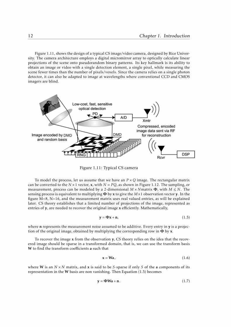
Figure 1.11, shows the design of a typical CS image/video camera, designed by Rice Univer-sity. The camera architecture employs a digital micromirror array to optically calculate linearprojections of the scene onto pseudorandom binary patterns. Its key hallmark is its ability toobtain an image or video with a single detection element, a single pixel, while measuring thescene fewer times than the number of pixels/voxels. Since the camera relies on a single photondetector, it can also be adapted to image at wavelengths where conventional CCD and CMOSimagers are blind.
Figure 1.11: Typical CS camera
To model the process, let us assume that we have an P ×Q image. The rectangular matrixcan be converted to the N ×1 vector, x, with N = PQ, as shown in Figure 1.12. The sampling, ormeasurement, process can be modeled by a 2-dimensional M ×Nmatrix Φ , with M ≤ N . Thesensing process is equivalent to multiplyingΦ by x to give theM×1 observation vector y. In thefigure M=8, N=16, and the measurement matrix uses real valued entries, as will be explainedlater. CS theory establishes that a limited number of projections of the image, represented asentries of y, are needed to recover the original image x efficiently. Mathematically,
y =Φx+n, (1.5)
where n represents the measurement noise assumed to be additive. Every entry in y is a projec-tion of the original image, obtained by multiplying the corresponding row in Φ by x.
To recover the image x from the observation y, CS theory relies on the idea that the recov-ered image should be sparse in a transformed domain, that is, we can use the transform basisW to find the transform coefficients a such that
x =Wa , (1.6)
where W is an N ×N matrix, and x is said to be S-sparse if only S of the a components of itsrepresentation in the W basis are non vanishing. Then Equation (1.5) becomes
y =ΦWa+n . (1.7)

1.1. Background 13
Figure 1.12: Compressed sensing acquisition model. Measurement matrix Φ with realentries, M=8, N=16
The coherence µ, of a CS system measures the maximum correlation between the measure-ment basis and transform basis vectors. It can be expressed as:
µ =√Nmax
k,j|ΦkWj | , (1.8)
where Φk represents the k−th vector of the Φ basis, Wj represents the j−th column in W with1 ≤ j ≤ N , and | . | is the absolute value. In Equation (1.8), if matrices used were in normalizedform, which is usually the case, then the range of possible values for µ is 1 ≤ µ ≤
√N . For a CS
theory efficient application, CS systems coherence coefficient values µ have to be low.
A measurement matrix Φ obeys the Restricted Isometry Property (RIP) of order S if theisometry constant δS of Φ is not too close to one for each integer S = 1,2, · · · . The δS is definedas the smallest number such that the following holds for all S-sparse vectors of x
(1− δS ) ∥ x ∥2≤∥Φx ∥2≤ (1 + δS ) ∥ x ∥2 (1.9)
This is equivalent also to say that all subsets of S columns taken fromΦ are nearly orthog-onal. Notice that the columns cannot be exactly orthogonal since number of columns usually islarger than number of rows in Φ , see [13, 16].
A random sensing matrix Φ and a basis W allowing an S-sparse representation of x willhave the RIP if the following expression is accomplished
M ≥ c.S log(N/S), (1.10)
where c is a constant. This ensures that the reconstruction of an x image with an S−sparse rep-resentation in a vector basis can be obtained from a compressed sensing observation y throughthe following minimization problem.
a = argmina
α2∥ΦWa− y ∥2 +τ ∥ a ∥1, (1.11)
where α and τ are positive parameters. ∥ . ∥ is the Eucledian norm and ∥ . ∥1 is the l1 norm.
CS is a promising technology which decreases the acquisition time and memory size byusing only one sensor. The use of a single sensor makes it suitable for imaging at wavelengthswhere CCD and CMOS are blind (see [13] for more information).
14 Chapter 1. Introduction
1.2 Objectives and Hypothesis
The main objective for this work is to apply SR techniques to multiple compressed sensing LRobservations. It is logical to tackle such a problem because it has been shown that a blurredimage is compressible in various scenarios and a constrained optimization framework for com-pressive BID has been proposed [5, 17].
If the blurred observations are sparse in some domain and CS techniques can be applied toa blurred HR image, then the LR images yq at Equation (1.1) are also expected to be sparse ina transformed domain, and CS can be applied to them. So why not to extend this idea to superresolve multiple LR images, by combining CS with SR techniques.
Following this preliminar idea, in a combined Compressed Sensing Super Resolution (CSSR)problem, we have two approaches to solve the problem: The first is the sequential approach,and the second is the alternate approach. The sequential approach consists of three steps: 1)the LR images are reconstructed, 2) the motion parameters are estimated and finally 3) the HRimage is estimated. Notice that this sequence is followed only once. The alternate approachestimates the three unknowns simultaneously in an iterative manner. In the alternate approachthe previous sequence is repeated, updating at each step the values obtained in the previousiteration. The alternate approach is expected to give better performance, as it will be provedexperimentally in this dissertation.
Another objective of this work is to include the estimation of all unknowns in an iterativeframework to solve the CSSR problem.
In this work, image registration parameters are assumed to be unknown. The parametersare estimated using four different approaches, as it will be discussed later in this dissertation.
Another important objective of this work is to apply the CSSR approach to PMMW images.Although they are important and powerful in threat detection problems and many other appli-cations, PMMW images have very poor image quality and suffer from small resolution and longacquisition times. The CSSR with its CS acquisition is expected to require shorter acquisitiontimes. Moreover, the SR step can increase the spatial resolution of these acquired images. Thishas been investigated in Chapter 4 as it will be shown later. Besides, the proposed frameworkis applied to color images.
1.3 Methodology and Contributions
A strict work plan has been prepared that starts with a wide literature survey to build a deepknowledge of CS and SR techniques. A model to combine both techniques is suggested andtested.
The work starts by assuming that some parameters are known, like the warping and reg-ularization parameters, to simplify matters, then these parameters are estimated as the workprogresses. Two types of images will be utilized in the experiments: simulated and real. Nu-merical measures can be applied only to simulated experiments, so it constituted most of thepreliminary work. The simulation followed the suggested degradation model, on which thereconstruction process also depends.
Before presenting the thesis outline, let us mention the main contributions of this work:

1.4. Thesis Document Structure 15
• We propose a degradation model to generate CS LR observations. The optimization pro-cess of the CSSR framework mainly depends on this degradation model.
• The combined CSSR approach. Until the time of writing this thesis, to the best of ourknowledge, there is no published work that combines compressed sensing and super res-olution techniques of multiple unregistered observations, except our published works.All existing published works that combine SR with CS perform SR from one single ob-servation. The following papers address the CSSR estimation process:
– [18]. W. AlSaafin, S. Villena, M. Vega, R. Molina, and A.K. Katsaggelos. Compres-sive Sensing Super Resolution From Multiple Observations With Application ToPassive Millimeter Wave Images. Digital Signal Processing, pages 180-190, 2016.DOI: 10.1016/j.dsp.2015.12.005
– [19]. Wael Saafin, Miguel Vega, Rafael Molina, and Aggelos K. Katsaggelos. ImageSuper Resolution From Compressed Sensing Observations. In Image Processing(ICIP), 2015 IEEE International Conference on, pages 4268-4272, Sept 2015.DOI: 10.1109/ICIP.2015.7351611
– [20]. Wael Saafin, Salvador Villena, Miguel Vega, Rafael Molina, and Aggelos K.Katsaggelos. PMMW Image Super Resolution From Compressed Sensing Obser-vations. In Signal Processing Conference (EUSIPCO), 2015 23rd European, pages1815-1819, Aug 2015.DOI: 10.1109/EUSIPCO.2015.7362697
• ADMM is used to include the estimation of the unknown regularization parameters.Motion vectors are estimated through ADMM, using four different approaches three ofthem were published in [18–20], the fourth is presented in this dissertation.
• The proposed CSSR is applied to PMMW images, to be considered as a first processingstep, that can serve, and enhance, later processing like threat detection problems. Therelated work has been published in [18, 20]. Also, the CSSR is applied to color images aswill be shown later in this dissertation ([21]).
1.4 Thesis Document Structure
This thesis is presented in the following order:
• The introductory work is presented in Chapter 1 where background is introduced. Thiscovers a discussion on classical digital imaging techniques to compare with CS tech-niques. SR and ID techniques are discussed for both natural and millimeter wave im-ages.
• In Chapter 2, the state of the art is studied. SR section includes a discussion of imageregularizers and some blur models utilized in the literature. CS works are discussed thenthe CSSR problem is modeled and formulated. Then some PMMW and CS color imageworks are presented.
• In Chapter 3 the proposed CSSR framework is introduced and stated.
• Experimental results are presented in Chapter 4 for gray scale, PMMW, and color images.
• Conclusions are drawn in Chapter 5. This chapter also includes future work that weconsider relevant to CSSR.


Chapter 2
State of the Art
In this chapter we discuss SR works that use images captured using conventional acquisitionsystems, we then analyze relevant works which utilize images acquired by CS cameras, andfinally the proposed Compressive Sensing Super Resolution (CSSR) problem is modeled andformulated.
2.1 Image Super Resolution Works
As explained in Section 1.1.4, the LR observation process can be modeled as follows,
yq =AHqC(sq)x+nq = Bq(sq)x+nq, (2.1)
where A is a down-sampling matrix, Hq is a blurring matrix, C(sq) is the warping matrix cor-responding to a motion vector sq, nq represents the noise accompanying the process. Bq(sq) isa matrix modeling the imaging process. SR techniques aim at finding an estimate of x given QLR images, yq.
SR research started in 1984 with the pioneer work by Tsai and Huang [22]. Many workssince then have addressed the problem (see [3, 6, 9, 23]). Many SR methods have been pro-posed, which can be grouped into the following classes: Frequency domain based approach[22, 24, 25], interpolation based approach [26], Bayesian approach [27–33], regularization basedapproach [34–38], and learning based approach [39–41]. There are some variants of the SRproblem: an HR image can be reconstructed from multiple LR observed images, it is also pos-sible to reconstruct an HR image sequence from an observed LR image sequence, and finallyan HR image can be reconstructed form only one LR observed image using the learning basedapproach.
In this work we use the regularization-based approach. The basic idea of this approach tosolve the ill-posed inverse SR problem, is to introduce in the cost function to be optimized aregularization term constraining the estimation process. This should be sufficient to solve forthe unknown HR image. From a Bayesian point view, the data fidelity term corresponds to the

18 Chapter 2. State of the Art
observation model probability distribution, and the regularization term to the prior probabilitydistribution which incorporates our a priori knowledge on the unknown HR image.
In Equation (2.1), beside the HR image x, the warping matrix C(sq) is also unknown andhas to be estimated. Those unknowns can be estimated sequentially or simultaneously. In thesequential approach, we use the LR images to estimate the first unknown, that is, the motionvector, just once, then the second unknown is estimated, that is, the HR image, assuming theblur in known. In the simultaneous approach, all unknowns are estimated alternatively in aniterative way, this allows to the estimated unknowns to feed some information into the esti-mation of the other unknowns. The simultaneous approach produces better results as we willshow in the experimental section (see also [18, 30]).
Given the motion vectors sq a regularization based SR solves the following optimizationproblem,
x = argminx
β
2
Q∑q=1
∥ Bq(sq)x− yq ∥2 + γ Q(x) , (2.2)
where β and γ are positive parameters, andQ(x) is the regularizer. In the following subsection,we present some regularization terms, Q(·), utilized in the SR literature.
2.1.1 Image Regularizers
In this section we explore some regularization terms, or priors under the Bayesian approach.For some of these regularizers, we describe SR algorithms which use them. The performance ofthe selected SR algorithms is compared with the proposed CSSR algorithm in Section 4.4.
• Huber Markov random field (HMRF)It is a convex non-quadratic regularizer, which results in nonlinear cost functions, usedto preserve edges, see [29, 42]. The energy function of an HMRF is defined as:
ρ(fx) =
f2x , if | fx |≤ α
2α | fx | −α2, otherwise(2.3)
where fx is the first or second order differences of the HR image x, α is a parameterseparating the quadratic and the linear regions, that controls the size of discontinuitiesmodeled by the prior by providing a less severe edge penalty. This regularizer has beenused in [29] to extract SR frames from video sequences.
• Total Variation (TV) regularizerThe TV regularizer preserves image edges while smooths flat regions and avoids ringingartifacts (see [43]. The TV energy function is defined as
ρ(x) =∥ ∇x ∥ , (2.4)
where ∇ is the gradient operator and ∥ . ∥ is the Euclidean norm. It can be approximatedusing
T V (x) =N∑i=1
√(∆h
i (x))2 + (∆v
i (x))2 , (2.5)

2.1. Image Super Resolution Works 19
where N is the number of pixels in x, ∆hi (x) and ∆h
i (x) correspond respectively to thehorizontal and vertical first order differences at pixel i.
• ℓ1 norm regularizer
It is similar to the TV regularizer in its capability to preserve edges while imposingsmoothness in the rest of image regions. Its energy function is defined as
ρ(x) =∥ ∇x ∥1, (2.6)
where ∇ is the gradient operator and ∥ . ∥1 is the ℓ1 norm, it can be expressed as
L1(x) =N∑i=1
αh ∥ ∆hi (x) ∥1 +
N∑i=1
αv ∥ ∆vi (x) ∥1 , (2.7)
where ∆hi (x) and ∆v
i (x) represent the horizontal and vertical first order differences, re-spectively, at pixel i, and αh,αv are regularizer parameters. Notice here the use of twomodel parameters αh and αv to make this model more adaptable to image characteristicsthan the TV regularizer case.
In Section 4.4, we compare the proposed CSSR algorithm with the SR using ℓ1 prior(L1S) algorithm [28] which solves the minimization problem in Equation (2.2).
• The Simultaneous Autoregressive (SAR) regularizer
It applies a uniform smoothness to all locations in the image. It is a non sparse priorthat reconstructs textures better, see [30]. It uses the Euclidean norm of the second orderdifference, as follows
SAR(x) =∥ Cx ∥2 , (2.8)
where C is the Laplacian operator, and ∥ . ∥ is the Euclidean norm.
In Section 4.4, we compare the proposed CSSR algorithm with the SR using SAR prior(SAS) algorithm [30] which solves the minimization problem in Equation (2.2).
• Bilateral Total Variation (BTV) regularizer
BTV preserves edges in the image, (see [34, 42, 44]). It is expressed as:
BTV (x) =P∑
l=−P
P∑m=0︸ ︷︷ ︸
l+m≥0
α|m|+|l| ∥ x−SlhSmv x ∥1 , (2.9)
where matrices Slh,Smv shift the image x by l,m pixels in the horizontal and vertical di-
rections, respectively; presenting several scales of derivatives. α is a positive parameterless than one, which gives more weight to closer pixels, ∥ . ∥1 is the ℓ1 norm and P is apositive integer. The BTV regularizer has been used in [34]. Notice that when P = 1, theregularizer becomes the TV regularizer, and a comparison between the two regularizerswas performed in [34].
A fast and robust SR (FRSR) algorithm has been proposed in [34] which employs the ℓ1norm minimization in pursuit of robustness against motion errors and blurring. It uses

20 Chapter 2. State of the Art
the BTV regularizer. The following minimization problem was solved to estimate x
x = argminx
∑q
∥ Bqx− yq ∥1 +P∑
l=−P
P∑m=0︸ ︷︷ ︸
l+m≥0
α|m|+|l| ∥ x−SlhSmv x ∥1
. (2.10)
In Section 4.4, we compare the proposed CSSR algorithm with the FRSR algorithm.
• Generalized Gaussian MRF (GGMRF)It is a convex non-quadratic regularizer, see [42, 45]. It has the following energy function:
ρ(x) =| x |p , (2.11)
where 1 < p < 2. This regularizer tends to overly smooth the whole image including theedges, see [46], and it has been utilized in [45] for tomographic image reconstructionproblems.
The combination of some image regularizers in SR and image restoration has been ad-dressed in [30, 47, 48]. In [30, 48] sparse and non sparse priors were combined and appliedto the SR image reconstruction problem.
A robust SR (RSR) Algorithm has been proposed in [49] where instead of minimizing thesum of the difference images, a robust median estimator is combined in an iterative processto obtain a SR algorithm. The HR image is estimated iteratively using the following updateequation
xk+1 = xk +Q ·λ ·medianBtq(Bqx
k − yq)Qq=1 , (2.12)
where k is the iteration number,Q is the number of LR input images, and λ is a scale factor. Theperformance of this algorithm is compared with the proposed CSSR algorithm in Section 4.4.
2.1.2 Image Registration
In the previous section, we discussed the modeling of the HR image. However, for the SR imageestimation to succeed, it is essential to find a highly accurate image registration of the input LRimages. Image registration will give us an estimation of the sq motion vectors and consequentlyof the warping matrix C(sq) appearing in Equation (2.1).
Image registration, in general, overlays multiple images of the same scene taken at differenttimes, from different viewpoints, and/or by different sensors. In the SR problem, image regis-tration finds a geometric transformation to align pixels in various images to the correspondinglocations in the estimated HR image, which is considered to be the reference image.
Many methods have been proposed in the literature, see [50] for details. In this work weuse the geometric transformation defined next.
The geometric transformations utilized in this dissertation consist of translations and rota-tions. Assume that it is required to register the image gwith respect to a reference image x, then
2.1. Image Super Resolution Works 21
the transformation relating pixel gi to xi , with coordinates (gih, giv) and (xih,xiv) respectively, ismodeled as
gihgiv1
=cosθ −sinθ csinθ cosθ d0 0 1
xihxiv1
(2.13)
where θ is the rotation angle, and c,d are the horizontal and vertical displacements, respec-tively. The motion vector, for observation q, can be expressed as sq = [θq, cq,dq]t . A detaileddescription of the registration model is presented later, in Section 2.3.
2.1.3 Blur Model
In this dissertation we assume that the blur affecting the image is known and can be approx-imated by a relevant blur model. Many models have been proposed in the literature whichsimulate blur encountered in real world imaging systems. Next we mention some blur models(see [5, 51, 52])
• 1DMotion BlurThis type of blur represents the one dimensional (1D) local averaging of neighboringpixels, a common result of camera panning or fast object motion. For example, the hori-zontal motion blur can be modeled by
h(u) =
1
L+1 , −L2 ≤ uh ≤ L
2 ;uv = 0
0 , otherwise(2.14)
where L is assumed to be an even integer, u = (uh,uv), being the pixel range of horizontaland vertical distance uh,uv from the current pixel. Motion blur may also occur in twodimensions (2D), e.g., following a random trajectory.
• Atmospheric Turbulence BlurThis type of blur represents a long term exposure through the atmosphere which is typ-ically modeled by a Gaussian Point Spread Function (PSF). A Gaussian blur can be mod-eled as
h(u) = K e− |u|
2
2σ2 (2.15)
where K is a constant ensuring that the blur values sum up to 1, σ2 is the variance thatdetermines the severity of the blur.
• Uniform Out-of-Focus BlurThis type of blur is primarily due to the effects of the camera focal length and the dis-tance between camera and observed scene. Out-of-Focus blur can coexist with diffractionblur, which depends on the camera aperture size and shape, and the wavelength of theincoming radiation. Accurate knowledge of all these parameters is not frequently avail-able when a picture is taken. When the blur due to poor focusing is large, the followinguniform model has been used as an approximation of such PSFs,
h(u) =
1
πr2, | u |≤ r
0 , otherwise(2.16)

22 Chapter 2. State of the Art
where r denotes radius and controls the severity of the blur.
A blurred image can be simulated utilizing a blur model by
BLURRED = h(u) ∗ x , (2.17)
where ∗ is the convolution operator.
2.2 Compressed Sensing Works
Different CS image/video cameras have been proposed (see [53–58]). The concept of singlepixel camera has been extended to a multi-detector device in [59], where the detectors areplaced on an arbitrary grid on the source signal and each detector integrates the source signalsonly locally to reduce the required measurements, and hence the measurement time, by usingmore detectors.
Super Resolution (SR) from a single image has benefited from the introduction of CS theoryin works like [60–62]. In [63, 64] learning based SR is used to estimate an HR image from asingle CS observation of a down-sampled remote sensing image. In [65] the down-sampling isincorporated in the measurement matrix, the CS image is reconstructed in the wavelet domainand the signal is deconvolved in the Fourier domain.
BID from CS measurement has been studied in [5, 66], and NBID in [67–71]. Next wedescribe selected CS ID works which will be compared with our proposed CSSR algorithm inSection 4.3.
The Large Scale ℓ1 regularized (L1-LS) logistic regression algorithm proposed in [67], andGradient Projection for Sparse Reconstruction (GPSR) algorithm proposed in [68], both solvethe following problem
a = argmina∥ΦHWa− y ∥2 +τ ∥ a ∥1 , (2.18)
where y is the CS blurred observation, Φ the measurement matrix, H the blur matrix, W isthe transform domain basis, a is the transformed domain representation of the original imagex =Wa and τ is a non-negative parameter.
The Compressive SamplingMatching Pursuit (CoSaMP) algorithm proposed in [69] is basedon Orthogonal Matching Pursuit (OMP) schemes and produces an s−sparse approximation zthat satisfies
∥ x− z ∥2≤ C ·maxη ,
1√s∥ x− xs/2 ∥1 + ∥ y−Φz ∥2
, (2.19)
where C and η are parameters, and xs/2 is the best (s/2)−sparse approximation to x.
The NESTerov’s Algorithm (NESTA) proposed in [70], and Your ALgorithm for L1 (YALL1)proposed in [71], solve the following problem
x = argminx∥W−1x ∥1 s.t. ∥ΦHx− y ∥< ϵ , (2.20)
2.3. CSSR Modeling and Formulation 23
2.3 CSSR Modeling and Formulation
In the Compressed Sensing Super Resolution (CSSR) problem, we are given multiple CS LRobservations of a scene to estimate an HR image. The LR images can be considered as a warped,blurred, and down-sampled versions of the HR image to be estimated. Let us assume that thenumber of input images is Q, the acquisition model for each observation is
yq =Φzq + rq q = 1, . . . ,Q, (2.21)
where yq is an M × 1 vector representing the compressed observations, Φ is a CS M ×D mea-surement matrix, zq is a column vector of size D × 1 representing the q−th LR image and rqrepresents the observation noise. We denote by R the compression ratio of the measurementsystem, that is, R =M/D, R ≤ 1.
As shown in Section 2.1 the observation process of the LR observations zq in Equation (2.21)can be modeled as follows,
zq =AHqC(sq)x+wq = Bq(sq)x+wq, (2.22)
where A is a D ×N down-sampling matrix, D ≤ N , which models the limited resolution of theacquisition system, when capturing the high resolution image, where N = P 2D and P≥1 is thezooming factor, in each dimension of the image. Hq is an N ×N blurring matrix, modelingthe blur action accompanying the imaging process. In this work, the convolution matrix Hq isassumed to be known. C(sq) is the N ×N warping matrix for the motion vector sq = [θq, cq,dq]
t ,where θq is the rotation angle, cq and dq are respectively the horizontal and vertical translationsof the q−th LR image with respect to the reference frame, and x is the HR image of size N ×1. Finally, wq models the noise associated to the LR acquisition process. We write Bq(sq) =AHqC(sq) for simplicity.
Using Equations (2.21) and (2.22) we can write
yq =ΦBq(sq)x+nq , for q = 1, . . . ,Q, (2.23)
where nq represents the combined CS and LR acquisition noise and x is the HR image we wantto estimate.
Next we describe the sensing matrices we use in this dissertation. The measurement matrixwe use (Φ) is a random circulant Toeplitz matrix. A circulant Toeplitz matrix is a matrix Tn, inwhich each row is a cyclic shift of the row above. It has the following form
Tn =
t0 t1 t2 · · · tn−1tn−1 t0 t1 tn−2tn−2 tn−1 t0...
. . .t1 t0
(2.24)
The entries in the first row are random, following a Gaussian, or Bernoulli distribution.Gaussian, or normal, distribution function is given by
f (x|µ,σ ) = 1
σ√2π
e− (x−µ)2
2σ2 (2.25)

24 Chapter 2. State of the Art
where µ and σ2 are respectively the mean and the standard deviation of the distribution.Bernoulli probability function is given by
f (k|p) = pk(1− p)1−k , for k ∈ 0,1 , (2.26)
where (p) and (1− p) are respectively the probabilities of k being 1 and 0.
Both Gaussian and Bernoulli random circulant Toeplitz matrices were tested to work wellin CS [72–74]. In both cases the rows of Φ are normalized to 1. However, a Gaussian matrixconsists of real entries while a Bernoulli matrix consists of binary entries, and hence it canbe synthesized 256 × 256 practically, see [18, 56]. In this dissertation we used the Bernoullicirculant Toeplitz matrix.
Next we describe the down-sampling matrix (A). Let us assume that we have an image x ofsize 256×256, and the zooming factor P=2. We divide the matrix x into P ×P blocks, then fromeach block only one pixel value is preserved, and the other three are discarded. The preservedpixels constitute a 128× 128 matrix, which is the down-sampled version of x. Notice here thatthere is no interpolation process neither in the down-sampling nor in the up-sampling process.If the down-sampled 128× 128 matrix in the previous example is up-sampled, then each pixelvalue will form a block in the up sampled image, the upper-left pixel of the four pixels formingthis block will have the pixel value from the down-sampled image, the other three pixels willhave a zero value.
The blur matrix (H) we used in all experiments utilizes a spatially invariant Gaussian blurfilter given by
h(u) = K e− |u|
2
2σ2 (2.27)
where K is a constant and σ2 is the blur variance.
Next we describe how to calculate the warping matrix (C(sq)). Let us denote the coordinatesof the reference HR grid by (u,v) and the coordinates of the q−thwarpedHR grid, after applyingC(sq) to x, by (uq,vq). Then it holds that
uq = u cos(θq)− v sin(θq) + cq (2.28)
vq = u sin(θq) + v cos(θq) + dq . (2.29)
Let us denote the displacements between the grids by ∆(uq,vq)T = (u,v)T − (uq,vq)T . The vectordifference between the pixel at (uq,vq) and the pixel at its top-left position in the reference HRgrid is denoted by (aq(sq),bq(sq))T (see Figure 2.1), that is,
aq(sq) = ∆uq −floor(∆uq) , (2.30)
bq(sq) = ∆vq −floor(∆vq) . (2.31)
Notice here that the relationships are non linear functions of sq due to the trigonometricfunctions in Equations (2.28) and (2.29). Using bilinear interpolation, the warped image C(sq)x

2.3. CSSR Modeling and Formulation 25
(a) (b)
Figure 2.1: q-th HR grid calculation. (a) HR grid (in black) and the q-th image grid (inred), (b) Detailed view of (a), with the pixel notation used for the bilinear interpolationof grid element (uq,vq)
can be approximated to obtain a linear transform matrix in sq as (see [18, 30, 37]),
C(sq)x ≈Dbq(sq)(I−Daq(sq))Lbl(sq)x+ (I−Dbq(sq))Daq(sq)Ltr(sq)x
+ (I−Dbq(sq))(I−Daq(sq))Ltl(sq)x+Dbq(sq)Daq(sq)Lbr(sq)x , (2.32)
where Daq(sq) and Dbq(sq) denote diagonal matrices with the vectors aq(sq) and bq(sq) in theirdiagonals, respectively. I is the identity matrix. Matrices Lz with z ∈ bl(sq),br(sq), tl(sq),tr(sq)are constructed in such a way that the product Lzx produces pixels at the bottom-left, bottom-right, top-left, and top-right, locations of (uq,vq), respectively. This approximated explicit formpresented in Equation (2.32) can be used when we are given the motion vectors of the input LRCS observations.
The noise matrix (nq) we used in all experiments is assumed to be white Gaussian noiseof zero mean, added to the CS observations. This noise arises during acquisition due to poorillumination, high temperature and electronic circuit noise, see [75].
Let us now show an example to clarify visually the presented warping model. Figure 2.2(a)shows the original Shepp-Logan image x. The original image is warped then blurred thendown-sampled, following Equation (2.22) to get Bq(sq)x for the case Q = 4. The warping uses

26 Chapter 2. State of the Art
the following motion vectors
s1 =
000
, s2 =
0.05242−3
, s3 =
−0.0698−1−2
, and s4 =
−0.03493−1
. (2.33)
To blur the warped image we used a Gaussian blur with variance 5, the down-samplingused a zooming factor P=2. The four generated LR images (Bq(sq)x) are shown in Figure 2.2(b).The simulated LR images then were compressed to get (ΦBq(sq)x), as in Equation (2.23). Firstlythe image is compressed using a compression ratio R=0.6 then noised by an additive white noiseof SNR=30dB. The four noised CS observations are shown in Figure 2.2(c). Figures 2.2(d,e,f)show the results obtained for the Lena image following the same procedure.
(a) (b) (c)
(d) (e) (f)
Figure 2.2: Simulation process. Warped with motion vectors (0,0,0)t, (.0524,2,−3)t,(−.0698,−1,−2)t, (−.0349,3,−1)t, Gaussian blur of variance 5, zooming factor 2, com-pression ratio R=0.6, SNR of added noise 30dB (a) Original Shepp-Logan image, (b)Four simulated LR images., (c) Four CS observations, (d) Original Lena image, (e) Foursimulated LR images, (f) Four CS observations.
CSSR aims at finding an estimate for the HR image in Figure 2.2(a) given some noised
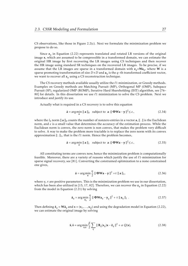
2.3. CSSR Modeling and Formulation 27
CS observations, like those in Figure 2.2(c). Next we formulate the minimization problem wepropose to do so.
Since zq in Equation (2.22) represents translated and rotated LR versions of the originalimage x, which are assumed to be compressible in a transformed domain, we can estimate theoriginal HR image by first recovering the LR images using CS techniques and then recoverthe HR image using standard SR techniques on the recovered LR images. To be precise, if weassume that the LR images are sparse in a transformed domain with zq=Waq, where W is asparse promoting transformation of size D×D and aq is the q−th transformed coefficient vector,we want to recover all zq using a CS reconstruction technique.
The CS recovery methods available usually utilize the ℓ1 minimization, or Greedy methods.Examples on Greedy methods are Matching Pursuit (MP), Orthogonal MP (OMP), SubspacePursuit (SP), regularized OMP (ROMP), Iterative Hard Shareholding (IHT) algorithm, see [76–80] for details. In this dissertation we use ℓ1 minimization to solve the CS problem. Next weintroduce and justify its use.
Actually what is required in a CS recovery is to solve this equation
a = argmina∥ a ∥0 subject to a :∥ΦWa− y ∥2≤ ϵ , (2.34)
where the l0 norm ∥ a ∥0 counts the number of nonzero entries in a vector a, ∥ . ∥ is the Euclideannorm, and ϵ is a small value that determines the accuracy of the estimation process. While theEuclidean norm is convex, the zero norm is non convex, that makes the problem very difficultto solve. A way to make the problem more tractable is to replace the zero norm with its convexapproximation ∥ . ∥1, that is the ℓ1 norm. Hence the problem becomes,
a = argmina∥ a ∥1 subject to a :∥ΦWa− y ∥2≤ ϵ , (2.35)
All constituting terms are convex now, hence the minimization problem is computationallyfeasible. Moreover, there are a variety of reasons which justify the use of ℓ1-minimization forsparse signal recovery, see [81]. Converting the constrained optimization to a none constrainedone gives,
a = argmina
η
2∥ΦWa− y ∥2 +τ ∥ a ∥1, (2.36)
where η, τ are positive parameters. This is the minimization problemwe use in our dissertation,which has been also utilized in [15, 17, 82]. Therefore, we can recover the zq in Equation (2.22)from the model in Equation (2.21) by solving
aq = argminaq
η
2∥ΦWaq − yq ∥
2 + τ ∥ aq ∥1 . (2.37)
Then defining zq =Waq and s = (s1, . . . ,sQ) and using the degradation model in Equation (2.22),we can estimate the original image by solving
x, s = argminx,s
β
2
∑q
∥ Bq(sq)x− zq ∥2 + α Q(x), (2.38)

28 Chapter 2. State of the Art
where α and β are non-negative parameters, and the term Q(x) is described next. In [18] thefollowing regularization term was used for the image
Q(x) =∑d∈∆
N∑i=1
log(|ωxd(i)|) , (2.39)
where ωxd(i) is the i-th pixel of the filtered image, and
ωxd = Fdx , (2.40)
where Fd is a high-pass filter operator, and the index d ∈ ∆ identifies one of the members ofthe used filter set. In this paper we have used a filter set with elements ∆ = h,v,hv,vh,hh,vv,where h,v represent the first order horizontal and vertical difference filters, hv and vh representfirst order differences along diagonals, and hh and vv the horizontal and vertical second orderdifferences. The regularization term favors sparsity of the high-pass filtered images Fdx, andcorresponds to the Super-Gaussian log prior used in blind deconvolution [83].
Since the log function can not be differentiated at zero, we consider in this work the follow-ing robust version of the log regularizer
logϵ(|s|) =
log(|s|) for |s| ≥ ϵs2
2ϵ2 − (12 − log(ϵ)) for 0 ≤ |s| ≤ ϵ
(2.41)
and replace Q(x) in Equation (2.39) by
Q(x) =∑d∈∆
N∑i=1
logϵ(|ωxd(i)|) , (2.42)
where we have removed the dependency of Q(·) on ϵ for simplicity.
We have two approaches to solve the CSSR problem: the sequential approach and the al-ternate approach (see [6]). The latter approach alternates between compressive sensing recon-struction, registration parameter estimation, and reconstruction of the HR image. The formerapproach estimates the unknowns sequentially, one after the other, as follows. Firstly, the LRimages are reconstructed using Equation (2.37), then motion parameters are estimated and fi-nally the HR image is estimated using Equation (2.38). Notice here that after an unknownis estimated, the sequential approach does not return back to it again, and every unknown isestimated only once.
As we will show in the experimental part, combining the two optimization problems inEquations (2.37) and (2.38) above into a simultaneous one leads to an improved performance,as this enables better exploitation of the compressibility of the LR observations using the ad-ditional information obtained from the estimated HR image, and the updated registration pa-rameters. Hence, in the following, this alternate approach has been adopted. According to it,let a = (a1, . . . ,aQ) and define
L(x,a) =η
2
Q∑q=1
∥ΦWaq − yq ∥2 + τ
Q∑q=1
∥ aq ∥1 + α Q(x) (2.43)

2.3. CSSR Modeling and Formulation 29
Then we approach the Compressed-Sensing Super Resolution (CSSR) problem by solvingthe following constrained optimization problem
minL(x,a)s.t. Bq(sq)x =Waq , for q = 1, . . . ,Q . (2.44)
This is the approach we will describe and use in Chapter 3. Notice that in Equation (2.43)we could have also introduced a regularizer on the motion vector s = (s1, . . . ,sQ), similar to[20, 30]. However, we have experimentally found that it is not necessary to use regularizationon the motion vectors.
Still we did not describe the transform basis (W) that serves well in the CS reconstruction.Suitable transformed domains for CS are Discrete Cosine Transform (DCT), Discrete WaveletTransform (DWT) and Discrete Fourier Transform (DFT). DWT is usually preferred over DCTbecause it better enables the removal of blocking artifacts [84]. In this dissertation we adaptedinterchangeably the DCT, and the DWT. Both are described next.
DCT attempts to make use of correlated data in the zq image. In the one-dimensional (1D)DCT, the signal is converted into a sum of cosine functions oscillating at different frequencies.It can be expressed as follows
aq(k) = ω(k)D∑i=1
zq(i)cos[ π2D
(2i − 1)(k − 1)], k = 1, · · · ,D, (2.45)
where zq is expressed in the vector form, and
ω(k) =
1√D, k = 1√
2D , 2 ≤ k ≤D
(2.46)
where D is the number of pixels in zq. The inverse 1D-DCT reconstructs a sequence from itstransform coefficients by
zq(i) =D∑k=1
ω(k)aq(k)cos[ π2D
(2i − 1)(k − 1)], i = 1, · · · ,D, (2.47)
DWT invokes two types of filters; the wavelet filter and the scaling vector. The wavelet filteris a high pass filter, and the scaling vector is a low pass filter. After applying a 1-level HaarDWT on an image zq in the matrix form, we decompose it into four frequency bands, namelythe approximation (LL1), horizontal (LH1), vertical (HL1), and diagonal (HH1) sub-bands. ThisDWT decomposition at the 1-level is shown in Figure 2.3 for Barbara image to represent theLR image zq. The original image is shown in Figure 2.3(a), while Figure 2.3(b) shows the fourdown-sampled sub-bands: approximation, horizontal, vertical and diagonal bands. Notice thatif we append the four bands together in one vector we obtain the 1-level coefficient vector whichhas the same size as zq.
If the 1-level DWT is applied again to the approximation sub-band LL1, then we obtain the2-level DWT, and hence we will have the new sub-bands LL2, LH2, HL2, and HH2. ApplyingDWT again to the resulting approximation sub-band LL2, then we will have the 3-level DWT,
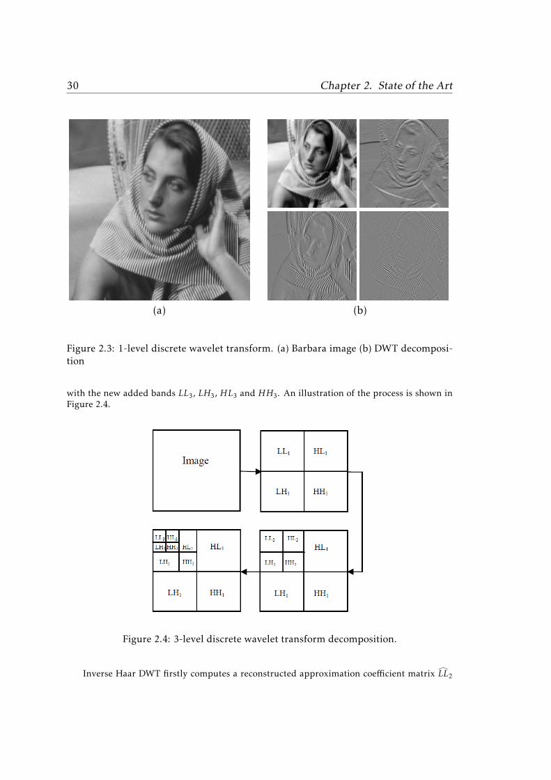
30 Chapter 2. State of the Art
(a) (b)
Figure 2.3: 1-level discrete wavelet transform. (a) Barbara image (b) DWT decomposi-tion
with the new added bands LL3, LH3, HL3 and HH3. An illustration of the process is shown inFigure 2.4.
Figure 2.4: 3-level discrete wavelet transform decomposition.
Inverse Haar DWT firstly computes a reconstructed approximation coefficient matrix LL∧
2

2.3. CSSR Modeling and Formulation 31
from LL3, LH3, HL3, and HH3. Notice that the size of LL∧
2 will be equal to the sum of the foursmaller sub-bands. Then using LL
∧
2, LH2, HL2 and HH2, the first level approximation LL∧
1 iscomputed. Finally, the reconstructed approximation of zq is computed by taking the inverse
Haar transform of the bands LL∧
1, LH1, HL1 and HH1.
In this dissertation we used 3-level Haar DWT as the wavelet transform domain.


Chapter 3
Compressive Sensing Super
Resolution Algorithm
Once the CSSR problem has been formulated in the previous chapter, this chapter presentsour CSSR approach to solve it. All the processing steps are investigated to describe their specificmerits. Then the algorithm is stated. The CSSR method can also be applied to Color CS imagesthrough our second proposed algorithm, CCSSR, which is presented in this chapter.
The CSSR problem has a large number of unknowns: the HR image x, the sparse coefficientsa corresponding to each LR image, the motion vectors s, and the parameters η,τ,α that affectthe solution inherently. In such a case, one should design a smart strategy to tackle the problemefficiently, and to try many possible solutions, sometimes trials may fail, others may succeed.
Hence, before continuing in describing the resulting approach, it is worthwhile to give ahistorical background to describe the road map followed in the preparation of this work, and todiscuss not only those adopted techniques, but also those which have not been adopted in thelast format of our solution to the CSSR problem.
3.1 Preliminary Work
To simplify matters, in the problem we started with there were two simulated CS observationscorresponding to the LR images. Given the motion vectors and the blur, the observations weredegraded as in Equation (2.1). The image was warped, then degraded by a Gaussian blur anddown-sampled, with a zooming factor P=2. The observation was then compressed using a circu-lant Gaussian Toeplitz measurement matrix and finally White Gaussian noise, with SNR=40dB,was added to the compressed observations.
From the CS observations the sparse coefficient vectors can be estimated using the following

34 Chapter 3. Compressive Sensing Super Resolution Algorithm
l1 minimization problem
aq = argminaq
α2∥ΦWaq − yq ∥
2 +τ ∥ aq ∥1, for q = 1, · · · ,Q. (3.1)
Notice that the sparse coefficients can be estimated using the algorithm in [82]. We usedthe 3-level Haar wavelet transform as a transform basis. The estimation process is performedfor each observation separately. Then the estimated LR images Waq can be super resolved toestimate an HR image using
x = argminx
β
2
∑q
∥AHqC(sq)x−Waq ∥2 + α Q(x), (3.2)
where we used the explicit form of C(sq) as in Equation (2.32), assuming knownmotion vectors.We used an lp quasi-norm with 0 < p < 1 to serve as the regularization termQ(x). This prior hasbeen used in compressive image deconvolution [5]. It can be expressed as
Q(x) =∑d
21−o(d)∑i
| ∆di (x) |
p , (3.3)
where o(d) ∈ 1,2 denotes the order of the difference operator ∆di (x) at pixel i, d ∈ h,v,hh,vv,
h,v denote horizontal, vertical first order differences, hh,vv denote horizontal, vertical secondorder differences, and 0 < p < 1. This Q(x) regularizer can be bounded by a tractable functionalR(x,V) such that
Q(x) ≤ R(x,V). (3.4)
In Equation (3.4) R(x,V) is defined as
R(x,V) =p
2
∑d
21−o(d)∑i
[∆di (x)]
2 + 2−pp vd,i
v1−p/2d,i
, (3.5)
where V is a diagonal matrix with elements vd,i > 0, and
vd,i = [∆di (x0)]
2 , (3.6)
where x0 is an initial estimate of x calculated by adding the up-sampled LR reconstructedimages, Waq. The derivation for the bound in Equation (3.5) is presented in [85]. The mini-mization problem in Equation (3.2) gives the following equation for estimating x,
x =
β Q∑q=1
Btq(sq)Bq(sq) +αp
∑d
21−o(d)∆dtΛd∆d
−1
βQ∑q=1
Btq(sq)Waq (3.7)
where Λd is a diagonal matrix with elements vp/2−1d,i in the diagonal, and ∆d is the convolution
matrix of the difference operator ∆di (·).
As an example, we degraded the Barbara image to simulate two CS LR images. The re-constructed LR images are shown in Figure 3.1(a). Figure 3.1(b) shows the HR initial image of

3.1. Preliminary Work 35
(a) (b) (c)
Figure 3.1: Sequential estimation process. Observations have been simulated usingGaussian Blur of variance 3, zooming factor P=2, Gaussian circulant Toeplitz measure-ment matrix with compression ratio R=0.8 and additive noise of SNR=40dB. (a) LR re-constructed observations, (b) initial estimate of HR image, PSNR=9.8 dB, (c) estimatedHR image, PSNR=23.2 dB
PSNR=9.8 dB, and the reconstructed image is shown in Figure 3.1(c), with PSNR=23.2 dB. Weused p = 0.8 in this and the following experiments.
Notice that the unknowns were estimated sequentially, not iteratively. Actually, this wasthe simplest initial approach to the problem, and the successful reconstruction proved the fea-sibility of our study. This encouraged us to go further in the solution, to jointly estimate theunknowns using the constrained optimization in Equation (2.44), repeated again here,
min
η2Q∑q=1
∥ΦWaq − yq ∥2 + τ
Q∑q=1
∥ aq ∥1 + α Q(x)
s.t. Bq(sq)x =Waq , for q = 1, . . . ,Q , (3.8)
where Φ is the CS measurement matrix, W is the transformation matrix, aq is the transformedcoefficient vector corresponding to the q−th CS observation yq, Q(x) is the regularization termbeing, at that time, the lp quasi norm defined in Equation (3.3) for which the upper bound de-fined in Equation (3.5) was used, Bq(sq) =AHqC(sq) is the modeling matrix, the motion vectorssq are assumed to be known, and η,τ,α are positive parameters.
This constrained optimization problem can be converted into an unconstrained optimiza-tion one, using the Alternate Direction Method of Multipliers (ADMM) [86, 87]. We define thefollowing augmented Lagrangian functional

36 Chapter 3. Compressive Sensing Super Resolution Algorithm
L(x,a,λ) =η
2
Q∑q=1
∥ΦWaq − yq ∥2 + τ
Q∑q=1
∥ aq ∥1 + α Q(x)
+Q∑q=1
λtq(Bq(sq)x−Waq) +
β
2
Q∑q=1
∥ Bq(sq)x−Waq ∥2, (3.9)
where a = (a1, . . . ,aQ), λq are D×1 Lagrangian multiplier vectors with λ = (λ1, . . . ,λQ), and β is anon-negative parameter. The ADMM leads to the following sequence of iterative unconstrainedproblems,
xk+1 = argminx
L(x,ak ,λk) , (3.10)
ak+1 = argmina
L(xk+1,a,λk) (3.11)
λk+1q = λk
q − β[Bq(sq)xk+1 −Wak+1q ] , q = 1, . . . ,Q, (3.12)
where k is the iteration number. Let us now describe the estimation process. The calculation ofeach λk+1
q is straightforward. The image x can be estimated by solving the following minimiza-tion problem
xk+1 = argminx
β2 ∑q
∥ Bq(sq)x−Waq ∥2 +αR(x,V) +∑q
λkqt(Bq(sq)x−Wakq)
. (3.13)
This and the optimization step in Equation (3.10) produce the following linear equation forxk+1
xk+1 =
β∑q
Btq(sq)Bq(sq) +αp
∑d
21−o(d)∆dtΛkd∆
d
−1∑
q
Bq(sq)t[βWakq −λk
q
](3.14)
We solved Equation (3.14) using the conjugate gradient algorithm. The estimation of thesparse coefficients is described in Section 3.2.
This estimation process has been performed for the Barbara image, and the obtained HR im-ages are shown in Figure 3.2. In Figure 3.2(a) it is shown the first iteration estimate (PSNR=22.8dB), and in Figure 3.2(b) the last estimate (PSNR=23.9 dB) is shown. The maximum number ofiterations was 20. The result obtained at the last iteration is better than the obtained at the firstone and this denotes a better performance for the CSSR joint estimation approach than for thesequential one.
The next stage was to adapt a realistic measurement matrix that can be physically synthe-sized, so we used a Bernoulli measurement matrix. Figure 3.3 shows the results obtained usingthis new Φ , with a PSNR of 22.7 dB for the first iteration and of 23.9 dB for the last one.
At these stages the motion vectors sq were assumed to be known. At the next stage themotion vectors began to be considered unknowns, to be estimated. The quality of the estimated

3.1. Preliminary Work 37
(a) (b)
Figure 3.2: Joint estimation process. Observations have been simulated using GaussianBlur of variance 3, zooming factor P=2, Gaussian circulant Toeplitz measurement ma-trix with compression ratio R=0.8, and additive noise of SNR=40dB. (a) First iterationestimate with PSNR=22.8 dB, (b) last iteration estimate with PSNR=23.9 dB
motion vectors is critical for the HR estimation quality, and many experiments and trials weremade to obtain more accurate results. While the trivial update of registration parameters canbe obtained by solving
sk+1q = argminsq∥ Bq(sq)x
k+1 −Wak+1q ∥2 (3.15)
However, at that stage, we observed experimentally that a fast and reliable estimation of theregistration parameters can be obtained by registering the reconstructed LR images estimatedin the previous step with respect to the reference LR observation, rather than registering thepreviously obtained HR image, see [19]. Thus minimizing
sk+1q = argminsq∥ C(sq) [AHr ]
tWak+1r −[AHq
]tWak+1q ∥2 (3.16)
where r denotes the reference image, usually to be the first one of the LR image sequence.
The next trial was to estimate the warping parameters by registering the up-sampled LRimages obtained in the previous step with respect to the obtained HR image, see [20].
sk+1q = argminsq
[β2∥ C(sq)xk+1 − [AHq]
tWak+1q ∥2 +(sq − skq)tΞq(sq − skq)], (3.17)
where Ξq is a 3 × 3 known matrix of regularization parameters. Figure 3.4(a) shows the esti-mated Barbara image obtained using Equation (3.16), while Figure 3.4(b) shows the result ob-tained using Equation (3.17). This trial showed that the minimization in Equation (3.16) givesa better performance. In the next section, it will be shown that registration could be performedinterchangeably from the estimated HR image or from the estimated LR reference image, in anefficient and accurate manner.

38 Chapter 3. Compressive Sensing Super Resolution Algorithm
(a) (b)
Figure 3.3: Joint estimation process. Observations have been simulated using GaussianBlur of variance 3, zooming factor P=2, Bernoulli circulant Toeplitz measurement ma-trix with compression ratio R=0.8 and additive noise of SNR=40dB. (a) First iterationestimate with PSNR=22.7 dB, (b) last iteration estimate with PSNR=23.9 dB
(a) (b)
Figure 3.4: Joint estimation process with motion estimation . Observations have beensimulated using Gaussian Blur of variance 3, zooming factor P=2, Bernoulli circu-lant Toeplitz measurement matrix with compression ratio R=0.8 and additive noiseof SNR=40dB. (a) Estimated image using the minimization in Equation (3.16), (b) esti-mated image using minimization in Equation (3.17)

3.2. The Proposed CSSR Approach 39
The regularization term utilized for HR image estimation took a special importance, andmany regularizers have been tested with the proposed framework. The best performance ofCSSR was obtained using the robust log-based regularizer introduced in the next section, whichwe finally used in all the experiments.
3.2 The Proposed CSSR Approach
The constrained optimization in Equation (3.8) can be changed into the following unconstrainedoptimization using ADMM. The new augmented Lagrangian functional is defined as follows
L(x,a,s,λ) =η
2
Q∑q=1
∥ΦWaq − yq ∥2 + τ
Q∑q=1
∥ aq ∥1 + α Q(x)
+Q∑q=1
λtq(Bq(sq)x−Waq) +
β
2
Q∑q=1
∥ Bq(sq)x−Waq ∥2, (3.18)
where s = (s1, . . . ,sQ) denotes the motion vector set. The HR regularization term Q(x) utilizedin this final version of the proposed CSSR algorithm is described next,
Q(x) =∑d∈∆
N∑i=1
log(|ωxd(i)|) , (3.19)
where ωxd(i) is the i-th pixel of the filtered ωx
d image and
ωxd = Fdx , (3.20)
where Fd is a high-pass filter operator, and the index d ∈ ∆ identifies one of the members ofthe used filter set. In this work we have used a filter set with elements ∆ = h,v,hv,vh,hh,vv,where h,v represent the first order horizontal and vertical difference filters, hv and vh representfirst order differences along diagonals, and hh and vv the horizontal and vertical second orderdifferences. This regularization term favors sparsity of the high-pass filtered images ωx
d , andcorresponds to the Super-Gaussian log prior used in Bayesian blind deconvolution [83].
Since the log function can not be differentiated at zero, we consider in this work the follow-ing robust version of the log regularizer
logϵ(|s|) =
log(|s|) for |s| ≥ ϵs2
2ϵ2 − (12 − log(ϵ)) for 0 ≤ |s| ≤ ϵ
(3.21)
and replace Q(x) in Equation (3.19) by
Q(x) =∑d∈∆
N∑i=1
logϵ(|ωxd(i)|) , (3.22)
where we have removed the dependency of Q(·) on ϵ for simplicity.

40 Chapter 3. Compressive Sensing Super Resolution Algorithm
The augmented Lagrangian functional in Equation (3.18) leads to the following iterativeunconstrained sub-problems;
xk+1 = argminx
L(x,ak ,sk ,λk) , (3.23)
ak+1 = argmina
L(xk+1,a,sk ,λk) (3.24)
sk+1 = argmins
L(xk+1,ak+1,s,λk) (3.25)
λk+1q = λk
q − β[Bq(sk+1q )xk+1 −Wak+1q ] , q = 1, . . . ,Q, (3.26)
where k is the iteration number. Notice that according to the ADMM approach Bq(sq) in Equa-tion (3.18) should not depend on the iteration index, as it is not the case here. However, wehave not encountered any convergence problems applying this iterative procedure.
The calculation of the λk+1q is straightforward again. The estimation process of the other
unknowns is described in the coming subsections.
3.2.1 HR Image Estimation
The function ρϵ(s) = logϵ(|s|) in Equation (3.22) is symmetric around 0, and ρ(√s) is concave
and increasing for s ∈ [0,∞) [83]. So, it can be represented as (see [88])
ρϵ(s) = infξ>0
12ξs2 − ρ∗ϵ(
12ξ) , (3.27)
where ρ∗ϵ(12ξ) is the concave conjugate function
ρ∗ϵ(12ξ) = inf
s>0
12ξs2 − ρϵ(s) . (3.28)
It is shown in [83] that the infimum in Equation (3.27) is achieved when ξ = ρ′ϵ(s)/s. Con-sequently, for the regularization term Q(x) in Equation (3.18), we can write
Q(x) ≤ R(x,ξ) =12
∑d∈∆
xtFtdΩdFdx−∑d∈∆
N∑i=1
ρ∗ϵ(12ξd(i)) (3.29)
where ξ = (ξ1, . . . ,ξQ), ξq = (ξq(1), . . . ,ξq(N )) for q = 1, . . . ,Q, with all its components positive,and Ωd is a diagonal matrix with entries
Ωd(i, i) = ξd(i) . (3.30)
For a given x, the inequality in Equation (3.29) becomes an equality if (see [83] for details),
ξxd (i) = min(1/ |ωx
d(i)|2,1/ϵ2) =
1|ωx
d (i)|2for |ωx
d(i)| ≥ ϵ1ϵ2
for 0 ≤ |ωxd(i)| ≤ ϵ
(3.31)
where ωxd(i) is defined from x in Equation (3.20). Then we can apply standard Majorization-
Minimization methods [89]. Given xk ,ak ,sk and defining
Lk(x) =β
2
∑q
∥ Bq(skq)x−Wakq ∥2 +
∑q
λkqt(Bq(s
kq)x−Wakq) (3.32)
3.2. The Proposed CSSR Approach 41
it can be easily shown that
Lk(xk) +αQ(xk) ≥ Lk(xk+1) +αQ(xk+1) (3.33)
where
xk+1 = argminx
β2 ∑q
∥ Bq(skq)x−Waq ∥2 +αR(x,ξxk ) +
∑q
λkqt(Bq(s
kq)x−Wakq)
. (3.34)
From Equation (3.34), the optimization step in Equation (3.23) produces the following lin-ear equation for xk+1
xk+1 =
β∑q
Bktq(s
kq)B
kq(s
kq) +α
∑d∈∆
FtdΩkdFd
−1∑
q
Bkq(s
kq)
t [βWakq −λk
q
](3.35)
where
Ωkd(i, i) = min(1/ |ωxk
d (i)|2,1/ϵ2). (3.36)
3.2.2 Transformed Coefficient Estimation
The optimization step in Equation (3.24) for each aq produces
ak+1q = argminaq
η2∥ΦWaq − yq ∥
2 +τ ∥ aq ∥1
+β
2∥ Bk
q(skq)x
k+1 −Waq ∥2 −λkqt(Bk
q(skq)x
k+1 −Waq)
(3.37)
which is equivalent to
ak+1q = argminaq
η2∥ΦWaq − yq ∥
2 +β
2∥ Bk
q(skq)x
k+1 −λkq −Waq ∥2 +τ ∥ aq ∥1
. (3.38)
The above equation can be rewritten as
ak+1q = argminaq∥Φ ′Waq − J′ ∥2 +τ ∥ aq ∥1, (3.39)
where
J′ =
√
η2yq√
β2 (B
kq(s
kq)x
k+1 −λkq)
and Φ ′ =
√
η2Φ√β2 I
(3.40)
with I the D ×D identity matrix. The optimization problem in Equation 3.39 can be solvedusing the algorithm in [82].
42 Chapter 3. Compressive Sensing Super Resolution Algorithm
3.2.3 Registration from Estimated HR Image
To estimate the registration parameters in Equation (3.25), we solve
sk+1q = argminsq
β′
2∥ Bq(sq)x
k+1 −Wak+1q ∥2, (3.41)
where β′ is a positive parameter. Notice that we could use regularization on the parameters tobe estimated as we did in [20]. However, we have observed that regularization was not neededfor the performed experiments. Bq(sq)x, can be approximated by expanding it into its first-orderTaylor series around the previous value skq. Hence obtaining (see [30, 37])
Bq(sq)xk+1 ≈ Bq(s
kq)x
k+1
+[Oq1(s
kq)x
k+1,Oq2(skq)x
k+1,Oq3(skq)x
k+1](sq − skq), (3.42)
where Oqi(skq)xk+1 =AHqNi(skq)x
k+1, and Ni(skq)xk+1 is defined as
[N1(s
kq)x
k+1,N2(skq)x
k+1,N3(skq)x
k+1]=[
(P1(skq)M1(s
kq) +P2(s
kq)M2(s
kq),M1(s
kq),M2(s
kq)]. (3.43)
In Equation (3.43)
M1(skq) = (I−Dbq(sq))(Ltr(sq) −Ltl(sq)) +Dbq(sq)(Lbr(sq) −Lbl(sq)) (3.44)
M2(skq) = (I−Daq(sq))(Lbl(sq) −Ltl(sq)) +Daq(sq)(Lbr(sq) −Ltr(sq)) (3.45)
P1(skq) = −[Du sin(θ
kq ) +Dv cos(θ
kq )] (3.46)
P2(skq) = [Du cos(θ
kq )−Dv sin(θ
kq )]. (3.47)
and Du and Dv are diagonal matrices whose diagonals respectively are the vectors u and v,representing pixel coordinates in x. Substituting Equation (3.42) into Equation (3.41), we obtainthe following update equation
sk+1q =[Λk
q
]−1(Υk
q +Λkqs
kq) = skq +
[Λk
q
]−1Υk
q, (3.48)
where Λkq and Υk
q correspond to the q−th observation at the k−th iteration with respectively(i, j) ∈ 1,2,3 element and i ∈ 1,2,3 element given by
Λkqij =
[AHqNi(s
kq)x
k+1]tAHqNj (s
kq)x
k+1, (3.49)
Υkqi =
[AHqNi(s
kq)x
k+1]t(Wak+1q −AHqNi(s
kq)x
k+1). (3.50)
where Ni were defined in Equation (3.43).
Utilizing the estimated sk+1q , the warping matrix can be calculated by the explicit formpresented in Equation (2.32)

3.2. The Proposed CSSR Approach 43
3.2.4 Registration from Estimated LR Reference Image
In Chapter 4 the registration estimation procedure using Equation (3.41) will be compared withregistration using the following equation,
sk+1Lq = argminsLq
β′
2∥ C′(sLq)zk+1r − zk+1q ∥2 . (3.51)
where C′(sLq) is a D ×D warping matrix, zk+1r = Wak+1r is the LR image used for registration(reference image), and zk+1q = Wak+1q is the q−th LR observation, obtained in the previous stepof the iterative process.
Notice that the warped LR observation C′(sLq)zr is equivalent to the LR version of Cq(sq)x.C′(sLq) can be approximated by expanding it into its first-order Taylor series around the previ-ous value skLq, hence obtaining (see [18, 30, 37])
C′(sLq)zk+1r ≈ C′(skLq)z
k+1r
+[Nq1(s
kLq)z
k+1r ,Nq2(s
kLq)z
k+1r ,Nq3(s
kLq)z
k+1r
](sLq − skLq), (3.52)
where Ni(skLq)zk+1r is defined as[
N1(skLq)z
k+1r ,N2(s
kLq)z
k+1r ,N3(s
kLq)z
k+1r
]=[(P1(s
kLq)M1(s
kLq) +P2(s
kLq)M2(s
kLq),M1(s
kLq),M2(s
kLq)
], (3.53)
with
M1(skLq) = (I−Dbq(sLq))(Ltr(sLq) −Ltl(sLq)) +Dbq(sLq)(Lbr(sLq) −Lbl(sLq)) (3.54)
M2(skLq) = (I−Daq(sLq))(Lbl(sLq) −Ltl(sLq)) +Daq(sLq)(Lbr(sLq) −Ltr(sLq)) (3.55)
P1(skLq) = −[Du sin(θ
kq ) +Dv cos(θ
kq )] (3.56)
P2(skLq) = [Du cos(θ
kq )−Dv sin(θ
kq ), (3.57)
where Du and Dv are diagonal matrices whose diagonals respectively are the vectors u and vrepresenting pixel coordinates in zr . Matrices Lκ with κ ∈ bl(sLq),br(sLq), tl(sLq), tr(sLq) areconstructed in such a way that the product Lκzr produces respectively pixels at the bottom-left,bottom-right, top-left, and top-right, pixel locations in zr . Substituting Equation (3.52) intoEquation (3.51), we obtain the following final update equation
sk+1Lq = skLq +[Λk
Lq
]−1Υ kLq, (3.58)
where ΛkLq and Υ k
Lq correspond to the q−th observation at the k−th iteration with respectively(i, j) ∈ 1,2,3 element and i ∈ 1,2,3 element given by
ΛkLqij =
[Ni(s
kLq)z
k+1r
]tNj (s
kLq)z
k+1r , (3.59)
Υ kLqi =
[Ni(s
kLq)z
k+1r
]t(zk+1q −Ni(s
kLq)z
k+1r ). (3.60)

44 Chapter 3. Compressive Sensing Super Resolution Algorithm
Algorithm 1 Compressive Sensing Super Resolution (CSSR) Algorithm
Require: Values α, β, τ , ηInitialize a0, s0, λ0, Ω0 = Ω0
d ,d ∈ ∆k = 0while convergence criterion is not met do1. Calculate xk+1 by solving Equation (3.35)2. For d ∈ ∆, calculate Ωk+1
d using Equation (3.36)3. For q = 1, . . . ,Q, calculate ak+1q using Equation (3.39)4. For q = 1, . . . ,Q, calculate sk+1q using one of Equations (3.48) or (3.61)5. For q = 1, . . . ,Q, update λk+1
q using Equation (3.26)6. Set k = k +1
end whilereturn x = xk
If sk+1Lq = [θLq, cLq,dLq]t then the HR motion vector is
sk+1q = [θLq, P · cLq, P · dLq]t . (3.61)
After estimating sk+1q , then the warping matrix can be obtained as in Equation (2.32).
3.2.5 CSSR Algorithm Statement
The complete CSSR algorithm is presented in Algorithm 1. Notice here the two possible regis-tration procedures from the HR image using Equation (3.48) and from the LR reference imageusing Equation (3.61).
3.3 Proposed Color CSSR (CCSSR)
In this section we propose a Color Compressed Sensing Super Resolution (CCSSR) algorithm.Firstly we present the modeling and problem formulation and finally the proposed algorithm.
3.3.1 Modeling and Problem Formulation
Let us assume that we have access to a set of Q CS LR RGB color images of the form
ycq =ΦcAHqC(sq)xc +ncq =ΦcBq(sq)xc +ncq , for q = 1, . . . ,Q, (3.62)
where c ∈ R,G,B denotes one of the three channels, ycq is an M × 1 vector representing the cchannel of the q-th CS-LR observation,Φc is the CSM ×D measurement matrix correspondingto the c channel. The down-sampling matrix A is a D × N matrix, D ≤ N , where N =P2Dand P≥ 1 is the zooming factor, in each dimension of the image. Hq is an N × N blurringmatrix, which is assumed to be known. C(sq) is the N ×N warping matrix for motion vector

3.3. Proposed Color CSSR (CCSSR) 45
sq = [θq, cq,dq]t , where θq is the rotation angle, and cq and dq are, respectively, the horizontal
and vertical translations of the q-th LR image with respect to the reference frame, xc is an N ×1vector representing the c HR channel we want to estimate, and ncq models the noise associatedwith the corresponding observation. We write Bq(sq) = AHqC(sq) for simplicity. We denote byR the compression factor of the measurement system, that is R=M/D, R≤ 1.
We assume in this work that the LR images are sparse in a transformed domain. Thatis, AHqC(sq)xc = Wacq, where W is a D ×D transformation (wavelet) matrix, acq is the D × 1LR transformed coefficient vector corresponding to the c channel of the q−th observation. Weassume that the acq vectors are sparse and then (see [18]) we can recover them by solving
min∑
c∈R,G,BL(xc,ac)
s.t. Bq(sq)xc =Wacq, for q = 1, . . . ,Q and c ∈ R,G,B , (3.63)
where
L(xc,ac) =η
2
Q∑q=1
∥ΦWac − ycq ∥2 + τQ∑q=1
∥ acq ∥1 +α Q(xc) , (3.64)
with ac = (ac1, . . . ,acQ), η, τ and α positive parameters, Q(xc) a regularization term which willbe described soon, ∥ . ∥ the Euclidean norm, and ∥ . ∥1 the ℓ1 norm.
3.3.2 CCSSR Optimization Approach
Next we describe the optimization approach to the CCSSR problem. To convert the constrainedoptimization problem in Equation (3.63) into an unconstrained one utilizing ADMM, we definethe following augmented Lagrangian functionals
L(x,a,s,λ) =∑
c∈R,G,BLc(xc,ac,s,λc), (3.65)
where
Lc(xc,ac,s,λc) = L(xc,ac) +Q∑q=1
λtcq(Bq(sq)xc −Wacq)
+β
2
Q∑q=1
∥ Bq(sq)xc −Wacq ∥2, (3.66)
and L(xc,ac) has been defined in Equation (3.64), s = (s1, . . . ,sQ) is the set of motion vectors,λc = (λc1, . . . ,λcQ) is the set of D × 1 Lagrangian multiplier vectors λcq, and β is a positiveparameter. The ADMM leads to the following sequence of iterative unconstrained problems,
xk+1c = argminxc
Lc(xc,akc ,s
k ,λkc ) , (3.67)
ak+1c = argminac
Lc(xk+1c ,ac,s
k ,λkc ) (3.68)
sk+1 = argmins
∑c∈R,G,B
Lc(xk+1c ,ak+1c ,s,λk
c ) (3.69)
λk+1cq = λk
cq − β[Bq(sk+1q )xk+1c −Wak+1cq ] , q = 1, . . . ,Q, (3.70)

46 Chapter 3. Compressive Sensing Super Resolution Algorithm
where k is the iteration index. Notice that according to the ADMM formulation, Bq(sq) in Equa-tion (3.63) should not depend on the iteration index, as is not the case here. However, we havenot encountered any convergence issues with this iterative procedure.
The regularization term Q(xc) is given by
Q(xc) =∑d∈∆
N∑i=1
logϵ(|ωxcd (i)|) , (3.71)
which replaces log |ωxcd (i)| by its robust version
logϵ(|ωxcd (i)|) =
log(|ωxcd (i)|), for |ωxc
d (i)| ≥ ϵ|ωxc
d (i)|2
2ϵ2 − (12 − log(ϵ)), for 0 ≤ |ωxcd (i)| ≤ ϵ
(3.72)
to avoid the singularity at zero. ωxcd (i) is the i-th pixel of the filtered channel, that is,
ωxcd = Fdxc , (3.73)
where Fd is a high-pass filter operator, and the index d ∈ ∆ denotes one of the filters in ∆. In thisdissertation we have used ∆ = h,v,hv,vh,hh,vv, where h,v represent the first order horizontaland vertical difference filters, hv and vh the first order differences along diagonals, and hh andvv the horizontal and vertical second order differences.
For the regularization term Q(xc) in Equation (3.71), we can write
Q(xc) ≤ R(xc,ξc) =12
∑d∈∆
xtcFtdΩdFdxc −
∑d∈∆
N∑i=1
ρ∗ϵ(12ξcd(i)) (3.74)
where ξ = (ξc1, . . . ,ξcQ), ξcq = (ξcq(1), . . . ,ξcq(N )) for q = 1, . . . ,Q, with all its components positive,Ωd is a diagonal matrix with entries
Ωcd(i, i) = ξcd(i) . (3.75)
For a given xc, the inequality in Equation (3.74) becomes an equality if ρ∗ϵ(12ξcd(i)) is defined
by(see [83] for details),
ξxccd(i) = min(
1
|ωxcd (i)|2
,1ϵ2
) =
1|ωxc
d (i)|2 , for |ωxcd (i)| ≥ ϵ
1ϵ2, for 0 ≤ |ωxc
d (i)| ≤ ϵ(3.76)
where ωxcd (i) is defined from xc in Equation (3.73). Then we can apply a standard Majorization-
Minimization method [89]. Given xkc ,akc ,s
k and defining
Lkc (xc) =β
2
∑q
∥ Bq(skq)xc −Wakcq ∥2 +
∑q
λkcq
t(Bq(s
kq)xc −Wakcq) (3.77)
it can be easily shown that
Lkc (xkc ) +αQ(xkc ) ≥ Lkc (x
k+1c ) +αQ(xk+1c ) (3.78)

3.3. Proposed Color CSSR (CCSSR) 47
where
xk+1c = argminxc
β2 ∑q
∥ Bq(skq)xc −Wacq ∥2 +αR(xc,ξ
xkcc )
+∑q
λkcq
t(Bq(s
kq)xc −Wakcq)
. (3.79)
From Equation (3.79), the optimization step in Equation (3.67) produces the following so-lution for xk+1c
xk+1c =
β∑q
Bktq(s
kq)B
kq(s
kq) +α
∑d∈∆
FtdΩkcdFd
−1
×∑q
Bkq(s
kq)
t [βWakcq −λk
cq
](3.80)
where
Ωkcd(i, i) = min(1/ |ωxkc
d (i)|2,1/ϵ2). (3.81)
The optimization step in Equation (3.68) for each acq produces
ak+1cq = argminacq
η2∥ΦWacq − ycq ∥2 +τ ∥ acq ∥1 +
β
2∥ Bk
q(skq)x
k+1c −Wacq ∥2
− λkcq
t(Bk
q(skq)xc −Wacq)
(3.82)
which is equivalent to
ak+1cq = argminacq
η2∥ΦWacq − ycq ∥2 +
β
2∥ Bk
q(skq)x
k+1c −λk
cq −Wacq ∥2 +τ ∥ acq ∥1. (3.83)
The above equation can be rewritten as
ak+1cq = argminacq∥Φ ′cWacq − J′c ∥2 +τ ∥ acq ∥1, (3.84)
where
J′c =
√
η2ycq√
β2 (B
kq(s
kq)x
k+1c −λk
cq)
and Φ ′c =
√
η2Φc√β2 I
(3.85)
with I the D × D identity matrix. The above optimization problem can be solved using thealgorithm in [82].
To estimate the registration parameters from the estimated HR image, the following equa-tion is solved
sk+1q = argminsq
β′
2∥ Bq(sq)Z
k+1 − zk+1q ∥2 . (3.86)
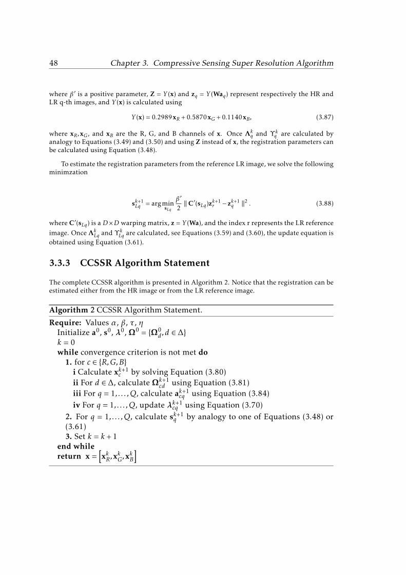
48 Chapter 3. Compressive Sensing Super Resolution Algorithm
where β′ is a positive parameter, Z = Y (x) and zq = Y (Waq) represent respectively the HR andLR q-th images, and Y (x) is calculated using
Y (x) = 0.2989xR +0.5870xG +0.1140xB, (3.87)
where xR,xG, and xB are the R, G, and B channels of x. Once Λkq and Υ k
q are calculated byanalogy to Equations (3.49) and (3.50) and using Z instead of x, the registration parameters canbe calculated using Equation (3.48).
To estimate the registration parameters from the reference LR image, we solve the followingminimzation
sk+1Lq = argminsLq
β′
2∥ C′(sLq)zk+1r − zk+1q ∥2 . (3.88)
where C′(sLq) is a D×D warping matrix, z = Y (Wa), and the index r represents the LR referenceimage. Once Λk
Lq and Υ kLq are calculated, see Equations (3.59) and (3.60), the update equation is
obtained using Equation (3.61).
3.3.3 CCSSR Algorithm Statement
The complete CCSSR algorithm is presented in Algorithm 2. Notice that the registration can beestimated either from the HR image or from the LR reference image.
Algorithm 2 CCSSR Algorithm Statement.
Require: Values α, β, τ , ηInitialize a0, s0, λ0, Ω0 = Ω0
d ,d ∈ ∆k = 0while convergence criterion is not met do1. for c ∈ R,G,Bi Calculate xk+1c by solving Equation (3.80)ii For d ∈ ∆, calculate Ωk+1
cd using Equation (3.81)iii For q = 1, . . . ,Q, calculate ak+1cq using Equation (3.84)iv For q = 1, . . . ,Q, update λk+1
cq using Equation (3.70)2. For q = 1, . . . ,Q, calculate sk+1q by analogy to one of Equations (3.48) or(3.61)3. Set k = k +1
end whilereturn x =
[xkR,x
kG,x
kB
]

Chapter 4
Experimental Results
This chapter analyzes the experimental results obtained for the proposed algorithms. Oncethe used assessment criteria are presented, an intra-process analysis is performed, i.e. a com-parative study of internal techniques for the different CSSR algorithm steps proposed in thethesis is presented, and how they affect the overall performance is analyzed. Then, the pro-posed framework is compared with existing SR and CS ID algorithms, which can be consideredas special cases of the general CSSR algorithm. This is followed by the analysis of the CSSR al-gorithm in its general case. Finally, two main applications of the CSSR algorithm are examined:PMMW and color images.
4.1 Quality Assessment
The CSSR reconstruction problem estimates one HR image of a scene. Usually, we do not havethe original image to compare it with the estimated one. However, there are some measuresthat can help indicating the performance level of the estimation process.
The first assessment criterion is the human eye perception which to some limit can beadopted. However, it does not give a standard measure and it may depend on the person him-self looking at the estimated image.
Another assessment criteria which may give a better judgment are machine vision tech-niques, where the estimated image is forwarded to another processing step to make a decisionor to operate a device. The reliability and accuracy measures of the machine are known, thenthe merits of the estimated image, which is fed as the input to the machine, will affect the per-formance of the machine. The change in overall performance of the machine definitely givesan indication about how much efficient the estimation process was. As an example, let us con-sider a set of PMMW images, how to measure the performance of the super resolved image?The answer is that when the HR is fed to a threat detection algorithm, and this leads to higherreliability then this will be a consequence of the higher quality of the estimated image.
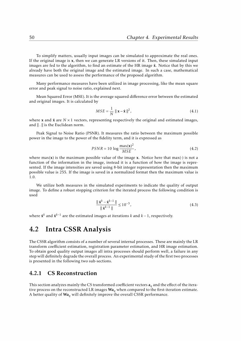
50 Chapter 4. Experimental Results
To simplify matters, usually input images can be simulated to approximate the real ones.If the original image is x, then we can generate LR versions of it. Then, these simulated inputimages are fed to the algorithm, to find an estimate of the HR image x. Notice that by this wealready have both the original image and the estimated image. In such a case, mathematicalmeasures can be used to assess the performance of the proposed algorithm.
Many performance measures have been utilized in image processing, like the mean squareerror and peak signal to noise ratio, explained next.
Mean Squared Error (MSE). It is the average squared difference error between the estimatedand original images. It is calculated by
MSE =1N∥ x− x ∥2 , (4.1)
where x and x are N × 1 vectors, representing respectively the original and estimated images,and ∥ . ∥ is the Euclidean norm.
Peak Signal to Noise Ratio (PSNR). It measures the ratio between the maximum possiblepower in the image to the power of the fidelity term, and it is expressed as
P SNR = 10 logmax(x)2
MSE, (4.2)
where max(x) is the maximum possible value of the image x. Notice here that max(·) is not afunction of the information in the image, instead it is a function of how the image is repre-sented. If the image intensities are saved using 8-bit integer representation then the maximumpossible value is 255. If the image is saved in a normalized format then the maximum value is1.0.
We utilize both measures in the simulated experiments to indicate the quality of outputimage. To define a robust stopping criterion for the iterated process the following condition isused
∥ xk − xk−1 ∥∥ xk−1 ∥
≤ 10−3 , (4.3)
where xk and xk−1 are the estimated images at iterations k and k − 1, respectively.
4.2 Intra CSSR Analysis
The CSSR algorithm consists of a number of several internal processes. These are mainly the LRtransform coefficient estimation, registration parameter estimation, and HR image estimation.To obtain good quality output images all intra processes should perform well, a failure in anystep will definitely degrade the overall process. An experimental study of the first two processesis presented in the following two sub-sections.
4.2.1 CS Reconstruction
This section analyzes mainly the CS transformed coefficient vectors aq and the effect of the itera-tive process on the reconstructed LR imagesWaq when compared to the first-iteration estimate.A better quality of Waq will definitely improve the overall CSSR performance.

4.2. Intra CSSR Analysis 51
Let us now illustrate how blurring affects image sparsity (see [5]). It was shown in [15] thatimages whose coefficients in a transformed domain follow a power decay law, when sorted bydecreasing magnitude, are sparse in this domain. In this dissertation the 3-level Haar waveletwill be used as the transform basis. Let us see how blurring does affect the decay of the trans-formed coefficients for the standard Cameraman and Shepp-Logan images. Gaussian blur ofvariances 3 and 9 has been applied to those images and white Gaussian noise with Signal-to-Noise ratio SNR= 40 dB has been added. Figures 4.1(a,b) show the magnitude versus sortedindices of the wavelet coefficients. Similarly, Figures 4.1(c,d) show the results for the standardShepp-Logan image for the two blur variances 3 and 9, respectively. More severe blur results ina faster magnitude decay, as it is clear in the figure.
(a) (b)
(c) (d)
Figure 4.1: LR 3-level Haar wavelet coefficient decay, using simulated observations(SNR= 40 dB), (a,b) Cameraman image affected by Gaussian blur of variance 3 and 9,respectively. (c,d) Shepp-Logan image affected by blur of variance 3 and 9, respectively.
The next point to discuss here is the effect of the pruning of the coefficients on the esti-mated image. Figure 4.2(a) shows the reconstructed LR Cameraman image by including allthe coefficients in the transformed vector aq. The experiment utilized R=0.8, P=1, blur Vari-

52 Chapter 4. Experimental Results
(a) (b) (c)
Figure 4.2: LR Cameraman image restoration using a simulated observation with blurvariance 3, zooming factor P=1, R=0.8, noise SNR= 40 dB. (a) LR reconstructed ob-servation using all elements of the coefficient vector aq (PSNR=22.65 dB), (b) LR re-constructed observation using the first 60% of elements in aq (PSNR=22.47 dB), (c)LR reconstructed observation using the first 20% of elements in aq (PSNR=22.24 dB).Transform basis used is 3-level Haar wavelet transform.
ance=3, and noise SNR= 40 dB, and the resulting PSNR is 22.65 dB. Next, only the first 60% ofthe transformed coefficients in aq were kept, while the others were pruned, then the resultingtransformed vector is used to estimate the LR image shown in Figure 4.2(b), with PSNR=22.47dB. Then, the LR image is estimated using only the first 20% of aq, the result is shown in Fig-ure 4.2(c) with PSNR=22.24 dB.
The previous experiment has been repeated for the Shepp-Logan image, whose results areshown as follows: Figure 4.3(a) shows the estimated image with all aq included (PSNR=21.35dB), Figure 4.3(b) utilized only 60% of aq (PSNR=21.18 dB), and finally, Figure 4.3(c) utilizedonly 20% of aq (PSNR=20.68 dB).
Next we discuss the effect of the iterative process on the performance of the CS reconstruc-tion. We use two simulated LR images of the standard Shepp-Logan image shown in Figure4.4(a). To simulate two LR observations, the HR image of size 256×256 pixels, was warped us-ing the following motion vectors: [0,0,0]t , [−0.1047,2,−3]t , then blurred with a Gaussian blurof variance=3, then down-sampled by a zooming factor P=2. The two simulated LR images areshown in Figure 4.4(b,c). These simulated LR images are then compressed with a compressionratio R=0.8, and noise is added with SNR=30dB.
Let us examine the first iteration LR estimations using Equation (3.38), without the regu-larization term. The estimated images are shown in Figure 4.4(d,e), and the PSNR values ofthe reconstructed LR images are 40.22 dB and 40.16 dB, respectively. As the CSSR process ad-vances, the inclusion of the registration term allows for a better extraction of the informationin the compressed observations; the final estimated LR images are shown in Figure 4.4(f,g),with PSNR values being 42.88 dB and 42.77 dB, respectively. Notice in this experiment that thePSNR values were calculated with respect to the simulated LR observations, not to the originalHR image.
For the Cameraman image shown in Figure 4.5(a), the down-sampled images are shown in

4.2. Intra CSSR Analysis 53
(a) (b) (c)
Figure 4.3: LR Shepp-Logan image restoration using a simulated observation with blurvariance 3, zooming factor P=1, R=0.8, noise SNR=40dB. (a) LR reconstructed obser-vation using all elements of the coefficient vector aq (PSNR=21.35 dB), (b) LR recon-structed observation using the first 60% of elements in aq (PSNR=21.18 dB), (c) LR re-constructed observation using the first 20% of elements in aq (PSNR=20.68 dB). Trans-form basis used is 3-level Haar wavelet transform.
(a)
(b)
(c)
(d)
(e)
(f)
(g)
Figure 4.4: Reconstruction of LR images. (a) Original HR Shepp-Logan image, (b,c)Down-sampled images Q=2, P=2, Blur Var=3, R=0.8, SNR=30 dB, (d,e) First estimatesof the LR images, PSNR= 40.22 dB and , 40.16 dB respectively, (f,g) Final estimates ofthe LR images, PSNR=42.88 dB and 42.77 dB respectively. PSNR values were calculatedwith respect to the simulated LR images.

54 Chapter 4. Experimental Results
(a)
(b)
(c)
(d)
(e)
(f)
(g)
Figure 4.5: Reconstruction of LR images. (a) Cameraman original HR image, (b,c)Down-sampled images Q=2, P=2, Blur Var=3, R=0.8, SNR=30dB, (d,e) First estimatesof the LR images, PSNR=35.52 dB and 35.29 dB, respectively, (f,g) Final estimates of theLR images, PSNR=35.55 dB and 35.34 dB, respectively. PSNR values were calculatedwith respect to the simulated LR images.
Figure 4.5(b,c), the initially estimated LR images are shown in Figure 4.5(d,e), with PSNR=35.52dB and 35.29 dB, respectively. The final estimated LR images are shown in Figure 4.5(f,g), withPSNRs equal to 35.55 dB and 35.34 dB, respectively. In this experiment the PSNR values werecalculated with respect to the simulated LR observations, not to the original HR image.
For the Lena image shown in Figure 4.6(a), the down-sampled images are shown in Figure4.6(b,c), the initially estimated LR images are shown in Figure 4.6(d,e), with PSNR=32.45 dBand 32.28 dB, respectively. The final estimated LR images are shown in Figure 4.6(f,g), withPSNRs equal to 34.24 dB and 34.07 dB, respectively. In this experiment the PSNR values werecalculated with respect to the simulated LR observations, not to the original HR image.
Notice that the inclusion of the regularization term in Equation (3.38) greatly contributes tothe PSNR improvement when using the CSSR algorithm. This improvement will be very usefulwhen super resolving the LR observations to estimate the HR image. Notice here also that theshown images are not the HR images but only the uncompressed versions of the LR images.
4.2.2 Registration Estimation
In this section we study the performance of various approaches to estimate the registrationparameters as a step that greatly affects the overall HR image estimation. To do so, two ex-periments were carried out, for every approach, to establish the CSSR accuracy when estimat-ing the registration parameters. The 256×256 pixel HR Shepp-Logan image, with Q=4, Blurvariance=3, SNR=40dB, and R=0.8 were used. P=2 and 4, were chosen to conduct these two

4.2. Intra CSSR Analysis 55
(a)
(b)
(c)
(d)
(e)
(f)
(g)
Figure 4.6: Reconstruction of LR images. (a) Lena original HR image, (b,c) Down-sampled images Q=2, P=2, Blur Var=3, R=0.8, SNR=30dB, (d,e) First estimates of theLR images, PSNR=40.22 dB and 40.16 dB, respectively, (f,g) Final estimates of the LRimages, PSNR=42.88 dB and 42.77 dB, respectively. PSNR values were calculated withrespect to the simulated LR images.
experiments, and the maximum number of iterations was 30.
Here are the approaches,
• App1, see also [19]. It estimates the parameters with respect to a reference LR image, atthe HR level, following the optimization in Equation (3.16). The results for this approachare tabulated in Table 4.1(a) which shows the real and estimated registration parameters.It contains also the absolute errors. Notice that for the first observation, which is thereference observation, the motion vector is [0,0,0]t , so the motion vectors were adjustedaccordingly to this.
• App2, see also [20]. It estimates the parameters with respect to the estimated image, atthe HR level, as in Equation (3.17). See Table 4.1(b) for results of this approach.
• App3, see also [18]. It estimates the parameters with respect to the estimated image, atthe LR level, as in Equation (3.41). See Table 4.2(a) for results of this approach.
• App4. It estimates the parameters with respect to a reference LR image, at the LR level,as in Equation (3.51). See Table 4.2(b) for results of this approach.
Figure 4.7 shows a plot of the average absolute errors for each element in sq, (q ∈ 1, · · · ,4),for the four approaches. The four approaches are suggested to be used with high accuracy. Laterin Section 4.5.3 we will investigate more the effects of using App3 and App4 on the overallperformance of the CSSR algorithm.
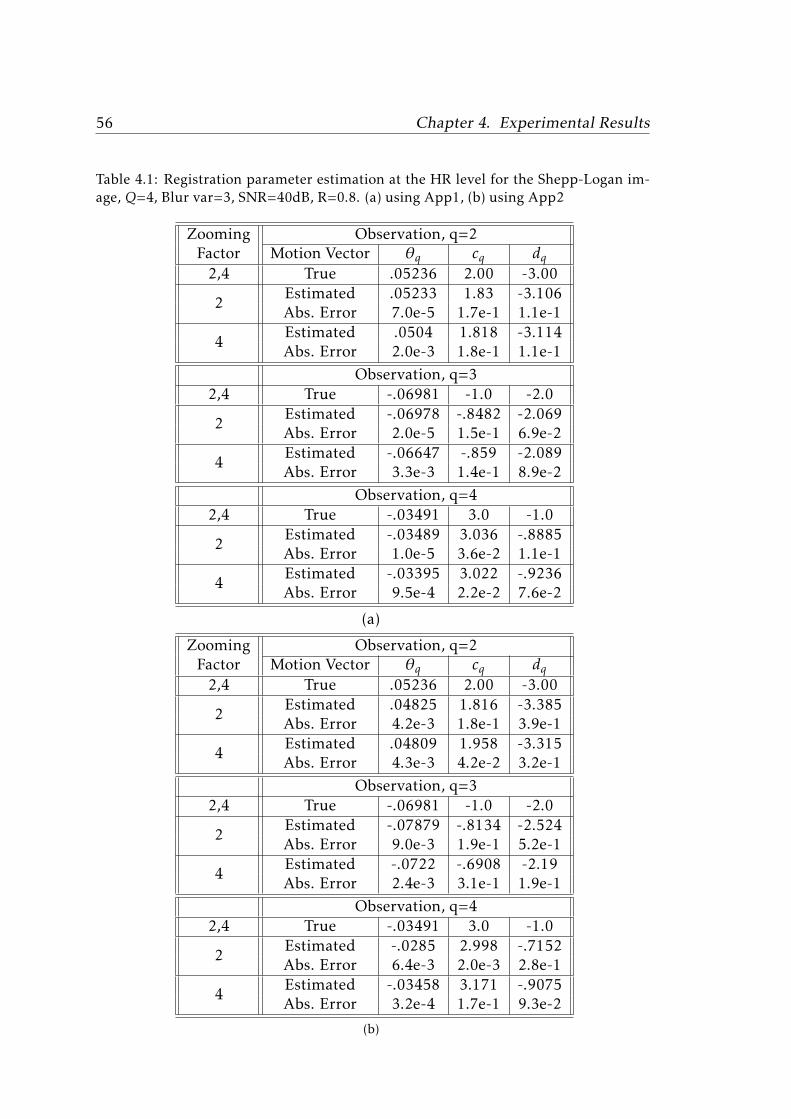
56 Chapter 4. Experimental Results
Table 4.1: Registration parameter estimation at the HR level for the Shepp-Logan im-age, Q=4, Blur var=3, SNR=40dB, R=0.8. (a) using App1, (b) using App2
Zooming Observation, q=2Factor Motion Vector θq cq dq2,4 True .05236 2.00 -3.00
2Estimated .05233 1.83 -3.106Abs. Error 7.0e-5 1.7e-1 1.1e-1
4Estimated .0504 1.818 -3.114Abs. Error 2.0e-3 1.8e-1 1.1e-1
Observation, q=32,4 True -.06981 -1.0 -2.0
2Estimated -.06978 -.8482 -2.069Abs. Error 2.0e-5 1.5e-1 6.9e-2
4Estimated -.06647 -.859 -2.089Abs. Error 3.3e-3 1.4e-1 8.9e-2
Observation, q=42,4 True -.03491 3.0 -1.0
2Estimated -.03489 3.036 -.8885Abs. Error 1.0e-5 3.6e-2 1.1e-1
4Estimated -.03395 3.022 -.9236Abs. Error 9.5e-4 2.2e-2 7.6e-2
(a)
Zooming Observation, q=2Factor Motion Vector θq cq dq2,4 True .05236 2.00 -3.00
2Estimated .04825 1.816 -3.385Abs. Error 4.2e-3 1.8e-1 3.9e-1
4Estimated .04809 1.958 -3.315Abs. Error 4.3e-3 4.2e-2 3.2e-1
Observation, q=32,4 True -.06981 -1.0 -2.0
2Estimated -.07879 -.8134 -2.524Abs. Error 9.0e-3 1.9e-1 5.2e-1
4Estimated -.0722 -.6908 -2.19Abs. Error 2.4e-3 3.1e-1 1.9e-1
Observation, q=42,4 True -.03491 3.0 -1.0
2Estimated -.0285 2.998 -.7152Abs. Error 6.4e-3 2.0e-3 2.8e-1
4Estimated -.03458 3.171 -.9075Abs. Error 3.2e-4 1.7e-1 9.3e-2
(b)

4.2. Intra CSSR Analysis 57
Table 4.2: Registration parameter estimation at the LR level for the Shepp-Logan image,Q=4, Blur var=3, SNR=40dB, R=0.8. (a) using App3 (b) using App4
Zooming Observation, q=2Factor Motion Vector θq cq dq2,4 True .05236 2.00 -3.00
2Estimated .05229 1.999 -3.002Abs. Error 7.0e-5 1.0e-3 2.0e-3
4Estimated .05163 2.033 -3.057Abs. Error 7.3e-4 3.3e-2 5.7e-2
Observation, q=32,4 True -.06981 -1.0 -2.0
2Estimated -.06916 -1.002 -2.005Abs. Error 6.5e-4 2.0e-3 5.0e-2
4Estimated -.06902 -1.012 -2.046Abs. Error 7.9e-4 1.2e-2 4.6e-2
Observation, q=42,4 True -.03491 3.0 -1.0
2Estimated -.03478 3.00 -1.001Abs. Error 1.3e-4 1.0e-3 1.0e-3
4Estimated -.03351 2.999 -1.041Abs. Error 1.4e-3 1.0e-3 4.1e-2
(a)
Zooming Observation, q=2Factor Motion Vector θq cq dq2,4 True .05236 2.00 -3.00
2Estimated .05255 1.999 -2.998Abs. Error 1.5e-4 1.0e-3 2.0e-3
4Estimated .05224 2.02 -3.058Abs. Error 1.6e-4 2.0e-2 5.8e-2
Observation, q=32,4 True -.06981 -1.0 -2.0
2Estimated -.06984 -1.001 -2.Abs. Error 4.0e-5 1.0e-3 0.0e0
4Estimated -.06899 -1.014 -2.052Abs. Error 8.1e-4 1.4e-2 5.2e-2
Observation, q=42,4 True -.03491 3.0 -1.0
2Estimated -.03497 2.999 -1.001Abs. Error 7.0e-5 1.0e-3 1.0e-3
4Estimated -.03388 2.967 -1.043Abs. Error 1.0e-3 3.3e-2 4.3e-2
(b)
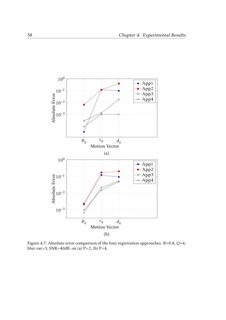
58 Chapter 4. Experimental Results
θqcq dq
10−3
10−2
10−1
100
Motion Vector
Absolute
Error
App1App2App3App4
(a)
θqcq dq
10−3
10−2
10−1
100
Motion Vector
Absolute
Error
App1App2App3App4
(b)
Figure 4.7: Absolute error comparison of the four registration approaches. R=0.8,Q=4,blur var=3, SNR=40dB. on (a) P=2, (b) P=4.
4.3. CSSR vs ID Works 59
4.3 CSSR vs IDWorks
In this section the performance of the proposed CSSR algorithm is compared with a set ofexisting image deconvolution CS algorithms, namely l1-ls [82], GPSR [68], NESTA [70], YALL1[71], and CoSaMP [69], using their native codes. These algorithms estimate x from one CSblurred observation. Results were tabulated in Tables 4.3 to 4.5, CSSR used P=1 and Q=1.
Figure 4.8 shows plots of the performance measure, for all tested algorithms, vs compres-sion ratio R, for the three test images, using Blur var=5 and SNR=30 dB. Figure 4.9 shows theplots for the case where Blur var=3 and SNR=40 dB. It is clear the quality level the CSSR offersin comparison to other works using one input CS observation. The performance of CSSR isexpected to be better if multiple input images are used.
Next we test the performance as a function of the variance of the blur. To compare the per-formance for all algorithms, plots are shown for the case R=0.6 and SNR=30 dB in Figure 4.10,and for R=0.8, SNR=40 dB in Figure 4.11. As the plots show, the proposed CSSR algorithmestimates images of good quality, even when compared with CS image deconvolution works.
4.4 CSSR vs SRWorks
This section compares the performance of the proposed CSSR algorithm with a set of existingSR algorithms, namely Bicubic Interpolation (BIC), SR using an l1 prior [28] (L1S), SR usingSAR priors [30] (SAS), a fast and robust SR [34] (FRSR), and a robust SR method [49] (RSR).Algorithms L1S [28] and SAS [30] estimate all their parameters. Since algorithms FRSR [34]and RSR [49] need some parameters to be set, we performed an exhaustive search to find theparameters resulting in the maximum PSNR values. We used the Cameraman, Shepp-Loganand Lena images. The number of observations was Q=4. For our CSSR, we used a unity com-pression ratio R=1.0 to compare with those SR algorithms which do not use CS observations.Notice that we still use CS but with 100% of the measurements which is equivalent to usingΦ = I. The results are tabulated in Tables 4.6 and 4.7.
The plots in Figures 4.12 and 4.13 compare the performance of SR algorithms as a functionof the variance of the blur affecting the test images for two different noise SNR 40 dB and 30dB, respectively. Both cases used Q=4 and P=4. Notice the relative improvement of the CSSRalgorithm, when compared with SR algorithms that do not use compressed sensing, for the twocases.
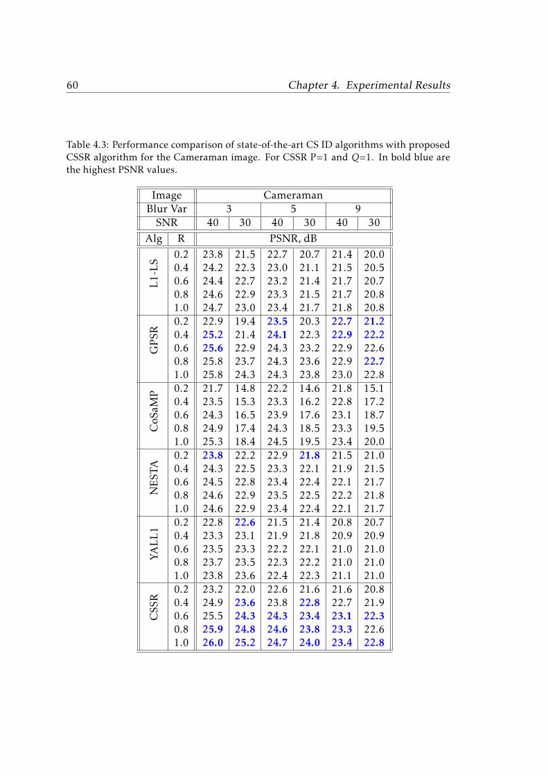
60 Chapter 4. Experimental Results
Table 4.3: Performance comparison of state-of-the-art CS ID algorithms with proposedCSSR algorithm for the Cameraman image. For CSSR P=1 and Q=1. In bold blue arethe highest PSNR values.
Image CameramanBlur Var 3 5 9SNR 40 30 40 30 40 30
Alg R PSNR, dB
L1-LS
0.2 23.8 21.5 22.7 20.7 21.4 20.00.4 24.2 22.3 23.0 21.1 21.5 20.50.6 24.4 22.7 23.2 21.4 21.7 20.70.8 24.6 22.9 23.3 21.5 21.7 20.81.0 24.7 23.0 23.4 21.7 21.8 20.8
GPSR
0.2 22.9 19.4 23.5 20.3 22.7 21.20.4 25.2 21.4 24.1 22.3 22.9 22.20.6 25.6 22.9 24.3 23.2 22.9 22.60.8 25.8 23.7 24.3 23.6 22.9 22.71.0 25.8 24.3 24.3 23.8 23.0 22.8
CoS
aMP 0.2 21.7 14.8 22.2 14.6 21.8 15.1
0.4 23.5 15.3 23.3 16.2 22.8 17.20.6 24.3 16.5 23.9 17.6 23.1 18.70.8 24.9 17.4 24.3 18.5 23.3 19.51.0 25.3 18.4 24.5 19.5 23.4 20.0
NEST
A
0.2 23.8 22.2 22.9 21.8 21.5 21.00.4 24.3 22.5 23.3 22.1 21.9 21.50.6 24.5 22.8 23.4 22.4 22.1 21.70.8 24.6 22.9 23.5 22.5 22.2 21.81.0 24.6 22.9 23.4 22.4 22.1 21.7
YALL1
0.2 22.8 22.6 21.5 21.4 20.8 20.70.4 23.3 23.1 21.9 21.8 20.9 20.90.6 23.5 23.3 22.2 22.1 21.0 21.00.8 23.7 23.5 22.3 22.2 21.0 21.01.0 23.8 23.6 22.4 22.3 21.1 21.0
CSS
R
0.2 23.2 22.0 22.6 21.6 21.6 20.80.4 24.9 23.6 23.8 22.8 22.7 21.90.6 25.5 24.3 24.3 23.4 23.1 22.30.8 25.9 24.8 24.6 23.8 23.3 22.61.0 26.0 25.2 24.7 24.0 23.4 22.8

4.4. CSSR vs SR Works 61
Table 4.4: Performance comparison of state-of-the-art CS ID algorithms with proposedCSSR algorithm for the Lena image. For CSSR P=1 and Q=1. In bold blue are thehighest PSNR values.
Image LenaBlur Var 3 5 9SNR 40 30 40 30 40 30
Alg R PSNR, dB
L1-LS
0.2 26.5 23.1 25.1 22.3 23.5 22.40.4 27.3 24.1 25.6 23.0 23.7 22.50.6 27.6 24.6 25.9 23.4 23.9 22.80.8 27.8 25.0 26.0 23.5 24.0 22.91.0 27.9 25.2 26.2 23.7 24.1 23.0
GPSR
0.2 25.3 22.2 26.8 23.9 26.1 24.70.4 29.3 25.3 28.2 26.3 26.5 25.80.6 30.0 26.9 28.5 27.2 26.5 26.10.8 30.4 28.1 28.6 27.7 26.6 26.31.0 30.7 28.7 28.7 28.0 26.6 26.4
CoS
aMP 0.2 23.9 16.4 24.9 16.1 25.1 16.9
0.4 26.2 16.8 26.7 18.0 26.4 19.50.6 27.4 18.0 27.6 19.5 26.9 21.00.8 28.2 19.1 28.1 20.6 27.1 21.91.0 28.7 20.1 28.6 21.7 27.2 22.9
NEST
A
0.2 26.5 24.8 25.4 24.3 23.6 23.20.4 27.3 25.3 25.9 24.7 24.1 23.70.6 27.6 25.7 26.2 25.1 24.2 24.00.8 27.8 25.9 26.4 25.3 24.4 24.01.0 27.8 25.8 26.2 25.0 24.3 24.0
YALL1
0.2 24.8 24.6 23.4 23.4 22.4 22.30.4 25.7 25.5 23.9 23.9 22.8 22.80.6 26.0 25.8 24.2 24.1 22.9 22.90.8 26.3 26.1 24.4 24.3 23.0 23.01.0 26.4 26.2 24.5 24.4 23.1 23.0
CSS
R
0.2 24.0 22.4 23.8 22.7 22.6 21.70.4 27.5 26.3 26.8 25.4 24.6 24.20.6 29.5 27.9 28.2 26.7 26.5 25.20.8 30.6 28.8 29.0 27.4 27.1 25.81.0 31.2 29.4 29.4 27.9 27.4 26.2

62 Chapter 4. Experimental Results
Table 4.5: Performance comparison of state-of-the-art CS ID algorithms with proposedCSSR algorithm for the Shepp-Logan image. For CSSR P=1 and Q=1. In bold blue arethe highest PSNR values.
Image Shepp-LoganBlur Var 3 5 9SNR 40 30 40 30 40 30
Alg R PSNR, dB
L1-LS
0.2 22.8 21.6 22.0 21.2 20.5 20.20.4 23.1 21.8 22.3 21.5 20.7 20.40.6 23.3 21.9 22.3 21.6 20.8 20.50.8 23.5 22.0 22.4 21.6 20.9 20.61.0 23.7 22.1 22.4 21.7 20.9 20.7
GPSR
0.2 24.1 20.5 23.6 20.9 22.2 21.10.4 25.2 21.4 24.0 22.4 22.3 21.90.6 25.4 22.7 24.1 23.1 22.3 22.10.8 25.5 23.6 24.1 23.5 22.5 22.21.0 25.5 24.1 24.1 23.68 22.4 22.3
CoS
aMP 0.2 22.9 17.5 22.6 17.6 21.9 18.3
0.4 23.8 19.3 23.3 19.3 22.2 19.80.6 24.2 20.6 23.5 20.4 22.4 20.70.8 24.6 21.4 23.6 21.2 22.4 21.21.0 24.6 21.9 23.6 21.7 22.4 21.4
NEST
A
0.2 22.8 22.4 22.1 21.7 20.5 20.40.4 23.2 22.8 22.3 22.0 20.8 20.80.6 23.4 23.1 22.4 22.2 21.0 21.10.8 23.5 23.2 22.5 22.3 21.2 21.21.0 23.6 23.3 22.4 22.2 21.0 21.2
YALL1
0.2 22.1 22.0 20.7 20.7 19.4 19.40.4 22.3 22.3 21.0 21.0 19.6 19.60.6 22.4 22.4 21.2 21.2 19.9 19.80.8 22.5 22.5 21.5 21.4 20.0 20.01.0 22.6 22.6 21.7 21.6 20.1 20.0
CSS
R
0.2 24.2 23.2 23.1 22.2 20.9 21.00.4 25.4 25.3 24.1 24.1 22.4 22.20.6 25.7 26.1 24.4 24.7 22.7 22.90.8 25.8 26.4 24.5 24.9 22.9 23.21.0 25.8 26.5 24.5 25.0 22.9 23.3

4.4. CSSR vs SR Works 63
0.2 0.4 0.6 0.8 114
16
18
20
22
24
Compression Ratio
PSN
R(dB)
CSSRL1-LSGPSR
CoSaMpNESTAYALL1
(a)
0.2 0.4 0.6 0.8 116
18
20
22
24
26
28
Compression Ratio
PSN
R(dB)
CSSRL1-LSGPSR
CoSaMpNESTAYALL1
(b)
0.2 0.4 0.6 0.8 1
18
20
22
24
Compression Ratio
PSN
R(dB)
CSSRL1-LSGPSR
CoSaMpNESTAYALL1
(c)
Figure 4.8: Proposed CSSR vs CS ID algorithms comparison (Blur Var=5, SNR=30dB,for CSSR P=1, Q=1). (a) Cameraman (b) Lena (c) Shepp-Logan.

64 Chapter 4. Experimental Results
0.2 0.4 0.6 0.8 1
22
24
26
Compression Ratio
PSN
R(dB)
CSSRL1-LSGPSR
CoSaMpNESTAYALL1
(a)
0.2 0.4 0.6 0.8 124
26
28
30
Compression Ratio
PSN
R(dB)
CSSRL1-LSGPSR
CoSaMpNESTAYALL1
(b)
0.2 0.4 0.6 0.8 1
22
24
26
Compression Ratio
PSN
R(dB)
CSSRL1-LSGPSR
CoSaMpNESTAYALL1
(c)
Figure 4.9: Proposed CSSR vs CS ID algorithms comparison (Blur Var=3, SNR=40dB,for CSSR P=1, Q=1). (a) Cameraman, (b) Lena, (c) Shepp-Logan.

4.4. CSSR vs SR Works 65
3 5 7 9
16
18
20
22
24
Blur Variance
PSN
R(dB)
CSSRL1-LSGPSR
CoSaMpNESTAYALL1
(a)
3 5 7 9
18
20
22
24
26
28
Blur Variance
PSN
R(dB)
CSSRL1-LSGPSR
CoSaMpNESTAYALL1
(b)
3 5 7 9
20
22
24
26
Blur Variance
PSN
R(dB)
CSSRL1-LSGPSR
CoSaMpNESTAYALL1
(c)
Figure 4.10: Proposed CSSR vs CS ID algorithms comparison (R=0.6, SNR=30dB, forCSSR P=1, Q=1). (a) Cameraman, (b) Lena, (c) Shepp-Logan.

66 Chapter 4. Experimental Results
3 5 7 920
22
24
26
Blur Variance
PSN
R(dB)
CSSRL1-LSGPSR
CoSaMpNESTAYALL1
(a)
3 5 7 922
24
26
28
30
Blur Variance
PSN
R(dB)
CSSRL1-LSGPSR
CoSaMpNESTAYALL1
(b)
3 5 7 9
20
22
24
26
Blur Variance
PSN
R(dB)
CSSRL1-LSGPSR
CoSaMpNESTAYALL1
(c)
Figure 4.11: Proposed CSSR vs CS ID algorithms comparison (R=0.8, SNR=40dB, forCSSR P=1, Q=1). (a) Cameraman, (b) Lena, (c) Shepp-Logan.

4.4. CSSR vs SR Works 67
Table 4.6: Comparison of state-of-the-art SR algorithms with the CSSR algorithm forCameraman and Lena images, with Q=4 and for CSSR R=1.0. In bold blue are thehighest PSNR values.
Image CameramanBlur Var 3 5 9SNR 40 30 40 30 40 30
Alg P PSNR, dB
BIC2 22.5 22.7 22.4 22.3 22.4 22.44 20.5 20.4 20.5 20.5 20.5 20.4
L1S2 24.1 24.5 23.9 24.2 24.1 23.94 21.9 22.1 21.7 21.3 21.7 21.6
SAS2 24.1 23.7 24.1 23.4 24.2 23.34 22.2 22.4 22.1 22.0 22.2 22.1
FRSR2 20.9 21.5 19.3 19.8 21.5 20.64 21.1 22.3 20.9 21.2 21.1 21.8
RSR2 22.5 22.2 21.1 21.6 21.3 22.04 20.5 20.6 20.4 20.5 20.5 20.6
CSSR2 25.9 24.8 24.6 23.8 23.4 22.64 25.0 24.1 24.0 23.3 23.1 22.3
Image Lena
BIC2 24.7 24.7 24.6 24.6 24.5 24.44 21.1 21.0 21.1 21.0 21.1 21.1
L1S2 27.0 27.4 27.2 27.5 26.7 27.44 25.8 25.7 25.9 25.4 25.9 26.0
SAS2 27.7 27.5 28.4 27.6 28.3 27.54 26.4 26.3 26.9 25.9 26.5 26.4
FRSR2 20.5 20.8 21.2 20.9 22.0 20.14 21.9 22.4 21.8 23.2 21.8 24.9
RSR2 23.1 25.2 25.0 25.1 24.2 23.04 21.7 21.9 21.7 21.8 21.9 22.0
CSSR2 31.1 29.0 29.4 27.6 27.3 26.04 29.4 27.4 28.2 26.4 26.7 25.2
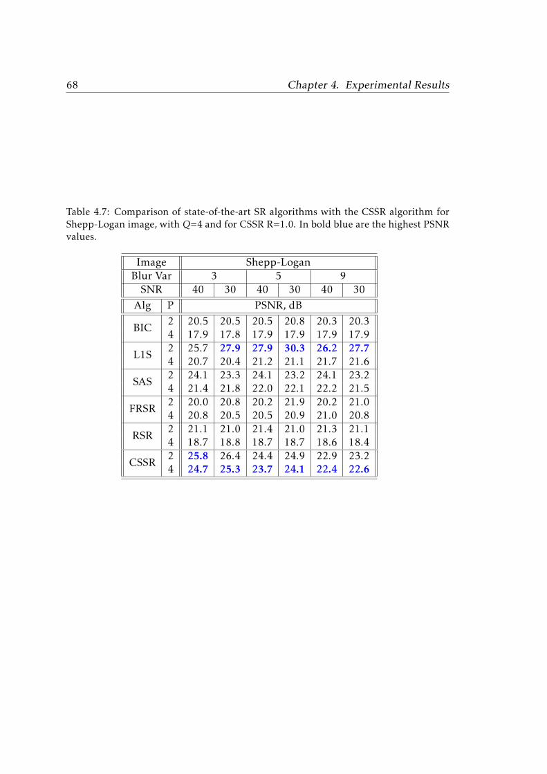
68 Chapter 4. Experimental Results
Table 4.7: Comparison of state-of-the-art SR algorithms with the CSSR algorithm forShepp-Logan image, with Q=4 and for CSSR R=1.0. In bold blue are the highest PSNRvalues.
Image Shepp-LoganBlur Var 3 5 9SNR 40 30 40 30 40 30
Alg P PSNR, dB
BIC2 20.5 20.5 20.5 20.8 20.3 20.34 17.9 17.8 17.9 17.9 17.9 17.9
L1S2 25.7 27.9 27.9 30.3 26.2 27.74 20.7 20.4 21.2 21.1 21.7 21.6
SAS2 24.1 23.3 24.1 23.2 24.1 23.24 21.4 21.8 22.0 22.1 22.2 21.5
FRSR2 20.0 20.8 20.2 21.9 20.2 21.04 20.8 20.5 20.5 20.9 21.0 20.8
RSR2 21.1 21.0 21.4 21.0 21.3 21.14 18.7 18.8 18.7 18.7 18.6 18.4
CSSR2 25.8 26.4 24.4 24.9 22.9 23.24 24.7 25.3 23.7 24.1 22.4 22.6

4.4. CSSR vs SR Works 69
3 5 7 9
20
22
24
26
Blur Variance
PSN
R(dB) CSSR
L1SSASFRSRRSRBIC
(a)
3 5 7 920
2224
26
28
30
Blur Variance
PSN
R(dB) CSSR
L1SSASFRSRRSRBIC
(b)
3 5 7 9
18
20
22
24
26
Blur Variance
PSN
R(dB) CSSR
L1SSASFRSRRSRBIC
(c)
Figure 4.12: Comparison between SR algorithms and the CSSR algorithm. P=4,SNR=40dB, Q=4, and for CSSR, R=1.0. (a) Cameraman image, (b) Lena, (c) Shepp-Logan image.
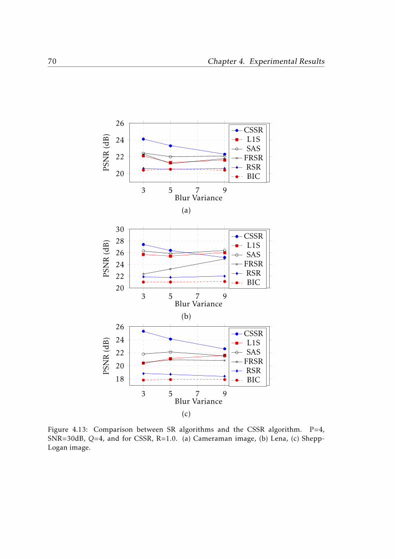
70 Chapter 4. Experimental Results
3 5 7 9
20
22
24
26
Blur Variance
PSN
R(dB) CSSR
L1SSASFRSRRSRBIC
(a)
3 5 7 920
2224
26
28
30
Blur Variance
PSN
R(dB) CSSR
L1SSASFRSRRSRBIC
(b)
3 5 7 9
18
20
22
24
26
Blur Variance
PSN
R(dB) CSSR
L1SSASFRSRRSRBIC
(c)
Figure 4.13: Comparison between SR algorithms and the CSSR algorithm. P=4,SNR=30dB, Q=4, and for CSSR, R=1.0. (a) Cameraman image, (b) Lena, (c) Shepp-Logan image.

4.5. CSSR: The General Case 71
4.5 CSSR: The General Case
In this section the overall behavior of the CSSR algorithm is investigated; both the compressionratio and zooming factor will be varied and the results analyzed. Notice here that we test theCSSR in its general case for different R and P values, while in the previous two sections R, P orQ were fixed at 1 to be able to compare our work with existing works which do not adapt to thisgeneral case. In this section we use the images shown in Figure 4.14, namely Satellite, Barbara,Peppers, and Alhambra images.
(a) (b)
(c) (d)
Figure 4.14: Original Images. (a) Satellite, (b) Barbara, (c) Peppers, (d) Alhambra.
The performance of CSSR is shown in Tables 4.8 and 4.9 for the four test images, usingQ=4.
Next we will choose four examples to precisely explore the CSSR performance. For everyzooming factor, two cases were chosen: in one the image is affected by simple degradations

72 Chapter 4. Experimental Results
Table 4.8: Performance of the CSSR algorithm for the Satellite and Barbara images,using Q = 4.
Blur Var 3 5 9SNR 40 30 40 30 40 30Image P R PSNR (dB)Satellite 2 0.2 26.5 24.9 26.0 24.4 24.9 23.8
0.4 28.1 26.9 27.1 26.1 25.8 25.10.6 28.4 27.7 27.3 26.8 26.0 25.70.8 28.5 28.1 27.4 27.1 26.1 25.91.0 28.5 28.3 27.4 27.3 26.1 26.0
4 0.2 21.0 20.7 20.9 20.1 20.1 19.70.4 27.0 25.8 26.3 25.1 25.3 24.20.6 27.5 27.0 26.7 26.2 25.6 25.10.8 27.6 27.3 26.8 26.6 25.7 25.51.0 27.6 27.4 26.8 26.7 25.8 25.6
Barbara 2 0.2 19.0 19.5 19.7 19.6 19.1 18.70.4 22.5 21.9 22.2 21.6 21.7 21.20.6 23.5 22.8 23.2 22.5 22.7 22.10.8 24.1 23.4 23.6 23.0 23.1 22.51.0 24.5 23.8 23.9 23.3 23.3 22.8
4 0.2 15.1 15.3 15.7 16.2 15.3 15.90.4 18.4 19.0 18.0 19.0 18.0 18.80.6 21.5 20.7 21.6 20.7 21.3 20.20.8 23.0 22.2 22.9 22.0 22.6 21.61.0 24.0 23.2 23.5 22.9 23.1 22.4

4.5. CSSR: The General Case 73
Table 4.9: Performance of the CSSR algorithm for the Peppers and Alhambra images,using Q = 4.
Blur Var 3 5 9SNR 40 30 40 30 40 30Image P R PSNR (dB)Peppers 2 0.2 16.2 17.6 15.5 17.3 13.7 16.8
0.4 24.3 21.9 23.8 22.2 22.7 21.20.6 27.3 25.3 26.1 24.3 24.6 23.00.8 29.1 26.8 27.6 25.6 25.7 24.01.0 30.2 27.9 28.4 26.5 26.4 24.7
4 0.2 13.0 13.0 13.0 12.9 12.3 12.90.4 15.1 15.0 15.3 15.2 15.0 15.40.6 18.4 16.3 23.3 16.4 22.5 20.40.8 26.2 25.2 25.5 23.5 24.4 22.51.0 28.1 26.0 27.0 25.1 25.6 23.8
Alhambra 2 0.2 15.0 18.8 15.0 18.6 18.3 18.20.4 24.2 22.4 21.1 21.9 22.5 21.00.6 26.5 24.5 25.4 23.6 23.9 22.40.8 28.0 25.9 26.5 24.8 24.7 23.31.0 28.9 26.9 27.1 25.6 25.1 23.9
4 0.2 12.3 13.7 12.7 14.0 13.0 13.70.4 13.3 15.7 18.4 17.1 18.4 16.90.6 21.7 20.7 22.1 20.4 21.1 19.70.8 25.2 23.2 24.6 22.8 23.4 21.71.0 27.2 25.5 25.9 24.5 24.3 23.2

74 Chapter 4. Experimental Results
while in the other is affected with hard degradations. These are:
• Case 1. P=2, Blur Variance=3, SNR=40 dB.
• Case 2. P=2, Blur Variance=5, SNR=30 dB.
• Case 3. P=4, Blur Variance=3, SNR=40 dB.
• Case 4. P=4, Blur Variance=5, SNR=30 dB.
Figures 4.15 and 4.16 show plots of the PSNR vs R. These plots, show how the PSNR, as afunction of compression ratio, is affected when changing P, blur variance, and the noise added tothe input images. As expected, PSNR increases when decreasing the zooming factor, decreasingthe blur, increasing R, and increasing the SNR of the observed image.
Let us now visually assess the quality of the CSSRmethod bywatching the estimated imagesfor some examples. To do so we choose R=0.8 to show the estimated images in Figure 4.17 Inall these experiments the number of observations was fixed at Q=5, while the values of P andthe blur variance have been varied. Figures 4.17 to 4.20(a-d) used respectively P=2, Blur Var 3,P=2, Blur Var=5, P=4, Blur Var 3, and P=4, Blur Var=5.
All the estimated images shown in Figures 4.17 to 4.20(a-d) present a good visual quality.In the next sub-section we investigate the performance of the CSSR algorithm further to thecase where only one input image is available.
4.5.1 CSSR from a single image
In this section, the performance of the CSSR algorithm is investigated when the input is a singleimage. Although it is not a normal case for such a problem, however, the CSSR can be adaptedfor this problem. Notice here that the problem is simpler since there are no registration param-eters to be estimated, however, the performance is expected to be worse than when multipleinput images are available. Tables 4.10 and 4.11 show the results obtained for the four testimages.
To compare this with the multiple input case, with Q=4, we choose P=4, Blur Var=3,SNR=40 dB for all test images. The plots are shown in Figures 4.21 and 4.22. The plots showhow increasing the input images can affect positively the estimated image quality. However, atvery low ratios R, which are not practical to be adapted, a single image processing may, in somecases, give a better performance.

4.5. CSSR: The General Case 75
0.2 0.4 0.6 0.8 1
20
22
24
26
28
Compression Ratio
PSN
R(dB)
Case 1Case 2Case 3Case 4
(a)
0.2 0.4 0.6 0.8 1
16
18
20
22
24
Compression Ratio
PSN
R(dB)
Case 1Case 2Case 3Case 4
(b)
Figure 4.15: Performance of the CSSR algorithm (Q=4). Case 1: P=2, Blur Var=3,SNR=40 dB, Case 2: P=2, Blur Var=5, SNR=30 dB, Case 3: P=4, Blur Var=3, SNR=40dB, Case 4: P=4, Blur Var=5, SNR=30 dB. (a) Satellite image, (b) Barbara image.

76 Chapter 4. Experimental Results
0.2 0.4 0.6 0.8 1
141618202224262830
Compression Ratio
PSN
R(dB)
Case 1Case 2Case 3Case 4
(a)
0.2 0.4 0.6 0.8 1121416182022242628
Compression Ratio
PSN
R(dB)
Case 1Case 2Case 3Case 4
(b)
Figure 4.16: Performance of the CSSR algorithm (Q=4). Case 1: P=2, Blur Var=3,SNR=40 dB, Case 2: P=2, Blur Var=5, SNR=30 dB, Case 3: P=4, Blur Var=3, SNR=40dB, Case 4: P=4, Blur Var=5, SNR=30 dB. (a) Peppers image, (b) Alhambra image

4.5. CSSR: The General Case 77
Table 4.10: Performance of the CSSR algorithm for the Satellite and Brabara images,using a single observation (Q = 1).
Blur Var 3 5 9SNR 40 30 40 30 40 30Image P R PSNR (dB)Satellite 2 0.2 25.3 23.7 24.9 23.5 24.4 23.1
0.4 27.4 26.2 26.6 25.5 25.4 24.60.6 27.9 27.1 26.9 26.2 25.7 25.20.8 28.0 27.6 26.9 26.6 25.7 25.51.0 28.0 27.7 27.0 26.7 25.7 25.6
4 0.2 22.0 20.2 21.3 20.1 20.6 20.20.4 25.7 24.5 25.3 24.1 24.5 23.50.6 26.1 25.8 25.9 25.4 25.2 24.60.8 26.1 26.1 26.0 25.8 25.3 25.01.0 26.1 26.2 26.0 25.9 25.4 25.1
Barbara 2 0.2 18.5 18.6 18.5 18.3 18.5 18.00.4 20.6 20.4 20.7 20.2 20.6 19.90.6 22.4 21.8 22.3 21.5 22.0 21.10.8 23.5 22.7 23.1 22.4 22.7 21.91.0 24.1 23.3 23.5 22.7 23.0 22.4
4 0.2 16.5 14.5 16.3 16.4 15.9 16.40.4 18.4 15.5 17.9 17.9 17.6 18.00.6 20.2 20.1 19.9 19.6 19.7 19.50.8 22.1 21.5 21.6 21.3 21.4 21.01.0 23.0 22.6 23.0 22.4 22.8 22.0

78 Chapter 4. Experimental Results
Table 4.11: Performance of the CSSR algorithm for the Peppers and Alhambra images,using a single observation (Q = 1).
Blur Var 3 5 9SNR 40 30 40 30 40 30Image P R PSNR (dB)Peppers 2 0.2 15.5 14.6 15.1 14.7 14.3 14.8
0.4 18.5 16.1 18.1 16.2 21.0 19.70.6 24.8 23.4 12.3 22.7 23.2 21.80.8 27.3 25.2 26.1 24.3 24.6 23.01.0 29.0 26.6 27.3 25.3 25.5 23.8
4 0.2 14.2 12.7 13.3 12.8 12.5 13.10.4 16.6 13.6 16.6 13.8 16.6 14.10.6 19.5 14.5 19.4 14.7 17.8 15.00.8 23.6 22.4 23.0 21.8 22.5 21.31.0 25.6 24.4 25.5 23.9 24.7 22.9
Alhambra 2 0.2 15.1 15.6 17.6 15.7 17.6 16.80.4 20.6 19.9 20.9 19.8 19.5 19.20.6 23.7 22.3 23.4 21.8 22.4 21.00.8 26.1 24.4 25.0 23.4 23.5 22.11.0 27.5 25.7 25.9 24.4 24.0 22.9
4 0.2 14.2 13.2 14.3 13.4 14.0 13.70.4 16.4 16.6 16.3 16.4 16.3 16.50.6 19.5 19.3 19.1 19.0 18.9 18.70.8 22.1 21.5 21.7 21.1 21.4 20.61.0 23.6 23.1 23.6 22.9 23.2 22.0

4.5. CSSR: The General Case 79
(a) (b)
(c) (d)
Figure 4.17: Estimated Satellite Images using the proposed CSSR method (R=0.8 andQ=5). (a) P=2, Blur Var=3, (b) P=2, Blur Var=5, (c) P=4, Blur Var=3, (d) P=4, BlurVar=5.

80 Chapter 4. Experimental Results
(a) (b)
(c) (d)
Figure 4.18: Estimated Barbara Images using the proposed CSSR method (R=0.8 andQ=5). (a) P=2, Blur Var=3, (b) P=2, Blur Var=5, (c) P=4, Blur Var=3, (d) P=4, BlurVar=5.

4.5. CSSR: The General Case 81
(a) (b)
(c) (d)
Figure 4.19: Estimated Peppers Images using the proposed CSSR method (R=0.8 andQ=5). (a) P=2, Blur Var=3, (b) P=2, Blur Var=5, (c) P=4, Blur Var=3, (d) P=4, BlurVar=5.

82 Chapter 4. Experimental Results
(a) (b)
(c) (d)
Figure 4.20: Estimated Alhambra Images using the proposed CSSR method (R=0.8 andQ=5). (a) P=2, Blur Var=3, (b) P=2, Blur Var=5, (c) P=4, Blur Var=3, (d) P=4, BlurVar=5.
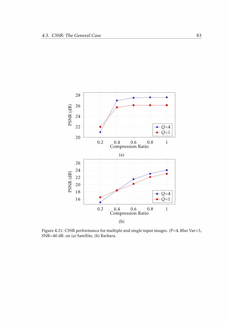
4.5. CSSR: The General Case 83
0.2 0.4 0.6 0.8 120
22
24
26
28
Compression Ratio
PSN
R(dB)
Q=4Q=1
(a)
0.2 0.4 0.6 0.8 1
16
18
20
22
24
26
Compression Ratio
PSN
R(dB)
Q=4Q=1
(b)
Figure 4.21: CSSR performance for multiple and single input images. (P=4, Blur Var=3,SNR=40 dB. on (a) Satellite, (b) Barbara.

84 Chapter 4. Experimental Results
0.2 0.4 0.6 0.8 1
14
16
18
20
22
24
26
28
Compression Ratio
PSN
R(dB)
Q=4Q=1
(a)
0.2 0.4 0.6 0.8 112
14
16
18
20
22
24
26
28
Compression Ratio
PSN
R(dB)
Q=4Q=1
(b)
Figure 4.22: CSSR performance for multiple and single input images. (P=4, Blur Var=3,SNR=40 dB. on (a) Peppers, (b) Alhambra.

4.5. CSSR: The General Case 85
Table 4.12: Performance of the sequential approach using Q = 4.
Blur Var 3 5 9SNR 40 30 40 30 40 30Image P R PSNR (dB)Satellite 2 0.2 22.4 24.0 22.6 23.6 21.6 23.0
0.4 26.0 26.2 25.6 25.5 24.4 24.60.6 25.7 26.7 26.4 25.9 25.2 24.90.8 27.6 26.9 26.7 26.0 25.5 25.01.0 27.9 27.0 26.9 26.1 25.6 25.1
4 0.2 17.4 19.1 17.2 18.8 16.6 18.50.4 23.3 24.3 22.9 23.8 22.3 23.20.6 26.2 25.4 25.5 24.8 24.4 24.10.8 26.9 25.6 26.1 25.1 25.0 24.41.0 27.1 25.6 26.4 25.1 25.3 24.4
Barbara 2 0.2 17.5 19.3 17.1 19.2 16.0 18.30.4 20.0 21.4 19.7 21.2 18.9 20.70.6 21.5 22.4 21.4 22.1 20.5 21.60.8 22.6 22.9 22.4 22.6 21.6 22.11.0 23.2 23.2 22.8 22.8 22.1 22.3
4 0.2 15.0 15.3 15.1 15.2 14.1 15.20.4 16.4 16.9 16.3 17.0 16.0 17.00.6 18.7 17.7 18.8 17.8 18.5 17.80.8 20.8 18.3 20.7 18.4 20.3 18.51.0 22.3 18.5 22.0 18.6 21.4 18.6
4.5.2 CSSR vs Sequential Approach
As mentioned earlier, the alternate approach is expected to produce a better estimated imagequality. The next experiment has been executed on both the Satellite and Barbara images. Weused four simulated CS LR images to test the sequential and the CSSR alternate estimations.The obtained results are tabulated in Table 4.12, using Q=4 in all cases.
Figure 4.23 shows plots of the PSNR vs R, for the Satellite image, for the two approaches.P=4, for the two cases in Figure 4.23(a) Blur Var=5, SNR=30dB and Figure 4.23(b) Blur Var=3,SNR=40 dB. Similarly, Figure 4.24 shows the results obtained for the Barbara image, for thetwo approaches, under the same conditions. Again the plots show, as expected, how the al-ternate approach outperforms the sequential approach. In all cases the obtained PSNR usingCSSR is better than when using the sequential approach. In the plots of the Satellite image inFigure 4.23(a) the alternate CSSR improves the PSNR by more than 1.2 dB when compared tothe sequential approach for all Rs, while in Figure 4.24(a), the estimated Barbara image usingCSSR has a 4 dB increment in PSNR compared to the sequential estimate, for the case when

86 Chapter 4. Experimental Results
0.2 0.4 0.6 0.8 1
20
24
28
Compression Ratio
PSN
R(dB)
CSSRSequential
(a)
0.2 0.4 0.6 0.8 1
20
24
28
Compression Ratio
PSN
R(dB)
CSSRSequential
(b)
Figure 4.23: Comparison of the proposed CSSR vs the sequential approach for theSatellite image, (Q=4, P=4), using (a) Blur Var=5, SNR=30 dB, (b) Blur Var=3, SNR=40dB.
R=1, Blur Var=5, and SNR=30 dB.
4.5.3 CSSR1 vs CSSR2
Now in this sub-section the performance is tested for two different registration approaches. Todistinguish the two used approaches, we denote by CSSR1 the one using App3 applying Equa-tion (3.41), and CSSR2 the App4 approach using Equation (3.51). Tables 4.13 and 4.14 showthe obtained results for both the Satellite and Barbara images, we used Q=4 in all experiments.
Figure 4.25 shows the plots for the Satellite image (using P=4 and Q=4). Figure 4.25(a)analyzes the case when Blur Var=5 and SNR=30 dB, while Figure 4.25(b) analyzes the casewhen Blur Var=3, SNR=40 dB. Similarly, Figure 4.26 shows the plots for the Barbara image(P=4 andQ=4): Figure 4.26(a) for the case when Blur Var=5 and SNR=30 dB, and Figure 4.26(b)for the case when Blur Var=3, SNR=40 dB. This proves that the two registration approaches are

4.5. CSSR: The General Case 87
0.2 0.4 0.6 0.8 114
18
22
Compression Ratio
PSN
R(dB)
CSSRSequential
(a)
0.2 0.4 0.6 0.8 1
14
18
22
Compression Ratio
PSN
R(dB)
CSSRSequential
(b)
Figure 4.24: Comparison of the proposed CSSR vs the sequential approach for the Bar-bara image, (Q=4, P=4), using (a) Blur Var=5, SNR=30 dB, (b) Blur Var=3, SNR=40dB.

88 Chapter 4. Experimental Results
Table 4.13: Comparison of CSSR1 vs CSSR2 algorithms for the Satellite image, usingQ = 4.
Blur Var 3 5 9SNR 40 30 40 30 40 30P Alg R PSNR (dB)2 CSSR1 0.2 26.5 24.9 26.0 24.4 24.9 23.8
0.4 28.1 26.9 27.1 26.1 25.8 25.10.6 28.4 27.7 27.3 26.8 26.0 25.70.8 28.5 28.1 27.4 27.1 26.1 25.91.0 28.5 28.3 27.4 27.3 26.1 26.0
CSSR2 0.2 26.5 24.9 26.0 24.4 24.9 23.80.4 28.1 26.9 27.1 26.1 25.8 25.10.6 28.4 27.7 27.3 26.8 26.0 25.70.8 28.5 28.1 27.4 27.1 26.1 25.91.0 28.5 28.3 27.4 27.3 26.1 26.6
4 CSSR1 0.2 21.0 20.7 20.9 20.1 20.1 19.70.4 27.0 25.8 26.3 25.1 25.3 24.20.6 27.5 27.0 26.7 26.2 25.6 25.10.8 27.6 27.3 26.8 26.6 25.7 25.51.0 27.6 27.4 26.8 26.7 25.8 25.6
CSSR2 0.2 21.0 20.7 20.8 20.1 20.1 19.60.4 27.0 25.8 26.3 25.1 25.3 24.20.6 27.5 27.0 26.7 26.2 25.6 25.10.8 27.6 27.3 26.8 26.6 25.7 25.51.0 27.6 27.5 26.8 26.7 25.8 25.6
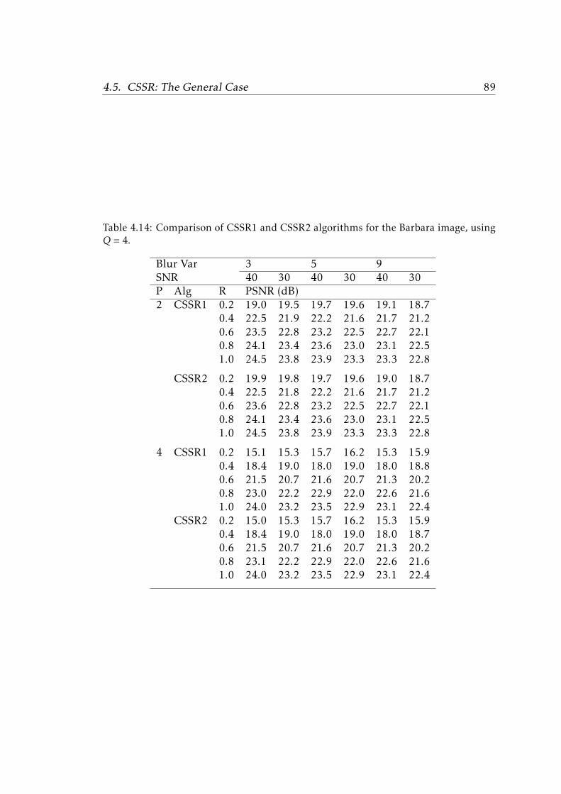
4.5. CSSR: The General Case 89
Table 4.14: Comparison of CSSR1 and CSSR2 algorithms for the Barbara image, usingQ = 4.
Blur Var 3 5 9SNR 40 30 40 30 40 30P Alg R PSNR (dB)2 CSSR1 0.2 19.0 19.5 19.7 19.6 19.1 18.7
0.4 22.5 21.9 22.2 21.6 21.7 21.20.6 23.5 22.8 23.2 22.5 22.7 22.10.8 24.1 23.4 23.6 23.0 23.1 22.51.0 24.5 23.8 23.9 23.3 23.3 22.8
CSSR2 0.2 19.9 19.8 19.7 19.6 19.0 18.70.4 22.5 21.8 22.2 21.6 21.7 21.20.6 23.6 22.8 23.2 22.5 22.7 22.10.8 24.1 23.4 23.6 23.0 23.1 22.51.0 24.5 23.8 23.9 23.3 23.3 22.8
4 CSSR1 0.2 15.1 15.3 15.7 16.2 15.3 15.90.4 18.4 19.0 18.0 19.0 18.0 18.80.6 21.5 20.7 21.6 20.7 21.3 20.20.8 23.0 22.2 22.9 22.0 22.6 21.61.0 24.0 23.2 23.5 22.9 23.1 22.4
CSSR2 0.2 15.0 15.3 15.7 16.2 15.3 15.90.4 18.4 19.0 18.0 19.0 18.0 18.70.6 21.5 20.7 21.6 20.7 21.3 20.20.8 23.1 22.2 22.9 22.0 22.6 21.61.0 24.0 23.2 23.5 22.9 23.1 22.4

90 Chapter 4. Experimental Results
0.2 0.4 0.6 0.8 120
24
Compression Ratio
PSN
R(dB)
CSSR1CSSR2
(a)
0.2 0.4 0.6 0.8 1
20
24
28
Compression Ratio
PSN
R(dB)
CSSR1CSSR2
(b)
Figure 4.25: Comparison of the proposed CSSR1 vs CSSR2 for the Satellite image,(Q=4, P=4), using (a) Blur Var=5, SNR=30 dB, (b) Blur Var=3, SNR=40 dB.

4.5. CSSR: The General Case 91
0.2 0.4 0.6 0.8 114
18
22
Compression Ratio
PSN
R(dB)
CSSR1CSSR2
(a)
0.2 0.4 0.6 0.8 1
14
18
22
Compression Ratio
PSN
R(dB)
CSSR1CSSR2
(b)
Figure 4.26: Comparison of the proposed CSSR1 vs CSSR2 algorithms for the Barbaraimage, (Q=4, P=4), using (a) Blur Var=5, SNR=30 dB, (b) Blur Var=3, SNR=40 dB.

92 Chapter 4. Experimental Results
effective and accurate and can be adopted interchangeably. This is clear in the plots where thecurves coincide.
Experimental results were performed on additional simulated and real images in our pub-lished works [18–20].
4.6 CSSR of PMMW Images
Due to their characteristics, Millimeter Wave (MMW) images are used in applications likeweather operations, low visibility navigation, and the imaging of people for concealed objectand threat detection [4, 90, 91], just to name a few.
Based on their interest, image processing techniques have recently started to be applied tothese images. For instance, Passive Millimeter Wave (PMMW) image enhancement has beenaddressed in [90, 92–95] to perform detection tasks. In [93] the high frequency componentsof those images were restored using a MAP estimator, and they were then added to the inputimage to produce an HR image. Registration and fusion of visible and MM images as well assegmentation of MMW images have been addressed in [90, 94, 95].
Unfortunately PMMW systems have two serious shortcomings: the long acquisition timeneeded to produce a PMMW image and the poor resolution of captured images. CS systems,with its reduced image acquisition time, have been applied to PMMW imaging, see[55, 56, 96,97]. In [96, 97] the authors utilize Hadamard masks to reduce the acquisition time in PMMWimagers. In [98] a PMMW imaging system with extended depth-of-field that can produce im-ages with reduced number of samples is presented. CS and Blind Image Deconvolution havebeen combined in [5]. By and large the resolution of MMW images is small, therefore makingtheir analysis a challenging task.
In our works [18, 20] HR images were super resolved for the first time from multiple CSobservations of unregistered LR PMMW images. We believe that PMMW images represent animportant application area where CS and LR to HR techniques can be combined to enhance theperformance of related application capabilities of current PMMW imaging systems.
Let us next present the obtained experimental results performed on real input images, ac-quired by a PMMW imager. These images were synthetically compressed using a circulantToeplitz matrix, to serve as a measurement matrix, following the Bernoulli probability distri-bution.
In the first experiment, four real PMMW images of a person were acquired, shown in Fig-ure 4.27(a). The estimated image using bilinear interpolation from one reconstructed LR imageis shown in Figure 4.27(b), and the estimated using CSSR is shown in Figure 4.27(c), both usingP=2, R=1.
In the second experiment we used four images, shown in Figure 4.28(a), of a man free ofthreats. These images were synthetically compressed with R=0.8. The interpolated versionof one reconstructed image is shown in Figure 4.28(b), while the estimated image using theCSSR algorithm is shown in Figure 4.28(c), both using P=2. Notice here that the interpolatedimage shows, by error, a cut near the hand, which means that the man has a threat attached tohim, which is not the case. This is clear in the estimated image using CSSR which shows thecontinuity near the left hand.

4.6. CSSR of PMMW Images 93
(a) (b) (c)
Figure 4.27: PMMW image of a man free of threats (Q=4, R=1, P=2).(a) Four noisy realobservations, (b) Bilinear interpolation from one reconstructed LR image, (c) Estimatedimage using CSSR algorithm.

94 Chapter 4. Experimental Results
(a) (b) (c)
Figure 4.28: PMMW image of a man free of threats (Q=4, R=0.8, P=2) (a) Four noisyreal observations, (b) Bilinear interpolation from one reconstructed LR image, (c) Esti-mated image using CSSR algorithm.
The next experiment used four real PMMW LR observations, of a man hiding a threat at-tached to his left arm, as shown in Figure 4.29(a). The estimated HR image using bilinearinterpolation of one reconstructed LR image, is shown in Figure 4.29(b), and the estimated us-ing the CSSR algorithm, with Q=4, is shown in Figure 4.29(c), using P=2, R=0.8. Also, thecorresponding estimated images using P=4, R=0.8 are shown in Figure 4.29(d) for bilinear in-terpolation, and Figure 4.29(e) for the CSSR algorithm. The obtained images clearly show thebetter reconstruction capabilities of the proposed method, this can be observed by the cleardiscontinuity of the arm indicating the attached threat.
The next experiment uses seven real PMMW images of a man with a threat attached tohis chest. The seven images, four of which are shown in Figure 4.30(a), were syntheticallycompressed using R=0.8, then used to estimate the image shown in Figure 4.30(c) using P=2.This result can be compared with the interpolated image from one reconstructed image in Fig-ure 4.30(d).
4.7 CCSSR of Color Images
There is nomuchwork dealing with color images fromCS observations. [99] proposed amethodfor color imaging via compressed sensing. It works on the color channels and random projec-tions from each channel, RGB, are acquired separately. The reconstruction process makes use ofthe correlation between the three color channels and it is based on group sparse optimization.
In [100], the single-pixel CS camera has been combined with a Bayer color filter to acquireCS color images, then joint sparsity models were applied to recover the three RGB channels.[65] estimated SR images from a single LR CS observation and applied this to color images.In [58] spatial multiplexing cameras were used to sample the scene through a series of codedprojections, this was applied to CS video super resolution and color videos.

4.7. CCSSR of Color Images 95
(a) (b) (c) (d) (e)
Figure 4.29: PMMW image of a man with a threat attached to his arm (Q=4, R=0.8).(a) LR images, (b) Bilinear interpolation from one reconstructed image, P=2, (c) Esti-mated HR image using the CSSR algorithm, P=2, (d) Bilinear interpolation from onereconstructed image, P=4, (e) Estimated HR image using the CSSR algorithm, P=4.

96 Chapter 4. Experimental Results
(a)(b) (c)
Figure 4.30: PMMW image of a man with a threat attached to his chest (Q=7, R=0.8,P=2). (a) LR images, (b) Bilinear interpolation from one reconstructed LR image, (c)Estimated HR image using the CSSR algorithm.

4.7. CCSSR of Color Images 97
Next we present experimental results obtained using the proposed CCSSR algorithm, as animportant application of the CSSR paradigm to color images. The experiments were performedusing both simulated and synthetically CS real color input images. We carried out a set ofexperiments on the images shown in Figures 4.31(a-c): Barbara, Lena, and Peppers images.The images have been warped, then degraded by Gaussian blurs of different known variancesand down-sampled. The LR RGB channels have been compressed separately using a circulantToeplitz matrix following the Bernoulli probability distribution. White Gaussian noise, withSNR=40 dB, has been finally added to the compressed channels.
Figures 4.31(d,e) show, respectively, examples of a simulated LR and a CS-LR observationfor the Barbara image using motion vector s = [.1222,−2,3]t , blur variance 7, P= 2 and R=0.5.We used a 3-level Haar wavelet transform as the transform basis W, and Peak Signal to NoiseRatio (PSNR) as the performance measure. The stopping criterion used was
norm(xk − xk−1)norm(xk−1)
≤ 10−3 (4.4)
In the first experimentQ=3 observations and a zooming factor P=1 have been used in orderto compare our method with the following CS reconstruction methods: Nagesh et. al [99] (Na) ,Wakin et al [101] (Wa), Angshul L2,1 (L1), L2,0.4 (L4), and SL2,0 (SL)[99]. Results are tabulatedin Table 4.15. Figure 4.32 shows a comparison between the results obtained using these CSalgorithms and the obtained using our proposed CCSSR algorithm, where PSNR vs R curvesare shown for the Lena image using P=1.0 and Q=3.
Table 4.15: Comparison of CS algorithms with the proposed CCSSR algorithm for CC-SSR P=1.0, Q=3. In bold blue are the highest PSNR values.
Alg Na Wa L1 L4 SL CCSSRImage R PSNR Values (dB)
.1 25.1 24.8 26.1 26.7 26.5 21.3Barbara .2 27.1 26.6 28.0 28.5 28.3 29.9
.3 28.8 27.9 29.3 30.0 29.7 34.0
.1 26.1 25.9 27.0 27.6 27.5 25.8Lena .2 28.3 27.7 29.0 29.7 29.5 31.6
.3 30.0 29.2 30.7 31.7 31.1 37.0
.1 25.0 24.5 25.6 26.3 26.0 24.8Peppers .2 27.1 26.1 27.9 28.5 28.1 32.5
.3 29.8 28.1 30.5 21.4 30.9 35.2
In the second experiment we investigate the performance of the proposed CCSSR algorithmfor practical P and R values. For all images we used Gaussian blur of variance 5, SNR=40dB,and Q=3. The results are tabulated in Table 4.16 for P=2 and 4. Shown in Figure 4.33(a,b) arecurves of the PSNR vs R for the three images used in our study, for the cases P=2 and P=4,respectively.

98 Chapter 4. Experimental Results
(a) (b)
(c) (d) (e)
Figure 4.31: Original Images (a) Barbara, (b) Lena, and (c) Peppers. (d) Simulated LRBarbara image (s = [.1222,−2,3]t, blur variance 7, P=2), (e) simulated CS observation(R=0.5, SNR=40 dB). The black line represents the added zero-valued entries to illus-trate a square image.
The reconstructed Peppers images are shown in Figures 4.34(a,b), using R=0.6, Blur Var=5,SNR=40dB, and Q=3, for the two cases P=2 and P=4, respectively.
In the third experiment we use real LR images of a toy, which have been synthetically com-pressed using R=0.8. We used a 16 input image sequence to reconstruct the HR image, withP=2, shown in Figure 4.35(d), while Figure 4.35(c) shows the reconstructed image obtainedusing only the first 4 input images of the previous sequence, shown in Figure 4.35(a). Fig-ure 4.35(b) shows an interpolated image from the first reconstructed LR image.
The next experiment is similar to the third and uses real images of a car. Figures 4.36(c,d)show the results obtained using CCSSR for respectively 4 and 16 CS observations from a se-quence of 16 input images whose first 4 images are shown in Figure 4.36(a). Figure 4.36(b)shows an interpolated image. We used P=2 in this experiment.
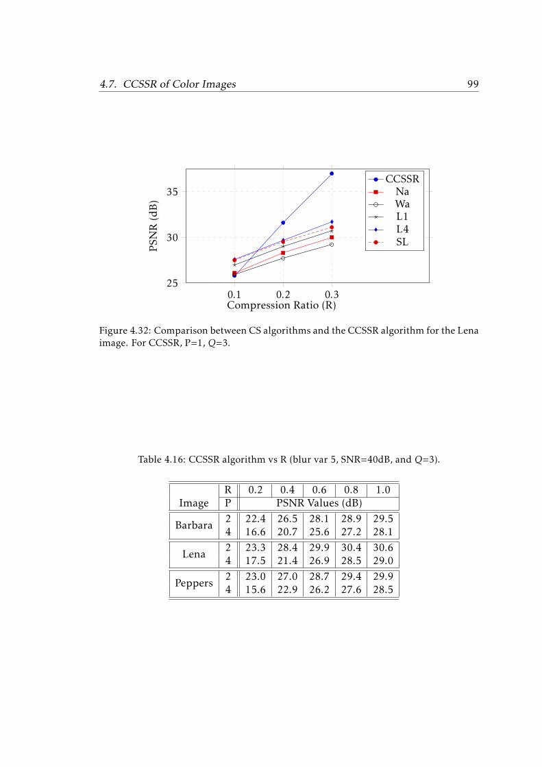
4.7. CCSSR of Color Images 99
0.1 0.2 0.325
30
35
Compression Ratio (R)
PSN
R(dB)
CCSSRNaWaL1L4SL
Figure 4.32: Comparison between CS algorithms and the CCSSR algorithm for the Lenaimage. For CCSSR, P=1, Q=3.
Table 4.16: CCSSR algorithm vs R (blur var 5, SNR=40dB, and Q=3).
R 0.2 0.4 0.6 0.8 1.0Image P PSNR Values (dB)
Barbara2 22.4 26.5 28.1 28.9 29.54 16.6 20.7 25.6 27.2 28.1
Lena2 23.3 28.4 29.9 30.4 30.64 17.5 21.4 26.9 28.5 29.0
Peppers2 23.0 27.0 28.7 29.4 29.94 15.6 22.9 26.2 27.6 28.5
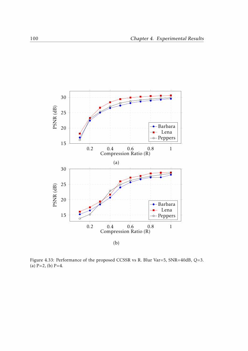
100 Chapter 4. Experimental Results
0.2 0.4 0.6 0.8 115
20
25
30
Compression Ratio (R)
PSN
R(dB)
BarbaraLena
Peppers
(a)
0.2 0.4 0.6 0.8 1
15
20
25
30
Compression Ratio (R)
PSN
R(dB)
BarbaraLena
Peppers
(b)
Figure 4.33: Performance of the proposed CCSSR vs R. Blur Var=5, SNR=40dB, Q=3.(a) P=2, (b) P=4.

4.7. CCSSR of Color Images 101
(a) (b)
Figure 4.34: Reconstructed Peppers Images using the CCSSR algorithm. R=0.6, BlurVar=5, SNR=40dB, and Q=3. (a) P=2, (b) P=4,
(a)
(b) (c) (d)
Figure 4.35: Image super resolution from real observations, R=0.8, P=2. (a) First 4LR images (b) Bilinear interpolation of one reconstructed LR image, (c) Estimated HRimage using the CCSSR algorithm, withQ=4, (d) Estimated HR image using the CCSSRalgorithm, with Q=16.

102 Chapter 4. Experimental Results
(a)
(b) (c) (d)
Figure 4.36: Image super resolution from real observations, R=0.8, P=2. (a) First 4LR images (b) Bilinear interpolation of one reconstructed LR image, (c) Estimated HRimage using the CCSSR algorithm, withQ=4, (d) Estimated HR image using the CCSSRalgorithm, with Q=16.
Chapter 5
Conclusions and Future Work
5.1 Conclusions
In this dissertation we have proposed a novel framework to reconstruct SR images from mul-tiple unregistered LR images acquired using CS techniques. Any classical SR and/or CS tech-niques can be incorporated in the developed methodology. The degradation model of this novelcombined problem has been modeled and a CSSR approach has been proposed in this work.
The CSSR method lowers the sampling frequency, transmission rates, the bandwidth ofthe image signal, and the memory requirements to store and/or send the image. Moreover,the acquisition time can be lowered, which is very important in medical and PMMW imagingapplications. The enhanced SR image quality is advantageous in pattern recognition, medicaldiagnostics, and to emphasize a specific area of an image in surveillance cameras and satelliteapplications.
The proposed HR reconstruction uses a new robust sparsity promoting prior and solvesa linear equation in x (the HR image), using conjugate gradient method. The transformedcoefficient vector estimation is an ℓ1 norm subject to a quadratic term optimization problem.The registration parameters can be estimated using four different procedures, to finally obtainaccurate results, since any SR estimation process is highly dependent on the performance of theregistration estimation step. The parameters can be estimated from the estimated HR image,or the LR images themselves, with the estimation from reconstructed LR images being lesssensitive to the initial conditions. Furthermore we found that the estimation at LR level resultsin better quality of the reconstructed image.
The proposed optimization framework uses ADMM to jointly estimate all the unknownsincluding HR image, LR images, and registration parameters. We have experimentally shownthat this simultaneous reconstruction outperforms the sequential method, that first performsLR reconstruction to then obtain an HR image from a set of LR observations. The sequential ap-proach estimates every unknown just once, while the alternate approach iteratively updates theestimated unknowns. The better performance of the alternate approach is due to the additionalinformation provided during the estimation process.

104 Chapter 5. Conclusions and Future Work
We also showed experimentally the enhancement obtained due to themultiple input imageswhen compared with a single one. This is expected due to the additional information everyinput image provides. However, the multiplicity necessitates accurate registration estimationprocedure which inherently affects the overall process.
The proposed framework has been tested and compared, at a unity compression ratio, withstate-of-the-art SR algorithms which do not use compression in their work. It has also beencompared, at a unity zooming factor, with state-of-the-art ID algorithms that deblur CS images,which do not use down-sampling in their work. Both comparisons used synthetic images andshowed better performance of the proposed CSSR over others. The performance of CSSR whenusing practical values of P and R has also been tested and analyzed.
Besides, the CSSR effectiveness has been demonstrated experimentally on synthetically CSnoisy real images. This represents the practical application of the CSSR method, which showedvery good results.
The proposed CSSR method has been tested on PMMW images. These images usually havepoor quality and limited resolution, which makes super resolving them a challenging task andis a hard test of the CSSR approach. The CSSR could be used to improve the quality of PMMWimages. This is expected to improve threat detection rates, which is an expected field of futureresearch. Notice here that the nature of PMMWI is similar to astronomical and medical images,and the good performance of the proposed CSSR algorithm can be extended to these images.
The proposed approach can also be applied to true color CS images. The separately sensedchannels are utilized in a joint registration estimation to effectively and accurately estimateregistration parameters for the three channels. The obtained results present an excellent im-age quality, even better than the obtained using previous CS reconstruction methods whichcorrelate the color channels.
5.2 Future work
Wefinally comment on few areas of interest where we plan to continue our work on CompressedSensing applied to LR images.
• To formulate the CSSR using Bayesian modeling and inference. This will allow us toestimate all the model parameters in an automatic manner.
• To include the estimation of the blur in the CSSR problem.
• To use image priors which cannot be formulated as super Gaussian distributions.
• To apply the developed framework to video sequences.
• To apply the proposed framework to images which are observed using the Bayer pattern.

Bibliography
[1] Chris Solomon and Toby Breckon. Fundamentals of Digital Image Processing: A practicalapproach with examples in Matlab. John Wiley & Sons, 2011.
[2] Sung Cheol Park, Min Kyu Park, and Moon Gi Kang. Super-resolution image reconstruc-tion: a technical overview. Signal Processing Magazine, IEEE, 20(3):21–36, 2003.
[3] Peyman Milanfar. Super-resolution imaging. CRC Press, 2010.
[4] L. Yujiri, M. Shoucri, and P.Moffa. Passivemillimeter wave imaging.MicrowaveMagazine,IEEE, 4(3):39–50, Sept 2003.
[5] B. Amizic, L. Spinoulas, R. Molina, and A.K. Katsaggelos. Compressive blind imagedeconvolution. Image Processing, IEEE Transactions on, 22(10):3994–4006, Oct 2013.
[6] Aggelos K Katsaggelos, Rafael Molina, and Javier Mateos. Super resolution of images andvideo. Synthesis Lectures on Image, Video, and Multimedia Processing, 1(1):1–134, 2007.
[7] Filip Sroubek and Jan Flusser. Multichannel blind iterative image restoration. ImageProcessing, IEEE Transactions on, 12(9):1094–1106, 2003.
[8] X. Zhou, J. Mateos, F. Zhou, R. Molina, and A. K. Katsaggelos. Variational dirichlet blurkernel estimation. IEEE Transactions on Image Processing, 24(12):5127–5139, Dec 2015.
[9] Jing Tian and Kai-Kuang Ma. A survey on super-resolution imaging. Signal, Image andVideo Processing, 5(3):329–342, 2011.
[10] Yi Tang, Hong Chen, Zhanwen Liu, Biqin Song, and Qi Wang. Example-based super-resolution via social images. Neurocomputing, 172:38–47, 2016.
[11] Dandan Si, Yuanyuan Hu, Zongliang Gan, Ziguan Cui, and Feng Liu. Edge directedsingle image super resolution through the learning based gradient regression estimation.In Image and Graphics, pages 226–239. Springer, 2015.
[12] Yanzi Wang, Jiulun Fan, Jian Xu, and Xiaomin Wu. Learning-based super-resolution viacanonical correlation analysis. literatures, 8(6), 2015.
[13] E.J. Candes and M.B. Wakin. An introduction to compressive sampling. Signal ProcessingMagazine, IEEE, 25(2):21–30, March 2008.

106 Bibliography
[14] M. Fornasier and H. Rauhut. Compressive sensing. In Handbook of mathematical methodsin imaging, pages 187–228. Springer, 2011.
[15] EJ Candes and J Romberg. Practical signal recovery from random projections. WaveletApplications in Signal and Image Processing XI, Proc. SPIE Conf., 5914, 2005.
[16] Emmanuel J Candes and Terence Tao. Decoding by linear programming. InformationTheory, IEEE Transactions on, 51(12):4203–4215, 2005.
[17] B. Amizic, L. Spinoulas, R. Molina, and A.K. Katsaggelos. Variational bayesian com-pressive blind image deconvolution. In Signal Processing Conference (EUSIPCO), 2013Proceedings of the 21st European, pages 1–5, Sept 2013.
[18] W. AlSaafin, S. Villena, M. Vega, R. Molina, and A.K. Katsaggelos. Compressive sensingsuper resolution from multiple observations with application to passive millimeter waveimages. Digital Signal Processing, pages 180–190, 2016.
[19] Wael Saafin, Miguel Vega, Rafael Molina, and Aggelos K. Katsaggelos. Image super-resolution from compressed sensing observations. In Image Processing (ICIP), 2015 IEEEInternational Conference on, pages 4268–4272, Sept 2015.
[20] Wael Saafin, Salvador Villena, Miguel Vega, Rafael Molina, and Aggelos K. Katsaggelos.Pmmw image super resolution from compressed sensing observations. In Signal Process-ing Conference (EUSIPCO), 2015 23rd European, pages 1815–1819, Aug 2015.
[21] Wael Saafin, Miguel Vega, Rafael Molina, and Aggelos K. Katsaggelos. Compressed sens-ing super resolution of color images. In Signal Processing Conference (EUSIPCO), 201624th European, Aug 2016.
[22] RY Tsai and Thomas S Huang. Multiframe image restoration and registration. Advancesin computer vision and Image Processing, 1(2):317–339, 1984.
[23] Gabriel Cristobal, Elena Gil, Filip Sroubek, Jan Flusser, Carlos Miravet, and Franciscode Borja Rodrıguez. Superresolution imaging: a survey of current techniques. In OpticalEngineering+ Applications, pages 70740C–70740C. International Society for Optics andPhotonics, 2008.
[24] Hui Ji and Cornelia Fermuller. Robust wavelet-based super-resolution reconstruction:theory and algorithm. Pattern Analysis and Machine Intelligence, IEEE Transactions on,31(4):649–660, 2009.
[25] Said E El-Khamy, Mohiy M Hadhoud, Moawad I Dessouky, Bassiouny M Salam, andFE Abd El-Samie. Regularized super-resolution reconstruction of images using waveletfusion. Optical Engineering, 44(9):097001–097001, 2005.
[26] Nirmal K Bose, Nilesh Ahuja, et al. Superresolution and noise filtering using movingleast squares. Image Processing, IEEE Transactions on, 15(8):2239–2248, 2006.
[27] Michael E Tipping and Christopher M Bishop. Bayesian image super resolution, Septem-ber 12 2006. US Patent 7,106,914.
Bibliography 107
[28] Salvador Villena, Miguel Vega, Rafael Molina, and Aggelos K Katsaggelos. Bayesiansuper-resolution image reconstruction using an l1 prior. In Image and Signal Process-ing and Analysis, 2009. ISPA 2009. Proceedings of 6th International Symposium on, pages152–157. IEEE, 2009.
[29] Richard R Schultz and Robert L Stevenson. Extraction of high-resolution frames fromvideo sequences. Image Processing, IEEE Transactions on, 5(6):996–1011, 1996.
[30] S. Villena, M. Vega, S.D. Babacan, R. Molina, and A.K. Katsaggelos. Bayesian combina-tion of sparse and non-sparse priors in image super resolution. Digital Signal Processing,23(2):530–541, 2013.
[31] Lyndsey C Pickup, David P Capel, Stephen J Roberts, and Andrew Zisserman. Bayesianmethods for image super-resolution. The Computer Journal, 52(1):101–113, 2009.
[32] Stefanos P Belekos, Nikolaos P Galatsanos, and Aggelos K Katsaggelos. Maximum a pos-teriori video super-resolution using a new multichannel image prior. Image Processing,IEEE Transactions on, 19(6):1451–1464, 2010.
[33] S.D. Babacan, R. Molina, and A.K. Katsaggelos. Variational bayesian super resolution.IEEE Transactions on Image Processing, 20(4):984–999, 2011.
[34] S. Farsiu, M.D. Robinson, M. Elad, and P. Milanfar. Fast and robust multiframe superresolution. IEEE Transactions on Image Processing, 13(10):1327–1344, 2004.
[35] Marcelo VW Zibetti, Fermın SV Bazan, and Joceli Mayer. Estimation of the parametersin regularized simultaneous super-resolution. Pattern Recognition Letters, 32(1):69–78,2011.
[36] Antonio Marquina and Stanley J Osher. Image super-resolution by tv-regularization andbregman iteration. Journal of Scientific Computing, 37(3):367–382, 2008.
[37] Y. He, KH. Yap, L. Chen, and L-P Chau. A nonlinear least square technique for simul-taneous image registration and super-resolution. Image Processing, IEEE Transactions on,16(11):2830–2841, 2007.
[38] SS Panda, G Jena, and SK Sahu. Image super resolution reconstruction using iterativeadaptive regularization method and genetic algorithm. In Computational Intelligence inData Mining-Volume 2, pages 675–681. Springer, 2015.
[39] Jianchao Yang, John Wright, Thomas S Huang, and Yi Ma. Image super-resolution viasparse representation. Image Processing, IEEE Transactions on, 19(11):2861–2873, 2010.
[40] Kwang In Kim and Younghee Kwon. Single-image super-resolution using sparse regres-sion and natural image prior. Pattern Analysis and Machine Intelligence, IEEE Transactionson, 32(6):1127–1133, 2010.
[41] JinjunWang, Shenghuo Zhu, and Yihong Gong. Resolution enhancement based on learn-ing the sparse association of image patches. Pattern Recognition Letters, 31(1):1–10, 2010.
[42] Kamal Nasrollahi and Thomas B Moeslund. Super-resolution: a comprehensive survey.Machine vision and applications, 25(6):1423–1468, 2014.

108 Bibliography
[43] Antonin Chambolle, Vicent Caselles, Daniel Cremers, Matteo Novaga, and Thomas Pock.An introduction to total variation for image analysis. Theoretical foundations and numeri-cal methods for sparse recovery, 9(263-340):227, 2010.
[44] Karl Nelson, Asim Bhatti, and Saeid Nahavandi. Performance evaluation of multi-framesuper-resolution algorithms. In Digital Image Computing Techniques and Applications(DICTA), 2012 International Conference on, pages 1–8. IEEE, 2012.
[45] Ken D Sauer, Sean Borman, Charles Bouman, et al. Parallel computation of sequentialpixel updates in statistical tomographic reconstruction. In Image Processing, 1995. Pro-ceedings., International Conference on, volume 2, pages 93–96. IEEE, 1995.
[46] David Capel and Andrew Zisserman. Computer vision applied to super resolution. Sig-nal Processing Magazine, IEEE, 20(3):75–86, 2003.
[47] Jean-Luc Starck, Michael Elad, and David L Donoho. Image decomposition via the com-bination of sparse representations and a variational approach. Image Processing, IEEETransactions on, 14(10):1570–1582, 2005.
[48] Salvador Villena, Miguel Vega, S Derin Babacan, Rafael Molina, and Aggelos K Katsagge-los. Using the kullback-leibler divergence to combine image priors in super-resolutionimage reconstruction. In Image Processing (ICIP), 2010 17th IEEE International Conferenceon, pages 893–896. IEEE, 2010.
[49] A. Zomet, A. Rav-Acha, and S. Peleg. Robust super-resolution. In Computer Vision andPattern Recognition, 2001. CVPR 2001. Proceedings of the 2001 IEEE Computer Society Con-ference on, volume 1, pages I–645–I–650 vol.1, 2001.
[50] Divya Gupta and Mahendra Kumar Patil. A review on image registration. InternationalJournal of Engineering Research Technology (IJERT), 3(2):2630–2633, 2014.
[51] Alan C Bovik. Handbook of image and video processing. Academic press, 2010.
[52] Netalee Efrat, Daniel Glasner, Alexander Apartsin, Boaz Nadler, and Anat Levin. Accu-rate blur models vs. image priors in single image super-resolution. In Proceedings of theIEEE International Conference on Computer Vision, pages 2832–2839, 2013.
[53] M.F. Duarte, M.A. Davenport, D. Takhar, J.N. Laska, Ting Sun, K.F. Kelly, and R.G. Bara-niuk. Single-pixel imaging via compressive sampling. Signal Processing Magazine, IEEE,25(2):83–91, March 2008.
[54] Wai Lam Chan, Kriti Charan, Dharmpal Takhar, Kevin F Kelly, Richard G Baraniuk,and Daniel M Mittleman. A single-pixel terahertz imaging system based on compressedsensing. Applied Physics Letters, 93(12):121105, 2008.
[55] W. L. Chan, K. Charan, D. Takhar, K. F. Kelly, R.G. Baraniuk, and D.M. Mittleman. Asingle-pixel terahertz imaging system based on compressed sensing. Applied Physics Let-ters, 93(12):121105–121105–3, Sep 2008.
[56] A. Heidari and D. Saeedkia. A 2d camera design with a single-pixel detector. In Infrared,Millimeter, and Terahertz Waves, 2009. IRMMW-THz 2009. 34th International Conferenceon, pages 1–2, Sept 2009.

Bibliography 109
[57] T. Li, X. Wang, W. Wang, and A. K. Katsaggelos. Compressive video sensing with limitedmeasurements. Journal of Electronic Imaging, 22(4):043003–043003, 2013.
[58] A.C. Sankaranarayanan, C. Studer, and R.G. Baraniuk. Cs-muvi: Video compressivesensing for spatial-multiplexing cameras. In Computational Photography (ICCP), 2012IEEE International Conference on, pages 1–10, April 2012.
[59] T. Edeler, K. Ohliger, S. Hussmann, and A. Mertins. Multi image super resolution us-ing compressed sensing. In Acoustics, Speech and Signal Processing (ICASSP), 2011 IEEEInternational Conference on, pages 2868–2871, May 2011.
[60] A. Fannjiang and W. Liao. Super-resolution by compressive sensing algorithms. CoRR,abs/1211.5870, 2012.
[61] H.P. Babcock, J.R. Moffitt, Y. Cao, and X. Zhuang. Fast compressed sensing analysis forsuperresolution imaging using l1-homotopy. Optics Express, 21(23):28583–28596, 2013.
[62] J. Fang, J. Li, Y. Shen, H. Li, and S. Li. Super-resolution compressed sensing: An iterativereweighted algorithm for joint parameter learning and sparse signal recovery. SignalProcessing Letters, IEEE, 21(6):761–765, June 2014.
[63] C. He, L. Liu, L. Xu, M. Liu, and M. Liao. Learning based compressed sensing for sarimage super-resolution. Selected Topics in Applied Earth Observations and Remote Sensing,IEEE Journal of, 5(4):1272–1281, 2012.
[64] S. Yang, F. Sun, M. Wang, Z. Liu, and L. Jiao. Novel super resolution restoration ofremote sensing images based on compressive sensing and example patches-aided dic-tionary learning. In Multi-Platform/Multi-Sensor Remote Sensing and Mapping (M2RSM),2011 International Workshop on, pages 1–6. IEEE, 2011.
[65] P. Sen and S. Darabi. Compressive image super-resolution. In Signals, Systems and Com-puters, 2009 Conference Record of the Forty-Third Asilomar Conference on, pages 1235–1242,Nov 2009.
[66] L. Spinoulas, B. Amizic, M. Vega, R. Molina, and A.K. Katsaggelos. Simultaneousbayesian compressive sensing and blind deconvolution. In Signal Processing Conference(EUSIPCO), 2012 Proceedings of the 20th European, pages 1414–1418, Aug 2012.
[67] K. Koh, S. J Kim, and S. P Boyd. An interior-point method for large-scale l1-regularizedlogistic regression. Journal of Machine learning research, 8(8):1519–1555, 2007.
[68] M. Figueiredo, R. Nowak, and S. Wright. Gradient projection for sparse reconstruction:Application to compressed sensing and other inverse problems. Selected Topics in SignalProcessing, IEEE Journal of, 1(4):586–597, 2007.
[69] D. Needell and J. A. Tropp. Cosamp: Iterative signal recovery from incomplete andinaccurate samples. Applied and Computational Harmonic Analysis, 26(3):301–321, 2009.
[70] S. Becker, J. Bobin, and E. J. Candes. Nesta: a fast and accurate first-order method forsparse recovery. SIAM Journal on Imaging Sciences, 4(1):1–39, 2011.
[71] J. Yang and Y. Zhang. Alternating direction algorithms for l1-problems in compressivesensing. SIAM Journal on Scientific Computing, 33(1):250–278, 2011.

110 Bibliography
[72] Waheed U Bajwa, Jarvis D Haupt, Gil M Raz, Stephen J Wright, and Robert D Nowak.Toeplitz-structured compressed sensing matrices. In Statistical Signal Processing, 2007.SSP’07. IEEE/SP 14th Workshop on, pages 294–298. IEEE, 2007.
[73] Gesen Zhang, Shuhong Jiao, Xiaoli Xu, and Lan Wang. Compressed sensing and re-construction with bernoulli matrices. In Information and Automation (ICIA), 2010 IEEEInternational Conference on, pages 455–460, June 2010.
[74] Wotao Yin, Simon Morgan, Junfeng Yang, and Yin Zhang. Practical compressive sens-ing with toeplitz and circulant matrices. In Visual Communications and Image Processing2010, pages 77440K–77440K. International Society for Optics and Photonics, 2010.
[75] Mohd Awais Farooque and Jayant S Rohankar. Survey on various noises and techniquesfor denoising the color image. International Journal of Application or Innovation in Engi-neering & Management (IJAIEM), 2(11):217–221, 2013.
[76] Sumit Budhiraja Meenakshi. A survey of compressive sensing based greedy pursuit re-construction algorithms. 2015.
[77] Honglin Huang and Anamitra Makur. Backtracking-based matching pursuit method forsparse signal reconstruction. Signal Processing Letters, IEEE, 18(7):391–394, 2011.
[78] Joel A Tropp and Anna C Gilbert. Signal recovery from random measurements via or-thogonal matching pursuit. Information Theory, IEEE Transactions on, 53(12):4655–4666,2007.
[79] Wei Dai and Olgica Milenkovic. Subspace pursuit for compressive sensing signal recon-struction. Information Theory, IEEE Transactions on, 55(5):2230–2249, 2009.
[80] Deanna Needell and Roman Vershynin. Signal recovery from incomplete and inaccuratemeasurements via regularized orthogonal matching pursuit. Selected Topics in SignalProcessing, IEEE Journal of, 4(2):310–316, 2010.
[81] Mark A Davenport, Marco F Duarte, Yonina C Eldar, and Gitta Kutyniok. Introductionto compressed sensing. Preprint, 93:1–64, 2011.
[82] S-J Kim, K. Koh, M. Lustig, S. Boyd, and D. Gorinevsky. An interior-point method forlarge-scale l1-regularized least squares. Selected Topics in Signal Processing, IEEE Journalof, 1(4):606–617, Dec 2007.
[83] S Derin Babacan, Rafael Molina, Minh N Do, and Aggelos K Katsaggelos. Bayesian blinddeconvolution with general sparse image priors. In Computer Vision–ECCV 2012, pages341–355. Springer, 2012.
[84] Vinay Jeengar, SN Omkar, Amarjot Singh, Maneesh Kumar Yadav, and Saksham Keshri.A review comparison of wavelet and cosine image transforms. International Journal ofImage, Graphics and Signal Processing (IJIGSP), 4(11):16, 2012.
[85] Bruno Amizic, Rafael Molina, and Aggelos K Katsaggelos. Sparse bayesian blind imagedeconvolution with parameter estimation. EURASIP Journal on Image and Video Process-ing, 2012(1):1–15, 2012.

Bibliography 111
[86] S. Boyd, N. Parikh, E. Chu, B. Peleato, and J. Eckstein. Distributed optimization andstatistical learning via the alternating direction method of multipliers. Foundations andTrends® in Machine Learning, 3(1):1–122, 2011.
[87] Y.-H. Xiao and Z.-F. Jin. An alternating direction method for linear-constrained matrixnuclear norm minimization. Numerical Linear Algebra with Applications, 19(3):541–554,2012.
[88] R Tyrrell Rockafellar. Convex analysis. Number 28. Princeton university press, 1997.
[89] K. Lange. Optimization. Springer-Verlag, 2013.
[90] H. Chen, S. Lee, R. Rao, M. Slamani, and P. Varshney. Imaging for concealed weapondetection: a tutorial overview of development in imaging sensors and processing. SignalProcessing Magazine, IEEE, 22(2):52–61, 2005.
[91] C. Zheng, X. Yao, A. Hu, and J. Miao. A passive millimeter-wave imager used for con-cealed weapon detection. Progress In Electromagnetics Research B, 46:379–397, 2013.
[92] J. Yang, J. Wang, and L. Li. A new algorithm for passive millimeter-wave image en-hancement. In Signal Processing Systems (ICSPS), 2010 2nd International Conference on,volume 3, pages V3–507. IEEE, 2010.
[93] Y. Li, Y. Li, J. Chen, and Y. Hou. Passive millimeter-wave image restoration based onimproved algorithm of nonlinear extrapolation in frequency space. International Journalof Digital Content Technology and its Applications, 5(5):42–49, 2011.
[94] P. Chen, T. Zou, J. Chen, Z. Gao, and J. Xiong. The application of improved pso algorithmin pmmw image ostu threshold segmentation. InAppliedMechanics andMaterials, volume721, pages 779–782. Trans Tech Publ, 2015.
[95] H. Lee, D. Lee, S. Yeom, J. Son, V. Guschin, and S. Kim. Passive millimeter wave imag-ing and analysis for concealed object detection. In Data Mining and Intelligent Informa-tion Technology Applications (ICMiA), 2011 3rd International Conference on, pages 98–101.IEEE, 2011.
[96] N. Gopalsami, S. Liao, T. W Elmer, E. R Koehl, A. Heifetz, A. C Raptis, L. Spinoulas, andA. K Katsaggelos. Passive millimeter-wave imaging with compressive sensing. OPTICALENGINEERING, 51(9), SEP 2012.
[97] N Gopalsami, TW Elmer, Shaolin Liao, R Ahern, A Heifetz, AC Raptis, M Luessi, D Baba-can, and AK Katsaggelos. Compressive sampling in passive millimeter-wave imaging.In SPIE Defense, Security, and Sensing, pages 80220I–80220I. International Society forOptics and Photonics, 2011.
[98] V. Patel and J. Mait. Passive millimeter-wave imaging with extended depth of field andsparse data. In Acoustics, Speech and Signal Processing (ICASSP), 2012 IEEE InternationalConference on, pages 2521–2524. IEEE, 2012.
[99] A. Majumdar and R. Ward. Compressed sensing of color images. Signal Processing,90(12):3122–3127, 2010.

112 Bibliography
[100] P. Nagesh and B. Li. Compressive imaging of color images. In Acoustics, Speech and SignalProcessing, 2009. ICASSP 2009. IEEE International Conference on, pages 1261–1264. IEEE,2009.
[101] Michael B Wakin, Jason N Laska, Marco F Duarte, Dror Baron, Shriram Sarvotham,Dharmpal Takhar, Kevin F Kelly, and Richard G Baraniuk. An architecture for compres-sive imaging. In Image Processing, 2006 IEEE International Conference on, pages 1273–1276. IEEE, 2006.