ph.d. thesis ph.d. thesis - göteborgs universitet for making my life a bit more crazy (in a good...

ISBN 978-91-629-0089-2 (PRINT)ISBN 978-91-629-0090-8 (PDF)

Viktor Jonsson did his doctoral studies in mathematical statistics at the Department of Mathematical Sciences, Chalmers University of Technology and University of Gothenburg.

Statistical Analysis and M

odelling of Gene C

ount Data in M

etagenomics | V

iktor Jonsson 2017

DEPARTMENT OF MATHEMATICAL SCIENCES

Statistical Analysis and Modelling of Gene Count Data in MetagenomicsViktor Jonsson

Ph.D. thesis PH.D. THESIS

THESIS FOR THE DEGREE OF DOCTOR OF PHILOSOPHY

Statistical analysis and modellingof gene count data in metagenomics

Viktor Jonsson

Division of Applied Mathematics and StatisticsDepartment of Mathematical Sciences

Chalmers University of Technology and University of GothenburgGöteborg, Sweden 2017

Statistical analysis and modelling of gene count data in metagenomicsViktor JonssonGöteborg 2017ISBN 978-91-629-0089-2 (printed version)ISBN 978-91-629-0090-8 (electronic version)

c© Viktor Jonsson, 2017

Cover illustration: Microorganisms by Kajsa Andersson

Division of Applied Mathematics and StatisticsDepartment of Mathematical SciencesChalmers University of Technology and University of GothenburgSE-412 96 GöteborgSwedenTelephone +46 (0)31 772 1000

Typeset with LATEXPrinted by Ineko ABGöteborg, Sweden 2017

Statistical analysis and modelling of gene countdata in metagenomics

Viktor Jonsson

Division of Applied Mathematics and StatisticsDepartment of Mathematical Sciences

Chalmers University of Technology and University of Gothenburg

Abstract

Microorganisms form complex communities that play an integral part of allecosystems on Earth. Metagenomics enables the study of microbial communi-ties through sequencing of random DNA fragments from the collective genomeof all present organisms. Metagenomic data is discrete, high-dimensional andcontains excessive levels of both biological and technical variability, whichmakes the statistical analysis challenging.

This thesis aims to improve the statistical analysis of metagenomic data in twoways; by characterising the variance structure present in metagenomic data,and by developing and evaluating methods for identification of differentiallyabundant genes between experimental conditions. In Paper I we evaluateand compare the statistical performance of 14 methods previously used formetagenomic data. In Paper II we implement an overdispersed Poisson modeland use it to show that the biological variability varies considerably betweengenes. The model is used to evaluate a range of assumptions for the varianceparameter, and we show that correct modelling of the variance is vital forreducing the number of false positives. In Paper III we extend the model usedin Paper II to incorporate zero-inflation. Using the extended model, we showthat metagenomic data does indeed contain substantial levels of zero-inflation.We demonstrate that the new model has a high power to detect differentiallyabundant genes. In Paper IV we suggest improvements to the annotation andquantification of gene content in metagenomic data. Our proposed method,HirBin, uses a data-centric approach to identify effects at a finer resolution,which in turn allows for more accurate biological conclusions.

This thesis highlights the importance of statistical modelling and the use ofappropriate assumptions in the analysis of metagenomic data. The presentedresults may also guides researchers to select and further refine statistical toolsfor reliable analysis of metagenomic data.

Keywords: metagenomics, statistical modelling, hierarchical statistical models,gene ranking, overdispersion, zero-inflation, false discovery rate, receiveroperating characteristic curves.

List of papers

Paper I : Jonsson, V., Österlund, T., Nerman, O., Kristiansson, E. (2016). Sta-tistical evaluation of methods for identification of differentially abun-dant genes in comparative metagenomics. BMC genomics, 17(1), 1. DOI:10.1186/s12864-016-2386-y

Paper II : Jonsson, V., Österlund, T., Nerman, O., Kristiansson, E. (2016). Vari-ability in metagenomic count data and its influence on the identificationof differentially abundant genes. Journal of Computational Biology, aheadof print. DOI:10.1089/cmb.2016.0180

Paper III : Jonsson, V., Österlund, T., Nerman, O., Kristiansson, E. (2017). Azero-inflated model for improved inference of metagenomic gene countdata. Manuscript.

Paper IV : Österlund, T., Jonsson, V., Kristiansson, E. (2017). HirBin: High-resolution identification of differentially abundant functions in metage-nomes. Submitted.

Additional published paper not included in thesis

Paper V : Bengtsson-Palme, J., Boulund, F., Edström, R., Feizi, A., Johnning,A., Jonsson, V. A., Karlsson, F. H., Pal, C., Pereira, M. B., Rehammar, A.,Sanchez, J., Sanli, K. and Thorell, K. (2016). Strategies to improve usabilityand preserve accuracy in biological sequence databases. Proteomics, 16:2454-2460. DOI: 10.1002/pmic.201600034

v

vi

Author contributions

Paper I : Participated in study design, implemented the previously proposedmethods in R, wrote the framework for data resampling and methodsevaluation, performed all comparisons and analysed the results, createdall figures, drafted and edited the manuscript.

Paper II : Participated in study design, developed and implemented theBayesian models, analysed model performance and convergence, per-formed the analysis on real data, performed all comparisons and analysedthe results, created all figures, drafted and edited the manuscript.

Paper III : Participated in study design, developed and implemented thezero-inflated model, analysed model performance and convergence, per-formed the analysis on real data, performed all comparisons and analysedthe results, created all figures, drafted and edited the manuscript.

Paper IV : Participated in study design, assisted in data analysis and theinterpretation of results, edited the manuscript.

AcknowledgementsFirst I would like thank the people who have collaborated with me and who madethis work possible. First, Erik Kristiansson, my supervisor, you have been a sourceof constant inspiration through your unceasing enthusiasm. Your ability to see theprogress that I have made when I have felt stuck, and your ability to put everything intoperspective, have been invaluable for me. You taught me how to do science but youalso gave me so much more. I would also like to thank Olle Nerman, my co-supervisor,for always being there to answer the trickiest questions. Your ability to quickly graspa problem and ask the right questions has helped me many a times. I also thank youfor your timely anecdotes, with topics ranging from growing up in Värmland to phase-type distributions. Finally, I would like to thank Tobias Österlund, your clear mindedinsights have helped me refine countless of arguments. In sharing your own experiencesof science you made my own journey that much easier.

My years at the department would not have been so bright if not for the wonderfulpeople here. Some people deserve a special mention for everything that they have donefor me. Mariana Pereira, from Berlin to the Rover you were always there for me, thankyou for making my life a bit more crazy (in a good way!), and always being there tobrighten my day. Fredrik Boulund, by my side since almost forever, now my personalonline support group for anything nerdy, and when you play your guitar know that I amyour number one fan. Anna Rehammar, I could not have dreamt of a better office mate,our long discussions on life and science has meant more to me than you know, I onlywish you were here a little more often. Anna Johnning, you personify the word epic,you have an incredible ability to see people, and I also thank you for introducing meto ever so many cultural activities. Johan Bengtsson-Palme, a better source of energyand enthusiasms is hard to find, I also remember a certain python project featuringkaminmannen, thank you for that. Fanny Berglund, from pole vaulting to minecraftyou never cease to amaze me, good times were had both when teaching together andat lunch. Olle Elias, you might be even nerdier than me, no kappa. Jonatan Kallus, abetter lunch companion for deep discussions is hard to find. Thank you all!

I would also like to thank some of the remaining, current and former, members ofthe bioinformatics group: Marija Cvijovic, Anders Sjögren, Marina Axelson-Fisk,Emma Wijkmark, Johannes Borgqvist, and Henrik Imberg. Special thanks to, MikaelWallroth for being the perfect master thesis student.

vii

viii

For exciting collaborations in the far north of Sweden I extend my thanks to MartinRosvall and Alcides Viamontes Esquivel.

I would also like to thank all my fellow PhD students throughout the years for makingthis a wonderful place to work, encouraging me to take hour-long coffee breaks byproviding excellent company, or spontaneously bumping in to me and saying hi onlate evenings. There are far too many fantastic people and simply not enough timefor all of you. Thank you: Henrike, Claes, Ivar, Sandra, Alexei, Anton, Magnus Ö,Anders M, Tobias A, John, Magnus R, Dawan, Peter, Jonas, Oscar, Emil, Hossein,Richard, Jakob, Malin PF, Åse, Åsa, Linnea, Marco, Ronny, Kristin, Carl, Valentina,Roza, Anders H, Zuzana, Anna P, Elizabeth, Elin, Andreas, Christoffer, Malin Ö,Medet, Oscar Hammar, Fredrik L, Adam, Urban, Emilio and everyone I might havemissed!. A special thanks to everyone else at the department, junior or senior, that haveassisted me in countless ways during my time here.

To the GoBig crowd, thank you for providing a wonderful arena for the exchange ideasbeyond the walls of the maths department. Some of you have already been mentionedabove but I would also like to extend thanks to: Leif, Franscesco, Kaisa, Kemal, Amir,Robert, Chandan, and Fredrik. Many of which also collaborated on the database paper.

A special thanks to my friends outside the department who continuously have remindedme that there is a world beyond the math building. I will not be able to mention youall here but I would like to extend a special thanks to Erik Sterner, my personal guidewhen it comes to new adventures, both in life and science, and an endless source ofenergy, enthusiasm, chocolate, and pomegranate. Remember Cochran. Lucas Gren, mynumber one dance partner (sorry Johan), I hope for many a fruitful collaborations inthe future, I especially want more breakfast meetings.

Extra special thanks to my family who has been there for me all these years. Momand Dad, when times are rough, I always long for a trip back to home, thank you foreverything. Olle and Sigrid, I could not have wished for more awesome siblings, I lookforward to finally being able to spend more time with you.

Finally, Kajsa, you made these last few years the best of my life, thank you for beingyou and for helping me be me. With all my heart, I love you!

Göteborg, januari, 2017

Viktor Jonsson

Contents

Abstract iii

List of publications v

Acknowledgements vii

Contents ix

1 Background 1

1.1 Metagenomics . . . . . . . . . . . . . . . . . . . . . . . . . . . . . 1

1.2 Quantification of genes . . . . . . . . . . . . . . . . . . . . . . . . 2

1.3 Statistical challenges . . . . . . . . . . . . . . . . . . . . . . . . . 3

2 Aims 7

3 Statistical analysis of metagenomic data 9

3.1 Identification of differentially abundant genes . . . . . . . . . . 9

3.2 Overview of statistical methods . . . . . . . . . . . . . . . . . . . 10

3.3 Evaluation of statistical performance . . . . . . . . . . . . . . . . 16

4 Summary of papers 23

4.1 Paper I . . . . . . . . . . . . . . . . . . . . . . . . . . . . . . . . . 23

4.2 Paper II . . . . . . . . . . . . . . . . . . . . . . . . . . . . . . . . . 26

4.3 Paper III . . . . . . . . . . . . . . . . . . . . . . . . . . . . . . . . 28

ix

x CONTENTS

4.4 Paper IV . . . . . . . . . . . . . . . . . . . . . . . . . . . . . . . . 31

5 Conclusion and outlook 35

Bibliography 39

Papers I-IV

1 Background

1.1 Metagenomics

Microorganisms, such as bacteria, viruses and fungi, are ubiquitously presenteverywhere around us (Pace, 1997; Whitman et al., 1998). Contrary to popularbelief, most microorganisms are not harmful to humans; rather, they consti-tute an integral part of all living ecosystems. Microorganisms are typicallystudied by isolating and cultivating single isolates. However, microorgan-isms form complex communities that contain thousands of species (Roeschet al., 2007). In addition, a vast proportion of microorganisms are difficult tocultivate using standard protocols (Schloss and Handelsman, 2005), thus mak-ing culture-dependent approaches unsuitable for capturing the intricacies ofmost microorganisms. Metagenomics was introduced as a culture-independentmethod for studying microbial communities at the genomic level (Handelsmanet al., 1998). In short, the DNA of all cells present within a sampled microbialcommunity is extracted. The DNA is then randomly sheared and sequenced,resulting in a large set of short DNA fragments, called reads. These readsrepresent a random sample from the metagenome, i.e. the collective genome ofall organisms present in the community (Rondon et al., 2000). Metagenomics,the study of the metagenome, therefore provides a way to analyse both thestructure and functional capability of metagenomic communities.

Originally, metagenomics was performed using slow and expensive Sanger se-quencing (Sanger and Coulson, 1975), with the first data sets consisting only ofthousands of reads (Healy et al., 1995). With the introduction of modern high-throughput sequencing methods, which have the ability to sequence multipleDNA fragments in parallel, the potential of metagenomics has considerablyincreased (van Dijk et al., 2014; Scholz et al., 2012). Large sequencing efforts,such as the Human Microbiome Project (Turnbaugh et al., 2007; Human Micro-biome Project Consortium, 2012) and the Earth Microbiome Project (Gilbert

1

2 1. Background

et al., 2014), have recently generated data sets consisting of billions of readscorresponding to trillion of nucleotides (base pairs). In addition the numberof applications of metagenomics to fields in the life sciences is continuouslyincreasing. Within medicine, metagenomics has been used to link changes inthe microbial communities living inside and on our bodies to common dis-eases, for example, type-II diabetes (Karlsson et al., 2013) and Crohn’s disease(Manichanh et al., 2006). In ecology, metagenomics has been applied to studythe microbial communities in a wide range of ecosystems from prairie soil(Howe et al., 2014), ocean water (Sunagawa et al., 2015; DeLong et al., 2006)and the cow rumen (Ross et al., 2013). In ecotoxicology, it has been used tounderstand the role of microbial ecosystems in biodegradation in waste wa-ter treatment (Fang et al., 2013), and to characterize the spread of antibioticresistance genes in the environment (Kristiansson et al., 2011; Bengtsson-Palmeet al., 2014).

1.2 Quantification of genes

Gene-centric metagenomics is the study of the functional capability of a mi-crobial community (Hugenholtz and Tyson, 2008). A gene is a short stretchof DNA that encodes a protein which in turn performs a specific biologicalfunction. The genome of a typical bacterial species contains thousands of genes,which means that the number of genes in a microbial community is in theorder of millions. Genes may exist in several variants across multiple speciesyet perform similar functions. To facilitate the biological interpretation, genesare often grouped together in protein domains, gene families or orthologousgroups that correspond to a similar biological function in different species (e.g ,eggNOG (Huerta-Cepas et al., 2015), KEGG (Kanehisa et al., 2008), TIGRFAM(Haft et al., 2013) and SEED (Overbeek et al., 2005)). The choice of resolutionused, from single genes to wide groups of genes, depends on the biologicalquestion. For consistency, the term gene will be used throughout this thesis torefer to each of these different options.

Beyond the experimental steps of sample preparation, DNA extraction andsequencing, several steps are necessary to quantify the gene content of a sample(Wooley et al., 2010). The steps are summarized in Figure 1. The raw data fromthe sequencing machine consist of a large number of short DNA fragmentscalled reads, which are typically 75-400 nucleotides in length depending onthe technology used (van Dijk et al., 2014; Scholz et al., 2012). However, DNAsequencing is not exact and the raw reads often contain sequencing errors,for example, misidentified nucleotides or insertion of extra nucleotides. De-pending on the outcome of the sequencing and the sequence technology used,

1.3. Statistical challenges 3

this error rate can be as high as 1% of the sequenced nucleotides (Quail et al.,2012). Sequencers provide a quality score for each nucleotide that reflects theprobability of an error, and this score is used to identify and remove low-qualityreads (Schmieder and Edwards, 2011). Next, the aim is to determine the geneticorigin of the remaining high-quality reads. To facilitate this process, each readis mapped to an annotated reference database. In the mapping step, reads arealigned to the sequences within the reference database in order to identify thepossible matches (Scholz et al., 2012). A read may match to several positionswithin the reference database, but only the best match is generally kept.

The reference database can be constructed in several different ways. For exam-ple, the reference database can be a collection of previously characterized genesor microbial genomes. Alternatively, the database can be constructed by directlyassembling the reads from the sequenced metagenome into longer stretchesof DNA (Mende et al., 2012). The sequences in the reference database aretypically annotated based on their biological function, which is often predictedbased on sequence similarity to previously studied genes. The annotation caneither be single genes or groups of genes predicted to have a similar structureor function depending on the desired level of resolution (see Paper IV). Thereference database typically contains several variants of every gene, for exam-ple, different bacterial species share core functionality (Human MicrobiomeProject Consortium, 2012). Every read that maps to a specific gene, regardlessof location in the database, is counted as an occurrence of that gene. In thisway, all reads are "binned" together resulting in a list that contains the numberof occurrences of each gene. The final gene counts are thus measures of therelative abundance of each gene in each sample.

1.3 Statistical challenges

An essential aspect of gene-centric metagenomics is detecting changes in rela-tive gene abundance in relation to experimental parameters. Examples of suchparameters are the health status of the human host, the temperature along agradient and the presence or absence of an anti-microbial compound. Differen-tially abundant genes are detected by statistically assessing whether specificgenes differ in relative abundance between communities. However, metage-nomic gene count data i) is discrete and undersampled, ii) is high-dimensional,iii) contains high levels of biological and technical variability and iv) is of-ten represented by few biological replicates. These characteristics make thestatistical analysis of metagenomic data challenging on many levels.

4 1. Background

Figure 1: Overview of gene quantification in metagenomics. DNA is extracted andrandomly sequenced from a microbial community. The resulting reads are then mappedto reference sequences that have been annotated according to their gene content. Eachread that matches a gene is counted as an occurrence of that gene. The end result is alist of counts for each sample providing the relative abundance of each gene.

Because genes are quantified by counting the number of reads matching specificgenes, metagenomic data becomes discrete, asymmetric and has a dependencybetween the expected value and the variance. This means that standard statis-tical methods that rely on normality assumptions are not suitable and can losepower to detect differences (Law et al., 2014). Metagenomes are also undersam-pled, meaning that the sequencing depth is not sufficient to reliably capture thefull genetic diversity present in a community (Paulson et al., 2013; Unterseheret al., 2011). This means that a large proportion of genes may be representedwith only a few reads, making the statistical analysis challenging. Rare geneswith low abundance can also fall below the detection limit while still beingpresent in the community, making it difficult to compare abundances betweensamples.

Metagenomic gene count data is high-dimensional and often thousands ofgenes are tested for differential abundance simultaneously. Each test may resultin a false positive making it difficult to distinguish the few truly differentiallyabundant genes. Correction for multiple-testing is therefore needed to controlthe type-I error rate, which reduces the power to detect the true differences(Dudoit et al., 2003). Thus, methods with high power and low type-I error rateare needed for accurate analysis of metagenomic data.

Metagenomic data is affected by high levels of biological and technical variabil-ity. The biological variability reflects the variation in gene abundances betweenmicrobial communities. The variation is induced by differences in uncontrolled

1.3. Statistical challenges 5

environmental factors between samples, for example temperature, salinity,nutrient availability, pH and host age (Fierer et al., 2012; Lozupone et al., 2012).Because the composition and abundance of species change due to these fac-tors the abundance of their genes also change. Furthermore, bacteria, whichconstitute a major part of many bacterial communities, have plastic genomes,and gene content can vary between individual strains of the same species(Greenblum et al., 2015). For example, the genome of Escherichia coli contains3188 genes within the core genome, while the plastic genome, which containsapproximately 1500 genes, can vary between strains and 90,000 possible genesvariants have been characterized to date (Land et al., 2015). Genes can also bepresent on horizontal gene transfer elements, such as plasmids, where it is pos-sible for a single bacterium to contain several copies of the same plasmid. Thehorizontal gene transfer elements further increase the variation in gene abun-dances between samples. Finally, microbial species are not omnipresent andcan be entirely missing in samples, causing observations represented by zeroreads (Sohn et al., 2015). These characteristics make the biological variabilitysubstantial in most metagenomic data sets.

Technical variability is introduced due to differences in sample preparationsample preparation (Morgan et al., 2010), sequencing errors (Quail et al., 2012),differences in sequencing depth between samples (McMurdie and Holmes,2014) and incorrectly mapped reads in the gene quantification step (Wooleyand Ye, 2009). The variability between technical replicates has been shown tobe smaller than the biological variability (Nayfach and Pollard, 2016). However,an unknown factor of technical errors is the bias introduced from biologicaldatabases. Metagenomics aims to study previously unknown microorganisms;however, all databases are based on previously identified genes and species(Rinke et al., 2013). In 2015, the number of completed bacterial genomes was4000 (Land et al., 2015), which is only a small proportion of the total number ofbacterial species, estimated to be at least 10 million (Curtis et al., 2002; Pedrós-Alió, 2006). The lack of accurate reference sequences can cause genes to beincorrectly annotated or missed completely (Wooley and Ye, 2009).

Metagenomic data sets often represented by few biological replicates due to thehigh sequencing costs (Knight et al., 2012; Prosser, 2010). The lack of replicatesworsens the problems induced by the other challenges. For example, correctlyestimating the variability of a gene is difficult when only a few samples areavailable. The obvious solution is to encourage replicated experimental designs.However, data sets with a low number of samples are still being produced andstatistical methods that can provide robust estimates even when few samplesare available are therefore vital.

6 1. Background

2 Aims

The aim of this thesis is to improve the statistical analysis of metagenomicgene count data. The many challenges that are present in the analysis ofmetagenomic data require special care to be taken in model developmentto maintain high power to detect differences and a low proportion of falsepositives. The papers included in this thesis cover the evaluation of previouslyproposed methods, the investigation of the data itself and the development ofnew methods. Specifically, the aims are as follows:

• Evaluate previously proposed statistical methods for detecting differen-tially abundant genes in metagenomic gene count data (Paper I).

• Investigate and characterize the variance structures present in metage-nomic gene count data (Papers II-III).

• Develop statistical models for improved detection of differentially abun-dant genes (Papers II-III).

• Extend the binning process to increase the power to detect biologicallyrelevant effects in metagenomic gene count data (Paper IV).

7

8 2. Aims

3 Statistical analysis of metage-nomic data

The following sections outline the statistical analysis of metagenomic genecount data and define the mathematical notation used throughout this thesis.This section also provides an overview of previously suggested statistical meth-ods. Note that this section does not include a discussion of the performance ofeach method; for such a discussion, see papers I and III.

3.1 Identification of differentially abundant genes

In the typical gene-centric metagenomic experiment considered, the aim isto identify differentially abundant genes associated to experimental factors.Throughout this thesis we will focus on the comparison between two groups ofsamples. Note that more complicated experimental designs are possible, suchas regression or comparisons between multiple conditions. For a comparisonbetween two groups, the data takes the form of a matrix of counts with n rowscorresponding to genes and m1 +m2 = m columns representing samples. LetYij be the counts of gene i in sample j, and let Nj denote the total sum ofcounts within each sample j.

Before the genes in the data are tested for differential abundance, the datais normalized to make the samples comparable and to reduce the variabilityin the data (Nayfach and Pollard, 2016). Commonly, the total sum of countswithin each sample, Nj , is used for normalization to correct for differences insequencing depth between samples. Other normalization methods have beenproposed but evaluation of these are beyond the scope of this thesis, for moreinformation see McMurdie and Holmes (2014). Throughout this thesis, thetotal sum, Nj , will be used for most methods, either to normalize the data or as

9

10 3. Statistical analysis of metagenomic data

an off-set specified within a model; the exception is software packages that bydefault use other normalization methods.

Each gene (row), i, is tested independently against the null hypothesis of nodifference in relative abundance between groups, i.e.,

H0i : No difference in relative abundance for gene i between groups,Hai : Difference in relative abundance for gene i between groups.

The exact formulation of the hypotheses varies depending on the underlyingdistributional assumption used by the specific method. Here we consider two-sided hypotheses for differential abundance but one-sided variants are alsopossible. The null hypotheses can then be rejected or not based on the outcomeof the test statistic used. In most situations, a p-value is calculated for each geneand used to rank genes based on the significance of their differential abundance.For Bayesian methods (for example in paper II and III) other decision rules ormetrics are used to rank the genes, such as the posterior probability for therelative abundance to differ between experimental conditions. The genes ontop of this ranking list are then considered likely candidates to be differentiallyabundant and investigated further. Ideally, all of the truly differentially abun-dant genes would end up in the top of the ranking list, but this is never thecase. These errors are often caused by small effect sizes, high variability in thedata and a lack of biological replicates.

3.2 Overview of statistical methods

3.2.1 Tests for comparing pairs of samples

A number of classical statistical methods have been proposed for and appliedto metagenomic data. In the early days of metagenomics, when sequencingwas expensive and replicated experimental designs were rare, methods forcomparing pairs of samples were used. Among the most prevalent is Fisher’sexact test (Fisher, 1922, 1925). The test uses a 2 × 2 contingency table to testindependence and tests whether there is an association between the numberof matching fragments and the experimental conditions (Smith et al., 2012).Fisher’s exact test has also been used to compare groups of metagenomeswhen the samples in each group have been pooled per gene, i.e. summing thecounts per gene within each group (Parks and Beiko, 2010). Let ysumi1 and ysumi2

denote the sum of counts in the two groups for gene i, let ri1 and ri2 denote thesum of counts for all genes excluding gene i, and let Nsum

1 and Nsum2 denote

3.2. Overview of statistical methods 11

the sum of the total counts in the two pooled groups (see Table 1).

Table 1: Contingency table for a pooled analysis with Fisher’s exact test.ysumi1 and ysumi2 is the sum of counts in each group, ri1 and ri2 the sum ofcounts in all genes excluding gene i and Nsum

1 and Nsum2 are the sum of the

total counts in the two pooled groups.

Group 1 Group 2

Counts in gene i: ysumi1 ysumi2

Counts in other genes: ri1 ri2

Total counts: Nsum1 Nsum

2

Assuming that the margins are fixed, the probability of observing a specific out-come in the pooled case can be calculated via the hyper-geometric distributionas,

P(Y sumi1 = ysumi1 ) =

(ysumi1 +ysum

i2ysumi1

)(ri1+ri2ri1

)(Nsum

1 +Nsum2

Nsum1

) . (3.1)

The p-value for a two-sided Fisher’s exact test is then calculated as the sum ofthe probabilities for all 2 x 2 tables with a lower probability than the observedtable.

Another commonly applied test used for pairwise comparisons between sam-ples is the binomial test, which has also been applied to metagenomics (Kris-tiansson et al., 2009; Mackelprang et al., 2011). This test compares the propor-tion of gene i to the total counts in each group. Under the null hypothesis of anequal proportion of gene i across both groups, the test statistic X follows thebinomial distribution:

X ∼ Binomial(ysumi1 + ysumi2 ,Ntot1

Ntot1 +Ntot2). (3.2)

The p-values are derived directly from the binomial distribution using a two-sided alternative hypothesis. When the total number of fragments is large thebinomial test is approximately equal to Fisher’s exact test assuming that thecounts for different genes are independent.

Another early method specifically designed for the analysis of metagenomicdata was XIPE-TOTEC (Rodriguez-Brito et al., 2006), which is still being usedtoday (Jeffries et al., 2015). XIPE-TOTEC focuses on pairwise comparisonsbetween samples and assesses significance by bootstrapping the counts within


each sample. In short, the algorithm works as follows. First, the counts ineach of the two samples are redrawn with replacement to generate a largenumber of mock data sets. The difference between samples for each gene inevery mock data set is calculated, and then the median difference for everygene is calculated. Next, a new set of mock data sets is created, but fragmentsbelonging to any gene in any of the two original data sets are selected and anew set of gene-wise differences are calculated. This new set of differencesconstitutes a reference distribution. To determine the significance of each gene,the median difference of the original data set is compared with the referencedistribution. At the 90% confidence level, a gene is considered significantif its median difference is smaller then the 5th percentile or larger than the95th percentile. Note that XIPE-TOTEC was not included in the comparisonperformed in Paper I of this thesis due to the lack of an easily accessibleimplementation.

3.2.2 Methods based on normality assumptions

The t-tests are among the most commonly used statistical tests and have beenapplied in various forms to metagenomic gene count data (Grzymski et al.,2012; Turnbaugh et al., 2009; Ward et al., 2013). This includes both Student’st-test assuming equal variances in both groups and Welch’s t-test assumingnon-equal variances. However, t-tests rely on the assumption that the datais normally distributed. Metagenomic count data is discrete, often skewedand has a dependency between the mean and the variance. Thus, normalityassumptions do not hold. To make the data symmetric and remove the depen-dency between the mean and the variance, the data is generally transformedbefore testing (Anscombe, 1948). Often used examples of transformations arethe square root and log(Yij + ε) where ε is a number e.g. 1 or 0.1.

The method metaStats is also based on a t-statistic but derives p-values usingpermutations (White et al., 2009). The raw counts are transformed using thebase-two logarithm, and Welch’s two sample t-statistics is computed for eachgene. A null distribution for the statistic is then computed by permutingsamples between groups and recalculating the t-statistic for each permutation.The p-values are then derived as the proportion of permuted t-statistics greaterthan the observed statistic as,

pi =1

B

B∑b=1

I{|t0bi | ≥ |ti|}, (3.3)

where B denotes the number of permutations, ti is the observed t-statistic of


gene i and t0bi are the permuted t-statistics. At low sample sizes (≤ 8), wherethere are too few permutations to accurately estimate the p-values, metaStatspools the resampled t-statistics for all genes to form a reference distributionand calculates the p-values according to

pi =1

nB

n∑j=1

B∑b=1

I{|t0bj | ≥ |ti|}, (3.4)

where the first sum is taken over all genes. The authors argue that the abovetests are inaccurate for genes with very low abundance, i.e. less than 1 counton average across all samples. For this case, they pool the counts within eachgroup and use Fishers’s exact test to derive the p-value (see above).

The method metagenomeSeq assumes that gene abundances in metagenomesfollow a log-normal distribution (Paulson et al., 2013). However, metagenomicdata is often sparse due to undersampling and contains excess zeros. Becausethe log-normal distribution does not support zeros, the authors extend themodel to include zero-inflation. The distribution of the log-transformed counts,xij = log2(1 + yij), is defined as a mixture distribution

fzig(xij ;Nj , µi, σi) = πj(Nj)I0(xij) + (1− πj(Nj))fcount(xij ;µi, σi), (3.5)

where πj(Nj) is a mixture parameter depending on the total counts (Nj),I0(xij) is a point mass at zero, and fcount(xij ;µi, σi) is a log-count distributionapproximated by a normal distribution. The estimates of differential abun-dance derived using the mixture distribution are tested using the moderatedt-statistic implemented in limma (Smyth, 2004). The limma package stabilizesthe variance estimates of each gene by sharing information between genesusing an empirical Bayes approach. The zero-inflation is modelled on a persample basis as a function of the sequencing depth within each sample withthe motivation to correct for undersampling. Note that metagenomeSeq wasprimarily developed for analysis at the species level (i.e. operational taxonomicunits (OTUs)), but it has also seen use on gene count data (Noyes et al., 2016).In addition to the statistical model metagenomeSeq also implements a newnormalization procedure, cumulative sum scaling; for details, see Paulson et al.(2013).

RAIDA (Sohn et al., 2015) features a zero-inflated log-normal model for dif-ferential abundance testing. Let ykj denote the sum of counts of the commondivisor in sample j. The ratio of the observed counts to the common divisor,rij =

yijykj

, is then modelled using the zero-inflated log normal distribution as


Rεij ∼

{Uniform(0, ε) w.p. ηi

Log-normal (µi, σi) w.p. 1− ηi(3.6)

where ε is used as an offset to account for the lack of support in the log-normaldistribution and ηi is the zero-inflation probability. In contrast to metagenome-Seq, RAIDA uses a gene-specific zero-inflation parameter. The model is fittedusing the EM algorithm with p-values derived using the moderated t-statisticof limma (Smyth, 2004). RAIDA also features a heuristic and robust approachfor selecting a set of genes to use as the common divisors. The assumption usedis that the proportion of differentially abundant genes between two conditionsshould be small. Thus, genes are selected to be included in the common divisorby iteratively testing which common divisor that yields the fewest significantgenes.

3.2.3 Non-parametric methods

Non-parametric methods are popular for inference because they avoid theproblem of making specific assumptions on the distribution of the gene countdata. The most commonly used non-parametric test is the Wilcoxon-Mann-Whitney test (WMW) (Karlsson et al., 2013; Sanli et al., 2013). The WMW testassumes that the data originates from distributions with the same shape andscale and tests whether one sample is stochastically larger than the other bycomparing the ranks of observations (Mann and Whitney, 1947; Wilcoxon,1946). The Kruskal-Wallis test which extends the WMW test to more than twogroups has also been applied to metagenomic data (Segata et al., 2011).

3.2.4 Generalized linear models

Another way to model count data is generalized linear models (GLM) (Mc-Cullagh and Nelder, 1989). GLMs is a term used for a wide range of modelsthat extend ordinary linear models beyond the assumptions of normality ofresiduals and permit other outcomes, e.g. counts or proportions that are oftenused in metagenomics. The expected outcome of gene i, E[Yi], is modelledusing a linear predictor via a link function g, i.e.,

g(E[Yi]) = Xβi, (3.7)


where X denotes a design matrix ans βi denotes a vector of predictors for gene i.Several different GLMs have been applied to metagenomic data. These includeGLMs based on the Poisson distribution, which has the assumption that themean is equal to the variance (E[Y ] = var[Y ] = λ) and was previously used in(Yatsunenko et al., 2012). Another is the quasi-Poisson, which includes a scalingfactor, θ, allowing for variability beyond the Poisson variability parameter, i.e.E[Y ] = λ and var[Y ] = λθ (Kristiansson et al., 2009). Other examples includethe negative-binomial (Zhang et al., 2017) zero-inflated negative binomial (Fanget al., 2016) and beta regression (Peng et al., 2016).

3.2.5 Methods from RNA sequencing

Much of the development of count-based statistical methods for large scalebiological data has taken place within the related field of RNA sequencing(RNAseq) (Robles et al., 2012; Soneson and Delorenzi, 2013). Here, the countsrepresent the expression levels of genes within a single organism, and whilethe structure of the final data is similar to that in metagenomics, the underlyingbiological process is very different. However, many of the techniques used,such as overdispersed count models are applicable to metagenomic data. Nu-merous methods have been proposed, and a subset of methods developed forRNAseq that have been applied to metagenomic data is presented below.

DESeq2 (Love et al., 2014) and edgeR (Robinson et al., 2010) are two of themost commonly used methods for RNAseq that have also been applied tometagenomic data (Castro-Nallar et al., 2015). Both methods model the data asoverdispersed counts using the negative binomial distribution and stabilizevariance estimates using an empirical Bayes approach. However, the methodsuse slightly different approaches for calculating the amount of variance infor-mation to share between genes and determining which genes that should havetheir variance estimates adjusted. In addition, the methods are implementedin software packages that by default rely on different normalization methods;trimmed mean of m-values (TMM) (Robinson and Oshlack, 2010) for edgeRand meadian-of-ratios (Anders and Huber, 2010) for DESeq2. DESeq2 alsoincludes automatic filtering for outliers and genes with low expression.

Voom (Law et al., 2014) was developed to retain the simplicity and ease ofuse of standard linear models while accounting for the count-based nature ofRNAseq data. Voom achieves this by modelling the expected value of the logcounts per million (log-cpm),

cij = log2

(yij + 0.5

Nj + 1.0× 106

)(3.8)


, as a standard linear model,

E[Cij ]) = xTj βi , (3.9)

with xj being a vector of co-variates and βi being a vector of coefficients. Usingthe fit of this simple model, Voom identifies the mean-variance dependencyfound in count data using a trend line between the mean log counts and thesquare root of the standard deviations. This trend line is translated into a set ofprecision weights wgi, which, together with the log-cpm counts, are fed intothe limma package to detect differential abundance.

3.3 Evaluation of statistical performance

The evaluation of statistical performance is a part of all papers included in thisthesis. This section describes how to generate suitable test data that is similarto real metagenomic data. This section also explains several of the performancemeasures used to evaluate statistical power and control of false positive rates.

3.3.1 Generating test data

To analyse the performance of statistical methods, suitable test data is needed,both to ensure that the type-I error rate is controlled and to evaluate the powerto detect differences. However, many different forms of test data can be used,e.g. data simulated from parametric distributions or real metagenomic data.In this thesis we primarily use resampled data, which can be viewed as a mixbetween real and simulated data.

Resampled data is generated by randomly drawing samples from a real metage-nomic data set and then adding simulated effects (see figure 2). The algorithmused in the papers proceeds as follows. Start with a large (>30 samples) metage-nomic data set that is representative of some environment, for example, thehuman gut or an environmental ecosystem. Next, randomly select the desirednumber of samples without replacement and divide them into two groups.This new data set will represent a null distribution where genes, on average,will have no effect.

Next, effects are added to the resampled data. There are several possibleways to add effects but we argue that downsampling (thinning) the countshas a low impact on the structure of the data. First, the desired proportion

3.3. Evaluation of statistical performance 17

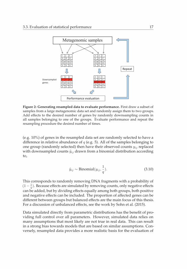
Figure 2: Generating resampled data to evaluate performance. First draw a subset ofsamples from a large metagenomic data set and randomly assign them to two groups.Add effects to the desired number of genes by randomly downsampling counts inall samples belonging to one of the groups. Evaluate performance and repeat theresampling procedure the desired number of times.

(e.g. 10%) of genes in the resampled data set are randomly selected to have adifference in relative abundance of q (e.g. 5). All of the samples belonging toone group (randomly selected) then have their observed counts yij replacedwith downsampled counts yij drawn from a binomial distribution accordingto,

yij ∼ Binomial(yij ,1

q). (3.10)

This corresponds to randomly removing DNA fragments with a probability of(1− 1

q ). Because effects are simulated by removing counts, only negative effectscan be added, but by dividing effects equally among both groups, both positiveand negative effects can be included. The proportion of affected genes can bedifferent between groups but balanced effects are the main focus of this thesis.For a discussion of unbalanced effects, see the work by Sohn et al. (2015).

Data simulated directly from parametric distributions has the benefit of pro-viding full control over all parameters. However, simulated data relies onmany assumptions that most likely are not true in real data. This can resultin a strong bias towards models that are based on similar assumptions. Con-versely, resampled data provides a more realistic basis for the evaluation of


statistical performance and it retains the within-sample variability present inreal data. Furthermore, downsampling provides a non-intrusive way to addeffects by preserving the variance structure of the affected gene. Note thatwhile resampling typically results in data that is more realistic compared tosimulations, it still presents an idealized case. In any real sampling situation,such as comparing a set of control samples with a treatment group, the samplesare never a true subset of the population, and there can be several parameters,such as pH, temperature, age of patient, and so forth, that may co-vary withthe groups and mask the effect of the treatment. On the other hand, resampleddata becomes truly randomized on average, and effects are added orthogonallyto all potential co-variates. In addition, effects are added independently andwith equal probability to all genes in the data set, disregarding the abundance,variability and proportion of zeros present in the genes. In the current imple-mentation, the added fold-change is equal for all gene with an effect and allsamples are are downsampled with the same parameter. In a real comparison,genes would be expected to have different effects and the effect size betweensamples is likely to vary for a single gene. Furthermore, differences in geneabundances between microbial communities are likely to be strongly correlated.For example, if an organism is favored in an environment, all genes specific tothat organism would increase their relative abundance. However, increasingthe complexity of the resampled data would make the results less transparent,and we argue that resampling still provides a suitable approach to evaluate theperformance of statistical methods.

The benefit of using real metagenomic data for testing is that no distributionalassumptions are needed. Real data is often used as a proof of concept thata new method works as intended. When reanalysing real data with a newmethod, the result can be compared to those previously attained, as was donein Paper IV. The downside is that the true differences, if any, are unknownand the performance of the method can therefore not be correctly estimated.For this reason, well-studied real data sets, such as the reference data setsgenerated by the sequence quality consortium for RNAseq data (Seqc/Maqc-IiiConsortium, 2014), can be used but no such initiative exists for metagenomicdata. Another approach is to create mock communities (Morgan et al., 2010),but these will not capture the full complexity of real metagenomic communitiesand should therefore be considered as idealized cases. Thus, it is not possibleto solely rely on real data for the evaluation of statistical performance withinmetagenomics.


3.3.2 Measures of statistical performance

A large proportion of this thesis focuses on the evaluation of statistical perfor-mance. Throughout these papers, three different aspects have been primarilybeen considered: the ability to rank genes based on differential abundanceby generating receiver operating characteristic (ROC) curves and calculatingthe area under the curve (AUC) (Fawcett, 2006) (Papers I-III), the ability tocontrol type I errors by investigating the distribution of p-values under thenull hypothesis (Paper I) and the ability to control errors in a multiple testingsituation through the false discovery rate (FDR) (Benjamini and Hochberg,1995)(Papers I and IV). This section will outline these different performancemeasures and their advantages and drawbacks.

Ranking genes based on differential abundance is a common way to analysemetagenomic data. Ideally, the list of ranked genes generated by a statisticaltest should contain the truly differentially abundant genes at the top andnon-differentially abundant genes at the bottom. However, ranking lists aretypically far from perfect due to the variability present in the data, lack ofreplicated samples, small effect sizes and non-optimal model assumptions.To evaluate ranking performance, we use ROC curves which are a commonmethod for visualising the statistical performance of a classifier, in this casethe test for differential abundance. In short, a ROC curve is created by goingthrough the ranking list and at each position calculating the true positive rate(TPR) and the false positive rate (FPR). The TPR is defined as the number oftrue positives above the threshold divided by the total number of true positivesin the data. The FPR is similarly defined as the proportion of false positivesabove the threshold in relation to all the false positives present in the data. Theresult is a curve for each ranking list, where each point is the FPR (x-value) andTPR (y-value) at a specific position in the ranking list (see Figure 2). Every truepositive encountered in the list is a step upwards, and every false positive isa step to the right. The area under the curve (AUC) summarizes the rankingperformance into a single value and is calculated as the area under the ROCcurve. A perfect ranking result corresponds to a ROC curve that immediatelyachieves and FPR of 1 and would therefore achieve an AUC of 1. A test thatrandomly selects between the hypotheses generates a ROC curve that is astraight line with a slope of 1, resulting in an AUC of 0.5. It is most commonto use the full AUC, which measures the quality of the entire ranking list.However, within metagenomics, the assumption is often that only a smallproportion of genes are truly differentially abundant. Thus, the quality of thetop of the ranking list, which hopefully contains the majority of true positives,is more important than the bottom. To provide a more representative value,we calculate the AUC up to some pre-specified FPR cut-off, e.g. the AUC up toa FPR value of 0.1, which we denote as AUC0.1.


Figure 3: Illustration of a receiver operating characteristic (ROC) curve. A ROC curvemeasures the quality of a ranking list by measuring the true positive rate and falsepositive rate along the list. The black line is an example ROC curve. The grey arearepresents the area under the curve (AUC), which is a measure of the average quality ofthe ranking list. The dashed line corresponds to the performance of a random classifier.

Gene ranking is often based on p-values, but only reporting ranking perfor-mance provides no information regarding the accuracy of the p-values them-selves. P-values depend on the validity of the model assumptions. Incorrectmodel assumptions can lead to strongly biased p-values, resulting either in anoverly optimistic classification with too many false positives or a pessimisticclassification where true differences are missed. If the model assumptions arecorrect, the distribution of p-values should be uniformly distributed under thenull-hypothesis. In paper I, we evaluated this property using resampled datawithout added effects to simulate a null distribution. The uniformity of thep-value distribution on the resampled data then provides a measure of howwell the assumptions behind each model fit the data and whether there is anyrisk of excess false positives.

For a single statistical test, the probability of a type-I error, i.e. a false positive,is controlled by specifying the significance level α. When several independentstatistical tests are performed simultaneously, e.g. one for each gene in ametagenomic data set, each test can result in a false positive. For this reason,several other measures of type-I error rates along with procedures to controlthem were introduced that were suitable for multiple-testing situations (Dudoitet al., 2003). One commonly used measure is the family wise error rate (FWER),


defined as the probability of getting at least one false positive among all tests.One method to control the FWER is the Bonferroni procedure, which insteadof α, uses the more strict significance cut-off αn , where n is the total number ofperformed tests. However, controlling the FWER is often overly conservativebecause a small proportion of false positives can be acceptable in order toretain a larger number of true positives. Controlling the false discovery rate(FDR), defined as the expected proportion of false positives, provides suchan alternative (Benjamini and Hochberg, 1995). Benjamini and Hochbergintroduced a method for estimating the FDR, which has become the mostcommon way to control type-I errors in multiple testing situation arising in theanalysis of high-dimensional data within the life-sciences. Given an orderedlist of p-values, the FDR at each position k can be estimated as

FDR(k) =np(k)

k. (3.11)

This creates a new list of values often referred to as q-values. A cut-off in theq-values would on average guarantee that the FDR is controlled below thatcut-off given that the assumptions of the Benjamini and Hochberg method aresatisfied ( see Benjamini and Yekutieli (2001) for details).

The accuracy of the FDR estimation can then be investigated in several ways.Of primary interest is the ability to control the FDR at the specified cut-offwhich is a fundamental requirement for sound statistical analysis. Given testdata with known effects, the true FDR at position k in gene list can be calculatedas,

FDR(k) =Number of false calls up until k

k. (3.12)

The bias in the estimated FDR compared to the true FDR can give an indicationthat a method is more or less conservative. Two methods that both are able tocontrol the FDR can still achieve a different number of true positives identified.That is, the ratio of false positives to total called genes is the same but onemethod has a higher number of called genes. Therefore it is also of interestto measure how many true and false positives are identified by each methodat the given FDR cut-off to obtain a sense of the power to detect differentiallyabundant genes.

The FDR is commonly used within metagenomics to control error rates and todetect differentially abundant genes. Thus, investigating the accuracy of FDRestimates provides important information about the reliability of a statisticalmethod. However, the accuracy of FDR estimates is not a transparent metric onits own. Biases observed in the FDR estimates can depend on the accuracy of


the underlying p-values, the quality of the ranking list and of the method usedfor estimating the FDR. Thus while FDR bias is a useful metric for evaluatingthe performance of a statistical method, other metrics are needed to show thecomplete picture.

4 Summary of papers

This section outlines the aims and backgrounds and highlights the main resultsof each of the four papers included in this thesis.

4.1 Paper I: Statistical evaluation of methods for iden-tification of differentially abundant genes in com-parative metagenomics

The aim of Paper I was to evaluate and compare statistical methods used fordetection of differentially abundant genes and provide a guide for the soundstatistical analysis of metagenomic data. In total, 14 different methods wereincluded, ranging from classical statistical tests to newly developed methodsfor metagenomic and RNAseq data. The performance was measured withrespect to their ability to rank genes, the control of the type 1 error rate andtheir ability to control the false discovery rate (FDR). To make the results asrealistic as possible, the comparison was based on resampled data generatedfrom two comprehensive metagenomes from the human gut (Qin et al., 2010;Yatsunenko et al., 2012).

Ranking performance was evaluated for each method with regard to groupsize, effect size and gene abundance. Group size had the largest impact onperformance both in terms of overall ranking accuracy and in the relativedifferences between methods. The overdispersed Poisson GLM had a highperformance and was the best method at a group size of 5+5 (see figure 4).DESeq2 and edgeR which use empirical Bayes to stabilize variance estimateshad high performance across all group sizes and had the largest advantageat the lowest group size (3+3). Next in terms of performance were a largenumber of methods that permit a gene-specific variance, such as the t-tests.

23

24 4. Summary of papers

These methods had a strong performance at higher group sizes with smalldifferences between methods but tended to have poor performance at lowergroup sizes. The methods that do not account for between-sample variability,i.e. Fisher’s exact test, the binomial-test and the Poisson GLM, had by far thelowest performance across all three group sizes (see Paper I, Figure S1). Fordetails on the performance of specific methods see the full paper.

Figure 4: Gene ranking performance on the Qin 2010 data set. Average ROC curvesfor each of the included methods. The group size was set to 6+6, and the effect size wasset to a fold-change of 5. OGLM is short for the overdispersed Poisson GLM and mSeqis short for metagenomeSeq. The results are averaged over 100 sets of resampled data.The plot corresponds to Figure 1 panel b of Paper I.

To investigate the type-I error rate, all methods were applied to resampleddata without added effects, i.e. under an empirical null distribution. Ideally,the p-values should be uniformly distributed in this case. Almost all methodssatisfied this criterion and had only minor deviations from uniformity. Themethod metagenomeSeq did show a clear sign of too optimistic p-values.However, the most striking result was again that the methods that do notaccount for between-sample variability, i.e. Fisher’s exact test, the binomial-testand the Poisson GLM, which had very skewed p-value distributions towardslow values, leading to a risk of a high number of false positives (see Paper I,Figure S6).

Finally, the ability to control the false discovery rate was investigated by com-paring the true FDR at an estimated FDR of 5% for each method (see Figure5). Most methods were indeed able to control the true FDR at the specifiedlevel. However, metagenomeSeq was not able to control the FDR. Addition-

4.1. Paper I 25

ally, the methods that do not account for between-sample variability werecompletely unable to control the FDR (see Paper I, Figure S8). Furthermore,the methods that were able to control the FDR varied in the number of truepositives detected. The three most powerful methods were edgeR, DESeq2 andthe overdispersed Poisson GLM.

Figure 5: Investigation of FDR control. Box plots showing the true FDR at an estimatedFDR of 5% for each method. The group size was set to 6+6, and the effect size was set toa fold change of 5. Each box corresponds to 100 resampled data sets from the Qin 2010data set. The plot corresponds to Figure 5 panel c of Paper I.

This paper represents the first comprehensive evaluation of statistical methodsfor metagenomic gene count data. The results showed that several methodsdeveloped for RNAseq do indeed also perform well also on metagenomic dataand should be recommended in many cases. In addition, the overdispersedPoisson GLM had a high performance and even outperformed the RNAseqmethods given that sufficient samples were available. More alarming was theperformance of the methods that do not handle the variability of metagenomicdata, i.e. Fisher’s exact test, the binomial-test and the Poisson GLM, whichcause a large number of false positives possibly leading to erroneous biologicalconclusions. Thus, this paper serves as a guide both for selecting the appropri-ate methods and for aiding the further development of statistical methods formetagenomic data.


4.2 Paper II: Variability in metagenomic count dataand its influence on the identification of differ-entially abundant genes

The aim of Paper II was to investigate the extent of variability present inmetagenomic count data and evaluate different ways of modelling this vari-ability. This work centers around a hierarchical Bayesian generalized linearmodel based on a Poisson distribution with a gene-specific variance parameter,σ2i . Letting Yij denote the count of gene i in sample j, the model is formulated

for a comparison between two groups as

log(E[Yij |αi, βi, uij ]) = αi + βiIG(j) + uij + log(Nj),

where αi is the baseline, βi is the difference between groups determined by theindicator function IG(j), uij are random effects, and Nj is a sample-specificnormalization factor. Conditioned on the parameters Yij is assumed to beindependent and Poisson distributed according to

Yij |αi, βi, uij ∼ Poisson(Njeαi+βiIG(j)+uij ).

The random effects, uij , are assumed to follow a normal distribution with thevariance parameter σ2

i , uij ∼ Normal(0, σ2i ), making the distribution of Yij

conditioned on αi, βi and σ2i a Poisson log-normal. This paper then focuses on

two main questions regarding σ2i . First, what does the distribution of σ2

i looklike in metagenomic data, and second, how do modelling assumptions on σ2

i

impact the power to detect differentially abundant genes?

To answer the first question, three comprehensive metagenomic data sets wereincluded: two from the human gut (denoted Human Gut I (Qin et al., 2012) andHuman Gut II (Yatsunenko et al., 2012)), and one sampled from oceanic surfacewater (Sunagawa et al., 2015) (denoted Marine). The model was fit to each ofthese data sets, and the posterior mean of the overdispersion defined as φij =eσ

2i −1 was calculated (see Figure 6). As expected, the overdispersion parameter

varied widely between different genes within each data set. However, thedistributions showed large similarities between data sets. Furthermore, thecorrelation of the gene-specific overdispersion between data sets was high,indicating that overdispersion has a link to the properties of each gene. Theoverdispersion was also shown to be linked to the biological properties ofeach gene by mapping every gene to their corresponding gene ontology (GO)

4.2. Paper II 27

term (Consortium, 2015). GO terms related to basal cell functions showed asignificant enrichment of genes with low overdispersion and 60 significantGO terms overlapped between all three data sets. This indicates that thegene-specific variability is indeed linked to biological function.

Human Gut Ia b c

Den

sity

Human Gut II Marine

Overdispersion log10( i) Overdispersion log10( i) Overdispersion log10( i)2 4 62 4 6

0.0

0.1

0.2

0.3

0.4

0.5

2 4 62 4 6

0.0

0.1

0.2

0.3

0.4

0.5

0.6

22 00 2 4 62 4 6

0.0

0.1

0.2

0.3

0.4

0.5

0.6

22 0022 00

Figure 6: Histograms of the posterior mean of the overdispersion parameter φij foreach gene in each dataset. The dashed line shows the median overdispersion. Panela shows the results for the Human Gut I data set, panel b shows the results for theHuman Gut II dataset, and panel c shows the results for the Marine data set. The figurecorresponds to Figure 1 of Paper II.

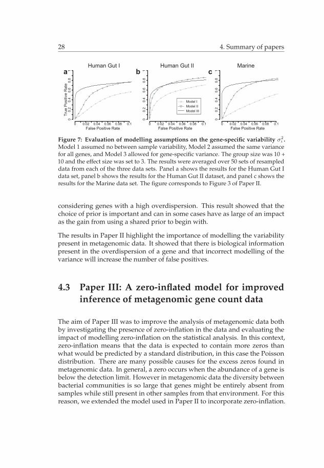
The second part of this paper targeted modelling of the gene-specific variabilityσ2i and how this impacts the ability to detect differentially abundant genes

through ranking. First, the three models assumed 1) σ2i = 0 (no between

sample variability beyond the Poisson variance), 2) σ2i = σ2 (same variance

for all genes) and 3) σ2i (gene-specific variance). The models were evaluated

on resampled data generated from the three data sets, and the ranking perfor-mance was measured (see Figure 7). The model using gene-specific variabilityoutperformed the other models on all but the third data set, where the modelassuming a single variance parameter for all genes had a slightly higher perfor-mance. Model 1, which did not account for between sample variability, had thelowest performance in all data sets and had up to 80% false positives amongthe top 10% of the ranking list. This shows the importance of modelling thegene-specific variability in metagenomics.

Model 3 was extended with a prior on the gene-specific variance parameter thatwas shared between genes to stabilize the variance estimates. Three differentshared priors for σ2

i were evaluated: a gamma distribution, an inverse-gammadistribution, and a log-normal distribution. For comparison, the model witha gene-specific flat prior was also included. The choice of prior did have alarge impact on the ranking performance, and all three prior distributions werepreferred to the gene-specific prior. However, none of the three priors wereclearly better than the others. The inverse-gamma had the best overall rankingperformance, but the gamma prior showed a better performance when only


Figure 7: Evaluation of modelling assumptions on the gene-specific variability σ2i .

Model 1 assumed no between sample variability, Model 2 assumed the same variancefor all genes, and Model 3 allowed for gene-specific variance. The group size was 10 +10 and the effect size was set to 3. The results were averaged over 50 sets of resampleddata from each of the three data sets. Panel a shows the results for the Human Gut Idata set, panel b shows the results for the Human Gut II dataset, and panel c shows theresults for the Marine data set. The figure corresponds to Figure 3 of Paper II.

considering genes with a high overdispersion. This result showed that thechoice of prior is important and can in some cases have as large of an impactas the gain from using a shared prior to begin with.

The results in Paper II highlight the importance of modelling the variabilitypresent in metagenomic data. It showed that there is biological informationpresent in the overdispersion of a gene and that incorrect modelling of thevariance will increase the number of false positives.

4.3 Paper III: A zero-inflated model for improvedinference of metagenomic gene count data

The aim of Paper III was to improve the analysis of metagenomic data bothby investigating the presence of zero-inflation in the data and evaluating theimpact of modelling zero-inflation on the statistical analysis. In this context,zero-inflation means that the data is expected to contain more zeros thanwhat would be predicted by a standard distribution, in this case the Poissondistribution. There are many possible causes for the excess zeros found inmetagenomic data. In general, a zero occurs when the abundance of a gene isbelow the detection limit. However in metagenomic data the diversity betweenbacterial communities is so large that genes might be entirely absent fromsamples while still present in other samples from that environment. For thisreason, we extended the model used in Paper II to incorporate zero-inflation.

4.3. Paper III 29

The new model was formulated as

Yij |αi, βi, uij ∼

{0 w.p. pi,

Poisson(Nje

αi+βiIG(j)+uij)

w.p. 1− pi,(4.1)

where pi is a gene-specific zero-inflation parameter. The result is that theobserved count is modelled to originate from either the previously definedPoisson-log-normal distribution or an independent zero-inflating processesgoverned by pi. The overdispersion parameter σ2

i is modelled via a globalgamma prior (σ2

i ∼ Gamma(η, κ) to permit sharing of variance between genes.For an overview of the model see Figure 8.

Figure 8: Illustration of model structure. The dashed boxes show which parametersare defined per gene, i, and sample, j, where n is the total number of genes and m is thetotal number of samples. η and κ are parameters for the global prior on the gene-specificoverdispersion σ2

i . uij are the random effects, αi denotes the baseline abundance, βidenotes the difference in abundance, Nj is a sample-specific normalization factor, λij isthe raw gene abundance, and Yij is the sampled gene abundance. pi is the gene-specificzero-inflation parameter controlling πij which indicates whether an observation iszero-inflated. The figure corresponds to Figure 1 of Paper III.

When zero-inflation is included in the model, the excess variability in the datais divided into two parts: zero-inflation for any extra zeros present in the dataand overdispersion to capture the between-sample variability. Without zero-inflation both forms of variability have to be captured by the overdispersionparameter which results in biased estimates. To examine this, we fitted themodel both with zero-inflation (denoted ZoP) and the model without zero-inflation (denoted oP) to simulated data, with and without added zeros, and


examined the posterior distributions of σ2i for all genes (see Figure 9). When

no extra zeros were added to the data, both models were similar to the truedistribution. However, when zeros were added to the data, the non-zeroinflated model showed a large increase in overdispersion estimates with morethan a 300% increase at the highest level. The zero-inflated model generatedalmost unbiased variance estimates regardless of the level of zero-inflationadded.

Figure 9: Effect of zero-inflation on overdispersion estimates in simulated data. Pos-terior means of the overdispersion parameter σ2

i for the model with zero-inflation (ZoP,solid line) and the model without zero-inflation (oP, dashed line). The levels of zero-inflation added were a) expected pi = 0 (no zeros added), panel b) expected pi = 0.034and panel c) expected pi = 0.11. The dotted line indicates the true distribution for σ2

i .The figure corresponds to Figure 2 of Paper III.

The zero-inflated model was then fit to three real metagenomic data sets fromthe human gut (Qin et al., 2010, 2012; Yatsunenko et al., 2012), and two ofthem showed a large amount of excess zeros. The same pattern of increasingoverdispersion estimates was observed on these two data sets, where therewere large differences between the estimates of the ZoP and oP.

The ZoP model was then evaluated on resampled data together with five othermethods: RAIDA and metagenomeSeq, which both model excess zeros, andedgeR, DESeq2 and voom, which were originally developed for RNAseq dataand do not incorporate zero-inflation. Incorporating zero-inflation did providea large increase in performance on resampled data, and the ZoP model andRAIDA had an overall high performance (see figure 10). The impact of addingzero-inflation was the largest at the higher group sizes. On resampled datafrom the third data set, which had a lower amount of zero-inflation, the ZoPmodel still performed on par with the best RNAseq methods. The two otherzero-inflated methods had a lower performance when no excess zeros werepresent. Thus, the ZoP model had the highest performance overall.

The results in Paper III show that excess zeros are a natural part of metagenomicdata. If not accounted for, excess zeros in the data will lower the power to detect

4.4. Paper IV 31

Figure 10: Ranking performance on resampled data from the Qin 2012 data set. Thegroup size was 10+10, and the effect size was 3. The results were averaged over 100resampled data sets. The figure corresponds to Figure 6 panel e of Paper III.

differentially abundant genes. However, care should be taken that sufficientsamples are available to accurately identify zero-inflated observations. Takentogether, the model proposed in this paper further improved the ability toidentify differentially abundant genes and provides insights into the variancestructure of metagenomic data.

4.4 Paper IV: HirBin: High-resolution identificationof differentially abundant functions in metage-nomes.

In Paper IV, we present a new method for quantifying the gene content inmetagenomic data (binning) with the aim of identify more specific biologicaleffects. The bins typically used in metagenomic data analysis are definedas groups of genes of similar function or structure and defined in variousdatabases, e.g. TIGRFAM (Haft et al., 2013), eggNOG (Huerta-Cepas et al.,2015) and KEGG (Kanehisa et al., 2008). However, the definitions of a bin insidethe databases are designed to cover many genes from multiple species and aretherefore not necessarily able to discern more specific functions. The main ideabehind this paper is that biological effects can act on several different levels,


from single genes to whole bins. If an effect acts on only a subset of the genesinside a bin, that effect will likely be diluted when viewed from the full bin.For example, if a specific gene variant is beneficial for surviving in a pollutedenvironment, it would become more prevalent in that environments. However,if that gene variant is binned together with other related genes that do notconfer this benefit, the effect on the gene will be reduced and its differentialabundance harder to identify. To solve this problem, we have developedHirBin, which uses a two-stage procedure for binning reads to improve theresolution of the analysis (see Figure 11). In the first supervised step, the datais annotated using standard methods against a pre-existing database. In thesecond unsupervised step, the sequences matching each bin are further dividedinto sub-bins by clustering based on sequence similarity. The result is a newset of sub-bins that represent more specific biological functions . The statisticalanalysis can then be performed at the sub-bin level at a pre-specified sequencesimilarity cut-off.

Figure 11: Overview of the HirBin method. The reference sequences are first annotatedaccording to gene content. For each gene, the sequences matching that gene are clustered,forming sub-bins. Finally, the gene content is quantified according to the sequenceswithin each sub-bin. The figure corresponds to Figure 1 of Paper IV.

To show the benefit of this methodology, HirBin was applied to a metagenomicdata set from a study of type II diabetes (Qin et al., 2012) at both 50% and 75%sequence similarity cut-offs. At the 50% cut-off, the total number of observedsub-bins increased to 15,740 compared to 2,465 observed without sub-binning.After bin-wise statistical testing between individuals with and without type-IIdiabetes, 4,436 sub-bins at 50% sequeance similary were deemed significant(FDR< 0.05) compared to 457 of the original bins. This corresponded to anincrease in the proportion of significant bins from 18.5% on the full bins to28.2% at the 50% sequence similarity cut-off. Considering the full bins, 987bins that were not significant had at least one significant sub-bin, while 112 ofthe previously significant bins were lost at the 50% sequence similarly cut-off.This means that the increase in the number of significant bins did indeed detectpreviously undetected functions.

4.4. Paper IV 33

To further explain the observed dilution of effects when analysing the full bins,HirBin was applied to resampled data from the same data set. Effects wereadded to 10% of the sub-bins at the 80% sequence similarity level. HirBin wasthen applied to this data and the ability to detect these effects wes analysedat 50% and 75% sequence similarity levels along with the analysis of the full-bin level (see Figure 12). The results showed that both the power to detectdifferences and the estimated fold-change substantially decreased at the lessprecise binning levels as a consequence of the dilution effect. At the full-binlevel the effects were almost completely diluted but were still detectable at thesub-bin levels.

Fold

cha

nge

Bins Sub−bins(50%)

Sub−bins(75%)

Sub−bins(80%)

12

34

56

7

APo

wer

Bins Sub−bins(50%)

Sub−bins(75%)

Sub−bins(80%)

0.0

0.2

0.4

0.6

0.8

1.0

B

Figure 12: Analysis of achieved fold-change and power when effects are added at asub bin level. Both panels show the results on resampled data where an effect hasbeen added at the 80% sequence similarity level. Panel A shows the average estimatedfold-change at each sequence similarity cut-off. Panel B shows the average powerto detect the effect at FDR< 0.05 at different sequence-similarity cut-offs. The figurecorresponds to Figure 4 of Paper IV.

In conclusion, HirBin provides a novel data-centric approach to binning thatmakes it possible to detect differences at finer resolution, effects which wouldbe missed using standard approaches to binning. This enables more accuratebiological interpretations, which will further our understanding of microbialcommunities.

5 Conclusion and outlook

This thesis targeted the statistical analysis and modelling of metagenomic genecount data. The work was centered around four main aims. Paper I providedthe first broad evaluation of statistical methods for metagenomic data basedon resampled data. It also gave a first indication of which modelling aspectsare the most important to consider. Paper II presented a more detailed evalua-tion of the variability present in metagenomic data from the perspective of anoverdispersed Poisson model. The paper also explicitly evaluated the impact ofmodelling this variability and the consequences of not properly accounting forthe between-sample variability. During the work on the first two papers andthrough the work of Paulson et al. (2013) and Sohn et al. (2015), it became ap-parent that excess zeros and sparsity might be an integral part of metagenomicdata. In Paper III, zero-inflation was introduced as an extension to the modelused in Paper II. Using this zero-inflated model, it was shown that metage-nomic data does indeed contain more zeros than predicted by most standardmodels. Furthermore, the proposed model showed a considerable increase inranking performance both on simulated and resampled data. Finally, PaperIV explored the impact of sub-clustering genes (bins) to identify differencesin biological functions at a more detailed level. It was shown that effects canindeed be missed when bins are too broad in their definition. This hints atthe complexity of the underlying biological processes, and HirBin provides auseful data-centric approach to identify effects at a more specific functionallevel.

Throughout this work, it has been shown that statistical modelling have a largeimpact on the analysis of metagenomic data. Using appropriate models cansubstantially improve the power to detect differentially abundant genes, whilenon-optimal models can cause an excess number of false positives. In summary,four main aspects of modelling metagenomic data have been observed. Thefirst is the discrete nature of the data. Count-based methods, for examplethe overdispersed Poisson GLM, were shown to have higher power to detect

35

36 5. Conclusion and outlook

differences than e.g. the t-tests and non-parametric methods in Paper I. Theimpact of modelling the counts is larger when the average observed count islower. As data becomes cheaper and easier to produce, the average sequencingdepth will increase, which will lower the impact of modelling the data ascounts. Still, when targeting less abundant genes or more specific functions,for example, the sub-bins generated by HirBin in Paper IV, the average countwill be lower, and using count-based methods is therefore recommended.

The second aspect was modelling of the between-sample variability and per-mitting a gene-specific variance. Not accounting for this variability was shownto cause a large increase in false positives in both Paper I and Paper II. Moststandard methods do permit gene-specific variability, for example, t-tests andthe overdispersed Poisson GLM. Unfortunately, the lack of replicates in theearly metagenomic era invited the use of too simplistic methods, and many ofthese are still in use. Thus, an essential step to improve the overall reliability ofmetagenomic data analysis is to completely stop using methods that do notaccount for between-sample variability.

The third aspect was extending the modelling of variance to permit sharingof information between genes. This results in variance estimates shrinkingtowards some common value. Shrinkage of the gene-specific variance estimateshas been an integral part in the analysis of high-dimensional genomic datasince the introduction in microarrays and was further developed for count-datain RNAseq data. DESeq2 and edgeR, which do permit shrinkage were shownto have a very high performance on metagenomic data in Paper I. Shrinkagehas the largest impact when the group size is small as very little information isavailable for gene-specific estimates and outliers are more likely to occur.

Finally, metagenomic data has been observed to be sparse with an excessnumber of zeros. Using the zero-inflated model of Paper III we confirmed thatmetagenomic data does contain excess zeros compared to what is expectedfrom the underlying model assumptions used today. When not accounted for,extra zeros cause the variance estimates of affected genes to be highly biased.Thus, not incorporating for zero-inflation will reduce the power to detectdifferences in abundance for affected genes. The gain in performance fromusing zero-inflated methods is especially large when the number of samples ishigh.

The analysis of metagenomic data is maturing to a point where standard proto-cols and software packages are available. However, many parts are still underconstant development. Improvements in sequencing technologies will lead tolarger amounts of higher quality data and the potential to study even morespecific functions. Reference databases are continually and rapidly expanding

37

as new sequence data is added. Although care has to be taken in the curationof these databases (Bengtsson-Palme et al., 2016), it will still lead to more genefamilies being identified and correctly annotated. New algorithms are beingdeveloped to process the ever expanding quantities of data. This thesis hasshown that the statistical analysis of metagenomic data also requires furtherwork. First, this thesis has highlighted that using flawed modelling assump-tions will cause unreliable results. To stop using those models that do notaccount for between-sample variability and to encourage replicated experi-mental designs, is of vital importance to establish a basis for sound statisticalanalysis. Second, the work presented in this thesis shows that statistical mod-elling of metagenomic data can provide large benefits in increasing the powerto detect differentially abundant genes. However, further research is neededto fully understand and utilize the complex variance structure exhibited bymetagenomic data.

38 5. Conclusion and outlook

Bibliography

Anders, S. and Huber, W. (2010). Differential expression analysis for sequencecount data. Genome biology, 11(10):R106.

Anscombe, F. (1948). The transformation of poisson, binomial and negative-binomial data. Biometrika, 35.

Bengtsson-Palme, J., Boulund, F., Edström, R., Feizi, A., Johnning, A., Jonsson,V. A., Karlsson, F. H., Pal, C., Pereira, M. B., Rehammar, A., Sanchez, J.,Sanli, K., and Thorell, K. (2016). Strategies to improve usability and preserveaccuracy in biological sequence databases. PROTEOMICS, 16(18):2454–2460.

Bengtsson-Palme, J., Boulund, F., Fick, J., Kristiansson, E., and Larsson, D.(2014). Shotgun metagenomics reveals a wide array of antibiotic resistancegenes and mobile elements in a polluted lake in india. Frontiers in microbiology,5:648.

Benjamini, Y. and Hochberg, Y. (1995). Controlling the false discovery rate:a practical and powerful approach to multiple testing. Journal of the royalstatistical society. Series B (Methodological), pages 289–300.

Benjamini, Y. and Yekutieli, D. (2001). The control of the false discovery rate inmultiple testing under dependency. Annals of statistics, pages 1165–1188.

Castro-Nallar, E., Shen, Y., Freishtat, R. J., Pérez-Losada, M., Manimaran, S., Liu,G., Johnson, W. E., and Crandall, K. A. (2015). Integrating microbial and hosttranscriptomics to characterize asthma-associated microbial communities.BMC medical genomics, 8(1):1.

Consortium, G. O. (2015). Gene ontology consortium: going forward. Nucleicacids research, 43(D1):D1049–D1056.

Curtis, T., Sloan, W., and Scannell, J. (2002). Estimating prokaryotic diversityand its limits. Proceedings of the National Academy of Sciences of the UnitedStates of America, 99(16):10494–9.

39

40 BIBLIOGRAPHY

DeLong, E. F., Preston, C. M., Mincer, T., Rich, V., Hallam, S. J., Frigaard,N.-U., Martinez, A., Sullivan, M. B., Edwards, R., Brito, B. R., et al. (2006).Community genomics among stratified microbial assemblages in the ocean’sinterior. Science, 311(5760):496–503.

Dudoit, S., Shaffer, J. P., and Boldrick, J. C. (2003). Multiple hypothesis testingin microarray experiments. Statistical Science, pages 71–103.

Fang, H., Cai, L., Yu, Y., and Zhang, T. (2013). Metagenomic analysis revealsthe prevalence of biodegradation genes for organic pollutants in activatedsludge. Bioresource technology, 129:209–218.

Fang, R., Wagner, B., Harris, J., and Fillon, S. (2016). Zero-inflated negativebinomial mixed model: an application to two microbial organisms importantin oesophagitis. Epidemiology and infection, pages 1–9.

Fawcett, T. (2006). An introduction to ROC analysis. Pattern Recognition Letters,27(8):861–874.

Fierer, N., Leff, J. W., Adams, B. J., Nielsen, U. N., Bates, S. T., Lauber, C. L.,Owens, S., Gilbert, J. A., Wall, D. H., and Caporaso, J. G. (2012). Cross-biomemetagenomic analyses of soil microbial communities and their functionalattributes. Proceedings of the National Academy of Sciences, 109(52):21390–21395.

Fisher, R. A. (1922). On the interpretation of χ2 from contingency tables, andthe calculation of p. Journal of the Royal Statistical Society, 85(1):87–94.

Fisher, R. A. (1925). Statistical methods for research workers. Genesis PublishingPvt Ltd.

Gilbert, J. A., Jansson, J. K., and Knight, R. (2014). The earth microbiome project:successes and aspirations. BMC biology, 12(1):1.

Greenblum, S., Carr, R., and Borenstein, E. (2015). Extensive strain-level copy-number variation across human gut microbiome species. Cell, 160(4):583–594.

Grzymski, J. J., Riesenfeld, C. S., Williams, T. J., Dussaq, A. M., Ducklow, H.,Erickson, M., Cavicchioli, R., and Murray, A. E. (2012). A metagenomic as-sessment of winter and summer bacterioplankton from antarctica peninsulacoastal surface waters. The ISME journal, 6(10):1901–1915.

Haft, D. H., Selengut, J. D., Richter, R. A., Harkins, D., Basu, M. K., and Beck,E. (2013). Tigrfams and genome properties in 2013. Nucleic acids research,41(D1):D387–D395.

Handelsman, J., Rondon, M., Brady, S., Clardy, J., and Goodman, R. (1998).Molecular biological access to the chemistry of unknown soil microbes: Anew frontier for natural products. Chemistry & Biology, 5.

BIBLIOGRAPHY 41

Healy, F., Ray, R., Aldrich, H., Wilkie, A., Ingram, L., and Shanmugam, K. (1995).Direct isolation of functional genes encoding cellulases from the microbialconsortia in a thermophilic, anaerobic digester maintained on lignocellulose.Applied microbiology and biotechnology, 43(4):667–674.

Howe, A. C., Jansson, J. K., Malfatti, S. A., Tringe, S. G., Tiedje, J. M., and Brown,C. T. (2014). Tackling soil diversity with the assembly of large, complexmetagenomes. Proceedings of the National Academy of Sciences, 111(13):4904–4909.

Huerta-Cepas, J., Szklarczyk, D., Forslund, K., Cook, H., Heller, D., Walter,M. C., Rattei, T., Mende, D. R., Sunagawa, S., Kuhn, M., et al. (2015). eggnog4.5: a hierarchical orthology framework with improved functional annota-tions for eukaryotic, prokaryotic and viral sequences. Nucleic acids research,page gkv1248.

Hugenholtz, P. and Tyson, G. (2008). Microbiology: metagenomics. Nature,455(7212):481–3.

Human Microbiome Project Consortium (2012). Structure, function and diver-sity of the healthy human microbiome. Nature, 486(7402):207–214.

Jeffries, T. C., Ostrowski, M., Williams, R. B., Xie, C., Jensen, R. M., Grzymski,J. J., Senstius, S. J., Givskov, M., Hoeke, R., Philip, G. K., et al. (2015). Spatiallyextensive microbial biogeography of the indian ocean provides insights intothe unique community structure of a pristine coral atoll. Scientific reports, 5.

Kanehisa, M., Araki, M., Goto, S., Hattori, M., Hirakawa, M., Itoh, M.,Katayama, T., Kawashima, S., Okuda, S., Tokimatsu, T., et al. (2008). Kegg forlinking genomes to life and the environment. Nucleic acids research, 36(suppl1):D480–D484.

Karlsson, F., Tremaroli, V., Nookaew, I., Bergström, G., Behre, C., Fagerberg, B.,J, N., and F, B. (2013). Gut metagenome in european women with normal,impaired and diabetic glucose control. Nature, 498:99–103.

Knight, R., Jansson, J., Field, D., Fierer, N., Desai, Nand Fuhrman, J., Hugen-holtz, P., van der Lelie, D., Meyer, F., Stevens, R., Bailey, M., Gordon, J.,Kowalchuk, G., and Gilbert, J. (2012). Unlocking the potential of meta-genomics through replicated experimental design. Nature biotechnology,30(6):513–20.

Kristiansson, E., Fick, J., Janzon, A., Grabic, R., Rutgersson, C., Weijdegå rd,B., Söderström, H., and Larsson, D. (2011). Pyrosequencing of antibiotic-contaminated river sediments reveals high levels of resistance and genetransfer elements. PLoS One, 6(2):e17038.

42 BIBLIOGRAPHY

Kristiansson, E., Hugenholtz, P., and Dalevi, D. (2009). ShotgunFunctionalizeR:an R-package for functional comparison of metagenomes. Bioinformatics(Oxford, England), 25(20):2737–8.

Land, M., Hauser, L., Jun, S.-R., Nookaew, I., Leuze, M. R., Ahn, T.-H.,Karpinets, T., Lund, O., Kora, G., Wassenaar, T., et al. (2015). Insights from20 years of bacterial genome sequencing. Functional & integrative genomics,15(2):141–161.

Law, C., Chen, Y., Shi, W., and Smyth, G. (2014). Voom: precision weightsunlock linear model analysis tools for RNA-seq read counts. Genome biology,15(2):R29.

Love, M. I., Huber, W., and Anders, S. (2014). Moderated estimation of foldchange and dispersion for rna-seq data with deseq2. Genome biology, 15(12):1–21.

Lozupone, C. A., Stombaugh, J. I., Gordon, J. I., Jansson, J. K., and Knight, R.(2012). Diversity, stability and resilience of the human gut microbiota. Nature,489(7415):220–230.

Mackelprang, R., Waldrop, M. P., DeAngelis, K. M., David, M. M., Chavarria,K. L., Blazewicz, S. J., Rubin, E. M., and Jansson, J. K. (2011). Metagenomicanalysis of a permafrost microbial community reveals a rapid response tothaw. Nature, 480(7377):368–371.

Manichanh, C., Rigottier-Gois, L., Bonnaud, E., Gloux, K., Pelletier, E., Frangeul,L., Nalin, R., Jarrin, C., Chardon, P., Marteau, P., et al. (2006). Reduceddiversity of faecal microbiota in crohn’s disease revealed by a metagenomicapproach. Gut, 55(2):205–211.

Mann, H. B. and Whitney, D. R. (1947). On a Test of Whether one of TwoRandom Variables is Stochastically Larger than the Other. 18:50–60.

McCullagh, P. and Nelder, J. A. (1989). Generalized linear models. LondonEngland Chapman and Hall, 2 edition.

McMurdie, P. J. and Holmes, S. (2014). Waste not, want not: why rarefyingmicrobiome data is inadmissible. PLoS Comput Biol, 10(4):e1003531.

Mende, D. R., Waller, A. S., Sunagawa, S., Järvelin, A. I., Chan, M. M., Aru-mugam, M., Raes, J., and Bork, P. (2012). Assessment of metagenomic assem-bly using simulated next generation sequencing data. PloS one, 7(2):e31386.

Morgan, J., Darling, A., and Eisen, J. (2010). Metagenomic sequencing of an invitro-simulated microbial community. PLoS ONE, 5:e10209.

BIBLIOGRAPHY 43

Nayfach, S. and Pollard, K. S. (2016). Toward accurate and quantitative com-parative metagenomics. Cell, 166(5):1103–1116.

Noyes, N. R., Yang, X., Linke, L. M., Magnuson, R. J., Cook, S. R., Zaheer, R.,Yang, H., Woerner, D. R., Geornaras, I., McArt, J. A., et al. (2016). Characteri-zation of the resistome in manure, soil and wastewater from dairy and beefproduction systems. Scientific reports, 6.

Overbeek, R., Begley, T., Butler, R. M., Choudhuri, J. V., Chuang, H.-Y., Cohoon,M., de Crécy-Lagard, V., Diaz, N., Disz, T., Edwards, R., et al. (2005). Thesubsystems approach to genome annotation and its use in the project toannotate 1000 genomes. Nucleic acids research, 33(17):5691–5702.

Pace, N. R. (1997). A molecular view of microbial diversity and the biosphere.Science, 276(5313):734–740.

Parks, D. and Beiko, R. (2010). Identifying biologically relevant differencesbetween metagenomic communities. Bioinformatics, 26(6):715–21.

Paulson, J. N., Stine, O. C., Bravo, H. C., and Pop, M. (2013). Differentialabundance analysis for microbial marker-gene surveys. Nature methods,10(12):1200–2.

Pedrós-Alió, C. (2006). Marine microbial diversity: can it be determined? Trendsin microbiology, 14(6):257–263.

Peng, X., Li, G., and Liu, Z. (2016). Zero-inflated beta regression for differentialabundance analysis with metagenomics data. Journal of Computational Biology,23(2):102–110.

Prosser, J. I. (2010). Replicate or lie. Environmental microbiology, 12(7):1806–1810.

Qin, J., Li, R., Raes, J., Arumugam, M., Burgdorf, K., Manichanh, C., Nielsen, T.,Pons, N., Levenez, F., Yamada, T., Mende, D., Li, J., Xu, J., Li, S., Li, D., Cao1,J., Wang, B., Liang, H., Zheng, H., Xie, Y., Tap, J., Lepage, P., Bertalan, M.,Batto, J.-M., Hansen, T., Paslier, D., Linneberg, A., Nielsen, H., Pelletier, E.,Renault, P., Sicheritz-Ponten, T., Turner, K., Zhu, H., Yu, C., Li, S., Jian, M.,Zhou, Y., Li, Y., Zhang, X., Li, S., Qin, N., Yang, H., Wang, J., Brunak, S., Doré,J., Guarner, F., Kristiansen, K., Pedersen, O., Parkhill1, J., Weissenbach, J.,MetaHIT Consortium, Bork, P., Ehrlich, D., and Wang, J. (2010). A human gutmicrobial gene catalogue established by metagenomic sequencing. Nature,464:59–65.

Qin, J., Li, Y., Cai, Z., Li, S., Zhu, J., Zhang, F., Liang, S., Zhang, W., Guan, Y.,Shen, D., Peng, Y., Zhang, D., Jie, Z., Wu, W., Qin, Y., Xue, W., Li, J., Han, L.,Lu, D., Wu, P., Dai, Y., Sun, X., Li, Z., Tang, A., Zhong, S., Li, X., Chen, W.,

44 BIBLIOGRAPHY

Xu, R., Wang, M., Feng, Q., Gong, M., Yu, J., Zhang, Y., Zhang, M., Hansen,T., Sanchez, G., Raes, J., Falony, G., Okuda, S., Almeida, M., LeChatelier, E.,Renault, P., Pons, N., Batto, J.-M., Zhang, Z., Chen, H., Yang, R., Zheng, W.,Li, S., Yang, H., Wang, J., Ehrlich, S., Nielsen, R., Pedersen, O., Kristiansen, K.,and Wang, J. (2012). A metagenome-wide association study of gut microbiotain type 2 diabetes. Nature, 490(7418):55–60.

Quail, M. A., Smith, M., Coupland, P., Otto, T. D., Harris, S. R., Connor, T. R.,Bertoni, A., Swerdlow, H. P., and Gu, Y. (2012). A tale of three next generationsequencing platforms: comparison of ion torrent, pacific biosciences andillumina miseq sequencers. BMC genomics, 13(1):1.

Rinke, C., Schwientek, P., Sczyrba, A., Ivanova, N., Anderson, I., Cheng, J.-F., Darling, A., Malfatti, S., Swan, B., Gies, E., Dodsworth, J., Hedlund,B., Tsiamis, G., Sievert, S., Liu, W.-T., Eisen, J., Hallam, S., Kyrpides, N.,Stepanauskas, R., Rubin, E., Hugenholtz, P., and Woyke, T. (2013). Insightsinto the phylogeny and coding potential of microbial dark matter. Nature,499:431–437.

Robinson, M., McCarthy, D., and Smyth, G. (2010). edger: a bioconductorpackage for differential expression analysis of digital gene expression data.Bioinformatics, 26:139–140.

Robinson, M. D. and Oshlack, A. (2010). A scaling normalization method fordifferential expression analysis of rna-seq data. Genome biology, 11(3):1.

Robles, J. A., Qureshi, S. E., Stephen, S. J., Wilson, S. R., Burden, C. J., andTaylor, J. M. (2012). Efficient experimental design and analysis strategies forthe detection of differential expression using rna-sequencing. BMC genomics,13(1):1.

Rodriguez-Brito, B., Rohwer, F., and Edwards, R. (2006). An application ofstatistics to comparative metagenomics. BMC bioinformatics, 7:162.

Roesch, L. F., Fulthorpe, R. R., Riva, A., Casella, G., Hadwin, A. K., Kent, A. D.,Daroub, S. H., Camargo, F. A., Farmerie, W. G., and Triplett, E. W. (2007).Pyrosequencing enumerates and contrasts soil microbial diversity. The ISMEjournal, 1(4):283–290.

Rondon, M. R., August, P. R., Bettermann, A. D., Brady, S. F., Grossman, T. H.,Liles, M. R., Loiacono, K. A., Lynch, B. A., MacNeil, I. A., Minor, C., et al.(2000). Cloning the soil metagenome: a strategy for accessing the genetic andfunctional diversity of uncultured microorganisms. Applied and environmentalmicrobiology, 66(6):2541–2547.

BIBLIOGRAPHY 45

Ross, E., Moate, P., Marett, L., Cocks, B., and Hayes, B. (2013). Investigatingthe effect of two methane-mitigating diets on the rumen microbiome usingmassively parallel sequencing. Journal of dairy science, 96(9):6030–6046.

Sanger, F. and Coulson, A. R. (1975). A rapid method for determining sequencesin dna by primed synthesis with dna polymerase. Journal of molecular biology,94(3):441–448.

Sanli, K., Karlsson, F., Nookaew, I., and Nielsen, J. (2013). FANTOM: Functionaland taxonomic analysis of metagenomes. BMC bioinformatics, 14(1):38.

Schloss, P. and Handelsman, J. (2005). Metagenomics for studying unculturablemicroorganisms: cutting the Gordian knot. Genome biology, 6(8):229.

Schmieder, R. and Edwards, R. (2011). Quality control and preprocessing ofmetagenomic datasets. Bioinformatics, 27(6):863–864.

Scholz, M. B., Lo, C.-C., and Chain, P. S. (2012). Next generation sequencing andbioinformatic bottlenecks: the current state of metagenomic data analysis.Current opinion in biotechnology, 23(1):9–15.

Segata, N., Izard, J., Waldron, L., Gevers, D., Miropolsky, L., Garrett, W., andHuttenhower, C. (2011). Metagenomic biomarker discovery and explanation.Genome biology, 12(6):R60.

Seqc/Maqc-Iii Consortium (2014). A comprehensive assessment of rna-seqaccuracy, reproducibility and information content by the sequencing qualitycontrol consortium. Nature biotechnology, 32(9):903–914.

Smith, R. J., Jeffries, T. C., Roudnew, B., Fitch, A. J., Seymour, J. R., Delpin,M. W., Newton, K., Brown, M. H., and Mitchell, J. G. (2012). Metagenomiccomparison of microbial communities inhabiting confined and unconfinedaquifer ecosystems. Environmental microbiology, 14(1):240–253.

Smyth, G. (2004). Linear models and empirical bayes methods for assessingdifferential expression in microarray experiments. Statistical Applications inGenetics and Molecular Biology, 3.

Sohn, M. B., Du, R., and An, L. (2015). A robust approach for identifyingdifferentially abundant features in metagenomic samples. Bioinformatics,page btv165.

Soneson, C. and Delorenzi, M. (2013). A comparison of methods for differentialexpression analysis of rna-seq data. BMC bioinformatics, 14(1):1.

Sunagawa, S., Coelho, L. P., Chaffron, S., Kultima, J. R., Labadie, K., Salazar, G.,Djahanschiri, B., Zeller, G., Mende, D. R., Alberti, A., et al. (2015). Structureand function of the global ocean microbiome. Science, 348(6237):1261359.

46 BIBLIOGRAPHY

Turnbaugh, P., Hamady, M., Yatsunenko, T., Cantarel, B., Duncan, A., Ley, R.,Sogin, M., Jones, W., Roe, B., Affourtit, J., Egholm, M., Henrissat, B., Heath,A., Knight, R., and Gordon, J. (2009). A core gut microbiome in obese andlean twins. Nature, 457(7228):480–4.

Turnbaugh, P., Ley, R., Hamady, M., Liggett, C., Knight, R., and Gordon, J.(2007). The human microbiome project: exploring the microbial part ofourselves in a changing world. Nature, 449:804–810.

Unterseher, M., Jumpponen, A., Öpik, M., Tedersoo, L., Moora, M., Dormann,C. F., and Schnittler, M. (2011). Species abundance distributions and rich-ness estimations in fungal metagenomics–lessons learned from communityecology. Molecular Ecology, 20(2):275–285.

van Dijk, E. L., Auger, H., Jaszczyszyn, Y., and Thermes, C. (2014). Ten years ofnext-generation sequencing technology. Trends in genetics, 30(9):418–426.

Ward, T. L., Hosid, S., Ioshikhes, I., and Altosaar, I. (2013). Human milkmetagenome: a functional capacity analysis. BMC microbiology, 13(1):1.

White, J., Nagarajan, N., and Pop, M. (2009). Statistical methods for detectingdifferentially abundant features in clinical metagenomic samples. PLoScomputational biology, 5(4):e1000352.

Whitman, W. B., Coleman, D. C., and Wiebe, W. J. (1998). Prokaryotes: theunseen majority. Proceedings of the National Academy of Sciences, 95(12):6578–6583.

Wilcoxon, F. (1946). Individual comparisons of grouped data by rankingmethods. Journal of economic entomology, 39:269.

Wooley, J., Godzik, A., and Friedberg, I. (2010). A primer on metagenomics.PLoS computational biology, 6(2):e1000667.

Wooley, J. and Ye, Y. (2009). Metagenomics: Facts and Artifacts, and Computa-tional Challenges*. Journal of computer science and technology, 25(1):71–81.

Yatsunenko, T., Rey, F., Manary, M., Trehan, I., Dominguez-Bello, M., Contreras,M., Magris, M., Hidalgo, G., Baldassano, R., Anokhin, A., Heath, A., Warner,B., Reeder, J., Kuczynski, J., Caporaso, J., Lozupone, C., Lauber, C., Clemente,J., Knights, D., Knight, R., and Gordon, J. (2012). Human gut microbiomeviewed across age and geography. Nature, 486(7402):222–7.

Zhang, X., Mallick, H., Tang, Z., Zhang, L., Cui, X., Benson, A. K., and Yi, N.(2017). Negative binomial mixed models for analyzing microbiome countdata. BMC Bioinformatics, 18(1):4.

ph.d. thesis ph.d. thesis - göteborgs universitet for making my life a bit more crazy (in a good...

Documents