phd thesis. soas, university londoneprints.soas.ac.uk/17372/1/michell_3516.pdf2 declaration for phd...
TRANSCRIPT

Michell, Jo (2012) Credit and investment in China: a flow‐of‐funds analysis. PhD
Thesis. SOAS, University of London
http://eprints.soas.ac.uk/17372
Copyright © and Moral Rights for this thesis are retained by the author and/or other
copyright owners.
A copy can be downloaded for personal non‐commercial research or study, without prior
permission or charge.
This thesis cannot be reproduced or quoted extensively from without first obtaining
permission in writing from the copyright holder/s.
The content must not be changed in any way or sold commercially in any format or
medium without the formal permission of the copyright holders.
When referring to this thesis, full bibliographic details including the author, title, awarding
institution and date of the thesis must be given e.g. AUTHOR (year of submission) "Full
thesis title", name of the School or Department, PhD Thesis, pagination.
Credit and Investment in China:
A Flow-of-Funds Analysis
Jo Michell
Thesis submitted for the degree of PhD in Economics
2012
Department of Economics
School of Oriental and African Studies
University of London

2
Declaration for PhD thesis
I have read and understood regulation 17.9 of the Regulations for students of
the School of Oriental and African Studies concerning plagiarism. I undertake
that all the material presented for examination is my own work and has not been
written for me, in whole or in part, by any other person. I also undertake that
any quotation or paraphrase from the published or unpublished work of another
person has been duly acknowledged in the work which I present for examination.
Signed: Date:

Acknowledgements
I am grateful to the Central Research Fund of the University of London and the
School of Oriental and African Studies for financial support in undertaking this
research.
There are too many people at SOAS who have helped me with this project
along the way to be able to thank them all individually. Without the support, en-
couragement, insight and inspiration of the staff and students of the Department,
this project would not have been possible.
I am very grateful for the advice and encouragement I have received from the
members of my supervisory committee, Prof. Machiko Nissanke and Dr. Damian
Tobin. I received very helpful comments during my viva examination from Prof.
Hansjorg Herr and Dr. Dic Lo. Some of these comments have been incorporated
into the thesis as part of the normal corrections procedure. At SOAS, my great-
est debt of gratitude is to my supervisor, Prof. Jan Toporowski. His intellectual
guidance, support and patience have been far in excess of the normal call of duty
for a PhD supervisor. None of these people are implicated in any mistakes which
remain, for which I take sole responsibility.
My deepest gratitude is to my family, for their support and guidance, and to
Mary McCarthy who has suffered for this project, without complaint, for the last
four years.
3
4
Abstract
This thesis presents a detailed flow-of-funds analysis of the Chinese economy
since 1992. An original theoretical approach to endogenous money, investment
and profits is developed alongside the empirical analysis.
It is argued that standard modern macroeconomic theory, such as the New
Keynesian monetary macroeconomics and neoclassical growth theory are un-
suited to the analysis of a long-run disequilibrium credit-financed investment-
driven growth path such as that which has taken place in China.
Using an approach built on accounting foundations, rather than the optimis-
ing behaviour of representative agents, an analysis of credit creation, investment
and growth is presented in which firms’ investment expenditures are the key fac-
tor in determining the dynamic evolution of the system. Steindl’s analysis of the
“maldistribution of profits” is updated and re-worked in the context of state con-
trol over the “cartelised” firms’ sector. It is argued that the credit-financed invest-
ment expenditures of the state-owned sector play the decisive role in generating
the aggregate demand which has driven high growth rates in China, while si-
multaneously conditioning the outcomes in terms of profit generation, monetary
expansion and the distribution of liquidity and leverage.
The development of the theoretical analysis is informed by a detailed em-
pirical examination of the processes of money creation, investment and profits
over the last twenty years in China. The empirical approach follows the theoret-
ical analysis in that it is also based around the flow-of-funds national accounting
system, resulting in an integrated and coherent analytical structure in which all
transactions are matched by equivalent and opposite transactions elsewhere in
the system.
Contents
1 Introduction 13
1.1 China’s development path . . . . . . . . . . . . . . . . . . . . . . . . 15
1.2 The flow-of-funds . . . . . . . . . . . . . . . . . . . . . . . . . . . . . 20
1.3 Thesis outline . . . . . . . . . . . . . . . . . . . . . . . . . . . . . . . 22
I Theory 24
2 Modern theories of money and growth 25
2.1 Introduction . . . . . . . . . . . . . . . . . . . . . . . . . . . . . . . . 25
2.2 New Keynesian monetary theory . . . . . . . . . . . . . . . . . . . . 26
2.2.1 Overview . . . . . . . . . . . . . . . . . . . . . . . . . . . . . 26
2.2.2 Monetary policy without money . . . . . . . . . . . . . . . . 31
2.2.3 Capital markets and the accumulation of capital . . . . . . . 37
2.3 Growth theory . . . . . . . . . . . . . . . . . . . . . . . . . . . . . . . 45
2.3.1 The aggregate production function . . . . . . . . . . . . . . . 45
2.3.2 Old growth . . . . . . . . . . . . . . . . . . . . . . . . . . . . 51
2.3.3 New growth . . . . . . . . . . . . . . . . . . . . . . . . . . . . 55
2.4 Conclusion . . . . . . . . . . . . . . . . . . . . . . . . . . . . . . . . . 58
3 Stock-flow accounting 61
3.1 Introduction . . . . . . . . . . . . . . . . . . . . . . . . . . . . . . . . 61
3.2 Simple “classical” system . . . . . . . . . . . . . . . . . . . . . . . . 64
3.3 Profits in the firm sector . . . . . . . . . . . . . . . . . . . . . . . . . 69
3.4 Excess capital . . . . . . . . . . . . . . . . . . . . . . . . . . . . . . . 74
3.5 Equity issuance . . . . . . . . . . . . . . . . . . . . . . . . . . . . . . 78
3.6 Foreign trade . . . . . . . . . . . . . . . . . . . . . . . . . . . . . . . . 84
3.7 Conclusion . . . . . . . . . . . . . . . . . . . . . . . . . . . . . . . . . 89
5
CONTENTS 6
4 Growth, income distribution and money 91
4.1 Introduction . . . . . . . . . . . . . . . . . . . . . . . . . . . . . . . . 91
4.2 Cambridge growth models . . . . . . . . . . . . . . . . . . . . . . . . 92
4.3 Steindl’s theory of stagnation . . . . . . . . . . . . . . . . . . . . . . 100
4.3.1 The case of an individual industry . . . . . . . . . . . . . . . 102
4.3.2 Accumulation in the economy as a whole . . . . . . . . . . . 104
4.4 The Kaleckian growth model . . . . . . . . . . . . . . . . . . . . . . 107
4.4.1 Outline of the model . . . . . . . . . . . . . . . . . . . . . . . 107
4.4.2 Critiques of the Kaleckian model . . . . . . . . . . . . . . . . 112
4.5 Money and finance . . . . . . . . . . . . . . . . . . . . . . . . . . . . 117
4.6 Growth in a pure-credit system . . . . . . . . . . . . . . . . . . . . . 122
4.6.1 Overview . . . . . . . . . . . . . . . . . . . . . . . . . . . . . 122
4.6.2 Model equations . . . . . . . . . . . . . . . . . . . . . . . . . 123
4.6.3 Analysis using simulations . . . . . . . . . . . . . . . . . . . 129
4.7 The distribution of profits . . . . . . . . . . . . . . . . . . . . . . . . 146
4.8 Conclusion . . . . . . . . . . . . . . . . . . . . . . . . . . . . . . . . . 148
II Evidence 150
5 Credit and banking in China 151
5.1 Introduction . . . . . . . . . . . . . . . . . . . . . . . . . . . . . . . . 151
5.2 Transition . . . . . . . . . . . . . . . . . . . . . . . . . . . . . . . . . 154
5.2.1 Monetary reform . . . . . . . . . . . . . . . . . . . . . . . . . 154
5.2.2 Banking sector structural and regulatory reforms . . . . . . 156
5.3 Monetary policy implementation details . . . . . . . . . . . . . . . . 165
5.3.1 Monetary policy operations . . . . . . . . . . . . . . . . . . . 165
5.3.2 Autonomous factors . . . . . . . . . . . . . . . . . . . . . . . 172
5.3.3 Interest rates . . . . . . . . . . . . . . . . . . . . . . . . . . . . 173
5.4 Conclusion . . . . . . . . . . . . . . . . . . . . . . . . . . . . . . . . . 175
6 China’s flow-of-funds I 179
6.1 Introduction . . . . . . . . . . . . . . . . . . . . . . . . . . . . . . . . 179
6.2 Background to the flow-of-funds accounts . . . . . . . . . . . . . . . 181
6.3 Data sources and description . . . . . . . . . . . . . . . . . . . . . . 185
6.3.1 NBS Flow-of-funds accounts . . . . . . . . . . . . . . . . . . 185
6.3.2 Financial stocks and flows . . . . . . . . . . . . . . . . . . . . 188
CONTENTS 7
6.4 Saving and Investment . . . . . . . . . . . . . . . . . . . . . . . . . . 198
6.4.1 Saving . . . . . . . . . . . . . . . . . . . . . . . . . . . . . . . 200
6.4.2 Investment . . . . . . . . . . . . . . . . . . . . . . . . . . . . . 206
6.4.3 Net financial balances . . . . . . . . . . . . . . . . . . . . . . 208
6.4.4 Income and expenditure shares . . . . . . . . . . . . . . . . . 213
6.5 Firms sector in more detail . . . . . . . . . . . . . . . . . . . . . . . . 220
6.5.1 Investment by ownership classification . . . . . . . . . . . . 222
6.5.2 Profits . . . . . . . . . . . . . . . . . . . . . . . . . . . . . . . 227
6.6 Conclusion . . . . . . . . . . . . . . . . . . . . . . . . . . . . . . . . . 234
7 China’s flow-of-funds II 240
7.1 Introduction . . . . . . . . . . . . . . . . . . . . . . . . . . . . . . . . 240
7.2 Sector financing . . . . . . . . . . . . . . . . . . . . . . . . . . . . . . 241
7.2.1 Firms . . . . . . . . . . . . . . . . . . . . . . . . . . . . . . . . 242
7.2.2 Households . . . . . . . . . . . . . . . . . . . . . . . . . . . . 254
7.2.3 Government . . . . . . . . . . . . . . . . . . . . . . . . . . . . 258
7.3 The financial system . . . . . . . . . . . . . . . . . . . . . . . . . . . 258
7.3.1 The financial system at the aggregate level . . . . . . . . . . 260
7.3.2 The monetary authority . . . . . . . . . . . . . . . . . . . . . 262
7.3.3 Financial institutions net of monetary authority . . . . . . . 275
7.4 Conclusion . . . . . . . . . . . . . . . . . . . . . . . . . . . . . . . . . 282
8 Conclusion 285
Bibliography 291
List of Figures
2.1 Causal structure of the New Keynesian model. . . . . . . . . . . . . 30
4.1 Rate of growth . . . . . . . . . . . . . . . . . . . . . . . . . . . . . . . 131
4.2 Increase in saving propensity: capacity utilisation . . . . . . . . . . 132
4.3 Increase in saving propensity: rate of profit . . . . . . . . . . . . . . 132
4.4 Increase in saving propensity: capital stock and household deposits 133
4.5 Increase in saving propensity: firms’ sector leverage . . . . . . . . . 134
4.6 Decrease in rate of interest: uniform saving . . . . . . . . . . . . . . 136
4.7 Decrease in rate of interest: income-specific saving . . . . . . . . . . 137
4.8 Increase in animal spirits . . . . . . . . . . . . . . . . . . . . . . . . . 140
4.9 Increase in animal spirits (contd.) . . . . . . . . . . . . . . . . . . . . 141
4.10 Exogenous reduction in investment . . . . . . . . . . . . . . . . . . . 144
(a) Growth rates: oligopoly . . . . . . . . . . . . . . . . . . . . . . 144
(b) Growth rates: competitive . . . . . . . . . . . . . . . . . . . . . 144
(c) Capacity utilisation: oligopoly . . . . . . . . . . . . . . . . . . 144
(d) Capacity utilisation: competitive . . . . . . . . . . . . . . . . . 144
(e) Profit rate: oligopoly . . . . . . . . . . . . . . . . . . . . . . . . 144
(f) Profit rate: competitive . . . . . . . . . . . . . . . . . . . . . . . 144
(g) Gearing ratio: oligopoly . . . . . . . . . . . . . . . . . . . . . . 144
(h) Gearing ratio: competitive . . . . . . . . . . . . . . . . . . . . . 144
5.1 Consumer price inflation . . . . . . . . . . . . . . . . . . . . . . . . . 157
5.2 Outstanding PBC bills . . . . . . . . . . . . . . . . . . . . . . . . . . 171
6.1 Saving and investment . . . . . . . . . . . . . . . . . . . . . . . . . . 199
6.2 Growth rate of real GDP . . . . . . . . . . . . . . . . . . . . . . . . . 199
6.3 Exports and imports . . . . . . . . . . . . . . . . . . . . . . . . . . . 200
6.4 Saving by sector . . . . . . . . . . . . . . . . . . . . . . . . . . . . . . 203
8
LIST OF FIGURES 9
6.5 Net tax and transfer payments by sector . . . . . . . . . . . . . . . . 204
6.6 Saving of households and firms net of taxes and fiscal transfers . . 205
6.7 Saving by sector after capital transfers . . . . . . . . . . . . . . . . . 207
6.8 Investment by sector . . . . . . . . . . . . . . . . . . . . . . . . . . . 209
(a) Gross capital formation . . . . . . . . . . . . . . . . . . . . . . 209
(b) GCF plus net aquisition of capital assets . . . . . . . . . . . . . 209
6.9 “Three balances”, percent of GDP . . . . . . . . . . . . . . . . . . . . 211
(a) From physical transaction tables . . . . . . . . . . . . . . . . . 211
(b) From financial transaction tables . . . . . . . . . . . . . . . . . 211
6.10 Net financial position by sector, percent of GDP . . . . . . . . . . . 212
(a) From physical transaction tables . . . . . . . . . . . . . . . . . 212
(b) From financial transaction tables . . . . . . . . . . . . . . . . . 212
6.11 Investment as share of GDP by various methods of calculation . . . 224
6.12 Investment in fixed assets by ownership classification . . . . . . . . 227
6.13 Measures of profit margin calculated from flow-of-funds . . . . . . 230
7.1 Firms’ financial transactions and net balance . . . . . . . . . . . . . 243
(a) Saving, investment and net financial balance . . . . . . . . . . 243
(b) Annual change in financial assets and liabilities . . . . . . . . 243
7.2 Loans and deposits of firms sector . . . . . . . . . . . . . . . . . . . 246
7.3 Growth in investment; loans and deposits of firms . . . . . . . . . . 249
(a) Growth of investment . . . . . . . . . . . . . . . . . . . . . . . 249
(b) Growth of deposits and loans of firms . . . . . . . . . . . . . . 249
7.4 Sources of investment funds . . . . . . . . . . . . . . . . . . . . . . . 251
7.5 Households’ financial transactions and net financial balance . . . . 255
(a) Saving, investment and net financial balance . . . . . . . . . . 255
(b) Annual change in financial assets and liabilities . . . . . . . . 255
7.6 Shanghai stock price index and turnover . . . . . . . . . . . . . . . . 257
7.7 Financial transactions of government sector . . . . . . . . . . . . . . 259
7.8 Flow transactions of aggregated financial system . . . . . . . . . . . 261
7.9 Balance sheet of the People’s Bank of China . . . . . . . . . . . . . . 263
(a) Assets . . . . . . . . . . . . . . . . . . . . . . . . . . . . . . . . 263
(b) Liabilities . . . . . . . . . . . . . . . . . . . . . . . . . . . . . . 263
7.10 Required reserve ratio . . . . . . . . . . . . . . . . . . . . . . . . . . 264
7.11 Estimated composition of reserves held at PBC . . . . . . . . . . . . 266
(a) Required and excess reserves . . . . . . . . . . . . . . . . . . . 266
LIST OF FIGURES 10
(b) Excess reserve ratio . . . . . . . . . . . . . . . . . . . . . . . . . 266
7.12 PBC and inter-bank interest rates . . . . . . . . . . . . . . . . . . . . 267
7.13 Foreign exchange and sterilisation flows . . . . . . . . . . . . . . . . 271
(a) Foreign exchange flows . . . . . . . . . . . . . . . . . . . . . . 271
(b) Sterilisation flows . . . . . . . . . . . . . . . . . . . . . . . . . . 271
7.14 Yields on PBC bills and US government securities . . . . . . . . . . 273
7.15 Flow operations of People’s Bank of China . . . . . . . . . . . . . . 275
7.16 Estimated balance sheet of financial institutions . . . . . . . . . . . 276
(a) Assets . . . . . . . . . . . . . . . . . . . . . . . . . . . . . . . . 276
(b) Liabilities . . . . . . . . . . . . . . . . . . . . . . . . . . . . . . 276
7.17 Flow transaction of financial institutions . . . . . . . . . . . . . . . . 277
7.18 Selected commercial bank interest rates . . . . . . . . . . . . . . . . 279
7.19 Holdings of bank deposits by sector . . . . . . . . . . . . . . . . . . 280
7.20 Estimated assets of financial institutions . . . . . . . . . . . . . . . . 281
(a) Assets of financial institutions in detail . . . . . . . . . . . . . 281
(b) Loans to households . . . . . . . . . . . . . . . . . . . . . . . . 281
List of Tables
3.1 Transactions matrix: “classical” case . . . . . . . . . . . . . . . . . . 66
3.2 Transactions matrix: retained earnings . . . . . . . . . . . . . . . . . 71
3.3 Transactions matrix: overcapitalisation . . . . . . . . . . . . . . . . . 73
3.4 Transactions matrix: speculative overcapitalisation . . . . . . . . . . 79
3.5 Balance sheet: households saving, equity bought by households . . 82
3.6 Balance sheet: households saving, equity bought by firms . . . . . . 83
3.7 Balance sheet: firms saving, equity bought by firms . . . . . . . . . 83
3.8 Foreign trade and sterilisation. . . . . . . . . . . . . . . . . . . . . . 85
4.1 Transactions flow matrix. . . . . . . . . . . . . . . . . . . . . . . . . . 124
5.1 Example central bank balance sheet . . . . . . . . . . . . . . . . . . 165
5.2 Balance sheet of PBC, December 2009 . . . . . . . . . . . . . . . . . 167
6.1 Simplified flow-of-funds system . . . . . . . . . . . . . . . . . . . . 182
6.2 Nominal GDP of China, original and revised figures . . . . . . . . . 187
6.3 Discrepancy of net financial position of flow-of-funds. . . . . . . . . . 189
6.4 Balance sheet of PBC, Dec. 2009 . . . . . . . . . . . . . . . . . . . . . 191
6.5 Sources and uses of credit funds of financial institutions, Dec. 2009 192
6.6 Assets and liabilities of financial system net of PBC, Dec. 2009 . . . 193
6.7 Flow of funds, financial transactions, 2009 . . . . . . . . . . . . . . . 195
6.8 Flow of funds, financial transactions, 2009, augmented . . . . . . . 196
6.9 Simplified physical flow-of-funds, 2008 . . . . . . . . . . . . . . . . 201
6.10 Government revenue and expenditure, official . . . . . . . . . . . . 215
6.11 Government revenue and expenditure, calculated . . . . . . . . . . 216
6.12 Sector shares in total income . . . . . . . . . . . . . . . . . . . . . . . 218
6.13 Saving as share of disposable income by sector . . . . . . . . . . . . 220
6.14 Investment in fixed assets by ownership classification . . . . . . . . 225
11

LIST OF TABLES 12
6.15 GFCF and GCF by sector . . . . . . . . . . . . . . . . . . . . . . . . . 226
6.16 Profit margin by type of ownership. . . . . . . . . . . . . . . . . . . 232
6.17 Output by ownership type . . . . . . . . . . . . . . . . . . . . . . . . 233
6.18 Profit to net fixed assets ratio . . . . . . . . . . . . . . . . . . . . . . 234
7.1 Ratio of liabilities to assets and revenues . . . . . . . . . . . . . . . . 252
Chapter 1
Introduction
The growth performance of China since 1978, when market-oriented reforms
were initiated, makes it one of the great success stories of recent economic history.
This performance has generated considerable debate because it has taken place
in a policy environment far removed from the idealised liberal market structure
advocated by standard economic theory. Very high rates of growth have been
achieved under a system of significant state ownership, strong restrictions on in-
ternational capital movements and a financial system dominated by a few large
state-owned banks. Furthermore, for much of this period, global economic per-
formance was weak, with stagnation occurring in much of the developing world.
In an attempt to reconcile the obvious success of the Chinese case with the
observation that China’s policy mix does not match standard prescriptions, anal-
ysis and debate have focused on attempts to identify those factors which have
enabled China to succeed despite such policy obstacles. This discussion has been
framed under the assumption that the optimal institutional and policy structures
for growth and development are those which conform to a liberalised market
system based on private ownership. This implies that debate hinges on a discus-
sion of those features of the Chinese economic and political system which may be
considered as complying with such a market system, and those which continue
to diverge from it.
In opposition to this dominant account of the Chinese experience is an alter-
native narrative which focuses on the specific form taken by China’s transition
to the market, and in particular on the role played by industrialisation. From
the point of view of textbook theory, the capital-intensive industrial growth path
taken by China appears contradictory, given the abundance of labour relative to
13
CHAPTER 1. INTRODUCTION 14
capital. However, this capital-intensive growth path can be explained with ref-
erence to the role played by increasing returns to scale in industry. In relating
increases in labour productivity to investment expenditures, an analysis of the
dynamic growth path taken by China can be constructed in which the role of
government and the structure of institutions no longer appear paradoxical.
This thesis complements such an alternative interpretation of China’s devel-
opment by putting forward an original account of the characteristics of circula-
tion and aggregate demand in the Chinese economy, during the period since the
early 1990s in which growth has been led by high levels of investment in fixed
capital. It is argued that China’s performance is the outcome of a dynamic credit-
investment process, in which the expenditures of firms are financed by a com-
bination of loans extended by the state-owned banking system and the retained
earnings of corporations. While growth has been driven by the productivity-
enhancing effects of investment, this development path has been facilitated by
a distinctive regime of monetary circulation and aggregate demand. In recent
years this regime been additionally influenced by the effects of a significant trade
surplus.
This characterisation of the demand and circulation regime of the Chinese
economy is operationalised through the development of an original theoretical
approach to endogenous money, aggregate demand and the distribution of prof-
its, based on a re-interpretation of Steindl’s analysis of the “maldistribution of
profits”. Using a modified version of the Kaleckian profit reflux mechanism, it
is argued that the investment expenditures of state-owned firms have led to a
concentration of profits in the private firms sector, while a disproportionate share
of the associated liabilities remain the responsibility of those state-owned enter-
prises which have led this investment.
Central to this argument is the notion that the financial system plays a key
role in accommodating the liquidity requirements of firms through endogenous
credit creation. As such, the role played by the financial system is not primarily
related to its efficiency or otherwise as an intermediary, allocating funds—in the
form of household savings—to those investment projects that generate the high-
est marginal returns. The real significance lies in the role of the financial system,
and the banking system in particular, as a creator of liquidity ex-nihilo, allow-
ing firms to initiate expenditure on investment projects, generating new income
which in turn results in increased savings and further economic growth. There
is thus an important distinction, originating with Schumpeter ([1938] 2008), be-
CHAPTER 1. INTRODUCTION 15
tween static notions of allocative efficiency, and the potential dynamic produc-
tivity increases which can occur in a growing economy. Central to Schumpeter’s
analysis was the crucial importance of the use of bank credit in sustaining such a
dynamic investment-led growth path.1
This thesis uses the flow-of-funds accounting system both as a basis for a the-
oretical account of this monetary credit-investment-growth process, and for an
empirical study of the recent macroeconomic history of China. The flow-of-funds
framework is used in the development of a stock-flow consistent model which
integrates a Kaleckian growth model with a “pure credit” monetary system. This
provides a theoretical basis for a detailed analysis of the Chinese flow-of-funds
accounts, augmented with balance sheet data from the People’s Bank of China
and disaggregated data from various other sources
1.1 China’s development path
The rapid growth of China is widely perceived as a “puzzle”, since it has taken
place despite apparently violating many of the the standard policy prescriptions:
“The Chinese path of reform and its associated rapid growth is puzzling because
it seems to defy... the conventional wisdom... China’s reform succeeded with-
out complete liberalization, without privatization, and without democratization”
(Qian, 2003, p. 298). It is argued by Lo (2012) that attempts to interpret the Chi-
nese growth experience in a way that is compatible with orthodox economic the-
ory have centred on two main propositions:
First, concerning institutions, it is claimed that China’s reformed eco-
nomic institutions have been a mix of market-conforming and market-
supplanting elements, that its developmental achievements have been
ascribable to the conforming elements while the accumulated prob-
lems have been ascribable to the supplanting elements, and that the
problems have tended to outweigh the achievements . . . Second, con-
cerning development, it is claimed that differences in country-specific
factors, most importantly the different levels of industrialization, have
largely explained the contrast between China’s sustained rapid growth
and the depression in countries of the former Soviet bloc, and that this
1The function of banks as creators of new money, and thus as initiators of fresh circuits of eco-nomic production, originates with Hartley Withers’ The Meaning of Money (1920), and was subse-quently developed by Keynes ([1930] 1971, 1937b), Hayek (1933) and Schumpeter ([1938] 2008)
CHAPTER 1. INTRODUCTION 16
contrast is largely unrelated to differences in the strategies of systemic
transformation. (Lo, 2012, pp. 100–101)
The first of these propositions has become increasingly untenable, given that
market-supplanting institutional forms have continued to prevail, while at the
same time growth rates have remained persistently high. Adherents to the or-
thodox view of the primacy of private property and the liberal market system
have thus fallen back on the second of these propositions, namely that the diverg-
ing experiences of China and the other transition economies of the former Soviet
Union—which pursued a much more extreme set of liberalisation policies—can
be attributed to differences in the initial conditions faced in each case. China’s
success can then be viewed as having occurred, in spite of the policy regime, as a
consequence of low initial levels of industrialisation.
Another interpretation, recently been put forward, avoids these problems by
simply arguing that the interpretation of the Chinese institutional environment
is incorrect. In this view, “there is no China puzzle at all. The true China mira-
cle is a classic and conventional one—the country grew because of private sector
dynamism, a relatively supportive financial environment, and increasing prop-
erty security.” (Huang, 2008, p. 55). Proponents of this view argue that private
property rights were established much earlier than is generally believed. Thus,
the success of China is presented as a straightforward story of “virtuous” pri-
vate entrepreneurship. It is argued that the private sector, after flourishing in the
1980s, was subsequently repressed in the 1990s as a result of increasing state bias
against rural entrepreneurs and small and medium enterprises and in favour of
large, inefficient, state-run corporations.
This view arose, in part, as a reaction against those theories which posit that
the economic success of China is a result of the existence of apparently ineffi-
cient institutional structures, that have performed “as-if” they were efficient by
operating as “second best” mechanisms that served to ameliorate the market fail-
ures that arise due to incomplete property rights and a weak financial system.
This view has focused in particular on the role of town and village enterprises
(TVEs) as a specific non-market institutional form that produces outcomes close
to those optimal allocations that would arise in the presence of a functioning mar-
ket (Che & Qian, 1988; Stiglitz, 2006). While this view represents a more nuanced
understanding of the transition path taken by China, it still retains the implicit as-
sumption that, in theory at least, the liberal market system represents the optimal
CHAPTER 1. INTRODUCTION 17
institutional structure. However, given the frictions and imperfections found in
the real world, the sequencing of reforms in the transition towards the market be-
comes significant, implying that the existence of various non-market institutions
can be justified during the transition period.
Common to the above viewpoints is the belief that China is suffering from “fi-
nancial repression”, resulting in market distortions which lead in turn to a mis-
allocation of capital (McKinnon, 1973; Shaw, 1973). Chinese financial institutions
are regarded as inefficient and biased against the private sector, resulting in a
lack of credit availability for small and medium sized private enterprises, stifling
innovation and progress (Lardy, 2008; Park & Sehrt, 2001).
At odds with these narratives stands an analytical account of the Chinese ex-
perience put forward by Lo (2012), based around the notion of dynamic increas-
ing returns to scale, driven by technological change. The “Kaldor-Verdoorn”
laws, associated with Nicholas Kaldor and Petrus Johannes Verdoorn, claim a
positive relationship between the rate of growth in manufacturing, and the growth
of productivity. In turn, this implies a relationship between aggregate demand
and productivity growth. This account also emphasises the role of Schumpete-
rian innovation: it is argued that the institutional structures most conducive to
the diffusion of technological change and the generation of innovative activity—
such as the maintenance of long-term business relationships—will entail signifi-
cant “rigidities” in the productive system. This view thus diverges significantly
from the usual emphasis placed on “flexibility” in generating efficient allocative
outcomes.
This thesis presents an original analysis of the Chinese regime of monetary
circulation and aggregate demand which is complementary to this Kaldorian-
Schumpeterian interpretation. In the account presented here, what is referred to
by Lo & Li (2011) as the “capital deepening” period—from around the start of
the 1990s—is characterised as representing an aggregate demand-led path of ac-
cumulation, driven by the investment expenditures of state-owned enterprises.
This demand-led growth path has resulted in a rising share of “internal accu-
mulation” on the part of private sector firms. Building on a novel theoretical
synthesis of Kaleckian and Steindlian theory, it is argued that this process may be
characterised as a dynamic “inverse Stendlian” process.
In Steindl’s analysis, increasing monopolisation of manufacturing firms leads
to greater concentration, reducing the profitability of “marginal” competitive firms
and ultimately leading to stagnation as a result of declining investment. It is ar-
CHAPTER 1. INTRODUCTION 18
gued that, as a consequence of the inelasticity of the investment of state-owned
firms with respect to excess capacity, the Chinese experience may be regarded
as representing the inverse of this stagnationary Steindlian process. However, in
line with Steindl’s analysis, the high rates of saving that have accompanied this
growth path have the potential to lead to stagnationary tendencies in the event
that investment expenditures were to decline.
This investment-led growth path has been facilitated by the creation of new
money by the commercial banking system, which in turn has been accommo-
dated in its liquidity requirements by the People’s Bank of China. In such a sys-
tem, success in generating growth depends fundamentally upon newly created
money being directed towards investment projects that both increase the capac-
ity of the economy and generate aggregate demand (Herr, 2010). The potential for
problems arises in the possibility of newly created liquidity being diverted into
foreign assets or used for speculative purchases of financial or other assets. In this
respect, restrictions on international capital movements and the relative under-
development of China’s capital markets may be regarded as having worked in
favour of a high-growth outcome: in approximating a Wicksellian “pure credit”
economy in which alternative financial assets are largely absent, the capacity for
speculative behaviour is curtailed.
A key feature of theories of endogenous money is the possibility for ex ante
saving and investment to diverge. With the generation of additional spending
power by bank lending, changes in aggregate income provide the mechanism by
which saving is adjusted to the desired level of investment expenditure. It is thus
argued that the tendency to focus on the behaviour of households as the driv-
ing force in generating high aggregate levels of saving—and thus investment—is
misguided. This high saving rate of Chinese households has been viewed in some
quarters as related to the recent “global imbalances” (eg. Bernanke, 2005). It is
demonstrated that this view is mistaken for two reasons.
Firstly, in such a view, saving must be regarded as the active variable, such
that changes to the rate of saving drive changes in the volume of investment and
the balance of payments. In the credit-investment theory put forward here, the
saving propensities of economic sectors influence aggregate demand, output, and
the leverage of firms, but do not determine the volume of investment—and thus
saving—which is the outcome of the investment decisions of firms.
Secondly, such a view places undue emphasis on the saving of households.
Although high, the saving of the household sector is of secondary significance in
CHAPTER 1. INTRODUCTION 19
comparison with the saving of firms, in the form of retained earnings. Although
there is an increasing awareness that firms’ profits are an important driver of
aggregate saving in China (eg. Ma & Yi, 2010; Kuijs, 2005), explaining this ob-
servation is problematic within the terms of reference of marginalist theories of
distribution.
In contrast, the account presented here, based on the theories of Kalecki ([1933]
1990) and Steindl (1952), shows that the causal link between investment and the
generation of profits is straightforward. At the aggregate level, the dynamics of
credit-funded investment in combination with the Kaleckian profit reflux mech-
anism determine the saving of firms. Using enterprise survey data, it is shown
that the relative degree of monopoly of the state-sector vis-a-vis the private sec-
tor, in conjunction with differential rates of investment between the sectors, has
led to increasing relative profitability of private firms. Further, it is demonstrated
that this “internal accumulation” in the firm sector is not, as would be predicted
by conventional theory, leading to a reduction in the volume of the outstand-
ing loans of the firm sector, but instead bank deposits are accumulating within
the firm sector, resulting in “over-capitalisation” of firms, a phenomenon increas-
ingly observed in advanced economies (Toporowski, 2008a).
Crucial to the success of a credit-investment process of this type is the role
played by the central bank in the provision and regulation of liquidity. The task
of the Peoples’ Bank of China is complicated in this respect by the restrictions im-
posed by a closely-managed currency and significant foreign exchange inflows.
It is argued that the commonly held view that the Peoples Bank of China has
operated a system of base money targeting, in line with monetarist doctrines, is
misleading. The banking system has maintained significant volumes of excess
reserves over the period of analysis, making it unlikely that lending has been
restrained through the direct control of bank reserves.
Finally, it should be emphasised that this thesis presents a characterisation
of the demand and circulation regime of the Chinese economy in terms of the
relationships between aggregate demand and monetary and financial variables,
but does not engage to any significant degree with supply-side considerations
such as productivity growth, technological innovation and so on. As such, the
analysis presented here can be regarded as representing only a partial account of
the recent development of the Chinese economy. The advantage this approach
lies with the ability to isolate of a few key relationships for detailed study, while
leaving other dynamics in the background of the analysis.
CHAPTER 1. INTRODUCTION 20
1.2 The flow-of-funds
The account given in this thesis of the circulation and aggregate demand char-
acteristics of the Chinese growth path is organised around the flow-of-funds ac-
counting system. The flow-of-funds, originally devised by Copeland (1947, 1949),
is an accounting system in which financial and real-sector flows are integrated
into an internally consistent, systematic and coherent macroeconomic framework.
In this framework, the macroeconomic system is disaggregated by sector—usually
households, firms, financial institutions, the government and the foreign sector—
and a double-entry book-keeping system used to track the balance sheet effects
of all inward and outward flows, both real and financial, for each sector.
The result is a system in which the inter-sectoral imbalances that arise as a
result of real investment, saving and capital accumulation may be directly inte-
grated with the accommodating financial and monetary flows that occur between
surplus and deficit economic sectors. Economic processes generate a sequence
of interconnected balance sheets such that all flows have both a ”source” and a
”use”, resulting in an internally consistent system which readily lends itself to
an integrated analysis of aggregate demand; saving, investment and accumula-
tion; money creation and the mechanics of financial markets; and the functional
distribution of income—all within a coherent and unified framework.
This thesis uses the flow-of-funds accounting system in two connected ways.
Firstly, the framework is used as the basis for a theoretical analysis of the pro-
cesses of money creation, investment and saving in a “pure credit” system. It is
argued that models constructed on the basis of accounting relationships provide
a viable alternative to the currently dominant optimising-agent macroeconomic
modelling paradigm based on the “new consensus” monetary models and “new
growth” models. Models formulated on the basis of an aggregate production
function suffer from intractable conceptual inconsistencies, while representative
agent-based Walrasian general equilibrium models are fundamentally unsuited
to the analysis of long-term disequilibrium monetary processes. An alternative
theoretical approach to the characterisation of the monetary demand regime is
thus taken, based on the flow-of-funds accounting system. This theoretical frame-
work is developed initially through the analysis of a sequence of flow models
which move from a simple system of bank lending through to the more complex
cases of firm over-capitalisation, speculation and asset-price inflation.
A growth model is then integrated with this monetary system. A number of
CHAPTER 1. INTRODUCTION 21
alternative theoretical approaches to growth are surveyed, including the Cam-
bridge growth models of the 1950s and 1960s, and the more recent Kaleckian
growth models. It is argued that, following Lavoie & Godley (2001), the incorpo-
ration of a Kaleckian growth model—in which excess capacity may persist even
in the long run—into a flow-of-funds accounting system provides a viable ba-
sis from which to construct more complex and institutionally specific models.
This model is used to demonstrate a number of results related to the modified
Steindlian theoretical framework developed in this thesis.
Secondly, a detailed analysis of the Chinese flow-of-funds accounts is pre-
sented. These accounts are used as the basis for an empirical study of recent
Chinese economic history, ensuring a coherent analysis of the interactions be-
tween real and financial variables. The official Chinese flow-of-funds accounts,
published by the statistical authorities, are updated and augmented using central
bank balance sheet data and enterprise survey data, to allow for the disaggrega-
tion of the financial institutions sector and the firms sector beyond the level of the
official statistics.
This empirical analysis gives a detailed picture of the dynamics of saving and
investment over a period of around twenty years. These processes are tracked
at the sectoral level, allowing for an analysis of the evolution of household and
firms’ behaviour, the associated financial balances, and the resulting changes in
stocks of financial assets and liabilities, primarily bank loans and deposits. The
government and external sector are integrated into the analysis, and the role of
the central bank in accommodating the reserve requirements of banks is analysed
in the context of the sterilisation requirements arising from the recent current
account surpluses.
It is shown is that a number of common narratives about the Chinese experi-
ence are not borne out by the data: high rates of aggregate saving are increasingly
arising as a result of firms’ retained earnings, rather than household saving. As a
result, the net financial deficit of the firms sector is falling, and firms at the aggre-
gate level are accumulating bank deposits at a rate close to that at which they are
taking on new loans. Within the firms sector, state-owned firms do not appear
to conform to the role, which they are often assigned, of a loss-making drag on
output. Profit margins are rising in both the SOE and private sectors, while the
household and wage shares in national income are falling.
The financial flow positions of each sector are analysed in detail and the mon-
etary policy and sterilisation operations of the central bank integrated with the
CHAPTER 1. INTRODUCTION 22
account of the behaviour of the state-owned banking system. It is shown that al-
though the firms sector is increasingly able to finance investment out of retained
earnings, the observed structure of monetary and financial flows strongly sup-
ports the hypothesis of an endogenous credit-investment process. Such a process
is incompatible with the PBC’s claim that its implementation of monetary pol-
icy is based on control of high-powered money, and thus broader monetary and
credit aggregates via a stable money multiplier. It is demonstrated that the levels
of excess liquidity within the banking system largely preclude such an approach
from being effective.
These trends are then evaluated in the light of the alternative analytical frame-
work developed in this thesis. It is argued that the patterns of expenditure and
distribution are better explained by the “inverse Steindlian” theory presented
here.
1.3 Thesis outline
The thesis is organised as follows. Chapter 2 presents a review of current theoret-
ical approaches to monetary macroeconomics and growth. The New Keynesian
monetary economics and neoclassical growth models are examined in detail. It
is argued that these theoretical systems suffer from serious flaws, both in general
terms and with respect to the the analysis of China.
An alternative approach to monetary analysis is developed in Chapter 3, with
the construction of a “pure-credit” stock-flow system. This system is first used
to demonstrate a number of simple “edge-case” systems wherein investment is
either purely funded by the saving of households or by the retained earning of
firms. The system is then augmented through the introduction of equity mar-
kets, leading to a discussion of the more advanced cases of speculative market
behaviour, capital market inflation, and firm over-capitalisation. Conceptual dif-
ficulties for flow-of-funds-based modelling due to issues such as intra-sectoral
trading and accounting for capital gains are explored. The effect of a current
account surplus in the context of inflexible exchange rates is examined, with a
particular focus on the resulting sterilisation operations of the central bank.
Chapter 4 brings the real sector into the theoretical framework. A survey is
presented of those theories of growth and distribution that offer an alternative
to the standard aggregate production function approach. The Cambridge growth
models of the 1950s and 1960s are discussed, followed by the stagnation theory of
CHAPTER 1. INTRODUCTION 23
Steindl and the more recent post-Keynesian or Kaleckian models. The Kaleckian
growth model is integrated with the pure credit system developed in the previous
chapter. The resulting monetary growth model is used to illustrate the Steindlian
theoretical framework used as the basis for the empirical flow-of-funds analysis
in the later chapters.
The subsequent three chapters focus on the empirical analysis of China. Chap-
ter 5 analyses the evolution of the Chinese financial system during the transition
from a centrally planned system. An overview is given of the institutional struc-
ture of the financial system and the operating procedures of the Peoples’ Bank of
China are reviewed and discussed.
Chapters 6 and 7 are the core empirical chapters of the thesis. These chapters
contain a detailed study of the Chinese flow-of-funds. The analysis is split over
two chapters to allow for a detailed study of both real flows, in Chapter 6, and
the associated financial flows in Chapter 7.
Chapter 6 examines the saving and investment behaviour of households and
firms, and analyses the resulting net financial balances. It is shown that high ag-
gregate saving is not primarily a result of the saving behaviour of households,
but arises from the dynamics of investment and retained profits in the firms sec-
tor. This chapter further develops the Steindlian theory presented in Chapter 4 in
the context of an examination of firm data which is disaggregated to the level of
different ownership types.
Chapter 7 presents the financial counterpart to the physical flow-of-funds
analysis of in Chapter 6. The financial flow positions of each sector are anal-
ysed in detail, allowing for the changes in stocks of financial assets and liabilities
to be connected with the saving and investment balances analysed in the previ-
ous chapter. The monetary policy and sterilisation operations of the central bank
are brought into the analysis. Chapter 8 concludes.
Finally, a note should be made regarding the sequencing of the thesis. For
the sake of clarity, theoretical material and empirical analysis are presented sepa-
rately. This may lead to the impression that the theoretical framework was devel-
oped in advance of, and independently of, the empirical material. This is not the
case: the theoretical and empirical analysis were developed simultaneously, with
each informing and influencing the other. In particular, the “inverse Steindlian”
theory of the investment and financing of different types of firms represents an at-
tempt to provide a characterisation of the specific demand and circulation regime
of the Chinese economy which fits the stylised facts.

Part I
Theory
24
Chapter 2
Modern theories of money and
growth
2.1 Introduction
This thesis aims to develop a theoretically coherent analysis of the evolution of
saving and investment in China and the interaction of these processes via the
financial system. Central to any such analysis is the role of the central bank in
regulating these processes through the implementation of monetary policy and
the influence held over the largely state-owned banking system. An analysis of
the conduct of monetary policy in China, and of the relationship between mon-
etary factors and the dynamics of savings and investment, will provide insights
into the international disequilibrium processes that characterised the period be-
fore the global financial crisis which began in 2007, as well as the conduct of
monetary policy in developing and transition economies.
The monetary analysis will be complemented by a study of the real-sector pro-
cesses which generate the sectoral imbalances which drive credit and monetary
relationships. These sectoral balances can only be understood in the context of the
very high rates of growth in China, the disequilibrium processes that have driven
this growth, and the outcomes of these processes in terms of income distribution,
investment and saving.
The starting point for the analysis is the construction of a theoretical system
which integrates these real and monetary factors in a coherent manner. This
chapter explores the current “state of the art” theoretical literature on monetary
macroeconomics and economic growth and considers the validity and relevance
25
CHAPTER 2. MODERN THEORIES OF MONEY AND GROWTH 26
of these approaches—both in general terms, and for the specific case of the anal-
ysis of the Chinese economy.
Two main theoretical strands are examined: the New Keynesian approach to
monetary macroeconomics and the neoclassical approach to economic growth. It
is argued that these currently fashionable approaches, organised around the con-
cept of the steady state in dynamic general equilibrium systems, are inadequate
for the the analysis of the dynamics of money and credit creation; and growth
and distribution in China.
The essentially non-monetary nature of the New Keynesian model, based on
Walrasian general equilibrium, is unsuited to the analysis of a long-run dise-
quilibrium process in which credit-financed investment drives the dynamics of
money, credit and sectoral imbalances. The profound structural and institutional
changes that have occurred in the context of high rates of growth imply that only
an analysis which is not fundamentally centred on the concept of long-run equi-
librium, will generate valid results.
2.2 New Keynesian monetary theory
2.2.1 Overview
The term “New Keynesian monetary theory” covers a range of related approaches
to constructing models which rely on market imperfections or frictions to gen-
erate their results. A number of different terms have been used to cover some
or all of these models, for example “New Neoclassical Synthesis”, and “neo-
Wicksellian” as well as the broader “New Consensus” which incorporates both
theoretical models and the associated policy conclusions. These conclusions are
centred on the assertion that monetary policy should be implemented using an
inflation-targeting regime which is carried out through the steering of short-term
interest rates in accordance with a known rule. The “consensus” refers to the in-
creasing degree of alignment on this point between the views of policy-makers
and academics (Goodfriend, 2007).
Two distinct themes exist within this theoretical framework. The first com-
prises a series of models which use frictions—most commonly asymmetric access
to information—to generate justifications for the existence of monetary phenom-
ena, and in particular the holding of money in equilibrium. By assuming that
creditors and debtors have unequal knowledge about the risks or outcomes of in-
CHAPTER 2. MODERN THEORIES OF MONEY AND GROWTH 27
vestment projects, explanations can be found for holdings of liabilities of financial
intermediaries in models populated by otherwise rational optimising agents.
These models typically assign to financial intermediaries the role of some kind
of “delegated monitoring”. The collective cost to risk-averse lenders of monitor-
ing the behaviour of creditors turns out to be minimised when they hold the lia-
bilities of financial institutions which in turn hold a diversified portfolio of assets
(Diamond, 1984). A number of contractual forms emerge from these models in-
cluding the standard debt contract (Gale & Hellwig, 1985) and the bank deposit
(Diamond & Dybvig, 1983). The latter of these is characterised by multiple equi-
libria, one of which is a scramble for liquidity akin to a bank run.
The second type of model is intended for use in analysing the out-of-equi-
librium effects of monetary policy—rather than as a way to provide a rationale
for the existence of money itself. Surprisingly, in these models, money plays no
role—monetary policy is implemented solely on the basis of fixing interest rates.
These models became the core forecasting tools of central banks in the period up
until the financial crisis.1 Despite the New Keynesian label these models in fact
owe as much to the Real Business Cycle (RBC) models of Kydland & Prescott
(1982) and others as they do to the market imperfections approach of Akerlof and
Stiglitz.
It is this second type of theory that is the main focus of this section. These
dynamic-stochastic general equilibrium models emerged as a synthesis between
the dominant RBC approach to macroeconomic modelling and the more recent
approach based around the introduction of rigidities into general equilibrium
models. In retaining the core of the RBC methodology, such as representative-
agent modelling under the assumption of rational expectations, but introducing
additional features such as sticky prices and monopolistic competition, the New
Keynesian models were viewed as injecting a degree of realism into RBC mod-
els, particularly with respect to monetary policy. These RBC models had come
under attack because the empirical evidence didn’t appear to conform to their
predictions of the neutrality of expected monetary policy. At the same time, the
New Keynesian models were viewed as better suited to explaining real-world
phenomena while retaining the theoretical rigour associated with the RBC frame-
work.
Several versions of the “baseline” New Keynesian model exist alongside a
large number of other implementations which incorporate various modifications.
1Eg. Bank of England (2005)
CHAPTER 2. MODERN THEORIES OF MONEY AND GROWTH 28
Presentations of the “canonical” New Keynesian model can be found in Good-
friend & King (1997), Clarida et al. (1999) and Galı (2008), while the most detailed
exposition is presented in Woodford’s Interest and Prices (2003).
The core of these models is what Galı (2008) refers to as a “Classical Monetary
Model”. This is a dynamic RBC system of equations in which an infinitely lived
representative household maximises expected utility, subject to a series of flow
budget constraints.
This household is able to adjust between future and current consumption of
the model’s single good by holding financial assets, one of which is a “distin-
guished monetary asset” issued by the central bank, and upon which the central
bank is able to determine the rate of return. This “money” asset holds no function
in the system as a means of transaction, or a store of value:
The key role of money emphasised in the new monetary models is its
function as a unit of account—that is, as the unit in which the prices of
goods and assets are quoted. The existence of money thus gives rise
to nominal prices. It is important, however, to distinguish between
money and monetary policy: Monetary policy affects real activity in
the short run purely through its effect on market interest rates... Be-
cause real money balances are a negligible component of total wealth,
the models are designed in a way that abstracts from wealth effects of
money on spending. Thus, while monetary policy is central in these
models, money per se plays no role other than to provide a unit of
account. (Galı & Gertler, 2007, pp. 28–29)
This role of money as a pure unit of account leads Woodford to characterise
his system as a “pure credit” economy, a system originally conceived by Wicksell
in his 1898 book Interest and Prices (1936), and explicitly acknowledged in the title
of Woodford’s book.
To the equations representing the inter-temporal choice of the household is
added a firm, usually represented as a Cobb-Douglas production function and
parameterised such that technology follows some exogenous stochastic process.
This system of equations can then be solved to find a labour-supply function,
and hence the level of employment and output. The dynamics of this “Classical”
core model will then result from shocks arising from the stochastic technology
parameter or shifts in household preferences. Alternative ways of specifying the
CHAPTER 2. MODERN THEORIES OF MONEY AND GROWTH 29
way in which monetary policy is conducted therefore have no effect on real out-
comes since utility is a function of real income and is unaffected by changes to
the nominal price.2
In order to give monetary policy traction, imperfections of some kind need to
be introduced into the model. It is these frictions that are the defining features
of the new consensus models. Firstly, a system of monopolistic competition is
introduced, along the lines of Dixit & Stiglitz (1977). Instead of a single good, it
is assumed there are a continuum of goods, produced by a continuum of firms.
Secondly, a system of sticky price adjustment is introduced such that, in each
time period, only a given fraction of producers will adjust their prices—a system
referred to as Calvo pricing after its originator, Guillermo Calvo (1983).
Under the first assumption of monopolistic competition, even in the absence
of sticky prices, each firm will be in a position to set the price of output at a
point above the marginal cost of production. Once Calvo-pricing is introduced,
changes to the nominal rate of interest will affect the real short-term rate of inter-
est, resulting in shifts in aggregate demand.
The aggregate demand function of the system can be specified in terms of
the deviation of the interest rate from the natural rate of interest that would pre-
vail in the case of flexible prices. Referring to the equilibrium rate of output as
the “natural rate of output”, and the deviation from it as the “output gap”, this
aggregate demand function can be used to derive an IS relationship connecting
changes in the rate of interest and changes in output. This IS function specifies
the proportional relationship between the output gap and the difference between
the current real rate of interest and the natural rate of interest.
The aggregate supply function of the model is derived from the price-setting
behaviour of firms. Given the presence of Calvo-pricing, only a proportion of
total firms will adjust their prices in each period. Those firms that are unable to
adjust their prices in any given period will simply supply the quantity demanded,
resulting in a counter-cyclical mark-up.
Combining these IS and AS functions, a relationship can be derived between
the output gap and inflation. This celebrated result is known as the New Keyne-
2This may be overcome by including real balances in the utility function. However this can leadto further problems, depending on the form of the utility function. If utility is non-separable inincome and real balances, monetary policy becomes non-neutral, but in the face of a shock thatcauses nominal rates to rise, real rates decrease along with inflation. The optimal policy is thus the‘Friedman Rule’, a constant zero nominal interest rate, under which the system exhibits constantsteady-state deflation at the rate of the representative household’s time preference. (Galı, 2008, p.34)
CHAPTER 2. MODERN THEORIES OF MONEY AND GROWTH 30
sian Phillips Curve (NKPC). Since agents in the model are assumed to be forward-
looking, inflation, demand and the price-setting of firms are all determined on the
basis of future as well as current values. Inflation is thus a function of expected
inflation and the output gap.
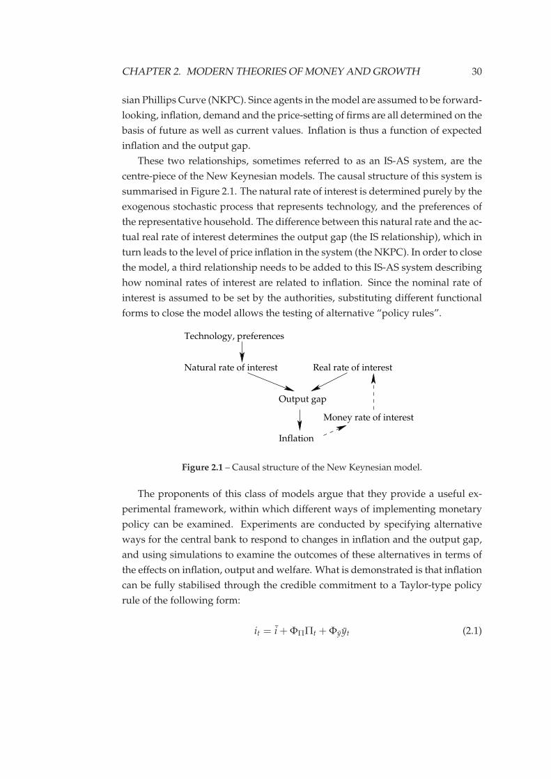
These two relationships, sometimes referred to as an IS-AS system, are the
centre-piece of the New Keynesian models. The causal structure of this system is
summarised in Figure 2.1. The natural rate of interest is determined purely by the
exogenous stochastic process that represents technology, and the preferences of
the representative household. The difference between this natural rate and the ac-
tual real rate of interest determines the output gap (the IS relationship), which in
turn leads to the level of price inflation in the system (the NKPC). In order to close
the model, a third relationship needs to be added to this IS-AS system describing
how nominal rates of interest are related to inflation. Since the nominal rate of
interest is assumed to be set by the authorities, substituting different functional
forms to close the model allows the testing of alternative “policy rules”.
Real rate of interest
Inflation
Money rate of interest
Output gap
Technology, preferences
Natural rate of interest
Figure 2.1 – Causal structure of the New Keynesian model.
The proponents of this class of models argue that they provide a useful ex-
perimental framework, within which different ways of implementing monetary
policy can be examined. Experiments are conducted by specifying alternative
ways for the central bank to respond to changes in inflation and the output gap,
and using simulations to examine the outcomes of these alternatives in terms of
the effects on inflation, output and welfare. What is demonstrated is that inflation
can be fully stabilised through the credible commitment to a Taylor-type policy
rule of the following form:
it = i+ ΦΠΠt + Φyyt (2.1)
CHAPTER 2. MODERN THEORIES OF MONEY AND GROWTH 31
Under a rule of this type (where it is the nominal rate of interest, Π is the rate
of inflation and yt is the output gap, and the parameters ΦΠ and Φy represent
policy variables), inflation will be stabilised at zero as long as i is fixed at the nat-
ural rate of interest. Further, it can be shown that there is an equivalence between
stabilising the rate of inflation, and stabilising the mark-up charged by firms to
the level that would prevail under flexible prices. Since welfare reductions in a
system of this type result from deviations of prices from the flexible-price equi-
librium, there is thus an equivalence between stabilising inflation and welfare
maximisation—even though there exists a short-term trade-off between inflation
and output, the Pareto-optimal solution is to stabilise inflation.3 The New Key-
nesian model thus provides the theoretical justification for the inflation-targeting
frameworks that have become the de-facto standard in central banks around the
world.
It is this system of using the nominal rate of interest for stabilising devia-
tions from the natural rate of output and—thus inflation—that makes the system
“Wicksellian” according to Woodford.
...the present theory of interest determination has a distinctly Wick-
sellian flavour: Variations in the rate of inflation depend on the in-
teractions between the real factors that determine the natural rate of
interest, on the one hand, and the way in which the central bank ad-
justs short-term nominal interest rates, on the other. (Woodford, 2003,
p. 84)
Having outlined the basic theoretical framework, a number of points are now
examined in more detail, and the strengths and weaknesses of this approach con-
sidered.
2.2.2 Monetary policy without money
The theoretical significance of quantitative measures of money, and the money
supply in particular, diminished with the shift in financially developed nations
away from the monetarist doctrines which held that credit should be regulated
through adjustments to the supply of base money. This view held that, via the
3Blanchard & Galı (2005) show that this “divine coincidence” depends on the assumption ofperfect labour markets. The introduction of real wage rigidities into the model removes the equiv-alence between stabilisation of the output gap—the welfare maximising solution—and stabilisationof inflation, implying that policy-makers face a trade-off between these two objectives.
CHAPTER 2. MODERN THEORIES OF MONEY AND GROWTH 32
existence of a set of stable multiplier relationships, alterations to the amount of
high-powered money supplied by the central bank would in turn result in pro-
portionate changes to broader monetary aggregates.
The influence of the monetarist view decreased in the face of both empirical
difficulties, and theoretical developments. The recent new consensus, associated
with the New Keynesian theoretical framework, amounts to a rejection of the
monetarist position, and instead argues that the short-term rate of interest is the
correct operational target for monetary policy. This academic shift was welcomed
by central bankers as recognition that the way they had long considered monetary
policy to be conducted was now being taken seriously.
The view of central bankers that monetary policy implementation is primarily
a task of fixing short-term interest rates is also one of the central claims of the post-
Keynesian school of thought, a long-standing source of opposition to the previous
monetarist doctrines. This approach emphasises the fact that that money is pro-
vided by private institutions—the commercial banking system—and argues that
money is created on demand in order to provide loans to credit-worthy borrow-
ers.
This creation of new money by the banking system is accommodated by the
provision of reserves by the central bank. These public liabilities are required by
the banking system to make up for those deposits lost through conversion to cash
by the public, and to fulfil regulatory requirements imposed by the authorities.
The supply of money is thus an endogenous, demand-led phenomenon with new
money passively created by the banking system as the counterpart liability to the
addition of new loans to the asset side of banks’ balance sheets.
The degree to which the provision of new loans and deposits is limitless at
a given rate of interest is a source of debate within the post-Keynesian school,
with “horizontalists” arguing that the money supply is perfectly elastic, while the
“structuralist” strand argue in favour of a slightly upward sloping money supply
function (Moore, 1988; Dow, 2006). The horizontalist position is summarised as
follows:
[T]he base interest rate is not a market phenomenon: it is a bureau-
cratically determined price, which may be more or less influenced by
the political class and the financial lobby... While the central bank
only indirectly influences the monetary aggregates, it can fix the base
interest rate with absolute precision... As a result the money supply
CHAPTER 2. MODERN THEORIES OF MONEY AND GROWTH 33
curve, in symmetry to the supply-offer curve for the goods supplied
by megacorps, is best seen as a horizontal curve (Lavoie, 1996, p. 278,
emphasis in original).
The new consensus appears to mark a significant shift in modelling of the
monetary system towards a recognition of the post-Keynesian position that the
quantity of money is not a variable over which the central bank operates any
direct control. However, this apparent similarity obscures significant differences
between the two theoretical systems, in particular with the respect to the role of
money within the economic system.
In the post-Keynesian view, as well as that of earlier neoclassical economists
such as Wicksell, the demand for money is driven primarily by the liquidity needs
of firms, for the purposes of investment.4 By creating new loans, banks can create
additional purchasing power, allowing investment to take place without a prior
decision to save by households. The additional income generated through in-
vestment expenditure accumulates as the deposits of either households or firms.
These deposits may then be used to finance further expenditures, exchanged for
other, less liquid securities, or held as liquid balances.
In this view, money operates as a means of transaction and potential store of
value as well as the numeraire. Whether inflation results from additional credit-
financed expenditures depends primarily on the level of employment: as long as
unemployed labour and excess capacity exist, additional expenditures will tend
to increase output and employment, rather than affecting the price level.
The question of what determines the demand for money in the “pure credit”
system assumed in the New Keynesian models has been the subject of some de-
bate.5 The concept of the pure credit economy originates with Wicksell’s system,
in which credit money is created by an integrated banking system and supplied
to firms for the purpose of financing working capital and wage payments. Once
production is complete, sales of goods by firms generate revenues which allow
the repayment of loans, thus destroying the previously created credit money and
returning the system to its starting state. Inflation arises in such a system when
the banking system supplies credit to firms at a rate below the natural rate of in-
terest. By holding the money rate of interest below the natural rate, the central
4Keynes used the term “neoclassical” in the General Theory to identify those theorists who, unlike“classical” economists, accepted the possibility of inequality between planned saving and invest-ment. (Toporowski, 2008b).
5See, for example, Costa & DeGrauwe (2001); Boianovsky & Trautwein (2006)
CHAPTER 2. MODERN THEORIES OF MONEY AND GROWTH 34
bank can set in motion a cumulative disequilibrium process such that prices rise
at an increasing rate while greater volumes of money circulate for production and
goods sales.
The “neo-Wicksellian” framework described by Woodford in his own Interest
and Prices refers to a base-line system in which cash and central bank reserves—
monetary “frictions”—are assumed to be insignificant enough to be ignored. At
the same time, it is assumed that the authorities are able to fix the nominal return
on some riskless asset which, in turn, determines the nominal returns on all other
financial assets in the system. Thus, in the absence of cash the government issues
an asset which provides no services to the holder, but provides the holder with
a nominal return (set by the central bank) denominated in terms of itself. It is
argued that in such a system, changes can be made to the rate of interest paid on
this asset—without affecting the quantity of the asset held by agents—which will
in turn alter the rates of return of every other asset within the system.
The way that the monetary transmission mechanism is presented varies across
the models, but the baseline case assumes perfect financial markets, allowing the
representative household to exactly satisfy its optimisation problem over con-
sumption and saving, both in the current period and over the expected future
time horizon:
In the baseline model, both capital and insurance markets are per-
fect. Within this frictionless setting, the household satisfies exactly
its optimizing condition for consumption/saving decisions. It thus
adjusts its expected consumption growth positively to movements in
the expected real interest rate. Similarly, with perfect capital markets,
the representative firm satisfies exactly its optimizing condition for
investment: it varies investment proportionately with Tobin’s q, the
ratio of the shadow value of installed capital to the replacement value
(Galı & Gertler, 2007, p. 30)
The transmission mechanism in Woodford’s model is designed such that house-
holds are presented with “complete financial markets” as well as the option of
holding a purely riskless asset in addition to the monetary liability of the gov-
ernment, giving them a choice between holding riskless “bonds” and “money”.
These assets are both issued by the government, such that the government’s fiscal
position is thus represented by the total quantity of these riskless assets held by
the private sector.
CHAPTER 2. MODERN THEORIES OF MONEY AND GROWTH 35
Since the rate of return on bonds and money must be equal due to arbitrage
opportunities (households are assumed able to borrow as well as lend at the risk-
less rate), the composition of demand between the two assets is indeterminate.
However, Woodford assumes that households will at all times hold a non-zero
quantity of money, in preference to bonds. The central bank is thus able to dis-
place, in arbitrary quantities and with its own liabilities, alternative assets with
identical risk and return characteristics.
Without a transactional demand for money balances, the rationale for hold-
ing money is undefined, leaving the demand for money, other than being posi-
tive by assumption, indeterminate: “...there will not actually be determinate de-
mands for individual assets (the assumption in the case of the monetary base).”
(Woodford, 2003, p. 65) Once the assumption has been made that households will
choose to hold some level of money balances, arbitrage relations ensure that the
bond rate of interest will remain pegged to the money rate. The distinction be-
tween money and bonds then becomes largely irrelevant, and Woodford is able
to proceed as if the central bank controls the “market” rate of interest directly.
In a modern monetary economic system there exist two types of money: that
which is issued by the central bank—cash and reserves or clearing balances—and
that which is issued by the commercial banking system—bank deposits of various
maturities. This distinction gives rise to the well-known Gurley and Shaw (1960)
definition of financial development: an increase in the ratio of “inside money” to
“outside money” (Toporowski, 2007). Each of these two types of liability will be
backed by certain assets on the balance sheet of the issuing bank. In general, the
liabilities issued by the central bank are backed by holdings of government debt,
which in turn represent past government expenditures. In a financially devel-
oped system, however, these represent only a small proportion of total monetary
liabilities. The majority of the monetary assets held by households are repre-
sented by the liabilities of commercial banks, which are backed, on the asset side
of banks’ balance sheets, by loans to firms. These loans are generally issued for
the purpose of investment in working capital and to cover wages in advance of
sales. The willingness of households to hold deposits—the liabilities of commer-
cial banks—is thus related to the fact that they have confidence that those deposits
will be accepted at some point in the future as payment for goods, and thus that
the loan-making decisions made by banks are sound.
The pure credit economy of the new consensus models then may be seen as a
system which has reached the limiting case in which the ratio of inside to outside
CHAPTER 2. MODERN THEORIES OF MONEY AND GROWTH 36
money becomes infinite. The theoretical difficulties that occur when dealing with
such a system have been the subject of considerable debate, going back to Fisher
Black’s (1970) argument that a system of purely private-sector financial interme-
diation would be unaffected by the actions of a central bank, leaving the price
level purely determined by the self-fulfilling expectations of the private sector.
Woodford uses a combination of two arguments to confront this issue.
Firstly he argues that the pure credit economy is the limiting case of a system
in which a small quantity of central bank balances are demanded for clearing
purposes and can thus be used to illustrate the frictionless case, in the same way
that a physicist does “when analysing the motion of a pendulum or the trajectory
of a cannonball.” (2003). This is a problematic analogy however, because the
“non-frictionless” case to which he is comparing his system is one in which the
demand for clearing balances arises from the needs of commercial banks, which
in turn issue their own money in response to demand for investment funds by
firms. This is the system described by Wicksell: an economy in which money is
created by private institutions in order to provide credit for the working capital
requirements of firms, with this money being destroyed upon completion of the
productive circuit.
The second element of Woodford’s justification for the existence of money
demand in his model is an appeal to the fact that the asset issued by the central
bank is the numeraire: a pure unit of account. This implies that even in the absence
of any holdings of this asset, the fact that a given nominal return is available
on it will result in this rate of return remaining effective on all riskless assets.
The problem with this line of reasoning is that there is nothing in Woodford’s
system that ensures that central bank liabilities are indeed used as the unit of
account. Without a defined demand for money function, there is no reason that
an alternative riskless asset shouldn’t take the place of the numeraire in the system.6
Much of the debate around these issues with respect to the new consensus
6The framework can be extended to include an explicit demand for money by including realbalances in the household utility function to represent the services that holding money provides tohouseholds in the form of facilitating transactions. The result of the “LM” relationship that arisesfrom this modification is that the requirement for equality between the rate of interest on moneyand other riskless asset no longer holds: households will be willing to hold money at a lower rate ofreturn than on equivalent assets, due to the utility yielded. In this case, the rate of interest on non-monetary riskless assets becomes the “money market” rate targeted by the central bank, whichcan then be achieved through adjustment either of the quantity of money supplied, or throughadjustments to the rate of interest on money.
CHAPTER 2. MODERN THEORIES OF MONEY AND GROWTH 37
models focuses on two questions: firstly, will the central bank retain control of
nominal interest rates in the limiting case of zero holdings of cash or zero reserve
requirements? Secondly, does the neglect of the quantity of money in the mod-
els matter? (Eg. McCallum, 2001). These questions—and the related technical
debates such as whether or not to include real balances in the utility function—
miss the more fundamental point that the role of bank money is to generate ad-
ditional purchasing power where previously it did not exist. Rather than the
riskless baseline instrument in a world in which all credit relationships occur di-
rectly in perfect financial markets, money bestows upon its holder the ability to
spend, regardless of whether a decision to “not-spend” of an equal amount has
occurred elsewhere.
Related to this is the point that credit and monetary relationships are persis-
tent. Rather than being able to continuously re-specify contracts in perfect credit
markets in response to unexpected shocks, borrowing and lending result in the
accumulation of assets and liabilities on the balance sheets of agents. These assets
and liabilities set up the requirement for future inward and outward cash-flows—
to be paid in money. The persistence of these balance sheet structures is of a much
deeper order than can be captured through the incorporation of “menu costs” for
instance.
The “cashless economy” then, rather than an updated and refined version
of Wicksell’s pure credit system in which all obligations are settled using bank
money, represents a non-monetary system—a Walrasian barter economy in which
agents that do not face uncertainty interact directly via perfect credit markets. In
simply assuming that the nominal terms of the entire structure of financial con-
tracts can be exogenously determined, these models provide little more than a
way to examine the reaction of an optimising household when these terms are
displaced from their equilibrium state.
2.2.3 Capital markets and the accumulation of capital
Not all of the assumptions described above are maintained across the full spec-
trum of New Keynesian monetary models—the discovery that rational expecta-
tions didn’t imply the end of the road for the short-term effectiveness of monetary
policy has led to a continual stream of updated and modified versions of these
models. All follow essentially the same methodological approach as the canoni-
cal models in starting from a baseline RBC system, and introducing frictions into
CHAPTER 2. MODERN THEORIES OF MONEY AND GROWTH 38
one or more of the otherwise perfect markets of the model, in addition to the slow
adjustment of prices.
For example, the assumption of a representative household implies that the
baseline model cannot generate unemployment, but only marginal adjustments
to the leisure-labour trade-off of this household. This is addressed by disaggre-
gating the representative households into a continuum of members, and making
hiring costly. As a result, deviations from equilibrium result in variations in em-
ployment. Whether these costs derive from trade-union power or some other
“friction”, out of the control of households, the implication is the same: labour
market “flexibility” will lead to full employment at the natural rate of output—a
concept no different in essence to Friedman’s natural rate of unemployment.
A notable contribution of this type was the introduction of imperfections into
the capital markets, resulting in the “financial accelerator” model of Bernanke
et al. (1999). The results of this model arise from the simple observation that
in the presence of imperfect credit markets, the cost of external funds and the
opportunity cost of financing investment from internal funds will diverge. This
divergence between internal and external funds is referred to as the “external fi-
nance premium”—essentially an additional risk premium which reflects factors
including “the lender’s expected costs of evaluation; monitoring and collection;
the ‘lemons’ premium that results from the fact that borrower inevitably has bet-
ter information about its prospects than does the lender; and from the costs of dis-
tortions in the borrower’s behaviour that stem from moral hazard...” (Bernanke
& Gertler, 1995, p. 35)
This external finance premium will depend in turn upon the “borrower net
worth”—the greater the value of the borrower’s balance sheet, the lower is the
premium required for external financing. This concept bears a strong similarity
to both Kalecki’s (1937) principle of increasing risk and to Minksy’s ([1975] 2008)
“borrower’s” and “lender’s risk”—this is not noted by Bernanke et al., although
Fisher’s debt-deflation theory is acknowledged.
In all three systems, the marginal cost of borrowing for investment purposes
begins to rise beyond a point determined by the “own capital” of the borrower,
defined somewhat differently in each case.
However, the purpose of Kalecki and Minsky’s concepts was to place a limit
on the level of investment undertaken by firms—since both rejected the standard
view of a falling marginal return to capital, some other influence is required in
order to determine the demand for new capital assets:
CHAPTER 2. MODERN THEORIES OF MONEY AND GROWTH 39
[I]n an abstract hypothetical world in which the supply of finance is
infinitely elastic, in which all prices and yields are independent of the
firm’s own scale of operation, and into which the realities of risk and
uncertainty never intrude... a firm would want to buy an unlimited—
nay—infinite amount of capital assets (Minsky, [1975] 2008, p. 107).
For Minsky, the standard New Keynesian assumption of perfect capital mar-
kets would thus lead to a limitless demand for capital assets.
The assumption of imperfect capital markets is less fundamental in the case of
Bernanke et al.: since the demand for capital is determined by the intersection of
the schedules of the expected marginal return and the “cost of funds”, demand for
investment goods remains determinate even in the case of perfect capital markets.
In equilibrium, the “cost of funds” will equal the rate of interest, which in turn is
defined by the inter-temporal preferences of the representative consumer. Thus,
investment is determined by the saving behaviour of the household.
Once capital market imperfections are introduced, the cost of funds diverges
from the rate of interest by an increasing margin beyond the point at which in-
vestment is internally financed. As a result, the demand for investment is below
the optimal perfect-market equilibrium point.
The key result of such models relates to the fact that the net worth of borrow-
ers does not remain constant with disequilibrium changes in output, but tends to
vary in a pro-cyclical way. This is justified by arguing that the strength of borrow-
ers’ balance sheets will be affected by changes in the rate of interest in a number
of ways: variable rate borrowing and changes in asset prices will affect balance
sheets directly, while falling revenues and sticky costs will affect balance sheets
indirectly. (Bernanke & Gertler, 1995)
While the dynamics of net worth due to asset price inflation and deflation
take a central role in balance-sheet approaches to the firm—as exemplified by
Minsky’s (1982) financial-fragility hypothesis—these ideas are harder to convinc-
ingly incorporate into general equilibrium systems in which “cash-flow” has no
meaning at the point of equilibrium, and even in the case of disequilibrium due to
rigidities represents only a position in which one or more optimising conditions
have not been met.
In the case of Bernanke et al., “entrepreneurial capital” is proxied by the sum
of saving in previous periods by firms, which are assumed able to accumulate
capital as well as borrowing indirectly from households. Since the price of this
CHAPTER 2. MODERN THEORIES OF MONEY AND GROWTH 40
capital is determined by the expected marginal return, changes in output in the
presence of sticky prices will affect the relative price of capital and thus the net
worth of firms. This in turn will affect the terms on which firms can borrow from
households to obtain further capital. This rather circular chain of logic demon-
strates the difficulties of incorporating lending and borrowing into a general equi-
librium system of representative agents.
In the face of a shock which reduces output below the equilibrium level, the
net worth of balance sheets falls and their access to capital decreases accordingly
as the external finance premium rises. This reduces the demand for investment,
leading to a further contraction of aggregate demand and output.
The introduction of capital market imperfections into the New Keynesian sys-
tem thus results in an amplification of the disturbances that occur when the sys-
tem is displaced from equilibrium. The authors claim that this allows the models
to more closely track the empirically observed dynamics of output and inflation
which result from changes to the nominal interest rate, or “monetary policy inno-
vations” as they are known in the literature.
While the shifts in borrower net worth that occur in these systems are de-
scribed as “pro-cyclical” (since net worth increases with output), there is in fact
nothing cyclical about the behaviour of these models—regardless of whether cap-
ital markets are perfect or imperfect. In both Minsky and Kalecki’s analysis, the
relationship between balance sheet strength and access to capital plays a funda-
mental role in the endogenous generation of business cycles:
The upper turning point is completely endogenous once it is accepted
that interest rates rise in an investment boom and that the successful
functioning of the economy induces profit-seeking bankers and their
customers to engage in speculative financial arrangements to econo-
mize on holdings of money and protected assets” (Minsky, 1982, p.
33)
In contrast, the New Keynesian models provide an analysis of the path back
to equilibrium in the aftermath of an exogenous shock in the form of a “mone-
tary policy innovation”, or change in technology or preferences. In the absence
of price stickiness and other imperfections, these RBC models would remain con-
tinuously in a state of full-employment equilibrium: even when hit by external
shocks, relative prices will immediately adjust to the new Pareto-efficient equilib-
rium. Changes to the nominal rate of interest will have no effect on any variable
CHAPTER 2. MODERN THEORIES OF MONEY AND GROWTH 41
other than the price level. In the absence of control over nominal interest rates,
the price level will be undefined.
The addition of Calvo-pricing to these models disables the instant-adjustment
mechanism. When hit by a shock, not all prices in the system will adapt imme-
diately, resulting in disequilibrium levels of output and consumption. Without
further shocks to the system however, these deviations from the long-run steady
state will be transitory. The system will always return to the flexible-price nat-
ural rate of output. Underlying these models is thus a view that there exists an
automatic stabilisation mechanism such that economic systems are continually
attracted to their long-run steady state, like a pendulum displaced from its rest-
ing point or a spring under tension.
The distinction between the long-run and the short-run is thus clearly defined
in the New Consensus models: the short-run is any point when the output-gap is
non-zero. The long-run equilibrium position in such models is determined purely
by the exogenous parameters of the system: the path taken back to equilibrium,
and the length of time until it is reached will depend on the nature and magnitude
of the shock, but the destination point will be fully determined.
To this point, the discussion has considered the relationship between capital
markets and investment. What has not been discussed is the role of investment
and capital accumulation in the context of these models. In this respect, the key
point is that these models are constructed in such a way that, despite borrowing
for the purposes of investment leading to changes in the stock of capital, no pro-
cess of long-run growth takes place in these models—the steady state equilibrium
is one of constant output.
The role performed by capital in these models is, like labour, to provide an
input to a production function in order to generate output. Since both labour
and capital exhibit diminishing marginal returns, there will exist some optimal
quantity of capital input, given the equilibrium level of output determined by the
intertemporal optimisation of the household. In the case of capital market im-
perfections, the model is set up somewhat artificially such that firms are able to
accumulate capital but less than the optimal input quantity in each period, requir-
ing that they borrow in order to rent the remainder from households. In order to
prevent firms accumulating enough capital that they become self-financing, firms
regularly “die” according to a given probability function, at which point accumu-
lated capital is “consumed” and disappears.7
7“The assumption of finite horizons for entrepreneurs is... to preclude the possibility that the en-
CHAPTER 2. MODERN THEORIES OF MONEY AND GROWTH 42
In the more straightforward case of perfect capital markets, although char-
acterised in various ways in the literature, the investment decision always es-
sentially decomposes to a forward-looking optimisation based on a trade-off be-
tween the intertemporal consumption preferences of the representative consumer
and the expected marginal return on capital as determined by the technical fea-
tures of the production function.
Given some exogenous rate of depreciation, along with preferences and tech-
nology, in the steady state there will therefore be a constant ratio of consumption
to investment and a constant level of output. Investment thus does not result
in the accumulation of capital, other than in the sense that out of equilibrium,
capital greater than that needed to cover depreciation might be produced, as a
result of sticky prices. The natural rate of interest then, rather than a share of the
profits generated in a expanding economy, essentially reduces to the “reward for
waiting” that would occur in the case of a pure barter system. This was noted by
Wicksell in the context of his pure credit economy:
There is a certain rate of interest on loans which is neutral in respect
to commodity prices, and tends neither to raise nor to lower them.
This is necessarily the same as the rate of interest which would be
determined by supply and demand if no use were made of money and
all lending were effected in the form of real capital goods. It comes to
much the same thing to describe it as the current value of the natural
rate of interest (Wicksell, 1936, p. 102).8
The significance of this point is that, in the case of a monetary economy, banks
are able to offer credit at a rate above or below the level that would be obtained
in the case of a pure exchange economy, leading to variations in the general price
level. Thus if banks advance credit at a rate below the natural rate, prices will
rise at a pace that brings the real rate of interest on money back into equality with
trepreneurial sector will ultimately accumulate enough wealth to be fully self-financing” (Bernankeet al., 1999, p. 1347)
8This bears a close resemblance to Keynes’ concept of the “own-rate of interest” (1936, p. 223), aconcept first elucidated by Piero Sraffa (1932) in his review of Hayek’s Prices and Production, (1935),the contents of which, he observes, “fully uphold the tradition which modern writers on money arerapidly establishing, that of unintelligibility” (1932, p. 42). He criticises Hayek for his acceptance ofWicksell’s identification of the natural rate with the equilibrium rate: “If money did not exist, andloans were made in terms of all sorts of commodities, there would be a single rate which satisfiesthe conditions of equilibrium, but there might be at any one moment as many ‘natural’ rates ofinterest as there are commodities, though they would not be ‘equilibrium’ rates.” (Sraffa, 1932, p.49)
CHAPTER 2. MODERN THEORIES OF MONEY AND GROWTH 43
the natural rate. For Wicksell, it is this power of the banks to create purchasing
power without limit at a fixed rate of interest that generates control over the price
level—in contrast to Woodford’s assumption of control due to agents choosing to
hold a marginal quantity of clearing balances.9
From our assumption that every withdrawal of a deposit must directly
entail the deposit of an equal sum elsewhere or the repayment of an
equal loan, it follows that the banks, or rather the aggregate of the
banks taken as a whole, can... lend any desired amount of money for
any desired period of time at any desired rate of interest, no matter
how low, without affecting their solvency, even though their deposits
may be falling due all to the time. (Wicksell, 1936, p. 111)
In his description of the pure credit system, Wicksell makes a number of sim-
plifying assumptions for the purposes of the exposition of the model. In doing
this, in the view of Hayek (1933), he makes one crucial mistake: he assumes that
the economy is in a stationary state. Hayek argues that once this assumption is
abandoned and instead an expanding economy is considered, that relative price
distortions—in particular the relative prices of capital and consumption goods—
must occur. Thus, if the rate of interest is viewed as the relative price of capital
and consumption goods, there can be no rate of interest that leads to an increas-
ing stock of capital goods while simultaneously keeping the general price level
constant:
“On the one hand we are told that the price level remains unaltered when
the money rate of interest is the same as the natural rate; and, on the other
that the production of capital goods is, at the same time, kept within the
limits imposed by the supply of real savings. One need say no more in
order to show that there are cases—certainly all cases of an expanding
economy, which are the most relevant to trade cycle theory—in which
the rate of interest that equilibrates the supply of real savings and the
9It is this ability of banks to extend credit without limit that leads Wicksell to his famous analogybetween the general level of prices and a cylinder resting on a plane: the point being that there isno predetermined “equilibrium” level at which the general price level should be set. With theapplication of force to the cylinder (a reduction of the money rate of interest below the naturalrate) it can be set in motion, and will continue to move while the force remains present. This iscontrasted with relative prices which are akin to a pendulum that always returns to its equilibriumpoint, since any displacement will result in forces that push the pendulum back to its position ofrest.
CHAPTER 2. MODERN THEORIES OF MONEY AND GROWTH 44
demand for capital cannot be the rate of interest that also prevents
changes in the price level. (Hayek, 1933, p. 113, emphasis in original)
Similarly to Wicksell, Hayek assumes that credit expands so that initial pay-
ments, made by entrepreneurs in receipt of additional liquid loan capital, are
made by cheque to other entrepreneurs for capital goods. Even without the as-
sumption of a pure credit system, in such a situation the overall level of deposits
in the banking system as a whole will not diminish, allowing for the further exten-
sion of credit elsewhere without the reduction of liquid reserves. Hayek argues
that only an increase in the rate of interest at which the central bank advances
funds to the banking system will be able to bring this process of credit expansion
to a to a halt.
In an expanding economy, Hayek argues, falling prices can only be avoided
by increasing the money supply. However, this expansion of the money supply
will lead to a discrepancy between “the amount of real savings and the volume of
investment” (p. 113), which can only be corrected by a rise in the rate of interest.
While Hayek’s analysis is faulty, particularly with respect to an economy in
which excess capacity exists, the debate touches on a number of points of rele-
vance. Firstly, the potential for the expansion of purchasing power by the bank-
ing system to allow for planned saving and investment to diverge. In particular,
Hayek is correct that by creating new credit money, the banking system has the
power to grant firms the liquidity required for investment to take place without a
corresponding decision to save. For Hayek this leads to misallocation of capital,
since the diminishing marginal productivity of capital requires that the rate of
interest rise as capital is accumulated: with the rate of interest on money set too
low, investment is undertaken in projects that do no generate a return sufficient
to “induce” an equivalent desired increase in saving.
However, if the assumption of a diminishing marginal return to investment is
discarded—as Kalecki argues it should be—then the problem is cast in a different
light: what limits investment is not the intersection of the schedules of willingness
to “not consume” and discounted expected profits, but access to finance.
This leads to another, more fundamental point: in both the neo-Wicksellian
system of the New Keynesian model and the original system of Wicksell, the anal-
ysis is rooted in the steady state. The question of how to theorise accumulation
in the case of a growing economy is not addressed.
In order to consider the current state of theoretical understanding on growth
CHAPTER 2. MODERN THEORIES OF MONEY AND GROWTH 45
and capital accumulation, it is necessary to first take a few steps back. In his
discussion of Woodford’s model, Laidler (2006) notes that “largely un-discussed
problems with capital theory still plague much modern macroeconomics”. He is
referring to what are known as the Cambridge capital controversies (Harcourt,
1972): the result that when aggregating over production functions with given
characteristics, the aggregate function may not inherit these characteristics.10 Re-
lated to this are the problems of representing capital with single index numbers,
since quantity and price effects become indistinguishable. This problem was
noted by Lindahl, who anticipates the later work of Sraffa in noting that “mod-
ern” (ie. marginal productivity of capital) theories of capital “have the disadvan-
tage that the measure of capital is made dependent on the prices of the services
invested and on the rate of interest—which belong to the unknown factors of the
problem” (Lindahl, 1970, p. 317).
These points are now briefly considered in more detail, before moving on to
a discussion of the implications for both modern growth theory, and the New
Keynesian monetary models.
2.3 Growth theory
2.3.1 The aggregate production function
The conception of capital as a homogeneous divisible input to a production pro-
cess represented by a mathematical function has long been a source of contro-
versy. At the heart of this controversy lies the relationship between production,
accumulation and the determination the distribution of income, and in particular
the distribution of income between wages and profits.
Harcourt & Cohen (2003) present the key tenets of the neo-classical approach
in the form of three “parables” (in reference to Samuelson (1962) who referred
to the conclusions that arise from the aggregate production function as the “J. B.
Clark parables”). These are:
(1) the real return on capital (the rate of interest) is determined by the
technical properties of the diminishing marginal productivity of cap-
ital; 2) a greater quantity of capital leads to a lower marginal product
10The same result in the case of the utility function is known as the Sonnenschein-Debreu-Manteltheorem (Colander et al., 2008)
CHAPTER 2. MODERN THEORIES OF MONEY AND GROWTH 46
of additional capital... 3) the distribution of income between labour-
ers and capitalists is determined by relative factor scarcities/supplies”
(Harcourt & Cohen, 2003, p. 201)
The theory of distribution that is described by these “parables” traces a one-
directional line of causation that leads—with given preferences and some exoge-
nous level of technological know-how—from the relative scarcity of factors of
production to the distribution of income, such that the owner of each factor of
production receives income equal to the additional output generated by that fac-
tor of production.
An early acknowledgement of this problem came from Marshall:
The doctrine that the earnings of a worker tend to be equal to the net
product of his work, has by itself no real meaning ; since in order to
estimate the net product, we have to take for granted all the expenses
of production of the commodity on which he works, other than his
own wages. (1920, Book VI, ch. I)
Similarly, he argues, the doctrine that the marginal productivity of capital will
tend to equal the rate of interest “cannot be made into a theory of interest, any
more than a theory of wages, without reasoning in a circle.” (1920, Book VI, ch. I)
Here Marshall touches upon the points that were to take centre stage half
century later in the exchanges between Cambridge, England on one side, and
Cambridge, Massachusetts on the other. These debate centred on the validity of
the neo-classical representation of “capital” as an input to a production function,
essentially indistinguishable from either labour or land, and in particular to the
implications of using such a production function to represent an economy at the
aggregate level.
The use of a continuous, aggregate function, tracing out a smooth relationship
between the factor ratio and relative factor incomes implied that “capital” was
infinitely divisible, malleable, and substitutable. No limit existed to the level of
granularity at which changes of technique could be enacted, with substitution of
capital for labour represented as a completely frictionless process, and a process
that instantaneously affects not only newly produced capital goods, but also all
capital goods currently in operation.
The debates on the production function began when Robinson (1953–1955)
resurrected Wicksell’s point that heterogeneous capital cannot be measured in a
“technical unit”. As Wicksell put it:
CHAPTER 2. MODERN THEORIES OF MONEY AND GROWTH 47
Whereas labour and land are measured each in terms of its own tech-
nical unit (e.g. working days or months, acre per annum) capital... is
reckoned... as a sum of exchange value—whether in money or as an
average of products. In other words, each particular capital-good is
measured by a unit extraneous to itself. However good the practical
reasons for this may be, it is a theoretical anomaly which disturbs the
correspondence which would otherwise exist between all the factors
of production. (1977 [1934], p. 149, emphasis in original)
In her 1953 essay, “The Production Function and the Theory of Capital”, Joan
Robinson wrote that “the production function has been a powerful tool of mised-
ucation.” (1953–1955, p. 81). Robinson observes that a student being instructed in
marginalist production theory is first taught that labour is to be measured in man-
hours, and then “hurried on to the next question, in the hope that he will forget
to ask in what units [capital] is measured. Before he ever does ask, he has become
a professor, so sloppy habits of thought are passed on from one generation to the
next.”
Robinson’s point is that any units that may be chosen for the measurement
of capital demonstrate serious conceptual problems upon careful examination.
Measurement in some physical per-period unit is impossible, at least as soon
as more than one type of capital good is included in the analysis: “whilst land
can be measured in acres-per-year and labour in man-hours, capital... cannot be
measured in terms of physical units” (Kaldor, 1955, p. 90). The alternative is to
value capital goods in terms of their rate of exchange with other goods—either as
an accumulation of consumption forgone in the past, the result of a “reward for
waiting”, or through discounting the stream of expected future yields that accrue
to the owners of capital assets.
However, in order to value capital as a “reward for waiting”, either in terms
of goods forgone or against the quantity of labour expended to produce those
goods, it is first required that the real wage is known. But, in marginalist theory,
the real wage itself depends on the relative factor ratio, which is the unknown of
the problem.
Likewise, if an attempt is made to value capital by discounting the future
yields obtained through ownership of it, it is necessary to first know the rate
of interest at which to discount those yields. But, again, according to the neo-
classical theory of distribution, the rate of interest is determined by the marginal
CHAPTER 2. MODERN THEORIES OF MONEY AND GROWTH 48
productivity of capital and thus depends on the quantity of capital that enters
into the production function.
Joan Robinson’s initial contribution (1953–1955) proposes a method to mea-
sure “real capital” in terms of labour time. In equilibrium, Robinson argued,
since resources remain tied up over the period of production of new goods, the
profit obtained on new capital equipment must include a ‘premium’ to cover the
interest forgone while resources are employed in its construction, or equivalently,
the supply price of new equipment will include profit at the going rate. Equilib-
rium can therefore only exist in a situation in which the quantity of capital valued
in terms of units of output is constant, and the rate of profit currently prevailing
is that which has been in effect over the entire period in which the current capital
stock has existed, which in turn must been that rate which was expected over the
period of production of those capital goods.
Robinson suggests a method by which the set of all such possible equilibria
can be aggregated into a production function: at any given rate of interest, the cost
of production of the capital goods required for every different known technique
of production is calculated. This cost includes the price of labour time expended
over the course of production, compounded at the given rate of interest. Then,
rank the set of known techniques according to the rate of output produced with
a fixed quantity of labour. Any techniques which incur a higher cost of capital
but do not generate a greater level of output than another technique are rejected
altogether. By repeating this procedure over all feasible rates of interest, while
assuming a fixed volume of labour input, a hierarchy is obtained such that, the
technique will be chosen which maximises profits at any given exogenous real
wage. At higher real wages, techniques that produce a greater level of output per
man, at a greater cost of capital will be chosen.
Thus a relationship between “real capital” per man (the “real factor ratio” and
per-capita output can be derived, where “real capital” is the cost of capital goods
valued in terms of what Robinson calls the “wage unit”: “the price of an hour’s
labour time in terms of the composite unit of product, no matter whether the
worker who performs an hour’s work is paid in cash or in peanuts.” (p. 86).11
The result of all this is that Robinson is able to obtain a measure of capital
in terms of pure labour time expended, such that a relationship can be traced
11Robinson thus uses a different meaning from that introduced by Keynes in the General Theory,wherein the “wage unit” that was used as the basic unit of analysis was the money wage, ratherthan the real wage in the case of Robinson.
CHAPTER 2. MODERN THEORIES OF MONEY AND GROWTH 49
between capital-valued-as-labour-time, and the rate of (real) output. The shape of
the resulting function has little in common, however, with “the smooth sweep of
the usual text-book production function” (p. 93), since the jumps in the wage rate
that are required to ascend the hierarchy of techniques result in corresponding
backward hops in the value of “real capital”.
This demonstrates the problem with the procedure proposed by Robinson:
the valuation of any given stock of physical capital, and thus the capital-labour
ratio, will not take a fixed value, but will be different at different combinations of
the real wage and rate of interest. Likewise, two different quantities of physical
capital may be valued equivalently at certain wage-profit combinations. Robin-
son refers to the effects of the rate of interest and the real wage on the value of
capital as the “Ricardesque effect” and the “Wicksell effect” respectively.
The “Ricardesque effect” refers to Hayek’s (1942) paper on the “Ricardo Ef-
fect”, in which Hayek argues that firms will always shift to techniques of a lower
capital intensity in the event of a fall in the real wage. Any attempt to both in-
crease the degree of mechanisation whilst simultaneously increasing the labour-
intensity of production, Hayek argues, will lead only to rises in the price of con-
sumer goods: “The question is rather similar to whether by pouring a liquid fast
enough into one side of a vessel we can raise the level at that side above that of
the rest to any extent to which we desire” (1942, p. 142).12
In opposition to the “Ricardo effect” stands the “Wicksell effect”. Wicksell was
concerned that the additional output that resulted from a greater capital intensity
of production would be partially absorbed by wages (and rent), and thus would
not accrue in its entirety as profits. Thus what Wicksell referred to as “Thunens
law”—the marginal productivity theory of distribution—could not be applied di-
rectly to “capital” at the aggregate level: only for labour and land would the
principle hold. (Uhr, 1951)
The meaning of the term “Wicksell effect” has subsequently altered slightly
from the sense in which Robinson initially used it, and relates to a phenomenon
mentioned by Robinson in her paper, but which was to subsequently take on a
greater significance in the capital debates—that of “reswitching”. Robinson noted
that when constructing the hierarchy of techniques of production, as the notional
rate of interest varies, techniques may be rejected on the basis of cost at one rate
12Hayek does however recognises the requirement of assuming full employment for such a Ri-cardian conclusion to hold: “So long as unused reserves of labour are available at an unchangedprice, unlimited funds mean unlimited control over resource” (1942, p. 144).
CHAPTER 2. MODERN THEORIES OF MONEY AND GROWTH 50
of interest, only to reappear subsequently at another rate of interest. This phe-
nomenon appears because the interaction of the wage rate and the rate of interest
in determining the cost of production is non-monotonic with respect to the wage
rate. This in turn is due to the way in which the distribution of labour costs over
the period of production enters into costs.
Although Joan Robinson noted this as a theoretical possibility, it was with
the publication of Piero Sraffa’s (1960) Production of Commodities by Means of Com-
modities that the implications of this anomaly for neo-classical theory began to be
debated more intensely.
Sraffa’s work was an attempt to resurrect Ricardian value theory by construct-
ing a system in which all commodities could be reduced to a dated sequence of
labour inputs. As in Robinson’s system, labour inputs are compounded at the
current rate of profit (interest), such that the effect of a change in the distribution
of income on the relative price (value) of a good depends on the way that the
labour embodied in that commodity is distributed over the period of production:
As the rate of profits rises, the value of each of the labour terms is
pulled in opposite directions by the rate of profits and by the wage,
and it moves up or down as the one or the other prevails... With
the rise in the rate of profits, terms divide into two groups: those
that correspond to labour done in the more recent past that begin at
once to fall in value... and those representing labour more remote in
time, which at first rise, ... and then begin the downward movement.
(Sraffa, 1960, pp. 35–36)
The result of the indeterminacy of the ‘value’ of the capital goods required by
a given technique of production is that that one technique of production might be
used at both a high and low rate of interest, but over an intermediate range be-
tween these two points, some other technique would be selected. This “reswitch-
ing” of technique has hugely damaging implications for the neoclassical produc-
tion function and Samuelson’s “parables.” In Samuelson’s own summing up of
the debates , he admits that:
Lower interest rates may bring lower steady-state consumption and
lower capital/output ratios, and the transition to such lower inter-
est rates can involve denial of diminishing returns and entail reverse
capital deepening in which current consumption is augmented rather
CHAPTER 2. MODERN THEORIES OF MONEY AND GROWTH 51
than sacrificed. There often turns out to be no unambiguous way of
characterizing different processes as more ”capital-intensive,” more
”mechanized,” more ”roundabout,” except in the ex post tautologi-
cal sense of being adopted at a lower interest rate and involving a
higher real wage. Such a tautological labeling is shown, in the case
of reswitching, to lead to inconsistent ranking between pairs of un-
changed technologies, depending upon which interest rate happens
to prevail in the market. If all this causes headaches for those nostal-
gic for the old time parables of neoclassical writing, we must remind
ourselves that scholars are not born to live an easy existence. We must
respect, and appraise, the facts of life. (Samuelson, 1966, pp. 582-583)
The smooth inverse relationship between the volume of capital in use and
the marginal product of that capital claimed by neoclassical authors was shown
to be an analytical fiction, at least as soon as one moves beyond the assumption
of a single-commodity economy. The corollaries of the neo-classical production
function—the well-behaved inverse relationships between the rate of interest on
one had and the capital-labour and capital-output ratios on the other—were like-
wise shown to be incapable of standing up to critical inspection.13
2.3.2 Old growth
The most immediate application of the aggregate production function apparatus,
which appeared almost contemporaneously with Joan Robinson’s initial argu-
ments, was in the model of economic growth introduced by Solow (1956) and
Swan (1956), which subsequently came to be known simply as the “neo-classical
growth model”. This model was represented by Solow as a version of the Harrod-
Domar model with a modification of the assumptions about the form of the pro-
duction function in use. The Harrod-Domar model itself is often presented as
an early attempt to provide a dynamic analogue to the statics of Keynes’ General
Theory.
In fact, although Harrod’s original formulation of the model is framed around
a discussion of a number of concepts elaborated by Keynes, in particular the dis-
tinction between ex-ante and ex-post investment, it is the Keynes of the Treatise on
Money ([1930] 1971) that Harrod makes direct reference to, not that of the General
13As more recently demonstrated by Mas-Colell (1989), the relationship between the capital-labour ratio and the rate of interest can take on almost any shape.
CHAPTER 2. MODERN THEORIES OF MONEY AND GROWTH 52
Theory. Further, Harrod is quite clear that his model is intended as a conceptual
device for consideration of cyclical behaviour: the question he is attempting to
answer is not “What are the determinants of economic growth?”, but “Why do
growing economies diverge from, or oscillate around, trend growth rates?”
To this end he defines the warranted rate of growth as that rate which would
occur if ex-post investment turned out to be equal to the ex-ante level of investment
implied by the saving propensity and capital-output ratio. The reasons that in-
vestment should diverge from a planned, or “warranted” level in Harrod’s model
are not clearly spelled out, but it seems obvious that he is not explicitly consid-
ering a monetary economy and thus is not referring to “forced saving” of the
Hayekian type: “I have no very clear view as to possible causes likely to operate
in a systematic way to distort ex post from ex ante saving, or of the probable im-
portance of such distortions.” (Harrod, 1939, p. 20). Nonetheless, he is grappling
with the potential for a discrepancy between planned and realised investment to
act as the source of a disequilibrium mechanism that results in the instability of
the growth path:
In his Treatise on Money Mr. Keynes formulated a proposition, which
has been widely felt to be enlightening, though experience has led him
subsequently to condemn the definitions employed as more likely to
be misconstrued than helpful. He said that if investment exceeded
saving, the system would be stimulated to expand, and conversely.
(Harrod, 1939, p. 19)
What has come to be generally taught as the Harrod model is that the rate
of growth of an economy is to be found by dividing the saving propensity of
the community by the capital-output ratio. However, what Harrod intended to
demonstrate with this formulation is the notional growth path of the economy
provided that expansionary or contractionary impulses do not arise from such di-
vergences as described above between actual and “warranted” investment. Once
such a disequilibrium mechanism is set in motion, Harrod argues that it will be-
come self-reinforcing: if investment is greater than the “warranted” rate of in-
vestment, a type of multiplier mechanism will result in an even greater increase
in output, since given the assumptions of a fixed capital-output ratio, the actual
level of investment will appear too low, despite being above the warranted rate,
leading to further increases in investment.
CHAPTER 2. MODERN THEORIES OF MONEY AND GROWTH 53
While Harrod includes no explicit aggregate production function in his model,
the assumption of a constant capital-output ratio leads Solow to conclude that
Harrod is using a fixed-proportions aggregate production function. Solow claims
that the instability discussed by Harrod is the result of this: the problem arises
from the selection of the wrong mathematical form for the production function.
Solow’s solution is to use an aggregate Cobb-Douglas production function,
with diminishing marginal returns to labour and capital. Then, in per-capita
terms, the relationship between of inputs of capital and output of goods assumes
the familiar convex shape. With respect to income distribution however, the prob-
lem of indeterminacy has been reintroduced since the rate of output varies with
the capital-output ratio, and at any given level of output, distribution is “deter-
mined” by the marginal productivities of the factors of production
Once we know the time path of the capital stock and that of the labour
force, we can compute from the production function the correspond-
ing time path of real output. The marginal productivity equation
determines the time path of the real wage rate... there is a similar
marginal productivity equation for capital which determines the real
rental per unit of time for the services of the capital stock (Solow, 1956,
p. 68).
Overlooking the problems of the inter-dependencies, and indeterminacy, of
the variables of the system, Solow finds that the instability of the Harrod model
can be eliminated by allowing the capital-labour ratio to adjust so that the fixed
proportion of output that is saved—and thus in a non-monetary economy of this
type, invested—is just sufficient to keep step with depreciation of the capital stock
and the rate of increase of population growth.
In doing so, however, Solow introduces a critical change of assumption: in-
vestment is no longer the source of accumulation. The level of investment now
only affects the short-term level of output, while in the long-run, the rate of
growth is exogenously determined by the growth of the labour force and rate
of depreciation. As Harcourt observes, the model “uses a Cobb-Douglas produc-
tion function and assumes perfect competition, saving determines investment,
constant returns to scale and full employment so that the wage of labour equals
its marginal product and the rate of profit on capital equals its marginal product”
(1972, p. 373). The only remaining element of what could be considered a Key-
nesian method is the assumption that saving is a constant proportion of output,
CHAPTER 2. MODERN THEORIES OF MONEY AND GROWTH 54
rather than being determined by some inter-temporal elasticity of substitution
parameter.
The Solow growth model gave rise to two important and, if one accepts the
arguments of the Cambridge, England scholars, theoretically flawed concepts:
the “Golden Rule” rate of saving, and “Total Factor Productivity”. The first of
these relates to the idea that, in the aggregate Cobb-Douglas world of the Solow
model, the steady-state rate of growth is exogenously given by the rate of popu-
lation growth. Thus the saving propensity of the community as a whole serves
only to affect the composition of output between consumption goods and cap-
ital goods, and has no effect on the long-run rate of growth. There thus exists
a unique “Golden Rule” rate of saving which maximises the steady-state rate of
per-capita consumption, dependent only on the specification of the production
function.
The second of these concepts, “Total Factor Productivity”, originates with
Solow’s (1957) description of “an elementary way of segregating variations in
output per head due to technical change from those due to changes in the avail-
ability of capital per head” (p. 312). Solow presents an empirical procedure that
he argues allows for the separation of the effects of changes of factor inputs from
changes in factor productivity. This technique has become the standard empirical
method for measuring the contribution of technological change to the growth of
output.
This is achieved by representing the economy under consideration as a one-
sector production function. Then, assuming perfect competition, full employ-
ment, and constant returns to scale, by examining the evolution of wages and
profits, the labour force and the “size” of the capital stock, the rate of technical
change can be empirically estimated as the residual not explained by increases in
the inputs to the production function.
This is done by using the functional distribution of income to calculate the
elasticity of output with respect to each of the factor inputs: assuming that labour
and capital receive their marginal products as compensation, the relative shares
of output will reveal the contribution of each to the production of that output.
Once these elasticities are known, they can be used to calculate the contribution
to output growth over a period of time, by multiplying the elasticity of output by
the growth of the factor input. Any residual growth not explained by changes in
factor inputs is then attributed to “total factor productivity”.
Even overlooking the problems of assuming that the functional distribution
CHAPTER 2. MODERN THEORIES OF MONEY AND GROWTH 55
of income is determined by the relative productivity of labour and capital, the se-
rious problems outlined above with the measurement of the capital stock in com-
bination with the assumption of a one-good aggregate production function lead
to the potential for highly misleading econometric results. Since capital is usu-
ally aggregated at current prices, this makes it impossible to distinguish between
changes in the prices of goods and changes in quantities: any increase in the price
of capital goods relative to consumption goods will translate into a change in the
quantity of capital in the one-good model. In such a case capital would have ap-
peared to have increased without a corresponding increase in output, leading to
the false conclusion of negative technical progress: “In short, changes in quanti-
ties and prices are treated as if they were purely changes in quantities. It is simply
empirical nonsense, as if the changes in the area of a rectangle could be measured
by reference to one side.” (Fine, 2003, p. 55).
Nonetheless, this method of econometric measurement based on the aggre-
gate production function has become the standard approach to analysis at the
aggregate level: “[T]he neoclassical production function is the cornerstone of
the theory and is used in virtually all applied aggregate analyses” (Nobel prize-
winner Edward C. Prescott 1998, p. 532, quoted in Lavoie 2008a)
2.3.3 New growth
Despite the severe theoretical problems associated with the single-sector aggre-
gate production function which were exposed by the controversies—and admit-
ted by those on the defending side such as Samuelson—a new generation of
growth models appeared from around the mid-1980s based on the aggregate pro-
duction function. Three main features can be identified which define these mod-
els and differentiate them from the previous generation of “old” growth models
based on the Solow-Swan approach.
The first key feature of these models is that, rather than treating growth as
exogenous—determined by saving, as in the Harrod-Domar model, or by pop-
ulation growth as in the Solow-Swan model—the rate of growth is determined
endogenously. However, in order for a model based on the neoclassical aggregate
production function to be capable of generating increasing per-capita output, the
assumption of diminishing marginal productivity of the non-labour inputs to the
production function must be dropped: for investment to generate productivity
growth, increasing returns to scale are required. The problem with this, how-
CHAPTER 2. MODERN THEORIES OF MONEY AND GROWTH 56
ever, lies with the fact that the non-linearities introduced with increasing returns
to scale result in serious mathematical problems such as multiple equilibria and
instability around the steady state.
The second key feature is that these models, like the New Keynesian mod-
els discussed earlier in this chapter, contain some kind of market imperfections.
Also in common with the New Keynesian models is the switch from a “static”
equilibrium—in which saving is determined exogenously, as in the Harrod Do-
mar model, or as a fixed share of income, as in the Solow models—to a dynamic
system in which saving is determined as the result of a forward-looking intertem-
poral choice problem. The incorporation of market imperfections results in the
fact that the level of saving chosen by the representative household does not equal
the Pareto-optimal level as determined by the productivity of capital and the in-
tertemporal preferences of the household.
Finally, in order that these models are able to endogenously “produce” pro-
ductivity change—so that growth rates may be determined by technology, prefer-
ences, market imperfections and so on—some additional category of reproducible
input is required, such that the production function is no longer confined to sim-
ply processing labour and capital. Generally this additional input is characterised
as some type of non-physical “capital”, such as human capital.
The contributions of Romer (1986) and Lucas (1988) are usually taken as the
starting point for the first generation of “endogenous” growth theories. In the
Romer model, the level of output is a function of capital, labour, and a new cat-
egory, human capital. Romer assumes that human capital is produced according
to diminishing returns to scale at the firm level, but the production of goods in the
economy overall is subject to increasing returns over all three inputs. However,
since firms are unable to prevent their competitors from sharing in the benefits
of expenditure on human capital formation, an externality exists: firms do not
take into account the social benefit of investment in human capital when decid-
ing upon the level of investment. The three key elements of the model—a new
type of input, increasing returns to scale and market imperfections—combine to
generate a non-Pareto-efficient equilibrium in which investment in human capital
is below the optimal level.
The key difference between the new growth theories and the Solow-Swan ap-
proach lies in the assumptions regarding the production function. The first gen-
eration of “endogenous” models abandon the assumption of diminishing returns
to scale for the inputs that can be accumulated. In order that constant returns
CHAPTER 2. MODERN THEORIES OF MONEY AND GROWTH 57
to scale are maintained at the the aggregate level, those inputs which do not ac-
cumulate (usually labour) must be dropped. Given this assumption of constant
returns to scale in the aggregate function, the ratio between physical capital and
the ‘other’ type of capital must remain fixed. Problems of this type can thus be
reduced to their essential form, y = Ak, such that the growth of output becomes
a linear function of the growth of the capital stock. Models of this type are thus
referred to as ‘AK models’. These models return to the conclusions of the Harrod-
Domar model, reinstating the rate of investment as the factor that sets the level of
growth, albeit via a more mathematically complex route that is able to endogenise
the sources of productivity increases, as a result of market imperfections.
The second generation of new growth models, such as Grossman & Helpman
(1991), Romer (1990) and Aghion & Howitt (1992) treat technological change in a
different way. In these models, technological change (and thus economic growth)
results from the search for innovation by profit-maximising individuals. This in-
novation process is incorporated into the models by again making alterations to
the assumptions regarding the form of the production function. These models
drop the assumption of constant returns to scale at the aggregate level, introduce
non-reproducible inputs back into the production function, allowing constant re-
turns to the reproducible inputs.
Generally, the non-reproducible input (labour), is then divided into two ac-
tivities, one directly productive and the other non-productive, but innovation-
producing. By altering the amount of labour assigned to each activity, the long-
run rate of growth can be affected, endogenising technological progress. Due
to market imperfections, the saving rate—determined by inter-temporal utility
maximisation—is generally found to be below the Pareto-efficient optimum value,
since individuals fail to take into account the existence of growth-inducing exter-
nalities.
The models overcome the problem posed to by increasing return to scale—
no set of prices will result in general equilibrium—either by allowing constant
returns at the firm level but increasing returns at the aggregate level as a result
of externalities (often characterised as technical spillover effects, or learning-by-
doing), or by abandoning the assumption of perfect competition, and allowing
rents to be assigned to activities such as research and development which result
in growth-inducing technological change. Thus, as noted by Fine (2000), these
models are essentially either a market-imperfections theory of growth, or an at-
tempt to model Schumpeter’s view of innovation and ‘creative destruction’ of
CHAPTER 2. MODERN THEORIES OF MONEY AND GROWTH 58
technologies within the neoclassical framework.
In the relatively short space of time since Romer and Lucas published their
contributions to growth theory, there has been an immense volume of work pub-
lished on long term growth theory, partly as a consequence of the increasing avail-
ability of data sets against which to test the models. Papers have been published
which go beyond human and physical capital, and R&D-type models. Gross-
man & Helpman (1991) present a model showing the possible effects of trade on
growth, while Basu & McLeod (1992) present a model in which the long run rate
of growth is altered by terms of trade shocks. Growth theory has thus adopted a
changing sequence of justifications for differences in observed growth rates across
countries and time-period, with each superseded by the next—partly due to fail-
ure to locate convincing empirical support for each supposedly growth-inducing
factor. Kenny & Williams summarise the chronology of growth requirements in
the literature as “physical capital, human capital, policy reform, institutional re-
form” (2001, p. 4), and note that sceptics may observe the increasing difficulty of
providing the requisite environment for growth in each successive generation of
models.
2.4 Conclusion
This chapter has examined the current “state of the art” theoretical literature
on monetary economics and economic growth. In addition, a brief historically-
rooted discussion of the serious internal flaws inherent in macroeconomic theo-
ries based around the aggregate production function is presented.
It is argued that both theoretical systems contain significant deficiencies, over
and above the methodological issues common to both. The new consensus mon-
etary approach is based on an essentially non-monetary theoretical framework—
that of Walrasian general equilibrium. The introduction of market imperfections
does not alter this, but leads to non-optimal equilibria and slow adjustment out
of equilibrium. In order to approximate the interest-rate setting behaviour of the
central bank, arbitrary assumptions are introduced regarding control of the be-
haviour of market interest rates. The assumption of agents with the essentially
perfect foresight provided by the assumption of rational expectations, operating
in complete and perfect financial markets, leaves no space for the analysis of fi-
nancial structure.
Even putting aside these issues, the focus on a system of monetary regulation
CHAPTER 2. MODERN THEORIES OF MONEY AND GROWTH 59
based on a pure interest rate setting regime is unsuited for the analysis of a coun-
try such as China in which most interest rates are not determined through market
interactions but are fixed by the authorities. In dismissing any role for mone-
tary aggregates, the theory amounts not so much to an endorsement of the post-
Keynesian argument that monetary aggregates are determined endogenously, but
instead to an argument that monetary aggregates have no economic relevance—a
quite different position. In a country such as China in which capital markets are
underdeveloped and bank intermediation represents the vast bulk of the finan-
cial system, the volume of lending by banks is an economic variable of central
importance. The significance of monetary aggregates in the case of China is rein-
forced by the requirements of dealing with the large inflows of foreign exchange
as a result of trade surpluses and intervention in the foreign exchange markets to
stabilise the exchange rate.
The theories of growth discussed in this chapter, based around equilibria gen-
erated by optimising representative agents, are likewise ill-suited for an analysis
of a decades-long investment-led growth boom which has taken place during a
period of profound structural change in the context of the transition from central
planning. The assumption that income distribution is determined as a result of
the relative marginal productivities of factor inputs is shown to be theoretically
incoherent, even in the case that the various assumptions required for the results
to hold are met. In the case of an economy evolving from a system of central plan-
ning in which the state still exerts considerable influence over the behaviour of
firms and the banking system, such a theoretical system will generate extremely
misleading conclusions. Despite this, these growth models form the basis for
much of the empirical work that informs current academic debate on China.
Having examined the current “standard” theoretical approaches to money
and growth and found them to be inapplicable to the case of China, the follow-
ing two chapters develop an approach based on alternative theoretical systems.
Chapter 3 examines the interactions of investment, saving and money creation
in the context of a true pure credit system using the stock-flow consistent ap-
proach of Godley & Lavoie (2007) as the underlying framework. This allows for
the analysis of the interaction of financial stocks and flows under various assump-
tions about the structure of real-sector accumulation in the context of a genuine
pure credit monetary system, which is subsequently augmented with other fi-
nancial features. The analysis of the real sector is pursued further in Chapter 4
based around the theoretical analysis of Steindl and the post-Keynesian Kaleck-

CHAPTER 2. MODERN THEORIES OF MONEY AND GROWTH 60
ian growth model. The two systems are integrated into a monetary growth model
in the later sections of Chapter 4.
Chapter 3
Stock-flow accounting in a
monetary production economy
3.1 Introduction
The concept of stock-flow consistency is most closely associated with the macroe-
conomic forecasting work of Wynne Godley and his co-authors Francis Cripps
and Marc Lavoie. The most recent, and most comprehensive, account of this
theoretical system is given in Monetary Economics, co-written with Lavoie (2007).
This book builds upon the earlier theoretical exposition of the “New Cambridge”
approach to macroeconomic modelling that was presented in Macroeconomics, co-
written by Godley and Cripps (1983)
This approach is founded on the simple assertion that for any formal model
to realistically incorporate the representation of specific financial structures, all
flows of funds through those financial structures—and the resulting changes in
stocks of financial assets and liabilities—should be explicitly accounted for within
the model.
As is the case with most non-marginalist approaches to macroeconomic mod-
elling, each sector of the economy (such as households, firms and government)
is treated as an economic ‘actor’ represented by an aggregated balance sheet.
Flow-of-funds accounting logic is then used to connect these balance sheets in
a way that ensures the internal consistency of the system. Rather than represent-
ing the macroeconomic system as a scaled-up analogue to the optimising agents
of marginalist microeconomics, stock-flow accounting approaches the macroe-
conomic system in a top-down manner, dividing the system into a number of
61
CHAPTER 3. STOCK-FLOW ACCOUNTING 62
sub-components, and analysing the interaction between these components.
A strong emphasis is placed on the importance of keeping track of the in-
teraction between flow variables and the levels of stocks. The failure of most
economic theory to heed to this principle is illustrated by a quote attributed to
Kalecki: “I have found out what economics is; it is the science of confusing stocks
with flows.” (Godley & Lavoie, 2007, p. 1) This consistency between stocks and
flows is achieved by the use of a double-entry book-keeping accounting system to
connect the flow transactions of the various sectors which make up the economic
system.
This system is based on the simple condition that every transaction between
agents sets up a flow resulting in equal and opposite changes to the respective
balance sheets of those agents. Further, the resulting changes to the balance sheets
of transacting sectors must be offset by other changes to the balance sheets of each
transacting sector. Thus, any transaction between two sectors will generate flows
resulting in a total of four changes to balance sheet stocks.
For example, a purchase by the government of capital goods from the firms
sector results in a flow of goods between the two sectors, reducing the stock held
by firms while increasing the stock held by the government sector by an equal
amount. However, payment for these goods requires that the volume of bank
deposits held by the government sector be reduced and those held by the firms
sector be increased by an equal amount. This introduces two more balance sheet
changes, as well as bringing a third sector into play: the banking system. The
government may wish to make up for the reduction in deposits by issuing bonds
or levying taxes. Such transactions would then each lead to another four changes
to balance sheets across the structure of the model.
In order to track the complete set of such changes within the macroeconomic
system, Godley & Lavoie make use of a transactions flow matrix. This matrix is the
theoretical analogue to the flow-of-funds national accounting system (see Section
6.2), and is generated by the cross-tabulation of all economic sectors (in columns)
with an enumeration of all of the different possible transactions types, both phys-
ical and financial (in rows). The matrix thus captures the complete set of all
possible flow transactions between economic sectors. Only a sub-set of the to-
tal implied transactions will be feasible, given the specific institutional structure
of the economy. For example, households do not generally have access to central
bank deposits. The institutional structure of the economy under consideration
may therefore be imposed on the matrix by specifying the set of all permissible
CHAPTER 3. STOCK-FLOW ACCOUNTING 63
transactions.
This matrix is used to track all chains of flow transactions—such as those de-
scribed above—across all sectors of the economy. In such a matrix, the macroe-
conomic condition that all flows must be matched by equivalent flows elsewhere
in the system reduces to the condition that all columns and rows of the matrix
must sum to zero. Total inflows (outflows) for any sector must be completely off-
set either by outflows (inflows) or accumulation (emission) of assets (liabilities).
Likewise, the total issuance of any type of asset must equal the total holdings of
that asset: every financial liability must also be, on the balance sheet of another
agent, a financial asset.
This accounting implies in turn that the total stock of all assets and liabilities
on the balance sheets of agents must sum to zero, with the exception of physical
assets such as capital, land or gold.
The failure to reason in this manner, Godley and Lavoie contend, can result in
significant logical errors of analysis. A famous example is the Pigou effect—the
claim that, in the face of falling prices and wages, the real value of money balances
would rise, leading to lower real interest rates and thus increased consumption
and employment. As was pointed out by Kalecki (1944), this assumes that the
nominal value of money balances remains constant in the face of falling wages
and prices. Further, a large proportion of those money balances will have coun-
terpart liabilities in the form of loans extended to firms by the banking system. As
the general level of prices falls, the real value of these debts will rise, potentially
offsetting the effect of increased balances on the other side of the balance sheet.
Pigou’s error thus lies in failing to consider the effect of the liabilities that are the
necessary counterpart to financial assets in a modern credit money system.1
That the SFC model is watertight in its accounting—and therefore not sus-
ceptible to the type of problems just mentioned—is verified by the fact that any
system of equations derived from a fully specified set of transactions will always
be over-determined: one equation in the system will always be logically implied
by all the others. This “quasi-Walrasian” principle gives a simple way to check
the stock-flow consistency of any system of equations representing a structure
1Another early example is given in Chick’s (1992) application of the principles of stock-flowconsistency to the IS-LM model. This led to the discovery that the demand function for bonds thatis logically implied by the other functions of the model—but had not before been full articulated—contained arguments that did not appear to make economic sense. Chick concluded that she:“learned, gradually, that economics is not about the logical consistency of models—mercifully, asvery few models are logically consistent and those which are, are sterile.” (Chick, 1992)
CHAPTER 3. STOCK-FLOW ACCOUNTING 64
of flows. In a credit money system, for example, the equation imposing equal-
ity between the supply and demand for deposits will be redundant. In a fully
accounted system where every financial asset has a counterpart liability, the de-
mand for the deposits will equal the supply as a logical implication of the sum of
the other flows.
This chapter uses the stock-flow accounting framework to demonstrate the
interactions between real variables and monetary variables in a stylised “pure
credit” economy. This is done through the analysis of a sequence of flow trans-
actions matrices, each a modified version of the previous one. Although the eco-
nomic system is presented at a highly abstract level, this allows for the illustration
of a number of key phenomena at the macroeconomic level, such as the monetary
consequences of saving in the firms sector, and the inflation of asset prices due
to speculative behaviour. This framework also allows for consideration of the
interactions between income distribution, accumulation and monetary variables,
topics which are examined more detail in Chapter 4.
Further, as is demonstrated in the empirical analysis in Chapters 6 and 7, such
a pure credit system is valid as an approximation of the Chinese financial system.
The underdevelopment of domestic capital markets, in conjunction with strong
restrictions on outward capital flows, results in banks deposits comprising the
vast majority of financial assets. At the same time, the bulk of firms investment is
financed either by loans or retained earnings.
Finally, as shown in Chapter 7, while current account surpluses have had a
strong effect on the balance sheet of the central bank, sterilisation operations have
been largely effective in isolating the domestic financial system from the flows
arising from these surpluses. The primary effect of external surpluses thus occurs
through the addition to effective demand in the real sector. Section 3.6 illustrates
these points by integrating the external sector with the previous analysis.
3.2 Simple “classical” system
The starting point for the analysis will be a simple system in which firms borrow
in order to invest in new capital, all saving takes place in the household sector,
and the only form of financial assets are bank deposits and loans. This system is
shown in Table 3.1
Following (Godley & Lavoie, 2007), the table shows a “transactions flow ma-
trix”: a specification of all the potential real and financial flows in the model
CHAPTER 3. STOCK-FLOW ACCOUNTING 65
economy. This is essentially an abstract representation of the accounts published
as the “flow of funds” in many countries. In the matrix, positive values represent
sources of funds while negative values represent uses of funds. For each sec-
tor, total sources and uses of funds must be equal, implying that columns must
sum to zero. Likewise, the constraint that all flows must ‘go somewhere’ implies
that all rows must also sum to zero: all liabilities issued must appear as assets
elsewhere in the system, and all spending in the real sector must be matched by
expenditure.
The variables used in the matrix are as follows: C, I, and W represent flows of
consumption goods, investment goods and wages respectively. Since investment
is both a source of expenditures and receipts for the firms sector, the firms sector
is divided into a capital account, in which financial transactions and investment
expenditure occur and a current account in which all current revenues and ex-
penditures take place. The banking sector is also divided into current and capital
accounts, allowing for the profits generated by the spread between lending and
interest rates to be recorded as a flow from the current account to the capital ac-
count. Interest flows are represented as the product of the rate of interest and the
previous-period stock of deposits or loans. Thus the volume of interest paid on
deposits in each time period is represented by rD · D(−1): the rate of interest on
deposits multiplied by the stock of deposits outstanding at the end of the previ-
ous period. Finally, changes in the issuance and holdings of bank deposits and
loans are represented by ∆L and ∆D respectively.
The zero column and row totals that enforce the stock-flow consistency of
the system allow one equation to be obtained from each row and column of the
system. In the matrix shown above, the rows are trivial and can thus be omitted,
giving the follow system of equations.
W + rD · D(−1) = C+ ∆D (3.1)
C+ I = W + rL · L(−1) (3.2)
I = ∆L (3.3)
∆D+ rL · L(−1) = ∆L+ rD · D(−1) (3.4)
As previously noted, any set of equations derived from a stock-flow consistent
taxonomy will be over-determined: any one equation in the system is implied
by the other three. While this system cannot be solved without dropping one
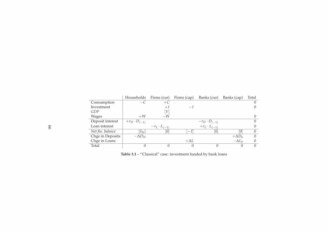
Households Firms (cur) Firms (cap) Banks (cur) Banks (cap) TotalConsumption −C +C 0Investment +I −I 0GDP [Y]Wages +W −W 0Deposit interest +rD · D(−1) −rD · D(−1) 0
Loan interest −rL · L(−1) +rL · L(−1) 0
Net fin. balance [SH ] [0] [−I] [0] [0] 0Chge in Deposits −∆DH +∆Db 0Chge in Loans +∆L −∆Lb 0Total 0 0 0 0 0 0
Table 3.1 – ‘‘Classical” case: investment funded by bank loans
66
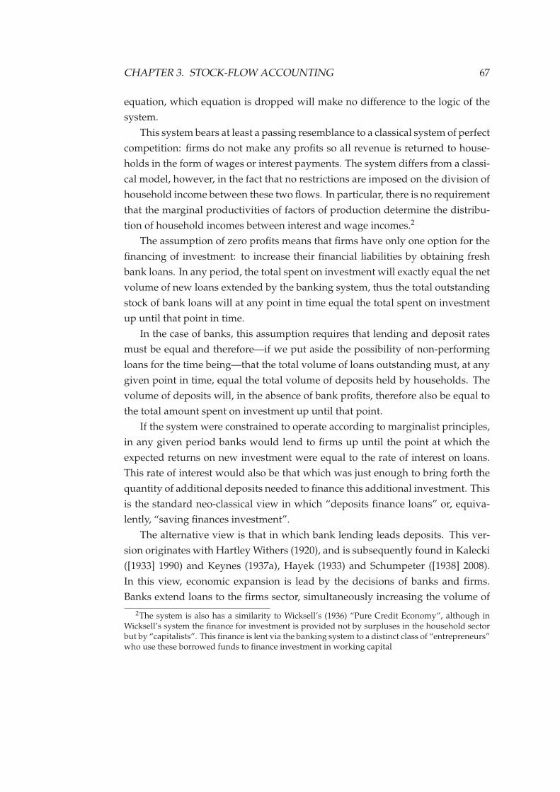
CHAPTER 3. STOCK-FLOW ACCOUNTING 67
equation, which equation is dropped will make no difference to the logic of the
system.
This system bears at least a passing resemblance to a classical system of perfect
competition: firms do not make any profits so all revenue is returned to house-
holds in the form of wages or interest payments. The system differs from a classi-
cal model, however, in the fact that no restrictions are imposed on the division of
household income between these two flows. In particular, there is no requirement
that the marginal productivities of factors of production determine the distribu-
tion of household incomes between interest and wage incomes.2
The assumption of zero profits means that firms have only one option for the
financing of investment: to increase their financial liabilities by obtaining fresh
bank loans. In any period, the total spent on investment will exactly equal the net
volume of new loans extended by the banking system, thus the total outstanding
stock of bank loans will at any point in time equal the total spent on investment
up until that point in time.
In the case of banks, this assumption requires that lending and deposit rates
must be equal and therefore—if we put aside the possibility of non-performing
loans for the time being—that the total volume of loans outstanding must, at any
given point in time, equal the total volume of deposits held by households. The
volume of deposits will, in the absence of bank profits, therefore also be equal to
the total amount spent on investment up until that point.
If the system were constrained to operate according to marginalist principles,
in any given period banks would lend to firms up until the point at which the
expected returns on new investment were equal to the rate of interest on loans.
This rate of interest would also be that which was just enough to bring forth the
quantity of additional deposits needed to finance this additional investment. This
is the standard neo-classical view in which “deposits finance loans” or, equiva-
lently, “saving finances investment”.
The alternative view is that in which bank lending leads deposits. This ver-
sion originates with Hartley Withers (1920), and is subsequently found in Kalecki
([1933] 1990) and Keynes (1937a), Hayek (1933) and Schumpeter ([1938] 2008).
In this view, economic expansion is lead by the decisions of banks and firms.
Banks extend loans to the firms sector, simultaneously increasing the volume of
2The system is also has a similarity to Wicksell’s (1936) “Pure Credit Economy”, although inWicksell’s system the finance for investment is provided not by surpluses in the household sectorbut by “capitalists”. This finance is lent via the banking system to a distinct class of “entrepreneurs”who use these borrowed funds to finance investment in working capital
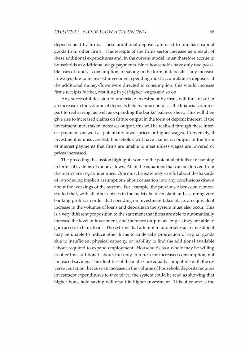
CHAPTER 3. STOCK-FLOW ACCOUNTING 68
deposits held by firms. These additional deposits are used to purchase capital
goods from other firms. The receipts of the firms sector increase as a result of
these additional expenditures and, in the current model, must therefore accrue to
households as additional wage payments. Since households have only two possi-
ble uses of funds—consumption, or saving in the form of deposits—any increase
in wages due to increased investment spending must accumulate as deposits: if
the additional money-flows were directed to consumption, this would increase
firms receipts further, resulting in yet higher wages and so on.
Any successful decision to undertake investment by firms will thus result in
an increase in the volume of deposits held by households as the financial counter-
part to real saving, as well as expanding the banks’ balance sheet. This will then
give rise to increased claims on future output in the form of deposit interest. If the
investment undertaken increases output, this will be realised through these inter-
est payments as well as potentially lower prices or higher wages. Conversely, if
investment is unsuccessful, households will have claims on output in the form
of interest payments that firms are unable to meet unless wages are lowered or
prices increased.
The preceding discussion highlights some of the potential pitfalls of reasoning
in terms of systems of money-flows. All of the equations that can be derived from
the matrix are ex-post identities. One must be extremely careful about the hazards
of introducing implicit assumptions about causation into any conclusions drawn
about the workings of the system. For example, the previous discussion demon-
strated that, with all other entries in the matrix held constant and assuming zero
banking profits, in order that spending on investment takes place, an equivalent
increase in the volumes of loans and deposits in the system must also occur. This
is a very different proposition to the statement that firms are able to automatically
increase the level of investment, and therefore output, as long as they are able to
gain access to bank loans. Those firms that attempt to undertake such investment
may be unable to induce other firms to undertake production of capital goods
due to insufficient physical capacity, or inability to find the additional available
labour required to expand employment. Households as a whole may be willing
to offer this additional labour, but only in return for increased consumption, not
increased savings. The identities of the matrix are equally compatible with the re-
verse causation: because an increase in the volume of household deposits requires
investment expenditures to take place, the system could be read as showing that
higher household saving will result in higher investment. This of course is the
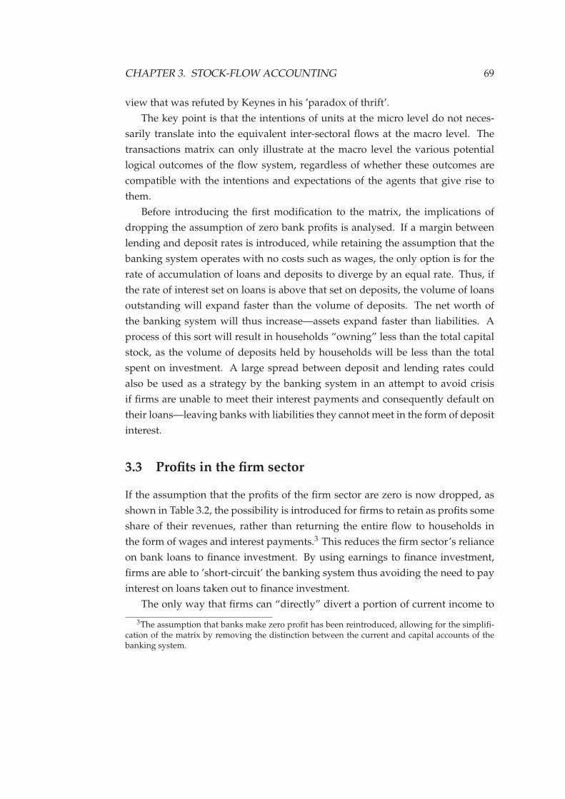
CHAPTER 3. STOCK-FLOW ACCOUNTING 69
view that was refuted by Keynes in his ’paradox of thrift’.
The key point is that the intentions of units at the micro level do not neces-
sarily translate into the equivalent inter-sectoral flows at the macro level. The
transactions matrix can only illustrate at the macro level the various potential
logical outcomes of the flow system, regardless of whether these outcomes are
compatible with the intentions and expectations of the agents that give rise to
them.
Before introducing the first modification to the matrix, the implications of
dropping the assumption of zero bank profits is analysed. If a margin between
lending and deposit rates is introduced, while retaining the assumption that the
banking system operates with no costs such as wages, the only option is for the
rate of accumulation of loans and deposits to diverge by an equal rate. Thus, if
the rate of interest set on loans is above that set on deposits, the volume of loans
outstanding will expand faster than the volume of deposits. The net worth of
the banking system will thus increase—assets expand faster than liabilities. A
process of this sort will result in households “owning” less than the total capital
stock, as the volume of deposits held by households will be less than the total
spent on investment. A large spread between deposit and lending rates could
also be used as a strategy by the banking system in an attempt to avoid crisis
if firms are unable to meet their interest payments and consequently default on
their loans—leaving banks with liabilities they cannot meet in the form of deposit
interest.
3.3 Profits in the firm sector
If the assumption that the profits of the firm sector are zero is now dropped, as
shown in Table 3.2, the possibility is introduced for firms to retain as profits some
share of their revenues, rather than returning the entire flow to households in
the form of wages and interest payments.3 This reduces the firm sector’s reliance
on bank loans to finance investment. By using earnings to finance investment,
firms are able to ’short-circuit’ the banking system thus avoiding the need to pay
interest on loans taken out to finance investment.
The only way that firms can “directly” divert a portion of current income to
3The assumption that banks make zero profit has been reintroduced, allowing for the simplifi-cation of the matrix by removing the distinction between the current and capital accounts of thebanking system.
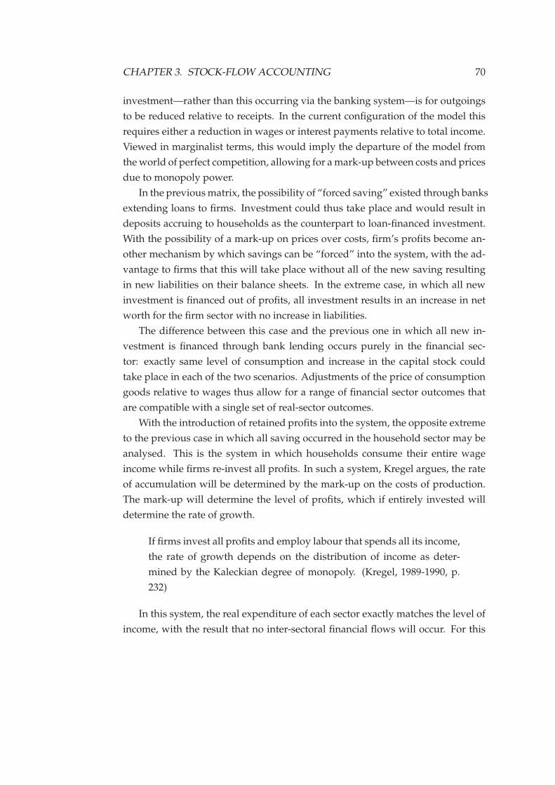
CHAPTER 3. STOCK-FLOW ACCOUNTING 70
investment—rather than this occurring via the banking system—is for outgoings
to be reduced relative to receipts. In the current configuration of the model this
requires either a reduction in wages or interest payments relative to total income.
Viewed in marginalist terms, this would imply the departure of the model from
the world of perfect competition, allowing for a mark-up between costs and prices
due to monopoly power.
In the previous matrix, the possibility of “forced saving” existed through banks
extending loans to firms. Investment could thus take place and would result in
deposits accruing to households as the counterpart to loan-financed investment.
With the possibility of a mark-up on prices over costs, firm’s profits become an-
other mechanism by which savings can be “forced” into the system, with the ad-
vantage to firms that this will take place without all of the new saving resulting
in new liabilities on their balance sheets. In the extreme case, in which all new
investment is financed out of profits, all investment results in an increase in net
worth for the firm sector with no increase in liabilities.
The difference between this case and the previous one in which all new in-
vestment is financed through bank lending occurs purely in the financial sec-
tor: exactly same level of consumption and increase in the capital stock could
take place in each of the two scenarios. Adjustments of the price of consumption
goods relative to wages thus allow for a range of financial sector outcomes that
are compatible with a single set of real-sector outcomes.
With the introduction of retained profits into the system, the opposite extreme
to the previous case in which all saving occurred in the household sector may be
analysed. This is the system in which households consume their entire wage
income while firms re-invest all profits. In such a system, Kregel argues, the rate
of accumulation will be determined by the mark-up on the costs of production.
The mark-up will determine the level of profits, which if entirely invested will
determine the rate of growth.
If firms invest all profits and employ labour that spends all its income,
the rate of growth depends on the distribution of income as deter-
mined by the Kaleckian degree of monopoly. (Kregel, 1989-1990, p.
232)
In this system, the real expenditure of each sector exactly matches the level of
income, with the result that no inter-sectoral financial flows will occur. For this
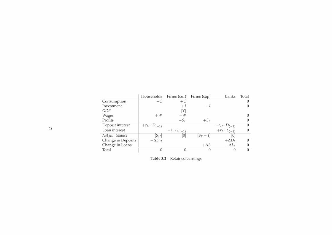
Households Firms (cur) Firms (cap) Banks TotalConsumption −C +C 0Investment +I −I 0GDP [Y]Wages +W −W 0Profits −SF +SF 0Deposit interest +rD · D(−1) −rD · D(−1) 0
Loan interest −rL · L(−1) +rL · L(−1) 0
Net fin. balance [SH ] [0] [SF − I] [0]Change in Deposits −∆DH +∆Db 0Change in Loans +∆L −∆Lb 0Total 0 0 0 0 0
Table 3.2 – Retained earnings
71
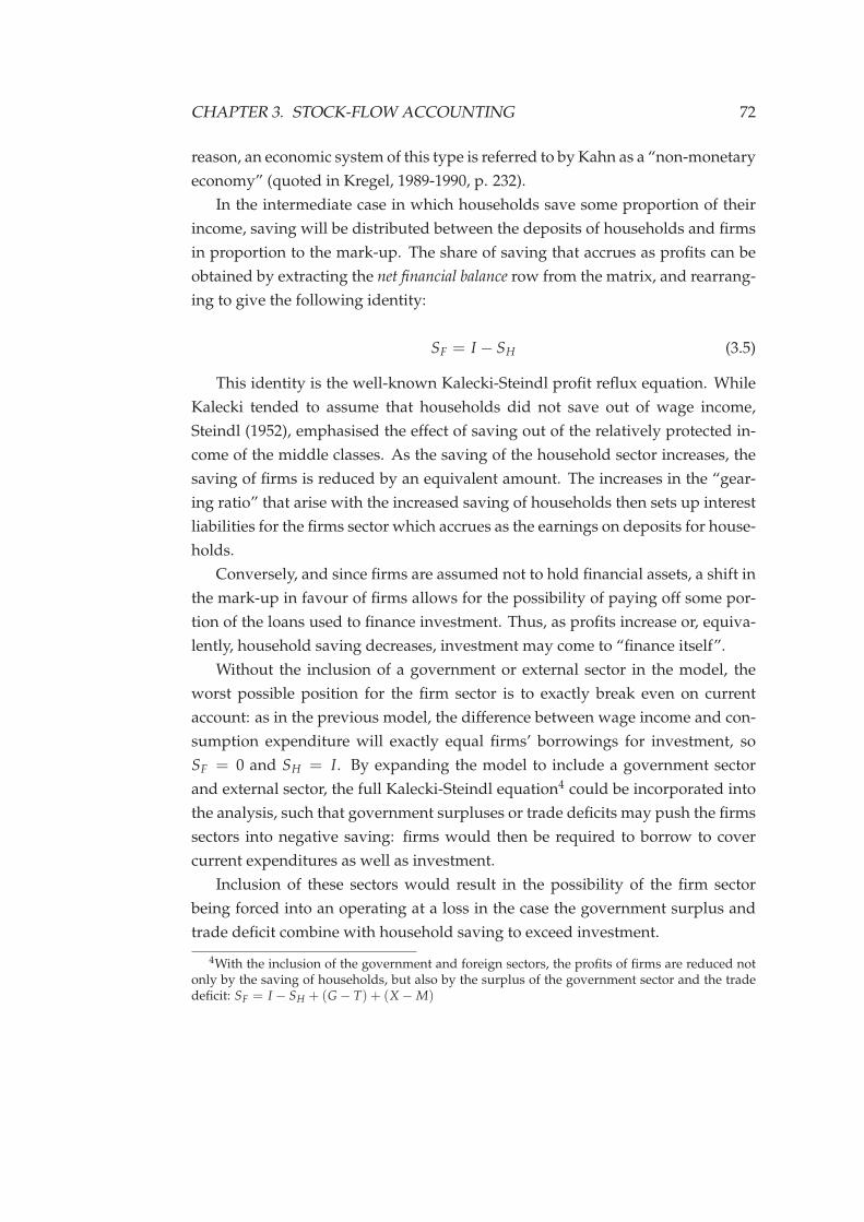
CHAPTER 3. STOCK-FLOW ACCOUNTING 72
reason, an economic system of this type is referred to by Kahn as a “non-monetary
economy” (quoted in Kregel, 1989-1990, p. 232).
In the intermediate case in which households save some proportion of their
income, saving will be distributed between the deposits of households and firms
in proportion to the mark-up. The share of saving that accrues as profits can be
obtained by extracting the net financial balance row from the matrix, and rearrang-
ing to give the following identity:
SF = I − SH (3.5)
This identity is the well-known Kalecki-Steindl profit reflux equation. While
Kalecki tended to assume that households did not save out of wage income,
Steindl (1952), emphasised the effect of saving out of the relatively protected in-
come of the middle classes. As the saving of the household sector increases, the
saving of firms is reduced by an equivalent amount. The increases in the “gear-
ing ratio” that arise with the increased saving of households then sets up interest
liabilities for the firms sector which accrues as the earnings on deposits for house-
holds.
Conversely, and since firms are assumed not to hold financial assets, a shift in
the mark-up in favour of firms allows for the possibility of paying off some por-
tion of the loans used to finance investment. Thus, as profits increase or, equiva-
lently, household saving decreases, investment may come to “finance itself”.
Without the inclusion of a government or external sector in the model, the
worst possible position for the firm sector is to exactly break even on current
account: as in the previous model, the difference between wage income and con-
sumption expenditure will exactly equal firms’ borrowings for investment, so
SF = 0 and SH = I. By expanding the model to include a government sector
and external sector, the full Kalecki-Steindl equation4 could be incorporated into
the analysis, such that government surpluses or trade deficits may push the firms
sectors into negative saving: firms would then be required to borrow to cover
current expenditures as well as investment.
Inclusion of these sectors would result in the possibility of the firm sector
being forced into an operating at a loss in the case the government surplus and
trade deficit combine with household saving to exceed investment.
4With the inclusion of the government and foreign sectors, the profits of firms are reduced notonly by the saving of households, but also by the surplus of the government sector and the tradedeficit: SF = I − SH + (G− T) + (X− M)
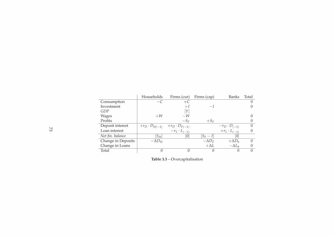
Households Firms (cur) Firms (cap) Banks TotalConsumption −C +C 0Investment +I −I 0GDP [Y]Wages +W −W 0Profits −SF +SF 0Deposit interest +rD · DH(−1) +rD · DF(−1) −rD · D(−1) 0
Loan interest −rL · L(−1) +rL · L(−1) 0
Net fin. balance [SH ] [0] [SF − I] [0]Change in Deposits −∆DH −∆DF +∆Db 0Change in Loans +∆L −∆Lb 0Total 0 0 0 0 0
Table 3.3 – Overcapitalisation
73
CHAPTER 3. STOCK-FLOW ACCOUNTING 74
3.4 Excess capital
The next modification introduced to the flow model allows for the holding of
bank deposits by firms. With this change comes a much broader range of possible
ways in which the configuration of assets and liabilities in the system can evolve.
By introducing the possibility that firms may choose to hold financial assets rather
than engage in productive investment, the potential for over-capitalisation of the
firm sector arises.
Over-capitalisation refers to the “holding of financial liabilities in excess of
those needed to undertake production” (Toporowski, 2008a). This possibility is
excluded in the previous stages of the model in which the only uses of funds
available to firms are the payment of wages and interest and investment in capital
goods. This changes once firms have the opportunity to accumulate funds in the
form of bank deposits: as long as a firm has both financial assets and liabilities on
its balance sheet it is, by the above definition, holding excess capital.
What are the implications of the holdings of excess capital by firms? This
depends in part on the way in which this capital is accumulated.
[I]t may be supposed that since saving equals investment, it is not
possible for firms to hold excess capital, except as net debt issued by
either households, the government, or the foreign sector. This is true
if it is assumed that all production is, and has only ever been, under-
taken by capitalistic firms. (Toporowski, 2008a, p. 8)
In this view, the only sector that could issue this net debt is the household
sector. Thus, as a consequence of the household sector consuming in excess of its
income, it would emit liabilities that would accumulate as financial assets held
by the firms sector. The problem with this is that, in order for the firms sector to
have become over-capitalised, it must have previously issued financial liabilities
in order to access the funds to purchase these financial assets. Where then will
the counterpart assets to these financial liabilities be held? If these assets are held
by households, these then would then offset household liabilities resulting in a
neutral net financial position, rather than a position of net issuance of debt.
There is another alternative suggested by the current configuration of the
model. The possibility of the household sector being in a negative net financial
position is excluded by the assumption that households are unable to issue any
financial liabilities. However, the firms sector as a whole may hold excess capital
CHAPTER 3. STOCK-FLOW ACCOUNTING 75
simply by accumulating both loans and deposits on its balance sheet.
This can be illustrated using the “non-monetary” case above in which house-
holds spend the entirety of wage income on consumption. Any credit-financed
increases in investment expenditure by firms will thus lead to an accumulation
of deposits in the firms sector equal to the increase in loans. If firms, instead of
choosing to pay off these loans, choose to hold the additional deposits, a situation
of overcapitalisation can arise without the net issuance of liabilities by any other
sector.
This case may be compared to the opposite extreme in which all saving ac-
crued in the form of households’ deposits: in that case, the final configuration of
deposits and liabilities represents net lending from the household sector to the
firm sector. The investment undertaken by firms must thus generate increased
output in future periods of an amount great enough to cover the interest liabili-
ties resulting from this lending. In the case of ‘over-capitalisation’, there has been
no inter-sectoral net lending: the increase in deposits held by the firm sector is
equal to the increase in loans it holds. Thus, the cost of borrowing to the firm
sector as a whole is in this case proportional to the margin between the loan and
deposit rates of interest, rather than the absolute value of the loan rate of inter-
est, as is usually assumed in discussion of the effect on investment of changes in
the rate of interest. (Toporowski, 2010). The per-period cost of additional excess
capital financed from bank lending is thus equal to the following:
∆L(rL − rD)
Toporowski describes the situation in which investment continues to be fi-
nanced as in this way, with further investment in subsequent periods also fi-
nanced out of bank lending:
What happens if firms finance their investment entirely through debt?
After a number of years, firms will end up with a stock of debt that
is exactly equal to the sum of their expenditures on capital formation
over those years. In addition... all firms will have deposited into their
banks retained profits exactly equal to the amount that the firms have
spent on capital formation. The banking system will have deposit li-
abilities to firms that exactly equal to the amount that the banks have
advanced to firms to pay for that capital formation. The firm sector as
a whole will have debts equal to the capital equipment that has been
CHAPTER 3. STOCK-FLOW ACCOUNTING 76
purchased over the years. But those debts will be exactly hedged (for
the capitalist firms as a whole) by cash deposits in the banking system.
If the financing structure of all firms corresponds to some representa-
tive ‘average’ firms, then the financing of every firm will be perfectly
hedged with bank deposits.” (2010, pp. 2–3)
Thus, once firms have undertaken investment financed in the way shown in
Table 3.3, at the start of the subsequent period the firm sector will be holding
deposits equal to the total expenditure in the current period. Firms thus only
need to expand the liability side of their balance sheet in subsequent periods if
they wish to undertake investment expenditures of an amount greater than their
accumulated spending—or if they wish to increase their level of excess capital
holdings. If firms continue to invest an amount equal to the deposits held, with
these deposits returning to the firms sector each period, these deposit holdings
come to play the role of Keynes’ “revolving fund of finance” (Keynes, 1937a, p.
247).
In either the case of complete over-capitalisation in which firms end up with
a stock of debt and deposits matched by the total spent on investment, or the case
of ‘marginal’ over-capitalisation in which which the stock of debt is incrementally
increased as desired investment exceeds the stock of retained profits, the rate of
interest—and thus the balance sheet of the firms sector—behaves in a way quite
different to that of standard marginalist theory. As previously noted, it is the
margin between the lending and deposit rates faced by firms that represents the
cost of over-capitalisation—and in this example, real investment.5 Thus, the stan-
dard view of the relationship between the investment decisions of firms and the
conduct of interest-rate policy by the central bank—higher bank rate will, ceteris
paribus, induce lower investment—may not hold unless a higher bank rate causes
a wider spread between lending and deposit rates.6 Similarly, if the central bank
were to operate in such a way as to attempt to restrict the availability of loans
through quantitative measures, textbook theory would argue that reduced avail-
ability of credit and the associated interest rate rises should ensure that only more
5We have assumed zero profits in the banking system for the sake of simplicity, which rulesout a spread between lending and deposit rates. However, if we were to instead assume that allbanking sector profits are returned to households, the difference between investment that resultsin households holding deposits, and investment that results in firms holding deposits is clear: inthe former, the cost to firms of investment is I · rL, whereas in the latter case it is I · (rL − rD)
6The current model would need to be extended to include a central bank as a separate sector inorder to consider the implementation of monetary policy in detail.
CHAPTER 3. STOCK-FLOW ACCOUNTING 77
potentially profitable investments would be undertaken. However, if the spread
between lending and deposit rates does not widen, the cost of investment will
not rise. The distribution of credit among firms may in this case be determined
by factors other than expected returns on investment.
It is at this point that some limitations of the accounting identities come into
focus. Firstly, just from inspection of the transactions matrix, there does not ap-
pear to be any direct connection between real investment and the financial assets
and liabilities of the firm sector. Given any initial set of valid values for the ma-
trix, spending on investment can be increased by any amount—without violating
any of the identities implied by the matrix—as long as profits are increased by
the same amount. However, we know that an increase in investment cannot take
place without a prior expansion of lending by banks to the firm sector—even if all
of this additional spending remains within the firm sector as retained profits. It
is of course possible that firms will borrow from banks to undertake investment,
and then in the same period use the retained earnings to repay the bank loans,
thus resulting in a set of net transactions that show only an increase in profits and
investment.
A second issue, and one that that is returned to later, is the problem of the level
of disaggregation in the model. By examining the money-flows through a number
of sectors of the economy, the dynamics of changes within each of those sectors
is obscured from view. There are several ways in which this could mask impor-
tant economic behaviour. One possibility relates to variations in the financing
structure of businesses within the firm sector: although in the over-capitalisation
case it appears that the firm sector as a whole is fully hedged against its liabilities
as deposits circulate within the sector as a whole and do not “leak” out into the
hands of households, it is possible for a redistribution of assets and liabilities to
take place within the sector.
For example, it is possible that larger firms are more profitable than smaller
firms, due to their ability to engage in monopoly pricing. This would result in
smaller firms requiring a higher level of loan finance to undertake investment,
while large firms are able to invest using retained earnings. In this case of “mald-
istribution of profits”, some part of the deposits that are the counterpart to the
loans used to finance investment end up not on the balance sheets of the small
firms that took out the loans, but on those of the larger monopolist firms (Steindl,
1952). This could be incorporated into the analysis by splitting the firm sector into
large and small firms. However, the intra-sectoral flow dynamics may be more
CHAPTER 3. STOCK-FLOW ACCOUNTING 78
subtle than can be captured by a simple two-way division: there may a distri-
bution of financing structures across firm sizes, or different financing structures
depending on the industry type.
3.5 Equity issuance
The final development to be analysed is the inclusion of equities as an asset class.
In most models, equity issuance is seen as an alternative way for firms to obtain
access to the savings of other sectors—primarily households— for use as invest-
ment funds. These transactions are often channelled via institutional intermedi-
aries such as pension funds. The issuance of equity allows for the expansion of
investment without the concomitant expansion of debt liabilities.
Recent literature on firms’ behaviour in relation to equity issuance tends to
focus on issues of “shareholder value”. This literature focuses on the pressure
placed on firms by shareholders to expand dividend payouts at the expense of
real investment. Models are constructed which examine the effects on growth of
the way in which firms allocate earnings between real investment and dividend
pay-outs, with increasing shareholder power resulting in a focus on short-term
profits at the expense of longer-term investment.7
Another approach is found in the work of Toporowski (2000) in which it is
argued that, rather than issuing equity for the purposes of financing new invest-
ment in real assets, those firms that have access to the capital markets use them to
maintain internal liquidity by raising cash against previous investment projects.
Equity issuance is thus used as a mechanism to maintain a state of overcapitalisa-
tion following the depletion of internal funds by spending on investment projects.
Furthermore, when faced with a situation of rising prices in the equities markets,
it may become profitable for overcapitalised firms to allocate excess capital to
financial assets in preference to engaging in real investment.
Table 3.4 shows the transactions matrix used in the previous examples, modi-
fied to include a new class of financial assets in the form of equities. The number
of equities issued is represented by e, the price is represented by p, and the div-
idend pay-out per-share by d. Two additional financial flows are thus shown in
the transactions matrix: the change in equity holdings by the household sector,
and the dividend pay-out based on holdings in the previous period.
7Eg. Hein (2008), van Treeck (2008), Stockhammer (2004).
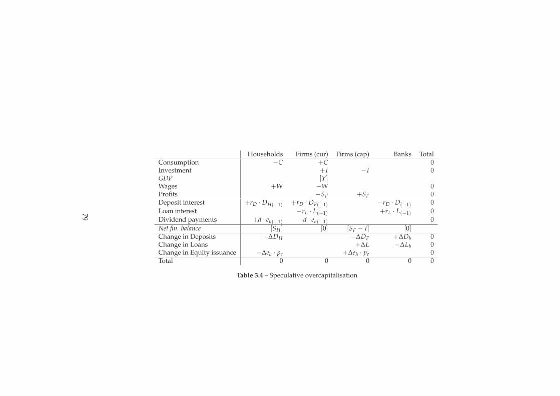
Households Firms (cur) Firms (cap) Banks TotalConsumption −C +C 0Investment +I −I 0GDP [Y]Wages +W −W 0Profits −SF +SF 0Deposit interest +rD · DH(−1) +rD · DF(−1) −rD · D(−1) 0
Loan interest −rL · L(−1) +rL · L(−1) 0
Dividend payments +d · eh(−1) −d · eh(−1) 0
Net fin. balance [SH ] [0] [SF − I] [0]Change in Deposits −∆DH −∆DF +∆Db 0Change in Loans +∆L −∆Lb 0Change in Equity issuance −∆eh · pe +∆eh · pe 0Total 0 0 0 0 0
Table 3.4 – Speculative overcapitalisation
79
CHAPTER 3. STOCK-FLOW ACCOUNTING 80
It was argued in the previous section that the cost to the firm sector of hold-
ing liquidity in the form of deposits depends on the profit margins of firms, or
equivalently the level of household saving: if firms do not turn a profit then any
liquidity held by the firm sector must be borrowed from the banking sector, with
the margin between deposit and lending rates as the cost of this liquidity. That
this liquidity is effectively “borrowed” from the household sector: both the loans
and deposits that are created with new bank lending appear on the balance sheets
of firms. If these liquid reserves are then depleted by investment in real assets,
the firm sector is then required to issue further liabilities in order to regain the
previous level of liquidity.
Once firms gain access to the capital markets, the issuance of equity provides
an alternative to debt as a way of maintaining a state of overcapitalisation. By
issuing fresh equity, firms can replenish their stocks of liquidity using the returns
on previous investment to fund the dividend payments.
The introduction of equities as an asset class also allows for the consideration
of capital gains, something that presents problems in the context of a flow-of-
funds analysis, as the prices of equities can change without resulting in any inter-
sectoral flows.
Broadly speaking, there are two reasons why the prices of equities would
change in the absence of any new issuance of shares. The first is the appearance of
some new piece of information on the prospective returns from real investment.
If there is a rise in the expected level of dividend payments, money-flows will
occur as a result of funds being reallocated between bank deposits and securities
in the portfolios of households.
The second possibility arises from to the fact that, once a rise in the prices of
shares has taken place, the expectation of further rises in share prices and thus
the prospect of capital gains for the owners of equity may cause further inflows
into these assets. In turn, this inflow of funds causes prices to rise, validating the
judgement of those astute enough to have seen them coming.
As always, in a closed flow-of-funds system, a flow into a class of assets can-
not happen in isolation: all flows must originate somewhere. If all equity is ini-
tially held by households, how can household buying of equity in response to
some exogenous event cause a rise in share prices? Again the problem of ag-
gregation in macroeconomic models shows itself: what is required is that some
sub-division of the household sector is willing to purchase equities at a higher
price than was paid by the current holders of equity. There is thus a redistri-
CHAPTER 3. STOCK-FLOW ACCOUNTING 81
bution of the ownership of equity within the household sector, accompanied by
a rise in the prices of shares. There must also be a corresponding intra-sectoral
flow in the opposite direction representing the payment for the newly purchased
shares. This is likely to take the form of a redistribution of bank deposits to offset
the change in equity holdings.
If it is assumed that all purchases of equity in the secondary markets by house-
holds are undertaken using bank deposits as payment, there is thus a limit to the
extent to which price inflation in the capital markets can take place, set by the
total stock of deposits in the household system: eventually the distribution of
equities and deposits within the household sector will take on a configuration
such that no further redistribution and price rises are possible, without further
deposits becoming available to the household sector to use as means of payment.
If the household sector turns to bank borrowing to enable continued purchases, a
classic credit-funded equity bubble will ensue.
We may also consider the situation wherein newly issued equities are pur-
chased by other firms within the corporate sector: in this situation there will be
a reallocation of deposits within the firm sector and an increase in both the hold-
ing and issuance of equities within the sector. However, none of these changes
will result in an inter-sectoral flow-of-funds, and thus entries on the transaction
matrix. Changes in the relative paper wealth of the household and firm sectors
are thus possible without any entry on the flow of funds matrix, in both the case
of a redistribution of equities within the household sector and the firm sector.
The only changes that will be visible in the current schema are those involving a
change in the total holdings of equities by households
What are the consequences of the holding of equities by the firm sector? In
a setting of rising prices in equity markets, overcapitalised firms face a trade-off
in how to allocate excess capital between real investment, deposits and equities:
it is possible that the expected capital gains on equities will be great enough to
offset the cost of overcapitalisation. The conditions under which this will be the
case depends initially on the historical profitability of firms, ie. to what extent
the financial assets corresponding to previous investment have accrued on the
balance sheets of households or firms, and upon whether equity was initially
purchased by households or firms. We can examine each combination of cases in
turn.
Consider first the case wherein firms collectively have made no profit, so the
deposits that correspond to real saving and investment are all held in the house-
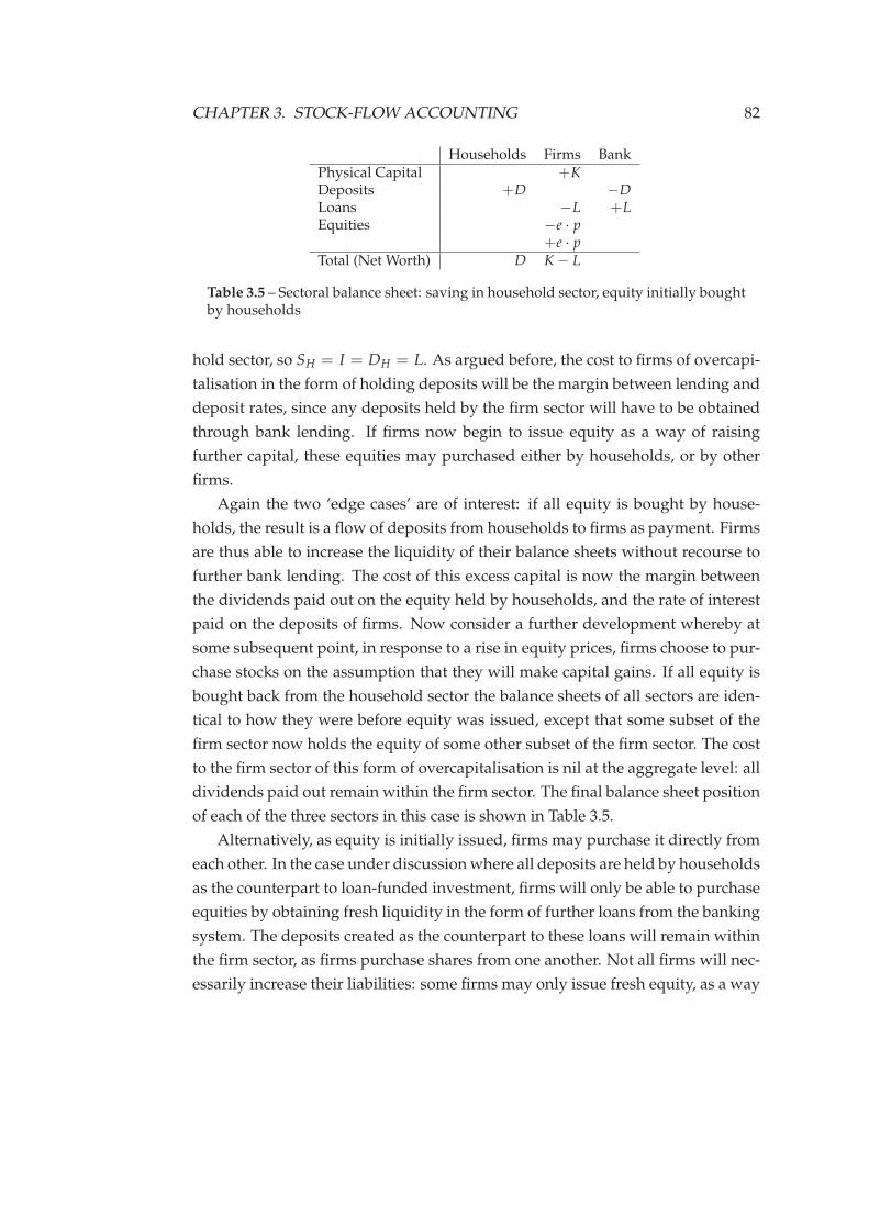
CHAPTER 3. STOCK-FLOW ACCOUNTING 82
Households Firms BankPhysical Capital +KDeposits +D −DLoans −L +LEquities −e · p
+e · pTotal (Net Worth) D K− L
Table 3.5 – Sectoral balance sheet: saving in household sector, equity initially boughtby households
hold sector, so SH = I = DH = L. As argued before, the cost to firms of overcapi-
talisation in the form of holding deposits will be the margin between lending and
deposit rates, since any deposits held by the firm sector will have to be obtained
through bank lending. If firms now begin to issue equity as a way of raising
further capital, these equities may purchased either by households, or by other
firms.
Again the two ‘edge cases’ are of interest: if all equity is bought by house-
holds, the result is a flow of deposits from households to firms as payment. Firms
are thus able to increase the liquidity of their balance sheets without recourse to
further bank lending. The cost of this excess capital is now the margin between
the dividends paid out on the equity held by households, and the rate of interest
paid on the deposits of firms. Now consider a further development whereby at
some subsequent point, in response to a rise in equity prices, firms choose to pur-
chase stocks on the assumption that they will make capital gains. If all equity is
bought back from the household sector the balance sheets of all sectors are iden-
tical to how they were before equity was issued, except that some subset of the
firm sector now holds the equity of some other subset of the firm sector. The cost
to the firm sector of this form of overcapitalisation is nil at the aggregate level: all
dividends paid out remain within the firm sector. The final balance sheet position
of each of the three sectors in this case is shown in Table 3.5.
Alternatively, as equity is initially issued, firms may purchase it directly from
each other. In the case under discussion where all deposits are held by households
as the counterpart to loan-funded investment, firms will only be able to purchase
equities by obtaining fresh liquidity in the form of further loans from the banking
system. The deposits created as the counterpart to these loans will remain within
the firm sector, as firms purchase shares from one another. Not all firms will nec-
essarily increase their liabilities: some firms may only issue fresh equity, as a way
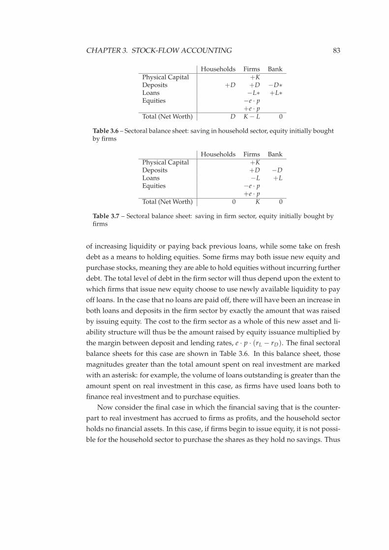
CHAPTER 3. STOCK-FLOW ACCOUNTING 83
Households Firms BankPhysical Capital +KDeposits +D +D −D∗
Loans −L∗ +L∗Equities −e · p
+e · pTotal (Net Worth) D K− L 0
Table 3.6 – Sectoral balance sheet: saving in household sector, equity initially boughtby firms
Households Firms BankPhysical Capital +KDeposits +D −DLoans −L +LEquities −e · p
+e · pTotal (Net Worth) 0 K 0
Table 3.7 – Sectoral balance sheet: saving in firm sector, equity initially bought byfirms
of increasing liquidity or paying back previous loans, while some take on fresh
debt as a means to holding equities. Some firms may both issue new equity and
purchase stocks, meaning they are able to hold equities without incurring further
debt. The total level of debt in the firm sector will thus depend upon the extent to
which firms that issue new equity choose to use newly available liquidity to pay
off loans. In the case that no loans are paid off, there will have been an increase in
both loans and deposits in the firm sector by exactly the amount that was raised
by issuing equity. The cost to the firm sector as a whole of this new asset and li-
ability structure will thus be the amount raised by equity issuance multiplied by
the margin between deposit and lending rates, e · p · (rL − rD). The final sectoral
balance sheets for this case are shown in Table 3.6. In this balance sheet, those
magnitudes greater than the total amount spent on real investment are marked
with an asterisk: for example, the volume of loans outstanding is greater than the
amount spent on real investment in this case, as firms have used loans both to
finance real investment and to purchase equities.
Now consider the final case in which the financial saving that is the counter-
part to real investment has accrued to firms as profits, and the household sector
holds no financial assets. In this case, if firms begin to issue equity, it is not possi-
ble for the household sector to purchase the shares as they hold no savings. Thus
CHAPTER 3. STOCK-FLOW ACCOUNTING 84
the only possibility is for firms to buy the stock of other firms. As this takes place,
there is once again no inter-sectoral flow of funds as the deposits used by firms
to buy stock are transferred to other firms. The additional costs to the firm sector
as a whole in holding additional capital in the form of equities is thus once again
zero in this case. The balance sheets for this case are shown in Table 3.7.
There are thus three potential ‘edge case’ configurations of firm overcapitali-
sation through the ownership of equity: two that originate with the situation in
which real investment was originally financed by a sectoral surplus in the house-
hold sector, and one in which retained earnings allowed firms to invest without
incurring any net financial liabilities. The balance sheets of these three possible
cases are shown in Tables 3.5-3.7. In each of the three cases, the combination of the
net worth of each sector, and the cost to the firm sector of holding excess capital
in the form of equity is different.
3.6 Foreign trade
The analysis to this point has assumed a closed economy. The case of an economy
with international trade is now examined. The example used will be tailored to-
wards the specific case of China. This will demonstrate that the presence of a
significant surplus on current account, in conjunction with the operations under-
taken by the central bank in the foreign exchange markets do not materially alter
the validity of the above analysis.
Table 3.8 shows the modifications required to incorporate the foreign sector
into the accounting matrix. An additional column has been introduced to repre-
sent the rest of the world as a macroeconomic sector. The domestic side of the
system is equivalent to the system discussed in Section 3.4—firms hold deposits
but there is no stock market. However, the complexity of the domestic finan-
cial system has increased as a result of the separation of the banking system into
“banks” and a central bank. There are thus two additional columns included in
the matrix.
To approximate the case of the Chinese economy, it is assumed that the ex-
change rate is fixed and international capital movements are prohibited. This
requires that any trade imbalance is counteracted by the purchase or sale of for-
eign currency by the central bank. The assumption of capital controls implies that
deposits remain the only financial asset available to households for the purpose
of saving.
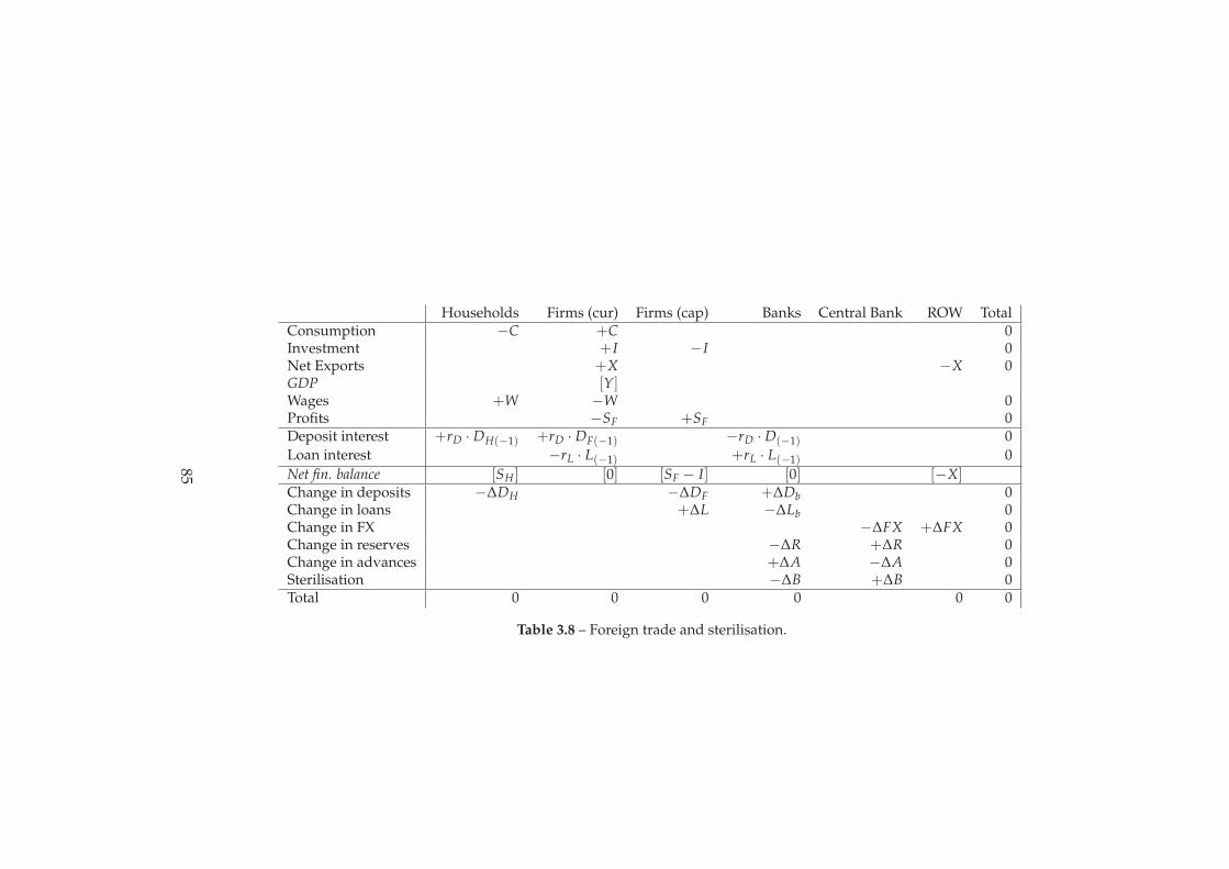
Households Firms (cur) Firms (cap) Banks Central Bank ROW TotalConsumption −C +C 0Investment +I −I 0Net Exports +X −X 0GDP [Y]Wages +W −W 0Profits −SF +SF 0Deposit interest +rD · DH(−1) +rD · DF(−1) −rD · D(−1) 0
Loan interest −rL · L(−1) +rL · L(−1) 0
Net fin. balance [SH ] [0] [SF − I] [0] [−X]Change in deposits −∆DH −∆DF +∆Db 0Change in loans +∆L −∆Lb 0Change in FX −∆FX +∆FX 0Change in reserves −∆R +∆R 0Change in advances +∆A −∆A 0Sterilisation −∆B +∆B 0Total 0 0 0 0 0 0
Table 3.8 – Foreign trade and sterilisation.
85
CHAPTER 3. STOCK-FLOW ACCOUNTING 86
The transactions of the foreign sector are straightforward. Exports and im-
ports have been combined into one “net exports” item, represented by X. The
discussion will assume that the domestic economy is running a trade surplus, so
that this variable is positive. This implies an addition to total domestic aggregate
demand of magnitude X. Firms are therefore in receipt of higher revenues than
would be the case in the absence of the trade surplus. These additional revenues
will be paid in foreign exchange. Assuming that firms are required to surrender
these foreign exchange earnings to banks, and these banks in turn are required to
surrender foreign exchange to the central bank, an amount of foreign exchange
equivalent to the trade surplus will thus accrue with the central bank.
With the inclusion of a trade surplus, the requirement that total domestic sav-
ing and investment be equal no longer holds. This can be seen by extracting the
net financial balance row from the matrix:
SF = I − SH + X
Thus domestic saving is equal to the sum of investment and the trade surplus.
In this form, the equation also shows how the trade surplus serves to offset the
profits “lost” by firms to the saving of households.
The greatest complexity is involved with the interactions of the banks and the
central bank. The analysis in the previous sections of this chapter has assumed a
single unified banking system, resulting in a Wicksellian pure credit system.
The current model may also be regarded as a pure credit system but instead
of the banking system passively accommodating all demands for loans from the
firms sector—as has been implicitly assumed until now—the requirement for
banks to hold reserves at the central bank is now introduced.
These reserves may be obtained by banks in one of two ways: either by sur-
rendering foreign exchange reserves, or by drawing on advances from the central
bank. Central bank reserves equal to a proportion of total deposits must be held—
a required reserve ratio. If θ is the required reserve ratio, then the balance sheet
of the banks sector must comply with the following identity:
R = θD
In the case of a balanced trade account, the lending operations of banks will
be constrained if the central bank does not provide these advances on demand.
However, the inflows of foreign exchange that occur in the case of a trade surplus
CHAPTER 3. STOCK-FLOW ACCOUNTING 87
will reduce this reliance on central bank advances, curtailing the power of the
central bank to restrain lending by restricting the supply of reserves. This is due
to central bank intervention in the foreign exchange markets to buy up the foreign
earnings of firms. This process takes place via the banking system: firms surren-
der their foreign exchange earnings in exchange for domestic bank deposits. In
turn the banks exchange foreign exchange for reserves with the central bank.
The balance sheet of the domestic banking system therefore expands, but the
increase in deposits on the liability side of the balance sheet will be backed on the
assets side by reserves with the central bank, not loans. Since only a proportion
of deposits are required to be backed by reserves this will allow for a greater
expansion of lending by the banking system since an equal expansion of reserves
and deposits on opposite sides of the banks balance sheets will lead to a reduction
in the current deposits to reserves ratio.
Whether or not the holding of excess reserves by the banking system leads to
an expansion of lending depends primarily on whether loans are demanded by
firms, given the rates of interest on loans and deposits. In the absence of such
demand, the result of a trade surplus will simply be the accumulation of excess
reserves by the banking system. However the central bank may choose to sterilise
the additional reserves by either converting excess reserves into required reserves
or substituting excess reserves for alternative central bank liabilities.
The first is achieved by raising the required reserve ratio, θ, so that as reserves
accumulate and the reserve to deposit ratio rises, the required reserve ratio rises
at an equal rate. The second option, shown in the in matrix by the entry “steril-
isation”, takes place through the open market operations of the central bank: by
issuing illiquid liabilities (bills, B, in the current example), the central bank re-
places the excess reserves of the banking system with alternative liabilities that
are ineligible for reserve requirements. Godley & Lavoie (2005–06) argue that in
the case of a central bank which is targeting an overnight rate of interest, these
sterilisation operations will happen “endogenously”—excess reserves will push
down the overnight rate of interest, requiring the central bank to sell securities in
order to push the rate of interest up again. Even in the case of a system in which
overnight rates of interest are not closely targeted, the central bank will almost
always be able to force reserves out of the system by offering to sell securities
that provide a higher yield than that paid on excess reserves.
This raises the issue of the interest paid on the various additional financial
instruments introduced into the analysis in the current section. For the sake of
CHAPTER 3. STOCK-FLOW ACCOUNTING 88
simplicity, it has been assumed that no interest is paid on the instruments in the
final four rows of the matrix and as a consequence the central bank imposes no
spread between advances and reserves and sterilisation bills.
In general, this will not be the case. The structure of relative interest rates
on foreign exchange (held as foreign government debt for example); central bank
reserves; advances and bills, will result in either costs or revenues for the banking
system and the central bank. The banking system will face a spread between the
rate of interest paid on deposits and the rate received on reserves and bills. The
central bank will face a spread between the rates paid on reserves and bill and
rates received on foreign exchange. (This point is considered in more detail in the
case of China in Section 7.3.2).
This accounting model demonstrates a number of important points. Firstly,
the conclusion of the standard open-economy model of Mundell and Fleming
that control of monetary policy will lost in the case of fixed exchange rates and
capital mobility is an extreme over-simplification. Even though a closed capital
account was assumed for this discussion, even in the case of free capital move-
ment, a large number of factors will serve to determine whether flows occur that
equalise returns across all assets, including the relative substitutability, liquid-
ity and risk of those assets. Further, the Mundell-Fleming analysis fails to dis-
tinguish between “inside” and “outside” money—increases in reserves will not
translate into an expansion of the “money supply” if firms choose to substitute
loan-financed investment with investment financed using the deposits obtained
in exchange for surrendering export earnings.
Secondly, the current model demonstrates the flaws of the “saving glut” argu-
ment which holds that global imbalances are the result of the high saving propen-
sity of Chinese households:8 this can be illustrated by considering, as before, the
extreme case in which households consume their entire income. Then, in the case
of a balanced trade account, all profits will accrue to the firms sector. Expansion of
output will be made possible by additional bank lending to the firms sector. If the
firms sector as a whole holds the resulting profits as bank deposits, reserves will
be provided by the central bank to the banking system in order to accommodate
the increase in deposits. This is an identical situation to the case of overcapital-
isation described in Section 3.4, with the difference that the central bank is now
explicitly incorporated.
If this expansion of investment by firms increases the domestic productive
8Eg. Bernanke (2005)
CHAPTER 3. STOCK-FLOW ACCOUNTING 89
capacity of some products that were previously imported, such as intermediate
goods, this will result in higher domestic output and and a trade surplus. As
described above, the trade surplus will increase the level of reserves in the bank-
ing system. If the increase in aggregate demand resulting from the trade surplus
stimulates a further increase in investment, the increase reserves of the banking
system will be either partially of fully absorbed by this new lending, serving as
the required reserves for the increased level of deposits. If firms do not continue
to increase the rate of expansion, these reserves will remain as excess reserves in
the banking system, or may be absorbed by increases to the required reserve ratio
or the issuance of bills.
In either case, the key point is illustrated by the configuration of the final bal-
ance sheets of the system: If firms have chosen to repay past loans out of profits,
total deposits of firms will equal the total volume of foreign exchange on the cen-
tral bank balance sheet. If firms are overcapitalised due to choosing not to repay
loans, then all loans and deposits will be held on the balance sheets of firms, with
the excess of deposits over loans equal to the cumulative trade surplus.
In this example, the “savings glut” is fully accounted for by the profits of
firms resulting from export demand. Even in the case of a lower mark-up, such
that saving also accumulates as household deposits, the cause of this accumula-
tion will not be located in the saving propensity of those households. A reduced
propensity to save by households would only reduce the trade surplus to the ex-
tent that additional household expenditure is directed towards imported goods.
If households were to increase their consumption of domestic goods, this would
simply stimulate a further expansion of domestic demand.
3.7 Conclusion
The chapter has used the stock-flow consistent framework as the basis for the
analysis of a number of phenomena of direct relevance to the recent economic
history of China. The analysis focuses on the financial and monetary implications
of credit-financed investment; saving and overcapitalisation in the firms sector;
export earnings and the operations of the central bank—topics that have largely
been overlooked or mis-represented in academic discussions.
While fully-specified mathematical models have not been presented, the stock-
flow consistent system has been used to organise discussion of these phenomena
in the context of a framework that ensures that the balance sheet effects of all eco-
CHAPTER 3. STOCK-FLOW ACCOUNTING 90
nomic interactions are fully accounted for. This allows for flexibility in analysing
the implications of different assumptions while exploring the “state space” of al-
ternative institutional structures. This analysis is extended in a more formal way
in the following chapter.
In demonstrating the balance sheet effects of the above phenomena, this chap-
ter lays the ground for the flow-of-funds analysis in Chapters 6 and 7. Although
the data categories of the empirical accounts are significantly more detailed and
complex than the simple framework used here, they are dominated by the dy-
namics of a number of key processes: investment financed with retained earnings
and bank credit; the saving of firms and households; export earnings; and the op-
erations of the banks and central bank. Thus the balance sheet configurations
which emerge in the abstract models in the current chapter will be replicated in
the concrete empirical analysis in these later chapters.
Chapter 4
Growth, income distribution and
money
4.1 Introduction
The previous chapter begins the development of a theoretical approach based
on the flow-of-funds accounting framework. The accounting system is used as
the basis for analysis of the monetary consequences of various possible configu-
rations of investment, profits and saving in the household and firms sectors, as
well as an examination of the balance sheet effects of sterilisation operations. The
analysis focuses on the monetary effects of various possible configurations of sav-
ing and investment at the level of macroeconomic sectors, while taking as given
the real sector balances that generate the expenditures and imbalances which un-
derpin these monetary phenomena.
This chapter extends this analysis by examining the dynamics of these real
sector processes in the context of economic growth. A survey is presented of those
approaches to growth and distribution which form an alternative to the models
constructed on the basis of the neoclassical aggregate production function dis-
cussed in Chapter 2. In particular, the Cambridge growth models of the 1950s and
1960s are contrasted with the analysis of Steindl and the post-Keynesian Kaleck-
ian growth model.
Both classes of models are designed to formalise the view that investment, not
saving, is the key behavioural variable for determining growth. An important
distinction is to be found, however, in the mechanism by which saving adapts to
this desired rate of investment. In the Cambridge models, this accommodation
91
CHAPTER 4. GROWTH, INCOME DISTRIBUTION AND MONEY 92
either occurs through shifts in the real wage or in the price of financial securities at
a fixed rate of employment. In the analysis of Steindl, the effect of retained profits
and excess capacity in determining the investment expenditures of firms plays
the central role. This mechanism also features in the Kaleckian growth model
such that changes in the rate of capacity utilisation provide the mechanism by
which saving adapts to growth.
The distributional consequences of changes in the rate of growth are thus dif-
ferent in each class of model: the Cambridge models require a shift from wages to
profits to accommodate higher growth, whereas higher growth is associated with
a higher real wage in the Kaleckian model.
In Section 4.6, the Kaleckian growth model is integrated with the pure credit
monetary system developed in Chapter 3. This allows for an integrated anal-
ysis of the monetary phenomena discussed in that chapter with the processes of
growth and distribution examined in this chapter. The resulting monetary growth
model is used to illustrate the Steindlian theoretical framework used as the basis
of the flow-of-funds analysis in Chapters 6 and 5.
4.2 Cambridge growth models
An alternative to the Solow-Swan analysis of growth and distribution began to be
developed in Cambridge, UK from the late 1950s in a series of papers primarily
authored by Kaldor and Pasinetti, informed by exchanges with US economists
such as Samuelson and Modigliani. The initial contribution to this strand came
with Kaldor’s preliminary attempt at a sketch of a “Keynesian” theory of growth
and distribution, inspired in part by the criticisms of the aggregate production
function approach by Joan Robinson and others:
In fact the whole approach which regards the share of wages and of
profits in output as being determined by the marginal rate of substi-
tution between Capital and Labour with its corollary, that the con-
stancy of relative shares is evidence of a unity-Elasticity of Substitu-
tion between Capital and Labour—is hardly acceptable to present-day
economists. Its inadequacy becomes evident as soon as it is realized
that the “marginal rate of substitution” between Capital and Labour-
as distinct from the marginal rate of substitution between labour and
land-can only be determined once the rate of profit and the rate of
CHAPTER 4. GROWTH, INCOME DISTRIBUTION AND MONEY 93
wages are already known. (Kaldor, 1955, p. 91)
Kaldor’s starting point in formulating an alternative approach to the problems
of growth and distribution is the difference in propensities to save out of different
types of income. If income, Y, is divided into wages, W, and profits, P, then the
total volume of saving forthcoming, S, will be equal to the sum of saving out of
wages and out of profits. The volume of saving from each class of income will
be determined by the propensity to save of wage-earners, sw, and capitalists, sp
respectively:
Y = W + P (4.1)
S = swW + spP (4.2)
Like Kalecki ([1939] 1990; [1954] 1965), Kaldor assumes that the propensity
to save out of profits is greater than that of the propensity to save out of wages.
Then, by setting saving equal to investment, some simple algebraic manipulation
generates the result that, with given saving propensities, the functional distribu-
tion of income—the division between wages and profit—depends only upon the
relative size of investment in output:
P
Y=
1
sp − sw
I
Y−
swsp − sw
(4.3)
In the special case emphasised where “workers spend what they get and capi-
talists get what they spend”, sw = 0, giving the well-known result that P = I. The
rate of profit—the volume of profit divided by the value of the capital stock—may
be determined similarly:1
P
K=
1
sp − sw
I
K−
swsp − sw
Y
K(4.4)
This model may be regarded as Keynesian in that investment is the active
variable—the exogenously determined rate of capital accumulation is indepen-
dent of the saving propensities of either workers or capitalists. However, this
independence is the result of assuming a pricing mechanism that operates such
that the real wage adjusts to accommodate any given desired rate of investment.
Thus, in producing a model which captures one key Keynesian result, Kaldor is
1This result is presented in Pasinetti’s 1962 reformulation of Kaldor’s model (discussed in sub-sequent paragraphs).
CHAPTER 4. GROWTH, INCOME DISTRIBUTION AND MONEY 94
forced to drop another central pillar of Keynesian theory in that the system is as-
sumed to operate at a point of full employment. The functional distribution of
income is thus determined by the exogenous rate of investment—an increase in
the level of investment is matched by a corresponding increase in desired saving
through redistribution from lower-saving-propensity workers to higher-saving-
propensity capitalists.
It is possible to detect hints of Say’s Law in this adjustment mechanism. Al-
though investment takes the active role with saving adjusting passively, it is as-
sumed that a price adjustment mechanism operates such that variations in em-
ployment and capacity utilisation are ruled out. Thus, the price of output goods
(or, equivalently, the real wage) takes the place of the rate of interest in the classi-
cal system.
This price adjustment mechanism also provides an alternative to the capital-
labour ratio adjustment process of the Swan-Solow growth model. Assuming
investment to be exogenous and at a level equivalent to Harrod’s ‘natural rate of
growth’—that which is just sufficient to cope with technical progress and popula-
tion growth—the instability arising from divergences between this ‘natural’ rate
and the actual, or ‘warranted’ rate in Harrod’s model can now be overcome by
changes in the distribution of income that cause an adjustment in the overall level
of saving.
Despite the somewhat unsatisfactory nature of this adjustment mechanism,
Kaldor’s formulation was greeted with enthusiasm by Pasinetti, who wrote:
One of the most exciting results of the macro-economic theories which
have recently been elaborated in Cambridge is a very simple relation
connecting the rate of profit and the distribution of income to the rate
of economic growth, through the interaction of the different propensi-
ties to save... it represents a break with the hundred-year-old tradition
of marginal theory. (1962, p. 267)
Nonetheless, Pasinetti goes on to point out a flaw—or perhaps an oversight—
in Kaldor’s reasoning. In assuming two types of income (wages and profits)
with different propensities to save out of each, Kaldor overlooks that fact that
saving out of wage income will result in the “ownership” of capital by wage-
earners, whether through direct equity ownership or indirectly through, for ex-
ample, holdings of liquid bank balances. Thus, the formulation S = swW + spP
either assumes that workers have the same propensity to save out of profits as
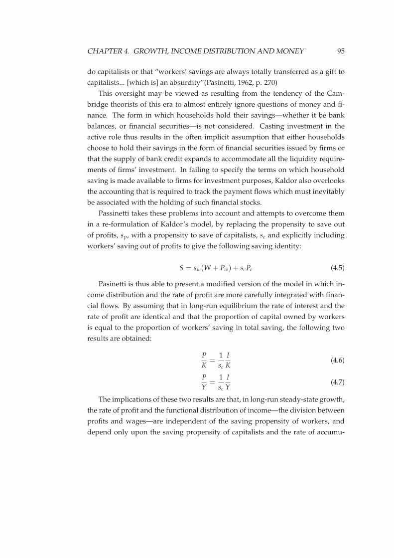
CHAPTER 4. GROWTH, INCOME DISTRIBUTION AND MONEY 95
do capitalists or that “workers’ savings are always totally transferred as a gift to
capitalists... [which is] an absurdity”(Pasinetti, 1962, p. 270)
This oversight may be viewed as resulting from the tendency of the Cam-
bridge theorists of this era to almost entirely ignore questions of money and fi-
nance. The form in which households hold their savings—whether it be bank
balances, or financial securities—is not considered. Casting investment in the
active role thus results in the often implicit assumption that either households
choose to hold their savings in the form of financial securities issued by firms or
that the supply of bank credit expands to accommodate all the liquidity require-
ments of firms’ investment. In failing to specify the terms on which household
saving is made available to firms for investment purposes, Kaldor also overlooks
the accounting that is required to track the payment flows which must inevitably
be associated with the holding of such financial stocks.
Passinetti takes these problems into account and attempts to overcome them
in a re-formulation of Kaldor’s model, by replacing the propensity to save out
of profits, sp, with a propensity to save of capitalists, sc and explicitly including
workers’ saving out of profits to give the following saving identity:
S = sw(W + Pw) + scPc (4.5)
Pasinetti is thus able to present a modified version of the model in which in-
come distribution and the rate of profit are more carefully integrated with finan-
cial flows. By assuming that in long-run equilibrium the rate of interest and the
rate of profit are identical and that the proportion of capital owned by workers
is equal to the proportion of workers’ saving in total saving, the following two
results are obtained:
P
K=
1
sc
I
K(4.6)
P
Y=
1
sc
I
Y(4.7)
The implications of these two results are that, in long-run steady-state growth,
the rate of profit and the functional distribution of income—the division between
profits and wages—are independent of the saving propensity of workers, and
depend only upon the saving propensity of capitalists and the rate of accumu-
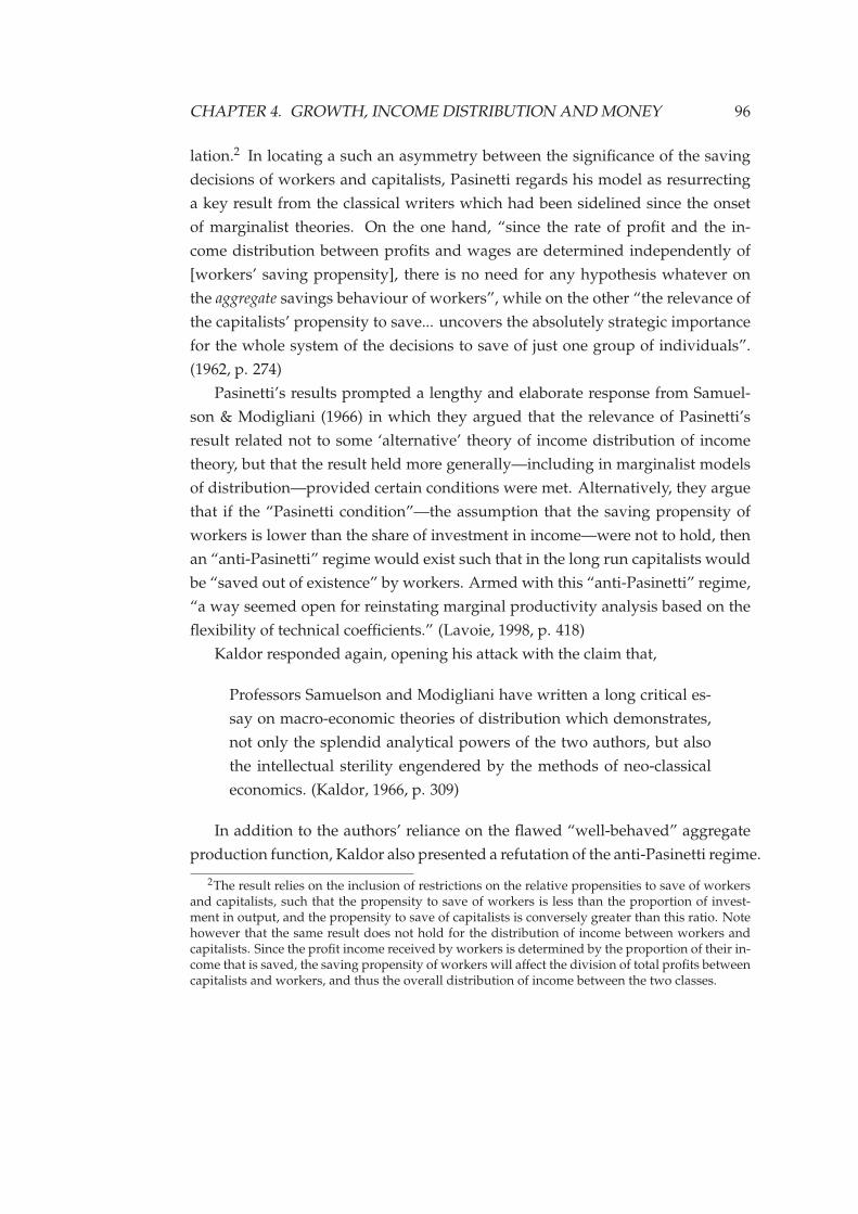
CHAPTER 4. GROWTH, INCOME DISTRIBUTION AND MONEY 96
lation.2 In locating a such an asymmetry between the significance of the saving
decisions of workers and capitalists, Pasinetti regards his model as resurrecting
a key result from the classical writers which had been sidelined since the onset
of marginalist theories. On the one hand, “since the rate of profit and the in-
come distribution between profits and wages are determined independently of
[workers’ saving propensity], there is no need for any hypothesis whatever on
the aggregate savings behaviour of workers”, while on the other “the relevance of
the capitalists’ propensity to save... uncovers the absolutely strategic importance
for the whole system of the decisions to save of just one group of individuals”.
(1962, p. 274)
Pasinetti’s results prompted a lengthy and elaborate response from Samuel-
son & Modigliani (1966) in which they argued that the relevance of Pasinetti’s
result related not to some ‘alternative’ theory of income distribution of income
theory, but that the result held more generally—including in marginalist models
of distribution—provided certain conditions were met. Alternatively, they argue
that if the “Pasinetti condition”—the assumption that the saving propensity of
workers is lower than the share of investment in income—were not to hold, then
an “anti-Pasinetti” regime would exist such that in the long run capitalists would
be “saved out of existence” by workers. Armed with this “anti-Pasinetti” regime,
“a way seemed open for reinstating marginal productivity analysis based on the
flexibility of technical coefficients.” (Lavoie, 1998, p. 418)
Kaldor responded again, opening his attack with the claim that,
Professors Samuelson and Modigliani have written a long critical es-
say on macro-economic theories of distribution which demonstrates,
not only the splendid analytical powers of the two authors, but also
the intellectual sterility engendered by the methods of neo-classical
economics. (Kaldor, 1966, p. 309)
In addition to the authors’ reliance on the flawed “well-behaved” aggregate
production function, Kaldor also presented a refutation of the anti-Pasinetti regime.
2The result relies on the inclusion of restrictions on the relative propensities to save of workersand capitalists, such that the propensity to save of workers is less than the proportion of invest-ment in output, and the propensity to save of capitalists is conversely greater than this ratio. Notehowever that the same result does not hold for the distribution of income between workers andcapitalists. Since the profit income received by workers is determined by the proportion of their in-come that is saved, the saving propensity of workers will affect the division of total profits betweencapitalists and workers, and thus the overall distribution of income between the two classes.
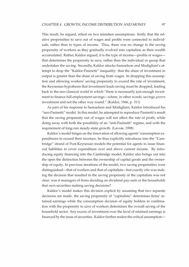
CHAPTER 4. GROWTH, INCOME DISTRIBUTION AND MONEY 97
This result, he argued, relied on two mistaken assumptions: firstly that the rel-
ative propensities to save out of wages and profits were connected to individ-
uals, rather than to types of income. Thus, there was no change in the saving
propensity of workers as they gradually evolved into capitalists as their wealth
accumulated. Rather, Kaldor argued, it is the type of income—profits or wages—
that determines the propensity to save, rather than the individual or group that
undertakes the saving. Secondly, Kaldor attacks Samuelson and Modigliani’s at-
tempt to drop the “Kaldor-Pasinetti” inequality: that the share of investment in
output is greater than the share of saving from wages. In dropping this assump-
tion and allowing workers’ saving propensity to exceed the rate of investment,
the Keynesian hypothesis that investment leads saving must be dropped, leading
back to the neo-classical world in which “there is necessarily just enough invest-
ment to finance full employment savings—where, in other words, savings govern
investment and not the other way round.” (Kaldor, 1966, p. 311)
As part of his response to Samuelson and Modigliani, Kaldor introduced his
“neo-Pasinetti” model. In this model, he attempted to reproduce Pasinetti’s result
that the saving propensity out of wages will not affect the rate of profit, while
doing away with both the possibility of an “anti-Pasinetti” regime, and with the
requirement of long-run steady-state growth. (Lavoie, 1998)
Kaldor’s model hinges on the innovation of allowing agents’ consumption ex-
penditures to exceed their incomes: he thus explicitly introduces into the “Cam-
bridge” strand of Post-Keynesian models the potential for agents to issue finan-
cial liabilities to cover expenditure over and above current income. By intro-
ducing equity financing into the Cambridge model, Kaldor also brings out into
the open the distinction between the ownership of capital goods and the owner-
ship of equity. In previous iterations of the model, two saving propensities were
distinguished—that of workers and that of capitalists—but exactly who was mak-
ing the decision that resulted in the saving propensity of the capitalists was not
clear: was it managers of firms deciding on dividend pay-outs or the households
that own securities making saving decisions?
Kaldor’s model makes this division explicit by assuming that two separate
decisions are made: the saving propensity of “capitalists” determines firms’ re-
tained earnings while the consumption decision of equity holders in combina-
tion with the propensity to save of workers determines the overall saving of the
household sector. Any excess of investment over the level of retained earnings is
financed by the issue of securities. Kaldor further makes the critical assumption—
CHAPTER 4. GROWTH, INCOME DISTRIBUTION AND MONEY 98
upon which the results of the model depend—that the owners of financial secu-
rities may choose not only to consume their entire dividend income, but may
also consume in excess of this income by selling securities to realise capital gains.
For goods market equilibrium, saving out of wages must therefore be exactly
sufficient to finance both investment in excess of retained earnings, and the con-
sumption of holders of securities out capital gains. These assumptions result in a
saving function of the following form:
S = swW + scP− c(vI − iI) (4.8)
In this function, v is the valuation ratio (or Tobin’s q—the ratio of equity prices
to capital goods prices), i is the proportion of investment financed by issuing new
assets, and c is the proportion of capital gains that equity owners choose to con-
sume by selling securities to wage-earners. In combination with an identity for
securities-market equilibrium, Kaldor demonstrates that in his model, desired
saving will always adjust to desired investment, regardless of the saving propen-
sity of households.
The mechanism that ensures this equality between saving and investment,
however, once again turns out to be rather unsatisfactory. Kaldor assumes that
all household saving takes the form of equity purchases, and that the valuation
ratio v—Tobin’s q ratio—adjusts such that household saving settles at exactly the
level required to finance new investment and off-set dis-saving out of capital
gains. Thus the neo-classical adjustment mechanism—smooth factor substitu-
tion within an aggregate production function—is replaced by another which also
has more than a whiff of the neo-classical about it. As Davidson (1968) points
out, by assuming that all household saving is used to purchase financial securi-
ties which entitle the holder to dividend payments, Kaldor essentially makes the
rate of return on securities the price which ensures equilibrium between saving
and investment at full employment! (This even prompted Samuelson to refer to
“Jean-Baptiste Kaldor” (Davidson, 1968)).
Despite the shortcomings of Kaldor’s model, all was not lost: two possible
routes back to firmer Keynesian ground seemed possible. The first relates to
Davidson’s point that the Say’s Law-like results of Kaldor’s model depend on
the problematic assumption that saving out of wages all takes the form of eq-
CHAPTER 4. GROWTH, INCOME DISTRIBUTION AND MONEY 99
uity purchases.3 Equities thus take a role equivalent to that taken by bonds in
the Keynesian model, such that the supply and demand of securities interact to
determine the equilibrium rate of return. However in the absence of any alter-
native financial asset, all saving is invested in securities, implying that the rate
of return on those securities operates essentially as an equilibrium real rate of in-
terest. If the possibility of households holding liquid money balances were to be
introduced into the model, the equity “valuation ratio” would be released from
this Say’s Law-like equilibrating role.
Secondly, like the previous iterations of Cambridge models discussed above,
Kaldor’s model operates under the assumption of a given rate of capacity utilisa-
tion. Although this does not imply, as some authors believed, a level of capacity
utilisation equivalent to the full employment rate of output (and thus a Golden
Age equilibrium growth path), the assumptions of a given rate of capacity utilisa-
tion and an exogenous rate of capital accumulation exclude the possibility of ag-
gregate demand-driven changes in the rate of output and employment from op-
erating as the mechanism that brings saving into line with investment decisions.
Davidson argued that once a portfolio choice mechanism was incorporated into
the model, and the rate of employment was allowed to vary with a given capital
stock, the usual Keynesian results would be reinstated:
... it is either changes in output (at less than full employment) or infla-
tionary changes in wages and prices at full employment which con-
stitutes the prime channels for working the appropriate changes in
the level of personal savings to bring it into equilibrium with the ex-
ogenously determined level of investment. The rate of growth, on
the other hand, is determined in a modern economy by the invest-
ment decisions (of business firms) which can be actually financed and
carried out within the monetary and resource constraints of society.
(Davidson, 1968, p. 268)
Davidson made an attempt at providing an improved system in his 1972 book
Money and the real world, but the version of the model he presented was not much
3The formulation of the model also gives the impression that the proceeds of any new issuanceof equity by firms is used for the purpose of investment. However, in the accompanying discus-sion it is clear that Kaldor does not believe this to be represent the general case: “in other words,they issue securities periodically, to make good any past depletion of their liquid reserves; in theconverse case, they respond ex-post to an accretion of cash reserves by redeeming securities”. Thus,it is the management of balance sheets to maintain adequate stocks of liquid reserves that Kaldoremphasises, although such operations were ruled formally out by the structure of Kaldor’s model.
CHAPTER 4. GROWTH, INCOME DISTRIBUTION AND MONEY 100
of an improvement on Kaldor’s version because, as Lavoie (2008b), notes, “de-
spite distinguishing between stocks of capital and flows of investment in the ear-
lier chapters, he introduced a flow parameter to deal with what was essentially a
stock issue, that of the choice between stocks of shares and money, when attempt-
ing to add money to the neo-Pasinetti framework”
By this time, the failure of the Cambridge Keynesians to convincingly inte-
grate monetary factors and aggregate demand into long-run models of distribu-
tion and growth was attracting criticism from the U.S. Keynesians, with Kregel
writing in 1985 in the American Economic Review on “Cambridge Macroeconomics
without Money: Hamlet without the Prince”. Nonetheless, it was to be some
time until any significant progress was made on the question of how to integrate
the insights of the U.S. scholars on monetary and financial issues into the U.K.
Cambridge models.
4.3 Steindl’s theory of stagnation
While the Cambridge economists were busy constructing models that demon-
strated that the saving of households held no relevance for the outcomes of the
system, they appear to have been largely unaware of a previous, rather more
sophisticated analysis which came to quite different conclusions. While Kalecki
tended to theorise in terms of cycles around the steady state, his follower Josef
Steindl used a closely related analytical framework to analyse the long-run inter-
action between growth, stagnation and saving. The key distinction between the
approach of Steindl and that of the Cambridge authors is that, while Kaldor and
Pasinetti assume a competitive system of fixed output and employment, Steindl
follows Kalecki in analysing the implications of an oligopolistic market structure
and the potential for excess capacity.4
Steindl’s book Maturity and Stagnation in American Capitalism (1952), is an at-
tempt to provide an explanation for the secular decline in the growth rate of the
American economy which culminated in the decade of depression which pre-
ceded the second World War. In Steindl’s analysis, what lies at the heart of this
decline is the inability of saving to adapt to a reduced rate of capital accumu-
lation: “the economy is unable to adjust to low growth rates because its saving
4Kaldor provides a brief and dismissive summary of Kalecki’s theories which he describes asbased on a “purely tautological approach according to which the ratio of price to prime costs isdefined simply as the ‘degree of monopoly’.” (1955, p. 91)
CHAPTER 4. GROWTH, INCOME DISTRIBUTION AND MONEY 101
propensity is adjusted to a high one” (Steindl, 1979, p. 1)
This rigidity stems from the saving behaviour of both firms and the public.
With increasing concentration in the firm sector, the saving of firms becomes
increasingly inelastic. This is a consequence of changes in the way that firms
respond to the unused productive capacity which results from an increasingly
oligopolistic market structure. The existence of undesired excess capacity, and
the way that firms react to it, are the central elements of Steindl’s analysis:
It is surprising that this equilibrium excess capacity should never have
been dealt with in the same way as other forms of idle reserves, for
example, stocks of commodities, or balances of money. It would then
have to be explained as a reserve held in anticipation of future events,
or in view of some existing uncertainty. (1979, p. 9)
Steindl argues that in a competitive market, firms will react to excess capacity
by cutting prices and thus reducing the mark-up on costs and thus profit mar-
gins. However, this cost-cutting will drive out “marginal” producers, resulting
in rising concentration. Once competition gives way to oligopoly, firms become
wary of cost-cutting and cease to react to excess capacity.
This leads Steindl to explicitly incorporate the distribution of profits within
the capitalist class into the theory. The long-run tendency towards increasing
industrial concentration results in a “cartelised” sector of the economy, charac-
terised by a high degree of monopoly. At the same time, it is argued, there re-
mains a fringe of firms operating in markets which reasonably approximate a
competitive structure. The relative inelasticity of mark-ups in the cartelised sec-
tor of the economy implies that gross profit margins will be higher for firms in
this sector. Further, the tendency towards increased concentration will result in
a rise in the relative share of profits accumulating in the cartelised sector, at the
expense of competitive firms. This “maldistribution of profits” will in turn lead
to disproportionately higher gearing ratios in the competitive firms sector.
Steindl thus develops and refines Kalecki’s insight that a long-run rise in the
degree of monopoly will be associated with a redistribution of profit income to
monopolised sectors of the economy at the expense of competitive firms:
The changes in the degree of monopoly are not only of decisive impor-
tance for the distribution of income between workers and capitalists,
but in some instances for the distribution of income within the capi-
talist class as well. Thus, the rise in the degree of monopoly caused
CHAPTER 4. GROWTH, INCOME DISTRIBUTION AND MONEY 102
by the growth of big corporations results in a relative shift of income
to industries dominated by such corporations from other industries.
In this way income is distributed from small to big business (Kalecki,
[1954] 1965, p. 18)
Like Kalecki, Steindl’s analysis is first carried out in the context of an individ-
ual industry, assumed to be “self-contained” in that firms do not invest outside
their own industry. The theory is then extended to the case of the economy as a
whole.
4.3.1 The case of an individual industry
In an industry where competitive conditions prevail, Steindl argues, there exist
forces which operate to prevent the build-up of idle productive capacity. These
mechanisms operate primarily through their influence on the gross profit margin.
Increasing concentration of industry leads to a reduction in the elasticity of the
mark-up, and thus the gross profit margin, with respect to excess capacity.
Concentration of industry is seen by Steindl as an inevitable consequence of
cost-cutting innovations. As some firms introduce lower-cost technologies, the
increased profit margins, and thus retained earnings, of these “progressive” firms
generate “internal accumulation” (retained earnings) in excess of that which may
be absorbed by investment, given the rate of expansion of the industry as a whole.
Steindl argues that this accumulation will lead to an “explosive force”: price-
cutting by lower-cost progressive firms will cause higher-cost firms to be driven
out of the industry. This expulsion of high-cost firms will act to reduce profit
margins once more, but will lead to a new equilibrium with fewer total firms.
The relationship between sales growth, capacity utilisation and profit margins
for an industry in which a process of concentration is underway can be analysed
algebraicly as follows. The overall rate of sales growth R, for the industry as a
whole is dictated by the growth of demand and is thus initially assumed to be
exogenous. The overall rate of expansion of sales for those firms which remain in the
industry at the end of a period in which a process of elimination has taken place
may then be decomposed into component rates of change, as in the following
equation,
R = u′ + g′ − k′ − c+ α (4.9)
in which c denotes the ratio of eliminated firms’ sales to total industry sales and
CHAPTER 4. GROWTH, INCOME DISTRIBUTION AND MONEY 103
the other terms represent proportionate rates of change of the following magni-
tudes: capacity utilisation u′, the gearing ratio, g′, capital intensity k′ and retained
earnings α (Steindl, 1952, p. 48).5
For any given firm, the rate of internal accumulation α, is determined by the
net profit margin, which at a given price of output is a function of the cost of
production and the level of capacity utilisation:
The net profit margin can, in fact, change for two quite different rea-
sons: either because of a change in utilisation of capacity, with an
otherwise unchanged structure of costs and prices; or the net profit
margin can change at a given level of capacity utilisation. (Steindl, 1952,
p. 46)
If the possibility of elimination of high-cost firms is initially put to one side,
with the rate of sales growth, R, assumed constant, an increase in the growth of
retained earnings, α, can only be accommodated by a fall in the rate of capacity
utilisation (as a result of over-investment), an increase in the capital intensity of
production, or a fall in the gearing ratio.
Steindl argues that, of these possibilities, an increase in capital intensity is the
most feasible “outlet for funds”. It is unlikely that leverage will be reduced in the
face of the new profit opportunities presented by an expanding industry, and it
is improbable that firms will voluntarily undertake investment in capacity that is
likely to stand idle.
Aside from the possibility of increasing capital intensity of production, it can
thus be seen that in the absence of elimination of high-cost producers, a maximum
is set on the rate of internal accumulation, and thus profit margins, by the overall
rate of expansion of the industry as a whole.6
The conclusion which emerges . . . is the following: the rate of internal
accumulation is limited by the rate of expansion of the the industry
and the rate of capital intensification. The net profit margin at given
levels of capacity utilisation... is therefore also limited by these fac-
tors.” (Steindl, 1952, p. 50)
5This result is derived from the following equation, by assuming that the proportionate rates ofchanges are small enough that the products of these rates of changes are negligible enough to bedropped: (1 + R)(1 + c) = (1 + u′) 1
1+k (1 + g′)(1 + α)6This result relies on the important assumption that firms do not invest outside their own in-
dustry, and thus enter into other, more rapidly expanding industries.
CHAPTER 4. GROWTH, INCOME DISTRIBUTION AND MONEY 104
This conclusion holds in the case that “conditions where the process of abso-
lute concentration is already over”, but is modified in the case that cost-cutting
innovations allow progressive firms to engage in competitive price-cutting, elim-
inating high-cost competitors and increasing market share. In this case, an in-
crease in α is accommodated by a corresponding temporary increase in c, repre-
senting the rate of elimination of uncompetitive firms. Once this process of elim-
ination has taken place, however, a new “equilibrium” is reached, with a lesser
number of firms, in which internal accumulation is once more constrained by the
factors described above.
At the industry-level, Steindl thus presents a rich analysis of the interaction
between cost competition, capacity utilisation and profit margins in which he con-
cludes that the rate of output growth for the industry as a whole acts as a restraint
on the volume of profits that can be “absorbed” by firms in that industry over any
time period. Other than increasing the capital intensity of production, this con-
straint can only be overcome through the elimination of high-cost producers by
competitive price cutting.
4.3.2 Accumulation in the economy as a whole
This industry-level analysis can be extended to the case of the economy as a
whole, with a few important modifications. Assuming now a fixed market struc-
ture, such that the elimination of low-cost firms is excluded from consideration,
the equation expressing the dynamics of growth for an industry can be applied
at the level of the entire economy. Rewriting Equation 4.9, and rearranging terms
gives the following:
R+ k′ − u′ = g′ + α (4.10)
The variables must now be taken to represent rates of change for the entire
economy, not an individual industry. This equation is in essence identical to
the Keynesian identity that ex post saving must equal investment, expressed in
growth terms. The left-hand side represents the growth rate of the capital stock,
decomposed into growth rates of output, capital intensity and capacity utilisa-
tion. The right-hand side equals the growth rate of total saving, since α is the
growth of “internal accumulation” while g′ is the rate of change of the gearing
ratio.
The meaning of the ratio g′ which must now be reconsidered. Whilst at the

CHAPTER 4. GROWTH, INCOME DISTRIBUTION AND MONEY 105
industry level this ratio refers to the ratio of borrowed funds to own capital, at
the aggregate level it represents the ratio of “internal accumulation” to “outside
saving” for the firm sector as a whole. Since g′ is the rate of change of the gearing
ratio, if “internal accumulation” and “outside saving” grow at an equal rate, then
g will remain constant and g′ = 0.
Achieving the desired value of this gearing ratio presents problems for firms,
since it is co-determined by their internal accumulation and “outside saving”—
the accumulation of financial assets by households. Any given desired gearing
ratio will only be attainable if the growth rate of saving of households exhibits
the same elasticity to the variables of the system as the rate of internal accumula-
tion, an unlikely scenario. In particular, Steindl emphasises the case where, in the
face of an initial fall in growth—due, for example, to an adjustment in one of the
structural coefficients of the system—the rate of investment growth falls below
the rate of (desired) saving growth.
In such a situation, the rate of profit will fall in line with the drop in the rate
of accumulation. Since Steindl follows Kalecki in assuming that the saving of
capitalists is determined as a constant proportion of profits, the rate of internal
accumulation will likewise fall. The fall in the rate of profit will also lead to a
reduction in the desired gearing ratio of firms, requiring that the growth rate of
household saving be reduced by a greater degree than the rate of internal accu-
mulation. However, since household saving is assumed to be less elastic than
retained earnings, this is impossible and the gearing ratio increases. Equivalently,
an exogenous increase in the rate of growth of the capital stock will lead to an in-
crease in the rate of profit. This in turn increases the rate of internal accumulation
and will therefore result in a reduction of the gearing ratio.
On the firms’ side, the fall in the rate of profit will result from a reduction in
net profit margins, but this reduction may be achieved either through a reduction
in the price mark-up or through a fall in the rate of capacity utilisation. Which of
these these predominates will largely be determined by the market structure: in
a competitive market a reduction in profit margins at unchanged capacity utili-
sation is to be expected. However, in an oligopolistic market in which a process
of concentration has been underway for some time, it is more likely that firms
will react by scaling back on production than by reducing price mark-ups. This
reduction in output will lead to an increase in unused capacity, which in turn is
likely to trigger further reductions in the growth of investment.
Reductions in the rate of growth are thus likely to be self-reinforcing. The
CHAPTER 4. GROWTH, INCOME DISTRIBUTION AND MONEY 106
resulting rise in the gearing ratio and fall in the rates of profit and capacity util-
isation will cause feedbacks leading to further falls in the rate of accumulation.
These effects will not be felt evenly across all firms, however. In particular, if
the process of concentration in the oligopolistic sector of the economy leads to
a rise in price mark-ups, this shift in income distribution towards profits in the
cartelised sector will place downward pressure on aggregate demand. But this
fall in aggregate demand will affect all industries simultaneously, and thus will
reduce rates of profit disproportionately in the competitive sectors of the econ-
omy. Reduced accumulation is thus accompanied both by increased overall gear-
ing, and a redistribution of profits from competitive to oligopolistic firms. This
“maldistribution of profits” will result in the gearing ratio rising disproportion-
ately in the competitive sectors of the economy as a greater share of profits accrues
in the oligopolistic sector.
Steindl’s analysis thus provides a detailed account of the processes which
combine to generate long run trends in growth or stagnation. Like Kalecki, Steindl
present his theoretical system first using a mixture of descriptive analysis and al-
gebraic formalations. He then presents a complete mathematical macroeconomic
model. While this model is not sophisticated enough to incorporate all the ele-
ments of his theoretical system, it contains a number of key features which have
since become standard in the literature that based around post-Kaleckian growth
models (discussed in more detail in the next section).
In Steindl’s mathematical model, aggregate demand is determined by the in-
vestment decisions of firms and the distribution of income between firms and
households—given the different saving propensities of the two classes. In ad-
dition to being a function of profits, as in Kalecki’s model, investment is also
influenced by the gearing ratio and the level of excess capacity. The inclusion of
these additional arguments into the investment function alters the way that the
system adjusts to a shift in the aggregate distribution of income: with an increase
in the mark-up, and thus the gross profit margin, aggregate demand and output
will fall. The resulting increase in the gearing ratio and rise in the level of excess
capacity will induce a fall in the rate of investment, and thus the growth rate.
An important feature of Steindl’s model is the inclusion of separate saving
and investment functions, specified such that the rate of accumulation is deter-
mined endogenously by the combination of the distribution of income and the
relative saving propensities of workers, capitalists and rentiers. In reversing the
Cambridge system, and making investment endogenous and the distribution of
CHAPTER 4. GROWTH, INCOME DISTRIBUTION AND MONEY 107
income exogenous, Steindl thus anticipates the better known “Kaleckian growth
model” that emerged some thirty years later.
4.4 The Kaleckian growth model
4.4.1 Outline of the model
In the early 1980s a second wave of post-Keynesian growth models emerged. Like
the previous generation of Cambridge models, these models largely overlooked
financial and monetary considerations. However, these models did mark a sig-
nificant step forward in that they relaxed the assumption of a constant rate of
capacity utilisation. In the Cambridge models, the assumptions of a fixed level of
output and fixed propensities to save out of wages and profits imply that the ad-
justment required for a higher rate of accumulation can only take place through
a redistribution of income between wages and profits. With the assumption of a
higher propensity to save out of profits than wages, higher investment requires
a greater share of income to accrue as profits, with investment financed out of
retained earnings. The resulting inverse relationship between wages and profits
gave rise to “the generally accepted idea, derived from Cambridge growth mod-
els, that higher growth requires greater inequality” (Dutt, 1984).
Marglin and Bhaduri’s description of the Keynesian objection to such a system
is the following.
[H]igher real wages should increase aggregate demand, at least un-
der the assumption that the propensity to save out of wages is less
than the propensity to save out of profits. Although higher wages
may diminish the profit per unit of output, business will make up the
difference by an increased volume of production and sales. If invest-
ment demand increases with the rate of capacity utilisation, there will
be even greater aggregate demand, and both aggregate profits and the
profit rate will be higher even as the profit share is lower (1990, p. 154)
Thus, if capacity utilisation is allowed to vary as in Steindl’s model, a higher
rate of accumulation may be accommodated without a change in the functional
distribution of income: higher output with a given capital stock and an unchanged
markup over costs (in the form of real wages) will result in a higher rate of profit.7
7“We need . . . distinguish between between those shifts to and from profits which are due to ef-
CHAPTER 4. GROWTH, INCOME DISTRIBUTION AND MONEY 108
It is this adjustment mechanism that is emphasised by more recent writers and its
introduction serves to free such models from the long-run steady state analysis
that confines the earlier Cambridge models.
As is well known, the notion of mark-up pricing is derived from Kalecki’s
(1971) work on the degree of monopoly power. As in Steindl’s model, the newer
“Kaleckian” models replace the competitive adjustment mechanism of the Cam-
bridge models with a oligopolistic mark-up pricing mechanism such that economies
may operate, even over the long period, at less than full-capacity output. The
long run thus becomes, as Kalecki argued, no more than a sequence of short-run
positions.
The Kaleckian growth model first appeared in two papers, Rowthorn (1981)
and Dutt (1984), which appear to have been been written independently.8 The
Kaleckian model in its most basic form comprises a set of three equations: a pric-
ing function, a saving function and an investment function (Lavoie, 2008b).
Pricing function
The pricing, or profits-cost function of the Kaleckian model derives from the na-
tional accounting identity which defines output as equal to wages plus profits,
pq = wL+ rpK (4.11)
where p is the price of output, q the quantity of output, w the money wage, r
the rate of profit on capital, and K and L represent the quantities of labour and
capital employed respectively. If aL is defined as the productivity of labour, u
as the ratio of output to full-capacity output, and v as the ratio of capital to full-
capacity output, equation 4.11 can be rewritten as follows.9
fective demand, and those which result from changed price-cost relations independent of demand.The neoclassical tradition now en-vogue takes great delight in confusing these two states of a shiftin profit. In fact, neoclassicism does not admit of anything but full utilisation in the long run, andeven in the short run adopts the same assumption when considering practical problems. For theKeynesian tradition, on the other hand, the concept of utilisation is of central importance” (Steindl,1979)
8According to Lavoie (1995), the main results were previously shown in a paper by Del Monte(1975), published in Italian. It seems appropriate that the model which has taken Kalecki’s nameshould have first been published in a language other than English and attributed to to the English-speaking authors who subsequently discovered it.
9This formulation assumes away any fixed costs such as overhead labour. These may be in-cluded in more advanced formulations of the model.
CHAPTER 4. GROWTH, INCOME DISTRIBUTION AND MONEY 109
rp(v
u) = p− wal (4.12)
This equation expresses the identity that money profit per unit is equal to the
sale price of output minus the cost of production. Rearranging for the rate of
profit gives,
r =u
v(1 −
w
pal) (4.13)
The rate of profit on capital thus depends on real unit costs, the rate of capacity
utilisation, and the capital to full-capacity output ratio. This can be expressed in
terms of the Kaleckian monopoly mark-up. If this mark-up is denoted as τ, the
gross profit margin is equal to the the following,
m =τ
1 + τ(4.14)
Substituting this into Equation 4.13 gives the Kaleckian profits-cost equation:
r =mu
v(4.15)
Thus, the rate of profit depends on the mark-up, the level of output and the
capital to full-capacity output ratio.
Saving function
In the Cambridge growth models, investment was held to take place at a constant
exogenous rate. Thus, the saving function of these models is the determinant
of aggregate demand. Once investment is included as an endogenous variable
however, this function becomes a “saving” function proper: aggregate effective
demand will now be determined by the intersection of the saving and investment
functions.
The saving function of the Kaleckian model can be derived from Equation 4.6,
the Pasinetti result, while the interpretation of the function must be adjusted, as
just described.
In order to derive the Pasinetti result, it was assumed that saving is equal
to the exogenously determined level of investment. The key innovation of the
Kaleckian model is the assumption that the level of output and capacity utilisa-
tion are free to vary, even in the long run. Aggregate demand and thus investment
CHAPTER 4. GROWTH, INCOME DISTRIBUTION AND MONEY 110
become endogenous variables. To locate the growth rate of saving, we therefore
replace investment with saving in Equation 4.6 and rearrange:
P
Ksc =
S
K(4.16)
Since PK is simply the rate of profit, r, and S
K is saving expressed in growth
terms, we can write this expression as follows:
gS = rsc (4.17)
Thus, saving—expressed in growth terms—depends only upon the rate of
profit, and the propensity to consume of capitalists. While was a general result
of the Pasinetti model, with the introduction of variation in capacity utilisation
and a fixed mark-up, the Pasinetti result will no longer hold. Thus, this equation
relies on the classical assumption that workers consume their entire income.10
Investment function
The final equation of the Kaleckian model is the investment function. The ques-
tion of what determines the rate of investment—and thus growth—is potentially
more controversial than what determines either the rate of saving or profit rate
since both, in the current formulation, are derived from national accounting iden-
tities. The rate of investment, however, is held to be autonomously determined by
the decisions of firms. The way in which firms make this decision, and the vari-
ables that enter into the decision-making process are thus the key determinants
of the dynamic behaviour of any model. Furthermore, once the rate of growth is
endogenised by specifying the level of investment as a function of the other vari-
ables in the model, the potential arises for feedback effects that either constrain
growth or make the model unstable.
The original formulations of the model by Rowthorn (1981) and Dutt (1984)
10Lavoie states that this will be the result of either “the standard assumptions, i.e. there are nosavings out of wages and salaries or the Pasinetti (1962) conditions apply.” (1995, p. 794, emphasisadded) This is mistaken, however: “the Pasinetti conditions” refers to the assumptions requiredfor stability of the Pasinetti (1962) model, discussed previously. This condition is that the rate ofinterest on loans must equal the rate of profit, resulting in the rate of profit being unaffected by thepropensity to save out of wages. This condition only applies, however, under the assumption offull employment output, such that the price mark-up (and thus real wage) adjusts to accommodatechanges in the desired investment of firms. In a variable-capacity model of the current type, with afixed cost mark-up (and thus fixed distribution of income between wages and profits) the Kaleckiansaving function can only be obtained by assuming away saving out of wage income.
CHAPTER 4. GROWTH, INCOME DISTRIBUTION AND MONEY 111
“assume that... investment decisions are made with regard for both the rate of
profit and the rate of capacity utilisation” (Dutt, 1984, p.28). Thus, investment
decisions are driven by profit expectations, which in turn are assumed to depend
on the current rate of profit. In addition, investment is also held to depend upon
the rate of capacity utilisation, as is central to Steindl’s analysis. This gives rise to
the canonical investment function of the Kaleckian growth model:
gI = γ + γuu+ γrr (4.18)
Combining this equation with the saving function, Equation 4.17, gives what
Rowthorn (1981) calls the realisation curve and Lavoie (1995) calls the effective
demand function:
r = (γuu+ γ)/(sp − γr) (4.19)
The solution to the Kaleckian growth model is to be found at the intersection
of Equations 4.15 and 4.19. At this point, with a given price mark-up—and thus
real wage—the rate of profit and level of capacity utilisation are such that the rate
of profit, determined via the profits-cost equation, is that rate at which saving
is equal to the level of investment desired at this rate of profit and rate capacity
utilisation.
Stability of the model depends on a lower sensitivity of investment to the rate
of profit than that of saving—the slope of the investment function with respect to
profits (or, equivalently, to capacity utilisation) must be less steep than that of the
saving function. Algebraically this implies:
sp > γr + γuv/m (4.20)
Intuitively this stability condition derives from the fact that, if the opposite
were the case and investment were more sensitive to capacity utilisation than
saving, then if capitalists were to make their investment decision based on overly-
optimistic projections of the rate of capacity utilisation then the realised rate of
capacity utilisation—given by the saving function—would be even greater than
the expected rate. This would prompt a further increase in investment, and even
higher output and capacity utilisation. If the stability condition, Equation 4.20
holds, the opposite will be the case: overly optimistic expectations of the rate of
capacity utilisation will result in a level of investment at which the realised level
CHAPTER 4. GROWTH, INCOME DISTRIBUTION AND MONEY 112
of capacity utilisation will be below the expected value, prompting a reduction in
investment and convergence towards the point of equilibrium effective demand.
The key feature of this model lies in the fact that the Keynesian distinction
between the long-run and the short-run is overcome: with the potential for ca-
pacity utilisation to vary, the long run simply becomes a sequence of short run
positions, thus projecting into the long period a number of key Keynesian short-
run features: “in particular, the model has shown that short-run macroeconomic
paradoxes, such as the paradox of thrift or the paradox of costs, whereby a de-
crease in the propensity to save or an increase in real wages leads to an increase in
output, could be extended to the long run” (Hein et al., 2010, p. 588). The paradox
of costs here refers to the breakdown of the Classical relationship between profits
and wages. That a decrease in the real wage does not necessarily result in higher
profits and output was established by Kalecki ([1939] 1990), who demonstrated
that “any increase in the degree of monopoly due to a wage cut reduces employ-
ment, the real wage rate and (for both these reason) the real wage bill, but it does
not increase capitalist income expressed in stable values” (p. 280)
4.4.2 Critiques of the Kaleckian model
The Kaleckian model has attracted criticism from a number of quarters, in partic-
ular the neo-Ricardians and neo-Marxists. Unsurprisingly, the conclusion that, in
the long-run, faster accumulation does not require a shift in income distribution
from wages to profits has been questioned by members of these two schools.
Debate has focused on a number of related areas. In particular, questions
have been raised over the stability of the model and around the assumption that
capacity usage can persistently diverge from its long-run “normal” rate. Related
to these queries, debate has taken place about the correct specification of the in-
vestment function. One development that has arisen out of this literature is that,
with a modified investment function, the “paradox of costs” may not hold. Thus,
growth may be either “wage-led” or “profit-led” depending on the parameters
of the model (Bhaduri & Marglin, 1990). These critiques are surveyed in Lavoie
(1995) and more recently in Hein et al. (2010). We briefly consider some of these
issues now.
The point upon which most criticism of the Kaleckian model focuses is the
question of whether long-run growth can take place at rates of capacity utilisation
other than some long-run “normal” rate of capacity utilisation—as is the case in
CHAPTER 4. GROWTH, INCOME DISTRIBUTION AND MONEY 113
the previous generation of Cambridge growth models discussed above.
These critical authors have proposed various alternative mechanisms by which
long-run accumulation and capacity utilisation will converge to “normal” rates.
These critiques may be distinguished from each other on the basis of the adjust-
ment mechanism proposed: either the investment function is re-specified in an
alternative form, or one of the “constant” terms in the model is assumed to vary
in response to changes in capacity utilisation. The implication is thus that the
Kaleckian model as described above is either incomplete or incorrectly specified.
Once the model is augmented with an additional long-run adjustment mecha-
nism, the possibility of a stable growth path at non-normal rates of utilisation
disappears. Further, depending on the form taken by the adjustment mechanism,
either one or both of the two key features of the model—the paradox of thrift and
the paradox of costs—may be eliminated.
The point pushed by these authors is that the Kaleckian model in its canonical
form represents a theoretically stable growth path that would in reality be subject
to instability and thus would be unsustainable in the long run. In turn, Kaleckian
authors have responded either by presenting arguments to support the position
that utilisation may in fact deviate from its “normal” rate over the long run, or
alternatively by rejecting altogether the concept of a “normal” rate of utilisation.11
If we consider first the possibility that one of the parameters of the model has
been mis-specified as “constant”, a number of arguments have been put forward
suggesting reasons such parameters may in fact be subject to shifts, occurring in
response to changes in capacity utilisation.
Firstly, associated with the original Cambridge models of Kaldor (1955) and
Robinson (1962) is the idea that the profit margin, m, may not remain constant, but
may increase in response to above-normal rates of capacity utilisation: nominal
price rises would alter the distribution of income in favour of profits over wages
in such a situation. In combination with a Robinson-type investment function in
which the rate of investment depends only upon the profit rate (and not capacity
utilisation), an increase in the profit margin implies a higher rate of profit (at any
given rate of capacity utilisation), thus the economy converges to a new steady
state in which capacity utilisation falls back to the normal rate, but at a higher
rate of profit. In such a system the paradox of thrift is retained—saving adjusts
11Authors such as Dutt (1990) have argued against the concept of a normal rate of utilisation.Hein et al. (2010) contrast this point of view with references to both Kalecki and Steindl in whichthey refer to a “normal rate”.
CHAPTER 4. GROWTH, INCOME DISTRIBUTION AND MONEY 114
to match investment through a change in output—but the paradox of costs dis-
appears: higher wages lead to lower profits and investment.
One obvious problem with this is that the price mechanism operates in the
opposite direction to that put forward by Kalecki (1938; [1954] 1965). In Kalecki’s
model the degree of monopoly is inversely elastic to the level of capacity utili-
sation, this being central to his argument as to why the share of wages remains
constant in national income.12
Other mechanisms have been proposed which also operate by converting one
of the fixed parameters of the model into a “variable”. These include such sug-
gestions as that of Shaikh (2009) in which the retention ratio—the saving propen-
sity of capitalists, S f —is influenced by the rate of capacity utilisation, or various
justifications for making the intercept term, γ, adjust in response to the level of
capacity usage, for example as a result of intervention by a monetary authority
(Dumenil & Levy, 1999), or constraints imposed by labour shortages Skott (2010).
Other critiques have focused on the specific form of the investment function.
In the canonical Kaleckian model, investment is a positive function of both the
rate of profit and the level of capacity utilisation (Equation 4.18). Since the rate
of capacity utilisation plays a role in determining the rate of profit—higher rates
of output result in a greater volume of profit for a given capital stock and thus a
higher rate of profit—the rate of capacity utilisation therefore affects the rate of
accumulation both directly and indirectly.
This aspect of the model has been criticised by neo-Ricardian authors such
as Vianello (1985) and neo-Marxists such as Bhaduri & Marglin (1990). The neo-
Ricardian critique centres on the assertion than firms will base their investment
decision upon the long-run normal rate of profit, and the currently realised rate
of profit will not affect firms’ expectations of future profits. Firms’ investment
behaviour will thus be unaffected by deviations of capacity utilisation away from
the long-run normal level, and the changes in the rate of profit that arise as a re-
sult. Since, in the absence of overhead labour at least, the long-run normal rate of
12In particular, Kalecki criticised Harrod’s claims regarding the dynamic evolution of incomedistribution over the course of the cycle: “It was recently admitted by Mr. Harrod that the degreeof monopoly increases in the boom and falls in the slump... Mr. Harrod was rightly criticised inthat there exist other factors which influence the degree of monopoly in the opposite direction. Forinstance, in the slump, cartels are created to save profits and this of course increases the degreeof monopoly, while they are afterwards dissolved in the boom because of improving prospects ofindependent activity and the emergence of outsiders... the influence of these factors in raising thedegree of monopoly during the slump is stronger than that of the diminishing imperfection of themarket.” (1938, p. 111)
CHAPTER 4. GROWTH, INCOME DISTRIBUTION AND MONEY 115
profit is determined only by the mark-up—and thus the gross profit margin, m—
the neo-Ricardian critique in its most extreme form implies an investment func-
tion of the following form such that the only determinant of the rate of growth is
the relative share of income going to profits and wages.
gI = γm ·m (4.21)
A related, and influential, critique of the Kaleckian investment function is
made by Bhaduri & Marglin (1990) who observe that while an investment func-
tion of the above type implies that higher investment growth requires a more un-
equal distribution of income, the effect on total output of such a shift in income
distribution from from profits to wages is ambiguous. This is due to the fact that
the overall effect of a change in the distribution of income on aggregate demand
will depend upon the relative strengths of the resulting shifts in consumption and
investment demand. Given that a decrease in the profit share will cause a reduc-
tion in investment demand, the overall effect on aggregate demand and thus on
output will depend upon whether this reduction in investment demand is more
than offset by the increase in consumption demand associated with the increased
wage share.
Two possible growth regimes are thus possible: in the case in which the rise in
consumption demand outweighs the fall in investment demand associated with
a greater share of wages in output, aggregate demand and total output increase
despite the fall in the rate of accumulation. On the other hand, if investment
demand is strongly responsive to the profit share and increases to more than off-
set the fall in consumption demand, then a fall in the wage share—and the real
wage—is associated with higher output and higher growth.
While the investment decisions of firms are held to be inversely related to the
profit share, Bhaduri & Marglin (1990) argue that the neo-Ricardian investment
function above, in which the mark-up is the only determinant of the rate of accu-
mulation, is problematic since investment decisions are usually held to depend
upon the rate of profit, not the share of profit in income. Since, in the short period
with a given capital stock, the rate of profit varies with both the mark-up and the
rate of capacity utilisation, Bhaduri & Marglin (1990) argue that the neo-Ricardian
investment function above is incomplete. However, they also argue against the
use of an investment function of the following form, in which accumulation is a
direct function of the rate of profit:
CHAPTER 4. GROWTH, INCOME DISTRIBUTION AND MONEY 116
gI = γr · r (4.22)
This is because an investment function of this type excludes the possibility
of differentiating between the degree to which investment is stimulated by an
increase in capacity utilisation on the one hand, and an increase in the mark-up
on the other. Bhaduri & Marglin (1990) argue that firms will distinguish between
these two effects when forming expectations about future profits:
... although it has been common to make the rate of investment de-
pend simply on the rate of profit... this is theoretically unsatisfactory,
because it does not go behind the rate of profit to its individual com-
ponents. For instance, it is simply assumed that a given rate of profit
will produce the same level of investment as results from high capac-
ity utilisation and a low profit margin or from low capacity utilisation
and a high profit margin. An investment function which depends sim-
ply on the rate of profit... neglects the possibility that, despite a high
profit margin, investors may not be inclined to invest in additional
capacity if massive excess capacity already exists. (p. 380)
At first glance, it would appear that the investment function of the Kaleckian
model, Equation 4.18, overcomes this issue by including the rate of profit and the
level of capacity utilisation as separate determinants of the rate of accumulation.
However, these two effects are not independent since the rate of capacity utilisa-
tion enters into the decision-making process twice: once directly, and once as a
determinant of the rate of profit. It is demonstrated by Bhaduri & Marglin (1990)
that a function of this type imposes restrictions on the relative weights of capacity
utilisation and the mark-up in the firm’s investment decision. This results in the
fact that the profit-led growth regime is ruled out in the Kaleckian model—the
“paradox of costs” will hold under any parameter set.
Bhaduri & Marglin (1990) argue instead for an investment function specified
in terms of the mark-up and the rate of capacity utilisation—the two components
of the profit rate:
gI = γm ·m+ γu · u (4.23)
With such an investment function, Bhaduri & Marglin (1990) demonstrate that
both “wage-led growth” and a “profit-led growth” are possible depending on the
CHAPTER 4. GROWTH, INCOME DISTRIBUTION AND MONEY 117
relative elasticity of investment demand to capacity utilisation and the mark-up.
This version of the model has subsequently become influential and has given rise
to a significant empirical literature which aims to determine which of the two
regimes characterise the growth path of various economies around the world.
Lavoie (1995) argues that the apparently separate critiques put forward by
Bhaduri & Marglin (1990) and those made by the neo-Ricardians such as Vianello
(1985), amount out to essentially the same thing. Since the neo-Ricardians argue
that the long-run rate of profit should determine expectations about the profit
rate and thus the level of investment, they are essentially arguing that the rate of
profit at normal levels of capacity utilisation is the basis of investment decisions.
Since, at the normal rate of capacity utilisation, the rate of profit is given by the
gross profit margin, m, the investment function proposed by Bhaduri & Marglin
(1990) is essentially a special case of that proposed by the neo-Ricardians, albeit
modulated by the current short-run rate of capacity utilisation.
4.5 Money and finance
This chapter has so far focused on real sector processes of growth, distribution,
investment and saving while largely omitting considerations of the monetary and
financial sector. In part, this reflects the particular historical evolution of the liter-
ature under discussion which, as previously noted, proceeded for a long period
without any significant attempt to integrate monetary factors into the analysis.
However, by examining the relationships between such real-sector variables,
wa are able to analyse the logic of the interaction between investment and saving
decisions, and the resulting outcomes, in isolation from monetary and financial
considerations. This interaction between on the one hand, saving and investment
decisions, and on the other, outcomes in terms of distribution and accumulation,
serves to determine the net flow position of each sector—the set of “net financial
balances” of the system. The key task that remains is thus to show how these
balances are financed, and how the financing of these balances may impose re-
strictions that alter the conclusions derived using pure real-sector systems.
In the simplest possible case—that in which the government and foreign sec-
tors are assumed away, and workers consume their entire income—the well-
known result is that firms’ profits are exactly equal to capitalist expenditure on
investment and consumption. Thus the net financial balance of each of the two
sectors is zero: income is equal to expenditure.
CHAPTER 4. GROWTH, INCOME DISTRIBUTION AND MONEY 118
In such a system, the saving and expenditure decisions of capitalists—which
uniquely determine the equilibrium rates of accumulation and profits—are made
in apparent isolation of any consideration of the constraints imposed on capital-
ists by the availability of the finance required to cover those expenditures, or of
the distributional consequences of such financing.
What is less immediately obvious is the fact that, in such systems, these expen-
diture decisions are also assumed to be made without reference to the levels—or
valuations—of stocks that have accumulated as a consequence of previous deci-
sions, other than the stock of physical capital. While the stock of capital enters
indirectly into the decision-making process as a determinant of the rate of rate
of profit, the influence of financial stocks (both assets and liabilities) is neglected.
In reality, these financial stocks will affect expenditure decisions in a number of
ways.
Firstly, stocks of liquid financial assets held by firms as the result of profits re-
alised in previous periods will provide a potential source of investment finance.
(Since some proportion of investment expenditures will return to firms in the
form of profits each period, which are then reinvested, we may consider the liq-
uid assets such as bank deposits that thus circulate within the firm sector as a
type of “revolving fund of finance” in Keynes’ term (1937a)). These stocks may
also serve as collateral for borrowing, thus providing the security which will en-
able firms to increase their level of bank-financed expenditures. Further, changes
in the valuation of such stocks may also influence the expenditure decisions of
households and firms. For example, increased financial wealth due to a rise in
the valuation of financial assets may serve to stimulate consumption on the part
of all holders of those assets—despite the fact that these paper gains would dis-
appear in the event that all holders of such assets attempted to realise their capital
gains.
The inclusion of such stocks will also alter the distribution of income from that
which would be predicted by pure real-sector models, both by setting up income
streams such as dividend and interest payments, and through capital gains as the
value of financial stocks changes over time. In turn, these income streams—or
expectations of them—will affect both the saving and portfolio decisions of the
holders of financial assets.
The observation that, over the long period, the relative volumes of stocks and
flows will tend to remain within the boundaries of certain “normal” ranges—and
that when they do diverge from these values they will eventually revert, often
CHAPTER 4. GROWTH, INCOME DISTRIBUTION AND MONEY 119
in a disorderly fashion—was a central assertion of the “New Cambridge” school.
These stock-flow norms are seen as “crucial to determining how actual economic
systems work” (Godley & Cripps, 1983, p. 43) In particular, the Cambridge group
economists argued that the private sector financial balance (or net acquisition of
financial assets, NAFA), tended to remain a constant proportion of income. This
proposition came to be referred to as the “New Cambridge equation”. (Maloney,
2012)
The significance of all this is that, once financial and monetary sectors are
included into growth models, the effects of portfolio decisions and wealth effects
on firm financing positions—and thus on investment and aggregate demand—
give rise to the potential for firms to face constraints in the level of investment
they are able to undertake.
As Lavoie puts it, “the issue is whether firms are truly free to accumulate as
they wish, whatever the saving rate of households.” (1998) Lavoie is referring to
Joan Robinson’s assertion that the Cambridge growth models “are designed to
project into the long period the central thesis of the General Theory, that firms are
free, within wide limits, to accumulate as they please and that the rate of saving
of the economy as a whole accommodates itself to the rate of investment that they
decree.” (1962, p. 82–3).
As discussed in previous sections, this question of how to integrate real-sector
models of growth and distribution (that do not rely on the neo-classical aggregate
production function) with rigorous monetary and financial theory failed to be
convincingly addressed by Post-Keynesian economists for a long period of time.
As a result, the Cambridge growth models fell into obscurity and lay almost en-
tirely ignored for several decades. This changed when these models reappeared
around the turn of the century after being rehabilitated, first in Lavoie (1998) and
subsequently in Lavoie & Godley (2001).
In Lavoie’s first attempt at rehabilitation of the neo-Pasinetti model (1998), the
problem of portfolio choice is not tackled, so that Davidson’s complaint about the
lack of money in the model remains unaddressed. Nonetheless, Lavoie modifies
the model to incorporate both changes in capacity utilisation and endogenous
determination of the rate of accumulation through explicit specification of an in-
vestment function.
The relaxation of the assumption of a given rate of capacity utilisation allows
for the incorporation into the neo-Pasinetti model of an alternative mechanism
by which the level of saving adjusts to accommodate desired investment. By
CHAPTER 4. GROWTH, INCOME DISTRIBUTION AND MONEY 120
combining the Kaleckian growth model with the neo-Pasinetti adjustment mech-
anism, the model is able to retain the “paradox of costs” and “paradox of thrift”
while including an explicit account of the way in which the adjustment of sav-
ing to the desired investment of firms takes place via the revaluation of financial
assets.
The key feature of the neo-Pasinetti model—that the rate of profit depends
only upon the rate of growth and the saving propensity of capitalists or profit
retention ratio—implies that, theoretically, the firm sector as a whole may set any
rate of accumulation it chooses, and this will be financed by a combination of
retained earnings and the saving of households, regardless of the propensity to
save of households.
The adjustment of household saving, such that it is always equal to the differ-
ence between retained earnings and desired accumulation, takes place through
changes in the valuation of financial securities. In the case of an increase in accu-
mulation, the additional issuance of securities by firms to finance this investment
results in a fall in the valuation of equities, thus reducing consumption out of
capital gains and increasing household saving. Any increase in the propensity
to save of households—rather than leading to a reduction in output because of
reduced aggregate demand—is offset by changes in consumption out of capital
gains.
In Kaldor’s initial version of the model, the rate of capacity utilisation is fixed,
thus any rise in the rate of profit must necessarily be the result of a redistribution
of income from wages to profits through a rise in the mark-up. In Lavoie’s up-
dated version, the mark-up is assumed to remain constant, while changes to the
rate of profit take place through changes to the rate of capacity utilisation as in
the Kaleckian model in Section 4.4.
In altering the way that the rate of profit adjusts to output growth by fixing the
price mark-up and allowing the rate of capacity utilisation to vary, Lavoie is able
to introduce the potential for an independent investment function into the model.
Two possible such specifications of such an investment function are examined in
which growth responds positively to either the rate of capacity utilisation or the
valuation ratio.
The key result that emerges from a model of this type is that firms are indeed
free to accumulate as they wish: investment causes saving. Further, the Kaleckian
“paradox of costs” holds, in contrast to the inverse relationship between wages
and saving when capacity utilisation is held constant. With variable capacity,
CHAPTER 4. GROWTH, INCOME DISTRIBUTION AND MONEY 121
higher rates of accumulation and output are compatible with higher wages, and
a lower profit margin but a higher rate of profit. Whether the “paradox of thrift”
holds depends on which specification of the investment function is used: with
investment a function of the value of financial securities, an increase in house-
hold saving results in higher accumulation due to the positive effect on the value
of securities. Thus, the paradox of thrift does not hold in the case that firms’
investment decisions are influenced by their market capitalisation.
However, despite the progress demonstrated by integrating a variable-capac-
ity Kaleckian growth model with a representation of the stock market, the model
remains problematic in the way it deals with the financial system. In particular,
the key criticism of the Kaldor’s original model remains its validity: all house-
hold saving is directed to purchasing stock market assets, so that the price of eq-
uities always adjusts to ensure the stock market clears at a price which generates
goods market equilibrium at the desired rate of accumulation. The equality be-
tween saving and investment is thus achieved by a pure price equilibrium system,
thus ruling out the potential effects of liquidity preference, speculative behaviour
or balance-sheet management by firms. It is this price-equilibrium mechanism
which leads to Kaldor’s result that the saving of households has no effect on the
rate of profit, and thus on the ability of firms to freely set the rate of accumulation
of the system.
These problems are addressed in an updated version of the model presented
by Lavoie & Godley (2001). The authors build upon the model put forward in
Lavoie (1998) to incorporate the Kaleckian growth model into a fully-specified
stock-flow accounting framework with both bank money and equities. Thus,
firms’ investment may be financed either through bank loans or equities issuance
and households allocate savings between money and equities using a Tobin-style
portfolio allocation process.
In switching from a continuous-time representation of the economy to a dis-
crete-time formalisation, the effects of changes to the value of stocks are explicitly
tracked, by allowing the level of stocks in previous time-periods to enter into
behavioural equations. This further results in the possibility of lags being intro-
duced into the model, allowing variables to adjust at differential rates.
A number of results are demonstrated by the updated model, which largely
echo those of Lavoie’s earlier version: higher real wages result in higher growth
(along with a higher firm leverage); whether the paradox of thrift holds depends
on the sensitivity of investment to the price of equities; and liquidity preference
CHAPTER 4. GROWTH, INCOME DISTRIBUTION AND MONEY 122
does affect real outcomes with an increased willingness to hold equities leading
to a higher growth rate. One result in particular stands out in that higher rates
of interest lead to higher rates of accumulation. This is the result of interest in-
come flows to households inducing increased consumption which in turn leads to
higher output and thus increased investment. This result depends in part how-
ever on the assumption that households hold no debt. If mortgages and other
forms of consumer debt were to be introduced, the effects of interest would de-
pend on the net position of households and the spread of interest rates on their
assets and liabilities.
4.6 Growth in a pure-credit system
4.6.1 Overview
This section brings together the monetary analysis of the previous chapter with
the growth theories discussed in the preceding sections of this chapter. This is
done by combining the Kaleckian growth model with the pure credit monetary
framework used in Chapter 3. This allows for an integrated analysis of the rela-
tionships between the real sector processes of saving, investment and growth and
the sectoral balances and financial flows that arise out of these processes.
The model is constructed on the basis of the transactions matrix used in Sec-
tion 3.4, reproduced in Table 4.1 in a slightly modified form. As described in
Chapter 3, this matrix gives a simplified account of the complete set of real and
financial transactions that take place within the model economy.
It is assumed that one financial asset is available—bank deposits—and this as-
set is used by households as a means of saving, and by firms as a means of holding
liquid assets. Capital investment by firms is financed using a combination of re-
tained earnings and loans obtained from the banking system. In assuming that
firms may hold bank deposits, we thus introduce into the model the possibility of
firm overcapitalisation—the holding of financial assets by firms in excess of those
assets required for productive investment.
Equity financing is not included in the stock-flow framework. It has been
ommitted from the current model for several reasons. As previously noted, the
Kaldorian equity price adjustment mechanism was regarded as unsatisfactory
because it resulted in Tobin’s q performing a role akin to the rate of interest in
neoclassical models, adjusting the desired saving of households to match firms’
CHAPTER 4. GROWTH, INCOME DISTRIBUTION AND MONEY 123
planned investment. Although Lavoie and Godley improve on Kaldor’s model
by introducing portfolio choice for households, the valuation ratio, q, still per-
forms the role of a market-clearing equilibrium price. Thus there is no possibility
of the type of speculative behaviour or intra-sectoral transactions of the kind dis-
cussed in Section 3.5. Finally, since the intended purpose of the model is the
analysis of the Chinese economy, the use of a pure credit bank-based model is
appropriate: it will be shown in later chapters that equity finance provides only a
marginal source of investment funds in China.
4.6.2 Model equations
This section defines the equations of the model. The full set of equations of the
model are presented, and briefly discussed. The specification of a number of the
equations is then analysed in more detail in the context of the model simulations.
Supply side
Firstly, it is assumed that the model represents an economy with excess capacity,
such that additional demand for both consumption and capital goods can be ac-
commodated. We thus assume that the supply of consumption goods, CS and of
investment goods, IS adjust to match their respective demands, CD and ID.
CS = CD (4.24)
IS = ID (4.25)
Likewise, the existence of a reserve army of labour is assumed, such that all
labour demanded is forthcoming.
NS = ND (4.26)
National accounting identities
A number of identities are implied by the transactions matrix and standard na-
tional accounting. Firstly, output is equal to consumption plus investment: the
GDP by expenditure identity
Y ≡ CS + IS (4.27)
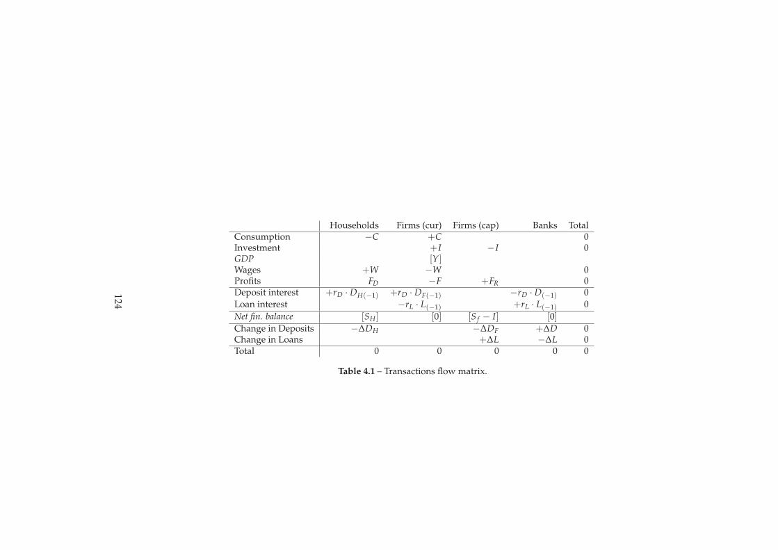
Households Firms (cur) Firms (cap) Banks TotalConsumption −C +C 0Investment +I −I 0GDP [Y]Wages +W −W 0Profits FD −F +FR 0Deposit interest +rD · DH(−1) +rD · DF(−1) −rD · D(−1) 0
Loan interest −rL · L(−1) +rL · L(−1) 0
Net fin. balance [SH ] [0] [S f − I] [0]Change in Deposits −∆DH −∆DF +∆D 0Change in Loans +∆L −∆L 0Total 0 0 0 0 0
Table 4.1 – Transactions flow matrix.
124
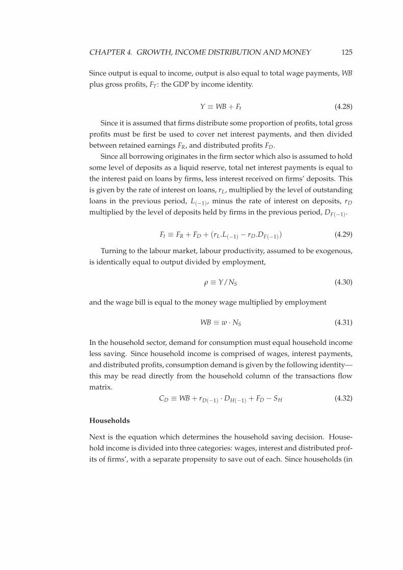
CHAPTER 4. GROWTH, INCOME DISTRIBUTION AND MONEY 125
Since output is equal to income, output is also equal to total wage payments, WB
plus gross profits, FT: the GDP by income identity.
Y ≡ WB+ Ft (4.28)
Since it is assumed that firms distribute some proportion of profits, total gross
profits must be first be used to cover net interest payments, and then divided
between retained earnings FR, and distributed profits FD.
Since all borrowing originates in the firm sector which also is assumed to hold
some level of deposits as a liquid reserve, total net interest payments is equal to
the interest paid on loans by firms, less interest received on firms’ deposits. This
is given by the rate of interest on loans, rL, multiplied by the level of outstanding
loans in the previous period, L(−1), minus the rate of interest on deposits, rD
multiplied by the level of deposits held by firms in the previous period, DF(−1).
Ft ≡ FR + FD + (rL.L(−1) − rD.DF(−1)) (4.29)
Turning to the labour market, labour productivity, assumed to be exogenous,
is identically equal to output divided by employment,
ρ ≡ Y/NS (4.30)
and the wage bill is equal to the money wage multiplied by employment
WB ≡ w · NS (4.31)
In the household sector, demand for consumption must equal household income
less saving. Since household income is comprised of wages, interest payments,
and distributed profits, consumption demand is given by the following identity—
this may be read directly from the household column of the transactions flow
matrix.
CD ≡ WB+ rD(−1) · DH(−1) + FD − SH (4.32)
Households
Next is the equation which determines the household saving decision. House-
hold income is divided into three categories: wages, interest and distributed prof-
its of firms’, with a separate propensity to save out of each. Since households (in
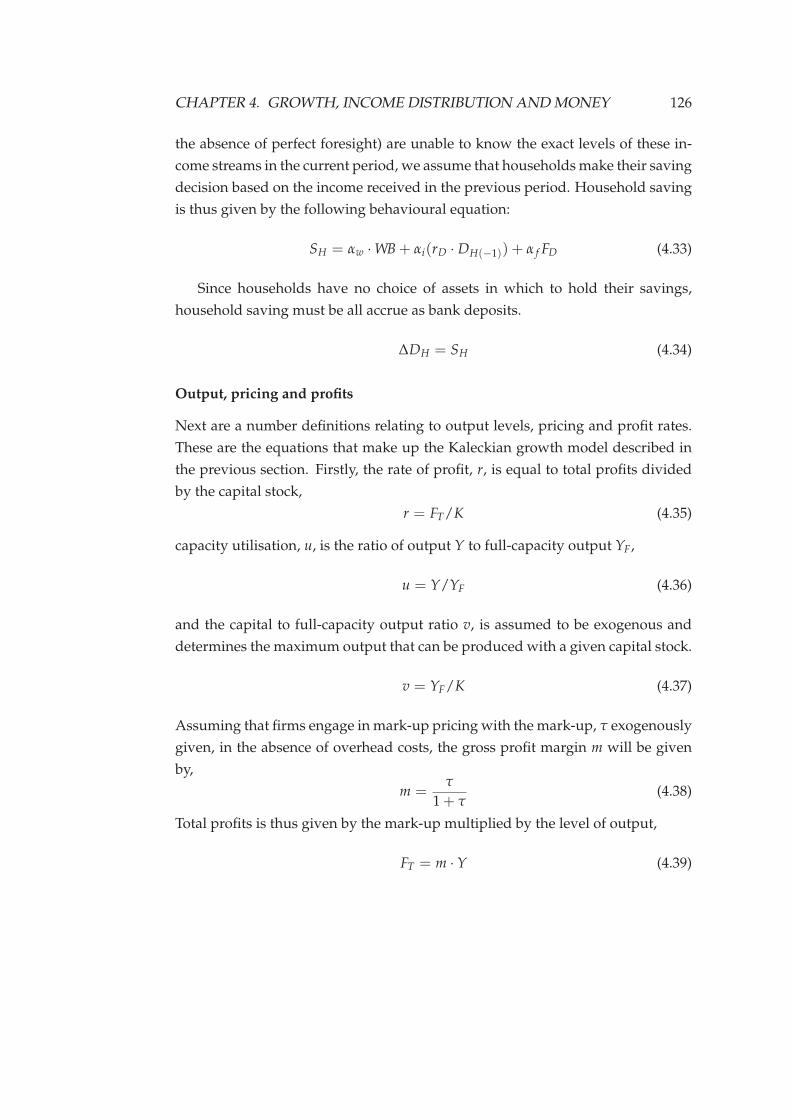
CHAPTER 4. GROWTH, INCOME DISTRIBUTION AND MONEY 126
the absence of perfect foresight) are unable to know the exact levels of these in-
come streams in the current period, we assume that households make their saving
decision based on the income received in the previous period. Household saving
is thus given by the following behavioural equation:
SH = αw ·WB+ αi(rD · DH(−1)) + α f FD (4.33)
Since households have no choice of assets in which to hold their savings,
household saving must be all accrue as bank deposits.
∆DH = SH (4.34)
Output, pricing and profits
Next are a number definitions relating to output levels, pricing and profit rates.
These are the equations that make up the Kaleckian growth model described in
the previous section. Firstly, the rate of profit, r, is equal to total profits divided
by the capital stock,
r = FT/K (4.35)
capacity utilisation, u, is the ratio of output Y to full-capacity output YF,
u = Y/YF (4.36)
and the capital to full-capacity output ratio v, is assumed to be exogenous and
determines the maximum output that can be produced with a given capital stock.
v = YF/K (4.37)
Assuming that firms engage in mark-up pricing with the mark-up, τ exogenously
given, in the absence of overhead costs, the gross profit margin m will be given
by,
m =τ
1 + τ(4.38)
Total profits is thus given by the mark-up multiplied by the level of output,
FT = m ·Y (4.39)
CHAPTER 4. GROWTH, INCOME DISTRIBUTION AND MONEY 127
Firms’ identities and investment decision
Next, the identities implied by the firm sector’s aggregated balance sheet, and
equations describing firms’ sector behaviour are introduced.
The proportion of earnings retained is given by a parameter λ, equivalent to
Kaldor and Pasinetti’s “savings propensity of capitalists”.
FR = λFT (4.40)
Now the factors that determine firms’ demand for capital investment are consid-
ered. The absolute level of investment demand in growth terms, as a proportion
of the previous level of the capital stock, can be written as follows,
ID = gI · K(−1) (4.41)
The desired rate of growth of the capital stock is given by the investment equation
of the system. As discussed above, this is one of the more controversial elements
of any growth model, with the form taken by the equation one of the key determi-
nants of the overall behaviour of the system. As a starting point, the investment
equation from the canonical Kaleckian growth model is used. As was the case for
the household saving equation, it is assumed that the decision is made upon the
basis of realised profits and capacity utilisation in the previous period.
gI = γ + γrr(−1) + γuu(−1) (4.42)
Assuming away capital depreciation, the change in the capital stock will be equal
to the supply of capital goods.
∆K = IS (4.43)
Next is the identity imposed by the flow budget constraint of the firm sector:
the sum of the column of the capital account of the firm in the transactions flow
matrix. This identity expresses the equality between any increase in demand for
bank loans from the firms sector and the sum of new investment that cannot be
funded out of retained earnings, plus any increase in desired holdings of liquid
assets.
∆LD ≡ (ID − FR) + ∆DF (4.44)
What remains is to determine the demand for banks deposits by the firm sector.
CHAPTER 4. GROWTH, INCOME DISTRIBUTION AND MONEY 128
As a first approximation, it is assumed that firms wish to hold some proportion
of current spending liabilities in the form of liquid assets. The spending commit-
ments of the firms sector, LB, are defined as the sum of wage payments and net
interest payments,
LB ≡ WB+ (rL · L(−1) − rD · DF(−1)) (4.45)
Then it is assumed that firms aim to hold a proportion θ of their previous-period
spending commitments as liquid assets, in this case bank deposits. When firms
find that they are holding a volume of deposits of a greater or lesser amount than
that desired, they will demand a new level of bank deposits that such that their
liquidity position will increase or decrease by a fraction β of the difference be-
tween the current and desired balances. Firms thus constantly adjust their hold-
ing of bank deposits in an attempt to maintain the desired liquidity ratio.
∆DF = β(DF − θLB(−1)) (4.46)
Money and Credit
The model is completed by specifying the identities implied by the balance sheet
of the banking sector, and the assumed behaviour of banks. Since the assumption
is initially made that banks passively accommodate all demand for loans, hold
no capital, and do not impose a spread between lending and borrowing rates of
interest, this section of the model is currently very simple. First, it is assumed that
banks accommodate all demands for loans.
∆LS = ∆LD (4.47)
Given that loans and deposits are the only financial instruments, the banks’ bal-
ance sheet identity required simply that any change in loans must be matched by
a change in deposits
∆LS = ∆DS (4.48)
There is a zero spread between the loan and deposit rates of interest,
rD = rL (4.49)
CHAPTER 4. GROWTH, INCOME DISTRIBUTION AND MONEY 129
And finally we assume an exogenous rate of interest on loans:
rL = rL (4.50)
The banking system is thus initially specified as an “inactive” sector which
passively intermediates between the firm and household sectors. However, the
current specification nonetheless allows for the incorporation of a money rate of
interest into our analysis which is determined entirely independently of the rate
of return on capital.
The stock-flow consistent accounting of the model ensures that the final equa-
tion of the model is redundant. This is the identity which expresses the equality
between changes in the supply and demand deposits.
∆DH + ∆DF = ∆D (4.51)
This equation must be dropped in order that the system is not over-determined.
Likewise, the identity that saving must equal investment,
gS = (FR + SH)/K(−1) = gI (4.52)
is not required, but will be found to be satisfied when the model is simulated.
4.6.3 Analysis using simulations
Household saving
The analysis proceeds by using numerical simulations to examine the dynamic
behaviour of the model. The first simulation will examine the effect of a change
in the saving behaviour of households. This will done by altering the parameters
of household saving function while simulating the model.
First, values must be selected for a number of other parameters: the capital
to full-capacity output ratio, v, the mark-up, τ, the saving propensity of capital-
ists, λ and the parameters of the investment function, γ, γu and γr. While the
model is not intended to produce empirically accurate projections, an attempt
will be made to use values that are feasible for the Chinese economy. A number
of attempts have been made to calculate the capital-output ratio of the Chinese
economy,13, with estimates ranging from around 1.0 to around 2.0, although some
13Eg. Bai et al. (2006), Geng & N’Diaye (2012), Sun et al. (2011)
CHAPTER 4. GROWTH, INCOME DISTRIBUTION AND MONEY 130
have claimed a value as high as 4.0 (REITI, 2012).14 For the simulations carried
out here a value of 2.8 for the capital-full-capacity output ratio is assumed. The
actual capital-output ratio will be determined by the model since it is assumed
that the economy to be operating at less than full capacity.15
A mark-up of 80 percent is assumed. Initially it is assumed that households
have an equal propensity to save of 0.25 percent out of wage income, interest
payments and distributed profits.16 Note that by including a specific parameter
for the propensity to save out of distributed profits into our model, we bring out
into the open the distinction between the decision made by firms on the level
of earnings to distribute, and the decisions made by households on whether or
not to consume those distributed earnings. This allows us to examine the case,
for instance, in which all distributed profits are saved, and thus end up being
returned to firms in the form of loans.
With such a configuration of parameters, and assuming initially a zero rate
of interest, the steady state of the model is one in which a growth rate of 11.7
percent is achieved by a rate of investment in output of 40 percent and a gross
profit margin (and thus profit share in national income) of 44 percent. Defining
the leverage ratio as the proportion of total capital expenditure financed by bank
loans, a leverage ratio of 44 percent is generated. Thus, around 44 percent of the
capital stock is indirectly ’owned’ by households.
In order to analyse the effect of changes in the propensity to save of house-
holds, the model is simulated starting from the steady state and the propensity to
save out of wage income is increased from 25 percent to 27 percent. The resulting
trajectories of the key variables of the model are shown in graphically in Figures
4.1–4.5
The effect on growth of the increase in the propensity to save out of wage
14The simple rule-of-thumb calculation method calculation for the incremental capital-output ra-tio is to divide the share of investment in output by the rate of growth. Taking the share in outputof investment as 40 percent and the rate of growth as 10 percent, this gives an ICOR of 4 for China.
15The behaviour of the model with respect to the capital-output ratio is somewhat counter-intuitive. In a full-employment long-run growth model, a higher capital-output ratio (or, to bemore precise, a higher incremental capital-output ratio), will result a lower rate of output growth,ceteris paribus. In the variable-capacity model presented here, a higher capital-output ratio resultsin higher steady-state long run growth, because a higher rate of capacity utilisation, and thus ahigher rate of profit and growth, is required for equilibrium between the ’aggregate demand’ and’profits-cost’ schedules.
16Although we have not incorporated a stock-market in our model, this does not preclude thedistribution of profits—in the case of state-owned corporations, distributed profits will accrue tothe state budget, and in the case of privately-owned corporations, profits may be distributed amongthe owners of those firms.
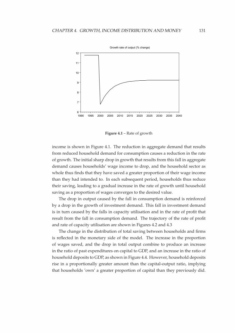
CHAPTER 4. GROWTH, INCOME DISTRIBUTION AND MONEY 131
6
7
8
9
10
11
12
1990 1995 2000 2005 2010 2015 2020 2025 2030 2035 2040
Growth rate of output (% change)
Figure 4.1 – Rate of growth
income is shown in Figure 4.1. The reduction in aggregate demand that results
from reduced household demand for consumption causes a reduction in the rate
of growth. The initial sharp drop in growth that results from this fall in aggregate
demand causes households’ wage income to drop, and the household sector as
whole thus finds that they have saved a greater proportion of their wage income
than they had intended to. In each subsequent period, households thus reduce
their saving, leading to a gradual increase in the rate of growth until household
saving as a proportion of wages converges to the desired value.
The drop in output caused by the fall in consumption demand is reinforced
by a drop in the growth of investment demand. This fall in investment demand
is in turn caused by the falls in capacity utilisation and in the rate of profit that
result from the fall in consumption demand. The trajectory of the rate of profit
and rate of capacity utilisation are shown in Figures 4.2 and 4.3
The change in the distribution of total saving between households and firms
is reflected in the monetary side of the model. The increase in the proportion
of wages saved, and the drop in total output combine to produce an increase
in the ratio of past expenditures on capital to GDP, and an increase in the ratio of
household deposits to GDP, as shown in Figure 4.4. However, household deposits
rise in a proportionally greater amount than the capital-output ratio, implying
that households ’own’ a greater proportion of capital than they previously did.
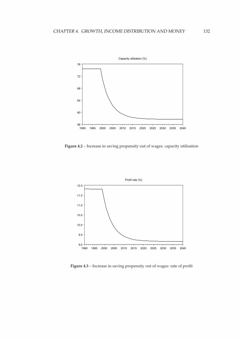
CHAPTER 4. GROWTH, INCOME DISTRIBUTION AND MONEY 132
56
60
64
68
72
76
1990 1995 2000 2005 2010 2015 2020 2025 2030 2035 2040
Capacity utilisation (%)
Figure 4.2 – Increase in saving propensity out of wages: capacity utilisation
9.0
9.5
10.0
10.5
11.0
11.5
12.0
1990 1995 2000 2005 2010 2015 2020 2025 2030 2035 2040
Profit rate (%)
Figure 4.3 – Increase in saving propensity out of wages: rate of profit
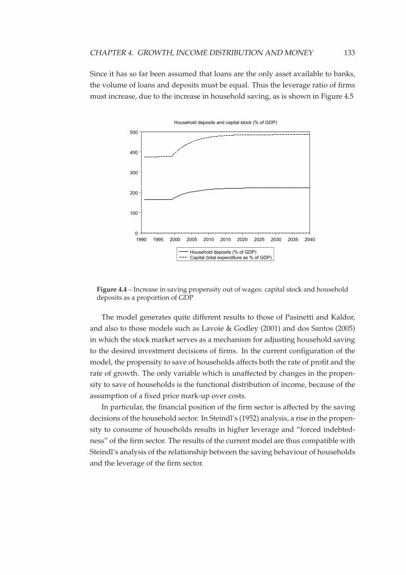
CHAPTER 4. GROWTH, INCOME DISTRIBUTION AND MONEY 133
Since it has so far been assumed that loans are the only asset available to banks,
the volume of loans and deposits must be equal. Thus the leverage ratio of firms
must increase, due to the increase in household saving, as is shown in Figure 4.5
0
100
200
300
400
500
1990 1995 2000 2005 2010 2015 2020 2025 2030 2035 2040
Household deposits (% of GDP)Capital (total expenditure as % of GDP)
Household deposits and capital stock (% of GDP)
Figure 4.4 – Increase in saving propensity out of wages: capital stock and householddeposits as a proportion of GDP
The model generates quite different results to those of Pasinetti and Kaldor,
and also to those models such as Lavoie & Godley (2001) and dos Santos (2005)
in which the stock market serves as a mechanism for adjusting household saving
to the desired investment decisions of firms. In the current configuration of the
model, the propensity to save of households affects both the rate of profit and the
rate of growth. The only variable which is unaffected by changes in the propen-
sity to save of households is the functional distribution of income, because of the
assumption of a fixed price mark-up over costs.
In particular, the financial position of the firm sector is affected by the saving
decisions of the household sector. In Steindl’s (1952) analysis, a rise in the propen-
sity to consume of households results in higher leverage and “forced indebted-
ness” of the firm sector. The results of the current model are thus compatible with
Steindl’s analysis of the relationship between the saving behaviour of households
and the leverage of the firm sector.
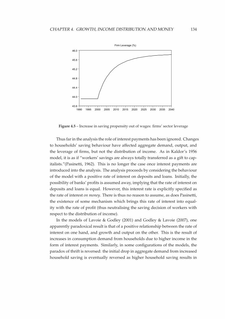
CHAPTER 4. GROWTH, INCOME DISTRIBUTION AND MONEY 134
43.6
44.0
44.4
44.8
45.2
45.6
46.0
1990 1995 2000 2005 2010 2015 2020 2025 2030 2035 2040
Firm Leverage (%)
Figure 4.5 – Increase in saving propensity out of wages: firms’ sector leverage
Thus far in the analysis the role of interest payments has been ignored. Changes
to households’ saving behaviour have affected aggregate demand, output, and
the leverage of firms, but not the distribution of income. As in Kaldor’s 1956
model, it is as if “workers’ savings are always totally transferred as a gift to cap-
italists.”(Pasinetti, 1962). This is no longer the case once interest payments are
introduced into the analysis. The analysis proceeds by considering the behaviour
of the model with a positive rate of interest on deposits and loans. Initially, the
possibility of banks’ profits is assumed away, implying that the rate of interest on
deposits and loans is equal. However, this interest rate is explicitly specified as
the rate of interest on money. There is thus no reason to assume, as does Pasinetti,
the existence of some mechanism which brings this rate of interest into equal-
ity with the rate of profit (thus neutralising the saving decision of workers with
respect to the distribution of income).
In the models of Lavoie & Godley (2001) and Godley & Lavoie (2007), one
apparently paradoxical result is that of a positive relationship between the rate of
interest on one hand, and growth and output on the other. This is the result of
increases in consumption demand from households due to higher income in the
form of interest payments. Similarly, in some configurations of the models, the
paradox of thrift is reversed: the initial drop in aggregate demand from increased
household saving is eventually reversed as higher household saving results in
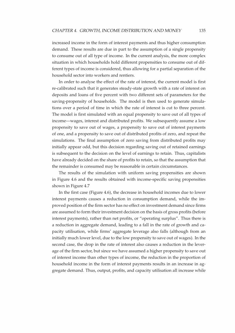
CHAPTER 4. GROWTH, INCOME DISTRIBUTION AND MONEY 135
increased income in the form of interest payments and thus higher consumption
demand. These results are due in part to the assumption of a single propensity
to consume out of all type of income. In the current analysis, the more complex
situation in which households hold different propensities to consume out of dif-
ferent types of income is considered, thus allowing for a partial separation of the
household sector into workers and rentiers.
In order to analyse the effect of the rate of interest, the current model is first
re-calibrated such that it generates steady-state growth with a rate of interest on
deposits and loans of five percent with two different sets of parameters for the
saving-propensity of households. The model is then used to generate simula-
tions over a period of time in which the rate of interest is cut to three percent.
The model is first simulated with an equal propensity to save out of all types of
income—wages, interest and distributed profits. We subsequently assume a low
propensity to save out of wages, a propensity to save out of interest payments
of one, and a propensity to save out of distributed profits of zero, and repeat the
simulations. The final assumption of zero saving from distributed profits may
initially appear odd, but this decision regarding saving out of retained earnings
is subsequent to the decision on the level of earnings to retain. Thus, capitalists
have already decided on the share of profits to retain, so that the assumption that
the remainder is consumed may be reasonable in certain circumstances.
The results of the simulation with uniform saving propensities are shown
in Figure 4.6 and the results obtained with income-specific saving propensities
shown in Figure 4.7
In the first case (Figure 4.6), the decrease in household incomes due to lower
interest payments causes a reduction in consumption demand, while the im-
proved position of the firm sector has no effect on investment demand since firms
are assumed to form their investment decision on the basis of gross profits (before
interest payments), rather than net profits, or “operating surplus”. Thus there is
a reduction in aggregate demand, leading to a fall in the rate of growth and ca-
pacity utilisation, while firms’ aggregate leverage also falls (although from an
initially much lower level, due to the low propensity to save out of wages). In the
second case, the drop in the rate of interest also causes a reduction in the lever-
age of the firm sector, but since we have assumed a higher propensity to save out
of interest income than other types of income, the reduction in the proportion of
household income in the form of interest payments results in an increase in ag-
gregate demand. Thus, output, profits, and capacity utilisation all increase while
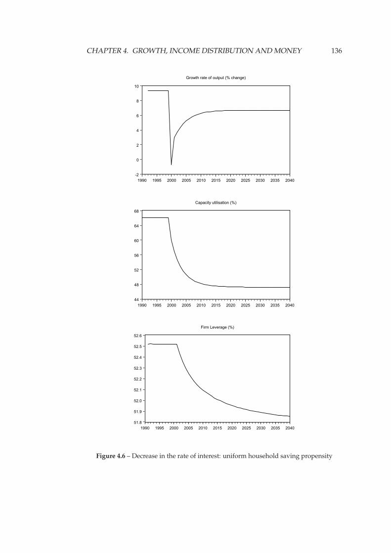
CHAPTER 4. GROWTH, INCOME DISTRIBUTION AND MONEY 136
-2
0
2
4
6
8
10
1990 1995 2000 2005 2010 2015 2020 2025 2030 2035 2040
Growth rate of output (% change)
44
48
52
56
60
64
68
1990 1995 2000 2005 2010 2015 2020 2025 2030 2035 2040
Capacity utilisation (%)
51.8
51.9
52.0
52.1
52.2
52.3
52.4
52.5
52.6
1990 1995 2000 2005 2010 2015 2020 2025 2030 2035 2040
Firm Leverage (%)
Figure 4.6 – Decrease in the rate of interest: uniform household saving propensity
CHAPTER 4. GROWTH, INCOME DISTRIBUTION AND MONEY 137
87.0
87.5
88.0
88.5
89.0
89.5
90.0
90.5
91.0
1990 1995 2000 2005 2010 2015 2020 2025 2030 2035 2040
Capacity utilisation (%)
7.50
7.75
8.00
8.25
8.50
8.75
9.00
9.25
9.50
1990 1995 2000 2005 2010 2015 2020 2025 2030 2035 2040
Firm Leverage (%)
0
2
4
6
8
10
12
1990 1995 2000 2005 2010 2015 2020 2025 2030 2035 2040
Interest income (% of GDP)
Profit income (% of GDP)
Household income (% of GDP)
Figure 4.7 – Decrease in the rate of interest: income-specific household savingpropensities
CHAPTER 4. GROWTH, INCOME DISTRIBUTION AND MONEY 138
firm leverage decreases.
Firms’ saving and over-capitalisation
The analysis up until this point has allowed for saving in the firm sector in the
form of retained earnings, but the assumption has been that all retained earnings
are directed towards investment. All accumulation in the firm sector thus takes
place in the form of capital assets.
One of the key innovations of the current approach is now introduced: that of
the possibility of firm over-capitalisation. The implications of firm over-capital-
isation in a stock-flow consistent system were discussed in detail in Section 3.4.
In particular, it was demonstrated that the cost to the firm sector as a whole of
maintaining a proportion of retained earnings in the form of liquid assets is given
by the margin between borrowing and lending rates on those assets. This inno-
vation is now incorporated into the current model by allowing firms to retain a
portion of their earnings in the form of bank deposits.
Equations 4.45 and 4.46 allow for the possibility of firm over-capitalisation in
the case that parameters Θ and β take non-negative values. Once potential for
firms’ to be over-capitalised is introduced into the model, a number of previous
definitions require re-examination, in particular that of the leverage ratio of the
firms’ sector. Whereas this was previously defined as the ratio of loans to capital
assets, the updated version defines it more broadly as the ratio of net liabilities to
non-liquid assets. Thus the leverage of the firm’s sector is now defined as follows:
LV = (LF − DF)/K (4.53)
It is likely that when firms find themselves to be over-leveraged or short on liq-
uidity they attempt to improve their position by cutting back on expenditures.
Thus, the Kaleckian investment function is augmented by including additional
terms for the leverage of the firm sector and the level of liquidity of the firm sec-
tor. We thus replace equation 4.42 with the following:
gI = γ + γrr(−1) + γuu(−1) + γlvLV(−1) + γlq(DF − θLB(−1)) (4.54)
These modifications result in a fully-specified stock-flow consistent macroe-
conomic model incorporating firm over-capitalisation, in which the firm sector
adjusts its expenditure behaviour in response to changes in its leverage and liq-
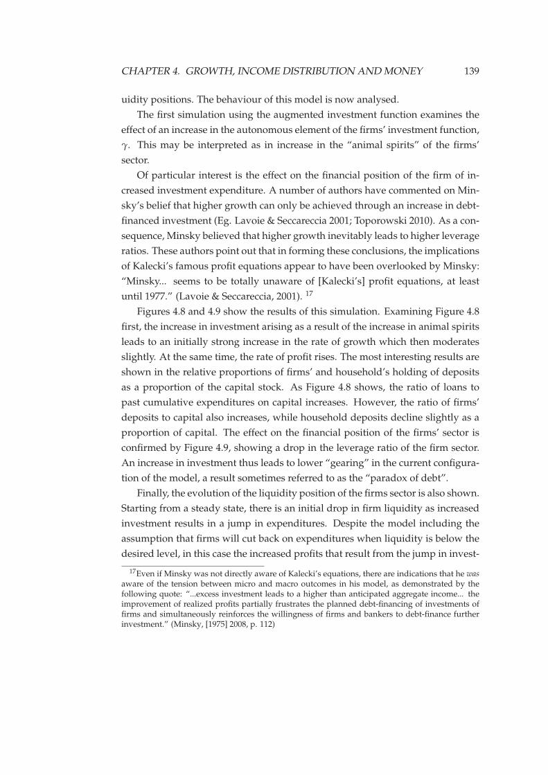
CHAPTER 4. GROWTH, INCOME DISTRIBUTION AND MONEY 139
uidity positions. The behaviour of this model is now analysed.
The first simulation using the augmented investment function examines the
effect of an increase in the autonomous element of the firms’ investment function,
γ. This may be interpreted as in increase in the “animal spirits” of the firms’
sector.
Of particular interest is the effect on the financial position of the firm of in-
creased investment expenditure. A number of authors have commented on Min-
sky’s belief that higher growth can only be achieved through an increase in debt-
financed investment (Eg. Lavoie & Seccareccia 2001; Toporowski 2010). As a con-
sequence, Minsky believed that higher growth inevitably leads to higher leverage
ratios. These authors point out that in forming these conclusions, the implications
of Kalecki’s famous profit equations appear to have been overlooked by Minsky:
“Minsky... seems to be totally unaware of [Kalecki’s] profit equations, at least
until 1977.” (Lavoie & Seccareccia, 2001). 17
Figures 4.8 and 4.9 show the results of this simulation. Examining Figure 4.8
first, the increase in investment arising as a result of the increase in animal spirits
leads to an initially strong increase in the rate of growth which then moderates
slightly. At the same time, the rate of profit rises. The most interesting results are
shown in the relative proportions of firms’ and household’s holding of deposits
as a proportion of the capital stock. As Figure 4.8 shows, the ratio of loans to
past cumulative expenditures on capital increases. However, the ratio of firms’
deposits to capital also increases, while household deposits decline slightly as a
proportion of capital. The effect on the financial position of the firms’ sector is
confirmed by Figure 4.9, showing a drop in the leverage ratio of the firm sector.
An increase in investment thus leads to lower “gearing” in the current configura-
tion of the model, a result sometimes referred to as the “paradox of debt”.
Finally, the evolution of the liquidity position of the firms sector is also shown.
Starting from a steady state, there is an initial drop in firm liquidity as increased
investment results in a jump in expenditures. Despite the model including the
assumption that firms will cut back on expenditures when liquidity is below the
desired level, in this case the increased profits that result from the jump in invest-
17Even if Minsky was not directly aware of Kalecki’s equations, there are indications that he wasaware of the tension between micro and macro outcomes in his model, as demonstrated by thefollowing quote: “...excess investment leads to a higher than anticipated aggregate income... theimprovement of realized profits partially frustrates the planned debt-financing of investments offirms and simultaneously reinforces the willingness of firms and bankers to debt-finance furtherinvestment.” (Minsky, [1975] 2008, p. 112)
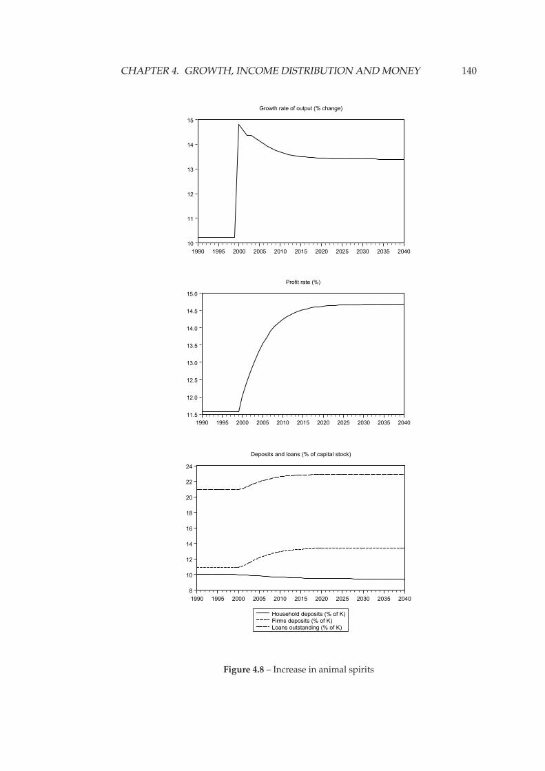
CHAPTER 4. GROWTH, INCOME DISTRIBUTION AND MONEY 140
10
11
12
13
14
15
1990 1995 2000 2005 2010 2015 2020 2025 2030 2035 2040
Growth rate of output (% change)
11.5
12.0
12.5
13.0
13.5
14.0
14.5
15.0
1990 1995 2000 2005 2010 2015 2020 2025 2030 2035 2040
Profit rate (%)
8
10
12
14
16
18
20
22
24
1990 1995 2000 2005 2010 2015 2020 2025 2030 2035 2040
Household deposits (% of K)
Firms deposits (% of K)
Loans outstanding (% of K)
Deposits and loans (% of capital stock)
Figure 4.8 – Increase in animal spirits
CHAPTER 4. GROWTH, INCOME DISTRIBUTION AND MONEY 141
9.4
9.5
9.6
9.7
9.8
9.9
10.0
10.1
1990 1995 2000 2005 2010 2015 2020 2025 2030 2035 2040
Firm Leverage (%)
99.0
99.5
100.0
100.5
101.0
101.5
1990 1995 2000 2005 2010 2015 2020 2025 2030 2035 2040
Firm Liquidity (% of desired liquidity)
Figure 4.9 – Increase in animal spirits (contd.)
ment more than offset the negative effects of decreased liquidity. Thus, firms are
able to recover their liquidity position in subsequent periods while growth and
the rate of profit remain above the initial level.
Adjustment of internal accumulation
The model is now used for an analysis of a number of aspects of Steindl’s analysis.
Steindl’s fundamental insight is that the adjustment of saving to a new rate of
investment growth will take place via different mechanisms in an oligopolistic
market in comparison to the situation in which competitive conditions prevail.
CHAPTER 4. GROWTH, INCOME DISTRIBUTION AND MONEY 142
Under either set of market conditions, an initial (exogenous) reduction in the
rate of accumulation requires that the growth of saving in the economy as a whole
be reduced to an equal rate, since ex-post, saving and investment must be equal.
Since “outside saving” is assumed to be relatively inelastic, the weight of this
adjustment falls disproportionately on “internal accumulation”, leading to an in-
evitable increase in the gearing ratio.
The mechanism by which internal accumulation adjusts to a level compatible
with the new rate of accumulation is central to Steindl’s analysis. The adjustment
of internal accumulation is the result of a fall in the rate of profit, which may arise
in one of two ways:
In considering the effects of a fall in the rate of growth of capital it has
rightly been assumed that the internal accumulation of funds will be
adjusted to it by a fall in the rate of profit... The fall in the rate of profit
will, of course, come about by a reduction of net profit margins... Now
the net profit margin can be reduced in two distinct ways: either by
a fall in the degree of utilisation of capacity; or else... if gross profit
margins are reduced... (p. 122)
Steindl defines a “profit function” which captures the relationship between
the gross rate of profit (net of interest payments), the rate of capacity utilisation,
u, and capital intensity, k:
e = F(u, k) (4.55)
This function contains an implicit “parameter” representing the gross mark-
up on costs, which in Steindl’s formulation is embedded in the functional form of
the equation. This profit function is thus essentially identical to the “profits-cost”
equation of the Kaleckian growth model:18
r =mu
v(4.56)
Given a profit function of this type, and assuming a fixed degree of capital
intensity, a reduction in the rate of profit may either result from of an increase in
excess capacity, or through a fall in the gross mark-up. Which of these two effects
18Steindl includes overhead labour in his formulation of the profits function, which is abstractedfrom in the formulation of the Kaleckian model presented here.
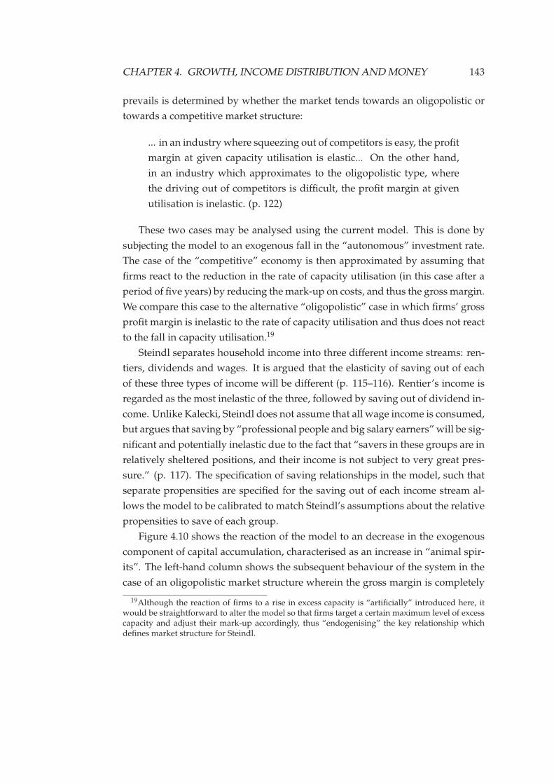
CHAPTER 4. GROWTH, INCOME DISTRIBUTION AND MONEY 143
prevails is determined by whether the market tends towards an oligopolistic or
towards a competitive market structure:
... in an industry where squeezing out of competitors is easy, the profit
margin at given capacity utilisation is elastic... On the other hand,
in an industry which approximates to the oligopolistic type, where
the driving out of competitors is difficult, the profit margin at given
utilisation is inelastic. (p. 122)
These two cases may be analysed using the current model. This is done by
subjecting the model to an exogenous fall in the “autonomous” investment rate.
The case of the “competitive” economy is then approximated by assuming that
firms react to the reduction in the rate of capacity utilisation (in this case after a
period of five years) by reducing the mark-up on costs, and thus the gross margin.
We compare this case to the alternative “oligopolistic” case in which firms’ gross
profit margin is inelastic to the rate of capacity utilisation and thus does not react
to the fall in capacity utilisation.19
Steindl separates household income into three different income streams: ren-
tiers, dividends and wages. It is argued that the elasticity of saving out of each
of these three types of income will be different (p. 115–116). Rentier’s income is
regarded as the most inelastic of the three, followed by saving out of dividend in-
come. Unlike Kalecki, Steindl does not assume that all wage income is consumed,
but argues that saving by “professional people and big salary earners” will be sig-
nificant and potentially inelastic due to the fact that “savers in these groups are in
relatively sheltered positions, and their income is not subject to very great pres-
sure.” (p. 117). The specification of saving relationships in the model, such that
separate propensities are specified for the saving out of each income stream al-
lows the model to be calibrated to match Steindl’s assumptions about the relative
propensities to save of each group.
Figure 4.10 shows the reaction of the model to an decrease in the exogenous
component of capital accumulation, characterised as an increase in “animal spir-
its”. The left-hand column shows the subsequent behaviour of the system in the
case of an oligopolistic market structure wherein the gross margin is completely
19Although the reaction of firms to a rise in excess capacity is “artificially” introduced here, itwould be straightforward to alter the model so that firms target a certain maximum level of excesscapacity and adjust their mark-up accordingly, thus “endogenising” the key relationship whichdefines market structure for Steindl.
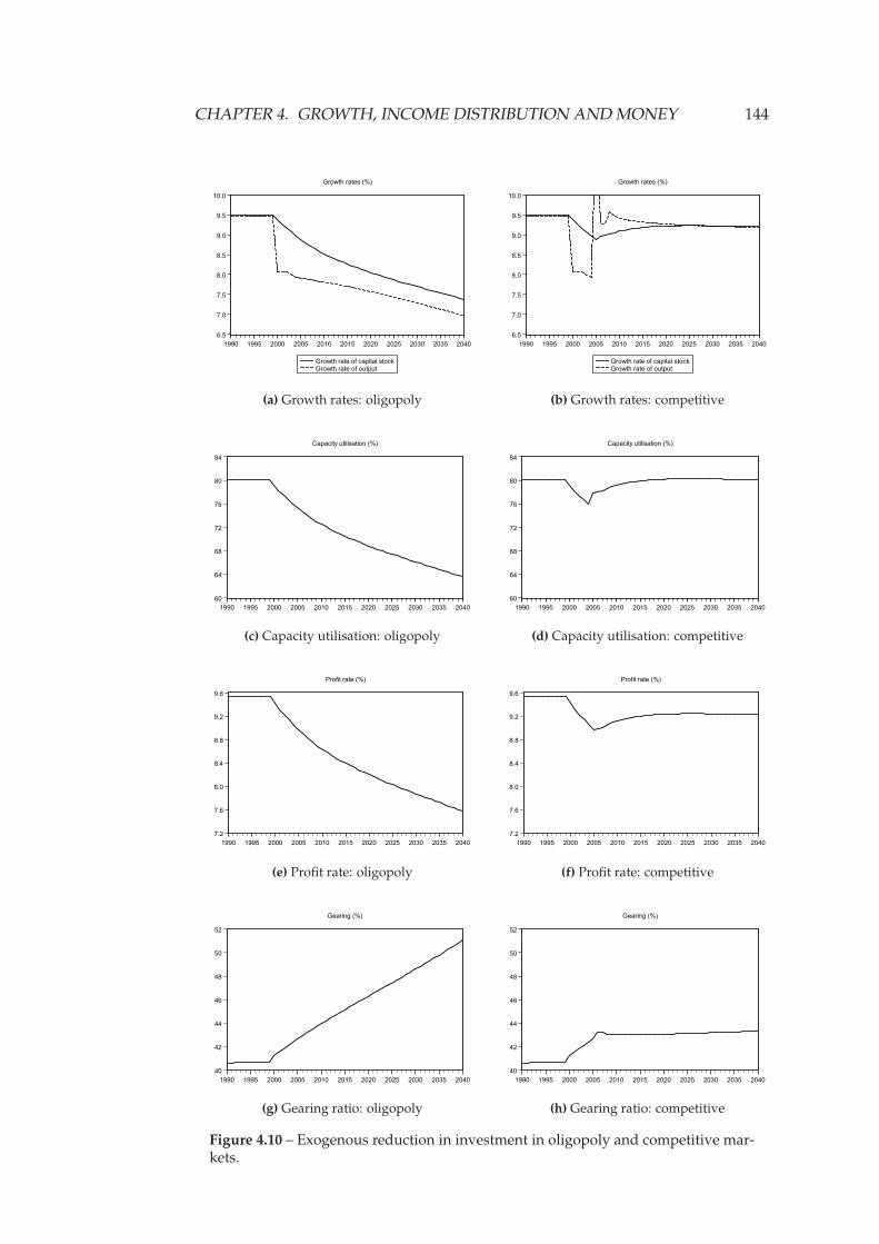
CHAPTER 4. GROWTH, INCOME DISTRIBUTION AND MONEY 144
6.5
7.0
7.5
8.0
8.5
9.0
9.5
10.0
1990 1995 2000 2005 2010 2015 2020 2025 2030 2035 2040
Growth rate of capital stockGrowth rate of output
Growth rates (%)
(a) Growth rates: oligopoly
6.5
7.0
7.5
8.0
8.5
9.0
9.5
10.0
1990 1995 2000 2005 2010 2015 2020 2025 2030 2035 2040
Growth rate of capital stockGrowth rate of output
Growth rates (%)
(b) Growth rates: competitive
60
64
68
72
76
80
84
1990 1995 2000 2005 2010 2015 2020 2025 2030 2035 2040
Capacity utilisation (%)
(c) Capacity utilisation: oligopoly
60
64
68
72
76
80
84
1990 1995 2000 2005 2010 2015 2020 2025 2030 2035 2040
Capacity utilisation (%)
(d) Capacity utilisation: competitive
7.2
7.6
8.0
8.4
8.8
9.2
9.6
1990 1995 2000 2005 2010 2015 2020 2025 2030 2035 2040
Profit rate (%)
(e) Profit rate: oligopoly
7.2
7.6
8.0
8.4
8.8
9.2
9.6
1990 1995 2000 2005 2010 2015 2020 2025 2030 2035 2040
Profit rate (%)
(f) Profit rate: competitive
40
42
44
46
48
50
52
1990 1995 2000 2005 2010 2015 2020 2025 2030 2035 2040
Gearing (%)
(g) Gearing ratio: oligopoly
40
42
44
46
48
50
52
1990 1995 2000 2005 2010 2015 2020 2025 2030 2035 2040
Gearing (%)
(h) Gearing ratio: competitive
Figure 4.10 – Exogenous reduction in investment in oligopoly and competitive mar-kets.
CHAPTER 4. GROWTH, INCOME DISTRIBUTION AND MONEY 145
inelastic to excess capacity. The right-hand column shows the system after an
identical shift to the investment function, but in this case it is assumed that sub-
sequently (in the period labelled 2005 although the numbering of the years holds
no significance) the gross margin of the firms sector is reduced in reaction to the
fall in capacity utilisation.
In both cases, the decrease in the rate of investment initially causes a reduction
in aggregate demand, reducing output growth and capacity utilisation. This in
turn reduces the rate of profit. The fall in the rate of profit and and the expansion
of excess capacity serve to reinforce the drop in accumulation. The relative inelas-
ticity of “outside saving” compared to retained earnings pushes up the gearing
ratio of the firm sector.
In the case of the “competitive” market the same initial trajectory is followed,
but firms are assumed to react to the increase in excess capacity by adjusting their
gross profit margin. This reduction in the profit margin generates an immediate
increase in output, by redistributing income to wage earners, who possess a lower
propensity to save. As well as increasing aggregate demand, this redistribution
of income from the high-saving-propensity firm sector to low-saving-propensity
wage earners reduces the rate of “outside saving” thus restoring the balance with
the rate of “internal accumulation”. Finally, in reducing the gross profit margin,
the adjustment of retained earnings to the lower rate of accumulation is able to
take place without requiring a reduction in the rate of capacity utilisation.
In the steady state obtained after the system has adjusted to the reduction in
the gross profit margin, capacity utilisation returns to its previous rate. The rate
of profit is reduced, due to a lower gross margin, as are the rate of accumulation
and output growth. The gearing ratio of firms stabilises at a higher, but constant
level.
The key distinction between the two cases is thus not only down to the values
of the various variables, but also in the relative speed of adjustment to a new
steady state. In the case in which profit margins are elastic, the system converges
to a new steady state fairly rapidly, whereas in the case of inelastic margins, the
self-reinforcing effects of a falling rate of profit and increasing excess capacity
result in a much slower rate of convergence. The results of the model thus closely
match Steindl’s analysis of the adjustment path under conditions of oligopoly:
The conclusion is that with the pattern of adjustment of the profit mar-
gin to be expected in modern times (owing to the predominance of
CHAPTER 4. GROWTH, INCOME DISTRIBUTION AND MONEY 146
oligopoly) a primary decline of capital accumulation will—via a re-
duced degree of capital utilisation—lead with a certain time lag to a
further reduction in capital accumulation. This cannot easily lead to
an equilibrium. The individual entrepreneur may think that by reduc-
ing investment he will cure his excess capacity, but in fact for industry
as a whole this strategy has only the effect of making excess capacity
even greater. The secondary fall in capital accumulation will again
produce a fall in the degree of utilisation, and after a certain time lag
this will reduce capital accumulation further. (1952, p. 123)
4.7 The distribution of profits
The analysis and simulations above treat the firms’ sector as a single entity. How-
ever, this overlooks important implications that arise out of the differences in
market structure across industries:
In reality the growth of oligopoly in a modern economy does not
affect all industries equally, and the inelasticity of profit margins at
given utilisation will therefore be very different in different industries.
(Steindl, 1952)
If the economy is composed of two sectors, an oligopolistic sector in which
profit margins are inelastic, and a competitive sector in which margins are elas-
tic, the dynamics of internal accumulation, capacity utilisation and sales growth
will differ in each. In particular, increasing concentration in the oligopolistic sec-
tor will not be felt only within that sector. The reduction in aggregate demand
and capacity utilisation, although arising from increasing concentration in the
oligopolistic sector, will feed through into a lower rate of growth in all sectors of
the economy.
This change in market structure will induce a reaction in both the competi-
tive and oligopolistic sectors, but an important distinction arises in the different
mechanisms by which adjustments to the reduction in aggregate demand take
place in each. In the competitive sector, it can be expected that cost-cutting will
take place, reducing profit margins and eliminating marginal firms, such that ca-
pacity utilisation will tend to remain steady. In contrast, in the oligopolistic sector
the inelasticity of profit margins will result in a reduction in the rate of capacity
utilisation.
CHAPTER 4. GROWTH, INCOME DISTRIBUTION AND MONEY 147
In such a situation, Steindl argues, the drop in the “internal accumulation”
of firms which is required to accommodate the reduction in the rate of growth
and output will take place disproportionately within the competitive firms sector.
Since firms within the competitive sector will reduce mark-ups over costs, the
profit margin of this sector as a whole adjust downwards. In turn, the rate of
profit in this sector will fall as a result of both reduced sales and reduced margins.
While the oligopolistic sector will also face reduced demand, the relative in-
elasticity of mark-ups will prevent a similar accommodating fall in the profit mar-
gin. Thus, the tendency towards stagnation that accompanies the increasing con-
centration in the oligopolistic sector is accompanied by a shift in the share of total
profits towards the oligopolistic sector. As a result there will be an accompanying
divergence of the relative indebtedness of the two sectors, such that the gearing
ratio of the competitive sector will rise relative to that of the oligopolistic sector.
It is possible however to imagine an inversion of the above dynamics. This
could arise if, for example, a significant share of the firms sector was to operate
in a way unlike that predicted either by the theory of competition or monopoly.
In particular, if a portion of the firms sector was strongly under the influence
of the government—such that the government could determine mark-up and in-
vestment behaviour—this bloc could exert a strong expansionary influence on the
dynamics of growth, profits and distribution.
This sector—despite having the monopoly power to impose significant mark-
ups—could operate such that mark-ups were at or below those levels found in the
competitive sector. Further, if the investment decisions of this sector were inelas-
tic with respect to the rate of excess capacity utilisation, the investment spending
of this sector would serve as a backstop against contraction.
In Steindl’s analysis, given a reduction in economic growth, the consequent
stagnation arises from the inelasticity of profit margins and the sensitivity to ex-
cess capacity in the cartelised sector. If the “state-cartel” sector were to respond
to a fall in growth not by scaling back investment expenditures, but by increasing
them, the consequent effects on the relative profits of the firms sectors would be
the opposite to that described by Steindl—the analysis of the “maldistribution of
profits” would have to be reversed.
In such a situation, rather than the investment expenditures of the compet-
itive sector accumulating as profits within the cartelised sector, the investment
expenditures of the state-cartel would accrue as profits in the competitive sector.
If the investment of this competitive sector were sensitive to profits, this could in
CHAPTER 4. GROWTH, INCOME DISTRIBUTION AND MONEY 148
turn spur further investment on the part of the competitive firms.
The effects on the aggregate balance sheets of the two sectors would likewise
be reversed. If the state-cartel were to expand investment in the face of reduced
aggregate demand—for example as a result of higher household saving or a drop
in export demand—it would need to finance these expenditures. Assuming that
this sector had good lines of credit with the banking system, such expenditures
could be financed by an expansion of bank credit. Some portion of the additional
deposits created would accumulate as saving in the household sector. Of the
new deposits which remained within circulation in the firms sector, a dispropor-
tionate amount would accrue as profits to private firms. In the limiting case in
which households consume their entire income (and assuming a closed system),
the increase in the deposits of the firms sector at the aggregate level would be
equal to the increase in loans. This would not imply, however, that the increase
of loans in each of the private and the state-cartel sectors would be hedged by an
equal increase in deposits: the increase in deposits in the private sector would be
greater than that in the state-cartel sector—while the opposite would be true of
bank loans.
The end result of loan-financed investment by the state-cartel sector being
used as an instrument to maintain the level of growth in the face of decreasing
aggregate demand would thus be increased gearing of the state-cartel sector rela-
tive to the private sector. Whether the absolute gearing ratio of the private sector
were higher or lower would depend on the parameters of the system. The expen-
ditures of the state-cartel system would thus operate in a similar way to deficit
expenditure by the government. However, the financial outcomes would differ.
In the case of deficit spending, if effective in increasing the level of growth the fi-
nancial position of the government would tend to improve automatically as out-
put increases, leading to higher tax revenues and lower social security spending.
In the case of a stimulus being implemented through the state-cartel firms, the
“maldistribution of profits” in favour of the private sector could be expected to
continue even in the face of higher growth, unless the state-cartel sector increased
its markup and profit margins and scaled back investment spending.
4.8 Conclusion
This chapter develops an integrated theoretical approach to investment and sav-
ing in the context of a pure credit stock-flow consisted framework. An original
CHAPTER 4. GROWTH, INCOME DISTRIBUTION AND MONEY 149
interpretation of Steindl’s theory of stagnation and “maldistribution of profits” is
introduced in which the main assumptions and results of the model are reversed.
The chapter gives an overview of alternatives to the neoclassical approach to
growth and income distribution that was discussed in Chapter 2. The theories
of the Cambridge UK scholars are discussed and contrasted with those of Steindl
and the post Keynesian Kaleckian growth model. The key difference between
these two approaches lies with the assumptions about capacity utilisation and
employment. The result of the assumption of excess capacity in the latter is that
the inverse relationship between the mark-up and the rate of growth that was a
feature of Cambridge model can be overcome.
A fully-specified monetary growth model is developed by embedding a mod-
ified version of the Kaleckian growth model within the pure credit stock flow sys-
tem of in Chapter 3. The behaviour of this model is analysed using simulations,
allowing the effects on model variables of changes in parameters to be tracked. In
particular, it is shown that it is possible for increases in investment expenditures
that lead to higher rates of growth to occur in conjunction with reduced leverage
of the firms sector and increased holdings of liquid assets by firms.
The use of the stock-flow consistent framework for this model allows for a the-
oretical analysis which is closely aligned with the data structures used in the em-
pirical work in the remainder of this thesis: since the transactions matrix on which
the model is based represents an abstract version of the flow-of-funds accounts—
around which the empirical analysis is based—the configurations of flows gener-
ated by the model will be qualitatively comparable with the empirical data.
This analysis is extended with reference to Steindl’s theory of the distribution
of “internal accumulation” of firms. It is argued that if a section of the firms sec-
tor operates in such a way that the rates of profit and capacity utilisation do not
affect the rate of investment, that those firms will see a reduction in profits and
an increase in leverage while the remained of the firms sector will benefit dis-
proportionately from the expenditures of the state-cartel sector. This theoretical
system will underpin the analysis of the relative profitability of the state-owned
and private firms sectors in the following chapter.

Part II
Evidence
150
Chapter 5
Credit and banking in China
5.1 Introduction
The current structure of the financial system in China is, above all, the result of
the path taken from a centrally planned system towards a market-based econ-
omy. The specific institutional forms that have arisen as a result of this transi-
tion are representative of a broader truth: financial structures are a function both
of their own history, and of the institutional history within which they evolve.
However, because modern marginalist theory is able to explain financial struc-
ture only in terms of the optimising behaviour of agents operating in imperfect
markets, most current empirical analyses of the function and behaviour of finan-
cial institutions can be characterised as attempts to isolate those features of fi-
nancial systems which deviate from some idealised universal structure. A more
persuasive view is that “the theory of saving and the rate of interest can—or at
any rate should—never be independent of the stage of development of financial
institutions” (Chick, 1986).
This chapter presents an overview of the development of China’s banking and
financial system in the context of the transition from central planning. The anal-
ysis shows how the current configuration of the system was formed through a
process of financial development over a period of structural change. The gradual
pace of transition from the mono-bank system served to minimise the loss of con-
fidence in the banking system that was experienced in other transition economies.
As a result, the volume of deposits within the banking system remained relatively
stable. Along with strict controls on outward capital movements, this enabled
the banking system to undergo the transition from a giro-clearing system for the
151
CHAPTER 5. CREDIT AND BANKING IN CHINA 152
planned economy to an set of institutions holding the key feature of a modern
banking system: creation of new liquidity through bank lending results in an
equivalent increase in the volume of deposits within the system, meaning that
loans create deposits.
Although the role and functions of the People’s Bank of China have changed
considerably over this period, it has retained its central position in the financial
system. Following the discussion of the transition period, and the associated
structural and regulatory reforms, this chapter provides an overview of current
operating procedures used by the People’s Bank of China in the implementation
of monetary policy. It is demonstrated that the focus of these procedures upon
quantitative measures of credit are the result of the evolution from a system in
which credit money operated as unit of account in the production of planned
quantities of of commodities. At the same time, a quantity-theoretic approach
was used to decide the volume of physical currency in circulation for the pur-
poses of consumer transactions demand.
Over the period of transition, the removal of the distinction between these two
monetary forms gave rise to a form of credit regulation in which monetary aggre-
gates became the primary targets of control. This approach has been reinforced
in recent years by the imposition of a closely-controlled exchange-rate regime,
requiring substantial intervention in the foreign exchange markets by the central
bank.
These operating procedures are contrasted with the recent New Consensus
approach to the conduct of monetary policy which regards such quantitative as-
pects of monetary control as secondary in importance to the role of interest rates.
This New Consensus view underlies much recent analysis of the Chinese finan-
cial system, resulting in a tendency to assume that all reforms are geared toward
achieving the final goal of a liberalised market-based inflation-targeting regime
under a flexible exchange rate. (eg. Laurens & Maino, 2007) This view regards
China’s banking system as inefficient and outmoded, giving rise to financial re-
pression and misallocation of resources (eg. Lardy, 2008).
The current financial structure may be regarded, instead, as an unstable point
along a transitional path in which reforms are implemented by the authorities
on a piecemeal basis in response to developments in the wider economic system.
By maintaining the ability to influence the allocation and quantity of bank credit
granted, in the form of policy loans, and the price of that credit, in the form of
centrally-administered interest rates, the state has used the banking system to
CHAPTER 5. CREDIT AND BANKING IN CHINA 153
play a significant developmental role in generating the high rates of growth ex-
perienced over the transition period.
The relationships between the state, the banking system and the investment
decisions of firms are complex, but the dynamics of this nexus may be charac-
terised as follows. In maintaining long-term relationships with both the state and
the banking system, the Chinese corporate structure shares characteristics with
the Japanese and other Eastern economic systems. These non-market “rigidi-
ties” would be viewed as leading to inefficiencies under standard marginalist eco-
nomic theory. The long-term orientation of firms may, however, be conducive to
productivity-raising and technology-enhancing effects in the presence of strong
aggregate demand. In the context of a credit-investment-led growth path, the role
of firms becomes a dual one, since the investment expenditure of firms provides a
key component of aggregate demand, while demand-induced manufacturing of
investment goods may result to dynamic productivity increases, in line with the
Kaldor-Verdoorn analysis. By creating the purchasing power required for these
investment outlays, and in allowing for the separation of investment and saving
decisions, the banking system plays a key role in the reproduction of this credit-
investment-growth process.
This dynamic growth process has thus far been sustained without being de-
railed by serious crises. While periods of fast credit expansion as a result of policy
lending and soft-budget-constraint behaviour on the part of state banks led to in-
flationary pressures late 1980s and early 1990s, and eventually to the build-up of
non-performing loans, inflation was subsequently brought under control with-
out major disruption to growth. Bad assets were gradually shifted from balance
sheets, using public money to cover much of the costs of the associated recap-
italisation of banks (Ma, 2006). Moreover, the separation of banking and capi-
tal markets, along with the underdevelopment of the non-bank financial system
have so far precluded serious speculative financial crises of the type experienced
in more financial advanced economies. Nonetheless, the fact that China has so
far avoided financial crisis is viewed, from the point of view of most mainstream
economists as a “no more than an accidental outcome” (Ju & Lo, 2012, p. 385)
While the current institutional framework, in the form of the state-bank-firm
nexus, has avoided major systemic crises, associated with the transition from cen-
tral planning to a more liberalised market-based banking and financial system
is a process of endogenous financial development in which privately-generated
credit claims come to represent a rising share of total credit. This phenomenon is
CHAPTER 5. CREDIT AND BANKING IN CHINA 154
illustrated by the growing role of informal and unregulated financial intermedia-
tion (Chu et al., 2010; Tsai, 2002). The diminishing share of output accounted for
by the large state-owned organisations that receive the bulk of bank credit, and
the increasing significance of retained earnings in the funding of investment will
make control of monetary aggregates increasingly difficult. Thus, with the con-
tinued implementation of liberalisation reforms, in line with standard economic
doctrines, the potential for financial crises may increase.
5.2 Transition
5.2.1 Monetary reform
Under the system of economic planning that was in place in China from the be-
ginning of Communist rule in 1948, until 1978 when central controls began to
be dismantled, there existed two distinct monetary circuits: a credit circuit and a
cash circuit. All investment and purchases of inventory by firms were undertaken
through the transfer of credit money. Fixed capital investment was financed by
transfers directly from the state budget in the form of non-repayable grants, al-
located in accordance with the physical plan for production and investment laid
down by the State Council. Working capital requirements were paid for by trans-
fer between the accounts of corporations: upon receipt of a delivery of capital
goods, the balance of the account of the firm receiving the goods would be deb-
ited for an amount calculated using the administratively-set price for the goods,
and a corresponding credit would be applied to the account of the producing
firm. There was therefore no circulation of currency in the productive sector of
the economy. All payments took the form of accounting operations: adjustments
to the balance sheets of transacting parties. The remainder of the economy op-
erated on the basis of transactions conducted using cash payments. These trans-
actions consisted of payments of wages, household purchases of consumption
goods, payment of taxes and personal savings.
These two forms of money were not freely convertible, although mechanisms
existed through which conversion would occur.1 Administrative control of the
two circuits was assumed through the application of three plans: the Cash Plan,
the Credit Plan and the State Budget. These were formulated in the following
1For example, firms often exceeded their quotas for the employment of workers, requiring anadditional cash allocation, which in turn would require increased allowances from the state budgetto accommodate the additional expenditure.
CHAPTER 5. CREDIT AND BANKING IN CHINA 155
manner: first, physical quantities for fixed capital investment and the production
of consumption goods would be decided by the State Council. Budget allocations
for firms would then be decided through an iterative process whereby details of
the target quantities for production and investment would be provided to local
branches of the central bank. These branches would then submit proposed bud-
gets to the central authorities who would compile final targets for the quantities
of credit and cash required to fulfil the physical plan (Girardin, 1997).
This system was similar in form to the approach taken by the Soviet Union
and other socialist countries such as Poland, with the key feature being the sepa-
ration of money for consumption and money for investment. Under a system of
this type, the characteristics and functions of money and credit are quite different
to those of a market economy with a developed banking system. The productive
sector effectively operates as a “pure credit” economy with all transactions tak-
ing place as balance sheet transfers. Fiat money performs no role as a store of
value or means of transaction but operates solely as the numeraire. Under such
conditions, with money operating as a pure unit of account, “notions such as
market-determined interest rates, liquidity preference, cost of funds, collateral,
and credit-worthiness” cease to hold any relevance (Dow et al., 2008).
The limited convertibility between the two forms of money reduces the active
status of cash. In a bank-based capitalist economy, cash forms one component
of high-powered money: those liabilities of the state to which all other forms of
money and credit are eventual claims. With the connection to productive invest-
ment severed, and with prices and wages fixed by the government, cash plays a
passive role in facilitating the purchase of consumption goods, as well as provid-
ing households with a means of saving.
The Cash Plan of the Chinese system was formulated with the intention of
controlling inflation through the maintenance of a fixed relationship between the
quantity of currency in circulation and some measure of sales of goods to house-
holds. The approach taken was therefore implicitly based on the quantity theory
of money in the formulation presented by Fisher (Guo, 2002; Tam, 1995b). This
approach was, to a large extent, retained after 1978 when the mono-bank system
began to be dismantled and China started the process of transition to commercial
banking and the use of indirect instruments of monetary policy.
During the process of transition, the barrier between the two monetary cir-
cuits was removed. The requirement for corporations to perform all transactions
using credit money was dropped, allowing for the use of cash within the pro-
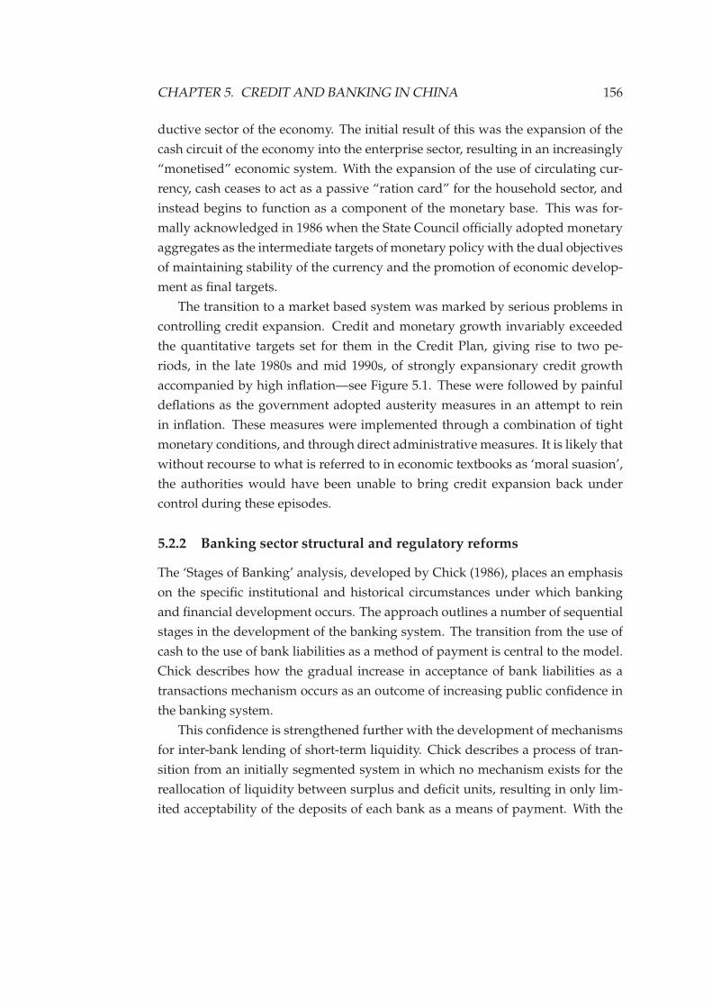
CHAPTER 5. CREDIT AND BANKING IN CHINA 156
ductive sector of the economy. The initial result of this was the expansion of the
cash circuit of the economy into the enterprise sector, resulting in an increasingly
“monetised” economic system. With the expansion of the use of circulating cur-
rency, cash ceases to act as a passive “ration card” for the household sector, and
instead begins to function as a component of the monetary base. This was for-
mally acknowledged in 1986 when the State Council officially adopted monetary
aggregates as the intermediate targets of monetary policy with the dual objectives
of maintaining stability of the currency and the promotion of economic develop-
ment as final targets.
The transition to a market based system was marked by serious problems in
controlling credit expansion. Credit and monetary growth invariably exceeded
the quantitative targets set for them in the Credit Plan, giving rise to two pe-
riods, in the late 1980s and mid 1990s, of strongly expansionary credit growth
accompanied by high inflation—see Figure 5.1. These were followed by painful
deflations as the government adopted austerity measures in an attempt to rein
in inflation. These measures were implemented through a combination of tight
monetary conditions, and through direct administrative measures. It is likely that
without recourse to what is referred to in economic textbooks as ‘moral suasion’,
the authorities would have been unable to bring credit expansion back under
control during these episodes.
5.2.2 Banking sector structural and regulatory reforms
The ‘Stages of Banking’ analysis, developed by Chick (1986), places an emphasis
on the specific institutional and historical circumstances under which banking
and financial development occurs. The approach outlines a number of sequential
stages in the development of the banking system. The transition from the use of
cash to the use of bank liabilities as a method of payment is central to the model.
Chick describes how the gradual increase in acceptance of bank liabilities as a
transactions mechanism occurs as an outcome of increasing public confidence in
the banking system.
This confidence is strengthened further with the development of mechanisms
for inter-bank lending of short-term liquidity. Chick describes a process of tran-
sition from an initially segmented system in which no mechanism exists for the
reallocation of liquidity between surplus and deficit units, resulting in only lim-
ited acceptability of the deposits of each bank as a means of payment. With the
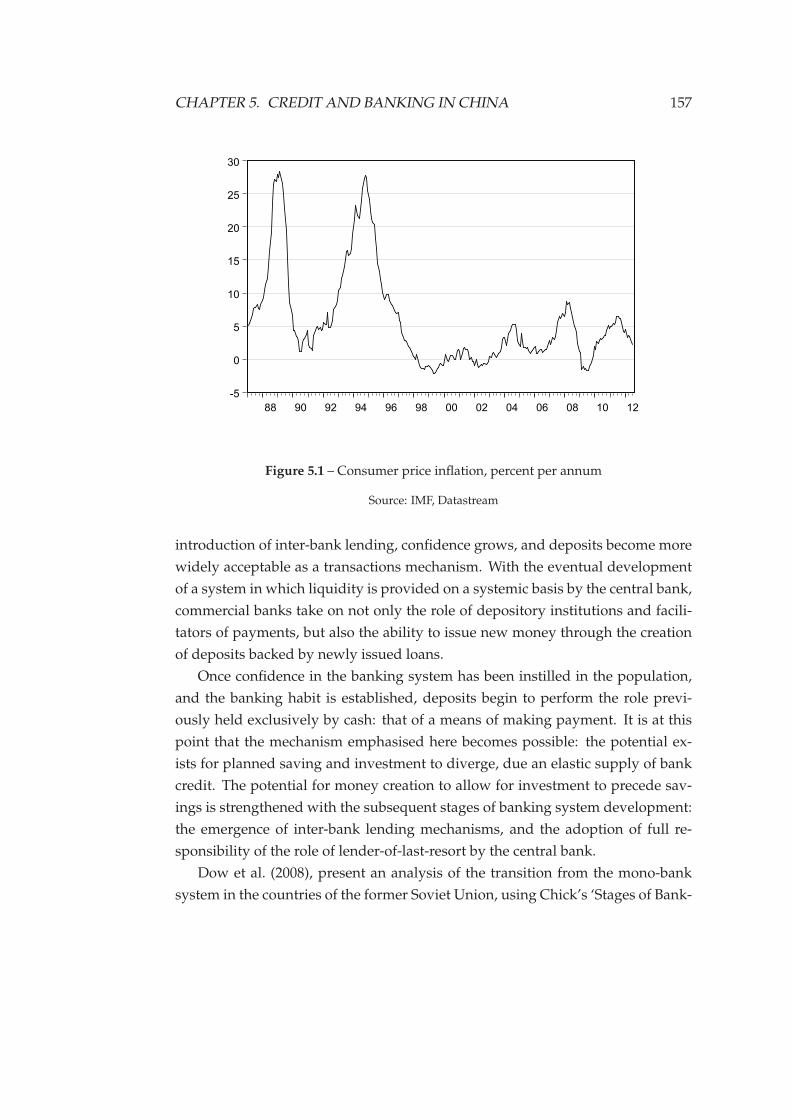
CHAPTER 5. CREDIT AND BANKING IN CHINA 157
-5
0
5
10
15
20
25
30
88 90 92 94 96 98 00 02 04 06 08 10 12
Figure 5.1 – Consumer price inflation, percent per annum
Source: IMF, Datastream
introduction of inter-bank lending, confidence grows, and deposits become more
widely acceptable as a transactions mechanism. With the eventual development
of a system in which liquidity is provided on a systemic basis by the central bank,
commercial banks take on not only the role of depository institutions and facili-
tators of payments, but also the ability to issue new money through the creation
of deposits backed by newly issued loans.
Once confidence in the banking system has been instilled in the population,
and the banking habit is established, deposits begin to perform the role previ-
ously held exclusively by cash: that of a means of making payment. It is at this
point that the mechanism emphasised here becomes possible: the potential ex-
ists for planned saving and investment to diverge, due an elastic supply of bank
credit. The potential for money creation to allow for investment to precede sav-
ings is strengthened with the subsequent stages of banking system development:
the emergence of inter-bank lending mechanisms, and the adoption of full re-
sponsibility of the role of lender-of-last-resort by the central bank.
Dow et al. (2008), present an analysis of the transition from the mono-bank
system in the countries of the former Soviet Union, using Chick’s ‘Stages of Bank-

CHAPTER 5. CREDIT AND BANKING IN CHINA 158
ing’ as a frame of reference. They show that the breakup of the mono-bank system
in these countries was initially accompanied by a sharp increase in the use of cash
as shown by an increase in the cash to deposits ratio and a corresponding decrease
in the deposits as a share of GDP. It is argued that the breakdown of confidence
in the banking system that accompanied the transition was in large part a result
of the speed of reforms.2 Dow et al. argue that the policies implemented during
the reforms period in the countries of the former Soviet were formulated without
consideration of the fact that the confidence in the banking systems that allows
for the eventual use of deposits as a means of payment has historically taken root
as part of gradual process over a period of time.
While the transition to a market-based system was of a piecemeal nature in
China, measures of cash usage increased significantly in the years following the
introduction of market reforms to the banking system. These increases were of a
lesser magnitude than those seen in the countries of the former Soviet Union, sug-
gesting that confidence in the banking system did not suffer to the same degree.
The increasing degree of monetisation of the economy was reflected in high rates
of growth of both base money and broader monetary aggregates. This increase in
the money supply in the period after the initial reforms was not at first accompa-
nied by high rates of inflation. Over this period, rates of monetary growth were
in fact higher than the sum of inflation and GDP growth (Girardin, 1997). Even
with the onset of austerity measures in the late 1980s to combat rising inflation,
the rate of increase of M2 remained above 25%, even as inflation was brought
back down under 5%.
Under central planning, all banks effectively operate as branches of the cen-
tral bank, serving primarily as cashiers for the mono-bank system. Starting in
1978, a series of reforms were enacted with the intention of devolving respon-
sibility for lending and deposit-taking from the central bank to newly created
state-owned commercial banks. These reforms took place alongside the introduc-
tion of a ‘dual-track’ pricing system, which allowed firms to begin selling, on the
free market, anything produced after fulfilling their planned quota.3 The inten-
tion of these reforms was to create a two-tier banking system. This would consist
of commercial banks, capable of making autonomous lending decisions based on
2Sachs & Woo (1997) argue that the gradualist approach taken in China would not have beenpossible in the former Soviet Union countries, due to differences in economic structure at the timeof transition
3This dual track system continued until around 1990, when the government began to allowprices to be fully market determined. (Mu, 2007)
CHAPTER 5. CREDIT AND BANKING IN CHINA 159
evaluations of the credit-worthiness of borrowers and the viability of investment
projects, leaving the central bank the role of supervision and liquidity provision.
Over the period 1979–1984, four specialised state-owned commercial banks
(SOCBs) were separated from the PBC and other state ministries and each given
responsibility for the provision of credit to enterprises in a specific sector of the
economy.4 The creation of these “Big Four” banks was intended to transfer com-
mercial activities away from the PBC, leaving the central bank the role of credit
provision to cover the shortfall between deposits and loans, and to cover short-
term and seasonal needs. Initially, however, the four new state-owned commer-
cial banks continued to operate essentially as arms of the People’s Bank. All de-
posits were initially required to be surrendered to the PBC, while credit would
be allocated to the banking system according to the Credit Plan. Between 1979
and 1984, gradual reforms were introduced, allowing the SOCBs to lend based
on the level of deposits held, and to allow the lending of excess reserves directly
between banks. (Wu, 1995, pp. 86–87) From 1985, the restrictions on the sectors
in which these banks were allowed to operate were relaxed. (Berger et al., 2009)
From 1985, another layer of financial institutions emerged, in the form of joint-
stock banks and regional banks, resulting in a three-tier banking system. The
gradual liberalisation of the banking system continued, alongside the introduc-
tion of more indirect regulatory controls, such as reserve requirements.
In practice these institutions found it impossible to restrain the growth of
credit, and in particular to control the credit extended to the large state-owned
enterprises that were the backbone of the Chinese economy. This was in part a
result of policy lending by state banks in excess of the Credit Plan. What tended
to happen in such situations was that any banks which found themselves with
a shortfall of funds would receive loans from the PBC in order to make up the
difference. According to Girardin, the PBC officially recognised the discrepancy
between the credit plan and actual lending:
The PBC even made known the imbalance in the credit plan. In official
Chinese terms, the plan had a gap. This term refers to the amount
of bank loans, usually for working-capital investment, recognised as
necessary but not included in planned credit growth. The gap was
quite large, usually over 10 per cent of the credit plan and 22 per cent
4The Agricultural Bank of China, the Bank of China and People’s Construction Bank of Chinawere established in 1979 and the Industrial and Commercial Bank of China in 1984
CHAPTER 5. CREDIT AND BANKING IN CHINA 160
of the credit plan on average between 1986 and 1990. (1997, p. 70)
During this transition period the PBC continued to rely heavily on adminis-
trative measures to control credit. This was possible due to the close relation-
ships between the PBC and the state commercial banks that existed as a legacy
of the mono-bank system. Nonetheless, with liberalisation, the use of indirect
instruments took on an increasing role. The PBC experimented with a number
of different instruments over this period: Xie (2004, p. 19) lists fourteen different
monetary policy instruments introduced since 1983. Some have since been aban-
doned, either temporarily or permanently, while the use of others has been been
retained.
The re-discounting of commercial bills was introduced by the PBC in 1986,
in response to problems caused by the mechanism by which banks were used
to collect trade debts. The clearing system in operation at the time was config-
ured in such a way that banks were responsible for the collection of outstanding
debts once delivery for goods had been made. The result of this was that banks
would often end up bailing out the creditor in situations where the company re-
ceiving goods was unable to pay. (Holz, 1992, pp 82–83)5 The introduction of re-
discounting by the PBC, and the legitimisation of the discounting of commercial
bills by banks was introduced as a way of allowing the banking system to ac-
commodate overdue trade credit, and prevent the “chain reaction” breakdowns
in production that can occur with enterprise defaults.
The tentative first steps towards a unified system of decentralised inter-bank
liquidity management took place while the Credit Plan was still operational. An
informal system of inter-bank lending had been in operation since the 1980s but
the system was thrown into disorder and progress on reforms halted by the infla-
tionary episodes experienced in the late 1980s and early 1990s when inter-bank
lending was increasingly used for illegitimate purposes. Girardin (1997) argues
that the system of inter-bank lending acted as a mechanism for side-stepping re-
gional credit ceilings. Although the inter-bank system was intended as a way for
banks to cover short-term liquidity needs, banks with excess reserves used inter-
bank lending to fund investment in other regions, thus breaching the limits set in
the Credit Plan. Although, in principle, the maximum allowable maturity of loans
5Similar problems occurred under the period of central planning in Poland under a system ofautomatic crediting whereby firms would send their invoices directly to banks rather than counter-part firms. These invoices would be paid automatically, regardless of whether the purchasing firmhad available credit. (Podolsky, 1973)
CHAPTER 5. CREDIT AND BANKING IN CHINA 161
was 7 days, in 1988 around 70% of loans between banks were of maturities of over
one month, suggesting that these loans were being used for purposes other than
short-term liquidity management. These problems continued into the early 1990s
during which time the inter-bank market was also used as a source of long-term
funds for speculative investment in real-estate (Guo, 2002; Duo, 2002).6 In ad-
dition to the restoration of inter-bank markets, this period also saw the gradual
introduction and spread of non-bank financial intermediation, in particular the
establishment of the Shanghai and Shenzen stock markets in 1990.
The excessive credit growth during this period is often characterised as result-
ing from soft budget constraint behaviour on the part of state banks. “Soft bud-
get constraint” refers to the prediction that institutions, and in particular banks,
which are not under private ownership will have an inherent expansionary ten-
dency, regardless of their capacity to finance such expansions. This arises be-
cause these institutions operate under the assumption that any financial shortfall
they may encounter will be made good using public resources (Kornai, 1979). In
this view, the sequence of “stop-go” cycles which occurred during the late 1980s
and 1990s are result of the interaction between the expansionary and inflationary
tendencies arising from excessive bank lending, and opposing contractionary re-
sponses from the state in the form of centrally imposed austerity. It is argued by
Lo et al. (2011) that this takes too narrow a view of the respective roles of banks
and the state: such a view overlooks, for example, the role played by state banks
in the late 1990s in acting strongly to constrain credit growth, and the effects of
government policy in generating expansionary impulses, for example in the pe-
riod following the 2008 global financial crisis.
Following the inflationary outburst of 1988, austerity measures were imposed,
remaining in place until around 1990 when easing began once more. Inflation re-
mained moderate until 1993 when credit extension once again ran out of control,
leading to the introduction of further austerity measures from the summer of
1993 through 1995. These initially took the form of restrictive policies on banks,
requiring lending to be withdrawn and interest rates to be raised. Subsequently
the emphasis switched to more direct administrative measures, aimed at bringing
down the rate of investment growth.
This period saw the formal adoption of market socialism by the State Council
6McKinnon & Schnabl (2009) argue that the failure to control credit during this period was aresult of China’s floating exchange rate. Once the currency was pegged to the dollar in 1997, thenominal anchor provided the credibility required to rein in inflation.
CHAPTER 5. CREDIT AND BANKING IN CHINA 162
in 1993, and the introduction of a further series of reforms of the banking system.
The most significant of these was the creation in 1994 of three state policy banks
(Wei, 1999), which were to take over the non-commercial roles of the “Big Four”
banks—issuing state-directed credit to SOEs—with the intention of further deep-
ening the commercialisation of lending by the state-owned commercial banks.7
In 1995, the role of the PBC as central bank was formally established by the Law
of the People’s Bank of China, as was the status of the commercial banks by the
Law of the Commercial Banks, which directed these banks towards commercial
lending instead of policy lending, and required these banks to take responsibility
for their own profits and losses.
The expansionary periods of the late 1980s and early 1990s resulted in a build-
up of bad debt on the books of the commercial banks. To deal with this problem,
a programme of recapitalisation was initiated, with non-performing loans gradu-
ally transfered to the balance sheets of newly established asset-management cor-
porations. This programme was highly successful, with NPLs falling from 30%
in 2001 to 6% in 2007. The majority of the remaining NPLs were left on the books
of the Agricultural Bank of China, which finally underwent a 130 billion yuan
recapitalisation in 2008. Over this period, the PBC continued to move towards
a more regulatory approach to control over the banks, with the NPL problems
resulting in a focus on capital adequacy requirements.
In 1996, the inter-bank system was unified from a collection of segmented re-
gional institutions into a national system based on electronic trading of reserves,
(the CHIBOR market) and base money was explicitly specified as the operational
target of monetary policy (Green, 2005). In 1998 the Credit Plan was switched
from being, at least in theory, a binding constraint on firms, to being “indica-
tive” in form. This took the form of targets announced by the PBC for both broad
money and the credit growth.8
In 2001, China’s formal entry into the WTO prompted a further sequence of
liberalisation reforms, in particular with respect to the foreign ownership of Chi-
nese banks. In 2003, the China Banking Regulatory Commission (CBRC) was es-
tablished, with the role of performing oversight of reforms and regulations. Soon
after its inception, the CBRC updated the rules on foreign ownership, such that
7These newly created policy banks were the National Development Bank, the Export-ImportBank and the Agricultural Development Bank.
8These targets were announced up until 2008 but as a result of the stimulus introduced followingthe collapse of Lehman Brothers, the 2008 targets were cancelled. No targets were announced in2009, but a broad money target was reintroduced in 2010 (Cassola & Porter, 2011).
CHAPTER 5. CREDIT AND BANKING IN CHINA 163
individual foreign investors could take stakes of up to 20% in Chinese banks, with
a maximum of 25% total foreign ownership. In 2004, the “Big Four” commercial
banks were converted to joint stock companies, with shares listed on both domes-
tic and foreign stock markets. Foreign banks have subsequently taken significant
states in the “Big Four” commercial banks.
Subsequent to China’s WTO entry, during the period from 2002 until the end
of 2006, a transitional regime was put in place during which the restrictions on
foreign control of banking institutions was gradually relaxed, leading to an in-
flux of foreign bank entry.9 Over this period, restrictions were relaxed first on the
provision of foreign currency services by foreign banks in 2002, and subsequently
on local currency services in 2004. (Berger et al., 2009). In January 2007 onwards
the transition to fully open status under WTO rules was completed, with foreign
banks free to conduct business in China from 2007 onwards (Meng, 2009). How-
ever, despite these reforms in the form of liberalisation and privatisation, state-
owned or state-controlled banks still account for the majority of China’s banking
system.
The CBRC maintains a comprehensive regime of bank regulations, which in-
corporate requirements on capital adequacy, liquidity provision, and credit risk.
These regulations stipulate loan-to-deposit ratios of 75 percent, and an even lower
ratio for the large state banks. In practice, as well as serving to control liquidity
risk, this requirement acts as a restraint on the ability of banks to lend.10 In Jan-
uary 2013, the CBRC issued new rules on capital adequacy ratios, in line with the
Basel III regulatory requirements. These new regulations specify minimum cap-
ital adequacy requirements of 11.5 per cent for systematically important banks,
and 10.5 per cent for other commercial banks (KPMG, 2012). These rules specify
that banks must comply with the new requirements by the end of 2018.
Since 2005, banks in China have been required to set aside loss provision re-
serves of at least 1% of loans outstanding. It was reported in 2010 that this ratio
will rise to 2.5% (China Daily, 2010). The CBRC also requires banks to hold loan-
loss reserves equal to 150% of current bad loans, although it has been reported
that this figure will be reduced to 100%, to assist banks in reaching the new capi-
9An earlier period of foreign bank entry took place over the period 1994–1997, following theopening of eleven inland cities to foreign financial institutions. (Meng, 2009). Prior to this reform,foreign banks were permitted to operate only in the four Special Economic Zones (SEZ’s) in south-ern China. (Han, 2006)
10It was recently reported that this requirement is to be relaxed, in order to reduce this restrictionon banks lending (Reuters, 2012a).
CHAPTER 5. CREDIT AND BANKING IN CHINA 164
tal adequacy requirements (Marketwatch, 2012).
As noted by Ju & Lo (2012), a significant additional role of the authorities lies
with their recognition of the importance of preventing the transmission of system
risk by maintaining a separation between banking and capital markets. This is
achieved by enforcing “lend as you pay” agreements which stipulate that funds
are not disbursed directly to the firms which have undertaken the borrowing,
but instead are directed to the trading partners of these firms. In this way, firms
are prevented from using borrowed funds for speculative activity in the financial
markets. Further, commercial and investment banking activities are separated,
with commercial banks prohibited from engaging in capital market activities and
investing directly in non-bank enterprises.
A major challenge is posed to the regulatory capabilities of the authorities
by the increasing scale and significance of informal financial intermediation. The
Chinese shadow financial system consists of a wide range of institutional forms—
from kerb-side lending and pawn shops to large banks and trust companies—
operating outside of the usual regulatory requirements. The increasing signifi-
cance of informal finance was thrown into the spotlight when the shadow bank-
ing system in the coastal city of Wenzhou collapsed after real estate prices fell
following official monetary tightening. The nature of these institutions makes
measurement of the scale of shadow financial structures difficult, but one recent
estimate has put shadow banking assets at around 11.5 trillion yuan (Deloitte,
2012, p. 21). Of particular significance is the increasing role of informal securi-
tisation activity, in which loans are re-packaged and sold to investors as “trust
products”. The rapid growth of such practices led the PBC to introduce new sta-
tistical measures on “total social financing” in an attempt to track the scale of
off-balance sheet lending.
There appears to be a close association between Chinese trust products and
housing and real estate activity: it was reported that real-estate trusts were the
fastest growing sector of the trust industry in China in 2010-2011 (Reuters, 2012b).
Since firms may operate using both informal and formal finance, and formal fi-
nancial institutions may provide a source of funding for informal lending, there
exists obvious potential for contagion effects between the two. Monetary tighten-
ing may result in funding problems in the informal sector, while problems in the
informal sector which lead to credit shortages for firms, could have spillover ef-
fects on the formal sector. This lack of a clear line of demarcation between formal
and informal financial structures results in mechanisms by which the strict official
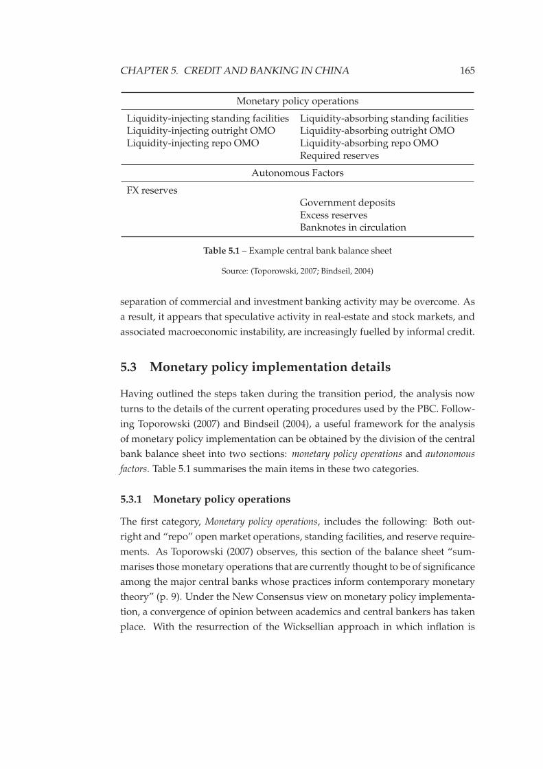
CHAPTER 5. CREDIT AND BANKING IN CHINA 165
Monetary policy operations
Liquidity-injecting standing facilities Liquidity-absorbing standing facilitiesLiquidity-injecting outright OMO Liquidity-absorbing outright OMOLiquidity-injecting repo OMO Liquidity-absorbing repo OMO
Required reserves
Autonomous Factors
FX reservesGovernment depositsExcess reservesBanknotes in circulation
Table 5.1 – Example central bank balance sheet
Source: (Toporowski, 2007; Bindseil, 2004)
separation of commercial and investment banking activity may be overcome. As
a result, it appears that speculative activity in real-estate and stock markets, and
associated macroeconomic instability, are increasingly fuelled by informal credit.
5.3 Monetary policy implementation details
Having outlined the steps taken during the transition period, the analysis now
turns to the details of the current operating procedures used by the PBC. Follow-
ing Toporowski (2007) and Bindseil (2004), a useful framework for the analysis
of monetary policy implementation can be obtained by the division of the central
bank balance sheet into two sections: monetary policy operations and autonomous
factors. Table 5.1 summarises the main items in these two categories.
5.3.1 Monetary policy operations
The first category, Monetary policy operations, includes the following: Both out-
right and “repo” open market operations, standing facilities, and reserve require-
ments. As Toporowski (2007) observes, this section of the balance sheet “sum-
marises those monetary operations that are currently thought to be of significance
among the major central banks whose practices inform contemporary monetary
theory” (p. 9). Under the New Consensus view on monetary policy implementa-
tion, a convergence of opinion between academics and central bankers has taken
place. With the resurrection of the Wicksellian approach in which inflation is
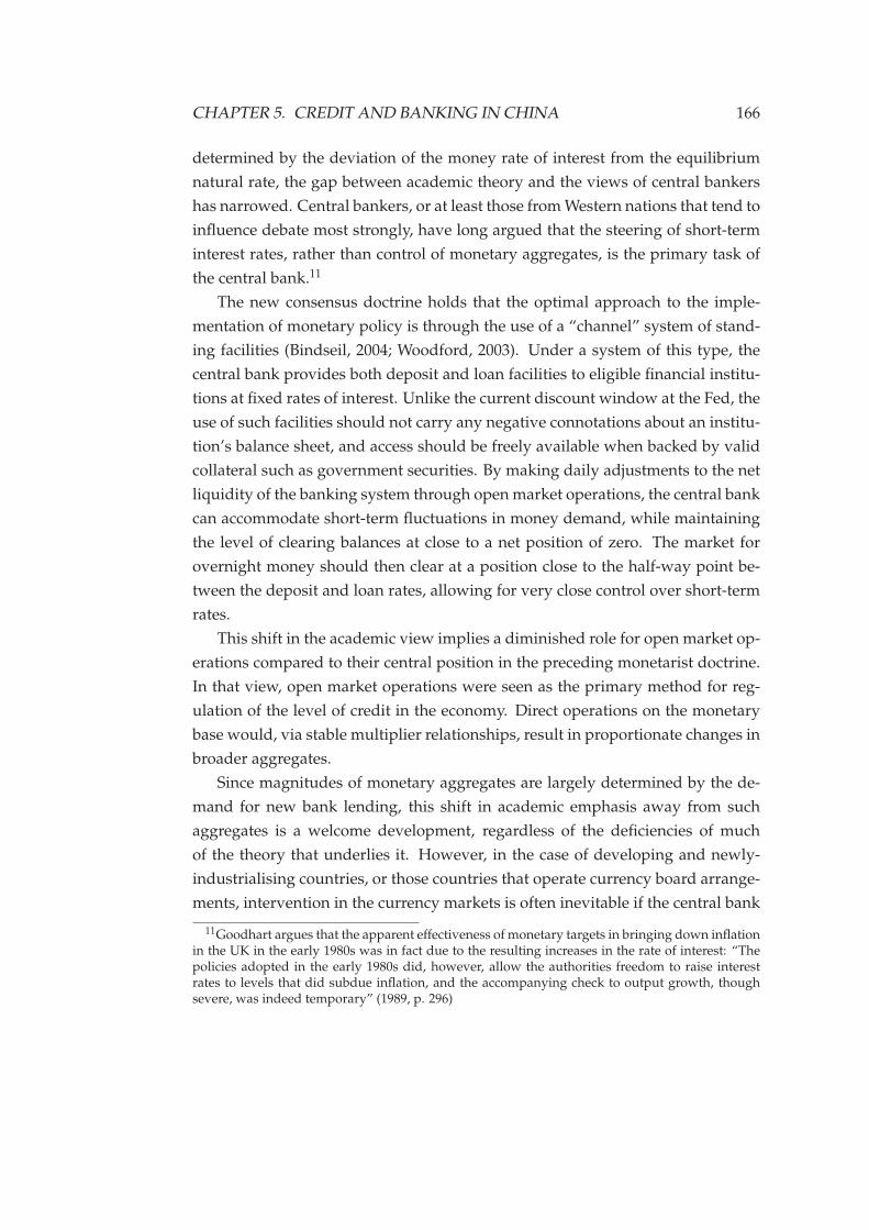
CHAPTER 5. CREDIT AND BANKING IN CHINA 166
determined by the deviation of the money rate of interest from the equilibrium
natural rate, the gap between academic theory and the views of central bankers
has narrowed. Central bankers, or at least those from Western nations that tend to
influence debate most strongly, have long argued that the steering of short-term
interest rates, rather than control of monetary aggregates, is the primary task of
the central bank.11
The new consensus doctrine holds that the optimal approach to the imple-
mentation of monetary policy is through the use of a “channel” system of stand-
ing facilities (Bindseil, 2004; Woodford, 2003). Under a system of this type, the
central bank provides both deposit and loan facilities to eligible financial institu-
tions at fixed rates of interest. Unlike the current discount window at the Fed, the
use of such facilities should not carry any negative connotations about an institu-
tion’s balance sheet, and access should be freely available when backed by valid
collateral such as government securities. By making daily adjustments to the net
liquidity of the banking system through open market operations, the central bank
can accommodate short-term fluctuations in money demand, while maintaining
the level of clearing balances at close to a net position of zero. The market for
overnight money should then clear at a position close to the half-way point be-
tween the deposit and loan rates, allowing for very close control over short-term
rates.
This shift in the academic view implies a diminished role for open market op-
erations compared to their central position in the preceding monetarist doctrine.
In that view, open market operations were seen as the primary method for reg-
ulation of the level of credit in the economy. Direct operations on the monetary
base would, via stable multiplier relationships, result in proportionate changes in
broader aggregates.
Since magnitudes of monetary aggregates are largely determined by the de-
mand for new bank lending, this shift in academic emphasis away from such
aggregates is a welcome development, regardless of the deficiencies of much
of the theory that underlies it. However, in the case of developing and newly-
industrialising countries, or those countries that operate currency board arrange-
ments, intervention in the currency markets is often inevitable if the central bank
11Goodhart argues that the apparent effectiveness of monetary targets in bringing down inflationin the UK in the early 1980s was in fact due to the resulting increases in the rate of interest: “Thepolicies adopted in the early 1980s did, however, allow the authorities freedom to raise interestrates to levels that did subdue inflation, and the accompanying check to output growth, thoughsevere, was indeed temporary” (1989, p. 296)
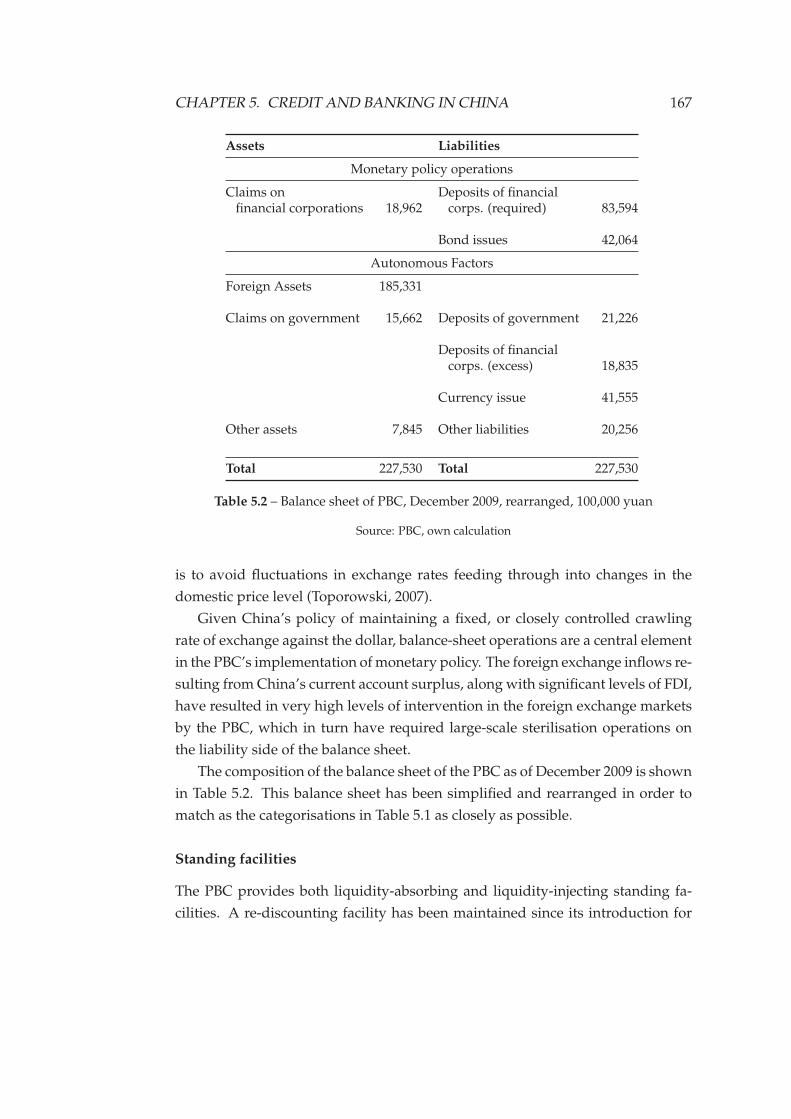
CHAPTER 5. CREDIT AND BANKING IN CHINA 167
Assets Liabilities
Monetary policy operations
Claims on Deposits of financialfinancial corporations 18,962 corps. (required) 83,594
Bond issues 42,064
Autonomous Factors
Foreign Assets 185,331
Claims on government 15,662 Deposits of government 21,226
Deposits of financialcorps. (excess) 18,835
Currency issue 41,555
Other assets 7,845 Other liabilities 20,256
Total 227,530 Total 227,530
Table 5.2 – Balance sheet of PBC, December 2009, rearranged, 100,000 yuan
Source: PBC, own calculation
is to avoid fluctuations in exchange rates feeding through into changes in the
domestic price level (Toporowski, 2007).
Given China’s policy of maintaining a fixed, or closely controlled crawling
rate of exchange against the dollar, balance-sheet operations are a central element
in the PBC’s implementation of monetary policy. The foreign exchange inflows re-
sulting from China’s current account surplus, along with significant levels of FDI,
have resulted in very high levels of intervention in the foreign exchange markets
by the PBC, which in turn have required large-scale sterilisation operations on
the liability side of the balance sheet.
The composition of the balance sheet of the PBC as of December 2009 is shown
in Table 5.2. This balance sheet has been simplified and rearranged in order to
match as the categorisations in Table 5.1 as closely as possible.
Standing facilities
The PBC provides both liquidity-absorbing and liquidity-injecting standing fa-
cilities. A re-discounting facility has been maintained since its introduction for
CHAPTER 5. CREDIT AND BANKING IN CHINA 168
the purposes of financing trade credit, as described in the previous section. The
rate at which the PBC discounts bills was reformed in 1998, in order to link this
discount rate to the official PBC policy rate of interest. Previous to this reform,
the rate at which the PBC would re-discount bills was set with reference to the
prevailing rates in the inter-bank market, rather than with a view to influencing
those rates, essentially severing any connection between the PBC policy rate and
money market rates.
On the liquidity-absorbing side of the balance sheet, the PBC provides a re-
munerated deposit facility for the excess reserves of commercial banks. This fa-
cility was combined with the required reserves account in 1998, such that both
required and excess reserves were remunerated at the same rate. This remained
the case until 2003 when, in response to concern about the high level of excess re-
serves held by the banking system, the PBC reintroduced the distinction between
required and excess reserves and reduced the rate of remuneration on excess re-
serves to 1.62% while leaving the rate paid on required reserves unchanged at
1.89%. The rate on excess reserves was subsequently cut again in 2005 to 0.99%
(Goodfriend & Prasad, 2006).
Although the provision of these two facilities does theoretically impose upper
and lower bounds on the levels at which the money market can clear, in practice
these rates have exerted little influence on the market. The spread between the
two rates is significantly larger than the 50 basis points advocated by proponents
of the new consensus system—for example, in 2005 it was over 200 basis points.
A notable feature of the relationship between the banking system and the PBC is
the lack of activity at the re-discount facility over the last decade: the high level
of liquidity of the banking system has meant that recourse to central bank credit
has been minimal, with only occasional borrowing to cover sudden increases in
demand for cash at busy times of the year. Thus, instead of adjusting the liquidity
of banking system such that net clearing balances are close to zero on a nightly
basis, the banking system has remained structurally in credit with the PBC, with
high levels of excess reserves left on deposit at the PBC, as indicated by the large
excess of deposits of financial corporations over claims on financial corporations.
Godley & Lavoie (2007) draw a distinction between asset-based and overdraft
financial systems. They argue that most textbooks describe asset-based systems,
characterised by large holdings of government securities by the banking sector,
whereas most economies operate as overdraft-based systems such that the bank-
ing systems remain in structural deficit towards the central bank. With the advent
CHAPTER 5. CREDIT AND BANKING IN CHINA 169
of liability management techniques in the last couple of decades, Anglo-Saxon
economies have moved closer to the overdraft-based model. (p. 374). With re-
spect to China, Lavoie & Wang claim that “central bank advances to commer-
cial banks and other financial institutions constitute an entry with substantial
amounts. By contrast, claims on domestic government are relatively small, at
least until recently, thus meaning that China can be said to be an overdraft econ-
omy.” (2012, pp. 292–293)
However, this view overlooks the significance of the very large volumes of
bank reserves held with the PBC. Although the majority of these reserves are
“illiquid” due to being held as required reserves (see next section), they still rep-
resent liabilities of the central bank. China does not therefore conform to either
classification, and instead should be classified separately as a foreign exchange-
based financial system in that the central bank is in structural deficit towards the
banking system while offsetting this deficit through foreign-exchange holdings.
Reserve requirements
As can be seen from Table 5.2, the majority of the deposits held by the the bank-
ing system with the PBC are made up of required reserves. In 2009, the main
required reserve ratio stood at 15.5%, while by late 2011 it had reached as high as
21.5%. The use of reserve requirements in this manner, as a policy tool for freez-
ing banking-sector liquidity on a large-scale basis, is unorthodox when viewed in
the context of the current consensus.
The justification given by Western economists and central bankers for impos-
ing reserve requirements on the banking sector has changed over time. The view
that required reserves provide a liquidity cushion to protect the banking system
against over-lending or unforeseen systemic risk has largely been discarded. Re-
serve requirements have been dropped completely in some economies, for exam-
ple the United Kingdom. The use of required reserves as a monetary policy tool
for directly controlling monetary variables through changes in the aggregate liq-
uidity of the banking sector has also fallen out of favour since around the 1970s,
with current opinion based around the view that reserve requirements are pri-
marily a mechanism for the stabilisation of short-term interest rates.
In an overdraft-based system, as described above, the structural liquidity def-
icit required to make standing facilities effective tends to result in the volatility
of short-term interest rates due to unexpected demand for reserves for clearing
CHAPTER 5. CREDIT AND BANKING IN CHINA 170
purposes or in response to other shocks. By imposing reserve requirements, the
central bank can ensure that the banking system maintains a level of reserves suf-
ficient to cover most of these unforeseen shocks, while still remaining dependent
on the central bank for liquidity provision (Bindseil, 2004, pp. 195–196).
In contrast, the required reserve ratio set by the PBC is set greatly above the
level required for liquidity management of the type described above, while the
increasing frequency of changes to the ratio demonstrate that this is a key tool of
monetary policy for the PBC.12
The use of this instrument on such a scale is the result of the sterilisation needs
imposed by intervention in the foreign exchange markets. The foreign reserve
accumulation resulting from operations to maintain the level of the exchange rate
have resulted in a large structural liquidity surplus, and reserve requirements
have become the policy tool of choice for absorbing this liquidity.
According to Ma et al. (2011, p. 14), this instrument has come to dominate over
other sterilisation tools, such as bond issuance, for a number of reasons. Firstly, it
is more permanent than bond issuance, since bonds are issued at relatively short
maturities and thus can be left to mature by banks that are in need of additional
liquidity. Further, these short-dated securities may be less effective as a means of
liquidity control once large and active markets for the bonds come into operation.
Secondly, the cost to the PBC is lower—the remuneration on required reserves has
generally been below the rate paid on bonds. Finally, changes to the required re-
serve ratio may be enacted without directly broadcasting any signals about policy
rates of interest. This leaves greater scope for open-market operations to be used
for manipulation of interest rates, rather than acting purely as liquidity-draining
operations at the current market rate.
The complexity of the system of required reserves has increased over time,
with differential rates applied to large and small banks, and much lower rates
imposed on foreign currency deposits. The ratio of required to excess reserves
shown in Table 5.2 is calculated using the average of the “small bank” and “large
bank” reserve ratios, which were 13.5% and 15.5% respectively. The figure shown
in Table 5.2 therefore probably underestimates the level of required reserves.
12Between 1984 and June 2003 the required reserve ratio was adjusted six times. Between July2006 and June 2011 it was altered 35 times (Ma et al., 2011).
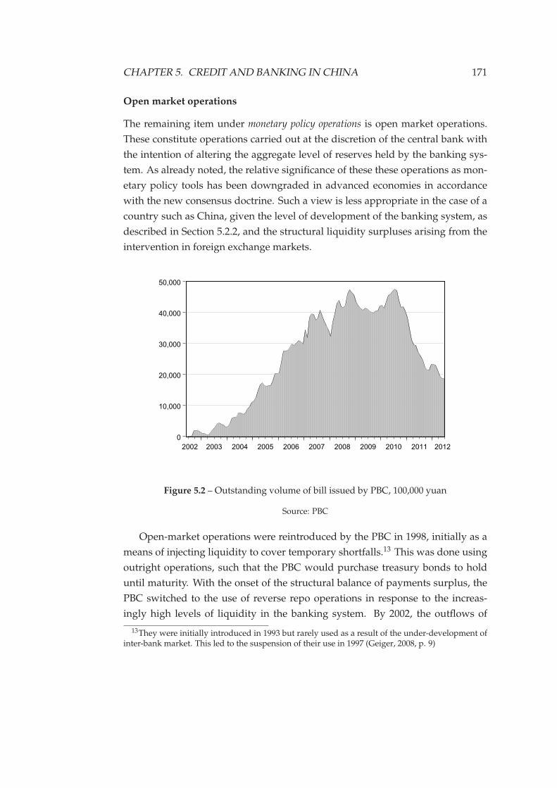
CHAPTER 5. CREDIT AND BANKING IN CHINA 171
Open market operations
The remaining item under monetary policy operations is open market operations.
These constitute operations carried out at the discretion of the central bank with
the intention of altering the aggregate level of reserves held by the banking sys-
tem. As already noted, the relative significance of these these operations as mon-
etary policy tools has been downgraded in advanced economies in accordance
with the new consensus doctrine. Such a view is less appropriate in the case of a
country such as China, given the level of development of the banking system, as
described in Section 5.2.2, and the structural liquidity surpluses arising from the
intervention in foreign exchange markets.
0
10,000
20,000
30,000
40,000
50,000
2002 2003 2004 2005 2006 2007 2008 2009 2010 2011 2012
Figure 5.2 – Outstanding volume of bill issued by PBC, 100,000 yuan
Source: PBC
Open-market operations were reintroduced by the PBC in 1998, initially as a
means of injecting liquidity to cover temporary shortfalls.13 This was done using
outright operations, such that the PBC would purchase treasury bonds to hold
until maturity. With the onset of the structural balance of payments surplus, the
PBC switched to the use of reverse repo operations in response to the increas-
ingly high levels of liquidity in the banking system. By 2002, the outflows of
13They were initially introduced in 1993 but rarely used as a result of the under-development ofinter-bank market. This led to the suspension of their use in 1997 (Geiger, 2008, p. 9)
CHAPTER 5. CREDIT AND BANKING IN CHINA 172
government securities from the PBC were unsustainable: a shortfall in eligible
government paper for OMOs led the PBC to begin issuing its own bills for the
purposes of sterilising foreign exchange inflows.
The volume of PBC bills total outstanding over time is shown in Figure 5.2.
As can be seen from the figure, the increasing issuance of bills for sterilisation
purposes continued until late 2008 when, in response to the Lehman’s crisis the
PBC reduced its sterilisation operations in order to increase the liquidity available
to the banking system. Issuance began again in 2009, but from late 2010 the PBC
began to significantly scale back bill issuance. By this point the use of central bank
bills was superseded by the required reserve ratio as the favoured sterilisation
tool, as described in the previous section.
In addition to sterilisation operations using its own bills, the PBC also con-
ducts repo operations with the banking system at maturities between seven days
and six months, again primarily for the purposes of draining liquidity.
5.3.2 Autonomous factors
The remaining items on the central bank balance sheet come under the heading
of autonomous factors. This section covers those items that the central bank has no
immediate control over on a day-to-day basis. This category is composed of such
items as banknotes in circulation, government deposits and foreign currency.
In advanced market economies, the most important of these items is usually
banknotes in circulation. Since these nations operate floating exchange rates, and
it is the institutional arrangements of such nations that tend to influence aca-
demic discussion on the implementation of monetary policy, the effect of foreign
exchange reserves on the balance sheet of the central bank tends to receive little
discussion.
During the period of transition described in Section 5.2, China operated a
dual-rate system of foreign exchange. These rates were unified in 1994, and in
1996 renminbi convertibility on current account was introduced. Since this point,
the Chinese authorities have kept the value of the yuan under tight control. A
fixed peg to the U.S. dollar was maintained from 1998 until 2005, when the State
Council announced a switch to a “basket, band and crawl” regime. Since then,
the yuan appreciated by around 20% against the dollar until the Lehman’s crisis
in 2008, at which point appreciation halted until late 2010. From late 2010 appre-
ciation resumed.
CHAPTER 5. CREDIT AND BANKING IN CHINA 173
This tight control on the value of the currency was maintained in the face of a
continuously increasing surplus on the current account, up until the crisis of 2008.
The PBC has thus been required to intervene heavily in foreign exchange markets
to prevent appreciation of the yuan. The result of this is that foreign currency re-
serves are the most significant item on the balance sheet, both in terms of size and
in terms of the influence exerted on monetary policy. By 2011, foreign exchange
reserves held on the balance sheet of the PBC had reached over RMB23 tn., the
equivalent of over US$3.5 tn. at current exchange rates.
The sterilisation operations required to counteract the expansion in bank re-
serves resulting from this intervention in the currency markets have mostly been
outlined in the previous sections. However, one item under autonomous factors is
also regarded by some as a form of sterilisation tool. This is the change in de-
posits held at the central bank by the government. Under monetarist doctrines, it
was held that “the net fiscal deficit was an addition to the deposits of the banking
system” (Toporowski, 2007, p. 19). Similarly, if the volume of government de-
posits rises due to payments to the government, rather than deficit financing, this
reduces the net deposits of the private sector, and may be regarded as liquidity-
reducing. Thus, in periods in which the level of government deposits have risen
autonomously, this has partially displaced the need for sterilisation through other
instruments such as bonds or required reserves.
5.3.3 Interest rates
Market rates
The new consensus regards the steering of short-term rates of interest as the most
effective procedure for central bank regulation of credit and inflation. Given the
assumption of perfect financial markets in many modern monetary models, any
adjustments to the risk-free rate of return at the short end of the yield curve are
immediately transmitted to all other maturities through arbitrage relations. Thus,
by maintaining control of short-term rates of interest, the structure of longer-term
rates can be shifted in response to changes in inflation. This understanding of the
way that the monetary transmission mechanism operates on financial markets
lies behind much current empirical research on credit markets in China. Such
studies attempt to isolate the degree to which longer term interest rates are “ar-
bitrage free” and “efficiently determined” (eg. Cassola & Porter, 2011; Feyzioglu
et al., 2009).
CHAPTER 5. CREDIT AND BANKING IN CHINA 174
While assumptions such as arbitrage-free yield curves are problematic in fi-
nancially advanced economies, they are even more so in the case of China, since
the determination of interest rates at various maturities occurs through a combi-
nation of market structures and PBC regulations.
At the longest maturities, the bond market is dominated by government debt.
While yields are determined by the market, they are kept low by the fact that cor-
porate debt issuance has been strongly discouraged by the authorities,14 meaning
that the depth of the market for longer-term debt is thin, with most enterprises
financed through bank credit or retained earnings. The use of sterilisation bills
by the PBC has added to the downward pressure on interest rates—it is in the in-
terests of the PBC to keep rates as low as possible on these bills, both to minimise
direct sterilisation costs and to avoid pressure on the exchange rate to appreciate.
At the short end of the curve, rates are set by inter-bank trading which now
includes both a repo market and a unsecured call-loan market.15 These interbank
markets are highly active but trading is almost entirely confined to maturities
of seven days or less. The rate of remuneration on excess reserves largely sets a
floor under these money market rates but the PBC appears sanguine about money
market rates drifting above the re-discounting rate, as has happened on a number
of occasions. The PBC thus appears to exert very little influence over these rates,
other than to set a floor. Further, given the levels of excess liquidity in the banking
system, the degree to which these interest rates feed into bank lending decisions
and pricing is questionable.
The PBC has been similarly inactive with respect to OMO at the short end of
the curve. Although it has periodically intervened in the market to drain liquidity
using repo operations, it has concentrated for the most part on sterilisation oper-
ations through bill issuance at 3-month and 1-year maturities. The lack of PBC
influence on money market rates is apparent in the regular divergence of short
term money market rates from the benchmark rates quoted by the PBC.
14The State Council’s antipathy towards corporate bond finance is seen by Huang & Zhu (2007)as partly informed by the historical experience of foreign borrowing during the Qing dynasty whenexcessive sovereign debt issuance eventually bankrupted the government.
15Upper limits on inter-bank lending rates were abolished in 1996, and repos were introduceda year later in 1997. (Porter & Xu, 2009) In addition to the uncollateralised call-loan (CHIBOR)market and the repo market, the SHIBOR benchmark yield curve was introduced in 2007 and isset in a similar fashion to the LIBOR, based on quotes submitted by a designated panel of clearingbanks.
CHAPTER 5. CREDIT AND BANKING IN CHINA 175
Bank rates
Until 2004, all interest rates on the loans and deposits of the banking system were
fixed by the State Council, leaving individual banks no leeway in pricing credit or
competing for deposits. In 2004 regulations were adjusted so that these centrally
imposed rates operated only as a floor to lending rates and a ceiling on deposit
rates. These regulations therefore set a minimum interest spread for the banking
system. As a results, deposit rates have remained fixed at the ceiling level, as
banks compete to attract deposits.
During the period of central planning, prices of goods were fixed by the State
Council in such a way as to impose implicit subsidies and taxes on different sec-
tors of the economy, in accordance with the development planning approach.
By setting the prices of final goods at above market levels, and capital goods at
below market levels, the authorities provided a stimulus to high levels of invest-
ment. Likewise, the imposition of a fixed structure of interest rates on the banking
system gives the authorities a powerful tool to affect the profitability of both the
banking system and the firms that rely on loans for investment—the high spreads
between lending and borrowing rates were imposed in part to protect the banking
system in the wake of the recapitalisation and removal of NPLs. This imposition
of interest rates, and in particular the capping of interest rates paid on deposits is
regarded as distortionary and a form of financial repression which imposes sig-
nificant costs on households in the absence of alternative financial assets in which
to invest (Lardy, 2008; Park & Sehrt, 2001).16
5.4 Conclusion
This chapter has described the process of financial development in China over the
period of transition from central planning and provided a detailed description of
the current financial structure and the operating procedures of the People’s Bank
of China.
Although China’s capital markets are extremely underdeveloped relative to
other economies at a similar level of development, this does not imply that the
16Lardy (2008) argues that the financial repression caused by the imposition of low rates of inter-est results in transfers of value from households to other sectors in the economy. By comparing thereal interest rate on deposits in 2008 with that which was paid in 2002—the point at which financialrepression is seen to have started—he calculates that that the implicit tax on households accountedfor over 4% of GDP in the first quarter of 2008.
CHAPTER 5. CREDIT AND BANKING IN CHINA 176
level of financial depth in China is low. In fact, although China’s financial system
is dominated by the banking system, the overall level of financial intermediation
in China is extremely high. In 2004, China’s banking system held assets equiva-
lent to 160 percent of GDP. This compares with figures of 77 percent in the United
States, 119 percent in Singapore and 145 percent in Japan (Farrell et al., 2006). By
the end of 2010, China’s asset to GDP ratio was almost 190 per cent.
This level of bank depth is made possible, at least in part, by the ability of the
authorities to prevent bank credit from flowing into other financial assets, either
domestically or abroad. This has allowed for high rates of loan growth without
the deposits created in the process fleeing the system. By forcing all of the new
saving that arises out investment spending to remain within the banking system
as deposits, the chances of banking crises are minimised, buying time for the au-
thorities to continue with economic and financial restructuring. On the domestic
side, this has been achieved by a strict separation of banking from the securities
market, while capital controls have served to prevent outflows internationally. In
this respect, the underdevelopment of capital markets and the lack of alternative
investment opportunities may be both a cause and consequence of the stability of
the banking system, despite high levels of credit growth. The increasing signifi-
cance of informal finance appears, however, to be leading to a weakening of the
barrier between bank lending and speculative activity.
The structural and institutional reforms outlined in this chapter have resulted
in a relatively sophisticated banking system. The prerequisites are in place for
the system as a whole to be able to generate new deposits, and thus savings, by
issuing loans for investment—an active and liquid inter-bank market, a central
bank providing liquidity to the system as a whole and standing ready to act as
lender-of-last resort, and most crucially, sufficient public confidence in the bank-
ing system for the deposit base to remain stable.
The path taken during the transition period is key to this outcome. By adopt-
ing reforms gradually, and allowing the banking system to evolve out of the
previous mono-bank system, the sharp loss of confidence experienced in other
transition economies was avoided. The transition from a mono-bank system in
which credit money performed to role of giro transfers to a modern banking sys-
tem avoided a phase of segmentation and disintermediation, resulting in a step
backwards to earlier banking stages in which deposits are required in advance
of lending. Instead, over the period of reform, the Chinese authorities have been
able to rely on directed credit to key industries to maintain aggregate demand
CHAPTER 5. CREDIT AND BANKING IN CHINA 177
and growth, while largely avoiding inflation from the mid-1990s onwards.
Although the current operating procedures of the PBC are based largely on
quantitative controls, the apparent similarity of the Chinese regime to episodes
in advanced economies during which policy was guided by monetarist doctrine
is misleading. The attempts of authorities in these economies to maintain control
over broad aggregates by targeting the monetary base were predicated on the as-
sumption of a stable multiplier relationship between monetary aggregates. These
attempts were confounded when it became apparent that the volume of money in
the system is “...institutionally determined and time-varying... the monetary base
multiplier is only applicable for some of the earlier stages of banking history...”
(Goodhart, 2002). In contrast, the Chinese monetary authorities have tended to
announce broad credit targets. These are achieved as much through “moral sua-
sion” with banks, and the influence of the authorities on the investment decisions
of state-owned corporations, as they are by controlling narrow monetary aggre-
gates.17 Over most of the last twenty years, the Chinese banking system has held
a significant volume of excess reserves with the central bank. Although some of
these reserves are used for the purposes of settlement, the liquidity of the banking
system implies that shortages of reserves have rarely served to restrain lending.
Only in recent years have excess reserves come down to levels that would be
likely to restrain credit growth. This has been accompanied by rising and increas-
ingly volatile short-term interest rates, in common with the experience of Western
economies during the period of attempted quantitative controls.
The doctrine of monetary control primarily through the use of operations
which directly affect the volume of base money is founded on the assumption of
stable relationship between output and the demand for various monetary aggre-
gates, a set of beliefs originating with Friedman’s (1956) restatement of the quan-
tity theory of money. A large number of econometric studies have attempted to
locate these stable money demand functions in the case of China, with little suc-
cess.18 Not only have estimated coefficients varied widely, but the signs of these
coefficients are sometimes the opposite of expected values (Zuo & Park, 2011).
Thus, as centralised control on the demand and supply of credit at the aggre-
gate level decreases as a result of endogenous financial development and the di-
17The PBC “maintains annual (and typically binding) bank-by-bank caps on creditgrowth”(Porter & Xu, 2009, p. 10)
18Eg. Merhotra (2008); Baharumshah et al. (2009); Bahmani-Oskooee & Wang (2007); Wu (2009);Xie (2004)
CHAPTER 5. CREDIT AND BANKING IN CHINA 178
minishing market share of state-owned enterprises, the PBC will inevitably move
towards a system of monetary regulation based on setting the price of reserves
and allowing monetary aggregates to be determined endogenously:
Central banks are... unable to reduce the rate of growth of the money
supply, except by raising the supply price of reserves and so the level
of short-term interest rates. Once it is recognized that loans are made
at borrower initiative, and that loans create deposits, it logically fol-
lows that the money supply, bank reserves, and the high-powered
base all vary endogenously (Moore, 1988, p. 26)
The PBC has already begun to move in this direction by allowing the inter-
est rates charged on loans to be set independently by the banking system, thus
conceding control of one key factor in determining the volume of loan demand.
However, as long as the Chinese authorities continue to target the exchange rate,
the resulting expansion of bank reserves will require the maintenance of sterilisa-
tion operations. As such, quantitative operations to influence the monetary base
will remain a central aspect of PBC monetary policy intervention.
Chapter 6
China’s flow-of-funds I: physical
transactions
6.1 Introduction
Official flow-of-funds accounts accounts have been published by the Chinese sta-
tistical bureau since 1992. These accounts aim to provide an integrated quan-
titative representation of the macroeconomic system. This chapter undertakes a
detailed study of these accounts, using them as a basis for a theoretically coherent
case history of the last two decades of capital accumulation in China.
These accounts are used to show as defective those commonplace narratives
which present the thrift of Chinese households as the virtuous trait which has
driven the growth “miracle”. It is demonstrated that the key to comprehending
the Chinese growth story is the rising share of saving accruing as profits. The
flow-of-funds system is used to show that “investment expenditure is ultimately
constrained by access to finance, not by a deficiency of saving, because actual in-
vestment creates an equivalent amount of saving.” (Harcourt, 1991, p. 1608). It
is the expenditures of firms in the People’s Republic that generate the savings of
those firms and households alike. Contrary to the conventional wisdom, these
firms as a whole do not face significant constraints in financing new outlays be-
cause of the availability of endogenously created bank credit, generating fresh
liquidity to cover those expenditures which are lost due to the rising saving of
households. Rather than being the virtue which has created the Chinese miracle,
the increasing tendency to save, rather than spend, raises the prospect of a slump
in the event that firms were to reign in investment spending.
179
CHAPTER 6. CHINA’S FLOW-OF-FUNDS I 180
The purpose of this chapter is to demonstrate that the patterns of investment
and saving—and the associated financial balances—of the Chinese economy are
the result of an endogenous credit-investment process. Using the flow-of-funds
accounts, in conjunction with a number of other data sources, a sector-based
macro-economic analysis is constructed in which the circular flow of income is
the primary organising principle. In analysing all variables in the context of their
place in a stock-flow consistent taxonomy, a system is derived in which the expen-
ditures and incomes of all sectors must find their counterpart in opposite flows
of other sectors.
This empirical framework is closely aligned with the theoretical system devel-
oped in Chapters 3 and 4. In particular a central role is given to the investment
decisions of firms and the income flows generated as a result of these expendi-
tures, in line with Kalecki’s reflux theory of profit.
It is shown that these investment expenditures of firms are the prime deter-
minant of the overall level of saving in the Chinese economy, reinforced in recent
years by current account surpluses. The analytical framework allows for the iso-
lation of the net financial balances of each sector, thus providing a coherent start-
ing point for the monetary and financial analysis of Chapter 7. It is shown that
the financial position of firms has improved over the last two decades such that
investment is increasingly funded from retained earnings.
The analysis goes beyond the level of disaggregation possible using the flow-
of-funds accounts by decomposing the firms sector by owership classification.
This is done using alternate data sources, and allows for a Steindlian analysis in
which investment and saving are unevenly distributed among the firms sector.
It is argued that although the share of output accounted for by the state-owned
sector is falling, the investment decisions of this sector are the crucial determining
factor in generating output growth and aggregate investment.
A reinterpretation of Steindl’s (1952) theoretical system is used in which the
relative positions of the “cartelised” and “marginal” firms are reversed: rather
than behaving as “parasitic” monopolists, the expenditures of the state-owned
sector are increasingly captured as profits by private-sector firms.
The chapter is organised as follows. Section 6.2 presents an overview of the
flow-of-funds accounts which provides some background to the original formu-
lation of the accounts, plus a description of the basic construction of the accounts
and the underlying principles. Section 6.3 outlines the sources of data used and
highlights a number of issues with these data. Section 6.4 analyses the “physi-
CHAPTER 6. CHINA’S FLOW-OF-FUNDS I 181
cal transactions” side of the flow-of-funds accounts, focusing on the dynamics of
investment and saving behaviour and the financial balances generated by the in-
teraction of these decisions. Section 6.5 analyses the firms sector in greater detail,
drawing on additional data sources to move beyond the aggregate data of the
flow-of-funds to differentiate between enterprises of different ownership types.
6.2 Background to the flow-of-funds accounts
Origination of the flow-of-funds accounts is credited to Morris Copeland who
in the 1940s published two papers (Copeland, 1947, 1949) on “moneyflows ac-
counting”, followed by a detailed study of Moneyflows in the United States in 1952
(Copeland, 1952). These writings put forward a systematic way in which to in-
tegrate, in a unified accounting framework, all real and financial transactions
within an economic system. This accounting framework was presented as an
alternative to the standard national accounts. Copeland’s ideas were taken up by
the Federal Reserve, which began publishing flow-of-funds accounts in 1955.
A simplified example flow-of-funds matrix is shown in Figure 6.1 The matrix
depicts, at the aggregate level, the complete set of real and financial transactions
in a closed system over a given time period. These transactions are classified
either as ’sources’ or ’uses’ of funds.
The economic system is divided into three sectors: households, firms, and a
unified banking system incorporating the central bank. The banking sector is as-
sumed not to engage in any real transactions, but operates as a pure intermediary
between the household and firm sectors.
The first two rows of the matrix contain the real income and expenditure of
each sector, with the difference between the two recorded in the third row as
net saving. The difference between this value and the level of real investment
recorded in row four gives the net financial balance of any sector.
For the sake of simplicity, financial transactions in the matrix are limited to
changes in the holdings of bank deposits and the issuance or repayment of loans
taken out against the banking system. An increase in the holdings of deposits
by households or firms corresponds to a use of funds by that sector, while the
issuance of fresh liabilities in the form of increased borrowing is a source of funds.
The inverse is the case for the banking system.
In order that the system retain internal consistency, the transactions that com-
prise the matrix must be constrained by a number of identities that ensure that
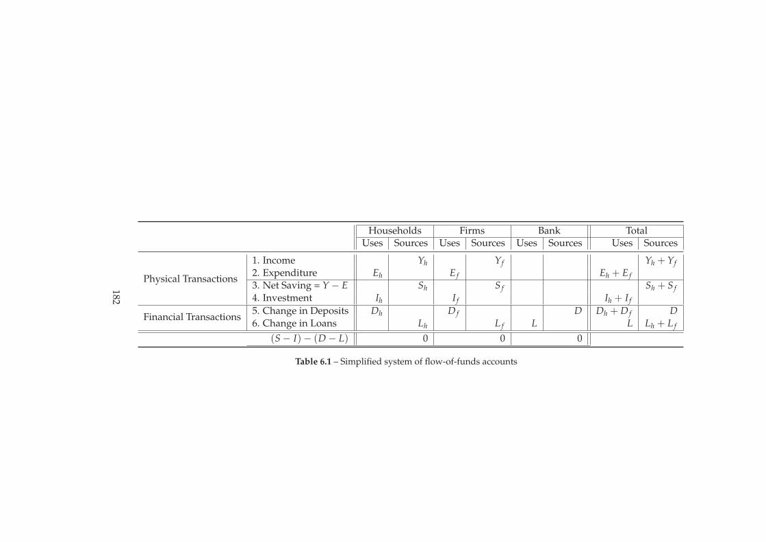
Households Firms Bank TotalUses Sources Uses Sources Uses Sources Uses Sources
Physical Transactions
1. Income Yh Yf Yh + Yf
2. Expenditure Eh E f Eh + E f
3. Net Saving = Y− E Sh S f Sh + S f
4. Investment Ih I f Ih + I f
Financial Transactions5. Change in Deposits Dh D f D Dh + D f D6. Change in Loans Lh L f L L Lh + L f
(S− I)− (D− L) 0 0 0
Table 6.1 – Simplified system of flow-of-funds accounts
182
CHAPTER 6. CHINA’S FLOW-OF-FUNDS I 183
two conditions are fulfilled. The first of these conditions is that the discrep-
ancy between real saving and real investment—the net financial balance—for any
given sector is exactly offset by a compensating change in the holdings of finan-
cial assets and issuance of liabilities. One identity per sector (represented by a
column of the matrix) is obtained by setting the difference between real uses and
sources to equal to the difference between financial sources and uses. These iden-
tities are implied by the zero totals at the bottom of each column.
The second constraint that must be imposed on the system is that, for each
transaction type, total uses of funds must equal total sources. For real sector trans-
actions this is equivalent to enforcing the Keynesian identity that saving must
equal investment.1 In the case of financial transactions this constraint ensures
that any new issuance of a given type of financial liability is exactly matched by
a corresponding increase in the holdings of that type of liability. One identity is
obtained from each row in the Financial Transactions section of the matrix.
For the simple matrix shown in Figure 6.1, these constraints result in a total
of six identities: one for each sector of the economy, one for each type of financial
asset—loans and deposits—and one which is equivalent to the Keynesian identity
that total real saving and investment must be equal:
Sh − Ih = Dh − Lh (6.1)
S f − I f = D f − L f (6.2)
D = L (6.3)
Sh + S f = Ih + I f (6.4)
Dh + D f = D (6.5)
Lh + L f = L (6.6)
Two important related points should be made about this system of identities.
The first is that these identities will only necessarily hold ex-post. The second is
that the system of equations derived from the identities of a flow-of-funds matrix
will be over-determined: any single equation in the system is implied by the other
remaining equations.
The connection between these points lies in the fact that they both relate to
1Income, Y, and expenditure, E, do not enter the identity directly because these are subsumedinto net real saving, S.
CHAPTER 6. CHINA’S FLOW-OF-FUNDS I 184
the problem of imposing causality on the system of identities. Whilst saving
and investment must be equal ex-post, the direction in which causation between
the two runs depends on one’s theoretical perspective. Likewise, given a col-
lection of flow-of-funds identities, without imposing further assumptions on the
system, we are faced with the problem that “everything depends on everything
else” (Green & Murinde, 2000).
To illustrate using our simple model, Equation 6.1 states that any surplus
occurring in the household sector, due to an excess of saving over investment
Sh − Ih, will have its counterpart in a reduction in the difference between the
sector’s financial assets and liabilities Dh − Lh: if the household sector does not
consume all of its real income, it will either be accumulating bank deposits or
paying off loans.2 For Equation 6.4, the Keynesian saving-investment identity, to
be fulfilled, firms collectively must be running a deficit exactly equal to the sur-
plus in the household sector. From Equation 6.2, financing this deficit requires
that the difference between changes in assets and liabilities in the firm sector will
be the inverse of the financial operations undertaken in the household sector: the
firm sector will face a net increase in liabilities. Finally Equations 6.5 and 6.6
ensure that that, for each of the two financial instruments, total issuance of liabil-
ities is equal to the total volume of purchases of the equivalent asset. These five
equations collectively imply that the total increase in the level of deposits in the
system is equal to the total increase in the level of loans. The remaining unused
identity—the balance sheet of the banking system, Equation 6.3—is redundant.
The problem with analyses of this type is that they do not overcome the prob-
lem of causation. Although the exposition started from household saving and
found the bank’s balance sheet to be the redundant equation, the correct causal
line runs from investment by firms, via new credit issued by the banking system,
to the requirement that the household sector balances its books through net real
saving.
Copeland (1952, p. 259) proposed a way to overcome this issue by using a
classification of sectors based on the relative rates of change of real incomes and
expenditures. Sectors are classified as either bulls, bears or sheep. Bulls are those
deficit sectors for which real outlays (expenditure plus investment) are increasing
faster than incomes, thus pushing the sector further into deficit. Conversely, bears
are those surplus sectors for which the level of real outgoings are decreasing faster
2More precisely, the rate at which deposits are being accumulated will be higher than the rate ofincrease of loan liabilities.
CHAPTER 6. CHINA’S FLOW-OF-FUNDS I 185
than their incomes, so that the financial surplus of the sector is increasing. Those
sectors which are neither bulls nor bears are classified as sheep. These are sec-
tors that are reducing their financial position—either surplus or deficit—in each
subsequent period. The real uses of funds by these sectors will increase less than
sources in expansionary periods, and decrease less than sources in deflationary
periods. They are thus “passive hoarders and dishoarders”.
The underlying assumption made by Copeland in this classification system is
that sectors have a greater ability to determine their expenditures than to deter-
mine than their incomes. The economic system is thus viewed as being driven by
investment and consumption decisions, with saving determined as the residual.
Those sectors for which expenditure is increasing faster than income are viewed
as exerting expansionary pressure on the system, leading to monetary expansion
and an increase in economic activity when these sectors are dominant. The op-
posite effect is observed when “bears” become the dominant sector, resulting in
deflation and a reduction in economic activity.
This classification system is closely aligned with the Kaleckian theoretical
framework in which investment financed via the creation of credit money gen-
erates additional saving, and the associated theories of distribution and accumu-
lation. These theories were discussed and integrated within an abstract flow-of-
funds system in Chapter 4. The resulting theoretical system thus closely matches
the intended spirit of Copeland’s concrete system of accounts.
6.3 Data sources and description
6.3.1 NBS Flow-of-funds accounts
The National Bureau of Statistics of China (NBS) has published flow-of-funds
accounts since 1992. The accounts are usually published in the Statistical Yearbook
dated three years after the year of the accounts. The most recent set of accounts
are those for 2008, published in the 2011 Statistical Yearbook (NBS, 2011).
These accounts disaggregate the economy into five sectors: households, non-
financial corporations, financial institutions, government and the rest of the world.
As in the example used in the previous section, the accounts are divided into a set
of “above the line” flows relating to physical transactions, and “below the line”
flows resulting from financial transactions. The physical transaction tables are
constructed by the NBS while the financial transactions tables are the responsibil-
CHAPTER 6. CHINA’S FLOW-OF-FUNDS I 186
ity of the Peoples’ Banks of China (PBC).3
Since the difference between “physical” incomes and expenditures for each
institutional sector is equal to the net financial balance of that sector, this mag-
nitude should in theory be identical to the net acquisition of financial assets—to
accommodate the difference between sources and uses of funds—for that sector
in the financial flow-of-funds table.
Some degree of error is inevitable in compiling data-sets of this type, and
this is reflected in the differences between the “net financial investment” figure
of the physical tables and the corresponding figure in the financial tables. This
discrepancy tended to be fairly minor in the earlier flow-of-funds accounts, but
has increased significantly in recent years.4 This is noted by an author at the NBS:
Theoretically, the item of “net lending and borrowing” should be com-
pletely in line in the two tables. However, due to the data gap, many
indicators need to be estimated or projected, these two “net lending
and borrowing” are inconsistent in reality. From the data in recent
years, the difference of this item between the two tables is getting big-
ger which is difficult to be explained by statistical error. (Xu et al.,
2012, p. 16)
This problem is compounded by the fact that the physical flow-of-funds ta-
bles were revised as a result of the two economic censuses that took place in 2004
and 2008. Each census resulted in a benchmark revision to the official statistics,
including the GDP figures. After the 2004 economic census, the figure for 2004
GDP was revised upwards by 16.8%; previous years were revised upwards in
decreasing proportions back to the 1992 figure which was increased by 1.07%.
A further benchmark revision took place in 2010 after the second economic cen-
sus in 2008. This second revision resulted in upward adjustments to the GDP
figures for 2005–2007. Table 6.2 compares the original GDP figures to the subse-
quently revised figures. The revised figures for the years 1992–2003 are from the
first benchmark revision and those for the years 2004–2007 are from the second
benchmark revision.
3The PBC has published a set of financial transactions accounts for 2009, but there is not yet amatching set of physical accounts from the NBS. The 2009 financial accounts will be used as anexample where required for the discussion in this chapter.
4Until 2004, the physical transactions table included a “statistical discrepancy” item which ad-justed the net financial investment position of each sector to match that of the financial transactionstable. This was dropped from the accounts for years after 2004.
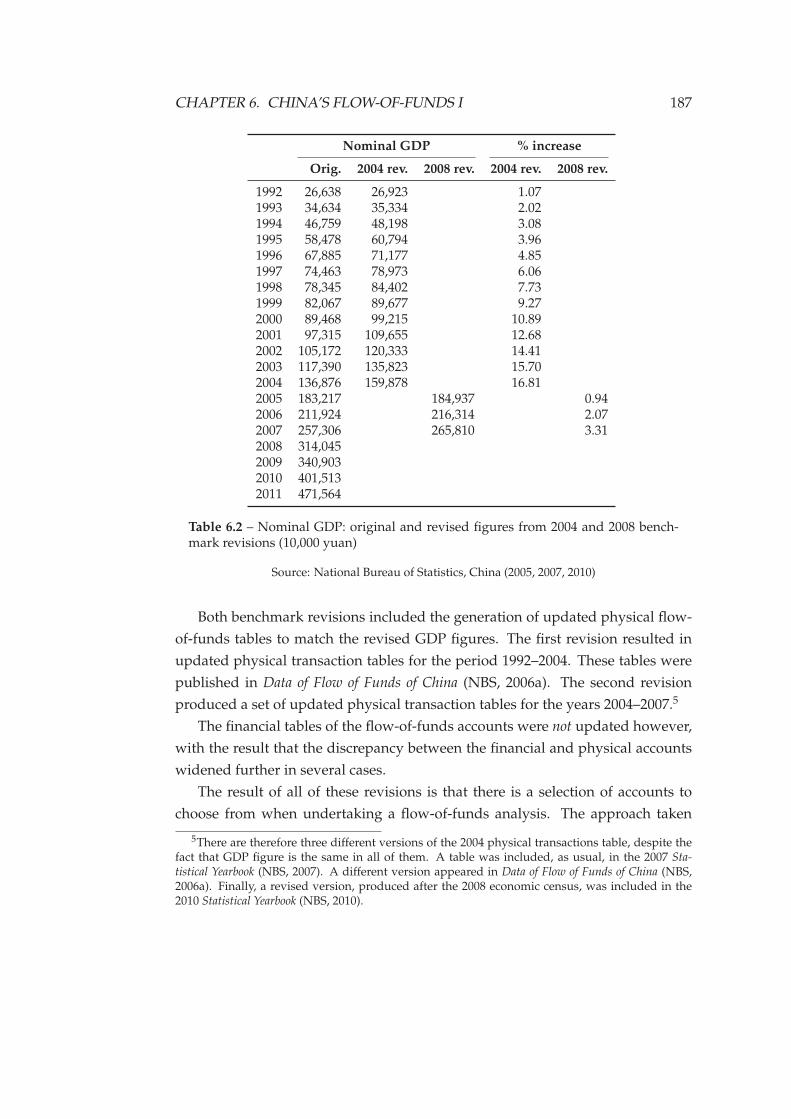
CHAPTER 6. CHINA’S FLOW-OF-FUNDS I 187
Nominal GDP % increase
Orig. 2004 rev. 2008 rev. 2004 rev. 2008 rev.
1992 26,638 26,923 1.071993 34,634 35,334 2.021994 46,759 48,198 3.081995 58,478 60,794 3.961996 67,885 71,177 4.851997 74,463 78,973 6.061998 78,345 84,402 7.731999 82,067 89,677 9.272000 89,468 99,215 10.892001 97,315 109,655 12.682002 105,172 120,333 14.412003 117,390 135,823 15.702004 136,876 159,878 16.812005 183,217 184,937 0.942006 211,924 216,314 2.072007 257,306 265,810 3.312008 314,0452009 340,9032010 401,5132011 471,564
Table 6.2 – Nominal GDP: original and revised figures from 2004 and 2008 bench-mark revisions (10,000 yuan)
Source: National Bureau of Statistics, China (2005, 2007, 2010)
Both benchmark revisions included the generation of updated physical flow-
of-funds tables to match the revised GDP figures. The first revision resulted in
updated physical transaction tables for the period 1992–2004. These tables were
published in Data of Flow of Funds of China (NBS, 2006a). The second revision
produced a set of updated physical transaction tables for the years 2004–2007.5
The financial tables of the flow-of-funds accounts were not updated however,
with the result that the discrepancy between the financial and physical accounts
widened further in several cases.
The result of all of these revisions is that there is a selection of accounts to
choose from when undertaking a flow-of-funds analysis. The approach taken
5There are therefore three different versions of the 2004 physical transactions table, despite thefact that GDP figure is the same in all of them. A table was included, as usual, in the 2007 Sta-tistical Yearbook (NBS, 2007). A different version appeared in Data of Flow of Funds of China (NBS,2006a). Finally, a revised version, produced after the 2008 economic census, was included in the2010 Statistical Yearbook (NBS, 2010).
CHAPTER 6. CHINA’S FLOW-OF-FUNDS I 188
here is to use the most recently produced version of the accounts for each year.
As noted above, the revised versions of the accounts have tended to introduce
greater discrepancies between the per-sector net financial position in the physical
and financial transaction tables. Table 6.3 shows these discrepancies between the
net financial position of each sector in the physical and financial tables. This
discrepancy is shown as as a percentage of GDP each year for both the original
and revised flow-of-funds accounts.
The largest divergence between the tables is recorded in the original accounts
for the years 2006 and 2007. In these years the discrepancy for the firms sector is
over 12% of GDP in both cases, with large discrepancies recorded for other sec-
tors also. The 2008 benchmark revision reduced these discrepancies significantly.
While the 2008 revisions tended to reduce this discrepancy, the 2004 revisions had
the opposite effect in many years, as can be seen by comparing “Total” column
for the original accounts and the 2004 revisions. In particular, the discrepancy be-
tween the figures for the household sector and the firms sector tended to increase
with this revision. These differences between the physical and financial transac-
tions tables will be considered in more detail later on, but the point of the current
discussion is to demonstrate that much of the divergence between the tables, at
least for the years prior to 2004, was not present in earlier versions of the tables,
and were introduced as result of data revisions.
6.3.2 Financial stocks and flows
The NBS flow-of-funds accounts combine financial institutions and the monetary
authority—the PBC—into a single sector. This presents some difficulties in trying
to isolate the effects of monetary policy on the balance sheets of the commercial
banks. These problems are partially offset by the inclusion of items for “vault
cash”, “required reserves” and “loans from central bank” in the list of financial
transactions. Since these flows are purely “internal” to the amalgamated financial
system, sources tend to equal uses for these items.
In addition to these difficulties in separating the monetary authority from the
commercial banks, the accounts provide information only on flow magnitudes,
and not stocks. For the real-sector this does not present many problems since the
only flow that results in real accumulation is investment. All other flows either
result in consumption or saving in the form of financial assets. Thus the only
stocks that are of significance—other than the stock of capital—are monetary or
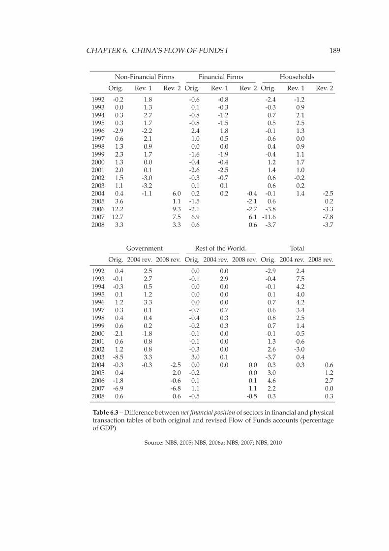
CHAPTER 6. CHINA’S FLOW-OF-FUNDS I 189
Non-Financial Firms Financial Firms Households
Orig. Rev. 1 Rev. 2 Orig. Rev. 1 Rev. 2 Orig. Rev. 1 Rev. 2
1992 -0.2 1.8 -0.6 -0.8 -2.4 -1.21993 0.0 1.3 0.1 -0.3 -0.3 0.91994 0.3 2.7 -0.8 -1.2 0.7 2.11995 0.3 1.7 -0.8 -1.5 0.5 2.51996 -2.9 -2.2 2.4 1.8 -0.1 1.31997 0.6 2.1 1.0 0.5 -0.6 0.01998 1.3 0.9 0.0 0.0 -0.4 0.91999 2.3 1.7 -1.6 -1.9 -0.4 1.12000 1.3 0.0 -0.4 -0.4 1.2 1.72001 2.0 0.1 -2.6 -2.5 1.4 1.02002 1.5 -3.0 -0.3 -0.7 0.6 -0.22003 1.1 -3.2 0.1 0.1 0.6 0.22004 0.4 -1.1 6.0 0.2 0.2 -0.4 -0.1 1.4 -2.52005 3.6 1.1 -1.5 -2.1 0.6 0.22006 12.2 9.3 -2.1 -2.7 -3.8 -3.32007 12.7 7.5 6.9 6.1 -11.6 -7.82008 3.3 3.3 0.6 0.6 -3.7 -3.7
Government Rest of the World. Total
Orig. 2004 rev. 2008 rev. Orig. 2004 rev. 2008 rev. Orig. 2004 rev. 2008 rev.
1992 0.4 2.5 0.0 0.0 -2.9 2.41993 -0.1 2.7 -0.1 2.9 -0.4 7.51994 -0.3 0.5 0.0 0.0 -0.1 4.21995 0.1 1.2 0.0 0.0 0.1 4.01996 1.2 3.3 0.0 0.0 0.7 4.21997 0.3 0.1 -0.7 0.7 0.6 3.41998 0.4 0.4 -0.4 0.3 0.8 2.51999 0.6 0.2 -0.2 0.3 0.7 1.42000 -2.1 -1.8 -0.1 0.0 -0.1 -0.52001 0.6 0.8 -0.1 0.0 1.3 -0.62002 1.2 0.8 -0.3 0.0 2.6 -3.02003 -8.5 3.3 3.0 0.1 -3.7 0.42004 -0.3 -0.3 -2.5 0.0 0.0 0.0 0.3 0.3 0.62005 0.4 2.0 -0.2 0.0 3.0 1.22006 -1.8 -0.6 0.1 0.1 4.6 2.72007 -6.9 -6.8 1.1 1.1 2.2 0.02008 0.6 0.6 -0.5 -0.5 0.3 0.3
Table 6.3 – Difference between net financial position of sectors in financial and physicaltransaction tables of both original and revised Flow of Funds accounts (percentageof GDP)
Source: NBS, 2005; NBS, 2006a; NBS, 2007; NBS, 2010
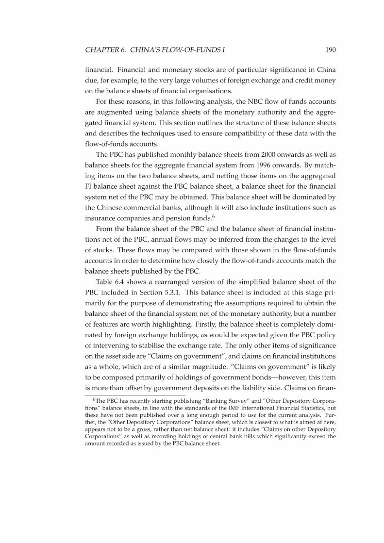
CHAPTER 6. CHINA’S FLOW-OF-FUNDS I 190
financial. Financial and monetary stocks are of particular significance in China
due, for example, to the very large volumes of foreign exchange and credit money
on the balance sheets of financial organisations.
For these reasons, in this following analysis, the NBC flow of funds accounts
are augmented using balance sheets of the monetary authority and the aggre-
gated financial system. This section outlines the structure of these balance sheets
and describes the techniques used to ensure compatibility of these data with the
flow-of-funds accounts.
The PBC has published monthly balance sheets from 2000 onwards as well as
balance sheets for the aggregate financial system from 1996 onwards. By match-
ing items on the two balance sheets, and netting those items on the aggregated
FI balance sheet against the PBC balance sheet, a balance sheet for the financial
system net of the PBC may be obtained. This balance sheet will be dominated by
the Chinese commercial banks, although it will also include institutions such as
insurance companies and pension funds.6
From the balance sheet of the PBC and the balance sheet of financial institu-
tions net of the PBC, annual flows may be inferred from the changes to the level
of stocks. These flows may be compared with those shown in the flow-of-funds
accounts in order to determine how closely the flow-of-funds accounts match the
balance sheets published by the PBC.
Table 6.4 shows a rearranged version of the simplified balance sheet of the
PBC included in Section 5.3.1. This balance sheet is included at this stage pri-
marily for the purpose of demonstrating the assumptions required to obtain the
balance sheet of the financial system net of the monetary authority, but a number
of features are worth highlighting. Firstly, the balance sheet is completely domi-
nated by foreign exchange holdings, as would be expected given the PBC policy
of intervening to stabilise the exchange rate. The only other items of significance
on the asset side are “Claims on government”, and claims on financial institutions
as a whole, which are of a similar magnitude. “Claims on government” is likely
to be composed primarily of holdings of government bonds—however, this item
is more than offset by government deposits on the liability side. Claims on finan-
6The PBC has recently starting publishing “Banking Survey” and “Other Depository Corpora-tions” balance sheets, in line with the standards of the IMF International Financial Statistics, butthese have not been published over a long enough period to use for the current analysis. Fur-ther, the “Other Depository Corporations” balance sheet, which is closest to what is aimed at here,appears not to be a gross, rather than net balance sheet: it includes “Claims on other DepositoryCorporations” as well as recording holdings of central bank bills which significantly exceed theamount recorded as issued by the PBC balance sheet.
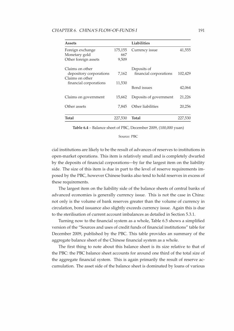
CHAPTER 6. CHINA’S FLOW-OF-FUNDS I 191
Assets Liabilities
Foreign exchange 175,155 Currency issue 41,555Monetary gold 667Other foreign assets 9,509
Claims on other Deposits ofdepository corporations 7,162 financial corporations 102,429
Claims on otherfinancial corporations 11,530
Bond issues 42,064
Claims on government 15,662 Deposits of government 21,226
Other assets 7,845 Other liabilities 20,256
Total 227,530 Total 227,530
Table 6.4 – Balance sheet of PBC, December 2009, (100,000 yuan)
Source: PBC
cial institutions are likely to be the result of advances of reserves to institutions in
open-market operations. This item is relatively small and is completely dwarfed
by the deposits of financial corporations—by far the largest item on the liability
side. The size of this item is due in part to the level of reserve requirements im-
posed by the PBC, however Chinese banks also tend to hold reserves in excess of
these requirements.
The largest item on the liability side of the balance sheets of central banks of
advanced economies is generally currency issue. This is not the case in China:
not only is the volume of bank reserves greater than the volume of currency in
circulation, bond issuance also slightly exceeds currency issue. Again this is due
to the sterilisation of current account imbalances as detailed in Section 5.3.1.
Turning now to the financial system as a whole, Table 6.5 shows a simplified
version of the “Sources and uses of credit funds of financial institutions” table for
December 2009, published by the PBC. This table provides an summary of the
aggregate balance sheet of the Chinese financial system as a whole.
The first thing to note about this balance sheet is its size relative to that of
the PBC: the PBC balance sheet accounts for around one third of the total size of
the aggregate financial system. This is again primarily the result of reserve ac-
cumulation. The asset side of the balance sheet is dominated by loans of various
CHAPTER 6. CHINA’S FLOW-OF-FUNDS I 192
Uses Sources
Industrial loans, s.t. 38,769 Enterprise deposits 217,110Commercial loans, s.t. 19,483 Fiscal deposits 22,411Other short-term loans 88,359 Deposits by govt. orgs. 29,560Loans, medium & l.t. 222,419 Household savings deposits 260,772Other loans 30,655 Other deposits 67,888
Portfolio investment 86,643 Bonds 16,203Foreign exchange 193,112 Currency in circulation 38,246
Other assets 2,771 Other liabilities 30,022
Total 679,103 Total 679,103
Table 6.5 – Sources and uses of credit funds of financial institutions, December 2009(100,000 yuan)
Source: PBC
types along with these foreign exchange reserves. The volume of loans is around
twice that of foreign exchange reserves. In addition there is an entry “Portfolio
Investment” which is around half the size of foreign exchange reserves and about
one quarter the volume of loans. This entry is made up of holdings of securi-
ties such as bonds and equities, and may be concentrated in non-bank financial
institutions.
On the liability side, the balance sheet is completely dominated by deposits—
these make up around RMB60tn. of the the total size of the balance sheet of RMB
68tn. In addition to these deposits are a small volume of bonds and a larger
volume of circulating currency. Chinese banks are bound by regulations which
stipulate loan-to-deposit ratios of 75 percent, and an even lower ratio for the large
state banks. It was reported in 2012 that this requirement is to be relaxed since it
is restraining the ability of banks to lend (Reuters, 2012a).
The composition of the aggregate balance sheet of the Chinese financial sys-
tem is strongly affected by the volume of accumulated foreign exchange reserves.
It is possible to view these reserves as a form of monetary “base” upon which the
credit system rests. In advanced economies the banking system—as distinct from
other financial institutions—generally represents a much smaller proportion of
the aggregate financial balance sheet than is the case in China. On the balance
sheets of those banks, deposits will generally provide the funding for only some
portion of total assets, rather then exceeding non-FX assets as is the case in China.
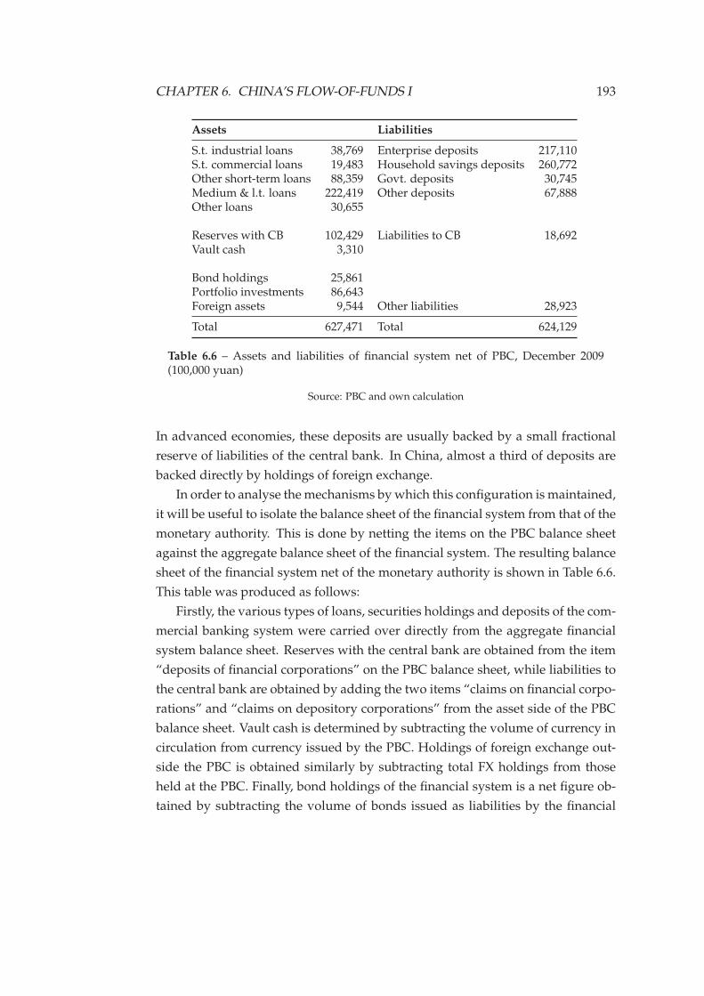
CHAPTER 6. CHINA’S FLOW-OF-FUNDS I 193
Assets Liabilities
S.t. industrial loans 38,769 Enterprise deposits 217,110S.t. commercial loans 19,483 Household savings deposits 260,772Other short-term loans 88,359 Govt. deposits 30,745Medium & l.t. loans 222,419 Other deposits 67,888Other loans 30,655
Reserves with CB 102,429 Liabilities to CB 18,692Vault cash 3,310
Bond holdings 25,861Portfolio investments 86,643Foreign assets 9,544 Other liabilities 28,923
Total 627,471 Total 624,129
Table 6.6 – Assets and liabilities of financial system net of PBC, December 2009(100,000 yuan)
Source: PBC and own calculation
In advanced economies, these deposits are usually backed by a small fractional
reserve of liabilities of the central bank. In China, almost a third of deposits are
backed directly by holdings of foreign exchange.
In order to analyse the mechanisms by which this configuration is maintained,
it will be useful to isolate the balance sheet of the financial system from that of the
monetary authority. This is done by netting the items on the PBC balance sheet
against the aggregate balance sheet of the financial system. The resulting balance
sheet of the financial system net of the monetary authority is shown in Table 6.6.
This table was produced as follows:
Firstly, the various types of loans, securities holdings and deposits of the com-
mercial banking system were carried over directly from the aggregate financial
system balance sheet. Reserves with the central bank are obtained from the item
“deposits of financial corporations” on the PBC balance sheet, while liabilities to
the central bank are obtained by adding the two items “claims on financial corpo-
rations” and “claims on depository corporations” from the asset side of the PBC
balance sheet. Vault cash is determined by subtracting the volume of currency in
circulation from currency issued by the PBC. Holdings of foreign exchange out-
side the PBC is obtained similarly by subtracting total FX holdings from those
held at the PBC. Finally, bond holdings of the financial system is a net figure ob-
tained by subtracting the volume of bonds issued as liabilities by the financial
CHAPTER 6. CHINA’S FLOW-OF-FUNDS I 194
system as a whole, from the volume issued by the central bank: the difference
should give the volume of central bank bonds held by the banking system as a
whole, although this should be seen as a net figure because commercial banks
may also issue some bonds of their own. In addition, a number of items of small
magnitudes on each balance sheet have been aggregated into the category “other
liabilities”
The resulting balance sheet in Table 6.6 requires a number of assumptions
to be made about the accounting categories of the aggregate balance sheet of the
financial system and the PBC balance sheet. The plausibility of these assumptions
is supported by the fact that the total assets and liabilities of the balance sheet
generated are close in magnitude, despite the composition and construction each
side being different. Having generated such balance sheets for the period 2000–
2009 (the PBC first began publishing balance sheets in 2000), it seems reasonable
to conclude that these provide a good representation of the aggregate financial
system balance, net of the monetary authority.
The final task required for integration with the flow-of-funds accounts is to
convert the balance sheets of the PBC and the financial system from stocks to
flows, and to compare these flow values with those of the financial institutions
sector in the flow-of-funds accounts.
This is done using Tables 6.7 and 6.8. Table 6.7 shows the Financial Trans-
actions of the flow-of-funds table for 2009. The order of the table has been re-
arranged slightly from the original published by the NBS, but the contents are
identical, as are the five institutional sectors. Table 6.8 shows the same set of ac-
counts, but in this case the financial institutions sector has been replaced with
two sectors, the monetary authority and financial institutions excluding the mon-
etary authority. The figures for these two sectors have been replaced using flow
values calculated from the balance sheets of the PBC and the balance sheet of the
financial institutions net of the PBC. By comparing the values in these two tables,
it will be possible to determine how closely aligned the financial balance sheets
and the flow-of-funds are.
The compatibility between these two sets of accounts will show up in partic-
ular in the differences between total sources and uses of funds for each item on
the sheet. In the original in Table 6.7, the construction of the accounts is such that
total sources and uses are exactly equal for each item.
The tables are divided into four sections horizontally. The first section con-
tains total uses and sources for each sector. The next two sectors contain trans-
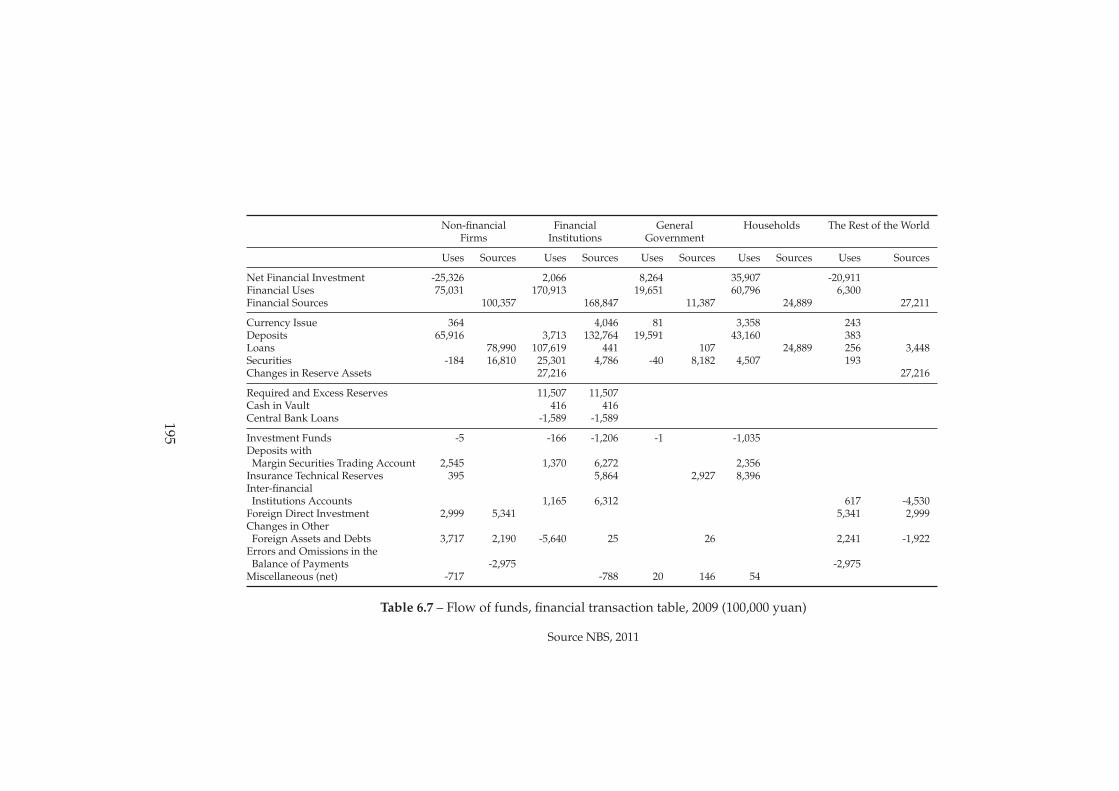
Non-financial Financial General Households The Rest of the WorldFirms Institutions Government
Uses Sources Uses Sources Uses Sources Uses Sources Uses Sources
Net Financial Investment -25,326 2,066 8,264 35,907 -20,911Financial Uses 75,031 170,913 19,651 60,796 6,300Financial Sources 100,357 168,847 11,387 24,889 27,211
Currency Issue 364 4,046 81 3,358 243Deposits 65,916 3,713 132,764 19,591 43,160 383Loans 78,990 107,619 441 107 24,889 256 3,448Securities -184 16,810 25,301 4,786 -40 8,182 4,507 193Changes in Reserve Assets 27,216 27,216
Required and Excess Reserves 11,507 11,507Cash in Vault 416 416Central Bank Loans -1,589 -1,589
Investment Funds -5 -166 -1,206 -1 -1,035Deposits with
Margin Securities Trading Account 2,545 1,370 6,272 2,356Insurance Technical Reserves 395 5,864 2,927 8,396Inter-financial
Institutions Accounts 1,165 6,312 617 -4,530Foreign Direct Investment 2,999 5,341 5,341 2,999Changes in Other
Foreign Assets and Debts 3,717 2,190 -5,640 25 26 2,241 -1,922Errors and Omissions in the
Balance of Payments -2,975 -2,975Miscellaneous (net) -717 -788 20 146 54
Table 6.7 – Flow of funds, financial transaction table, 2009 (100,000 yuan)
Source NBS, 2011
195
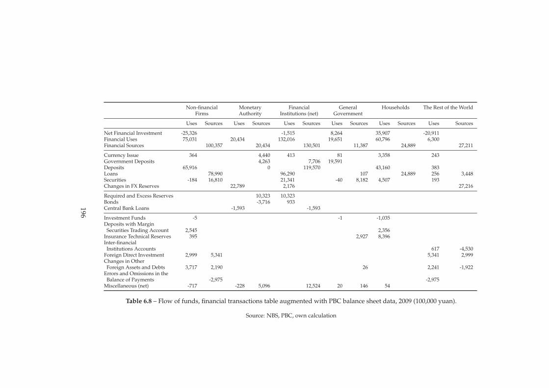
Non-financial Monetary Financial General Households The Rest of the WorldFirms Authority Institutions (net) Government
Uses Sources Uses Sources Uses Sources Uses Sources Uses Sources Uses Sources
Net Financial Investment -25,326 -1,515 8,264 35,907 -20,911Financial Uses 75,031 20,434 132,016 19,651 60,796 6,300Financial Sources 100,357 20,434 130,501 11,387 24,889 27,211
Currency Issue 364 4,440 413 81 3,358 243Government Deposits 4,263 7,706 19,591Deposits 65,916 0 119,570 43,160 383Loans 78,990 96,290 107 24,889 256 3,448Securities -184 16,810 21,341 -40 8,182 4,507 193Changes in FX Reserves 22,789 2,176 27,216
Required and Excess Reserves 10,323 10,323Bonds -3,716 933Central Bank Loans -1,593 -1,593
Investment Funds -5 -1 -1,035Deposits with Margin
Securities Trading Account 2,545 2,356Insurance Technical Reserves 395 2,927 8,396Inter-financial
Institutions Accounts 617 -4,530Foreign Direct Investment 2,999 5,341 5,341 2,999Changes in Other
Foreign Assets and Debts 3,717 2,190 26 2,241 -1,922Errors and Omissions in the
Balance of Payments -2,975 -2,975Miscellaneous (net) -717 -228 5,096 12,524 20 146 54
Table 6.8 – Flow of funds, financial transactions table augmented with PBC balance sheet data, 2009 (100,000 yuan).
Source: NBS, PBC, own calculation
196
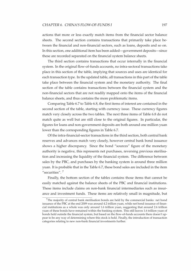
CHAPTER 6. CHINA’S FLOW-OF-FUNDS I 197
actions that more or less exactly match items from the financial sector balance
sheets. The second section contains transactions that primarily take place be-
tween the financial and non-financial sectors, such as loans, deposits and so on.
In this section, one additional item has been added—government deposits—since
these are recorded separated on the financial system balance sheets.
The third section contains transactions that occur internally in the financial
system. In the original flow-of-funds accounts, no intra-sectoral transactions take
place in this section of the table, implying that sources and uses are identical for
each transaction type. In the updated table, all transactions in this part of the table
take place between the financial system and the monetary authority. The final
section of the table contains transactions between the financial system and the
non-financial sectors that are not readily mapped onto the items of the financial
balance sheets, and thus contains the more problematic items.
Comparing Table 6.7 to Table 6.8, the first items of interest are contained in the
second section of the table, starting with currency issue. These currency figures
match very closely across the two tables. The next three items of Table 6.8 do not
match quite as well but are still close to the original figures. In particular, the
figures for loans and non-government deposits are both around one million yuan
lower than the corresponding figures in Table 6.7.
Of the intra-financial-sector transactions in the third section, both central bank
reserves and advances match very closely, however central bank bond issuance
shows a higher discrepancy. Since the bond “sources” figure of the monetary
authority is negative, this represents net purchases, reversing previous sterilisa-
tion and increasing the liquidity of the financial system. The difference between
sales by the PBC, and purchases by the banking system is around three million
yuan. It is probable that in the Table 6.7, these bond sales are included in the item
“securities”. 7
Finally, the bottom section of the tables contains those items that cannot be
easily matched against the balance sheets of the PBC and financial institutions.
These items include claims on non-bank financial intermediaries such as insur-
ance and investment funds. These items are relatively small in magnitude, but
7The majority of central bank sterilisation bonds are held by the commercial banks: net bondissuance of the PBC at the end 2009 was around 4.2 trillion yuan, while net bond issuance of finan-cial institutions as a whole was only around 1.6 trillion yuan, suggesting that around 2.6 trillionyuan of these bonds have remained within the banking system. This still leaves 1.6 trillion yuan ofbonds held outside the financial system, but based on the flow-of-funds accounts there doesn’t ap-pear to be any way of determining where this stock is held. Finally, the introduction of transactioncategories relating to new non-bank financial investments further.
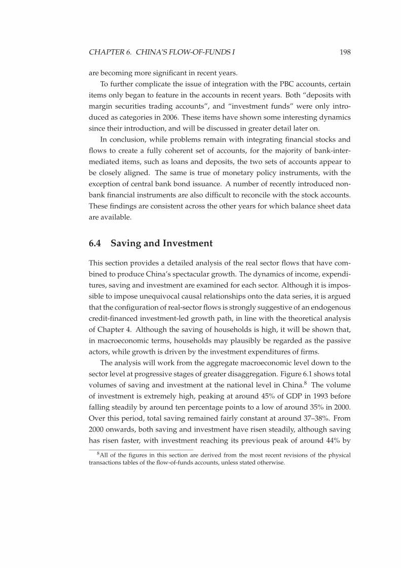
CHAPTER 6. CHINA’S FLOW-OF-FUNDS I 198
are becoming more significant in recent years.
To further complicate the issue of integration with the PBC accounts, certain
items only began to feature in the accounts in recent years. Both “deposits with
margin securities trading accounts”, and “investment funds” were only intro-
duced as categories in 2006. These items have shown some interesting dynamics
since their introduction, and will be discussed in greater detail later on.
In conclusion, while problems remain with integrating financial stocks and
flows to create a fully coherent set of accounts, for the majority of bank-inter-
mediated items, such as loans and deposits, the two sets of accounts appear to
be closely aligned. The same is true of monetary policy instruments, with the
exception of central bank bond issuance. A number of recently introduced non-
bank financial instruments are also difficult to reconcile with the stock accounts.
These findings are consistent across the other years for which balance sheet data
are available.
6.4 Saving and Investment
This section provides a detailed analysis of the real sector flows that have com-
bined to produce China’s spectacular growth. The dynamics of income, expendi-
tures, saving and investment are examined for each sector. Although it is impos-
sible to impose unequivocal causal relationships onto the data series, it is argued
that the configuration of real-sector flows is strongly suggestive of an endogenous
credit-financed investment-led growth path, in line with the theoretical analysis
of Chapter 4. Although the saving of households is high, it will be shown that,
in macroeconomic terms, households may plausibly be regarded as the passive
actors, while growth is driven by the investment expenditures of firms.
The analysis will work from the aggregate macroeconomic level down to the
sector level at progressive stages of greater disaggregation. Figure 6.1 shows total
volumes of saving and investment at the national level in China.8 The volume
of investment is extremely high, peaking at around 45% of GDP in 1993 before
falling steadily by around ten percentage points to a low of around 35% in 2000.
Over this period, total saving remained fairly constant at around 37–38%. From
2000 onwards, both saving and investment have risen steadily, although saving
has risen faster, with investment reaching its previous peak of around 44% by
8All of the figures in this section are derived from the most recent revisions of the physicaltransactions tables of the flow-of-funds accounts, unless stated otherwise.
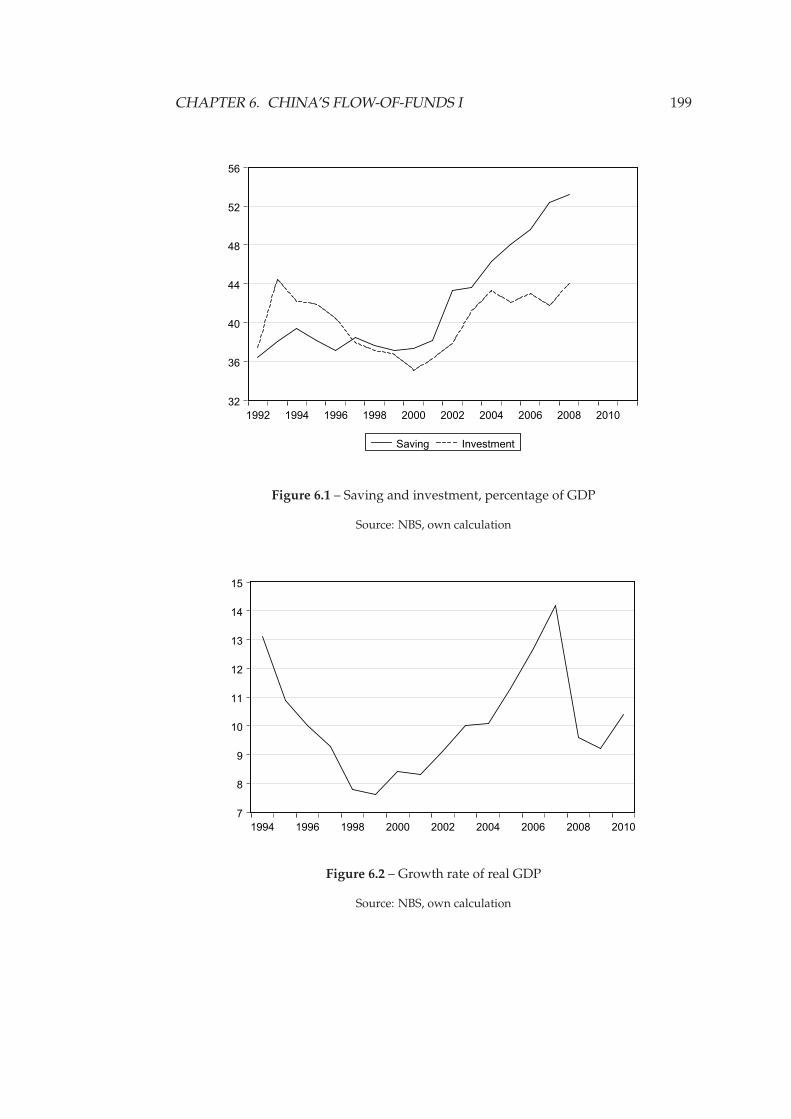
CHAPTER 6. CHINA’S FLOW-OF-FUNDS I 199
32
36
40
44
48
52
56
1992 1994 1996 1998 2000 2002 2004 2006 2008 2010
Saving Investment
Figure 6.1 – Saving and investment, percentage of GDP
Source: NBS, own calculation
7
8
9
10
11
12
13
14
15
1994 1996 1998 2000 2002 2004 2006 2008 2010
Figure 6.2 – Growth rate of real GDP
Source: NBS, own calculation
CHAPTER 6. CHINA’S FLOW-OF-FUNDS I 200
2008, while saving exceeded 50% in 2007.
Figure 6.2 shows the rate of growth of real GDP over a period extended by two
years at the end of the range. The share of investment in GDP and the growth rate
of GDP have followed a closely aligned path, at least until 2004. After 2004, the
share of investment in GDP flattened out, while saving continued to increase as a
share of GDP.
This excess of saving over investment is reflected in the trade balance, as
shown in Figure 6.3. This figure is not generated from the flow-of-funds accounts,
but shows the official volumes of exports and imports from NBS balance of pay-
ments data. The trade balance implied by these figures differs somewhat from
that obtained from the flow-of-funds which only include a figure for net exports.
12
16
20
24
28
32
36
40
1992 1994 1996 1998 2000 2002 2004 2006 2008 2010
Exports Imports
Figure 6.3 – Exports and imports, percentage of GDP
Source: NBS, own calculation
6.4.1 Saving
The high total level of saving in China is spread across the institutional sec-
tors, although the proportion assigned to each sector—firms, households and
governments—depends in part on assumptions regarding the classification of
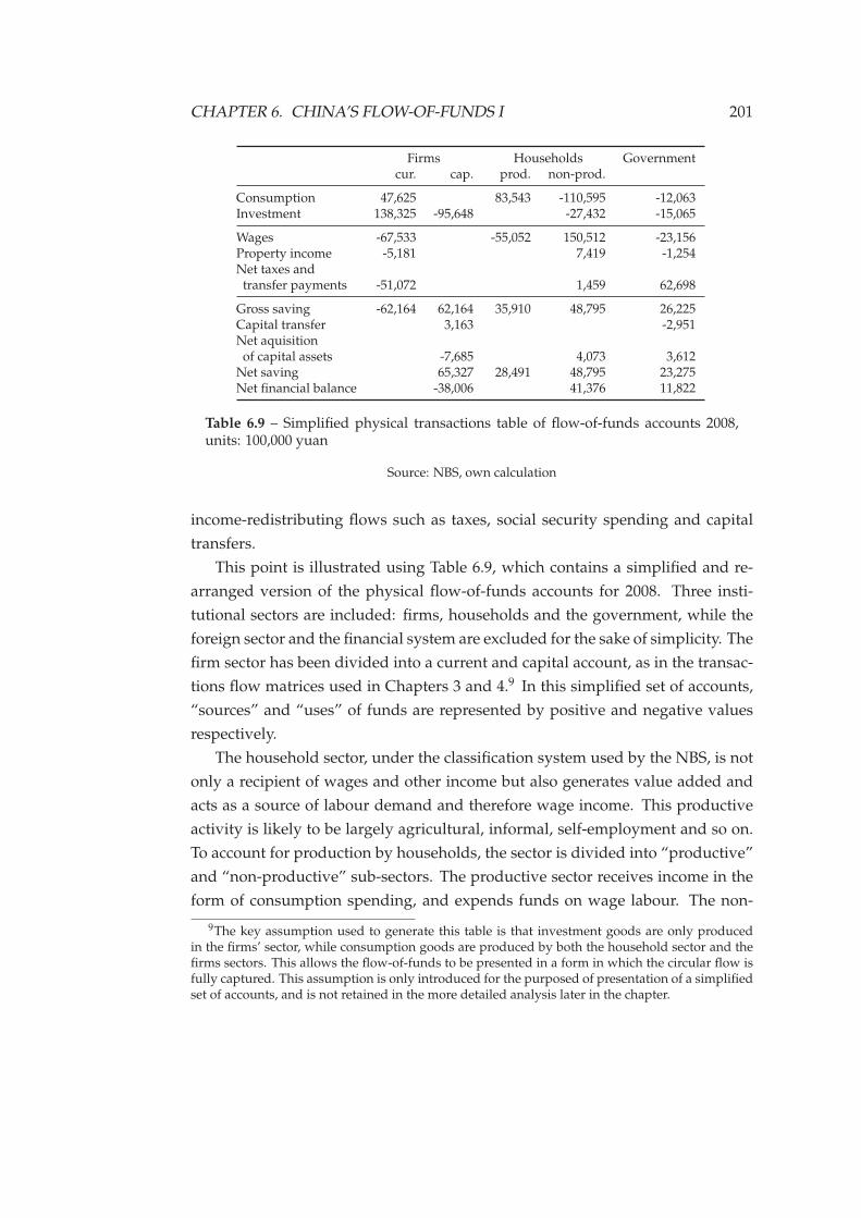
CHAPTER 6. CHINA’S FLOW-OF-FUNDS I 201
Firms Households Governmentcur. cap. prod. non-prod.
Consumption 47,625 83,543 -110,595 -12,063Investment 138,325 -95,648 -27,432 -15,065
Wages -67,533 -55,052 150,512 -23,156Property income -5,181 7,419 -1,254Net taxes andtransfer payments -51,072 1,459 62,698
Gross saving -62,164 62,164 35,910 48,795 26,225Capital transfer 3,163 -2,951Net aquisitionof capital assets -7,685 4,073 3,612
Net saving 65,327 28,491 48,795 23,275Net financial balance -38,006 41,376 11,822
Table 6.9 – Simplified physical transactions table of flow-of-funds accounts 2008,units: 100,000 yuan
Source: NBS, own calculation
income-redistributing flows such as taxes, social security spending and capital
transfers.
This point is illustrated using Table 6.9, which contains a simplified and re-
arranged version of the physical flow-of-funds accounts for 2008. Three insti-
tutional sectors are included: firms, households and the government, while the
foreign sector and the financial system are excluded for the sake of simplicity. The
firm sector has been divided into a current and capital account, as in the transac-
tions flow matrices used in Chapters 3 and 4.9 In this simplified set of accounts,
“sources” and “uses” of funds are represented by positive and negative values
respectively.
The household sector, under the classification system used by the NBS, is not
only a recipient of wages and other income but also generates value added and
acts as a source of labour demand and therefore wage income. This productive
activity is likely to be largely agricultural, informal, self-employment and so on.
To account for production by households, the sector is divided into “productive”
and “non-productive” sub-sectors. The productive sector receives income in the
form of consumption spending, and expends funds on wage labour. The non-
9The key assumption used to generate this table is that investment goods are only producedin the firms’ sector, while consumption goods are produced by both the household sector and thefirms sectors. This allows the flow-of-funds to be presented in a form in which the circular flow isfully captured. This assumption is only introduced for the purposed of presentation of a simplifiedset of accounts, and is not retained in the more detailed analysis later in the chapter.
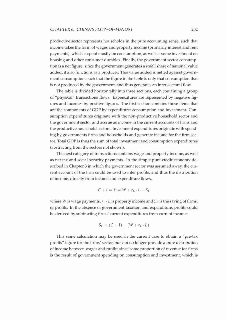
CHAPTER 6. CHINA’S FLOW-OF-FUNDS I 202
productive sector represents households in the pure accounting sense, such that
income takes the form of wages and property income (primarily interest and rent
payments), which is spent mostly on consumption, as well as some investment on
housing and other consumer durables. Finally, the government sector consump-
tion is a net figure: since the government generates a small share of national value
added, it also functions as a producer. This value added is netted against govern-
ment consumption, such that the figure in the table is only that consumption that
is not produced by the government, and thus generates an inter-sectoral flow.
The table is divided horizontally into three sections, each containing a group
of “physical” transactions flows. Expenditures are represented by negative fig-
ures and incomes by positive figures. The first section contains those items that
are the components of GDP by expenditure: consumption and investment. Con-
sumption expenditures originate with the non-productive household sector and
the government sector and accrue as income in the current accounts of firms and
the productive household sectors. Investment expenditures originate with spend-
ing by governments firms and households and generate income for the firm sec-
tor. Total GDP is thus the sum of total investment and consumption expenditures
(abstracting from the sectors not shown).
The next category of transactions contains wage and property income, as well
as net tax and social security payments. In the simple pure-credit economy de-
scribed in Chapter 3 in which the government sector was assumed away, the cur-
rent account of the firm could be used to infer profits, and thus the distribution
of income, directly from income and expenditure flows,
C+ I = Y = W + rL · L+ SF
where W is wage payments, rL · L is property income and SF is the saving of firms,
or profits. In the absence of government taxation and expenditure, profits could
be derived by subtracting firms’ current expenditures from current income:
SF = (C+ I)− (W + rL · L)
This same calculation may be used in the current case to obtain a “pre-tax
profits” figure for the firms’ sector, but can no longer provide a pure distribution
of income between wages and profits since some proportion of revenue for firms
is the result of government spending on consumption and investment, which is
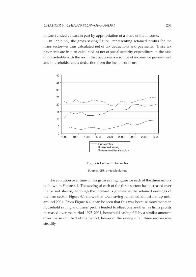
CHAPTER 6. CHINA’S FLOW-OF-FUNDS I 203
in turn funded at least in part by appropriation of a share of that income.
In Table 6.9, the gross saving figure—representing retained profits for the
firms sector—is thus calculated net of tax deductions and payments. These tax
payments are in turn calculated as net of social security expenditure in the case
of households with the result that net taxes is a source of income for government
and households, and a deduction from the income of firms.
0
5
10
15
20
25
30
35
40
1992 1994 1996 1998 2000 2002 2004 2006 2008
Firms profits
Household saving
Government fiscal surplus
Figure 6.4 – Saving by sector
Source: NBS, own calculation
The evolution over time of this gross saving figure for each of the three sectors
is shown in Figure 6.4. The saving of each of the three sectors has increased over
the period shown, although the increase is greatest in the retained earnings of
the firm sector. Figure 6.1 shows that total saving remained almost flat up until
around 2001. From Figure 6.4 it can be seen that this was because movements in
household saving and firms’ profits tended to offset one another: as firms profits
increased over the period 1997–2001, household saving fell by a similar amount.
Over the second half of the period, however, the saving of all three sectors rose
steadily.
CHAPTER 6. CHINA’S FLOW-OF-FUNDS I 204
Table 6.9 shows that in 2008 firms were the primary source of tax revenues,
while households were net recipients of fiscal transfers. Figure 6.5 shows the
distribution of taxation and transfer payments over the three sectors for the full
period of analysis. The pattern has remained fairly steady over this period: firms
provide the major source of fiscal revenue, with the tax liabilities of firms remain-
ing fairly constant at around 15% of GDP. At the same time, the position of house-
holds as net beneficiaries of fiscal transfers has declined while governments have
increased their tax revenues from a low of around 15% of GDP to a maximum of
20% of GDP in 2007 and 2008.
-20
-15
-10
-5
0
5
10
15
20
25
1992 1994 1996 1998 2000 2002 2004 2006 2008
Firms Households Government
Figure 6.5 – Net tax and transfer payments by sector
Source: NBS, own calculation
By subtracting the net tax and current income figure from gross saving, it is
possible to obtain a pre-tax profit figure for firms and a saving figure for house-
holds net of taxes. While it is impossible to isolate the effects of taxation and
government transfer payments on saving and expenditure due the aggregate de-
mand effects of such policy, this gives some indication of relative levels of saving
in the firms and household sectors before fiscal transfers. These pre-fiscal-transfer
saving magnitudes are shown in Figure 6.6. Removing fiscal transfer payments
from the picture reverses the relative positions of firms and the household sector:
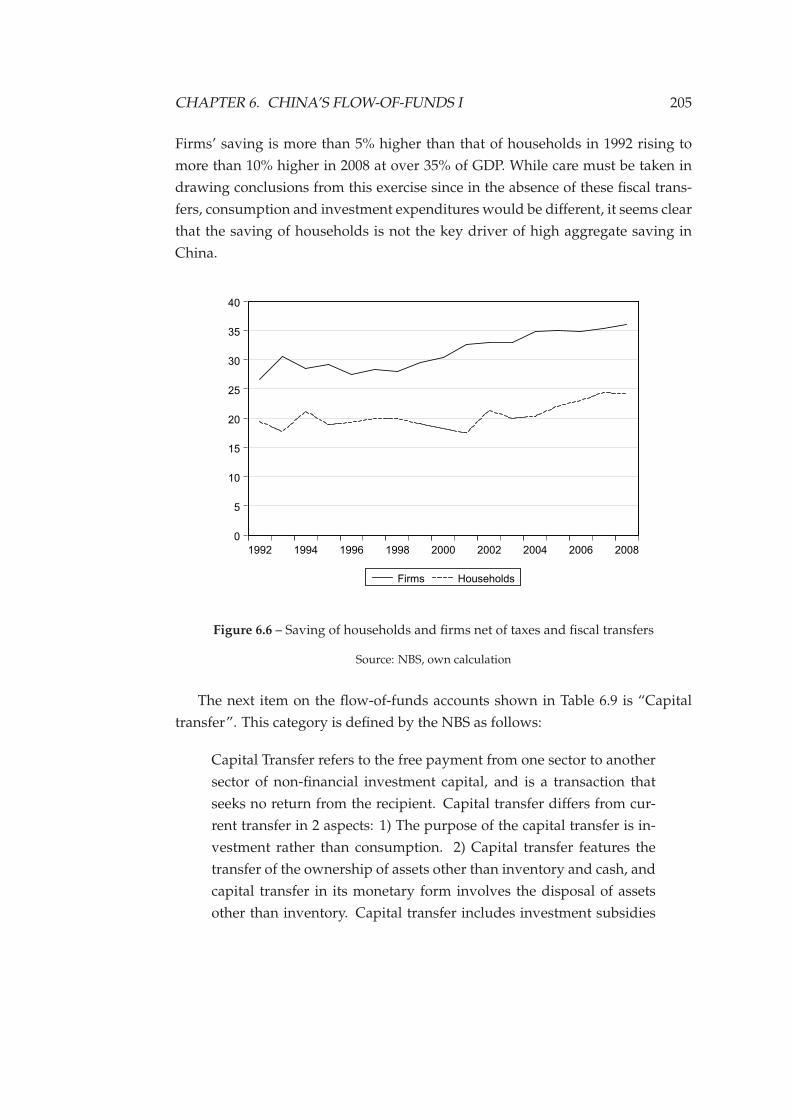
CHAPTER 6. CHINA’S FLOW-OF-FUNDS I 205
Firms’ saving is more than 5% higher than that of households in 1992 rising to
more than 10% higher in 2008 at over 35% of GDP. While care must be taken in
drawing conclusions from this exercise since in the absence of these fiscal trans-
fers, consumption and investment expenditures would be different, it seems clear
that the saving of households is not the key driver of high aggregate saving in
China.
0
5
10
15
20
25
30
35
40
1992 1994 1996 1998 2000 2002 2004 2006 2008
Firms Households
Figure 6.6 – Saving of households and firms net of taxes and fiscal transfers
Source: NBS, own calculation
The next item on the flow-of-funds accounts shown in Table 6.9 is “Capital
transfer”. This category is defined by the NBS as follows:
Capital Transfer refers to the free payment from one sector to another
sector of non-financial investment capital, and is a transaction that
seeks no return from the recipient. Capital transfer differs from cur-
rent transfer in 2 aspects: 1) The purpose of the capital transfer is in-
vestment rather than consumption. 2) Capital transfer features the
transfer of the ownership of assets other than inventory and cash, and
capital transfer in its monetary form involves the disposal of assets
other than inventory. Capital transfer includes investment subsidies
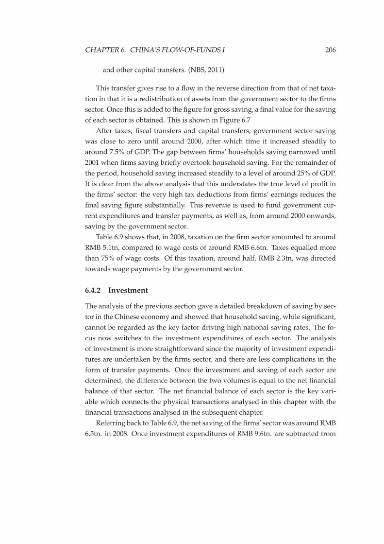
CHAPTER 6. CHINA’S FLOW-OF-FUNDS I 206
and other capital transfers. (NBS, 2011)
This transfer gives rise to a flow in the reverse direction from that of net taxa-
tion in that it is a redistribution of assets from the government sector to the firms
sector. Once this is added to the figure for gross saving, a final value for the saving
of each sector is obtained. This is shown in Figure 6.7
After taxes, fiscal transfers and capital transfers, government sector saving
was close to zero until around 2000, after which time it increased steadily to
around 7.5% of GDP. The gap between firms’ households saving narrowed until
2001 when firms saving briefly overtook household saving. For the remainder of
the period, household saving increased steadily to a level of around 25% of GDP.
It is clear from the above analysis that this understates the true level of profit in
the firms’ sector: the very high tax deductions from firms’ earnings reduces the
final saving figure substantially. This revenue is used to fund government cur-
rent expenditures and transfer payments, as well as, from around 2000 onwards,
saving by the government sector.
Table 6.9 shows that, in 2008, taxation on the firm sector amounted to around
RMB 5.1tn, compared to wage costs of around RMB 6.6tn. Taxes equalled more
than 75% of wage costs. Of this taxation, around half, RMB 2.3tn, was directed
towards wage payments by the government sector.
6.4.2 Investment
The analysis of the previous section gave a detailed breakdown of saving by sec-
tor in the Chinese economy and showed that household saving, while significant,
cannot be regarded as the key factor driving high national saving rates. The fo-
cus now switches to the investment expenditures of each sector. The analysis
of investment is more straightforward since the majority of investment expendi-
tures are undertaken by the firms sector, and there are less complications in the
form of transfer payments. Once the investment and saving of each sector are
determined, the difference between the two volumes is equal to the net financial
balance of that sector. The net financial balance of each sector is the key vari-
able which connects the physical transactions analysed in this chapter with the
financial transactions analysed in the subsequent chapter.
Referring back to Table 6.9, the net saving of the firms’ sector was around RMB
6.5tn. in 2008. Once investment expenditures of RMB 9.6tn. are subtracted from
CHAPTER 6. CHINA’S FLOW-OF-FUNDS I 207
-5
0
5
10
15
20
25
30
1992 1994 1996 1998 2000 2002 2004 2006 2008
Firms Households Government
Figure 6.7 – Saving by sector after capital transfers
Source: NBS, own calculation
this figure, the net financial position of the firm sector shows a deficit of around
RMB 3tn.
A final additional item included in Table 6.9 is “Net acquisitions of capital
assets”. This item refers to the transfer of ownership of already-existing capital
goods between sectors. It may thus be regarded as contributing to net capital
investment from the point of view of any individual sector, although at the ag-
gregate level it only represents a redistribution of ownership. Once this figure of
RMB 7.7tn. is added to the investment figure above, the final net deficit position
of RMB 3.8tn. is obtained. This is the amount that firms are thus required to
finance through the net issuance of new financial liabilities.
The item “Net acquisitions of capital assets” is a new category which was only
introduced to the the flow-of-funds accounts in 2004. It therefore has no influence
on the investment position of sectors prior to this point.
Figure 6.8 shows the investment expenditures of each sector. Figure 6.8a ex-
cludes inter-sector capital asset purchases, while it is included in Figure 6.8b. This
inter-sectoral transfer of capital assets serves to offset what appears to be a rise
CHAPTER 6. CHINA’S FLOW-OF-FUNDS I 208
in the investment expenditure of households and the government from around
2002, and maintains the trend for a widening gap between the investment expen-
ditures of firms and households. The net investment position of firms’ in Figure
6.8b shows a steady rise in investment expenditure from around 2000 back to
levels close to the 1993 peak of 35% of GDP.
6.4.3 Net financial balances
So far, the evolution of saving and investment have been examined individually
on a sector by sector basis. These are now combined in an analysis of the net
financial position of each sector. This type of analysis is best known known in the
form of the “three balances” approach of Godley and Cripps. (1976; 1983), and
the closely related “twin deficits” hypothesis.
The “three balances” system arose out of the observation that in the UK post-
war period, the government deficit and the trade deficit tended to be very closely
linked. From this observation came the Cripps-Godley hypothesis that the pri-
vate sector financial balance tends to be small, positive and stable. This, it was
argued, is because of the behavioural tendency of the private sector to aim for
a stable ratio of income to savings—a behavioural stock-flow norm. If this hy-
pothesis correctly describes private sector behaviour, the implication is that that
expansionary fiscal policy will not be matched by increased output—due for ex-
ample to higher profits in the firm sector providing a stimulus to investment—but
will only result in an increase in the trade deficit. This hypothesis was central to
the criticisms of the activist fiscal policies of the time that were levelled by Godley,
Cripps and other members of the Cambridge Economic Policy Group (Maloney,
2012).
However, since the “three balances” approach only relies on accounting iden-
tities—and is thus always true ex post—there is no need for it to remain linked
with the hypothesis of a stable private sector net balance (dos Santos, 2010).
Nonetheless, as was shown in Chapter 4 in relation to the work of Steindl (1952)
in particular, it is the internal dynamics of the private sector that are key in deter-
mining whether an economy tends towards growth or stagnation.10 In particular,
it is the relative saving propensities of households, large monopolistic firms and
smaller “marginal” firms that combine to determine the rate of accumulation.
10Godley and Cripps themselves pointed out that “their adjustment mechanism is only consis-tent with a constant level of income because the path becomes unstable when growth is endoge-nous” (Shaikh, 2012, p. 130)
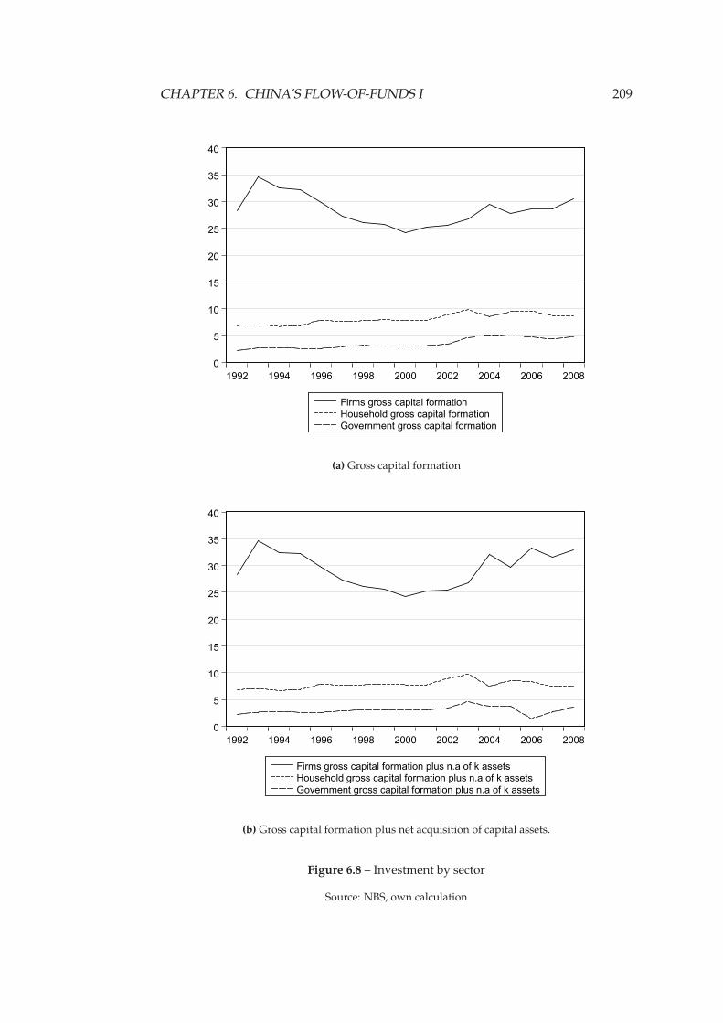
CHAPTER 6. CHINA’S FLOW-OF-FUNDS I 209
0
5
10
15
20
25
30
35
40
1992 1994 1996 1998 2000 2002 2004 2006 2008
Firms gross capital formation
Household gross capital formation
Government gross capital formation
(a) Gross capital formation
0
5
10
15
20
25
30
35
40
1992 1994 1996 1998 2000 2002 2004 2006 2008
Firms gross capital formation plus n.a of k assets
Household gross capital formation plus n.a of k assets
Government gross capital formation plus n.a of k assets
(b) Gross capital formation plus net acquisition of capital assets.
Figure 6.8 – Investment by sector
Source: NBS, own calculation
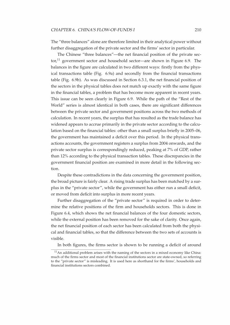
CHAPTER 6. CHINA’S FLOW-OF-FUNDS I 210
The “three balances” alone are therefore limited in their analytical power without
further disaggregation of the private sector and the firms’ sector in particular.
The Chinese “three balances”—the net financial position of the private sec-
tor,11 government sector and household sector—are shown in Figure 6.9. The
balances in the figure are calculated in two different ways: firstly from the phys-
ical transactions table (Fig. 6.9a) and secondly from the financial transactions
table (Fig. 6.9b). As was discussed in Section 6.3.1, the net financial position of
the sectors in the physical tables does not match up exactly with the same figure
in the financial tables, a problem that has become more apparent in recent years.
This issue can be seen clearly in Figure 6.9. While the path of the “Rest of the
World” series is almost identical in both cases, there are significant differences
between the private sector and government positions across the two methods of
calculation. In recent years, the surplus that has resulted as the trade balance has
widened appears to accrue primarily in the private sector according to the calcu-
lation based on the financial tables: other than a small surplus briefly in 2005–06,
the government has maintained a deficit over this period. In the physical trans-
actions accounts, the government registers a surplus from 2004 onwards, and the
private sector surplus is correspondingly reduced, peaking at 7% of GDP, rather
than 12% according to the physical transaction tables. These discrepancies in the
government financial position are examined in more detail in the following sec-
tion.
Despite these contradictions in the data concerning the government position,
the broad picture is fairly clear. A rising trade surplus has been matched by a sur-
plus in the “private sector”, while the government has either run a small deficit,
or moved from deficit into surplus in more recent years.
Further disaggregation of the “private sector” is required in order to deter-
mine the relative positions of the firm and households sectors. This is done in
Figure 6.4, which shows the net financial balances of the four domestic sectors,
while the external position has been removed for the sake of clarity. Once again,
the net financial position of each sector has been calculated from both the physi-
cal and financial tables, so that the difference between the two sets of accounts is
visible.
In both figures, the firms sector is shown to be running a deficit of around
11An additional problem arises with the naming of the sectors in a mixed economy like China:much of the firms sector and most of the financial institutions sector are state-owned, so referringto the “private sector” is misleading. It is used here as shorthand for the firms’, households andfinancial institutions sectors combined.
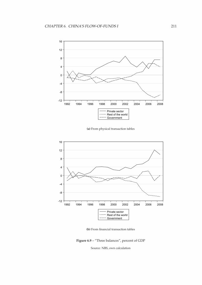
CHAPTER 6. CHINA’S FLOW-OF-FUNDS I 211
-12
-8
-4
0
4
8
12
16
1992 1994 1996 1998 2000 2002 2004 2006 2008
Private sector
Rest of the world
Government
(a) From physical transaction tables
-12
-8
-4
0
4
8
12
16
1992 1994 1996 1998 2000 2002 2004 2006 2008
Private sector
Rest of the world
Government
(b) From financial transaction tables
Figure 6.9 – “Three balances”, percent of GDP
Source: NBS, own calculation
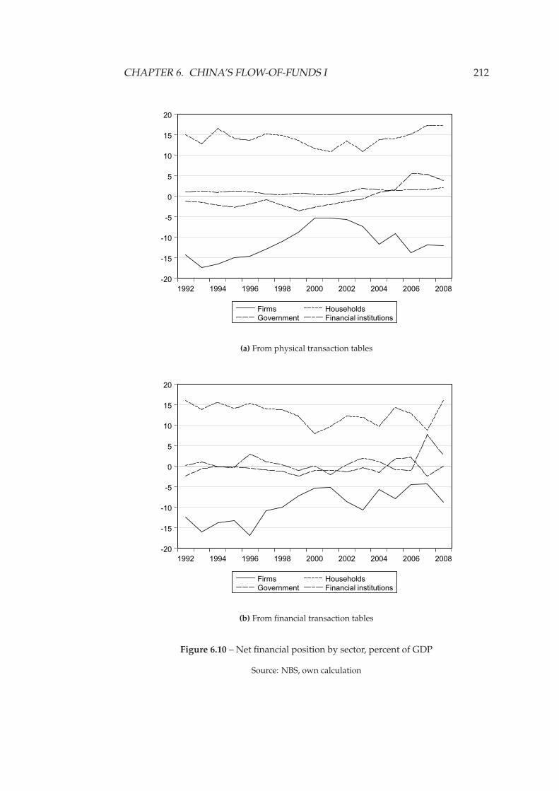
CHAPTER 6. CHINA’S FLOW-OF-FUNDS I 212
-20
-15
-10
-5
0
5
10
15
20
1992 1994 1996 1998 2000 2002 2004 2006 2008
Firms Households
Government Financial institutions
(a) From physical transaction tables
-20
-15
-10
-5
0
5
10
15
20
1992 1994 1996 1998 2000 2002 2004 2006 2008
Firms Households
Government Financial institutions
(b) From financial transaction tables
Figure 6.10 – Net financial position by sector, percent of GDP
Source: NBS, own calculation
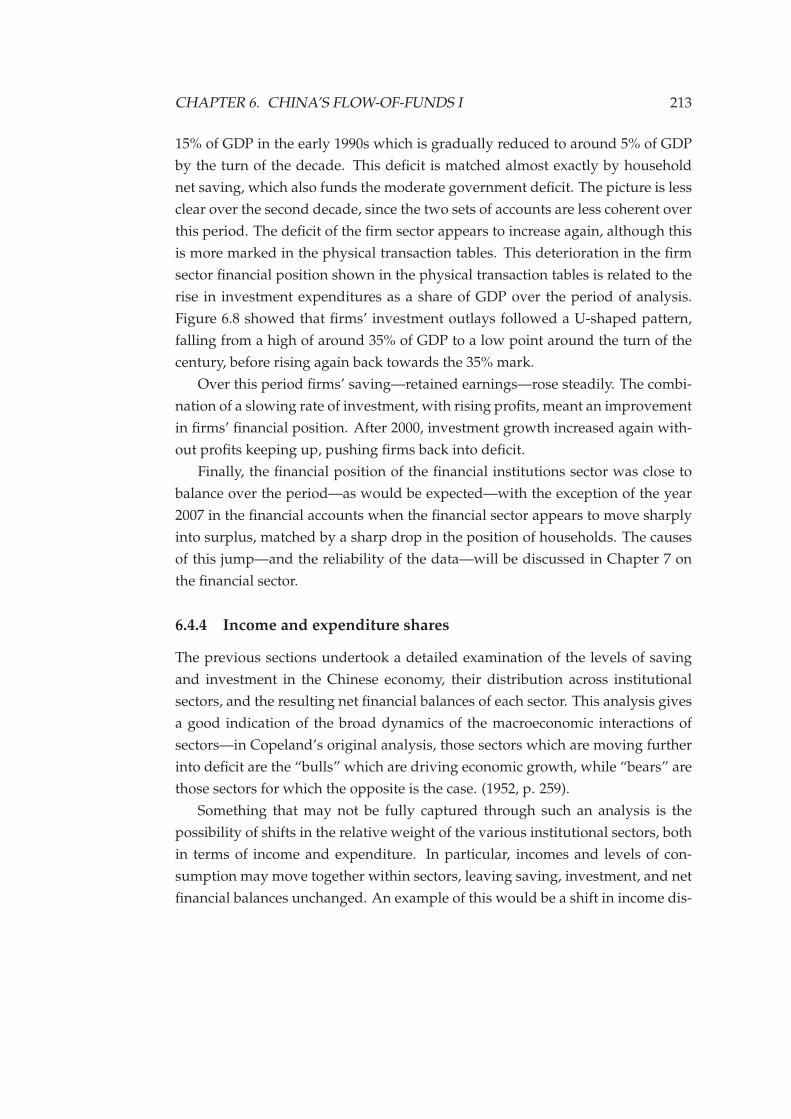
CHAPTER 6. CHINA’S FLOW-OF-FUNDS I 213
15% of GDP in the early 1990s which is gradually reduced to around 5% of GDP
by the turn of the decade. This deficit is matched almost exactly by household
net saving, which also funds the moderate government deficit. The picture is less
clear over the second decade, since the two sets of accounts are less coherent over
this period. The deficit of the firm sector appears to increase again, although this
is more marked in the physical transaction tables. This deterioration in the firm
sector financial position shown in the physical transaction tables is related to the
rise in investment expenditures as a share of GDP over the period of analysis.
Figure 6.8 showed that firms’ investment outlays followed a U-shaped pattern,
falling from a high of around 35% of GDP to a low point around the turn of the
century, before rising again back towards the 35% mark.
Over this period firms’ saving—retained earnings—rose steadily. The combi-
nation of a slowing rate of investment, with rising profits, meant an improvement
in firms’ financial position. After 2000, investment growth increased again with-
out profits keeping up, pushing firms back into deficit.
Finally, the financial position of the financial institutions sector was close to
balance over the period—as would be expected—with the exception of the year
2007 in the financial accounts when the financial sector appears to move sharply
into surplus, matched by a sharp drop in the position of households. The causes
of this jump—and the reliability of the data—will be discussed in Chapter 7 on
the financial sector.
6.4.4 Income and expenditure shares
The previous sections undertook a detailed examination of the levels of saving
and investment in the Chinese economy, their distribution across institutional
sectors, and the resulting net financial balances of each sector. This analysis gives
a good indication of the broad dynamics of the macroeconomic interactions of
sectors—in Copeland’s original analysis, those sectors which are moving further
into deficit are the “bulls” which are driving economic growth, while “bears” are
those sectors for which the opposite is the case. (1952, p. 259).
Something that may not be fully captured through such an analysis is the
possibility of shifts in the relative weight of the various institutional sectors, both
in terms of income and expenditure. In particular, incomes and levels of con-
sumption may move together within sectors, leaving saving, investment, and net
financial balances unchanged. An example of this would be a shift in income dis-
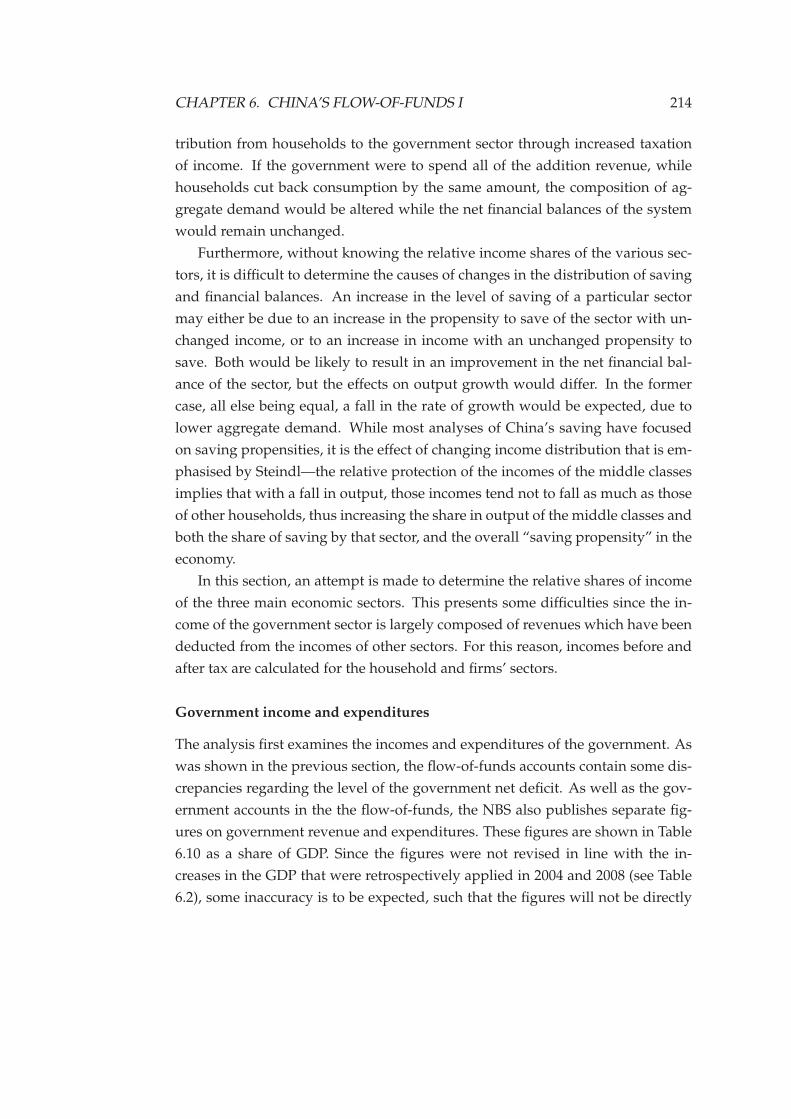
CHAPTER 6. CHINA’S FLOW-OF-FUNDS I 214
tribution from households to the government sector through increased taxation
of income. If the government were to spend all of the addition revenue, while
households cut back consumption by the same amount, the composition of ag-
gregate demand would be altered while the net financial balances of the system
would remain unchanged.
Furthermore, without knowing the relative income shares of the various sec-
tors, it is difficult to determine the causes of changes in the distribution of saving
and financial balances. An increase in the level of saving of a particular sector
may either be due to an increase in the propensity to save of the sector with un-
changed income, or to an increase in income with an unchanged propensity to
save. Both would be likely to result in an improvement in the net financial bal-
ance of the sector, but the effects on output growth would differ. In the former
case, all else being equal, a fall in the rate of growth would be expected, due to
lower aggregate demand. While most analyses of China’s saving have focused
on saving propensities, it is the effect of changing income distribution that is em-
phasised by Steindl—the relative protection of the incomes of the middle classes
implies that with a fall in output, those incomes tend not to fall as much as those
of other households, thus increasing the share in output of the middle classes and
both the share of saving by that sector, and the overall “saving propensity” in the
economy.
In this section, an attempt is made to determine the relative shares of income
of the three main economic sectors. This presents some difficulties since the in-
come of the government sector is largely composed of revenues which have been
deducted from the incomes of other sectors. For this reason, incomes before and
after tax are calculated for the household and firms’ sectors.
Government income and expenditures
The analysis first examines the incomes and expenditures of the government. As
was shown in the previous section, the flow-of-funds accounts contain some dis-
crepancies regarding the level of the government net deficit. As well as the gov-
ernment accounts in the the flow-of-funds, the NBS also publishes separate fig-
ures on government revenue and expenditures. These figures are shown in Table
6.10 as a share of GDP. Since the figures were not revised in line with the in-
creases in the GDP that were retrospectively applied in 2004 and 2008 (see Table
6.2), some inaccuracy is to be expected, such that the figures will not be directly
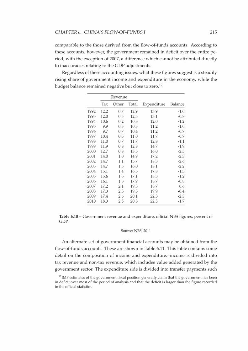
CHAPTER 6. CHINA’S FLOW-OF-FUNDS I 215
comparable to the those derived from the flow-of-funds accounts. According to
these accounts, however, the government remained in deficit over the entire pe-
riod, with the exception of 2007, a difference which cannot be attributed directly
to inaccuracies relating to the GDP adjustments.
Regardless of these accounting issues, what these figures suggest is a steadily
rising share of government income and expenditure in the economy, while the
budget balance remained negative but close to zero.12
Revenue
Tax Other Total Expenditure Balance
1992 12.2 0.7 12.9 13.9 -1.01993 12.0 0.3 12.3 13.1 -0.81994 10.6 0.2 10.8 12.0 -1.21995 9.9 0.3 10.3 11.2 -1.01996 9.7 0.7 10.4 11.2 -0.71997 10.4 0.5 11.0 11.7 -0.71998 11.0 0.7 11.7 12.8 -1.11999 11.9 0.8 12.8 14.7 -1.92000 12.7 0.8 13.5 16.0 -2.52001 14.0 1.0 14.9 17.2 -2.32002 14.7 1.1 15.7 18.3 -2.62003 14.7 1.3 16.0 18.1 -2.22004 15.1 1.4 16.5 17.8 -1.32005 15.6 1.6 17.1 18.3 -1.22006 16.1 1.8 17.9 18.7 -0.82007 17.2 2.1 19.3 18.7 0.62008 17.3 2.3 19.5 19.9 -0.42009 17.4 2.6 20.1 22.3 -2.32010 18.3 2.5 20.8 22.5 -1.7
Table 6.10 – Government revenue and expenditure, official NBS figures, percent ofGDP.
Source: NBS, 2011
An alternate set of government financial accounts may be obtained from the
flow-of-funds accounts. These are shown in Table 6.11. This table contains some
detail on the composition of income and expenditure: income is divided into
tax revenue and non-tax revenue, which includes value added generated by the
government sector. The expenditure side is divided into transfer payments such
12IMF estimates of the government fiscal position generally claim that the government has beenin deficit over most of the period of analysis and that the deficit is larger than the figure recordedin the official statistics.
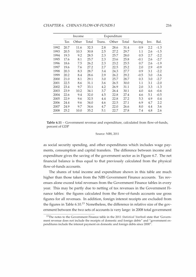
CHAPTER 6. CHINA’S FLOW-OF-FUNDS I 216
Income Expenditure
Tax Other Total Trans. Other Total Saving Inv. Bal.
1992 20.7 11.6 32.3 2.8 28.6 31.4 0.9 2.2 -1.31993 20.5 10.3 30.8 2.5 27.2 29.7 1.1 2.6 -1.51994 19.3 9.2 28.5 2.3 25.7 28.0 0.5 2.7 -2.21995 17.6 8.1 25.7 2.3 23.6 25.8 -0.1 2.6 -2.71996 18.6 7.5 26.2 2.3 23.2 25.5 0.7 2.6 -1.91997 19.6 7.6 27.2 2.7 22.5 25.2 2.0 2.9 -0.91998 20.3 8.3 28.7 3.4 24.3 27.7 0.9 3.1 -2.21999 20.2 8.4 28.6 2.9 26.2 29.2 -0.5 3.0 -3.62000 21.0 8.1 29.1 3.0 25.7 28.7 0.3 3.0 -2.72001 22.5 8.6 31.1 3.6 26.5 30.0 1.1 3.1 -2.02002 23.4 9.7 33.1 4.2 26.9 31.1 2.0 3.3 -1.32003 23.9 10.2 34.1 3.7 26.4 30.1 4.0 4.6 -0.62004 22.6 9.4 32.0 4.5 22.8 27.4 4.6 5.1 -0.52005 22.9 9.6 32.5 4.4 22.8 27.2 5.3 4.9 0.42006 24.4 9.6 34.0 4.6 22.5 27.1 6.9 4.7 2.22007 24.9 9.7 34.6 4.7 22.0 26.6 8.0 4.4 3.62008 25.2 10.0 35.2 5.1 22.7 27.8 7.4 4.8 2.6
Table 6.11 – Government revenue and expenditure, calculated from flow-of-funds,percent of GDP
Source: NBS, 2011
as social security spending, and other expenditures which includes wage pay-
ments, consumption and capital transfers. The difference between income and
expenditure gives the saving of the government sector as in Figure 6.7. The net
financial balance is thus equal to that previously calculated from the physical
flow-of-funds accounts.
The shares of total income and expenditure shown in this table are much
higher than those taken from the NBS Government Finance accounts. Tax rev-
enues alone exceed total revenues from the Government Finance tables in every
year. This may be partly due to netting of tax revenues in the Government Fi-
nance tables: the figures calculated from the flow-of-funds accounts use gross
figures for all revenues. In addition, foreign interest receipts are excluded from
the figures in Table 6.10.13 Nonetheless, the difference in relative size of the gov-
ernment between the two sets of accounts is very large: in 2008 total government
13The notes to the Government Finance table in the 2011 Statistical Yearbook state that ‘Govern-ment revenue does not include the receipts of domestic and foreign debts” and “government ex-penditures include the interest payment on domestic and foreign debts since 2000”.
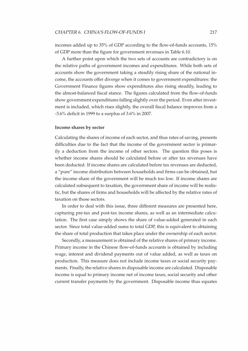
CHAPTER 6. CHINA’S FLOW-OF-FUNDS I 217
incomes added up to 35% of GDP according to the flow-of-funds accounts, 15%
of GDP more than the figure for government revenues in Table 6.10.
A further point upon which the two sets of accounts are contradictory is on
the relative paths of government incomes and expenditures. While both sets of
accounts show the government taking a steadily rising share of the national in-
come, the accounts offer diverge when it comes to government expenditures: the
Government Finance figures show expenditures also rising steadily, leading to
the almost-balanced fiscal stance. The figures calculated from the flow-of-funds
show government expenditures falling slightly over the period. Even after invest-
ment is included, which rises slightly, the overall fiscal balance improves from a
-3.6% deficit in 1999 to a surplus of 3.6% in 2007.
Income shares by sector
Calculating the shares of income of each sector, and thus rates of saving, presents
difficulties due to the fact that the income of the government sector is primar-
ily a deduction from the income of other sectors. The question this poses is
whether income shares should be calculated before or after tax revenues have
been deducted. If income shares are calculated before tax revenues are deducted,
a “pure” income distribution between households and firms can be obtained, but
the income share of the government will be much too low. If income shares are
calculated subsequent to taxation, the government share of income will be realis-
tic, but the shares of firms and households will be affected by the relative rates of
taxation on those sectors.
In order to deal with this issue, three different measures are presented here,
capturing pre-tax and post-tax income shares, as well as an intermediate calcu-
lation. The first case simply shows the share of value-added generated in each
sector. Since total value-added sums to total GDP, this is equivalent to obtaining
the share of total production that takes place under the ownership of each sector.
Secondly, a measurement is obtained of the relative shares of primary income.
Primary income in the Chinese flow-of-funds accounts is obtained by including
wage, interest and dividend payments out of value added, as well as taxes on
production. This measure does not include income taxes or social security pay-
ments. Finally, the relative shares in disposable income are calculated. Disposable
income is equal to primary income net of income taxes, social security and other
current transfer payments by the government. Disposable income thus equates
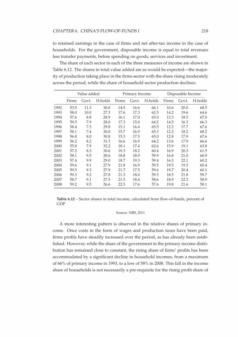
CHAPTER 6. CHINA’S FLOW-OF-FUNDS I 218
to retained earnings in the case of firms and net after-tax income in the case of
households. For the government, disposable income is equal to total revenues
less transfer payments, before spending on goods, services and investment.
The share of each sector in each of the three measures of income are shown in
Table 6.12. The shares in total value added are as would be expected—the major-
ity of production taking place in the firms sector with the share rising moderately
across the period, while the share of household sector production declines.
Value added Primary Income Disposable Income
Firms Govt. H.holds Firms Govt. H.holds Firms Govt. H.holds
1992 53.9 11.3 30.0 14.9 16.6 66.1 10.6 20.0 68.51993 58.0 10.0 27.3 17.6 17.3 62.5 14.2 19.6 64.61994 57.6 8.8 28.9 16.1 17.0 65.0 13.3 18.5 67.01995 59.5 7.9 28.0 17.3 15.0 64.2 14.5 16.3 66.31996 58.4 7.3 29.8 15.1 16.4 65.5 12.2 17.7 67.61997 58.1 7.4 30.0 15.7 16.9 65.3 12.2 18.2 68.21998 56.8 8.0 30.8 15.3 17.5 65.0 12.8 17.9 67.61999 56.2 8.2 31.3 16.6 16.9 64.2 13.6 17.9 66.62000 55.8 7.9 32.2 18.1 17.4 62.6 15.9 19.1 63.82001 57.2 8.3 30.6 19.3 18.2 60.4 16.9 20.3 61.52002 58.1 9.5 28.6 18.8 18.9 59.9 16.8 21.0 60.92003 57.4 9.9 29.0 18.7 19.3 59.4 16.3 22.1 60.22004 59.6 9.1 27.9 21.8 16.9 59.5 19.5 19.5 60.42005 59.5 9.3 27.9 21.7 17.5 59.6 19.7 20.4 60.12006 59.3 9.2 27.8 21.3 18.0 59.3 18.5 21.8 59.72007 58.7 9.1 27.5 21.5 18.4 58.6 18.9 22.3 58.92008 59.2 9.5 26.6 22.5 17.6 57.6 19.8 21.6 58.1
Table 6.12 – Sector shares in total income, calculated from flow-of-funds, percent ofGDP
Source: NBS, 2011
A more interesting pattern is observed in the relative shares of primary in-
come. Once costs in the form of wages and production taxes have been paid,
firms profits have steadily increased over the period, as has already been estab-
lished. However, while the share of the government in the primary income distri-
bution has remained close to constant, the rising share of firms’ profits has been
accommodated by a significant decline in household incomes, from a maximum
of 66% of primary income in 1993, to a low of 58% in 2008. This fall in the income
share of households is not necessarily a pre-requisite for the rising profit share of
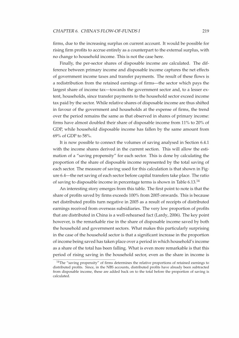
CHAPTER 6. CHINA’S FLOW-OF-FUNDS I 219
firms, due to the increasing surplus on current account. It would be possible for
rising firm profits to accrue entirely as a counterpart to the external surplus, with
no change to household income. This is not the case here.
Finally, the per-sector shares of disposable income are calculated. The dif-
ference between primary income and disposable income captures the net effects
of government income taxes and transfer payments. The result of these flows is
a redistribution from the retained earnings of firms—the sector which pays the
largest share of income tax—towards the government sector and, to a lesser ex-
tent, households, since transfer payments to the household sector exceed income
tax paid by the sector. While relative shares of disposable income are thus shifted
in favour of the government and households at the expense of firms, the trend
over the period remains the same as that observed in shares of primary income:
firms have almost doubled their share of disposable income from 11% to 20% of
GDP, while household disposable income has fallen by the same amount from
69% of GDP to 58%.
It is now possible to connect the volumes of saving analysed in Section 6.4.1
with the income shares derived in the current section. This will allow the esti-
mation of a “saving propensity” for each sector. This is done by calculating the
proportion of the share of disposable income represented by the total saving of
each sector. The measure of saving used for this calculation is that shown in Fig-
ure 6.4—the net saving of each sector before capital transfers take place. The ratio
of saving to disposable income in percentage terms is shown in Table 6.13.14
An interesting story emerges from this table. The first point to note is that the
share of profits saved by firms exceeds 100% from 2005 onwards. This is because
net distributed profits turn negative in 2005 as a result of receipts of distributed
earnings received from overseas subsidiaries. The very low proportion of profits
that are distributed in China is a well-rehearsed fact (Lardy, 2006). The key point
however, is the remarkable rise in the share of disposable income saved by both
the household and government sectors. What makes this particularly surprising
in the case of the household sector is that a significant increase in the proportion
of income being saved has taken place over a period in which household’s income
as a share of the total has been falling. What is even more remarkable is that this
period of rising saving in the household sector, even as the share in income is
14The “saving propensity” of firms determines the relative proportions of retained earnings todistributed profits. Since, in the NBS accounts, distributed profits have already been subtractedfrom disposable income, these are added back on to the total before the proportion of saving iscalculated.

CHAPTER 6. CHINA’S FLOW-OF-FUNDS I 220
Households Firms Government
1992 31.8 99.9 4.51993 30.7 99.5 5.61994 34.6 99.0 2.71995 31.6 91.0 -0.71996 31.7 89.5 3.81997 33.5 90.7 10.81998 33.3 88.3 5.21999 32.2 90.8 -3.02000 30.3 89.6 1.72001 30.2 90.1 5.32002 36.7 92.8 9.72003 34.4 96.1 18.02004 35.2 97.8 23.72005 37.5 100.9 26.02006 39.3 101.5 31.82007 41.9 102.1 35.72008 42.4 101.0 34.2
Table 6.13 – Saving as share of disposable income by sector, percent
Source: NBS, 2011
declining, is that for much of this period—from 1997 to 2007—GDP growth rates
were rising steadily.
6.5 Firms sector in more detail
Up until this point, the analysis has treated the firms sector as a aggregate bloc.
This is problematic in a system such as China’s in which firms fall into a num-
ber of quite distinct groups. The influence of the the state-owned sector is—by
most measures—falling in significance. Nonetheless, the Chinese economy re-
mains centred on a core of large, protected, state-owned firms, concentrated in
capital-intensive industrial production. Around this state-owned core is a grow-
ing “fringe” of privately-owned firms which are primarily oriented towards do-
mestic demand for lower-capital intensity production such as consumer items.
Finally there is a large export-oriented sector, clustered to an extent in designated
“special economic zones” in which foreign capital investment plays a significant
role.
In this section, an attempt is made to get beyond the aggregated figures of
CHAPTER 6. CHINA’S FLOW-OF-FUNDS I 221
the flow-of-funds accounts and examine the dynamics of accumulation in these
different strata of the firms sector. The analysis concentrates primarily on the
domestically-oriented sectors—the state-owned corporations and the private sec-
tor. In part this is due to the fact that these two sectors are likely to be more
individually homogeneous than the foreign sector, in terms of such indicators as
profit margins, capital intensity and capacity utilisation.
Within the export sector, a range of firm types is observed, from low-tech, pri-
marily domestically owned companies exporting low-value-added manufactures
to higher-tech, high-value-added exporters in which foreign investment and eq-
uity stakes play more significant role.
From the perspective of Steindlian and Kaleckian theory, it is hard to recon-
cile the observation of high and rising growth rates with a sharp decline in con-
sumption expenditures. The evidence presented in this chapter suggests both a
decreasing share of income accruing to those sectors with a relatively low saving-
propensity—the household and government sectors—and an increase in the pro-
pensity to save in those sectors. Steindl’s explanation for the stagnation of the US
economy in the inter-war period was that “the economy is unable to adjust to low
growth rates because its savings propensity is adjusted to a high one” (1979, p.
1). For Steindl, this “stickiness” of the propensity to save arises both because of
shifts in the distribution of income towards those households which tend to save
a significant share of their income—the middle classes—and because, with the
increasing monopolisation of the corporate sector, the saving propensity of firms
tends to rise as a consequence of a diminished sensitivity to excess capacity.
The analysis so far appears to show that the saving propensity of the house-
hold sector in the aggregate has risen significantly over the period of analysis.
What is not clear at this stage is whether this is due to a change in the behaviour
of households, or to a shift in income distribution within the household sector
towards those households that tend to save more.
Also remaining to be analysed are the internal dynamics of the firms sector. In
Steindl’s analysis, the increasing inelasticity of profit margins in the “cartelised”
sector causes an excessive share of profits to accrue to these firms at the expense
of those “marginal” firms in the competitive fringe. At the same time, the in-
crease in excess capacity provides a disincentive to investment, exerting a further
depressing force on growth.
It is clear that any such disinventive to investment has yet to materialise in
China. Despite the rising rate of saving, investment growth has remained strong
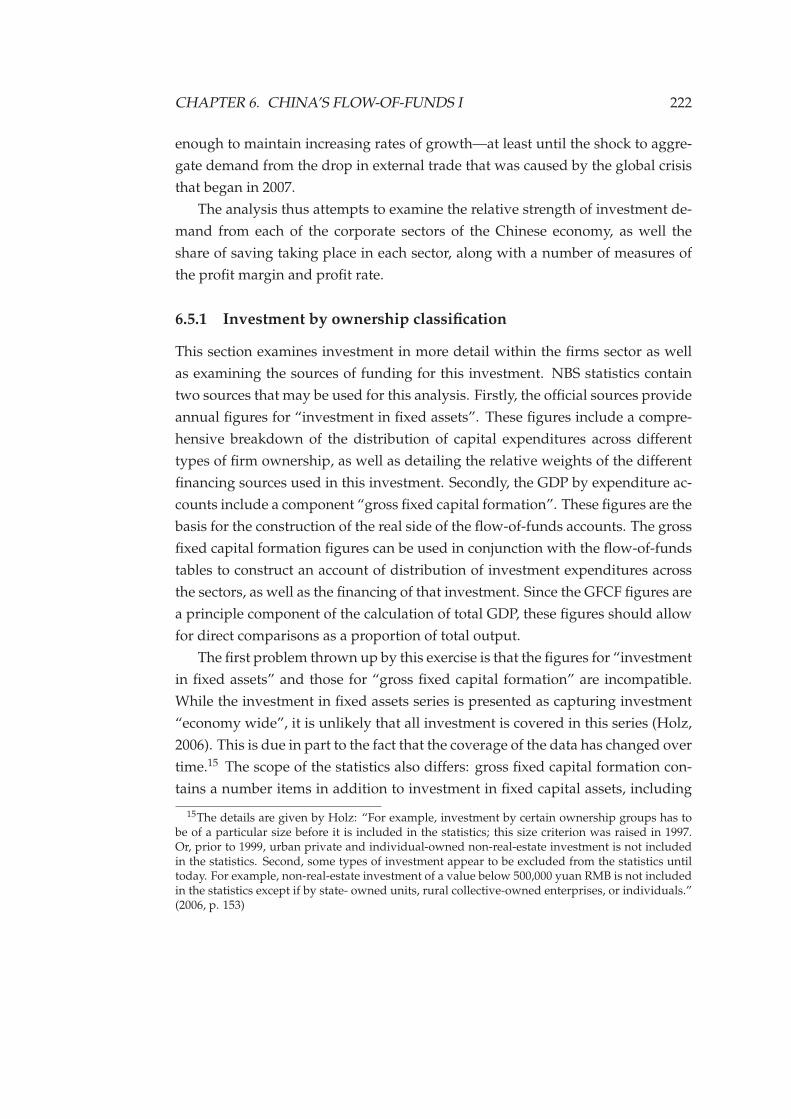
CHAPTER 6. CHINA’S FLOW-OF-FUNDS I 222
enough to maintain increasing rates of growth—at least until the shock to aggre-
gate demand from the drop in external trade that was caused by the global crisis
that began in 2007.
The analysis thus attempts to examine the relative strength of investment de-
mand from each of the corporate sectors of the Chinese economy, as well the
share of saving taking place in each sector, along with a number of measures of
the profit margin and profit rate.
6.5.1 Investment by ownership classification
This section examines investment in more detail within the firms sector as well
as examining the sources of funding for this investment. NBS statistics contain
two sources that may be used for this analysis. Firstly, the official sources provide
annual figures for “investment in fixed assets”. These figures include a compre-
hensive breakdown of the distribution of capital expenditures across different
types of firm ownership, as well as detailing the relative weights of the different
financing sources used in this investment. Secondly, the GDP by expenditure ac-
counts include a component “gross fixed capital formation”. These figures are the
basis for the construction of the real side of the flow-of-funds accounts. The gross
fixed capital formation figures can be used in conjunction with the flow-of-funds
tables to construct an account of distribution of investment expenditures across
the sectors, as well as the financing of that investment. Since the GFCF figures are
a principle component of the calculation of total GDP, these figures should allow
for direct comparisons as a proportion of total output.
The first problem thrown up by this exercise is that the figures for “investment
in fixed assets” and those for “gross fixed capital formation” are incompatible.
While the investment in fixed assets series is presented as capturing investment
“economy wide”, it is unlikely that all investment is covered in this series (Holz,
2006). This is due in part to the fact that the coverage of the data has changed over
time.15 The scope of the statistics also differs: gross fixed capital formation con-
tains a number items in addition to investment in fixed capital assets, including
15The details are given by Holz: “For example, investment by certain ownership groups has tobe of a particular size before it is included in the statistics; this size criterion was raised in 1997.Or, prior to 1999, urban private and individual-owned non-real-estate investment is not includedin the statistics. Second, some types of investment appear to be excluded from the statistics untiltoday. For example, non-real-estate investment of a value below 500,000 yuan RMB is not includedin the statistics except if by state- owned units, rural collective-owned enterprises, or individuals.”(2006, p. 153)
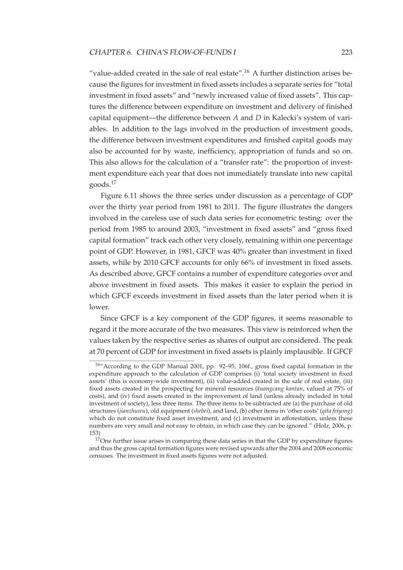
CHAPTER 6. CHINA’S FLOW-OF-FUNDS I 223
“value-added created in the sale of real estate”.16 A further distinction arises be-
cause the figures for investment in fixed assets includes a separate series for “total
investment in fixed assets” and “newly increased value of fixed assets”. This cap-
tures the difference between expenditure on investment and delivery of finished
capital equipment—the difference between A and D in Kalecki’s system of vari-
ables. In addition to the lags involved in the production of investment goods,
the difference between investment expenditures and finished capital goods may
also be accounted for by waste, inefficiency, appropriation of funds and so on.
This also allows for the calculation of a “transfer rate”: the proportion of invest-
ment expenditure each year that does not immediately translate into new capital
goods.17
Figure 6.11 shows the three series under discussion as a percentage of GDP
over the thirty year period from 1981 to 2011. The figure illustrates the dangers
involved in the careless use of such data series for econometric testing: over the
period from 1985 to around 2003, “investment in fixed assets” and “gross fixed
capital formation” track each other very closely, remaining within one percentage
point of GDP. However, in 1981, GFCF was 40% greater than investment in fixed
assets, while by 2010 GFCF accounts for only 66% of investment in fixed assets.
As described above, GFCF contains a number of expenditure categories over and
above investment in fixed assets. This makes it easier to explain the period in
which GFCF exceeds investment in fixed assets than the later period when it is
lower.
Since GFCF is a key component of the GDP figures, it seems reasonable to
regard it the more accurate of the two measures. This view is reinforced when the
values taken by the respective series as shares of output are considered. The peak
at 70 percent of GDP for investment in fixed assets is plainly implausible. If GFCF
16“According to the GDP Manual 2001, pp. 92–95, 106f., gross fixed capital formation in theexpenditure approach to the calculation of GDP comprises (i) ‘total society investment in fixedassets’ (this is economy-wide investment), (ii) value-added created in the sale of real estate, (iii)fixed assets created in the prospecting for mineral resources (kuangcang kantan, valued at 75% ofcosts), and (iv) fixed assets created in the improvement of land (unless already included in totalinvestment of society), less three items. The three items to be subtracted are (a) the purchase of oldstructures (jianzhuwu), old equipment (shebei), and land, (b) other items in ‘other costs’ (qita feiyong)which do not constitute fixed asset investment, and (c) investment in afforestation, unless thesenumbers are very small and not easy to obtain, in which case they can be ignored.” (Holz, 2006, p.153)
17One further issue arises in comparing these data series in that the GDP by expenditure figuresand thus the gross capital formation figures were revised upwards after the 2004 and 2008 economiccensuses. The investment in fixed assets figures were not adjusted.
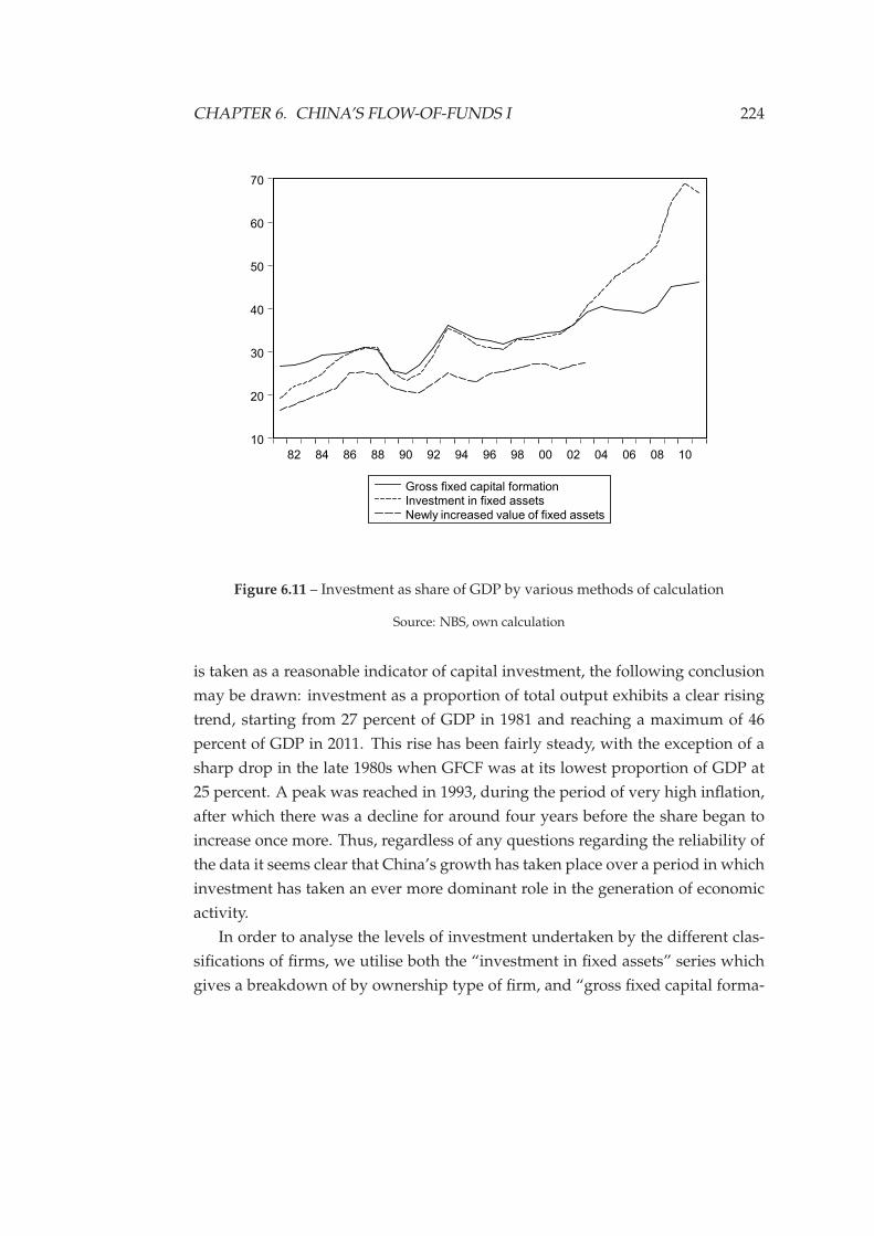
CHAPTER 6. CHINA’S FLOW-OF-FUNDS I 224
10
20
30
40
50
60
70
82 84 86 88 90 92 94 96 98 00 02 04 06 08 10
Gross fixed capital formationInvestment in fixed assets
Newly increased value of fixed assets
Figure 6.11 – Investment as share of GDP by various methods of calculation
Source: NBS, own calculation
is taken as a reasonable indicator of capital investment, the following conclusion
may be drawn: investment as a proportion of total output exhibits a clear rising
trend, starting from 27 percent of GDP in 1981 and reaching a maximum of 46
percent of GDP in 2011. This rise has been fairly steady, with the exception of a
sharp drop in the late 1980s when GFCF was at its lowest proportion of GDP at
25 percent. A peak was reached in 1993, during the period of very high inflation,
after which there was a decline for around four years before the share began to
increase once more. Thus, regardless of any questions regarding the reliability of
the data it seems clear that China’s growth has taken place over a period in which
investment has taken an ever more dominant role in the generation of economic
activity.
In order to analyse the levels of investment undertaken by the different clas-
sifications of firms, we utilise both the “investment in fixed assets” series which
gives a breakdown of by ownership type of firm, and “gross fixed capital forma-
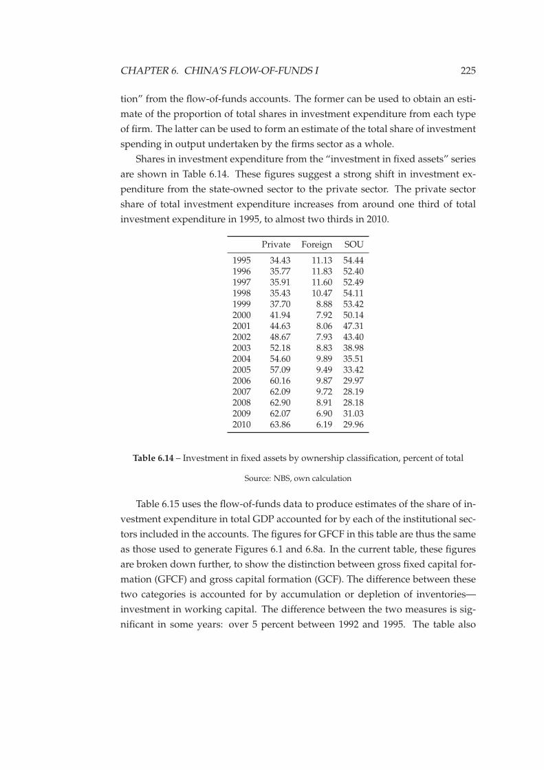
CHAPTER 6. CHINA’S FLOW-OF-FUNDS I 225
tion” from the flow-of-funds accounts. The former can be used to obtain an esti-
mate of the proportion of total shares in investment expenditure from each type
of firm. The latter can be used to form an estimate of the total share of investment
spending in output undertaken by the firms sector as a whole.
Shares in investment expenditure from the “investment in fixed assets” series
are shown in Table 6.14. These figures suggest a strong shift in investment ex-
penditure from the state-owned sector to the private sector. The private sector
share of total investment expenditure increases from around one third of total
investment expenditure in 1995, to almost two thirds in 2010.
Private Foreign SOU
1995 34.43 11.13 54.441996 35.77 11.83 52.401997 35.91 11.60 52.491998 35.43 10.47 54.111999 37.70 8.88 53.422000 41.94 7.92 50.142001 44.63 8.06 47.312002 48.67 7.93 43.402003 52.18 8.83 38.982004 54.60 9.89 35.512005 57.09 9.49 33.422006 60.16 9.87 29.972007 62.09 9.72 28.192008 62.90 8.91 28.182009 62.07 6.90 31.032010 63.86 6.19 29.96
Table 6.14 – Investment in fixed assets by ownership classification, percent of total
Source: NBS, own calculation
Table 6.15 uses the flow-of-funds data to produce estimates of the share of in-
vestment expenditure in total GDP accounted for by each of the institutional sec-
tors included in the accounts. The figures for GFCF in this table are thus the same
as those used to generate Figures 6.1 and 6.8a. In the current table, these figures
are broken down further, to show the distinction between gross fixed capital for-
mation (GFCF) and gross capital formation (GCF). The difference between these
two categories is accounted for by accumulation or depletion of inventories—
investment in working capital. The difference between the two measures is sig-
nificant in some years: over 5 percent between 1992 and 1995. The table also
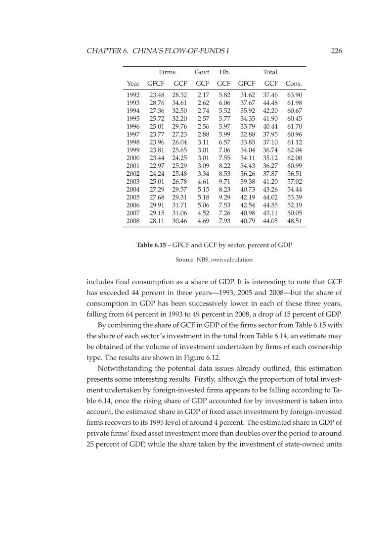
CHAPTER 6. CHINA’S FLOW-OF-FUNDS I 226
Firms Govt Hh. Total
Year GFCF GCF GCF GCF GFCF GCF Cons.
1992 23.48 28.32 2.17 5.82 31.62 37.46 63.901993 28.76 34.61 2.62 6.06 37.67 44.48 61.981994 27.36 32.50 2.74 5.52 35.92 42.20 60.671995 25.72 32.20 2.57 5.77 34.35 41.90 60.451996 25.01 29.76 2.56 5.97 33.79 40.44 61.701997 23.77 27.23 2.88 5.99 32.88 37.95 60.961998 23.96 26.04 3.11 6.57 33.85 37.10 61.121999 23.81 25.65 3.01 7.06 34.04 36.74 62.042000 23.44 24.25 3.01 7.55 34.11 35.12 62.002001 22.97 25.29 3.09 8.22 34.43 36.27 60.992002 24.24 25.48 3.34 8.53 36.26 37.87 56.512003 25.01 26.78 4.61 9.71 39.38 41.20 57.022004 27.29 29.57 5.15 8.23 40.73 43.26 54.442005 27.68 29.31 5.18 9.29 42.19 44.02 53.392006 29.91 31.71 5.06 7.53 42.54 44.55 52.192007 29.15 31.06 4.52 7.26 40.98 43.11 50.052008 28.11 30.46 4.69 7.93 40.79 44.05 48.51
Table 6.15 – GFCF and GCF by sector, percent of GDP
Source: NBS, own calculation
includes final consumption as a share of GDP. It is interesting to note that GCF
has exceeded 44 percent in three years—1993, 2005 and 2008—but the share of
consumption in GDP has been successively lower in each of these three years,
falling from 64 percent in 1993 to 49 percent in 2008, a drop of 15 percent of GDP
By combining the share of GCF in GDP of the firms sector from Table 6.15 with
the share of each sector’s investment in the total from Table 6.14, an estimate may
be obtained of the volume of investment undertaken by firms of each ownership
type. The results are shown in Figure 6.12.
Notwithstanding the potential data issues already outlined, this estimation
presents some interesting results. Firstly, although the proportion of total invest-
ment undertaken by foreign-invested firms appears to be falling according to Ta-
ble 6.14, once the rising share of GDP accounted for by investment is taken into
account, the estimated share in GDP of fixed asset investment by foreign-invested
firms recovers to its 1995 level of around 4 percent. The estimated share in GDP of
private firms’ fixed asset investment more than doubles over the period to around
25 percent of GDP, while the share taken by the investment of state-owned units
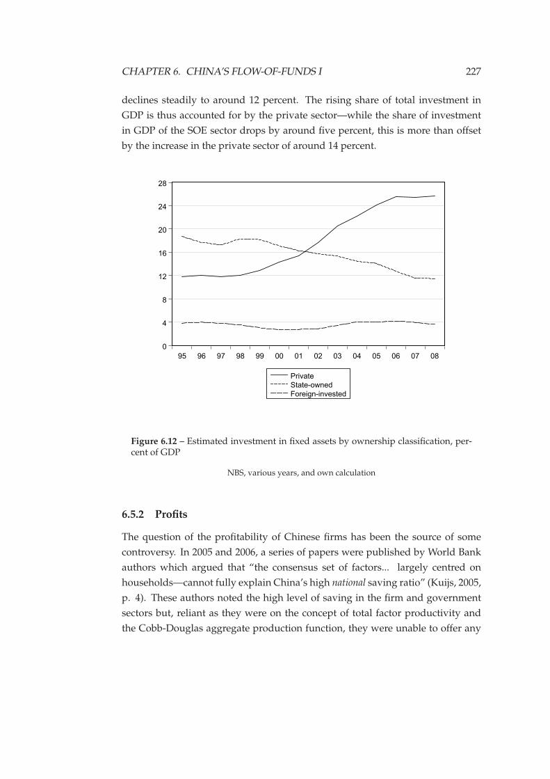
CHAPTER 6. CHINA’S FLOW-OF-FUNDS I 227
declines steadily to around 12 percent. The rising share of total investment in
GDP is thus accounted for by the private sector—while the share of investment
in GDP of the SOE sector drops by around five percent, this is more than offset
by the increase in the private sector of around 14 percent.
0
4
8
12
16
20
24
28
95 96 97 98 99 00 01 02 03 04 05 06 07 08
Private
State-owned
Foreign-invested
Figure 6.12 – Estimated investment in fixed assets by ownership classification, per-cent of GDP
NBS, various years, and own calculation
6.5.2 Profits
The question of the profitability of Chinese firms has been the source of some
controversy. In 2005 and 2006, a series of papers were published by World Bank
authors which argued that “the consensus set of factors... largely centred on
households—cannot fully explain China’s high national saving ratio” (Kuijs, 2005,
p. 4). These authors noted the high level of saving in the firm and government
sectors but, reliant as they were on the concept of total factor productivity and
the Cobb-Douglas aggregate production function, they were unable to offer any
CHAPTER 6. CHINA’S FLOW-OF-FUNDS I 228
coherent theoretical explanation for these observations.
However, their claim that “the increase in enterprise saving in the last 10 years
is associated with a steady rise in profits and profitability of enterprises” (Kuijs,
2006, p. 9) sparked a heated debate in the pages of the Far Eastern Economic Re-
view. An article entitled “The World Bank’s China Delusions” (Shan, 2006) argued
that the World Bank findings were impossible to square with “well-known truths
about the Chinese economy”such as the high proportion of non-performing loans
on the books of the state-owned banking system.
Shan took issue with the World Bank authors’ findings that the return on eq-
uity had risen substantially over the decade to 2005, because their figures did not
include taxes on production which, as already established, are very high—over
30 percent according to Shan.
Shan claimed further that gross profit margins for Chinese firms—the differ-
ence between revenues and costs as a share of revenues—has been falling consis-
tently due to rising costs of raw materials.
The World Bank authors responded (Hofman & Kuijs, 2006) by arguing that
the gross profit margin calculated by Shan included only a subset of the total costs
of production, and produced calculations that showed that margins, although
much lower than those calculated by Shan, had in fact risen substantially over
the period under consideration.
Further, they argued, by focusing on profit margins alone, Shan had failed to
grasp the significance of increases in turnover:
Mr. Shan neglects the effect that rapid turnover growth has on prof-
its. By definition, total profits equal profit margin on sales times sales
volume, and rapid economic growth boosted sales volumes in recent
years.” (Hofman & Kuijs, 2006, emphasis in original).
However, this claim is misleading because it fails to distinguish between in-
creased sales revenues from higher growth at constant levels of capacity utilisa-
tion, and shifts in capacity utilisation, as emphasised by Steindl (1979).
In a closed growing economy, the distribution of saving between households
and firms is determined by the saving propensities of each sector, and the dis-
tribution of income between the two sectors. The very low level of dividend
payments by Chinese firms implies that the “saving propensity of capitalists” in
China is effectively one hundred percent. The distribution of total saving is thus
determined by the household saving propensity and the distribution of income.
CHAPTER 6. CHINA’S FLOW-OF-FUNDS I 229
In Steindl’s analysis, the distribution of income shifts towards profits at higher
rates of capacity utilisation due to the existence of overhead labour costs. How-
ever, higher growth rates at constant capacity utilisation will have no effect on
the relative shares of saving in output. Thus, the rising share of saving in the en-
terprise sector cannot be directly connected to increased sales revenues without
further assumptions about profit margins.
This is not the case however in an economy with a rising trade surplus—the
increased sales revenue may accrue as the enterprise sector increases its relative
market share globally, without changes to the internal distribution of income or
saving propensities. Further, the data used by the authors in this debate all use
data from the “industrial enterprise survey”. Shifts in the relative shares of agri-
culture, industry and services in the structure of the economy may therefore affect
the results.
Part of the confusion surrounding this debate relates to the uncritical use of ac-
counting measures which are designed to describe the characteristics of publicly-
traded, privately-owned companies. Applying such concepts are “the return on
owners equity” to the state-owned sector of the Chinese economy leads to faulty
conclusions.
In the following sections, the evidence is reviewed and updated in an attempt
to clarify some of the main points of contention, and provide the groundwork for
a coherent analysis of the dynamics of accumulation.
Profit margins
One way to obtain an estimate of the share of firms’ revenue that accrues as profits
is to use the flow-of-funds data. As with estimating income shares (Section 6.4.4),
a decision must be made on the proportion of total tax revenues that should be de-
ducted from the income of the firm sector before calculating the remaining share
of income as profit. Because the flow-of-funds works on the basis of net value-
added, the intermediate costs of all firms are netted out of the figures. Thus, once
tax, interest and dividend payments are subtracted from income, all that remains
is wage costs. The only indicators that may be obtained from the flow-of funds
are thus the shares of these categories in the total value-added accruing to the
firm’s sector.
Three such measures are shown in Figure 6.13. The first shows the ratio of
value added less wage costs to value added in the firm sector. The other two indi-
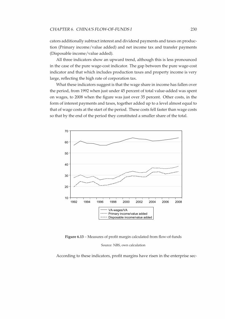
CHAPTER 6. CHINA’S FLOW-OF-FUNDS I 230
cators additionally subtract interest and dividend payments and taxes on produc-
tion (Primary income/value added) and net income tax and transfer payments
(Disposable income/value added).
All three indicators show an upward trend, although this is less pronounced
in the case of the pure wage-cost indicator. The gap between the pure wage-cost
indicator and that which includes production taxes and property income is very
large, reflecting the high rate of corporation tax.
What these indicators suggest is that the wage share in income has fallen over
the period, from 1992 when just under 45 percent of total value-added was spent
on wages, to 2008 when the figure was just over 35 percent. Other costs, in the
form of interest payments and taxes, together added up to a level almost equal to
that of wage costs at the start of the period. These costs fell faster than wage costs
so that by the end of the period they constituted a smaller share of the total.
10
20
30
40
50
60
70
1992 1994 1996 1998 2000 2002 2004 2006 2008
VA-wages/VA
Primary income/value added
Disposable income/value added
Figure 6.13 – Measures of profit margin calculated from flow-of-funds
Source: NBS, own calculation
According to these indicators, profit margins have risen in the enterprise sec-
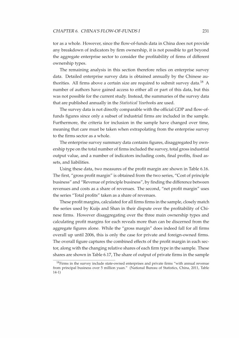
CHAPTER 6. CHINA’S FLOW-OF-FUNDS I 231
tor as a whole. However, since the flow-of-funds data in China does not provide
any breakdown of indicators by firm ownership, it is not possible to get beyond
the aggregate enterprise sector to consider the profitability of firms of different
ownership types.
The remaining analysis in this section therefore relies on enterprise survey
data. Detailed enterprise survey data is obtained annually by the Chinese au-
thorities. All firms above a certain size are required to submit survey data.18 A
number of authors have gained access to either all or part of this data, but this
was not possible for the current study. Instead, the summaries of the survey data
that are published annually in the Statistical Yearbooks are used.
The survey data is not directly comparable with the official GDP and flow-of-
funds figures since only a subset of industrial firms are included in the sample.
Furthermore, the criteria for inclusion in the sample have changed over time,
meaning that care must be taken when extrapolating from the enterprise survey
to the firms sector as a whole.
The enterprise survey summary data contains figures, disaggregated by own-
ership type on the total number of firms included the survey, total gross industrial
output value, and a number of indicators including costs, final profits, fixed as-
sets, and liabilities.
Using these data, two measures of the profit margin are shown in Table 6.16.
The first, “gross profit margin” is obtained from the two series, “Cost of principle
business” and “Revenue of principle business”, by finding the difference between
revenues and costs as a share of revenues. The second, “net profit margin” uses
the series “Total profits” taken as a share of revenues.
These profit margins, calculated for all firms firms in the sample, closely match
the series used by Kuijs and Shan in their dispute over the profitability of Chi-
nese firms. However disaggregating over the three main ownership types and
calculating profit margins for each reveals more than can be discerned from the
aggregate figures alone. While the “gross margin” does indeed fall for all firms
overall up until 2006, this is only the case for private and foreign-owned firms.
The overall figure captures the combined effects of the profit margin in each sec-
tor, along with the changing relative shares of each firm type in the sample. These
shares are shown in Table 6.17, The share of output of private firms in the sample
18Firms in the survey include state-owned enterprises and private firms “with annual revenuefrom principal business over 5 million yuan.” (National Bureau of Statistics, China, 2011, Table14-1)
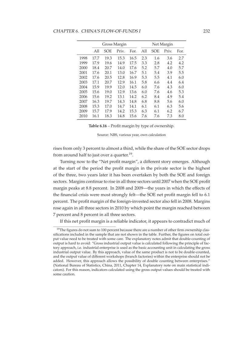
CHAPTER 6. CHINA’S FLOW-OF-FUNDS I 232
Gross Margin Net Margin
All SOE Priv. For. All SOE Priv. For.
1998 17.7 19.3 15.3 16.5 2.3 1.6 3.6 2.71999 17.9 19.6 14.9 17.5 3.3 2.8 4.2 4.22000 18.4 20.7 14.0 17.6 5.2 5.7 4.0 5.72001 17.6 20.1 13.0 16.7 5.1 5.4 3.9 5.52002 17.6 20.5 12.8 16.9 5.3 5.5 4.1 6.02003 17.1 20.7 12.9 16.1 5.8 6.6 4.4 6.42004 15.9 19.9 12.0 14.5 6.0 7.6 4.3 6.02005 15.6 19.0 12.9 13.6 6.0 7.6 4.6 5.32006 15.6 19.2 13.1 14.2 6.2 8.4 4.9 5.42007 16.3 19.7 14.3 14.8 6.8 8.8 5.6 6.02008 15.3 17.0 14.7 14.1 6.1 6.1 6.3 5.62009 15.7 17.9 14.2 15.3 6.3 6.1 6.2 6.72010 16.1 18.3 14.8 15.6 7.6 7.6 7.3 8.0
Table 6.16 – Profit margin by type of ownership.
Source: NBS, various year, own calculation
rises from only 3 percent to almost a third, while the share of the SOE sector drops
from around half to just over a quarter.19.
Turning now to the “Net profit margin”, a different story emerges. Although
at the start of the period the profit margin in the private sector is the highest
of the three, two years later it has been overtaken by both the SOE and foreign
sectors. Margins continue to rise in all three sectors until 2007 when the SOE profit
margin peaks at 8.8 percent. In 2008 and 2009—the years in which the effects of
the financial crisis were most strongly felt—the SOE net profit margin fell to 6.1
percent. The profit margin of the foreign-invested sector also fell in 2008. Margins
rose again in all three sectors in 2010 by which point the margin reached between
7 percent and 8 percent in all three sectors.
If this net profit margin is a reliable indicator, it appears to contradict much of
19The figures do not sum to 100 percent because there are a number of other firm ownership clas-sifications included in the sample that are not shown in the table. Further, the figures on total out-put value need to be treated with some care. The explanatory notes admit that double-counting ofoutput is hard to avoid: “Gross industrial output value is calculated following the principle of fac-tory approach, i.e. industrial enterprise is used as the basic accounting unit in calculating the grossindustrial output value. By this approach, value of the same product is not to be double-counted,and the output value of different workshops (branch factories) within the enterprise should not beadded. However, this approach allows the possibility of double counting between enterprises.”(National Bureau of Statistics, China, 2011, Chapter 14, Explanatory note on main statistical indi-cators). For this reason, indicators calculated using the gross output values should be treated withsome caution.
CHAPTER 6. CHINA’S FLOW-OF-FUNDS I 233
SOE Private Foreign
1998 49.6 3.1 24.71999 48.9 4.5 26.12000 47.3 6.1 27.42001 44.4 9.2 28.52002 40.8 11.7 29.32003 37.5 14.7 31.22004 34.8 17.4 32.72005 33.3 19.0 31.72006 31.2 21.2 31.62007 29.5 23.2 31.52008 28.4 26.9 29.52009 26.7 29.6 27.82010 26.6 30.5 27.2
Table 6.17 – Output of by ownership type, percent of total output of firms in survey
Source: NBS, own calculation
the current consensus that regards the state-owned sector as inefficient and un-
profitable. What cannot be determined from these figures is the degree to which
rising profit margins are the result of monopolisation, and to what extent they are
due to increasing efficiency of production.
These figures also suggest that the SOE sector was affected more than the
other sectors by the global financial crisis. The fall in the net profit margin in 2008
and 2009 was the result of an absolute fall in profits in these two years in the SOE
sector. This is the only such occurrence across all of the sectors—apart from these
two years, absolute profits rose every year in all sectors
Profit rates
The analysis in this section has so far examined the share of investment under-
taken by each type of firm, relative profit margins and shares of gross output.
What remains is to consider the rate of profit—the ratio the volume of profit to
the size of the capital stock. The enterprise survey provides a number of mea-
sures of the volumes of assets held by firms. Series are provided both for “Total
assets”, which includes working capital and other assets as well as fixed capital,
and “Original value of fixed assets”. Two indicators of the rate of profit are calcu-
lated here using these series. These are found by dividing the final profit figure
used above to calculate the “net profit margin” by each of these measures of the
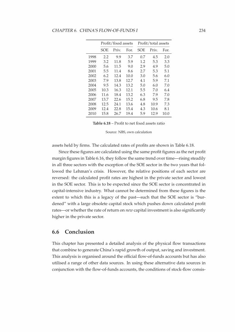
CHAPTER 6. CHINA’S FLOW-OF-FUNDS I 234
Profit/fixed assets Profit/total assets
SOE Priv. For. SOE Priv. For.
1998 2.2 9.9 3.7 0.7 4.5 2.01999 3.2 11.8 5.9 1.2 5.3 3.32000 5.6 11.5 9.0 2.9 4.9 5.02001 5.5 11.4 8.6 2.7 5.3 5.12002 6.2 12.4 10.0 3.0 5.6 6.02003 7.9 13.8 12.7 4.1 5.9 7.12004 9.5 14.3 13.2 5.0 6.0 7.02005 10.3 16.3 12.1 5.5 7.0 6.42006 11.6 18.4 13.2 6.3 7.9 7.02007 13.7 22.6 15.2 6.8 9.5 7.82008 12.5 24.1 13.6 4.8 10.9 7.32009 12.4 22.8 15.4 4.3 10.6 8.12010 15.8 26.7 19.4 5.9 12.9 10.0
Table 6.18 – Profit to net fixed assets ratio
Source: NBS, own calculation
assets held by firms. The calculated rates of profits are shown in Table 6.18.
Since these figures are calculated using the same profit figures as the net profit
margin figures in Table 6.16, they follow the same trend over time—rising steadily
in all three sectors with the exception of the SOE sector in the two years that fol-
lowed the Lehman’s crisis. However, the relative positions of each sector are
reversed: the calculated profit rates are highest in the private sector and lowest
in the SOE sector. This is to be expected since the SOE sector is concentrated in
capital-intensive industry. What cannot be determined from these figures is the
extent to which this is a legacy of the past—such that the SOE sector is “bur-
dened” with a large obsolete capital stock which pushes down calculated profit
rates—or whether the rate of return on new capital investment is also significantly
higher in the private sector.
6.6 Conclusion
This chapter has presented a detailed analysis of the physical flow transactions
that combine to generate China’s rapid growth of output, saving and investment.
This analysis is organised around the official flow-of-funds accounts but has also
utilised a range of other data sources. In using these alternative data sources in
conjunction with the flow-of-funds accounts, the conditions of stock-flow consis-
CHAPTER 6. CHINA’S FLOW-OF-FUNDS I 235
tency are kept constantly in mind—since all series are part of a stock-flow tax-
onomy, changes in any individual series imply that accomodating changes must
take place elsewhere in the macroeconomic structure.
The findings of this analysis are now summarised, before the financial coun-
terparts to these flows are examined in the following chapter.
Firstly, over the longer time-horizon of the transition from planning, invest-
ment has risen steadily as a share of output from under 30 percent in 1980 to
close to 45 percent in 2010. More recently, two distinct phases have occured. Both
output and investment growth fell during most of the 1990s due to the imple-
mentation of austerity measures. These measures were a response to excessive
spending—particularly by local governments, due to “soft budget constraints”—
which resulted in consistent breaches of the Credit Plan and two major outbreaks
of inflation.
Up until the late 1990s, the external position was close to balance, although the
flow-of-funds accounts report domestic investment as higher than saving for the
first half of the 1990s. Until around the turn of the century, growth was therefore
less skewed towards investment expenditure that in more recent years: output
growth was above 10 percent in the first half of the 1990s while investment growth
was below 10 percent, leading to a falling share of investment in output over the
1990s.
The most recent boom cycle began around the turn of the century. Output
growth increased steadily over this period until the outbreak of the global finan-
cial crisis in 2007–08. Investment as a share of output rose sharply over the first
half of the decade, due to a strong emphasis on fixed capital investment, before
levelling out at around 40 percent of GDP in the middle of the decade. From
this point, expanding export demand continued to drive growth until the onset
of the crisis. In response to the crisis a further stimulus was introduced, pushing
investment up to almost 45 percent of GDP.
Since saving is by definition equal to the sum of investment and the exter-
nal surplus, saving has also risen steadily over this period as a share of output.
However this saving has been unevenly distributed among the domestic sectors.
While saving as a share of total output has risen in all three sectors, it has done so
most significantly in the firms sector.
In any given sector, rising saving as a share of total output may come about
in two possible ways: either an increase in the proportion of income saved, or
an increase in the share of total income of that sector. When rising saving across
CHAPTER 6. CHINA’S FLOW-OF-FUNDS I 236
sectors is broken down in this way, a different pattern emerges for each sector.
Firstly, the government share of income has risen moderately. Government in-
come is primarily derived from taxation of the firms sector, thus government ex-
penditures and saving are essentially deductions from firms’ profits. While the
government share of income has risen moderately, government saving appears
to have risen more quickly, although this trend is likely to have reversed in 2009
due to the fiscal stimulus.
More interesting is the contrast between the household and firms sectors.
Since firms distribute almost no dividends, firms “save” all profits. Thus ris-
ing firms saving is the result of profits increasing as a share of national income.
The counterpart to rising firms profits is falling household income due to a lower
wage share. The rising share of household saving in output is thus the result of
the “saving propensity” of households rising fast enough to more than offset their
falling share of income.
This shift in the distribution of income towards the firms sector has reduced
the reliance of firms on credit for the financing of investment. Although invest-
ment exceeds after-tax profits in the firms sector, the deficit is narrowing such that
a rising proportion of investment is funded through retained earnings.
The distribution of both investment and saving within the firms sector has
also shifted considerably over the period from 1998 onwards for which disaggre-
gated data are available. In particular, the share of output, saving and investment
by private firms rose, while the SOE sector declined in significance. What the ev-
idence appears to suggest is that profit margins have risen steadily, with that rise
distributed fairly uniformly across the firms sector, regardless of ownership type
of firms.
Despite relatively uniform profit margins across the firms sector, the share of
output and investment accounted for by private firms has risen, while the share
accounted for by SOEs has fallen. The foreign sector appears to have maintained
a steady share of output but investment expenditures have been decreasing. Fi-
nally, rates of profit have risen in all sectors, but these rates are much higher in
the non-state sectors—around twice as high.
How are these observations to be explained?
Firstly, the combination of a rising share of profits in national income, widen-
ing profit margins and rising rates of profit suggest a significant rise in the Kaleck-
ian monopoly mark-up. This result is at odds with Kalecki’s own findings on the
relative constancy of the wage share in national income over extended periods of
CHAPTER 6. CHINA’S FLOW-OF-FUNDS I 237
time. Kalecki concluded that this was due to the fact that the cost of raw materials
and the degree of monopoly tended to move in opposite directions, but that this
was not a general result which would continue to hold indefinately:
It is, of course, not at all certain that in the future the rise in the degree
of monopoly will continue to be compensated by a fall in the price of
“basic raw materials”. If it is not, the relative share of manual labour
will tend to decline (Kalecki, [1939] 1990, p. 248).
Over the period under consideration, the cost of raw materials has risen. This
is why, of the two measures of the profit margin that are calculated, the “gross
margin” has fallen while the “net margin” has risen—the net margin includes
other costs which have fallen faster than the rise in raw materials.
However, Kalecki is here referring specifically to the case of an economic
downturn in which monopoly pricing power increases and the prices of raw ma-
terials fall.
It has recently been argued by Mr Harrod that the degree of monopoly
increases in the boom and falls in the slump... Mr Harrod was rightly
criticized in that there exist other factors which influence the degree of
monopoly in the other direction. For instance, in the slump, cartels are
created to save profits... More important still is the fact that, in spite of
the fall of prices of raw materials and wages, some prices of finished
goods tend to be relatively “sticky” in the slump... it can be concluded
that the degree of monopoly tends to increase in the depression and
decline in the boom (Kalecki, [1939] 1990, pp. 248–9).
The rise in the mark-up observed in China has, however, taken place—at least
from around the turn of the century until the onset of the global financial crisis—
during a sustained boom.
This rise in profits also presents conceptual difficulties for marginal analysis
based on the neo-classical aggregate production function: if the return to capital
and labour are determined by their relative marginal products, the assumption of
declining marginal productivity should result in the price of labour rising and the
price of capital falling as an investment boom and the “Lewis turning point” co-
incide. The usual explanation is that labour productivity has risen, but other than
being true in the tautological sense that output has risen faster than employment,
CHAPTER 6. CHINA’S FLOW-OF-FUNDS I 238
this explanation offers little in the way of enlightenment and simply leads to in-
creasingly incoherent discussion about the employment of factor inputs versus
shifts in total factor productivity.
A more likely explanation is to be found in the behaviour of the state-owned
firms. Although the significance of these firms is diminishing in terms of share
output, they still comprise the industrial “core” of the Chinese economy, concen-
trated in heavy industrial production. In a capitalist market economy, it is these
firms that would be most likely to form the types of “cartels” that would lead to
monopoly pricing, excess capacity and the slowing of growth.
Such outcomes result from the attempts of firms to set prices and output such
that profits are maximised at a point as close to the “monopoly” position as posi-
ble, thorugh various price coordination measures between firms operating in os-
tensibly “competitive” markets (Baran & Sweezy, 1966).
State-owned firms in China are unlikely to operate in this way. Along with
control over the banking system, these firms provide the state with its most im-
portant levers of control over the economy. The investment decisions of these
firms are not be dictated by profit maximisation, but by the political authorities.
Finance for investment by these firms is provided by the state-owned banking
system. Of particular significance is that it is likely that these firms will not react
to excess capacity by scaling back investment expenditures.
These firms therefore perform a quasi-fiscal role in the economic system. Over
the period of transition from planning, as direct government economic activity
was reduced, these firms substituted for the government in maintaining aggre-
gate demand, despite the resulting losses eventually being placed on the books
of the banking system as non-performing loans.
From around the turn of the century, the ability of these firms to generate prof-
its appears to have recovered, while at the same time the share of profits in na-
tional income gradually rose. However, the rates of profits in the state-owned sec-
tor are considerably lower than those in the private sector. This reflects a higher
intensity of investment expenditure as a share of revenues in the state sector—as
would be expected in the heavy industrial sector—while profits as a share of rev-
enues are approximately equal. The implication of this is that profit income will
not be evenly distributed among the firms sector: some share of the investment
outlays of state-owned firms will accrue as profits in the private sector.
In an economy such as China where consumption out of profits is close to
zero, the profits of firms are determined by investment expenditures less saving
CHAPTER 6. CHINA’S FLOW-OF-FUNDS I 239
by households and government. Despite rising household saving rates, house-
hold saving as a share of total saving is falling, while the opposite the is case
in the government sector, but to a lesser degree. An increasing share of the in-
vestment outlays of firms thus accumulates as profits within the firms sector, but
these profits do not accrue in proportion to the investment outlays of these firms:
a portion of the investment expenditure of the state-owned sector returns as the
saving of private-owned corporations, rather than profits in the state-owned sec-
tor.
If the investment decisions of firms in the private sector are influenced by the
rate of return on capital investment, this dynamic will result in a strong induce-
ment toward investment on the part of these firms also: the additional profits
that accrue in this sector as a result of the investment outlays of the state-owned
sector will serve to raise the rate of profit in the private sector. This in turn will
stimulate private-sector investment, resulting in even higher rates of profit.
This result is the symmetric opposite of the case of “monopoly capital” in
which those firms operating in the cartelised sector of the economy extract a share
of the investment outlays of competitive firms. In the case described by Steindl,
this “maldistribution of profits”, in conjunction with the high saving of house-
holds, leads to excess capacity, further reducing the incentive of firms to invest.
In the analysis presented here, the investment behaviour of the state-owned
sector, and in particular the insensitivity of this investment to excess capacity,
becomes the key determining factor in generating growth.
While this analysis provides a justification for the high rates of growth of out-
put and investment, the question of the apparent increase in the profit margin
is at least partially unresolved. Traditional explanations based on the degree of
monopoly mark-up do not seem to fit the observed facts.
This analysis also strongly implies that China’s growth has not followed any
kind of steady-state “balanced” growth path in which all variables grow in step
and at equal rates. Growth has resulted from a series of disequilibrium processes.
With the shift to a “capital deepening” path, growth has been maintained by suc-
cessive rounds of increasing capital intensity, leading to an ever higher share of
investment in national income.
Chapter 7
China’s flow-of-funds II: financial
transactions
7.1 Introduction
Chapter 6 presented a detailed analysis of the evolution of real macroeconomic
variables, disaggregated by institutional sector. It was shown that the retained
profits of firms account for a high and rising share of national income, driven by
the investment expenditure of firms. These retained earnings are heavily taxed
by the government which, in combination with the very high level of investment
expenditure by firms, results in the firms sector running a financial deficit overall.
The counterpart to this deficit is located in the strongly positive net financial
position of households. The surplus of households has also financed a moderate
government deficit for most of the period under analysis, although the flow-of-
funds data record a shift into surplus for the government sector from around the
mid-2000s, contradicting the official government finance figures.
Despite the deficit of the firms sector, the majority of investment is funded
out of retained earnings. Using disaggregated data on the firms sector, it was
shown that investment and earnings are unevenly distributed across the firms
sector. It was argued that this is the result of a quasi-Steindlian process in which
the normal outcomes of monopoly are reversed.
The focus of investigation now switches to the financial system. The mone-
tary and financial transactions of each institutional sector—and the inter-sectoral
flows that those transactions generate—are examined in detail. By analysing the
financial flows that are the counterpart to the system of sector deficits and sur-
240
CHAPTER 7. CHINA’S FLOW-OF-FUNDS II 241
pluses, the flow-of-funds analysis of the previous chapter may be “closed”.
While the physical flow analysis of the previous chapter constructed an empir-
ical framework in which the circular flow of income is broken down on a sector-
by-sector basis, the analysis in the current chapter examines the role of the finan-
cial system in bridging between those sectors in which incomes and expenditures
are unequal.
The primary purpose of the chapter is to demonstrate that the expansion
of credit and money in China have been the result of an endogenous credit-
investment process, driven by the investment dynamics analysed in the previous
chapter. This contrasts with the widely held view that China’s monetary policy
operates through control of the monetary base, and that this control is compli-
cated by the requirements of sterilising the expansion of reserves resulting from
the current account surplus.
Instead, it is demonstrated that reserves have been freely available over the
period for which data are available, as shown by the large volume of excess re-
serves in the banking system and the liquid inter-bank market. Over the recent
period of current account surpluses, the level of excess reserves has been succes-
sively reduced through balance sheet operations on the part of the PBC, although
not to a point that would significantly constraint the lending ability of banks.
Control of credit growth has instead primarily taken place through administra-
tive influence of state-owned enterprises and the banking system.
Since the official flow-of-funds accounts do not provide separate entries for
the monetary authority and banking system, the analysis of the interaction be-
tween the banking system and the central bank is achieved through generating a
set of augmented flow-of-funds accounts using monthly balance sheet data from
the PBC.
7.2 Sector financing
The analysis in this chapter will start from the point of intersection between the
physical and financial flow-of-funds accounts: the net financial balances of the
system.1 The real income and expenditure flows that combine to generate these
financial balances were analysed in the previous chapter. Stock-flow accounting
1As was noted in Section 6.3.1, there is some divergence between the net financial position figurereported in the physical transactions table and that reported in the financial transactions table (seeFigure 6.10).
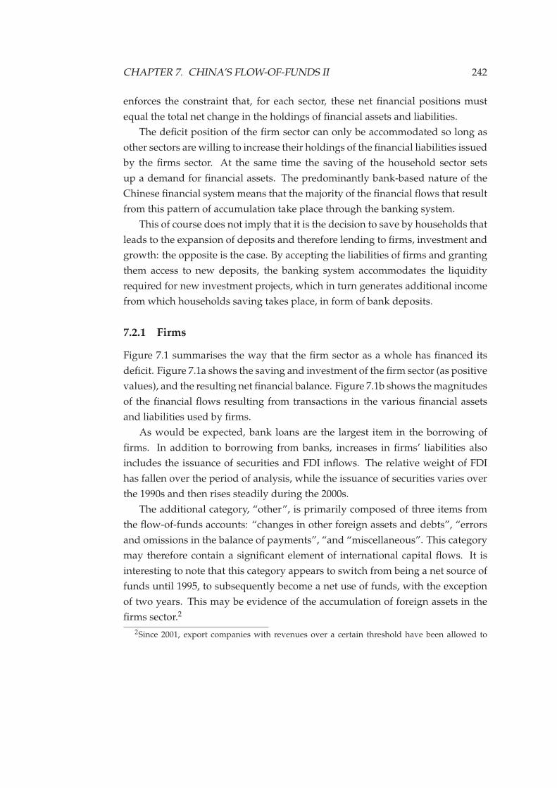
CHAPTER 7. CHINA’S FLOW-OF-FUNDS II 242
enforces the constraint that, for each sector, these net financial positions must
equal the total net change in the holdings of financial assets and liabilities.
The deficit position of the firm sector can only be accommodated so long as
other sectors are willing to increase their holdings of the financial liabilities issued
by the firms sector. At the same time the saving of the household sector sets
up a demand for financial assets. The predominantly bank-based nature of the
Chinese financial system means that the majority of the financial flows that result
from this pattern of accumulation take place through the banking system.
This of course does not imply that it is the decision to save by households that
leads to the expansion of deposits and therefore lending to firms, investment and
growth: the opposite is the case. By accepting the liabilities of firms and granting
them access to new deposits, the banking system accommodates the liquidity
required for new investment projects, which in turn generates additional income
from which households saving takes place, in form of bank deposits.
7.2.1 Firms
Figure 7.1 summarises the way that the firm sector as a whole has financed its
deficit. Figure 7.1a shows the saving and investment of the firm sector (as positive
values), and the resulting net financial balance. Figure 7.1b shows the magnitudes
of the financial flows resulting from transactions in the various financial assets
and liabilities used by firms.
As would be expected, bank loans are the largest item in the borrowing of
firms. In addition to borrowing from banks, increases in firms’ liabilities also
includes the issuance of securities and FDI inflows. The relative weight of FDI
has fallen over the period of analysis, while the issuance of securities varies over
the 1990s and then rises steadily during the 2000s.
The additional category, “other”, is primarily composed of three items from
the flow-of-funds accounts: “changes in other foreign assets and debts”, “errors
and omissions in the balance of payments”, “and “miscellaneous”. This category
may therefore contain a significant element of international capital flows. It is
interesting to note that this category appears to switch from being a net source of
funds until 1995, to subsequently become a net use of funds, with the exception
of two years. This may be evidence of the accumulation of foreign assets in the
firms sector.2
2Since 2001, export companies with revenues over a certain threshold have been allowed to
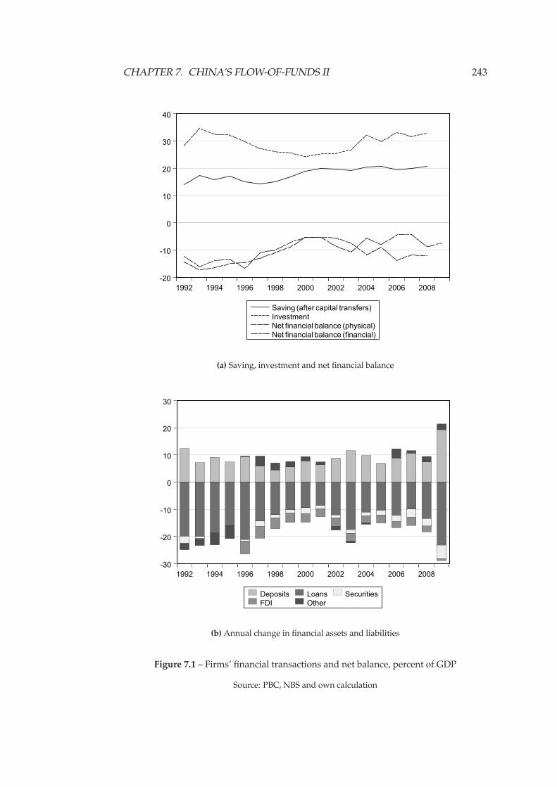
CHAPTER 7. CHINA’S FLOW-OF-FUNDS II 243
-20
-10
0
10
20
30
40
1992 1994 1996 1998 2000 2002 2004 2006 2008
Saving (after capital transfers)Investment
Net financial balance (physical)
Net financial balance (financial)
(a) Saving, investment and net financial balance
-30
-20
-10
0
10
20
30
1992 1994 1996 1998 2000 2002 2004 2006 2008
Deposits Loans Securities
FDI Other
(b) Annual change in financial assets and liabilities
Figure 7.1 – Firms’ financial transactions and net balance, percent of GDP
Source: PBC, NBS and own calculation
CHAPTER 7. CHINA’S FLOW-OF-FUNDS II 244
The most interesting feature of this summary of the financial operations of
the firms sector is the volume of deposits accumulating in the firms’ sector. The
holding of liquid balances has always posed problems for marginalist economics.
As noted in Section 2.2, the New Keynesian model—widely regarded as the pin-
nacle of achievement in monetary theory—simply assumes the holding of money
balances by households. Without such an assumption, no baseline rate of interest
exists in the model and monetary policy loses all power, even in the presence of
nominal rigidities.
Authors in the Post Keynesian tradition have taken a more coherent approach
to such matters, emphasising the roles of uncertainty and liquidity preference in
the holding of money balances. However, this analysis has primarily concen-
trated on households and—to a lesser extent—the banking system (eg. Chick &
Dow, 2002).
A thorough theoretical treatment of the holding of liquid financial assets by
the firms sector is to be found in Toporowski’s work on “overcapitalisation” (2008a).
Section 3.4 examined the effects of overcapitalisation on the sectoral balances of
a stock-flow consistent framework. This analysis was developed further through
the incorporation of the holding of deposits by firms into the growth model de-
veloped in Section 4.6.3.
The accounts shown in Figure 7.1b clearly demonstrate the empirical rele-
vance of this analysis. The volume of issuance of financial liabilities by firms
greatly exceeds the borrowing requirements implied by the net financial balance
of the sector, with the excess of borrowing over investment expenditure diverted
mostly towards the accumulation of liquid balances.
What is impossible to discern at this level of aggregation is how deposits and
loans are distributed within the firms sector. Two possible extreme cases can be
imagined: firstly, the case in which every firm in the sector corresponds exactly
to the “representative” firm given by the aggregate statistics. In such a situation,
the increasing loan liabilities of each firm would be partially hedged by increas-
ing holdings of bank deposits, with the remaining loan liabilities accounted for
by capital investment. The opposite extreme case of “maldistribution of prof-
its” would occur when all investment was undertaken by “marginal” competitive
firms using bank credit, but the structure of the economy were such that all profits
hold foreign currency bank deposits. The amount of foreign exchange that is allowed to be heldis calculated as a percentage of total export earnings, with the initial threshold of 20% raised to30–50% in March 2004 and then raised again to 50-80% in August 2005 (Nagai & Wang, 2007).
CHAPTER 7. CHINA’S FLOW-OF-FUNDS II 245
accrued to a “cartelised” sector with high mark-ups and low capacity utilisation
(Steindl, 1952).
The reality will of course lie somewhere between these to extremes, and with-
out further evidence, at this stage no hypothesis can be advanced as to which
more correctly characterises the firms’ sector in China. However, the evidence
examined so far appears to closely conform to that which would be expected
from Kalecki’s analysis of the relationship between credit-financed investment,
profits and the bank deposits of firms:
It should be emphasised that the equality between savings and invest-
ment plus export surplus plus budget deficit in the general case—or
investment alone in the special case—will be valid under all circum-
stances... If investment increases by a certain amount, savings out of
profits are pro tanto higher.
To put it in a more concrete fashion: if some capitalists increase their
investment by using for this purpose their liquid reserves, the prof-
its of other capitalists will rise pro tanto, and thus the liquid reserves
invested will pass into the possession of the latter. If additional in-
vestment is financed by bank credit, the spending of the amounts in
question cause equal amounts of saved profits to accumulate as bank
deposits. The investing capitalists will thus find it possible to float
bonds to the same extent, and thus to repay the bank credits. (Kalecki,
[1954] 1990, p. 244)
Kalecki’s final point rests on the assumption that the additional saving which
accumulates in the form of bank deposits as a result of newly increased credit-
financed investment will subsequently be used to purchase securities issued by
those firms which undertook the investment expenditures. These firms will thus
be able to substitute short-term bank financing for long-term funding in the cap-
ital markets. The distinction between financing and funding is emphasised by
Davidson:
[T]he role of the banking system... is to create additional short-term
finance whenever entrepreneurs wish to increase the flow of real in-
vestment. This bank-created (non-resource using) finance must be dis-
tinguished from the role of long-term financial markets which require
the public to give up an amount of liquidity equal to real savings (i.e.,
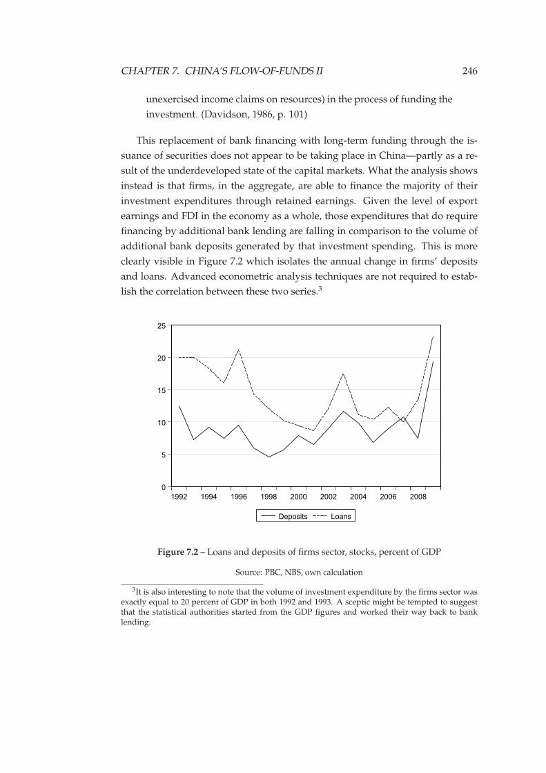
CHAPTER 7. CHINA’S FLOW-OF-FUNDS II 246
unexercised income claims on resources) in the process of funding the
investment. (Davidson, 1986, p. 101)
This replacement of bank financing with long-term funding through the is-
suance of securities does not appear to be taking place in China—partly as a re-
sult of the underdeveloped state of the capital markets. What the analysis shows
instead is that firms, in the aggregate, are able to finance the majority of their
investment expenditures through retained earnings. Given the level of export
earnings and FDI in the economy as a whole, those expenditures that do require
financing by additional bank lending are falling in comparison to the volume of
additional bank deposits generated by that investment spending. This is more
clearly visible in Figure 7.2 which isolates the annual change in firms’ deposits
and loans. Advanced econometric analysis techniques are not required to estab-
lish the correlation between these two series.3
0
5
10
15
20
25
1992 1994 1996 1998 2000 2002 2004 2006 2008
Deposits Loans
Figure 7.2 – Loans and deposits of firms sector, stocks, percent of GDP
Source: PBC, NBS, own calculation
3It is also interesting to note that the volume of investment expenditure by the firms sector wasexactly equal to 20 percent of GDP in both 1992 and 1993. A sceptic might be tempted to suggestthat the statistical authorities started from the GDP figures and worked their way back to banklending.
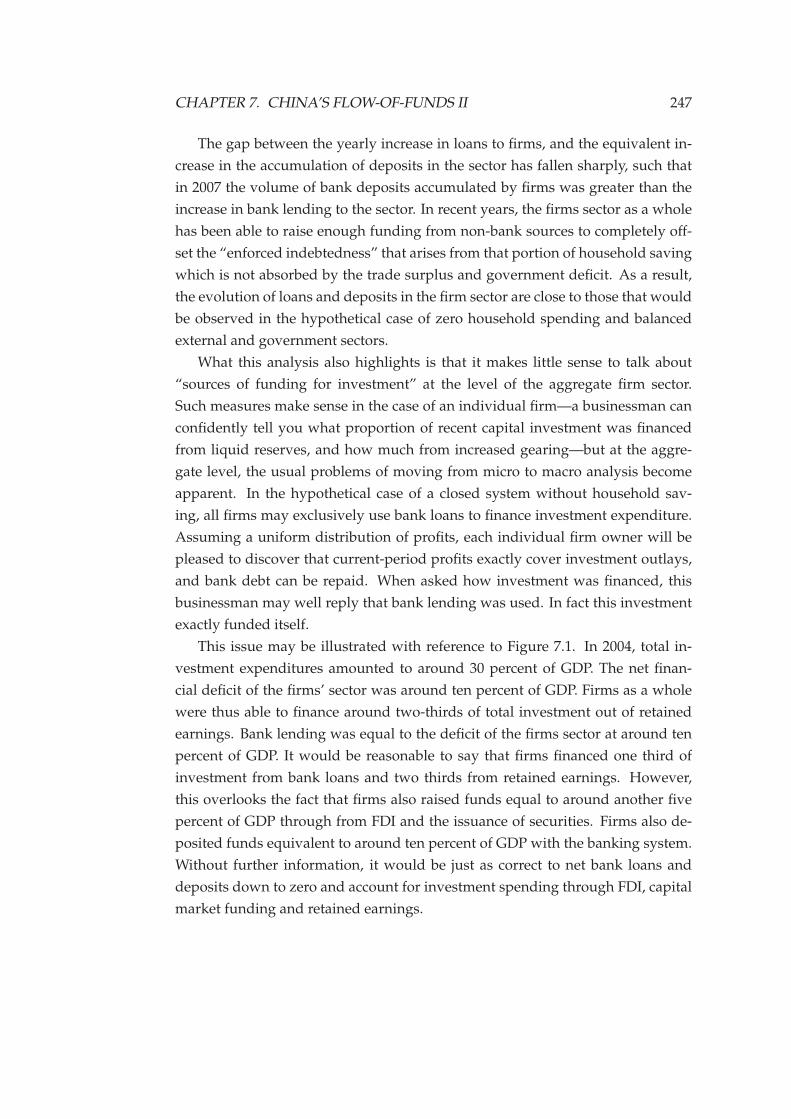
CHAPTER 7. CHINA’S FLOW-OF-FUNDS II 247
The gap between the yearly increase in loans to firms, and the equivalent in-
crease in the accumulation of deposits in the sector has fallen sharply, such that
in 2007 the volume of bank deposits accumulated by firms was greater than the
increase in bank lending to the sector. In recent years, the firms sector as a whole
has been able to raise enough funding from non-bank sources to completely off-
set the “enforced indebtedness” that arises from that portion of household saving
which is not absorbed by the trade surplus and government deficit. As a result,
the evolution of loans and deposits in the firm sector are close to those that would
be observed in the hypothetical case of zero household spending and balanced
external and government sectors.
What this analysis also highlights is that it makes little sense to talk about
“sources of funding for investment” at the level of the aggregate firm sector.
Such measures make sense in the case of an individual firm—a businessman can
confidently tell you what proportion of recent capital investment was financed
from liquid reserves, and how much from increased gearing—but at the aggre-
gate level, the usual problems of moving from micro to macro analysis become
apparent. In the hypothetical case of a closed system without household sav-
ing, all firms may exclusively use bank loans to finance investment expenditure.
Assuming a uniform distribution of profits, each individual firm owner will be
pleased to discover that current-period profits exactly cover investment outlays,
and bank debt can be repaid. When asked how investment was financed, this
businessman may well reply that bank lending was used. In fact this investment
exactly funded itself.
This issue may be illustrated with reference to Figure 7.1. In 2004, total in-
vestment expenditures amounted to around 30 percent of GDP. The net finan-
cial deficit of the firms’ sector was around ten percent of GDP. Firms as a whole
were thus able to finance around two-thirds of total investment out of retained
earnings. Bank lending was equal to the deficit of the firms sector at around ten
percent of GDP. It would be reasonable to say that firms financed one third of
investment from bank loans and two thirds from retained earnings. However,
this overlooks the fact that firms also raised funds equal to around another five
percent of GDP through from FDI and the issuance of securities. Firms also de-
posited funds equivalent to around ten percent of GDP with the banking system.
Without further information, it would be just as correct to net bank loans and
deposits down to zero and account for investment spending through FDI, capital
market funding and retained earnings.
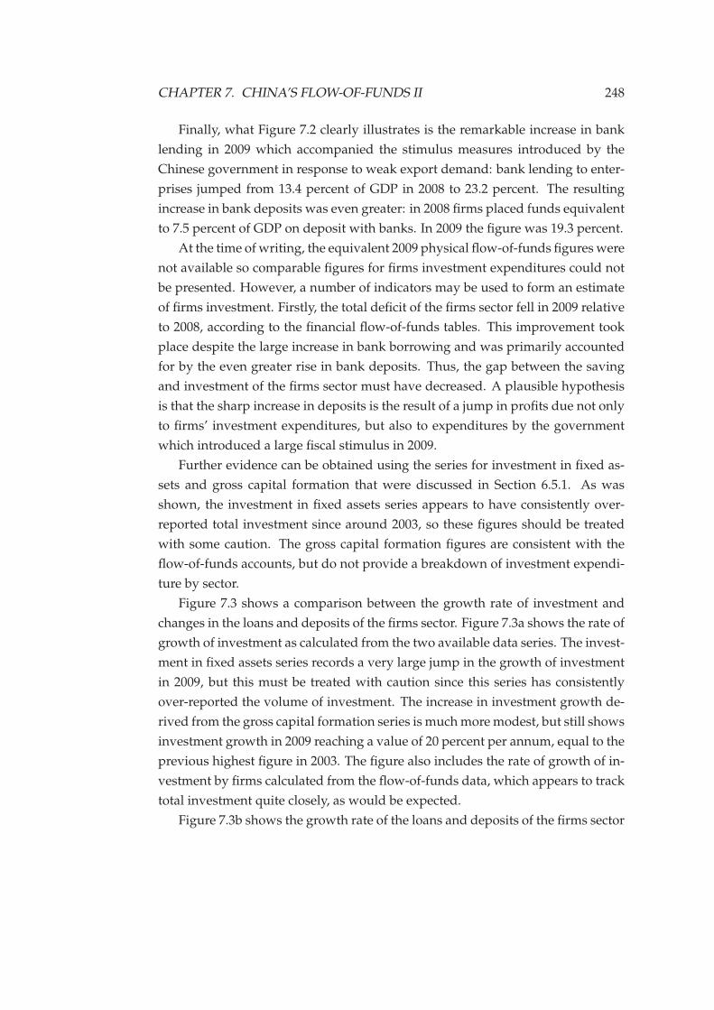
CHAPTER 7. CHINA’S FLOW-OF-FUNDS II 248
Finally, what Figure 7.2 clearly illustrates is the remarkable increase in bank
lending in 2009 which accompanied the stimulus measures introduced by the
Chinese government in response to weak export demand: bank lending to enter-
prises jumped from 13.4 percent of GDP in 2008 to 23.2 percent. The resulting
increase in bank deposits was even greater: in 2008 firms placed funds equivalent
to 7.5 percent of GDP on deposit with banks. In 2009 the figure was 19.3 percent.
At the time of writing, the equivalent 2009 physical flow-of-funds figures were
not available so comparable figures for firms investment expenditures could not
be presented. However, a number of indicators may be used to form an estimate
of firms investment. Firstly, the total deficit of the firms sector fell in 2009 relative
to 2008, according to the financial flow-of-funds tables. This improvement took
place despite the large increase in bank borrowing and was primarily accounted
for by the even greater rise in bank deposits. Thus, the gap between the saving
and investment of the firms sector must have decreased. A plausible hypothesis
is that the sharp increase in deposits is the result of a jump in profits due not only
to firms’ investment expenditures, but also to expenditures by the government
which introduced a large fiscal stimulus in 2009.
Further evidence can be obtained using the series for investment in fixed as-
sets and gross capital formation that were discussed in Section 6.5.1. As was
shown, the investment in fixed assets series appears to have consistently over-
reported total investment since around 2003, so these figures should be treated
with some caution. The gross capital formation figures are consistent with the
flow-of-funds accounts, but do not provide a breakdown of investment expendi-
ture by sector.
Figure 7.3 shows a comparison between the growth rate of investment and
changes in the loans and deposits of the firms sector. Figure 7.3a shows the rate of
growth of investment as calculated from the two available data series. The invest-
ment in fixed assets series records a very large jump in the growth of investment
in 2009, but this must be treated with caution since this series has consistently
over-reported the volume of investment. The increase in investment growth de-
rived from the gross capital formation series is much more modest, but still shows
investment growth in 2009 reaching a value of 20 percent per annum, equal to the
previous highest figure in 2003. The figure also includes the rate of growth of in-
vestment by firms calculated from the flow-of-funds data, which appears to track
total investment quite closely, as would be expected.
Figure 7.3b shows the growth rate of the loans and deposits of the firms sector
CHAPTER 7. CHINA’S FLOW-OF-FUNDS II 249
-5
0
5
10
15
20
25
30
35
1994 1996 1998 2000 2002 2004 2006 2008 2010
Investment in fixed assetsTotal gross capital formation
Firms investment
(a) Growth of investment, various measures
-40
0
40
80
120
160
200
1992 1994 1996 1998 2000 2002 2004 2006 2008
Annual change in deposits, inflation adjustedAnnual change in loans, inflation adjusted
(b) Growth of deposits and loans of firms, inflation adjusted
Figure 7.3 – Growth in investment; growth in loans and deposits of firms, percentper annum
Source: PBC, NBS, own calculation
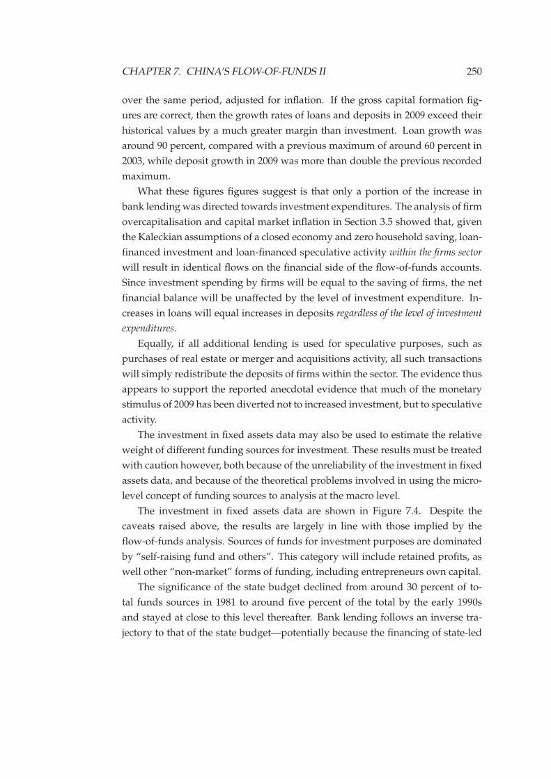
CHAPTER 7. CHINA’S FLOW-OF-FUNDS II 250
over the same period, adjusted for inflation. If the gross capital formation fig-
ures are correct, then the growth rates of loans and deposits in 2009 exceed their
historical values by a much greater margin than investment. Loan growth was
around 90 percent, compared with a previous maximum of around 60 percent in
2003, while deposit growth in 2009 was more than double the previous recorded
maximum.
What these figures figures suggest is that only a portion of the increase in
bank lending was directed towards investment expenditures. The analysis of firm
overcapitalisation and capital market inflation in Section 3.5 showed that, given
the Kaleckian assumptions of a closed economy and zero household saving, loan-
financed investment and loan-financed speculative activity within the firms sector
will result in identical flows on the financial side of the flow-of-funds accounts.
Since investment spending by firms will be equal to the saving of firms, the net
financial balance will be unaffected by the level of investment expenditure. In-
creases in loans will equal increases in deposits regardless of the level of investment
expenditures.
Equally, if all additional lending is used for speculative purposes, such as
purchases of real estate or merger and acquisitions activity, all such transactions
will simply redistribute the deposits of firms within the sector. The evidence thus
appears to support the reported anecdotal evidence that much of the monetary
stimulus of 2009 has been diverted not to increased investment, but to speculative
activity.
The investment in fixed assets data may also be used to estimate the relative
weight of different funding sources for investment. These results must be treated
with caution however, both because of the unreliability of the investment in fixed
assets data, and because of the theoretical problems involved in using the micro-
level concept of funding sources to analysis at the macro level.
The investment in fixed assets data are shown in Figure 7.4. Despite the
caveats raised above, the results are largely in line with those implied by the
flow-of-funds analysis. Sources of funds for investment purposes are dominated
by “self-raising fund and others”. This category will include retained profits, as
well other “non-market” forms of funding, including entrepreneurs own capital.
The significance of the state budget declined from around 30 percent of to-
tal funds sources in 1981 to around five percent of the total by the early 1990s
and stayed at close to this level thereafter. Bank lending follows an inverse tra-
jectory to that of the state budget—potentially because the financing of state-led
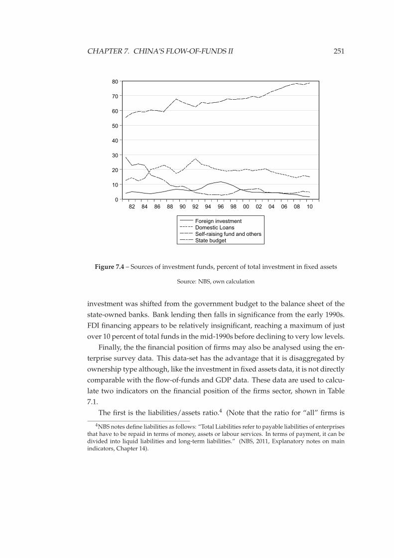
CHAPTER 7. CHINA’S FLOW-OF-FUNDS II 251
0
10
20
30
40
50
60
70
80
82 84 86 88 90 92 94 96 98 00 02 04 06 08 10
Foreign investment
Domestic Loans
Self-raising fund and others
State budget
Figure 7.4 – Sources of investment funds, percent of total investment in fixed assets
Source: NBS, own calculation
investment was shifted from the government budget to the balance sheet of the
state-owned banks. Bank lending then falls in significance from the early 1990s.
FDI financing appears to be relatively insignificant, reaching a maximum of just
over 10 percent of total funds in the mid-1990s before declining to very low levels.
Finally, the the financial position of firms may also be analysed using the en-
terprise survey data. This data-set has the advantage that it is disaggregated by
ownership type although, like the investment in fixed assets data, it is not directly
comparable with the flow-of-funds and GDP data. These data are used to calcu-
late two indicators on the financial position of the firms sector, shown in Table
7.1.
The first is the liabilities/assets ratio.4 (Note that the ratio for “all” firms is
4NBS notes define liabilities as follows: “Total Liabilities refer to payable liabilities of enterprisesthat have to be repaid in terms of money, assets or labour services. In terms of payment, it can bedivided into liquid liabilities and long-term liabilities.” (NBS, 2011, Explanatory notes on mainindicators, Chapter 14).
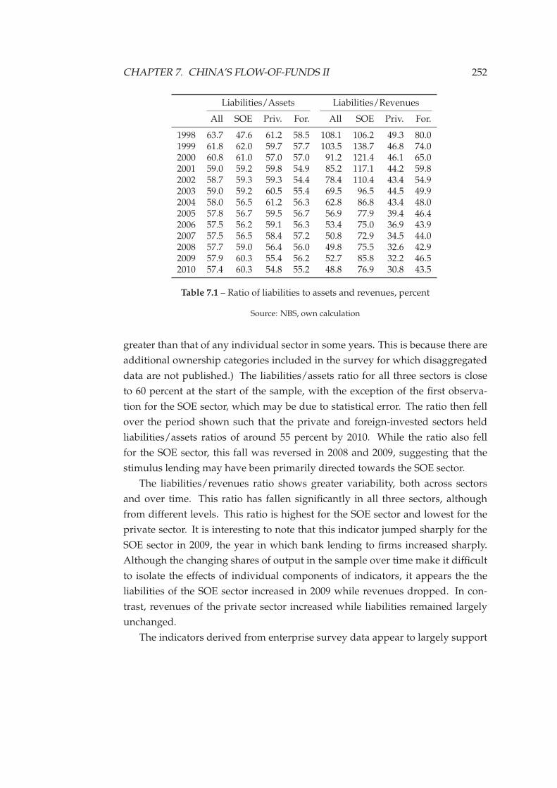
CHAPTER 7. CHINA’S FLOW-OF-FUNDS II 252
Liabilities/Assets Liabilities/Revenues
All SOE Priv. For. All SOE Priv. For.
1998 63.7 47.6 61.2 58.5 108.1 106.2 49.3 80.01999 61.8 62.0 59.7 57.7 103.5 138.7 46.8 74.02000 60.8 61.0 57.0 57.0 91.2 121.4 46.1 65.02001 59.0 59.2 59.8 54.9 85.2 117.1 44.2 59.82002 58.7 59.3 59.3 54.4 78.4 110.4 43.4 54.92003 59.0 59.2 60.5 55.4 69.5 96.5 44.5 49.92004 58.0 56.5 61.2 56.3 62.8 86.8 43.4 48.02005 57.8 56.7 59.5 56.7 56.9 77.9 39.4 46.42006 57.5 56.2 59.1 56.3 53.4 75.0 36.9 43.92007 57.5 56.5 58.4 57.2 50.8 72.9 34.5 44.02008 57.7 59.0 56.4 56.0 49.8 75.5 32.6 42.92009 57.9 60.3 55.4 56.2 52.7 85.8 32.2 46.52010 57.4 60.3 54.8 55.2 48.8 76.9 30.8 43.5
Table 7.1 – Ratio of liabilities to assets and revenues, percent
Source: NBS, own calculation
greater than that of any individual sector in some years. This is because there are
additional ownership categories included in the survey for which disaggregated
data are not published.) The liabilities/assets ratio for all three sectors is close
to 60 percent at the start of the sample, with the exception of the first observa-
tion for the SOE sector, which may be due to statistical error. The ratio then fell
over the period shown such that the private and foreign-invested sectors held
liabilities/assets ratios of around 55 percent by 2010. While the ratio also fell
for the SOE sector, this fall was reversed in 2008 and 2009, suggesting that the
stimulus lending may have been primarily directed towards the SOE sector.
The liabilities/revenues ratio shows greater variability, both across sectors
and over time. This ratio has fallen significantly in all three sectors, although
from different levels. This ratio is highest for the SOE sector and lowest for the
private sector. It is interesting to note that this indicator jumped sharply for the
SOE sector in 2009, the year in which bank lending to firms increased sharply.
Although the changing shares of output in the sample over time make it difficult
to isolate the effects of individual components of indicators, it appears the the
liabilities of the SOE sector increased in 2009 while revenues dropped. In con-
trast, revenues of the private sector increased while liabilities remained largely
unchanged.
The indicators derived from enterprise survey data appear to largely support
CHAPTER 7. CHINA’S FLOW-OF-FUNDS II 253
the analysis of the flow-of-funds and investment in fixed-assets data—falling val-
ues for the derived indicators are to be expected if firms are increasingly using
retained earnings as a source of investment finance. However these indicators
suggest that the process is not even across the different ownership types: the lia-
bility indicators are lower and fall more significantly in the private sector.
At this point, a picture of the changing structure and dynamics of Chinese
industry begins to emerge from the statistics. The capital-intensive “core” of the
Chinese economy is made up of the SOE sector. While the share of total output
and investment expenditure by the SOE sector is falling, this is primarily due to
the higher growth rate of the private sector.
This SOE core is made up of the firms that would most readily become “cartelised”
in the Baran-Sweezy-Steindl Monopoly Capital analysis (Baran & Sweezy, 1966;
Steindl, 1952). The result of this cartelisation of the economy would be cooper-
ation between these large firms in order to set price mark-ups at levels which
increased the profits of the cartelised sector at the expense of “marginal” firms,
while producing a level of output that resulted in significant excess capacity. This
“maldistribution of profits” would result in the investment expenditures of firms
in the competitive sector accruing as profits to the “predatory” cartelised sec-
tor. The “enforced indebtedness” of the firms sector arising from the saving of
households would be skewed towards the competitive marginal firms. The re-
sulting excess of saving over investment expenditure would result in a slowdown
in growth and eventually stagnation.
This pattern of accumulation does not appear to characterise the Chinese case.
Instead, net profit margins appear to approximately equal across the different
firm ownership types and to rise over time. (see Section 6.5.2). At the same time,
the rates of profits appear to be significantly higher in the private sector. With
roughly equal profit margins, higher profit rates can only result from lower rates
of investment. Thus, although the share of total investment by private firms is
rising, it is likely that investment as a share of output is actually lower in the
private sector.
On the liability side, indebtedness appears to be higher in the SOE sector, a
finding that fits with the often reported preference of the banking system for lend-
ing to the SOE sector. As shown above, the rate of loan growth in the firms sector
is almost exactly matched by deposit growth. As demonstrated by Kalecki, loan-
financed investment expenditures of firms accrue as profits in the form of bank
deposits within the firms sector. However, if growth rate of the credit-financed
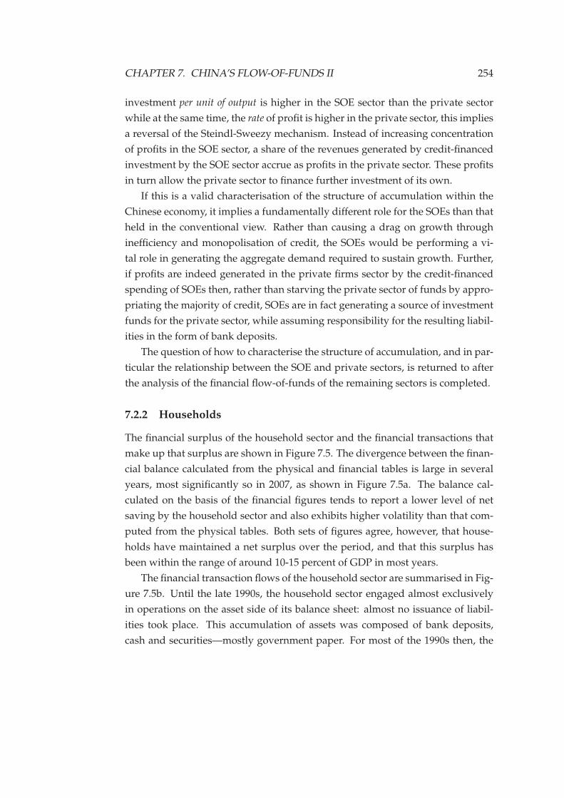
CHAPTER 7. CHINA’S FLOW-OF-FUNDS II 254
investment per unit of output is higher in the SOE sector than the private sector
while at the same time, the rate of profit is higher in the private sector, this implies
a reversal of the Steindl-Sweezy mechanism. Instead of increasing concentration
of profits in the SOE sector, a share of the revenues generated by credit-financed
investment by the SOE sector accrue as profits in the private sector. These profits
in turn allow the private sector to finance further investment of its own.
If this is a valid characterisation of the structure of accumulation within the
Chinese economy, it implies a fundamentally different role for the SOEs than that
held in the conventional view. Rather than causing a drag on growth through
inefficiency and monopolisation of credit, the SOEs would be performing a vi-
tal role in generating the aggregate demand required to sustain growth. Further,
if profits are indeed generated in the private firms sector by the credit-financed
spending of SOEs then, rather than starving the private sector of funds by appro-
priating the majority of credit, SOEs are in fact generating a source of investment
funds for the private sector, while assuming responsibility for the resulting liabil-
ities in the form of bank deposits.
The question of how to characterise the structure of accumulation, and in par-
ticular the relationship between the SOE and private sectors, is returned to after
the analysis of the financial flow-of-funds of the remaining sectors is completed.
7.2.2 Households
The financial surplus of the household sector and the financial transactions that
make up that surplus are shown in Figure 7.5. The divergence between the finan-
cial balance calculated from the physical and financial tables is large in several
years, most significantly so in 2007, as shown in Figure 7.5a. The balance cal-
culated on the basis of the financial figures tends to report a lower level of net
saving by the household sector and also exhibits higher volatility than that com-
puted from the physical tables. Both sets of figures agree, however, that house-
holds have maintained a net surplus over the period, and that this surplus has
been within the range of around 10-15 percent of GDP in most years.
The financial transaction flows of the household sector are summarised in Fig-
ure 7.5b. Until the late 1990s, the household sector engaged almost exclusively
in operations on the asset side of its balance sheet: almost no issuance of liabil-
ities took place. This accumulation of assets was composed of bank deposits,
cash and securities—mostly government paper. For most of the 1990s then, the
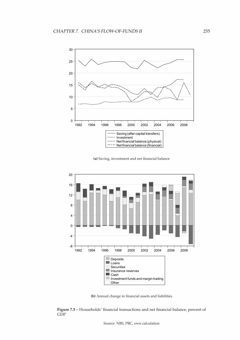
CHAPTER 7. CHINA’S FLOW-OF-FUNDS II 255
0
5
10
15
20
25
30
1992 1994 1996 1998 2000 2002 2004 2006 2008
Saving (after capital transfers)Investment
Net financial balance (physical)
Net financial balance (financial)
(a) Saving, investment and net financial balance
-8
-4
0
4
8
12
16
20
1992 1994 1996 1998 2000 2002 2004 2006 2008
Deposits
Loans
Securities
Insurance reserves
Cash
Investment funds and margin trading
Other
(b) Annual change in financial assets and liabilities
Figure 7.5 – Households’ financial transactions and net financial balance, percent ofGDP
Source: NBS, PBC, own calculation
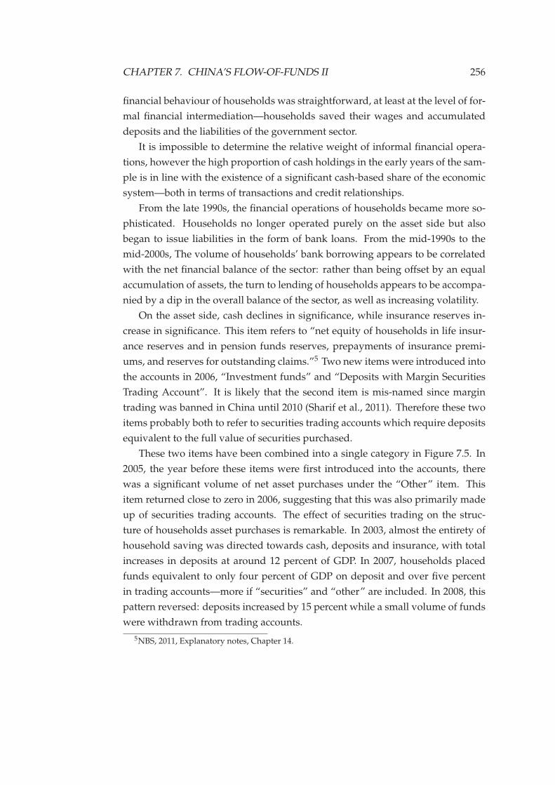
CHAPTER 7. CHINA’S FLOW-OF-FUNDS II 256
financial behaviour of households was straightforward, at least at the level of for-
mal financial intermediation—households saved their wages and accumulated
deposits and the liabilities of the government sector.
It is impossible to determine the relative weight of informal financial opera-
tions, however the high proportion of cash holdings in the early years of the sam-
ple is in line with the existence of a significant cash-based share of the economic
system—both in terms of transactions and credit relationships.
From the late 1990s, the financial operations of households became more so-
phisticated. Households no longer operated purely on the asset side but also
began to issue liabilities in the form of bank loans. From the mid-1990s to the
mid-2000s, The volume of households’ bank borrowing appears to be correlated
with the net financial balance of the sector: rather than being offset by an equal
accumulation of assets, the turn to lending of households appears to be accompa-
nied by a dip in the overall balance of the sector, as well as increasing volatility.
On the asset side, cash declines in significance, while insurance reserves in-
crease in significance. This item refers to “net equity of households in life insur-
ance reserves and in pension funds reserves, prepayments of insurance premi-
ums, and reserves for outstanding claims.”5 Two new items were introduced into
the accounts in 2006, “Investment funds” and “Deposits with Margin Securities
Trading Account”. It is likely that the second item is mis-named since margin
trading was banned in China until 2010 (Sharif et al., 2011). Therefore these two
items probably both to refer to securities trading accounts which require deposits
equivalent to the full value of securities purchased.
These two items have been combined into a single category in Figure 7.5. In
2005, the year before these items were first introduced into the accounts, there
was a significant volume of net asset purchases under the “Other” item. This
item returned close to zero in 2006, suggesting that this was also primarily made
up of securities trading accounts. The effect of securities trading on the struc-
ture of households asset purchases is remarkable. In 2003, almost the entirety of
household saving was directed towards cash, deposits and insurance, with total
increases in deposits at around 12 percent of GDP. In 2007, households placed
funds equivalent to only four percent of GDP on deposit and over five percent
in trading accounts—more if “securities” and “other” are included. In 2008, this
pattern reversed: deposits increased by 15 percent while a small volume of funds
were withdrawn from trading accounts.
5NBS, 2011, Explanatory notes, Chapter 14.
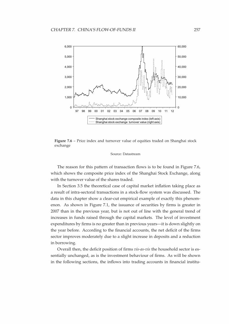
CHAPTER 7. CHINA’S FLOW-OF-FUNDS II 257
0
1,000
2,000
3,000
4,000
5,000
6,000
0
10,000
20,000
30,000
40,000
50,000
60,000
97 98 99 00 01 02 03 04 05 06 07 08 09 10 11 12
Shanghai stock exchange composite index (left axis)
Shanghai stock exchange turnover value (right axis)
Figure 7.6 – Price index and turnover value of equities traded on Shanghai stockexchange
Source: Datastream
The reason for this pattern of transaction flows is to be found in Figure 7.6,
which shows the composite price index of the Shanghai Stock Exchange, along
with the turnover value of the shares traded.
In Section 3.5 the theoretical case of capital market inflation taking place as
a result of intra-sectoral transactions in a stock-flow system was discussed. The
data in this chapter show a clear-cut empirical example of exactly this phenom-
enon. As shown in Figure 7.1, the issuance of securities by firms is greater in
2007 than in the previous year, but is not out of line with the general trend of
increases in funds raised through the capital markets. The level of investment
expenditures by firms is no greater than in previous years—it is down slightly on
the year before. According to the financial accounts, the net deficit of the firms
sector improves moderately due to a slight increase in deposits and a reduction
in borrowing.
Overall then, the deficit position of firms vis-as-vis the household sector is es-
sentially unchanged, as is the investment behaviour of firms. As will be shown
in the following sections, the inflows into trading accounts in financial institu-
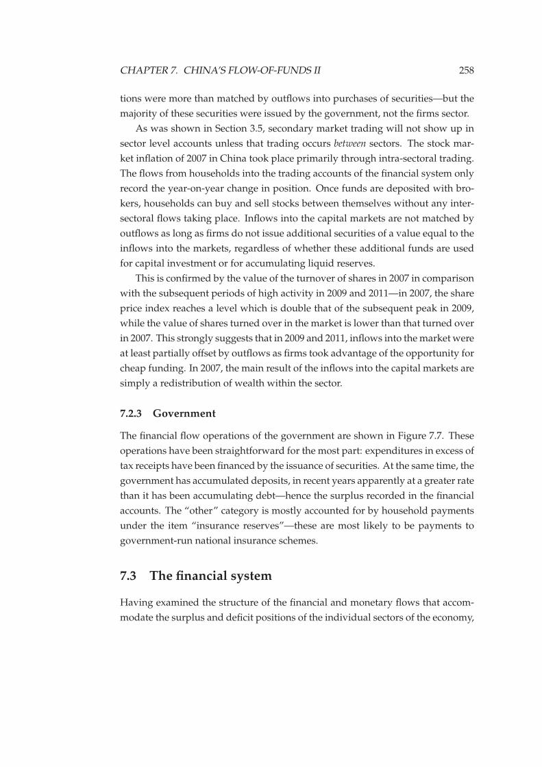
CHAPTER 7. CHINA’S FLOW-OF-FUNDS II 258
tions were more than matched by outflows into purchases of securities—but the
majority of these securities were issued by the government, not the firms sector.
As was shown in Section 3.5, secondary market trading will not show up in
sector level accounts unless that trading occurs between sectors. The stock mar-
ket inflation of 2007 in China took place primarily through intra-sectoral trading.
The flows from households into the trading accounts of the financial system only
record the year-on-year change in position. Once funds are deposited with bro-
kers, households can buy and sell stocks between themselves without any inter-
sectoral flows taking place. Inflows into the capital markets are not matched by
outflows as long as firms do not issue additional securities of a value equal to the
inflows into the markets, regardless of whether these additional funds are used
for capital investment or for accumulating liquid reserves.
This is confirmed by the value of the turnover of shares in 2007 in comparison
with the subsequent periods of high activity in 2009 and 2011—in 2007, the share
price index reaches a level which is double that of the subsequent peak in 2009,
while the value of shares turned over in the market is lower than that turned over
in 2007. This strongly suggests that in 2009 and 2011, inflows into the market were
at least partially offset by outflows as firms took advantage of the opportunity for
cheap funding. In 2007, the main result of the inflows into the capital markets are
simply a redistribution of wealth within the sector.
7.2.3 Government
The financial flow operations of the government are shown in Figure 7.7. These
operations have been straightforward for the most part: expenditures in excess of
tax receipts have been financed by the issuance of securities. At the same time, the
government has accumulated deposits, in recent years apparently at a greater rate
than it has been accumulating debt—hence the surplus recorded in the financial
accounts. The “other” category is mostly accounted for by household payments
under the item “insurance reserves”—these are most likely to be payments to
government-run national insurance schemes.
7.3 The financial system
Having examined the structure of the financial and monetary flows that accom-
modate the surplus and deficit positions of the individual sectors of the economy,
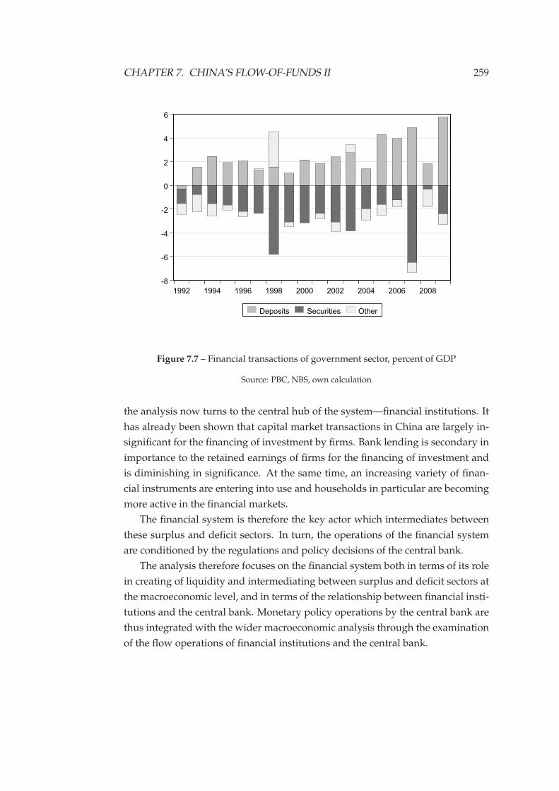
CHAPTER 7. CHINA’S FLOW-OF-FUNDS II 259
-8
-6
-4
-2
0
2
4
6
1992 1994 1996 1998 2000 2002 2004 2006 2008
Deposits Securities Other
Figure 7.7 – Financial transactions of government sector, percent of GDP
Source: PBC, NBS, own calculation
the analysis now turns to the central hub of the system—financial institutions. It
has already been shown that capital market transactions in China are largely in-
significant for the financing of investment by firms. Bank lending is secondary in
importance to the retained earnings of firms for the financing of investment and
is diminishing in significance. At the same time, an increasing variety of finan-
cial instruments are entering into use and households in particular are becoming
more active in the financial markets.
The financial system is therefore the key actor which intermediates between
these surplus and deficit sectors. In turn, the operations of the financial system
are conditioned by the regulations and policy decisions of the central bank.
The analysis therefore focuses on the financial system both in terms of its role
in creating of liquidity and intermediating between surplus and deficit sectors at
the macroeconomic level, and in terms of the relationship between financial insti-
tutions and the central bank. Monetary policy operations by the central bank are
thus integrated with the wider macroeconomic analysis through the examination
of the flow operations of financial institutions and the central bank.
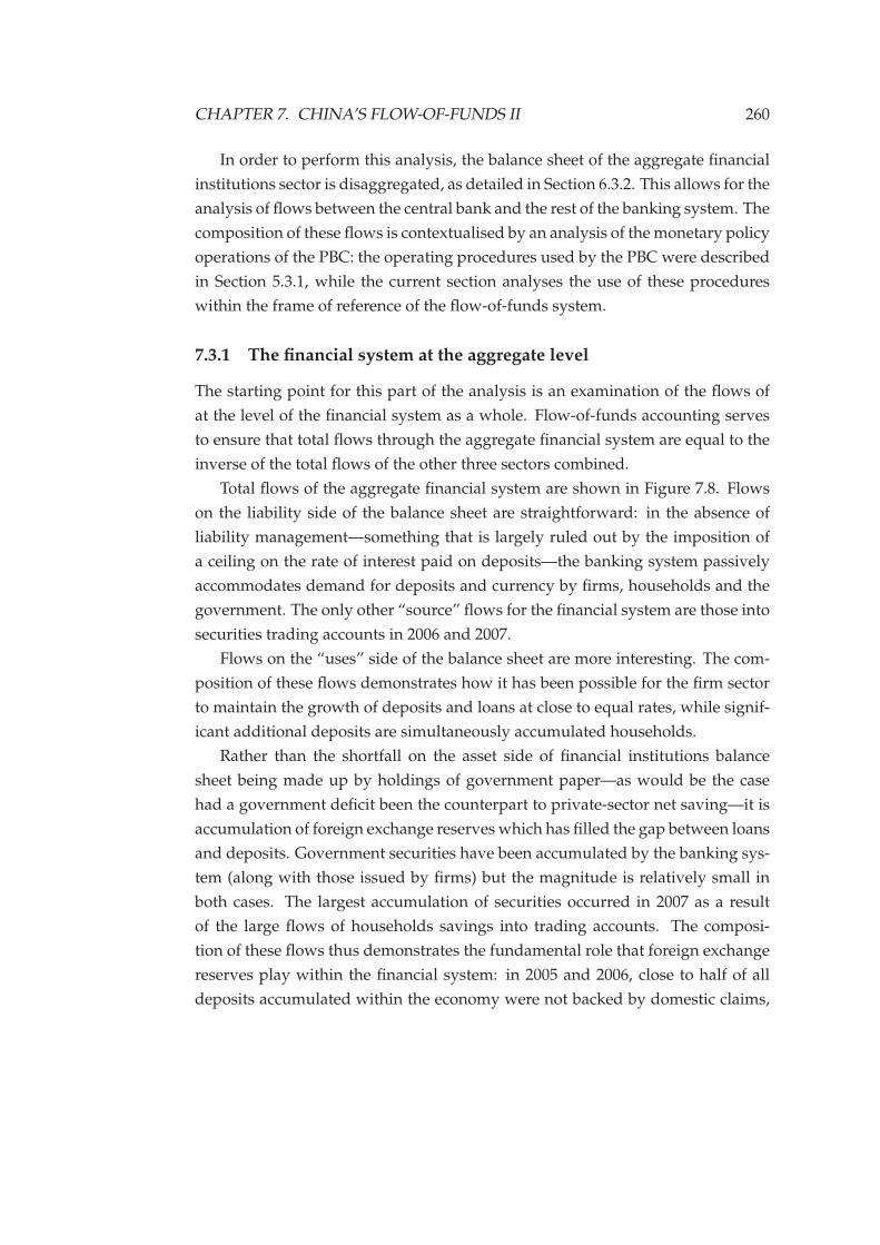
CHAPTER 7. CHINA’S FLOW-OF-FUNDS II 260
In order to perform this analysis, the balance sheet of the aggregate financial
institutions sector is disaggregated, as detailed in Section 6.3.2. This allows for the
analysis of flows between the central bank and the rest of the banking system. The
composition of these flows is contextualised by an analysis of the monetary policy
operations of the PBC: the operating procedures used by the PBC were described
in Section 5.3.1, while the current section analyses the use of these procedures
within the frame of reference of the flow-of-funds system.
7.3.1 The financial system at the aggregate level
The starting point for this part of the analysis is an examination of the flows of
at the level of the financial system as a whole. Flow-of-funds accounting serves
to ensure that total flows through the aggregate financial system are equal to the
inverse of the total flows of the other three sectors combined.
Total flows of the aggregate financial system are shown in Figure 7.8. Flows
on the liability side of the balance sheet are straightforward: in the absence of
liability management—something that is largely ruled out by the imposition of
a ceiling on the rate of interest paid on deposits—the banking system passively
accommodates demand for deposits and currency by firms, households and the
government. The only other “source” flows for the financial system are those into
securities trading accounts in 2006 and 2007.
Flows on the “uses” side of the balance sheet are more interesting. The com-
position of these flows demonstrates how it has been possible for the firm sector
to maintain the growth of deposits and loans at close to equal rates, while signif-
icant additional deposits are simultaneously accumulated households.
Rather than the shortfall on the asset side of financial institutions balance
sheet being made up by holdings of government paper—as would be the case
had a government deficit been the counterpart to private-sector net saving—it is
accumulation of foreign exchange reserves which has filled the gap between loans
and deposits. Government securities have been accumulated by the banking sys-
tem (along with those issued by firms) but the magnitude is relatively small in
both cases. The largest accumulation of securities occurred in 2007 as a result
of the large flows of households savings into trading accounts. The composi-
tion of these flows thus demonstrates the fundamental role that foreign exchange
reserves play within the financial system: in 2005 and 2006, close to half of all
deposits accumulated within the economy were not backed by domestic claims,
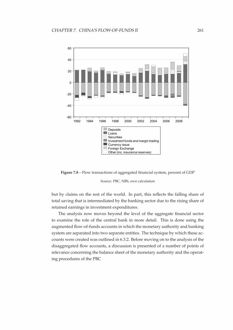
CHAPTER 7. CHINA’S FLOW-OF-FUNDS II 261
-60
-40
-20
0
20
40
60
1992 1994 1996 1998 2000 2002 2004 2006 2008
Deposits
Loans
Securities
Investment funds and margin trading
Currency issue
Foreign Exchange
Other (inc. insurance reserves)
Figure 7.8 – Flow transactions of aggregated financial system, percent of GDP
Source: PBC, NBS, own calculation
but by claims on the rest of the world. In part, this reflects the falling share of
total saving that is intermediated by the banking sector due to the rising share of
retained earnings in investment expenditures.
The analysis now moves beyond the level of the aggregate financial sector
to examine the role of the central bank in more detail. This is done using the
augmented flow-of-funds accounts in which the monetary authority and banking
system are separated into two separate entities. The technique by which these ac-
counts were created was outlined in 6.3.2. Before moving on to the analysis of the
disaggregated flow accounts, a discussion is presented of a number of points of
relevance concerning the balance sheet of the monetary authority and the operat-
ing procedures of the PBC
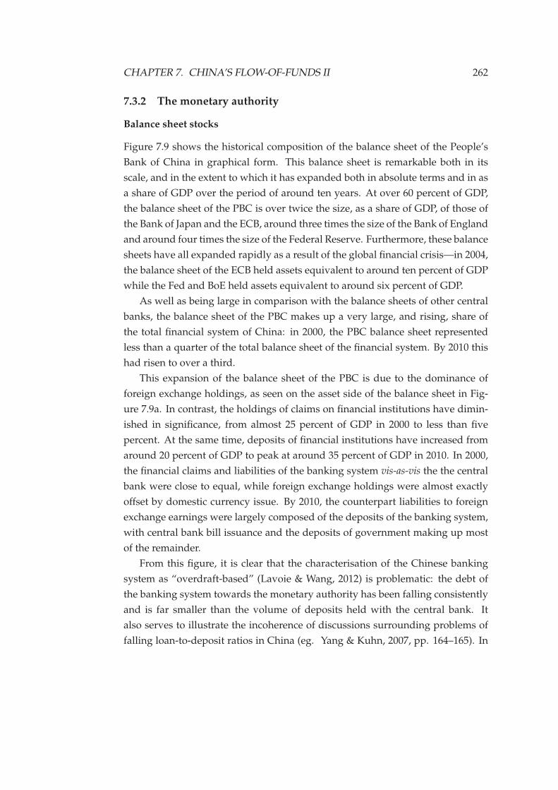
CHAPTER 7. CHINA’S FLOW-OF-FUNDS II 262
7.3.2 The monetary authority
Balance sheet stocks
Figure 7.9 shows the historical composition of the balance sheet of the People’s
Bank of China in graphical form. This balance sheet is remarkable both in its
scale, and in the extent to which it has expanded both in absolute terms and in as
a share of GDP over the period of around ten years. At over 60 percent of GDP,
the balance sheet of the PBC is over twice the size, as a share of GDP, of those of
the Bank of Japan and the ECB, around three times the size of the Bank of England
and around four times the size of the Federal Reserve. Furthermore, these balance
sheets have all expanded rapidly as a result of the global financial crisis—in 2004,
the balance sheet of the ECB held assets equivalent to around ten percent of GDP
while the Fed and BoE held assets equivalent to around six percent of GDP.
As well as being large in comparison with the balance sheets of other central
banks, the balance sheet of the PBC makes up a very large, and rising, share of
the total financial system of China: in 2000, the PBC balance sheet represented
less than a quarter of the total balance sheet of the financial system. By 2010 this
had risen to over a third.
This expansion of the balance sheet of the PBC is due to the dominance of
foreign exchange holdings, as seen on the asset side of the balance sheet in Fig-
ure 7.9a. In contrast, the holdings of claims on financial institutions have dimin-
ished in significance, from almost 25 percent of GDP in 2000 to less than five
percent. At the same time, deposits of financial institutions have increased from
around 20 percent of GDP to peak at around 35 percent of GDP in 2010. In 2000,
the financial claims and liabilities of the banking system vis-as-vis the the central
bank were close to equal, while foreign exchange holdings were almost exactly
offset by domestic currency issue. By 2010, the counterpart liabilities to foreign
exchange earnings were largely composed of the deposits of the banking system,
with central bank bill issuance and the deposits of government making up most
of the remainder.
From this figure, it is clear that the characterisation of the Chinese banking
system as “overdraft-based” (Lavoie & Wang, 2012) is problematic: the debt of
the banking system towards the monetary authority has been falling consistently
and is far smaller than the volume of deposits held with the central bank. It
also serves to illustrate the incoherence of discussions surrounding problems of
falling loan-to-deposit ratios in China (eg. Yang & Kuhn, 2007, pp. 164–165). In
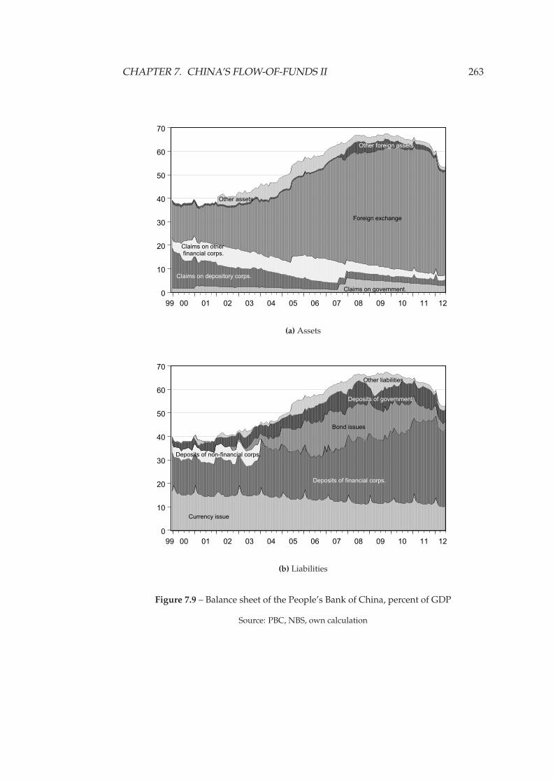
CHAPTER 7. CHINA’S FLOW-OF-FUNDS II 263
0
10
20
30
40
50
60
70
99 00 01 02 03 04 05 06 07 08 09 10 11 12
Other assets
Other foreign assets
Foreign exchange
Claims on depository corps.
Claims on other financial corps.
Claims on government.
(a) Assets
0
10
20
30
40
50
60
70
99 00 01 02 03 04 05 06 07 08 09 10 11 12
Other liabilities
Deposits of government
Bond issues
Deposits of non-financial corps.
Deposits of financial corps.
Currency issue
(b) Liabilities
Figure 7.9 – Balance sheet of the People’s Bank of China, percent of GDP
Source: PBC, NBS, own calculation
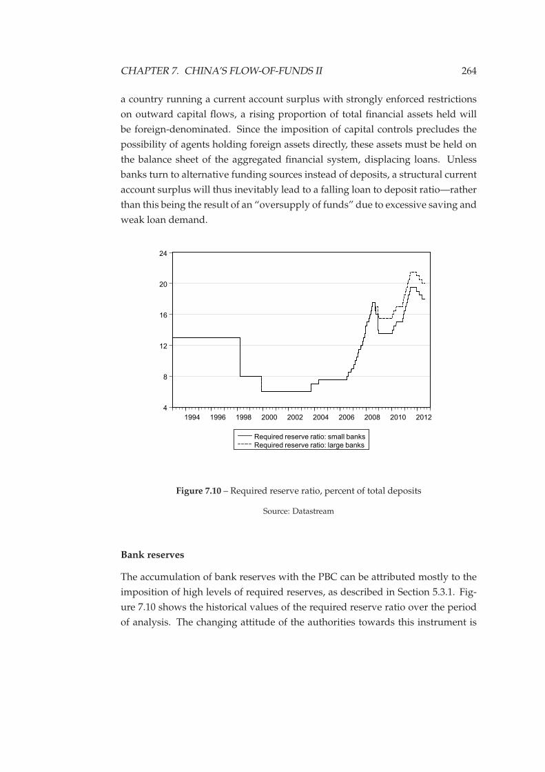
CHAPTER 7. CHINA’S FLOW-OF-FUNDS II 264
a country running a current account surplus with strongly enforced restrictions
on outward capital flows, a rising proportion of total financial assets held will
be foreign-denominated. Since the imposition of capital controls precludes the
possibility of agents holding foreign assets directly, these assets must be held on
the balance sheet of the aggregated financial system, displacing loans. Unless
banks turn to alternative funding sources instead of deposits, a structural current
account surplus will thus inevitably lead to a falling loan to deposit ratio—rather
than this being the result of an “oversupply of funds” due to excessive saving and
weak loan demand.
4
8
12
16
20
24
1994 1996 1998 2000 2002 2004 2006 2008 2010 2012
Required reserve ratio: small banks
Required reserve ratio: large banks
Figure 7.10 – Required reserve ratio, percent of total deposits
Source: Datastream
Bank reserves
The accumulation of bank reserves with the PBC can be attributed mostly to the
imposition of high levels of required reserves, as described in Section 5.3.1. Fig-
ure 7.10 shows the historical values of the required reserve ratio over the period
of analysis. The changing attitude of the authorities towards this instrument is
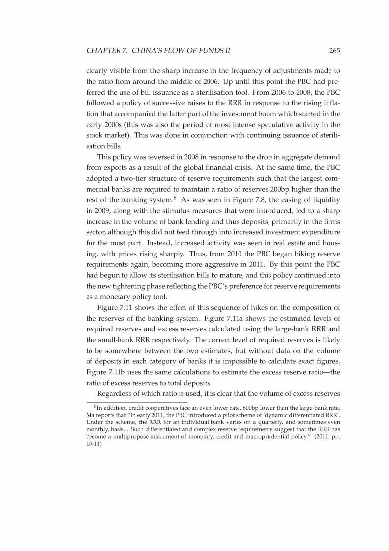
CHAPTER 7. CHINA’S FLOW-OF-FUNDS II 265
clearly visible from the sharp increase in the frequency of adjustments made to
the ratio from around the middle of 2006. Up until this point the PBC had pre-
ferred the use of bill issuance as a sterilisation tool. From 2006 to 2008, the PBC
followed a policy of successive raises to the RRR in response to the rising infla-
tion that accompanied the latter part of the investment boom which started in the
early 2000s (this was also the period of most intense speculative activity in the
stock market). This was done in conjunction with continuing issuance of sterili-
sation bills.
This policy was reversed in 2008 in response to the drop in aggregate demand
from exports as a result of the global financial crisis. At the same time, the PBC
adopted a two-tier structure of reserve requirements such that the largest com-
mercial banks are required to maintain a ratio of reserves 200bp higher than the
rest of the banking system.6 As was seen in Figure 7.8, the easing of liquidity
in 2009, along with the stimulus measures that were introduced, led to a sharp
increase in the volume of bank lending and thus deposits, primarily in the firms
sector, although this did not feed through into increased investment expenditure
for the most part. Instead, increased activity was seen in real estate and hous-
ing, with prices rising sharply. Thus, from 2010 the PBC began hiking reserve
requirements again, becoming more aggressive in 2011. By this point the PBC
had begun to allow its sterilisation bills to mature, and this policy continued into
the new tightening phase reflecting the PBC’s preference for reserve requirements
as a monetary policy tool.
Figure 7.11 shows the effect of this sequence of hikes on the composition of
the reserves of the banking system. Figure 7.11a shows the estimated levels of
required reserves and excess reserves calculated using the large-bank RRR and
the small-bank RRR respectively. The correct level of required reserves is likely
to be somewhere between the two estimates, but without data on the volume
of deposits in each category of banks it is impossible to calculate exact figures.
Figure 7.11b uses the same calculations to estimate the excess reserve ratio—the
ratio of excess reserves to total deposits.
Regardless of which ratio is used, it is clear that the volume of excess reserves
6In addition, credit cooperatives face an even lower rate, 600bp lower than the large-bank rate.Ma reports that “In early 2011, the PBC introduced a pilot scheme of ‘dynamic differentiated RRR’.Under the scheme, the RRR for an individual bank varies on a quarterly, and sometimes evenmonthly, basis... Such differentiated and complex reserve requirements suggest that the RRR hasbecome a multipurpose instrument of monetary, credit and macroprudential policy.” (2011, pp.10-11)
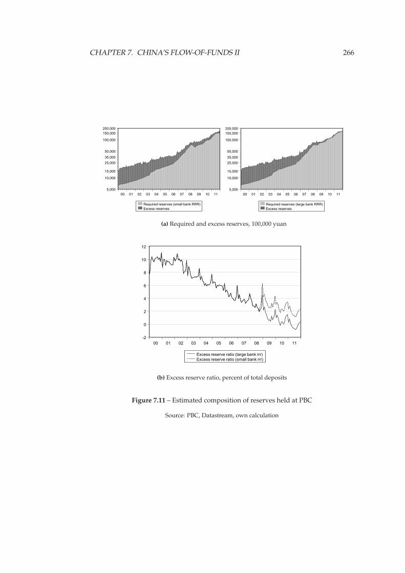
CHAPTER 7. CHINA’S FLOW-OF-FUNDS II 266
200,000
150,000
100,000
50,000
35,000
25,000
15,000
10,000
5,000
00 01 02 03 04 05 06 07 08 09 10 11
Required reserves (small bank RRR)
Excess reserves
200,000
150,000
100,000
50,000
35,000
25,000
15,000
10,000
5,000
00 01 02 03 04 05 06 07 08 09 10 11
Required reserves (large bank RRR)
Excess reserves
(a) Required and excess reserves, 100,000 yuan
-2
0
2
4
6
8
10
12
00 01 02 03 04 05 06 07 08 09 10 11
Excess reserve ratio (large bank rrr)
Excess reserve ratio (small bank rrr)
(b) Excess reserve ratio, percent of total deposits
Figure 7.11 – Estimated composition of reserves held at PBC
Source: PBC, Datastream, own calculation
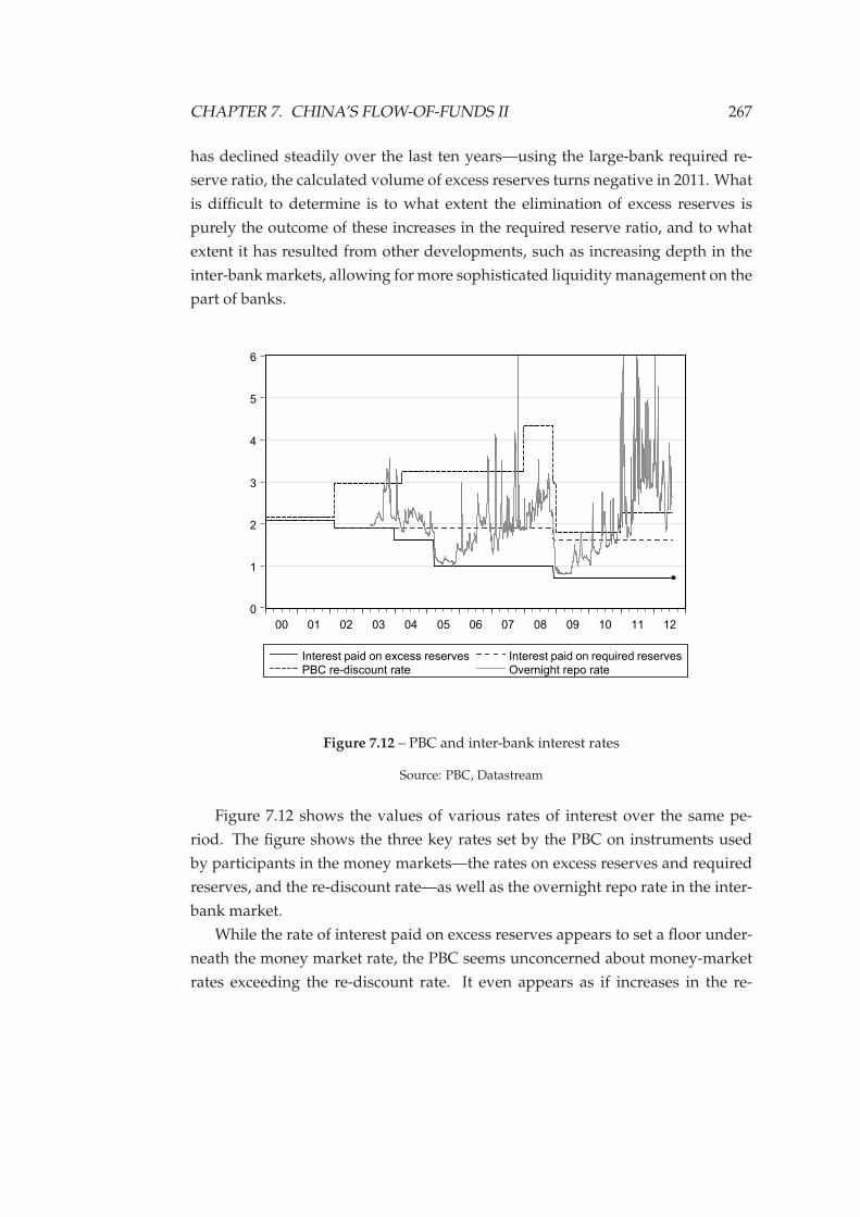
CHAPTER 7. CHINA’S FLOW-OF-FUNDS II 267
has declined steadily over the last ten years—using the large-bank required re-
serve ratio, the calculated volume of excess reserves turns negative in 2011. What
is difficult to determine is to what extent the elimination of excess reserves is
purely the outcome of these increases in the required reserve ratio, and to what
extent it has resulted from other developments, such as increasing depth in the
inter-bank markets, allowing for more sophisticated liquidity management on the
part of banks.
0
1
2
3
4
5
6
00 01 02 03 04 05 06 07 08 09 10 11 12
Interest paid on excess reserves Interest paid on required reserves
PBC re-discount rate Overnight repo rate
Figure 7.12 – PBC and inter-bank interest rates
Source: PBC, Datastream
Figure 7.12 shows the values of various rates of interest over the same pe-
riod. The figure shows the three key rates set by the PBC on instruments used
by participants in the money markets—the rates on excess reserves and required
reserves, and the re-discount rate—as well as the overnight repo rate in the inter-
bank market.
While the rate of interest paid on excess reserves appears to set a floor under-
neath the money market rate, the PBC seems unconcerned about money-market
rates exceeding the re-discount rate. It even appears as if increases in the re-
CHAPTER 7. CHINA’S FLOW-OF-FUNDS II 268
discount rate tend to take place after money-market rates have breached the re-
discount rate.
Figure 7.12 shows that the volatility of short-term interest rates has increased
significantly, with money market rates remaining higher than the ceiling of the
“corridor” for much of 2011. The loosening of policy in 2008 in the aftermath of
the Lehman’s crisis is also clearly visible from the drop in both market rates and
the level of volatility.
It would thus appear that as PBC operations begin to restrain the availability
of reserves, and banks face genuine shortages of liquidity, the same phenomena as
those observed during the monetarist period in the US and UK arise in the form of
rising and volatile short-term interest rates. The behaviour of short-term interest
rates over the last decade or so appear to support the view that the PBC has not
been using targets for base money as a means of controlling wider aggregates—
it is only since 2011 that reserves have been tight enough for short-term rates to
consistently breach the PBC “corridor”.
This also demonstrates an example of what Borio & Disyatat (2009) have re-
ferred to as the “decoupling principle”. This refers to the potential for quantities
of reserves and short-term interest rates to become entirely de-coupled, in con-
tradiction to the standard view that central banks are able to fix either the rate
of interest or the volume of reserves in the system, but not both. It was noted
by Lavoie (2010) that this decoupling occurred in the US in the aftermath of the
sub-prime crisis: as the Fed supplied large volumes of liquidity to the inter-bank
markets, the Federal funds rate could not be kept at the Fed’s target rate, but re-
mained persistently below it. Once the Fed accepted a target rate of “between
zero and a quarter percent”, it was free to adjust the reserves to any level desired
as long as excess reserves remained within the system:
[I]f the central bank is ready to let the overnight rate of interest drop
to zero, or if there is a corridor system, it is possible for central banks
to control the amount of reserves in the system, as long as they are
willing to accept that the target rate of interest be set at the deposit
rate on bank reserves at the central bank. There can thus be a sup-
ply of reserves that far exceeds the amount of required or demanded
reserves. (Lavoie, 2010, p. 20)
The key implication of this is that the central bank is able to influence the rate
of interest in the money markets, without the need to alter the volume of reserves
CHAPTER 7. CHINA’S FLOW-OF-FUNDS II 269
in the system, as long as the system is in a structural liquidity surplus. This can be
seen for example in the case of the reduction of the rate of remuneration on excess
reserves that took place in early 2005. In response, the repo rate immediately
dropped by around 75bp., without any adjustment being made by the PBC to the
liquidity of the inter-bank market.
Sterilisation flows
As discussed in 5.3.1 and the previous section, sterilisation of liquidity resulting
from intervention in the foreign exchange markets has become the dominating
influence on PBC monetary policy.
Standard open-economy macroeconomics in the form of the Mundell-Fleming
model holds that it is impossible under a fixed (or managed) exchange rate regime
to maintain control of domestic monetary policy if capital is able to flow freely.
This view was crystallised in the “macroeconomic trilemma”, in which countries
may only choose two of the following three desirable objectives: a fixed exchange
rate, international capital mobility and control over domestic monetary policy
(Obstfeld et al., 2005).
Given China’s policy of targeting the exchange rate, this view holds that con-
trol over domestic monetary policy will only be possible through the mainte-
nance of capital controls. While China maintains tight controls on outward cap-
ital flows, a sequence of successive liberalisations have gradually reduced the
restrictions on inward capital controls. The conventional logic would therefore
posit that China’s attempts to maintain control of the international valuation of
the yuan will be unsustainable due to the resulting increases in domestic bank
reserves. The inevitable increases in interest rates that would accompany rising
inflation would induce capital inflows, further exacerbating pressure to appreci-
ate the currency.
This view is hard to reconcile with the case of China. The PBC has targeted the
level of the exchange rate over a sustained period, while continuously sterilising
the associated increases in domestic liquidity. At the same time, inflation has
remained fairly steady and pressure on domestic interest rates to rise does not
seem to have materialised.
Further, although there appears to be evidence that the PBC has set interest
rates on a number of occasions with reference to foreign interest rates rather than
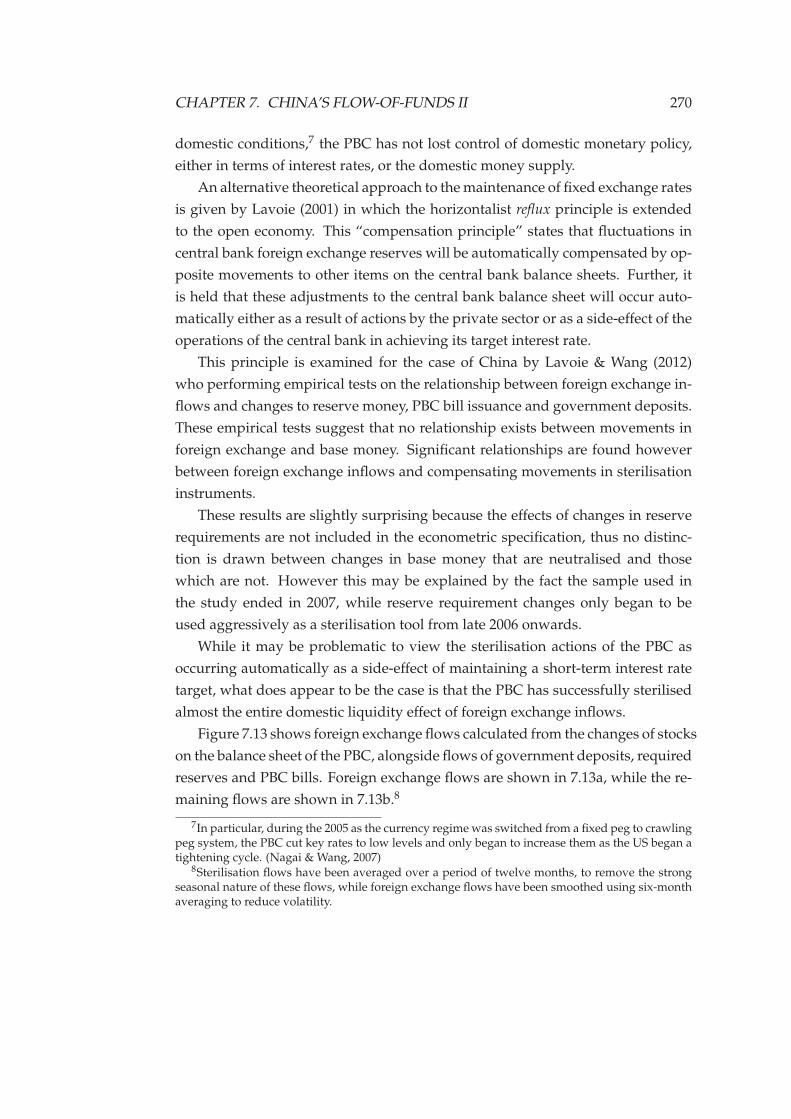
CHAPTER 7. CHINA’S FLOW-OF-FUNDS II 270
domestic conditions,7 the PBC has not lost control of domestic monetary policy,
either in terms of interest rates, or the domestic money supply.
An alternative theoretical approach to the maintenance of fixed exchange rates
is given by Lavoie (2001) in which the horizontalist reflux principle is extended
to the open economy. This “compensation principle” states that fluctuations in
central bank foreign exchange reserves will be automatically compensated by op-
posite movements to other items on the central bank balance sheets. Further, it
is held that these adjustments to the central bank balance sheet will occur auto-
matically either as a result of actions by the private sector or as a side-effect of the
operations of the central bank in achieving its target interest rate.
This principle is examined for the case of China by Lavoie & Wang (2012)
who performing empirical tests on the relationship between foreign exchange in-
flows and changes to reserve money, PBC bill issuance and government deposits.
These empirical tests suggest that no relationship exists between movements in
foreign exchange and base money. Significant relationships are found however
between foreign exchange inflows and compensating movements in sterilisation
instruments.
These results are slightly surprising because the effects of changes in reserve
requirements are not included in the econometric specification, thus no distinc-
tion is drawn between changes in base money that are neutralised and those
which are not. However this may be explained by the fact the sample used in
the study ended in 2007, while reserve requirement changes only began to be
used aggressively as a sterilisation tool from late 2006 onwards.
While it may be problematic to view the sterilisation actions of the PBC as
occurring automatically as a side-effect of maintaining a short-term interest rate
target, what does appear to be the case is that the PBC has successfully sterilised
almost the entire domestic liquidity effect of foreign exchange inflows.
Figure 7.13 shows foreign exchange flows calculated from the changes of stocks
on the balance sheet of the PBC, alongside flows of government deposits, required
reserves and PBC bills. Foreign exchange flows are shown in 7.13a, while the re-
maining flows are shown in 7.13b.8
7In particular, during the 2005 as the currency regime was switched from a fixed peg to crawlingpeg system, the PBC cut key rates to low levels and only began to increase them as the US began atightening cycle. (Nagai & Wang, 2007)
8Sterilisation flows have been averaged over a period of twelve months, to remove the strongseasonal nature of these flows, while foreign exchange flows have been smoothed using six-monthaveraging to reduce volatility.
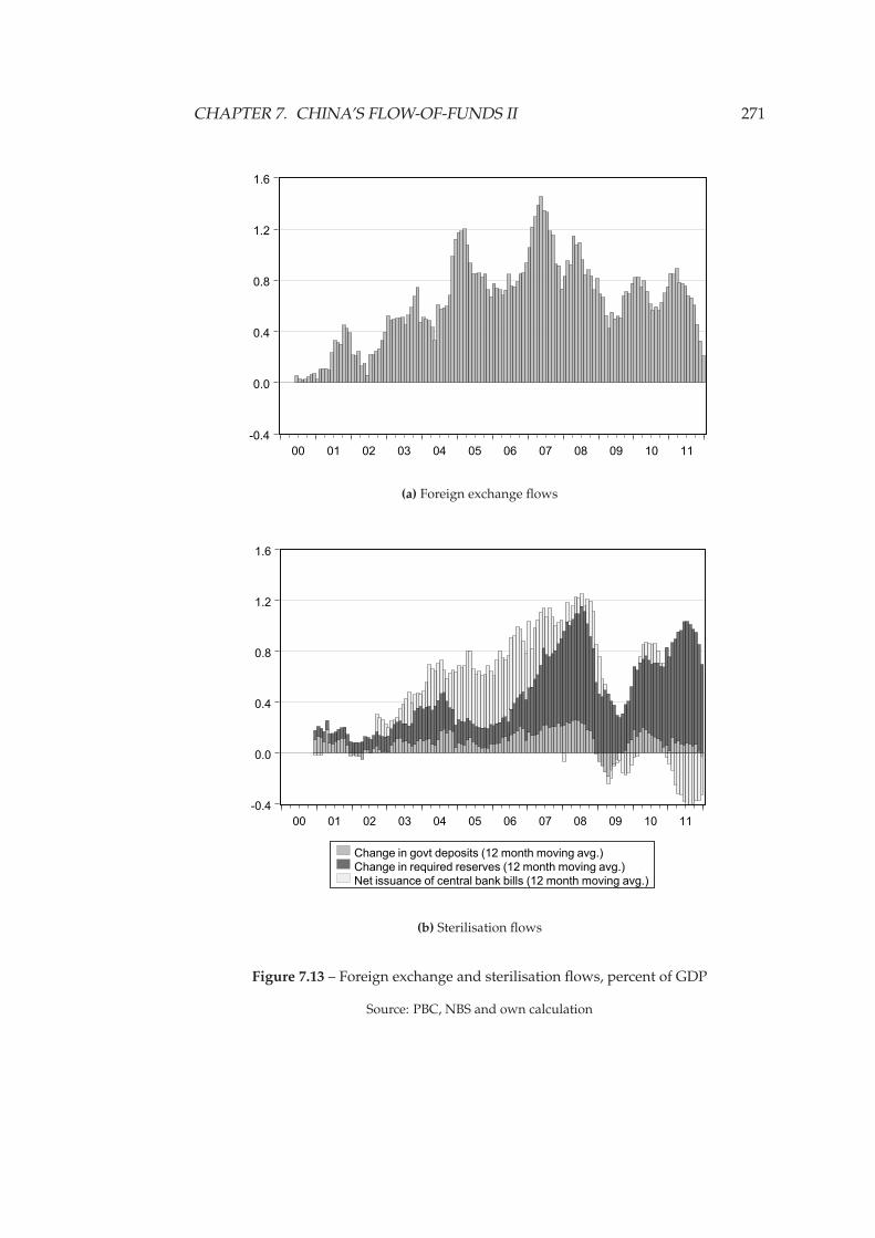
CHAPTER 7. CHINA’S FLOW-OF-FUNDS II 271
-0.4
0.0
0.4
0.8
1.2
1.6
00 01 02 03 04 05 06 07 08 09 10 11
(a) Foreign exchange flows
-0.4
0.0
0.4
0.8
1.2
1.6
00 01 02 03 04 05 06 07 08 09 10 11
Change in govt deposits (12 month moving avg.)
Change in required reserves (12 month moving avg.)
Net issuance of central bank bills (12 month moving avg.)
(b) Sterilisation flows
Figure 7.13 – Foreign exchange and sterilisation flows, percent of GDP
Source: PBC, NBS and own calculation
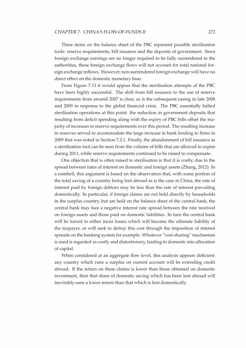
CHAPTER 7. CHINA’S FLOW-OF-FUNDS II 272
Three items on the balance sheet of the PBC represent possible sterilisation
tools: reserve requirements, bill issuance and the deposits of government. Since
foreign exchange earnings are no longer required to be fully surrendered to the
authorities, these foreign exchange flows will not account for total national for-
eign exchange inflows. However, non-surrendered foreign exchange will have no
direct effect on the domestic monetary base.
From Figure 7.13 it would appear that the sterilisation attempts of the PBC
have been highly successful. The shift from bill issuance to the use of reserve
requirements from around 2007 is clear, as is the subsequent easing in late 2008
and 2009 in response to the global financial crisis. The PBC essentially halted
sterilisation operations at this point: the reduction in government deposits that
resulting from deficit spending along with the expiry of PBC bills offset the ma-
jority of increases in reserve requirements over this period. The resulting increase
in reserves served to accommodate the large increase in bank lending to firms in
2009 that was noted in Section 7.2.1. Finally, the abandonment of bill issuance as
a sterilisation tool can be seen from the volume of bills that are allowed to expire
during 2011, while reserve requirements continued to be raised to compensate.
One objection that is often raised to sterilisation is that it is costly, due to the
spread between rates of interest on domestic and foreign assets (Zhang, 2012). In
a nutshell, this argument is based on the observation that, with some portion of
the total saving of a country being lent abroad as is the case in China, the rate of
interest paid by foreign debtors may be less than the rate of interest prevailing
domestically. In particular, if foreign claims are not held directly by households
in the surplus country, but are held on the balance sheet of the central bank, the
central bank may face a negative interest rate spread between the rate received
on foreign assets and those paid on domestic liabilities. In turn the central bank
will be forced to either incur losses which will become the ultimate liability of
the taxpayer, or will seek to defray this cost through the imposition of interest
spreads on the banking system for example. Whatever “cost-sharing” mechanism
is used is regarded as costly and distortionary, leading to domestic mis-allocation
of capital.
When considered at an aggregate flow level, this analysis appears deficient:
any country which runs a surplus on current account will be extending credit
abroad. If the return on these claims is lower than those obtained on domestic
investment, then that share of domestic saving which has been lent abroad will
inevitably earn a lower return than that which is lent domestically.
CHAPTER 7. CHINA’S FLOW-OF-FUNDS II 273
Regardless of the validity of the theoretical arguments, given the relative rates
of return on domestic and foreign assets, It would appear that the interest rate
spread faced by the PBC has been positive for most of the period of sustained
sterilisation operations, as shown in Figure 7.14.
0
1
2
3
4
5
6
2003 2004 2005 2006 2007 2008 2009 2010 2011 2012
US Treasury bill 1 year yield
US Treasury note 10 year yield
PBC bill 3 month yield
PBC bill 1 year yield
Figure 7.14 – Yields on PBC bills and US government securities, percent
Source: Datastream
The figure compares the yields on US Treasury paper at one-year and ten-year
maturity with the yields on PBC bills at three-month and one-month maturities.
Other than during the recent period in which the Fed’s “operation twist” has
reduced long-dated yields to extremely low levels, the return on PBC bills has
been consistently lower than the yield on ten-year US notes, with the exception of
a period in 2008 when the one-year PBC bill rate rose above the ten-year Treasury
rate. For an extended period over 2004–2008, even short-dated US paper was
providing a higher yield than PBC bills of a similar maturity, due to the inversion
of the US yield curve in the run-up to the sub-prime crisis.
From the evidence presented here, there appears no reason to believe that the
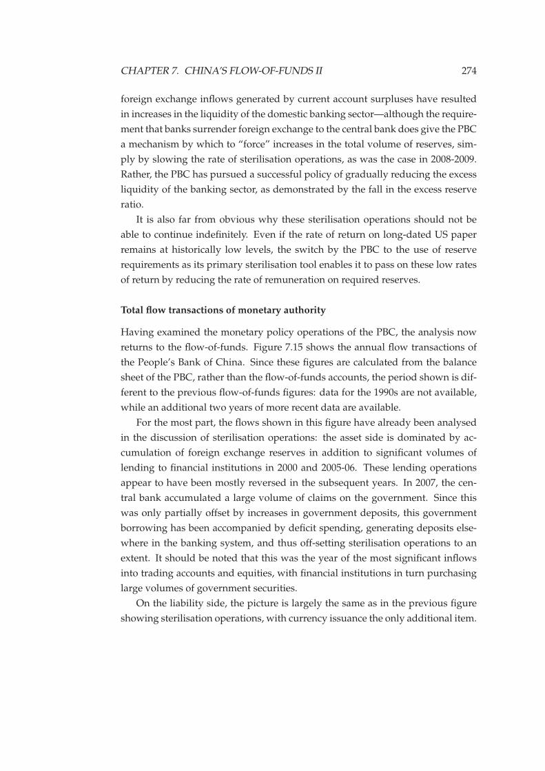
CHAPTER 7. CHINA’S FLOW-OF-FUNDS II 274
foreign exchange inflows generated by current account surpluses have resulted
in increases in the liquidity of the domestic banking sector—although the require-
ment that banks surrender foreign exchange to the central bank does give the PBC
a mechanism by which to “force” increases in the total volume of reserves, sim-
ply by slowing the rate of sterilisation operations, as was the case in 2008-2009.
Rather, the PBC has pursued a successful policy of gradually reducing the excess
liquidity of the banking sector, as demonstrated by the fall in the excess reserve
ratio.
It is also far from obvious why these sterilisation operations should not be
able to continue indefinitely. Even if the rate of return on long-dated US paper
remains at historically low levels, the switch by the PBC to the use of reserve
requirements as its primary sterilisation tool enables it to pass on these low rates
of return by reducing the rate of remuneration on required reserves.
Total flow transactions of monetary authority
Having examined the monetary policy operations of the PBC, the analysis now
returns to the flow-of-funds. Figure 7.15 shows the annual flow transactions of
the People’s Bank of China. Since these figures are calculated from the balance
sheet of the PBC, rather than the flow-of-funds accounts, the period shown is dif-
ferent to the previous flow-of-funds figures: data for the 1990s are not available,
while an additional two years of more recent data are available.
For the most part, the flows shown in this figure have already been analysed
in the discussion of sterilisation operations: the asset side is dominated by ac-
cumulation of foreign exchange reserves in addition to significant volumes of
lending to financial institutions in 2000 and 2005-06. These lending operations
appear to have been mostly reversed in the subsequent years. In 2007, the cen-
tral bank accumulated a large volume of claims on the government. Since this
was only partially offset by increases in government deposits, this government
borrowing has been accompanied by deficit spending, generating deposits else-
where in the banking system, and thus off-setting sterilisation operations to an
extent. It should be noted that this was the year of the most significant inflows
into trading accounts and equities, with financial institutions in turn purchasing
large volumes of government securities.
On the liability side, the picture is largely the same as in the previous figure
showing sterilisation operations, with currency issuance the only additional item.
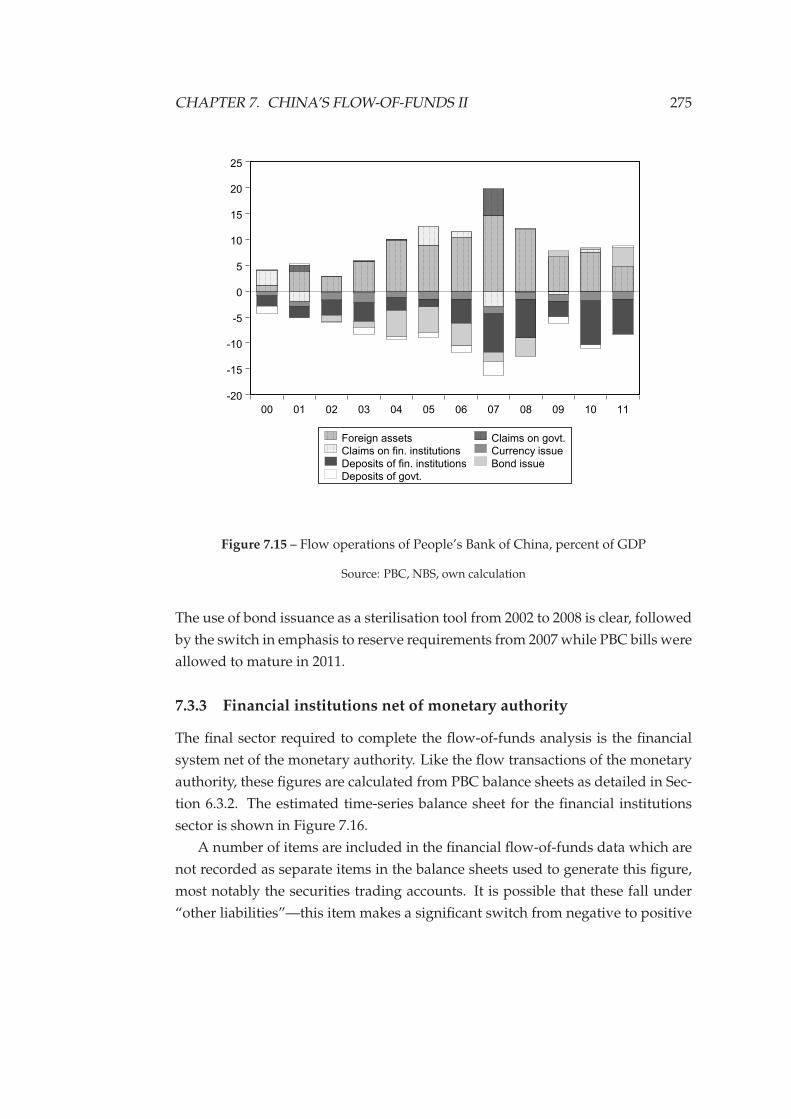
CHAPTER 7. CHINA’S FLOW-OF-FUNDS II 275
-20
-15
-10
-5
0
5
10
15
20
25
00 01 02 03 04 05 06 07 08 09 10 11
Foreign assets Claims on govt.
Claims on fin. institutions Currency issue
Deposits of fin. institutions Bond issue
Deposits of govt.
Figure 7.15 – Flow operations of People’s Bank of China, percent of GDP
Source: PBC, NBS, own calculation
The use of bond issuance as a sterilisation tool from 2002 to 2008 is clear, followed
by the switch in emphasis to reserve requirements from 2007 while PBC bills were
allowed to mature in 2011.
7.3.3 Financial institutions net of monetary authority
The final sector required to complete the flow-of-funds analysis is the financial
system net of the monetary authority. Like the flow transactions of the monetary
authority, these figures are calculated from PBC balance sheets as detailed in Sec-
tion 6.3.2. The estimated time-series balance sheet for the financial institutions
sector is shown in Figure 7.16.
A number of items are included in the financial flow-of-funds data which are
not recorded as separate items in the balance sheets used to generate this figure,
most notably the securities trading accounts. It is possible that these fall under
“other liabilities”—this item makes a significant switch from negative to positive
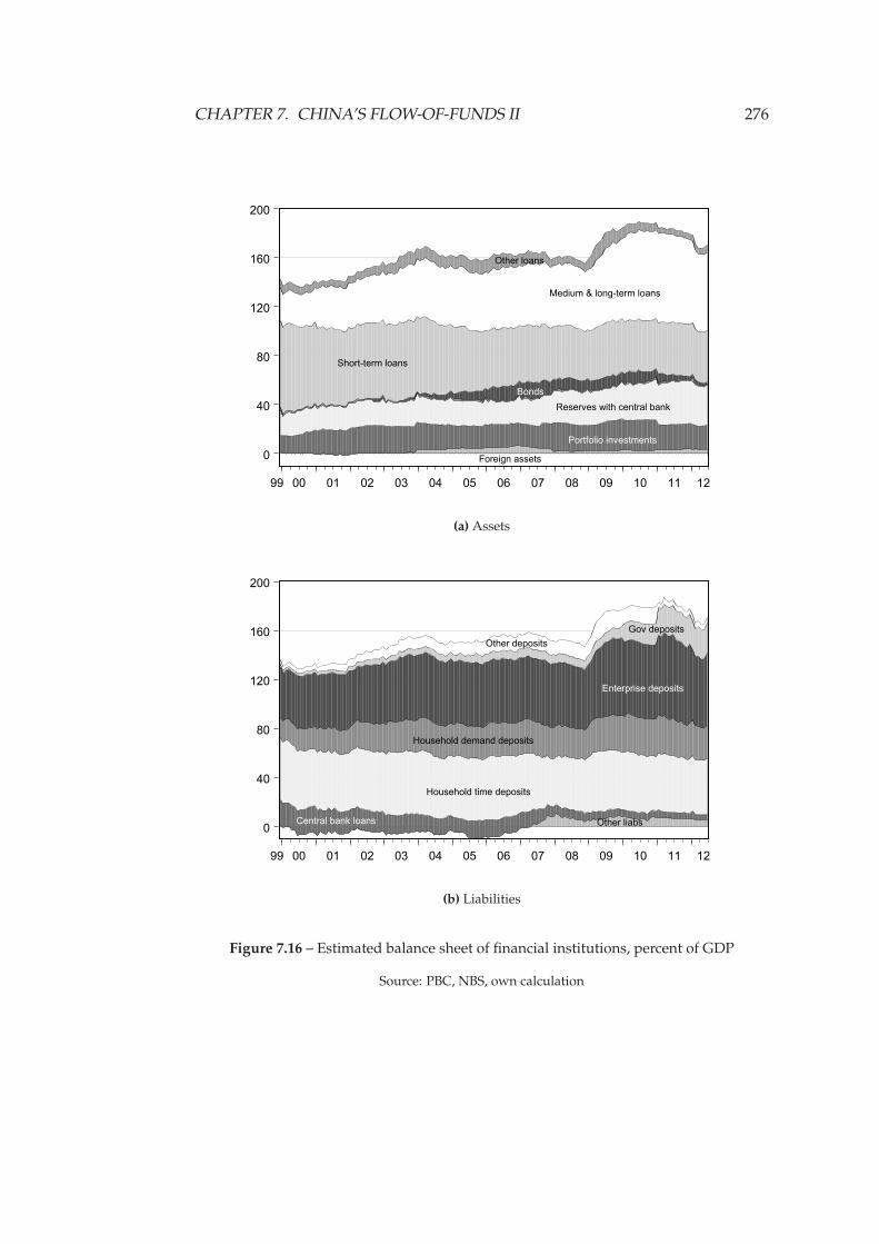
CHAPTER 7. CHINA’S FLOW-OF-FUNDS II 276
0
40
80
120
160
200
99 00 01 02 03 04 05 06 07 08 09 10 11 12
Medium & long-term loans
Short-term loans
Bonds
Reserves with central bank
Portfolio investments
Foreign assets
Other loans
(a) Assets
0
40
80
120
160
200
99 00 01 02 03 04 05 06 07 08 09 10 11 12
Other deposits
Gov deposits
Enterprise deposits
Household demand deposits
Household time deposits
Central bank loans Other liabs
(b) Liabilities
Figure 7.16 – Estimated balance sheet of financial institutions, percent of GDP
Source: PBC, NBS, own calculation
CHAPTER 7. CHINA’S FLOW-OF-FUNDS II 277
in 2006-07, the period in which large volumes of household saving was directed
towards trading accounts.
The remarkable size of the balance sheet of the Chinese banking system rela-
tive to GDP has already been remarked upon—by 2011, the total volume of de-
posits in Chinese banks exceeded those in US banks, at current exchange rates.
What also stands out from this figure is the extent to which the Chinese author-
ities were able engineer a very large expansion of bank lending in 2009. As was
shown in the analysis of the flows of the firm sector, almost all of the deposits
created by this expansion of bank loans remained on the balance sheets of firms.
This is confirmed by the balance sheet of the banking system—the increase in
firm’s deposits closely matches the expansion of medium & long-term loans.
-.4
-.3
-.2
-.1
.0
.1
.2
.3
.4
00 01 02 03 04 05 06 07 08 09 10 11
Foreign Assets Portfolio investments
Deposits with CB Bonds
Loans Loans from CB
Household deposits Enterprise deposits
Government deposits Other deposits
Figure 7.17 – Flow transaction of financial institutions, percent of GDP
Source: PBC, NBS, own calculation
The annual flows derived from this estimated balance sheet are shown in
Figure 7.17. These flows “close” the sectoral level flow-of-funds analysis. The
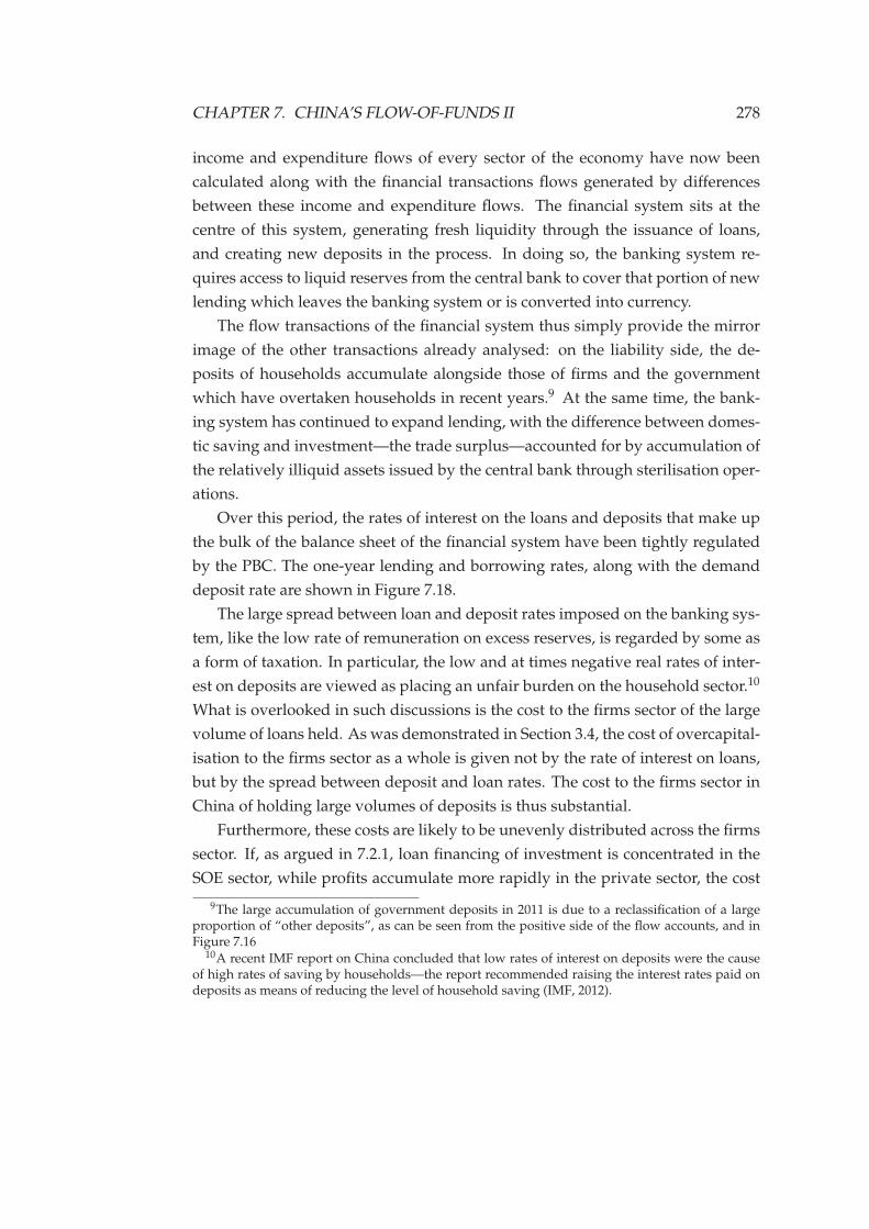
CHAPTER 7. CHINA’S FLOW-OF-FUNDS II 278
income and expenditure flows of every sector of the economy have now been
calculated along with the financial transactions flows generated by differences
between these income and expenditure flows. The financial system sits at the
centre of this system, generating fresh liquidity through the issuance of loans,
and creating new deposits in the process. In doing so, the banking system re-
quires access to liquid reserves from the central bank to cover that portion of new
lending which leaves the banking system or is converted into currency.
The flow transactions of the financial system thus simply provide the mirror
image of the other transactions already analysed: on the liability side, the de-
posits of households accumulate alongside those of firms and the government
which have overtaken households in recent years.9 At the same time, the bank-
ing system has continued to expand lending, with the difference between domes-
tic saving and investment—the trade surplus—accounted for by accumulation of
the relatively illiquid assets issued by the central bank through sterilisation oper-
ations.
Over this period, the rates of interest on the loans and deposits that make up
the bulk of the balance sheet of the financial system have been tightly regulated
by the PBC. The one-year lending and borrowing rates, along with the demand
deposit rate are shown in Figure 7.18.
The large spread between loan and deposit rates imposed on the banking sys-
tem, like the low rate of remuneration on excess reserves, is regarded by some as
a form of taxation. In particular, the low and at times negative real rates of inter-
est on deposits are viewed as placing an unfair burden on the household sector.10
What is overlooked in such discussions is the cost to the firms sector of the large
volume of loans held. As was demonstrated in Section 3.4, the cost of overcapital-
isation to the firms sector as a whole is given not by the rate of interest on loans,
but by the spread between deposit and loan rates. The cost to the firms sector in
China of holding large volumes of deposits is thus substantial.
Furthermore, these costs are likely to be unevenly distributed across the firms
sector. If, as argued in 7.2.1, loan financing of investment is concentrated in the
SOE sector, while profits accumulate more rapidly in the private sector, the cost
9The large accumulation of government deposits in 2011 is due to a reclassification of a largeproportion of “other deposits”, as can be seen from the positive side of the flow accounts, and inFigure 7.16
10A recent IMF report on China concluded that low rates of interest on deposits were the causeof high rates of saving by households—the report recommended raising the interest rates paid ondeposits as means of reducing the level of household saving (IMF, 2012).
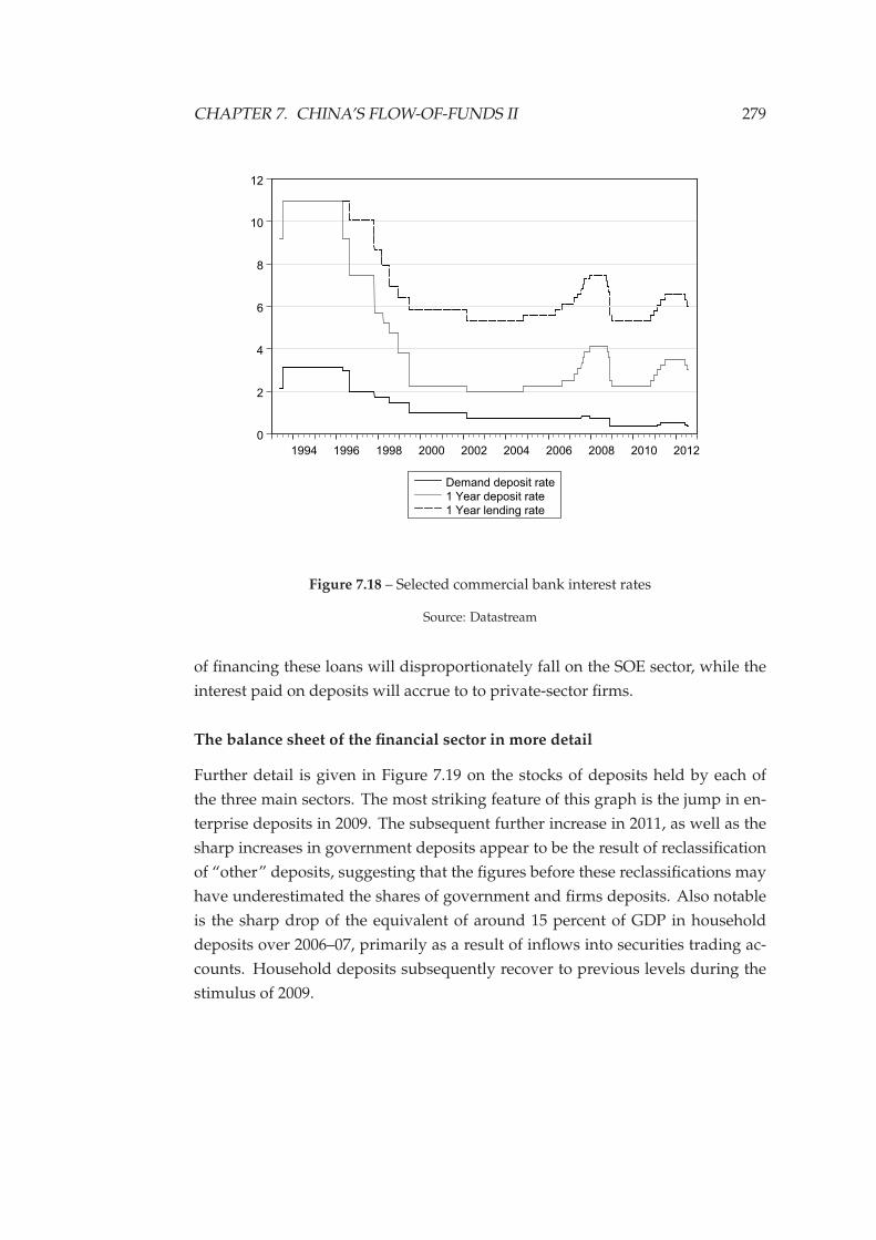
CHAPTER 7. CHINA’S FLOW-OF-FUNDS II 279
0
2
4
6
8
10
12
1994 1996 1998 2000 2002 2004 2006 2008 2010 2012
Demand deposit rate
1 Year deposit rate
1 Year lending rate
Figure 7.18 – Selected commercial bank interest rates
Source: Datastream
of financing these loans will disproportionately fall on the SOE sector, while the
interest paid on deposits will accrue to to private-sector firms.
The balance sheet of the financial sector in more detail
Further detail is given in Figure 7.19 on the stocks of deposits held by each of
the three main sectors. The most striking feature of this graph is the jump in en-
terprise deposits in 2009. The subsequent further increase in 2011, as well as the
sharp increases in government deposits appear to be the result of reclassification
of “other” deposits, suggesting that the figures before these reclassifications may
have underestimated the shares of government and firms deposits. Also notable
is the sharp drop of the equivalent of around 15 percent of GDP in household
deposits over 2006–07, primarily as a result of inflows into securities trading ac-
counts. Household deposits subsequently recover to previous levels during the
stimulus of 2009.

CHAPTER 7. CHINA’S FLOW-OF-FUNDS II 280
0
10
20
30
40
50
60
70
80
90
00 01 02 03 04 05 06 07 08 09 10 11
Government deposits
Enterprise deposits
Households deposits
Figure 7.19 – Holdings of bank deposits by sector, percent of GDP
Source: PBC, NBS, own calculation
A reclassification of the aggregated balance sheet of financial institutions by
the PBC in 2007 provides further detail on the asset side of banks balance sheets,
and in particular on the composition of lending. The interesting feature of this
balance sheet is the separation of loans into those issued to enterprises and those
issued to households.
Figure 7.20 shows a decomposition of this balance sheet. Figure 7.20a com-
bines the re-classified balance sheet figures from 2007 onwards with the previous
less detailed figures from previous years into a single time series. The loans to the
household sector are extracted from this balance sheet and shown in 7.20b. The
rise in household consumption loans from around 2009 is readily apparent. This
increase occurs at the same time as the broader expansion of lending as part of
the stimulus measures.
Since the demand for credit at the household is predominantly for mortgage
lending, the increase in household consumption loans provides further evidence
to support the hypothesis that much of the monetary expansion that took place
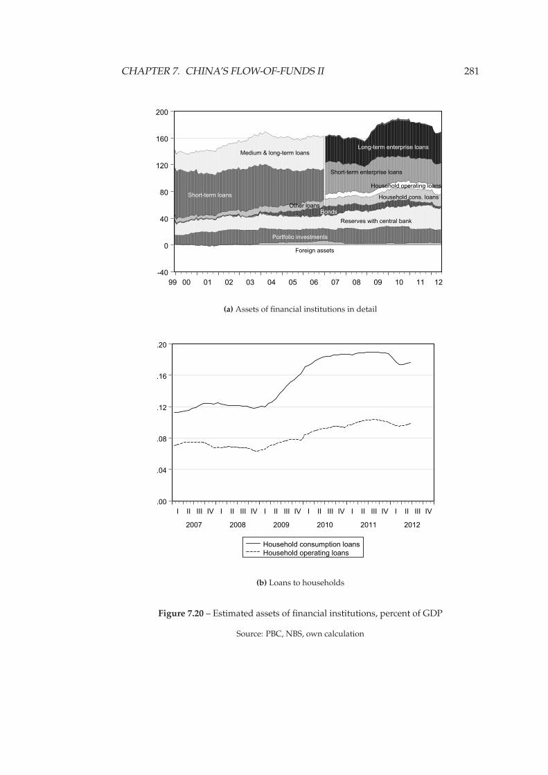
CHAPTER 7. CHINA’S FLOW-OF-FUNDS II 281
-40
0
40
80
120
160
200
99 00 01 02 03 04 05 06 07 08 09 10 11 12
Short-term enterprise loans
Long-term enterprise loans
Household operating loans
Household cons. loans
Bonds
Reserves with central bank
Portfolio investments
Foreign assets
Other loans
Short-term loans
Medium & long-term loans
(a) Assets of financial institutions in detail
.00
.04
.08
.12
.16
.20
I II III IV I II III IV I II III IV I II III IV I II III IV I II III IV
2007 2008 2009 2010 2011 2012
Household consumption loans
Household operating loans
(b) Loans to households
Figure 7.20 – Estimated assets of financial institutions, percent of GDP
Source: PBC, NBS, own calculation
CHAPTER 7. CHINA’S FLOW-OF-FUNDS II 282
in 2009 was directed to speculative activity in housing and real-estate.
7.4 Conclusion
This chapter completed the flow-of-funds analysis of the previous chapter by pro-
viding a detailed examination of the financial side of the accounts. As in the previ-
ous chapter, this analysis was augmented with additional data, while remaining
within the conceptual framework of a stock-flow consistent taxonomy.
The analysis presented evidence of a pattern of monetary and financial flows
that strongly support the hypothesis of an endogenous credit-investment process.
The evidence also demonstrated that the foreign exchange inflows resulting from
the trade surplus have not been the cause of increases in the money supply, as
predicted by the textbook model. Rather, the increases in bank credit and deposits
are the result of investment demand by the firms sector. The rising growth rate of
investment, in combination with a shift in income distribution in favour of profits
has resulted in a rising stock of deposits in the firms sector. Over the same period,
the level of excess reserves in the banking system has steadily decreased due to
the sterilisation operations of the central bank.
The analysis of the previous chapter showed that while China conformed to
the “standard” configuration of investment in the firms sector being financed by
the saving of households, intermediated via the banking system, the relative po-
sitions of the domestic sectors has altered over time.
In particular, despite a very high and rising share of investment spending
in GDP, the deficit run by the firms sector has been falling over the period of
analysis due to rising profits. Firms have thus relied less on bank credit and have
increasingly financed investment out of retained earnings. This reduced reliance
on bank credit for the aggregate firms sector has not however resulted in reduced
demand for bank lending—rather, the result has been an accumulation of bank
deposits held by firms. It is argued that this is the result of a combination of
two factors. The first is the tendency for firms to hold “excess capital”—since the
investment expenditures of firms generate profit income for other firms through
their purchases of capital equipment, an investment boom results in an increasing
volume of bank deposits circulating within the firms sector. Secondly, it is argued
that this process does not result in an even distribution of deposits within the
firms sector. Investment expenditures as a share of revenues are higher in the
SOE sector, while the rate of profit on this investment is lower. Thus, the SOE
CHAPTER 7. CHINA’S FLOW-OF-FUNDS II 283
sector is increasingly accumulating the credit liabilities which are the counterpart
to the rising deposits of the private sector.
This is particularly clear from the liabilities/assets ratios of the different firms
sectors: during the recent period of high investment spending to counteract the
fall in export demand due to the global crisis, the liabilities/assets ratio of the SOE
sector rose significantly while falling in the private and foreign-owned sectors. At
the same time the net financial position of the firms sector as a whole improved
due to a large increase in the holdings of deposits. This resulted from investment
spending by the SOE and government sectors accruing as profits of private firms.
Evidence is also presented of reduced dependence of the firms sector on bank
credit due to funding from FDI and, increasingly, issuance of securities. These
additional sources of financing were almost equal that portion of household sav-
ing not absorbed by the external balance. Thus the household saving “leakage”
from firms profits was entirely absorbed by non-bank credit, resulting in the ob-
servation that changes in firms’ deposits and loans followed an almost identical
trajectory.
This trajectory of growth of loans and deposits in the firms sector was not
matched by changes in the growth of investment, suggesting that deposits are
increasingly held by firms for use in speculative activity such as real-estates pur-
chases, rather than real investment spending. These deposits may also serve as
the basis for the informal credit relationships which are increasingly used as a
source of funding for those small “marginal” firms that cannot gain access to for-
mal bank financing.
The analysis of the operations of central bank demonstrates that the growth
of bank credit and deposits are not the result of loss of control of monetary policy
by the central bank due to the surplus on current account and associated foreign
exchange inflows. Instead, over the period of analysis, central bank operations
have successfully sterilised the increase in reserves resulting from this inflow. At
the same time, the increasing demand for bank credit has reduced the level of ex-
cess reserves within the banking system. The increasing tightness of credit in the
interbank markets is visible in rising interest rates and volatility levels. Thus, the
primary effect of the current account surplus has been through aggregate demand
effects in the real sector, rather than monetary or financial channels.
Finally, evidence is presented of factors that could lead to increasing finan-
cial fragility in the household sector. Despite the rising share of income saved
by households, demand for bank lending by households has risen significantly,

CHAPTER 7. CHINA’S FLOW-OF-FUNDS II 284
particularly consumption loans. The explanation for this probably lies with a
combination of factors: increasing inequality of household income, speculative
activity in asset markets, particularly the stock market and housing, and changes
in techniques in banking leading to increased availability of consumer credit. A
particularly clear-cut example of capital market inflation was shown in the case of
the stock price bubble of 2007, in which household saving was diverted from de-
posits to stock purchases, while firms issuance of securities increased only mod-
erately.
Chapter 8
Conclusion
This thesis presents an original characterisation of the Chinese aggregate demand
and monetary circulation regime using a novel synthesis of Kaleckian-Steindlian
theory and flow-of-funds accounting. An analysis of credit creation, investment
and growth is presented in which firms’ investment expenditures are the key
driver of the dynamic evolution of the system. Steindl’s analysis of the “maldis-
tribution of profits” is updated and re-worked in the context of state control over
the “cartelised” firms’ sector. It is argued that the credit-financed investment ex-
penditures of the state-owned sector have played a decisive role in generating the
aggregate demand which has, in turn, been a key factor in generating and main-
taining the high rate of growth of China. The pattern of investment expenditures,
in concert with the specific institutional configuration of the firms sector, has con-
ditioned the outcomes with respect to profit generation, monetary expansion and
the distribution of liquidity and leverage.
The theoretical analysis is informed and substantiated by a detailed empiri-
cal examination of the processes of money creation, investment and profits over
the last twenty years in China. The empirical approach, also based around an
accounting framework, is closely aligned with the theoretical analysis. The flow-
of-funds national accounting system is used, resulting in an integrated and coher-
ent analytical structure in which all transactions are matched by equivalent and
opposite transactions elsewhere in the system.
As emphasised in the introduction, in choosing to focus on the characteristics
of the demand regime, supply side factors are largely excluded from considera-
tion. In particular, questions surrounding issues such as productivity growth, in-
novation, and technological change and diffusion are left in the background. This
285
CHAPTER 8. CONCLUSION 286
thesis cannot therefore be regarded as presenting full theoretical account of the re-
cent economic development of China, but rather as providing a characterisation
of the specific demand and monetary configuration which has accompanied and
facilitated the Chinese development path. The depiction of a growth path led
by investment spending is compatible with, and complementary to, accounts of
China’s development which emphasise the Kaldorian interaction between aggre-
gate demand and productivity growth, such as that of Lo (2012).
It is argued that the theoretical and empirical system developed here, built on
accounting foundations rather than the optimising behaviour of representative
agents, has a number of significant advantages in the analysis of demand-side
characteristics. Instead of money representing a friction which must be either
justified or abstracted away, the endogenous creation of credit money for the pur-
poses of investment expenditures takes a central role. Credit-financed invest-
ment, rather than arising automatically as result of optimisation over current and
future consumption by a representative household, is determined by the ways in
which different types of firms react to realised profits and excess capacity.
This analysis of credit-financed investment is synthesised with a novel rein-
terpretation of Steindl’s stagnationist account of the inter-war period in the US.
Steindl’s results derived from the assumption that, with increasing monopolisa-
tion, the elasticity of the price mark-up of firms falls, leading to excess capacity.
In turn, this excess capacity discourages investment leading to reduced aggregate
demand and growth.
The account presented in this thesis takes Steindl’s theory of stagnation as a
starting point but alters the assumptions made about the determinants of invest-
ment. The analysis is founded on the premise that investment by the state-owned
sector cannot be specified on the same behavioural basis as that of private firms
operating either in competitive or oligopolistic markets. If the investment and
pricing decisions of firms in the state-owned sector are based instead on targets
for output and employment, the resulting outcomes in terms of output growth,
excess capacity, the distribution of profits, and the gearing ratios of firms of dif-
ferent ownership type will be significantly altered.
Early attempts at formulating non-marginalist theories of growth and dis-
tribution regarded investment as exogenously determined and accommodated
by changes in the real wage at constant rates of employment. At first glance,
the empirical evidence on China appears to fit reasonably well with these Cam-
bridge growth models—an increasing share of profits in national income has
CHAPTER 8. CONCLUSION 287
accompanied a rising share of investment in output. However, by modifying
the assumptions of the Kaleckian-Steindlian system as described above, an “in-
verse Steindlian” growth process can be conceptualised, which characterises the
stylised facts of the Chinese growth experience in a more sophisticated way.
In such a system, if the state-owned sector maintains a pricing policy such
that profit margins are kept close to, or slightly below, margins in the private sec-
tor, the distribution of “internal accumulation” between the two sectors should
likewise be evenly distributed. With an increase in the pricing power of the pri-
vate sector, profit margins will rise. In such a case, the potential slowdown in
accumulation resulting from reduced aggregate demand could be offset by addi-
tional credit-financed investment by the state-owned sector. However, additional
investment expenditure by the state-owned sector would result in a dispropor-
tionate increase in the accumulation of profits in the private sector, leading to a
rise in the gearing ratio of the state-owned sector relative to the private sector.
In generating retained profits for the private sector, this mechanism would
thus serve as a substitute for borrowing by these firms. This is significant because
it is regularly reported that non-state firms face significant difficulties in obtaining
credit through the official state-owned banking system. In the case that credit-
financed investment by the state-owned sector were to accrue disproportionately
as retained earnings to private sector firms, these firms would be able to increase
investment expenditures, without accumulating the associated liabilities in the
form of additional bank loans which would instead fall on the balance sheets of
state-owned firms. Thus, the Kalecki-Steindl profit-reflux mechanism serves as a
way of overcoming the problems of access to bank finance by small businesses.
Another important strand of the argument presented in this thesis addresses
the commonly held misconception that the saving behaviour of Chinese house-
holds lies behind the growth boom of the past decades and, as a corollary, that
the saving of these households is therefore related to the global imbalances in
the period before the global financial crisis. If the central hypothesis of this the-
sis is correct—that it is loan-financed investment expenditure that is driving the
growth of China—then the interpretation that seeks to draws a correspondence
between saving behaviour at the household level, and saving at the national level
is faulty. Nonetheless, this is the view that is drawn naturally from an analysis
based on the theories of money and growth that are discussed in Chapter 2.
In the interpretation put forward in this thesis, the rising share of income
saved by Chinese households serves to dampen aggregate demand, necessitat-
CHAPTER 8. CONCLUSION 288
ing ever greater expenditure on investment in order to maintain the growth of
aggregate demand, which in turn leads to greater absolute levels of saving. At
the same time, the financial behaviour of households is changing. The falling
level of government transfer payments as a share of national income reflects a
growing dependence on non-state forms of saving for retirement and insurance.
Households have increasingly begun to operate in financial markets, both indi-
rectly through insurance and pension providers, and directly—as exemplified by
the stock market bubble of 2007. At the same time, household borrowing from the
banking system has gone from virtually non-existent to representing a significant
share of total household financial activity over a short period. Without further
research, it is impossible to know for certain what lies behind this development,
but it seems reasonable to posit some combination of inequality of wealth and in-
come, rising property prices, speculative behaviour in asset markets, and changes
to the way that commercial banks operate.
These phenomena pose challenges for the implementation of monetary policy.
This thesis has demonstrated that the view that China has operated a system
of base money targeting, in line with monetarist doctrines, is misleading. The
banking system has maintained a position of excess liquidity for the whole of the
period of analysis. Instead of attempting to restrict supplies of bank reserves, the
authorities have tended to use direct intervention at the level of both banks and
state-owned firms as a way of keeping credit growth in check.
A number of developments will make the task of the central bank more com-
plex in this regard. Firstly, the dynamic process by which credit-financed invest-
ment leads to rising holdings of bank deposits in the private firms sector will
serve to reduce the influence of the central bank—regardless of whether this in-
fluence is exerted through the setting of interest rates or through more direct
controls. Secondly, as emphasised in Chapter 5, rather than a smooth path of
convergence on the perfect financial markets of the New Keynesian system, fi-
nancial development is a process which takes place through historical time. The
resulting financial structures that arise out of this process are conditioned by the
economic and political environment in which they are embedded. In this respect
China may be viewed as having drawn benefits from maintaining significant con-
trol over the banking system during the transition from a mono-bank system to a
modern commercial banking system. Although widely regarded as a source of in-
efficiency and distortion, the banking system has provided a key lever of control
for the Chinese authorities.
CHAPTER 8. CONCLUSION 289
However, as demonstrated by the increasing prevalence of informal credit
relationships in China—from kerb-side lending organisations to the proliferation
of off-balance-sheet structures created by the large banks—financial development
represents a deeply endogenenous process, driven by privately generated credit
relationships. It is evident that with each additional round of bank-financed
investment expenditure, the control of the authorities over credit aggregates is
weakened. The prevention of destabilising speculative behaviour will become
ever more difficult.
The Chinese authorities thus face significant obstacles in maintaining growth
at such high levels. A slowdown has so far been avoided through a combina-
tion of factors. The inelasticity of investment demand to excess capacity has so
far served to maintain aggregate demand and offset rising saving, and has stim-
ulated ongoing increases in productivity. The rapid adoption and diffusion of
new technology, much of which has been imported from abroad via the Chinese
external sector, has ensured that the goods produced as a result of this invest-
ment have continued to find a market. Recent external surpluses have provided
a further addition to aggregate demand.
However, the international cost structures which have led to the current ac-
count surpluses will not last indefinitely. Without a shift back towards a more
egalitarian distribution of income, the diminishing share of consumption demand
in national income will increasingly drag on demand. With financial liberalisa-
tion and innovation, the potential gains from speculative financial operations will
increasingly appeal to firms in possession of high levels of liquidity. Thus, the
maintenance of aggregate demand and growth though continued real investment
expenditures and export demand is likely to become increasingly precarious.
In Steindl’s view, the pre-war stagnation of the US economy was explained
in the following terms: “the economy is unable to adjust to low growth rates be-
cause its saving propensity is adapted to a high one.” (1979, p. 1) The rising share
of income saved by all sectors in the Chinese economy implies that the saving
propensity of the economy as a whole is undoubtedly adapted to a very high rate
of growth. With the inevitable transition to lower rates of growth that will accom-
pany the maturing of the Chinese economy, the question that remains is whether
this transition can be achieved without significant dislocation. With the shift from
planning to a market based system, the Chinese economy will inevitably have to
face the fundamental contradiction that lies at the heart of any investment-driven
growth regime:
CHAPTER 8. CONCLUSION 290
Investment considered as expenditure is the source of prosperity, and
every increase of it improves business and stimulates a further rise
in investment. But at the same time every investment is an addition
to capital equipment, and right from birth it competes with the older
generation of this equipment. The tragedy of investment is that it
causes crisis because it is useful. Doubtless many people will consider
this theory paradoxical. But it is not the theory which is paradoxical,
but its subject—the capitalist economy. (Kalecki, [1939] 1990, p. 318)
While the Chinese economy may not yet be characterised as capitalist, this
does not diminish the significance of Kalecki’s point. Investment results in addi-
tional productive capacity—as long as this capacity remains substantially under-
utilised, whether due to insufficient spending power, or to an inelastic propensity
to save, the potential for crisis rises with each additional increase in investment.
Whether the Chinese economy will be able to successfully navigate these poten-
tial dangers remains to be seen.
Bibliography
Aghion, P., & Howitt, P. (1992). A model of growth through creative destruction.
Econometrica, (pp. 323–51).
Baharumshah, A. Z., Mohd, S. H., & Masih, A. M. (2009). The stability of money
demand in China: Evidence from the ARDL model. Economic Systems, 33, 231–
244.
Bahmani-Oskooee, M., & Wang, Y. (2007). How stable is the demand for money
in China? Journal of Economic Development, 32, 21–33.
Bai, C.-E., Hsieh, C.-T., & Qian, Y. (2006). The return to cap-
ital in China. NBER working paper 12755, available online at:
http://www.nber.org/papers/w12755.
Bank of England (2005). The Bank of England Quarterly Model. London: The Bank
of England.
Baran, P. A., & Sweezy, P. M. (1966). Monopoly Capital. New York: Monthly Review
Press.
Basu, P., & McLeod, D. (1992). Terms of trade fluctuations and economic growth
in devloping economies. Journal of Development Economics, 37, 89–110.
Berger, A. N., Hasan, I., & Zhou, M. (2009). Bank ownership and efficiency in
China: What will happen in the world s largest nation? Journal of Banking and
Finance, 33, 113–130.
Bernanke, B. (2005). The global saving glut and the US current account deficit.
Speech made at the Sandridge Lecture, Virginia Association of Economics.
291
BIBLIOGRAPHY 292
Bernanke, B., Gertler, M., & Gilchrist, S. (1999). The financial accelerator in a quan-
titative business cycle framework. In J. Taylor, & M. Woodford (Eds.) Handbook
of Macroeconomics, vol. 1C, chap. 21. North-Holland.
Bernanke, B. S., & Gertler, M. (1995). Inside the black box: The credit channel of
monetary policy transmission. Journal of Economic Perspectives, 9(4), 27–48.
Bhaduri, A., & Marglin, S. (1990). Unemployment and the real wage: the eco-
nomic basis for contesting political ideologies. Cambridge Journal of Economics,
14, 375–393.
Bindseil, U. (2004). Monetary Policy Implementation: Theory, Past, and Present. Ox-
ford University Press, USA.
Black, F. (1970). Banking and interest in a world without money: The effects of
uncontrolled banking. Journal of Bank Research, 1, 9–20.
Blanchard, O., & Galı, J. (2005). Real wage rigidities and the New Keynesian
model. Massachusetts Institute of Technology Department of Economics Working
Paper Series, (05-28).
Boianovsky, M., & Trautwein, H.-M. (2006). Wicksell after Woodford. Journal of
the History of Economic Thought, 28(2), 171–185.
Borio, C., & Disyatat, P. (2009). Unconventional monetary policies: an appraisal.
Bank for International Settlements, BIS Working Paper no. 292.
Calvo, G. (1983). Staggered prices in a utility-maximising framework. Journal of
Monetary Economics, 12, 383–398.
Cassola, N., & Porter, N. (2011). Understanding Chinese bond yields and their
role in monetary policy. IMF Working Paper WP/11/225.
Che, J., & Qian, Y. (1988). Insecure property rights and government ownership of
firms. Quarterly Journal of Economics, 113(2), 467–496.
Chick, V. (1986). The evolution of the banking system and the theory of saving,
investment and interest. Economies et societies, 3(8-9), 111–126.
Chick, V. (1992). Financial counterparts of saving and investment and inconsis-
tency in a simple macro model. In P. Arestis, & S. Dow (Eds.) OnMoney, Method
and Keynes, (pp. 81–94). New York: St. Martins Press.
BIBLIOGRAPHY 293
Chick, V., & Dow, S. (2002). Monetary policy with endogenous money and liq-
uidity preference: A nondualistic treatment. Journal of Post Keynesian Economics,
24(4), 587–607.
China Daily (2010). State banks raise provision ratio above 2.5%. 20 September.
Chu, C., Wen, C., & He, H. (2010). Chinese banks: informal securitization increas-
ingly distorting credit data. Fitch Ratings Special Report.
Clarida, R., Galı, J., & Gertler, M. (1999). The science of monetary policy: a New
Keynesian perspective. Journal of Economic Literature, 37(4), 1661–1707.
Colander, D., Howitt, P., Kirman, A., Leijonhufvud, A., & Mehrling, P. (2008). Be-
yond DSGE models: towards an empirically based macroeconomics. American
Economic Review, 98(2), 236–40.
Copeland, M. A. (1947). Tracing moneyflows through the United States economy.
American Economic Review, 38(2), 31–49.
Copeland, M. A. (1949). Social accounting for moneyflows. The Accounting Review,
24, 254–64.
Copeland, M. A. (1952). A Study Of Moneyflows In The United States. New York:
NBER.
Costa, C., & DeGrauwe, P. (2001). Monetary policy in a cashless society. CEPR
Discussion Paper No. 2696.
Cripps, F., & Godley, W. (1976). A formal analysis of the Cambridge Economic
Policy Group model. Economica, 43(172), 335–348.
Davidson, P. (1968). The demand and supply of securities and economic growth
and its implications for the Kaldor-Pasinetti versus Samuelson-Modigliani con-
troversy. American Economic Review, (pp. 252–69).
Davidson, P. (1972). Money and The Real World. New York: John Wiley & Sons.
Davidson, P. (1986). Finance, funding, saving and investment. Journal of Post
Keynesian Economics, 9(1), 101–110.
Del Monte, A. (1975). Grado di monopolio e sviluppo economico. Rivista Inter-
nazionale di Scienze Sociali, 83(3), 231–363.
BIBLIOGRAPHY 294
Deloitte (2012). China banking industry: Top ten trends and outlook.
Diamond, D. W. (1984). Financial intermediation and delegated monitoring. Re-
view of Economic Studies, 51(3), 393–414.
Diamond, D. W., & Dybvig, P. H. (1983). Bank runs, deposit insurance and liq-
uidity. Journal of Political Economy, 91(3), 410–419.
Dixit, A., & Stiglitz, J. (1977). Monopolistic competition and optimum product
diversity. American Economic Review, 67(3), 297–308.
dos Santos, C. H. (2005). A stock-flow consistent general framework for formal
Minskyan analyses of closed economies. Journal of Post Keynesian Economics,
27(4), 711–735.
dos Santos, C. H. (2010). Revisiting ‘New Cambridge’: The three financial bal-
ances in a general stock-flow consistent applied modeling strategy. Levy Eco-
nomics Institute Working Paper No. 594.
Dow, S. (2006). Endogenous money: structuralist. In P. Arestis, & M. Sawyer
(Eds.) A Handbook of Alternative Monetary Economics, chap. 3, (pp. 35–51). Ed-
ward Elgar.
Dow, S., Ghosh, D., & Ruziev, K. (2008). A stages approach to banking develop-
ment in transition economies. Journal of Post Keynesian economics, 31(1).
Dumenil, G., & Levy, D. (1999). Being Keynesian in the short term and Classical in
the long term: the traverse to Classical long-term equilibrium. The Manchester
School, 67(6), 684–716.
Duo, X. (2002). Analysis of the development of China’s money market. China &
World Economy, (1), 29–37.
Dutt, A. K. (1984). Stagnation, income distribution and monopoly power. Cam-
bridge Journal of Economics, 8(1), 25–40.
Dutt, A. K. (1990). Growth, Distribution and Uneven Development. Cambridge UK:
Cambridge University Press.
Farrell, D., Lund, S., Rosenfeld, J., Morin, F., Gupta, N., & Greenberg, E. (2006).
Putting China’s capital to work: the value of financial system reform. McKinsey
Global Institute Report.
BIBLIOGRAPHY 295
Feyzioglu, T., Porter, N., & Takats, E. (2009). Interest rate liberalisation in China.
IMF Working Paper WP/09/171.
Fine, B. (2000). Endogenous growth theory: A critical assessment. Cambridge
Journal of Economics, 24(2).
Fine, B. (2003). Capital theory. In J. King (Ed.) The Elgar Companion to Post Keyne-
sian Economics, (pp. 51–57). Cheltenham: Edward Elgar.
Friedman, M. (1956). The quantity theory of money—a restatement. In M. Fried-
man (Ed.) Studies in the Quantity Theory of Money. Chicago: University of
Chicago Press.
Gale, D., & Hellwig, M. (1985). Incentive-compatible debt contracts: The one-
period problem. The Review of Economic Strudies, 52(4), 647–663.
Galı, J. (2008). Monetary Policy, Inflation, and the Business Cycle An Introduction to
the New Keynesian Framework. Princeton University Press.
Galı, J., & Gertler, M. (2007). Macroeconomic Modelling for Monetary Policy
Evaluation. Journal of Economic Perspectives, 21(4), 25–45.
Geiger, M. (2008). Instruments of monetary policy in China and their effective-
ness: 1994-2006. UNCTAD Discussion Papers No. 187.
Geng, N., & N’Diaye, P. (2012). Determinants of corporate in-
vestment in China: evidence from cross-country firm level
data. IMF Working Paper WP/12/80, available online at
http://www.imf.org/external/pubs/ft/wp/2012/wp1280.pdf.
Girardin, E. (1997). Banking sector reform and credit control in China. Paris : Develop-
ment Centre of the Organisation for Economic Co-operation and Development.
Godley, W., & Cripps, F. (1983). Macroeconomics. Fontana.
Godley, W., & Lavoie, M. (2005–06). Comprehensive accounting in simple open
economy macroeconomics with endogenous sterilisation or flexible exchange
rates. Journal of Post Keynesian Economics, 28(2), 241–276.
Godley, W., & Lavoie, M. (2007). Monetary Economics: An Integrated Approach to
Credit, Money, Income, Production and Wealth. Palgrave Macmillan.
BIBLIOGRAPHY 296
Goodfriend, M. (2007). How the world achieved consensus on monetary policy.
Journal of Economic Perspectives, 21(4), 47–68.
Goodfriend, M., & King, R. G. (1997). The new neoclassical synthesis and the role
of monetary policy. In NBER Macroeconomics Annual, (pp. 231–82). Cambridge
MA: MIT Press.
Goodfriend, M., & Prasad, E. S. (2006). A framework for independent monetary
policy in China. BIS Working Paper WP/06/111.
Goodhart, C. (1989). The conduct of monetary policy. The Economic Journal,
99(396), 293–346.
Goodhart, C. (2002). The endogenity of money. In V. Chick, P. Arestis, M. De-
sai, & S. Dow (Eds.) Money, Macroeconomics and Keynes, chap. 3, (pp. 14–24).
Routledge.
Green, C. J., & Murinde, V. (2000). Flow of funds: Implications for research on
financial sector development and the real economy. Economic Research Paper
No 00/6, Loughborough University.
Green, S. (2005). Making monetary policy work in China: a report from the money
market front line. Stanford Center for International Development Working Pa-
per Series.
Grossman, G., & Helpman, E. (1991). Innovation and Growth in the Global Economy.
Cambridge: MIT Press.
Guo, Y. (2002). Banking reforms and monetary policy in in PR China: is the Chinese
central banking system ready for joining the WTO?. Palgrave Macmillan.
Gurley, J., & Shaw, E. (1960). Money in a Theory of Finance. Brookings Institute.
Han, B. (2006). China’s state-owned commercial banks : Reform and foreign cap-
ital participation. The journal of the study of modern society and culture, 37.
Harcourt, G. (1972). Some Cambridge Controversies in the Theory of Capital. Cam-
bridge Univesity Press.
Harcourt, G. C. (1991). Review of Collected Works of Michał Kalecki, Volume
I: Capitalism: Business Cycles and Full Employment by Jerzy Osiatynski. The
Economic Journal, 101(409), 1608–1610.
BIBLIOGRAPHY 297
Harcourt, G. C., & Cohen, A. J. (2003). Whatever happened to the Cambridge
capital theory controversies? Journal of Economic Perspectives, 17(1), 199–214.
Harrod, R. F. (1939). An essay in dynamic theory. The Economic Journal, 49(193),
14–33.
Hayek, F. A. (1933). Monetary Theory and the Trade Cycle. The Mises Institute. Alt:
(London: Jonathan Cape); originally published in German in 1929 as Geldtheorie
und Konjunkturtheorie, (Wien: Verlag von Julius Springer) (Steele 2007).
Hayek, F. A. (1935). Prices and Production. Augustus M. Kelly. Alt: (London:
Routledge and Paul Kegan); first edition, 1931, (London: George Routledge
and Sons); originally published in German in 1929 as Presie und Produktione
(Wien-Leipzig: Holder-Pichler-Tempsky A.G.) Steele (2007).
von Hayek, F. A. (1942). The Ricardo Effect. Economica, 9(34), 127–152.
Hein, E. (2008). ‘Financialisation’ in a comparative static, stock-flow consistent
Post-Kaleckian distribution and growth model. IMK Working Paper.
Hein, E., Lavoie, M., & van Treeck, T. (2010). Some instability puzzles in Kaleck-
ian models of growth and distribution: a critical survey. Cambridge Journal of
Economics, 35(3), 587–612.
Herr, H. (2010). Credit expansion and development—A Schumpeterian and Key-
nesian view of the Chinese miracle. Intervention, 7(1), 71–89.
Hofman, B., & Kuijs, L. (2006). A note on saving, investment, and profits of
China’s enterprises. Available on World Bank website.
URL http://go.worldbank.org/3EQL46KTS0
Holz, C. (1992). The Role of Central Banking in China’s Economic Reforms. Cornell
University.
Holz, C. A. (2006). New capital estimates for China. China Economic Review, 17,
142–185.
Huang, H., & Zhu, N. (2007). The Chinese bond market: historical lessons,
present challenges and future perspectives. SSRN eLibrary Working Paper Se-
ries.
BIBLIOGRAPHY 298
Huang, Y. (2008). Capitalism with Chinese Characteristics. Cambridge University
Press.
IMF (2012). China Economic Outlook. Available at
http://www.imf.org/external/country/CHN/rr/2012/020612.pdf.
Ju, X., & Lo, D. (2012). The cost and benefit of banking regulations and controls,
Chinese style. PSL Quarterly Review, 65(263), 385–402.
Kaldor, N. (1955). Alternative theories of distribution. The Review of Economic
Studies, 23(2), 83–100.
Kaldor, N. (1966). Marginal productivity and the macro-economic theories of
growth and distribution. Review of Economic Studies, 33, 309–319.
Kalecki, M. ([1933] 1990). Essay in the business cycle theory. In J. Osiatynski (Ed.)
Collected Works of MichałKalecki, vol. I, (pp. 67–108). Oxford: Oxford University
Press.
Kalecki, M. (1937). The principle of increasing risk. Economica, 4(16), 440–447.
Kalecki, M. (1938). The determinants of distribution of the national income.
Econometrica, 6(2), 97–112.
Kalecki, M. ([1939] 1990). Essays in the theory of economic fluctuations. In J. Os-
iatynski (Ed.) Collected Works of Michał Kalecki, vol. I, (pp. 231–317). Oxford:
Oxford University Press.
Kalecki, M. (1944). Professor Pigou on the stationary state: a comment. Economic
Journal, 54(213), 131–2.
Kalecki, M. ([1954] 1965). Theory of Economic Dynamics: An Essay on Cyclical and
Long-Run Changes in Capitalist Economy. London: George Allen and Unwin,
revised 2nd ed.
Kalecki, M. ([1954] 1990). Theory of economic dynamics: An essay on cyclical and
long-run changes in capitalist economy. In J. Osiatynski (Ed.) Collected Works of
Michał Kalecki, vol. II. Oxford: Oxford University Press.
Kalecki, M. (1971). Selected Essays on the Dynamics of the Capitalist Economy. Cam-
bridge University Press.
BIBLIOGRAPHY 299
Kenny, C., & Williams, D. (2001). What do we know about economic growth? Or,
why don’t we know very much? World Development, 29(1), 1–22.
Keynes, J. M. ([1930] 1971). A Treatise onMoney: The Pure Theory of Money. Macmil-
lan Cambridge University Press.
Keynes, J. M. (1936). The General Theory of Money, Interest and Employment. Royal
Economic Society.
Keynes, J. M. (1937a). Alternative theories of the rate of interest. Economic Journal,
47, 242–52.
Keynes, J. M. (1937b). The “ex-ante” theory of the rate of interest. Economic Jour-
nal, 47, 663–69.
Kornai, J. (1979). Resource-constrained versus demand-constrained systems.
Econometrica, 47(4), 801–19.
KPMG (2012). China financial regulation alert – banking.
Kregel, J. (1985). Cambridge macroeconomics without money: Hamlet without
the prince. American Economic Review, 75(2), 133–139. Papers and Proceedings
of the Ninety-Seventh Annual Meeting of the American Economic Association.
Kregel, J. (1989-1990). Operational and financial leverage, the firm, and the cy-
cle: reflections on vickers’ money capital constraint. Journal of Post-Keynesian
Economics, 12(2), 224–236.
Kuijs, L. (2005). Investment and saving in China. World Bank China Office Re-
search Working Paper No.1.
Kuijs, L. (2006). How will China’s saving-investment balance evolve? World
Bank Policy Research Working Paper 3958.
Kydland, F. E., & Prescott, E. C. (1982). Time to build and aggregate fluctuations.
Econometrica, 50(6), 1345–1370.
Laidler, D. (2006). Woodford and Wicksell on interest and prices: the place of the
pure credit economy in the theory of monetary policy. Journal of the History of
Economic Thought, 28(2), 151–159.
Lardy, N. R. (2006). China: Towards a consumption-driven growth path. Peterson
Institute Policy Brief Number PB-06-06.
BIBLIOGRAPHY 300
Lardy, N. R. (2008). Financial repression in China. Peterson Institute Policy Brief
Number PB-08-8.
Laurens, B. J., & Maino, R. (2007). China: strengthening monetary policy imple-
mentation. IMF Working Paper WP/07/14.
Lavoie, M. (1995). The Kaleckian model of growth and distribution and its neo-
Ricardian and neo-Marxian critiques. Cambridge Journal of Economics, 19, 789–
818.
Lavoie, M. (1996). Horizontalism, structuralism, liquidity preference and the
principle of increasing risk. Scottish Journal of Political Economy, 43(3), 275–300.
Lavoie, M. (1998). The neo-Pasinetti theorem in Cambridge and Kaleckian models
of growth and distribution. Eastern Economic Journal, 24(4), 417–434.
Lavoie, M. (2001). The reflux mechanism and the open economy. In L. Rochon, &
M. Vernengo (Eds.) Credit, interest rates and the open economy: Essays on horizon-
talism, (pp. 215–242). Cheltenham: Edward Elgar.
Lavoie, M. (2008a). Neoclassical empirical evidence on employment and pro-
duction laws as artefact. ROBINSON Working Paper No. 08-09, University of
Ottawa.
Lavoie, M. (2008b). Towards a post-Keynesian consensus in macroeconomics:
Reconciling the Cambridge and Wall Street views. Paper presented for the
12th conference of the Research Network Macroeconomics and Macroeconomic
Policy, ”Macroeconomic Policies on Shaky foundations—Wither mainstream
economics”, Berlin.
Lavoie, M. (2010). Changes in central bank procedures during the subprime crisis
and their repercussions on monetary theory. International Journal of Political
Economy, 39(2), 3–23.
Lavoie, M., & Godley, W. (2001). Kaleckian models of growth in a coherent stock-
flow monetary framework: a Kaldorian view. Journal of Post Keynesian Eco-
nomics, 24(2), 277–311.
Lavoie, M., & Seccareccia, M. (2001). Minsky’s financial fragility hypothesis:
a missing macroeconomic link? In R. BelloFiore, & P. Ferri (Eds.) Financial
BIBLIOGRAPHY 301
Fragility and Investment in the Capitalist Economy: The Economic Legacy of Hyman
Minsky, vol. II, chap. 4. Cheltenham: Edward Elgar.
Lavoie, M., & Wang, P. (2012). The compensation thesis as exmplified by the
Chinese central bank. International Review of Applied Economics, 26(3), 287–302.
Lindahl, E. R. (1970). Studies in the theory of money and capital. A. M. Kelley.
Lo, D. (2012). Alternatives to Neoliberal Globalization, chap. 6. Basingstoke: Palgrave
MacMillan.
Lo, D., & Li, G. (2011). China’s economic growth, 1978–2007: structural-
institutional changes and efficiency attributes. Journal of Post-Keynesian Eco-
nomics, 34(1), 59–83.
Lo, D., Li, G., & Jiang, Y. (2011). Financial governance and economic develop-
ment: making sense of the Chinese experience. PSL Quarterly Review, 64(258),
267–286.
Lucas, R. E. (1988). On the mechanics of economic development. Journal of Mone-
tary Economics, XXXIV, 359–82.
Ma, G. (2006). Sharing China’s bank restructuring bill. China and World Economy,
14(3), 19–37.
Ma, G., Xiandong, Y., & Xi, L. (2011). China’s evolving reserve requirements. Bank
of Finland Institute for Economies in Transition (BOFIT) Discussion Paper 30.
Ma, G., & Yi, W. (2010). China’s high saving rate: Myth and reality. Economie
Internationale, 2(122), 5–40.
Maloney, J. (2012). The Treasury and the New Cambridge School in the 1970s.
Cambridge Journal of Economics. Forthcoming.
Marglin, S. A., & Bhaduri, A. (1990). Profit squeeze and Keynesian theory. In S. A.
Marglin, & J. B. Schor (Eds.) The Golden Age of Capitalism, chap. 4, (pp. 153–186).
Oxford, UK: Clarendon.
Marketwatch (2012). China may cut loan-loss provision ratio: report. Feb 13.
Marshall, A. (1920). Principles of Economics. London: Macmillan and Co., Ltd.
BIBLIOGRAPHY 302
Mas-Colell, A. (1989). Capital theory paradoxes: Anything goes. In G. R. Feiwel
(Ed.) Joan Robinson and Modern Economic Theory. New York: New York Univer-
sity Press.
McCallum, B. T. (2001). Monetary policy analysis in models without money.
NBER Working Paper 8174.
McKinnon, R., & Schnabl, G. (2009). China’s financial conundrum and global
imbalances. BIS Working Papers, 277.
McKinnon, R. I. (1973). Money and Capital in Economic Development. The Brookings
Institute.
Meng, C. (2009). Multinational Banking in China: Theory and Practice. Edward Elgar.
Merhotra, A. N. (2008). Demand for money in transition: Evidence from China’s
disinflation. International Advanced in Economic Research, 14, 36–47.
Minsky, H. P. ([1975] 2008). John Maynard Keynes. McGraw Hill.
Minsky, H. P. (1982). The financial-instability hypothesis: Capitalist processes and
the behaviour of the economy. In C. P. Kindleberger, & J. P. Laffargue (Eds.)
Financial Crisis: Theory, History and Policy. New York: Cambdridge University
Press.
Moore, B. (1988). Horizontalists and Verticalists: TheMacroeconomics of CreditMoney.
Cambridge University Press.
Mu, Y. (2007). Chinese Bank’s Credit Risk Assessment. Ph.D. thesis, University of
Stirling.
Nagai, S., & Wang, H. (2007). money market operations in China: monetary
policy or FX policy? Bank of Japan Working Paper Series.
National Bureau of Statistics, China (2005). China Statistical Yearbook 2005. Beijing:
China Statistics Press.
National Bureau of Statistics, China (2006). Data of Flow of Funds of China. Beijing:
China Statistics Press.
National Bureau of Statistics, China (2007). China Statistical Yearbook 2007. Beijing:
China Statistics Press.
BIBLIOGRAPHY 303
National Bureau of Statistics, China (2010). China Statistical Yearbook 2010. Beijing:
China Statistics Press.
National Bureau of Statistics, China (2011). China Statistical Yearbook 2011. Beijing:
China Statistics Press.
Obstfeld, M., Shambaugh, J. C., & Taylor, A. M. (2005). The trilemma in history:
Tradeoffs among exchange rates, monetary policies and capital mobility. The
Review of Economics and Statistics, 87(3), 423–438.
Park, A., & Sehrt, K. (2001). Tests of financial intermediation and banking reform
in China. Journal of Comparative Economics, 29(4), 608–644.
Pasinetti, L. L. (1962). Rate of profit and income distribution in relation to the rate
of economic growth. The Review of Economic Studies, 29(4), 267–279.
Podolsky, T. M. (1973). Socialist Banking and Monetary Control: The Experience of
Poland. Cambridge University Press.
Porter, N., & Xu, T. (2009). What drives China’s interbank market? IMF Working
Paper WP/09/189.
Prescott, E. C. (1998). Needed: A theory of total factor productivity. International
Economic Review, 39(3), 525–552.
Qian, Y. (2003). How reform worked in China. In D. Rodrik (Ed.) In Search of
Prosperity: Analytic Perspectives on Economic Growth, (pp. 297–333). Princeton
NJ: Princeton University Press.
REITI (2012). Why China’s investment efficiency is low - financial reforms are lag-
ging behind. Research Institute of Economy, Trade & Industry, IAA, available
online at http://www.rieti.go.jp/en/china/04061801.html.
Reuters (2012a). China seen to be loosening loan-to-deposit ratio to spur lending.
http://uk.reuters.com/article/2012/03/15/idUKL4E8EF3V220120315.
Reuters (2012b). Shadow banking looms over China.
http://www.reuters.com/article/2012/09/28/china-trusts-banking-idUSL4E8KS50J20120
Robinson, J. (1953–1955). The production function and the theory of capital. Re-
view of Economic Studies, 21(2), 81–106.
BIBLIOGRAPHY 304
Robinson, J. (1962). Essays in the Theory of Economic Growth. London: Macmillan.
Romer, P. M. (1986). Increasing returns and long-run growth. Journal of Political
Economy, XCIV, 1002–37.
Romer, P. M. (1990). Endogenous technical change. Journal of Political Economy,
XCIV, 71–103.
Rowthorn, R. (1981). Demand, real wages and economic growth. Thames papers
on Political Economy, (pp. 1–39).
Sachs, J. D., & Woo, W. T. (1997). Understanding China’s economic performance.
Harvard Institute of Economic Research Paper No. 1793.
Samuelson, P. A. (1962). Parable and realism in capital theory: The surrogate
production function. The Review of Economic Studies, 29(3), 193–206.
Samuelson, P. A. (1966). A summing up. The Quarterly Journal of Economics, 80(4),
568–583.
Samuelson, P. A., & Modigliani, F. (1966). The Pasinetti paradox in neoclassical
and more general models. The Review of Economic Studies, 33(4), 269–301.
Schumpeter, J. A. ([1938] 2008). The Theory of Economic Development. Library of
Congress.
Shaikh, A. (2009). Economic policy in a growth context: a classical synthesis of
Keynes and Harrod. Metroeconomica, 60(3), 455–94.
Shaikh, A. (2012). Three Balances and Twin Deficits: Godley versus Ruggles and
Ruggles. In D. Papadimitriou, & G. Zezza (Eds.) Contributions to Stock-Flow
Modeling: Essays in Honor of Wynne Godley, chap. 6, (pp. 125–136). Basingstoke:
Palgrave Macmillan.
Shan, W. (2006). The World Bank’s China Delusions. Far Eastern Economic Review,
169(7).
Sharif, S., Anderson, H. D., & Marshall, B. R. (2011). Against the tide: The
commencement of short selling and margin trading in mainland China. 24th
Australasian Finance and Banking Conference 2011 Paper. Available at SSRN:
http://dx.doi.org/10.2139/ssrn.1823943.
BIBLIOGRAPHY 305
Shaw, E. S. (1973). Financial Deepening in Economic Development. Oxford University
Press.
Skott, P. (2010). Growth, instability and cycles: Harrodian and Kaleckian models
of accumulation and income distribution. In Handbook of Alternative Theories of
Economic Growth. Cheltenham: Edward Elgar.
Solow, R. M. (1956). A contribution to the theory of growth. The Quarterly Journal
of Economics, 70(1), 65–94.
Solow, R. M. (1957). Technical change and the aggregate production function. The
Review of Economics and Statistics, 39(3), 312–320.
Sraffa, P. (1932). Mr. Hayek on money and capital. Economic Journal, 42(165),
42–53.
Sraffa, P. (1960). Production of Commodities by Means of Commodities. Cambridge
UK: Cambridge University Press.
Steindl, J. (1952). Maturity and Stagnation in American Capitalism. Oxford: Basil
Blackwell.
Steindl, J. (1979). Stagnation theory and stagnation policy. Cambridge Journal of
Economics, 3(1), 1–14.
Stiglitz, J. (2006). The transition from communism to market: A reappraisal after
15 years. In European Bank for Reconstruction and Development Annual Meeting.
London.
Stockhammer, E. (2004). Financialization and the slowdown of accumulation.
Cambridge Journal of Economics, 28(5), 719–741.
Sun, W., Yang, X., & Xiao, G. (2011). Understanding China’s high investment rate
and FDI levels: A comparative analysis of the return to capital in China, the
United States and Japan. Journal of International Commerce and Economics, 3(1),
157–188.
Swan, T. W. (1956). Economic growth and capital accumulation. Economic Record,
32(2), 334–361.
Tam, O. K. (Ed.) (1995a). Financial Reform In China. London: Routledge.
BIBLIOGRAPHY 306
Tam, O. K. (1995b). Monetary management and financial reform. In Tam (1995a).
Toporowski (2000). The End of Finance: The Theory of Capital Market Inflation, Fi-
nancial Derivatives and Pension Fund Capitalism. London: Routledge.
Toporowski, J. (2007). Open market operations: Beyond the new consensus. Bank
of Finland Research Discussion Paper No. 14/2006.
Toporowski, J. (2008a). Excess capital and liquidity management. Levy Institute
Working Paper No. 549.
Toporowski, J. (2008b). Keynes Betrayed? Review of Geoff Tily’s ‘Keynes’s Gen-
eral Theory, the Rate of Interest and Keynesian Economics: Keynes Betrayed’.
Intervention. European Journal of Economics and Economic Policies, 5(2), 282–286.
Toporowski, J. (2010). Corporate liquidity and financial fragility. Paper presented
at the Boeckler Foundation Macroeconomics Conference, Berlin.
Tsai, K. S. (2002). Back-Alley Banking: Private Entrepreneurs in China. New York:
Cornell University Press.
Uhr, C. G. (1951). Knut Wicksell—a centenial evaluation. The American Economic
Review, XLI(5), 831–860.
van Treeck, T. (2008). A synthetic, stock-flow consistent macroeconomic model of
‘financialisation’. Cambridge Journal of Economics, 33(3), 467–493.
Vianello, F. (1985). The pace of accumulation. Political Economy, 1(1), 69–87.
Wei, F. (1999). China’s Financial Sector Reform in the Transition to a Market Economy.
Hamburg: LIT.
Wicksell, K. (1936). Interest and Prices. A Study of the Causes Regulating the Value of
Money. London: Macmillan. Originally published as Geldzins und Guterpreise
(1898), Jena: Gustav Fischer.
Wicksell, K. (1977 [1934]). Lectures in Political Economy, vol. I. Fairfield, NJ: Au-
gustus M. Kelly.
Withers, H. (1920). The Meaning of Money. New York: E. P. Dutton and Company.
Woodford, M. (2003). Interest and Prices: Foundations of a Theory of Monetary Policy.
Princeton University Press.
BIBLIOGRAPHY 307
Wu, G. (2009). Broad money demand and asset substitution in China. IMF Work-
ing Paper WP/09/131.
Wu, J. (1995). China’s economic and financial reform. In Tam (1995a).
Xie, P. (2004). China’s monetary policy: 1998 - 2002. Stanford Centre for Interna-
tional Development, Working Paper No.217.
Xu, X., Shi, F., & Xu, Y. (2012). Reforms and improvement of compiling methods
of flow of funds in physical transaction in China. Paper prepared for the 32nd
General Conference of The International Association for Research in Income
and Wealth, Boston, USA.
Yang, L., & Kuhn, R. L. (2007). China’s Banking and Financial Markets: The Internal
Research Report of the Chinese Government. Singapore: John Wiley & Sons (Asia).
Zhang, M. (2012). Chinese stylized sterilisation: The cost-sharing mechanism and
financial repression. China & World Economy, 20(2), 41–58.
Zuo, H., & Park, S. Y. (2011). Money demand in China and time-varying cointe-
gration. China Economic Review, 22, 330–343.