phenomenology of pure-gauge hidden valleys at …
TRANSCRIPT

PHENOMENOLOGY OF PURE-GAUGE HIDDEN
VALLEYS AT HADRON COLLIDERS
BY JOSE E. JUKNEVICH
A dissertation submitted to the
Graduate School—New Brunswick
Rutgers, The State University of New Jersey
in partial fulfillment of the requirements
for the degree of
Doctor of Philosophy
Graduate Program in Physics and Astronomy
Written under the direction of
Professor Matthew J. Strassler
and approved by
New Brunswick, New Jersey
October, 2010

ABSTRACT OF THE DISSERTATION
Phenomenology of Pure-Gauge Hidden Valleys at Hadron
Colliders
by Jose E. Juknevich
Dissertation Director: Professor Matthew J. Strassler
Expectations for new physics at the LHC have been greatly influenced by the Hierarchy problem
of electroweak symmetry breaking. However, there are reasons to believe that the LHC may
still discover new physics, but not directly related to the resolution of the Hierarchy problem.
To ensure that such a physics does not go undiscovered requires precise understanding of how
new phenomena will reveal themselves in the current and future generation of particle-physics
experiments. Given this fact it seems sensible to explore other approaches to this problem; we
study three alternatives here.
In this thesis I argue for the plausibility that the standard model is coupled, through new
massive charged or colored particles, to a hidden sector whose low energy dynamics is con-
trolled by a pure Yang-Mills theory, with no light matter. Such a sector would have numerous
metastable “hidden glueballs” built from the hidden gluons. These states would decay to parti-
cles of the standard model. I consider the phenomenology of this scenario, and find formulas for
the lifetimes and branching ratios of the most important of these states. The dominant decays
are to two standard model gauge bosons or to fermion-antifermion pairs, or by radiative decays
with photon or Higgs emission, leading to jet- and photon-rich signals, and some occasional
leptons. The presence of effective operators of different mass dimensions, often competing with
each other, together with a great diversity of states, leads to a great variability in the lifetimes
and decay modes of the hidden glueballs. I find that most of the operators considered in this
work are not heavily constrained by precision electroweak physics, therefore leaving plenty of
room in the parameter space to be explored by the future experiments at the LHC. Finally, I
ii

discuss several issues on the phenomenology of the new massive particles as well as an outlook
for experimental searches.
iii

Acknowledgements
First, I would like to thank my advisor Matthew Strassler for his guidance, help and support
during these years. His unique way of approaching physics has opened my mind to new possi-
bilities. I am very grateful to Prof. Emanuel Diaconescu for his support during my first years
at Rutgers and to Dmitry Melnikov for many interesting physics discussions. Thanks go also to
all of the Professors at the NHETC from whom I have learned many valuable lessons, through
courses and collaborations. From my first steps in theoretical physics I have had the guidance
of my M.S. advisor Gerardo Aldazabal; he has always been there when I needed him. I would
also like to thank Diane Soyak for all her support, and Prof. Ron Ransome for his constant
help through my graduate studies.
I would like thank my fellow students and friends at Rutgers: Evgeny, Haile, Iskander, Sam,
Korneel and Jeff for the stimulating discussions, and for all the good moments we have had in
the last five years.
My time at Rutgers was made enjoyable in large part due to the many friends that became
a part of my life. I am very grateful to my friends in New Jersey: Luca, Merce, Stacey, Greg
and Vale, the Mosteiro family, Alberto, Roberto, Marcos, Loreto, Silvia and Nuria. They
have changed my life in the US. My deepest gratitude goes my housemates and friends Gonza,
Nachi and Gabi for their support through good and bad times during my last five years; this
dissertation is simply impossible without them. I am also indebted to my best friends in Bahia
Blanca, Seba and Leo, for all the good times and wonderful asados. Lastly, I would like to
thank my family for all their love and encouragement. I would not have been able to make it
without the support and love from my parents.
iv

Dedication
Para Mama y Papa.
Por ensenarme las cosas importantes de la vida.
v

Table of Contents
Abstract . . . . . . . . . . . . . . . . . . . . . . . . . . . . . . . . . . . . . . . . . . . . ii
Acknowledgements . . . . . . . . . . . . . . . . . . . . . . . . . . . . . . . . . . . . . iv
Dedication . . . . . . . . . . . . . . . . . . . . . . . . . . . . . . . . . . . . . . . . . . . v
List of Figures . . . . . . . . . . . . . . . . . . . . . . . . . . . . . . . . . . . . . . . . . viii
1. Introduction and overview . . . . . . . . . . . . . . . . . . . . . . . . . . . . . . . 1
1.1. Hidden valleys . . . . . . . . . . . . . . . . . . . . . . . . . . . . . . . . . . . . . 5
1.2. Quirks . . . . . . . . . . . . . . . . . . . . . . . . . . . . . . . . . . . . . . . . . . 8
2. A pure-glue hidden valley . . . . . . . . . . . . . . . . . . . . . . . . . . . . . . . . 11
2.1. The model and the hidden valley sector . . . . . . . . . . . . . . . . . . . . . . . 13
2.2. Effective Lagrangian . . . . . . . . . . . . . . . . . . . . . . . . . . . . . . . . . . 18
2.3. Decay rates for lightest v-glueballs . . . . . . . . . . . . . . . . . . . . . . . . . . 22
2.4. Conclusions . . . . . . . . . . . . . . . . . . . . . . . . . . . . . . . . . . . . . . . 34
3. Pure-glue hidden valleys through the Higgs portal . . . . . . . . . . . . . . . . 37
3.1. The model and the effective action . . . . . . . . . . . . . . . . . . . . . . . . . . 38
3.2. Decay rates . . . . . . . . . . . . . . . . . . . . . . . . . . . . . . . . . . . . . . . 42
3.3. Constraints on new physics . . . . . . . . . . . . . . . . . . . . . . . . . . . . . . 49
3.4. Numerical analysis . . . . . . . . . . . . . . . . . . . . . . . . . . . . . . . . . . . 53
3.5. Other extensions . . . . . . . . . . . . . . . . . . . . . . . . . . . . . . . . . . . . 62
3.6. Conclusions . . . . . . . . . . . . . . . . . . . . . . . . . . . . . . . . . . . . . . . 66
4. Phenomenology of quirkonia . . . . . . . . . . . . . . . . . . . . . . . . . . . . . . 68
4.1. The problem of quirkonium production . . . . . . . . . . . . . . . . . . . . . . . . 70
4.2. Non-relativistic potential model . . . . . . . . . . . . . . . . . . . . . . . . . . . . 73
4.3. Decay modes of heavy quirkonia . . . . . . . . . . . . . . . . . . . . . . . . . . . 78
4.4. Radiative transitions in quirkonium . . . . . . . . . . . . . . . . . . . . . . . . . . 83
vi

4.5. Non-perturbative v-color interactions . . . . . . . . . . . . . . . . . . . . . . . . . 88
4.6. Fragmentation Probabilities . . . . . . . . . . . . . . . . . . . . . . . . . . . . . . 90
4.7. Numerical analysis . . . . . . . . . . . . . . . . . . . . . . . . . . . . . . . . . . . 91
4.8. The case of uncolored quirks . . . . . . . . . . . . . . . . . . . . . . . . . . . . . 100
4.9. Collider searches . . . . . . . . . . . . . . . . . . . . . . . . . . . . . . . . . . . . 101
4.10. Summary . . . . . . . . . . . . . . . . . . . . . . . . . . . . . . . . . . . . . . . . 102
5. Hadron collider searches . . . . . . . . . . . . . . . . . . . . . . . . . . . . . . . . . 104
5.1. V-glueball Production . . . . . . . . . . . . . . . . . . . . . . . . . . . . . . . . . 104
5.2. Tevatron results and existing experimental bounds . . . . . . . . . . . . . . . . . 105
5.3. LHC searches for prompt v-glueballs . . . . . . . . . . . . . . . . . . . . . . . . . 109
5.4. Signal and Background for Displaced Decays . . . . . . . . . . . . . . . . . . . . 111
6. Conclusion and open problems . . . . . . . . . . . . . . . . . . . . . . . . . . . . . 115
References . . . . . . . . . . . . . . . . . . . . . . . . . . . . . . . . . . . . . . . . . . . 117
Appendix A. . . . . . . . . . . . . . . . . . . . . . . . . . . . . . . . . . . . . . . . . . . 121
A.1. Three-body decays . . . . . . . . . . . . . . . . . . . . . . . . . . . . . . . . . . . 121
A.2. Computation of L(6)eff . . . . . . . . . . . . . . . . . . . . . . . . . . . . . . . . . . 122
A.3. The form factors M(i)JJ′ . . . . . . . . . . . . . . . . . . . . . . . . . . . . . . . . 124
A.4. The virial theorem and related theorems . . . . . . . . . . . . . . . . . . . . . . . 127
Vita . . . . . . . . . . . . . . . . . . . . . . . . . . . . . . . . . . . . . . . . . . . . . . . 130
vii
List of Figures
1.1. A despiction of a hidden valley. The mountain represents massive states which
may connect the Standard Model sector to light states in the valley sector. . . . 6
1.2. The class of models we are considering for a hidden sector. . . . . . . . . . . . . 7
1.3. The production and hadronization of v-quarks. . . . . . . . . . . . . . . . . . . . 7
1.4. Pictorial diagram of quirk confinement. A flux tube of SU(nv) chromoelectric
field forms between quirks. Since the mass of the quirks satisfies MX ≫ Λv, flux
tube in SU(nv) are stable. . . . . . . . . . . . . . . . . . . . . . . . . . . . . . . . 9
2.1. Spectrum of stable glueballs in pure glue SU(3) theory [24]. . . . . . . . . . . . . . . 11
2.2. Diagrams contributing to the effective action . . . . . . . . . . . . . . . . . . . . . . 18
2.3. Kinematic suppression factor f(a). Point corresponds to a value of a taken for v-glueball
masses from the Morningstar and Peardon spectrum [24]. . . . . . . . . . . . . . . . . 26
3.1. Diagrams contributing to the effective action . . . . . . . . . . . . . . . . . . . . 40
3.2. The bounds at 95% CL on the (M, y) parameters from constraints on the oblique
parameters (S, T ) for nv = 2, 3, 4 and two different regimes: ρr ≈ 1 (y =√7yl)
(Left panel), and ρd = ρu = ρq ≫ ρl = ρe ≈ 1(y = yl) (Right panel). The
upper-left region is excluded in these plots. . . . . . . . . . . . . . . . . . . . . . 52
3.3. Curves of constant branching ratio BR(6) in the parameter space (m0, yM) for
various representative states and mH = 120 GeV. Left: 0++, Center: 2++,
Right: 1−−. . . . . . . . . . . . . . . . . . . . . . . . . . . . . . . . . . . . . . . 55
3.4. Same as figure 3.3 for mH = 200 GeV. . . . . . . . . . . . . . . . . . . . . . . . 55
3.5. The branching ratios of the 0++ v-glueball as a function of m0 for yM ∼ 1 TeV.
Left Panel: mH = 120 GeV. Right Panel: mH = 200 GeV. For clarity, only the
main decay modes are shown. . . . . . . . . . . . . . . . . . . . . . . . . . . . . 57
3.6. Lifetimes of the v-glueballs as a function of the v-glueball mass scale m0 for three
representative regimes: yM ≈ 0 (Left panel), yM ≈ 10 TeV (Middle panel), and
yM ≈ 1 TeV (Right panel). . . . . . . . . . . . . . . . . . . . . . . . . . . . . . 60
viii

4.1. The differential cross-section for colored quirk pair production at the LHC (√s =
14 TeV) for M = 250 GeV. . . . . . . . . . . . . . . . . . . . . . . . . . . . . . . . 72
4.2. The differential cross-section for colored quirk pair production at the LHC (√s =
14 TeV) for M = 500 GeV. . . . . . . . . . . . . . . . . . . . . . . . . . . . . . . . 73
4.3. The differential cross-section for colored quirk pair production at the LHC (√s =
14 TeV) for 1000 GeV. . . . . . . . . . . . . . . . . . . . . . . . . . . . . . . . . . 73
4.4. Quirk production cross section at the LHC (√s = 14 TeV) as a function of the quirk
mass. . . . . . . . . . . . . . . . . . . . . . . . . . . . . . . . . . . . . . . . . . . 74
4.5. Spectrum of the system consisting of two heavy quirks. In the case shown, horizontal
lines correspond to the binding energies of a color-singlet bound state of quirkonium. . 78
4.6. A depiction of a v-glueball emission process. . . . . . . . . . . . . . . . . . . . . . . . 88
4.7. The binding energies of low-lying, S-wave color-singlet states in a quirkonium system
as a function of the v-glueball mass m0 for different values of M . For very small m0,
the levels gather around the crossover region between the linear and Coulombic parts
of the nonrelativistic potential. However, as long as m0 becomes larger than about 100
GeV only a few states remain in the Coulombic regime. . . . . . . . . . . . . . . . . . 93
4.8. The fraction of bound states produced in the non-perturbative QCD regime as a function
of m0 for M = 250, 500, 100 GeV. . . . . . . . . . . . . . . . . . . . . . . . . . . . . 94
4.9. The energy splitting for highly excited states such that rXX = Λ−1QCD as a function of
M and m0. The contour lines correspond to ∆E = 1, 2, 3, 4, 5 and 6 GeV. . . . . . . . 95
4.10. The different regimes described in section 4.7.2: 1) Most states will decay via emission
of a hard perturbative gluon. Typical energies are insufficient to radiate a glueball.
2) Some moderately hard gluons and a few v-glueballs. 3) Non-perturbative QCD
regime. Large number of soft hadrons and possibly many v-glueballs. The shaded
region represents the exclusion region. . . . . . . . . . . . . . . . . . . . . . . . . . 97
4.11. Simulated gluon-radiative decays vs. hard annihilations for the S-wave state of quirko-
nium as a function of the binding energy for M = 500 GeV and m0 = 100 GeV. The
curves show that gluon-radiative transitions are the dominant modes of highly-excited
quirkonium, except for states produced sufficiently close to threshold. Small fluctua-
tions are due to inherent uncertainties in the evaluation of the wave functions for highly
excited states with large radial quantum numbers. . . . . . . . . . . . . . . . . . . . 98
ix

4.12. A typical cascade of decays in a quirkonium system. Full lines show a particular tran-
sition with multiple gluon emission when non-perturbative color interactions are not
efficient. Dashed arrows are an example of a cascade decay with v-glueball emission,
in which the initial quirkonium state relaxes quickly down to the ground state in a few
steps. . . . . . . . . . . . . . . . . . . . . . . . . . . . . . . . . . . . . . . . . . . 98
4.13. The low-lying quirkonium states, with selected transitions, for M = 500 GeV and
m0 = 100 GeV. . . . . . . . . . . . . . . . . . . . . . . . . . . . . . . . . . . . . . . 99
4.14. The branching fractions of the low lying states in the quikonium spectrum as a function
of M for m0 = 100 GeV and nv = 3. . . . . . . . . . . . . . . . . . . . . . . . . . . . 100
5.1. Depiction of quirkonium production and decay. . . . . . . . . . . . . . . . . . . . . . 105
A.1. Graphs contributing to gg → HH . . . . . . . . . . . . . . . . . . . . . . . . . . . 123
x

1
Chapter 1
Introduction and overview
The last century has seen revolutionary discoveries in particle physics, where a vast number
of ambitious experiments have been conducted in concordance with major theoretical break-
throughs. The Standard Model (SM) has emerged as the best construct for explaining the
range and behavior of particle interactions, as it has ability to explain a wide range of observed
phenomena down to distances of order of 10−16 centimeters. Its electroweak sector has been
probed to better than 1% level by precision experiments at low energy as well as at the Z-pole
by LEP and SLC, severely constraining possible extensions of the SM at the TeV scale [1].
Yet, there are high hopes that new phenomena beyond the Standard Model are awaiting to
be discovered already at the TeV scale. The reason is founded on the principle of naturalness,
according to which the parameters of a low energy effective theory should not be much smaller
than the contributions that come from running them up to the cutoff. Applying this principle to
the Standard Model means that despite its incredible precision this theory cannot be complete
due to an instability in the Higgs sector: radiative corrections to the mass parameter in the
Higgs potential tend to scale with the largest mass scale in the theory M , with M being the
Planck scale or any other high energy scale. IfM is too large, the Higgs mass must be fine-tuned
to an accuracy of order (MW /M)2 to explain the weak scale. In the absence of highly unnatural
fine-tuning of the parameters in the underlying theory, the stabilization of the electroweak scale
would then suggest the existence of new particles at the TeV scale.
Our best hope for the resolution of the hierarchy problem is now at the Large Hadron
Collider (LHC) at the CERN laboratory in Geneva. With the LHC, particle physics enters a
new era of potential discovery, one which may provide insights into the many puzzles of the SM.
Given the immense challenges of hadron collider physics, and the degree to which the future of
particle physics rests on the LHC, it is important to ensure that the LHC community is fully
prepared for whatever might appear in the data. This requires consideration of a wide variety
of models and signatures in advance of the experimental program.
Most of the effort for searches of physics beyond the Standard Model (BSM) has focused on
“minimal” models which solve the hierarchy problem. The most favored solution is presently

2
Supersymmetry (SUSY), with others including the little Higgs, warped extra dimensions and
technicolor. However, experience has taught us that the most striking experimental discoveries
may a priori be unrelated to the fundamental questions. We have also learned that BSM physics
may be especially difficult to discover, either because SM backgrounds are large or because
special discriminating variables are needed to extract a signal from backgrounds. Therefore,
it is prudent that we explore as many scenarios for BSM physics as possible, with particular
emphasis on models with varied experimental signatures, to ensure that their signatures would
not be missed at the LHC.
Among the extensions of the SM not directly tied to electroweak symmetry breaking, those
with an additional U(1) factor in the gauge group, associated with a heavy neutral gauge
boson Z ′, have often been considered in direct and indirect searches for new physics, and in
the studies of possible early discoveries at the LHC (for recent reviews and references, see
e.g. [2–4]). While not prescribed by compelling theoretical or phenomenological arguments,
these extensions naturally arise from Grand Unified Theories (GUTs) based on groups of rank
larger than four and from higher-dimensional constructions such as string compactifications.
Z ′ bosons also appear in little Higgs models, composite Higgs models, technicolor models and
other more or less plausible scenarios for physics at the Fermi scale.
One likely possibility for new non-minimal physics involves the presence of a hidden sector
with TeV-scale couplings to the standard model. A large fraction of these models fall within
the “hidden valley scenario” [6–11]. In the hidden valley scenario, a new hidden sector (the
“hidden valley sector”, or “v-sector” for short) is coupled to the SM in some way at or near the
TeV scale, in such a way that the cross sections for SM visible particles disappearing into the
hidden sector are small enough to evade the current experimental limits, and yet large enough
to be observable at LHC. Typically, the valley particles “v-particles” are charged under a valley
group Gv and neutral under the SM group GSM , and the SM particles are neutral under Gv.
The v-sector’s dynamics also generates a mass gap. Such a mass gap,1 independent of the
dynamics leading to that gap, ensures that there are particles that are stable or metastable
within the v-sector. These can only decay, if at all, via their very weak interactions with the
SM. A common choice is to have a coupling via a Z ′ or via loops of heavy particles carrying
both GSM and Gv charges. Processes that access the hidden valley are often quite unusual
compared to those in minimal supersymmetric or other well-studied models. Production of
v-sector particles commonly leads to final states with a high multiplicity of SM particles. Also,
1or more generally a mass “ledge” where one or more new particles in the hidden sector, unable to decaywithin its own sector, is forced to decay via its weak coupling to the SM sector

3
a hidden valley often leads to particles that decay with macroscopic decay distances. The
resulting phenomenological signatures can be difficult, or at least subtle, for detection at the
Tevatron or LHC; see for example [6, 7, 11].
Hidden valleys have arisen in bottom-up models such as the twin Higgs and folded supersym-
metry models [12, 13] that attempt to address the hierarchy problem, and in a recent attempt
to explain the various anomalies in dark-matter searches [17] which requires a dark sector with
a new force and a 1 GeV mass scale. They are also motivated by top-down model building:
hidden sectors that are candidate hidden valleys arise in many string theory models, see for
example [18]. In recent years string theorists have found many models that apparently have the
minimal supersymmetric standard model as the chiral matter of the theory, but which typically
have extra vector-like matter and extra gauge groups. The non-minimal particles and forces
which arise in these various models may very well be visible at the LHC [6].
Interestingly enough, the case in which the hidden sector consists of some new vectorlike
particles X and X that couple to a new confining gauge group SU(nv) leads to a surprisingly
exotic phenomenology, if the following condition is satisfied:
MX ≫ Λv, (1.1)
where MX is the X mass and Λv is the scale where the SU(nv) gauge coupling gets strong.
The reason is that, once produced, the X particles are eternally bound by an SU(nv) confining
string, leading to a quite unusual, “quirky” phenomenology. By this reason, the X particles
have been dubbed “quirks”. This model was first considered in [47, 48], and more recently
in [49]. In [6], this model was also mentioned as an example of a hidden valley model.
In this dissertation we attempt to continue this effort by exploiting the ideas of hidden
valleys and quirks in order to extract concrete predictions for a variety of experiments at the
LHC. A full study of all classes of hidden valleys is not feasible, and would not be particularly
useful, given that many models are less likely to be found than others. Therefore in this thesis
we focus on a hidden valley that at low energy is a pure-Yang-Mills theory, a theory that has
its own gluons (“v-gluons”) and their bound states (“v-glueballs”) [19]. This scenario easily
arises in models; for example, in many supersymmetric v-sectors, supersymmetry breaking and
associated scalar expectation values may lead to large masses for all matter fields.
In these theories there are two interesting subjects to consider, which will comprise the bulk
of this thesis. The first subject is determining under what circumstances hidden valleys can
give signals that might result interesting and often difficult for the LHC experiments to detect,
so as to assure no phenomena are overlooked. The questions we will attempt to answer are of

4
phenomenological origin: What new physics are we looking for? What are their mass scales?
How do they couple to SM fields? and what are their signatures? To answer these questions,
we will need to construct the low-energy effective action coupling the two sectors. Then we
will use it to compute formulas for the partial widths of various decay modes of the v-glueballs,
concentrating on the lighter v-glueball states, which we expect to be produced most frequently.
This is accomplished in chapters 2 and 3 in two different hidden valley models.
The “pure glue” hidden valleys are phenomenologically interesting candidates for what new
phenomena may lie at the TeV scale, which might represent our first indication of an even
richer structure at even higher energies. They have a number of attractive features from both
theoretical and experimental point of view, as well as prospects for rich LHC phenomenology.
Hidden valley confinement can indeed lead to a very rich spectrum of accessible v-glueball
physics, as we shall discuss below. But because the dominant bridge between the SM and the
new physics is provided by the very weak interactions induced by TeV scale mediator fields, the
new physics is not in conflict with existing experiments, and will be more stringently tested in the
near future. Furthermore, assuming that the mediators transform in vectorlike representation
of SM gauge group, one can naturally evade precision electroweak tests.
While pure glue hidden valleys involve very modest additions to the SM, as measured by
either the fundamental particle content or complexity of Lagrangian, it can naturally give rise
to a remarkable array of distinct experimental behaviors, including di-gauge-boson resonances,
fermion pairs, radiative decays with photon and/or Higgs emission and long-lived neutral states,
leading to jet- and photon-rich signals and perhaps displaced vertices. In this thesis we show
how such signals can arise in the hidden valley scenario which has very few parameters and
need not be tuned to avoid exclusion. Some of these signals have appeared previously in other
scenarios, but often within models which are tightly constrained already by experiments. We
will also see that there are some qualitatively distinct signals that have not been discussed
before, such as displaced vertices coexisting with prompt diphoton resonances.
The second subject is related to the question of whether the aforementioned signatures are
likely to be detectable at the LHC. To discover a promptly decaying v-glueball, the cleanest
signature would be its decay to two photons, from which a resonance can be reconstructed. Late
decaying v-glueballs are more complicated, since displaced jet pairs have no physics background
but suffer from various detector and triggering issues, and detection of displaced photon pairs
is often difficult and very dependent upon details of the detector. In either case, a full study
of signal and background is subtle because the dynamics of the production process (e.g. non-
perturbative glueball emission) are not calculable either analytically or numerically, and cannot

5
be compared with any known physical process. Besides, there is little that a theorist can do
to study backgrounds from displaced vertices. So in this work we will limit ourselves to some
discussion of the signal rates and of the most likely strategies for discovery.
This thesis is aimed at highlighting some of the generic features of the rich phenomenology
in the pure-gauge hidden valley scenario as well as demonstrating consistency with all present
experimental data, both in the form of exclusion from direct searches as well as the non-
observation of any virtual effect.
This thesis focuses on the papers [19,20,40] published during the course of graduate studies
and on ongoing work [60]. Their results appear as follows:
• Chapter 2 is based on [19].
• Chapter 3 and section 5.2 is based on [20, 40]
• Section 4.6 is based on [40].
• Chapters 4 and 5 are based on [60] and contain work in progress.
The rest of this chapter contain a brief introduction to the theory of hidden valleys and
quirks. In chapter 2 we will qualitatively describe the short distance physics in the hidden
valley scenario with quirks, and set up an effective Lagrangian to compute the decay rates for
some of the most important states. Next, in chapter 3 we will extend our results on pure gauge
hidden valleys to include couplings of the quirks to the SM Higgs sector. We go on to discuss
several issues on the phenomenology of bound states of quirks and their more salient features in
chapter 4. Further details of the phenomenology as well as an outlook for experimental searches
will be presented in chapter 5. Our conclusions will be summarized in chapter 6.
1.1 Hidden valleys
A hidden valley sector (“v-sector”) is defined by the following properties, depicted in figure
1.1 [6]. First, like an ordinary hidden sector, it has its own gauge symmetries and matter
particles, with the property that no light particles carry charges under both Standard Model
gauge groups and under the v-sector gauge groups. A mass gap ensures that not all the particles
in the v-sector decay to extremely-light, invisible particles. An energetic barrier resulting from
the very weak interactions between the SM sector and the v-sector has prevented v-particle
production at LEP. However, collisions of Standard Model particles at higher energy at the
LHC may be able to go over the mountain to produce v-sector particles. Finally, massive long-
lived v-sector particles can decay back to light standard model particles. These decays have
6
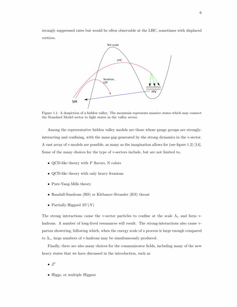
strongly suppressed rates but would be often observable at the LHC, sometimes with displaced
vertices.
HV
SM
Tevatron,
LEP
LHC
TeV scale
Figure 1.1: A despiction of a hidden valley. The mountain represents massive states which may connectthe Standard Model sector to light states in the valley sector.
Among the representative hidden valley models are those whose gauge groups are strongly-
interacting and confining, with the mass gap generated by the strong dynamics in the v-sector.
A vast array of v-models are possible, as many as the imagination allows for (see figure 1.2) [14].
Some of the many choices for the type of v-sectors include, but are not limited to,
• QCD-like theory with F flavors, N colors
• QCD-like theory with only heavy fermions
• Pure-Yang-Mills theory
• Randall-Sundrum (RS) or Klebanov-Strassler (KS) throat
• Partially Higgsed SU(N)
The strong interactions cause the v-sector particles to confine at the scale Λv and form v-
hadrons. A number of long-lived resonances will result. The strong-interactions also cause v-
parton showering, following which, when the energy scale of a process is large enough compared
to Λv, large numbers of v-hadrons may be simultaneously produced.
Finally, there are also many choices for the communicator fields, including many of the new
heavy states that we have discussed in the introduction, such as
• Z ′
• Higgs, or multiple Higgses

7
• Loops of heavy particles
• Heavy sterile neutrinos
Communicator
Standard Model Hidden valley
Figure 1.2: The class of models we are considering for a hidden sector.
The canonical example of a confining hidden valley, proposed by the authors of [6], is that of
a QCD-like scenario, having only two light flavors with a SU(N) gauge group. The dynamics of
the model is determined by the confining scale Λv, where the strong coupling constant becomes
strong. Light or heavy flavor is defined with respect to Λv : light quarks have masses mQ < Λv
and heavy quarks have masses mv > Λv. Production and decay processes of the hidden sector
quarks (“v-quarks”) can occur, for example, through a Z ′, whose charges are from an extra
U(1)χ gauge group. As in QCD, the v-quarks undergo a v-parton shower and form v-jets of
v-hadrons. In the two light flavor model the v-hadrons are electrically neutral v-pions, π±v and
π0v , which are the analogue of SM π± and π0 - the labels are simply meant to indicate the
analogy with pions, they do not denote electric charge. Some of these v-hadrons can decay back
to Standard Model particles, making a complex, high-multiplicity final state. This situation is
illustrated in figure 1.3. Depending on parameters, the decays of the v-hadrons may be prompt
or displaced.
v
v
v
vv
v
π
π
π
π
+
π+
b
b
b
bπ
−
−
ο
ο
U
UZ’
q
q
Figure 1.3: The production and hadronization of v-quarks.
This scenario was investigated by Strassler and Zurek with tools analogous to the ones used
to simulate QCD [6]. It displays some rather startling features. For instance, a πv could have a
displaced decay in the muon spectrometer in the ATLAS detector, resulting in a large number

8
of charged hadrons traversing the spectrometer, or it could decay in the hadronic calorimeter
producing a jet with no energy deposited in the electromagnetic calorimeter and no associated
tracks in the inner detector. Experimental studies for these scenarios are currently under way,
by the D0, CDF, LHCb, ATLAS and CMS collaborations.
This is just one simple model with two light flavors. However, the number of possibilities is
huge, and it is possible to think of other simple variants. For example, in the case of one light
flavor instead of two, the phenomenology is widely different. In this case, the light degrees of
freedom are the ηv (pseudoscalar) and the ρv (pseudovector), with masses of order mv ≃ Λv. It
was shown in [6] that the ρv will decay democratically to all SM flavors. As a result, it may be
possible to tag such events using multiple leptons from the decay of the vector. This aids the
task of extracting a signal from the background.
However, in the case of hidden valleys with many light flavors, detection may be especially
difficult [10]. These models predict a high multiplicity of v-hadrons, which in turn implies that
the number of jets in their decay products will be especially large. So for jets produced in
v-hadron decays, QCD backgrounds will be large and unknown, and any signal will be tough
to extract.
The limit where there are no light v-quarks, but only a hidden sector with a low confinement
scale is particularly interesting. In this case, the lightest states in the v-sector are glueballs of
SU(N) (“v-glueballs”). The v-color interactions ensure that all the heavy v-hadrons annihilate
efficiently into v-glueballs. These can then decay back into SM states via their coupling to
electroweak boson or the Higgs.
1.2 Quirks
Theories with an extra confining gauge group SU(nv) sector and some heavy matter fields
charged under both SM and SU(nv) gauge group such that there is a large hierarchy between
the masses of the matter fields, MX , and the confining scale, Λv, give rise to very unusual
dynamics [6, 47–49]. For this reason the quarks (or scalar quarks) of such a sector have been
dubbed quirks [49]. To understand this, let us first recall the dynamics of normal QCD. Consider
two heavy quarks that are produced back-to-back in a hard process. As the two quarks fly away
from each other and their distance approaches Λ−1QCD, confining dynamics sets in and creates a
gluonic flux tube extending between them. When the local energy density in the flux tube is
high enough it is energetically favorable to pair create a light quark anti-quark pair, breaking
the tube. This mechanism of soft hadronization allows the two heavy quarks to hadronize

9
separately.
In the quirk scenario, on the other hand, such a soft hadronization mechanism is absent
because there are no quarks with mass less than or comparable to Λv (see figure 4). The
energy density in the flux tube, or more simply, the tension of the SU(nv) string, cannot
exceed Λ2v which is far less than the MQ per Compton wavelength needed to create a heavy
quirk anti-quirk pair. The splitting of the SU(nv) string by a quirk anti-quirk pair is indeed
exponentially suppressed as exp (−M2/Λ2) [16]. In fact, one may view the entire process as
single production of a highly excited bound state, quirkonium. All of the kinetic energy that
the quirks posses at production,√s− 2MQ, which is typically of order MQ, can be interpreted
as quirkonium excitation energy. This energy is radiated away into glueballs of SU(nv) and
hadrons. Eventually the two quirks annihilate into lighter states.
Figure 1.4: Pictorial diagram of quirk confinement. A flux tube of SU(nv) chromoelectric field formsbetween quirks. Since the mass of the quirks satisfies MX ≫ Λv, flux tube in SU(nv) are stable.
Because the quirks are very heavy, MQ ≫ Λv, the light degrees of freedom in the v-sector
are glueballs of SU(nv). However, the standard model is uncharged under the new SU(nv)
gauge group, and therefore a quirk loop is required to couple the sectors at low energies. As
a result, effective couplings to the v-sector are highly suppressed at low energies. Specifically,
the leading coupling between the standard model and the hiddden valley sector at low energies
arises from a loop of virtual heavy quirks. This gives rise to dimension-8 effective operators
of the form tr F 2tr G2 and F tr G3, which mediate glueball decay, for example to photons or
gluons.
The existence of additional gauge groups with matter in bifundamental representations is a
hallmark of string theory model building. A quirk sector with vectorlike quirks and an extra
gauge group SU(nv) sector can therefore arise naturally from string theory. It is also trivial
to preserve gauge coupling unification in supersymmetric theories by assuming that the quirks
come in complete GUT representations, e.g. 5⊕ 5 and/or 10⊕ 10 [15].
In fact, a quirk-like sector has already appeared in some supersymmetric extensions of the
Standard Model motivated by the hierarchy problem. Such a sector was proposed in [15] to
give additional loop contributions to the physical Higgs mass in supersymmetry. Scalar quirks
appear in models of folded supersymmetry [13].

10
The collider phenomenology of quirks depends crucially on the length of the strings [49].
This is set by the scale where the kinetic energy is converted to potential energy of the string.
Since the typical quirk pair production event is not close to threshold, the maximal length is
L =E
Λ2v
(1.2)
where E =√s− 2M is the kinetic energy of the quirks upon production. One can distinguish
three different regimes.
• 100eV . Λv . 10keV: In this case oscillations will be macroscopic. Since it takes many
crossings before the quirks annihilate, one only observes the tracks of stable quirks in the
detector.
• 10keV . Λv . 1MeV: This is the case of mesoscopic strings. In this case one cannot
resolve the oscillations, and the quirks look like a stable charged particle.
• 1MeV . Λv . 100GeV: Here the strings are microscopic and the quirks get close enough
to each other that they can annihilate. For Λv & ΛQCD the annihilation is dominantly
into gluons of SU(nv) gauge group, which at long distance become glueballs.
In the following we will be mostly interested in the case of microscopic strings where the
quirks can annihilate producing visible signals.
So the overall picture in the quirk limit is that quirks are pair produced, and they fly away
from each other, sometimes macroscopic distances before the string pulls them back together.
They oscillate back and forth this way many times before the quirks can find each other and
annihilate. Whether the annihilation occurs in the detector and whether the string oscillations
are large enough to be visible will depend on the size of the confinement scale. We will see that
the collider phenomenology will be very sensitive to the confinement scale in the hidden sector,
leading to some remarkable, unstudied phenomena.

11
Chapter 2
A pure-glue hidden valley
In this chapter we consider a hidden valley that at low energy is a pure-Yang-Mills theory,
a theory that has its own gluons (“v-gluons”) and their bound states (“v-glueballs”). This
scenario easily arises in models; for example, in many supersymmetric v-sectors, supersymmetry
breaking and associated scalar expectation values may lead to large masses for all matter fields.
The spectrum of stable bound states in a pure Yang-Mills theory is known, to a degree,
from lattice simulations [24]. The spectrum of such states for an SU(3) gauge group is shown
in figure 2.1. The spectrum includes many glueballs of mass of order the confinement scale Λv
(actually somewhat larger), and various JPC quantum numbers. All of the states shown are
stable against decay to the other states, due to kinematics and/or conserved quantum numbers.
Figure 2.1: Spectrum of stable glueballs in pure glue SU(3) theory [24].
In this work we will further specialize to the case where the coupling between the SM sector
and the v-sector occurs through a multiplet of massive particles (which we will call X) charged
under both SM-sector and v-sector gauge groups.1 A loop of X particles2 induces dimension-D
1Recently such states, considered long ago [47,48], have been termed “quirks”; some of their very interestingdynamics, outside the regime we consider here, have been studied in [49].
2Much of the study covered in this and the next chapter was carried out before the proposal of [49] to namethe X particles as “quirks”. In most of the following discussion, the names “X particles” and “quirks” are usedindistinctly.
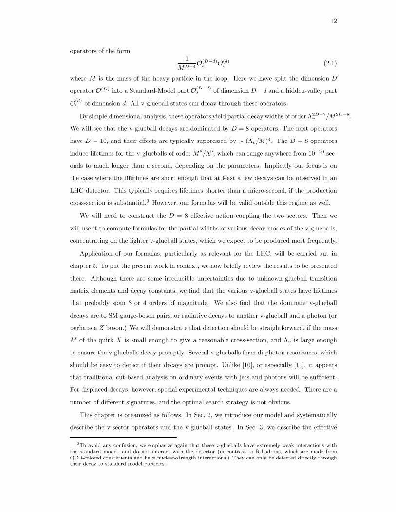
12
operators of the form1
MD−4O(D−d)
s O(d)v (2.1)
where M is the mass of the heavy particle in the loop. Here we have split the dimension-D
operator O(D) into a Standard-Model part O(D−d)s of dimension D−d and a hidden-valley part
O(d)v of dimension d. All v-glueball states can decay through these operators.
By simple dimensional analysis, these operators yield partial decay widths of order Λ2D−7v /M2D−8.
We will see that the v-glueball decays are dominated by D = 8 operators. The next operators
have D = 10, and their effects are typically suppressed by ∼ (Λv/M)4. The D = 8 operators
induce lifetimes for the v-glueballs of order M8/Λ9, which can range anywhere from 10−20 sec-
onds to much longer than a second, depending on the parameters. Implicitly our focus is on
the case where the lifetimes are short enough that at least a few decays can be observed in an
LHC detector. This typically requires lifetimes shorter than a micro-second, if the production
cross-section is substantial.3 However, our formulas will be valid outside this regime as well.
We will need to construct the D = 8 effective action coupling the two sectors. Then we
will use it to compute formulas for the partial widths of various decay modes of the v-glueballs,
concentrating on the lighter v-glueball states, which we expect to be produced most frequently.
Application of our formulas, particularly as relevant for the LHC, will be carried out in
chapter 5. To put the present work in context, we now briefly review the results to be presented
there. Although there are some irreducible uncertainties due to unknown glueball transition
matrix elements and decay constants, we find that the various v-glueball states have lifetimes
that probably span 3 or 4 orders of magnitude. We also find that the dominant v-glueball
decays are to SM gauge-boson pairs, or radiative decays to another v-glueball and a photon (or
perhaps a Z boson.) We will demonstrate that detection should be straightforward, if the mass
M of the quirk X is small enough to give a reasonable cross-section, and Λv is large enough
to ensure the v-glueballs decay promptly. Several v-glueballs form di-photon resonances, which
should be easy to detect if their decays are prompt. Unlike [10], or especially [11], it appears
that traditional cut-based analysis on ordinary events with jets and photons will be sufficient.
For displaced decays, however, special experimental techniques are always needed. There are a
number of different signatures, and the optimal search strategy is not obvious.
This chapter is organized as follows. In Sec. 2, we introduce our model and systematically
describe the v-sector operators and the v-glueball states. In Sec. 3, we describe the effective
3To avoid any confusion, we emphasize again that these v-glueballs have extremely weak interactions withthe standard model, and do not interact with the detector (in contrast to R-hadrons, which are made fromQCD-colored constituents and have nuclear-strength interactions.) They can only be detected directly throughtheir decay to standard model particles.

13
action coupling the two sectors and the SM matrix elements relevant for the decays. Our main
results for the decay modes and their branching fractions appear in Sec. 4. We conclude in
Sec. 5 with some final comments and perspective. Additional results appear in the Appendix.
2.1 The model and the hidden valley sector
2.1.1 Description of the Model
Consider adding to the standard model (SM) a new gauge group G, with a confinement scale Λv
in the 1–1000 GeV range. We will refer to this sector as the “hidden valley”, or the “v-sector”
following [6]. What makes this particular confining hidden valley special is that it has no light
charged matter; its only light fields are its gauge bosons, which we will call “hidden gluons”
or “v-gluons”. At low energy, confinement generates (meta)stable bound states, “v-glueballs”,
from the v-gluons. The SM is coupled to the hidden valley sector only through heavy fields Xr,
in vector-like representations of both the SM and G, with masses of order the TeV scale. These
states can be produced directly at the LHC, but because of v-confinement they cannot escape
each other; they form a bound state which relaxes toward the ground state and eventually
annihilates. The products of the annihilation are often v-glueballs. (Other annihilations lead
typically to a hard pair or trio of standard model particles.) Thereafter, the v-glueballs decay,
giving a potentially visible signal.
For definiteness, we take the gauge group G to be SU(nv), and the particles Xr to trans-
form as a fundamental representation of SU(nv) and in complete SU(5) representations of the
Standard Model, typically 5+ 5 and/or 10+10. We label the fields and their masses as shown4
in table 3.1. In this work, we will calculate their effects as a function of mr. The approximate
Field SU(3) SU(2) U(1) SU(nv) Mass
Xd 3 1 13 nv md
Xℓ 1 2 − 12 nv mℓ
Xu 3 1 − 23 nv mu
Xq 3 2 16 nv mq
Xe 1 1 1 nv me
Table 2.1: The new fermions Xr that couple the hidden valley sector to the SM sector.
global SU(5) symmetry of the SM gauge couplings suggests that the masses md and mℓ should
4In this work, we normalize hypercharge as Y = T3 −Q, where T3 is the third component of weak isospin.

14
be roughly of the same order of magnitude, and similarly for the masses mq,mu,me. It is often
more convenient to express the answer as a function of the (partially redundant) dimensionless
parameters
ρr ≡ mr/M . (2.2)
Here M is a mass scale that can be chosen arbitrarily; depending on parameters, it is usually
most natural to take it to be the mass of the lightest Xr particle.
Integrating out these heavy particles generates an effective Lagrangian Leff that couples
the v-gluons and the SM gauge bosons. The terms in the effective Lagrangian are of the
form (2.1), with operators O(d)v constructed from the gauge invariant combinations5 tr FµνFαβ
and tr FµνFαβFδσ, contracted according to different irreducible representations of the Lorentz
group.
The interactions in the effective action then allow the v-glueballs in figure 2.1, which cannot
decay within the v-sector, to decay to final states containing SM particles and at most one
v-glueball. This is analogous to the way that the Fermi effective theory, which couples the
quark sector to the lepton sector, permits otherwise stable QCD hadrons to decay weakly to
the lepton sector. As is also true for leptonic and semileptonic decays of QCD hadrons, our
calculations for v-hadrons decaying into SM particles simplify because of the factorization of
the matrix elements into a purely SM part and a purely hidden-sector part. To compute the
v-glueball decays, we will only need the following factorized matrix elements, involving terms
in the effective action of dimension eight:
〈SM |O(8−d)s |0〉〈0|O(d)
v |Θκ〉 , (2.3)
〈SM |O(8−d)s |0〉〈Θκ′ |O(d)
v |Θκ〉 . (2.4)
Here d is the mass dimension of the operator in the v-sector, 〈SM | schematically represents a
state built from Standard Model particles, and |Θκ〉 and |Θκ′〉 refer to v-glueball states with
quantum numbers κ, which include spin J , parity P and charge-conjugation C. We will see later
that we only need to consider d = 4 and 6; there are no dimension D = 8 operators in Leff for
which d = 5, since there are no appropriate dimension-three SM operators to compensate. The
SM part 〈SM |O(8−d)s |0〉 can be evaluated by the usual perturbative methods of quantum field
theory, but a computation of the hidden-sector matrix elements 〈0|O(d)v |Θκ〉 and 〈Θκ′ |O(d)
v |Θκ〉
requires the use of non-perturbative methods.
5Here we represent the v-gluon fields as Fµν = Faµν Ta, where Ta denote the generators of the SU(nv)
algebra with a common normalization tr TaT b = 12δab.

15
2.1.2 Classification of v-glueball states
In this section we shall classify the nonvanishing v-sector matrix elements. A v-glueball state Θκ
with quantum numbers JPC can be created by certain operators O(d)v acting on the vacuum | 0〉.
We wish to know which matrix elements, 〈0|O(d)v |Θκ〉 and 〈Θ′
κ|O(d)v |Θκ〉, are nonvanishing. This
is equivalent to finding how the operators in various Lorentz representations are projected onto
states with given quantum numbers JPC . Their classification was carried out in [46]. At mass
dimension d = 4 there are four different operators transforming in irreducible representations
of the Lorentz group. These are shown6 in table 2.2. From now on, we denote the operators
Oξv, where ξ runs over different irreducible operators ξ = S, P, T, L, · · · .
Operator Oξv JPC
S = tr FµνFµν 0++
P = tr FµνFµν 0−+
Tαβ = tr FαλF λβ − 1
4 gαβS 2++, 1−+, 0++
Lµναβ = tr FµνFαβ − 12 (gµαTνβ + gνβTµα − gµβTνα − gναTµβ) 2++, 2−+
− 112 (gµαgνβ − gµβgνα)S + 1
12 ǫµναβP
Table 2.2: The dimension d = 4 operators, and the states that can be created by these operators [46].We denote Fµν = 1
2ǫµναβFαβ .
The study of irreducible representations of dimension-six operators is more involved. A
complete analysis in terms of electric and magnetic gluon fields, ~Ea and ~Ba, was also presented
in [46], with a detailed description of the operators and the states contained in their spectrum.
There are only two such operators of relevance for our work, which we denote Ω(1)µν and Ω
(2)µν
as shown in table 2.3. The other dimension-six operators simply cannot be combined with any
SM operator to make a dimension-eight interaction.
2.1.3 Matrix elements
As we saw, the matrix elements are factorized into a purely SM part and a purely v-sector part.
We will first consider the v-sector matrix elements relevant to v-glueball transitions, 〈0|Oξv|Θκ〉
6As explained in [46], when an operator Oξv is conserved and the associated symmetry is not spontaneously
broken, some states must decouple. For example, with
〈0| Tµν | 1−+〉 = (pµǫν + pνǫµ)FT
1−+ ,
the conservation of Tµν requires FT
1−+ = 0, and thus T does not create a 1−+ state. Similarly
〈0| Tµν | 0++〉 = (ap2gµν + bpµpν)FT
0++ ,
where a and b are some functions of p2, must vanish for Tµν conserved and traceless. Note that the traceanomaly complicates this discussion, but its effect in this model is minimal; see Sec. 3.1 below.

16
Operator Oξv JPC
Ω(1)µν = tr FµνFαβFαβ 1−−, 1+−
Ω(2)µν = tr Fα
µFβαFβν 1−−, 1+−
Table 2.3: The important d = 6 operators. The states that can be created by these operators areshown [46].
and 〈Θκ′ |Oξv|Θκ〉, where |Θκ〉 and |Θκ′〉 refer to v-glueball states with given quantum numbers
and Oξv is any of the operators in tables 2.2 and 2.3.
It is convenient to write the most general possible matrix element in terms of a few Lorentz
invariant amplitudes or form factors. For the annihilation matrix elements we will write
〈0|Oξv|Θκ〉 = Πξ
κ,µν···Fξκ , (2.5)
where Fξκ is the decay constant of the v-glueball Θκ, and Πξ
κ,µν··· is determined by the Lorentz
representations of Θκ and Oξv. In table 2.4 we list Πξ
κ,µν··· for each operator.
The decay constants Fξκ depend on the internal structure of the v-glueball states and, with
the exception of those that vanish due to conservation laws (see footnote 6), must be deter-
mined by non-perturbative methods, for instance, by numerical calculations in lattice gauge
theory. Only the first three non-vanishing decay constants in table 2.4 have been calculated, for
SU(3) Yang-Mills theory [25], although the reported values are not expressed in a continuum
renormalization scheme. The other decay constants have not been computed.
Likewise, the transition matrix elements 〈Θκ′ |Oξv|Θκ〉 are of the form
〈Θκ′ |Oξv|Θκ〉 = Πξ
κκ′,µν···Mξκ,κ′, (2.6)
where now Mξκ,κ′ is the transition matrix, which depends only on the transferred momentum. In
table 2.5 we have listed Πξκκ′,µν··· for the simplest cases considered later in this work. In several
other cases more than one Lorentz structure Πξκκ′,µν··· contributes to the transition element. In
such cases, since none of these matrix elements are known from numerical simulation, we will
usually simplify the problem by using the lowest partial-wave approximation for the amplitudes.
More details will follow in Sec. 2.3.
Clearly, any numerical results arising from our formulas, as we ourselves will obtain in
our LHC study [60], will be subject to some large uncertainties, due to the unknown matrix
elements. Of course, with sufficient motivation, such as a hint of a discovery, many of these
could be determined through additional lattice gauge theory computations.
Now we turn to the SM part of the matrix element, which can be treated perturbatively,

17
Oξv (Θκ) Πξ
κ,µν··· Fξκ
S (0++) 1 FS
0++
P (0−+) 1 FP
0−+
Tαβ (0++) gαβ − pαpβ
p2 0
Tαβ (1−+) pαǫβ + pβǫα 0Tαβ (2++) ǫαβ F
T
2++
Lµναβ (2++) ǫµαPνβ + ǫνβPµα − ǫναPµβ − ǫµβPνα FL2++
Lµναβ (2−+) (ǫµνρσǫσβp
ρpα − ǫµνρσǫσαpρpβ FL
2−+
+ǫαβρσǫσνp
ρpµ − ǫαβρσǫσµp
ρpν)/p2
Ω(n)µν (1−−) m1−(pµǫν − pνǫµ) FΩ(n)
1−−
Ω(n)µν (1+−) m1+ǫµναβ(p
αǫβ − pβǫα) FΩ(n)
1+−
Table 2.4: Annihilation matrix elements. ǫµ and ǫµν are the polarization vectors of 1−−, 1+− andpolarization tensor of 2++, 2−+ respectively. Pαβ = gαβ − 2pαpβ/p
2. m1− ,m1+ are the masses of the1−−, 1+− states; their appearance merely reflects our normalization convention.
Oξv (Θκ Θκ′) Πξ
κκ′,µν··· Mξκκ′
P (0−+, 0++) 1 MP0+0−
Ω(n)µν (1−−, 0++) pµǫν − pνǫµ MΩ(n)
1−−0++
Ω(n)µν (1+−, 0−+) pµǫν − pνǫµ MΩ(n)
1+−0−+
Ω(n)µν (1−−, 0−+) ǫµναβp
αǫβ MΩ(n)
1−−0−+
Ω(n)µν (1+−, 0++) ǫµναβp
αǫβ MΩ(n)
1+−0++
P (1−−, 1+−) ǫ+ · ǫ− MP1−−1+−
L (1−−, 1+−) ǫµνρσpρǫ−
σ(pαǫ
+β − pβǫ
+α) + µν ↔ αβ − traces ML
1−−1+−
Ω(n)µν (2−+, 1+−) pµǫναǫ
α − pνǫµαǫα MΩ(n)
2−+1+−
Ω(n)µν (1+−, 2++) ǫµναβǫ
αλǫλpβ , ǫµναβǫ
αλpλǫβ MΩ(n)
1+−2++
Table 2.5: Transition matrix elements. Momentum of the final glueball Θκ′ is denoted pµ; ǫα and ǫαβ
are polarization tensors of spin 1 and spin 2 states respectively. The bottom part of the table containsmatrix elements in the lowest partial wave approximation.
since we will only consider v-glueballs with masses well above ΛQCD.7 In all of our calculations,
the SM gauge-boson field-strength tensors, which appear in the operators, are replaced in the
matrix element by the substitution Gµν ↔ kµεν − kνεµ. For example, for a transition to two
gauge bosons, we write8
〈k1, εa1 ; k2, εb2|tr GµνGαβ |0〉 = δab(k1µε1ν − k1νε
1µ)(k
2αε
2β − k1αε
2β), (2.7)
where k1(2), ε1(2) are the gauge-bosons’ momenta and polarizations respectively. Later in the
7We will do all our calculations at SM-tree level; loop corrections for v-glueball decays to ordinary gluonsshould be accounted for when precision is required.
8Note that one has to take into account a factor of 2 which comes from the two different ways of con-tracting each Ga
µν operator with |k1, εa1 ; k2, εb2〉. This factor then cancels an explicit 12
factor appearing in the
normalization of the trace.

18
text we will sometimes use the following notation for the SM matrix elements
〈SM |Oηs |0〉 = hµν···η , (2.8)
where hµν···η = hµν···η (k1, k2, · · · ) is a function of the momenta of the SM particles in the final
state.
2.2 Effective Lagrangian
In this section we discuss the effective action Leff linking the SM sector with the v-sector, and
discuss the general form of the amplitudes controlling v-glueball decays. We will confirm that
all the important decay modes are controlled by D = 8 operators involving the d = 4 and 6
operators listed in tables 2.2 and 2.3.
2.2.1 Heavy particles and the computation of Leff
The low-energy interaction of v-gluons and v-glueballs with SM particles is induced through
a loop of heavy X-particles. In this section we present the one-loop effective Lagrangian that
describes this interaction, to leading non-vanishing order in 1/M , namely 1/M4, which we will
see is sufficient for inducing all v-glueball decays. The relevant diagrams all have four external
gauge boson lines, as depicted in figure 2.2. They give the amplitude for scattering of two
v-gluons to two SM gauge bosons, of either strong (gluons g), weak (W and Z) or hypercharge
(photon γ or Z) interactions (figure 2.2a), as well as the conversion of three v-gluons to a γ or
Z (figure 2.2b).
v
v
X SM
SM(a)
v
v
v
SM
(b)
X
Figure 2.2: Diagrams contributing to the effective action
The dimension-eight operators appearing in the action can be found in studies of Euler-
Heisenberg-like Lagrangians in the literature. Within the SM, effective two gluon - two photon,
four gluon, and three gluon - photon vertices can be found in [42], [43] and [44] respectively.
These results can be adapted for our present purposes.
19
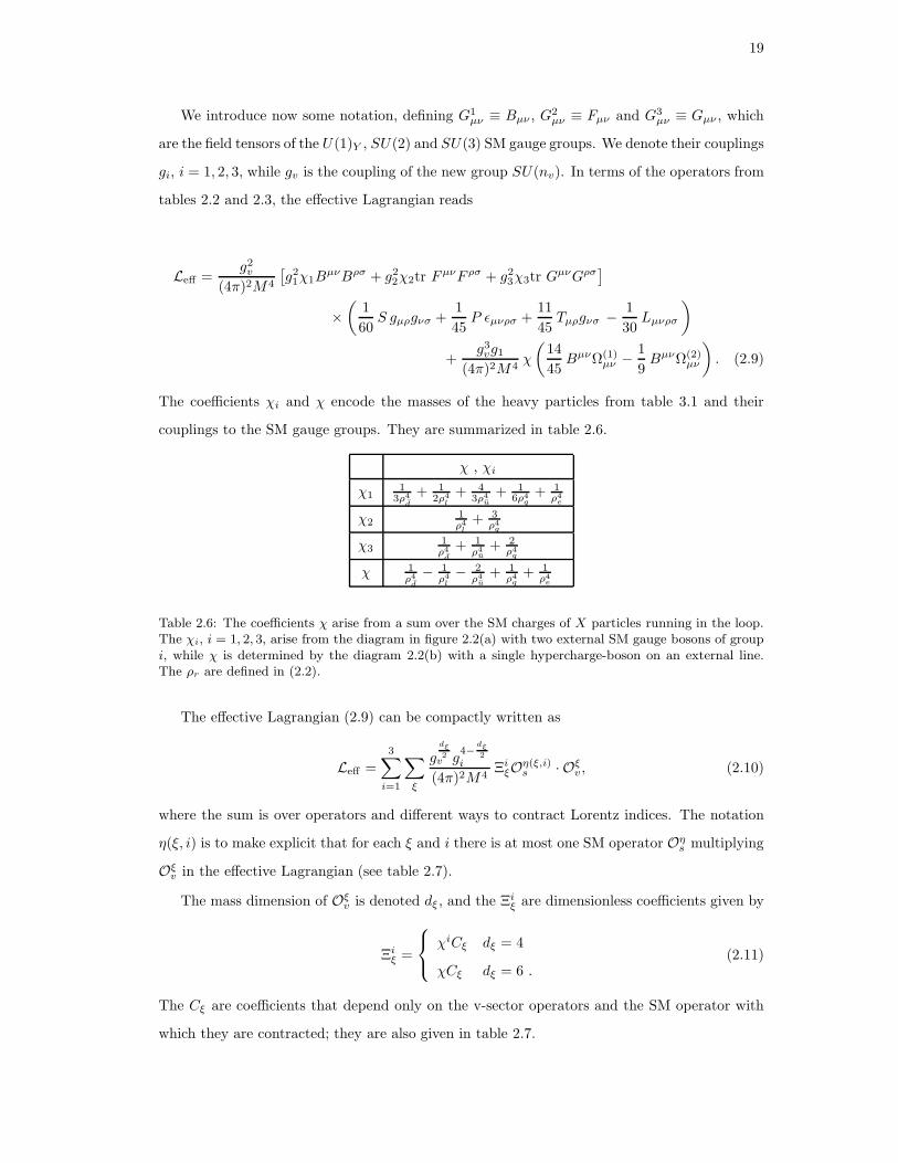
We introduce now some notation, defining G1µν ≡ Bµν , G
2µν ≡ Fµν and G3
µν ≡ Gµν , which
are the field tensors of the U(1)Y , SU(2) and SU(3) SM gauge groups. We denote their couplings
gi, i = 1, 2, 3, while gv is the coupling of the new group SU(nv). In terms of the operators from
tables 2.2 and 2.3, the effective Lagrangian reads
Leff =g2v
(4π)2M4
[
g21χ1BµνBρσ + g22χ2tr F
µνF ρσ + g23χ3tr GµνGρσ
]
×(
1
60S gµρgνσ +
1
45P ǫµνρσ +
11
45Tµρgνσ − 1
30Lµνρσ
)
+g3vg1
(4π)2M4χ
(
14
45BµνΩ(1)
µν − 1
9BµνΩ(2)
µν
)
. (2.9)
The coefficients χi and χ encode the masses of the heavy particles from table 3.1 and their
couplings to the SM gauge groups. They are summarized in table 2.6.
χ , χi
χ11
3ρ4d
+ 12ρ4
l
+ 43ρ4
u+ 1
6ρ4q+ 1
ρ4e
χ21ρ4l
+ 3ρ4q
χ31ρ4d
+ 1ρ4u+ 2
ρ4q
χ 1ρ4d
− 1ρ4l
− 2ρ4u+ 1
ρ4q+ 1
ρ4e
Table 2.6: The coefficients χ arise from a sum over the SM charges of X particles running in the loop.The χi, i = 1, 2, 3, arise from the diagram in figure 2.2(a) with two external SM gauge bosons of groupi, while χ is determined by the diagram 2.2(b) with a single hypercharge-boson on an external line.The ρr are defined in (2.2).
The effective Lagrangian (2.9) can be compactly written as
Leff =
3∑
i=1
∑
ξ
gdξ2
v g4−
dξ2
i
(4π)2M4ΞiξOη(ξ,i)
s · Oξv, (2.10)
where the sum is over operators and different ways to contract Lorentz indices. The notation
η(ξ, i) is to make explicit that for each ξ and i there is at most one SM operator Oηs multiplying
Oξv in the effective Lagrangian (see table 2.7).
The mass dimension of Oξv is denoted dξ, and the Ξi
ξ are dimensionless coefficients given by
Ξiξ =
χiCξ dξ = 4
χCξ dξ = 6 .(2.11)
The Cξ are coefficients that depend only on the v-sector operators and the SM operator with
which they are contracted; they are also given in table 2.7.
20
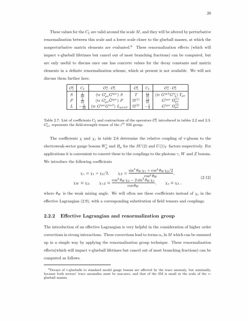
These values for the Cξ are valid around the scaleM , and they will be altered by perturbative
renormalization between this scale and a lower scale closer to the glueball masses, at which the
nonperturbative matrix elements are evaluated.9 These renormalization effects (which will
impact v-glueball lifetimes but cancel out of most branching fractions) can be computed, but
are only useful to discuss once one has concrete values for the decay constants and matrix
elements in a definite renormalization scheme, which at present is not available. We will not
discuss them further here.
Oξv Cξ Oη
s · Oξv Oξ
v Cξ Oηs · Oξ
v
S 160 (tr Gi
µνGiµν) S T 11
45 (tr GiµλGiνλ) Tµν
P 245 (tr Gi
µνGiµν ) P Ω(1) 14
45 G1µν Ω(1)µν
L − 130 (tr GiµνGiαβ) Lµναβ Ω(2) − 1
9 G1µν Ω(2)µν
Table 2.7: List of coefficients Cξ and contractions of the operators Oξv introduced in tables 2.2 and 2.3.
Giµν represents the field-strength tensor of the ith SM group.
The coefficients χ and χi in table 2.6 determine the relative coupling of v-gluons to the
electroweak-sector gauge bosons W iµ and Bµ for the SU(2) and U(1)Y factors respectively. For
applications it is convenient to convert these to the couplings to the photons γ,W and Z bosons.
We introduce the following coefficients
χγ ≡ χ1 + χ2/2, χZ ≡ sin4 θWχ1 + cos4 θWχ2/2
cos2 θW,
χW ≡ χ2, χγZ ≡ cos2 θWχ2 − 2 sin2 θWχ1
cos θW, χs ≡ χ3 ,
(2.12)
where θW is the weak mixing angle. We will often use these coefficients instead of χi in the
effective Lagrangian (2.9), with a corresponding substitution of field tensors and couplings.
2.2.2 Effective Lagrangian and renormalization group
The introduction of an effective Lagrangian is very helpful in the consideration of higher order
corrections in strong interactions. These corrections lead to terms αv lnM which can be summed
up in a simple way by applying the renormalization group technique. These renormalization
effects(which will impact v-glueball lifetimes but cancel out of most branching fractions) can be
computed as follows.
9Decays of v-glueballs to standard model gauge bosons are affected by the trace anomaly, but minimally,because both sectors’ trace anomalies must be non-zero, and that of the SM is small at the scale of the v-glueball masses.

21
Let us first write the effective Lagrangian (2.9) as
Leff =∑
ξ
CξOξ, (2.13)
where
Oξ =
3∑
i=1
gdξ2
v g4− dξ
2
i
(4π)2M4Ξ′iξOη(ξ,i)
s · Oξv, (2.14)
with Ξ′iξ = Ξi
ξ/Cξ. Here the operators Oξ must be treated on equal footing with the original
terms in the Lagrangian, with the coefficients Cξ considered as some new charges.
To lowest order in αv the coefficients Cξ can be read off table 2.7. These values arise from
quirk loops and hence are valid at the scale M . To consider contributions of these operators to
v-glueball matrix elements, one must use the renormalization group to evolve the coefficients
down to a scale closer to the glueball masses, at which the nonperturbative matrix elements are
evaluated. To do this, the anomalous dimensions of the operators Oξ are required.
To calculate the anomalous dimension γξ of an operator Oξ, we add the operator to the
Lagrangian with coupling Cξ, shift A→ A+a, expand to O(a2), calculate the functional deter-
minant, and expand it in powers Gµν , looking for the appearance of Oξ with a logarithmically
divergent coefficient. Specifically, in the path integral picture,
∫
Da exp[
i(S + a) + iCξ
∫
Oξ(A+ a)dx4]
→ exp
[
iZ−1ξξ′Cξ
∫
Oξ′(A)dx4 + · · ·
]
, (2.15)
where, to lowest order,
Z−1ξξ′ = 1 +
γξξ′
2
g2
16πln
[
M2
µ2
]
. (2.16)
The last expression defines the matrix of reduced anomalous dimensions.
The couplings Cξ(µ) are found by solving the generalized Gell-Mann-Low equations,
µdCξ
dµ= −αv
2πγξξ′Cξ′ , (2.17)
µdαv
dµ= − b
2πα2v, (2.18)
with b = (11/3)nv. The required anomalous dimensions for the operators shown in table 2.7
can be calculated using a systematic algorithm developed by Morozov [23]. The anomalous
dimension for S was also obtained in [21, 22]. One finds that S, P, T, L, Ω1, Ω2 have reduced
anomalous dimensions γSS = 0, γPP = 0, γTT = b0 = 11, γLL = 6, γΩ1Ω1 = γΩ2Ω2 = 23/2 and
γΩ1Ω2 = γΩ2Ω1 = 1/2, with all remaining coefficients equal to zero.

22
2.2.3 Decay amplitudes
Now, using (2.5), (2.8) and the couplings from (2.14), we obtain that the amplitude for a decay
of a v-glueball into SM particles is given by
M =g
dξ2
v g4−
dξ2
i
(4π)2M4Ξiξ(ρu, ..., ρe)〈SM |Oη
s | 0〉〈0|Oξv|Θκ〉 =
=g
dξ2
v g4− dξ
2
i
(4π)2M4Ξiξ(ρu, ..., ρe)f
iξ,η(p, q1, q2, ...)F
ξκ, (2.19)
where
f iξ, η(p, k1, k2, ...) = hµν···η (k1, k2, ...)Π
ξκ, µν···(p)
encodes all the information about the matrix element that can be determined from purely
perturbative computations and Lorentz or gauge invariance, and Fξκ is the v-glueball decay
constant. See Eq. (2.11) for the definition of Ξ and Eq. (2.2) and table 2.6 for the definition of
ρ.
Similarly, using (2.6), (2.8) and (2.14), the amplitude for the decay of a v-glueball into
another v-glueball and SM particles reads
M =g
dξ2
v g4− dξ
2
i
(4π)2M4Ξiξ(ρu, ..., ρe)〈SM |Oη
s | 0〉〈Θκ′ |Oξv|Θκ〉 =
=g
dξ2
v g4−dξ
2
i
(4π)2M4Ξiξ(ρu, ..., ρe)f
iκκ′;ξ,η(p, p
′, k1, k2, ...)Mξκκ′(k). (2.20)
Here Mξκκ′(k) is the glueball-glueball transition matrix, which for given masses of Θκ and Θκ′
is a function of transferred momentum k ≡ p′ − p, and
f iκκ′; ξ,η = Πξ
κκ′, µν···(p, p′)hµν···η (k1, k2, ...).
2.3 Decay rates for lightest v-glueballs
In this section we will compute the decay rates for some of the v-glueballs in figure 2.1. Let us
make a quick summary of the results to come.
The operators shown in tables 2.2 and 2.3 induce the dominant decay modes of the v-glueball
states appearing in figure 2.1. In the PC =++ sector, the lightest 0++ and 2++ v-glueballs
will mostly decay directly to pairs of SM gauge bosons via S, T and L operators. Three-body
decays 2++ → 0++ plus two SM gauge bosons are also possible, but are strongly suppressed by
phase space. In the PC = −+ sector the lightest states are the 0−+ and 2−+ v-glueballs. These
will also decay predominantly to SM gauge boson pairs, via P and L operators respectively.
23
There are also C-changing 2−+ → 1+− + γ decays, induced by the d = 6 D = 8 operators
Ωµν (table 2.3), but the small mass-splitting found in the lattice computations [24] suggests
these decays are probably very rare or absent. In the PC =+− sector, the leading decays are
two-body C-changing processes, because C-conservation forbids annihilation to pairs of gauge
bosons, and because three-body decays are phase-space suppressed. In particular, the 1+−, the
lightest v-glueball in that sector, will decay to the lighter C-even states 0++, 2++ and 0−+ by
radiating a photon (or Z when it is possible kinematically). The same is true for the states in
the PC = −− sector, with an exception that the lightest 1−− v-glueball can annihilate to a
pair of SM fermions through an off-shell photon or Z. The latter decay is also induced by Ωµν
operators.
We shall study decays of the 0++, 2++, 0−+, 2−+, 1+− and 1−− v-glueballs in some detail.
Since for this set of v-glueballs the combination of J and P quantum numbers is unique, we
shall often omit the C quantum number from our formulas to keep them a bit shorter, referring
simply to the 0+, 2+, 0−, 2−, 1+ and 1− states. At the end we shall make some brief comments
about the other states, the 3++, 3+−, 3−−, 2+−, 2−− and 0+−.
Of course the allowed decays and the corresponding lifetimes are dependent upon the masses
of the v-glueballs. While the results of Morningstar and Peardon [24], understood as dimen-
sionless in units of the confinement scale Λ, can be applied to any pure SU(3) gauge sector,
the glueball spectrum for SU(4) or SU(7) are not known. Fortunately, at least for SU(nv), the
spectrum is expected to be largely independent of nv. Still, the precise masses will certainly
be different for nv > 3, and for some v-glueballs this could have a substantive effect on their
lifetimes and branching fractions.
For other gauge groups, however, the spectrum may be qualitatively different; in particular,
the C-odd sector may be absent or heavy. We will briefly discuss this in our concluding section.
The 0±+ and 2±+ states are expected to be present in any pure-gauge theory, with similar
production and decay channels, and as such are the most model-independent. Fortunately, it
turns out they are also the easiest to study theoretically, and, as we will see below and in our
LHC study [60], the easiest to observe.
2.3.1 Light C-even sector decays
We begin with the C-even 0++, 2++, 0−+ and 2−+ v-glueballs, which can be created by dimen-
sion 4 operators. The first three have been studied in some detail in various contexts; see for
example [25–31] and a recent review [37]. The dominant decays of these states are annihilations

24
Θκ → GaGb, where Θκ denotes a v-glueball state and Ga, Gb is a pair of SM gauge bosons:
gg, γγ, ZZ, W+W− or γZ. We will also consider radiative decays Θκ → Θκ′ + γ/Z, and
three-body decays of the form Θκ → GaGbΘ′κ, and will see they are generally subleading for
these states.
Annihilations are mediated by the dimension d = 4 operators in Eq. (3.5). In particular, we
know from the previous discussion (see [46] and table 2.2 above) that the 0++ v-glueball can
be annihilated (created) by the operator S. The 0−+ and 2−+ states are annihilated by the
operators P and Lµναβ respectively. The tensor 2++ can be destroyed by both Tµν and Lµναβ .
Radiative two-body decays are induced by the dimension d = 6 operators in Eq. (3.6).
However, the decays Θκ → Θκ′ + γ/Z are forbidden if Θκ and Θκ′ are both from the C-even
subsector. For the spectrum in figure 2.1, appropriate for nv = 3, the only kinematically allowed
radiative decay is therefore 2−+ → 1+− + γ; the 1+− + Z final state is kinematically allowed
only for very large Λv. For nv > 3, the glueball spectrum is believed to be quite similar to
nv = 3, but the close spacing between these two states implies that the ordering of masses
might be altered, so that even this decay might be absent for larger nv.
Decays of the 0++ state.
The scalar state can be created or destroyed by the operator S.
Then, according to a general discussion in Sec. 2.2, the amplitude of the decay of the scalar
to two SM gauge bosons Ga and Gb is given by the expression
αiαv
M4χiCS〈Ga, Gb|tr GµνG
µν | 0〉 〈 0|S| 0++〉, (2.21)
where αi and χi encode the couplings of the bosons a and b of a SM gauge group i to the loop,
introduced in Sec. 2.2; see (2.14), (2.11) and table 2.6.
For the decay of the scalar to two gluons, (2.21) takes the form
αsαv
M4χsCS〈ga1gb2| tr GµνG
µν | 0〉 〈 0|S| 0++〉 =
=αsαv
M4
δab
2χsCSF
S0++2(k1µε
1ν − k1νε
1µ)(k
2µε2ν − k2
νε2
µ), (2.22)
where, according to our conventions, constant FS0++ denotes the matrix element 〈0|S| 0++〉. We
are using the notation αs ≡ α3, χs ≡ χ3. The rate of the decay (accounting for a 1/2 from Bose
statistics) is then given by
Γ0+→gg =α2sα
2v
16πM8(N2
c − 1)χ2sC
2Sm
30+(F
S0++)2. (2.23)
Here and below we make explicit the SU(3)-color origin of a factor of 8 = N2c − 1.

25
The branching ratios for the decays to the photons, Z and W± are
Γ0+→γγ
Γ0+→gg
=1
2
α2
α2s
χ2γ
χ2s
, (2.24)
Γ0+→ZZ
Γ0+→gg=
1
2
α2w
α2s
χ2Z
χ2s
(
1− 4m2
Z
m20+
)1/2 (
1− 4m2
Z
m20+
+ 6m4
Z
m40+
)
, (2.25)
Γ0+→γZ
Γ0+→gg=
1
4
ααw
α2s
χ2γZ
χ2s
(
1− m2Z
m20+
)3
, (2.26)
Γ0+→W+W−
Γ0+→gg=
1
4
α2w
α2s
χ2W
χ2s
(
1− 4m2
W
m20+
)1/2 (
1− 4m2
W
m20+
+ 6m4
W
m40+
)
, (2.27)
The coefficients χ used here were defined in Eq. (2.12). Factors of 1/2 in the above ratios come
from the color factor N2c −1 = 8 and a difference in the normalization of abelian and non-abelian
generators. An extra 1/2 is required if the particles in the final state are not identical, such as
W+W− and γZ.
Of course these are SM-tree-level results. There will be substantial order-αs corrections to
the gg final state, so the actual lifetimes will be slightly shorter and the branching fractions to
other final states slightly smaller than given in these formulas.
Decays of the 0−+ state.
The decay of the pseudoscalar state 0−+ to two gauge bosons proceeds in a similar fashion.
This decay is induced by the operator P :
αiαv
M4χiCP 〈Ga, Gb| tr GµνG
µν | 0〉 〈0|P |0−+〉. (2.28)
The amplitude leads to the following two-gluon decay rate:
Γ0−→gg =α2sα
2v
16πM8(N2
c − 1)χ2sC
2Pm
30−(F
P0−+)2, (2.29)
and the same branching fractions as for 0++, except for the decays to ZZ and W+W−,
Γ0−→ZZ
Γ0−→gg
=1
2
α2w
α2s
χ2Z
χ2s
(
1− 4m2
Z
m20−
)3/2
, (2.30)
Γ0−→W+W−
Γ0−→gg
=1
4
α2w
α2s
χ2W
χ2s
(
1− 4m2
W
m20−
)3/2
. (2.31)
The 0−+ state can also decay to lower lying states by emitting a pair of gauge bosons, but
these decays are suppressed. For instance, the amplitude for the decay of 0−+ → 0++gg is
αiαv
M4χiCP 〈Ga, Gb | tr GµνG
µν | 0〉 〈0++|P |0−+〉 . (2.32)

26
The matrix element MP0+0− = 〈0++|P |0−+〉 is a function of the momentum transferred. Let us
first treat it as approximately constant. Then we obtain the decay rate
Γ0−→0++gg =α2sα
2v
256π3M8(N2
c − 1)χ2sC
2Pm
50−f(a)(M
P0+0−)2, (2.33)
where f is the dimensionless function of the parameter a = m20+/m
20− ,
f(a) =1
12(1 − a2)(1 + 28a+ a2) + a(1 + 3a+ a2) ln a, (2.34)
We plot f in figure 2.3; it falls rapidly from 1/12 to 0, because of the rapid fall of phase space
as the two masses approach each other. For the masses in figure 2.1, a = 0.44 and f ≈ 10−4.
This is in addition to the usual 1/16π2 suppression of three-body decays compared to two-body
decays. Thus the branching fraction for this decay is too small to be experimentally relevant,
and our approximation that the matrix element is constant is inconsequential. This will be our
general conclusion for three-body decays of the light v-glueball states, and in most cases we will
not bother to present results for such channels.
0.0 0.2 0.4 0.6 0.8 1.0a10-16
10-13
10-10
10-7
10-4
0.1
100
f HaL
a=m0++
2
m0-+2
Figure 2.3: Kinematic suppression factor f(a). Point corresponds to a value of a taken for v-glueballmasses from the Morningstar and Peardon spectrum [24].
Decays of the 2++ state.
Decays of the 2++ glueball to two gauge bosons are induced by more than one operator in (2.9).
In particular, the 2++ decays due to the Tµν and Lµναβ operators. This corresponds to the
amplitude
αiαv
M4χi
[
CT 〈Ga, Gb| tr GµαGαν | 0〉 〈0|T µν|2++〉+
+CL〈Ga, Gb| tr GµνGαβ | 0〉〈0|Lµναβ |2++〉]
. (2.35)

27
The width of the decay to two gluons is
Γ2+→gg =α2sα
2v(N
2c − 1)
160πM8χ2sm
32+
(
1
2C2
T (FT2++)2 +
4
3C2
L(FL2++)2
)
. (2.36)
Here we used the following expressions for the matrix elements:
〈0|T µν|2++〉 = FT2++ ǫµν , (2.37)
〈0|Lµναβ |2++〉 = FL2++ [Pµαǫνβ − Pµβǫνα + Pνβǫµα − Pναǫµβ] , (2.38)
where Pαβ is defined in the caption to table 2.4.
The branching fraction for the decay to two photons is again similar to (2.24). For two Z
bosons in the final state, the width of the decay is equal to
Γ2+→ZZ =α2wα
2v
40πM8χ2Zm
32+(1− 4ζ2)
1/2
(
1
2C2
T fT (ζ2)(FT2++)2+
4
3C2
LfL(ζ2)(FL2++)2 +
40
3CTCLfTL(ζ2)F
T2++F
L2++
)
, (2.39)
where fT , fL, fTL are the following functions of the parameter ζ2 = m2Z/m
22+ .
fT (ζ2) = 1− 3ζ2 + 6ζ22 , fL(ζ2) = 1 + 2ζ2 + 36ζ22 , fTL(ζ2) = ζ2(1 − ζ2) . (2.40)
The decay to W+W− is obtained from Eq. (2.39) by substituting χZ → χW , mZ → mW
and multiplying by 1/2. For the γZ final state, the decay rate is
Γ2+→γZ =ααwα
2v
80πM8χ2γZm
32+(1 − ζ2)
3
(
1
2C2
T gT (ζ2)(FT2++)2+
4
3C2
LgL(ζ2)(FL2++)2 +
20
3CTCLζ2F
T2++F
L2++
)
, (2.41)
where
gT (ζ2) = 1 +1
2ζ2 +
1
6ζ22 , gL(ζ2) = 1 + 3ζ2 + 6ζ22 . (2.42)
As in the case of the 0−+, we can ignore the three-body transitions 2++ → 0++ + gg, etc.
Decays of the 2−+ state.
The dominant decays of the 2−+ state occur due to the Lµναβ operator. The amplitude for
such decays is given by
αiαv
M4χiCL〈Ga, Gb| tr GµνGαβ | 0〉〈0|Lµναβ| 2−+〉. (2.43)
The correct Lorentz structure that singles out the negative parity part of the operator Lµναβ
is as follows:
〈0|Lµναβ | 2−+〉 = FL2−+
(
ǫµνρσǫσβn
ρnα − ǫµνρσǫσαn
ρnβ+
+ǫαβρσǫσνn
ρnµ − ǫαβρσǫσµn
ρnν
)
, (2.44)

28
where nµ = pµ/m2− is a unit vector in the direction of the 4-momentum of the v-glueball.
The decay rate to two gluons is then given by
Γ2−→gg =α2sα
2v
120πM8(N2
c − 1)χs2m3
2−C2L(F
L2−+)2 (2.45)
and Γ2−→γγ is provided by the same relation as (2.24). The widths of the decay to ZZ and γZ
can be found from the ratios
Γ2−→ZZ
Γ2−→gg
=1
2
α2w
α2s
χ2Z
χ2s
(
1− 4m2
Z
m22−
)1/2(
1 + 2m2
Z
m22−
− 24m4
Z
m42−
)
, (2.46)
Γ2−→γZ
Γ2−→gg
=1
4
ααw
α2s
χ2γZ
χ2s
(
1− m2Z
m22−
)3(
1 + 3m2
Z
m22−
+ 6m4
Z
m42−
)
, (2.47)
and the width for the decay to W+W− is again obtained by substituting in (2.46) χZ → χW ,
mZ → mW and dividing the result by 2.
As before, we can neglect 3-body decays. However, there is a 2-body radiative decay that
we should consider, although, as we will see, for the masses in figure 2.1 it is of the same order
as the 3-body decays. For the SU(3) spectrum in [24] (and possibly all pure glue SU(n), n ≥ 3)
the 2−+ state is slightly heavier than the lightest state in the C-odd sector, the pseudovector
1+−. Thus, we need at least to consider the decay 2−+ → 1+− + γ. This decay is induced
by the second type of operators (table 2.3) in the effective action (2.9). The amplitude of the
decay reads
eg3v(4π)2M4
χ〈γ|Gµν | 0〉(
CΩ(1)〈1+−|Ω(1)µν | 2−+〉+ CΩ(2)〈1+−|Ω(2)
µν | 2−+〉)
. (2.48)
Unfortunately nothing quantitative is known about matrix elements like 〈1+−|Ω(n)µν | 2−+〉.
In fact each contains multiple Lorentz structures, constructed out of polarization tensors ǫα,
ǫβγ and momenta p and q of the 1+− and 2−+ v-glueballs, times functions of the momentum
transfer, cf. [38]. Some simplification can be made if one takes into account the fact that masses
of the v-glueballs are close, which we will assume below.
We start by writing the general expression for the amplitude (2.48):
〈 γ|Gµν | 0〉 〈 1+−|Ω(n)µν | 2−+〉 = 2MΩ(n)
2−+1+−(k · p εαǫαβǫβ − p · ε kαǫαβǫβ)+
+ 2MΩ(n)′2−+1+−(k · p ε · ǫ− k · ǫp · ε) p
αǫαβpβ
m22−
+
+ 2MΩ(n)′′2−+1+−(k · p εαǫαβpβ − p · ε kαǫαβpβ)
q · ǫm2
2−, (2.49)
where n = 1, 2 and k, εα are the momentum and polarization of the photon. All contributions
of the terms proportional to primed form-factors (which correspond to higher partial waves)

29
are suppressed by powers of (m2− −m1+)/(m2− +m1+) ≃ 0.017, so we may neglect them.10
Note, however, that if the mass splitting is much larger for nv > 3, then there will be additional
unknown quantities that will modify our result below.
We now find
Γ2−→1++γ =αα3
v
960πM8χ2 (m2
2− −m21+)
3
m52−m
21+
×
× (3m42− + 34m2
2−m21+ + 3m4
1+)(
MΩ2−+1+−
)2. (2.50)
Here we introduced the notation
MΩ2−+1+− ≡ CΩ(1)MΩ(1)
2−+1+− + CΩ(2)MΩ(2)
2−+1+− . (2.51)
Since the the form-factors MΩ(n)
2−+1+− are unknown, we shall not distinguish between them and
will use a collective notation, similar to (2.51), for them in the future. In the same manner we
will use the notation
Ωµν ≡ CΩ(1)Ω(1)µν + CΩ(2)Ω(2)
µν . (2.52)
The factor (m22−−m2
1+)3 strongly suppresses the amplitude, given the spectrum of figure 2.1,
and a rough estimate suggests it is of the same size as the three-body decays of the 2− state,
and consequently negligible. However this splitting is so small that it is sensitive to numerical
uncertainties in the lattice calculation, and might well be different for other gauge groups. In
particular, this decay channel might be closed, or might be more widely open than suggested
by figure 2.1, depending on the mass spectrum.
Given the uncertainty on the spectrum and the unknown v-glueball mass scale, it is worth
noting that the radiative decay of 2−+ to 1+− can in principle occur through an emission of the
Z boson. This decay is slightly more involved than the decay with photon emission considered
above. Additional unknown form factors related to the finiteness of the Z mass further reduce
the predictive power of any computation. But such a decay may be forbidden by kinematics,
and if allowed it is probably of little importance for the discovery of v-glueballs. Its rate will
almost certainly lie somewhere between 0 and tan2 θW ∼ 20% of the rate for decays to a photon.
There is no reason for the form factors M(k2) to be enhanced at k2 ≃ m2Z . Since the Z boson
has only a few percent branching fraction to electrons and muons, the ratio of identifiable Z
decays to photon decays is less than 2%. We therefore will not present formulas for this decay
mode.
10Here we assume that the primed form-factors M are at most of the same order of magnitude as MΩ
(n)
2−+1+− .
30
Again we emphasize that in obtaining the results (2.50) we made some assumptions and
approximations, including ∆m ≪ m2− , and these results may require generalization in other
calculations. However, we will adhere to similar simplifying approximations in the other radia-
tive decays computed below.
2.3.2 Decays of the vector and pseudovector
In the C-odd sector, the lightest v-glueballs are the pseudovector 1+− and vector 1−−. The
lowest-dimension operators that can create or destroy 1−− and 1+− v-glueballs are the d = 6
Ωµν operators (table 2.3). Direct annihilation to non-abelian SM gauge bosons would require
an operator in the effective action of dimension D = 12, and is hence negligible. Instead these
operators, combined with a hypercharge field strength tensor to form an operator of dimension
8, induce radiative decays to C-even v-glueballs, and potentially, for the 1−− state, annihilation
to SM fermions via an off-shell γ or Z. Three-body decays induced by the dimension 4 operators
S, P, T, L, although quite uncertain because of the presence of many decay channels with many
form factors, appear to be sufficiently suppressed by phase space that they can be disregarded.
Below, we will generally not write formulas for radiative decays by Z emission. As we
discussed for the 2− → 1+ + γ/Z decay, the ratio of leptonic Z bosons to photons is unlikely
to reach 2%, even if there is no phase space suppression (which there typically is.) Moreover,
decays to Z are described by a larger number of unknown form factors, making any attempt
to predict the corresponding decay widths and branching ratios even more uncertain than for
photon emission.
Decays of the 1+− state.
Since the 1+− is the lightest v-glueball in the C-odd sector, it can only decay, radiatively, to
the lighter v-glueballs in the C-even sector.
According to table 2.5, the amplitude of the decay 1+− → 0++ + γ is given by11
eg3v(4π)2M4
χ〈 γ|Gµν | 0〉 〈0++|Ωµν | 1+−〉 = eg3vχ
(4π)2M42kµενǫ
µναβpαǫβMΩ1+−0++ , (2.53)
where εµ and ǫµ are the polarization vectors of the photon and the pseudovector v-glueball
respectively; pµ is the 4-momentum of the 0++. The Levi-Civita tensor assures the final particles
11Similar amplitudes are used in the studies of vector and pseudovector mesons. See for example [32], [33]and [36].

31
are in a p-wave, as required by parity conservation. The decay rate of this process is
Γ1+→0++γ =αα3
v
24πM8χ2 (m2
1+ −m20+)
3
m31+
(MΩ1+−0++)2. (2.54)
In the case of the decay to the pseudoscalar v-glueball 1+− → 0−+ + γ, the amplitude is
given by
eg3v(4π)2M4
χ〈 γ|Gµν | 0〉 〈0−+|Ωµν | 1+−〉 =
=eg3v
(4π)2M4χ 2kµεν(pµǫν − pνǫµ)M
Ω1+−0−+ , (2.55)
where pµ is the 4-momentum of the 0−+. The rate of the decay to the pseudoscalar is then
Γ1+→0−+γ =αα3
v
24πM8χ2 (m2
1+ −m20−)
3
m31+
(MΩ1+−0−+)2. (2.56)
The ratio of the decay rates to 0−+ and 0++ is
Γ1+→0−+γ
Γ1+→0++γ
=
(
m21+ −m2
0−
m21+ −m2
0+
)3(MΩ
1+−0−+
MΩ1+−0++
)2
. (2.57)
For the spectrum of figure 2.1, the factor involving the masses is about 0.39; the ratio of matrix
elements is unknown, but if we guess that MΩ1−−0±+ ∼ 1/FS,P
0±+, as would be true for pion
emission, and use the lattice results from [25], we would find this ratio to be slightly larger than
1. In any case, there is no sign of a significant suppression of one rate relative to the other.
Finally, in the case of the decay to the tensor v-glueball, the amplitude 1+− → 2++ +
γ contains two independent form factors in the lowest partial wave approximation, denoted
MΩ1+−0−+ and M′Ω
1+−0−+ ,
eg3v(4π)2M4
χ〈 γ|Gµν | 0〉 〈2++|Ωµν | 1+−〉 =
=eg3v
(4π)2M4χ 2kµενǫµναβǫβλ(ǫλpαM
Ω1+−0−+ + ǫαpλM
′Ω1+−0−+) (2.58)
and the corresponding decay rate is
Γ1+→2++γ =αα3
v
576πM8χ2 (m2
1+ −m22+)
3
m51+m
22+
(
3m42+ + 34m2
1+m22+ + 3m4
1+
)
×
×[
(
MΩ1+−2++ +M′Ω
1+−2++f(m1+ ,m2+))2
+(
M′Ω1+−2++
)2
g(m1+ ,m2+)
]
, (2.59)
where f and g are the following functions of the v-glueball masses,
f(m1+ ,m2+) =
(
m22+ −m2
1+
) (
3m22+ + 7m2
1+
)
3m42+ + 34m2
1+m22+ + 3m4
1+, (2.60)
g(m1+ ,m2+) = 12
(
m22+ −m2
1+
)2m2
1+(6m42+ + 8m2
1+m22+ +m4
1+)
m22+
(
3m42+ + 34m2
1+m22+ + 3m4
1+
)2 . (2.61)
32
Decays of the 1−− state.
The decays of the vector v-glueball are similar to the decays of the pseudovector, with a few
additions. In contrast to the case of the 1+−, the 1−− can annihilate through an off-shell vector
boson to a SM fermion-antifermion pair. But the radiative decays to light v-glueballs in the
C-even sector still typically dominate.
The radiative decay to the scalar, 1−− → 0+++γ, is analogous to the decay 1−− → 0+++γ;
see table 2.5 and (2.56). Thus, its rate is
Γ1−→0++γ =αα3
v
24πM8χ2 (m2
1− −m20+)
3
m31−
(MΩ1−−0++)2. (2.62)
The decay to the pseudoscalar is analogous to the decay (3.17) and has the rate
Γ1−→0−+γ =αα3
v
24πM8χ2 (m2
1− −m20−)
3
m31−
(MΩ1−−0−+)2. (2.63)
The amplitude of the decay to the 2++ state is similar to the amplitude (2.49) of the decay
2−+ → 1+− + γ. However, in this case the masses of the two states are not close, and our
approximation which allowed us to ignore the contribution of three additional form factors is
not valid. We therefore restrict ourselves to just demonstrating the general expression for the
amplitude.
eg3vχ
(4π)2M4〈 γ|Gµν | 0〉〈2++|Ωµν | 1−−〉 = 2MΩ
1−−2++(k · p εαǫαβǫβ − p · ε kαǫαβǫβ)
+ 2MΩ′1−−2++(k · q ε · ǫ − k · ǫq · ε) q
αǫαβqβ
m21−
+
+ 2MΩ′′1−−2++(k · q εαǫαβqβ − q · ε kαǫαβqβ)
p · ǫm2
1−. (2.64)
A complete formula for the decay rate is not very useful, given the large number of unknown
form factors that enter.
The 1−− state is also massive enough to decay to the 2−+ state. This decay has an amplitude
similar to the decay 1+− → 2++ + γ, given in (2.58). One can find the decay rate
Γ1−→2−+γ =αα3
v
576πM8χ2 (m2
1− −m22−)
3
m51−m
22−
(
3m42− + 34m2
1−m22− + 3m4
1−
)
×
×[
(
MΩ1−−2−+ +M′Ω
1−−2−+f(m1− ,m2−))2
+(
M′Ω1−−2−+
)2
g(m1− ,m2−)
]
, (2.65)
where functions f and g are defined by (2.60) and (2.61) respectively.
Now we consider the decay of the 1−− to SM fermion pairs through an off-shell γ or Z. For
large m1− we can neglect the Z mass and treat the radiated particle as an off-shell hypercharge

33
boson. The amplitude reads
αg3v2πM4
χ
cos2 θW〈f, f |YLψLγ
µψL + YRψRγµψR| 0〉
1
p2〈0|pνΩνµ|1−−〉. (2.66)
Here YL and YR are left and right hypercharges of the emitted fermions. The matrix element
of Ωµν can be read off from table 2.4. The width (ignoring the fermion masses) is given by
Γ1−→ff =2α2α3
v
3M8
χ2
cos4 θW(Y 2
L + Y 2R)m
31−(F
Ω1−−)2. (2.67)
For quarks a factor of 3 must be included to account for color.
The above result is valid form1− ≫ mZ . For smallerm1− one must account for the non-zero
Z mass through the substitution
(Y 2L + Y 2
R)
cos4 θW→(
Q− Q cos2 θW − YLcos2 θW
m21−
m21− −m2
Z
)2
+
+ Y 2R
(
1 +sin2 θWcos2 θW
m21−
m21− −m2
Z
)2
, (2.68)
which accounts for a finite mass of the Z-boson. Here Q = T3 + Y is the charge of f . A quick
check shows that this rate, whose ratio to radiative decays is (for large m1−)
Γ1−→γ∗/Z∗→ff
Γ1−→0++γ
=16πα
cos4 θW(Y 2
L + Y 2R)
(
m21−
m21− −m2
0+
)3 (FΩ
1−−
MΩ1−−0++
)2
, (2.69)
is not negligible. The first factor in curved brackets is a factor of a few, while the second factor
in curved brackets may be large, especially at large nv. Decays to electrons and muons will be
reconstructable as a resonance, so despite the uncertain branching fractions this decay mode is
worthy of careful consideration.
Decay of the 1−− state to the 1+− v-glueball can only proceed with the emission of at least
two SM gauge bosons. Although such decays are suppressed, the details of the calculation for
1−− → 1+− + gg are presented in the Appendix.
2.3.3 Decays of the remaining states
We may infer without detailed calculation that the likely decays of the other v-glueballs in
the C-odd sector are radiative. Three-body decays to two gauge bosons plus another C-odd
v-glueball are quite suppressed by phase space, because the mass splittings in the C-odd sector
are never large. Even the splitting of the 0+− state from the 1+− state is only 1.1 m0++ . By
contrast, two-body radiative decays into the C-even sector have significantly larger phase space.
(In the appendix A.1, we confirm this for decays of the 1−− state.) Meanwhile, no operator
appearing in the effective action at dimension D = 8 permits the 0+−, 2±−, or 3±− states to

34
annihilate directly to standard model particles. Therefore, we should expect that all of these
states decay radiatively, emitting typically a photon or more rarely (if kinematically allowed) a
Z, to a v-glueball of opposite C. Their lifetimes will be of order or slightly shorter than that of
the 1−+, due to enhanced phase space and additional decay channels.
The 3++ state is more complicated. No operator allows it to annihilate directly to standard
model gauge bosons, so it will decay either by a two-body radiative transition to the C-odd
sector or by a three-body decay to two gauge bosons plus a C-even v-glueball. For this state,
in contrast to the C-odd states, the mass splittings tend to suppress the radiative decay and
enhance the three-body decays. With many contributing decay channels and unknown form
factors, it seems impossible to estimate which type of decay is dominant. Indeed simple estimates
suggest they are of the same order, with large uncertainties. Qualitatively, if the colored X
particles are very heavy and χs is very small, radiative decays will probably dominate, while
tight degeneracies within the X multiplet(s) could suppress χ and reverse the situation. But
quantitative prediction seems impossible.
2.4 Conclusions
Let us first summarize our results and their immediate implications.
• We have seen that annihilation decays dominate those states that can be created by
dimension d = 4 operators (the 0±+ and 2±+). Their branching fractions are dominated
by decays to gg, with decays to γγ having a branching fraction of ∼ 0.4%, assuming the
X fields form complete SU(5) multiplets of equal mass. If the colored X particles are
much heavier than the uncolored ones, then decays to electroweak bosons can dominate.
• Most other states decay by radiatively emitting a photon, or (at a rate that is at most
tan2 θW compared to photon emission) a Z boson.
• The 1−− is a special case; it typically prefers to decay radiatively but has a non-negligible
annihilation decay to an off-shell γ or Z.
• The 3++ is also special; three-body decays to gluons plus a C-even v-glueball could be of
the same order or even dominate over radiative decays to the C-odd sector.
• In all, we expect the final states from v-glueball production to be rich in jets and stray
photons, with occasional photon pairs, leptons and some missing energy from neutrinos.
The two-photon resonances from the annihilation decays of C-even v-glueballs are likely to

35
be the discovery signatures, along with the γγγ and γgg resonances from cascade decays
of C-odd v-glueballs.
• Depending on the parameters, the lifetime of any given state can vary over many orders of
magnitude. But for any fixed choice of parameters, lifetimes of the v-glueballs vary over
at least three or four orders of magnitude, the details depending on unknown v-glueball
matrix elements and mass ratios, as well as the X mass spectrum. Displaced vertices can
potentially serve as a discovery channel.
• There are several opportunities for discovery of this signal in displaced vertices. One
option arises from gg decays in events triggered by photons, another from W+W− decays
triggered by the muon or electron in a leptonic W decay, and a third from photons that
arrive late or (if converted) point away from the primary vertex.
Our results are robust, but some cautionary and clarifying remarks are in order. Clearly,
numerical application of our formulas is currently subject to considerable uncertainties, due
especially to the many unknown matrix elements that arise, and due also to the unknown
spectrum for gauge groups other than SU(3). Of course these uncertainties are largely reducible
through additional lattice gauge theory computations, should a discovery of a sector of this type
be made. However, there are other potential subtleties to keep in mind. If the X fields and the
v-glueball states have comparable masses, then mixing between these states cannot be neglected.
This could lead to additional physical effects that we have not considered. We also remind the
reader that we have worked at leading non-vanishing order and that higher-order corrections
are not negligible when precise predictions are required.
A more qualitative uncertainty, and an interesting opportunity, arises from the gauge group.
For SU(n), n > 2, it is anticipated that the glueball spectrum is similar to that of SU(3), as
calculated by [24]. However the SU(2) spectrum, and more generally that of any Sp(2nv) or
SO(2nv + 1) gauge group, has no C-odd sector. The operators Ω(i)µν do not exist, as they are
built from the dabc symbol absent from such groups, and the corresponding C-odd states are
also absent.
For SO(2nv) the situation is more subtle. The first cases are SO(4), which is not simple
and has two sets of SU(2) v-glueballs, and SO(6), which is the same as SU(4). The d = 6 Ω(i)µν
operators are present for SO(6), but for general SO(2nv) the Ω(i)µν operators become Pfaffian
operators of dimension 2nv, built from a single epsilon symbol and nv field strengths. As
suggested by [46] and as verified by [24], there is a correlation in the QCD spectrum and
in the glueball spectrum between the dimension of an operator and the mass of the lightest
36
corresponding state. For this reason we expect that for a pure SO(2nv) gauge theory with
nv > 3, the C-odd states are heavier than in figure 2.1 relative to the C-even states. Their
production rate is likely to be quite suppressed as a result, but are still interesting, since several
are likely to be unable to decay to other v-glueballs alone, and will be metastable. Certainly the
lightest C-odd state (probably still the 1+−) cannot decay to two or more C-even v-glueballs,
so it will likely decay by radiating a photon or Z. Moreover, the degeneracy of the light C-odd
states seen in SU(3) may well persist more generally, making these states potentially unable
to decay to two v-glueballs in a C-odd final state, such as 1+− + 0++. All of these states will
decay therefore to the C-even sector by radiating a photon (or Z), except the 1−− that may
again decay to standard model fermions. The larger phase space for nv > 3 means the lifetimes
may be much shorter than those of the C-even states, a fact which could be phenomenologically
important if Λv and Λv/M are so small that the C-even states are unobservably long-lived.
Thus study of the spectrum of the v-glueballs may provide some information on the gauge
group. Combined with some partial information about the X production rate and the branching
fractions of XX annihilations, it may well be possible to identify the gauge group precisely.
Finally, we have assumed here that the v-glueballs are the low-energy degrees of freedom of
an asymptotically weakly-coupled gauge theory. The AdS/CFT correspondence [69, 70] allows
us to learn what one might observe if the theory has a large ’t Hooft coupling in the ultraviolet.
In particular, the low-lying glueballs of such a theory can be described as modes of a string
theory on a 10-dimensional space compactified to 5 dimensions. Such a theory [71–73] will have
light scalars, pseudoscalars, tensors, etc., but will not have any light 2−+ state. Apparently the
mass of this state may serve as a crude probe of the size of the ultraviolet ’t Hooft coupling, as
long as its mass is not so high as to render the state unstable to decay to lighter glueballs.

37
Chapter 3
Pure-glue hidden valleys through the Higgs portal
Based on [20], in this chapter we shall our extend earlier results on hidden valleys to include
couplings of the messenger fields to the standard model Higgs sector, with the aim of obtaining
an acceptable phenomenology for even lower v-glueball masses.
The v-glueballs are non-interacting with the SM particles, except for higher dimension op-
erators in the effective Lagrangian induced by the heavy mediators Xr. In this work, we will
focus on the possibility of operators between the v-sector and the Higgs sector (also referred to
as the Higgs portal),
1
MD−4OD−d
s (H†, H)O(d)v (3.1)
where H is the standard model Higgs doublet; M is a heavy mass scale, associated with the
masses of the heavy mediator fields. Here we have split the dimension-D operator into a
Standard-Model part O(D−d)s of dimension D− d and a hidden-valley part O(d)
v of dimension d.
The O(d)v are constructed from gauge invariant combinations of v-gluon fields such as tr F2 or
tr F3, while the O(D−d)s involve gauge invariant operators built out of the Higgs field, such as
H†H or H†DµH . We will see that the lowest order term is given by the dimension-six operators
of the form H†H tr F2. With some exceptions to be discussed below, most of the v-glueballs
in figure 2.1 can decay via the Higgs portal interaction (3.1), with a strong dependence of the
lifetimes on the confinement scale Λv and the mass scale M .
Loops of the heavy particles also induce dimension-eight effective interactions coupling the
v-gluons to the standard model gauge bosons, either of the form tr F 2i tr F2 or F1 tr F3 where
Fi (F) is the field strength tensor for standard model (hidden-valley) gauge bosons. The field
strength tensors are contracted according to different irreducible representations of the Lorentz
group. A detailed study of the phenomenology of these operators in the context of hidden
valleys was carried out in [19]. In this case the v-glueball widths are dominated by decays into
SM gauge-boson pairs, or radiative decays to another v-glueball and a photon (or to a lesser
extent a Z boson), leading to jet and photon rich final states.
In this chapter, we will first extend the results of [19] on v-glueball decays in pure-Yang-Mills

38
theory to allow for higher dimension interactions of the form (3.1). We will need to compute
the effective Lagrangian coupling the v-gluons to the Higgs sector. Then we will use it to find
formulas for the decay widths of the states in the spectrum shown in figure 2.1. Specifically,
we will find that the 0++ state can decay via the Higgs portal to standard model particles with
branching ratios which are determined by the couplings of the standard model Higgs boson.
Other states can decay to a lighter state by emission of a Higgs boson. For v-glueball states
which can decay either through dimension-eight operators or through the emission of a Higgs
boson the situation is rather involved, with the relative branching ratios depending on the
various parameters and the unknown v-glueball matrix elements.
Our primary motivation here is in the case where the lifetimes are short enough that at
least a few v-glueball decays can be observed at the LHC detectors. This typically requires the
lifetimes of the hidden particles to be shorter than a few micro-seconds, if the production cross-
section is substantial. The key point in our scenario is that with different operators describing
the decays, often competing with each other, we typically find a large spread in the lifetimes
of the v-glueballs, even after all the parameters have been fixed. Then there is no necessity to
adjust any parameter to obtain short lifetimes.
Incidentally, our results are also relevant for studies of dark matter, either in the case of
self-interacting dark matter [39], where the v-glueballs would be the dark matter candidates, or
indirectly, in a recent attempt to study scenarios of dark matter with novel signatures [40, 41].
This chapter is organized as follows. In section 2, we introduce our model and describe the
effective interactions coupling the two sectors. We also classify the matrix elements. Section
3 presents our computation of the decay modes. Section 4 is devoted to a summary of the
different experimental constraints on the parameters of the model. Then in section 5 we present
our numerical estimates for the branching ratios. Possible generalizations of the model are
described in section 6. Finally, we conclude in section 7 with a brief summary of our results
and some comments. Additional computations appear in the appendix.
3.1 The model and the effective action
We first set up our framework and conventions. The generic scenario of hidden valleys with a
pure-gauge hidden sector can be characterized as follows [6, 19],
• The SM is extended by the addition of an extra SU(nv) gauge group, with a mass scale
scale m0 in the 1− 1000 GeV range. We will refer to this sector as the hidden valley, or
briefly the v-sector. There are no light flavours in the v-sector, so after confinement the

39
lightest states in the spectrum are bound states of v-gluons, or v-glueballs.
• There are heavy vector-like particles Xr (“mediators”) that couple the v-sector very
weakly to the visible sector at low energies. For definiteness, we will take the Xr to
transform as a fundamental representation of SU(nv) and in complete SU(5) represen-
tations of the standard model. We label the fields and their masses as shown in table
3.1. Also, for convenience, we define dimensionless parameters ρr = mr/M where M is
an arbitrarily chosen mass scale, usually taken as the mass of the lightest Xr particle1.
Field SU(3) SU(2) U(1) SU(nv) Mass
Xd 3 1 13 nv md
Xℓ 1 2 − 12 nv mℓ
Xu 3 1 − 23 nv mu
Xq 3 2 16 nv mq
Xe 1 1 1 nv me
Table 3.1: The new fermions Xr that couple the hidden valley sector to the SM sector.
In addition, we assume that the mediators Xr can get part of their mass from electroweak
symmetry breaking through Yukawa-like interactions. For concreteness, we consider the follow-
ing Lagrangian (in four-component Dirac notation),
Lmass =∑
r=d,l,u,q,e
mrXrXr +(
ylXlHXe + yuXqHXu + ydXqHXd + h.c.)
(3.1)
where H = ǫ ·H†. For the moment, we will restrict ourselves to the case in which the Yukawa
couplings conserve both C and P independently. In general one or more of the Yukawa couplings
could be CP -violating. This CP violation can contribute new terms to the effective action and
can induce additional v-glueball decays, as will be discussed in section 6.
There are several constraints on the couplings yr and the mass scale M from precision
electroweak measurements. These constraints will be discussed in some detail in section 4. We
require that yr . 1 and M & 250 GeV in order to avoid potentially dangerous corrections
to precision electroweak bounds. A high mass scale is in any case necessary to avoid current
experimental bounds from collider searches for extra particles.
We are concerned with the low-energy effective theory of the model described above. The
effective interaction that couples the v-gluons and v-glueballs to the SM particles is induced
1In this work, we normalize hypercharge as Y = Q− T3, where T3 is the third component of weak isospin.

40
through a loop of X particles. The coupling between the Higgs sector and the v-sector to non-
vanishing leading order in 1/M at low energies arises from a diagram with four external lines,
as depicted in figure 3.1a. This gives rise to the dimension-six operator
L(6) =αv y
2
3πM2H†H tr FµνFµν (3.2)
where αv is the SU(nv) coupling, Fµν is the v-gluon field strength tensor2. The coefficient y
depends on the mass ratios of the heavy particles from table 3.1 and their couplings to the
Higgs field. It is given by
y2 ≡ y2lρlρe
+3y2dρqρd
+3y2uρqρu
. (3.3)
The computation of (3.2) is presented in appendix A.2. Note that (3.2)-(3.3) are strictly valid
in the βr ≡ y2rv2H/2M
2 ≪ 1 limit; otherwise, the corrections to these equations can be readily
obtained by the substitutions ρrρr′ → ρrρr′ − βr in (3.3). Once the Higgs gets an expectation
value, the following interaction terms are induced between the v-sector and the physical standard
model Higgs boson (h),
L(6) =αv y
2
3πM2vH h tr FµνFµν +
αv y2
3πM2
h2
2tr FµνFµν (3.4)
where vH = 246 GeV is the Higgs vacuum expectation value3.
H
H†
v
v
SM
SM
SM
v
v
v
v
v
X X
X
(a) (b) (c)
Figure 3.1: Diagrams contributing to the effective action
While dimension-six operators are only suppressed by two powers of the mass scale M ,
further suppression can arise if the operators are suppressed by small coupling y. This requires
us to consider effective operators of dimension higher than six as well.
The next operators have D = 8, and they describe the coupling of the two v-gluons to two
SM gauge bosons (figure 3.1b), either gluons (g), weak bosons (W and Z) or photons (γ), as well
2Here we represent the v-gluon fields as Fµν = FaµνT
a, where Ta denote the generators of the SU(nv) algebra
with a common normalization tr TaT b = 12δab.
3In (3.4), we have not included a term which is proportional to the v-gluon kinetic term. This term can beremoved by redefining the v-gluon coupling.

41
as the fusion of three v-gluons into a γ or Z (figure 3.1c). Within the SM, effective two gluon
- two photon, four gluon, and three gluon - photon vertices can be found in [42], [43] and [44]
respectively. They were also extensively discussed in the previous chapter. The pure-gauge
effective Lagrangian linking the SM sector with the v-sector is given in (2.9).
We will not consider operators of dimension 8 containing both gauge-boson fields and the
Higgs field, as well as dimension-ten or higher operators, since their effects are suppressed by
extra powers of M and/or y.
The interactions in the effective action then allow the v-glueballs that cannot decay within
the v-sector to decay to final states with SM particles and at most one v-glueball. This is similar
to the weak decays of hadrons, such as π+ → lν, n → pνee−, and so forth, where the Fermi
effective interaction allows otherwise stable hadrons to decay into leptons. To compute these
decays, we will only need the following factorized matrix elements4:
〈SM |O(D−d)s |0〉〈0|O(d)
v |Θκ〉 , (3.5)
〈SM |O(D−d)s |0〉〈Θκ′ |O(d)
v |Θκ〉. (3.6)
Here d is the mass dimension of the operator in the v-sector, 〈SM | schematically represents a
state built from Standard Model particles, and |Θκ〉 and |Θκ′〉 refer to v-glueball states with
quantum numbers κ, which include spin J , parity P and charge-conjugation C. The SM part
〈SM |O(D−d)s |0〉 can be evaluated by the usual perturbative methods of quantum field theory,
but a computation of the hidden-sector matrix elements 〈0|O(d)v |Θκ〉 and 〈Θκ′ |O(d)
v |Θκ〉 requires
the use of non-perturbative methods.
3.1.1 Matrix elements
We wish to classify the non-vanishing v-sector matrix elements of the scalar operator S ≡
tr FµνFµν in (3.2). As we saw, the matrix elements relevant to v-glueball transitions are given
by 〈0|S|Θκ〉 and 〈Θκ′ |S|Θκ〉, where Θκ and Θκ′ refer to v-glueball states with given quantum
numbers.
It is convenient to write the most general possible matrix elements in terms of a few Lorentz
invariant amplitudes or form factors. The decomposition of S into irreducible representations
of the Lorentz group contains only the 0++ quantum numbers [46]. This allows the 0++ state
to decay directly to standard model particles. For the annihilation matrix element of the 0++
4As mentioned in the introduction, decays with no SM particles in the final state are forbidden because ofkinematics and/or conserved quantum numbers.
42
v-glueball, we will write
〈0|S|0++〉 ≡ FS0+ (3.7)
where FS0+ is the 0++ decay constant.
Likewise, we can consider the transition matrix elements of the operator S between a spin
J state with momentum p and a spin J ′ state with momentum q. For the moment we make no
assumptions about the parity or charge conjugation quantum numbers of the states. Of course,
if we impose parity some of the transitions may be forbidden. The matrix elements can be
compactly written as
〈J ′|S|J〉 ≡∑
i
M(i)JJ′ M
S(i)JJ′ (3.8)
where now MS(i)JJ′ is the transition matrix, which depends on the transferred momentum, and
M(i)JJ′ is determined by the Lorentz representations of |J〉 and |J ′〉. In Appendix C we have
listed M(i)JJ′ for the simplest cases considered later in this work.
The main uncertainties in the study of decays of the v-glueballs stem from the evaluation
of the transition matrix elements MS(i)JJ′ which at present are unknown. Many of these could be
in principle be determined by additional lattice computations. In spite of these uncertainties,
we will still be able to obtain many interesting and robust results.
3.2 Decay rates
An interesting feature of the model described above is that it has a spectrum of v-glueballs which
can interact very weakly with the particles in the standard model through effective operators of
different mass dimensions. The dimension-six operator, as we see below, permits the v-glueballs
to decay directly into standard model particles (the 0++) or radiatively by emitting a Higgs
boson (the 2++, 2−+, 3++, 3+−, 2+−, 0+−, 1−−, 2−−, 3−−). On the other hand, dimension-
eight operators contribute with additional decay modes. As shown in [19], these include direct
annihilations into SM gauge-boson pairs (the 0++, 2++, 0−+ and 2−+) or C-changing radiative
transitions with emission of a photon or a Z boson (all others).
In this section, we will compute the decay rates for most of the v-glueballs in figure 2.1. We
will first present our results for the v-glueball decays induced by dimension-six operators given
in (3.2). Then we will make a quick review of the results of [19] for dimension-eight operators
that are relevant for our work.

43
3.2.1 V-glueball decays by dimension-six operators
We begin with the 0++ v-glueball, which can be created by the operator S. The dimension-six
coupling leads to 0++ → ζζ annihilations, where ζ denote any of the final states of the Higgs
boson. Above the threshold for Higgs boson pair production, the 0++ → hh decay can also
proceed with a sizeable rate. Other decay modes induced by dimension-six couplings include
processes of the form Θκ → Θκ′h, where Θκ, Θκ′ denote two v-glueballs with given quantum
numbers. As an example of a Higgs-radiative decay, we will present the computation of the
2++ → 0++h decay with some detail. Then we will consider the general case Θκ → Θκ′h for
v-glueballs with arbitrary quantum numbers. In the end, we make some comments on the 0−+
and 1+− v-glueballs, which are the only ones that are not permitted to decay via dimension-six
operators.
Annihilation of the 0++ state
The scalar state can be created or destroyed by the S operator. Then, the effective interaction
(3.2) allows the decay of the 0++ state via s-channel Higgs-boson exchange 0++ → h∗ → ζζ,
where ζ collectively denotes a standard model particle. According to (3.2), the amplitude for
this decay reads
y2 αv
3πM2〈ζζ|mf f f +m2
ZZµZµ + 2m2
WW+µ W
µ−| 0〉 1
m2H −m2
0
〈0|S|0++〉 (3.1)
where αv = g2v/(4π) and mH is the Higgs mass. The width of the decay is given by
Γ0++→ζζ =
(
y2 vH αv FS0+
3πM2(m2H −m2
0)
)2
ΓSMh→ζζ(m
20+) (3.2)
where FS0+ ≡ 〈0|S|0++〉 is the 0++ decay constant. Here ΓSM
h→ζζ(m20+) is the width for the
decay h→ ζζ for a standard model Higgs boson with a mass m0+ . Then, formula (3.2) implies
that the branching ratios of the 0++ are those of the SM Higgs boson in the range of mass of
interest. Expressions for the branching ratios and full width of the Higgs boson can be found
in the literature, for masses ranging from a few MeV up to 1 TeV (for a review, see [45]).
Although these are standard model tree-level results, we should also remark that the range
of validity of (3.2) is beyond the simple perturbative QCD domain. For masses below 2−3 GeV,
the 0++ v-glueball can decay into a pair of hadrons via its interaction with two gluons through
a top-quark loop or its interaction with quarks. The hadronization of these quarks and gluons
is a rather complex and non-perturbative process. However, the branching ratios are still given
by (3.2), with ζ now running over the possible hadrons in the final states, such as π, K, and so
forth.

44
If m0+ > 2mh, the decay channel 0++ → hh opens up and the partial width is given by
Γ0+→hh =1
32πm0+
(
y2 αv FS0+
3πM2
)2(
1 +3m2
H
(m20+ −m2
H)
)2[
g(m2H ,m
2H ;m2
0+)]1/2 (3.3)
where g(x, y; z) ≡ (1− x/z − y/z)2 − 4xy/z2. The off-shell decays 0++ → h∗h and 0+ → h∗h∗
are also possible in the intermediate mass range. However, these channels receive an extra
suppression from the smaller available phase space, so it is reasonable to expect they will have
little effect on the full 0++ width.
As m0+ becomes larger than 2mt and 2mH , we have the following approximate relationship
among the dominant decay rates
ΓW+W− : ΓZZ : Γhh : Γtt = 2 : 1 : 1 : 3 xt√1− xt (3.4)
where xt = 4m2t/m
20+ .
An example of Higgs-radiative decays: the 2++ → 0++h case
As an illustration of the computation of the decay rates for transitions with the emission of
Higgs boson, let us first consider in some detail the decay of the 2++ v-glueball. Contrarily to
the 0++, direct annihilation of the 2++ v-glueball into Higgs bosons would require an operator in
the effective action of dimension D = 8, and is hence negligible. Instead, for m2+ −m0+ > mH ,
the S operator induces the 2++ → 0++h decay. In a parton-model picture, one may imagine
this process as being caused by the radiative emission of a Higgs boson through gv → gvh, with
one spectator v-gluon going to the final state. The amplitude of this two-body decay is given
by
y2 αv
3πM2〈h|h|0〉〈0++|S|2++〉 = y2
3πM2MS
0+2+ ǫµνqµqν (3.5)
where qµ is the momentum of the 0++ and ǫµν the polarization of 2++. Here MS0+2+ denotes
the transition matrix element defined by MS0+2+ǫµνq
µqν = 〈0++|S|2++〉; for simplicity we have
assumed it is independent of the transferred momentum. The corresponding width of the decay
reads
Γ =y4 α2
v
480π(3π)2M4m3
2+
[
g(m20+ ,m
2H ;m2
2+)]5/2
(MS0+2+)2. (3.6)
If the 2++ is not heavy enough, m2+ −m0+ < mH , it can decay to the 0++ and SM particles
through the emission of an off-shell Higgs. The corresponding amplitude for the three-body
decay 2++ → 0++ζζ is
y2αv
3πM2〈ζζ|mf ff +m2
ZZµZµ + 2m2
WW+µ W
µ−| 0〉 1
k2 −m2H + iΓSM
h mH〈0++|S|2++〉 (3.7)

45
where k2 is the transferred momentum. The width is given by
Γ2++→0++ζζ =m3
2+(MS0+2+)2
160π2
(
y2 αvvH3πM2
)2 ∫
dm212
[
g(m20+ ,m
212;m
22+)]5/2
ΓSMh→ζζ(m12)
(m212 −m2
H)2 + (ΓSMh )2m2
H(3.8)
where the limits of integration are set by available phase space.
Higgs-radiative decays. General case J → J ′h
We now consider the 2-body decays ΘJ → ΘJ′ h, in which ΘJ , ΘJ′ are v-glueballs with spin
J , J ′ respectively. For the moment, we make no reference to the parity of the v-glueballs and
proceed generally. Parity conservation will force some of the matrix elements to be zero. Making
use of the general formulas for the matrix elements (A.24)-(A.31), we arrive at the decay rate
Γ(i)J→J′h(m
2H) =
y4 v2h α2v
16π(3π)2M4mJ (2J + 1)|MS
J,J′|2 Γ(i)JJ′
[
g(m2J′ ,m2
H ;m2J)]1/2
(3.9)
where i runs over the various form factors. The coefficients Γ(i)JJ′ are dimensionless functions
of the masses and depend on the angular momentum transfer associated with each transition.
They are summarized in table 3.2.
i 1 2 3 4 5
Γ(i)32
x15 (4x
2 + 28x+ 35) 4x3
15 (x + 2) 4x5
152x2
15 (2x+ 7) 4x4
15
Γ(i)31
2x2
15 (3x+ 7) 2x4
58x3
15 - -
Γ(i)30
2x3
5 - - - -
Γ(i)22
19 (4x
2 + 30x+ 45) x2
18 (8x+ 17) 4x4
9x2 (x+ 5) x3
2
Γ(i)21
x3 (2x+ 5) 2x3
3 x2 - -
Γ(i)20
2x2
3 - - - -
Γ(i)11 x+ 3 x2 2x - -
Γ(i)10 x - - - -
Table 3.2: The coefficients Γ(i)JJ′ arise from the average of the squared matrix elements. We denote
x =m2
J
4m2J′
g(m2J′ ,m2
H ;m2J ). The dashes denote those cases where form factors are absent.
Below the threshold for Higgs boson production, the decay rate for the 3-body decay ΘJ →
ΘJ′ ζζ reads,
ΓJ→J′ζζ =1
π
∫
dm212m12Γ
(i)J→J′h(m12)
1
∆(m212,m
2H)
ΓSMh→ζζ(m12). (3.10)
where ∆(m212,m
2H) = (m2
12 −m2H)2 +m2
H(ΓSMh )2. The integration automatically includes the
case where the radiated Higgs boson can be close to onshell.

46
Some of the transitions may be parity-forbidden (e.g. 0−+ → 1+−h). However, it is a
straightforward exercise to check that for each v-glueball Θκ in figure 2.1 , there exists at least
one other v-glueball Θκ′ such that the transition Θκ → Θκ′h is allowed, with a rate which is
given by (3.9)-(3.10). The only exceptions are the 0+− and 1+− v-glueballs that we discuss
next.
Decays of the pseudoscalar and pseudovector
The only states that are not allowed to decay via dimension-six operators are the 1+− and the
0−+ v-glueballs.
Since the 1+− state is the lightest state in the C-odd sector, it necessarily has to decay to a
v-glueball of opposite C. One possibility is that the 1+− decays by radiatively emitting a Higgs
boson (e.g. 1+− → 0−+h). However, this decay mode would violate C and, hence, is forbidden.
A second way to induce decays of the 1+− v-glueball would be via its coupling to the
hypercharge current H†DµH . In this case, there are three v-sector operators that can be
contracted with H†DµH , namely,
tr FαβDµFαβ, tr FαβDβFαµ, tr FµβDαFαβ . (3.11)
However, one can see that these operators cannot induce C-changing transitions. First, notice
that classically tr FαβDµFαβ = 12∂µtr FαβFαβ. As explained in [46], this implies that the
transitions induced by the first operator in (3.11) are not new. They are just the same ones
created by the operator S. Likewise, using equations of motion and conservation of the energy-
momentum tensor, the second operator in (3.11) can be related to a total derivative of the
operator S. Finally, equations of motion also imply that the last operator in (3.11) vanishes
identically. Therefore, up to operators of total mass dimension six, the 1+− state is stable. In
the next subsection, we shall see that dimension-eight operators can induce photon-radiative
decays of the 1+− v-glueball to C-even v-glueballs.
On the other hand, C-invariance by itself would allow the Higgs-radiative transition 0−+ →
0++h. However, this decay could not conserve both angular momentum and parity P : since
the initial state is 0−, angular momentum conservation requires the orbital angular momentum
of the 0+ and h final state to be L = 0, which in turn requires total parity P = +1, rather
than P = −1 as demanded by parity conservation. This decay mode is thus forbidden. This is
analogous to the way that the η meson strong interaction mode η → ππ is forbidden in the SM.
A similar argument shows that the three-body decay 0−+ → 0++hh is not permitted. In this
case, the corresponding η → πππ decay is allowed in the SM because, contrary to the 0++ and

47
h, the pions have intrinsic parity −1. As we will see in section 6, this line of argument alters if
we relax our assumptions and allow for P -violating couplings.
3.2.2 V-glueball decays by dimension-eight operators
The operators in the effective action (2.9) induce decays for all of the v-glueball states in figure
2.1. The lightest states in the C-even sector (the 0++, 2++, 0−+ and 2−+) can directly decay
to pairs of standard model gauge bosons (gg, γγ, ZZ, WW or γZ) via the S, P , T and L
operators. All other states can decay by radiatively emitting a photon or, to a lesser extent, a
Z boson, via the d = 6 D = 8 operators Ωµν . Here we briefly summarize our results concerning
the computation of the decay rates induced by D = 8 operators in chapter 2.
In order to retain simplicity, we will often assume, in the subsequent discussion, the X fields
form approximately degenerate multiplets of SU(5), i.e. ρr ≈ 1. When there is a large hierarchy
between the colored and the uncolored X particles, ρd ≫ ρl = ρe and ρu ≈ ρq ≫ ρe, the decay
pattern becomes slightly more complicated because the decay channels into γγ, γZ, ZZ and
WW may all play a role and even dominate in some regions of the parameter space. We will
make some comments later in this paper on some of the interesting phenomenology that arises
in this regime.
For the decay of the 0++, 2++, 0−+ and 2−+ v-glueballs into gluons we have the following
rates,
Γ(0+ → gg) =α2sα
2v
2πM8χ23
(
1
60
)2
m30+(F
S0++)2. (3.12)
Γ(2+ → gg) =α2sα
2v
20πM8χ23m
32+
[
1
2
(
11
45
)2
(FT2++)2 +
4
3
(
1
30
)2
(FL2++)2
]
, (3.13)
Γ(0− → gg) =α2sα
2v
2πM8χ23
(
2
45
)2
m30−(F
P0−+)2 (3.14)
Γ(2− → gg) =α2sα
2v
15πM8χ3
2m32−
(
1
30
)2
(FL2−+)2 (3.15)
where αs = g23/(4π) is the QCD coupling constant and the coefficient χ3 is given in table 2.6.
Of great interest is the branching fraction into two photons,
Γ(Θ → γγ)
Γ(Θ → gg)=
1
2
α2
α2s
χ2γ
χ23
(3.16)
for Θ = 0++, 2++, 0−+, 2−+. Here α is the fine structure constant and χγ ≡ χ1 + χ2/2, where
χ1 and χ2 are shown in table 2.6. The expressions for the branching fractions into electroweak
bosons are omitted for the sake of brevity but can be found in [19]. Some comments on the
weak boson decay modes will be given in section 5.

48
In the C-odd sector, all the v-glueballs decay radiatively with the emission of a photon to
the lightest v-glueballs in the C-even sector. Direct annihilations into three SM gauge bosons
are suppressed since they would be induced by dimension-twelve operators. One can also show
that three-body decays are suppressed due to the small phase space that is available for these
decays [19].
The lightest states in the C-odd sector are the pseudovector 1+− and the vector 1−−. The
width of the decay 1+− → 0++ + γ is given by
Γ1+→0++γ =αα3
v
24πM8χ2 (m2
1+ −m20+)
3
m31+
(MΩ1+−0++)2. (3.17)
A similar expression holds for the decay 1−− → 0++ + γ
Γ1−→0++γ =αα3
v
24πM8χ2 (m2
1− −m20+)
3
m31−
(MΩ1−−0++)2. (3.18)
For the 1−− state, annihilation to SM fermions via an off-shell γ or Z is also possible, with
branching ratio
Γ1−→γ∗/Z∗→ff
Γ1−→0++γ
=16πα
cos4 θW(Y 2
L + Y 2R)
(
m21−
m21− −m2
0+
)3 (FΩ
1−−
MΩ1−−0++
)2
. (3.19)
Here YL and YR are left and right hypercharge of the emitted fermions. Decay to electrons and
muons will be reconstructable as a resonance, so despite its uncertain branching fractions, this
decay mode is mode is worthy of careful consideration.
One can also generalize formulas (3.17) and (3.18) to include the radiative decays of the
heavier C-odd v-glueballs. Easy computations show that
ΓJ→0++γ =αα3
v χ2
4πM8
(J + 1) (J !)2
2J J (2J)! (2J + 1)
(m2J −m2
0+)2J+1
m2J+1J m2J−2
0+
(MΩJ0++)2 (3.20)
ΓJ→2++γ =αα3
v
48πM8χ2 (m2
J −m22+)
2J+1
m2J+3J m2J
2+
2J−7(J !)2
3 J (2J)! (2J + 1)
(
2(71J + 65)m2Jm
22++ + 3(5J + 3)m4
J + 3(5J + 3)mJ2++
)
(MΩJ2++)2. (3.21)
with similar expressions for the modes J → 0−+γ and J → 2−+γ.
3.2.3 Summary of decays
In table 3.3 we summarize the final states for the most important decay channels of the v-
glueballs in figure 2.1 for D = 6 and D = 8 operators. We therefore see the presence of
operators of different mass dimensions opens a plethora of decay modes, which is particularly
interesting from the phenomenological point of view, but complex to analyze. It is the purpose
of the next two sections to disentangle the effects from D = 6 and D = 8 operators, and extract
the most frequent decay modes.
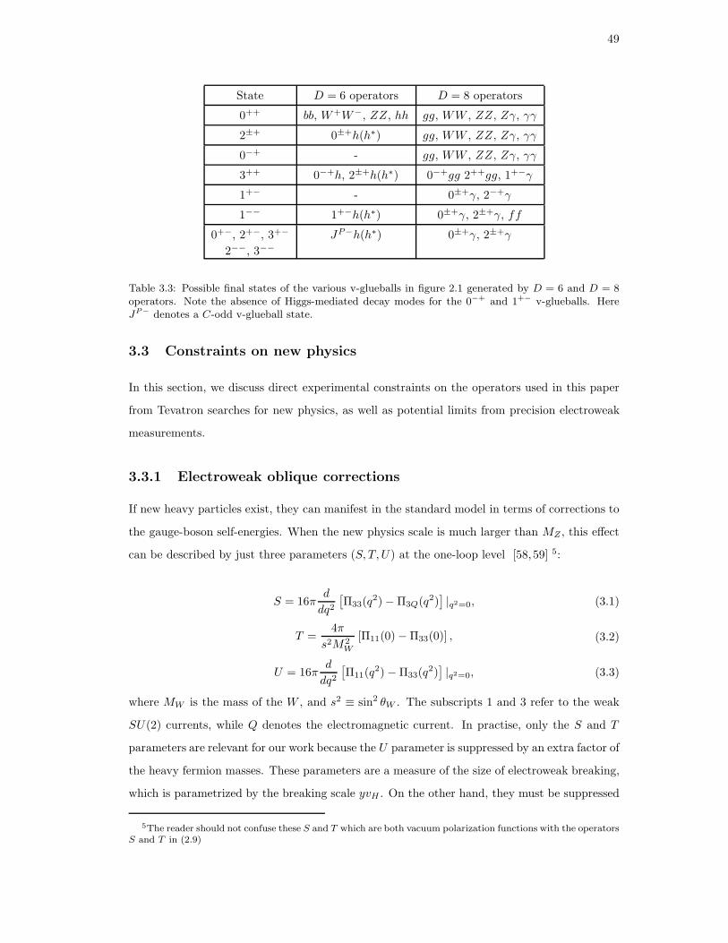
49
State D = 6 operators D = 8 operators
0++ bb, W+W−, ZZ, hh gg, WW , ZZ, Zγ, γγ
2±+ 0±+h(h∗) gg, WW , ZZ, Zγ, γγ
0−+ - gg, WW , ZZ, Zγ, γγ
3++ 0−+h, 2±+h(h∗) 0−+gg 2++gg, 1+−γ
1+− - 0±+γ, 2−+γ
1−− 1+−h(h∗) 0±+γ, 2±+γ, ff
0+−, 2+−, 3+− JP−h(h∗) 0±+γ, 2±+γ
2−−, 3−−
Table 3.3: Possible final states of the various v-glueballs in figure 2.1 generated by D = 6 and D = 8operators. Note the absence of Higgs-mediated decay modes for the 0−+ and 1+− v-glueballs. HereJP− denotes a C-odd v-glueball state.
3.3 Constraints on new physics
In this section, we discuss direct experimental constraints on the operators used in this paper
from Tevatron searches for new physics, as well as potential limits from precision electroweak
measurements.
3.3.1 Electroweak oblique corrections
If new heavy particles exist, they can manifest in the standard model in terms of corrections to
the gauge-boson self-energies. When the new physics scale is much larger than MZ , this effect
can be described by just three parameters (S, T, U) at the one-loop level [58, 59] 5:
S = 16πd
dq2[
Π33(q2)−Π3Q(q
2)]
|q2=0, (3.1)
T =4π
s2M2W
[Π11(0)−Π33(0)] , (3.2)
U = 16πd
dq2[
Π11(q2)−Π33(q
2)]
|q2=0, (3.3)
where MW is the mass of the W , and s2 ≡ sin2 θW . The subscripts 1 and 3 refer to the weak
SU(2) currents, while Q denotes the electromagnetic current. In practise, only the S and T
parameters are relevant for our work because the U parameter is suppressed by an extra factor of
the heavy fermion masses. These parameters are a measure of the size of electroweak breaking,
which is parametrized by the breaking scale yvH . On the other hand, they must be suppressed
5The reader should not confuse these S and T which are both vacuum polarization functions with the operatorsS and T in (2.9)
50
by the mass scale M in the limit M → ∞. Therefore even if one introduces heavy fermions
with extremely large couplings, their contributions to the S, T and U parameters can become
small at least in the limit M ≫ yvH . This leaves ample available parameter space within which
extra vector-like fermions are in agreement with all experimental constraints.
In this section, we analyze how current limits on S and T from precision electroweak fits
can be used to obtain constraints on the mass splittings of heavy fermions. To calculate S and
T , we use exact one-loop expressions for the gauge-bosons self-energies which are valid for all
values of the new vector-like fermion masses.
Our scenario contains three vector-like fermion fields, one doublet and two singlets of
SU(2)L, transforming under the fundamental representation of SU(nv),
ψq =
QU
QD
ψu = U ψd = D (3.4)
with hypercharge Y , Y + 1/2 and Y − 1/2, respectively. We will make our computations using
the above quark-like fermions. With a simple modification, our results can be readily applied
to the case in which the fermions have lepton quantum numbers.
The full fermionic Lagrangian is given by
L = ψq(Dµγµ +mq)ψq + ψu(Dµγ
µ +mu)ψu + ψd(Dµγµ +md)ψd+
+ (yuψqHψu + ydψqHψd + h.c.) (3.5)
where mq, mu and md are Dirac masses. For simplicity we have assumed that the mass matrix
is symmetric and real, but complex masses may be present as well. Finally, the covariant
derivative is
Dµ = ∂µ − igTaWaµ − ig′Y Bµ. (3.6)
When the Higgs acquires an expectation value 〈H〉 =
0
v
, off-diagonal mass terms are
induced for ψq, ψu and ψd
Mu =
mq yu v
yu v mu
Md =
mq yd v
yd v md
(3.7)
The mass matrix M is diagonalized by
ψ1
ψ2
=
c1 s1
−s1 c1
Qu
ψu
ψ3
ψ4
=
c2 s2
−s2 c2
Qd
ψd
(3.8)

51
where c1 = cosφ1, s1 = sinφ1, c2 = cosφ2, s2 = sinφ2 with
tan 2φ1 =2yuv
mq −mutan 2φ2 =
2ydv
mq −md. (3.9)
The corresponding eigenvalues are given by
m1,2 =1
2
(
mq +mu ±√
(mq −mu)2 + 4y2u
)
(3.10)
m3,4 =1
2
(
mq +md ±√
(mq −md)2 + 4y2d
)
(3.11)
with the following inverse relations,
mq = c21m1 + s21m2 = c22m3 + s22m4 (3.12)
mu = s21m1 + c21m2
md = s22m3 + c22m4
2 yu v = (m1 −m2) sin 2φ1
2 yd v = (m3 −m4) sin 2φ2.
These expressions now permit the evaluation of the S and T parameters as follows,
S =nvNc
3π
−c21
2(Y +
s212) logm2
1 −s212(Y +
c212) logm2
2 +c222(Y − s22
2) logm2
3+
+s222(Y − c22
2) logm2
4 +3c21s
21
8Π
′
(0,m1,m2) +3c22s
22
8Π
′
(0,m3,m4)
(3.13)
T =nvNc
8πs2M2W
c21c22Π(0,m1,m3) + c21s
22Π(0,m1,m4) + s21s
22Π(0,m2,m4)+
+s21c22Π(0,m2,m3)− c21s
21Π(0,m1,m2)− c22s
22Π(0,m3,m4)
(3.14)
where the functions Π(0,m1,m2) and Π′(0,m1,m2) are given by
Π (0,m1,m2) =1
m21 −m2
2
(
−m41 + 4m3
1m2 + 4m31(m1 − 2m2) logm1 − 4m1m
32+
+4m32(2m1 −m2) logm2 +m4
2
)
(3.15)
Π′
(0,m1,m2) =2
9(m21 −m2
2)3
(
−12m31(m
31 − 3m1m
22 + 3m3
2) logm1+
+12m32(3m
31 − 3m2
1m2 +m32) logm2+
+(m21 −m2
2)(2m41 + 9m3
1m2 − 16m21m
22 + 9m1m
32 + 2m4
2))
. (3.16)
In this context, the S and T parameters are a measure of the deviation of the heavy particles
from the pure Dirac mass case. When the couplings yr are turned off, the custodial SU(2)c and

52
isospin SU(2)L symmetries are restored, and both S and T vanish. To see this in more detail,
we can expand the S and T parameters in powers of (m1−m2)/(m1+m2), (m3−m4)/(m3+m4).
If mq = mu = md =M ≫ yuv, ydv we obtain,
S =Nc nv v
2[
(11 + 20Y )y2u + (11− 20Y )y2d]
30πM2(3.17)
T =Nc nv v
4 (y2u − y2d)2
40π s2W M2W M2
. (3.18)
where sW = sin θW and MW is the mass of the W boson. Then we see that S, T → 0 when
yu, yd → 0, i.e., m2 → m1 and m4 → m3 . The corresponding formulas for the lepton-like
fermion case can be obtained by substituting yu → 0, yd → yl, Nc → 1 in equations (3.17) and
(3.18).
Figure 3.2: The bounds at 95% CL on the (M,y) parameters from constraints on the oblique parameters(S, T ) for nv = 2, 3, 4 and two different regimes: ρr ≈ 1 (y =
√7yl) (Left panel), and ρd = ρu = ρq ≫
ρl = ρe ≈ 1(y = yl) (Right panel). The upper-left region is excluded in these plots.
Fits of the combined electroweak data provide constraints on the S and T parameters and
have been obtained in many places. Here we use the results from the PDG fits. The standard
model is defined by (S, T ) = (0, 0) with mt = 170.9 GeV and mH = 115 GeV. The best fit to
data is (without fixing U = 0)
S = −0.10± 0.10 (3.19)
T = −0.08± 0.11. (3.20)
These equations then imply the bounds S ≤ 0.10 and T ≤ 0.13 at 95% CL. From the ex-
perimental data, we can readily find the constraints on the parameters of the model. For
example, for lepton-like fermions, if we take Y = −1/2 and m1 = 1 TeV, then S ∼ 0.01y2l nv
and T ∼ 0.08y4l nv. Notice that the small value of S leads to only mild constraints on yl and
nv. By constrast, the parameter T provides the most stringent bounds.

53
There is, however, one important effect that can mitigate the contribution to T . From
(3.18), we see that electroweak corrections to the T parameter are insensitive along the yu = yd
direction in the parameter space, where the isospin symmetry is restored. In this case, the only
constraints on the yu and yd contributions to y are given by the S parameter, which, as we have
just seen, are less stringent.
In figure 3.2 we show the bounds on y at the 95% C.L. from the X particles in table 3.1
as a function of the mass scale M and for nv = 2, 3, 4. For illustration, we have considered
yu = yd = yl and two different regimes: the degenerate case, ρr ≈ 1, (Left panel) and the non-
degenerate case, ρd = ρu = ρq ≫ ρl = ρe ≈ 1, (Right panel). In this case, one has y =√7yl
and y = yl for the degenerate and non-degenerate cases, respectively, (cf. (3.3)). Since yu and
yd are unconstrained by T along the yu = yd line, and the limits from S are less severe, the only
bound we can obtain on y comes from the most stringent bound on yl due to the T parameter.
We then see that typical values M ≃ 1, 1.5 TeV and y ≃ 1 are permitted for nv = 2. For larger
values of nv, the allowed split between the mass eigenstates is smaller, but still large enough
that a coupling y ≃ 0.5 is not unreasonable.
To summarize, we conclude that for a sufficiently large range of the parameters the fit to
electroweak observables is in agreement with the existence of extra vector-like fermions. This
parameter space is characterized by
ρr ≈ 1 : y . 1.2− 1.6
ρd = ρu = ρq ≫ ρl = ρe : y . 0.6− 1.2 (3.21)
together with the current direct search limits
Ml,Me & 200 GeV
Mq,Mu,Md & 250 GeV. (3.22)
3.4 Numerical analysis
An interesting feature of the pure-glue hidden valley is that the v-glueballs can have many decay
modes, depending on their quantum numbers and on the values of the various parameters. To
give a general survey of decays is beyond the scope of this work, since a more detailed treatment
would have to incorporate precise values of the matrix elements which at present are unknown.
However, a few examples are useful to illustrate the main qualitative features of v-glueball
decays.

54
3.4.1 Decay patterns of v-glueballs
The relevant parameter space consists of the mass scale M , the 0++ mass m0, the coupling y
and the Higgs mass mH . Here we present our results in terms of m0 which is more transparent
than the confining scale Λv, since m0 is the relevant parameter for LHC studies. To simplify
the discussion in the SM, it is convenient to assume that the Higgs boson is SM-like and fix its
mass to be mH = 120 (“low mass” range) or mH = 200 GeV (“high mass” range). Moreover,
since the branching ratios depend on M and y only through the combination yM , our problem
is reduced to a two-dimensional parameter space described by yM and m0.
For our estimates below, we will use the lattice results [25] 6
4παvFS0++ = 3.06m3
0, FT2++ = 0.03m3
0 (nv/3), 4παvFP0−+ = 0.83m3
0. (3.1)
We also need estimates of the other v-glueball decay constants and transition matrix elements,
which at this point are unknown. A reasonable educated guess is that they are of order FT2++ ,
which is the only known decay constant that is largely independent of the size of the v-glueballs.
We can also guess MΩ1−−0++ ∼ 1/FS
0++, as it would be true for pion emission. In the following,
we will therefore assume
FL2±+ =
nv
3M
S(i)
2++0++m0 ≃ FT2++ , M
S(i)
1−−1+−m1+− =
√
nv
3MΩ
1−−0++ ≃ nv
3m6
0/FS0++ .
(3.2)
Later in this section, we will comment on how large deviations from this guess might affect our
estimates.
Using the decay rates expressed in section 3, we identify Γ(6) and Γ(8) as the summed
contributions to the decay rates from dimension-six and dimension-eight operators, respectively.
The corresponding branching ratios are denoted byBR(6) andBR(8), satisfyingBR(6)+BR(8) =
1. To illustrate the dependence of the branching fractions on yM and m0, we present in figures
3.3 and 3.4 contours of constant BR(6) in the m0 vs yM plane for various choices of v-glueball
states and mH = 120 GeV, 200 GeV. In figure 3.3, we see that the values of BR(6)0++ are large
over most of the parameter space plane, except at very low yM . By contrast, the values of
BR(6)2++ are small, except for a small region at large yM . The most interesting decay pattern is
found in the 1−− v-glueball. We see that BR(8)
1−− typically dominates when m1−− −m1+− < mH
6Here the coupling constant 4παv is included alongside FS
0++ and FP
0−+ to make them renormalization
invariant so that there is no question at which point 4παv is normalized. On the contrary, FT
2++ is renormal-ization invariant as is, since it is the matrix element of the energy-momentum tensor which is known to be scaleinvariant. Also, since the values reported in [25] are not expressed in a continuum renormalization scheme, wehave converted g2FT
2++ to FT
2++ using the value of the lattice parameter β = 6/g2 = 3.2 as an approximation
to the continuum limit.

55
and the emitted Higgs boson is off-shell, whereas BR(6)1−− dominates when m1−− −m1+− > mH
and the emitted Higgs boson is on-shell. An analogous behaviour is found for mH = 200 GeV,
as demonstrated in figure 3.4.
Figure 3.3: Curves of constant branching ratio BR(6) in the parameter space (m0, yM) for variousrepresentative states and mH = 120 GeV. Left: 0++, Center: 2++, Right: 1−−.
Figure 3.4: Same as figure 3.3 for mH = 200 GeV.
The values of yM determine to a large extent the decay pattern of v-glueballs with three
distinctive energy regions: (i) yM ≪ 1 TeV, (ii) yM ≫ 1 TeV and (iii) yM ≈ 1 TeV. Recall
that these ranges of parameters are further constrained by existing experimental limits, as
described in section 4. As will be discussed below, the common feature of all these different
regimes is the great diversity of decay modes and lifetimes, even for a given choice of parameters.
(i) yM ≪ 1 TeV. For sufficiently small yM , the contribution of the dimension-six operators
can be effectively disregarded and, hence, the dimension-eight operators have the largest effects
on v-glueball decays. As shown in [19], annihilation decays dominate the 0++, 2++, 0−+ and
2−+ v-glueballs. Their branching ratios are dominated by decays to gg, with decays to γγ having
a branching fraction of ∼ 0.4%, assuming the X fields form complete SU(5) multiplets of equal

56
mass. If the colored particles are much heavier than the uncolored particles, then decays to
electroweak bosons and photons can dominate. Most other states decay by radiatively emitting
a photon, or a Z boson. In addition, the 1−− state can also decay to standard model fermions via
an off-shell γ or Z. The 3++ state is special in that its three-body decay mode 3++ → 0++gg
could be of the same rate as the radiative 3++ → 1+−γ decay. The clearest signatures for
this regime are likely to be the two-photon resonances from the prompt annihilation decays
of C-even v-glueballs. In addition, for part of the parameter space, the v-glueballs are rather
long-lived particles, so that they produced displaced vertices in the detectors, which can be an
experimentally challenging, but certainly important signature.
(ii) yM ≫ 1 TeV. In this case, the Higgs couplings to v-glueballs dominate over all other
couplings. As a result, the decay pattern is relatively simple. In the PC = ++ sector, we
find that the 0++ v-glueball annihilates directly into pairs of standard model particles via
0++ → h∗ , with the same final states and branching fractions of a Higgs boson with mass
m0. For m0 > 2mh, the mode 0++ → hh opens up, in addition to 0++ → h∗, contributing
20 − 25% to the total width with the decays into weak boson and top quark pairs accounting
for the remaining 75 − 80%. The 2++ v-glueball decays predominantly to the lighter 0++
by radiatively emitting a Higgs boson. In the PC = −+ sector the lightest states are the
0−+ and 2−+ v-glueballs. The 2−+ v-glueball decays in a similar way to the 2++, with the
rate dominated by 2−+ → 0−+h. Although the 2−+ v-glueball is heavier than the 0++, the
2−+ → 0++h decay is not allowed, due to parity and conserved angular momentum. The 0−+
v-glueball is a special case. Without explicit breaking of parity, the 0−+ v-glueball decays slowly
into gg via dimension-eight operators.
Turning to the PC = +− sector, we find that most of the states can decay by emission of a
Higgs boson, through processes of the form Θκ → Θκ′h, where Θκ, Θκ′ denote two v-glueballs
with given quantum numbers. Since C-changing transitions are not allowed by the S operator,
the v-glueballs in that sector typically undergo a cascade decay, radiating a Higgs boson at
each step, which ends at the lightest 1+− state. The v-glueballs in the PC = −− sector decay
in a similar manner, with the lightest 1−− v-glueball decaying to the 1+− v-glueball with the
emission of a Higgs boson. Since the 1+− v-glueball is not permitted to decay via dimension-six
operators, its dominant decay modes are photon-radiative transitions to C-even v-glueballs, as
in (i).
We should note that this theoretical regime may be difficult to access in practice. For the
2++ v-glueball (and hence the 2−+), this requires yM & 10 TeV (see figures 3.3 and 3.4). As

57
Figure 3.5: The branching ratios of the 0++ v-glueball as a function of m0 for yM ∼ 1 TeV. Left Panel:mH = 120 GeV. Right Panel: mH = 200 GeV. For clarity, only the main decay modes are shown.
shown in (3.21), the heavy mediators can at most have Yukawa couplings y ∼ 1 in order to avoid
potentially dangerous electroweak corrections. With M ∼ O(10 TeV), the rate for production
of v-glueballs (∝ σgg→XX ≪ 1fb) is rather small, rendering this region of parameter space
experimentally inaccessible to the future experiments at the LHC.
(iii) yM ≈ 1 TeV. For Higgs couplings with intermediate strength, the v-glueball decay
pattern is more complicated because the couplings to the gauge bosons become important,
leading to a interesting interplay between dimension-six and dimension-eight operators. From
the point of view of prospective experiments at the LHC, this is also the most interesting regime,
due to the diversity of v-glueball decay channels and variability of lifetimes as well.
The 0++ v-glueball still decays predominantly to pairs of standard model particles via 0++ →
h∗ or, if kinematically allowed, 0++ → hh. The branching ratios for the main decay channels
of the 0++ v-glueball are shown in figure 3.5 for yM = 1 TeV in the cases of mH = 120 GeV
and mH = 200 GeV.
For the 2++ and 2−+ v-glueballs, the dominant decay mode is gg. This is because the 2±+ →
0±+h(h∗) decay is phase-space suppressed by a 10−8 − 10−3 factor. For m2++ −m0++ > mH ,
the phase space suppression is smaller ∼ 0.01, but in this regime the (m2++/M)4 suppression
of D = 8 operators is inefficient, rendering the D = 6 operators subdominant.
The dominant decay modes of the 1−− v-glueball are transitions with a Higgs boson in the
final state, 1−− → 1+−h, for m1−− − m1+− > mH or, photon-radiative decays to the lighter
v-glueballs in the C-odd sector for m1−− −m1+− < mH . The decays of the other v-glueballs in
the C-odd sector proceed in a similar fashion. In addition, the decay of the 1−− v-glueball into
fermion pairs can play a significant role for m1−− −m1+− < mH .
Since the 1+− and 0−+ v-glueballs cannot decay via their couplings to the Higgs boson, their
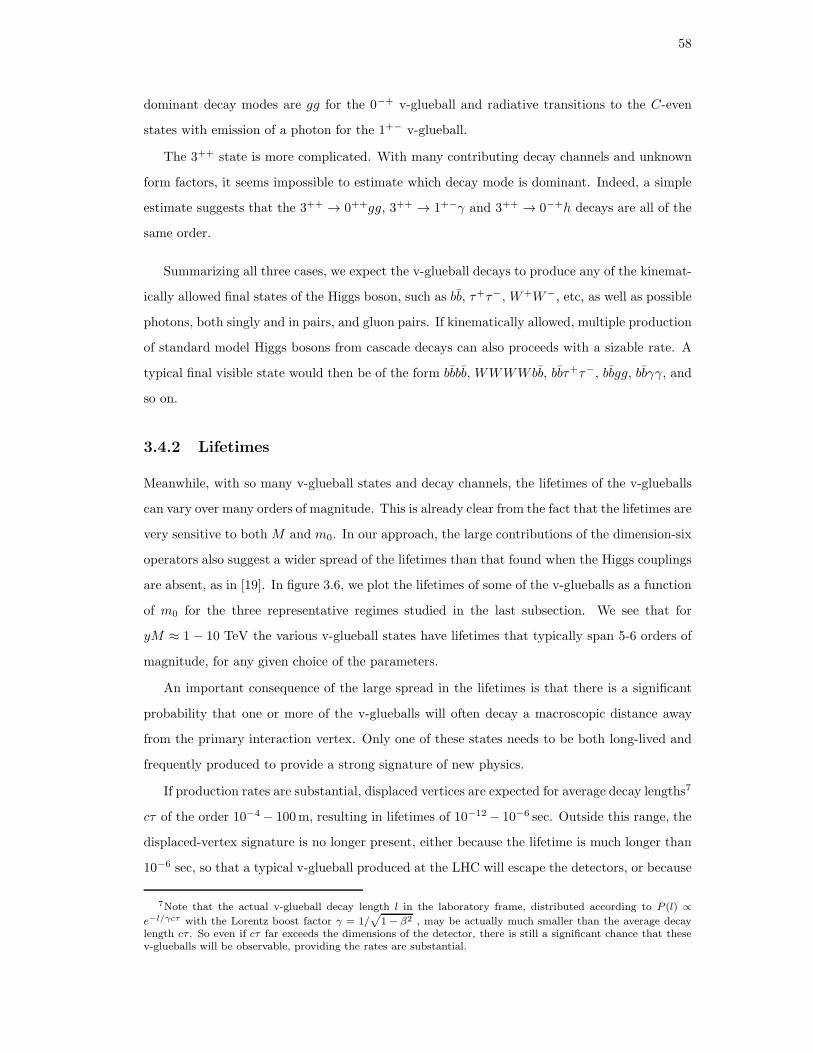
58
dominant decay modes are gg for the 0−+ v-glueball and radiative transitions to the C-even
states with emission of a photon for the 1+− v-glueball.
The 3++ state is more complicated. With many contributing decay channels and unknown
form factors, it seems impossible to estimate which decay mode is dominant. Indeed, a simple
estimate suggests that the 3++ → 0++gg, 3++ → 1+−γ and 3++ → 0−+h decays are all of the
same order.
Summarizing all three cases, we expect the v-glueball decays to produce any of the kinemat-
ically allowed final states of the Higgs boson, such as bb, τ+τ−, W+W−, etc, as well as possible
photons, both singly and in pairs, and gluon pairs. If kinematically allowed, multiple production
of standard model Higgs bosons from cascade decays can also proceeds with a sizable rate. A
typical final visible state would then be of the form bbbb, WWWWbb, bbτ+τ−, bbgg, bbγγ, and
so on.
3.4.2 Lifetimes
Meanwhile, with so many v-glueball states and decay channels, the lifetimes of the v-glueballs
can vary over many orders of magnitude. This is already clear from the fact that the lifetimes are
very sensitive to both M and m0. In our approach, the large contributions of the dimension-six
operators also suggest a wider spread of the lifetimes than that found when the Higgs couplings
are absent, as in [19]. In figure 3.6, we plot the lifetimes of some of the v-glueballs as a function
of m0 for the three representative regimes studied in the last subsection. We see that for
yM ≈ 1 − 10 TeV the various v-glueball states have lifetimes that typically span 5-6 orders of
magnitude, for any given choice of the parameters.
An important consequence of the large spread in the lifetimes is that there is a significant
probability that one or more of the v-glueballs will often decay a macroscopic distance away
from the primary interaction vertex. Only one of these states needs to be both long-lived and
frequently produced to provide a strong signature of new physics.
If production rates are substantial, displaced vertices are expected for average decay lengths7
cτ of the order 10−4 − 100m, resulting in lifetimes of 10−12 − 10−6 sec. Outside this range, the
displaced-vertex signature is no longer present, either because the lifetime is much longer than
10−6 sec, so that a typical v-glueball produced at the LHC will escape the detectors, or because
7Note that the actual v-glueball decay length l in the laboratory frame, distributed according to P (l) ∝e−l/γcτ with the Lorentz boost factor γ = 1/
√
1− β2 , may be actually much smaller than the average decaylength cτ . So even if cτ far exceeds the dimensions of the detector, there is still a significant chance that thesev-glueballs will be observable, providing the rates are substantial.

59
the decays are prompt and the v-glueball decay lengths cannot be resolved.
As shown in figure 3.6, displaced vertices could be observed for 10 GeV . m0 . 200 GeV
and 0 . yM . 1 TeV or for 10 GeV . m0 . 400 GeV and yM ≫ 1 TeV. As long as m0
becomes greater than about 400 GeV, all v-glueball decays will be prompt and the displaced-
vertex signature will be absent. In the case yM ≈ 0 the 1+− and 1−− v-glueball lifetimes reach
values high enough for displaced vertices for m0 between 50 GeV and 150 GeV. The 0++, 0−+,
2++ and 2−+ v-glueballs may also decay with displaced vertices in the very low mass range
m0 . 70 GeV. On the other hand, in the case yM ≈ 10 TeV the spread in the lifetimes is two
or three orders of magnitude larger, so even larger v-glueball masses 150 GeV < m0 < 400 GeV
may allow for displaced vertices. This is the case of the 2++ and 2−+ v-glueballs, as shown in
the middle panel of figure 3.6. Their lifetimes are so long that these v-glueballs may escape the
detectors for m0 . 100 GeV. In the low mass range 50 GeV < m0 < 200 GeV other v-glueballs
such as the 1+− and 1−− also have a significant chance to decay with displaces vertices. In
this case, the 0++ and 2++ v-glueballs will remain short-lived over most of the parameter space
down to masses of order 50 GeV where displaced vertices may start to occur for these states as
well. Finally, the case yM ≈ 1 TeV shown in the right panel of figure 3.6 is an example of an
intermediate situation, with the 0++ v-glueball being short-lived, except for very-low masses
m0 . 50 GeV, and at least five states having a chance to decay with displaced vertices in some
part of the parameter space: the 1+− and 1−− v-glueballs for m0 . 200 GeV, and the 2++,
2−+ and 0−+ v-glueballs for 20 GeV . m0 . 100 GeV.
From the analysis above it is quite evident that long-lived resonances are a common feature
of pure-glue hidden valleys for an ample range of parameters. Nonetheless, detecting long-lived
particles presents several experimental challenges. Displaced jets, though they have no stan-
dard model background, suffer from substantial detector backgrounds from secondary vertices
inside the detector material. On the other hand, displaced leptons are technically easier, and
have much less background, but branching ratios to leptons are usually quite small. Displaced
photons also present several experimental challenges, since one has to detect not only the posi-
tion where the photons enter the electromagnetic calorimeter but also their angle of incidence.
Thus the issue of detecting displaced vertices is not straightforward, and requires novel analysis
strategies.
Interestingly enough, the v-glueball masses can be as low as a few GeV’s and at the same
time the lifetimes could be short enough that a few v-glueball events could be observed at the
LHC. Specifically, let us examine closely the case of the scalar 0++ v-glueball. From (3.2) we

60
Figure 3.6: Lifetimes of the v-glueballs as a function of the v-glueball mass scale m0 for three rep-resentative regimes: yM ≈ 0 (Left panel), yM ≈ 10 TeV (Middle panel), and yM ≈ 1 TeV (Rightpanel).
see that for X particles of order 1 TeV the lifetime of the 0++ v-glueball is of order
cτ ∼ 1cm
(
M
1 TeV
)4(20 GeV
m0
)7(5 GeV
mb
)2(
1−4m2
f
m20
)−1.5
. (3.3)
We see that for m0 & 10 GeV the 0++ state can decay inside the detector. It is important to
remark that even for cτ well above 10 meters, a significant fraction of the v-glueballs will still
decay inside the detector. If detector backgrounds are sufficiently low, and production cross-
section is substantial, discovery would also be possible, in principle, for states in the low-mass
range 1 GeV . m0 . 10 GeV.
3.4.3 Uncolored X particles
If there is a substantial hierarchy between the coloredX particles and the uncoloredX particles,
the latter may dominate v-glueball decays. Decay rates to a pair of SM gluons in the C-even
sector are proportional to the coefficients χ23 (3.12), which would be suppressed. If the particles
carrying QCD color are heavier by factors of 2 or more, the hierarchy of decay rates changes,
as χ23/χ
2γ ∼ 10−2 − 10−4. In this case, decays to gluons no longer dominate the partial widths
Γ(8) for the C-even states. Also, the regime for m0 and yM in which Γ(8) dominates over Γ(6)
is somewhat reduced. Without any detailed computation, we may infer from figures 3.3 and 3.4
that the decays of the 0++ v-glueball, with its large branching fraction to off-shell Higgs boson,
will not be much affected. For m0− < 2mW , the dominant decay mode of the 0−+ v-glueball
is now γγ with a branching ratio of 90% with the decays into gg and Zγ accounting for the
remaining 10%. In the high mass range m0− > 2mW , the 0−+ v-glueball decays dominantly
into WW with a branching ratio of ∼ 70% followed by the decays into ZZ, γγ and Zγ with
branching ratios of 20%, 5% and 5%, respectively. Also, the lifetime of the 0−+ v-glueball
is longer. For the 2++ and 2−+ v-glueballs, the decays into photon pairs typically dominate

61
for m2±+ −m0±+ < mH , while the Higgs-radiative transitions 2±+ → 0±+h can dominate for
m2±+ −m0±+ > mH . The decays of the v-glueballs in the C-odd sector are largely unaffected.
We will comment further in the conclusions and in our LHC study [60], but suffice it to say that
the fact that the annihilation into photon pairs may dominate the lifetimes of some v-glueballs
(the 0−+, 2++, 2−+) has important consequences for experimental searches.
3.4.4 Uncertainties in the v-glueball matrix elements
In another respect, we should emphasize that even though our estimates are in general robust,
they are subject to significant uncertainties, due especially to the many unknown v-glueball
matrix elements. Although lattice computations are at present not available, it is of interest to
see what one might expect once lattice computations are incorporated. Of course, the decays
of the 0++ v-glueball will remain unchanged, since its branching ratios are independent of the
decay constant Fs0+ . The same is true for the 1+− and 0−+ v-glueballs. On the contrary,
the decays of the 2++ and 1−− v-glueballs depend on ratios of the unknown non-perturbative
matrix elements,
r2+ =MS
2++0++m0
FT2++
r1− =MS
1−−1+−m1+−
MΩ1−−0++
. (3.4)
Since there is no reason for the form factors MS2++0++ and MS
1−−1+− to be significantly sup-
pressed or enhanced at k2 = m2H , the ratios r2+ and r1− are probably of order O(1) (actually
somewhat smaller8, especially at large nv). To illustrate the possible range of impact lattice com-
putations may lead to, we can simply make the rescaling yM → yM√r2+ and yM → yM
√r1−
in figure 3.3. One can see that when r2+ is varied by a factor of 10 in both directions around
r2+ ∼ 1 for yM ∼ 1 TeV, the ratio BR(6)2+ changes by around 10 − 20%, and the dominant
mode of the 2++ v-glueball is still gg. A similar conclusion is obtained for the 2−+ v-glueball.
For the 1−− v-glueball, in contrast to the 2++ and 2−+, the branching ratios are more uncer-
tain. The reason is that the contributions from D = 6 and D = 8 operators are comparable
in strength, so a small enhancement in one of the matrix elements can lead to a large effect
on the branching ratios. For r1− ∼ 0.1, the photon-radiative decay gets enhanced very greatly
and could dominate the branching ratio in most of the mass range, while r1− ∼ 10 tends to
enhance the Higgs-radiative decay. Therefore, additional lattice computations would be needed
to distinguish between these two modes. Fortunately, it turns out that the impact of precise
lattice computations on the phenomenology of the lightest v-glueballs 0++, 2++, 0−+ and 2−+,
8Using standard large-nv counting rules and taking into account explicit factors of 1/√nv in the coupling
constant, one obtains r2+ ∼ O(1/nv) and r1− ∼ O(1/√nv); see (3.2).

62
which, as will be argued in our LHC study, are probably the most copiously produced, is in
general very mild.
3.5 Other extensions
In this section, we consider two simple extensions that may alter the phenomenology of v-
glueballs in a number of ways, with a special emphasis on the 0−+ and 1+− v-glueballs. Firstly,
we analyze the two Higgs doublet model (2HDM), which is the simplest extension of the standard
model Higgs sector, and secondly, we study the possibility of CP violation in the theory and
its implications for v-glueball decays. We will not attempt to systematically compute all the
decay rates, but simply point out a few salient features of these extensions.
3.5.1 2HDM
As in the MSSM, we consider the SM with two Higgs doublets Hu and Hd, where Hu only
couples to up-type quarks and neutrinos and Hd only couples to down-type quarks and leptons.
In this model, there are five physical Higgs bosons: two charged scalars (H±); two neutral
scalars (H and h); and a neutral CP -odd scalar (A). The presence of the CP -odd scalar A is
of particular interest. Since the A is CP -odd, a gauge invariant CP -conserving coupling to the
v-gluons must be of the form ǫµναβtr FµνFαβAΦ, with Φ = 1, H, h. Because of this coupling,
new possible decays of the pseudoscalar 0−+ state emerge in the 2HDM. These are
0−+ → A∗ → ff, (3.1)
0−+ → HA, (3.2)
0−+ → hA (3.3)
0−+ → 0++A. (3.4)
For all other v-glueballs, there are new contributions to their decays in the 2HDM, but the decay
pattern as described in sections 3 and 5 remains basically unchanged. For the 0++ v-glueball,
the new channels include 0++ → hh,Hh,AA as well as the off-shell Higgs decay 0++ → h∗. For
all other states, new decay modes arise from the processes Θκ → Θκ′φ, where now φ = H,h,A.
Recall that in the single-Higgs model, the lowest-dimension operators that can induce decays
of the 1+− v-glueball arise at mass dimension eight. A similar conclusion applies to the 1+−
v-glueball in the context of the 2HDM. Therefore, while the CP -odd scalar A makes a drastic
change on the 0−+, it does not affect the 1+− v-glueball.

63
To estimate the effect of the CP -odd scalar A on the branching ratios, we will need to find
the effective Lagrangian. Using the basic results of section 2, the effective Higgs couplings to
v-gluons, induced at one-loop by the X particles, is given by
L(6) =αv
3πM2
[
y2uH†uHu + y2dH
†dHd
]
tr FµνFµν+
+αv
2πM2
[
y2d
(
Hd −H∗d
2i
)†(Hd +H∗
d
2
)
+ y2u
(
Hu −H∗u
2i
)†(Hu +H∗
u
2
)
]
tr FµνFµν . (3.5)
Here yu and yd represent the couplings of the X particles to the Higgs doublets Hu and Hd,
respectively. The couplings of the physical Higgs bosons to v-gluon pairs are readily obtained
by including the appropriate mixing angle factors
L(6) =αv
6πM2
(
ξHHH2 + ξhhh
2 + ξHhHh+ ξAAA2)
tr FµνFµν +αv vH2πM2
ξAA tr FµνFµν
+αv vH3πM2
(ξHH + ξhh) tr FµνFµν +αv
4πM2(ξAHAH + ξAhAh) tr FµνFµν (3.6)
where the coeffients ξij and ξi are given by
ξHH = y2us2α + y2dc
2α ξhh = y2uc
2α + y2ds
2α ξHh = 2sαcα(y
2u − y2d)
ξAH = y2usαcβ − y2dcαsβ ξAh = y2ucαcβ + y2dsαsβ ξAA = y2uc2β − y2ds
2β
ξH = y2usαsβ + y2dcαcβ ξh = y2ucαsβ − y2dsαcβ ξA = sβcβ(y2u − y2d) (3.7)
where α the mixing angle and the ratio of the vacuum expectation values tanβ = vu/vd. The
combination v2d + v2u is fixed by the electroweak scale vH =√
v2d + v2u = 246 GeV.
The decay rates can be readily extracted from our general results in section 3 by replacing
y2 with the appropriate couplings in (3.7). For the scalar 0++ state, the decay rates for the
off-shell Higgs decay 0++ → H∗/h∗ → ζζ can be read from (3.2) through the substitution
y2
m20 −m2
H
→ ξHm2
0 −m2H
+ξh
m20 −m2
h
, (3.8)
while the rate for the two-body decays 0++ → HH, hh, Hh, AA is obtained from (3.3) by
replacing
y2(
1 +3m2
Z
2(m20 −m2
H)
)
→ ξij +ξHgHij
m20 −m2
H
+ξhghij
m20 −m2
h
, (3.9)
where i, j = HH,Hh, hh,AA and gijk are the cubic self-couplings in the 2HDM. Likewise,
the width of the decays Θκ → Θ′κΦi, Φi = H,h,A, can be obtained from (3.9) and (3.10) by
substituting y2 → ξi. Finally, we summarize the rates for the new decay modes of the 0−+
v-glueball (3.1-3.4),
Γ0−+→ff =
(
ξA tanβ vH FP0+
2πM2(m2A −m2
0)
)2
ΓSMh→ff(m
20−) (3.10)

64
Γ0−+→0++A =1
16πm0−
(
MP0−0+ξA
2πM2
)2[
g(m2H ,m
2A;m
20−)]1/2 (3.11)
Γ0−+→AH =1
16πm0−
(
FP0−
2πM2
)2(
ξAH +3ξA
2(m20− −m2
A)
)2[
g(m2H ,m
2A;m
20−)]1/2
(3.12)
Γ0−+→Ah =1
16πm0−
(
FP0−
2πM2
)2(
ξAh +3m2
ZξA2(m2
0− −m2A)
)2[
g(m2h,m
2A;m
20−)]1/2
. (3.13)
The expressions above are clearly very model dependent. First, notice that for yu ≃ yd, ξA
is very small, and the decay rate of the 0−+ v-glueball is suppressed. On the other hand, for
yd ≃ 0, a quick check shows that this rate, whose ratio to the 0++ width is (for small masses
m0 < mh)
Γ0−+
Γ0++
≃ 0.5
(
sαm2
A
m2H
+ cαm2
A
m2h
)−2
, (3.14)
is not negligible. This ratio may be anywhere from ∼ 0.1 up to about 4 depending on the
mixing angle and the masses of the scalars. Unless the 0−+ decay rate is unduly suppressed,
the lifetimes of the 0++ and 0−+ v-glueballs are in general within one order of magnitude from
each other.
3.5.2 Models of explicit CP violation
It is of interest to see what one might expect once CP -violation effects are incorporated in the
theory, in the context of a single-Higgs model. For example, parity-violating interaction terms
can be induced in the effective Lagrangian if we assume that the couplings of the heavy particles
Xr to the Higgs boson are complex. In this case, a P -odd C-even interaction is generated of
the form H†H tr FµνFµν . As in the 2HDM, this interaction drastically changes 0−+ decays,
since without it, the 0−+ v-glueball would decay via dimension-eight operators, suffering an
extra suppression. The 0−+ v-glueball can then decay via 0−+ → h∗, producing any of the
kinematically-allowed final states of the Higgs boson.
Similarly, one can contemplate interactions that explicitly break C-invariance. Interestingly
enough, the lowest-dimension operators of this kind (e.g. H†HdabefcdeFaµνFb
µνFcαβFd
αβ) arise
at dimension ten and, therefore, their effects are extremely suppressed by extra powers of 1/M .
The dominant decay modes of the 1+− v-glueball are then induced by dimension-eight operators,
even if we allow for CP -violation.
In the rest of this section, then, we will focus on P -violating but C-conserving interactions.
To estimate the decay widths, let us consider the following Lagrangian, in two-component
notation,
Lmass = ydXqH†Xc
d + ydXcqHXd + h.c. (3.15)

65
where yd is a complex Yukawa coupling. By integrating out the Xq and Xd particles, we obtain
the following dimension-six operators9:
L(6) =αv (y
2 − y2)
3πM2H†H tr FµνFµν +
αv (2 y y)
πM2H†H tr FµνFµν . (3.16)
where y = Re yd and y = Imyd. Here Fµν = (1/2)ǫµνλσFµν denotes the dual of the field
strength tensor. The first term on the right-hand side of (3.16) is the same operator that we
had already found in (3.2). The second term of (3.16) is new and violates P . As mentioned
above, the P -odd interaction allows the pseudoscalar 0−+ state to decay into SM particles via
s-channel Higgs-boson exchange 0−+ → h∗ → ζζ, where ζ denotes a standard model particle.
The width of the decay is given by
Γ0−+→ζζ =
(
2yy vH αv FP0−
πM2(m2H −m2
0−)
)2
ΓSMh→ζζ(m
20−) (3.17)
where FP0− ≡ αv 〈0|tr FµνFµν |0++〉 is the 0−+ decay constant. The same operator also induces
the decay 0−+ → 0++h, with partial width
Γ0−+→0++h =1
16πm0−
(
2yy vH αv MP0−0+
πM2
)2[
g(m2H ,m
20+ ;m
20−)]1/2 (3.18)
where now MP0−0+ is the transition matrix. This decay is phase-space suppressed for m0−+ −
m0++ < mh, but may be quite significant for m0−+ − m0++ > mh when the radiated Higgs
boson is onshell. For example, for mh ∼ 100 GeV we obtain BR(0−+ → 0++h) ∼ 0.3.
In the SM, the most stringent limits on the size of the CP violation effects come from
experimental limits on the electric dipole moment of the neutron. The same experimental
constraints also allow us to place limits on the CP -violating operator in (3.16). To see this,
let us recall that the X particles can also carry QCD color. Then, the following dimension-six
operators are induced:
L(6) =αs (y
2 − y2)
3πM2H†H tr GµνG
µν +αs (2 y y)
πM2H†H tr GµνG
µν . (3.19)
where now Gµν denotes the SM gluon field strength tensor and Gµν its dual. The CP violating
term in (3.19) with the Higgs field replaced by its vacuum expectation value contributes to the
9The effective Lagrangian (3.16) can be evaluated either by following the procedure displayed in appendix Aor, equivalently, in the limit of vanishing Higgs momentum by taking derivatives of the v-gluon self-energy andthe axial anomaly:
L(6) = H†H/v2H (y2d∂2/∂y2d + y∗d
2∂2/∂y∗d2)L,
whereL = (αv/6π) ln(Λ
2UV /detM†M) tr FµνFµν + (αv/2πi) ln(detM/detM†) tr Fµν Fµν
with M =
(
M ydvHydvH M
)
.

66
θ angle. We assume that this contribution to the θ angle is removed by whatever mechanism
that solves the strong CP problem in QCD. The next operators in the expansion around the
Higgs VeV contain one or two powers of the Higgs field. Their contribution to the electric dipole
moment of the neutron can be estimated using Naive Dimensional Analysis [61, 62]. Following
the analysis of [63, 64], we estimate the neutron electric dipole moment as
dn =e
2πfπ
αs (2 y y)
4πM2
(2πfπ)2
(4π)2∼ 10−25e− cm × (2yy)αs
8π2× (1 TeV/M2). (3.20)
where 2πfπ ≃ 1190 MeV is the chiral-symmetry-breaking scale. Combining this result with the
current experimental bound on dn, we derive a limit on 2yy
|2yy| < 10× (M/1 TeV)2. (3.21)
Consequently, values for |y|, |y| in the range 0.01−1 are consistent with the existing experimental
limits.
3.6 Conclusions
In this work, we have investigated a particularly challenging hidden valley scenario with a
broader class of couplings to SM particles than those considered in [19]. In particular, we have
focused on the effect of dimension-six operators by which the hidden sector interacts with the
standard model through the Higgs sector.
The resulting v-glueball phenomenology is fairly complex in this scenario, but there are some
simple features. In particular, we find the following interesting signatures:
• Decays of the 0++ v-glueball through h∗, producing any of the kinematically-allowed Higgs
final states such as bb, τ+τ−, WW , etc.
• Multiple Higgs boson emission, from cascade decays Θκ → Θκ′h, or annihilations 0++ →
hh.
• Due to the diversity of v-glueball states, and the presence of operators of different mass
dimension, the lifetimes can vary at least over 5 or 6 orders of magnitude, for any given
choice of parameters (see figure 3.6). This has two immediate consequences: (i) Displaced
vertices are quite common, which could potentially serve as a discovery channel, and (ii)
v-glueballs can be as light as a few GeV’s and still be visible.
• For sufficiently small v-glueball masses, a different opportunity arises in the form of non-
standard Higgs decays such as h → ΘκΘκ′ , with branching ratio to v-glueballs of order
10−3 − 10−2.

67
In addition, other possible final states include gg, γγ, and radiative transitions with emission
of a photon, all of which are induced by dimension-eight operators [19]. The rare diphoton
channel is particularly interesting because, thanks to its moderate QCD background, it may
serve as the discovery channel for the v-glueballs at the LHC.
We should nevertheless emphasize that some of our results are subject to significant theoret-
ical and numerical uncertainties. In this respect, it would be interesting to know the spectrum
of pure-Yang-Mills theory for gauge groups other than SU(3), as well as the various v-glueball
matrix elements that arise. With enough motivation, such as a hint for discovery, these could
in principle be determined by additional lattice computations. If the v-sector gauge group is
not SU(nv), some of the v-glueballs may not be present; for instance, for SO(nv) or Sp(nv)
gauge groups the C-odd sector is absent or heavy. However, as explained in [19], the lightest
C-even v-glueballs are expected to be present in any pure-gauge theory, with similar production
and decay channels, so at least for them, the basic features of a pure-gauge hidden valley are
expected to be retained. We also have not considered higher-order corrections to the decay
rates, and they should be taken into account when precise predictions are required.
We have seen that the operators considered in this paper are not heavily constrained by
current experimental searches or precision electroweak data, thus leaving ample parameter space
to be explored by the next generation of hadron collider experiments. Application of our results
for phenomenological studies, particularly as relevant for the LHC, will be carried out in a
companion paper [60]. We expect that detection should be feasible, if the mass M of the X
particles is small enough to give a reasonable large cross-section, and Λv is large enough to
ensure the v-glueballs decay inside the detectors. Decays to bottom quarks and gluons often
dominate, but they suffer from a huge multijet background. At the Tevatron and at the LHC,
the v-glueballs are most likely to be found in searches for diphoton resonances in events with
2 photons plus jets or with 3 or more photons and possibly additional jets, or in searches for
displaced decays to jet pairs, W/Z pairs, or photon pairs. A potentially novel signature, which
could be currently searched for at the Tevatron, arises in the form of two b-tagged jets plus
diphoton events. Contrary to the models of [65–67], the branching ratio to bbγγ in our model
can be O(1), since the bb and γγ final states originate in different resonances, leading to a
potentially discoverable signal despite the background of 2j + 2γ. Altogether, these signatures
provide an interesting opportunity to search for new physics at the Tevatron and at the LHC,
which motivates further theoretical and experimental study.

68
Chapter 4
Phenomenology of quirkonia
The quirk limit has a splendid simplicity, largely devoid of all the complications of relativistic
quantum fields, in particular multiparticle production and pair creation. Recall that this theory
can be regarded as a certain limit of SU(nv) gauge theory with heavy quarks such that their
masses are much larger than the scale Λv where the gauge group SU(nv) becomes strong. One
of the reasons for its simplicity is absence of string breaking. Heavy quirks are confined by a
flux tube with energy per length unit of order Λ2v. Hence the v-color field contained in the flux
tube is too feeble to create a quirk-antiquirk pair: that would require an energy of order ∼ 2M
localized in a small region of radius ∼M i.e. an energy density ∼ M2 ≫ Λ2v. This mechanism
is indeed exponentially suppressed.
Furthermore, for sufficiently heavy quirks, one might hope that the characteristic time scale
associated with the motion of the constituents quirks inside the quirk mesons is much larger
than the time scale associated with the motion of the fast surrounding v-gluons [51]. In this
case the adiabatic approximation applies and the effect of the v-gluons can be represented by an
average instantaneous interaction potential V (r) between the heavy quirk sources. Moreover,
the bound state problem will become non-relativistic, and in the leading order in β the dynamics
will be controlled by the Schodinger equation,
− ~2
2µ∇2Ψ(r) + [V (r)− E] Ψ(r) = 0, (4.1)
where µ = m1m2/(m1 + m2) is the reduced mass of the system formed by the quirks with
masses m1 and m2, r is the distance between the quirks, V (r) is the interaction potential, E is
the energy eigenvalue, and Ψ(r) is the wave function.
In this work, we assume the quirk mass is in the phenomenologically interesting range
200 GeV . MX . 1 TeV that is not excluded by existing experiments but may be probed at
the LHC. The emphasis is on models in which the confining scale in the hidden valley sector,
Λv, is higher than about 5 GeV, where the v-glueballs produced in quirk annihilation and/or
relaxation may decay inside the detectors. Also, for simplicity, we will first consider the case of
colored quirks, which are expected to have a larger production cross section than the uncolored

69
ones unless the mass of the colored quirks is of order 3 times larger than that of the uncolored
ones. Then we will comment on the uncolored quirk case.
In this model, quirks can be copiously produced at the LHC via normal QCD interactions.
The subsequent evolution of the quirk-antiquirk pair is not familiar so we review it here [47–49].
It is easiest to first view the evolution in the center of mass frame. In that frame the quirks
simply oscillate back and forth between their classical turning points. The amplitude of the
oscillation can be approximately estimated as E/σ, where E is the energy given to the quirk
pair by the collision and σ is the string tension, or energy per unit length of the string, and
is about ∼ Λ2v. Eventually the oscillations will be damped. In the case of a high confinement
scale, two mechanisms are in principle responsible for energy lost. The first is emission of v-
glueballs. These can be modeled as bits of closed flux tube, with mass of order a few Λv and
size ∼ Λ−1v . Because v-glueballs have a non-perturbative, extended structure their coupling
constant to quirks is uncertain. But there is not much reason to expect it to be extremely
small, except perhaps the poor overlap between the wave functions of the initial and final quirk
states and the fact that v-glueball emission is suppressed by powers of 1/nv.
A second mechanism is emission of perturbative gluons. This mechanism appears to be
highly important, as it can effectively work to suppress quirk annihilation at high orbital angular
momentum waves. Other damping mechanisms may also be present, e.g. non-perturbative
hadron emission or radiative transitions with emission of a photon. But it is almost sure that
the oscillations will be highly underdamped.
When the quirk and antiquirk come near to rest they will annihilate. The annihilation can
be into SM gauge bosons and/or fermion pairs, but also into v-gluons, which at long distance
become two or more v-glueballs. The annihilation rate can be estimated using factorization,
as in the quarkonium system, where the decay rate is factored into a short-distance part that
is related to the annihilation rate of the heavy quirk and antiquirk, and a long-distance factor
containing all the nonperturbative effects of SU(nv) gauge theory. The short-distance factor
is calculated in terms of the running coupling constant αv(M) of SU(nv), evaluated at the
scale of the heavy quirk mass M , while the long-distance factor is expressed in terms of the
nonrelativistic quirk meson wavefunction, or its derivatives, evaluated at the origin.
In this work, we focus on some of the key issues outlined above. Our results extend a
previous study on quirk phenomenology [49] to our current interest in high confinement scale
quirks, Λv ≫ 1 GeV. We will consider only one generation of vector-like quirks. Extension to
multiple quirk generations is straightforward. First, we need to find formulas for production
of colored quirks. We also show that the majority of quirks are produced with kinetic energy

70
of order M or less. In this regime, the typical separation of the quirk and antiquirk is shorter
than Λ−1QCD and therefore nonperturbative QCD effects will in general be unimportant.
Second, we want to solve for the spectrum of quirkonium bound states, particularly to exam-
ine mass splittings in different regimes. We will proceed by numerically solving the Schrodinger
equation in a appropriately chosen nonrelativistic potential. As part of this process we prove
that in general the mass splittings between color octet and color singlet states can be signifi-
cantly large so that one needs to keep track of quirk color states in detail. 1
In addition to the production and spectrum calculations, we set up detailed formulas for
decay properties of the color-singlet and color-octet quirkonium states. The computation of the
rates for gluon radiation and quirk annihilation is relatively simple and can be carried out by
following closely the corresponding results for charmonium/bottomium systems. However, the
energy loss due to v-glueball emissions is harder to estimate and we will content ourselves by
giving some general qualitative arguments.
The organization of the present work is as follows. In the next section, we present the
cross-sections for open production of quirks and use them to find the corresponding formulas
for production of quirkonium bound states. In section 3, we review the nonrelativistic potential
model and its application to the quirkonia spectrum. In section 4, we present the results
on the radiative transitions and annihilations of quirkonium and discuss the decay patterns.
Conclusions are made in section 5.
4.1 The problem of quirkonium production
The total cross-section σXX for production of quirkonium states can be estimated using the
operator product expansion, as in the QCD rate for e+e− → hadrons, where the rate is well-
estimated by treating the quarks as free, plus a small αs correction, where αs is evaluated
at the center-of-mass energy√s [76]. We can thus consider the production of quirkonium as
proceeding in two steps. The first step is the production of a XX pair, and the second step is
the binding of the XX pair into a quirkonium state. Any Feynman diagram for the production
of a quirk pair must involve virtual particles that are off their mass shells by amounts on the
order of M or larger. The part of the amplitude in which all internal lines are off-shell by such
amounts is called the short-distance part, and it is calculable by using perturbation theory in
αv(M) . The parts of the amplitude in which the X and X lines are off-shell by amounts much
1This is in contrast to the case of very small Λv studied in [49] where the bound states are very closely spacedin the spectrum and the QCD color of colored quirks is uncorrelated, so averaging over quirk colors is a goodapproximation.

71
less than M can be considered part of the amplitude for the formation of the bound state.
The short-distance part of the amplitude describes the production of a XX pair with a
spatial separation that is of the order of 1/M or smaller. This follows from the fact that the
short-distance part is insensitive to changes in the relative 3-momentum of the X and X that
are much less than M . Since 1/M is much smaller than the time scale associated with the
quirkonium wavefunction, M/Λ2v, the XX pair is essentially pointlike on that scale. By that
time, the original quirks are far away from each other so that a residual interaction cannot
significantly alter the transition cross section which was decided at the first quirk stage. Thus,
we need only consider the amplitude for a pointlike XX pair to bind to form a quirkonium
state. This amplitude will necessarily depend on the quirkonium state and on the quantum
numbers of the quirk pair.
In the local duality approach [76–79], the cross section for producing any quirkonium bound
state is equal to the cross section for producing a free quirk-antiquirk pair in an appropriately
chosen energy interval. The physical picture is that the quirkonium resonances introduce large
fluctuations of the cross-section as a function of√s, and these ought to be convolved with the
parton distribution functions. But the resonances are closely spaced well above threshold, so
averaging over them is a reasonable approximation for an estimate of an overall rate.
The production of XX bound states in hadroproduction can then be estimated by the free
XX cross section integrated from the kinematical lower limit up to proton energy√s,
∑
ΘXX
σ(pp→ ΘXX + X ) ≃∫
√s
2M
dσ
ds(pp→ XX; s; s), (4.2)
where the sum on the LHS of (4.2) is over all possible quirkonium resonances in the energy
interval 2M · · · √s. Here s denotes the squared beam energy. The differential cross section
for heavy quirk pair production can be read off the corresponding differential cross section for
heavy quark production.
Hadroproduction of open colored quirks in leading perturbative QCD proceeds via quark-
antiquark annihilation and gluon-gluon fusion in lowest order [78]. In the former case, a highly
virtual gluon is produced, which materializes into a XX pair. The XX state is thus produced
exclusively in the color-octet state. The cross section is given by:
σqq→XX(s) =2
9
4π nv α2s
3s
(
1 +1
2z
)
β. (4.3)
Here we have defined z = 4M2/s, β =√1− z. The subprocess g + g → X + X is similar
to γγ → e+e− but contains in addition the fusion of two incident gluons into a virtual gluon,

72
which then decays into a XX state
σgg→XX (s) =π nv α
2s
3s
[
(1 + z +1
16z2) ln
1 + β
1− β− β
(
7
4+
31
16z
)]
. (4.4)
Hence, gg gives a mixture of color-singlets and color octets.
The cross section for free XX production is
dσ
ds(AB → XX; s; s) =
1
s
∫ 1
τ
dx
xHAB(x,
τ
x; s), (4.5)
where τ = s/s. We have introduced the function
HAB(xA, xB; s) = gA(xA, µ2)gB(xB, µ
2)σ(gg → XX; s)+
∑
q
qA(xA, µ2)qB(xB , µ
2) + qA(xA, µ2)qB(xB , µ
2)
σ(qq → XX; s) (4.6)
where the sum is over light quark flavors relevant to XX production. The mass scale µ is of
the order of the heavy quirk mass.
In figures 4.1-4.3 we present the LO XX differential cross sections at√s = 14 TeV as a
function of√s for different quirk masses M = 250, 500, 1000 GeV and µ2 = M2. Notice that
the cross sections are proportional to nv.
0.5 1.0 1.5 2.0 2.5
0
1
2
3
4
5
6
7
Figure 4.1: The differential cross-section for colored quirk pair production at the LHC (√s = 14 TeV)
for M = 250 GeV.
With the above formulas (4.2) and (4.5) we present in figure 4.4 the total cross section for
colored quirk production at the LHC at leading order in perturbation theory. The production
rates are significant at to several TeV even though the quirks are heavy.
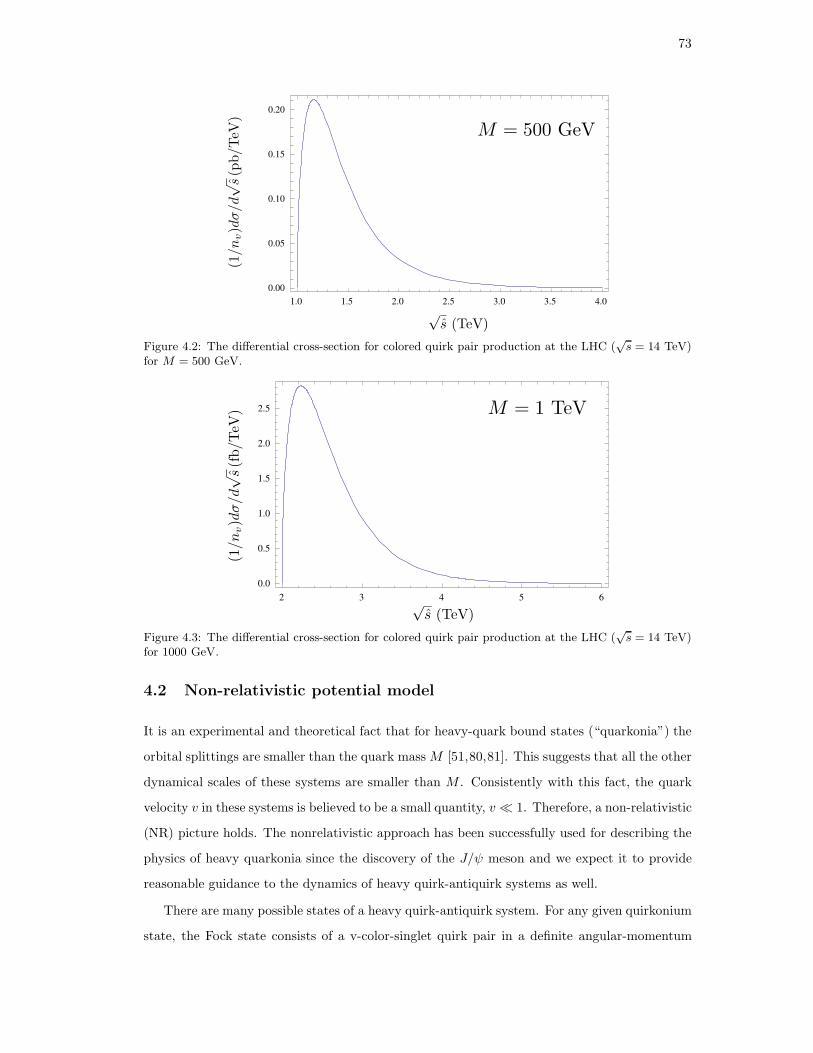
73
1.0 1.5 2.0 2.5 3.0 3.5 4.0
0.00
0.05
0.10
0.15
0.20
Figure 4.2: The differential cross-section for colored quirk pair production at the LHC (√s = 14 TeV)
for M = 500 GeV.
2 3 4 5 6
0.0
0.5
1.0
1.5
2.0
2.5
Figure 4.3: The differential cross-section for colored quirk pair production at the LHC (√s = 14 TeV)
for 1000 GeV.
4.2 Non-relativistic potential model
It is an experimental and theoretical fact that for heavy-quark bound states (“quarkonia”) the
orbital splittings are smaller than the quark massM [51,80,81]. This suggests that all the other
dynamical scales of these systems are smaller than M . Consistently with this fact, the quark
velocity v in these systems is believed to be a small quantity, v ≪ 1. Therefore, a non-relativistic
(NR) picture holds. The nonrelativistic approach has been successfully used for describing the
physics of heavy quarkonia since the discovery of the J/ψ meson and we expect it to provide
reasonable guidance to the dynamics of heavy quirk-antiquirk systems as well.
There are many possible states of a heavy quirk-antiquirk system. For any given quirkonium
state, the Fock state consists of a v-color-singlet quirk pair in a definite angular-momentum

74
500 1000 1500 2000
10- 6
10- 5
10- 4
0.001
0.01
0.1
1
Figure 4.4: Quirk production cross section at the LHC (√s = 14 TeV) as a function of the quirk mass.
state. We denote the two possible QCD color states of a quirk pair by 1 for color-singlet
and 8 for color-octet. In the nonrelativistic approximation, the states of quirkonium can be
cataloged according to the standard spectroscopic notation n2s+1LJ , where n denotes the
radial excitations and L denotes the orbital angular momenta S, P , D, · · · for L = 0, 1, 2, · · ·
respectively. Each constituent quirk has spin 12 , and so the total spin quantum number can be
either S = 0 or 1. J is the quantum number of the total momentum, a vector sum of the spin
and orbital momenta. An alternative notation used to denote the quirkonium states is JPC
, where P is the space parity and C is the charge conjugation parity. For a quirk-antiquirk
system these can be expressed as P = (−1)L+1 and C = (−1)L+S , respectively. In table 4.1 we
have collected the quantum numbers of the lightest quirkonium states in the spectrum.
State JPC 2S+1LJ
η1, η8 0−+ 1S0
ψ1, ψ8 1−− 3S1
h1, h8 1+− 1P1
χJ,1, χJ,8 J++ 3PJ
Table 4.1: The quantum numbers of the low lying states in the spectrum.
A complete treatment of the spectrum of quirkonium in non-relativistic effective field theory
(NREFT) is beyond the scope of this work. We will discuss briefly when the nonrelativistic
potential model is expected to work. The validity of the potential model rests upon the existence
of a hierarchy of energy scales, M ≫ Mv ≫ Mv2 in nonrelativistic systems with mass M
and velocity v [81]. This hierarchy allows for the construction of a sequence of effective field
theories: nonrelativistic (NREFT) and potential NREFT (pNREFT). First, the transition is

75
from the effective field theory with relativistic quirks to NRQCD with the quirks (and larger
momenta ∼ M) integrated out. The theory describes dynamics of heavy quirk-antiquirk pairs
at energy scales in the center-of-mass frame much smaller than their masses. A higher degree
of simplification can be achieved by exploitingMv ≫Mv2 and building the so-called potential-
NREFT (or pNREFT), where degrees of freedom of ∼ Mv are integrated out. In this way, an
analytical calculation of the spectrum becomes possible.
As in QCD, the choice of the potential is not unique, in view of the absence of a consis-
tent theory at all distances. However, it is restricted by theoretical arguments concerning the
properties of the interaction between quirks at different distances. The shape of the potential is
determined by asymptotic freedom at very short distances and by quirk confinement at very long
quirk separations. In the first case, the potential can be computed accurately in SU(nv) pertur-
bation theory, and in the lowest order it is dominated by single v-gluon exchange between the
static quirks. At distances of roughly 1/Λv, αv increases significantly and one-gluon-exchange is
no longer a good approximation. In long distances one calculates the potential in a model which
is assumed to be a good approximation to pure-Yang-Mills theory, usually in quenched lattice
QCD but also in string or flux tube models. A popular suggestion is that at long distances the
potential should behave as a linearly growing function of the quirk separation. Qualitatively
this linear behavior can be seen as arising from the chromoelectric lines of force that bunch
together into a flux tube which leads to a distance independent force or the potential. Thus, in
the case of interest the v-color potential has the following asymptotic limits:
r ≫ 1
Λv: Vv(r) = σ r (4.7)
r ≪ 1
Λv: Vv(r) = −C αv(r)
r(4.8)
where σ is the string tension, αv(r) is the SU(nv) running coupling constant. The color factor
C is obtained by evaluating the product of SU(nv) generators. Labeling the particles 1 and 2,
this product is −T a1 T
a2 = 1
2 ((Ta1 )
2) + (T a2 )
2)− (T a1 + T a
2 )2), which leads to
C =1
2
(
C1 + C2 − C(12)
)
, (4.9)
where C1 and C2 are the quadratic Casimirs for the two particles and C(12) that for the bound
state. For the case of a quirk-antiquirk pair, the v-color decomposition
nv ⊗ nv = 1⊕ (n2v − 1) (4.10)
shows that quirkonium can be a v-color singlet or a v-color adjoint. Then
C1 = CF =n2v − 1
2nvCAdj = CF − CA
2= − 1
2nv. (4.11)

76
Thus the v-color Coulomb force is always attractive in the v-color singlet channel.
One can then use a smooth interpolating function for the transition region, smoothly join
the non-perturbative potential to the perturbative one or simply add the perturbative and
nonperturbative contributions.
In our numerical study, we have considered the following potential-model choices.
(1) Cornell potential [84]. This is the simplest possibility of a quirk potential satisfying the
asymptotic limits above. The potential is simply given by the sum of (4.7) and (4.8) with
αv(r) = αv = const,
V (r) = −4
3
αv
r+ σr. (4.12)
(2) Richardson potential [85]. A different possibility which incorporates the two concepts
of asymptotic freedom and linear confinement in a unified manner is the Richardson
potential. In this case the potential is constructed by Fourier transforming a smartly
chosen, ad-hoc expression for the potential in momentum space
V (q2) = −4
3
1
q2
4π/11
ln (1 + q2/Λ2v). (4.13)
The potential grows linearly at long distances and has the short-range behavior to one-loop
order in perturbation theory,
V (q2) = −4
3
16π2αv(q2)
q2, (4.14)
where
αv(q2) ∼ 4π/11
ln (q2/Λ2v)
q2 → ∞. (4.15)
Upon performing the Fourier transform of (4.13) Richardson showed that the potential
V (r) can be written in the form
V (r) =8π
33Λv
(
Λvr −f(Λvr)
Λvr
)
, (4.16)
where
f(t) =4
π
∫ ∞
0
dqsin (qt)
q
[
1
ln (1 + q2)− 1
q2
]
. (4.17)
The potential (4.16) has the nice feature that its behavior is determined by a single
parameter, the scale Λv. The value of Λv is conveniently chosen to reproduce the large-
distance string tension, i.e. σ = 8πΛ2v/33.
(3) Wisconsin potential [86]. In order to be able to relate the short-distance behavior of the
potential to the parameter ΛMSv , perturbative corrections up to two loops have to be

77
included [82]. As an alternative we have adopted the potential proposed in [86] which
incorporates the asymptotic behavior predicted by the two-loop calculation, with ΛMS
not directly tied to the string tension,
Vv(r) = σr − 4
3
1
r
4π
b0f(r)
1 +c
f(r)− b1 ln f(r)
b20f(r)
(4.18)
where
f(r) = ln
(rΛv)−2 + b
b0 = 11− 2
3nf (4.19)
b1 = 102− 38
3nf c =
1
360
(
31− 10
3+ 2γE
)
. (4.20)
Here nf denotes the number of effective flavors; nf = 0 in the hidden sector, and nf =
3, 4, 5 in QCD. The parameter b is introduced to regularize the potential at large distances
r. The potential (4.18) grows linearly at long distances and has a short-range asymptotic
behavior to two-loop in perturbation theory.
One should be aware of what is being neglected in calculations within the naive potential
model. Relativistic and quantum effects such as spin dependence and pair creation, as well as
mixing between among states induced by coupling to decay channels, are ignored in the present
discussion. Also, as is, the potential model has little to say on the important question of how
v-gluonic degrees of freedom may affect the computation of the spectrum.
The size of the relativistic corrections can be estimated by computing the average relative
velocity v of quirks in a specific state [87]. At long distances, the potential behaves approx-
imately linearly, V (r) ∼ σr. In such a potential the expectation value of the kinetic energy
〈T 〉 = 〈 r2 dVdr 〉 is just 〈T 〉 = 〈V/2〉 = E/3 with σ = m2
0/3.72. Since 〈T 〉 = 2(1/2)Mv2, one has
v2 ≃ 1/3 for quirk pairs with kinetic energy E ∼ M/4, where the majority of the states are
produced. Thus a nonrelativistic description for highly excited quirkonium states is quite crude,
whereas it is substantially better for the states produced near threshold.
In writing the XX interaction for colored quirks we must also keep track of the color state
c of the quirk pair. The SU(3)C color potentials in momentum space take the form,
Vs(q) = −4
3g2
1
q2, Vo(q) =
g2
6
1
q2= −1
8Vs(q), (4.21)
governing interactions between colored quirks in color-singlet and color-octet states, respectively.
The force in the singlet channel is attractive while that in the octet channel is repulsive and
smaller in size.
We shall use the two-loop expression for αs,
αs(Q2) =
4π
β0 log [Q2/ΛMS ]2
1− 2β1β20
log[
log[
Q2/Λ2MS
]]
log[
Q2/Λ2MS
]
, (4.22)

78
with β0 = 11− 23nf , β1 = 51− 19
3 nf and ΛMS ≃ 250 GeV.
We distinguish a priori three regimes in r:
1. For large r the interaction is negligible and the QCD color of colored quirks (which is
irrelevant to their motion) is uncorrelated so, to a good approximation, we can average
over quirk colors.
2. For intermediate r one must keep track of the color state in detail, and propagate the
quirks according to the potential appropriate to their color state. This the regime of
non-perturbative QCD transitions, such as pion emission.
3. For small r the large gap between color singlet and octet might induce a large transition
rate due to gluon radiation, which changes the color state of the quirks.
The boundaries of these regions must be determined by explicit computation.
0.02 0.04 0.06 0.08 0.10 0.12 0.14
- 100
- 50
50
100
Figure 4.5: Spectrum of the system consisting of two heavy quirks. In the case shown, horizontal linescorrespond to the binding energies of a color-singlet bound state of quirkonium.
The energy spectrum of the system of two heavy quirks therefore looks as shown schemati-
cally in figure 4.5. The low-lying states are Coulombic, with energy splittings of order α2vM ≫
Λv ∼ m0/7, while the states near the continuum threshold are dominated by the linear term.
Spin-dependent interactions are suppressed by 1/M , so spin excitations are small and we do not
expect them to play an important role in the process we are considering. The energy splitting
between highly-excited states scale as ∼ n−1/3, where n denotes the radial quantum excitation
number. Hence, as n goes to infinity, the highly excited states become closely spaced.
4.3 Decay modes of heavy quirkonia
In this section, we present formulas for the decay widths of color-singlet and color-octet states
of heavy quirkonia.
79
If the quirks are colored, the quirkonium states have many possible ways to decay. To a great
extent, the decays of quirkonium fall naturally into three main classes: hard annihilations, SM
radiative decays and radiative decays by the v-color strong interaction (“v-glueball radiative
decays”).
(a) Hard annihilations: The quirk and antiquirk pair annihilates into v-gluons, which at long
distance become two or more v-glueballs, or into SM gluons and quarks, which fragment
into two or more jets. Note that color-octet quirkonium states cannot annihilate into
v-glueballs alone.
(b) SM radiative decays: The quirk and antiquirk pair undergo a cascade decay with emission
of a perturbative gluon or two soft gluons which materialize into hadrons (mostly pions
and kaons). In the transitions with single-gluon emission a color singlet state is promoted
to a color octet state. Electromagnetic cascade transitions with emission of a photon are
possible for electrically-charged quirks, but these will be typically suppressed with respect
to the hadronic decays.
(c) v-glueball radiative decays: Non-perturbative v-color transitions ΨI → ΨJ + Θκ are an
example of this kind. Here, ΨI, ΨJ and Θκ stand for the initial state quirkonium, final
state quirkonium and emitted v-glueball, respectively.
Some comments are in order. First, we should note that the decays are constrained by
conserved quantum numbers. For instance, it is impossible for a color-singlet quirkonium state
with JPC = 1−− to decay through a single gluon as the particle is colorless but a gluon carries
color. Decays to two SM gluons are also forbidden by C conservation.
Also, as explained in the introduction to this chapter, the coupling of quirkonium to v-
glueballs is due to non-perturbative v-color effects and is subject to significant uncertainties.
Therefore, in this work we will consider two extreme scenarios: one where there is no suppression
of v-glueball production, and one where nonperturbative v-color interactions are effectively
absent. In the first case, the quirkonium states can decay quickly down to the ground state
by emitting a few v-glueballs if Λ is sufficiently high, or lot of v-glueballs for low Λ. In the
second case, the main mechanisms of energy loss are soft-gluon emission or perturbative-gluon
emission, depending on the spacing of the excited quirkonium states.

80
4.3.1 Annihilation decays
In this section we present the decay widths of all color-singlet and color-octet quirkonium states
to two-body final states within the hidden valley or the standard model.
The fact that the decay rate factors into a short-distance and a long-distance part was
already explained in the introduction. The first is related to the probability that quirk and
antiquirk pair annihilate when they are near each other. Since the mass M of the quirks is
large the annihilation takes place in a small region of size ∼ 1/M and is described by the small
coupling constant of strong or v-color interactions. Therefore, one can use perturbation theory
to compute the corresponding matrix elements. This is analogous to the way annihilation decays
of charmonium are calculated in QCD. In fact, the calculations of the short-distance part in
QCD, QED or Pure-Yang-Mills theory are very similar. The reason is that we are considering
decays with the minimum number of particles in the final states. Besides, the details of strong
or v-strong interactions take place at a much longer time scale, so they should not affect the
total annihilation rates. The only difference between photonic, gluonic or v-gluonic annihilation
amplitudes reduces to a simple multiplicative color or v-color factor and to the difference of the
coupling constants. We will elaborate these factors in detail below.
The evaluation of the long-distance part of the annihilation rate is slightly more subtle. It
was shown in [49] that one needs to distinguish between two different cases: λ ≫ M−1 and
λ≪ M−1, where λ is the de Broglie wavelength of the quirks
λ =2π~√2µE
. (4.23)
where K = E − 2µ is the kinetic energy, µ = M/2 is the invariant mass of the reduced
system. For λ ≪ M−1, one obtains that in a highly excited state the probability to find the
quirks near each other is proportional to the fraction of time that the quirks spends in a small
region of radius M−1. In the opposite limit λ ≫ M−1 one obtains the familiar result from
positronium and quarkonium physics that the S-wave annihilation probability is proportional
to the wavefunction at the origin.
It turns out that in the cases considered the majority of the events that produce quirks are
such that λ≫M−1. Hence inclusive decay widths of quirkonia take the factorized form
Γ(XX → v-glueballs) =
∣
∣
∣
∣
dl
drlRnl(0)
∣
∣
∣
∣
2
F (αv), (4.24)
and a similar expression for Γ(XX → hadrons). In (4.24) F (αv) comes from the short-distance
matrix element.

81
One cannot expect to compute Rnl(0) from perturbative theory in an expansion in αv. The
reason is that the majority of quirkonium states have a mean radius rXX ≫ 1/Λv, a distance
at which nonperturbative effects are important. Thus Rnl(0) will be determined in part by the
long range part of the potential (4.7), as in the determination of the spectrum. Perturbation
theory will only be applicable to quirkonium states whose average radius is smaller than 1/Λv,
which is predicted for the ground state of XX for large quirk masses.
The rate also depends crucially on the angular momentum and spin of the quirk-antiquirk
pair. Using the semiclassical formulas for the wave function at the origin (A.46) and (A.47),
one can show that
Γl 6=0
Γl=0∼ 1
l
(
β
l
)l+1
. (4.25)
This suppression implies that annihilation is dominated by small l.
We now present our results for the annihilation rates of S-wave quirkonia. As explained
above most of the results can be obtained from previous similar calculations for quarkonium
decays with appropiate modifications to include color or v-color factors (see for example [42,49,
88]). Let us start with the case of color-singlet annihilations.
A. Color-singlet quirkonium
1. η1(S) → gvgv, gg, γγ For the color-singlet η1(S) quirkonium the leading decay mode is
gvgv with rate:
Γ(η1(S) → gvgv) =n2v − 1
4nvNc
4πα2v
M2|ψ(0)|2 (4.26)
where the gauge coupling is to be evaluated at the renormalization scale M . For the
v-color coupling, we use
αv(M) =6π
11nv lnM/Λv. (4.27)
These v-gluon fields are converted into v-glueballs at long distance, which in turn can
decay back to standard model fields as discussed in the previous chapters.
For quirks carrying QCD color, we also have
Γ(η1(S) → gg) =N2
c − 1
4Ncnv
4πα23
M2|ψ(0)|2, (4.28)
The QED annihilation processes are
Γ(η1(S) → γγ) = nvNce4X
4πα2
M2|ψ(0)|2, (4.29)
where eX is the electric charge of the quirk and Nc = 3 is the number of QCD colors .

82
We have neglected the contribution from Z boson exchange, which gives a small correction.
There are similar expressions for annihilation through a W in the case where the electric
charge of the quirks differs by one unit.
2. ψ1(S) → Z∗/γ∗, gvgvgv, γgvgv
Γ(ψ1(S) → γ∗ → f f) =4nvNcNCfe
2Xe
2f
3
4πα2
M2|ψ(0)|2, (4.30)
For the color-singlet ψ1(S) quirkonium the leading decay mode is gvgvgv. The width of
this decay is
Γ(ψ1(S) → gvgvgv) =α3v
9π
(n2v − 1)(n2
v − 4)Nc
4n2v
4π|ψ(0)|2M2
(π2 − 9). (4.31)
Γ(ψ1(S) → γgvgv) =4α2
vα e2XNc
3π
(n2v − 1)
nv
4π|ψ(0)|2M2
(π2 − 9). (4.32)
B. Color-octet quirkonium
We now present the results for S-wave annihilation decays of color-octet quirkonium. In this
case, annihilations to v-gluons are forbidden in decays with less than four gauge bosons in the
final state.
1. η8(S) → gg.
For the η8(S) quirkonium, the dominant decay mode is gg with width
Γ(η8(S) → gg) =N2
c − 4
Ncnv
4πα23
M2|ψ(0)|2, (4.33)
2. ψ8(S) → g∗, ggg, ggγ, gγγ.
Since the ψ8(S) quirkonium has the same quantum numbers of a gluon, it can decay to
SM quarks of either flavor through an off-shell gluon. The width of the decay is given by
Γ(ψ8(S) → f f) =nv
4
4πα23
M2|ψ(0)|2. (4.34)
It is important to observe that the decay involving two on-shell SM gluons, ψ1(S) → gg,
vanishes as a consequences of Yang’s theorem which forbids a massive J = 1 vector boson
from decaying to two massless J = 1 bosons [92]. The leading decay modes involving SM
gauge bosons are ggg, ggγ and gγγ, and their respective rates read
Γ(ψ8(S) → ggg) =α3s
9π
(N4c − 4N2
c + 12)nv
64N2c
4π|ψ(0)|2M2
(π2 − 9) (4.35)

83
Γ(ψ8(S) → ggγ) =α2sα
9π
(N2c − 4)nv
4N2c
4π|ψ(0)|2M2
(π2 − 9), (4.36)
Γ(ψ8(S) → gγγ) =αsα
2
9π
nv
4N2c
4π|ψ(0)|2M2
(π2 − 9). (4.37)
4.4 Radiative transitions in quirkonium
Another class of transition rates that can be calculated in the nonrelativistic potential model
are the radiative ones. We have seen in the last section that annihilation is dominated at small l.
This means that annihilations can be effectively suppressed if there are other interactions that
can change the orbital angular momentum of the quirks. Therefore the radiative transitions be-
tween quirkonium states which have this property certainly deserve consideration. Interestingly
enough, the soft particles emitted during quirk radiation could, in some regimes, potentially
serve as the discovery channel for hidden valleys [50].
The multipole expansion in electrodynamics has been widely used for studying radiation
processes in which the electromagnetic field is radiated from local sources [42]. If the radius a
of a local source is smaller than the wave length λ of the radiated electromagnetic field such
that a/λ ∼ ak < 1 (k stands for the momentum of the photon), ak can be a good expansion
parameter, i.e., we can expand the electromagnetic field in powers of ak. This is the well-known
multipole expansion in QED. The multipole expansion in QED has also been generalized by
many authors to describe hadronic transitions in quarkonium systems (See for example [89,90]
for a review).
We now discuss gluon radiative decays in quirkonium systems. We begin with the case
r ≪ Λ−1QCD. For sufficiently excited quirks to use the WKB approximation, the typical radius
a = 〈r〉 obtained by using the virial theorem is of order
a ≃ 2
3
K
σ, (4.38)
where K is the kinetic energy of the quirk pair and σ is the string tension. A similar estimation
for the typical energy splitting at binding energies of order K ∼ 0.5M gives ∆E ∼ .25m20/M .
For a gluon emission with gluon energy k = ∆E, ka ∼ 1. Therefore, this suggests that one
can apply the idea of multipole expansion in QCD to calculation of the transitions between
quirkonium levels with emission of a gluon2. Aside from color factors, the radiative transitions
2In classical electrodynamics, the coefficient of the (ak)l term in the multipole expansion contains an extrafactor 1
(2l+1)!!. Hence the multipole expansion actually works better than what is expected by simply estimating
the size of (ak)l.
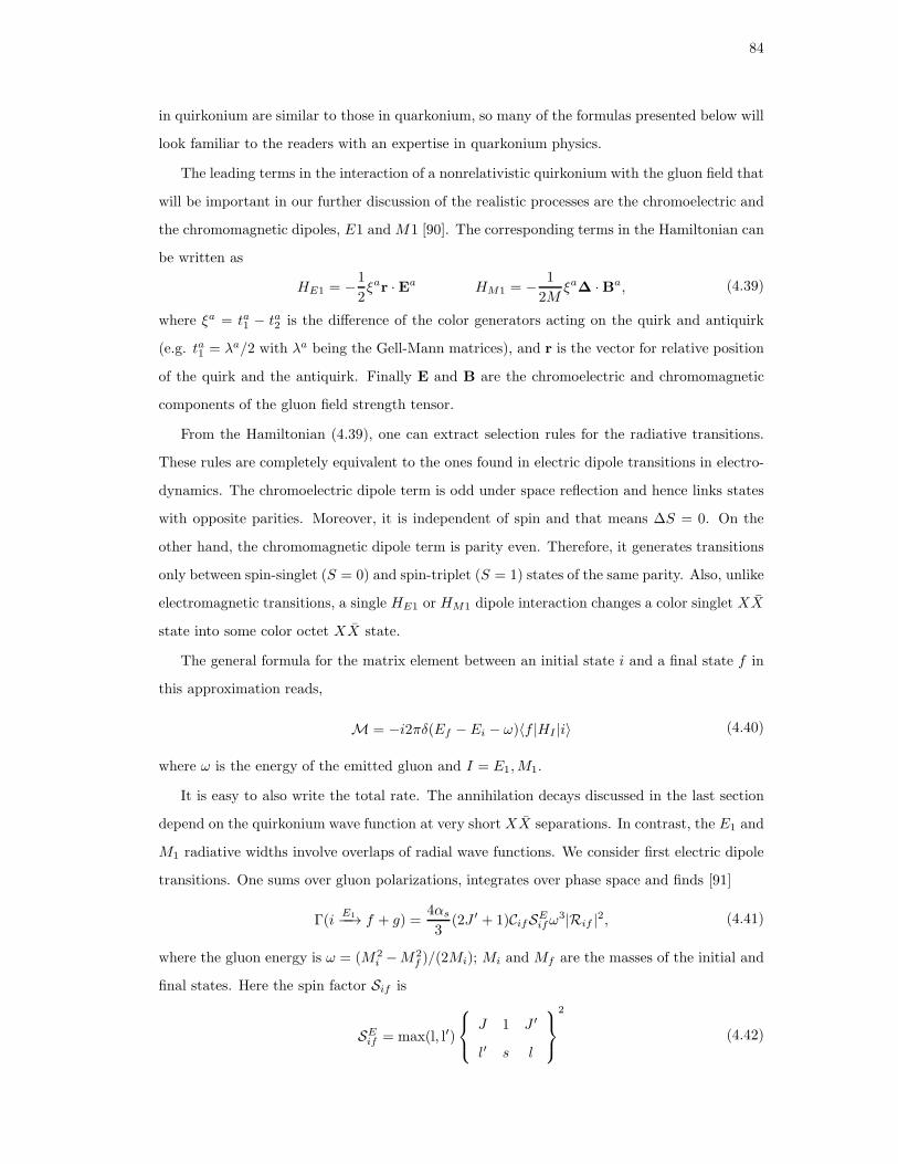
84
in quirkonium are similar to those in quarkonium, so many of the formulas presented below will
look familiar to the readers with an expertise in quarkonium physics.
The leading terms in the interaction of a nonrelativistic quirkonium with the gluon field that
will be important in our further discussion of the realistic processes are the chromoelectric and
the chromomagnetic dipoles, E1 andM1 [90]. The corresponding terms in the Hamiltonian can
be written as
HE1 = −1
2ξar · Ea HM1 = − 1
2Mξa∆ ·Ba, (4.39)
where ξa = ta1 − ta2 is the difference of the color generators acting on the quirk and antiquirk
(e.g. ta1 = λa/2 with λa being the Gell-Mann matrices), and r is the vector for relative position
of the quirk and the antiquirk. Finally E and B are the chromoelectric and chromomagnetic
components of the gluon field strength tensor.
From the Hamiltonian (4.39), one can extract selection rules for the radiative transitions.
These rules are completely equivalent to the ones found in electric dipole transitions in electro-
dynamics. The chromoelectric dipole term is odd under space reflection and hence links states
with opposite parities. Moreover, it is independent of spin and that means ∆S = 0. On the
other hand, the chromomagnetic dipole term is parity even. Therefore, it generates transitions
only between spin-singlet (S = 0) and spin-triplet (S = 1) states of the same parity. Also, unlike
electromagnetic transitions, a single HE1 or HM1 dipole interaction changes a color singlet XX
state into some color octet XX state.
The general formula for the matrix element between an initial state i and a final state f in
this approximation reads,
M = −i2πδ(Ef − Ei − ω)〈f |HI |i〉 (4.40)
where ω is the energy of the emitted gluon and I = E1,M1.
It is easy to also write the total rate. The annihilation decays discussed in the last section
depend on the quirkonium wave function at very short XX separations. In contrast, the E1 and
M1 radiative widths involve overlaps of radial wave functions. We consider first electric dipole
transitions. One sums over gluon polarizations, integrates over phase space and finds [91]
Γ(iE1−−→ f + g) =
4αs
3(2J ′ + 1)CifSE
ifω3|Rif |2, (4.41)
where the gluon energy is ω = (M2i −M2
f )/(2Mi); Mi and Mf are the masses of the initial and
final states. Here the spin factor Sif is
SEif = max(l, l′)
J 1 J ′
l′ s l
2
(4.42)

85
and the color factor Cif is shown in table 4.2. The overlap integral Rif is given by
Rif =3
ω
∫
drr2Ri(r)Rf (r)[ωr
2j0
(ωr
2
)
− j1
(ωr
2
)]
(4.43)
where Ri(r) (Rf (r)) is the initial (final) state wave function and jn(x), n = 0, 1 are spherical
Bessel functions of the first kind. This expression is valid for quirkonium states of any size. A
widely used approximation is the long wave length approximation which consists in taking the
limit ω → 0 in (4.43). In this case the overlap integral simplifies as
Rif =
∫
drr2Ri(r)Rf (r)r (4.44)
For the typical E1 transitions one expects Rif very nearly to the average radius of the initial
state, because ωr ≪ 1 and the initial and final states are sufficiently close to produce a good
overlap. On the other hand, E1 transitions between S and P states with changes in the number
of nodes by greater than one are suppressed due to poor overlap between initial and final wave
functions. The larger the difference in number of nodes, the greater the suppression.
Transition Cifsinglet-singlet 0singlet-octet (N2
c − 1)/2Nc
octet-singlet 1/2Nc
octet-octet 2(N2c − 1)/Nc
Table 4.2: List of coefficients Cif introduced in (4.41).
Magnetic transitions flip the quirk spin. These transitions have ∆l = 0, ∆s = ±1. The
spin-flip radiative transition between an initial state n2s+1lJ , i, and a final state n′2s′+1l′′J , f ,
is:
Γ(iM1−−→ f + g) =
4παs
3M2(2J ′ + 1)CifSM
if ω3|Rif |2, (4.45)
where the overlap integral is given by
Rif =
∫
drr2Ri(r)Rf (r)j0
(ωr
2
)
. (4.46)
Here the spin factor SMif is
SMif = 6(2s+ 1)(2s′ + 1)
J 1 J ′
s′ l s
2
1 12
12
12 s′ s
2
(4.47)
and the color factor Cif is shown in table 4.2. The M1 transitions are suppressed by a factor
ω/M . Thus, unless forbidden, the E1 transitions are expected to dominate.

86
For r ≫ Λ−1QCD, quirks undergo QCD hadronization and therefore we need to consider non-
perturbative QCD interactions between the quirks and the QCD brown muck. The brown muck
will interact only when the quirks come within a distance of order Λ−1QCD. It was argued in [49]
that these interactions will transfer an energy of order ΛQCD and an angular momuntum of order
∆l ∼ 1 from the bound state roughly once every crossing time. As a consequence, one light
QCD hadron, typically a neutral pion, will be emitted in a single brown muck interaction. If the
quirks do not annihilate for a number of crossings, a large number of hadrons ∼ 102−103 will be
emitted with energy ∼ GeV each. These new hadrons have been dubbed “hadronic fireballs”,
and may be the source of a promising discovery signal in the case of very low hidden confining
scale [50]. However, in the regime we are considering in this work, these hadronic fireballs are
not expected to contribute a significant fraction of the energy loss, as long as m0 & 50 GeV.
Before moving on to the discussion of non-perturbative v-color interactions we should con-
sider some concerns. For example, in order for a large amount of energy to be emitted in
radiation of perturbative gluons we must ensure that the quirks do not annihilate in a highly
excited state. We argue now that this is unlikely.
The probability for annihilation in a single crossing depends strongly on the angular mo-
mentum of the bound system and is dominated by low l. From our partial wave analysis in
section 4.3.1, we know that the annihilation probability scales like σann ∝ (β/l)l+2. Given that
the angular momentum will grow on average as radiation is emitted, the likelihood of early
annihilation is determined by a competition between the annihilation cross section and the ra-
diation rate. Very naively one can expect that radiation would win since the radiation rate is
proportional to αs and the annihilation cross section scales like α2v. However to make a clear
determination a more careful estimate is required.
Since annihilation rates are dominated by low l we only need to consider S-wave states. The
S states η1(nS), ψ1(nS) can make E1 transitions to the P states: η1(nS) → h8((n − 1)P )g,
ψ1(nS) → χJ,8((n − 1)P )g (the M1 transitions are negligible). Using (4.41) with J = l =
0, J ′ = l′ = 1, we can write the width for η1(nS) → h8(P )g
Γ =16
3αsω
3|RSP |2, (4.48)
where RSP is the overlap integral between S- and P -wave states. For those states produced
near the point where the cross section for quirk pair production peaks, E ∼ M/4, one has
ω = ∆E ∼ πσ/M . The overlap integral is given by (4.43) and is of the order of the quirkonium
radius, RSP ∼ 2E/3σ. The probability for emitting a gluon per period is therefore estimated

87
as
Prad = TΓ ≃ 4π3
27αsβ ∼ 2αs. (4.49)
This can be compared with the probability of annihilating at low l’s. For example, in the case of
the η1(nS) quirkonium annihilation goes dominantly to v-gluons i.e. v-glueballs, with a width
given by (4.26). Using (A.33) the width can be rewritten as
Γ(η1(S)) → gvgv) =2α2
v σ
M(4.50)
where we have set nv = 3. Following [49], the probability for S-wave annihilation per crossing
at high velocities is
Pann = 2TΓ ∼ 4βα2v ∼ 2α2
v (4.51)
where β is typically of order 1/2.
We see that perturbative gluon emissions will typically dominate over hard annihilations
for highly excited states. As the states approach the Coulombic regime, annihilation rates are
expected to increase. However, the change in angular momentum due to the emission of these
gluons (by ∆l ∼ 10 on average) will significantly reduce the probability to annihilate. Therefore,
we expect that the quirkonium states to radiate most of their kinetic energy before they can
pair annihilate into v-gluons or SM particles.
Calculation of color factors
The summation over colors must be done carefully because of the condition that the initial and
final states can be in either color singlet or color octet states. We define a basis of color states
|ij〉, where i, j = 1, 2, 3 denote the color indices of quirk and antiquirk, respectively. Then the
singlet state is given by
|1〉 = 1√Nc
∑
i
|ii〉. (4.52)
while the octet can be written as
|8; a〉 =√2∑
ij
T aij |ij〉, (4.53)
where the color matrices are normalized in the usual way tr T aT b = δab/2. When the initial
state is a singlet, and the final state and octet, the matrix element contains a color factor
〈8; a|T b|1〉 = δab√2Nc
, (4.54)
where the color operator T a acts on either the quirk or the antiquirk state only. Squaring the
matrix element, summing over the final color of the emitted gluon and final octet gives
∑
ab
|〈8; a|T b|1〉|2 =N2
c − 1
2Nc. (4.55)

88
The transitions in which the initial state is an octet can be computed analogously, with the
addition that one also needs to average over initial color. This way we obtain the color factors
in table 4.2.
4.5 Non-perturbative v-color interactions
Although the spectrum of heavy quirkonium systems can be adequately explained by nonrela-
tivistic potential models, some of their decays concerning nonperturbative v-color interactions
are difficult to deal with. Non-perturbative v-color transitions
ΨI → ΨJ +Θκ (4.56)
are an example of this kind. In (4.56), ΨI, ΨJ and Θκ stand for the initial state quirkonium, final
state quirkonium and emitted v-glueball, respectively. These v-glueball radiative transitions are
important decay modes of heavy quirkonia. For instance, if the v-glueball decays into photons,
one could use the photon signature to search for these states.
In the absence of light fundamentals, the v-color tube connecting heavy quirks cannot break.
Instead, v-glueball formation in a pure Yang-Mills theory occurs heuristically through the cross-
ing of the tube onto itself, a process qualitatively different from fragmentation in QCD (see figure
4.6). In order to make crisp predictions about detection signals coming from quirkonium decay,
we therefore need to understand the process of glueball emission in pure Yang-Mills theory. In
general this is a subtle problem whose solution is unknown, so for this case we limit ourselves
to some qualitative discussion of the dynamics.
(a) (b) (c)
Figure 4.6: A depiction of a v-glueball emission process.
In the semiclassical limit, the momentum which the heavy quirk can exchange with the v-
color flux tube is of the order Λv and the corresponding uncertainty in the energy of the heavy
quirk is of the order Λ2v/MX . No particle in the v-sector spectrum is light enough to be radiated
in this energy. When the quirks are close to one another the semiclassical limit breaks down
and v-glueball emission is possible.
Non-perturbative interactions of the quirks can convert some of the their kinetic energy into
vibrational energy of the flux tube. If enough energy is pumped into the flux tube so as to
89
excite it to a high vibrational mode, self interactions of the flux tube may result in v-glueball
emission (see figure 4.6). It follows that the rate for conversion of quirk kinetic energy into
the v-glueball radiation should be proportional to the rate of energy delivered into flux tube
vibrations.
We may thus consider the emission of v-glueballs as proceeding in two stages. The first
stage is the excitation of vibrational modes of the flux tube by the non-perturbative v-color
interactions, and the second stage is the actual radiation of a v-glueball by a vibrational excited
flux tube. The rates of these processes are determined by the population of high vibrational
levels of quirkonium. The non-perturbative v-color will only take place when the quirks come
within a distance of order Λ−1v . Following [49], the typical energy transfer from the bound state
can be estimated from
∆E ∼ F∆r ∼ Λ2vΛ
−1v ∼ Λv. (4.57)
The probability that the quirks are within a distance Λ−1v from each other is given by the
fraction of time that the quirks are within a distance Λ−1v ,
Prob(rXX . Λ−1v ) ∼ Λ−1
v /β
T(4.58)
where β is the classical quirk velocity at the origin and we have used the fact that the Compton
wavelength of the heavy quirk is much smaller than Λ−1v . If we assume as in [49] that the
nonperturbative v-color interactions have a geometrical cross section, we can estimate its rate
as
Γ ∼ 1
T∼ σ
Mβ(4.59)
where T is the classical crossing time. Thus, we expect these interactions occur roughly once
per classical crossing.
One may naively argue that in the case Λv > ΛQCD v-glueball emission is likely to dominate
over radiation of perturbative gluons because of the strong coupling in the v-sector. However,
emission of a v-glueball may be suppressed. First, we know from figure 2.1 that the mass of the
lightest v-glueball is about 3.6 times heavier than the square root of the string tension. Therefore
we can expect that there is some suppression for v-glueball emission, depending on how many
transitions are needed to transfer an energy of order m0 to the flux tube. Furthermore, in the
large nv limit, the v-glueball emission should be suppressed by a factor O(1/n2v), giving an order
of magnitude suppression for nv = 3. Combining this with (4.59) and including a phase space
factor, we may obtain an upper bound for the rate for v-glueball emission as
Γ .1
n2v
σ
Mβ× Phase space (4.60)

90
Nonetheless, one should keep in mind the possibility that the actual rates for radiation of
v-glueballs may differ substantially from the estimate (4.60).
4.6 Fragmentation Probabilities
While it is possible to work out quirkonium and v-glueball branching fractions for a given medi-
ation model with the help of lattice data for N = 3, it is considerably more difficult to arrive at
the full spectrum of visible standard model particles produced in a single quirkonium annihila-
tion. The final state of visible standard model particles depends on the number and spectra of
glueballs initially produced in the quirkonium decay. In order to make crisp predictions about
indirect detection signals coming from quirkonium decay, we therefore need to understand the
process of fragmentation in pure Yang-Mills theory. Unfortunately, this is a situation where
neither phenomenological examples from QCD nor data from the lattice can be of help. In the
absence of light fundamentals, the color tube connecting hard partons cannot break. Glueball
formation in a pure Yang-Mills theory occurs heuristically through the crossing of the tube onto
itself, a process qualitatively different from fragmentation in QCD.
One simple approach to estimating the relative abundances of different glueball species is a
thermal model. In such a model, the ratio and yield of the multiplicity of glueballs is given by
the partition function Z. In a grand-canonical ensemble of glueballs of species i the partition
function with chemical potential µ is given by
Z ∝∑
N
∏
i
(2Ji + 1)m3/2i e−(nimi−µni)/T
(4.61)
where mi, Ji and ni are the mass, spin and multiplicity of a glueball of species i, respectively.
The temperature T of the spectrum would be taken to be Λv. Unlike QCD, where this temper-
ature is comparable to the masses of the pions, the corresponding temperature is much lower
than the masses of the glueballs in pure Yang-Mills theories, so that if this is true, the excited
v-glueballs are rarely produced. We may guess that, as in QCD, the effective temperature in
hadronization models is comparable to the deconfinement phase transition, which is of order
180 MeV in QCD, about 1/10 the QCD glueball mass, but which is significantly higher, about
1/5 - 1/6 m0 [], for a pure Yang-Mills theory. In particular, accounting for the fact that the
spin-two states have a spin-multiplicity of 5, we would have production of the 0++ state at
50–60%, and of the 2++ state at around 30%, with 2–4% each for the 0−+, 2−+ and 1+− states.
All other states would be produced at lower rates.
Nevertheless, we should keep in mind that the statistical quasi-thermal model is unlikely to
be accurate. Formation of hadrons in QCD occurs through the local snapping of a flux tube
91
by light-quark pair production, a local effect on its world sheet. Formation of v-glueballs in
a Yang-Mills theory occurs through the crossing of a flux tube onto itself, a non-local effect
on the worldsheet that involves color rearrangement. The excitation of the flux tube created
in the X-onium annihilation may therefore influence the production of v-glueballs, and greatly
enhance the rate for the production of heavier v-glueball states, including ones which are un-
stable and decay immediately to multiple stable v-glueballs. In this scenario, the probability
of producing the heavier stable v-glueballs, and perhaps the total number of v-glueballs per
X-onium annihilation, could be much larger than estimated in the quasi-thermal model.
Strictly speaking, these estimates should be thought as a priori estimates for the relative
abundances of v-glueballs in a given quirkonium annihilation. In general, the actual fragmen-
tation probabilities will be further constrained by conservation of quantum numbers and/or
kinematics and may be significantly different from the predictions obtained by naive appli-
cation of the fragmentation thermal model. For example, because of conservation of charge
conjugation the vector ψ1 can only annihilate to final states containing an odd number of C-
odd v-glueballs. Also, the pseudoscalar η1 cannot annihilate to final states containing only two
0++ v-glueballs, because of parity and angular momentum conservation.
4.7 Numerical analysis
From the above discussion it is clear that the characteristic collider signatures of quirkonium
are determined both by the final states that the quirks can annihilate into and by the nature
of the energy loss during quirk de-excitation to the ground state. In what follows we calculate
numerically the quirkonium spectrum, and evaluate the branching ratios for radiative transitions
of quirkonium and for pair annihilation into various final states. To give a general survey
of decays is beyond the scope of this work, since a more detailed treatment would have to
incorporate precise values of the non-perturbative matrix elements for v-glueball emission which
at present are unknown. However, a few examples are useful to illustrate the main qualitative
features of quirkonium decay pattern.
4.7.1 Quirkonium spectrum
This section is concerned with the energy of a single quirk-antiquirk pair moving in a central
potential and obeying nonrelativistic quantum mechanics. The main result is the evaluation of
the energy eigenvalues. The Schrodinger equation is numerically integrated using the generalized
Runge-Kutta algorithm described in [75].

92
In order to conduct an analysis of the phenomenology, we first need to have some information
about the various scales in the model. The scale, ΛQCD, where SU(3)C gauge coupling blows
up is around 250 MeV. The remaining parameter space consists of the mass scale M and the
0++ mass m0. Here we present our results in terms of m0 which is more transparent than the
confining scale Λv, sincem0 is the relevant parameter for LHC studies. To simplify the discussion
in the v-sector, it is convenient to assume that the 0++ mass is in the phenomenologically
interesting range 25 GeV . m0 . 500 GeV where v-glueballs may decay visibly. Moreover,
since the branching ratios depend on M and m0 only through the combination M/m0, our
problem is reduced to a two-dimensional parameter space described by M and ξ ≡M/m0.
The mass scale M sets the value of the total production rate and defines the energy region
where the majority of the quirks are produced. On the other hand, our focus here is on the main
qualitative features of the quirkonium spectrum and decay pattern, which to a great extent are
controlled by the single parameter ξ. Therefore it is convenient in this first attempt to fix the
quirk mass and choose three representative values of M , 250 GeV, 500 GeV and 1000 GeV.
This scenario implies that three different regimes need to be distinguished: (i): Coulombic
regime, rXX ≪ Λ−1v ; (ii) intermediate linear regime, rXX ≫ Λ−1
v and rXX ≪ Λ−1QCD ; and (iii)
and nonperturbative QCD linear regime, rXX ≫ Λ−1v and rXX ≫ Λ−1
QCD (We will not consider
the regime for which rXX ≪ Λ−1v and rXX ≫ Λ−1
QCD, because our focus here is on the case
Λv ≫ ΛQCD where the v-glueballs can decay visibly). As explained above, there is a qualitative
difference between (ii) and (iii): for rXX ≪ Λ−1QCD, emitted SU(3)C gluons will be perturbative
and will change the spin of the state by one unit. In this case, the width of the decay is
proportional to αs, and the transition can occur at any moment during the quirk oscillation.
This implies that the quirkonium states can make a transition down to a lower excited state
with ∆E ≫ ΛQCD. In contrast, for rXX ≪ Λ−1QCD, non-perturbative QCD interactions are only
efficient in damping the quirk oscillation only when the quirk separation is of the order or less
than Λ−1QCD. This results in an energy of order ΛQCD emitted in the form of light QCD hadrons
about once during every crossing time.
The spectrum of quirkonium binding energies is amenable to an analytical description for
both Coulombic and linear regimes, rXX ≪ Λv and rXX ≫ Λv. Results for these regimes give
good qualitative insight also for the crossover region of intermediate coupling constants αv ∼ 1,
where an analytical description becomes more cumbersome.
Now we want to argue that in the case of interest the Coulombic regime is in general
unimportant. We plot numerical results for the quirkonium binding energies Enl as a function
of m0 for three different values of the quirk mass, M = 250, 500, 1000 GeV. For simplicity,

93
only the S-wave l = 0 energies are shown. As shown in the figure 4.7 for very low m0 many
excited states tend to gather around the crossover region where Coulombic and linear potential
are approximately of the same strength (E ≃ 0). However, in the energy interval of interest
50 GeV . m0 . 500 GeV there are only O(1) states in the Coulombic region.
0 100 200 300 400 500
0
200
400
600
800
0 100 200 300 400 500
0
100
200
300
400
500
600
0 200 400 600 800 1000
0
200
400
600
800
1000
1200
Figure 4.7: The binding energies of low-lying, S-wave color-singlet states in a quirkonium system asa function of the v-glueball mass m0 for different values of M . For very small m0, the levels gatheraround the crossover region between the linear and Coulombic parts of the nonrelativistic potential.However, as long as m0 becomes larger than about 100 GeV only a few states remain in the Coulombicregime.
This result agrees to a very good approximation with a quasi-analytical result for the number
of bound states in the Coulomb region. To see this, let us recall that the average radius of the
bound states in a Coulomb potential is given by
rn = n2 rB (4.62)
where rB = (µα)−1 is the Bohr radius,n is principal quantum number; µ =M/2 is the reduced
mass of the quirk-antiquirk and α is the gauge coupling constant. From the Cornell potential
(4.12) we can estimate the cross-over point as r2 ≃ α/σ. It follows that the number of states
in the Coulombic region is approximately given by
n2Coulomb ∼ 1.85α3/2 M
m0∼ M
m0, (4.63)

94
where we have used m0 = 3.7√σ and α ≃ (4/3)(αs + αv) ≈ 0.8. Therefore, we arrive at the
same conclusion as above that about one or two color-singlet states are in the Coulomb region
in the range of parameter of interest.
Next, we show that regime (iii) only accounts for a relatively small fraction of the total cross
section. In order to demonstrate this, we integrate (4.5) over the mass range corresponding to
rXX > Λ−1QCD, namely
√s− 2M > 1.5 σΛ−1
QCD, where in the last inequality we have used (A.37)
with E =√s − 2M . The numerical results are shown in figure 4.8 as a function of m0 for
M = 250, 500, 1000 GeV. We see that for very low v-glueball masses the majority of the states
will be produced in the non-perturbative QCD regime. This is indeed the regime considered by
the authors of [49]. However, for the interval 100 GeV < m0 < 500 GeV, the states produced
in regime (iii) only contribute less than about 20% to the total cross section.
0 50 100 150
0.0
0.2
0.4
0.6
0.8
1.0
Figure 4.8: The fraction of bound states produced in the non-perturbative QCD regime as a functionof m0 for M = 250, 500, 100 GeV.
The results above allow us to restrict attention to regime (ii). In this case, crucial simpli-
fications occur due to the fact that QCD interactions of the quirks are perturbative. This is
because rXX < Λ−1QCD and the energy transfer ∆E associated with QCD processes involving
quirks and SU(3)C gluons is greater than ΛQCD. Indeed, the mass splitting between quirkonium
states for transitions with single gluon emission are such that ∆E ≫ ΛQCD in the parameter
range of interest. This is illustrated in figure 4.9 which shows contour lines of constant ∆E in
the M -m0 plane. In figure 4.9, ∆E is evaluated at the boundary between regime (ii) and (iii),
i.e. for highly excited states such that rXX = Λ−1QCD. We see that for very small m0, ∆E may
be smaller than ΛQCD. However, as long as m0 & 50 GeV the energy splitting between two
consecutive states becomes larger than ΛQCD, and QCD interactions, i.e. gluon emission are
perturbative.
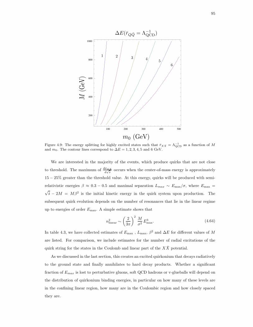
95
100 200 300 400 500
200
400
600
800
1000
Figure 4.9: The energy splitting for highly excited states such that rXX = Λ−1QCD as a function of M
and m0. The contour lines correspond to ∆E = 1, 2, 3, 4, 5 and 6 GeV.
We are interested in the majority of the events, which produce quirks that are not close
to threshold. The maximum of dσXX
d√s
occurs when the center-of-mass energy is approximately
15− 25% greater than the threshold value. At this energy, quirks will be produced with semi-
relativistic energies β ≈ 0.3 − 0.5 and maximal separation Lmax ∼ Emax/σ, where Emax =√s − 2M = Mβ2 is the initial kinetic energy in the quirk system upon production. The
subsequent quirk evolution depends on the number of resonances that lie in the linear regime
up to energies of order Emax. A simple estimate shows that
n2linear ∼
(
2
3π
)2M
σ2E3
max. (4.64)
In table 4.3, we have collected estimates of Emax , Lmax, β2 and ∆E for different values of M
are listed. For comparison, we include estimates for the number of radial excitations of the
quirk string for the states in the Coulomb and linear part of the XX potential.
As we discussed in the last section, this creates an excited quirkonium that decays radiatively
to the ground state and finally annihilates to hard decay products. Whether a significant
fraction of Emax is lost to perturbative gluons, soft QCD hadrons or v-glueballs will depend on
the distribution of quirkonium binding energies, in particular on how many of these levels are
in the confining linear region, how many are in the Coulombic region and how closely spaced
they are.

96
M( GeV) Emax/m0 n2Coulomb nlinear β2 ∆E/
√σ < r >max
√σ
250 0.5ξ .8ξ 1.03ξ2 .5 1.20ξ−1 1.23ξ
500 0.4ξ .8ξ 0.73ξ2 .4 1.34ξ−1 0.99ξ
1000 0.3ξ .8ξ 0.48ξ2 .3 1.55ξ−1 0.74ξ
Table 4.3: Some quantities of interest evaluated around the point where the majority of the quirk pairsare produced at the LHC as a function of the parameter ξ = M/m0 and for different quirk masses.
4.7.2 Decay patterns
Quirkonium phenomenology depends sensitively on the parameter ξ = M/m0. Notice that
radiative emission of v-glueballs may only be present providing Emax > m0. Also as long as
Lmax becomes of the order of or greater than 1 GeV, non-perturbative QCD interactions need
to be taken into account. Therefore we can distinguish several very different cases.
1) 0.5 . ξ . 2.5: In this case, v-glueballs are too heavy to be produced during quirk
relaxation. Instead, the quirk-antiquirk pair will lose energy by emitting a few pertur-
bative gluons, eventually (unless kinematically forbidden) annihilating into at most two
v-glueballs. Besides, only a few quirkonium resonances will be produced so the decay
pattern turns out to be very simple. The simplicity of the spectrum is likely to be spoiled
by mixing effects between the heavy v-glueballs and the quirkonia.
2)√
M/3.7ΛQCD . ξ . 40: Here the states are very closely spaced in the spectrum. Upon
production, the size of the highly excited quirkonium states will be larger than ∼ Λ−1QCD
so non-perturbative QCD effects will be important. The relaxation process was already
described in [49]. A significant fraction of colored quirk pairs will lose most of their kinetic
energy because of interactions of the nonperturbative QCD and/or v-color interactions,
until the typical radius of the states becomes smaller than about Λ−1QCD. Meanwhile,
if QCD interactions dominate, an energy of order .5M will be radiated as light QCD
hadrons each with energy of order GeV (a hadronic fireball). If, on the contrary, v-color
interactions dominate around O(10) v-glueballs will be radiated. The hard annihilation
final states will contain several v-glueballs, but also some occasional SM quarks and gluons.
3) 2.5 . ξ .√
M/3.7ΛQCD: In this range, quirk kinetic energy is converted to several
perturbative gluons and possibly a few v-glueballs. The quirk-antiquirk pair annihilates
into v-glueballs, but also into two SM quarks and gluons.
The boundary of these regions is shown in figure 4.10. The shaded region is excluded by
current experimental bounds on the mass of heavy colored particles.

97
Figure 4.10: The different regimes described in section 4.7.2: 1) Most states will decay via emission ofa hard perturbative gluon. Typical energies are insufficient to radiate a glueball. 2) Some moderatelyhard gluons and a few v-glueballs. 3) Non-perturbative QCD regime. Large number of soft hadronsand possibly many v-glueballs. The shaded region represents the exclusion region.
We present the decay branching ratios of the S-wave quirkonium in figure 4.11 as a function
of the S-wave quirkonium binding energy forM = 500 GeV and m0 = 100 GeV. For the gluon-
radiative decay, we show the summed branching fraction over all the radiative decay modes. We
then see that gluon-radiative decays are the dominant decay modes of highly-excited quirkonium
states for M = 500 GeV and m0 = 100 GeV.
We expect other regions in parameter space to have a similar behavior. This fact may be
understood from the following argument. For a linear potential V (r) = σr, the gluon-radiative
width scales as
Γ(η1(S) → h8(P )g) ∼m
8/30
M5/3, (4.65)
when the quirk and v-glueball masses are changed. The annihilation decay width scales as
Γ(η1(S) → gvgv) ∼m
10/30
M7/3. (4.66)
We then see that the ratio
Γ(η1(S) → h8(P )g)
Γ(η1(S) → gvgv)∼(
M
m0
)2/3
(4.67)
does not decrease as M increases. This is a direct verification of our expectations that anni-
hilation decays are not significantly important until the quirkonium state has lost most of its
kinetic energy to radiation of gluons. This argument implies the quirkonium states will likely

98
50 100 150 200
0.2
0.4
0.6
0.8
1.0
Figure 4.11: Simulated gluon-radiative decays vs. hard annihilations for the S-wave state of quirkoniumas a function of the binding energy for M = 500 GeV and m0 = 100 GeV. The curves show that gluon-radiative transitions are the dominant modes of highly-excited quirkonium, except for states producedsufficiently close to threshold. Small fluctuations are due to inherent uncertainties in the evaluation ofthe wave functions for highly excited states with large radial quantum numbers.
decay radiatively to a low lying state before annihilating (see figure 4.12). This is fortunate not
only because the soft radiation may provide an interesting signal, but also because the hard
annihilation will often occur near the invariant mass of the ground state, easing its identification
independently.
- 50
0
50
100
0 1 2
Figure 4.12: A typical cascade of decays in a quirkonium system. Full lines show a particular transitionwith multiple gluon emission when non-perturbative color interactions are not efficient. Dashed arrowsare an example of a cascade decay with v-glueball emission, in which the initial quirkonium state relaxesquickly down to the ground state in a few steps.
Finally, we should discuss the possibility of losing energy by the emission of v-glueballs. In
the case we are considering hidden glueballs may decay inside the detectors and therefore lead
to an observable signal. In fact, one may naively argue that v-glueball emission is likely to
dominate over radiation of perturbative gluons because of the strong coupling in the v-sector.
However, as we pointed out in the last section, the probability for such an emission may be
suppressed, because of a small hierarchy between the glueball mass and Λv. Using (4.59), we

99
can naively estimate that the rate of energy loss due to v-glueball emission per period as
P = 2TΓ ∼ (2/n2v). (4.68)
Given the theoretical uncertainties, and the absence of experimental evidence, the latter quantity
is rather rough, but it may well be the only semi-quantitative estimates available for some time.
If the rate of v-glueball emission dominates over the radiation of gluons, the decay pattern
is simple. This situation is illustrated in figure 4.12 by dashed arrows. The quirk and antiquirk
quickly lose their kinetic energy by radiating one or a few v-glueballs, and the orbitals of the
bound state shrink to a point where annihilation is very likely. During the last stages in the
cascade decay, a few hard gluon jets can be emitted, before the hard annihilation takes place.
The lightest states in the spectrum require a special consideration. As an example, the
low-lying spectrum of quirkonia with their transitions for M = 500 GeV and m0 = 100 GeV
is shown in figure 4.13. The pseudoscalar and vector states, η8(1S) and ψ8(1S), have the
lowest mass within the color octet sector and are stable against decay by E1 transition. The
only possible decays of these states are the hard annihilations and the M1 transitions to the
lighter η1(1S) and ψ1(1S) color singlet states. We present the decay branching ratios of the
- 60
- 50
- 40
- 30
- 20
- 10
0
Mass -
2M
(G
eV
)
Figure 4.13: The low-lying quirkonium states, with selected transitions, for M = 500 GeV and m0 =100 GeV.
S-wave color-singlet η1(1S) and ψ1(1S) quirkonium, and the color-octet η8(1S) and ψ8(1S)
in figure 4.14. In these plots we have set nv = 3 and a v-glueball mass m0 = 100 GeV. The

100
pseudoscalar state, η1(1S), only decays into a pair of gauge bosons, as shown in the top left
panel of figure 4.14. The dominant mode for η1(1S) is gvgv, which is expected to be valid
for m0 & 100 GeV. In this range it gives a visible decay, from v-glueballs decaying inside the
detectors. The second largest mode is gg, followed by γγ. On the other hand, gvgvgv modes is
dominant in the decay of ψ1(1S), up to quirk masses of order M ∼ 500 GeV, followed by the
decay into fermion-antifermion pairs. The branching fraction into gvgvγ is small.
We also show the branching fractions of the color-octet states, η1(1S) and ψ1(1S), in the
bottom panels of figure 4.14. The dominant mode for η8(1S) is gg, followed by the M1 gψ8(1S)
decay mode, which accounts for less than 10% of the total width. The color-octet vector state,
ψ8(1S), decays dominantly into SM quark pairs, via an off-shell gluon. The branching fraction
for the M1 mode η1(1S)g is about 15%, and the remaining modes (ggg, ggγ and gγγ) are
suppressed by more than 10−3.
200 400 600 800 1000
0.01
0.02
0.05
0.10
0.20
0.50
1.00
200 400 600 800 1000
0.10
1.00
0.50
0.20
0.30
0.15
0.70
200 400 600 800 1000
0.10
1.00
0.50
0.20
0.30
0.15
0.70
200 400 600 800 1000
10- 5
0.001
0.1
Figure 4.14: The branching fractions of the low lying states in the quikonium spectrum as a functionof M for m0 = 100 GeV and nv = 3.
4.8 The case of uncolored quirks
In the class of theories we have studied in this thesis the collider phenomenology crucially
depends on whether or not the quirks carry SM color. While up to this point in this chapter we
101
have focused on hidden valley models where the quirks are indeed charged under SM color, in
general this need not be the case. One possibility is that the quirks are only charged under SM
SU(2)× U(1)Y gauge group, but neutral under SU(3)C gauge group. The spectrum of states
in this theory is similar to that of the colored quirks, but with the crucial difference that the
color-octet bound states are absent, and the non-relativistic potential is simply given by the
v-color potential e.g. the Richardson potential, without the SM color term.
In addition to the modifications of the spectrum, the uncolored quirks will be produced at
the LHC via weak interactions by either a Drell-Yan process or gauge boson fusion. As in the
colored quirk case, they will be typically be semi relativistic upon production, with a velocity
β2 of order .5 or so. The radiation emitted during the decay from the highly excited to the
ground state is, however, different from that of the colored quirk case. In the case of uncolored
quirks the signal will consist of many unclustered soft to hard photons. The hard annihilation
products depend on whether the quirkonium bound state are electrically charged. A neutral
quirkonium state will typically decay to two hard v-glueballs, which depending on parameters
may be long-lived. However, the dominant production of uncolored quirks will be an s-channel
W± and thus the produced quirkonium is charged under SM electric charge. Its decay products
will then always contain a charged particle and leave a visible signal in detectors. An interesting
decay channel is W±γ. Because the annihilation is expected to be at or near the ground state,
a resonance peak is expected at the invariant mass of Wγ. The details of the search for the
hard annihilation of uncolored quirks were discussed in [13] for the case in which Λv is close to
ΛQCD.
4.9 Collider searches
When the quirks finally annihilate, they are essentially at rest in their center of mass frame,
so the annihilation products appear as a narrow resonance with mass ∼ 2M . The dominant
decay modes of the η1 are into v-glueballs, which in turn decay to SM gauge boson pairs. The
dominant decay modes of the v-glueballs will be to two jets, which may be a difficult signal
due to large backgrounds. The v-glueball decay to photons has a suppressed branching ratio,
but offers a cleaner signal that may be easier to look for. The hard annihilation products from
v-glueballs will provide the hard primary signal.
In the last section we argued that a significant fraction of the quirks kinetic energy may be
lost by radiating soft QCD jets, v-glueballs or a combination thereof. if nonperturbative v-color
interactions are inefficient, in most events much of it will appear as low-pT hadrons or soft jets.

102
This energy could, in principle, significantly alter the appearance of the events and, importantly
for our study, impact the photon isolation cut. If too much of this energy enters the isolation
cone around the photon, then it either will reduce the signal substantially or will force the use
of a looser isolation criterion. The latter will allow in more fake photons, potentially increasing
the backgrounds significantly. The question is then, how serious a problem is this likely to be?
Keeping the issue of photon isolation in mind we leave this question for future work.
Conversely, if nonperturbative v-color interactions are efficient, additional v-glueballs might
be created either at the production stage (through radiation of hard v-gluons), or in radiation off
of quirkonium states (which may be suppressed, since it requires the quirkonium states to make
a large jump from a highly-excited state to a much less highly-excited state), Generally, if there
are more than three v-glueballs, the rare decays to photons will be more common and easier
to observe. However, the events may be more cluttered and the energy of the photons lower,
leading potentially to lower detection efficiencies and larger backgrounds from fake photons.
While high v-glueball multiplicity is unlikely here, simply due to the kinematics, events with
several v-glueballs might be common which may aid to extract a signal from the background.
4.10 Summary
In this chapter, we have discussed various aspects of quirkonium physics. We have shown
that the non-relativistic potential model inspired by heavy quarkonium physics allows one to
obtain an overall picture of the distribution of binding energies in the quirkonium system. This
potential may include both a Coulombic and a linear part for the v-color interactions and also
both a Coulombic and a linear part for the QCD color interactions. We dedicated much effort
to the regime where the majority of quirkonium states are produced, namely the linear regime
of the v-color potential up to energies somewhat below the point where non-perturbative QCD
effects set in.
The basic processes which allow excited quirks to deexcite through the bound state are
gluon emission in which an SU(3)C gluon is radiated off between the states with ∆E ≫ ΛQCD
and v-glueball radiative emission with ∆E ≫ Λv. Gluon-radiative emissions necessarily change
the color state of the quirkonium. Assuming rXX ≫ Λ−1v , v-glueballs may only be radiated
once ∆En,1 > m0. Because v-glueballs are non-perturbative, extended objects, their coupling
to quirks is uncertain. Therefore we consider two different scenarios, one in which v-glueball
emissions dominate, and another where v-glueball emissions are effectively absent. In the first
case, excited quirkonium decays quickly by big transitions with ∆E ≫ Λv. Once the remaining

103
splittings are too small for v-glueball emission, then the states usually radiate SM-gluons and
relax down to the ground state, where they annihilate. In the second case, ∼ 10 − 100 gluons
are expected to be radiated off the quirkonium states, before the quirk can annihilate, giving a
high multiplicity of soft jets.
In both cases, the sensitivity depends strongly on the background and on the theoreti-
cal assumptions of the model. It would be interesting to combine all these efforts to invent
intelligent strategies for determining the nature of hidden valley sector. The drawback of a
model-independent framework is largely compensated by an extremely rich and exotic collider
phenomenology.

104
Chapter 5
Hadron collider searches
In this chapter we will address the question of whether the signatures discussed in the previous
chapters are likely to be detectable at the LHC. These questions are subtle because, as discussed
in chapter 4, the dynamics of the production process are not calculable either analytically or
numerically, and cannot be compared with any known physical process. A full analysis of the
signal to background ratios is beyond the scope of the present study and will be considered in
a future work. Our aim here is to point out generic signals which may not yet have been fully
explored at the Tevatron or in studies for the LHC.
To discover a promptly decaying v-glueball, given the branching fractions computed in
chapters 2 and 3, one should clearly make use of its decay to two photons, from which a
resonance can be reconstructed. This motivates us to consider signals and backgrounds with 2
photons plus jets.
Late decaying v-glueballs are more complicated, since displaced jet pairs have no physics
background but suffer from various detector and triggering issues, and detection of displaced
photon pairs are subtle and very dependent upon details of the detector. There is little that a
theorist can do to study these backgrounds, so for this case we limit ourselves to some discussion
of the signal rates and of the most likely strategies for discovery.
5.1 V-glueball Production
Let us summarize the phenomenological possibilities and reemphasize the main points. Direct
resonant production of a single v-glueball, for example through gg → Θ, is extremely small,
suffering an (m0/M)8 suppression. Instead, production of v-glueballs occurs as a byproduct of
the production of quirks, X and X, as follows (see figure 5.1).
• An XX pair is produced in a gg or qq collision, possibly along with a hard v-gluon or SM
gauge boson.
• The XX pair is bound by v-color interactions into a bound state of quirkonium.

105
• The quirkonium state decays gradually down toward its ground state, eventually annihi-
lating.
• The annihilation is into SM gauge bosons, fermion pairs, or into v-gluons; at long-distance
the latter become two or more v-glueballs.
Much of this process is difficult to model. An attempt to address the dynamics of the quirkonium
state was made in chapter 4.
Figure 5.1: Depiction of quirkonium production and decay.
An estimate of the total rate can be obtained, conservatively, by treating the quirks as unaf-
fected by the dynamics of the v-sector. The quirkonium resonances introduce large fluctuations
of the cross-section as a function of√s, and these ought to be convolved with the parton distri-
bution functions. However, as long as the resonances are closely spaced well above threshold,
averaging over them is a reasonable approximation for an estimate of an overall rate.
Given the high level of uncertainty in the fraction of excitation energy that is lost to v-
glueballs, a full computation of the relaxation process is subtle and beyond the scope of the
present work. A more sensible approach would be to consider two phenomenologically different
cases: case (i) in which v-glueball emission is highly suppressed and all of the energy is emitted
in SM gluons (∆En,n−1 > 1 GeV), or pions (∆En,n−1 < 1 GeV), and case (ii) in which most
of the energy is lost to v-glueballs until ∆En,1 < m0 and the rest is lost to relatively hard SM
gluons.
5.2 Tevatron results and existing experimental bounds
At the Tevatron, color-singlet quirks could be pair produced through an off-shell photon, Z, or
W . If the quirks are colored, their pair production through an off-shell gluon is also possible.

106
To a great extent, the production rate is only dependent on the gauge couplings of the quirks
and so is fixed by their standard model quantum numbers. In the case of colored quirks, the
annihilation of neutral quirkonium is most often into v-gluons, which at long-distance become
two or more v-glueballs. As explained in section 3, the v-glueballs can then decay via a loop of
quirks, producing photons, gluons, bottom quarks, and so forth. As will be seen in section 5, v-
glueball decays typically result in an observable signal, providing Λv & 1 GeV. For color-singlet
quirks that are produced via an off-shell photon or Z, the primary annihilation channel is also
to v-glueballs, which can decay back to SM particles. However, the dominant cross-section for
production of color-singlet quirks is through an off-shell W boson [13]. The resulting X+X0
bound state is electrically charged and cannot annihilate into v-glueballs alone1. Instead, it
may annihilate to leptons or quarks via an off-shell W , to Wγ or WZ, or to Wgvgv, that is W
plus some v-glueballs. Other contributions to the final states arise from the v-glueballs radiated
during the quirkonium relaxation [6,13,49]. These might help increase the discovery reach and
deserve further investigation which we leave for future work.
The Wγ process might allow quirkonium to be discovered directly. Events with a photon,
lepton and missing energy ( l+ γ + 6ET ) would reveal a quirkonium resonance in the transverse
mass distribution above the Wγ background. On the other hand, when the v-glueballs decay,
they may produce spectacular collider signals, such as pp → XX → γγγγ, γγτ+τ−. The 4γ
channel, in particular, is very clean, since it is essentially background free, and would reveal the
v-glueballs, if the rate is large enough to be detected.
There have not been specific searches for quirks as yet. Present limits are in general very
mild because the cross-section for production of quirks at the Tevatron becomes very small once
the quirk masses are larger than ∼ 250 GeV and because not all the collected data has been
analyzed yet. Below we present bounds on the masses of the quirks from CDF searches for new
physics in l + γ + 6ET events and in searches for anomalous production of two photons and at
least one more energetic, isolated and well-identified object (τ lepton or γ). This analysis by no
means is exhaustive, but is meant to illustrate potential discovery signals and the bounds that
can arise.
Our estimates below are based on the following assumptions. First, we determine the rate for
production of quirks through perturbative computations; the cross-section σXX is estimated as
a function of the massMX and for nv = 2, both for the cases of colored and uncolored particles.
Second, motivated by a thermal model of fragmentation [40], we have estimated the relative
1One can show that the splitting between X+ and X0 is so small that X+ is stable against decay to X0 onthe time scales of interest; for example, see [13].

107
probability of producing any v-glueball in quirkonium annihilations assuming production of
the 0++ at 50 − 60%, and that of the 2++, 0−+ and 2−+ totaling 40 − 50% in all. Finally,
for the purpose of obtaining an approximate bound we assume a 100% efficiency for detecting
v-glueballs. The last two assumptions are unlikely to be accurate, as we will discuss more
thoroughly in our LHC study, but they are intended to give a rough estimate for the bounds.
(i) l+ γ+ 6ET : The CDF collaboration has searched for the anomalous production of events
containing a high-transverse momentum charged lepton and photon, accompanied by missing
transverse energy [52]. Using 929pb−1 of CDF Run II data, these searches exclude X masses
below 200 GeV for color-singlet X particles and 250 GeV for colored quirks, under the assump-
tion that the quirkonium has lost most of its energy by radiation of photons and/or v-glueballs
and the annihilation takes place at or near the ground state.
(ii) 2γ+γ and 2γ+τ : The CDF collaboration has also searched for the inclusive production of
diphoton events [53]. Using 1155 pb−1 of integrated luminosity, the diphoton plus third photon
search places lower limits on the X mass below 200 GeV for color-singlet quirks and y ∼ 0.
The corresponding limit on the X mass for colored quirks turns out to be less severe, roughly
below 150 GeV, because, in this case, the branching fraction to photons is . 0.35%. If quirks
couple to the SM Higgs boson additional constraints arise because of the 0++ branching ratio
to tau leptons ∼ 10%. Using 2014 pb−1, the diphoton plus tau search places lower limits on the
X mass for y ∼ 1 below 250 GeV for color-singlet quirks and 175 GeV for colored particles.
Some comments are in order. The mass bounds from potential v-glueball signals are neces-
sarily model dependent. Unfortunately, unlike our computations of the branching ratios, there
is no way to make a reliable estimate of the probability for producing any given v-glueball
state in quirkonium annihilation, since phenomenological input from QCD is not relevant to the
pure-glue case. V-glueballs could be created during the relaxation of quirkonia, and during their
annihilation, so events with more than two v-glueballs might be common. Generally, with more
than two v-glueballs produced in each quirkonium annihilation, events with multiple photons
would be common and easier to observe. However, the events may be more cluttered and the
energy of the photons lower, leading potentially to lower detection efficiencies. Since we cannot
model this reliably, in the simple analysis of this paper, we will rely on the model independent
bounds from the production of quirkonium through s-channel W± outlined above.
Moreover, the bounds from the W+ photon final state assume that the quirkonium state
decays to its ground state before annihilating. However, it has been argued in [49] that the
annihilation may often occur at higher energy, before the ground state is reached. With many

108
quirkonium states annihilating at different energies, the signal in the transverse mass distri-
bution will be diluted. Besides, annihilation to two fermions via an off-shell W or to W+
v-glueballs becomes increasingly significant at higher energies. While the branching ratios to
Wγ/Z, f f and W+v-glueballs can be estimated, the wide range of quirkonium states and
the uncertain annihilation probability as a function of the energy make any precise evaluation
almost impossible. Therefore, the Tevatron limits are in fact weaker than suggested above.
In passing, we note that the bounds on a fourth generation of particles from Higgs searches
at the Tevatron do not apply to heavy fermions that get only part of their mass from elec-
troweak symmetry breaking, such as the quirks in our work. For an additional pair of fermions
that get most of their mass from electroweak symmetry breaking, the Higgs production cross-
section σgg→H is known to increase by a factor of roughly 9, making a dramatic effect on Higgs
physics [55]. This allowed CDF and D0 to rule out fourth generation quarks for a Higgs mass
in the window 145 GeV < mH < 185 GeV. However, for heavy particles that get only part
of their mass by electroweak symmetry breaking, their contribution to the cross-section σgg→H
decreases and the bounds are generally much weaker or absent.
Before moving on to the discussion of electroweak precision constraints we should briefly com-
ment on the possibility of producing v-glueballs in Higgs decays. Up to now we have considered
the production of v-glueballs as a by-product of quirkonium annihilation and relaxation. How-
ever, there is another possibility for this production to occur. For sufficiently small v-glueball
masses, the interaction (3.2) can also mediate processes such as h→ ΘκΘκ and h→ ΘκΘκΘκ.
Assuming only minor phase space suppression, the branching ratio to v-glueballs for a SM Higgs
below 140 GeV and nv = 2−4 is of order (αvy2v2hmh/3πM
2mb)2 ∼ 10−3−10−2. This implies a
cross-section for producing v-glueballs at the Tevatron of order a few fb. Even though the cross-
section is small, when combined with quirkonium annihilations, the production of v-glueballs in
Higgs decays may be useful in the low mass range m0 ≃ 1− 70 GeV. The produced v-glueballs
can then decay to a wide variety of final states, including b quarks, τ leptons, and multiple
photons, among others; for small v-glueball masses, a significant fraction of these decays may
occur with displaced vertices. At the Tevatron, there may be potential to observe a few events in
the bbτ+τ− or bbbb channels, although with limited statistics. In the case of displaced vertices,
the D0 collaboration has searched for pair production of neutral long-lived particles decaying
to a bb pair, and found no significant excess above the background [56]. This search could only
exclude branching fractions of order 1, so that in our case it does not imply any bounds. At
the LHC, the background problem is more severe, but with a larger cross-section and a larger
integrated luminosity than at the Tevatron, the observation of a few v-glueball events may

109
also be possible. Depending on kinematics, the case of photons that originate away from the
primary interaction point may also play an interesting role. A search for displaced photons has
been done at D0 [57], and may be possible at ATLAS, due to the longitudinal structure of the
electromagnetic calorimeter (ECAL). Besides, CDF and CMS allow the identification of delayed
photons from long-lived particles using ECAL timing information (see [54] for results obtained
using the CDF detector). The question then is whether at a branching ratio ∼ 10−3− 10−2 the
LHC will have some sensitivity. Keeping these non-standard Higgs decays in mind we leave the
analysis of the discovery reach for future work.
5.3 LHC searches for prompt v-glueballs
5.3.1 Colored quirks
A priori, the most spectacular signal is from high pT photons from the v-glueball decays, which
typically have pT of order 100 GeV or more. The search strategy would be to detect at least
two photons and reconstruct their invariant mass.
Given the high pT of the photons and the simplicity of the measurement, detection could
be possible, but challenging. The effects of parton showering, hadronization, initial and final
state radiation, and the underlying event impact this measurement in reducing the efficiency
for photon detection through the failure of a photon isolation criterion. We should impose a
rather simple photon isolation cut, demanding any photon be isolated from any gluon from the
second v-glueball decay, to account for the largest effect. Some small efficiency loss should be
expected mainly due to ISR and FSR jets, to the underlying event, and to particles emitted in
quirkonium relaxation, such as discussed in [13, 49, 50].
To study the signal, we have to choose a fragmentation model; in the last chapter we
described a simple way to compute the fragmentation probabilities in the case they are described
by a thermal model. Then we allow the v-glueballs to decay according to the branching fractions
given in chapters 2 and 3. An important point to note is that only the color singlet states, η1
and ψ1, are expected to annihilate significantly into v-glueballs, and only a fraction of the decays
will produce the 0±+ and 2±+ states. The color octet states, η8 and ψ8, will decay mostly to
gg or g∗, but the backgrounds will be larger in this case. Therefore, even if a small fraction of
events leads to final states with the 0±+ and 2±+ states, the diphoton decay mode might still
be the cleanest signature.
Since the signal photons are very high-pT , we believe (based on conversations with LHC
experimental experts, and on the fact that fake and real photons play a comparable role in the

110
lower-pT light-Higgs search) that the contribution to the background from fake photons is prob-
ably comparable to or smaller than the real-photon background. The real-photon background
arise from production of two photons plus two quarks or gluons. In the case that M/m0 is very
large, the two gluons from a v-glueball decay will merge into a single very-high-pT jet, so we
also should consider backgrounds from two photons plus one higher-pT quark or gluon.
Since we will be relying on very crude estimates, in a first attempt signal and background
can be both computed at leading order. Next-to-leading-order corrections are likely to increase
both signal and background by a comparable amount. Since we do not count the number of
jets or impose a jet veto, initial and final state radiation should not significantly change the
acceptance or efficiency. The extra radiation and the underlying event will slightly reduce our
photon isolation efficiency.
The abundance of radiative decays also leads to new signatures, which might not not be the
discovery modes, but which will nevertheless be of great interest, and should be studied further
if any excess of multi-photon events or two photon plus Z events are observed at the LHC.
First, there is the possibility of three-photon resonances in the decays such as 1+− → γ0++
followed by 0++ → γγ. Of course the branching fraction of this process may be low, but the
signal has very low background, so a few events may suffice. Other +− and −− states may
also have radiative decays, giving three-photon resonances. These states may also decay to γgg,
which may provide a third photon in events where some other v-glueball decays to γγ; again
this may help separate the signal from backgrounds. Second, there is the possibility of double-
radiative decays such as 3++ → 1−+γ followed by 1−+ → γ0++. Even if the 0++ state decays
to jets, one expects an edge in the two photon invariant mass, and rare three- and four-photon
events will show additional kinematic structure. Radiative decays of v-glueballs to Z bosons
may not always be kinematically allowed, and even when present, the small branching fraction
to dileptons makes leptonic Z’s relatively rare compared to photons. Nevertheless, they should
clearly be included in this search, since ℓ+ℓ−γγ events with jets are rare, and since kinematic
features in this channel would not only help identify the signal but would constrain the effective
action generating the radiative decay.
5.3.2 Uncolored quirks
Uncolored quirks are produced with much lower rates, and colored quirks will dominate over
uncolored ones unless the mass of the colored quirks is of order 3 times larger than that of
the uncolored ones. In this case, decays to gluons are no longer dominant, as we showed in

111
the section 3.4.3. The lower rates for quirkonium production are somewhat compensated by
the higher rate for two and even four photons. Also, the v-glueball lifetimes are longer. Since
m0 < M , the regime for m0 in which all v-glueballs decay promptly is much reduced.
Annihilation to W plus one or more v-glueballs will consume a substantial fraction of the
quirkonium states. This in turn can lead to final states with two photons plus jets, or to events
with two photons, a lepton, missing transverse momentum, and possibly jets. Although it is
plausible that this channel will be sufficient for a discovery, the probability of four-photon events
is not negligible. For heavier v-glueballs (m0 > 160 GeV) these make up of order 4 percent
or more of v-glueball-pair final states, while for light v-glueballs (m0 < 160 GeV) they will
make up as many as 60 percent, enough that a simple counting of 3- and 4-photon events may
reveal a signal without kinematic constraints. (However in this case the photons may also be
highly displaced, undermining kinematic reconstruction; we will comment on this in more detail
below.) If the decays are prompt, a four-photon signal from a two-glueball final state would be
fully reconstructable with high resolution, and the spectrum of quirkonium would be identified
much more clearly and precisely than in the Wγ final states from charged quirkonium.
More precisely, the ratio of charged quirkonium prodution to neutral quirkonium production
is about 4. Even if the branching fraction of charged quirkonium annihilation toWγ is 1/3 (the
other 2/3 going to WZ), the branching fraction of the W to an electron or muon is 2/9, and
measurement of a structure in transverse mass requires more than a few events. Meanwhile, the
probability of neutral pseudoscalar quirkonium production to produce v-glueballs is about 70%.
Thus the four-photon signal, with a tiny background and a spectacular signature, is likely to be
at least 15 percent as large as the Wγ signal, and possibly larger. Geometrical acceptance will
reduce the four photon signal, but its special nature still probably makes it the best target for
a search — assuming the v-glueballs are long-lived enough to decay within the detector. If the
v-glueballs decay invisibly, the Wγ signal reemerges as the ideal approach. And if the decays
are displaced, other issues arise, to which we now turn.
5.4 Signal and Background for Displaced Decays
Despite a long history of theoreticians predicting the possibility of new long-lived particles at
the Tevatron or LHC, displaced vertices from new particles are often treated as unlikely exotica
to be searched for when all else has failed. Few Tevatron studies of displaced particle decays
have been performed until very recently, and few LHC studies were performed until this past
year. No Tevatron triggers are optimized for signatures of displaced vertices, and until recently

112
there was no discussion of adding trigger pathways at the LHC. Specialized tracking algorithms
could only be applied at the Tevatron through full reconstruction of very large event samples.
Recently this has changed [94–96].
Of course if m0 is small, there are a variety of states to consider, with a wide variety of
lifetimes. Only one of these need be both long-lived and regularly produced to provide a strong
signature for new physics.
New long-lived particles, though they have no standard model backgrounds, pose special
challenges at the Tevatron and the LHC. The ATLAS and CMS detectors were not designed to
detect displaced vertices beyond the beampipe; indeed, they are designed with so much material
that they create displaced vertices from secondary pion-detector interactions at a distressingly
large rate. Even CDF and D0, with less material, have very substantial detector backgrounds
from secondary vertices.
The LHCb detector may have an interesting role to play if there are new particles with
displaced vertices in the 1 to 100 cm range [7]. It has a material-free region extending out
to tens of centimeters, somewhat compensating for the small angular acceptance of the de-
tector. However, it can only handle an instantaneous luminosity of 3 × 1032cm−2s−1, a tenth
of the moderate-luminosity running expected in the early years of the LHC. Even the colored
quirkonium production process is typically too small, unless M ≪ 1 TeV, to contribute many
v-glueballs into the LHCb detector.
In models with a single new metastable resonance (such as the next-to-lightest supersym-
metric particle in gauge-mediated models) it is somewhat fine-tuned for this single long-lived
state to have a lifetime between picoseconds and microseconds, so that it has a reasonable
chance of decaying with a displaced vertex inside the detector. However, in many hidden valley
models, there are multiple metastable states, making this possibility much less fine-tuned. In
our current case, there are numerous v-glueball states with quite different lifetimes, and at least
one is long-lived in a wide range of the parameter space. The v-glueballs decay to a wide variety
of final states, all of which might appear at displaced vertices. These include
• jet pairs (from gg, or from ZZ with one Z decaying to neutrinos)
• jet quartets (from WW or ZZ),
• photon pairs,
• lepton pairs (µ+µ−, e+e−, µ±e∓) (from ZZ with one Z decaying to neutrinos, or from
WW leptonic decays),

113
• jets and photons (from radiative decays such as γgg or Zγγ)
• leptons and photons (from γWW , γZZ, Zγγ)
• jets and leptons (from Zgg, WW , ZZ)
Here we view taus as either jets or leptons, since their displacement is far more striking than
their identity.
All of these signatures are easy in principle — there are no standard model backgrounds —
but all are challenging in practise, with the possible exception of displaced muon pairs. For this
reason, along with the various possible arrangements of branching fractions, it is by no means
obvious which of the various final states is best for an analysis. Moreover the optimal choices
are likely to vary from detector to detector. We limit ourselves, therefore, to comments that
may be useful to an experimentalist considering this type of signature.
If only colorless quirks are light and mΘ < 2mW , then, as we saw in chapter 2 and chapter
3, decays to γγ will dominate. Four-photon events are sufficiently striking that discovery with
few events may not require observation of displacement; whether and how to measure the long
lifetime is a subtle issue we will discuss further below. For mΘ > 2mW , 2mZ the WW and ZZ
signals come into play. There are several possible strategies. The first would be to select events
with two photons and look for displaced jets from WW or ZZ; nearly half of the quirkonium
annihilations would be of this type. But displaced jet pairs have large backgrounds, depending
on the precise kinematics, from secondary interactions (hard hadrons striking the beampipe,
detector material, or even air molecules), which will be all too common at the LHC detectors.
A second approach would be to select events with two hard (possibly non-isolated) leptons and
see if they reconstruct a displaced Z boson, possibly with additional tracks (from the second Z
emerging from the same vertex.) The rate for this process could be of order 2.5% per glueball,
or 5% per quirkonium annihilation. This signal is technically easier, much cleaner, and has
much lower background, so it might be an earlier priority and perhaps is better overall than the
displaced-jet signature. One could also drop the mass constraint and look merely for two leptons
from WW , with a large opening angle and invariant mass larger than the Z, that reconstruct
a vertex.
If the colored quirks are sufficiently light compared to their colorless partners, jet pairs
will dominate. The first non-pure-jet signals by branching fraction are di-photon and lepton-
plus-jets (from WW ). For di-photon signals, the displacement hurts twice; it is hard to detect
the displacement, unless it is quite substantial, and it will also degrade the di-photon mass
resolution since the reconstructed photon three-momenta will be incorrect. Meanwhile it is far

114
from obvious that a vertex with two jets and a lepton is much easier to reconstruct than a vertex
with two jets alone. The first ultra-clean signature is again e+e− or µ+µ− (plus two neutrinos)
from WW or ZZ. Unfortunately the branching fraction is now quite small, approximately 0.06
percent of all v-glueball decays, and thus perhaps 0.12 percent of all quirkonium annihilations.
Moreover, this signal is only present for those v-glueballs with mass well above 2mZ . Thus one
may try to find displaced Z bosons, but one must also be prepared to observe displaced jets or
photons.
An event with two pairs of displaced jets may not even pass jet triggers in some cases.
New trigger strategies for events in which one of the v-glueballs decays in the calorimeters or
muon system are under development [94,95] but their effectiveness and practicality are not yet
demonstrated. Moreover, this strategy is only useful if one of the v-glueballs serves as a trigger,
in which case it is unlikely to be reconstructable, and at least one other v-glueball has decayed
sufficiently early in the tracker that its tracks can be reconstructed convincingly. Even then,
there will be backgrounds from secondary interactions.
Fortunately, the reasonable rate for photon pairs will ensure some fraction of quirkonium
events are captured. An interesting strategy, therefore, will be to take two-photon-plus-jets
events and search for a displaced vertex involving pairs of jets. (One should also remember
that the jets might merge, if M/m0 is large enough, so vertices involving single high-pT jets
must also be considered.) An intermediate step would be to detect the presence of a high-pT jet
with no normal tracks, for which outside-in tracking and calorimetry information might detect
charged tracks entering at unusual angles.
Eventually, one would hope to maximize the ability to detect displaced jets, especially
ones with high pT . For instance, if m ∼ 1.5 TeV and m0 ∼ 300 GeV, then the number of
quirkonium events may be quite small. In this case the diphoton events will be very few.
The jets, meanwhile, will have pT above 500 GeV. Thus one might also consider looking at
the tracking in events with three or four jets at high pT . Such high-pT jets in QCD events
will unfortunately have a high hadron multiplicity and a corresponding high probability of
high-energy secondary interactions [96]. However, the signal will have special characteristics
unlike most QCD events: no hard primary tracks near the secondary vertex; two or more such
secondary vertices; a possible large opening angle at the vertex. One would hope that such a
signal could be extracted from the background of secondary interactions, but this requires a
detailed study, and probably some actual LHC data, as opposed to mere simulation.

115
Chapter 6
Conclusion and open problems
We discussed the importance and relevance of hidden valley models in the realm of Beyond
the Standard Model physics. To ensure that such physics does not go undiscovered requires
precise understanding of how new physics will reveal itself in the current and future generation
of particle-physics experiments. This thesis discussed various aspects of collider phenomenology
in the quirk and hidden valley scenario, and its implications for undergoing experiments at the
LHC.
We considered a hidden valley that at low energy is a pure-Yang-Mills theory, a theory that
has numerous metastable v-glueballs built from the hidden valley gluons. A v-glueball can decay
into a set of SM particles through a loop of heavy charged or colored particles. We constructed
the D = 8 effective action coupling the two sectors. We considered the phenomenology of this
scenario, and found formulas for the lifetimes and branching ratios of the most important of
these states. The dominant decays are to two standard model gauge bosons, or by radiative
decays with photon emission, leading to jet- and photon-rich signals.
With the similar objective of studying phenomenologically rich models, we considered models
in which glueballs may be able to decay inside inside the detectors even for low confinement
scale. Our scenario is motivated by Higgs portal hidden valleys models , in which the hidden
glueballs interact with the SM sector through Higgs interactions. One of the most remarkable
features of this scenario is the large spread in v-glueball lifetimes, even for a fixed choice of
the parameters. The formalism of Peskin and Takeuchi was employed to show that operators
considered in this work are not heavily constrained by precision electroweak physics, therefore
leaving plenty of room in the parameter space to be explored by the future experiments at the
LHC. We further investigated its phenomenology and possible discovery signatures.
In order to determine whether the aforementioned signatures are likely to be detectable
at the LHC, it remains to investigate the dynamics of the production process. We studied
several aspects of v-glueball production and discussed in some detail the dynamics of colored
quirkonia. It would be interesting to extend these results by determining whether the energy
lost during quirk relaxation may contribute with another discovery channel for glueballs and

116
quirks in other regions of parameter space. It remains an open problem to determine the non-
perturbative couplings of glueballs to quirks and whether the amplitudes for glueball emission
are further suppressed.
We also commented on the issue of hadron collider searches and discussed briefly the most
likely strategies for discovery. For promptly decaying v-glueballs, the di-photon resonance from
C-even glueball decays is likely to be the discovery channel for these glueballs at the LHC. The
case of late decaying v-glueballs deserves further investigation.
Our models predict that a significant amount of energy is lost during quirkonium decay
to v-glueballs and/or perturbative gluons. The latter will affect photon isolation, potentially
increasing the backgrounds and lowering the sensitivity. It would be interesting to determine
the effect on photon isolation of the quirkonium relaxation in order to get concrete predictions
for the background. To accomplish this task, it is near certainty that new MonteCarlo tools
will have to be designed or modified from existing ones to deal with backgrounds from multijets
signal events.
We have seen that the pure-glue hidden valley scenario gives rise to spectacular phenomeno-
logy at hadron colliders. These phenomena are sufficiently exotic that they could be missed
unless a reasonable strategy is designed to search for them. Given the simple nature of these
models, it is worthwhile to put some effort in this direction. We plan to continue our investi-
gations by doing an analysis of signal to background ratios. The next step will be to produce
event generators for this exotic physics that can be used to develop concrete search strategies.
It is important in this data driven era, however, to continue to take a pragmatic and impartial
approach and investigate both minimal and non-minimal theories. It remains for the LHC to
confirm whether there is a role for any of these particular theories in what physics lies beyond
the SM.

117
References
[1] C. Amsler et al. [Particle Data Group], Phys. Lett. B 667, 1 (2008).
[2] D. Feldman, Z. Liu and P. Nath, Phys. Rev. D 75, 115001 (2007) [arXiv:hep-ph/0702123].
[3] K. Cheung and T. C. Yuan, JHEP 0703, 120 (2007) [arXiv:hep-ph/0701107].
[4] Y. Gershtein, F. Petriello, S. Quackenbush and K. M. Zurek, Phys. Rev. D 78, 095002(2008) [arXiv:0809.2849 [hep-ph]].
[5] Y. Li, F. Petriello and S. Quackenbush, Phys. Rev. D 80, 055018 (2009) [arXiv:0906.4132[hep-ph]].
[6] M. J. Strassler and K. M. Zurek, Phys. Lett. B 651 (2007) 374 [arXiv:hep-ph/0604261].
[7] M. J. Strassler and K. M. Zurek, Phys. Lett. B 661, 263 (2008) [arXiv:hep-ph/0605193].
[8] M. J. Strassler, arXiv:hep-ph/0607160.
[9] M. J. Strassler, arXiv:0801.0629 [hep-ph].
[10] T. Han, Z. Si, K. M. Zurek and M. J. Strassler, JHEP 0807, 008 (2008) [arXiv:0712.2041[hep-ph]].
[11] M. J. Strassler, arXiv:0806.2385 [hep-ph].
[12] Z. Chacko, H. S. Goh and R. Harnik, Phys. Rev. Lett. 96, 231802 (2006) [arXiv:hep-ph/0506256].
[13] G. Burdman, Z. Chacko, H. S. Goh and R. Harnik, JHEP 0702, 009 (2007) [arXiv:hep-ph/0609152].
[14] K. M. Zurek, arXiv:1001.2563 [hep-ph].
[15] K. S. Babu, I. Gogoladze and C. Kolda, arXiv:hep-ph/0410085.
[16] J. Schwinger, Phys. Rev. 82, 664 (1951); A. Casher, H. Neuberger and S. Nussinov, Phys.Rev. D 20, 179 (1979).
[17] K. M. Zurek, arXiv:0811.4429 [hep-ph]; J. March-Russell, S. M. West, D. Cumberbatchand D. Hooper, JHEP 0807 (2008) 058 [arXiv:0801.3440 [hep-ph]]; N. Arkani-Hamed andN. Weiner, JHEP 0812, 104 (2008) [arXiv:0810.0714 [hep-ph]]; A. E. Nelson and C. Spitzer,arXiv:0810.5167 [hep-ph].
[18] R. Blumenhagen, M. Cvetic, P. Langacker and G. Shiu, Ann. Rev. Nucl. Part. Sci. 55, 71(2005) [arXiv:hep-th/0502005].
[19] J. E. Juknevich, D. Melnikov and M. J. Strassler, JHEP 0907, 055 (2009) [arXiv:0903.0883[hep-ph]].
[20] J. E. Juknevich, JHEP 1008, 121 (2010) [arXiv:0911.5616 [hep-ph]].
[21] B. Grinstein and L. Randall, Phys. Lett. B 217, 335 (1989).

118
[22] R. Tarrach, Nucl. Phys. B 196, 45 (1982).
[23] A.Y. Morozov, Sov. J. Nucl. Phys. 40 (1984), p. 505.
[24] C. J. Morningstar and M. J. Peardon, Phys. Rev. D 60 (1999) 034509 [arXiv:hep-lat/9901004].
[25] Y. Chen et al., Phys. Rev. D 73 (2006) 014516 [arXiv:hep-lat/0510074].
[26] V. A. Novikov, M. A. Shifman, A. I. Vainshtein and V. I. Zakharov, Nucl. Phys. B 165,67 (1980).
[27] V. A. Novikov, M. A. Shifman, A. I. Vainshtein and V. I. Zakharov, Nucl. Phys. B 165, 55(1980); V. A. Novikov, M. A. Shifman, A. I. Vainshtein and V. I. Zakharov, Phys. Lett. B86, 347 (1979) [JETP Lett. 29, 594.1979 ZFPRA,29,649 (1979 ZFPRA,29,649-652.1979)].
[28] J. F. Donoghue, K. Johnson and B. A. Li, Phys. Lett. B 99 (1981) 416.
[29] J. M. Cornwall and A. Soni, Phys. Lett. B 120 (1983) 431.
[30] J. Kuti, Nucl. Phys. Proc. Suppl. 73 (1999) 72 [arXiv:hep-lat/9811021]
[31] M. Loan and Y. Ying, Prog. Theor. Phys. 116, 169 (2006) [arXiv:hep-lat/0603030].
[32] S. Gao and C. Gale, Phys. Rev. C 57, 254 (1998) [arXiv:nucl-th/9711006].
[33] R. Rapp and C. Gale, Phys. Rev. C 60, 024903 (1999) [arXiv:hep-ph/9902268].
[34] V. A. Novikov, M. A. Shifman, A. I. Vainshtein and V. I. Zakharov, Nucl. Phys. B 165,67 (1980).
[35] V. A. Novikov, M. A. Shifman, A. I. Vainshtein and V. I. Zakharov, Nucl. Phys. B 165, 55(1980); V. A. Novikov, M. A. Shifman, A. I. Vainshtein and V. I. Zakharov, Phys. Lett. B86, 347 (1979) [JETP Lett. 29, 594.1979 ZFPRA,29,649 (1979 ZFPRA,29,649-652.1979)].
[36] N. Kaiser and U. G. Meissner, Nucl. Phys. A 519 (1990) 671.
[37] V. Mathieu, N. Kochelev and V. Vento, Int. J. Mod. Phys. E 18, 1 (2009) [arXiv:0810.4453[hep-ph]].
[38] R. Delbourgo and D. s. Liu, Phys. Rev. D 51, 118 (1995) [arXiv:hep-ph/9403372].
[39] A. E. Faraggi and M. Pospelov, Astropart. Phys. 16, 451 (2002) [arXiv:hep-ph/0008223].
[40] A. Falkowski, J. Juknevich and J. Shelton, arXiv:0908.1790 [hep-ph].
[41] G. D. Kribs, T. S. Roy, J. Terning and K. M. Zurek, arXiv:0909.2034 [hep-ph].
[42] V. A. Novikov, L. B. Okun, M. A. Shifman, A. I. Vainshtein, M. B. Voloshin and V. I. Za-kharov, Phys. Rept. 41, 1 (1978).
[43] M. J. Strassler, SLAC-PUB-5978
[44] S. Groote and A. A. Pivovarov, Eur. Phys. J. C 21, 133 (2001) [arXiv:hep-ph/0103313].
[45] For a review on Higgs Physics, see: J. F. Gunion, H. E. Haber, G. Kane, S. Dawson, TheHiggs Hunter’s guide (Addison-Wesley, Reading Mass., 1990)
[46] R. L. Jaffe, K. Johnson and Z. Ryzak, Annals Phys. 168 (1986) 344.
[47] L. B. Okun, JETP Lett. 31 (1980) 144 [Pisma Zh. Eksp. Teor. Fiz. 31 (1979) 156], Nucl.Phys. B 173 (1980) 1.

119
[48] S. Gupta and H. R. Quinn, Phys. Rev. D 25 (1982) 838.
[49] J. Kang, M. A. Luty and S. Nasri, JHEP 0809, 086 (2008) [arXiv:hep-ph/0611322].
J. Kang and M. A. Luty, JHEP 0911, 065 (2009) [arXiv:0805.4642 [hep-ph]].
[50] R. Harnik and T. Wizansky, Phys. Rev. D 80, 075015 (2009) [arXiv:0810.3948 [hep-ph]].
[51] T. Appelquist and H. D. Politzer, Phys. Rev. Lett. 34, 43 (1975).
[52] A. Abulencia et al. [CDF Collaboration], Phys. Rev. D 75, 112001 (2007) [arXiv:hep-ex/0702029].
[53] T. Aaltonen et al., arXiv:0910.5170 [hep-ex].
R. Culbertson et al.,[CDF Collaboration], Public note
[54] T. Aaltonen et al. [CDF Collaboration], Phys. Rev. D 78, 032015 (2008) [arXiv:0804.1043[hep-ex]].
[55] G. D. Kribs, T. Plehn, M. Spannowsky and T. M. P. Tait, Phys. Rev. D 76, 075016 (2007)[arXiv:0706.3718 [hep-ph]].
[56] V. M. Abazov et al. [D0 Collaboration], Phys. Rev. Lett. 103, 071801 (2009)[arXiv:0906.1787 [hep-ex]].
[57] V. M. Abazov et al. [D0 Collaboration], Phys. Rev. Lett. 101, 111802 (2008)[arXiv:0806.2223 [hep-ex]].
[58] B. W. Lynn, G. Penso and C. Verzegnassi, Phys. Rev. D 35, 42 (1987).
[59] M. E. Peskin and T. Takeuchi, Phys. Rev. D 46, 381 (1992).
[60] J. E. Juknevich, D. Melnikov and M.J. Strassler, in preparation.
[61] H. Georgi, A. Manohar and G. W. Moore, Phys. Lett. B 149, 234 (1984).
[62] H. Georgi and L. Randall, Nucl. Phys. B 276, 241 (1986).
[63] A. V. Manohar and M. B. Wise, Phys. Lett. B 636, 107 (2006) [arXiv:hep-ph/0601212].
[64] S. Weinberg, Phys. Rev. Lett. 63, 2333 (1989).
[65] S. Chang, P. J. Fox and N. Weiner, Phys. Rev. Lett. 98, 111802 (2007) [arXiv:hep-ph/0608310].
[66] R. Dermisek and J. F. Gunion, Phys. Rev. D 77, 015013 (2008) [arXiv:0709.2269 [hep-ph]].
[67] B. A. Dobrescu, G. L. Landsberg and K. T. Matchev, Phys. Rev. D 63, 075003 (2001)[arXiv:hep-ph/0005308].
[68] G. ’t Hooft and M. J. G. Veltman, Nucl. Phys. B 153, 365 (1979).
[69] J. M. Maldacena, Adv. Theor. Math. Phys. 2, 231 (1998) [Int. J. Theor. Phys. 38, 1113(1999)] [arXiv:hep-th/9711200]; for a review see O. Aharony, S. S. Gubser, J. M. Maldacena,H. Ooguri and Y. Oz, Phys. Rept. 323, 183 (2000) [arXiv:hep-th/9905111].
[70] S. S. Gubser, I. R. Klebanov and A. M. Polyakov, Phys. Lett. B 428, 105 (1998) [arXiv:hep-th/9802109]; E. Witten, Adv. Theor. Math. Phys. 2, 253 (1998) [arXiv:hep-th/9802150].
[71] E. Witten, Adv. Theor. Math. Phys. 2, 505 (1998) [arXiv:hep-th/9803131].
[72] C. Csaki, H. Ooguri, Y. Oz and J. Terning, JHEP 9901, 017 (1999) [arXiv:hep-th/9806021];also see R. C. Brower, S. D. Mathur and C. I. Tan, Nucl. Phys. B 587, 249 (2000)[arXiv:hep-th/0003115] and references therein.

120
[73] M. Berg, M. Haack and W. Mueck, Nucl. Phys. B 789, 1 (2008) [arXiv:hep-th/0612224];A. Dymarsky and D. Melnikov, JHEP 0805, 035 (2008) [arXiv:0710.4517 [hep-th]];M. K. Benna, A. Dymarsky, I. R. Klebanov and A. Solovyov, JHEP 0806, 070 (2008)[arXiv:0712.4404 [hep-th]]; A. Dymarsky, D. Melnikov and A. Solovyov, arXiv:0810.5666[hep-th].
[74] N. Brambilla et al. [Quarkonium Working Group], arXiv:hep-ph/0412158.
[75] W. Lucha and F. F. Schoberl, Int. J. Mod. Phys. C 10, 607 (1999) [arXiv:hep-ph/9811453].
[76] T. Appelquist and H. D. Politzer, Phys. Rev. D 12, 1404 (1975).
[77] E. C. Poggio, H. R. Quinn and S. Weinberg, Phys. Rev. D 13, 1958 (1976).
[78] H. Fritzsch, Phys. Lett. B 67, 217 (1977).
[79] J. S. Bell and J. Pasupathy, Phys. Lett. B 83, 389 (1979).
[80] C. Quigg, Acta Phys. Polon. B 15, 53 (1984).
[81] M. Beneke, arXiv:hep-ph/9703429.
[82] K. Igi and S. Ono, Phys. Rev. D 33, 3349 (1986).
[83] T. Appelquist, M. Dine and I. J. Muzinich, Phys. Lett. B 69, 231 (1977).
[84] E. Eichten and K. Gottfried, Phys. Lett. B 66, 286 (1977).
[85] J. L. Richardson, Phys. Lett. B 82, 272 (1979).
[86] V. D. Barger, E. W. N. Glover, K. Hikasa, W. Y. Keung, M. G. Olsson, C. J. . Suchytaand X. R. Tata, Phys. Rev. D 35, 3366 (1987) [Erratum-ibid. D 38, 1632 (1988)] [Phys.Rev. D 38, 1632 (1988)].
[87] C. Quigg and J. L. Rosner, Phys. Lett. B 71, 153 (1977).
[88] K. Cheung, W. Y. Keung and T. C. Yuan, Nucl. Phys. B 811, 274 (2009) [arXiv:0810.1524[hep-ph]].
[89] Y. P. Kuang, Front. Phys. China 1, 19 (2006) [arXiv:hep-ph/0601044].
[90] Y. P. Kuang,
[91] N. Brambilla and A. Vairo, Acta Phys. Polon. B 38, 3429 (2007) [arXiv:0711.1328 [hep-ph]].
[92] P. L. Cho and A. K. Leibovich, Phys. Rev. D 53, 150 (1996) [arXiv:hep-ph/9505329].
[93] K. J. Juge, J. Kuti and C. J. Morningstar, arXiv:hep-ph/9711451.
[94] O. Harris [ATLAS Collaboration], PoS HCP2009, 076 (2009).
[95] A. Policicchio [ATLAS Collaboration], PoS E PS-HEP2009, 423 (2009).
[96] V. M. Abazov et al. [D0 Collaboration], Phys. Rev. Lett. 103, 071801 (2009)[arXiv:0906.1787 [hep-ex]].

121
Appendix A
A.1 Three-body decays
In the main body of the text we have argued that three-body decays of states in the C-odd
sector are largely suppressed as compared to their radiative decays to light C-even states. As
an example, here we consider a three-body decay 1−− → 1+−gg and demonstrate that there is
a substantial suppression of its rate. We will restrict ourselves to consider the case of the s-wave
decay mode since this is expected to give the highest contribution to the decay rate in a partial
wave expansion. In this approximation only P and Lµναβ operators contribute (table 2.2). This
corresponds to the amplitude
αsαv
M4χs
[
CP 〈ga, gb| tr GµνGµν | 0〉 〈1+−|P |1−−〉 +
+CL〈ga, gb| tr GµνGαβ | 0〉〈1+−|Lµναβ |1−−〉]
,
where the s-wave approximation implies the following form of the matrix elements;
〈1+−|P |1−−〉 = ǫ+ · ǫ−m1−
MP1−−1+− ,
〈1+−, q|Lµναβ |1−−, p〉 = ML1−−1+−
m31−
(ǫµνρσpρǫ−
σ(pαǫ
+β − pβǫ
+α)+
+ ǫαβρσpρǫ−
σ(pµǫ
+ν − pνǫ
+µ)− traces) + . . . ,
The above amplitude gives a decay rate
Γ1−→1+gg =α2sα
2v
29π3M8
1
3(N2
c − 1)χ2sm
31−
(
4C2L(M
L1−−1+−)2 fL(a)+
+C2P (M
P1−−1+−)2 fP (a)
)
+ . . . , (A.1)
where we define the dimensionless functions fL(a) and fP (a) of a ≡ m21+/m
21− as
fL(a) = − 1
15120a(171a7 − 1295a6 + 4410a5 − 9450a4 + 11025a3−
− 4221a2 − 630a− 10)− 1
36a(5a− 9) log(a),

122
fP (a) = − 1
120a
(
a6 + 36a5 + 1305a4 − 1305a2 − 36a− 1)
+
+1
2a(
9a2 + 28a+ 9)
log(a).
For the values of v-glueball masses from the spectrum in figure 2.1, a ≃ 0.6, fL(0.6) ≃ 3× 10⁻⁵
and fP (0.6) ≃ 7× 10⁻⁵.
The ratio of the decay rate (A.1) to the radiative two-body decay (3.18) is
Γ1−→1+gg
Γ1−→0+γ
= 6× 10⁻⁶ α2s
ααv
χ2s
χ2
(
4C2L(M
L1−−1+−)2 +
fPfLC2
P (ML1−−1+−)2
(MΩ1−−0++)2
)
.
Unless there is an extreme degeneracy in the SU(5) multiplet of X particles, which is
unnatural due to SU(5)-asymmetric renormalization of the masses, we expect χ is at least of
order 0.1, so the coefficient in front of the ratio of the form-factors will be around 10−2 or
smaller.
For other states in the C-odd sector, a rough estimate confirms that the ratio of the three-
body decays to the radiative decays is never greater than 1/10 and is typically much smaller.
Thus, we conclude that the three-body decays in this sector are never dominant. Since most
such decays are to gluons, and are therefore very difficult to observe, the three-body processes
can for current purposes be ignored.
A.2 Computation of L(6)eff
Definitions
In the following the momenta of the initial gluons (p1, p2) and final Higgs bosons (k1, k2) are
all chosen to be incoming. We make use of the following invariants
s = (p1 + p2)2 t = (p1 + k4)
2 u = (p1 + k3)2 (A.2)
obeying the condition
s+ t+ u = k23 + k24 (A.3)
where we have assumed that the gluons are massless, p21 = p22 = 0.
Pasarino-Veltman functions C0 and D0
The computation of the Feynman graphs is performed using the Passarino-Veltman decompo-
sition of the one-loop tensor integrals [68]. For our results below we will make use of the 3 and
4 point scalar functions C0 and D0. The explicit expressions are rather lengthy and have to be

123
handled numerically. However, one can derive an integral representation
C0(r1, r2, s,M1,M2,M3) =
∫ 1
0
∫ x
0
[
−r2x2 − r1y2 + (−s+ r1 + r2)xy+
+(M3 −M2 + r2)x+ (M2 −M1 + s− r2)y −M3]−1dydx (A.4)
D0(r1, r2, r3, r4, s, t,M1,M2,M3,M4) =
∫ 1
0
∫ x
0
∫ y
0
[
−r3x2 − r2y2 − r1z
2+
+(−t+ r1 + r4)xy + (s+ t− r2 − r4)xz + (−s+ r1 + r2)yz + (M4 −M3 + r3)x+
+ (M3 −M2 + t− r3)y + (M2 −M1 + r4 − t)z −M4]−2 dz dy dx (A.5)
Fermion loop
Figure A.1: Graphs contributing to gg → HH
The amplitude for the fusion of two massless v-gluons into a pair of Higgs boson fields arises
at lowest order in perturbation theory from a loop of heavy particles. The relevant graphs are
depicted in figure A.1. We assume that there is a pair of vector-like fermion fields, a doublet and
a singlet of SU(2)L, transforming under the fundamental representation of SU(nv). The doublet
and singlet have masses M and m, respectively. Gauge invariance constrains the amplitude to
be
M =y2g2v8π2
(pν1pµ2 − p1 · p2gµν)F ǫ1µǫ
2νδab + · · · (A.6)
where ǫ1µ, ǫ2µ are the polarization vectors of the incoming v-gluons. The form factor F is given
by:
F = f(s, t, u, k23, k24 ,m,M) + f(s, t, u, k24, k
23 ,m,M) + (M ↔ m) (A.7)

124
where
f(s, t, u, k23, k24 ,m,M) =
− 1
s2(k23+k
24−2(M+m)2)
[
(k24 − u)C0(0, k24 , u,M
2,M2,m2) + (k24 − t)C0(0, k24, t,m
2,m2,M2)
+(k23 − u)C0(0, u, k23,m
2,m2,M2) + (k23 − t)C0(0, t, k23 , u,M
2,M2,m2)]
+ 8m2
sC0(0, 0, s,m
2,m2,m2)
− 2m2
s(−2(m+M)2 + k23 + k24 +
M
ms)[
D0(0, 0, k23, k
24 , s, t,m
2,m2,m2,M2)
+D0(0, 0, k24, k
23 , s, u,m
2,m2,m2,M2)]
+
1
s2(
2m4s+ 4m3Ms+m2(s(4M2 − k24) + 2k33k24 − k23(2k
24 + s)) + 2mM(2M2s− 2k23(k
24 − t)
+2k24t− s2 − 2st− 2t2) + (2M2 − k23 − k24)(sM2 + k33k
24 − k23k
24)
+s(2m2 + 2M2 − k23 − k24)p2t
)
D0(0, k24, 0, k
23 , t, u,m
2,m2,M2,M2) + 4 (A.8)
with pt = 2(p1k3)(p2k3)/(p1p2)− k23 .
Large fermion mass limit and effective Lagrangian
The form factor can be evaluated by taking the limit M,m≫ s, t, u, k23, k24 . At leading order in
the mass splitting of the heavy fermions M ≈ m, the form factor reads
F =8
3Mm+O(s/M2). (A.9)
The matrix element for gagb → HH can be obtained in perturbation theory from the following
non-renormalizable interaction
L(6)eff =
y2αv
3πMmH†Htr FµνFµν . (A.10)
A.3 The form factors M(i)JJ ′
In addition to the momenta p and q, we introduce a pair of tensors ǫµ1,··· ,µJ(p) and ǫµ1,··· ,µJ′ (q)
to represent the polarizations of the spin-J and spin-J’ states respectively. It will be convenient
to define ”reduced” polarization tensors by contracting some of the indices with the vectors p
and q,
ǫµ1,··· ,µJ−K(p) = ǫµ1,··· ,µJ
(p)qµJ−K+1 · · · qµJ ǫµ1,··· ,µJ′−K′ (q) = ǫµ1,··· ,µJ(q)pµJ′−K′+1 · · · pµJ′ .
(A.11)
The invariant form factors are constructed from the reduced polarization tensors and the vectors
p and q. For the simplest J → 0 case, the only form factor is obtained when all the indices of

125
the polarization tensor are fully contracted with q,
ǫ(p) = ǫµ1,··· ,µJ(p) qµ0 · · · qµJ . (A.12)
This gives the matrix element
〈0, q|S|J, p〉 = MS0J ǫµ1,··· ,µJ
(p) qµ0 · · · qµJ (A.13)
where now MS0J is the transition matrix which depends on the transferred momentum. For the
more complex J → J ′ = 1 case, there are two form factors parametrizing the matrix element,
ǫµ,µ2··· ,µJ(p) qµ2 · · · qµJ ǫµ(q), ǫµ1,µ2··· ,µJ
(p) qµ1 · · · qµJ ǫν(q) pν . (A.14)
In the reduced notation, these are simply ǫµ ǫµ = and ǫ ǫ. In addition, we can contract the
polarization tensors with a Levi-Civita tensor as follows,
ǫµνρσǫµ(p) pρ qσ ǫν(q) = ǫµνρσǫµ,µ2··· ,µJ(p) qµ2 · · · qµJ pρ qσ ǫν(q) (A.15)
Collecting all terms, we obtain the following matrix element
〈1, q|S|J, p〉 = MS1Jǫµ,µ2··· ,µJ
(p) qµ2 · · · qµJ ǫµ(q) +MS′
1Jǫµ1,µ2··· ,µJ(p) qµ1 · · · qµJ ǫν(q) p
ν+
MS′′
1J ǫµνρσǫµ,µ2··· ,µJ
(p) qµ2 · · · qµJ pρ qσ ǫν(q) (A.16)
We next turn to the more complicated matrix element for the J → J ′ = 2 transition. Firstly,
we define the auxiliary tensors
ǫµν(p) = ǫµ,ν,µ3··· ,µJ(p) qµ3 · · · qµJ , ǫµ(p) = ǫµ,µ2··· ,µJ
(p) qµ2 · · · qµJ (A.17)
and
ǫµ(q) = ǫµν(q) pν . (A.18)
From ǫµν(p), ǫµ(p), ǫµν(q) and ǫµ(q) we can form the following three invariants
ǫµν(p) ǫµν(q), ǫµ(p) ǫµ(q), (ǫµ(p) qµ) (ǫν(q) p
ν) (A.19)
In addition, contracting with the Levi-Civita tensor gives two more invariants,
ǫµνρσǫµ(p) pρ qσ ǫν(q), ǫµνρσǫµλ(p) pρ qσ ǫλ
ν (q). (A.20)
Therefore, there are five form factors in the J → J ′ = 2 case. The general rule to find all the
form factors in the case J → J ′ case is now clear. Without loss of generality we can assume
J > J ′. First we construct the reduced spin-J tensor with J ′ indices,
ǫµ1,··· ,µJ′ (p) = ǫµ1,··· ,µJ(p)qµJ−J′ · · · qµJ (A.21)

126
so that we have two tensors with J ′ indices. Then we form the invariants
ǫµ1,··· ,µJ′ (p)ǫµ1,···µJ′ (q), · · · , ǫµ(p) ǫµ(q), ǫ(p) ǫ(q), (A.22)
for a total of J ′+1 invariant form factors. Secondly, there are contractions with the Levi-Civita
tensor as follows
ǫµνρσpρqσǫµ,µ2,··· ,µJ′ (p)ǫ
νµ2,···µJ′ (q), · · · , ǫµνρσpρqσǫµ(p) ǫν(q) (A.23)
giving J ′ additional invariants. Hence, the total number of Lorentz invariant form factors is
2J ′ +1 for the transitions J → J ′, J ′ < J . To see that this contemplate all the possibilities, we
can apply angular momentum counting rules. By composing the spin J and spin J ′ states we
obtain total spin |J − J ′|, · · · , J + J ′. For a scalar operator, these have to be combined with
total angular momentum L = |J − J ′|, · · · , J + J ′ in order to give total spin 0. So for J ′ < J
we get 2J ′ + 1 form factors associated with the different values of L.
i 1 2 3 4 5
M(2,i)αβρσ gαρ gβσ gαρ qβ pσ qαpρ qβ pσ gβρ ǫασzw p
z qw qβ pρ ǫασzw pz qw
M(1,i)αρ gαρ qα pρ ǫαρzw p
z q w - -
Table A.1: The auxiliary tensors M(J,i). Here qα = qα/√
q2 and pα = pα/√
p2.
To summarize, we show the matrix elements up to spin 3 that are needed to compute the
decays of the v-glueballs in figure 2.1. In terms of the auxiliary tensors shown in table A.1, the
matrix elements read,
M(i)32 = qγ ǫ
αβγ(p) ǫ ρσ(q)M(2,i)αβρσ
(A.24)
M(i)31 = qγ qβ ǫ
αβγ(p) ǫ ρ(q)M(1,i)αρ
(A.25)
M30 = qα qβ qγ ǫαβγ(p) (A.26)
M(i)22 = ǫαβ(p) ǫ ρσ(q)M(2,i)
αβρσ(A.27)
M(i)21 = qβ ǫ
αβ(p) ǫ ρ(q)M(1,i)αρ
(A.28)
M20 = qα qβ ǫαβ(p) (A.29)
M(i)11 = ǫα(p) ǫ ρ(q)M(1,i)
αρ(A.30)
M10 = qα ǫα(p) (A.31)

127
where we denote qα = qα/√
q2. For the sake of brevity, we have not shown the seven matrix
elements that correspond to the 3 → 3 transition. These can be obtained along the same line
that led to (A.24)-(A.31).
A.4 The virial theorem and related theorems
Two results of considerable general utility for the study of bound states in a central potential
are the virial theorem,
〈T 〉 = E = 〈V 〉 = 〈r2
dV
dr〉 (A.32)
and the connection between the s-wave wave function at the origin and the gradient of the
potential,
|ψ(0)|2 = µ 〈dVdr
〉, (A.33)
where µ = M/2 is the reduced mass, T , V and E are the kinetic, potential and total energy,
respectively. An important case occurs for power law potential of the form
V (r) = λ rν , (A.34)
for which kinetic, potential and total energy are related by
〈T 〉 = ν
2〈V 〉 = ν
ν + 2E, (A.35)
or equivalently,
< V >=2
ν + 2E. (A.36)
Thus for the linear potential (ν = 1) we find
〈r〉 = 2E
3λ. (A.37)
The mass and coupling strength dependences of the level spacings are prescribed by the
Schrodinger equation as
∆E ∝ (2µ)−ν/(2+ν) |λ|2/(2+ν). (A.38)
Thus for the Coulomb potential (ν = −1), ∆E ∝ µ|λ|2, while for the linear potential (ν =
1),∆E ∝ (λ2/µ)1/3.
According to the scaling rules of the Schrodinger equation, quantities with the dimensions
of length scale as
L ∝ (µ/|λ|)1/(2+ν). (A.39)

128
An important quantity is the probability density at the origin, |ψ(0)|2, which has dimensions
of inverse volume and so scales as
|ψ(0)|2 ∝ (µ|λ|)3/(2+ν). (A.40)
For a Coulomb potential, therefore, |ψ(0)|2 ∝ (µ|λ|)3, while for a linear potential |ψ(0)|2 ∝ µλ.
Transition matrix elements of electric and magnetic multipole operators and sizes of bound
states with given quantum numbers are other examples of quantities to which the scaling rule
(A.39) may be applied. Electric dipole matrix elements scale as
〈n′ | E |n〉 ∝ L (A.41)
while the magnetic dipole matrix element behaves as
〈n′ |M |n〉 ∝ 1. (A.42)
Since radiative widths are given by
Γ(E or M) ∝ ω3〈n′ | E or M|n〉 (A.43)
with ω ∼ ∆E, we find
Γ(E) ∝ µ−(2+3ν)/(2+ν)λ4/(2+ν) (A.44)
and
Γ(M) ∝ µ−(4+5ν)/(2+ν)λ6/(2+ν). (A.45)
The WKB approximation is a very useful and powerful method to solve bound state problems
for highly excited states. An useful result is
|Rn,0(0)|2 =(2µ)3/2
πE1/2
n
dEn
dn, (A.46)
where Rn,0 ≡√4πψ(0) is the S-wave radial wavefunction. This expression has been generalized
to include higher angular momentum waves,∣
∣
∣
∣
dl
drlRnl(0)
∣
∣
∣
∣
2
=1
π
[
l!
(2l + 1)!!
]2
(2µEn,l)l+1/2 ∂(2µEn,l)
∂n. (A.47)
For a potential (A.34) the energy eigenvalues in the WKB approximation are given by
Enl = λ2/(2+ν) (2ν)−ν/(2+ν)
[
A(ν)
(
n+l
2− 1
4
)]2ν/(2+ν)
, (A.48)
A(ν) =2ν
√πΓ(32 + 1
ν )
Γ( 1ν ), ν > 0. (A.49)
Plugging (A.48) into (A.50) one can show that the squares of S-wave radial wavefunctions at
the origin are given by
|Rn,0(0)|2 =2
π(2µλ)3/(2+ν) ν
2 + ν[A(ν)]3ν/(2+ν)
(
n− 1
4
)2(ν−1)/(2+ν)
(A.50)
with A(ν) given by (A.49).

Vita
Jose Juknevich
EDUCATION
2010 Rutgers University, Department of Physics, New Jersey, USAPhD in Physics. Advisor : Prof. Matthew J. StrasslerThesis topic: Phenomenology of Pure-Gauge Hidden Valleys at Hadron Col-liders
2003 Balseiro Institute, Bariloche, Argentina M. S. in Physics
Advisor : Prof. Gerardo AldazabalThesis topic: String Theory on Orientififolds and Gepner points
2002 Balseiro Institute, Bariloche, Argentina B. S. in Physics
PUBLICATIONS
1. J. E. Juknevich, “Pure-Glue Hidden Valleys through the Higgs Portal,” JHEP 1008,121(2010) arXiv:0911.5616 [hep-ph]
2. J. E. Juknevich, D. Melnikov and M. J. Strassler, “A Pure-Glue Hidden Valley I. States
and Decays,” JHEP 0907, 055 (2009) arXiv:0903.0883 [hep-ph].
3. A. Falkowski, J. Juknevich and J. Shelton, “Dark Matter Through the Neutrino Portal,”
arXiv:0908.1790 [hep-ph].
4. G. Aldazabal, E. Andres and J. E. Juknevich, “On SUSY standard-like models from orb-
ifolds of D = 6 Gepner orientifolds,” JHEP 0607, 039 (2006) [arXiv:hep-th/0603217].
5. G. Aldazabal, E. C. Andres and J. E. Juknevich, “Particle models from orientifolds at
Gepner-orbifold points,” JHEP 0405, 054 (2004) [arXiv:hep-th/0403262].
ACADEMIC EXPERIENCE
2008-2010 Graduate Assistant, New High Energy Theory Center, Rutgers
2007-2008 Teaching Assistant, Department of Physics and Astronomy, Rutgers, Gen-
eral Physics Lab 205, General Physics Lab 206.
2004-2005 Reseach Assistant, University of Buenos Aires