philippine institute for development studies 1977...
TRANSCRIPT
25
For comments, suggestions or further inquiries please contact:
Philippine Institute for Development StudiesSurian sa mga Pag-aaral Pangkaunlaran ng Pilipinas
The PIDS Discussion Paper Seriesconstitutes studies that are preliminary andsubject to further revisions. They are be-ing circulated in a limited number of cop-ies only for purposes of soliciting com-ments and suggestions for further refine-ments. The studies under the Series areunedited and unreviewed.
The views and opinions expressedare those of the author(s) and do not neces-sarily reflect those of the Institute.
Not for quotation without permissionfrom the author(s) and the Institute.
Service through policy research
1977197720022002
April 2002
The Research Information Staff, Philippine Institute for Development Studies3rd Floor, NEDA sa Makati Building, 106 Amorsolo Street, Legaspi Village, Makati City, PhilippinesTel Nos: 8924059 and 8935705; Fax No: 8939589; E-mail: [email protected]
Or visit our website at http://www.pids.gov.ph
Development of Tax ForecastingModels: Corporate
and Individual Income Taxes
Ana Ma. Sophia J. Gamboa
DISCUSSION PAPER SERIES NO. 2002-06
Final Draft
DEVELOPMENT OF TAX FORECASTING MODELS: CORPORATE AND INDIVIDUAL INCOME TAXES*
by
Ana Ma. Sophia J. Gamboa**
October 2001 Philippine Institute for Development Studies
* The views expressed in this study are those of the author and do not necessarily reflect those of the
Institute. ** With technical advice of Dr. Rosario G. Manasan, Senior Research Fellow of PIDS.

ii
ABSTRACT
Assessment of the fiscal sector performance in the last decade has often laid the
blame on poor revenue performance to below-target tax collection performance of
government tax collection agencies, frequently attributed to graft and corruption among
its officials and employees. The attribution, generally, is warranted. But other public
economists have been looking into the possibility that the revenue targets in the last
decade may not have been realistic in the first place, which may account for some of the
recorded shortfalls in revenue collections.
The importance of realistic revenue forecasts cannot be downplayed. At the macro
level, realistic revenue targets are important inputs to effective and efficient public
expenditure management. At the micro level, realistic revenue forecasts become effective
standards of measurement against which the actual performance of collecting agencies
are assessed. Further, realistic revenue forecasts imply good and realistic revenue
forecasting methodologies. These methodologies may be used not only as a gauge to
measure the revenue impact of proposed tax reforms but also as a tool to evaluate the
efficiency and equity implications of said tax reforms.
The main objective of the study is to develop tax forecasting model(s) for
corporate and individual income taxes, which revenue collecting agencies and
policymakers may opt to use in coming up with their forecasts of corporate and
individual income taxes.
Existing tax forecasting methodologies both here and abroad, showed that the tax
elasticity approach using regression procedure is the preferred, and deemed to be the
better forecasting methodology to apply for corporate and individual income taxes. Thus,
for purposes of this study, the tax elasticity approach is used. Structural single equation
forecasting models were specified and estimated. Both linear and double logarithmic
functions were tried using the ordinary least squares method as a regression procedure. In
general, two main explanatory variables were included in the model specification (a) the
tax base variable, and (b) the tax rate/structure variable.

iii
For each of the forecasting equations estimated, the following statistics were
considered to evaluate the relative merits of the alternative forecasting equations: (a) t-
statistic; (b) coefficient of determination of R-square (R2); and (c) percentage root mean
square error (RPMSE). As the main purpose of the study is to develop forecasting models
for corporate and individual income taxes, and reiterating what Pindyck and Rubinfield
opined, the RPMSE was considered the more important criterion among the three
outlined above in evaluating which of the alternative forecasting equations is the “best”
equation.
A previous study by Manasan concluded that “elasticities approach in tax
forecasting resulted in the lowest average RPMSE forecasting error, indicating in turn
that the functional relationship between the different tax categories and their respective
bases is better described by the power function and the simple linear one”. This study
has arrived at a similar conclusion. The linear models used in this study, however,
yielded very high RPMSEs, unlike in Manasan’s earlier study where the linear equations
seem to have better forecasting results. In fact, all forecasting equations that ‘best’
explain income tax movements (both corporate and individual) are power functions,
implying that the income taxation system has a regressive tendency.
The forward simulations derived would have to be evaluated vis-à-vis that of the
DOF, the official tax forecaster of the national government before these could be used as
official forecasts. If the forecast errors in the study would still be lower than those of the
DOF’s, only then may the forward simulations in this study be considered as the official
forecast by the DBCC.
Key words: Philippine Tax Forecasting Models, Corporate and Individual Income Taxes
iv
TABLE OF CONTENTS
Page
Abstract ……………………………………………………………………….…… ii
1. Introduction …………………………………………………………………….. 1
1.1 Significance of the Study …………………………………………………….... 2
1.2 Objectives of the Study ……………………………………………….….….... 3
1.3 Features of the Philippine Income Tax System ……………………………….. 4
1.4 Structure of the Study ………………………………………………….……… 5
1.5 Terminology Used in the Study ……………………………………..…..…….. 5
2. Tax Forecasting Methodologies ……………………………..………….……… 6
2.1 Existing Tax Forecasting Methodologies for Corporate and Individual
Income Taxes ….……………………………………………………….……….. 8
3. Framework of the Study …...………………………………….…….……...…. 34
3.1 Methodology ……………………………………………………….………….. 34
3.2 Variables ……………………………………………………………....……...... 36
3.3 Data and Sources ……………………………………………………..…….….. 37
3.4 The Regression Models ……………………………………………….....…..… 37
3.5 Model Specifications Used in the Study ………………………………………. 40
4. Results of the Study ………………………………………………………….…45
4.1 Alternative Forecasting Equations ……………………………………………...46
4.2 The “Best” Equations …………………………………………………………...49
4.3 Forward Simulations ……………………………………………………………57
5. Conclusion ………………………………………………………………………60
Bibliography ………………………………………………………………….….….63
Appendix A – Methods of Adjusting Data Series to Remove Discretionary
Changes …………………………………………………………...……....…..….65
v
Page
Appendix B.1 – Data Series for Dependent Variables (Tax Variables),
In million pesos, 1980-2000 ………………………………...…………………. 69
Appendix B.2 – Data Series for Independent Variables (Tax Base
Variables) for CIT Models, In million pesos, 1980-2006 …..…………………..70
Appendix B.3 – Data Series for Independent Variables (Dummy
Variables) for CIT Models, 1980-2006 …………….………………………….. 71
Appendix B.4 – Data Series for Independent Variables (Tax Base
Variables) for IIT, IND, and INDOTH Models, In million pesos,
1980-2006 ………………………………………….…………………………...76
Appendix B.5 – Data Series for Independent Variables (Dummy
Variables) for IIT, IND, and INDOTH Models, 1980-2006 .…………….……..77
vi
LIST OF TABLES
Page
Table 1. Mean Square errors of Historical Simulations Using Existing
Methodologies, Corporate Income Tax ……………………………………..… 27
Table 2. Mean Square errors of Historical Simulations Using Existing
Methodologies, Individual Income Tax …………………………………..……..28
Table 3. Regression Results of Selected CIT Equations ……………………………47
Table 4. Regression Results of Selected IIT Equations …………………………... 48
Table 5. Regression Results of Selected INDOTH Equations ……………………..49
Table 6. Forward Estimates for CIT, 2001-2006, In million pesos …………..……..57
Table 7. Forward Estimates for IIT, 2001-2006, In million pesos ……………..…. 58
Table 8. Forward Estimates for INDOTH, 2001-2006, In million pesos ……..…… 59
Table 9. Forward Estimates for IIT, 2001-2006, In million pesos …………..……...60

vii
LIST OF FIGURES
Page
Figure 1. Elasticity with respect to the Intercept …………………………………… 39
Figure 2. Elasticity with respect to the Slope ……………………………………… 39
Figure 3. Elasticity with respect to the Intercept and the Slope ……………………. 40
Figure 4. CIT Forecast vs. Actual, 1980-20000, Using CIT Equation 4,
In million pesos ……………………………………………………………..……51
Figure 5. CIT Forecast vs. Actual, 1980-20000, Using CIT Equation 5,
In million pesos …………………………………………………………………. 52
Figure 6. IIT Forecast vs. Actual, 1980-20000, Using IIT Equation 3,
In million pesos ………………………………………………………..…………54
Figure 7. INDOTH Forecast vs. Actual, 1980-20000, Using INDOTH
Equation 5, In million pesos …………………………………………………...…56

1
DEVELOPMENT OF TAX FORECASTING MODELS: CORPORATE AND INDIVIDUAL INCOME TAXES
1. INTRODUCTION.
The national government’s (NG’s) fiscal performance in the last decade
(1991-2000) has been deteriorating with the average budget deficit for the period
reaching almost double the average for the previous decade (1981-1990).1 The fiscal
gap in the last three years (1998, 1999 and 2000) soared at record highs due primarily
to poor revenue performance particularly in the collection of taxes. A closer look at
revenue performance in the last decade will show that actual revenues have fallen
below target levels except in the years 1991, 1994 and 1995.2 In 1994, the positive
revenue performance was attributed mainly on the huge collections of nontax
revenues coming from the government’s share from privatization proceeds and not on
impressive tax collections. This notwithstanding, in the last decade, about 87 percent
of total NG revenues came from taxes. Of this amount, around 71 percent came from
internal revenue taxes collected by the Bureau of Internal Revenue (BIR). Further, the
share of total taxes to total revenues has risen by some two percentage points from the
previous decade while the share of internal revenue taxes to total taxes has increased
by some seven percentage points for the same period. This implies that the fiscal
program of the national government is highly dependent on internal revenue taxes.
Yet the average growth rate in the tax collections of the BIR has declined in the last
decade to about 13 percent compared to the average growth rate of 20 percent in the
previous decade with the lowest growth rate posted in 1999 at less than two percent.
Expectedly, the budget gap has ballooned especially in the last three years taking a
toll on the government’s expenditure program. Budget deficits are funded by
borrowings, both local and foreign, and have interest costs. These costs eat up a large
part of the government’s budget, shifting needed resources away from other
government programs.
1 The average fiscal gap for the period 1990-2000 is about P33.1 billion while the average for the period 1980-1990 is about P17 billion. 2 Contained in the Budget of Expenditures and Sources of Financing (BESF) prepared by the Department of Budget and Management (DBM)

2
Assessment of the fiscal sector performance in the last decade has often laid
the blame on poor revenue performance to below-target tax collection performance of
government tax collection agencies. The dismal collection performance of these
agencies may be attributed to the presence of graft and corruption among officials and
employees of collection agencies as well as the taxpayers themselves. Graft and
corruption may take the form of either tax evasion or tax avoidance. Exacerbating the
situation is the inefficiency and ineffectiveness of collecting agencies as may be
gleaned in the non-expansion, if not, the shrinkage of the tax net. Further, there is also
the possibility that the revenue targets in the last decade particularly those for tax
collections may not have been realistic in the first place, which may account for some
of the recorded shortfalls in revenue collections.
1.1 Significance of the Study.
The importance of realistic revenue forecasts cannot be downplayed. At the
macro level, realistic revenue targets are important inputs to effective and efficient
public expenditure management. When revenue targets are not met, the expenditure
program is undermined. The government has two options either to contain the fiscal
deficit by cutting expenditures or to allow the budget deficit to expand by the amount
of revenue shortfall. Either option endangers fiscal discipline and reduces the
allocative efficiency of the government budget. The imposition of expenditure
controls to put a cap on the fiscal deficit weakens the planning and budgeting linkage
and puts the expenditure program at the mercy of politics. In imposing budget cuts or
reserves, the prioritization of programs and projects of government becomes a
political issue especially when the criteria for the release of spending authorities and
notices of cash allocations are compromised. This makes budget releases to the
different government departments and agencies unpredictable creating delays in the
execution of programs and projects. One adjustment, either through cuts or reserves,
leads to another until it becomes a regular undertaking that eventually transforms the
budget process into a more tedious one, and thereby, jeopardizes the government’s
development plan.
3
At the micro level, realistic revenue forecasts become effective standards of
measurement against which the actual performance of collecting agencies are
assessed. At the same time, when revenue forecasts are realistic, these become
acceptable to concerned parties (i.e., collecting agencies, policymakers, etc.), and
thus, make these targets more attainable. With the current lateral attrition policy3
being imposed on revenue collecting agencies particularly the BIR and the Bureau of
Customs (BOC), officials and employees of these agencies exert extra effort to attain
their respective targets. Otherwise, their jobs are at stake. In this case, realistic
revenue forecast becomes an important factor in improving revenue collection
efficiency. If revenue targets are met and even surpassed, the fiscal deficit is reduced.
This strengthens fiscal discipline and enhances the allocative efficiency of the
expenditure program.
Further, realistic revenue forecasts imply good and realistic revenue
forecasting methodologies. These kinds of methodologies are necessary tools in
policy analysis, especially that of tax policies. These methodologies may be used not
only as a gauge to measure the revenue impact of proposed tax reforms but also as a
tool to evaluate the efficiency and equity implications of said tax reforms.
1.2 Objectives of the Study.
Inasmuch as about 53 percent of BIR collections in the last decade came from
net income and profit taxes, of which, 46 percent were corporate income taxes (CITs)
and 36 percent were individual income taxes (IITs), this study focuses on these two
major internal revenue taxes. The main objective of the study is to develop tax
forecasting model(s) for corporate and individual income taxes, which revenue
collecting agencies and policymakers may opt to use in coming up with their forecasts
of corporate and individual income taxes. In particular, the study will (a) review
existing studies and methodologies on tax forecasting developed and used by
government agencies/academic institutions both here and abroad for corporate and
individual income taxes; and (b) assess the suitability of these tax forecasting
3 As of June 2001, the subject attrition policy has been put on hold by President Gloria Macapagal-Arroyo.

4
methodologies given data, time, and other constraints with the end view of improving
the existing tax forecasting methodologies for corporate and individual income taxes,
or, if warranted, develop alternative ones.
1.3 Features of the Philippine Income Tax System.
The current Philippine income tax is levied on all annual profits or incomes
accruing from property, profession, office, trade, or business. It is classified into (a)
corporate, and (b) individual.
Domestic corporations are levied income tax on all incomes derived within
and without the Philippines. Foreign corporations, however, are levied income tax
only on incomes derived from sources within the Philippines. Similarly, incomes of
citizens of the Philippines derived from all sources within and without the country are
subject to income tax. Citizens who are working and deriving incomes abroad as
overseas contract workers (OCWs), however, are levied income tax only on their
incomes derived within the Philippines.4 Non-resident citizens, however, are only
levied income tax on their incomes derived from sources within the Philippines.
Resident and non-resident alien individuals are levied income tax only on their
incomes derived within the Philippines.
CIT. Currently, the CIT is imposed on all corporations foreign or domestic at a fixed
rate of 32 percent (starting January 1, 2000 and thereafter). Previously, the rates were
33 percent (January 1, 1999 – December 31, 1999), 34 percent (January 1, 1998 –
December 31, 1998), 35 percent (Fourth Quarter of 1986 – December 31, 1997), and a
dual tax rate of 25 percent on the first P100,000.00 of net income and 35 percent on
the excess (January 1, 1980 – Third quarter of 1986).
IIT. At present, the IIT may be subdivided into three groups, (a) tax on compensation
incomes, (b) tax on business incomes and incomes from profession, and (c) tax on
passive incomes (e.g., interest incomes, royalties, dividends, capital gains, etc.).
4 A caveat, however, was provided in the NIRC of 1997, that is, with respect to Philippine seafarers, only a seaman who is receiving compensation for services rendered abroad, and is employed by a vessel engaged exclusively in international trade is considered an OCW.

5
Groups (a) and (b) may best be described as schedular taxes while group (c) is a final
tax. Personal exemptions and allowable deductions are removed from gross incomes
of individuals earning compensation income or deriving incomes from their own
businesses or professions before the appropriate income tax rate is levied. The income
tax rates range from a low of 5 percent to as high as 32 percent.
The official annual collection targets for CIT and IIT are calculated by the
DOF using its point elasticity approach, and are subsequently approved by the NEDA
Board’s Development Budget Coordination Committee (DBCC).5
1.4 Structure of the Study.
Section 1 gives an overview of the study stating the rationale, significance,
objectives, features of the Philippine income tax system, and structure of the study.
Section 2 enumerates the tax forecasting methodologies particularly those that are
currently being used within and without the Philippines, and compares the tax
forecasting capabilities of selected tax forecasting methodologies for CIT and IIT
used in the Philippines. Section 3 provides the framework of the study consisting of
the tax forecasting methodology, the variables, the data and sources of data, the
regression models, and model specifications used in the study. Section 4 discusses
the results of the study including the proposed alternative model(s), the “best”
alternative model(s), and the ensuing forward simulations using the “best” alternative
model(s). Finally, Section 5 concludes the study.
1.5 Terminology Used in the Study
The terms dependent variable(s), explained variable(s), and regressand(s) are
used interchangeably to refer to the tax variables, and the terms independent
5 The DBCC is Cabinet-level Inter-Agency Committee of the NEDA Board chaired by the Secretary of Budget and Management and co-chaired by the Secretary of Socioeconomic Planning with the Executive Secretary, the Secretary of Finance, and the Governor of the Bangko Sentral ng Pilipinas as members. It recommends to the President the following: (a) the level of annual government expenditures and the ceiling of government spending in each sector based on the projected available resources; (b) the proper allocation of expenditures between operating expenses and capital outlays for each development activity; and (c) the amount to be allocated for capital spending by project.

6
variable(s), explanatory variable(s), determinant(s), and regressor(s) are also used
interchangeably to refer to the tax base and/or tax structure(s)/rate(s).
2. TAX FORECASTING METHODOLOGIES
Tax forecasting methodologies are used for (a) performance evaluation, (b)
projecting tax revenues, and (c) policy analysis. There are various methodologies in
estimating and forecasting tax revenues. Among these are (a) extrapolation by
forecasting revenue collections from a particular tax by regressing actual collections
against time, (b) conditional approach using elasticities where the potential tax
revenue is estimated based on a tax function wherein the relationship of the tax
collection and the appropriate tax base (explanatory variable) for a particular tax is
determined through simple regression, (c) macroeconomic models using regression
methods to estimate functional relationships between collections of a particular tax
and certain macroeconomic variables, (d) structure models especially for individual
income taxes, and (e) integrated forecasting systems or microsimulation models
(King, 1995).
Methodology (a) is similar to trend analysis wherein the upward or downward
movement of collections over time is determined, and the average growth rate is
arrived at. This average growth rate is then applied to estimate future collections.
Methodologies (b) and (c), on the other hand, are regression procedures wherein the
tax receipts are related to the tax base or proxy tax base (mostly gross national
product (GNP) or gross domestic product (GDP), which are macroeconomic
variables). The difference is seen when these two methodologies are used to forecast
tax receipts from one type of tax, that is, the independent variables used differ. In
some instances, however, the regressors may be the same, which in effect make both
methods exactly the same. Specifically, methodology (b) as use in revenue or tax
forecasting may either be the tax buoyancy approach or the tax elasticity approach.
Tax buoyancy measures the responsiveness of tax revenue to a change in income or
tax base. The base use is usually a country’s GNP or GDP. Other tax bases may also
be used whenever available. Tax elasticity also measures the responsiveness of tax
revenue to a change in income or tax base. The techniques in calculating tax elasticity

7
are the same as that for tax buoyancy. The main difference is that the impact of
discretionary changes in the tax system, which include, among others, amendments to
existing tax laws (e.g., increases or decreases in the tax rates, expansion or reduction
in the tax base, etc.), on tax revenues should be removed from the tax revenue data
series before calculating for the tax elasticity. Various methods may be used to
remove discretionary changes in the tax system (see Appendix A for details).
Several techniques may be applied to compute for the tax buoyancy/elasticity
for a certain period. The tax buoyancy/elasticity may either be (a) a point estimate or
the average of point estimates (i.e., calculate the tax buoyancy/elasticity for each year
in the time frame, and then take the simple average, etc.), and (b) the regression
coefficient of the explanatory variable, usually a tax base. The advantage of using a
regression method like the ordinary least squares (OLS) over a simple point estimate
is that the procedure minimizes the errors between the actual and the estimates. In the
point estimate method, there is a tendency of errors to grow over time.
Clearly, the above shows that different tax model forms may be used to derive
the tax buoyancy/elasticity. Specifically, three types of tax models may be used (a)
linear function, (b) semilog function, and (c) double logarithmic function. Function
(a) is a model where both sides (right- and left-hand sides) are linear and the
coefficient of the independent variable is the marginal coefficient. To derive the tax
buoyancy/ elasticity using the linear function the marginal coefficient must be
evaluated at a given point or at the mean. Function (b) is a model where one side is
linear and the other side is logarithmic.6 Function (c) is a model where both sides are
logarithmic and the coefficient of the explanatory variable is directly interpreted as
the tax buoyancy/ elasticity. The choice of the functional form to be used would be
determined by the results of the regression runs. The model form that shows the best
fit or the least errors is usually the choice model. As would be shown later, in the case
of this tax forecasting study, the double logarithmic models have shown better fit and
were chosen as the ‘best’ tax forecasting equations.
6 Semilog models may be classified into (a) log-lin where the regressand is logarithmic and the regressor(s) is(are) linear, and (b) lin-log where the regressand is linear, and the regressor(s) is(are) logarithmic.

8
Other methodologies, which were not included above, are the (a) gap approach
where the “true“ tax base is determined independent of the tax returns, then with the
use of a tax calculator model, the potential tax collection7 is computed; and (b) audit
approach where the amount of tax gap is equated to the additional taxes assessed on
taxpayers who have been audited. How these two approaches are used to forecast
future tax receipts is highly dependent on the forecaster. Let us consider the gap
approach where the forecaster may opt to take the entire estimated potential tax
collection or a portion of the said estimate as the forecast value.
Meanwhile, in the audit approach, the forecaster may add the estimated tax
gap to the actual tax receipts to arrive at an adjusted tax receipts. Then he/she may
apply the other methods like the elasticity approach. Or the forecaster may consider
this sum as the potential tax collection and opt to consider this as the forecast value.8
In short, the determination of what would be the ultimate forecast may be considered
subjective and arbitrary.
The abovementioned methodologies are used by governments, research and
academic institutions, and private consulting firms, both here and abroad, in
forecasting and estimating revenues particularly taxes as well as in undertaking
impact analyses of policy shifts, and performance evaluations of tax collecting
agencies.
2.1 Existing Tax Forecasting Methodologies for Corporate and Individual
Income Taxes.
Literature shows that in forecasting and estimating corporate and individual
income taxes, the most common methodologies used by governments, and research
7 Potential tax collection is computed by multiplying the applicable tax rate to the potential taxable income or tax base. Usually, the potential taxable income or tax base is the GNP or GDP with or without adjustments, although other income or tax base data are also used depending on data availability. The tax gap is the difference between the potential tax collection and the actual tax collection.

9
and academic institutions are (a) the buoyancy approach, (b) the elasticity approach,
and (c) the gap approach.
In the Philippines.
National Tax Research Center. The NTRC estimates the tax collections from
corporate and individual income taxes using all three methods mentioned above --
buoyancy, elasticity and gap approaches, the results of which are used for policy
assessment and performance evaluation rather than for forecasting or target setting.
The buoyancy approach used by the NTRC is a simple double logarithmic
regression equation where the actual collection of a tax is related to a broad measure
of income, which is a proxy tax base. Income is either GDP or GNP. As the
buoyancy approach assumes that the tax system has remained unchanged over time,
but in reality it has not, the NTRC has not often used this methodology in estimating
tax revenues. Rather, it uses the elasticity approach together with the gap approach.
The NTRC uses two types of elasticity approaches, (a) the traditional
approach, and (b) the partitioning approach. But for forecasting purposes the
traditional approach is commonly used. The traditional approach uses the double log
formula relating tax collections to a broad measure of income. There are two steps to
be undertaken to derive the tax elasticity. First is the ‘cleaning’ stage where the
effects of discretionary changes on the tax system are removed from the tax data
series. The second stage is to relate the tax collection to an explanatory variable. The
independent variable may either be a broad measure of income or a specific tax base.
The NTRC uses either the GNP or the GDP, which are broad measures of income. For
the first stage, the NTRC has five options in adjusting the data series. These are (a)
the Allan Prest Backward Adjustment Method, (b) the Allan Prest Forward
Adjustment Method, (c) the Constant Rate Structure Method, (d) the Sahota Method
8 The determination of what proportion of the potential tax receipts corresponds to the forecast value may be facilitated by assessing the historical trends and current administrative realities. Other factors may also be considered after an evaluation of the tax system has been made with respect to the tax in question.

10
of Proportional Adjustment, and (e) the Singer Method commonly called the “Dummy
Variable” Procedure.
Methods (a) and (b) are conceptually the same except that the reference year
for each method is different. These adjustment methods eliminates the effects of
discretionary changes in the affected years and then re-estimates the yields for all the
other years taking into account the tax policy changes. The output is a set of
“cleaned” data series for tax collections. The forward method takes the first year of
the series as the reference year while the backward method takes the last year of the
series as the reference year.
Method (c) involves the use of the current year as the reference year to
calculate the tax yield in the past years based on the present tax rate structure or
construct past year’s times series data as the initial step for tax forecasting. This
method, however, requires sufficiently disaggregated data series. Meanwhile, in
method (d), a series adjusted to the tax structure of the preceding years is first
determined. This is calculated by deducting the estimated revenues due to
discretionary changes from the actual tax collections in the year where such changes
in tax structure occurred. Next, a series of growth rates between adjacent years is
determined by dividing the adjusted yield of a given year by the actual yield of the
preceding year. This series of growth rates are then converted into indices with a
selected year as the base.
In methods (a) to (d), the quality of the estimates of the revenue impact of the
discretionary changes in the tax system is important when used in regression
procedures as the results of the runs may be compromised.
Method (e) involves the use of a dummy variable to represent important
discretionary changes in the tax system for every year when such policy shifts
occurred. This procedure is used when not any of the four methods earlier mentioned
can be utilized to “clean” the tax data series of the impact of discretionary changes in
the tax system. This is particularly true when the effects of policy changes are
difficult to determine due to lack of data or if said effects are difficult to quantify. The
Singer Method or Dummy Variable Procedure is quite useful if there are only a few

11
discretionary tax changes over the period of study. Otherwise the tax equation would
be peppered with dummy variables. Unlike the four aforementioned methods wherein
the actual tax data series should first be “cleaned” before using the series in the
regression equation, here, the actual tax data series is used as is and the dummy
variable(s) is (are) just added to the equation.
Of the five options, the NTRC uses the Prest Backward Adjustment Method
for “cleaning “ the tax collections data series. After adjusting or “cleaning” the tax
collections data series, the NTRC then does simple regression in double logarithmic
form where the “cleaned” tax collections data series is then regressed against a proxy
tax base, either GDP or GNP.
The gap approach is used by the NTRC to compute for the potential tax
collections of different types of taxes like the CIT and the IIT, and evaluate how much
of these potential tax collections are not captured. The reliability of the gap approach
depends on the availability of independent data sources that closely tracks taxable
income of corporations and individuals. Below are the steps used by the NTRC in
calculating for the corporate income tax and individual income tax gaps:
CIT Gap Approach. To calculate the CIT gap, the potential taxable corporate
income (CITpot) must first be derived. To derive the potential taxable income
of corporations, the first step is to add up the net operating surpluses (NOSs)
of private corporations (PVCs), government-owned and/or -controlled
corporations (GOCCs), and partnerships exclusive of general professional
partnerships (PARWO).9 This is called the adjusted NOS of corporations and
is represented by the equation below:

12
NOScorpadj = NOSpvcs + NOSgoccs + NOSparwo
where:
NOScorpadj is the adjusted NOS of corporations;
NOSpvcs is the NOS for PVCs;
NOSgoccs is the NOS for GOCCs; and
NOSparwo is the NOS for PARWO.
The NOS of PVCs is obtained from the NIA and are represented by the
equations10 below:
NOSpvcs = NIBT –IRosb – NOI + IP + NCIPr + D – CCA
where:
NIBT is the net income or profit before taxes of the top 1,000 corporations;
IRosb is the interest receipts by banks or loans financed by bank funds other
than depositors’ money;
NOI is the non-operating income generally observed to be consisting of
property income and capital gains;
IP is interest payments;
NCIPr is net casualty insurance premiums;
D is donations and contributions; and
CCA is depreciation based on replacement cost of the asset less depreciation
based on book value.
9 The NOS of corporations may be obtained from the national income accounts (NIA) of the National Statistical Coordination Board (NSCB). For computation of taxable corporate income, however, only the NOS of PVCs, GOCCs and PARWO should be included. The NOS of PVCs and GOCCs may also be obtained from the NIA. In addition, the NTRC had to derive the NOS of partnerships exclusive of general professional partnerships as this not disaggregated in the NIA. 10 Note that the NOS of PVCs does not include resident foreign corporations. In addition, not all interest payments, donations and contributions, should be included as part of the NOS of PVCs (i.e., interest receipts by banks are already part of their NIBT, etc.). Also, NCIPr should no longer be added to the NIBT, as it has not been deducted in the first place. But for lack of data the NTRC uses the NOS of PVCs found in the NIA.

13
The NOS of GOCCs is also taken from the NIA, which is derived by
deducting from the gross output of the enterprises the expenses incurred to
produce the output. Such expenses include the cost of supplies and materials,
communication, utilities, insurance, transport, repair and maintenance,
compensation, taxes and licenses, and adjusted depreciation. The gross output
of GOCCs is equal to the sum of the operating income and other operating
income from secondary activities as sourced from the Annual Financial
Reports of the Commission on Audit. In equation form, this is:
NOSgoccs = OUTgoccs – OPEREXgoccs – DEPadjgoccs
where:
OUTgoccs is the sum of the operating and other operating incomes of GOCCs;
OPEREXgoccs is the operating expenses of the GOCCs needed to produce the
output; and
DEPadjgoccs is the adjusted depreciation for GOCCs.
To derive the NOS of partnerships, the ratio of the number of newly registered
partnerships to the total number of newly registered corporate business
organizations is calculated and then multiplied to the total NOS of
corporations. To derive the NOS for general professionals, the same procedure
is applied. The ratio of the number of general professional partnerships to
total number of partnerships is computed then multiplied to the total NOS of
partnerships earlier estimated. The estimated NOS for general professional
partnerships is then deducted from the estimated NOS of partnerships to arrive
at the NOS of partnerships without general professional partnerships. These
derivations are represented by the equations below:
NOSpar = (Noparnew/Nocorpnew) x NOScorp
NOSgenpropar = (Nogenpropar/Nopartot) x NOSpar
NOSparwo = NOSpar – NOSgenpropar
where:
NOSpar is the NOS of partnerships;
14
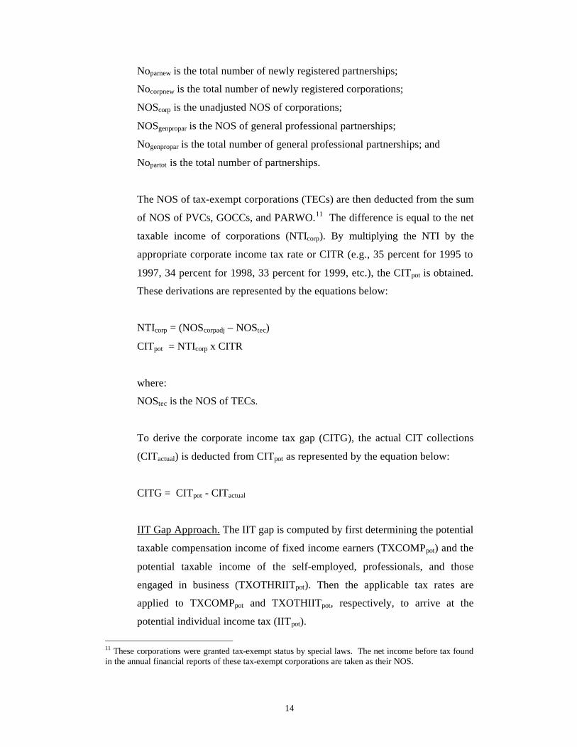
Noparnew is the total number of newly registered partnerships;
Nocorpnew is the total number of newly registered corporations;
NOScorp is the unadjusted NOS of corporations;
NOSgenpropar is the NOS of general professional partnerships;
Nogenpropar is the total number of general professional partnerships; and
Nopartot is the total number of partnerships.
The NOS of tax-exempt corporations (TECs) are then deducted from the sum
of NOS of PVCs, GOCCs, and PARWO.11 The difference is equal to the net
taxable income of corporations (NTIcorp). By multiplying the NTI by the
appropriate corporate income tax rate or CITR (e.g., 35 percent for 1995 to
1997, 34 percent for 1998, 33 percent for 1999, etc.), the CITpot is obtained.
These derivations are represented by the equations below:
NTIcorp = (NOScorpadj – NOStec)
CITpot = NTIcorp x CITR
where:
NOStec is the NOS of TECs.
To derive the corporate income tax gap (CITG), the actual CIT collections
(CITactual) is deducted from CITpot as represented by the equation below:
CITG = CITpot - CITactual
IIT Gap Approach. The IIT gap is computed by first determining the potential
taxable compensation income of fixed income earners (TXCOMPpot) and the
potential taxable income of the self-employed, professionals, and those
engaged in business (TXOTHRIITpot). Then the applicable tax rates are
applied to TXCOMPpot and TXOTHIITpot, respectively, to arrive at the
potential individual income tax (IITpot).
11 These corporations were granted tax-exempt status by special laws. The net income before tax found in the annual financial reports of these tax-exempt corporations are taken as their NOS.

15
To calculate TXCOMPpot, the total compensation income obtained from the
NIA is adjusted by the amount of the employers’ share of social security
contributions (SSCempyer) as these are not actually received by the employees,
and thus, should not form part of their compensation income.12 Then, the total
personal and additional exemptions (PAEs) for those with compensation or
fixed income (PAECOMPtot) are deducted to get TXCOMPpot as shown in the
following equations:
TXCOMPpot = COMPtot - SSCempyer - PAECOMPtot
or
TXCOMPpot = COMPtot - SSCempyer – SSCempyee - PAECOMPtot
where:
COMPtot is the total compensation income.
To compute for the potential tax collection on compensation income
(COMPIITpot), the average tax rate (ATR) is multiplied to TXCOMPpot as
shown by the equation below:
COIMPIITpot = TXCOMPpot x ATR13
To derive TXOTHRIITpot, the NOSparwo and the NOS of cooperatives
(NOScoop) are deducted from the NOS accruing to the household (HH) sector
12 Based on the historical trends, the NTRC assumed that 60 percent of total social security contributions are the employers’ share. For the years 1998 onwards, the employees’ share of social security contributions (SSCempyee) must also be deducted, as this has been tax-exempted by the enactment of the Comprehensive Tax Reform Act of 1997. 13 The ATR is derived by deducting the appropriate PAEs to the average family income of each family size as provided for by the Family Income and Expenditure Survey (FIES) of the National Statistics Office (NSO) to get the net taxable income and the tax due. The PAEs used are based on the actual BIR distribution of tax filers by status. Summing up the total tax due and the total net taxable income of each family size will give the total tax due and total net taxable income for all family sizes. By dividing by the total tax due for all families by the total net taxable income for all families the ATR is derived.
16
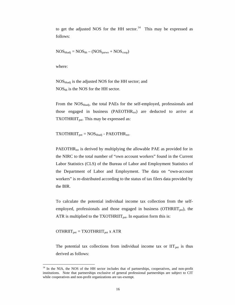
to get the adjusted NOS for the HH sector.14 This may be expressed as
follows:
NOShhadj = NOShh – (NOSparwo + NOScoop)
where:
NOShhadj is the adjusted NOS for the HH sector; and
NOShh is the NOS for the HH sector.
From the NOShhadj, the total PAEs for the self-employed, professionals and
those engaged in business (PAEOTHRtot) are deducted to arrive at
TXOTHRIITpot. This may be expressed as:
TXOTHRIITpot = NOShhadj - PAEOTHRtot.
PAEOTHRtot is derived by multiplying the allowable PAE as provided for in
the NIRC to the total number of “own account workers” found in the Current
Labor Statistics (CLS) of the Bureau of Labor and Employment Statistics of
the Department of Labor and Employment. The data on “own-account
workers” is re-distributed according to the status of tax filers data provided by
the BIR.
To calculate the potential individual income tax collection from the self-
employed, professionals and those engaged in business (OTHRIITpot), the
ATR is multiplied to the TXOTHRIITpot. In equation form this is:
OTHRIITpot = TXOTHRIITpot x ATR
The potential tax collections from individual income tax or IITpot is thus
derived as follows:
14 In the NIA, the NOS of the HH sector includes that of partnerships, cooperatives, and non-profit institutions. Note that partnerships exclusive of general professional partnerships are subject to CIT while cooperatives and non-profit organizations are tax-exempt.
17
IITpot = COMPIITpot + OTHRIITpot.
To compute for the IITgap, IITactual is deducted from IITpot. The difference is
the IITgap. IITactual is the actual IIT collections.
National Economic and Development Authority. The NEDA validates the
feasibility of attaining the full year tax collections targets given the first quarter actual
tax collections and national income accounts by doing either a simple trend analysis
or a buoyancy approach. The analysis is done primarily to determine if the full year
deficit target would still be met given the actual revenue collections and expenditures,
and if not, how such change would impact on economic growth. The NEDA has a
Quarterly Macroeconometric Model or QMM15 that contains tax equations that
may be useful for tax forecasting purposes, which to date have not been used for such.
For the corporate and individual income taxes, the tax equations of the QMM are as
follows:
CIT Equation16.
LCORP = -4.80 + 5.29 LOG (TAXCORPRT) + 1.53 LOG ([PVIS/100] x VIS)
+ 0.50 S2
CORP = EXP (LCORP)
where:
LCORP is the natural logarithm of corporate income tax collections or CORP;
TAXCORPRT is the corporate tax rate;
PVIS is the price index of the value-added in industry and services;
15 The QMM has a fiscal block with a revenue sub-block composed of individual equations for major taxes that may be used to forecast collections of said taxes. Looking at each tax equation shows that these are actually tax buoyancy/elasticity equations.

18
VIS is the value-added in industry and services; and
S2 is the seasonality variable for the second quarter where annual income tax
payments for the preceding year are due and thus, CIT collections surged.
IIT Equation17.
LIYTAXDOF = 0.82 + 1.36 LOG (@MOVAV(QSE1,4)) – 0.52 DUMEX87D
+ 0.27 S2
INDIV = EXP (LIYTAXDOF) x FITINDTXDOF
where:
LIYTAXDOF is the natural logarithm of quotient of individual income tax
collections divided by forecasted average individual income tax rate;
@MOVAV (QSE1,4) is the moving average of four quarters of the
compensation of employees index;
DUMEX87D is the dummy variable to represent the increase in the exemption
levels of individual income tax payers where DUMEX87D = 1 from
the fourth quarter of 1987 onwards, and DUMEX87D = 0 for the
quarters preceding the fourth quarter of 1987;
INDIV is the IIT collections; and
FITINDTXDOF is the forecasted average individual income tax rate.
16 The left-hand side of the equation is the log of actual CIT collections. Note that actual CIT collections are computed by multiplying the actual taxable corporate incomes with the applicable CIT rate. Yet, the right-hand side of the equation has as an explanatory variable the log of the CIT rate. The equation, thus, becomes more of an identity rather than a behavioral one. An attempt by the author to use the corporate tax rate as one of the explanatory variables in a tax elasticity equation for an annual data series yielded a near singular matrix. 17 Note that the index of compensation of employees reflects only those in the private sector. Thus, it understates the total compensation income. Further, studies have shown that bulk of individual income tax payers are fixed income earners, and a large portion of these taxpaying fixed income earners are government employees. Moreover, the impact of the increases in PAEs in the recent years (after 1987) was not decomposed from the actual tax data series.

19
To compute for FITINDTXDOF, INDIV was divided by the sum of the
nominal value of disposable income and direct taxes. The resulting trend value
was then forecasted yielding FITINDTXDOF.
Department of Finance. The DOF, which is the government agency mandated
to produce official revenue forecasts, uses the elasticity approach in forecasting
collections of corporate and individual income taxes. It first removes from its data
series the effects of discretionary changes in the tax system prior to computing the
elasticity of CIT collections over the tax base. DOF uses GDP as a proxy tax base for
its forecast for CIT collections. DOF does the same for IIT collections.
The DOF has its own estimates of how much of the taxes collected come from
the new system (with policy reform) and how much is accounted for by the existing
system (status quo). Depending on the timeframe DOF wants to consider, the amount
due to discretionary changes in the tax system also varies. Then, the DOF calculates
for the elasticity of CIT collections over GDP as well as the elasticity of IIT
collections over GDP. In some instances, the DOF adjusts GDP to account for the
tax-exempt status of certain sectors like the agriculture and exports sectors. Note,
however, that if the adjusted GDP is used, the elasticities computed are higher.
After computing for the elasticities of CIT collections and IIT collections with
respect to GDP or adjusted GDP, the DOF calculates for the forecasts in the medium-
term (five to six years). The elasticities here are simple point elasticities.
The DOF, however, also uses the gap approach to compute for the potential
collections from individual income taxes. This method is being used by DOF solely
for the purpose of estimating the potential collections and the gap. The gap computed
is assumed to be due to tax evasion, tax avoidance, and inefficiency of the collecting
agency, the BIR. The estimates are used for policy analysis and performance
evaluation rather than on forecasting or target setting.
The gap approach for IIT is represented by the equation below:
IITpot = i * (Yf +Yu –Yn – Ye)

20
where:
i is the average IIT rate;
Yf is the family income as reported by the NSO;
Yu is the income of unincorporated enterprises detached from households;
Yn is non-taxable income; and
Ye is the amount of exemption.
Bureau of Internal Revenue. The BIR simply uses the buoyancy approach
that computes for the buoyancy coefficient similarly with the elasticity approach of
the DOF but with one difference, the data series on tax collections used remains
untouched or “uncleaned”. This assumes that the tax system has remained unchanged
over the years, and that only the natural tendency for collections to increase over time
is considered.
Philippine Institute for Development Studies. In a 1981 study of Manasan for
the PIDS, an econometric model for internal revenue taxes was developed. In that
study, Manasan reiterated her findings in an unpublished PIDS paper (March 1981)
that reviewed the existing tax forecasting models in the Philippines then. To wit, “(1)
a high degree of disaggregation in tax forecasting models yields low performance in
statistical tests reflecting the greater difficulty involved in capturing the volatile
movements inherent in each tax category; (2) the use of tax bases and other variables
expected, a priori, to be more reflective of the tax structure than simpler variables like
time in explaining the level of tax receipts, is not a guarantee in obtaining more
accurate forecasts; and (3) the elasticities approach in tax forecasting resulted in the
lowest average root mean square percentage forecasting error, indicating in turn that
the functional relationship between the different tax categories and their respective
bases is better described by the power function and the simple linear one.”

21
Although various estimated forecasting equations where used to forecast
corporate and individual income taxes, the “best” equations, which passed a set of
criteria18, are the following linear models:
TIT = -199.27 + 0.03 GNPC
CIT = -22.09 + 0.36 CI + 220.55 DI
IIT = TIT – CIT
where:
TIT is the total income tax collections in million pesos;
GNPC is the GNP at current prices in million pesos;
CIT is the corporate income tax collections in million pesos;
CI is the corporate income at current prices in million pesos;
DI is the dummy variable where DI = 0 for 1961-1967, and DI = 1 for 1968-
1978, reflecting the corporate income tax rate change in 1968; and
IIT is the individual income tax collections in million pesos.
When no values are available for CI, estimates where made using the
following:
CI = -1,052.92 + 0.07 GNPC.
Note that IIT forecast is just the residual of the forecasted TIT and CIT.
In its studies in the late ‘80s to the ‘90s, the PIDS has been using the elasticity
and gap approaches to measure tax evasion and performance evaluation of the tax
yields of IIT. In ‘cleaning’ the tax data series, the proportional adjustment methods
18 The set of criteria include: (a) the t-statistic; (b) the coefficient of determination or the R2; and (c) the percentage root mean square error (RPMSE). According to Pindyck and Rubinfield, for purposes of assessing forecasting capabilities of regression models, the more important criterion among the three is the RPMSE.
22
(PAMs) were used in the early to mid-‘80s.19 PAMs may either be the Prest Forward
Adjustment method or the Sahota method. But lately, especially for tax forecasting
purposes, the Singer Method (or the “Dummy Variable” Technique) is being applied.
The PIDS uses the gap approach to measure the level of tax evasion of IIT
payers. Given that the IIT is applied to incomes of fixed income earners (those
earning purely compensation income), and to individuals who are self-employed,
professionals, or engaged in business (entrepreneurial activity), the PIDS computes
for the potential individual income from compensation, and from other sources,
respectively. The PIDS gap approach is similar to the NTRC gap approach but for
some refinements on the number of income earners, number of potential tax payers,
number of dependents, and the sources of income.
To derive the potential compensation income, the formula20 is:
Comphhpot = COMPhh – ½ SSC
where:
Comphhpot is the potential compensation income of HHs;
COMPhh is the compensation income of HHs; and
SSC is the total social security contributions.
To derive the potential tax base of individual income from other sources, the
formula is:
OTHhhpot = NOShhunincorp - NOSunincorp
where:
OTHhhpot is the potential income of HHs coming from other sources;
19 The NTRC estimates of the impact of discretionary changes on tax collections are often used by the PIDS. 20 The employers’ share of SSCs is included in the calculation of compensation income of HHs but it must be deducted, as it does not actually accrue to the HHs. The PIDS assumes that the burden of SSCs is equally shared between the employer and the employee. It should be noted, however, that from 1998 onwards, the total SSCs have been tax-exempted.

23
NOShhunincorp is the NOS of HHs and unincorporated enterprises; and
NOSunincorp is the NOS of unincorporated enterprises.
Data on NOSunincorp is not disaggregated in the NIA. This is, thus, derived as
follows:
NOSunincorp = ½ (NOShhunincorp – NOSentrefies)
where:
NOSentrefies is the income from entrepreneurial activity as reported in the FIES.21
Data on NOSentrefies is only available every three years because the FIES is
conducted only every three years. For the non-FIES years, NOSentrefies must be
derived. To do this, the ratio of NOSunincorp over NOShhunincorp is used to
estimate OTHhhpot for non-FIES years. The formula is:
OTHhhpotT = Ra1F x NOShhunincorp
where:
Ra1F is NOSunincorpF/NOShhunincorpF;
F is the corresponding FIES year; and
T is the corresponding non-FIES year22.
The total potential individual income is thus derived as follows:
IYpot = COMPhhpot + OTHhhpot
21 Under the FIES, entrepreneurial income is the difference between the gross receipts from entrepreneurial activity, and the cost of goods sold. Removing depreciation cost from entrepreneurial income will make it comparable to NOShhunincorp. According to experts, the difference between the NOSentrefies and NOShhunincorp is due to income of private non-profit corporations (unincorporated enterprises) and statistical discrepancy. For the PIDS’ gap approach, the difference is equally distributed between the two factors. 22 F varies depending on the FIES years within the period of study. For example, if the period covered is 1991-1996, FIES for 1991 and 1994 are available. The 1991 ratio may be applied to the year 1992 while the 1994 ratio may be applied to the years 1993, 1995, and 1996.
24
where:
IYpot is the total potential individual income.
As OTHhhpot is not purely entrepreneurial income, IYpot must be refined to
reflect what is compensation income and what is entrepreneurial income. This
is needed so that the appropriate PAEs may be applied. The refinement is done
as follows:
COMPYT = Ra2F x IYpotT
ENTREYT = (1-Ra2F) x IYpotT
where:
COMPYT is the potential individual income from compensation at period T;
Ra2F is COMPhhpotF/(COMPhhpotF+NOSentrefiesF);
ENTREYT is the potential individual income from entrepreneurial activity;
and
F is the FIES years.
To derive the taxable COMPY and ENTREY, applicable PAEs must be
deducted. Unlike the NTRC gap approach where the PAEs for fixed income
earners are deducted from the average family income of each family size per
the FIES, and the PAEs of other earners are deducted from their income after
determining the number of these other earners using the CLS and BIR data,
the PIDS uses only the FIES data sets.
To arrive at the number of HHs for non-FIES years, the average national
population growth rate was applied to the number of HHs in the FIES years.
Total ENTREY and total COMPREY where then distributed to the different
income groups using the decile distribution of said incomes, respectively. For
example, ENTREY and COMPREY for 1991-1992 are distributed according
to the 1991 FIES income distribution while ENTREY for 1993-1996 are
distributed according to the 1994 FIES income distribution.

25
FIES data sets are further processed to show the number of dependent children
(0,1,2,3,4, or 5), the number of income earners (0,1,2,3, or 4), and the sources
of income (compensation income, entrepreneurial income, dividends, interest
income, imputed rent, and gifts) per decile. The number of income earners
determines the number of potential income tax payers in a HH and the amount
of personal exemptions that may be applied. It is assumed that the first two
income earners in a HH are married, and file a joint income tax return. The
third, and fourth income earners of a HH are assumed to file separate income
tax returns, and are treated as additional potential taxpayers.
In addition, the number of dependent children determines the additional
exemptions of a HH. It is assumed that if there are more than two income
earners in a HH, the total number of dependent children belong to the first two
income earners. Further, the source of income of each earner in a HH
determines which income source is subject to individual income tax23, and
which income tax rate schedule is applicable, the compensation income tax
rate schedule, or the business/professional IIT rate schedule24.
The total HH income subject to IIT for each income subgroup is divided by
the total number of HHs, and by the number of income earners in each HH to
arrive at the gross income of each representative income earner.25 Given the
exemptions earlier estimated, a tax calculator model26 is used to estimate the
potential individual income tax liability27.
23 Dividends, and interest incomes are already subject to final tax, and therefore are no longer subject to IIT. Also, imputed rent, and gifts are not subject to IIT. These should therefore be deducted from the total income of the decile sub-group. 24 The distinction is relevant during years when the schedular system was in place. 25 The number of potential IIT payers for each year is derived by getting the number of income earners who are required by law to file an income tax return (e.g., those with taxable incomes of P60,000 and below are not required to file a tax return), and adjusting the same to account for some HHs which have more than two income earners. 26 The tax calculator model has four steps. Step 1 – the PAEs for the representative income earner in each sub-group are calculated using the data on the number of income earners, and the number of dependent children. Step 2 – these estimated PAEs are deducted from the total gross income of each representative income earner to arrive at estimates of legally taxable income. Step 3 – the taxable income of each representative income earner is multiplied by the corresponding tax rate using the applicable tax schedule to get the estimated potential tax liability. Step 4 – the potential tax liability of
26
In the recent exercise of the various subgroups of the Inter-Agency Task Force
on the Improvement of Tax Related Database spearheaded by the BIR, forecasting
exercises were made using some of these current tax forecasting methods. Taking the
lead for the CIT subgroup is the PIDS while for the IIT subgroup is the NTRC.28
For CIT collections, the historical simulations using the buoyancy (BIR),
elasticity (NTRC and NEDA), and gap (NTRC) approaches were compared to the
actual tax data series. In the buoyancy approach, BIR related CIT collections to GDP.
The mean square errors (MSEs) for the BIR approach cover the period 1998-2000. In
the NTRC elasticity approach, a double logarithmic equation was used where CIT
collections (adjusted using the PAM technique, see Appendix A) were related to
GDP.
The MSEs for the NTRC approach covers the period 1995-1999. The NEDA-
QMM’s CIT equation earlier discussed was also used, and the MSEs calculated cover
the period 1996-2000. The BIR and the NTRC used annual data (1990-2000 for BIR
and 1981-2000 for NTRC) while the NEDA-QMM used quarterly data (1992-2000).
The application of these forecast approaches by these three agencies yielded the
forecasting error statistics shown in Table 1.
In Table 1, the root mean square error (RMSE) and root percentage mean
square error (RPMSE) of the forecasts using the NTRC gap approach are the highest.
These high MSEs were expected of the gap approach. As discussed in Section 2, the
gap approach estimates the potential CIT collections. Given that collection
efficiency29 is always way below 100 percent, it is expected that the computed MSEs
using the gap approach will actually be large.
each representative income earner is multiplied by the number of HHs in each income sub-group to get the total potential tax revenues from IIT. 27 The tax liability of compensation income earners in the current year is assumed to be paid in the same year while the tax liability of business/professional income earners in the current year is assumed to be paid in the following year. 28 The author is a member of both subgroups. 29 Collection efficiency is the ratio of actual collections over potential collections.
27
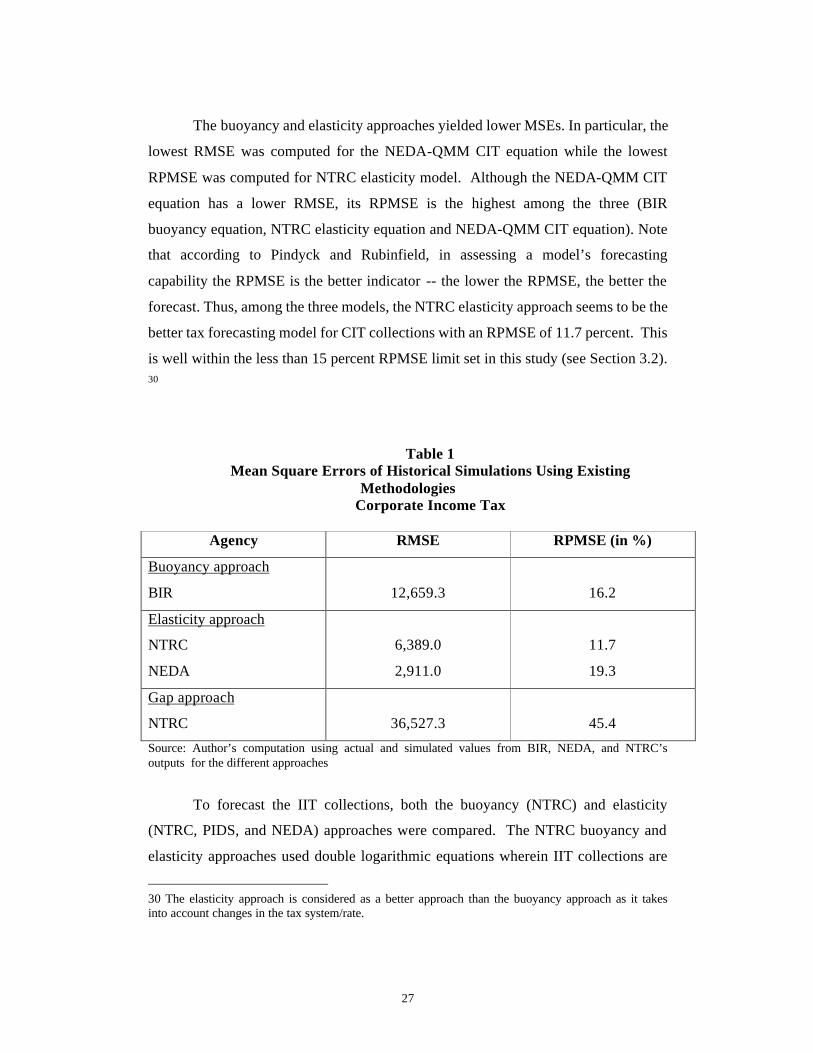
The buoyancy and elasticity approaches yielded lower MSEs. In particular, the
lowest RMSE was computed for the NEDA-QMM CIT equation while the lowest
RPMSE was computed for NTRC elasticity model. Although the NEDA-QMM CIT
equation has a lower RMSE, its RPMSE is the highest among the three (BIR
buoyancy equation, NTRC elasticity equation and NEDA-QMM CIT equation). Note
that according to Pindyck and Rubinfield, in assessing a model’s forecasting
capability the RPMSE is the better indicator -- the lower the RPMSE, the better the
forecast. Thus, among the three models, the NTRC elasticity approach seems to be the
better tax forecasting model for CIT collections with an RPMSE of 11.7 percent. This
is well within the less than 15 percent RPMSE limit set in this study (see Section 3.2). 30
Table 1
Mean Square Errors of Historical Simulations Using Existing Methodologies
Corporate Income Tax
Agency RMSE RPMSE (in %)
Buoyancy approach
BIR
12,659.3
16.2
Elasticity approach
NTRC
NEDA
6,389.0
2,911.0
11.7
19.3
Gap approach
NTRC
36,527.3
45.4
Source: Author’s computation using actual and simulated values from BIR, NEDA, and NTRC’s outputs for the different approaches
To forecast the IIT collections, both the buoyancy (NTRC) and elasticity
(NTRC, PIDS, and NEDA) approaches were compared. The NTRC buoyancy and
elasticity approaches used double logarithmic equations wherein IIT collections are
30 The elasticity approach is considered as a better approach than the buoyancy approach as it takes into account changes in the tax system/rate.

28
regressed on income (either GDP or GNP). For the elasticity approach, the actual IIT
series was cleaned using the Prest Backward Method (see Appendix A). The PIDS
equation is a double logarithmic one. The NTRC and PIDS’ equations cover the
period 1990-1999 and uses annual data. The NEDA IIT equation, which came from
the NEDA-QMM discussed in Section 2, covers the period 1985-2000 (Q2), and uses
quarterly data.
Table 2 shows that the NEDA-QMM IIT equation yielded the highest RPMSE
at 39.7 percent while the NTRC buoyancy equation using GNP as the independent
variable had the lowest RPMSE at 5.3 percent. But as earlier noted, the elasticity
approach is deemed a better method than the buoyancy approach as the impact of
discretionary changes on the tax system is netted out. The non-removal of this impact
may distort the relationship among the dependent tax variables and the explanatory
variables. Taking off from this discussion, the NTRC and the PIDS elasticity
equations using GDP as the determinant variable are the “best” models with RPMSE
of 8.1 percent each.
Table 2
Mean Square Errors of Historical Simulations Using Existing Methodologies
Individual Income Tax
Agency RMSE RPMSE (in %)
Buoyancy approach
NTRC (using GNP)
NTRC (using GDP)
3.6
3.7
5.3
5.5
Elasticity approach
NTRC (using GNP)
NTRC (using GDP)
PIDS (using GNP)
PIDS (using GDP)
NEDA
3.9
4.1
3.9
4.0
2.5
8.3
8.1
8.2
8.1
39.7
Source: NTRC’s computation using actual and simulated values from NEDA, and its own outputs for the different approaches

29
Based on the foregoing forecasting error statistics and the discussions on
existing methodologies for tax forecasting, the tax elasticity approach applying
regression analysis is deemed to be the “best” tax forecasting methodology for both
the CIT and the IIT.
Outside the Philippines.
Republic of Ireland. There are three main government entities that are
involved in tax and macroeconomic forecasting in Ireland. These are the Central
Budget Office (CBO), the Economic Forecasting Unit (EFU) of its Finance
Department, and the Revenue Commission (RC).
The EFU prepares preliminary economic forecast generating economic
variables (e.g., earnings, employment, personal consumption expenditures, etc.) that
are used to derive the tax forecasts. The CBO and the RC use these forecasted
economic variables to prepare preliminary disaggregated tax forecasts independently.
A discussion ensues to assess their respective tax forecasts. The final arbiter is the
Finance Department, which decides which forecast to use. The tax forecasting
process is undertaken on a rolling basis throughout the forecasting time frame (about
March/April to the Budget enactment). Moreover, twice within the said period the
RC is requested to provide detailed tax forecasts on May/June and October/December.
The first is considered the status quo or the ‘no policy change’ forecast phase while
the second is called the pre-Budget phase. The CBO, on the other hand, makes a
number of individual forecasts throughout the period. To make tax and
macroeconomic forecasts consistent, dialogues are frequently conducted between the
RC and the CBO.
Studies undertaken by Irish experts and European Community experts showed
that Ireland’s corporation taxes (corresponds to the Philippines’ CIT) are highly
sensitive to GDP growth by a 2.5%:1% ratio (assuming no tax reduction measures).
Income tax elasticity, on the other hand, is 1.3 (with policy changes). With no policy
shifts, this elasticity would be higher.

30
In general, the tax elasticity approach is employed to forecast the major taxes
in the Republic of Ireland. Regression procedure is applied in using the tax elasticity
approach. Econometric modeling was also tried but Irish experts concluded that there
appears to be a limited role for a more intensive use of a macroeconometric model to
improve tax forecasting.
In the Republic of Ireland, corporation and income taxes are forecasted as
follows:
Corporation Tax. The elasticity approach is applied to forecast corporation tax
receipts. Actual corporate tax receipts of previous years are usually used to
determine the forecast base for the current year. This forecast base is then
adjusted for budget or collection factors. Then it is increased by the average
percentage projected growth in company profits. Preliminary forecasts of
corporate profitability used a GNP-related elasticity of 1.5. But as the year
progresses, various sector-based databases are used to determine current year
profits. The resultant estimate is the corporation tax forecast.
Pay As You Earn (PAYE) Tax (corresponds to the Philippines’ IIT) forecasts
are made by applying macroeconomic determinants like earnings and
employment numbers to the baseline. The baseline is usually the actual tax
revenue collections on a net receipts basis of the previous year. By adjusting
or “cleaning” the baseline for factors like budget and collection efficiency, a
forecast base is established, where forecasts for succeeding years will be built
on. This is the simple approach to forecast PAYE taxes.
Another more complicated approach is to adjust further the forecast base by
the product of the percentage change in non-agricultural per capita pay rates
and the elasticity factor.31 This is further increased by the estimated extra tax
derived by applying an agreed percentage of the forecast base to the forecast
31
percentage growth in non-agricultural employment numbers.32 The resultant
estimate is further modified to reflect the impact of budget changes and other
factors. This is now the revised PAYE tax forecast.
Some weaknesses in the forecasting method for PAYE taxes have been
identified by Irish experts. Among these are (a) the macroeconomic factors
used to adjust the baseline may be understated, (b) the macro forecasts used
are averages, and the revenue model spreads them evenly over all income
levels of the tax population using the distribution path of the baseline year
without accounting for the variations in population increases of each income
group, and (c) the core baseline data used in the model are usually out of date,
thus, structural changes in the nature and composition of employees’ earnings
are not captured by the model. Overall, however, the elasticity approach to
forecast PAYE taxes is deemed acceptable.
Barents Group. The private international consulting firm Barents Group has
developed a system of tax policy simulation and forecasting models, which are tools
that may provide policymakers with robust and dynamic revenue impact assessments
of fundamental tax policy reforms. These tools are State-specific, user-friendly
models that allow the simulation of alternative tax policy changes. The system
comprises of (a) a corporate income tax model, (b) an individual income tax model,
(c) a sales/consumption tax model, (d) a property tax model, (e) a multi-tax incidence
model, and (f) a dynamic economic impact model. Of interest to this study is (a) and
(b) although a discussion on (e) is provided as it also measures the impact of changes
31 The elasticity factor is the percentage increase in PAYE tax, which is likely to arise from an average overall increase of one percent in income. A revenue tax model is used to derive this elasticity factor. This model is a distributional model of income tax payers, which provides (a) estimates of costs and distributional impact changes to the income system, (b) estimates current costs of major personal allowances and reliefs, and (c) current provisional estimates of income distribution. 32 The growth in non-agricultural employment numbers refers only to new employees, who, by definition, do not move from one tax rate to another in the first year of employment. At first, a flat rate increase in the tax equal to the projected growth in employment numbers is assumed. This is then adjusted to assume that new wage earners are paid less than existing employees. This is, however, counterbalanced by the fact that a significant number of new employees are married women, who, in general, have substantial tax liabilities.

32
in corporate and individual income tax policies. Models (a), (b), and (e) are discussed
below33:
CIT Model. This microsimulation model for the CIT analyzes the liability and
distributional effects of alternative business tax policies. The model is also
capable of projecting business tax liabilities under alternative economic
forecasts. The model has four components, (a) two tax calculators, (b)
parameter file, (c) database, and (d) forecasting procedure.
The model uses micro data from a sample of CIT returns filed within a State.
The model also developed a set of parameters (e.g., marginal tax rates, income
brackets, deductions, and credits, etc.) for each input file.
The two tax calculators of the model allow for the generation of two
simulations, the base run (for the status quo) and the impact run (for the
variation on the status quo). The difference between the two runs measures
the change in tax liability associated with changes in tax policy.
To forecast tax liabilities, the model reads the database one record at a time. It
then applies an appropriate growth rate by industry to the data record.
The CIT model produces three standard output tables, (a) output 1 - total
income tax liability by industry and income class for each tax calculator
showing also how many tax returns will have tax liability reduction and how
many will have tax liability increase based on the simulation, (b) output 2 –
additional tax liability variables due to State tax structure to include domestic
income tax, foreign income tax, domestic franchise tax, federal net income,
State taxable income, US capital base, and State capital base, and (c) output 3
– tabulations of certain variables by industry and by income class.
IIT Model. The IIT model developed by the Barents Group is a
microsimulation model designed to forecast the distribution of the tax burdens
33 Culled from the Barents Group website.

33
resulting from reforms in the IIT policy. The model replicates the calculations
made by each sample taxpayer to determine the tax liability under each tax
law.
The model has five components, (a) four tax calculators, (b) parameter file, (c)
database, (d) forecasting component, and (e) tabulation utility.
Two of the four tax calculators are for State-specific income taxes while the
other two are for Federal-specific income taxes. The model is an “X-Y”
convention type that measures tax liability changes given a particular tax
policy – status quo (X) and alternative (Y). The difference between X and Y
is the impact on tax liability of a tax policy reform on individual income tax.
The features of State and Federal income tax laws are incorporated in the
model and are defined in the default parameter file, which are then altered for
simulation purposes. Micro data derived from IIT returns are used. These data
are merged with census data to define family units/households and capture
non-taxable income.
In forecasting the IIT liability, two steps are followed. Step 1 is to forecast the
economic scenario for the next 10 to 15 years. Step 2 is to attain the scenario
determined in step 1 using a sophisticated mathematical algorithm wherein the
different tax concepts (e.g., adjusted gross income or AGI, capital gains, etc.)
are defined consistent with the economic growth projections such as
composition of population cohort groups, unemployment rate, changes in real
income, price levels, and interest rates.
The model also has a tabulation utility that allows the examination of the data
used in the model. Database variables may be tabulated using different types
of classifiers and are presented by income class.
The model generates various output tables at different levels of detail. The
resulting estimates of IIT liability, effective tax rates, the number of new
taxpayers, the number of delisted taxpayers, and the number of taxpayers
shifting between the use of standard or itemized allowable deductions may be
34
displayed by income class. Other output tables show diagnostic data, and the
“winners and losers” of a certain tax policy change.
Multi-tax Incidence Model. The Multi-tax incidence model developed by the
Barents Group may be used to analyze the impacts of tax reform measures
involving two or more taxes on households. The model can measure the
combined incidence of a broad range of taxes – individual income,
consumption, residential and business property, and corporate income taxes.
The final or net effect of changes in tax policy may be calculated involving
two or more tax policy reforms undertaken simultaneously.
Each tax model (e.g., residential property tax, income tax, and consumer sales
tax, etc.) has its own parameter file that may either reflect the status quo or the
policy shift. The tax incidence model generates an output showing the tax
liability by type of tax and by income class. The model also generates the
overall tax incidence by family and by State. For residential rental property
tax, the Multi-tax incidence model assumes that the tax burden from said tax is
transferred to the tenants. For business property and income taxes, the model
assumes that the tax burdens are shifted to capital owners, labor or consumers.
3. FRAMEWORK OF THE STUDY
3.1 Methodology.
Section 2, which discusses existing tax forecasting methodologies both here
and abroad, showed that the tax elasticity approach using regression procedure
showed a better fit where the errors of estimation are minimized. Thus, for purposes
of this study, the tax elasticity approach is used.
Although Tables 1 and 2 in Section 2.1 showed RPMSEs less than 15 percent
for CIT and less than 10 percent for IIT for the NTRC elasticity equations, alternative
structural single equation tax elasticity models were still specified for both the
corporate and individual income taxes. Recall that in applying the elasticity approach,
the NTRC uses a proportional adjustment method to remove the impact of
35
discretionary changes in the tax system. As discussed in Section 2, this method is
considered subjective and arbitrary. In the alternative equations for this study, a less
subjective and arbitrary method was used, the “Dummy Variable” technique. Further,
this technique is able to distinguish not only which coefficient (intercept or slope) is
different but also the source of the difference (intercept, slope or both). In addition,
the period covered was expanded to cover 1980-2000. The general estimation
procedure used was the ordinary least squares (OLS) method.
In defining the functional relationship between the dependent variable (tax
variable) and the explanatory variables, both the linear and double logarithmic forms
were considered.
For each of the forecasting equations estimated, the following statistics were
considered to evaluate the relative merits of the alternative forecasting equations:
(a) t-statistic indicates the statistical significance of the regression coefficients
of the independent variables; with 21 observations in this study, and more
than two explanatory variables, a computed t-statistic greater than 1.76 in
absolute value implies that the corresponding regression coefficient of the
independent variable is statistically different from zero at the 10 percent
level of significance and a t-statistic greater than 2.14 at the five percent
level of significance;
(b) coefficient of determination of R-square (R2) measures the extent to which
the estimated regression line fits the actual observation points; it also
measures the proportion of the total variation of the tax variable explained
by the independent variables; a high value of R2 implies a good fit of the
regression line while a low R2 is associated with a poor fit; as a rule of
thumb, an R2 greater than 0.70 is considered satisfactory; and
(c) percentage root mean square error (RPMSE) indicates how closely the
simulated values from historical simulation of the dependent variable
move in relation to the actual data series; it is defined as:
______________________

36
� N ^ RPMSE = � 1/N � ((Yi –Yi)/Yi)
2 i = 1
where:
Yi is the simulated value of the dependent variable; Yi is the actual value of the dependent variable; and N is the number of observations in the simulations.
As a rule of thumb, an RPMSE less than 10 percent is an acceptable
indicator of the forecasting capability of a model/equation. This is also the
standard set by the National Bureau of Economic Research, an
independent, private, non-partisan research organization in the USA for
evaluating the forecasting capability of an equation. In a previous study of
the PIDS on tax forecasting model, however, an RPMSE less than 20
percent was the standard accepted. For purposes of this study, an RPMSE
less than 15 percent (the average of the 10 percent RPMSE and the 20
percent RPMSE) was deemed acceptable.
As the main purpose of the study is to develop forecasting models for corporate and
individual income taxes, and reiterating what Pindyck and Rubinfield opined, the
RPMSE was considered the more important criterion among the three outlined above
in evaluating which of the alternative forecasting equations is the “best” equation.
Moreover, the forward simulations or tax forecasts crunched out by the models
developed in the study are considered “conditional” forecasts as the explanatory
variables have to be predicted into the future before the single equation multiple
regression models can be used to forecast the tax variables (corporate and individual
income taxes). Thus, the tax forecast values may be interpreted as the amount of tax
revenues to be realized if the plan targets for the aggregate economic variables are
met.
3.2 Variables.
Dependent variable(s). As mentioned earlier, time series data covering the
period 1980-200 for both the CIT and IIT were used. IIT was further disaggregated
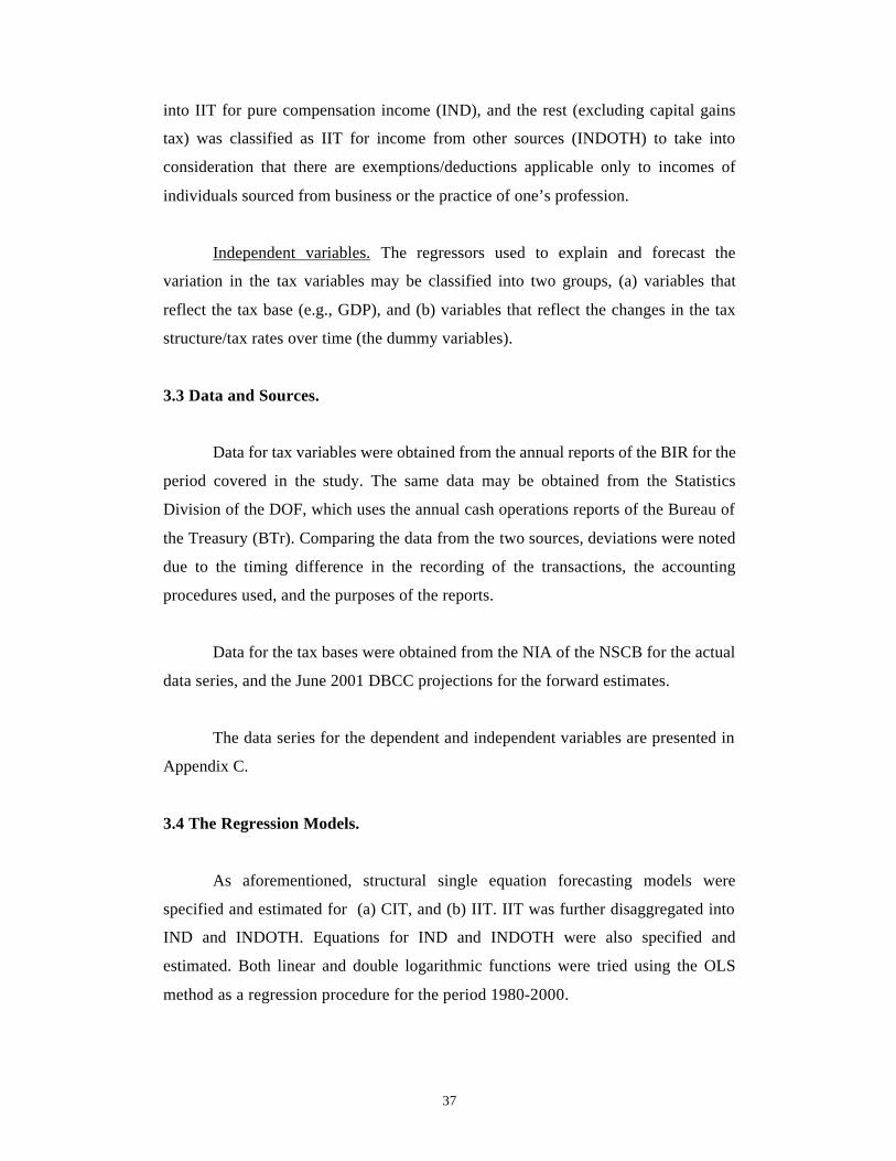
37
into IIT for pure compensation income (IND), and the rest (excluding capital gains
tax) was classified as IIT for income from other sources (INDOTH) to take into
consideration that there are exemptions/deductions applicable only to incomes of
individuals sourced from business or the practice of one’s profession.
Independent variables. The regressors used to explain and forecast the
variation in the tax variables may be classified into two groups, (a) variables that
reflect the tax base (e.g., GDP), and (b) variables that reflect the changes in the tax
structure/tax rates over time (the dummy variables).
3.3 Data and Sources.
Data for tax variables were obtained from the annual reports of the BIR for the
period covered in the study. The same data may be obtained from the Statistics
Division of the DOF, which uses the annual cash operations reports of the Bureau of
the Treasury (BTr). Comparing the data from the two sources, deviations were noted
due to the timing difference in the recording of the transactions, the accounting
procedures used, and the purposes of the reports.
Data for the tax bases were obtained from the NIA of the NSCB for the actual
data series, and the June 2001 DBCC projections for the forward estimates.
The data series for the dependent and independent variables are presented in
Appendix C.
3.4 The Regression Models.
As aforementioned, structural single equation forecasting models were
specified and estimated for (a) CIT, and (b) IIT. IIT was further disaggregated into
IND and INDOTH. Equations for IND and INDOTH were also specified and
estimated. Both linear and double logarithmic functions were tried using the OLS
method as a regression procedure for the period 1980-2000.

38
In general, two main explanatory variables were included in the model
specification (a) the tax base variable, and (b) the tax rate/structure variable. For the
CIT, the taxable bases considered were (a) net operating surplus of private and
government corporations (NOSPVGC) from the NIA, and (b) GDP. For IIT, the
taxable bases studied were (a) GDP, (b) compensation of employees net of social
security contributions (COEMPNET) found in the income approach side of the NIA,
and (c) NOS of households net of social security contributions (NOSHHNET) also
from the NIA. For IND, the taxable bases used were (a) COEMPNET, and (b) GDP.
For INDOTH, the taxable bases employed were (a) NOSHHNET, and (b) GDP.
To capture the changes in the tax rate/structure during the time period covered
in the study, appropriate dummy variables were used (see Figures 1-3). Figures 1 to 3
show how a change in the tax system shifts the tax equation through the intercept
(Figure 1), through the slope (Figure 2) and through both the slope and the intercept
(Figure 3).
For CIT, dummy variables were included to represent the changes in CIT
rates/structure in 1986, 1998, 1999, and 2000. For certain specifications, the dummy
variables for 1998, 1999, and 2000 were merged into one. For IIT, dummy variables
were used to represent changes in IIT rates/structure in 1986, 1992, and 1997. The
same dummy variables were used for IND and INDOTH.
In addition, to determine the elasticities with respect to the slope or the change
in the tax elasticity with respect to the base due to the change in the tax structure/rate,
the dummy variables were multiplied to each of the tax bases to form a new
explanatory variable (e.g., D86GDP, D92GDP, etc.).
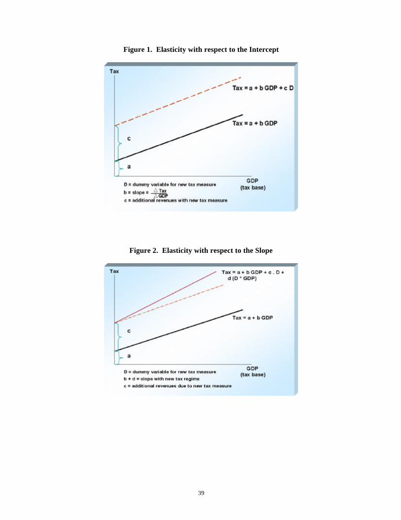
39
Figure 1. Elasticity with respect to the Intercept
Figure 2. Elasticity with respect to the Slope

40
Figure 3. Elasticity with respect to the Intercept and the Slope
3.5 Model Specifications Used in the Study.
CIT. Various model specifications were used to determine which gives the
best fit. Broad and specific measures of CIT tax bases were used as well as different
dummy variables that represent the elasticities with respect to the intercept, the slope,
and both. And the following are the model specifications using both linear and double
logarithmic functions that gave the best fits:
CIT Functions.
(1) CIT = f (NOSPVGC, D86, D98, D99, D00) (2) CIT = f (NOSPVGC, D86, D9800) (3) CIT = f (NOSPVGC, D86, D86NOS, D9800, D9800NOS) (4) CIT = f (NOSPVGC, D86, D86NOS, D98, D99, D00) (5) CIT = f (NOSPVGC, D86, D86NOS, D98, D98NOS, D99, D99NOS, D00, D00NOS) (6) CIT = f (NOSPVGC, D86NOS, D98NOS, D99NOS, D00NOS) (7) CIT = f(NOSPVGC, D86NOS, D9800NOS) (8) CIT = f (GDP, D86, D98, D99, D00) (9) CIT = f (GDP, D86, D9800) (10) CIT = f (GDP, D86, D86GDP, D9800, D9800GDP) (11) CIT = f (GDP, D86, D86GDP, D98, D99, D00) (12) CIT = f (GDP, D86, D86GDP, D98, D98GDP, D99, D99GDP, D00, D00GDP) (13) CIT = f (GDP, D86, D86GDP, D98GDP, D99GDP, D00GDP)

41
(14) CIT = f (GDP, D86GDP, D98GDP, D99GDP, D00GDP) (15) CIT = f (GDP, D86GDP, D9800GDP)
where:
CIT is the corporate income tax collections in million pesos;
NOSPVGC is the NOS of private and government corporations in million pesos;
GDP is nominal gross domestic product in million pesos;
D86 is the dummy variable to represent the tax reform in 1986 when the dual CIT rate
was merged into one, where the value of 1 is given for the years 1986-1997,
and the value of 0 for the years 1980-1985 and 1998-2000;
D98 is the dummy variable to represent the one percent CIT rate cut in 1998 as
provided for under the 1997 CTRP where the value of 1 is given for the year
1998 and the value of 0 for the years 1980-1997, 1999, and 2000;
D99 is the dummy variable to represent another one percent CIT rate cut in 1999 as
provided for in the 1997 CTRP where the value of 1 is given for the year 1999
and the value of 0 for the years 1980-1998, and 2000;
D00 is the dummy variable to represent the final one percent CIT rate cut in 2000 as
provided for in the 1997 CTRP where the value of 1 is given for the year 2000
and the value of 0 for the years 1980-1999;
D9800 is the dummy variable to represent the three-time annual one percent CIT rate
cut as provided for in the 1997 CTRP beginning 1998 where the value of 1 is
given for the years 1998-2000 and the value of 0 for the years 1980-1997.
D86NOS is the product of the dummy variable D86 and the explanatory variable
NOSPVGC forming a new independent variable, which shows how the slope
coefficient with respect to NOSPVGC has been affected by the 1986 tax
reform;
D98NOS is the product of the dummy variable D98 and the explanatory variable
NOSPVGC forming a new independent variable, which shows how the slope
coefficient with respect to NOSPVGC has been affected by the one percent
CIT tax rate cut in 1998;
D99NOS is the product of the dummy variable D99 and the explanatory variable
NOSPVGC forming a new independent variable, which shows how the slope
coefficient with respect to NOSPVGC has been affected by the one percent
CIT tax rate cut in 1999;
42
D00NOS is the product of the dummy variable D00 and the explanatory variable
NOSPVGC forming a new independent variable, which shows how the slope
coefficient with respect to NOSPVGC has been affected by the one percent
CIT tax rate cut in 2000;
D9800NOS is the product of the dummy variable D9800 and the explanatory variable
NOSPVGC forming a new independent variable, which shows how the slope
coefficient with respect to NOSPVGC has been affected by the three-time
annual one percent CIT tax rate cut beginning 1998;
D86GDP is the product of the dummy variable D86 and the explanatory variable GDP
forming a new independent variable, which shows how the slope coefficient
with respect to GDP has been affected by the 1986 tax reform;
D98GDP is the product of the dummy variable D98 and the explanatory variable GDP
forming a new independent variable, which shows how the slope coefficient
with respect to GDP has been affected by the one percent CIT tax rate cut in
1998;
D99GDP is the product of the dummy variable D99 and the explanatory variable GDP
forming a new independent variable, which shows how the slope coefficient
with respect to GDP has been affected by the one percent CIT tax rate cut in
1999;
D00GDP is the product of the dummy variable D00 and the explanatory variable GDP
forming a new independent variable, which shows how the slope coefficient
with respect to GDP has been affected by the one percent CIT tax rate cut in
2000; and
D9800GDP is the product of the dummy variable D9800 and the explanatory variable
GDP forming a new independent variable, which shows how the slope
coefficient with respect to GDP has been affected by the three-time annual one
percent CIT tax rate cut beginning 1998.
IIT. Similar to the CIT, various model specifications were used to determine
which gives the best fit. Broad and specific measures of IIT tax bases were used as
well as different dummy variables that represent the elasticities with respect to the
intercept, the slope, and both. And the following are the model specifications using
both linear and double logarithmic functions that gave the best fits:

43
IIT Functions.
(1) IIT = f (GDP, D86, D92, D97) (2) IIT = f (GDP, D86, D86GDP, D92, D92GDP, D97, D97GDP) (3) IIT = f (GDP, D86GDP, D92GDP, D97GDP) (4) IIT = f (COEMPNET, D86, D92, D97) (5) IIT = f (COEMPNET, D86, D86COEMP, D92, D92COEMP, D97, D97COEMP) (6) IIT = f (COEMPNET, D86COEMPNET, D92COEMPNET, D97COEMPNET)
where:
IIT is the individual income tax collections in million pesos;
GDP is nominal gross domestic product in million pesos;
COEMPNET is the compensation of employees net of social security contributions in
million pesos;
NOSHHNET is the NOS of households net of social security contributions in million
pesos;
D86 is the dummy variable to represent the tax reform in 1986 where the value of 1 is
given for the years 1986-1991, and the value of 0 for the years 1980-1985 and
1992-2000;
D92 is the dummy variable to represent the reforms on the IIT system in 1992 as
provided for under Republic Act 7496, otherwise known as the Simplified Net
Income Tax Scheme and Republic Act 7497 where the value of 1 is given for
the years 1992-1996 and the value of 0 for the years 1980-1991, and 1997-
2000;
D97 is the dummy variable to represent the reform on the IIT system under the CTRP
when personal and additional exemptions were increased where the value of 1
is given for the years 1997-2000 and the value of 0 for the years 1980-1996;
D86GDP is the product of the dummy variable D86 and the explanatory variable GDP
forming a new independent variable, which shows how the slope coefficient
with respect to GDP has been affected by the 1986 tax reform;
D92GDP is the product of the dummy variable D92 and the explanatory variable GDP
forming a new independent variable, which shows how the slope coefficient
with respect to GDP has been affected by the 1992 IIT reform;
D97GDP is the product of the dummy variable D97 and the explanatory variable GDP
forming a new independent variable, which shows how the slope coefficient
with respect to GDP has been affected by the 1997 IIT reform under the
CTRP;

44
D86COEMP is the product of the dummy variable D86 and the explanatory variable
COEMPNET forming a new independent variable, which shows how the slope
coefficient with respect to COEMPNET has been affected by the 1986 tax
reform;
D92COEMP is the product of the dummy variable D92 and the explanatory variable
COEMPNET forming a new independent variable, which shows how the slope
coefficient with respect to COEMPNET has been affected by the 1992 IIT
reform; and
D97COEMP is the product of the dummy variable D97 and the explanatory variable
COEMPNET forming a new independent variable, which shows how the slope
coefficient with respect to COEMPNET has been affected by the 1997 IIT
reform under the CTRP.
As discussed earlier, IIT was further disaggregated into IND and INDOTH,
both having been separately specified and estimated using the same independent tax
base variables as those in the IIT equations, and similar “dummy variables”. The
following were the model specifications for IND and INDOTH using both linear and
double logarithmic functions that gave the best fits:
IND Functions:
(1) IND = f (COEMPNET, D86, D92, D97) (2) IND = f (COEMPNET, D86, D86COEMP, D92, D92COEMP, D97,
D97COEMP) (3) IND = f (COEMPNET, D86, D86COEMP, D92COEMP, D97, D97COEMP) INDOTH Functions:
(1) INDOTH = f (NOSHHNET, D86, D92, D97) (2) INDOTH = f (NOSHHNET, D86, D86NOSHH, D92, D92NOSHH, D97, D97NOSHH) (3) INDOTH = f (NOSHHNET, D86, D86NOSHH, D92, D92NOSHH,
D97NOSHH)
where:
IND is collections of IIT on pure compensation in million pesos;
INDOTH is collections of IIT on other sources of income in million pesos; and

45
D86NOSHH is the product of the dummy variable D86 and the explanatory variable
NOSHHNET forming a new independent variable, which shows how the slope
coefficient with respect to NOSHHNET has been affected by the 1986 tax
reform;
D92NOSHH is the product of the dummy variable D92 and the explanatory variable
NOSHHNET forming a new independent variable, which shows how the slope
coefficient with respect to NOSHHNET has been affected by the 1992 IIT
reform; and
D97NOSHH is the product of the dummy variable D97 and the explanatory variable
NOSHHNET forming a new independent variable which shows how the slope
coefficient with respect to NOSHHNET has been affected by the 1997 IIT
reform.
LNINDOTH is collections of IIT on other sources of income in million pesos in
natural logarithm form.
In Section 4, it would be shown that the alternative equations that passed at
least two of the three main statistical criteria are mostly in double logarithmic form.
Thus, these have to be transformed into linear equations to be able to compare the
results of the historical tax simulations with the actual tax series (CIT or IIT or IND or
INDOTH). The basic transformation formula is:
Y = Antilog (LNY)
where:
Y is the estimated value of the tax; and
LNY is the estimated value of the tax in natural logarithm form.
4. RESULTS OF THE STUDY
The model specifications mentioned in the preceding Section were estimated
using OLS procedure. Below are the regression results of the equations that have
RPMSEs less than 15 percent.

46
4.1 Alternative Forecasting Equations.
CIT. Among the 30 specifications for CIT (linear and double logarithmic),
only six had less than 15 percent RPMSE, all in double logarithmic form. Further, all
six alternative equations have lower RPMSEs than the computed RPMSEs for
existing CIT forecasting methodologies in the Philippines shown in Table 1. Recall
that the lowest RPMSE in Table 1 is 11.7 percent. Moreover, all six equations have
coefficients of determination greater than or equal to 0.98. Most t-statistics of the
explanatory variables passed the 10 percent level of significance (t-statistics are
greater than 1.76 in absolute terms). The independent tax base for all six alternative
equations is GDP in logarithmic form with different mixes of the “dummy variables”
identified in Section 3. The regression results of these six alternative CIT equations
are shown in Table 3.
Although all six alternative equations have lower RPMSEs than those for
existing CIT forecasting methodologies, those with less than 10 percent RPMSEs
were considered as candidates for “best” CIT forecasting equation for the study. Of
these five alternative equations, only equations (3), (4), and (5) have RPMSEs less
than 10 percent with each having an R2 of 0.98. Only equations (4) and (5), however,
have all independent variables statistically significant between the five to 15 percent
level of significance. Thus, equations (4) and (5) were considered as the “best”
alternative CIT forecasting equations.
IIT. Among the six alternative specifications for IIT (linear and double
logarithmic) mentioned in Section 3, only four had RMSEs lower than 15 percent,
two are linear equations and the remaining two are double logarithmic equations. All
four had coefficients of determination greater than 0.99. Most t-statistics of the
independent variables passed the 10 percent level of significance (t-statistics are
greater than 1.77 in absolute terms). The regression results of these alternative model
specifications are shown in Table 4.
Of these four alternative equations, only two have RPMSEs lower than the
lowest computed RPMSE (8.1 percent) for the elasticity approach shown in Table 2.
These are equations (3) and (4). The lowest RPMSE was computed for equation (3)

47
at 6.2 percent. All regressors in equation (3) are statistically significant between the
five to 10 percent level of significance. Thus, equation (3) was considered as the
“best” IIT alternative forecasting equation.
Table3
Regression Results of Selected CIT Equations a/
LNCIT C LNGDP D86 D98 D99 D00 D9800 D86LNGDP D98LNGDP D99LNGDP D00LNGDP D9800LNGDP
Eq.1 -9.76 1.43 -0.1 -0.17 -0.3 -0.37
(18.06) (-0.89) (-0.79) (-1.38) (-1.63)
R2 0.99
RMPSE (%) 11.3
Eq. 2 -9.67 1.42 -0.1 -0.26
(18.48) (-0.83) (-1.42)
R2 0.99
RMPSE (%) 11.7
Eq. 3 -4.57 1.03 -6.77 8.88 0.51 -0.56
(7.92) (-3.56) (0.88) (3.51) (-0.82)
R2 0.98
RMPSE (%) 8.3
Eq. 4 -4.57 1.03 -6.77 0.64 0.54 0.52 0.51
(7.68) (-3.45) (2.22) (1.81) (1.67) (3.40)
R2 0.98
RMPSE (%) 8.3
Eq. 5 -4.57 1.03 -6.77 0.51 0.04 0.04 0.03
(7.68) (-3.45) (3.40) (2.22) (1.81) (1.67)
R2 0.98
RMPSE (%) 8.3
Eq. 6 -9.73 1.43 -0.01 -0.01 -0.02 -0.02
(16.66) (-0.76) (-0.70) (-1.27) (-1.50)
R2 0.99
RMPSE (%) 11.3
a/ Numbers in parentheses are t-statistics.

48
Table 4
Regression Results of Selected IIT Equations a/
IIT or LNIIT
C
GDP
or
LNGDP
COEMPNET
or
LCOMEMPNET
D86
D92
D97
D86GDP
or
D86LNGDP
D92GDP
or
D92LNGDP
D97GDP
or
D97LNGDP
D86COEMP
or
D86LCOEMP
D92COEMP
or
D92LCOEMP
D97COEMP
or
D97LCOEMP
Eq. 1 (GDP) 2,114.40 0.01 -10,605.55 -19,081.51 -15,205.16 0.02 0.02 0.02
(1.55) (-4.96) (-6.48) (-3.37) (4.38) (6.19) (6.16)
R2 0.99+
RPMSE (%) 8.1
Eq. 2 (COEMPNET) 1,785.88 0.02 -7,655.04 -44,306.16 20,438.17 0.04 0.13 0.02
(0.62) (-1.44) (-3.89) (2.75) (1.12) (3.12) (0.66)
R2 0.99+
RPMSE (%) 9.0
Eq. 3 (LGDP) 2.48 0.45 -16.55 -14.30 -9.02 1.25 1.08 0.73
(4.46) (-7.61) (-4.47) (-1.75) (7.65) (4.78) (2.08)
R2 0.99+
RPMSE (%) 6.2
Eq. 4 (LCOEMPNET) 2.37 0.52 -11.33 -23.32 0.51 0.95 1.88 0.08
(3.55) (-4.72) (-4.03) (0.14) (4.71) (4.18) (0.30)
R2 0.99+
RPMSE (%) 7.8
a/ numbers in parenthesis are t-statistics.
Further disaggregating IIT into IND and INDOTH, and applying the OLS
regression procedure individually to each of the six alternative model specifications
for IND, and the six alternative model specifications for INDOTH shown in Section
3, regression results show that all six alternative equations for IND have RPMSEs
greater than 15 percent, the lowest being 18.5 percent. None of the six alternative
equations for IND passed the study’s primary criterion of less than 15 percent
RPMSE. Thus, the alternative IND equations were not considered as “best”
alternative IND forecasting equations.
Meanwhile, the regression results of the six alternative model specifications
for INDOTH showed that five equations have RPMSEs less than 15 percent, two are
linear equations while the remaining three are double logarithmic equations. All have
coefficients of determination greater than 0.98. Most explanatory variables in each
equation are statistically significant at the 10 percent level (t-statistics are greater than
1.77 in absolute terms). The regression results are shown in Table 5.

49
Of these five alternative equations for INDOTH, two have RPMSEs lower
than the 8.1 percent RPMSE of existing IIT forecasting methodologies shown in
Table 2. Both are double logarithmic equations. These are equations (4) and (5). Only
equation (5), however, has all statistically significant explanatory variables. Thus, it
was considered as the “best” INDOTH alternative forecasting equation.
4.2 The “Best” Equations
The discussions in Sections 2 and 3 on the level of importance of the three
statistical criteria (t-statistic, R2, and RPMSE) to evaluate the forecasting capability of
a regression model emphasized that the RPMSE is the more important criterion
among the three. Following this line, the “best” alternative forecasting equation(s) for
CIT, IIT, and INDOTH are enumerated below (see also Figures 4 – 7):
Table 5 Regression Results of Selected INDOTH Equations a/
INDOTH or LNINDOTH
C NOSHHNET
or LNOSHHNET
D86 D92 D97 D86NOSHH or D86LNOSHH
D92NOSHH or D92LNOSHH
D97NOSHH or D97LNOSHH
Eq. 1 (INDOTH) 135.09 0.01 -10,602.21 -25,336.69 -10,843.28 0.03 0.06 0.05 (2.30) (-4.23) (-7.13) (-2.10) (4.09) (7.73) (6.88) R2 0.99+ RPMSE (%) 8.8 Eq. 2 (INDOTH) -606.53 0.02 -9,860.58 -24,595.07 0.03 0.06 0.04 (2.61) (-3.57) (-6.24) (3.36) (6.69) (7.49) R2 0.99+ RPMSE (%) 9.60 Eq. 3 (LNINDOTH) -8.32 1.34 0.05 0.48 0.78 (9.42) (0.39) (2.37) (3.06) R2 0.98+ RPMSE (%) 13.0 Eq. 4 (LNINDOTH) -4.16 1.00 -13.05 -11.30 -1.39 1.03 0.91 0.20 (8.77) (-4.73) (-2.74) (-0.22) (4.77) (2.92) (0.44) R2 0.99+ RPMSE (%) 7.3 Eq. 5 (LNINDOTH) -4.23 1.00 -12.98 -11.23 1.03 0.90 0.10 (9.36) (-4.91) (-2.82) (4.95) (3.02) (7.14) R2 0.99+ RPMSE (%) 7.3
a/ numbers in parentheses are t-statistics
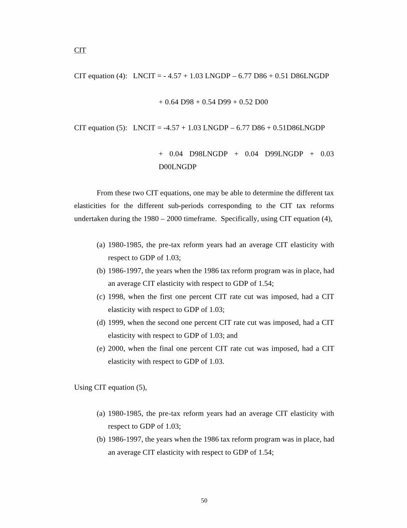
50
CIT
CIT equation (4): LNCIT = - 4.57 + 1.03 LNGDP – 6.77 D86 + 0.51 D86LNGDP
+ 0.64 D98 + 0.54 D99 + 0.52 D00
CIT equation (5): LNCIT = -4.57 + 1.03 LNGDP – 6.77 D86 + 0.51D86LNGDP
+ 0.04 D98LNGDP + 0.04 D99LNGDP + 0.03
D00LNGDP
From these two CIT equations, one may be able to determine the different tax
elasticities for the different sub-periods corresponding to the CIT tax reforms
undertaken during the 1980 – 2000 timeframe. Specifically, using CIT equation (4),
(a) 1980-1985, the pre-tax reform years had an average CIT elasticity with
respect to GDP of 1.03;
(b) 1986-1997, the years when the 1986 tax reform program was in place, had
an average CIT elasticity with respect to GDP of 1.54;
(c) 1998, when the first one percent CIT rate cut was imposed, had a CIT
elasticity with respect to GDP of 1.03;
(d) 1999, when the second one percent CIT rate cut was imposed, had a CIT
elasticity with respect to GDP of 1.03; and
(e) 2000, when the final one percent CIT rate cut was imposed, had a CIT
elasticity with respect to GDP of 1.03.
Using CIT equation (5),
(a) 1980-1985, the pre-tax reform years had an average CIT elasticity with
respect to GDP of 1.03;
(b) 1986-1997, the years when the 1986 tax reform program was in place, had
an average CIT elasticity with respect to GDP of 1.54;
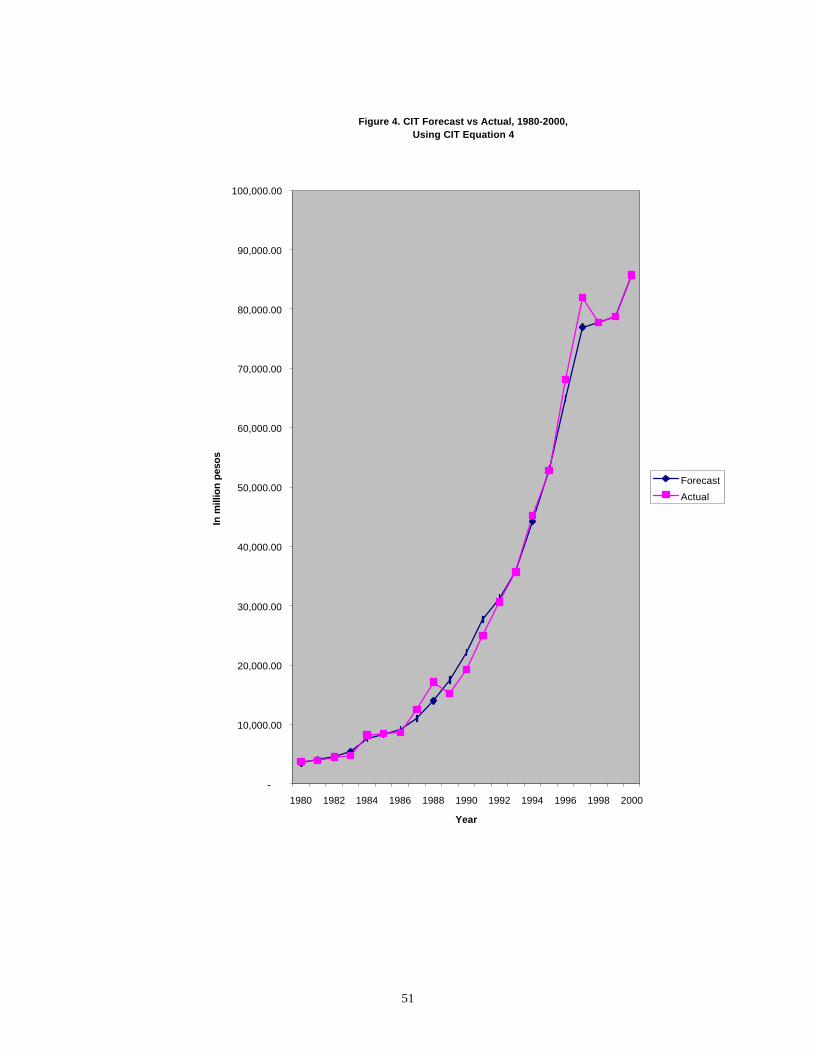
51
Figure 4. CIT Forecast vs Actual, 1980-2000,Using CIT Equation 4
-
10,000.00
20,000.00
30,000.00
40,000.00
50,000.00
60,000.00
70,000.00
80,000.00
90,000.00
100,000.00
1980 1982 1984 1986 1988 1990 1992 1994 1996 1998 2000
Year
In m
illio
n p
eso
s
Forecast
Actual

52
Figure 5. CIT Forecast vs. Actual, 1980-2000,Using CIT Equation 5
-
10,000.00
20,000.00
30,000.00
40,000.00
50,000.00
60,000.00
70,000.00
80,000.00
90,000.00
100,000.00
1980 1982 1984 1986 1988 1990 1992 1994 1996 1998 2000
Year
In m
illio
n p
eso
s
Forecast
Actual

53
(c) 1998, when the first one percent CIT rate cut was imposed, had a CIT
elasticity with respect to GDP of 1.07;
(d) 1999, when the second one percent CIT rate cut was imposed, had a CIT
elasticity with respect to GDP of 1.07; and
(e) 2000, when the final one percent CIT rate cut was imposed, had a CIT
elasticity with respect to GDP of 1.06.
The tax elasticities of the different sub-periods imply that the Aquino tax
reform program (the 1986 Tax Reform Act) pertaining to CIT is more elastic than that
of the Ramos tax reform program. Recall that the Aquino reform on CIT was
primarily the unification of the CIT rates, the higher rate being the CIT rate to be
imposed while the Ramos reform on CIT was a three-time one percent rate cut
beginning 1998.
IIT
IIT equation (3): LNIIT = 2.48 + 0.45 LGDP – 16.55 D86 + 1.25 D86LGDP
– 14.30 D92 + 1.08 D92LGDP – 9.02 D97 + 0.73
D97LGDP
From this IIT equation, one may be able to determine the different tax
elasticities for the different sub-periods corresponding to the IIT tax reforms
undertaken during the 1980 – 2000 timeframe. Specifically,
(a) 1980-1985, the pre-tax reform years had an average IIT elasticity with
respect to GDP of 0.45;
(b) 1986-1991, the years when the 1986 tax reform program was in place had
an average IIT elasticity with respect to GDP of 1.70;
(c) 1992-1996, when the first IIT reforms of 1992 were in place, had an
average IIT elasticity with respect to GDP of 1.53; and

54
Figure 6. IIT Forecast vs. Actual, 1980-2000Using IIT Equation 3
-
10,000.00
20,000.00
30,000.00
40,000.00
50,000.00
60,000.00
70,000.00
80,000.00
90,000.00
100,000.00
1980 1982 1984 1986 1988 1990 1992 1994 1996 1998 2000
Year
In m
illio
n p
eso
s
Forecast
Actual

55
(d) 1997-2000, when additional exemptions and deductions were given the
taxpayers, had an average IIT elasticity with respect to GDP of 1.18.
The tax elasticities of the different sub-periods imply that the Aquino tax
reform program (the 1986 Tax Reform Act) pertaining to IIT is also more elastic than
that of the Ramos tax reform program.
INDOTH
INDOTH equation (5): LNINDOTH = - 4.23 + 1.00 LNOSHHNET – 12.98 D86
+ 1.03 D86LNOSHH - 11.23 D92
+ 0.90 D92LNOSHH + 0.10 D97LNOSHH
From this INDOTH equation, one may be able to determine the different tax
elasticities for the different sub-periods corresponding to the INDOTH tax reforms
undertaken during the 1980 – 2000 timeframe. Specifically,
(a) 1980-1985, the pre-tax reform years had an average INDOTH elasticity
with respect to NOSHHNET of 1.00;
(b) 1986-1991, the years when the 1986 tax reform program was in place had
an average INDOTH elasticity with respect to NOSHHNET of 2.03;
(c) 1992-1996, when the first INDOTH reforms of 1992 were in place, had an
average INDOTH elasticity with respect to NOSHHNET of 1.90; and
(d) 1997-2000, when additional exemptions and deductions were given the
taxpayers, had an average INDOTH elasticity with respect to NOSHHNET
of 1.10.
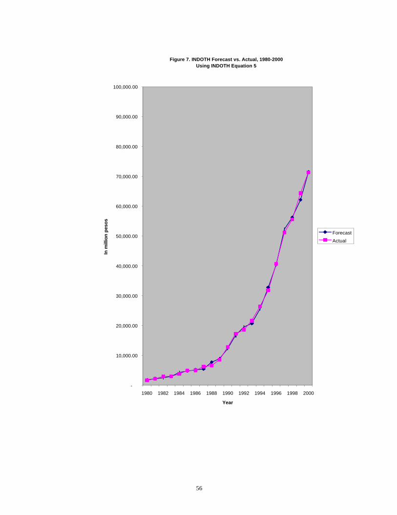
56
Figure 7. INDOTH Forecast vs. Actual, 1980-2000Using INDOTH Equation 5
-
10,000.00
20,000.00
30,000.00
40,000.00
50,000.00
60,000.00
70,000.00
80,000.00
90,000.00
100,000.00
1980 1982 1984 1986 1988 1990 1992 1994 1996 1998 2000
Year
In m
illio
n p
eso
s
Forecast
Actual

57
The tax elasticities of the different sub-periods imply that the Aquino tax
reform program (the 1986 Tax Reform Act) pertaining to INDOTH is also more
elastic than that of the Ramos tax reform program.
4.3 Forward Simulations
CIT. In Section 4.1, two alternative equations were chosen as the “best”
forecasting equations for CIT. Applying these equations, forward estimates were
calculated for the period 2001-2006 using the June 2001 DBCC medium-term
macroeconomic projections. The calculations yielded estimates for LNCIT. These
estimates were transformed into CIT estimates by taking the antilog of LNCIT (see
Table 6).
Table 6
Forward Estimates for CIT, 2001-2006
(In million pesos)
Years Eq. 4 est.
(1)
Eq. 6 est.
(2)
DBCC est.
(3)
Difference
(1) – (3)
Difference
(2) – (4)
2001 94,059 94,357 96,602 (2,543) (2,245)
2002 103,244 103,899 112,261 (9,017) (8,362)
2003 114,019 115,130 129,362 (15,343) (14,232)
2004 126,301 127,975 151,027 (24,726) (23,052)
2005 140,413 142,786 177,970 (37,557) (35,184)
2006 156,479 159,710 210,877 (54,398) (51,167)
The forward estimates for CIT for 2001-2006 derived using the “best” CIT
equations identified in Section 4.2 are lower than the June 2001 DBCC estimates by
an average of 13.82 percent.
IIT. In Section 4.1, one alternative equation was chosen as the “best”
forecasting equation for IIT. Using this equation will yield estimates for LNIIT for the

58
period 2001-2006. These LNIIT estimates were transformed into IIT estimates by
taking the antilog of LNIIT (see Table 7).
Table 7
Forward Estimates for IIT, 2001-2006
(In million pesos)
Years Eq. (4) est.
(1)
DBCC est.
(2)
Difference
(1) – (2)
2001 86,314 86,552 (238)
2002 96,124 95,762 362
2003 107,807 109,405 (1,598)
2004 121,333 126,611 (5,278)
2005 137,128 147,838 (10,710)
2006 155,413 173,160 (17,747)
The forward estimates for IIT for 2001-2006 derived using the “best” IIT
equation identified in Section 4.2 are lower than the June 2001 DBCC estimates
except in 2002 where the estimate is higher by P362 million (or by 0.38 percent). On
the average, the estimates are lower than those of the DBCC by 3.84 percent.
INDOTH. In like manner, using the “best” forecasting equation for INDOTH
to generate forward estimates for the period 2001-2006 yielded estimates for
LNINOTH. Transforming these LNINDOTH estimates by taking the antilog of
LNINDOTH yielded INDOTH estimates (see Table 8).
Given that the June 2001 DBCC projections do not have forward estimates for
NOSHHNET, which is the tax base for INDOTH, forward estimates were derived
using this equation: NOSHHNET = 99,455.94 + 0.35 GDP.

59
Table 8
Forward Estimates for INDOTH, 2001-2006
(In million pesos)
Years Eq. (7) est.
(1)
DBCC est.*
(2)
Difference
(1) – (2)
2001 7,9419 78,703 716
2002 87,135 87,077 58
2003 96,242 99,483 (3,241)
2004 106,690 115,129 (8,439)
2005 118,778 134,431 (15,653)
2006 132,636 157,456 (24,820) * Derived by applying the share of INDOTH to IIT in 2000 to the IIT estimates for 2001-2006 of the
DBCC.
The forward estimates for INDOTH for 2001-2006 derived using the “best”
INDOTH equation identified in Section 4.2 are lower than the June 2001 DBCC
estimates except in 2001 and 2002 where the estimates are higher by P716 million (or
by 0.91 percent) and P58 million (or by 0.07 percent), respectively. On the average,
the estimates are lower than those of the DBCC by 6.17 percent.
IND. In Section 4.1, the alternative equations for IND were not accepted.
Thus, estimates for IND were residually derived using forward estimates of IIT and
INDOTH as specified in this equation: IND = IIT – INDOTH. Table 9 shows the
forward estimates for IND as a residual of Tables 7 and 8.
The forward estimates for IND for 2001-2006 are higher than the June 2001
DBCC estimates except in 2001 where the estimate is lower by P954 million (or by
12.15 percent). On the average, the estimates are higher than those of the DBCC by
19.56 percent.
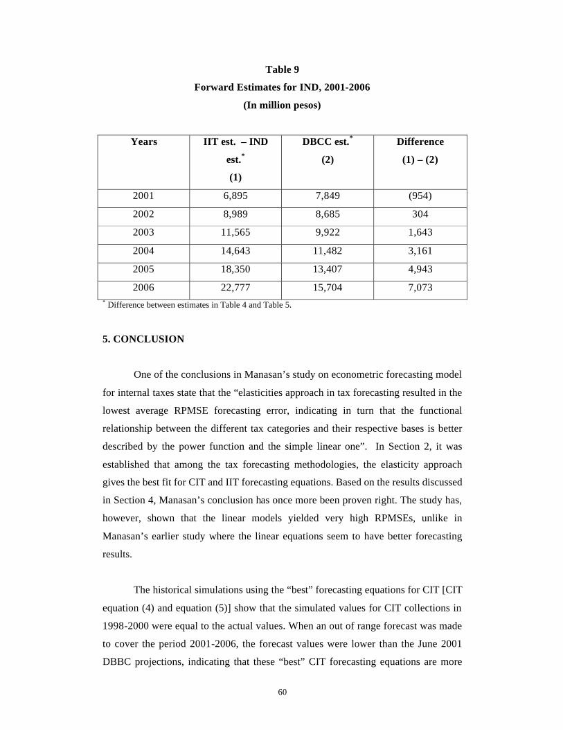
60
Table 9
Forward Estimates for IND, 2001-2006
(In million pesos)
Years IIT est. – IND
est.*
(1)
DBCC est.*
(2)
Difference
(1) – (2)
2001 6,895 7,849 (954)
2002 8,989 8,685 304
2003 11,565 9,922 1,643
2004 14,643 11,482 3,161
2005 18,350 13,407 4,943
2006 22,777 15,704 7,073 * Difference between estimates in Table 4 and Table 5.
5. CONCLUSION
One of the conclusions in Manasan’s study on econometric forecasting model
for internal taxes state that the “elasticities approach in tax forecasting resulted in the
lowest average RPMSE forecasting error, indicating in turn that the functional
relationship between the different tax categories and their respective bases is better
described by the power function and the simple linear one”. In Section 2, it was
established that among the tax forecasting methodologies, the elasticity approach
gives the best fit for CIT and IIT forecasting equations. Based on the results discussed
in Section 4, Manasan’s conclusion has once more been proven right. The study has,
however, shown that the linear models yielded very high RPMSEs, unlike in
Manasan’s earlier study where the linear equations seem to have better forecasting
results.
The historical simulations using the “best” forecasting equations for CIT [CIT
equation (4) and equation (5)] show that the simulated values for CIT collections in
1998-2000 were equal to the actual values. When an out of range forecast was made
to cover the period 2001-2006, the forecast values were lower than the June 2001
DBBC projections, indicating that these “best” CIT forecasting equations are more
61
conservative than the DBCC’s. Assuming that the DBCC estimates are the “actual”
values for 2001-2006, the forecast errors using these “best” CIT forecasting equations
are increasing. This implies that there is a tendency for power functions (logarithmic
equations) to overestimate the effect of the movement of the tax base on the actual
level of tax collections. Nevertheless, among the model specifications utilized in the
study these are still the “best” CIT forecasting equations.
The historical simulations using the “best” forecasting equation for IIT [IIT
equation (3)] show that the simulated values for IIT collections in 1998-2000 deviated
from the actual values by an average of 0.53 percent, with the 1998 and 1999
simulations slightly higher than actual values by 2.07 percent and 0.54 percent,
respectively, while the 2000 simulation slightly lower than the actual value by 1.01
percent. When an out of range forecast was made to cover the period 2001-2006, the
forecast values were on the average lower than the June 2001 DBBC projections,
indicating that the “best” IIT forecasting equations are more conservative than the
DBCC’s. Assuming that the DBCC estimates are the “actual” values for 2001-2006,
the average forecast error using this “best” IIT forecasting equation for 2001-2003 is
about 0.45 percent, slightly lower than that for 1998-2000. The forecast errors,
however, increased in 2004-2006. Nonetheless, among the model specifications
utilized in the study this is still the “best” IIT forecasting equation.
The historical simulations using the “best” forecasting equation for INDOTH
[IIT equation (5)] show that the simulated values for INDOTH collections in 1998-
2000 deviated from the actual values by an average of 0.69 percent, with the 1998 and
2000 simulations slightly higher than actual values by 1.23 percent and 0.18 percent,
respectively, while the 1999 simulation lower than the actual value by 3.49 percent.
When an out of range forecast was made to cover the period 2001-2006, the forecast
values were on the average lower than the June 2001 DBBC projections, indicating
that the “best” INDOTH forecasting equations are more conservative than the
DBCC’s. Assuming that the DBCC estimates are the “actual” values for 2001-2006,
the average forecast error using this “best” INDOTH forecasting equation for 2001-
2002 is about 0.49 percent, slightly lower than that for 1998-2000. The forecast
errors, however, increased in 2003-2006. However, among the model specifications
utilized in the study this is still the “best” INDOTH forecasting equation.

62
Before the forward simulations could be used as official forecast, the
methodologies used in this study may have to be evaluated vis-à-vis that of the DOF,
the official tax forecaster of the national government.34 If the forecast errors in the
study would still be lower than those of the DOF’s, only then may the forward
simulations in this study be considered as the official forecast by the DBCC.
In addition, all the forecasting equations that ‘best’ explain income tax
movements (both corporate and individual) are power functions, implying that the
income taxation system has a regressive tendency. Perhaps, a reexamination of the
income taxation system is warranted considering the number of reforms undertaken in
the last 15 years that may have distorted it, and the possible reform that is currently
being proposed in Congress on the gross income taxation scheme.
34 It should be emphasized that constraints beyond the author’s control rendered it impossible to compare the tax elasticity models DOF uses for tax revenue target setting, specifically for CIT and IIT, with that of the other agencies as well as the alternative equations used in the study.
63
BIBLIOGRAPHY.
Barents Group. “Tax Policy Decision Support Tools”, 2001.
Beacon Hill Institute. “The Texas State Tax Analysis Modeling Program (Texas-
Stamp), Methodology and Applications: An Executive Summary”, 2001.
Bureau of Internal Revenue. Annual Reports, various years.
Department of Finance (Ireland). “Report of the Tax Forecasting Methodology
Group”, 1998.
Department of Finance (Philippines). “Revenue Estimation Methodology (handout)”,
2001.
Development Budget and Coordination Committee. “Medium-Term Macroeconomic
and Fiscal Targets, 1998-2006”, June 2001.
Gujarati, D. Basic Econometrics, Third edition, 2000.
Haughton J. “Estimating Tax Buoyancy, Elasticity, and Stability”, African Economic
Policy Paper, Discussion Paper 11, July 1998.
King, J.R. “Alternative Methods of Revenue Forecasting and Estimating: An
Abstract”, 1996.
Lerche, D. “Tax Potential and Tax Estimate, Plan and Experiences in the Indonesian
Tax Potential Indicator System Project, 2000.
Manasan, R. G. “Survey and Review of Forecasting Models in Internal Government
Revenues”, Philippine Institute for Development Studies (PIDS) Working
Paper 81-13, March 1981.
____________. “An Econometric Model for Forecasting Internal Taxes: A National
Level Approach”, PIDS Working Paper 81-08, September 1981.
____________. “Review of Philippine Tax Administration and Performance”.
Revised final report submitted to the Office of Economic Development of the
United States Aid for International Development/Manila, April 1998.
____________. “Improving Tax Administration: A New view from the Theory of Tax
Evasion in a Corrupt Regime”, PIDS Policy Notes 11, September 2000.
____________ and Rosario G. Querubin. “Revenue Performance of National
Government Taxes, 1975-1985”, PIDS Staff Paper 8701, 1986.
McCrae J. “The Development and Uses of Tax and Benefit Simulation Models”,
Brazilian Electronic Journal of Economics, Volume II, No.1, January 1999.
64
National Economic and Development Authority. “Quarterly Macroecomomic Model:
Fiscal Block”, 2001.
National Internal Revenue Code, 1997.
National Statistical Coordination Board. The National Accounts of the Philippines,
Annual, various years.
National Tax Research Center. “Philippine Tax and Tariff System”, 1991.
________________________. “Comprehensive Index on Taxation in the
Philippines”, October 1998.
________________________. “Revenue Forecasting Techniques”. A handout
distributed to the Inter-Agency Taskforce on the Improvement of Tax Related
Database, 2001.
Nolledo, J.N. and M.S. Nolledo. The National Internal Revenue Code of the
Philippines, Annotated, 17th Revised edition, 1996.
Pindyck R. and D. Rubinfield. Econometric Models and Economic Forecasts, 1991.
Rylander, C.K. “Dynamic Modeling: New Method of Tax Analysis Accounts for
Taxpayer Behavior”, Fiscal Notes, April 2001.
Sunley, Emil M. and R. D. Weiss. “The Revenue Estimating Process”. A paper
prepared for the Conference on Improving the Tax Legislative Process, May
1991.
Statistical Research and Training Center. “Statistical Forecasting Techniques”.
Handouts distributed during a Training Course, July 1999.
Teichmann, D. “Study Group Forecasts”. Handout distributed during a BIR
Workshop, April 2000.
65
Appendix A
Methods of Adjusting Data Series to Remove Discretionary Changes*
The Allan Prest Forward and Backward Adjustment Methods were developed
by Alan R. Prest for his study of the sensitivity of the British Tax System in 1962.
The methods are conceptually the same except that the reference year for each method
is different. These adjustment methods eliminates the effects of discretionary changes
in the affected years and then re-estimates the yields for all the other years taking into
account the tax policy changes. The output is a set of “cleaned” data series for tax
collections. The forward method takes the first year of the series as the reference year
while the backward method takes the last year of the series as the reference year. The
formulae are:
Forward Method:Ti,j = Ti,j-1 + {([(Tj-Dj)-Tj-1]/[Tj-1]) x Ti,j-1}
where:
Tj is the actual tax collections in the jth year;
Ti,j is the actual tax collections in the jth year adjusted to the structure of the
base year (ith year);
Dj is the imputed tax collections due to discretionary change;
Ti,j-1 is the preceding year’s revenue adjusted to the base year’s structure; and
j is the years in the series from i, …, n where the first year (i) is the base, and n
is last year in the series.
Backward Method:Tn,j = Tj x (Tj+1/Tj, j+1) x … x (Tn/Tn-1, n)
where:
Tj is the actual tax collections in the jth year;
* Prepared by the NTRC.

66
Tn,j is the actual collections in the jth year adjusted to the structure of the base
year (nth year); and
j is the years in the series where j=1, …, n, and where 1 is the first year in the
series, and n is the base year or the end-year of the series.
The Constant Rate Structure Method involves the use of the current year as
the reference year to calculate the tax yield in the past years based on the present tax
rate structure or construct past year’s times series data as the initial step for tax
forecasting. This method, however, requires sufficiently disaggregated data series.
For example, with respect to individual income taxes, the method requires the
calculation of effective tax rates per income bracket for individual income taxpayers
for the reference year and subsequently applying these rates to the taxable income
across income brackets in all the other years. The output generated is a set of
“cleaned” data series for individual income tax collections. The formula is:
(Tj/Xj) x Xij
where:
Tj is tax collection at the jth bracket of the base year;
Xj is the taxable income at the jth bracket of the base year;
Xij is the taxable income at the jth bracket of the ith year; and
Tj/Xj is the effective tax rate for the jth bracket of the base year.
The Sahota Method was developed by Professor G.S. Sahota in 1961, and is
similar to the Prest Methods. In the Sahota Method, a series adjusted to the tax
structure of the preceding years is first determined. This is calculated by deducting the
estimated revenues due to discretionary changes from the actual tax collections in the
year where such changes in tax structure occurred. Next, a series of growth rates
between adjacent years is determined by dividing the adjusted yield of a given year by
the actual yield of the preceding year. This series of growth rates are then converted
into indices with a selected year as the base. The formula is:
Ij = (Tj-1, j/Tj-1) x Ij-1
67
where:
Ij is the index of the jth year;
Tj-1, j is the tax collection of the jth year adjusted to the structure of the
preceding year;
Tj-1 is the actual tax collections of the preceding year;
Ij-1 is the index reflecting the automatic growth of the preceding year; and
j is years from i, …, n where i is the first year in the series and is designated as
the base year, and n is the last year of the series.
The fifth data adjustment technique is the Singer Method or the Dummy
Variable Procedure, which involves the use of a dummy variable to represent
important discretionary changes in the tax system for every year when such policy
shifts occurred. This procedure is used when not any of the four methods earlier
mentioned can be utilized to “clean” the tax data series of the impact of discretionary
changes in the tax system. This is particularly true when the effects of policy changes
are difficult to determine due to lack of data or if said effects are difficult to quantify.
The Singer Method or Dummy Variable Procedure is quite useful if there are only a
few discretionary tax changes over the period of study. Otherwise the tax equation
would be peppered with dummy variables. Unlike the four aforementioned methods
wherein the actual tax data series should first be “cleaned” before using the series in
the regression equation, here, the actual tax data series is used as is and the dummy
variable(s) is (are) just added to the equation. This may be expressed in a tax function
form:
Log Tj = α + β log Xj +∑ CjDj
where:
Tj is the tax revenue collection at the jth year;
α is the constant;
β is the elasticity coefficient;

68
Xj is the taxable income or base at the jth year;
Cj is the impact or coefficient of the discretionary change; and
Dj is the discretionary change at the jth year, which may either take a value of 0
(no discretionary change) or 1 (a change occurred in that year).
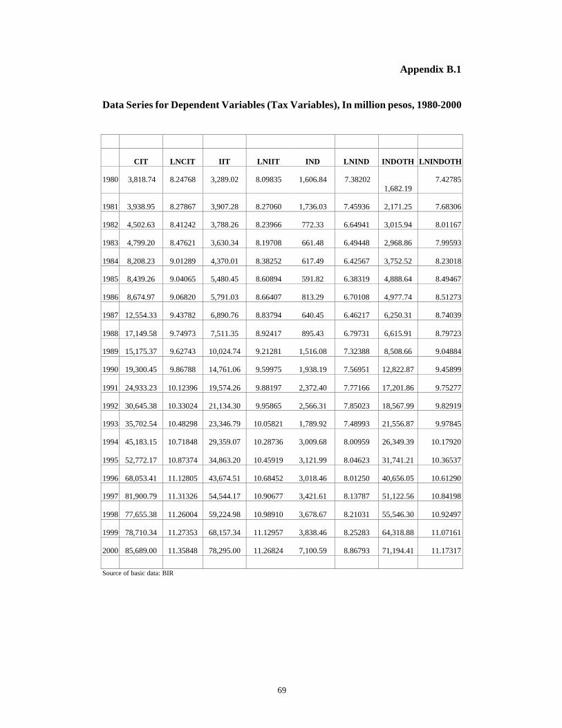
69
Appendix B.1
Data Series for Dependent Variables (Tax Variables), In million pesos, 1980-2000
CIT
LNCIT
IIT
LNIIT
IND
LNIND
INDOTH
LNINDOTH
1980
3,818.74
8.24768
3,289.02
8.09835
1,606.84
7.38202
1,682.19
7.42785
1981
3,938.95
8.27867
3,907.28
8.27060
1,736.03
7.45936
2,171.25
7.68306
1982
4,502.63
8.41242
3,788.26
8.23966
772.33
6.64941
3,015.94
8.01167
1983
4,799.20
8.47621
3,630.34
8.19708
661.48
6.49448
2,968.86
7.99593
1984
8,208.23
9.01289
4,370.01
8.38252
617.49
6.42567
3,752.52
8.23018
1985
8,439.26
9.04065
5,480.45
8.60894
591.82
6.38319
4,888.64
8.49467
1986
8,674.97
9.06820
5,791.03
8.66407
813.29
6.70108
4,977.74
8.51273
1987
12,554.33
9.43782
6,890.76
8.83794
640.45
6.46217
6,250.31
8.74039
1988
17,149.58
9.74973
7,511.35
8.92417
895.43
6.79731
6,615.91
8.79723
1989
15,175.37
9.62743
10,024.74
9.21281
1,516.08
7.32388
8,508.66
9.04884
1990
19,300.45
9.86788
14,761.06
9.59975
1,938.19
7.56951
12,822.87
9.45899
1991
24,933.23
10.12396
19,574.26
9.88197
2,372.40
7.77166
17,201.86
9.75277
1992
30,645.38
10.33024
21,134.30
9.95865
2,566.31
7.85023
18,567.99
9.82919
1993
35,702.54
10.48298
23,346.79
10.05821
1,789.92
7.48993
21,556.87
9.97845
1994
45,183.15
10.71848
29,359.07
10.28736
3,009.68
8.00959
26,349.39
10.17920
1995
52,772.17
10.87374
34,863.20
10.45919
3,121.99
8.04623
31,741.21
10.36537
1996
68,053.41
11.12805
43,674.51
10.68452
3,018.46
8.01250
40,656.05
10.61290
1997
81,900.79
11.31326
54,544.17
10.90677
3,421.61
8.13787
51,122.56
10.84198
1998
77,655.38
11.26004
59,224.98
10.98910
3,678.67
8.21031
55,546.30
10.92497
1999
78,710.34
11.27353
68,157.34
11.12957
3,838.46
8.25283
64,318.88
11.07161
2000
85,689.00
11.35848
78,295.00
11.26824
7,100.59
8.86793
71,194.41
11.17317
Source of basic data: BIR

70
Appendix B.2
Data Series for Independent Variables (Tax Base Variables) for CIT Models,
In million pesos, 1980-2006
GDP LNGDP NOSPVGC LNNOSPVGC
1980 243,749.00 12.40389 18,292.00 9.81422 1981 281,596.00 12.54823 17,103.00 9.74701 1982 317,177.00 12.66722 15,295.00 9.63528 1983 369,077.00 12.81876 21,194.00 9.96147 1984 524,481.00 13.17016 37,008.00 10.51889 1985 571,883.00 13.25669 22,906.00 10.03915 1986 608,887.00 13.31939 31,712.00 10.36445 1987 682,764.00 13.43390 56,564.00 10.94313 1988 799,182.00 13.59134 84,061.00 11.33930 1989 925,444.00 13.73803 97,173.00 11.48425 1990 1,077,237.00 13.88991 119,207.00 11.68862 1991 1,248,011.00 14.03706 127,309.00 11.75437 1992 1,351,559.00 14.11677 145,397.00 11.88722 1993 1,474,457.00 14.20380 179,183.00 12.09616 1994 1,692,932.00 14.34197 217,844.00 12.29153 1995 1,905,951.00 14.46049 232,601.00 12.35708 1996 2,171,922.00 14.59112 293,818.00 12.59072 1997 2,426,743.00 14.70206 364,610.00 12.80658 1998 2,678,187.00 14.80065 382,506.00 12.85450 1999 2,976,904.00 14.90639 482,900.00 13.08756 2000 3,302,589.00 15.01022 559,585.00 13.23495 2001 3,616,486.00 15.10101 n.a. n.a. 2002 3,960,148.00 15.19179 n.a. n.a. 2003 4,362,317.00 15.28851 n.a. n.a. 2004 4,819,508.00 15.38818 n.a. n.a. 2005 5,343,437.00 15.49138 n.a. n.a. 2006 5,938,275.00 15.59693 n.a. n.a.
n.a. - not available
Source of basic data: NSCB
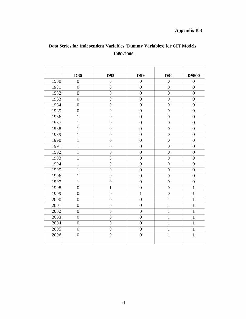
71
Appendix B.3
Data Series for Independent Variables (Dummy Variables) for CIT Models,
1980-2006
D86 D98 D99 D00 D9800
1980 0 0 0 0 0 1981 0 0 0 0 0 1982 0 0 0 0 0 1983 0 0 0 0 0 1984 0 0 0 0 0 1985 0 0 0 0 0 1986 1 0 0 0 0 1987 1 0 0 0 0 1988 1 0 0 0 0 1989 1 0 0 0 0 1990 1 0 0 0 0 1991 1 0 0 0 0 1992 1 0 0 0 0 1993 1 0 0 0 0 1994 1 0 0 0 0 1995 1 0 0 0 0 1996 1 0 0 0 0 1997 1 0 0 0 0 1998 0 1 0 0 1 1999 0 0 1 0 1 2000 0 0 0 1 1 2001 0 0 0 1 1 2002 0 0 0 1 1 2003 0 0 0 1 1 2004 0 0 0 1 1 2005 0 0 0 1 1 2006 0 0 0 1 1
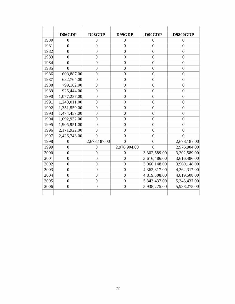
72
D86GDP D98GDP D99GDP D00GDP D9800GDP
1980 0 0 0 0 0 1981 0 0 0 0 0 1982 0 0 0 0 0 1983 0 0 0 0 0 1984 0 0 0 0 0 1985 0 0 0 0 0 1986 608,887.00 0 0 0 0 1987 682,764.00 0 0 0 0 1988 799,182.00 0 0 0 0 1989 925,444.00 0 0 0 0 1990 1,077,237.00 0 0 0 0 1991 1,248,011.00 0 0 0 0 1992 1,351,559.00 0 0 0 0 1993 1,474,457.00 0 0 0 0 1994 1,692,932.00 0 0 0 0 1995 1,905,951.00 0 0 0 0 1996 2,171,922.00 0 0 0 0 1997 2,426,743.00 0 0 0 0 1998 0 2,678,187.00 0 0 2,678,187.00 1999 0 0 2,976,904.00 0 2,976,904.00 2000 0 0 0 3,302,589.00 3,302,589.00 2001 0 0 0 3,616,486.00 3,616,486.00 2002 0 0 0 3,960,148.00 3,960,148.00 2003 0 0 0 4,362,317.00 4,362,317.00 2004 0 0 0 4,819,508.00 4,819,508.00 2005 0 0 0 5,343,437.00 5,343,437.00 2006 0 0 0 5,938,275.00 5,938,275.00

73
D86LNGDP D98LNGDP D99LNGDP D00LNGDP D9800LNGDP 1980 0 0 0 0 0 1981 0 0 0 0 0 1982 0 0 0 0 0 1983 0 0 0 0 0 1984 0 0 0 0 0 1985 0 0 0 0 0 1986 13.31939 0 0 0 0 1987 13.43390 0 0 0 0 1988 13.59134 0 0 0 0 1989 13.73803 0 0 0 0 1990 13.88991 0 0 0 0 1991 14.03706 0 0 0 0 1992 14.11677 0 0 0 0 1993 14.20380 0 0 0 0 1994 14.34197 0 0 0 0 1995 14.46049 0 0 0 0 1996 14.59112 0 0 0 0 1997 14.70206 0 0 0 0 1998 0 14.80065 0 0 14.80065 1999 0 0 14.90639 0 14.90639 2000 0 0 0 15.01022 15.01022 2001 0 0 0 15.10101 15.10101 2002 0 0 0 15.19179 15.19179 2003 0 0 0 15.28851 15.28851 2004 0 0 0 15.38818 15.38818 2005 0 0 0 15.49138 15.49138 2006 0 0 0 15.59693 15.59693

74
D86NOS D98NOS D99NOS D00NOS D9800NOS 1980 0 0 0 0 0 1981 0 0 0 0 0 1982 0 0 0 0 0 1983 0 0 0 0 0 1984 0 0 0 0 0 1985 0 0 0 0 0 1986 31,712.00 0 0 0 0 1987 56,564.00 0 0 0 0 1988 84,061.00 0 0 0 0 1989 97,173.00 0 0 0 0 1990 119,207.00 0 0 0 0 1991 127,309.00 0 0 0 0 1992 145,397.00 0 0 0 0 1993 179,183.00 0 0 0 0 1994 217,844.00 0 0 0 0 1995 232,601.00 0 0 0 0 1996 293,818.00 0 0 0 0 1997 364,610.00 0 0 0 0 1998 0 382,506.00 0 0 382,506.00 1999 0 0 482,900.00 0 482,900.00 2000 0 0 0 559,585.00 559,585.00 2001 n.a. n.a. n.a. n.a. n.a. 2002 n.a. n.a. n.a. n.a. n.a. 2003 n.a. n.a. n.a. n.a. n.a. 2004 n.a. n.a. n.a. n.a. n.a. 2005 n.a. n.a. n.a. n.a. n.a. 2006 n.a. n.a. n.a. n.a. n.a.
n.a. – not available

75
D86LNNOS D98LNNOS D99LNNOS D00LNNOS D9800LNNOS 1980 0 0 0 0 0 1981 0 0 0 0 0 1982 0 0 0 0 0 1983 0 0 0 0 0 1984 0 0 0 0 0 1985 0 0 0 0 0 1986 10.36445 0 0 0 0 1987 10.94313 0 0 0 0 1988 11.33930 0 0 0 0 1989 11.48425 0 0 0 0 1990 11.68862 0 0 0 0 1991 11.75437 0 0 0 0 1992 11.88722 0 0 0 0 1993 12.09616 0 0 0 0 1994 12.29153 0 0 0 0 1995 12.35708 0 0 0 0 1996 12.59072 0 0 0 0 1997 12.80658 0 0 0 0 1998 0 12.85450 0 0 12.85450 1999 0 0 13.08756 0 13.08756 2000 0 0 0 13.23495 13.23495 2001 n.a. n.a. n.a. n.a. n.a. 2002 n.a. n.a. n.a. n.a. n.a. 2003 n.a. n.a. n.a. n.a. n.a. 2004 n.a. n.a. n.a. n.a. n.a. 2005 n.a. n.a. n.a. n.a. n.a. 2006 n.a. n.a. n.a. n.a. n.a.
n.a. – not available
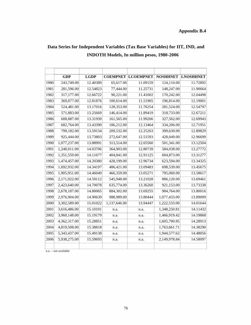
76
Appendix B.4
Data Series for Independent Variables (Tax Base Variables) for IIT, IND, and
INDOTH Models, In million pesos, 1980-2006
GDP LGDP COEMPNET LCOEMPNET NOSHHNET LNOSHHNET
1980 243,749.00 12.40389 65,617.00 11.09159 124,110.00 11.72892
1981 281,596.00 12.54823 77,444.00 11.25731 148,247.00 11.90664
1982 317,177.00 12.66722 90,221.00 11.41002 170,242.00 12.04498
1983 369,077.00 12.81876 100,614.00 11.51905 196,814.00 12.19001
1984 524,481.00 13.17016 128,353.00 11.76254 281,524.00 12.54797
1985 571,883.00 13.25669 146,414.00 11.89419 318,733.00 12.67211
1986 608,887.00 13.31939 161,565.00 11.99266 327,562.00 12.69943
1987 682,764.00 13.43390 186,212.00 12.13464 334,206.00 12.71951
1988 799,182.00 13.59134 209,532.00 12.25263 399,630.00 12.89829
1989 925,444.00 13.73803 272,647.00 12.51593 428,049.00 12.96699
1990 1,077,237.00 13.88991 313,514.00 12.65560 501,341.00 13.12504
1991 1,248,011.00 14.03706 364,903.00 12.80739 584,038.00 13.27772
1992 1,351,559.00 14.11677 404,841.00 12.91125 604,873.00 13.31277
1993 1,474,457.00 14.20380 428,199.00 12.96734 623,594.00 13.34325
1994 1,692,932.00 14.34197 486,421.00 13.09483 698,539.00 13.45675
1995 1,905,951.00 14.46049 466,359.00 13.05271 795,060.00 13.58617
1996 2,171,922.00 14.59112 545,948.00 13.21028 886,120.00 13.69461
1997 2,423,640.00 14.70078 635,774.00 13.36260 921,153.00 13.73338
1998 2,678,187.00 14.80065 884,302.00 13.69255 984,764.00 13.80016
1999 2,976,904.00 14.90639 988,989.00 13.80444 1,077,433.00 13.89009
2000 3,302,589.00 15.01022 1,137,646.00 13.94447 1,222,533.00 14.01644
2001 3,616,486.00 15.10101 n.a. n.a. 1,348,250.81 14.11432
2002 3,960,148.00 15.19179 n.a. n.a. 1,466,919.42 14.19868
2003 4,362,317.00 15.28851 n.a. n.a. 1,605,790.85 14.28913
2004 4,819,508.00 15.38818 n.a. n.a. 1,763,661.71 14.38290
2005 5,343,437.00 15.49138 n.a. n.a. 1,944,577.62 14.48056
2006 5,938,275.00 15.59693 n.a. n.a. 2,149,978.84 14.58097
n.a. – not available
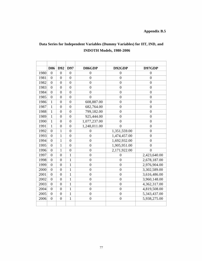
77
Appendix B.5
Data Series for Independent Variables (Dummy Variables) for IIT, IND, and
INDOTH Models, 1980-2006
D86 D92 D97 D86GDP D92GDP D97GDP
1980 0 0 0 0 0 0 1981 0 0 0 0 0 0 1982 0 0 0 0 0 0 1983 0 0 0 0 0 0 1984 0 0 0 0 0 0 1985 0 0 0 0 0 0 1986 1 0 0 608,887.00 0 0 1987 1 0 0 682,764.00 0 0 1988 1 0 0 799,182.00 0 0 1989 1 0 0 925,444.00 0 0 1990 1 0 0 1,077,237.00 0 0 1991 1 0 0 1,248,011.00 0 0 1992 0 1 0 0 1,351,559.00 0 1993 0 1 0 0 1,474,457.00 0 1994 0 1 0 0 1,692,932.00 0 1995 0 1 0 0 1,905,951.00 0 1996 0 1 0 0 2,171,922.00 0 1997 0 0 1 0 0 2,423,640.00 1998 0 0 1 0 0 2,678,187.00 1999 0 0 1 0 0 2,976,904.00 2000 0 0 1 0 0 3,302,589.00 2001 0 0 1 0 0 3,616,486.00 2002 0 0 1 0 0 3,960,148.00 2003 0 0 1 0 0 4,362,317.00 2004 0 0 1 0 0 4,819,508.00 2005 0 0 1 0 0 5,343,437.00 2006 0 0 1 0 0 5,938,275.00

78
D86LGDP D92LGDP D97LGDP D86COEMP D92COEMP D97COEMP
1980 0 0 0 0 0 0
1981 0 0 0 0 0 0
1982 0 0 0 0 0 0
1983 0 0 0 0 0 0
1984 0 0 0 0 0 0
1985 0 0 0 0 0 0
1986 13.31939 0 0 161,565.00
0 0
1987 13.43390 0 0 186,212.00
0 0
1988 13.59134 0 0 209,532.00
0 0
1989 13.73803 0 0 272,647.00
0 0
1990 13.88991 0 0 313,514.00
0 0
1991 14.03706 0 0 364,903.00
0 0
1992 0 14.11677 0 0 404841.00 0
1993 0 14.20380 0 0 428199.00 0
1994 0 14.34197 0 0 486421.00 0
1995 0 14.46049 0 0 466359.00 0
1996 0 14.59112 0 0 545948.00 0
1997 0 0 14.7007811 0 0 635,774.00
1998 0 0 14.8006506 0 0 884,302.00
1999 0 0 14.9063944 0 0 988,989.00
2000 0 0 15.01
0 0 1,137,646.00
2001 0 0 15.10
n.a. n.a. n.a.
2002 0 0 15.19
n.a. n.a. n.a.
2003 0 0 15.29
n.a. n.a. n.a.
2004 0 0 15.39
n.a. n.a. n.a.
2005 0 0 15.49
n.a. n.a. n.a.
2006 0 0 15.60
n.a. n.a. n.a.
n.a. – not available
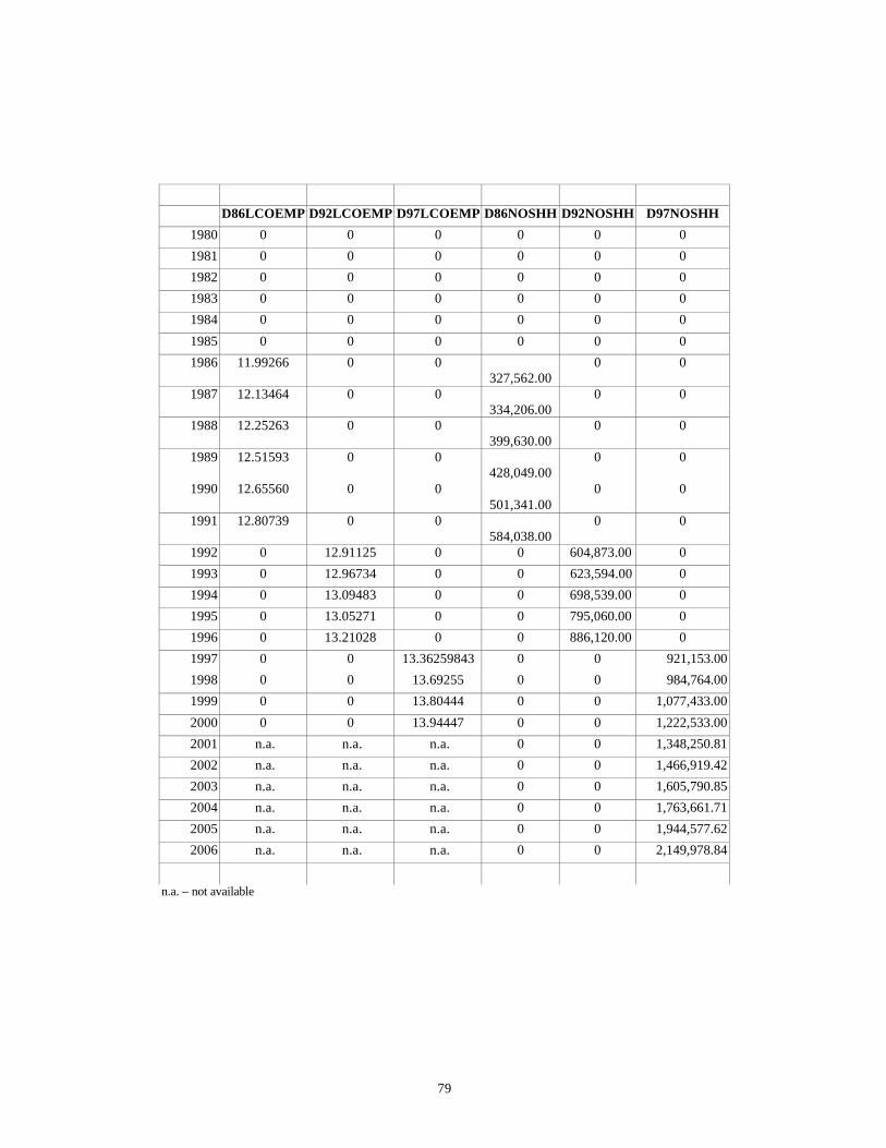
79
D86LCOEMP D92LCOEMP D97LCOEMP D86NOSHH D92NOSHH D97NOSHH
1980 0 0 0 0 0 0
1981 0 0 0 0 0 0
1982 0 0 0 0 0 0
1983 0 0 0 0 0 0
1984 0 0 0 0 0 0
1985 0 0 0 0 0 0
1986 11.99266 0 0 327,562.00
0 0
1987 12.13464 0 0 334,206.00
0 0
1988 12.25263 0 0 399,630.00
0 0
1989 12.51593 0 0 428,049.00
0 0
1990 12.65560 0 0 501,341.00
0 0
1991 12.80739 0 0 584,038.00
0 0
1992 0 12.91125 0 0 604,873.00 0
1993 0 12.96734 0 0 623,594.00 0
1994 0 13.09483 0 0 698,539.00 0
1995 0 13.05271 0 0 795,060.00 0
1996 0 13.21028 0 0 886,120.00 0
1997 0 0 13.36259843 0 0 921,153.00
1998 0 0 13.69255 0 0 984,764.00
1999 0 0 13.80444 0 0 1,077,433.00
2000 0 0 13.94447 0 0 1,222,533.00
2001 n.a. n.a. n.a. 0 0 1,348,250.81
2002 n.a. n.a. n.a. 0 0 1,466,919.42
2003 n.a. n.a. n.a. 0 0 1,605,790.85
2004 n.a. n.a. n.a. 0 0 1,763,661.71
2005 n.a. n.a. n.a. 0 0 1,944,577.62
2006 n.a. n.a. n.a. 0 0 2,149,978.84
n.a. – not available

80
D86LNOSHH D92LNOSHH D97LNOSHH
1980 0 0 0 1981 0 0 0 1982 0 0 0 1983 0 0 0 1984 0 0 0 1985 0 0 0 1986 12.69943263 0 0 1987 12.71951285 0 0 1988 12.8982944 0 0 1989 12.96699295 0 0 1990 13.12504179 0 0 1991 13.27772133 0 0 1992 0 13.3127738 0 1993 0 13.34325479 0 1994 0 13.45674629 0 1995 0 13.58617286 0 1996 0 13.69460766 0 1997 0 0 13.73338 1998 0 0 13.80016 1999 0 0 13.89009 2000 0 0 14.01644 2001 0 0 14.11432 2002 0 0 14.19868 2003 0 0 14.28913 2004 0 0 14.38290 2005 0 0 14.48056 2006 0 0 14.58097