philosophy of statistics: an...

PHILOSOPHY OF STATISTICS:

AN INTRODUCTION

Prasanta S. Bandyopadhyay and Malcolm R. Forster

1 PHILOSOPHY, STATISTICS, AND PHILOSOPHY OF STATISTICS

The expression “philosophy of statistics” contains two key terms: “philosophy”and “statistics.” Although it is hard to define those terms precisely, they conveysome intuitive meanings. For our present purpose, those intuitive meanings are agood place to embark on our journey. Philosophy has a broader scope than thespecific sciences. It is concerned with general principles and issues. In contrast,“statistics” is a specific branch of knowledge that, among many other activities,includes addressing reliable ways of gathering data and making inferences basedon them. Perhaps the single most important topic in statistics is how to makereliable inferences. As a result, statisticians are interested in knowing which toolsto use and what mechanisms to employ in making and correcting our inferences.In this sense, the general problem of statistics is very much like the problem ofinduction in which philosophers have long been interested. In fact, statisticiansas diverse as Ronald Fisher [1973], Jerzy Neyman [1967] and Bruno de Finetti[1964] characterized the approaches they originated as methods for inductive in-ferences.1,2

Before we begin our discussion, it is worthwhile mentioning a couple of salientfeatures of this volume. It contains thirty-seven new papers written by forty-eightauthors coming from several fields of expertise. They include philosophy, statis-tics, mathematics, computer science, economics, ecology, electrical engineering,epidemiology, and geo-science. In the introduction, we will provide an outline ofeach paper without trying to offer expert commentary on all of them. Our empha-sis on some topics rather than others in the following discussion reflects our owninterest and focus without downplaying the significance of those topics less dis-cussed. We encourage readers to start with the paper(s) that kindles their interestand lie within their own research areas.

In the western world, David Hume [1739] has been credited with formulatingthe problem of induction in a particularly compelling fashion. The problem ofinduction arises when one makes an inference about an unobserved body of data

1See [Seidenfeld, 1979] for a close look at Fisher’s views on statistical inference.2For a clear discussion of de Finetti’s view on the connection between the subjective degree

of belief and inductive learning, see [Skyrms, 1984].

Handbook of the Philosophy of Science. Volume 7: Philosophy of Statistics.Volume editors: Prasanta Bandyopadhyay and Malcolm Forster. General Editors: Dov M.Gabbay, Paul Thagard and John Woods.c© 2010 Elsevier BV. All rights reserved.

2 Prasanta S. Bandyopadhyay and Malcolm R. Forster

based on an observed body of data.3 However, there is no assurance that theinference in question will be valid because the next datum we observe may differfrom those already gathered. Furthermore, to assume that they will be the same,according to Hume, is to assume what we need to prove. The problem of inductionin this sense has very possibly turned out to be an irresolvable problem. Insteadof addressing the problem of induction in the way Hume has described it, in termsof certainty, we are more often interested in knowing how or whether we wouldbe able to make better inductive inferences in the sense that they are likely to betrue most of the time, that is, in terms of reliability.

However, to be able to make reliable inferences we still require substantial as-sumptions about the relationship between the observed data and the unobserveddata. One such assumption, which is sometimes called “the uniformity of nature”assumption and was questioned by Hume, is that the future data will be like thepast data. In addition, we sometime also make some empirical assumptions aboutthe world. One such assumption is that the world is simple, such as in the senseof being isotropic that there are laws that apply across all points in space andtime, or at least across the domain of interest. For philosophers, this assumptionis, in some sense, reminiscent of the assumption involved in the contrast betweenthe green hypothesis (i.e., all emeralds are green) and the grue-hypothesis (i.e.,all emeralds are grue.) X is defined as grue if and only if x is green and wasobserved before time t or x is blue and was not observed before t. The hypothesesare equally consistent with current data, even though the hypotheses are differ-ent. So, which hypothesis should we choose given they are equally supported bythe data? The grue-green problem teaches us that we do commonly make (un-usually unexamined) assumptions about the concepts we can use and the way wecan use them in constructing hypotheses. That is, we make (often unarticulated)assumptions about the ways in which the world is uniform or simple.

As there is a quandary over whether simplicity is a legitimate factor in sci-entific inference, so there is another heated discussion regarding what kinds ofassumptions other than the uniformity of nature assumption, and perhaps alsosimplicity, are warranted. These debates over the correct assumptions and ap-proaches to inductive inference are as rampant in the choice of one’s statisticalparadigm (for example, classical/error statistics, Bayesianism, likelihoodism orthe Akaikean framework, to mention only the most prominent) as they are inthe applied approaches to automated inductive inference in computer science. Inphilosophy of statistics, we are interested in the foundational questions includingthe debates about statistical paradigms regarding which one provides the rightdirection and method for carrying out statistical inference, if indeed any of themdo in general. On one end of the spectrum, we will discuss several major sta-tistical paradigms with their assumptions and viewpoints. On the other end, wealso consider broader issues — like the issue of inductive inference — after under-standing these statistical paradigms in more detail. We are likewise interested in

3Taleb has adopted a distinctively unique approach to the issues concerning induction espe-cially when they involve the 9/11 event and the Wall-Street crash of 2008 [Taleb, 2010].

Philosophy of Statistics: An Introduction 3

specific questions between these two extremes, as well as more modern viewpointsthat adopt a “tool-kit” perspective. In that tool-kit perspective, each paradigmis merely a collection of inferential tools with limitations and appropriate (as wellas inappropriate) domain of application. We will thus consider issues includingthe following: the causal inference in observational studies; the recent advancesin model selection criteria; such foundational questions as “whether one shouldaccept the likelihood principle (LP)” and “what is conditional probability”; thenature of statistical/probabilistic paradoxes, the problems associated with under-standing the notion of randomness, the Stein phenomenon, general problems indata mining, and a number of applied and historical issues in probability andstatistics.

2 FOUR STATISTICAL PARADIGMS

Sometimes different approaches to scientific inference among philosophers, com-puter scientists, and statisticians stem from their adherence to competing sta-tistical paradigms. Four statistical paradigms will be considered in the follow-ing discussion: (1) classical statistics or error statistics, (ii) Bayesian statistics,(iii) likelihood-based statistics, and (iv) the Akaikean-Information Criterion-basedstatistics. How do they differ in their approaches to statistical inference?

2.1 Four statistical paradigms and four types of questions

To address this question, consider two hypotheses: H, representing that a pa-tient suffers from tuberculosis, and ∼H, its denial. Assume that an Xray, whichis administered as a routine test, comes out positive for the patient. Based onthis simple scenario, following the work of Richard Royall, one could pose threequestions that underline the epistemological issue at stake within three competingstatistical paradigms [Royall, 1997]:

(i) Given the datum, what should we believe and to what degree?

(ii) What does the datum say regarding evidence for H against its alternative?

(iii) Given the datum what should we do?

The first question we call the belief question, the second the evidence question, andthe third the decision question. Royall thinks that Bayesians address the beliefquestion, that classical/error statistics address the decision question, and thatonly the likelihood program addresses the evidence question. Sharpening Royall’sevidence question, the AIC framework can be taken to be addressing what we callthe prediction question:


(iv) What does the datum tell us about the predictive accuracy of the hypothesis?

We will discuss how four statistical paradigms revolve round these four typesof questions: (i) the belief question, (ii) the evidence question, (iii) what to doquestion, and (iv) the prediction question.

2.2 Classical statistics/error statistics paradigm

Deborah Mayo and Aris Spanos have put forward an error statistical approachto statistical inference. Unlike Royall, however, they think that error statisticsis successful in addressing the evidence question as well as the decision question.Error statistics provides both a tool-kit for doing statistics as well as advancing aphilosophy of science in which probability plays a key role in arriving at reliableinferences and severe tests. Mayo and Spanos have proposed a detailed account ofthe severity of testing within error statistical framework. Suppose George measureshis weight on a scale on two dates, and considers the hypothesis H that he hasgained no more than 3 pounds during that time. If the measured difference isone pound, and the scale is known to be sensitive to the addition of a 0.1 poundpotato, then we can say that the hypothesis has survived a severe test becausethe measured difference would have been greater if the hypothesis were false, andhe had gained more than 3 pounds. The correct justification for such an inferenceis not that it would rarely be wrong in the long run of repetitions of weighingas on the strict behavioristic interpretation of tests. Instead, they argue, it isbecause the test had a very high capacity to have detected the falsity of H, anddid not. Focusing on a familiar one sided Normal test of the mean, Mayo andSpanos show how a severity interpretation of tests addresses each of the criticismsoften raised against the use of error probabilities in significance tests. Pre-data,error probabilities ensure that a rejection indicates with severity some discrepancyfrom the null, and that failing to reject the null rules out with severity thosealternatives against which the test has high power. Post-data, one can go muchfurther in determining the discrepancies from the null warranted by the actual datain hand. This is the linchpin of their error statistical philosophy of statistics.4

Taking frequency statistics as crucial for understanding significance tests,Michael Dickson and Davis Baird have discussed how, on numerous occasionsin social science literature, significance tests have been used, misused and abusedwithout implying that a well-designed significance test may not have any value.Both authors have explored the history of the use of significance tests, includingthe controversy between Mendelians and Darwinists in examining Mendel’s workfrom a statistical perspective. In this regard, they discuss how Ronald Fisher,while attempting to reconcile the debates between Mendelians and Darwinists,came to realize that Mendel’s report on 600 plants is questionable since the data

4We have lumped classical statistics with Fisher’s significance testing following some of theauthors of this volume. Historically, however, classical statistics is distinguished from the theoryof significance testing. We owe this point of clarification to Sander Greenland.


that report exploited “were too good to be true”. One of the issues both Dick-son and Baird wonder about is how auxiliaries along with the hypotheses aretested within this significance test framework. In a theory testing framework,philosophers are usually concerned about how or when a theory is confirmed ordisconfirmed. According to P. Duhem and W. V. Quine and, a theory is confirmedor disconfirmed as a whole along with its auxiliaries and background information.Their view is known not surprisingly as the Duhem-Quine thesis. In the originalDuhem’s statement: “[a]n experiment in physics can never condemn an isolatedhypothesis but only a whole theoretical group.” Dickson and Baird wonder (with-out offering a solution) how or whether significance testing could contribute to ourunderstanding of drawing inferences from a body of evidence within the contextof the Duhem-Quine thesis.

2.3 Bayesian statistics paradigm

It is generally agreed by its supporters and critics alike that Bayesianism5 cur-rently is the dominant view in the philosophy of science. Some statisticians havegone further, conjecturing years ago that Bayesian statistics will be the dominantstatistics for the twenty-first century. Whether this claim can be substantiatedis beyond the scope of this introduction. However, it is uncontestable that theBayesian paradigm has been playing a central role in such disciplines as philoso-phy, statistics, computer science, and even jurisprudence.

Bayesians are broadly divided into subjective and objective categories. Accord-ing to all Bayesians, an agent’s belief must satisfy the rules of the probabilitycalculus. Otherwise, in accordance with the familiar “Dutch Book” argument, theagent’s degree of belief is incoherent. Subjective Bayesians take this (probabilistic)coherence to be both a necessary and a sufficient condition for the rationality ofan agent’s beliefs, and then (typically) argue that the beliefs of rational agents willconverge over time. The point of scientific inference, and the source of its “objec-tivity,” is to guarantee coherence and ensure convergence. Objective Bayesians,on the other hand, typically insist that while the coherence condition is necessary,it is not also sufficient for the kind of objectivity which scientific methodologiesare intended to make possible.

Paul Weirich’s paper in this volume focuses primarily on subjective probability.Weirich has developed a Bayesian decision theoretic approach where he considershow an agent’s beliefs can be revised in light of data. Probabilities represent anagent’s degree of belief. Weirich evaluates several charges against Bayesians. Ac-cording to one objection he has considered, Bayesianism allows an agent’s degreesof belief to be anything as long as they satisfy the probability calculus. Weirichtakes the objection to be implying that Bayesian subjective probabilities mustrepresent an agent’s idiosyncratic beliefs. He has, however, rejected permissiveBayesianism in favor of his version of Bayesianism. The notion of conditional

5Howson and Urbach’s [2006] book, which is now a classic, has provided a clear account ofBayesian view.


probability on which the principle of conditionalization rests is central for him.According to this principle, an agent should update her degree of belief in a hy-pothesis (H) in light of data (D) in accordance with the principle of conditional-ization, which says that her degree of belief in H after the data is known is givenby the conditional probability P (H|D) = P (H&D)/P (D), assuming that P (D) isnot zero. Weirich also evaluates charges brought against the use of the principle ofconditionalization. Finally, he compares Bayesian statistical decision theory withclassical statistics, concluding his paper with an evaluation of the latter.

One central area of research in the philosophy of science is Bayesian confir-mation theory. James Hawthorne takes Bayesian confirmation theory to providea logic of how evidence distinguishes among competing hypotheses or theories.He argues that it is misleading to identify Bayesian confirmation theory with thesubjective account of probability. Rather, any account that represents the degreeto which a hypothesis are supported by evidence as a conditional probability ofthe hypothesis on the evidence, where the probability function involved satisfiesthe usual probabilistic axioms, will be a Bayesian confirmation theory, regardlessof the interpretation of the notion of probability it employs. For, on any suchaccount Bayes’ theorem will express how what hypotheses say about evidence (viathe likelihoods) influences the degree to which hypotheses are supported by evidence(via posterior probabilities). Hawthorne argues that the usual subjective interpre-tation of the probabilistic confirmation function is severely challenged by extendedversions of the problem of old evidence. He shows that on the usual subjectivistinterpretation even trivial information an agent may learn about an evidence claimmay completely undermine the objectivity of the likelihoods. Thus, insofar as thelikelihoods are supposed to be objective (or intersubjectively agreed), the confir-mation function cannot bear the usual subjectivist reading. Hawthorne does takeprior probabilities to depend on plausibility assessments, but argues that such as-sessments are not merely subjective, and that Bayesian confirmation theory is notseverely handicapped by the sort of subjectivity involved in such assessments. Hebases the latter claim on a powerful Bayesian convergence result, which he calls thelikelihood ratio convergence theorem. This theorem depends only on likelihoods,not on prior probabilities; and it’s a weak law of large numbers result that suppliesexplicit bounds on the rate of convergence. It shows that as evidence increases,it becomes highly likely that the evidential outcomes will be such as to make thelikelihood ratios come to strongly favor a true hypothesis over each evidentiallydistinguishable competitor. Thus, any two confirmation functions (employed bydifferent agents) that agree on likelihoods but differ on prior probabilities for hy-potheses (provided the prior for the true hypothesis is not too near 0) will tend toproduce likelihood ratios that bring posterior probabilities to converge towards 0for false hypotheses and towards 1 for the true alternative.6

6Our readers might wonder if Hawthorne’s Likelihood Ratio Convergence Theorem (LRCT)is different from de Finetti’s theorem since in both theorems, in some sense, the swamping ofprior probabilities can occur. According de Finetti’s theorem, if two agents are not pigheaded —meaning that neither of them assign extreme (0 or 1) but divergent probabilities to a hypothesis


John D. Norton seeks to provide a counterbalance to the now dominant viewthat Bayesian confirmation theory has succeeded in finding the universal logic that

(event) and that they accept the property of exchangeability for experiments — then as thedata become larger and larger, they tend to assign the same probability value to the hypothesis(event) in question. In fact, Hawthorne’s LRCT is different from de Finetti’s theorem. Thereare several reasons for regarding why they are different.

(i) de Finetti’s theorem assumes exchangeability, which is weaker than probabilistic indepen-dence, but exchangeability also entails that the evidential events are “identically distributed” —i.e. each possible experiment (or observation) in the data stream has the same number of “pos-sible outcomes,” and for each such possible outcome of one experiment (or observation) there isa “possible outcome” for each other experiment (or observation) that has the same probability.The version of the LRCT assumes the probabilistic independence of the outcomes relative to eachalternative hypothesis (which is stronger than exchangeability in one respect), but does not as-sume “identically distributed experiments (or observations).” That is, each hypothesis or theoryunder consideration may contain within it any number of different statistical hypotheses aboutentirely different kinds of events, and the data stream may draw on such events, to which thevarious statistical hypotheses within each theory apply.

de Finetti’s theorem would only apply (for example) to repeated tosses of a single coin (orof multiple coins, but where each coin is weighted in the same way). The theorem implies thatregardless of an agent’s prior probabilities about how the coin is weighted, the agent’s posteriorprobabilities would “come to agree” with the posterior probabilities of those who started withdifferent priors than the agent in question. By contrast, the LRCT could apply to alternativetheories about how “weighting a coin” will influence its chances of coming up heads. Eachalternative hypothesis (or theory) about how distributing the weight influences the chances of“heads” will give an alternative (competing) formula for determining chances from weightings.Thus, each alternative hypothesis implies a whole collection of different statistical hypothesesin which each statistical hypothesis will represent each different way of weighting the coin. Sotesting two alternative hypotheses of this sort against each other would involve testing onecollection of statistical hypotheses (due to various weightings) against an alternative collectionof statistical hypotheses (that propose different chances of heads on those same weightings).de Finetti’s theorem cannot apply to such hypotheses, because testing hypotheses about howweightings influence chances (using various different weightings of the coins) will not involveevents that are all exchangeable with one another. (ii) de Finetti’s theorem need not be abouttesting one scientific hypothesis or theory against another, but the LRCT is about that. TheLRCT shows that sufficient evidence is very likely to make the likelihood ratio that compares afalse hypothesis (or theory) to a true hypothesis (or theory) very small — thus, favoring the truehypothesis. The LRCT itself only depends on likelihoods, not on prior probabilities. But theLRCT does imply that if the prior probability of the true hypothesis isn’t too near 0, then theposterior probability of false competitors will be driven to 0 by the diminishing likelihood ratios,and as that happens the posterior probability of the true hypothesis goes towards 1. So the LRCTcould be regarded as a “convergence to truth” result in the sense de Finetti’s theorem is. Thelatter shows that a sufficient amount of evidence will yield posterior probabilities that effectivelyact as though there is an underlying simple statistical hypothesis governing the experiments;where, with regard to that underlying statistical hypothesis, the experiments will be independentand identically distributed. Regardless of the various “prior probability distributions” over thealternative possible simple statistical hypotheses, there will be “converge to agreement” result onthe best statistical model (the best simple statistical hypothesis) that models the exchangeable(identically distributed) events as though they were independent (identically distributed) events.But de Finetti didn’t think of this as “convergence to a true statistical hypothesis”. He seemedto think of it as converging to the best instrumental model.

Summing up, the LRCT is more general than de Finetti’s theorem in that the former appliesto all statistical theories, not just to those that consist of a single simple statistical hypothesisthat only accounts for “repetitions of the same kinds of experiments” that have the same (butunknown) statistical distribution. We owe this point to Hawthorne (in an email communication).


governs evidence and its inductive bearing in science. He allows that Bayesianshave good reasons for optimism. Where many others have failed, their systemsucceeds in specifying a precise calculus, in explicating the inductive principles ofother accounts and in combining them into a single consistent theory. However,he urges, its dominance arose only recently in the centuries of Bayesian theorizingand may not last given the persistence of the problems it faces.

Many of the problems Norton identifies for Bayesian confirmation theory con-cern technicalities that our readers may find more or less troubling. In his view,the most serious challenge stems from the Bayesian aspiration to provide a com-plete account of inductive inference that traces our inductive reasoning back toan initial, neutral state, prior to the incorporation of any evidence. What defeatsthis aspiration, according to Norton, is the well-known, recalcitrant problem ofthe priors, recounted in two forms in his chapter. In one form, the problem is thatthe posterior P (H|D&B), which expresses the inductive support of data D forhypothesis H in conjunction with background information B, is fixed completelyby the two “prior” probabilities, P (H&D|B) and P (D|B). If one is a subjectivistand holds that the prior probabilities can be selected at whim, subject only tothe axioms of the probability calculus, then, according to Norton, the posteriorP (H|D&B) can never be freed of those whims. Or if one is an objectivist andholds that there can be only one correct prior in each specific situation, then, asexplained in his chapter, the additivity of a probability measure precludes one as-signing truly “informationless priors.” That is for the better, according to Norton,since a truly informationless prior would assign the same value to every contin-gent proposition in the algebra. The functional dependence of a posterior on thepriors would then force all non-trivial posteriors to a single, informationless value.Hence, a Bayesian account can be non-trivial, Norton contends, only if it beginswith a rich prior probability distribution whose inductive content is provided byother, non-Bayesian means.

Three papers in the volume explore the possibility that Bayesian account couldbe shown as a form of logic. Colin Howson contends that Bayesianism is a form ofdeductive logic of inference, while Roberto Festa and Jan-Willem Romeijn contendthat Bayesian theory can be cast in the form of inductive inference. To investigatewhether Bayesian account can be regarded as a form of deductive inference, How-son looks briefly at the last three hundred’s years of scientific inference and thenfocuses on why he thinks that Bayesian inference should be considered a form ofpure logic of inference. Taking into account the debate over whether probabilis-tic inference can be regarded as logic of consistency or coherence, he discussesde Finetti’s theory of probability where de Finetti took the theory of probabilityto say nothing about the world, but takes it as a “logic of uncertainty.” Onemotivating reason to consider why Bayesian inference should be taken as a logicof pure logic is to note his disagreement with Kyburg’s distinction between theexpression “consistency” to be applicable to a system which contains no two incon-sistent beliefs and the expression “coherence” to be applicable to degrees of belief.For Howson, the analogy with deductive logic is between the latter imposing con-


sistency constraints on truth-evaluations and the rules of the probability theoryimposing constraints in degree of belief. The remainder of his paper is devoted todeveloping and interpreting Bayesian inference as a form of pure logic of inference.

Both Festa and Romeijn regret that in the past century statistics and inductiveinference have developed and flourished more or less independently of one another,without clear signs of symbiosis. Festa zooms in on Bayesian statistics and theCarnap’s theory of inductive probabilities, and shows that in spite of their differentconceptual bases, the methods worked out within the latter are essentially identicalto those used within the former. He argues that some concepts and methods ofinductive logic may be applied in the rational reconstruction of several statisticalnotions and procedures. According to him, inductive logic suggests some newmethods which can be used for different kinds of statistical inference involvinganalogical considerations. Finally, Festa shows how a Bayesian version of truthapproximation can be developed and integrated into a statistical framework.7

Romeijn also investigates the relationship between statistics and inductive logic.Although inductive logic and statistics have developed separately, Romeijn thinks,like Festa, that it is time to explore the interrelationship between the two. In hispaper, he investigates whether it is possible to represent various modes of statisticalinference in terms of inductive logic. Romeijn considers three key ideas in statisticsto forge the link. They are (i) Neyman-Pearson hypothesis testing (NPTH), (ii)maximum-likelihood estimation, and (iii) Bayesian statistics. Romeijn shows, us-ing both Carnapian and Bayesian inductive logic, that the last of two of these ideas(i.e., maximum-likelihood estimation and Bayesian statistics) can be representednaturally in terms of a non-ampliative inductive logic. In the final section of hischapter, NPTH is joined to Bayesian inductive logic by means of interval-basedprobabilities over the statistical hypotheses.

As there are subjective Bayesians so there are objective Bayesians. Jose Bernardois one of them. Since many philosophers are not generally aware of Bernardo’swork, we will devote a relatively longer discussion to it. Bernardo writes that “[i]thas become standard practice,. . . , to describe as ‘objective’ any statistical analysiswhich only depends on the [statistical] model assumed. In this precise sense (andonly in this sense) reference analysis is a method to produce ‘objective’ Bayesianinference” [Bernardo, 2005].

For Bernardo, the reference analysis that he has advocated to promote his brandof objective Bayesianism should be understood in terms of some parametric modelof the form M ≡ P (x|w), x ∈ X,w ∈ Ω, which describes the conditions underwhich data have been generated. Here, the data x are assumed to consist of oneobservation of the random process x ∈ X with probability distribution P (x|w) forsome w ∈ Ω. A parametric model is an instance of a statistical model. Bernardodefines θ = θ(w) ∈ Θ to be some vector of interest. All legitimate Bayesianinferences about the value θ are captured in its posterior distribution P (θ|x) ∝∫

ΛP (x|θ, λ)P (θ, λ)dλ provided these inferences are made under an assumed model.

7For an excellent discussion on the history of inductive probability, see Zabell’s series of papers[2005].


Here, λ is some vector of nuisance parameters and is often referred to as “model”P (x|λ).

The attraction of this kind of objectivism is its emphasis on “reference analy-sis,” which with the help of statistical tools has made further headway in turningits theme of objectivity into a respectable statistical school within Bayesianism.As Bernardo writes, “[r]eference analysis may be described as a method to derivemodel-based, non-subjective posteriors, based on the information-theoretical ideas,and intended to describe the inferential content of the data for scientific communi-cation” [Bernardo, 1997]. Here by the “inferential content of the data” he meansthat the former provides “the basis for a method to derive non-subjective posteri-ors” (Ibid). Bernardo’s objective Bayesianism consists of the following claims.

First, he thinks that the agent’s background information should help the inves-tigator build a statistical model, hence ultimately influence which prior the lattershould assign to the model. Therefore, although Bernardo might endorse arrivingat a unique probability value as a goal, he does not require that we need to havethe unique probability assignment in all issues at our disposal. He writes, “[t]heanalyst is supposed to have a unique (often subjective) prior p(w), independentlyof the design of the experiment, but the scientific community will presumably beinterested in comparing the corresponding analyst’s personal posterior with thereference (consensus) posterior associated to the published experimental design.”[Bernardo, 2005, p. 29, the first emphasis is ours]. Second, for Bernardo, statis-tical inference is nothing but a case of deciding among various models/theories,where decision includes, among other things, the utility of acting on the assump-tion of the model/theory being empirically adequate. Here, the utility of acting onthe empirical adequacy of the model/theory in question might involve some lossfunction [Bernardo and Smith, 1994, p.69]. In his chapter for this volume, he hasdeveloped his version of objective Bayesianism and has addressed several chargesraised against his account.

In their joint chapter, Gregory Wheeler and Jon Williamson have combined ob-jective Bayesianism with Kyburg’s evidential theory of probability. This positionof Bayesianism or any form of Bayesianism seems at odds at Kyburg’s approach tostatistical inference that rests on his evidential theory of probability. We will con-sider Kyburg’s one argument against Bayesianism. Kyburg thinks that we shouldnot regard partial beliefs as “degrees of belief” because (strict) Bayesians (like Sav-age) are associated with the assumption of a unique probability of a proposition.He discussed the interval-based probability as capturing our partial beliefs aboutuncertainty. Since the interval-based probability is not Bayesian, it follows that weare not allowed to treat partial beliefs as degrees of belief. Given this oppositionbetween Kyburg’s view on probability and objective Bayesian view, Wheeler andWilliamson have tried to show how core ideas of both these two views could befruitfully accommodated within a single account of scientific inference.

To conclude our discussion on Bayesian position while keeping in mind Royall’sattribution of the belief question to Bayesians, many Bayesians would have mixedfeelings about this attribution. To some extent some of them might consider it


to be inappropriately simple-minded. Howson would agree with this attributionwith the observation that this would miss some of the nuances and subtleties ofBayesian theory. He broadly follows de Finetti’s line in taking subjective evalua-tions of probability. These evaluations are usually called “degrees of belief.” Soto that extent he certainty thinks that there is a central role for degrees of belief,since after all they are what is referred to directly by the probability function.Therefore, according to him, the attribution of the belief question to Bayesiansmakes some sense. However, he thinks that the main body of the Bayesian the-ory consists in identifying the constraints which should be imposed on these toensure their consistency/coherence. His paper has provided that framework forBayesianism. Hawthorne might partially disagree with Royall since his LikelihoodRatio Convergence Theorem shows that how different agents could agree in the endeven though they could very well start with varying degrees of belief in a theory.Both Weirich and Norton, although they belong to opposing camps insofar as theirstances toward Bayesianism are concerned, might agree that Royall’s attributionto Bayesians is after all justified. With regard to the prediction question, manyBayesians, including those who work within the confines of confirmation theory,would argue that an account of confirmation that responds to the belief questionis able to handle the prediction question as, for Bayesians, the latter is a sub-classof the belief question.

2.4 Likelihood-based statistics paradigm

Another key statistical paradigm is the “likelihood framework,” broadly construed.It stands between Bayesianism and error statistics (i.e., Frequentist, or hypothesistesting), because it focuses on what is common to both frameworks: the likeli-hood function. The data influence Bayesian calculations only by the way of thelikelihood function, and this is also true of most Frequentist procedures. So Likeli-hoodists argue that one should simply interpret this function alone to understandwhat the data themselves say. In contrast, most Bayesians combine the likelihoodfunction with a subjective prior probability about the hypotheses of interest andFrequentists combine the likelihood function with a decision theory understoodin terms of two types of errors (See Mayo and Spanos’s chapter for a discussionof those types of errors.) The Likelihood function is the same no matter whichapproach is taken and Likelihoodists have been quick to point out that historicdisagreements between Bayesian and Frequentists can be traced back to theseadditions to the likelihood function.

Jeffrey Blume, however, argues that the disagreement between different sta-tistical paradigms is really due to something more fundamental: the lack of anadequate conceptual framework for characterizing statistical evidence. He arguesthat any statistical paradigm purporting to measure the strength of statistical ev-idence in data must distinguish between the following three distinct concepts: (i)a measure of the strength of evidence (“How strong is the evidence for one hy-pothesis over another?”), (ii) the probability that a particular study will generate


misleading evidence (“what is the chance that the study will yield evidence thatis misleading?”) and (iii) the probability that observed evidence — the collecteddata — is misleading (What is the chance that this final result is wrong or mis-leading?”) Blume uses the likelihood paradigm to show that these quantities areindeed conceptually and mathematically distinct. However, this framework clearlytranscends any single paradigm. All three concepts, he contends, are essential tounderstanding statistics and its use in science for evaluating the strength of evi-dence in data for competing theories. One need to take note of the fact is thathere “evidence” means “support for one hypothesis over its rival” without implying“support for a single hypothesis being true” or some other kind of truth-relatedvirtues.

Before collecting any data, Blume contends, we should identify the mathemat-ical tool that we will use to measure the evidence at the end of the study andwe should report the tendency for that tool to be mistaken (i.e., to favor a falsehypothesis over the true hypothesis). Once data are collected, we use that tool tocalculate the strength of observed evidence. Then, we should report the tendencyfor those observed data to be mistaken (i.e., the chance that the observed dataare favoring a false hypothesis over the true one). The subtle message is thatthe statistical properties of the study design are not the statistical properties ofthe observed data. Blume contends that this common mistake — attributing theproperties of the data collection procedure to the data themselves — is partly toblame for those historic disagreements.

Let us continue with our earlier tuberculosis (TB) example to explore howBlume has dealt with these three distinct concepts, especially when they providephilosophers with an opportunity of investigating the notion of evidence from adifferent angle. Suppose it is known that the individuals with TB are positive73.33% of the time and individuals without TB test positive only 2.85% of thetime. As before, let H represent the simple hypothesis that an individual hastuberculosis and ∼ H the hypothesis that she does not. These two hypothesesare mutually exclusive and jointly exhaustive. Suppose our patient tests positiveon an X-ray. Now, let D, for data, represents the positive X-ray result. Blumeoffers the likelihood ratio (LR) as a measure of the strength of evidence for onehypothesis over another. The LR is an example of the first concept; the firstevidential quantity (EQ1).

LR =[

P (D|H1)/P (D|H2)

]

(E1)

According to the law of the likelihood, the data D, a positive X-ray in our exampleprovide support for H1 over H2 if and only if their ratio is greater than one. Animmediate corollary of equation 1 is that there is equal evidential support for bothhypotheses only when LR = 1 (the likelihood ratios are always positive). Notethat in (E1) if 1 < LR ≤ 8, then D is often said to provide weak evidence forH1 against H2, while when LR > 8, D provides fairly strong evidence. Thisbenchmark, discussed in [Royall, 1997], holds the same meaning regardless of thecontext. In the tuberculosis example, the LR for H1 (presence of the disease)


over it H2 (absence of the disease) is = (0.7333/0.0285) ≈ 26. So, the strength ofevidence is strong and the hypothesis that the disease is present is supported bya factor of 26 over its alternative.

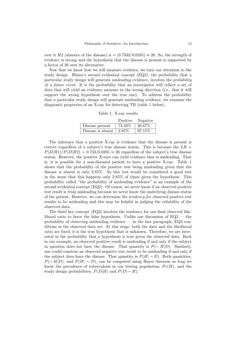
Now that we know how we will measure evidence, we turn our attention to thestudy design. Blume’s second evidential concept (EQ2), the probability that aparticular study design will generate misleading evidence, involves the probabilityof a future event. It is the probability that an investigator will collect a set ofdata that will yield an evidence measure in the wrong direction (i.e., that it willsupport the wrong hypothesis over the true one). To address the probabilitythat a particular study design will generate misleading evidence, we examine thediagnostic properties of an X-ray for detecting TB (table 1 below).

Table 1. X-ray results

Positive NegativeDisease present 73.33% 26.67%Disease is absent 2.85% 97.15%

The inference that a positive X-ray is evidence that the disease is present iscorrect regardless of a subject’s true disease status. This is because the LR =P (D|H1)/P (D|H2) = 0.733/0.0285 ≈ 26 regardless of the subject’s true diseasestatus. However, the positive X-rays can yield evidence that is misleading. Thatis, it is possible for a non-diseased patient to have a positive X-ray. Table 1shows that the probability of the positive test being misleading given that thedisease is absent is only 2.85%. So this test would be considered a good testin the sense that this happens only 2.85% of times given the hypothesis. Thisprobability called “the probability of misleading evidence” is an example of thesecond evidential concept (EQ2). Of course, we never know if an observed positivetest result is truly misleading because we never know the underlying disease statusof the patient. However, we can determine the tendency for observed positive testresults to be misleading and this may be helpful in judging the reliability of theobserved data.

The third key concept (EQ3) involves the tendency for our final observed like-lihood ratio to favor the false hypothesis. Unlike our discussion of EQ2 — theprobability of observing misleading evidence — in the last paragraph, EQ3 con-ditions in the observed data set. At this stage, both the data and the likelihoodratio are fixed; it is the true hypothesis that is unknown. Therefore, we are inter-ested in the probability that a hypothesis is true given the observed data. Backin our example, an observed positive result is misleading if and only if the subjectin question does not have the disease. That quantity is P (∼ H|D). Similarly,one could construe an observed negative test result to be misleading if and only ifthe subject does have the disease. That quantity is P (H| ∼D). Both quantities,P (∼ H|D), and P (H| ∼ D), can be computed using Bayes theorem as long weknow the prevalence of tuberculosis in our testing population, Pr(H), and thestudy design probabilities, P (D|H) and P (D| ∼H).


P (H) is a prior probability and typically the specification of this probabilitywould be subjective. But in our example it is easy to imagine that this probabilityis known and would be agreed upon by many experts. Here we will use a 1987survey where there were 9.3 cases of tuberculosis per 100,000 population [Paganoand Gauvrau, 2000]. Consequently, P (H) = 0.0093% and P (∼ H) = 99.9907%.From an application of Bayes Theorem we obtain P (∼H|D) = (0.028/0.0280) ≈ 1and P (H| ∼D) = 0.0025%. Thus the probability that an observed positive testresult is misleading is nearly 100% because the disease is so rare. Nevertheless, ourinterpretation of the LR as strong evidence the disease is present is correct. It iswrong to argue that a positive test for TB is evidence that disease is absent! Blumeand Royall [1997] independently provide less extreme examples, but this scenarioshows why it is important to distinguish between the first and third evidentialquantities (See Blume’s chapter for the full reference to this paper.) A positivetest result is evidence that the disease is present even though in this populationa positive test is not all that reliable (this is not the case for all populations ofcourse, just those with very rare diseases).

One of the problems of invoking prior probabilities, as we know, is the problem ofsubjectivity. The prior probabilities we have discussed in the diagnostic case studyare frequency-based prior probabilities; as a result, the problem of subjectivity doesnot arise. However, there are often cases when the invocation of prior probabilitiesmight be required to handle the third concept within the likelihood framework,thus potentially leading to subjectivity. At first this seems to pose a problem.However Blume shows that, for any prior, the probability that observed data aremisleading is driven to zero as the likelihood grows. Large likelihood ratios aremisleading less often. Therefore, the prior plays an important role in the startingpoint for this probability, but the data — acting through the likelihood ratio —will eventually drive this probability to zero. Thus, Blume argues, it is not criticalto know the prior, since a large enough likelihood ratio will render the effect of anyreasonable prior moot. In any case, we need to be aware of this dependence onwhich the third key concept might rely in some cases. Here, readers are invited toexplore how Hawthorne’s Bayesian Likelihood Ratio Convergence Theorem couldbe compared and contrasted with the result Blume has been discussing in regardto likelihood framework.

This third concept, the probability that observed evidence is misleading, helpsbridge the gap between the likelihood and Bayesian frameworks: The Bayesianposterior probability is the probability that the observed evidence is misleading.What is missing in the Bayesian framework, Blume implies, are the first twoconcepts. Exactly what is the Bayesian measure of the strength of evidence andhow often is that measure misleading? Likewise, Blume argues, the frequentistsalso must provide similar clarity. They cannot use a tail area probability for boththe first and second quantities and then misinterpret that tail area probability asthe third quantity once data are observed.

Taking a cue from Royall’s work on likelihood framework and in some sensesimilar to Blume’s paper, Mark Taper and Subhash Lele have proposed a more


general version of the likelihood framework that they call “evidentialism.” To givea motivation for why they think that likelihood framework is a special case of thelatter here is some justification one of the authors provides elsewhere [Lele, 2004].Lele defines a class of functions called “the evidence functions” to quantify thestrength of evidence for one hypothesis over the other. He imposes some desiderataon this class of evidence functions, which could be regarded as epistemologicalconditions. Some of the conditions satisfied by the evidence function are:

1. The translation invariance condition: If one translates an evidence functionby adding a constant to it to change the strength of the evidence, then theevidence function should remain unaffected by that addition of a constant.

2. The scale invariance condition: If one multiplies an evidence function bya constant to change the strength of evidence, then the evidence functionshould remain unaffected by that constant multiplier.

3. The reparameterization invariance: The evidence function must be invariantunder reparameterization. It means that if there is an evidence function,Ev1 and the latter is reparameterized to Ev2, then both Ev1 and Ev2 mustprovide the identical quantification of the strength of evidence.

4. The invariance under transformation of the data: The evidence functionshould remain unaffected insofar as the quantification of the strength is con-cerned if one uses different measuring units.

Lele adds two more conditions on the evidence function, which he calls “regular-ity conditions,” so that the probability of strong evidence for the true hypothesisshould converge to 1 as the sample size increases. He demonstrates that the like-lihood ratio becomes an optimal measure of evidence under those epistemologicaland regularity conditions, providing a justification for the use of likelihood ratio asa measure of evidence. Lele believes that showing the optimality of the likelihoodratio amounts to providing necessary and sufficient conditions for the optimalityof the law of likelihood. According to the law of likelihood, observation O favorsH1 over H2 if and only if P (O|H1) > P (O|H2). Taper and Lele also mentionthat information criteria, or at least order-consistent information criteria, are alsoevidence functions. By “order-consistent information criteria”, they mean that ifthe true model is in the model set, then sufficient amount of data should be ableto find the true model.

Having established the relationship between both the likelihood and informationcriteria paradigms and evidentialism, Taper and Lele explore the likelihood andinformation criteria, another pillar of frequentist statistics-error statistics. Theydistinguish between two concepts: global reliability and local reliability. Theyseem to be sympathetic with some sort of reliable account of justification which,roughly speaking, states that strength of evidence is justified if and only if it hasbeen produced by a reliable evidence producing mechanism. Given their opinionthat scientific epistemology is, or at least should be, a public and not a private epis-temology, Taper and Lele are no friends of Bayesians because they think Bayesian


subjectivity infects the objective enterprise of scientific knowledge8 accumulation.They contend that “evidentialism” of their variety will track the truth in the longrun.9 According to them, global reliability describes the truth-tracking or erroravoidance behavior of an inference procedure over all of its potential applicationsin the long run. They argue that global reliability measures commonly used instatistics are provided by Neyman/Pearson test sizes (α and β) and confidenceinterval levels. These measures, according to them, describe the reliability of thetest procedures (and not individual inferences) as a global reliability that is a prop-erty of a long-run relative frequency of repeatable events. Royall’s probability ofmisleading evidence is a similar measure of the long run reliability of evidenceprocedures to produce evidence. Taper and Lele distinguish this global reliabilitymeasure from its local version, which is the acquisition of or arriving at the truthin a specific scenario. They think that Fisher’s p-values and Mayo and Spanos’concept of severity provide a local reliability measure. The probability of obtain-ing a value for the test statistic that is as extreme, or more extreme, is called thep-value. According Mayo and Spanos the test passes with severity with respect tospecific observed outcome relative to a specific test (see section 2.2 for Mayo andSpanos’s view on severity). Taper and Lele define the notion of local reliabilityof the evidence that they call “ML”, as the probability of obtaining misleadingevidence for one model over the alternative at least as strong as the observed ev-idence. The smaller “ML” is, the greater one’s confidence that one’s evidence isnot misleading. What is significant in their paper is that their concept of evidenceand reliability are distinct, and that both may be used in making inference. Thisdiffers from an error statistical analysis such as given by Mayo and Spanos.

According to them, “ML”, is clearly different from their notion of global relia-bility. It is also different from the third key concept (discussed in Blume’s chapter)that is interested in knowing the probability of the observed evidence to be mis-leading. To compute the probability of the observed evidence to be misleading,one needs to fall back on the posterior probability value; as a result, the measureassociated with the third concept is open to the charge of subjectivity. However,ML does not depend on any posterior probability calculation. In the remainder ofthe paper, they connect philosophers’ work on “reliability” with their evidential-ism, although they think that the latter is a research program which is evolvingand thriving. As a result, more research needs to be carried out before we wouldhave a fully developed account of evidentialism of their variety.

8By “knowledge,” they must be meaning something different than what would be called“knowledge” in most epistemological literature in philosophy. They reject the truth of any com-prehensible proposition of scientific interest and don’t believe that belief is a necessary componentin any scientific enterprise concerning “knowledge.”

9Any reader familiar with epistemological literature in philosophy might wonder about theapparent problem of reconciling “reliability” with “evidentialism” since evidentialists have raisedobjections to any account of justification that rests on reliabilism. However, Taper and Lele’ssenses of “reliabilism” and “evidentialism” may not be mapped exactly onto philosophers’ locu-tion. Hence, there is less chance of worrying about an inconsistency in their likelihood framework.


2.5 The Akaikean information-criterion-based statistics paradigm

The last paradigm to be considered is the Akaikean paradigm. In philosophy ofscience, the Akaikean paradigm has emerged as a prominent research programdue primarily to the work of Malcolm Forster and Elliott Sober on the curve-fitting problem [Forster and Sober, 1994]. An investigator comes across “noisydata” from which she would like to make a reliable inference about the underlyingmechanism that has generated the data. The problem is to draw inferences aboutthe “signal” behind the noise. Suppose that the signal is described in terms ofsome mathematical formula. If the formula has too many adjustable parameters,then it will begin to fit mainly to the noise. On the other hand, if the formula hastoo few adjustable parameters, then the formula provides a small family of curves,thereby reducing the flexibility needed to capture the signal itself. The problemin curve-fitting is to find a principled way of navigating between these undesirableextremes. In other words, how should one trade off the conflicting considerationsof simplicity and goodness-of-fit. This is a problem that applies to any situationin which sets of equations with adjustable parameters, commonly called models,are fitted to data, and subsequently used for prediction.

In general, with regard to the curve-fitting problem, the goal of Forster andSober is to measure the degree to which a model is able to capture the signalbehind the noise, or equivalently, to maximizing the accuracy of predictions, sinceonly the signal can be used for prediction, given that noise is unpredictable byits very nature. The Akaikean Information Criterion (AIC) is one possible way ofachieving this goal. AIC assumes that a true probability distribution exists thatgenerates independent data points. Even though the true probability distributionis unknown, AIC provides an unbiased estimate of the predictive accuracy of afamily of curves that are fitted to a data set of that size under surprisingly weakassumptions about the nature of the true distribution.

Forster and Sober want to explain how we can predict future data from pastdata. An agent uses the available data to obtain the maximum likelihood estimates(MLE) of the parameters of the model under consideration, which yields a single“best-fitting curve” that is capable of making predictions. The question is howwell this curve will perform in predicting unseen data. A model might fare wellon one occasion, but fail to do so on another. The predictive accuracy of a modeldepends on how well it would do on average, were these processes repeated againand again.

AIC can be considered to be an approximately unbiased estimator for the pre-dictive accuracy of a model. By an “unbiased estimator,” we mean that theestimator will equal the population parameter on average, with the avearge beingrelative to repeated random sampling of data of the same size as the actual data.Using AIC, the investigator attempts to select the model with minimum expectedKullback-Leibler (KL) distance across these repeated random samples, based ona single observed random sample. For each model, the AIC score is

AIC = −2 log(L) + 2k (E2)


Here “k” represents the number of adjustable parameters. The maximum like-lihood, represented by L, is simply the probability of the actual data given by themodel fitted to the same data. The fact that the maximum likelihood term usesthe same data twice (once to fit the model and once to determine the likelihood ofthat the fitted model) introduces a bias; the same curve will not fit unseen dataquite as well. The penalty for complexity is introduced in order to correct for thatbias.

Another goal of AIC is to minimize the average (expected) distance betweenthe true distribution and the estimated distribution. It is equivalent to the goal ofmaximizing predictive accuracy. AIC was designed to minimize the KL distancebetween a fitted MLE model and the distribution actually generating the data.Specifically, AIC can be considered as an approximately unbiased estimator for theexpected KL divergence which uses a MLE to create estimates for the parametersof the model.

With this background, it is worthwhile to consider their contribution to thevolume where Forster and Sober analyze the Akaikean framework from a differentperspective. AIC is a frequentist construct in the sense that AIC provides acriterion, or a rule of inference, that is evaluated according to the characteristicsof its long-run performance in repeated instances. Bayesians find the use of thefrequency-based criteria to be problematic. Since AIC is a frequentist construct,Bayesians worry about the foundation of AIC. What Forster and Sober have donein their chapter is to show that Bayesians can regard AIC scores as providingevidence for hypotheses about the predictive accuracies of models. A key pointin their paper is to point out that this difference of evidential strength betweenhypotheses about predictive accuracy can be interpreted in terms of the law oflikelihood (LL), which is something that Bayesians can accept. According to theLL, observation O favors H1 over H2 if and only if P (O|H1) > P (O|H2). Thesecret is to take O to be the “observation” that AIC has a certain value and H1 andH2 to be competing “meta”-hypotheses about the predictive accuracy of a model(or of the difference in predictive accuracies between two models). According toForster and Sober, Bayesians’ worry about AIC has turned out to be untenablebecause now AIC scores are evidence for hypotheses about predictive accuracyaccording to the LL which is one of the cornerstones of Bayesianism.

Revisiting the four types of questions, we find that the Akaike framework iscapable of responding to the prediction question. Forster and Sober maintainthat, in fact, it is able to do this in terms of the evidence question because theprediction question can be viewed a sub-class of the evidence question.

3 THE LIKELIHOOD PRINCIPLE

So far, we have considered four paradigms in statistics along with their varyingand often conflicting approaches to statistical inference and evidence. However, wealso want to discuss some of the most significant principles whose acceptance andrejection pinpoint the central disagreement among the four schools. The likelihood


principle (LP) is definitely one of the most important. In his chapter, JasonGrossman analyzes the nature and controversies surrounding the LP. Bayesians arefond of this principle. To know whether a theory is supported by data, accordingto Bayesians, LP says that the only part of data that is relevant is the likelihoodof the actual data given the theory.

The LP is derivable from two principles; the first is the weak sufficiency prin-ciple (WSP) and the second is the weak conditionality principle (WCP). TheWSP claims that if T is sufficient statistic and if T (x1) = T (x2), then both x1

and x2 will provide equal evidential support. A statistic is sufficient, if givenit, the distribution of any other statistic does not involve the unknown parame-ter θ. Both Bayesians and likelihoodists like both Royall and Blume accept theLP, whereas classical/error statisticians do not. Grossman clarifies the reasonthat classical/error statisticians question the principle. What data investigatorsmight have obtained, but do not actually have, according to error statisticians,should play a significant role in evaluating statistical inference. Significance test-ing, hypothesis testing and confidence interval approach, which are tool-kits forclassical/error statistics, violate the LP since they incorporate both actual andpossible data in their calculation. In this sense, Grossman’s chapter overlaps withmany papers in the section on “Four Paradigms,” especially Mayo and Spanos’paper in this volume.

Grossman also discusses the relationship between the law of likelihood (LL)and LP. They are different concepts; hence, supporting or denying one does notnecessarily lead to supporting the other, and conversely. The LP only says wherethe information about the parameter θ is and suggests that the data summarizationcan be done through the likelihood function, in some way. It does not clearlyindicate how to compare the evidential strength of two competing hypotheses. Incontrast, the LL compares the evidential strength of two contending hypotheses.

4 THE CURVE-FITTING PROBLEM, PROBLEM OF INDUCTION, ANDROLE OF SIMPLICITY IN INFERENCE

The previous discussion of four statistical paradigms and how they address fourtypes of questions provides a framework for evaluating several approaches to induc-tive inference. Two related problems that often confront any approach to inductiveinference are the pattern recognition problem and the “the curve-fitting problem.”In both cases one is confronted with two conflicting desiderata, “simplicity” and“goodness-of-fit.” Numerous accounts within statistics and outside statistics havebeen proposed about how to understand these desiderata and to reconcile them inan optimal way.

Statistical learning theory (SLT) is one such approach that looks at these prob-lems while being motivated by certain sets of themes. Learning from a pattern is afundamental aspect of inductive inference. It becomes all the more significant if atheory is able to capture our learning via pattern recognition in our day to day lifeas this type of learning is not easily suited to systematic computer programming.


Suppose for example that we want to develop a system for recognizing whether agiven visual image is an image of a cat. We would like to come up with a func-tion from a specification of an image to a verdict, a function that maximizes theprobability of a correct verdict. To achieve this goal, the system is given severalexamples of cases in which an “expert” has classified an image as of a cat or notof a cat. We have noted before that there is no assumption-free inference possiblein the sense that we have to assume that data at hand must provide some cluesabout the future data. Note that this assumption is a version of the uniformity ofnature assumption. In order for the investigator to generate examples, she assumesthat there is an unknown probability distribution characterizing when particularimages will be encountered and relating images and their correct classification.We assume that the new cases of the examples that we will come across are alsorandomly sampled from that probability distribution. This is similar to what isassumed in the Akaikean framework, discussed earlier.

We assume that the probability of the occurrence of an item with a certaincharacterization and classification is independent of the occurrence of other itemsand that the same probability distribution governs the occurrence of each item.The reason for having the probabilistic independence assumption is to imply thateach new observation provides maximum information. The identical probabil-ity distribution assumption implies that each observation gives exactly the sameinformation about the underlying probability distribution as any other. (Theseassumptions can be relaxed in various ways.) One central notion in SLT is thenotion of VC-Dimension, which is defined in terms of shattering. A set of hy-pothesis S shatters certain data if and only if S is compatible with every way ofclassifying the data. That is, S shatters a given feature vectors if for every labelingof the feature vectors (e.g., as “cat” or “not cat”) the hypothesis in S generatesthis labeling. The finite VC-dimension of a set of rules C is the largest finitenumber N for which some set of N points is shattered by rules in C; otherwisethe VC-dimension is infinite. The VC-dimension of C provided a measure of the“complexity” of C. Various learning methods aim to choose a hypothesis in sucha way as to minimize the expected error of prediction about the next batch ofobservations. In developing their account about inductive inference, Gilbert Har-man and Sanjeev Kulkarni in their joint paper have contended that SLT has alot to offer to philosophers by way of better understanding the problem of induc-tion and finding a reliable method to arrive at the truth. They note similaritiesbetween Popper’s notion of falsifiability and VC-dimension and distinguish lowVC-dimension from simplicity in Popper’s or any ordinary sense. Both Harmanand Kulkarni address those similarities between the two views and argue how SLTcould improve Popper’s account of simplicity. Daniel Steel, while bringing in Pop-per’s notion of falsifiablity, has gone further to argue that the aim of Popper’saccount seems different from the aim of SLT. According to Popper, the scientificprocess of conjectures and refutations generates ever more testable theories thatmore closely approximate the truth. This staunch realism toward scientific theo-ries, according to Steel, is absent in SLT which aims at minimizing the expected


error of prediction. Even though there is an apparent difference between these twoapproaches, Steel conjectures, there might be some underlying connection betweenpredictive accuracy and efficient convergence to truth.

Like SLT, both the Minimum Description Length (MDL) principle and the ear-lier Minimum Message Length (MML) principle aim to balance model complexityand goodness-of-fit in order to make reliable inferences. Like SLT, the MDL andMML, are also motivated by a similar consideration regarding how to make re-liable inferences from data.10 In both these approaches, the optimal tradeoff isconsidered to be the one that allows for the best compression of the data, in thesense that the same information is described in terms of a shorter representation.In MML, it is important that the compression be in two parts: hypothesis (H1)followed by data given the hypothesis (D given H1).

According to the MDL principle, the more one could compress a given set ofdata, the more one has learned about the data. The MDL inference requires thatall hypotheses ought to be specified in terms of codes. A code is a function thatmaps all possible outcomes to binary sequences such that the length of the encodedrepresentation can be expressed in terms of bits. The MDL principle provides arecipe regarding how to select the hypothesis: choose the hypothesis H for whichthe length of the hypothesis L(H) along with the length of the description of thedata using the hypothesis LH(D) is the shortest. The heart of the matter is, ofcourse, how these codes L(H) and LH(D) should be defined. In their introductionto MDL learning, Steven de Rooij and Peter Grunwald explain why these codesshould be defined to minimize the worst-case regret (roughly, the coding overheadcompared to the best of the considered codes), while at the same time achievingespecially short code-lengths if one is lucky, in the sense that the data turn out tobe easy to compress.

By minimizing regret in the worst case over all possible data sequences, it is notnecessary to make any assumptions as to what the data will be like. If one performsreasonably for the worst possible data set, then one will perform reasonably well forany data set. However, in general it may not even be possible to learn from data.Rather than assuming the truth to be simple, De Rooij and Grunwald introducethe alternative concept of luckiness: codes are designed in such a way that if thedata turn out to be simple, we are lucky and we will learn especially well.

The Minimum Message Length (MML) principle is similar to the MDL principlein that it is also interested in proposing a resolution for what we have called thecurve-fitting problem. Like MDL, data compression plays a key role in MML.

10There are considerable disagreements among experts on the SLT, MML, and MDL regardingwhich one is a more general theory than the other in the sense whether, for example, the SLT isable to include discussion of the properties of the rest. The SLT adherents argue that the SLT isthe only general theory, whereas the MML adherents contend that the MML should be creditedwith the only approach which is the most general between the two. One MDL author, however,thinks that it is misleading to take any of the three approaches as any more fundamental thanthe rest. We are thankful to Gilbert Harman, David Dowe and especially Peter Grunwald fortheir comments on this debate. For a discussion of these entangled issues, see [Grunwald, 2007,chapter 17]. We, as editors, however, would like to report those disagreements among theseexperts without taking sides in the debate.


The more one could compress the data, the more we are able to get informationfrom the data; moreover, the shorter the length of the code for presenting thatinformation, the better will it be in terms of MML. One way to motivate eitherthe MDL or the MML approach is to think of the length of codes in terms ofKolmogorov complexity in which the shortest input to a Turing Machine willgenerate the original data string (For Kolmogorov’s complexity and its relationto random sequences see section 7.3). This approach uses two-part codes. Thefirst part always represents the information one is trying to learn, that is, ofencoding the hypothesis H and then making the Turing Machine prepare to readand generate data, assuming that the data were generated by the hypothesis Hencoded in the first part. In the first part of the message, the codes do not causethe Turing Machine to write. The second part of the message encodes the dataassuming the (hypothesis or) model given in the first part, and then makes theTuring Machine write the data. In the use of two-part codes there is very littledifference between MML and MDL. However, there is a fundamental differencebetween the two. MML is a subjective Bayesian approach in its interpretation ofthe used codes, whereas MDL eschews any subjectivism in favor of the conceptof luckiness. The MML can exploit an agent’s prior (degree of) beliefs about thedata generating process, but it can also attempt to make our priors as objectiveas possible in MML by using a simplest Universal Turing Machine.

In his paper on the Bayesian information-theoretic MML principle, David Dowesurveys a variety of statistical and philosophical applications of MML, includingrelating MML to hybrid Bayesian nets. The relationship underlying MML is theidea of information theory where information is taken to be the negative logarithmof probability. This view has also led him to his two recent results: (i) the only scor-ing system which remains invariant under-reframing of questions is the logarithmof probability score, and (ii) a related new uniqueness result about the Kullback-Leibler divergence between probability distributions. Dowe re-states his conjec-ture that, for problems where the amount of data per parameter is bounded above(e.g., Neyman-Scott problem, latent factor analysis, etc.), to guarantee both sta-tistical invariance and statistical consistency in general, it appears that one needseither MML or a closely-related Bayesian approach. Using the statistical consis-tency of MML and its relation to Kolmogorov complexity, Dowe independentlyre-discovers Scriven’s human unpredictability as the “elusive model-paradox” andthen, resolves the paradox (independently of Lewis and Shelby Richardson [1966])using the undecidibility of the Halting problem. He also provides an outline ofthe differences between MML and the various variations of the later MDL prin-ciple that have appeared over the years (for references of the papers in the lastparagraph, see Dowe’s paper in the volume.)

The notion of simplicity in statistical inference is a recurring theme in severalpapers in this volume. De Rooij and Grunwald have addressed the role of simplic-ity, which they call “the principle of parsimony” in learning. Those who think thatsimplicity has an epistemological role to play in statistical inference contend thatsimpler theories more likely to be true. There could be two opposing camps in


statistical inference regarding the epistemological role of simplicity. One could beBayesians. The other could be non-Bayesian [Forster and Sober, 1994]. De Rooijand Grunwald have, however, identified the epistemological interpretation of sim-plicity with Bayesians. A likely natural extension of the epistemological construalof simplicity in statistical inference is to believe that simpler theories are morelikely to be true. Subjective Bayesians subscribe to this epistemological accountof simplicity. The hypothesis with a maximum posteriori probability is believedmost likely to be true. De Rooij and Grunwald distance themselves from this in-terpretation, because the philosophy behind MDL aims to find useful hypotheseswithout making any assertions as to their truth.

De Rooij and Grunwald assert that one fundamental difference between MDL,on the one hand, and MML and SLT, on the other, is that the former does not seemto have any form of the uniformity of nature assumption inbuilt in its philosophythat we find in the latter two. They would hesitate to assume that the data at handnecessarily provide clues about the future data. They prefer not to discount thepossibility that it may not. Instead, they design methods so that we learn from thedata if we are in the lucky scenario, where such is possible. According to them,this is a key distinction between the MDL approach and any other approachesincluding MML and SLT.

In his paper, Kevin Kelly agrees with non-Bayesians like De Rooij and Grunwaldabout the Bayesian explanation of the role of simplicity in scientific theory choice.The standard Bayesian argument for simplicity, as already stated, is that simplertheories are more likely to be true. Bayesians use some form of Bayes’ theorem todefend their stance toward the role of simplicity in theory choice. This could takethe form of comparing posterior probabilities of two competing theories in termsof the posterior ratio:

P (S|D)

P (C|D)=

P (S)

P (C)× P (D|S)

P (D|C), (E3)

where theory S is simple (in the sense of having no free parameters) and theoryC is more complex (in the sense of having free parameter θ that ranges, say, overk discrete values). The first-quotient on the right hand side of (E3) is the ratioof the prior probabilities. According to Kelly, setting P (S) > P (C) clearly begsthe question in favor of simplicity. So he supposes, out of “fairness”, that P (S) isroughly equal to P (C), so that the comparison depends on the second quotient onthe right hand side of (E3), which is called the Bayes factor. According to him,the Bayes factor appears “objective”, but when expanded out by the rule of totalprobability, it assumes the form:

P (S|D)

P (C|D)=

P (S)

P (C)× P (D|S)∑

θ

P (D|Cθ)P (Cθ|C),

which involves the subjective prior probabilities P (C0|C). Kelly’s point is thattypically there is some value of θ such that P (D|S) = P (D|Cθ). If P (C0|C) = 1,


then the posterior ratio evaluates to 1 (the complex theory is as credible as thesimple theory). But, in that case the parameter θ is not “free”, since one hasstrong a priori views about how it would be set if C were true. To say that is“free” is to adopt a more or less uniform distribution over k values of θ. In thatcase, the posterior ratio evaluates to k — a strong advantage for the simple theorythat becomes arbitrarily large as the number of possible values of θ goes to infinity.But, objectively speaking, C0 predicts D just as accurately as S does. The onlyreason C is “disconfirmed” compared to S in light of D is that the subjective priorprobability P (C0|C) = 1/k gets passed through Bayes’ theorem. Kelly concludes,therefore, that the Bayesian argument for simplicity based on Bayes’ factor isstill circular, since it amounts to a prior bias in favor of the simple world S incomparison to each of the complex possible C0.

Kelly proposes a new, alternative explanation of Ockham’s razor that is sup-posed to connect simplicity with truth in a non-circular way. The explanation isbased on the Ockham Efficiency theorem, according to which Ockham’s razor isthe unique strategy that keeps on the most direct path to truth, where directnessis measured in terms of jointly minimizing course reversals en route to the truthand the times at which these courses reversals occur. Since no prior probabilitiesare involved in the theorem, Kelly maintains that it does not beg the questionthe way simplicity-biased prior probabilities do. Furthermore, since Kelly viewsdirectness of pursuit of the truth as a concept of truth conduciveness, he views theOckham Efficiency Theorem, as a foundation for scientific inference rather thaninstrumentalistic model selection. In that respect, he parts company with the anti-realism of De Rooij and Grunwald, who maintain, in light of the MDL approach,that simplicity plays primarily a heuristic role in making a theory useful. Kellyargues that in the case of causal theory choice from non-experimental data (seesection 6 below), getting the causal arrows backwards yields extremely inaccu-rate policy predictions, so the Ockham Efficiency Theorem, according to Kelly, isthe only available, non-circular foundational viewpoint for causal discovery fromnon-experimental data.

5 RECENT ADVANCES IN MODEL SELECTION

We touched on the model selection problems when we discussed the curve-fittingproblem, especially with regard to the AIC paradigm in statistics. Model selectionis such a hotly debated topic in statistical literature that it deserves a special placein our volume. However, model selection has a narrowly focused area in statisticsin which investigators are confronted with choosing the model that provides thebest possible account for the underlying mechanism generating the data and therole simplicity contributes to their choice. It is a delicate question whether thereis a characteristic difference between theory choice and model selection. In revo-lutions in physical theories, Einstein’s theory replaced the Newtonian theory or anew disciple like bio-chemistry emerged as the theory of double helical structureof the DNA was discovered. However, model selection cannot or should not de-


cide between two contending theories, as we see in the case of physical theories.In contrast, model selection addresses a narrow topic with specific problems, likewhether the data in question are coming from a normal distribution or from othernon-normal distributions.

Setting the model selection issues in this context of theory choice in advancedphysical theories, Arijit Chakrabarti and Jayanta Ghosh address two widely dis-cussed model selection criteria: AIC and Bayesian Information Criterion (BIC).BIC says that Prob (Hk| data) is proportional to the log-likelihood of the samplen multiplied by n−k/2. Surveying the literature in statistics and computer sciencewhere model selection criteria are extensively applied, Chakrabarti and Ghoshdistinguish between the purposes for which AIC and BIC are introduced. Theyargue that the BIC is more useful when the true model is included within themodel space. In contrast, the AIC is more effective in predicting the future obser-vation. This depiction of the difference between the BIC and AIC sets the tonefor a peaceful co-existence of both model selection criteria; too often, statisticiansand philosophers are involved in “statistics war” pleading for the superiority ofone criterion over the other. This also provides an elegant connection between thetheme echoed in Chakrabarti and Ghosh’s paper on the one hand, and Norton’sand Kelly’s papers on the other. The common theme that has been shared by allfour authors is that there should not be any such account of inductive inferencethat could defend “one-size-fits-all” philosophy. Although both Norton and Kellyare non-Bayesians and their targets of criticism are Bayesians, Chakrabarti andGhosh are themselves Bayesians and their targets could be both Bayesians andnon-Bayesians.

A.P. Dawid in his chapter has also focused on Bayesian model selection issues.Within a Bayesian framework, the conventional wisdom about the problem ofmodel choice is that model choice is more sensitive to the prior than is standardparametric inference. Working with a Bayesian framework, he, however, rejectsthis conventional wisdom based on the study of the asymptotic dependency of pos-terior model probabilities on the prior specifications and the data. Moreover, thepaper suggests a possible solution to the problematic Bayes factor with respect toimproper priors by specifying a single overall prior and then focusing on the poste-rior model distributions. The general theory has been illustrated by constructingreference posterior probabilities for both normal regression models and analyses ofan ESP experiment. However, in a sense, Dawid’s interest is much broader thanjust model selection issues. He is interested in Bayesian inference. Consequently,he has developed a general Bayesian theory of inference with a specific type ofposterior probability construction.

6 CAUSAL INFERENCE IN OBSERVATIONAL STUDIES

Whether we engage in statistical inference or are involved with statistical evidenceor model selection problem, data are enormously important for statistics and mak-ing reliable inference. Often, data or observations are randomized. Frequently, we


do not have the luxury of randomly sampling our observations so that our inferencewould be reliable in the sense of minimizing biases or systematic errors. Thosecases arise in observational studies when we have no randomization option, but westill need to make inferences. Sometimes, we also make causal inferences based onobservational studies. Peter Spirtes and Sander Greenland’s two papers addressthese issues regarding how one could successfully make a reliable causal inferencewhen topics in question involve observational studies.

In building a causal model from observational studies, Spirtes distinguishes be-tween two kinds of questions, (i) qualitative and (ii) quantitative. A qualitativequestion asks “will manipulating a barometer reading affect subsequent rainfall?”A quantitative question asks, “how much does manipulating a barometer readingaffect subsequent rainfall?” With observational studies, one might be confrontedwith several issues about how to make a reliable qualitative or quantitative in-ference. Spirtes is interested in making reliable causal inference in observationalstudies when two variables may be connected by an unmeasured common cause.For example, the correlation between two observed variables barometer readingand rainfall could be due to an unmeasured (latent) common cause such as at-mospheric pressure; without further background knowledge the correlation couldalso be due to the barometer reading causing rainfall. Without some substantivecausal assumptions of this entire causal setup, one cannot hope to make any reli-able inference about which of these causal relationships between barometer readingand rainfall is correct simply from observing the correlation between them. Some-times attempts are made to make reliable inferences about the causal relationshipbetween barometer reading and rainfall by using temporal information and con-ditioning on as many potential causes as possible prior to the occurrence of theputative cause. However, in this scenario there is still no way to make reliablecausal inferences without substantive causal assumptions regarding whether allthe relevant variables are conditioned on; in addition standard causal inferencemethods can be misled by conditioning on too many variables, as well as too few.Spirtes discusses some general assumptions relating causal relationships to statis-tical relationships, which causal inferences cannot be reliably made under theseassumptions when unmeasured common causes may be present, and alternativereliable methodologies for reliable causal inferences when it is possible.

Like Spirtes, Greenland is also interested in causal inference in observationalstudies. However, he is focused on a manipulative account of causation where aninvestigator wants to observe a particular outcome in a subject after she is givena treatment. This model is called the Potential outcome or Counterfactual model.In the potential outcome model, the investigator approaches the issue by definingthe effects of a cause or intervention and then defining the effects of treatment.Suppose, we would like to observe the effects of different doses of AZT on patientsaffected with HIV virus. We would compare the one year mortality rate that wouldoccur in a given population after they are administered certain doses of AZT ornone at all. Here, the range of intervention in terms of patient’s doses of AZTcould very well correspond to different levels of their physical discomfitures, in


which the potential outcomes could be their length of survival, e.g., if the patientssurvive another year or not. Or it could be that their survival time range from oneyear to another five year from the day of the introduction of the drug to them.

In the deterministic situations like the case of the AZT doses and the survivalrate of the patients, the purpose of observational studies, according to Green-land, is to find a causal link connecting treatments of the patients to their recov-ery/survival rate. In the deterministic world, we use probability to capture uncer-tainty, although ambiguity remains if the intervention is not completely specified.The situation becomes more complex in a stochastic world, such as in quantumworld, where it is not even theoretically possible to know the future fully. Theproblem can be dealt with by allowing the potential outcomes to refer to distribu-tions (or parameters) instead of realizations [Greenland et al., 1999].

In the present chapter, however, Greenland confines himself to the determin-istic world. In articulating the potential outcome model for such a deterministicworld, he discusses the role of causal laws (expressed in terms of some structuralequations) in which one shifts from the understanding of the counterfactual (if youwould have administered treatment x instead of y to the patient, then what couldhave happened to her?) to the understanding of the law connecting the outcomevariable to the antecedent variable. The law in question could be “if one dropsboth a feather and a coin at the same time from a height to the ground where thereis no air-resistance, then they would reach the ground simultaneously.” Greenlandthinks that if we find that the predictions of the theory have turned out to be falsemore often than not, then they would provide reasons to question its tenability. Asstudents of philosophy of science we know, however, that the falsity of predictionsshould not necessarily lead to the rejection of that theory as its various auxiliariescould be called into question rather than the theory itself because of its wrongpredictions. Similar tangled issues could crop up in studying causal inference inobservational studies

To circumvent this possible objection that the falsity of predictions should notnecessarily lead to the wholesale rejection of the theory, Greenland has demon-strated the benefits of the use of causal diagrams in similar and other relevantsituations. A “causal system” as he calls it consists of the output w of a functionf(u, v) which might become an input to a later function g(u,w) with output x.The arrows in the diagram representing this system are to be taken as causal ar-rows connecting input variables to output variables. The advantage of this kindof diagrams lies in its ability to do “local surgeries” if and when required. Theyare devised in such a way that they are able to isolate the effect of that rejectionmentioned above in that causal network of relations among variables, and thus areable to pinpoint which specific part of theory or its auxiliaries have to be calledinto question when predictions of the theory don’t result in what is expected.

While developing the potential outcome models along with their structural equa-tion generalizations, he makes the reader aware of the possible theoretical problemsof this model. However, he concludes with a pragmatic note. What matters most,according to him, is the practical significance of these causal diagrams applied to


varied situations, although many foundational questions about the model are yetto be satisfactorily resolved.

7 SPECIFIC TOPICS OF INTEREST

We began this “Introduction” with the types of questions/problems with whichphilosophers are often confronted. We have seen that they are more often inter-ested in general epistemic and causal issues, including issues about the foundationsof statistical inference. Philosophers who are trained primarily in analytic tradi-tion are sometimes interested in simple/specific problems. Nonetheless, it wouldbe a mistake to think that only philosophers are interested in specific problems.This section examines how statisticians, mathematicians, and computer scientistsalong with philosophers are busy working out the details of some of the specificproblems in the topics of their interest.

7.1 Conditional probability

One of these specific problems in which various philosophers have lately been get-ting interested is “what is conditional probability?” The conditional probabilityof P (H|D) is traditionally defined as P (H&D)/P (D) when P (D) is greater thanzero. Here, as before, “H” stands for a hypothesis and “D” stands for data. AlanHajek in his contribution suggests that although this way of understanding condi-tional probability is common and has been proposed by Kolmogorov, it is actuallya conceptual analysis of conditional probability. According to Hajek, one is freeto stipulate that a particular technical expression is a short-hand for a particularconcept, but one is not free to assign that concept any meaning he/she chooses.Conditional probability is not simply an abbreviation; rather, it is answerableto certain pre-theoretical intuitions. Thus, although we could choose to make“P (H|D)” a shorthand for this ratio, he argues, we do not have any good rea-son to identify the expression “the probability of H given D” with this ratio. Heevaluates several arguments for the ratio analysis, and ultimately rejects them.Instead, he argues, conditional probability should be taken as primitive.

One of the arguments he offers for dispensing with the ratio analysis is by wayof illustrated by an example. What is the probability that a coin turns up headsgiven that I toss it fairly? It should be 1

2. The problem, Hajek contends, is that

according to the ratio analysis, the conditional probability is the ratio:

P (the coin lands heads & I toss the coin fairly)/P (I toss the coin fairly)

and both unconditional probabilities need not be defined. After all, he argues,“you may simply not assign them values. After some thought, you may start toassign them values, but the damage has already been done; and then again, youmay still not do so.” The damage that has been done is that there is a time atwhich an agent assigns a conditional probability (1

2) in the absence of the corre-

sponding unconditional probabilities required by the ratio formula. As is evident,this is an immediate counterexample to the ratio formula. It does not save the


formula from this counterexample if later on the agent in question happens toassign the requisite unconditional probabilities; the counterexample concerned theearlier time, and its existence provides a refutation of the ratio analysis of theconditional probability. However, in this example, Hajek thinks that there is aclear-cut conception of conditional probability according to which the answer is 1

2.

He explores the fundamental nature of conditional probability in the various inter-pretations of probability. He canvases other arguments against the ratio analysis:cases in which the condition (D) has probability 0 (and thus can’t appear in thedenominator of the ratio), or unsharp probability, or vague probability. (Thesenotions are explained in sections 4.2 and 4.3. of his chapter) He also shows howconditional probability plays a key role in various paradoxes, including Simpson’sparadox (see section 7.2 for an example and exposition.)

One highlight of Hajek’s paper is to investigate the debate over whether thenotion of conditional probability is a primitive or a defined concept. In the usualway that we learn probability theory, conditional probability is defined in terms oftwo unconditional probabilities. Since he thinks that we have an intuitive under-standing of conditional probability, he recommends reversing the order of analysis.Like Popper, Hajek argues that one should take conditional probability, P (, ) tobe fundamental and unconditional probability to be derivative: the unconditionalprobability of a is P (a,T), where T is a logical truth.11 Hajek presents Pop-per’s axioms and postulates of primitive conditional probability functions, knownas the Popper Functions. This mathematical set-up offers a rival approach toKolmogorov’s. Hajek also points out that Popper’s approach has no difficulty inhandling the objections raised against the ratio analysis.

Building on Hajek’s paper, Kenny Easwaran has both addressed and evaluatedmany of the issues raised by Hajek. He agrees with Hajek that the ratio analysisof the conditional probability is faulty. However, he disagrees sharply with Hajekregarding his claim that conditional probability rather than unconditional proba-bility should be regarded as primitive. Easwaran thinks that Hajek’s argument inthis connection needs to be separated for each interpretation of probability ratherthan taking it as one argument that cuts across all interpretations together. Hethinks that, especially with regard to subjective interpretation of probability, a dis-tinction needs to be made between between P (H|D), where “D” are themselvessome possible event later in time than t, and P (H|D), where “D” encompasses acomplete description of the history of the universe up to time t. Easwaran con-tends that although it is evident that all non-logical interpretations (for example,the subjective or propensity interpretation) of probability depend on some infor-mation in order for some probabilities to be assigned to some particular cases, therole this information plays could very well vary. Thus, he concludes that Hajekhas not provided a good argument for the claim that the notion of conditionalprobability should be counted as a primitive notion rather than the notion of theunconditional probability.

11Hajek prefers to reserve the notations, “P (|)” for the ratio analysis and “P (, )” for theconditional probability being primitive.


7.2 Probabilistic and statistical paradoxes

Paradoxes, albeit entertaining, challenge our intuitions in a fundamental way.There is no exception to this whether we are concerned with probabilistic or sta-tistical paradoxes. It is often hard to distinguish between probabilistic paradoxesand statistical paradoxes. One could, however, propose that all statistical para-doxes are probabilistic paradoxes, whereas probabilistic paradoxes are not exactlystatistical paradoxes. This leaves a more basic question unanswered: “what is astatistical paradox?” A statistical paradox is a paradox that can be understoodin terms of notions that need not be probabilistic, for example, “confounding,”“intervening,” and so on. It still might not settle the dispute about the differencesbetween statistical and probabilistic paradoxes, because probability theorists couldcontend that notions like “confounding” are subject to probabilistic reduction. Itis, however, sufficient for our purpose to appreciate the difficulty associated withgiving a clear-cut definition of either of the terms as we proceed to discuss prob-ability paradoxes. One way to understand the difference between the two is toconsider the “Monty Hall problem” (named after a television game show host),which, among many other paradoxes, Susan Vineberg discusses in her chapter.

Suppose you are a contestant on a quiz show. The host, Monty Hall, showsyou the three doors (A,B, and C). Behind one door is an expensive new car andbehind others are goats. You are to choose one door. If you choose the door withthe car, you get it as a prize. If you choose a door with a goat, you get nothing.You announce your choice, and Monty Hall opens one of the unchosen doors,showing you a goat, and offers to let you change your choice. Should you change?Three crucial points need to be clearly stated which are usually overlooked in apopularized version of the Monty Hall problem. They are (i) the expensive car hasan equal chance of being distributed behind any of the doors. (ii) If you chooseone door without the prize behind it, Monty will open the door that does not havethe prize behind it. And (iii) if you choose the door behind which there is a prizebehind it, then Monty will open the door randomly which does not have the prizebehind it. Given this setup, let us calculate the probability of opening the doorB (Monty B) when the prize is behind A (A). Suppose the contestant has chosendoor A.

The probability of Monty’s opening door B given that the prize is behind doorA equals P (B|A) = 1

2. (Recall that once you have chosen the door A Monty is

not going to open it. So Monty is left with two choices.)

Compute the probability of Monty’s opening the door (Monty B) when there isthe prize behind the door B.

P (Monty B|B) = 0 ( Recall that he is not going to open the door behind whichthere is the prize).

Compute the probability of opening the door B when there is the prize behinddoor C.

P (Monty B|C) = 1 ( because the contestant has chosen door A and the prizeis behind door C. He is left with no other option than to open door B.)


We would like to know whether you should stay where you are (A) conditional(given) on the information that Monty has opened door B. That is, P (A| Monty B).According to the Bayes’ theorem,

P (A| MontyB) = ((P (A) × P (MontyB|A))÷((P (A) × P (MontyB|A)) + ((P (B) × P (MontyB|B))+((P (C) × P (MontyB|C))

Consider P (A) × P (MontyB|A) = 1/3 × 1

2= 1/6

P (B) × P (Monty B|B) = 1/3 × 0 = 0.P (C) × P (Monty C|C) = 1/3 × 1 = 1/3

Now P (A| MontyB) = 1/6

1/6+0+1/3= 1/6 ÷ 1

2= 1/3.

Thus, if you switch, you will get 2/3 of a chance of winning.Vineberg has considered the Monty Hall problem to be a probability paradox.

One needs to be careful as to her reason for classifying this problem to be a paradoxof probability. She takes it to be a paradox of probability because probabilitiesare appealed to in the reasoning that gives us the paradox, and not because ofits solution which rests on using Bayes’ theorem. This paradox might be saidto be essentially probabilistic, because it is resolved by highlighting the correctuse of Bayes’ theorem, which yields 1/3 along with the assumptions noted before.In contrast, Simpson’s paradox, another paradox that Vineberg considers, canbe considered to be both a statistical and a probability paradox at the sametime. Simpson’s Paradox involves the reversal of the direction of a comparisonor the cessation of an association when data from several groups are combined toform a single whole. Suppose you are considering the acceptance rates for malesand females in a graduate program that includes two departments. Consider anexample of Simpson’s paradox.

Table 2. Simpson’s Paradox

CVDept. 1 Dept. 2 Acceptance Rates

Overall Acceptance RatesAccept Reject Accept Reject Dept. 1 Dept. 2

F 180 20 100 200 90% 33% 56%M 480 120 10 90 80% 10% 70%

Here, “CV” includes two categorical variables, “F” for “females” and “M” for“men.” “A” and “R” represent “the rates of acceptance/rejection” for two depart-ments, D1, and D2. Here is a formulation of the paradox, in which the associationin the subpopulations is reversed in the combined population. Although the ac-ceptance rates for females are higher than for males in each department, in thecombined population, the rates have reversed. Vineberg has explained why it couldbe explained within the confines of the probability theory. However, as we know, itcould also be regarded as a statistical paradox because notions like “confounding,”


which many statisticians consider to be statistical notions, could be used to explainit. In the above example of the paradox, for example, the effect on acceptance(A) of the explanatory variable, sex (S), is hopelessly mixed up (or “confounded”)with the effects on A of the other variable, department (D). According to somestatisticians, we are interested in the direct effect of sex on acceptance and not anindirect effect by way of another variable such as department. The effect of S onA is confounded with the effect on A of a third variable D.

Although Vineberg is fully aware of this difficulty of characterizing a paradoxcompletely in terms of the probability theory or statistics, she confines herselfto the probability paradoxes, investigating possible reasons for regarding themas probability paradoxes. She counts all of the paradoxes that she has consid-ered paradoxes of probability because the reasoning (and/or premise) involved inthem is probabilistic, and not because of the form of their solution (for a clearunderstanding of the relationship between probabilistic reasoning and probabilis-tic/inductive inference, see the concluding section of Bandyopadhyay and Cherry’schapter.) On her account, Simpson’s paradox is a paradox of probability is due tothis specific reason. She argues that some of the paradoxes arise from misapplica-tions of the rules of the probability theory. Some of the resolutions of the paradoxes(like the Monty Hall problem) are less controversial, whereas others are more con-troversial; as a result, they are hotly debated. She cites Newcomb’s problem as onesuch paradox in the latter category since it is liable to several competing solutionsrequiring radical rethinking about the foundations of Bayesian decision theory (see[Savage, 1972] for classical Bayesian decision theory).12 The rationale she offersfor not regarding it as a paradox of probability is that the reasoning leading tothis problem requires non-probabilistic decision theoretic considerations.

C. Andy Tsao reviews two statistical paradoxes: (i) Lindley’s paradox and (ii)the Fieller-Creasy problem. There are already some discussions on those paradoxesin the literature, since both arose in the early 1960s. We will confine ourselvesto Tsao’s discussion of the Lindley’s paradox. To set the paradox in a broaderperspective, consider the formulation of the hypothesis testing problem where twohypotheses are H0 = the null hypothesis and H1 = the alternative hypothesis.There are infinitely many tests possible regarding the tenability of a hypothesis;some are conservative and some are liberal. In this connection, the term “con-servative” (“liberal”) refers to a specific property of the tests that have a smaller(larger) probability of rejecting the null when the alternative is typically a new,or previously uncontested statement of a hypothesis/theory. Let us assume thatH0 = the suspect is innocent vs. H1 = the suspect is guilty. A conservativejudge will presume the innocence of the suspect even at the cost of letting someguilty walk free, while controlling the rate of error associated with judging theinnocent to be guilty. “Is this statistical procedure justified” is one basic question

12In the last ten to fifteen years, in several fields a great deal of research has been done onBayesian decision theory. See Berger [1985] for Bayesian decision theory from a statistician’s pointof view. Joyce [1999] has addressed Bayesian decision theory from a causal decision-theoreticperspective. See also Weirich [2004] for a realistic non-ideal agents’ decision theory.


of statistical decision theory. Depending on the criterion, one could consider thisprocedure to be problematic, whereas under other criterion, one could deem itto be justified. However, we also have a sense of what counts as “justified,” andstatisticians often fall back on it for supporting their stance toward evaluating atheory.

Lindley’s paradox demonstrates that the common belief about classical statis-tics being conservative is mistaken. Consider why conservatism has been usuallyassociated with classical statistics. The confidence coefficient on which the idea ofa confidence interval rests is the smallest coverage probability among all possibleθ rather than the average of them or the size of a test is the largest of probabilityof Type I error for all possible θ in the null parameter space. Classical statisticsis taken to be more conservative in rejecting the null. It is harder to reject thenull if one’s tests are conservative. Consider two values, “a” and “b”, denoted bya(x), b(x) as functions of the observed data. These two values are such that forany x, we have a(x) < b(x). Thus, in this hypothesis testing setup, we will rejectH0 if a(x) < α (similarly b(x) < α). Therefore, under this scenario, using b(x)will be harder to reject H0 than using a(x).

According to Tsao’s analysis, classical statistics, however, has turned out tobe less conservative than its Bayesian counterpart. In the literature, many clas-sical/frequentist statistics are shown to be minimax procedure-based, in a waythat they work best in the worst scenarios, therefore, they are conservative. Lind-ley’s paradox is a paradox in the sense that given the same data and setting,the “frequentist” p-value has become substantially smaller (less than α) than theminimum of “reasonable” Bayes estimates (greater than 1-α).

We need to mention a couple of especially worthwhile points about the paper.Lindley’s paradox, according to Tsao, is mathematically correct. This, in fact,points out that frequentist and Bayesian procedures may lead to different conclu-sions. Given the same data, a frequentist using p-value may reject H0, whereas,according to Bayesian use of the posterior probability argument, there is a veryhigh probability for H0 to be true. What his paper brings out is that those sta-tistical procedures derived from frequentist and Bayesian principles have differenttypes of guarantee. Frequentist hypothesis testing theory (Neyman-Pearson for-mulation) guarantees that the long run frequency of the Type I error will be lessthan α while Bayesian procedure will minimize the posterior expected loss func-tion. In decision theory, a Bayesian estimator is a decision rule that minimizesthe posterior expected value of a loss function. These two criteria are foundation-ally different and not necessarily lead to same procedure nor the correspondingconclusion

One needs to be careful that it not because of the goals of the two paradigms,(i) classical statistics, and (ii) Bayesian statistics, are different that the conclusionsare different. Tsao contends in fact that the goal of both paradigms in this specificcase is the same: that is, to assess which hypothesis H0 or H1 is more likely to bethe correct hypothesis. Typically, the frequentist procedures perform well whenused repeatedly in the long run while the Bayesian procedure work well for the


current experiment if the prior agrees well with the parameter uncertainty. Thereaders will be able to find that some of the issues raised in this paper overlap withsome of the issues covered both in Mayo and Spanos’s paper on error statistics,and in Weirich’s paper on Bayesian theory when Weirch contrasts the latter withclassical statistical theory.

7.3 On randomness

Like probability and statistical paradoxes, the concept of randomness is a favoritetopic for many probability theorists, philosophers, and other scholars. This con-cept initially plays a crucial role in understanding the frequency interpretation ofprobability. The frequency account of probability requires that the probabilityof an event is the long-run relative frequency in a sequence of repeatable events.The long-run relative frequency in a sequence of repeatable events is an objec-tive property that the frequency theorists could measure and sample. To estimatelong-run relative frequencies, we would like to measure the relative frequency ina random sub-sequence. We have two papers, one by Deborah Bennett and theother one by Abhijit Dasgupta, which discuss this elusive notion. Bennett providesan accessible introduction to the topic detailing some of the problems associatedwith defining “randomness.” Dasgupta has provided rigorous mathematical foun-dations for randomness; he traces both its history and the mathematics leadingto our present-day understanding of the topic. Since the topic itself along withits mathematical history could be of interest to our various readers, we will pro-vide a background for both articles. We address the topic from three interrelatedways, borrowing insights from Dasgupta’s paper: (i) the statement and scope ofthe problem, (ii) an historical outline, and (iii) the three paradigms of algorithmicrandomness.

(i) Statement and scope of the problem:

We begin with two intuitive views about randomness and a problem regardingwhich/when sequences can be considered random. We also contrast this view withwhat Dasgupta calls the extensional “black-box view.” Consider some examplesthat seem “random” from our intuitive understanding of what counts as random.Among the examples of these processes are the following: flipping a coin, turninga gambling wheel, taking a snapshot of weather data, measuring the time betweentwo successive clicks of a Geiger counter detecting radioactive decay, or collectingthe stock market index value. The outcomes of any such process is recorded as alist of symbols or numbers, technically called a sequence. Here, we assume thatthe list of outcomes is available to us only as a sequence of observations. The innerworkings of the process is assumed to be unknown and will not concern us in anyway. This is why the view is called the extensional “blackbox” view. This way,we completely “decouple” the generated sequence of outcomes from the processgenerating it.


The main problem can now be stated in the following:

Find a precise criterion to distinguish, among the collection of all pos-sible sequences, the random ones from the non-random ones. In otherwords, which sequences are random and which are not?

Here is a further simplification: Consider the example of repeatedly flipping a faircoin, where heads and tails are equally likely and those flips are probabilisticallyindependent of one another. Denoting heads by 1 and tails by 0, the outcomesof this process can be represented as the collection of all binary sequences like1010011010. . . . Let us call this probability space the binary sequences with uni-form probability. Restricting our attention to this special case, our main problembecomes this: Find a precise criterion to distinguish the random binary sequencesfrom the non-random ones (for the uniform probability case). It is a remarkablebut technical mathematical fact that this special case is able to simulate and modelother complex processes in a faithful way, hence the restriction is not as severeas it may first appear. From now on, we only work with binary sequences withuniform probability.

(ii) An historical outline:

Our outline consists of seven short paragraphs showing the historical developmentof the problem about randomness leading to the present state of research on this.

1. Absolute lawlessness is impossible! The first intuitive and imprecise ap-proach to the problem is to classify the random binary sequences as the oneswhose bit-patterns obey no “law of regularity” whatsoever. Unfortunately,this intuitive approach is incorrect, since standard mathematical results (e.g.,van der Waerden’s theorem) show that all binary sequences satisfy certainlaws of regularity. In fact, as Borel showed in 1909, random sequences, in-stead of being completely lawless, will satisfy a law of frequency stability.

2. 1909: Borel’s strong law of large numbers. In 1909, Borel proved his stronglaw of large numbers, which is a law of frequency stability, and is the firstsignificant law of randomness. It states (recall our restriction to the uniformprobability case) that the probability is one that in a binary sequence theproportion of 1’s among the first n terms approaches the value 1

2in the limit

as n approaches infinity (the frequency of 1’s stabilizes to the value 1

2). While

Borel’s law of randomness is satisfied by all random binary sequences (seefootnote 9 of Dasgupta’s article for an explanation), it fails to capture thenotion of randomness since there are also many non-random sequences satis-fying it. Thus, Borel’s strong law is a necessary but not sufficient conditionfor randomness, and so, in particular, it is not a criterion for randomness.

3. 1919: Von Mises defines randomness using frequency stability. In 1919,Richard von Mises turned things around and gave a definition of, i.e. acriterion for, randomness in terms of frequency stability. He realized the


fundamental importance of frequency stability for defining randomness, andhis definition of randomness is highly intuitive and appealing. A binarysequence, according to him, is random if and only if after erasing any “ad-missible” part of the sequence, the remaining sequence still satisfies Borel’scondition of frequency stability. This was considered to be the first math-ematical definition of randomness. The idea of von Mises can be statedas follows: The randomness of a sequence is equivalent to its inherent un-predictability, which amounts to unbiasedness (frequency stability) in all itsadmissible parts. For von Mises, this also served as the foundation for thefrequentist theory of probability that he was developing during this period.

4. 1940: Church brings in algorithms, forever. The definition of von Mises,while being highly intuitive, was not precise mathematically, since he didnot specify what the term “admissible” in his definition really means. In1940, Church rectified the situation by bringing in the notion of algorithmsto rigorously and precisely interpret the word “admissible” in von Mises’ def-inition. This gave the first mathematically precise definition of randomness.In addition, Church’s use of algorithms turned the subject of randomnesspermanently algorithmic, and the use of the notion of algorithm became in-creasingly important and relevant in the study of randomness. However, aswill see, Church’s modification of von Mises’ definition has turned out to beinadequate.

5. 1965: Martin-Lof finds the first satisfactory definition of randomness. Evenafter Church made von Mises’ definition of randomness mathematically pre-cise, the definition remained inadequate. Ville showed that Church’s modifi-cation of von Mises’s definition was again only a necessary but not sufficientcondition for randomness, and therefore is still not a criterion for random-ness. To provide a rough understanding about Martin-Lof’s definition, calla property of sequences special if and only if the probability that a sequencehas this property is zero. Some examples of special properties are “eventuallyconstant”, every third term is 0”, “there is no run of zeros of length five”,etc. If such a special property S is effectively specified, we observe first thatthe terms of any sequence satisfying S will be, roughly speaking, so containedthat the sequence can’t be random. Second, by definition, the probability iszero that a “random” sequence will have this property S. Thus, a specialproperty makes a sequence highly non-random, and, it is impossible for arandom sequence to satisfy an effectively specified special property. We cannow classify all sequences into two types. A sequence is special if and onlyif it satisfies at least one effectively specified special property. Otherwise,it is typical. If a sequence is to be random, it can’t be special. Hence, itmust be typical. Thus, like the von Mises-Church definition, typicality is anecessary condition for randomness. Martin-Lof [Martin-Lof, 1965] turnedthis around to make typicality also a sufficient condition for randomness. Abinary sequence is random according to Martin-Lof if and only if it is typi-


cal, i.e., if and only if it does not satisfy any all effectively specifiable typicalproperty. Martin-Lof’s work showed that this indeed constitutes a desirabledefinition of randomness, and does not exhibit the problems that plaguedthe von Mises-Church definition. In fact, Martin- Lof’s definition has beenthe most satisfactory definition of randomness till to date.

6. 1960s–1970s: Solomonoff, Kolmogorov, Chaitin, etc, introduce the idea ofcomplexity of finite strings. This approach, now known as Kolmogorov Com-plexity, solved the problem of degrees of randomness in finite binary strings.The main idea is that a finite binary string is non-random if it has algo-rithmic descriptions that are shorter than the string itself, and it is randomotherwise. More precisely, given a string x, the length K(x) of its shortestdescription can be used to measure its degree of randomness: The smallerthe value of K(x) compared to the length of x, the less random x is. Ac-cording to this idea, the randomness of a binary sequence is equivalent toits incompressibility, which means that none of its initial segments has muchshorter descriptions.

7. Martingales and an “unpredictability definition” of randomness. It is alsopossible to give a stronger version of the von Mises-Church definition usingcapital betting strategies, or gambling strategies which take into accountthe amount of bet, technically known as martingales. This has resultedin a more satisfactory definition of randomness, equivalent to Martin-Lof’sdefinition of randomness. In the following, when we mention randomness asunpredictability, we will mean this martingale definition.

(iii) Three paradigms of algorithmic randomness:

We discuss how apparently three distinct approaches to algorithmic randomnesshave merged in the end to an equivalent definition of randomness. As indicatedin the brief historical outline above, there are three “paradigms” for defining ran-domness:

1. Unpredictability,

2. Typicality, and

3. Incompressibility.

The three paradigms appear to be very different approaches for defining random-ness. It is therefore a remarkable mathematical theorem that the three apparentlydistinct notions in fact coincide! Roughly speaking, this means that a sequence isunpredictable if and only if it is typical if and only if it is incompressible. Thisremarkable coincidence has led to the formulation of the so called Martin-Lof-Chaitin thesis, which says that each (and so all) of these definitions gives thetrue definition of randomness. Like the Church-Turing thesis for the definitionof algorithm, the Martin-Lof-Chaitin thesis is not a mathematical theorem or a


conjecture subject to proof, but rather a proposal arising from strong evidence.Algorithmic randomness thus provides so far an unrivaled mathematical founda-tion for randomness. Furthermore, since the works of von Mises, Church, andMartin-Lof, algorithmic randomness has been a very active and lively area of re-search providing deep philosophical insights into the notion of randomness and itsfiner ramifications. Dasgupta’s article provides a survey of such research up to thepresent day.

In this subsection, so far we have followed Dasgupta’s both mathematical andhistorical development of the topic. The difference between Dasgupta’s paper andBennett’s paper is that the former is more mathematically oriented without be-ing oblivious of the history of the development of the randomness of a sequence,whereas Bennett’s paper is more intuitively accessible. Bennett discusses why ran-domness is hard to define. She makes a distinction between “relative randomness”and “absolute randomness” when the notion of relative randomness is definedrelative to a set of properties. She thinks that both “relative randomness” and“absolute randomness” seem “fickle and unfair” in the short run, but they mustappear predictable in the long run. She argues that we need the relative random-ness to satisfy our notion of uncertainty. In fact, she also thinks that we need bothnotions of randomness, because we want the relative randomness to measure upto ideal randomness as much as possible.

Some special topics like “normal approximations”, the “Stein phenomenon”(also known as the “Stein paradox”), and “data mining” are also crucial for un-derstanding the state of the art research that has been done in statistics, computerscience and other fields.

7.4 Normal approximations

The technique of approximating the distribution of a random variable by a normal(Gaussian) distribution is known as a normal approximation. It is the central limittheorem that justifies the use of normal approximations in commonly encounteredsettings. Boik describes the theory and application of the central limit theorem(CLT). According to the CLT, if certain mild regularity conditions are satisfied,then the distribution of suitably standardized sum or mean of a sequence of a ran-dom variable approaches a normal distribution as the number of random variablesin the sequence increases. For example, if Y1, Y2, . . .Yn is a random sample froman infinite sized population, whose mean and standard deviation are µ and σ re-spectively, then the distribution

√n(Y − µ)/σ converges to a normal distribution

as the value of n increases to infinity, where Y is the mean of the random sample.Boik has considered how the scope of the CLT can be expanded to include non-linear functions of means and sums by the delta method and Slutsky’s theorem.He also describes and illustrates several applications of the CLT. These applica-tions include approximating the distributions of sums or means of discrete randomvariables; approximating the sampling distributions of sums or means of randomsamples from finite sized populations; approximating the sampling distributions


of test statistics in permutation tests; and many more. One highlight of his paperis a discussion of a result that justifies multivariate normal approximations forBayesian posterior distributions of parameters. In addition, he describes how theaccuracy of normal approximations can be improved by making small adjustmentsto the approximations.

7.5 Stein phenomenon

Richard Charnigo and Cidambi Srinivasan have written on the topic of the Steinphenomenon. Since among philosophers there is an intense interest in the problem,we will discuss this topic to make it more accessible to our general readers [Sober,2008]. We first consider some elementary ideas from statistics to see how “Stein’sphenomenon” is startling from the perspective of the relation between the samplemean and the population mean. The sample mean is widely regarded as a goodestimate of the population mean, since its expected value is the same as the popu-lation mean (it is an unbiased estimator) and it has the least variation around thepopulation value compared to any other unbiased estimator under normal condi-tions. If we assume the data to be normally distributed with some unknown meanand variance, then the sample mean is, in fact, the maximum likelihood estimate(MLE) of the population mean. For a given data set and an underlying probabil-ity model, MLE picks the values of model parameter that makes the data “mostlikely.” In sum, the sample mean provides a natural way of “extracting informa-tion” about the population mean from the data. The sample mean is assumedto be optimal with regard to estimating the population mean because no otherestimator has all these properties. Several optimality properties of the samplemean have been subsequently proved, providing a sound foundation for statisticalmethodology. These features of the sample mean led to the belief that when onewould like to estimate several population means simultaneously, one should usesample means as they are likely to be optimal. Charles Stein showed that thisbelief is unfounded. In fact, when three or more parameters are estimated simul-taneously, their combined estimator is more accurate (in the sense of minimizingthe expected squared error) than any other statistic that estimates the parametersseparately. This is known as the “Stein Phenomenon.”

Consider that we are running doughnut shops in the state of New York. Ourintention is to know how many doughnuts we should expect to sell this year(2010) based on how many products we sold last year in each of our eight stores(S1, S2, S3, . . .S8). Let us assume further that stores are positioned geographicallyso that sales in each store may be regarded as statistically independent of the salesof the other stores.13 We would like to estimate the parameter, µ1 = the expected

13To make this example more intuitive, we could assume that we sell doughnuts in one storeand completely unrelated items in the other stores. In the second store, we sell shoes, in thethird store, we sell like insurance. In accordance with this setup of the example, our discussionin this subsection will change correspondingly. For example, we have to write now, similarly, µ =the expected sale of shoes in store two in 2010 based on the sample, X2 = the observed sale ofshoes of per 10,000 people in 2009 and so on for both another six parameters and observed sale


sale of doughnuts in store one in 2010 assuming that each month consists of 30days, based on the sample X1 = the observed sale of doughnuts in 2009. Similarly,µ2 = the expected sale of doughnuts in store two in 2010 based on the sample,X2 = the observed sale of doughnuts of per 10,000 people in 2009 and so on forboth another six parameters and observed sale of doughnuts in 2009. “Stein’sPhenomenon” shows that if we are interested in estimating µ1 through µ8, simul-taneously, the best guesses are not X1 through X8 respectively. Rather we get abetter estimate for each of the eight parameters by a formula that makes use ofthe other data points than any measure that estimates the parameters separately.

Consider taking the MLE of each population parameter based on each samplemean separately. Let x be the n-tuple of the observed values of X1,X2, . . .,Xn.Whereas x is the MLE estimate of the n-tuple of population means, the Steinestimator is

(

1 − (n − 2) σ2

|x|2

)

x,

where σ2 is the common variance of each random variable, which we assume tobe known. The Stein “correction” has the effect of shifting all the values towardszero. Compare these two estimates. In the Stein case, we get a better estimate ofthe eight parameters than what we can get in the first case, where “better” meansthat the sum of the expected squared errors is lower. In fact, Stein proved that theStein estimator dominates the MLE estimator when n is three or more although forany single estimate MLE could perform better. In addition, for a specific estimateof a single parameter, the MLE and Stein estimate could be comparable. The factthat the Stein estimator dominates MLE and its cognates shows that the latterare suboptimal. The MLE and the like are not optimal in correctly estimatingthree or more unrelated parameters simultaneously.

Stein estimation has a seemingly paradoxical nature. As a result, it is alsocalled “Stein’s Paradox.” When estimating the expected doughnut sale in store 1in 2010 (i.e., µ1), we should use the observations of the other stores even thoughtheir sales are statistically independent of doughnut sales. It seems paradoxicalthat the estimate for µ1 should depend on X2 or X3, since they are statistically in-dependent. We need to be careful about the exact import of the Stein’s estimator.If we are only interested in minimizing the expected squared error for the salesin store 1, then there is no advantage of using the other variables. It is the sumof the expected squared errors that is made reliably smaller by Stein’s estimator,and not the expected squared errors individually

One way to provide an intuitive understanding behind the Stein phenomenonand thereby to take away some paradoxical air from “Stein’s paradox” is to thinkof estimating eight parameters simultaneously as being randomly generated froma single distribution with one common mean, π, in terms of the expected annualsale of in 2010 per 10,000 people over eight stores. Then, even though every

for other unrelated items in 2009. Since this will make the discussion more complex, we haveworked with the doughnut store example as stated above with some oversimplification.


observation X1,X2,X3. . .X8 contains information about the common mean, π,and X1 contains the most information about µ1,X2,X3,X4, . . .X8 also containssome indirect information about µ1. Whether this intuitive clarification reallytakes away the paradoxical nature of Stein phenomenon, one should be careful toremember that Stein’s result is a mathematical result that holds independently ofwhether an intuitive explanation makes sense. Both Charnigo and Srinivas havemade this point very clear in their chapter.

To return to the theme of the paradoxical nature of Stein’s phenomenon, Rob-bins [1951] wrote “X1 could be an observation on a butterfly in Ecuador, X2 onan oyster in Maryland, X3 the temperature of a star, and so on.” The seemingweirdness of Stein’s phenomenon is to ask, “to estimate the number of butterfliesin Ecuador, should one jointly estimate the number of butterflies in Ecuador andoysters in Maryland”? If what we want to estimate is the number of butterflies,then we should estimate it. But, if we are concerned with both butterflies inEcuador and oysters in Maryland, then we should get an estimate for both. Forthe latter estimating these two quantities jointly will be quite reasonable sinceStein’s phenomenon would allow for reduction in the expected error.

7.6 Data-mining

In the twenty-first century, we cannot afford to live without the use of data insome form or the other, whether the data involve our credit card information,information about car theft, or information about our genotype. How investigatorscould make use of data effectively to extract the right sort of information from themis a daunting task. Although there are traditional statistical tools available, todaywe tend to rely increasingly on computer applications for processing informationfrom the data. Choh Man Teng in her chapter gives an overview of the area wheredata mining is at work. Knowledge discovery from data is one area that extractsinformation from a huge body of data. The information that can be discoveredfrom several such areas need not be mutually exclusive. These areas could beunderstood as performing different tasks, namely (i) description, (ii) prediction,and (iii) explanation. Descriptive tasks consist of describing a large amount of datasuccinctly. This task does not involve uncertainty. The prediction task involvesfinding a mechanism that will reliably foretell the value of a target feature of anunseen instance based on information about some known features. Unlike thedescriptive task, it makes an inference that involves uncertainty. However, inthe prediction task, predictive accuracy is a central concept. The explanationtask aims at discovering the underlying mechanism that generates the data thusproviding an explanation for the generation of this set of data rather than another.To retrieve or construct a model from a given data set, investigators sometimesface both under-fitting and over-fitting problems and thus construction of a modelresults in a trade-off between bias and variance. Here, many statistical tools andanalysis are applied to resolve or minimize the problem.


Interestingly, the reference class problem, well known to philosophers of proba-bility, arises in data-mining. Consider an example of the reference class problemto see how the latter could arise in data-mining. In one dorm, there are studentsexcept Mary who watched a rental movie, which 90% of them dislike. In anotherdorm, all of them are French majors; 95% of them liked the film very much. Maryis a French major, but Mary lives in the first dorm. Mary is yet to watch themovie. Mary has no access to any other information on which to base an estimateof how much she will like the movie. Which reference class should Mary belong to?Teng discusses some measures of handling the reference class problem. Besides thereference class problem, she also discusses how sometimes we fall back on expertsboth to ensure correct analysis and to check whether procedures are properly ex-ecuted. She also considers the advantages and disadvantages of replacing expertsor statisticians by automatic computer guided data analysis.

8 AN APPLICATION OF STATISTICS TO CLIMATE SCIENCE

A great deal of statistical research has been used to analyze issues that confrontmodern society. The topics range from determining the causes of the cholera epi-demic in London in 1854, to finding the cause of arsenic poisoning in Bangladesh,to the current hotly debated topic of climate change. Mark Greenwood, a statis-tician, teamed with Joel Harper and Johnnie Moore, two geo-scientists, to write apaper on the application of statistics to climate change focusing on finding evidenceof climate change in a specific area. They provide an application of statistical mod-eling to climate change research. They assess the evidence of climate change inthe timing of northern Rocky Mountains’ stream-flows, which is one way of mea-suring potentially earlier snowmelt caused by warming climate. A nonparametricspatial-temporal model is used to assess evidence for change and then to estimatethe amount of change by using that model. The methods illustrate estimationof nonlinear components in complicated models that account for spatial-temporalcorrelations in measurements. They found evidence for the presence of climatechange by using a model selection criterion, the AIC (see section 2.5 for more onthe AIC framework). What they have done in this paper is to use AIC with theassumption that data have a linear trend, and then applied AIC with the assump-tion that data have a non-linear trend. Strikingly, AIC with the non-linear trendagrees with the historical data much better, although the non-linear model usesmany more degrees of freedom than the model that assumes the change has beenlinear. They compare results for models that include the non-linear trend, andthen they constrain it to be linear; later, they remove it entirely from the model.Using AIC to assess evidence of climate change is a new idea because much ofthe literature on climate change has focused on hypothesis testing methods forevidence of climate change.

In contrast to much of the other research on stream-flow timing measures in theWestern US, their methods provide a regional level estimate of the common climatechange signal. They find the trend to be more complicated than a linear trend.


Thus, they conclude, the impacts in this region on the timing of stream-flow arenot linear over the time period. In fact, their findings imply that the magnitudeof the change is lower than has been previously suggested in other research. Theypropose methods that have the potential for application in other areas of climatechange research, where a priori assumptions of linear change in systems over timemay be suspect and the data sets are collected over space as well as time.

9 HISTORICAL TOPICS IN PROBABILITY AND STATISTICS

The final two papers of the volume are of historical nature. One chapter examineshow the subjective and objective notions in probability evolved and developed inthe western world over a period of three centuries, culminating in the middle ofnineteenth century. The other paper looks at how the notion of probability hasbeen used in Ancient India before probability made inroads in the western world.Let us begin with Sandy Zabell’s paper on the first topic. The use of subjectiveand objective probabilities has been a great source of debate currently amongdifferent statistical paradigms. Bayesians often are pitted against non-Bayesianswhen the former are taken to invoke subjective priors, whereas the latter eschewthem. Zabell looks closely at the historical development of the subjective andobjective probabilities in the western world dating back to seventeenth century.Although there is no clear-cut distinction between subjective and objective prob-ability reasoning as early as in seventeenth and eighteenth centuries, he contendsthat a clear-cut distinction between the two, subjective and objective probabilities,has emerged much later in the middle of the nineteenth century.

Looking at the original texts of the giants of the probability theory like Bernoullibrothers, Cournot, Poisson, Laplace, De Morgan, D’Alambert including Mill, Vennand others- he has set the debate in the context of some well-known philosophersof that era like Voltaire, Leibniz, Kant and Hume. Thus, Zabell is able to create aperspective where one could see the historical development of the distinction be-tween the subjective and objective. In this paper, there are several historical andphilosophical comments that many modern probability theorists might find fasci-nating. He discusses how meanings of some words like “subjectivity” underwent asea-change as the expression “subjectivity” was used to mean “objectivity” duringsixteenth century. Descartes’ Meditation III is a case in point. He also discussesthe influence of Kant on the thinking about probability, although the probabil-ity statement is not included in Kant’s list of judgments. His interest does notoverlook little known figures like Ellis. He discusses how Venn’s The Logic ofChance, although borrowing most his ideas from Ellis’ work, makes only one pass-ing reference to it. Some of the most exciting comments of Zabell occur when hedistinguishes three senses of epistemic probability while he discusses Bertrand’swork. These three senses are

1. an epistemic probability could be subjective in the first sense when it is anattribute of the subject perceiving rather than the object perceived.


2. an epistemic probability could be subjective in the second sense because itcan vary from one individual to another as different individuals might possessdifferent information.

3. an epistemic probability could be subjective in the third sense because itcould vary from one individual to another even if they possess the sameinformation.

He attributes the first sense to Cournot and Venn and the second one toBertrand. The third sense he thinks goes at the heart of the debate betweenthe objective and subjective probability theorists of the 20th century (see section2.3 for more on this debate).

C.K. Raju investigates the notion of probability and to some extent mathematicsin Ancient India. He discusses how the notion of permutation and combinationwere connected with poetic meters and allied themes before the 3rd century CEin the Chandahsutra. He explains how the ideas of permutation and combinationwere actually applied to the Vedic meter, the earliest known written accountsrelating to permutations and combinations. This dates back even earlier than thethird century CE. He discusses how the game of dice is central to understandingprobabilistic reasoning in Ancient India, because there are numerous stories inAncient India where many of the protagonists were addicted gamblers. Raju goesback to some of the claims made by Ian Hacking who attributes it to an Indianstatistician, Godambe, and claims that the notion of sampling is found first in theMahabharata, one of two epics of Indian culture written more than 2000 years ago[Hacking, 1975].

Raju discusses the story behind Hacking’s attribution of the idea of samplingto the Mahabharata. In the Nala-Damayanti episode, the King Rituparna toldNala, his charioteer, exactly how many nuts the entire tree had by sampling justone branch of the tree. However, Raju suggests why we will not find numerousreferences to the art of probabilistic reasoning in Ancient India by referring to theNala-Rituparna dialogue. In this dialogue, Nala asked the king “how he couldtell the exact number of nuts in the tree without counting them individually.”Rituparna, the king, said “this knowledge is secret,” implying that it should seldombe shared with others. This observation is as old as India herself. This is one of thereasons for the West tends to call much of ancient Indian philosophy “mystical”and “irrational.” Raju shows that a philosophy of mathematics, which he calls“zeroism” can resolve a long-standing difficulty with the frequentist interpretationof probability, namely that relative frequency converges to probability only in aprobabilistic sense. Further, he explores the relation of both Buddhist and Jainalogic to probabilities in quantum mechanics as, all of them, both Buddhist andJaina logic, and probabilities in quantum mechanics, are non-truth-functional. Alogic is considered to be non-truth-functional if and only if the truth value of acompound sentence is not function of its constituent sentences. Raju discusses howthe distribution law between two truth-functional operators “and” and “or” fails inquantum mechanics. In a double-slit experiment, to say, that ‘the electron reached


the screen and passed through slit A or slit B’ is not the same thing as sayingthat ‘the electron reached the screen and passed through slit A or the electronreached the screen and passed through slit B.’ In one case, the author contends,we get a diffraction pattern, whereas in the other, we get a superimposition of twonormal distributions. Exploiting this result in quantum mechanics, Raju explainsin which sense the Buddhist and Jaina logic are quantum mechanical.

10 PLANS BEHIND ARRANGING MAJOR SECTIONS/CHAPTERS

Having discussed all the papers briefly in our volume, it is worthwhile to give thereader some idea why we divided the entire volume into fourteen major divisions.Since many of the chapters have addressed key issues in philosophy of statistics,those issues and topics lend themselves to technicalities and intricacies in proba-bility and statistics. To get our readers up to the speed, so to speak, regardingvarious papers in the volume, Prasanta Bandyopadhyay and Steve Cherry havewritten a primer on probability and statistics without presupposing any technicalknowledge. The notion of conditional probability is a central concept for probabil-ity and statistics. However, it has raised several philosophical problems regardingits correct interpretation. As already noted, we have a section heading on “Philo-sophical Controversies about Conditional Probability” which contains two papers:(i) Hajek’s paper on “Conditional Probability” followed by Easwaran’s paper on“The Varieties of Conditional Probability,” which explain the concept in detail.

Given this preparation on the fundamentals of probability and statistics, wehave then introduced four influential statistical paradigms: (1) Classical/error-statistics, (2) Bayesianism, (3) Likelihoodism, and finally (4) the Akaikean frame-work. Each section dealing with the four paradigms usually consists of morethan one paper. The classical/error statistics section consists of two papers: (i)Mayo and Spanos’ paper on “error statistics” followed by Dickson and Baird’spaper on “Significance Testing.” Our largest section is on Bayesian paradigm. Wedivide that section under several sub-headings. Under the subsection on “Sub-jectivism”, we have Weirich’s paper on “Bayesian Decision Theoretic Approach.”The subsection on “Objective Bayesianism” consists of two papers: (i) Bernardo’spaper on “Modern Bayesian Inference: Foundations and Objective Methods” and(ii) Wheeler and Williamson’s paper on “Evidential Probability and ObjectiveBayesian Epistemology.” The next subsection on “Confirmation Theory and itsChallenges,” consists of two papers: (i) Hawthorne’s “Confirmation Theory” fol-lowed by (ii) Norton’s paper “Challenges to Bayesian Confirmation Theory.” Thesubsection on “Bayesianism as a form of “logic” consists of (i) Howson’s paper“Bayesianism as a Pure Logic of Inference”, and (ii) Festa’s paper on “BayesianInductive Logic, Verisimilitude and Statistics.” The next paradigm is the likeli-hood framework. Two papers, (i) Blume’s paper on “Likelihood and its EvidentialFramework”, and (ii) Taper and Lele’s paper on “Evidence, Evidence Functions,and Error Probabilities” belong to this section. The section on the Akaikean frame-work has just only one paper which is, Forster and Sober’s paper on “AIC Scores


as Evidence: A Bayesian Interpretation.” The next section consists of a singlepaper by Grossman on “The Likelihood Principle.” This is followed by the sectioncalled “Recent Advances in Model Selection.” This section contains two papers:(i) Chakrabarti and Ghosh’s paper on “The AIC, BIC and Recent Advances inModel Selection” and Dawid’s paper on “Posterior Model Probabilities.” Sectionsix titled “Attempts to Understand Aspects of Randomness” has two papers. Thefirst one is by Deborah Bennett on “Defining Randomness” and the second one isby Abhijit Dasgupta on “Mathematical Foundations of Randomness.”

Our section on “Probabilistic and Statistical Paradoxes” consists two papers.One is by Vineberg on “Paradoxes of Probability” and the other one is by Tsaoon “Statistical Paradoxes: Take it to the Limit.” We have a single article byRomeijn under the section heading “Statistics as inductive inference”. This sec-tion on “Various Issues about Causal Inference” has two papers. One is by Spirteson “Common Cause in Causal Inference” and the other one is by Greenland on“The Logic and Philosophy of Causal Inference: A Statistical Perspective.” Wehave two papers on the section on “Some Philosophical Issues Concerning Statis-tical Learning Theory.” The fist paper is by Harman and Kulkarni on “StatisticalLearning Theory as a Framework for Philosophy of Induction” and the second oneis by Steel on “Testability and Statistical Learning Theory.” In the next section wehave brought three papers under the heading “Different Approaches to SimplicityRelated to Inference and Truth.” They are (i) Dowe’s paper on “MML, Hy-brid Bayesian Network Graphical Models, Statistical Consistency, Invariance, andUniqueness” and (ii) De Rooij and Grunwald’s paper on “Luckiness, and Regret inMinimum Description Length” and (iii) Kelly’s paper on “Simplicity, Truth, andProbability.” The section on “Special Problems in Statistics/Computer Science”includes three papers. They are (i) Boik’s paper on “Normal Approximations,” (ii)Charnigo and Srinivasan’s paper on “Stein Phenomenon”, and thirdly and finally(iii) Teng’s paper on “Data, Data, Everywhere: Statistical issues in Data Mining.”Greenwood, Harper, and Moore’s paper on “Applications of Statistics in ClimateChange: Detection of Non-Linear Changes in a Stream-flow Timing Measure inthe Columbia and Missouri Headwaters” constitutes a single contribution in thesection on “A Statistical Application to Climate Change”. Our last section onthe “Historical Approaches to Probability and Statistics” consists of two papers:(i) Zabell’s paper on “The Subjective and the Objective”, and Raju’s paper on“Probability in Ancient India”.

11 CODA14

We began our journey with the claim that both philosophers and statisticians arein a sense interested in the same problem, i.e., “the problem of induction”. The pa-pers discussed in this Introduction explain at some length how they approach theproblems and issues pertaining to statistical inference, broadly construed. How-

14The section has been promoted by Jayanta Ghosh’s observation.


ever, the time has come when we need to take pause and enumerate what orwhether we have learned about the “philosophy of statistics” from these papers.

Readers have no doubt noticed disagreements between various authors regardingthe proper approach to statistical problems. Observing such a disagreement, theBritish philosopher, George Berkeley might have commented, “[they] have firstraised a dust and then complain that [they] cannot see [Berkeley, 1970, 1710].”However, this time “they” include both philosophers and non-philosophers.

We mentioned in the beginning that the philosophy of statistics is concernedwith foundational questions in statistics. In fact, the debate in philosophy of statis-tics is, in some sense, comparable to the debate in the foundations of mathematicsthat began in the early part of 20th century. It is well-known that Frege, workingon the foundations of arithmetic, assumed the consistency of set-theoretical ax-ioms, that Russell showed later to be inconsistent. This was followed by Godel’sincompleteness results shaking the very foundation of mathematics. It is true thatthere has not been any comparable result in the foundations of statistics as in thefoundations of mathematics. Yet there is a similarity between the two in termsof the debates about their foundations and their subsequent developments towardreal-world applications. Despite the fact that there are foundational questions thatremain unresolved in mathematics, the latter has been used and applied exten-sively including in the development of the Newtonian physics, relativistic theories,quantum mechanics, the construction of the double helical structure of the DNAand the like that make stunning predictions. The point of this is that foundationaldebates have no longer stopped mathematics to be exploited, and then later onused to solve real world problems. In the same vein, even though there are debatesabout the correct foundation of statistics, statistics has an applied side in whichdifferent statistical tools and soft-wares have been widely used to make diagnosticsstudies, weather forecasting, estimating the possibility of the distribution of life inand beyond our solar system and so on.

The question remains, “what then is the philosophy of statistics that is taughtby our esteemed authors?” Without waiting to see whether the dust has fullysettled on the foundational issues, one could venture to address this pressing ques-tion. For a sympathetic reader, philosophy of statistics will appear to be morelike a mosaic of themes consisting of several seemingly unrelated features. Dif-ferent statistical schools contribute different aspects of our understanding of itsunderlying themes. Error statistics provides us with tools for handling errors intesting hypotheses while making us aware of the key role “errors” play in scien-tific investigations. The likelihood framework shows why the concept of evidenceis so crucial in science and consequently needs to be separated from the conceptof belief. The Akaikean framework is interested in the concept of prediction andprovides a way of capturing this concept to some extent. In contrast, Bayesianismis an over-arching school which covers many of the concepts just mentioned if oneis allowed to have prior information about the topics in question. In this mosaicof themes, both computer scientists and mathematicians have not lagged behind.They also help us understand the uncertainty involved in carrying out inductive


inference. Similarly, applied statisticians have helped us to appreciate anotherside of this problem. This applied side of statistics, in the form of making reliableinference, causal and non-causal in which new algorithms and causal diagrams,has begun to make breakthroughs in wider contexts, like diagnostic studies. Twohistorical papers have also their place in this mosaic. One traces back the debateabout the subject/object notions of probability as early as to the seventeenth cen-tury western intellectual history. The other paper contends that we can’t affordto be ethno-centric about some of the probabilistic/statistical notions as the lattercan be found in other tradition(s) much before the emergence of probability andstatistics in the western tradition. Much more research needs to be conducted inthe emergence of probability in non-western traditions.

The philosophy of statistics has this huge canvass that includes, among othertopics, these theoretical and practical sides that have so far been treated as twodifferent aspects, with literally no hope of converging. Hopefully, in the next quar-ter of a century, we might be able to see much more interaction between them, sothat the next generation of this series will keep us abreast of this symbiosis in ad-dition to the raging foundational debates that will remain a staple of philosophersfor many years to come.

ACKNOWLEDGEMENTS

We have received numerous help from several people while writing this introduc-tion. Individuals who have offered their help in terms of their expertise are Debo-rah Bennett, Jeffrey Blume, Robert Boik, Richard Carnigo, Arijit Chakrabarti,Abhijit Dasgupta, Jason Davey, Philip Dawid, Steven de Rooij, David Dowe,Roberto Festa, Mark Greenwood, Peter Grunwald, Alan Hajek, Gilbert Harman,James Hawthorne, Colin Howson, Kevin Kelly, Deborah Mayo, Sanjeev Kulkarni,John Norton, C. K. Raju, Jan-Willem Romeijn, Peter Spirtes, Cidambi Srinivasan,Mark Taper, Choh Man Teng, C. Andy Tsao, Susan Vineberg, Gregory Wheeler,Paul Weirich, Jon Williamson, and John Woods. We are thankful to Jane Spurrfor her willingness to incorporate even very minor changes numerous times whenthe introduction has been written. We are especially indebted to Gordon Brittan,Jayanta Ghosh, John G. Bennett, Sander Greenland and Billy Smith for theirsubstantive suggestions regarding the entire manuscript either in terms of helpingus sharpen various philosophical/statistical arguments or improving our writingstyle. Without the help from all these individuals, it would have been a muchworse paper. We are, however, solely responsible for any error that it might stillcontain. PSB’s research has been supported by the NASA’s Astrobiology ResearchCenter grant (#4w1781.)


BIBLIOGRAPHY

[Berger, 1985] J Berger. Statistical Decision Theory and Bayesian Analysis, 2nd edn. Berlin:Springer-Verlag, 1985.

[Berkeley, 1710] G. Berkeley. A Treatise Concerning the Principles of Human Knowledge. Tur-bayne, C. M., ed., Indianapolis: Bobbs-Merrill, 1710; Edition used is by Turbayne’s 1970edition.

[Bernardo, 2005] J. Bernardo. Reference Analysis. In Handbook of Statistics. 25. P.17-90. (D.K.Dey and C.R. Rao, eds). Elsevier, North-Holland, 2005.

[Beranardo, 1997] J. Bernardo. Noninformative Priors Do not Exist: A Dialogue with JoseBernardo. Journal of Statistical Planning and Inference. 65, p.157-189, 1997.

[Bernardo and Smith, 1994] J. Bernardo and A. Smith. Bayesian Theory. New York. John Wi-ley, 1994.

[De Finetti, 1937] B. De Finetti. La prevision: ses lois logiques, ses sources subjectives. Trans-lated in H.E. Kyburg, Jr. and H.E. Smokler (eds.) Studies in Subjective Probability, NewYork: Wiley, 1964, pp. 93-158, 1937.

[Fisher, 1973] R. Fisher. Statistical Methods and Scientific Inference. 3rd edition. New York:Wiley, 1973.

[Forster and Sober, 1994] M. Forster and E. Sober. How to Tell when Simpler, More Unified,or Less Ad Hoc Theories will Provide More Accurate Predictions. British Journal for thePhilosophy of Science 45. Pp.1-36, 1994.

[Greenland et al., 1999] S. Greenland, J. M. Robins, and J. Pearl. Confounding and Collapsi-bility in Causal Inference. Statistical Science, Vol. 19, pp. 29-46, 1999.

[Grunwald, 2007] P. Grunwald. The Minimum Description Length Principle, MIT Press, 2007.[Hacking, 1975] I. Hacking. The Emergence of Probability. Cambridge University Press. UK,

1975.[Howson and Urbach, 2006] C. Howson and P. Urbach. Scientific Reasoning: The Bayesian

Approach, 3rd edn. Open Court, Illinois, 2006.[Hume, 1739] D. Hume. A Treatise of Human Nature. London, 1739. Edition referred is by P.H.

Nidditch, Oxford, The Clarendon Press, 1978 edition.[Joyce, 1999] J. Joyce. The Foundations of Causal Decision Theory, Cambridge University

Press, UK, 1999.[Lele, 2004] S. Lele. Evidence Functions and the Optimality of the Law of Likelihood. In M.

Taper, and L. S (eds.) The Nature of Scientific Evidence. University of Chicago Press. Chicago,2004.

[Lewis and Shelby-Richardson, 1966] D. Lewis and J. Shelby-Richardson. Scriven on HumanUnpredictibility. Philosophical Studies, vol 17, number, 5, Pp.69–74, 1966.

[Martin-Lof, 1965] P. Martin-Lof. The Definition of Random Sequences. Inform. Control 9. 1966.pp.602-619, 1965.

[Neymean, 1967] J. Neyman. A Selection of Early Papers by J. Neyman. Berkeley: Universityof California Press, 1967.

[Pagano and Gauvreau, 2000] M. Pagano and K. Gauvreau. Principles of Biostatistics. (Secondedition). Duxbury, Australia, 2000.

[Robins, 1951] H. Robins. Asymptotically Subminimax Solutions of Compound Statistical Deci-sion Problems. Proceedings of the Fifth Berkeley Symposium on Mathematical Statistics andProbability. L. LeCam and J. Neyman (eds.) pp.355-372. University of California Press, 1951.

[Royall, 1997] R. Royall. Statistical Evidence. A Likelihood Paradigm. Chapman & Hall. Lon-don, 1997.

[Savage, 1972] L. Savage. Foundations of Statistics, Dover, New York, 1972.[Scriven, 1965] M. Scriven. An essential unpredictability in human behavior. In Scientific Psy-

chology: Principles and Approaches, B. B. Wolman and E. Nagel, eds, pp. 411–425. BasicBooks (Perseus Books), 1965.

[Seidenfeld, 1979] T. Seidenfeld. Philosophical Problems of Statistical Inference: Learning fromR. A. Fisher, Dordrecht, Boston. D. Reidal Publishing Company, 1979.

[Skyrms, 1984] B. Skyrms. Learning from Experience. In Pragmatics and Empiricism. Yale Uni-versity Press: New Haven; pp. 37-82, 1984.

[Sober, 2008] E. Sober. Evolution and Evidence. Cambridge University Press. United Kingdom,2008.


[Taleb, 2010] N. Taleb. The Black Swan: The Impact of the Highly Improbable, 2nd edn. Ran-dom House. New York, 2010.

[Vapnik, 1998] V. Vapnik. Statistical Learning Theory. New York. John Wiley, 1998.[Weirich, 2004] P. Weirich. Realistic Decision Theory. Oxford, 2004.[Zabell, 2005] S. Zabell. Symmetry and its Discontents: Essays on the History of Inductive

Probability. Cambridge University Press, United Kingdom, 1998.

philosophy of statistics: an...

Documents