Phylogenetic reconstruction

Types of data used in phylogenetic inference:

Distance-based methods: Transform the sequence data into pairwise distances, and use the matrix during tree building.

A B C D E Species A ---- 0.20 0.50 0.45 0.40 Species B 0.23 ---- 0.40 0.55 0.50 Species C 0.87 0.59 ---- 0.15 0.40 Species D 0.73 1.12 0.17 ---- 0.25 Species E 0.59 0.89 0.61 0.31 ----

Character-based methods: Use the aligned characters directly. Taxa Characters

Species A ATGGCTATTCTTATAGTACGSpecies B ATCGCTAGTCTTATATTACASpecies C TTCACTAGACCTGTGGTCCASpecies D TTGACCAGACCTGTGGTCCGSpecies E TTGACCAGTTCTCTAGTTCG

Example 1: Uncorrected“p” distance(=observed percentsequence difference)

Example 2: Kimura 2-parameter distance(estimate of the true number of substitutions between taxa)

Tree-Building Methods

• Distance• UPGMA, NJ, FM, ME

• Character• Maximum Parsimony• Maximum Likelihood

Distance Methods

• Measure distance (dissimilarity)

• Methods• UPGMA (Unweighted Pair Group

Method with Arithmetic Mean)• NJ (Neighbor joining)• ME (Minimal Evolution)

UPGMA: Distance measure

ijd

Clustering: All leaves are assigned to a cluster, which then are iteratively merged according to their distance.

The distance between two clusters i and j can be defined as:

Number of mismatches in gap free alignment

2jlil

kl

ddd

jik CCC (1)

(2)

UPGMA: ReplacingNode k replaces nodes i and j with their union:

The new distances between the new node k and all other clusters l are computed according to:

UPGMA: Algorithm

• Initialization:• Assign each sequence i to its own cluster Ci .• Define one leaf of T for each sequence, and place at height zero.

• Iteration • Determine the two clusters i, j for which di,j is minimal.• Define a new cluster k by Ck = Ci U Cj, and define dkl for all l by (2).• Define a node k with daughter nodes i and j, and place it at height

di,j/2.• Add k to the current clusters and remove i.

• Termination• When only two clusters i, j remain, place the root at height di,j/2.

UPGMA example: Step 1 Alignment -> distance

A B C D E F G

A -

B 63 -

C 94 79 -

D 111 96 47 -

E 67 20 83 100 -

F 23 58 89 106 62 -

G 107 92 43 16 96 102 -

Example: observed percent sequence differenceDistance:

Distance matrix:

GD

Step 2: distance -> cladeA B C D E F G

A -

B 63 -

C 94 79 -

D 111 96 47 -

E 67 23 83 100 -

F 20 58 89 106 62 -

G 107 92 43 16 96 102 -

A B C E F DG

A -

B 63 -

C 94 79 -

E 67 23 83 -

F 20 58 89 62 -

DG 109 94 45 98 104 -

GD

Step 3: merge D and G

A B C D E F G

A -

B 63 -

C 94 79 -

D 111 96 47 -

E 67 23 83 100 -

F 20 58 89 106 62 -

G 107 92 43 16 96 102 -

2jlil

kl

ddd

A B C E F DG

A -

B 63 -

C 94 79 -

E 67 23 83 -

F 20 58 89 62 -

DG 109 94 45 98 104 -

GD A F

Step 4

AF B C E DG

AF -

B 61 -

C 92 79 -

E 65 23 62 -

DG 107 94 45 98 -

A F

Step 5

GD

A B C E F DG

A -

B 63 -

C 94 79 -

E 67 23 83 -

F 20 58 89 62 -

DG 109 94 45 98 104 -

AF B C E DG

AF -

B 61 -

C 92 79 -

E 65 23 62 -

DG 107 94 45 98 -

A F

Step 6

GD B E

AF BE C DG

AF -

BE 63 -

C 92 71 -

DG 107 96 45 -

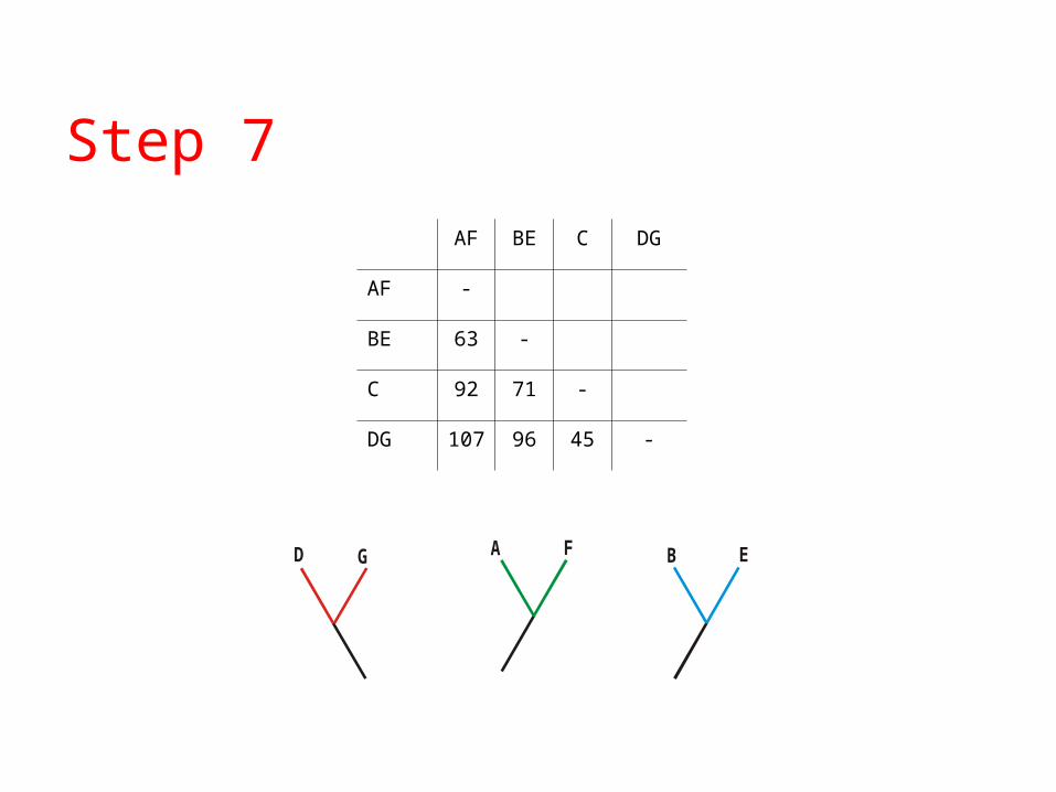
Step 7

A FGD B E

AF BE C DG

AF -

BE 63 -

C 92 71 -

DG 107 96 45 -

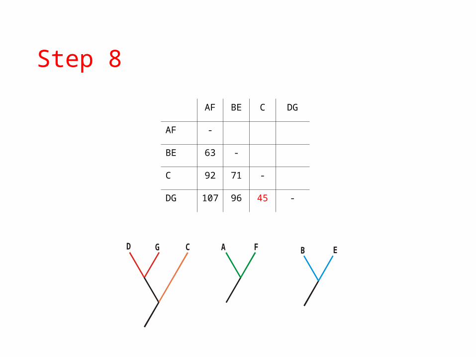
GD C

Step 8

A F B E

GD C

Step 9

A F B E

AF BE CDG

AF -

BE 63 -

CDG 102 88 -

GD C

Step 10

AF BE CDG

AF -

BE 63 -

CDG 102 88 -

B EA F

Root

B E

AFBE CDG

AFBE -

CDG 94 -

GD C A F

UPGMA: distance -> phylogeny

B E GD CA F

Additivity

a

b

ec

d

A

B

C

D

eddedcbadddd CDABBCADBDAC 22

Neighbors

Fourpoint condition

BDACCDAB dddd

BCADCDAB dddd

Neighbor-joining (N-J)

• Starts with a star-like tree

• Neighbors are sequentially merged, if they minimize the total length of branches

A

BC

D

EF

A

B

C

DEF

ididdNQ 21)2( 1212Find 1 and 2 that give minimum Q

Clustering methods (UPGMA & N-J)

Optimality criterion: NONE. The algorithm itself builds‘the’ tree.

UPGMA: rootet treeN-J: unrootet tree

Minimum evolution (ME) methods

Optimality criterion: The tree with the shortest overall tree lengthis chosen as the best tree.

Character Methods

• Maximum Parsimony• minimal changes to produce data

• Maximum Likelihood

Parsimony methods:Optimality criterion: The ‘most-parsimonious’ tree is the one thatrequires the fewest number of evolutionary events (e.g., nucleotidesubstitutions, amino acid replacements) to explain the sequences.

• Occam’s razor: “Of two competing theories or explanations, all other things being equal, the simpler one is to be preferred.” (William of Occam, 1280-1347)

Parsimony

1 CCCAGG2 CCCAAG3 CCCAAA4 CCCAAC

Comparison # changes

1-2 1

1-3 2

1-4 2

2-3 1

2-4 1

3-4 1

1,2 can be sister taxaAND

3,4 can be sister taxa

Infer ancestor of 1,2 and 3,4

Parsimony

CCCAGGCCCAAG->

CCCAAGCCCAAA->

CCCAAACCCAAA->

CCCAAC

3 changes

Calculate # changes | tree

acgtatgga acgggtgca aacggtgga aactgtgca

: c

: c

: a

: a

: c

: c

: a

: a

: c

: a

: a

: c

Total tree length: 7 Total tree length: ? Total tree length: ?

Calculate # changes | tree

acgtatgga acgggtgca aacggtgga aactgtgca

: c

: c

: a

: a

: c

: c

: a

: a

: c

: a

: a

: c

Total tree length: 7 Total tree length: 8 Total tree length: 8

Maximum likelihood (ML) methodsOptimality criterion: ML methods evaluate phylogenetic hypothesesin terms of the probability that a proposed model of the evolutionaryprocess and the proposed unrooted tree would give rise to theobserved data. The tree found to have the highest ML value isconsidered to be the preferred tree.

Using modelsObserved differences

Actual changes

A G

C T

Q

3 3 3 3

Example: Jukes-Cantor

pij 1

4

1

4e 4t

pij 1

4

3

4e 4t

, if i=j

, if i≠j

pt : proportion of different nucleotides

Maximum likelihood

• Given two trees, the one with the higher likelihood, i.e. the one with the higher conditional probability of observing the data, is the better

LH P(D | H ) P(D | T ,)

-55.0

-54.5

-54.0

-53.5

-53.0

-52.5

-52.0

-51.5

-51.0

-50.5

0 0.02 0.04 0.06 0.08 0.1

30 nucleotides from -globin genes of two primates on a one-edge tree

* *Gorilla GAAGTCCTTGAGAAATAAACTGCACACTGGOrangutan GGACTCCTTGAGAAATAAACTGCACACTGG

There are two differences and 28 similarities

28

42

4 3116

11

16

1

tt eeL

t

lnL

t= 0.02327lnL= -51.133956

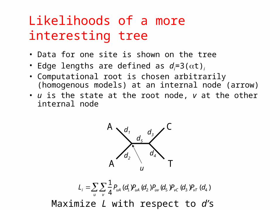
Likelihoods of a more interesting tree

• Data for one site is shown on the tree• Edge lengths are defined as di=3(t)i

• Computational root is chosen arbitrarily (homogenous models) at an internal node (arrow)

• u is the state at the root node, v at the other internal node

Li 1

4PuA(d1)

v

u PuA(d2 )Puv(d5 )PvC (d3 )PvT (d4 )

A

A

C

T

d1 d3

d4d2

d5

u

Maximize L with respect to d’s

Confidence assesment

• Bootstrap

1 2 3 4 5 6 7 8 9 10 11 12 13 14 15 16 17 18 19 20Aus C G A C G G T G G T C T A T A C A C G ABeus C G G C G G T G A T C T A T G C A C G GCeus T G G C G G C G T C T C A T A C A A T ADeus T A A C G A T G A C C C G A C T A T T G

Original data set with n characters.

2 3 13 8 3 19 14 6 20 20 7 1 9 11 17 10 6 14 8 16Aus G A A G A G T G A A T C G C A T G T G CBeus G G A G G G T G G G T C A C A T G T G CCeus G G A G G T T G A A C T T T A C G T G CDeus A A G G A T A A G G T T A C A C A A G T

Draw n characters randomly with re-placement. Repeat m times.

m pseudo-replicates, each with n characters.

Aus

Beus

Ceus

Deus

Original analysis, e.g. MP, ML, NJ.

Aus

Beus

Ceus

Deus

75%

Evaluate the results from the m analyses.

Aus

Beus

Ceus

Deus

Aus

Beus

Ceus

Deus

Aus

Beus

Ceus

Deus

Aus

Beus

Ceus

Deus

Aus

Beus

Ceus

Deus

Aus

Beus

Ceus

Deus

Repeat original analysis on each of the pseudo-replicate data sets.

Bootstrap

Pros and cons of some methods• Pair-wise, algorithmic approach

+ Fast

+ Models can be used when transforming to distances

- Information is lost when transforming to pair-wise distances

- One will get a tree, but no measure of goodness to compare with other hypotheses

• Parsimony+ Philosophically appealing

- Models can not be used

- Can be computationally slow

• Maximum likelihood+ Model based

- Model based

- Computationally veeeeery slow

Computation

• For large data sets (many taxa) exact solutions for any method employing an optimality criterion (parsimony, maximum likelihood, minimum evolution) are not possible

• => Use Neghbor-Joining

What can go wrong?

• Reality• A tree may be a poor model of the real

history• Information has been lost by subsequent

evolutionary changes• “Species” vs. “gene” trees

Canis MusGadus

What is wrong with this tree?

100

100

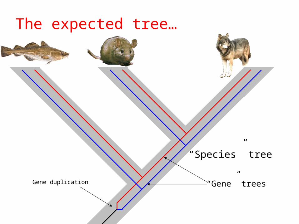
Gene duplication

“Species” tree

“Gene” trees

The expected tree…

Canis Mus Gadus Gadus Mus Canis

Two copies (paralogs) present in the genomes

Paralogous

Orthologous Orthologous

Canis Gadus Mus

What we have studied…

HIV Genome Diversity

• Error prone (RT) replication

• High rate of replication• 1010 virions/day

• In vivo selection pressure

HIV tree

Recombinants!

ENV

GAG

AIDS 1996, 10:S13

To conclude–

• Trash in, trash out : Alignment crucial• Try several methods, for consistency• Beware of paraloges• Choos outgroup wisly: related sequence of

more ancient origin than ”ingroup”• If recombinations possible: each site has its

own tree.