phylogenetics bioinformatics workshop · phylogenetics" • what is phylogenetics?" –...
TRANSCRIPT
Phylogenetics ���
Bioinformatics Workshop Jessica Kissinger
Trinidad 2010
Why do Phylogenetics?
• We make evolutionary assumptions in our everyday research life. For example, we need a drug that will kill the parasite and not us. Thus, we need a target that is present in the parasite and not us.
• We need a good model system, Which parasite (or host) is most closely related to P. falciparum or Humans?
Why Phylogenetics?
• This strain is resistant to drug and this one is sensitive, what has changed?
• Where did this parasite come from? Has it “co-evolved” with humans? Did it enter the human lineage from another source?
• Which other mosquitoes are likely to serve as a host for my parasite in nature?
Phylogenetics
• What is Phylogenetics? – Molecular Systematics
• The use of molecular data to infer the relationships of the host species e.g. using rRNA to build trees to look at the relationship of the bacteria to the eukaryotes
– Molecular Evolution • Use trees to infer how a molecule, protein, or gene
has evolved (insertions, deletions, substitutions).
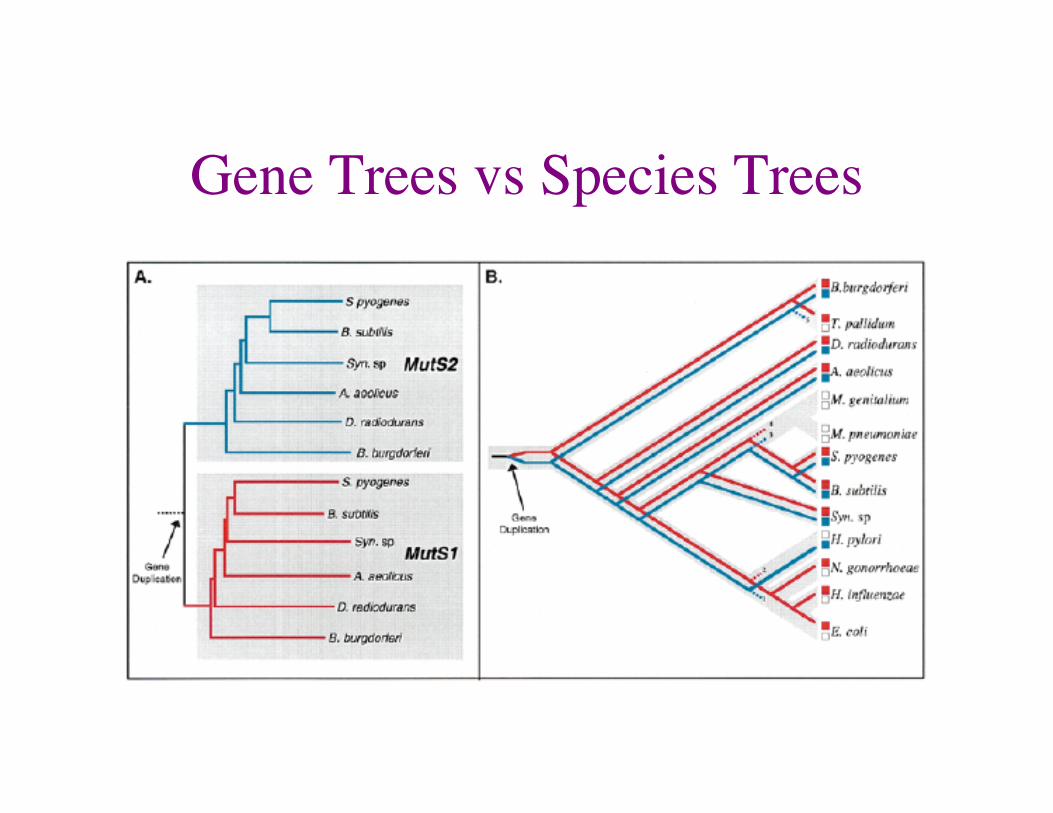
Gene Trees vs Species Trees
You Can Make Phylogenies of Many Things:
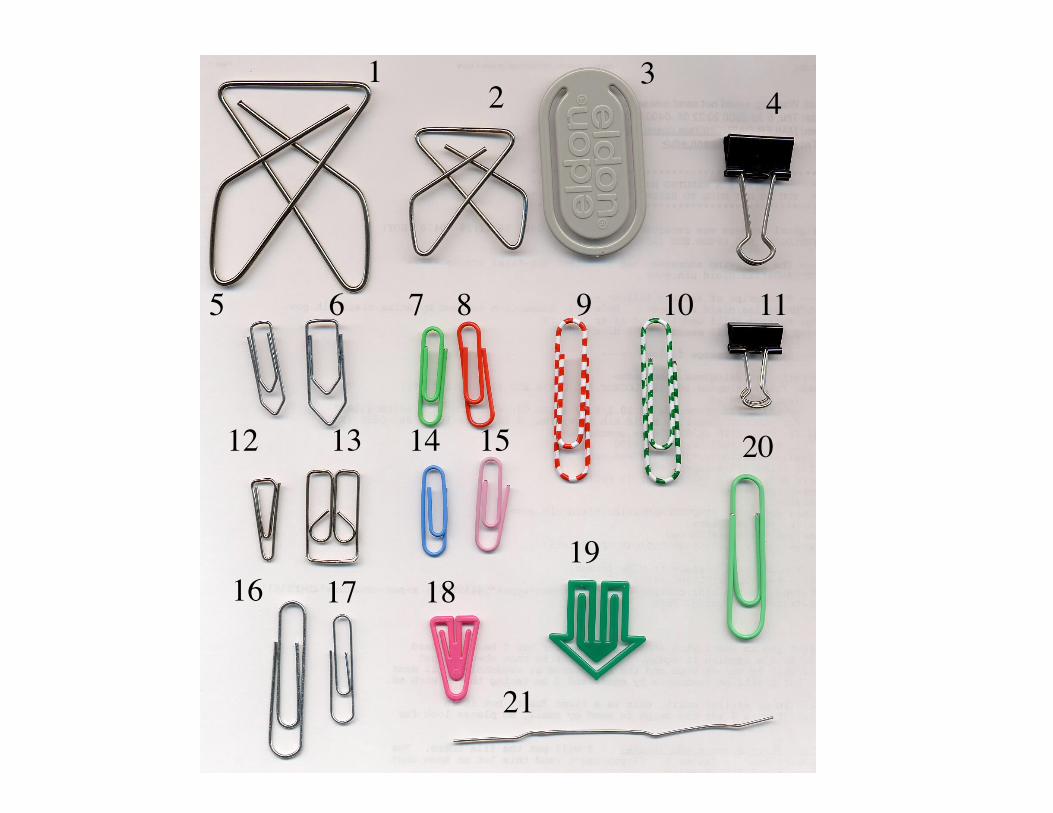
• Amino acid sequences • Nucleotide sequences • RFLP data • Morphological data • “Paper fastening devices”
1 2
3 4
5 6 7 8 9 10 11
12 13 14 15
16 17 18 19
20
21
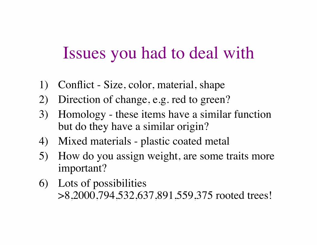
Issues you had to deal with 1) Conflict - Size, color, material, shape 2) Direction of change, e.g. red to green? 3) Homology - these items have a similar function
but do they have a similar origin? 4) Mixed materials - plastic coated metal 5) How do you assign weight, are some traits more
important? 6) Lots of possibilities
>8,2000,794,532,637,891,559,375 rooted trees!
Goals for this lecture
• Become familiar with concepts • Become familiar with vocabulary • Become familiar with the data analysis flow • Reach the point where you can read the
available literature on how to use these methods in greater detail
Assumptions made by Phylogenetic algorithms
• The sequences are correct • The sequence are homologous • Each position is homologous • The sampling of taxa or genes is sufficient to resolve the
problem of interest • Sequence variation is representative of the broader group
of interest • Sequence variation contains sufficient phylogenetic signal
(as opposed to noise) to resolve the problem of interest • Each position in the sequence evolved independently
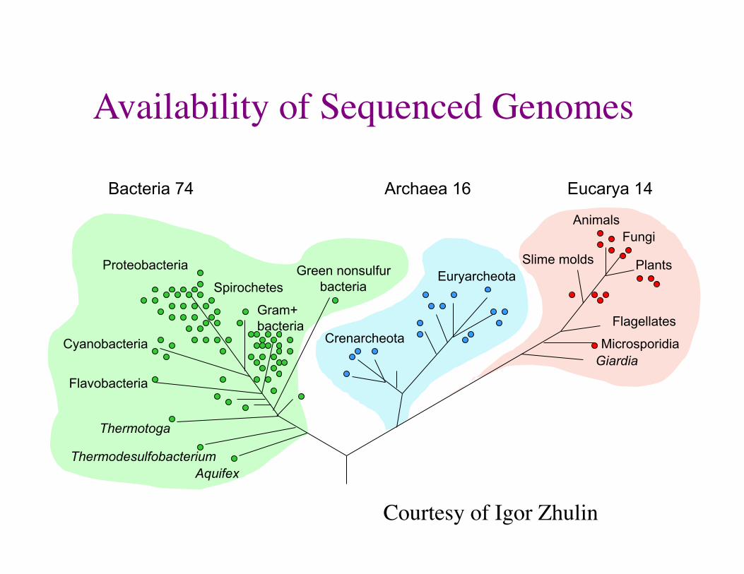
Availability of Sequenced Genomes
Aquifex Thermodesulfobacterium
Thermotoga
Flavobacteria
Cyanobacteria
Proteobacteria Green nonsulfur bacteria
Gram+ bacteria
Spirochetes Euryarcheota
Crenarcheota
Animals Fungi
Plants Slime molds
Flagellates
Microsporidia Giardia
Bacteria 74 Archaea 16 Eucarya 14
Courtesy of Igor Zhulin
Apicomplexans
Giardia lamblia Varimorpha necatrix
Trichomonas vaginallis Trichomonas foetus
Physarum polycephalum Euglenoids
Kinetoplastids Bodonids
Amoebamastigote
Dictyostelium discoideum Entamoebae histolytica
Entamoebae invadens
Naegleria gruberi
STRAMENOPILES
Cnidaria
EUBACTERIA
ALVEOLATES GREEN PLANTS
ANIMALS FUNGI
EUKARYOTES
PROTISTS
ARCHAEBACTERIA
Chry
soph
ytes
Diatom
s
Oom
ycet
es
Dinoflagelates Red Algae
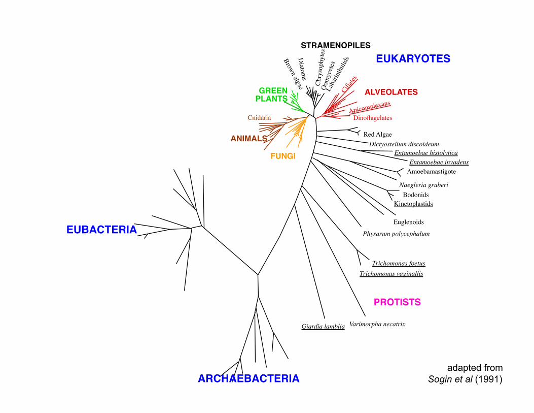
adapted from Sogin et al (1991)
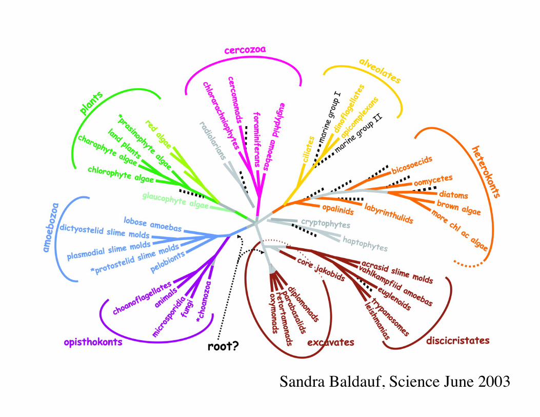
Sandra Baldauf, Science June 2003
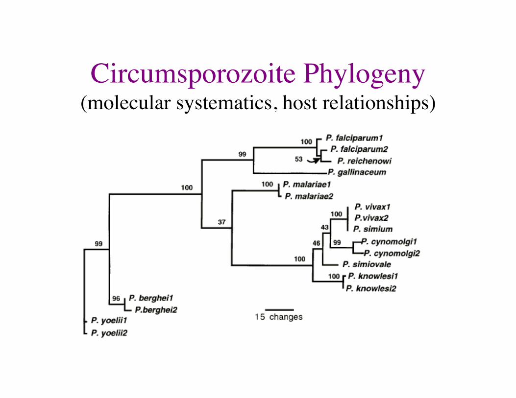
Circumsporozoite Phylogeny ���(molecular systematics, host relationships)
How to do an analysis
• Define a question • Select sequences appropriate to answer your
question (not all sequences are equally good!) • Make a multiple sequence alignment • Edit your alignment to make it better • Perform lots and lots of analyses • Perform Bootstrap analyses to test confidence
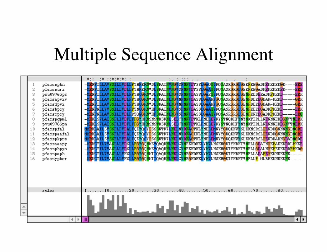
Multiple Sequence Alignment
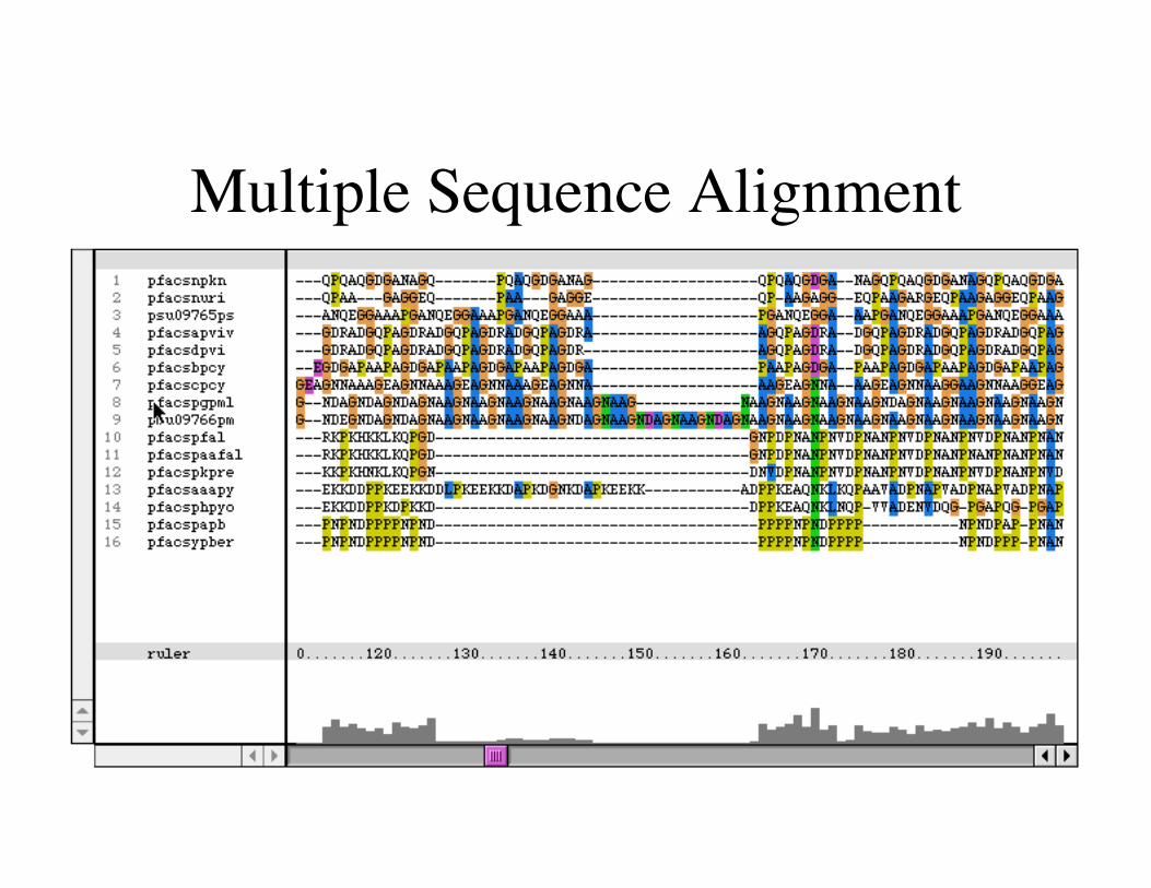
Multiple Sequence Alignment
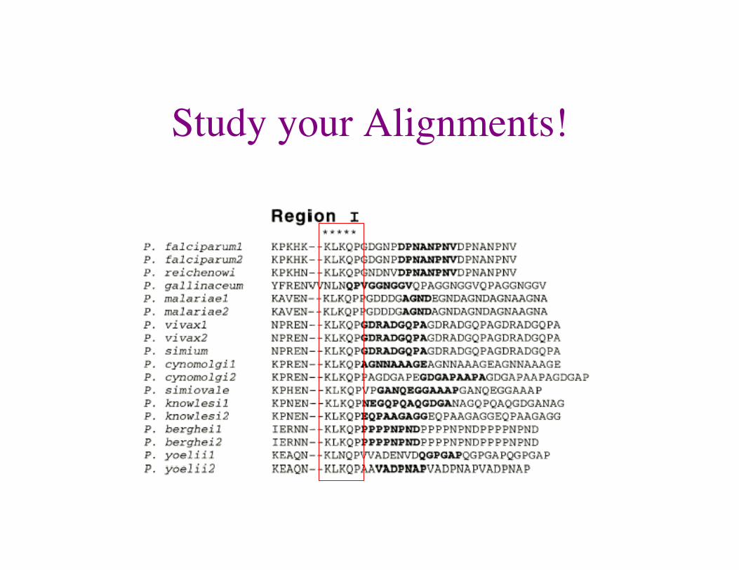
Study your Alignments!
A Word About Methods • There are two overall categories of methods
– Transformed distance methods (data are transformed into a distance matrix). The matrix is used to build a single tree. UPGMA and Neighbor-Joining are examples of this method. They are computationally simple and very fast.
– Optimality methods (tree generation is separate from tree evaluation). Parsimony and Maximum-likelihood methods divorce the issue of tree generation from evaluating how good a tree is. For parsimony, there many be more than 1 “most parsimonious” or “shortest” tree found.
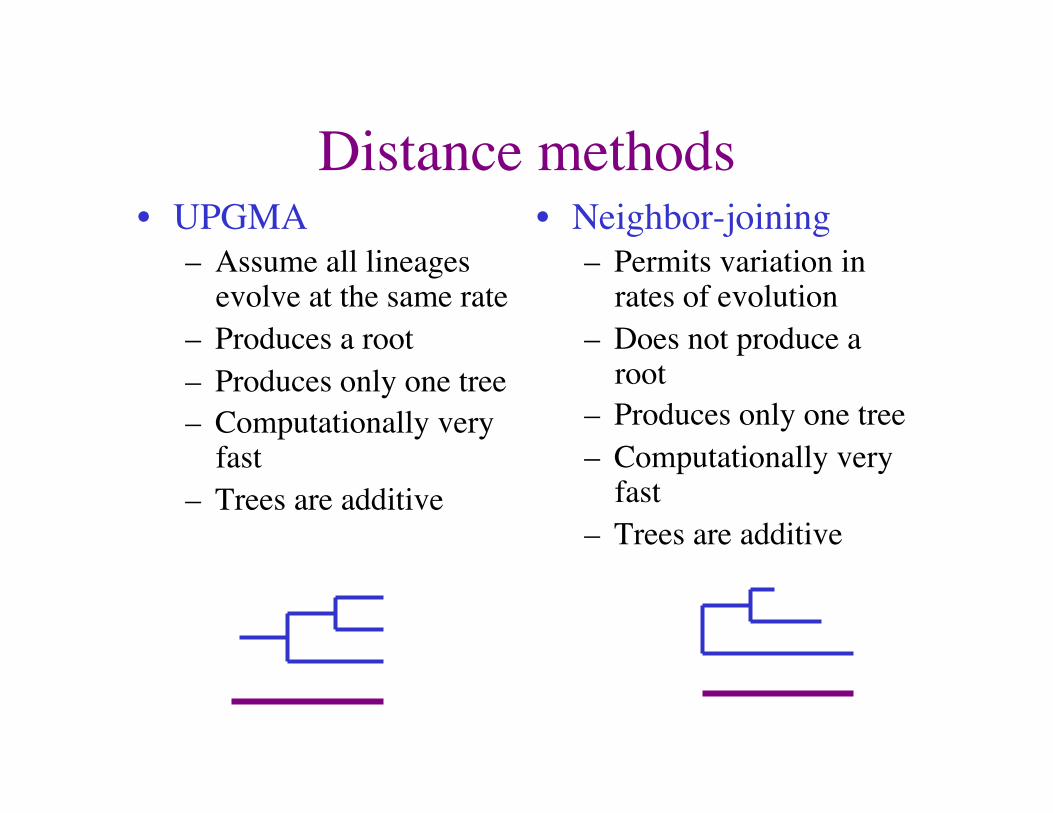
Distance methods • UPGMA
– Assume all lineages evolve at the same rate
– Produces a root – Produces only one tree – Computationally very
fast – Trees are additive
• Neighbor-joining – Permits variation in
rates of evolution – Does not produce a
root – Produces only one tree – Computationally very
fast – Trees are additive
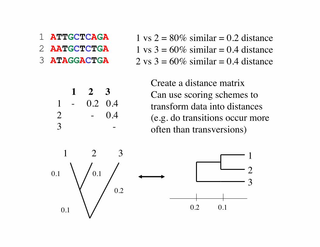
1 ATTGCTCAGA 2 AATGCTCTGA 3 ATAGGACTGA
1 vs 2 = 80% similar = 0.2 distance 1 vs 3 = 60% similar = 0.4 distance 2 vs 3 = 60% similar = 0.4 distance
0.1
0.1
0.1
0.2
1 2 3 1 2 3
0.1 0.2
1 2 3 1 - 0.2 0.4 2 - 0.4 3 -
Create a distance matrix Can use scoring schemes to transform data into distances (e.g. do transitions occur more often than transversions)
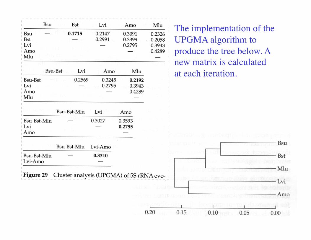
The implementation of the UPGMA algorithm to produce the tree below. A new matrix is calculated at each iteration.
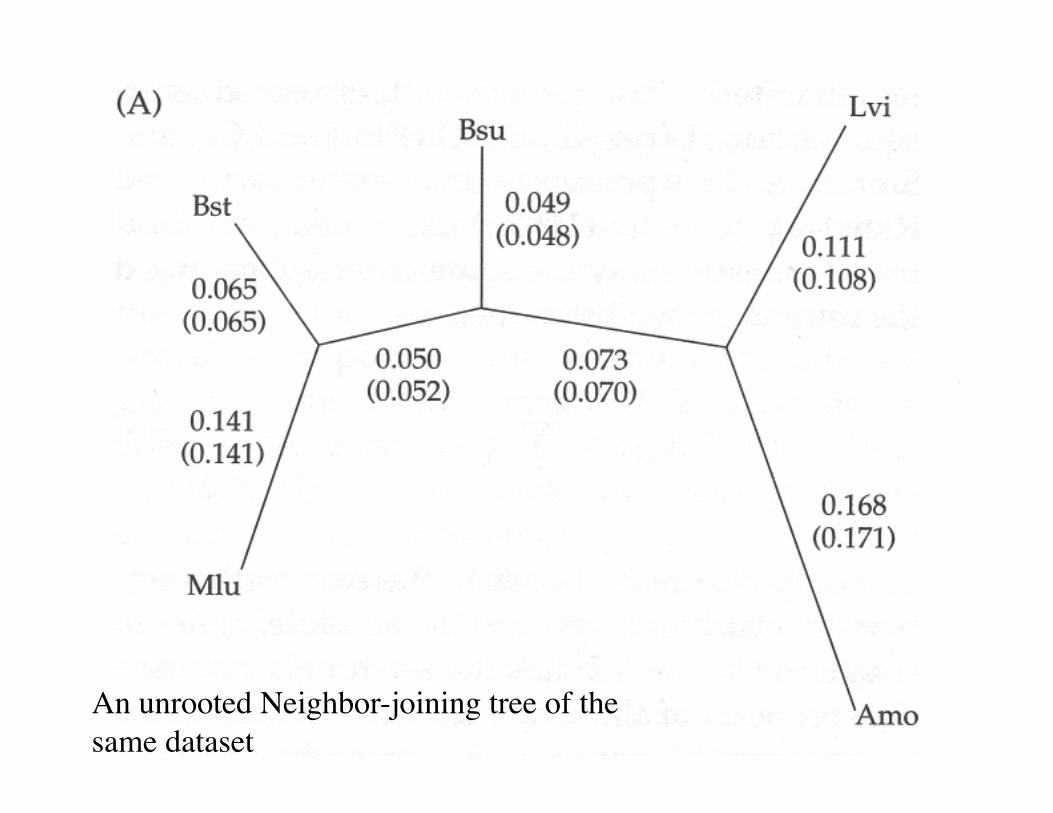
An unrooted Neighbor-joining tree of the same dataset
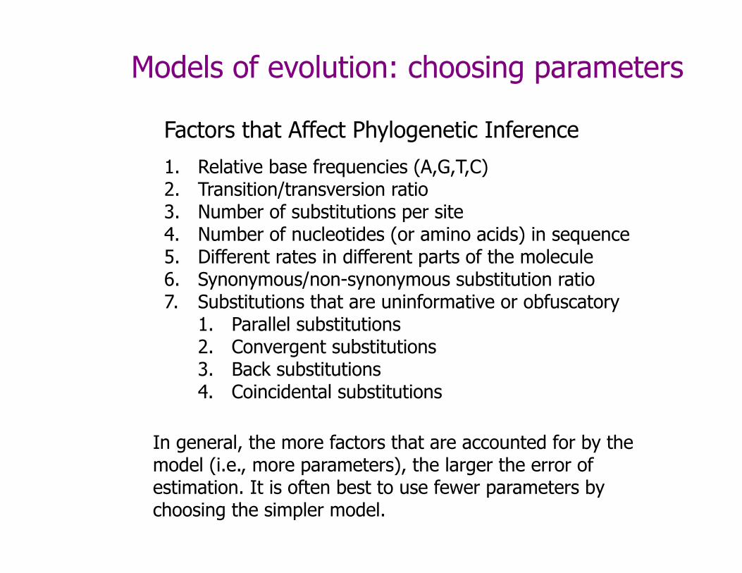
Factors that Affect Phylogenetic Inference
1. Relative base frequencies (A,G,T,C) 2. Transition/transversion ratio 3. Number of substitutions per site 4. Number of nucleotides (or amino acids) in sequence 5. Different rates in different parts of the molecule 6. Synonymous/non-synonymous substitution ratio 7. Substitutions that are uninformative or obfuscatory
1. Parallel substitutions 2. Convergent substitutions 3. Back substitutions 4. Coincidental substitutions
In general, the more factors that are accounted for by the model (i.e., more parameters), the larger the error of estimation. It is often best to use fewer parameters by choosing the simpler model.
Models of evolution: choosing parameters
Some distance models: p-distance
• p = nd/n, where n is the number of sites (nucleotides or amino acids), and nd is the number of differences between the two sequences examined. • Very robust when divergence times are recent and the affect of complicating phenomena is minor
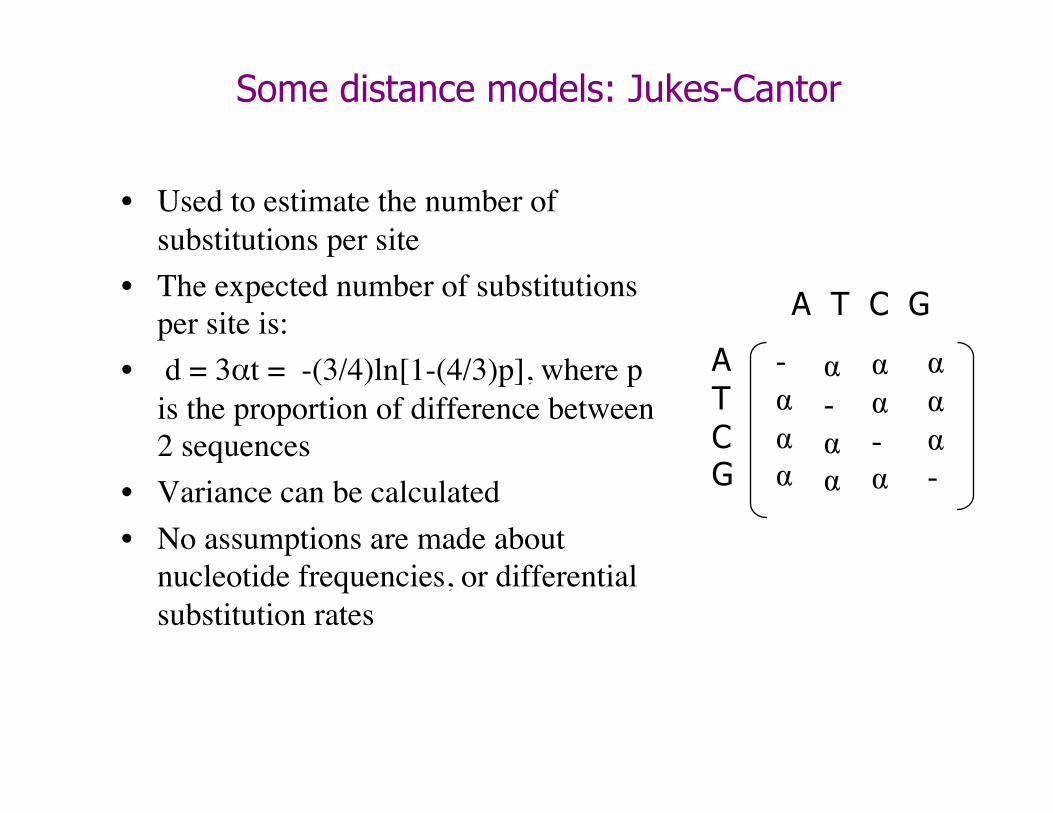
Some distance models: Jukes-Cantor
• Used to estimate the number of substitutions per site
• The expected number of substitutions per site is:
• d = 3αt = -(3/4)ln[1-(4/3)p], where p is the proportion of difference between 2 sequences
• Variance can be calculated • No assumptions are made about
nucleotide frequencies, or differential substitution rates
A T C G
A T C G
- α α α
α - α α
α α -α
α α α -
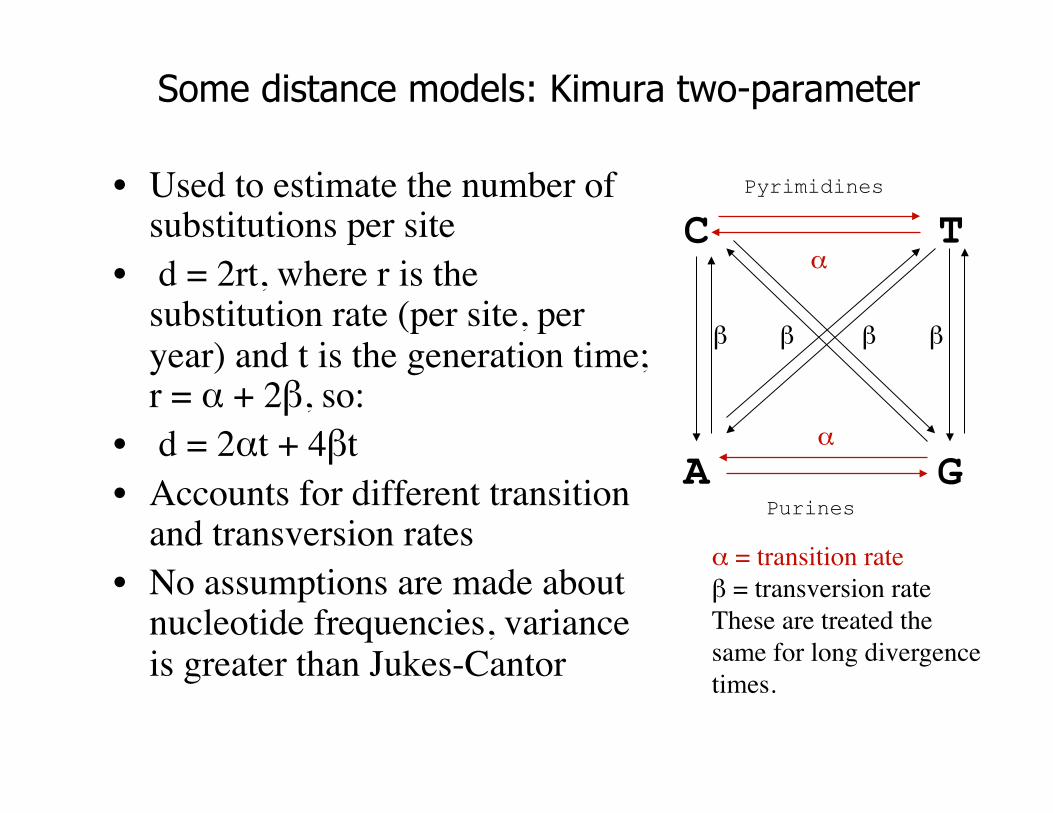
Some distance models: Kimura two-parameter
• Used to estimate the number of substitutions per site
• d = 2rt, where r is the substitution rate (per site, per year) and t is the generation time; r = α + 2β, so:
• d = 2αt + 4βt • Accounts for different transition
and transversion rates • No assumptions are made about
nucleotide frequencies, variance is greater than Jukes-Cantor
C T
A G
Pyrimidines
Purines
α
α
β β β β
α = transition rate β = transversion rate These are treated the same for long divergence times.
Other models
• Hasegawa, Kishino, Yano (HKY): corrects for unequal nucleotide frequencies and transition/ transversion bias into account
• Unrestricted model: allows different rates between all pairs of nucleotides
• General Time Reversible model: allows different rates between all pairs of nucleotides and corrects for unequal nucleotide frequencies
• Many other models have been invented to correct for specific problems
• The more parameters are introduced, the larger the variance becomes
Optimality Methods
• All possible trees (or a heuristic sampling of trees) are generated and evaluated according to Parsimony or Maximum likelihood.
• Note: Tree generation is divorced from tree evaluation. More than one tree topology may be optimal according to your criteria
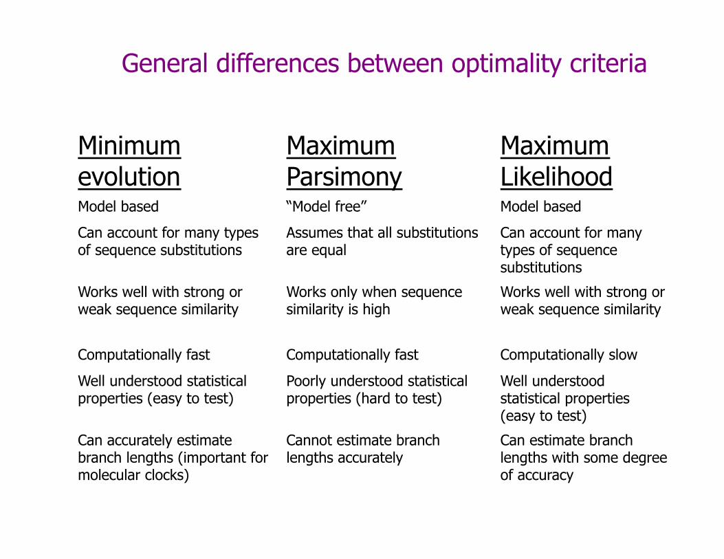
General differences between optimality criteria
Minimum evolution
Maximum Parsimony
Maximum Likelihood
Model based “Model free” Model based
Can account for many types of sequence substitutions
Assumes that all substitutions are equal
Can account for many types of sequence substitutions
Works well with strong or weak sequence similarity
Works only when sequence similarity is high
Works well with strong or weak sequence similarity
Computationally fast Computationally fast Computationally slow
Well understood statistical properties (easy to test)
Poorly understood statistical properties (hard to test)
Well understood statistical properties (easy to test)
Can accurately estimate branch lengths (important for molecular clocks)
Cannot estimate branch lengths accurately
Can estimate branch lengths with some degree of accuracy
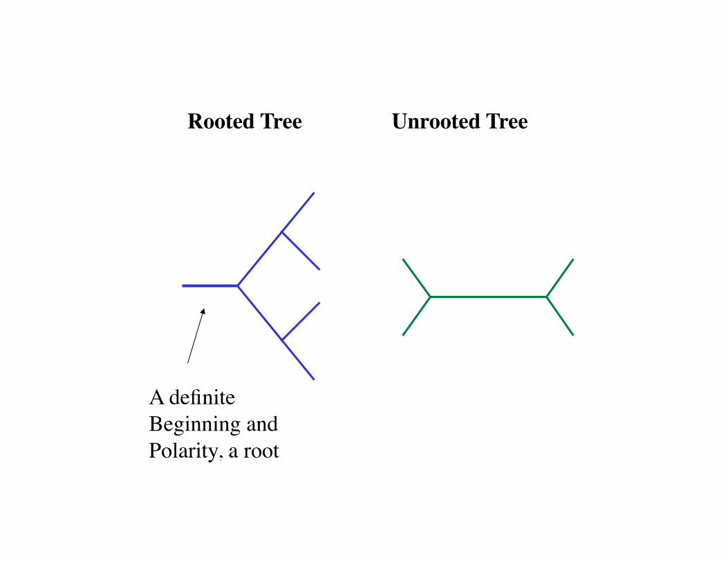
Rooted Tree Unrooted Tree
A definite Beginning and Polarity, a root
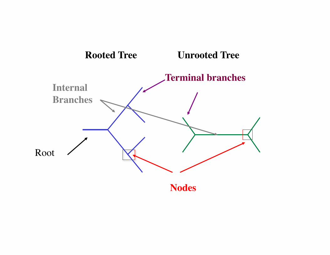
Rooted Tree Unrooted Tree
Terminal branches
Nodes
Internal Branches
Root
1 2 3 1 2 3 1 2 3
1
2
3
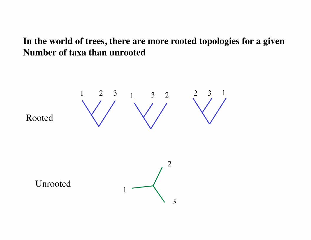
In the world of trees, there are more rooted topologies for a given Number of taxa than unrooted
Rooted
Unrooted
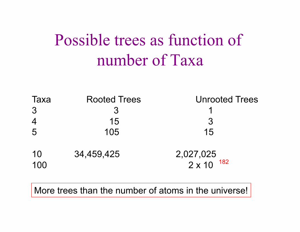
Possible trees as function of number of Taxa
Taxa Rooted Trees Unrooted Trees 3 3 1 4 15 3 5 105 15
10 34,459,425 2,027,025 100 2 x 10 182
More trees than the number of atoms in the universe!
Tree search considerations
• Exhaustive searches are searches of all possible trees for the number of Taxa in your data set (15 Taxa or less)
• If you have more than 15 Taxa, then heuristic methods must be employed in which you search a sample of all possible trees. There are many algorithms for the generation of different populations of trees.
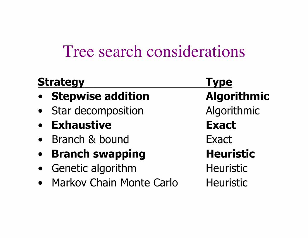
Tree search considerations Strategy Type • Stepwise addition Algorithmic • Star decomposition Algorithmic • Exhaustive Exact • Branch & bound Exact • Branch swapping Heuristic • Genetic algorithm Heuristic • Markov Chain Monte Carlo Heuristic
Parsimony basics & scores • Based on shared derived characters
(synapomorphies) • Identical characters which evolve more than once
are “homoplasies” • Unique characters are “autapomorphies” • The score of the tree is the total of all the changes
needed to map the data. The scale bar is #of changes.
• Smaller, i.e. more parsimonious scores are better • More than one tree topology may have the same
score
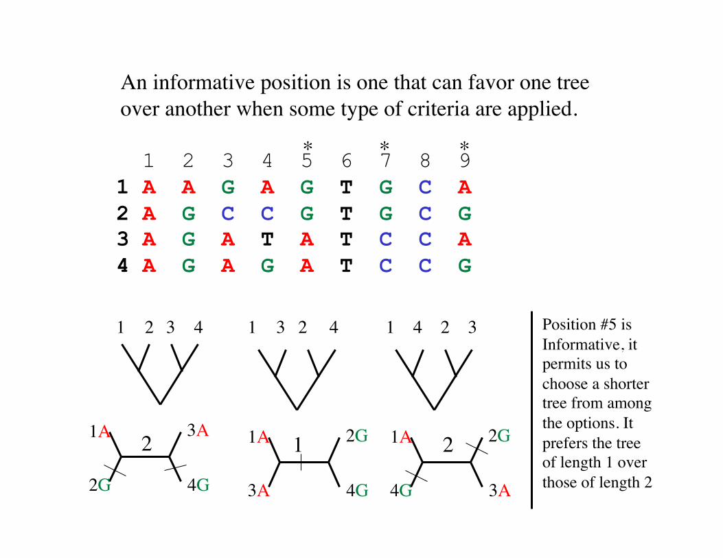
An informative position is one that can favor one tree over another when some type of criteria are applied.
1 2 3 4 5 6 7 8 9 1 A A G A G T G C A 2 A G C C G T G C G 3 A G A T A T C C A 4 A G A G A T C C G
* * *
1 2 3 4 2 3 4 1 1 2 3 4
1A
2G
3A
4G
1A
3A
2G
4G
1A
4G
2G
3A
2 1 2
Position #5 is Informative, it permits us to choose a shorter tree from among the options. It prefers the tree of length 1 over those of length 2
1 2 3 4 5 6 7 8 9 1 A A G A G T G C A 2 A G C C G T G C G 3 A G A T A T C C A 4 A G A G A T C C G
* * *
1G
2C
3A
4A
1G
3A
2C
4A
1G
4A
2C
3A
1G
2A
3G
4G
1G
3G
2A
4G
1G
4G
2A
3G
1A
2A
3A
4A
1A
3A
2A
4A
1A
4A
2A
3A
Pos 1
Pos 2
Pos 3
0 0 0
2 2 2
1 1 1
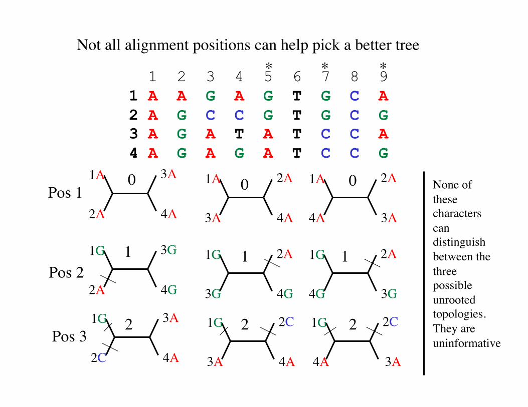
Not all alignment positions can help pick a better tree
None of these characters can distinguish between the three possible unrooted topologies. They are uninformative
Maximum Likelihood • Is an optimality method, it is an algorithm which
evaluates trees according to some criterion • The algorithm searches for trees which maximize
the probability of observing the data • Trees are scored with Log likelihoods • This is the most computationally intensive method
available • More tractable versions include (puzzle) • Alternate approaches include Bayesian inference
(Mr. Bayes)
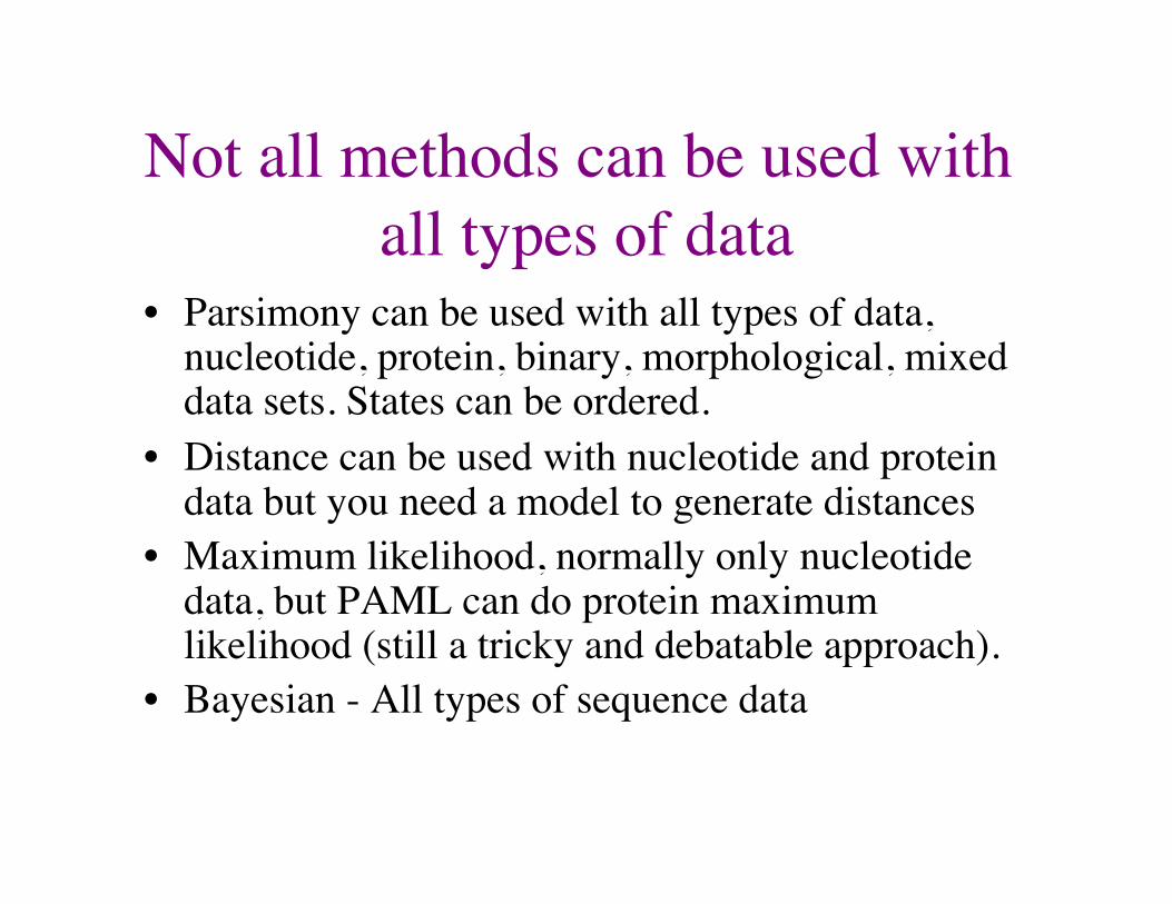
Not all methods can be used with all types of data
• Parsimony can be used with all types of data, nucleotide, protein, binary, morphological, mixed data sets. States can be ordered.
• Distance can be used with nucleotide and protein data but you need a model to generate distances
• Maximum likelihood, normally only nucleotide data, but PAML can do protein maximum likelihood (still a tricky and debatable approach).
• Bayesian - All types of sequence data
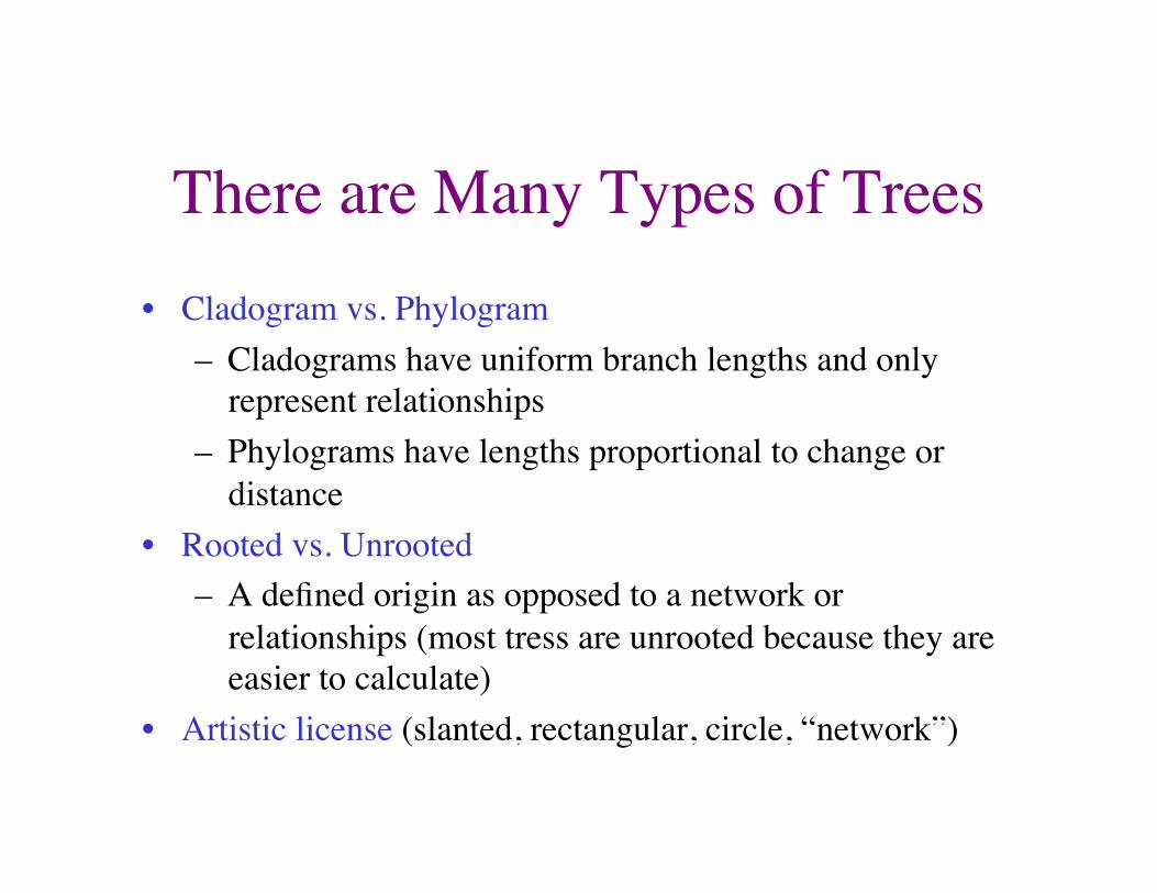
There are Many Types of Trees • Cladogram vs. Phylogram
– Cladograms have uniform branch lengths and only represent relationships
– Phylograms have lengths proportional to change or distance
• Rooted vs. Unrooted – A defined origin as opposed to a network or
relationships (most tress are unrooted because they are easier to calculate)
• Artistic license (slanted, rectangular, circle, “network”)
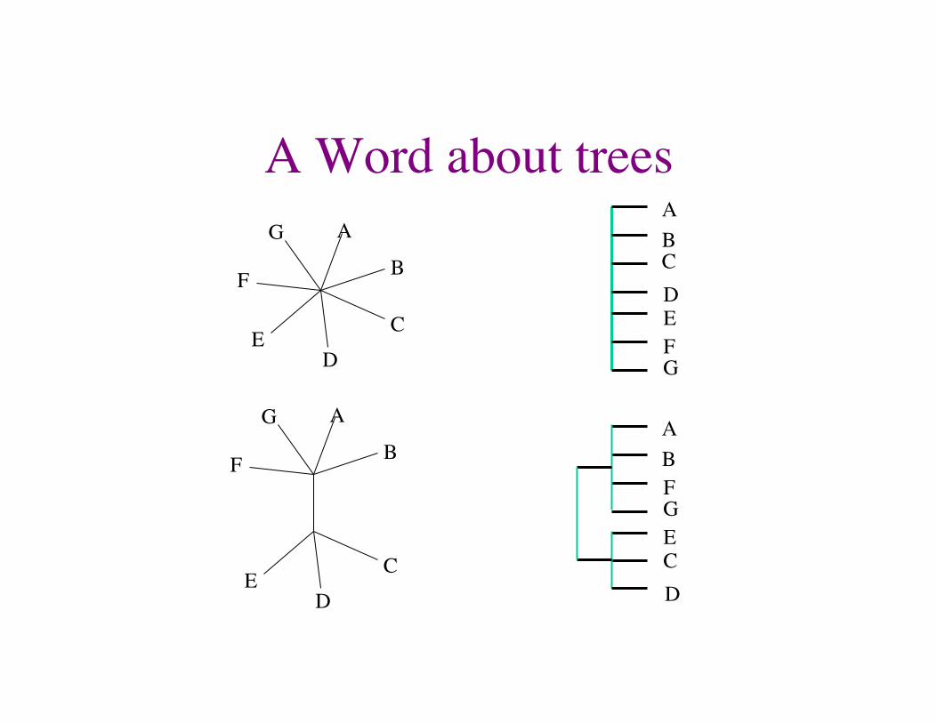
A Word about trees A B C D E F G
A
B
C D
E
F
G
A B
C D
E
F G
A
B
C D
E
F
G
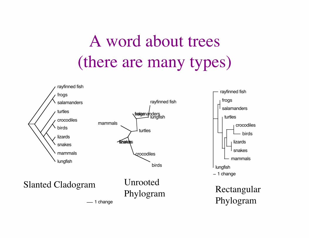
A word about trees ���(there are many types)
rayfinned fishfrogssalamanders
turtles
crocodilesbirds
lizardssnakes
mammalslungfish
birds
crocodiles
snakeslizards
mammals
frogssalamanders
rayfinned fish
lungfish
turtles
1 change
rayfinned fish
frogssalamanders
turtlescrocodiles
birdslizards
snakesmammals
lungfish1 change
Slanted Cladogram Rectangular Phylogram
Unrooted Phylogram
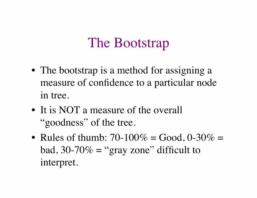
The Bootstrap
• The bootstrap is a method for assigning a measure of confidence to a particular node in tree.
• It is NOT a measure of the overall “goodness” of the tree.
• Rules of thumb: 70-100% = Good, 0-30% = bad, 30-70% = “gray zone” difficult to interpret.
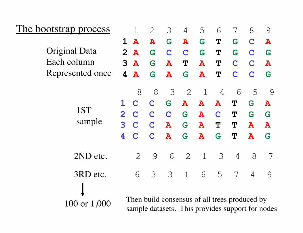
1 2 3 4 5 6 7 8 9 1 A A G A G T G C A 2 A G C C G T G C G 3 A G A T A T C C A 4 A G A G A T C C G
8 8 3 2 1 4 6 5 9 1 C C G A A A T G A 2 C C C G A C T G G 3 C C A G A T T A A 4 C C A G A G T A G
1ST sample
Original Data Each column Represented once
2ND etc.
3RD etc.
2 9 6 2 1 3 4 8 7
6 3 3 1 6 5 7 4 9
100 or 1,000
The bootstrap process
Then build consensus of all trees produced by sample datasets. This provides support for nodes
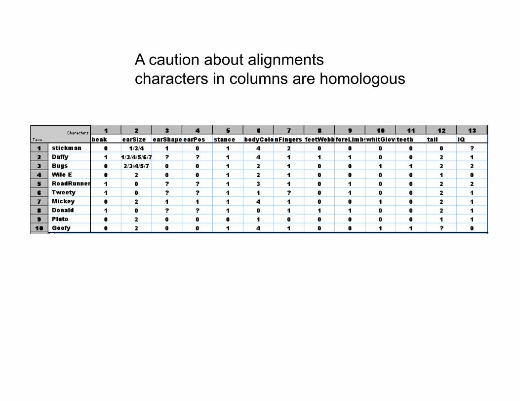
A caution about alignments characters in columns are homologous
stickmanDaffyDonaldRoadRunnerTweety
BugsGoofy
MickeyWile EPluto
1 change
stickmanDaffyDonaldRoadRunnerTweety
BugsGoofy
MickeyWile EPluto
1 change
stickmanDaffyDonaldRoadRunnerTweety
BugsGoofy
MickeyPluto
Wile E1 change
stickmanDaffy
RoadRunnerTweety
DonaldBugsGoofyMickey
Wile EPluto
1 change
stickmanDaffy
RoadRunnerTweety
DonaldBugsGoofyMickeyWile EPluto
1 change
stickmanDaffy
RoadRunnerTweety
DonaldBugsGoofyMickeyPluto
Wile E1 change
stickmanDaffy
RoadRunnerTweety
DonaldBugsGoofy
MickeyWile EPluto
1 change
stickmanDaffy
RoadRunnerTweety
DonaldBugsGoofy
MickeyWile EPluto
1 change
stickmanDaffy
RoadRunnerTweetyDonald
BugsGoofyMickeyPluto
Wile E1 change
stickmanDaffy
RoadRunnerDonaldTweety
BugsGoofy
MickeyWile EPluto
1 change
stickmanDaffy
RoadRunnerDonaldTweety
BugsGoofy
MickeyWile EPluto
1 change
stickmanDaffy
RoadRunnerDonaldTweety
BugsGoofyMickeyPluto
Wile E1 change
stickmanDaffyDonaldRoadRunner
TweetyBugsGoofy
MickeyWile EPluto
1 change
stickmanDaffyDonaldRoadRunner
TweetyBugsGoofy
MickeyWile EPluto
1 change
stickmanDaffyDonaldRoadRunnerTweety
BugsGoofyMickeyPluto
Wile E1 change
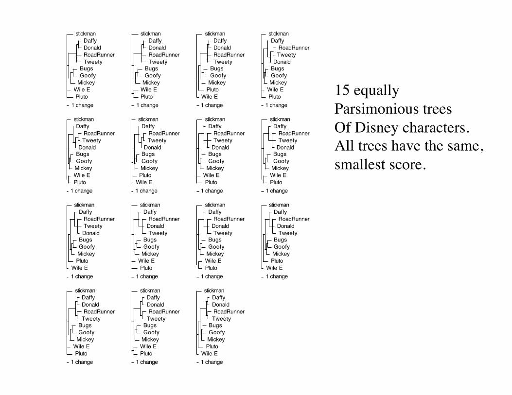
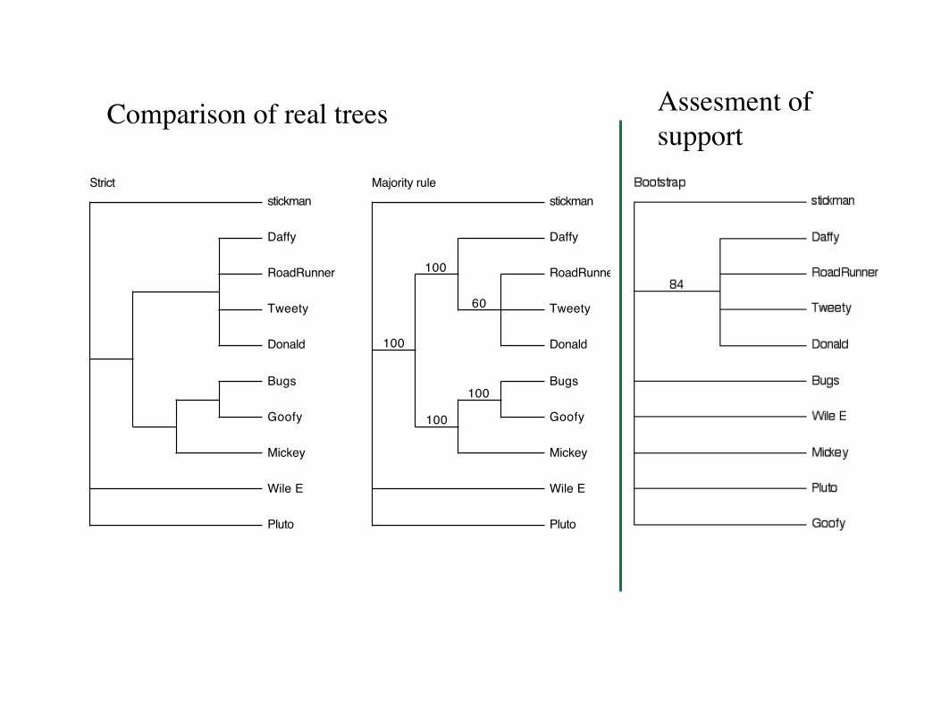
15 equally Parsimonious trees Of Disney characters. All trees have the same, smallest score.
stickman
Daffy
RoadRunner
Tweety
Donald
Bugs
Goofy
Mickey
Wile E
Pluto
Strictstickman
Daffy
RoadRunner
Tweety
Donald
Bugs
Goofy
Mickey
Wile E
Pluto
100
100
60
100
100
Majority rule
Comparison of real trees Assesment of support
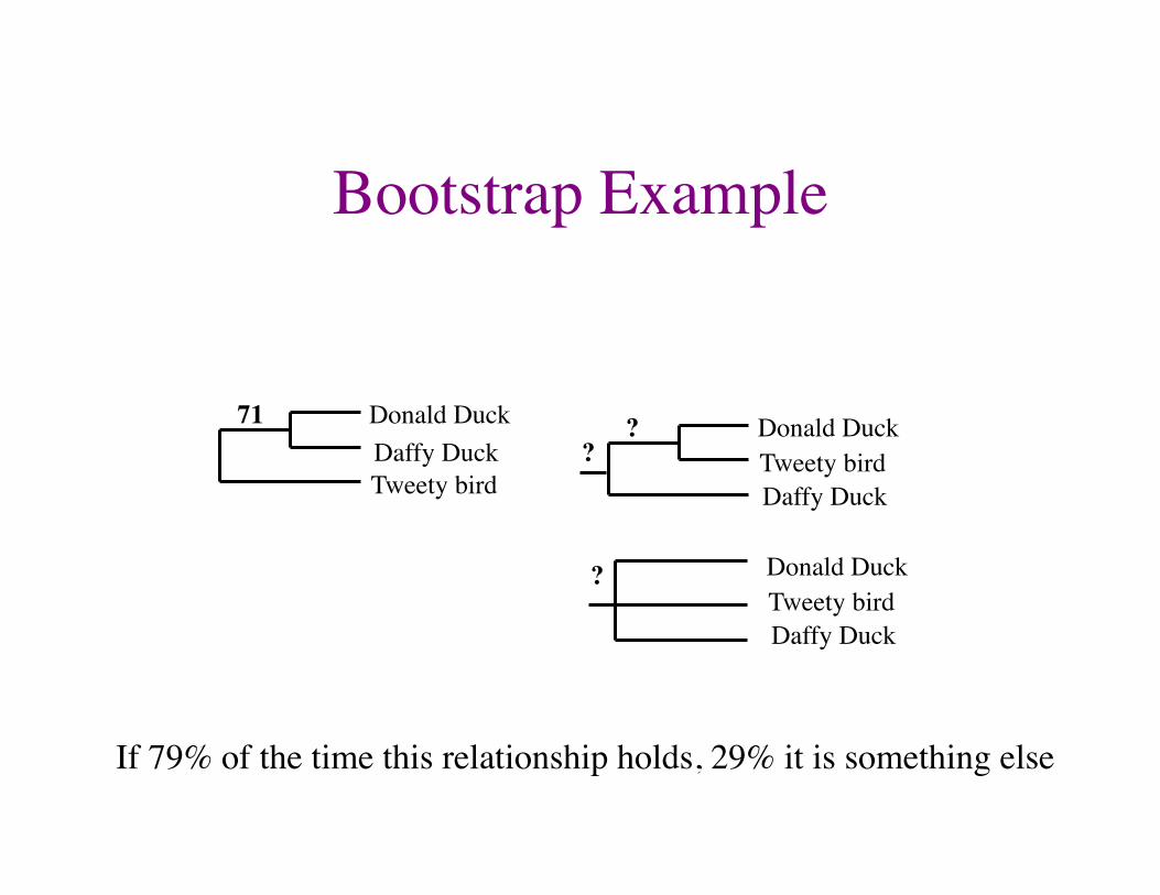
Bootstrap Example
Donald Duck Daffy Duck Tweety bird
71 Donald Duck
Daffy Duck Tweety bird
?
Donald Duck
Daffy Duck Tweety bird
?
?
If 79% of the time this relationship holds, 29% it is something else
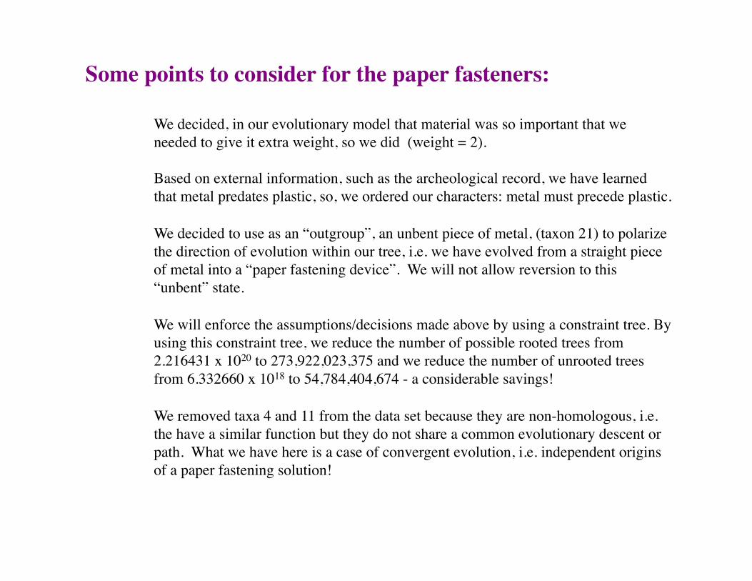
Some points to consider for the paper fasteners:
We decided, in our evolutionary model that material was so important that we needed to give it extra weight, so we did (weight = 2).
Based on external information, such as the archeological record, we have learned that metal predates plastic, so, we ordered our characters: metal must precede plastic.
We decided to use as an “outgroup”, an unbent piece of metal, (taxon 21) to polarize the direction of evolution within our tree, i.e. we have evolved from a straight piece of metal into a “paper fastening device”. We will not allow reversion to this “unbent” state.
We will enforce the assumptions/decisions made above by using a constraint tree. By using this constraint tree, we reduce the number of possible rooted trees from 2.216431 x 10²⁰ to 273,922,023,375 and we reduce the number of unrooted trees from 6.332660 x 10¹⁸ to 54,784,404,674 - a considerable savings!
We removed taxa 4 and 11 from the data set because they are non-homologous, i.e. the have a similar function but they do not share a common evolutionary descent or path. What we have here is a case of convergent evolution, i.e. independent origins of a paper fastening solution!
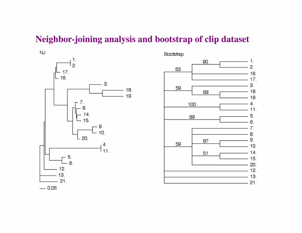
Neighbor-joining analysis and bootstrap of clip dataset
1.2.3.18.19.7.9.10.20.14.15.8.16.17.12.4.11.5.6.13.21.1 change
1.2.3.18.19.7.9.10.20.14.15.8.16.17.12.4.11.5.6.13.21.1 change
1.2.3.18.19.7.9.10.20.14.15.8.16.12.17.4.11.5.6.13.21.1 change
1.2.3.18.19.7.9.10.20.14.15.8.16.17.12.4.11.5.6.13.21.1 change
1.2.3.18.19.7.8.9.10.20.14.15.16.17.12.4.11.5.6.13.21.1 change
1.2.3.18.19.7.9.10.20.15.14.8.16.17.12.4.11.5.6.13.21.1 change
1.2.3.18.19.7.9.10.20.14.15.8.16.17.12.4.11.5.6.13.21.1 change
1.2.3.18.19.7.9.10.20.14.15.8.16.17.12.4.11.5.6.13.21.1 change
1.2.3.18.19.7.9.10.20.14.15.8.16.17.4.11.5.6.12.13.21.1 change
1.2.3.18.19.7.9.10.20.14.15.8.16.17.12.4.11.5.6.13.21.1 change
1.2.3.18.19.7.9.10.20.14.15.8.16.17.4.11.5.6.12.13.21.1 change
1.2.3.18.19.7.9.10.20.14.15.8.16.17.12.4.11.5.6.13.21.1 change
1.2.3.18.19.7.9.10.20.14.15.8.16.17.12.13.4.11.5.6.21.1 change
1.2.17.3.18.19.7.9.10.20.14.15.8.16.12.4.11.5.6.13.21.1 change
1.2.3.18.19.7.9.10.20.14.15.8.16.17.12.4.11.5.6.13.21.1 change
1.2.3.18.19.7.9.10.20.14.15.8.16.17.12.4.11.5.6.13.21.1 change
1.2.3.18.19.7.9.10.20.14.15.8.16.17.5.6.4.11.12.13.21.1 change
1.2.3.18.19.7.9.10.20.14.15.8.16.17.12.4.11.5.6.13.21.1 change
1.2.3.18.19.7.9.10.20.14.15.8.16.17.4.11.5.6.12.13.21.1 change
1.2.3.18.19.7.9.10.20.14.15.8.16.12.17.4.11.5.6.13.21.1 change
1.2.3.18.19.7.9.10.20.14.15.8.16.4.11.5.6.12.17.13.21.1 change
1.2.3.18.19.7.8.9.10.20.14.15.16.17.12.4.11.5.6.13.21.1 change
1.2.3.18.19.7.8.14.15.9.10.20.16.17.12.4.11.5.6.13.21.1 change
1.2.3.18.19.7.8.9.10.20.15.14.16.17.12.4.11.5.6.13.21.1 change
1.2.3.18.19.7.8.9.10.20.14.15.16.17.12.4.11.5.6.13.21.1 change
1.2.3.18.19.7.8.14.15.9.10.20.17.16.12.4.11.5.6.13.21.1 change
1.2.3.18.19.7.8.14.15.9.10.20.16.17.12.4.11.5.6.13.21.1 change
1.2.3.18.19.7.8.9.10.20.15.14.16.17.12.4.11.5.6.13.21.1 change
1.2.3.18.19.7.8.9.10.20.14.15.16.17.12.4.11.5.6.13.21.1 change
1.2.3.18.19.7.8.9.10.20.14.15.16.17.12.4.11.5.6.13.21.1 change
1.2.3.18.19.7.8.14.15.9.10.20.16.17.12.4.11.5.6.13.21.1 change
1.2.3.18.19.7.8.9.10.20.14.15.16.17.12.4.11.5.6.13.21.1 change
1.2.3.18.19.7.8.9.10.20.14.15.12.16.17.4.11.5.6.13.21.1 change
1.2.3.18.19.7.8.14.15.9.10.20.17.16.12.4.11.5.6.13.21.1 change
1.2.3.18.19.7.8.9.10.20.14.15.16.17.12.4.11.5.6.13.21.1 change
1.2.3.18.19.7.9.10.20.14.15.8.16.17.12.4.11.5.6.13.21.1 change
1.2.3.18.19.14.15.7.9.10.20.8.16.17.12.4.11.5.6.13.21.1 change
1.2.3.18.19.9.10.20.7.15.14.8.16.17.12.4.11.5.6.13.21.1 change
1.2.3.18.19.9.10.20.7.15.14.8.16.17.12.4.11.5.6.13.21.1 change
1.2.3.18.19.15.7.9.10.20.14.8.16.17.12.4.11.5.6.13.21.1 change
1.2.3.18.19.7.9.10.20.15.8.14.16.17.12.4.11.5.6.13.21.1 change
1.2.3.18.19.7.9.10.20.15.8.14.16.17.12.4.11.5.6.13.21.1 change
1.2.3.18.19.7.9.10.20.14.15.8.16.17.12.4.11.5.6.13.21.1 change
1.2.3.18.19.7.9.10.20.8.14.15.16.17.12.4.11.5.6.13.21.1 change
1.2.3.18.19.7.9.10.20.15.14.8.16.17.12.4.11.5.6.13.21.1 change
1.2.3.18.19.14.15.7.9.10.20.8.16.17.12.4.11.5.6.13.21.1 change
1.2.3.18.19.7.9.10.20.14.15.8.16.17.12.4.11.5.6.13.21.1 change
1.2.3.18.19.7.9.10.20.14.8.15.16.17.12.4.11.5.6.13.21.1 change
1.2.3.18.19.7.9.10.20.14.8.15.16.17.12.4.11.5.6.13.21.1 change
1.2.3.18.19.14.15.7.9.10.20.8.16.17.12.4.11.5.6.13.21.1 change
1.2.3.18.19.15.14.7.9.10.20.8.16.17.12.4.11.5.6.13.21.1 change
1.2.3.18.19.9.10.20.7.14.15.8.16.17.12.4.11.5.6.13.21.1 change
1.2.3.18.19.7.8.14.9.10.20.15.16.17.12.4.11.5.6.13.21.1 change
1.2.3.18.19.7.8.15.9.10.20.14.16.17.12.4.11.5.6.13.21.1 change
1.2.17.3.18.19.7.9.10.20.14.15.8.16.12.4.11.5.6.13.21.1 change
1.2.3.18.19.7.9.10.20.14.15.8.16.4.11.5.6.17.12.13.21.1 change
1.2.3.18.19.7.9.10.20.14.15.8.16.4.11.5.6.17.12.13.21.1 change
1.2.3.18.19.7.9.10.20.14.15.8.16.17.12.4.11.5.6.13.21.1 change
1.2.3.18.19.7.9.10.20.14.15.8.16.12.17.4.11.5.6.13.21.1 change
1.2.3.18.19.7.9.10.20.14.15.8.16.17.12.13.4.11.5.6.21.1 change
1.2.3.18.19.7.9.10.20.14.15.8.16.12.17.13.4.11.5.6.21.1 change
1.2.3.18.19.7.9.10.20.14.15.8.16.17.4.11.5.6.12.13.21.1 change
1.2.3.18.19.7.9.10.20.14.15.8.16.4.11.5.6.17.12.13.21.1 change
1.2.3.18.19.7.9.10.20.14.15.8.16.4.11.5.6.17.12.13.21.1 change
1.2.3.18.19.7.9.10.20.14.15.8.16.17.4.11.6.5.12.13.21.1 change
1.2.3.18.19.7.9.10.20.14.15.8.16.17.4.11.5.6.12.13.21.1 change
1.2.3.18.19.7.9.10.20.14.15.8.16.17.12.13.4.11.5.6.21.1 change
1.2.3.18.19.7.9.10.20.14.15.8.16.17.12.4.11.5.6.13.21.1 change
1.2.3.18.19.7.9.10.20.14.15.8.16.17.4.11.5.6.12.13.21.1 change
1.2.3.18.19.7.9.10.20.14.15.8.16.17.4.11.5.6.12.13.21.1 change
1.2.3.18.19.7.9.10.20.14.15.8.16.4.11.6.5.17.12.13.21.1 change
1.2.3.18.19.7.9.10.20.14.15.8.16.4.11.6.5.17.12.13.21.1 change
1.2.3.18.19.7.9.10.20.14.15.8.16.4.11.5.6.17.12.13.21.1 change
1.2.3.18.19.7.9.10.20.14.15.8.16.4.11.5.6.17.12.13.21.1 change
1.2.3.18.19.7.9.10.20.14.15.8.16.5.6.17.12.4.11.13.21.1 change
1.2.3.18.19.7.9.10.20.14.15.8.16.5.6.17.12.4.11.13.21.1 change
1.2.3.18.19.7.9.10.20.14.15.8.16.17.4.11.5.6.12.13.21.1 change
1.2.3.18.19.7.9.10.20.14.15.8.16.17.12.4.11.5.6.13.21.1 change
1.2.12.3.18.19.7.9.10.20.14.15.8.16.17.4.11.13.5.6.21.1 change
1.2.3.18.19.7.9.10.20.14.15.8.16.17.4.11.5.6.12.13.21.1 change
1.2.3.18.19.7.9.10.20.14.15.8.16.17.4.11.5.6.12.13.21.1 change
1.2.3.18.19.7.9.10.20.14.15.8.16.17.4.11.5.6.13.12.21.1 change
1.2.3.18.19.7.9.10.20.14.15.8.16.17.4.11.5.6.12.13.21.1 change
1.2.3.18.19.7.8.9.10.20.14.15.4.11.5.6.12.16.17.13.21.1 change
1.2.3.18.19.7.9.10.20.14.15.8.16.12.17.4.11.5.6.13.21.1 change
1.2.3.18.19.7.9.10.20.14.15.8.16.17.12.4.11.5.6.13.21.1 change
1.2.3.18.19.7.9.10.20.14.8.15.16.17.12.4.11.5.6.13.21.1 change
1.2.3.18.19.7.9.10.20.14.15.8.16.17.12.4.11.5.6.13.21.1 change
1.2.3.18.19.9.10.20.7.14.15.8.16.17.12.4.11.5.6.13.21.1 change
1.2.3.18.19.7.9.10.20.14.8.15.16.17.12.4.11.5.6.13.21.1 change
1.2.3.18.19.7.9.10.20.14.15.8.16.17.12.4.11.5.6.13.21.1 change
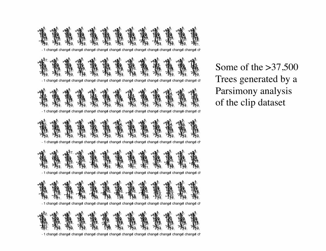
Some of the >37,500 Trees generated by a Parsimony analysis of the clip dataset
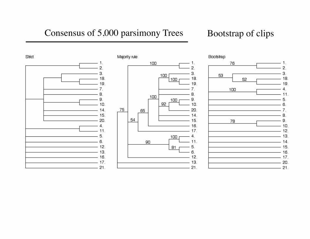
Consensus of 5,000 parsimony Trees Bootstrap of clips
Software and Books
• “How to make a phylogenetic Tree” by Barry Hall, comes with PAUP* CD, ~$30, Sinauer Press
• Phylip - Joe Felsenstein, Free via internet • PAML - Free via internet • Mr. Bayes - Free via internet • ClustalW or ClustalX - Free via internet • Fundamentals of molecular evolution, Second
edition, Wen-Hsiung Li, Sinauer Press
* Best on a MAC, but also command line

Giving Credit
• Several slides in this presentation were provided by Mike Thomas, via a presentation he posted on the internet in 2002.