phys 331: ch 5. damped & driven harmonic oscillator 1
TRANSCRIPT

Phys 331: Ch 5. Damped & Driven Harmonic Oscillator 1
Mass on spring with force probe
Why need two independent solutions?
What is ?
Graph in 186
Damped Oscillations:
So far, we have just considered a restoring force. If we include linear resistive force (the simplest
case), the net force on a particle moving in 1-D is:
xbkxxFx .
Newton’s second law gives:
xbkxxm ,
or defining the natural frequency o k m (frequency without damping) and the damping
constant b 2m (the “two” makes later result neater) we get:
02 2
o xxx .
Note: As the book points out (and anyone who’s taken our Electronics course would recognize)
The form of the equation for the charge on a capacitor q t in an RLC circuit is the same, replace
x with q (for charge), replace m with L (for inductance), replace with R (for resistance), and
replace k with 1/C (for capacitance).
Second-order differential equation.
Think about when you solve the very simple second order differential equation d2y/dt
2 = 0. You
integrate once and get v = v0, then you integrate again and get y = yo + vo t. Notice that, along
the way, you introduced two constants that can only be set by knowing some boundary
conditions; in this case, the initial position and initial velocity of the object. That’s generally true
of a 2nd
-order differential equation – your general solution must have two free parameters with
which to fit specific boundary conditions.
Thurs 10/11
Fri., 10/12
5.4-.5 Damped & Driven Oscillations
HW5a (5.2, 5.10)
Mon. 10/15
Tues. 10/16
Wed. 10/17
Thurs 10/18
Fri. 10/19
5.5-.6 Resonance
5.7 -.8 Fourier Series
6.1-.2 Calculus of Variations – Euler-Lagrange
HW5b (5.26-.43)
HW5c (5.46-.52), Project Bibliography

2
We will once again guess that the solutions are of the form x t ert , so rtrex and rterx 2 .
Substituting this into our differential equation (and canceling out ert from each term) yields the
auxiliary equation:
r2 2 r o
2 0,
Applying the quadratic equation solves this with:
r2 2
24 o
2
2.
Cancel out a “2” (the reason one is in the definition of ) and define:
r12
o
2 ,
r22
o
2 .
As long as r1 r2, er1t and er2t are independent solutions (they are not constant multiples of each
other). So, most generally, a solution can be linear combination of them. In the case that r1 r2,
this gives:
x t C1er1t C2e
r2t e t C1e2
o2 t
C2e2
o2 t
.
Notice that this gives us our two free parameters, C1 and C2. This should be sufficient for fitting
any specific scenario; any specific initial position and initial velocity for example.
The damping constant is real and positive, so one effect of the resistive force is to make the
size of x t decrease over time.
Qualitatively different Cases.
There are 4 qualitatively different possibilities for . = 0, = o, < o, and > o. These
will give qualitatively different mathematical results / physical behaviors.
Let’s look at the four possible cases:
(1) 0 Undamped Oscillations: If 0, there is no damping and:
x t C1ei o t C2e
i o t ,
Which can be rewritten as
tACostx o
as in the first section of this chapter. This describes an oscillation with an angular frequency o
and a constant amplitude. We already discussed the many ways of writing this solution.
(2) o Weak Damping / Underdamped Oscillations: The obvious thing to compare the
damping constant with is the natural frequency o since they appear together under the square

3
root. We will say that the damping constant is small if o. In that case, the quantity under the
square root is negative, so:
2
o
2 i o
2 2 i 1,
where 1 o
2 2 . This frequency 1 is less than the natural frequency o, but if o
then 1 o. The general solution is:
x t e t C1ei 1t C2e
i 1t ,
which can also be written as (the part in brackets is the same form as the undamped solution):
x t Ae t cos 1t .
So this looks like sinusoidal oscillation with an exponentially-decaying amplitude. Sometimes
is called the decay parameter for this type of motion because it determines how quickly the
amplitude decreases.
(3) o Strong Damping / Overdamped Oscillations: We will say that the damping constant
is large if o. In that case, the quantity under the square root is positive and the exponents
are real, so the general solution is:
x t C1e2
o2 t
C2e2
o2 t
.
This solution does not oscillate because both terms are decaying exponentials. The factor in
brackets is smaller for the first term, so it decays more slowly and determines the motion at large
times. Therefore, the decay constant for overdamped motion is 2
o
2 . The greater the
damping constant, the longer it takes for the system to return to equilibrium once it’s been
displaced (think of a mass on a spring hanging in oil.)
(4) o Critical Damping: The last case to consider is the threshold between these two
previous cases, when o. In this case r1 r2 which means that our two previously-
independent solutions aren’t so independent anymore and we’ll need to go hunting for a new

4
solution (there must be two because this is a second order linear differential equation), and we
don’t have our two constants with which to fit all possible initial conditions.
We know that there is one solution of the form x1 t e t .
The book proposes that x2 t te t is also a solution. Of course, we can plug this back into the
equation,
02 2 xxx
(rephrased using that o in this special case.)
Let’s find those two derivatives and then plug their expressions in (use the product rule):
tt teetx2 ,
tttt etteeetx 22
2 .
Okay, plugging these into the equation:
02 2 xxx ,
2t 2 e t 2 e t te t 2te t ? 0,
which works.
So, the general solution in this case is:
ttt etCCteCeCtx 2121 .
Both terms decay with the same decay parameter o. Graphically, these solutions are similar
to the overdamped solutions. There are no oscillations. This is actually the case that decays the
quickest – it’s decay rate depends on just, , as for the underdamped case, however, we’ve
cranked up the value of to be as large as it can be without flipping over to the overdamped case
which then decays according to 2
o
2 .
Summary:
There are two coefficients in each solution to be determined by the initial conditions (usually
x 0 and 0x ) of a particular problem.
For cases (1), (2), and (4) where 0 o, the decay parameter is , which is zero for case (1)
and o for case (4).
For case (3) where o, the decay parameter is 2
o
2 which decreases as increases!

5
0
0 1 2
de
cay
pa
ra
me
te
r
o
Too much damping (overdamping) does not cause the motion to decay more quickly! If you
want an object subjected to a restoring force to come to rest as quickly as possible, you should
make sure o . Applications include the needle on a meter and the motion of a car body
relative to its wheels (springs and shocks in between).
Example #1: For an underdamped case, show that the ratio of the amplitudes at two
successive maxima in the displacement is constant. (The maxima do not occur where x t
contacts the curve Ae t .)
Find the times when:
x t Ae t cos 1t ,
is maximum by setting the derivative equal to zero:
0sincos 111 m
t
m
t
m tAetAetx mm ,
1 sin 1tm cos 1tm ,
tan 1tm 1 ,
tm1
1
tan 1
1 .
Actually, we’ve found the times for maxima and minima, so every other solution is for a
maximum. The tangent repeats every radians, tan tan where 1,2, . If t1 is
the time for the first maximum, the subsequent maxima are at:
tn t1 n 1 2 1 ,
or:
tn 1 tn 2 1 .
The ratio of the amplitudes at two successive maxima is:
x tn 1
x tn
Aetn 2 1 cos 1 tn 2 1
Ae tn cos 1tne 2 1 ,

6
because cos cos 2 .
Example #2: Suppose the angular frequency of a underdamped oscillator is 628 Hz
(frequency of 100 Hz) and the ratio of the amplitudes at two successive maxima is one half.
What is the natural frequency o?
Using the result of Example 1 to find :
x tn 1
x tn
1
2e 2 1 ,
e 2 1 2,
2 1 ln2,
1 2 ln2 628 Hz 2 ln2 69.3 Hz.
The damped frequency is related to the natural frequency by:
1 o
2 2 ,
so:
o 1
2 2 628 Hz2
69.3 Hz2
632 Hz .
Linear Differential Operators:
The book sets up the discussion of the driven oscillator by first pointing out some general
properties of linear differential operators. I’m not sure that that discussion isn’t more work than
it’s worth.
The left side of the differential equation we solved today:
02 2
o xxx ,
can be thought of as the result of an operator acting on the function x t . Define the differential
operator D by:
Dd2
dt22d
dto
2 .
When this acts on x, it gives:
xxxDx 2
o2 ,
so the differential equation above can be written as Dx 0 . The operator is linear if:
D ax1 bx2 aDx1 bDx2.
We use the fact that the operator we’ve been dealing with is linear when we form general
solutions.

7
Driven Damped Oscillations:
Before we embark on this, let’s pause and think about complex numbers.
If you write out the Taylor series for ie , all even terms will be real and all odd terms will be
imaginary, gathering all those even/real terms together, you’ll recognize the Taylor expansion for
cos ; similarly, if you gather all the imaginary/odd terms together, you’ll recognize the Taylor
expansion for sin . So, strange but true,
sincos ie i
Rather trivially, if we multiply this by some constant, cal it r, then we have
imaginaryreal
i irrrirre sincos
I did this because the expression on the right looks kind of familiar; it looks a lot like the two
components of a 2-D vector:
yrxrr ˆsinˆcos
We can push this analogy further by representing it in the complex plain: that’s
That might help you to remember how to translate between the two representations
Ir
i irrerr )
where rrrrr Ir
*22
and
rI rr /tan 1
Damed-Driven Oscillator
Okay, this will come in handy shortly. Now on to the task at hand. Suppose a damped oscillator
is “driven” by an additional time-dependent force tFd , so the net force on the oscillator is
kx bv F t . Newton’s second law gives:
matFbvkx d ,
Real
Imaginary
cosrrreal
sinrrimag

8
or:
tFkxxbxm d .
If we define the force per unit mass mtFtf dd and recall the definition of the damping
constant b 2m, then we can write:
tfxxx d
2
o2 .
Fourier’s theorem can be rephrased as saying that any complicated function can be phrased as a
linear combination of complex exponential terms. Got to love exponentials – it’s so easy to take
their derivatives!
Of course, the driving force can have any functional dependence on time; however, we’ll focus
on a specific driving force. Fourier’s theorem tells us that any complicated function can be built
of a combination of sines and cosines. So a natural place to start is solving this problem for a
cosine driving force:
tfxxx doccc cos2 2
o
Or maybe for a sine driving force
tfxxx dosss sin2 2
o
Or here’s a crazy thought, since this is a linear differential equation, add these two equations and
simultaneously find a solution for a cosine and sine driving forces, or, heck if the cosine and sine
have different amplitudes, say by a factor of i, we could multiply the second equation by i and
then add it:
tatfaxxxaxxax ddoscscsc sincos2 2
o
Okay, so we could do that, but why? Well, only if it makes life easier, and there is one choice if
a that does make life easier: i.
The actual problem we’ll tackle is
ti
odeftxtxtx )()(2)( 2
o
So, rather perversely, it’s actually going to be easier for us to solve this equation for a 2-D vector
than for a scalar. The solutions we’ll get will also be complex, so they could be written in either
of two forms
tiytxetrtz ti )()(
where )()()()( *22tztztztytxtr
and
txtyt /tan)( 1
Formally then, say we find a complex solution, that is
ti
odeftztztz )()(2)( 2
o

9
Then that’s equivalent to saying
)sin()cos()()()()(2)()( 2
o tiftftytxtyitxtyitx dodo
or we can break this one ‘vector’ equation into two component equations: one relating just the
real terms and one relating just the imaginary terms.
)cos()()(2)( 2
o tftxtxtx do
)sin()()(2)( 2
o tftytyty do
So, we’ll actually solve the problem of a complex driving force, but from that we’ll be able to
extract the solution for a cosine driving force or the solution for the sine driving force, and of
course, we can build any complicated driving force (and its solutions) from linear combinations
of these.
Okay, here we go; our equation has the form
ti
odeftztztz )()(2)( 2
o
It’s hard to imagine being able to generate a “characteristic equation” unless our solution had the
same time dependence as does the driving force, that is
ti dCetz ,
where C is an undetermined complex constant. Substitute this into the differential equation to
get:
titi
dd
tititi ddddd efCeiCeCedt
dCe
dt
do
2
o
22
o2
2
22 .
This is a good solution if:
dd i
fC
222
o
o .
Looking at the denominator, that has one of two classic forms of a complex number, and we can
rewrite it in the other:
tiytxetrtz ti )()(
where )()()()( *22tztztztytxtr
and
txtyt /tan)( 1
i
dd
i
dd
ef
e
fC
2222
o
o
2222
o
o
22
where
10
22
o
1 2tan
d
d
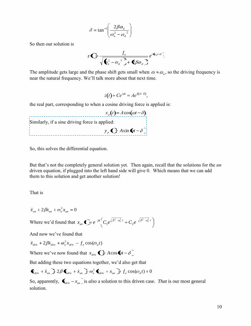
So then our solution is
ti
dd
def
tz2222
o
o
2
.
The amplitude gets large and the phase shift gets small when o , so the driving frequency is
near the natural frequency. We’ll talk more about that next time.
z t Cei t Aei t
,
the real part, corresponding to when a cosine driving force is applied is:
xp t Acos t .
Similarly, if a sine driving force is applied:
tAty p sin
So, this solves the differential equation.
But that’s not the completely general solution yet. Then again, recall that the solutions for the un
driven equation, if plugged into the left hand side will give 0. Which means that we can add
them to this solution and get another solution!
That is
02 2
o ununun xxx
Where we’d found that ttt
un eCeCetx2o
22o
2
21
And now we’ve found that
)cos(2 2
o tfxxx dodrivdrivdriv
Where we’ve now found that tAtxdriv cos
But adding these two equations together, we’d also get that
0)cos(2 2
o tfxxxxxx doundrivundrivundriv
So, apparently, undriv xx is also a solution to this driven case. That is our most general
solution.

11
ttt
undriv eCeCetAxxtx2o
22o
2
21cos
The book couches this result in more general differential-equations language; for many of you, I
hope that helps to make connections, and understand this better. I’ve avoided using that
language (homogeneous, inhomogeneous, particular,…) in case it was more useful just focusing
on the specific case at hand.
The homogeneous solution determined by the initial conditions must be added to this to get the
general solution. Note that the homogeneous solution decays, so it can also be called the
transient solution. Only the early motion of the oscillator depends on how it starts out. The
particular solution is an oscillatory solution with the same frequency as the driving frequency,
which can also be called the steady-state solution. The motion for large times only depend on the
parameters of the system (including the driving force), not the initial conditions.
Example: (similar to Ex. 5.3) Suppose o 10 rad/s, o 20 2 rad/s,
f0 1000 m/s2 , and 4 rad/s (only difference from Ex. 5.3). If the oscillator starts at rest
at the orign, find and plot the function for position as a function of time. Compare with the
results for Ex. 5.3.
The frequency for the undriven oscillator (and the homogeneous solution) is:
1 o
2 2 102
22
9.987 .
The amplitude of the particular solution is:
Afo
o
2 2 2
4 2 2
1000 m/s2
2 rad/s2 102 42 2
4 1 22
42
1.177 m,
and the phase angle is:
tan 1 2
o
2 2tan 1 2 2 4
102
42
0.0465 radians.
The general solution for an underdamped, driven oscillator can be written as:
x t Acos t e t B1 cos 1t B2 sin 1t ,
where the coefficients B1 and B2 must be determined from the initial conditions xo vo 0.
From the equation above:
xo Acos B1,
B1 xo Acos 0 1.177 m cos 0.0465 rad 1.176 m.
Taking the derivative of x t gives:
v t Asin t e t B1 cos 1t B2 sin 1t 1et B1 sin 1t B2 cos 1t ,
vo Asin B1 B2,
B2
1
1
vo Asin B1
1
9.9870 4 1.177 m sin 0.0465 rad 1 2 1.176 m ,

12
B2 0.807 m.
The graph of the solution is shown below (solid line) along with the solution of Ex. 5.3
(dashed line) where the driving frequency is 2 rad/s . The steady state solution for this
example has a slightly larger amplitude because the driving frequency is closer to the natural
frequency. It also lags a little farther behind the driving force.
-2
-1.5
-1
-0.5
0
0.5
1
1.5
2
0 1 2 3 4
t
x(t
)
In the formal language of Differential Equations, what I just argued is that if you have a
particular, linear differential equation,
tftxD p )(ˆ (using the Quantum notation of ‘hat’ for an operator)
Then the general solution is the linear combination of a particular solution to this equation, xp(t)
and the solutions to this simpler “homogenious” equation
0)(ˆ txD h
Since
0ˆˆˆ tfxDxDxxD hphp