Physica D 261 (2013) 19–30

Contents lists available at ScienceDirect

Physica D

journal homepage: www.elsevier.com/locate/physd

Isostables, isochrons, and Koopman spectrum for the action–anglerepresentation of stable fixed point dynamicsA. Mauroy ∗, I. Mezić, J. MoehlisDepartment of Mechanical Engineering, University of California Santa Barbara, Santa Barbara, CA 93106, USA

h i g h l i g h t s

• While isochrons reduce limit cycle dynamics, isostables reduce fixed point dynamics.• The isostables are the level sets of an eigenfunction of the Koopman operator.• We provide a method for computing the isostables in the entire basin of attraction.• The framework is related to action–angle coordinates and special Lyapunov functions.

a r t i c l e i n f o

Article history:Received 2 February 2013Received in revised form10 June 2013Accepted 14 June 2013Available online 22 June 2013Communicated by S. Coombes

Keywords:Nonlinear dynamicsIsochronsExcitable systemsKoopman operatorAction–angle coordinatesLyapunov function

a b s t r a c t

For asymptotically periodic systems, a powerful (phase) reduction of the dynamics is obtained bycomputing the so-called isochrons, i.e. the sets of points that converge toward the same trajectory onthe limit cycle. Motivated by the analysis of excitable systems, a similar reduction has been attemptedfor non-periodic systems admitting a stable fixed point. In this case, the isochrons can still be defined butthey do not capture the asymptotic behavior of the trajectories. Instead, the sets of interest – that we call‘‘isostables’’ – are defined in the literature as the sets of points that converge toward the same trajectoryon a stable slow manifold of the fixed point. However, it turns out that this definition of the isostablesholds only for systems with slow–fast dynamics. Also, efficient methods for computing the isostables aremissing.

The present paper provides a general framework for the definition and the computation of theisostables of stable fixed points, which is based on the spectral properties of the so-called Koopmanoperator. More precisely, the isostables are defined as the level sets of a particular eigenfunction of theKoopman operator. Through this approach, the isostables are unique and well-defined objects related tothe asymptotic properties of the system. Also, the framework reveals that the isostables and the isochronsare two different but complementary notions which define a set of action–angle coordinates for thedynamics. In addition, an efficient algorithm for computing the isostables is obtained, which relies onthe evaluation of Laplace averages along the trajectories. The method is illustrated with the excitableFitzHugh–Nagumo model and with the Lorenz model. Finally, we discuss how these methods based onthe Koopman operator framework relate to the global linearization of the system and to the derivation ofspecial Lyapunov functions.

© 2013 Elsevier B.V. All rights reserved.

1. Introduction

Among the abundant literature on networks of coupled sys-tems, a vast majority of studies focus on asymptotically periodicsystems (i.e. coupled oscillators) while only a few consider cou-pled systems characterized by a stable fixed point. This is particu-larly surprising since the latter can exhibit excitable regimes thatare relevant in many situations (e.g. neuroscience [1]). One reason

∗ Corresponding author.E-mail addresses: alex.mauroy@engr.ucsb.edu (A. Mauroy),

mezic@engr.ucsb.edu (I. Mezić), moehlis@engineering.ucsb.edu (J. Moehlis).

0167-2789/$ – see front matter© 2013 Elsevier B.V. All rights reserved.http://dx.doi.org/10.1016/j.physd.2013.06.004

for this disproportion is probably related to phase reductionmeth-ods. For asymptotically periodic systems, powerful phase reduc-tion methods turn the (complex, high-dimensional) system into aphase oscillator evolving on the circle, making the study of com-plex networks more amenable to mathematical analysis [2–4]. Incontrast, in the case of systems admitting a stable fixed point, thedevelopment of equivalent reduction methods is more recent anda general framework is still in its infancy.

The goal of reduction methods is to assign the same value toa (codimension-1) set of initial conditions that are characterizedby the same asymptotic behavior, in turn designing a coordinateon the state space. In the case of asymptotically periodic systems,these sets of identical (phase) value are the so-called isochrons,

20 A. Mauroy et al. / Physica D 261 (2013) 19–30

which approach the same trajectory on the limit cycle [5]. Thisconcept has been recently extended to heteroclinic cycles [6]. Forsystems admitting a stable focus, the isochrons (or isochronoussections) can still be defined as the sets of points that are invari-ant under a particular return map [7,8]. This notion is of particularinterest in the case of weak foci (i.e. characterized by a Jacobianmatrix with purely imaginary eigenvalues) and non-smooth vec-tor fields, where the existence of isochrons is a non-trivial problemrelated to the stability of the fixed point. However, the isochronsprovide in this case no information on the asymptotic convergenceof the trajectories toward the fixed point and are not useful for thesystem reduction. (Note also that they do not exist for fixed pointscharacterized by a Jacobian matrix with real eigenvalues.) There-fore, the isochrons must be complemented by another family ofsets: the so-called isostables.

Excitable systems are characterized by slow–fast dynamicswith a stable fixed point and, in the plane, they admit a particulartrajectory – the transient attractor or slow manifold – thattemporarily attracts all the trajectories as they approach the fixedpoint. In this case, the isostables are naturally defined as the setsof points that converge to the same trajectory on the transientattractor [9]. (Note that these sets are called ‘‘isochrons’’ in [9], butwe feel that the proper sense is ‘‘isostables’’ instead, in order toavoid the confusion with the isochrons of foci studied in [7,8].) Fornon-planar systems possessing amulti-dimensional slowmanifoldor center manifold, a (more rigorous) framework was previouslydeveloped in [10,11]. In that work, the sets of interest (called‘‘projection manifolds’’ in [10]) are closely related to the notionof isostable and correspond to the invariant fibers of the (slow orcenter) manifold, i.e. the sets of initial conditions characterizedby the same long-term behavior on that manifold. Through thereduction obtained with the isostables, excitable systems havebeen studied in various contexts (sensitivity to periodic pulses[12–14], network synchronization [15], etc.).

Since the isostables provide a characterization of the systemdynamics around the fixed point, their computation is also desir-able for systems which do not contain multiple time scales (i.e.with no slow or center manifold). For instance, the computationof the isostables can be useful to achieve an optimal control thatminimizes the time of convergence toward a steady state or toinvestigate the delay of convergence to a stable equilibrium indecision-making models [16]. But in these cases, a more generalframework is required, which defines the isostables as particular(and unique) codimension-1 sets capturing the asymptotic behav-ior of the system. In addition, the computation of the isostablesthrough backward integration [9] or normal form of the dynam-ics [11] is limited to a neighborhood of the slow manifold. In thiscontext, an efficient method for computing the isostables in theentire basin of attraction is also missing.

In this paper, we propose a general framework for the reduc-tion of systems admitting a stable fixed point, which is not lim-ited to excitable systems with slow–fast dynamics. This approachis based on the spectral properties of the so-called Koopman oper-ator [17,18]. More precisely, we propose a general and unique defi-nition of the isostables in terms of a particular eigenfunction of theKoopman operator. In addition, the framework yields an efficientmethod to compute the isostables in the whole basin of attraction.This method relies on the estimation of Laplace averages along thetrajectories and can be seen as an extension of the approach re-cently developed in [19] to compute the isochrons of limit cycles.

Viewed through the Koopman operator framework, the isosta-bles and the isochrons appear to be two different but complemen-tary concepts. On the one hand, they are different since they arerelated to the absolute value and to the argument, respectively,of the eigenfunction of the Koopman operator. On the other hand,they are complementary in the sense that they define a set of ac-tion–angle coordinates for the system dynamics. This action–angle

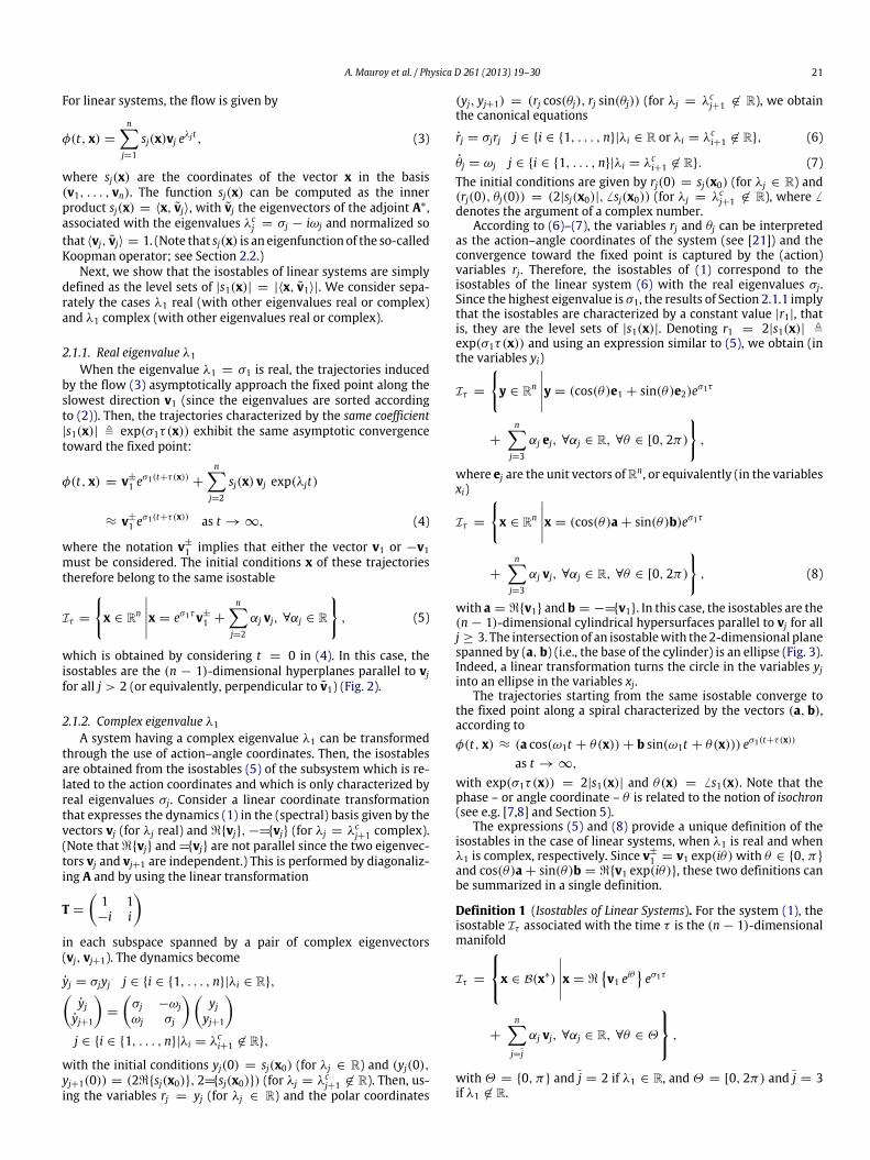
Fig. 1. Trajectories starting from the same isostable Iτ0 are characterized bythe same convergence toward the fixed point. They simultaneously intersect thesuccessive isostables Iτn and approach the fixed point synchronously.

representation is related to important properties of the isosta-bles, such as the global linearization of the dynamics [20] and thederivation of special Lyapunov functions, that we discuss in the pa-per.

The paper is organized as follows. In Section 2, we introducethe concept of isostable in the context of the Koopman operatorframework, both for linear and nonlinear systems.We also proposea rigorous definition of the isostables and discuss their mainproperties. The relation between the isostables and the Laplaceaverages is developed in Section 3. This provides an efficientalgorithm for the computation of the isostables which is illustratedin Section 4 for the excitable FitzHugh–Nagumo model andthe Lorenz model. Finally, the related concepts of action–anglerepresentation, global linearization, and Lyapunov function arediscussed in Section 5. Section 6 gives some concluding remarks.

2. Isostables and Koopman operator

The isostables of an asymptotically stable fixed point x∗ are thesets of points that share the same asymptotic convergence towardthe fixed point. More precisely, trajectories with an initial condi-tion on an isostable Iτ0 simultaneously intersect the successiveisostables Iτn after a time interval τn − τ0, thereby approachingthe fixed point synchronously (Fig. 1). The isostables partition thebasin of attraction of the fixed point and define a new coordinateτ that satisfies τ = 1 along the trajectories. Or equivalently, theydefine a coordinate r , exp(λτ) with the linear dynamics r = λr .This new coordinate can be used in a context of model reduction.

At this point, it is important to remark that this (intuitive) def-inition of isostable is not complete. Indeed, there exist an infinityof families of sets that satisfy the above-described property. Butamong these families, only one defines a smooth change of coor-dinates and is relevant to capture the asymptotic behavior of thetrajectories. In this section, wewill give a rigorous definition of thisunique family of isostables. To do so, we first consider the particu-lar case of linear systems. Then,we extend the concept to nonlinearsystems, using the Koopman operator framework.

2.1. Linear systems

Consider the stable linear system

x = Ax, x ∈ Rn, (1)and assume that each eigenvalue λj = σj + iωj of the matrix Ais of multiplicity 1, has a strictly negative real part σj < 0, and isassociated with the right eigenvector vj (which is normalized, thatis, ∥vj∥ = 1). By convention, we sort the eigenvalues so that λ1 isthe eigenvalue related to the ‘‘slowest’’ direction, that isσj ≤ σ1 < 0, j = 2, . . . , n. (2)The flow induced by (1) is the continuous-timemap φ : R×Rn

→

Rn, that is, φ(t, x) is the solution of (1) with the initial condition x.

A. Mauroy et al. / Physica D 261 (2013) 19–30 21

For linear systems, the flow is given by

φ(t, x) =

nj=1

sj(x)vj eλjt , (3)

where sj(x) are the coordinates of the vector x in the basis(v1, . . . , vn). The function sj(x) can be computed as the innerproduct sj(x) = ⟨x, vj⟩, with vj the eigenvectors of the adjoint A∗,associated with the eigenvalues λc

j = σj − iωj and normalized sothat ⟨vj, vj⟩ = 1. (Note that sj(x) is an eigenfunction of the so-calledKoopman operator; see Section 2.2.)

Next, we show that the isostables of linear systems are simplydefined as the level sets of |s1(x)| = |⟨x, v1⟩|. We consider sepa-rately the cases λ1 real (with other eigenvalues real or complex)and λ1 complex (with other eigenvalues real or complex).

2.1.1. Real eigenvalue λ1

When the eigenvalue λ1 = σ1 is real, the trajectories inducedby the flow (3) asymptotically approach the fixed point along theslowest direction v1 (since the eigenvalues are sorted accordingto (2)). Then, the trajectories characterized by the same coefficient|s1(x)| , exp(σ1τ(x)) exhibit the same asymptotic convergencetoward the fixed point:

φ(t, x) = v±

1 eσ1(t+τ(x))

+

nj=2

sj(x) vj exp(λjt)

≈ v±

1 eσ1(t+τ(x)) as t → ∞, (4)

where the notation v±

1 implies that either the vector v1 or −v1must be considered. The initial conditions x of these trajectoriestherefore belong to the same isostable

Iτ =

x ∈ Rn

x = eσ1τv±

1 +

nj=2

αj vj, ∀αj ∈ R

, (5)

which is obtained by considering t = 0 in (4). In this case, theisostables are the (n − 1)-dimensional hyperplanes parallel to vjfor all j > 2 (or equivalently, perpendicular to v1) (Fig. 2).

2.1.2. Complex eigenvalue λ1

A system having a complex eigenvalue λ1 can be transformedthrough the use of action–angle coordinates. Then, the isostablesare obtained from the isostables (5) of the subsystem which is re-lated to the action coordinates and which is only characterized byreal eigenvalues σj. Consider a linear coordinate transformationthat expresses the dynamics (1) in the (spectral) basis given by thevectors vj (for λj real) and ℜ{vj}, −ℑ{vj} (for λj = λc

j+1 complex).(Note that ℜ{vj} and ℑ{vj} are not parallel since the two eigenvec-tors vj and vj+1 are independent.) This is performed by diagonaliz-ing A and by using the linear transformation

T =

1 1−i i

in each subspace spanned by a pair of complex eigenvectors(vj, vj+1). The dynamics become

yj = σjyj j ∈ {i ∈ {1, . . . , n}|λi ∈ R},yj

yj+1

=

σj −ωjωj σj

yj

yj+1

j ∈ {i ∈ {1, . . . , n}|λi = λc

i+1 ∈ R},

with the initial conditions yj(0) = sj(x0) (for λj ∈ R) and (yj(0),yj+1(0)) = (2ℜ{sj(x0)}, 2ℑ{sj(x0)}) (for λj = λc

j+1 ∈ R). Then, us-ing the variables rj = yj (for λj ∈ R) and the polar coordinates

(yj, yj+1) = (rj cos(θj), rj sin(θj)) (for λj = λcj+1 ∈ R), we obtain

the canonical equations

rj = σjrj j ∈ {i ∈ {1, . . . , n}|λi ∈ R or λi = λci+1 ∈ R}, (6)

θj = ωj j ∈ {i ∈ {1, . . . , n}|λi = λci+1 ∈ R}. (7)

The initial conditions are given by rj(0) = sj(x0) (for λj ∈ R) and(rj(0), θj(0)) = (2|sj(x0)|, sj(x0)) (for λj = λc

j+1 ∈ R), where

denotes the argument of a complex number.According to (6)–(7), the variables rj and θj can be interpreted

as the action–angle coordinates of the system (see [21]) and theconvergence toward the fixed point is captured by the (action)variables rj. Therefore, the isostables of (1) correspond to theisostables of the linear system (6) with the real eigenvalues σj.Since the highest eigenvalue is σ1, the results of Section 2.1.1 implythat the isostables are characterized by a constant value |r1|, thatis, they are the level sets of |s1(x)|. Denoting r1 = 2|s1(x)| ,exp(σ1τ(x)) and using an expression similar to (5), we obtain (inthe variables yi)

Iτ =

y ∈ Rn

y = (cos(θ)e1 + sin(θ)e2)eσ1τ

+

nj=3

αj ej, ∀αj ∈ R, ∀θ ∈ [0, 2π)

,

where ej are the unit vectors ofRn, or equivalently (in the variablesxi)

Iτ =

x ∈ Rn

x = (cos(θ)a + sin(θ)b)eσ1τ

+

nj=3

αj vj, ∀αj ∈ R, ∀θ ∈ [0, 2π)

, (8)

with a = ℜ{v1} and b = −ℑ{v1}. In this case, the isostables are the(n − 1)-dimensional cylindrical hypersurfaces parallel to vj for allj ≥ 3. The intersection of an isostablewith the 2-dimensional planespanned by (a, b) (i.e., the base of the cylinder) is an ellipse (Fig. 3).Indeed, a linear transformation turns the circle in the variables yjinto an ellipse in the variables xj.

The trajectories starting from the same isostable converge tothe fixed point along a spiral characterized by the vectors (a, b),according toφ(t, x) ≈ (a cos(ω1t + θ(x)) + b sin(ω1t + θ(x))) eσ1(t+τ(x))

as t → ∞,

with exp(σ1τ(x)) = 2|s1(x)| and θ(x) = s1(x). Note that thephase – or angle coordinate – θ is related to the notion of isochron(see e.g. [7,8] and Section 5).

The expressions (5) and (8) provide a unique definition of theisostables in the case of linear systems, when λ1 is real and whenλ1 is complex, respectively. Since v±

1 = v1 exp(iθ) with θ ∈ {0, π}

and cos(θ)a + sin(θ)b = ℜ{v1 exp(iθ)}, these two definitions canbe summarized in a single definition.

Definition 1 (Isostables of Linear Systems). For the system (1), theisostable Iτ associated with the time τ is the (n − 1)-dimensionalmanifold

Iτ =

x ∈ B(x∗)

x = ℜv1 eiθ

eσ1τ

+

nj=j

αj vj, ∀αj ∈ R, ∀θ ∈ Θ

,

with Θ = {0, π} and j = 2 if λ1 ∈ R, and Θ = [0, 2π) and j = 3if λ1 ∈ R.

22 A. Mauroy et al. / Physica D 261 (2013) 19–30

ba

Fig. 2. (a) The isostables of linear systems with a real eigenvalue λ1 are the hyperplanes spanned by the eigenvectors vj , with j > 2. The particular isostable I∞ containsthe fixed point. (b) For two-dimensional systems (or in the plane v1 − v2), the isostables are pairs of parallel lines.

Fig. 3. (a) The isostables of linear systems with a complex eigenvalue λ1 are cylindrical hypersurfaces spanned by vj for all j ≥ 3. (b) For two-dimensional linear systems(or in the plane a − b), the isostables are ellipses with constant axes.

2.2. Nonlinear systems

Now, we consider a nonlinear system

x = F(x), x ∈ Rn (9)

where F is an analytic vector field, which admits a stable fixedpoint x∗ with a basin of attraction B(x∗) ⊆ Rn. In addition, weassume that the Jacobian matrix J computed at x∗ has n distinct(nonresonant) eigenvalues λj = σj + iωj characterized by strictlynegative real partsσj < 0 and sorted according to (2). (For unstablefixed points or for multiple eigenvalues, see Remarks 1 and 2,respectively.)

The isostables of linear systems have been defined as thelevel sets of the coefficient s1(x) that appears in the expressionof the flow (3). For nonlinear systems, an expression of theflow similar to (3) can be obtained through the framework ofKoopman operator [17,18]. The Koopman semigroup of operatorsU t describes the evolution of a (vector-valued) observable f : Rn

→

Cm along the trajectories of the system and is rigorously definedas the composition U t f(x) = f ◦ φ(t, x). Throughout the paper,we will make no assumption on the observables, except that theyare analytic in the neighborhood of the fixed point. In the space ofanalytic observables, the operator has only a point spectrum andits spectral decomposition yields [22]

U t f(x) =

{k1,...,kn}∈Nn

sk11 (x) · · · sknn (x) vk1···kn e(k1λ1+···+knλn)t . (10)

A detailed derivation of the decomposition in the case of a stablefixed point is given in the Appendix. The functions sj(x), j =

1, . . . , n, are the smooth eigenfunctions of U t associated with theeigenvalues λj, i.e.

U tsj(x) = sj(φ(t, x)) = sj(x)eλjt , (11)

and the vectors vk1···kn are the so-called Koopman modes [23], i.e.the projections of the observable f onto sk11 (x) · · · sknn (x). For theparticular observable f(x) = x, (10) corresponds to the expressionof the flow and can be rewritten as

φ(t, x) = U tx = x∗+

nj=1

sj(x)vj eλjt

+

{k1,...,kn}∈Nn

0k1+···+kn>1

sk11 (x) · · · sknn (x) vk1···kn e(k1λ1+···+knλn)t . (12)

The first part of the expansion is similar to the linear flow (3). Theeigenvalues λj and the Koopmanmodes vj are the eigenvalues andeigenvectors of J, respectively. Although the eigenfunctions sj(x)are not computed as the inner products ⟨x, vj⟩ as in the linear case,they can be interpreted as the inner products ⟨z, vj⟩, where z isthe initial condition of a virtual trajectory evolving according tothe linearized dynamics z = Jz and characterized by the sameasymptotic evolution as φ(t, x) [20]. The other terms in (12) donot appear in the expression of the linear flow (3) and account forthe transient behavior of the trajectories owing to the nonlinearityof the dynamics.

The isostables can be rigorously defined as the level sets of theabsolute value of the eigenfunction |s1(x)|. Indeed, the asymptoticevolution of the flow (12) is dominated by the firstmode associated

A. Mauroy et al. / Physica D 261 (2013) 19–30 23

with λ1. Then, a same argument as in Section 2.1 shows that thepoints x characterized by the same value |s1(x)| are the initialconditions of trajectories that converge synchronously to the fixedpoint, with the evolution

φ(t, x) ≈

x∗+ v±

1 eσ1(t+τ(x)), eσ1τ(x)

= |s1(x)|, λ1 ∈ R,

x∗+ ℜ

v1 ei(ω1t+θ(x)) eσ1(t+τ(x)),

eσ1τ(x)= 2|s1(x)|, θ(x) = s1(x) λ1 ∈ R.

(13)

We are now in a position to propose a general definition forthe isostables of a fixed point, which is valid both for linear andnonlinear systems andwhich is reminiscent of the usual definitionof isochrons for limit cycles [5,24].

Definition 2 (Isostables). For the system (9), the isostable Iτ ofthe fixed point x∗, associated with the time τ , is the (n − 1)-dimensional manifold

Iτ = {x ∈ B(x∗)|∃ θ ∈ Θ s.t.limt→∞

e−σ1t∥φ(t, x) − x∗− ℜ{v1 ei(ω1t+θ)

}eσ1(t+τ)∥ = 0},

with Θ = {0, π} and ω1 = 0 if λ1 ∈ R and Θ = [0, 2π) if λ1 ∈ R.The reader will easily verify that, for all x belonging to the

same isostable, Definition 2 imposes the same value |s1(x)| in thedecomposition of the flow (12) and the same asymptotic behavior(13). Note that without the multiplication by the increasingexponential e−σ1t , one would have Iτ = B(x∗)∀τ since φ(t, x) −

x∗→ 0 as t → ∞ for all x ∈ B(x∗).Except for the case of multiple eigenvalues, for which v1

might not be unique (see Remark 2), the isostables are uniquelydefined through Definition 2. Uniqueness of the isostables alsofollows from the fact that the Koopman operator has a uniqueeigenfunction s1(x) which is continuously differentiable in theneighborhood of the fixed point. Since it is precisely thiseigenfunction s1(x) that appears in (12), the isostables are the onlysets that are relevant to capture the asymptotic behavior of thetrajectories.

Remark 1 (Unstable Fixed Point). Definition 2 is easily extendedto unstable fixed points characterized by σj > σ1 > 0 for allj. Indeed, the isostables are still given by Definition 2, where thelimit t → ∞ is replaced by t → −∞, that is, one considers theflow φ(−t, x) induced by the (stable) backward-time system. Inthis case, the isostables are related to the unstable eigenfunctions1(x) of the Koopman operator.

Remark 2 (Multiple Eigenvalues). When the eigenvalue λ1 has amultiplicitym > 1, the fixed point is either a star node (m linearlyindependent eigenvectors) or a degenerate node (m linearlydependent eigenvectors). In the case of a star node, Definition 2is not unique since it depends on the direction of the eigenvectorv1 (in other words, a C1 eigenfunction of the Koopman operatorcorresponding to the eigenvalue λ1 is not unique). Actually, v1should be replaced in Definition 2 by any linear combination of morthonormal eigenvectors of λ1, a situation where the isostableslying in the vicinity of the fixed point correspond to cylindricalhypersurfaces whose intersection with the hyperplane spannedby the eigenvectors of λ1 is a hypersphere. In the case of adegenerate node, the asymptotic evolution toward the fixed pointis dominated by the (slowest) term s1(x)v1 tm−1 exp(σ1t). Then,the increasing exponential exp(−σ1t) in Definition 2 must bereplaced by t1−m exp(−σ1t).

2.3. Some remarks on the isostables

Equivalent definitions for excitable systems. In [9], the authors con-sidered two-dimensional excitable systems characterized by atransient attractor (i.e. slow manifold) which attracts all the tra-jectories as they approach the fixed point. They defined the isosta-bles (they actually used the term ‘‘isochrons’’; see Section 5.1) as

the sets of points that converge to the same trajectory on the tran-sient attractor. This definition is equivalent to Definition 2 sinceboth impose that trajectories on the same isostable have the sameasymptotic behavior (see also Section 4.1). However, the definitionof [9] is qualitative since no trajectory effectively reaches the tran-sient attractor (which may even lose its normal stability propertynear a fixed point with complex eigenvalues). Also, it is valid onlyif the system admits a transient attractor induced by the slow–fastdynamics. In contrast, Definition 2 is more general and does notrely on the existence of a transient attractor.

For systems with a slow (or center) manifold, the ‘‘projectionmanifolds’’ studied in [10,11] are related to the isostables. They arethe sets of initial conditions for which the trajectories share thesame long-term behavior on the slow manifold. In addition, theycan be obtained through the normal form of the dynamics [11]. Ifthe slow manifold is one-dimensional and if λ1 is real, the projec-tion manifolds are identical to the isostables. Otherwise, they donot correspond to the isostables since they are not related to theslowest direction v1 only and are not of codimension-1.Isostables and flow. The flow φ(1t, ·) maps the isostable Iτ to theisostable Iτ+1t , for all 1t ∈ R (as explained in the beginning ofSection 2). Indeed, if x ∈ Iτ , Definition 2 implies that

limt→∞

e−σ1tφ(t, x) − x∗

− ℜv1 ei(ω1t+θ)

eσ1(t+τ)

= 0

for some θ ∈ Θ . Using the substitution t = t ′ + 1t , we have

limt ′→∞

e−σ1t ′∥φt ′, φ(1t, x)

− x∗

− ℜ{v1 ei(ω1t ′+θ ′)}eσ1(t ′+τ+1t)

∥ = 0,

with θ ′= θ + ω11t ∈ Θ , so that φ(1t, x) ∈ Iτ+1t .

Local geometry near the fixed point. The isostables close to the fixedpoint have a geometry similar to the isostables of the linearizeddynamics, i.e. parallel hyperplanes (if λ1 ∈ R) or cylindricalhypersurfaces with constant axes of the elliptical sections (if λ1 ∈

R) (see Section 2.1). This follows from the fact that, in the vicinity ofthe fixed point, the flow (12) and the flow induced by the linearizeddynamics are (approximately) equal, so that their eigenfunctionss1(x) have (approximately) the same value for ∥x − x∗

∥ ≪ 1 (seealso (A.4) in the Appendix).Invariant fibration. When the eigenvalue λ1 is real, the isostablesare the invariant fibers of the 1-dimensional invariant manifoldV defined as the trajectory associated with the slow direction v1(i.e. the transient attractor in the case of slow–fast systems). Giventheir local geometry, it is clear that the isostables near the fixedpoint are the fibers defined by the splitting N ⊕ TV , where N =

span{v2, . . . , vn} and TV = span{v1}. Moreover, it follows fromthe invariance property of the isostables that this local fibrationis naturally extended to the whole invariant manifold V by back-ward integration of the flow. Provided that σ2 < σ1, the normalhyperbolicity of V implies that the isostables are characterized bysmoothness properties and persist under a small perturbation ofthe vector field [25,26]. In addition, this description also impliesthe uniqueness of the concept of isostables. Note that Definition 2is recovered in [27, Theorem 3], and corresponds to the propertythat the points on the same fiber converge to a trajectory on V withthe fastest rate.

When λ1 is complex, however, the isostables cannot beinterpreted as the invariant fibers of an invariant manifold. Theyare homeomorphic to a circle (or to a cylinder) and cannot be thesets of points converging to the same trajectory, since the flow iscontinuous. Moreover, in the neighborhood of the fixed point, oneobserves no particular one-dimensional invariant manifold (e.g.a slow manifold) that is tangent to the ℜ{v1} − ℑ{v1} plane. Inthat case, the only definition of the isostables is in terms of aneigenfunction of the Koopman operator.

24 A. Mauroy et al. / Physica D 261 (2013) 19–30

Extension to other eigenfunctions. The isostables Iτ are related to thefirst eigenfunction s1(x) of the Koopman operator, but the conceptcan be directly generalized to other eigenfunctions. Namely, thesets I(j)

τ (j) , j ∈ J = {i ∈ {1, . . . , n}|λi ∈ R or λi = λci+1 ∈ R},

are obtained by considering the level sets of |sj(x)|. The extensionis useful to derive an action–angle coordinates representation ofthe system, to perform a global linearization of the dynamics (seeSection 5.2), or to compute the (un)stable manifold of an attractor.

The intersection between the sets I(j)τ (j) , with j ≤ j, is defined as

the generalization of Definition 2

j∈Jj≤j

I(j)τ (j) =

x ∈ B(x∗)

∃ θj ∈ Θj s.t. limt→∞

e−σjt

φ(t, x) − x∗

−

j∈Jj≤j

ℜvj ei(ωjt+θj)

eσj(t+τ (j))

= 0

, (14)

with Θj = {0, π} if λj ∈ R and Θj = [0, 2π) if λj ∈ R. Whenτ (j)

= ∞ for all j < j ∈ J , (14) is equivalent to Definition 2, sothat it can be interpreted as an isostable for the system restrictedto the invariant manifold Mj =

j∈J ,j<j I(j)

τ (j)=∞. (The manifold Mj

is tangent to the fast directions vj, j = j, . . . , n.) In addition, ifλj ∈ R, (14) defines a codimension-j invariant fibration of the in-variant manifold Vj =

j∈J ,j>j I(j)

τ (j)=∞. (Themanifold Vj is tangent

to the slowdirections vj, j = 1, . . . , j.) If Vj is a slowmanifold, thenthe fibration (14) corresponds to the projection manifolds consid-ered in [10,11]. Note that the family of manifolds Vj generalizes thenotion of slow manifold observed for systems with slow–fast dy-namics.

3. Laplace averages

In this section, we show that the isostables can be obtainedthrough the computation of the so-called Laplace averages. TheLaplace averages of a scalar observable f : Rn

→ C are given by

f ∗

λ (x) = limT→∞

1T

T

0(f ◦ φt)(x) e−λt dt, (15)

with φt(x) = φ(t, x) and λ ∈ C. (The observable f has to sat-isfy some conditions which ensure that the averages exist.) Whenit exists and is nonzero for some λ and f , the Laplace average f ∗

λ (x)corresponds to the eigenfunction of the Koopman operator associ-ated with the eigenvalue λ [22]. Indeed, one easily verifies that

U t ′ f ∗

λ (x) = limT→∞

1T

T

0(f ◦ φt+t ′)(x) e−λt dt

= eλt ′ limT→∞

1T

T+t ′

t ′(f ◦ φt)(x) e−λt dt

= eλt ′ f ∗

λ (x)where the second equality is obtained by substitution. For systemswith a stable fixed point, the Laplace average f ∗

λ1(x) corresponds

(up to a scalar factor) to the eigenfunction s1(x), and is thereforerelated to the concept of isostable. In addition, the Laplace aver-ages are an extension of the Fourier averages [17,18] that wereused in [19] to compute the isochrons of limit cycles.

Remark 3. Instead of (15), the generalized Laplace averages [22]

f ∗

λj(x) = lim

T→∞

1T

T

0

(f ◦ φt)(x) − f (x∗) −

j−1k=1

f ∗

λk(x)eλkt

× e−λjt dt

must be considered to obtain other eigenfunctions sj(x), j ≥ 2, andthe associated sets I(j)

τ (j) considered in (14). However, their compu-tation is delicate since it requires a very accurate computation ofthe other (generalized) Laplace averages f ∗

λk(x), k < j, and goes be-

yond the scope of the present paper.

3.1. The main result

The exact connection between the Laplace averages and theisostables is given in the following proposition.

Proposition 1. Consider an observable f ∈ C1 such that f (x∗) = 0and ⟨∇f (x∗), v1⟩ = 0. Then, a unique level set of the Laplace average|f ∗

λ1| corresponds to a unique isostable. That is, |f ∗

λ1(x)| = |f ∗

λ1(x′)|,

with x ∈ Iτ and x′∈ Iτ ′ , if and only if τ = τ ′. In addition,

τ − τ ′=

1σ1

ln

f ∗

λ1(x)

f ∗

λ1(x′)

.Proof. If x belongs to the isostable Iτ , one has, for some θ ∈ Θ ,

limt→∞

e−σ1t |(f ◦ φt)(x) − f (x∗)

− ⟨∇f (x∗), ℜ{v1 ei(ω1t+θ)}⟩eσ1(t+τ)

|

= limt→∞

e−σ1t |⟨∇f (x∗), φt(x) − x∗⟩ + o(∥φt(x) − x∗

∥)

− ⟨∇f (x∗), ℜ{v1 ei(ω1t+θ)}⟩eσ1(t+τ)

|

≤ ∥∇f (x∗)∥ limt→∞

e−σ1t∥φt(x) − (x∗+ ℜ{v1 ei(ω1t+θ)

} eσ1(t+τ))∥

+ limt→∞

e−σ1to

nj=1

sj(x)vj eλjt

+

{k1,...,kn}∈Nn

0k1+···+kn>1

sk11 (x) · · · sknn (x) vk1···kn e(k1λ1+···+knλn)t

= 0 (16)

with λ1 = σ1 + iω1. The first equality is obtained through afirst-order Taylor approximation, the inequality results from theCauchy–Schwarz inequality and the expression of the flow (12),and the last equality is implied byDefinition 2. Then, it follows from(16) that limT→∞

1T

T

0(f ◦ φt)(x) e−λ1t dt − lim

t→∞

1T

T

0

f (x∗)

+ ⟨∇f (x∗), ℜ{v1 ei(ω1t+θ)}⟩eσ1(t+τ)

e−λ1t dt

≤ lim

T→∞

1T

T

0e−σ1t |(f ◦ φt)(x) − f (x∗)

− ⟨∇f (x∗), ℜ{v1 ei(ω1t+θ)}⟩eσ1(t+τ)

|dt = 0,

or equivalently, given (15) and since f (x∗) = 0,

f ∗

λ1(x) = lim

T→∞

1T

T

0

f (x∗) + ⟨∇f (x∗), ℜ{v1 ei(ω1t+θ)

}⟩

× eσ1(t+τ)e−λ1t dt

= limT→∞

1T

T

0

∇f (x∗),

v1 ei(ω1t+θ)+ vc1 e

−i(ω1t+θ)

2

× eσ1τ−iω1t dt

A. Mauroy et al. / Physica D 261 (2013) 19–30 25

= limT→∞

12T

T

0

∇f (x∗), v1

eσ1τ+iθdt

+

T

0

∇f (x∗), vc1

eσ1τ−i(2ω1t+θ)dt

. (17)

If λ1 ∈ R, one has ω1 = 0, v1 = vc1, and eiθ = e−iθ (sinceθ ∈ Θ = {0, π}). Then, it follows from (17) that

f ∗

λ1(x) = lim

T→∞

1T

T

0

∇f (x∗), v1

eσ1τ+iθdt

=∇f (x∗), v1

eσ1τ+iθ (18)

and

|f ∗

λ1(x)| = |⟨∇f (x∗), v1⟩| eσ1τ , λ1 ∈ R. (19)

If λ1 ∈ R, ω1 = 0 implies that the second term of (17) is equal tozero, which yields

|f ∗

λ1(x)| =

|⟨∇f (x∗), v1⟩|2

eσ1τ , λ1 ∈ R. (20)

For x′∈ Iτ ′ , the inequalities (19) or (20) still hold (with τ replaced

by τ ′), so that the result follows provided that ⟨∇f (x∗), v1⟩= 0. �

The Laplace average f ∗

λ1(x) considered in Proposition 1 actually

extracts the term v10···0 s1(x) from the expression of U t f (x) (10).The Koopman mode v10···0 corresponds to ⟨∇f (x∗), v1⟩, as shownby (19) and (20) (recall that |s1| = exp(σ1τ) when λ1 ∈ R or|s1| = exp(σ1τ)/2 when λ1 ∈ R). This value must be nonzeroto ensure that f has a nonzero projection onto s1.

Remark 4 (Unstable Fixed Point and Multiple Eigenvalues (See AlsoRemarks 1 and 2)).(i) For unstable fixed points with σj > σ1 > 0 for all j, the

isostables are the level sets of the Laplace averages |f ∗

−λ1|

computed for backward-in-time trajectories φ(−t, ·).(ii) In the case of a star node (e.g. with a real eigenvalue of

multiplicity m), the isostables obtained through the Laplaceaverages depend on the choice of the observable f , whichmayhave a nonzero projection

∇f (x∗), vj

, j = 1, . . . ,m, on

several eigenfunctions of the Koopman operator associatedwith the eigenvalue λ1. However, a unique family of isostablesis obtained by considering the level sets of

mk=1(f

∗

λ1,k)2,

where f ∗

λ1,kdenotes the Laplace average for an observable fk

that satisfies∇fk(x∗), vj

= 0 for all j ∈ {1, . . . ,m} \ {k}.

(iii) In the case of a degenerate fixed point (eigenvalue ofmultiplicity m), the isostables are computed with the Laplaceaverages, but the exponential exp(−λ1t) in (15) must bereplaced by t1−m exp(−λ1t).

3.2. Numerical computation of the Laplace averages

Proposition 1 shows the strong connection between theisostables and the Laplace averages, a result which provides astraightforward method for computing the isostables. Similarly tothe method developed in [19], the computation of isostables isrealized in two steps: (i) the Laplace averages are computed (overa finite time horizon) for a set of sample points (distributed on aregular grid or randomly); (ii) the level sets of the Laplace averages(i.e. the isostables) are obtained using interpolation techniques.The proposed method is flexible and well-suited to the use ofadaptive grids, for instance. In addition, the averages can becomputed either in the whole basin of attraction of the fixed pointor only in regions of interest.

It is important to note that the computation of the Laplaceaverages involves the multiplication of the very small quantity(f ◦ φt)(x) with the very large quantity exp(−λ1t), as t → ∞.

When the trajectory approaches the fixed point, the relative errorof the integrationmethod implies that the (numerically computed)quantity (f ◦ φt)(x) does not compensate exactly the valueexp(−λ1t), and the computation becomes numerically unstable.Therefore, a high accuracy of the numerical integration scheme anda reasonably small time horizon T are required for the computationof the Laplace averages.

In spite of the numerical issue mentioned above, an algorithmbased on a straightforward calculation of the Laplace averagesproduces good results. However, it is improved if one canavoid computing the integral. Toward this end, we remark thatevaluating the integral (15) is not necessary when λ1 is real, sincethe integrand converges to a constant value. When λ1 is complex,we consider the successive iterations of the discrete time-T1 mapφ(T1, ·), with T1 = 2π/ω1. The result is summarized as follows.

Proposition 2. (i) Real eigenvalue λ1. Consider an observable f ∈

C1 that satisfies f (x∗) = 0. Then, the Laplace average f ∗

λ1(x)

corresponds to the limit

f ∗

λ1(x) = lim

T→∞

e−σ1T (f ◦ φT )(x). (21)

(ii) Complex eigenvalue λ1. Consider two observables f1 ∈ C1 andf2 ∈ C1 that satisfy

f1(x∗) = f2(x∗) = 0∇f1(x∗), a =

∇f2(x∗), b = 0

∇f1(x∗), b=∇f2(x∗), a

= 0

with a = ℜ{v1} and b = −ℑ{v1}. Then the Laplace average|f ∗

λ1(x)| of an observable f ∈ C1 is proportional to the limit

|f ∗

λ1(x)| ∝ lim

n→∞

n∈N

e−σ1nT1

(f1 ◦ φnT1)(x)2

+(f2 ◦ φnT1)(x)

2,

with T1 = 2π/ω1.Proof. (i) Real eigenvalue λ1. Since f (x∗) = 0, the result followsfrom (16) and (18). (ii) Complex eigenvalue λ1. Provided thatf (x∗) = 0, (16) implies that

limn→∞

e−σ1nT1(f ◦ φnT1)(x) =∇f (x∗), ℜ

v1eiθ

eσ1τ

=∇f (x∗), a cos(θ) + b sin(θ)

eσ1τ

and since f1(x∗) = f2(x∗) = 0,

limn→∞

e−σ1nT1(f1 ◦ φnT1)(x) = cos(θ)∇f1(x∗), a

eσ1τ

limn→∞

e−σ1nT1(f2 ◦ φnT1)(x) = sin(θ)∇f2(x∗), b

eσ1τ .

Then, one has

limn→∞

e−σ1nT1

(f1 ◦ φnT1)(x)2

+(f2 ◦ φnT1)(x)

2= |⟨∇f1(x∗), a⟩|eσ1τ

and it follows from (20) that the limit is proportional to |f ∗

λ1(x∗)|,

with the factor of proportionality 2| ⟨∇f1(x∗), a⟩ / ⟨∇f (x∗), v1⟩ |.�

Proposition 2 implies that the isostables can be computed as thelevel sets of particular limits. In the case λ1 ∈ R, the computationof the limit (21) is interpreted as the infinite-dimensional versionof the power iteration method used to compute the eigenvectorof a matrix associated with the largest eigenvalue. While thestraightforward computation of the Laplace averages (15) ischaracterized by a rate of convergence T−1, the computation ofthe limits is characterized by an exponential rate of convergence.Hence, the results of Proposition 2 are of great interest froma numerical point of view, and it is particularly so since thenumerical instability imposes an upper bound on the finite timehorizon T .

26 A. Mauroy et al. / Physica D 261 (2013) 19–30

Remark 5. In the case λ1 ∈ R, the limit (21) is characterized bythe rate of convergence exp(ℜ{λ2 − λ1}T ), which can still be slowif λ1 ≈ λ2. This rate can be further improved by choosing an ob-servable f that has no projection onto the eigenfunction s2, i.e. thatsatisfies ⟨∇f , v2⟩ = 0. In that case, the rate of convergence will beexp(ℜ{λ3 − λ1}T ). Similarly, the convergence can be made as fastas required by choosing an observable that has no projection ontomany other eigenfunctions (i.e. with many zero Koopman modesvk1···kn ; see the Appendix).

4. Applications

The concept of isostables of fixed points is now illustratedwith some examples. These examples show that the framework iscoherent and general, coherent with the equivalent definition ofisostable for excitable systems and general since it is not limited tothe particular class of excitable systems.

The isostables are computed according to the algorithmproposed at the beginning of Section 3.2. The Laplace averages arenumerically computed through the integral (15) (e.g. Section 4.2)or through the limits derived in Proposition 2 (e.g. Section 4.1).

4.1. The excitable FitzHugh–Nagumo model

The concept of isostables is primarily motivated by the reduc-tion of excitable systems characterized by slow–fast dynamics. Inthis case, trajectories with initial conditions on the same isostableshare the same asymptotic behavior on a stable slow manifold.

We compute the isostables for the well-known FitzHugh–Nagumo model [28,29]

v = −w − v(v − 1)(v − a) + I,w = ϵ(v − γw),

which admits an excitable regime with a stable fixed point (x∗=

(v∗, w∗), with v∗= w∗) for the parameters I = 0.05, ϵ =

0.08, γ = 1, and a ∈ {0.1, 1}. The eigenvalues (of the Jacobianmatrix at the fixed point) are either real (e.g., a = 1) or complex(e.g., a = 0.1). We consider both cases in the sequel.

In [9], the isostables were computed for the FitzHugh–Nagumomodel through the backward integration of trajectories startingin a close neighborhood of the stable slow manifold (or transientattractor). Here, we obtain the same results using a forwardintegration method based on the computation of the Laplaceaverages.

4.1.1. Real eigenvalues (a = 1)The Laplace averages are computed according to the result of

Proposition 2(i),with the observable f (v, w) = (v−v∗)+(w−w∗).The level sets of the Laplace averages (isostables) are representedin Fig. 4.

One first verifies that the isostables are parallel to the eigen-vector v2 in the neighborhood of the fixed point. In addition,two trajectories with an initial condition on the same isostablesynchronously converge to the fixed point. For instance, two tra-jectories that start from the same level set |s1(x′)| = 1.74 syn-chronously reach the level set |s1(x)| = 0.17 after a time τ − τ ′

≈

12. This observation confirms the result of Proposition 1, since

1σ1

ln s1(x)s1(x′)

=1

−0.1933ln

0.171.74

≈ 12.

The system admits an unstable slow manifold (transient re-peller), which corresponds to a stable slow manifold (transient at-tractor) for the backward-time system. The unstable slowmanifoldlies in the highly sensitive region v < 0, w ≈ −0.3 characterizedby a high concentration of isostables. Consider a trajectory that is

Fig. 4. The level sets of the Laplace averages |f ∗

λ1| are the isostables (black curves)

of the fixed point (red dot), here for the FitzHugh–Nagumomodel with λ1 real. Thecolor refers to the value of |f ∗

λ1|. In the neighborhood of the fixed point, the isostables

are parallel to the direction v2 ≈ (−1, 0.1133) (red arrow). Two trajectories withan initial condition on the same isostable ((−0.0303, −0.5152) for the solid curve,(1.7879, −0.8182) for the dashed curve) synchronously reach the same isostableafter a time τ − τ ′

≈ 12. They also reach the stable slow manifold (transientattractor) (green curve) synchronously. (The averages are computed on a regulargrid 100 × 100, with a finite time horizon T = 50; the black dotted–dashed curvesare the nullclines.) (For interpretation of the references to color in this figure legend,the reader is referred to the web version of this article.)

near the fixed point and that belongs to the isostable Iτ . If it isweakly perturbed, it will jump to the isostable Iτ ′ , with τ ′

≈ τ ,and will reach the initial isostable after a short time τ − τ ′

≪ 1.In contrast, if the trajectory is perturbed beyond the unstable slowmanifold, it will reach the isostable Iτ ′ , with τ ′

≪ τ . As a con-sequence, the trajectory will not immediately converge toward itsinitial position near the fixed point but will exhibit a large excur-sion in the state space, whose duration is given by τ −τ ′

≫ 1. Thisphenomenon induced by the unstable slow manifold is character-istic of slow–fast excitable systems and is related to the concentra-tion of isostables. Note that for slow–fast asymptotically periodicsystems, a high concentration of isochrons is also observed nearthe unstable slow manifold [30].

4.1.2. Complex eigenvalues (a = 0.1)The Laplace averages are computed according to the result of

Proposition 2(ii), with the observables f1(v, w) = b2(v − v∗) −

b1(w−w∗) and f2(v, w) = a2(v −v∗)−a1(w−w∗), a = (a1, a2),b = (b1, b2). The level sets (isostables) are represented in Fig. 5.We verify that the isostables are ellipses in the neighborhood ofthe fixed point (Fig. 5(b)). In addition, two trajectories with aninitial condition on the same isostable synchronously converge tothe fixed point (Fig. 5(a)). For instance, two trajectories that startfrom the same level set |s1(x′)| = 0.10 synchronously reach thelevel set |s1(x)| = 0.051 after a time τ − τ ′

≈ 16. This observationconfirms the result of Proposition 1, since

1σ1

ln s1(x)s1(x′)

=1

−0.041ln

0.0510.10

≈ 16.

As in the case λ1 real, the system admits an unstable slowmanifold (region v < 0 and w ≈ 0) characterized by a highconcentration of isostables.

4.2. The Lorenz model

The framework developed in this paper is not limited to two-dimensional excitable models, but can also be applied to higher-dimensional models, including those which are not characterizedby slow–fast dynamics. For instance, we compute in this sectionthe isostables of the Lorenz model

x1 = a(x2 − x1),x2 = x1(ρ − x3) − x2,x3 = x1x2 − bx3.

A. Mauroy et al. / Physica D 261 (2013) 19–30 27

Fig. 5. The level sets of the Laplace averages |f ∗

λ1| are the isostables (black curves) of the fixed point (red dot), here for the FitzHugh–Nagumo model with λ1 complex.

(a) Two trajectories with an initial condition on the same isostable ((0.7688, −0.5779) for the solid curve, (−0.1960, −0.1558) for the dashed curve) synchronously reachthe same isostable after a time τ − τ ′

≈ 16. (The averages are computed on a regular grid 100 × 100, with a finite time horizon T = 250, that is, with 11 iterations of thetime-T1 map; the black dotted–dashed curves are the nullclines.) (b) In the neighborhood of the fixed point, the isostables are ellipses. The arrows represent the vectorsa = ℜ{v1} ≈ (0.96, 0.03) and b = −ℑ{v1} ≈ (0, 0.27). (The averages are computed on a regular grid 50 × 50). (For interpretation of the references to color in this figurelegend, the reader is referred to the web version of this article.)

Fig. 6. The isostables can be computed for three-dimensional models, includingthose which are not characterized by slow–fast dynamics (in this case, the Lorenzmodel with λ1 real). Four isostables are represented, which are the level sets of theLaplace averages |f ∗

λ1| ∈ {0.5, 1, 1.5, 2}. (The averages are computed on a regular

grid 75 × 75 × 75, with a finite time horizon T = 20; the red dot corresponds tothe fixed point.) (For interpretation of the references to color in this figure legend,the reader is referred to the web version of this article.)

With the parameters a = 10, ρ = 0.5, b = 8/3, the origin isa stable fixed point with a real eigenvalue λ1. Several isostablesare depicted in Fig. 6. They are the two-dimensional level sets—i.e., the isosurfaces—of the Laplace averages f ∗

λ1computed for the

observable f (x1, x2, x3) = x1 + x2 + x3. Note that the isostables areapproximated by a plane in the vicinity of the fixed point.

When the parameter ρ exceeds the critical value ρ = 1, the ori-gin becomes unstable and two stable fixed points (±x∗

1, ±x∗

2, x∗

3)appear. Since these fixed points are characterized by the sameeigenvalues, their isostables can be obtained through the computa-tion of a single Laplace average f ∗

λ1. In Fig. 7, the isostables are com-

puted for the value ρ = 2, a situation characterized by a complexeigenvalue λ1. Note that the isostables are cylinders in the vicinityof the fixed point. In addition, the level set |f ∗

λ1| → ∞ corresponds

to the separatrix between the two basins of attraction (i.e. the sta-ble manifold of the fixed point at the origin).

5. Discussion

In this section, we discuss some topics related to the concept ofisostables. Through the Koopman operator framework, we claimthat the notion of isostables is different from but complementaryto the known notion of isochrons. Isostables and isochrons definea set of action–angle coordinates and are related to a globallinearization of the dynamics. In addition, we briefly show that theisostables are the level sets of a special Lyapunov function for thefixed point dynamics.

Fig. 7. The level sets of the Laplace averages |f ∗

λ1| ∈ {1, 2, 3, 4, 5} represent five

isostables of the two stable fixed points, for the Lorenz model with λ1 complex.(The averages are computed on a regular grid 50 × 50 × 50, with a finite timehorizon T = 15; the red dot corresponds to the (visible) stable fixed point.) (Forinterpretation of the references to color in this figure legend, the reader is referredto the web version of this article.)

5.1. Isostables vs. isochrons

The isostables are the sets of points that approach the sametrajectory when they converge toward the fixed point. Similarly,in the case of asymptotically periodic systems, the isochrons arethe set of points that converge toward the same trajectory onthe limit cycle [5]. It follows that isostables (of fixed points) andisochrons (of limit cycles) are conceptually related. However, thesetwo concepts are also characterized by intrinsic differences andturn out to be complementary.

The difference between isostables and isochrons can beunderstood through the framework of the Koopman operator. Theisostables have been defined as the level sets of the absolute valueof the Koopman eigenfunction |s1(x)| (Section 2.2). In contrast,the isochrons of limit cycles were computed in [19] by using theargument of a Koopman eigenfunction. Similarly, the isochrons offixed points (characterized by a complex eigenvalue λ1) can bedefined as the levels sets of the argument s1(x). These sets (alsocalled isochronous sections) are well-known and usually definedas the sets invariant under a particular returnmap (i.e. the discretemap φ(T1, ·) considered in Proposition 2). Also, their existence,which is not trivial in the case of weak foci (i.e. with purelyimaginary eigenvalues) or non-smooth vector fields, has beeninvestigated in [7,8]. In the case of linear systems, the isochronscorrespond to radial lines that intersect at the fixed point (seeFig. 3(b)). For nonlinear systems, they are tangent to radial lines atthe fixed point but are characterized by a more complex geometry(see Fig. 8). Note that, when they exist, the isochrons are uniquely

28 A. Mauroy et al. / Physica D 261 (2013) 19–30

Fig. 8. For a fixed point with a complex eigenvalue λ1 , the isostables (black curves)and the isochrons (red curves) of the fixed point are the level sets of |s1(x)| and s1(x), respectively. In the vicinity of the fixed point, the isostables are ellipses andthe isochrons are straight lines. (The numerical computations are performed for theFitzHugh–Nagumomodel,with the parameters considered in Section 4.1.2; the bluedot represents the fixed point.) (For interpretation of the references to color in thisfigure legend, the reader is referred to the web version of this article.)

determined by their topological properties: they define the uniqueperiodic partition of the state space (of period T1). In contrast,morecare was needed to define the isostables as the level sets of theunique smooth Koopman eigenfunction s1.

Isostables and isochrons appear to be two different butcomplementary notions. On one hand, the isostables are relatedto the stability property of the system and provide informationon how fast the trajectories converge toward the attractor. On theother hand, the isochrons are related to a notion of phase andprovide information on the asymptotic behavior of the trajectorieson the attractor. Given (11), the isostables are related to theproperty

ddt

|s1(φt(x))| = σ1|s1(φt(x))| (22)

while the isochrons are characterized by

ddt

s1(φt(x)) = ω1. (23)

In the case of fixed points, it is clear that the isochrons arenot relevant to characterize the synchronous convergence of thetrajectories, a fact that stresses the importance of considering theisostables instead.

5.2. Action–angle coordinates and global linearization

For a two-dimensional dynamical system which admits aspiral sink (i.e. with two complex eigenvalues), the two familiesof isostables and isochrons provide an action–angle coordinatesrepresentation of the dynamics. More precisely, (22) and (23)imply that, with the variables (r, θ) = (|s1(x)|, s1(x)), the systemis characterized by the (action–angle) dynamicsr = σ1rθ = ω1

in the basin of attraction of the fixed point. For systems of higherdimension, the action–angle dynamics are obtained with severalKoopman eigenfunctions, i.e. (rj, θj) = (|sj(x)|, sj(x)) leads torj = σjrj, θj = ωj. Note that this was also shown in Section 2.1.2 inthe case of linear systems with λ1 ∈ R.

When expressed in the action–angle coordinates, the dynamicsbecome linear. This is in agreement with the recent work [20]showing that a coordinate systemwhich linearizes the dynamics isnaturally provided by the eigenfunctions of the Koopman operator

Fig. 9. The coordinates z1 (black curves) and z2 (red curves) correspond to Cartesiancoordinates in the vicinity of the fixed point but are deformed when far from thefixed point. (The numerical computations are performed for the FitzHugh–Nagumomodel, with the parameters considered in Section 4.1.2; the blue dot represents thefixed point.) (For interpretation of the references to color in this figure legend, thereader is referred to the web version of this article.)

(see also the Appendix). Namely, in the new variables yj = sj(x),the system dynamics are given by

ddt

y1...yn

=

λ1 0. . .

0 λ2

y1

...yn

.

Moreover, the linear change of coordinatesz1...zn

= V

y1...yn

, (24)

where the columns of V are the eigenvectors vj of the Jacobianmatrix J at the fixed point, leads to the linear dynamics

ddt

z1...zn

= J

z1...z2

.

For the two-dimensional FitzHugh–Nagumo model, the coordi-nates (z1, z2) are represented in Fig. 9 and are equivalent to the ac-tion–angle coordinates (r, θ) (Fig. 8). They correspond to Cartesiancoordinates in the vicinity of the fixed point, where the linearizeddynamics are a good approximation of the nonlinear dynamics (seealso (A.3) in the Appendix). But owing to the nonlinearity, the co-ordinates are deformed as their distance from the fixed point in-creases. The comparison between these coordinates and regularCartesian coordinates therefore appears as ameasure of the systemnonlinearity.

In the case of two-dimensional systemswith a stable spiral sink,the derivation of action–angle coordinates and the global lineariza-tion are obtained through the isostables and the isochrons, thatis, with only the first Koopman eigenfunction s1(x). For higher-dimensional systems (or two-dimensional systems with a sinknode), global linearization involves several Koopman eigenfunc-tions sj(x) (see [20] for a detailed study), which can be obtainedthrough the generalized Laplace averages (see Remark 3). In thecontext ofmodel reduction, orwhen the dynamics are significantlyslow in one particular direction, the first eigenfunction—related tothe isostable—is however sufficient to retain the main informationon the system behavior.

A. Mauroy et al. / Physica D 261 (2013) 19–30 29

Fig. 10. The function V = |s1(x)| is a particular Lyapunov function for thesystem (here, the FitzHugh–Nagumo model with the parameters considered inSection 4.1.2). One verifies that the function decreases with a constant rate alonga trajectory (black curve). Note also that the unstable slow manifold (region v <

0, w ≈ 0) is characterized by a line of maxima of the Lyapunov function.

5.3. Lyapunov function and contracting metric

As a consequence of the linearization properties illustratedin the previous section, the Koopman eigenfunctions – and inparticular the isostables – canbeused to derive Lyapunov functionsand contracting metrics for the system.

In the particular case of two-dimensional systems with a spiralsink, the isostables are the level sets of the particular Lyapunovfunction V(x) = |s1(x)| (see Fig. 10 for the FitzHugh–Nagumomodel). Indeed, (22) implies that V(x) = σ1V(x) < 0∀x ∈ B(x∗) \

{x∗} and one verifies that V(x∗) = 0. This function is a special

Lyapunov function of the system, in the sense that its decay rate isconstant everywhere. (Note that the function V = ln(|s1(x)|)/σ1satisfies V = −1 but with V(x∗) = −∞.)

In addition, the isostables are related to a metric which iscontracting in the basin of attraction of the fixed point. Namely,the distanced(x, x′) = |s1(x) − s1(x′)|

is well-defined and (11) implies thatddt

dφt(x), φt(x′)

= σ1d(x, x′) < 0, ∀x = x′

∈ B(x∗).

For more general systems that admit a stable fixed point, the func-tion V(x) = |s1(x)| is still decreasing along the trajectories, butV(x) = 0 does not imply x = x∗ (V is zero on the whole isostableIτ=∞ that contains the fixed point). However, the function can beused with the LaSalle invariance principle. To obtain a good Lya-punov function, several Koopman eigenfunctions must be consid-ered. For instance, the function

V(x) =

n

j=1

|sj(x)|p1/p

,

with the integer p ≥ 1, satisfies

V(x) =

n

j=1

|sj(x)|p 1

p −1 nj=1

σj|sj(x)|p ≤ σ1V(x)

and V(x) = 0 iff x = x∗. In addition, a contracting metric is givenby

dx, x′

=

n

j=1

|sj(x) − sj(x′)|p

1/p

and one hasddt

dφt(x), φt(x′)

≤ σ1d(x, x′), ∀x, x′

∈ B(x∗).

It follows from the above observations that showing the existenceof stable eigenfunctions of the Koopman operator is sufficient toprove the global stability of the attractor. Therefore, the Koopman

operator framework could potentially yield an alternative methodfor the global stability analysis of nonlinear systems.

6. Conclusion

In this paper, thewell-knownphase reduction of asymptoticallyperiodic systems has been extended to the class of systems whichadmit a stable fixed point. In the context of the Koopman operatorframework, the approach is not restricted to excitable systemswith slow–fast dynamics but is valid in more general situations.The isostables required for the reduction of the dynamics, whichcorrespond in some cases to the fibers of a particular invariantmanifold of the system, are interpreted as the level sets ofan eigenfunction of the Koopman operator. In addition, theyare shown to be different from the concept of isochrons thatprevails for asymptotically periodic systems. Beyond its theoreticalimplications, the framework also yields an efficient (forwardintegration) method for computing the isostables, which is basedon the estimation of Laplace averages along the trajectories.

The reduction of the dynamics through the Koopman operatorframework leads to an action–angle coordinates representationthat is intimately related to a global linearization of the system.More precisely, the proposed reduction procedure is nothing buta global linearization of the system where only one direction ofinterest is considered, which retains the main information on thesystem behavior (i.e. the slowest direction). In this context, theisostables – related to the action – or the isochrons – related tothe angle – used for the reduction are particular objects involvedin the global linearization process. Given this relation betweenreduction methods and linearization, research perspectives aretwofold. On the one hand, convenient Laplace average methodscould be developed for linearization purposes (e.g. computationof the isostables of limit cycles [31] in the whole – possibly high-dimensional – basin of attraction), and for the computation of(un)stable manifolds as well. On the other hand, the Koopmanoperator framework can be further exploited for the reduction ofmore general dynamical systems (e.g. chaotic systems).

Acknowledgments

The work was completed while A. Mauroy held a postdoctoralfellowship from the Belgian American Educational Foundation andwas partially funded by Army Research Office Grant W911NF-11-1-0511, with Program Manager Dr. Sam Stanton.

Appendix. Spectral decomposition of the Koopman operator

In this appendix, we derive the expansion (10) of an observableonto the eigenfunctions of the Koopman operator. Consider thechange of variable s : x → y, with yj = sj(x), where sj is aneigenfunction of the Koopman operator. It follows that s(x∗) =

0 and, given (11), the dynamics is linearized in the y variable,i.e. yj = λj yj. According to the linearization Poincaré theorem [32],the transformation s is analytic since the vector field F is analyticand the eigenvalues are nonresonant (and provided there is nounstable fixed point in B(x∗)). If an observable f is analytic, theTaylor expansion of f (s−1(y)) around the origin yields

f (s−1(y)) = f (x∗) + ∇f T (x∗) Js−1y +12yT JTs−1HJs−1 y

+12yT

nk=1

∂ f∂xk

x∗

Hs−1k

y + h.o.t., (A.1)

where Js−1 is the Jacobian matrix of s−1 at the origin (i.e. Js−1,ij =

∂s−1i /∂yj(0)), H is the Hessian matrix of f at x∗ (i.e. Hij = ∂2f /

(∂xi∂xj)(x∗)), andHs−1k

is the Hessianmatrix of s−1k at the origin (i.e.

Hs−1k ,ij = ∂2s−1

k /(∂yi∂yj)(0)). Using the relationship y = (s1(x),. . . , sn(x)), we can turn the expansion (A.1) into an expansion of

30 A. Mauroy et al. / Physica D 261 (2013) 19–30

f onto the products of the eigenfunctions sj. For a vector-valuedobservable f, we obtain

f(x) =

{k1,...,kn}∈Nn

vk1···kn sk11 (x) · · · sknn (x) (A.2)

with the (first) Koopman modes

vk1···kn =

f(x∗) kj = 0∀j,n

k=1

∂f∂xk

x∗

∂s−1k

∂yj

0

kj = 1, ki = 0∀i = j,

nk=1

nl=1

∂2f∂xk∂xl

x∗

∂s−1k

∂yi

0

∂s−1l

∂yj

0

+

nk=1

∂f∂xk

x∗

∂2s−1k

∂yi∂yj

0

ki = kj = 1, kr = 0∀r = {i, j},

12

nk=1

nl=1

∂2f∂xk∂xl

x∗

∂s−1k

∂yi

0

∂s−1l

∂yi

0

+12

nk=1

∂f∂xk

x∗

∂2s−1k

∂y2i

0

ki = 2, kj = 0∀j = i.

The other (higher-order) Koopmanmodes can be derived similarlyfrom (A.1). Since the eigenfunctions satisfy (11), the relationship(10) directly follows from (A.2).

For the observable f (x) = x, the Koopman modes are given by

vk1···kn =1

k1! · · · kn!∂k1···kns−1

∂k1y1 · · · ∂knyn

0.

In particular, the eigenvectors of the Jacobianmatrix J of F (i.e. vj =

vk1···kn , with kj = 1, ki = 0∀i = j) correspond to

vj =∂s−1

∂yj

0

and one has Js−1 = V, where the columns of V are the eigenvectorsvj. It follows that the variables z introduced in (24) satisfy z = Js−1yso that (A.1) implies

x = x∗+ z + o(∥z∥). (A.3)

In addition, the derivation of y = s(s−1(y)) at the origin leadsto

δij =

∇si(x∗),

∂s−1

∂yj

c0

=∇si(x∗), vcj

.

Therefore, the gradient ∇si(x∗) is the left eigenvector vci of J(associated with the eigenvalue λi) and one has

si(x) = ⟨x − x∗, ∇sci (x∗)⟩ + o(∥x − x∗

∥)

= ⟨x − x∗, vi⟩ + o(∥x − x∗∥), (A.4)

which implies that, for ∥x − x∗∥ ≪ 1, the eigenfunction si(x) is

well approximated by the eigenfunction of the linearized system.

References

[1] E.M. Izhikevich, Dynamical Systems in Neuroscience: The Geometry ofExcitability and Bursting, MIT Press, 2007.

[2] E. Brown, J.Moehlis, P. Holmes, On the phase reduction and response dynamicsof neural oscillator populations, Neural Comput. 16 (2004) 673–715.

[3] I.G. Malkin, TheMethods of Lyapunov and Poincare in the Theory of NonlinearOscillations, Gostekhizdat, Moscow-Leningrad, 1949.

[4] A. Winfree, The Geometry of Biological Time, second ed., Springler-Verlag,New York, 2001.

[5] A.T. Winfree, Patterns of phase compromise in biological cycles, J. Math. Biol.1 (1974) 73–95.

[6] K. Shaw, Y. Park, H. Chiel, P. Thomas, Phase resetting in an asymptoticallyphaseless system: on the phase response of limit cycles verging on aheteroclinic orbit, SIAM J. Appl. Dyn. Syst. 11 (2012) 350–391.

[7] J. Giné, M. Grau, Characterization of isochronous foci for planar analyticdifferential systems, Proc. Roy. Soc. Edinburgh Sect. A 135 (2005) 985–998.Cambridge Univ Press.

[8] M. Sabatini, Non-periodic isochronous oscillations in plane differentialsystems, Ann. Mat. Pura Appl. 182 (2003) 487–501.

[9] A. Rabinovitch, I. Rogachevskii, Threshold, excitability and isochrones in theBonhoeffer–van der Pol system, Chaos 9 (1999) 880–886.

[10] A.J. Roberts, Appropriate initial conditions for asymptotic descriptions of thelong term evolution of dynamical systems, J. Aust. Math. Soc. B 31 (1989)48–75.

[11] S.M. Cox, A.J. Roberts, Initial conditions for models of dynamical systems,Physica D 85 (1995) 126–141.

[12] S. Coombes, A. Osbaldestin, Period-adding bifurcations and chaos in aperiodically stimulated excitable neural relaxation oscillator, Phys. Rev. E 62(2000) 4057.

[13] N. Ichinose, K. Aihara, K. Judd, Extending the concept of isochrons fromoscillatory to excitable systems for modeling an excitable neuron, Int. J.Bifurcation Chaos 8 (1998) 2375–2385.

[14] A. Rabinovitch, R. Thieberger, M. Friedman, Forced Bonhoeffer–van der Poloscillator in its excited mode, Phys. Rev. E 50 (1994) 1572–1578.

[15] N. Masuda, K. Aihara, Synchronization of pulse-coupled excitable neurons,Phys. Rev. E 64 (2001) 051906.

[16] L. Trotta, E. Bullinger, R. Sepulchre, Global analysis of dynamical decision-making models through local computation around the hidden saddle, PLoSOne 7 (2012) e33110.

[17] I. Mezic, Spectral properties of dynamical systems, model reduction anddecompositions, Nonlinear Dynam. 41 (2005) 309–325.

[18] I. Mezic, A. Banaszuk, Comparison of systems with complex behavior, Phys. D197 (2004) 101–133.

[19] A. Mauroy, I. Mezic, On the use of Fourier averages to compute the globalisochrons of (quasi)periodic dynamics, Chaos 22 (2012) 033112.

[20] Y. Lan, I. Mezic, Linearization in the large of nonlinear systems and Koopmanoperator spectrum, Physica D 242 (2013) 42–53.

[21] V. Arnold, Mathematical Methods of Classical Mechanics, Vol. 60, Springer,1989.

[22] I. Mezic, Analysis of fluid flows via spectral properties of Koopman operator,Annu. Rev. Fluid Mech. 45 (2013).

[23] C.W. Rowley, I. Mezic, S. Bagheri, P. Schlatter, D.S. Henningson, Spectralanalysis of nonlinear flows, J. Fluid Mech. 641 (2009) 115–127.

[24] J. Guckenheimer, Isochrons and phaseless sets, J. Math. Biol. 1 (1975) 259–273.[25] N. Fenichel, Persistence and smoothness of invariant manifolds for flows,

Indiana Univ. Math. J. 21 (1971) 1972.[26] M.W. Hirsch, C.C. Pugh, M. Shub, Invariant Manifolds, in: Lecture Notes in

Mathematics, vol. 583, Springler-Verlag, 1977.[27] N. Fenichel, Asymptotic stability with rate conditions, Indiana Univ. Math. J.

23 (1973) 74.[28] R. FitzHugh, Impulses and physiological states in models of nerve membrane,

Biophys. J. 1 (1961) 445–466.[29] J. Nagumo, S. Arimoto, S. Yoshizawa, An active pulse transmission line

simulating nerve axon, Proceedings of the IRE 50 (1962) 2061–2070.[30] H.M. Osinga, J. Moehlis, Continuation-based computation of global isochrons,

SIAM J. Appl. Dyn. Syst. 9 (2010) 1201–1228.[31] A. Guillamon, G. Huguet, A computational and geometric approach to phase

resetting curves and surfaces, SIAM J. Appl. Dyn. Syst. 8 (2009) 1005–1042.[32] P. Gaspard, G. Nicolis, A. Provata, S. Tasaki, Spectral signature of the pitchfork

bifurcation: Liouville equation approach, Phys. Rev. E 51 (1995) 74.