physical review b97, 125117 (2018)cmt.harvard.edu/demler/publications/ref273.pdf · holon lines in...
TRANSCRIPT

PHYSICAL REVIEW B 97, 125117 (2018)Editors’ Suggestion Featured in Physics
Angle-resolved photoemission spectroscopy with quantum gas microscopes
A. Bohrdt,1,2 D. Greif,2 E. Demler,2 M. Knap,1 and F. Grusdt21Department of Physics and Institute for Advanced Study, Technical University of Munich, 85748 Garching, Germany
2Department of Physics, Harvard University, Cambridge, Massachusetts 02138, USA
(Received 27 October 2017; published 13 March 2018)
Quantum gas microscopes are a promising tool to study interacting quantum many-body systems and bridgethe gap between theoretical models and real materials. So far, they were limited to measurements of instantaneouscorrelation functions of the form 〈O(t)〉, even though extensions to frequency-resolved response functions〈O(t)O(0)〉 would provide important information about the elementary excitations in a many-body system.For example, single-particle spectral functions, which are usually measured using photoemission experimentsin electron systems, contain direct information about fractionalization and the quasiparticle excitation spectrum.Here, we propose a measurement scheme to experimentally access the momentum and energy-resolved spectralfunction in a quantum gas microscope with currently available techniques. As an example for possible applications,we numerically calculate the spectrum of a single hole excitation in one-dimensional t-J models with isotropicand anisotropic antiferromagnetic couplings. A sharp asymmetry in the distribution of spectral weight appearswhen a hole is created in an isotropic Heisenberg spin chain. This effect slowly vanishes for anisotropic spininteractions and disappears completely in the case of pure Ising interactions. The asymmetry strongly depends onthe total magnetization of the spin chain, which can be tuned in experiments with quantum gas microscopes. Anintuitive picture for the observed behavior is provided by a slave-fermion mean-field theory. The key propertiesof the spectra are visible at currently accessible temperatures.
DOI: 10.1103/PhysRevB.97.125117
I. INTRODUCTION
Ultracold atomic gases provide a versatile platform to studyquantum many-body physics from a new perspective. Theyenable insights into systems that are on one hand challenging todescribe theoretically and on the other hand difficult to realizewith a comparable amount of isolation, control, and tunabil-ity in solid state systems. Recently, we have seen dramaticprogress in the quantum simulation of the Fermi-Hubbardmodel, which in 2D is believed to capture essential featuresof high-temperature cuprate superconductors [1–3]. Exper-imental results from quantum gas microscopy of ultracoldfermions in optical lattices [4–11] have already demonstratedspin-charge separation in one-dimensional (1D) systems [12]as well as long-range antiferromagnetic correlations [13] andcanted antiferromagnet states [14] in two dimensions. In orderto relate cold atom experiments to their solid state counterpartsand facilitate direct comparisons, it is desirable to measuresimilar physical observables in both systems [3,15–20].
Traditional solid state experiments rely on measurementsof time-dependent response functions of the form 〈O(t)O(0)〉in the frequency domain [21]. Examples include inelas-tic neutron scattering, x-ray spectroscopy, scanning tunnel-ing microscopy, angle-resolved photoemission spectroscopy(ARPES), or purely optical probes. In contrast, quantum gasmicroscopes are used to perform destructive measurementsaccompanied by a collapse of the many-body wave function.While this gives immediate access to instantaneous correlationfunctions of the form 〈O1(t)O2(t) . . . On(t)〉, extensions tofrequency-resolved response functions have not been realizedso far.
One of the most powerful tools for studying stronglycorrelated electrons in solids is angle-resolved photoemissionspectroscopy (ARPES). In this technique, electrons are ejectedfrom the surface of a sample through the photoelectric effect.By counting the number of photoelectrons and measuringtheir energy ω and momentum k, the single-particle excitationspectrum A(k,ω) is obtained. The spectral function reveals fun-damental properties of the system and its excitations [22,23],and important insights about high-Tc cuprate superconductorshave been obtained from ARPES measurements. One of themost puzzling observations in this context is the appearanceof Fermi arcs in the spectrum below optimal doping in thepseudogap phase [23]. A microscopic understanding of thisphenomenon is currently lacking, and it is expected thatexperiments with ultracold atoms can shed new light on thislong-standing problem.
Spectral functions have already been measured in fermionicquantum gas experiments, for instance, by radio-frequencyspectroscopy [15] and its momentum-resolved extension [24],Bragg spectroscopy [25], and lattice modulation spectroscopy[26,27]. Although these techniques have been very successfulin characterizing strongly correlated systems, acquiring asufficiently strong signal has always required creating multipleexcitations. In addition, final-state interactions often compli-cate the interpretation of the obtained spectra.
In this paper, we propose a scheme for the measurement ofmomentum-resolved single-particle excitation spectra withoutfinal-state interactions, similarly to ARPES, using a quantumgas microscope. As illustrated in Fig. 1(a) for a 1D spin sys-tem, the scheme involves modulating the tunneling amplitude
2469-9950/2018/97(12)/125117(23) 125117-1 ©2018 American Physical Society

A. BOHRDT, D. GREIF, E. DEMLER, M. KNAP, AND F. GRUSDT PHYSICAL REVIEW B 97, 125117 (2018)
Δk
−kSdet
S
λy
λy /2
x
y
(a)
(b)
δVλ
0 /-8
-4
0
0
0.2
0.4
0.6
A(k, ω)π π2
(c)
spinonmomentum
energ
y
0 π
spinon band
/−π 2−π / π2
lattice modulation
λy
λy /2
λx
λx
k [1/a]
ω[J
]
FIG. 1. Measuring the single-hole spectral function. (a) Proposedexperimental setup. A lattice modulation along the y direction createsa hole in the physical system S by transferring a single particle intothe neighboring, thermodynamically disconnected detection systemSdet , which is offset in energy by �. A subsequent momentum spacemapping technique enables the determination of the momentum k
of the excitation. The rate of the transferred atoms is proportionalto the spectral function A(k,ω). (b) Exemplary calculated spectralfunction of the t-J model with next-nearest-neighbor interactionsand isotropic spin couplings for L = 16 sites, tunneling t/J = 4,temperature T/J = 0.2 and open boundary conditions. The spectralweight in units of 1/J is color coded. Individual holon and spinonbranches in the spectrum are clearly visible, as indicated by the dashedand dashed-dotted lines. (c) In a mean-field approach, the groundstate of the effective spin degrees of freedom, which is a Luttingerspin liquid, is described as a half-filled Fermi sea of spinons. In themeasurement process, a holon is created and a spinon is removed,such that the accessible momenta are restricted to k � π/2 at lowenergies, which explains the asymmetry in (b).
between the chain and an initially empty detection system ata frequency ωshake. By measuring the resulting transfer ratefrom the system to the probe, the spectral function A(ω,k) fora single hole inside the spin chain can be obtained. We presentseveral ways how the momentum (k) can be resolved usingthe capabilities of quantum gas microscopy. It generalizesmethods based on radio-frequency spectroscopy [15,17,28–30] and theory proposals to perform the equivalent of scanningtunneling microscopy on ultracold atoms [16,31].
To demonstrate our scheme, we consider variations of thet-J model with isotropic and anisotropic spin interactions. Thecase of isotropic spin interactions has been realized experi-mentally as a limit of the 1D Fermi-Hubbard model at half-filling and strong coupling [12,13]. Anistropic spin interactionscan be realized with Rydberg dressing [32,33], using polarmolecules [34] or employing spin-dependent interactions [35].Theoretical calculations [36] have shown for both models that
the shape of the spectral function can be understood fromspin-charge separation. Here, we demonstrate that spinon andholon lines in the spectrum can be individually resolved atall energies in comparatively small systems of ten to twentyultracold atoms at currently achievable temperatures.
The ground state of the 1D t-J model with isotropic spininteractions does not possess long-range order and is describedby Luttinger liquid theory instead [37]. The spin-liquid natureof this ground state leads to an intriguing signature in thespectral function already for a single hole [36]; at low energies,most of the spectral weight is found for momenta 0 � k � π/2,with lattice constant a = 1, whereas between π/2 < k � π thespectral weight is suppressed by several orders of magnitude,see Fig. 1(b). This phenomenon is to some extent reminiscentof the Fermi arcs observed by ARPES in the pseudogap phaseof cuprates [23]. To explain the sharp reduction of spectralweight by a simple physical picture, we describe the Luttingerliquid ground state of the spin chain as a quantum spin liquidusing slave-fermion mean-field theory. In this formalism, theground state of the Heisenberg chain with zero total magne-tization can be understood as two identical, half-filled Fermiseas of spinons. As illustrated in Fig. 1(c), the asymmetry inthe spectrum A(k,ω) is easily understood by noting that thecreation of a hole in an ARPES-type measurement correspondsto removing a spinon from one of the Fermi seas. In this work,we show that the asymmetry of the spectral function aroundπ/2 in the t-J model with isotropic spin couplings can beobserved in experiments with ultracold atoms.
In contrast, the ground state of the anisotropic t-J modelwith dominant Ising interactions between the spins is not aspin liquid, but possesses long-range Néel order. In this case,the sublattice symmetry is spontaneously broken [37], andthe spectrum is approximately symmetric around π/2, i.e.,A(π/2 + k,ω) ≈ A(π/2 − k,ω). We extend the slave-fermionmean-field theory to this regime and find that it correctlypredicts the broken sublattice symmetry when Jz/J⊥ is varied,where J⊥ denotes the coupling strength in the XY plane ofthe spins. Spinon excitations become gapped for Jz > J⊥, andthe mean-field gap � is a nonanalytic function of Jz/J⊥ inagreement with exact Bethe ansatz calculations [38].
Our paper is organized as follows. In Sec. II, we introducethe experimental scheme for measuring the spectral functionusing a quantum gas microscope. In Sec. III, we introduce twovariations of the 1D t-J model with isotropic and anisotropicspin couplings, for which we study the spectral function inSec. IV. We present results from exact numerical simulationswhich take into account effects of finite size and temperature.Two physical phenomena are discussed, which can be mea-sured using our scheme: spin-charge separation for arbitraryenergies (Sec. IV A) and the asymmetry of the spectrum, whichis a signature of the Luttinger spin-liquid, for the case ofisotropic spin couplings (Sec. IV B) and finite magnetization(Sec. IV C). A theoretical analysis of our findings is providedin Sec. V. In Sec. V A, we use a slave-fermion mean-fieldtheory to describe a spin chain and explain the asymmetry in thespectral function. Analytical results for the renormalization ofa spin-less holon by collective spin excitations are discussed inSec. V B. Extensions to the measurement scheme are discussedin Sec. VI. We close with a summary and by giving an outlookin Sec. VII.
125117-2

ANGLE-RESOLVED PHOTOEMISSION SPECTROSCOPY … PHYSICAL REVIEW B 97, 125117 (2018)
II. MEASURING SPECTRAL FUNCTIONS IN A QUANTUMGAS MICROSCOPE
In the following, we outline our proposal to experimentallymeasure the spectral function of a single hole with simul-taneous momentum and energy resolution in a quantum gasmicroscope. The basic idea is to excite a single particle froma filled 1D system S by lattice modulation into an adjacent1D “detection” system Sdet. The latter consists of emptysites and is offset in energy by � � ty where ty is the baretunneling amplitude between S and Sdet, see Fig. 1(a). Thelattice modulation can be described by a perturbation term
Hpert(τ ) = δty sin(ωshakeτ )Ty (1)
in the Hamiltonian. Here, τ denotes time, δty is the modulationamplitude of the hopping between S and Sdet described by theoperator Ty , and ωshake is the modulation frequency.
A. Single-particle transfer
A successful excitation transfers a single particle from S
to Sdet. As the modulation is only along the y axis (i.e.,perpendicular to the 1D system), the total momentum isconserved and the excitation couples simultaneously to allindividual momenta k. This can be seen by rewriting theperturbation (1) in momentum space,
Ty = −∑i,σ
(d†i,σ ci,σ + H.c.) = −
∑k,σ
(d†k,σ ck,σ + H.c.). (2)
Here, ci(k),σ denotes the annihilation operator at site i (momen-tum k) in S and d
†i(k),σ denotes the respective creation operator
in Sdet. The spin index is σ = ↑,↓. The energy change of thesystem with one hole as compared to the initial state without ahole is hω = EN−1 − EN . For a lattice modulation frequencyωshake, this is determined by energy conservation,
hω = hωshake − Es(k) − �, (3)
where � is the energy offset and Es(k) = −2t cos(ka) is theenergy of the particle in the detection system, with t thehopping amplitude of the particle in Sdet. As explained inSec. II B, a subsequent momentum-space mapping techniqueof the single particle in Sdet allows one to determine the mo-mentum k of the transferred atom. Thus both full momentumand energy resolution are achieved.
By measuring the final position of the transferred atom andrepeating the same measurement for various lattice modulationtimes, the excitation rate �(k,ω) can be determined. This ratequantifies the probability for creating a hole with momentum k
and energy hω in S, normalized by the modulation time. Up toconstant prefactors, it is identical to the hole spectral function,
�(k,ω) = 2π
h|δty |2A(k,ω), (4)
as obtained by Fermi’s golden rule.The spectral function of the hole A(k,ω) is defined as
A(k,ω) = 1
Z0
∑n,m
∑σ
e−βENn
∣∣⟨ψN−1m
∣∣ck,σ
∣∣ψNn
⟩∣∣2
× δ(hω − EN−1
m + ENn
), (5)
with |ψNn 〉, EN
n denoting the eigenstates and energies of thesystem S with N particles. Furthermore, β = 1/kBT is theinverse temperature and Z0 = ∑
n e−βENn denotes the partition
function before the perturbation Eq. (1) is switched on.For small system sizes it is important to choose a sufficiently
small excitation amplitude δty/ty , such that at most a singleparticle is transferred, in order to avoid multiple excitationsas well as final state interactions. The latter can also beavoided by implementing a spin-changing Raman transfer toa noninteracting spin state instead of a lattice modulation. Forlarge systems, we expect multiple excitations to not alter thespectral function as long as the average fraction of excitedparticles remains sufficiently small.
In addition, a sufficiently long modulation time is requiredin the experiment to achieve the required resolution of thespectral function. For the commonly used fermionic atomicspecies 6Li and 40K and typical lattice parameters, this resultsin modulation times >50 ms, which have already been used inprevious experiments [39].
B. Momentum resolution
A crucial step for measuring the spectral function is themomentum detection in the probe system Sdet. This can beachieved by combining the capabilities of a quantum gasmicroscope with a digitial micromirror device (DMD), whichgives control over the optical potential of the atoms on a site-resolved level. This precise control has already been demon-strated with bosonic and fermionic atoms with single-site res-olution [13,40]. By illuminating the DMD with blue-detunedlight, a boxlike potential with hard walls at the two ends of the1D systems can be created. This limits the size of both systemsS and Sdet to L sites. By adding a parabolic potential, any har-monic confinement in the 1D system caused by the underlyingGaussian beam shape of the lattice beams can additionally becanceled over the region of interest. The box geometry ensuresthat the absolute value of the momentum |k| of the transferredparticle remains unchanged after the action of the perturbationHpert(τ ), while still confining the particle within Sdet.
The perturbation is followed by a band-mapping step, whichconverts momentum space into position space. Subsequentsite-resolved imaging then allows one to reconstruct the par-ticle’s momentum. We now discuss three possibilities howsuch a mapping procedure can be implemented and give anestimate for the achievable momentum resolution in typicalexperimental setups. The momentum resolution κ is quantifiedby the inverse number Nk of different momentum states in thelowest band with |k| < π/a that are detectable,
κ = 1
Nk
. (6)
1. Wannier-Stark mapping
The first method for mapping momentum space intoposition space is to smoothly introduce a potential gradientalong the x direction, which causes an energy shift of Egrad
per lattice site. Such a potential gradient can be implementedfor example by applying a magnetic field gradient exploitingthe atomic Zeeman shift or by using the DMD. In the limitof a vanishing gradient Egrad t , the single-particle energy
125117-3

A. BOHRDT, D. GREIF, E. DEMLER, M. KNAP, AND F. GRUSDT PHYSICAL REVIEW B 97, 125117 (2018)
Sdet
Method 1 Method 2 Method 3
time
Egrad
bandmapping
position detection
Vx Vx
bandmapping
T/4 evolution in harmonic trap
potential gradient
k
free expansion
L
Ltof Lposition detection
k
k
-10-50510
0Egrad/t
0.5 1.0 1.5 2.0
E/t
Ewall
Ewall = 0Ewall = 0
Sdet
Method 1 Method 2 Method 3
time
Egrad
bandmapping
position detection
VxVV VxVV
bandmapping
T/4 evolution in harmonic trap
potentialgradient
k
free expansion
L
Ltof Lposition detection
k
k
-10-50510
000
Egrad/t0.5 1.0 1.5 2.0
E/t
EwEE all
EwEE all = 0EwEE all = 0
FIG. 2. Measuring the momentum of the excitation. The momen-tum of the hole-excitation in S is measured from the momentum of theexcited particle in Sdet, which has a finite size of L sites determined bythe energy offset Ewall at the edges. Ewall is chosen to be larger than allrelevant energy scales in S. The three methods discussed in the maintext are illustrated. The exemplary diagram shown in the first columnillustrates that the eigenenergies in Sdet are smoothly connected whenintroducing a potential gradient Egrad (here L = 10). For Egrad � t ,the eigenstates are localized on individual lattice sites. For the firstmethod, we keep Ewall unchanged, whereas we set Ewall = 0 for theother two methods before the band mapping.
eigenstates in Sdet are quasimomentum states Es(kn) withdiscrete momenta kn = nπ/L owing to the finite size ofthe box. For very large gradients Egrad � t , the eigenstatesare Wannier-Stark states localized on single lattice sites andseparated in energy by Egrad. As shown in the left columnof Fig. 2, these eigenstates are smoothly connected for anincreasing potential gradient Egrad.
The momentum resolution of this method is determinedby the initial number of lattice sites in Sdet and is given by1/L. Adiabatic mapping requires the gradient ramp time tobe much slower than the smallest energy splitting δEs , whichin this case is given by the energy spacing between adjacentquasi-momentum states at Egrad = 0. The finite lifetime ofatomic quantum gases sets an upper limit for the gradientramp time and thus a lower limit to δEs . This limits themaximum box size and hence the momentum resolution ofthis method. Experimentally, ramp timescales of hundreds oftunneling times are routinely used in lattice loading protocols,corresponding to an energy of about 0.01t [8]. Assuminga tenfold slower gradient ramp time to ensure adiabaticity(δEs = 0.1t), we find L = 20. This demonstrates that alreadythis simple scheme gives a very good momentum resolution
of about κ ≈ 1/20. Furthermore, the ramp velocity can beincreased at later times in the protocol, since the energyspacings become larger with growing Egrad, thus enhancingthe momentum resolution.
2. Time-of-flight mapping
An alternative method of determining the momentum is toperform a time-of-flight expansion along the x direction inSdet after exciting the single particle. This can be done bysuddenly turning off the DMD light, which creates the boxpotential and applying a band mapping of the lattice in thex direction, see Eq. (A1). This maps quasimomentum statesinto momentum states [41] of Sdet. Ballistic expansion of thesingle particle along the x direction for a duration of τtof andsubsequent detection of the displaced atomic position xtof usingthe quantum gas microscope then allows one to determinethe atomic momentum via k = πmλ2
xxtof/(2hτtof ), where m
is the atomic mass, h is the Planck constant and xtof and k arenormalized to the lattice spacing.
This procedure requires a sufficiently long time-of-flightexpansion such that the initial system size is negligible, i.e.,2hτtof/(mλ2
x) � L. During the detection procedure the latticedepths along the y direction remain unchanged to ensure thatthe particle remains trapped inside the 1D tube. The largestachievable value of τtof is determined by the largest spatialseparation Ltof under the microscope where site-resolvedimaging can still be reliably performed. As the particles areinitially located in a box of L sites, there are also L momentumstates. After free expansion to a size of Ltof , a particle initiallyin a momentum state will then be detected within a spatialregion that approaches Ltof/L sites for long time-of-flighttimes. Corrections due to a finite time-of-flight are thereforenegligible if this size exceeds the initial system size L. Fromthis we obtain an upper bound for the initial system size ofL = √
Ltof . In addition, clean mapping requires a flat systemalong the x direction after the band mapping. The harmonicconfinement along that direction caused by the y-lattice beamscan be canceled by a blue detuned anticonfinement beamcreated by a DMD or Gaussian beam with a suitable beamwaist.
In bosonic quantum gas microscopy, a related variant ofthe proposed technique has already been implemented, whereatoms in a small system of a few sites were expanded in 1Dtubes to a width of about Ltof = 100 sites and successfullydetected with single-site resolution [42]. For these parameterswe estimate a momentum resolution of κ ≈ 1/10 for ourscheme.
3. T/4 mapping
A third technique for mapping momentum-space into realspace that does not rely on a long expansion distance is basedon a quarter period rotation in phase-space in the presence of aharmonic trap [43]. After suddenly introducing an underlyingharmonic confinement with period T into the probe systemSdet, the real-space distribution after a time evolution of T/4will precisely correspond to the initial momentum distributionof the transferred particle (and vice versa).
To achieve this, we propose to first suddenly turn off theDMD light for the box potential and apply a band mapping of
125117-4

ANGLE-RESOLVED PHOTOEMISSION SPECTROSCOPY … PHYSICAL REVIEW B 97, 125117 (2018)
the Vx lattice, as before. Then a strong harmonic confinementcan be introduced by rapidly increasing the lattice depthalong the y direction. This leads to an increased harmonicconfinement along the x direction owing to the Gaussianbeam shape of the laser beam. Alternatively, a DMD withred-detuned light could be used. After letting the single particlein Sdet evolve for a quarter period, its position can be measuredwith the quantum gas microscope. The advantage of thismethod compared to the previous one is that it does not requireimaging over large distances for good momentum resolution.By adjusting the frequency ω of the strong harmonic trap,the largest displacement of the single particle relative to thecenter of the box can be controlled. It can be chosen to becomparable to the initial system size L. Assuming a maximumimaging width of 100 sites (as before), this method would allowa momentum resolution of about κ ≈ 1/100.
Current typical sizes of fermionic lattice systems at lowtemperatures with single-site resolution are on the order often sites [12,13]. The highest desirable momentum resolutionis therefore κ = 1/10, which would be provided by all threeproposed methods. In the future, when larger system sizesbecome available experimentally, the Wannier-Stark mappingand the quarter-period rotation scheme promise the highestmomentum resolution.
III. THE MODELS
In this section, we introduce the two models on whichour theoretical calculations are performed. Both Hamiltoniansare closely related to the t-J model. Note, however, that ourscheme for measuring the spectral function is not specific tothese models.
A. The t- J∗ model
The 1D Fermi-Hubbard model is described by the Hamil-tonian
HFH = −t∑
〈i,j〉,σc†i,σ cj,σ + U
∑j
nj,↑nj,↓. (7)
Here, c†j,σ creates a fermion with spin σ on site j and nj,σ =
c†j,σ cj,σ denotes the density operator of fermions with spin σ .
The local Hubbard interaction is given by U and fermions arehopping with rate t between neighboring sites 〈i,j 〉.
In the large-U limit and below half-filling the Fermi-Hubbard Hamiltonian (7) can be mapped to the t-J ∗ model.Up to order O(t2/U ) the exact representation is
Ht−J ∗ = P
⎡⎣−t
∑〈i,j〉,σ
c†i,σ cj,σ +J
∑j
(Sj+1 · Sj − nj+1nj
4
)
− J
8
i �=r∑〈i,j,r〉,σ
(c†i,σ cr,σ nj −
∑σ ′,τ,τ ′
c†i,σσ σ,σ ′ cr,σ ′
· c†j,τσ τ,τ ′ cj,τ ′
)]P, (8)
see, e.g., Ref. [44]. Here, P denotes the projection operatoron the subspace without double occupancy, and 〈i,j,r〉 is a
sequence of neighboring sites. The operator c†j,σ creates a
fermion with spin σ on site j and nj,σ = c†j,σ cj,σ denotes
the density operator of fermions with spin σ . The spin op-erators are defined by Sj = 1
2
∑σ,σ ′ c
†j,σ σ σ,σ ′ cj,σ ′ , where σ
denotes a vector of Pauli matrices. The first term in Eq. (8)describes tunneling of holes with amplitude t . The secondterm corresponds to spin-exchange interactions of Heisenbergtype, with anti-ferromagnetic coupling constant J = 4t2/U .For a single hole, the term nj+1nj leads to a constant shiftin energy, which we will not include in the analysis in thefollowing sections. Together these first two terms define thet-J model. It is extended to the t-J ∗ model by including thelast term, which describes next-nearest-neighbor tunneling ofholes correlated with spin-exchange interactions.
We discuss in more detail in Appendix A how the measure-ment scheme for the spectral function can be implemented forthe t-J ∗ model using ultracold fermions in optical lattices.
B. The t-XXZ model
The t-XXZ model is described by the Hamiltonian
Ht−XXZ = P
⎡⎣−t
∑〈i,j〉,σ
c†i,σ cj,σ + Jz
∑j
Szj+1S
zj
+ J⊥2
∑j
(S+j+1S
−j + H.c.)
⎤⎦P, (9)
with the same terminology as introduced above. Hamiltoniansclosely related to Eq. (9) can be realized in a quantum gas mi-croscope using polar molecules [34], Rydberg dressing [32,33]or by spin-dependent interactions [35]. In this case, thereis no next-nearest-neighbor hole hopping term. Furthermore,anisotropic spin coupling constants can also be realized withspin-dependent lattices [45].
IV. SPECTRA OF HOLES IN THE 1DANTIFERROMAGNETIC SPIN CHAINS
In the following, we present numerical results for thespectral function of a single hole in a one-dimensional, antifer-romagnetic spin chain, see Fig. 3. Similar results for periodicboundary conditions and at zero temperatures have beenobtained, e.g., in Refs. [36,46–48]. Here we generalize thosestudies to systems with open boundary conditions, finite tem-peratures and spin imbalance. Several ARPES measurementshave been performed in quasi-one-dimensional materials, see,e.g., Refs. [48–50], and direct signatures of independent spinonand holon branches have been found at low energies [51].
The spectral function as defined in Eq. (5) is related to theGreen’s function of the hole via A(k,ω) = −(1/π )ImG(k,ω)and can be calculated using standard Lanczos techniques. Theδ peaks obtained by this means are slightly broadened to endup with a smoother spectral function.
A. Spin-charge separation at arbitrary energies
In this subsection, we consider the t-J ∗ model, see Eq. (8).Remarkably, a single hole moving with hopping amplitude t
125117-5
A. BOHRDT, D. GREIF, E. DEMLER, M. KNAP, AND F. GRUSDT PHYSICAL REVIEW B 97, 125117 (2018)
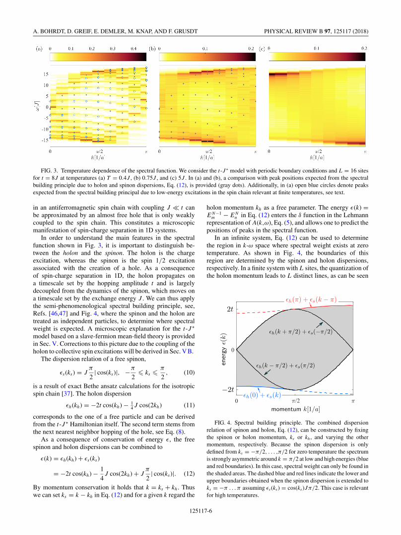
FIG. 3. Temperature dependence of the spectral function. We consider the t-J ∗ model with periodic boundary conditions and L = 16 sitesfor t = 8J at temperatures (a) T = 0.4J , (b) 0.75J , and (c) 5J . In (a) and (b), a comparison with peak positions expected from the spectralbuilding principle due to holon and spinon dispersions, Eq. (12), is provided (gray dots). Additionally, in (a) open blue circles denote peaksexpected from the spectral building principal due to low-energy excitations in the spin chain relevant at finite temperatures, see text.
in an antiferromagnetic spin chain with coupling J t canbe approximated by an almost free hole that is only weaklycoupled to the spin chain. This constitutes a microscopicmanifestation of spin-charge separation in 1D systems.
In order to understand the main features in the spectralfunction shown in Fig. 3, it is important to distinguish be-tween the holon and the spinon. The holon is the chargeexcitation, whereas the spinon is the spin 1/2 excitationassociated with the creation of a hole. As a consequenceof spin-charge separation in 1D, the holon propagates ona timescale set by the hopping amplitude t and is largelydecoupled from the dynamics of the spinon, which moves ona timescale set by the exchange energy J . We can thus applythe semi-phenomenological spectral building principle, see,Refs. [46,47] and Fig. 4, where the spinon and the holon aretreated as independent particles, to determine where spectralweight is expected. A microscopic explanation for the t-J ∗model based on a slave-fermion mean-field theory is providedin Sec. V. Corrections to this picture due to the coupling of theholon to collective spin excitations will be derived in Sec. V B.
The dispersion relation of a free spinon,
εs(ks) = Jπ
2| cos(ks)|, −π
2� ks �
π
2, (10)
is a result of exact Bethe ansatz calculations for the isotropicspin chain [37]. The holon dispersion
εh(kh) = −2t cos(kh) − 14J cos(2kh) (11)
corresponds to the one of a free particle and can be derivedfrom the t-J ∗ Hamiltonian itself. The second term stems fromthe next nearest neighbor hopping of the hole, see Eq. (8).
As a consequence of conservation of energy ε, the freespinon and holon dispersions can be combined to
ε(k) = εh(kh) + εs(ks)
= −2t cos(kh) − 1
4J cos(2kh) + J
π
2| cos(ks)|. (12)
By momentum conservation it holds that k = ks + kh. Thuswe can set ks = k − kh in Eq. (12) and for a given k regard the
holon momentum kh as a free parameter. The energy ε(k) =EN−1
m − ENn in Eq. (12) enters the δ function in the Lehmann
representation of A(k,ω), Eq. (5), and allows one to predict thepositions of peaks in the spectral function.
In an infinite system, Eq. (12) can be used to determinethe region in k-ω space where spectral weight exists at zerotemperature. As shown in Fig. 4, the boundaries of thisregion are determined by the spinon and holon dispersions,respectively. In a finite system with L sites, the quantization ofthe holon momentum leads to L distinct lines, as can be seen
FIG. 4. Spectral building principle. The combined dispersionrelation of spinon and holon, Eq. (12), can be constructed by fixingthe spinon or holon momentum, ks or kh, and varying the othermomentum, respectively. Because the spinon dispersion is onlydefined from ks = −π/2, . . . ,π/2 for zero temperature the spectrumis strongly asymmetric around k = π/2 at low and high energies (blueand red boundaries). In this case, spectral weight can only be found inthe shaded areas. The dashed blue and red lines indicate the lower andupper boundaries obtained when the spinon dispersion is extended toks = −π . . . π assuming εs(ks) = cos(ks)Jπ/2. This case is relevantfor high temperatures.
125117-6
ANGLE-RESOLVED PHOTOEMISSION SPECTROSCOPY … PHYSICAL REVIEW B 97, 125117 (2018)
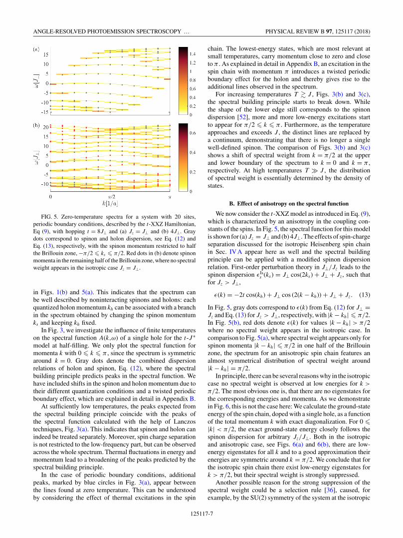
FIG. 5. Zero-temperature spectra for a system with 20 sites,periodic boundary conditions, described by the t-XXZ Hamiltonian,Eq (9), with hopping t = 8J⊥ and (a) Jz = J⊥ and (b) 4J⊥. Graydots correspond to spinon and holon dispersion, see Eq. (12) andEq. (13), respectively, with the spinon momentum restricted to halfthe Brillouin zone, −π/2 � ks � π/2. Red dots in (b) denote spinonmomenta in the remaining half of the Brillouin zone, where no spectralweight appears in the isotropic case Jz = J⊥.
in Figs. 1(b) and 5(a). This indicates that the spectrum canbe well described by noninteracting spinons and holons: eachquantized holon momentum kh can be associated with a branchin the spectrum obtained by changing the spinon momentumks and keeping kh fixed.
In Fig. 3, we investigate the influence of finite temperatureson the spectral function A(k,ω) of a single hole for the t-J ∗model at half-filling. We only plot the spectral function formomenta k with 0 � k � π , since the spectrum is symmetricaround k = 0. Gray dots denote the combined dispersionrelations of holon and spinon, Eq. (12), where the spectralbuilding principle predicts peaks in the spectral function. Wehave included shifts in the spinon and holon momentum due totheir different quantization conditions and a twisted periodicboundary effect, which are explained in detail in Appendix B.
At sufficiently low temperatures, the peaks expected fromthe spectral building principle coincide with the peaks ofthe spectral function calculated with the help of Lanczostechniques, Fig. 3(a). This indicates that spinon and holon canindeed be treated separately. Moreover, spin charge separationis not restricted to the low-frequency part, but can be observedacross the whole spectrum. Thermal fluctuations in energy andmomentum lead to a broadening of the peaks predicted by thespectral building principle.
In the case of periodic boundary conditions, additionalpeaks, marked by blue circles in Fig. 3(a), appear betweenthe lines found at zero temperature. This can be understoodby considering the effect of thermal excitations in the spin
chain. The lowest-energy states, which are most relevant atsmall temperatures, carry momentum close to zero and closeto π . As explained in detail in Appendix B, an excitation in thespin chain with momentum π introduces a twisted periodicboundary effect for the holon and thereby gives rise to theadditional lines observed in the spectrum.
For increasing temperatures T � J , Figs. 3(b) and 3(c),the spectral building principle starts to break down. Whilethe shape of the lower edge still corresponds to the spinondispersion [52], more and more low-energy excitations startto appear for π/2 � k � π . Furthermore, as the temperatureapproaches and exceeds J , the distinct lines are replaced bya continuum, demonstrating that there is no longer a singlewell-defined spinon. The comparison of Figs. 3(b) and 3(c)shows a shift of spectral weight from k = π/2 at the upperand lower boundary of the spectrum to k = 0 and k = π ,respectively. At high temperatures T � J , the distributionof spectral weight is essentially determined by the density ofstates.
B. Effect of anisotropy on the spectral function
We now consider the t-XXZ model as introduced in Eq. (9),which is characterized by an anisotropy in the coupling con-stants of the spins. In Fig. 5, the spectral function for this modelis shown for (a)Jz = J⊥ and (b) 4J⊥. The effects of spin-chargeseparation discussed for the isotropic Heisenberg spin chainin Sec. IV A appear here as well and the spectral buildingprinciple can be applied with a modified spinon dispersionrelation. First-order perturbation theory in J⊥/Jz leads to thespinon dispersion εIs
s (ks) = J⊥ cos(2ks) + J⊥ + Jz, such thatfor Jz > J⊥,
ε(k) = −2t cos(kh) + J⊥ cos (2(k − kh)) + J⊥ + Jz. (13)
In Fig. 5, gray dots correspond to ε(k) from Eq. (12) for J⊥ =Jz and Eq. (13) for Jz > J⊥, respectively, with |k − kh| � π/2.In Fig. 5(b), red dots denote ε(k) for values |k − kh| > π/2where no spectral weight appears in the isotropic case. Incomparison to Fig. 5(a), where spectral weight appears only forspinon momenta |k − kh| � π/2 in one half of the Brillouinzone, the spectrum for an anisotropic spin chain features analmost symmetrical distribution of spectral weight around|k − kh| = π/2.
In principle, there can be several reasons why in the isotropiccase no spectral weight is observed at low energies for k >
π/2. The most obvious one is, that there are no eigenstates forthe corresponding energies and momenta. As we demonstratein Fig. 6, this is not the case here: We calculate the ground-stateenergy of the spin chain, doped with a single hole, as a functionof the total momentum k with exact diagonalization. For 0 �|k| < π/2, the exact ground-state energy closely follows thespinon dispersion for arbitrary Jz/J⊥. Both in the isotropicand anisotropic case, see Figs. 6(a) and 6(b), there are low-energy eigenstates for all k and to a good approximation theirenergies are symmetric around k = π/2. We conclude that forthe isotropic spin chain there exist low-energy eigenstates fork > π/2, but their spectral weight is strongly suppressed.
Another possible reason for the strong suppression of thespectral weight could be a selection rule [36], caused, forexample, by the SU(2) symmetry of the system at the isotropic
125117-7

A. BOHRDT, D. GREIF, E. DEMLER, M. KNAP, AND F. GRUSDT PHYSICAL REVIEW B 97, 125117 (2018)
-13
-12.5
-12
-11.5
-11
-10.5
-15
-14.5
-14
-13.5
FIG. 6. The ground-state energy as a function of the total momen-tum k is shown for a single hole in a spin chain (full symbols). We usedthe same parameters as in Figs. 5(a) and 5(b), respectively. The dashedline corresponds to the free spinon dispersion (a) in the Heisenbergmodel with Jz = J⊥ and (b) in the XXZ model with Jz = 4J⊥.
point J⊥ = Jz. Because the ground state of the Heisenbergmodel is a singlet, only states with total spin S = 1/2 and onehole can have finite weight in the spectrum at zero temperature.It has been found by exact numerical simulations in Ref. [36]that this selection rule indeed applies for the ground state ofthe spin chain with one hole at momenta |k| > π/2, which hasS = 3/2. However, at only slightly higher energies of the orderof J , we have numerically found eigenstates with S = 1/2, forwhich the selection rule does not apply. In fact, these states giverise to a nonzero spectral weight at low energies for |k| > π/2.Since it is suppressed by about three orders of magnitudecompared to the spectral weight observed at the same energiesfor |k| < π/2, it is not noticeable in Fig. 5(a). In contrast towhat has been suggested in Ref. [36], a selection rule seemsnot to be sufficient to explain the asymmetry of the spectralweight observed for a hole created in a Heisenberg chain.
Above, we have ruled out the simplest two explanationswhy the spectral weight at low energies is almost completelyrestricted to one half of the Brillouin zone in the isotropic case,Jz = J⊥. This effect hints at a more fundamental structurein the ground-state wave function of the one-dimensionalHeisenberg antiferromagnet. In contrast to the Ising case,the Heisenberg spin chain has singlet character and can beunderstood as a resonating valence-bond state [44]. So, itis interesting to ask whether the valence-bond character ofthe ground-state wave function is sufficient to explain thesharp drop of the spectral weight when the spinon momentumcrosses k = π/2. We have checked that this is not the case,by calculating the spectral function for a hole created insidea spin chain with Majumdar-Gosh couplings [53,54], seeAppendix C. The ground state of this model is a valence bondsolid. While the spectral weight is asymmetric around k = π/2
in this case, it smoothly drops as the spinon momentum π/2is traversed.
We argue instead that the sharp decrease of the spectralweight for a single hole in the Heisenberg chain can beunderstood as a direct signature for the presence of a Fermi seaof spinons, see Fig. 1(c). This is characteristic for a quantumspin liquid [55]. In Ref. [48], it has been suggested that theFermi sea is formed by Jordan-Wigner fermions, which canbe introduced by fermionizing the spins. However, at theisotropic point Jz = J⊥ these Jordan-Wigner fermions arestrongly interacting, and the noninteracting Fermi sea is not agood approximation. Instead, slave fermions can be introducedas in the usual mean-field description of quantum spin liquids[55]. They are weakly interacting at the isotropic point andform two half-filled spinon Fermi seas. These arguments aresupported by slave particle mean-field calculations. In Sec. V Aof this paper, we present a mean-field theory for a single holeand arbitrary values of the anisotropy J⊥/Jz. A related work onslave-particle mean-field descriptions of one-dimensional spinchains has been presented in Ref. [56]. In our paper, we utilizethe slave-fermion theory to analyze the spectral function.
C. Spectral function of spin-imbalanced systems
In the slave-particle mean-field picture, the slave fermionsform two spinon Fermi seas. Therefore we expect to see twodifferent Fermi momenta when the system is spin-imbalanced.Our scheme to measure the spectral function in experimentswith cold atoms is particularly well suited to access the spectralfunction of a single hole in a system with finite magnetization.Moreover, by detecting the spin of the removed particle [9], thespin-resolved version of the spectral function can be measured.
In Fig. 7(a), the spectral function of a single hole in a spinimbalanced system is shown for a removed particle with spinup and down, respectively. As in Fig. 3, gray dots denote the po-sitions of expected peaks due to holon and spinon dispersions,Eq. (12) for −k
↑/↓F � k � k
↑/↓F with k
↑/↓F = πN↑/↓/L. In the
slave-fermion mean-field theory, the spinons form two Fermiseas, which are filled corresponding to the spin imbalance inthe system. Accordingly, in Fig. 7(a), the sharp decrease inspectral weight occurs at different momenta for the removedparticle belonging to the majority or minority species.
V. THEORETICAL ANALYSIS
In the previous section, we have explained the numericalresults for the single-hole spectral function using the semiphe-nomenological spectral building principle. We now present atheoretical formalism to obtain the results in Eqs. (10) and(11) directly from the microscopic Hamiltonian. We describea single hole in an antiferromagnetic spin chain. In order todescribe the spin chain, we use a slave-fermion mean-fieldtheory [55–57], which contains a nontrivial order parameter,that is finite even in one dimension. For simplicity, we considersituations with zero total magnetization.
Our starting point is the t-XXZ model (9) with zero or onehole. We introduce slave boson operators hj to describe theholons, and constrained fermions fj,α describing the remainingspins [44]. The index α = ↑,↓ corresponds to the two spin
125117-8

ANGLE-RESOLVED PHOTOEMISSION SPECTROSCOPY … PHYSICAL REVIEW B 97, 125117 (2018)
(b)
spinon momentum
energ
y
0 π
spinon band
/−π 2−π / π2
lattice modulation
k↑F k↓
F
-10
0
10
0.4
0.8
1.2
0 /π π2k [1/a]
ω[J
]
-10
0
10
0.1
0.2
0.3
ω[J
]
A(k, ω)
(a) minority spectrum
majority spectrum
FIG. 7. Spectral function in a spin-imbalanced system with 20sites and N↑ = 4, N↓ = 16 at zero temperature and with periodicboundary conditions. (a) shows the minority (top) and majority(bottom) spectrum, resolved after the spin of the removed particle.(b) depicts the spinon Fermi seas for the two different species, whichare filled correspondingly.
states and it holds
Si = 1
2
∑α,β
f†i,ασ α,β fi,β . (14)
The slave particles satisfy the condition∑α
f†j,αfj,α + h
†j hj = 1 (15)
and the original fermionic operators can be expressed as
cj,α = h†j fj,α. (16)
Using the new operators, one can identify a spin state|σ1, . . . ,σL〉 with σj = ↑,↓ as
|σ1, . . . ,σL〉 ≡ f†1,σ1
. . . f†L,σL
|0〉 (17)
and create all states with holes by applying h†j fj,α from
Eq. (16). Note that the ordering of f operators in Eq. (17)is important due to their fermionic anticommutation relations.
We can substantially simplify the formalism by introducinga new basis where the holons occupy bonds between thelattice sites j of the so-called squeezed space [12,58,59],which is obtained by removing all holes from the spin chain.By including only operators fj,α on sites j , we obtain new
operators ˆfj,α = fj ,α with j = j + ∑i�j h
†i hi . The main ad-
vantage of this mapping is the form of the hopping term in
Eq. (9): using the original operators fj,α , we obtain a difficultquartic expression −t
∑〈i,j〉
∑σ h
†j hi f
†i,σ fj,σ . In contrast, in
terms of the operators ˆfj,α , a quadratic term involving onlyholons is obtained, −t
∑〈i,j〉 h
†j hi , see Appendix D. This
leaves the spin order in squeezed space unchanged. Moreover,this term yields the dominant part of the free holon dispersionrelation Eq. (11), −2t cos(kh). Corrections due to next-nearest-neighbor tunneling, which is included in the t-J ∗ model, arederived in Appendix D.
By creating a hole and removing a spin, the number ofˆf fermions changes according to Eq. (16). The total spin is
thus changed by 1/2 and the operators ˆf can be identifiedwith fermionic spinons [55]. In squeezed space, the last twoterms of Eq. (9) do not change and correspond to a spin chainwithout doping. In Sec. V A, we derive the shape of the spinondispersion Eq. (10) by considering the undoped spin chain.
In addition, there exist interactions between the holon andthe surrounding spins in squeezed space. As discussed in detailin Appendix D, the presence of a holon on the bond betweensites j and j + 1 effectively switches off the coupling betweenthe corresponding spins in the t-XXZ model (9). In the t-J ∗model (8), it also affects next-nearest-neighbor couplings. Wediscuss in Sec. V B how these interactions renormalize theholon properties.
A. Slave-fermion mean-field theory of undoped spin chains
In this section, we present a slave-fermion mean-fieldtheory for the undoped XXZ spin chain which—up to aprefactor—allows us to derive the exact spinon dispersionrelation known from Bethe ansatz. Furthermore, it enables anintuitive understanding of the asymmetry in the distribution ofspectral weight around k = π/2 found in the case of isotropicHeisenberg couplings, see Sec. IV B.
We consider the slave fermion operators ˆfj,α discussedabove by introducing the notion of squeezed space. TheHamiltonian of the spin chain, Eq. (9) at half-filling, can beexpressed in terms of the spinon operators [55],
HXXZ = − 1
2
∑i,α
ˆf †i,α
ˆfi+1,α[J⊥ ˆf †i+1,α
ˆfi,α + Jzˆf †i+1,α
ˆfi,α]
+ Jz
2
∑i,α
ˆf †i,α
ˆfi,α − Jz
4
∑i,α,β
ˆf †i,α
ˆfi,αˆf †i+1,β
ˆfi+1,β ,
(18)
where ↑ = ↓ and ↓ = ↑. This expression is exact within thesubspace defined by the constraint
∑α
ˆf †i,α
ˆfi,α = 1. In themean-field approximation applied below, this constraint isreplaced by its ground-state expectation value∑
α
〈 ˆf †i,α
ˆfi,α〉 = 1. (19)
1. Mean-field description
In the following, we consider the case of zero total mag-netization in the thermodynamic limit. At the isotropic point,Jz = J⊥, Eq. (18) becomes the SU(2) invariant HeisenbergHamiltonian HH. In this case we replace the operator ˆf †
i,αˆfi+1,α
125117-9
A. BOHRDT, D. GREIF, E. DEMLER, M. KNAP, AND F. GRUSDT PHYSICAL REVIEW B 97, 125117 (2018)
by its ground-state expectation value
χi,α = 〈 ˆf †i,α
ˆfi+1,α〉. (20)
When χi,α = χ is independent of the spin index α, theresulting mean-field Hamiltonian is also SU(2) invariant. Bydiagonalizing the latter, we obtain a self-consistency equationfor χ , which will be solved numerically below.
To obtain a mean-field description away from the SU(2)invariant Heisenberg point, i.e., when Jz �= J⊥, we can writethe original Hamiltonian as a sum of the Heisenberg term HH
plus additional Ising couplings,
HXXZ = HH + (Jz − J⊥)︸ ︷︷ ︸=�Jz
1
4
∑i
δi δi+1, (21)
where δi = 2Szi is the local magnetization,
δi =∑
α
(−1)α ˆf †i,α
ˆfi,α, (−1)↑ = 1, (−1)↓ = −1. (22)
We also allow for a finite expectation value of the magneti-zation in the mean-field description. Assuming that the discretesymmetry T x Sx , which flips the spins and translates the systemby one lattice site, is unbroken, we obtain
〈δi〉 = (−1)iδ. (23)
This leads to a second self-consistency equation for thestaggered magnetization δ.
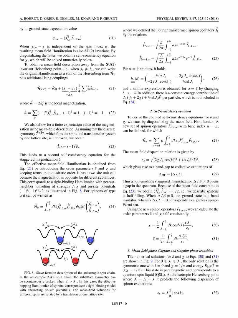
The effective mean-field Hamiltonian is obtained fromEq. (21) by introducing the order parameters δ and χ andkeeping terms up to quadratic order. It has a two-site unit cellbecause the magnetization is opposite for different sublattices.This corresponds to a tight-binding Hamiltonian with nearest-neighbor tunneling of strength J⊥χ and on-site potentials(−1)i(−1)αδ/2, as illustrated in Fig. 8. For spinons of typeα it can be written as
Hα =∫ π
2
− π2
dk( ˆf †k,A,α
ˆf †k,B,α)hα(k)
(ˆfk,A,α
ˆfk,B,α
), (24)
FIG. 8. Slave-fermion description of the anisotropic spin chain.In the anisotropic XXZ spin chain, the sublattice symmetry canbe spontaneously broken when Jz > J⊥. In this case, the effectivehopping Hamiltonian of spinons corresponds to a tight-binding modelwith alternating on-site potentials. The mean-field solutions fordifferent spins are related by a translation of one lattice site.
where we defined the Fourier transformed spinon operators ˆfk
by the relations
ˆf2n,α =√
L
2π
∫ π2
− π2
dke−2ikn ˆfk,A,α,
ˆf2n+1,α =√
L
2π
∫ π2
− π2
dke−2ikne−ik ˆfk,B,α. (25)
For α = ↑ spinons, it holds
h↑(k) =( −δ/2�Jz −2χJ⊥ cos(kx)
−2χJ⊥ cos(kx) δ/2�Jz
), (26)
and a similar expression is obtained for α = ↓ by changingδ → −δ. In addition, there is a constant energy contribution ofJ⊥(1/4 + 2χ ) + 1/4�Jzδ
2 per particle, which is not included inEq. (24).
2. Self-consistency equation
To derive the coupled self-consistency equations for δ andχ , we start by diagonalizing the mean-field Hamiltonian. Anew set of spinon operators Fk,μ,α , with band index μ = ±,can be defined, for which
Hα =∑
μ=±1
μ
∫ π2
− π2
dkεkF†k,μ,αFk,μ,α. (27)
The mean-field dispersion relation is given by
εk =√
(2χJ⊥ cos(k))2 + (�Jzδ/2)2, (28)
which gives rise to a band-gap to collective excitations of
�MF = |�Jzδ|. (29)
Thus a nonvanishing staggered magnetization �Jzδ �= 0 opensa gap in the spectrum. Because of the mean-field constraint inEq. (23), we obtain 〈 ˆf †
i,αˆfi,α〉 = 1/2, i.e., we describe spinons
at half-filling. When �Jzδ �= 0, the ground state is a bandinsulator, whereas �Jzδ = 0 corresponds to a gapless spinonFermi sea.
Using the new spinon operators Fk,μ,α , we can calculate theorder parameters δ and χ self-consistently,
χ = 1
π
∫ π2
− π2
dk cos2(k)χJ⊥εk
, (30)
δ = 1
2π
∫ π2
− π2
dk�Jzδ
εk
. (31)
3. Mean-field phase diagram and singular phase transition
The numerical solutions for δ and χ to Eqs. (30) and (31)are shown in Fig. 9. For 0 � Jz � J⊥, the only solution is thesymmetric one with δ = 0 and χ = 1/π and energy EMF(δ =0,χ = 1/π ). This state is paramagnetic and corresponds to aquantum spin liquid (QSL). At the isotropic Heisenberg pointwhere Jz = J⊥ = J it predicts the following dispersion ofspinon excitations:
εk = J2
π| cos k|. (32)
125117-10

ANGLE-RESOLVED PHOTOEMISSION SPECTROSCOPY … PHYSICAL REVIEW B 97, 125117 (2018)
FIG. 9. Mean-field theory for the spin chain. Numerical solutionof the self-consistency equations for the order parameters χ and δ,Eqs. (30) and (31). For 0 � Jz � J⊥, the ground state is a gaplessquantum spin liquid (QSL). For Jz � J⊥, the two order parameters δ
and χ are both nonvanishing and the ground state is a spin-densitywave (SDW).
The analytical form of the spinon dispersion ∼| cos(k)| iscorrectly described by the mean-field theory. Compared tothe exact result from Bethe ansatz calculations, Eq. (10), thisexpression is too small by a factor of π2/4 ≈ 2.47. Deviationsfrom the exact solution are a result of the mean-field approxi-mation, i.e., our neglecting of gauge fluctuations ensuring theconstraint of single occupancy [55].
For Jz > J⊥, two additional solutions ±δ �= 0 with anenergy below EMF(δ = 0,χ = 1/π ) appear (only the solutionwith δ > 0 is shown in Fig. 9). In this regime, the translationalsymmetry of the original Hamiltonian Eq. (18) is sponta-neously broken. Because there exists a nonzero staggeredmagnetization δ �= 0, this phase can be identified with a spindensity wave (SDW). At large couplings, Jz � 2J⊥, we findthat the mean-field order parameter χ vanishes and the systemis fully ordered with δ = ±1 as expected in the classical Néelstate. This second transition is an artifact of the mean-fieldtheory: from exact Bethe ansatz calculations it is known thatthe staggered magnetization approaches the classical valueδ = ±1 monotonically until it is asymptotically reached forJz/J⊥ → ∞. Here, we are more interested in the behavior ofthe transition at Jz = J⊥.
As can be seen from Fig. 9, the order parameter δ onlytakes a significant value for Jz � 1.2J⊥. By solving the ellipticintegral in Eq. (31) perturbatively in the limit δ 1, we findthat the staggered magnetization depends nonanalytically onJz − J⊥, with all derivatives dnδ/d�Jn
z = 0 vanishing at theHeisenberg point:
δ � 4
π
J⊥Jz − J⊥
e−2 J⊥
Jz−J⊥ . (33)
From Eq. (29), it follows that the excitation gap has theasymptotic form
�MF � 4
πJ⊥ exp
(−2
J⊥Jz − J⊥
). (34)
The excitation gap �MF close to the transition point fromQSL to SDW can be compared to exact results �B obtainedfrom Bethe ansatz methods for the XXZ chain. From theexact expressions derived in Ref. [38], we obtain the following
asymptotic behavior:
�B � 4πJ⊥ exp
[− π2
2√
2
(J⊥
Jz − J⊥
)1/2]. (35)
The nonanalyticity is correctly predicted by the mean-fieldtheory, and only the power-law exponent appearing in theexponential function is not captured correctly.
We conclude that the slave-fermion mean-field theoryprovides a rather accurate description of the one-dimensionalspin chain near the critical Heisenberg point. This is possiblebecause a nontrivial order parameter (χ ) is introduced thatdoes not vanish even in one dimension. The theory providesquantitatively reasonable results and describes correctly thequalitative behavior at the singular phase transition fromQSL to the conventional symmetry broken SDW phase. Wenow show that it moreover offers a simple explanation ofthe observed asymmetric spectral weight in the single-holespectral function of the Heisenberg spin chain.
4. Spectral weight of spinon excitations
We proceed by calculating the matrix elements that de-termine the weight in the single-hole spectra based on theslave-fermion mean-field theory. The relevant matrix elementsare of the form
λnks
= |〈ψn| ˆfks,σ |ψ0〉|2 −π � ks � π, (36)
which describe the creation of a hole in the ground state of thespinon system. Here,
|ψ0〉 =π/2∏
k=−π/2
∏σ
F†k,−,σ |0〉 (37)
is the ground state of the undoped spin chain.The full spectral function A(k,ω) is a convolution of the
spinon part and the holon part,
A(k,ω) =π∑
kh,ks=−π
∫dωhdωsδ(ω − ωs − ωh)
× δk,kh+ksAs(ks,ωs)Ah(kh,ωh). (38)
Neglecting the coupling of the holon to collective excitations ofthe spin chain, see Sec. V B, the holon spectrum is determinedby Ah(kh,ωh) = δ(ωh − εh(kh)). The spinon part is given byAs(ks,ωs) = ∑
n δ(ωs − ωn)λnks
, where the eigenstate |ψn〉 hasenergy ωn.
For every ks , there exists one unique state |ψn〉 with λnks
�= 0.The corresponding λks
:= λnks
can be calculated by mapping the
original spinon operators ˆfks,σ onto the transformed operatorsFks ,±,σ . This leads to
λks=
{cos2
( θks
2
) |ks | � π/2,
sin2( θks
2
) |ks | > π/2,(39)
where the mixing angle is determined by
tan θks= δ(Jz − J⊥)
4χJ⊥ cos(ks). (40)
In the isotropic Heisenberg case, J⊥ = Jz = J , the onlysolution to the self-conistency equation is δ = 0, leading to
125117-11
A. BOHRDT, D. GREIF, E. DEMLER, M. KNAP, AND F. GRUSDT PHYSICAL REVIEW B 97, 125117 (2018)
θks= 0 and thus
λks=
{1 |ks | � π/2,
0 |ks | > π/2.(41)
This discontinuity in λksgives rise to the sharp drop of spectral
weight observed in Figs. 1(b), 3, and 5(a) when ks is variedacross the value π/2. It is a direct signature for the spinon Fermisea, which in turn is a key signature of a quantum spin liquid.
In the Ising limit J⊥ = 0, we obtain the classical Néel statewith δ = ±1 and χ = 0. This yields θks
= π/2, i.e.,
λks= 1
2 . (42)
In this case, discrete translational symmetry is broken, whichleads to a mixing of momenta ks and ks + π and a homoge-neous redistribution of spectral weight across all ks . There istherefore no discontinuity in the distribution spectral weight atthe zone boundary ks = ±π/2.
B. Renormalization of holon properties: The holon-polaron
In our analysis of the single-hole spectrum in Sec. IV A,based on the spectral building principle, we neglected cou-plings of the holon to the spin environment. We now discussleading order corrections to this picture, which scale as J/t .Experimentally, the relevant parameter regime of the t-J ∗model is J/t 1, therefore these corrections are genericallysmall.
The essence of spin-charge separation is that the spinonand the holon are not bound to one another and can betreated independently. Nevertheless, when the holon is movingthrough the spin chain, it interacts with the surrounding spinsand becomes dressed by collective excitations with vanishingtotal spin. This effect can be understood by the formation ofa polaronic quasiparticle [60], which we will refer to as theholon-polaron from now on. Note that this situation is differentfrom two dimensions. In that case, there is no spin-chargeseparation and a magnetic polaron carrying spin 1/2 is formedby a hole moving in a two-dimensional Néel state [61–69].
We start from the t-J ∗ Hamiltonian (8), which is an exactasymptotic representation of the Fermi-Hubbard model forlarge U at half-filling. Then we use a formulation in squeezedspace [59], where the holon effectively moves between thebonds of the lattice on which it switches off the superexchangeinteraction. The collective excitations of the spin chain, whichcan be understood as particle-hole pairs ˆf † ˆf in the spinonFermi sea discussed in the previous section, are then describedusing the bosonization formalism [70] and assuming an infinitesystem. In combination, we arrive at a conventional polaronHamiltonian that can be solved perturbatively for weak po-laronic couplings J t . Note that weak polaronic couplingcorresponds to large coupling U � t in the original FermiHubbard model. For details of our calculations, we refer toAppendix E.
We calculated the leading-order corrections to the holon-polaron properties. For the ground-state energy of the holon-polaron, we obtain
E0h = −2t − J
4− J 2
t(0.0343 + 6.54m2 + 5.31|C|4). (43)
This energy is measured relative to a chain with the samenumber of spins but without the holon. Here, m = (N↑ −N↓)/2L denotes the magnetization per length. The nonuniver-sal constant |C|2 ≈ 0.14 was determined by Eggert and Affleck[71] from comparison of the spin-structure factor obtainedfrom bosonization and quantum Monte Carlo calculations.
The effective mass of the holon polaron is defined byexpanding its energy Eh(ph) around momentum ph = 0 whereEh is minimized,
Eh(ph) = E0h + 1
2Mhp2
h + Op4h. (44)
For the renormalized holon mass, we obtain
1
Mh= 2t − 2.77J + 39.5Jm2
− J 2
t(0.188 + 87.2m2 + 43.2|C|4). (45)
The expressions (43) and (45) are correct up to terms of orderO(J 3/t2).
For parameters as in Fig. 5(a), i.e., t = 8J and m = 0, weobtain corrections to the holon energy of �E0
h = E0h + 2t =
−0.27J . The ground-state energy per bond in the spin-chainwithout the hole is E0/L ≈ −0.44J , see, e.g., Ref. [37].Hence we expect the lower edge of the spectrum at ω− =−2t + (0.44 − 0.27)J = −15.83J . The corrections are of thecorrect order of magnitude, as can be seen by comparison to thevalue ω− ≈ −15.80J , which has been obtained from a finitesize scaling of exact diagonalization results [72]. We expectthat the dominant source for errors are finite size effects and theambiguity of the ultraviolet cut-off chosen in the bosonization.In the context of Bose polarons in one dimension, it has beenshown that the latter effect can lead to sizable corrections tobosonization results [73]. For the renormalized mass, we obtain2tMh = 1.22, which corresponds to a 22% mass enhancement.This value is consistent with the exact numerical results inFig. 5, but it is too small for a meaningful direct comparison dueto finite-size effects and in particular the required momentumresolution.
In principle, both the holon mass and energy renormaliza-tion can be measured experimentally by close inspection of thespectrum. However, as demonstrated above, the overall effectis very weak. Using ultracold atoms, the t-J model can also beimplemented independently of the Fermi-Hubbard model byusing polar molecules [34] or Rydberg dressing [32,33]. Thisallows one, in principle, to tune the polaronic coupling J/t toarbitrary values, smaller or larger than one. When J � t , weexpect a strong renormalization of the holon-polaron propertieswhich can be studied in the future using a formalism along thelines of the one presented in Appendix E.
In contrast to the situation for the t-J ∗ model, the limitJ/t → 0 is not well defined for the t-J model. We show inAppendix E that one obtains infrared-divergent integrals tolowest order for the energy and the effective mass because thenext-nearest-neighbor terms are missing.
The dressing of the holon with collective excitations canlead to small corrections in the shape of the spectral function.In addition to coherent delta peaks, an incoherent backgroundassociated with collective excitations appears, as expected
125117-12
ANGLE-RESOLVED PHOTOEMISSION SPECTROSCOPY … PHYSICAL REVIEW B 97, 125117 (2018)
from the Luttinger liquid description. The latter can be derivedeven at finite doping using a squeezed space description [74].
VI. EXTENSIONS
The scheme for measuring the spectral function of a singlehole can be generalized to implement different spectroscopicprobes using ultracold atoms. In this section, we brieflyillustrate two examples, although a detailed analysis is devotedto future work. We show how the dynamical structure factorS(ω,k) can be measured in one-dimensional spin chains(Sec. VI A), and discuss how the scheme can be extended toimplement the analog of double photoelectron spectroscopy[75,76] (Sec. VI B).
A. Dynamical spin structure factor
The spectral function A(k,ω) probes the properties of asingle hole interacting with the surrounding spins. To obtaininformation about the spin system alone, more direct mea-surement schemes are required where no charge excitationsare generated. The most common example is the dynamicalspin structure factor S(k,ω), where a spin-flip excitation withmomentum k is created at an energy ω. Using a Lehmannrepresentation similar to Eq. (5) it can be defined by
S(k,ω) = 1
2Z0
∑n,m
e−βEMn
∣∣⟨ψM+1m
∣∣S+k
∣∣ψMn
⟩∣∣2
× δ(hω − EM+1
m + EMn
), (46)
with |ψMn 〉, EM
n denoting the eigenstates and energies of thesystem S with total magnetization M . In solids, S(k,ω) can bemeasured in inelastic neutron scattering experiments [77].
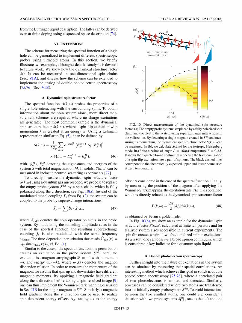
To directly measure the dynamical spin structure factorS(k,ω) using a quantum gas microscope, we propose to replacethe empty probe system Sdet by a spin chain, which is fullypolarized along the z direction, see Fig. 10(a). Instead of themodulated tunnel coupling Ty from Eq. (2), the system can becoupled to the probe by superexchange interactions,
Jy =∑
i
Si · Si,det, (47)
where Si,det denotes the spin operator on site i in the probesystem. By modulating the tunneling amplitude ty as in thecase of the spectral function, the resulting superexchangecoupling jy is also modulated with the same frequencyωshake. The time-dependent perturbation thus reads Hpert(τ ) =δjy sin(ωshakeτ )Jy , cf. Eq. (1).
Similar to the case of the spectral function, the perturbationcreates an excitation in the probe system Sdet; here, theexcitation is a magnon carrying spin Sz = −1 with momentum−k and energy ωm(−k), where ωm(k) denotes the magnondispersion relation. In order to measure the momentum of themagnon, we assume that spin up and down states have differentmagnetic moments. By applying a magnetic field gradientalong the x direction before taking a spin-resolved image [9]one can thus implement the Wannier-Stark mapping discussedin Sec. II B for the single magnon in Sdet. Similarly, a magneticfield gradient along the y direction can be used to realizespin-dependent energy offsets �σ , analogous to the energy
k
−kSdet
S
(a)
-1
0
1
2
3
0.5
1
1.5
2
et
Δ↓Δ↑
ω[J
]
0 /π π2k [1/a]
spin excitationmomentum
(b)
S(k, ω)
FIG. 10. Direct measurement of the dynamical spin structurefactor. (a) The empty probe system is replaced by a fully polarized spinchain and coupled to the system using superexchange interactions inthe y direction. By detecting a single magnon created in Sdet and mea-suring its momentum, the dynamical spin structure factor S(k,ω) canbe measured. In (b), we calculate S(k,ω) for the isotropic Heisenbergmodel in a finite-size box of length L = 16 at a temperature T = 0.2J .It shows the expected broad continuum reflecting the fractionalizationof a spin-flip excitation into a pair of spinons. The black dashed linescorrespond to the theoretically expected upper and lower boundariesat zero temperature.
offset � considered in the case of the spectral function. Finally,by measuring the position of the magnon after applying theWannier-Stark mapping, the excitation rate �(k,ω) is obtained,which is directly related to the dynamical spin structure factor
�(k,ω) = 2π
h|δjy |2S(k,ω), (48)
as obtained by Fermi’s golden rule.In Fig. 10(b), we show an example for the dynamical spin
structure factor S(k,ω), calculated at finite temperature and forrealistic system sizes accessible in current experiments. Thespin flip creates a pair of two fractionalized spinon excitations.As a result, one can observe a broad spinon continuum, whichis considered a key indicator for a quantum spin liquid.
B. Double photoelectron spectroscopy
Further insight into the nature of excitations in the systemcan be obtained by measuring their spatial correlations. Aninteresting method which achieves this goal in solids is doublephotoelectron spectroscopy [75,76], where a correlated pairof two photoelectrons is emitted and detected. Similarly,processes can be considered where two atoms are transferredinto the initially empty probe system Sdet. To avoid interactionsbetween the two emitted atoms, one could e.g. consider asituation with two probe systems Sdet
L,R, one to the left and one
125117-13
A. BOHRDT, D. GREIF, E. DEMLER, M. KNAP, AND F. GRUSDT PHYSICAL REVIEW B 97, 125117 (2018)
to the right of the system S, and post-select on cases with oneatom per probe system.
The resulting spectrum contains pairs of individual one-particle events as well as two-particle processes which provideadditional information about the system. The two-particlecontributions can be distinguished from one-particle effectsby using coincidence measurements. In this technique, onepost-selects events where both excitations are created simulta-neously. In the quantum gas microscope setups discussed here,this can be achieved by extending Sdet
L,R in the y direction. Onecan use the traveled distance from the system S in y directionas a measure of the time that passed between the creation andthe detection of a particle.
From the coincidence measurements describedabove, information about the two-hole spectral functionA12(k1,k2,k
′1,k
′2; ω) can be extracted, see Ref. [76]. It
contains information about the correlations between thetwo created holes in the system. These correlations areexpected to be weak in a system with one-dimensional chainswith spin-charge separation, where holons form a weaklyinteracting Fermi sea [37,78]. On the other hand, in systemsthat are superconducting, correlations are expected to playan important role and give rise to distinct features of Cooperpairing in the two-hole spectrum [79]. Using ultracold atoms,situations with attractive Hubbard interactions U < 0 havebeen realized [11], which become superconducting at lowtemperatures. Here the method described above could beapplied to directly access the strong two-particle correlationspresent in this system.
VII. SUMMARY AND OUTLOOK
In this work, we have proposed a measurement scheme forthe single-particle excitation spectrum A(k,ω) in a quantumgas microscope. Our method can be understood as an analog ofangle-resolved photoemission spectroscopy (ARPES), whichhas been key to the study of excitation spectra in manystrongly correlated materials. In our method, the weak tunnelcoupling from the system under investigation to an initiallyempty detection system is modulated with frequency ω. Thespectral function A(k,ω) can then be obtained directly from thetunneling rate into a single-particle eigenstate of the detectionsystem with momentum k and energy ε(k).
We have analyzed the scheme for single-hole spectra inone-dimensional spin chains. Effects from finite size, nonzerotemperature, and the presence of sharp edges are includedin our numerical simulations. We discussed two characteris-tic features of the spectral function A(k,ω): (i) spin-chargeseparation and (ii) the distribution of the spectral weight.(i) Spin-charge separation can be identified in the spectralfunction both for isotropic and anisotropic spin couplings. Itreveals that a hole created in the system separates into a spin-less holon and a spinon. Moreover, their different characteristicenergy scales t and J , respectively, can be resolved. (ii) For theisotropic Heisenberg model, we observed a strong suppressionof the low-energy spectral weight at momenta k > π/2. Theground state of the isotropic Heisenberg model is a quantumspin liquid with gapless excitations [37]. We discussed aslave-fermion mean-field description of this state, which canbe qualitatively understood as a Fermi sea of noninteracting
spinons with Fermi momentum π/2 [55]. This description canexplain the sharp decrease of the spectral weight when thespinon momentum ks crosses the corresponding spinon Fermimomentum at π/2.
While related ARPES measurements of the spectral func-tion in solids have already shown distinct spinon and holonpeaks at low energies [51], an observation with ultracold atomswould allow to distinguish spinon and holon dispersions onall energy scales, because phonon contributions and effectsfrom higher bands are absent. Moreover, the sharp decrease ofthe spectral weight at π/2 is present at temperatures currentlyachievable in experiments with ultracold fermions. Hence itcould provide the first direct signature of a Luttinger spin liquidof cold atoms.
The sharp step in the spinon spectral weight across its Fermimomentum is to some extent reminiscent of the Fermi arcsobserved in the pseudogap phase of quasi-2D cuprates. Toexplore the relation of these two phenomena experimentally,ultracold atoms can be used to study the dimensional crossoverbetween the 1D and 2D Fermi Hubbard model in the future. Intwo-dimensional systems with long-range antiferromagneticorder it is expected that spinon and holon are bound together ina confined phase [61–66], similar to mesons, which are boundstates of two quarks [80,81]. The transition to the pseudogapphase at finite doping and the microscopic origin of Fermiarcs observed in ARPES is poorly understood. Our methodfor measuring the spectral function can be generalized to twodimensions, where a second layer can be utilized as the probesystem.
Much of the physics discussed in this paper can be relatedto simple models of noninteracting spinon and holon slaveparticles. This approach is successful due to a large separationof energy scales associated with holon and spinon dynamics(t and J , respectively). When t and J become comparable,however, corrections to the simple physical pictures becomerelevant. We systematically studied leading order correctionsin J/t for the Fermi-Hubbard model at strong coupling.A bosonization formalism was used to describe the holondressing by collective excitations of the spin chain, and wehave derived expressions for the renormalized holon energyand its effective mass.
An interesting future direction of research is the study ofthe t-J Hamiltonian with a single hole by tuning the ratiot/J . The holon can be understood as a mobile impurity, witha tunable bare mass given by ∼1/2t , which is interacting withcollective excitations of the spin chain. This allows one toexplore connections with one-dimensional impurity problems,for which rich physics have been found close to [73,82–86]and far from equilibrium [87–89].
ACKNOWLEDGMENTS
The authors would like to thank Christie Chiu and GeoffreyJi for carefully reading our manuscript and for providing usefulcomments. The authors also acknowledge fruitful discus-sions with Gregory Astrakharchik, Immanuel Bloch, SebastianEggert, Markus Greiner, Christian Gross, Timon Hilker, Ran-dall Hulet, Márton Kanász-Nagy, Salvatore Manmana, Ef-stratios Manousakis, Matthias Punk, Subir Sachdev, Guil-laume Salomon, Richard Schmidt, Imke Schneider, Maksym
125117-14
ANGLE-RESOLVED PHOTOEMISSION SPECTROSCOPY … PHYSICAL REVIEW B 97, 125117 (2018)
Serbyn, Yulia Shchadilova, Tao Shi, Yao Wang, and JohannesZeiher. We acknowledge support from the Technical Universityof Munich - Institute for Advanced Study, funded by the Ger-man Excellence Initiative and the European Union FP7 underGrant Agreement 291763 (A.B., M.K.), the DFG Grant No.KN 1254/1-1 (A.B., M.K.), the Studienstiftung des deutschenVolkes (A.B.), the Harvard Quantum Optics Center and theSwiss National Science Foundation (D.G.), the Gordon andBetty Moore foundation (F.G.) and from Harvard-MIT CUA,NSF Grant No. DMR-1308435 as well as AFOSR QuantumSimulation MURI, AFOSR Grant No. FA9550-16-1-0323(F.G., E.D.).
APPENDIX A: IMPLEMENTATION OF THEMEASUREMENT SCHEME FOR THE t- J∗ MODEL
A balanced two-component spin mixture of ultracoldfermionic atoms in an optical lattice allows for a clean imple-mentation of the t-J ∗ model introduced in Eq. (8) in the limitof large U/t � 1. To create the optical lattice configurationnecessary for the detection scheme, we propose a standardretroreflecting laser configuration along the x direction witha lattice depth of Vx and tunneling t , and a superlatticeconfiguration in the y direction that creates several copies ofdecoupled double-well systems [see Fig. 1(a)]. This has theadvantage of obtaining several measurements per experimentalcycle. However, a standard lattice along the y direction couldalso be used and the energy offset � could be created with adigital micromirror device.
The superlattice potential can be created for example bytwo retroreflected laser beams at wavelengths λy/2 and λy
[90], which create a short and long wavelength lattice of depthV l
y and V sy . By setting their phase difference ϕ close to π/2
a controlled energy offset between the two sites of the doublewell can be introduced with bare tunneling ty . The total opticalpotential is given by
V (x,y) = Vx cos2(2πx/λx) + V ly cos2(2πy/λy)
+V sy cos2(4πy/λy − ϕ). (A1)
The lattice depths along the y direction can be chosen suffi-ciently deep, such that the tunneling between different doublewells is negligible. In addition, the energy offset is much largerthan all other energy scales � � U,t (but smaller than theenergy gap to the next band) to make direct tunneling processesoff resonant. This also ensures that there are no atoms inSdet when loading the fermionic spin mixture from the initialharmonic trap into the lattice.
To implement the detection scheme for the spectralfunction, we propose to periodically modulate the depthof the long wavelength lattice according to V l
y (t) = V ly +
δV ly sin(ωshakeτ ). This leads to an induced oscillatory tun-
nel coupling δty along the y direction between the spinsystem S and the detection system Sdet. Thereby theperturbation described in Eq. (2) can be realized. Thestrength of the induced tunneling is given by δty =δVλ
∫w∗
L(y) cos2(2πy/λ)wR(y)dy, where wL(y) and wR(y)denote the Wannier functions of the left and right lattice sitesof the double-well system created by the lattices along the y
direction [91].
APPENDIX B: MOMENTUM SHIFTS FOR THE SPECTRALBUILDING PRINCIPLE
In this Appendix, we discuss the different shifts for holonand spinon momenta that have to be taken into account in theapplication of the spectral building principle in Eqs. (12) and(13). Strictly speaking, there is no translational invariance insqueezed space. However, it is a good approximation up to 1/L.The first momentum shift we discuss is due to these corrections.The holon moves along L lattice sites. Its momentum istherefore quantized in units of 2π/L. By contrast, there areonly L − 1 spins, such that the spinon momentum is ks =ns2π/(L − 1) with ns integer. Therefore we have to shift themomentum to account for the different quantization conditionsfor spinon and holon. The spinon momentum ks = k − kh inEq. (12) is thus replaced by
k′s = k − kh + k − kh
L − 1. (B1)
This is the smallest possible shift to obtain the correct quanti-zation of k′
s as an integer multiple of 2π/(L − 1).In a chain with periodic boundary conditions, a further
momentum correction arises: the holon shifts the spins by onelattice site every time it moves across the entire system. Whenthe spins are translated by one site, the wave function picksup an overall phase eiPs , where Ps is the total momentumof the spin chain after removing the holon. Ps = P0 + ks isdetermined from the spinon momentum ks up to an additiveconstant P0, which is independent of the momentum. Therebya twisted periodic boundary effect with twist angle given bythe spinon momentum Ps is introduced. This corresponds toa shift of all holon momenta kh by the momentum Ps of thespins divided by the system size L. For periodic boundaryconditions, we thus have to replace kh in Eq. (12) with
k′h = kh − Ps
L. (B2)
In Figs. 3(a) and 3(b), we included the corrections fromEq. (B1) and (B2) for the positions of the gray dots and foundby comparison to our numerical calculations that P0 = π .
At small but finite temperatures, there exist collectiveexcitations which carry momentum π . They contribute to Ps
in Eq. (B2) and thus shift the holon momentum in the case ofperiodic boundary conditions by an additional amount of π/L,
k′h = kh − 2π + ks
L. (B3)
Correspondingly, additional peaks appear between the onesfound at zero temperature, which are marked by blue circlesin Fig. 3(a).
APPENDIX C: THE SPECTRAL FUNCTIONOF THE MAJUMDAR-GHOSH MODEL
We would like to gain a deeper understanding how the natureof the ground state in a spin chain is related to the single-holespectral function. Many models underlying frustrated quantumspin systems can be described in terms of resonating valence-bond states [44]. To understand how the valence-bond natureinfluences the spectral function, we study the Majumdar-Ghosh
125117-15
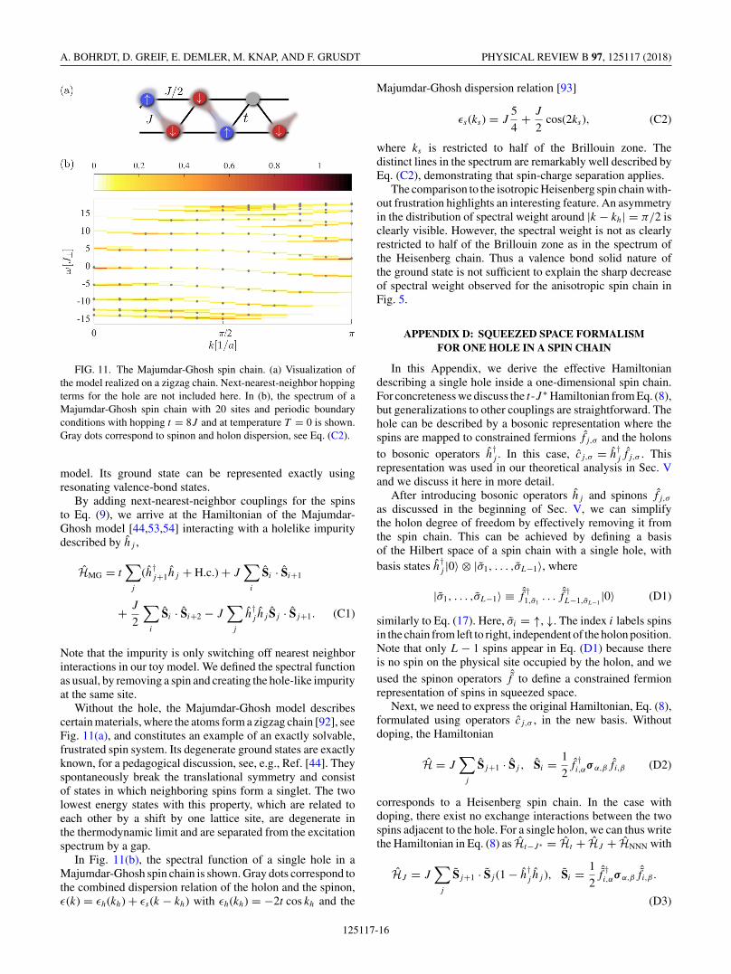
A. BOHRDT, D. GREIF, E. DEMLER, M. KNAP, AND F. GRUSDT PHYSICAL REVIEW B 97, 125117 (2018)
FIG. 11. The Majumdar-Ghosh spin chain. (a) Visualization ofthe model realized on a zigzag chain. Next-nearest-neighbor hoppingterms for the hole are not included here. In (b), the spectrum of aMajumdar-Ghosh spin chain with 20 sites and periodic boundaryconditions with hopping t = 8J and at temperature T = 0 is shown.Gray dots correspond to spinon and holon dispersion, see Eq. (C2).
model. Its ground state can be represented exactly usingresonating valence-bond states.
By adding next-nearest-neighbor couplings for the spinsto Eq. (9), we arrive at the Hamiltonian of the Majumdar-Ghosh model [44,53,54] interacting with a holelike impuritydescribed by hj ,
HMG = t∑
j
(h†j+1hj + H.c.) + J
∑i
Si · Si+1
+ J
2
∑i
Si · Si+2 − J∑
j
h†j hj Sj · Sj+1. (C1)
Note that the impurity is only switching off nearest neighborinteractions in our toy model. We defined the spectral functionas usual, by removing a spin and creating the hole-like impurityat the same site.
Without the hole, the Majumdar-Ghosh model describescertain materials, where the atoms form a zigzag chain [92], seeFig. 11(a), and constitutes an example of an exactly solvable,frustrated spin system. Its degenerate ground states are exactlyknown, for a pedagogical discussion, see, e.g., Ref. [44]. Theyspontaneously break the translational symmetry and consistof states in which neighboring spins form a singlet. The twolowest energy states with this property, which are related toeach other by a shift by one lattice site, are degenerate inthe thermodynamic limit and are separated from the excitationspectrum by a gap.
In Fig. 11(b), the spectral function of a single hole in aMajumdar-Ghosh spin chain is shown. Gray dots correspond tothe combined dispersion relation of the holon and the spinon,ε(k) = εh(kh) + εs(k − kh) with εh(kh) = −2t cos kh and the
Majumdar-Ghosh dispersion relation [93]
εs(ks) = J5
4+ J
2cos(2ks), (C2)
where ks is restricted to half of the Brillouin zone. Thedistinct lines in the spectrum are remarkably well described byEq. (C2), demonstrating that spin-charge separation applies.
The comparison to the isotropic Heisenberg spin chain with-out frustration highlights an interesting feature. An asymmetryin the distribution of spectral weight around |k − kh| = π/2 isclearly visible. However, the spectral weight is not as clearlyrestricted to half of the Brillouin zone as in the spectrum ofthe Heisenberg chain. Thus a valence bond solid nature ofthe ground state is not sufficient to explain the sharp decreaseof spectral weight observed for the anisotropic spin chain inFig. 5.
APPENDIX D: SQUEEZED SPACE FORMALISMFOR ONE HOLE IN A SPIN CHAIN
In this Appendix, we derive the effective Hamiltoniandescribing a single hole inside a one-dimensional spin chain.For concreteness we discuss the t-J ∗ Hamiltonian from Eq. (8),but generalizations to other couplings are straightforward. Thehole can be described by a bosonic representation where thespins are mapped to constrained fermions fj,σ and the holonsto bosonic operators h
†j . In this case, cj,σ = h
†j fj,σ . This
representation was used in our theoretical analysis in Sec. Vand we discuss it here in more detail.
After introducing bosonic operators hj and spinons fj,σ
as discussed in the beginning of Sec. V, we can simplifythe holon degree of freedom by effectively removing it fromthe spin chain. This can be achieved by defining a basisof the Hilbert space of a spin chain with a single hole, withbasis states h
†j |0〉 ⊗ |σ1, . . . ,σL−1〉, where
|σ1, . . . ,σL−1〉 ≡ ˆf †1,σ1
. . . ˆf †L−1,σL−1
|0〉 (D1)
similarly to Eq. (17). Here, σi = ↑, ↓. The index i labels spinsin the chain from left to right, independent of the holon position.Note that only L − 1 spins appear in Eq. (D1) because thereis no spin on the physical site occupied by the holon, and weused the spinon operators ˆf to define a constrained fermionrepresentation of spins in squeezed space.
Next, we need to express the original Hamiltonian, Eq. (8),formulated using operators cj,σ , in the new basis. Withoutdoping, the Hamiltonian
H = J∑
j
Sj+1 · Sj , Si = 1
2f
†i,ασ α,β fi,β (D2)
corresponds to a Heisenberg spin chain. In the case withdoping, there exist no exchange interactions between the twospins adjacent to the hole. For a single holon, we can thus writethe Hamiltonian in Eq. (8) as Ht−J ∗ = Ht + HJ + HNNN with
HJ = J∑
j
Sj+1 · Sj (1 − h†j hj ), Si = 1
2ˆf †i,ασ α,β
ˆfi,β .
(D3)
125117-16

ANGLE-RESOLVED PHOTOEMISSION SPECTROSCOPY … PHYSICAL REVIEW B 97, 125117 (2018)
The hopping term
Ht = −tP∑
〈i,j〉,σc†i,σ cj,σP (D4)
moves the holon by one site while the order of fermions ˆfin squeezed space is not modified. One can write Ht mostconveniently as
Ht = −t∑〈i,j〉
h†j hi = −2t
∑k
cos(k)h†khk. (D5)
For the next-nearest-neighbor tunnelings, the situation ismore complicated. They are of a general form
HNNN =∑
σ,σ ′,τ,τ ′gσ,σ ′,τ,τ ′
∑i
c†i+2,σ c
†i+1,τ ci+1,τ ′ ci,σ ′ + H.c.,
(D6)
where the coefficients g can be read off from Eq. (8). The termin Eq. (D6) modifies the order of spins because it moves afermion from site i to i + 2. This involves an exchange of thefermions at sites i and i + 1, which introduces an additionalminus sign. We can see this by calculating the action of HNNN
on a basis state:
HNNNh†i+2|0〉 ⊗ |. . . ,σi ,σi+1, . . .〉. (D7)
To lighten the notation, we consider the action of a single termin the sum in Eq. (D6). Representing the basis state in termsof the original c
†i,σ operators yields
c†i+2,σ c
†i+1,τ ci+1,τ ′ ci,σ ′ c
†1,σ1
. . . c†i,σi
c†i+1,σi+1
. . . |0〉= c
†1,σ1
. . . c†i−1,σi−1
(−1)i−1δσ ′,σiδτ ′,σi+1
× c†i+1,τ (−1)i c†i+2,σ . . . |0〉. (D8)
In the notation introduced above, this state can be identifiedwith
−δσ ′,σiδτ ′,σi+1 h
†i+2 ⊗ |. . . ,σi−1,τ,σ,σi+2, . . .〉. (D9)
The next-nearest-neighbor term leads to an exchange of thespins on sites i and i + 1 in squeezed space, which can bedescribed by a term of the form 4Si · Si+1 − 1, see, e.g.,Supplementary Material in Ref. [12]. By taking into accountthe minus sign from the fermion exchange above, we arrive atthe following expression,
HNNN = J
2
∑j
h†j+2hj
(Sj+1 · Sj − 1
4
)+ H.c.. (D10)
From the second term in the brackets, we derive the corre-sponding term − 1
4J cos(2kh) in the holon dispersion, Eq. (11).In summary, the t-J ∗ Hamiltonian for a single hole can be
written in squeezed space as
Ht−J ∗ = −∑kh
h†kh
hkh
(2t cos(kh) + 1
4J cos(2kh)
)
+ J
2
∑j
[h†j+2hj Sj+1 · Sj + H.c.]
+ J∑
j
Sj+1 · Sj (1 − h†j hj ). (D11)
APPENDIX E: EFFECTIVE POLARON DESCRIPTION
We study the interaction of a single holon with the sur-rounding spin environment. It can be created by first removinga fermion from the spin chain, leading to the creation ofa spinon-holon pair. The essence of spin-charge separationis that the spinon is not bound to the holon. Thus, afterwaiting for sufficiently long, we can assume that spinon andholon propagate through the system independently. We nowprovide a detailed calculation of the holon properties whenit becomes dressed by collective spin excitations and forms aholon-polaron. In particular, we derive Eqs. (43) and (45) fromthe main text for its renormalized energy and the renormalizedmass.
Starting from the t-J ∗ Hamiltonian, we first perform aLee-Low-Pines transformation into the holon frame. As a nextstep, bosonization techniques are employed to describe the spinchain itself, as well as the interaction of the holon with the col-lective spin excitations. Here we assume an infinite system andneglect finite-size corrections. Finally, we explicitly calculatethe holon energy and its renormalized mass in the regime ofweak polaronic coupling, J t .
1. Lee-Low-Pines transformation
Our starting point is the t-J ∗ Hamiltonian (8) formulatedin squeezed space [59], see Eq. (D11), where the spinlessholon is effectively hopping between the bonds of the physicallattice. As a first step, we apply the unitary Lee-Low-Pinestransformation [94]
ULLP = exp(iPsxh), (E1)
where xh = ∑j j h
†j hj is the position operator of the holon
and Ps is the total momentum operator of the spins. In thenew basis, the holon is always placed in the center, and thetransformed Hamiltonian reads
U†LLPHULLP = − 2t cos(ph − Ps) + J
∑〈i,j〉
Si · Sj
− J S0 · S1 − J
4cos(2ph − 2Ps)
+ J
2
(S−1 · S0e
2i(ph−Ps) + S1 · S2e−2i(ph−Ps)
).
(E2)
Here, ph denotes the total conserved momentum of the holon-polaron.
The first term in Eq. (E2) corresponds to the recoil energyof the holon when it scatters on a spin-wave excitation whichchanges the total momentum Ps carried by the spin system. Thesecond term describes the unperturbed spin chain without theholon. The interaction between the holon and the spin chainwithin the t-J model is given by −J S0 · S1. The last threeterms in the equation describe next-nearest-neighbor hoppingprocesses present in the Fermi-Hubbard model at large U .These terms have the same scaling with J as the interactions−J S0 · S1 in the simpler t-J model and should be treated onequal footing to understand the properties of the holon-polaron.
125117-17

A. BOHRDT, D. GREIF, E. DEMLER, M. KNAP, AND F. GRUSDT PHYSICAL REVIEW B 97, 125117 (2018)
FIG. 12. Bosonization of a spin chain doped by a mobile holon.The spin operators can be described by two chiral fermions ψL,R(x)interacting with the holon at position xh. Our starting point is theunperturbed chain, which is an exact solution when the tunneling ratet of the holon is larger than spin-exchange interactions, t � J .
2. Bosonization
In order to calculate ground-state properties of Hamiltonian(E2), we use the bosonization technique to describe theunperturbed spin chain. Here we provide a brief overview,see, e.g., Refs. [37,70,95] for a complete derivation. In thisformalism, spin operators are first expressed in terms ofJordan-Wigner fermions ψ(x) counting the number of up spins.In this basis, Sz(x) = ψ†(x)ψ(x) − 1/2 and the case of zeromagnetization corresponds to a system at half-filling. When thenet magnetization vanishes and mutual interactions betweenthe Jordan-Wigner fermions are neglected, they form a Fermisea around kF = π/2, in units of the inverse lattice constanta = 1. By linearizing around kF and extending the linearizedbranches to momenta ±∞, one can introduce two chiral fieldsψR,L(x) corresponding to right (R) and left (L) movers. Thesituation is illustrated in Fig. 12.
The interactions between Jordan-Wigner fermions renor-malize the properties of collective particle-hole excitationsaround the Fermi surface. In the bosonization formalism, this isdescribed by introducing bosonic fields φL,R(x), related to theJordan-Wigner fermions by ψL,R(x) ∝ exp(∓i
√4πφL,R(x)).
The fields φL,R(x) can be decomposed into normal modesbq with momentum q > 0 for right movers (q < 0 for leftmovers), where [bq ,b
†q ′ ] = δq,q ′ . In addition, so-called zero
modes have to be included, where nL,R counts the total numberof left and right movers relative to the Fermi sea at kF = ±π/2.Their number can be changed by the operators exp(i
√4πφ
L,R0 ),
namely exp(i√
4πφL,R0 )nL,R = (nL,R ∓ 1) exp(i
√4πφ
L,R0 ).
Putting everything together one obtains [95]
φL,R(x) = φL,R0 +
√πx
LnL,R +
∑q≶0
sgn(q)√2L|q| (eiqx bq + H.c.),
(E3)
where L is the length of the spin chain (not counting theholon) and we assumed periodic boundary conditions.We furthermore introduce the shorthand notationφL,R(x) = φ
L,R0 +
√πx
LnL,R + φ
≶L,R(x).
Using the formalism described above, the collective excita-tions of the antiferromagnetic spin chain can be described as
H0 = J∑〈i,j〉
Si · Sj (E4)
= E0 + πJ
∫dx : (∂xφ(x))2 + 1
4(∂xθ (x))2 : (E5)
= E0 +∑
q
vs|q|b†q bq + Jπ
L
(n2
L + n2R
). (E6)
In the second line, we introduced φ(x) = φR(x) + φL(x),θ (x) = φR(x) − φL(x) and : · · · : denotes normal orderingwith respect to operators bq . Note that umklapp terms havebeen neglected in this expression. The ground-state energyE0 of the spin chain is known exactly from Bethe-ansatzcalculations [37],
E0 = L(
14 − ln(2)
)J = −L × 0.4431J. (E7)
The excitations described by b†q carry no spin and their velocity
vs is given by [37]
vs = Jπ
2. (E8)
The ultraviolet momentum cut-off �UV is determined by theinverse lattice scale 1/a. We set �UV = π/2 in units wherea = 1.
The total momentum operator of the spin system containscontributions from collective excitations as well as the zeromodes. Assuming that |nL,R| L for typical values of nL,R,we can write
Ps = π
2(nR − nL) +
∑q
qb†q bq . (E9)
3. Interaction terms
The interaction of the holon with collective spin excitationsis determined by the term
Hint = −J S0 · S1 + J
2(S−1 · S0e
2i(ph−Ps) + H.c.x) (E10)
in the Lee-Low-Pines frame, see Eq. (E2). To express it in termsof bosonized operators, we first note that the energy density ofthe free spin chain is given by J S(x) · S(x + 1). By inspectionof Eq. (E5) we can write
S(x) · S(x + 1) ≈ E0
JL+ : π (∂xφ(x))2 + π
4(∂xθ(x))2 : .
(E11)
This term describes correctly the effect of long-wavelengthfluctuations on nearest neighbor spin correlations. Because ofthe constant term added to the expression, the ground-stateexpectation value 〈S(x) · S(x + 1)〉, is correctly reproduced.
In combination with Eq. (E7) we obtain the followingrepresentation:
S(x) · S(x + 1)
= 1
4− ln(2) + π2
(n2
−4L2
+ n2+
L2
)
+ π
(n+L
+ n−4L
)√2π
L
∑q
√|q|eiqxi(bq − b
†−q)
+ π
4L
∑qq ′>0
√|qq ′| : b
†qWq,q ′ (x)bq ′ :
+ 4|C|2eiπx cos[√
4π (φL(x) + φR(x))]. (E12)
125117-18

ANGLE-RESOLVED PHOTOEMISSION SPECTROSCOPY … PHYSICAL REVIEW B 97, 125117 (2018)
Here, n± = nR ± nL and we defined
Wq,q ′ (x) =(
e−i(q−q ′)x −e−i(q+q ′)x
−ei(q+q ′)x ei(q−q ′)x
)(E13)
and b†q = (b†q,bq). In the last line of Eq. (E12), we have
also included umklapp scattering terms. Their prefactor is thenumber |C|2, which is a nonuniversal constant that cannot bederived within the bosonization formalism. Its numerical value|C|2 ≈ 0.14 has been determined by Eggert and Affleck [71]from comparison of the spin-structure factor obtained frombosonization and quantum Monte Carlo calculations.
The first three lines in Eq. (E12) describe forward scatteringprocesses, which leave the populations nL,R of the zero modesunchanged. The last line corresponds to umklapp scattering,where the n− changes by two units because a right moverscatters into a left-mover or vice versa. The sum n+ = nR +nL = mL is conserved and can be expressed in terms of themagnetization per unit length
m = (N↑ − N↓)/2L. (E14)
In the following, we allow for a finite magnetization m �= 0 butassume that n− = O(L0) is not an extensive quantity.
To understand the scaling in the thermodynamic limitL → ∞, we introduce operators b(q) = √
L/2πbq with[b(q),b†(q ′)] = δ(q − q ′) and write Eq. (E12) in an integralform using
∑q 2π/L → ∫
dq with q integrated over −�UV �q � �UV,
S(x) · S(x + 1)
= 1
4− ln(2) + π2m2 + πm
∫dq
√|q|eiqxi(b(q) − b†(−q))
+ 1
8
∫qq ′>0
dqdq ′√|qq ′| : b†(q)Wq,q ′ (x)b(q ′) :
+ 4|C|2eiπx cos[√
4π (φL(x) + φR(x))]. (E15)
The field φR(x) can be expressed as
φR(x) = φR0 +
√πx
LnR +
∫ �UV
0dq
|q|−1/2
√4π
(eiqx b(q) + H.c.),
(E16)
and a similar expression exists for φL(x).The interactions in Eq. (E10) can now be written in the
bosonization language using Eq. (E15). We will distinguishforward scattering terms (F) of different orders in b andumklapp (U) scattering terms:
Hint = H(1)F + H(2)
F + HU + (14 − ln(2) + π2m2
)× J [cos(2(ph − Ps)) − 1]. (E17)
a. Linear Fröhlich-type terms
First, we consider only forward scattering terms that arelinear in b operators in Eq. (E10),
H(1)F = Jπm
∫dq
√|q|i(b(q) − b†(−q))
× [1 − cos(2(ph − Ps) − q)]. (E18)
Notably, the form of this term is identical to the interac-tion terms in the ubiquitous Fröhlich polaron Hamiltonian[73,83,96].
This allows us to introduce a dimensionless polaroniccoupling constant αF = (πm)2. When αF 1, the Fröhlichcoupling is weak and can be treated perturbatively. The startingpoint for such analysis is Eq. (E17) with H(1,2)
F = 0 whenαF = 0. The resulting Hamiltonian commutes with b
†q bq and
can be solved exactly by plane waves. When αF � 1, on theother hand, the strong-coupling (or Landau-Pekar) variationalwave function can be used [60,97]. Note that our derivation isonly valid at weak polaron couplings αF 1. By expandingaround the Fermi sea at half-filling of Jordan-Wigner fermions,we assumed that m 1 is small.
b. Two-particle excitations
By keeping only forward scattering terms which arequadratic in b operators in Eq. (E10), we obtain
H(2)F = − J
8
∫qq ′>0
dqdq ′√|qq ′| :
[b†(q)Wq,q ′ (0)b(q ′)
− 1
2b†(q)(Wq,q ′ (−1)e2i(ph−Ps) + H.c.)b(q ′)
]: .
(E19)
The matrix Wq,q ′ (x) in the LLP frame becomes
Wq,q ′ (x) =(
e−i(q−q ′)xe−2iq ′ −e−i(q+q ′)xe2iq ′
−ei(q+q ′)xe−2iq ′ei(q−q ′)xe2iq ′
). (E20)
For a system at zero magnetization, m = 0, these are theleading-order terms in the effective holon-polaron Hamilto-nian.
c. Umklapp scattering
Finally, umklapp scattering terms give rise to the followinginteractions:
HU = − 2J |C|2[2 cos(√
4πφ(0)) + cos(√
4πφ(−1))
× e2i(ph−Ps) + cos(√
4πφ(1))e−2i(ph−Ps)], (E21)
where φ(x) = φL(x) + φR(x).
4. Holon polaron at weak polaronic coupling
Now we analyze the properties of the holon polaron in theweak polaronic coupling regime, J t . Our starting point isa free holon at momentum ph and no spin excitations,
|ψ0〉 = |ph〉h|0〉0|0〉b. (E22)
The occupation of the zero modes is characterized by |n−〉0and n+ = Lm is conserved.
To zeroth order, the holon energy is given by
E(0)h = −2t cos(ph). (E23)
We obtain the following first-order contribution to the holon-polaron energy,
E(1)h = J (π2m2 − ln(2))[cos(2ph) − 1] − J/4. (E24)
125117-19

A. BOHRDT, D. GREIF, E. DEMLER, M. KNAP, AND F. GRUSDT PHYSICAL REVIEW B 97, 125117 (2018)
In the following we calculate second order corrections inJ to the holon-polaron energy term by term. Furthermore,by expanding the result around ph = 0 to quadratic order, wecalculate the mass renormalization of the holon-polaron.
a. Forward scattering
From the Fröhlich-type terms (E18), we obtain the follow-ing second-order contribution,
E(2)h,F1 = −J 2π2m2
∫dq|q| [1 − cos(2ph − q)]2
2t cos(ph) − 2t cos(ph − q).
(E25)
From the two-particle terms (E19), we obtain a second-ordercontribution,
E(2)h,F2 = − J 2
64
∫qq ′>0
dqdq ′|qq ′|
× [1 − cos(2ph + q + q ′)]2
�q,q ′ (ph), (E26)
where �q,q ′ (ph) = −2t cos(ph − q − q ′) + 2t cos(ph).
b. Umklapp scattering
Now, we calculate the leading-order contribution of theumklapp scattering term Eq. (E21) to the holon-polaron energy.We start by noting that
e±i√
4π(φL0 +φR
0 +√
πx
L(nL+nR))|n−〉0 = |n− ± 2〉0. (E27)
The momentum is given by Ps|n−〉0 = n−π/2, see Eq. (E9).The action of exp(i
√4πφ(x)) on the bosonic state |0〉b can be
understood by writing
ei√
4πφb(x)|0〉b = exp
(−
∫dqβ∗
x (q)b(q) − H.c.
)|0〉b,
(E28)
where φb(x) = φ<L (x) + φ>
R (x). The last expression corre-sponds to a coherent state
∏q |βx(q)〉, with
βx(q) = isgn(q)|q|−1/2e−iqx . (E29)
Note that the amplitude
|βx(q)|2 = |q|−1 ≡ |β(q)|2 (E30)
is independent of x.By summing over the allowed virtual states, defined by Fock
states of b operators and |±2〉0, we obtain an expression forthe holon-polaron energy due to umklapp scattering,
E(2)h,U = 8J 2|C|4
∑nq
(∏q
|β(q)|2nq
nq!e−|β(q)|2
)1
�Q(ph)
×(
3
2+ 1
2cos(2Q + 4ph) + 2 cos(Q + 2ph)
).
(E31)
The energy denominator is given by
�Q(ph) = −2t cos(ph) + 2t cos(ph − π − Q) (E32)
and depends only on the total momentum
Q =∫
dqqnq. (E33)
To simplify Eq. (E31), we note that the sum∑
nqof the
occupations nq is taken over
λ(nq) = |β(q)|2nq
nq!e−|β(q)|2 . (E34)
This defines independent Poisson distributions for all momen-tum modes q. Because the remaining terms only depend on thetotal momentum Q, it is sufficient to know the full countingstatistics p(Q) of the latter with respect to the independentPoisson distributions:
E(2)h,U = 8J 2|C|4
∑Q
p(Q)1
�Q(ph)
×(
3
2+ 1
2cos(2Q + 4ph) + 2 cos(Q + 2ph)
).
(E35)
To calculate the full counting statistics p(Q), we constructthe generating functional
G(X) =∑nq
λ(nq)e−iXQ = exp
[−
∫dq|β(q)|2(1 − e−iXq)
]
= e−2γ 4
π2X2e2Ci(Xπ/2). (E36)
Here, γ = 0.577216 is the Euler constant and Ci(x) =− ∫ ∞
xcos(t)/tdt denotes the cosine integral. By taking a
Fourier transform, we obtain the full counting statistics
p(Q) = 1
2π
∫dXG(X)eiXQ. (E37)
Combining this with Eq. (E35), we arrive at
E(2)h,U = J 2|C|4e−2γ 25
π3
∫ ∞
−∞dQ
∫ ∞
0dX
cos(XQ)
X2�Q(ph)e2Ci(Xπ/2)
×(
3
2+ 1
2cos(2Q + 4ph) + 2 cos(Q + 2ph)
).
(E38)
c. Renormalized mass and energy around ph = 0
Now we analyze the results from Eqs. (E23)–(E26) and(E38) and calculate the holon-polaron ground-state propertiesat ph = 0. Up to quadratic order in ph, we obtain
Eh(ph) = Eh(0) + 12p2
hM−1h + O
(p4
h
). (E39)
The ground-state energy Eh(0) contains contributions from thefive different terms in the effective Hamiltonian,
Eh(0) = E(0)h (0) + E
(1)h (0) + E
(2)h,F1(0) + E
(2)h,F2(0) + E
(2)h,U(0).
(E40)
A similar expression follows for the holon-polaron mass:
1
Mh= 1
M(0)h
+ 1
M(1)h
+ 1
M(2)h,F1
+ 1
M(2)h,F2
+ 1
M(2)h,U
. (E41)
125117-20

ANGLE-RESOLVED PHOTOEMISSION SPECTROSCOPY … PHYSICAL REVIEW B 97, 125117 (2018)
The different contributions are given by
E(0)h (0) = −2t, (E42)
E(1)h (0) = −J
4, (E43)
E(2)h,F1(0) = −J 2
tm2π2
(1 + π2
8− π
2
), (E44)
E(2)h,F2(0) = −J 2
t
π
4096(64 − 16π + π3), (E45)
E(2)h,U(0) = −J 2
t|C|4 × 5.31. (E46)
By combining these results, we obtain Eq. (43). For theeffective mass, we obtain(
M(0)h
)−1 = 2t, (E47)(M
(1)h
)−1 = −4J [ln(2) − π2m2], (E48)
(M
(2)h,F1
)−1 = −J 2
tm2π2 3
8(12π + π2 − 24), (E49)
(M
(2)h,F2
)−1 = −J 2
t
π
4096(400π + 19π3 − 1600), (E50)
(M
(2)h,U
)−1 = −J 2
t|C|4 × 43.16. (E51)
By combining these results, we arrive at Eq. (45).
d. Divergent integrals in the t- J model
In our discussion of the holon-polaron, so far, we restrictedourselves to the t-J ∗ model where next-nearest-neighbor holonhopping is included. We can repeat our perturbative analysis
for the simpler t-J model, where the last three terms inEq. (E2), corresponding to next-nearest-neighbor hopping, arediscarded. In this case, we obtain
Eh(ph) = −2t cos(ph) + J(
ln(2) − 14 − π2m2
), (E52)
plus terms of orders O(J 2/t).The second-order expressions O(J 2/t) involve divergent
integrals when the t-J model is used. For example, the Fröhlichtype terms from Eq. (E18) give rise to an energy correction
E(2)h,F1(ph = 0) = −J 2
tm2π2
∫ π/2
0dq
q
1 − cos(q)(E53)
for the t-J model. This expression diverges logarithmicallywith the infrared cutoff �IR,
E(2)h,F1(ph = 0) � −
∫�IR
dq1
q� ln �IR. (E54)
In a finite-size system, �IR = 1/L with L the system size, andE
(2)h,F1(ph = 0) � − ln L is weakly divergent.Similarly, we find that the correction to the effective mass
from two-particle excitations is logarithmically divergent in thet-J model, 1/M
(2)h,F2 � − ln L. On the other hand, the energy
E(2)h,F2 is convergent. The umklapp terms lead to a power-law
divergence of the holon-polaron ground-state energy,
E(2)h,U(ph = 0) � − J 2
t
∫dQ
p(Q)
1 + cos Q
� −∫
dQp(π )
(Q − π )2, (E55)
in the t-J model.
[1] W. Hofstetter, J. I. Cirac, P. Zoller, E. Demler, and M. D. Lukin,Phys. Rev. Lett. 89, 220407 (2002).
[2] D. Greif, T. Uehlinger, G. Jotzu, L. Tarruell, and T. Esslinger,Science 340, 1307 (2013).
[3] R. A. Hart, P. M. Duarte, T.-L. Yang, X. Liu, T. Paiva, E. Khatami,R. T. Scalettar, N. Trivedi, D. A. Huse, and R. G. Hulet, Nature519, 211 (2015).
[4] M. F. Parsons, F. Huber, A. Mazurenko, C. S. Chiu, W. Setiawan,K. Wooley-Brown, S. Blatt, and M. Greiner, Phys. Rev. Lett. 114,213002 (2015).
[5] A. Omran, M. Boll, T. A. Hilker, K. Kleinlein, G. Salomon, I.Bloch, and C. Gross, Phys. Rev. Lett. 115, 263001 (2015).
[6] L. W. Cheuk, M. A. Nichols, M. Okan, T. Gersdorf, V. V.Ramasesh, W. S. Bakr, T. Lompe, and M. W. Zwierlein, Phys.Rev. Lett. 114, 193001 (2015).
[7] E. Haller, J. Hudson, A. Kelly, D. A. Cotta, B. Peaudecerf,G. D. Bruce, and S. Kuhr, Nat. Phys. 11, 738 (2015).
[8] M. F. Parsons, A. Mazurenko, C. S. Chiu, G. Ji, D. Greif, andM. Greiner, Science 353, 1253 (2016).
[9] M. Boll, T. A. Hilker, G. Salomon, A. Omran, J. Nespolo, L.Pollet, I. Bloch, and C. Gross, Science 353, 1257 (2016).
[10] L. W. Cheuk, M. A. Nichols, K. R. Lawrence, M. Okan, H.Zhang, E. Khatami, N. Trivedi, T. Paiva, M. Rigol, and M. W.Zwierlein, Science 353, 1260 (2016).
[11] D. Mitra, P. T. Brown, E. Guardado-Sanchez, S. S. Kondov, T.Devakul, D. A. Huse, P. Schauss, and W. Bakr, Nat. Phys. 14,173 (2018).
[12] T. A. Hilker, G. Salomon, F. Grusdt, A. Omran, M. Boll, E.Demler, I. Bloch, and C. Gross, Science 357, 484 (2017).
[13] A. Mazurenko, C. S. Chiu, G. Ji, M. F. Parsons, M. Kanasz-Nagy,R. Schmidt, F. Grusdt, E. Demler, D. Greif, and M. Greiner,Nature (London) 545, 462 (2017).
[14] P. T. Brown, D. Mitra, E. Guardado-Sanchez, P. Schauß, S. S.Kondov, E. Khatami, T. Paiva, N. Trivedi, D. A. Huse, andW. S. Bakr, Science 357, 1385 (2017).
[15] C. Chin, M. Bartenstein, A. Altmeyer, S. Riedl, S. Jochim, J. H.Denschlag, and R. Grimm, Science 305, 1128 (2004).
[16] C. Kollath, M. Köhl, and T. Giamarchi, Phys. Rev. A 76, 063602(2007).
[17] T.-L. Dao, A. Georges, J. Dalibard, C. Salomon, and I. Carusotto,Phys. Rev. Lett. 98, 240402 (2007).
[18] M. Knap, A. Shashi, Y. Nishida, A. Imambekov, D. A. Abanin,and E. Demler, Phys. Rev. X 2, 041020 (2012).
[19] M. Knap, A. Kantian, T. Giamarchi, I. Bloch, M. D. Lukin, andE. Demler, Phys. Rev. Lett. 111, 147205 (2013).
[20] M. Cetina, M. Jag, R. S. Lous, I. Fritsche, J. T. M. Walraven, R.Grimm, J. Levinsen, M. M. Parish, R. Schmidt, M. Knap, andE. Demler, Science 354, 96 (2016).
125117-21

A. BOHRDT, D. GREIF, E. DEMLER, M. KNAP, AND F. GRUSDT PHYSICAL REVIEW B 97, 125117 (2018)
[21] More precisely, one measures retarded correlation func-tions, i.e., in the case of bosonic operators φ, DR(t) =�(t)〈φ(t)φ(0) − φ(0)φ(t)〉 and for fermionic operators ψ ,GR(t) = �(t)〈ψ(t)ψ †(0) − ψ †(0)ψ(t)〉.
[22] A. Damascelli, Z. Hussain, and Z.-X. Shen, Rev. Mod. Phys. 75,473 (2003).
[23] P. A. Lee, N. Nagaosa, and X.-G. Wen, Rev. Mod. Phys. 78, 17(2006).
[24] J. T. Stewart, J. P. Gaebler, and D. S. Jin, Nature (London) 454,744 (2008).
[25] G. Veeravalli, E. Kuhnle, P. Dyke, and C. J. Vale, Phys. Rev.Lett. 101, 250403 (2008).
[26] R. Jordens, N. Strohmaier, K. Gunter, H. Moritz, and T.Esslinger, Nature (London) 455, 204 (2008).
[27] D. Greif, L. Tarruell, T. Uehlinger, R. Jördens, and T. Esslinger,Phys. Rev. Lett. 106, 145302 (2011).
[28] P. Törmä and P. Zoller, Phys. Rev. Lett. 85, 487 (2000).[29] Q. Chen, Y. He, C.-C. Chien, and K. Levin, Rep. Prog. Phys. 72,
122501 (2009).[30] P. Torma, Phys. Scr. 91, 043006 (2016).[31] A. Kantian, U. Schollwöck, and T. Giamarchi, Phys. Rev. Lett.
115, 165301 (2015).[32] J. Zeiher, R. van Bijnen, P. Schausz, S. Hild, J.-y. Choi, T. Pohl,
I. Bloch, and C. Gross, Nat. Phys. 12, 1095 (2016).[33] J. Zeiher, J.-Y. Choi, A. Rubio-Abadal, T. Pohl, R. van Bijnen,
I. Bloch, and C. Gross, Phys. Rev. X 7, 041063 (2017).[34] A. V. Gorshkov, S. R. Manmana, G. Chen, J. Ye, E. Demler, M. D.
Lukin, and A. M. Rey, Phys. Rev. Lett. 107, 115301 (2011).[35] L. M. Duan, E. Demler, and M. D. Lukin, Phys. Rev. Lett. 91,
090402 (2003).[36] K. J. von Szczepanski, P. Horsch, W. Stephan, and M. Ziegler,
Phys. Rev. B 41, 2017 (1990).[37] T. Giamarchi, Quantum Physics in One Dimension (Oxford
University Press, Oxford, 2003).[38] Sutherland, Beautiful Models, 70 Years of Exactly Solved Quan-
tum Many-Body Problems (World Scientific, Singapore, 2004).[39] M. Endres, T. Fukuhara, D. Pekker, M. Cheneau, P. Schauß, C.
Gross, E. Demler, S. Kuhr, and I. Bloch, Nature (London) 487,454 (2012).
[40] P. Zupancic, P. M. Preiss, R. Ma, A. Lukin, M. Eric Tai, M.Rispoli, R. Islam, and M. Greiner, Opt. Express 24, 13881(2016).
[41] M. Greiner, I. Bloch, O. Mandel, T. W. Hänsch, and T. Esslinger,Phys. Rev. Lett. 87, 160405 (2001).
[42] R. Islam, R. Ma, P. M. Preiss, M. Eric Tai, A. Lukin, M. Rispoli,and M. Greiner, Nature (London) 528, 77 (2015).
[43] P. A. Murthy, D. Kedar, T. Lompe, M. Neidig, M. G. Ries, A. N.Wenz, G. Zürn, and S. Jochim, Phys. Rev. A 90, 043611 (2014).
[44] A. Auerbach, Interacting Electrons and Quantum Magnetism(Springer, Berlin, 1998).
[45] R. C. Brown, R. Wyllie, S. B. Koller, E. A. Goldschmidt, M.Foss-Feig, and J. V. Porto, Science 348, 540 (2015).
[46] R. N. Bannister and N. d’Ambrumenil, Phys. Rev. B 61, 4651(2000).
[47] R. Eder and Y. Ohta, Phys. Rev. B 56, 2542 (1997).[48] C. Kim, Z.-X. Shen, N. Motoyama, H. Eisaki, S. Uchida, T.
Tohyama, and S. Maekawa, Phys. Rev. B 56, 15589 (1997).[49] C. Kim, A. Y. Matsuura, Z.-X. Shen, N. Motoyama, H. Eisaki,
S. Uchida, T. Tohyama, and S. Maekawa, Phys. Rev. Lett. 77,4054 (1996).
[50] M. Sing, U. Schwingenschlögl, R. Claessen, P. Blaha, J. M. P.Carmelo, L. M. Martelo, P. D. Sacramento, M. Dressel, andC. S. Jacobsen, Phys. Rev. B 68, 125111 (2003).
[51] B. J. Kim, H. Koh, E. Rotenberg, S.-J. Oh, H. Eisaki, N.Motoyama, S. Uchida, T. Tohyama, S. Maekawa, Z.-X. Shen,and C. Kim, Nat. Phys. 2, 397 (2006).
[52] R. Hayn and R. O. Kuzian, Phys. Rev. B 62, 12156 (2000).[53] C. K. Majumdar and D. K. Ghosh, J. Math. Phys. 10, 1388
(1969).[54] C. K. Majumdar, J. Phys. C 3, 911 (1970).[55] X.-G. Wen, Quantum Field Theory of Many-Body Systems
(Oxford University Press, Oxford, 2004).[56] Z. Y. Weng, D. N. Sheng, and C. S. Ting, Phys. Rev. B 52, 637
(1995).[57] G. Baskaran, Z. Zou, and P. Anderson, Solid State Commun. 63,
973 (1987).[58] J. Zaanen, O. Y. Osman, H. V. Kruis, Z. Nussinov, and J.
Tworzydlo, Philos. Mag. B 81, 1485 (2001).[59] H. V. Kruis, I. P. McCulloch, Z. Nussinov, and J. Zaanen, Phys.
Rev. B 70, 075109 (2004).[60] L. D. Landau and S. I. Pekar, Zh. Eksp. Teor. Fiz. 18, 419 (1948)
[Ukr. J. Phys., Special Issue 53, 71 (2008)].[61] L. N. Bulaevskii, E. L. Nagaev, and D. I. Khomskii, Sov. Phys.
JETP 27, 836 (1968).[62] W. F. Brinkman and T. M. Rice, Phys. Rev. B 2, 1324 (1970).[63] S. Schmitt-Rink, C. M. Varma, and A. E. Ruckenstein, Phys.
Rev. Lett. 60, 2793 (1988).[64] C. L. Kane, P. A. Lee, and N. Read, Phys. Rev. B 39, 6880 (1989).[65] S. Sachdev, Phys. Rev. B 39, 12232 (1989).[66] Z. Liu and E. Manousakis, Phys. Rev. B 44, 2414 (1991).[67] G. Martinez and P. Horsch, Phys. Rev. B 44, 317 (1991).[68] A. S. Mishchenko, N. V. Prokof’ev, and B. V. Svistunov, Phys.
Rev. B 64, 033101 (2001).[69] E. Manousakis, Phys. Rev. B 75, 035106 (2007).[70] F. D. M. Haldane, J. Phys. C 14, 2585 (1981).[71] S. Eggert and I. Affleck, Phys. Rev. Lett. 75, 934 (1995).[72] To perform the finite size scaling, we calculated the energy of a
single hole for system sizes L = 10,12,?,20 and used a fit up toquadratic order 1/L2.
[73] F. Grusdt, G. E. Astrakharchik, and E. Demler, New J. Phys. 19,103035 (2017).
[74] Z. Y. Weng, Phys. Rev. B 50, 13837 (1994).[75] R. Herrmann, S. Samarin, H. Schwabe, and J. Kirschner, Phys.
Rev. Lett. 81, 2148 (1998).[76] N. Fominykh, J. Henk, J. Berakdar, P. Bruno, H. Gollisch, and
R. Feder, Solid State Commun. 113, 665 (2000).[77] S. E. Nagler, D. A. Tennant, R. A. Cowley, T. G. Perring, and
S. K. Satija, Phys. Rev. B 44, 12361 (1991).[78] M. Ogata and H. Shiba, Phys. Rev. B 41, 2326 (1990).[79] K. A. Kouzakov and J. Berakdar, Phys. Rev. Lett. 91, 257007
(2003).[80] P. Beran, D. Poilblanc, and R. Laughlin, Nucl. Phys. B 473, 707
(1996).[81] F. Grusdt, M. Kanasz-Nagy, A. Bohrdt, C. S. Chiu, G. Ji, M.
Greiner, D. Greif, and E. Demler, arXiv:1712.01874.[82] W. Casteels, J. Tempere, and J. T. Devreese, Phys. Rev. A 86,
043614 (2012).[83] J. Catani, G. Lamporesi, D. Naik, M. Gring, M. Inguscio, F.
Minardi, A. Kantian, and T. Giamarchi, Phys. Rev. A 85, 023623(2012).
125117-22

ANGLE-RESOLVED PHOTOEMISSION SPECTROSCOPY … PHYSICAL REVIEW B 97, 125117 (2018)
[84] J. Bonart and L. F. Cugliandolo, Phys. Rev. A 86, 023636 (2012).[85] T. Fukuhara, A. Kantian, M. Endres, M. Cheneau, P. Schauss,
S. Hild, D. Bellem, U. Schollwoeck, T. Giamarchi, C. Gross, I.Bloch, and S. Kuhr, Nat. Phys. 9, 235 (2013).
[86] A. G. Volosniev and H.-W. Hammer, Phys. Rev. A 96, 031601(2017).
[87] C. J. M. Mathy, M. B. Zvonarev, and E. Demler, Nat. Phys. 8,881 (2012).
[88] M. Knap, C. J. M. Mathy, M. Ganahl, M. B. Zvonarev, and E.Demler, Phys. Rev. Lett. 112, 015302 (2014).
[89] F. Meinert, M. Knap, E. Kirilov, K. Jag-Lauber, M. B. Zvonarev,E. Demler, and H.-C. Naegerl, Science 356, 945 (2017).
[90] S. Foelling, S. Trotzky, P. Cheinet, M. Feld, R. Saers, A. Widera,T. Mueller, and I. Bloch, Nature (London) 448, 1029 (2007).
[91] Y.-A. Chen, S. Nascimbène, M. Aidelsburger, M. Atala, S.Trotzky, and I. Bloch, Phys. Rev. Lett. 107, 210405 (2011).
[92] C. Lacroix, P. Mendels, and F. Mila, eds., Introduction toFrustrated Magnetism (Springer Series in Solid-State Sciences,Heidelberg, 2011).
[93] B. S. Shastry and B. Sutherland, Phys. Rev. Lett. 47, 964(1981).
[94] T. D. Lee, F. E. Low, and D. Pines, Phys. Rev. 90, 297(1953).
[95] S. Eggert, Theoretical Survey of One Dimensional Wire Systems,edited by Y. Kuk et al. (Sowha, Seoul, 2007), Chap. 2.
[96] H. Fröhlich, Adv. Phys. 3, 325 (1954).[97] W. Casteels, T. Van Cauteren, J. Tempere, and J. T. Devreese,
Laser Phys. 21, 1480 (2011).
125117-23