PHYSICAL REVIEW RESEARCH 2, 043006 (2020)

Assessing the role of initial correlations in the entropy production ratefor nonequilibrium harmonic dynamics

Giorgio Zicari ,1,* Matteo Brunelli ,2 and Mauro Paternostro1

1Centre for Theoretical Atomic, Molecular, and Optical Physics, School of Mathematics and Physics,Queen’s University, Belfast BT7 1NN, United Kingdom

2Cavendish Laboratory, University of Cambridge, Cambridge CB3 0HE, United Kingdom

(Received 1 May 2020; accepted 11 September 2020; published 1 October 2020)

Entropy production provides a general way to state the second law of thermodynamics for nonequilibriumscenarios. In open quantum system dynamics, it also serves as a useful quantifier of the degree of irreversibility.In this work we shed light on the relation between correlations, initial preparation of the system, and non-Markovianity by studying a system of two harmonic oscillators independently interacting with their local baths.Their dynamics, described by a time-local master equation, is solved to show, both numerically and analytically,that the global purity of the initial state of the system influences the behavior of the entropy production rate andthat the latter depends algebraically on the entanglement that characterizes the initial state.

DOI: 10.1103/PhysRevResearch.2.043006

I. INTRODUCTION

Entropy production plays a fundamental role in both clas-sical and quantum thermodynamics: by being related to thesecond law at a fundamental level, it enables to identify andquantify the irreversibility of physical phenomena [1]. Thisintimate connection has raised a great deal of interest in re-lation to the theory of open quantum systems, where one isconcerned about the dynamics of a system interacting withthe infinitely many environmental degrees of freedom [2].In this scenario, a plethora of genuine quantum effects isbrought about and a general and exhausting theory of entropyproduction is hitherto missing [3].

The second law of thermodynamics can be expressed in theform of a lower bound to the entropy change �S undergoneby the state of a given system that exchanges an amount ofheat Q when interacting with a bath at temperature T , that is,

�S �∫

δQ

T. (1)

The strict inequality holds if the process that the system isundergoing is irreversible. One can thus define the entropyproduction � as

� ≡ �S −∫

δQ

T� 0. (2)

*gzicari01@qub.ac.uk

Published by the American Physical Society under the terms of theCreative Commons Attribution 4.0 International license. Furtherdistribution of this work must maintain attribution to the author(s)and the published article’s title, journal citation, and DOI.

From Eq. (2), one can obtain the following expression involv-ing the rates [4,5]:

dS

dt= �(t ) − �(t ), (3)

where �(t ) is the entropy production rate and �(t ) is theentropy flux from the system to the environment: at any timet , in addition to the entropy that is flowing from the systemto the environment, there might thus be a certain amount ofentropy intrinsically produced by the process and quantifiedby �(t ).

Entropy production is an interesting quantity to monitorin the study of open quantum systems since this is the con-text where irreversibility is unavoidably implied. The issuehas been addressed in order to obtain an interesting char-acterization and measure of the irreversibility of the systemdynamics [3]. In particular, it has been recently shown thatthe entropy production of an open quantum system can besplit into different contributions: one is classically related topopulation unbalances, while the other is a genuine quantumcontribution due to coherences [6–8]. This fundamental resultholds whenever the system dynamics is either described bya map microscopically derived through the Davies approachor in the case of a finite map encompassing thermal oper-ations [6]. Most of these works, though, are solely focusedon the Markovian case, when the information is monoton-ically flowing from the system to the environment. Underthis hypothesis, the open dynamics is formally described bya quantum dynamical semigroup; this is essential to mathe-matically prove that the entropy production is a non-negativequantity [9–11]. Moreover, whenever the quantum systemundergoing evolution is composite (i.e., multipartite) besidesystem-environment correlations, also intersystem correla-tions will contribute to the overall entropy production. A fullaccount of the role of such correlations (entanglement aboveall) on the entropy balance is not known.

2643-1564/2020/2(4)/043006(10) 043006-1 Published by the American Physical Society

ZICARI, BRUNELLI, AND PATERNOSTRO PHYSICAL REVIEW RESEARCH 2, 043006 (2020)

However, a strictly Markovian description of the dynam-ics does not encompass all possible evolutions. There mightbe circumstances in which there is no clear separation oftimescales between system and environment: this hampers theapplication of the Born-Markov approximation [2]. In somecases, a backflow of information going from the environmentto the system is observable, usually interpreted as a signatureof a quantum non-Markovian process [12,13]. From a ther-modynamical perspective the non-negativity of the entropyproduction rate is not always guaranteed, as there might beintervals of time in which it attains negative values. It hasbeen argued that this should not be interpreted as a violationof the second law of thermodynamics [14], but it should callfor a careful use of the theory, in the sense that, in the en-tropy production balance, the role of the environment cannotbe totally neglected. This idea can be justified in terms ofthe backflow of information that quantum non-Markovianityentails: the system retrieves some of the information thathas been previously lost because of its interaction with thesurroundings.

In this paper, we investigate the way initial correlationsaffect the entropy production rate in an open quantum systemby considering the case of non-Markovian Brownian motion.We focus on the case of an uncoupled bipartite system con-nected to two independent baths. The rationale behind thischoice is related to the fact that any interaction between thetwo oscillators would likely generate, during the evolution,quantum correlations between the two parties. In general, theentanglement dynamically generated through the interactionwould be detrimental to the transparency of the picture wewould like to deliver, as it would be difficult to isolate thecontribution to �(t ) coming from the initial intersystem cor-relations. To circumvent this issue, in our study we choose aconfiguration where the intersystem dynamics is trivial (twoindependent relaxation processes) but the bipartite state is ini-tially correlated. De facto, the entanglement initially presentin the state of our “medium” acts as an extra knob whichcan be tuned to change the rate of entropy production, thussteering the thermodynamics of the open system that weconsider.

The paper is organized as follows. In Sec. II we introduce aclosed expression of the entropy production rate for a systemwhose dynamics is described in terms of a differential equa-tion in the Lyapunov equation. In Sec. III we introduce themodel we would like to study: a system of two uncoupled har-monic oscillators, described by a non-Markovian time-localmaster equation. We also discuss the spectral properties ofthe two local reservoirs. This minimal, yet insightful, settingallows us to investigate, both numerically and analytically,how different initial states can affect the entropy produc-tion rate. We investigate this relation in depth in Sec. IV,where, by resorting to a useful parametrization for two-modeentangled states, we focus on the role of the purity of thetotal two-mode state and on the link between the entangle-ment we input in the initial state and the resulting entropyproduction. In Sec. V we assess whether our results survivewhen we take the Markovian limit. Finally, in Sec. VI, wesummarize the evidence we get and we eventually draw ourconclusions.

II. ENTROPY PRODUCTION RATEFOR GAUSSIAN SYSTEMS

We restrict our investigation to the relevant case of Gaus-sian systems [15–17]. This choice dramatically simplifies thestudy of our system dynamics since the evolution equationsonly involve the finite-dimensional covariance matrix (CM) ofthe canonically conjugated quadrature operators. Accordingto our notation, the CM σ, defined as

σi j = 〈{Xi, Xj}〉 − 2〈Xi〉〈Xj〉, (4)

satisfies the Lyapunov equation

σ̇ = Aσ + σAT + D, (5)

where A and D are the drift and the diffusion matrices,respectively, and X = {q1, p1, . . . , qN , pN }T is the vector ofquadratures for N bosonic modes. In particular, the CM repre-senting a two-mode Gaussian state can always be brought inthe standard form [15,16]

σ =

⎛⎜⎝

a 0 c+ 00 a 0 c−

c+ 0 b 00 c− 0 b

⎞⎟⎠, (6)

where the entries a, b, and c± are real numbers. Furthermore,a necessary and sufficient condition for separability of a two-mode Gaussian state is given by the Simon criterion [18]

ν̃− � 1, (7)

where ν̃− is the smallest symplectic eigenvalue of the par-tially transposed CM σ̃ = PσP, being P = diag(1, 1, 1,−1).This bound expresses in the phase-space language the Peres-Horodecki PPT (Positive Partial Transpose) criterion forseparability [18–21].

Therefore, the smallest symplectic eigenvalue encodes allthe information needed to quantify the entanglement forarbitrary two-mode Gaussian states. For example, one canmeasure the entanglement through the violation of the PPTcriterion [22]. Quantitatively, this is given by the logarithmicnegativity of a quantum state , which, in the continuous vari-ables formalism, can be computed considering the followingformula [18,23]:

EN () = max[0,− ln ν̃−]. (8)

Given the global state and the two single-mode states i =Tr j �=i, global μ ≡ Tr2 and the local μ1,2 ≡ Tr2

1,2 puritiescan be used to characterize entanglement in Gaussian systems.It has been shown that two different classes of extremal statescan be identified: states of maximum negativity for fixedglobal and local purities (GMEMS) and states of minimumnegativity for fixed global and local purities (GLEMS) [24].

Moreover, the continuous variables approach provides aremarkable advantage: the open quantum system dynamicscan be remapped into a Fokker-Plank equation for the Wignerfunction of the system. This formal result enables us to carryout our study of the entropy production using a differentapproach based on phase-space methods, instead of resortingto the usual approach based on von Neumann entropy. Theharmonic nature of the system we would like to considermakes our choice perfectly appropriate to our study and, as

043006-2

ASSESSING THE ROLE OF INITIAL CORRELATIONS … PHYSICAL REVIEW RESEARCH 2, 043006 (2020)

we will show in Secs. IV and V, well suited to systematicallyscrutinize intersystem correlations. Our analysis is thus basedon the Wigner entropy production rate [5], defined as

�(t ) ≡ −∂t K (W (t )||Weq ), (9)

where K (W ||Weq ) is the Wigner relative entropy between theWigner function W of the system and its expression for theequilibrium state Weq.

Furthermore, we are in the position of using the closedexpressions for �(t ) and �(t ) coming from the theory ofclassical stochastic processes [4,25]. In particular, it has beenshown that the entropy production rate �(t ) can be expressedin terms of the matrices A, D, σ as [25]

�(t ) = 12 Tr[σ−1D] + 2 Tr[Airr]

+ 2 Tr[(Airr )TD−1Airrσ], (10)

where Airr is the irreversible part of matrix A, given byAirr = (A + EAET)/2, where E = diag(1,−1, 1 − 1) is thesymplectic representation of time-reversal operator.

III. QUANTUM BROWNIAN MOTION

We study the relation between the preparation of the initialstate and the entropy production rate considering a rathergeneral example: the quantum Brownian motion [2,26], alsoknown as Caldeira-Leggett model [27]. More specifically, weconsider the case of a harmonic oscillator interacting with abosonic reservoir made of independent harmonic oscillators.The study of such a paradigmatic system has been widelyexplored in both the Markovian [2,27] and non-Markovian[28] regimes using the influence functional method: in thiscase, one can trace out the environmental degrees of freedomexactly. One can also solve the dynamics of this model us-ing the open quantum systems formalism [2,29], where theBrownian particle represents the system, while we identify thebosonic reservoir with the environment. The usual approachrelies on the following set of assumptions, which are collec-tively known as Born-Markov approximation [2]:

(1) The system is weakly coupled to the environment.(2) The initial system-environment state is factorized.(3) It is possible to introduce a separation of the

timescales governing the system dynamics and the decay ofthe environmental correlations.

However, we aim to solve the dynamics in a more generalscenario, without resorting to assumption 3. We are thus con-sidering the case in which, although the system-environmentcoupling is weak, non-Markovian effects may still be relevant.Under such conditions, one can derive a time-local masterequation for the reduced dynamics of the system [30,31].

More specifically, we consider a system consisting of twoquantum harmonic oscillators, each of them interacting withits own local reservoir (see Fig. 1). Each of the two reser-voirs is modeled as a system of system of N noninteractingbosonic modes. In order to understand the dependence of theentropy production upon the initial correlations, we choosethe simplest case in which the two oscillators are identical,i.e., characterized by the same bare frequency ω0 and thesame temperature T , and they are uncoupled, so that onlythe initial preparation of the global state may entangle them.

FIG. 1. System of two uncoupled quantum harmonic oscillatorsinteracting with their local reservoirs. The latter are characterizedby the same temperature T and the same spectral properties. Thetwo parties of the systems are initially correlated and we study theirdynamics under the secular approximation so that non-Markovianeffects are present.

The Hamiltonian of the global system thus reads as (we con-sider units such that h̄ = 1 throughout the paper)

H =∑j=1,2

ω0 a†j a j +

∑j=1,2

∑k

ω jk b†jkb jk

+α∑j=1,2

∑k

(a j + a†

j√2

)(g∗

jkb jk + g jkb†jk ), (11)

where a†j (a j) and b†

jk (b jk) are the system and reservoirscreation (annihilation) operators, respectively, while ω1k andω2k are the frequencies of the reservoirs modes. The dimen-sionless constant α represents the coupling strength betweeneach of the two subsystems and the their local bath, while theconstants g jk quantify the coupling between the jth oscillator( j = 1, 2) and the kth mode of its respective reservoir. Thesequantities therefore appear in the definition of the spectraldensity (SD)

Jj (ω) =∑

k

|g jk|2 δ(ω − ω jk ). (12)

In what follows, we will the consider the case of symmetricreservoirs, i.e., J1(ω) = J2(ω) ≡ J (ω).

We would also like to work in the secular approximationby averaging over the fast oscillating terms after tracing outthe environment: unlike the rotating-wave approximation, inthis limit not all non-Markovian effects are washed out [30].

Under these assumptions, the dynamics of this system isgoverned by a time-local master equation, that in the interac-tion picture reads as

ρ̇(t ) = −�(t ) + γ (t )

2

∑j=1,2

({a†j a j, ρ} − 2a jρa†

j )

− �(t ) − γ (t )

2

∑j=1,2

({a ja†j , ρ} − 2a†

jρa j ), (13)

where ρ is the reduced density matrix of the global system,while the time-dependent coefficients �(t ) and γ (t ) accountfor diffusion and dissipation, respectively. The coefficientsin Eq. (13) have a well-defined physical meaning: [�(t ) +γ (t )]/2 is the rate associated with the incoherent loss ofexcitations from the system, while [�(t ) − γ (t )]/2 is the rateof incoherent pumping.

043006-3

ZICARI, BRUNELLI, AND PATERNOSTRO PHYSICAL REVIEW RESEARCH 2, 043006 (2020)

The coefficients �(t ) and γ (t ) are ultimately related to thespectral density J (ω) as

�(t ) ≡ 1

2

∫ t

0κ (τ ) cos (ω0τ )dτ, (14)

γ (t ) ≡ 1

2

∫ t

0μ(τ ) sin (ω0τ )dτ, (15)

where κ (τ ) and μ(τ ) are the noise and dissipation kernels, re-spectively, which, assuming reservoirs in thermal equilibrium,are given by[

κ (τ )μ(τ )

]= 2α2

∫ ∞

0J (ω)

[cos (ωτ ) coth

(β

2 ω)

sin(ωτ )

]dω, (16)

where β = (kBT )−1 is the inverse temperature and kB theBoltzmann constant.

Moreover, it can be shown that the dynamics of a harmonicsystem that is linearly coupled to an environment can bedescribed in terms of a differential equation in the Lyapunovform given by Eq. (5) [16]. We can indeed notice that inEq. (11) the interaction between each harmonic oscillatorand the local reservoir is expressed by a Hamiltonian that isbilinear (i.e., quadratic) in the system and reservoir creationand annihilation operators. Hamiltonians of this form lead toa master equation as in Eq. (13), where the dissipators arequadratic in the system creation and annihilation operatorsa†

j , a j . Under these conditions, one can recast the dynamicalequations in the Lyapunov form in Eq. (5) [15], where the ma-trices A and D are time dependent, due to non-Markovianity.Indeed, we get A = −γ (t )14 and D = 2�(t )14 (here 14 is the4 × 4 identity matrix).

The resulting Lyapunov equation can be analyticallysolved, giving the following closed expression for the CM ata time t :

σ(t ) = σ(0)e−�(t ) + 2�� (t )14, (17)

with

�(t ) ≡ 2∫ t

0dτ γ (τ ) and �� (t ) ≡ e−�(t )

∫ t

0dτ �(τ )e�(τ ).

(18)

Moreover, a straightforward calculation allows us to deter-mine the steady state of our two-mode system. By imposingσ̇ ≡ 0 in Eq. (5), one obtains that the system relaxes toward adiagonal state with associated CM σ∞ ≡ �(∞)/γ (∞)14. Byplugging σ∞ in Eq. (10), we find �∞ ≡ limt→∞ �(t ) = 0,showing a vanishing entropy production at the steady state.This instance can also be justified by noticing that, as t → ∞,we approach the Markovian limit. Therefore, the Brownianparticles, exclusively driven by the interaction with their localthermal baths, will be relaxing toward the canonical Gibbsstate with a vanishing associated entropy production rate[2,6,9].

Choice of the spectral density

In order to obtain a closed expression for the time-dependent rates �(t ) and γ (t ), one has to assume a specificform for the spectral density J (ω), which, to generate anirreversible dynamics, is assumed to be a continuous function

of the frequency ω. In quite a general way, we can express theSD as

J (ω) = η ω1−εc ωε f (ω,ωc), (19)

where ε > 0 is known as the Ohmicity parameter and η > 0.Depending on the value of ε, the SD is said to be Ohmic(ε = 1), super-Ohmic (ε > 1), or sub-Ohmic (ε < 1). Thefunction f (ω,ωc) represents the SD cutoff and ωc is thecutoff frequency. Such function is introduced so that J (ω)vanishes for ω → 0 and ω → ∞. We focus on two differentfunctional forms for f (ω,ωc), namely, the Lorentz-Drudecutoff f (ω,ωc) ≡ ω2

c/(ω2c + ω2) and the exponential cutoff

f (ω,ωc) ≡ e−ω/ωc . In particular, we choose an Ohmic SDwith a Lorentz-Drude cutoff

J (ω) = 2ω

π

ω2c

ω2c + ω2

, (20)

where η ≡ 2/π . Note that this choice is mathematically con-venient, but is inconsistent from a physical point of view,as it implies instantaneous dissipation, as acknowledged inRefs. [28,32]. We also consider the following SDs:

J (ω) = ω1−εc ωε e−ω/ωc , (21)

with ε = 1, 3, 12 and η ≡ 1, as the coupling strength is al-

ready contained in the constant α. In all these cases, thetime-dependent coefficients �(t ) and γ (t ) can be evaluatedanalytically [33].

IV. INITIAL CORRELATIONS AND ENTROPYPRODUCTION

We can now use our system to claim that initial correla-tions shared by the noninteracting oscillators do play a rolein the entropy production rate. We do this by employing aparametrization that covers different initial preparations [18].The entries of the matrix given by Eq. (6) can be expressed asfollows:

a = s + d, b = s − d, (22)

and

c± =√

(4d2 + f )2 − 4g2 ±√

(4s2 + f )2 − 4g2

4√

s2 − d2, (23)

with f = (g2 + 1)(λ − 1)/2 − (2d2 + g)(λ + 1). This allowsus to parametrize the CM using four parameters: s, d, g, λ.The local purities are controlled by the parameters s and d asμ1 = (s + d )−1 and μ2 = (s − d )−1, while the global purityis μ = 1/g. Furthermore, in order to ensure legitimacy of aCM, the following constraints should be fulfilled:

s � 1, |d| � s − 1, g � 2|d| + 1. (24)

Once the three aforementioned purities are given, the remain-ing degree of freedom required to determine the negativitiesis controlled by the parameter λ, which encompasses all thepossible entangled two-mode Gaussian states. The two classesof extremal states are obtained upon suitable choice of λ.For λ = −1 (λ = +1) we recover the GLEMS (GMEMS)mentioned in Sec. II.

043006-4

ASSESSING THE ROLE OF INITIAL CORRELATIONS … PHYSICAL REVIEW RESEARCH 2, 043006 (2020)

0 20 40 60 80 100

ω0t

−1

0

1

2

Π(t

)

×10−1

c± �= 0

c± = 0

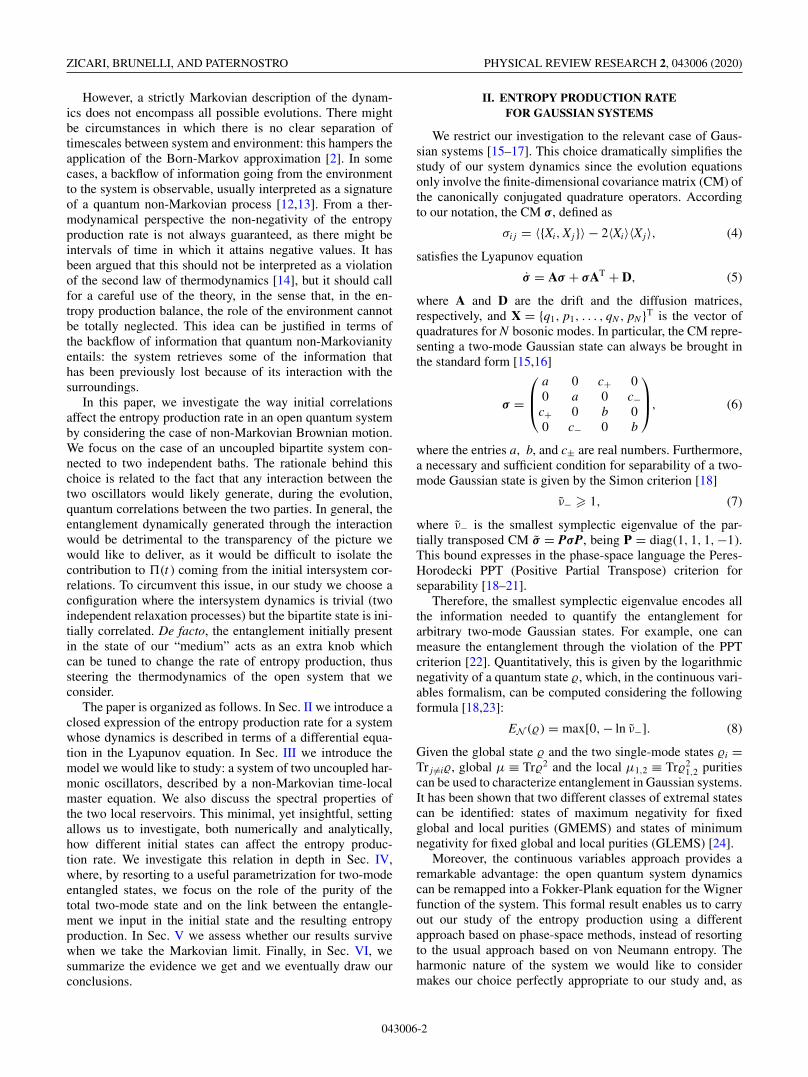
FIG. 2. Entropy production rate in a system of two noninteract-ing oscillators undergoing the non-Markovian dynamics describedin Sec. III. We compare the behavior of the entropy production rateresulting from a process where the system is initialized in a statewith no initial correlations (solid line) to what is obtained startingfrom a correlated state (dashed-dotted line). The latter case refersto the preparation of a system in a pure (g = 1), symmetric (d = 0)squeezed state (λ = 1). The former situation, instead, corresponds totaking the tensor product of the local states. In this plot we have takens = 2 and an Ohmic SD with Lorentz-Drude cutoff. The systemparameters are α = 0.1ω0, ωc = 0.1ω0, β = 0.1ω−1

0 .

To show a preview of our results, we start with a con-crete case shown in Fig. 2. We prepare the system in a pure(g = 1) symmetric (d = 0) state, and investigate the effectsof initial correlations on �(t ) by comparing the value takenby this quantity for such an initial preparation with what isobtained by considering the covariance matrix associated withthe tensor product of the local states of the oscillators, i.e.,by forcefully removing the correlations among them. Non-Markovian effects are clearly visible in the oscillations of theentropy production and lead to negative values of �(t ) inthe first part of the evolution. This is in stark contrast withthe Markovian case, which entails non-negativity of the en-tropy production rate. Crucially, we see that, for a fixed initialvalue of the local energies, the presence of initial correlationsenhances the amount of entropy produced at later times, in-creasing the amplitude of its oscillations. We also stress thatboth curves eventually settle to zero (on a longer timescalethan shown in Fig. 2) as argued in Sec. III.

We now move to a more systematic investigation of �(t )and its dependence on the specific choice of s, d, g, λ. In orderto separate the contributions, we first study the behavior of�(t ) when we vary one of those parameters, while all theothers are fixed. We can first rule out the contribution ofthermal noise by considering the case in which the reservoirsare in their vacuum state. Such zero-temperature limit canbe problematic, as some approaches to the quantification ofentropy production fail to apply in this limit [5]. In contrast,phase-space methods based on the Rényi-2-Wigner entropyallow to treat such a limit without pathological behaviorsassociated with such zero-temperature catastrophe [5]. Thisformal consistency is preserved also in the case of a system

0 10 20 30 40 50

ω0t

−6

−4

−2

0

2

4

6

Π(t

)

×10−4

0 20 400.0

0.5

1.0

EN

g = 1g = 2g = 3

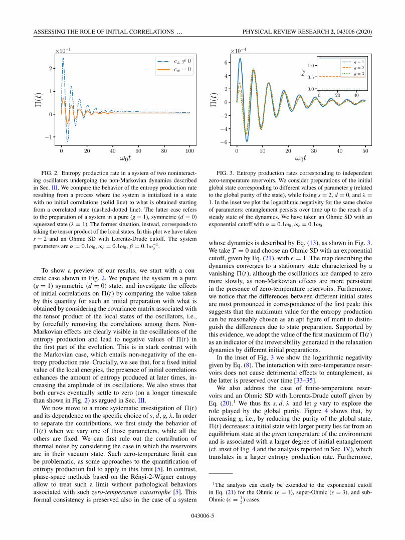
FIG. 3. Entropy production rates corresponding to independentzero-temperature reservoirs. We consider preparations of the initialglobal state corresponding to different values of parameter g (relatedto the global purity of the state), while fixing s = 2, d = 0, and λ =1. In the inset we plot the logarithmic negativity for the same choiceof parameters: entanglement persists over time up to the reach of asteady state of the dynamics. We have taken an Ohmic SD with anexponential cutoff with α = 0.1ω0, ωc = 0.1ω0.

whose dynamics is described by Eq. (13), as shown in Fig. 3.We take T = 0 and choose an Ohmic SD with an exponentialcutoff, given by Eq. (21), with ε = 1. The map describing thedynamics converges to a stationary state characterized by avanishing �(t ), although the oscillations are damped to zeromore slowly, as non-Markovian effects are more persistentin the presence of zero-temperature reservoirs. Furthermore,we notice that the differences between different initial statesare most pronounced in correspondence of the first peak: thissuggests that the maximum value for the entropy productioncan be reasonably chosen as an apt figure of merit to distin-guish the differences due to state preparation. Supported bythis evidence, we adopt the value of the first maximum of �(t )as an indicator of the irreversibility generated in the relaxationdynamics by different initial preparations.

In the inset of Fig. 3 we show the logarithmic negativitygiven by Eq. (8). The interaction with zero-temperature reser-voirs does not cause detrimental effects to entanglement, asthe latter is preserved over time [33–35].

We also address the case of finite-temperature reser-voirs and an Ohmic SD with Lorentz-Drude cutoff given byEq. (20).1 We thus fix s, d, λ and let g vary to explore therole played by the global purity. Figure 4 shows that, byincreasing g, i.e., by reducing the purity of the global state,�(t ) decreases: a initial state with larger purity lies far from anequilibrium state at the given temperature of the environmentand is associated with a larger degree of initial entanglement(cf. inset of Fig. 4 and the analysis reported in Sec. IV), whichtranslates in a larger entropy production rate. Furthermore,

1The analysis can easily be extended to the exponential cutoffin Eq. (21) for the Ohmic (ε = 1), super-Ohmic (ε = 3), and sub-Ohmic (ε = 1

2 ) cases.

043006-5

ZICARI, BRUNELLI, AND PATERNOSTRO PHYSICAL REVIEW RESEARCH 2, 043006 (2020)

0 20 40 60 80 100

ω0t

−0.1

0.0

0.1

0.2

Π(t

) 0 50 1000.0

0.5

1.0

EN

g=1g=2g=3

FIG. 4. Entropy production rates corresponding to differentpreparations of the initial global state. We consider different valuesof parameter g, while taking s = 2, d = 0, and λ = 1. In the inset weplot the logarithmic negativity for the same choice of the parameters.The dynamics of the system has been simulated using an Ohmic SDwith a Lorentz-Drude cutoff. The system parameters are α = 0.1ω0,ωc = 0.1ω0, β = 0.1ω−1

0 .

our particular choice of the physical parameters leads to theobservation of “entanglement sudden death” [33,34]: an initialstate with non-null logarithmic negativity completely disen-tangles in a finite time due to interaction with environment,the disentangling time being shortened by a growing g (cf.inset of Fig. 4).

Similarly, we can bias the local properties of the oscillatorsby varying d and, in turn, g = 2d + 1, while keeping s, λfixed: In Fig. 5 we can observe that, when the global energy isfixed, the asymmetry in the local energies, and purities μ1 andμ2, reduces the entropy production rate. In the inset we showthat, by increasing the asymmetry between the two modes,the entanglement takes less time to die out. These results areconsistent with the trends observed in Fig. 4. Indeed, a bias inthe local energies would make the reduced state of one of the

0 20 40 60 80 100

ω0t

−0.2

−0.1

0.0

0.1

0.2

0.3

0.4

Π(t

) 0 50 1000

1

2

EN

d=0d=1d=2d=3

FIG. 5. Entropy production rates corresponding to different val-ues of d and g = 2d + 1 in the parametrization of the initial state (wehave taken s = 4 and λ = 1). In the inset, the behavior of the loga-rithmic negativity is shown. In this figure, we take an Ohmic SD witha Lorentz-Drude cutoff and α = 0.1ω0, ωc = 0.1ω0, β = 0.1ω−1

0 .

0 2 4 6 8 10

ω0t

0.0

0.2

0.4

0.6

|Π(t

)|

g = 1

FIG. 6. Entropy production rates �(t ) (absolute value) as a func-tion of time. The initial CM is parametrized by fixing s (s = 10 in thefigure) and randomly choosing d, g, λ such that they are uniformlydistributed in the intervals [0, s − 1], [2d + 1, d + 10], and [−1, 1],respectively. The figure reports NR = 1000 different realizations ofthe initial state. The dashed line corresponds to the globally pure state(g = 1) with d = 0, λ = 1. All the plots are obtained considering anOhmic SD with a Lorentz-Drude cutoff and α = 0.1ω0, ωc = 0.1ω0,β = 0.1ω−1

0 .

two oscillators more mixed, and thus less prone to preserve theentanglement that is initially set in the joint harmonic state.Such imbalance would give different weights to the two localdissipation processes, thus establishing an effective preferredlocal channel for dissipation. In turn, this would result in alesser weight to the contribution given by correlations.

We conclude our analysis in this section by exploring theparameter space in a more systematic way by fixing the globalenergy s and randomly choosing the three parameters left,provided that the constraints in Eq. (24) are fulfilled. We seefrom Fig. 6 that the curve for �(t ) comprising all the othersis the one corresponding to unit global purity, i.e., g = 1, andd = 0, λ = 1 (dashed line). The globally pure state is indeedthe furthest possible from a diagonal one: the rate at whichentropy production varies is increased in order to reach thefinal diagonal state σ∞.

Dependence on the initial entanglement

We now compare the trends corresponding to differentchoices of the parameters characterizing the initial state. Asnon-Markovian effects are reflected in oscillating behavior ofthe entropy production, we can contrast cases correspondingto different initial preparations by looking at the maximumand the minimum values �max and �min that the entropyproduction rate assumes for each choice of the parameters.Taking into account the evidence previously gathered, in thesimulations reported in this section we fix the minimum valuefor g, i.e., g = 2d + 1, and λ = +1 as significant for the pointsthat we want to put forward. In fact, with such choices we areable to parametrize the initial state with a minimum number ofvariables, while retaining the significant features that we aimat stressing. We can further assume, without loss of generality,d � 0: this is simply equivalent to assuming that the firstoscillator is initially prepared in a state with a larger degree

043006-6

ASSESSING THE ROLE OF INITIAL CORRELATIONS … PHYSICAL REVIEW RESEARCH 2, 043006 (2020)

0.0 0.5 1.0 1.5 2.0

E (t = 0)

0.0

0.5

1.0

1.5

Entr

opy

pro

duct

ion

rate

Πmax Numerical

Πmax Analytical

Πmin Numerical

Πmin Analytical

FIG. 7. Maximum and minimum of the entropy production rate�max and �min as functions of the entanglement negativity at t = 0.We take s = 4, g = 2d + 1, λ = 1, while 0 � d � 3. We comparethe numerical results (triangles and circles) to the analytical solutionin Eq. (A1) (solid line). We have used an Ohmic SD with a Lorentz-Drude cutoff and α = 0.1ω0, ωc = 0.1ω0, β = 0.01ω−1

0 .

of mixedness than the second one, i.e., μ1 � μ2. In this case,we can express d in terms of the smallest symplectic eigen-value of the partially transposed CM ν̃−. Therefore, takinginto account the constraints given by Eq. (24), one has thatd = − 1

2 (ν̃2− − 2sν̃− + 1). We already mentioned in Sec. III

that we are able to derive a closed expression for the CMat any time t , given by Eq. (17). We can further notice thatthe positive and negative peaks in the entropy production rateare attained at short times. We can thus perform a Taylorexpansion of �(t ) in Eq. (18) to obtain

�� (t ) = [1 − �(t )]∫ t

0dτ�(τ )

+∫ t

0dτ �(τ )�(τ ) + O(α4). (25)

As �(t ) ∝ α2 and �(t ) ∝ α2, we can retain only the first termconsistently with the weak coupling approximation we areresorting to. Therefore, we can recast Eq. (17) in a form thatis more suitable for numerical evaluations, namely,

σ(t ) = [1 − �(t )]σ(0) +[

2∫ t

0dτ�(τ )

]14. (26)

By substituting Eq. (26) into (10), we get the analytic expres-sion for the entropy production rate, given in Appendix for thesake of completeness but whose explicit form is not crucial forour analysis here.

In this way, all the information about the initial state isencoded in the value of ν̃− while s is fixed. Note that thisexpression holds for any SD: once we choose the latter, we candetermine the time-dependent coefficients �(t ) and γ (t ) andthus the entropy production rate �(t ). We can then computethe maximum of the entropy production rate and study thebehavior of �max and �min as functions of the entanglementnegativity EN at t = 0. In Fig. 7 we compare numerical resultsto the curve obtained by considering the analytical solutiondiscussed above and reported in Eq. (A1). Remarkably, we

−2.0 −1.5 −1.0 −0.5 0.0

ln(ν̃ t=0)

−3.0

−2.5

−2.0

−1.5

−1.0

ln(Π

max

)

Ohmic - Lorentz-Drude

sub-Ohmic - exp

super-Ohmic - exp

Ohmic - exp

FIG. 8. Plot of �max against the smallest symplectic eigenvalueof the partially transposed CM at t = 0 (logarithmic scale) for dif-ferent SDs (as stated in the legend). The initial state is preparedusing the same parametrization chosen in Fig. 7, while we have takenα = 0.1ω0, ωc = 0.1ω0, β = 0.1ω−1

0 .

observe a monotonic behavior of our chosen figure of meritwith the initial entanglement negativity: the more entangle-ment we input at t = 0 the higher the maximum of the entropyproduction rate is. We can get to the same conclusion (inabsolute value) when we consider the negative peak �min.

The monotonic behavior highlighted above holds regard-less of the specific form of the spectral density. In Fig. 8we study �max against the smallest symplectic eigenvalueν̃− of the partially transposed CM for the various spectraldensities we have considered, finding evidence of a power lawof the form �max ∝ ν̃δ

−, where the exponent δ depends on thereservoir’s spectral properties.

V. MARKOVIAN LIMIT

We are now interested in assessing whether the analyticaland numerical results gathered so far bear dependence onthe non-Markovian character of the dynamics. With this inmind, we explore the Markovian limit, in which the problemis fully amenable to an analytical solution, that can also beused to validate our numerical results. Such limit is obtainedby simply choosing an Ohmic SD with a Lorentz-Druderegularization [Eq. (20)] and taking the long-time and high-temperature limits, i.e., ω0t � 1 and β−1 � ω0. This yieldsthe time-independent coefficients

�(t ) − γ (t )

2−→ γM[2n̄(ω0) + 1], (27)

�(t ) + γ (t )

2−→ γM n̄(ω0), (28)

where n̄(ω0) = (eβω0 − 1)−1 is the average number of excita-tions at a given frequency ω0, whereas γM ≡ 2α2ω2

cω0/(ω2c +

ω20 ). Therefore, Eq. (13) reduces to a master equation de-

scribing the dynamics of two uncoupled harmonic oscillatorsundergoing Markovian dynamics, for which we take A =−γM14 and D = 2γM[2n̄(ω0) + 1]14 in Eq. (5).

Working along the same lines as in the non-Markoviancase, we study the behavior of �(t ) by suitably choosing the

043006-7

ZICARI, BRUNELLI, AND PATERNOSTRO PHYSICAL REVIEW RESEARCH 2, 043006 (2020)

0 20 40 60 80 100

ω0t

0.00

0.05

0.10

0.15

0.20

0.25

0.30

Π(t

) 0 50 1000.0

0.5

1.0

EN

g = 1g = 2g = 3

FIG. 9. Entropy production rates corresponding to differentpreparations of the initial global state in the Markovian limit. Wehave taken different values of g (thus varying the global purityof the state of the system) with s = 2, d = 0, λ = 1, α = 0.1ω0,ωc = 0.1ω0, β = 0.01ω−1

0 .

parameters encoding the preparation of the initial state. Forexample, in Fig. 9 we plot the entropy production rate as afunction of time for different values of g. The limiting pro-cedure gives back a coarse-grained dynamics monotonicallydecreasing toward the thermal state, to which it corresponds anon-negative entropy production rate, asymptotically vanish-ing in the limit t → ∞. Moreover, the memoryless dynamicsleads to a monotonic decrease of the entanglement negativity,as shown in the inset of Fig. 9. In this case, the globally purestate (g = 1, dashed line in Fig. 10) still plays a special role:all the curves corresponding to value of g smaller than theunity remains below it.

The Markovian limit provides a useful comparison interms of integrated quantities. In this respect, we can study

0 2 4 6 8 10

ω0t

0.00

0.25

0.50

0.75

1.00

1.25

1.50

Π(t

)

g = 1

FIG. 10. Entropy production rate �(t ) plotted against the di-mensionless time ω0t in the Markovian regime. The initial CM isparametrized by setting s = 10 and randomly sampling (in a uniformmanner) d, g, λ from the intervals [0, s − 1], [2d + 1, d + 10], and[−1, 1], respectively. We present NR = 100 different realizations ofthe initial state. The dashed line represents the state with unit globalpurity (g = 1) and d = 0, λ = 1. For the dynamics, we have takenα = 0.1ω0, ωc = 0.1ω0, β = 0.01ω−1

0 .

0.00 0.25 0.50 0.75 1.00 1.25

E (t = 0)

3.4

3.6

3.8

4.0

4.2

4.4

4.6

Σ

Ohmic (Lorentz-Drude)

Markovian Limit

FIG. 11. Entropy production in the non-Markovian case (solidline) as a function EN (t = 0), compared with its counterpartachieved in the corresponding Markovian limit (dashed line). Wehave taken s = 2, d = 0, λ = 1, α = 0.1ω0, ωc = 0.1ω0, β =0.01ω−1

0 .

what happens to the entropy production � = ∫ +∞0 �(t )dt .

Although the non-Markovian dynamics entails the negativityof the entropy production rate in certain intervals of time,the overall entropy production is larger than the quantity wewould get in the corresponding Markovian case, as can benoticed in Fig. 11.

Finally, we can study the dependence of the Markovianentropy production rate on the initial entanglement. Note that,in this limit, Eq. (10) yields an analytic expression for theentropy production rate at a generic time t , which we writeexplicitly in Eq. (A2). From our numerical inspection, wehave seen that the entropy production rate is maximum at

0.2 0.4 0.6 0.8 1.0

ν̃ t=0

0.2

0.4

0.6

0.8

Πm

ax

Analytical

Numerical

FIG. 12. Markovian limit: maximum entropy production rate�max as a function of the minimum symplectic eigenvalue of thepartially transposed CM at t = 0. We have taken s = 4, g = 2d + 1,λ = 1, 0 � d � 3, α = 0.1ω0, ωc = 0.1ω0, β = 0.1ω−1

0 . We com-pare the curve obtained numerically (triangles) to the analytical trend(solid line) found through Eq. (29).

043006-8

ASSESSING THE ROLE OF INITIAL CORRELATIONS … PHYSICAL REVIEW RESEARCH 2, 043006 (2020)

t = 0, so that

�max ≡ �(0) = −8γM + 4s γM tanh

(βω0

2

)

+ 4s γM coth(

βω0

2

)(2s − ν̃−)ν̃−

. (29)

If we fix the parameter s and plot �max against ν̃−, wecan contrast analytical and numerical results (cf. Fig. 12).We can draw the same conclusion as in the non-Markoviancase: the more entanglement we input, the higher the entropyproduction rate.

VI. CONCLUSIONS

We have studied, both numerically and analytically, thedependence of the entropy production rate on the initial cor-relations between the components of a composite system.We have considered two noninteracting oscillators exposedto the effects of local thermal reservoirs. By using a generalparametrization of the initial state of the system, we havesystematically explored different physical scenarios. We haveestablished that correlations play an important role in the rateat which entropy is intrinsically produced during the process.Indeed, we have shown that, when the system is prepared ina globally pure state, we should expect a higher entropy pro-duction rate. This is the case, regardless of the spectral densitychosen, for initial entangled states of the oscillators: largerinitial entanglement is associated with higher rates of entropyproduction, which turns out to be a monotonic function of the

initial degree of entanglement. Remarkably, our analysis takesinto full consideration signatures of non-Markovianity in theopen system dynamics.

It would be interesting, and indeed very important, to studyhow such conclusions are affected by the possible interac-tion between the constituents of our system, a situation thatis currently at the focus of our investigations, as well asnon-Gaussian scenarios involving either nonquadratic Hamil-tonians or spinlike systems.

ACKNOWLEDGMENTS

We thank R. Puebla for insightful discussions and valuablefeedback about the work presented in this paper. We ac-knowledge support from the H2020 Marie Skłodowska-CurieCOFUND project SPaRK (Grant No. 754507), the H2020-FETPROACT-2016 HOT (Grant No. 732894), the H2020-FETOPEN-2018-2020 project TEQ (Grant No. 766900), theDfE-SFI Investigator Programme (Grant No. 15/IA/2864),COST Action CA15220, the Royal Society Wolfson ResearchFellowship (RSWF\R3\183013) and International ExchangesProgramme (IEC\R2\192220), the Leverhulme Trust Re-search Project Grant (Grant No. RGP-2018-266).

APPENDIX: ANALYTIC EXPRESSIONS FOR THEENTROPY PRODUCTION RATE

We report the expression for the entropy production rate inthe non-Markovian regime and the Markovian limit. By usingA = −γ (t )14, D = 2�(t )14, and σ(t ) given by Eq. (26),one obtains the following expression for the general non-Markovian case:

�(t ) = −8γ (t ) + 4γ 2(t )[s − 2s �(t ) + �̄(t )]

�(t )+ 4�(t )[s − 2s �(t ) + �̄(t )]

ν̃−(2s − ν̃−)[1 − �(t )]2 + 2s�̄(t )[1 − �(t )] + �̄2(t ), (A1)

where �̄(t ) = 2∫ t

0 �(τ )dτ .On the other hand, in the Markovian limit discussed in Sec. V, Eq. (A1) reads as

�(t ) = −8γM + 4γM

[1 + e−2γMt s tanh

(βω0

2

)]+ 4γM coth

(βω0

2

)e2γMt

[s + (e2γMt − 1) coth

(βω0

2

)][2s − ν̃− + (e2γMt − 1) coth

(βω0

2

)][ν̃− + (e2γMt − 1) coth

(βω0

2

)] . (A2)

[1] S. R. D. Groot and P. Mazur, Non-equilibrium Thermodynamics(North-Holland, Amsterdam, 1961).

[2] H.-P. Breuer and F. Petruccione, The Theory of OpenQuantum Systems (Oxford University Press, Oxford,2002).

[3] T. Batalhão, S. Gherardini, J. Santos, G. Landi, and M.Paternostro, Thermodynamics in the Quantum Regime, Funda-mental Theories of Physics, Vol. 195, edited by F. Binder, L.Correa, C. Gogolin, J. Anders, and G. Adesso (Springer, Berlin,2018), Chap. 16.

[4] G. T. Landi, T. Tomé, and M. J. de Oliveira, J. Phys. A: Math.Theor. 46, 395001 (2013).

[5] J. P. Santos, G. T. Landi, and M. Paternostro, Phys. Rev. Lett.118, 220601 (2017).

[6] J. P. Santos, L. C. Céleri, G. T. Landi, and M. Paternostro,npj Quantum Inf. 5, 23 (2019).

[7] A. Polkovnikov, Ann. Phys. 326, 486 (2011).[8] G. Francica, J. Goold, and F. Plastina, Phys. Rev. E 99, 042105

(2019).[9] H. Spohn, J. Math. Phys. 19, 1227 (1978).

[10] R. Alicki, J. Phys. A: Math. Gen. 12, L103 (1979).[11] H.-P. Breuer, Phys. Rev. A 68, 032105 (2003).[12] Á. Rivas, S. F. Huelga, and M. B. Plenio, Rep. Prog. Phys. 77,

094001 (2014).[13] H.-P. Breuer, E.-M. Laine, J. Piilo, and B. Vacchini, Rev. Mod.

Phys. 88, 021002 (2016).[14] S. Marcantoni, S. Alipour, F. Benatti, R. Floreanini, and A. T.

Rezakhani, Sci. Rep. 7, 12447 (2017).

043006-9

ZICARI, BRUNELLI, AND PATERNOSTRO PHYSICAL REVIEW RESEARCH 2, 043006 (2020)

[15] A. Ferraro, S. Olivares, and M. Paris, Gaussian States in Quan-tum Information (Bibliopolis, Naples, 2005).

[16] A. Serafini, Quantum Continuous Variables (CRC Press, BocaRaton, FL, 2017).

[17] H. Carmichael, Statistical Methods in Quantum Optics(Springer, Berlin, 1999).

[18] G. Adesso and F. Illuminati, Phys. Rev. A 72, 032334 (2005).[19] A. Peres, Phys. Rev. Lett. 77, 1413 (1996).[20] P. Horodecki, Phys. Lett. A 232, 333 (1997).[21] R. Simon, Phys. Rev. Lett. 84, 2726 (2000).[22] K. Audenaert, M. B. Plenio, and J. Eisert, Phys. Rev. Lett. 90,

027901 (2003).[23] G. Vidal and R. F. Werner, Phys. Rev. A 65, 032314 (2002).[24] G. Adesso, A. Serafini, and F. Illuminati, Phys. Rev. Lett. 92,

087901 (2004).[25] M. Brunelli and M. Paternostro, arXiv:1610.01172.[26] U. Weiss, Quantum Dissipative Systems (World Scientific,

Singapore, 1999).

[27] A. Caldeira and A. Leggett, Phys. A (Amsterdam) 121, 587(1983).

[28] B. L. Hu, J. P. Paz, and Y. Zhang, Phys. Rev. D 45, 2843 (1992).[29] A. Rivas and S. F. Huelga, Open Quantum Systems: An Intro-

duction, 1st ed. (Springer, Berlin, 2012).[30] F. Intravaia, S. Maniscalco, and A. Messina, Phys. Rev. A 67,

042108 (2003).[31] F. Intravaia, S. Maniscalco, and A. Messina, A. Eur. Phys. J. B

32, 97 (2003).[32] J. Paz and W. Zurek, in Coherent Atomic Matter Waves, Les

Houches Summer School, Session 72, edited by R. Kaiser, C.Westbrook, and F. David (EDP Sciences, Les Ulis, 2001).

[33] R. Vasile, S. Olivares, M. G. A. Paris, and S. Maniscalco,Phys. Rev. A 80, 062324 (2009).

[34] J. P. Paz and A. J. Roncaglia, Phys. Rev. Lett. 100, 220401(2008).

[35] S. Maniscalco, S. Olivares, and M. G. A. Paris, Phys. Rev. A75, 062119 (2007).

043006-10