physical review x 9, 041012 (2019)

Asymmetric Protocols for Scalable High-Rate Measurement-Device-IndependentQuantum Key Distribution Networks

Wenyuan Wang ,1,* Feihu Xu,2,† and Hoi-Kwong Lo1,‡1Centre for Quantum Information and Quantum Control (CQIQC), Dept. of Electrical & ComputerEngineering and Department of Physics, University of Toronto, Toronto, Ontario, M5S 3G4, Canada

2Shanghai Branch, National Laboratory for Physical Sciences at Microscale,University of Science and Technology of China, Shanghai, 201315, China

(Received 14 April 2018; revised manuscript received 11 July 2019; published 16 October 2019)

Measurement-device-independent quantum key distribution (MDI-QKD) can eliminate detector sidechannels and prevent all attacks on detectors. The future of MDI-QKD is a quantum network that providesservice to many users over untrusted relay nodes. In a real quantum network, the losses of various channelsare different and users are added and deleted over time. To adapt to these features, we propose a type ofprotocol that allows users to independently choose their optimal intensity settings to compensate fordifferent channel losses. Such a protocol enables a scalable high-rate MDI-QKD network that can easily beapplied for channels of different losses and allows users to be dynamically added or deleted at any timewithout affecting the performance of existing users.

DOI: 10.1103/PhysRevX.9.041012 Subject Areas: Quantum Information

I. INTRODUCTION

Quantum computing threatens the security of conven-tional public key cryptography [1]. To address this increas-ing threat, quantum key distribution (QKD) allows twoparties to share a pair of random keys with information-theoretic security and protects users from the attack of evenquantum computers. Because of this, QKD is consideredas one of the strong candidates for the next-generationtechnology for secure communications. Moreover, as wenow live in the era of the Internet of Things that inter-connects many users and devices, for QKD to be widelydeployed in the future, an important step is to study it in anetwork setting, i.e., designing quantum networks that canconnect and provide service to numerous users, who mayfreely join or leave a network.The problem is, while QKD is theoretically secure, side

channels still exist in a system built with practical compo-nents. Therefore, an important question in quantum cryp-tography is to determine how secure a system really is inpractice. There havebeenmultiple quantumhacking attacks,e.g., Refs. [2–7], that target the practicalweaknesses inQKD

systems. Among the components of a QKD system, detec-tors are especially susceptible to attacks (and a majority ofhacking attempts target the detectors), making them theAchilles’ heel of QKD systems. The measurement-device-independent (MDI) QKD [8] protocol allows an untrustedthird party tomakemeasurements, thus avoiding all securitybreaches from detector side channels. Since its proposal,MDI-QKD has attracted worldwide interest, and there havebeen hundreds of follow-up theory and experimental papers.For example, some notable experimental implementationshave been reported in Refs. [9–15]. An illustration of theMDI-QKD setup is shown in Fig. 1.Up till now, multiple field implementations of point-

to-point QKD networks have been reported in, e.g.,Refs. [16–18]; however, they all relied on trusted relays(where the information stops being quantum at the relays),which are undesirable for security. MDI-QKD solves thisproblem by allowing untrusted relays in a quantum net-work, which is a huge advantage over previous point-to-point QKD networks, making MDI-QKD a powerfulcandidate for future quantum networks. For instance, thefirst three-user star-shaped MDI-QKD network experimentin a metropolitan setting has been reported in Ref. [19].However, a major limitation of MDI-QKD is that it

requires all users to have near-identical (i.e., symmetric)distances to the untrusted relay for the protocol to workwell [20,21], and the key rate will degrade very quicklywith an increased level of asymmetry between channels.[22] Because of this limitation, previous experiments ofMDI-QKD either were performed in the laboratory oversymmetric fiber spools [9–14] or had to deliberately add a

*[email protected]†[email protected]‡[email protected]

Published by the American Physical Society under the terms ofthe Creative Commons Attribution 4.0 International license.Further distribution of this work must maintain attribution tothe author(s) and the published article’s title, journal citation,and DOI.

PHYSICAL REVIEW X 9, 041012 (2019)

2160-3308=19=9(4)=041012(30) 041012-1 Published by the American Physical Society

https://orcid.org/0000-0002-8516-9168

https://crossmark.crossref.org/dialog/?doi=10.1103/PhysRevX.9.041012&domain=pdf&date_stamp=2019-10-16

https://doi.org/10.1103/PhysRevX.9.041012




https://creativecommons.org/licenses/by/4.0/

https://creativecommons.org/licenses/by/4.0/

tailored length of fiber to the shorter channel (to introduceadditional loss) in exchange for better symmetry [15].Adding additional fibers not only is cumbersome as itrequires halting the system (and not practical when thereare many pairs of connections in a quantum network orwhen channel loss is changing), but also results in asuboptimal key rate when the channels are asymmetric.An intuitive illustration of this can be found in theAppendix A.In a realistic setup, a quantum network will very likely

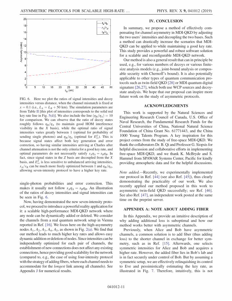
have asymmetric channels due to different geographicallocations of sites. For instance, the channel losses inRefs. [16,17] are largely different. Here, we select fivenodes from the Vienna QKD network [16] and show themin Fig. 2(a), where the biggest difference between channelsis as large as 66 km. If we want to perform MDI-QKD overthese locations, although one can add additional fibersto each channel to compensate for channel differences,users have to accommodate for the lowest-transmittancechannel—just like in “Liebig’s barrel”—and have a sub-optimal rate. Moreover, in a scalable network with largenumbers of dynamically added or deleted users, it is notpractical to add fibers and maintain symmetry between

each pair of users all the time. Additionally, if one is toimplement a MDI-QKD network over free space betweenmobile platforms (e.g., satellite-based MDI-QKD [25] ormaritime MDI-QKD between ships), the losses in thechannels are constantly changing, and the channels willoften be highly asymmetric, as shown in Fig. 2(b). Insummary, the requirement on symmetric channels signifi-cantly limits the key rate of previous MDI-QKD protocolsin a general quantum network, thus seriously hindering thewidespread deployment of MDI-QKD.The issue of MDI-QKD with asymmetric channel losses

was first considered in Ref. [4], which provided a rule ofthumb on the ratio of intensities between Alice’s and Bob’ssignals. However, Ref. [4] assumes infinitely large datasize and was also restricted to protocols where the same setof intensities for the optical signals are used in the twobases X and Z. In this paper, we make no such assumptions.In this work, we present a new method to overcome this

crucial limitation directly and enable high-rate MDI-QKD

FIG. 1. An example schematic setup of MDI-QKD [8]. Aliceand Bob, respectively, send signals through two channels, andCharles measures the signals with a Bell-state measurement [byobserving the coincidence click events in detectors D1H, D1V ,D2H , D2V behind the beam splitter (BS) and polarizing beamsplitters (PBSs)] and announces the results. Here, weak coherentpulse (WCP) sources are used, in combination with decoy statescreated with intensity modulators (Decoy-IM). In this particularsetup, polarization encoding is used [with polarization modu-lators (Pol-M)], but MDI-QKD can be performed with otherdegrees of freedom, such as time-bin phase encoding, too.

FIG. 2. (a) Part of the QKD network setup from Ref. [16]. Hereas an example, we focus on the five nodes with high asymmetry(nodes A1, A3, A4, A5 connected with A2, corresponding to nodes1–5 in Ref. [16]), where A2 can be set up as an untrusted relay. Wekeep the same topology and redraw it as a star-shaped MDI-QKDnetwork with four users connected to a single untrusted relay.When performing MDI-QKD, all users need to accommodate forthe longest channel (i.e., A1) and add losses to their channels(e.g., extending to A0

3, A04, A

05) if previous protocols are used.

(b) Ship-to-ship communication and ground-satellite communi-cation, where the participants’ distances to the detector areconstantly changing, and the channels will thus have quicklyvarying asymmetry.

WENYUAN WANG, FEIHU XU, and HOI-KWONG LO PHYS. REV. X 9, 041012 (2019)

041012-2

with arbitrary user locations. First of all, our work providesan important conceptual insight: A common folklore in thefield is that MDI-QKD relies on the Hong-Ou-Mandel(HOM) dip, and therefore, it is important to use matchedintensities at the beam splitter of the receiver Charles inMDI-QKD. Here, we show that such a folklore is, in fact, amisconception.We show that there is an intrinsic asymmetrybetween the two bases ofMDI-QKD:Only theX basis relieson the indistinguishability of photons from the two beams,while the Z basis does not. We later show that one can makeuse of such an asymmetry to create protocols resilientagainst asymmetric channels. We also show that this is ageneral theoretical result applicable to many protocols,including various types of MDI-QKD protocols and poten-tially other protocols such asMDI quantum-digital signature[26,27] and twin-field QKD [28] in asymmetric settings.Following this conceptual insight, we present a novel

method in this paper to combat channel asymmetry. Wemake use of the inherent asymmetry between bases inMDI-QKD and propose a type of asymmetric MDI-QKDprotocol where intensities are not only different for Aliceand Bob, but also different in the X and Z bases. In thisway, by decoupling the bases and also allowing Alice andBob to independently vary their intensities, the users caneffectively compensate for channel asymmetry in one basisand optimize the key generation rate in another basis,enabling a much higher key rate of our asymmetricprotocols in the presence of channel asymmetry.Additionally, we present a technique that makes it possibleto efficiently perform a local search for high-speed param-eter optimization over the extremely large parameter spacefor such asymmetric protocols (which would be otherwiseimpossible to optimize using previous algorithms such as inRefs. [20,29]).The protocols we propose have important practical

impacts. We show that, when channels are asymmetric,our protocols can provide a much higher key rate thanprevious protocols [30,31] that were designed for sym-metric channels [for instance, 1 to 2 orders of magnitudehigher rate at mid-to-close distances, e.g., 60 km (10 km)for Alice’s (Bob’s) channels, with a 50-km difference inchannel distances]. Moreover, it enables a much largerregion of possible combinations of channels: For instance,even at a small data size of N ¼ 1011 (N is defined as thetotal number of pulses sent by Alice and Bob), one cangenerate a high secret key rate of R ¼ 10−7 per pulse eventhrough an extremely asymmetric channel pair of 0 km(90 km) for Alice’s (Bob’s) channels, whereas withprevious protocols no key could be generated at all.Using the type of protocol we propose, one can completelyremove the requirement of symmetric channels in MDI-QKD. This makes our proposal a powerful solution thatenables high-rate MDI-QKD under arbitrary asymmetry,which paves the way for practical MDI-QKD networkswhere users can be placed at arbitrary locations.

The structure of this paper is as follows: In Sec. II A,we point out a theoretical insight that there is aninherent asymmetry between the two bases of MDI-QKD. In Sec. II B we make use of this insight and proposea type of asymmetric protocol that simultaneously has twokinds of asymmetries: the asymmetry between Alice andBob and the asymmetry between the X and Z bases, which,together, enable the protocol to effectively compensate fordifferent pairs of channels and maintain a good keygeneration rate. We show the security of such a schemein Sec. II C. We then describe how to optimally choose theasymmetric parameters in Sec. II D. While our proposalapplies to a general type of MDI-QKD protocol, we alsohighlight a specific implementation, a “seven-intensityprotocol,” and show that it is a good trade-off betweenthe key rate and ease of implementation. Lastly, we presentthe simulation results to show the effectiveness of ourprotocol compared with prior protocols in Sec. III.

II. ASYMMETRIC PROTOCOLS

In this section, we present a general theoretical frame-work for designing protocols that can effectively compen-sate for channel asymmetry and provide a good key rate.Note that our method proposed here is a general result thatcan be applied to any decoy-state MDI-QKD protocol withWCP sources for both asymptotic and finite-size cases aslong as (1) decoupled bases are used and (2) Alice and Bobhave asymmetric intensities. We show in Appendixes Band C that the scaling of the key rate versus distance isdetermined by the signal states, so in principle, any numberof decoy states (e.g., two decoys, three decoys, and fourdecoys) can be used so long as they can effectively estimatethe single-photon contributions. In principle, such a methodcan potentially be applied even to other types of protocolsin asymmetric settings, such as MDI quantum digitalsignature [26,27] and twin-field QKD [28], which are alsocurrently limited to symmetric intensities between Aliceand Bob and which also use two asymmetric bases X and Z.

A. Asymmetry between bases in MDI-QKD

Here, we start by making a key theoretical observationon MDI-QKD:Observation 1: For MDI-QKD, there is an inherent

asymmetry between the bases: Only the diagonal (X) basisrequires the indistinguishability of the signals from Aliceand Bob, while the rectilinear (Z) basis does not.Such an observation is because in MDI-QKD, Charles

performs a Bell-state measurement with postselection,making the protocol different from a simple two-photoninterference in a standard HOM dip. Here, let us follow thediscussions in Ref. [8] (and consider the experimental setupfrom Fig. 1 in Ref. [8]). Note that while Alice and Bobrandomly send signals in the X and Z bases, Charles alwaysmeasures in the Z basis (as defined by his PBS) and

ASYMMETRIC PROTOCOLS FOR SCALABLE HIGH-RATE … PHYS. REV. X 9, 041012 (2019)

041012-3

postselects detector click events that correspond to thetwo Bell states jψþi ¼ 1=

ffiffiffi2

p ðjHVi þ jVHiÞ and jψ−i ¼1=

ffiffiffi2

p ðjHVi − jVHiÞ. Such a postselection results in anasymmetry between the two bases. In the Z basis, onlyevents where Alice and Bob sent opposite states (e.g., jHVior jVHi) are accepted as bits. In these cases, no photoninterference takes place, and indistinguishability betweenthe two input photon beams is not required because each ofthe clicking detectors, respectively, receives only a signalfrom either Alice or Bob but never both. For WCP sources,in the ideal case with no misalignment or dark counts, theintensities of the pulses and even their spectrum and timingneed not be matching at all. In the X basis, however, theevents may correspond to identical states sent by Alice andBob [e.g., j þ þi and j − −i corresponding to jψþi ¼1=

ffiffiffi2

p ðj þ þi − j − −iÞ], which do interfere at the beamsplitter. [35] To ensure that the correct events are triggered,a good visibility of such a two-photon interference isrequired. Note that for WCP sources, the interferencevisibility is at most 50% (resulting in a 25% observedQBER in the X basis even in the ideal case—for instance,EXμμ, EX

νν when Alice and Bob use decoy states with inten-sities μA, μB and νA, νB—but we can perform a decoy-stateanalysis to correctly estimate a low QBER among single-photon components, eX;U11 ), and the visibility will quicklydrop when intensities are mismatched, such as observedin Ref. [21].Therefore, a low QBER in the X basis heavily relies on

the indistinguishability of the signals and the balance ofincoming intensities at Charles, while such a dependence isnot present in the Z basis. [37] Such a conclusion is rathergeneral and also not dependent on the degree of freedomused for qubit encoding, such as polarization encoding ortime-bin phase encoding (where jHVi and jVHi in the Zbasis correspond to pairs of early and late pulses, whichwill similarly not interfere at the beam splitter since theyhave different timing).

B. Using decoupled bases and asymmetric intensities

Here, let us consider the key rate formula of MDI-QKD[8,30]:

R ¼ PsAPsBfðsAe−sAÞðsBe−sBÞYX;L11 ½1 − h2ðeX;U11 Þ�

− feQZssh2ðEZ

ssÞg; ð1Þwhere sA, sB are the intensities of signal states, QZ

ss, EZss are

the gain and QBER in the Z (signal) basis, YX;L11 , eX;U11 are

the lower (upper) bounds of single-photon yield and QBERestimated from the decoy-state statistics in the X basis (i.e.,the observed gain and QBER for decoy states QX

ij, EXij,

where i, j are decoy intensities, such as in fμA; νA;ωg andfμB; νB;ωg if Alice and Bob each choose three decoystates), h2 is the binary entropy function, and fe is the error-correction efficiency.

In the key rate formula, the first part corresponds to keygeneration (where the privacy amplification depends on thesingle-photon contributions estimated from decoy-stateanalysis), and the second part corresponds to error correc-tion for the signal states. We can make another keyobservation on the intensities used in the two bases:Observation 2: In our protocol, the intensities of the

signal states fsA; sBg used in the Z basis are independentfrom those of the decoy states used in the X basis, whichmeans that the privacy amplification process (to boundEve’s information on the final key, i.e., estimate the phaseerror rate) in the X basis is completely decoupled from errorcorrection in the Z basis for key generation.This decoupling of bases means that it is possible for us

to independently adjust the decoy states and the signalstates in their respective bases to compensate for channelasymmetry or to optimize the key rate.For the decoy states, their role is to estimate the single-

photon contributions as accurately as possible. As wemention above, when channels are asymmetric, using thesame intensities for Alice and Bob (hence different inten-sities arriving at Charles after the channels’ attenuation)will result in poor interference visibility and high QBER inthe X basis, and consequently poor estimationof eX;U11 . For a good interference visibility, Alice andBob should try to maintain similar intensities arriving atCharles, so the decoy intensities should be chosen toroughly satisfy

μAηA ¼ μBηB; ð2Þ

where ηA and ηB are the channel transmittances in Alice’sand Bob’s channels. A similar equation holds true for νAand νB.In contrast, for the signal states, they are not involved in

privacy amplification. On the other hand, they affect thesignal-state gain and QBER QZ

ss, EZss (which determine the

amount of error correction) and the probability of sendingsingle photons for key generation sAe−sAsBe−sB . The keypoint is, the QBER EZ

ss does not require indistinguishabilityof the signals. If there is no misalignment or noise, EZ

sswould be zero regardless of incoming intensities. Inpractice, due to imperfections such as misalignment, theQBER EZ

ss [whose full expression can be found inAppendix C Eq. (C3)] still slightly depends on channelasymmetry and is also minimal if incoming intensities atCharles are balanced, but this dependence is for a muchdifferent reason (due to misalignment) than that in the Xbasis (mostly due to two-photon interference).Furthermore, EZ

ss is much less sensitive to channel asym-metry than QBER in the X basis. We can observe thisfrom Fig. 3.Note that, not only do signal intensities affect the signal-

state QBER, they also determine the probabilities ofsending single photons, hence affecting key generation,


041012-4

too. This means that, while having similar received signalintensities at Charles is surely one important criterion inachieving a good key rate, the optimal choice of signal-stateintensities requires a trade-off between the single-photonprobabilities and the error correction (and their optimalvalues can be found by numerical optimization). Generallyspeaking, the ratio of signal intensities sA=sB does notsatisfy a similar relation as Eq. (2), i.e., generally,

sAηA ≠ sBηB: ð3ÞTherefore, the protocols we propose have two inherentasymmetries: an asymmetry between Alice and Bob (sothat they can have different intensities and establish goodtwo-photon interference in the X basis) and an asymmetrybetween the X and Z bases (which allows decoy and signalstates to be independently optimized). Such inherentasymmetries in the protocols allow us to have a novelchoice of parameters and maintain a good key rate of MDI-QKD, even when Alice’s and Bob’s channels have verydifferent levels of loss. A more detailed discussion on howsuch independent choices of decoy and signal states affectthe key rate can be found in Appendix D.We discuss the security of such a scheme in Sec. II C,

and in Sec. II D, we discuss how to actually choose theoptimal decoy and signal intensities. We introduce the mainchallenge in implementing such asymmetric protocols—performing efficient parameter optimization over a hugeparameter space—and how we address this problem byproposing two important theoretical results for the key ratefunction of asymmetric MDI-QKD and using them todesign an efficient optimization algorithm.

C. Security

In this subsection, we show that the security of ourprotocol with decoupled bases and asymmetric intensitiesis not compromised compared to prior art protocols. Here,we state two facts that its security relies upon, both ofwhich have been proven in established papers [8,32]:(1) Given the same photon number i in a pulse, Eve has

no way of differentiating whether it came from thedecoy states or the signal states in the same basis.

(2) The single-photon pairs in the X and Z bases cannotbe distinguished from each other.

The first fact is proven in Ref. [32], which ensures thedecoy-state analysis works even with asymmetric inten-sities, and the second fact is proven in Ref. [8], whichensures that the decoupling of bases works.For fact (1), note that the density matrices for the two

states are the same, independent of whether they came fromthe decoy states or signal states. In quantum mechanics,whenever two density matrices are the same, they areindistinguishable. Similarly, for fact (2), note that the densitymatrices for the two cases are the same. Therefore, it is notpossible to distinguish them even in principle.

FIG. 3. An example of the respective quantum bit error rate(QBER) in the X basis and Z basis, EX

μμ and EZss (we consider a

pair of decoy states with intensities μA, μB in the X basis andsignal-state intensities sA, sB in the Z basis) versus the ratio ofintensities for MDI-QKD using WCP sources. Parameters fromTable II are used. Here we consider the case where the respectivedistances from Alice and Bob to Charles are LA ¼ 60 km, LB ¼10 km (i.e., the ratio of transmittances in the two channelssatisfies ηB=ηA ¼ 10). We fix sB ¼ 0.2 (or μB ¼ 0.2) and scanover different sA (or μA). Specifically, we also mark out theposition where sAηA ¼ sBηB (μAηA ¼ μBηB). Because QBER inthe X basis heavily depends on the visibility of two-photoninterference, it is lowest when intensities arriving at Charles’sbeam splitter are equal (a similar observation has been made inRef. [21]). However, importantly, the Z basis does not requiresignal indistinguishability, and its QBER is determined mainly bymisalignment. The misalignment makes the Z basis QBER alsoslightly dependent on the interference visibility and lowest whenarriving intensities are equal, but such a QBER is much lesssensitive to unbalanced intensities and is relatively low even ifsAηA ≠ sBηB. Therefore, by decoupling the X and Z bases, wecan maintain highly balanced decoy-state intensities arriving atCharles in the X basis, while further optimizing signal intensitiesto obtain a higher key rate. As a quantitative example of such adifference in sensitivity, let us consider LA¼60km, LB ¼ 10 km,and N ¼ 1011 (Table IV, line 1) and focus on two pairs of decoystates with intensities μA, μB, νA, νB. An optimal key rate ofR ¼ 3.1 × 10−5 can be achieved, where optimal decoy-stateintensities satisfy μA=μB ¼ νA=νB ¼ 9 ≈ ηB=ηA, and EX

μμ, EXνν

are both close to 25% (see Table IV for the full list of intensitiesand probabilities). Even a relatively small deviation, such aschoosing μA=μB ¼ νA=νB ¼ 100.5 ¼ 3.16 when fixing μB, νB(which results in EX

μμ and EXνν close to 32%) results in zero rate.

On the other hand, the optimal signal states satisfy sA=sB ¼ 3.5,which deviates from ηB=ηA, but EZ

μμ is still a rather small 0.013. Infact, even if we choose sA ¼ sB ¼ 0.2 here, we can still get R ¼1.0 × 10−5 while EZ

μμ ¼ 0.029.


041012-5

In more detail, for fact (1), let us first consider a verysimilar process in traditional decoy-state BB84 [32–34].Consider Alice using a laser with intensities μ or ν to sendweak coherent pulses to Bob. The photon number i followsa Poissonian distribution, e.g.,

pðijμÞ ¼ e−μμi

i!;

pðijνÞ ¼ e−ννi

i!: ð4Þ

The crucial point is that the conversion from such aprobability distribution described by intensities μ or ν to acertain photon number i is a Markov process, i.e., it ismemoryless, and for any given photon number i in thechannel, it does not contain any information of the intensityit came from. Surely, Eve can guess with a conditionaldistribution, e.g., pðμjiÞ, the likelihood that it comes from acertain intensity, but whatever actions Eve chooses toperform on the signal (e.g., choosing different levels ofyields YE1

i ; YE2i ;… with different probabilities for a given

photon number i) will be completely independent of theintensities Alice chose when sending the signal. This meansthat in the asymptotic case with infinite data, [38] given thesame photon number i in a pulse, we will still always haveyield Yi and QBER ei satisfying

YiðμÞ ¼ YiðνÞ;eiðμÞ ¼ eiðνÞ ð5Þ

when Alice uses intensities μ, ν. This is the exactobservation made in Ref. [32] [in Eqs. (4) and (5)].Similarly, for MDI-QKD, for any given pair of i-photon

and j-photon pulse, there is no information on which pair ofintensity settings (e.g., μ1A, μ

1B or μ2A, μ

2B) they came from.

That is, the yield Yi;j and QBER ei;j will satisfy

YXi;jðμ1A; μ1BÞ ¼ YX

i;jðμ2A; μ2BÞ;eXi;jðμ1A; μ1BÞ ¼ eXi;jðμ2A; μ2BÞ;YZi;jðμ1A; μ1BÞ ¼ YZ

i;jðμ2A; μ2BÞ;eZi;jðμ1A; μ1BÞ ¼ eZi;jðμ2A; μ2BÞ ð6Þ

for signals in each of the bases X and Z (the latter twoequations are meaningful if one also uses multiple decoyintensities in the Z basis, although here we use only the firsttwo equations as decoy-state analysis is performed only inthe X basis for our protocols). This, again, is a well-established result for decoy-state MDI-QKD as used in theoriginal MDI-QKD paper [8]. Note that this result (whichsimply comes from the fact that the sending of photonnumber i from an intensity μ is a Markov process) does notrely on the fact that Alice and Bob use the same intensities,and will remain unchanged for asymmetric intensities, too,

i.e., μ1A ≠ μ1B and μ2A ≠ μ2B. Also, note that for successfuldecoy-state analysis, we do not require the symmetrybetween the two bases, i.e., YX

i;jðμ1A; μ1BÞ ¼ YZi;jðμ2A; μ2BÞ

or eXi;jðμ1A; μ1BÞ ¼ eZi;jðμ2A; μ2BÞ for multiphoton pulses arenot required.Fact (2) stems from the fact that, for single-photon

components, Alice and Bob send the same density matricesρX1;1 ¼ ρZ1;1; that is, the single-photon pairs are basisindependent. This is an important result explicitly statedin the original MDI-QKD paper [8] (in the SecurityAnalysis section in the Supplemental Material). Usingdecoupled bases (i.e., a different set of intensities for theX and Z bases) does not affect the single photonsthemselves at all but affects only the probability of sendingthese single-photon pairs. However, this process of sendingsingle-photon pairs is again a Markov process. That is,although the single-photon pairs might have differentprobabilities of coming from either the X or Z bases(which Eve can fully be aware of, just like in “efficientBB84” [39], where basis choice probability is biased onpurpose), for any given pair of single photons that are sent,they are described by exactly the same density matrix, andthere is no information contained on which basis they camefrom; i.e., they are basis independent. Therefore, we cansafely conclude that YX

11 ¼ YZ11, which is the reason we can

perform decoy states in the X basis only to estimate YX11 and

use YZ11 ¼ YX

11 to obtain the single-photon yield in theZ basis.The security of a scheme of decoupling the bases in

MDI-QKD and using YZ11 ¼ YX

11 has also been theoreticallystudied in Ref. [30] and in the Appendix of Ref. [40,41],and the scheme has also been experimentally demonstratedin Refs. [13,40], although all these works were focused onthe scenario of symmetric channels only and did not discussthe role of decoupled bases in compensating channelasymmetry, which is one of the main novelties of ourwork. However, physically, the only difference between thesignals sent from Alice and Bob in our protocol and thosein prior protocols is the different intensities on the two arms[which we know, from fact (1) YX

i;jðμ1A; μ1BÞ ¼ YXi;jðμ2A; μ2BÞ,

will not affect the security of the decoy-state analysis], andfor decoupled bases, we use the same result YZ

11 ¼ YX11 for

single-photon pairs, which is no less secure than priorworks either.

D. Parameter optimization

In this section, we discuss how to perform efficientparameter optimization for such asymmetric protocols.Here, we highlight an implementation which we denoteas the seven-intensity protocol (which is the case wherethree decoy intensities are used in the X basis). We showthat it is a good trade-off between the key rate and ease ofimplementation and focus on this implementation whendiscussing parameter optimization (and the following


041012-6

numerical simulations). Nonetheless, we also show thegenerality of our method by including the results for otherprotocol cases (e.g., two-intensity and four-intensity) inAppendix E.Note that the results in the previous subsection are

general and not limited to the number of decoys Aliceand Bob use in the X basis. For instance, while using signalstates fsA; sBg in the Z basis, in the X basis Alice and Bobcan each use a different set of two decoy states fμ; νg, threedecoy states fμ; ν;ωg, or even four decoy statesfμ; ν; ν2;ωg. In principle, the concept of asymmetricintensities between Alice and Bob can also be applied toprior art protocols with nondecoupled bases, such as inRefs. [20,43] (where Alice and Bob use the same threedecoy states fμ; ν;ωg for both bases, and the Z basis μ isused as the signal state for key generation)—it is just thatsuch a protocol will have a lower key rate since μ cannotsimultaneously satisfy asymmetry compensation and keyrate optimization.As an example, in Table I we list a comparison between

the key rate of using different numbers of decoy states (withand without asymmetric intensities between Alice and Bob)in the presence of asymmetric channels. We include thenon-decoupled-bases case [20,43], too. We can see that,regardless of the protocol, using asymmetric intensitiesbetween Alice and Bob always provides a higher key ratewhen the channels are asymmetric. Also, the three-decoycase provides significant performance improvement overthe two-decoy case or the prior art protocol (which also hasthree decoy states, meaning that decoupled bases arecrucial in the compensation for channel asymmetry).While the asymmetric four-decoy case can provide thehighest key rate, it provides a limited performance increase(60%) over the three-decoy case, but it comes at a cost of amore complex experimental implementation as well asmore difficult data collection and analysis. See Appendix Efor a more detailed comparison between the protocols.Overall, we can see that the three-decoy case providesa good balance between ease of implementation andperformance.

Therefore, for practicality here, in the following we focuson the three-decoy case as a concrete example (whosesymmetric case is the four-intensity protocol [30]) andgeneralize it to the asymmetric case by allowing Alice andBob to have independent intensities and probabilities. Sucha setting enables a seven-intensity protocol (with threeindependent fs; μ; νg for each of Alice and Bob, and thevacuum state ωA ¼ ωB ¼ ω ¼ 0) in the asymmetric case.For such a protocol, efficient and accurate parameter

optimization is crucial for obtaining a good key rate(especially when considering the finite-size effects). Forthe seven-intensity protocol, we need to use a total of 12parameters for a full finite-size parameter optimization:

v ¼ ½sA; μA; νA; PsA; PμA ; PνA ; sB; μB; νB; PsB; PμB ; PνB �:

Here, we denote the parameters as a vector v, and when alldevices and channel parameters (e.g., channel loss, mis-alignment, dark count rate, detector efficiency, etc.) arefixed, the key rate is a function of the intensities andprobabilities RðvÞ, and the question of intensity parameteroptimization can be viewed as searching for

vopt ¼ arg maxv∈V ½RðvÞ�; ð7Þ

where V is the search space for the parameters.To provide a high key rate under finite-size effects, the

optimal choice of parameters is very important in imple-menting the protocol. However, the seven-intensity proto-col has an extremely large parameter space of 12dimensions, for which a brute-force search is next toimpossible. Therefore, to efficiently search over the param-eters in a reasonable time, a local search algorithm must beapplied. But, as we show here, an important characteristicof asymmetric MDI-QKD is the discontinuity of first-orderderivatives for the function RðvÞ with respect to theintensity parameters in v. This means that a straightforwardlocal search algorithm, such as previously proposed inRef. [29], will inevitably fail to find the optimal point, since

TABLE I. Example key rate comparison among MDI-QKD protocols where Alice and Bob use different numbersof decoy states in the X basis (and each keep one signal state in the Z basis). The protocol in Refs. [20,43] where thebases are not decoupled is also included for comparison. We use parameters from Table II, LA ¼ 60 km,LB ¼ 10 km, and N ¼ 1011. We can see that, regardless of the protocol, using asymmetric intensities between Aliceand Bob always provides a higher key rate when the channels are asymmetric. The three-decoy protocol has asignificantly higher key rate than either the prior art protocol (which also uses three decoy states but usesnondecoupled bases) or the two-decoy case. While the asymmetric four-decoy case can provide the highest key rate,it provides a limited performance increase of 60%, but comes at a cost of a more complex experimentalimplementation and more difficult data collection and analysis. Therefore, in the presence of channel asymmetry, thethree-decoy case, whose asymmetric case corresponds to the seven-intensity protocol (marked in bold), provides agood trade-off between ease of implementation and performance.

Parameters Prior art protocol in Refs. [20,43] Two-decoy Three-decoy Four-decoy

Symmetric 6.834 × 10−10 0 3.890 × 10−7 1.057 × 10−5

Asymmetric 5.378 × 10−7 7.715 × 10−6 3.106 × 10−5 4.932 × 10−5


041012-7

it requires continuous first-order derivatives of the searchedfunction.Here, we present two important theoretical results for the

key rate versus parameter function and propose a method tocircumvent the problem of discontinuous derivatives andperform an efficient and correct local search in parameterspace. This method helps us overcome the biggest challengein successfully implementing the seven-intensity protocol.First, we propose that there is an inherent symmetry

constraint for the ratio of optimal decoy intensities.Theorem I: For any arbitrary choice of device and

channel parameters, the optimal decoy intensities μoptA , νoptA ,μoptB , νoptB that maximize the key rate always satisfy theconstraint

μoptA

μoptB

¼ νoptA

νoptB

: ð8Þ

Second, we make an important observation.Theorem II: The key rate versus (μA, μB) function for

any given νA, νB does not have continuous first-orderderivatives.Both of these theorems result from the fact that the lower

bound for single-photon yieldYL11 in the decoy-state analysis

(whose expression can be found in Refs. [20,43]) is apiecewise function that depends on whether ðμA=μBÞ ≤ðνA=νBÞ, where a boundary line ðμA=μBÞ ¼ ðνA=νBÞ exists.Theorem I states that the optimal parameters that

maximize the key rate must lie exactly on this boundaryline, while Theorem II states that the key rate does not havea continuous partial derivative with respect to μA or μBacross this boundary line. This will cause the boundary lineto behave like a sharp “ridge,” on which the gradient is notdefined. An illustration for this ridge can be seen in Fig. 4.A rigorous proof for Theorems I and II in the asymptoticlimit can be found in Appendix F.

Using Theorems I and II, it is possible to transform thecoordinates of the search variables and eliminate theundefined gradient problem of the key rate function.More specifically, instead of expressing ðμA; μBÞ; ðνA; νBÞin Cartesian coordinates, we can express them in polarcoordinates ðrpolarμ ; θpolarμ Þ, ðrpolarν ; θpolarν Þ, where polar anglessatisfy θpolarμ ¼ θpolarν due to Theorem I. This means we canjointly search for

θpolarμν ¼ θpolarμ ¼ θpolarν ð9Þ

with respect to which the key rate is a smooth function(graphically, this is because we are now always searchingalong the ridge). In Appendix G, we describe in more detailhow to perform an optimization of the parameters effi-ciently based on local search to obtain a high secure keyrate for our seven-intensity protocol. Our method allowsextremely fast and highly accurate optimization for asym-metric MDI-QKD and takes below 0.1 s for each full localsearch (at any given distance) on a quad-core i7-4790k 4.0-GHz PC. Such computing efficiency makes it possible forreal-time optimization of intensities on the field and alsomakes possible a dynamic MDI-QKD network that mightadd or delete new user nodes in real time. In addition, inAppendix G we also discuss the effect of inaccuracies andfluctuations of the intensities and probabilities on the keyrate and show that our method is robust even in the presenceof inaccuracies and fluctuations of the parameters.In summary, using our two theorems and switching to

polar coordinates as in Eq. (6) allow us to greatly simplifythe optimization problem and allow the standard coordinatedescent method to be applied here.

III. SIMULATION RESULTS

Now, we can proceed to study the performance of asym-metric MDI-QKD protocols with full parameter optimiza-tion. Again, we use the seven-intensity protocol as aconcrete example, as it provides a good trade-off betweenperformance and practicality. We also include simulationresults for protocols with alternative numbers of decoystates in Appendix E.In the main text, we focus on the practical case of having

finite data size. The asymptotic case of infinite data size(and an analytical understanding of the ideal infinite-decoycase) is discussed in Appendixes B and C, and itssimulation results can be found in Fig. 9.Our finite-key analysis is described in more detail in

Appendix H. For simplicity, we consider a standard erroranalysis in numerical simulations, but it is important to notethat our theory is fully compatiblewith composable security.SeeAppendixH for discussion. In addition, compared to the“joint-bound” analysis as proposed in Ref. [21] (whichjointly considers the statistical fluctuation of multipleobservables; such an analysis model increases the key rate

FIG. 4. An example of the discontinuity of first-order deriva-tives of the YL

11 vs μA, μB function in decoy-state MDI-QKD forfixed values of νA ¼ 0.2, νB ¼ 0.1. Note the ridge on the lineðμA=μBÞ ¼ ðνA=νBÞ ¼ 2.


041012-8

but introducesmultiple maxima undesirable for local search),in themain text here, we choose use an “independent-bound”analysis for our simulations, which considers each variable’sstatistical fluctuations independently and is far more stableand faster in simulations. However, we specifically notehere that all our methods are fully compatible with joint-bound analysis. We list some representative results generatedwith joint-bound analysis in Table IV for comparison anddiscuss the different finite-size analysis models in moredetail in Appendix H.First, we consider the key rate for an arbitrary combi-

nation of ðLA; LBÞ and perform a simulation of the key rateover all possible range of Alice and Bob’s channels. Thisprovides a bird’s-eye view of how using 7-intensities canaffect the performance in asymmetric channels. We showthe results in Figs. 5(a) and 5(b). From the plot, we canmake three important observations:

(1) Using seven-intensity protocol, we have a muchwider applicable region for asymmetric MDI-QKD,and an acceptable key rate can be acquired evenfor highly asymmetric channels. In addition, seven-intensity protocol will always provide a higher keyrate than four-intensity protocol, except when chan-nels are already symmetric.

(2) No matter what position one is at, there is never anynecessity for adding loss when seven-intensity pro-tocol is used, and optimizing on the spot alwaysprovides the highest rate. Details are provided in theFig. 5 caption.

(3) Using seven-intensity protocol, even extremelyasymmetric scenarios, such as ðL; 0Þ whereLB ¼ 0, can be used to generate a good key rate.In fact, such a scenario provides an even higher ratethan with symmetric channels such as ðL;LÞ (as thecomparison between points A and B in Fig. 5).

Point 3 has an important practical implication: It can leadto a new type of “single-arm” MDI-QKD setup. Moredetails can be found in Appendix I and Fig. 14.Here, for points 1–3, we have a good physical under-

standing of why allowing different intensities for Alice andBob can provide a larger region where the key rate ispositive. As we discuss in Sec. II B, MDI-QKD requireshighly balanced intensities arriving at Charles on the twoarms in theX basis for good interference visibility, as well asroughly similar (but not necessarily balanced) levels ofarriving intensities in the Z basis, which optimize a trade-offbetween error correction and the probability of sendingsingle photons. (The optimal choice of intensities is subjectto numerical optimization as described in Sec. II D). Priormethods with the same intensities for Alice and Bob willsuffer from high QBER in both theX and Z bases, while ourmethod decouples the X and Z bases and optimally choosesAlice’s and Bob’s signal and decoy intensities, respectively,to compensate for channel asymmetry in both bases, ensuinglow QBER and allowing for a much higher key rate underchannel asymmetry. Such an effect is present in bothasymptotic and finite-key scenarios, and it is the underlyingreason that the seven-intensity protocol can allow high-rateMDI-QKD regardless of channel asymmetry.Additionally, we show that when channels are highly

asymmetric, the asymptotic key rate of the seven-intensityprotocol scales quadratically with the lower transmittance

FIG. 5. Left: Comparison of rate vs ðLA; LBÞ. The rates areplotted in contours in log scale from 10−2 to 10−10. We use theparameters from Table II, and N ¼ 1011. (a) Using a previousfour-intensity protocol; (b) using our seven-intensity protocol. Ascan be seen, while four-intensity MDI-QKD is limited to onlyhigh-symmetry regions, using seven-intensity can greatly in-crease the applicable region of MDI-QKD, even in extremelyasymmetric regions such as ðLA; 0Þ where one channel has zerodistance (point B). Moreover, we see that with seven-intensityprotocol, both LA, LB components of the gradient for the key rate(red dotted arrow) are always negative, meaning that with seven-intensity protocol, it is always optimal to adjust only theintensities and never necessary to add any fiber, while forfour-intensity protocol, adding fiber (e.g., increasing LB at pointC) will sometimes increase the rate. Right: Comparison of rate vsdistance (Bob to Charles) for various fixed levels of mismatchx ¼ ðηA=ηBÞwhere ηA, ηB are the channel transmittances (c) usingfour-intensity protocol and (d) using seven-intensity protocol. Ascan be observed, the higher the mismatch, the more advantageseven-intensity protocol has (and only when the channels aresymmetric will the two protocols perform identically). Datapoints from A1, A3, B1, and B3 from Table III are also shownin the plots.

TABLE II. Parameters for numerical simulations adopted fromRef. [13] including detector dark count rate and efficiency Y0, ηd,optical misalignment ed, error-correction efficiency f, and failureprobability ϵ. Here the value Y0 we use is for each two detectors,while the dark count rate per detector pd ¼ 1 − ffiffiffiffiffiffiffiffiffiffiffiffiffi

1 − Y0

p, which

is approximately half of Y0.

Y0 ηd ed f ϵ

8 × 10−7 65% 0.5% 1.16 10−7


041012-9

among the two channels, which means that, albeit alwaysbeing able to provide a higher key rate and being much moreconvenient than, e.g., adding fibers when channels areasymmetric (which is a relation we rigorously prove inAppendix C 2 for the asymptotic case), the seven-intensityprotocol will not change the asymptotic scaling properties ofthe MDI-QKD key rate, which is still quadratically related totransmittance. Physically, this behavior is understandable,since although we effectively compensate for channelasymmetry with optimized intensities and allow goodHong-Ou-Mandel interference at Charles for the decoystates, MDI-QKD still fundamentally depends on two singlesignal photons both passing through the channels; hence, itskey rate is quadratically related to transmittance, even in theasymmetric case with compensated intensities. Moredetailed discussions and analytical proofs of the aboveobservations can be found in Appendixes B and C.Now, as a concrete example, let us consider two sets of

channels at (LB ¼ 10 km, LA ¼ 60 km) and (LB ¼ 30 km,LA ¼ 60 km), through which Alice and Bob would like toperform MDI-QKD. We compare strategies of using thefour-intensity protocol, directly or with fibers added until thechannels are symmetric, with directly using our seven-intensity protocol. As can be seen in Table III, in thisspecific example, using seven-intensity protocol can provide1 or 2 magnitudes higher key rate, and its rate is also always

higher than either strategy with the four-intensity protocol. Infact, we can also show such an advantage of our protocol byplotting the key rate vs LB under a fixed mismatchx ¼ ðηA=ηBÞ, where ηA, ηB are the channel transmittances(i.e., a fixed difference between LA and LB). This is also thescenario studied by Ref. [20]. The results are shown inFigs. 5(c) and 5(d). The data points A1, A3, B1, and B3 inTable III are also plotted. As can be seen, the higher theasymmetry between the channels, the more improvement wecan gain from using seven-intensity protocol.Here, we also list some examples of optimal parameters

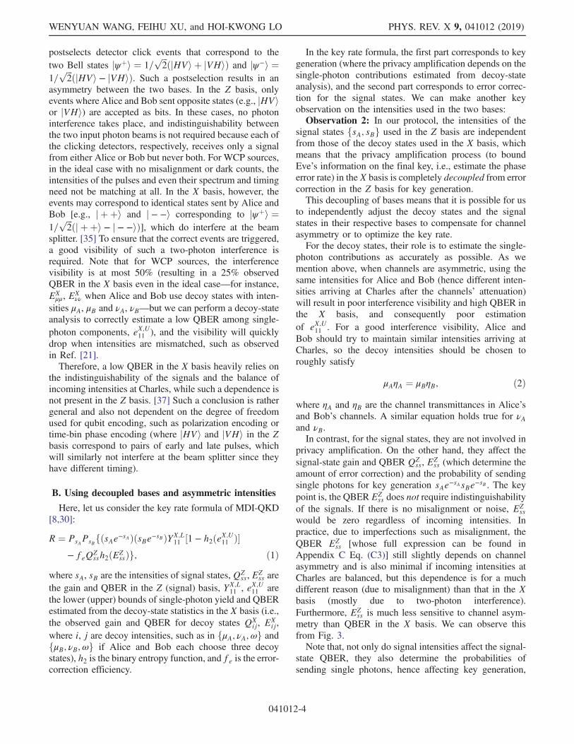
found by the optimization algorithm, which are listed inTable IV. As we can observe from the table, Alice and Bobadjust their intensities to compensate for channel asym-metry. Physically, since MDI-QKD depends on Hong-Ou-Mandel interference of two WCP sources in the X basis, weexpect the received intensity for decoy state at Charles to besimilar on the two arms to ensure good visibility (andconsequently lower QBER) in the X basis; i.e., the ratio ofdecoy intensities μA=μB and νA=νB would roughly followthe rule of thumb of μAηA ¼ μBηB, which is indeed what wecan observe from Table IV and Fig. 6.On the other hand, the ratio of signal intensities sA=sB

deviates more from ηB=ηA. This is because, as we mentionin Sec. II A, signal intensities not only affect the Z basisQBER, but also need to optimize a trade-off between the

TABLE III. Simulation results for asymmetric MDI-QKD in two scenarios: case A (10 km, 60 km) and case B (30 km, 60 km) usingparameters from Table II and N ¼ 1011. We define channel mismatch as x ¼ ðηA=ηBÞ where ηA, ηB are the channel transmittances. Notethat in reality, Alice and Bob cannot modify the physical channels, and they can either add loss to the channels or keep them as is, butthey cannot decrease channel loss. Three strategies are compared here: A1 and B1 represent using the old four-intensity protocol directly.A2 and B2 (not in Fig. 5) represent adding fiber to the shorter channel to match the longer channel, i.e., making the channels (60 km,60 km). A3, B3 represent using our new seven-intensity protocol without modifying the channels. As shown here, seven-intensityprotocol always returns a higher rate than both strategies using four-intensity protocol.

Protocol Point x LB LA Rate Comparison with four-intensity protocol

Four-intensity protocol A1 0.1 10 km 60 km 3.891 × 10−7 � � �Four-intensity protocolþ fiber A2 1 60 km 60 km 1.862 × 10−6 þ379%Our protocol A3 0.1 10 km 60 km 3.106 × 10−5 þ7883%Four-intensity protocol B1 0.25 30 km 60 km 4.746 × 10−6 � � �Four-intensity protocolþ fiber B2 1 60 km 60 km 1.862 × 10−6 −61%Our protocol B3 0.25 30 km 60 km 1.445 × 10−5 þ204%

TABLE IV. Examples of optimal parameters for the seven-intensity protocol using simulation parameters from Table II. The numericalvalues are rounded to the accuracy of 0.001 in the table here. As can be observed, Alice and Bob’s intensities compensate for channelasymmetry, while their intensity probabilities are mostly identical—since the intensities have already compensated for the asymmetry—despite having have some numerical noise (as the key rate is not sensitive to the probabilities near the maximum, the algorithm satisfieswith them having close enough, rather than perfectly identical, values, so the optimal values found are still slightly different even whenx ¼ 1). As we show in Sec. II, the optimal decoy-state intensity ratios are the same, i.e., ðμA=μBÞ ¼ ðνA=νBÞ. Moreover, we can observethat the ratio of decoy-state intensities more closely follows 1=x than the ratio of signal intensities.

LA LB x sA μA νA PsA PμA PνA sB μB νB PsB PμB PνB R

60 km 10 km 0.1 0.662 0.522 0.100 0.600 0.033 0.255 0.202 0.058 0.011 0.600 0.031 0.256 3.106 × 10−5

60 km 30 km 0.25 0.593 0.457 0.089 0.581 0.036 0.266 0.294 0.125 0.024 0.580 0.034 0.269 1.445 × 10−5

60 km 60 km 1 0.402 0.305 0.063 0.478 0.047 0.330 0.402 0.305 0.063 0.480 0.047 0.329 1.862 × 10−6


041012-10

single-photon probabilities and error correction. Thismakes it usually not follow sAηA ¼ sBηB. An illustrationof the ratios of decoy intensities and signal intensities canbe seen in Fig. 6.Now, having demonstrated the new seven-intensity proto-

col, we proceed to introduce a powerful reality application forit: a scalable high-performance MDI-QKD network whereany node can be dynamically added or deleted. We considerthe channels from a real quantum network setup in Viennareported in Ref. [16]. We focus here on the high-asymmetrynodes A1, A2, A3, A4, A5, as shown in Fig. 2(a). We find thatour method leads to much higher key rates and allows easydynamic additionor deletionofnodes.Since intensities canbeindependently optimized for each pair of channels, theestablishment of new connections does not affect any existingconnections, hence providing good scalability for thenetwork(compared to, e.g., the case of using four-intensity protocolwith the strategyof adding fibers,where each channel needs toaccommodate for the longest link among all channels). SeeAppendix J for numerical results.

IV. CONCLUSION

In summary, we propose a method of effectively com-pensating for channel asymmetry in MDI-QKD by adjustingthe two users’ intensities and decoupling the two bases. Sucha method can drastically increase the scenarios that MDI-QKD can be applied to while maintaining a good key rate.This study provides a powerful and robust software solutionfor a scalable and reconfigurable MDI-QKD network.Our method is also a general result that can in principle be

used, e.g., for various numbers of decoys or various finite-size analysis models (e.g., joint-bound analysis or compos-able security with Chernoff’s bound). It is also potentiallyapplicable to other types of quantum communication pro-tocols such as twin-field QKD [28] or MDI quantum digitalsignature [26,27], which both use WCP sources and decoy-state analysis. We hope that our proposal can inspire morefuture work on the study of asymmetric protocols.

ACKNOWLEDGMENTS

This work is supported by the Natural Sciences andEngineering Research Council of Canada, U.S. Office ofNaval Research, the Fundamental Research Funds for theCentral Universities of China, National Natural ScienceFoundation of China Grant No. 61771443, and the China1000 Young Talents Program. A key inspiration for thisproject comes from the study of free-space MDI-QKD. Wethank the collaborators Dr. B. Qi and Professor G. Siopsis forhelpful discussion and collaborative efforts in implementingfree-space MDI-QKD, and we thank K. McBryde and S.Hammel from SPAWAR Systems Center, Pacific for kindlyproviding atmospheric data and for the helpful discussions.

Note added.—Recently, we experimentally implementedour protocol in Ref. [44] (see also Ref. [45]), thus clearlydemonstrating the practicality of our work. We alsorecently applied our method proposed in this work toasymmetric twin-field QKD successfully; see Ref. [46].See also Ref. [47], an independent work posted at the sametime on the preprint server.

APPENDIX A: NOTE ABOUT ADDING FIBER

In this Appendix, we provide an intuitive description ofwhy adding additional loss is suboptimal and how ourmethod works better with asymmetric channels.Previously, when Alice and Bob have asymmetric

channels, a common solution is to add fiber (thus addingloss) to the shorter channel in exchange for better sym-metry, such as in Ref. [15]. Afterwards, one selectssymmetric intensities for Alice and Bob and acquires ahigher rate. However, the added fiber lies in Bob’s lab andis in fact securely under control of Bob. But by assuming asymmetric setup, we are effectively relinquishing its controlto Eve and pessimistically estimating the key rate, asillustrated in Fig. 7. Therefore, intuitively, this is not

FIG. 6. Here we plot the ratios of signal intensities and decoyintensities versus distance, when the channel mismatch is fixed atx ¼ 0.1 (i.e., LA ¼ LB þ 50 km). The simulation parameters arefrom Table II [this plot of intensities corresponds to the solid redkey rate line in Fig. 5(d)]. We also include the line ðηB=ηAÞ ¼ 10for comparison. We can observe that the ratio of decoy statesroughly follows ηB=ηA (to maintain good HOM interferencevisibility in the X basis), while the optimal ratio of signalintensities varies greatly between 1 (optimal for probability ofsending single photons) and ηB=ηA (optimal for EZ

ss). This isbecause signal states affect both key generation and errorcorrection, so having similar intensities arriving at Charles afterchannel attenuation is not the only criteria for a good key rate, andoptimal parameters do not necessarily satisfy sAηA ¼ sBηB. Infact, since signal states in the Z basis are decoupled from the Xbasis, and EZ

ss is less sensitive to unbalanced arriving intensities,sA=sB can be much more freely optimized between 1 and ηB=ηA,allowing seven-intensity protocol to have a higher key rate.


041012-11

necessarily the optimal strategy. We show with our newprotocol that when the channels are asymmetric, Alice andBob can independently choose their optimal intensities, andthat optimizing intensities and probabilities alone is suffi-cient to compensate for the different channel losses.

APPENDIX B: SCALING OF KEY RATE WITHTRANSMITTANCE

In this Appendix, we discuss the scaling properties of thekey rate versus transmittance for prior protocols with thesame parameters for Alice and Bob and our new protocolthat uses different intensities for Alice and Bob. We showhere and in Appendix C that the scaling of the key rateversus distance is mainly determined by the signal states(so long as we have a good single-photon estimation fromthe decoy states). This also means that the advantage of ourmethod is really not dependent on the number of decoystates used or the finite-size analysis model used (or lackthereof, in the asymptotic case), and our results are inprinciple applicable to any protocol that decouples thesignal and decoy states in the Z and X bases and allowsdifferent intensities for Alice and Bob.The transmittance of the two channels are ðηA; ηBÞ, and

the asymmetry (mismatch) x is defined as

x ¼ ηAηB

: ðB1Þ

1. Single-photon source

Now, let us consider the single-photon case first. That is,suppose Alice and Bob both send perfect single photonsonly, and the key is generated from two-photon interfer-ence. If we ignore the dark counts, the asymptotic key ratecan be written as [48]

RSP ¼ ηA × ηB × ½1 − 2h2ðe11Þ�; ðB2Þ

where h2 is the binary entropy function, and e11 is theQBER (which is a quantity that, when the dark count rate isignored is independent of the transmittance). Here we cansee that in the perfect single-photon case, the key rate isproportional to ηAηB, and the mismatch x does not ex-plicitly appear in its expression:

RSP ∝ ηAηB: ðB3Þ

In fact, for a given total distance LA þ LB ¼ L, anypositioning of the untrusted relay Charles (e.g., at themidpoint, in Alice’s lab, or in Bob’s lab) would not affectthe key rate, since ηAηB depends only on L.

2. Weak coherent pulse source

The previous discussion for single-photon MDI-QKDsuggests that, by nature, there is not really any limitation onsymmetry forMDI-QKD, at least for the ideal single-photoncase. Then, where does this dependence of the key rate onchannel symmetry which we observe come from? In thissection, we show that the scaling of the key rate depends onthe signal states’ trade-off between error correction and theprobabilities of sending single photons when using WCPsources rather than privacy amplification (which depends onthe estimation of single-photon contributions).More concretely, (as we prove in the next section) for

protocols with symmetric intensities, there are two sharpcutoff values for the mismatch xmax and xmin that preventthe protocol from acquiring any key rate when x > xmax orx < xmin (and optimizing identical intensities sA ¼ sBcannot circumvent this problem). This is why protocolssuch as the four-intensity protocol are limited to near-symmetric positions.On the other hand, when a protocol allows independent

intensities for Alice and Bob (such as our new seven-intensity protocol described in the main text), we show thatthe mismatch can always be compensated by optimizingintensities sA and sB (hence lifting the limitations xmax andxmin). In fact, we show that for positions with highasymmetry, the key rate no longer depends on mismatchx ¼ ðηA=ηBÞ at all, and the optimal key rate scales onlywith the smaller of the two channel transmittances. That is,

Roptimal ∝ minðη2A; η2BÞ; ðB4Þ

which means that the biggest advantage of protocols withindependent intensities for Alice and Bob (e.g., seven-intensity protocol) is to completely lift the limitation onchannel asymmetry. When compared with adding fiber tomaintain asymmetry, we see that its scaling property is stillthe same, i.e., quadratically related to the (smaller of)channel transmittances, although our method will alwaysperform better (by a constant coefficient) than adding fiber.Moreover, it provides the convenience of not needing

FIG. 7. Setup for asymmetric MDI-QKD. When channels arehighly asymmetric (e.g., Alice and Bob1), to increase thesymmetry in the channel, sometimes one adds additional lossto the system in Bob’s lab [15] in exchange for better symmetry.When estimating the key rate, Bob assumes that both Charles-Bob1 and Bob1-Bob2 channels are controlled by Eve. This istherefore a pessimistic estimation of the key rate, and it is notnecessarily the optimal strategy.


041012-12

additional fiber, which may not be feasible in free-spacechannels or when channel mismatch is changing.Proofs for the above scaling properties can be found in

the next Appendix.

APPENDIX C: PROOF OF SCALINGPROPERTIES OF THE KEY RATE WITH

TRANSMITTANCE

In this Appendix, we outline the analytical proofs for theobservations on the scaling properties of the asymptoticMDI-QKD key rate versus transmittance in the presence ofasymmetry described in Appendix B. We also discuss howthe finite-decoy and finite-size effects can be considered asimperfections in the infinite-decoy, infinite-data case, andthat the scaling properties are still approximately the same,which are determined only by the signal states’ trade-offbetween error correction and probabilities of sending singlephotons and not affected by decoy states.To simplify the discussion, it is convenient to first use a

few crucial approximations as described in Ref. [20].(1) We consider the asymptotic case with infinite data

size.(2) We assume an infinite number of decoy states, i.e.,

Alice and Bob can perfectly estimate the single-photon gain Y11 and QBER e11. In this case, Aliceand Bob need only to choose appropriate signalintensities sA, sB.

(3) We ignore the dark count rate Y0 when studying thescaling properties with distance (as backgroundnoise affects only the maximum transmission dis-tance where transmittance is at the same order as thedark count rate, but it does not affect the overallscaling properties of the key rate versus distance).

(4) When describing the channel model to estimate theobservable gain and QBER QZ

ss and EZss (which

affect the error correction), we make second-orderapproximations to two functions:

I0ðxÞ ≈ 1þ x2

4þOðx4Þ;

ex ≈ 1þ xþ x2

2þOðx3Þ; ðC1Þ

where I0 is the modified Bessel function of the firstkind. This approximation is relatively accurate whensAηAηd and sBηBηd are both small, where ηd is thedetector efficiency.

With the above approximations, one can write the keyrate conveniently as [excerpting Eqs. (C.1) and (C.2) fromRef. [20] ],

R ¼ η2Bη2d

2Gðx; sA; sBÞ; ðC2Þ

where Gðx; sA; sBÞ is a function determined by ðsA; sBÞ andthe asymmetry x only:

Gðx; sA; sBÞ ¼ xsAsBe−ðsAþsBÞ�1 − h2

�ed −

e2d2

��

−2xsAsB þ ðs2B þ x2s2AÞð2ed − e2dÞ

2

× feh2½EZssðx; sA; sBÞ�

EZssðx; sA; sBÞ ¼

ðsB þ xsAÞ2ð2ed − e2dÞ2½2xsAsB þ ðs2B þ x2s2AÞð2ed − e2dÞ�

;

ðC3Þ

where h2 is the binary entropy function.Now, having described the key rate function, we are

interested in how it scales with the transmittances ηA, ηBusing different optimization strategies for the intensities.We discuss two cases:(1) Rsymmetric, where Alice and Bob use the same

intensity s ¼ sA ¼ sB and optimize s.(2) Roptimal, where Alice and Bob fully optimize a pair of

intensities sA, sB, which can take different values.

1. Symmetrically optimized intensities

Let us consider the case where Alice and Bob use thesame intensity s ¼ sA ¼ sB and optimize s. This is the casediscussed by previous protocols (such as the four-intensityprotocol, although here to simplify the proof we focus onthe infinite-decoy case and consider only signal intensities).In this case, the function G is optimized over s (and is a

function of x only). The rate satisfies

Rsymmetric ¼ maxs

R ∝ η2Bmaxs

Gðx; s; sÞ; ðC4Þ

therefore, Rsymmetric is proportional to η2B when channelmismatch ηA=ηB is fixed.Moreover, since Rsymmetric is also proportional to GðxÞ,

we have Rsymmetric ¼ 0 if GðxÞ ¼ 0. Note that we canrewrite the signal-state QBER EZ

ss as

EZssðxÞ ¼

ð1þ xÞ2ð2ed − e2dÞ2½2xþ ð1þ x2Þð2ed − e2dÞ�

ðC5Þ

since the equal intensities are canceled out; i.e., EZss is only

a function of x. In fact, EZss is a function that minimizes at

x ¼ 1 and reaches 50% (where Rsymmetric is naturally zero)when x → 0 or x → ∞. Therefore, if GðxÞ ≠ 0 at x ¼ 1,there must exist some critical values of xmax and xmin whichresult in a sufficiently large QBER such that GðxÞ ¼ 0 (andRsymmetric ¼ 0). This means that Rsymmetric is quadraticallyrelated to ηB (or ηA) when mismatch ηA=ηB is fixed, but italso has two cutoff positions for critical levels of mismatch,beyond which no key can be generated. These two criticalmismatch positions are what limit previous MDI-QKDprotocols to near-symmetric positions. Also, as we havepreviously mentioned, we see that this critical dependence


041012-13

on mismatch actually comes from the error-correction part(which involves EZ

ss).

2. Fully optimized intensities

Now, let us consider the case where Alice and Bob areallowed to fully optimize their intensities sA, sB (such as inthe seven-intensity protocol, although again, here we focusonly on the signal states in the infinite-decoy case).In this case, the function G is optimized over sA, sB. The

rate satisfies

Roptimal ¼ maxsA;sB

R ∝ η2BmaxsA;sB

Gðx; sA; sBÞ: ðC6Þ

Now, let us focus on the properties of Gðx; sA; sBÞ.Looking at its expression Eq. (C3) in the previous section,we make the important observation that, except for the terme−ðsAþsBÞ in the single-photon probabilities, every otherterm is only a function of sB and xsA (rather than x and sAseparately). We can rewrite Gðx; sA; sBÞ as

G0ðx; s0A; sBÞ ¼ s0AsBe½ð−s0AÞ=x�e−sB

�1 − h2

�ed −

e2d2

��

−2s0AsB þ ðs2B þ s0A

2Þð2ed − e2dÞ2

× feh2½EZssðs0A; sBÞ�

EZssðs0A; sBÞ ¼

ðsB þ s0AÞ2ð2ed − e2dÞ2½2s0AsB þ ðs2B þ s0A

2Þð2ed − e2dÞ�; ðC7Þ

where we define equivalent intensity s0A as

s0A ¼ sA × x: ðC8ÞMoreover, if ηA ≫ ηB (i.e., mismatch x ≫ 1), we can

approximately assume that

e½ð−s0AÞ=x� ≈ 1; ðC9Þwhich means that we can rewrite maxsA;sBGðx; sA; sBÞ as

Gmax ¼ maxs0A;sB

G0ðs0A; sBÞ; ðC10Þ

which, importantly, is a constant value not dependent on thevalue of x when x ≫ 1. The actual value of sA equals

sA ¼ s0Ax: ðC11Þ

Physically, this means that when there is asymmetrybetween Alice and Bob’s channels, we can compensatefor this asymmetry by adjusting the intensities to keep thesame “equivalent intensity” received by Charles and keepEZss at a low value. In this case, EZ

ss is no longer limited bythe mismatch x, and we can performMDI-QKD at arbitraryvalues of asymmetry. Also, the key rate is now given by

Roptimal ∝ η2BGmax: ðC12Þ

This means that when ηA ≫ ηB (e.g., the “single-arm” casepreviously mentioned where LA is much shorter than LB),the key rate of asymmetric MDI-QKD is related only to ηBand still quadratically scales with ηB. When ηB ≫ ηA,though, we can rewrite x0 ¼ ðηB=ηAÞ and rewrite

Roptimal ∝ η2Amaxs0B;sA

G0ðs0B; sAÞ: ðC13Þ

Therefore, overall,

Roptimal ∝ minðη2A; η2BÞ: ðC14ÞNow, we plot the two cases (symmetric intensities and

fully optimized intensities) in a contour plot. As we canobserve in Fig. 8, the key rate Rsymmetric has two cutoffmismatch positions beyond which the key rate is zero. Thislimitation is removed when full optimization of intensitiesis implemented. Moreover, for Roptimal, we see that thecontours are perpendicular to the axes in high-asymmetryregions, which means that the key rate scales only with thelonger of the two channels.Also, note that from Eqs. (C4) and (C6), we can make the

observation that there is never any need to add fiber to theshorter channel when fully optimizing the intensities, andour new method always provides a higher key rate than theprior art technique of adding fiber until channels aresymmetric, while using same intensities for Alice and Bob.To show this point, consider the system having a fixed

longer channel LB (i.e., suppose ηB is fixed and ηA > ηB,x ¼ ðηA=ηBÞ > 1). Adding loss to ηA is equivalent todecreasing x.With symmetric intensities (and adding loss till

ηA ¼ ηB), the key rate can be written as

Rsymmetric ¼η2dη

2B

2maxs

Gð1; s; sÞ: ðC15Þ

Suppose we fully optimize the intensities for this casewith added fiber, we will obtain the same key rate (since forx ¼ 1, i.e., symmetric setup, the optimal choice of inten-sities satisfies sA ¼ sB):

maxs

Gð1; s; sÞ ¼ maxsA;sB

Gð1; sA; sBÞ: ðC16Þ

However, let us compare it with the case of using fullyoptimized intensities and no additional loss:

Roptimal ¼η2dη

2B

2maxsA;sB

Gðx; sA; sBÞ: ðC17Þ

As we describe in Eq. (C7), we can rewrite Gðx; sA; sBÞas G0ðx; s0A; sBÞ (recall that the equivalent intensity s0A isdefined as xsA). We make the observation that G0ðx; s0A; sBÞ


041012-14

strictly increases with x. That is, for any two given values ofs0A; sB, and x > 1,

G0ðx; s0A; sBÞ > G0ð1; s0A; sBÞ; ðC18Þhence, after optimization we also have

maxs0A;sB

G0ðx; s0A; sBÞ > maxs0A;sB

G0ð1; s0A; sBÞ; ðC19Þ

which means that when fully optimizing Alice and Bob’sintensities (which already compensate for the mismatchbetween channels), it is always optimal not to add anyadditional loss to the channels. Moreover, combiningEqs. (C15)–(C17) and (C19), we can see that

Roptimal ¼η2dη

2B

2maxsA;sB

Gðx; sA; sBÞ

>η2dη

2B

2max

sGð1; s; sÞ ¼ Rsymmetric: ðC20Þ

That is, compared to the case where one adds loss to ηAuntil ηA ¼ ηB, our new protocol always provides a higherkey rate as long as the channels are asymmetric. Intuitively,this is because adding fiber while using the same intensitiesfor Alice and Bob is in fact an suboptimal subset of theoverall set of strategies Alice and Bob can take (whichincludes adjusting Alice and Bobs intensities independ-ently, as well as adding any length of fibers to change x).Even when considering adding fiber as one of the validvariables, we show that the optimal point always happenswhen no fiber is added. Therefore, our method is a betteroptimized strategy than adding fiber because it considers alarger parameter space.Note that fully optimizingAlice andBob’s intensities does

not change the fundamental scaling property; the key rate isstill quadratically related to transmittance in the longer arm.However, it always provides a better key rate than prior arttechniques, and it also offers the great convenience of nothaving to physically add loss to the channels and being ableto implement everything in software.

3. Practical imperfections

Up to here, we have analytically shown how choosingto fully optimize the intensities can affect the key ratefor the asymptotic, infinite-decoy case. The behaviorof contours as shown in Fig. 8 is a result of sA, sBcompensating for the difference in channel loss. However,we have so far assumed perfect knowledge of single-photon contributions and have not yet discussed thedecoy-state intensities. Moreover, nonideal experimentalparameters (including dark count rate and detector effi-ciency) and finite-size effects will both affect the key rate.Here in this subsection, we compare the key rate undermore practical assumptions and show that the abovefactors can be considered as imperfections that reducethe key rate but maintain similar contour shapes and

scaling properties for the key rate; that is, we still observea high dependence on asymmetry for protocols withidentical intensities for Alice and Bob, and fully optimiz-ing intensities can completely lift this limitation.In practice, with a finite number of decoys (for instance,

for four-intensity and seven-intensity protocols, whereAlice and Bob each choose three decoy intensities μ, ν,ω), the estimation of Y11 and e11 is not perfect; therefore,the key rate will be slightly lower than the aforementionedinfinite-decoy case. Moreover, to accurately estimate Y11

and e11, the decoy intensities need to be optimized tocompensate for channel loss, too. As we describe in Sec. IIA in the main text, the decoy states should maintainbalanced arriving intensities at Charles (e.g.,μAηA ¼ μBηB) to ensure good HOM visibility and lowQBER in the X basis. Note that the optimization of decoy

FIG. 8. Rate vs distance contours for single-photon MDI-QKDRSP, decoy-state MDI-QKD with symmetric intensities Rsymmetric,and with fully optimized intensities Roptimal. We plot the contourline of R ¼ 10−9.5. Here, for a better comparison with WCPsources, we arbitrarily set a probability P11 ¼ sAsB × e−ðsAþsBÞ(where sA ¼ sB ¼ 0.6533) of single photon pairs being sentwhen calculating RSP. For the decoy-state case, as we describe atthe beginning of this appendix we assume infinite decoys, infinitedata size, ignore dark count rate, and take second-order approxi-mation when calculating gain and QBER (so that we focus onlyon the ideal scaling properties of the key rate with distance). Ascan be seen, RSP is not limited by asymmetry and takes a constantvalue for any fixed LA þ LB (meaning that the dependence of thekey rate on asymmetry does not come from single-photoncontributions in the privacy amplification part when usingWCP sources). For decoy-state MDI-QKD, we can clearly seeRsymmetric being limited by the two cutoff lines where jLA − LBjtakes maximum value (which corresponds to critical values ofchannel mismatch xmax and xmin). On the other hand, Roptimal isnot limited by asymmetry and has contours nearly perpendicularto the axes when asymmetry is high (meaning that, when onechannel is significantly longer than the other, Roptimal is dependentonly on the longer channel).


041012-15

intensities has a very different purpose from that of thesignal intensities sA, sB; the signal intensities are optimizedso as to reduce EZ

ss (while keeping single-photon proba-bility sAsBe−ðsAþsBÞ high) and maximize the key rate, whilethe decoy intensities are optimized to estimate YL

11 and eU11as accurately as possible, whose ideal values Y11 and e11(used in the infinite-decoy case above) provide an upperbound for the practical key rate with a finite number ofdecoys. As we see in Fig. 9, the asymptotic key rate with afinite number of decoys follows a similar shape as itsupper bound, the infinite-decoy case.Additionally, the detector efficiency (which is equivalent

to channel loss) contributes to a uniformly shifted key ratein both LA and LB directions, while dark counts reduce thekey rate more significantly in the higher loss region (both ofwhich we have so far ignored in the ideal case as wedescribe at the beginning of this section). However, as weobserve in Fig. 9 (the solid lines consider both finite-decoysand practical parameters), these factors do not change theoverall shape of the contours either.Lastly, finite-size effects will reduce the key rate sig-

nificantly. As we observe in Fig. 9 bottom plot, while thekey rate is reduced, the contour shapes remain largelyunchanged (meaning that even under finite-size effects, theseven-intensity protocol can still effectively compensate forchannel asymmetry effectively). In Fig. 9 top plot, we canfind similar observations that finite-size effects reduces theoverall key rate. However, note that under finite-sizeeffects, the shapes of the key rate contours for the four-intensity protocol are somewhat different and no longerfollow the two cutoff positions xupper, xlower for channelmismatch (which appear as straight lines in, e.g., Fig. 8).This is because, though the key rate is still limited by EZ

ss(which causes the cutoff mismatch positions), it is alsolimited by the estimation of YL

11 and eU11 using the decoystates. Compared to the asymptotic case, here under finite-size effects, the increased eU11 is likely a more severelimiting factor than EZ

ss, and not being able to chooseindependent intensities for Alice and Bob prevents anaccurate estimation of YL

11 and eU11 (due to poor HOMvisibility in the X basis caused by unbalanced intensities).Therefore, here the dependence of the key rate on channelasymmetry is present in both privacy amplification anderror-correction terms, and the shapes of contours are aresult of both effects. (The difference in contour shape fromthe infinite-decoy case is more prominent for the finite-sizecase, likely because the key rate is more sensitive to eU11here). Importantly, under finite-size effects, the key rate forfour-intensity protocol is still highly limited by channelasymmetry, while seven-intensity protocol completelyremoves such a constraint and allows two channels witharbitrary asymmetry between them.

FIG. 9. Contours of rate vs distance for decoy-state MDI-QKDunder different assumptions for practical imperfections, for thekey rates for the asymptotic case with infinite decoys (and idealassumption of zero dark count rate and 100% detector effi-ciency), asymptotic case with four-intensity or seven-intensityprotocol (with practical device parameters), and finite-sizecase with four-intensity or seven-intensity protocol. Top: Pro-tocols with identical intensities for Alice and Bob. Bottom:Protocols with fully optimized intensities. (Note that in thebottom plot there are some noises in the asymptotic seven-intensity protocol key rate. This is because the optimal ν cantake a very small value in the ideal case where data size isinfinitely large, which results in some numerical noise incomputer simulations). We plot the contour lines of R¼10−7.As can be observed here, the finite number of decoys, thenonideal experimental parameters, and the finite-size effects areall imperfections that reduce the key rate. However, the overallshapes of the contours still remain largely the same, whichfollow the upper bounds given by the ideal infinite-decoy case.(Except for four-intensity protocol under finite-size effects,which no longer has two clear cutoff mismatch positions, butit is still severely limited by channel asymmetry, while seven-intensity protocol lifts this constraint completely).


041012-16

APPENDIX D: NOTE ABOUT DECOUPLINGSIGNAL AND DECOY INTENSITIES

In this Appendix, we provide a simple intuitive explan-ation for why our protocol provides a better choice of decoyand signal intensities.Let us recall again the key rate formula of MDI-QKD

[8,30]:


− feQZssh2ðEZ

ssÞg: ðD1Þ

Here, there are three criteria that determine whether aMDI-QKD protocol generates good key rate in the presenceof channel asymmetry:(a) Similar arriving intensities at Charles in the X basis in

order to have good HOM interference and keep QBERlow in the X basis (which is important for a goodestimation of eX;U11 ).

(b) Similar arriving intensities at Charles in the Z basis inorder to keep QBER EZ

ss low in the Z basis (which isdue to misalignment), although this term is much lesssensitive to difference in intensities than (a).

(c) A high enough probability of sending single photonssAe−sAsBe−sB . Note that both criteria (b) and (c) involvethe signal states sA, sB, so there is a trade-off between(b) and (c).

Prior protocols require Alice and Bob to use the same setof intensities. This overly constrains the solution space[because Alice and Bob try to use the same set of intensitiesto satisfy (a)–(c) simultaneously] and leaves high QBER inboth the X and Z bases and thus resulting in a low key ratewhen channels are asymmetric.By relaxing this constraint (allowing Alice and Bob to

have different intensities) and decoupling criteria (a) fromcriteria (b) and (c) by allowing independent decoy andsignal intensities, we can satisfy (a) nicely, while simulta-neously achieving a good trade-off between (b) and (c),hence ensuring a high key rate.Remark: For more detail on the trade-off between (b) and

(c), here (b) is optimal when arriving intensities arematched, i.e., sA=sB ¼ ηB=ηA, and (c) is independent ofasymmetry and is optimal when signal intensities are both1. In fact, since EZ

ss is much less sensitive to sA=sB, such atrade-off between two terms favors (c) more than (b); thus,the optimal sA=sB is often closer to 1 than ηB=ηA. Theactual optimal signal intensities can be found by numericaloptimization, as we describe in Sec. II D. An example ofμA=μB and sA=sB can also be seen in Fig. 6, where weobserve that μA=μB follows ηB=ηA rather closely, whilesA=sB has relatively much more freedom in its optimization(between 1 and ηB=ηA).

APPENDIX E: GENERALITY OF OUR METHOD:MDI-QKD PROTOCOLS OTHER THAN THREE

DECOY STATES

In the main text, we focus on the seven-intensityprotocol, where Alice and Bob each use one signal intensitysA (sB), and three decoy intensities μA, νA, ω (μB, νB, ω).However, the core idea of our protocol lies in two keypoints: (1) the X and Z bases are decoupled, where decoystates in the X basis bound Eve’s information and the signalstate in the Z basis encodes the key, and (2) Alice and Bobuse different intensities to compensate for channel asym-metry. This means that our protocol is not limited to theseven-intensity protocol, but can easily be applied to otherprotocols, too, as long as points (1) and (2) are satisfied.In this Appendix, we demonstrate the generality of our

method by actually applying it to other kinds of MDI-QKDprotocols where Alice and Bob use a different number ofdecoy intensities in the X basis and show that similaradvantages as with the seven-intensity protocol can beobserved when using asymmetric intensities. We also showwith numerical results, that although these alternativeprotocols will certainly work, the seven-intensity protocolprovides a good balance between performance and ease ofexperimental implementation.Here we compare three cases:(1) Alice and Bob each use two decoy intensities μA, νA

(μB, νB) in the X basis. We denote this case as a six-intensity protocol (including the two signal inten-sities), where the parameter choices are

½sA; μA; νA; PsA; PμA ; PνA ;

sB; μB; νB; PsB ; PμB ; PνB �: ðE1Þ

Here, PνA ¼ 1 − PsA − PμA and PνB ¼ 1 − PsB−PμB . This is similar to the “one-decoy” setup thatwas discussed in Ref. [29]. Note that here it is not a“five-intensity” protocol because using μA, μB, ωalone is not sufficient to satisfactorily bound thesingle-photon contributions and will result in a lowor zero key rate. Therefore, in this setup, the vacuumstate is not used, and Alice and Bob each use twononzero decoy states.

(2) Alice and Bob each use three decoy intensities μA,νA, ω (μB, νB, ω) in the X basis. This case is theseven-intensity protocol that we discuss in the maintext, where the parameter choices are

½sA; μA; νA;ω; PsA; PμA ; PνA ; PωA;

sB; μB; νB;ω; PsB ; PμB ; PνB ; PωB�: ðE2Þ

Here, PωA¼ 1 − PsA − PμA − PνA , PωB

¼ 1 − PsB−PμB − PνB , and ω is the vacuum state (for simplicity,we can assume ω ¼ 0).


041012-17

(3) Alice and Bob each use four decoy intensities μA, νA,ν2A, ω (μB, νB, ν2B, ω) in the X basis. We denote thiscase as a nine-intensity protocol, where the param-eter choices are

½sA; μA; νA; ν2A;ω; PsA ; PμA ; PνA ; Pν2A ; PωA;

sB; μB; νB; ν2B;ω; PsB; PμB ; PνB ; Pν2B ; PωB�: ðE3Þ

Here, PωA¼ 1 − PsA − PμA − PνA − Pν2A , PωB

¼ 1 − PsB−PμB − PνB − Pν2B , and ω is the vacuum state.Note that in all of these three protocols, the key rate

formula stays the same as Eq. (1):


− feQZssh2ðEZ

ssÞg: ðE4ÞWhat is changing here is only the estimation of the single-photon contributions, namely, the yield YX;L

11 and QBEReX;U11 . While we have analytical bounds for the decoy-stateanalysis [20] for the seven-intensity protocol, we use alinear programming approach to numerically estimate YX;L

11

and QBER eX;U11 in the six-intensity and nine-intensitycases. Such an approach has been widely discussed in theliterature, as in Refs. [29,49,50].Now, we perform numerical simulations with the six-

intensity, seven-intensity, and nine-intensity protocols andshow that they all have much higher performance than theirsymmetric intensity counterparts when channel asymmetryis present. This demonstrates the generality of our method,as using asymmetric intensities can always improve theperformance of MDI-QKD with asymmetric channels.We also compare the performances of the three protocols

with each other and show that using more decoy intensitiescan always guarantee higher or equal performance thanusing fewer decoy intensities, regardless of data size andasymmetry. The seven-intensity protocol never provides asmaller key rate than the six-intensity protocol, andalthough the nine-intensity protocol can potentially providean even higher key rate, the advantage is small, and theseven-intensity protocol that we use in the main text is agood balance between key rate performance and ease ofexperimental implementation.Interestingly, as observed in Figs. 10(a) and 10(b), for the

six-intensity and nine-intensity protocols, although theyield YX;L

11 and QBER eX;U11 are estimated numerically usinglinear programming, there is still a ridge (discontinuity infirst-order derivatives) along ðμA=μBÞ ¼ ðνA=νBÞ, andðνA=νBÞ ¼ ðν2A=ν2BÞ as we see for the seven-intensityprotocol in the main text. For the six-intensity protocol,the ridge is very clearly shown. For the nine-intensityprotocol, the ridge exists but it is less prominent andsometimes not visible (likely because, e.g., if two pairs ofproportional decoy states ðνA=νBÞ ¼ ðν2A=ν2BÞ already

provide good estimation of YX;L11 , eX;U11 , the third pair μA,

μB has more freedom, and would not affect the decoy-stateanalysis or the key rate too much even if it does not providegood HOM visibility and results in high EX

μμ).We plot the simulated key rate for the protocols in

Figs. 10(c) and 10(d). We first consider a similar scenario asFigs. 5(c) and 5(d) using parameters from Table II, achannel mismatch of ðηA=ηBÞ ¼ x ¼ 0.1, and data size ofN ¼ 1012 (here we use a larger data size than in the maintext, since for N ¼ 1011 the six-intensity protocol withsymmetric intensities cannot generate a key rate even atLB ¼ 0 km, so a comparison is not immediately clear in theplot). As we show in Fig. 10, for each protocol, allowingasymmetric intensities provides a much higher key rate

FIG. 10. Left: Examples of YX;L11 versus μA and μB where other

parameters are all fixed for (a) six-intensity protocol and (b) nine-intensity protocol. Just like for the seven-intensity protocol, wecan see a ridge along ðμA=μBÞ ¼ ðνA=νBÞ or ðμA=μBÞ ¼ðνA=νBÞ ¼ ðν2A=ν2BÞ. Note that the ridge is a lot less obviousfor the nine-intensity protocol (and sometimes is not visible),likely because two proportional pairs of decoy states can estimatesingle-photon contribution reasonably well, so the third pair (μA,μB) here has more freedom in the choice of intensities. Right:Comparison of rate vs LB for six-intensity, seven-intensity, andnine-intensity protocols, where mismatch x ¼ 0.1, i.e., LA ¼LB þ 50 km (assuming fiber loss 0.2 dB=km). The rates areplotted in log scale. We use the parameters from Table II andN ¼ 1012. (c) Using symmetric intensities for Alice and Bob;(d) using fully optimized asymmetric parameters for Alice andBob. As can be seen, using asymmetric intensities can greatlyimprove the key rate for all three protocols when channelasymmetry is present. Note that there is a higher amount ofnoise present for the nine-intensity case due to the numericalinstability brought by linear program solvers (similar to that ofjoint-bound finite-size analysis, which we discuss in Appen-dix H), but the key points here are that the nine-intensity protocolalso benefits considerably from using asymmetric intensities, andthat the nine-intensity protocol does not have a significantadvantage over the seven-intensity protocol despite being morecomplex to implement.


041012-18

than using symmetric intensities only, demonstrating thegeneral effectiveness of our method for different protocolsunder channel asymmetry.We also make an important observation here: The more

decoy intensities one uses, the higher key rate one canobtain after parameter optimization, even with finite-sizeeffects considered (e.g., the nine-intensity protocol alwayshas a higher key rate than the seven-intensity, and theseven-intensity also always has a higher rate than the six-intensity). This is because, for instance, the six-intensityprotocol can in fact be considered a special case of theseven-intensity protocol, just with PωA

and PωBinfinitely

close to zero, and with nine instead of four constraints, e.g.,the gainsQX

ij when estimating YX;L11 . With close to zero data,

the five new constraints are obviously very loose (with verylarge finite-size fluctuation) and will not provide any usefulinformation, but the key point is, in a linear program theseloose constraints will not decrease the key rate. Therefore,any optimal set of parameters for the six-intensity protocolcan also be considered a valid set of parameters for theseven-intensity protocol; i.e., the parameter space of thesix-intensity protocol is a subset of that of the seven-intensity protocol, and the latter protocol always providesno smaller key rate than the former (and often the seven-intensity protocol can find a better parameter set in thelarger parameter space, resulting in a higher key rate).The same goes for the nine-intensity protocol, but as we

see in Fig. 10, the advantage it provides over the seven-intensity protocol is rather small (compared to, e.g., six-intensity versus seven-intensity), while requiring morecomplex control of the intensity modulators in the exper-imental setup and more complicated data collection andanalysis: The users need to collect 16 sets of gains and errorgains, and the parameter optimization is also a lot slowerand more unstable (evaluating the linear program is onaverage slower than analytical expression by about 50times, and linear programs also introduce numerical insta-bilities). Similar observations have been made for thesymmetric case in Ref. [29] (although in this paper,the signal states are not decoupled from decoy states, sothe protocols are slightly different), that using decoy statesfμ; ν;ωg provides a higher key rate than fμ; νg, but addingone more decoy state ν2 provides little further advantage.Therefore, our conclusion is that, while our method

of asymmetric intensities and decoupled bases surely workswell with other protocols such as the six-intensity andnine-intensity protocols, the seven-intensity protocol weintroduce in the main text strikes a good balance betweenkey rate performance and the ease of both experimentalimplementation and data analysis.

APPENDIX F: DECOY-STATE INTENSITIES

In this Appendix, we describe Theorems I and II in moredetail and show their theoretical proofs in the asymptotic

limit of infinite data size (moreover, numerically, we findthat Theorems I and II in fact hold true even under finite-size effects).

1. Symmetry of Optimal Decoy Intensities

To prove Theorem I, here we actually propose an evenstronger assumption for μA, μB:Theorem III: For any arbitrary choice of device and

channel parameters and any two given values of νA, νB, theoptimal decoy intensities μoptA , μoptB that maximize R alwayssatisfy the constraint

μoptA

μoptB

¼ νAνB

: ðF1Þ

Remark: As we show below, Theorem I is simply acorollary of Theorem III.Proof for Theorem III: Here for convenience, we first

limit the discussion to the asymptotic case (i.e., infinite datasize), and we assume that the vacuum intensity is indeedω ¼ 0. Throughout the rest of the text, we use Qk

ij and Ekij

to denote the observed gain and QBER, where, if notspecified, the first subscript is Alice’s intensity, and thesecond is Bob’s intensity, which can be chosen fromfsA; μA; νA;ωg and fsB; μB; νB;ωg for Alice and Bob,respectively. The superscript k signifies the basis X or Z(although, here we only explicitly write the basis forillustration purposes, since the basis is already impliedby the choice of intensities).First, looking at the key rate expression [8,30]


− feQZssh2ðEZ

ssÞg; ðF2Þ

we can see that the term YX;L11 ½1 − h2ðeX;U11 Þ�, i.e., the decoy-

state analysis and privacy amplification, is determined bythe decoy intensities (and probabilities, if finite-size effectis considered) only and not affected by the signal intensitiessA, sB. This is an important and very convenient character-istic of the four-intensity and seven-intensity protocols, thatthe signal state is concerned only with key generation,while the decoy states are responsible only for privacyamplification. That is, the optimization of decoy-stateintensities is decoupled from the key generation. Now,we can make an observation that, under given deviceparameters and channel loss, the optimization of the decoyintensities is independent of sA, sB, and its only goal is tomaximize YX;L

11 ½1 − h2ðeX;U11 Þ�. Furthermore, to perform thedecoy-state analysis, we note that the upper bound forsingle-photon QBER satisfies the form of

eX;U11 ¼ fðYX;L11 ; νA; νBÞ; ðF3Þ


041012-19

where eX;U11 is determined only by YX;L11 , νA, and νB. The full

expression, as in Ref. [20], is

eX;U11 ¼ 1

νAνBYX;L11

ðeνAþνBQXννEX

νν − eνAQXνωEX

νω

− eνBQXωνEX

ων þQXωωEX

ωωÞ: ðF4ÞNow, suppose we first fix two arbitrary values of νA, νB

and try to maximize YX11½1 − h2ðeX11Þ� by optimizing μA, μB,

we can see that maximizing YX;L11 will suffice, since it will

simultaneously minimize eX;U11 , whose only componentdependent on μA, μB is YX;L

11 . The question now becomessimply finding

ðμoptA ; μoptB Þ ¼ argmax½YX;L11 ðμA; μBÞ�: ðF5Þ

A very important characteristic of YX;L11 is that its ex-

pression is dependent upon whether ðμA=μBÞ ≤ ðνA=νBÞ;i.e., it is a piecewise function, as described in Ref. [20].Case 1: If ðμA=μBÞ ≤ ðνA=νBÞ:

YX;L11 ¼ Ya

11 ¼1

ðμA − νAÞ�μAνAνB

QM1νν −

νAμAμB

QM2μμ

�: ðF6Þ

Case 2: Otherwise, if ðμA=μBÞ > ðνA=νBÞ:

YX;L11 ¼ Yb

11 ¼1

ðμB − νBÞ�μBνAνB

QM1νν −

νBμAμB

QM2μμ

�; ðF7Þ

where we denote the two expressions of YX;L11 in the two

cases as Ya11 and Yb

11, and the two terms QM1νν and QM2

μμ arelinear combinations of the observable gain and are func-tions of ðνA; νBÞ and ðμA; μBÞ only, respectively. Their fullexpressions can be found in Appendix F 3. Also, note that ifðμA=μBÞ ¼ ðνA=νBÞ, the two cases Ya

11 ¼ Yb11.

Now, we can make a key observation that in case 1, forany given μA, the partial derivative ð∂Ya

11Þ=ð∂μBÞ alwayssatisfies

∂Ya11

∂μB < 0: ðF8Þ

(The actual expression of the partial derivative and proof ofits positivity are shown in Appendix F 3). However, in case1, μB is bounded by μB ≥ ½ðμAνBÞ=νA�, so the only optimalcase is to take the boundary condition

μoptB ¼ μAνBνA

: ðF9Þ

This means that in the region of ðμA=μBÞ ≤ ðνA=νBÞ,any pair of optimal values ðμoptA ; μoptB Þ must satisfyðμoptA =μoptB Þ ¼ ðνA=νBÞ, or else we can always decreaseμB to get a higher rate, meaning that the previous pointis not the actual maximum. We illustrate this behaviorin Fig. 11.Similarly, for case 2, the partial derivative with respect to

μA satisfies

FIG. 11. An example of the two different cases of the YX;L11 vs μA, μB function for fixed values of νA ¼ 0.2, νB ¼ 0.1. Left: Ya

11, whereðμA=μBÞ ≤ ðνA=νBÞ (case 1). Right: Yb

11, where ðμA=μBÞ > ðνA=νBÞ (case 2). Allowed regions are marked in color for both cases. In case1, we show that ½ð∂Ya

11Þ=ð∂μBÞ� < 0, so any given point A can descend along the μB axis (the solid black arrow) to get a higher rate, untilit reaches the boundary line ðμA=μBÞ ¼ ðνA=νBÞwhere μB is highest. Similarly, in case 2, ½ð∂Yb

11Þ=ð∂μAÞ� < 0, so any given point B candescend along the μA axis until ðμA=μBÞ ¼ ðνA=νBÞ to get the highest rate. Therefore, the optimal ðμoptA ; μoptB Þ that maximize thepiecewise function YX;L

11 always occur on the boundary line. Moreover, for any given point CðμA; μBÞ on the boundary line, the functionvalues of Ya

11, Yb11 are the same. However, we show that ð∂Ya

11Þ=ð∂μAÞ at C1 is not equal to ð∂Yb11Þ=ð∂μAÞ at C2 (along the dot-dash red

lines). Therefore, the piecewise function YX;L11 is not smooth.


041012-20

∂Yb11

∂μA < 0; ðF10Þ

and μA is bounded by μA > ½ðμBνAÞ=νB�. In the same way,in case 2 for any given μB, we can acquire

μoptA ¼ μBνAνB

: ðF11Þ

Up to here, we have proven that Theorem III is indeedcorrect. ▪Proof for Theorem I: Now, following the same idea,

any optimal four values ðμoptA ; μoptB ; νoptA ; νoptB Þ must satisfyðμoptA =μoptB Þ ¼ ðνoptA =νoptB Þ, or else we can always varyðμA; μBÞ while keeping ðνA; νBÞ fixed and let ðμA=μBÞ ¼ðνA=νBÞ to get a higher rate, meaning that the previouspoint is not the actual maximum. Therefore, we show thatTheorem I is indeed correct and that the optimal decoyintensities always satisfy

μoptA

μoptB

¼ νoptA

νoptB

: ðF12Þ

▪Note that the same conclusion does not hold true for

traditional three-intensity MDI-QKD (i.e., using fμ; ν;ωgfor both X and Z bases and using μ in the Z basis togenerate the key), that is because the key rate for three-intensity depends on μ for both key generation and errorcorrection, such that the QZ

μμ, EZμμ terms and the single-

photon probability μe−μ both depend on μ; hence, optimiz-ing only YL

11 is no longer sufficient. Therefore, thisindependence of s from μ, ν is an additional advantagethat the four-intensity or seven-intensity protocol canprovide under asymmetric conditions.Also, one thing to note is that, although the above

theorem provides us with a way to constrain μA=μB, νA=νB,the actual values of these ratios still need to be found byoptimization. In Ref. [20], the authors have proposed a rule-of-thumb formula for finding optimal intensities

μAηA ¼ μBηB ðF13Þfor which we now have a good understanding of the reason:Such a relation keeps the arriving intensities balanced atCharles in order to maintain good HOM visibility in the Xbasis and low QBER. However, this formula is still only arough approximation, and it is an exact relation only whenthe dark count rate Y0 is ignored, the data size is infinite,and an infinite number of decoys are used [Ref. [20]considered the case where μ is both the signal and decoyintensity, and only proved Eq. (E13) to be exact in the idealinfinite-decoy case with no noise]. For a general case,μA=μB is not always exactly equal to ηB=ηA (and does notonly depend on the mismatch x ¼ ηA=ηB) but ratherdeviates slightly from it when ðηA; ηBÞ changes. But atleast, one general rule is that μA=μB decreases with

x ¼ ηA=ηB, or, to put in more simple words, the largerthe channel loss, the higher the intensities we shouldchoose to compensate for the loss.

2. Nonsmoothness of Key Rate vs Intensities Function

In the previous section, we show that the piecewiseexpression for YX;L

11 causes the optimal value to occur on theboundary line ðμA=μBÞ ¼ ðνA=νBÞ. Here, we continue toshow that Theorem II is a result of this piecewisefunction, too.Proof of Theorem II: The theorem means that the key

rate does not have a continuous partial derivative withrespect to μA or μB at the boundary line. Such discontinuitywill cause the boundary line to behave like a sharp ridge. Toprove this theorem, instead of differentiating Ya

11 vs μB andYb11 vs μA, here we perform partial differentiation of both

Ya11, Y

b11 vs μA, and observe this discontinuity of derivative.

First, we rewrite Y11 into

Ya11 ¼

νAðμA − νAÞ

�1

νAνBQM1

νν −1

μAμBQM2

μμ

�þ 1

νAνBQM1

νν ;

Yb11 ¼

νBðμB − νBÞ

�1

νAνBQM1

νν −1

μAμBQM2

μμ

�þ 1

νAνBQM1

νν :

ðF14ÞThe last term is not dependent on either μA or μB. Note

that here on the boundary of ðμA=μBÞ ¼ ðνA=νBÞ, the valuesof Ya

11 and Yb11 are equal:

Ya11 ¼ Yb

11: ðF15ÞPerforming the partial differentiation against μA, we can

get

∂Ya11

∂μA ¼ −νA

μA − νA

∂∂μA

�QM2

μμ

μAμB

�

þ νAðμA − νAÞ2

�QM2

μμ

μAμB−QM1

νν

νAνB

�;

∂Yb11

∂μA ¼ −νB

μB − νB

∂∂μA

�QM2

μμ

μAμB

�: ðF16Þ

We can see that on the boundary of ðμA=μBÞ ¼ ðνA=νBÞ,the first terms are again equal; however, the second term inð∂Ya

11Þ=ð∂μAÞ is strictly larger than 0 (A detailed proofby expanding QM2

μμ , QM1νν is shown in Appendix F 3).

Therefore,

∂Ya11

∂μA ≠∂Yb

11

∂μA : ðF17Þ

The derivatives of YX;L11 vs μA on the two sides of the

ridge are not equal, causing the rate function R to have anondefined gradient. A similar proof can be applied to μB,and it leads to the same result. ▪


041012-21

An illustration can be seen in the main text Fig. 2, whichchooses a given set of values ðνA ¼ 0.2; νB ¼ 0.1Þ andplots the key rate over ðμA; μBÞ. As can be clearly observed,there is a sharp ridge on the line ðμA=μBÞ ¼ ðνA=νBÞ ¼ 2,meaning the key rate function versus intensities is notsmooth.

3. Proof of Negativity of Partial Derivativesfor Decoy Intensities

As we describe above, the expression for the single-photon yield YX;L

11 depends on whether ðμA=μBÞ ≤ ðνA=νBÞ.For case 1, if ðμA=μBÞ ≤ ðνA=νBÞ, we would like toprove thatLemma I: ð∂Ya

11Þ=ð∂μBÞ and ð∂Yb11Þ=ð∂μAÞ are both

always negative.Proof of Lemma I: Here, we use a simplified model

of the gains QXij as in Ref. [20], which ignores the dark

count rate Y0 and takes a second-order approximation forthe modified Bessel function:

QXμμ ¼

η2Bη2d

4½2xμAμB þ ðμ2B þ x2μ2AÞð2ed − e2dÞ�; ðF18Þ

where ηB is the transmittance in Bob-Charles channel,x ¼ ðηA=ηBÞ is the channel mismatch, ηd is the detectorefficiency, and ed is the misalignment. Here for conven-ience, we can further define

ϵ ¼ 2ed − e2d; T ¼ η2Bη2d

4; ðF19Þ

such that

QXμμ ¼ Tð2xμAμB þ ϵμ2B þ ϵx2μ2AÞ: ðF20Þ

Now, let us consider ð∂Ya11Þ=ð∂μBÞ, where

YX;L11 ¼ Ya

11 ¼1

ðμA − νAÞ�μAνAνB

QM1νν −

νAμAμB

QM2μμ

�: ðF21Þ

To calculate the single-photon gain, the two terms

QM1νν ¼ eνAþνBQX

νν − eνAQXνω − eνBQX

ων þQXωω;

QM2μμ ¼ eμAþμBQX

μμ − eμAQXμω − eμBQX

ωμ þQXωω ðF22Þ

are linear combinations of the observable gains QZij.

We can make the observation that, only the term

−νA

ðμA − νAÞμA

�QM2

μμ

μB

�ðF23Þ

contains μB, so, we only need to prove the positivity ofð∂=∂μBÞðQM2

μμ =μBÞ, where



ωμ þQXωω

¼ eμAþμBQXμμ − eμAQX

μω − eμBQXωμ ðF24Þ

substituting with Eq. (E20),

1

TQM2

μμ ¼ð2xμAμBþx2ϵμ2Aþϵμ2BÞeμAþμB−x2ϵμ2AeμA−ϵμ2BeμB

¼2xμAμBeμAþμB

þx2ϵμ2AeμAðeμB−1Þþϵμ2Be

μBðeμA−1Þ: ðF25Þ

Therefore,

QM2μμ

μB¼ T × ½2xμAeμAþμB þ x2ϵμ2Ae

μAeμB − 1

μB

þ ϵðeμA − 1ÞμBeμB �: ðF26ÞNote that here, as μA, μB > 0, we have eμA , eμB > 1, andeach of the three functions satisfy

∂∂μB ðe

μAþμBÞ > 0;

∂∂μB

�eμB − 1

μB

�> 0;

∂∂μB ðμBe

μBÞ > 0: ðF27Þ

Therefore, we have proven that ð∂=∂μBÞðQM2μμ =μBÞ > 0

and that ∂Ya11=∂μB < 0. Similarly, we can also prove that

∂Yb11=∂μA < 0. Thus, the optimal point ðμoptA ; μoptB Þ must

happen on the boundary, i.e.,

μoptA

μoptB

¼ νAνB

: ðF28Þ▪

4. Proof of Discontinuity of Partial Derivativesfor Decoy Intensities

Now, to prove the discontinuity of the first-orderderivatives of the key rate function, we need to show thatLemma II: Partial derivatives of Ya

11 and Yb11 with

respect to μA, i.e., ð∂Ya11Þ=ð∂μAÞ and ð∂Yb

11Þ=ð∂μAÞ, arenot equal.Proof of Lemma II:

∂Ya11

∂μA ¼ −νA

μA − νA

∂∂μA

�QM2

μμ

μAμB

�

þ νAðμA − νAÞ2

�QM2

μμ

μAμB−QM1

νν

νAνB

�;

∂Yb11

∂μA ¼ −νB

μB − νB

∂∂μA

�QM2

μμ

μAμB

�: ðF29Þ

On the boundary of ðμA=μBÞ ¼ ðνA=νBÞ, the first termsare equal, i.e.,

−νA

μA − νA

∂∂μA

�QM2

μμ

μAμB

�¼ −

νBμB − νB

∂∂μA

�QM2

μμ

μAμB

�: ðF30Þ

However, here we have to show that the second term inð∂Ya

11Þ=ð∂μAÞ is strictly larger than zero:


041012-22

νAðμA − νAÞ2

�QM2

μμ

μAμB−QM1

νν

νAνB

�> 0; ðF31Þ

or, since μA > νA and μA, νA > 0, simply

QM2μμ

μAμB−QM1

νν

νAνB> 0: ðF32Þ

Just like in Appendix F 3, we can expand the gains QXij

using Eq. (E20):

QM1νν

νAνB¼ 2xeνAþνB þ x2ϵ

νAνB

eνAðeνB − 1Þ

þ ϵνBνA

eνBðeνA − 1Þ;

QM2μμ

μAμB¼ 2xeμAþμB þ x2ϵ

μAμB

eμAðeμB − 1Þ

þ ϵμBμA

eμBðeμA − 1Þ: ðF33Þ

Subtracting them, we can acquire

QM2μμ

μAμB−QM1

νν

νAνB¼ 2xðeμAþμB − eνAþνBÞ

þ x2ϵ

�μAeμA

eμB − 1

μB− νAeνA

eνB − 1

νB

�

þ ϵ

�μBeμB

eμA − 1

μA− νBeνB

eνA − 1

νA

�:

ðF34ÞNote that when a given variable x > 0, the functions

ddx

ðexÞ > 0;

ddx

�ex − 1

x

�> 0;

ddx

ðxexÞ > 0: ðF35Þ

Therefore, these three functions strictly increase with theirvariable x, i.e., for any x1 > x2, fðx1Þ > fðx2Þ. Now, wecan use the conditions μA > νA, μB > νB, and acquire

eμAþμB > eνAþνB ;

μAeμA > νAeνA ;

μBeμB > νBeνB ;

eμA − 1

μA>

eνA − 1

νA;

eμB − 1

μB>

eνB − 1

νB: ðF36Þ

Therefore, we have proven that QM2μμ =ðμAμBÞ −QM1

νν =ðνAνBÞ > 0, i.e.,

∂Ya11

∂μA ≠∂Yb

11

∂μA : ðF37Þ

Similarly, one can show that

∂Yb11

∂μB ≠∂Ya

11

∂μB : ðF38Þ

Therefore, for any given intensities ðνA; νBÞ, the ratefunction RðμA; μBÞ is not smooth against the two intensitiesðμA; μBÞ. ▪Remark: Also, though not explicitly proven here, since

νA, νB also not only YX;L11 but also eX;U11 , their derivatives will

be a lot more complex than μA, μB. Numerically, weobserve that for any given ðμA; μBÞ, the rate functionRðνA; νBÞ is actually not smooth against the two inten-sities ðνA; νBÞ either, and the ridge still appearsat ðμA=μBÞ ¼ ðνA=νBÞ.

APPENDIX G: LOCAL SEARCH ALGORITHM

In this Appendix, we describe how to perform theoptimization for the parameters, which is an indispensableprocess in obtaining the optimal key rate. In addition, wealso discuss the effect of inaccuracies and fluctuations ofthe intensities and probabilities on the key rate and showthat our method is robust even in the presence of inaccur-acies and fluctuations of the parameters.To provide a good key rate under finite-size effects, an

optimal choice of parameters is an extremely importantfactor in implementing the protocol. However, the seven-intensity protocol has an extremely large parameter spaceof 12 dimensions, for which a brute-force search is next toimpossible. To put it into context, a desktop PC (quad-corei7-4790k 4.0 GHz) can evaluate the function RðvÞ atapproximately 105 parameter combinations v per second.Simply searching over a very crude ten-sample resolutionfor each parameter would take over four months, anda 100-sample resolution for each parameter would take3 × 1011 years, a time longer than the age of the Universe!Therefore, a local search algorithm must be used to effici-ently search the parameters in a reasonable time.There have been studies to apply convex optimization to

QKD, e.g., in Ref. [29] to find the optimal set of parametersand in Refs. [51–53] to bound the information leakage andsecure key rate. Here, we start by adopting a local searchalgorithm for parameter optimization proposed in Ref. [29]called “coordinate descent” (CD), which requires drasticallyless time than using an exhaustive search. Instead ofperforming an exhaustive search over the parameter space,we can descend along each axis at a time and iterate over eachaxis in turn. For instance, suppose we currently iterate sA,


041012-23

Riþ1 ¼ maxsA∈ðsAmin;sAmaxÞ

RðsA; μiA; νiA; PisA ; P

iμA ; P

iνA ;

siB; μiB; ν

iB; P

isB ; P

iμB ; P

iνBÞ

¼ Rðsiþ1A ; μiA; ν

iA; P

isA ; P

iμA ; P

iνA ;

siB; μiB; ν

iB; P

isB ; P

iμB ; P

iνBÞ; ðG1Þ

which freezes the other coordinates and replaces sA with theoptimal position on the current coordinate axis sA. In the nextiteration, the algorithm will descend along axis μA, etc.,hence the name coordinate descent. The search spacesatisfies that the probabilities lie within (0,1), and whilethe intensities could be larger than 1 in principle, typicallythat does not provide a good key rate, so here we also definethe domain for all intensities as (0,1). The decoy intensitiesalso follow two additional constraints μA > νA and μB > νB.The CD algorithm is able to reach the same optimal positionas a gradient descent algorithm (which descends along thegradient vector), the commonly used approach for parameteroptimization.However, a significant limitation of coordinate descent is

that it does not work correctly over functions that havediscontinuous first-order derivatives (which cause thegradient to be nondefined). For instance, in the presenceof a sharp ridge as in Fig. 2 in the main text, any arbitrarypoint P on the ridge will cause the CD algorithm toterminate incorrectly and fail to find the maximum point.Mathematically, this is caused by the gradient being notclearly defined at a position where derivatives are discon-tinuous. Therefore, coordinate descent does not workanymore for asymmetric MDI-QKD.As we discuss above, such a discontinuity of derivatives

comes from the ridge ðμA=μBÞ ¼ ðνA=νBÞ. Moreover, weknow that the optimal parameters must satisfy ðμoptA =μoptB Þ ¼ðνoptA =νoptB Þ. Therefore, here we propose to use polarcoordinates instead of Cartesian coordinates to performcoordinate descent and jointly search μA=μB and νA=νB. Inthis way, we can make the rate vs parameter functionsmooth. We redefine v as

vpolar ¼ ½sA; sB; rμ; rν; θμν; PsA; PμA ; PνA ; PsB; PμB ; PνB �;ðG2Þ

where

rμ ¼ffiffiffiffiffiffiffiffiffiffiffiffiffiffiffiffiμ2A þ μ2B

q; rν ¼

ffiffiffiffiffiffiffiffiffiffiffiffiffiffiffiffiν2A þ ν2B

q;

θμν ¼ tan−1ðμA=μBÞ ¼ tan−1ðνA=νBÞ: ðG3Þ

In this way, the expression of YL11 always takes the

boundary value (and has only a single expression).Therefore, when other parameters are fixed, RðθμνÞ isactually a smooth function; therefore, by searching over

the parameters vpolar, we can successfully find the optimalparameters and maximum rate.After converting to polar coordinates and jointly search-

ing θμν, the coordinate descent algorithm becomes

Riþ1 ¼ maxsA∈ðsAmin;sAmaxÞ

RðsA; siB; riμ; riν; θiμν;

PisA ; P

iμA ; P

iνA ; P

isB ; P

iμB ; P

iνBÞ

¼ Rðsiþ1A ; siB; r

iμ; riν; θiμν;

PisA ; P

iμA ; P

iνA ; P

isB ; P

iμB ; P

iνBÞ: ðG4Þ

Additionally, when searching along each coordinate (forinstance, fixing other parameters and searching sA), weemploy an iterative searching technique to further accel-erate the algorithm, which starts out with a coarse reso-lution and iteratively narrows the search region whileincreasing the resolution (this is a similar technique asintroduced in Ref. [29] but efficiently parallelized to utilizemultithreading on modern PCs). For instance, we can startout with, e.g., 100 samples within the (0,1) region andevaluate them in parallel. After the maximal point is found,we can then choose two neighboring samples on the leftand right of the maximal point and start a finer searchamong ten more samples between them. This process canbe iterated until the maximum value no longer changessignificantly or until the maximum depth is reached. Such atechnique allows a search resolution that dynamicallychanges as needed (from 10−2 down to even 10−5, althoughin practice often 10−3 is sufficient), and it efficiently uses,e.g., all eight threads on a quad-core CPU, enabling fast andaccurate optimization below 0.1 s.One more note is that the key rate obtained by our

method is in fact robust against small inaccuracies in theparameters. For instance, for point A3 (10 km, 60 km) inTable III, if we round all parameters to an accuracy of 0.001(as shown in Table IV) and use it for simulation, we can stillget 99.5% of the optimal key rate 3.106 × 10−5, whilerounding the parameters to 0.01 will still give us 93.0% ofthe optimal key rate. In fact, even if we just keep onesignificant digit of each parameter, we can still get 47.6% ofthe optimal key rate. This would make it much easier for anexperimental implementation of our method, as the key rateis very forgiving of inaccuracies in the parameters, whichmakes a much less stringent requirement on the intensitymodulators and random number generators.Note that the above “accuracy” discusses how strict the

requirement is for us to generate an intensity or probabilitywith mean value close to the desired optimal value (e.g.,limited by bits in the random number generator or theaccuracy of the intensity modulator), but we are stillassuming we have perfect knowledge of the variables wegenerate. In addition, here we would like to point out thatour conclusions remain unchanged, even in the presence of


041012-24

intensity fluctuations or imprecision in the intensityprobabilities.First, the system is not very sensitive to the probabilities

(since the partial derivatives with respect to them are zero atthe optimal points), so even if all signal and decoyprobabilities are simultaneously set 5% away from optimalvalue (and we take the global worst-case key rate valueamong all possible combinations of positive or negativedeviation for each variable), the key rate will not signifi-cantly drop; for instance, for the (10 km, 60 km) case, onecan still obtain 92.3% the ideal key rate (2.869 × 10−5

versus 3.106 × 10−5) even with a 5% deviation for theprobabilities.Similarly, for intensity fluctuations, even if we add a 5%

deviation to all intensities [again, taking the (10 km, 60 km)case as an example], we can still get 73.1% the ideal keyrate (2.270 × 10−5 versus 3.106 × 10−5). Moreover, oneimportant point to note is that intensity fluctuation is not aproblem unique to asymmetric MDI-QKD (or the newasymmetric protocol that we propose in this work). Even ifone uses prior protocols (such as the four-intensity proto-col), one would still obtain a significantly lower key rate iftaking intensity fluctuation into consideration, such as39.9% the key rate (3.671 × 10−5 versus 9.206 × 10−6

with no fluctuation) at (0 km, 50 km), and zero key rate(versus 3.891 × 10−7 with no fluctuation) at (10 km,60 km). Therefore, the advantage of our method remainsunchanged, even if intensity fluctuations are considered.

APPENDIX H: FINITE-SIZE ANALYSIS

In this Appendix, we describe the finite-key analysisused in our simulations.The analytical proofs in Appendix F are shown for the

asymptotic case. Numerically, we show that the seven-intensity protocol works effectively in the finite-key regimetoo, as can be observed in the main text Fig. 5.To account for finite-size effects, we perform a standard

error analysis [29,30] and estimate the expected value hniof an observable n by

n ¼ n − γffiffiffin

p≤ hni ≤ nþ γ

ffiffiffin

p ¼ n; ðH1Þ

where we define the upper and lower bound for anobservable n as n and n. Here, γ is the number of standarddeviations the confidence interval of the observed value isfrom the expected value (for instance, for a required failureprobability of no more than ϵ ¼ 10−7, we shouldset γ ¼ 5.3).We can denote the observed counts as nXμi;μj , and error

counts as mXμi;μj , where μi ∈ fμA; νA;ωg, μj ∈ fμB; νB;ωg.

Then, the observed gain and error can be acquired from

QXμi;μj ¼

nXμi;μjNPμiPμj

;

TXμi;μj ¼

mXμi;μj

NPμiPμj

;

EXμi;μj ¼

TXμi;μj

QXμi;μj

; ðH2Þ

where N is the total number of signals sent, and Pμi ; Pμj arethe probabilities for Alice and Bob to send the respectiveintensities. Note that here we define the QBER in terms oferror gains:

TXμi;μj ¼ QX

μi;μjEXμi;μj : ðH3Þ

As we describe in Appendix F, we can define the key rateexpression as [8,30]

R ¼ PsAPsBfsAsBe−ðsAþsBÞYX;L11 ½1 − h2ðeX;U11 Þ�

− feQZssh2ðEZ

ssÞg; ðH4Þ

and the single-photon gain and error estimated by [20]

YX;L11 ¼ 1

μA − νA

�μAνAνB

QM1νν −

νAμAμB

QM2μμ

�

eX;U11 ¼ 1

νAνBYX;L11

ðeνAþνBTνν − eνATνω

− eνBTων þ TωωÞ; ðH5Þ

where QM1νν , QM2

μμ are linear combination terms of theobservables

QM1νν ¼ eνAþνBQX

νν − eνAQXνω − eνBQX

ων þQXωω;



ωμ þQXωω: ðH6Þ

Now, with standard error analysis, we can define theupper and lower bounds for the gain and error gain:

QXμiμj ¼ QX

μiμj þ γ

ffiffiffiffiffiffiffiffiffiffiffiffiffiffiffiffiffiQX

μiμj

NPμiPμj

s;

QXμiμj

¼ QXμiμj − γ

ffiffiffiffiffiffiffiffiffiffiffiffiffiffiffiffiffiQX

μiμj

NPμiPμj

s;

TXμiμj ¼ TX

μiμj þ γ

ffiffiffiffiffiffiffiffiffiffiffiffiffiffiffiffiffiTXμiμj

NPμiPμj

s;

TXμiμj ¼ TX

μiμj − γ

ffiffiffiffiffiffiffiffiffiffiffiffiffiffiffiffiffiTXμiμj

NPμiPμj

s: ðH7Þ

Therefore, we have


041012-25

QM1νν

¼ eνAþνBQXνν− eνAQX

νω − eνBQXων þQX

ωω;


μμ − eμAQXμω

− eμBQXωμ

þQXωω;

YX;L11 ¼ 1

μA − νA

�μAνAνB

QM1νν

−νA

μAμBQM2

μμ

�;

eX;U11 ¼ 1

νAνBYX;L11

ðeνAþνBTνν − eνATνω

− eνBTων þ TωωÞ; ðH8Þ

which we can use to substitute into Eq. (G4) to obtain thekey rate under finite-size effects. (Note that here,QX

ωω takes

the lower bound in both QM1νν

and QM2μμ , because its overall

coefficient is positive in YX;L11 .)

Note that in Ref. [30], in addition to proposing the four-intensity protocol, Zhou et al. has proposed a “joint-bound”finite-key analysis which jointly considers the statisticalfluctuations of observable gain and QBER. It is a tighterbound and can provide a higher rate than considering eachobservable’s fluctuation independently as we discuss abovein this section (i.e., using “independent bounds”). Toillustrate this, we perform a simple simulation of the keyrate versus distance plot using independent bounds andjoint bounds (as well as using traditional three-intensityprotocol [29] for comparison). As can be seen in Fig. 12,the four-intensity protocol with joint-bound analysis pro-vides a higher rate than independent bounds (and both havea higher rate than the three-intensity protocol). However,the joint-bound analysis is based on linear optimization andsometimes brings multiple maxima for RðvÞ, which isundesirable for local search and will result in unpredictablebehaviors (such as sudden “jitters” in the resulting rateversus distance plot, as can be observed in the joint-boundplot in Fig. 12; similar behavior is observed inRef. [30], too).Here, just for comparison, we list in Table V some

example data points where we apply both independent-bound and joint-bound analysis. As can be seen, using jointbounds, we can indeed gain a further improved key rate.However, this comes at the expense of not knowingwhether we are indeed at the global maximum or not,due to the existence of multiple maxima (and it is not idealfor comparing asymmetric and symmetric protocols, as thekey rate estimated could be just local maxima for both ofthem). Therefore, as the purpose of this work is studyingasymmetric MDI-QKD, we focus on independent boundsthroughout the main text.Also, note that although we have so far used standard

error analysis for simplicity, our method here can inprinciple be applied to finite-key analysis with composablesecurity, too, such as using the Chernoff bound [50]. Thekey point is that (as explicitly demonstrated in AppendixesB and C), the scaling of the asymmetric MDI-QKD key rateversus distance depends on the signal states (which perform

a trade-off between error correction and single-photonprobability). The decoy states need to maintain balancedarriving intensities at Charles but serve only to estimate thesingle-photon contributions as accurately as possible,whose asymptotic bounds are given by the infinite-data,infinite-decoy case. Adopting a different finite-key analysis(or no analysis at all, as in the asymptotic case) affects thebounds on single-photon yield and QBER YL

11 and eU11. The

finite-size case can be seen as the asymptotic case withcorrection terms (i.e., imperfections) added to the privacyamplification, but its key rate will have a similar scalingproperty as the asymptotic case. This means that theadvantage of our method is independent of the finite-sizeanalysis model used (or lack thereof, in the asymptoticcase).

FIG. 12. Rate vs distance (Alice to Bob) for the symmetric case,for N ¼ 1011 using parameters Y0 ¼ 6.02 × 10−6, ηd ¼ 14.5%,ed ¼ 1.5%, a parameter set in Zhou et al.’s paper [30]. Here, wecompare the traditional three-intensity protocol as proposed inRef. [29] (red solid line) and the four-intensity protocol [30] withindependent-bound (blue solid line) and joint-bound analysis(blue dot-dash line).

TABLE V. Simulation results of the key rate estimated withindependent bounds versus joint bounds using the parameters inTable II. The data points for independent bounds correspond tothe solid red curve in Fig. 5(d). As can be seen, using joint boundsfor finite-size estimation can improve the key rate significantly.However, this will result in multiple maxima and cause insta-bilities in simulations. Therefore, we use independent boundsthroughout the main text.

LA LB Rindependent Rjoint

60 km 10 km 3.106 × 10−5 6.714 × 10−5

100 km 50 km 4.677 × 10−11 7.568 × 10−8

113 km 63 km 0 7.311 × 10−10


041012-26

APPENDIX I: SINGLE-ARM MDI-QKD

In the main text, we propose a new type of “single-arm”MDI-QKD setup, which is the extremely asymmetric casewhere one channel has high loss while the other channelhas close to zero loss. In this Appendix, we describe it inmore detail and outline its potential applications.Suppose we have one crucial channel (e.g., a free-space

channel, say, in a satellite-ground connection, or a ship-to-ship connection) through which we would like to sendquantum signals. Wewould like to prevent all attacks on thedetector and improve the security with MDI-QKD, but wecannot add a third party in the middle of the free-spacechannel. In this case, it is possible to add another sourceBob in the laboratory (alongside Charles’s detectors, withas small loss as possible in the Bob-Charles channel) anduse it to interfere with the signals coming from Alice overthe longer free-space channel, as shown in Fig. 13. Withseven-intensity protocol, a high key rate can be generated

from this extremely asymmetric case, providing the secu-rity of MDI-QKD to a single channel where relays cannotbe added while still maintaining good performance.If one uses four-intensity protocol, Bob has to add a fiber

similar in loss to that of the free-space channel (to maintainthe symmetry), while as we show with seven-intensityprotocol, Bob can simply choose as small a loss as possibleand obtain maximum acceptable loss in Alice’s channel.Not only does seven-intensity protocol make such a highlyasymmetric MDI-QKD possible, it actually provides ahigher rate compared to the symmetric case (if Bob addsa fiber). Moreover, since Alice’s channel loss might beconstantly changing, it can be very difficult to adjust anadded fiber and maintain the symmetry; thus, the conven-ience of not having to add any loss with seven-intensityprotocol is a significant factor, too.As we can observe in the main text Figs. 5(a) and 5(b),

for the same required minimum rate, rather than performingan experiment at ðLmax; LmaxÞ, if we are free to adjust onechannel (and want maximum distance in the other channel),we can set the shorter channel to zero and obtain a longerdistance in the other channel, e.g., ðL0

max; 0Þ with L0max >

Lmax. For instance, in the main text Figs. 5(a) and 5(b),choosing point B (102 km, 0 km) can extend the longer armfrom 85 to 102 km, from the symmetric point A (85 km,85 km) for the same R ¼ 10−10.Here, we list the simulations results for single-arm MDI-

QKD. To demonstrate the advantage, we study three cases:using four-intensity (but being able to add fiber until thechannels are symmetric), using four-intensity (however,due to being, e.g., in a free-space channel or a dynamicnetwork, without the luxury to add fibers and compensatefor the channels), and using seven-intensity directly on theasymmetric channels. As can be seen in Fig. 14, seven-intensity protocol provides better performance than bothstrategies using four-intensity and increases maximumdistance from 56.8 and 72.5 km (respectively, for addingor not adding fiber) to 90 km. Thus, our new protocol canenable a unique new application of providing the securityof MDI-QKD to a single channel where relays cannot beadded (e.g., a free-space link), while still maintaining ahigh key rate.

FIG. 13. Single-arm MDI-QKD where Bob and Charles areboth in the same lab, with Bob’s channel having as little loss aspossible. By optimizing intensities, we can achieve the maximumdistance (loss) in the single channel between Alice and Charles,while enjoying the security of MDI-QKD.

TABLE VI. Simulation results of the key rate between each pair of nodes in a MDI-QKD network, using parameters from Table II,N ¼ 1011, and channels in main text Fig. 1(a). As can be seen, using seven-intensity protocol always provides a higher rate than eitherusing four-intensity directly (which fails to establish some connections) or using four-intensity after adding fiber to each channel toaccommodate the longest channel (which results in an identical low rate for every connection since every channel equals the longestchannel after adding fiber). The seven-intensity protocol therefore enables high scalability and reconfigurability because each link isindependent of other links and no added fiber is needed.

Method A1-A3 A1-A4 A1-A5 A3-A4 A3-A5 A4-A5

Four-intensity, add fiber 1.28 × 10−10 1.28 × 10−10 1.28 × 10−10 1.28 × 10−10 1.28 × 10−10 1.28 × 10−10

Four-intensity, direct 0 0 0 2.41 × 10−4 3.22 × 10−4 5.77 × 10−4

Seven-intensity, direct 1.97 × 10−7 2.42 × 10−7 2.77 × 10−7 2.48 × 10−4 3.53 × 10−4 5.87 × 10−4


041012-27

APPENDIX J: MDI-QKD NETWORKNUMERICAL RESULTS

In this Appendix, we consider the channels from a realquantum network setup in Vienna reported in Ref. [16] andnumerically show that using seven-intensity protocol canprovide high-rate communication between each pair ofusers, while previous protocols either fail to establish someconnections in the network or suffer from low key rate forall connections.Here, we focus on the high-asymmetry nodes in

Ref. [16] A1, A2, A3, A4, A5 plotted in the main textFig. 1(a) and consider the case where an untrusted relay isplaced at A2. The topology here is a commonly studiedmodel of a star-type network, which is considered for aQKD network in Refs. [54,55], and it is also the model forthe MDI-QKD network experiment in Ref. [19]. Such anetwork can provide a complete graph of connectionsbetween any two users, but it requires only one physicalconnection from each user. We show the simulation resultsin Table VI, where using seven-intensity protocol consis-tently provides high-rate connections even for nodes withvery high asymmetry and maintains the same (in fact,moderately higher) key rate for nodes that are near-symmetric; i.e., including a long channel does not affectthe rate between pairs of existing shorter channels.

Being able to establish connections with arbitrarily placednew nodes without affecting existing nodes is a veryimportant property for a protocol to be used in a scalableand reconfigurable network, whose links will obviously be,more often than not, asymmetric. For the four-intensityprotocol, to accommodate the highest-loss channel, allconnections will suffer from a nonoptimal key rate.Moreover, since new users might be added or deleteddynamically, such an adding-fiber strategy will have poorscalability, since each new node affects the performance ofall existing nodes and also causes interruption of servicewhen users update their fibers. With seven-intensity proto-col, we are completely free of the worries of asymmetry andcan directly use the protocol on any channel combinationoptimally, so each node can be added or deleted withoutaffecting the rest. This greatly improves not only the key ratebut also the scalability of a MDI-QKD network.

[1] P. W. Shor, Algorithms for Quantum Computation: DiscreteLogarithms and Factoring, in Proceedings of the 35thAnnual IEEE Symposium on Foundations of ComputerScience (IEEE, New York, 1994).

[2] Y. Zhao, C. H. F. Fung, B. Qi, C. Chen, and H. K. Lo,Quantum Hacking: Experimental Demonstration of Time-Shift Attack against Practical Quantum-Key-DistributionSystems, Phys. Rev. A 78, 042333 (2008).

[3] L. Lydersen, C. Wiechers, C. Wittmann, D. Elser, J. Skaar,and V. Makarov, Hacking Commercial Quantum Cryptog-raphy Systems by Tailored Bright Illumination, Nat. Pho-tonics 4, 686 (2010).

[4] F. Xu, B. Qi, and H. K. Lo, Experimental Demonstration ofPhase-Remapping Attack in a Practical Quantum KeyDistribution System, New J. Phys. 12, 113026 (2010).

[5] I. Gerhardt, Q. Liu, A. Lamas-Linares, J. Skaar, C.Kurtsiefer, and V. Makarov, Full-Field Implementation ofa Perfect Eavesdropper on a Quantum CryptographySystem, Nat. Commun. 2, 349 (2011).

[6] H. Weier, H. Krauss, M. Rau, M. Fũrst, S. Nauerth, and H.Weinfurter, Quantum Eavesdropping without Interception:An Attack Exploiting the Dead Time of Single-PhotonDetectors, New J. Phys. 13, 073024 (2011).

[7] N. Jain, C. Wittmann, L. Lydersen, C. Wiechers, D. Elser, C.Marquardt, V. Makarov, and G. Leuchs, Device CalibrationImpacts Security of Quantum Key Distribution, Phys. Rev.Lett. 107, 110501 (2011).

[8] H. K. Lo, M. Curty, and B. Qi, Measurement-Device-Independent Quantum Key Distribution, Phys. Rev. Lett.108, 130503 (2012).

[9] T. F. da Silva, D. Vitoreti, G. B. Xavier, G. C. do Amaral,G. P. Temporão, and J. P. von der Weid, Proof-of-PrincipleDemonstration of Measurement-Device-Independent Quan-tum Key Distribution Using Polarization Qubits, Phys. Rev.A 88, 052303 (2013).

[10] Y. Liu et al., Experimental Measurement-Device-Independent Quantum Key Distribution, Phys. Rev. Lett.111, 130502 (2013).

FIG. 14. Simulations of single-arm MDI-QKD. We use param-eters from Table II and set N ¼ 1011. The three lines aregenerated using four-intensity protocol and adding fiber untilLA ¼ LB (black solid line), using four-intensity protocol butwithout being able to add fiber (black dashed line), and usingseven-intensity protocol directly (red dot-dash line). As can beseen, using seven-intensity protocol tremendously increases thekey rate and maximum distance for the longer single arm. AtR ¼ 10−7, using seven-intensity protocol (having maximumdistance at 90 km) increases the maximum distance by 17.5 or33.2 km (or 3.5 to 6.6 dB of loss) compared to four-intensity withor without fiber, respectively.


041012-28

https://doi.org/10.1103/PhysRevA.78.042333

https://doi.org/10.1038/nphoton.2010.214


https://doi.org/10.1088/1367-2630/12/11/113026

https://doi.org/10.1038/ncomms1348

https://doi.org/10.1088/1367-2630/13/7/073024

https://doi.org/10.1103/PhysRevLett.107.110501








[11] Z. Tang, Z. Liao, F. Xu, B. Qi, L. Qian, and H. K. Lo,Experimental Demonstration of Polarization EncodingMeasurement-Device-Independent Quantum Key Distribu-tion, Phys. Rev. Lett. 112, 190503 (2014).

[12] Y. L. Tang et al., Measurement-Device-Independent Quan-tum Key Distribution over 200 km, Phys. Rev. Lett. 113,190501 (2014).

[13] H. L. Yin et al., Measurement-Device-Independent Quan-tum Key Distribution over a 404 km Optical Fiber, Phys.Rev. Lett. 117, 190501 (2016).

[14] L. C. Comandar, M. Lucamarini, B. Fröhlich, J. F. Dynes,A.W. Sharpe, S. W.-B. Tam, Z. L. Yuan, R. V. Penty, and A.J. Shields, Quantum Key Distribution without DetectorVulnerabilities Using Optically Seeded Lasers, Nat.Photonics 10, 312. (2016).

[15] A. Rubenok, J. A. Slater, P. Chan, I. Lucio-Martinez, and W.Tittel, Real-World Two-Photon Interference and Proof-of-Principle Quantum Key Distribution Immune to DetectorAttacks, Phys. Rev. Lett. 111, 130501 (2013).

[16] M. Peev et al., The SECOQC Quantum Key DistributionNetwork in Vienna, New J. Phys. 11, 075001 (2009).

[17] M. Sasaki et al., Field Test of Quantum Key Distribution inthe Tokyo QKD Network, Opt. Express 19, 10387 (2011).

[18] R, Courtland, China’s 2,000-km Quantum Link Is AlmostComplete, IEEE Spectrum 53, 11 (2016).

[19] Y. L. Tang et al., Measurement-Device-Independent Quan-tum Key Distribution over Untrustful Metropolitan Net-work, Phys. Rev. X 6, 011024 (2016).

[20] F. Xu, M. Curty, B. Qi, and H. K. Lo, Practical Aspects ofMeasurement-Device-Independent Quantum Key Distribu-tion, New J. Phys. 15, 113007 (2013).

[21] E. Moschandreou, J. I. Garcia, B. J. Rollick, B. Qi, R.Pooser, and G. Siopsis, Experimental Study of Hong-Ou-Mandel Interference Using Independent Phase RandomizedWeak Coherent States, arXiv:1804.02291.

[22] Note that there have also been proposals for continuous-variable MDI-QKD [23,24], which provides a high key ratefor short distances but is typically limited to distances<25 km even when assuming a high detector efficiencyof 98%. In this work, we focus on only discrete-variableMDI-QKD.

[23] Z. Li, Y. C. Zhang, F. Xu, X. Peng, and H. Guo, Continuous-Variable Measurement-Device-Independent Quantum KeyDistribution, Phys. Rev. A 89, 052301 (2014).

[24] S. Pirandola, C. Ottaviani, G. Spedalieri, C. Weedbrook,S. L. Braunstein, S. Lloyd, T. Gehring, C. S. Jacobsen, andU. L. Andersen,High-RateMeasurement-Device-IndependentQuantum Cryptography, Nat. Photonics 9, 397 (2015).

[25] J. Yin et al., Satellite-Based Entanglement Distribution over1200 Kilometers, Science 356, 1140 (2017).

[26] I. V. Puthoor, R. Amiri, P. Wallden, M. Curty, and E.Andersson, Measurement-Device-Independent QuantumDigital Signatures, Phys. Rev. A 94, 022328 (2016).

[27] G. L. Roberts, M. Lucamarini, Z. L. Yuan, J. F. Dynes, L. C.Comandar, A.W. Sharpe, A. J. Shields, M. Curty, I. V.Puthoor, and E. Andersson, Experimental Measurement-Device-Independent Quantum Digital Signatures, Nat.Commun. 8, 1098 (2017).

[28] M. Lucamarini, Z. L. Yuan, J. F. Dynes, and A. J. Shields,Overcoming the Rate-Distance Limit of Quantum Key

Distribution without Quantum Repeaters, Nature (London)557, 400 (2018).

[29] F. Xu, H. Xu, and H. K. Lo, Protocol Choice and Para-meter Optimization in Decoy-State Measurement-Device-Independent Quantum Key Distribution, Phys. Rev. A 89,052333 (2014).

[30] Y. H. Zhou, Z. W. Yu, and X. B. Wang, Making the Decoy-State Measurement-Device-Independent Quantum KeyDistribution Practically Useful, Phys. Rev. A 93, 042324(2016).

[31] A previous protocol of interest for MDI-QKD is the four-intensity protocol proposed by Zhou et al. [30]. In thisprotocol, Alice and Bob each use three intensities fμ; ν;ωgin the X basis to perform a decoy-state analysis [32–34]and uses one signal intensity fsg in the Z basis to generatethe secret key. The four-intensity protocol can greatlyimprove MDI-QKD performance under limited data size.However, it limits its discussions to the symmetric case only(Alice and Bob using identical parameters), which issuboptimal in an asymmetric setting. Although Ref. [30]mentioned in passing the possibility of using differentintensities of optical signals for Alice and Bob, little analysisof this important case was performed there. So, up till now,it has not been clear how exactly Alice and Bob couldcompensate for asymmetric channel losses with differentsignal intensities.

[32] H. K. Lo, X. Ma, and K. Chen, Decoy State Quantum KeyDistribution, Phys. Rev. Lett. 94, 230504 (2005).

[33] W. Y. Hwang, Quantum Key Distribution with High Loss:Toward Global Secure Communication, Phys. Rev. Lett. 91,057901 (2003).

[34] X. B. Wang, Beating the Photon-Number-Splitting Attack inPractical Quantum Cryptography, Phys. Rev. Lett. 94,230503 (2005).

[35] Another case where Alice and Bob sent j þ −i or j −þicorresponds to the other Bell state jψ−i. A two-photoninterference happens not at the beam splitter but at the PBSinstead. This setup is slightly different from HOM inter-ference but similar to that of Ref. [36] and also requiresindistinguishability of, e.g., spectrum, timing, and matchingintensities. For simplicity, here we use the term “two-photoninterference” for both cases.

[36] J. Beugnon, M. P. A. Jones, J. Dingjan, B. Darquie, G.Messin, A. Browaeys, and P. Grangier, Quantum Interfer-ence between Two Single Photons Emitted by IndependentlyTrapped Atoms, Nature (London) 440, 779 (2006).

[37] In the nonideal case with basis misalignment, there may be aslight dependence in the Z basis, too, as we see in Fig. 3,because misalignment results in crosstalk between signalsfrom the two bases, but it will be a much smaller depend-ence than that in the X basis.

[38] For the finite-size case, the yield and QBER in Eq. (5) arereplaced with their expected values hYii and heii, and theresult still holds true, i.e., hYiiðμÞ ¼ hYiiðνÞ, heiiðμÞ ¼heiiðνÞ. Similar applies for the yield and QBER in MDI-QKD. More details on finite-size analysis can be found inAppendix H.

[39] H. K. Lo, H. F. Chau, and M. Ardehali, Efficient QuantumKey Distribution Scheme and a Proof of Its UnconditionalSecurity, J. Cryptol. 18, 133 (2005).


041012-29









https://doi.org/10.1088/1367-2630/11/7/075001

https://doi.org/10.1364/OE.19.010387

https://doi.org/10.1109/MSPEC.2016.7607012


https://doi.org/10.1088/1367-2630/15/11/113007

https://arXiv.org/abs/1804.02291



https://doi.org/10.1126/science.aan3211


https://doi.org/10.1038/s41467-017-01245-5

https://doi.org/10.1038/s41467-017-01245-5

https://doi.org/10.1038/s41586-018-0066-6

https://doi.org/10.1038/s41586-018-0066-6










https://doi.org/10.1038/nature04628

https://doi.org/10.1007/s00145-004-0142-y

[40] L. C. Comandar, M. Lucamarini, B. Fröhlich, J. F. Dynes,A. W. Sharpe, S. W.-B. Tam, Z. L. Yuan, R. V. Penty, andA. J. Shields, Quantum Key Distribution without DetectorVulnerabilities Using Optically Seeded Lasers, Nat.Photonics 10, 312 (2016).

[41] The idea of decoupling the bases was first studied for BB84in Ref. [42]. There, the relation YZ

1 ¼ YX1 was used for single

photons instead of single-photon pairs.[42] Z. Wei, W. Wang, Z. Zhang, M. Gao, Z. Ma, and X. Ma,

Decoy-State Quantum Key Distribution with Biased BasisChoice, Sci. Rep. 3, 2453 (2013).

[43] X. B. Wang, Three-Intensity Decoy-State Method forDevice-Independent Quantum Key Distribution withBasis-Dependent Errors, Phys. Rev. A 87, 012320 (2013).

[44] H. Liu et al., Experimental Demonstration of High-RateMeasurement-Device-Independent Quantum Key Distribu-tion over Asymmetric Channels, Phys. Rev. Lett. 122,160501 (2019).

[45] http://2018.qcrypt.net/scientific-program/#Wednesday_1110.[46] W.Wang and H. K. Lo, Simple Method for Asymmetric Twin

Field Quantum Key Distribution, arXiv:1907.05291.[47] F. Grasselli, A. Navarrete, and M. Curty, Asymmetric Twin-

Field Quantum Key Distribution, arXiv:1907.05256.[48] P. Shor and J. Preskill, Simple Proof of Security of the BB84

Quantum Key Distribution Protocol, Phys. Rev. Lett. 85,441 (2000).

[49] X. Ma, C. H. F. Fung, and M. Razavi, StatisticalFluctuation Analysis for Measurement-Device-IndependentQuantum Key Distribution, Phys. Rev. A 86, 052305(2012).

[50] M. Curty, F. Xu, C. C. W. Lim, K. Tamaki, and H. K.Lo, Finite-Key Analysis for Measurement-Device-Independent Quantum Key Distribution, Nat. Commun.5, 3732 (2014).

[51] P. Coles, E. Metodiev, and N. Lütkenhaus, NumericalApproach for Unstructured Quantum Key Distribution,Nat. Commun. 7, 11712 (2016).

[52] N. Islam, C. C. W. Lim, C. Cahall, J. Kim, and D. Gauthier,Securing Quantum Key Distribution Systems Using FewerStates, Phys. Rev. A 97, 042347 (2018).

[53] A. Winick, N. Lütkenhaus, and P. J. Coles, ReliableNumerical Key Rates for Quantum Key Distribution,Quantum 2, 77 (2018).

[54] E. Y. Zhu, C. Corbari, A. V. Gladyshev, P. G. Kazansky,H. K. Lo, and L. Qian, Multi-Party Agile QuantumKey Distribution Network with a Broadband Fiber-Based Entangled Source, J. Opt. Soc. Am. B 36, B1(2019).

[55] S. Wengerowsky, S. K. Joshi, F. Steinlechner, H. Hübel, andR. Ursin, Entanglement-Based Wavelength MultiplexedQuantum Communication Network, Nature (London) 564,225 (2018).


041012-30



https://doi.org/10.1038/srep02453




http://2018.qcrypt.net/scientific-program/#Wednesday_1110













https://doi.org/10.22331/q-2018-07-26-77

https://doi.org/10.1364/JOSAB.36.0000B1

https://doi.org/10.1364/JOSAB.36.0000B1

https://doi.org/10.1038/s41586-018-0766-y

https://doi.org/10.1038/s41586-018-0766-y

physical review x 9, 041012 (2019)

Documents