physical understanding of the tropical cyclone wind
TRANSCRIPT
ARTICLE
Physical understanding of the tropical cyclonewind-pressure relationshipDaniel R. Chavas 1, Kevin A. Reed 2 & John A. Knaff 3
The relationship between the two common measures of tropical cyclone intensity, the central
pressure deficit and the peak near-surface wind speed, is a long-standing problem in tropical
meteorology that has been approximated empirically yet lacks physical understanding. Here
we provide theoretical grounding for this relationship. We first demonstrate that the central
pressure deficit is highly predictable from the low-level wind field via gradient wind balance.
We then show that this relationship reduces to a dependence on two velocity scales:
the maximum azimuthal-mean azimuthal wind speed and half the product of the Coriolis
parameter and outer storm size. This simple theory is found to hold across a hierarchy of
models spanning reduced-complexity and Earth-like global simulations and observations.
Thus, the central pressure deficit is an intensity measure that combines maximum wind
speed, storm size, and background rotation rate. This work has significant implications for
both fundamental understanding and risk analysis, including why the central pressure better
explains historical economic damages than does maximum wind speed.
DOI: 10.1038/s41467-017-01546-9 OPEN
1 Purdue University, Department of Earth, Atmospheric, and Planetary Sciences, 550 Stadium Mall Drive HAMP 3221, West Lafayette, IN 47907, USA.2 School of Marine and Atmospheric Sciences, Stony Brook University, Stony Brook, NY 11794, USA. 3 NESDIS/STAR, CIRA/Colorado State University,Campus Delivery 1375, Fort Collins, CO 80523-1375, USA. Correspondence and requests for materials should be addressed toD.R.C. (email: [email protected])
NATURE COMMUNICATIONS |8: 1360 |DOI: 10.1038/s41467-017-01546-9 |www.nature.com/naturecommunications 1
1234
5678
90
The relationship between the central pressure deficit andpeak near-surface wind speed in a tropical cyclone is along-standing unsolved problem in tropical meteorology,
one that has significant implications for both our physicalunderstanding of the tropical cyclone as well as the commu-nication and interpretation of hazard information for evaluatingrisk of damage and loss of life. Historically, both metrics havebeen employed as essentially interchangeable measures of tropicalcyclone intensity (the Saffir-Simpson Hurricane Scale was mod-ified to focus solely on peak wind speed in 20091). Variousempirical estimates of the relationship between the two quantities,termed the wind-pressure relationship (WPR), are commonlyemployed2–7. However, the lack of a physical understanding ofthe relationship between the two quantities is problematic in bothoperations and research. In operations, their interchangeableusage leads to confusion when communicating potential short-term risk to the public given that the potential for significantimpacts depends on many factors beyond simply peak windspeed8,9. This issue is especially important for rare cases, such asHurricane Sandy (2012), that exhibit significantly lower centralpressures than is expected for the given peak wind speed10. Inresearch, authors typically select one of the two metrics arbitrarilyfor analysis11–13, thereby rendering intercomparison of resultsacross studies difficult. Moreover, in climate modeling studies, thewind-pressure scattergram is commonly used to compare thestatistics of a simulated tropical cyclone climatology against theobservational record as a validation test14,15 despite the absenceof a physical foundation for interpreting the result of this com-parison. Curiously, general circulation models at resolutions of50–100 km are capable of reproducing the range of centralpressure deficit values found in observations despite theirinability to reproduce the upper end of the range of peak windspeeds14,16,17, perhaps due to variations in other relevant stormproperties, such as storm size. Finally, in the context of risk, theuse of dual metrics muddies the interpretation of historical trendsof storm intensity, particularly at landfall18–21, as well as thestatistical assessment of long-term risk that necessarily employintensity-dependent damage functions22–25. Importantly, though,econometric analysis has found that the minimum central pres-sure is a better predictor of historical hurricane economicdamages in the United States than maximum wind speed26, afinding that currently lacks a physical explanation.
Although physical understanding is currently lacking, theprevailing empirical model6,7 for this relationship trained onhistorical observations determined that the central pressure def-icit depends principally on storm peak wind speed and secon-darily on latitude and a normalized measure of storm size. Thechoice of their parameters were broadly motivated by gradientwind balance, which directly relates the low-level radial dis-tributions of pressure and wind. This balance is central to extanttropical cyclone theory27 and has been shown to hold reasonablywell for tropical cyclones in high-resolution global climate modelsimulations28 and in observations29. However, the prediction ofthe central pressure deficit by gradient wind balance has yet to bedirectly tested, nor has its implicit dependence on the nature ofthe low-level wind field been rigorously analyzed in pursuit of asimpler physical understanding that is both operationally acces-sible and consistent with prevailing empirical models.
Here we seek to understand the fundamental physics governingthe central pressure deficit and its relationship to the low-levelwind field. Beginning from gradient wind balance, we exploitrecent advances in our understanding of the wind field to derive asimple theoretical prediction for this relationship that depends onmaximum wind speed and a parameter that combines outerstorm size and background rotation rate. We then test this theoryacross a hierarchy of models30 that spans a reduced-complexity
global model simulation experiment, an Earth-like simulation,and historical observations and discuss the experimental utility ofeach rung for both testing theory and bridging the gap betweenidealized experiments and the real Earth. We find that the simpletheory holds well across the hierarchy, indicating that this theorycaptures the fundamental dependence of the central pressuredeficit for real storms in nature. This understanding of the rela-tionship between central pressure and maximum wind speed canbe used to improve the interpretation of real-time tropical cycloneobservations of storm intensity and size as well as to betterunderstand variability in tropical cyclones and long-term hazardrisk in both the historical record and in model simulations ofpresent and future climate states.
ResultsTheory. The relationship between the radial distributions ofpressure and azimuthal wind may be approximated from theradial momentum equation by assuming cylindrical gradientwind balance (GWB), i.e.
� 1ρ
∂P∂r
þ v2
rþ fv ¼ 0; ð1Þ
where P is air pressure, r is radius from the storm center, v is theazimuthal wind, ρ is air density, and f is the Coriolis parameterevaluated at the latitude of the storm center. Radial integration ofthis balance equation over the entire storm circulation yields aprediction for the central pressure deficit in a tropical cyclone,
ΔP ¼ P0 � Pm ð2Þ
where Pm is the minimum central pressure near the surface andP0 is the environmental pressure at the outer edge of the storm6.Here we pursue this integration formally in combination withrecent theoretical advances in our understanding of stormstructure.
Equation (1) may be rephrased in terms of absolute angularmomentum, M ¼ rv þ 1
2 fr2 , as:
� 1ρ
∂P∂r
þM2
r3� 14f 2r ¼ 0: ð3Þ
We non-dimensionalize Eq. (3) with
~M ¼ MM0
; ð4Þ
~r ¼ rr0; ð5Þ
~P ¼ PP0
; ð6Þ
~ρ ¼ ρ
ρ0; ð7Þ
where r0 is the outer radius of vanishing wind, M0 ¼ 12 fr
20 is the
angular momentum at r= r0, P0 is the air pressure at r= r0, andρ0 is the air density at r= r0; the latter two may be consideredthe pressure and density of the ambient environment in whichthe storm is embedded. The result, following substitution ofM0 ¼ 1
2 fr20 , is
� 4P0ρ0f 2r
20
1~ρ
∂~P∂~r
þ~M
2
~r3� ~r ¼ 0: ð8Þ
ARTICLE NATURE COMMUNICATIONS | DOI: 10.1038/s41467-017-01546-9
2 NATURE COMMUNICATIONS |8: 1360 |DOI: 10.1038/s41467-017-01546-9 |www.nature.com/naturecommunications

From the Ideal Gas Law,
P ¼ ρRdTρ; ð9Þ
where Rd is the dry gas constant and Tρ is the densitytemperature, we may substitute P0
ρ0¼ RdTρ0. The final result is
the following non-dimensional equation
� 1β
1~ρ
∂~P∂~r
þ~M
2
~r3� ~r ¼ 0; ð10Þ
with a single non-dimensional parameter, β, given by
β ¼12fr0� �2
RdTρ0
ð11Þ
Here we absorb the factor 14 into the velocity scale 1
2 fr0 in thenumerator. This quantity is fundamental, as it represents theplanetary tangential velocity intrinsic to the planetary angularmomentum available to the tropical cyclone at the outer radius,i.e., M0 ¼ ðΩsinðϕÞr0Þ ´ r0, where Ωsin(ϕ) is the projection ofthe planetary rotation rate, Ω, onto the local vertical at latitude ϕ,and the second r0 is the moment arm of the storm.
Next, we seek analytical insight into the non-dimensionalcentral pressure deficit, Δ~P ¼ 1� Pm
P0, where Δ~P is defined as a
positive value following standard convention. Rearranging Eq.(10) and integrating from the storm center (~r ¼ 0) to the non-dimensional outer radius (~r ¼ 1) yields
Δ~P ¼ β
Z 1
0~ρ
~M2
~r3� ~r
!
d~r; ð12Þ
where β is independent of ~r and so may be pulled out of theintegral. Thus, Eq. (12) dictates that Δ~P is purely a function of~Mð~rÞ, β, and radial variations in air density (~ρ).Recent work31,32 developed a solution for the complete ~Mð~rÞ in
a tropical cyclone that numerically merges analytical solutions forthe convecting inner region33 and the non-convecting outerregion34. Though this model does not have a closed-formanalytical solution, the solution was shown to depend exclusivelyon three parameters: the maximum azimuthal-mean azimuthalwind speed, Vm;
Cd fr0wcool
, where wcool is the radiative-subsidence ratein the non-convecting outer region and Cd is the surfacemomentum exchange coefficient; and the ratio of surfaceexchange coefficients of enthalpy and momentum in the innerregion, Ck
Cd. These parameters were separated into two storm-
specific parameters, Vm and fr0, which vary significantly in spaceand time both within the storm life-cycle and across storms, andtwo environmental parameters, wcool
Cdand Ck
Cd, which vary less
strongly and in principle may be estimated in the absence of anactual storm (though whose values could be modified by thestorm itself). Thus, the non-dimensional radial structure of ~M isprincipally controlled by two velocity scales: Vm and fr0.
We now extend this analysis to our solution for Δ~P given byEq. (12). We first separate β itself into the product of the samestorm parameter identified from the wind structure model (nowincluding the factor 1
2),12 fr0, and the environmental parameter
RdTρ0. Thus, Eq. (12) dictates that Δ~P depends principally on Vm,12 fr0, and ~ρ; it depends secondarily on the environmentalparameters wcool
Cd, CkCd, and RdTρ0. Variations in ~ρ, which represents
density variations relative to the ambient environment, are smallrelative to the much larger variations in intensity (Vm), latitude(f), and storm size (r0) exhibited by tropical cyclones on Earth,and thus ~ρ may be taken as constant (shown below). Finally,translation of the non-dimensional central pressure deficit, Δ~P, tothe traditional dimensional central pressure deficit, ΔP= P0 − Pmdepends only on the environmental pressure P0. Because ΔP istypically at least an order of magnitude smaller than P0(10–100 hPa and 1000 hPa, respectively), variations in Δ~P andΔP are approximately equivalent. A credible estimate of P0 isimportant specifically for the precise estimation of Pm, thoughspace-time variation of P0 is relatively small compared to thatof Pm. Similarly, space-time variation in Tρ0 may also be assumedto be relatively small, though its variation due to changes in seasurface temperature (e.g., in space or under climate change) couldin principle be accounted for externally assuming constantboundary layer relative humidity within the tropics.
Thus, theoretically the central pressure deficit should dependprincipally on the velocity scales Vm and 1
2 fr0, i.e.,
ΔP � F Vm;12fr0
� �: ð13Þ
Specifically, the central pressure deficit increases with increasingintensity, size, and Coriolis parameter, though the precisequantitative dependence lacks an analytical solution and so isthe subject of the remainder of this manuscript. This result isconsistent with the prevailing empirical model6, which takesintensity, size, and latitude as predictors for the central pressure
OMEGA
AMIP
OBS
1200((1000 km)–2 yr–1)
1000
800
600
400
200
0
12
70
60
50
40
30
20
10
0
10
8
6
4
2
0
a
b
c
Fig. 1 Storm count density across simulations and observations. a OMEGA.b AMIP. c Observations. Density is defined as number of track points per(1000 km)2 per year, calculated from data binned into lat-lon boxes of sidelength 5° weighted by the cosine of the box central latitude. Maximumvalue set to 99th percentile for clarity; gray dashed line denotes zerodensity contour. No data filters are applied
NATURE COMMUNICATIONS | DOI: 10.1038/s41467-017-01546-9 ARTICLE
NATURE COMMUNICATIONS |8: 1360 |DOI: 10.1038/s41467-017-01546-9 |www.nature.com/naturecommunications 3

deficit. This also provides a physical basis for understanding whyparticularly large storms in nature have been observed to possessabnormally large central pressure deficits despite modest peakwind speeds.
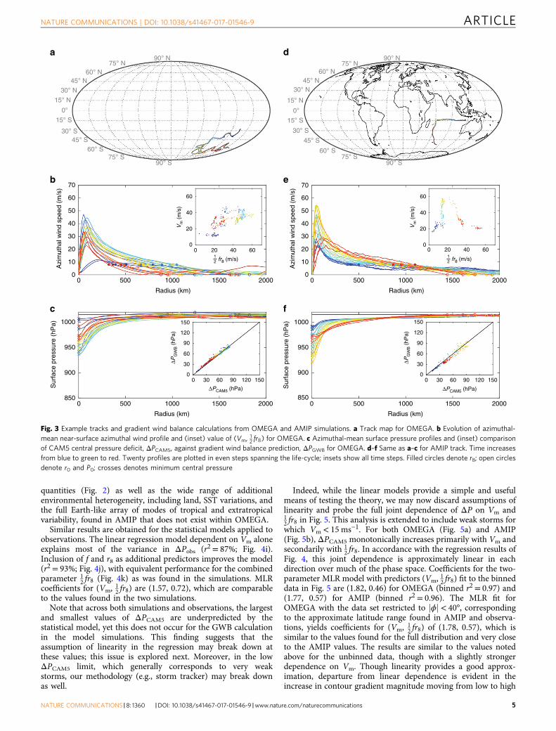
Hierarchy of models. As described in Methods section, we testthis theoretical prediction for ΔP across a hierarchy of modelsthat spans a reduced-complexity aquaplanet simulation experi-ment (OMEGA), an Earth-like simulation (AMIP), and obser-vations. The spatial distribution of storms and joint distributionsof key quantities for both simulations and observations are pro-vided in Figs 1, 2, respectively. We first test the prediction of thecentral prssure deficit directly from gradient wind balance.Example tracks and gradient wind balance calculations forOMEGA and AMIP are provided in Fig. 3. We then test how wellthis prediction can be replicated by a hierarchy of three simplemultiple-linear regression (MLR) models that take as predictors:Vm only (standard wind-only baseline); Vm, f, and the radius of8 ms−1, r8 (analogous to the prevailing empirical model6); and Vm
and 12 fr8 (new theory).
Figure 4 compares the model predictions of ΔP against theirtrue values, ΔPCAM5, across simulations and observations for thedirect gradient wind balance calculation as well as each of threeMLR statistical models. The gradient wind balance calculation isnot performed for observations as it requires a credible estimationof the entire wind profile out to large radii, a suitable database ofwhich is not available. For the gradient wind calculations, theazimuthal wind profile has been multiplied by the constant
factors (αV) of 1.15 and 1.11 for OMEGA and AMIP, respectively.These values yield a slope of approximately one for the linear fitbetween ΔPGWB and ΔPCAM5. The square of the Pearsoncorrelation coefficient, r2, and the root-mean-square error, εrms,are calculated as measures of performance for each model.
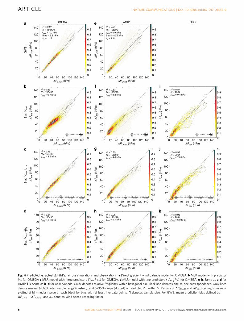
We begin with the simulations. The prediction ΔPGWB
performs very well in explaining the vast majority of variancein ΔPCAM5 for both OMEGA (r2= 0.97; Fig. 4a) and AMIP(r2= 0.94; Fig. 4e). Moreover, performance is consistent across allΔPCAM5 values, with minimal conditional bias and only modestincreases in the spread of the interquartile and 5–95% rangesmoving towards large ΔPCAM5 values. The linear regressionmodel dependent on Vm alone explains a substantial fraction ofthis variance (r2= 0.83), though not all of it (Fig. 4b, f). Inclusionof f and r8 as additional predictors largely eliminates this gap(Fig. 4c, g) for both OMEGA (r2= 0.95) and AMIP (r2= 0.95),consistent with the prevailing empirical model6. Note that themagnitudes of the MLR coefficients for r8 and f are not directlycomparable across the simulations because of large differences inthe covariance between the two parameters (Fig. 2). Finally, thetheory-based MLR model dependent on Vm and the combinedparameter 1
2 fr8 performs equally well (Fig. 4d, h) for bothOMEGA (r2= 0.94) and AMIP (r2= 0.95), providing strongevidence in favor of the theoretical prediction for the centralpressure deficit presented above. MLR coefficients for (Vm, 12 fr8)are (1.79, 0.56) for OMEGA and (1.62, 0.61) for AMIP, indicatingthat OMEGA and AMIP exhibit quantitatively similar parametricdependencies despite large qualitative differences in their spatialdistributions (Fig. 1) and distributions of relevant dynamical
1020
1000
2000
1800
1600
1400
1200
1000
800
600
400
200
00 2 4 6 8 10 12 14
f (10–5 s–1)0 2 4 6 8 10 12 14
f (10–5 s–1)0 2 4 6 8 10 12 14
f (10–5 s–1)
� = –0.34 � = 0.48 � = 0.20
� = –0.94� = –0.92� = –0.90
2000
1800
1600
1400
1200
1000
800
600
400
200
0
2000
1800
1600
1400
1200
1000
800
600
400
200
0
980
960
940
Pm
in (
hPa)
920
900
880
860
1020
1000
980
960
940
920
900
880
860
1020
1000
980
960
940
Pm
in (
hPa)
r 8 (
km)
r 8 (
km)
r 8 (
km)
920
900
880
860
Vm (m/s)
0 20 40 60 80 100
Vm (m/s)
AMIP OBSOMEGA
0 20 40 60 80 100
Vm (m/s)
0 20 40 60 80 100
Pm
in (
hPa)
a c e
b d f
Fig. 2 Joint distributions of key storm quantities across simulations and observations. a Pm and Vm in OMEGA. b r8 and f in OMEGA. c, d Same as a, b forAMIP. e, f Same as a, b for observations. Data set is filtered as described in the text
ARTICLE NATURE COMMUNICATIONS | DOI: 10.1038/s41467-017-01546-9
4 NATURE COMMUNICATIONS |8: 1360 |DOI: 10.1038/s41467-017-01546-9 |www.nature.com/naturecommunications
quantities (Fig. 2) as well as the wide range of additionalenvironmental heterogeneity, including land, SST variations, andthe full Earth-like array of modes of tropical and extratropicalvariability, found in AMIP that does not exist within OMEGA.
Similar results are obtained for the statistical models applied toobservations. The linear regression model dependent on Vm aloneexplains most of the variance in ΔPobs (r2= 87%; Fig. 4i).Inclusion of f and r8 as additional predictors improves the model(r2= 93%; Fig. 4j), with equivalent performance for the combinedparameter 1
2 fr8 (Fig. 4k) as was found in the simulations. MLRcoefficients for (Vm, 12 fr8) are (1.57, 0.72), which are comparableto the values found in the two simulations.
Note that across both simulations and observations, the largestand smallest values of ΔPCAM5 are underpredicted by thestatistical model, yet this does not occur for the GWB calculationin the model simulations. This finding suggests that theassumption of linearity in the regression may break down atthese values; this issue is explored next. Moreover, in the lowΔPCAM5 limit, which generally corresponds to very weakstorms, our methodology (e.g., storm tracker) may break downas well.
Indeed, while the linear models provide a simple and usefulmeans of testing the theory, we may now discard assumptions oflinearity and probe the full joint dependence of ΔP on Vm and12 fr8 in Fig. 5. This analysis is extended to include weak storms forwhich Vm< 15 ms−1. For both OMEGA (Fig. 5a) and AMIP(Fig. 5b), ΔPCAM5 monotonically increases primarily with Vm andsecondarily with 1
2 fr8. In accordance with the regression results ofFig. 4, this joint dependence is approximately linear in eachdirection over much of the phase space. Coefficients for the two-parameter MLR model with predictors (Vm, 12 fr8) fit to the binneddata in Fig. 5 are (1.82, 0.46) for OMEGA (binned r2= 0.97) and(1.77, 0.57) for AMIP (binned r2 = 0.96). The MLR fit forOMEGA with the data set restricted to ϕj j< 40°, correspondingto the approximate latitude range found in AMIP and observa-tions, yields coefficients for (Vm, 1
2 fr8) of (1.78, 0.57), which issimilar to the values found for the full distribution and very closeto the AMIP values. The results are similar to the values notedabove for the unbinned data, though with a slightly strongerdependence on Vm. Though linearity provides a good approx-imation, departure from linear dependence is evident in theincrease in contour gradient magnitude moving from low to high
70
60 60
60
Vm
(m
/s)
ΔPG
WB (
hPa)
50
40
40
150
150
120
120
90
90
60
60
30
300
0
40
Azi
mut
hal w
ind
spee
d (m
/s)
30
20
20
20
10
0
00
0 500
70
90° S75° S
60° S
45° S
30° S
15° S
15° N
30° N45° N
60° N75° N
90° N
0°
90° S75° S
60° S45° S
30° S
15° S
15° N
30° N
45° N60° N
75° N90° N
0°
60
50
40
Azi
mut
hal w
ind
spee
d (m
/s)
Sur
face
pre
ssur
e (h
Pa)
30
20
10
0
1000
950
850
900
Sur
face
pre
ssur
e (h
Pa) 1000
1000
Radius (km) Radius (km)
20001500
0 500 1000
Radius (km)
20001500
0 500 1000 20001500
0 500 1000
Radius (km)
20001500
950
850
900
fr8 (m/s)12
60
60
Vm
(m
/s)
40
40
20
200
0
fr8 (m/s)12
ΔPCAM5 (hPa)
ΔPG
WB (
hPa)
150
150
120
120
90
90
60
60
30
300
0
ΔPCAM5 (hPa)
a d
eb
fc
Fig. 3 Example tracks and gradient wind balance calculations from OMEGA and AMIP simulations. a Track map for OMEGA. b Evolution of azimuthal-mean near-surface azimuthal wind profile and (inset) value of (Vm, 12 fr8) for OMEGA. c Azimuthal-mean surface pressure profiles and (inset) comparisonof CAM5 central pressure deficit, ΔPCAM5, against gradient wind balance prediction, ΔPGWB for OMEGA. d–f Same as a–c for AMIP track. Time increasesfrom blue to green to red. Twenty profiles are plotted in even steps spanning the life-cycle; insets show all time steps. Filled circles denote r8; open circlesdenote r0 and P0; crosses denotes minimum central pressure
NATURE COMMUNICATIONS | DOI: 10.1038/s41467-017-01546-9 ARTICLE
NATURE COMMUNICATIONS |8: 1360 |DOI: 10.1038/s41467-017-01546-9 |www.nature.com/naturecommunications 5
140
r 2 = 0.97N = 150430
rms = 4.0 hPaBias = 2.8 hPa�v = 1.15
r 2 = 0.83N = 150430
rms = 6.7 hPa120
100
100 120 140
80
80
60
60
ΔPst
at (h
Pa)
ΔPG
WB (
hPa)
Sta
t: V
max
GW
B
40
40
20
200
140
120
100
80
60
40
20
0
0ΔPCAM5 (hPa)
140
120
1
0.9
0.8
0.7
0.6
0.5
0.4
0.3
0.2
0.1
0
1
0.9
0.8
0.7
0.6
0.5
0.4
0.3
0.2
0.1
0
1
0.9
0.8
0.7
0.6
0.5
0.4
0.3
0.2
0.1
0
1
0.9
0.8
0.7
0.6
0.5
0.4
0.3
0.2
0.1
0
1
0.9
0.8
0.7
0.6
0.5
0.4
0.3
0.2
0.1
0
1
0.9
0.8
0.7
0.6
0.5
0.4
0.3
0.2
0.1
0
1
0.9
0.8
0.7
0.6
0.5
0.4
0.3
0.2
0.1
0
1
0.9
0.8
0.7
0.6
0.5
0.4
0.3
0.2
0.1
0
1
0.9
0.8
0.7
0.6
0.5
0.4
0.3
0.2
0.1
0
1
0.9
0.8
0.7
0.6
0.5
0.4
0.3
0.2
0.1
0
1
0.9
0.8
0.7
0.6
0.5
0.4
0.3
0.2
0.1
0
100
100 120 140
80
80
60
60
ΔPst
at (h
Pa)
ΔPG
WB (
hPa)
40
40
20
200
140
120
100
80
60
40
20
0
0ΔPCAM5 (hPa)
100 120 140806040200ΔPCAM5 (hPa)
OMEGA
100 120 140806040200ΔPCAM5 (hPa)
AMIP
140
120
100
100 120 140
80
80
60
60
ΔPst
at (h
Pa)
40
40
20
200
0ΔPobs (hPa)
OBS
100 120 140806040200ΔPCAM5 (hPa)
100 120 140806040200ΔPCAM5 (hPa)
100 120 140806040200ΔPobs (hPa)
100 120 140806040200ΔPCAM5 (hPa)
100 120 140806040200ΔPCAM5 (hPa)
100 120 140806040200ΔPobs (hPa)
140
120
100
80
60ΔPst
at (h
Pa)
40
20
0
140
120
100
80
60ΔPst
at (h
Pa)
40
20
0
140
120
100
80
60ΔPst
at (h
Pa)
40
20
0
140
120
100
80
60ΔPst
at (h
Pa)
Sta
t: V
max
, f, r
8
40
20
0
140
120
100
80
60ΔPst
at (h
Pa)
40
20
0
140
120
100
80
60ΔPst
at (h
Pa)
40
20
0
∋
∋
r 2 = 0.83N = 125279rms = 8.3 hPa∋
r 2 = 0.87N = 2094
rms = 9.4 hPa∋
r 2 = 0.95N = 150430
rms = 3.6 hPa∋
r 2 = 0.95N = 125279rms = 4.6 hPa∋
r 2 = 0.93N = 2094
rms = 7.0 hPa∋
r 2 = 0.94N = 150430
rms = 4.1 hPa∋
r 2 = 0.95N = 125279rms = 4.7 hPa∋
r 2 = 0.93N = 2094
rms = 6.9 hPa∋
r 2 = 0.94N = 125279
rms = 4.9 hPaBias = –0.5 hPa�v = 1.11
∋
a e
b f i
d h k
c g j
= –0.69 + 1.62( ) + 0.73( ) + 0.07( )ΔP50
Vm
50rs
1e+06f
5e+05 = –0.58 + 1.53( ) + 0.48( ) + 0.12( )ΔP50
Vm
50rs
1e+06f
5e+05 = –0.84 + 1.58( ) + 0.44( ) + 0.22( )ΔP50
Vm
50rs
1e+06f
5e+05
= –29.82 + 1.79(Vm) + 0.56( fr8)ΔP 12
= –22.45 + 1.62(Vm) + 0.61( fr8)ΔP 12
= –28.83 + 1.57(Vm) + 0.72( fr8)ΔP 12
= –0.43 + 2.11( )ΔP50
Vm
50= –0.35 + 1.74( )ΔP
50
Vm
50= –0.42 + 1.65( )ΔP
50
Vm
50
Sta
t: V
max
, f
r 81 2
Fig. 4 Predicted vs. actual ΔP (hPa) across simulations and observations. a Direct gradient wind balance model for OMEGA. b MLR model with predictorVm for OMEGA c MLR model with three predictors (Vm, f, r8) for OMEGA. d MLR model with two predictors (Vm, 12 fr8) for OMEGA. e–h, Same as a–d forAMIP. i–k Same as b−d for observations. Color denotes relative frequency within hexagonal bin. Black line denotes one-to-one correspondence. Gray linesdenote median (solid), interquartile range (dashed), and 5–95% range (dotted) of predicted ΔP within 5 hPa bins of ΔPCAM5 and ΔPobs starting from zero,plotted at bin-median value of each (dot) for bins with at least five data points. N denotes sample size. For GWB, mean prediction bias defined asΔPGWB � ΔPCAM5, and αV denotes wind speed rescaling factor
ARTICLE NATURE COMMUNICATIONS | DOI: 10.1038/s41467-017-01546-9
6 NATURE COMMUNICATIONS |8: 1360 |DOI: 10.1038/s41467-017-01546-9 |www.nature.com/naturecommunications
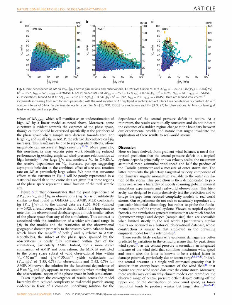
values of ΔPCAM5, which will manifest as an underestimation ofhigh ΔP by a linear model as noted above. Moreover, somecurvature is evident towards the extremes of the phase space,though caution should be exercised specifically at the periphery ofthe phase space where sample sizes decrease towards zero. Forlarge Vm and small 12 fr8 in AMIP, the relative dependence on 1
2 fr8increases. This result may be due to super-gradient effects, whosemagnitude can increase at high curvature35,36. More generally,this non-linearity may explain prior work identifying reducedperformance in existing empirical wind-pressure relationships athigh intensity37. For large 1
2 fr8 and moderate Vm in OMEGA,the relative dependence on Vm increases, perhaps suggestingasymptotic behavior in the combined effect of size and rotationrate on ΔP at particularly large values. We note that curvatureeffects at the extremes in Fig. 5 will be poorly represented in astatistical model fit to the entire data set given that these regionsof the phase space represent a small fraction of the total samplesize.
Figure 5 further demonstrates that the joint dependence ofΔPobs on Vm and 1
2 fr8 in observations (Fig. 5c) is quantitativelysimilar to that found in OMEGA and AMIP. MLR coefficientsfor (Vm, 1
2 fr8) fit to the binned data are (1.55, 0.64) (binnedr2= 0.92), a result comparable to that of AMIP. It is important tonote that the observational database spans a much smaller subsetof the phase space than any of the simulations. This contrast isassociated with the combination of a wider simulated range in12 fr8 in the models and the restriction of the observationalgeographic domain primarily to the western North Atlantic basin,which limits the range38 of both f and r8 relative to AMIP.Nonetheless, the subset of the phase space spanned by theobservations is nearly fully contained within that of thesimulations, particularly AMIP. Indeed, for a more directcomparison of AMIP and observations, the MLR fit restrictedto the phase space subset of valid observational bins withinVm≤ 70 ms−1 and 1
2 fr8 � 30ms�1 yields coefficients for(Vm, 1
2 fr8) of (1.53, 0.73) for observations and (1.62, 0.79) forAMIP. Moreover, the solution for the functional dependence ofΔP on Vm and 1
2 fr8 appears to vary smoothly when moving intothe observational region of the phase space in both simulations.
Taken together, the convergence of results across the modelhierarchy from reduced-complexity to real-world provide strongevidence in favor of a common underlying solution for the
dependence of the central pressure deficit in nature. At aminimum, the results are mutually consistent and do not indicatethe existence of a sudden regime change at the boundary betweenour experimental worlds and nature that might invalidate theapplication of these results to real-world storms.
DiscussionHere we have derived, from gradient wind balance, a novel the-oretical prediction that the central pressure deficit in a tropicalcyclone depends principally on two velocity scales: the maximumazimuthal-mean azimuthal wind speed and half the product ofthe Coriolis parameter and a measure of outer storm size. Thelatter represents the planetary tangential velocity component ofthe planetary angular momentum available to the outer circula-tion of the storm. This prediction is then demonstrated to per-form well across a hierarchy of models spanning global numericalsimulation experiments and real-world observations. This hier-archy was designed to comprehensively test the prediction and tobridge the gaps from reduced-complexity models to real-worldstorms. Our experiments do not seek to accurately reproduce anyparticular historical climatology but rather to probe the funda-mental nature of the tropical cyclone. Viewed as tropical cyclonefactories, the simulations generate statistics that are much broader(parameter range) and deeper (sample size) than are accessiblewhen limited strictly to the real world. Quantitatively similarresults are obtained in a historical observational database, whoseconstruction is similar to that employed in the prevailingempirical model for this relationship6.
These results likely explain why economic damages are betterpredicted by variations in the central pressure than by peak stormwind speed26, as the central pressure is essentially an integratedmeasure of the wind field that combines maximum wind speedand storm size; the latter is known to be a critical factor indamage potential, particularly due to storm surge8,9,39,40. Indeed,the central pressure is a single well-estimated quantity that issimpler than energy-based measures of the wind field41 thatrequire accurate wind speed data over the entire storm. Moreover,these results may explain why climate models can reproduce theobserved range of central pressure deficit despite cutting off theupper end of the distribution of peak wind speed, as lowerresolution tends to produce weaker but larger storms16,42–45,
100
90
80
70
60
5060
90
30
Vm
(m
/s)
40
30
20
10
0
100
90
80
70
60
50
Vm
(m
/s)
40
30
20
10
0
100
90
80
70
60
50
Vm
(m
/s)
40
30
20
10
00 20
140
120
100
100
80
80
fr8 (m/s)12
60
60
40
40
OMEGA AMIP OBS
(hPa)
20
0
140
120
100
80
60
40
(hPa)
20
0
140
120
100
80
60
40
(hPa)
20
00 20 10080
fr8 (m/s)12
6040 0 20 100801 fr8 (m/s)2
6040
60
90
30
60
90
30
a b c
Fig. 5 Joint dependence of ΔP on (Vm, 12 fr8) across simulations and observations. a OMEGA; binned MLR fit ΔPbin ¼ �25:9þ 1:82ðVmÞ þ 0:46ð12 fr8Þ
(r2 ¼ 0:97; Nbin ¼ 528; ϵRMS ¼ 4:9hPa). b AMIP; binned MLR fit ΔPbin ¼ �25:2þ 1:77ðVmÞ þ 0:57ð12 fr8Þ (r2 ¼ 0:96; Nbin ¼ 641; ϵRMS ¼ 5:5hPa).c Observations; binned MLR fit ΔPbin ¼ �26:2þ 1:55ðVmÞ þ 0:64 1
2 fr8� �
(r2 ¼ 0:92; Nbin ¼ 281; ϵRMS ¼ 7:8hPa). Data are binned into 2.5 ms−1
increments increasing from zero for each parameter, with the median value of ΔP displayed in each bin (color). Black lines denote lines of constant ΔP withcontour interval of 5 hPa. Purple lines denote bin count for N= [10, 100, 1000] for simulations and N= [3, 9, 27] for observations. All bins containing atleast one data point are plotted
NATURE COMMUNICATIONS | DOI: 10.1038/s41467-017-01546-9 ARTICLE
NATURE COMMUNICATIONS |8: 1360 |DOI: 10.1038/s41467-017-01546-9 |www.nature.com/naturecommunications 7
whose competing effects on the central pressure deficit may lar-gely offset. Finally, our results lend further support for the simpletheoretical wind structure model exploited above, in particularthe fast adjustment timescale of the structure of the wind fieldrelative to that of outer storm size and intensity. This fast time-scale underlies the prediction that the radial integral of gradientwind balance over the full wind field may be reduced simply to adependence on maximum wind speed and a single measure ofouter storm size as is borne out in our analysis.
There are a number of additional avenues that may warrantfurther research. First, though gradient wind balance appears toperform well in our analysis, gradient wind imbalance is knownto occur in the vicinity of the eyewall and may induce secondaryeffects on the central pressure deficit not accounted for here.Second, resolution limitations prevent our model simulationsfrom capturing particularly small, intense storms occasionallyfound in nature, and it is possible that the dependence on theseparameters may yet differ moving towards the small size limit.Experiments in high-resolution simulations could provide addi-tional evidence in this regime. Resolution limitations may alsominimize more complex variability in the inner-core windstructure, such as eyewall replacement cycles and small-scalevariability within the eye, that may further modulate the centralpressure deficit. Finally, experiments testing the independenteffects of varying surface enthalpy and momentum exchangecoefficients on these dependencies may yield further insights,though our results do not appear to be strongly dependent on thedetails of their representation given that these coefficients areimplicitly allowed to vary in CAM5.
For practical applications such as operations, additional work isrequired to develop an optimal predictive model for the centralpressure deficit in nature; here we have focused on the basicunderlying physics. Though the character of the functionaldependence of ΔP is found to be similar across experiments andobservations, the absolute values of that dependence may vary inmore complex ways in nature as well as in alternative computermodels. This variability reflects the uncertainty inherent in themessy details of boundary layer processes, represented crudelyhere by our wind rescaling factor for the gradient wind balancecalculations; these processes can exert a strong and variableinfluence on how wind speeds vary with altitude relative to z=10 m. Moreover, we do not address the specific operational needto predict the local (point) maximum wind speed, which mustaccount for, e.g., the effects of azimuthal asymmetries in the windfield that can modulate peak local wind speed with minimalimpact on both the azimuthal-mean wind speed and the centralpressure deficit. Nonetheless, this same modeling framework mayultimately be useful for estimating the complete TC vortex, aWMO recommendation46, from the limited operationally avail-able observations; this is a topic for future applicationdevelopment.
Overall, to our knowledge this is the first effort to explicitly testthe fundamental physical relationship between the central pres-sure deficit of a tropical cyclone and its wind field. The apparentconvergence of theory, reduced-complexity modeling experi-ments, Earth-like model simulations, and historical observationsprovides strong evidence for a fundamental, physically-intuitiveunderlying relationship among the two common measures ofintensity (maximum wind speed, minimum central pressure),outer storm size, and latitude (Coriolis). The result has significantvalue for operational forecasting, risk assessment, and basicresearch and understanding of the tropical cyclone. For example,this framework may be applied to the evaluation of tropicalcyclone climatologies and their intercomparison across climatemodels on the basis of the joint variability in these storm prop-erties. Moreover, given independent measurements of maximum
wind speed and minimum central pressure, these results may beused to infer storm size in the early-period historical record in theabsence of modern remotely-sensed and in situ measurements.
More broadly, we highlight that this work seeks insight intothe behavior of tropical cyclones on Earth in part via theiranalysis within alternative worlds. Indeed, OMEGA is a plausibleyet imaginary world, perhaps analogous in certain respectsto a planet such as Jupiter that is principally heated uniformlyfrom within rather than non-uniformly by an external star.The combination of such reduced-complexity experiments withEarth-like simulations offer the best hope30 for improvingthe understanding and predictability of real storms in naturesimultaneously, an objective that is otherwise difficult to achievevia the simulation of the real Earth and its myriad complexitiesalone.
MethodsExperimental design. We test the theoretical prediction for the dependence of ΔPacross a hierarchy of models over a range of complexities that spans a reduced-complexity aquaplanet simulation experiment (OMEGA), an Earth-like simulation(AMIP), and real-world observations. The hierarchy is designed with two principalpurposes: to provide a clean experimental testing ground in which parametric andphenomenological complexity is minimized (i.e., reduced-complexity) whileretaining essential modes of variability; and to explicitly connect results fromreduced-complexity experiments to those of a real-world setting. These simulationexperiments are treated essentially as tropical cyclone factories containingthousands of snapshots of the phenomenon of interest. Our objective is not toaccurately reproduce any particular historical climatology of tropical cyclones butrather to test hypotheses about the fundamental nature of the tropical cyclone ingeneral.
Simulation experiments. The first experiment, OMEGA, is a global radiative-convective equilibrium simulation with horizontally uniform sea surface tem-perature (29 °C) and solar insolation (340Wm−2 diurnal-mean)16; this set-up issimilar to previous global aquaplanet experiments17,47. The mean state is a world inwhich tropical cyclones are the dominant form of internal variability in the system.The spatial distribution of tropical cyclones is approximately zonally symmetric(Fig. 1) with storms that typically follow Earth-like poleward tracks due to theeffect of beta drift48–50. Storms exist within a tightly controlled global climate statecharacterized by a homogeneous thermodynamic environment devoid of land,extratropical jet interaction, or other features that may inhibit storm formation orpropagation. As a result, storm tracks are capable of extending all the way to thepoles. Experimentally, then, OMEGA generates storms with a wide range ofvariability in Vm, r0, and f within an otherwise homogeneous environment, whichoffers a clean setting in which to test our theory. The second experiment, AMIP,is an Earth-like historical simulation (i.e., following Atmospheric Model Inter-comparison protocols51) over the period 1979–2012; this set-up was examined inprevious work15,52. AMIP builds on OMEGA by adding full Earth-like environ-mental heterogeneity, including land masses and a jet stream, resulting in theconfinement of storm tracks to specific ocean basins (Fig. 1) akin to the spatialdistribution found on present-day Earth. A third experiment was also run that isidentical to OMEGA except with the Coriolis parameter set to its value at ϕ= 10 °N everywhere on the planet, thereby imposing uniform dynamical forcing in thesystem; this experiment yields more complex results and is discussed in Supple-mentary Note 1 (Supplementary Figs 1, 2).
Our experimental laboratory is the Community Atmosphere Model, version 5(CAM5). As the atmospheric component of the Community Earth System Model(CESM), CAM5 is typically used for conventional climate simulations. The spectralelement dynamical core on a cubed-sphere grid53,54, used for all simulations, hasdemonstrated an ability to simulate tropical cyclones in a range of experimentalsetups16,52,55,56. All three simulations are run at a resolution of ne120, where “ne”denotes the number of spectral elements along each cube edge. This resolutionyields a horizontal grid spacing of ~25 km that is nearly uniform around the globeowing to the cubed-sphere grid of the dynamical core. The same physicalparameterization suite57 is employed across all experiments, with the exception ofvarious simplifications required for the reduced complexity of OMEGA58. CAM5employs a hybrid-sigma model vertical coordinate whose lowest model levelsconveniently are nearly equivalent to levels of constant altitude when surfaceelevation is constant. OMEGA was also run at a lower horizontal resolution of100 km and yields similar conclusions (Supplementary Figs 3, 4). OMEGA was runfor 2 years, while AMIP spans the period 1979–2015. To allow for modelequilibration, the first six simulation months are discarded for OMEGA and thefirst year (1979) is discarded for AMIP.
For each simulation, tropical cyclones are first identified using a tracker thatalso extracts the surface central pressure at the storm center. For OMEGA, thestorm center is determined on the quasi-uniform native cubed-sphere grid using an
ARTICLE NATURE COMMUNICATIONS | DOI: 10.1038/s41467-017-01546-9
8 NATURE COMMUNICATIONS |8: 1360 |DOI: 10.1038/s41467-017-01546-9 |www.nature.com/naturecommunications
early release version of the open-source TempestExtremes59. Given the simplicityof the simulations, the algorithm searches for a surface pressure minimum thatincludes a 4-hPa closed contour within five great circle degrees of the location ofthe minimum at 6-hour increments. The storm locations are then stitched togetherby searching for candidates at the next 6-hourly time step that are within five greatcircle degrees. A track is defined as having at least four storm points, with gapsbetween consecutive track points not exceeding 24 hours. For AMIP, due to itsgreater phenomenological complexity, the storm center is tracked at three-hourincrements with an alternate algorithm60 commonly used for Earth-likesimulations. This algorithm associates storm centers on a latitude-longitude grid(via bilinear interpolation from the native grid) by matching a local minimum insurface pressure with a maximum in relative vorticity at 850 hPa and a warm-corebetween 500 and 300 hPa. These storm centers are then stitched together bylooking to the next time step for another center that is within 400 km. A track isdefined to have a lowermost model level wind speed great than 17 m s−1 for aminimum of three days. All analysis throughout is performed on the native grid,which requires simple relocation of the storm center to the native grid for AMIP(due to the tracking being performed on a latitude-longitude grid).
For each identified center at each time step, azimuthal-mean radial profiles ofazimuthal wind and pressure are calculated from data on the native grid at thelowest model level out to 5000 km radius. Radial profiles of density were alsocalculated for OMEGA, but the requisite data was not available for AMIP. Data arebinned into Δr= 25 km bins in increments of 14Δr. For the AMIP simulations, dataare first blocked out at all gridpoints where the CAM5 land fraction variable is >0.1and the surface geopotential height is outside the range z∈ [−10, 10] m in order tominimize biases induced by land or elevated terrain as well as to ensure that thelowest hybrid-sigma model level corresponds closely to a surface of constantaltitude.
Given that the relationship between theory and prediction is mediated bygradient wind balance, we first test the extent to which gradient wind balance maybe directly applied to the full radial profile of azimuthal-mean azimuthal wind inorder to predict the central pressure deficit of the storms. The radial profile of theazimuthal-mean azimuthal wind is first multiplied by a constant factor for eachsimulation (values given in the main text); this factor is interpreted here as a simpleaccounting for the reduction in wind speed due to friction within the boundarylayer (i.e., the reciprocal of the gradient-to-surface wind reduction factor61). Thisapproach avoids the many complexities of defining the top of the boundary layer62
and aligns with the overarching objective in operations and research of relating thenear-surface maximum wind speed to the central surface pressure and vice versa.This wind profile is interpolated to a 1-km resolution radial grid using a PiecewiseCubic Hermite Interpolating Polynomial, which is similar to a cubic spline butprevents overshoot between neighboring data points. Given this wind profile, thegradient wind equation (Eq. 1) is integrated radially outward from the center to thefirst radius of vanishing wind, r0, in 2-km increments using a centered-differencescheme to yield a prediction for the storm central pressure deficit ΔPGWB. Airdensity is set constant at ρ= 1.155 kgm−3; inclusion of the full radial profile ofdensity in the GWB integration for OMEGA does not significantly change theresult (Supplementary Fig. 5). This prediction is compared against the true centralpressure deficit, ΔPCAM5, with the environmental pressure defined as P0= P(r= r0)from the radial profile of pressure. For a small fraction of cases, the azimuthal windgets very close to zero but does not cross it; in such cases the largest valid integerwind radius (e.g., radius of 1 ms−1) of the raw CAM5 wind profile is used instead.The wind profile at small wind speeds in the far outer circulation tends to exhibitsignificantly more variability, which may introduce additional noise in our analysisthat might be avoided by applying an outer wind model instead31. However, ΔPitself is relatively insensitive to these very weak winds at very large radii due to thenature of Eq. (1), and thus we elect to use the wind profile alone for the sake ofsimplicity. Examples of the methodology applied to one storm from each ofOMEGA and AMIP are provided in Fig. 2.
Next, we test the extent to which the results of the gradient wind balanceprediction can be replicated by a simple statistical multiple linear regression modelthat employs the parameters identified above by theory: Vm and 1
2 fr0. In contrast tothe gradient wind balance calculation, large variability at small wind speeds in thefar outer circulation will have an outsized effect on the statistical model prediction,and thus in lieu of r0 we employ the inner-most radius of 8 ms−1, r8, as our measureof outer storm size (Fig. 3). This choice has the added benefit that r8 typically lieswell above the noise of the background environmental flow; typically liessufficiently far outside the radius of maximum wind (even for relatively weakstorms) so as to lie beyond the turbulently convecting inner core; and maypotentially be observed in situ or through remote sensing or calculated fromreanalysis data and thus be accessible in an operational setting. Moreover, r8performs best in comparison of the outer wind field between reanalysis andobservations63. Three versions of the statistical model are tested, each takingdifferent input parameters: Vm only; Vm, f, and r8; and Vm and 1
2 fr8. The first modelprovides a pure wind-pressure model as a baseline; the second model addsinformation about f and r8 separately and is analogous to the prevailing empiricalmodel6; the third model tests the theoretical prediction that the effects of f and r8manifest themselves as a single joint parameter 1
2 fr8.The above tests are performed using subsets of storm snapshots filtered to
exclude cases with Vm< 15 ms−1 to avoid very weak storms, as well as rare
instances where rm< 10 km or rm> 500 km; the latter may occur briefly inOMEGA if a weak storm is very close to a strong storm. For AMIP simulations,cases in which the center is less than 100 km from land are also excluded in orderto minimize land effects on the wind profile. Furthermore, to avoid cases with poorazimuthal data coverage, an asymmetry parameter38, whose values range from zero(perfect azimuthal symmetry) to one (single point), cannot exceed 0.5 at r8; thisfilters out ~1% of cases and has a negligible effect on the results. Filters arecalculated from the raw CAM5 radial profiles of the azimuthal wind.
Observations. Finally, atop the model hierarchy is the our best estimate of the realEarth itself. We construct an aircraft-based observational data set for 2004–2015from the Atlantic and East Pacific basins (Fig. 1) using a similar methodologyto the prevailing empirical model6. Tropical cyclone Best Track intensity andpositions are interpolated to the time of aircraft-based estimates of central pressure.The interpolated intensity is slightly reduced64 to account for the effect of stormmotion by removing the asymmetry, a, owing to storm motion, c, given bya= 1.173c0.63 ms−1. Both Best Track and aircraft reconnaissance central pressurefixes come from the databases of the Automated Tropical Cyclone Forecast system(ATCF65) available from the NHC. To estimate r8, Global Forecast System (GFS)operational analyses are utilized to calculate the radial profile of 850 hPa windsusing adjacent analysis times and linearly interpolating to a single radial profile.850-hPa winds are reduced to a marine exposure using a factor of 0.80. The valueof r8 is defined as the inner-most wind radius beyond the radius of maximum wind,and the algorithm saturates at 1500 km; a small subset of values associated withSandy (2012) attain this upper bound and thus may be slightly underestimated.The environmental pressure is estimated by the azimuthal-mean pressure at900 km (r8< 600 km), 1200 km (r8∈ [600, 900) km), 1500 km (r8∈ [900, 1200)km), 1800 km (r8∈ [1200, 1500) km), and 2100 km (r8≥ 1500 km). Finally, thecentral pressure deficit, ΔPobs, is calculated by subtracting the central pressure fromthe environmental pressure. As with AMIP, only cases in which the center is atleast 100 km from land are included. Distributions of key quantities for theobservational database are provided in Fig. 2.
Code availability. All code used to perform the analyses in this work are availableupon request from the corresponding author.
Data availability. The data sets analyzed in this study are available from thecorresponding author on reasonable request. All model output is accessible viathe National Center for Atmospheric Research (NCAR) Yellowstonesupercomputer.
Received: 25 July 2017 Accepted: 26 September 2017
References1. Schott, T. et al. The Saffir-Simpson hurricane wind scale. National Weather
Services, National Hurricane Centre, National Oceanic and AtmosphericAdministration (NOAA) factsheet. http://www.nhc.noaa.gov/pdf/sshws.pdf(2012).
2. Dvorak, V. F. Tropical cyclone intensity analysis and forecasting from satelliteimagery. Mon. Weather Rev. 103, 420–430 (1975).
3. Dvorak, V. F. Tropical cyclone intensity analysis using satellite data(US Department of Commerce, National Oceanic and AtmosphericAdministration, National Environmental Satellite, Data, and InformationService, 1984).
4. Atkinson, G. D. & Holliday, C. R. Tropical cyclone minimum sea level pressure/maximum sustained wind relationship for the western north pacific. Mon.Weather Rev. 105, 421–427 (1977).
5. Koba, H., Hagiwara, T., Osano, S. & Akashi, S. Relationship between theCI-number and central pressure and maximum wind speed in typhoons.J. Meteor. Res. 42, 59–67 (1990).
6. Knaff, J. A. & Zehr, R. M. Reexamination of tropical cyclone wind-pressurerelationships. Weather Forecast. 22, 71–88 (2007).
7. Courtney, J. & Knaff, J. A. Adapting the Knaff and Zehr wind-pressurerelationship for operational use in tropical cyclone warning centres. Aust.Meteorol. Oceanogr. J. 58, 167 (2009).
8. Chavas, D., Yonekura, E., Karamperidou, C., Cavanaugh, N. & Serafin, K. UShurricanes and economic damage: extreme value perspective. Nat. Hazards Rev.14, 237–246 (2013).
9. Done, J. M., PaiMazumder, D., Towler, E. & Kishtawal, C. M. Estimatingimpacts of North Atlantic tropical cyclones using an index of damage potential.Clim. Change 1–13 (2015).
10. Blake, E. S., Kimberlain, T. B., Berg, R. J., Cangialosi, J. P. & Beven, J. L. IITropical cyclone report: hurricane sandy. Natl Hurric. Center 12, 1–10 (2013).
NATURE COMMUNICATIONS | DOI: 10.1038/s41467-017-01546-9 ARTICLE
NATURE COMMUNICATIONS |8: 1360 |DOI: 10.1038/s41467-017-01546-9 |www.nature.com/naturecommunications 9

11. Sobel, A. H. et al. Human influence on tropical cyclone intensity. Science 353,242–246 (2016).
12. Korty, R. L., Emanuel, K. A., Huber, M. & Zamora, R. A. Tropical cyclonesdownscaled from simulations with very high carbon dioxide levels. J. Clim. 30,649–667 (2017).
13. Kossin, J. P. Hurricane intensification along United States coast suppressedduring active hurricane periods. Nature 541, 390–393 (2017).
14. Knutson, T. R. et al. Global projections of intense tropical cyclone activity forthe late twenty-first century from dynamical downscaling of CMIP5/RCP4.5 scenarios. J. Clim. 28, 7203–7224 (2015).
15. Reed, K. A. et al. Impact of the dynamical core on the direct simulation oftropical cyclones in a high-resolution global model. Geophys. Res. Lett. 42,3603–3608 (2015).
16. Reed, K. A. & Chavas, D. R. Uniformly rotating global radiative-convectiveequilibrium in the Community Atmosphere Model, version 5. J. Adv. Model.Earth Syst. 7, 1938–1955 (2015).
17. Merlis, T. M., Zhou, W., Held, I. M. & Zhao, M. Surface temperaturedependence of tropical cyclone-permitting simulations in a spherical modelwith uniform thermal forcing. Geophys. Res. Lett. 43, 2859–2865 (2016).
18. Webster, P. J., Holland, G. J., Curry, J. A. & Chang, H.-R. Changes in tropicalcyclone number, duration, and intensity in a warming environment. Science309, 1844–1846 (2005).
19. Elsner, J. B., Kossin, J. P. & Jagger, T. H. The increasing intensity of thestrongest tropical cyclones. Nature 455, 92–95 (2008).
20. Hall, T. & Hereid, K. The frequency and duration of US hurricane droughts.Geophys. Res. Lett. 42, 3482–3485 (2015).
21. Hart, R. E., Chavas, D. R. & Guishard, M. P. The arbitrary definition of thecurrent atlantic major hurricane landfall drought. Bull. Am. Meteorol. Soc. 97,713–722 (2016).
22. Pielke, R. A. Jr. Future economic damage from tropical cyclones: sensitivities tosocietal and climate changes. Philos. Trans. R. Soc. A: Math., Phys. Eng. Sci. 365,2717–2729 (2007).
23. Nordhaus, W. D. The economics of hurricanes and implications of globalwarming. Clim. Change Econ. 1, 1–20 (2010).
24. Murnane, R. J. & Elsner, J. B. Maximum wind speeds and US hurricane losses.Geophys. Res. Lett. 39 (2012) (http://onlinelibrary.wiley.com/doi/10.1029/2012GL052740/full).
25. Peduzzi, P. et al. Global trends in tropical cyclone risk. Nat. Clim. Change 2,289–294 (2012).
26. Bakkensen, L. A. & Mendelsohn, R. O. Risk and adaptation: evidence fromglobal hurricane damages and fatalities. J. Assoc. Environ. Resour. Econ. 3,555–587 (2016).
27. Emanuel, K. A. An air-sea interaction theory for tropical cyclones. Part I:steady-state maintenance. J. Atmos. Sci. 43, 585–605 (1986).
28. Miyamoto, Y. et al. Gradient wind balance in tropical cyclones inhigh-resolution global experiments. Mon. Weather Rev. 142, 1908–1926(2014).
29. Willoughby, H. E. Gradient balance in tropical cyclones. J. Atmos. Sci. 47,265–274 (1990).
30. Held, I. M. The gap between simulation and understanding in climatemodeling. Bull. Am. Meteorol. Soc. 86, 1609–1614 (2005).
31. Chavas, D. R., Lin, N. & Emanuel, K. A model for the complete radial structureof the tropical cyclone wind field. Part I: Comparison with observed structure*.J. Atmos. Sci. 72, 3647–3662 (2015).
32. Chavas, D. R. & Lin, N. A model for the complete radial structure of thetropical cyclone wind field. Part II: Wind field variability. J. Atmos. Sci. 73,3093–3113 (2016).
33. Emanuel, K. & Rotunno, R. Self-stratification of tropical cyclone outflow. Part I:Implications for storm structure. J. Atmos. Sci. 68, 2236–2249 (2011).
34. Emanuel, K. Tropical cyclone energetics and structure. Atmos. Turbul.Mesoscale Meteorol. 165–191 (2004).
35. Bryan, G. H. & Rotunno, R. Evaluation of an analytical model for the maximumintensity of tropical cyclones. J. Atmos. Sci. 66, 3042–3060 (2009).
36. Stern, D. P., Brisbois, J. R. & Nolan, D. S. An expanded dataset of hurricaneeyewall sizes and slopes. J. Atmos. Sci. 71, 2747–2762 (2014).
37. Kieu, C. Q., Chen, H. & Zhang, D.-L. An examination of the pressure-windrelationship for intense tropical cyclones. Weather Forecast. 25, 895–907(2010).
38. Chavas, D. R., Lin, N., Dong, W. & Lin, Y. Observed tropical cyclone sizerevisited. J. Clim. 29, 2923–2939 (2016).
39. Irish, J. L. & Resio, D. T. A hydrodynamics-based surge scale for hurricanes.Ocean Eng. 37, 69–81 (2010).
40. Zhai, A. R. & Jiang, J. H. Dependence of U.S. hurricane economicloss on maximum wind speed and storm size. Environ. Res. Lett. 9, 064019(2014).
41. Powell, M. D. & Reinhold, T. A. Tropical cyclone destructive potential byintegrated kinetic energy. Bull. Am. Meteorol. Soc. 88, 513–526 (2007).
42. Bengtsson, L., Botzet, M. & Esch, M. Hurricane-type vortices in a generalcirculation model. Tellus A 47, 175–196 (1995).
43. Schenkel, B. A. & Hart, R. E. An examination of tropical cyclone position,intensity, and intensity life cycle within atmospheric reanalysis datasets. J. Clim.25, 3453–3475 (2012).
44. Rotunno, R. & Bryan, G. H. Effects of parameterized diffusion on simulatedhurricanes. J. Atmos. Sci. 69, 2284–2299 (2012).
45. Chavas, D. R. & Emanuel, K. Equilibrium tropical cyclone size in an idealizedstate of axisymmetric radiative–convective equilibrium*. J. Atmos. Sci. 71,1663–1680 (2014).
46. IWTC8. World meteorological organization eighth international workshop ontropical cyclones list of recommendations (2014). http://www.wmo.int/pages/prog/arep/wwrp/tmr/documents/ListofRecommendations.pdf [Online; accessed18 July 2017.
47. Shi, X. & Bretherton, C. S. Large-scale character of an atmosphere inrotating radiative-convective equilibrium. J. Adv. Model. Earth Syst. 6, 616–629(2014).
48. Holland, G. J. Tropical cyclone motion: Environmental interaction plus a betaeffect. J. Atmos. Sci. 40, 328–342 (1983).
49. Chan, J. C. & Williams, R. Analytical and numerical studies of the beta-effect intropical cyclone motion. part I: zero mean flow. J. Atmos. Sci. 44, 1257–1265(1987).
50. Smith, R. B. A hurricane beta-drift law. J. Atmos. Sci. 50, 3213–3215 (1993).51. Gates, W. L. et al. An overview of the results of the atmospheric model
intercomparison project (AMIP I). Bull. Am. Meteor. Soc. 80, 29–55 (1999).52. Bacmeister, J. T. et al. Projected changes in tropical cyclone activity under
future warming scenarios using a high-resolution climate model. Clim. Change1–14 (2016).
53. Taylor, M. A. & Fournier, A. A compatible and conservative spectral elementmethod on unstructured grids. J. Comput. Phys. 229, 5879–5895 (2010).
54. Dennis, J. et al. CAM-SE: a scalable spectral element dynamical core for theCommunity Atmosphere Model. Int. J. High Perform. Comput. Appl. 26, 74–89(2012).
55. Reed, K. A., Jablonowski, C. & Taylor, M. A. Tropical cyclones in the spectralelement configuration of the Community Atmosphere Model. Atmos. Sci. Lett.13, 303–310 (2012).
56. Zarzycki, C. M. & Jablonowski, C. A multidecadal simulation of Atlantictropical cyclones using a variable-resolution global atmospheric generalcirculation model. J. Adv. Model. Earth Syst. 6, 805–828 (2014).
57. Neale, R. B. et al. Description of the NCAR Community Atmosphere Model(CAM 5.0). NCAR Tech. Note NCAR/TN-486+STR (National Center forAtmospheric Research, Boulder, Colorado, 2010).
58. Reed, K. A., Medeiros, B., Bacmeister, J. T. & Lauritzen, P. H. Global radiative-convective equilibrium in the Community Atmosphere Model 5. J. Atmos. Sci.72, 2183–2197 (2015).
59. Ullrich, P. A. & Zarzycki, C. M. TempestExtremes: a framework for scale-insensitive pointwise feature tracking on unstructured grids. Geosci. Model Dev.10, 1069–1090 (2017).
60. Zhao, M., Held, I. M., Lin, S.-J. & Vecchi, G. A. Simulations of global hurricaneclimatology, interannual variability, and response to global warming using a50-km resolution GCM. J. Clim. 22, 6653–6678 (2009).
61. Franklin, J. L., Black, M. L. & Valde, K. GPS dropwindsonde wind profiles inhurricanes and their operational implications. Weather Forecast. 18, 32–44(2003).
62. Kepert, J. D., Schwendike, J. & Ramsay, H. Why is the tropical cycloneboundary layer not well mixed? J. Atmos. Sci. 73, 957–973 (2016).
63. Schenkel, B. A., Lin, N., Chavas, D. R., Oppenheimer, M. & Brammer, A.Evaluating outer tropical cyclone size in reanalysis datasets using QuikSCATdata. J. Clim. http://journals.ametsoc.org/doi/abs/10.1175/JCLI-D-17-0122.1(2017).
64. Schwerdt, R. W., Ho, F. P. & Watkins, R. R. Meteorological criteria for standardproject hurricane and probable maximum hurricane windfields, Gulf and eastcoasts of the United States. NOAA Tech. Rep. NWS 23, 317 pp. [Available fromNational Hurricane Center Library, 11691 S.W. 117th St., Miami, FL33165–2149.] (1979).
65. Sampson, C. R. & Schrader, A. J. The automated tropical cyclone forecastingsystem (version 3.2). Bull. Am. Meteorol. Soc. 81, 1231–1240 (2000).
AcknowledgementsWe would like to acknowledge high-performance computing support from Yellowstone(ark:/85065/d7wd3xhc) provided by National Center for Atmospheric Research’s(NCAR) Computational and Information Systems Laboratory, sponsored by the NationalScience Foundation, for the FCNST and OMEGA simulations. The authors thank JulioBacmeister, Susan Bates, and Nan Rosenbloom (NCAR) for access to the AMIP simu-lation output. The views, opinions, and findings contained in this report are those of theauthors and should not be construed as an official National Oceanic and Atmospheric
ARTICLE NATURE COMMUNICATIONS | DOI: 10.1038/s41467-017-01546-9
10 NATURE COMMUNICATIONS |8: 1360 |DOI: 10.1038/s41467-017-01546-9 |www.nature.com/naturecommunications

Administration or U.S. Government position, policy, or decision. Support for K.A.R. wasprovided in part by the U.S. Department of Energy Office of Science grant DE-SC0016605.
Author contributionsThe study was conceived by D.R.C. and K.A.R.; D.R.C. and K.A.R. designed the research;D.R.C. and K.A.R. analyzed the model simulation data; D.R.C. and J.A.K. analyzed theobservational data; D.R.C. wrote the manuscript, K.A.R. wrote the model description andprovided manuscript feedback, J.A.K. wrote the observational data description andprovided manuscript feedback.
Additional informationSupplementary Information accompanies this paper at doi:10.1038/s41467-017-01546-9.
Competing interests: The authors declare no competing financial interests.
Reprints and permission information is available online at http://npg.nature.com/reprintsandpermissions/
Publisher's note: Springer Nature remains neutral with regard to jurisdictional claims inpublished maps and institutional affiliations.
Open Access This article is licensed under a Creative CommonsAttribution 4.0 International License, which permits use, sharing,
adaptation, distribution and reproduction in any medium or format, as long as you giveappropriate credit to the original author(s) and the source, provide a link to the CreativeCommons license, and indicate if changes were made. The images or other third partymaterial in this article are included in the article’s Creative Commons license, unlessindicated otherwise in a credit line to the material. If material is not included in thearticle’s Creative Commons license and your intended use is not permitted by statutoryregulation or exceeds the permitted use, you will need to obtain permission directly fromthe copyright holder. To view a copy of this license, visit http://creativecommons.org/licenses/by/4.0/.
© The Author(s) 2017
NATURE COMMUNICATIONS | DOI: 10.1038/s41467-017-01546-9 ARTICLE
NATURE COMMUNICATIONS |8: 1360 |DOI: 10.1038/s41467-017-01546-9 |www.nature.com/naturecommunications 11