physics - andrews university · pdf fileexperiment 7 conservation of mechanical energy ......
TRANSCRIPT

Physicsin the LaboratoryPHYS130 Applied Physics for theHealth ProfessionsFirst EditionSpring Semester 2001
Robert KingmanandGary W. Burdick
January 15, 2001

The authors express appreciation to the Physics faculty and many students who havecontributed to the development of the laboratory program and this manual. Specialrecognition is acknowledged to professor Bruce Lee for the many years that he taught theGeneral Physics course and the introductory laboratories. Professors Margarita Mattingly,and Mickey Kutzner have made substantial contributions to the laboratory and to individualexperiment instructions. This manual has become a reality because of the efforts of JosephSoo and Tiffany Karr for rewriting, editing and taking and including the photographs and theoutstanding editorial assistance of Anita Hubin.
Copyright © 2001 by Robert Kingman and Gary Burdick

i
Preface
It is the purpose of the science of Physics to explain natural phenomena. It is in thelaboratory where new discoveries are made. This is where the physicist makes observationsfor the purpose of identifying patterns which later may be fit by mathematical equations.Theories are constructed to describe patterns observed and are tested by further experiment.Therefore, it is imperative that students in an introductory Physics course are introduced toboth the existing theories in the classroom and to the ways of recognizing natural patternsin the laboratory. In addition, the effort put into the laboratory experiments will ultimatelyreward the student with a better understanding of the concepts presented in the classroom.
This manual is intended for use in an introductory Physics course. Prior experience inPhysics is not a requirement for understanding the concepts outlined within. The book waswritten with this in mind and therefore every experiment contains a Physical Principlessection which outlines the basic ideas used.
The student is required to keep a laboratory journal in which the raw data will be recordedas well as the analysis, any graphs and calculations. The lab write-ups form a permanentrecord of your work, and must be done in ink. Attached is a copy of the Lab Evaluation formwhich should be placed at the end of each laboratory writeup. This will form the outlinewhich the lab instructor will use for grading. Copies of this evaluation form are attached tothe end of your lab manual.
Each laboratory writeup should have the following sections:
1. Layout: Where you write the laboratory title, the date and time of the laboratorysection, and the name(s) of your lab partner(s).
2. Preliminaries: Where you make a brief statement of the laboratory objectives in yourown words, a description of the methods to be used in order to achieve the statedobjectives, a labeled sketch of the setup to be used, and completed predictions (ifrequired).
3. Data: Here is where you record the actual procedures as they are performed. Recordthe actual time that you start each procedure section, and include data as it is taken.If the data is recorded by the computer, include computer graphs of raw sample data.
4. Results: Include here all equations used in the calculations, computer graphs ofanalyzed data, and fitting results. Include analyses of the error in your results.
5. Conclusions: This should include a more general statement of whether yourmeasurements confirm the stated objectives, what fundamental physical laws wereillustrated by the experiment, and how the experimental error could have beenreduced in the experiment. Also include here a constructive critique of the lab,stating what went well, what didn’t, and how the laboratory could be improved.

ii
6. Abstract: This is a formal statement of what this laboratory experiment was allabout. Included in this paragraph should be something about the objectives, results,and conclusions of the laboratory.
7. Certification: You must get the signature of the lab instructor in your journal beforeleaving the lab. This will indicate how much of the writeup you did in the laboratoryperiod, and how much you did outside the lab. One point extra credit will be givenif you complete the laboratory writeup (including the evaluation form) before the endof the laboratory period and get your lab assistant’s signature after the evaluationform. You must also sign the evaluation form. “Your signature certifies that thislaboratory writeup represents a true and accurate presentation of your work.”
8. Bonus: Extra credit (up to 10% of the laboratory) will be given in selected labs forthe completion of the “further investigation” section. This is in addition to the onepoint you can receive for completing the writeup during the laboratory time.
In conclusion, we hope that the experiments in this manual will enhance your understandingof the concepts presented in class and will add pleasure to your journey through this excitingfield of Physics. Any comments you may have about the laboratories presented in this bookare welcomed and encouraged. We hope that you will overlook any missspellings, omisions, errors and inconsistencies and report such to the authors.

iii
Applied Physics for the Health Professions Lab Evaluation Form
Name: Box #
Lab date/time: Completion date/time:
Signature:
Pgs Pts
/1 Layout: Title, Date, Time, Partner(s)
/3 Preliminaries: Statement of objectives, methods to be used, predictions(if required), labeled sketch of setup
/5 Data: Record of procedures as they are performed, actual time record foreach procedure, raw data
/6 Results: Calculations, computer graphs and data fits, analysis of results,error analysis
/4 Conclusions: What physical laws were discovered, were the objectivesmet, what effects (if any) were the result of possible errors, critique of lab(what went well, what didn’t, how it could be improved)
/1 Certification: Signature of lab assistant before leaving lab, inclusion ofsigned evaluation form. Your signature certifies that this laboratorywriteup represents a true and accurate presentation of your work.
/0 Bonus: Extra credit for promptness, further investigation
Total: / 20 Lab Assistant: Date Scored:

iv
Table of Contents
Preface . . . . . . . . . . . . . . . . . . . . . . . . . . . . . . . . . . . . . . . . . . . . . . . . . . . i
Experiment 1 Uniform Motion . . . . . . . . . . . . . . . . . . . . . . . . . . . . . . . . . . . . 1
Experiment 2 Uniform Acceleration . . . . . . . . . . . . . . . . . . . . . . . . . . . . . . . 7
Experiment 3 Forces in Equilibrium . . . . . . . . . . . . . . . . . . . . . . . . . . . . . . . . 13
Experiment 4 Force and Acceleration - Newton’s Second Law . . . . . . . . . . . 21
Experiment 5 Torque and Angular Acceleration . . . . . . . . . . . . . . . . . . . . . 25
Experiment 6 Rotational Equilibrium - Torques . . . . . . . . . . . . . . . . . . . . . . . . 31
Experiment 7 Conservation of Mechanical Energy . . . . . . . . . . . . . . . . . . . . 35
Experiment 8 Elastic and Inelastic Collisions . . . . . . . . . . . . . . . . . . . . . . . . . 39
Experiment 9 Conservation of Energy of a Rolling Object . . . . . . . . . . . . . . 43
Experiment 10 Resonant Vibrations of a Wire . . . . . . . . . . . . . . . . . . . . . . . . 47
Experiment 11 Current, Voltage and Power - Ohm’s Law . . . . . . . . . . . . . . . 51
Experiment 12 Series and Parallel DC Circuits . . . . . . . . . . .. . . . . . . . . . . . . 55
Experiment 13 Magnetic Field, Force on a Current . . . . . . . . . . . . . . . . . . . . 61
Experiment 14 Motional EMF . . . . . . . . . . . . . . . . . . . . . . . . . . . . . . . . . . . . 67

Page 1
x ' v t%xo (1)
Figure 1 Slope, v, and intercept, xo.
v ' slope 'riserun
')x)t
'x2&x1
t2& t1
(2)
Applied Physics for the Health Professions Experiment 1
Uniform Motion - Graphing and Analyzing Motion
Objectives:
< To take data using a computer and signal interface< To use computer software programs to interpret data< To observe the distance-time relation for motion at constant velocity
Equipment:
< Motion sensor< Pasco 1.2 m track and dynamics cart< Computer with Signal Interface, Science Workshop and Vernier Graphical Analysis
software
Physical Principles:
The position of an object moving along a line is indicated by its displacement. Thedisplacement is the positive or negative of the distance of the object from a reference pointcalled the origin, the numbers being positive to the right of the origin and negative to the left.Denoting the displacement as x and the time as t,
The initial displacement xo is the starting positionwhen time t equals zero. This value is where theline crosses the vertical axis and is called theintercept. In a graph of displacement x (on thevertical axis) versus time t (on the horizontal axis)the velocity of the motion v is equal to the slope ofthe line,
The best fit of a straight line to a data set is the onewith the smallest value of the average squaredeviation.

Page 2
Prediction:
Consider the following two cases:
A. Motion away from the originCart has an initial position at +50 cm,travels for a time duration of 2 seconds,at a constant velocity of +50 cm/s
B. Motion towards the originCart has an initial position at +50 cm,travels for a time duration of 2 seconds,at a constant velocity of !50 cm/s
Draw graphs in your journal of what you think the motion will be for these two cases,plotting the displacement x versus the time t. Then answer the following questions for bothcases:1. Will the graph be straight or curved? 2. Will the graph slope up or down?3. If it is curved will it curve up or down?
Explain your reasoning for each of these answers.
Procedure:
Setup motion sensor:1. Plug the motion sensor’s phone plugs into digital channels 1 and 2 with the yellow
banded plug into channel 1. 2. Mount the motion sensor at the end of the track opposite the bumper.3. Align the sensor so that the sound waves will travel directly along the track.4. Use the screw adjustment on the bottom end of the track to level the track.
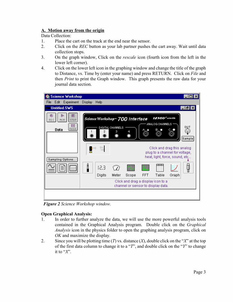
Setup Science Workshop: (See Figure 2 below.)1. If necessary, double click the left mouse button on the physics labs folder to open it.2. Double click on the science workshop icon in the folder to open Science Workshop.3. Click on the maximize icon to maximize the display.4. Click on Sampling Options, change the sampling rate to 10,000 Hz, and the stop time
to 3 sec. Press RETURN and click on OK to accept these values.5. Click and drag the phone plug icon to digital channel 1, choose Motion Sensor.
Change the trigger rate to 50 Hz.6. Drag the Graph icon onto the Motion Sensor icon below digital channels 1 and 2.
Click on position to display the position vs. time graph.7. Drag the Table icon onto the Motion Sensor icon. Click on position to display the
position vs. time data. Click on the clock to the right of the E at the upper left of theTable window to display times.
8. Move the graph and table windows so that all three windows are accessible.
Page 3
Figure 2 Science Workshop window.
A. Motion away from the originData Collection:1. Place the cart on the track at the end near the sensor.2. Click on the REC button as your lab partner pushes the cart away. Wait until data
collection stops.3. On the graph window, Click on the rescale icon (fourth icon from the left in the
lower left corner).4. Click on the lower left icon in the graphing window and change the title of the graph
to Distance, vs. Time by (enter your name) and press RETURN. Click on File andthen Print to print the Graph window. This graph presents the raw data for yourjournal data section.
Open Graphical Analysis:1. In order to further analyze the data, we will use the more powerful analysis tools
contained in the Graphical Analysis program. Double click on the GraphicalAnalysis icon in the physics folder to open the graphing analysis program, click onOK and maximize the display.
2. Since you will be plotting time (T) vs. distance (X), double click on the “X” at the topof the first data column to change it to a “T”, and double click on the “Y” to changeit to “X”.

Page 4
Transferring data to Graphical Analysis:1. In Science Workshop: Click and drag your cursor to highlight a rectangle of the best
data on the graph display. Then click once on the table display to select thehighlighted data on the table. Under the Edit menu, choose copy to store the datatemporarily in the Window’s “clipboard”.
2. In Graphical Analysis: Click on the upper left data position. Under the Edit menuoption choose paste to copy your data from the “clipboard”. Note that thedisplacement is plotted vertically (y-axis) and the time data is plotted horizontally (x-axis).
Analyzing Data: (See Figure 3 above)Manual Fitting:1. Click on the graph of your data on the right to select the graph.2. Choose Analyze from the main menu and click on Manual Curve Fit.3. Select the function M*x + B to select a linear (straight-line) model. (According to
Eq. (1), the “x” here corresponds to your time values, the M corresponds to yourvelocity values, and B corresponds to your beginning location xo at time equal zero).
4. Change the values in the intercept box B = at the lower left and the slope box M = tovary the intercept and slope of the model line.
5. Note values of the Mean Square Error at the lower right of the graph for each valueof slope M and intercept B.
6. Do this until the model line visually fits most closely to the data and then makefurther adjustments until the Mean Square Error is as small as possible.
7. Record the values of the slope M, intercept B and the Mean Square Error in yourjournal.
8. Click on OK-Keep Fit.Automatic Fitting:1. Choose Analyze from the main menu and click on Automatic Curve Fit.2. Select the function M*x + B to select a linear (straight-line) model. 3. Record the values of the slope M, intercept B and the Mean Square Error in your
journal.4. Click on OK-Keep Fit.

Page 5
Figure 3 Graphical Analysis window.
Analyze Results:1. Compare the values obtained in your manual fit, with the automatic fit values.2. Click on the graph title and change the title to Displacement versus Time.3. Click in the text window and enter your name, experiment name, date and
experiment details, ie motion away from detector.4. Choose File in the main menu, then Print to print the entire screen.
Questions (to be included in your Results):1. How does your observed curve compare with your predicted curve? 2. What is the speed of the cart? 3. How far from the detector is the cart when the detector begins measuring its motion?4. What does the value of the Mean Square Error indicate?
B. Motion towards the origin1. Return to the Science Workshop window and repeat the experiment, placing the cart
on the end opposite the motion sensor and pushing it toward the sensor.2. Repeat the Data Collection, Transferring data to Graphical Analysis, Analyzing
Data, and Questions sections above.
Further Questions:1. How are the results for parts A and B similar?2. How are the results for parts A and B different?

Page 6
Page 7
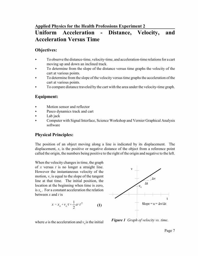
Figure 1 Graph of velocity vs. time.
x ' xo%vo@t%12
a @ t 2(1)
Applied Physics for the Health Professions Experiment 2
Uniform Acceleration - Distance, Velocity, andAcceleration Versus Time
Objectives:
< To observe the distance-time, velocity-time, and acceleration-time relations for a cartmoving up and down an inclined track.
< To determine from the slope of the distance versus time graphs the velocity of thecart at various points.
< To determine from the slope of the velocity versus time graphs the acceleration of thecart at various points.
< To compare distance traveled by the cart with the area under the velocity-time graph.
Equipment:
< Motion sensor and reflector< Pasco dynamics track and cart< Lab jack< Computer with Signal Interface, Science Workshop and Vernier Graphical Analysis
software
Physical Principles:
The position of an object moving along a line is indicated by its displacement. Thedisplacement, x, is the positive or negative distance of the object from a reference pointcalled the origin, the numbers being positive to the right of the origin and negative to the left.
When the velocity changes in time, the graphof x versus t is no longer a straight line.However the instantaneous velocity of themotion, v, is equal to the slope of the tangentline at that time. The initial position, thelocation at the beginning when time is zero,is xo . For a constant acceleration the relationbetween x and t is
where a is the acceleration and vo is the initial

Page 8
v ' vo%a @ t (2)
a ' gsin(2) (3)
velocity. The relation between velocity v and time t is
which is the equation of a straight line with a slope, a, and intercept, vo.
According to Galileo, the acceleration of an object down a slope is equal to the componentof the constant gravitational acceleration directed down the slope. That is,
where 2 is the angle between the track and the horizontal.
Prediction:
Consider the following scenerio: A physics student pushes the dynamics cart up the inclinedtrack and observes its distance-time motion with a motion sensor.
Draw graphs in your journal of what the distance vs. time and velocity vs. time graphs wouldlook like. Title the graph and label the axes indicating distance in meters, velocity inmeters/second, and time in seconds. Then answer the following questions:
3. Will the distance vs. time graph be a straight line or curved?4. Will the velocity vs. time graph be a straight line or curved?5. Is the velocity zero at any point? If so, where?6. Is the acceleration zero at any point? If so, where?
Explain your reasoning for each of these answers.
Procedure:
Setup motion sensor:1. Plug the motion sensor’s phone plugs into digital channels 1 and 2 with the yellow
banded plug into channel 1. 2. Place the reflector upright on the dynamics cart and secure it with a rubber band. 3. Elevate one end of the track by placing the lab jack under one end. Set the lab jack
to its lowest position. 4. Place the cart on the low end of the track. 5. Mount the motion sensor at the upper end of the track. 6. Align the sensor so that it is directed down along the track and toward the reflector
on the cart.

Page 9
y ' a1 % a2 x % a3 x 2 (4)
x ' xo%vo@t%12
a @ t 2(5)
Setup Science Workshop:1. Open Science Workshop.2. Click on Sampling Options to change the sampling rate to 10,000 Hz, and the stop
time to 3 sec. 3. Click and drag the phone plug icon to digital channel 1, choose Motion Sensor.
Change the trigger rate to 50 Hz.4. Drag the Graph icon onto the Motion Sensor icon below digital channels 1 and 2.
Click on position, velocity, and acceleration to display the three graphs: position vs.time, velocity vs. time, and acceleration vs. time. On the graph window, click on theE icon (lower left corner) to display statistics.
5. Maximize the display and move the graph window so that all windows are accessible.
Data Collection:1. Click on the REC button while your lab partner gives the cart a quick thrust up the
track. BE CAREFUL NOT TO SEND THE CART OFF THE TOP END OF THETRACK.
2. Click on the Rescale icon (fourth from the left in the lower left of the graph window).3. Click on the lower left icon in the graphing window and change the title of the graph
to Distance, Velocity, and Acceleration vs Time by (enter your name) and pressRETURN. Click on File and then Print to print the Graph window. This graphpresents the raw data for your journal data section.
Analysis:
A. AccelerationOn the graph display, click and drag the curser to select regions of good data for analysis.You should select the same (or nearly the same) starting and ending times in each of the threegraphs, and the data in the velocity vs. time graph should be approximately a straight line. Acceleration from distance-time dataClick on the E to the right of the position vs. time graph and drag the mouse down to CurveFit. Then click on Polynomial Fit. This will give a fit of the y-axis (position) versus the x-axis (time) given by the equation:
which when compared to Eq. (1), yields the equivalences: y = position x, a1 = initial position
Page 10
y ' a1 % a2 x (6)
v ' vo%a @ t (7)
a ' g sin(2) ' gHL
(8)
%Err '|acalculated&ameasured |
ameasured
×100% .
x0, a2 = initial velocity v0, x = time t, and a3 = 1/2 acceleration a. Thus, we have a = 2 a3.Record the value of a3, and two times a3 (which equals a) in your journal.
Acceleration from velocity-time dataClick on the E to the right of the velocity vs. time graph and drag the mouse down to CurveFit. Then click on Linear Fit. This will give a fit given by the equation:
which when compared to Eq. (2), yields the equivalences: y = velocity v, a1 = initial velocityv0, a2 = acceleration a, and x = time t. Thus, we have a = a2. Record the value of a = a2 inyour journal.
Acceleration from acceleration-time dataClick on the E to the right of the acceleration vs. time graph and drag the mouse down toMean. Repeat to select Standard Deviation. The mean of the y data gives the accelerationdirectly, with the plus-or-minus error in the acceleration given by the standard deviation ofthe y data. Record the acceleration and plus-or-minus error in the acceleration in yourjournal.
Acceleration from predictionMeasure the length L and height H of the track. Since sin(2) = H / L, calculate theacceleration from Eq. (3) as:
where g = 9.81 m/s2. Record the calculated value of acceleration in your journal.
Compare the three values for the acceleration that you obtained from the three graphs. Calculate the percent difference between the average of the three acceleration valuesobtained from the graphs with the value obtained through calculation, using the expression,

Page 11
B. Velocity
Velocity from distance-time data1. Click and drag to select about three data points on the distance-time graph. 2. Click on the E to the right of this graph and drag the mouse down to Curve Fit. Then
click on Linear Fit. Record the velocity from the slope listed as a2 and the time atthe midpoint of the small time interval. This is an approximation to the slope of thedistance-time curve at the midpoint.
3. Click on the examine icon next to the E at the lower left of the Graph Displaywindow and move the cross hair so that it is on the velocity-time graph at themidpoint time. Record the velocity and time values from the cross-hair and comparethe velocity value with that obtained from the slope of the distance-time graph at thattime. Calculate the percentage difference.
4. This shows that the velocity is equal to the slope of the distance vs. time graph. Incalculus, we call this the “Derivative.”
C. Displacement
Distance traveled from velocity-time data1. Click and drag on the positive velocity data, then click on the E at the right and click
on Integration. The area under this region of the velocity-time graph is displayed.Record this value in your journal.
2. Click on the cross-hair examine icon at the bottom left and move the mouse so thatthe cursor is vertically at the left edge of the gray shaded region in the velocity-timegraph and the cross is on the distance-time graph. Read the initial position from thedistance (y) axis and record this value in your journal. Repeat this process at the rightedge of the gray shaded region. The difference between these two values is thedistance traveled.
3. Compare the distance traveled with the area under the curve. Calculate thepercentage difference.
4. This shows that the displacement is equal to the area under the velocity vs. timegraph. In calculus, we call this the “Integral” or “Integration.”
Conclusions:In your conclusions, compare the graphs that you obtained with those that you drew in yourpredictions, and write down the correct answers to the questions in the prediction section.Explain any differences between your answers now and what you wrote at the beginning ofthe lab.

Page 12
%Err '|g&gstandard |
gstandard
×100% .
Further Investigation: Measuring the value of the acceleration ofgravity directly using a falling ball.
From Eq. (3) we have a = g sin(2). If 2 = 90E, then sin(2) = 1, and a = g. We can thusmeasure g directly if we let a ball drop vertically downward, rather than having the object godown a slope.
In this experiment, attach your motion sensor, pointed vertically downward, to a horizontalrod at the top of a vertical stand about one meter above the table. Make sure that there isroom for a ball to bounce on the table directly under the motion sensor.
Hold the ball directly beneath the motion sensor about 50 cm above the table. Release theball and as it is falling click on the record button. You should record two or three bouncesof the ball.
In the graph display, select a region of the position vs. time graph that is approximatelyparabolic, and determine the acceleration of the ball using a polynomial fit on the data. Thenselect a region of the velocity vs. time graph and determine the acceleration of the ball usinga linear fit on the data. Then select a region of the acceleration vs. time graph and determinethe acceleration using the mean of the data. Record these three values for the acceleration dueto gravity, and calculate their average.
Compute the percentage error using g = 9.81 m/s2 as the standard:
Print out the graph display, and explain the setup, calculations, and conclusions in yourjournal.
Page 13
Applied Physics for the Health Professions Experiment 3
Forces in Equilibrium
Objective:
< To test the hypothesis that forces combine by the rules of vector addition and that thenet force acting on an object at rest is zero (Newton’s First Law).
Equipment:
< Pasco force table with four pulleys< Hooked weight set< Dual Range Force Sensor with force table bracket< Ruler, protractor, right triangle
Physical principles:
Definitions of Sine, Cosine, and Tangent of an Angle
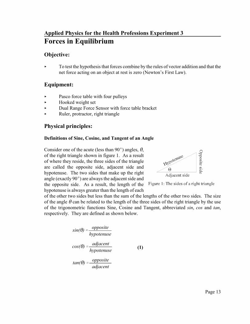
Consider one of the acute (less than 90E) angles, 2,of the right triangle shown in figure 1. As a resultof where they reside, the three sides of the triangleare called the opposite side, adjacent side andhypotenuse. The two sides that make up the rightangle (exactly 90E) are always the adjacent side andthe opposite side. As a result, the length of thehypotenuse is always greater than the length of eachof the other two sides but less than the sum of the lengths of the other two sides. The sizeof the angle 2 can be related to the length of the three sides of the right triangle by the useof the trigonometric functions Sine, Cosine and Tangent, abbreviated sin, cos and tan,respectively. They are defined as shown below.
sin(2)'opposite
hypotenuse
cos(2)'adjacent
hypotenuse
tan(2)'oppositeadjacent
(1)
Page 14
X axis
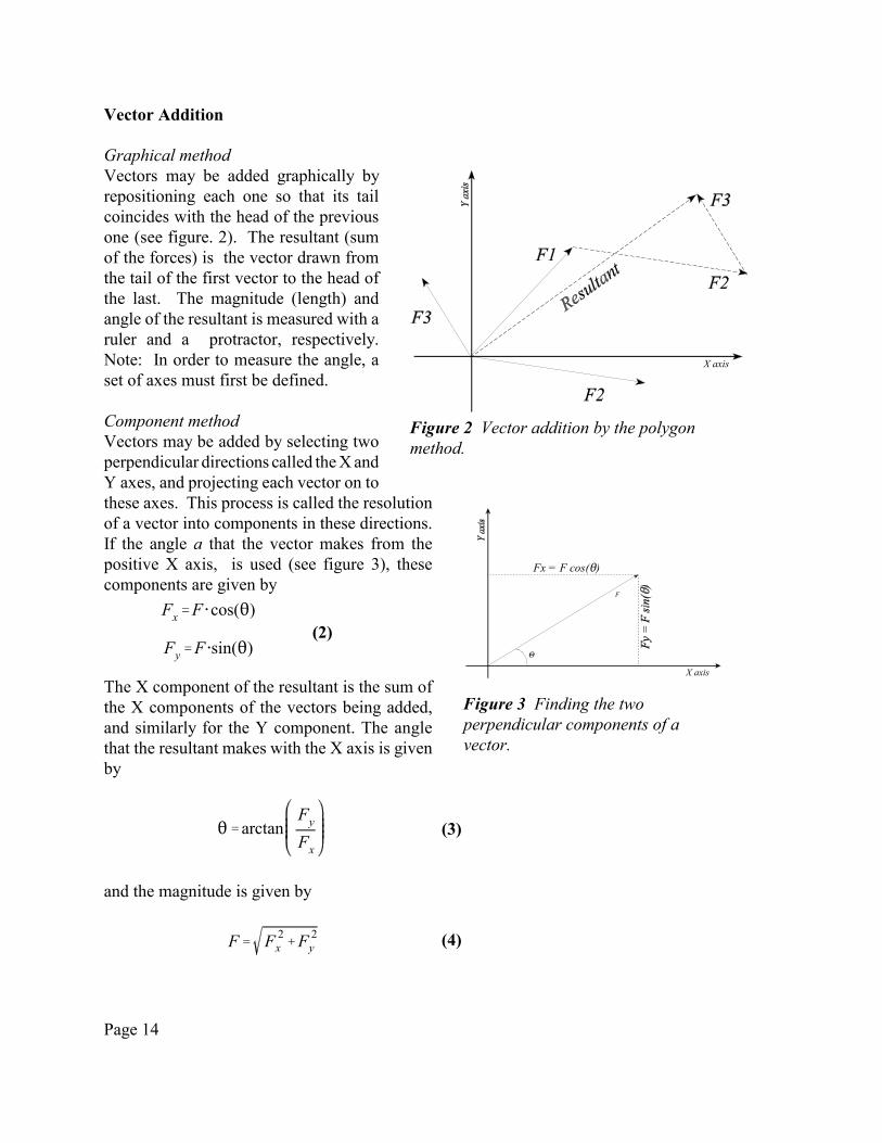
Figure 2 Vector addition by the polygonmethod.
1
F
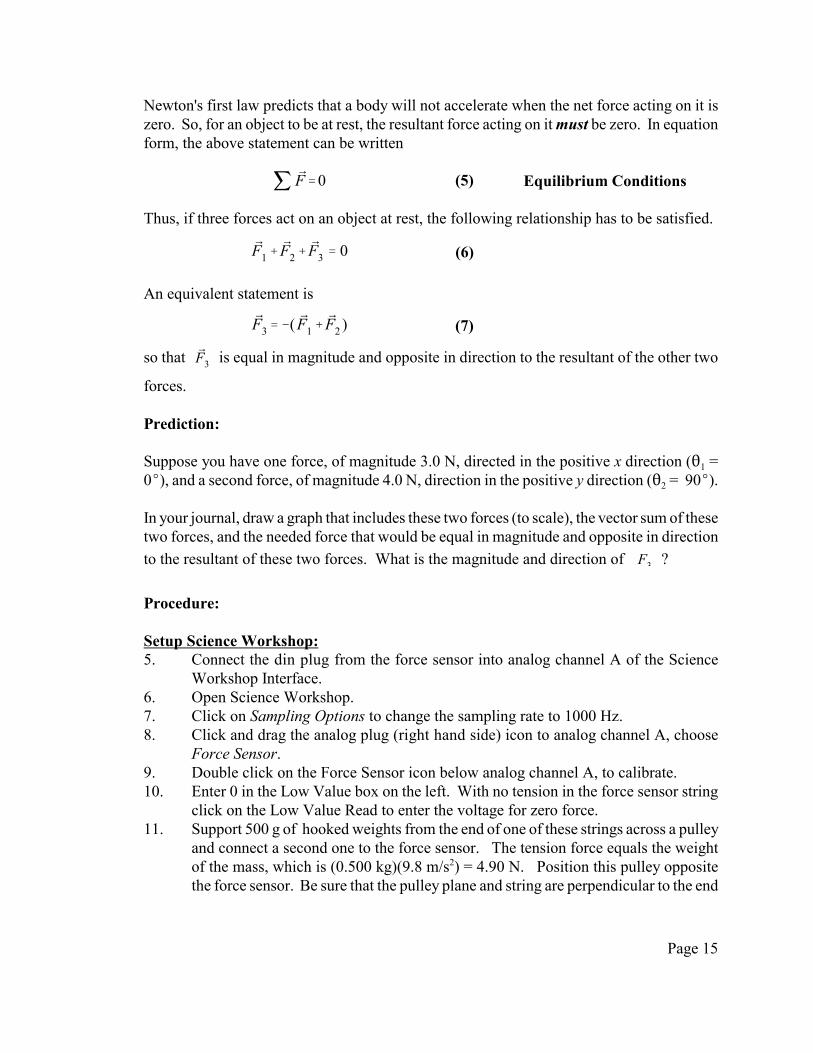
Fx = F cos(2)
X axis
Figure 3 Finding the twoperpendicular components of avector.
Fx'F @cos(2)
Fy'F @sin(2)(2)
2'arctanFy
Fx
(3)
F' F 2x %F 2
y (4)
Vector Addition
Graphical methodVectors may be added graphically byrepositioning each one so that its tailcoincides with the head of the previousone (see figure. 2). The resultant (sumof the forces) is the vector drawn fromthe tail of the first vector to the head ofthe last. The magnitude (length) andangle of the resultant is measured with aruler and a protractor, respectively.Note: In order to measure the angle, aset of axes must first be defined.
Component methodVectors may be added by selecting twoperpendicular directions called the X andY axes, and projecting each vector on tothese axes. This process is called the resolutionof a vector into components in these directions.If the angle a that the vector makes from thepositive X axis, is used (see figure 3), thesecomponents are given by
The X component of the resultant is the sum ofthe X components of the vectors being added,and similarly for the Y component. The anglethat the resultant makes with the X axis is givenby
and the magnitude is given by
Page 15
j PF'0 (5)
PF1%PF2%
PF3 ' 0 (6)
PF3'&( PF1%PF2 ) (7)
Newton's first law predicts that a body will not accelerate when the net force acting on it iszero. So, for an object to be at rest, the resultant force acting on it must be zero. In equationform, the above statement can be written
Equilibrium Conditions
Thus, if three forces act on an object at rest, the following relationship has to be satisfied.
An equivalent statement is
so that is equal in magnitude and opposite in direction to the resultant of the other twoPF3
forces.
Prediction:
Suppose you have one force, of magnitude 3.0 N, directed in the positive x direction (21 =0E), and a second force, of magnitude 4.0 N, direction in the positive y direction (22 = 90E).
In your journal, draw a graph that includes these two forces (to scale), the vector sum of thesetwo forces, and the needed force that would be equal in magnitude and opposite in direction
to the resultant of these two forces. What is the magnitude and direction of ?F3
Procedure:
Setup Science Workshop:5. Connect the din plug from the force sensor into analog channel A of the Science
Workshop Interface. 6. Open Science Workshop.7. Click on Sampling Options to change the sampling rate to 1000 Hz. 8. Click and drag the analog plug (right hand side) icon to analog channel A, choose
Force Sensor. 9. Double click on the Force Sensor icon below analog channel A, to calibrate. 10. Enter 0 in the Low Value box on the left. With no tension in the force sensor string
click on the Low Value Read to enter the voltage for zero force. 11. Support 500 g of hooked weights from the end of one of these strings across a pulley
and connect a second one to the force sensor. The tension force equals the weightof the mass, which is (0.500 kg)(9.8 m/s2) = 4.90 N. Position this pulley oppositethe force sensor. Be sure that the pulley plane and string are perpendicular to the end
Page 16
Figure 5. Force table setup with two forces balanced bythe force sensor.
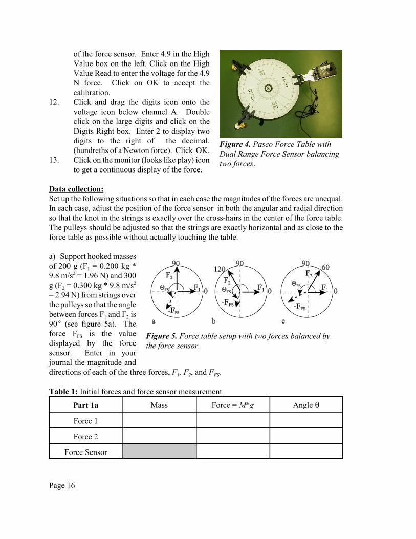
Figure 4. Pasco Force Table withDual Range Force Sensor balancingtwo forces.
of the force sensor. Enter 4.9 in the HighValue box on the left. Click on the HighValue Read to enter the voltage for the 4.9N force. Click on OK to accept thecalibration.
12. Click and drag the digits icon onto thevoltage icon below channel A. Doubleclick on the large digits and click on theDigits Right box. Enter 2 to display twodigits to the right of the decimal.(hundreths of a Newton force). Click OK.
13. Click on the monitor (looks like play) iconto get a continuous display of the force.
Data collection:Set up the following situations so that in each case the magnitudes of the forces are unequal.In each case, adjust the position of the force sensor in both the angular and radial directionso that the knot in the strings is exactly over the cross-hairs in the center of the force table.The pulleys should be adjusted so that the strings are exactly horizontal and as close to theforce table as possible without actually touching the table.
a) Support hooked massesof 200 g (F1 = 0.200 kg *9.8 m/s2 = 1.96 N) and 300g (F2 = 0.300 kg * 9.8 m/s2
= 2.94 N) from strings overthe pulleys so that the anglebetween forces F1 and F2 is90E (see figure 5a). Theforce FFS is the valuedisplayed by the forcesensor. Enter in yourjournal the magnitude anddirections of each of the three forces, F1, F2, and FFS.
Table 1: Initial forces and force sensor measurement
Part 1a Mass Force = M*g Angle 2
Force 1
Force 2
Force Sensor

Page 17
Select your x axis to be along the line of force F1. Make a sketch in your journal showingthese forces as arrows and write the values of each force alongside its arrow. Draw to scaletwo vectors for F1 and F2 and add the vectors graphically. Use at least 1/2 of a page for thegraphical solution in order to improve the accuracy of your measurement. Then compare theresults from the force sensor with the graphical measurements.
Table 2: Comparison of Graphical solution with Force Sensor measurement
Part 1a Force Angle
Force Sensor + 180E
Graphical Solution
% Error / Angle Error
For the force sensor, add 180E to the angle measured in Table 1 in order to compare it withthe resultant force calculated graphically. Then calculate the % error of the force, and theangle error (2FS + 180E- 2GS).
b) Repeat the measurement with forces F1 and F2 120E apart (see Figure 5b), and write theresults in your journal.
Table 3: Initial forces and force sensor measurement
Part 1b Mass Force = M*g Angle 2
Force 1
Force 2
Force Sensor
Make a sketch in your journal showing these forces as arrows and write the values of eachforce alongside its arrow. Use the component method to add forces F1 and F2. Thencompare the results from the force sensor with the component method calculations.
Table 4: Component method calculation
Part 1b Fx = F cos 2 Fy = F sin 2
Force 1
Force 2
Resultant Force

Page 18
Resultant force magnitude = = ________, Angle = = ________F 2x % F 2
y tan&1Fy
Fx
Table 5: Comparison of Component solution with Force Sensor measurement
Part 1b Force Angle
Force Sensor + 180E
Component Solution
% Error / Angle Error
c) Repeat the measurement with forces F1 and F2 60E apart (see Figure 5c), and write theresults in your journal.
Table 6: Initial forces and force sensor measurement
Part 1c Mass Force = M*g Angle 2
Force 1
Force 2
Force Sensor
Make a sketch in your journal showing these forces as arrows and write the values of eachforce alongside its arrow. Use the component method to add forces F1 and F2. Thencompare the results from the force sensor with the component method calculations.
Table 7: Component method calculation
Part 1c Fx = F cos 2 Fy = F sin 2
Force 1
Force 2
Resultant Force
Resultant force magnitude = = ________, Angle = = ________F 2x % F 2
y tan&1Fy
Fx

Page 19
Figure 6 Force table setup withthree forces.
Table 8: Comparison of Component solution with Force Sensor measurement
Part 1c Force Angle
Force Sensor + 180E
Component Solution
% Error / Angle Error
2. Support three different masses in an arrangementapproximately as shown in Figure 6. Using thecomponent addition method, find and add thecomponents of F1, F2, and F3. Compute the magnitudeand direction of the sum of these forces and compareyour result with 2FS + 180E and FFS.
Table 9: Initial forces and force sensor measurement
Part 2 Mass Force = M*g Angle 2
Force 1
Force 2
Force 3
Force Sensor
Make a sketch in your journal showing these forces as arrows and write the values of eachforce alongside its arrow. Use the component method to add forces F1 , F2 , and F3. Thencompare the results from the force sensor with the component method calculations.
Table 10: Component method calculation
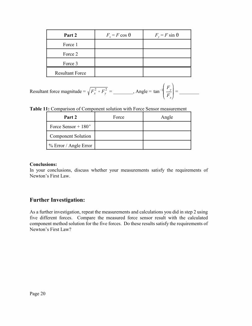
Page 20
Part 2 Fx = F cos 2 Fy = F sin 2
Force 1
Force 2
Force 3
Resultant Force
Resultant force magnitude = = ________, Angle = = ________F 2x % F 2
y tan&1Fy
Fx
Table 11: Comparison of Component solution with Force Sensor measurement
Part 2 Force Angle
Force Sensor + 180E
Component Solution
% Error / Angle Error
Conclusions:In your conclusions, discuss whether your measurements satisfy the requirements ofNewton’s First Law.
Further Investigation:
As a further investigation, repeat the measurements and calculations you did in step 2 usingfive different forces. Compare the measured force sensor result with the calculatedcomponent method solution for the five forces. Do these results satisfy the requirements ofNewton’s First Law?
Page 21
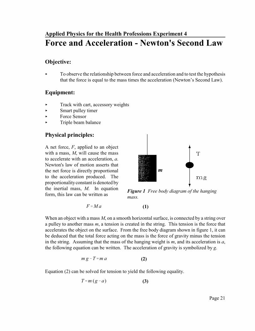
Figure 1 Free body diagram of the hangingmass.
F'M a (1)
m g&T'm a (2)
T'm (g&a ) (3)
Applied Physics for the Health Professions Experiment 4
Force and Acceleration - Newton's Second Law
Objective:
< To observe the relationship between force and acceleration and to test the hypothesisthat the force is equal to the mass times the acceleration (Newton’s Second Law).
Equipment: < Track with cart, accessory weights< Smart pulley timer< Force Sensor< Triple beam balance Physical principles: A net force, F, applied to an objectwith a mass, M, will cause the massto accelerate with an acceleration, a.Newton's law of motion asserts thatthe net force is directly proportionalto the acceleration produced. Theproportionality constant is denoted bythe inertial mass, M. In equationform, this law can be written as
When an object with a mass M, on a smooth horizontal surface, is connected by a string overa pulley to another mass m, a tension is created in the string. This tension is the force thataccelerates the object on the surface. From the free body diagram shown in figure 1, it canbe deduced that the total force acting on the mass is the force of gravity minus the tensionin the string. Assuming that the mass of the hanging weight is m, and its acceleration is a,the following equation can be written. The acceleration of gravity is symbolized by g.
Equation (2) can be solved for tension to yield the following equality.

Page 22
T'M a (4)
Figure 2 Free body diagram of thecart.
Since the tension is constant in the string, the cartand the mass hanging on the string have the sameacceleration. Thus, Newton’s law of motion for thecart is
Procedure:
Setup Science Workshop:1. Open Science Workshop.2. Plug in the smart pulley into digital channels 1 and 2.3. Drag the digital plug icon over digital channel 1 and select smart pulley (linear).
Double click on the smart pulley to calibrate it. Follow the instructions of the labinstructor, or use the average calibration value of 0.0155.
4. Plug the force sensor into analog channel A.5. Drag the analog plug icon over analog channel A and select force sensor. Double
click on the force sensor to calibrate it. Set the low value to zero, and click on lowvalue read with no mass hanging from the force sensor. Set the high value to 4.9Nand click on the high value read with a 500g mass (weight = 4.9N) hanging from theforce sensor.
6. Click on Sampling Options to change the sampling rate to 1000 Hz and the stop timeto 5 sec.
7. Make a graph of velocity versus time by clicking on the graph icon, dragging it overthe smart pulley icon, selecting velocity, and clicking on OK. Add the force sensorgraph to the graph window by clicking on the multiple graph icon (lower right iconin the lower left corner of the graph) and selecting analog A and force sensor.
8. Start statistics by clicking on the E button in the graph window, then click on the Ebutton beside the smart pulley graph and select curve fit and then linear fit. Click onthe E button beside the force sensor graph and select mean and standard deviation.
Setup system:1. Measure and record in your journal the mass of the free-hanging pulley. This mass
will be added to the masses of the weights hung on the pulley during the experiment.2. Measure and record in your journal the mass of the cart, Mcart. Measure and add the
masses of the two blocks to the mass of the cart. Record the total mass, Mtotal.3. Place the cart on the track and level the track so that the cart does not accelerate in
either direction. 4. With a table clamp, position the smart pulley (see figure 3) at the aisle end of the
track. Run the cable through the second, free-hanging pulley and back up to a forcesensor mounted vertically.

Page 23
Figure 3 Smart pulley.
Data Collection:Part 1:1. Hang 30 g mass from the free-hanging
pulley, and position the cart so that thefree-hanging pulley is just below thesmart pulley. Click on the REC button asyour lab partner releases the cart.
2. Reproduce Table 1 (below) in yourjournal. Click and drag the curser toselect the best data from the velocity vs.time graph. The statistics section will fita straight line to the selected data. Theslope of the line, a2, is the acceleration ofthe cart. Record the value of theacceleration in the column titled a inTable 1. Click and drag the curser toselect the same data on the force vs. timegraph. Record the mean value of the force in the Tmeasured column of Table 1.
3. Take a series of seven (7) more measurements, increasing the mass by 10 g eachtime. Record effective mass (m + mpulley)/2 and the acceleration and force for eachmass in Table 1.
Table 1 Cart without additional mass
(m+mpulley)/2 a g-a Tcalc = m(g-a) Tmeasured Tmeasured - Tcalc
4. Complete the table by calculating the other columns. For the value of g use theaccepted value of 9.81 m/s2. Print out one of the data graphs and place in the datasection of your journal as a “sample” raw data measurement.

Page 24
T'M a (4)
%Err'*slope&M*
M×100 (5)
Part 2:1. Place the two blocks on the cart and repeat the experiment. 2. Fill in a second table in your journal in a similar manner to Table 1 as given above.
3. Print out one of the data graphs and place in the data section of your journal as a“sample” raw data measurement.
Analysis of Data:1. Use Graphical Analysis to plot a graph of measured tension T (y axis) vs. acceleration
a (x axis) for the data in Table 1. Click on the y axis and change the setting toAutoscale at 0. Repeat for the x axis. This will include the origin (0,0) point in thegraph. Put a title and label the axes of the graph.
2. To fit the data to a straight line click on Analyze and Automatic Curve Fit and selectfunction y = M*x + B to select a linear (straight-line) function. Since we have Tgiven as y, and a given as x, the slope M should be the same as the mass M in Eq. (4):
Theoretically, the value of the intercept B should be zero, since no T0 appears in Eq.(4). However, T0 can be thought of as the tension required to cause the cart to movewith zero acceleration, that is, the tension required to overcome kinetic friction. Thusthe intercept B provides a measure of the friction of the system. Print your graph.
3. Record in your journal the slope M and the intercept B . As equation (4) predicts, thisslope should be very close to the mass of the cart (Mcart) in the case of Table 1. In thecase of Table 2 the slope should be very close to the total mass (Mtotal). Calculate thepercent error for both cases by using
4. Repeat the above analysis for Table 2.
In your conclusions you should:1. Discuss the percent error that you calculated for both graphs.2. Interpret the value of the intercept and discuss how the presence of constant frictional
force would affect the results of the experiment.3. Speculate on the origin(s) of error.4. Discuss the difference between the measured and calculated tensions.5. Mention what you learned in this experiment.
Page 25
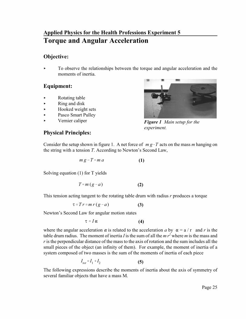
Figure 1 Main setup for theexperiment.
m g&T'm a (1)
T'm (g&a ) (2)
J'T r'm r (g&a ) (3)
J ' I " (4)
Itot' I1% I2 (5)
Applied Physics for the Health Professions Experiment 5
Torque and Angular Acceleration
Objective:
< To observe the relationships between the torque and angular acceleration and themoments of inertia.
Equipment:
< Rotating table< Ring and disk< Hooked weight sets< Pasco Smart Pulley< Vernier caliper
Physical Principles:
Consider the setup shown in figure 1. A net force of acts on the mass m hanging onm g&Tthe string with a tension T. According to Newton’s Second Law,
Solving equation (1) for T yields
This tension acting tangent to the rotating table drum with radius r produces a torque
Newton’s Second Law for angular motion states
where the angular acceleration " is related to the acceleration a by " = a / r and r is thetable drum radius. The moment of inertia I is the sum of all the m r2 where m is the mass andr is the perpendicular distance of the mass to the axis of rotation and the sum includes all thesmall pieces of the object (an infinity of them). For example, the moment of inertia of asystem composed of two masses is the sum of the moments of inertia of each piece
The following expressions describe the moments of inertia about the axis of symmetry ofseveral familiar objects that have a mass M.
Page 26
Idisk'12
M R 2 , Iring ' M R 2(6)
where R is the outer radius of the disk, or the average of the inner and outer radii of the ring.
Procedure:
General Measurements and SetupUsing the vernier caliper measure the diameter, ddrum, of the drum on which the string iswrapped. Compute the radius of the drum, rdrum, and record these values. This radius willbe used to calculate the torque acting upon the rotating platform by means of Eq. (3). Run Science Workshop. Plug the smart pulley into the digital slot #1 on the Pasco computerinterface and do the same on the screen by clicking on the digital plug, dragging it overdigital channel 1, selecting smart pulley (linear) and clicking on OK. Calibrate the smartpulley by double clicking on the smart pulley icon and entering a radius of 0.0155 .
Create a graph of velocity vs. time by dragging the graph icon over the smart pulley icon andselecting velocity. Click on the statistics buttons E and select curve fit and linear fit. Thecurve fit will give an equation y = a1 + a2 x, corresponding to the equation v = v0 + a t.Thus, the acceleration will be displayed as a2. Make sure, in reading the value foracceleration, that you have selected only the good data that appears as a straight line in thegraph.
Take care that the rotating platform does not rotate except when taking accelerationdata! Keep the string taut with care that it does not become wrapped around the axle!
Inertia of the rotating platform Hook a 50 g mass to the loose end of the string that is wrapped around the rotating platformdrum and drape the string over the smart pulley timer. Rotate the platform so that the massis just below the top of the smart pulley. Release the platform and click on Record after it hasstarted to rotate. Make sure the string is short enough so that the weight will not hit the floor.Record the value for the acceleration of the string in a table (similar to Table 1 below) inyour journal.
Repeat using 60 g, 70 g, 80 g, 90 g, and 100 g.
Open Graphical Analysis and plot the values for torque J on the y-axis vs. angularacceleration " on the x-axis. Fit a linear curve fit to the data, and record the values of theslope M and intercept B in your journal. The slope M = J / " is simply the moment ofinertia I of the rotating platform, and the intercept B is that torque needed to overcomefriction (i.e., the frictional torque).

Page 27
Table 1: Inertia of the rotating platform
m [kg]
a [m/s2]
F=m(g - a) [N]
J = F rdrum
[Nm]"= a/rdrum
[rad/s2]
0.050
0.060
0.070
0.080
0.090
0.100
Inertia of the diskPlace the disk on the rotating platform and by following the procedure of the previousexperiment take a series of readings of the acceleration, a, for masses on the string of about50, 100, 150, 200, 250, and 300 grams. Record the results in Table 2, analogous to Table 1.
Table 2: Inertia of the disk and rotating platform
m [kg]
a [m/s2]
F=m(g - a) [N]
J = F rdrum
[Nm]"= a/rdrum
[rad/s2]
0.050
0.100
0.150
0.200
0.250
0.300
Plot the values for torque J on the y-axis vs. angular acceleration " on the x-axis usingGraphical Analysis. Fit a linear curve fit to the data, and record the values of the slope Mand intercept B in your journal. Record the difference between the moments of inertiarecorded in your second graph minus that recorded for your first graph. This difference isyour measured value for the moment of inertia of the disk by itself.
Page 28
Measure the radius of the disk, and record the mass value stamped on the disk. Using thesevalues, and Eq. (6), compute a calculated value for the moment of inertia of the disk.Compare the calculated moment of inertia for the disk with the measured value, and recordthe percent error of difference:
%Err '|Icalc & Imeas |
Icalc
× 100
Inertia of the ringWith the ring on the platform, determine the moment of inertia of the system as done for thedisk. Use masses of 50 g, 100 g, 150 g, 200 g, 250 g, and 300 g, and generate a Table 3 forthe inertia of the ring, analogous to Table 2 for the disk.
Plot the values for torque J on the y-axis vs. angular acceleration " on the x-axis usingGraphical Analysis. Fit a linear curve fit to the data, and record the values of the slope Mand intercept B in your journal. Record the difference between the moments of inertiarecorded in this graph minus that recorded for your first graph. This difference is yourmeasured value for the moment of inertia of the ring by itself.
Measure the average radius of the ring, and record the mass value stamped on the ring.Using these values and Eq. (7), compute a calculated value for the moment of inertia of thering. Compare the calculated moment of inertia for the ring with the measured value, andrecord the percent error of difference.
Inertia of the ring and disk togetherWith both the ring and the disk on the platform determine the moment of inertia as done inthe previous measurements. Use masses of 100 g, 200 g, 300 g, 400 g, 500 g, and 600 g, andgenerate a Table 4 for the inertia of the disk plus ring, analogous to the previous tables.
Plot the values for torque J on the y-axis vs. angular acceleration " on the x-axis usingGraphical Analysis. Fit a linear curve fit to the data, and record the values of the slope Mand intercept B in your journal. Record the difference between the moments of inertiarecorded in this graph minus that recorded for your first graph. This difference is yourmeasured value for the moment of inertia of the ring plus the disk. Compare the measuredmoment of inertia with the sum of the calculated moments of inertia for the ring and disk,and record the percent error of difference.
Conclusions:
In your conclusions, include a discussion of the source of the intercept values B in each ofyour calculations.
Page 29
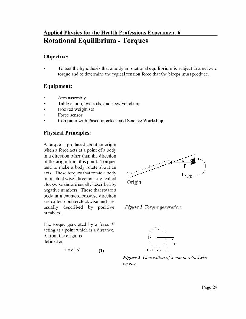
Figure 1 Torque generation.
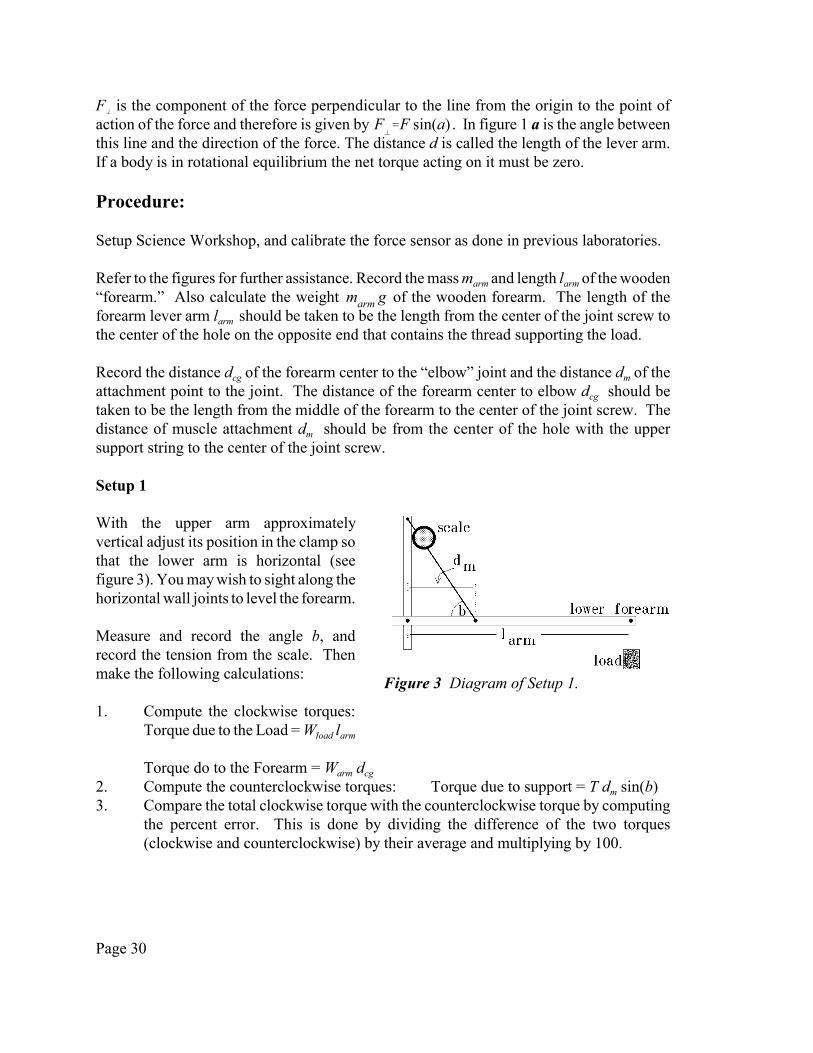
Figure 2 Generation of a counterclockwisetorque.
J'Fz d (1)
Applied Physics for the Health Professions Experiment 6
Rotational Equilibrium - Torques
Objective: < To test the hypothesis that a body in rotational equilibrium is subject to a net zero
torque and to determine the typical tension force that the biceps must produce. Equipment:
< Arm assembly < Table clamp, two rods, and a swivel clamp < Hooked weight set < Force sensor< Computer with Pasco interface and Science Workshop Physical Principles: A torque is produced about an originwhen a force acts at a point of a bodyin a direction other than the directionof the origin from this point. Torquestend to make a body rotate about anaxis. Those torques that rotate a bodyin a clockwise direction are calledclockwise and are usually described bynegative numbers. Those that rotate abody in a counterclockwise directionare called counterclockwise and areusually described by positivenumbers. The torque generated by a force Facting at a point which is a distance,d, from the origin is defined as
Page 30
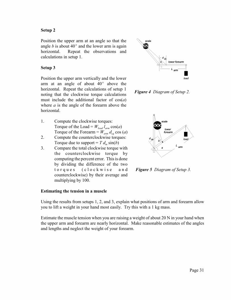
Figure 3 Diagram of Setup 1.
Fz is the component of the force perpendicular to the line from the origin to the point ofaction of the force and therefore is given by . In figure 1 a is the angle betweenFz'F sin(a)this line and the direction of the force. The distance d is called the length of the lever arm.If a body is in rotational equilibrium the net torque acting on it must be zero.
Procedure:
Setup Science Workshop, and calibrate the force sensor as done in previous laboratories.
Refer to the figures for further assistance. Record the mass marm and length larm of the wooden“forearm.” Also calculate the weight of the wooden forearm. The length of themarm gforearm lever arm larm should be taken to be the length from the center of the joint screw tothe center of the hole on the opposite end that contains the thread supporting the load.
Record the distance dcg of the forearm center to the “elbow” joint and the distance dm of theattachment point to the joint. The distance of the forearm center to elbow dcg should betaken to be the length from the middle of the forearm to the center of the joint screw. Thedistance of muscle attachment dm should be from the center of the hole with the uppersupport string to the center of the joint screw.
Setup 1
With the upper arm approximatelyvertical adjust its position in the clamp sothat the lower arm is horizontal (seefigure 3). You may wish to sight along thehorizontal wall joints to level the forearm.
Measure and record the angle b, andrecord the tension from the scale. Thenmake the following calculations:
1. Compute the clockwise torques:Torque due to the Load = Wload larm
Torque do to the Forearm = Warm dcg
2. Compute the counterclockwise torques: Torque due to support = T dm sin(b)3. Compare the total clockwise torque with the counterclockwise torque by computing
the percent error. This is done by dividing the difference of the two torques(clockwise and counterclockwise) by their average and multiplying by 100.
Page 31
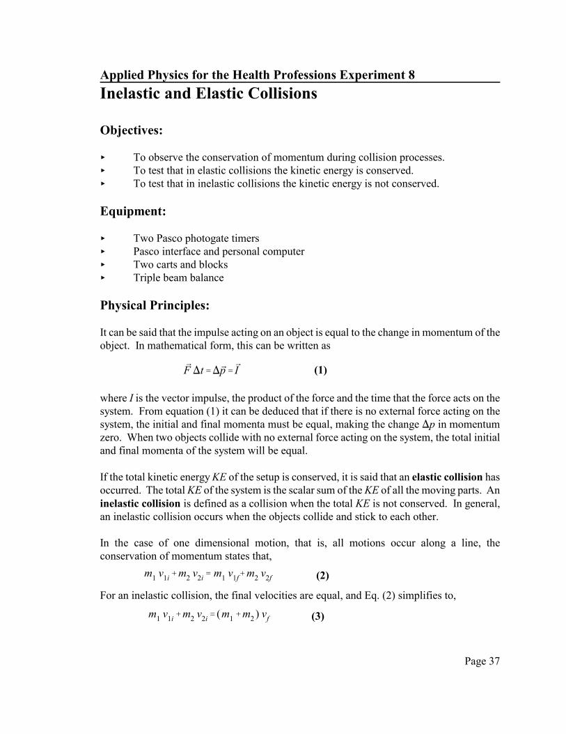
Figure 4 Diagram of Setup 2.
Figure 5 Diagram of Setup 3.
Setup 2 Position the upper arm at an angle so that theangle b is about 40E and the lower arm is againhorizontal. Repeat the observations andcalculations in setup 1.
Setup 3
Position the upper arm vertically and the lowerarm at an angle of about 40E above thehorizontal. Repeat the calculations of setup 1noting that the clockwise torque calculationsmust include the additional factor of cos(a)where a is the angle of the forearm above thehorizontal.
1. Compute the clockwise torques:Torque of the Load = Wload larm cos(a)Torque of the Forearm = Warm dcg cos (a)
2. Compute the counterclockwise torques:Torque due to support = T dm sin(b)
3. Compare the total clockwise torque withthe counterclockwise torque bycomputing the percent error. This is doneby dividing the difference of the twot o r q u e s ( c l o c k w i s e a n dcounterclockwise) by their average andmultiplying by 100.
Estimating the tension in a muscle
Using the results from setups 1, 2, and 3, explain what positions of arm and forearm allowyou to lift a weight in your hand most easily. Try this with a 1 kg mass.
Estimate the muscle tension when you are raising a weight of about 20 N in your hand whenthe upper arm and forearm are nearly horizontal. Make reasonable estimates of the anglesand lengths and neglect the weight of your forearm.

Page 32

Page 33
Figure 1: Velocity components fora swinging pendulum.
KE '12
mv 2(1)
v 2 ' v 2x %v 2
y . (2)
Applied Physics for the Health Professions Experiment 7
Conservation of Mechanical Energy
Objective:
< To measure kinetic and potential energies of a simple pendulum and test thehypothesis that the total mechanical energy is conserved for a system involving onlyconservative forces.
Equipment:
< Mass suspended from string approximately 1.5 m in length< Meter stick< Video camera on tripod< Computer with video capture board< Videopoint software
Physical principles: Kinetic Energy
A body which has a mass m and moves with a speedv has energy by virtue of its motion. This energy iscalled kinetic energy and is defined as
At any instant of time in the swing of a pendulum,the velocity vector, v, can be broken up into its xand y components, vx and vy, respectively (see Fig.1). The magnitude of the velocity vector is relatedto the components by the Pythagorean theorem
Gravitational Potential EnergyA body moving in a force field has energy by virtue of its position. This energy is calledpotential energy. The potential energy of an object at a point B with respect to a point A isthe work which must be done to move the object from A to B. In the case of a pendulum the

Page 34
PE ' mgy (3)
ETotal ' KE % PE ' constant . (4)
work is done against gravity, so that the gravitational potential energy is given by
where y is the height of the pendulum bob above some reference level.
Conservation of Total Mechanical Energy
When no non-conservative forces (e.g., frictional forces) are present, the total mechanicalenergy is conserved, that is,
When the pendulum bob is suspended from a string, it will come to rest with the string at thevertical position (equilibrium). When displaced slightly and released, the pendulum willoscillate about the equilibrium position. At the top of its swing, the pendulum will be brieflyat rest with zero kinetic energy and a maximum in potential energy. As the pendulum swingsthrough the equilibrium position, the kinetic energy is a maximum and the potential energyis a minimum. At any point in its swing, the sum of the kinetic and potential energiesremains constant. The effect of frictional forces is to cause the total energy to graduallydecrease as it dissipates into heating the surroundings.
Prediction:
Consider a pendulum swinging with an amplitude of 20 cm. Draw graphs in your journal ofposition vs. time, velocity vs. time, and acceleration vs. time for one complete cycle ofoscillation. Where on the cycle will the following occur:1. Where will the displacement (position) be equal to zero?2. Where will the displacement (position) have maximum magnitude?3. Where will the velocity be equal to zero?4. Where will the velocity have maximum magnitude?5. Where will the acceleration be equal to zero?6. Where will the acceleration have maximum magnitude?
Explain your reasoning for each of these answers.
Procedure:
Video Capture
1. Set the pendulum against a light colored background and lay a meter stick directlyunderneath the bob to indicate the scale of distances in the video picture.
2. Double click on the Digital Video Producer Capture icon on the computer screen.

Page 35
3. From the menu choose Capture / Settings and set stop time to 5 seconds. 4. Make sure the video camera is directly facing the pendulum, not leaning at an angle,
connected to the S-Video input of the video capture board, and on. Set thependulum into oscillation and note the video in the preview screen. Make sure thatyou are far enough from the pendulum to take in the full swing.
5. From the menu choose Capture / Video Capture. Select OK just after your labpartner releases the pendulum. At 30 frames per second, you will get about 150 dataframes in two full swings of the pendulum to analyze.
6. The video file will automatically be saved to a file called “ball991.avi” in the physvidfolder. Change the file name in the physvid folder to yourname.mov (make sure theextension is .mov or else the Videopoint program will not be able to recognize it).
Collecting Data from Video
1. Return to your computer station in the laboratory and click on the videopoint programicon.
2. Close the introductory window.3. Open your movie from the shared Network folder.4. Indicate that you will be tracking the location of only 1 object.5. From the menu choose Movie / Double Size in order to better see the pendulum bob.6. Starting with the first frame, center the cursor on the pendulum bob and click. The
movie automatically advances to the next frame and records the location of the bobin the table.
7. After taking data on the location of the bob for all 150 points, you must scale thepicture using the ruler icon in the left column. Choose 1 meter for the length , thenclick on the two ends of the meter stick in your video.
8. From the menu choose Movie / Normal Size so that you can see the data table. Allthe data should now be entered in the table. Now you will need to copy the data toGraphical Analysis in order to analyze the data.
Transferring data to Graphical Analysis
1. Start the Vernier Graphical Analysis program. 2. Change the titles of the first two columns to t and x by double-clicking on the titles.3. Add a third column by clicking on the new column icon (second from right end).
Title the new column y. 4. Copy and paste the three columns of data from the table in Videopoint to the table in
Graphical Analysis. Examine plots of x vs. t and y vs. t to see that they arereasonable. Print out these plots and include in the data section of your journal.

Page 36
%Err 'stdev(E)mean(E)
×100%
Analyzing Data:
1. Calculate the x-component of velocity by taking the derivative (slope) of the x datawith respect to time: Select the last icon on the right to create a new column that isto be computed from data in the x column. Call the new column vx (x-component ofvelocity). The functional form for this column is derivative (“x”,“ t”).
2. Calculate the y-component of velocity in a new column in a similar manner.3. Calculate the kinetic energy per unit mass (1/2mv2)/m by creating a column (titled
“KE”) defined by the relation 0.5*(“vx”^2+“vy”^2). 4. Calculate the potential energy per unit mass (mgy)/m by creating a column (titled
“PE”) with 9.81*“y”. To make it more tidy, you can scan through your values in they column to find the lowest equilibrium point and subtract that value, yo, from y inthe potential energy column 9.81*(“y”-yo). This assigns yo as the point of zeropotential energy.
5. Calculate the total mechanical energy per unit mass Etot/m by creating a column(titled “E”) which sums the kinetic and potential energy columns “KE” + “PE”.
6. Plot columns “KE”, “PE”, and “E” on the same graph. Double click on any datapoint to get Graph Options. Turn on the Legend, and select Column Appearance touse different symbols for “KE”, “PE”, and “E”.
7. Select all the data on the graph of total energy and choose analyze, then statisticsfrom the menu. The standard deviation is an indicator of the amount of spread in thetotal energy from the mean value. Calculate the percent error from the equation
8. Select the Analyze / Automatic Curve Fit from the menu. Select Perform fit on “E”to perform a linear fit. Compare the results of the linear fit with the mean andstandard deviation determined from the statistics fit.
Title and print your Graph!
Questions:1. What is the period of the oscillation? 2. How does the variation of the total energy compare with the variation of the kinetic
energy and potential energy? 3. Was the total energy conserved during the two swings of the pendulum?
Page 37
PF )t')Pp' PI (1)
m1 v1i%m2 v2i' m1 v1f%m2 v2f (2)
m1 v1i%m2 v2i' (m1%m2 ) vf (3)
Applied Physics for the Health Professions Experiment 8
Inelastic and Elastic Collisions
Objectives:
< To observe the conservation of momentum during collision processes.< To test that in elastic collisions the kinetic energy is conserved.< To test that in inelastic collisions the kinetic energy is not conserved.
Equipment:
< Two Pasco photogate timers < Pasco interface and personal computer< Two carts and blocks< Triple beam balance
Physical Principles:
It can be said that the impulse acting on an object is equal to the change in momentum of theobject. In mathematical form, this can be written as
where I is the vector impulse, the product of the force and the time that the force acts on thesystem. From equation (1) it can be deduced that if there is no external force acting on thesystem, the initial and final momenta must be equal, making the change )p in momentumzero. When two objects collide with no external force acting on the system, the total initialand final momenta of the system will be equal.
If the total kinetic energy KE of the setup is conserved, it is said that an elastic collision hasoccurred. The total KE of the system is the scalar sum of the KE of all the moving parts. Aninelastic collision is defined as a collision when the total KE is not conserved. In general,an inelastic collision occurs when the objects collide and stick to each other.
In the case of one dimensional motion, that is, all motions occur along a line, theconservation of momentum states that,
For an inelastic collision, the final velocities are equal, and Eq. (2) simplifies to,

Page 38
m1 v1' (m1%m2 ) vf (4)
KEi'12
m1 @v21i (5)
KEf'(m1%m2 )
2@v 2
f '(m1%m2 )
2@
m 21 @v
21i
(m1%m2 )2'
12
(m1
m1%m2
) @m1 @v21i'
m1
m1%m2
@KEi
(6)
KEf
KEi
'm1
m1%m2
(7)
A further simplification is possible if one of the carts (say m2) is initially at rest,
The initial KE of the system now consists of only the initial KE of m1 (since the initial KEof m2 is zero) and is
The final KE can be related to the initial KE by a series of steps involving equations (4) and(5), as follows.
It can be seen that the initial and final KE are not equal, with a ratio given by,
Procedure:
Place a cart on the track and level the track so that the cart does not roll in either direction.Place the photogates about 50 cm apart along the track and plug them into slots 1 and 2 onthe Pasco computer interface. The photogates should be far enough apart so that the collisionprocess occurs entirely between the gates. The left photogate should be connected to slot 1.Also, connect the two photogates to the interface on the screen by dragging the digital plugicon to channels 1 and 2 and selecting photogate and solid object. Adjust the photogateheights so that the beam is blocked by the blocks on the cart when the blocks are placed ontheir sides. Measure and record the lengths of the blocks on the carts. Make sure that youplace 2 blocks on the left cart and record it as L 1 and 1 block on the right cart and record itas L2 . Under recording options, set the periodic sample rate at 10,000 Hz. Finally, make atable for each gate by dragging the table icon over its respective icon and selecting velocity.
In each of the following collisions, make sure that the carts are moving freely before theyenter the photogates and that the collisions occur when the carts are entirely between the twophotogates.
Use the balance to determine the masses of the carts, including blocks and record thesevalues as m1 and m2 (m1>m2).

Page 39
1. Inelastic collisions
Place cart 2 at rest between the photogates with the velcro end to the left. Click on record,then push cart 1 towards the photogate and cart 2. Let the combined setup (cart 1 and 2) goall the way through the second photogate and then click on stop. Make sure the collisionoccurs between the two photogates. On the table for the first photogate, there is one valuedisplayed. This is the velocity of cart 1 as it passed through the first photogate. Record thisvalue as v1I . On the second table there are two values displayed. The first one is the velocityof cart 2 as it passed through the second photogate, and the second number is the velocity ofcart 1 as it passed through the second photogate, which should be nearly identical to that ofcart 1. Reproduce Table 1 (below) in your journal and record the data.
Table 1: Inelastic collision
m vi vf pi pf KEi KEf
cart 1
cart 2 0 0 0
both
Repeat the experiment, reversing carts 1 and 2 to get a second set of data, this time with thelighter cart hitting the heavier cart.
Table 2: Inelastic collision
m vi vf pi pf KEi KEf
cart 1 0 0 0
cart 2
both
Compute and record the initial and final momenta and kinetic energies by filling in the tablesin your journal. Compare the ratios of pf / pi. Also compare the ratios of KEf /KEi for eachrun with the prediction of equation (7).
2. Elastic collisions
Turn cart 2 around so that the non velcro end faces cart 1. Place cart 2 between thephotogates, click on record, and then send in cart 1 from the left. Cart 2 will pass throughthe right photogate (remove it from the track after it passes completely through thephotogate) followed a short time later by cart 1. Click on stop after cart 1 passes through the

Page 40
second photograte. Reproduce Table 2 (below) in your journal and record the data. Recordthe one value displayed in the table for photogate 1 as v1i, the first value in the table forphotogate 2 as v2f and the second value in this table as v1f.
Compute and record the initial and final momenta and kinetic energies by filling in the tablein your journal. Compare the ratios of pf / pi. Also compare the ratios of KEf /KEi for eachrun.
Table 3: Elastic Collision
m vi vf pi pf KEi KEf
cart 1
cart 2 0 0 0
total
Repeat the experiment, reversing carts 1 and 2 to get a second set of data, this time with thelighter cart hitting the heavier cart.
Table 4: Elastic Collision
m vi vf pi pf KEi KEf
cart 1 0 0 0
cart 2
total
Questions:1. Was momentum conserved in the inelastic collision? 2. Was Kinetic Energy conserved in the inelastic collision? 3. Was momentum conserved in the elastic collision? 4. Was Kinetic Energy conserved in the elastic collision? 5. Compare the actual loss of Kinetic Energy in the inelastic collision with the
prediction of Eq. (5), calculating the percentage error.

Page 41
KEi%PEi'KEf%PEf (1)
Applied Physics for the Health Professions Experiment 9
Conservation of Energy of a Rolling Object
Objective:
< To test the principle of conservation of energy in the case of rolling motion for threeobjects with different moments of inertia.
Equipment:
< Racquetball sphere< Superball< PVC tube< Track< Motion sensor connected to a PC through a data acquisition board< Triple beam balance< Vernier caliper< Lab jack
Physical Principles:
A very important concept in physics is the Law of Conservation of Energy. According to thisprinciple, the difference between the final and initial energy of an object is the work done onthe object itself. Recall that the work done on an object is given by the product of the forceacting on the mass and the distance it moved. If there is no net force acting on the body, andfriction is neglected, the total work done on the object is zero and, as a result, the final andinitial energy of the object must be equal. In other words, the total energy of a system staysconstant.
At any given time, total energy is the sum of two components. One of the components,caused by motion, is the kinetic energy KE, and the other is a result of position and is calledthe potential energy PE. It follows that the law of conservation of energy can be writtenmathematically as
The PE of the object is given by mgh. However, it must be recognized that the KE consists
of two parts. The first is given by and is called the “translational” Kinetic Energy.12
m v 2
If an object is spinning in one place, with no net translational movement, the velocity v iszero, and it therefore has no translational Kinetic Energy. However, it still has a KE caused
Page 42
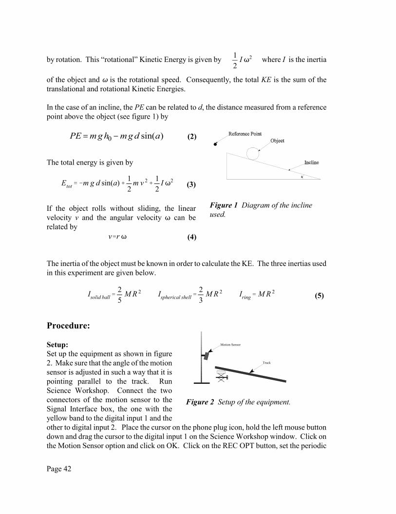
Figure 1 Diagram of the inclineused.
Etot'&m g d sin(a)%12
m v 2%12
I T2(3)
v'r T (4)
Isolid ball'25
M R 2 Ispherical shell'23
M R 2 Iring' M R 2(5)
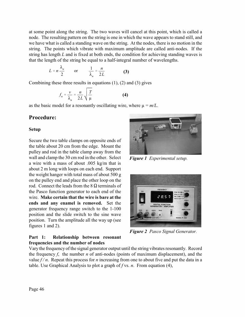
Motion Sensor
Track
Figure 2 Setup of the equipment.
PE m g h m g d a= −0 sin( ) (2)
by rotation. This “rotational” Kinetic Energy is given by where I is the inertia12
I T2
of the object and T is the rotational speed. Consequently, the total KE is the sum of thetranslational and rotational Kinetic Energies.
In the case of an incline, the PE can be related to d, the distance measured from a referencepoint above the object (see figure 1) by
The total energy is given by
If the object rolls without sliding, the linearvelocity v and the angular velocity T can berelated by
The inertia of the object must be known in order to calculate the KE. The three inertias usedin this experiment are given below.
Procedure:
Setup:Set up the equipment as shown in figure2. Make sure that the angle of the motionsensor is adjusted in such a way that it ispointing parallel to the track. RunScience Workshop. Connect the twoconnectors of the motion sensor to theSignal Interface box, the one with theyellow band to the digital input 1 and theother to digital input 2. Place the cursor on the phone plug icon, hold the left mouse buttondown and drag the cursor to the digital input 1 on the Science Workshop window. Click onthe Motion Sensor option and click on OK. Click on the REC OPT button, set the periodic

Page 43
samples rate to 50,000 Hz and set the stop condition to 2 seconds.
Data collection:Place the PVC tube between the two edges of the track, close to the top, so that it can rolldown the incline. Move the motion sensor or the tube so that the distance between them isat least 40 cm. At this point you are ready to take data. Let go of the tube and click on theREC button to start recording the data. The velocity graph should be straight line and thedistance graph should be parabolic. If they are not, the angle of the motion sensor needs tobe adjusted and the experiment redone. It will take you several trials to get a good set ofdata. Once you have a good set, record the mass and radius of the tube and complete theanalysis of this data.
Repeat the data collection using the spherical shell (racquetball) and a solid sphere(superball).
Analysis:
Open the calculator window which can be found in the experiment window. Enter theequation for kinetic energy using the mass, radius, and velocity that you measured. To enterthe velocity values from the experiment click on the input button and select velocity. Enterkinetic energy for the calculation name, KE for the short name, then click on the equalsbutton. Now click on new and enter the equation for the potential energy using the mass,angle and distance that you measured. Get the symbol for distance in the same manner asyou did for kinetic energy. Name the calculation potential energy, the short name PE andclick on the equals button. Finally enter the equation for the total energy, the sum of thekinetic and potential energies. To reference these values click on the input button and selectcalculator and then KE or PE. Enter energy for the calculation name and E for the shortname, then click on equals. Graph the kinetic energy, potential energy and total energyversus time by clicking on the down arrow to the left of the graph in the graph displaywindow and selecting calculations. The total energy should be constant with time. Calculatethe percent error by the formula.
%Err'*stdev(Etot)*
max(KE)×100 (6)

Page 44

Page 45
f 'v8 (1)
v 'Tµ
(2)
Applied Physics for the Health Professions Experiment 10
Resonant Vibrations of a Wire
Objectives: < To determine the relation between the frequencies of resonant vibrations of a wire
and the physical parameters of tension, length, and mass per unit length of the wire.< To determine the relation between the velocity of waves on a wire and the tension
and mass per unit length of the wire.
Equipment: < Pasco Digital Function Generator-Amplifier< Banana leads, 2, 1.5 m long, alligator clips, 2< Large magnet < Table clamps, 2 < Pulley, rods, weight set< Wires with m/L about .02, .005, .002, .001, .0005, .0003 kg/m < Graphical Analysis software
Physical Principles: The relation between frequency f, speed of wave propagation v, and wavelength 8, is givenby
The velocity of a wave in a string or wire will depend on the tension T and the mass per unitlength (µ = m/L) of the string. When a string under tension is pulled sideways and released,the tension in the string is responsible for accelerating a particular segment back toward itsequilibrium position. The acceleration and wave velocity increase with increasing tensionin the string. Likewise, the wave velocity v is inversely related to the mass per unit lengthof the string. This is because it is more difficult to accelerate (and impart a large wavevelocity) to a massive string compared to a light string. The exact relationship between thewave velocity v, the tension T, and the mass per length µ, is given by
If a stretched string is clamped at both ends, traveling waves will reflect from the fixed ends,creating waves traveling in both directions. The incident and reflected waves will combineaccording to the superposition principle. As an example, when the string is vibrated atexactly the right frequency, a crest moving toward one end and a reflected trough will meet
Page 46
L ' n8n
2or
1
8n
'n
2L(3)
fn 'v8n
'n
2LTµ
(4)
Figure 1 Experimental setup.
Figure 2 Pasco Signal Generator.
at some point along the string. The two waves will cancel at this point, which is called anode. The resulting pattern on the string is one in which the wave appears to stand still, andwe have what is called a standing wave on the string. At the nodes, there is no motion in thestring. The points which vibrate with maximum amplitude are called anti-nodes. If thestring has length L and is fixed at both ends, the condition for achieving standing waves isthat the length of the string be equal to a half-integral number of wavelengths.
Combining these three results in equations (1), (2) and (3) gives
as the basic model for a resonantly oscillating wire, where µ = m/L.
Procedure:
Setup
Secure the two table clamps on opposite ends ofthe table about 20 cm from the edge. Mount thepulley and rod in the table clamp away from thewall and clamp the 30 cm rod in the other. Selecta wire with a mass of about .005 kg/m that isabout 2 m long with loops on each end. Supportthe weight hanger with total mass of about 500 gon the pulley end and place the other loop on therod. Connect the leads from the 8 S terminals ofthe Pasco function generator to each end of thewire. Make certain that the wire is bare at theends and any enamel is removed. Set thegenerator frequency range switch to the 1-100position and the slide switch to the sine waveposition. Turn the amplitude all the way up (seefigures 1 and 2).
Part 1: Relationship between resonantfrequencies and the number of nodesVary the frequency of the signal generator output until the string vibrates resonantly. Recordthe frequency f, the number n of anti-nodes (points of maximum displacement), and thevalue f / n. Repeat this process for n increasing from one to about five and put the data in atable. Use Graphical Analysis to plot a graph of f vs. n. From equation (4),

Page 47
fn '1
2LTµ
n (5)
fn 'n
2L µT (6)
v '1
µT (7)
and the quantity in parenthesis will be the slope of the graph. Print the graph.
Analysis:1. Compute the percentage error between the theoretical value and the plotted slope of
the graph. 2. The slope of the graph is the calculated value of the fundamental frequency f1. The
y-intercept, b, which should be zero, gives a measure of the uncertainty in yourdetermination of the fundamental frequency. Compute the value of 100% * b /slopeand record the fundamental frequency and uncertainty.
3. Compare the two different calculated percentage errors. Explain why they are similar(or different).
4. What is the velocity v of the wave in this experiment? Calculate the velocity v twodifferent ways: First, using equation (2), . Second, using equation (4), v =v ' T/µ2 L f1. Compare the two values by calculating the percentage error.
Part 2: Relationship between resonant frequencies and tension
Using the same string from part 1, vary the frequency until resonance occurs for five tensionvalues of between 1 and 15 Newton (hanging masses of between 100 and 1500g). Use thesame number of anti-nodes (e.g. three) in each step. Record the values for m, T = mg, fn, ,Tand in a table. Use Graphical Analysis to construct a graph of f vs. . Fromv ' 2Lfn /n Tequation 4,
and the quantity in parenthesis will be the slope of the graph. Print the graph. Also useGraphical Analysis to construct a graph of v vs. . From equation 2, T
and the quantity in parenthesis will be the slope. Print the graph.
Analysis:
1. Compute the percentage error between the theoretical value and the plotted slope ofthe fn vs. graph.T
2. Compute the percentage error between the theoretical value of and the plotted1/ µ

Page 48
slope of the v vs. graph.T
Part 3: Relationship between mass per unit length and the resonant frequency
Holding the tension at about 5N (m = 0.5kg) and using the same number of anti-nodes (e.g.three), select strings with masses per unit length of about 0.02, 0.003, 0.001, 0.0006, 0.0004kg/m. For each of these strings with the same tension and mode number, find the frequency
of resonant vibration. Record the values for µ = m/L, f, , and in a table.1/ µ v' 2Lfn /n
Plot a graph of f vs. in Graphical Analysis. From equation 4, 1/ µ
fn 'n T2L
1
µ(8)
and the quantity in parenthesis will be the slope of the graph. Print the graph. Also use
Graphical Analysis to construct a graph of v vs. . From equation 2, 1/ µ
v ' T1
µ(9)
and the quantity in parenthesis will be the slope. Print the graph.
Analysis:
1. Compute the percentage error between the theoretical value and the plotted slope ofthe f vs. graph. 1/ µ
2. Compute the percentage error between the theoretical value of and the plottedTslope of the v vs. graph.1/ µ
Page 49
I 'qt
(1)
R 'VI
(2)
Applied Physics for the Health Professions Experiment 11
Current, Voltage and Power in DC Circuits
Objective:
< To study the relation between current and voltage in direct current circuits, to makedirect measurements of resistance, current and voltage, and to make calculations ofpower dissipation.
Equipment:
< Digital multimeters, 2< DC power supply, IP18, 0-15 V< 6 Selected Resistors, such as 100 S, 300 S, 1000 S, 2200 S, 3300 S, 4700 S< Bread boards, bread board leads< Graphical Analysis software
Physical Principles:
Current
The current in a circuit, measured in Ampere, is defined to be the rate charge passes a pointin a circuit.
Voltage and Ohm’s Law
The voltage at a point, measured in volts, is the work per unit charge required to move acharge from some arbitrary reference point to that point. Voltage is sometimes called theelectromotive force, it "pushes" the current through circuits. When a voltage is appliedacross a conductor the resulting current is directly proportional to the applied voltage. Theproportionality constant is defined by
where R is called the resistance and is measured in ohms (S).

Page 50
Figure 1 Resistor with colorbands.
R'N×10M (4)
Electrical Power
When current flows in a circuit, the voltage (work/charge) times the current, (charge/time)is the power (work/time) supplied to the material. The electrical power P measured in wattsis
P ' I V ' I 2 R 'V 2
R(3)
Resistor Color Code
The resistance of a resistor is indicated by thecolor bands on it according to the formula below,
where N is called the two digit nominal value andM is the multiplier exponent. The values of theseparameters are given in the table below.
Color Value
Black 0
Brown 1
Red 2
Orange 3
Yellow 4
Green 5
Blue 6
Violet 7
Gray 8
White 9
Gold -1
Silver -2
For example, a resistor with bands [Brown, Black, Red] would be R = 10 x 102 S = 1000 S.Some resistors also have a fourth band, which represents precision according to the followingtable.
Color Precision
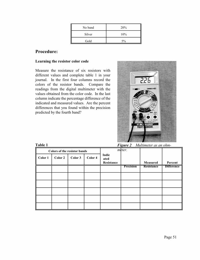
Page 51
Figure 2 Multimeter as an ohm-meter.
No band 20%
Silver 10%
Gold 5%
Procedure:
Learning the resistor color code
Measure the resistance of six resistors withdifferent values and complete table 1 in yourjournal. In the first four columns record thecolors of the resistor bands. Compare thereadings from the digital multimeter with thevalues obtained from the color code. In the lastcolumn indicate the percentage difference of theindicated and measured values. Are the percentdifferences that you found within the precisionpredicted by the fourth band?
Table 1
Colors of the resistor bandsIndicatedResistance
PrecisionMeasuredResistance
PercentDifference
Color 1 Color 2 Color 3 Color 4
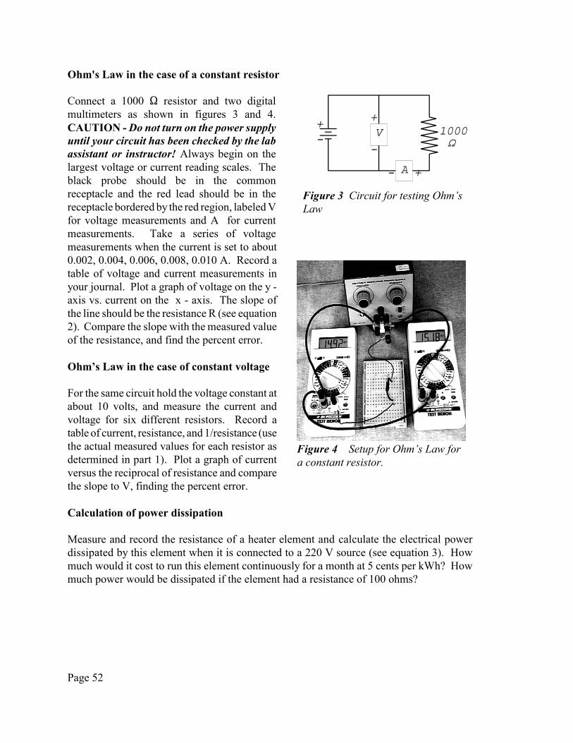
Page 52
Figure 3 Circuit for testing Ohm’sLaw
Figure 4 Setup for Ohm’s Law fora constant resistor.
Ohm's Law in the case of a constant resistor
Connect a 1000 S resistor and two digitalmultimeters as shown in figures 3 and 4.CAUTION - Do not turn on the power supplyuntil your circuit has been checked by the labassistant or instructor! Always begin on thelargest voltage or current reading scales. Theblack probe should be in the commonreceptacle and the red lead should be in thereceptacle bordered by the red region, labeled Vfor voltage measurements and A for currentmeasurements. Take a series of voltagemeasurements when the current is set to about0.002, 0.004, 0.006, 0.008, 0.010 A. Record atable of voltage and current measurements inyour journal. Plot a graph of voltage on the y -axis vs. current on the x - axis. The slope ofthe line should be the resistance R (see equation2). Compare the slope with the measured valueof the resistance, and find the percent error.
Ohm’s Law in the case of constant voltage
For the same circuit hold the voltage constant atabout 10 volts, and measure the current andvoltage for six different resistors. Record atable of current, resistance, and 1/resistance (usethe actual measured values for each resistor asdetermined in part 1). Plot a graph of currentversus the reciprocal of resistance and comparethe slope to V, finding the percent error.
Calculation of power dissipation
Measure and record the resistance of a heater element and calculate the electrical powerdissipated by this element when it is connected to a 220 V source (see equation 3). Howmuch would it cost to run this element continuously for a month at 5 cents per kWh? Howmuch power would be dissipated if the element had a resistance of 100 ohms?
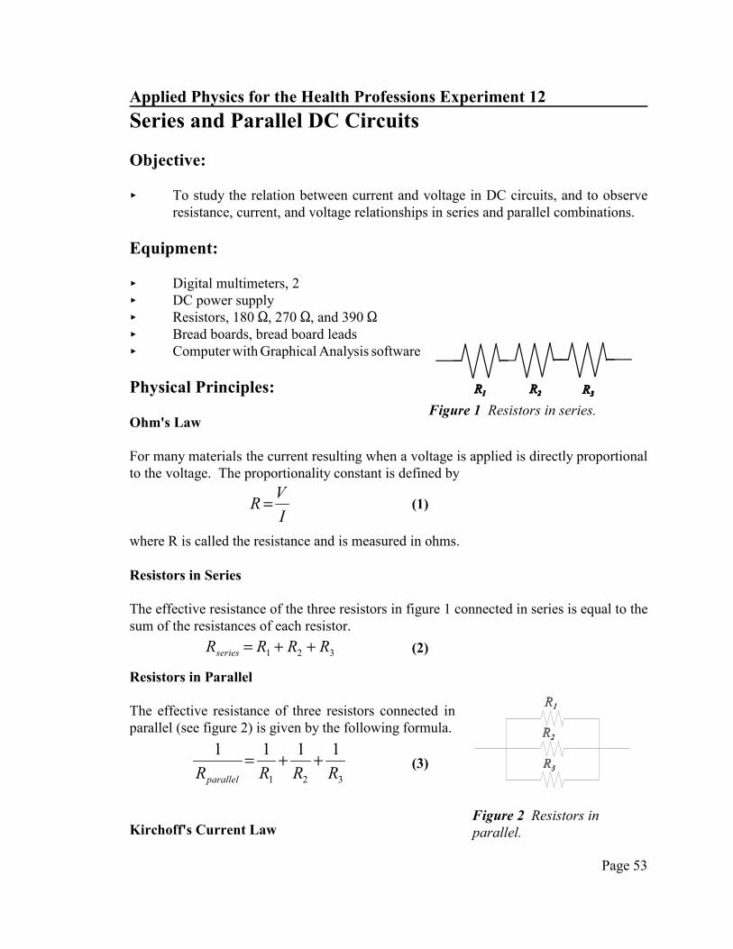
Page 53
Figure 1 Resistors in series.
Figure 2 Resistors inparallel.
RV
I= (1)
R R R Rseries = + +1 2 3 (2)
1 1 1 1
1 2 3R R R Rparallel
= + + (3)
Applied Physics for the Health Professions Experiment 12
Series and Parallel DC Circuits
Objective:
< To study the relation between current and voltage in DC circuits, and to observeresistance, current, and voltage relationships in series and parallel combinations.
Equipment:
< Digital multimeters, 2< DC power supply< Resistors, 180 S, 270 S, and 390 S< Bread boards, bread board leads< Computer with Graphical Analysis software
Physical Principles:
Ohm's Law
For many materials the current resulting when a voltage is applied is directly proportionalto the voltage. The proportionality constant is defined by
where R is called the resistance and is measured in ohms.
Resistors in Series
The effective resistance of the three resistors in figure 1 connected in series is equal to thesum of the resistances of each resistor.
Resistors in Parallel
The effective resistance of three resistors connected inparallel (see figure 2) is given by the following formula.
Kirchoff's Current Law
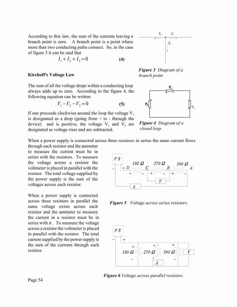
Page 54
Figure 3 Diagram of abranch point.
Figure 4 Diagram of a closed loop.
Figure 5 Voltage across series resistors.
Figure 6 Voltage across parallel resistors.
I I I1 2 3 0+ + = (4)
V V V1 2 3 0− − = (5)
According to this law, the sum of the currents leaving abranch point is zero. A branch point is a point wheremore than two conducting paths connect. So, in the caseof figure 3 it can be said that
Kirchoff's Voltage Law
The sum of all the voltage drops within a conducting loopalways adds up to zero. According to the figure 4, thefollowing equation can be written
If one proceeds clockwise around the loop the voltage V1
is designated as a drop (going from + to - through thedevice) and is positive, the voltage V3 and V2 aredesignated as voltage rises and are subtracted.
When a power supply is connected across three resistors in series the same current flowsthrough each resistor and the ammeterto measure the current must be inseries with the resistors. To measurethe voltage across a resistor thevoltmeter is placed in parallel with theresistor. The total voltage supplied bythe power supply is the sum of thevoltages across each resistor.
When a power supply is connectedacross three resistors in parallel thesame voltage exists across eachresistor and the ammeter to measurethe current in a resistor must be inseries with it . To measure the voltageacross a resistor the voltmeter is placedin parallel with the resistor. The totalcurrent supplied by the power supply isthe sum of the currents through eachresistor.

Page 55
Figure 7 Circuit board with threeresistors.
Figure 8 Jumper connections forthree resistors in series.
Figure 9 Jumper connections forthree resistors in parallel.
Procedure:
Place the ohmmeter leads into the connectionholes in blocks A and B. Record the value of theresistance R1. Repeat for resistors R2 and R3.
R1 = ______ R2 = _______ R3 = _______
Series Resistors:To connect the three resistors in series place ajumper between blocks B and C and a secondjumper between blocks D and E. Place theohmmeter leads in blocks A and D to measure theresistance between these points. Compare thisvalue to that of R1 + R2. Repeat this betweenbusses C and F. Repeat this between busses A andF.
RAD = __________ R1 + R2 = __________
RCF = __________ R2 + R3 = __________
RAF = __________ R1 + R2 + R3 = __________
Parallel Resistors:To connect the three resistors in parallel place ajumper between blocks A and C and a secondjumper between blocks C and E. Similarly placejumpers between blocks B and D and betweenblocks D and F. Place the ohmmeter leads inblocks A and B to measure the resistance betweenthese points. Compare this value to that of Rp
where Rp is calculated from 1/Rp = 1/R1 + 1/R2 +1/R3.
Rp meas = _________ Rp calc = _________

Page 56
Figure 10 Voltage and currentmeasurements for three resistors inseries.
Voltages in Series Resistors:Place jumpers between the blocks as shown infigure 10. Connect the power supply positive leadto block G and the negative lead to block L. Turnon the power supply and set the voltage to 5 V.Set the voltmeter to the 20 V scale. Place theleads of the voltmeter across each resistor andmeasure the voltages. Place the leads of thevoltmeter across the blocks A and D. Comparethe values of the voltages across resistors R1 andR2 with the measured voltages between blocks Aand D. Place the leads of the voltmeter across theblocks C and F. Compare the voltage acrossblocks C and F with the voltages across resistorsR2 and R3. Place the leads of the voltmeter acrossthe blocks A and F. Compare the voltage across blocks A and F with the voltages acrossresistors R1, R2 and R3.
VR1 = ________ VR2 = ________ VR3 = ________
VAD = ________ VR1 + VR2 = __________
VCF = ________ VR2 + VR3 = __________
VAF = ________ VR1 + VR2 + VR3 = __________
Currents in Series Resistors:Turn off the power supply. Remove the jumper between blocks G and A. Connect the leadsof the ammeter to these blocks and set the ammeter to the 20 mA scale. Turn on the powersupply. Record the current. Repeat this for the jumpers between the blocks B and C , theblocks D and E and finally the blocks F and L. Record the average of these four values asIave.
IGA = ________ IBC = ________ IDE = ________ IFL = ________ Iave = ________
Multiply each of the resistance values R1, R2 and R3 by the average current Iave and record the results.
VR1 = Iave R1 = ________ VR2 = Iave R2 = ________ VR3 = Iave R3 = ________
Compare these results with the measured voltages above.

Page 57
Figure 12 A simple current network.
Figure 11 Voltage and currentmeasurements for three resistors inparallel.
Voltages in Parallel Resistors:Place jumpers between the blocks as shown infigure 11. Connect the power supply positive leadto buss G and the negative lead to buss L. Turn onthe power supply and set the voltage to 5 V. Setthe voltmeter to the 20 V scale. Place the leads ofthe voltmeter across each resistor and measure thevoltages.
VAB = _______ VCD = ________
VEF = ________
Currents in Parallel Resistors:Turn off the power supply. Remove the jumper between blocks G and A. Connect the leadsof the ammeter to these blocks and set the ammeter to the 20 mA scale. Turn on the powersupply and set the voltage to 5 V. Record the current. Repeat this for the jumpers betweenthe blocks B and H , the blocks D and J and finally the blocks F and L. Compare the currentIGA to the sum of the currents IBH, IDJ, and IFL.
IGA = ______ IBL= _______ IDL = _______ IFL = _______ IBL + IDL + IFL = ________
From Ohm’s law predict the current in each resistor and record the results.
I1 = VAB / R1 = _______ I2 = VCD / R2 = _______ I3 = VEF / R3 = _______
Compare these currents with the values of IBL, IDL and IFL.
Describe in your conclusion what youhave learned about how resistors,currents and voltages combine in seriesand parallel circuits.
5. Complex Circuit
Choose three resistors with valuesabout 200 S, 300 S and 500 S. Sincethese values are not exact, measure thevalue of each resistor using the meters

Page 58
I1 % I2 % I3 ' 0R1 I1 & R2 I2& 0 I3 ' V1
0 I1 % R2 I2 & R3 I3 ' V2
(7)
provided. Build the circuit in figure 11, and then record the values of V1, V2 and I1, I2, I3 andcompare with the theoretical values that you can find by using Ohm’s Law and Kirchoff’sLaws. The values of I1, I2 and I3 are determined theoretically from the three equations
The first equation is the current law, equation (4), the second is the voltage law, equation (5)applied to the left side loop and the last equation is the voltage law applied to the right sideloop of the circuit shown in figure 11. Solve for the theoretical values of the three currentsusing a method of your choice and compare the results to your measured values.

Page 59
F ' B I R sin2 (1)
F ' N B I R (2)
B 'µ0
4BILsin2
r 2(3)
Applied Physics for the Health Professions Experiment 13
Magnetic Forces and Ampere’s Law
Objectives:
< To determine the forces on a current carrying coil due to the magnetic field.< To determine magnetic field strengths generated by simple current geometries
Equipment:
< Power Supplies, Pasco, 8 amp< Lab jacks, clamps and stands< Bell Gauss meters with Hall element probes< Vernier Hall element probes< Solenoid with side slit, coils, 50 turns< Long wire mounted on a meter stick< Round and rectangular coils< Dual range force sensor< Science Workshop and Graphical Analysis software
Physical Principles:
Magnetic Force
The force on a current-carrying wire segment in a magnetic field is given by,
where B is the magnetic field (in units of Tesla), I is the current, R is the length of the wire,and 2 is the angle between the current and the direction of the magnetic field. For currentflowing through multiple wires, such as a rectangular coil, the force on a single wire mustbe multiplied by the number of wires in the coil, N. If B and I are perpendicular to eachother, then sin 2 = 1, and the equation simplifies to,
Biot - Savart Law
According to the Biot-Savart Law, the strength of the magnetic field at a point P, caused bythe current I in a short segment of wire of length L is given by the following formula:
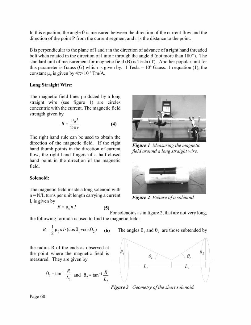
Page 60
Figure 1 Measuring the magneticfield around a long straight wire.
B 'µ0 I
2Br(4)
Figure 2 Picture of a solenoid.
B ' µ0 n I (5)
Figure 3 Geometry of the short solenoid.
B '12
µ0 nI @ (cos21%cos22 ) (6)
In this equation, the angle 2 is measured between the direction of the current flow and thedirection of the point P from the current segment and r is the distance to the point.
B is perpendicular to the plane of I and r in the direction of advance of a right hand threadedbolt when rotated in the direction of I into r through the angle 2 (not more than 180E). Thestandard unit of measurement for magnetic field (B) is Tesla (T). Another popular unit forthis parameter is Gauss (G) which is given by: 1 Tesla = 104 Gauss. In equation (1), theconstant µ0 is given by 4B×10-7 Tm/A.
Long Straight Wire:
The magnetic field lines produced by a longstraight wire (see figure 1) are circlesconcentric with the current. The magnetic fieldstrength given by
The right hand rule can be used to obtain thedirection of the magnetic field. If the righthand thumb points in the direction of currentflow, the right hand fingers of a half-closedhand point in the direction of the magneticfield.
Solenoid:
The magnetic field inside a long solenoid withn = N/L turns per unit length carrying a currentI, is given by
For solenoids as in figure 2, that are not very long,the following formula is used to find the magnetic field:
The angles 21 and 22 are those subtended by
the radius R of the ends as observed atthe point where the magnetic field ismeasured. They are given by
and 21' tan&1 RL1
22' tan&1 RL2
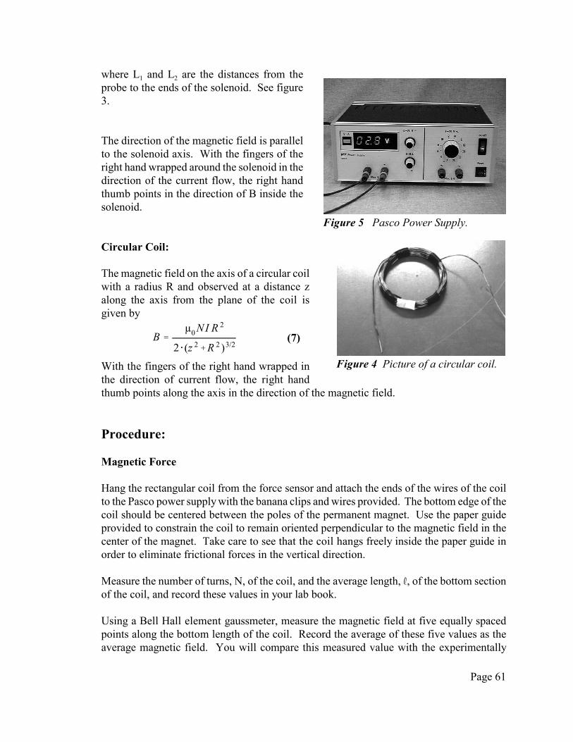
Page 61
Figure 4 Picture of a circular coil.
B 'µ0 NI R 2
2 @ (z 2%R 2 )3/2(7)
Figure 5 Pasco Power Supply.
where L1 and L2 are the distances from theprobe to the ends of the solenoid. See figure3.
The direction of the magnetic field is parallelto the solenoid axis. With the fingers of theright hand wrapped around the solenoid in thedirection of the current flow, the right handthumb points in the direction of B inside thesolenoid.
Circular Coil:
The magnetic field on the axis of a circular coilwith a radius R and observed at a distance zalong the axis from the plane of the coil isgiven by
With the fingers of the right hand wrapped inthe direction of current flow, the right handthumb points along the axis in the direction of the magnetic field.
Procedure:
Magnetic Force
Hang the rectangular coil from the force sensor and attach the ends of the wires of the coilto the Pasco power supply with the banana clips and wires provided. The bottom edge of thecoil should be centered between the poles of the permanent magnet. Use the paper guideprovided to constrain the coil to remain oriented perpendicular to the magnetic field in thecenter of the magnet. Take care to see that the coil hangs freely inside the paper guide inorder to eliminate frictional forces in the vertical direction.
Measure the number of turns, N, of the coil, and the average length, R, of the bottom sectionof the coil, and record these values in your lab book.
Using a Bell Hall element gaussmeter, measure the magnetic field at five equally spacedpoints along the bottom length of the coil. Record the average of these five values as theaverage magnetic field. You will compare this measured value with the experimentally
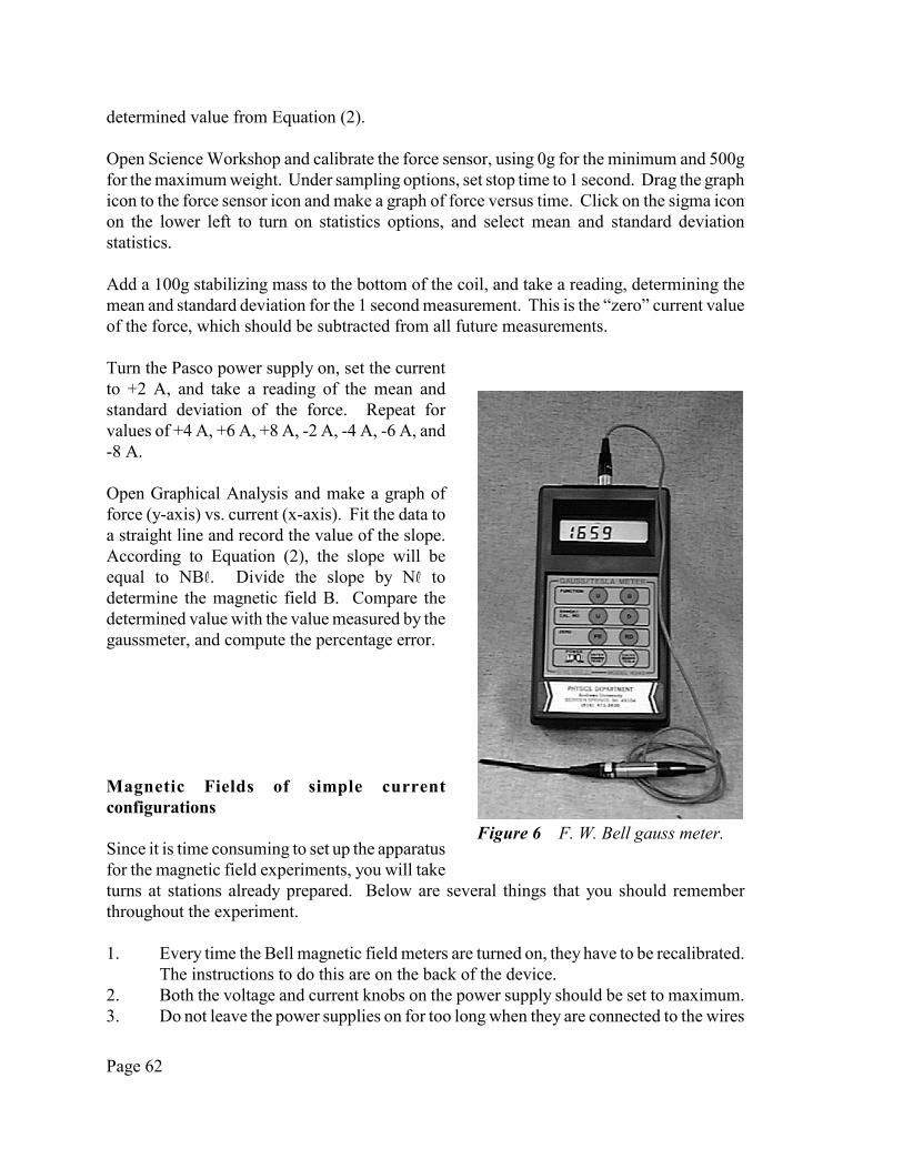
Page 62
Figure 6 F. W. Bell gauss meter.
determined value from Equation (2).
Open Science Workshop and calibrate the force sensor, using 0g for the minimum and 500gfor the maximum weight. Under sampling options, set stop time to 1 second. Drag the graphicon to the force sensor icon and make a graph of force versus time. Click on the sigma iconon the lower left to turn on statistics options, and select mean and standard deviationstatistics.
Add a 100g stabilizing mass to the bottom of the coil, and take a reading, determining themean and standard deviation for the 1 second measurement. This is the “zero” current valueof the force, which should be subtracted from all future measurements.
Turn the Pasco power supply on, set the currentto +2 A, and take a reading of the mean andstandard deviation of the force. Repeat forvalues of +4 A, +6 A, +8 A, -2 A, -4 A, -6 A, and-8 A.
Open Graphical Analysis and make a graph offorce (y-axis) vs. current (x-axis). Fit the data toa straight line and record the value of the slope.According to Equation (2), the slope will beequal to NBR. Divide the slope by NR todetermine the magnetic field B. Compare thedetermined value with the value measured by thegaussmeter, and compute the percentage error.
Magnetic Fields of simple currentconfigurations
Since it is time consuming to set up the apparatusfor the magnetic field experiments, you will taketurns at stations already prepared. Below are several things that you should rememberthroughout the experiment.
1. Every time the Bell magnetic field meters are turned on, they have to be recalibrated.The instructions to do this are on the back of the device.
2. Both the voltage and current knobs on the power supply should be set to maximum.3. Do not leave the power supplies on for too long when they are connected to the wires
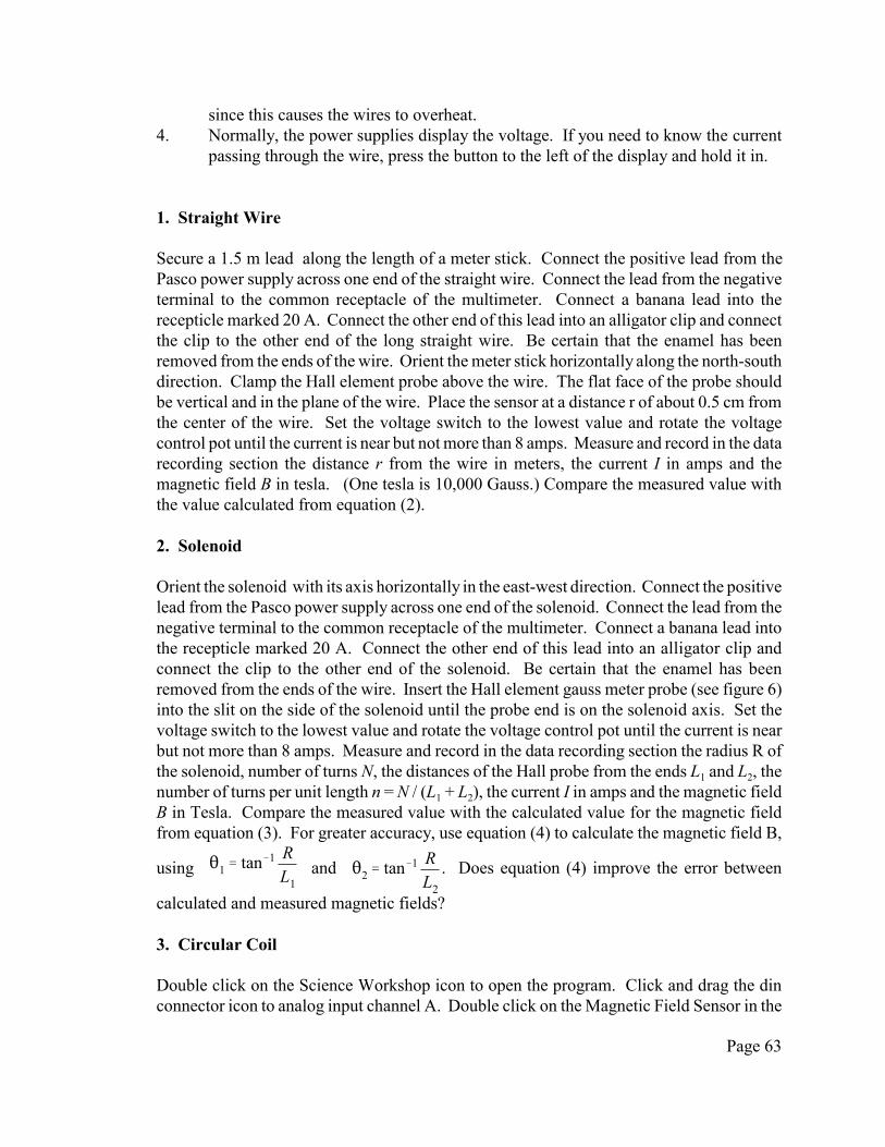
Page 63
since this causes the wires to overheat.4. Normally, the power supplies display the voltage. If you need to know the current
passing through the wire, press the button to the left of the display and hold it in.
1. Straight Wire
Secure a 1.5 m lead along the length of a meter stick. Connect the positive lead from thePasco power supply across one end of the straight wire. Connect the lead from the negativeterminal to the common receptacle of the multimeter. Connect a banana lead into therecepticle marked 20 A. Connect the other end of this lead into an alligator clip and connectthe clip to the other end of the long straight wire. Be certain that the enamel has beenremoved from the ends of the wire. Orient the meter stick horizontally along the north-southdirection. Clamp the Hall element probe above the wire. The flat face of the probe shouldbe vertical and in the plane of the wire. Place the sensor at a distance r of about 0.5 cm fromthe center of the wire. Set the voltage switch to the lowest value and rotate the voltagecontrol pot until the current is near but not more than 8 amps. Measure and record in the datarecording section the distance r from the wire in meters, the current I in amps and themagnetic field B in tesla. (One tesla is 10,000 Gauss.) Compare the measured value withthe value calculated from equation (2).
2. Solenoid
Orient the solenoid with its axis horizontally in the east-west direction. Connect the positivelead from the Pasco power supply across one end of the solenoid. Connect the lead from thenegative terminal to the common receptacle of the multimeter. Connect a banana lead intothe recepticle marked 20 A. Connect the other end of this lead into an alligator clip andconnect the clip to the other end of the solenoid. Be certain that the enamel has beenremoved from the ends of the wire. Insert the Hall element gauss meter probe (see figure 6)into the slit on the side of the solenoid until the probe end is on the solenoid axis. Set thevoltage switch to the lowest value and rotate the voltage control pot until the current is nearbut not more than 8 amps. Measure and record in the data recording section the radius R ofthe solenoid, number of turns N, the distances of the Hall probe from the ends L1 and L2, thenumber of turns per unit length n = N / (L1 + L2), the current I in amps and the magnetic fieldB in Tesla. Compare the measured value with the calculated value for the magnetic fieldfrom equation (3). For greater accuracy, use equation (4) to calculate the magnetic field B,
using and . Does equation (4) improve the error between21' tan&1 RL1
22' tan&1 RL2
calculated and measured magnetic fields?
3. Circular Coil
Double click on the Science Workshop icon to open the program. Click and drag the dinconnector icon to analog input channel A. Double click on the Magnetic Field Sensor in the

Page 64
list of sensors. Double click on the magnetic field sensor icon under channel A to open thecalibration window. With the probe plane along the earth’s magnetic field and no currentin the coil set the low value to 0 gauss and click on the read button. Mount the coil coaxiallyon a meter stick with the meter stick along the coil axis in the east-west direction. Mount theBell Hall element probe of the gauss meter on the coil axis with the flat face of the probevertical and perpendicular to the coil axis. Position the probe so that it is a distance of 9 cmfrom the coil plane. Set the voltage switch to the lowest value and rotate the voltage controlpot until the current is near but not more than 8 amps. Read and enter this value of themagnetic field in the Science Workshop calibration window in tesla. Click on the Readbutton, then click on OK to complete the calibration. Replace the Bell Hall probe with theVernier Hall probe and take all readings with it. For a series of distances z of the probe fromthe plane of the coil, measure the magnetic field and complete table 1 in the data recordingsection. Use values of z of about 9, 10, 11, 14, and 20 cm. Using Graphical Analysis plot
a graph of B as the ordinate (y) and as the abscissa (x) and compute a value of1
z 2%R 2 3/2
µo from the value of the slope which is as predicted by equation 5.µ0 NIR 2
2Circular Coil
z (z2 + R2)3/2 1/(z2 + R2)3/2 B
Page 65
V ' B R v (1)
V ' N B R v (2)
Applied Physics for the Health Professions Experiment 14
Electromotive Forces
Objective:
< To measure the motional emf induced on a coil passing through a magnetic field.
Equipment:
< Motion sensor< Pasco 1.2 m dynamics track< Dynamics cart with coil mounting bracket and rectangular coil< Permanent magnet< Banana clips< Bell Gauss meters with Hall element probes< Science Workshop and Graphical Analysis software
Physical Principles:
When a conducting wire, attached to a circuit, is passed through a perpendicular magneticfield, the induced emf (voltage) on the wire is given by,
where B is the magnetic field (in Tesla), R is the length of the wire, and v is the speed of thewire through the magnetic field. For a coil, with N turns, the induced emf is,
If the maximum induced voltage is measured for different velocities of the coil through themagnet, a plot of maximum voltage (y-axis) vs. velocity (x-axis) will yield a slope equal toN B R. Thus, the average magnetic field of the magnet can be determined by dividing theslope of the graph by N R.
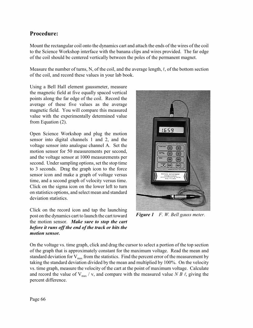
Page 66
Figure 1 F. W. Bell gauss meter.
Procedure:
Mount the rectangular coil onto the dynamics cart and attach the ends of the wires of the coilto the Science Workshop interface with the banana clips and wires provided. The far edgeof the coil should be centered vertically between the poles of the permanent magnet.
Measure the number of turns, N, of the coil, and the average length, R, of the bottom sectionof the coil, and record these values in your lab book.
Using a Bell Hall element gaussmeter, measurethe magnetic field at five equally spaced verticalpoints along the far edge of the coil. Record theaverage of these five values as the averagemagnetic field. You will compare this measuredvalue with the experimentally determined valuefrom Equation (2).
Open Science Workshop and plug the motionsensor into digital channels 1 and 2, and thevoltage sensor into analogue channel A. Set themotion sensor for 50 measurements per second,and the voltage sensor at 1000 measurements persecond. Under sampling options, set the stop timeto 3 seconds. Drag the graph icon to the forcesensor icon and make a graph of voltage versustime, and a second graph of velocity versus time.Click on the sigma icon on the lower left to turnon statistics options, and select mean and standarddeviation statistics.
Click on the record icon and tap the launchingpost on the dynamics cart to launch the cart towardthe motion sensor. Make sure to stop the cartbefore it runs off the end of the track or hits themotion sensor.
On the voltage vs. time graph, click and drag the cursor to select a portion of the top sectionof the graph that is approximately constant for the maximum voltage. Read the mean andstandard deviation for Vmax from the statistics. Find the percent error of the measurement bytaking the standard deviation divided by the mean and multiplied by 100%. On the velocityvs. time graph, measure the velocity of the cart at the point of maximum voltage. Calculateand record the value of Vmax / v, and compare with the measured value N B R, giving thepercent difference.

Page 67
Repeat the previous measurement and analysis for four more data runs, varying the speed ofthe cart for each run.
Open Graphical Analysis and make a graph of voltage (y-axis) vs. velocity (x-axis). Fit thedata to a straight line and record the value of the slope. According to Equation (2), the slopewill be equal to NBR. Divide the slope by NR to determine the magnetic field B. Comparethe determined value with the value measured by the gaussmeter, and compute thepercentage error.
Question: How does the percentage error of the magnetic field determined from the slopeof the graph compare to the percentage error calculated from the individual data points?Explain.