physics-based models for human gait analysis · physics-based models for human gait analysis...

Physics-Based Models for Human GaitAnalysis

Petrissa Zell, Bastian Wandt, and Bodo Rosenhahn

AbstractThis chapter deals with fundamental methods as well as current research onphysics-based human gait analysis. We present valuable concepts that allowefficient modeling of the kinematics and the dynamics of the human body. Theresulting physical model can be included in an optimization-based framework. Inthis context, we show how forward dynamics optimization can be used todetermine the producing forces of gait patterns.

To present a current subject of research, we provide a description of a 2Dphysics-based statistical model for human gait analysis that exploits parameterlearning to estimate unobservable joint torques and external forces directly frommotion input. The robustness of this algorithm with respect to occluded jointtrajectories is shown in a short experiment. Furthermore, we present a method thatuses the former techniques for video-based gait analysis by combining them witha nonrigid structure from motion approach. To examine the applicability of thismethod, a brief evaluation of the performance regarding joint torque and groundreaction force estimation is provided.

KeywordsComputer vision • Human motion analysis • Physics-based simulation • Forwarddynamics optimization • Data-driven regression • 3D motion reconstruction •Video-based force estimation

ContentsIntroduction . . . . . . . . . . . . . . . . . . . . . . . . . . . . . . . . . . . . . . . . . . . . . . . . . . . . . . . . . . . . . . . . . . . . . . . . . . . . . . . . . . . . . . . 2State of the Art . . . . . . . . . . . . . . . . . . . . . . . . . . . . . . . . . . . . . . . . . . . . . . . . . . . . . . . . . . . . . . . . . . . . . . . . . . . . . . . . . . . . 3Models and Methodology . . . . . . . . . . . . . . . . . . . . . . . . . . . . . . . . . . . . . . . . . . . . . . . . . . . . . . . . . . . . . . . . . . . . . . . . 5

P. Zell (*) • B. Wandt • B. RosenhahnInstitut für Informationsverarbeitung, Leibniz Universität Hannover, Hannover, Germanye-mail: [email protected]; [email protected]; [email protected]

# Springer International Publishing AG 2016B. Müller, S.I. Wolf (eds.), Handbook of Human Motion,DOI 10.1007/978-3-319-30808-1_164-1

1

mailto:[email protected]



Kinematics and Dynamics of Physical Models . . . . . . . . . . . . . . . . . . . . . . . . . . . . . . . . . . . . . . . . . . . . . . 5Optimization-Based Methods . . . . . . . . . . . . . . . . . . . . . . . . . . . . . . . . . . . . . . . . . . . . . . . . . . . . . . . . . . . . . . . . . 12Learning Force Patterns in 2D . . . . . . . . . . . . . . . . . . . . . . . . . . . . . . . . . . . . . . . . . . . . . . . . . . . . . . . . . . . . . . . . 14Video-Based Gait Analysis . . . . . . . . . . . . . . . . . . . . . . . . . . . . . . . . . . . . . . . . . . . . . . . . . . . . . . . . . . . . . . . . . . . 18

Future Directions . . . . . . . . . . . . . . . . . . . . . . . . . . . . . . . . . . . . . . . . . . . . . . . . . . . . . . . . . . . . . . . . . . . . . . . . . . . . . . . . . 23References . . . . . . . . . . . . . . . . . . . . . . . . . . . . . . . . . . . . . . . . . . . . . . . . . . . . . . . . . . . . . . . . . . . . . . . . . . . . . . . . . . . . . . . . 24

Introduction

The human locomotor system is a complex construction consisting of the skeleton,the nervous system, muscles, tendons, and ligaments. Its functionality is a basichuman need and the focus of numerous biomechanical studies. In the course of thesestudies, researchers require a measure to quantify healthiness of movement. Amathematically straightforward approach to describing the action of the neuromus-cular system is to compute the net joint moments acting on the segments throughinverse dynamics analysis. These net moments form a first approximation to theanalysis of stress at the skeletal joint and are the foundation for classifying humanmotion. Let us consider an isolated joint in the human body. It might be effected bythe pressure of neighboring bone segments, muscular exertion, and the strain oftendons and ligaments. In order to facilitate research, all of these forces are summa-rized in one vector, the joint torque.

Based on inverse dynamics, researchers develop and evaluate rehabilitationtechniques, e.g., prosthetics alignment (Schmalz et al. 2002) and patient-specificgait modification (Fregly et al. 2007). Others investigate interdependencies in thelocomotor system and their effect, such as the influence of abnormal hip mechanicson knee injury (Powers 2010). Many of these studies focus on analyzing gaitpatterns, as the basic form of human movement. A well-balanced walking style isan essential feature of a healthy locomotor system.

Unfortunately joint torques are not directly measurable but have to be assessed byinterpreting their external effect, that is, the ground reaction force (GRF), which isexerted by the feet on the ground. The clinical standard to estimate joint torques is toinversely calculate them from the GRF vector, the geometry of the skeleton, and therecorded motion of the body. For this purpose, the subject’s gait pattern has to berecorded by a motion capture (MoCap) system, and the GRF has to be measured withforce plates, which restricts this method to a laboratory setup.

For more flexibility, researchers use the profound knowledge introduced byphysical models to support gait analysis. These models yield a comprehensivedescription and control over the correlation between acting forces and resultingmotion. Based on a physical model, joint torques can be estimated in the contextof an optimization problem. There exist several established optimization formula-tions for this particular problem, namely, forward, inverse, and predictive dynamicsoptimization. A comparison of these approaches and a detailed description offorward dynamics optimization can be found in section “Optimization-BasedMethods.”

2 P. Zell et al.

Optimization-based torque estimation entails several challenges: A representationof the entire body rather than just isolated segments (e.g., only one leg) is oftenrequired, and model properties such as the inertial parameters and the formulation offoot-ground contact model have to be defined with care. Furthermore, optimizationapproaches are usually connected with high computational cost and the necessity forconsiderable stabilization of the dynamic system. These issues might be addressedby the use of sophisticated optimization algorithms and refined constraints, butresearchers also propose an alternative route, circumventing the optimization prob-lem and instead relying on machine learning techniques. In such a framework, theconnection between a motion pattern and the underlying forces is learned on thebasis of a training set of motion sequences and associated optimization results. Thisway, the gait pattern of a new subject can be assessed using the knowledge gained inthe training phase, i.e., unobservable joint torques are directly inferred from themotion data.

With the ever-increasing amount of easily accessible video data, the demand formotion analysis based on image sequences is inevitable. In this context, a combina-tion of 3D motion reconstruction from 2D landmarks (nonrigid structure frommotion) and physics-based motion analysis is sought for and determines the direc-tion of research in this field.

This chapter is structured in the following way: First of all, we present state-of-the-art methods for physics-based modeling and motion analysis. Then, we describefundamental concepts to formulate the kinematics and dynamics of physical modelsand introduce optimization-based methods for the estimation of effective forces. Onthe basis of this methodology, we present two approaches and related experimentalresults in more detail: a two-dimensional statistical model and a video-based frame-work for human gait analysis. Both approaches are data-driven, i.e., the respectivealgorithm learns parameter correlations on a training set and uses this knowledge todirectly infer underlying forces from input motion data. Finally, we point to possiblefuture research directions in this field.

State of the Art

A wide range of state-of-the-art methods related to human motion simulation andanalysis rely on physics-based modeling as a tool to control movement or to gainvaluable insides into the dynamics of human motion. In the field of computergraphics, physical models enable researchers to synthesize realistic looking humanmotions (Fang and Pollard 2003; Liu et al. 2005; Safonova et al. 2004; Sok et al.2007; Wei et al. 2011; Zordan et al. 2005). The naturalness of a generated motion iseither ensured by the closeness to motion capture (MoCap) data or by an efficiencymeasure. The latter case is based on the assumption that humans perform lowenergetic movement. Both approaches can be applied in an optimization framework.General issues of physics-based optimization are computational expense concerningcalculation of objectives, constraints, and the associated derivatives and a high-dimensional search space, which complicates the optimization process. Fang and

Physics-Based Models for Human Gait Analysis 3

Pollard (2003) introduce efficient physical constraints and objective functions for afast optimization-based character animation. The authors formulate constraints andobjectives in such a way that first derivatives can be computed analytically in lineartime. The reduction of a high-dimensional parameter space to an appropriate sub-space is addressed in Safonova et al. (2004). In this work, the authors use MoCapdata to transfer the optimization problem to a low-dimensional subspace thatincludes the desired motion characteristics, exclusively.

While the minimization of an energy function to simulate movement correspondsto the overall tendency of humans to avoid energy expenditure, this technique fails tocatch subject-specific motion traits and is not suitable for expressive motions, suchas dancing or acting. In those cases, an approach based on MoCap data that providesmore extensive information is sensible. Following this observation, Liu et al. (2005)propose a physics-based dynamical model that incorporates specific features of apersons’ motion style, e.g., the tendency to strain certain muscles more than others.

These characteristics are learned on a training set of MoCap sequences using anintroduced method called nonlinear inverse optimization.

A physical background is also suitable to support statistical approaches byproviding necessary constraints on the utilized model, e.g., (Wei et al. 2011)combines statistical motion priors with physical constraints in a probabilistic frame-work. The authors use a maximum a posteriori approach to synthesize a wide rangeof physically realistic motions and motion interactions.

Apart from these graphic applications, physics-based models can be found,facilitating typical computer vision tasks, like robust person tracking and 3D poseestimation (Bhat et al. 2002; Brubaker and Fleet 2008; Vondrak et al. 2008; Wrenand Pentland 1998). Brubaker and Fleet (2008) use a simple planar model to estimatebiomechanical characteristics of gait and combine it with a 3D kinematic model formonocular tracking. Due to the underlying physics, the model is able to handle largeocclusions. While this approach solely focuses on walking motions, a related workby Vondrak et al. (2008) considers a wide range of motion types. The authorsintroduce a full-body 3D physical prior that integrates the corresponding dynamicsinto a Bayesian filtering framework. In addition to the motion dynamics, thealgorithm is able to model ground contact and environment interaction.

The previously described works concentrate on human pose tracking withphysics-based constraints but do not analyze the resulting force patterns. Thisbiomechanical objective, i.e., the estimation of inner joint torques and externalcontact forces, is referred to as motion analysis and has been extensively treated invarious fields (Blajer et al. 2007; Brubaker et al. 2009; Johnson and Ballard 2014;Stelzer and von Stryk 2006; Xiang et al. 2010; Zell and Rosenhahn 2015). In thefollowing, we will list a selection of recent works.

Brubaker et al. (2009) use an articulated body model to infer joint torques andcontact dynamics from motion data. They accelerate the optimization procedure byintroducing additional root forces and effectively decoupling the problem at differenttime frames. This way an optimization step does not include the integration of EOM.A similar goal is pursued by Xiang et al. (2010). The authors introduce predictivedynamics as an approach for human motion simulation. Recently, researchers tried to

4 P. Zell et al.

learn a direct mapping from a motion parametrization (joint angles) to the actingforces (joint torques) on the basis of MoCap data: Johnson and Ballard (2014)investigate sparse coding for inverse dynamics regression and Zell and Rosenhahn(2015) introduces a two dimensional statistical model for human gait analysis.

The transfer of motion analysis to a 2D setting, i.e., a video-based framework, is arelatively novel subject of research (Brubaker et al. 2009). By combining physics-based modeling with standard nonrigid structure-from-motion techniques (e.g.,(Bregler et al. 2000)), it is possible to infer the unobservable physical parametersfrom monocular image sequences. State-of-the-art human pose estimation methodsrely either on anthropometric constraints (Akhter and Black 2015; Ramakrishnaet al. 2012; Wang et al. 2014) or on temporal bone length constancy (Wandt et al.2015, 2016). These assumptions are relatively weak compared to a kinematic model.Therefore, the next step is a combination of pose estimation with a physics-basedmodel of humans. This will not only improve the 3D reconstruction but also allowfor the estimation of joint torques from an image sequence. An example implemen-tation of a joint model for pose estimation and physical parameter regression isdescribed in section “Combining Physical Models with 3D Reconstruction.”

Models and Methodology

Kinematics and Dynamics of Physical Models

The groundwork of physics-based human motion analysis is a physical model of thehuman body. The literature offers a large amount of different models with varyingcomplexity from which many have been developed in the scope of robotics appli-cations. A frequently used type are mass-spring models that consist of bone seg-ments and connected by joints which are provided with torsional springs to createjoint torques. Beyond that, muscular skeletal models are applied (especially inbiomechanical research) for a more realistic presentation of the human locomotorsystem, modeling the interaction between bone segments, joints, and an elaboratestructure of muscles. Since the methods described in this chapter are more suitablefor simple skeletal models, we focus on the portrayal of mass-spring models in thissection.

The modeled skeleton comprises a number of bone segments with associatedinertial properties (mass and inertial tensor) and connecting torsional springs foreach joint degree of freedom (DOF). Examples of a 2D and a 3D model can be seenin Fig. 1. An essential part of these models is the kinematic chain that provides thelinkage between all segments and predefines the space of possible motions. In thefollowing part, we show how a kinematic chain can be defined using the Denavit-Hartenberg notation (Steinparz 1985), well-known from robotics.

Denavit-Hartenberg ConventionIn 1955, Jacques Denavit and Richard Hartenberg introduced a convention tocharacterize a kinematic chain by a minimal set of four parameters for each interlink


transformation. A link refers to a rotational or translational degree of freedom. In thispresentation, coordinate frames are attached to every link of the chain, and theDenavit-Hartenberg parameters specify the transformation between successive linkcoordinate systems.

LetHj�1j be the transformation matrix from link j � 1 to link j and [θj,dj,αj,aj] the

constituting parameters. Then the following operations are performed consecutively:A rotation of the coordinate system around the zj�1-axis by the angle θj, a translationalong the zj�1-axis by the distance dj, a second rotation around the new xj-axis by theangle αj, and a final translation along the xj-axis by the distance aj. The

corresponding transformation matrix Hj�1j is composed of the total rotation R

j�1j

and total translation Tj�1j , with

ð1Þ

When considering a kinematic chain consisting of several links, the position andorientation of every link are determined by its predecessor transformations. There-fore, the transformation from the coordinate system at link j to the world coordinateframe L0 is obtained by the product of all transformations in the sub-chain from theroot link to the respective link:

Hj0 ¼ ∏

j

i¼1

Hii�1 ¼ Ri

0 Tj0

0T 1

� �(2)

The linear coordinates p0ci of the center of mass (COM) of segment i can bederived from the total translation and the total rotation of the coordinate systemattached to link j with respect to L0:

p0ci ¼ T0j þ R0

j pjci, (3)

where pjci are the coordinates of the considered segment COM in the coordinatesystem of the preceding link.

6 P. Zell et al.

TMT MethodThe dynamics of the considered mass-spring model are specified by a set ofequations of motion (EOM), which we will formulate using the TMT method(Schwab and Delhaes 2009). This approach combines advantages of both theNewton-Euler method and the Lagrange-Euler formulation by basically trans-forming from constrained to unconstrained dynamics. In the Newton-Eulerapproach, the EOM have to be extended to differential algebraic equations byadditional constraints that model the interconnection (kinematic chain) betweenthe model coordinates. This often leads to poor accuracy of solutions provided bynumerical solvers. In contrast to that, the Lagrange-Euler approach deals with aminimum set of independent generalized coordinates, and the EOM are formulatedbased on an energetic view point. For this purpose, all arising energies have to beidentified and their derivatives have to be calculated analytically, which might bedifficult in the case of complex, large DOF models.

To exploit the benefits of both methods, the TMT method uses a force approach,but incorporates the kinematic constraints in a transformation T from dependentcoordinates x (segment COM position and orientation) to independent generalizedcoordinates q (joint angles):

x ¼ T qð Þ (4)

Derivation supplies the corresponding linear and angular velocities andaccelerations:

_x ¼ @T

@q_q (5)

€x ¼ @T

@q€qþ @

@q

@T

@q_q

� �_q (6)

The second term in Eq. (6) is referred to as convective acceleration

G ¼ @@ q

@ T@ q

_qÞ _q:�

Furthermore the relation

δx ¼ @T

@qδq (7)

between virtual displacements of the coordinates is valid and can be inserted intoD’Alembert’s principle of virtual work:

δx F�M€xð Þ ¼ 0 (8)

@T

@qδq F�M

@T

@q€qþ G

� �� ¼ 0 (9)


Here F summarizes all applied forces and torques and M is the system’s inertiamatrix. Because of the independence of δq and the validity of virtual displacementslarger than zero, we can write Eq. (9) as

@T

@q

� �T

F�M@T

@q€qþ G

� �� ¼ 0 (10)

Rearranging of Eq. (10) yields the EOM, formulated in independent generalizedcoordinates:

@T

@q

� �T

M@T

@q€q ¼ @T

@q

� �T

F�MGð Þ (11)

This equation can be simplified by introducing the Jacobian J ¼ @ T@ q and the

generalized inertia matrix M ¼ @ T@ q

� �TM @ T

@ q, so that

M€q ¼ JT F�MGð Þ: (12)

Formulating the Equations of MotionFor a clearer insight into the described methods, we will now provide an outline ofthe derivation of EOM following Eq. (12) and using the 3D mass-spring modeldepicted in Fig. 1 on the right-hand side. The model has 23 joint DOF and 6 DOF forthe global position and orientation of the root joint, resulting in a total of 29 DOF.Therefore, we will receive a set of 29 coupled EOM.

The kinematic interconnection between the DOF q, i.e., between the generalizedcoordinates, is defined via the Denavit-Hartenberg transformation matrices. In thiscontext, the coordinates q appear either as a translation a or d (prismatic joints) or asa rotation α or θ (revolute joints). The Jacobian J of the according coordinatetransformation T (q) from generalized coordinates to Cartesian coordinates (positionand orientation of segment COM) is composed of a linear and a rotational part:

_x ¼ Jlin

Jrot

� �_q (13)

Instead of formulating T (q) and calculating every differential @ Ti

@ qjto determine

the Jacobian, we choose a geometric approach. In the Denavit-Hartenberg conven-tion, the rotation and translation axis associated with a DOF qj is always equal to thez-axis of the respective coordinate frame Lj�1. This leads to the following equationsfor prismatic joints (Spong et al. 2005):

Jlinij ¼ z0j�1

Jrotij ¼ 0,(14)

8 P. Zell et al.

and for revolute joints:

Jlinij ¼ z0j�1 � p0ci � T0j�1

� �Jrotij ¼ z0j�1,

(15)

with T0j�1 and p0ci calculated according to Eqs. (2) and (3), respectively.

Apart from the Jacobian, we also need an expression for the convective acceler-ation G, which can be derived in a similar fashion with

G ¼ Glin

Grot

� �_q: (16)

The corresponding sectional matrices for prismatic joints are

Glinij ¼ 0

Grotij ¼ 0,

(17)

and for revolute joints, we get

segment COM

joint DOF with torsionalspring

x

y

(0,0)

y

zx

contact point

global DOF

Fig. 1 Physical mass-spring-models in 2D (left) and 3D (right). Joint degrees of freedom (DOF)are depicted in blue and global DOF in green. Each joint degree of freedom is equipped with atorsional spring and each segment is assigned with a mass and a tensor of inertia.


Glinij ¼

Xi�1

k¼0

z0min j�1, kf g � z0max j�1, kf g � p0ci � T0max j�1, kf g

� �� _qk

Grotij ¼ z0j�1 �

Xi�1

k¼j

z0k _qk:

(18)

The Jacobian together with the convective acceleration describes the kinematic ofour model. To characterize the dynamics of the system, i.e., formulate the EOM, weneed further properties, more precisely, the inertia matrixM and the active forces andtorques F (cf. Eq. (12)).

The inertia matrix is composed of mass values and inertia tensors for all modelsegments. Let Mci and Ici be diagonal matrices containing masses and moments ofinertia in the segment coordinate frames, i.e., the values for the inertial propertiescorrespond to the rotation axes in the local frames attached to the individual segmentCOM. Then the inertia matrix related to the coordinates x in the global frame L0 is

M ¼ Mci

R0ciIciR0T

ci

� �, (19)

with the rotationR0cigiven by Eq. (2). Finally, the generalized inertia matrix required

for the EOM is obtained by M = JTMJ.The motion of the 3D mass-spring model is driven by spring torques and outer

contact forces. The spring torques τj are applied at every joint DOF of the model(represented by blue arrows in Fig. 1). A commonly used parametrization is

τj ¼ �κj qj � q0ð Þj

� �� dj _qj, (20)

with a linear resetting torque depending on the spring constant κj and the resting

angle q 0ð Þj and an additional damping term proportional to the angular velocity of the

joint DOF with damping constant dj (Brubaker and Fleet 2008). To simulateincreasingly dynamic and natural-looking motions, additional nonlinear termsmight be added, e.g., Zell and Rosenhahn (2015):

τj ¼ �κj qj � q0ð Þj qð Þ

� �� dj _qj,

q0ð Þj qð Þ ¼ q

0ð Þj þ

X4k¼1

ckxkCoM qð Þ:

(21)

Here, the resting angle is characterized by a fourth-order polynomial of theposition of the whole body COM. It is noteworthy that this representation is onlysensible for motions like walking or running that exhibit an even forward movementof the COM. The single joint torques are summarized in the vector τ with τj = 0 forj � 6 (six global DOF that are not actuated by a joint torque).

10 P. Zell et al.

When the model is in contact with its environment, e.g., standing on the ground orlifting objects, it is effected by contact forces, denoted by Fc in the following. For themajority of human motion types, our feet have to touch the ground and so-calledground reaction forces (GRF) act on the sole of the foot. These forces mostlyaccelerate the body in vertical direction, balancing the gravitational force. They actas a braking force when the foot contacts the ground and a propulsive force at push offfrom the ground. Furthermore, a horizontal friction force, depending on the propertiesof the touching materials and the vertical force, prevents a sliding of the feet on theground. There are several possibilities to model the ground contact: The 2D modelillustrated in Fig. 1 is equipped with circular feet that enables a rolling motion of thefeet on the ground during gait. The GRF is concealed in a model constraint, bydefining the contact point as the root of the kinematic chain and effectively settingits vertical coordinate to zero (Zell and Rosenhahn 2015). This approach is notadvisable for a 3D model with a significantly larger DOF, since it would result inintolerably long kinematic chains that entail high simulation uncertainties.

As an alternative, Brubaker et al. (2009) suggest a spring contact force thataccelerates points on the sole of the foot, when approaching the ground plane. Theforce is modulated by two sigmoid functions, which on the one hand ensure that acontact point p is only effected when it is very close to the ground surface S and onthe other hand prevent an acceleration toward the ground. The force is defined by thefollowing equations:

Fc p, _p, θSð Þ ¼ h �60dS pð Þð Þh 5nc pð Þð Þ nc pð ÞnS pð Þ þ tc pð Þ½ �,nc pð Þ ¼ �κN dS pð Þ � 1ð Þ � δN _pTnY pð Þ,tc pð Þ ¼ �δT _p� nS pð ÞT _pÞnS pð Þ

� �,

� (22)

with the sigmoid h xð Þ ¼ 121þ tanh xð Þð Þ. The total force is composed of the normal

force ncnS and the tangential attenuation tc, where nc denotes the magnitude and nS isthe surface normal. The sigmoidal modulation depends on the shortest distance d(p)between the point p and the ground surface S. Finally, model parameters are includedin the vector θS, namely, the position and orientation of the ground plane, the springstiffness κN, the normal damping constant δN, and the tangential damping constant δT.

The last force term we are still missing for a complete description of the 3D modelwith our EOM is the gravitational force:

Fg ¼ Mg, (23)

where g is the gravitational acceleration with respect to the dependent coordinates x.Since the acceleration g = �9.81 m/s2 only affects the linear coordinates of thesegment COM in vertical direction, all other components are set to zero.

Finally, we insert all discussed terms into Eq. (12) and receive the model EOM:

M€q ¼ JT τ þ Fc þ Fg �MG� �

: (24)


This equation determines the dynamics of our model; in other words, it predictsthe development originating from an initial configuration of joint angles and angularvelocities. The acting forces and therefore the accelerations of the generalizedcoordinates are completely defined by the model parameters θ and the current state

of the model q, _q½ �T. The model parameters include all spring and contact parameters,e.g., stiffness and damping constants, resting angles and the position and orientationof the contact plane.

Optimization-Based Methods

On the basis of the previously described physical models, we can estimate theunderlying forces and torques of motion data in an optimization framework. Thecorresponding approaches found in the literature can be divided into three differentcategories, inverse dynamics, forward dynamics, and predictive dynamics.

The inverse dynamics approach considers the motion parameters (e.g., jointangles q) as optimization variables. A suitable objective function, e.g., the distanceto a target motion or a human performance measure, is minimized and joint torquesare calculated inversely. This way, the expensive integration of EOM is avoided andthe optimization problem is easily controlled, i.e., no sophisticated constraints arenecessary. A disadvantage of this method is the indirect derivation of forces that isaffected by the characteristic inaccuracy of joint trajectories and their accelerations.

In contrast to that, forward dynamics treats the forces and joint torques as designvariables that generate a motion through integration of EOM. As a result, theoptimization problem induces large computational cost and accurate boundariesare crucial for the convergence of the optimization algorithm. Advantages of thisapproach are the directly optimized forces and a natural conclusion of motionparameters via EOM. Inverse as well as forward dynamics depends on the accuracyof the inertial properties to achieve a sound torque estimation.

A rather novel approach, called predictive dynamics, was introduced by Xianget al. (2010). Both the joint torques and the model states are optimization parametersand the EOM are treated as equality constraints. The method is closely related todirect collocation methods (Stelzer and von Stryk 2006). It is computationallyefficient since no integration of EOM is required but because of the large numberof design variables an optimization algorithm suitable for large-scale problems thathas to be used.

Optimization Problem SetupIn this section, we will focus on forward dynamics optimization, since it is based onthe natural relation between forces and motion and provides a convenient frame tointroduce optimization principles. We will formulate the problem and present appro-priate objective functions, regularization, and constraint terms. Let us consider aproblem of the form

12 P. Zell et al.

minθ

f θð Þf gs:t:gi θð Þ � 0, i ¼ 1, . . . ,mhi θð Þ ¼ 0, i ¼ 1, . . . , n,

(25)

where θ are model parameters, f denotes the objective function, and gi and hi areinequality and equality constraints, respectively. The forward dynamics step, i.e., theintegration of the EOM, is represented by the functionD and results in the temporaldevelopment of the model states

q tð Þ, _q tð Þ½ �Tmod ¼ D t, θ, q 0ð Þ, _q 0ð ÞÞ,ð (26)

with the initial state q 0ð Þ, _q 0ð Þ½ �T. For the approximate solution, an ordinary differ-ential equation (ODE) solver has to be used. These solvers are generally based on aRunge-Kutta method (Mayers and Sli 2003).

In our problem statement, the motion data exists as input information, e.g.,recorded by a MoCap system and we want to estimate appropriate joint torques.Therefore, it is reasonable to define an objective function that includes the distance

between modeled states and target states: q tð Þ, _q tð Þ½ �Ttarg,e.g., the quadratic L2-norm of

their difference:

f θð Þ ¼ðT0

D t, θ, q 0ð Þ, _q 0ð Þð Þ � q tð Þ, _q tð Þ½ �Ttarg�� 2: (27)

Since the optimization algorithm generally has to deal with a high-dimensionalparameter space and the subspace that creates realistic motions is non-convex,careful regularization and constraints on the system are indispensable. A numberof human performance measures can be used to support the optimization routine.These measures penalize motions with high energetic cost which are considered tobe unnatural. Commonly used quantities are the dynamic effort:

f ¼ðT0

jjτjj2dt, (28)

and the jerk:

f ¼ðT0

jj _τjj2dt: (29)

Minimizing the jerk increases the smoothness of the simulated motion.Furthermore, we can reduce the searched parameter space by incorporating prior

knowledge as constraints gi and hi. Obviously, it is advisable to set boundaries on themodel parameters, such as


0 � κj � uκj ,

lqj � q0ð Þj � uqj ,

0 � dj � udj ,

(30)

with the respective lower and upper bounds l and u for the joint spring parameters. Inaddition to that, we might have knowledge about the motion of certain points of ourmodel, e.g., the contact points during walking are not supposed to slide over theground, but have to stay fixed. This information can be taken into account by theequality constraint

hc ¼ðT0

jjJc _qjj2dt ¼ 0, (31)

where Jc is the section of the Jacobian that is associated with the coordinates of thecontact points.

In some scenarios, GRF have been recorded with force plates and can be used asground truth data Ftarg. Then we can constrain the modeled contact force with

hf ¼ðT0

jjFc � Ftragjj2dt ¼ 0: (32)

In practice, it is often beneficial to formulate equality constraints as soft inequalityconstraints by introducing an upper threshold or to include them as regularizationterms. This way the convergence of the optimization algorithm is more likely.

Learning Force Patterns in 2D

In this section, we will present a statistical approach for the analysis of human gait(Zell and Rosenhahn 2015). The general idea of this work is to learn modelparameters on a set of MoCap walking sequences from 115 subjects and then usethis knowledge to infer the underlying joint torques of a new gait pattern directlyfrom the motion data. The proposed model considers the 2D projection of walking inthe sagittal plane (cf. Fig. 1 on the left-hand side). It consists of ten segments andnine DOF for the joint angles. The corresponding EOM can be derived as describedin section “Formulating the Equations of Motion” and have the form

M qð Þ€q ¼ F q, _q, θÞ:ð (33)

Based on this, movement can be simulated by solving the related initial valueproblem according to Eq. (26).

14 P. Zell et al.

Combined Statistical ModelFor the direct regression of joint torques from motion, a statistical model has to belearned that combines motion characteristics with a physical representation. Follow-ing Troje (2002a), the authors represent walking as a linear combination of principlecomponent postures pi with sinusoidal variation of coefficients:

p tð Þ ¼ p0 þ p1 sin ωtð Þ þ p2 sin ωtþ ϕ2ð Þþ p3 sin 2ωtþ ϕ3ð Þ þ p4 sin ωtþ ϕ4ð Þ: (34)

Here, ω is the fundamental frequency of the gait and (ϕ2,ϕ3,ϕ4) are phase shifts.In Troje (2002a), a posture consists of 15 three-dimensional joint positions, resultingin a 45-dimensional vector p. For a full motion representation, all characterizingparameters are summarized in one vector:

u ¼ p0, p1, p2, p3, p4,ω,ϕ2,ϕ3,ϕ4½ �T : (35)

To include information about physical properties, the gait patterns from thetraining set are approximated using a forward dynamics optimization approach(cf. section “Optimization-Based Methods”). The EOM are integrated, resulting ina simulated motion which is compared to the target motion at a set of key times {tk}k.The authors optimize the physical model parameters θ together with the initial state

q0, _q0�Th

by minimizing the sum of squared reconstruction errors and constraining

the simulated GRF Fc to lie in the vicinity of ground truth data Ftarg. This way,realistic force patterns are ensured. The optimization problem is formulated asfollows:

q0, _q0, θð Þ ¼ arg minqo, _q0 , θ

Xk

D tk, q0, _q0, θð Þ � q tkð Þ, _q tkð Þ½ �Ttarg�� 2

( ),

s:t: Fc q tkð Þ, _q tkð Þ, €q tkð ÞÞ � Ftarg

� �� ηk,��

with thresholds ηk. The simulated GRF vectors are normalized with respect to bodyweight and compared to a normalized mean ground truth force Ftarg, obtained fromforce plate measurements. The effective GRF is calculated via

Fc q, _q,€qð Þ ¼Xi

mi

Mai q, _q,€qÞ � gð Þ,ð (37)

where g is the gravitational acceleration and ai is the Cartesian acceleration of bodysegment i with respective to mass mi. The total body mass is denoted by M.

The optimization problem can be solved by sequential quadratic programming(SQP) (Powell 1978) and the resulting physics-based model parameters are


v ¼ q0, _q0, θ,M½ �T : (38)

Based on the combined parametrization of u and v, it is possible to infer jointtorques from joint angle trajectories and vice versa. The corresponding parametervectors are optimized for each walking sequence in the training set and then stackedin one matrix:

W ¼ u1...u115v1...v115

h i|fflfflfflfflffl{zfflfflfflfflffl}115 subjects

�ℝ229 motion Eq: 35ð Þð Þ�ℝ52 physical model Eq: 38ð Þð Þ (39)

The combined statistical model encompasses geometrical properties, dynamicalbehavior, and the physical description of a walking motion. All of these featurescontribute to the characteristics of a gait pattern, and their mutual dependence can beexploited to infer missing information based on an incomplete parameter set. Twodifferent regression methods are applied: a k-nearest neighbor (k-NN) regression andan asymmetrical projection into the principal component space (aPCA), as intro-duced by Al-Naser and Söderström (2012).

Force Estimation with Occluded InputThe proposed direct regression methods are evaluated regarding the deviation ofestimated 2D GRF and stance knee torques from ground truth data and inverselycalculated torques, respectively. For this purpose, MoCap sequences of three differ-ent subjects with synchronized force plate measurements were recorded. Based onthe motion parameters u of the considered sequence, the physical parameters v areinferred and used as input to the physical model simulation. This yields the estimatedGRF via Eq. (37) and the estimated joint torques through the respective spring torqueequation, e.g., Eqs. (20) or (21).

In order to evaluate the robustness of the direct regression methods with respect toincomplete input information, joint trajectories are iteratively removed from theconsidered gait sequence. Starting with missing left-hand trajectory, the authorssuccessively remove the trajectories of the left elbow, ankle, and knee, resulting ina final regression based solely on the right-hand side of the human body. The numberof missing joint trajectories is denoted by N. Results for one example subject areillustrated in Fig. 2. For a quantitative evaluation, the symmetric mean absolutepercentage errors (SMAPE) eF and eτ for GRF Fc and stance knee torques τK1

,respectively, are listed in Table 1 together with the arising computation times. Tocompare the performance of the direct regression methods to an optimizationprocedure, a third method (OPT) following the forward dynamics optimization inEq. (36) was implemented. In the case of missing joint trajectories, an additionalterm, based on the dynamic effort, is minimized to compensate for the incompleteinformation.

With zero missing input trajectories, the best approximation is achieved by theoptimization-based method OPT, as expected. Under these circumstances, the phys-ical parameters are optimized, to create a simulated motion as close to the target

16 P. Zell et al.

motion as possible with no additional energy minimization that affects the results. Asthe input information is reduced, the direct regression methods (k-NN, aPCA)increasingly outperform OPT. In particular, the estimates based on the k-NN methodshow consistently low SMAPE values. In regard to the computational cost, theoptimization requires computation times that are at least three orders of magnitudehigher than those for the direct regression methods. All of these values weregenerated using unoptimized Matlab code.

In summary, the combination of motion and force parameters in one statisticalrepresentation allows a fast and robust regression of joint torques from MoCap data.In this work, a limiting factor of the approximation quality is the rather simple 2Dphysical model.

Stance Phase [%]20 40 60 80

Fx[

N/k

g]

-2

-1

0

1

2 k-NNaPCAOPTground truth


Fy[

N/k

g]

8

9

10

11


τ K1/ M

[Nm

/kg]

-0.6

-0.4

-0.2

0

0.2

0.4

0.6


Fx

[N/k

g]

-2

-1

0

1

2


Fy

[N/k

g]

8

9

10

11


τ K1/ M

[Nm

/kg]

-0.6

-0.4

-0.2

0

0.2

0.4

0.6

a

b

Fig. 2 Comparison between different regression and optimization methods concerning estimatedGRF components Fy, Fx and knee torques τK1. Positive values correspond to flexor torques. Theresults are based on full joint trajectory information (in (a)) and on partial information with N = 4(in (b)), respectively. In the case of GRF components, the black line illustrates ground truth data,and in the case of joint torques, it represents torques calculated via inverse dynamics. A quantitativeevaluation can be found in Table 1

Table 1 SMAPE values EF and Et for GRF and knee torque estimates with related computationtimes tc

k-NN aPCA OPT

N eF eτ tc [s] eF eτ tc [s] eF ετ tc [s]

0 1.504 1.624 2.994 1.726 2.019 0.881 1.483 1.420 8103

1 1.504 1.586 2.117 1.780 2.052 0.934 1.811 1.851 4358

2 1.496 1.582 2.112 2.005 2.083 0.913 1.890 1.793 3096

3 1.524 1.562 2.583 1.606 2.169 0.619 1.843 2.069 3229

4 1.528 1.565 2.538 1.594 2.072 0.669 1.911 2.188 2092

N indicates the number of missing input joint trajectories


Video-Based Gait Analysis

As shown in the previous sections, methods based on motion capture recordscombined with additional force measurement achieve high-quality results. However,they require expensive and complex laboratory setups. With the increasing ease ofcapturing videos, for example, with mobile devices, the demand for purely video-based motion capture rises. In the combination of structure-from-motion methodswith complex physical models, researchers found a tool to infer physical parametersdirectly from monocular input videos.

A Short Introduction to NRSfMStructure-from-motion (SfM) describes techniques to infer a 3D structure of anobject from its 2D projections into an image plane. Early work concerning the 3Dreconstruction of rigid objects was done in the 90s by Tomasi and Kanade (1992). Intheir seminal work, they proposed to decompose a 2D measurement matrixW2D intocamera matrices K and a shape matrix S:

W2D ¼ KS: (40)

With observations from multiple viewpoints, they were able to reconstruct therigid 3D structure of the object. In 2000, Bregler et al. (2000) generalized Tomasiand Kanades work to the nonrigid case, where the observed object is allowed todeform over time. Their method rests upon the idea that a deformable shape S can berepresented by a linear combination of K-weighted base shapes Qi:

S5XKi¼1

diQi, (41)

where di is the weighting factor for the i-th base shape. This leads to a generalizationof Eq. (40):

W2D ¼ KDQ, (42)

where D contains the weighting factors di for the base shapes in Q. A commonapproach is to minimize a reprojection error er such as

er ¼ W2D � KDQk k (43)

for the different variable sets with respect to orthogonality constraints on the cameramatrix. For further detail, the reader is referred to Bregler et al. (2000).

Since the base shapes in this mathematical representation are nonunique in thefollowing years, numerous authors (e.g., Dai and Li 2012; Hamsici et al. 2011; Parket al. 2010; Torresani et al. 2003, 2008) proposed several constraints to convert thisproblem into a more feasible one.

18 P. Zell et al.

NRSfM for 3D Reconstruction of Human MotionAlthough the methods briefly introduced in section “A Short Introduction toNRSfM” were developed for arbitrary deformable objects, they also showed greatsuccess in the 3D reconstruction of human motion. However, they require a suffi-cient camera or object motion to achieve acceptable results. Therefore, they are notapplicable for more realistic scenarios with limited camera motion such as insurveillance situations. This leads to the idea of including prior knowledge aboutthe observed object into the problem formulation.

In 2002, N. Troje (2002a, b) showed that a single human pose during a gaitmotion can be described by the linear combination of specific weighted vectors.These vectors (named eigenpostures) are obtained by performing a PCA on multiple3D gait sequences. It was shown that the first four eigenpostures were sufficient tocover more than 98% of the variance of a walking motion. N. Troje also discoveredthat for a walking motion, the weights for the eigenpostures describe a sine curve.This leads to the conclusion that the human gait can be described by just the foureigenpostures and the corresponding sine functions which are defined by theiramplitude, frequency, and phase shift. In Troje (2002a, b), this discovery was usedto identify and create gait patterns for different gait characteristics. Since Troje’sformulation is in close proximity to Eqs. (41) and (42), the applicability for 3Dreconstruction is obvious.

Multiple researchers used the idea of representing human poses in a PCA basis forthe 3D reconstruction from single images, e.g., Akhter and Black (2015), Ramakrishnaet al. (2012), and Wang et al. (2014). Since these learned bases also include manynonhuman poses, further anthropometric priors are applied, such as symmetry andpredefined bone length relations. Wandt et al. (2015, 2016) were the first to combinetemporal information of the skeletal structure with the learning of subspaces byemploying a bone length constancy term. They also exploited the periodic behaviorof the eigenpostures coefficients for periodic motions as proposed by Troje (2002a).Thus, their method appears to be well suited for gait reconstruction tasks in general,but not for a detailed analysis of idiosyncratic gait (e.g., pathological gait caused byneurological disorders) due to the limited number of used principle components.

Combining Physical Models with 3D ReconstructionHere an algorithm is presented to jointly infer the 3D pose and physical parametersfrom monocular input data. The presented algorithm first performs the 3D posereconstruction followed by the physical simulation to eliminate any ambiguitiesbetween camera and object motion as well as enforcing a physically plausiblereconstruction. The dynamical description is based on a 3D physical mass-springmodel (cf. Fig. 1 on the right-hand side) with spring and contact parameters θ thatresult from the following optimization procedure:


θ5 arg minθ

w0

T

XTt¼1

q, _q½ �mod, tT � q, _q½ �Ttarg, t

�� 2(

þ w1

T

XTt¼1

τtk k2 þ _τtk k2� �

þ w2

T

XTt¼1

Jc _qmod, tk2�� )

,

(44)

with regularization weights (w0,w1,w2). A description of the individual terms hasbeen given in section “Optimization Problem Setup.”

A joint parameter space is built consisting of the weighting matrix D fromEq. (43) and the physical parameters θ. As shown in Eq. (42), the 3D shape can bewritten as S = DQ. For known 3D shapes S from the training data, D can be directlycalculated via

D ¼ SQþ, (45)

where Q+ denotes the Moore-Penrose pseudoinverse of Q. Finally, a vector vkcomposed of the vectorized weighting matrix D and the physical parameters θ isassigned to each sequence k in the training set:

vk ¼ vec Dð Þθ

� �: (46)

Here, vec(�) is the vectorization operator which stacks the columns of the matrixinto a vector. We assume that a newly observed motion lies in the space spanned bythe vectors vk for each sequence k.

In the first step, the algorithm performs a 3D reconstruction of the observationmatrixW2d alternatingly minimizing Eq. (43) for the camera matrix K and coefficientmatrix D. The consequent 3D shapes are calculated by S= DQ. Since a linear modelis used to represent nonlinear deformations, the estimated 3D motion is expected todiffer from the real motion. This can be easily seen when analyzing the temporalbehavior of the bone lengths, shown on the left in Fig. 3. After the 3D reconstruction,the bone lengths fluctuate heavily due to the above mentioned linear model. Thisissue is addressed by limiting the parameter space to physically valid motions; inother words, the weighting coefficients and physical parameters are inferred bymeans of a k-nearest neighbor (k-NN) regression in the space spanned by the vectorsvk. As suggested by Zell and Rosenhahn (2015), a local k-NN regression can be used,which outperforms global approaches like PCA or asymmetric PCA for this partic-ular problem.

The recovered physical parameters θ are now employed to simulate a 3D motionby integrating the corresponding set of EOM. This step provides the resulting jointtorques and contact forces and converts the rough 3D pose estimation to a physicallyfeasible 3D reconstruction of the observed motion. Comparing the bone lengthvariation before (cf. Fig. 3 left) and after physical simulation (cf. Fig. 3 right)indicates an improvement regarding plausibility.

Additionally, the use of the physical model allows for resolving the ambiguitybetween camera and object motion. Based on the knowledge gained from thephysical simulation of the observed object, e.g., the forward movement during

20 P. Zell et al.

Fig.3

Com

parisonof

thetempo

ralbehaviorof

bone

leng

thsafter3D

reconstructio

n(left)andafterapplying

theph

ysicalmod

el(right).Obv

iously,the

desired

bone

leng

thconstancyisassured


walking, a standard camera calibration technique with known 2D-3D point corre-spondences can be used to reconstruct the camera parameters.

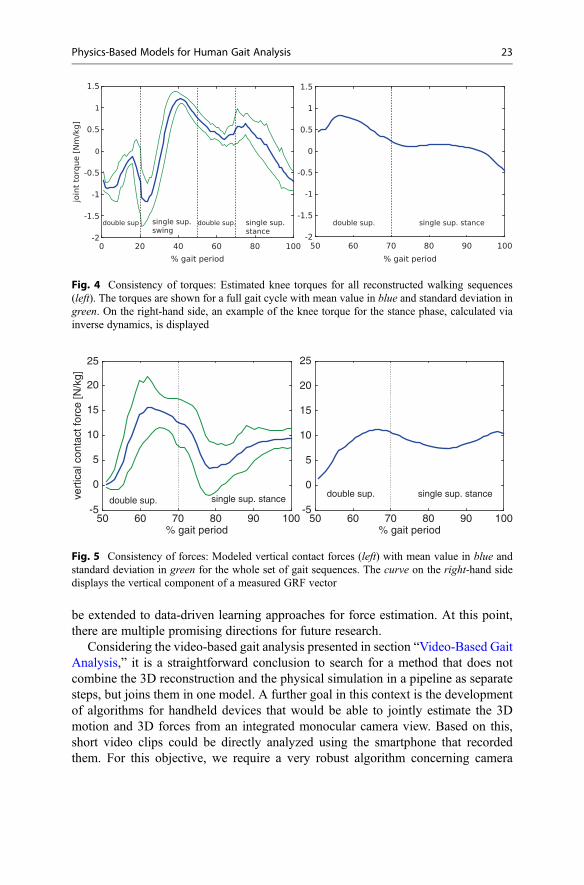
Experiments on Force EstimationThe joint model is evaluated on a training set consisting of 45 MoCap walkingsequences with synchronized force plate data. For each reconstruction, the consid-ered sequence is excluded from the training set. First of all, the estimation of kneetorques from video data is assessed. The torque profiles are generated as described inthe previous section. Figure 4 shows the mean value of estimated knee torques for allreconstructed gait sequences together with the related standard deviation. The graphon the right-hand side of Fig. 4 displays the inversely calculated knee torque of anexample sequence for comparison.

The torque was computed based on force plate data using a bottom-up procedure,i.e., calculating all acting lever arms, joint forces, and torques from the center ofpressure (COP) on the ground to the knee joint. Because of this, only the torqueduring the stance phase is shown. The kinematic chain from the COP to the knee atthe swing leg would be too long and consequently the accumulated error wouldbecome too high. It can be seen that the estimated torques are consistent for allreconstructed 3D motions and the absolute values are similar to inverse dynamicstorques. The maximal extension torque is reached during the second half of theswing phase and not during double support.

This discrepancy is mainly due to the estimated contact model, that is verysensitive to the distance of contact points to the ground. Further error sources aremodel inaccuracies, e.g., concerning mass distribution, imprecision of the fittedskeleton, and of course the reconstruction error of θ.

To further analyze the joint model regression, vertical GRF are compared toground truth data in Fig. 5. The absolute values of the extremal points are slightlyhigh, but the overall curve progression resembles ground truth reaction forces. Theexperiment shows that the joint model provides a sound estimation of unobservable3D torques from monocular videos without the need for tedious optimization.

To demonstrate the applicability of the algorithm to real-world scenarios, asequence from the KTH football database (Kazemi et al. 2013) has beenreconstructed. This dataset contains multiview sequences of a challenging noisyoutdoor scene that shows a football player walking over a playfield. The 3Dreconstruction from camera 1 with estimated torques is illustrated in Fig. 6. Asexpected, the reconstructions from the remaining two cameras yield very similarresults with a maximal reconstruction error of 0.05 m.

Future Directions

In this chapter, we gave you an overview over motion, in particular gait analysisbased on a physical simulation. We presented basic concepts of physical modeling,parameter optimization, and 3D reconstruction and showed how these methods can

22 P. Zell et al.

be extended to data-driven learning approaches for force estimation. At this point,there are multiple promising directions for future research.

Considering the video-based gait analysis presented in section “Video-Based GaitAnalysis,” it is a straightforward conclusion to search for a method that does notcombine the 3D reconstruction and the physical simulation in a pipeline as separatesteps, but joins them in one model. A further goal in this context is the developmentof algorithms for handheld devices that would be able to jointly estimate the 3Dmotion and 3D forces from an integrated monocular camera view. Based on this,short video clips could be directly analyzed using the smartphone that recordedthem. For this objective, we require a very robust algorithm concerning camera

% gait period200

join

t tor

que

[Nm

/kg]

-2

-1.5

-1

-0.5

0

0.5

1

1.5

double sup double sup. single sup.stance

% gait period

-2

-1.5

-1

-0.5

0

0.5

1

1.5

double sup. single sup. stancesingle sup.swing

40 60 80 100 6050 70 80 90 100

Fig. 4 Consistency of torques: Estimated knee torques for all reconstructed walking sequences(left). The torques are shown for a full gait cycle with mean value in blue and standard deviation ingreen. On the right-hand side, an example of the knee torque for the stance phase, calculated viainverse dynamics, is displayed

% gait period % gait period50

vert

ical

con

tact

forc

e [N

/kg]

-5

0

5

10

15

20

25

double sup.double sup.

-5

0

5

10

15

20

25

60 70 80 90 100 50 60 70 80 90 100

single sup. stance single sup. stance

Fig. 5 Consistency of forces: Modeled vertical contact forces (left) with mean value in blue andstandard deviation in green for the whole set of gait sequences. The curve on the right-hand sidedisplays the vertical component of a measured GRF vector


motion and an implementation that enables real-time processing, in order to ensurethe applicability in everyday life.

Another interesting, sparsely treated research direction is the fusion of differentsensor types to facilitate human motion analysis. For example, prior knowledgeabout the acceleration and the orientation of a subset of body segments could besupplied by including inertial measurement units (IMU). This way, the search spacefor underlying forces could be reduced significantly. In addition, when considering amuscular skeletal model, the fusion between video data and electromyograph (EMG)measurements might provide vital constraints on the high-dimensional system.

References

Akhter I, Black MJ (2015) Pose-conditioned joint angle limits for 3D human pose reconstruction.In: IEEE Conference on computer vision and pattern recognition (CVPR 2015). IEEE, pp1446–1455

Al-Naser M, Söderström U (2012) Reconstruction of occluded facial images using asymmetricalprincipal component analysis. Integrated Comput Aided Eng 19(3):273–283

Bhat KS, Seitz SM, Popović J, Khosla PK (2002) Computer vision – ECCV 2002: 7th Europeanconference on computer vision copenhagen, Denmark, 2002. In: Proceedings, Part I, chaptercomputing the physical parameters of rigid-body motion from video, Springer, Berlin/Heidel-berg, pp 551–565, 28–31 May 2002

Blajer W, Dziewiecki K, Mazur Z (2007) Multibody modeling of human body for the inversedynamics analysis of sagittal plane movements. Multibody Sys Dyn 18(2):217–232

Bregler C, Hertzmann A, Biermann H (2000) Recovering non-rigid 3D shape from image streams.In: IEEE Conference on computer vision and pattern recognition (CVPR). IEEE, pp 690–696

Brubaker MA, Fleet DJ (2008) The kneed walker for human pose tracking. In: IEEE conference on,computer vision and pattern recognition, 2008 (CVPR 2008). pp 1–8, June 2008

Brubaker MA, Sigal L, Fleet DJ (2009) Estimating contact dynamics. In: IEEE 12th internationalconference on Computer vision 2009. IEEE, pp 2389–2396

Dai Y, Li H (2012) A simple prior-free method for non-rigid structure-from-motion factorization.In: Conference on computer vision and pattern recognition (CVPR), CVPR’12, IEEE ComputerSociety, Washington DC, pp 2018–2025, 2012

Fig. 6 3D reconstruction and estimated torques of the KTH football dataset. The reconstructionsand torques (red spheres) appear to be plausible compared to the corresponding images and torquesin Fig. 4

24 P. Zell et al.

Fang AC, Pollard NS (2003) Efficient synthesis of physically valid human motion. ACM TransGraph 22(3):417–426

Fregly BJ, Reinbolt JA, Rooney KL, Mitchell KH, Chmielewski TL (2007) Design of patient-specific gait modifications for knee osteoarthritis rehabilitation. IEEE Trans Biomed Eng 54(9):1687–1695

Hamsici O, Gotardo P, Martinez A (2011) Learning spatially-smooth mappings in non-rigidstructure from motion. In: European conference on computer vision (ECCV). Springer,Berlin/Heidelberg

Johnson L, Ballard DH (2014) Efficient codes for inverse dynamics during walking. In: Proceedingsof the twenty-eighth AAAI press conference on artificial intelligence, AAAI’14. AAAI Press,pp 343–349

Kazemi V, Burenius M, Azizpour H, Sullivan J (2013) Multi-view body part recognition withrandom forests. In: British machine vision conference (BMVC). BMVC Press, Bristol

Liu CK, Hertzmann A, Popović Z (2005) Learning physics-based motion style with nonlinearinverse optimization. ACM Trans Graph 24(3):1071–1081

Mayers D, Sli E (2003) An introduction to numerical analysis. Cambridge University Press,Cambridge

Park HS, Shiratori T, Matthews I, Sheikh Y (2010) 3D reconstruction of a moving point from aseries of 2D projections. In: European conference on computer vision (ECCV). Springer, Berlin/Heidelberg

Powell MJD (1978) Numerical analysis. In: Proceedings of the Biennial Conference held atDundee, chapter A fast algorithm for nonlinearly constrained optimization calculations,Springer, Berlin/Heidelberg, pp 144–157, June 28–July 1 1977

Powers CM (2010) The influence of abnormal hip mechanics on knee injury: a biomechanicalperspective. J Orthop Sports Phys Ther 40(2):42–51

Ramakrishna V, Kanade T, Sheikh YA (2012) Reconstructing 3D human pose from 2D imagelandmarks. In: European conference on computer vision (ECCV). Springer, Berlin/Heidelberg

Safonova A, Hodgins JK, Pollard NS (2004) Synthesizing physically realistic human motion inlow-dimensional, behavior-specific spaces. ACM Trans Graph 23(3):514–521

Schmalz T, Blumentritt S, Jarasch R (2002) Energy expenditure and biomechanical characteristicsof lower limb amputee gait: the influence of prosthetic alignment and different prostheticcomponents. Gait Posture 16(3):255–263

Schwab AL, Delhaes GMJ (2009) Lecture notes multibody dynamics B, wb1413Sok KW, Kim M, Lee J (2007) Simulating biped behaviors from human motion data. ACM Trans

Graph 26(3):107:1–107:9Spong M, Hutchinson S, Vidyasagar M (2005) Robot modeling and control. WileySteinparz F (1985) Co-ordinate transformation and robot control with denavit-hartenberg matrices.

J Microcomput Appl 8(4):303–316Stelzer M, von Stryk O (2006) Efficient forward dynamics simulation and optimization of human

body dynamics. ZAMM – J Appl Math Mech/Zeitschrift fr Angewandte Mathematik undMechanik 86(10):828–840

Tomasi C, Kanade T (1992) Shape and motion from image streams under orthography: a factori-zation method. Int J Comput Vis 9:137–154

Torresani L, Hertzmann A, Bregler C (2003) Learning non-rigid 3D shape from 2D motion. In:Thrun S, Saul LK, Schölkopf B (eds) Neural information processing systems (NIPS). MITPress, Cambridge, MA

Torresani L, Hertzmann A, Bregler C (2008) Nonrigid structure-from-motion: estimating shape andmotion with hierarchical priors. In: IEEE Transactions pattern analysis and machine intelli-gence, IEEE, 21 March 2008

Troje NF (2002a) Decomposing biological motion: a framework for analysis and synthesis ofhuman gait patterns. J Vis 2(5):371–387

Troje NF (2002b) The little difference: Fourier based synthesis of gender-specific biologicalmotion. AKA Press, Berlin, pp 115–120


Vondrak M, Sigal L, Jenkins OC (2008) Physical simulation for probabilistic motion tracking. In:IEEE conference on computer vision and pattern recognition, 2008 (CVPR 2008), pp 1–8, June2008. IEEE

Wandt B, Ackermann H, Rosenhahn B (2015) 3d human motion capture from monocular imagesequences. In: IEEE conference on computer vision and pattern recognition workshops, June2015. IEEE

Wandt B, Ackermann H, Rosenhahn B (2016) 3d reconstruction of human motion from monocularimage sequences. IEEE Trans Pattern Anal Mach Intell 38(8):1505–1516

Wang C, Wang Y, Lin Z, Yuille A, Gao W (2014) Robust estimation of 3d human poses from asingle image. In: IEEE Conference on computer vision and pattern recognition (CVPR). IEEE

Wei X, Min J, Chai J (2011) Physically valid statistical models for human motion generation. ACMTrans Graph 30(3):19:1–19:10

Wren CR, Pentland AP (1998) Dynamic models of human motion. In: Proceedings of the thirdIEEE internatonal conference on automatic face and gesture recognition, Nara, April 1998.

Xiang Y, Chung H-J, Kim JH, Bhatt R, Rahmatalla S, Yang J, Marler T, Arora JS, Abdel-Malek K(2010) Predictive dynamics: an optimization-based novel approach for human motion simula-tion. Struct Multidiscip Optim 41(3):465–479

Zell P, Rosenhahn B (2015) Pattern recognition: 37th German conference, GCPR 2015. In: Pro-ceedings, chapter A physics-based statistical model for human gait analysis, Springer Interna-tional Publishing, Aachen, Germany, October 7–10, 2015, pp 169–180.

Zordan VB, Majkowska A, Chiu B, Fast M (2005) Dynamic response for motion capture animation.ACM Trans Graph 24(3):697–701

26 P. Zell et al.

physics-based models for human gait analysis · physics-based models for human gait analysis...

Documents