physics laboratory manual phyc 10180 physics for ag ... · on building from existing sources of...
TRANSCRIPT

Physics Laboratory Manual
PHYC 10180 Physics for Ag. Science
2019-2020
Name.................................................................................
Partner’s Name ................................................................
Demonstrator ...................................................................
Group ...............................................................................
Laboratory Time ...............................................................

2
Contents
Introduction 3
Laboratory Schedule 4
Grading Process and Lab Rules
5
UCD plagiarism statement 6
Experiments: Springs 9
Investigating the Behaviour of Gases 20
Investigation of Acceleration 31
Investigation of Heat Capactity 42
Investigation of Fluid Flow
53
Investigation of Archimedes’ Principle
61
Investigation of Rotational Motion
69
Appendix 1: Appendix 2:
Graphing Grading scheme
79
82

3
Introduction Physics is an experimental science. The theory that is presented in lectures has its origins in, and is validated by, experiment.
Laboratories are staged through the semester in parallel to the lectures. They serve a number of purposes:
an opportunity, as a scientist, to test theories by conducting meaningful scientific experiments;
a means to enrich and deepen understanding of physical concepts presented in lectures;
an opportunity to develop experimental techniques, in particular skills of data analysis, the understanding of experimental uncertainty, and the development of graphical visualisation of data.
Based on these skills, you are expected to present experimental results in a logical fashion (graphically and in calculations), to use units correctly and consistently, and to plot graphs with appropriate axis labels and scales. You will have to draw clear conclusions (as briefly as possible) from the experimental investigations, on what are the major findings of each experiment and whetever or not they are consistent with your predictions. You should also demonstrate an appreciation of the concept of experimental uncertainty and estimate its impact on the final result.
Some of the experiments in the manual may appear similar to those at school, but the emphasis and expectations are likely to be different. Do not treat this manual as a ‘cooking recipe’ where you follow a prescription. Instead, understand what it is you are doing, why you are asked to plot certain quantities, and how experimental uncertainties affect your results. It is more important to understand and show your understanding in the write-ups than it is to rush through each experiment ticking the boxes. This manual includes blanks for entering most of your observations. All data, observations and conclusions should be entered in this manual. Graphs may be produced by hand or electronically (details of a simple computer package are provided) and should be secured to this manual.
These laboratories are two hours long. At the end of each laboratory session, your demonstrator will collect your work and mark it.

4
Laboratory Schedule
Please consult the laboratory notice board to see which of the experiments you will be performing each week. You can also contact the lab manager, Thomas O’Reilly (Room Science East 1.41) to clarify anything. This information is also summarized below. Timetable: Wednesday 2-4: Groups 1, 3, 5, and 7 Wednesday 4-6: Groups 2, 4, 8,10 and 11 Friday 3-5: Groups 6 and 9.
Semester Week
Week Start Date 2018
Room
Science East 143 Science East 144 Science East 145
1 9th Sep Springs: 1,2
Springs: 3,4
Springs: 5,6
2 16th Sep Springs: 7,8
Springs: 9,10
Springs: 11
3 23rd Sep Gas: 1,2
Newton 2: 3,4
Heat Capacity: 5,6
4 30th Sep Gas: 7,8
Newton 2: 9,10
Heat Capacity: 11
5 7th Oct Gas: 5,6
Newton 2: 1,2
Heat Capacity: 3,4
6 14th Oct Gas: 11
Newton 2: 7,8
Heat Capacity: 9,10
7 21st Oct Gas: 3,4
Newton 2: 5,6
Heat Capacity: 1,2
8 28th Oct Gas: 9,10
Newton 2: 11
Heat Capacity: 7,8
9 4th Nov Rotation: 1,2
Archimedes: 3,4
Fluids: 5,6
10 11th Nov Rotation: 7,8
Archimedes: 9,10
Fluids: 11
11 18th Nov Rotation: 5,6
Archimedes: 1,2
Fluids: 3,4
12 25th Nov Rotation: 11
Archimedes: 7,8
Fluids: 9,10
5
Grading Process
Grading is an important form of feedback for students, who benefit from this feedback for continuous improvement. Grading is staged through the semester in synchronisation with the labs. This is the grading process:
1. See appendix 2 for the labs grading scheme.
2. A lab script is graded by the lab demonstrator and returned to the student in the
subsequent scheduled lab slot. Students resolve concerns regarding their grade with
this demonstrator either during or immediately after this lab slot.
3. The grade is visible online within a week of the script being returned. Grades are
preliminary but can be expected to count towards a module grade once visible
online.
If the above doesn’t happen, it is the student responsibility to resolve this with the
demonstrator as early as possible.
Lab Rules
1. No eating or drinking.
2. Bags and belongings are placed on the shelves provided in the labs.
3. Students are only permitted to start a lab where they have this school of physics
manual in A4-sized print. The school of physics lab manual for your module is
available in print from the school of physics admin office and is also available online
from the school of physics pages.
4. It is the student’s responsibility to attend an originally assigned lab slot. Zero grade
is assigned by default for no attendance at this lab.
In the case of unavoidable absence, it is the student’s responsibility to complete the
lab in an alternative slot as soon as possible. If this is done, the default student
grade of zero is updated online with the awarded grade after an additional two
weeks. However, such an alternative lab slot can’t be guaranteed as lab numbers
are strictly limited. The lab manager, Thomas O’Reilly (Room Science East 1.41),
may be of help in discussing potential alternative lab times. Where best efforts have
been made to attend an alternative lab slot but this hasn’t been possible, students
should then discuss with their module coordinator.
5. Students work in pairs in the lab, however reports are prepared individually and must
comply with UCD plagiarism policy (see next page).

6
UCD Plagiarism Statement
(taken from http://www.ucd.ie/registry/academicsecretariat/docs/plagiarism_po.pdf)
The creation of knowledge and wider understanding in all academic disciplines depends on building from existing sources of knowledge. The University upholds the principle of academic integrity, whereby appropriate acknowledgement is given to the contributions of others in any work, through appropriate internal citations and references. Students should be aware that good referencing is integral to the study of any subject and part of good academic practice.
The University understands plagiarism to be the inclusion of another person’s writings or ideas or works, in any formally presented work (including essays, theses, projects, laboratory reports, examinations, oral, poster or slide presentations) which form part of the assessment requirements for a module or programme of study, without due acknowledgement either wholly or in part of the original source of the material through appropriate citation. Plagiarism is a form of academic dishonesty, where ideas are presented falsely, either implicitly or explicitly, as being the original thought of the author’s. The presentation of work, which contains the ideas, or work of others without appropriate attribution and citation, (other than information that can be generally accepted to be common knowledge which is generally known and does not require to be formally cited in a written piece of work) is an act of plagiarism. It can include the following:
1. Presenting work authored by a third party, including other students, friends, family, or work purchased through internet services;
2. Presenting work copied extensively with only minor textual changes from the internet, books, journals or any other source;
3. Improper paraphrasing, where a passage or idea is summarised without due acknowledgement of the original source;
4. Failing to include citation of all original sources; 5. Representing collaborative work as one’s own;
Plagiarism is a serious academic offence. While plagiarism may be easy to commit unintentionally, it is defined by the act not the intention. All students are responsible for being familiar with the University’s policy statement on plagiarism and are encouraged, if in doubt, to seek guidance from an academic member of staff. The University advocates a developmental approach to plagiarism and encourages students to adopt good academic practice by maintaining academic integrity in the presentation of all academic work.

7

8
9
UCD Physics Laboratory: Investigation of Springs Student Name: Student Number: Lab Partner Name: Demonstrator Name Lab Date/Time:
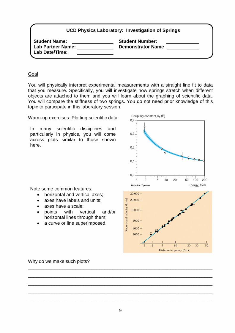
Goal You will physically interpret experimental measurements with a straight line fit to data that you measure. Specifically, you will investigate how springs stretch when different objects are attached to them and you will learn about the graphing of scientific data. You will compare the stiffness of two springs. You do not need prior knowledge of this topic to participate in this laboratory session. Warm-up exercises: Plotting scientific data In many scientific disciplines and particularly in physics, you will come across plots similar to those shown here. Note some common features:
horizontal and vertical axes;
axes have labels and units;
axes have a scale;
points with vertical and/or horizontal lines through them;
a curve or line superimposed.
Why do we make such plots? ______________________________________________________________________
______________________________________________________________________
______________________________________________________________________
______________________________________________________________________
______________________________________________________________________
10
What features of the graphs do you think are important and why? ______________________________________________________________________
______________________________________________________________________
______________________________________________________________________
______________________________________________________________________
______________________________________________________________________
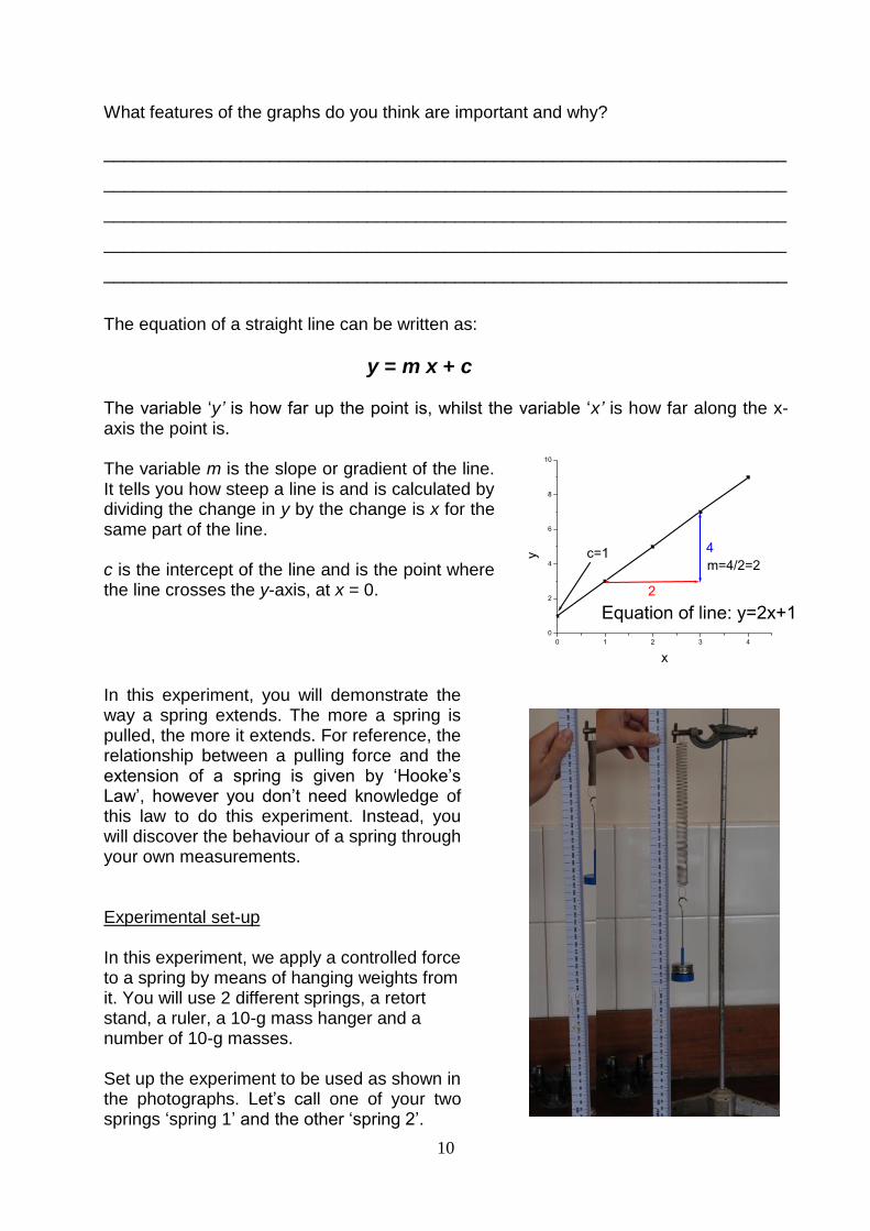
The equation of a straight line can be written as:
y = m x + c The variable ‘y’ is how far up the point is, whilst the variable ‘x’ is how far along the x-axis the point is. The variable m is the slope or gradient of the line. It tells you how steep a line is and is calculated by dividing the change in y by the change is x for the same part of the line. c is the intercept of the line and is the point where the line crosses the y-axis, at x = 0.
In this experiment, you will demonstrate the way a spring extends. The more a spring is pulled, the more it extends. For reference, the relationship between a pulling force and the extension of a spring is given by ‘Hooke’s Law’, however you don’t need knowledge of this law to do this experiment. Instead, you will discover the behaviour of a spring through your own measurements. Experimental set-up In this experiment, we apply a controlled force to a spring by means of hanging weights from it. You will use 2 different springs, a retort stand, a ruler, a 10-g mass hanger and a number of 10-g masses. Set up the experiment to be used as shown in the photographs. Let’s call one of your two springs ‘spring 1’ and the other ‘spring 2’.
11
Calculate the natural (unstretched) length of spring 1: _______________ Calculate the natural (unstretched) length of spring 2: _______________ The spring stretches when you add the mass hanger and masses to it. We will call the difference between the natural and stretched length, the extension. Now you will collect all your data. Then you will interpret the data graphically. Procedure and Data Borrowing the adage from DIY, “Measure twice and cut once”, it is good practice in science to take a measurement more than once and preferably many times. It is a typical scientific process to take data whilst increasing a (controlled) parameter and then again whilst decreasing that parameter. This is one way of taking a measurement twice and this way is also good in that it serves to see if something has changed with the equipment over time. In the case of your spring, it might elongate permanently to a degree if over-stretched. So this method is what you are asked to apply here, where the controlled parameter is the mass on the spring. Add the mass hanger then the 10-g disks one at a time whilst measuring the revised length of the spring. Once all your masses have been added, continue taking measurements whilst removing one mass off at a time. Fill in the following tables.

12
Measurements for spring 1:
Object Added
Total mass added to the spring (g)
Spring extension whilst adding masses, in cm (plot as crosses)
Spring extension whilst removing masses, in cm (plot as dots)
Nothing 0
Hanger 10
Disk 1 20
Disk 2 30
Measurements for spring 2:
Object Added Total mass added to the spring hanger (g)
Spring length whilst adding masses in cm (plot as crosses)
Spring length whilst taking away masses, in cm (plot as dots)
Nothing 0
Hanger 10
Disk 1 20
Disk 2 30
Results Add the data you have gathered for both springs to your graph on the following page. You should plot the extension of the spring in centimetres on the vertical y-axis and the total mass added to the hanger in grams on the horizontal axis. Plot your first column points as crosses and your second column of points as dots (small solid circles). You might also differentiate these with different colour pens if you are able. Suggested is for you to start the y-axis at say -10 cm. Choose a scale that is simple to read and that spreads the data across the page. Label your axes and give them units, something you should always do even if not asked. Include other features of the graph that you consider important.

13
Plot your graph by hand on this page and make your best estimate for a straight line fit to your data. Note, your tutor will account for fitting done by hand. Alternatively you can print your graph electronically (see appendix 1) and attach your printed graph to this page, annotated as necessary.
14
Fit a straight line as best as you can to your data for each of the two springs (2 lines in total). Do this by eye. Your tutor will account for your fitting by hand. Note: we want to examine how a spring extends as a function of the mass hanging from it. For this, it’s only useful to fit a line to data from where the spring starts to extend. A straight line is the simplest curve to fit to data. For this experiment, we will assume that your data follows a straight line for each spring, once it starts to extend. In everyday language we may use the word ‘slope’ to describe a property of a hill. For example, we may say that a hill has a steep or gentle slope. Generally, the slope tells you how much a value on the y-axis changes for a change on the x-axis.
As discussed in the ‘warm-up’, a straight line can be described by y = mx + c, where m is the steepness (slope) of the line i.e., the change in y divided by the change in x for the line, and c is the y-value where the line intercepts (crosses) the y-axis i.e., where x = 0. Note that c is not the same intercept that we calculated above, which was for where the line crosses the x-axis. Calculate the slopes of the two lines that you have drawn (fitted by eye) for each of springs 1 and 2. Also provide correct units for your slopes in terms of grams and centimetres.
______________________________________________________________________
______________________________________________________________________
______________________________________________________________________
______________________________________________________________________
______________________________________________________________________
Use the slopes of these two lines to compare the stiffness of the springs and explain. ______________________________________________________________________
______________________________________________________________________
______________________________________________________________________
______________________________________________________________________
______________________________________________________________________
______________________________________________________________________
______________________________________________________________________

15
Physically interpret the meaning of your c-values i.e., the values of y where your fitted lines intercept the y-axis. ______________________________________________________________________
______________________________________________________________________
______________________________________________________________________
______________________________________________________________________
______________________________________________________________________
______________________________________________________________________
Look at the example graphs given in the earlier ‘warm-up exercises’ section and in Appendix 1. Horizontal and vertical error-bars through data points are used to represent experimental uncertainty. They can be derived from a variation in values where taking measurements say 10 times or more, or from determining a precision from known accuracies of instruments. The first way of actually measuring an accuracy, is better. In this experiment, uncertainty in the masses is insignificant, but there may be uncertainty in the length measurements. To consider errors in your length measurements, compare your data taken where adding weights (first column of your data tables) to that taken where taking away weights (second column of your data tables). Estimate (don’t calculate) by how much these two columns of data differ for each of spring 1 and spring 2. Do this by inspecting your graphs or tables. ______________________________________________________________________
______________________________________________________________________
______________________________________________________________________
Is this observed uncertainty in length larger or smaller than that determined from the accuracy of your ruler? Discuss. ______________________________________________________________________
______________________________________________________________________
______________________________________________________________________
16
Conclusion The behaviour of springs is said to be ‘linear’. Explain this more clearly with reference to your responses and graphs in this lab. ______________________________________________________________________
______________________________________________________________________
______________________________________________________________________
______________________________________________________________________
______________________________________________________________________
______________________________________________________________________
______________________________________________________________________
______________________________________________________________________
______________________________________________________________________
Implications An ear receives small forces from sound waves that result in small mechanical deviations of the eardrum and the mechanics behind it (the ossicles). Even though the coupling mechanisms are complex, remarkably maybe, these deviations still approximate to being linear with the applied force. Where the ear drum stiffens in aging, hearing declines. Explain your reasoning referring to what you have learned in this laboratory. ______________________________________________________________________
______________________________________________________________________
______________________________________________________________________
______________________________________________________________________
______________________________________________________________________

17
The deviation of a car suspension can be considered ‘linear’ with an applied force. Car 1 is twice as heavy as car 2 and it compresses its suspension by one third as much as car 2. Comment on the relative stiffness of the suspensions referring to what you have learned in this laboratory. ______________________________________________________________________
______________________________________________________________________
______________________________________________________________________
______________________________________________________________________
______________________________________________________________________

18

19

20
UCD Physics Laboratory: Investigating the Behaviour of Gases Student Name: Student Number: Lab Partner Name: Demonstrator Name Lab Date/Time:
Goal You will experimentally investigate the validity of a physical law. After this session, you will have more understanding of the process of experimental verification, and how the law you are testing is relevant to everyday experiences. Specifically, you will test the Ideal Gas Law relating three variables of Volume, Pressure and Temperature using containers of air. To do this, you will keep one quantity fixed so that you can investigate how two other variables are related. In the first part you will keep the temperature constant and vary the volume to see how the pressure changes. In the second part you will keep the volume constant and vary the temperature to see how the pressure changes. Warmup exercises In this laboratory session, we investigate the relationship between the three properties of gases that we can most readily sense: volume, temperature and pressure. We call these macroscopic properties. But we understand that these properties derive from the movement of individual atoms/molecules (microscopic behaviour) that make up a gas, which move randomly, colliding with each other and the sides of the container.
Pressure, P. The motion of billions of billions of gas particles in a container, causes them to collide with each other and with the sides of their container. In doing so they push on the sides of the container and we measure this as a pressure. For pressure, we use the S.I., unit of a force divided by an area, N/m2 which is also called the Pascal, Pa.
Volume, V. A gas is a collection of atoms and/or molecules that expands to fill any container of any shape. For volume, we use the S.I., unit of m3.
Temperature, T. When a container of gas is heated, energy is transferred to the gas from a source of heat. Both the temperature and the internal energy (U) of the gas
increase, and we find that T ∝ U. This internal energy is in the form of a kinetic (motion) energy for the molecules. The molecules move faster as the temperature of a gas increases. Likewise, when a gas is cooled, the molecules slow down.

21
Using the above information, circle the correct answers below:
If you heat a gas, do the molecules move faster or slower? faster / slower If moving faster, do the molecules collide with the container walls more, or less, frequently?
more / less
If the molecules collide more frequently with the container walls, does the pressure increase or decrease?
increase / decrease
If you increase the container volume, are molecular collisions more or less frequent?
more / less
If the molecules collide less frequently, does the pressure increase or decrease?
increase / decrease
Clearly, all three gas properties are interconnected, but how? If we keep one property fixed, we can investigate the relationship between the other two. For example: If we keep the gas temperature fixed, we can see how changes in volume affect pressure.
If we keep the gas volume fixed, we can see how changes in temperature affect pressure.
These two relationships were first investigated by Irish scientist, Robert Boyle (1662), and French chemist, Gay-Lussac (1701). From the above information, can you figure out what remaining relationship was investigated by French scientist, J Charles (1780)?
A relationship between measurable quantities that is demonstrated experimentally and repeated in different ways over many years, can be said to be a physical law. Three scientists proved three relationships between the gas properties, leading to:
Boyle’s Law relating P and V.
Gay-Lussac’s Law relating P and T
Charles’ Law relating V and T
Since these three relationships are interconnected, we can combine them and we call the combined relationship the Ideal Gas Law, which is given by:
𝑃𝑉 = 𝑛𝑅𝑇 where the constant of proportionality is the product of two constants, nR, where n is the number of moles of gas atoms/molecules there are and R is the ideal gas constant. Let’s now explore these ideas with two experiments.

22
Experiment 1: How the pressure of a gas changes when its volume is changed
Apparatus A pressure
gauge, with a scale in units of pressure i.e. pascals (Pa).
A sealed glass tube of gas (air), with a volume scale marked in either 1 cm3 (1 mL, a millilitre) or 10 cm3 (10 mL) steps. If the units aren’t stated on the tube, you are able to tell which of these scale-units you have from considering the tube radius and so estimating a volume.
Procedure Open the tap (by turning it to a position parallel to the tube). Note the pressure reading. This
is your baseline pressure; the pressure of the air all around us.
Twist the adjustable screw to move the stopper to about a fifth of the way along the tube (as shown in the picture). This is simply a practical starting point for the number of readings to be conducted within the timeframe for the experiment.
Close the tap to define a fixed amount/mass of gas. Record the baseline pressure.
Twist the adjustable screw so that the stopper reduces the volume that the gas can occupy within the tube. As you do, notice what happens to the pressure reading. Take readings of pressure as you reduce the volume.
Estimate the accuracy of your measurements of volume and pressure.
Open the tap, to release pressure, and unscrew the stopper to return it to its original position.
Note: the equipment is only designed to work up to the maximum pressure on the scale. Keep below this pressure.
Data
Volume (ml)
Pressure (Pa)
Estimate of error in Volume
measurements (ml)
Estimated Error in Pressure
measurements (Pa)
Volume scale

23
Plot our data on this page, preferably by hand. Note your tutor will account for fitting where done by hand. Alternatively you can print graphs electronically (see appendix 1) and attach your two printed graphs to this page, annotated as necessary. Include abscissa and ordinate error bars on at least your first two and last two data points of each graph to represent your estimated errors (see appendix 1). Take care to label axes correctly and include units. Plot P along the y-axis, as a function of V along the x-axis:
Plot P along the y-axis, as a function of 1/V along the x-axis:

24
From your graphs, describe how the gas properties are related. Is there a linear relationship between any two variables i.e., does a straight line fit to your points?
A straight-line graph is given by the equation y = m x + c, where m is the slope and c is the value of y where the line intercepts the y-axis i.e., where x = 0. Determine this intercept value, c for your straight-line graph and give this value here including units.
Would you expect this intercept to be at the origin where P = 0 and 1/V = 0? Discuss.
Conclusion We investigated the relationship between pressure and volume, where temperature is held constant. This is Boyle's Law. From this experiment, briefly state this relationship in
your own words and state if this is consistent with the Ideal Gas Law, for which 𝑃𝑉 ∝ 𝑇.
Implications When we inhale, we lower the diaphragm muscle to increase the volume of our lungs. When we exhale, we raise the diaphragm to decrease the volume. Relate this to differences in pressure between the inside and outside of the lungs with the aid of Boyle's Law (the Ideal Gas Law).
Explain another everyday example that relates pressure and volume (for a temperature that’s approximately fixed), using the Ideal Gas Law.

25
Experiment 2: How the pressure of a gas change when its temperature is changed
Apparatus
A sealed container of gas (air) plus an internal heater.
A white box containing connections to temperature and pressure sensors.
Two multi-meters, one to read pressure and one to read temperature.
Procedure
Ensure all connections are in place (see picture).
Turn the dial on the “pressure” multi-meter to V (volts), and press the “range” button until it is set to the millivolt (mV) range. You can record mV as a proxy for the units of pressure, Pascals (Pa). Set the “temperature” multi-meter to degrees Celsius (oC).
Turn on the sensors, by checking that the white box is plugged in and then flipping the switch so that its light comes on. Record the temperature and pressure, as per the multi-meters.
Turn on the heater. For this, first check that the large transformer is plugged in and then press the on-switch. At this point the gas is being heated and you will notice the temperature readings will slowly increase.
Take temperature and pressure readings at intervals of about 5 oC until the temperature reaches about 80 oC. Then immediately switch off the heater by pressing the green button.
Estimate the accuracy of your measurements of temperature and pressure.
Turn off all equipment, by returning switches to original positions and disconnecting power.
Data
Temperature (oC)
Pressure (Pa)
Estimated error in Temperature
measurements (oC)
Estimated Error in Pressure
measurements (Pa)
Electronics
Gas container
and heater
Pressure
sensor

26
Results Plot pressure, P, (y-axis) as a function of temperature, T in oC (x-axis), preferably by hand. Note your tutor will account for fitting where done by hand. Alternatively you can print graphs electronically (see appendix 1) and attach your two printed graphs to this page, annotated where necessary. Include abscissa and ordinate error bars on at least your first two and last two data points of each graph to represent your estimated errors (see appendix 1). Take care to label axes correctly and include units.

27
From your graph, describe how the gas properties of pressure and temperature are related. Would you say there a linear relationship between any two variables i.e., does a straight line fit to your points?
Fit a straight line to your plot as well as you can by eye. A straight-line is given by the equation y = m x + c, where m is the slope and c is the value of y where the line intercepts the y-axis i.e., where x = 0. Determine m and c for your fitted straight-line and give these values here, including units.
From your values of m and c, determine a value of temperature in oC for which P extrapolates to zero. Let’s call this temperature, T0.
In everyday language, describe what the molecules of the gas would be doing at this temperature, T0 (for which P = 0)?
Conclusion We investigated the relationship between pressure and temperature, where volume is held constant. This is Gay-Lussac’s Law. From this experiment, briefly state this relationship in your own words.
Explain how your measurements are consistent with the Ideal Gas Law, for which
𝑃𝑉 ∝ 𝑇.

28
Implications Car tyres increase in pressure by 3 x10⁴ N/m2 after driving for 20 mins. Explain this with the aid of the Ideal Gas Law
A jam jar can be easier to open after warming it up in a bowl of hot water. Explain this with the aid of the Ideal Gas Law.
Explain another everyday example that relates pressure and temperature (for a volume that’s approximately fixed), using the Ideal Gas Law.

29

30
31
UCD Physics Laboratory: Investigation of Acceleration Student Name: Student Number: Lab Partner Name: Demonstrator Name Lab Date/Time:
Goal You will experimentally investigate the validity of a physical law. After this session, you will have more understanding of the process of experimental verification, and how the law you are testing is relevant to everyday experiences. You do not need prior knowledge of this topic to participate in this laboratory session. Specifically, you investigate test Newton's 2nd Law, a law relating three variables of force, mass and acceleration, using a cart on a track. It is useful to keep one quantity fixed so that you can investigate how two other variables are related. To do this, you will keep a force fixed along the direction of motion, and relate an acceleration to a mass. Warmup exercises
Newton’s second law is given by the vector relationship, amF , for which a force causes an acceleration and the constant of proportionality is mass, m. However, for motion confined to a straight line (one dimensional motion), we can simplify this law to the scalar relationship, F = m a, where F is the value of the net force acting on an object along its allowed direction of motion, and a is the value of acceleration in this direction of motion. We consider only motion in a straight line in this laboratory and so we are able to use this scalar form of the law.
If you throw a heavy ball with a force F and then throw a light ball with the same force, which ball gathers more speed? heavy/light Acting under constant acceleration, a cart starts from rest and has a speed of 2 m/s after 5 s. What is the acceleration of the cart? _________
Forces cause acceleration. For example if you kick a ball of mass m with a force 'F', its acceleration is 'a'; if you then kick the same ball with a force twice as big, '2F', then it accelerates at '2a'. In other words, the acceleration, a, is larger when the force, F, is larger:
𝑎 ∝ 𝐹 The acceleration is larger when the mass, m, of the object is smaller:
𝑎 ∝ 1
𝑚
We can combine these two relationships into one:
𝑎 ∝ 𝐹
𝑚
32
Isaac Newton (1687) provided experimental evidence of this relationship, and so it became a 'Law'. It is now called Newton's 2nd Law, and is more commonly written as:
𝐹 = 𝑚 𝑎 The unit of force is kg·m/s2 which is called the Newton (symbol N), in honour of Isaac Newton. If an apple falls from a tree, it speeds up until it hits the ground. So there must be a force which causes this acceleration. The acceleration due to the Earth's gravitational
force field has been measured experimentally to be 9.8 m/s2. We denote this as '𝑔' since its value is always the same, instead of generic acceleration '𝑎' (which can have many values). So the gravitational force is the product, 𝑚𝑔. To test Newton's 2nd Law, you will keep one quantity fixed so that you can investigate how two other variables are related. Specifically, you will keep the force fixed and relate a horizontal acceleration to a mass which is varied. Apparatus
One cart, of mass 0.5 kg
A low-friction track, with a pulley wheel on one end
A string, with a ring weight tied to one end and a hook to the other, threaded over the pulley wheel with the hook attached to the cart.
Two photogates connected to a blue data-logger
Three metal bars, of mass 0.5 kg each, which can be added to the cart to increase its mass
Where using a pulley, the string has an equal tension throughout. This simplifies our thinking, because we can consider the stage as being accelerated horizontally due to a constant horizontal force of magnitude, F, and we also consider F to be the magnitude of force exerted vertically between the string and the ring-weight. We return to this with an equation later.

33
Experiment: Acceleration from a constant force along a horizontal plane
Experimental set-up
Fig 1
i) Setting up the cart on the track: Position the track on the laboratory bench in such a way that the pulley wheel hangs
over one end of the bench.
Ensure the track is level. This is done via an adjustable leg at one end.
Place the cart on the track at the opposite end to the pulley wheel.
You will find a string, with a ring tied to one end and a hook tied to the other. Attach the hook to the cart and thread the string over the pulley wheel so that the ring hangs down. The weight of the ring will accelerate the cart along the track.
Insert the rectangular metal "flag" into the hole at head of the cart, with the largest surface facing you. Make sure the flag is secure and does not move. (This can be achieved by lifting it slightly out of the hole). The role of the flag is to interrupt the light beam of the photogates (see below).
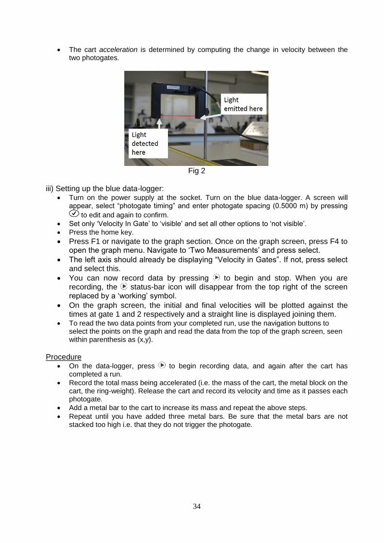
ii) Setting up the two photogates:
The photogates comprise an infrared light source on one side, and a detector on the other, fig 2. Infrared light is invisible to the human eye but is represented by the red line in the figure. When the beam is interrupted it sends a signal to the blue data-logger.
Place the photogates at positions 30 cm and 80 cm on the track. In this way, the distance between the gates is 50 cm.
In order to calculate acceleration, we must measure the change in velocity in a given time interval.
The velocity is determined by how long the cart's metal flag takes to move past a given photogate. The photogate is connected to a blue data-logger, which reports how long the beam is interrupted for (i.e. time). It then uses the width of the flag (i.e. distance) to estimate the velocity of the cart. For this reason, we must input the width of the flag (or flag length) when we set up the data-logger (below). The cart velocity is calculated from how long it takes its flag to pass through the photogate beam. To output these results, the blue data-logger must be set up correctly (see below).
34
The cart acceleration is determined by computing the change in velocity between the two photogates.
Fig 2
iii) Setting up the blue data-logger:
Turn on the power supply at the socket. Turn on the blue data-logger. A screen will appear, select “photogate timing” and enter photogate spacing (0.5000 m) by pressing
to edit and again to confirm.
Set only ‘Velocity In Gate’ to ‘visible’ and set all other options to ‘not visible’.
Press the home key.
Press F1 or navigate to the graph section. Once on the graph screen, press F4 to open the graph menu. Navigate to ‘Two Measurements’ and press select.
The left axis should already be displaying “Velocity in Gates”. If not, press select and select this.
You can now record data by pressing to begin and stop. When you are recording, the status-bar icon will disappear from the top right of the screen replaced by a ‘working’ symbol.
On the graph screen, the initial and final velocities will be plotted against the times at gate 1 and 2 respectively and a straight line is displayed joining them.
To read the two data points from your completed run, use the navigation buttons to select the points on the graph and read the data from the top of the graph screen, seen within parenthesis as (x,y).
Procedure
On the data-logger, press to begin recording data, and again after the cart has completed a run.
Record the total mass being accelerated (i.e. the mass of the cart, the metal block on the cart, the ring-weight). Release the cart and record its velocity and time as it passes each photogate.
Add a metal bar to the cart to increase its mass and repeat the above steps.
Repeat until you have added three metal bars. Be sure that the metal bars are not stacked too high i.e. that they do not trigger the photogate.

35
Data:
Mass of ring, mring
(kg)
Mass of cart, mcart
(kg)
Velocity
1, 𝑣1 (m/s)
Velocity
2, 𝑣2 (m/s)
Time 1,
𝑡1 (s)
Time 2,
𝑡2 (s)
Acceleration, a
(m/s2)
Calculate the acceleration (i.e. the change in velocity during a given time interval):
𝑎 = 𝑣2 − 𝑣1
𝑡2 − 𝑡1
On the blue data-logger, use the arrow keys to highlight your data file in the RAM memory and press “F4 files”. Select the “copy file” option and then choose the external USB as the destination for the file, and press “F1 OK”. Before transferring the USB data stick to the lab computer to create a graph, we must decide what to put on the x and y axes (see below).
Results
If Newton's 2nd Law is indeed, 𝐹 = 𝑚 𝑎, it will plot as a straight line i.e., it will take the form:
𝑦 = 𝑘 𝑥 + 𝑐 where k is the gradient (slope), and c is what we will call the intercept (the value of y where x is zero). Here we refer to k instead of the traditional m for the gradient of a straight line, because we have already used m to mean mass. In this investigation, we kept the force constant and increased the mass in order to investigate how acceleration changes. Therefore, we put mass on the x-axis and acceleration on the y-axis. How can we rearrange Newton's 2nd Law into the mathematical format of a straight line graph, where the x-axis is the mass and the y-axis is the acceleration?
We could rearrange 𝐹 = 𝑚 𝑎 into the format 𝑦 = 𝑘 𝑥 + 𝑐 as follows:
1
𝑎 =
1
𝐹 𝑚
where a is acceleration, F is force, m is mass and c = 0
36
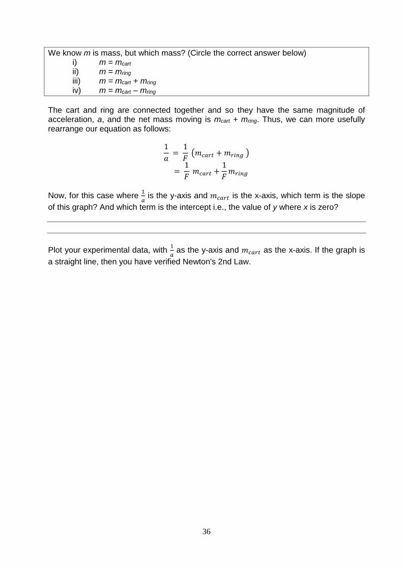
We know m is mass, but which mass? (Circle the correct answer below) i) m = mcart ii) m = mring iii) m = mcart + mring iv) m = mcart – mring
The cart and ring are connected together and so they have the same magnitude of acceleration, a, and the net mass moving is mcart + mring. Thus, we can more usefully rearrange our equation as follows:
1
𝑎 =
1
𝐹 (𝑚𝑐𝑎𝑟𝑡 + 𝑚𝑟𝑖𝑛𝑔 )
= 1
𝐹 𝑚𝑐𝑎𝑟𝑡 +
1
𝐹𝑚𝑟𝑖𝑛𝑔
Now, for this case where 1
𝑎 is the y-axis and 𝑚𝑐𝑎𝑟𝑡 is the x-axis, which term is the slope
of this graph? And which term is the intercept i.e., the value of y where x is zero?
Plot your experimental data, with 1
𝑎 as the y-axis and 𝑚𝑐𝑎𝑟𝑡 as the x-axis. If the graph is
a straight line, then you have verified Newton's 2nd Law.

37
Plot your graph by hand on this page and make your best estimate for a straight line fit to your data. Note, your tutor will account for your fitting by hand. Important: take care to label axes correctly and include units.
38
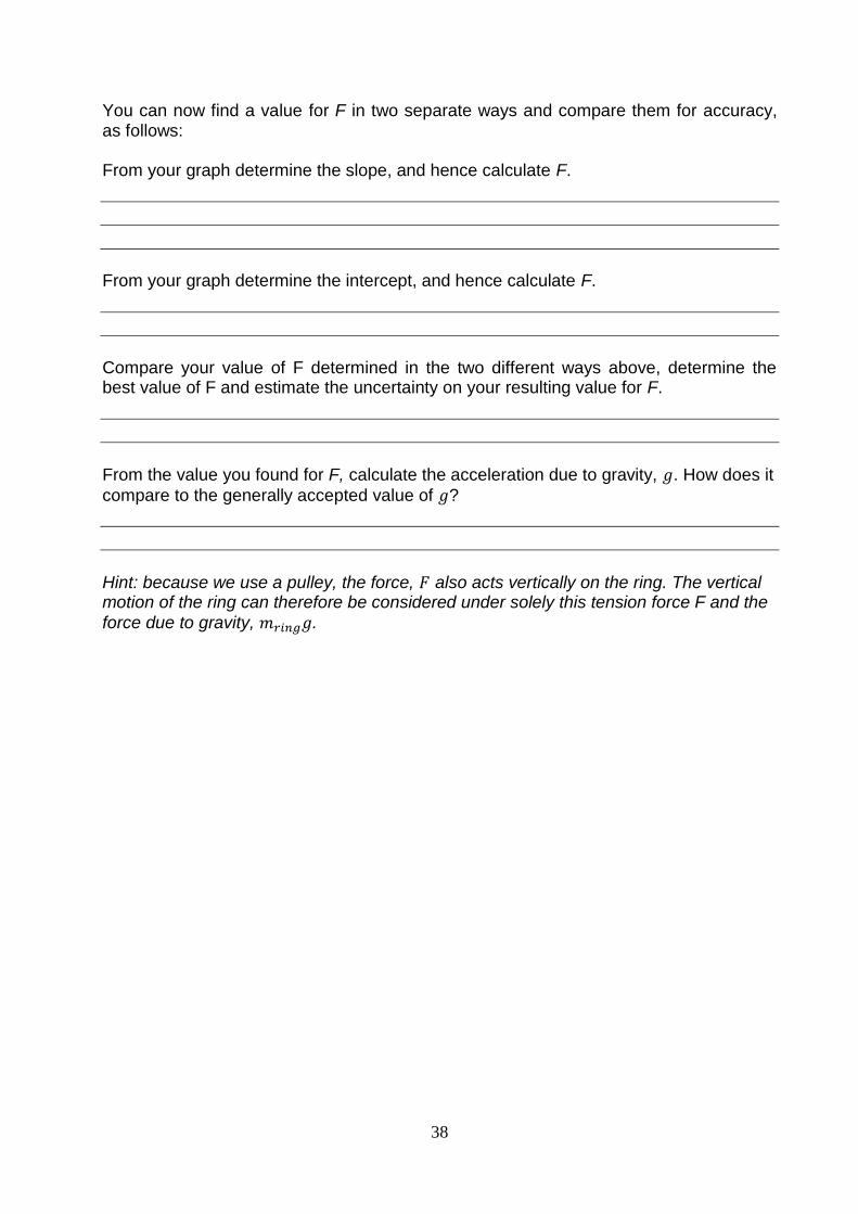
You can now find a value for F in two separate ways and compare them for accuracy, as follows: From your graph determine the slope, and hence calculate F.
From your graph determine the intercept, and hence calculate F.
Compare your value of F determined in the two different ways above, determine the best value of F and estimate the uncertainty on your resulting value for F.
From the value you found for F, calculate the acceleration due to gravity, 𝑔. How does it
compare to the generally accepted value of 𝑔?
Hint: because we use a pulley, the force, 𝐹 also acts vertically on the ring. The vertical motion of the ring can therefore be considered under solely this tension force F and the
force due to gravity, 𝑚𝑟𝑖𝑛𝑔𝑔.
39
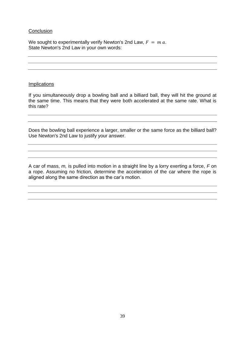
Conclusion
We sought to experimentally verify Newton's 2nd Law, 𝐹 = 𝑚 𝑎. State Newton's 2nd Law in your own words:
Implications If you simultaneously drop a bowling ball and a billiard ball, they will hit the ground at the same time. This means that they were both accelerated at the same rate. What is this rate?
Does the bowling ball experience a larger, smaller or the same force as the billiard ball? Use Newton's 2nd Law to justify your answer.
A car of mass, m, is pulled into motion in a straight line by a lorry exerting a force, F on a rope. Assuming no friction, determine the acceleration of the car where the rope is aligned along the same direction as the car’s motion.

40

41
42
UCD Physics Laboratory: Investigation of Heat Capacity Student Name: Student Number: Lab Partner Name: Demonstrator Name Lab Date/Time:
Goal You will experimentally investigate the validity of a physical law relating heat and temperature. After this session, you will have more understanding of the process of experimental verification, and how the law you are testing is relevant to everyday experiences. You do not need prior knowledge of this topic to participate in this laboratory session. Specifically, you will determine the heat capacity of two metals from measurements you make of their temperature on being heated and you will consider experimental errors. Warm-up exercises Heat can be thought of as energy that flows from one object to another due to their temperature difference. We will use the variable, Q for an amount of heat and this is in units are Joules, J. When we heat an object, we increase the object’s internal energy and as a result let’s say we increase its temperature, T by an amount, ∆𝑇.
Heat Capacity for an object is defined as 𝑄/∆𝑇. So where different objects, of different forms and materials, experience different increases in temperature after receiving the same amount of heat, we can say that they have different Heat Capacities.
Which do you think takes more energy, to heat a bath of water from 20 oC to 30 oC, or to heat a cup of coffee from 20 oC to 30 oC? Bath / Coffee
For the same value of ∆𝑇, two identical objects where combined will require double the amount of heat as just one of the objects. This is required for the law of Conservation of Energy to be obeyed. It follows that it takes more heat to increase the temperature of a more massive object, and we find that the heat capacity for an object depends on its mass. To best define a property for a material, we use the idea of Specific Heat Capacity, which is the Heat Capacity per kilogram of the material. As such, Specific Heat Capacity, c is defined as:
𝑐 = 𝑄
𝑚 ∆𝑇
where the heat supplied is Q in units of Joules, the mass is m in units of kg, the
temperature change is ∆𝑇 in units of degrees Celsius, oC, or equivalently in Kelvin, K, given this is a temperature difference. We can see from this equation that the Specific Heat Capacity is the energy transferred to raise the temperature of a 1 kg object by 1 oC (or 1 K).

43
Write here the units for specific heat capacity, worked out from its definition in the previous equation:
In this laboratory session, we will add an amount of heat, Q, to a metal sample of known mass, m and measure the resulting temperature, T. From this, we will calculate the specific heat capacity, c. We will do this for an aluminium block and for a copper block. Then we will consider errors in that measurement. Safety
Do not place the metal blocks or the heating element directly onto the lab bench. Use an insulating mat.
Take care when handling the metal blocks and the heating element, as they can be hot.
Switch off all of the apparatus when you have completed the experiment.
Apparatus
Power supply
Joule-Watt meter (meter which measures energy)
Heating element (metal rod/element which inserts into the centre of the metal blocks)
Aluminium block, mass 1 kg
Copper block, mass 1 kg
Thermometer
Stop-watch
Experiment: Measuring the heat capacity of two metals, aluminium and copper

44
Experimental Set-up We will use electricity to generate heat. As current flows through the heating element, its temperature increases.
Place the heating element into the central hole of the metal block. Start with the aluminium block.
We then need to connect the heating element to the power supply. To measure the amount of heat energy generated, in Joules, we conveniently have a ‘Joule-meter’ in our circuit.
Connect the positive (red) and negative (black) sockets of the Joule-meter to the positive and negative sockets of power supply.
Connect the two wires of the heating element to the Joule-meter where it says ‘load’. Be aware of the positive and negative polarity.
Set the power supply to 12 volts DC.
Insert the thermometer into the other hole in the metal block to allow measurement of temperature in oC.
Procedure
Four sets of measurements will be taken. First whilst heating and then cooling the aluminium block and then whilst heating and then cooling the copper block.
Press reset on the Joule-Watt meter, reset and start the timer.
Record the initial temperature of the block, T0, at time t = 0.
Switch on the power supply and start the timer.
Insert the heating element as far as possible into the block.
Record the energy, Q in Joules supplied to the heating element using the Joule-meter.
Record temperatures at the times set out on the following tables. The maximum time for each table is t1.
When you have reached the maximum heating time for each table, switch off the power supply and take out the heating element. Then reset the timer and starting from time, t = 0, begin recording measurements of the temperature as a function of time as the block cools.
Be sure to not exceed a temperature rise of 30 deg for any reason and always switch off the heating apparatus when not in use.

45
Data Record your data below. Time is valuable, so start plotting your Al data whilst you are taking your Al cooling data and so on. Also you might share the data taking, freeing one person to measure data whilst the other plots.
Al (Aluminium) heating Cu (Copper) heating
Time, t (mins)
Heat transferred,
Q (J)
Temp, T (oC)
Time, t (mins)
Heat transferred,
Q (J)
Temp, T (oC)
0 0
2 1
4 2
6 3
8 4
10 5
12 6
14 (t1) 7 (t1)
Al Cooling (no heating) Cu Cooling (no heating)
Time, t (mins)
Temp, T (oC)
Time, t (mins)
Temp, T (oC)
0 0
2 1
4 2
6 3
8 4
10 5
12 6
14 (t1) 7 (t1)
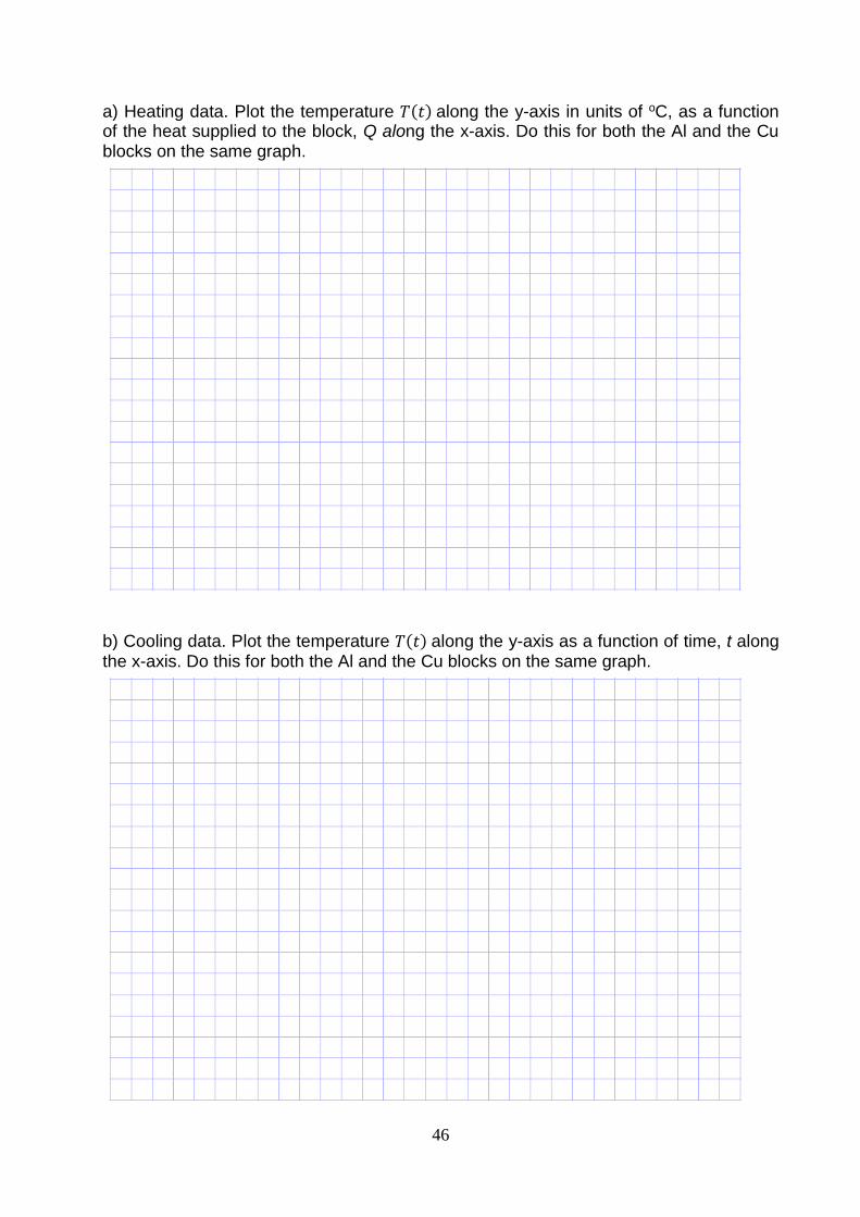
Be sure to turn off the equipment when you have finished taking data. Results Make plots by hand on the following page. Label axes correctly and include units. Note, your tutor will account for fitting done by hand.
46
a) Heating data. Plot the temperature 𝑇(𝑡) along the y-axis in units of oC, as a function of the heat supplied to the block, Q along the x-axis. Do this for both the Al and the Cu blocks on the same graph.
b) Cooling data. Plot the temperature 𝑇(𝑡) along the y-axis as a function of time, t along the x-axis. Do this for both the Al and the Cu blocks on the same graph.
47
For plot ‘a’, describe the relationship between the parameters, 𝑇 and Q.
For plot ‘a’, determine the slopes for your best straight-line fits to your Al and Cu points. Give these values here, including units:
Al: ____________ Cu: ____________ A general straight-line graph is given by the equation y = n x + k, where n is the gradient (slope) and k is the value of y where the line intercepts the y-axis i.e., where x = 0. Note, it’s more typical to refer to ‘m’ and ‘c’ for the gradient and intercept, but you’ll remember we are already using these variables for defining Specific Heat Capacity,
c = Q
m ∆T. Taking ΔT = T - To and rearranging:
𝑇 = (1
𝑚𝑐) 𝑄 + 𝑇0
From inspecting this equation, what can you expect gradients in your graph ‘a’ to be equivalent to in terms of mass, m and specific heat capacity, c.
Now from your estimated gradients, calculate the specific heat capacity, c¸ of the two metals and fill them in below.
Metal Specific Heat Capacity, c, as measured by you in units of J kg-1 oC-1
Specific Heat Capacity, c, generally accepted values
in units of J kg-1 oC-1
Aluminium 960
Copper 385
Accounting for errors Your results likely differ from the generally accepted values given, but then we have yet to consider sources of error. An inspection of your plot ‘b’ for when the blocks are cooling, should convince you that heat is being lost from the blocks when they are hot. So this will surely be happening when you are heating them too (plot ‘a’). This heat transfer out of the block is due to air-convection (going to air) and radiative emission (going to infrared light). This makes for a reproduceable error in our above measurement of heat capacity and so is called more generally, a systematic error. Let’s now take this into account and see if we can remove this error.
48
Compare the gradients of the two cooling plots on graph ‘b’. Which of the blocks cool quicker? Explain why.
What is the temperature change, ΔTcool, where cooling the blocks over the full measurement time of t1 i.e., the difference between the initial and final measured temperatures on cooling:
Metal ΔTcool as measured for cooling, in oC
Aluminium
Copper
If the block was thermally insulated so preventing heat loss, then we expect the final temperature of the block to be greater than that measured, T(t1), by approximately the value, ΔTcool. If we call this revised final temperature, T(t1)’, then we can write:
T(t1)’ = T(t1) + ΔTcool. Calculate this revised final temperature, T(t1)’, for each block:
Metal T(t1)’, the final temp as predicted for heating insulated blocks, in oC
Aluminium
Copper
Mark these revised final temperatures, T(t1)’ as points at the respective times, t1 on plot ‘a’. Draw a line from each of these points to the respective starting points at time t = 0 for each metal. Using these now revised (steeper) gradients, calculate revised specific heat capacities, c’:
Metal Revised estimate of Specific Heat Capacity, c’,
in units of J kg-1 oC-1
Specific Heat Capacity, c, generally accepted values
in units of J kg-1 oC-1
Aluminium 960
Copper 385
Estimates can be useful and we should just be clear on assumptions made. For the above estimate, we are assuming that the rate of heat loss is the same in both cases of heating and cooling.

49
Does heat loss to the surroundings explain the difference between your original measured values for heat capacities and the generally accepted values? Explain this based on your data.
Compare your estimate of heat capacities to others around you in the lab. You will find a variation. Propose and explain a likely physical mechanism for this.
Conclusions In this experiment, we explored the relationship between heat and temperature and we measured the specific heat capacity, c, for two metals. We then revised these values by taking into account the effects of the blocks losing heat to the surroundings whilst they are being heated. Heat and temperature are often confused in everyday life. We might hear it said that the ‘fridge door was opened and the cold got out’, or ‘the water in the kettle contains a lot of heat’. Clearly state what heat, Q, really is, so differentiating it from temperature.

50
Implications 1. An electric heater supplies 18 kJ of heat energy to a metal block of mass 0.5 kg. The temperature of the block rises from 20 oC to 100 oC during the heating process. Assuming that no heat is lost from the block during heating, determine the specific heat capacity of the metal. Show your working.
Ans. 450 J kg-1 oC-1 2. Estimate how much heat energy is required to boil just enough water to make two full cups of tea. Take a full cup to be 250 ml and take the heat capacity of water to be 4.2 kJ kg-1 oC-1. Show your working.
Ans. about 170kJ
3. Two kettles are identical except for their heating elements. One has a 0.5 kW heating element and one has a 4 kW heating element. Which is the more efficient and why?
Hint. Consider heat loss to the surroundings during the time of heating

51

52
53
UCD Physics Laboratory: Investigation of Fluid Flow Student Name: Student Number: Lab Partner Name: Demonstrator Name Lab Date/Time:
Theory
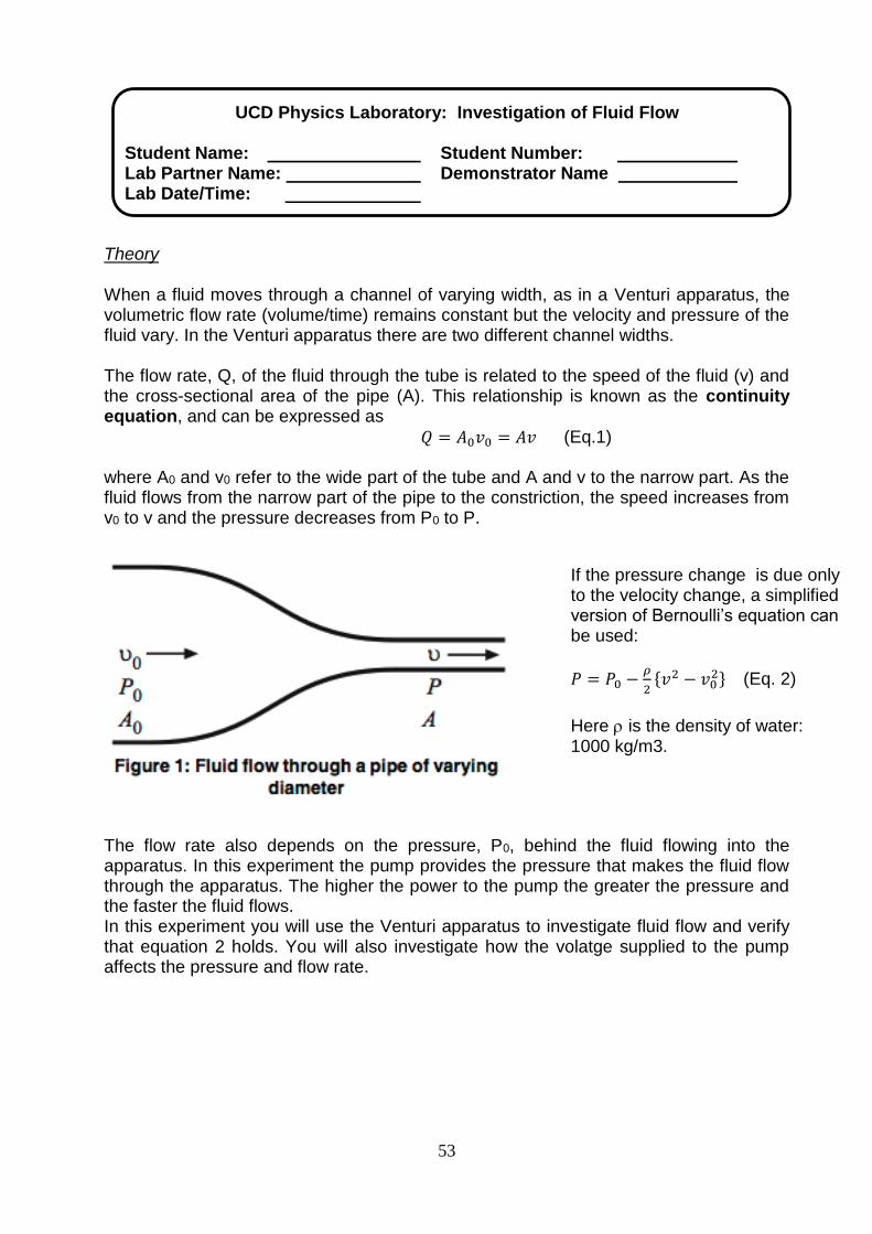
When a fluid moves through a channel of varying width, as in a Venturi apparatus, the volumetric flow rate (volume/time) remains constant but the velocity and pressure of the fluid vary. In the Venturi apparatus there are two different channel widths. The flow rate, Q, of the fluid through the tube is related to the speed of the fluid (v) and the cross-sectional area of the pipe (A). This relationship is known as the continuity equation, and can be expressed as
𝑄 = 𝐴0𝑣0 = 𝐴𝑣 (Eq.1)
where A0 and v0 refer to the wide part of the tube and A and v to the narrow part. As the fluid flows from the narrow part of the pipe to the constriction, the speed increases from v0 to v and the pressure decreases from P0 to P.
The flow rate also depends on the pressure, P0, behind the fluid flowing into the apparatus. In this experiment the pump provides the pressure that makes the fluid flow through the apparatus. The higher the power to the pump the greater the pressure and the faster the fluid flows. In this experiment you will use the Venturi apparatus to investigate fluid flow and verify that equation 2 holds. You will also investigate how the volatge supplied to the pump affects the pressure and flow rate.
If the pressure change is due only to the velocity change, a simplified version of Bernoulli’s equation can be used:
𝑃 = 𝑃0 −𝜌
2{𝑣2 − 𝑣0
2} (Eq. 2)
Here is the density of water: 1000 kg/m3.
54
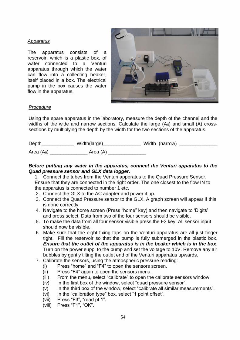
Apparatus
The apparatus consists of a reservoir, which is a plastic box, of water connected to a Venturi apparatus through which the water can flow into a collecting beaker, itself placed in a box. The electrical pump in the box causes the water flow in the apparatus.
Procedure
Using the spare apparatus in the laboratory, measure the depth of the channel and the widths of the wide and narrow sections. Calculate the large (A0) and small (A) cross-sections by multiplying the depth by the width for the two sections of the apparatus.
Depth____________ Width(large)______________ Width (narrow) ______________
Area (A0) ______________ Area (A) ______________
Before putting any water in the apparatus, connect the Venturi apparatus to the Quad pressure sensor and GLX data logger.
1. Connect the tubes from the Venturi apperatus to the Quad Pressure Sensor. Ensure that they are connected in the right order. The one closest to the flow IN to the apparatus is connected to number 1 etc. 2. Connect the GLX to the AC adapter and power it up. 3. Connect the Quad Pressure sensor to the GLX. A graph screen will appear if this
is done correctly. 4. Navigate to the home screen (Press “home” key) and then navigate to ‘Digits’
and press select. Data from two of the four sensors should be visible. 5. To make the data from all four sensor visible press the F2 key. All sensor input
should now be visible. 6. Make sure that the eight fixing taps on the Venturi apparatus are all just finger
tight. Fill the reservoir so that the pump is fully submerged in the plastic box. Ensure that the outlet of the apparatus is in the beaker which is in the box. Turn on the power suppl to the pump and set the voltage to 10V. Remove any air bubbles by gently tilting the outlet end of the Venturi apparatus upwards.
7. Calibrate the sensors, using the atmospheric pressure reading: (i) Press “home” and “F4” to open the sensors screen. (ii) Press “F4” again to open the sensors menu. (iii) From the menu, select “calibrate” to open the calibrate sensors window. (iv) In the first box of the window, select “quad pressure sensor”. (v) In the third box of the window, select “calibrate all similar measurements”. (vi) In the “calibration type” box, select “1 point offset”. (vii) Press “F3”, “read pt 1”. (viii) Press “F1”, “OK”.
55
Measure the time that it takes for 400 ml (0.4l = 4x10⁻⁴ m3) of water to flow through the Venturi apparatus. Be sure to read the water level by looking at the bottom of the meniscus. When the flow is steady note the pressures on the four sensors. Enter your data in the table. Repeat the measurements twice more. Be sure to return all the water to the reservoir (plastic box). Make sure that the apparatus stays free of air bubbles.
Run P1 /kPa
P2 /kPa
P3 /kPa
P4 /kPa
Time /s
1
2
3
Average
Calculate the flow rate, Q, volume/time, from the average value of the time taken for 400 ml to flow through the apparatus. 1ml = 1cm3 = 1x10⁻⁶ m3.
____________________________________________________________________
____________________________________________________________________
____________________________________________________________________
Use equation (1) and the cross-sectional areas that you calculcated to work out the velocity of the water in the wide (v0) and narrow (v) sections of the apparatus.
v0= ______________________________________________________________
v= ______________________________________________________________
Which is larger v or v0, is this what you expected?
____________________________________________________________________
____________________________________________________________________
If the apparatus was not constricted the pressure at point 2 (P0) is equal to the average value of P1 and P3. Use you average valies of P1 and P3 to calculate P0:
P0=1/2(P1+P3) _______________________________________________________
____________________________________________________________________

56
Use equation 2 and your values for P0,v0 and v to calculate a value for P, the pressure in the narrow section of the apparatus. The SI unit for pressure is the Pascal (Pa), 1kPa = 1000 Pa = 1000 N/m2 = 1000 kg s-2 m-1.
P= _________________________________________________________________
____________________________________________________________________
____________________________________________________________________
How does your value for the pressure in the constriction compare to the measured values P2 and P4? You might consider how precisely you can determine both the calculated and measured pressures.
_________________________________________________________________
____________________________________________________________________
____________________________________________________________________
____________________________________________________________________
____________________________________________________________________
____________________________________________________________________
Next measure the pressure as for five diferent pump supply voltages to the pump. Be sure to let the flow stabalise before taking your readings. Complete the table below.
Voltage /V
P1 /kPa
P2 /kPa
P3 /kPa
P4 /kPa Average of P1 and P3 /kPa
Average of P2 and P4 /kPa
5
6
8
10
12
When you have finished, allow the reservoir to run empty and tilt the Venturi apparatus to empty water from it. Once the apparatus is empty of water remove the pressure tubes from the sensor by gently twisting the white plastic collars that connected the hoses to the sensor (leave the tubes connected to the underside of the Venturi apparatus). Empty as much water as you can from the apparatus and then all of the water into the sink in the laboratory.
57
Plot the two average pressures on the same graph, as a function of pump voltage. Do this by hand on this page, or, use JagFit (see back of manual) and attach your printed graphs to this page. Label axes correctly and include units. Note, your tutor will account for fitting done by hand.

58
Comment on your graph, is it consistent with what you expected to happen? __________________________________________________________________
____________________________________________________________________
____________________________________________________________________
____________________________________________________________________
____________________________________________________________________
What can you conclude from this part of the experiment?
____________________________________________________________________
____________________________________________________________________
____________________________________________________________________
____________________________________________________________________
____________________________________________________________________
____________________________________________________________________
____________________________________________________________________
____________________________________________________________________
____________________________________________________________________
____________________________________________________________________

59

60

61
UCD Physics Laboratory: Investigation of Archimedes’ Principle
Student Name: Student Number: Lab Partner Name: Demonstrator Name Lab Date/Time:
Introduction All the technology we take for granted today, from electricity to motor cars, from television to X-rays, would not have been possible without a fundamental change, around the time of the Renaissance, to the way people questioned and reflected upon their world. Before this time, great theories existed about what made up our universe and the forces at play there. However, these theories were potentially flawed since they were never tested. As an example, it was accepted that heavy objects fall faster than light objects – a reasonable theory. However it wasn’t until Galileo1 performed an experiment and dropped two rocks from the top of the Leaning Tower of Pisa that the theory was shown to be false. Scientific knowledge has advanced since then precisely because of the cycle of theory and experiment. It is essential that every theory or hypothesis be tested in order to determine its veracity. Physics is an experimental science. The theory that you study in lectures is derived from, and tested by experiment. Therefore in order to prove (or disprove!) the theories you have studied, you will perform various experiments in the practical laboratories. First though, we have to think a little about what it means to say that your experiment confirms or rejects the theoretical hypothesis. Let’s suppose you are measuring the acceleration due to gravity and you know that at sea level theory and previous experiments have measured a constant value of g=9.81m/s2. Say your experiment gives a value of g=10 m/s2. Would you claim the theory is wrong? Would you assume you had done the experiment incorrectly? Or might the two differing values be compatible? What do you think? ______________________________________________________________________
______________________________________________________________________
______________________________________________________________________
______________________________________________________________________
______________________________________________________________________
______________________________________________________________________
______________________________________________________________________
1 Actually, the story is probably apocryphal. However 11 years before Galileo was born, a similar experiment was
published by Benedetti Giambattista in 1553.
62
Experimental Uncertainties When you make a scientific measurement there is some ‘true’ value that you are trying to estimate and your equipment has some intrinsic uncertainty. Thus you can only estimate the ‘true’ value up to the uncertainty inherent within your method or your equpiment. Conventionally you write down your measurement followed by the symbol
, followed by the uncertainty. A surveying company might report their results as 5245 km, 1253 km, 1.02.254 km. You can interpret the second number as the
‘margin of error’ or the uncertainty on the measurement. If your uncertainties can be described using a Gaussian distribution, (which is true most of the time), then the true value lies within one or two units of uncertainty from the measured value. There is only a 5% chance that the true value is greater than two units of uncertainty away, and a 1% chance that it is greater than three units. Errors may be divided into two classes, systematic and random. A systematic error is one which is constant throughout a set of readings. A random error is one which varies and which is equally likely to be positive or negative. Random errors are always present in an experiment and in the absence of systematic errors cause successive readings to spread about the true value of the quantity. If in addition a systematic error is present, the spread is not about the true value but about some displaced value. Estimating the experimental uncertainty is at least as important as getting the central value, since it determines the range in which the truth lies.
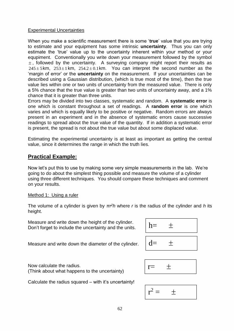
Practical Example: Now let’s put this to use by making some very simple measurements in the lab. We’re going to do about the simplest thing possible and measure the volume of a cylinder using three different techniques. You should compare these techniques and comment on your results. Method 1: Using a ruler The volume of a cylinder is given by πr2h where r is the radius of the cylinder and h its height. Measure and write down the height of the cylinder. Don’t forget to include the uncertainty and the units. Measure and write down the diameter of the cylinder. Now calculate the radius. (Think about what happens to the uncertainty) Calculate the radius squared – with it’s uncertainty!
h=
d=
r2 =
r=

63
One general way of determining the uncertainty in a quantity f calculated from others is to use the following method..
From your measurements, calculate the final result. Call this f , your answer.
Now move the value of the source up by its uncertainty.
Recalculate the final result. Call this f .
The uncertainty on the final result is the difference in these values. Finally work out the volume. Estimate how well you can determine the volume. Method 2: Using a micrometer screw This uses the same prescription. However your precision should be a lot better. Measure and write down the height of the cylinder. Don’t forget to include the uncertainty and the units. Measure and write down the diameter of the cylinder. Now calculate the radius.
(Show your workings)
V=
h=
d=
r=

64
Calculate the radius squared, along with it’s uncertainty Finally work out the volume. Method 3: Using Archimedes’ Principle You’ve heard the story about the ‘Eureka’ moment when Archimedes dashed naked through the streets having realised that an object submerged in water will displace an equivalent volume of water. You will repeat his experiment (the displacement part at least) by immersing the cylinder in water and working out the volume of water displaced. You can find this volume by measuring the mass of water and noting that a volume of 0.001m3 of water has a mass2 of 1kg.
2 In fact this is how the metric units are related. A litre of liquid is that quantity that fits into a cube of side 0.1m and
a litre of water has a mass of 1kg.
(Show your workings)
V=
(Show your workings)
r2 =

65
Write down the mass of water displaced. Calculate the volume of water displaced. What is the volume of the cylinder? Discussion and Conclusions. Summarise your results, writing down the volume of the cylinder as found from each method. Comment on how well they agree, taking account of the uncertainties. _____________________________________________________________________
______________________________________________________________________
______________________________________________________________________
______________________________________________________________________
______________________________________________________________________
______________________________________________________________________
______________________________________________________________________
______________________________________________________________________
______________________________________________________________________
______________________________________________________________________
Can you think of any systematic uncertainties that should be considered? Can you estimate their size? ______________________________________________________________________
______________________________________________________________________
______________________________________________________________________
______________________________________________________________________
______________________________________________________________________
______________________________________________________________________
______________________________________________________________________

66
Requote your results including the systematic uncertainties. What do you think the volume of the cylinder is? and why? My best estimate of the volume is because ______________________________________________________________ ______________________________________________________________________
______________________________________________________________________
______________________________________________________________________
______________________________________________________________________
______________________________________________________________________
______________________________________________________________________
______________________________________________________________________
______________________________________________________________________
______________________________________________________________________

67

68

69
UCD Physics Laboratory: Investigation of Rotational Motion Student Name: Student Number: Lab Partner Name: Demonstrator Name Lab Date/Time:
What should I expect in this experiment? This experiment introduces you to some key concepts concerning rotational motion.
These are: torque (), angular acceleration (), angular velocity (), angular
displacement () and moment of inertia (I). They are the rotational analogues of force (F), acceleration (a), velocity (v), displacement (s) and mass (m), respectively. Pre-lab assignment A full revolution of 360o is equivalent to 2π radians. What is the angular velocity (in radians) of a spinning disk that completes 2 full revolutions in 10 seconds? Introduction: The equations of motion with constant acceleration are similar whether for linear or rotational motion:
Linear Rotational
12
12
tt
ssvaverage
12
12
ttaverage
Eq.1
2
21 vvvaverage
2
21
average
Eq.2
atvv 12 t 12 Eq.3
s2 = v1t +at2
2 q2 =w1t +
at22
Eq.4
Furthermore, just as a force is proportional to acceleration through the relationship F=ma, a net torque changes the state of a body’s (rotational) motion by causing an angular acceleration.
I (Eq.5)
The body’s moment of inertia is a measure of resistance to this change in rotational motion, just as mass is a measure of a body’s resistance to change in linear motion.
The equation I is the rotational equivalent of Newton’s 2nd law maF .
You will use two pieces of apparatus to investigate these equations. The first lets you apply and calculate torque, measure angular acceleration and determine an unknown moment of inertia, I of a pair of cylindrical weights located at the ends of a bar. The
70
second apparatus lets you investigate how I depends on the distribution of mass about the axis of rotation and lets you determine the value of I, already measured in the first part, by a second method. You can then compare the results you obtained from the two methods. Investigation 1: To measure the moment of inertia, I, from the torque and angular acceleration.
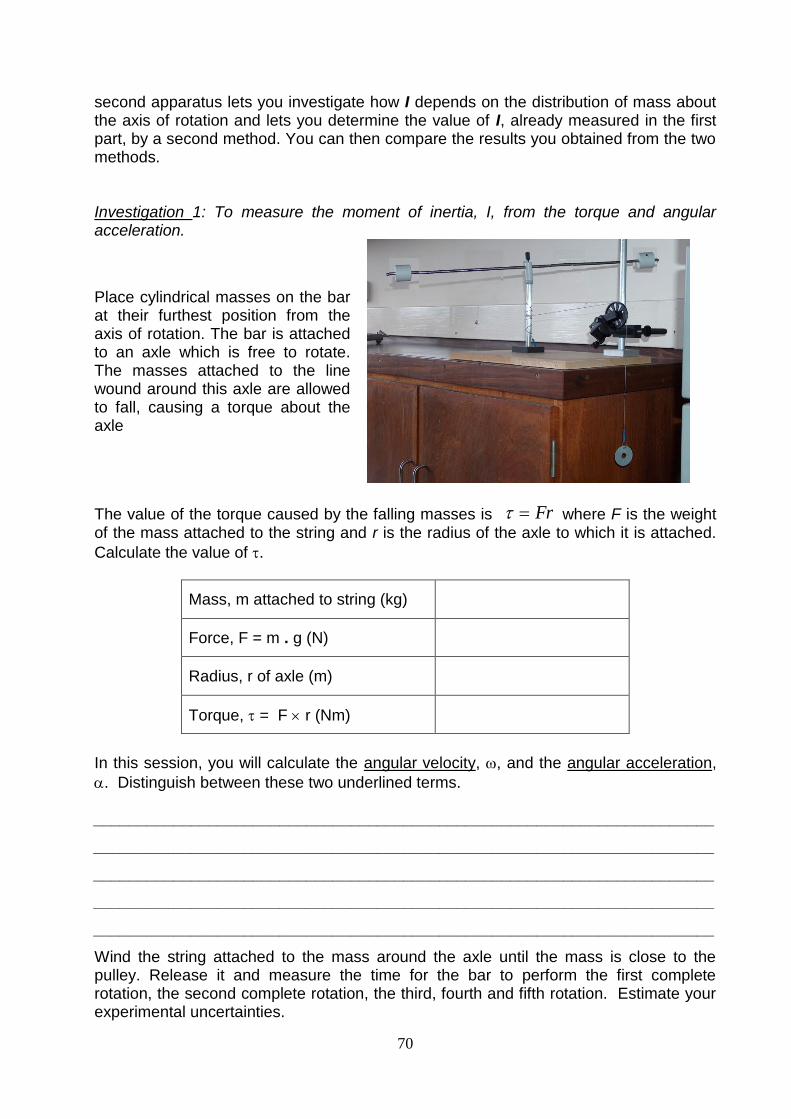
Place cylindrical masses on the bar at their furthest position from the axis of rotation. The bar is attached to an axle which is free to rotate. The masses attached to the line wound around this axle are allowed to fall, causing a torque about the axle
The value of the torque caused by the falling masses is Fr where F is the weight of the mass attached to the string and r is the radius of the axle to which it is attached.
Calculate the value of .
Mass, m attached to string (kg)
Force, F = m . g (N)
Radius, r of axle (m)
Torque, = F r (Nm)
In this session, you will calculate the angular velocity, , and the angular acceleration,
. Distinguish between these two underlined terms. ______________________________________________________________________
______________________________________________________________________
______________________________________________________________________
______________________________________________________________________
______________________________________________________________________
Wind the string attached to the mass around the axle until the mass is close to the pulley. Release it and measure the time for the bar to perform the first complete rotation, the second complete rotation, the third, fourth and fifth rotation. Estimate your experimental uncertainties.

71
Number of
Rotations (rad) Time (s)
0 0 0
1
2
3
4
5
Since you have the angular distance travelled in a given time you can use Eq. 4 to find
the angular acceleration . Explain how you can do this and find a value for ______________________________________________________________________
______________________________________________________________________
______________________________________________________________________
______________________________________________________________________
______________________________________________________________________
______________________________________________________________________
______________________________________________________________________
______________________________________________________________________
______________________________________________________________________
______________________________________________________________________
______________________________________________________________________
______________________________________________________________________
______________________________________________________________________
______________________________________________________________________
=

72
Using Eq.1, calculate the average velocity, average , during each rotation and fill in the
table below.
If angular acceleration is constant, then average is equal to the instantaneous velocity
at the time half-way between the start and the end of a rotation, tmid. Can you understand this? Explain. ______________________________________________________________________
______________________________________________________________________
______________________________________________________________________
______________________________________________________________________
______________________________________________________________________
______________________________________________________________________
Enter the values in the table below and make a plot of average on the y-axis against
tmid on the x-axis.
Number of
Rotation average (rad / s) tmid (s)
1
2
3
4
5
Since this graph gives the instantaneous velocity at a given time, Eq. 3 can be used to
find the angular acceleration, .
What value do you get for ?
Now you know and , so work out I from Eq. 5.

73
Create your graph of average on the y-axis against tmid on the x-axis.
Do the following plot by hand on this page, or, use JagFit (see back of manual) and attach your printed graph to this page. Important: take care to label axes correctly and include units. Note, your tutor will account for fitting where done by hand.

74
Investigation 2: To determine how the moment of inertia, I, depends on the distribution of mass in a body. Take the metal bar on the bench and roll it between your hands. Now hold it in the middle and rotate it about its centre so that the ends are moving most. Which is easier? Which way does the bar have a higher value of I?
______________________________________________________________________
______________________________________________________________________
______________________________________________________________________
______________________________________________________________________
______________________________________________________________________
______________________________________________________________________
______________________________________________________________________
______________________________________________________________________
______________________________________________________________________
Attach the weights and the bar to the rotational apparatus known as a torsion axle. This consists of a vertical axle connected to a spring which opposes any departure from the angle of rotational equilibrium.
Note: The apparatus is delicate. So as not to damage the spring, please keep the rod to within half a rotation from equilibrium.
When you rotate the bar, the spring causes a torque about the axis of rotation which acts to restore the bar to the equilibrium angle. Usually the bar overshoots, causing an oscillation to occur. This is exactly analogous to the way a mass on a linear spring undergoes simple harmonic motion. The period of the oscillations, T, is determined by the restoring torque in the spring, D, and the moment of inertia, I, of the object rotating, in this case the bar and cylindrical weights. They are related by:
D
IT 2
The value of D is written on each torsion axle. Note it here.
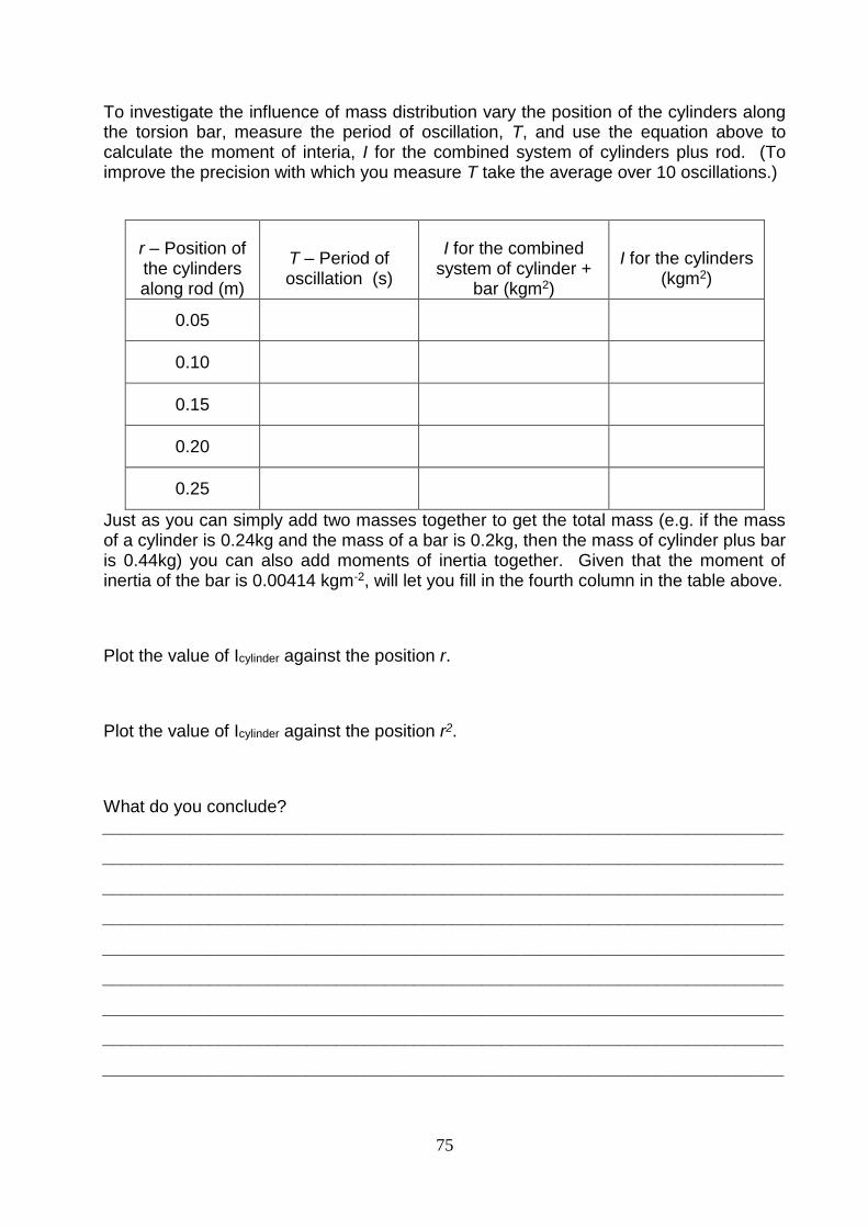
75
To investigate the influence of mass distribution vary the position of the cylinders along the torsion bar, measure the period of oscillation, T, and use the equation above to calculate the moment of interia, I for the combined system of cylinders plus rod. (To improve the precision with which you measure T take the average over 10 oscillations.)
r – Position of the cylinders along rod (m)
T – Period of oscillation (s)
I for the combined system of cylinder +
bar (kgm2)
I for the cylinders (kgm2)
0.05
0.10
0.15
0.20
0.25
Just as you can simply add two masses together to get the total mass (e.g. if the mass of a cylinder is 0.24kg and the mass of a bar is 0.2kg, then the mass of cylinder plus bar is 0.44kg) you can also add moments of inertia together. Given that the moment of inertia of the bar is 0.00414 kgm-2, will let you fill in the fourth column in the table above.
Plot the value of Icylinder against the position r.
Plot the value of Icylinder against the position r2.
What do you conclude? ______________________________________________________________________
______________________________________________________________________
______________________________________________________________________
______________________________________________________________________
______________________________________________________________________
______________________________________________________________________
______________________________________________________________________
______________________________________________________________________
______________________________________________________________________

76
Create a graph of Icylinder against the position, r. Do the following plot by hand on this page, or, use JagFit (see back of manual) and attach your printed graph to this page. Important: take care to label axes correctly and include units. Note, your tutor will account for fitting where done by hand.

77
Create a graph of Icylinder against the position, r2. Do the following plot by hand on this page, or, use JagFit (see back of manual) and attach your printed graph to this page. Important: take care to label axes correctly and include units. Note, your tutor will account for fitting where done by hand.

78
The last measurement in the table above, with r = 0.25m, returns the bar + cylinders system to the orientation used in your first investigation. You have thus measured the moment of inertia of the bar + cylinder system in two independent ways. Write down the two answers that you got.
I from investigation 1:
I from investigation 2:
How do the two values compare? Which is more precise?
______________________________________________________________________
______________________________________________________________________
______________________________________________________________________
______________________________________________________________________
______________________________________________________________________
______________________________________________________________________
______________________________________________________________________
______________________________________________________________________
______________________________________________________________________
______________________________________________________________________
______________________________________________________________________
______________________________________________________________________
______________________________________________________________________
______________________________________________________________________
______________________________________________________________________

79
Appendix 1. Graphing Many of the experiments in the 1st Year laboratory involve the plotting of a graph. Graphs are very important in Physics as they provide a rich display of the results obtained in an experiment. One third of the human brain is devoted to images, and so we are well optimised to interact with graphs rather than with tables of numbers. Plotting graphs by hand (1) Scale: It is important to choose the scales so as to make full use of the squared
page. The scale divisions should be chosen for convenience; that is, one unit is either 1, 2 or 5 times a power of ten e.g. 0.5, 5, 100 etc., but never 3, 7, 9 etc.
(2) Marking the points: Readings should be clearly indicated on the graph. Where in
pencil, this is best done by a ringed dot drawn with pencil, so that it is possible to erase and correct any unsatisfactory data.
(3) Joining the points: In the case of a straight line which indicates a direct proportion
between the variables, the ruler is positioned so that the line drawn will pass through as many points as possible. Those points which do not lie on the line should be equally distributed on both sides of the line. Ideally a recheck would be made on a point that lies well away from the line because this can be due to an error, but it shouldn’t just be assumed that an errant data point is by error. In the case of a curve, the individual experimental points are not joined with straight lines but a smooth curve is drawn through them so that as many as possible lie on the curve.
(4) Units: The graph is drawn on squared page. Each graph should carry title at the
top e.g. Time squared vs. Length. The axes should be labelled with the name and units of the quantities involved.
(5) You may be asked in some labs to represent an estimated error as a bar on a graph. You
can represent your estimated error in the abscissa (the primary axis, horizontal as shown) and/or the ordinate (the secondary axis, vertical as shown). Generally an error bar represents the extent covered by plus or minus (‘+/-) a given amount. The example of figure A shows both abscissa and ordinate error bars. If you have uncertainty in both the ordinate and abscissa, this results in square regions of uncertainty.
(6) A best-fit line is one drawn to best represent the distribution of points on a graph.
In the case of a straight-line graph, the equation of the line representing the relationship between the quantities x and y may be expressed in the form
y = mx + c where m is the slope of the line and c the intercept on the y-axis. The slope may
be positive or negative. Many experiments require you to fit a straight line to a distribution of points by eye and then to read off the slope, m, and the intercept, c of your line.

80
0 2 4 6 8 10
0
5
10
15
20
25 Extension of elsatic object under tensionE
xte
nsio
n, E
(cm
)
Force, F (N)
Extension data
Linear fit
Figure A: Example of a linear fit to some experimental data with both ordinate and abscissa error bars as estimated by the experimenter. For this linear fit, m = 2.1 and c = 0.47. Example table of data used for figure A
F (N) E (cm) Err in F (N)
Err in E (cm)
1.0 3.0 0.5 1.0
2.0 4.0 0.5 1.0
3.0 7.0 0.5 1.0
4.0 8.0 0.5 1.0
5.0 11.5 0.5 1.0
6.0 13.0 0.5 1.5
7.0 16.5 0.5 1.5 8.0 17.0 0.5 2.0
9.0 18.0 0.5 2.0
10.0 21.0 0.5 2.5
81
Plotting directly from the GLX data logger You can plug in the data logger to a lab printer directly to print out data without a laptop or PC. Using JagFit (on a PC) In the examples above we have somewhat causally referred to the ‘best fit’ through the data. What we mean is, the curve which comes closest to the data points having due regard for the experimental uncertainties. We can judge this really quite well by eye, but to so isn’t quantitative or reproducible between people necessarily, and so doing this manually isn’t always the best way. We can determine a straight line fit to data that varies due to random fluctuations using so-called ‘least square fitting’, but this requires a calculator/computer and sufficiently large data sets. At least 10 measurements are required to be usefully quantitative in this way, and more typically more than 30 measurements are needed.
A computer can make a difference where data sets are large enough then, and a plotting program called Jagfit is installed on the computers. Jagfit is freely available for download from this address: http://www.southalabama.edu/physics/software/software.htm If you are to use it, then double-click on the JagFit icon to start the program. The working of JagFit is fairly intuitive. Enter your data in the columns on the left.
Under Graph, select the columns to graph, and the name for the axes.
Under Error Method, you can include uncertainties on the points.
Under Tools, you can fit the data using a function as defined under Fitting_Function. Normally you will just perform a linear fit.
Three of the experiments in this manual were initially developed by the Physics Education Group, CASTeL, Dublin City University.

82
Appendix 2. Grading scheme
Grading is consistent with the UCD grade scale:
Net lab Score
UCD level UCD description
0 - 2 NG - G wholly unacceptable
2 - 4 F - E unacceptable - marginal
4 - 6 D – C acceptable - good
6 - 8 B - A very good - excellent
8 - 10 A+ excellent - exceptional
Demonstrators are asked to discuss with the 1st year labs academic coordinator, Ian Mercer, if they think their grading varies significantly from this reference. Feedback The net grade comprises three components for a report, the beginning, the middle and the end. Demonstrators mark this net grade as an integer (whole number) on the front of a report and also mark the three component grades within a report. The component grades can be to half grades at the demonstrator’s discretion. The net grade is rounded up to an integer. The distribution of grades is:
Component of Report Grade
1 Beginning – ‘Data and Preparation’ between 0 and 4
2 Middle – ‘Results’ between 0 and 4
3 End – ‘Conclusions’ between 0 and 2
Net grade integer between 0 and 10
Demonstrators are not asked to otherwise annotate reports. Instead, the demonstrator feeds back to the class on say three main areas to improve at the start of the following lab session. Also, demonstrators respond to questions raised by individuals about their last graded report either during or after the lab session in which the report is returned. The demonstrator submits the net (integer) grades for their class to the physics admin office immediately after their return of scripts/grades to a class, using the template excel sheet provided by the physics school admin office. Net grades are then uploaded by the school office within an additional week so as to be visible to students in their online grade centre. Where unable to take a lab, the scheduled demonstrator finds a replacement aided by the lab manager, Thomas O’Reilly. The scheduled demonstrator primes their replacement for interaction with students on their recently graded report.

83
Three graded components 1. Preparation and data (the beginning) A grade of between 0 and 4 awarded for a cumulative performance across the following:
Warm up. Intro exercise/s.
Setup procedure. Follow guided procedure to first useful data.
Method and range. Take data over a range of parameter space so as to allow for the most robust conclusions. Apply critical thinking, for example check or repeat measurements to expose an apparatus weakness or source of error.
Ordered data. Record data in a clear and ordered way using the tables provided.
A grade of 4 is awarded for an exceptional performance only. 2. Results (the middle) A grade of between 0 and 4 awarded for a cumulative performance across the following:
Plot (distil) data. Plot, or otherwise distil as guided, all useful data from tables.
Clarity of plot. Include axes labels, scale and correct units.
Slope and intercept. Determine slope and intercept for a linear relationship. This generally involves assigning a straight line/s by eye. We as humans are remarkably adept at doing this and the grader accounts for a reasonable fit done by eye. But you may choose to use a device (see appendix 1) for this.
Relate to physical law. Relate these variables to a physical law with consideration of errors where helpful. Where appropriate, systematic uncertainty and possible imperfections in an apparatus should also be considered.
A grade of 4 is awarded for an exceptional performance only. Consider uncertainty in measurements. Use units correctly and consistently. Whilst plotting is the main means of distilling data in our experiments, the Momentum experiment requires the distillation and interpretation of information by other means which include estimations of measurement uncertainty. The first three grades for this component are attributed to this. For labs in this semester, we don’t expect the student to propagate random errors by adding in quadrature. We do expect some critical thinking about the extent and source of errors. 3. Conclusions and implications (the end) A grade of between 0 and 2 awarded for a cumulative performance across conclusions and implications. A grade of 2 is awarded for an exceptional performance only. This may require the demonstration of some independent and critical thinking on the impact of measurement uncertainty on conclusions.
84
Tutor discretion 1. Reward diligence or critical thinking It may be that exceptional diligence and/or critical thinking has led directly to students not completing a lab. To account for this, 2 net grade units can be awarded at the tutor’s discretion. It remains that the overall student performance is considered in keeping with the UCD grade scale (see above). By critical thinking, we mean thinking about the exercise that goes beyond regurgitation of material in the lab manual or delivered during the class. Generally, this is the mark of the stronger student. 2. PHYC10180 This module contains less maths than some others. For experiments such as gases and rotation, there are two parts. If students have been diligent but there is not enough time to complete both parts then the first part is sufficient. 3. Electrical experiments These are designed as enquiry based and credit should be given for testing of even erroneous models for circuits. The grade should be awarded for addressing questions across the script and should be broadly in keeping with the UCD grade scale (see above). 4. PHYC20080 Whilst the style of these experiments varies, the grading distribution remains as given above. Where the intro contains no questions, the first component of grade is given for preparation to first useful data, range and ordered recording of data.