(NASA-CR-138306) NUCLEAR QUADRUPOLE 074-31023RESONANCE STUDIES IN SENI-NETALLICSTRUCTURES Semiannual Status Report(Grambling State Univ., La.) p HC Umclas$4.75 9 CSCL 11D G3/18 45718

DEPARTMENT OF

PHYSICSGRAMBLING COLLEGEGrambling, Louisiana

https://ntrs.nasa.gov/search.jsp?R=19740022910 2018-08-03T04:52:22+00:00Z

ThirdSemi-Annual Status Report

on the project

NUCLEAR QUADRUPOLE RESONANCE STUDIESIN SEMI-METALLIC STRUCTURES

(NGR-19-011l-016)

by

A. Narasimha MurtyDepartment of Physics

Grambling State University

August 15, 1974

THIRD SEMI-ANNUAL STATUS REPORT

SUBMITTED TO: NASA Scientific and TechnicalInformation Facility

Post Office Box 33College Park, Maryland 20740

REFERENCE NUMBER: NGR-19-O11-016Supplement No. I

INSTITUTION: Grambling State UniversityGrambling, Louisiana 71245

TITLE: Study of the Distribution ofExtra-Ionic Electrons in Semi-Metallic Environments byNuclear Quadrupole ResonanceTechniques

PRINCIPAL INVESTIGATOR: Dr. A. N. Murty, ProfessorDepartment of Physics

DURATION:

Original Grant One (1) YearSupplement No. I One (1) Year

SUM GRANTED BY NASA: $15,305 (lst Year)$17,494 (2nd Year)

DATE:

(Project Started) January 1, 1973(1st Semi-Annual Report) October 12, 1973(2nd Semi-Annual Report) February 18, 1974(3rd Semi-Annual Report) August 15, 1974

SIGNATURE:

Principal Investigator . ~AaDr. A. Narasimha Murty

, Department of PhysicsGrambling State UniversityGrambling, Louisiana 71245

INTRODUCTION

This report describes the results of our studies in the Nuclear Quadru-

pole Resonance project at Grambling State University, sponsored by the

National Aeronautics and Space Administration. The results are presented in

two sections: A-experimental, and B-theoretical. Section A deals with an

analysis of the NQR spectra of the tellurides of Antimony and Arsenic, and

Section B presents numerical solutions for the secular equations of the

quadrupole interaction energy.

A. Experimental:

Nuclear quadrupole resonance studies of the oxides, sulfides, and sele-

nides of Arsenic and Antimony have been made by earlier investigators.1 -7

The tellurides of Arsenic and Antimony have been studied by us for the first

time in this laboratory with a view to complete the data for the V and VI

group compounds and examine the nature of bonding.

The chemicals As2Te 3 and Sb2Te 3 were obtained from Alfa Inorganics,

Ventron Corporation, Beverley, Massachusetts. The samples were finely pow-

dered and sifted through a 325 mesh sieve. The samples were very lossy when

directly introduced in the R.F. coil of the oscillator. They were mixed

with 325 mesh vycor glass powder, 50% by volume to reduce the R.F. losses.

The NQR spectra were observed on a Wilks servo controlled coherent

super-regenerative NQR spectrometer. The frequency measurements were made

by beating a standard signal generator (McGraw-Edison Model 80) with the NQR

oscillator just before and after the observation of the resonance. Since

the signal is repeated in a number of side bands, the resonance frequency is

ReprOOU"e' copVI3 ~~~best av-1"~~ . - __ _

-T I

_ 17

-iI 7

~ [-- I ~ 1.7*j~*~*...I I -~~ -- I_

2

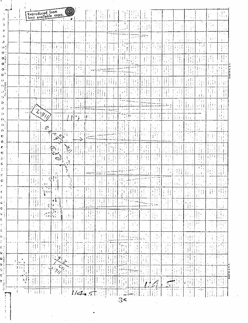
taken as the centre of the envelop by interpolating between the two frequency

markers. The marker frequencies were directly read from a GR 1192 Z counter-

scaler unit connected to the standard signal generator. A representative

signal pattern along with the marrkers is shown in Figure 1. Each measure-

ment is repeated six times and the average value of frequency is used in

estimating the coupling constant e2Qq.

Results and Discussion:

The measured resonance frequency of As7 5 in Arsenic telluride (As2Te )and the frequencies for the two isotopes of Antimony Sb121 , and Sb123 in

Antimony telluride (Sb2Te ) are presented in Table I. All measurements were

made at room temperature.

Since the spin of As7 5 is 3/2, and only one isotope is present with

natural abundance of 100%, in the absence of unequal crystalline environ- .

ments; one resonance line is expected due to the transition between the

energy levels E3/2 -- El/2. The resonance frequency is given by5

1/2 e (1 - - - - - - - - - (1)

where Q is the nuclear quadrupole moment, qzz the field gradient tensor com-

ponent along the principal axis of symmetry and (\the asymmetry paremeter

defined by = xy - - - - - - - - - (2)

The nuclear quadrupole coupling constant e2Qq given in Table I is

obtained by doubling the NQR frequency assuming that RCis very small. At

present, no crystal structure data is available for As2Te 3 to justify the

assumption; but it may not be far from being correct since the metal atom in

the homologues Sb2Te 3 and Bi2Te 3 are in highly symmetric environments.

4<

TABLE I

NATURAL QUADRUPOLE UNBALANCEDABUNDANCE FREQUENCY COUPLING CONSTANT P-ELECTRON Up

ONMPOUND SPIN PERCET TRANSITION MHz MHz EXPER. CAL.

As2Te (As75 Z 100 2 1 115.9 + 0.5 232 + 1 0.3862Te3 2 2 2

b2Te (Sb1 2 1 ) 571 82.8 + 0.2 552+ 1 0.276 0.05622 2 8 2-80-

(sb121) 2 57 5 1 165.3 + 0.5 551 + 2 0.276 0.0562 2 2

(sb123) 7 4 3 --> 1(Sb ) 2 2 3 2 50.1 + 0.2 701 + 1 0.280 0.0562 2 2

Ratio (e2 Qq)1 2 3

(e2Qq) 121

Present Estimate = 1.271

Literature Value 5 = 1.274

3

The crystal structure of Sb2Te is8 rhombohedral. The corresponding

hexagonal cell containing three molecules has the following unit cell

dimensions. A = 4.25 A.U. and C = 30.4 A.U. This structure can be ima-

gined as composed of layers of atoms along C axis following one another in

the succession Te-Sb-Te-Te-Sb-Te-Te-. The immediate neighbor environment of

the Antimony atoms is shown in Figure 2. Each Antimony atom (centre circle)

is surrounded by 6 tellurium atoms. Three tellurium atoms (broken circles)

are 1.69 A.U. above the plane of the paper at a distance of 2.98 A.U. from

Sb, and three are 2.03 A.U. below the plane at a distance of 3.18 A.U. As

such, the asymmetry parameter becomes zero and the quadrupole resonance fre-

quencies can be directly expressed in terms of the quadrupole coupling con-

stant e2 Qqzz. Antimony has two isotopes: Sb121 and Sb123 with natural

abundance of 57 and 43 percent respectively. For the isotope Sb121 having a

spin of 5/2, two lines are expected with resonance frequencies given by5

1= E3 / 2 -E 1 / 2 = e2 Qq (1+59 - - - - - - - - (3)( -E 115 + - - - - - - -- (3)

32 E5 / 2 h E3 / 2 1 e 2 Qqzz (1-

The observed frequencies, and the coupling constants obtained by substi-

tutingy~ = O in the above equations are shown in Table I. For the isotope

Sb123, the spin is 7/2 and the three resonance frequencies are given by5

E -E 1 e2Qq 109, 2

S E3/2 1/2 = ) e2 qzz (1- -""- - (5)1h =

h1 2 - ... ) - - - - - - - - - (6)h7 zz 30

III %

r\

I \

/ I

/b

/

Fire 2: TitE IMNIIAE NEIGHBOR ENVIRONMSJT IN ANTI1EONY T'ELURIDE

7</" \

4

= E7 /2-E5 2 = i- e2 qzz (1 2 (7)

Of the three expected lines only \) could be observed. Even after

annealing at 5000C for 24 hours, there appeared no change in the intensity

of the lines. Presently, we are scanning the spectra at dry ice and liquid

nitrogen temperatures.

An elementary analysis of the bond character on the basis of Townes and

Dailey theory9' 10 is instructive and interesting. The observed quadrupole

coupling constant is related to the coupling constant due to a pure p-elec-

tron by

e2qobs = Up e2qnl -- (8)

e2 Qq10 = -2e 2 Qqn1 (9)

75 2 121The atomic coupling constants for As (eQq4 1 1 = 300 MHz) and Sb

(e 2Qq11 = 1000 MHz) are taken from Townes and Schallow Table9 . The values

of Up, the number of unbalanced p-electrons calculated from equation (8) are

given in Table I as the experimental value. If double bond character and

d-hybridization are neglected; treating that each Antimony atoms has s-p

hybridized orbitals which form three covalent bonds with the tellurium atoms,

and an unshared pair, u can be expressed as 1 3

u = -3cc(l-3f+ 4 (1+)) - - - - - - - - - - - - - - - (10)

whereoc is the s-character of the bond determined by the inter-orbital

angle 8 as

oC = cos /(cose-1) - - - -- (11)

where is the ionic character and C the screening constant. For Sb2Te3 the

inter-orbital angle Te Sb Te is about 91o giving a value of 1.7% for ac-the

s-character of the bond. The electronegativity difference A-for Sb-Te is

about 0.3, and f the ionic character is about 6% (vide pages 236, 237 in

Ref. 9). The unbalanced p-electron value calculated in Table I is obtained

from equation (10). On this basis, the valance electron contribution to the

field gradient is only about 20%.

There are various factors to be considered to account for this large

difference. First, there are considerable uncertainties in the value of

atomic quadrupole coupling constants and the electronegativity difference

6 values used in arriving at u calculated. The literature values forSb-Te P

e2 Qq5 O for Sb121 range perhaps anywhere from 734 MHz - 2000 MHz 1 4 ,1 5 and

16-18the electronegativity difference, Sb-Te ranges anywhere from 0.3 - 0.19.

Secondly, up value is very sensitive to the bond angle especially when it is

very close to 900 and the validity of application of Townes and Dailey1 0

theory to such cases may not be justifiable.

In addition to these uncertainties there is one important factor to be

considered particularly in the case of inter-semi-metallic structures. The

compounds As2Te 3 and Sb 2 Te 3 are electrically conducting with a specific

resistance fin the range of 102 ohm cm. A simple measurement on a compac-

ted column of the powder gives values 9Sb2Te = 212 ohm cm and VAs2Te 3

296 ohm cm. This value falls in between that of a metal (-metal6l10 ohm cm)

and a semi-conductor (emi-c0 oonductor10O6 ohm cm). Earlier measurements on

the nuclear quadrupole resonance spectra of Gallium1 9 , Indium2 0 , and Anti-

6

mony 2 1 indicate that the usual metallic model consisting of positive ions

situated in a smooth electronic charge distribution of conduction electrons

is inadequate to explain the observed results and that the spatial p-elec-

trons may not be completely delocalized and should provide appreciable con-

tribution to the field gradient at the site of the quadrupole nucleus. In

the case of the tellurides of Arsenic and Antimony, we believe that the con-

duction electron contribution to the field gradient might be appreciable.

Other P-Block Elements Studied:

Since the tellurides of Antimony and Arsenic present an interesting

situation where both the ionic character and s-hybridization are very small,

but the coupling constants are large; we felt further examination of this

feature in the tellurides of Indium and Gallium should lead to a better

understanding.

Unfortunately, the sesqui selenides and tellurides of Indium and Gallium

have a deficit cubic structure which becomes hexagonal at high temperature.

It has not been possible to observe resonance in these samples even after

annealing at 10000C. But the mono-selenides and tellurides of Indium and

Gallium have a favorable structure amenable to NQR studies. In these struc-

tgres double layers of metal atoms succeed double layers of metalloid atoms.

Presently, we are scanning the spectra of InSe and GaSe.

A thorough search was made in the frequency region 5-50 MHz to observe

the resonance of pure Bismuth. Bismuth has similar rhombohedral structure

as Arsenic and Antimony. Finite field gradient, almcet the same as in Anti-

mony is expected at the site of the Bismuth nuclei. 2 7 Our repeated searches

both at room temperature and liquid nitrogen temperatures proved negative.

Annealing the sample at 2500C also did not improve the situation.

7

In accordance with our proposed plan, we have investigated a number of

Indium and Bismuth doped Antimony samples. The samples were prepared in the

zone levelling unit developed in our laboratory. 2 8 In the first place, the

Antimony NQR signals in pure Antimony were neither sharp nor strong at room

temperature. The resonance signals observed in the doped samples with

impurity concentrations in range of 0.5 - 2.0 percent by weight were consi-

derably weak and broad. It has not been possible to make any quantitative

measurements since our present frequency measurement method is accurate only

up to 0.1 MHz. Presently, we are adding a spectrum analyzer unit to our

existing spectrometer system. With this improved facility we hope to be

able to arrive at more quantitative data.

B. Numerical Solutions for Pure Quadrupole Interaction Secular Equations:

Introduction:

The assignment of the nuclear quadrupole resonance spectra of nuclei

(I>,5/2) in asymmetric environments (q,0.5) presently involves graphical

methods23,2 4 based on the numerical eigen value tables of Cohen.22 From

these tables the experimenter should develop the relative frequency factors

(eigen value differences) and the possible ratios for the various frequen-

cies, and plot these ratios as a function of the asymmetry parameter. By a

trial and error process, one can arrive at the proper experimental ratio

points that fall on the calculated ratio curves forming a straight line per-

pendicular to the (q-axis. The ( value is interpolated from the intersec-

tion of this ordinate and f-axis, and the coupling constant from the corres-

ponding frequency factor curve.

8

We have developed ready reference tables for the determination of I and

eQq from the observed NQR frequencies for values of C ranging from 0 - 1 in

intervals of 0.01 for all values of I = 5/2, 7/2, and 9/2. So far such data

is available in the form of eigen values only from Cohen's tables,22 for

values of lfrom 0.1 to 1.0 in intervals of 0.1 for all values of I = 5/2,

7/2, and 9/2; and from the tables of Livingston and Zeldes25 for I = 5/2

with q ranging from 0 to 1 at intervals of 0.001. The latter is only for

I = 5/2 and available in the Oak Ridge National Laboratory reports. Hence,

the complete set of tables developed by us giving the frequency ratios and

corresponding asymmetry parameters directly should be very convenient for

the assignment of the NQR spectra.

Numerical Method:

The secular equations for pure quadrupole interaction energy 2 3 2 6 are

given in Table II.

Exact solutions of E can be obtained only for I = 3/2, and the transi-

tion frequency \1(3/2'l/2) is given by E3 /2-E 1/2 = e2 (1+2/3) 1 / 2 .

h 2hSince only one resonance line will be observed it is not possible to obtain

both the asymmetry parameter fq, and the quadrupole coupling constant e Qq

separately unless one studies the zeeman spectra. For nuchei of spin values

I ).5/2, there are two or more transition frequencies connecting the two

unknowns q and e2Qq and hence both can be obtained. But unfortunately it is

not possible to obtain exact solutions in closed form as for I = 3/2, for

the secular equations for spin values I , 5/2.

Bersohn2 6 and Wang have obtained the solutions by a perturbation pro-

cedure in the form of an expansion series in powers of '2 up to q8. These

TABLE II

I UNITS OF E SECULAR EQUATION

2 .2 E2 - 3 9 9 0 (1)12

Se 2Q E 7 (3 q2 ) E - 20 (1- 2) = 0 (2)

7 E 4 /3) E2- 64 (1- ) E + 105 (1+q r3) 0 (3)I 2 - -(+/ =

SE 5 11 (3+2)E3 (12)E2 (3+2 E+ 48 (3+q2) (1-2 (4)

9

expressions aro not valid for values of t ,,0.5 and introduce significant

errors23 even for r = 0.1; for the lower transitions of high spin nuclei;

ouch as the 3/2 - 1/2 transitions of Bismuth and Indium compounds for which

I = 9/2.

Using Newton Raphson2 9 iteration method we have obtained numerical

solutions to the secular equations. The computations were carried out on

the IBM 360 computer at Louisiana Tech University, Ruston, Louisiana. The

program involves obtaining successive values of energy for the secular equa-

tion starting from a trial value until the successive values are satisfacto-

rily convergent. We have conveniently used Cohen's 2 2 initial values as our

starting eigen values (Ei).

The general iteration formula is given by:

E F(E)1+1 1 F'(E)

and the iteration process is continued until E i+-E i = 0.0001. The itera-

tion formulae used for obtaining eigen values for spin values I = 5/2, 7/2,

and 9/2 are given in Table III. The eigen values (Ei) obtained for all "I

values ranging from 0 - 1 at intervals of 0.01 are presented in the enclosed

set of tables.

Explanation and Use of Tables:

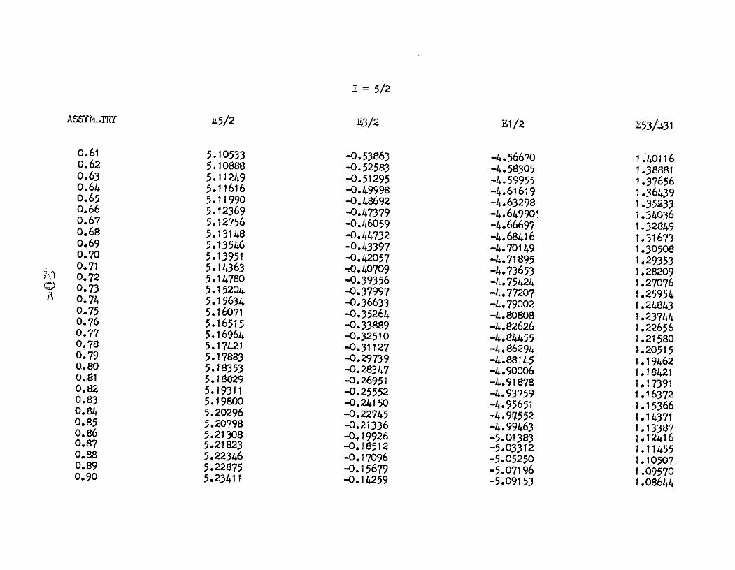
The results are presented in three sets of tables for the three spin

values I = 5/2, 7/2, and 9/2. The (212+ 1) eigen values E values, m = 1/2,2 e m

3/2, 5/2, 7/2, and 9/2) for each spin value are given in multiples of e2Qq

as indicated in Table II, in successive columns corresponding to the value

of the asymmetry parameter. Following these, the various frequency factor

r. i, ..2

TABLE III

2"

2E3 + 20 (1- 2 )Ei+1 = 1

3E 2- 7 (3+2

_ 7 .

2'S2 2

E 3+1

4E - 84 (1+ ) E - 64 (1- 2 )

S9.2

E. 4 - 22 (3+ e) E3 - 44 (1- 2) E-48 (3+1 (1-qi+1 -

5E - 33 (3+qr ) E. -88 E(1- i q2 (3E i

10

ratios are tabulated. For example E5 3/E 7 5 indicates the ratio of frequen-

cies a2 5/2-E /2 and E97/E75 indictes the ratio E9/2E7/2 , etc.

t o3/2 WE1/2 E7/2 5/2

With a tentative assignment for the observed NQR spectral lines one can

easily verify whether the observed ratios of the assigned lines lie in the

same row corresponding to a specific asymmetry parameter, in the table for

that spin value. More accurate value of the asymmetry parameter up to a 3rd

place can be obtained by interpolation. Now from the eigen value factors

(Em values) corresponding to the assigned asymmetry parameter the frequency

factors (f) can be readily obtained; as the eigen value differences (Em-Em)

for the energy levels representing the transition. The quadrupole coupling

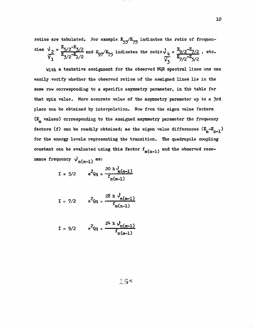
constant can be evaluated using this factor fm(m-l) and the observed reso-

nance frequency .m(m-l) as:

20 hdI = 5/2 e2q m(m-l)

m(m-l)

I = 7/2 e2Qq 28 h m(m-1)fm(m-l)

I = 9/2 e2q= 24 h (m-1)m(m-1)

Jii<=

TABLES

OF

NUCGLAR QUADRUPOLE R&SONANCE

FRQUNCY RATIOS AND ASSYI4TRY PARAMLT.RS

I 5/2

ASSY~ETRY E5/2 E3/2 E1/2 L53A31

0.0 5.00000 -1.00000 -4.00000 2.000000.01 5.00002 -0.99985 -4.00018 1.999740.02 5.00011 -0.99940 -4.00071 1.998960.03 5.00025 -0.99865 -4.00160 1.997670a1, 5.00044 -0.99760 -4.00284 1.995860.05 5.00069 -0.99626 -4.00444 1.993550.06 5.00100 -0.99461 -4.00639 1.990720oa' 5.00136 -0.99267 -4.00869 1.98740p008 5.00178 -0.99044 -4.01134 1.98359.0.09 5.00225 -0.98791 -4.01434 1.979290.10 5.00278 -0.98509 -4.01768 1.974510.11 5.00336 -0.98199 -4.02137 .96926

A 0.12 5.00400 -0.97860 -4.02541 1.963560.13 5.00469 -0.97492 -4.02978 1.957410.14 5.00545 -0.97096 -4.03449 1.950820.15 5.00625 -0.96672 -4.03953 1.943820.16 5.00712 -0.96221 -4.04491 1.936400.17 5.00804 -0.95743 -4.05061 1.928580.18 5.00901 -0.95237 -4.05664 1.920380.19 5.01004 -0.94705 -4.06299 1.911810,20 5.01113 -0.94147 -4406966 1.902890.21 5.01227 -0.93563 -4.07665 1.893620.22 5.01347 -0.92954 -4.08394 1.884030.23 5.01473 -0.92319 -4.09154 1.874130.24 5.01605 -0o.91660 -4.099 1.80.25 5.017 -0.90976 -4.10766 .8 60.26 .UI884 -0.90269 -4.11616 1.842720.27 5.02032 -0.89538 -4.12495 1.831730.28 5.02186 -0.88784 -4.13403 1.820500.29 5.02346 -0.88007 -4.14339 1.809060.30 5.02512 -0.87209 -4.15303 1.797410. 1. 5.02683 -0.86389 -4.16294 1.78557

I = 5/2

ASSrW TRY E5/2 E3/2 E1/2 E53/E31

0.31 5.02683 -0.86389 -4.16294 1.785570.32 5.02859 -0.85547 -4.17313 1.773560.33 5.03042 -0.84685 -4.18357 1.761380.34 5.03230 -0.83802 -4.19428 1.749060.35 5.03424 -0.82899 -4.20525 1.736610.36 5,03624 -0.81977 -4.21647 1.724030.37 5.03830 -0.81036 -4.22794 1.711350.38 5.04041 -0.80076 -4.23965 1.698570.39 5.04258 -0.79099 -4.25160 1.685700.40 5.04481 -0.78103 -4.26378 1.672770.41 5.04710 -0.77091 -4.27620 1.659780.42 5.04945 -0.76061 -4.28884 1.646740.43 5.05185 -0.75015 -4.30170 1.633660.44 5.05431 -0.73954 -4.31478 1.62055

S0.45 5.05684 -0.72876 -4.32808 1.607420.46 5.05942 -0.71784 -4.34158 1.594280.47 5.06206 -0.70677 -4.35529 1.581140.48 5.06476 -0.69556 -4.36921 1.568010.49 5.06752 -0.68421 -4.38331 1.554900.50 5.07034 -0.67272 -4.39762 1.541810.51 5.07322 -0.66111 -4.41211 1.528740.52 5.07616 -0.64937 -4.42679 1.515720.53 5.07915 -0.63750 -4.44166 1.502740.54 5.08222 -0.62552 -4.45670 1.489810.55 5.08533 -0.61343 -4.47191 1.476940.56 5.08851 -0.60122 -4.48730 1.464130.57 5.09175 -0.58890 -4.50286 1.451380.58 5.09506 -0.57648 -4.51858 1.438710.59 5.09842 -0.56396 -4.53446 1.426110.60 5.10184 -0.55134 -4.55051 1.41359

I = 5/2

ASSYLTRY 85/2 B3/2 El/2 L53/31

0.61 5.10533 -0.53863 -4. 56670 1.401160.62 5.10888 -0.52583 -4.58305 1.388810.63 5.11249 -0.51295 -4.59955 1.376560.64 5.11616 -0.49998 -4.61619 1.364390.65 5.11990 -0.48692 -4.63298 1.3$2330.66 5.12369 -0.47379 -4.64990" 1.340360.67 5.12756 -0.46059 -4.66697 1.328490.68 5.13148 -0.44732 -4.68416 1.316730.69 5.13546 -0.43397 -4.70149 1.305080.70 5.13951 -0.42057 -4.71895 1.293530.71 5.14363 -0. 40709 -4.73653 1.28209

\) 0.72 5.14780 -0.39356 -4.75424 1.270760.73 5.15204 -0.37997 -4.77207 1.25954A 0.74 5.15634 -0.36633 -4.79002 1.248430.75 5.16071 -0.35264 -4.80808 1.237440.76 5.16515 -0.33889 -4,82626 1.226560.77 5.16964 -0.32510 -4.84455 1.215800.78 5.17421 -0.31127 -4.86294 1.205150.79 5.17883 -0.29739 -4.88145 1.194620.80 5.18353 -0.28347 -4.90006 1,.184210.81 5.18829 -0.26951 -4.91878 1.173910.82 5.19311 -0.25552 -4.93759 1.163720.83 5.19800 -0.24150 -4.95651 1.153660.84 5.20296 -0.22745 -4.979552 1.143710.85 5.20798 -0.21336 -4.99463 1.133870.86 5.21308 -0.19926 -5.01383 1,124160.87 5.21823 -0.18512 -5.03312 1.114550.88 5.22346 -0.17096 -5.05250 1.105070.89 5.22875 -0.15679 -5.07196 1.095700.90 5.23411 -0.14259 -5.09153 1.08644

I = 5/2

ASSY1iTRY .5/2 E3/2 E1/2 E53/E31

0.91 5.23954 -0.12838 -5.11116 1, 077290.92 5.24504 -0.11415 -5.13089 1.068260.93 5.25060 -0.09991 -5.15069 1.059340.94 5.25624 -0.08566 -5.17058 1.050540.95 5.26194 -0.07140 -5.19054 1.041840.96 5.26771 -0.05713 -5.21059 1.033250.97 5.27355 -0.04285 -5.23070 1.024780.98 5.27947 -0.02857 -5.25089 1.016410.99 5.28545 -0.01429 -5.27116 1.008151.00 5.29150 -0.00000 -5.29149 1.00000

'

I = 7/2

ASSYTRY E7/2 E5/2 13/2 E1/2 E75/31 E53/E31 E75/E53

0.0 7.00000 1.00000 .3.00000 -5,00000 3.00000 2.00000 1.500000.01 7.00002 1.00008 -2.99970 -5.00040 2.99891 1.99918 1.500070.02 7.00009 1.00033 -2.99876 -5.00165 2.99555 1.99666 1.500280.03 7.00021 1.00075 -2.99722 -5.00374 2.98998 1.99249 1.500630.04 7.00038 1.00133 -2.99507 -5.00664 2.98226 1.98670 1.501110.05 7.00058 1.00208 -2.99230 -5.01036 2.97241 1.97932 1.501730.06 7.00084 1 .00300 . -2.98894 -5.01490 2.96048 1.97038 I. 502490.07 7.00114 1.00408 -2.98498 -5.02024 2.94659 1.95998 1.503370.08 7.00149 .1.00534 -2.98046 -5.02637 2.93081 1.94818 1.504380.09 7.00189 1.00676 -2.97536 -5.03328 2.91320 1,.93502 1.505510.10 7.00234 1.00834 -2.96971 -5.04097 2.89388 1.92059 1.506770.11 .7.00282 1.01010 -2.96352 -5.04940 2.87300 1.90501 1.50813

, 0.12 .7.00336 1.01202 -2.95681 -5.05857 2.85063 1.88834 1.50960e) 0.13 7.00394 1.01411 -2.94959 -5.06846 2.82689 1.87066 1.51117A 0.14 7.00458 1.01638 -2.94187 -5.07907 2.80190 1.85208 1.51284

0.15. 7.00526 1.01881 -2.93369 -5.09037 2.77577 1.83267 1.514600.16 7.00598 1.02141 -2.92505 -5.10233 2.74864 1.81256 1.516440.17 7.00675 1.02418 -2.91597 -5.11495 2.72060 1.79180 1.518360.18 7.00757 1.02712 -2.90647 -5.12821 2.69178 1.77049 1.520360.19 7.008.-3 1.03023 -2.89657 -5. 14209 2.66228 1,74872 1.522410.20 7.00934 1.03351 -2.88629 -5.15656 2.63220 1.72657 1.524520.21 7.01031 1.03697 -2.87564 -5.17163 2.60164 1.70411 1.526690.22 7.01131 1.04059 -2.86465 -5.18725 2.57070 1.68141 1.528900.23 7.01236 1.04440 -2.85334 -5.20342 2.53947 1.65855 1.531140.24 7.01347 1.04837 -2.84171 -5.22012 2.50803 1.63558 1.533410.25 7.01462 1.05252 -2.82980 -5.23733 2.47644 1.61258 1.535700.26 7.01581 1.05684 -2.81762 -5.25502 2.44480 1.58958 1.538010.27 7..01705 ."' '1. 06134 -2.80518 -5.27320 2.41315 1.56665 1.540330.28 7.01834 1.06601 -2.79250 -5.29184 2.38156 1.54381 1.542650.29 7.01967 1.07086 -2.77961 -5.31092 2.35009 1.52114 1.544960.30 7.02106 1.07588 -2.76651 -5.33043 2.31878 1.49864 1.547260.31 7,02250 1.08109 -2.75322 -5.35036 2.28767 1.47636 1.549540.32 7.02397 1.08647 -2.73975 -5.37068 2.25681 1.45432 1.551790.33 7.02550 1.09203 -2.72613 -5.39139 2.22622 1.43256 1.55401

I = 7/2

ASSYM~sTRY h7/2 E5/2 E3/2 E1/2 E75/E31 E53/E31 E75/E53

0,34 7,02708 1.09777 -2.71236 -5.41248 2.19594 1.41109 1.556200.35 7.02869 1.10369 -2.69846 -5.43392 2.16599 1.38994 1.558330.36 7.03036 1.10979 -2.68444 -5,45571 2,13641 1.36913 1.560420,37 7.03208 1.11607 -2.67032 -5.47783 2.10721 1.34866 1.562440.38 7.03385 1.12253 -2.65610 -5.50029 2.07839 1.32855 1.564410139 7.03567 1.12918 -2,64180 -5.52304 2.04998 1.30880 1,566300.40 7.03753 1.13601 -2.62744 -5.54609 2.02200 1.28945 1.568120.41 7.03944 1 14302 -2.61301 -5.56945 1.99443 1.27046 1.569850.42 7.04140 1.15021 -2.59853 -5.59307 1,96731 1.25186 1.571510.43 7.04340 1.15759 -2.58402 -5.61697 1.94062 1.23366 1.573060.44 7.04546 1.16516 -256949 -5.64113 1.91439 1.21585 1.574530.45 7.04756 1.17291 -2.55493 -5;66554 1.88858 1.1984/2 1,575890.46 7.04972 1.18085 -2.54036 -5.69020 1.86323 1.18140 1,577140,47 7.05191 1.18897 -2.52580 -5.71508 1.83832 1.16476 1,578280.48 7.05417 1.19728 -2.51124 -5.74021 1.81385 1.14851 1.579300.49 7.05647 1I20578 -2.49669 -5.76555 1.78983 1.13265 1,580210.50 7.05882 1.21447 -2.48218 -5.79111 1.76623 1.11717 1,580990.51 7.06122 1.22335 -2.46769 -5.81687 1.74307 1.10207 1.581640.52 7.06366 1.23241 -2.45324 -5.84283 1.72034 1.08734 1.582150.53 7,06615 1.24167 -2.43883 -5.86898 f.69803 1.07298 1,582530.54 7,06870 1.25111 -2.42447 -5.89533 1.67613 1.05898 1.582770.55 7.07129 1.26074 -2.41018 -5.92185 1.65464 1.04535 1.582860.56 7.07394 1.27056 -2.39594 -5.4855 1.63355 1.03206 1.582810.57 7.07663 1.28058 -2.38178 -5.97542 1.61286 1.01912 1.582600.58 7.07938 1,29078 -2.36769 -6.00246 1.59256 1.00652 1.582240.59 7.08216 1.30118 -2.35368 -6.02966 1.57264 0.99426 1.581730.60 7.08501 1.31176 -2.33975 -6.05701 1.55309 0.98231 1.581050.61 7.08790 1.32254 -2.32592 -6.08452 1.53391 0.97070 1.580220.62 7.09085 1.33351 -2.31218 -6.11217 1.51509 0.95939 1.579220.63 7.09384 1.34466 -2.29853 -6.13996 1.49662 0.94840 1.578060.64 7.09688 1.35601 -2.28499 -6.16790 1.47850 0.93770 1.576730.65 7.09998 1.36755 -2.27156 -6.19597 1.46071 0.92730 1.575230.66 7.10313 1.37928 -2.25823 -6.22417 1.44325 0.91719 1.573560.67 7.10633 1.39120 -2.24502 -6.25250 1.42611 0.90736 1.57172

I = 7/2

ASSYMvTRY E7/2 E5/2 E3/2 E1/2 E75/E31 E53/E31 i75/53

0.68 7.10958 1,.40331 -2.23192 -6.28096 1.40929 0.89780 1.569710.69 7.11287 1.41560 -2.21895 -6.30952 1.39278 0.88852 1.567530.70 7.11622 1.42809 -2.20609 -6.33821 1.37656 0.87950 1.565170.71 7.11962 1.44077 -2.19337 -6.36702 1.36064 0.87073 1.562640.72 7.12308 1.45363 -2.18077 -6.39594 1.34501 0.86222 1.559940.73 7.12659 1.46668 -2.16830 -6.42496 1.32966 0.85395 1.557060.74 7.13015 1.47992 -2.15597 -6.45410 1.31458 0.84592 1.554010.75 7.13376 1.49335 -2.14377 -6.48334 1,29976 0.83813 1.550790.76 7.13743 1.50696 -2.13171 -6.51268 .1.28521 0.83056 1.547400.77 7,14114 1.52076 -2.11979 -6.54211 1.27091 0.82322 1.543830.78 7.14491 1.53474 -2.10801 -6.57164 1.25686 0.81609 1.540100.79 7.14873 1.54890 -2.09639 -6.60126 1.24306 0.80918 1.536190.80 7,15260 1.56325 -2.0488 -6.63098 1.22948 0.80247 1.53212.3 0.81 7.15653 1.57777 -2.07353 -6.66078 1.21614 0.79597 1.52788

r 0.82 7.16052 1.59248 -2.06233 -6.69067 1.20303 0.78966 1.52348A 0.83 7.16454 .1.60737 -2.05128 -6.72064 1.19013 0.78354 1.51891

0.84 7.16864 1.62244 -2.04037 -6.75070 1.17745 0. 77761 1.514190.85 7.17278 !1.63768 -2.02962 -6.78084 1.16499 0.77187 1.509310.86 7.17698 1.65310 -2.01902 -6.81107 1.15272 0.76629 1.504270.87 7.18124 1.66870 -2.00857 -6.84136 1.14065f. , '; 0. 76090 1.499090.88 7.18554 1.68447 -1.99827 -6.87173 1.12878 0.75567 1.493740.89 7.18990 1.70041 -1.98812 -6.90218 1.11710 0.75061 1.488260.90 7.19432 1.71652 -1.97814 -6.93270 1.10561 0.74571 1.482630.91 7.19880 1.73280 -1.96830 -6.96329 1.09429 0.74096 1.476860.92 7.20332 1.74925 -1.95861 -6.99395 1.08316 0.73637 1.470950.93 7.20790 1.76586 -1.94908 -7.02467 1.07220 0.73192 1.464900.94 7.21254 1.78264 -1.93971 -7.05547 1.06140 0.72762 1.458730.95 7.21723 1.79958 -1.93049 -7.08633 1.05078 0.72347 1.452420.96 7.22199 1.81669 -1.92142 -7.11726 1.04031 0.71944 1.446000.97 7.22680 1.83395 -1.91251 -7.14824 1.03001 0.71556 1.439450.98 7.23166 1.85138 -1.90375 -7.17929 1.01985 0.71180 1.432790.99 7.23659 1,86895 -1.89514 -7.21041 1.00985 0.70817 1.426011.00 7.24158 1.88669 -1.88669 -7.241"58 1.00000 0.70466 1.41912

I = 9/2

ASSYM.TRY E9/2 B7/2 E5/2 E3/2 E1/2

0.0 6.00000 2.00000 -1.00000 -3.00000 -4.000000.01 6.00001 2.00005 -0.99990 -2.99962 -4.000530.02 6.00005 2.00019 -0.99959 -2.99852 -4.002120.03 6.00012 2.00042 -0.99908 -2.99669 -4.004780.04 6.00023 2.00075 -0.99836 -2.99411 -4.008470.05 6.00036: 2.00 117. -0. 99744 -2.99087 -4.013190.06 6.00051 2.00168 -0.99631 -2.98697 -4.018900.07 6.00070 2.00229 -0.99497 -2.98239 -4.025630.08 6.00091 2.00299 -0.99343 -2.97721 -4.033270.09 6.00116 2.00378 -0.99168 -2.97143 -4.041790.10 6.00143 2.00467 -0.98972 -2.96510 -4.051260.11 6.00173 2.00565 -0.98756 -2.95827 -4.061550.12 6.00206 2.00672 -0.98518 -2.95096 -4.072620.13 6.00241 2.00789 -0.98259 -2.94321 -4.084510.14 6.00280 2.00916 -0.97979 -2.93505 -4.097120.15 6.00322 2.01051 -0.97678 -2.92653 -4.110400.16 6.00366 2.01196 -0.97355 -2.91767 -4.124380.17 6.00413 2.01350 -0.97010 -2.90852 -4.139000.18 6.00463 2.01514 -0.96644 -2.89911 -4.154220.19 6.00516 2.01687 -0.96257 -2.88948 -4.169990.20 6.00573 2.01870 -0o.95847 -2.87965 -4.186300.21 6.00631 2.02062 -0.95415 -2.85965 -4.203120.22 6.00693 2.02264 -0.94962 -2.85953 -4.220420.23 6.00757 2.02475 -0.94486 -2.84928 -4.238180.24 6.00824 2.02695 -0.93987 -2.83895 -4.256370.25 6.00894 2.02925 -0.93466 -2.82856 -4.274970.26 6.00967 2.03165 -0.92923 -2.81814 -4.293950.27 6.01044 2.03414 -0.92357 -2.80770 -4.313300.28 6.01122 2.03672 -0.91768 -2.79725 -4.333000.29 6.01205 2.03940 -0.91157 -2.78684 -4.353040.30 6.01290 2.04218 -0. 90522 -2.77647 -4.373380.31 6.01377 2.04505 -0.89865 -2.76614 -4.394020.32 6.01468 2.04802 -0.89184 -2.75590 -4.414950.33,'! 6.01561 2.05108 -0.88481 -2.74574 -4.43615

I = 9/2

ASSYIvTY h97/E31 i75A/31 E53/E31 E97/53 E75/53 E97/75

0.0 4.000 3.000 2.000 2.000 1.500 1.3330.01 3.996 2.997 1;998 2.000 1.500 1.3330.02 3.986 2.989 1.992 2.001 1.501 1.3330.03 3.968 2.975 1.982 2.002 1.502 -1.3330.04 3.943 2.957 1.968 2.004 1.503 1.3340.05 3.912 2.933 1.950 2.006 1.504 1.3340.06 3.875 2.905 1.929 2.009 1.506 1.3340.07 3.833 2.873 1.905 2.012 1.508 1.3340.08 3.786 2.837 1.878 2.015 1.510 1.334.0.09 3.735 2.799 1.850 2.019 1.513 1.3340.10 3.680 2.757 1.819 2.023 1.516 1.3350.11 3,622 2.713 1.786 2.028 1.519 1.3350.12 3.562 2.667 1.753 2.032 1,522 1.3350.13 3.500 2.620 1.718 2.037 1.525 1.336

J0 0.14 3.437 2.572 1.683 2.043 1.529 1.336A 0.15 3.373 2.523 1.647 2.048 1.532 1.3370.16. 3.308 2.474 1.611 2.053 1.536 1.3370.17 3.243 2.425 1.575 2.059 1.539 1.3380.18 3.179 2.376 1.540 2.064 1.543 1.3380.19 3.115 2.327 1.505 2.070 1.546 1.3390.20 3.051 2.278 1.470 2.075 1.550 1.3390.21 2.989 2.231 1.436 2.081 1.553 1.3400.22 2.928 2.184 1.403 2.086 1.556 1.3400.23 2.868 2.138 1.371 2.091 1,559 1.3410.24 2.809 2.093 1.340 2.096 1.562 1.3420.25 2.751 2.049 1.309 2.101 1.565 1.3430.26 2.695 2.006 1.280 2.106 1.568 1.3440.27 2.641 1.964 1.251 2.110 1.570 1.3440.28 2.588 1.924 1.224 2.115 1.572 1.3450,29 2.536 1.884 1.197 2.118 1.574 1.3460.30 2.486 1.846 1.172 2.122 1.575 1.3470.31 2.438 1.808 1,147 2.125 1.576 1.3-480.32 2.391 1.772 1.124 2.128 1.577 1.3490.33 2.345 1.737 1.101 2.130 1.578 1.350

I = 9/2

ASSYYLTRY ,9/2 17/2 65/2 43/2 E1/2

0.34 6.01657 2.05424 -0.87754 -2.73568 -4.457600.35 6.01757 2.05750 -0.87004 -2.72573 -4.479290.36 6.01859 2.06085 -0.86231 -2.71590 -4.501220.37 6.01964 2.06430 -0.85435 -2.70622 -4.523370.38 6.02071 2.06785 -0.84616 -2.69667 -4.545740.39 6.02183 2.07150 -0.83773 -2.68728 -4.568310.40 6.02297 2.07524 -0.82908 -2.67805 -4.591070.41 6.02413 2.07908 -0.82020 -2.66899 -4.614020.42 6.02533 2.08302 -0.81109 -2.66011 -4.637150.43 6.02656 2.08705 -0.80175 -2.65141 -4.660460.44 6.02782 2.09119 -0.79219 -2.64290 -4.683910.45 6.02911 2.09542 -0.78240 -2.63458 -4.707540.46 6.03042 2.09976 -0.77239 -2.62647 -4.731310.47 6.03177 2.10419 -0.76217 -2.61856 -4.755240.48 6.03314 2.10872 -0.75172 -2.61085 -4.779290.49 6.03455 2.11335 -0.74105 -2.60336 -4.80349.50 6.03598 2.11809 -0.73017 -2.59608 -4.82782

0.51 6.03745 2.12292 -0.71908 -2.58902 -4.852270.52 6.03894 2.12786 -0.70778 -2.58218 -4.876840.53 6.04047 2.13289 -0.69628 -2.57555 -4.901530.54 6.04203 2.13803 -0.68457 -2.56915 -4.926340.55 6.04360 2.14327 -0.67266 -2.56297 -4.951250.56 6.04523 2.14862 -0.66056 -2.55701 -4.976270.57 6.04687 2.15406 -0.64826 -2.55128 -5.001390.58 6.04854 2.15961 -0.63578 -2.54576 -5.026610.59 6.05025 2.16526 -0.62311 -2.54048 -5.051930.60 6.05199 2.17102 -0.61026 -2.53541 -5.077340.61 6.05375 2.17688 -0.59723 -2.53056 -5.102830.62 6.05555 2.18285 -0.58403 -2.52594 -5.128430.63 6.05738 2.18892 -0.57067 -2.52153 -5.154100.64 6.05923 2.19509 -0.55713 -2.51735 -5.179860.65 6.06113 2.20138 -0.54344 -2.51338 -5.205680.66 6.06305 2.20777 -0.52960 -2.50962 -5.231600.67 6.06500 2.21426 -0.51560 -2.50608 -5.25758

I = 9/2

ASSYMUTRY 97/E31 E75/E31 E53/E31 Z97/E53 E75/E53 E97/h75

0.34 2.301 1.703 1.079 2.132 1.578 1.3520.35 2.258 1.669 1.058 2.134 1.578 1.3530.36 2.217 1.637 1.038 2.135 1.577 1.3540.37 2.177 1.606 1.019 2.136 1.576 1.3550.38 2.138 1.576 1.001 2.136 1.575 1.3570.39 2.100 1.547 0.983 2.136 1.573 1.3580.40 2.064 1.518 0.967 2.135 1.571 1.3590.41 2.028 1.491 0.951 2.134 1.568 1.3610.42 1.994 1.464 0.935 2.132 1.565 1.3620.43 1.961 1.438 0.921 2.130 1.562 1.3640.44 1.929 1.413 0.907 2.127 1.558 1.3650.45 1.898 1.388 0.893 2.124 1.554 1.3670.46 1.867 1.365 0.881 2.120 1.549 1.3690.47 ; 1.838 1.342 0.869 2.116 1.544 1.3700.48 1.810 1.319 0.857 2.111 1.539 1.3720.49 1.782 1.297 0.846 2.106 1.533 1.3740.50 1.756 1.276 0.836 2.100 1.526 1.3760.51 1.730 1.256 0.826 2.093 1.520 1.3770.52 1.704 1.236 0.817 2.087 1.513 1.3790.53 1.680 1.216 0.808 2.079 1.505 1.3810.54 1.656 1,.197 0.800 2.072 1.498 1.3830.55 1.633 1.179 0.791 2.063 1.490 1.3850.56 1.611 1.161 0.784 2.055 1.481 1.3870.57 1.589 1.144 0.777 2.046 1.473 1.3890.58 1.568 1.127 0.770 2.036 1.464 1.3910.59 1.547 1.110 0.763 2.026 1.454 1.3930.60 1.527 1.094 0.757 2.016 1.445 1.3950.61 1.507 1.078 0.752 2.005 1.435 1.3980.62 1.488 1.063 0.746 1.994 1.425 1.4000.63 1.469 1.048 0.741 1.983 1.415 1.4020.64 1.451 1.034 0.736 1.971 1.404 1.4040.65 1.434 1.020 0.732 1.959 1.393 1.4060.66 1.416 1.006 0.727 1.947 1.382 1.4080.67 1.400 0.992 0.723 1.935 1.371 1.411

I = 9/2

ASSYNMTRY E9/2 E7/2 E5/2 3/2 E1/2

0.68 6.06698 2.22087 -0. 50146 -2.50274 -5.283640.69 6.06900 2.22758 -0.48717 -2.49962 -5.309780.70 6.07104 2.23440 -0.47275 -2.49670 -5.335990.71 6.07312 2.24133 -0.45820 -2.49399 -5.362260.72 6.07523 2.24836 -0.44352 -2.49148 -5.388590.73 6.07736 2.25551 -0.42872 -2.48917 -5.415000.74 6.07955 2.26277 -0.41380 -2.48705 -5.441470.75 6.08174 2.27014 -0.39877 -2.48513 -5.468000.76 6.08397 2.27762 -0.38363 -2.48340 -5.494590.77 6.08624 2.28521 -0.36838 -2.48185 -5.521230.78 6.08854 2.29292 -0.35304 -2.48050 -5.547910.79 6.09087 2.30074 -0.33761 -2.47932 -5.574680.80 6.09323 2.30867 -0.32209 -2.47833 -5.60149

L 0.81 6.09563 2.31672 -0.30648 -2.47751 -5.62835j 0.82 6.09805 2.32487 -0.29080 -2.47687 -5.65527

0.83 6.10051 2.33315 -0.27504 -2.47640 -5.682230.84 6.10301 2.34154 -0.25921 -2.47610 -5.709240.85 6.10553 2.35005 -0.24331 -2.47596 -5.736310.86 6.10810 2.35867 -0.22736 -2.47598 -5.763410.87 6.11067 2.36741 -0.21135 -2.47617 -5.790570.88 6.11330 2.37627 -0.19528 -2.47651 -5.817770.89 6.11595 2.38524 -0.17917 -2.47701 -5.845030.90 6.11864 2.39434 -0.16302 -2.47766 -5.872300.91 6.12136 2.40355 -0.14682 -2.47846 -5.899640.92 6.12412 2.41289 -0.13060 -2.47941 -5.927000.93 6.12691 2.42234 -0.11434 -2.48049 -5.954420.94 6.12972 2.43191 -0.09805 -2.48172 -5.981870.95 6.13258 2.44161 -0.08174 -2.48309 -6.009360.96 6.13547 2.45143 -0.06542 -2.48460 -6.036890.97 6.13840 2.46137 -0.04908 -2.48623 -6.064460.98 6.14136 2.47143 -0.03272 -2.48801 -6.092060.99 6.14435 2.48162 -0.01636 -2.48991 -6.119701.00 6.14737 2.49193 -0.00000 -2.49193 -6.14737

I = 9/2

ASSYiviTHY L97/31 E75/E31 E53/31 E97/E53 i75/53 97/P75

0.68 1.383 0.979 0.720 1.922 1.360 1.4130.69 1.367 0.966 0.716 1.909 1.349 1.4150.70 1.351 0.953 0.713 1.896 1.338 1.4170.71 1.336 0.941 0.710 1.882 1.326 1.4190.72 1.321 0.929 0.707 1.869 1.314 1.4220.73 1.306 0.917 0.704 1.855 1.303 1.4240.74 1.292 0.906 0.702 1.841 1.291 1.4260.75 1.278 0.895 0.699 1.827 1.279 1.4280.76 1.264 0.884 0.697 1.813 1.267 1.4300.77 1.251 0.873 0.695 1.798 1.256 1.4320.78 1.237 0.863 0.694 1.784 1,244 1.4340.79 1.224 0.852 0.692 1.770 1.232 1.4370.80 1.212 0.842 0.690 1.755 1.220 1.4390.81 1.199 0.833 0.689 1.741 1.208 1.4410.82 1.187 0.823 0.688 1.726 1.197 1.443

, 0.83 1.175 0.814 0.687 1.711 1.185 1.444A 0.84 1.163 0.804 0.686 1.697 1.173 1.446

0.85 1.152 0.795 0.685 1.682 1.162 1.4480.86 1.141 0.787 0.684 1.667 1.150 1.4500.87 1.129 0.778 0.683 1.653 1.139 1.4520.88 1.118 0.770 0.683 1.638 1,127 1.4530.89 1.108 0.761 0.682 1.624 1.116 1.4550.90 1.097 0.753 0.682 1.609 1.105 1.4560.91 1.087 0.745 0.682 1.595 1.094 1.4580.92 1.076 0.738 0.681 1.580 1.083 1.4590.93 1.066 0.730 0.681 1.566 1.072 1.4600.94 1.056 0.723 0.681 1.551 1.061 1.4620.95 1.047 0.716 0.681 1.537 1.051 1.463O.96 1.037 0.709 0.681 1.523 1.040 1.4640.97 1.028 0.702 0.681 1.509 1.030 1.4650.98 1.018 0.695 0.681 1.495 1.020 1.4660.99 1.009 0.688 0.681 1.481 1.010 1.4661.00 1.000 0.682 0.682 1.467 1.000 1.467

REFERENCES

1. Bray, P.J., G.O. O'Keefe and R.G. Barnes, J. Chem. Phys., 2, 792 (1956).

2. Crane, L., R. Anderson and H.G. Robinson, Bull. Amer, Chem. Soc. Ser.

11, 4, 11 (1959).

3. Penkov, I.N. and I.A. Saffin, Tables of NQR Frequencies; I.P. Biryukovet al, Israel Program for Scientific Translations Jerusalem (1969).

4. Barnes, R.G. and P.J. Bray, J. Chem. Phys., 23, 1177 (1955).

5. Wang, T.C., Phys. Rev., 99, 566 (1955).

6. Chiba, T.J., Phys. Soc. Japan, 13, 860 (1958).

7. Penkov, I.N. and I.A. Saffin, Danssr, 153, 692 (1963).

8. Wyckoff, R.W.G., "Structures of Crystals", 2, 30 (1960); John Wiley andSons: New York.

9. Townes, C.H. and A.L. Schallow, "Microwave Spectroscopy" (1955); McGraw-Hill Book Company: New York.

10. Townes, C.H. and B.P. Dailey, J. Chem. Phys., 17, 782 (1949); 20, 35

(1952); 23, 118 (1955).

11. King, J.G. and V. Jaccarino, Phys. Rev., 94, 1610 (1954).

12. Ramsey, N.F., "Nuclear Moments" (1953); John Wiley and Sons: New York.

13. Gordy, W., W.V. Smith and R.F. Trambarulo, "Microwave Spectroscopy

(1953); John Wiley and Sons: New York.

14. Shizuko Ogawa, J. Phys. Soc. Japan, 13, 618 (1958).

15. Lucken, E.A.C., "Nuclear Quadrupole Coupling Constants" (1969), p. 276;Academic Press: New York.

16. Pauling, L., Nature of the Chemical Bond; Cornell University Press:

Ithaca, New York (1960).

17. Huggins, M.L., J. Amer. Chem. Soc., 275, 4123 (1953).

18. Royer, D.J., "Bonding Theory" (1968); McGraw-Hill Book Co.: New York.

19. Knight, W.D., R.R. Hewitt and M. Pomerantz, Phys. Rev., 104, 271 (1956).

12

20. Simmons, W.W., and C.P. Slichter, Phys. Rev., 121, 1580 (1961).

21. Hewitt, R.R. and B.F. Williams, Phys. Rev., 129, 1188 (1963).

22. Cohen, M.H., Phys. Rev., 96, 1278 (1954).

23. Robinson, H.G., Phys. Rev., 100, 1731 (1955).

24. Swiger, E.D., P.J. Green, et al, J. Phys. Chem., 69, 949 (1965).

25. Livingston, R. and H. Zeldes, Tables of Eigen Values for Pure Quadru-pole Spectra, Spin 5/2; Oak Ridge National Laboratory Report,ORNL-1913 (1955)-

26. Bersohn, R., J. Chem. Phys., 20, 1505 (1952).

27. Taylor, T.T. and E.H. Hygh, Phys. Rev., 129, 1193 (1963).

28. A. Narasimhamurty, Second Semi-Annual Status Report (1974), NASA Scien-tific and Technical Information Facility; College Park, MD.

29. Hildebrand, F.B., (1974) "Introduction to Numerical Analysis"; McGraw-Hill Book Company: New York.